1

Creating a DTM GeoTiff from a Lidar (.las) Aerial Scan

A LAS file may be used to create an elevation GeoTiff raster file (.tif).

Open Autodesk ReCap 360.Click OK on any window showing “Welcome” if shown.Go to

Fill out the create new project window with the name of the project and a location.

Pick a folder for the work files. Create one if necessary.Click Proceed.

Click Select a .las file. Open.

2

Click Wait

Click Wait

When done, click

Change the colour to Intensity.

When open, navigate to the area of interest.

3

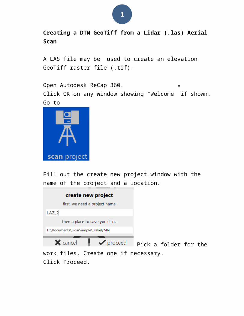
Select a window by Victoria Park and Reg Cooper Square.

Use Clip Outside.

4

Only the selected area remains.

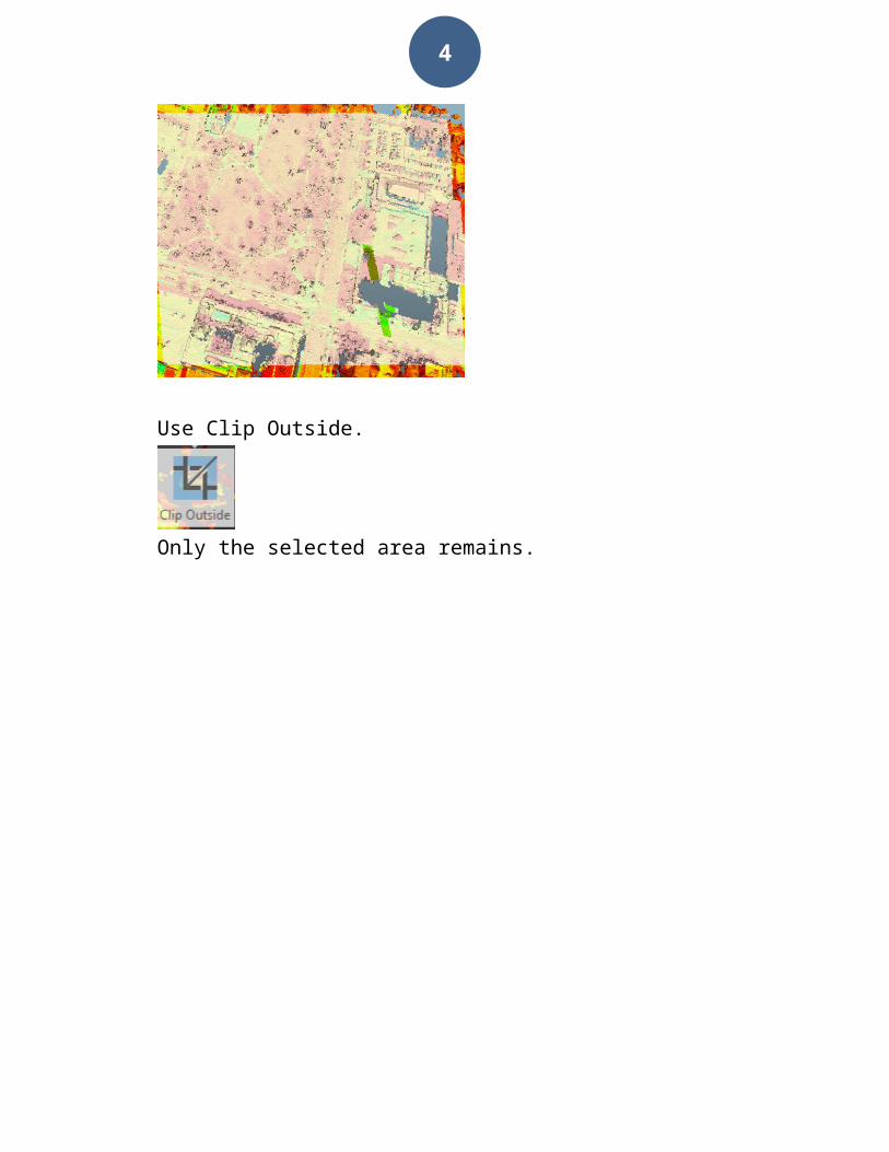
Use Save As

5

Note the name used.

Close ReCap 360Open Civil 3D 2016 Metric

In this part of the exercise, the ground surface will be extracted which is a means of classifying the data.

The coordinates system has been pre-assigned to UTM84-17 using the CSASSIGN command. A backdrop map from MS Bing is turned on using GEOMAP -> Aerial. An Autodesk student account (Edcuational Community) is required for this service + an internent connection.

Go to

6

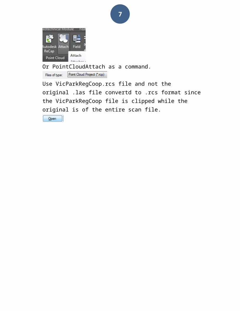
Or PointCloudAttach as a command.

Use VicParkRegCoop.rcs file and not the original .las file convertd to .rcs format since the VicParkRegCoop file is clipped while the original is of the entire scan file.

OK

7

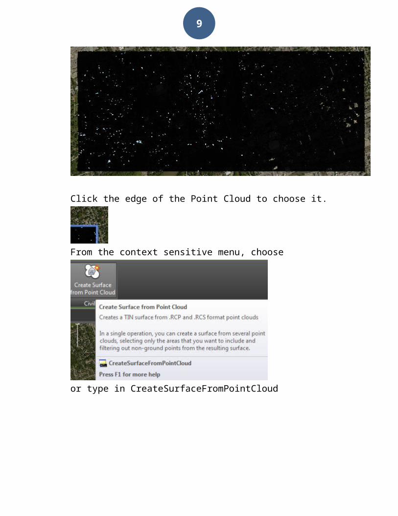
Click the edge of the Point Cloud to choose it.

From the context sensitive menu, choose

or type in CreateSurfaceFromPointCloud

8

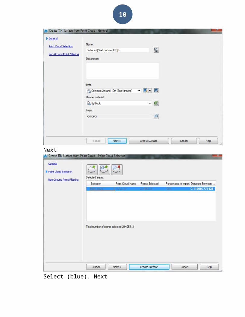
Next

Select (blue). Next

9

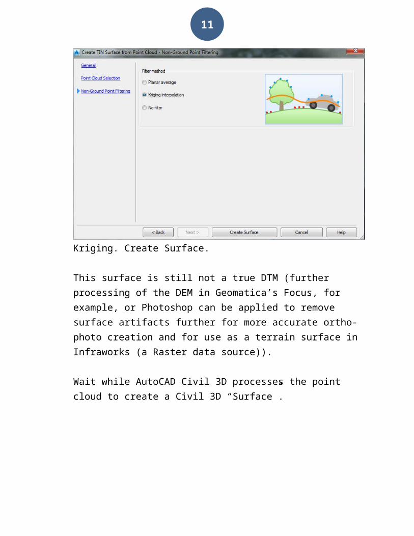
Kriging. Create Surface.

This surface is still not a true DTM (further processing of the DEM in Geomatica’s Focus, for example, or Photoshop can be applied to remove surface artifacts further for more accurate ortho-photo creation and for use as a terrain surface in Infraworks (a Raster data source)).

Wait while AutoCAD Civil 3D processes the point cloud to create a Civil 3D “Surface”.

10

When complete, click the edge of the point cloud and from the menu set the transparency to about 90

Then the surface can be seen similar to that as follows:

11

In the Toolspace (if not seen, type in the TOOLSPACE command), find the Prospector tab. Click the + sign beside Surfaces.

Right click the Surface under Surfaces in the Prospector tab of the TOOLSPACE and choose the Export to DEM… option.

Click the folder icon next to the Dem file name area.

12

The resulting GeoTiff may:1. Be edited further to create a true DTM using Geomatica

Focus or Photoshop.2. The file may be used as the “DEM” file for orthophoto

creation in Geomatica OrthoEngine3. Added to Infraworks as a Data Source (Raster variety) to

become a more accurate representation of the terrain than that of the default terrain surface based on SRTM (Space shuttle Radar Topography Mission) data.

Appendix:

LAStools

LAStools are a set of programs that can be run independently or run from within the Toolbox in ArcMap.

LAStools are free to download from: http://rapidlasso.com/lastools/

Unzip the files to one folder on the desktop or other location of your choice.

13

Within these files is one folder -> which has the file. This file can be used by the ArcMap Toolbox.

Using ArcMap with LAStools (and with built in LIDAR based tools in ArcMap)

Open ArcMap.

To use the sample file, HumesRanch, mentioned on page 4, above; a coordinate system has to be set up for it in ArcMap.

Start with a Blank Map template.

Right click to get the Data Frame Properties

UTM

14

Right click

Activate the 3D Analyst Extension in ArcGIS

15

Start with ArcMap’s

Open the las file for HumesRanch

Set the Coordinate System

OK

Zoom in to 1:4000

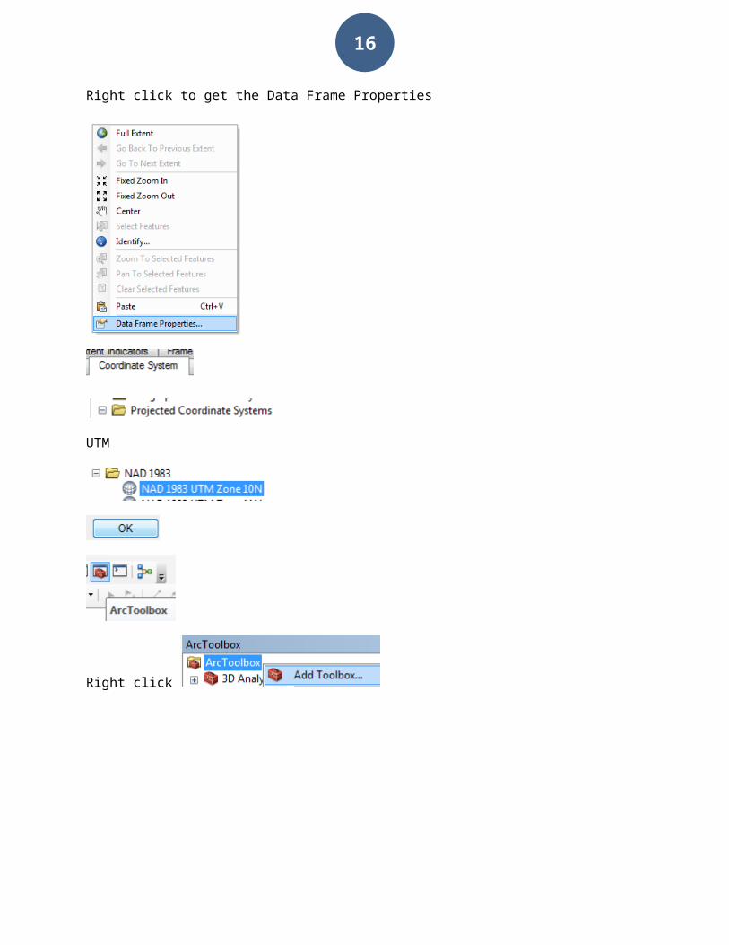
16

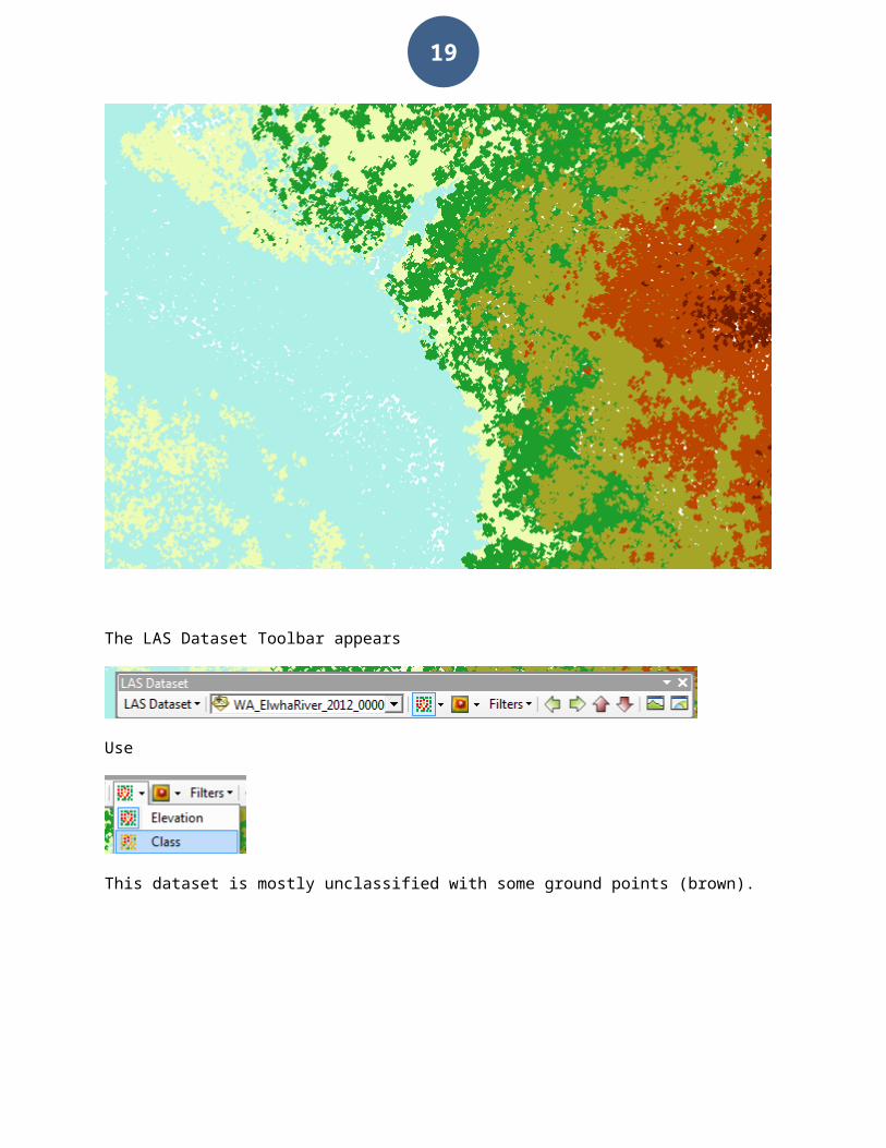
The LAS Dataset Toolbar appears

Use

This dataset is mostly unclassified with some ground points (brown).

17

Do not use any of these for these will change the view without the classification

Use

3D View

18

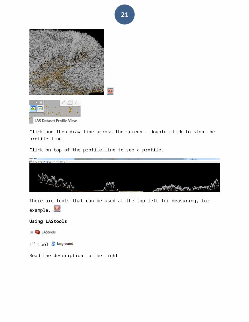
Click and then draw line across the screen – double click to stop the profile line.

Click on top of the profile line to see a profile.

There are tools that can be used at the top left for measuring, for example.

Using LAStools

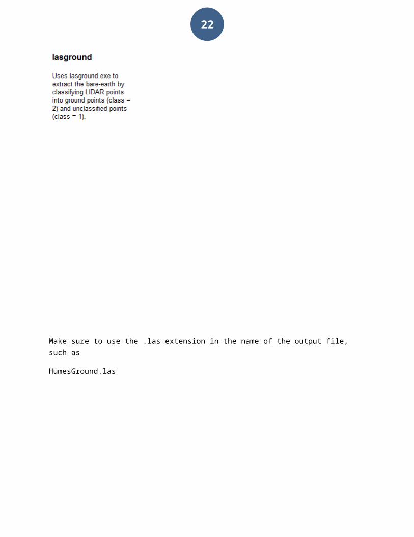
1st tool

Read the description to the right

19

Make sure to use the .las extension in the name of the output file, such as

HumesGround.las

OK

20

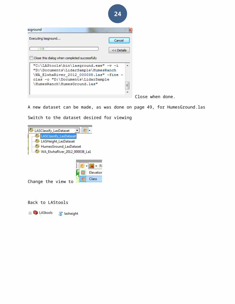
Wait for processing to finish

Close when done.

A new dataset can be made, as was done on page 49, for HumesGround.las

Switch to the dataset desired for viewing

Change the view to

Back to LAStools

21

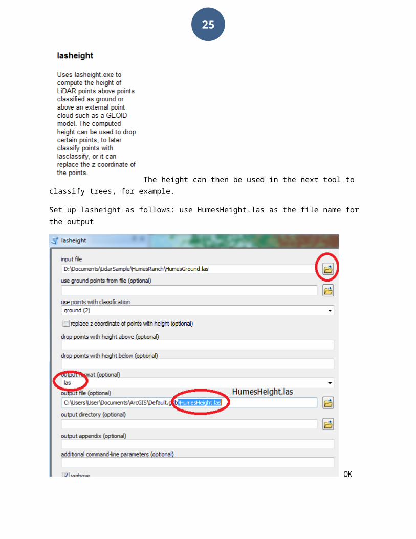
The height can then be used in the next tool to classify trees, for example.

Set up lasheight as follows: use HumesHeight.las as the file name for the output

OK

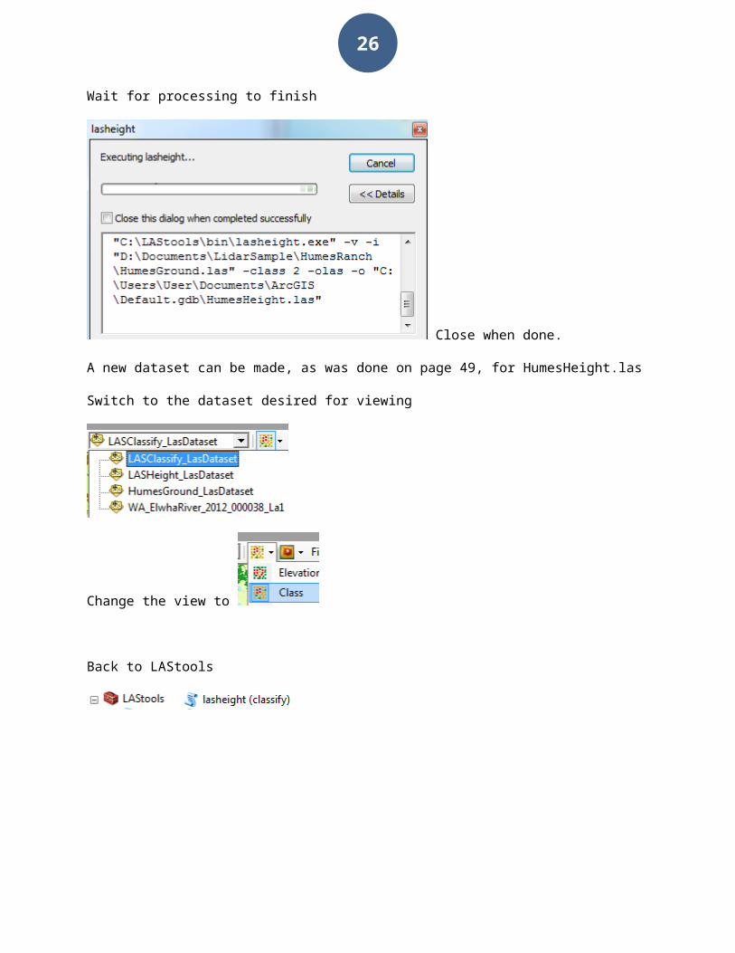
Wait for processing to finish

22

Close when done.

A new dataset can be made, as was done on page 49, for HumesHeight.las

Switch to the dataset desired for viewing

Change the view to

Back to LAStools

Fill out lasheight as follows: Use HumesClassified.las as the file name for output

23

OK

24

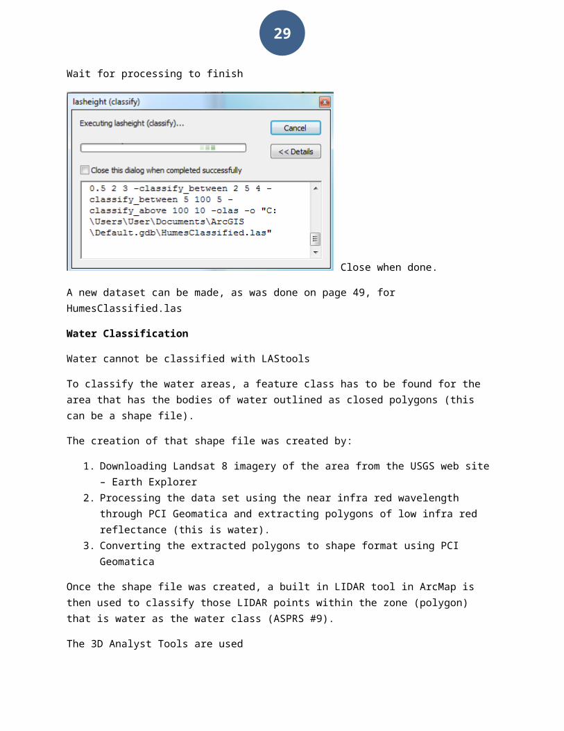
Wait for processing to finish

Close when done.

A new dataset can be made, as was done on page 49, for HumesClassified.las

Water Classification

Water cannot be classified with LAStools

To classify the water areas, a feature class has to be found for the area that has the bodies of water outlined as closed polygons (this can be a shape file).

The creation of that shape file was created by:

1. Downloading Landsat 8 imagery of the area from the USGS web site – Earth Explorer2. Processing the data set using the near infra red wavelength through PCI Geomatica and

extracting polygons of low infra red reflectance (this is water).3. Converting the extracted polygons to shape format using PCI Geomatica

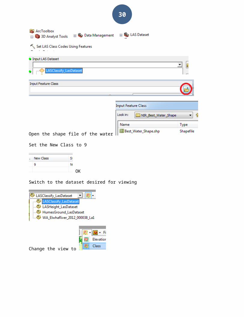
Once the shape file was created, a built in LIDAR tool in ArcMap is then used to classify those LIDAR points within the zone (polygon) that is water as the water class (ASPRS #9).

The 3D Analyst Tools are used

25

Open the shape file of the water

Set the New Class to 9

OK

Switch to the dataset desired for viewing

Change the view to

26

27

What is lidar data?

Lidar (light detection and ranging) is an optical remote-sensing technique that uses laser light to densely sample the surface of the earth, producing highly accurate x,y,z measurements. Lidar, primarily used in airborne laser mapping applications, is emerging as a cost-effective alternative to traditional surveying techniques such as photogrammetry. Lidar produces mass point cloud datasets that can be managed, visualized, analyzed, and shared using ArcGIS.

The major hardware components of a lidar system include a collection vehicle (aircraft, helicopter, vehicle, and tripod), laser scanner system, GPS (Global Positioning System), and INS (inertial navigation system). An INS system measures roll, pitch, and heading of the lidar system.

Lidar is an active optical sensor that transmits laser beams toward a target while moving through specific survey routes. The reflection of the laser from the target is detected and analyzed by receivers in the lidar sensor. These receivers record the precise time from when the laser pulse left the system to when it is returned to calculate the range distance between the sensor and the target. Combined with the positional information (GPS and INS), these distance measurements are transformed to measurements of actual three-dimensional points of the reflective target in object space.

The point data is post-processed after the lidar data collection survey into highly accurate georeferenced x,y,z coordinates by analyzing the laser time range, laser scan angle, GPS position, and INS information.

28

Lidar laser returns

Laser pulses emitted from a lidar system reflect from objects both on and above the ground surface: vegetation, buildings, bridges, and so on. One emitted laser pulse can return to the lidar sensor as one or many returns. Any emitted laser pulse that encounters multiple reflection surfaces as it travels toward the ground is split into as many returns as there are reflective surfaces.

The first returned laser pulse is the most significant return and will be associated with the highest feature in the landscape like a treetop or the top of a building. The first return can also represent the ground, in which case only one return will be detected by the lidar system.

Multiple returns are capable of detecting the elevations of several objects within the laser footprint of an outgoing laser pulse. The intermediate returns, in general, are used for vegetation structure, and the last return for bare-earth terrain models.

The last return will not always be from a ground return. For example, consider a case where a pulse hits a thick branch on its way to the ground and the pulse does not actually reach the ground. In this case, the last return is not from the ground but from the branch that reflected the entire laser pulse.

Lidar point attributes

Additional information is stored along with every x, y, and z positional value. The following lidar point attributes are maintained for each laser pulse recorded: intensity, return number, number of returns, point classification values, points that are at the edge of the flight line, RGB (red, green, and blue) values, GPS time, scan angle, and scan direction. The following table describes the attributes that can be provided with each lidar point.

29

Lidar attribute Description

Intensity The return strength of the laser pulse that generated the lidar point.

Return number

An emitted laser pulse can have up to five returns depending on the features it is reflected from and the capabilities of the laser scanner used to collect the data. The first return will be flagged as return number one, the second as return number two, and so on.

Number of returns

The number of returns is the total number of returns for a given pulse. For example, a laser data point may be return two (return number) within a total number of five returns.

Point Classification

Every lidar point that is post-processed can have a classification that defines the type of object that has reflected the laser pulse. Lidar points can be classified into a number of categories including bare earth or ground, top of canopy, and water. The different classes are defined using numeric integer codes in the LAS files.

Edge of flight line

The points will be symbolized based on a value of 0 or 1. Points flagged at the edge of the flight line will be given a value of 1, and all other points will be given a value of 0.

RGBLidar data can be attributed with RGB (red, green, and blue) bands. This attribution often comes from imagery collected at the same time as the lidar survey.

GPS time The GPS time stamp at which the laser point was emitted from the aircraft. The time is in GPS seconds of the week.

Scan angle

The scan angle is a value in degrees between -90 and +90. At 0 degrees, the laser pulse is directly below the aircraft at nadir. At -90 degrees, the laser pulse is to the left side of the aircraft, while at +90, the laser pulse is to the right side of the aircraft in the direction of flight. Most lidar systems are currently less than ±30 degrees.

Scan direction

The scan direction is the direction the laser scanning mirror was traveling at the time of the output laser pulse. A value of 1 is a positive scan direction, and a value of 0 is a negative scan direction. A positive value indicates the scanner is moving from the left side to the right side of the in-track flight direction, and a negative value is the opposite.

What is a point cloud?

Post-processed spatially organized lidar data is known as point cloud data. The initial point clouds are large collections of 3D elevation points, which include x, y, and z, along with additional attributes such as GPS time stamps. The specific surface features that the laser encounters are classified after the initial lidar point cloud is post-processed. Elevations for the ground, buildings, forest canopy, highway overpasses, and anything else that the laser beam encounters during the survey constitutes point cloud data.

30

Lidar point classification

Every lidar point can have a classification assigned to it that defines the type of object that has reflected the laser pulse. Lidar points can be classified into a number of categories including bare earth or ground, top of canopy, and water. The different classes are defined using numeric integer codes in the LAS files.

Classification codes were defined by the American Society for Photogrammetry and Remote Sensing (ASPRS) for LAS formats 1.1, 1.2, or 1.3.

Only LAS 1.1 and higher has a predefined classification system in place. Unfortunately, the LAS 1.0 specification does not have a predefined classification scheme, nor do the files summarize what, if any, class codes are used by the points. You need to be given this information from the data provider.

Classification Bit Field Encoding

31

When a classification is carried out on lidar data, points may fall into more than one category of the classification. Classification bit fields are used to provide a secondary description or classification for lidar points. With the LAS version 1.0, a lidar point could not simultaneously maintain two assigned classification attributes.

For example, a lidar return from water may need to be removed from the final output dataset, but it still should remain and be managed in the LAS file as a collected lidar point. Using LAS version 1.0, this point could not be set as both water and withheld from analysis.

In later versions (LAS 1.1, 1.2, and 1.3), the original eight-bit encoded field was split to solve this problem. The lower five bits were used to define the classification codes 0 through 31, and the three high bits were used for flags. Three classification flags were added to the LAS standard to flag points with information additional to the traditional classification. Synthetic, key-point, and withheld flags can be set for each lidar point. These flags can be set along with the classification codes.

For example, in LAS versions 1.1, 1.2, and 1.3, a water record could be given a classification code for water (9), as well as a withheld flag. The point will remain in the dataset but will be withheld from any additional analysis on the LAS files.

The following table describes the bit definition for LAS classification.

Classification Bit Field EncodingBits

Field Name Description

0–4 Classification The ASPRS standard classification shown below

5 Synthetic A point that was created by other than lidar collection, such as digitized from a photogrammetric stereo model

6 Key-point A point considered to be a model key-point and should not be withheld in any thinning algorithm

7 Withheld The point should not be included in processing

Classification Codes

If you are working with the LAS 1.1, 1.2, or 1.3 specification, refer to the predefined classification schemes defined by American Society for Photogrammetry and Remote Sensing (ASPRS) for the desired data category. The following table lists the LAS classification codes defined by ASPRS.

ASPRS Standard Lidar Point Classes

32

Classification Value (bits 0-4) Meaning

0 Never classified1 Unassigned2 Ground3 Low Vegetation4 Medium Vegetation5 High Vegetation6 Building7 Noise8 Model Key9 Water10 Reserved for ASPRS

Definition11 Reserved for ASPRS

Definition12 Overlap13–31 Reserved fro ASPRS

Definition