1  

WETLAND PROFILE AND CONDITION ASSESSMENT OF THE UPPER GREEN RIVER BASIN, WYOMING

FINAL REPORT

9/23/2015

Teresa M. Tibbets1, Holly E. Copeland1, Lindsey Washkoviak1,3, Susan Patla2, and George Jones3

1The Nature Conservancy, Wyoming Chapter, 258 Main Street, Lander, WY 82520 2Wyoming Game and Fish Department, 420 North Cache Drive, Jackson, WY 83001 3Wyoming Natural Diversity Database, University of Wyoming, 1000 East University Avenue, Department 3381, Laramie, WY 82071

2  

Wetland Profile and Condition Assessment of the Upper Green River Basin, Wyoming

Prepared for: U.S. Environmental Protection Agency, Region 8

1595 Wynkoop Street Denver, CO 80202

EPA Assistance ID No. CD-96812401-0

Prepared by:

Teresa M. Tibbets, Holly E. Copeland and Lindsey Washkoviak The Nature Conservancy – Wyoming Chapter

258 Main Street, Suite 200 Lander, WY 82520

Susan Patla

Wyoming Game and Fish Department 20 North Cache Drive Jackson, WY 83001

George Jones Wyoming Natural Diversity Database

University of Wyoming Department 3381, 1000 East University Avenue

Laramie, WY 82071

This document should be cited as follows:

Tibbets TM, Copeland HE, Washkoviak L, Patla S, and Jones, G (2015) Wetland Profile and Condition Assessment of the Upper Green River Basin, Wyoming. Report to the U.S. Environmental Protection Agency. The Nature Conservancy – Wyoming Chapter, Lander, Wyoming. 56 pp. plus appendices.

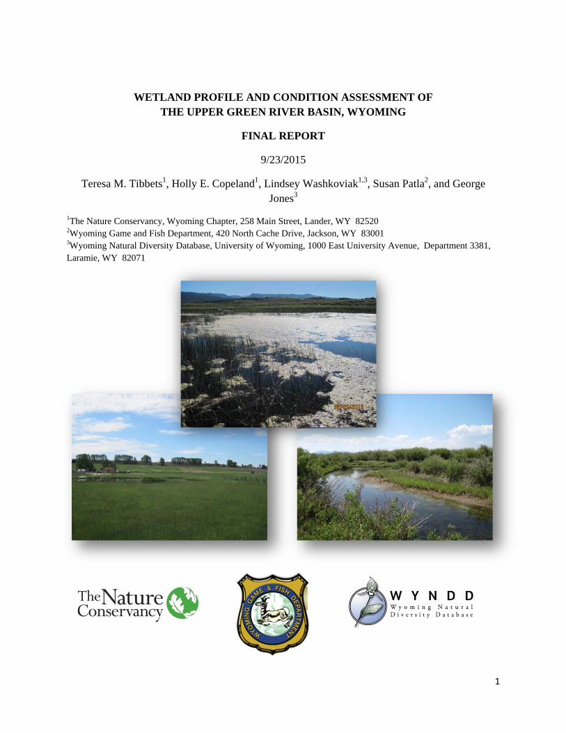
Cover photographs: Lindsey Washkoviak.

3  

Table of Contents EXECUTIVE SUMMARY .................................................................................................................................. 5 

ACKNOWLEDGEMENTS ................................................................................................................................. 7 

1.0 INTRODUCTION ....................................................................................................................................... 8 

1.1 Objectives ............................................................................................................................................ 9 

2.0 STUDY AREA ............................................................................................................................................ 9 

2.1 Geography .......................................................................................................................................... 9 

2.2 Geology ............................................................................................................................................... 9 

2.3 Climate and Hydrology ........................................................................................................................ 9 

3.0 METHODS .............................................................................................................................................. 11 

3.1 Wetland Profiles and Condition Assessment Framework ................................................................. 11 

3.1.2 Wildlife Habitat Value ................................................................................................................ 13 

3.2 Wetland Landscape Profile for Upper Green River Basin ................................................................. 13 

3.3 Survey Design and Site Selection ...................................................................................................... 14 

3.3.1 Target Population ...................................................................................................................... 14 

3.3.2 Subpopulation and Classification ............................................................................................... 15 

3.4 Field Methods ................................................................................................................................... 16 

3.4.1 Wetland Assessment Area (AA) ................................................................................................. 16 

3.4.2 Rapid Assessment Method (RAM) .............................................................................................. 17 

3.4.3 Plant Community ........................................................................................................................ 17 

3.4.4 Soils ............................................................................................................................................ 18 

3.4.5 Water Quality ............................................................................................................................. 18 

3.4.6 Avian Richness Evaluation Method ............................................................................................ 18 

3.5 Data Management ............................................................................................................................ 18 

3.6 Data Analysis ..................................................................................................................................... 18 

3.6.1. USA‐RAM Metric Score Adjustments ........................................................................................ 18 

3.6.2. Landscape Hydrology Metric (LHM) .......................................................................................... 19 

3.6.3. Floristic Quality Assessment (FQA) ........................................................................................... 21 

3.6.4. Defining Reference Condition .................................................................................................... 22 

3.6.5. Wyoming Rapid Assessment Method (WYRAM) ....................................................................... 22 

3.6.6. Assessment of Wildlife Habitat ................................................................................................. 23 

4.0 RESULTS ................................................................................................................................................. 24 

4  

4.1 Wetland Landscape Profile for Upper Green River Basin .................................................................. 24 

4.2 Description of Sampled Wetlands .................................................................................................... 29 

4.2.1 Implementation of the Survey Design ........................................................................................ 29 

4.2.2 Description of Sampled Wetlands by Ecological System ............................................................ 32 

4.2.2 Wetland Soil Profiles and Water Chemistry ............................................................................... 33 

4.3 Characterization of Wetland Vegetation .......................................................................................... 35 

4.3.1 Species diversity of Wetland Vegetation .................................................................................... 35 

4.3.2 Floristic Quality Assessment ....................................................................................................... 36 

4.3.3 Landscape Hydrology Metric ...................................................................................................... 38 

4.4.1 WYRAM Scores of Sampled Wetlands ........................................................................................ 39 

4.4.2 Population Estimate of Wetland Condition ................................................................................ 40 

4.4.3 USA‐RAM ‐ Indicators of disturbance ......................................................................................... 42 

4.4.4 Analysis of WYRAM Metrics ....................................................................................................... 44 

4.4.5 Evaluation of Wildlife Habitat .................................................................................................... 44 

5.0 Discussion .............................................................................................................................................. 46 

5.1 Wetland Priorities for Conservation and Restoration ...................................................................... 50 

LITERATURE CITED ...................................................................................................................................... 52 

Appendix A. Decision rules and description of wetland subpopulations for inclusion of NWI polygons in 

the UGRB sample frame. ............................................................................................................................. 57 

Appendix B. Field Key to Wetland and Riparian Ecological Systems of Wyoming...................................... 58 

Appendix C. Upper Green River Basin Field Manual ................................................................................... 66 

Appendix D. Field Survey Forms …………………………………………………………………… ......................................... 71 

Appendix E. Changes to RAM metric scores ………………………………………………………. ................................... 99 

Appendix F. Surrogate C‐values for wetland plants of Wyoming ………………………………………………………...100 

Appendix G. Screening criteria for reference and most disturbed sites ……………………………………………….106 

Appendix H. Stressors observed in the buffer of wetland sites ……………………………………………………………107 

5  

EXECUTIVE SUMMARY This report summarizes the results of the first basin-wide assessment of wetlands in the Upper Green River Basin (UGRB) based on rigorous randomly-sampled field survey methods. The four primary objectives of this project were to: [1] create a landscape level NWI wetland profile of wetlands in the UGRB; [2] conduct a statistically valid, field-based assessment of wetland condition, [3] model the distribution of wetland condition throughout the basin, and [4] determine key wetland habitat features and resources for wetland-dependent wildlife species. We developed the Wyoming Rapid Assessment Method (WYRAM), using a multi-level approach to measure wetland condition and identify stressors. Determining “condition” or “status” of wetlands in the UGRB focused on evaluating the identity and scope of anthropogenic disturbance, hydrologic alteration, and floristic quality.

Based on National Wetland Inventory (NWI) data, there are 177,648 acres of wetlands and water bodies which represent approximately 20% of the total land area of the UGRB. Most private lands occur in the floodplains of the Green River and its tributaries; consequently the largest proportion of wetlands, water bodies and irrigated lands are privately owned. Of the 65 study sites sampled, 23% were in the low-disturbance category, 26% in the high-disturbance category, and 51% were moderately disturbed. Cumulative distribution function projections for the basin revealed that 96% of wetlands are moderately to highly disturbed and less than 4% are in the low disturbance category. Among wetland types, emergent marshes (generally higher elevation glacial pothole wetlands) were the least disturbed, followed by riparian woodland and shrublands. Wet meadows, mainly irrigated hayfields, were the most disturbed and hydrologically modified. The most widespread anthropogenic disturbances, or stressors, identified across all wetland types were agricultural practices associated with pastures and cattle grazing and hydrologic alterations. We measured extensive hydrologic alteration in the basin, especially of wet meadows, of which 93% had altered hydrology and less than 10% had low disturbance scores. Emergent marshes experienced less hydrologic alteration (40% altered hydrology) and disturbance (33% had low disturbance). Riparian woodland and shrubland wetlands had either historic (30%) or altered-hybrid (70%) hydrology, largely from the Upper Green River or major tributaries. About 50% of the riparian woodland and shrubland sites were moderately disturbed, 20% had low disturbance scores, and over 25% of sites had high disturbance scores.

We identified 122 plant species during wetland assessments, representing 4% of Wyoming’s known flora (Dorn 2001). Plant species richness was highest for riparian woodland and shrublands and lowest for wet meadows. Evidence of grazing by native ungulates was recorded at 100% of riparian woodland and shrublands, 40% of wet meadows, and 33% of emergent marshes. Based on habitat suitability models using Avian Richness Evaluation Method (AREM),

6  

over one hundred bird species were predicted to have suitable habitat during the breeding season across all wetlands sampled in the UGRB.

These results represent a baseline for understanding the condition of existing wetland resources in the UGRB and demonstrate the merits of utilizing methods at varying levels of effort to provide quantitative data about different components of the wetland resources, including wildlife habitat. They also show the importance of assessment methods that recognize irrigation as a mechanism for creating novel wetland systems and increasing the area of existing wetlands, as well as a stressor that may affect the condition of naturally-created wetlands. Major changes to land use, irrigation practices, and climate could have widespread implications to wetlands in the UGRB. For example, our results suggests that approximately 40% of wet meadow wetlands are directly created or supported by irrigation; conversion to pivot irrigation could potentially affect an estimated 50,000 acres of temporary and seasonal wetlands and the wildlife habitat they provide. Conservation strategies aimed at protecting lands designated as wetlands may fall short of their intended purpose if water quantity and timing crucial to wetland function and habitat value are also not retained.

7  

ACKNOWLEDGEMENTS  

This project was funded by a Wetland Program Development Grant (#CD-96812401-0) from the U.S. Environmental Protection Agency Region 8. This report represents a collective effort of many people that has spanned several years. Rich Sumner and Tony Olsen of the EPA provided guidance and support on the survey design and data analysis. Chad Rieger with the Wyoming Department of Environmental Quality provided guidance on methods and overall approach, as well as assistance with our initial grant applications. Steve Tessmann and Bob Lanka with Wyoming Game and Fish Department were instrumental throughout the process in supporting this effort.

We owe particular thanks to Joanna Lemly and Laurie Gilligan of the Colorado Natural Heritage Program who shared advice and suggestions for the wetland condition assessment methods that shaped the development of our approach and analyses of the study.

We extend our gratitude to our field technician, Adam Skadson, for his hard work collecting and entering data, and to field technician David Schimelphenig for database review and quality assurance.

Jim Platt, a member of the Science/GIS team for the North American Region of The Nature Conservancy, brought the AREM database into the 21st century by translating the original version (Adamus 1993) into a user-friendly template in Microsoft ACCESS. We thank Paul Adamus, who provided comments and insight on using AREM. Grant Frost also completed the bird database that was integral to the completion of the project.

The project would not be possible if not for the public and private landowners that allowed us on their lands to access wetlands. We extend our gratitude to landowners for their support of this project.

8  

1.0 INTRODUCTION

Freshwater wetland ecosystems, including marshes, wet meadows, playas, and fens, exist at the interface between land and water. This interface, or ecotone, of environment and biological gradients creates diverse and productive habitats that integrate both aquatic and terrestrial ecosystems. Wetlands provide a suite of ecosystem services including flood attenuation, stream flow maintenance, aquifer recharge, sediment retention, water quality improvement, production of food and goods for human use, and maintenance of biodiversity. The global economic value of ecosystem services provided by wetland ecosystems is estimated to be higher than that of lakes, streams, forests, and grasslands and is second only to services provided by coastal ecosystems (Costanza et al. 1997). In addition, wetlands provide critical habitat for wildlife. More than one-third of species listed as threatened or endangered in the United States live solely in wetlands and almost half use wetlands at some point in their lives (US EPA 1995).

In the Intermountain West, more than 140 bird species, 30 mammal species, 36 amphibians, and 30 reptiles are either dependent on or associated with wetlands (Gammonley 2004). While only occupying 1.5% of the total land area of Wyoming, wetlands support a disproportionately high number of plant and wildlife species (Knight et al. 2014). For instance, approximately 90% of the wildlife species in Wyoming use wetland and riparian habitats daily or seasonally during their life cycle, and about 70% of Wyoming bird species are wetland or riparian obligates (Nicholoff 2003). However, wetlands remain highly threatened ecosystems and experience pressures from many uses, including agricultural, residential, and energy development. Dahl (1990) estimates that between 1780 and the mid-1980s, 38% of wetlands were lost in Wyoming. Recent studies identify wetland habitats in Wyoming as one of the most vulnerable to future development and changes in climate (Copeland et al. 2010, Pocewicz et al. 2014). There is an urgent need to quantitatively assess the current ecological condition of existing wetlands in Wyoming to better inform the conservation and management of this vital natural resource.

The basin has experienced a recent shift in land use patterns. While historically, agriculture and recreation were the primary land uses, a recent boom in energy development has led to rapid growth in industrial and residential construction and to development of new roads, pipelines, and subdivisions. Potential impacts to wetlands include habitat fragmentation and disturbance, altered water quality, and increased demand for limited water resources. These changes amplify the importance and need for effective and efficient conservation action and management of wetlands, guided by sound scientific baseline information.

Our objective in this effort is to develop the first river basin-scale wetland profile and condition assessment within Wyoming to meet the demonstrated conservation needs. This study builds upon several previously completed assessments and studies: the State Wildlife Wetlands Strategy (2010), the State Wildlife Action Plan (Wyoming Game and Fish Department 2010) and the recently completed Wyoming Level 1 wetlands assessment (Copeland et al. 2010). The Upper Green River Basin (UGRB) was one of nine wetland complexes identified as a statewide priority

9  

in the Level 1 assessment (Copeland et al. 2010) and was identified by Wyoming Game and Fish Department WGFD as the most extensive riverine-palustrine wetland system in the state (Wyoming Joint Ventures Steering Committee 2010).

1.1 Objectives The four objectives of this project were to: [1] create a landscape level NWI wetland profile of the UGRB; [2] conduct a statistically valid, field-based assessment of wetland condition, [3] model the distribution of wetland condition throughout the basin, and [4] determine key wetland habitat features and resources for wetland-dependent wildlife species.

2.0 STUDY AREA

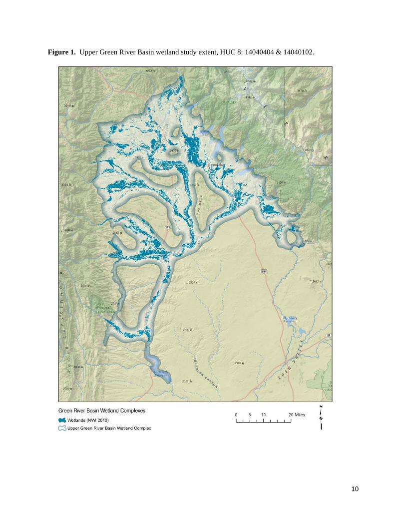
2.1 Geography The Upper Green River Basin is located in west central Wyoming (Figure 1) between the Wind River and Wyoming ranges in Sublette and Lincoln counties. The Upper Green River is the fourth largest river basin in Wyoming and the northern headwaters of the Colorado River. For the purposes of this project, the study boundary defined in Copeland et al. (2010), was modified to include only the northern section of their wetland complex, from Fontenelle Reservoir upstream on the Green River and its tributaries, excluding Fontenelle Creek and the Hams Fork (Figure 1). All references to wetland complexes in the Upper Green River Basin in this report apply only to this specific study area.

2.2 Geology The wetland complexes in the study area are located primarily on unconsolidated Quaternary sediment and on sedimentary rocks of the Green River Formation deposited in the Eocene (Wyoming State Geological Society 2014). These Eocene rocks contain mineral resources such as coal, uranium, trona, and oil shale (Mason and Miller 2004). In addition, the tight-gas sandstones from rocks of the Late Cretaceous in the Pinedale Anticline contain significant quantities of natural gas that support recent energy development in the area. Glacial activity in the Wind River Mountain Range in the last ice age resulted in the formation of glacial potholes in the foothills in the northeastern part of the study area.

2.3 Climate and Hydrology The semiarid climate in this region is typical of high desert areas of the western United States. The climate within the study area varies as a function of elevation, with more precipitation and lower temperatures in the higher-elevation areas. The lower elevations of the Green River Basin receive an average of 10-15 inches of precipitation annually with upper elevations near the mountains receiving over 20 inches (Schroeder 2010). Peak precipitation occurs during April and May. The maximum annual temperature ranges from 70o F at higher elevations to 90o F in lower elevations of the basin. Minimum annual temperature ranges from <0o F to 5o F during the winter months.

10  

Figure 1. Upper Green River Basin wetland study extent, HUC 8: 14040404 & 14040102.

11  

The UGRB includes the northernmost headwaters of the Green River, the largest tributary to the Colorado River in the Upper Colorado River Basin. A majority of the stream flow within the basin originates from the snowpack in the Wind River and Wyoming mountain ranges. The melting snowpack in late spring and early summer results in increased surface flows and seasonal flooding in the Upper Green River and its tributaries. Natural wetland complexes are fed by surface and groundwater sources that decrease into the late summer, coinciding with seasonal decrease in wetland area due to high evaporation rates. Wetlands within or surrounded by irrigated fields can have a longer period of inundation or saturation into the later summer and early fall.

The UGRB lies within the Wyoming Basin Level III ecoregion (Chapman et al. 2004). The study area is further divided into three Level IV ecoregions. Most of the study area is located within the Sub-Irrigated High Valley Level IV ecoregion and is dominated by wet meadows and riparian floodplain habitats that support communities of mixed willow species (Salix sp.), narrowleaf cottonwood (Populus angustifolia), sedges (Carex sp.), and mixed grasses. Upland plant communities in the Rolling Sagebrush Steppe Level IV ecoregion include Wyoming big sagebrush (Artemisia tridentata), rabbitbrush (Ericameria sp.) and various grass, forbs, and shrub species. The Foothill Shrublands and Low Mountain Level IV ecoregion lies adjacent to the western side of the Wind River Range and the lower elevation vegetation within this part of the study area is composed of various shrubs and grasses, interspersed with Douglas-fir (Pseudotsuga menziesii), pine, juniper ,and aspen (Populus tremuloides) woodlands.

3.0 METHODS

3.1 Wetland Profiles and Condition Assessment Framework Wetland profiles and condition assessments can be an effective means of summarizing the distribution and diversity of wetland resources and can be used to establish baseline conditions, assess cumulative impacts to wetland condition and function, and inform strategic conservation goals (Fennessy et al. 2007, Lemly and Gillian 2012). A number of sampling methodologies have been developed in the past fifteen years to monitor wetland condition at a variety of spatial scales (US EPA 2011a, Adamus 1993, DeKeyser et al. 2003, Jacobs et al. 2010, Lemly and Gillian 2012, Vance et al. 2012). Currently, a three-tiered approach to wetland assessments is recommended by the US EPA, with each tier increasing in degree of effort, cost, and scale:

Level 1 assessments are broad in geographic coverage and are used to characterize land use and the distribution of resources, such as wetland types, across the landscape. These assessments primarily utilize digital information or remote sensing data in a Geographic Information Systems (GIS) to provide a “desktop analysis” of wetlands at the landscape scale.

Level 2 assessments evaluate the condition of individual wetlands using field-based methods that focus on indicators, including anthropogenic disturbances, also known as

12  

stressors, which are rapid and easy to measure. Level 2 Rapid Assessment Methods (RAMs) are used throughout a number of regions in the USA because they provide an on-site assessment of wetland condition with relatively little effort (Fennessy et al. 2007). Common RAMs estimate the ecological condition of the wetland landscape, by integrating metrics that focus primarily on hydrology, and physical and biological structure. RAM metrics focus on observable stressors and disturbances known to degrade the ecological integrity of wetlands. Metric scores and identification of stressors are incorporated into a wetland profile to provide information about the integrity of a basin's wetland resources.

Lastly, Level 3 assessments utilize more intensive methods, such as measures of diversity, to collect quantitative field data using metrics of biological integrity.

Depending on the availability of resources and the scope of a study, assessments can combine approaches from different levels to produce data at the required level of detail.

3.1.1. WYOMING RAPID ASSESSMENT METHOD APPROACH In the context of the Level 1-2-3 Framework, we developed an approach to assessing wetlands within the UGRB, the Wyoming Rapid Assessment Method (WYRAM), which utilized data collection at all three levels to satisfy the main objectives of the study (Figure 2). The goals of the assessment were to determine “condition” or “status” of wetlands in the UGRB by focusing on evaluating [1] the identity and scope of anthropogenic disturbance, [2] hydrologic alteration, and [3] floristic quality.

Figure 2. A schematic illustrating the approach used to assess wetland condition for the UGRB.

We utilized Level 2 field metrics largely based on the USA-Rapid Assessment Method (USA-RAM), (U.S. Environmental Protection Agency 2011b). The USA-RAM framework applies tested methodology from established wetland assessment frameworks, including the California

13  

RAM for Wetlands (Sutula et al. 2006) and the Ohio RAM (EPA 2001). The overall goal of USA-RAM is to provide a rapid, repeatable, scientifically-defensible evaluation of the overall ecological condition of a wetland. At each wetland, field metrics are evaluated using descriptive ratings. The metrics are tied to four wetland attributes: Buffer, Hydrology, Physical Structure, and Biological Structure. Each field metric has been developed with the assumption that it reflects a readily observable aspect of the complex ecological structure and function of a wetland ecosystem. USA-RAM metrics focus heavily on identifying the severity of anthropogenic disturbance, or “stressors”, associated with degradation of wetland ecosystems. Metric values are combined into a score that can be used to describe wetlands along a disturbance gradient in relation to reference condition.

Level 3 field protocols were incorporated from Colorado’s Ecological Integrity Assessment (EIA) framework, including methods for floristic quality assessment of the plant community, soil characterization, and water quality (Lemly and Gillian 2012).

We developed a Landscape Hydrology Metric (LHM), a Level 1.5 assessment of alteration to hydrologic regime, which incorporates landscape-level 1 data on alterations to hydroperiod and water source with level 2 field data for wetland soils. This metric was developed because the original USA-RAM hydrology metrics did not adequately identify hydrologic alterations (See section 3.6.2 in Methods).

3.1.2 Wildlife Habitat Value Lastly, we updated and adapted the Avian Richness Evaluation Method (AREM) (Adamus 1993), a Level 2 assessment of habitat suitability for wetland-specific birds, for use in Wyoming. Information from AREM, plant diversity measures, and other field metrics provide a link between habitat quality, wetland condition, and biodiversity in the basin.

 

3.2 Wetland Landscape Profile for Upper Green River Basin A wetland landscape profile was created using digital wetland mapping compiled from the U.S. Fish and Wildlife Service (USFWS) National Wetland Inventory (NWI) database and additional data layers for irrigation and land management/ownership within the Upper Green River Basin study area. NWI maps for Wyoming were created from aerial photography in the 1970s and 1980s, and subsequently digitized. The landscape profile summarizes the extent of wetland area in the UGRB by wetland and waterbody type, hydrologic regime, extent modified/irrigated (Wyoming Wildlife Consultants 2007), and land management/ownership (Bureau of Land Management 2010) . The wetland landscape profile includes all wetland types and waterbodies as defined by Cowardin codes (Cowardin et al. 1979).

14  

3.3 Survey Design and Site Selection

3.3.1 Target Population For site selection we used the National Wetlands Inventory (NWI) data as the basis for the sample frame (that is, the set of target wetlands from which the sample sites would be drawn). The target population was determined to be palustrine wetlands including all naturally occurring and human-created, vegetated wetlands within the UGRB, but not including deep water lakes, stream channels, or forested wetlands based on Cowardin hydrologic codes and modifiers (Appendix A). Palustrine wetlands can be situated shoreward of lakes or river channels, on floodplains, isolated from water bodies, in depressions or on slopes. To be selected for sampling wetlands had to cover at least 0.1 hectare (1000 square meters) and be at least 10 meters wide to capture abandoned stream channels and oxbows. The original sample frame was refined by excluding non-target attribute classes, however, the remaining sample frame still included non-target areas that were rejected through desktop review or on-site evaluation. The operational definition of wetland used in this project is based on the U.S. Fish and Wildlife Service (USFWS) definition used for the National Wetland Inventory (Cowardin et al. 1979):

“Wetlands are lands transitional between terrestrial and aquatic systems where the water table is usually at or near the surface or the land is covered by shallow water. For purposes of this classification wetlands must have one or more of the following attributes: (1) at least periodically, the land supports predominantly hydrophytes; (2) the substrate is predominantly undrained hydric soil; and (3) the substrate is nonsoil and is saturated with water or covered by shallow water at some time during the growing season of each year.”

However, it is important to note that standard wetland delineation techniques have been developed based on a different definition of wetland used by the U.S. Army Corps of Engineers (ACOE) and the EPA for regulatory purposes under Section 404 of the Federal Clean Water Act (ACOE 2008):

“[Wetlands are] those areas that are inundated or saturated by surface or ground water at a frequency and duration sufficient to support, and under normal circumstances do support, a prevalence of vegetation typically adapted for life in saturated soil conditions.”

The primary difference between the two definitions is that the ACOE definition requires positive identification of all three wetland parameters (hydrology, vegetation, and soils), while the USFWS definition requires only one to be present. (The USFWS definition also includes non-vegetated areas and deep water habitats, which were excluded from this study.) We used the USFWS definition of a wetland but adapted the ACOE Dominance Test (ACOE 2008) for determining whether a site supported primarily hydrophyites. The Dominance Test defines

15  

hydrophytic vegetation as: “More than 50 percent of the dominant plant species across all strata are rated Obligate wetland, Facultative wetland, or Facultative”. We excluded Facultative vegetation from this evaluation because many common agricultural hay plants are listed as facultative in the State of Wyoming wetland plant list (Lichvar et al. 2014).

3.3.2 Subpopulation and Classification The target population was classified into subpopulations based on NWI Cowardin water regimes: 1) semi-permanent and permanent non-riverine wetlands, 2) temporary and seasonal wetlands, and 3) riverine willow and oxbow wetlands. A list of NWI subpopulations included in the sample frame is provided in Appendix A. We selected all wetlands within the study area boundary and allowed NWI polygons that extended beyond the boundary to be included. The study area boundary was re-delineated to include these wetlands. Our target number of sample sites was 60 (Appendix A). Sample sites were randomly selected from the target population by using a generalized random tessellation stratified survey design outlined by the EPA’s Environmental Monitoring and Assessment Program (Stevens and Olsen 2004, Stevens and Jensen 2007). After potential sites had been selected, and prior to field sampling, a desktop site evaluation was performed to determine: 1) whether the presence of a wetland was likely based on examination of the site with aerial imagery (USDA Farm Service Agency 2009), and 2) land ownership status (private, state, federal) of the wetland in order to contact the landowner for permission to sample. In addition to the 60 target sample sites, four wetlands were hand-selected as potential reference sites based on professional judgment of regional wildlife managers. The primary goal of classification is to reduce the effect of within-class variability on the assessment scores to better discern differences in condition among wetlands. We classified wetlands sites in the study area by both the Cowardin classification framework (Cowardin et al. 1979) and by Ecological Systems (Comer et al. 2003). The Cowardin classification (used in the NWI) emphasizes hydrologic regime and substrate, and the Ecological System classification uses both biotic (vegetation structure and floristics) and abiotic (hydrogeomorphology, elevation, etc.) elements. In highly managed landscapes, such as the UGRB, it is difficult to correctly identify the hydrologic regime in one site visit, which limits the utility of the Coward classification. Moreover, wetland types in the Cowardin classification can represent a variety of Ecological Systems. Consequently, using the Ecological Systems classification reduced the amount of variability within our sample frame. Classification by Ecological Systems is the dominant system used regionally for wetland condition assessments (Lemly and Gillian 2012, Newlon et al. 2013). In addition, classification by ecological system is more readily adaptable to evaluation of wetland habitat value for wildlife since the focus is on organization of plant community types. In this study, wetlands were classified by Ecological System a posteriori based on information gathered during the site visit. Descriptions for Ecological System classes observed in the UGRB (Appendix B) were developed based on national and regional classification frameworks (Comer et al. 2003, Luna et al. 2010,

16  

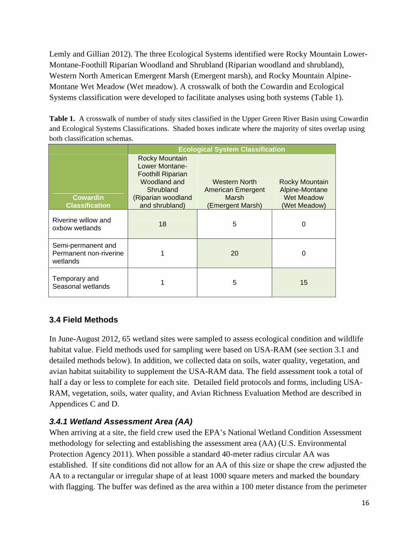
Lemly and Gillian 2012). The three Ecological Systems identified were Rocky Mountain Lower-Montane-Foothill Riparian Woodland and Shrubland (Riparian woodland and shrubland), Western North American Emergent Marsh (Emergent marsh), and Rocky Mountain Alpine-Montane Wet Meadow (Wet meadow). A crosswalk of both the Cowardin and Ecological Systems classification were developed to facilitate analyses using both systems (Table 1). Table 1. A crosswalk of number of study sites classified in the Upper Green River Basin using Cowardin and Ecological Systems Classifications. Shaded boxes indicate where the majority of sites overlap using both classification schemas.

Ecological System Classification

Cowardin Classification

Rocky Mountain Lower Montane-Foothill Riparian Woodland and

Shrubland (Riparian woodland

and shrubland)

Western North American Emergent

Marsh (Emergent Marsh)

Rocky Mountain Alpine-Montane

Wet Meadow (Wet Meadow)

Riverine willow and oxbow wetlands

18 5 0

Semi-permanent and Permanent non-riverine wetlands

1 20 0

Temporary and Seasonal wetlands

1 5 15

3.4 Field Methods

In June-August 2012, 65 wetland sites were sampled to assess ecological condition and wildlife habitat value. Field methods used for sampling were based on USA-RAM (see section 3.1 and detailed methods below). In addition, we collected data on soils, water quality, vegetation, and avian habitat suitability to supplement the USA-RAM data. The field assessment took a total of half a day or less to complete for each site. Detailed field protocols and forms, including USA-RAM, vegetation, soils, water quality, and Avian Richness Evaluation Method are described in Appendices C and D.

3.4.1 Wetland Assessment Area (AA) When arriving at a site, the field crew used the EPA’s National Wetland Condition Assessment methodology for selecting and establishing the assessment area (AA) (U.S. Environmental Protection Agency 2011). When possible a standard 40-meter radius circular AA was established. If site conditions did not allow for an AA of this size or shape the crew adjusted the AA to a rectangular or irregular shape of at least 1000 square meters and marked the boundary with flagging. The buffer was defined as the area within a 100 meter distance from the perimeter

17  

of the AA. Standard descriptions of site characteristics were collected at each wetland including UTM coordinates, Cowardin and Ecological System classification, HGM classification, presence or signs of wildlife, and photos of the buffer and AA.

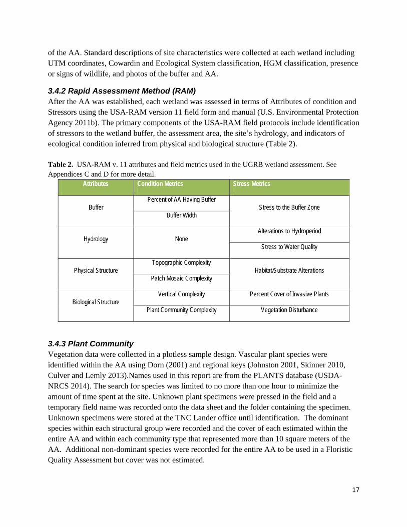
3.4.2 Rapid Assessment Method (RAM) After the AA was established, each wetland was assessed in terms of Attributes of condition and Stressors using the USA-RAM version 11 field form and manual (U.S. Environmental Protection Agency 2011b). The primary components of the USA-RAM field protocols include identification of stressors to the wetland buffer, the assessment area, the site’s hydrology, and indicators of ecological condition inferred from physical and biological structure (Table 2). Table 2. USA-RAM v. 11 attributes and field metrics used in the UGRB wetland assessment. See Appendices C and D for more detail.

Attributes Condition Metrics Stress Metrics

Buffer Percent of AA Having Buffer

Stress to the Buffer Zone Buffer Width

Hydrology None Alterations to Hydroperiod

Stress to Water Quality

Physical Structure Topographic Complexity

Habitat/Substrate Alterations Patch Mosaic Complexity

Biological Structure Vertical Complexity Percent Cover of Invasive Plants

Plant Community Complexity Vegetation Disturbance

3.4.3 Plant Community Vegetation data were collected in a plotless sample design. Vascular plant species were identified within the AA using Dorn (2001) and regional keys (Johnston 2001, Skinner 2010, Culver and Lemly 2013).Names used in this report are from the PLANTS database (USDA-NRCS 2014). The search for species was limited to no more than one hour to minimize the amount of time spent at the site. Unknown plant specimens were pressed in the field and a temporary field name was recorded onto the data sheet and the folder containing the specimen. Unknown specimens were stored at the TNC Lander office until identification. The dominant species within each structural group were recorded and the cover of each estimated within the entire AA and within each community type that represented more than 10 square meters of the AA. Additional non-dominant species were recorded for the entire AA to be used in a Floristic Quality Assessment but cover was not estimated.

18  

3.4.4 Soils At least two soil pits were dug within the AA. One pit was placed in each community type present in the AA unless the community type was completely covered with water. A maximum of 4 soil pits were dug per AA. Each soil pit was marked with a GPS way point and its location was marked on the map. Pits were dug to 40 cm deep (about one shovel length) when possible. The core was removed and set down next to the pit, ensuring all horizons were intact and in order. For each horizon the following information was recorded: 1) color (based on a Munsell Soil Color Chart) of the matrix and any redoximorphic concentrations (mottles and oxidized root channels) and depletions; 2) the soil texture; and 3) any specifics about the concentration of roots, the presence of gravel or cobble, or any unusual features in the soil. Based on these characteristics, hydric soil indicators were identified following guidance from the ACOE Regional Supplement for the western mountains (2008) and the National Resources Conservation Service (NRCS) Field Indicators of Hydric Soils in the United States and Hydric Soil Indicators in the Mountain West (NRCS 2010).

3.4.5 Water Quality The crew estimated the percent cover and patch complexity (interspersion) of open water for the total AA. The range in water depth and the average water depth were estimated by recording the minimum, mode, and maximum water depth in the AA. The crew measured common water quality parameters (pH, salinity, conductivity, total dissolved solids and temperature) from permanent, undisturbed, standing water closest to the center point of the AA.

3.4.6 Avian Richness Evaluation Method All wetlands were assessed for habitat characteristics by completing field forms for the Avian Richness Evaluation Method (AREM) that included a 200 m buffer surrounding the AA (Adamus 1993).

3.5 Data Management

All field data were entered into a relational Microsoft Access and/or ArcGIS 10.1 database. After entry, the data were reviewed and errors corrected before analysis. The data is stored and served on a TNC data server that is backed up nightly and stored off-site weekly. Final copies of the datasets were sent to each partner for archiving.

3.6 Data Analysis

3.6.1. USA-RAM Metric Score Adjustments To be an effective tool for assessing wetland condition, metrics included in an assessment of ecological condition should provide information about the integrity of major ecological attributes relative to a gradient of disturbance or stressors. Performance of each RAM metric was evaluated based on methods used for the refinement of indices of condition in stream and wetland ecosystems (Stoddard et al. 2006, Jacobs et al. 2010, Faber-Langendoen et al. 2011). Evaluation

19  

of USA-RAM methods and scoring was a vital step to ensure applicability of the USA-RAM methods for wetlands in Wyoming. The range and representativeness of each metric was determined by examining histograms of the data for range and distribution of scores. Scoring was adjusted if needed by using raw field data to calibrate scoring categories. We evaluated metric redundancy by calculating Spearman correlation coefficients among all metrics. None of the metrics within an attribute category were highly correlated (as determined by a coefficient value r > 0.8). We identified 10 out of the 12 original USA-RAM metrics that needed adjustments to scoring (see Appendix E). Topographic complexity (RAM Metric 4) and Plant Community Complexity (RAM Metric 7), were not included in final RAM scores because of lack of responsiveness. Alterations to Hydroperiod (RAM Metric 9) was replaced by the Landscape Hydrology Metric because alterations on the landscape potentially affecting wetland hydrology were missed using the field metric (see next section). The RAM score for each wetland was calculated as the average value of the final nine metrics.

3.6.2. Landscape Hydrology Metric (LHM) Hydrology—the movement, distribution and quality of water across the landscape—is the primary driver of the establishment and maintenance of wetlands, including the ecological, physical, and chemical processes that sustain ecosystem function and associated services and value to people (Mitch and Gosselink 2007).Therefore, it is important to identify alteration to the natural hydrologic regime that may be detrimentally affecting the structure and function of the wetland.

USA-RAM assesses stressors to hydrology using two metrics observed within the AA: Stress to Water Quality (Metric 8) and Alterations to Hydroperiod (Metric 9). Inclusion of only these two metrics to assess hydrology is based on the assumption that changes to hydrology will be also reflected in the physical and biological structure and buffer condition of a wetland that “tend to be correlated with hydrology” (U.S. Environmental Protection Agency 2011b). When we reviewed field data for Metric 9, Alterations to Hydroperiod, only six sites were observed with field stressor indicators in the AA. Identification of only six sites with alterations to hydrology within a basin with 20-50% of wetland area classified as irrigated (Table 9) raised concern about the efficacy of Metric 9. We developed an alternative hydrology metric, the Landscape Hydrology Metric, to more effectively identify alterations to the natural hydrologic regime affecting each wetland AA. The LHM primarily utilizes Level 1 landscape-scale information that is supplemented with Level 2 field data for the presence of histic soils.

LHM Submetric 1: Alteration of hydroperiod To identify hydroperiod alteration affecting each wetland AA, we conducted a desktop assessment of potential stressors to hydrology using high-resolution (0.3 meter) satellite imagery in ArcGIS from Digital Globe. For each field site, we recorded the presence of possible indicators of hydroperiod alteration such as the presence of irrigation ditches and canals, dams, and berms, or points of diversion that were upstream or at a higher position in the watershed from each AA. Major dams or reservoirs upstream or near a site were noted. A major dam was

20  

defined as being on the main-stem of the river, 50 ft tall with a storage capacity of at least 5,000 acre-feet, or of any height with a storage capacity of 25,000 acre-feet (ACOE 2006). Mapped GIS data from the US Geological Survey National Hydrologic Dataset (USGS NHD high-resolution version) were used to confirm or support satellite imagery interpretations. To evaluate the accuracy of Submetric 1 in identifying alterations to hydroperiod, we compared the number of indicators identified in the field using USA RAM metric 9 to the number identified in desktop analysis using LHM Submetric 1. Of the 65 wetlands analyzed, 27 were identified as having alterations to hydroperiod using LHM that were not identified in the field using USA RAM metric 9. We found agreement between the methods (both positive and negative identification of stressors) 65% of the time. Only one site was positively identified as having a ditch using USA RAM metric 9 that was not identified using LHM Submetric 1. The LHM score for this one site was adjusted to incorporate the field data.

LHM Submetric 2: Evidence of a natural water source We used GIS data from USGS NHD and satellite imagery to conduct a desktop evaluation of all field sites for evidence of natural surface water sources that could influence the site. A site was considered to have a natural water source if a permanent or intermittent stream was identified within 50 meters; or if an active beaver dam was present; or if it was located within a glacial pothole or playa. Additionally, we evaluated the likelihood that the site might be influenced by the presence of groundwater using a GIS-based model of depth to groundwater (Wyoming Department of Environmental Quality 2005) to identify field sites where groundwater is within 20 feet from the surface. The site was also considered to have a natural water source if none could be identified in the desktop GIS evaluation but histic soils were identified in the field.

LHM Submetric 3: Calculation of wetness We identified wet areas using the Compound Topographic Index (CTI), a steady state wetness index model available in a toolbox for ArcGIS 10.1 (Evans et al. 2014). The CTI is a function of both the slope and the upstream contributing area per unit width orthogonal to the flow direction CTI was derived for the entire study area using “filled” 30 meter National elevation dataset (US Geological Survey 2009). We applied a 3x3 (90m) smoothing focal mean filter to the resulting CTI model and then sliced the model into ten equal-area classes. Final CTI pixel values were extracted to sample sites (0=driest and 10=wettest).

LHM Submetric 4: Evidence of historic saturated conditions from soils data Soil profile data collected in the field were used to identify sites with a histic epipedon (surface organic matter > 20 cm thick) or a histosol (organic soil, with > 40 cm of organic matter). These organic soil layers are indicative of long-term saturated conditions, and provide evidence for hydrologic conditions that historically supported the development of a wetland at that site.

LHM Scoring Criteria Using the LHM criteria outlined above, we identified four main categories of landscape hydrology based on a gradient from low to high levels of hydrologic alteration: historic, hybrid,

21  

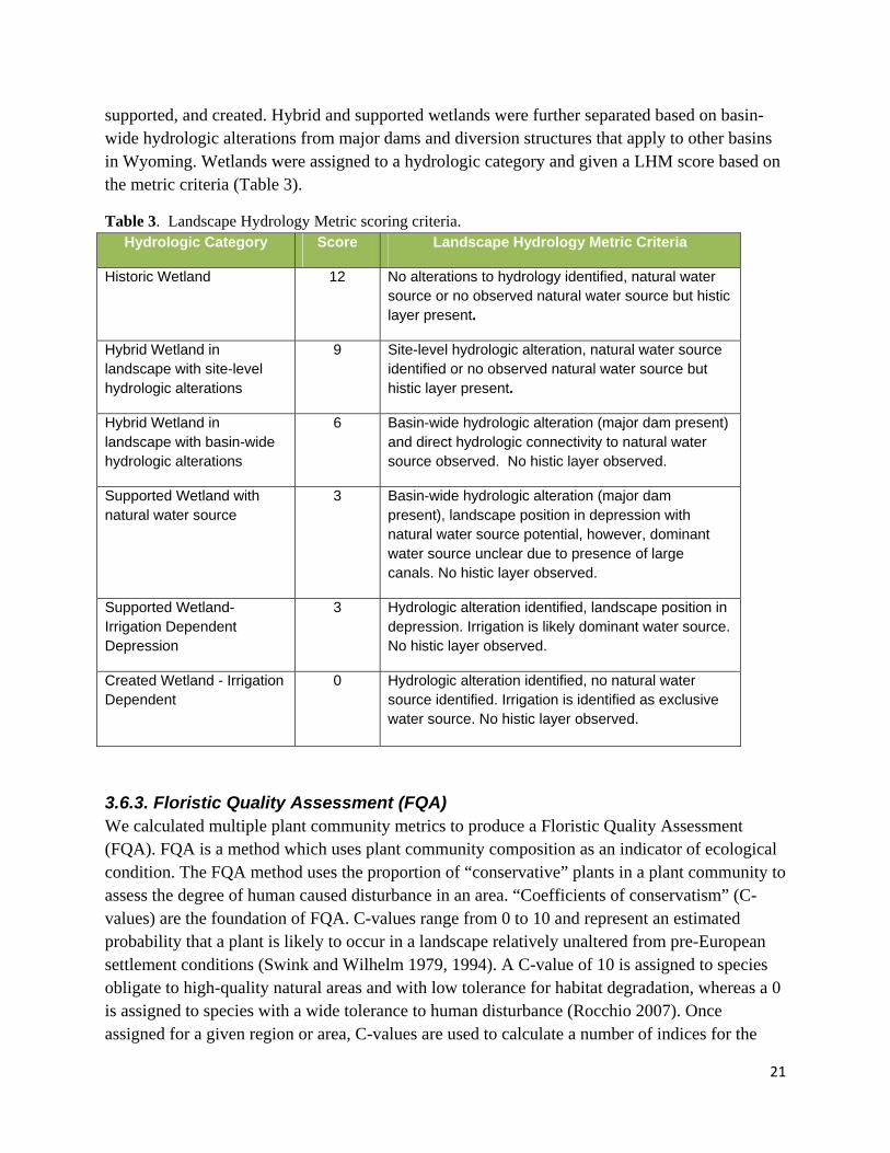
supported, and created. Hybrid and supported wetlands were further separated based on basin-wide hydrologic alterations from major dams and diversion structures that apply to other basins in Wyoming. Wetlands were assigned to a hydrologic category and given a LHM score based on the metric criteria (Table 3).

Table 3. Landscape Hydrology Metric scoring criteria.

 

 

 

 

 

 

 

 

 

3.6.3. Floristic Quality Assessment (FQA) We calculated multiple plant community metrics to produce a Floristic Quality Assessment (FQA). FQA is a method which uses plant community composition as an indicator of ecological condition. The FQA method uses the proportion of “conservative” plants in a plant community to assess the degree of human caused disturbance in an area. “Coefficients of conservatism” (C-values) are the foundation of FQA. C-values range from 0 to 10 and represent an estimated probability that a plant is likely to occur in a landscape relatively unaltered from pre-European settlement conditions (Swink and Wilhelm 1979, 1994). A C-value of 10 is assigned to species obligate to high-quality natural areas and with low tolerance for habitat degradation, whereas a 0 is assigned to species with a wide tolerance to human disturbance (Rocchio 2007). Once assigned for a given region or area, C-values are used to calculate a number of indices for the

Hydrologic Category Score Landscape Hydrology Metric Criteria

Historic Wetland 12 No alterations to hydrology identified, natural water source or no observed natural water source but histic layer present.

Hybrid Wetland in landscape with site-level hydrologic alterations

9 Site-level hydrologic alteration, natural water source identified or no observed natural water source but histic layer present.

Hybrid Wetland in landscape with basin-wide hydrologic alterations

6 Basin-wide hydrologic alteration (major dam present) and direct hydrologic connectivity to natural water source observed. No histic layer observed.

Supported Wetland with natural water source

3 Basin-wide hydrologic alteration (major dam present), landscape position in depression with natural water source potential, however, dominant water source unclear due to presence of large canals. No histic layer observed.

Supported Wetland- Irrigation Dependent Depression

3 Hydrologic alteration identified, landscape position in depression. Irrigation is likely dominant water source. No histic layer observed.

Created Wetland - Irrigation Dependent

0 Hydrologic alteration identified, no natural water source identified. Irrigation is identified as exclusive water source. No histic layer observed.

22  

FQA, such as the average C-value of a site (Mean C) and the Floristic Quality Assessment Index (FQAI) (Swink and Wilhelm 1979, 1994). Formal C-values do not currently exist for Wyoming. TNC staff developed a series of rules to assign surrogate C-values for the USDA Wetland Plant List (~1500 species) for Wyoming based on existing C-value data from Colorado, Nebraska, the Dakotas and Montana (Appendix F).

Using the species list from each wetland study site, we calculated Mean C, total species richness, and the number of native versus non-native species. Mean C is calculated by summing the C-values for the plant species found at a site and then dividing that value by the number of species. We also calculated Spearman’s correlation coefficients to evaluate the relationship between FQA metrics and disturbance indices and stressors metrics.

3.6.4. Defining Reference Condition Wetland RAM scores for each sample site were evaluated against those measured at reference sites for each wetland type. Reference sites ideally represent the natural variability of an expected reference condition. Reference condition is used to provide benchmarks in setting qualitative disturbance category boundaries (High, Moderate, Low) and to identify departures from an expected ecological condition. The selection of criteria for defining reference condition has a direct effect on the thresholds set for the disturbance category boundaries. Therefore, selection criteria for reference condition must be explicit and specific for the basin of study. Ideally, reference sites are those in minimally disturbed condition (MDC), representing the best approximation of “naturalness” or “biological integrity” on the landscape (Stoddard et al. 2006). Reference condition in the UGRB is defined as least disturbed condition (LDC), “in the best available physical, chemical and biological habitat conditions given today’s state of the landscape” (Stoddard et al. 2006). Because LDC can be different from MDC, our reference sites may represent a condition that does not reflect the full potential for biological integrity. We defined explicit inclusion and rejection criteria, or screens, for determining whether a given site meets the definition of LDC. These screens were derived from the data collected at the sites that had the least degree of exposure to the stressors of concern (Appendix G). The sites that passed all the screens within each wetland type were classified as being in reference condition. Three of the four of sites originally recommended as reference sites passed reference screening criteria. The same process was used to identify sites of highest disturbance, using screens derived from the data collected at the sites with the most exposure to the stressors of concern.

3.6.5. Wyoming Rapid Assessment Method (WYRAM) WYRAM scores were calculated using the submetric scores for RAM, LHM, and the Mean C. We used the following scoring formula based on regional EIA methods (Lemly and Gillian 2012; Newlon et al 2013) to assign weights to each submetric of the WYRAM:

WYRAM Score = (RAM Score*0.6) + (LHM Score*0.20) + (Mean C Score*0.20)

23  

While most RAMs are used to infer the ecological condition categories of a wetland resource, we chose to interpret the scores of WYRAM relative to disturbance categories. This decision was based on the fact that 7 of the 10 metrics used for RAM and the scoring criteria for LHM measure the presence and severity of anthropogenic alteration and stressors, not ecological condition of the resource directly. The remaining metrics measure the response of biological indicators of community integrity that are degraded in the presence of anthropogenic stressors and disturbance.

The WYRAM scores from reference and high disturbance sites were used to assign thresholds for high, medium, and low disturbance categories. Thresholds for disturbance categories were defined using the percentile of reference sites approach used for stream and wetland assessments (Paulsen et al. 2008; Jacobs et al. 2009). We defined the “low disturbance” category as those wetlands with a WYRAM score greater than or equal to the 25th percentile of the reference site scores within each wetland type. Sites with WYRAM scores less than or equal to the 75th percentile of the highest disturbance class sites were assigned to the “high” disturbance category. Sites with WYRAM scores in between the low and high disturbance categories were assigned to the “medium” disturbance category.

Cumulative distribution function (CDF) plots were used to estimate the percent of the total area of the target wetland population (i.e., all wetlands in the UGRB) that is less than or equal to a particular WYRAM score (Whittier et al. 2002). Disturbance categories assigned from WYRAM scores for each wetland type were used for estimates of percent and standard error of total target wetland area with each disturbance category.

3.6.6. Assessment of Wildlife Habitat The database and models used for the Avian Richness Evaluation Method (Adamus 1993) were updated from MS-DOS to Microsoft Access. Habitat indicators were entered for a total of 261 wetland and riparian birds found in Wyoming. The list of birds included in the model was primarily determined using the Atlas of Birds, Mammals, Amphibians, and Reptiles in Wyoming (Orabona et al. 2012) to include all bird species that use wetlands, riparian areas and irrigated lands. Rare species were not included. The final list was narrowed by considering professional opinion (S. Patla, personal communication), regional abundance information, and checklists (WGFD 2008, Faulkner 2010). Data were analyzed using the AREM database and models for birds located in the SW region of Wyoming during the breeding season (WGFD 2008). The model uses site-specific habitat data to determine the “habitat suitability” for each species, ranging from 0 (least suitable) to 1 (most suitable) based on habitat indicators for each site. A bird species is included in a list of species for each site based on set thresholds of habitat suitability scores defined by the AREM user. For example, if the habitat suitability score for a bird species is 0.65, that bird would not be included in a species list for a wetland if the threshold score is set to 0.75. Species richness estimates for the UGRB were calculated at each wetland using the 0.75 threshold value because this threshold was successfully used to predict species presence of wetland birds in the Colorado Plateau (Adamus 1993). We calculated Spearman’s

24  

correlation coefficients to evaluate the relationship between AREM species richness results and WYRAM metrics.

4.0 RESULTS

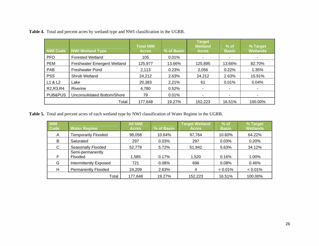
4.1 Wetland Landscape Profile for Upper Green River Basin We created a landscape profile for the Upper Green River Basin that covers 921,948 acres of southwest Wyoming which includes both target and non-target wetlands and waterbodies based on NWI data. There are 177,648 acres of wetlands and water bodies which represent approximately 20% of the total land area of the basin (Table 4). Target wetlands included in our study design account for 152,223 acres and represent 16% of the basin’s area. The NWI data includes non-wetland features such as deep water lakes and stream channels as well as non-target forested wetlands. While these features are important water resources in the basin and represent 25,286 acres or 3% of total land area, they were not included as part of the study design. Freshwater emergent wetlands are the most common wetland type mapped in the basin. These wetlands cover 125,977 total acres or approximately 14% of the basins area and represent 83% of the total wetland acres. Freshwater emergent wetlands include irrigated hayfields, wet meadows, and emergent vegetation zones around more permanent water features like rivers and ponds. The second most common wetland type is shrub wetlands, which are typically interspersed with freshwater emergent wetlands in riverine flood plains. Shrub wetlands cover 24,212 total acres or approximately 3% of the basin and represent 16% of the total wetland acres. Temporarily flooded and seasonally flooded are the two most common wetland hydrologic regimes in the basin. Temporarily flooded wetlands have surface water for brief periods during the growing season. Many freshwater emergent wetlands are temporarily flooded. Approximately 10% of the basin area, and 64% of the wetland area, is mapped as temporarily flooded (Table 5). Seasonally flooded wetlands have surface water present for extended periods during the growing season but are dry by the end of the season in most years. Many riverine shrublands located along rivers and streams that depend on snow melt fall into this category. Seasonally flooded wetlands account for 6% of the basins area and 34% of the target wetland acres. Permanently flooded water bodies, such as lakes and river channels, make up 24,209 acres (~3%) of the basin area but account for only 4 (<0.01%) wetland acres.

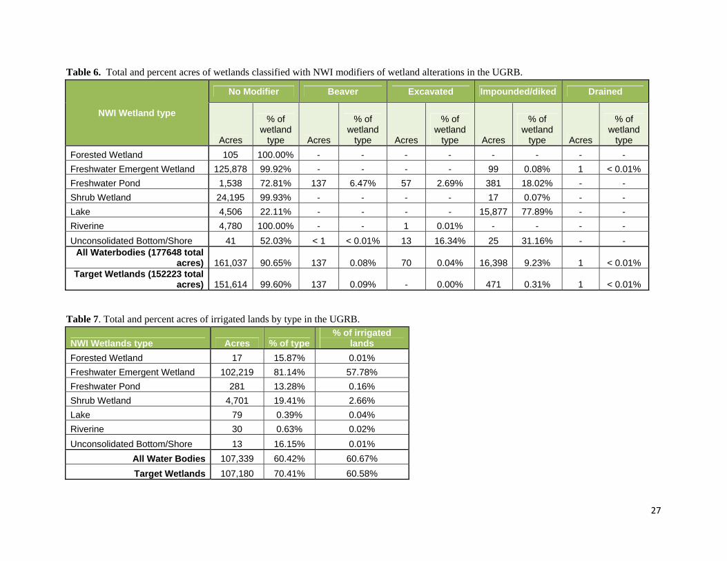
NWI maps include modifiers to identify water bodies that have man-made and natural alterations. More than 90% of all water bodies and over 99% of target wetlands in the UGRB have no modifiers (Table 6). Beaver activity is the only natural alteration mapped. Beaver influenced wetlands account for approximately 137 acres of water bodies, mainly freshwater ponds, which is less than 1 percent of the total area. The highest proportion of man-made alterations affects lakes and unconsolidated bottoms/shores, representing 9% of the total water body area. These water features are typically impounded or diked reservoirs, which account for

25  

78% and 32% of the water bodies’ area respectively. Excavation is the second-largest man-made alteration to the landscape, representing less than 0.04 % of the total area.

Irrigation was not explicitly included in the NWI mapping as a modifier, even though much of the basin receives irrigation for agricultural hay production. There are approximately 107,339 acres (19% of the study area) mapped as irrigated lands (Wyoming Wildlife Consultants 2007)(Table 7). According to NWI mapping almost 100% of the freshwater emergent wetlands have no anthropogenic modification. Irrigation data shows that over 81% of freshwater marshes receive irrigation inputs. Shrub wetlands represent the second-largest wetland, group receiving irrigation inputs. Approximately 20% of shrub lands are irrigated, representing approximately 3% of all irrigated lands. These two wetland types often occur in flood plains that are used for hay production and cattle grazing.

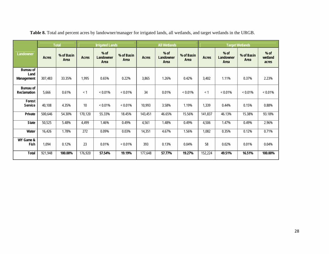
Private landowners and the Bureau of Land Management (BLM) are the two largest landowners/managers in the UGRB, representing 54% and 33% of the study area, respectively (Table 8). Lands managed by the U.S. Forest Service and the State of Wyoming each account for approximately 5% of the study area. Less than 2% of the area is managed by the Bureau of Reclamation, the Wyoming Game and Fish Department, or is mapped as water that lacks direct ownership. This includes major reservoirs at the base of the Wind River Mountains such as Fremont and New Fork Lakes, Fontenelle Reservoir, and portions of the Green River.

Most private lands occur in the floodplains of the Green River and its tributaries; consequently, the largest proportions of wetlands, water bodies and irrigated lands are privately owned as compared to other landowners or managers (Table 8). Approximately 55% of all private lands (141,837 acres) are irrigated and they contain over 93% of target wetlands acres. These irrigated private lands constitute 15% of the area of the basin. The second-largest concentration of targeted wetland acres occurs on State and BLM land (~5% of target wetlands, combined). Less than 1% of these lands receive irrigation inputs, mainly from adjacent private lands.

26  

Table 4. Total and percent acres by wetland type and NWI classification in the UGRB.

NWI Code NWI Wetland Type Total NWI

Acres % of Basin

Target Wetland

Acres % of

Basin % Target Wetlands

PFO Forested Wetland 105 0.01% - - -

PEM Freshwater Emergent Wetland 125,977 13.66% 125,895 13.66% 82.70%

PAB Freshwater Pond 2,113 0.23% 2,056 0.22% 1.35%

PSS Shrub Wetland 24,212 2.63% 24,212 2.63% 15.91%

L1 & L2 Lake 20,383 2.21% 61 0.01% 0.04%

R2,R3,R4 Riverine 4,780 0.52% - - -

PUB&PUS Unconsolidated Bottom/Shore 79 0.01% - - -

Total 177,648 19.27% 152,223 16.51% 100.00%

Table 5. Total and percent acres of each wetland type by NWI classification of Water Regime in the UGRB.

NWI Code Water Regime

All NWI Acres % of Basin

Target Wetland Acres

% of Basin

% Target Wetlands

A Temporarily Flooded 98,058 10.64% 97,764 10.60% 64.22%

B Saturated 297 0.03% 297 0.03% 0.20%

C Seasonally Flooded 52,779 5.72% 51,942 5.63% 34.12%

F Semi-permanently Flooded 1,585 0.17% 1,520 0.16% 1.00%

G Intermittently Exposed 721 0.08% 696 0.08% 0.46%

H Permanently Flooded 24,209 2.63% 4 < 0.01% < 0.01%

Total 177,648 19.27% 152,223 16.51% 100.00%

27  

Table 6. Total and percent acres of wetlands classified with NWI modifiers of wetland alterations in the UGRB.

NWI Wetland type

No Modifier Beaver Excavated Impounded/diked Drained

Acres

% of wetland

type Acres

% of wetland

type Acres

% of wetland

type Acres

% of wetland

type Acres

% of wetland

type

Forested Wetland 105 100.00% - - - - - - - -

Freshwater Emergent Wetland 125,878 99.92% - - - - 99 0.08% 1 < 0.01%

Freshwater Pond 1,538 72.81% 137 6.47% 57 2.69% 381 18.02% - -

Shrub Wetland 24,195 99.93% - - - - 17 0.07% - -

Lake 4,506 22.11% - - - - 15,877 77.89% - -

Riverine 4,780 100.00% - - 1 0.01% - - - -

Unconsolidated Bottom/Shore 41 52.03% < 1 < 0.01% 13 16.34% 25 31.16% - - All Waterbodies (177648 total

acres) 161,037 90.65% 137 0.08% 70 0.04% 16,398 9.23% 1 < 0.01% Target Wetlands (152223 total

acres) 151,614 99.60% 137 0.09% - 0.00% 471 0.31% 1 < 0.01%

Table 7. Total and percent acres of irrigated lands by type in the UGRB.

NWI Wetlands type Acres % of type % of irrigated

lands

Forested Wetland 17 15.87% 0.01%

Freshwater Emergent Wetland 102,219 81.14% 57.78%

Freshwater Pond 281 13.28% 0.16%

Shrub Wetland 4,701 19.41% 2.66%

Lake 79 0.39% 0.04%

Riverine 30 0.63% 0.02%

Unconsolidated Bottom/Shore 13 16.15% 0.01%

All Water Bodies 107,339 60.42% 60.67%

Target Wetlands 107,180 70.41% 60.58%

28  

Table 8. Total and percent acres by landowner/manager for irrigated lands, all wetlands, and target wetlands in the URGB.

Landowner

Total Irrigated Lands All Wetlands Target Wetlands

Acres % of Basin

Area Acres

% of Landowner

Area

% of Basin Area

Acres % of

Landowner Area

% of Basin Area

Acres % of

Landowner Area

% of Basin Area

% of wetland acres

Bureau of Land

Management 307,483 33.35% 1,995 0.65% 0.22% 3,865 1.26% 0.42% 3,402 1.11% 0.37% 2.23%

Bureau of Reclamation 5,666 0.61% < 1 < 0.01% < 0.01% 34 0.01% < 0.01% < 1 < 0.01% < 0.01% < 0.01%

Forest Service 40,108 4.35% 10 < 0.01% < 0.01% 10,993 3.58% 1.19% 1,339 0.44% 0.15% 0.88%

Private 500,646 54.30% 170,120 55.33% 18.45% 143,451 46.65% 15.56% 141,837 46.13% 15.38% 93.18%

State 50,525 5.48% 4,499 1.46% 0.49% 4,561 1.48% 0.49% 4,506 1.47% 0.49% 2.96%

Water 16,426 1.78% 272 0.09% 0.03% 14,351 4.67% 1.56% 1,082 0.35% 0.12% 0.71%

WY Game & Fish 1,094 0.12% 23 0.01% < 0.01% 393 0.13% 0.04% 58 0.02% 0.01% 0.04%

Total 921,948 100.00% 176,920 57.54% 19.19% 177,648 57.77% 19.27% 152,224 49.51% 16.51% 100.00%

29  

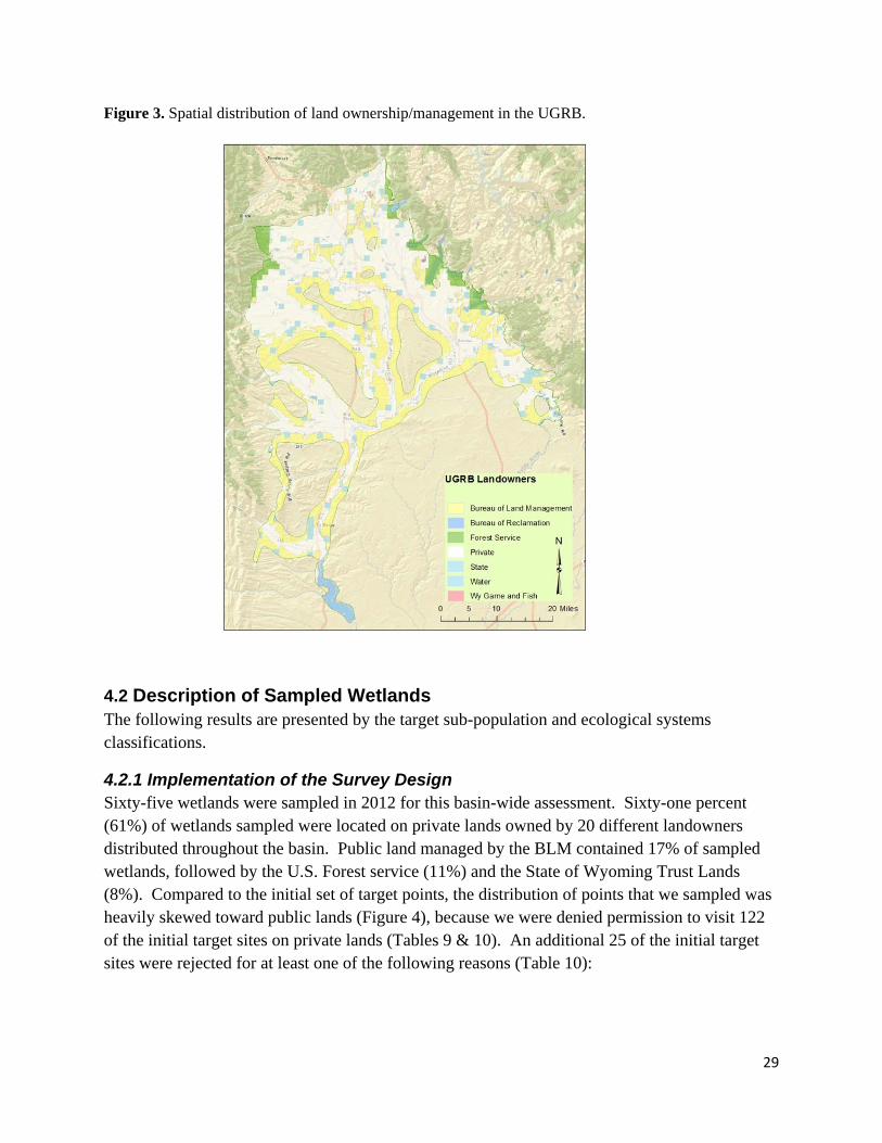
Figure 3. Spatial distribution of land ownership/management in the UGRB.

 

4.2 Description of Sampled Wetlands The following results are presented by the target sub-population and ecological systems classifications.

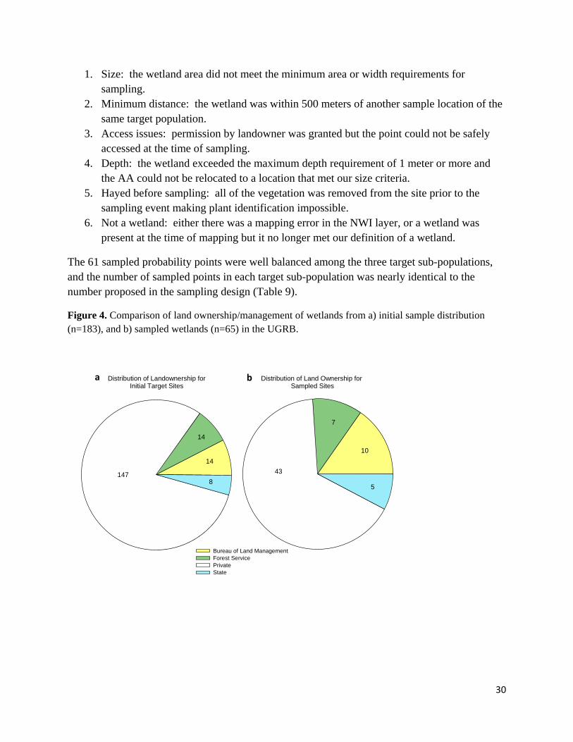
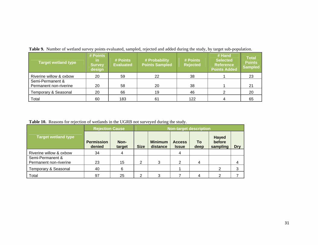
4.2.1 Implementation of the Survey Design Sixty-five wetlands were sampled in 2012 for this basin-wide assessment. Sixty-one percent (61%) of wetlands sampled were located on private lands owned by 20 different landowners distributed throughout the basin. Public land managed by the BLM contained 17% of sampled wetlands, followed by the U.S. Forest service (11%) and the State of Wyoming Trust Lands (8%). Compared to the initial set of target points, the distribution of points that we sampled was heavily skewed toward public lands (Figure 4), because we were denied permission to visit 122 of the initial target sites on private lands (Tables 9 & 10). An additional 25 of the initial target sites were rejected for at least one of the following reasons (Table 10):

30  

1. Size: the wetland area did not meet the minimum area or width requirements for sampling.

2. Minimum distance: the wetland was within 500 meters of another sample location of the same target population.

3. Access issues: permission by landowner was granted but the point could not be safely accessed at the time of sampling.

4. Depth: the wetland exceeded the maximum depth requirement of 1 meter or more and the AA could not be relocated to a location that met our size criteria.

5. Hayed before sampling: all of the vegetation was removed from the site prior to the sampling event making plant identification impossible.

6. Not a wetland: either there was a mapping error in the NWI layer, or a wetland was present at the time of mapping but it no longer met our definition of a wetland.

The 61 sampled probability points were well balanced among the three target sub-populations, and the number of sampled points in each target sub-population was nearly identical to the number proposed in the sampling design (Table 9).

Figure 4. Comparison of land ownership/management of wetlands from a) initial sample distribution (n=183), and b) sampled wetlands (n=65) in the UGRB.

Bureau of Land ManagementForest ServicePrivateState

147

14

14

8

43

10

7

5

Distribution of Landownership forInitial Target Sites

Distribution of Land Ownership for Sampled Sites

a  b

31  

Table 9. Number of wetland survey points evaluated, sampled, rejected and added during the study, by target sub-population.

Target wetland type

# Points in

Survey design

# Points Evaluated

# Probability Points Sampled

# Points Rejected

# Hand Selected

Reference Points Added

Total Points

Sampled

Riverine willow & oxbow 20 59 22 38 1 23 Semi-Permanent & Permanent non-riverine 20 58 20 38 1 21

Temporary & Seasonal 20 66 19 46 2 20

Total 60 183 61 122 4 65

Table 10. Reasons for rejection of wetlands in the UGRB not surveyed during the study.

Target wetland type

Rejection Cause Non-target description

Permission denied

Non-target Size

Minimum distance

Access Issue

To deep

Hayed before

sampling Dry

Riverine willow & oxbow 34 4 4 Semi-Permanent & Permanent non-riverine 23 15 2 3 2 4 4

Temporary & Seasonal 40 6 1 2 3

Total 97 25 2 3 7 4 2 7

32  

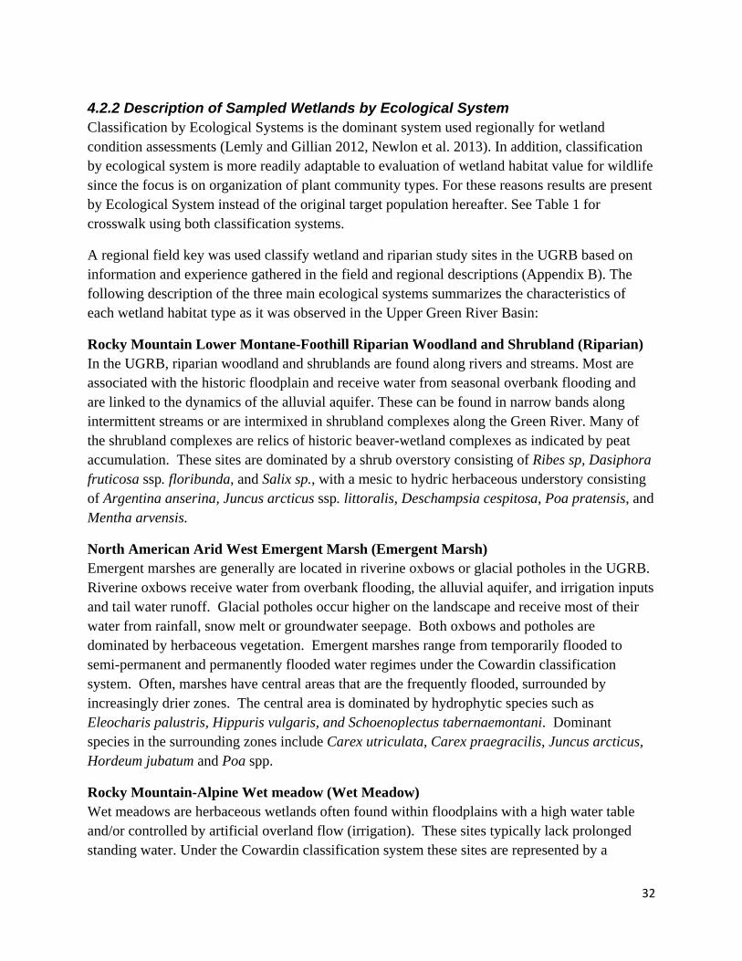
4.2.2 Description of Sampled Wetlands by Ecological System Classification by Ecological Systems is the dominant system used regionally for wetland condition assessments (Lemly and Gillian 2012, Newlon et al. 2013). In addition, classification by ecological system is more readily adaptable to evaluation of wetland habitat value for wildlife since the focus is on organization of plant community types. For these reasons results are present by Ecological System instead of the original target population hereafter. See Table 1 for crosswalk using both classification systems.

A regional field key was used classify wetland and riparian study sites in the UGRB based on information and experience gathered in the field and regional descriptions (Appendix B). The following description of the three main ecological systems summarizes the characteristics of each wetland habitat type as it was observed in the Upper Green River Basin:

Rocky Mountain Lower Montane-Foothill Riparian Woodland and Shrubland (Riparian) In the UGRB, riparian woodland and shrublands are found along rivers and streams. Most are associated with the historic floodplain and receive water from seasonal overbank flooding and are linked to the dynamics of the alluvial aquifer. These can be found in narrow bands along intermittent streams or are intermixed in shrubland complexes along the Green River. Many of the shrubland complexes are relics of historic beaver-wetland complexes as indicated by peat accumulation. These sites are dominated by a shrub overstory consisting of Ribes sp, Dasiphora fruticosa ssp. floribunda, and Salix sp., with a mesic to hydric herbaceous understory consisting of Argentina anserina, Juncus arcticus ssp. littoralis, Deschampsia cespitosa, Poa pratensis, and Mentha arvensis.

North American Arid West Emergent Marsh (Emergent Marsh) Emergent marshes are generally are located in riverine oxbows or glacial potholes in the UGRB. Riverine oxbows receive water from overbank flooding, the alluvial aquifer, and irrigation inputs and tail water runoff. Glacial potholes occur higher on the landscape and receive most of their water from rainfall, snow melt or groundwater seepage. Both oxbows and potholes are dominated by herbaceous vegetation. Emergent marshes range from temporarily flooded to semi-permanent and permanently flooded water regimes under the Cowardin classification system. Often, marshes have central areas that are the frequently flooded, surrounded by increasingly drier zones. The central area is dominated by hydrophytic species such as Eleocharis palustris, Hippuris vulgaris, and Schoenoplectus tabernaemontani. Dominant species in the surrounding zones include Carex utriculata, Carex praegracilis, Juncus arcticus, Hordeum jubatum and Poa spp.

Rocky Mountain-Alpine Wet meadow (Wet Meadow) Wet meadows are herbaceous wetlands often found within floodplains with a high water table and/or controlled by artificial overland flow (irrigation). These sites typically lack prolonged standing water. Under the Cowardin classification system these sites are represented by a

33  

temporary or seasonal water regime. Vegetation is dominated by native or non-native herbaceous species, with graminoids contributing the most canopy cover. Species composition may be dominated by non-native hay grasses such as Poa spp., Alopecurus spp., Phleum pretense, and Bromus inermis ssp. inermis. There can be patches of emergent marsh vegetation and standing water less than 0.1 ha in size but these are not the predominant vegetation. While very rare in the UGRB, some wet meadows are associated with groundwater seepage and have fen like characteristics represented by histic soils. Under the Cowardin classification system these sites have a saturated water regime. Typical dominant species in these sites include Carex nebrascensis, Deschampsia cespitosa, Pedicularis groenlandica, and Caltha leptosepala.

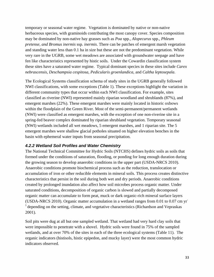
The Ecological Systems classification schema of study sites in the UGRB generally followed NWI classifications, with some exceptions (Table 1). These exceptions highlight the variation in different community types that occur within each NWI classification. For example, sites classified as riverine (NWI) represented mainly riparian woodland and shrublands (87%), and emergent marshes (22%). These emergent marshes were mainly located in historic oxbows within the floodplain of the Green River. Most of the semi-permanent/permanent wetlands (NWI) were classified as emergent marshes, with the exception of one non-riverine site in a spring-fed beaver complex dominated by riparian shrubland vegetation. Temporary seasonal (NWI) wetlands included all wet meadows, 5 emergent marshes, and 1 riparian site. The 5 emergent marshes were shallow glacial potholes situated on higher elevation benches in the basin with ephemeral water inputs from seasonal precipitation.

4.2.2 Wetland Soil Profiles and Water Chemistry The National Technical Committee for Hydric Soils (NTCHS) defines hydric soils as soils that formed under the conditions of saturation, flooding, or ponding for long enough duration during the growing season to develop anaerobic conditions in the upper part (USDA-NRCS 2010). Anaerobic conditions promote biochemical process such as the reduction, translocation or accumulation of iron or other reducible elements in mineral soils. This process creates distinctive characteristics that persist in the soil during both wet and dry periods. Anaerobic conditions created by prolonged inundation also affect how soil microbes process organic matter. Under saturated conditions, decomposition of organic carbon is slowed and partially decomposed organic matter can accumulate to form peat, muck or dark organic-rich mineral surface layers (USDA-NRCS 2010). Organic matter accumulation in a wetland ranges from 0.01 to 0.07 cm yr-

1 depending on the setting, climate, and vegetative characteristics (Richardson and Vepraskas 2001).

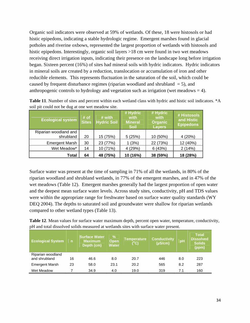
Soil pits were dug at all but one sampled wetland. That wetland had very hard clay soils that were impossible to penetrate with a shovel. Hydric soils were found in 75% of the sampled wetlands, and at over 70% of the sites in each of the three ecological systems (Table 11). The organic indicators (histisols, histic epipedon, and mucky layer) were the most common hydric indicators observed.

34  

Organic soil indicators were observed at 59% of wetlands. Of these, 18 were histosols or had histic epipedons, indicating a stable hydrologic regime. Emergent marshes found in glacial potholes and riverine oxbows, represented the largest proportion of wetlands with histosols and histic epipedons. Interestingly, organic soil layers >18 cm were found in two wet meadows receiving direct irrigation inputs, indicating their presence on the landscape long before irrigation began. Sixteen percent (16%) of sites had mineral soils with hydric indicators. Hydric indicators in mineral soils are created by a reduction, translocation or accumulation of iron and other reducible elements. This represents fluctuation in the saturation of the soil, which could be caused by frequent disturbance regimes (riparian woodland and shrubland = 5), and anthropogenic controls to hydrology and vegetation such as irrigation (wet meadows = 4).

Table 11. Number of sites and percent within each wetland class with hydric and histic soil indicators. *A soil pit could not be dug at one wet meadow site.

Ecological system # of

Sites # with

Hydric Soil

# Hydric with

Mineral Soil

# Hydric with

Organic Layers

# Histosols and Histic Epipedons

Riparian woodland and shrubland 20 15 (75%) 5 (25%) 10 (50%) 4 (20%)

Emergent Marsh 30 23 (77%) 1 (3%) 22 (73%) 12 (40%) Wet Meadow* 14 10 (71%) 4 (29%) 6 (43%) 2 (14%)

Total 64 48 (75%) 10 (16%) 38 (59%) 18 (28%)

Surface water was present at the time of sampling in 71% of all the wetlands, in 80% of the riparian woodland and shrubland wetlands, in 77% of the emergent marshes, and in 47% of the wet meadows (Table 12). Emergent marshes generally had the largest proportion of open water and the deepest mean surface water levels. Across study sites, conductivity, pH and TDS values were within the appropriate range for freshwater based on surface water quality standards (WY DEQ 2004). The depths to saturated soil and groundwater were shallow for riparian wetlands compared to other wetland types (Table 13).

Table 12. Mean values for surface water maximum depth, percent open water, temperature, conductivity, pH and total dissolved solids measured at wetlands sites with surface water present.

Ecological System n Surface Water

Maximum Depth (cm)

% Open Water

Temperature (oC)

Conductivity (µS/cm)

pH

Total Dissolved

Solids (ppm)

Riparian woodland and shrubland 16 46.6 8.0 20.7 446 8.0 223

Emergent Marsh 23 58.0 23.1 20.2 565 8.2 287

Wet Meadow 7 34.9 4.0 19.0 319 7.1 160

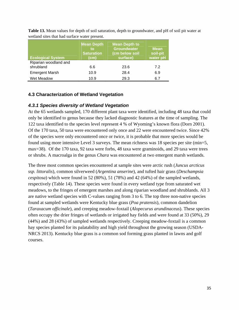
35  

Table 13. Mean values for depth of soil saturation, depth to groundwater, and pH of soil pit water at wetland sites that had surface water present.

Ecological System

Mean Depth to

Saturation (cm)

Mean Depth to Groundwater

(cm below soil surface)

Mean soil-pit

water pH Riparian woodland and shrubland 6.6 23.6 7.2

Emergent Marsh 10.9 28.4 6.9

Wet Meadow 10.9 29.3 6.7

4.3 Characterization of Wetland Vegetation

4.3.1 Species diversity of Wetland Vegetation At the 65 wetlands sampled, 170 different plant taxa were identified, including 48 taxa that could only be identified to genus because they lacked diagnostic features at the time of sampling. The 122 taxa identified to the species level represent 4 % of Wyoming’s known flora (Dorn 2001). Of the 170 taxa, 50 taxa were encountered only once and 22 were encountered twice. Since 42% of the species were only encountered once or twice, it is probable that more species would be found using more intensive Level 3 surveys. The mean richness was 18 species per site (min=5, max=38). Of the 170 taxa, 92 taxa were forbs, 48 taxa were graminoids, and 29 taxa were trees or shrubs. A macroalga in the genus Chara was encountered at two emergent marsh wetlands.

The three most common species encountered at sample sites were arctic rush (Juncus arcticus ssp. littoralis), common silverweed (Argentina anserine), and tufted hair grass (Deschampsia cespitosa) which were found in 52 (80%), 51 (78%) and 42 (64%) of the sampled wetlands, respectively (Table 14). These species were found in every wetland type from saturated wet meadows, to the fringes of emergent marshes and along riparian woodland and shrublands. All 3 are native wetland species with C-values ranging from 3 to 6. The top three non-native species found at sampled wetlands were Kentucky blue grass (Poa pratensis), common dandelion (Taraxacum officinale), and creeping meadow-foxtail (Alopecurus arundinaceus). These species often occupy the drier fringes of wetlands or irrigated hay fields and were found at 33 (50%), 29 (44%) and 28 (43%) of sampled wetlands respectively. Creeping meadow-foxtail is a common hay species planted for its palatability and high yield throughout the growing season (USDA-NRCS 2013). Kentucky blue grass is a common sod forming grass planted in lawns and golf courses.

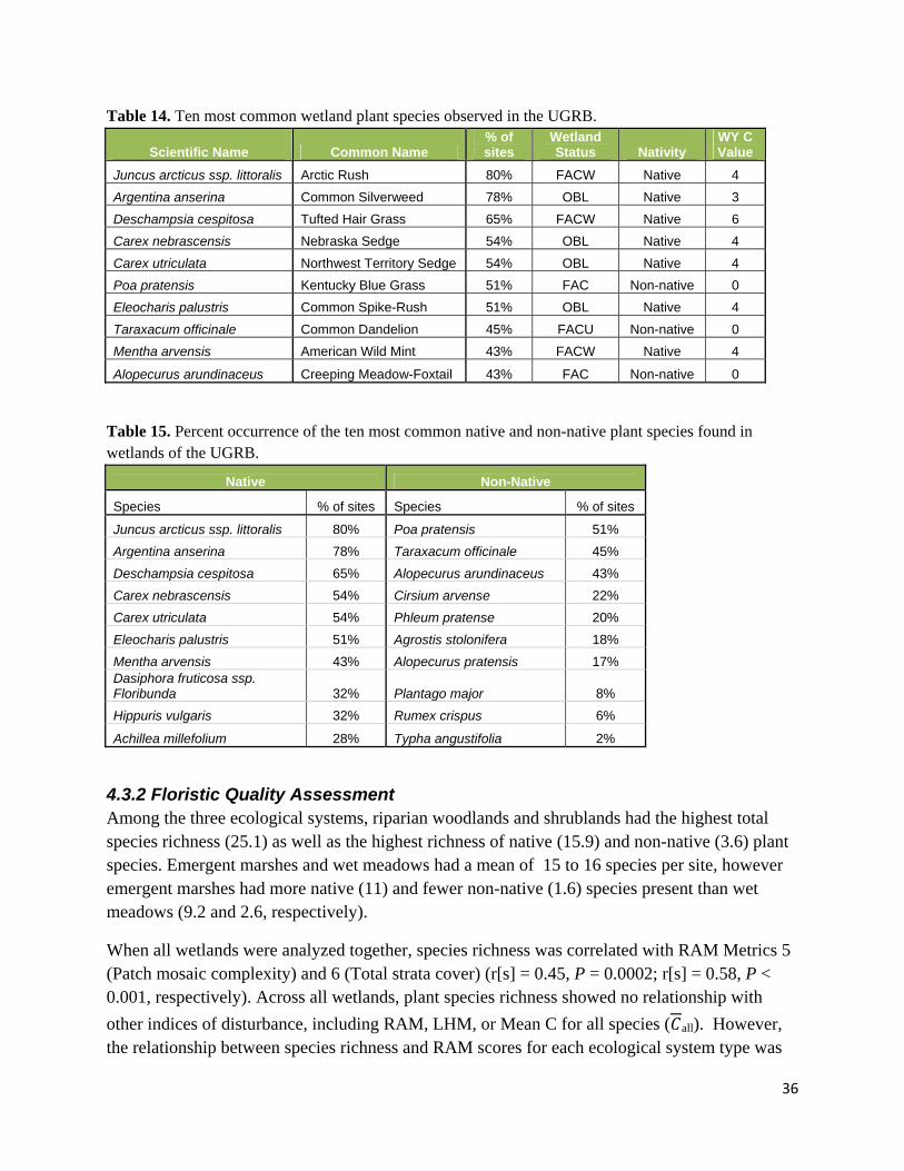
36  

Table 14. Ten most common wetland plant species observed in the UGRB.

Scientific Name Common Name % of sites

Wetland Status Nativity

WY C Value

Juncus arcticus ssp. littoralis Arctic Rush 80% FACW Native 4

Argentina anserina Common Silverweed 78% OBL Native 3

Deschampsia cespitosa Tufted Hair Grass 65% FACW Native 6

Carex nebrascensis Nebraska Sedge 54% OBL Native 4

Carex utriculata Northwest Territory Sedge 54% OBL Native 4

Poa pratensis Kentucky Blue Grass 51% FAC Non-native 0

Eleocharis palustris Common Spike-Rush 51% OBL Native 4

Taraxacum officinale Common Dandelion 45% FACU Non-native 0

Mentha arvensis American Wild Mint 43% FACW Native 4

Alopecurus arundinaceus Creeping Meadow-Foxtail 43% FAC Non-native 0

Table 15. Percent occurrence of the ten most common native and non-native plant species found in wetlands of the UGRB.

Native Non-Native

Species % of sites Species % of sites

Juncus arcticus ssp. littoralis 80% Poa pratensis 51%

Argentina anserina 78% Taraxacum officinale 45%

Deschampsia cespitosa 65% Alopecurus arundinaceus 43%

Carex nebrascensis 54% Cirsium arvense 22%

Carex utriculata 54% Phleum pratense 20%

Eleocharis palustris 51% Agrostis stolonifera 18%

Mentha arvensis 43% Alopecurus pratensis 17% Dasiphora fruticosa ssp. Floribunda 32% Plantago major 8%

Hippuris vulgaris 32% Rumex crispus 6%

Achillea millefolium 28% Typha angustifolia 2%

4.3.2 Floristic Quality Assessment Among the three ecological systems, riparian woodlands and shrublands had the highest total species richness (25.1) as well as the highest richness of native (15.9) and non-native (3.6) plant species. Emergent marshes and wet meadows had a mean of 15 to 16 species per site, however emergent marshes had more native (11) and fewer non-native (1.6) species present than wet meadows (9.2 and 2.6, respectively).

When all wetlands were analyzed together, species richness was correlated with RAM Metrics 5 (Patch mosaic complexity) and 6 (Total strata cover) (r[s] = 0.45, P = 0.0002; r[s] = 0.58, P < 0.001, respectively). Across all wetlands, plant species richness showed no relationship with

other indices of disturbance, including RAM, LHM, or Mean C for all species ( all). However, the relationship between species richness and RAM scores for each ecological system type was

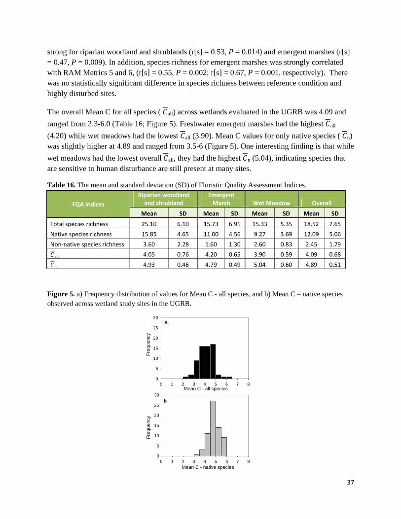
37  

strong for riparian woodland and shrublands (r[s] = 0.53, P = 0.014) and emergent marshes (r[s] = 0.47, P = 0.009). In addition, species richness for emergent marshes was strongly correlated with RAM Metrics 5 and 6, (r[s] = 0.55, P = 0.002; r[s] = 0.67, P = 0.001, respectively). There was no statistically significant difference in species richness between reference condition and highly disturbed sites.

The overall Mean C for all species ( all) across wetlands evaluated in the UGRB was 4.09 and

ranged from 2.3-6.0 (Table 16; Figure 5). Freshwater emergent marshes had the highest all

(4.20) while wet meadows had the lowest all (3.90). Mean C values for only native species ( n) was slightly higher at 4.89 and ranged from 3.5-6 (Figure 5). One interesting finding is that while

wet meadows had the lowest overall all, they had the highest n (5.04), indicating species that are sensitive to human disturbance are still present at many sites.

Table 16. The mean and standard deviation (SD) of Floristic Quality Assessment Indices.

FQA Indices 

Riparian woodland and shrubland 

Emergent Marsh  Wet Meadow  Overall 

Mean  SD  Mean  SD  Mean  SD  Mean  SD 

Total species richness  25.10  6.10  15.73  6.91  15.33  5.35  18.52  7.65 

Native species richness  15.85  4.65  11.00  4.56  9.27  3.69  12.09  5.06 

Non‐native species richness  3.60  2.28  1.60  1.30  2.60  0.83  2.45  1.79 

all  4.05  0.76  4.20  0.65  3.90  0.59  4.09  0.68 

n  4.93  0.46  4.79  0.49  5.04  0.60  4.89  0.51 

Figure 5. a) Frequency distribution of values for Mean C - all species, and b) Mean C – native species observed across wetland study sites in the UGRB.

Mean C - all species0 1 2 3 4 5 6 7 8

Fre

que

ncy

0

5

10

15

20

25

30

0 1 2 3 4 5 6 7 80

5

10

15

20

25

30

Fre

que

ncy

Mean C - native species

a.

b.

 

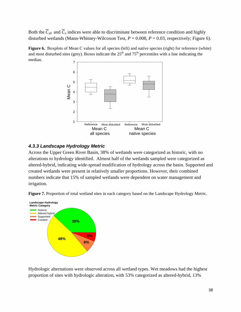
38  

Mea

n C

1

2

3

4

5

6

7

Mean C all species

Mean C native species

Reference Most disturbed Reference Most disturbed

Both the  all and n indices were able to discriminate between reference condition and highly disturbed wetlands (Mann-Whitney-Wilcoxon Test, P = 0.008, P = 0.03, respectively; Figure 6).

Figure 6. Boxplots of Mean C values for all species (left) and native species (right) for reference (white) and most disturbed sites (grey). Boxes indicate the 25th and 75th percentiles with a line indicating the median.

 

 

 

 

 

 

 

4.3.3 Landscape Hydrology Metric Across the Upper Green River Basin, 38% of wetlands were categorized as historic, with no alterations to hydrology identified. Almost half of the wetlands sampled were categorized as altered-hybrid, indicating wide-spread modification of hydrology across the basin. Supported and created wetlands were present in relatively smaller proportions. However, their combined numbers indicate that 15% of sampled wetlands were dependent on water management and irrigation.

Figure 7. Proportion of total wetland sites in each category based on the Landscape Hydrology Metric.

Landscape Hydrology Metric Category

HistoricAltered hybridSupportedCreated

 

38%

8%48%

6%

 

Hydrologic alternations were observed across all wetland types. Wet meadows had the highest proportion of sites with hydrologic alteration, with 53% categorized as altered-hybrid, 13%

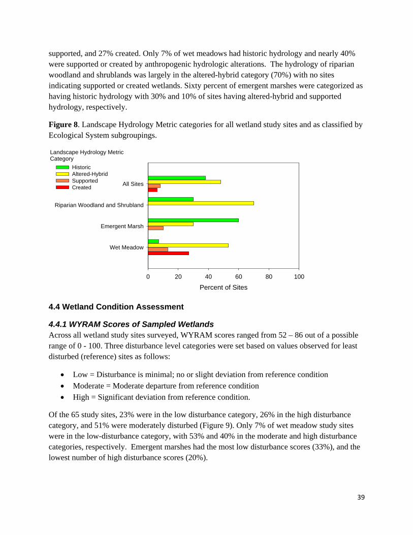
39  

supported, and 27% created. Only 7% of wet meadows had historic hydrology and nearly 40% were supported or created by anthropogenic hydrologic alterations. The hydrology of riparian woodland and shrublands was largely in the altered-hybrid category (70%) with no sites indicating supported or created wetlands. Sixty percent of emergent marshes were categorized as having historic hydrology with 30% and 10% of sites having altered-hybrid and supported hydrology, respectively.

Figure 8. Landscape Hydrology Metric categories for all wetland study sites and as classified by Ecological System subgroupings.

Landscape Hydrology Metric Category

Percent of Sites

0 20 40 60 80 100

All Sites

Riparian Woodland and Shrubland

Emergent Marsh

Wet Meadow

HistoricAltered-HybridSupportedCreated

4.4 Wetland Condition Assessment

4.4.1 WYRAM Scores of Sampled Wetlands Across all wetland study sites surveyed, WYRAM scores ranged from 52 – 86 out of a possible range of 0 - 100. Three disturbance level categories were set based on values observed for least disturbed (reference) sites as follows:

Low = Disturbance is minimal; no or slight deviation from reference condition

Moderate = Moderate departure from reference condition

High = Significant deviation from reference condition.

Of the 65 study sites, 23% were in the low disturbance category, 26% in the high disturbance category, and 51% were moderately disturbed (Figure 9). Only 7% of wet meadow study sites were in the low-disturbance category, with 53% and 40% in the moderate and high disturbance categories, respectively. Emergent marshes had the most low disturbance scores (33%), and the lowest number of high disturbance scores (20%).

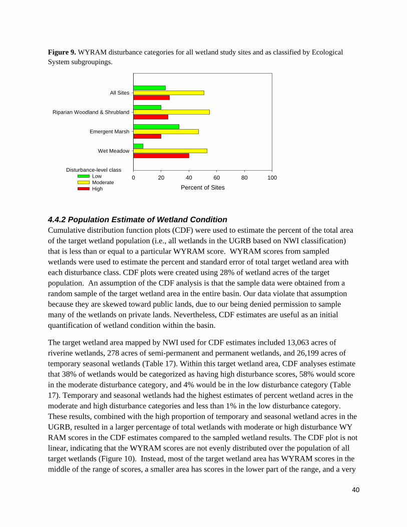
40  

Disturbance-level class

Percent of Sites

0 20 40 60 80 100

All Sites

Riparian Woodland & Shrubland

Emergent Marsh

Wet Meadow

LowModerateHigh

Figure 9. WYRAM disturbance categories for all wetland study sites and as classified by Ecological System subgroupings.  

4.4.2 Population Estimate of Wetland Condition Cumulative distribution function plots (CDF) were used to estimate the percent of the total area of the target wetland population (i.e., all wetlands in the UGRB based on NWI classification) that is less than or equal to a particular WYRAM score. WYRAM scores from sampled wetlands were used to estimate the percent and standard error of total target wetland area with each disturbance class. CDF plots were created using 28% of wetland acres of the target population. An assumption of the CDF analysis is that the sample data were obtained from a random sample of the target wetland area in the entire basin. Our data violate that assumption because they are skewed toward public lands, due to our being denied permission to sample many of the wetlands on private lands. Nevertheless, CDF estimates are useful as an initial quantification of wetland condition within the basin.

The target wetland area mapped by NWI used for CDF estimates included 13,063 acres of riverine wetlands, 278 acres of semi-permanent and permanent wetlands, and 26,199 acres of temporary seasonal wetlands (Table 17). Within this target wetland area, CDF analyses estimate that 38% of wetlands would be categorized as having high disturbance scores, 58% would score in the moderate disturbance category, and 4% would be in the low disturbance category (Table 17). Temporary and seasonal wetlands had the highest estimates of percent wetland acres in the moderate and high disturbance categories and less than 1% in the low disturbance category. These results, combined with the high proportion of temporary and seasonal wetland acres in the UGRB, resulted in a larger percentage of total wetlands with moderate or high disturbance WY RAM scores in the CDF estimates compared to the sampled wetland results. The CDF plot is not linear, indicating that the WYRAM scores are not evenly distributed over the population of all target wetlands (Figure 10). Instead, most of the target wetland area has WYRAM scores in the middle of the range of scores, a smaller area has scores in the lower part of the range, and a very

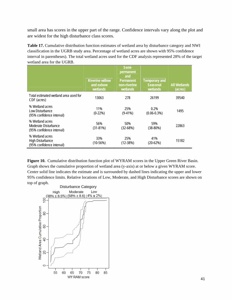
41  

small area has scores in the upper part of the range. Confidence intervals vary along the plot and are widest for the high disturbance class scores.

Table 17. Cumulative distribution function estimates of wetland area by disturbance category and NWI classification in the UGRB study area. Percentage of wetland acres are shown with 95% confidence interval in parentheses). The total wetland acres used for the CDF analysis represented 28% of the target wetland area for the UGRB.

Riverine willow and oxbow wetlands

Semi-permanent

and Permanent

non-riverine wetlands

Temporary and Seasonal wetlands

All Wetlands (acres)

Total estimated wetland area used for CDF (acres) 13063 278 26199 39540

% Wetland acres Low Disturbance (95% confidence interval)

11% (0-22%)

25% (9-41%)

0.2% (0.06-0.3%) 1495

% Wetland acres Moderate Disturbance (95% confidence interval)

56% (31-81%)

50% (32-68%)

59% (38-80%)

22863

% Wetland acres High Disturbance (95% confidence interval)

33% (10-56%)

25% (12-38%)

41% (20-62%)

15182

Figure 10. Cumulative distribution function plot of WYRAM scores in the Upper Green River Basin. Graph shows the cumulative proportion of wetland area (y-axis) at or below a given WYRAM score. Center solid line indicates the estimate and is surrounded by dashed lines indicating the upper and lower 95% confidence limits. Relative locations of Low, Moderate, and High Disturbance scores are shown on top of graph.

High (38% ± 8.5%)

Low (4% ± 2%)

Moderate (58% ± 8.6)

Disturbance Category

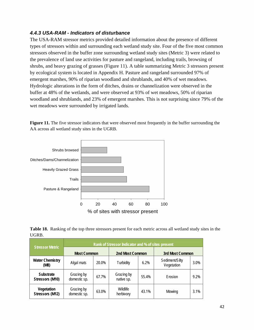
42  

4.4.3 USA-RAM - Indicators of disturbance The USA-RAM stressor metrics provided detailed information about the presence of different types of stressors within and surrounding each wetland study site. Four of the five most common stressors observed in the buffer zone surrounding wetland study sites (Metric 3) were related to the prevalence of land use activities for pasture and rangeland, including trails, browsing of shrubs, and heavy grazing of grasses (Figure 11). A table summarizing Metric 3 stressors present by ecological system is located in Appendix H. Pasture and rangeland surrounded 97% of emergent marshes, 90% of riparian woodland and shrublands, and 40% of wet meadows. Hydrologic alterations in the form of ditches, drains or channelization were observed in the buffer at 48% of the wetlands, and were observed at 93% of wet meadows, 50% of riparian woodland and shrublands, and 23% of emergent marshes. This is not surprising since 79% of the wet meadows were surrounded by irrigated lands.

Figure 11. The five stressor indicators that were observed most frequently in the buffer surrounding the AA across all wetland study sites in the UGRB.

% of sites with stressor present

0 20 40 60 80 100

Pasture & Rangeland

Trails

Heavily Grazed Grass

Ditches/Dams/Channelization

Shrubs browsed

Table 18. Ranking of the top three stressors present for each metric across all wetland study sites in the UGRB.

Stressor Metric Rank of Stressor Indicator and % of sites present

Most Common 2nd Most Common 3rd Most Common

Water Chemistry (M8) Algal mats 20.0% Turbidity 6.2%

Sediment/Silty Vegetation 3.0%

Substrate Stressors (M10)

Grazing by domestic sp. 67.7%

Grazing by native sp. 55.4% Erosion 9.2%

Vegetation Stressors (M12)

Grazing by domestic sp.

63.0% Wildlife herbivory

43.1% Mowing 3.1%

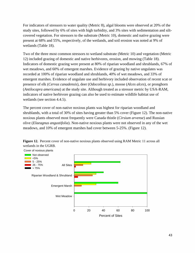
43  

For indicators of stressors to water quality (Metric 8), algal blooms were observed at 20% of the study sites, followed by 6% of sites with high turbidity, and 3% sites with sedimentation and silt-covered vegetation. For stressors to the substrate (Metric 10), domestic and native grazing were present at 68% and 55%, respectively, of the wetlands, and soil erosion was noted at 9% of wetlands (Table 18).

Two of the three most common stressors to wetland substrate (Metric 10) and vegetation (Metric 12) included grazing of domestic and native herbivores, erosion, and mowing (Table 18). Indicators of domestic grazing were present at 80% of riparian woodland and shrublands, 67% of wet meadows, and 60% of emergent marshes. Evidence of grazing by native ungulates was recorded at 100% of riparian woodland and shrublands, 40% of wet meadows, and 33% of emergent marshes. Evidence of ungulate use and herbivory included observation of recent scat or presence of elk (Cervus canadensis), deer (Odocoileus sp.), moose (Alces alces), or pronghorn (Antilocapra americana) at the study site. Although treated as a stressor metric by USA-RAM, indicators of native herbivore grazing can also be used to estimate wildlife habitat use of wetlands (see section 4.4.5).

The percent cover of non-native noxious plants was highest for riparian woodland and shrublands, with a total of 30% of sites having greater than 5% cover (Figure 12). The non-native noxious plants observed most frequently were Canada thistle (Cirsium arvense) and Russian olive (Elaeagnus angustifolia). Non-native noxious plants were not observed in any of the wet meadows, and 10% of emergent marshes had cover between 5-25%. (Figure 12).

Figure 12. Percent cover of non-native noxious plants observed using RAM Metric 11 across all wetlands in the UGRB. Cover of noxious plants

Percent of Sites

0 20 40 60 80 100

All Sites

Riparian Woodland & Shrubland

Emergent Marsh

Wet Meadow

Not observed<5%5 - 25%26 - 75%> 75%

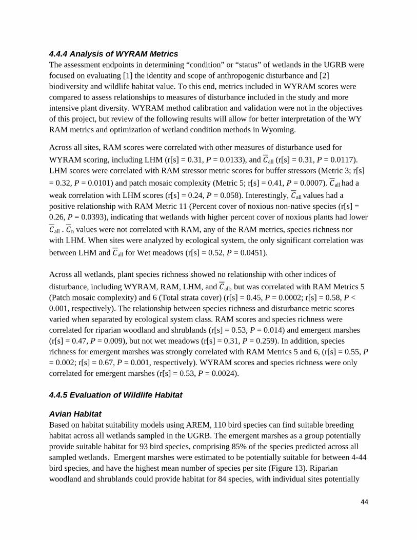
44  

4.4.4 Analysis of WYRAM Metrics The assessment endpoints in determining “condition” or “status” of wetlands in the UGRB were focused on evaluating [1] the identity and scope of anthropogenic disturbance and [2] biodiversity and wildlife habitat value. To this end, metrics included in WYRAM scores were compared to assess relationships to measures of disturbance included in the study and more intensive plant diversity. WYRAM method calibration and validation were not in the objectives of this project, but review of the following results will allow for better interpretation of the WY RAM metrics and optimization of wetland condition methods in Wyoming.

Across all sites, RAM scores were correlated with other measures of disturbance used for

WYRAM scoring, including LHM (r[s] = 0.31, P = 0.0133), and all (r[s] = 0.31, P = 0.0117). LHM scores were correlated with RAM stressor metric scores for buffer stressors (Metric 3; r[s]

= 0.32, P = 0.0101) and patch mosaic complexity (Metric 5; r[s] = 0.41, P = 0.0007). all had a

weak correlation with LHM scores (r[s] = 0.24, P = 0.058). Interestingly, all values had a positive relationship with RAM Metric 11 (Percent cover of noxious non-native species (r[s] = 0.26, P = 0.0393), indicating that wetlands with higher percent cover of noxious plants had lower

all . n values were not correlated with RAM, any of the RAM metrics, species richness nor with LHM. When sites were analyzed by ecological system, the only significant correlation was

between LHM and all for Wet meadows (r[s] = 0.52, P = 0.0451). Across all wetlands, plant species richness showed no relationship with other indices of

disturbance, including WYRAM, RAM, LHM, and all, but was correlated with RAM Metrics 5 (Patch mosaic complexity) and 6 (Total strata cover) (r[s] = 0.45, P = 0.0002; r[s] = 0.58, P < 0.001, respectively). The relationship between species richness and disturbance metric scores varied when separated by ecological system class. RAM scores and species richness were correlated for riparian woodland and shrublands (r[s] = 0.53, P = 0.014) and emergent marshes (r[s] = 0.47, P = 0.009), but not wet meadows (r[s] = 0.31, P = 0.259). In addition, species richness for emergent marshes was strongly correlated with RAM Metrics 5 and 6, (r[s] = 0.55, P = 0.002; r[s] = 0.67, P = 0.001, respectively). WYRAM scores and species richness were only correlated for emergent marshes (r[s] = 0.53, P = 0.0024). 4.4.5 Evaluation of Wildlife Habitat

Avian Habitat Based on habitat suitability models using AREM, 110 bird species can find suitable breeding habitat across all wetlands sampled in the UGRB. The emergent marshes as a group potentially provide suitable habitat for 93 bird species, comprising 85% of the species predicted across all sampled wetlands. Emergent marshes were estimated to be potentially suitable for between 4-44 bird species, and have the highest mean number of species per site (Figure 13). Riparian woodland and shrublands could provide habitat for 84 species, with individual sites potentially

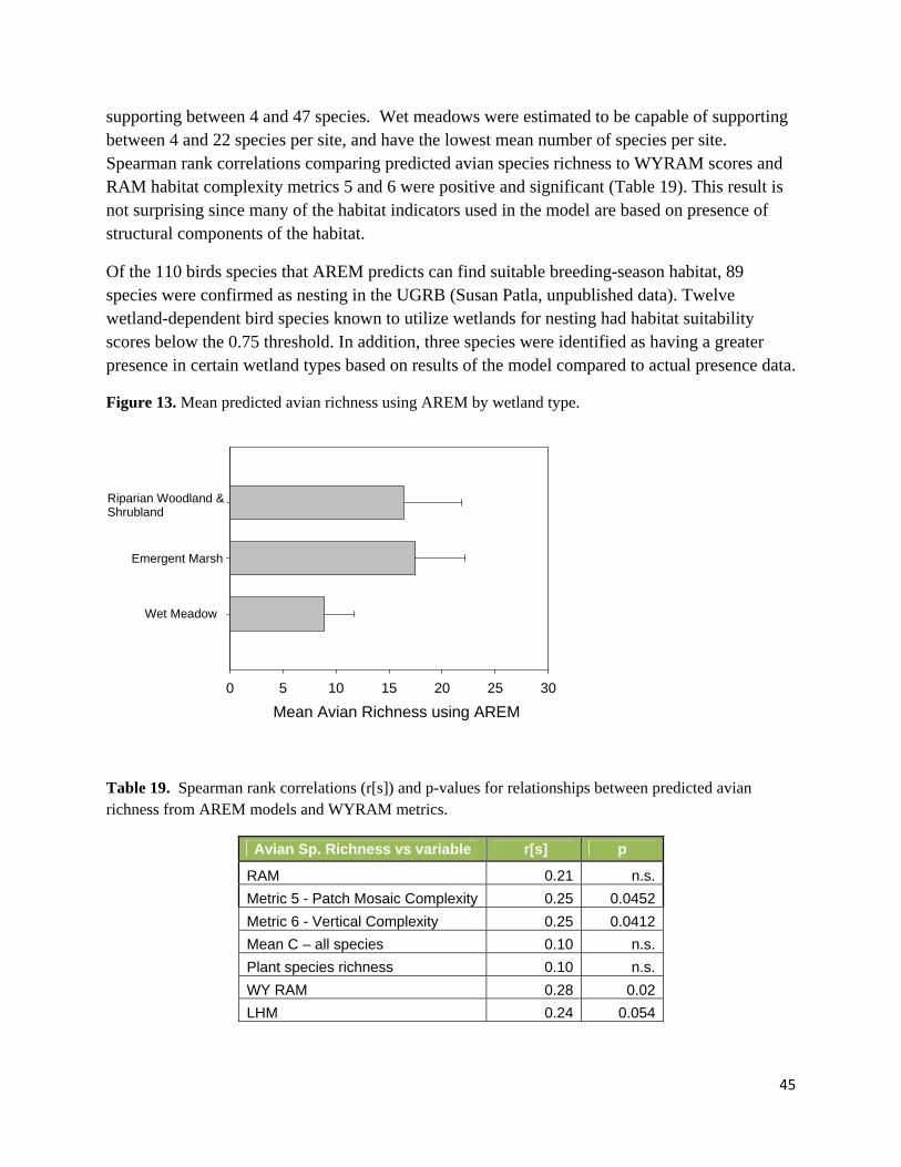
45  

supporting between 4 and 47 species. Wet meadows were estimated to be capable of supporting between 4 and 22 species per site, and have the lowest mean number of species per site. Spearman rank correlations comparing predicted avian species richness to WYRAM scores and RAM habitat complexity metrics 5 and 6 were positive and significant (Table 19). This result is not surprising since many of the habitat indicators used in the model are based on presence of structural components of the habitat.

Of the 110 birds species that AREM predicts can find suitable breeding-season habitat, 89 species were confirmed as nesting in the UGRB (Susan Patla, unpublished data). Twelve wetland-dependent bird species known to utilize wetlands for nesting had habitat suitability scores below the 0.75 threshold. In addition, three species were identified as having a greater presence in certain wetland types based on results of the model compared to actual presence data.

Figure 13. Mean predicted avian richness using AREM by wetland type.

Mean Avian Richness using AREM

0 5 10 15 20 25 30

Riparian Woodland &Shrubland

Emergent Marsh

Wet Meadow

 

Table 19. Spearman rank correlations (r[s]) and p-values for relationships between predicted avian richness from AREM models and WYRAM metrics.

Avian Sp. Richness vs variable r[s] p

RAM 0.21 n.s.

Metric 5 - Patch Mosaic Complexity 0.25 0.0452

Metric 6 - Vertical Complexity 0.25 0.0412

Mean C – all species 0.10 n.s.

Plant species richness 0.10 n.s.

WY RAM 0.28 0.02

LHM 0.24 0.054

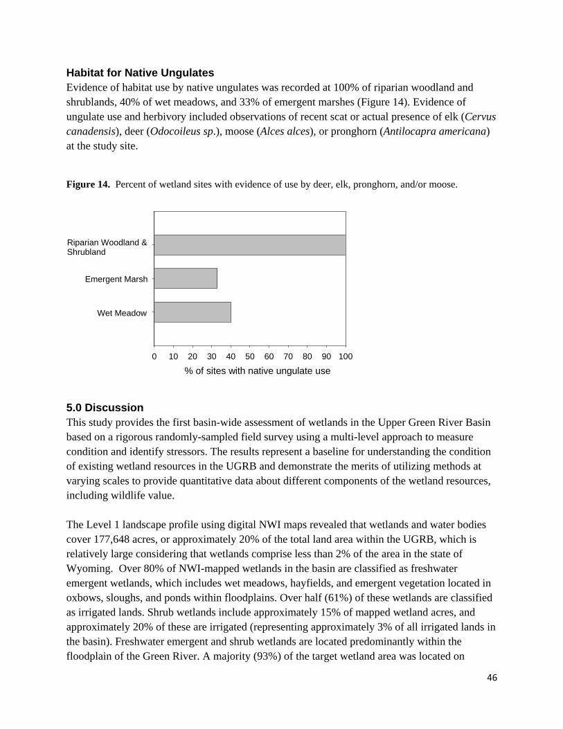
46  

Habitat for Native Ungulates Evidence of habitat use by native ungulates was recorded at 100% of riparian woodland and shrublands, 40% of wet meadows, and 33% of emergent marshes (Figure 14). Evidence of ungulate use and herbivory included observations of recent scat or actual presence of elk (Cervus canadensis), deer (Odocoileus sp.), moose (Alces alces), or pronghorn (Antilocapra americana) at the study site.

Figure 14. Percent of wetland sites with evidence of use by deer, elk, pronghorn, and/or moose.

% of sites with native ungulate use

0 10 20 30 40 50 60 70 80 90 100

Riparian Woodland &Shrubland

Emergent Marsh

Wet Meadow

 

5.0 Discussion This study provides the first basin-wide assessment of wetlands in the Upper Green River Basin based on a rigorous randomly-sampled field survey using a multi-level approach to measure condition and identify stressors. The results represent a baseline for understanding the condition of existing wetland resources in the UGRB and demonstrate the merits of utilizing methods at varying scales to provide quantitative data about different components of the wetland resources, including wildlife value. The Level 1 landscape profile using digital NWI maps revealed that wetlands and water bodies cover 177,648 acres, or approximately 20% of the total land area within the UGRB, which is relatively large considering that wetlands comprise less than 2% of the area in the state of Wyoming. Over 80% of NWI-mapped wetlands in the basin are classified as freshwater emergent wetlands, which includes wet meadows, hayfields, and emergent vegetation located in oxbows, sloughs, and ponds within floodplains. Over half (61%) of these wetlands are classified as irrigated lands. Shrub wetlands include approximately 15% of mapped wetland acres, and approximately 20% of these are irrigated (representing approximately 3% of all irrigated lands in the basin). Freshwater emergent and shrub wetlands are located predominantly within the floodplain of the Green River. A majority (93%) of the target wetland area was located on

47  

private lands, emphasizing the need to coordinate basin-wide wetland resource management with both public land managers and private landowners within the basin.

We classified the randomly sampled wetlands into types from two classification systems: Cowardin and Ecological Systems classification criteria (Table 1). By doing so, we provide the first crosswalk between these two classification schema for wetlands in the UGRB. This effort was possible because we collected detailed floristic and abiotic data about each sampled wetland. The riparian woodland and shrublands ecological system corresponds closely to the riverine & oxbow NWI type, and the wet meadow ecological system appears to exclusively match the temporary & seasonal wetlands NWI type. The emergent marsh ecological system, spans all three Cowardin wetland types, although most of the emergent marshes are semi-permanent & permanent non-riverine wetlands. Our results indicate that using the NWI wetlands layer to determine the area and location of wetland ecological systems in the UGRB will be problematic. Use of the NWI layer is also made complicated by seasonal and year-to-year fluctuations in water levels, which cause the apparent area of wetlands to change. And finally, use of the NWI layer can be complicated because, often, a wetland observed on the ground comprises several types of wetland features mapped separately in the NWI layer.

Level 2 WYRAM methods were developed to measure the condition of wetlands in the basin, as expressed by the amount of anthropogenic disturbance. By knowing the WYRAM scores for reference wetlands (sites defined as least disturbed using selection criteria), we were able to assign our sampled wetlands to disturbance categories. Within wetland types, emergent marshes (generally higher elevation glacial pothole wetlands) were the least disturbed as a group, followed by riparian woodland and shrublands. Wet meadows, mainly irrigated hayfields, were the most disturbed and hydrologically modified and represented the largest proportion of target wetland acres. Using a cumulative distribution function (CDF) to apply the data from our sampled sites to the basin, we estimated that 96% of wetland acres are moderately to highly disturbed and less than 4% are minimally disturbed. Because our samples were heavily skewed to wetlands on public lands, our CDF extrapolation of wetland condition was limited to 39,540 of the wetland acres in the basin. Still, the CDF analysis provides a valuable first approximation of wetland condition across the basin.

The most widespread anthropogenic disturbances, or stressors, identified across all wetland types sampled were agricultural practices associated with pasture and cattle grazing, and hydrologic alterations (primarily dams, diversions, and ditches). This is not a surprising result since our LHM analysis indicated that 67% of wetlands in the basin have modifications to hydrology, and 15% of those were supported or created by irrigation and impoundments.

We were able to identify patterns in wetland condition and hydrologic alteration for each of the target wetland types. Wet meadows were the most affected by hydrologic and anthropogenic disturbance - 93% had altered hydrology and less than 10% had low disturbance WYRAM scores. Because a large proportion of the wetland area in the basin is mapped as the temporary &

48  

seasonal wetlands that corresponds to wet meadows, the results from our sample data translates into the large proportion of wetlands in the basin in the highly- and moderately-disturbed categories. Emergent marshes had a smaller proportion of sites with hydrologic alteration (40% altered hydrology) and disturbance (33% had low disturbance). This lower degree of disturbance may be an artifact of the distribution of the emergent marsh samples, 67% of which were located in glacial potholes at higher elevations. Moreover, five emergent marsh sites were in riverine oxbows, potentially limiting their proximity to anthropogenic disturbance and exposure to the direct effects of irrigation. Riparian woodland and shrubland wetlands had either historic (30%) or altered-hybrid (70%) hydrology, largely influenced by their location along the Upper Green River and its tributaries. About half of the riparian woodland and shrubland sites were moderately disturbed, 20% had low disturbance scores, and over a quarter of sites had high disturbance scores. Riparian wetlands had the highest proportion of noxious non-native plants present – including Russian olive, an invasive shrub with high potential for increasing in the future.

Our results point to the challenges in quantifying the ecological condition of wetlands with an altered hydrologic regime because many wetlands in the basin, regardless of ecological integrity, are influenced by irrigation (70% of target wetlands in basin, Table 7). LHM identified 14% of sampled wetlands as created or supported by hydrologic alterations associated with irrigation (Figures 7 & 8). These results point to the influence of irrigation on wetland acreage in the UGRB, including the creation of wetlands that wouldn’t exist without irrigation inputs.

Separating irrigation from natural water inputs to individual wetlands is difficult, as is determining how irrigation inputs might have altered the natural condition and function of these wetlands. Our LHM analysis assigned higher scores to wetlands that apparently have natural hydrologic regimes, and lower scores to those with apparently altered hydrology. Those LHM

scores are positively correlated with patch-mosaic complexity, overall RAM scores, and all

values (see Section 4.4.4), all of which are based on data collected on-site. Thus our data suggest that wetlands with altered hydrology have lower biological condition values. This result agrees with the results of research elsewhere, which shows that created wetlands usually lack biological and hydrological features of natural wetlands (Mitch and Gosselink 2007).The data do not tell us, though, to what degree hydrologic alteration might have changed existing biological values, or how much the hydrology of a wetland must be altered before the biological values change. For example, we did not find a correlation between LHM and plant species richness, suggesting that plant diversity, as measured in this study, is influenced by other factors.

We found strong relationships between plant species richness and patch mosaic complexity (RAM Metric 5) and total strata cover (RAM Metric 6), indicating that RAM field metrics reflect

elements of diversity in the wetland plant community. Both the  all and n indices were able to

discriminate between reference condition and highly disturbed wetlands. all was correlated with overall RAM scores and RAM estimates of percent cover of noxious non-native species

49  

(Metric 11), but n was not. Previous wetland studies have examined the relationship between floristic quality and human disturbance and found that wetlands with low floristic quality scores

were in highly cultivated landscapes (Lopez and Fennessy 2002). Mean all values in this study were 4.0, and ranged from 2.3-6.0, similar to those from wetland condition assessments in other irrigated basins in the region (Lemly and Gillian 2012, Vance et al. 2012). It is important to note

that wet meadows had the lowest overall all, but the highest n, suggesting that irrigated wet meadows in the UGRB still support native species sensitive to disturbance. These results suggest that C-values andFQA indices add to the assessment of biological condition that is missing from the typical RAM techniques. Formal C-values for Wyoming will become available in 2017 from the Wyoming Natural Diversity Database at the University of Wyoming.

We found a correlation between AREM estimates of potential bird species richness and overall WYRAM scores. This result may be explained by the field indicators used for AREM models, which measure the complexity and structure of the vegetation within and surrounding the wetland. These field indicators resemble patch mosaic complexity (RAM Metric 5) and total strata cover (RAM Metric 6) included in the WYRAM scores. Empirical evidence also shows a positive relationship between habitat heterogeneity, structure of vegetation, and bird species diversity (Tews et al. 2004). Additional field validation of AREM is needed before it can be used to reliably indicate presence of specific species, but we are optimistic about its utility in future wetland assessments when combined with WYRAM or other condition scores to inform managers about optimal wetlands to support a diverse bird community. Approximately 70% of Wyoming’s wetland bird species are considered wetland obligates (WGFD 2003), and therefore it is important to continue studying the effects of anthropogenic change on wetland habitat quality and value.

In addition to supporting wetland birds, the UGRB is an area of known importance for migrating mule deer and pronghorn (Berger 2004, Copeland et al. 2014, Sawyer et al. 2014). We found evidence of habitat use by native ungulates in 100% of riparian woodland and shrublands, 40% of wet meadows, and 33% of emergent marshes (Figure 13). Forage quality is known to influence migration and stopover habitat selection for mule deer (Sawyer and Kauffman 2011, Lendrum et al. 2012) and herbaceous wetlands and riparian can be a source of high-quality forage and water for migrating ungulates (Collins and Urness 1983, Lendrum et al. 2012).

There is increasing recognition that hybrid and novel ecosystems may have considerable ecological value, and should no longer be viewed primarily as departures from pristine ecological conditions (Hobbs et al. 2014). Our finding of apparent widespread hydrologic alteration to the wetland systems we studied may indicate novel, irrigation-created or supported ecosystems in this landscape. Traditional RAM metrics assign lower values to wetlands with anthropogenic influences, and by themselves are inadequate for assessing the values of novel wetland ecosystems. Recognizing this shortcoming, we combined RAM scores with LHM and

50  

mean C-values to create WYRAM scores that integrate relationships between hydrology and habitat.

Assessment methods that equate human influence with a decline in condition not only may give misleading results for individual wetlands, they may also give an inaccurate profile of the wetlands in a basin. For example, if irrigation influence is considered to be a sign of departure from natural conditions and earns a low hydrologic score for individual wetlands, and if many of the wetlands in a basin are influenced by irrigation, then when the scores from the individual wetlands are applied to the basin as a whole, wetland condition basin-wide will look degraded. But if irrigation creates wetlands where they would not exist otherwise (see, for example, Peck and Lovvorn 2001), or increases the size of already-existing wetlands, then the net effect of irrigation basin-wide may be to provide more wetland habitat. This created or augmented habitat may lack some of the values of natural wetlands, but it has more wetland value than does non-wetland. Understanding the values of whole landscapes in this way, including a spectrum of natural, historic to hydrologically-altered to created wetlands, is necessary for effective management of these systems.

5.1 Wetland Priorities for Conservation and Restoration Considerable land use changes have occurred and are predicted to occur in the future within the UGRB, driven in large part by energy development (Copeland et al. 2014) and residential subdivision (Gude et al. 2006). These changes are likely to increase human disturbance near wetlands and affect wetland condition. Land management policies that discourage further human disturbance and encourage sustainable grazing management in and near wetlands will help to maintain wetland function and prevent further declines in condition. We did not examine the relationship between current oil and gas development and potential water quality and quantity impacts to wetlands; but identify this as an area of future research given the level of energy development in this landscape and potential impacts to wetland hydrology and quality.

Climate change was identified as an extreme threat in the Upper Green Wetland Core Complex Regional Wetland Conservation Plan (Patla 2014) and wetlands were identified as highly vulnerable to climate change in a recent statewide report (Pocewicz et al. 2014). Our study was completed in 2012, a dry year when USDA declared Sublette County a drought disaster area. Drought conditions likely affected many of the sampled wetlands during our study. We observed that many of the glacial potholes, largely classified as emergent marshes, had shrunk in size or completely dried up. This suggests that change in climate may influence the hydrologic regime on wetlands in the basin in the future.

Hydrology is the primary driver of the establishment and maintenance of wetlands, affecting the ecological processes that sustain ecosystem function (Barker and Maltby 2009). Therefore, the presence of dams and diversions for irrigation alters the timing and quantity of water available within the basin, directly or indirectly affecting the quantity and type of wetlands present. Both the seasonal flood pulse and the late-summer low flow periods are vital for the structure and

51  

function of wetlands that are linked to rivers through surface and groundwater sources (Junk et al. 1989). Hydrologic alterations were observed for a majority of the sites within the floodplain of the Upper Green River compared to wetlands perched higher in the basin, for example, in the New Fork Pothole region. Wetlands identified as historic using the LHM analysis (38% of sample wetlands) and/or having high WYRAM scores are likely to have a high potential for ecologic integrity and conservation value, providing key habitat for the native flora and fauna whose life-histories are tied to the natural hydrologic regime (Poff et al. 1997, Barker and Maltby 2009).

Many studies have begun to quantify the importance of irrigation-influenced wetlands for migrating birds and other wildlife (Chester and Robson 2013, Moulton et al. 2013, Patla 2015, Donnelly et al. In press), but additional work is needed to quantify ecosystem services and wildlife value of irrigation-influenced and created wetlands. Somewhat surprisingly, peat layers thicker than 18 cm were identified in two irrigated wet meadows, indicating that wetlands with low LHM scores but high restoration and conservation value are present in the existing floodplain. Beavers historically were keystone species in the UGRB, and wetland habitats created by beaver support a diversity of bird species and ecosystem services (McKinstry et al. 2001).Current regional models and tools could be utilized to assess the potential for restoration of beaver in the UGRB (Wheaton and Macfarlane 2014). In addition to wildlife habitat, there is increased recognition of the ecosystem services provided by agriculturally influenced wetlands (Tanner et al. 2013) for pesticide de-contamination (Tournebize et al. 2013), reduction of nitrogen transport from agricultural catchments, and increases in species richness(Strand and Weisner 2013).

Water shortages in the Colorado River Basin due to climate alteration and predicted drought (Cook et al. 2004) and increased population (Hansen et al. 2002) are likely to put pressure on Wyoming agricultural producers to alter current irrigation practices and convert to center-pivot irrigation. According to the Upper Green wetland plan (Patla 2015), flood irrigation is used on most irrigated lands. The number and location of temporary and seasonal wetlands in floodplains suggests high vulnerability to habitat loss in the future from conversion to sprinklers or residential development (Copeland et al. 2010, Pocewicz et al. 2014). Approximately 40% of wet meadows we sampled were observed as directly created or supported by irrigation; conversion to center pivot irrigation could potentially affect an estimated 50,000 acres of wetlands mapped as temporary and seasonal in the basin and the wildlife habitat they provide. Conservation strategies aimed at protecting lands designated as wetlands may fall short of their intended purpose if water quantity and timing crucial to wetland function are also not retained (Downard and Endter-Wada 2013).

6.0 Conclusion

This study is the first basin-wide assessment of wetlands in the Upper Green and represents a baseline for understanding existing wetland conditions. We provide a framework for beginning

52  

to understand the complex relationships between human disturbance, hydrologic alteration, and wildlife values, based on a randomly-sampled field survey that combines data at multiple scales (Level 1, 2 and 3). Additional analyses focusing on the functional and wildlife habitat value of wetlands, as well as the relationship between anthropogenic disturbance and condition are needed. We are just beginning to understand the biodiversity supported by these wetland systems as well as the ecosystem service values that they provide.

 

 

LITERATURE CITED 

ACOE. 2008. Interim Regional Supplement to the Corps of Engineers Wetland Delineation Manual: Western Mountains, Valleys, and Coast Region. Army Corps of Engineers.

Adamus, P. R. 1993. User's Manual: Avian Richness Evaluation Method (AREM) for Lowland Wetlands of the Colorado Plateau. US EPA Environmental Research Labratory, Corvallis, Oregon.

Agency, U. S. E. P. 1995. America's Wetlands: Our vital link between land and water. Washington, D.C. Barker, T., and E. Maltby. 2009. Introduction-The dynamics of wetlands.in E. Maltby and T. Barker,

editors. The Wetlands Handbook. Wiley-Blackwell, Oxford, UK. Berger, J. 2004. The last mile: how to sustain long-distance migration in mammals. Conservation Biology

in Practice 18:320-331. Bureau of Land Management. 2010. Wyoming surface and mineral ownership. Bureau of Land

Management. Chapman, S. S., S. A. Bryce, J. M. Omernik, D. G. Despain, J. ZumBerge, and M. Conrad. 2004.

Ecoregions of Wyoming. U.S. Geological Survey, Reston, Virginia. Chester, E. T., and B. J. Robson. 2013. Anthropogenic refuges for freshwater biodiversity: Their

ecological characteristics and management. Biological Conservation 166:64-75. Collins, W. B., and P. J. Urness. 1983. Feeding Behavior and Habitat Selection of Mule Deer and Elk on

Northern Utah Summer Range. The Journal of Wildlife Management 47:646-663. Comer, P., D. Faber-Langendoen, R. Evans, S. Gawler, C. Josse, G. Kittel, S. Menard, M. Pyne, M. Reid,

K. Schulz, K. Snow, and J. Teague. 2003. Ecological Systems of the United States: A Working Classification of U.S. Terrestrial Systems. NatureServe, Arlington, VA.

Committee, W. J. V. S. 2010. Wyoming Wetlands Conservation Strategy. Cheyenne, WY. Cook, E. R., C. A. Woodhouse, C. M. Eakin, D. M. Meko, and D. W. Stahle. 2004. Long-Term Aridity

Changes in the Western United States. Science 306:1015-1018. Copeland, H. E., H. Sawyer, K. L. Monteith, D. E. Naugle, A. Pocewicz, N. Graf, and M. J. Kauffman.

2014. Conserving migratory mule deer through the umbrella of sage-grouse. Ecosphere 5. Copeland, H. E., S. A. Tessman, E. H. Girvetz, L. Roberts, C. Enquist, A. Orabona, S. Patla, and J.

Kiesecker. 2010. A geospatial assessment on the distribution, condition, and vulnerability of Wyoming's wetlands. Ecological Indicators 10:869-879.

Costanza, R., R. dArge, R. deGroot, S. Farber, M. Grasso, B. Hannon, K. Limburg, S. Naeem, R. V. Oneill, J. Paruelo, R. G. Raskin, P. Sutton, and M. vandenBelt. 1997. The value of the world's ecosystem services and natural capital. Nature 387:253-260.

Cowardin, L. M., F. C. Golet, and E. T. LaRoe. 1979. Classification of wetlands and deepwater habitats of the United States.in U. S. F. a. W. Service, editor. U.S. Fish and Wildlife Service, Washington, DC.

53  

Culver, D., and J. Lemly. 2013. Field Guide to Colorado’s Wetland Plants: Identification, Ecology, Conservation. Colorado Natural Heritage Program, Colorado State University, Ft. Collins, CO.

Dahl, T. E. 1990. Wetlands losses in the United States 1780s to 1980s. U.S. Department of the Interior, Fish and Wildlife Service, Washington, D.C.

DeKeyser, E. S., D. R. Kirby, and M. J. Ell. 2003. An index of plant community integrity: development of the methodology for assessing prairie wetland plant communities. Ecological Indicators 3:119-133.

Donnelly, J. P., D. E. Naugle, J. D. Maestas, and C. A. Hagen. In press. Public lands and private waters: scarce mesic resources structure land tenure sage-grouse distributions. Ecosphere.

Dorn, R. D. 2001. Vascular Plants of Wyoming. Mountain West Publishing, Cheyenne, WY. Downard, R., and J. Endter-Wada. 2013. Keeping wetlands wet in the western United States: Adaptations

to drought in agriculture-dominated human-natural systems. J Environ Manage 131:394-406. EPA, O. 2001. Ohio rapid assessment method for wetlands. version 5.0. Ohio EPA, Division of Surface

Water. Evans, J., J. Oakleaf, S. Cushman, and D. Theobald. 2014. An ArcGIS Toolbox for Surface Gradient and

Geomorphometric Modeling, version 2.0-0. Faber-Langendoen, D., C. Hedge, S. Kost, L. Thomas, R. Smart, J. Smyth, J. Drake, and S. Menard.

2011. Assessment of wetland ecosystem condition across landscape regions: a multi-metric approach. NatureServe, Arlington, VA.

Faulkner, D. 2010. Birds of Wyoming. Roberts and Company Publishers, Greenwood Village, CO. Fennessy, M. S., A. D. Jacobs, and M. E. Kentula. 2007. An evaluation of rapid methods for assessing the

ecological condition of wetlands. Wetlands 27:543-560. Gammonley, J. H., editor. 2004. Wildlife of natural palustrine wetlands. University of Texas Press,

Austin, TX. Gude, P. H., A. J. Hansen, R. Rasker, and B. Maxwell. 2006. Rates and drivers of rural residential

development in the Greater Yellowstone. Landscape and Urban Planning 77:131-151. Hansen, A. J., R. Rasker, B. Maxwell, J. J. Rotella, J. D. Johnson, A. W. Parmenter, U. Langner, W. B.

Cohen, R. L. Lawrence, and P. V. Kraska. 2002. Ecological causes and consequences of demographic change in the New West. Bioscience 52:151-162.

Hobbs, R. J., E. Higgs, C. M. Hall, P. Bridgewater, F. S. Chapin, III, E. C. Ellis, J. J. Ewel, L. M. Hallett, J. Harris, K. B. Hulvey, S. T. Jackson, P. L. Kennedy, C. Kueffer, L. Lach, T. C. Lantz, A. E. Lugo, J. Mascaro, S. D. Murphy, C. R. Nelson, M. P. Perring, D. M. Richardson, T. R. Seastedt, R. J. Standish, B. M. Starzomski, K. N. Suding, P. M. Tognetti, L. Yakob, and L. Yung. 2014. Managing the whole landscape: historical, hybrid, and novel ecosystems. Frontiers in Ecology and the Environment 12:557-564.

Jacobs, A. D., M. E. Kentula, and A. T. Herlihy. 2010. Developing an index of wetland condition from ecological data: An example using HGM functional variables from the Nanticoke watershed, USA. Ecological Indicators 10:703-712.

Johnston, B. 2001. Field Guide to Sedge Species of the Rocky Mountain Region. Pub. R2-RR-01-03. USDA Forest Service, Rocky Mountain Region, Denver, CO.

Junk, W. J., P. B. Bayley, and R. E. Sparks. 1989. The flood pulse concept in river-floodplain systems. Canadian Special Publication of Fisheries and Aquatic Sciences 106:110-127.

Knight, D. H., G. P. Jones, W. A. Reiners, and W. H. Romme. 2014. Mountains and plains: the ecology of Wyoming landscapes. Second edition edition. Yale University Press, New Haven and London.

Lemly, J., and L. Gillian. 2012. North Platte River Basin Wetland Profile and Condition Assessment. Colorado Natural Heritage Program, Fort Collins, CO.

Lendrum, P. E., C. R. Anderson, R. A. Long, J. G. Kie, and R. T. Bowyer. 2012. Habitat selection by mule deer during migration: effects of landscape structure and natural-gas development. Ecosphere 3:1-19.

Lichvar, R., M. Butterwick, N. C. Melvin, and W. N. Kirchner. 2014. The National Wetland Plant List: 2014 Updated of Wetland Ratings. Phytoneuron 2014-41:1-42.

54  

Lopez, R. D., and S. Fennessy. 2002. Testing the floristic quality assessment index as an indictor of wetland condition. Ecological Applications 12:487-497.

Luna, T., C. McIntyre, and L. K. Vance. 2010. Ecological Systems Field Guide. Montana Field Guide. Mason, J. P., and K. A. Miller. 2004. Water Resources of Sweetwater County, Wyoming. U.S.

Department of Interior, U.S. Geological Survey. McKinstry, M. C., P. Caffrey, and S. H. Anderson. 2001. The importance of beaver to wetland habitats

and waterfowl in Wyoming. Journal of the American Water Resources Association 37:1571-1577.

Mitch, W., and J. Gosselink. 2007. Wetlands. John Wiley and Sons, Inc., New York, WY. Moulton, C., J. Carlisle, K. Brenner, and R. Cavallaro. 2013. Assessment of Foraging Habitats of White-

faced Ibis near Two Important Breeding Colonies in Eastern Idaho. Idaho Falls, ID. Newlon, K., K. Ramstead, and J. Hahn. 2013. Southeast Montana Wetland Assessment: Developing and

Refining Montana's Wetland Assessment and Monitoring Strategy. Report to the U.S. Environmental Protection Agency. Page 43. Montana Natural Heritage Program, Helena, Montana.

Nicholoff, S. H. 2003. Wyoming Bird Conservation Plan, Version 2.0., Wyoming Game and Fish Department, Lander, WY.

Orabona, A., C. Rudd, M. Grenier, Z. Walker, S. Patla, and B. Oakleaf. 2012. Atlas of Birds, Mammals, Amphibians, and Reptiles in Wyoming. Page 232. Wyoming Game and Fish Department, Lander, WY.

Patla, S. 2015. Upper Green River Wetland Core Complex: Regional Wetland Conservation Plan. Wyoming Wetlands Conservation Strategy, Jackson, WY.

Peck, D. E., and J. R. Lovvorn. 2001. The importance of flood irrigation in water supply to wetlands in the Laramie Basin, Wyoming, USA. Wetlands 21:370-378.

Pocewicz, A., H. C. Copeland, M. B. Grenier, D. A. Keinath, and L. M. Waskoviak. 2014. Vulnerability of Wyoming's terrestrial wildlife and habitats. The Nature Conservancy, Wyoming Game and Fish Department, Wyoming National Diversity Database, Lander, WY.

Poff, N. L., J. D. Allan, M. B. Bain, J. R. Karr, K. L. Prestegaard, B. D. Richter, R. E. Sparks, and J. C. Stromberg. 1997. The natural flow regime. Bioscience 47:769-784.

Program, C. N. H. 2010. North Platte Basinwide Wetland Condition Assessment 2010 Field Manual. Colorado State University, Fort Collins, CO.

Richardson, J. L., and M. J. Vepraskas. 2001. Wetland soils: genesis, hydrology, landscapes, and classification. Lewis Scientific Publications, Boca Raton, FL.

Rocchio, J. 2007. Assessing ecological condition of headwater wetlands in the southern Rocky Mountians using a vegetation index of biotic integrity (version 1.0). Unpublished report prepared for the Colorado Department of Natural Resources and US EPA Region 8. Ft. Collins, CO.

Savage, R., K. Gianopulos, J. Graham, B. Munoz, R. Wenerick, G. Curvin, and B. Moody. 2015. Results of the Southeast Wetland Monitoring and Assessment Intensification Study with North Carolina, South Carolina, Alabama, and Georgia. Report to the EPA Region IV.

Sawyer, H., M. Hayes, B. Rudd, and M. J. Kauffman. 2014. The Red Desert to Hoback Mule Deer Migration Assessment. Wyoming Migration Initiative, Laramie, WY.

Sawyer, H., and M. J. Kauffman. 2011. Stopover ecology of a migratory ungulate. Journal of Animal Ecology 80:1078-1087.

Schroeder, M. T. 2010. Green River Basin Plan. Wyoming Water Development Office, Cheyenne, WY. Skinner, Q. 2010. A field guide to Wyoming grasses. Education Resources Publishing, Cumming, GA. Stevens, D. L., Jr., and S. F. Jensen. 2007. Sample design, execution, and analysis for wetland

assessment. Wetlands 27:515-523. Stevens, D. L., and A. R. Olsen. 2004. Spatially balanced sampling of natural resources. Journal of the

American Statistical Association 99:262-278.

55  

Stoddard, J. L., D. P. Larsen, C. P. Hawkins, R. K. Johnson, and R. H. Norris. 2006. Setting expectations for the ecological condition of streams: The concept of reference condition. Ecological Applications 16:1267-1276.

Strand, J. A., and S. E. B. Weisner. 2013. Effects of wetland construction on nitrogen transport and species richness in the agricultural landscape—Experiences from Sweden. Ecological Engineering 56:14-25.

Sutula, M. A., E. D. Stein, J. N. Collins, A. E. Fetscher, and R. Clark. 2006. A practical guide for the development of a wetland assessment method: the California experience. Journal of the American Water Resources Association 42:157-175.

Swink, F., and G. Wilhelm. 1979. Plants of the Chicago Region. Morton Arboretum, Lisle, IL. Swink, F., and G. Wilhelm. 1994. 4th edition edition. Indiana University Press, Bloomington, IN. Tanner, C. C., C. Howard-Williams, M. D. Tomer, and R. Lowrance. 2013. Bringing together science and

policy to protect and enhance wetland ecosystem services in agricultural landscapes. Ecological Engineering 56:1-4.

Tews, J., U. Brose, V. Grimm, K. Tielborger, M. C. Wichmann, M. Schwager, and F. Jeltsch. 2004. Animal species diversity driven by habitat heterogeneity/diversity: the importance of keystone structures. Journal of Biogeography 31:79-92.

Tournebize, J., E. Passeport, C. Chaumont, C. Fesneau, A. Guenne, and B. Vincent. 2013. Pesticide de-contamination of surface waters as a wetland ecosystem service in agricultural landscapes. Ecological Engineering 56:51-59.

U.S. Department of Agriculture - National Resource Conservation Service. 2013. Release Brochure for 'Garrison' creeping foxtail (Alopecurus arundinaceus Poir). USDA-NRCS, Bridger PMC, Bridger, MT.

U.S. Department of Agriculture - Natural Resource Conservation Service. 2010. Field indicators of hydric soils in the United States, version 7.0. USDA-NRCS in cooperation with the National Technical Committee for Hydric Soils, Washington, DC.

U.S. Department of Agriculture-National Resources Conservation Service. 2014. The PLANTS database. National Plant Data Team, Greensboro, NC.

U.S. Environmental Protection Agency. 2011a. National Wetlands Condition Assessment: Field Operations Manual.in U. S. E. P. Agency, editor., Washington DC.

U.S. Environmental Protection Agency. 2011b. USA RAM Manual. Corvallis, OR. US Army Corps of Engineers. 2006. National Inventory of Dams.in U. A. C. o. Engineers, editor.,

Alexandria, VA. US Geological Survey. 2009. National Elevation Data (NED).in U. G. Survey, editor., Sioux Falls, SD. USDA Farm Service Agency. 2009. National High Altitude Aerial Photography (NAIP). USDA Farm

Service Agency. Vance, L., K. Newlon, J. Lemly, and G. Jones. 2012. Rocky Mountain REMAP Project 2009-2011.

Montana Natural Heritage Program, Helena, Montana. Wheaton, J. M., and W. W. Macfarlane. 2014. The Utah Beaver Restoration Assessment Tool: A

Decision Support and Planning Tool – Manager Brief., Ecogeomorphology and Topographic Analysis Lab, Utah State University, Logan, UT.

Whittier, T. R., S. G. Paulsen, D. P. Larsen, S. A. Peterson, A. T. Herlihy, and P. R. Kaufmann. 2002. Indicators of ecological stress and their extent in the population of northeastern lakes: A regional-scale assessment. Bioscience 52:235-247.

Wyoming Department of Environmental Quality. 2005. Depth to Groundwater.in W. D. o. E. Quality, editor., Cheyenne, WY.

Wyoming Department of Water Quality. 2004. Wyoming Water Quality Standards. Water Quality Division.

Wyoming Game and Fish Department. 2008. Wyoming Bird Checklist. Wyoming Game and Fish Nongame Program, Lander, WY.

Wyoming Game and Fish Department. 2010. Wyoming State Wildlife Action Plan. Cheyenne, WY.

56  

Wyoming Joint Ventures Steering Committee. 2010. Wyoming Wetlands Conservation Strategy. Cheyenne, WY.

Wyoming State Geological Society. 2014. Generalized Geologic Map of Wyoming. Laramie, WY. Wyoming Wildlife Consultants. 2007. Irrigated lands of Wyoming. Wyoming Geographic Information

Services (WYGISC), Laramie, Wyoming.

 

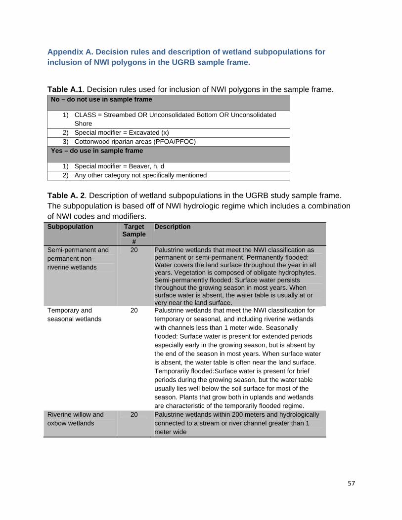
57  

Appendix A. Decision rules and description of wetland subpopulations for inclusion of NWI polygons in the UGRB sample frame.  

Table A.1. Decision rules used for inclusion of NWI polygons in the sample frame. No – do not use in sample frame

1) CLASS = Streambed OR Unconsolidated Bottom OR Unconsolidated Shore

2) Special modifier = Excavated (x) 3) Cottonwood riparian areas (PFOA/PFOC)

Yes – do use in sample frame

1) Special modifier = Beaver, h, d 2) Any other category not specifically mentioned

Table A. 2. Description of wetland subpopulations in the UGRB study sample frame. The subpopulation is based off of NWI hydrologic regime which includes a combination of NWI codes and modifiers. Subpopulation Target

Sample #

Description

Semi-permanent and permanent non-riverine wetlands

20 Palustrine wetlands that meet the NWI classification as permanent or semi-permanent. Permanently flooded: Water covers the land surface throughout the year in all years. Vegetation is composed of obligate hydrophytes. Semi-permanently flooded: Surface water persists throughout the growing season in most years. When surface water is absent, the water table is usually at or very near the land surface.

Temporary and seasonal wetlands

20 Palustrine wetlands that meet the NWI classification for temporary or seasonal, and including riverine wetlands with channels less than 1 meter wide. Seasonally flooded: Surface water is present for extended periods especially early in the growing season, but is absent by the end of the season in most years. When surface water is absent, the water table is often near the land surface. Temporarily flooded:Surface water is present for brief periods during the growing season, but the water table usually lies well below the soil surface for most of the season. Plants that grow both in uplands and wetlands are characteristic of the temporarily flooded regime.

Riverine willow and oxbow wetlands

20 Palustrine wetlands within 200 meters and hydrologically connected to a stream or river channel greater than 1 meter wide

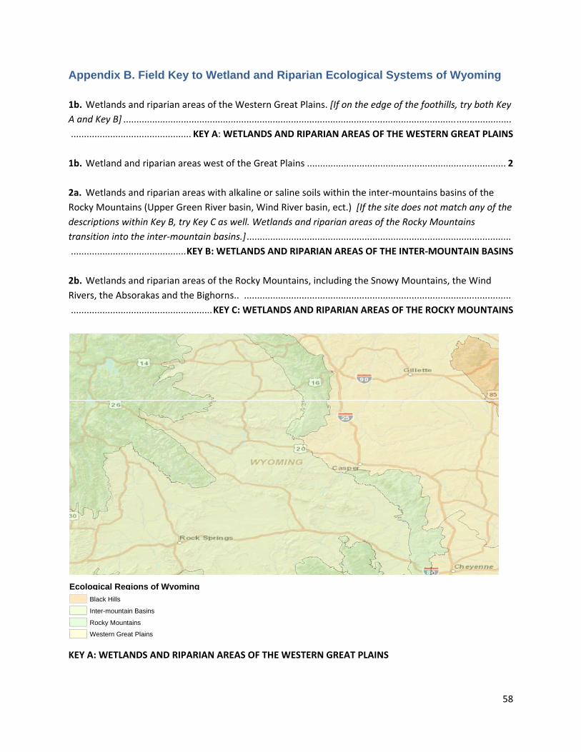
58  

Ecological Regions of Wyoming   

Black Hills Inter-mountain Basins

Rocky Mountains

Western Great Plains 

Appendix B. Field Key to Wetland and Riparian Ecological Systems of Wyoming    

1b. Wetlands and riparian areas of the Western Great Plains. [If on the edge of the foothills, try both Key 

A and Key B] ....................................................................................................................................................  

 .............................................. KEY A: WETLANDS AND RIPARIAN AREAS OF THE WESTERN GREAT PLAINS 

 

1b. Wetland and riparian areas west of the Great Plains ............................................................................ 2   

 

2a.  Wetlands and riparian areas with alkaline or saline soils within the inter‐mountains basins of the 

Rocky Mountains (Upper Green River basin, Wind River basin, ect.)  [If the site does not match any of the 

descriptions within Key B, try Key C as well. Wetlands and riparian areas of the Rocky Mountains 

transition into the inter‐mountain basins.] .....................................................................................................  

 ............................................ KEY B: WETLANDS AND RIPARIAN AREAS OF THE INTER‐MOUNTAIN BASINS 

 

2b. Wetlands and riparian areas of the Rocky Mountains, including the Snowy Mountains, the Wind 

Rivers, the Absorakas and the Bighorns..  ......................................................................................................   

 ...................................................... KEY C: WETLANDS AND RIPARIAN AREAS OF THE ROCKY MOUNTAINS 

 

 

 

 

 

 

KEY A: WETLANDS AND RIPARIAN AREAS OF THE WESTERN GREAT PLAINS 

 

59  

1a.  Low stature shrublands dominated by species such as Sarcobatus vermiculatus, Atriplex spp., 

Ericameria nauseosa, Artemisia sp. Vegetation may be sparse and soils may be saline. Sites may be 

located on the edge alkali depressions, or in flats or washes not typically associated with river and 

stream floodplains. [These systems were originally described for the Inter‐Mountain Basins, but may 

extend to the plains.]  ................................................................................................................................... 2 

 

1b. Wetland is not a low stature shrub‐dominated saline wash or flat. ...................................................... 3 

 

2a.  Shrublands with sparse (<20%) vegetation cover, located on flats or in temporarily or intermittently 

flooded drainages, or on the edge of playas and alkali depressions. They are typically dominated by 

Sarcobatus vermiculatus and Atriplex spp. with inclusions of Sporobolus airoides, Pascopyrum smithii, 

Distichlis spicata, Puccinellia nuttalliana, and Eleocharis palustris herbaceous vegetation 

………………………………………………………………………………………………….Inter‐Mountain Basins Greasewood Flat 

 

2b. Sites with > 20% total vegetation cover and restricted to temporarily or intermittently flooded 

drainages with a variety of sparse or patchy vegetation including Sarcobatus vermiculatus, Ericameria 

nauseosa, Artemisia sp., Grayia spinosa, Distichlis spicata, and Sporobolus airoides. ..................................  

…………………………………………………………………………………………………………………….Inter‐Mountain Basins Wash 

 

 

3a.  Sites located within the floodplain or immediate riparian zone of a river or stream. Vegetation may 

be entirely herbaceous or may contain tall stature woody species, such as Populus spp. or Salix spp. 

Water levels variable. Woody vegetation that occurs along reservoir edges can also be included here.... 4 

 

3b. Herbaceous wetlands of the Western Great Plains that are isolated or partially isolated from 

floodplains and riparian zones, often depressional with or without an outlet. ........................................... 8  

 

4a. Herbaceous wetlands within the floodplain with standing water at or above the surface throughout 

the growing season, except in drought years. Water levels are often high at some point during the 

growing season, but managed systems may be drawn down at any point depending on water 

management regimes. Vegetation typically dominated by species of Typha, Scirpus, Schoenoplectus, 

Carex, Eleocharis, Juncus, and floating genera such as Potamogeton, Sagittaria, and Ceratophyllum. The 

hydrology may be entirely managed. Water may be brackish or not. Soils are highly variable. This system 

includes natural warm water sloughs and other natural floodplain marshes as well as a variety of 

managed wetlands on the floodplain (e.g., recharge ponds, moist soil units, shallow gravel pits, 

etc.)……… ................................................................................... Western North American Emergent Marsh 

 

4b. Not as above. Wetland and riparian vegetation that typically lacks extensive standing water. 

Vegetation may be herbaceous or woody. Management regimes variable ................................................. 5 

 

5a. Large herbaceous wetlands within the floodplain associated with a high water table that is 

controlled by artificial overland flow (irrigation). Sites typically lack prolonged standing water.  

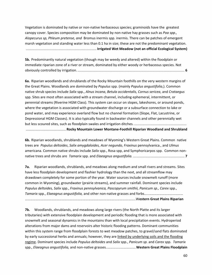
60  

Vegetation is dominated by native or non‐native herbaceous species; graminoids have the  greatest  

canopy cover. Species composition may be dominated by non‐native hay grasses such as Poa spp., 

Alopecurus sp, Phleum pretense, and  Bromus inermis spp. inermis. There can be patches of emergent 

marsh vegetation and standing water less than 0.1 ha in size; these are not the predominant vegetation.  

 .......................................................................... Irrigated Wet Meadow (not an official Ecological System) 

 

5b. Predominantly natural vegetation (though may be weedy and altered) within the floodplain or 

immediate riparian zone of a river or stream, dominated by either woody or herbaceous species. Not 

obviously controlled by irrigation. ................................................................................................................ 6 

 

6a. Riparian woodlands and shrublands of the Rocky Mountain foothills on the very western margins of 

the Great Plains. Woodlands are dominated by Populus spp. (mainly Populus angustifolia,). Common 

native shrub species include Salix spp., Alnus incana, Betula occidentalis, Cornus sericea, and Crataegus 

spp. Sites are most often associated with a stream channel, including ephemeral, intermittent, or 

perennial streams (Riverine HGM Class). This system can occur on slopes, lakeshores, or around ponds, 

where the vegetation is associated with groundwater discharge or a subsurface connection to lake or 

pond water, and may experience overland flow but no channel formation (Slope, Flat, Lacustrine, or 

Depressional HGM Classes). It is also typically found in backwater channels and other perennially wet 

but less scoured sites, such as floodplain swales and irrigation ditches. .......................................................  

 .......................................... Rocky Mountain Lower Montane‐Foothill Riparian Woodland and Shrubland 

 

6b. Riparian woodlands, shrublands and meadows of Wyoming’s Western Great Plains. Common  native 

trees are  Populus deltoides, Salix amygdaloides, Acer negundo, Fraxinus pennsylvanica., and Ulmus 

americana. Common native shrubs include Salix spp., Rosa spp, and Symphoricarpos spp.  Common non‐

native trees and shrubs are  Tamarix spp. and Elaeagnus angustifolia. ...................................................... 7 

 

7a.  Riparian woodlands, shrublands, and meadows along medium and small rivers and streams. Sites 

have less floodplain development and flashier hydrology than the next, and all streamflow may 

drawdown completely for some portion of the year. Water sources include snowmelt runoff (more 

common in Wyoming), groundwater (prairie streams), and summer rainfall. Dominant species include 

Populus deltoides, Salix spp., Fraxinus pennsylvanica, Pascopyrum smithii, Panicum sp., Carex spp., 

Tamarix spp., Elaeagnus angustifolia, and other non‐native grasses and forbs…..………………………………… 

……………………………………………………………………………………………………….……..Western Great Plains Riparian  

 

7b.  Woodlands, shrublands, and meadows along large rivers (the North Platte and its larger 

tributaries) with extensive floodplain development and periodic flooding that is more associated with 

snowmelt and seasonal dynamics in the mountains than with local precipitation events. Hydroperiod 

alterations from major dams and reservoirs alter historic flooding patterns. Dominant communities 

within this system range from floodplain forests to wet meadow patches, to gravel/sand flats dominated 

by early successional herbs and annuals; however, they are linked by underlying soils and the flooding 

regime. Dominant species include Populus deltoides and Salix spp., Panicum sp. and Carex spp.  Tamarix 

spp., Elaeagnus angustifolia, and non‐native grasses..…………………….……. Western Great Plains Floodplain  

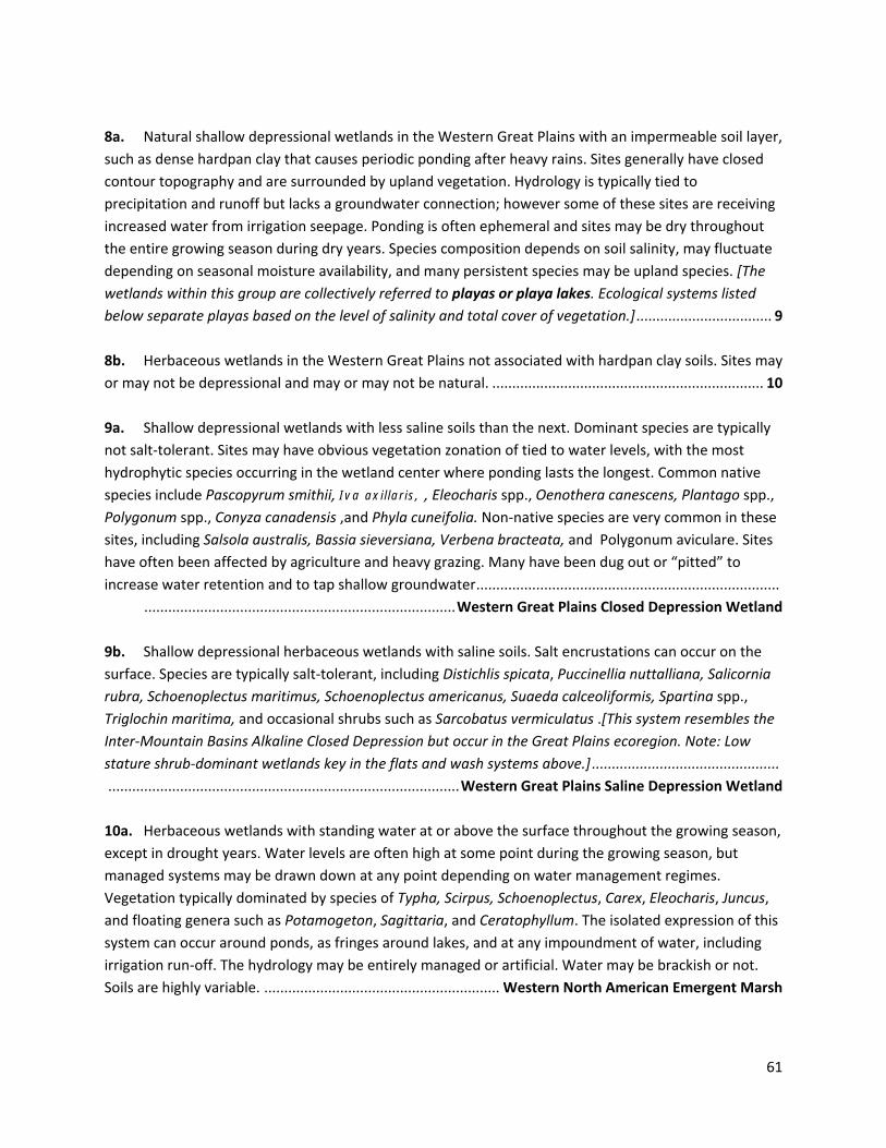
61  

 

8a.  Natural shallow depressional wetlands in the Western Great Plains with an impermeable soil layer, 

such as dense hardpan clay that causes periodic ponding after heavy rains. Sites generally have closed 

contour topography and are surrounded by upland vegetation. Hydrology is typically tied to 

precipitation and runoff but lacks a groundwater connection; however some of these sites are receiving 

increased water from irrigation seepage. Ponding is often ephemeral and sites may be dry throughout 

the entire growing season during dry years. Species composition depends on soil salinity, may fluctuate 

depending on seasonal moisture availability, and many persistent species may be upland species. [The 

wetlands within this group are collectively referred to playas or playa lakes. Ecological systems listed 

below separate playas based on the level of salinity and total cover of vegetation.] .................................. 9 

 

8b.   Herbaceous wetlands in the Western Great Plains not associated with hardpan clay soils. Sites may 

or may not be depressional and may or may not be natural. .................................................................... 10 

 

9a.  Shallow depressional wetlands with less saline soils than the next. Dominant species are typically 

not salt‐tolerant. Sites may have obvious vegetation zonation of tied to water levels, with the most 

hydrophytic species occurring in the wetland center where ponding lasts the longest. Common native 

species include Pascopyrum smithii, Iva axillaris, , Eleocharis spp., Oenothera canescens, Plantago spp., 

Polygonum spp., Conyza canadensis ,and Phyla cuneifolia. Non‐native species are very common in these 

sites, including Salsola australis, Bassia sieversiana, Verbena bracteata, and  Polygonum aviculare. Sites 

have often been affected by agriculture and heavy grazing. Many have been dug out or “pitted” to 

increase water retention and to tap shallow groundwater ............................................................................    

   .............................................................................. Western Great Plains Closed Depression Wetland  

 

9b.  Shallow depressional herbaceous wetlands with saline soils. Salt encrustations can occur on the 

surface. Species are typically salt‐tolerant, including Distichlis spicata, Puccinellia nuttalliana, Salicornia 

rubra, Schoenoplectus maritimus, Schoenoplectus americanus, Suaeda calceoliformis, Spartina spp., 

Triglochin maritima, and occasional shrubs such as Sarcobatus vermiculatus .[This system resembles the 

Inter‐Mountain Basins Alkaline Closed Depression but occur in the Great Plains ecoregion. Note: Low 

stature shrub‐dominant wetlands key in the flats and wash systems above.] ...............................................  

 ........................................................................................ Western Great Plains Saline Depression Wetland 

 

10a.  Herbaceous wetlands with standing water at or above the surface throughout the growing season, 

except in drought years. Water levels are often high at some point during the growing season, but 

managed systems may be drawn down at any point depending on water management regimes. 

Vegetation typically dominated by species of Typha, Scirpus, Schoenoplectus, Carex, Eleocharis, Juncus, 

and floating genera such as Potamogeton, Sagittaria, and Ceratophyllum. The isolated expression of this 

system can occur around ponds, as fringes around lakes, and at any impoundment of water, including 

irrigation run‐off. The hydrology may be entirely managed or artificial. Water may be brackish or not. 

Soils are highly variable. ........................................................... Western North American Emergent Marsh 

 

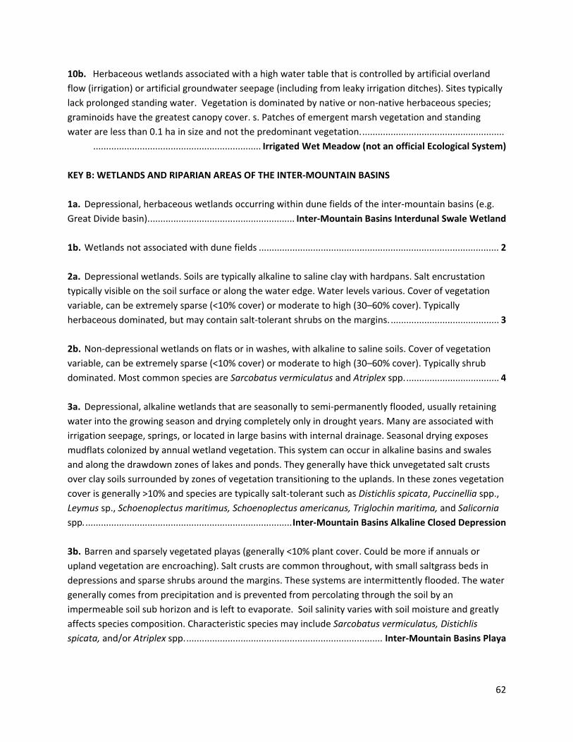
62  

10b.  Herbaceous wetlands associated with a high water table that is controlled by artificial overland 

flow (irrigation) or artificial groundwater seepage (including from leaky irrigation ditches). Sites typically 

lack prolonged standing water.  Vegetation is dominated by native or non‐native herbaceous species; 

graminoids have the greatest canopy cover. s. Patches of emergent marsh vegetation and standing 

water are less than 0.1 ha in size and not the predominant vegetation. .......................................................    

   ................................................................. Irrigated Wet Meadow (not an official Ecological System) 

 

KEY B: WETLANDS AND RIPARIAN AREAS OF THE INTER‐MOUNTAIN BASINS 

 

1a. Depressional, herbaceous wetlands occurring within dune fields of the inter‐mountain basins (e.g. 

Great Divide basin). ........................................................ Inter‐Mountain Basins Interdunal Swale Wetland 

 

1b. Wetlands not associated with dune fields ............................................................................................. 2 

 

2a. Depressional wetlands. Soils are typically alkaline to saline clay with hardpans. Salt encrustation 

typically visible on the soil surface or along the water edge. Water levels various. Cover of vegetation 

variable, can be extremely sparse (<10% cover) or moderate to high (30–60% cover). Typically 

herbaceous dominated, but may contain salt‐tolerant shrubs on the margins. .......................................... 3 

 

2b. Non‐depressional wetlands on flats or in washes, with alkaline to saline soils. Cover of vegetation 

variable, can be extremely sparse (<10% cover) or moderate to high (30–60% cover). Typically shrub 

dominated. Most common species are Sarcobatus vermiculatus and Atriplex spp. .................................... 4 

 

3a. Depressional, alkaline wetlands that are seasonally to semi‐permanently flooded, usually retaining 

water into the growing season and drying completely only in drought years. Many are associated with 

irrigation seepage, springs, or located in large basins with internal drainage. Seasonal drying exposes 

mudflats colonized by annual wetland vegetation. This system can occur in alkaline basins and swales 

and along the drawdown zones of lakes and ponds. They generally have thick unvegetated salt crusts 

over clay soils surrounded by zones of vegetation transitioning to the uplands. In these zones vegetation 

cover is generally >10% and species are typically salt‐tolerant such as Distichlis spicata, Puccinellia spp., 

Leymus sp., Schoenoplectus maritimus, Schoenoplectus americanus, Triglochin maritima, and Salicornia 

spp. ................................................................................ Inter‐Mountain Basins Alkaline Closed Depression  

 

3b. Barren and sparsely vegetated playas (generally <10% plant cover. Could be more if annuals or 

upland vegetation are encroaching). Salt crusts are common throughout, with small saltgrass beds in 

depressions and sparse shrubs around the margins. These systems are intermittently flooded. The water 

generally comes from precipitation and is prevented from percolating through the soil by an 

impermeable soil sub horizon and is left to evaporate.  Soil salinity varies with soil moisture and greatly 

affects species composition. Characteristic species may include Sarcobatus vermiculatus, Distichlis 

spicata, and/or Atriplex spp. ............................................................................ Inter‐Mountain Basins Playa 

 

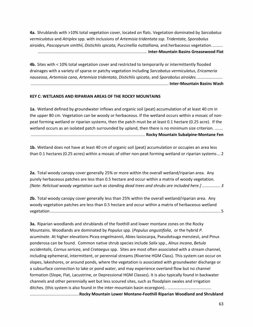
63  

4a.  Shrublands with >10% total vegetation cover, located on flats. Vegetation dominated by Sarcobatus 

vermiculatus and Atriplex spp. with inclusions of Artemisia tridentata ssp. Tridentate, Sporobolus 

airoides, Pascopyrum smithii, Distichlis spicata, Puccinellia nuttalliana, and.herbaceous vegetation. .........  

   ................................................................................................ Inter‐Mountain Basins Greasewood Flat 

 

4b. Sites with < 10% total vegetation cover and restricted to temporarily or intermittently flooded 

drainages with a variety of sparse or patchy vegetation including Sarcobatus vermiculatus, Ericameria 

nauseosa, Artemisia cana, Artemisia tridentata, Distichlis spicata, and Sporobolus airoides. ......................    

 ......................................................................................................................... Inter‐Mountain Basins Wash 

 

KEY C: WETLANDS AND RIPARIAN AREAS OF THE ROCKY MOUNTAINS 

 

1a. Wetland defined by groundwater inflows and organic soil (peat) accumulation of at least 40 cm in 

the upper 80 cm. Vegetation can be woody or herbaceous. If the wetland occurs within a mosaic of non‐

peat forming wetland or riparian systems, then the patch must be at least 0.1 hectare (0.25 acre).  If the 

wetland occurs as an isolated patch surrounded by upland, then there is no minimum size criterion. .......  

 .................................................................................................... Rocky Mountain Subalpine‐Montane Fen 

 

1b. Wetland does not have at least 40 cm of organic soil (peat) accumulation or occupies an area less 

than 0.1 hectares (0.25 acres) within a mosaic of other non‐peat forming wetland or riparian systems ... 2 

 

 

2a. Total woody canopy cover generally 25% or more within the overall wetland/riparian area.  Any 

purely herbaceous patches are less than 0.5 hectare and occur within a matrix of woody vegetation.  

[Note: Relictual woody vegetation such as standing dead trees and shrubs are included here.] ................ 3 

 

2b. Total woody canopy cover generally less than 25% within the overall wetland/riparian area.  Any 

woody vegetation patches are less than 0.5 hectare and occur within a matrix of herbaceous wetland 

vegetation ..................................................................................................................................................... 5 

 

3a. Riparian woodlands and shrublands of the foothill and lower montane zones on the Rocky 

Mountains. Woodlands are dominated by Populus spp. (Populus angustifolia,  or the hybrid P. 

acuminate. At higher elevations Picea engelmannii, Abies lasiocarpa, Pseudotsuga menziesii, and Pinus 

ponderosa can be found.  Common native shrub species include Salix spp., Alnus incana, Betula 

occidentalis, Cornus sericea, and Crataegus spp.  Sites are most often associated with a stream channel, 

including ephemeral, intermittent, or perennial streams (Riverine HGM Class). This system can occur on 

slopes, lakeshores, or around ponds, where the vegetation is associated with groundwater discharge or 

a subsurface connection to lake or pond water, and may experience overland flow but no channel 

formation (Slope, Flat, Lacustrine, or Depressional HGM Classes). It is also typically found in backwater 

channels and other perennially wet but less scoured sites, such as floodplain swales and irrigation 

ditches. (this system is also found in the inter‐mountain basin ecoregion).. ...................................... 

………………………………………..Rocky Mountain Lower Montane‐Foothill Riparian Woodland and Shrubland 

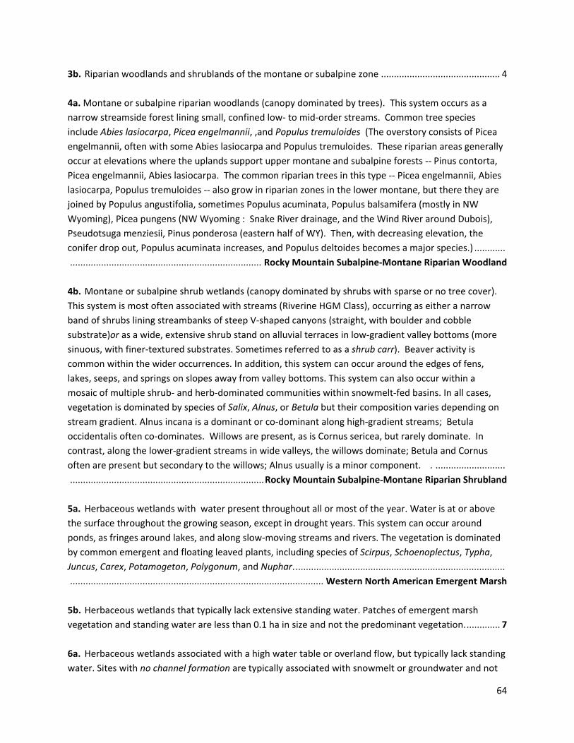
64  

3b. Riparian woodlands and shrublands of the montane or subalpine zone .............................................. 4 

 

4a. Montane or subalpine riparian woodlands (canopy dominated by trees).  This system occurs as a 

narrow streamside forest lining small, confined low‐ to mid‐order streams.  Common tree species 

include Abies lasiocarpa, Picea engelmannii, ,and Populus tremuloides  (The overstory consists of Picea 

engelmannii, often with some Abies lasiocarpa and Populus tremuloides.  These riparian areas generally 

occur at elevations where the uplands support upper montane and subalpine forests ‐‐ Pinus contorta, 

Picea engelmannii, Abies lasiocarpa.  The common riparian trees in this type ‐‐ Picea engelmannii, Abies 

lasiocarpa, Populus tremuloides ‐‐ also grow in riparian zones in the lower montane, but there they are 

joined by Populus angustifolia, sometimes Populus acuminata, Populus balsamifera (mostly in NW 

Wyoming), Picea pungens (NW Wyoming :  Snake River drainage, and the Wind River around Dubois), 

Pseudotsuga menziesii, Pinus ponderosa (eastern half of WY).  Then, with decreasing elevation, the 

conifer drop out, Populus acuminata increases, and Populus deltoides becomes a major species.) ............    

 .......................................................................... Rocky Mountain Subalpine‐Montane Riparian Woodland 

 

4b. Montane or subalpine shrub wetlands (canopy dominated by shrubs with sparse or no tree cover).  

This system is most often associated with streams (Riverine HGM Class), occurring as either a narrow 

band of shrubs lining streambanks of steep V‐shaped canyons (straight, with boulder and cobble 

substrate)or as a wide, extensive shrub stand on alluvial terraces in low‐gradient valley bottoms (more 

sinuous, with finer‐textured substrates. Sometimes referred to as a shrub carr).  Beaver activity is 

common within the wider occurrences. In addition, this system can occur around the edges of fens, 

lakes, seeps, and springs on slopes away from valley bottoms. This system can also occur within a 

mosaic of multiple shrub‐ and herb‐dominated communities within snowmelt‐fed basins. In all cases, 

vegetation is dominated by species of Salix, Alnus, or Betula but their composition varies depending on 

stream gradient. Alnus incana is a dominant or co‐dominant along high‐gradient streams;  Betula 

occidentalis often co‐dominates.  Willows are present, as is Cornus sericea, but rarely dominate.  In 

contrast, along the lower‐gradient streams in wide valleys, the willows dominate; Betula and Cornus 

often are present but secondary to the willows; Alnus usually is a minor component.    . ...........................  

 ........................................................................... Rocky Mountain Subalpine‐Montane Riparian Shrubland 

 

5a. Herbaceous wetlands with  water present throughout all or most of the year. Water is at or above 

the surface throughout the growing season, except in drought years. This system can occur around 

ponds, as fringes around lakes, and along slow‐moving streams and rivers. The vegetation is dominated 

by common emergent and floating leaved plants, including species of Scirpus, Schoenoplectus, Typha, 

Juncus, Carex, Potamogeton, Polygonum, and Nuphar. .................................................................................  

 .................................................................................................. Western North American Emergent Marsh 

 

5b. Herbaceous wetlands that typically lack extensive standing water. Patches of emergent marsh 

vegetation and standing water are less than 0.1 ha in size and not the predominant vegetation. ............. 7 

 

6a. Herbaceous wetlands associated with a high water table or overland flow, but typically lack standing 

water. Sites with no channel formation are typically associated with snowmelt or groundwater and not 

65  

subjected to high disturbance events such as flooding (Slope HGM Class). Sites associated with a stream 

channel are more tightly connected to overbank flooding from the stream channel than with snowmelt 

and groundwater discharge. Vegetation is dominated by herbaceous species; typically graminoids have 

the highest canopy cover including Carex spp., Calamagrostis spp., and Deschampsia caespitosa ..............  

 ......................................................................................... Rocky Mountain Alpine‐Montane Wet Meadow 

 

6b. Large herbaceous wetlands associated with a high water table that is controlled by artificial overland 

flow (irrigation). Sites typically lack prolonged standing water, but may have standing water early in the 

season if water levels are very high. Vegetation is dominated by native or non‐native herbaceous 

species; graminoids have the highest canopy cover ......................................................................................  

  . ................................................................... Irrigated Wet Meadow (not an official Ecological System) 

66  

Appendix C. Upper Green River Basin Field Manual Upon arriving at a site, the field crew members will verify that:

(1) a wetland is present that (a) contains > 0.1 ha of the target wetland type and (b) has dimensions large enough to contain an AA; and meets the criteria defined in the “target population” (see below)

(2) an AA can be located in the targeted wetland that meets the criteria for being sampled (that is, < 10% of the AA is covered by water 1 m deep or deeper, by areas that cannot be safely or effectively sampled, or by upland, alone or in combination).

If a wetland is present at the original point but it is not within the target population the wetland will be sampled and its classification will be changed. For example if the wetland was classified as a temporary seasonal wetland by the desktop evaluation but it is actually a riverine wetland the crew will still sample the wetland but change its subclass on the site evaluation sheet.

If the original point is unsampleable the crew will relocate the point to the nearest sampleable wetland within the same target population up to 200 m away from the original point.

If there are no wetlands within the same target population within 200 m of the original point but there is a sampleable wetland of a different target population the crew will relocate to that wetland and sample it.

The target population will be classified into subpopulations using NWI classes of wetlands The subpopulation includes three main wetland types:

1) Semi-permanent and permanent non-riverine wetlands (with open water): Water covers the land surface throughout the year in all years or throughout the growing season in most years. When Surface water is absent, the water table is usually at or very near the land surface.

2) Temporary and seasonal wetlands: Surface water is present for brief to extended periods during the growing season but is absent by the end of most seasons. When surface water is absent the water table is near the land surface but generally lies below the soil surface. Vegetation can be composed of both wetland and upland plants.

3) Riverine willow and oxbows wetlands: defined as wetlands within 200 meters of a stream

or river channel and hydrologically connected to that channel

These classifications that were assigned from the NWI Cowardin class will be verified in the field and changed if necessary to place it in the correct subpopulation. If possible, only one wetland within each subclass sampled within .5 kilometer. If the crew determines that the site does not meet the conditions for sampling, they will explain the reasons on the site evaluation form and abandon further work at that site. If they determine that the site meets the requirements for sampling, they will mark the center point with a flag and proceed as follows.

67  

Assessment Area and the Buffer Area Establishment

The crew will establish a Standard AA when possible or will adjust to a Shifted Standard AA, a Polygon AA or a Wetland boundary AA when necessary as defined by the National Wetland Condition Assessment Field Operations Manual (U.S. Environmental Protection Agency 2011a).

The center of the AA will be marked with a flag, as will enough points on the AA perimeter to allow the crew to tell when they are inside the AA. The location of the original point, the AA center, the relocated point when necessary, and a tract of the perimeter will be recorded with a GPS receiver and onto the site evaluation sheet. We will be using true north for this project and will adjust our compass and GPS receivers to the correct declination. The crew will draw the AA, a 100 meter buffer area surrounding the AA and any other distinguishing features useful for later delineation in ArcGIS onto the photo map.

The crew will take 4 photographs, from the center of the AA, one looking in each cardinal direction as well as pictures of the original point, the center point, and the relocated point when necessary. Any photo numbers, way points, and comments will be recorded on the site evaluation sheet.

USA RAM

Once the AA has been established both crew members will walk through the entire AA and buffer area to complete USA RAM metrics 1 - 12. Please refer to the USA RAM manual for complete directions (U.S. Environmental Protection Agency 2011b).

Water Characteristics of the AA (UGR Metric 13)

The crew will examine the entire AA and estimate the percent cover and patch complexity (interspersion) of open water for the total AA.

The crew will also measure common water quality parameters (water pH, total dissolved solids, conductivity, and temperature) from an area of undisturbed standing water closest to the center point within the AA if permanent water is present using a hand-held meter. The crew will estimate the range in water depth and the average water depth in the AA by recording the min, mode, and max water depth in the AA.

Community type evaluation (UGR12 Metric 14)

Community-types present: The field crew will document the community-types present in the AA by examining patches of vegetation. The minimum size of a patch will be 10 square meters. Areas of water shallower than 1 m will qualify as patches. Patches that share a common vegetation structure and composition will be grouped together into the same community-type, and patches that obviously differ in vegetation structure or composition will be placed into different community-types. Community-types will be differentiated from one another by such criteria as the presence of different vegetation strata dominance of the same stratum by different plant species, or different-sized individuals of the same shrub or tree species in the same over story stratum.

We will collect the following information onto the community attributes data sheets about each community-type:

68  

(a) describe how the community-type differs from the other community-types present, and

(b) label each community-type on the aerial photo

Botanical attributes present: Document the plant strata present and the percent coverage of the dominant plant species in each stratum.

Physical patch types present: The field crew will record the patch-types from Table 1 that they observe in the community-type.

Table 1. Physical patch types. Adapted from Table 4 in North Platte Basinwide Wetland Condition Assessment 2010 Field Manual. Colorado Natural Heritage Program (2010).

Patch Type Description Open water – swales on floodplain or along shoreline

Broad, elongated, vegetated, shallow depressions. Lack obvious banks, regularly-spaced deeps and shallows, or other characteristics of channels. Can entrap water after flood flows recede.

Open water – oxbow / backwater channel

Areas of stagnant or slow-moving water, partially or completely cut off from flow in main channel

Open water – rivulets / streamlets

Flowing water in a small, diffuse channel. Often occurs near outlet of a wet meadow or fen, or at very headwaters of a stream

Open water – pond / lake Med.-size to large body of water

Open water – pool Stagnant or slow-moving water from groundwater discharge, no associated with channel

Open water – beaver pond Stagnant or slow-moving water behind a beaver dam

Active beaver dam

Beaver canals Canals cut by beaver through emergent vegetation Debris jam / woody debris in channel Aggregated woody debris in stream channel, deposited by high flows

Point bar Low ridge of sediment on inner bank of a stream meander

Interfluve on floodplain Area between two adjacent streams or channels that flow in the same general direction

Bank slump Portion of stream bank or lake/pond shore that has broken free from rest of bank but not eroded away

Undercut bank Area along bank or shore excavated by waves or flowing water.

Seep or spring Localized point of emerging groundwater

Animal mound or burrow

Mudflat Accumulation of mud at the edge of shallow water, often intermittently flooded or exposed.

Alkali flat Dry, open area of fine sediment and accumulated salt. Often wet in winter or after heavy precipitation

Hummock / tussock In fens, mound composed of peat (created by Sphagnum moss or other moss) or formed by graminoids with a tussock habit

Water tracks / hollows In fens, depressions found between hummocks or mounds, that remain permanently saturated or are inundated with slow-moving, surface water

Floating mat Mat of peat held together by roots and rhizomes of sedges. Found along edges of ponds and lakes. Underlain by water or loose peat

Marl / limonite bed Marl is calcium carbonate precipitate often found in calcareous fens. Limonite forms

69  

in iron fens when iron precipitating from groundwater incorporates organic matter

The point of gathering this information is to document the nature of the community-types represented by the patches, not to describe each patch individually (unless each patch represents a different community-type from the others). Specimens of unknown plants will be collected by the same process listed above.

Ground cover: We will estimate the percent of the ground surface in each community-type covered by each of these classes of material: water > 20 cm deep, water < 20 cm deep, bare substrate (particles < 2 mm), gravel (particles 2 – 75 mm), rock (particles > 75 mm), plant litter, wood, lichen, sphagnum moss, and non-sphagnum moss. Each of these will be a single estimate made from observation of all the patches in a community-type.

Water depth: We will estimate the range in water depth and the average water depth in the community-type by recording the min, mode, and max water depth in the AA.

Type of submerged substrate: In communities occupying permanent water, we will estimate the percent of the submerged substrate covered by bare substrate (particles < 2 mm), gravel (particles 2 – 75 mm), or rock (particles > 75 mm).

Soil Sampling (UGR12 Form 14a)

Soil profile: One member from the crew will dig a soil pit to a depth of 40 cm in each community-type not covered by water, and record the following:

(a.) for each obvious layer in the soil profile, the depths of the upper and lower boundaries, soil texture (taken by hand), moist color of matrix, presence of redox concentrations, and presence of redox depletions;

(b.) depth to saturated soil and depth to standing water; and

(c.) presence of hydric soil indicators (histosol, histic epipedon, mucky mineral horizon, hydrogen sulfide odor, gleyed matrix, depleted matrix, redox concentrations, redox depletions) anywhere in the profile.

A GPS point will be taken at each soil pit and the location will be recorded onto the site map. Photos of the soil horizons will be taken for later verification.

If the soil pit contains standing water, we will use a hand-held meter to measure the water temperature, pH, total dissolved solids and electrical conductivity. We will dig a maximum of the 4 soil pits per AA, 1 pit for each community type present in the AA not covered by standing water. If there are more than 4 community types present in an AA we will exclude the additional community types and explain why they were not chosen for soil sampling.

Avian Richness Evaluation Method (AREM)

An available crew member will fill out the AREM data sheets as described by (Adamus 1993).

Sample Handling and Custody

70  

Unknown Plant Specimens: Each specimen will be pressed and the temporary field name recorded on the data sheet for it will be written on the folder containing the specimen. A list of specimens collected will be maintained by the crew, and this list will show, for each specimen, the field name, the date of collection, and the collection site. The unknown plant specimens will be stored at the Nature Conservancy office in Lander, WY for the duration of the field season. At the end of the field season, these specimens will be identified, and those identifications confirmed (when necessary) using the collection at the Rocky Mountain Herbarium of the University of Wyoming in Laramie.

QA plant specimens: All QA specimens will be collected and stored in the same manner as the unknown specimens. When possible during the field season they will be transferred to Laramie for confirmation.

Data Sheets: All data sheets will be copied at the end of each stint. The originals will be stored at the Nature Conservancy office in Lander, WY for the duration of the field season and the copies will be stored offsite.

2012 UPPER GREEN RIVER WETLAND CONDITION SITE EVALUATION FORM

LOCATION AND GENERAL INFORMATION

Point Code: _____________________ Date ____________ Surveyors: ______________________________________________

Directions to Point and Access Comments:

Is the original or relocated point the center point : Yes No

GPS COORDINATES OF TARGET POINT AND ASSESSMENT AREA Elevation (m): ______________

Original Point WP #: __________ UTM E: ___ ___ ___ ___ ___ ___ UTM N: ___ ___ ___ ___ ___ ___ ___ Error (+/-): ______________

Wetland type:

____ Within target population

____ Not within target population, but ŀ sampleable wetland ƛǎ ǿƛǘƘƛƴ нлл Ƴ ƻŦ ǘƘŜƻNJƛƎƛƴŀƭ LJƻƛƴǘ

Wetland type: ____ Semi-permanent_ permanent

____ Temporary _Seasonal

____ Riverine

Dimensions of AA:

____ 40 m radius circle ____ Polygon AA ____ Wetland boundary

Depression _____ Flat_____ Lacustrine Fringe_____ Riverine_____ Slope_____

Point Relocation Comments:

Wildlife:

PHOTOS OF ASSESSMENT AREA

AA-2 Photo #: _____________ Aspect: _____________ AA-3 Photo #: _____________ Aspect: _____________

AA-4 Photo #: _____________ Aspect: _____________

Additional AA Photos and Comments:

Center Point WP #: __________ UTM E: ___ ___ ___ ___ ___ ___ UTM N: ___ ___ ___ ___ ___ ___ ___ Error (+/-): ______________

Was the Point Relocated : Yes No Distance to new point : _______________ Relocated Point WP #: __________ UTM E: ___ ___ ___ ___ ___ ___ UTM N: ___ ___ ___ ___ ___ ___ ___ Error (+/-): ______________

Wetland Characteristics

Hydrogeomorphic Class

Point Photo #: _____________ Aspect: _____________

AA-1 Photo #: _____________ Aspect: _____________

Center Photo #: _____________ Aspect: _____________

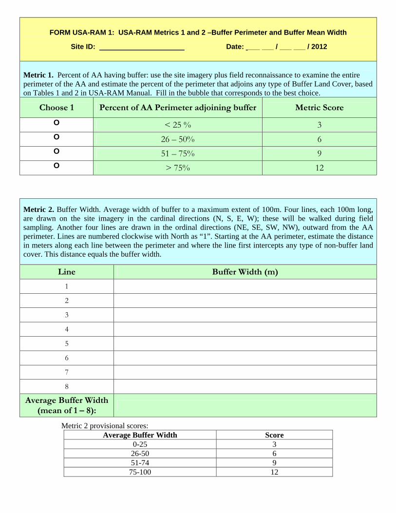
FORM USA-RAM 1: USA-RAM Metrics 1 and 2 –Buffer Perimeter and Buffer Mean Width

Site ID: Date: ___ ___ / ___ ___ / 2012

Metric 1. Percent of AA having buffer: use the site imagery plus field reconnaissance to examine the entire perimeter of the AA and estimate the percent of the perimeter that adjoins any type of Buffer Land Cover, based on Tables 1 and 2 in USA-RAM Manual. Fill in the bubble that corresponds to the best choice.

Choose 1 Percent of AA Perimeter adjoining buffer Metric Score

O < 25 % 3 O 26 – 50% 6 O 51 – 75% 9 O > 75% 12

Metric 2. Buffer Width. Average width of buffer to a maximum extent of 100m. Four lines, each 100m long, are drawn on the site imagery in the cardinal directions (N, S, E, W); these will be walked during field sampling. Another four lines are drawn in the ordinal directions (NE, SE, SW, NW), outward from the AA perimeter. Lines are numbered clockwise with North as “1”. Starting at the AA perimeter, estimate the distance in meters along each line between the perimeter and where the line first intercepts any type of non-buffer land cover. This distance equals the buffer width.

Line Buffer Width (m)

1

2

3

4

5

6

7

8

Average Buffer Width (mean of 1 – 8):

Metric 2 provisional scores: Average Buffer Width Score

0-25 3 26-50 6 51-74 9 75-100 12

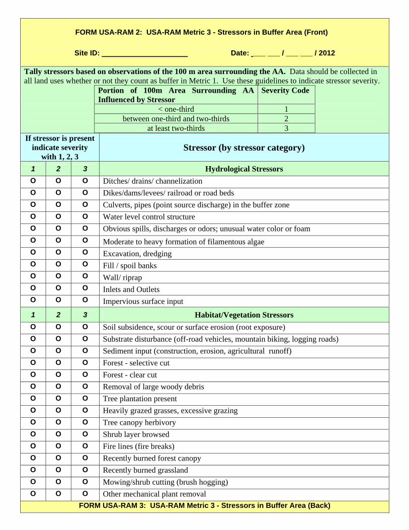
FORM USA-RAM 2: USA-RAM Metric 3 - Stressors in Buffer Area (Front)

Site ID: Date: ___ ___ / ___ ___ / 2012

Tally stressors based on observations of the 100 m area surrounding the AA. Data should be collected in all land uses whether or not they count as buffer in Metric 1. Use these guidelines to indicate stressor severity.

Portion of 100m Area Surrounding AA Influenced by Stressor

Severity Code

< one-third 1 between one-third and two-thirds 2

at least two-thirds 3

If stressor is present indicate severity

with 1, 2, 3 Stressor (by stressor category)

1 2 3 Hydrological Stressors

O O O Ditches/ drains/ channelization

O O O Dikes/dams/levees/ railroad or road beds

O O O Culverts, pipes (point source discharge) in the buffer zone

O O O Water level control structure

O O O Obvious spills, discharges or odors; unusual water color or foam

O O O Moderate to heavy formation of filamentous algae O O O Excavation, dredging O O O Fill / spoil banks O O O Wall/ riprap O O O Inlets and Outlets O O O Impervious surface input

1 2 3 Habitat/Vegetation Stressors

O O O Soil subsidence, scour or surface erosion (root exposure)

O O O Substrate disturbance (off-road vehicles, mountain biking, logging roads)

O O O Sediment input (construction, erosion, agricultural runoff)

O O O Forest - selective cut

O O O Forest - clear cut

O O O Removal of large woody debris

O O O Tree plantation present

O O O Heavily grazed grasses, excessive grazing

O O O Tree canopy herbivory

O O O Shrub layer browsed

O O O Fire lines (fire breaks)

O O O Recently burned forest canopy

O O O Recently burned grassland

O O O Mowing/shrub cutting (brush hogging)

O O O Other mechanical plant removal

FORM USA-RAM 3: USA-RAM Metric 3 - Stressors in Buffer Area (Back)

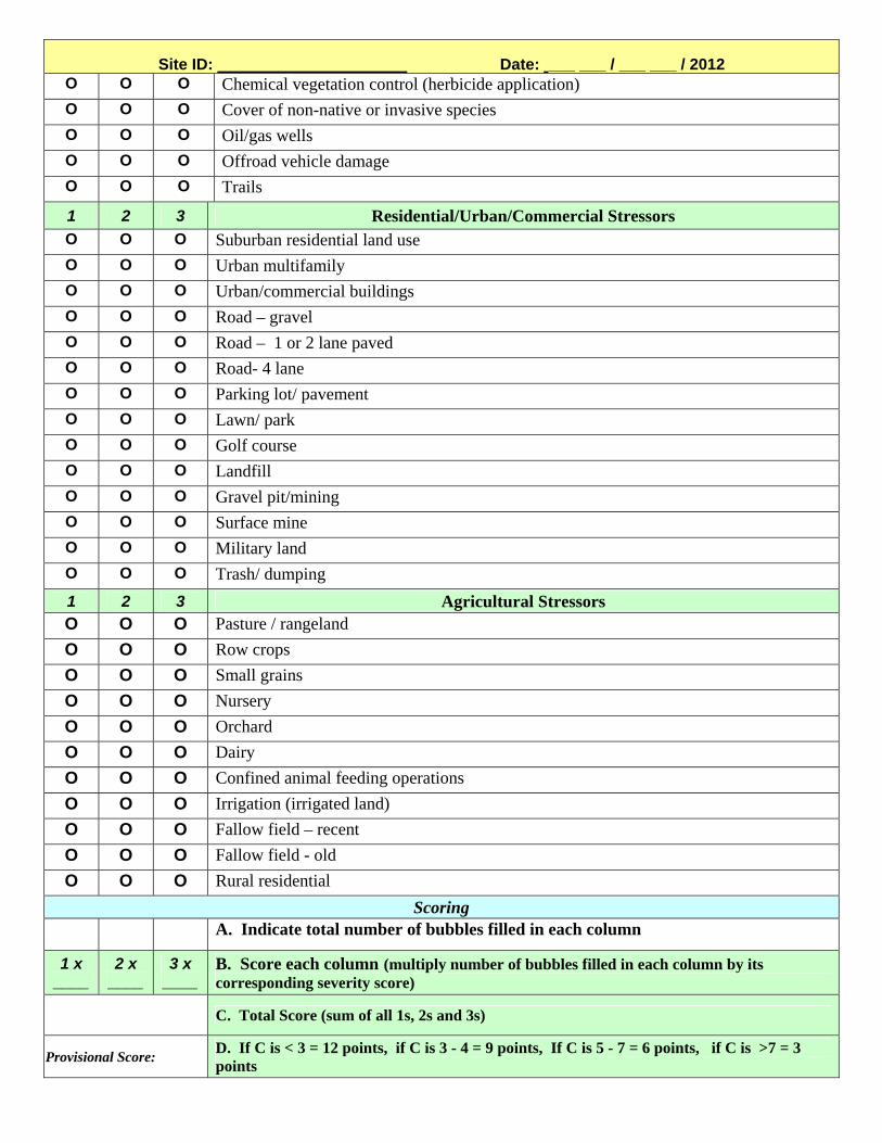
Site ID: Date: ___ ___ / ___ ___ / 2012 O O O Chemical vegetation control (herbicide application)

O O O Cover of non-native or invasive species

O O O Oil/gas wells

O O O Offroad vehicle damage

O O O Trails

1 2 3 Residential/Urban/Commercial Stressors O O O Suburban residential land use

O O O Urban multifamily

O O O Urban/commercial buildings

O O O Road – gravel

O O O Road – 1 or 2 lane paved

O O O Road- 4 lane

O O O Parking lot/ pavement

O O O Lawn/ park

O O O Golf course

O O O Landfill

O O O Gravel pit/mining

O O O Surface mine

O O O Military land

O O O Trash/ dumping

1 2 3 Agricultural Stressors O O O Pasture / rangeland

O O O Row crops

O O O Small grains

O O O Nursery

O O O Orchard

O O O Dairy

O O O Confined animal feeding operations

O O O Irrigation (irrigated land)

O O O Fallow field – recent

O O O Fallow field - old

O O O Rural residential

Scoring A. Indicate total number of bubbles filled in each column

1 x ____

2 x ____

3 x ____

B. Score each column (multiply number of bubbles filled in each column by its corresponding severity score)

C. Total Score (sum of all 1s, 2s and 3s)

Provisional Score: D. If C is < 3 = 12 points, if C is 3 - 4 = 9 points, If C is 5 - 7 = 6 points, if C is >7 = 3 points

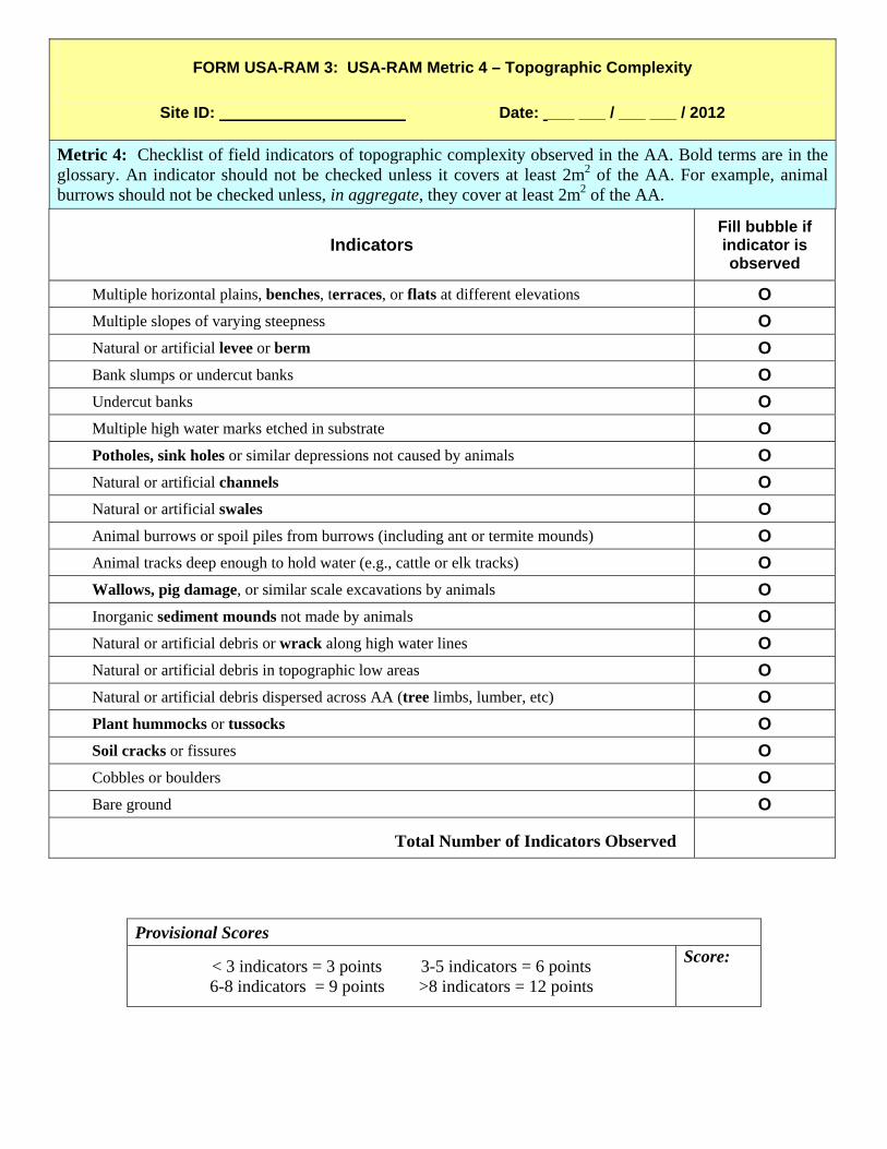
FORM USA-RAM 3: USA-RAM Metric 4 – Topographic Complexity

Site ID: Date: ___ ___ / ___ ___ / 2012

Metric 4: Checklist of field indicators of topographic complexity observed in the AA. Bold terms are in the glossary. An indicator should not be checked unless it covers at least 2m2 of the AA. For example, animal burrows should not be checked unless, in aggregate, they cover at least 2m2 of the AA.

Indicators Fill bubble if indicator is observed

Multiple horizontal plains, benches, terraces, or flats at different elevations O

Multiple slopes of varying steepness O

Natural or artificial levee or berm O

Bank slumps or undercut banks O

Undercut banks O

Multiple high water marks etched in substrate O

Potholes, sink holes or similar depressions not caused by animals O

Natural or artificial channels O

Natural or artificial swales O

Animal burrows or spoil piles from burrows (including ant or termite mounds) O

Animal tracks deep enough to hold water (e.g., cattle or elk tracks) O

Wallows, pig damage, or similar scale excavations by animals O

Inorganic sediment mounds not made by animals O

Natural or artificial debris or wrack along high water lines O

Natural or artificial debris in topographic low areas O

Natural or artificial debris dispersed across AA (tree limbs, lumber, etc) O

Plant hummocks or tussocks O

Soil cracks or fissures O

Cobbles or boulders O

Bare ground O

Total Number of Indicators Observed

Provisional Scores

< 3 indicators = 3 points 3-5 indicators = 6 points 6-8 indicators = 9 points >8 indicators = 12 points

Score:

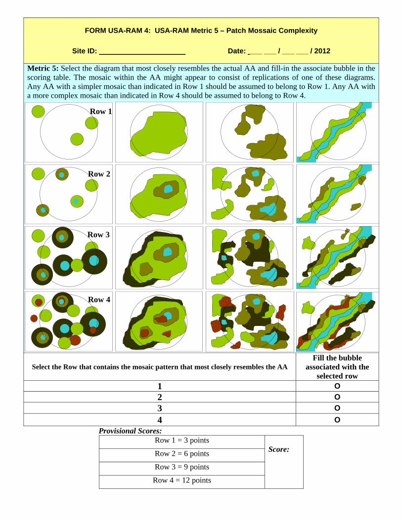
FORM USA-RAM 4: USA-RAM Metric 5 – Patch Mossaic Complexity

Site ID: Date: ___ ___ / ___ ___ / 2012

Metric 5: Select the diagram that most closely resembles the actual AA and fill-in the associate bubble in the scoring table. The mosaic within the AA might appear to consist of replications of one of these diagrams. Any AA with a simpler mosaic than indicated in Row 1 should be assumed to belong to Row 1. Any AA with a more complex mosaic than indicated in Row 4 should be assumed to belong to Row 4.

Select the Row that contains the mosaic pattern that most closely resembles the AA Fill the bubble

associated with the selected row

1 O

2 O

3 O

4 O

Provisional Scores: Row 1 = 3 points

Score:

Row 2 = 6 points

Row 3 = 9 points

Row 4 = 12 points

Row 1

Row 2

Row 3

Row 4

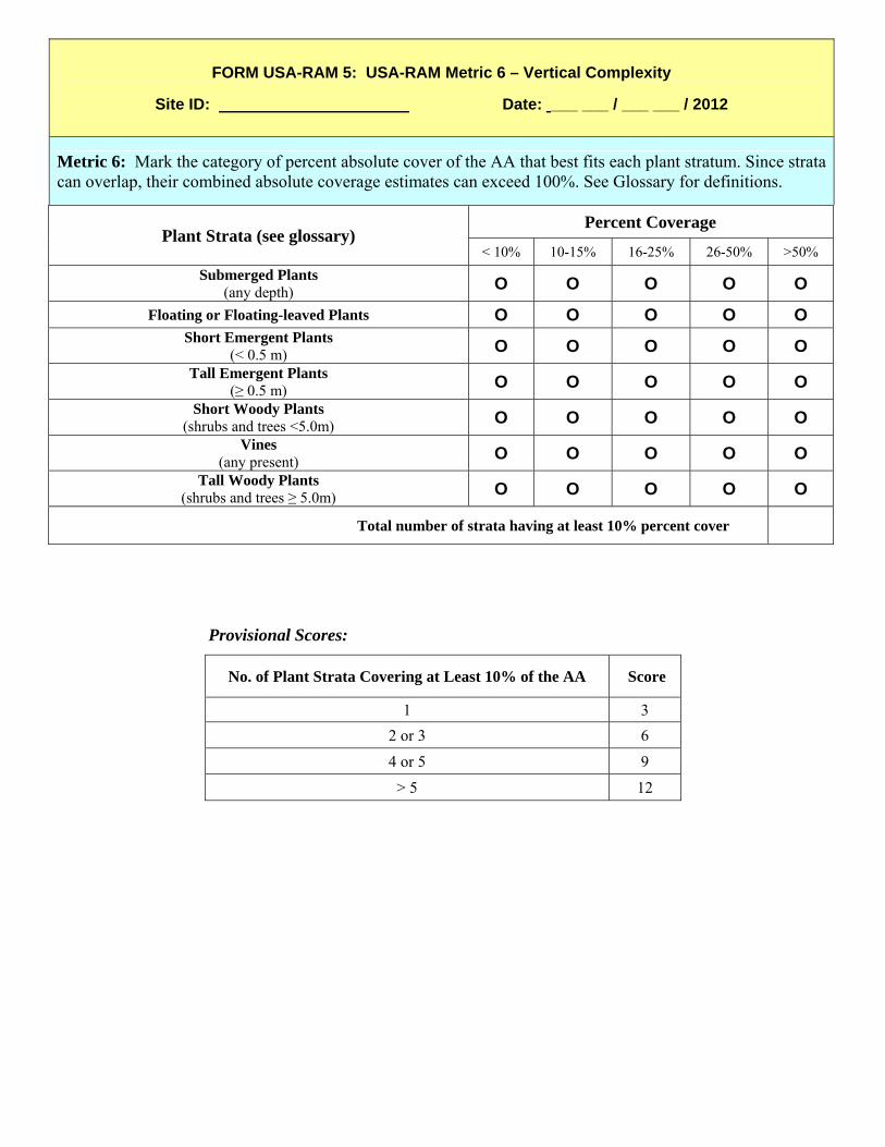
FORM USA-RAM 5: USA-RAM Metric 6 – Vertical Complexity

Site ID: Date: ___ ___ / ___ ___ / 2012

Metric 6: Mark the category of percent absolute cover of the AA that best fits each plant stratum. Since strata can overlap, their combined absolute coverage estimates can exceed 100%. See Glossary for definitions.

Plant Strata (see glossary) Percent Coverage

< 10% 10-15% 16-25% 26-50% >50%

Submerged Plants (any depth) O O O O O

Floating or Floating-leaved Plants O O O O O Short Emergent Plants

(< 0.5 m) O O O O O

Tall Emergent Plants (≥ 0.5 m) O O O O O

Short Woody Plants (shrubs and trees <5.0m) O O O O O

Vines (any present) O O O O O

Tall Woody Plants (shrubs and trees ≥ 5.0m) O O O O O

Total number of strata having at least 10% percent cover

Provisional Scores:

No. of Plant Strata Covering at Least 10% of the AA Score

1 3

2 or 3 6

4 or 5 9

> 5 12

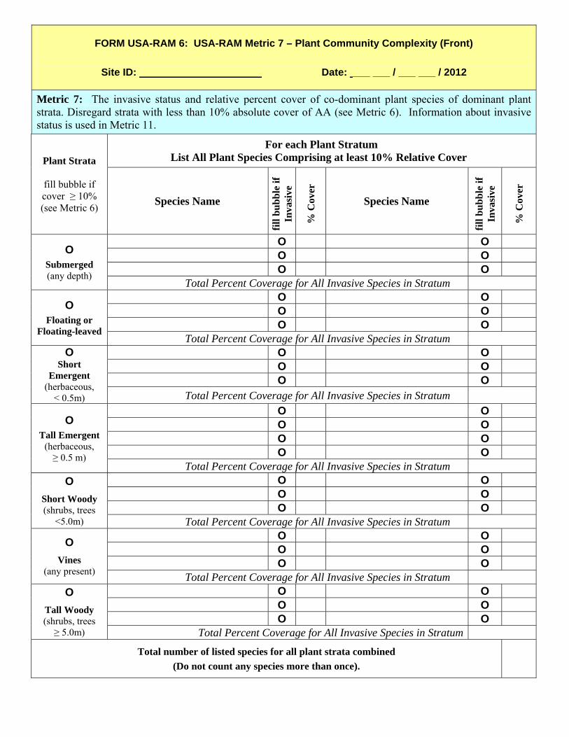
FORM USA-RAM 6: USA-RAM Metric 7 – Plant Community Complexity (Front)

Site ID: Date: ___ ___ / ___ ___ / 2012

Metric 7: The invasive status and relative percent cover of co-dominant plant species of dominant plant strata. Disregard strata with less than 10% absolute cover of AA (see Metric 6). Information about invasive status is used in Metric 11.

Plant Strata

fill bubble if cover ≥ 10% (see Metric 6)

For each Plant Stratum List All Plant Species Comprising at least 10% Relative Cover

Species Name

fill

bu

bb

le if

In

vasi

ve

% C

over

Species Name

fill

bu

bb

le if

In

vasi

ve

% C

over

O

Submerged (any depth)

O O

O O

O O

Total Percent Coverage for All Invasive Species in Stratum

O

Floating or Floating-leaved

O O

O O

O O

Total Percent Coverage for All Invasive Species in Stratum

O Short

Emergent (herbaceous,

< 0.5m)

O O

O O

O O

Total Percent Coverage for All Invasive Species in Stratum

O

Tall Emergent (herbaceous, ≥ 0.5 m)

O O

O O

O O

O O

Total Percent Coverage for All Invasive Species in Stratum

O

Short Woody (shrubs, trees

<5.0m)

O O

O O

O O

Total Percent Coverage for All Invasive Species in Stratum

O

Vines (any present)

O O

O O

O O

Total Percent Coverage for All Invasive Species in Stratum

O

Tall Woody (shrubs, trees ≥ 5.0m)

O O

O O

O O

Total Percent Coverage for All Invasive Species in Stratum

Total number of listed species for all plant strata combined

(Do not count any species more than once).

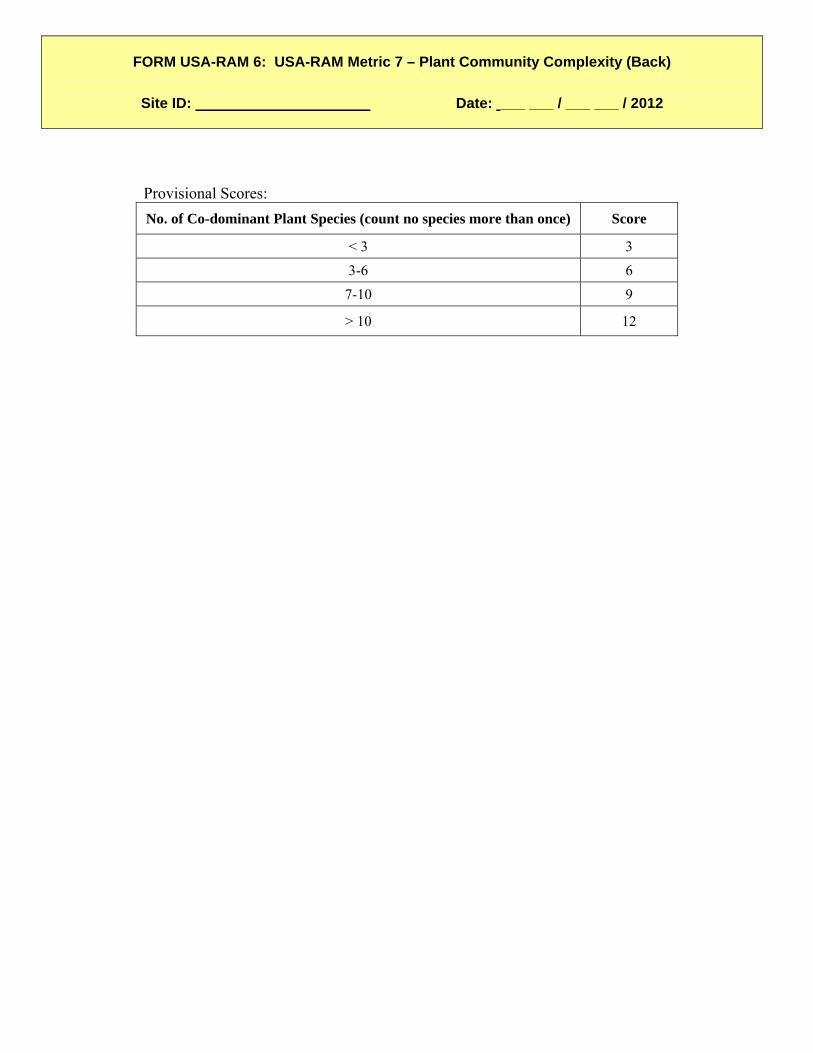
FORM USA-RAM 6: USA-RAM Metric 7 – Plant Community Complexity (Back)

Site ID: Date: ___ ___ / ___ ___ / 2012

Provisional Scores:

No. of Co-dominant Plant Species (count no species more than once) Score

< 3 3

3-6 6

7-10 9

> 10 12

FORM USA-RAM 7: USA-RAM Stressor Metric 8 –Stressors to Water Quality in the AA

Site ID: Date: ___ ___ / ___ ___ / 2012

Metric 8: Indicate water quality stressors observed in the AA. Each observed indicator is ranked as: 1) not severe (stressor is present, but does not appear to negatively affect any condition attribute in the AA), 2) moderately severe (stressor is present and appears to have moderately negative impacts on one or more condition attributes); or 3) severe (stressor is present and appears to have major negative impacts on one or more condition attribute). Each indicator can have only one severity rank. Fill in the bubble corresponding to the choice for each stressor indicator that is observed, then provide an overall rank for each Stressor Category. Tally all the marked ranks for the final score (excluding scores for Stressor Categories). If stressor present,

mark severity Field Indicators by Stressor Category 1 2 3

O O O Point Sources

O O O Point source inputs (discharge from wastewater plants, factories, etc)

O O O Stormwater inputs (discharge pipes, culverts, sewer outfalls)

O O O Sedimentation/Pollutants

O O O Debris lines on plants, trees or silt-laden vegetation

O O O Sedimentation (e.g., the presence of sediment fans, deposits or plumes)

O O O Industrial or domestic spills or discharges (odors; color, oil sheen*, foam)

O O O Turbidity in the water column

O O O Eutrophication

O O O Direct discharges from feedlot manure pits, etc.

O O O Direct discharges from septic or sewage systems

O O O Direct application of fertilizer

O O O Agricultural runoff (drain tiles, etc. discharging to site)

O O O Formation of heavy algal or Lemna sp. surface mats or heavy benthic algal growth

Mining Impacts

O O O Acid mine drainage discharge (excessively clear water (low pH) or presence/accumulation of

“yellow-boy” orange precipitate)

Salinity

O O O Obvious increases in the concentration of dissolved salts (dead or stressed plants; salt

encrustations, etc)

Scoring A. Indicate total number of bubbles filled in each column (not including those for

Stressor Categories). 1 x

____ 2 x

____ 3 x

____ B. Multiply “A” above by its corresponding severity score.

C. Add together the numbers from “B” above.

Provisional Score:

D. If C is 0-1= 12 points; if C is 2-4 = 9 points; if C is 5-6 = 6 points; if C is ≥ 7 = 3 points

FORM USA-RAM 8: USA-RAM Stressor Metric 9 –Alterations to Hydroperiod in the AA

Site ID: Date: ___ ___ / ___ ___ / 2012

Metric 9: Indicators of altered hydroperiod observed in AA. Each observed indicator is ranked as: 1) not

severe (stressor is present, but does not appear to negatively affect any condition attribute in the AA), 2) moderately severe (stressor is present and appears to have moderately negative impacts on one or more condition attributes in the AA); or 3) severe (stressor is present and appears to have major negative impacts on one or more condition attribute in the AA). Each indicator can have only one severity rank. Fill in the bubble corresponding to the choice for each stressor indicator that is observed. Tally all the marked ranks for the final score.

If stressor is

present, mark its severity Field Stressor Indicators

1 2 3

O O O Ditches/channelization within AA

O O O Dikes/dams/levees/berms at AA margin or within AA or roadbed or railroad (acting as block to water flows into or through AA)

O O O Channels have deeply undercut banks and/or bank slumps or slides

O O O Culverts, pipes (point sources) into AA (change in water quantity)

O O O Water level control structure that impound water in all or part of the AA

O O O Upland plant species encroaching into AA (due to drying of wetland)

O O O Die-off of trees within AA due to increased ponding (exempting beaver impounded sites)

O O O Tidal restriction in tidal wetlands (restricts flows to and from AA)

O O O Presence of agricultural tiles or culverts at AA margin or within AA

O O O Siphons, pumps moving water in or out of AA

O O O Stormwater inputs from impervious surfaces/flashy flows into AA

Scoring

A. Indicate total number of bubbles filled in each column

1 x ____

2 x ____

3 x ____ B. Multiply “A” above by its corresponding severity score.

C. Add together the numbers from “B” above.

Provisional Score:

D. If C is 0-1 = 12 points; if C is 2-3 = 9 points; if C is 4-5 = 6 points; if C is ≥ 6 = 3 points

FORM USA-RAM 9: USA-RAM Stressor Metric 10 –Stress to substrate in the AA

Site ID: Date: ___ ___ / ___ ___ / 2012

Metric 10. Indicators of altered substrate observed in AA. Each observed indicator is ranked as: 1) not severe

(stressor is present, but does not appear to negatively affect any condition attribute in the AA), 2) moderately severe (stressor is present and appears to have moderately negative impacts on one or more condition attributes); or 3) severe (stressor is present and appears to have major negative impacts on one or more condition attribute). Each indicator can have only one severity rank. Fill in the bubble corresponding to the choice for each stressor indicator that is observed. Tally all the marked ranks for the final score.

If stressor is present, mark its

severity Field Stressor Indicators

1 2 3

O O O Soil subsidence, scour or surface erosion (root exposure, etc)

O O O Off-road vehicles, mountain biking, trails cut, etc.

O O O Inorganic sedimentation inflow (sediment accumulation around vegetation, deep sediment

splays, recent vegetation burial, etc)

O O O Dredging or other prominent excavation at AA margin or in AA

O O O Grazing by domesticated or feral animals in AA (includes trampling, digging, wallowing, etc)

O O O Grazing by native ungulates.

O O O Recent farming activity (plowing, disking, etc.)

O O O Soil compaction by human activity (parking by cars, heavy machinery, etc)

O O O Filling, grading, or other prominent deposition of sediment

O O O Dumping of garbage or other debris

O O O Mechanical plant removal that disturbs substrate (rutting, grubbing by heavy machinery, etc.)

Fire lines (fire breaks) dug in AA or at AA margin

Scoring

A. Indicate total number of bubbles filled in each column

1 x ____

2 x ____

3 x ____ B. Multiply “A” above by its corresponding severity score.

C. Add together the numbers from “B” above.

Provisional Score:

D. If C is 0-1 = 12 points; if C is 2-3 = 9 points; if C is 4-5 = 6 points; if C is ≥ 6 = 3 points

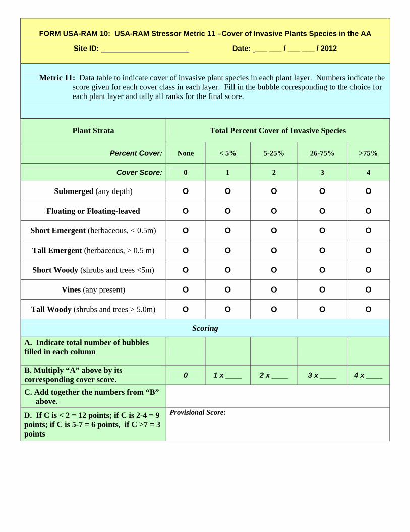
FORM USA-RAM 10: USA-RAM Stressor Metric 11 –Cover of Invasive Plants Species in the AA

Site ID: Date: ___ ___ / ___ ___ / 2012

Metric 11: Data table to indicate cover of invasive plant species in each plant layer. Numbers indicate the

score given for each cover class in each layer. Fill in the bubble corresponding to the choice for each plant layer and tally all ranks for the final score.

Plant Strata Total Percent Cover of Invasive Species

Percent Cover: None < 5% 5-25% 26-75% >75%

Cover Score: 0 1 2 3 4

Submerged (any depth) O O O O O

Floating or Floating-leaved O O O O O

Short Emergent (herbaceous, < 0.5m) O O O O O

Tall Emergent (herbaceous, > 0.5 m) O O O O O

Short Woody (shrubs and trees <5m) O O O O O

Vines (any present) O O O O O

Tall Woody (shrubs and trees > 5.0m) O O O O O

Scoring

A. Indicate total number of bubbles filled in each column

B. Multiply “A” above by its corresponding cover score. 0 1 x ____ 2 x ____ 3 x ____ 4 x ____

C. Add together the numbers from “B” above.

D. If C is < 2 = 12 points; if C is 2-4 = 9 points; if C is 5-7 = 6 points, if C >7 = 3 points

Provisional Score:

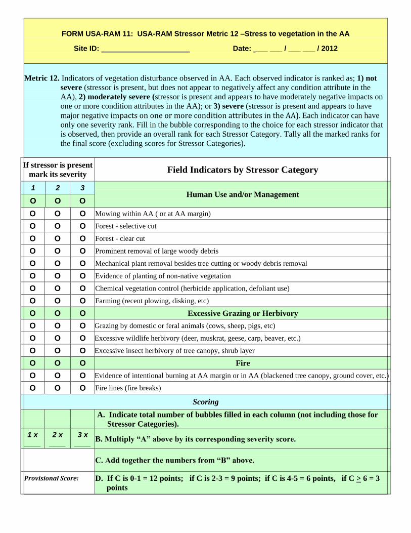
FORM USA-RAM 11: USA-RAM Stressor Metric 12 –Stress to vegetation in the AA

Site ID: Date: ___ ___ / ___ ___ / 2012

Metric 12. Indicators of vegetation disturbance observed in AA. Each observed indicator is ranked as; 1) not

severe (stressor is present, but does not appear to negatively affect any condition attribute in the

AA), 2) moderately severe (stressor is present and appears to have moderately negative impacts on

one or more condition attributes in the AA); or 3) severe (stressor is present and appears to have

major negative impacts on one or more condition attributes in the AA). Each indicator can have

only one severity rank. Fill in the bubble corresponding to the choice for each stressor indicator that

is observed, then provide an overall rank for each Stressor Category. Tally all the marked ranks for

the final score (excluding scores for Stressor Categories).

If stressor is present

mark its severity Field Indicators by Stressor Category

1 2 3 Human Use and/or Management

O O O

O O O Mowing within AA ( or at AA margin)

O O O Forest - selective cut

O O O Forest - clear cut

O O O Prominent removal of large woody debris

O O O Mechanical plant removal besides tree cutting or woody debris removal

O O O Evidence of planting of non-native vegetation

O O O Chemical vegetation control (herbicide application, defoliant use)

O O O Farming (recent plowing, disking, etc)

O O O Excessive Grazing or Herbivory

O O O Grazing by domestic or feral animals (cows, sheep, pigs, etc)

O O O Excessive wildlife herbivory (deer, muskrat, geese, carp, beaver, etc.)

O O O Excessive insect herbivory of tree canopy, shrub layer

O O O Fire

O O O Evidence of intentional burning at AA margin or in AA (blackened tree canopy, ground cover, etc.)

O O O Fire lines (fire breaks)

Scoring

A. Indicate total number of bubbles filled in each column (not including those for

Stressor Categories).

1 x ____

2 x ____

3 x ____

B. Multiply “A” above by its corresponding severity score.

C. Add together the numbers from “B” above.

Provisional Score:

D. If C is 0-1 = 12 points; if C is 2-3 = 9 points; if C is 4-5 = 6 points, if C > 6 = 3

points

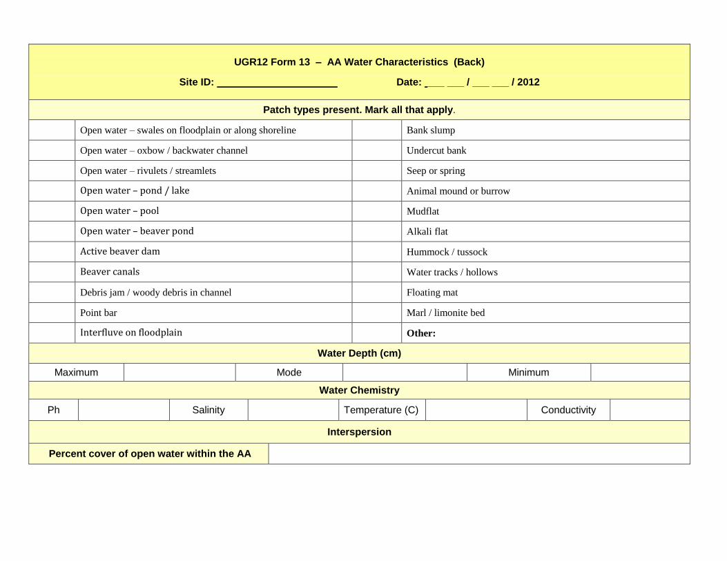
UGR12 Form 13 – AA Water Characteristics (Back)

Site ID: Date: ___ ___ / ___ ___ / 2012

Patch types present. Mark all that apply.

Open water – swales on floodplain or along shoreline Bank slump

Open water – oxbow / backwater channel Undercut bank

Open water – rivulets / streamlets Seep or spring

Open water – pond / lake Animal mound or burrow

Open water – pool Mudflat

Open water – beaver pond Alkali flat

Active beaver dam Hummock / tussock

Beaver canals Water tracks / hollows

Debris jam / woody debris in channel Floating mat

Point bar Marl / limonite bed

Interfluve on floodplain Other:

Water Depth (cm)

Maximum Mode Minimum

Water Chemistry

Ph Salinity Temperature (C) Conductivity

Interspersion

Percent cover of open water within the AA

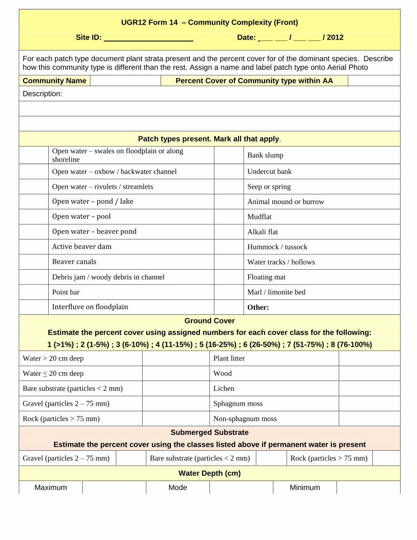
UGR12 Form 14 – Community Complexity (Front)

Site ID: Date: ___ ___ / ___ ___ / 2012

For each patch type document plant strata present and the percent cover for of the dominant species. Describe how this community type is different than the rest. Assign a name and label patch type onto Aerial Photo

Community Name Percent Cover of Community type within AA

Description:

Patch types present. Mark all that apply.

Open water – swales on floodplain or along

shoreline Bank slump

Open water – oxbow / backwater channel Undercut bank

Open water – rivulets / streamlets Seep or spring

Open water – pond / lake Animal mound or burrow

Open water – pool Mudflat

Open water – beaver pond Alkali flat

Active beaver dam Hummock / tussock

Beaver canals Water tracks / hollows

Debris jam / woody debris in channel Floating mat

Point bar Marl / limonite bed

Interfluve on floodplain Other:

Ground Cover

Estimate the percent cover using assigned numbers for each cover class for the following:

1 (>1%) ; 2 (1-5%) ; 3 (6-10%) ; 4 (11-15%) ; 5 (16-25%) ; 6 (26-50%) ; 7 (51-75%) ; 8 (76-100%)

Water > 20 cm deep Plant litter

Water < 20 cm deep Wood

Bare substrate (particles < 2 mm) Lichen

Gravel (particles 2 – 75 mm) Sphagnum moss

Rock (particles > 75 mm) Non-sphagnum moss

Submerged Substrate

Estimate the percent cover using the classes listed above if permanent water is present

Gravel (particles 2 – 75 mm) Bare substrate (particles < 2 mm) Rock (particles > 75 mm)

Water Depth (cm)

Maximum Mode Minimum

UGR12 Form 14 – Community Complexity (Back)

Site ID: Date: ___ ___ / ___ ___ / 2012

List dominant species within each stratum if it makes up more than 10 % of the community type. Do not

count any species more than once.

Plant Strata

fill bubble if

cover ≥ 10%

(see Metric 6)

For each Plant Stratum

List All Plant Species Comprising at least 10% Relative Cover

Species Name

fill

bu

bb

le

if I

nv

asi

ve

% C

ov

er

Species Name

fill

bu

bb

le

if I

nv

asi

ve

% C

ov

er

O

Submerged (any depth)

O O

O O

O O

Total Percent Coverage for All Invasive Species in Stratum

O

Floating or

Floating-leaved

O O

O O

O O

Total Percent Coverage for All Invasive Species in Stratum

O

Short

Emergent

(herbaceous,

< 0.5m)

O O

O O

O O

Total Percent Coverage for All Invasive Species in Stratum

O

Tall Emergent

(herbaceous,

≥ 0.5 m)

O O

O O

O O

O O

Total Percent Coverage for All Invasive Species in Stratum

O

Short Woody (shrubs, trees

<5.0m)

O O

O O

O O

Total Percent Coverage for All Invasive Species in Stratum

O

Vines (any present)

O O

O O

O O

Total Percent Coverage for All Invasive Species in Stratum

O

Tall Woody

(shrubs, trees

≥ 5.0m)

O O

O O

O O

Total Percent Coverage for All Invasive Species in Stratum

Total Number of Listed Species for all plant strata combined ( Do not count species more than once)

Provisional Scores: No. of Co-dominant Plant Species

(count no species more than once) Score

< 3 3

3-6 6

7-10 9

> 10 12

UGR12 Form 14 – Community Complexity (Front)

Site ID: Date: ___ ___ / ___ ___ / 2012

For each patch type document plant strata present and the percent cover for of the dominant species. Describe how this community type is different than the rest. Assign a name and label patch type onto Aerial Photo

Community Name Percent Cover of Community type within AA

Description:

Patch types present. Mark all that apply.

Open water – swales on floodplain or along

shoreline Bank slump

Open water – oxbow / backwater channel Undercut bank

Open water – rivulets / streamlets Seep or spring

Open water – pond / lake Animal mound or burrow

Open water – pool Mudflat

Open water – beaver pond Alkali flat

Active beaver dam Hummock / tussock

Beaver canals Water tracks / hollows

Debris jam / woody debris in channel Floating mat

Point bar Marl / limonite bed

Interfluve on floodplain Other:

Ground Cover

Estimate the percent cover using assigned numbers for each cover class for the following:

1 (>1%) ; 2 (1-5%) ; 3 (6-10%) ; 4 (11-15%) ; 5 (16-25%) ; 6 (26-50%) ; 7 (51-75%) ; 8 (76-100%)

Water > 20 cm deep Plant litter

Water < 20 cm deep Wood

Bare substrate (particles < 2 mm) Lichen

Gravel (particles 2 – 75 mm) Sphagnum moss

Rock (particles > 75 mm) Non-sphagnum moss

Submerged Substrate

Estimate the percent cover using the classes listed above if permanent water is present

Gravel (particles 2 – 75 mm) Bare substrate (particles < 2 mm) Rock (particles > 75 mm)

Water Depth (cm)

Maximum Mode Minimum

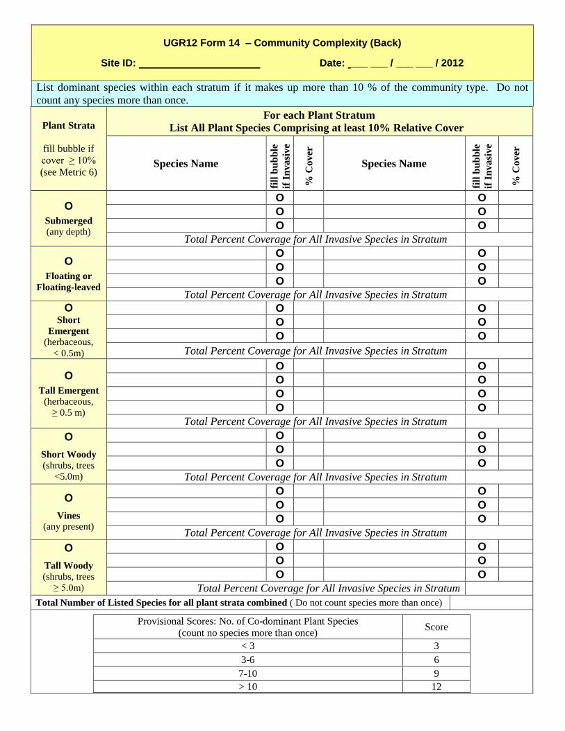
UGR12 Form 14 – Community Complexity (Back)

Site ID: Date: ___ ___ / ___ ___ / 2012

List dominant species within each stratum if it makes up more than 10 % of the community type. Do not

count any species more than once.

Plant Strata

fill bubble if

cover ≥ 10%

(see Metric 6)

For each Plant Stratum

List All Plant Species Comprising at least 10% Relative Cover

Species Name

fill

bu

bb

le

if I

nv

asi

ve

% C

ov

er

Species Name

fill

bu

bb

le

if I

nv

asi

ve

% C

ov

er

O

Submerged (any depth)

O O

O O

O O

Total Percent Coverage for All Invasive Species in Stratum

O

Floating or

Floating-leaved

O O

O O

O O

Total Percent Coverage for All Invasive Species in Stratum

O

Short

Emergent

(herbaceous,

< 0.5m)

O O

O O

O O

Total Percent Coverage for All Invasive Species in Stratum

O

Tall Emergent

(herbaceous,

≥ 0.5 m)

O O

O O

O O

O O

Total Percent Coverage for All Invasive Species in Stratum

O

Short Woody (shrubs, trees

<5.0m)

O O

O O

O O

Total Percent Coverage for All Invasive Species in Stratum

O

Vines (any present)

O O

O O

O O

Total Percent Coverage for All Invasive Species in Stratum

O

Tall Woody

(shrubs, trees

≥ 5.0m)

O O

O O

O O

Total Percent Coverage for All Invasive Species in Stratum

Total Number of Listed Species for all plant strata combined ( Do not count species more than once)

Provisional Scores: No. of Co-dominant Plant Species

(count no species more than once) Score

< 3 3

3-6 6

7-10 9

> 10 12

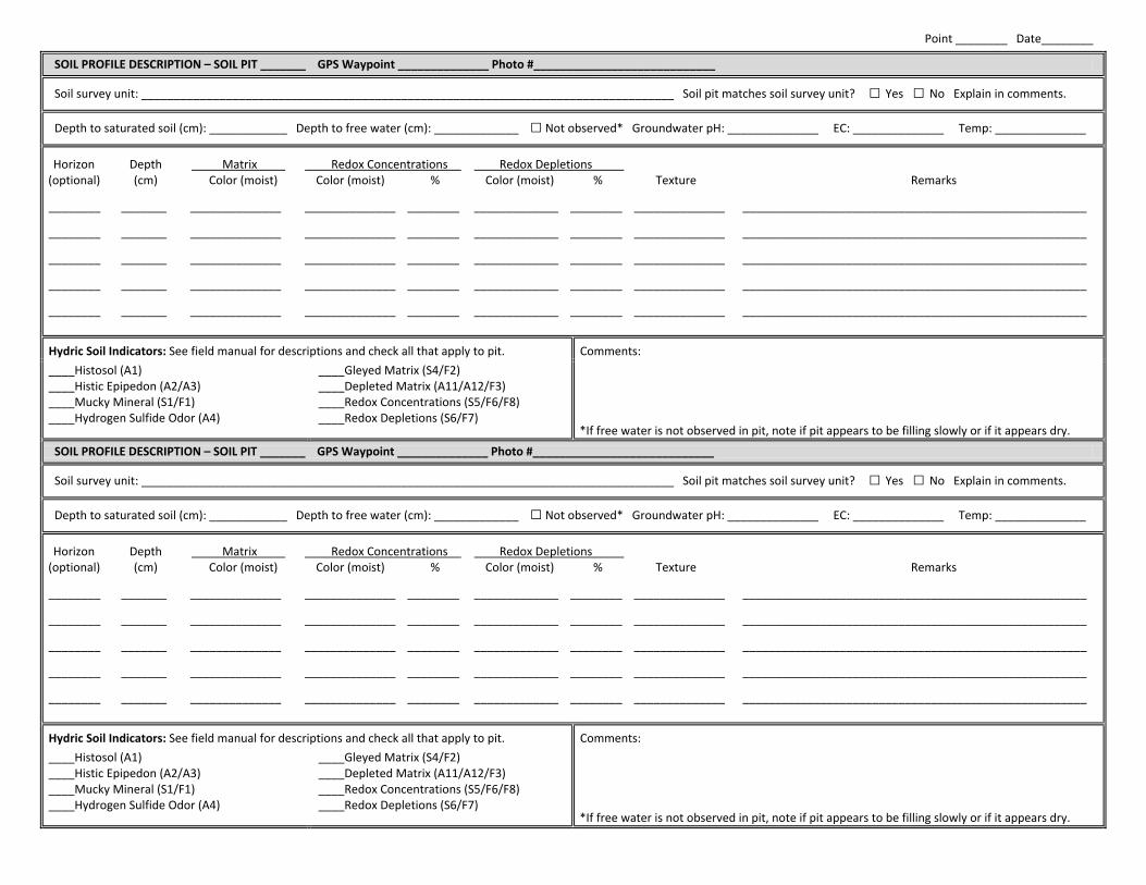
Point ________ Date________

SOIL PROFILE DESCRIPTION – SOIL PIT _______ GPS Waypoint ______________ Photo #____________________________

Soil survey unit: __________________________________________________________________________________ Soil pit matches soil survey unit? □ Yes □ No Explain in comments.

Depth to saturated soil (cm): ____________ Depth to free water (cm): _____________ □ Not observed* Groundwater pH: ______________ EC: ______________ Temp: ______________

Horizon Depth Matrix Redox Concentrations Redox Depletions (optional) (cm) Color (moist) Color (moist) % Color (moist) % Texture Remarks

________ _______ ______________ ______________ ________ _____________ ________ ______________ _____________________________________________________

________ _______ ______________ ______________ ________ _____________ ________ ______________ _____________________________________________________

________ _______ ______________ ______________ ________ _____________ ________ ______________ _____________________________________________________

________ _______ ______________ ______________ ________ _____________ ________ ______________ _____________________________________________________

________ _______ ______________ ______________ ________ _____________ ________ ______________ _____________________________________________________

Hydric Soil Indicators: See field manual for descriptions and check all that apply to pit. Comments: *If free water is not observed in pit, note if pit appears to be filling slowly or if it appears dry.

____Histosol (A1) ____Histic Epipedon (A2/A3) ____Mucky Mineral (S1/F1) ____Hydrogen Sulfide Odor (A4)

____Gleyed Matrix (S4/F2) ____Depleted Matrix (A11/A12/F3) ____Redox Concentrations (S5/F6/F8) ____Redox Depletions (S6/F7)

SOIL PROFILE DESCRIPTION – SOIL PIT _______ GPS Waypoint ______________ Photo #____________________________

Soil survey unit: __________________________________________________________________________________ Soil pit matches soil survey unit? □ Yes □ No Explain in comments.

Depth to saturated soil (cm): ____________ Depth to free water (cm): _____________ □ Not observed* Groundwater pH: ______________ EC: ______________ Temp: ______________

Horizon Depth Matrix Redox Concentrations Redox Depletions (optional) (cm) Color (moist) Color (moist) % Color (moist) % Texture Remarks

________ _______ ______________ ______________ ________ _____________ ________ ______________ _____________________________________________________

________ _______ ______________ ______________ ________ _____________ ________ ______________ _____________________________________________________

________ _______ ______________ ______________ ________ _____________ ________ ______________ _____________________________________________________

________ _______ ______________ ______________ ________ _____________ ________ ______________ _____________________________________________________

________ _______ ______________ ______________ ________ _____________ ________ ______________ _____________________________________________________

Hydric Soil Indicators: See field manual for descriptions and check all that apply to pit. Comments: *If free water is not observed in pit, note if pit appears to be filling slowly or if it appears dry.

____Histosol (A1) ____Histic Epipedon (A2/A3) ____Mucky Mineral (S1/F1) ____Hydrogen Sulfide Odor (A4)

____Gleyed Matrix (S4/F2) ____Depleted Matrix (A11/A12/F3) ____Redox Concentrations (S5/F6/F8) ____Redox Depletions (S6/F7)

Point ________ Date________

SOIL PROFILE DESCRIPTION – SOIL PIT _______ GPS Waypoint ______________ Photo #____________________________

Soil survey unit: __________________________________________________________________________________ Soil pit matches soil survey unit? □ Yes □ No Explain in comments.

Depth to saturated soil (cm): ____________ Depth to free water (cm): _____________ □ Not observed* Groundwater pH: ______________ EC: ______________ Temp: ______________

Horizon Depth Matrix Redox Concentrations Redox Depletions (optional) (cm) Color (moist) Color (moist) % Color (moist) % Texture Remarks

________ _______ ______________ ______________ ________ _____________ ________ ______________ _____________________________________________________

________ _______ ______________ ______________ ________ _____________ ________ ______________ _____________________________________________________

________ _______ ______________ ______________ ________ _____________ ________ ______________ _____________________________________________________

________ _______ ______________ ______________ ________ _____________ ________ ______________ _____________________________________________________

________ _______ ______________ ______________ ________ _____________ ________ ______________ _____________________________________________________

Hydric Soil Indicators: See field manual for descriptions and check all that apply to pit. Comments: *If free water is not observed in pit, note if pit appears to be filling slowly or if it appears dry.

____Histosol (A1) ____Histic Epipedon (A2/A3) ____Mucky Mineral (S1/F1) ____Hydrogen Sulfide Odor (A4)

____Gleyed Matrix (S4/F2) ____Depleted Matrix (A11/A12/F3) ____Redox Concentrations (S5/F6/F8) ____Redox Depletions (S6/F7)

SOIL PROFILE DESCRIPTION – SOIL PIT _______ GPS Waypoint ______________ Photo #____________________________

Soil survey unit: __________________________________________________________________________________ Soil pit matches soil survey unit? □ Yes □ No Explain in comments.

Depth to saturated soil (cm): ____________ Depth to free water (cm): _____________ □ Not observed* Groundwater pH: ______________ EC: ______________ Temp: ______________

Horizon Depth Matrix Redox Concentrations Redox Depletions (optional) (cm) Color (moist) Color (moist) % Color (moist) % Texture Remarks

________ _______ ______________ ______________ ________ _____________ ________ ______________ _____________________________________________________

________ _______ ______________ ______________ ________ _____________ ________ ______________ _____________________________________________________

________ _______ ______________ ______________ ________ _____________ ________ ______________ _____________________________________________________

________ _______ ______________ ______________ ________ _____________ ________ ______________ _____________________________________________________

________ _______ ______________ ______________ ________ _____________ ________ ______________ _____________________________________________________

Hydric Soil Indicators: See field manual for descriptions and check all that apply to pit. Comments: *If free water is not observed in pit, note if pit appears to be filling slowly or if it appears dry.

____Histosol (A1) ____Histic Epipedon (A2/A3) ____Mucky Mineral (S1/F1) ____Hydrogen Sulfide Odor (A4)

____Gleyed Matrix (S4/F2) ____Depleted Matrix (A11/A12/F3) ____Redox Concentrations (S5/F6/F8) ____Redox Depletions (S6/F7)

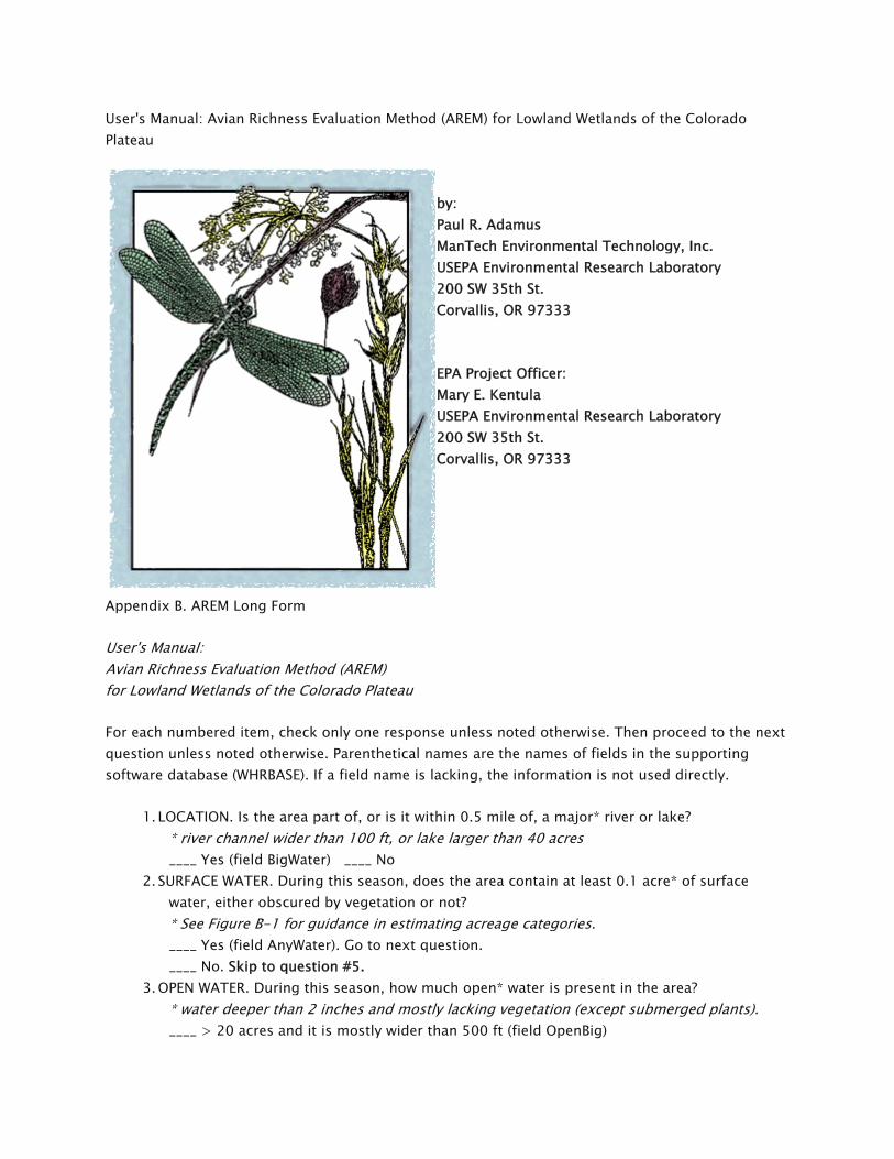
User's Manual: Avian Richness Evaluation Method (AREM) for Lowland Wetlands of the Colorado Plateau

by: Paul R. Adamus ManTech Environmental Technology, Inc. USEPA Environmental Research Laboratory 200 SW 35th St. Corvallis, OR 97333

EPA Project Officer: Mary E. Kentula USEPA Environmental Research Laboratory 200 SW 35th St. Corvallis, OR 97333

Appendix B. AREM Long Form

User's Manual: Avian Richness Evaluation Method (AREM) for Lowland Wetlands of the Colorado Plateau

For each numbered item, check only one response unless noted otherwise. Then proceed to the next question unless noted otherwise. Parenthetical names are the names of fields in the supporting software database (WHRBASE). If a field name is lacking, the information is not used directly.

1. LOCATION. Is the area part of, or is it within 0.5 mile of, a major* river or lake? * river channel wider than 100 ft, or lake larger than 40 acres ____ Yes (field BigWater) ____ No

2. SURFACE WATER. During this season, does the area contain at least 0.1 acre* of surface water, either obscured by vegetation or not? * See Figure B-1 for guidance in estimating acreage categories. ____ Yes (field AnyWater). Go to next question. ____ No. Skip to question #5.

3. OPEN WATER. During this season, how much open* water is present in the area? * water deeper than 2 inches and mostly lacking vegetation (except submerged plants). ____ > 20 acres and it is mostly wider than 500 ft (field OpenBig)

____ < 1 acre, or, >1 acre but mostly narrower than 3 ft (field OpenSmall) ____ Other conditions (field OpenOther)

4. SPECIFIC AQUATIC CONDITIONS Check all that apply during this season: ____ > 0.1 acre of the surface water is still, i.e., usually flows at less than 1 ft/s (field StillWater) ____ The evaluated area can be assumed to contain fish (field Fish) ____ The evaluated area can be assumed to contain frogs, salamanders, and/or crayfish (field Amphibs) ____ Water transparency in the deepest part of the area is (or would be, if depth is shallow) sufficient to see an object 10 inches below the surface, and the area is not known to have problems with metal contamination (field Clear) ____ The evaluated area is highly enriched by direct fertilizer applications, water from nearby feedlots, or other sources (field Enriched) ____ Most of the normally-flooded part of the area goes dry at least one year in five, or, is subject to flooding from a river at least as often (field Drawdown)

5. BARE SOIL. Is there at least 0.1 acre of mud*, alkali flat, gravel/sand bar, recently tilled soil, and/or heavily grazed open (grassy, non-shrubby) areas during this season? * includes soil that is continually saturated up to the surface, or which was previously covered by water but has become exposed to the air during this period ____ Yes (field Bare). Go to next question. ____ No. Skip to question #7.

6. LARGE MUDFLAT. Does the area at this season contain mud that has all these features?: o At least 1 acre in size o Maximum dimension is greater than 100 ft o Salt crust or salt stains are not apparent o Not recessed within a wash or canal whose depth (relative to surrounding landscape)

is greater than half its width.

____ Yes (field MudBig) ____ No

7. TREES. Are there at least 3 trees*: * woody plants taller than 20 ft. ____ in the evaluation area? (field TreeIn). ____ within 1000 ft of the evaluation area? (field TreeNear). Go to #8. ____ neither of the above. Skip to #11.

8. TREE COVER. Check one or more responses below that describe the maximum cumulative acreage of various conditions of tree cover in the evaluation area. Also include areas within 300 ft: ____ >1 acre, dense*, and wide** (field ForestDens) ____ >1 acre and open; or, dense but narrow (field ForestOpen) ____ 0.1-1 acre, dense* (field WoodDens) ____ 0.1-1 acre, open (field WoodOpen) ____ <0.1 acre

* Dense= the tree canopy, viewed from the ground during midsummer, appears at least 50% closed, as averaged across an area that is at least as large as the acreage specified. ** Wide= the wooded area is wider than 300 ft (average).

9. BIG TREES. Are there at least three trees whose trunk diameter 20 ft above the ground is >12 inches? ____ Yes (field TreesBig) ____ No

10. SNAGS. Are there at least three snags, or trees with dead limbs with diameter >5 inches? ____ Yes (field Snags) ____ No

11. SHRUBS. Is there at least 0.1 acre of shrubs*: * woody plants 2-20 ft in height. ____ in the evaluation area? (field ShrubIn). ____ within 1000 ft of the wetland (including the wetland itself)? (field ShrubNear). Go to #12. ____ Neither of the above. Skip to #13.

12. SHRUB SPECIES AND DENSITY. Check one or more responses below that describe the maximum cumulative extent of various types and conditions of shrub cover in the evaluation area. Also include areas within 300 ft. Willow: ____ >1 acre, dense*, and wide** (field WwMuchDens) ____ >1 acre and open; or, dense but narrow (field WwMuchOpen) ____ 0.1-1 acre, dense* (field WwSomeDens) ____ 0.1-1 acre, open (field WwSomeOpen) ____ <0.1 acre; or larger area but height mostly <4 ft and openly spaced Greasewood or other tall desert shrubs: ____ >1 acre, dense*, and wide** (field GrMuchDens) ____ >1 acre and open; or, dense but narrow (field GrMuchOpen) ____ 0.1-1 acre, dense* (field GrSomeDens) ____ 0.1-1 acre, open (field GrSomeOpen) ____ <0.1 acre Russian olive, sumac, buffaloberry, wild rose, or others with fleshy fruit: ____ >1 acre, dense*, and wide** (field FrMuchDens) ____ >1 acre, open; or, dense but narrow (field FrMuchOpen) ____ 0.1-1 acre, dense (field FrSomeDens) ____ 0.1-1 acre, open (field FrSomeOpen) ____ <0.1 acre; or larger area but height mostly <4 ft Tamarisk (salt cedar): ____ >1 acre, dense*, and wide** (field TmMuchDens) ____ >1 acre, open; or, dense but narrow (field TmMuchOpen) ____ 0.1-1 acre, dense (field TmSomeDens) ____ 0.1-1 acre, open (field TmSomeOpen) ____ <0.1 acre; or larger area but height mostly <4 ft

* Dense= the shrub canopy, as viewed from a height of 100 ft during midsummer, appears to be >50% closed, as averaged across an area that is at least as large as the acreage specified. ** Wide= the shrub area is wider than 300 ft (average).

13. HERBACEOUS VEGETATION. Is there at least 0.1 acre of herbaceous vegetation*: * Nonwoody plants such as cattail, bulrush, sedges, grasses, and forbs. ____ in the evaluation area? (field HerbIn). ____ within 1000 ft? (field HerbNear). Go to #14. ____ Neither of the above. Skip to #15.

14. HERBACEOUS SPECIES. Check one or more responses below that describe the maximum cumulative extent of various types and conditions of shrub cover in the evaluation area. Also include areas within 300 ft. Robust emergents (e.g., cattail, phragmites) ____ >1 acre, dense*, and wide** (field RbMuchDens) ____ >1 acre, open; or dense but narrow (field RbMuchOpen) ____ 0.1-1 acre, dense (field RbSomeDens) ____ 0.1-1 acre, open (field RbSomeOpen) Other wet** emergents (e.g., bulrush, sedge) ____ >1 acre, dense*, wide**, and tall*** (field WEMuchDens) ____ >1 acre, tall, open; or dense but narrow (field WEMuchOpen) ____ >1 acre, dense or open, and short (field WEMuchShrt) ____ 0.1-1 acre, tall, dense (field WESomeDens) ____ 0.1-1 acre, tall, open; or dense but narrow (field WESomeOpen) ____ 0.1-1 acre, dense or open, and short (field WESomeShrt) Drier emergents (e.g., saltgrass, other grasses) ____ >1 acre, dense*, wide**, and tall*** (field DEMuchDens) ____ >1 acre, tall, open; or dense but narrow (field DEMuchOpen) ____ >1 acre, dense or open, and short (field DEMuchShrt) ____ 0.1-1 acre, tall, dense (field DESomeDens) ____ 0.1-1 acre, tall, open; or dense but narrow (field DESomeOpen) ____ 0.1-1 acre, dense or open, and short (field DESomeShrt) Broad-leaved Forbs (e.g., milkweed, thistle, alfalfa) ____ >1 acre (field ForbMuch) ____ 0.1-1 acre (field ForbSome) Aquatic plants (e.g., watercress, sago pondweed, duckweed) ____ >10 acres (field AqMuch) ____ 0.1-10 acres (field AqSome)

* Dense= plants are so close together that the duff layer or soil beneath the plants is mostly obscured by foliage, when looking down from just above the plant tops. ** Wet= water is visible at or above the soil surface during most of the growing season. *** Wide= the shrub area is wider than 300 ft (average). **** Tall= taller than 1 ft.

15. SURROUNDING LAND COVER. Check one: Within 0.5 mi of the wetland, >60% of the land cover is: ____ Pasture, alfalfa, grain crops, row crops, other wetlands, grass lawns, and/or weed fields (field SurAgwet) ____ Desert shrubs (e.g., sagebrush, shadscale, rabbitbrush)(field SurDesrt) ____ Pinyon-juniper (field SurPJ) ____ Oak scrub (e.g., Gambel oak, serviceberry, skunkbrush)(field SurOak) ____ Other, or none of the above comprise >60%

16. LOCAL LAND COVER. Check one: Within 3 mi of the wetland, > 60% of the land cover is: ____ Pasture, alfalfa, grain crops, row crops, other wetlands, grass lawns, and/or weed fields (field LocAgWet) ____ Desert shrubs (e.g., sagebrush, shadscale, rabbitbrush)(field LocDesrt) ____ Pinyon-juniper (field LocPJ) ____ Oak scrub (e.g., Gambel oak, serviceberry, skunkbrush)(field LocOak) ____ Other, or none of the above comprise >60%

17. VISUAL SECLUSION Check only one: ____ Both of the following: (a) wetland is seldom visited by people on foot or boat (less than once weekly), (b) there are no paved roads within 600 ft, or if there are, wetland is not visible from the roads (field SeclusionH). ____ Either (a) or (b) above (field SeclusionM). ____ Other condition.

18. PREDATION POTENTIAL Check only one. The evaluation area: ____ is linear*, adjoins a heavily-traveled road (usual maximum of >1 car/minute), and/or is in a high-density housing area (>1 house/5 acres) (field PredHPot) ____ adjoins a less-traveled road, and/or is in an area with sparser housing density but is closer than 1000 ft to a normally-occupied building (field PredMPot) ____ Other condition. * at least 90% of the area being evaluated is within 25 ft of a canal, road, railroad tracks, or other artificially linear feature.

19. GRAZED, BURNED, MOWED. Is the area mowed, burned, or grazed intensively (i.e., with clearly visible effects on vegetation) during this season? ____ Yes (field GrazBurnMo) ____ No

20. NESTING LOCATIONS Check all that apply:

____ Semi-open structures (bridges, barns) suitable for nesting swallows are present within 300 ft (field SwallNest) ____ Platforms suitable for nesting geese are present in the wetland or along its perimeter (field GooseNest) ____ Vertical, mostly bare dirt banks at least 5 ft high are present within 0.5 mi., of potential use to nesting kingfishers, barn owls, and swallows (field Banks)

This concludes the initial evaluation. If you intend to infer the value of this wetland at seasons or years other than the present one, you should go back over all your responses and, on a new form, change the responses that would be different at that season/year. Then, proceed to the analysis described by the User's Manual.

 

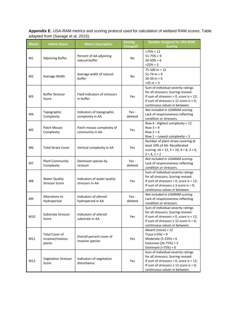
Appendix E. USA-RAM metrics and scoring protocol used for calculation of wetland RAM scores. Table adapted from (Savage et al. 2015).

Metric  Metric Name  Metric Description Scoring Changed? 

Number Assigned for USA‐RAM Scoring 

M1  Adjoining Buffer Percent of AA adjoining natural buffer 

No 

>75% = 12 51‐75% = 9 26‐50% = 6 <25% = 3 

M2  Average Width Average width of natural buffer 

No 

75‐100 m = 12 51‐74 m = 9 26‐50 m = 6 <25 m = 3 

M3 Buffer Stressor Score 

Field indicators of stressors in buffer 

Yes 

Sum of individual severity ratings for all stressors; Scoring revised: If sum of stressors = 0, score is = 12; If sum of stressors ≥ 12 score is = 0;  continuous values in between. 

M4 Topographic Complexity 

Indicators of topographic complexity in AA 

Yes ‐ deleted 

Not included in USARAM scoring. Lack of responsiveness reflecting condition or stressors. 

M5 Patch Mosaic Complexity 

Patch mosaic complexity of community in AA 

Yes 

Row 4 ‐ Highest complexity = 12 Row 3 = 9 Row 2 = 6 Row 1 – Lowest complexity = 3 

M6  Total Strata Cover  Vertical complexity in AA  Yes 

Number of plant strata covering at least 10% of AA‐ Recalibrated scoring: ≥6 = 12, 5 = 10, 4 = 8, 3 = 6, 2 = 4, 1 = 2 

M7 Plant Community Complexity 

Dominant species by stratum 

Yes ‐ deleted 

Not included in USARAM scoring. Lack of responsiveness reflecting condition or stressors. 

M8 Water Quality Stressor Score 

Indicators of water quality stressors in AA 

Yes 

Sum of individual severity ratings for all stressors; Scoring revised: If sum of stressors = 0, score is = 12; If sum of stressors ≥ 3 score is = 9;  continuous values in between. 

M9 Alterations to Hydroperiod  

Indicators of altered hydroperiod in AA 

Yes ‐ deleted 

Not included in USARAM scoring. Lack of responsiveness reflecting condition or stressors. 

M10 Substrate Stressor Score 

Indicators of altered substrate in AA 

Yes 

Sum of individual severity ratings for all stressors; Scoring revised: If sum of stressors = 0, score is = 12; If sum of stressors ≥ 12 score is = 0;  continuous values in between. 

M11 Total Cover of invasive/noxious plants 

Overall percent cover of invasive species 

Yes 

Absent (none) = 12 Trace (<5%) = 9 Moderate (5‐25%) = 6 Extensive (26‐75%) = 3 Dominant (>75%) = 0 

M12 Vegetation Stressor Score 

Indicators of vegetation disturbance 

Yes 

Sum of individual severity ratings for all stressors; Scoring revised: If sum of stressors = 0, score is = 12; If sum of stressors ≥ 12 score is = 0;  continuous values in between. 

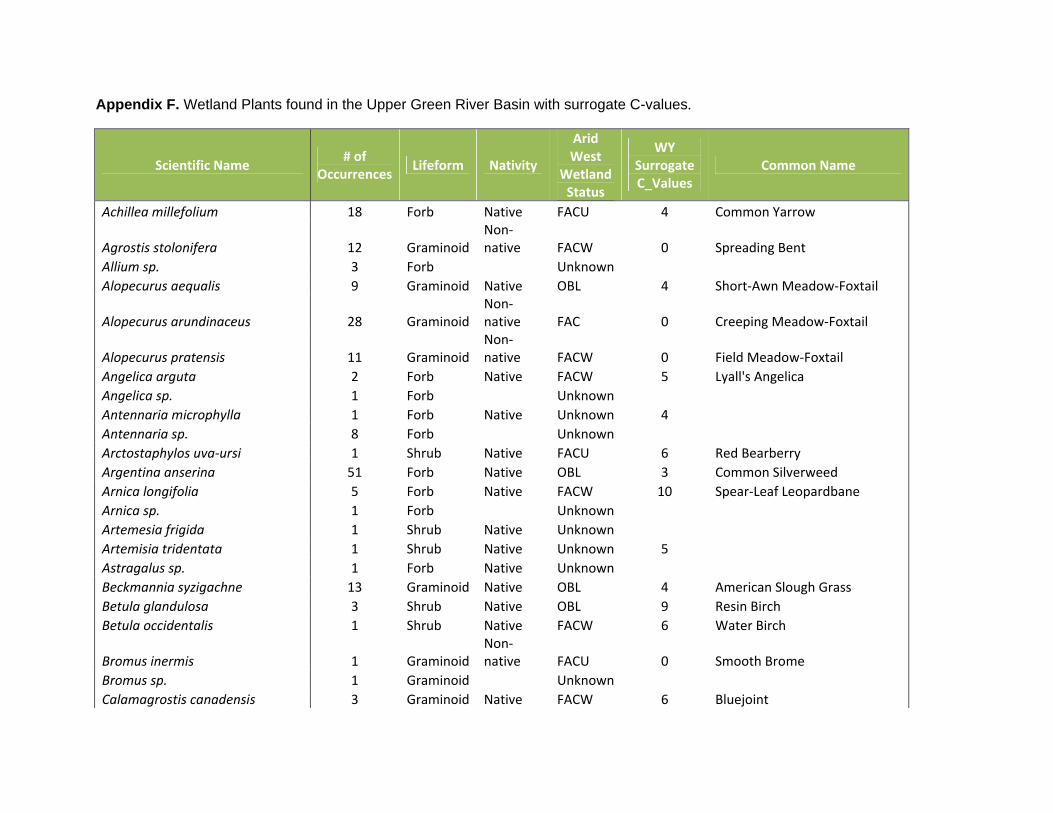
Appendix F. Wetland Plants found in the Upper Green River Basin with surrogate C-values.

Scientific Name # of 

Occurrences Lifeform  Nativity 

Arid West 

Wetland Status 

WY Surrogate C_Values 

Common Name 

Achillea millefolium  18  Forb  Native  FACU  4  Common Yarrow 

Agrostis stolonifera  12  GraminoidNon‐native  FACW  0  Spreading Bent 

Allium sp.  3  Forb  Unknown    

Alopecurus aequalis  9  Graminoid Native  OBL  4  Short‐Awn Meadow‐Foxtail 

Alopecurus arundinaceus  28  GraminoidNon‐native  FAC  0  Creeping Meadow‐Foxtail 

Alopecurus pratensis  11  GraminoidNon‐native  FACW  0  Field Meadow‐Foxtail 

Angelica arguta  2  Forb  Native  FACW  5  Lyall's Angelica 

Angelica sp.  1  Forb  Unknown    

Antennaria microphylla  1  Forb  Native  Unknown  4    

Antennaria sp.  8  Forb  Unknown    

Arctostaphylos uva‐ursi  1  Shrub  Native  FACU  6  Red Bearberry 

Argentina anserina  51  Forb  Native  OBL  3  Common Silverweed 

Arnica longifolia  5  Forb  Native  FACW  10  Spear‐Leaf Leopardbane 

Arnica sp.  1  Forb  Unknown    

Artemesia frigida  1  Shrub  Native  Unknown    

Artemisia tridentata  1  Shrub  Native  Unknown  5    

Astragalus sp.  1  Forb  Native  Unknown    

Beckmannia syzigachne  13  Graminoid Native  OBL  4  American Slough Grass 

Betula glandulosa  3  Shrub  Native  OBL  9  Resin Birch 

Betula occidentalis  1  Shrub  Native  FACW  6  Water Birch 

Bromus inermis  1  GraminoidNon‐native  FACU  0  Smooth Brome 

Bromus sp.  1  Graminoid Unknown    

Calamagrostis canadensis  3  Graminoid Native  FACW  6  Bluejoint 

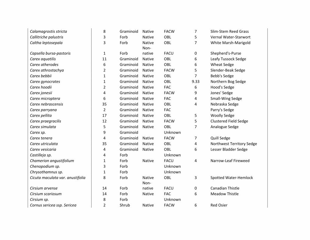
Calamagrostis stricta  8  Graminoid Native  FACW  7  Slim‐Stem Reed Grass 

Callitriche palustris  3  Forb  Native  OBL  5  Vernal Water‐Starwort 

Caltha leptosepala  3  Forb  Native  OBL  7  White Marsh‐Marigold 

Capsella bursa‐pastoris  1  Forb Non‐native  FACU  0  Shepherd's‐Purse 

Carex aquatilis  11  Graminoid Native  OBL  6  Leafy Tussock Sedge 

Carex atherodes  6  Graminoid Native  OBL  6  Wheat Sedge 

Carex athrostachya  2  Graminoid Native  FACW  5  Slender‐Beak Sedge 

Carex bebbii  1  Graminoid Native  OBL  7  Bebb's Sedge 

Carex gynocrates  1  Graminoid Native  OBL  9.33  Northern Bog Sedge 

Carex hoodii  2  Graminoid Native  FAC  6  Hood's Sedge 

Carex jonesii  4  Graminoid Native  FACW  9  Jones' Sedge 

Carex microptera  6  Graminoid Native  FAC  4  Small‐Wing Sedge 

Carex nebrascensis  35  Graminoid Native  OBL  4  Nebraska Sedge 

Carex parryana  2  Graminoid Native  FAC  Parry's Sedge 

Carex pellita  17  Graminoid Native  OBL  5  Woolly Sedge 

Carex praegracilis  12  Graminoid Native  FACW  5  Clustered Field Sedge 

Carex simulata  5  Graminoid Native  OBL  7  Analogue Sedge 

Carex sp.  9  Graminoid Unknown    

Carex tenera  4  Graminoid Native  FACW  7  Quill Sedge 

Carex utriculata  35  Graminoid Native  OBL  4  Northwest Territory Sedge 

Carex vesicaria  4  Graminoid Native  OBL  6  Lesser Bladder Sedge 

Castilleja sp.  4  Forb  Unknown    

Chamerion angustifolium  1  Forb  Native  FACU  4  Narrow‐Leaf Fireweed 

Chenopodium sp.  3  Forb  Unknown    

Chrysothamnus sp.  1  Forb  Unknown    

Cicuta maculata var. anustifolia  8  Forb  Native  OBL  3  Spotted Water‐Hemlock 

Cirsium arvense  14  Forb Non‐native  FACU  0  Canadian Thistle 

Cirsium scariosum  14  Forb  Native  FAC  6  Meadow Thistle 

Cirsium sp.  8  Forb  Unknown    

Cornus sericea ssp. Sericea  2  Shrub  Native  FACW  6  Red Osier 

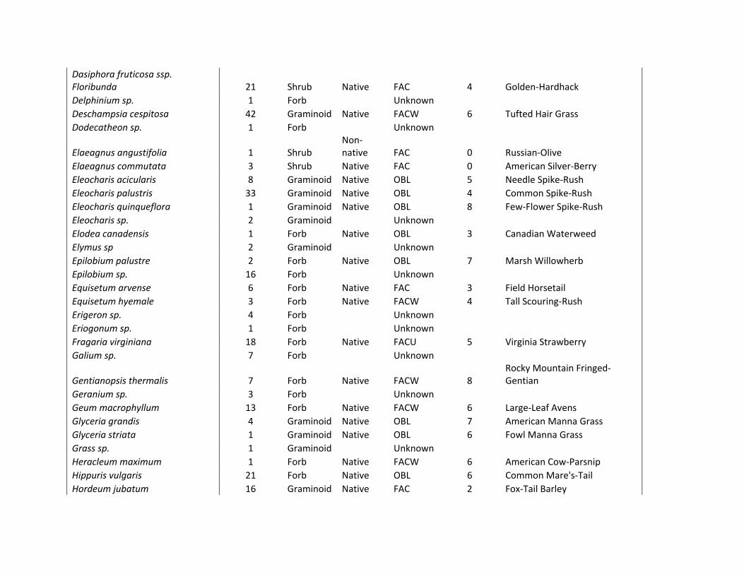
Dasiphora fruticosa ssp. Floribunda  21  Shrub  Native  FAC  4  Golden‐Hardhack 

Delphinium sp.  1  Forb  Unknown    

Deschampsia cespitosa  42  Graminoid Native  FACW  6  Tufted Hair Grass 

Dodecatheon sp.  1  Forb  Unknown    

Elaeagnus angustifolia  1  Shrub Non‐native  FAC  0  Russian‐Olive 

Elaeagnus commutata  3  Shrub  Native  FAC  0  American Silver‐Berry 

Eleocharis acicularis  8  Graminoid Native  OBL  5  Needle Spike‐Rush 

Eleocharis palustris  33  Graminoid Native  OBL  4  Common Spike‐Rush 

Eleocharis quinqueflora  1  Graminoid Native  OBL  8  Few‐Flower Spike‐Rush 

Eleocharis sp.  2  Graminoid Unknown    

Elodea canadensis  1  Forb  Native  OBL  3  Canadian Waterweed 

Elymus sp  2  Graminoid Unknown    

Epilobium palustre  2  Forb  Native  OBL  7  Marsh Willowherb 

Epilobium sp.  16  Forb  Unknown    

Equisetum arvense  6  Forb  Native  FAC  3  Field Horsetail 

Equisetum hyemale  3  Forb  Native  FACW  4  Tall Scouring‐Rush 

Erigeron sp.  4  Forb  Unknown    

Eriogonum sp.  1  Forb  Unknown    

Fragaria virginiana  18  Forb  Native  FACU  5  Virginia Strawberry 

Galium sp.  7  Forb  Unknown    

Gentianopsis thermalis  7  Forb  Native  FACW  8 Rocky Mountain Fringed‐Gentian 

Geranium sp.  3  Forb  Unknown    

Geum macrophyllum  13  Forb  Native  FACW  6  Large‐Leaf Avens 

Glyceria grandis  4  Graminoid Native  OBL  7  American Manna Grass 

Glyceria striata  1  Graminoid Native  OBL  6  Fowl Manna Grass 

Grass sp.  1  Graminoid Unknown    

Heracleum maximum  1  Forb  Native  FACW  6  American Cow‐Parsnip 

Hippuris vulgaris  21  Forb  Native  OBL  6  Common Mare's‐Tail 

Hordeum jubatum  16  Graminoid Native  FAC  2  Fox‐Tail Barley 

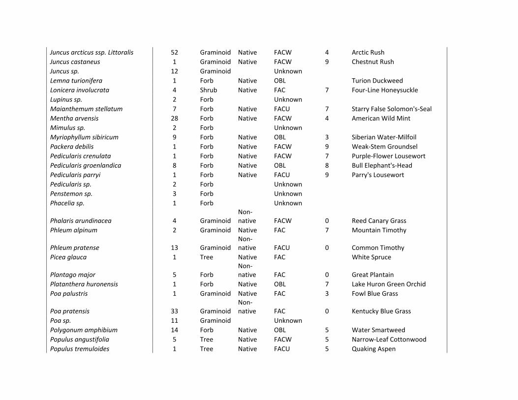
Juncus arcticus ssp. Littoralis  52  Graminoid Native  FACW  4  Arctic Rush 

Juncus castaneus  1  Graminoid Native  FACW  9  Chestnut Rush 

Juncus sp.  12  Graminoid Unknown    

Lemna turionifera  1  Forb  Native  OBL  Turion Duckweed 

Lonicera involucrata  4  Shrub  Native  FAC  7  Four‐Line Honeysuckle 

Lupinus sp.  2  Forb  Unknown    

Maianthemum stellatum  7  Forb  Native  FACU  7  Starry False Solomon's‐Seal 

Mentha arvensis  28  Forb  Native  FACW  4  American Wild Mint 

Mimulus sp.  2  Forb  Unknown    

Myriophyllum sibiricum  9  Forb  Native  OBL  3  Siberian Water‐Milfoil 

Packera debilis  1  Forb  Native  FACW  9  Weak‐Stem Groundsel 

Pedicularis crenulata  1  Forb  Native  FACW  7  Purple‐Flower Lousewort 

Pedicularis groenlandica  8  Forb  Native  OBL  8  Bull Elephant's‐Head 

Pedicularis parryi  1  Forb  Native  FACU  9  Parry's Lousewort 

Pedicularis sp.  2  Forb  Unknown    

Penstemon sp.  3  Forb  Unknown    

Phacelia sp.  1  Forb  Unknown    

Phalaris arundinacea  4  GraminoidNon‐native  FACW  0  Reed Canary Grass 

Phleum alpinum  2  Graminoid Native  FAC  7  Mountain Timothy 

Phleum pratense  13  GraminoidNon‐native  FACU  0  Common Timothy 

Picea glauca  1  Tree  Native  FAC  White Spruce 

Plantago major  5  Forb Non‐native  FAC  0  Great Plantain 

Platanthera huronensis  1  Forb  Native  OBL  7  Lake Huron Green Orchid 

Poa palustris  1  Graminoid Native  FAC  3  Fowl Blue Grass 

Poa pratensis  33  GraminoidNon‐native  FAC  0  Kentucky Blue Grass 

Poa sp.  11  Graminoid Unknown    

Polygonum amphibium  14  Forb  Native  OBL  5  Water Smartweed 

Populus angustifolia  5  Tree  Native  FACW  5  Narrow‐Leaf Cottonwood 

Populus tremuloides  1  Tree  Native  FACU  5  Quaking Aspen 

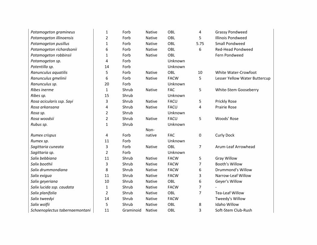
Potamogeton gramineus  1  Forb  Native  OBL  4  Grassy Pondweed 

Potamogeton illinoensis  2  Forb  Native  OBL  5  Illinois Pondweed 

Potamogeton pusillus  1  Forb  Native  OBL  5.75  Small Pondweed 

Potamogeton richardsonii  6  Forb  Native  OBL  6  Red‐Head Pondweed 

Potamogeton robbinsii  1  Forb  Native  OBL  Fern Pondweed 

Potamogeton sp.  4  Forb  Unknown    

Potentilla sp.  14  Forb  Unknown    

Ranunculus aquatilis  5  Forb  Native  OBL  10  White Water‐Crowfoot 

Ranunculus gmelinii  6  Forb  Native  FACW  5  Lesser Yellow Water Buttercup 

Ranunculus sp.  20  Forb  Unknown    

Ribes inerme  1  Shrub  Native  FAC  5  White‐Stem Gooseberry 

Ribes sp.  15  Shrub  Unknown    

Rosa acicularis ssp. Sayi  3  Shrub  Native  FACU  5  Prickly Rose 

Rosa arkansana  4  Shrub  Native  FACU  4  Prairie Rose 

Rosa sp.  2  Shrub  Unknown    

Rosa woodsii  2  Shrub  Native  FACU  5  Woods' Rose 

Rubus sp.  1  Shrub  Unknown    

Rumex crispus  4  Forb Non‐native  FAC  0  Curly Dock 

Rumex sp.  11  Forb  Unknown    

Sagittaria cuneata  3  Forb  Native  OBL  7  Arum‐Leaf Arrowhead 

Sagittaria sp.  2  Forb  Unknown    

Salix bebbiana  11  Shrub  Native  FACW  5  Gray Willow 

Salix boothii  3  Shrub  Native  FACW  7  Booth's Willow 

Salix drummondiana  8  Shrub  Native  FACW  6  Drummond's Willow 

Salix exigua  11  Shrub  Native  FACW  3  Narrow‐Leaf Willow 

Salix geyeriana  10  Shrub  Native  OBL  6  Geyer's Willow 

Salix lucida ssp. caudata  1  Shrub  Native  FACW  7  ‐ 

Salix planifolia  2  Shrub  Native  OBL  7  Tea‐Leaf Willow 

Salix tweedyi  14  Shrub  Native  FACW  Tweedy's Willow 

Salix wolfii  5  Shrub  Native  OBL  8  Idaho Willow 

Schoenoplectus tabernaemontani  11  Graminoid Native  OBL  3  Soft‐Stem Club‐Rush 

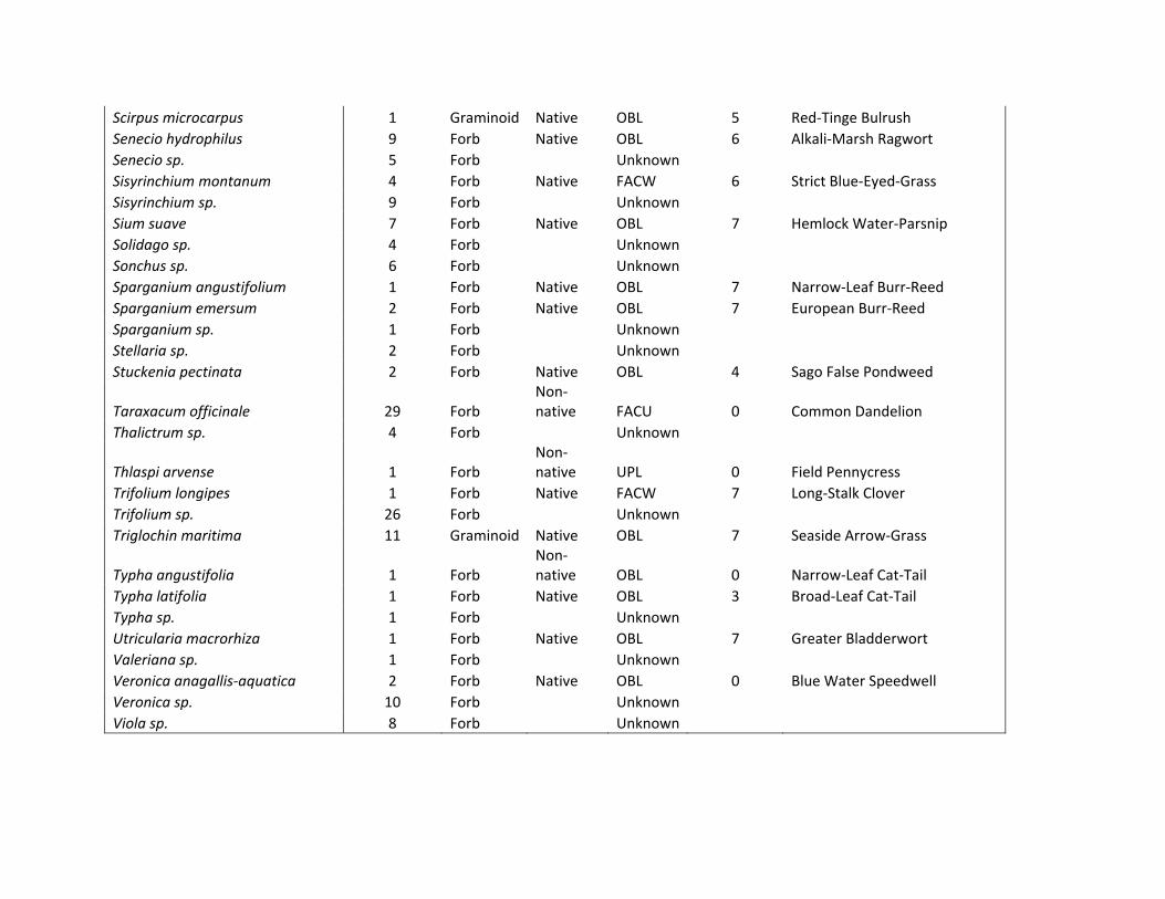
Scirpus microcarpus  1  Graminoid Native  OBL  5  Red‐Tinge Bulrush 

Senecio hydrophilus  9  Forb  Native  OBL  6  Alkali‐Marsh Ragwort 

Senecio sp.  5  Forb  Unknown    

Sisyrinchium montanum  4  Forb  Native  FACW  6  Strict Blue‐Eyed‐Grass 

Sisyrinchium sp.  9  Forb  Unknown    

Sium suave  7  Forb  Native  OBL  7  Hemlock Water‐Parsnip 

Solidago sp.  4  Forb  Unknown    

Sonchus sp.  6  Forb  Unknown    

Sparganium angustifolium  1  Forb  Native  OBL  7  Narrow‐Leaf Burr‐Reed 

Sparganium emersum  2  Forb  Native  OBL  7  European Burr‐Reed 

Sparganium sp.  1  Forb  Unknown    

Stellaria sp.  2  Forb  Unknown    

Stuckenia pectinata  2  Forb  Native  OBL  4  Sago False Pondweed 

Taraxacum officinale  29  Forb Non‐native  FACU  0  Common Dandelion 

Thalictrum sp.  4  Forb  Unknown    

Thlaspi arvense  1  Forb Non‐native  UPL  0  Field Pennycress 

Trifolium longipes  1  Forb  Native  FACW  7  Long‐Stalk Clover 

Trifolium sp.  26  Forb  Unknown    

Triglochin maritima  11  Graminoid Native  OBL  7  Seaside Arrow‐Grass 

Typha angustifolia  1  Forb Non‐native  OBL  0  Narrow‐Leaf Cat‐Tail 

Typha latifolia  1  Forb  Native  OBL  3  Broad‐Leaf Cat‐Tail 

Typha sp.  1  Forb  Unknown    

Utricularia macrorhiza  1  Forb  Native  OBL  7  Greater Bladderwort 

Valeriana sp.  1  Forb  Unknown    

Veronica anagallis‐aquatica  2  Forb  Native  OBL  0  Blue Water Speedwell 

Veronica sp.  10  Forb  Unknown    

Viola sp.  8  Forb     Unknown       

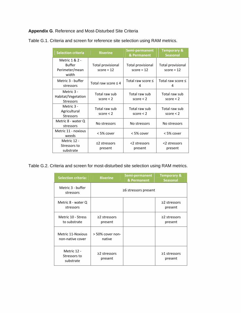
Appendix G. Reference and Most-Disturbed Site Criteria

Table G.1. Criteria and screen for reference site selection using RAM metrics.

Selection criteria  Riverine Semi‐permanent & Permanent 

Temporary & Seasonal 

Metric 1 & 2 ‐  Buffer 

Perimeter/mean width 

Total provisional score = 12 

Total provisional score = 12 

Total provisional score = 12 

Metric 3 ‐ buffer stressors 

Total raw score ≤ 4 Total raw score ≤ 

4 Total raw score ≤ 

4 

Metric 3 ‐ Habitat/Vegetation 

Stressors 

Total raw sub score < 2 

Total raw sub score < 2 

Total raw sub score < 2 

Metric 3 ‐ Agricultural Stressors 

Total raw sub score < 2 

Total raw sub score < 2 

Total raw sub score < 2 

Metric 8 ‐ water Q stressors 

No stressors  No stressors  No stressors 

Metric 11 ‐ noxious weeds 

< 5% cover  < 5% cover  < 5% cover 

Metric 12 ‐ Stressors to substrate 

≤2 stressors present 

<2 stressors present 

<2 stressors present 

Table G.2. Criteria and screen for most-disturbed site selection using RAM metrics.

Selection criteria:  Riverine Semi‐permanent & Permanent 

Temporary & Seasonal 

Metric 3 ‐ buffer stressors 

≥6 stressors present 

Metric 8 ‐ water Q stressors     

≥2 stressors present 

Metric 10 ‐ Stress to substrate 

≥2 stressors present   

≥2 stressors present 

Metric 11‐Noxious non‐native cover 

> 50% cover non‐native     

Metric 12 ‐ Stressors to substrate 

≥2 stressors present   

≥1 stressors present 

 

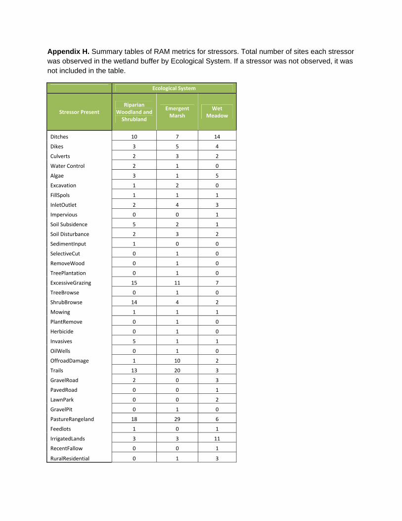
Appendix H. Summary tables of RAM metrics for stressors. Total number of sites each stressor was observed in the wetland buffer by Ecological System. If a stressor was not observed, it was not included in the table.

   Ecological System 

Stressor Present Riparian 

Woodland and Shrubland 

Emergent Marsh 

Wet Meadow 

Ditches  10  7  14 

Dikes  3  5  4 

Culverts  2  3  2 

Water Control  2  1  0 

Algae  3  1  5 

Excavation  1  2  0 

FillSpols  1  1  1 

InletOutlet  2  4  3 

Impervious  0  0  1 

Soil Subsidence  5  2  1 

Soil Disturbance  2  3  2 

SedimentInput  1  0  0 

SelectiveCut  0  1  0 

RemoveWood  0  1  0 

TreePlantation  0  1  0 

ExcessiveGrazing  15  11  7 

TreeBrowse  0  1  0 

ShrubBrowse  14  4  2 

Mowing  1  1  1 

PlantRemove  0  1  0 

Herbicide  0  1  0 

Invasives  5  1  1 

OilWells  0  1  0 

OffroadDamage  1  10  2 

Trails  13  20  3 

GravelRoad  2  0  3 

PavedRoad  0  0  1 

LawnPark  0  0  2 

GravelPit  0  1  0 

PastureRangeland  18  29  6 

Feedlots  1  0  1 

IrrigatedLands  3  3  11 

RecentFallow  0  0  1 

RuralResidential  0  1  3