1

Wavenumber-Frequency Spectra of Pressure Fluctuations Measured via Fast-Response

Pressure-Sensitive Paint

J. Panda*, N. H. Roozeboom†, J. C. Ross* NASA Ames Research Center, Moffett Field, CA

Abstract The recent advancement in fast-response Pressure-Sensitive Paint (PSP) allows time-resolved measurements of unsteady pressure fluctuations from a dense grid of spatial points on a wind tunnel model. This capability allows for direct calculations of the wavenumber-frequency (k-ω) spectrum of pressure fluctuations. Such data, useful for the vibro-acoustics analysis of aerospace vehicles, are difficult to obtain otherwise. For the present work, time histories of pressure fluctuations on a flat plate subjected to vortex shedding from a rectangular bluff-body were measured using PSP. The light intensity levels in the photographic images were then converted to instantaneous pressure histories by applying calibration constants, which were calculated from a few dynamic pressure sensors placed at selective points on the plate. Fourier transform of the time-histories from a large number of spatial points provided k-ω spectra for pressure fluctuations. The data provides first glimpse into the possibility of creating detailed forcing functions for vibro-acoustics analysis of aerospace vehicles, albeit for a limited frequency range. List of symbols:

Φ: power spectrum W: width of the plate used for k-ω spectrum k: wavevector whose components along x and y directions are kx and ky

r: correlation coefficient

Kx, Ky : non-dimensional wave number, kxH, kyH ∆: separation in space Ψ: complex spectrum τ : correlation time f: frequency *: complex-conjugate ω: =2πf, circular frequency C: PSP calibration constant H: height of the bluff body F : Discrete Fourier Transform U: free-stream velocity t: time Ω: non-dimensional frequency, =2πfH/U η : number of grid points along a direction p: fluctuating part of pressure N : no of frames = data points in time Cp: coefficient of fluctuating pressure =p/q P: pressure Subscripts: q: dynamic pressure c: convective speed x: stream-wise direction m, n: structural modes y: cross-stream direction ref: no-flow reference I: light intensity measured by a pixel rms: root-mean-square i: grid index along x-direction j: grid index along y-direction Superscripts: ℓ: index along time ʹ: fluctuating component L: length of the plate used for k-ω spectrum ̅: (overbar) time average

________________________

*Associate Fellow, † Member, AIAA

https://ntrs.nasa.gov/search.jsp?R=20160012548 2018-06-04T11:43:14+00:00Z

2

I. INTRODUCTION

The subject of “flow induced sound and vibration1”, also known as “aero-vibro-acoustics2” in the aerospace community, finds a wide swath of applications in space vehicles, airplanes, automobiles and underwater vehicles. In all of these applications the exterior surface is subjected to turbulent pressure fluctuations from the flow of air or water; which is the “aero” part. The panel structure then vibrates and transmit the pressure fluctuations to the interior; which is the “vibro-acoustics” part. The transmitted pressure fluctuations are responsible for the interior acoustic environment of an automobile2, 3, the cabin of an aircraft4, 5 and the payload and crew-compartment of a space vehicle6. The panel vibration issue takes significance in higher Mach number flows, particularly experienced by space vehicles, which are subjected to large amplitude pressure fluctuations from flow separation and shock oscillation7. Determination of the vibro-acoustic environment requires knowledge of the external pressure fluctuations and the vibrational properties of the panel structure. For the former, one needs the amplitude as well as the space-time correlation of the pressure-fluctuations which is expressed as the wavenumber-frequency

spectrum: Φ𝑝(𝑘𝑥, 𝑘𝑦, 𝜔). For the latter, one needs the material properties, such as mass distribution, stiffness,

acoustic admittance and the spatial mode shapes: 𝑆𝑚𝑛(𝑘𝑥, 𝑘𝑦). The coupling between the two is expressed as a

convolution between the two spectra as the joint acceptance function1, 2, 7:

Φ𝑝𝑚𝑛(𝜔) = ∬ Φ𝑝(𝑘𝑥, 𝑘𝑦, 𝜔)𝑘𝑥,𝑘𝑦

|𝑆𝑚𝑛(𝑘𝑥, 𝑘𝑦)|2

𝑑𝑘𝑥 𝑑𝑘𝑦 (1)

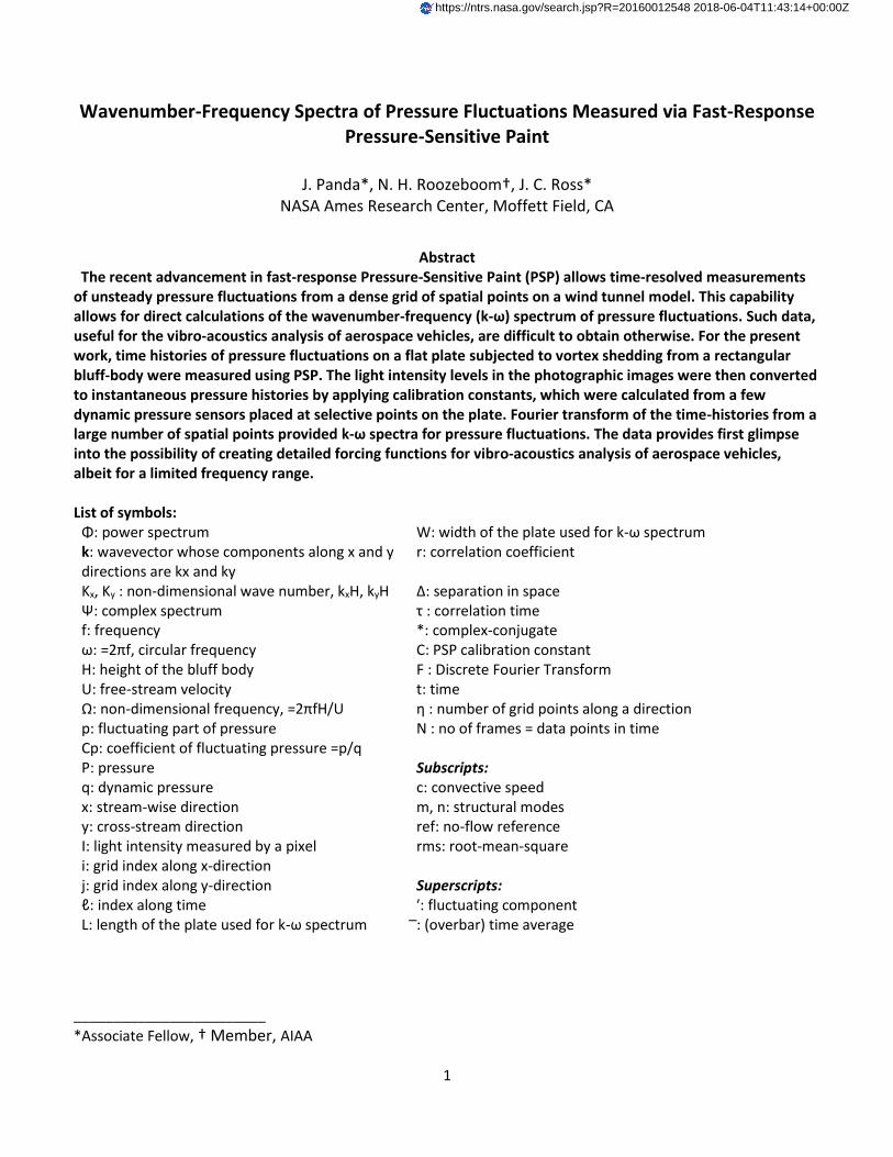
Fig. 1. Wavenumber-frequency (k-ω) diagram for surface pressure spectrum φp(k, ω) of a low subsonic turbulent flow showing convective (kc) and acoustic k0 energy components and typical resonance wavenumber for a thin panel (from Bremner & Wilby2, reproduced with permission) The joint acceptance function produces different results for different applications. For low velocity flows, analytical expectation of the wavenumber-frequency spectrum is shown in fig. 1. It is expected to have two distinct components: the higher wavenumber, higher energy part arising from the convection of the turbulent eddies, and the lower energy, low wavenumber part due to the radiation of sound waves by such eddies. Recent measurement3 in low-speed boundary layers in a quiet wind tunnel has confirmed the presence of these peaks. In such flows, structural resonances can filter out a very large part of the external pressure fluctuations, while in high Mach number application the reverse is true. For aerospace applications interest is in high speed flows where measurements of the wavenumber-frequency spectrum of pressure fluctuations are unavailable. As the Mach number increases, the convective peak of the wave number spectrum is known to strongly drive the structural modes, such as in the aircraft cabins and the payload fairings4, 5, 6. Typical flight data from space vehicles show the largest response in the transonic and low supersonic Mach number range of the flight. There is a distinct need to measure k-ω spectra for the Mach number range of interest for aerospace vehicles.

The advancement of structural dynamics facilitates reliable prediction of the structural mode shapes, based on the mass, size, boundary condition etc. However the same cannot be said for the spectrum of pressure fluctuations. Gross assumptions are involved in the specification of the pressure field, which ultimately are the

3

major contributors to the uncertainties in the vibro-acoustics estimations. While computational fluid dynamics has made significant strides for low Reynolds number flows8, the specification of wavenumber-frequency spectra for large aerospace structures has remained mostly outside its ability. It has been customary to perform model-scale wind tunnel tests to obtain some measure of the pressure field. Typical wind tunnel tests employ few dynamic pressure transduces (whose numbers are increasing over the years) to determine spectra of local fluctuations and correlation lengths, which are then employed to approximately model the wavenumber-frequency spectrum following various models, such as Corcos, Efimtsov, Ffowcs-Williams, Chase etc. (see Blake1, Graham4). Any attempt to verify these models require direct measurement of the k-ω spectrum.

To directly measure the wave-number frequency spectrum, one needs to measure pressure fluctuations over a very large number of spatial points. The goal of this work is to demonstrate from a small-scale wind tunnel experiment the potential of unsteady PSP to fill this void. The fast-response, unsteady PSP effectively produces distributed “microphones” that can be painted on the surface of a test article. The “microphone density” is related to the pixel numbers of the camera used to measure the photo-luminescence. At the present time, unsteady PSP is an evolving technology and requires independent validation. A second goal of the present report is to find suitable data analysis and calibration procedures, and finally to validate the PSP measured data. The first part of the paper describes the data analysis and calibration procedures; the second part uses the pressure time histories to establish the wavenumber-frequency spectra. The present experiment preceded a large scale test in a transonic wind tunnel; various lessons learned from this experiment were used to plan and process data from that test. Ia. Fast response pressure-sensitive paint

Pressure-Sensitive Paints have become a matured experimental tool to measure time-averaged surface pressure distribution in model-scale wind tunnel test9, 10. There has been a steady push to increase the frequency sensitivity of the paint and the binder combination to measure unsteady fluctuations (Gregory et al11 provides a good review of the work). For the present work, a PtTFPP-based porous polymer paint manufactured by Innovative Scientific Solutions, Inc. (ISSI) was used12, 13. Adding porosity to the binder creates a microscopically pitted surface onto which the luminescent molecules can be applied. This allows the oxygen to reach the luminescent molecules much faster, resulting in a higher frequency response. In addition, the effective surface area of a porous binder is much larger than its non-porous counterpart, resulting in higher radiative intensity. This is counterbalanced by a decrease in the radiative intensity due to increased quenching since the oxygen has much easier access to the luminophore. Previous studies have shown the frequency response of this paint to be over 20 kHz12, 13.

II. EXPERIMENTAL PROCEDURE

The test was conducted in the 14”X14” test section of a small, high-subsonic wind tunnel in the Fluid Mechanics Laboratory of NASA Ames Research Center. A detailed description of the experiment and PSP application procedure can be found in Roozeboom et al14; following is a brief description. A part of the wind tunnel floor was replaced by a flush mounted aluminum plate. A solid aluminum block, 2” (height) x 2” (wide) x 1” (long), was mounted at the center of the plate. The pressure fluctuations on the plate were created by flow separation and the periodic vorticity in the wake of the cuboid bluff body. A 7 11/16” (long) x 4 3/16” (wide) part of the plate was coated with PSP (fig 2.). In addition to the pressure-sensitive paint, six dynamic pressure sensors were mounted on the plate (one malfunctioned during the test). The tunnel was operated at four different Mach number: M= 0 (no flow), 0.31, 0.41 and 0.48; the corresponding free-stream velocities in ft/s were 0, 345, 454 and 520 ft/s, respectively.

PSP was applied on the plate. For the “Intensity-based” mode of operation, the paint was excited by continuous light at a nominal 400nm wavelength, produced from two Light Emitting Diode (LED) units. The luminescent light emitted by the PSP was measured with a Phantom v2011 high-speed camera, equipped with a 1280X800 pixel, 12-bit resolution CMOS chip. A total of 16542 images were recorded at a frame rate of 2000/s. The camera internal memory was capable of holding 16542 frames, the selected frame rate was a compromise between the length of the time record and the frequency range to be resolved. The collected light was at first

4

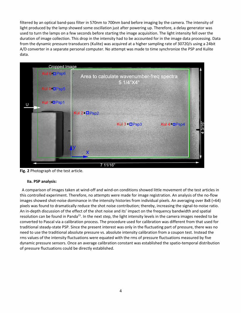
filtered by an optical band-pass filter in 570nm to 700nm band before imaging by the camera. The intensity of light produced by the lamp showed some oscillation just after powering up. Therefore, a delay generator was used to turn the lamps on a few seconds before starting the image acquisition. The light intensity fell over the duration of image collection. This drop in the intensity had to be accounted for in the image data processing. Data from the dynamic pressure transducers (Kulite) was acquired at a higher sampling rate of 30720/s using a 24bit A/D converter in a separate personal computer. No attempt was made to time synchronize the PSP and Kulite data.

Fig. 2 Photograph of the test article.

IIa. PSP analysis:

A comparison of images taken at wind-off and wind-on conditions showed little movement of the test articles in this controlled experiment. Therefore, no attempts were made for image registration. An analysis of the no-flow images showed shot-noise dominance in the intensity histories from individual pixels. An averaging over 8x8 (=64) pixels was found to dramatically reduce the shot noise contribution; thereby, increasing the signal-to-noise ratio. An in-depth discussion of the effect of the shot noise and its’ impact on the frequency bandwidth and spatial resolution can be found in Panda15. In the next step, the light intensity levels in the camera images needed to be converted to Pascal via a calibration process. The procedure used for calibration was different from that used for traditional steady-state PSP. Since the present interest was only in the fluctuating part of pressure, there was no need to use the traditional absolute pressure vs. absolute intensity calibration from a coupon test. Instead the rms values of the intensity fluctuations were equated with the rms of pressure fluctuations measured by five dynamic pressure sensors. Once an average calibration constant was established the spatio-temporal distribution of pressure fluctuations could be directly established.

5

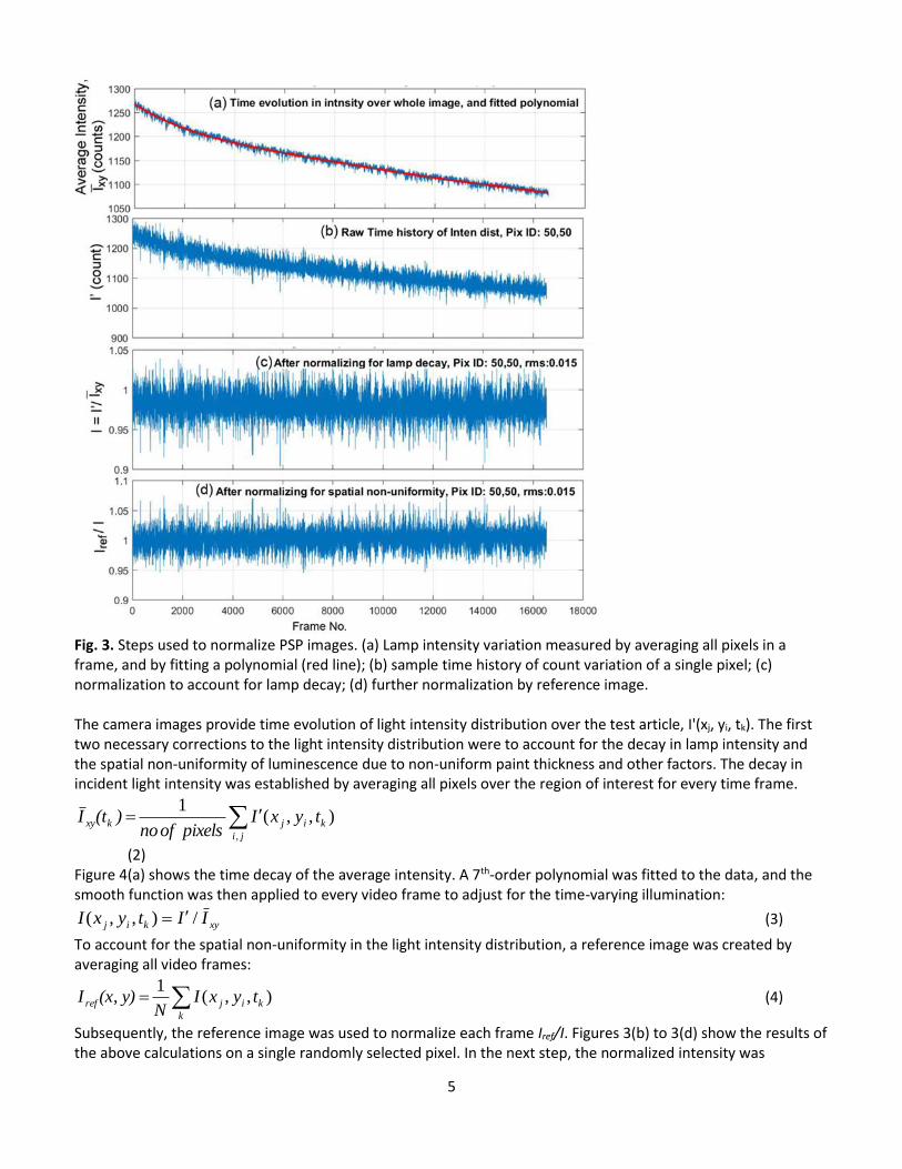
Fig. 3. Steps used to normalize PSP images. (a) Lamp intensity variation measured by averaging all pixels in a frame, and by fitting a polynomial (red line); (b) sample time history of count variation of a single pixel; (c) normalization to account for lamp decay; (d) further normalization by reference image. The camera images provide time evolution of light intensity distribution over the test article, I'(xj, yi, tk). The first two necessary corrections to the light intensity distribution were to account for the decay in lamp intensity and the spatial non-uniformity of luminescence due to non-uniform paint thickness and other factors. The decay in incident light intensity was established by averaging all pixels over the region of interest for every time frame.

ji

kijkxy tyxIpixelsofno

)(tI,

),,(1

(2) Figure 4(a) shows the time decay of the average intensity. A 7th-order polynomial was fitted to the data, and the smooth function was then applied to every video frame to adjust for the time-varying illumination:

xykij IItyxI /),,( (3)

To account for the spatial non-uniformity in the light intensity distribution, a reference image was created by averaging all video frames:

k

kijref tyxIN

y)(xI ),,(1

, (4)

Subsequently, the reference image was used to normalize each frame Iref/I. Figures 3(b) to 3(d) show the results of the above calculations on a single randomly selected pixel. In the next step, the normalized intensity was

6

converted to Pascal. The intensity of the luminescent light is known to be related to static pressure by the Stern-Volmer formula10, 11: 𝐼𝑟𝑒𝑓

𝐼= 𝐴 + 𝐵

𝑃

𝑃𝑟𝑒𝑓 (5)

Where P is the unknown pressure to be determined via (temperature-dependent) calibration constants A and B, and Pref is a reference pressure. Since Iref was obtained via averaging over time instances, it is representative of the luminescent intensity from time averaged static pressure Pref = P̅, specifically the average static pressure distribution over the plate. Also the large thermal mass of the plate minimized fluctuations in temperature; therefore, A and B were fixed constants. The present interest is in the dynamic, fluctuating part of the pressure which is much smaller than the absolute pressure. Therefore, applying Reynolds decomposition, and also by noting the following:

I

I

I

IBApPP

refref1,1, (6)

the following simple relationship between the fluctuating (normalized) intensity and the fluctuating pressure is reached:

B

PCwhere

I

ICp

ref

,

(7) The calibration constant could be easily determined by equating rms fluctuations:

rms

ref

rmsI

ICp

(8)

A pixel ( specifically an average of 8x8 adjacent pixels) next to each dynamic pressure sensor (Fig. 2) were identified, and the rms of the fluctuations in the frequency interval of 10Hz ≤ f ≤ 900Hz were determined from the spectrum of the dynamic pressure sensor and also from the PSP pixel. Application of equation (8) above provided the calibration constant. An average of the calibration constants (126738Pa) was applied to all pixels to determine the space-time distribution of the pressure fluctuations: p(xj, yi, tk).

III. RESULTS AND DISCUSSIONS

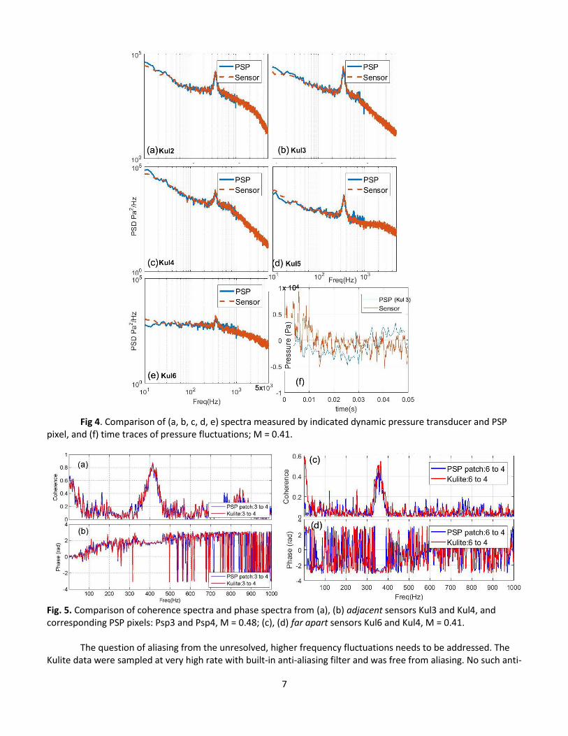
IIIa. Validation of PSP Power spectra of pressure fluctuations measured by dynamic pressure sensors and by corresponding PSP pixels are compared in fig. 4 (a-e). The PSP spectra are available for f ≤ 1 kHz range while the spectra from Kulites are shown for a wider range: f ≤ 5 kHz. the Good correspondence seen over the entire frequency range, and for all five sensors proves excellent dynamic response of PSP over the frequency range of interest. Flow physics-wise, the hump centered around 360 Hz was due to the periodic vortex shedding by the bluff cuboid, and the low frequency fluctuations are due to the “breathing” of the separation bubble. Figure 4(f) shows a comparison of the time traces. Note that the PSP camera and the Kulite data acquisition system were not time-synchronized. Therefore, the comparison in fig. 4(f) is shows relative magnitudes. Nonetheless, it can be said that the magnitude of PSP time trace is comparable to that from the Kulite sensor; the higher frequency content in the latter is also apparent.

7

Fig 4. Comparison of (a, b, c, d, e) spectra measured by indicated dynamic pressure transducer and PSP pixel, and (f) time traces of pressure fluctuations; M = 0.41.

Fig. 5. Comparison of coherence spectra and phase spectra from (a), (b) adjacent sensors Kul3 and Kul4, and corresponding PSP pixels: Psp3 and Psp4, M = 0.48; (c), (d) far apart sensors Kul6 and Kul4, M = 0.41.

The question of aliasing from the unresolved, higher frequency fluctuations needs to be addressed. The Kulite data were sampled at very high rate with built-in anti-aliasing filter and was free from aliasing. No such anti-

8

aliasing process could be used for the PSP images. For the 2000/s frame rate imaging, the camera shutter was kept open for nearly the entire 500 micro-s duration of each frame, followed by a fast readout, and a new exposure. This photon accumulation process in effect created an integrate-and-dump filter. Panda & Seasholtz16 showed that such a process created a low pass filter with sharp drops around frequencies which are integer multiples of the frame rate. Additionally, an examination of the Kulite data shows continuous decay of spectral energy beyond 1000Hz. Therefore, the effect of aliasing on the PSP data is expected to be small. Spectral comparison of figure 4 confirms this statement.

Figure 5 compares the coherence and phase spectra between the two dynamic pressure sensors along with those from PSP pixels adjacent to the sensors. Figure 2 ought to be consulted to see the locations of the sensor pair. The phase and coherence spectra show excellent comparison for near-by pair (fig 5a, 5b). The comparison remains still very good for the far-way pairs (fig 5c, 5d) yet at the very low frequency end, f<20Hz, there occurs some difference. The sensor pair 6 and 4 are separated by more than the plate length, which is believed to have accentuated the effect of any small vibration, leading to the discrepancy at the very low frequency. Perhaps an attempt to register the images would have reduced the difference. Nonetheless, figures 4 and 5 confirm the good phase and amplitude response within the range of interest.

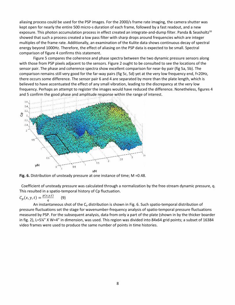
Fig. 6. Distribution of unsteady pressure at one instance of time; M =0.48. Coefficient of unsteady pressure was calculated through a normalization by the free-stream dynamic pressure, q. This resulted in a spatio-temporal history of Cp fluctuation.

𝐶𝑝(𝑥, 𝑦, 𝑡) =𝑝(𝑥,𝑦,𝑡)

𝑞 (9)

An instantaneous shot of the Cp distribution is shown in Fig. 6. Such spatio-temporal distribution of pressure fluctuations set the stage for wavenumber-frequency analysis of spatio-temporal pressure fluctuations measured by PSP. For the subsequent analysis, data from only a part of the plate (shown in by the thicker boarder in fig. 2), L=5¼” X W=4” in dimension, was used. This region was divided into 84x64 grid points; a subset of 16384 video frames were used to produce the same number of points in time histories.

9

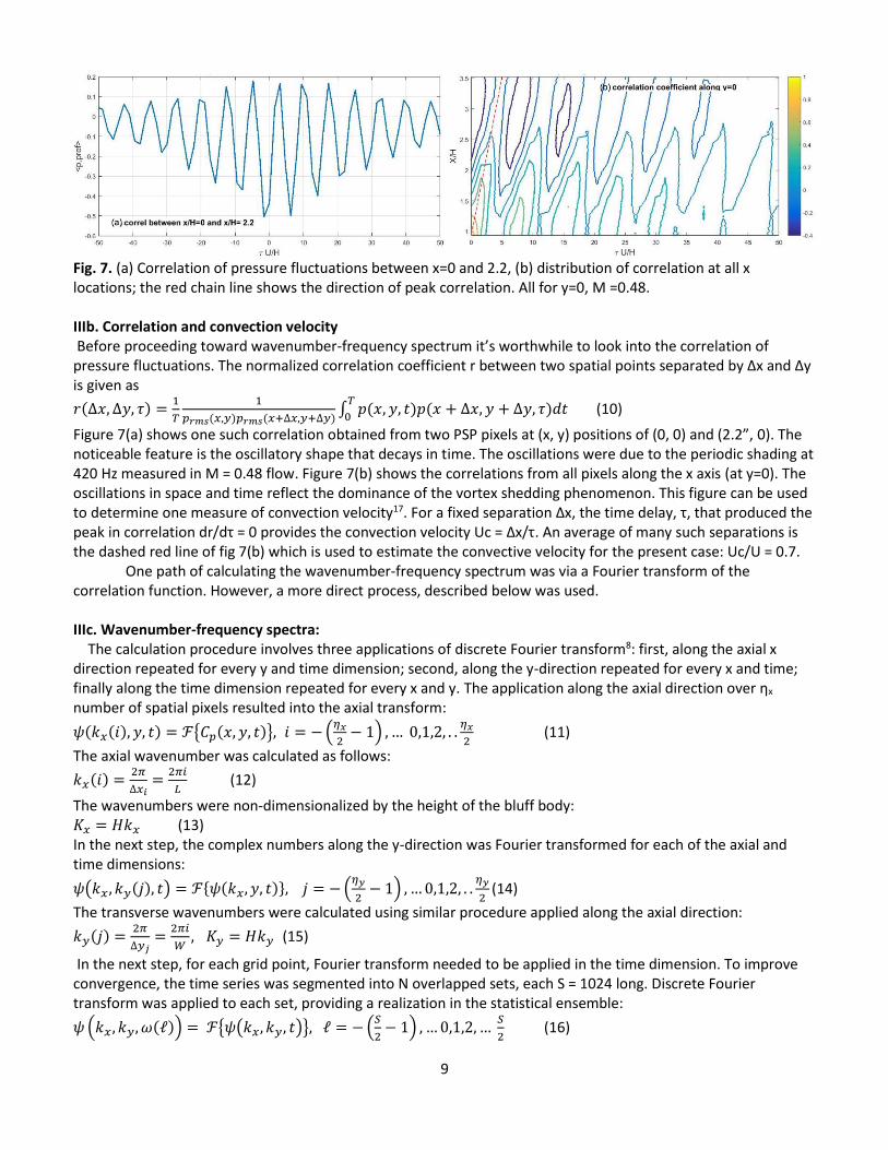
Fig. 7. (a) Correlation of pressure fluctuations between x=0 and 2.2, (b) distribution of correlation at all x locations; the red chain line shows the direction of peak correlation. All for y=0, M =0.48. IIIb. Correlation and convection velocity Before proceeding toward wavenumber-frequency spectrum it’s worthwhile to look into the correlation of pressure fluctuations. The normalized correlation coefficient r between two spatial points separated by ∆x and ∆y is given as

𝑟(∆𝑥, ∆𝑦, 𝜏) =1

𝑇

1

𝑝𝑟𝑚𝑠(𝑥,𝑦)𝑝𝑟𝑚𝑠(𝑥+∆𝑥,𝑦+∆𝑦)∫ 𝑝(𝑥, 𝑦, 𝑡)𝑝(𝑥 + ∆𝑥, 𝑦 + ∆𝑦, 𝜏)𝑑𝑡

𝑇

0 (10)

Figure 7(a) shows one such correlation obtained from two PSP pixels at (x, y) positions of (0, 0) and (2.2”, 0). The noticeable feature is the oscillatory shape that decays in time. The oscillations were due to the periodic shading at 420 Hz measured in M = 0.48 flow. Figure 7(b) shows the correlations from all pixels along the x axis (at y=0). The oscillations in space and time reflect the dominance of the vortex shedding phenomenon. This figure can be used to determine one measure of convection velocity17. For a fixed separation ∆x, the time delay, τ, that produced the peak in correlation dr/dτ = 0 provides the convection velocity Uc = ∆x/τ. An average of many such separations is the dashed red line of fig 7(b) which is used to estimate the convective velocity for the present case: Uc/U = 0.7. One path of calculating the wavenumber-frequency spectrum was via a Fourier transform of the correlation function. However, a more direct process, described below was used. IIIc. Wavenumber-frequency spectra: The calculation procedure involves three applications of discrete Fourier transform8: first, along the axial x direction repeated for every y and time dimension; second, along the y-direction repeated for every x and time; finally along the time dimension repeated for every x and y. The application along the axial direction over ηx

number of spatial pixels resulted into the axial transform:

𝜓(𝑘𝑥(𝑖), 𝑦, 𝑡) = ℱ{𝐶𝑝(𝑥, 𝑦, 𝑡)}, 𝑖 = − (𝜂𝑥

2− 1) , … 0,1,2, . .

𝜂𝑥

2 (11)

The axial wavenumber was calculated as follows:

𝑘𝑥(𝑖) =2𝜋

∆𝑥𝑖=

2𝜋𝑖

𝐿 (12)

The wavenumbers were non-dimensionalized by the height of the bluff body: 𝐾𝑥 = 𝐻𝑘𝑥 (13) In the next step, the complex numbers along the y-direction was Fourier transformed for each of the axial and time dimensions:

𝜓(𝑘𝑥 , 𝑘𝑦(𝑗), 𝑡) = ℱ{𝜓(𝑘𝑥, 𝑦, 𝑡)}, 𝑗 = − (𝜂𝑦

2− 1) , … 0,1,2, . .

𝜂𝑦

2 (14)

The transverse wavenumbers were calculated using similar procedure applied along the axial direction:

𝑘𝑦(𝑗) =2𝜋

∆𝑦𝑗=

2𝜋𝑖

𝑊, 𝐾𝑦 = 𝐻𝑘𝑦 (15)

In the next step, for each grid point, Fourier transform needed to be applied in the time dimension. To improve convergence, the time series was segmented into N overlapped sets, each S = 1024 long. Discrete Fourier transform was applied to each set, providing a realization in the statistical ensemble:

𝜓 (𝑘𝑥 , 𝑘𝑦, 𝜔(ℓ)) = ℱ{𝜓(𝑘𝑥, 𝑘𝑦, 𝑡)}, ℓ = − (𝑆

2− 1) , … 0,1,2, …

𝑆

2 (16)

10

Where ωℓ are the discrete frequencies:

𝜔(ℓ) =2𝜋ℓ

𝑇 (17)

In the above equation T is the time duration for the 1024 data points used in the individual realization. The physical frequencies were non-dimensionalized as Strouhal frequency Ω:

Ω(ℓ) =2𝜋ℓ𝐻

𝑇𝑈 (18)

The power spectral density of the wavenumber-frequency spectrum was calculated via multiplying the complex spectra, for each realization, by its conjugate, and then taking an average over all N sets.

ϕ(𝑘𝑥 , 𝑘𝑦, Ω) = 1

𝑁 ∑ {𝜓(𝑘𝑥 , 𝑘𝑦 , Ω) 𝜓∗(𝑘𝑥 , 𝑘𝑦, Ω)}

𝑠𝑁𝑠=1 (19)

An important property of Fourier transform is the equality in the variance of the time-series data and the integrated power spectrum. This requires Ф to be scaled such that the following holds.

∑ 𝐶𝑝2

𝑥,𝑦,𝑡 = ∑ Φ (𝐾𝑥(𝑖), 𝐾𝑦(𝑗), Ω(ℓ)) ∆𝐾𝑥 ∆𝐾𝑦 ∆Ω𝑖,𝑗,ℓ (20)

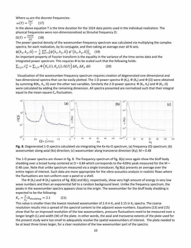
Visualization of the wavenumber-frequency spectrum requires creation of degenerated one-dimensional and two-dimensional spectra that can be easily plotted. The 1-D power spectra Ф (Kx), Ф (Ky) and Ф (Ω) were obtained by summing Ф(Kx, Ky, Ω) over the other two variables. Similarly the 2-D power spectra: Ф (Kx, Ky) and Ф (Kx, Ω) were calculated by adding the remaining dimension. All spectra presented are normalized such that their integral equal to the mean-square Cp fluctuation.

Fig. 8. Degenerated 1-D spectra calculated via integrating the Kx-Ky-Ω spectrum, (a) frequency (Ω) spectrum; (b) wavenumber along axial (Kx) direction; (c) wavenumber along transverse direction (Ky); M = 0.48 The 1-D power spectra are shown in fig. 8. The frequency spectrum of fig. 8(a) once again show the bluff body shedding over a broad hump centered at Ω = 0.84 which corresponds to the 420Hz peak measured for the M = 0.48 case. Note that unlike spectrum measured via a single transducer, fig 8(a) presents an average over the entire region of interest. Such data are more appropriate for the vibro-acoustics analysis in realistic flows where the fluctuations are non-uniform over a panel or a shell.

The Ф (Kx) and Ф (Ky) spectra of fig. 8(b) and 8(c), respectively, show very high amount of energy in very low wave numbers and then an exponential fall to a random background level. Unlike the frequency spectrum, the peaks in the wavenumber spectra appears close to the origin. The wavenumber for the bluff body shedding is expected to be the following:

𝐾𝑥 =𝑈

𝑈𝑐Ω𝑠ℎ𝑒𝑑𝑑𝑖𝑛𝑔 = 2.1 (21)

This value is smaller than the lowest resolved wavenumber of 2.4 in Kx and 3.15 in Ky spectra. The coarse resolution results into a spread of the spectral content to the adjacent wave-numbers. Equations (13) and (15) show that for an improved resolution of the low wavenumbers, pressure fluctuations need to be measured over a longer length (L) and width (W) of the plate. In other words, the axial and transverse extents of the plate used for the present study were too small to adequately resolve the spatial wavenumbers of interest. The plate needed to be at least three times larger, for a clear resolution of the low wavenumber part of the spectra.

11

This brings out an important discussion on the image resolution required in unsteady PSP applications. The present experiment resolved f ≤ 1 kHz range. The wavelength of pressure fluctuations at the highest frequency was 4.2 inches (at M = 0.48, with Uc/U = 0.7). According to the Nyquist criteria one needs only two points per wavelength; for improved phase resolution if one uses eight points, still an imaging system where every pixel covered ~ 0.5 inch would have been sufficient. The resolution in the present test was 0.0078 inch. Various lessons learned from this small scale test was used for the processing of the PSP data from the large wind tunnel test that followed.

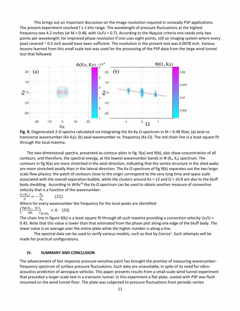
Fig. 9. Degenerated 2-D spectra calculated via integrating the Kx-Ky-Ω spectrum in M = 0.48 flow; (a) axial vs. transverse wavenumber (Kx-Ky); (b) axial wavenumber vs. frequency (Kx-Ω). The red chain line is a least square fit through the local maxima.

The two-dimensional spectra, presented as contour plots in fig. 9(a) and 9(b), also show concentration of all

contours, and therefore, the spectral energy, at the lowest wavenumber bands in Ф (Kx, Ky) spectrum. The contours in fig 9(a) are more stretched in the axial direction, indicating that the vortex structure in the shed wake are more stretched axially than in the lateral direction. The Kx-Ω spectrum of fig 9(b) separates out the two large-scale flow physics: the patch of contours close to the origin correspond to the very long time and space scale associated with the overall separation bubble, while the clusters around Kx = ±2 and Ω = ±0.8 are due to the bluff body shedding. According to Wills16 the Kx-Ω spectrum can be used to obtain another measure of convective velocity that is a function of the wavenumber: 𝑈𝑐(𝐾𝑥)

𝑈= −

Ω𝑐

𝐾𝑥 (22)

Where for every wavenumber the frequency for the local peaks are identified:

(𝜕𝜙(𝐾𝑥 , Ω)

𝜕Ω)

Ω=Ω𝑐

= 0 (23)

The chain line in figure 9(b) is a least square fit through all such maxima providing a convection velocity Uc/U = 0.45. Note that this value is lower than that estimated from the phase plot along one edge of the bluff body. The lower value is an average over the entire plate while the higher number is along a line. The spectral data can be used to verify various models, such as that by Corcos2. Such attempts will be made for practical configurations.

IV. SUMMARY AND CONCLUSION

The advancement of fast response pressure-sensitive paint has brought the promise of measuring wavenumber-frequency spectrum of surface pressure fluctuations. Such data are unavailable, in spite of its need for vibro-acoustics prediction of aerospace vehicles. This paper presents results from a small-scale wind tunnel experiment that preceded a larger-scale test in a transonic tunnel. In this experiment a flat plate, coated with PSP was flush mounted on the wind tunnel floor. The plate was subjected to pressure fluctuations from periodic vortex

12

shedding from a cuboid bluff-body placed upstream. The wind tunnel was operated at three different Mach numbers of 0.31, 0.41 and 0.48. The paper describes the procedures for both unsteady PSP analysis and wavenumber-frequency calculations, and presents such data for the first time from PSP measurements. The plate was coated with a highly porous binder, and then a PtTFPP-based porous polymer paint manufactured by Innovative Scientific Solutions, Inc. (ISSI) was applied. In the “Intensity-based” mode of operation, the paint was excited by continuous light at a nominal 400nm wavelength, produced from two Light Emitting Diode (LED) units. The luminescent light was measured with a Phantom v2011 high-speed camera. The frame rate of 2000/s limited the resolved frequency range to 1 kHz. The first step in the processing of the camera images was an averaging over 8x8 adjacent pixels to reduce the shot noise contribution. In the next step the images needed to be corrected for changes in the lamp brightness and spatial non-uniformity from the paint application. Finally the light intensity fluctuations were converted to pressure fluctuations via calibration constants calculated from five unsteady pressure transducers placed on the plate. A simple linear relationship was derived between the normalized fluctuations of luminescence and unsteady pressure fluctuations. Over the relatively modest frequency band of interest: f ≤ 1 kHz, PSP derived power, phase and coherence spectra showed excellent match with the corresponding ones calculated from dynamic pressure sensors. Application of the calibration constant converted the PSP high-speed videos to time histories of pressure fluctuations over a large number of spatial points that could not be obtained otherwise. The detailed time histories were explored to determine spatial correlations and an average convective velocity. The wavenumber-frequency spectrum was calculated via three applications of discrete Fourier transform: first in the axial direction, then in the transverse direction and finally along the time dimension. The content of the three-dimensional (Kx, Ky, Ω) spectra were examined via degenerated 1-D and 2-D plots. The frequency power-spectra Ф (Ω) showed large humps centered at the bluff-body shedding frequency of Ω=0.84, and a large low frequency content. It was pointed out that such spectra are more appropriate for vibro-acoustics analysis, since they represent an average over the entire plate surface. The wave-number spectra Ф (Kx) and Ф (Ky) were found to be poorly resolved leading to a strong peak close to the origin. The limitation was not due to the technique, but for relatively shorter plate size used in the experiment. The 2-D spectra of Ф (Kx, Ω), and Ф (Kx, Ky) are shown to contain various measurements of length scales and convection velocity. The paper demonstrates the capability of PSP in measuring the wavenumber-frequency spectra. Various lessons learnt from this experiment were used in a larger wind tunnel test that followed.

Acknowledgements: Mr. Nathan J. Burnside of NASA Ames setup the dynamic pressure sensors suite. The test was funded by NASA Engineering Safety Center with Dr. David Schuster of NASA Langley as a principal investigator. Reference: 1Blake, W. K. “Mechanics of Flow-Induced Sound and Vibration,” two volumes, Academic Press, 1986.

2Bremner, P.G. & Wilby, J. F., “Aero-Vibro-Acoustics: Problem Statement and Methods for Simulation-Based Design Solution,” AIAA paper 2002-2551, 2002 3Salaze, E., Bailly, C., Marsden, O., Jondeau, E., & Juve, D., “An Experimental Characterisation of Wall Pressure Wavevector-Frequency Spectra in the Presence of Pressure Gradients,” AIAA paper 2014-2909, 2014. 4Graham, W. R. “A Comparison of Models for the Wavenumber-Frequency Spectrum of Turbulent Boundary Layer Pressures,” J. Sound & Vib., 206(4), 1997, pp. 544-565. 5Mathur, G. P, “Evaluation of Turbulent Boundary Layer Pressure Wavenumber-Frequency Spectrum Using a Fixed Probe Pair,” AIAA 1990-3926, 1990 6Cockburn, J. A. & Robertson, J. E. “Vibration Response of Spacecraft Shrouds to in-Flight Fluctuating Pressures,” J. Sound & Vib., 33(4), 1974, pp.399-425. 7Himelblau, H., Fuller, C. M. & Scharton, “Assessment of Space Vehicle Aeroacoustic-Vibration Prediction, Design and Testing,” NASA CR 1596, July 1970. 8Choi, H. & Moin, P., “On the Space-Time Characteristics of Wall-Pressure Fluctuations,” Phys. Fluids A 2(8), Aug. 1990.

13

9Sellers, M.E., “Demonstration of a Temperature Compensated Pressure-sensitive Paint on the Orion Launch abort Vehicle” AIAA paper 2011-3166, 2011. 10Bell, J. H., Schairer, E.T., Hand, L. A. & Mehta, R. D. “Surface pressure Measurements Using Luminescent Coatings,” Ann. Rev. Fluid Mech. 31, pp. 155-206, 2001 11Gregory, J. W., Sakaue, H., Liu, T, Sullivan, J. P., “Fast Pressure-Sensitive Paint for Flow and Acoustic Diagnostics,” Ann. Rev. Fluid. Mech., 2014. 12Crafton, J., Forlines, A., Palluconi S., Hsu K., Campbell, C. & Gruber, M., “Investigation of Transverse Jet Injections in a Supersonic Crossflow Using Fast Responding Pressure-Sensitive Paint”, AIAA Paper 2011-3522. 13Flaherty, W., Reedy, T.M., Elliot, G.S., Austin, J.M., Schmit, R. F., & Crafton, J. “Investigation of Cavity Flow Using Fast-Response Pressure-sensitive Paint.” AIAA Paper 2013-0678, 51st AIAA Aerospace Sciences Meeting, Grapevine, TX, January 2015. 14Roozeboom, N.H., Diosady, L.T. , Murman, S.M., Burnside, N. J., Panda ,J., & Ross, J.C. “Unsteady PSP Measurements on a Flat Plate Subject to Vortex Shedding from a Rectangular Prism”, AIAA paper 2016-2017, presented at SciTech2016, Jan. 2016. 15 Panda, J., “Experimental Verification of Buffet Calculation Procedure using Unsteady PSP,” NASA TM 2016-219069, Feb. 2016 (also submitted for publication in J. Aircraft). 16Panda, J. & Seasholtz, R. G. “Experimental investigation of density fluctuations in high-speed jets and correlation with generated noise,” J. Fluid Mech., vol. 450, pp. 97-130, 2002. 17Wills, J. A. B. “On convection velocities in turbulent shear flows,” J. Fluid Mech., 20(3), 417-432, 1964.