Embed Size (px)
Citation preview
WAVENUMBER EXPLICIT ANALYSIS FOR TIME-HARMONIC MAXWELL
EQUATIONS IN A SPHERICAL SHELL AND SPECTRAL APPROXIMATIONS
LINA MA1, JIE SHEN2, LI-LIAN WANG3 AND ZHIGUO YANG3
Abstract. This paper is devoted to wavenumber explicit analysis of the electric field satisfying the
second-order time-harmonic Maxwell equations in a spherical shell and hence for variant scattererswith ε-perturbation of the inner ball radius. The spherical shell model is obtained by assuming that
the forcing function is zero outside a circumscribing ball, and replacing the radiation condition with
a transparent boundary condition involving the capacity operator. Using the divergence-free vectorspherical harmonic (VSH) expansions for two components of the electric field, the Maxwell system is
reduced to two sequences of decoupled one-dimensional boundary value problems (BVPs) in the radial
direction. The reduced problems naturally allow for truncated VSH spectral approximation of the electricfield and one-dimensional global polynomial approximation of the BVPs. We analyze the error in the
resulting spectral approximation for the spherical shell model. Using a perturbation transformation, we
generalize the approach for ε-perturbed non-spherical scatterers by representing the resulting field inε-power series expansion with coefficients being spherical shell electric fields.
1. Introduction
This paper is concerned with wavenumber explicit analysis and spectral-Galerkin approximation ofthe time-harmonic Maxwell equations:
∇×∇×Ea,b − k2Ea,b = F a,b, in Ω = B \ D ; (1.1)
Ea,b × er = 0, on ∂D; (∇×Ea,b)× er − ikTb[Ea,bS ] = h, at r = b, (1.2)
where Ω = a < r = |r| < b is the spherical shell formed by two concentric spheres D and B of radii a
and b, respectively, Ea,b is the electric field, Ea,bS = −Ea,b × er × er (with er = r/r) is the tangential
field, k > 0 is the wavenumber, i =√−1 and Tb is the capacity operator (see [39, (5.3.88)] and (3.13)
below). Here, the source term F a,b is assumed to be compactly supported in Ω, and the function h in(1.2) is added for potentially inhomogeneous boundary conditions.
We also consider (1.1)-(1.2) with the spherical shell Ω being replaced with B \ D, where D is anε-perturbation of the inner ball of radius a :
D =
(r, θ, φ) : 0 < r < a+ εf(θ, φ), θ ∈ [0, π], φ ∈ [0, 2π). (1.3)
Based on the transformed field expansion [13], the electric field in Ω = a + εf(θ, φ) < r < b canbe represented as an ε-power series with the expansion coefficients being spherical shell electric fields.
2000 Mathematics Subject Classification. 65N35, 65N22, 65F05, 35J05.Key words and phrases. Maxwell equations, Helmholtz equation, wavenumber explicit analysis, Dirichlet-to-Neumann
boundary conditions, divergence-free vector spherical harmonic expansions.1Department of Mathematics, Department of Mathematics Penn State University, University Park, PA 16802, USA.
Email: [email protected] of Mathematics, Purdue University, West Lafayette, IN, 47907, USA. The work of this author is partially
supported by NFS grant DMS-1419053 and AFOSR FA9550-11-1-0328. Email: [email protected] of Mathematical Sciences, School of Physical and Mathematical Sciences, Nanyang Technological Univer-
sity, 637371, Singapore. The research of the authors is partially supported by Singapore MOE AcRF Tier 1 Grant(RG27/15), and MOE AcRF Tier 2 Grant (MOE 2013-T2-1-095, ARC44/13). Emails: [email protected] (L. Wang) [email protected] (Z. Yang).
1
2 L.N. MA, J. SHEN, L.L. WANG & Z.G. YANG
Therefore, the spectral algorithm and analysis for the Maxwell equations in the spherical shell are essentialfor such a variant.
The study of the above model problems is motivated by the exterior Maxwell system:
− iωµH +∇×E = 0, −iωεE −∇×H = J , in R3\D;
(E × n)|∂D = 0; limr→∞
r(√
µ/εH × x−E)
= 0,(1.4)
where the scatterer D is a simply connected, bounded, perfect conductor, E,H are respectively theelectric and magnetic fields, µ is the magnetic permeability, ε is the electric permittivity, ω is the frequencyof the harmonic wave, n is the outward normal and x = x/|x|. The boundary condition at infinity in(1.4) is known as the Silver-Muller radiation condition. Typically, the electric current density J islocalised in space; for example, it is restricted to flow on an antenna (cf. [43]). The Maxwell system(1.4) plays an important role in many scientific and engineering applications, including in particularelectromagnetic wave scattering, and is also of mathematical interest (see, e.g., [39, 37, 11]). Despiteits seeming simplicity, the system (1.4) is notoriously difficult to solve numerically. Some of the mainchallenges include: (i) the indefiniteness when ω is not sufficiently small; (ii) highly oscillatory solutionswhen ω is large; (iii) the incompressibility (i.e., div(µH) = div(εE) = 0), which is implicitly implied by(1.4); and (iv) the unboundedness of the domain. On the one hand, one needs to construct approximationspaces such that the discrete problems are well posed and lead to good approximations for a wide rangeof wavenumbers. On the other hand, one needs to develop efficient algorithms for solving the indefinitelinear system, particularly for large wavenumber, resulted from a given discretization. We refer to [37]and the references therein, for various contributions with respect to numerical approximations of thetime-harmonic Maxwell equations. The methods of choice for dealing with unbounded domains includethe perfectly matched layer (PML) technique [6], boundary integral method [29, 32, 44, 8, 10, 31], andthe artificial boundary condition (ABC) [16, 23, 24]. The last approach is to enclose the obstacles andinhomogeneities (and nonlinearities at times) with an artificial boundary. A suitable boundary conditionis then imposed, leading to a numerically solvable boundary value problem in a finite domain. The ABCis known as a transparent (or nonreflecting) boundary condition (TBC) (or NRBC), if the solution of thereduced problem coincides with the solution of the original problem restricted to the finite domain.
The TBC characterised by the capacity operator Tb (cf. [39]) can reduce the exterior Maxwell equationsto an equivalent BVP. With this, we obtain the second-order problem (1.1)-(1.2) by eliminating themagnetic field H, and adding h in (1.2) to deal with potentially inhomogeneous boundary conditions.
Note that the wavenumber k = ω√µε and we denote η =
√µ/ε. In [39] and other related works (e.g.,
[33]), the usual VSH are used to expand the electric field Ea,b. Then the problem (1.1)-(1.2) can be
reduced to a coupled system of two components of Ea,b, while the other component satisfies the sameequation reduced from the Helmholtz equation (cf. [33]):
−∆Ua,b − k2Ua,b = F a,b, in Ω = B\D , (1.5)
Ua,b|∂D = 0; ∂rUa,b − Tb[Ua,b] = H, at r = b, (1.6)
where Tb is the Dirichlet-to-Neumann (DtN) operator [39] (see (2.1) below). The wavenumber explicitanalysis for the above Helmholtz equation has been carried out in [47] (also see [9] for starlike scatterers),but the analysis for two coupled components appears very difficult. In fact, only the result on well-posedness of (1.1)-(1.2) was obtained in [33]. However, if we use divergence-free vector spherical harmonics[38, 7], the Maxwell system (1.1)-(1.2), in the case D is a sphere, can be reduced to two sequences ofone-dimensional problems, which are completely decoupled and the same as those obtained from theHelmholtz equations (1.5) (note: one sequence is with the boundary conditions (1.6), but the other iswith a slightly different boundary condition at r = a). Therefore, we can carry out wavenumber explicit
MAXWELL EQUATIONS 3
analysis for these decoupled problems, leading to wavenumber explicit estimates for the Maxwell equationsin a spherical shell with exact TBC.
There has been a longstanding research interest in wavenumber explicit estimates for the Helmholtzand Maxwell equations. In particular, much effort has been devoted to the Helmholtz problems (see, e.g.,[15, 28, 4, 14, 3, 46, 12, 47, 25, 9, 20, 21, 35, 19, 48, 36, 5] as a partial list of literature). The Rellichidentities played an essential role in obtaining wavenumber explicit estimates for the Helmholtz equationin a star-shaped domain (cf. [34, 46, 12, 47, 25, 9, 35]). In this paper, we shall also use a Rellich typeidentity, but apply on one-dimensional equations reduced from the Helmholtz or Maxwell equations, toderive wavenumber explicit estimates.
It is noteworthy that most of the results were established for the Helmholtz equation with an approx-imate boundary condition: ∂rU − ikU = 0. However, as shown in [47, 9], the presence of the exact DtNboundary condition brought about significant challenges for the analysis. It is also important to pointout that some new estimates for more general settings were recently obtained in [48, 36, 5]. On the otherhand, Hiptmair et al. [27] (and Feng [18] independently) extended the argument based on the Rellichidentities to the time-harmonic Maxwell equations, and derived for the first time the wavenumber explicitestimates but with the approximate boundary condition: (∇×E)× er − ikES = h.
The main purposes of this paper are to extend the analysis in [47] to the Maxwell equations (1.1)-(1.2),and in the meantime, provide an essential improvement, which is critical to obtaining the desired estimatefor the Maxwell equations, to an estimate for the Helmholtz equation in [47]. We demonstrate that thespectral algorithm and analysis for the Maxwell equations in the spherical shell are essential for dealingwith the perturbed scattering problem by using the transformed field expansion (TFE) approach [13].
The rest of the paper is organized as follows. In Section 2, we conduct a delicate study of the DtNkernel in (2.2), and use the new estimates to improve the estimates for the Helmholtz equation (cf.Lemma 2.2 and Theorem 2.2), by removing the factor k1/3 in [47, Thm. 3.1]. Using the divergence-freeVSH expansion of the electric field, we reduce in Section 3 the Maxwell system (1.1)-(1.2) in the sphericalshell to two sequences of decoupled one-dimensional BVPs in the radial direction. This is essential toderive the wavenumber explicit bounds in Theorem 3.4. In Section 4, we study a spectral approximationof the reduced Maxwell equations, and derive the corresponding wavenumber explicit error estimates forthe one-dimensional problems (cf. Lemmas 4.1 and 4.3), which finally lead to the wavenumber expliciterror estimates for the Maxwell system (cf. Theorem 4.2). In Section 5, we apply the transformed fieldexpansion (TFE) [13] to deal with an ε-perturbed scatterer, and using the general framework derived in[41], we obtain rigorous wavenumber explicit error estimates for the complete algorithm. Some concludingremarks are presented in the last section.
2. Improved wavenumber explicit estimates for the Helmholtz equation
In this section, we improve the a priori estimates for the Helmholtz equation (1.5)-(1.6) in [47, Thm.3.1], where the DtN operator is defined by
Tb[Ua,b] =
∞∑l=1
l∑|m|=0
kh
(1)l
′(kb)
h(1)l (kb)
Uml Y ml , where Uml =
∫S
Ua,b∣∣r=b
Y ml dS, (2.1)
and Y ml are spherical harmonics (SPH) defined on the unit spherical surface S (cf. Appendix A).
2.1. Properties of the DtN kernel. The key is to conduct a delicate analysis of the DtN kernel:
Tl,κ =:h
(1)l
′(κ)
h(1)l (κ)
, l ≥ 1, κ > 0. (2.2)
4 L.N. MA, J. SHEN, L.L. WANG & Z.G. YANG
Recall that (cf. [47, (2.16)])
Re(Tl,κ) = − 1
2κ+Jν(κ)J ′ν(κ) + Yν(κ)Y ′ν(κ)
J2ν (κ) + Y 2
ν (κ), Im(Tl,κ) =
2
πκ
1
J2ν (κ) + Y 2
ν (κ), (2.3)
for ν = l+ 1/2, where Jν and Yν are Bessel functions of the first and second kinds, respectively, of orderν (cf. [1]). Alternatively, we can formulate
Re(Tl,κ) =l
κ− Yν+1(κ)
Yν(κ)− Im(Tl,κ)
Jν(κ)
Yν(κ)= − 1
2κ+Y ′ν(κ)
Yν(κ)− Im(Tl,κ)
Jν(κ)
Yν(κ), (2.4)
which can be derived from (2.3) and the properties of Bessel functions. Recall that (see [39, Page 87]):
− l + 1
κ≤ Re(Tl,κ) < − 1
κ, 0 < Im(Tl,κ) < 1. (2.5)
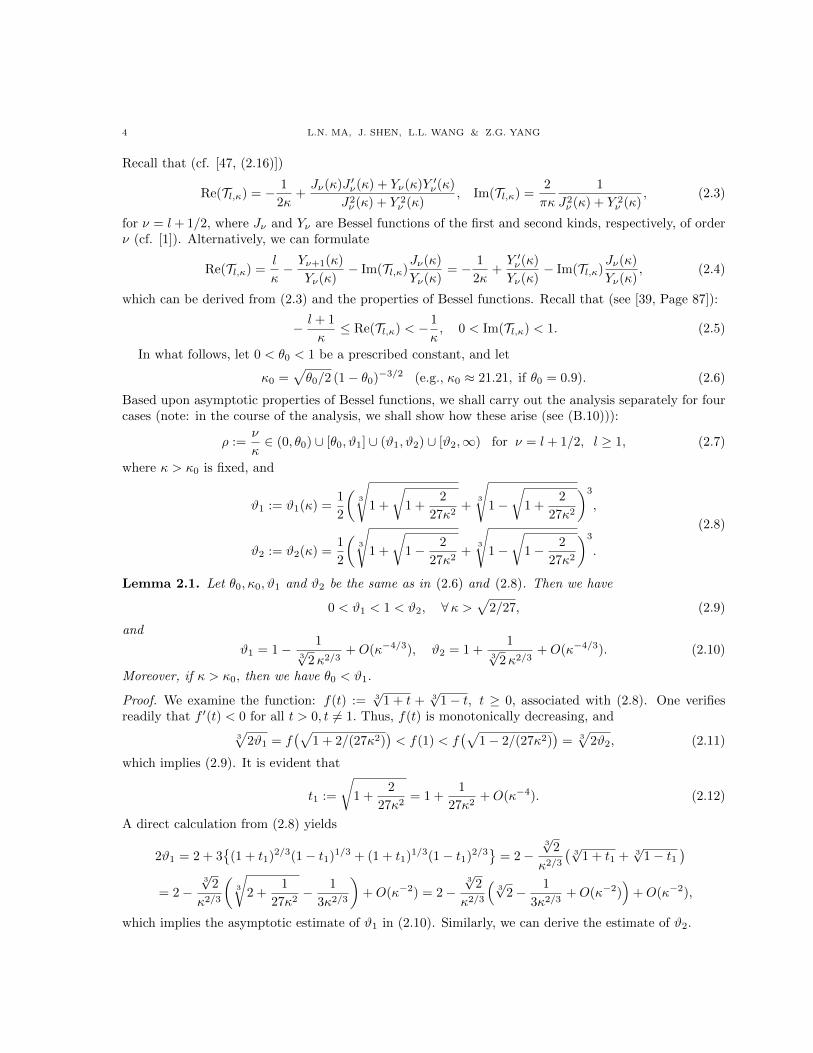
In what follows, let 0 < θ0 < 1 be a prescribed constant, and let
κ0 =√θ0/2 (1− θ0)−3/2 (e.g., κ0 ≈ 21.21, if θ0 = 0.9). (2.6)
Based upon asymptotic properties of Bessel functions, we shall carry out the analysis separately for fourcases (note: in the course of the analysis, we shall show how these arise (see (B.10))):
ρ :=ν
κ∈ (0, θ0) ∪ [θ0, ϑ1] ∪ (ϑ1, ϑ2) ∪ [ϑ2,∞) for ν = l + 1/2, l ≥ 1, (2.7)
where κ > κ0 is fixed, and
ϑ1 := ϑ1(κ) =1
2
(3
√1 +
√1 +
2
27κ2+
3
√1−
√1 +
2
27κ2
)3
,
ϑ2 := ϑ2(κ) =1
2
(3
√1 +
√1− 2
27κ2+
3
√1−
√1− 2
27κ2
)3
.
(2.8)
Lemma 2.1. Let θ0, κ0, ϑ1 and ϑ2 be the same as in (2.6) and (2.8). Then we have
0 < ϑ1 < 1 < ϑ2, ∀κ >√
2/27, (2.9)
and
ϑ1 = 1− 13√
2κ2/3+O(κ−4/3), ϑ2 = 1 +
13√
2κ2/3+O(κ−4/3). (2.10)
Moreover, if κ > κ0, then we have θ0 < ϑ1.
Proof. We examine the function: f(t) := 3√
1 + t + 3√
1− t, t ≥ 0, associated with (2.8). One verifiesreadily that f ′(t) < 0 for all t > 0, t 6= 1. Thus, f(t) is monotonically decreasing, and
3√
2ϑ1 = f(√
1 + 2/(27κ2))< f(1) < f
(√1− 2/(27κ2)
)= 3√
2ϑ2, (2.11)
which implies (2.9). It is evident that
t1 :=
√1 +
2
27κ2= 1 +
1
27κ2+O(κ−4). (2.12)
A direct calculation from (2.8) yields
2ϑ1 = 2 + 3
(1 + t1)2/3(1− t1)1/3 + (1 + t1)1/3(1− t1)2/3
= 2−3√
2
κ2/3
(3√
1 + t1 + 3√
1− t1)
= 2−3√
2
κ2/3
(3
√2 +
1
27κ2− 1
3κ2/3
)+O(κ−2) = 2−
3√
2
κ2/3
(3√
2− 1
3κ2/3+O(κ−2)
)+O(κ−2),
which implies the asymptotic estimate of ϑ1 in (2.10). Similarly, we can derive the estimate of ϑ2.
MAXWELL EQUATIONS 5
We now show that θ0 < ϑ1, for all κ > κ0 with κ0 given by (2.6). Observe from (2.11)-(2.12) that3√
2ϑ1 = f(t1), so it suffices to show 3√
2ϑ0 <3√
2ϑ1 = f(t1). Using the monotonic decreasing property of
f , we just require f−1( 3√
2θ0) > t1 =√
1 + 2/(27κ2), so working out f−1, we can obtain κ0 in (2.6).
In what follows, the expression “A . B” means that there exists a positive constant C, only dependingon the domain (but independent of k, and the related unknowns or functions), such that A ≤ CB. Aswith [1, 42], the notation “A ∼ B” stands for A(ν) = B(ν) + LH(ν) or A(ν) = B(ν)(1 + LH(ν)), wherefor sufficiently small or large parameter ν, LH(ν) is some insignificant lower-order or higher-order termto be dropped in the bound or estimate.
We have the following estimates of Re(Tl,κ), and the refined estimates of Im(Tl,κ) in [47, (2.35)].
Theorem 2.1. Let θ0, ϑ1, ϑ2 and κ0 be the same as in (2.6) and (2.8). Denote ν = l+ 1/2 and ρ = ν/κ.Then for any κ > κ0, we have the approximation
Re(Tl,κ) ∼ ERl,κ, Im(Tl,κ) ∼ EIl,κ, ∀ l ≥ 1, (2.13)
where
(i) for ρ = ν/κ ∈ (0, θ0),
ERl,κ = − 1
2κ
(1 +
1
1− ρ2
), EIl,κ =
√1− ρ2 ; (2.14)
(ii) for ρ = ν/κ ∈ [θ0, ϑ1],
ERl,κ = − 1
2κ
(1 +
1
2(1− ρ)
), EIl,κ =
√2ρ(1− ρ) ; (2.15)
(iii) for ρ = ν/κ ∈ (ϑ1, ϑ2),
ERl,κ = − 1
c1
(2
ν
)1/3(1 + 2c1t+ c2t
2)− 1
2κ, EIl,κ =
√3c1ρ
(1− 2c1t
)(2
ν
)1/3
, (2.16)
where t = − 3√
2 (κ− ν)/ 3√ν (note: |t| < 1), and
c1 =3
13
2
Γ( 23 )
Γ( 13 )≈ 0.3645, c2 =
1− 16c312c1
≈ 0.3088; (2.17)
(iv) for ρ = ν/κ ∈ [ϑ2,∞),
ERl,κ = −√ρ2 − 1− 1
2κ
(1− 1
ρ2 − 1
), EIl,κ =
√ρ2 − 1 e−2νΨ, where (2.18)
Ψ = ln(ρ+√ρ2 − 1)−
√ρ2 − 1
ρ, ρ > 1. (2.19)
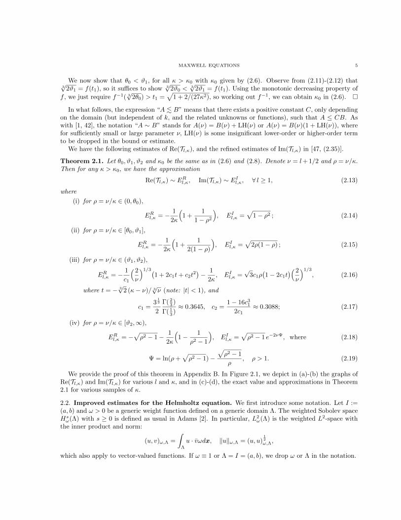
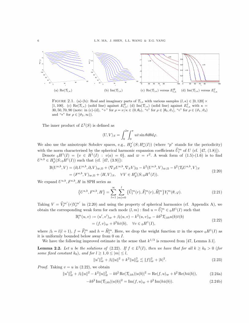
We provide the proof of this theorem in Appendix B. In Figure 2.1, we depict in (a)-(b) the graphs ofRe(Tl,κ) and Im(Tl,κ) for various l and κ, and in (c)-(d), the exact value and approximations in Theorem2.1 for various samples of κ.
2.2. Improved estimates for the Helmholtz equation. We first introduce some notation. Let I :=(a, b) and ω > 0 be a generic weight function defined on a generic domain Λ. The weighted Sobolev spaceHsω(Λ) with s ≥ 0 is defined as usual in Adams [2]. In particular, L2
ω(Λ) is the weighted L2-space withthe inner product and norm:
(u, v)ω,Λ =
∫Λ
u · vωdx, ‖u‖ω,Λ = (u, u)12
ω,Λ,
which also apply to vector-valued functions. If ω ≡ 1 or Λ = I = (a, b), we drop ω or Λ in the notation.
6 L.N. MA, J. SHEN, L.L. WANG & Z.G. YANG
040
80120
20
40
60
80
100
−6
−4
−2
0
lg
Re(
Tl,g)
(a) Re(Tl,κ)
040
80120
20
40
60
80
100
0
0.5
1
lg
Im( T
l,g)
(b) Im(Tl,κ)
0 30 50 70 90 150−5
−4
−3
−2
−1
0
l
g=30
g=90
(c) Re(Tl,κ) versus ERl,κ
0 30 50 70 90 1500
0.2
0.4
0.6
0.8
1
l
g=30
g=90
(d) Im(Tl,κ) versus EIl,κ
Figure 2.1. (a)-(b): Real and imaginary parts of Tl,κ with various samples (l, κ) ∈ [0, 120]×[1, 100]. (c) Re(Tl,κ) (solid line) against ERl,κ; (d) Im(Tl,κ) (solid line) against EIl,κ with κ =30, 50, 70, 90 (note: in (c)-(d), “+” for ρ = ν/κ ∈ (0, θ0), “” for ρ ∈ [θ0, ϑ1], “” for ρ ∈ (ϑ1, ϑ2)and “∗” for ρ ∈ [ϑ2,∞)).
The inner product of L2(S) is defined as
〈U, V 〉S =
∫ 2π
0
∫ π
0
uv sin θdθdϕ.
We also use the anisotropic Sobolev spaces, e.g., Hs′
p (S;Hsω(I)) (where “p” stands for the periodicity)
with the norm characterised by the spherical harmonic expansion coefficients Uml of U (cf. [47, (1.8)]).Denote 0H
1(I) = v ∈ H1(I) : v(a) = 0, and $ = r2. A weak form of (1.5)-(1.6) is to findUa,b ∈ H1
p (S; 0H1(I)) such that (cf. [47, (3.9)]):
B(Ua,b, V ) = (∂rUa,b, ∂rV )$,Ω + (∇SUa,b,∇SV )Ω − k2(Ua,b, V )$,Ω − b2〈TbUa,b, V 〉S
= (F a,b, V )$,Ω + 〈H,V 〉S , ∀V ∈ H1p (S; 0H
1(I)).(2.20)
We expand Ua,b, F a,b, H in SPH series asUa,b, F a,b, H
=
∞∑l=1
l∑|m|=0
Uml (r), Fml (r), Hm
l
Y ml (θ, ϕ). (2.21)
Taking V = V m′
l′ (r)Y m′
l′ in (2.20) and using the property of spherical harmonics (cf. Appendix A), we
obtain the corresponding weak form for each mode (l,m) : find u = Uml ∈ 0H1(I) such that
Bml (u, v) := (u′, v′)$ + βl(u, v)− k2(u, v)$ − kb2Tl,kbu(b)v(b)
= (f, v)$ + b2hv(b), ∀v ∈ 0H1(I),
(2.22)
where βl = l(l + 1), f = Fml and h = Hml . Here, we drop the weight function $ in the space 0H
1(I) asit is uniformly bounded below away from 0 on I.
We have the following improved estimate in the sense that k1/3 is removed from [47, Lemma 3.1].
Lemma 2.2. Let u be the solutions of (2.22). If f ∈ L2(I), then we have that for all k ≥ k0 > 0 (forsome fixed constant k0), and for l ≥ 1, 0 ≤ |m| ≤ l,
‖u′‖2$ + βl‖u‖2 + k2‖u‖2$ . ‖f‖2$ + |h|2. (2.23)
Proof. Taking v = u in (2.22), we obtain
‖u′‖2$ + βl‖u‖2 − k2‖u‖2$ − kb2 Re(Tl,kb)|u(b)|2 = Re(f, u)$ + b2 Re(hu(b)), (2.24a)
−kb2 Im(Tl,kb)|u(b)|2 = Im(f, u)$ + b2 Im(hu(b)). (2.24b)
MAXWELL EQUATIONS 7
Next taking v = 2(r − a)u′ in (2.22), and following the derivations in [47, (3.26)-(3.28)], we obtain
b2|I||u′(b)|2 + βl|I||u(b)|2 + 2a‖√ru′‖2 + k2
∫ b
a
(3− 2a
r
)|u|2r2dr
= ‖u′‖2$ + βl‖u‖2 + k2b2|I||u(b)|2 + 2 Re(f, (r − a)u′)$
+ 2b2|I|Re(hu′(b)
)+ 2kb2|I|Re
Tl,kb u(b)u′(b)
,
(2.25)
where |I| = b− a. Substituting ‖u′‖2$ + βl‖u‖2 in the identity (2.24a) into the above, and collecting theterms, we obtain
b2|I||u′(b)|2 +βl|I| − kb2 Re(Tl,kb)
|u(b)|2 + 2a‖
√ru′‖2 + 2k2
∫ b
a
(1− a
r
)|u|2r2dr
= k2b2|I||u(b)|2 + 2kb2|I|ReTl,kb u(b) u′(b)
+ 2b2|I|Re
(hu′(b)
)+ 2 Re(f, (r − a)u′)$ + b2 Re(hu(b)) + Re(f, u)$.
(2.26)
Hereafter, let C and Ci, εi be generic constants independent of k, l,m, and any function. Using theCauchy-Schwarz inequality, we obtain
2kb2|I|∣∣ReTl,kb u(b) u′(b)
∣∣ ≤ ε1b2|I||u′(b)|2 + ε−1
1 k2b2|I||Tl,kb|2|u(b)|2;
2b2|I|∣∣Re(hu′(b)
)∣∣ ≤ ε2b2|I||u′(b)|2 + ε−1
2 b2|I||h|2;
b2∣∣Re(hu(b))
∣∣ ≤ ε3kb2 |Re(Tl,kb)||u(b)|2 +
b2
ε3k |Re(Tl,kb)||h|2;
2∣∣Re(f, (r − a)u′)$
∣∣ ≤ ε4‖√ru′‖2 + ε−1
4 b|I|2‖f‖2$;∣∣Re(f, u)$∣∣ ≤ ε5‖u‖2$ + (4ε5)−1‖f‖2$.
(2.27)
Thus, by choosing suitable εi, we obtain from (2.26)-(2.27) that
C1b2|I||u′(b)|2 +Dl,k|I||u(b)|2 + C2a‖
√ru′‖2 + C3k
2‖u‖2$ . ‖f‖2$ +(
1 +1
k |Re(Tl,kb)|
)|h|2, (2.28)
where C1 = 1− (ε1 + ε2), C2 = 2− ε4, C3 = 2(1− a/ξ)− ε5/k2 with ξ ∈ (a, b), and
Dl,k = βl − (1− ε3)kb2|I|−1 Re(Tl,kb)− k2b2(1 + ε−1
1 |Tl,kb|2). (2.29)
It remains to estimate Dl,k, which can be negative for small l. According to the estimates in Theorem2.1, we conduct the analysis for four different cases as in (2.7).
(i) If ρ = νkb ∈ (0, θ0] for fixed 0 < θ0 < 1, we obtain from (2.24b) that
k2b2 |u(b)|2 ≤ k
|Im(Tl,kb)||Im(f, u)$|+ b2 |Im(hu(b))|
≤ ε7
2k2‖u‖2$ +
‖f‖2$2ε7|Im(Tl,kb)|2
+k2b2
2|u(b)|2 +
|h|2
2|Im(Tl,kb)|2.
(2.30)
By (2.14), Im(Tl,kb) in this range behaves like a constant, so (2.30) implies
k2b2 |u(b)|2 ≤ ε7k2‖u‖2$ + C
(‖f‖2$ + |h|2
). (2.31)
By (2.14), |Tl,kb|2 ≤ C, so Dl,k ≤ −Ck2b2. Therefore, using (2.28) and (2.31) leads to
‖√ru′‖2 + k2‖u‖2$ + k2|u(b)|2 ≤ C
(‖f‖2$ + |h|2
). (2.32)
8 L.N. MA, J. SHEN, L.L. WANG & Z.G. YANG
Thus, we derive the desired estimate in this case from (2.24a) and (2.32).
(ii) For ρ = νkb ∈ (θ0, ϑ1], we first show that for any c0 ∈ (1 − θ0, 1/
3√
2) and kb > 1, there exists aunique γ0 ∈ [1/3, 1) such that
ρ = 1− c0(kb)γ0−1, i.e., γ0 = 1 +ln((1− ρ)/c0)
ln(kb). (2.33)
Apparently, γ0 decreases with respect to ρ, so by (2.10),
1
3− ln( 3
√2c0)
ln(kb)+
ln(1 +O((kb)−2/3)
ln(kb)= 1 +
ln((1− ϑ1)/c0)
ln(kb)≤ γ0 < 1 +
ln((1− θ0)/c0)
ln(kb), (2.34)
Then one verifies readily that for c0 ∈ (1 − θ0, 1/3√
2), we have γ0 ∈ [1/3, 1). In view of (2.33), we canwrite
ν = kb− c0(kb)γ0 . (2.35)
Thus, by (2.15),
Re(Tl,kb) ∼ −1
2c0(kb)−γ0 , Im(Tl,kb) ∼
√2c0(kb)(γ0−1)/2, |Tl,kb|2 ∼ 2c0(kb)γ0−1, (2.36)
which implies
Dl,k ∼ ν2 − 1
4+ (1− ε3)
b
2|I|c0(kb)1−γ0 − k2b2
(1 + ε−1
1 2c0(kb)γ0−1)∼ −2c0(1 + ε−1
1 )(kb)γ0+1. (2.37)
By (2.24b) and the Cauchy-Schwarz inequality,
(kb)γ0+1 |u(b)|2 ≤ (kb)γ0
|Im(Tl,kb)||Im(f, u)$|+ b2 |Im(hu(b))|
≤ ε7
2k2‖u‖2$ +
(kb)2γ0−2
2ε7|Im(Tl,kb)|2‖f‖2$ +
(kb)γ0+1
2|u(b)|2 +
(kb)γ0−1
2|Im(Tl,kb)|2|h|2.
(2.38)
Then by (2.36) and (2.38),
(kb)γ0+1 |u(b)|2 ≤ ε7k2‖u‖2$ + C
((kb)γ0−1‖f‖2$ + |h|2
). (2.39)
Thus, we derive from (2.28) that
‖√ru′‖2 + k2‖u‖2$ + (kb)γ0+1|u(b)|2 ≤ C
(‖f‖2$ + |h|2
). (2.40)
Therefore, we obtain (2.23) from (2.24a) and (2.40).
(iii) If ρ = νkb ∈ (ϑ1, ϑ2], we find from (2.10) that
kb− 3
√kb
2+O(k−1/3) < ν ≤ kb+
3
√kb
2+O(k−1/3). (2.41)
By (2.16),
Re(Tl,kb) ∼ −c1(kb)−1/3, Im(Tl,kb) ∼ c2(kb)−1/3, |Tl,kb|2 ∼ c3(kb)−2/3, (2.42)
where ci are some positive constants independent of k, l. We can follow the same procedure as for Case(ii) (but with γ0 = 1/3) to derive
‖√ru′‖2 + k2‖u‖2$ + (kb)4/3|u(b)|2 ≤ C
(‖f‖2$ + |h|2
). (2.43)
Similarly, (2.23) follows from (2.24a) and (2.43).
(iv) If ρ = νkb ∈ (ϑ2,∞), we find from (2.18) that Im(Tl,kb) decays exponentially with respect to l, so
we cannot get a useful bound of |u(b)| from (2.24b). We therefore consider two cases:
(a) ν = kb+ c5(kb)γ1 with 1/3 < γ1 < 1; (b) ν ≥ η kb, (2.44)
MAXWELL EQUATIONS 9
for constant c5 ∈ (η− 1, 1/ 3√
2) and 1 < η < 1 + 1/ 3√
2. Here, we show that Case (a) can cover ρ ∈ (ϑ2, η).Indeed, similar to (2.33)-(2.34), we have ρ = 1 + c5(kb)γ1−1, and
1
3− ln( 3
√2c5)
ln(kb)+
ln(1 +O((kb)−2/3)
ln(kb)= 1 +
ln((ϑ2 − 1)/c5)
ln(kb)< γ1 < 1 +
ln((η − 1)/c5)
ln(kb). (2.45)
This implies if c5 ∈ (η − 1, 1/ 3√
2) and 1 < η < 1 + 1/ 3√
2, then 1/3 < γ1 < 1 and we can write ν in theform of (a).
In the first case, we derive from (2.18) that
Re(Tl,kb) ∼√
2c5(kb)(γ1−1)/2, |Tl,kb|2 ∼ 2c5(kb)γ1−1, Dl,k ∼ −2c5(ε−11 − 1)(kb)γ1+1, (2.46)
where we recall that ε1 < 1. Noticing that
βl‖u‖2 − k2‖u‖2$ ≥ (βl − k2b2)‖u‖2 ≥ 0, (2.47)
and Re(Tl,kb) < 0, we deduce from (2.24a) that
− kb2 Re(Tl,kb)|u(b)|2 ≤ |Re(f, u)$|+ b2 |Re(hu(b))|. (2.48)
Using (2.46), (2.48) and following the derivation of (2.38), we can get
(kb)γ1+1 |u(b)|2 ≤ ε8k2‖u‖2$ + C
((kb)γ1−1‖f‖2$ + |h|2
). (2.49)
We then derive from (2.28) that
‖√ru′‖2 + k2‖u‖2$ + (kb)γ1+1|u(b)|2 ≤ C
(‖f‖2$ + |h|2
). (2.50)
Thus, we derive (2.23) for this case from (2.24a) and (2.50).In the second case of (2.44), we observe from (2.18) that
Re(Tl,kb) ∼ −ν
kb, |Tl,kb|2 ∼
ν2
k2b2, (2.51)
which implies
Dl,k ∼ ν2 − 1
4+ (1− ε3)
bν
|I|− k2b2 − ε−1
1 ν2 ∼ −c6 βl. (2.52)
Then, by (2.51) and (2.48),
βl|u(b)|2 ≤ ε8βl‖u‖2 + C(‖f‖2$ + |h|2
). (2.53)
We then derive from (2.28) that
‖√ru′‖2 + k2‖u‖2$ + βl|u(b)|2 ≤ C
(‖f‖2$ + |h|2
). (2.54)
Finally, we obtain (2.23) from (2.24a) and (2.54).
Thanks to the above lemma and the orthogonality of SPH, one can easily derive the following improvedresult, where a factor of k1/3 is removed from the upper bound of [47, Thm. 3.1].
Theorem 2.2. Let Ua,b be the solution of (2.20). If F a,b ∈ L2(Ω) and H ∈ L2(S), then we have
‖∇Ua,b‖Ω + k‖Ua,b‖Ω . ‖F a,b‖Ω + ‖H‖L2(S). (2.55)
Remark 2.1. Similar wavenumber explicit estimate was derived by Chandler-Wilde and Monk [9, Lemma3.8] for general starlike scatterers and H = 0, together with an explicit constant in the upper bound.However, the result therein does not imply the mode-by-mode estimate in Lemma 2.2. The analysis inthis paper essentially relies on the estimates bounded by the corresponding mode of the data.
10 L.N. MA, J. SHEN, L.L. WANG & Z.G. YANG
3. A priori estimates for the reduced Maxwell equations
In this section, we perform the wavenumber explicit a priori estimates for the Maxwell equations(1.1)-(1.2). The key is to employ a divergence-free vector harmonic expansion of the fields and reduce theproblem of interest into two sequences of decoupled one-dimensional Helmholtz problems. This decouplingnot only leads to a more efficient numerical algorithm, but also greatly simplifies its analysis.
3.1. Dimension reduction via divergence-free VSH expansions. Introduce the spaces
H(div; Ω) =E ∈ L2(Ω) : divE ∈ L2(Ω)
, H(div0; Ω) =
E ∈ H(div; Ω) : divE = 0
, (3.1)
where H(div; Ω) is equipped with the graph norm as defined in [37, P. 52].Built upon the spherical harmonics Y ml , the VSH
Y ml er,∇SY ml ,Tm
l = ∇SY ml × er
forms a
complete, orthogonal system of (L2(S))3, and refer to Appendix A for some relevant properties. Thefollowing VSH expansion of a solenoidal (or divergence-free) field plays an important role in our analysisand spectral algorithm.
Proposition 3.1. For any E ∈ (L2(Ω))3, we expand it as
E = v02,0 Y
00 er +
∞∑l=1
l∑|m|=0
vm1,l T
ml + vm2,l Y
ml er + vm3,l∇SY ml
, (3.2)
where
vm1,l = β−1l 〈E,T
ml 〉S , vm2,l = 〈E, Y ml er〉S , vm3,l = β−1
l 〈E,∇SYml 〉S , βl = l(l + 1). (3.3)
If E ∈ H(div0; Ω), then we have( ddr
+2
r
)v0
2,0 = 0,r
βl
( ddr
+2
r
)vm2,l = vm3,l, (3.4)
and we can write
E = u00 Y
00 er +
∞∑l=1
l∑|m|=0
um1,l T
ml +∇×
(um2,l T
ml
), (3.5)
where
u00 = v0
2,0 =c
r2, um1,l = vm1,l, um2,l = β−1
l rvm2,l, (3.6)
with c being an arbitrary constant.
Proof. Since div(vm1,l Tml ) = 0 (cf. (A.4)), we obtain from (4.8) and (A.6)-(A.7) that
divE =( ddr
+2
r
)v0
2,0 +
∞∑l=1
l∑|m|=0
( ddr
+2
r
)vm2,l −
βlrvm3,l
Y ml . (3.7)
Then the identities in (3.4) follow from divE = 0 immediately.Note that the equation of v0
2,0 in (3.4) has the general solution: v02,0 = c/r2. To derive (3.5) under
(3.6), it suffices to show that
β−1l ∇×
(rvm2,l T
ml
)= vm2,l Y
ml er + vm3,l∇SY ml . (3.8)
It follows from a direct calculation using (A.4), that is,
β−1l ∇×
(rvm2,l T
ml
)= vm2,l Y
ml er + β−1
l ∂r(rvm2,l)∇SY ml = vm2,l Y
ml er +
r
βl
( ddr
+2
r
)vm2,l∇SY ml . (3.9)
Therefore, the expansion (3.5) is a direct consequence of (3.2), (3.4) and (3.6).
MAXWELL EQUATIONS 11
Remark 3.1. Equivalently, we can reformulate (3.5) as
E = u00 Y
00 er +
∞∑l=1
l∑|m|=0
um1,l T
ml + ∂ru
m2,l∇SY ml +
βlrum2,l Y
ml er
, ∂r =
d
dr+
1
r, (3.10)
which allows for exact imposition of the divergence-free condition. Such a VSH expansion turns out tobe a very useful analytic and numerical tool for e.g., Maxwell equations and Navier-Stokes equations inspherical geometry (see, e.g., [38, 7, 39, 37, 22, 11]).
Denote by L2T (S) the space of tangential components of vector fields in (L2(S))3. Then we can expand
Ea,bS ∈ L2
T (S) as
Ψ = Ea,bS |r=b =
∞∑l=1
l∑|m|=0
ψmT,l T
ml + ψmY,l∇SY ml
, (3.11)
where the expansion coefficients
ψmT,l = β−1l
⟨Ψ,Tm
l
⟩S, ψmY,l = β−1
l
⟨Ψ,∇SY ml
⟩S. (3.12)
Recall that the capacity operator in (1.2) is defined by (cf. [39, (5.3.88)]):
Tb[Ψ] := ηH × er∣∣r=b
=
∞∑l=1
l∑|m|=0
− i
∂rh(1)l (kb)
h(1)l (kb)
ψmT,l Tml + i
h(1)l (kb)
∂rh(1)l (kb)
ψmY,l∇SY ml, (3.13)
where η =√µ/ε, h
(1)l is the spherical Bessel function of the first kind (cf. [1]), and
∂rh(1)l (kb) =
( ddr
+1
r
)h
(1)l (r)
∣∣∣r=kb
. (3.14)
As F a,b in (1.1) is a solenoidal field, we can expand it as (3.5) with the coefficients f00 and fm1,l, fm2,l.
We also expand the data h ∈ L2T (S) in (1.6) as
h =
∞∑l=1
l∑|m|=0
hmT,l T
ml + hmY,l∇SY ml
, (3.15)
where the expansion coefficients are given by (3.12) with h in place of Ψ.
Proposition 3.2. Denote
u1 = um1,l, u2 = um2,l, f1 = fm1,l, f2 = fm2,l, h1 = hmT,l, h2 = k−1(Tl,kb + (kb)−1
)hmY,l, (3.16)
for l ≥ 1. Then the Maxwell equations (1.1)-(1.2) reduce to −k2u00 = f0
0 , and the following two sequencesof one-dimensional problems:
− 1
r2(r2u′i)
′ +βlr2ui − k2ui = fi, r ∈ I = (a, b); u′i(b)− k Tl,kb ui(b) = hi, i = 1, 2, (3.17)
but with different boundary conditions at r = a :
u1(a) = 0, u′2(a) + a−1u2(a) = 0. (3.18)
Proof. We first consider (1.1). Recall that if divu = 0, then we have ∇ × ∇ × u = −∆u. Sincediv(∇× (fTm
l ))
= 0 (cf. (A.4)), we derive from (3.5) and (A.4)-(A.5) that
∇×∇×(um1,lT
ml
)= −∆
(um1,lT
ml
)= −Ll
(um1,l)Tml ,
∇×∇×∇×(um2,lT
ml
)= −∇×
(∆(um2,lT
ml
))= −∇×
(Ll(um2,l)Tml
),
(3.19)
12 L.N. MA, J. SHEN, L.L. WANG & Z.G. YANG
where the Bessel operator Ll is given in (A.3). Thus, using the expansions (3.5), we can reduce (1.1) to
− (Ll + k2)w(r) = f(r) for w, f = um1,l, fm1,l or um2,l, fm2,l, (3.20)
for l ≥ 1 and r ∈ I. In addition, we have
− k2u00 = f0
0 , as ∇× (u00 Y
00 er) = ∇× (f0
0 Y00 er) = 0, (3.21)
since Ea,b and F a,b are solenoidal. This leads to the mode u00, so we only consider the modes with l ≥ 1
and 0 ≤ |m| ≤ l. A direct calculation using (A.2)-(A.3) and (A.4)-(A.5) leads to the reduction of theboundary condition (1.2):
um1,l(a) = 0 , ∂rum2,l(a) = 0, where ∂r :=
d
dr+
1
r. (3.22)
We now turn to the DtN boundary condition (1.2). By (3.5) and (3.19),
∇×Ea,b =
∞∑l=1
l∑|m|=0
∇×
(um1,lT
ml
)− Ll(um2,l)T
ml
. (3.23)
Again from (A.2)-(A.3) and (A.4)-(A.5), we derive(∇×Ea,b
)× er
∣∣r=b
=
∞∑l=1
l∑|m|=0
(∂ru
m1,l
)Tml + Ll(um2,l)∇SY ml
∣∣∣r=b
,
Ea,bS
∣∣r=b
=
∞∑l=1
l∑|m|=0
um1,lT
ml + ∂ru
m2,l∇SY ml
∣∣∣r=b
.
(3.24)
Then, by (3.13) and (3.24),
− ikTb[Ea,bS ] =
∞∑l=1
l∑|m|=0
− k
∂rh(1)l (kb)
h(1)l (kb)
um1,l(b)Tml + k
h(1)l (kb)
∂rh(1)l (kb)
∂rum2,l(b)∇SY ml
. (3.25)
Consequently, by (3.15) and (3.24), the DtN boundary condition (1.2) reduces to
∂rum1,l(b)− k
∂rh(1)l (kb)
h(1)l (kb)
um1,l(b) = hmT,l; Ll(um2,l)(b) + kh
(1)l (kb)
∂rh(1)l (kb)
∂rum2,l(b) = hmY,l. (3.26)
By the equation (3.20) (note: fm2,l(b) = 0 as the source field is assumed to be compact supported), we
have Ll(um2,l)(b) = −k2um2,l(b), so we can simplify (3.26) as
∂rum2,l(b)− k
∂rh(1)l (kb)
h(1)l (kb)
um2,l(b) =1
k
∂rh(1)l (kb)
h(1)l (kb)
hmY,l. (3.27)
This ends the derivation.
3.2. A priori estimates for um1,l, um2,l. A weak form of (3.17)-(3.18) is to find u1 ∈ 0H1(I) such that
Bml (u1, w) = (f1, w)$ + b2h1w(b) , ∀w ∈ 0H1(I), (3.28)
and to find u2 ∈ H1(I) such that
Bml (u2, w)− au2(a)w(a) = (f2, w)$ + b2h2w(b), ∀w ∈ H1(I), (3.29)
where the sesquilinear form Bml (·, ·) is defined in (2.22).Observe that the weak form for u1 is the same as that of the Helmholtz equation in (2.22), while (3.29)
differ from (3.28) with an extra term: −au2(a)w(a). As a result, we can obtain the a priori estimateslike Lemma 2.2 by using the same argument.
MAXWELL EQUATIONS 13
Theorem 3.1. Let u1 and u2 be solutions of (3.28) and (3.29), respectively. If f1, f2 ∈ L2(Λ), then forall k ≥ k0 > 0 (for some fixed constant k0), and l ≥ 1, 0 ≤ |m| ≤ l, we have
‖u′i‖2$ + βl‖ui‖2 + k2‖ui‖2$ . ‖fi‖2$ + |hi|2, i = 1, 2. (3.30)
Proof. The estimates in Lemma 2.2 carry over to u1, so it suffices to consider u2 and deal with the extraterm herein. Following the proof of Lemma 2.2, we take two test functions: w = u2 and w = 2(r − a)u′2,and note that the term “−au2(a)w(a)” vanishes for the second test function. Thus, we only need to dealwith the contribution from this extra term as follows:
‖u′2‖2$ + βl‖u2‖2 + k2‖u2‖2$ − a|u2(a)|2 . ‖f2‖2$ + |h2|2. (3.31)
Using the Sobolev inequality (see, e.g., [45, (B.33)]), we obtain
a|u2(a)|2 ≤ a(
2 +1
b− a
)‖u2‖‖u2‖1 ≤ a
(2 +
1
b− a
)(‖u2‖2 + ‖u2‖‖u′2‖
)≤ a−3
(2 +
1
b− a
)(‖u2‖2$ + ‖u2‖$‖u′2‖$
).
(3.32)
where we used the simple inequality:√A2 +B2 ≤ |A|+ |B|, and the fact $/a2 ≥ 1. Thus,
a|u2(a)|2 ≤ 1
2‖u′2‖2$ + C‖u2‖2$. (3.33)
Thus, by (3.31) and (3.33),
1
2‖u′2‖2$ + βl‖u2‖2 + k2
(1− Ck−1
)‖u2‖2$ . ‖f2‖2$ + |h2|2. (3.34)
This leads to the desired estimate.
It is important to point out that as the expansion in (3.10) involves ∂rum2,l, the direct use of Theorem
3.1 and the orthogonality of VSH only leads to an overly pessimistic estimate: ‖Ea,b‖Ω = O(1). However,
the expected optimal estimate should be ‖Ea,b‖Ω = O(k−1). In view of this, we next derive an “auxiliary”
equation of ∂rum2,l and apply the analysis similar to that for um1,l, um2,l in the previous subsection.
3.3. A priori estimates for ∂rum2,l.
3.3.1. Equation of ∂rum2,l. Denote
v2 = βlum2,l/r = βlu2/r, v3 = ∂ru
m2,l = ∂ru2, hY = −kSl,kbh2 = hmY,l,
g2 = βlfm2,l/r = βlf2/r, g3 = ∂rf
m2,l = ∂rf2,
(3.35)
where the DtN kernel pertinent to (3.13) is defined by
Sl,κ := −h
(1)l (κ)
∂rh(1)l (κ)
= −h
(1)l (κ)
h(1)l
′(κ) + κ−1h
(1)l (κ)
= − 1
Tl,κ + κ−1, l ≥ 1, κ > 0. (3.36)
Recall that Tl,κ is defined in (2.2).From the equation of u2 in Proposition 3.2, we can derive the following “auxiliary” equation.
Proposition 3.3. Let v3 = ∂ru2. Then we have
− 1
r2(r2v′3)′ +
βlr2v3 − k2v3 −
2
r2v2 = g3, r ∈ I,
v3(a) = 0, v′3(b)− k(Sl,kb − (kb)−1
)v3(b)− b−1v2(b) = hY .
(3.37)
14 L.N. MA, J. SHEN, L.L. WANG & Z.G. YANG
Alternatively, we can replace the boundary condition at r = b in (3.37) by
v′3(b)− σl,kbb
v2(b) =hY
kbSl,kb= −h2
b, (3.38)
where
σl,kb := 1− k2b2
βl
(1− 1
kbSl,kb
)= 1− k2b2
βl
(1 +Tl,kbkb
+1
k2b2
). (3.39)
Proof. One verifies readily that ∂rv3 = ∂r(∂ru2) = r−2(r2u′2)′, so by (3.17),
− ∂rv3 +βlr2u2 − k2u2 = f2, r ∈ I. (3.40)
Applying ∂r to both sides of the above equation, we obtain the first equation in (3.37) by a direct
calculation. Since v3(a) = ∂ru2(a), the boundary condition v3(a) = 0 is a direct consequence of (3.18).Noting that u′2(b) = v3(b)− u2(b)/b, we obtain from (3.36) and the boundary condition in (3.17) that
u2(b) +Sl,kbk
v3(b) =Sl,kbk
h2 = −hYk2. (3.41)
Taking r = b in (3.40) (note: f2(b) = 0), we obtain
u2(b) = −k−2(v′3(b) + b−1v3(b)− b−1v2(b)
). (3.42)
Inserting (3.42) into (3.41) yields the boundary condition at r = b in (3.37).The alternative boundary condition (3.38) can be obtained by eliminating v3(b) in (3.37). More
precisely, solving out v3(b) from (3.41), and using the fact u2(b) = bv2(b)/βl, we can obtain (3.38)-(3.39)from (3.37).
3.3.2. Properties of the DtN kernel Sl,κ. By (3.36), we have that for integer l ≥ 1 and real κ > 0,
Re(Sl,κ) = − Re(Tl,κ) + κ−1
(Re(Tl,κ) + κ−1)2 + (Im(Tl,κ))2; Im(Sl,κ) =
Im(Tl,κ)
(Re(Tl,κ) + κ−1)2 + (Im(Tl,κ))2, (3.43)
which, together with (2.5), implies
Re(Sl,κ) > 0, Im(Sl,κ) > 0, for l ≥ 1, κ > 0. (3.44)
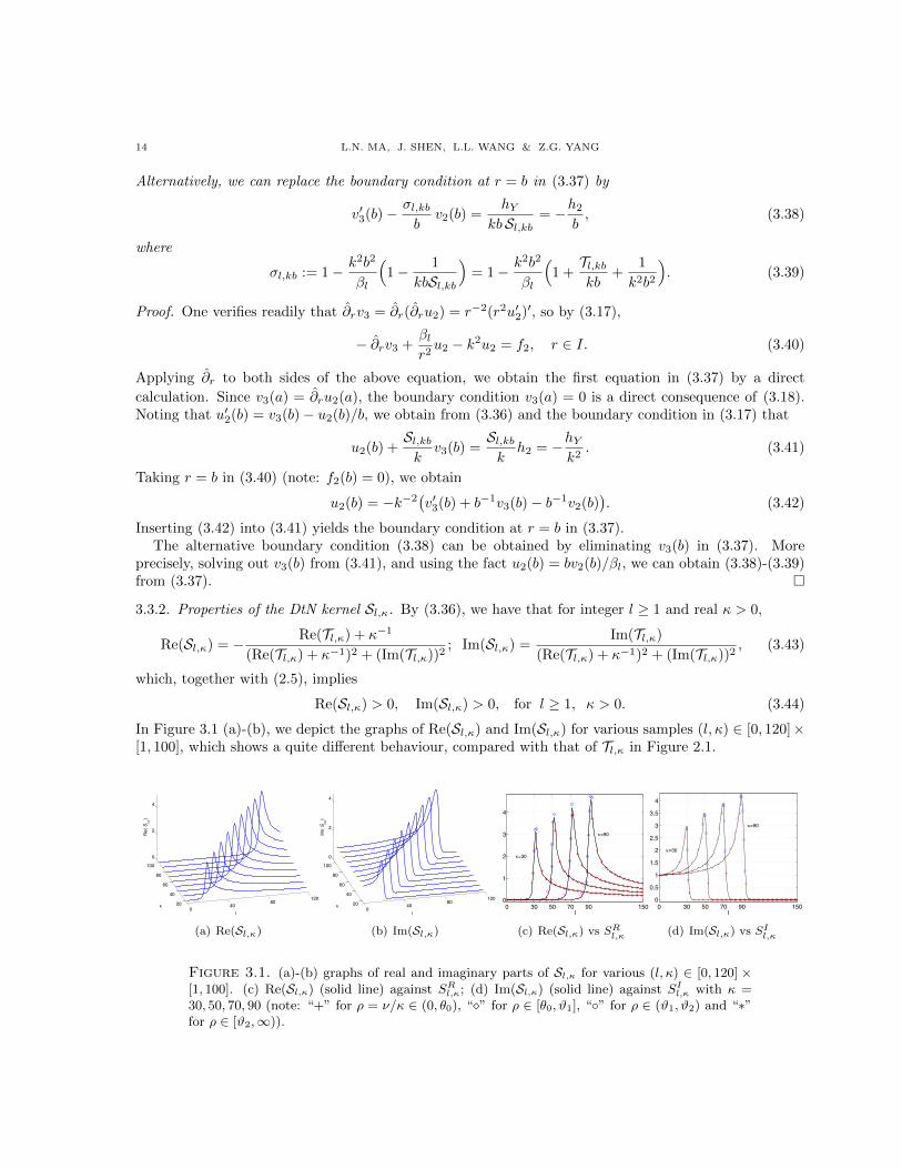
In Figure 3.1 (a)-(b), we depict the graphs of Re(Sl,κ) and Im(Sl,κ) for various samples (l, κ) ∈ [0, 120]×[1, 100], which shows a quite different behaviour, compared with that of Tl,κ in Figure 2.1.
040
80120
20
40
60
80
100
0
2
4
lg
Re(
Sl,g)
(a) Re(Sl,κ)
040
80120
20
40
60
80
100
0
2
4
lg
Im( S
l,g)
(b) Im(Sl,κ)
0 30 50 70 90 1500
1
2
3
4
l
g=30
g=90
(c) Re(Sl,κ) vs SRl,κ
0 30 50 70 90 1500
0.5
1
1.5
2
2.5
3
3.5
4
l
g=30
g=90
(d) Im(Sl,κ) vs SIl,κ
Figure 3.1. (a)-(b) graphs of real and imaginary parts of Sl,κ for various (l, κ) ∈ [0, 120] ×[1, 100]. (c) Re(Sl,κ) (solid line) against SRl,κ; (d) Im(Sl,κ) (solid line) against SIl,κ with κ =30, 50, 70, 90 (note: “+” for ρ = ν/κ ∈ (0, θ0), “” for ρ ∈ [θ0, ϑ1], “” for ρ ∈ (ϑ1, ϑ2) and “∗”for ρ ∈ [ϑ2,∞)).
MAXWELL EQUATIONS 15
Thanks to (3.43) and the estimates in Theorem 2.1, we can analyze the behaviour of Sl,κ. In Figure3.1 (c)-(d), we plot the exact value and approximations in Theorem 3.2 below for various samples of κ.
Theorem 3.2. Let θ0, ϑ1, ϑ2 and κ0 be the same as in (2.6) and (2.8). Denote ν = l+ 1/2 and ρ = ν/κ.Then for any κ > κ0,
Re(Sl,κ) ∼ SRl,κ, Im(Sl,κ) ∼ SIl,κ, ∀ l ≥ 1, where (3.45)
(i) for ρ = ν/κ ∈ (0, θ0),
SRl,k =1
2κ
( ρ
1− ρ2
)2
, SIl,k =1√
1− ρ2; (3.46)
(ii) for ρ = ν/κ ∈ [θ0, ϑ1],
SRl,κ =1
4ρ(1− ρ)κ
(1 +
1
2(1− ρ)
), SIl,κ =
1√2ρ(1− ρ)
; (3.47)
(iii) for ρ = ν/κ ∈ (ϑ1, ϑ2),
SRl,κ =1
4c1
(ν2
)1/3
HR(t), SIl,κ =
√3
4c1
(ν2
)1/3
HI(t), (3.48)
where t = − 3√
2 (κ− ν)/ 3√ν (note: |t| < 1), and
HR(t) =1 + 2c1t+ c2t
2
1− 2c1t+ (4c21 + c2/2)t2 + c1c2t3 + c22t4/4
,
HI(t) =1− 2c1t
1− 2c1t+ (4c21 + c2/2)t2 + c1c2t3 + c22t4/4
,
(3.49)
with c1, c2 given by (2.17);(iv) for ρ = ν/κ ∈ [ϑ2,∞),
SRl,κ =1√ρ2 − 1
(1 +
1
2κ√ρ2 − 1
(1 +
1
ρ2 − 1
)), (3.50)
SIl,κ =e−2νΨ√ρ2 − 1
(1 +
1
κ√ρ2 − 1
(1 +
1
ρ2 − 1
)), (3.51)
where Ψ is defined in (2.19).
We postpone the derivation of the above estimates to Appendix C.
Remark 3.2. With some careful calculations, one can verify that for t ∈ [−1, 1],
minHR(t) = HR(t = −1) ≈ 0.2493, maxHR(t) = HR(t ≈ 0.8004) ≈ 1.9291,
minHI(t) = HI(t = 1) ≈ 0.2479, maxHI(t) = HI(t = 0) = 1.
Thus, we roughly have 0.2493 ≤ HR(t) ≤ 1.9291 and 0.2479 ≤ HI(t) ≤ 1 for t ∈ [−1, 1].
A weak form of (3.37) is to find v3 ∈ 0H1(I) such that
Bml (v3, w) = Gml (w), ∀w ∈ 0H1(I), (3.52)
where
Bml (v3, w) = (v′3, w′)$ + βl(v3, w)− k2(v3, w)$ − kb2
(Sl,kb − (kb)−1
)v3(b)w(b);
Gml (w) := b v2(b)w(b) + 2(v2, w) + b2hY w(b) + (g3, w)$, $ = r2.(3.53)
16 L.N. MA, J. SHEN, L.L. WANG & Z.G. YANG
Alternatively, we can use the equivalent boundary condition (3.38)-(3.39), and modify (3.53) as
Bml (v3, w) = (v′3, w′)$ + βl(v3, w)− k2(v3, w)$;
Gml (w) = b σl,kbv2(b)w(b) + 2(v2, w) + (g3, w)$ + b2hY
k Sl,kbw(b).
(3.54)
Theorem 3.3. Let θ0 and ϑi2i=1 be the same as in (2.6) and (2.8). If g2, g3 ∈ L2(I), then we havethat for all k ≥ k0 > 0 (for some fixed constant k0), and l ≥ 1, 0 ≤ |m| ≤ l,
‖v′3‖2$ + βl‖v3‖2 + k2‖v3‖2$ ≤ Cl,k( 1
βl‖g2‖2$ + ‖g3‖2$
)+ C
(1 +
β2l
k4
)|hY |2, (3.55)
where C is a generic positive constant independent of k, l,m and v3, and
Cl,k = C
1, if ρ = ν/(kb) ∈ (0, θ0] ∪ (ϑ2,∞),
(kb)1−γ , if ρ = ν/(kb) ∈ (θ0, ϑ2].(3.56)
Note that for ρ ∈ (θ0, ϑ2], we have ρ = 1 + ξ(kb)−γ or ν = l+ 1/2 = kb+ ξ(kb)γ−1, for some γ ∈ [1/3, 1),and some constant ξ.
Proof. Taking w = v3 in (3.52), we obtain
‖v′3‖2$ + βl‖v3‖2 − k2‖v3‖2$ − kb2 Re(Sl,kb)|v3(b)|2 + b|v3(b)|2
= bRe(v2(b)v3(b)) + 2Re(v2, v3) + b2 Re(hY v3(b)) + Re(g3, v3)$,(3.57a)
−kb2 Im(Sl,kb)|v3(b)|2 = b Im(v2(b)v3(b)) + 2Im(v2, v3) + b2 Im(hY v3(b)) + Im(g3, v3)$. (3.57b)
Next taking w = 2(r − a)v′3 in (3.52), and following the derivation of (2.25)-(2.26), we can obtain
b2|I||v′3(b)|2 + (βl|I|+ b)|v3(b)|2 + 2a‖√rv′3‖2 + 2k2
∫ b
a
[1− a
r
]|v3|2r2dr
=(k2b2|I|+ kb2 Re(Sl,kb)
)|v3(b)|2 + 2kb2|I|Re
(Sl,kb − (kb)−1)v3(v)v′3(b)
+ bRe(v2(b)v3(b)) + b2 Re(hY v3(b)) + 2Re(v2, v3) + Re(g3, v3)$ + 2b|I|Re
(v2(b)v′3(b)
)+ 2b2|I|Re
(hY v
′3(b)
)+ 4 Re(v2, (r − a)v′3) + 2 Re(g3, (r − a)v′3)$.
(3.58)
Then we can derive the estimate similar to (2.28) (by noting that Sl,kb − (kb)−1 should be in place ofTl,kb and the term of the left endpoint r = a is not involved):
b2|I||v′3(b)|2 +Dl,k|I||v3(b)|2 + a‖√rv′3‖2 + k2‖v3‖2$ ≤ C
(‖v2‖2$ + |v2(b)|2 + ‖g3‖2$ + |hY |2
), (3.59)
whereDl,κ := βl − (1− ε3)|I|−1 kb2 Re(Sl,kb)− k2b2
(1 + ε−1
1
∣∣Sl,kb − (kb)−1∣∣2). (3.60)
Thus, it remains to bound the term Dl,κ|I||v3(b)|2 (note: it is negative for some range of l), and to estimatethe terms of v2 by using that of u2 in Theorem 3.1 and its proof. Following the proof of Theorem 3.1,we proceed with four cases.
(i) If ρ = νkb ∈ (0, θ0) for fixed 0 < θ0 < 1, we find from (3.46) that both kbRe(Sl,kb) and Im(Sl,kb)
behave like constants. Thus, from (3.57b), we can obtain the bound like (2.31):
k2b2 |v3(b)|2 ≤ εk2‖v3‖2$ + C(‖v2‖2$ + |v2(b)|2 + ‖g3‖2$ + |hY |2
). (3.61)
Noting from (3.46) and (3.60) thatDl,κ ∼ βl − Ck2b2, (3.62)
we infer from (3.59) that
b2|I||v′3(b)|2 + βl|I||v3(b)|2 + a‖√rv′3‖2 + k2‖v3‖2$ ≤ C
(‖v2‖2$ + |v2(b)|2 + ‖g3‖2$ + |hY |2
). (3.63)
MAXWELL EQUATIONS 17
Recall from (3.35) that h2 = −hY /(k Sl,kb), u2 = rβ−1l v2 and f2 = rβ−1
l g2. Then by (2.32),
‖v2‖2$ + |v2(b)|2 ≤ C( 1
k2‖g2‖2$ +
β2l
k4|hY |2
)≤ C
( 1
βl‖g2‖2$ +
β2l
k4|hY |2
). (3.64)
Thus, using (3.57a), (3.61), (3.63), (3.64) and the Cauchy-Schwarz inequality, we can obtain (3.55).
(ii) If ρ = νkb ∈ [θ0, ϑ1], we start with (2.35), and find from (3.47) that
Re(Sl,kb − (kb)−1) ∼ 1
8c20(kb)1−2γ0 , Im(Sl,kb) ∼
1√2c0
(kb)(1−γ0)/2, (3.65)
where 1/3 ≤ γ0 < 1. Thus, by (3.62)-(3.65), Dl,k ∼ −C(kb)3−γ0 . As with (2.37)-(2.39), we can derive
(kb)3−γ0 |v3(b)|2 ≤ εk2‖v3‖2$ + C(
(kb)1−γ0(‖v2‖2$ + ‖g3‖2$) + |v2(b)|2 + |hY |2). (3.66)
Therefore, we have
‖√rv′3‖2 + k2‖v3‖2$ + (kb)3−γ0 |v3(b)|2 ≤ C
((kb)1−γ0(‖v2‖2$ + ‖g3‖2$) + |v2(b)|2 + |hY |2
). (3.67)
Like (3.64), we derive from (2.40) (note: h2 = −hY /(k Sl,kb), u2 = rβ−1l v2, f2 = rβ−1
l g2) and (3.65) that
k1−γ0‖v2‖2$ + |v2(b)|2 ≤ C( 1
k1+γ0‖g2‖2$ +
β2l
k4|hY |2
)≤ C
(k1−γ0
βl‖g2‖2$ +
β2l
k4|hY |2
). (3.68)
Thus, as with the previous case, we can obtain the desired estimate.
(iii) If ρ = νkb ∈ (ϑ1, ϑ2), we have the range in (2.41). Using (3.48)-(3.49), we can show that in this
range, the bound is the same as (2.50) with γ0 = 1/3 :
‖√rv′3‖2 + k2‖v3‖2$ + (kb)8/3|v3(b)|2 ≤ C
((kb)2/3(‖v2‖2$ + ‖g3‖2$) + |v2(b)|2 + |hY |2
). (3.69)
Similarly, we can bound the terms involving v2 by (3.68) with γ0 = 1/3.
(iv) If ρ = νkb ∈ [ϑ2,∞), we find from (3.51) that Im(Sl,kb) decays exponentially with respect to l.
However, since Re(Sl,kb − (kb)−1) > 0, we do not have (2.48) to bound the term Dl,k|I||v3(b)|2 (note:Dl,k < 0), as opposite to the estimate of u2 in Theorem 3.1. For this purpose, we use the equivalentboundary condition (3.38)-(3.39). Correspondingly, we modify the weak form (3.52) as
(v′3, w′)$ + βl(v3, w)− k2(v3, w)$ = bσl,kbv2(b)w(b) + 2(v2, w)
+ (g3, w)$ + b2hY
k Sl,kbw(b) , ∀w ∈ 0H
1(Λ).(3.70)
Taking w = v3 in (3.70), leads to
‖v′3‖2$ + βl‖v3‖2 − k2‖v3‖2$ = bRe(σl,kb v2(b)v3(b))
+ Re(g3, v3)$ + 2Re(v2, v3) + b2Re( hYk Sl,kb
v3(b)),
(3.71)
Next taking w = 2(r − a)v′3 and following the same procedure in deriving (2.25)-(2.26), we have
b2|I||v′3(b)|2 + (βl − k2b2)|I||v3(b)|2 + 2a‖√rv′3‖2 + 2k2
∫ b
a
(1− a
r
)|v3|2r2dr
= 2b|I|Reσl,kb v2(b)v′3(b)+ bReσl,kbv2(b)v3(b)+ 4 Re(v2, (r − a)v′3) + 2Re(v2, v3)
+ 2Re(g3, (r − a)v′3)$ + Re(g3, v3)$ + 2b2|I|Re( hYk Sl,kb
v′3(b))
+ b2Re( hYk Sl,kb
v3(b)).
(3.72)
18 L.N. MA, J. SHEN, L.L. WANG & Z.G. YANG
Using the Cauchy-Schwarz inequality, we can derive
|v′3(b)|2 + (βl − k2b2)|v3(b)|2 + ‖√rv′3‖2 + k2‖v3‖2$ ≤ C
|σl,kb|2
(1 + (βl − k2b2)−1
)|v2(b)|2
+ ‖v2‖2$ + ‖g3‖2$ +1
(kb)2 |Sl,kb|2(1 + (βl − k2b2)−1
)|hY |2
.
(3.73)
We first consider the range (a) in (2.44), i.e., ν ∼ kb + c5(kb)γ1 for 1/3 ≤ γ1 < 1 and some constantc5 > 0. From (3.39) and (3.50), one verifies
βl − k2b2 ∼ 2c5(kb)1+γ1 , |Sl,kb| ∼ |Re(Sl,kb)| ∼1√
2c5(kb)γ1−1, |σl,kb| ∼ 2c5(kb)γ1−1. (3.74)
Then we obtain from (3.73)-(3.74) that
k2‖v3‖2$ ≤ C(
(kb)2(γ1−1)|v2(b)|2 + ‖v2‖2$ + ‖g3‖2$ + (kb)−(1+γ1)|hY |2). (3.75)
Recalling that h2 = −hY /(k Sl,kb), u2 = rβ−1l v2 and f2 = rβ−1
l g2, we have from (2.50) and (3.74) that
‖v2‖2$ + (kb)2(γ1−1)|v2(b)|2 ≤ C( 1
βl‖g2‖2$ +
β2l
k4|hY |2
). (3.76)
As v3 ∈ 0H1(I), one verifies readily that
|v3(b)| ≤∫ b
a
|v′3(r)|dr ≤ C‖v′3‖$. (3.77)
Thus, using (3.71) and the Cauchy-Schwarz inequality, we can obtain the same upper bound as (3.75)for ‖v′3‖2$ + βl‖v3‖2. This leads to the desired estimate for this case.
We then consider the range (b) in (2.44), i.e., ν > η kb with η > 1. Once again, by (3.39) and (3.50),
|Sl,kb| ∼ |Re(Sl,kb)| ∼kb
ν√
1− η−2, |σl,kb| ∼ 1− η−2. (3.78)
It is evident that
βl‖v3‖2 − k2‖v3‖2$ ≥ (βl − k2b2)‖v3‖2 ≥ βl(1− η−2)‖v3‖2. (3.79)
Using the Cauchy-Schwarz inequality, and (3.77)-(3.79), we have from (3.71) that
‖v′3‖2$ + βl‖v3‖2 ≤ C(|v2(b)|2 + β−1
l ‖v2‖+ β−1l ‖g3‖2$ +
βlk4|hY |2
). (3.80)
Then by (2.23), (2.54) and the fact that h2 = −hY /(k Sl,kb), u2 = rβ−1l v2 and f2 = rβ−1
l g2, we obtain
|v2(b)|2 + β−1l ‖v2‖2 ≤ C
( 1
βl‖g2‖2$ +
β2l
k4|hY |2
). (3.81)
Then we can derive the desired estimates.
Remark 3.3. It is seen from (3.30) that ‖u′2‖$ = O(1), while by (3.55), ‖u′2‖$ = O(k−1√Cl,k) (note:
v3 = ∂ru2).
MAXWELL EQUATIONS 19
3.4. Main result on a priori estimates of Ea,b. We are in a position to derive a prior estimates forthe Maxwell equations (1.1)-(1.2). Recall the space H(div0; Ω) defined in (3.1). We further introduce
H(curl; Ω) =E ∈ (L2(Ω))3 : ∇×E ∈ (L2(Ω))3
;
H0(curl; Ω) =E ∈ H(curl; Ω) : E × er|r=a = 0
,
(3.82)
which are equipped with the graph norm as defined in [37].
A weak form of (1.1)-(1.2) is to find Ea,b ∈ V := H0(curl; Ω) ∩H(div0; Ω) such that
B(Ea,b,Ψ) :=(∇×Ea,b,∇×Ψ
)Ω− k2
(Ea,b,Ψ
)Ω− ikb2
⟨TbE
a,bS ,ΨS
⟩S
=(F a,b,Ψ
)Ω
+ b2⟨h,ΨS
⟩S, ∀Ψ ∈ V.
(3.83)
Its well-posedness can be established using the property: Re〈TbEa,bS ,Ea,b
S 〉S > 0 (see, e.g., Nedelec [39,Chapter 5] and Monk [37, Chapter 10]).
By [39, (5.3.47)], the surface divergence of h (with the expansion (3.15)) can be expressed as
divS h = −∞∑l=1
l∑|m|=0
βl hmY,l Y
ml , so ‖divS h‖2L2(S) =
∞∑l=1
l∑|m|=0
β2l
∣∣hmY,l∣∣2. (3.84)
Theorem 3.4. Let Ea,b be the solution to (3.83). If F a,b ∈ L2(Ω), h ∈ L2T (S) and divS h ∈ L2(S),
then we have Ea,b ∈ H0(curl; Ω) and
‖∇ ×Ea,b‖Ω + k‖Ea,b‖Ω ≤ C(k1/3‖F a,b‖Ω + ‖h‖L2
T (S) + k−2‖divSh‖L2(S)
), (3.85)
for all k ≥ k0 > 0 (k0 is some positive constant), where C is independent of k,Ea,b,F a,b and h.
Proof. With the notation in (3.35), we can rewrite the field Ea,b in (3.10) as
Ea,b = u00 Y
00 er +
∞∑l=1
l∑|m|=0
um1,l T
ml + vm2,l Y
ml er + vm3,l∇SY ml
, (3.86)
where we recall (cf. Proposition 3.2): −k2u00 = f0
0 . Thus, by the orthogonality and (A.1),
‖Ea,b‖2Ω = ‖u00‖2$ +
∞∑l=1
l∑|m|=0
βl
‖um1,l‖2$ + β−1
l ‖vm2,l‖2$ + ‖vm3,l‖2$
. (3.87)
Working out ∇×Ea,b via (3.86) and (A.4)-(A.5), we obtain from (A.1) that
‖∇ ×Ea,b‖2Ω =
∞∑l=1
l∑|m|=0
βl
‖∂rum1,l‖2$ + βl‖um1,l‖2 + ‖vm2,l/r − ∂rvm3,l
∥∥2. (3.88)
Noting that βl + 2 ≤ 2βl, and ‖∂rum1,l‖2$ ≤ 2(∥∥(um1,l)
′∥∥2
$+ ‖um1,l‖2
), we obtain from (3.87)-(3.88) that
‖∇ ×Ea,b‖2Ω + k2‖Ea,b‖2Ω ≤ ‖u00‖2$ +
∞∑l=1
l∑|m|=0
βl
2(‖(um1,l)′‖2$ + βl‖um1,l‖2
)+ k2‖um1,l‖2$
+
∞∑l=1
l∑|m|=0
βl
2‖vm2,l‖2 + k2β−1
l ‖vm2,l‖2$
+
∞∑l=1
l∑|m|=0
βl
4(‖(vm3,l)′‖2$ + ‖vm3,l‖2
)+ k2‖vm3,l‖2$
.

20 L.N. MA, J. SHEN, L.L. WANG & Z.G. YANG
Similarly, using the orthogonality of VSH, we have
‖F a,b‖2Ω = ‖f00 ‖2$ +
∞∑l=1
l∑|m|=0
βl
‖fm1,l‖2$ + β−1
l ‖gm2,l‖2$ + ‖gm3,l‖2$
,
‖h‖2L2T (S) =
∞∑l=1
l∑|m|=0
βl∣∣hmT,l∣∣2 +
∣∣hmY,l∣∣2.(3.89)
Recall from (3.35) that hm2,l = −hmY,l/(k Sl,kb), um2,l = rβ−1l vm2,l and fm2,l = rβ−1
l gm2,l. Then by Theorem 3.1,
‖vm2,l‖2 + k2β−1l ‖v
m2,l‖2$ ≤ C
β−1l ‖g
m2,l‖2$ + k−4β2
l |hmY,l|2, (3.90)
where we have used the fact |Sl,kb|−2 ≤ Cβl/k2 for all the ranges of l, k in the proof of Theorem 3.3. Wefurther derive from Theorems 3.1-3.3 and (3.90) that
‖∇ ×Ea,b‖2Ω + k2‖Ea,b‖2Ω ≤ k−2‖f00 ‖2$ + C
∞∑l=1
l∑|m|=0
βl
‖fm1,l‖2$ +
∣∣hmT,l∣∣2+ C
∞∑l=1
l∑|m|=0
βl
β−1l ‖g
m2,l‖2$
+ k−4β2l |hmY,l|2
+
∞∑l=1
l∑|m|=0
βl
Cl,k
(β−1l ‖g
m2,l‖2$ + ‖gm3,l‖2$
)+ C
(1 + k−4β2
l
)|hmY,l|2
.
Finally, the desired estimate follows from (3.84), (3.89) and the above.
Remark 3.4. We point out that the estimate in Theorem 3.4 is suboptimal, due to the presence of thefactor k1/3. In the bound of the “auxiliary” variable v3 in Theorem 3.3, we have Cl,k = O(k1/3), whichbrings about this but appears hard to be removed.
4. Spectral-Galerkin approximation and its wavenumber explicit analysis
In this section, we consider the analysis of spectral-Galerkin approximation to (3.83). We look for the
approximation of Ea,b in the form
ELN = −k−2f0
0 Y00 er +
L∑l=1
l∑|m|=0
uN,m1,l Tm
l +∇×(uN,m2,l Tm
l
), (4.1)
where uN,m1,l =: uN1 and uN,m2,l =: uN2 are respectively the solutions of the spectral-Galerkin schemes:
(i) Find uN1 ∈ 0PN := 0H1(I) ∩ PN (where PN is the space of polynomials of degree at most N)
such that
Bml (uN1 , ϕ) = (f1, ϕ)$ + b2h1ϕ(b), ∀ϕ ∈ 0PN ; (4.2)
(ii) Find uN2 ∈ PN such that
Bml (uN2 , ψ)− auN2 (a)ψ(a) = (f2, ψ)$ + b2h2ψ(b), ∀ψ ∈ PN . (4.3)
Here, the sesquilinear forms Bml is defined in (2.22). It is evident that by Proposition 3.1, the expansionin (4.1) preserves the divergence-free property of the continuous field.
Theorem 4.1. Theorem 3.1 hold when uN1 , uN2 are in place of u1, u2 in (3.30), respectively.
Remark 4.1. The algorithm in the recent work [33] was based on the VSH expansion in [39], so thedivergence-free condition could only be fulfilled approximately. Moreover, one had to deal three compo-nents where two were coupled. In a nutshell, the above algorithm is much more efficient.
MAXWELL EQUATIONS 21
4.1. Error estimates. As before, we start with the schemes (4.2)-(4.3) in one dimension. To describethe errors more precisely, we introduce the weighted Sobolev space
Xs(I) :=u ∈ L2(I) : [(r − a)(b− r)]
l−12 u(l) ∈ L2(I), 1 ≤ l ≤ s
, s ∈ N := 1, 2, · · · , ,
with the norm and semi-norm
‖u‖Xs(I) =(‖u‖2 +
s∑l=1
∥∥[(r − a)(b− r)]l−12 u(l)
∥∥2)1/2
, |u|Xs(I) =∥∥[(r − a)(b− r)]
s−12 u(s)
∥∥.Define X0(I) = L2(I). Following the proof of [47, Thm 4.2] (but using the improved estimate in Theorem3.1), we have the following error estimate for the scheme (4.2).
Lemma 4.1. Let u1 and uN1 be the solution of (3.28) and (4.2), respectively, and define eu1
N = u1 − uN1 .If u1 ∈ 0H
1(I) ∩ Xs(I) with integer s ≥ 1, then for all k ≥ k0 (where k0 is a certain constant ), we have∥∥(eu1
N )′∥∥$
+√βl‖eu1
N ‖+ k‖eu1
N ‖$ .(√
βl + k2N−1)N1−s|u1|Xs(I), (4.4)
where βl = l(l + 1) and $ = r2 as before.
Now, we turn to (4.3). Consider the orthogonal projection π1N : H1(I)→ PN defined by(
(π1Nv − v)′, φ′
)$
+(π1Nv − v, φ
)$
= 0, ∀φ ∈ PN . (4.5)
Noting that the weight function $ is uniformly bounded below and above, we follow the argument in [45,Ch. 3], and derive the following estimate.
Lemma 4.2. For any v ∈ Xs(I) with s ∈ N, we have
‖(π1Nv − v)′‖$ +N‖π1
Nv − v‖$ . N1−s|v|Xs(I). (4.6)
Lemma 4.3. Let u2 and uN2 be the solution of (3.29) and (4.3), respectively, and define eu2
N = u2 − uN2 .If u2 ∈ Xs(Λ) with s ∈ N, then for all k ≥ k0 (where k0 is a certain constant ), then the estimate (4.4)holds when u2 and eu2
N are in place of u1 and eu1
N , respectively.
Proof. Let eN = uN2 − π1Nu2 and eN = u2 − π1
Nu2. Then eu2
N = eN − eN . By (3.29) and (4.3),
Bml (eu2
N , ψ)− aeu2
N (a)ψ(a) = 0 = Bml (eN , ψ)− aeN (a)ψ(a)− Bml (eN , ψ) + aeN (a)ψ(a), ∀ψ ∈ PN .
Thus, by (4.5),
Bml (eN , ψ)− aeN (a)ψ(a) = Bml (eN , ψ)− aeN (a)ψ(a)
= βl(eN , ψ)− (k2 + 1)(eN , ψ)$ − a eN (a)ψ(a)− kb2Tl,kbeN (b)ψ(b), ∀ψ ∈ PN .(4.7)
Compared with the analysis for (4.2), the only difference is the presence of the extra term “−a eN (a)ψ(a)”,which is akin to the situation in the proof of Theorem 3.1. We omit the details, as one can refer to theproofs of [47, Thm 4.2] and Theorem 3.1.
We now estimate the error between the electric field and its spectral approximation in (4.1)-(4.3).We first introduce suitable functional spaces to characterize the regularity of the electric field. For anyEa,b ∈ L2(Ω), we write
Ea,b = v02,0(r)Y 0
0 er +
∞∑l=1
l∑|m|=0
vm1,l(r)T
ml + vm2,l(r)Y
ml er + vm3,l(r)∇SY ml
. (4.8)
22 L.N. MA, J. SHEN, L.L. WANG & Z.G. YANG
We introduce the anisotropic Sobolev space Ht(S;Hs$(I)) for t ≥ 0 and integer s ≥ 0, equipped with
the norm:
‖Ea,b‖Ht(S;Hs$(I)) =(‖v0
2,0‖2Hs$(I) +
∞∑l=1
l∑|m|=0
β1+tl
‖vm1,l‖2Hs$(I) + β−1
l
∥∥vm2,l∥∥2
Hs$(I)+ ‖vm3,l‖2Hs$(I)
) 12
.
Note that H0(S;H0$(I)) = L2(Ω). Here, we are interested in the divergence-free fields. In this case, like
Proposition 3.1, we can rewrite Ea,b ∈ H0(curl; Ω) in the divergence-free form:
Ea,b =c
r2Y 0
0 er +
∞∑l=1
l∑|m|=0
um1,l(r)T
ml +∇×
(um2,l(r)T
ml
), (4.9)
where c is an arbitrary constant, and for l ≥ 1,
vm1,l(r) = um1,l(r), vm2,l(r) =βlrum2,l(r), vm3,l(r) =
( ddr
+1
r
)um2,l(r) . (4.10)
Note that we can substitute (4.10) into (4.1) to express the norm in (4.1) in terms of um1,l, um2,l.
Theorem 4.2. If Ea,b ∈ H0(curl; Ω) ∩L2(S;Hs$(I)) ∩Hs(S;L2
$(I)) with s ∈ N, then
‖Ea,b −ELN‖Ω . (1 + k−1N)(L+ k2N−1)N−s
∥∥Ea,b∥∥L2(S;Hs$(I))
+ L−s∥∥Ea,b
∥∥Hs(S;L2
$(I)), (4.11)
for all k ≥ k0 with k0 being a positive constant.
Proof. By (3.5) and (4.1),
Ea,b −ELN =
L∑l=1
l∑|m|=0
(um1,l − u
N,m1,l )Tm
l +∇×((um2,l − u
N,m2,l )Tm
l
)+
∞∑l=L+1
l∑|m|=0
um1,l T
ml +∇×
(um2,l T
ml
)= S1 + S2,
(4.12)
where S2 counts the error from truncating the VSH series. It is clear that by the orthogonality of VSH,(4.1) and (4.10),
‖S2‖2Ω =
∞∑l=L+1
l∑|m|=0
βl‖um1,l‖2$ +
∥∥∂rum2,l∥∥2
$+ βl‖um2,l‖2
≤ L−2s
∥∥Ea,b∥∥2
Hs(S;L2$(I))
. (4.13)
Next, by (3.87), Lemma 4.1, Lemma 4.3 and (4.10),
‖S1‖2Ω .L∑l=1
l∑|m|=0
βl
‖um1,l − u
N,m1,l ‖
2$ +
∥∥(um2,l − uN,m2,l )′
∥∥2
$+ βl
∥∥um2,l − uN,m2,l
∥∥2
.L∑l=1
l∑|m|=0
βl(√
βl + k2N−1)2k−2N2−2s|um1,l|2Xs(I)
+
L∑l=1
l∑|m|=0
βl(√
βl + k2N−1)2N−2s|um2,l|2Xs+1(I).
(4.14)
By (4.10) and a direct calculation,
|um2,l|2Xs+1(I) . ‖∂s+1r um2,l‖2L2(I) = ‖∂sr(∂ru
m2,l)− ∂sr(um2,l/r)‖2L2(I)
. ‖∂sr(∂rum2,l)‖2L2(I) + ‖∂sr(um2,l/r)‖2L2(I) = ‖∂srvm3,l‖2L2(I) + β−2
l ‖∂srvm2,l‖2L2(I).
(4.15)
MAXWELL EQUATIONS 23
As the weight $ is uniformly bounded below and above for r ∈ (a, b), we derive from (4.1), (4.10) and(4.14)-(4.15) that
‖S1‖Ω . (1 + k−1N)(L+ k2N−1)N−s∥∥Ea,b
∥∥L2(S;Hs$(I))
. (4.16)
A combination of (4.13) and (4.16) leads to the desired estimate.
Note that the estimate in (4.11) is in the L2-norm, not in the usual energy norm. For the continuous
problem, we were able to obtain the bound for the energy norm through a further estimate of ∂rum2,l in
Subsection 3.3. However, this approach does not carry over to the discrete problem, as the second testfunction does not belong to the finite dimensional space for the spectral-Galerkin approximation of (3.52).We shall derive below a sub-optimal error estimate in the energy norm through a different approach.
Theorem 4.3. If Ea,b ∈ L2(S;Hs$(I)) ∩Hs−1(S;H1
$(I)) ∩Hs(S;L2$(I)) with s ≥ 3, then∥∥∇× (Ea,b −EL
N )∥∥w,Ω.(N + (1 + kN−1)(L+ k2N−1)
)N1−s∥∥Ea,b
∥∥L2(S;Hs$(I))
+ L1−s‖Ea,b‖Hs−1(S;H1$(I)) + ‖Ea,b‖Hs(S;L2
$(I))
,
(4.17)
for all k ≥ k0 with k0 being a positive constant, where w = (b− r)(r − a).
Proof. For notational convenience, let euilm = umi,l − uN,mi,l (i = 1, 2). By (4.12), (A.1) and (A.5)-(A.4),
∥∥∇× (Ea,b −ELN )∥∥2
w,Ω.
L∑l=1
l∑|m|=0
βl‖r∂reu1
lm‖2w + βl‖eu1
lm‖2w + ‖rLl(eu2
lm)‖2w
+
∞∑l=L+1
l∑|m|=0
βl‖r∂rum1,l‖2w + βl‖um1,l‖2w + ‖rLl(um2,l)‖2w
= T1 + T2.
(4.18)
We first estimate T2. It is clear that by (4.1) and (4.10),
‖r∂rum1,l‖2w + βl‖um1,l‖2w . ‖vm1,l‖2H1$(I) + βl‖vm1,l‖2L2
$(I),
‖rLl(um2,l)‖2w = ‖r∂2ru
m2,l − βlr−1um2,l‖2w = ‖r∂2
rum2,l − βlr−1um2,l‖2w = ‖r∂rvm3,l − vm2,l‖2w
. ‖vm3,l‖2H1$(I) + ‖vm2,l‖2L2
$(I),
(4.19)
so we have
T2 ≤∞∑
l=L+1
l∑|m|=0
βl‖vm1,l‖2H1
$(I) + ‖vm2,l‖2L2$(I) + ‖vm3,l‖2H1
$(I)
+
∞∑l=L+1
l∑|m|=0
β2l ‖vm1,l‖2L2
$(I) . β1−sL+1
‖Ea,b‖2Hs−1(S;H1
$(I)) + ‖Ea,b‖2Hs(S;L2$(I))
.
(4.20)
We next turn to estimating T1. We see that it is necessary to obtain H2-estimate of eu2
lm. To simplifythe notation, we will drop l,m from the notations if no confusion may arise. Taking ψ = we′′N (∈ PN )with w(r) = (r − a)(b− r) in (4.7), and using integration by parts, we obtain
Bml (eN , we′′N ) = −((r2e′N )′, we′′N ) + βl(eN , we
′′N )− k2(r2eN , we
′′N )
= βl(eN , we′′N )− (k2 + 1)(r2eN , we
′′N ).
(4.21)

24 L.N. MA, J. SHEN, L.L. WANG & Z.G. YANG
Using integration by parts again, we derive from a direct calculation that
− Re((r2e′N )′, we′′N
)= −‖re′′N‖2w − 2Re
(re′N , we
′′N
)= −‖re′′N‖2w +
∫ b
a
|e′N |2(rw)′dr;
Re(eN , we′′N ) = −‖e′N‖2w − Re
∫ b
a
eN e′Nw′dr = −‖e′N‖2w −
1
2|eN |2w′
∣∣ba
+1
2
∫ b
a
|eN |2w′′dr
= −‖e′N‖2w +b− a
2
(|eN (a)|2 + |eN (b)|2
)− ‖eN‖2;
− Re(r2eN , we′′N ) = ‖re′N‖2w +
1
2|eN |2(r2w)′
∣∣ba− 1
2
∫ b
a
|eN |2(r2w)′′dr
= ‖re′N‖2w −b− a
2
(a2|eN (a)|2 + b2|eN (b)|2
)− 1
2
∫ b
a
|eN |2(r2w)′′dr,
and further by the Cauchy-Schwartz inequality,
|(eN , we′′N )| ≤∫ b
a
|(weN )′||e′N |dr ≤1
2‖e′N‖2 +
1
2‖(weN )′‖2 ≤ 1
2‖e′N‖2 + c
(‖eN‖2 + ‖e′N‖2
);
|(r2eN , we′′N )| ≤
∫ b
a
|(r2weN )′||e′N |dr ≤1
2‖e′N‖2 +
1
2‖(r2weN )′‖2 ≤ 1
2‖e′N‖2 + c
(‖eN‖2 + ‖e′N‖2
).
Thus, we obtain from (4.21) and the above estimates that
‖re′′N‖2w . (βl + k2)(‖eN‖2H1(I) + ‖eN‖2H1(I)
). (4.22)
Recall that eN = uN2 − π1Nu2, eN = u2 − π1
Nu2 and eu2
N = eN − eN , so we derive from Lemma 4.1 andLemma 4.3 that
‖r(eu2
N )′′‖2w . ‖r(eN )′′‖2w + (βl + k2)(‖eu2
N ‖2H1(I) + ‖eN‖2H1(I)
). ‖(u2 − π1
Nu2)′′‖2 + (βl + k2)(√βl + k2N−1)2N−2s|u2|2Xs+1(I).
(4.23)
In order to estimate ‖(u2 − π1Nu2)′′‖2, we need to use the orthogonal projection π2
N : H2(I) → PN ,and recall its approximation result (cf. [45, Ch. 4]): for any v ∈ Xs(I),
‖π2Nv − v‖Hµ(I) . N
µ−s|v|Xs(I), µ = 0, 1, 2, s ≥ 2. (4.24)
Applying the inverse inequality (cf. [45, Thm 3.33]) and the above approximation result , we obtain
‖(π1Nv − π2
Nv)′′‖ . N2‖(π1Nv − π2
Nv)′‖ . N3−s|v|Xs(I), s ≥ 2.
Therefore, we have
‖(π1Nv − v)′′‖ ≤ ‖(π1
Nv − π2Nv)′′‖+ ‖(v − π2
Nv)′′‖ . N3−s|v|Xs(I). (4.25)
From (4.23) and (4.25), we have
‖(eu2
N )′′‖2w .N4 + (βl + k2)(
√βl + k2N−1)2
N−2s|u2|2Xs+1(I). (4.26)
Now, we are ready to estimate T1 in (4.18). Using Lemma 4.3, we obtain
‖rLl(eu2
lm)‖2w . ‖(eu2
lm)′′‖2w + β2l ‖e
u2
lm‖2 .
N4 + (βl + k2)(
√βl + k2N−1)2
N−2s|um2,l|2Xs+1(I). (4.27)
MAXWELL EQUATIONS 25
Therefore, we derive from Lemma 4.1, (4.27) and (4.15),
T1 .L∑l=1
l∑|m|=0
βl(√
βl + k2N−1)2N2−2s|um1,l|2Xs(I)
+
L∑l=1
l∑|m|=0
N4 + (βl + k2)(
√βl + k2N−1)2
N−2s|um2,l|2Xs+1(I)
.N2 + (1 + k2N−2)(L+ k2N−1)2
N2−2s
∥∥Ea,b∥∥2
L2(S;Hs$(I)).
(4.28)
A combination of (4.18), (4.20) and (4.28) leads to the desired estimate.
5. Perturbed scatterers through transformed field expansion
We consider a perturbed scatterer enclosed by
D =
(r, θ, φ) : 0 < r < a+ g(θ, φ), θ ∈ [0, π], φ ∈ [0, 2π),
for some a > 0 and given g. Let us choose the radius b of the artificial spherical boundary such thatb > maxθ,φa+g(θ, φ), and consider the Maxwell equations (1.1)-(1.2) in the domain Ω = a+g(θ, φ) <r < b. An effective approach to deal with scattering problems in general domains with moderately largewave numbers is the so-called transformed field expansion (TFE) [13]. It has been successfully appliedto various situations, including in particular acoustic scattering problems in 2-D [40] and 3-D [17].
In our recent work [33], we applied the TFE approach to the Maxwell equation (1.1)-(1.2) in Ω. Weoutline below the essential steps of this approach, and refer to [33] for more details.
• The first step is to transform the general domain Ω = a + g < r < b to the spherical shellΩ = a < r′ < b in (1.1) with the change of variables:
r′ =(b− a)r − b g(θ, φ)
b− a− g(θ, φ), θ′ = θ, φ′ = φ. (5.1)
With this change of variable, the Maxwell equation (1.1)-(1.2) in Ω is transformed to a Maxwellequation in Ω which can still be written in the form (1.1)-(1.2) with the understanding that
all new terms (induced by the transform) are included in F a,b and h (cf. [33, (3.6)]). With aslight abuse of notation, we shall still use r to denote r′ and the same notations to denote thetransformed functions.• The second step is to assume g(θ, φ) = εf(θ, φ) and for clarity, we denote the electric field and
the data by Eεf ,F εf and hεf , respectively. We expand them in ε-power series:
Eεf (r, θ, φ) =
∞∑n=0
Ea,bn (r, θ, φ)εn, F εf (r, θ, φ) =
∞∑n=0
F a,bn (r, θ, φ)εn,
hεf (θ, φ) =
∞∑n=0
hn(θ, φ)εn.
(5.2)
One can then derive a recursion formula for Ea,bn (for n ≥ 0):
∇×∇×Ea,bn − k2Ea,b
n = F a,bn + Ga,b
n , in Ω; (5.3)
Ea,bn × er = 0, at r = a; (5.4)
(∇×Ea,bn )× er − ikTb
[(Ea,b
n )S)]
= hn + gn, at r = b, (5.5)
where Ga,bn and gn are given by explicit recurrence formulae in [33, Appendix B].
26 L.N. MA, J. SHEN, L.L. WANG & Z.G. YANG
• The third step is to obtain the approximation ELn,N (in the form of (4.1)) to Ea,b
n (for 0 ≤ n ≤M)by solving the above Maxwell equations (5.3)-(5.5) in the spherical shell Ω using the decoupled
method presented in Section 4. Then, we define our approximation to Eεf by
EL,MN (r, θ, φ) =
M∑n=0
ELn,N (r, θ, φ) εn. (5.6)
Next, we shall use the general convergence theory developed in [41] to give an error estimate for
Eεf − EL,MN . Using essentially the same argument as in the proof of [41, Thm 5.5] for the Helmholtz
equation, we can prove the following bounds.
Proposition 5.1. Let F a,bn ∈ (Hs−2(Ω))3, f ∈ Hs(S) and hn ∈ (Hs−3/2(S))2 for an integer s ≥ 2.
Then, the expansion (5.2) converges strongly, i.e., there exists C1, C2 > 0 such that
‖Ea,bn ‖(Hs(Ω))3 ≤ C1
(‖F a,b
n ‖(Hs−2(Ω))3 + ‖hn‖(Hs−3/2(S))2)Bn, for some B > C2‖f‖Hs(S). (5.7)
On the other hand, it can be shown that the space with the norm in (4.1) satisfies Ht(S;Hs$(I)) ⊆
(Hs+t(Ω))3. Therefore, with the above result and Theorems 4.2-4.3 at our disposal, we can then applyTheorem 2.1 in [41] to obtain the following estimates.
Theorem 5.1. Let Eεf be the solution of the Maxwell equations in Ω and EL,MN be its approximation
defined in (5.6). Then, under the condition of Proposition 5.1 and Theorems 4.2-4.3, we have
‖Eεf −EL,MN ‖Ω . (Bε)M+1 +
(1 + k−1N)(L+ k2N−1)N−s + L−s
(‖F εf‖(Hs−2(Ω))3 + ‖hεf‖(Hs(S))2),
and
‖∇ × (Eεf −EL,MN )‖w,Ω . (Bε)M+1 +
(N + (1 + kN−1)(L+ k2N−1)
)N1−s
+ L1−s(‖F εf‖(Hs−2(Ω))3 + ‖hεf‖(Hs(S))2),
for any B > C2‖f‖Hs(S), where C2 is the constant in Proposition 5.1.
6. Concluding remarks
We summarise below the major contributions of this paper.First, we considered the Maxwell equations in a spherical shell.
• We reduced the Maxwell system into two sequences of decoupled one-dimensional problems byusing divergence-free vector spherical harmonics. This reduction not only led to a more efficientspectral-Galerkin algorithm, but also greatly simplified its analysis.• We derived wavenumber explicit bounds for the (continuous) Maxwell system with (exact) trans-
parent boundary conditions, and wavenumber explicit error estimates for its spectral-Galerkinapproximation.• We derived optimal wavenumber explicit a priori bounds and error estimates for the Helmholtz
equation, which improved the results in [47].
Then, we applied the transformed field expansion (TFE) approach [13] to deal with general scatterers.By using the general framework developed in [41], we derived rigorous wavenumber explicit error estimatesfor the complete algorithm for the ε-perturbed variant. To the best of our knowledge, these are the firstestimates for time-harmonic Maxwell equations with exact TBCs.
Acknowledgements: The authors would like to thank Dr. Xiaodan Zhao at the National Heart CenterSingapore, for earlier attempts on the error analysis. The authors are also grateful to the anonymousreviewers for their valuable comments that lead to significant improvement of the paper.
MAXWELL EQUATIONS 27
Appendix A. Properties of vector spherical harmonics
We adopt the notation and normalization of spherical harmonics in Nedelec [39]. Let (r, θ, φ) (withθ ∈ [0, π] and φ ∈ [0, 2π)) be the spherical coordinates. Then the (right-handed) orthonormal coordinatebasis consists of er, eθ, eφ. Denote by ∇S and ∆S the tangent gradient operator and the Laplace-Beltrami operator on S (the unit spherical surface). We denote by Y ml (θ, φ) the (scalar) sphericalharmonics which are eigenfunctions of ∆S , and form an orthonormal basis of L2(S).
We use the family of VSH:Y ml er,∇SY ml ,Tm
l = ∇SY ml × er
in the SpherePack [49] (also see [38]).
They are mutually orthogonal in L2(S) (for vector fields), and normalised such that⟨Tml ,T
ml
⟩S
= l(l + 1),⟨∇SY ml ,∇SY ml
⟩S
= l(l + 1),⟨Y ml er, Y
ml er
⟩S
= 1. (A.1)
We have
Tml × er = −∇SY ml , ∇SY ml × er = Tm
l , Y ml er × er = 0. (A.2)
Define the differential operators:
d±l =d
dr± l
r, Ll =
d2
dr2+
2
r
d
dr− l(l + 1)
r2, ∂r =
d
dr+
1
r. (A.3)
Let f be a scalar function of r. The following properties can be derived from [26]:
div(fTm
l
)= 0, ∆
(fTm
l
)= Ll(f)Tm
l , ∇×(fTm
l
)= ∂rf ∇SY ml + l(l + 1)
f
rY ml er, (A.4)
∇×(f∇SY ml
)= −∂rf Tm
l , ∇×(fY ml er
)=f
rTml . (A.5)
Moreover, we have
div(f∇SY ml
)=l(l + 1)
2l + 1
(d−l−1 − d
+l+2
)f Y ml = −l(l + 1)
f
rY ml , (A.6)
div(fY ml er
)=
1
2l + 1
(ld−l−1 + (l + 1)d+
l+2
)f Y ml =
( ddr
+2
r
)f Y ml . (A.7)
Appendix B. Proof of Theorem 2.1
Case (i) ρ = ν/κ ∈ (0, θ0). Set secβ = κ/ν = ρ−1, i.e., cosβ = ρ with 0 < β < π/2. One verifies
sinβ =√
1− ρ2, tanβ =
√1− ρ2
ρ, cotβ =
ρ√1− ρ2
, 0 < ρ < θ0 < 1. (B.1)
Recall the formulas (cf. [1, (9.3.15-9.3.20)])
Jν(ν secβ) =
√2
πν tanβ
(L1 cosψ +M1 sinψ
), Yν(ν secβ) =
√2
πν tanβ
(L1 sinψ −M1 cosψ
),
J ′ν(ν secβ) = −√
sin 2β
πν
(L2 sinψ +M2 cosψ
), Y ′ν(ν secβ) =
√sin 2β
πν
(L2 cosψ −M2 sinψ
),
where ψ = ν(tanβ − β) − 1/4, and Li = Li(ν, β),Mi = Mi(ν, β), i = 1, 2 are given in [1, P. 366-367].Inserting them into (2.3) leads to
Re(Tl,κ) = − 1
2κ− sinβ
L1M2 + L2M1
L21 +M2
1
, Im(Tl,κ) =ρ tanβ
L21 +M2
1
. (B.2)
We find it suffices to take the leading term of Li,Mi, i = 1, 2 in [1, P. 366-367], that is,
L1 ∼ 1, L2 ∼ 1, M1 ∼3 cotβ + 5 cot3 β
24ν, M2 ∼
9 cotβ + 7 cot3 β
24ν. (B.3)
28 L.N. MA, J. SHEN, L.L. WANG & Z.G. YANG
By a direct calculation and using (B.1), we obtain
sinβ(L1M2 + L2M1
)∼ sinβ
cotβ + cot3 β
2ν=
1
2κ
1
1− ρ2, (B.4)
and
M21 ∼
3 + 5ρ2
192(1− ρ2)2
1
κ2,
1
L21 +M2
1
∼ 1−M21 = 1 +O(κ−2). (B.5)
Then we obtain (2.14) from (B.2) and the above.
Cases (ii)-(iii) ρ = ν/κ ∈ [θ0, ϑ1] ∪ (ϑ1, ϑ2). We adopt the asymptotic formulas [1, (9.3.23-9.3.28)]:
Jν(ν + z 3√ν) ∼
(2
ν
) 13
Ai(− 3√
2z) +O(ν−1), Yν(ν + z 3√ν) ∼ −
(2
ν
) 13
Bi(− 3√
2z) +O(ν−1),
J ′ν(ν + z 3√ν) ∼ −
(2
ν
) 23
Ai′(− 3√
2z) +O(ν−43 ), Y ′ν(ν + z 3
√ν) ∼
(2
ν
) 23
Bi′(− 3√
2z) +O(ν−43 ),
(B.6)
where Ai(t) and Bi(t) are Airy functions of the first and second kinds, respectively. Set
t = − 3√
2 z, κ = ν + z 3√ν (i.e., z = (κ− ν)/ 3
√ν ). (B.7)
We obtain from (B.6) and (2.3) that
Re(Tl,κ) ∼ − 1
2κ−(2
ν
)1/3
TR(t), Im(Tl,κ) ∼ 2
πκ
(ν2
)2/3
TI(t), (B.8)
where
TR(t) =Ai(t)Ai′(t) + Bi(t)Bi′(t)
Ai2(t) + Bi2(t), TI(t) =
1
Ai2(t) + Bi2(t). (B.9)
Note that the Airy functions have different asymptotic behaviours for t ≤ −1 and −1 < t < 1 (see,
e.g., [1, 50]). We therefore solve the equations: t = − 3√
2 z = − 3√
2(κ− ν)/ 3√ν = ∓1, that is,
ν + 2−13 ν
13 − κ = 0, ν − 2−
13 ν
13 − κ = 0. (B.10)
Both are cubic equations in ν13 with only one real root each. We find the real root of the first equation
is κϑ1, while that of the second one is κϑ2, where ϑ1 and ϑ2 are given in (2.8).
(a) For ρ ∈ [θ0, ϑ1] (note: t = − 3√
2z ≤ −1), we recall the asymptotic formulas (see [1, (10.4.60)])
Ai(t) ∼ 14√−π2t
(sin ξ − 5
72ηcos ξ
), Ai′(t) ∼ − 4
√− t
π2
(cos ξ − 7
72ηsin ξ
),
Bi(t) ∼ 14√−π2t
(cos ξ +
5
72ηsin ξ
), Bi′(t) ∼ 4
√− t
π2
(sin ξ +
7
72ηcos ξ
),
(B.11)
where
ξ = η +π
4, η =
2
3(−t)3/2 =
2
3
(3√
2z)3/2
.
Thus, a direct calculation leads to
Ai(t)Ai′(t) + Bi(t)Bi′(t) ∼ 1
6πη=
1
4π(−t)−3/2,
Ai2(t) + Bi2(t) ∼ 1
π√−t
(1 +
( 5
72η
)2)=
1
π√−t
+O((−t)−7/2).
(B.12)
Inserting them into (B.9), we obtain
TR(t) ∼ − 1
4t=
1
4 3√
2
3√ν
κ− ν, TI(t) ∼
π√−t
1 +O((−t)−3)∼ 21/6π
(κ− νν1/3
)1/2
. (B.13)
MAXWELL EQUATIONS 29
We derive from (B.8) that
Re(Tl,κ) ∼ − 1
2κ− 1
4(κ− ν), Im(Tl,κ) ∼ ν
κ
√2(κν− 1). (B.14)
This yields (2.15).
(b) For ρ ∈ (ϑ1, ϑ2) (note: |t| = 3√
2|z| < 1), we approximate TR(t) and TI(t) in (B.9) by their Taylor
expansions at t = 0, which requires to evaluate Ai(m)(0) and Bi(m)(0) for m ≥ 1. Recall that theAiry functions satisfy the Airy equation: w′′(t)− tw(t) = 0, t ∈ R, and some special values are
Ai(0) =1
323 Γ( 2
3 ), Ai′(0) = − 1
313 Γ( 1
3 ), Bi(0) =
1
316 Γ( 2
3 ), Bi′(0) =
316
Γ( 13 ). (B.15)
With these and some tedious calculation, we can obtain
TR(t) = TR(0) + T ′R(0)t+T ′′R(0)
2t2 +O(t3), TI(t) = TI(0) + T ′I(0)t+
T ′′I (0)
2t2 +O(t3),
with
c1 = TR(0) =3
13
2
Γ( 23 )
Γ( 13 )≈ 0.3645, T ′R(0) = 2c21, T ′′R(0) = 1− 16c31,
TI(0) =3
43
4
(Γ(2
3
))2
=√
3πc1, T ′I(0) = −2√
3πc21, T ′′I (0) = 0.
Noting that t = − 3√
2(κ− ν)/ 3√ν, Thus, we derive from (B.8)-(B.9) that
Re(Tl,κ) ∼ − 3
√2
ν
(c1 + 2c21t+
1
2
(1− 16c31
)t2)− 1
2κ, (B.16)
Im(Tl,κ) ∼ 213
√3c1
ν2/3
κ
(1− 2c1t
), where t = − 3
√2κ− ν
3√ν. (B.17)
Hence, we obtain the desired estimates for this case.
Case (iv) ρ = ν/κ ∈ [ϑ2,∞). Set sechα = ρ−1, i.e., coshα = ρ with α > 0. One verifies
sinhα =√ρ2 − 1, tanhα =
√ρ2 − 1
ρ, Ψ = α− tanhα > 0. (B.18)
Recall the asymptotic formulas [1, (9.3.7-9.3.8)]:
Jν(ν sechα) ∼ e−νΨ
√2πν tanhα
1 +O(ν−1)
; Yν(ν sechα) ∼ − eνΨ√
π/2 ν tanhα
1 +O(ν−1)
. (B.19)
Note that by (B.18),
Ψ(ρ) = arccosh ρ−√
1− ρ−2 = ln(ρ+√ρ2 − 1)−
√ρ2 − 1
ρ, ρ > 1, (B.20)
which is monotonically increasing with respect to ρ. By (2.10), we have
Ψ(ϑ2) ∼ ln(1 + τ +√
2τ + τ2)−√
2τ + τ2
1 + τ∼ τ +
√2τ + τ2 −
√2τ + τ2
1 + τ
= τ + τ
√2τ + τ2
1 + τ∼ τ, where τ =
13√
2κ2/3.
(B.21)
30 L.N. MA, J. SHEN, L.L. WANG & Z.G. YANG
Thus, we observe from (B.19) that in the range of interest, Jν , J′ν decay exponentially, while Yν , Y
′ν grow
exponentially. By (2.3) and (B.19),
Im(Tl,κ) =2
πκ
1
J2ν (κ) + Y 2
ν (κ)∼ 4ν
κtanhα
e−2νΨ
4 + e−4νΨ∼√ρ2 − 1 e−2νΨ, (B.22)
which leads to the estimate of the imaginary part in (2.18). As Im(Tl,κ) decays exponentially with respectto l. We derive from (2.4) that
Re(Tl,κ) =l
κ− Yν+1(κ)
Yν(κ)− Im(Tl,κ)
Jν(κ)
Yν(κ)∼ l
κ− Yν+1(κ)
Yν(κ). (B.23)
In order to obtain better estimate, we resort to the asymptotic approximation of the ratio (cf. [30]):
Yν+1(κ)
Yν(κ)=
1 +√
1− ρ−2
ρ−1
1− 1−
√1− ρ−2
2(1− ρ−2)
1
ν+O
( 1
ν2
), (B.24)
which is valid for ν > κ and κ ∼ ν. In fact, as shown in [30], it is derived from the formula (B.19) withmore terms. Inserting (B.24) into (B.23) leads to the estimate of the real part in (2.18).
Appendix C. Proof of Theorem 3.2
Case (i) ρ = ν/κ ∈ (0, θ0). By (3.43) and (2.14),
Re(Sl,κ) ∼ ρ2
2κ
1− ρ2
(1− ρ2)3 + κ−2ρ4∼ ρ2
2κ
1
(1− ρ2)2, Im(Sl,κ) ∼ (1− ρ2)2
√1− ρ2
(1− ρ2)3 + 4κ−2ρ4∼ 1√
1− ρ2.
This leads to (3.46).
Case (ii) ρ = ν/κ ∈ [θ0, ϑ1]. By (3.43) and (2.15),
Re(Sl,κ) ∼ 1
2κ
(1 +
1
2(1− ρ)
)( 1
4κ2(1 +
1
2(1− ρ))2 + 2ρ(1− ρ)
)−1
∼ 1
4ρ(1− ρ)κ
(1 +
1
2(1− ρ)
),
and
Im(Sl,κ) ∼√
2ρ(1− ρ)1
4κ2 (1 + 12(1−ρ) )2 + 2ρ(1− ρ)
∼ 1√2ρ(1− ρ)
.
so (3.47) follows.
Case (iii) ρ = ν/κ ∈ (ϑ1, ϑ2). By (3.43) and (2.16),
Re(Sl,κ) ∼3√
2/ν(c1 + 2c21t+ 1
2
(1− 16c31
)t2)− 1/(2κ)(
3√
2/ν(c1 + 2c21t+ 1
2
(1− 16c31
)t2)− 1/(2κ)
)2+(
3√
2/ν√
3c1ρ(1− 2c1t))2
∼ 1
c1
(ν2
)1/3 1 + 2c1t+ c2t2
(1 + 2c1t+ c2t2)2 + 3ρ2(1− 2c1t)2∼ 1
c1
(ν2
)1/3 1 + 2c1t+ c2t2
(1 + 2c1t+ c2t2)2 + 3(1− 2c1t)2
=1
4c1
(ν2
)1/3 1 + 2c1t+ c2t2
1− 2c1t+ (4c21 + c2/2)t2 + c1c2t3 + c22t4/4
.
where c2 = (1− 16c31)/(2c1) ≈ 0.3088. In the above, we dropped the term −1/(2κ), and used ρ ≈ 1.Similarly, we can derive
Im(Sl,κ) ∼√
3
4c1
(ν2
)1/3 1− 2c1t
1− 2c1t+ (4c21 + c2/2)t2 + c1c2t3 + c22t4/4
.
Thus, we obtain (3.48).
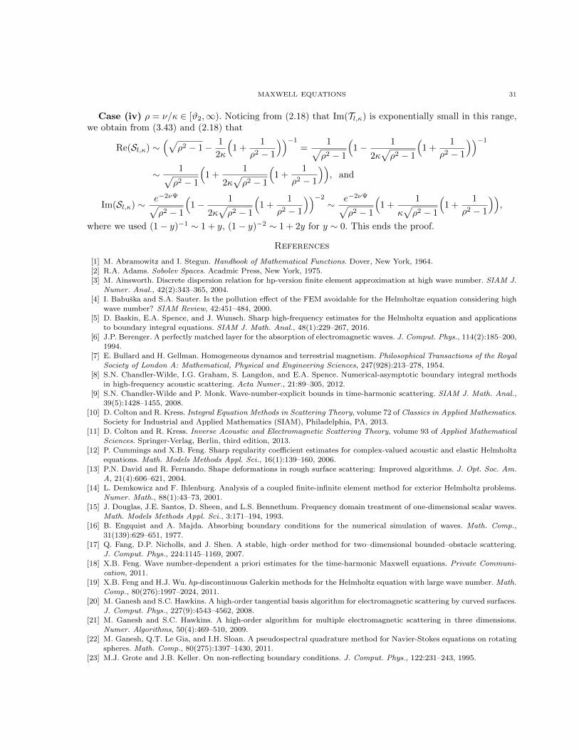
MAXWELL EQUATIONS 31
Case (iv) ρ = ν/κ ∈ [ϑ2,∞). Noticing from (2.18) that Im(Tl,κ) is exponentially small in this range,we obtain from (3.43) and (2.18) that
Re(Sl,κ) ∼(√
ρ2 − 1− 1
2κ
(1 +
1
ρ2 − 1
))−1
=1√ρ2 − 1
(1− 1
2κ√ρ2 − 1
(1 +
1
ρ2 − 1
))−1
∼ 1√ρ2 − 1
(1 +
1
2κ√ρ2 − 1
(1 +
1
ρ2 − 1
)), and
Im(Sl,κ) ∼ e−2νΨ√ρ2 − 1
(1− 1
2κ√ρ2 − 1
(1 +
1
ρ2 − 1
))−2
∼ e−2νΨ√ρ2 − 1
(1 +
1
κ√ρ2 − 1
(1 +
1
ρ2 − 1
)),
where we used (1− y)−1 ∼ 1 + y, (1− y)−2 ∼ 1 + 2y for y ∼ 0. This ends the proof.
References
[1] M. Abramowitz and I. Stegun. Handbook of Mathematical Functions. Dover, New York, 1964.
[2] R.A. Adams. Sobolev Spaces. Acadmic Press, New York, 1975.
[3] M. Ainsworth. Discrete dispersion relation for hp-version finite element approximation at high wave number. SIAM J.Numer. Anal., 42(2):343–365, 2004.
[4] I. Babuska and S.A. Sauter. Is the pollution effect of the FEM avoidable for the Helmholtze equation considering highwave number? SIAM Review, 42:451–484, 2000.
[5] D. Baskin, E.A. Spence, and J. Wunsch. Sharp high-frequency estimates for the Helmholtz equation and applications
to boundary integral equations. SIAM J. Math. Anal., 48(1):229–267, 2016.[6] J.P. Berenger. A perfectly matched layer for the absorption of electromagnetic waves. J. Comput. Phys., 114(2):185–200,
1994.
[7] E. Bullard and H. Gellman. Homogeneous dynamos and terrestrial magnetism. Philosophical Transactions of the RoyalSociety of London A: Mathematical, Physical and Engineering Sciences, 247(928):213–278, 1954.
[8] S.N. Chandler-Wilde, I.G. Graham, S. Langdon, and E.A. Spence. Numerical-asymptotic boundary integral methods
in high-frequency acoustic scattering. Acta Numer., 21:89–305, 2012.[9] S.N. Chandler-Wilde and P. Monk. Wave-number-explicit bounds in time-harmonic scattering. SIAM J. Math. Anal.,
39(5):1428–1455, 2008.
[10] D. Colton and R. Kress. Integral Equation Methods in Scattering Theory, volume 72 of Classics in Applied Mathematics.Society for Industrial and Applied Mathematics (SIAM), Philadelphia, PA, 2013.
[11] D. Colton and R. Kress. Inverse Acoustic and Electromagnetic Scattering Theory, volume 93 of Applied MathematicalSciences. Springer-Verlag, Berlin, third edition, 2013.
[12] P. Cummings and X.B. Feng. Sharp regularity coefficient estimates for complex-valued acoustic and elastic Helmholtz
equations. Math. Models Methods Appl. Sci., 16(1):139–160, 2006.[13] P.N. David and R. Fernando. Shape deformations in rough surface scattering: Improved algorithms. J. Opt. Soc. Am.
A, 21(4):606–621, 2004.
[14] L. Demkowicz and F. Ihlenburg. Analysis of a coupled finite-infinite element method for exterior Helmholtz problems.Numer. Math., 88(1):43–73, 2001.
[15] J. Douglas, J.E. Santos, D. Sheen, and L.S. Bennethum. Frequency domain treatment of one-dimensional scalar waves.
Math. Models Methods Appl. Sci., 3:171–194, 1993.[16] B. Engquist and A. Majda. Absorbing boundary conditions for the numerical simulation of waves. Math. Comp.,
31(139):629–651, 1977.
[17] Q. Fang, D.P. Nicholls, and J. Shen. A stable, high–order method for two–dimensional bounded–obstacle scattering.J. Comput. Phys., 224:1145–1169, 2007.
[18] X.B. Feng. Wave number-dependent a priori estimates for the time-harmonic Maxwell equations. Private Communi-
cation, 2011.[19] X.B. Feng and H.J. Wu. hp-discontinuous Galerkin methods for the Helmholtz equation with large wave number. Math.
Comp., 80(276):1997–2024, 2011.[20] M. Ganesh and S.C. Hawkins. A high-order tangential basis algorithm for electromagnetic scattering by curved surfaces.
J. Comput. Phys., 227(9):4543–4562, 2008.[21] M. Ganesh and S.C. Hawkins. A high-order algorithm for multiple electromagnetic scattering in three dimensions.
Numer. Algorithms, 50(4):469–510, 2009.[22] M. Ganesh, Q.T. Le Gia, and I.H. Sloan. A pseudospectral quadrature method for Navier-Stokes equations on rotating
spheres. Math. Comp., 80(275):1397–1430, 2011.[23] M.J. Grote and J.B. Keller. On non-reflecting boundary conditions. J. Comput. Phys., 122:231–243, 1995.
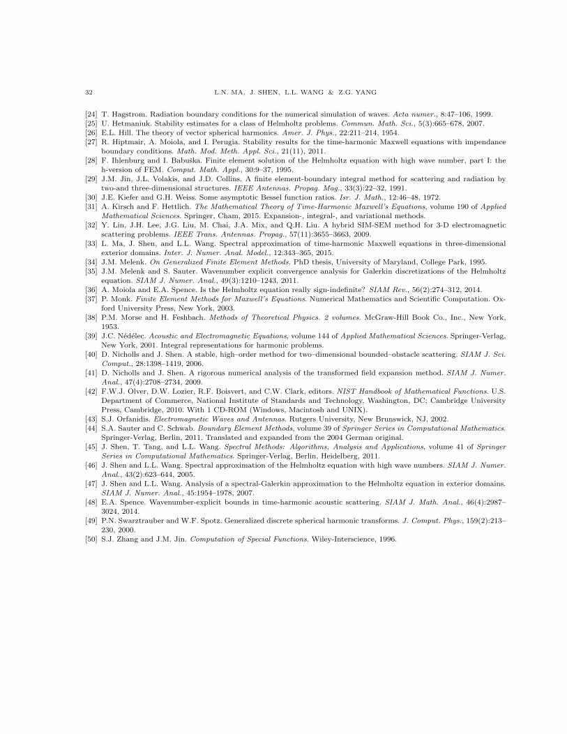
32 L.N. MA, J. SHEN, L.L. WANG & Z.G. YANG
[24] T. Hagstrom. Radiation boundary conditions for the numerical simulation of waves. Acta numer., 8:47–106, 1999.
[25] U. Hetmaniuk. Stability estimates for a class of Helmholtz problems. Commun. Math. Sci., 5(3):665–678, 2007.
[26] E.L. Hill. The theory of vector spherical harmonics. Amer. J. Phys., 22:211–214, 1954.[27] R. Hiptmair, A. Moiola, and I. Perugia. Stability results for the time-harmonic Maxwell equations with impendance
boundary conditions. Math. Mod. Meth. Appl. Sci., 21(11), 2011.
[28] F. Ihlenburg and I. Babuska. Finite element solution of the Helmholtz equation with high wave number, part I: theh-version of FEM. Comput. Math. Appl., 30:9–37, 1995.
[29] J.M. Jin, J.L. Volakis, and J.D. Collins. A finite element-boundary integral method for scattering and radiation by
two-and three-dimensional structures. IEEE Antennas. Propag. Mag., 33(3):22–32, 1991.[30] J.E. Kiefer and G.H. Weiss. Some asymptotic Bessel function ratios. Isr. J. Math., 12:46–48, 1972.
[31] A. Kirsch and F. Hettlich. The Mathematical Theory of Time-Harmonic Maxwell’s Equations, volume 190 of Applied
Mathematical Sciences. Springer, Cham, 2015. Expansion-, integral-, and variational methods.[32] Y. Lin, J.H. Lee, J.G. Liu, M. Chai, J.A. Mix, and Q.H. Liu. A hybrid SIM-SEM method for 3-D electromagnetic
scattering problems. IEEE Trans. Antennas. Propag., 57(11):3655–3663, 2009.[33] L. Ma, J. Shen, and L.L. Wang. Spectral approximation of time-harmonic Maxwell equations in three-dimensional
exterior domains. Inter. J. Numer. Anal. Model., 12:343–365, 2015.
[34] J.M. Melenk. On Generalized Finite Element Methods. PhD thesis, University of Maryland, College Park, 1995.[35] J.M. Melenk and S. Sauter. Wavenumber explicit convergence analysis for Galerkin discretizations of the Helmholtz
equation. SIAM J. Numer. Anal., 49(3):1210–1243, 2011.
[36] A. Moiola and E.A. Spence. Is the Helmholtz equation really sign-indefinite? SIAM Rev., 56(2):274–312, 2014.[37] P. Monk. Finite Element Methods for Maxwell’s Equations. Numerical Mathematics and Scientific Computation. Ox-
ford University Press, New York, 2003.
[38] P.M. Morse and H. Feshbach. Methods of Theoretical Physics. 2 volumes. McGraw-Hill Book Co., Inc., New York,1953.
[39] J.C. Nedelec. Acoustic and Electromagnetic Equations, volume 144 of Applied Mathematical Sciences. Springer-Verlag,
New York, 2001. Integral representations for harmonic problems.[40] D. Nicholls and J. Shen. A stable, high–order method for two–dimensional bounded–obstacle scattering. SIAM J. Sci.
Comput., 28:1398–1419, 2006.[41] D. Nicholls and J. Shen. A rigorous numerical analysis of the transformed field expansion method. SIAM J. Numer.
Anal., 47(4):2708–2734, 2009.
[42] F.W.J. Olver, D.W. Lozier, R.F. Boisvert, and C.W. Clark, editors. NIST Handbook of Mathematical Functions. U.S.Department of Commerce, National Institute of Standards and Technology, Washington, DC; Cambridge University
Press, Cambridge, 2010. With 1 CD-ROM (Windows, Macintosh and UNIX).
[43] S.J. Orfanidis. Electromagnetic Waves and Antennas. Rutgers University, New Brunswick, NJ, 2002.[44] S.A. Sauter and C. Schwab. Boundary Element Methods, volume 39 of Springer Series in Computational Mathematics.
Springer-Verlag, Berlin, 2011. Translated and expanded from the 2004 German original.
[45] J. Shen, T. Tang, and L.L. Wang. Spectral Methods: Algorithms, Analysis and Applications, volume 41 of SpringerSeries in Computational Mathematics. Springer-Verlag, Berlin, Heidelberg, 2011.
[46] J. Shen and L.L. Wang. Spectral approximation of the Helmholtz equation with high wave numbers. SIAM J. Numer.
Anal., 43(2):623–644, 2005.[47] J. Shen and L.L. Wang. Analysis of a spectral-Galerkin approximation to the Helmholtz equation in exterior domains.
SIAM J. Numer. Anal., 45:1954–1978, 2007.[48] E.A. Spence. Wavenumber-explicit bounds in time-harmonic acoustic scattering. SIAM J. Math. Anal., 46(4):2987–
3024, 2014.
[49] P.N. Swarztrauber and W.F. Spotz. Generalized discrete spherical harmonic transforms. J. Comput. Phys., 159(2):213–230, 2000.
[50] S.J. Zhang and J.M. Jin. Computation of Special Functions. Wiley-Interscience, 1996.