Wall pressure spectra on a DU96-W-180 pro le from low to

Wall pressure spectra on a DU96-W-180 profile from

low to pre-stall angles of attack

Alexandre Suryadi∗† and Michaela Herr∗‡

German Aerospace Center (DLR), D-38108 Braunschweig, Germany

In an effort to characterize noise induced by separated turbulent boundary layers, sur-face pressure fluctuations on a DU96-W-180 airfoil were measured using miniature pressuresensors. Because of limitation in amplifier channels and available sensors, a rearrangeableconfiguration of sensors was applied. Chordwise distributions of the surface pressure wereobtained for aerodynamic angles of attack of −0.8◦ ≤ α ≤ 10.3◦ and at three Reynoldsnumbers (0.8, 1.0, and 1.2) ×106. The boundary layer profile at 1%c behind the trailingedge was measured using constant temperature anemometry. The boundary layer thick-ness compares well with that simulated using XFOIL for α ≤ 7.8◦. Within the limits ofthe simulation, other relevant boundary layer properties from XFOIL were used to calcu-late the surface pressure spectrum predicted from published empirical models for zero andnon-zero pressure gradient turbulent boundary layers. Finally, a modified Blake-TNO semi-empirical model was used to predict the surface pressure spectrum near the trailing edgefor separated flow. The modification is introduced to the so called ‘moving axis spectrum’and the chord-normal correlation length scale. It is found that in the low frequency range,the modified semi-empirical model fits well with the measured surface pressure spectrumof a separated turbulent boundary layer.

Nomenclature

a Speed of sound, m·s−1

c Chord length, mcl Coefficient of lift, -c1, c2 Modification parameters to Φm, -ke Eddy containing wavenumber, 0.7468/Ly, m−1

kx Chordwise wavenumber, 2π/Lx, rad·m−1

kz Spanwise wavenumber, 2π/Lz, rad·m−1

L Wetted span, m`mix Mixing length, 0.085δ tanh(κy/0.085δ), mLx Chordwise correlation length scale, mLy Chord-normal correlation length scale, mLz Spanwise correlation length scale, mR Radial distance from a sound source, mRe Reynolds number, -RT Ratio of the outer and inner boundary layer time scales, uτδ/ν

√Cf/2

U(y) Time averaged velocity component, m·s−1

U∞ Freestream velocity, m·s−1

Uc(y) Convective velocity, m·s−1

Ue Turbulent boundary layer edge velocity, m·s−1

u, v, w Instantaneous velocity components in the order x, y, z, m·s−1

∗Research Engineer, Institute of Aerodynamics and Flow Technology, Technical Acoustics; Lilienthalplatz 7, 38108 Braun-schweig;†[email protected]‡[email protected]

1 of 18

American Institute of Aeronautics and Astronautics

u′, v′, w′ Fluctuating velocity components in the order x, y, z, m·s−1

uτ Friction velocity, m·s−1

S(ω) Far-field noise power spectral density, Pa2·sx, y, z Chordwise, chord-normal, and spanwise spatial directionsα Aerodynamic angle of attack, ◦

βc Clauser parameter, θ/τwdP/dx, -δ Boundary layer thickness, mδ∗ Boundary layer displacement thickness, mθ Boundary layer momentum thickness, mκ von Karman constant, 0.41ν Kinematic viscosity, m2·s−1

ρ Density, kg·m−3

Φm Moving axis spectrum, sΦpp Surface pressure power spectral density, Pa2·sΦvv Vertical velocity wavenumber power spectral density, -τw Wall shear stress, Paτmax Maximum shear stress, Paω Angular frequency, 2πf , rad·s−1

AbbreviationsAPG Adverse Pressure GradientAWB Acoustic Wind Tunnel BraunschweigCFAS Catlett, Forest, Anderson, and Stewart5

LWT Laminar Wind TunnelRRM Rozenberg, Robert, and Moreau11

SR Schule and Rossignol14

ZPG Zero Pressure Gradient

I. Introduction

Wind turbines in Germany are located near residential areas. To limit the acoustic effect of wind turbineinstallations to nearby populations, noise compliances are followed strictly. Because of atmospheric gust, theeffective angle of attack of a wind turbine blade section can increase. Above a critical angle the boundarylayer separates and it provide an additional component to the far-field noise. The mechanism of the gen-eration of trailing edge noise and its prediction under attached boundary layer condition has been studiedwell.3,4, 9 An effort to improve the prediction of far-field noise for separated flow was reported in Schuleand Rossignol14 by modifying the modeled surface pressure power spectral density that was described inParchen.10 While the result looks promising there is a lack of validation data on the behavior of the modelat low frequency, mainly due to the limited resolution of available acoustic measurements techniques, suchas elliptical-mirror directional microphone or microphone array systems. To bridge this gap, the surfacepressure fluctuations were measured using miniature pressure sensors from Kulite semiconductors. Spanwiseand chordwise distributions of surface pressure fluctuations were obtained for aerodynamic angles of attack−0.8◦ ≤ α ≤ 10.3◦ and at three Reynolds numbers Re=(0.8, 1.0, and 1.2) ×106 in the Acoustic Wind TunnelBraunschweig (AWB).

Under the assumptions that the flow is incompressible, the noise is solely produced by hydrodynamicsurface pressure fluctuations, and the surface pressure from two sides contribute to the total far-field noiseindependently. The far-field noise on each side, S(ω), can be expressed as3

S(ω) =1

4πR2

(ωL

a

)∫ ∞−∞

Φpp(kx, 0, ω)|kx|[1− ω/(akx)]

dkx (1)

where R is the radial distance of the source to the observer, L is the wetted span, Φpp is the surface pressurespectrum, a is the speed of sound at sea level, ω is the angular frequency, and kx is the chordwise wavenumber.The surface pressure power spectral density Φpp(kx, ky, ω) can be modeled in terms of the air density ρ, themean shear dU/dy, the correlation length scale Ly, the turbulent stress v′v′, the turbulent spectra Φvv, anda modeled eddy decay spectrum, named ‘moving axis spectrum’ Φm that depends on the local convective

2 of 18


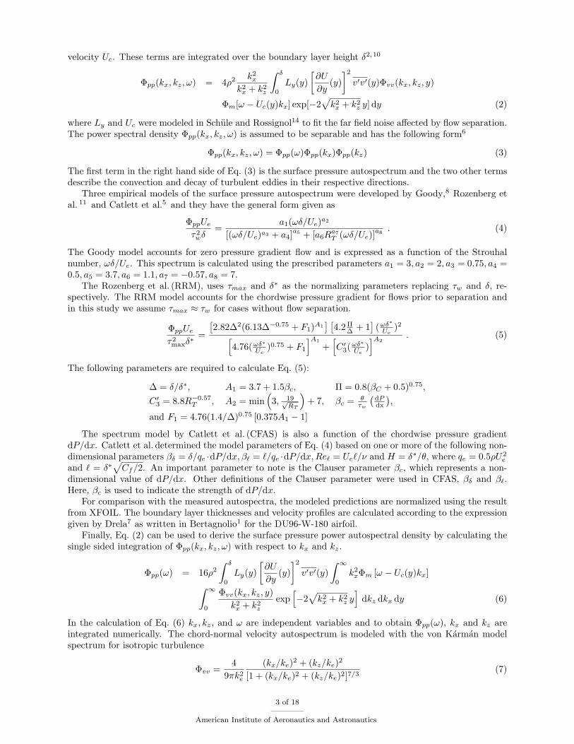
velocity Uc. These terms are integrated over the boundary layer height δ2,10

Φpp(kx, kz, ω) = 4ρ2 k2x

k2x + k2

z

∫ δ

0

Ly(y)[∂U

∂y(y)]2

v′v′(y)Φvv(kx, kz, y)

Φm[ω − Uc(y)kx] exp[−2√k2x + k2

z y] dy (2)

where Ly and Uc were modeled in Schule and Rossignol14 to fit the far field noise affected by flow separation.The power spectral density Φpp(kx, kz, ω) is assumed to be separable and has the following form6

Φpp(kx, kz, ω) = Φpp(ω)Φpp(kx)Φpp(kz) (3)

The first term in the right hand side of Eq. (3) is the surface pressure autospectrum and the two other termsdescribe the convection and decay of turbulent eddies in their respective directions.

Three empirical models of the surface pressure autospectrum were developed by Goody,8 Rozenberg etal. 11 and Catlett et al.5 and they have the general form given as

ΦppUeτ2wδ

=a1(ωδ/Ue)a2

[(ωδ/Ue)a3 + a4]a5 + [a6Ra7T (ωδ/Ue)]

a8 . (4)

The Goody model accounts for zero pressure gradient flow and is expressed as a function of the Strouhalnumber, ωδ/Ue. This spectrum is calculated using the prescribed parameters a1 = 3, a2 = 2, a3 = 0.75, a4 =0.5, a5 = 3.7, a6 = 1.1, a7 = −0.57, a8 = 7.

The Rozenberg et al. (RRM), uses τmax and δ∗ as the normalizing parameters replacing τw and δ, re-spectively. The RRM model accounts for the chordwise pressure gradient for flows prior to separation andin this study we assume τmax ≈ τw for cases without flow separation.

ΦppUeτ2maxδ

∗ =

[2.82∆2(6.13∆−0.75 + F1)A1

] [4.2 Π

∆ + 1]

(ωδ∗

Ue)2[

4.76(ωδ∗Ue)0.75 + F1

]A1

+[C ′3(ωδ∗Ue

)]A2

. (5)

The following parameters are required to calculate Eq. (5):

∆ = δ/δ∗, A1 = 3.7 + 1.5βc, Π = 0.8(βC + 0.5)0.75,C ′3 = 8.8R−0.57

T , A2 = min(

3, 19√RT

)+ 7, βc = θ

τw

(dPdx

),

and F1 = 4.76(1.4/∆)0.75 [0.375A1 − 1]

The spectrum model by Catlett et al. (CFAS) is also a function of the chordwise pressure gradientdP/dx. Catlett et al. determined the model parameters of Eq. (4) based on one or more of the following non-dimensional parameters βδ = δ/qe ·dP/dx, β` = `/qe ·dP/dx,Re` = Ue`/ν and H = δ∗/θ, where qe = 0.5ρU2

e

and ` = δ∗√Cf/2. An important parameter to note is the Clauser parameter βc, which represents a non-

dimensional value of dP/dx. Other definitions of the Clauser parameter were used in CFAS, βδ and β`.Here, βc is used to indicate the strength of dP/dx.

For comparison with the measured autospectra, the modeled predictions are normalized using the resultfrom XFOIL. The boundary layer thicknesses and velocity profiles are calculated according to the expressiongiven by Drela7 as written in Bertagnolio1 for the DU96-W-180 airfoil.

Finally, Eq. (2) can be used to derive the surface pressure power autospectral density by calculating thesingle sided integration of Φpp(kx, kz, ω) with respect to kx and kz.

Φpp(ω) = 16ρ2

∫ δ

0

Ly(y)[∂U

∂y(y)]2

v′v′(y)∫ ∞

0

k2xΦm [ω − Uc(y)kx]∫ ∞

0

Φvv(kx, kz, y)k2x + k2

z

exp[−2√k2x + k2

z y]

dkz dkx dy (6)

In the calculation of Eq. (6) kx, kz, and ω are independent variables and to obtain Φpp(ω), kx and kz areintegrated numerically. The chord-normal velocity autospectrum is modeled with the von Karman modelspectrum for isotropic turbulence

Φvv =4

9πk2e

(kx/ke)2 + (kz/ke)2

[1 + (kx/ke)2 + (kz/ke)2]7/3(7)

3 of 18


Figure 1. Open test section of the Acoustic Wind Tunnel Braunschweig (AWB). The airfoil and the airfoil relativecoordinate system is illustrated.

with ke = 0.7468/Ly and Ly = `mix/κ, where `mix = 0.085δ tanh(κy/0.085δ).1 The moving axis spectrumis

Φm(ω − Uc(y)kx) =1

αGauss√π

exp[− (ω − Uc(y)kx)2

α2Gauss

](8)

with αGauss = 0.05Uc(y)/Ly(y) and Uc(y) will be defined in Sec. III.F.

II. Experimental setup

Measurements were performed in the anechoic open section of the AWB as shown in figure 1. The windtunnel’s nozzle dimension is 800 mm wide and 1200 mm high with maximum exit velocity of 65 m/s. Theturbulence level is 0.3% at the nozzle exit. The airfoil relative coordinate system is given as x chordwise, zspanwise and y chord-normal direction with x = 0 at the leading edge and z = 0 at the mid-span.

The DU96-W-180 has a span of 800 mm and chord of 300 mm and it is equipped with 62 static pressuretaps on both suction and pressure sides. The trailing edge thickness is 0.5 mm. A panel on each side of themodel is removable to equip the model with sensors. The panel is 180 mm × 100 mm and when placed onthe model the panel adhered to the surface curvature of the model. The wind tunnel model with removablepanels is shown in figure 2.

II.A. Surface pressure measurement

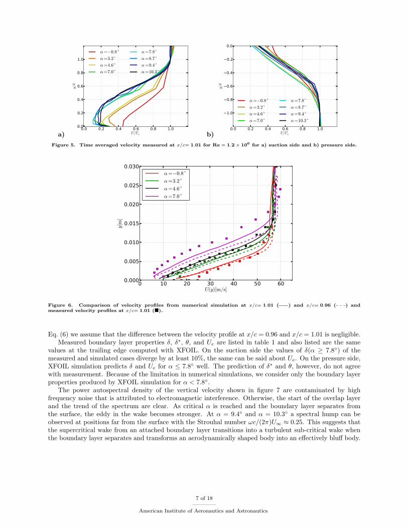
Eight piezo-resistive pressure transducers was used with one failing on the last day of the measurementcampaign. Major dimensions and the principal setup are documented in figure 3. The mounting of thesesensors was designed to be removable, rearrangeable, and can reproduce results easily. To do so, a 12 mmwide channel was milled on the underside of the removable panels and several sensor stations with �=3 mmdiameter and 0.5 mm depth were drilled on them. Pinholes of � =0.5 mm were drilled at the center of thesestations. Silicone was molded on the station to fit the sensor’s head and create a sealant, while maintaininga clear air passage for the pinhole. To keep the sensors in place mechanical holders in the shape of rods withfoam attached on one end were glued on the panels.

The model’s lift coefficient were measured in the Laminar Wind Tunnel (LWT) of the Institute of Aero-dynamics and Gas Dynamics at the University of Stuttgart and again in the AWB. A zig-zag boundary layertrip (0.205 mm high) was placed at 5% chord from the leading edge on the suction side and another one(0.4 mm high) at 10% chord on the pressure side. The lift coefficient distribution cl for a range of α and

4 of 18


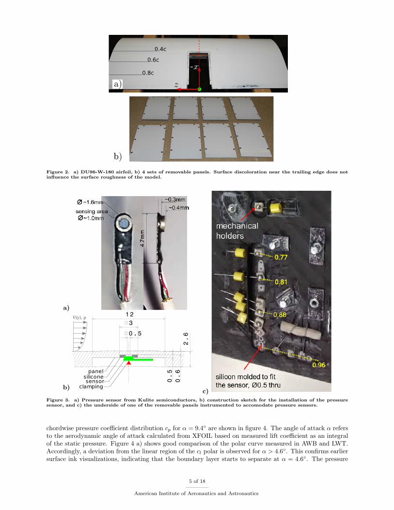
Figure 2. a) DU96-W-180 airfoil, b) 4 sets of removable panels. Surface discoloration near the trailing edge does notinfluence the surface roughness of the model.

a)

b)

siliconesensor

clamping

panel

U(y), p

c)Figure 3. a) Pressure sensor from Kulite semiconductors, b) construction sketch for the installation of the pressuresensor, and c) the underside of one of the removable panels instrumented to accomodate pressure sensors.

chordwise pressure coefficient distribution cp for α = 9.4◦ are shown in figure 4. The angle of attack α refersto the aerodynamic angle of attack calculated from XFOIL based on measured lift coefficient as an integralof the static pressure. Figure 4 a) shows good comparison of the polar curve measured in AWB and LWT.Accordingly, a deviation from the linear region of the cl polar is observed for α > 4.6◦. This confirms earliersurface ink visualizations, indicating that the boundary layer starts to separate at α = 4.6◦. The pressure

5 of 18


a)

4 2 0 2 4 6 8 10 12α [deg]

0.0

0.2

0.4

0.6

0.8

1.0Cl

AWB

LWT

linear region

b)

0.0 0.2 0.4 0.6 0.8 1.0x/c

−3.0

−2.5

−2.0

−1.5

−1.0

−0.5

0.0

0.5

1.0

1.5

Cp

DU96-W-180

removable panel

AWB

XFOIL

Figure 4. a) lift coefficient and b) pressure coefficient at α = 9.4◦ of the DU96-W-180 airfoil. The airfoil’s profile andremovable panel are shown as gray colored lines and the range of sensor locations on the suction side is shown in red.

coefficient distributions at α = 9.4◦ measured in AWB and simulated in XFOIL is shown in figure 4 b)showing good agreement, except for x/c > 0.6, where the effect of three-dimensionality from flow separationis strong. Also shown in figure 4 b) is the airfoil’s profile and the location of the removable panel in thickgray line. The range of sensor location is shown in red.

An overall number of 8 sensor positions was finally realized with this modular setup. The full measurementmatrix included measurements with 5 different sensor arrangements, which were operated at 8 angles of attackα = (−0.8◦, 3.2◦, 4.6◦, 7.0◦, 7.8◦, 8.7◦, 9.4◦, and 10.3◦) and 3 Reynolds numbers Re = (0.8, 1.0, 1.2) × 106.Only surface pressure data for chordwise sensor distributions are shown for Re = 1.2 × 106 to keep thiscommunication brief.

II.B. Velocity measurement

The mean velocity profile at x/c = 1.01 was measured using constant temperature anemometry, applyingboth single-wire and cross-wire probes for the same α and Re = 1.2× 106.

Computational fluid dynamics (CFD) simulations using the DLR TAU code along with the Reynoldsstress turbulence model were additionally performed to evaluate the velocity profiles at the given sensor po-sitions. It was found that the integrated results from CFD simulation is similar to that of XFOIL simulation.

III. Results

III.A. Velocity measurement

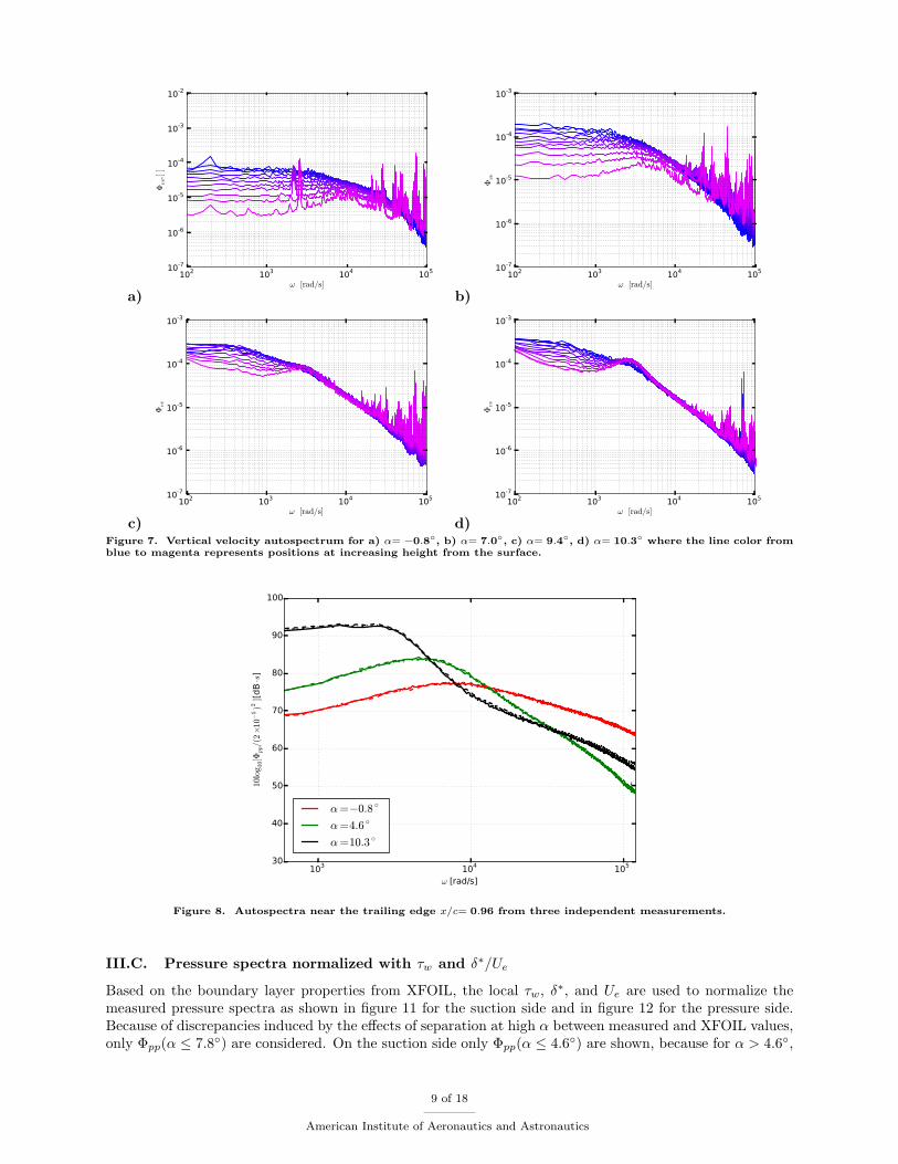
The distributions of U(y;x/c = 1.01) are shown in figure 5 for both suction and pressure sides normalizedby δ and Ue. These profiles were measured using single wire probes; therefore, figure 5 shows the magnitudeof the local velocity. The result of numerical simulations at x/c = 0.96 and x/c = 1.01 and measurementsat x/c = 1.01 are compared in figure 6. For α ≤ 4.6◦ the velocity profiles from numerical simulations agreewell with the measured profiles, but at α = 7.0◦ this agreement starts to decline. This is mainly because ofthe two-dimensionality of the flow is kept in the numerical simulation while in wind tunnel conditions flowseparation causes a break in the symmetry of the flow. Based on figure 6, for the prediction of Φpp(ω) using

6 of 18


a)0.0 0.2 0.4 0.6 0.8 1.0

U/Ue

0.0

0.2

0.4

0.6

0.8

1.0

y/δ

α=−0.8 ◦

α=3.2 ◦

α=4.6 ◦

α=7.0 ◦

α=7.8 ◦

α=8.7 ◦

α=9.4 ◦

α=10.3 ◦

b)0.0 0.2 0.4 0.6 0.8 1.0

U/Ue

1.0

0.8

0.6

0.4

0.2

0.0

y/δ

α=−0.8 ◦

α=3.2 ◦

α=4.6 ◦

α=7.0 ◦

α=7.8 ◦

α=8.7 ◦

α=9.4 ◦

α=10.3 ◦

Figure 5. Time averaged velocity measured at x/c= 1.01 for Re = 1.2× 106 for a) suction side and b) pressure side.

0 10 20 30 40 50 60U(y)[m/s]

0.000

0.005

0.010

0.015

0.020

0.025

0.030

y[m

]

α=−0.8 ◦

α=3.2 ◦

α=4.6 ◦

α=7.0 ◦

Figure 6. Comparison of velocity profiles from numerical simulation at x/c= 1.01 ( ) and x/c= 0.96 ( ) andmeasured velocity profiles at x/c= 1.01 (�).

Eq. (6) we assume that the difference between the velocity profile at x/c = 0.96 and x/c = 1.01 is negligible.Measured boundary layer properties δ, δ∗, θ, and Ue are listed in table 1 and also listed are the same

values at the trailing edge computed with XFOIL. On the suction side the values of δ(α ≥ 7.8◦) of themeasured and simulated cases diverge by at least 10%, the same can be said about Ue. On the pressure side,XFOIL simulation predicts δ and Ue for α ≤ 7.8◦ well. The prediction of δ∗ and θ, however, do not agreewith measurement. Because of the limitation in numerical simulations, we consider only the boundary layerproperties produced by XFOIL simulation for α < 7.8◦.

The power autospectral density of the vertical velocity shown in figure 7 are contaminated by highfrequency noise that is attributed to electromagnetic interference. Otherwise, the start of the overlap layerand the trend of the spectrum are clear. As critical α is reached and the boundary layer separates fromthe surface, the eddy in the wake becomes stronger. At α = 9.4◦ and α = 10.3◦ a spectral hump can beobserved at positions far from the surface with the Strouhal number ωc/(2π)U∞ ≈ 0.25. This suggests thatthe supercritical wake from an attached boundary layer transitions into a turbulent sub-critical wake whenthe boundary layer separates and transforms an aerodynamically shaped body into an effectively bluff body.

7 of 18


Table 1. Boundary layer properties of the DU96-W-180 measured at x/c= 1.01 and simulated at x/c= 1.00. δ, δ∗, θ aregiven in mm and Ue is given in m/s.

Suction sideAWB XFOIL

α[◦] δ δ∗ θ Ue δ δ∗ θ Ue

-0.8 12 2.61 1.61 54.83 12 4 2 53.143.2 16 5.21 2.50 56.97 15 6 2 54.294.6 16 5.77 2.55 56.71 16 7 2 55.057.0 20 9.37 3.16 57.61 19 10 2 57.327.8 22 10.51 3.39 59.63 20 12 2 58.158.7 26 12.86 3.91 63.38 22 14 2 59.089.4 34 16.40 5.09 64.94 24 16 2 59.77

10.3 40 19.39 6.32 66.71 27 19 3 60.71Pressure side

AWB XFOILα[◦] δ δ∗ θ Ue δ δ∗ θ Ue

-0.8 10 2.37 1.45 54.35 9 2.1 1.3 53.143.2 8 1.77 1.05 56 7 1.4 0.9 54.294.6 7 2.16 1.08 54.62 7 1.2 0.8 55.057.0 7 1.56 0.86 57.76 6 0.9 0.6 57.327.8 6 1.88 0.9 57.31 5 0.8 0.6 58.158.7 7 1.84 0.91 62.44 5 0.8 0.5 59.089.4 7 1.59 0.85 63.66 5 0.7 0.5 59.77

10.3 7 1.7 0.88 65.39 4 0.7 0.5 60.71

III.B. Pressure spectra of the turbulent boundary layer with non zero pressure gradient

Figure 8 shows Φpp for the position closest to the trailing edge x/c = 0.96 from 3 independent measurements.The spectra fit each other very well showing that the installation of the sensors can produce repeatable results.The maximum of Φpp increases proportionally with α and the peak frequency shifts to the lower frequencies.An increase of approximately 15 dB is shown in figure 8 between α = −0.8◦ and α = 10.3◦. The roll-offstarts earlier and the spectrum decays more rapidly with increasing α.

Tables 2 and 3 list the Rotta-Clauser parameter βc that is the non-dimensional representation of thepressure gradient. These parameters are calculated using both measurement data (dP/dx) and XFOILsimulation (θ and τw). Only βc values where the boundary layer remains attached, i.e. has a finite τw, arelisted.

Figure 9 shows Φpp(ω, x/c) for each α. With higher α and stronger adverse pressure gradient, the spectraldecay becomes more rapid and starts earlier. Particularly, a frequency shift towards lower frequencies withgrowing δ(x/c) is observable. For −0.8◦ ≤ α ≤ 4.6◦ Φpp(ω, x/c) is distinct. This distinction becomes lessclear with higher α and with positions x/c sufficiently close to the trailing edge. For example, at α = 10.3◦

Φpp(ω, x/c) collapse to almost a single spectrum. Figure 9 suggests that for separated turbulent boundarylayers the pressure spectra can be treated as a homogeneous flow in the chordwise direction.

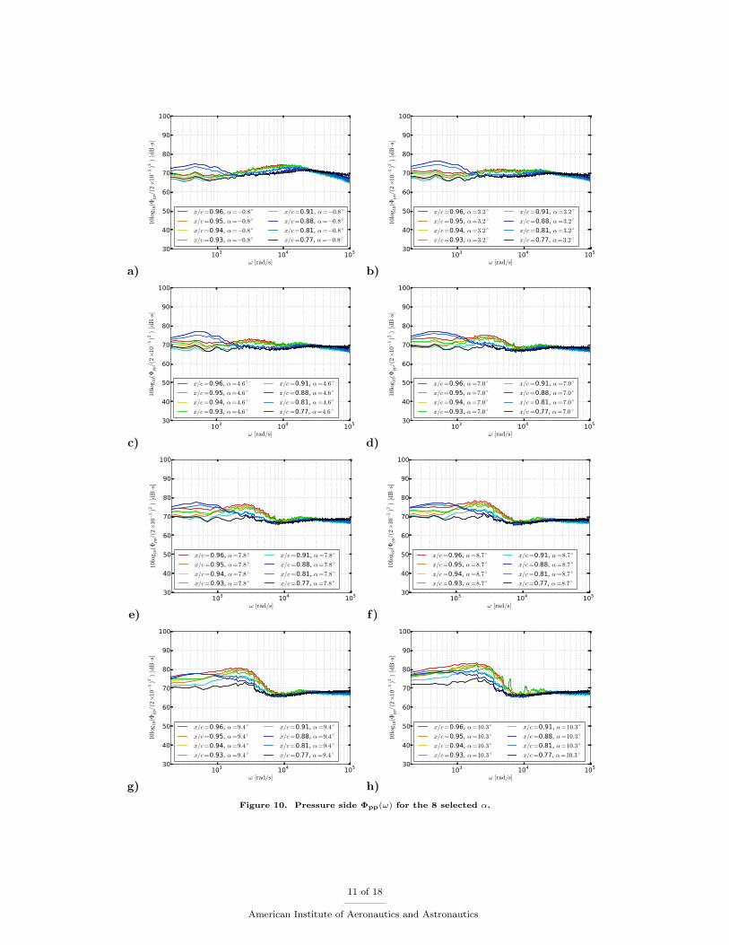
The pressure spectra Φpp(ω, x/c) on the pressure side as shown in figure 10 shows a flattening of thespectra for the high frequency region as an effect of favorable pressure gradient. Two sensors at x/c = 0.88and 0.81 show a discrepancy in the low frequency region, which suggest that they were misaligned duringthe measurement. A single peak in the spectra is shown to develop with increasing α and with downstreamchordwise positions. This peak appears at the same frequencies as the respective spectral maxima in thesuction side Φpp. The characteristics of the pressure fluctuation spectra can be better understood afternon-dimensionalization of Φpp using boundary layer values.

8 of 18


a)

102 103 104 105

ω [rad/s]

10-7

10-6

10-5

10-4

10-3

10-2

Φvv,[

]

b)

102 103 104 105

ω [rad/s]

10-7

10-6

10-5

10-4

10-3

Φvv

c)

102 103 104 105

ω [rad/s]

10-7

10-6

10-5

10-4

10-3

Φvv

d)

102 103 104 105

ω [rad/s]

10-7

10-6

10-5

10-4

10-3

Φvv

Figure 7. Vertical velocity autospectrum for a) α= −0.8◦, b) α= 7.0◦, c) α= 9.4◦, d) α= 10.3◦ where the line color fromblue to magenta represents positions at increasing height from the surface.

103 104 105

ω [rad/s]

30

40

50

60

70

80

90

100

10lo

g 10[Φpp/(

2×1

0−5)2

][dB·s

]

α=−0.8 ◦

α=4.6 ◦

α=10.3 ◦

Figure 8. Autospectra near the trailing edge x/c= 0.96 from three independent measurements.

III.C. Pressure spectra normalized with τw and δ∗/Ue

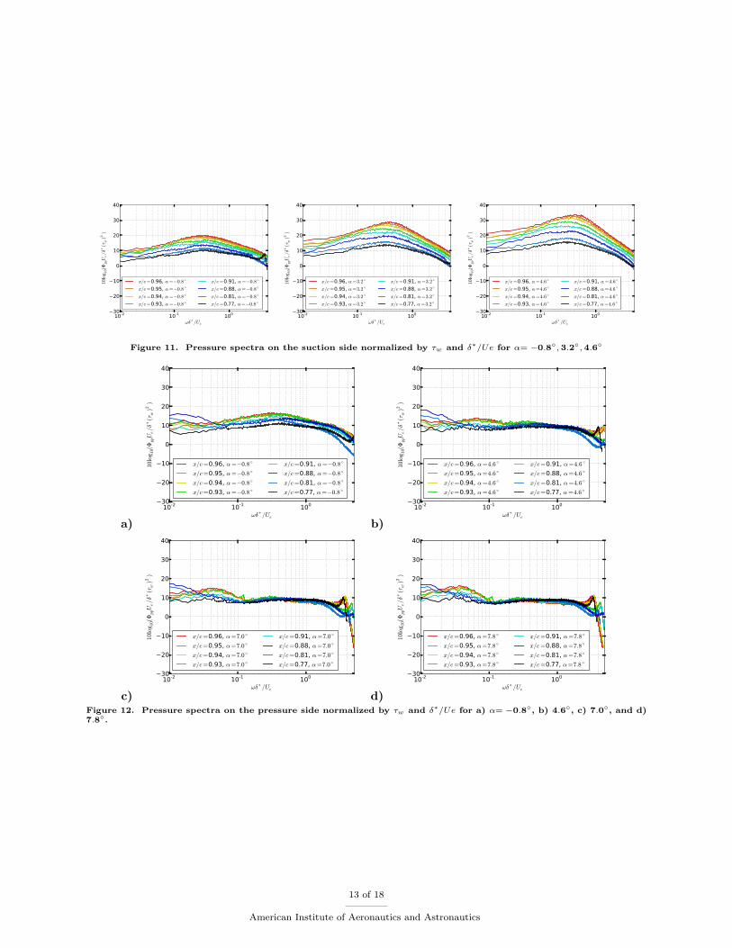
Based on the boundary layer properties from XFOIL, the local τw, δ∗, and Ue are used to normalize themeasured pressure spectra as shown in figure 11 for the suction side and in figure 12 for the pressure side.Because of discrepancies induced by the effects of separation at high α between measured and XFOIL values,only Φpp(α ≤ 7.8◦) are considered. On the suction side only Φpp(α ≤ 4.6◦) are shown, because for α > 4.6◦,

9 of 18


a)103 104 105

ω [rad/s]

30

40

50

60

70

80

90

100

10lo

g 10(

Φpp/(

2×1

0−

5)2

)[d

B·s]

x/c=0.96, α=−0.8 ◦

x/c=0.95, α=−0.8 ◦

x/c=0.94, α=−0.8 ◦

x/c=0.93, α=−0.8 ◦

x/c=0.91, α=−0.8 ◦

x/c=0.88, α=−0.8 ◦

x/c=0.81, α=−0.8 ◦

x/c=0.77, α=−0.8 ◦

b)103 104 105

ω [rad/s]

30

40

50

60

70

80

90

100

10lo

g 10(

Φpp/(

2×1

0−

5)2

)[d

B·s]

x/c=0.96, α=3.2 ◦

x/c=0.95, α=3.2 ◦

x/c=0.94, α=3.2 ◦

x/c=0.93, α=3.2 ◦

x/c=0.91, α=3.2 ◦

x/c=0.88, α=3.2 ◦

x/c=0.81, α=3.2 ◦

x/c=0.77, α=3.2 ◦

c)103 104 105

ω [rad/s]

30

40

50

60

70

80

90

100

10lo

g 10(

Φpp/(

2×1

0−5)2

)[d

B·s]

x/c=0.96, α=4.6 ◦

x/c=0.95, α=4.6 ◦

x/c=0.94, α=4.6 ◦

x/c=0.93, α=4.6 ◦

x/c=0.91, α=4.6 ◦

x/c=0.88, α=4.6 ◦

x/c=0.81, α=4.6 ◦

x/c=0.77, α=4.6 ◦

d)103 104 105

ω [rad/s]

30

40

50

60

70

80

90

100

10lo

g 10(

Φpp/(

2×1

0−5)2

)[d

B·s]

x/c=0.96, α=7.0 ◦

x/c=0.95, α=7.0 ◦

x/c=0.94, α=7.0 ◦

x/c=0.93, α=7.0 ◦

x/c=0.91, α=7.0 ◦

x/c=0.88, α=7.0 ◦

x/c=0.81, α=7.0 ◦

x/c=0.77, α=7.0 ◦

e)103 104 105

ω [rad/s]

30

40

50

60

70

80

90

100

10lo

g 10(

Φpp/(

2×1

0−5)2

)[d

B·s]

x/c=0.96, α=7.8 ◦

x/c=0.95, α=7.8 ◦

x/c=0.94, α=7.8 ◦

x/c=0.93, α=7.8 ◦

x/c=0.91, α=7.8 ◦

x/c=0.88, α=7.8 ◦

x/c=0.81, α=7.8 ◦

x/c=0.77, α=7.8 ◦

f)103 104 105

ω [rad/s]

30

40

50

60

70

80

90

100

10lo

g 10(

Φpp/(

2×1

0−5)2

)[d

B·s]

x/c=0.96, α=8.7 ◦

x/c=0.95, α=8.7 ◦

x/c=0.94, α=8.7 ◦

x/c=0.93, α=8.7 ◦

x/c=0.91, α=8.7 ◦

x/c=0.88, α=8.7 ◦

x/c=0.81, α=8.7 ◦

x/c=0.77, α=8.7 ◦

g)103 104 105

ω [rad/s]

30

40

50

60

70

80

90

100

10l

og10

(Φpp/(

2×1

0−

5)2

)[d

B·s]

x/c=0.96, α=9.4 ◦

x/c=0.95, α=9.4 ◦

x/c=0.94, α=9.4 ◦

x/c=0.93, α=9.4 ◦

x/c=0.91, α=9.4 ◦

x/c=0.88, α=9.4 ◦

x/c=0.81, α=9.4 ◦

x/c=0.77, α=9.4 ◦

h)103 104 105

ω [rad/s]

30

40

50

60

70

80

90

100

10l

og10

(Φpp/(

2×1

0−

5)2

)[d

B·s]

x/c=0.96, α=10.3 ◦

x/c=0.95, α=10.3 ◦

x/c=0.94, α=10.3 ◦

x/c=0.93, α=10.3 ◦

x/c=0.91, α=10.3 ◦

x/c=0.88, α=10.3 ◦

x/c=0.81, α=10.3 ◦

x/c=0.77, α=10.3 ◦

Figure 9. Suction side Φpp(ω) for the 8 selected α.

10 of 18


a)103 104 105

ω [rad/s]

30

40

50

60

70

80

90

100

10lo

g 10(

Φpp/(

2×1

0−

5)2

)[d

B·s]

x/c=0.96, α=−0.8 ◦

x/c=0.95, α=−0.8 ◦

x/c=0.94, α=−0.8 ◦

x/c=0.93, α=−0.8 ◦

x/c=0.91, α=−0.8 ◦

x/c=0.88, α=−0.8 ◦

x/c=0.81, α=−0.8 ◦

x/c=0.77, α=−0.8 ◦

b)103 104 105

ω [rad/s]

30

40

50

60

70

80

90

100

10lo

g 10(

Φpp/(

2×1

0−

5)2

)[d

B·s]

x/c=0.96, α=3.2 ◦

x/c=0.95, α=3.2 ◦

x/c=0.94, α=3.2 ◦

x/c=0.93, α=3.2 ◦

x/c=0.91, α=3.2 ◦

x/c=0.88, α=3.2 ◦

x/c=0.81, α=3.2 ◦

x/c=0.77, α=3.2 ◦

c)103 104 105

ω [rad/s]

30

40

50

60

70

80

90

100

10lo

g 10(

Φpp/(

2×1

0−5)2

)[d

B·s]

x/c=0.96, α=4.6 ◦

x/c=0.95, α=4.6 ◦

x/c=0.94, α=4.6 ◦

x/c=0.93, α=4.6 ◦

x/c=0.91, α=4.6 ◦

x/c=0.88, α=4.6 ◦

x/c=0.81, α=4.6 ◦

x/c=0.77, α=4.6 ◦

d)103 104 105

ω [rad/s]

30

40

50

60

70

80

90

100

10lo

g 10(

Φpp/(

2×1

0−5)2

)[d

B·s]

x/c=0.96, α=7.0 ◦

x/c=0.95, α=7.0 ◦

x/c=0.94, α=7.0 ◦

x/c=0.93, α=7.0 ◦

x/c=0.91, α=7.0 ◦

x/c=0.88, α=7.0 ◦

x/c=0.81, α=7.0 ◦

x/c=0.77, α=7.0 ◦

e)103 104 105

ω [rad/s]

30

40

50

60

70

80

90

100

10lo

g 10(

Φpp/(

2×1

0−5)2

)[d

B·s]

x/c=0.96, α=7.8 ◦

x/c=0.95, α=7.8 ◦

x/c=0.94, α=7.8 ◦

x/c=0.93, α=7.8 ◦

x/c=0.91, α=7.8 ◦

x/c=0.88, α=7.8 ◦

x/c=0.81, α=7.8 ◦

x/c=0.77, α=7.8 ◦

f)103 104 105

ω [rad/s]

30

40

50

60

70

80

90

100

10lo

g 10(

Φpp/(

2×1

0−5)2

)[d

B·s]

x/c=0.96, α=8.7 ◦

x/c=0.95, α=8.7 ◦

x/c=0.94, α=8.7 ◦

x/c=0.93, α=8.7 ◦

x/c=0.91, α=8.7 ◦

x/c=0.88, α=8.7 ◦

x/c=0.81, α=8.7 ◦

x/c=0.77, α=8.7 ◦

g)103 104 105

ω [rad/s]

30

40

50

60

70

80

90

100

10l

og10

(Φpp/(

2×1

0−

5)2

)[d

B·s]

x/c=0.96, α=9.4 ◦

x/c=0.95, α=9.4 ◦

x/c=0.94, α=9.4 ◦

x/c=0.93, α=9.4 ◦

x/c=0.91, α=9.4 ◦

x/c=0.88, α=9.4 ◦

x/c=0.81, α=9.4 ◦

x/c=0.77, α=9.4 ◦

h)103 104 105

ω [rad/s]

30

40

50

60

70

80

90

100

10l

og10

(Φpp/(

2×1

0−

5)2

)[d

B·s]

x/c=0.96, α=10.3 ◦

x/c=0.95, α=10.3 ◦

x/c=0.94, α=10.3 ◦

x/c=0.93, α=10.3 ◦

x/c=0.91, α=10.3 ◦

x/c=0.88, α=10.3 ◦

x/c=0.81, α=10.3 ◦

x/c=0.77, α=10.3 ◦

Figure 10. Pressure side Φpp(ω) for the 8 selected α.

11 of 18


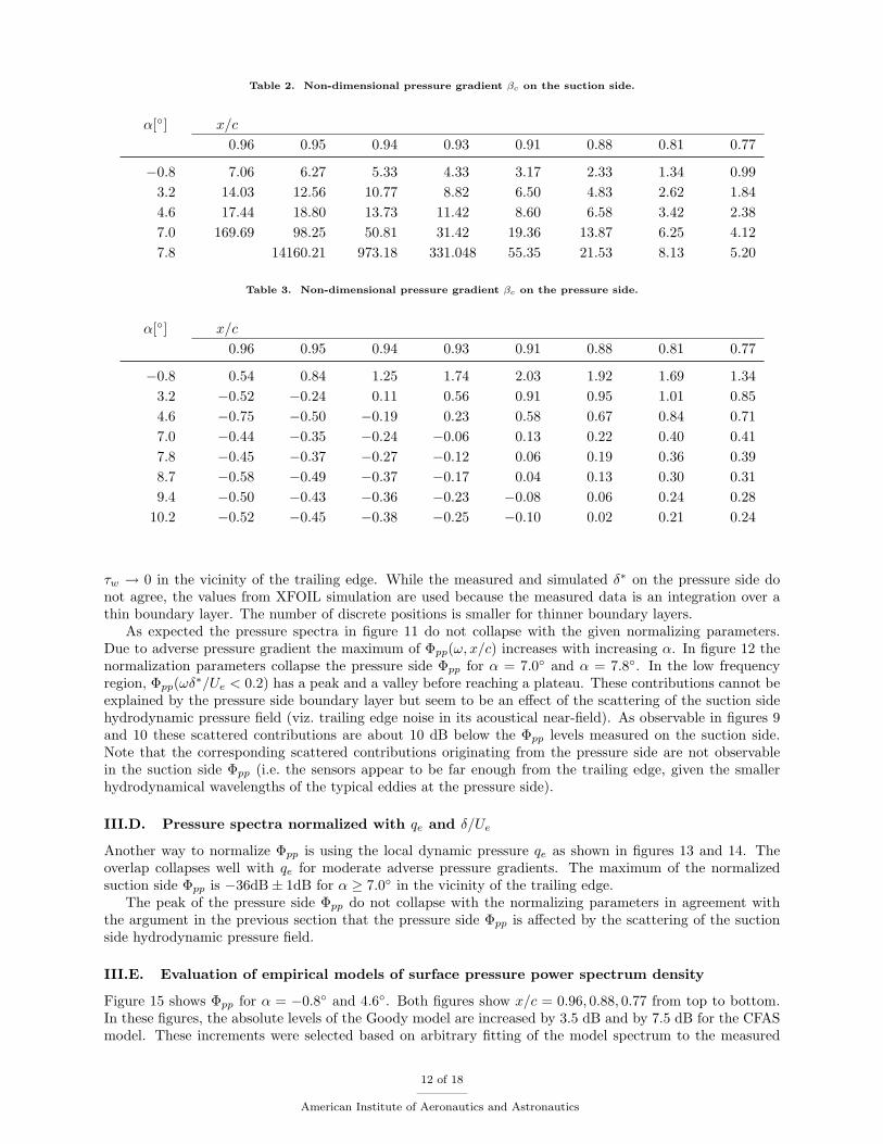
Table 2. Non-dimensional pressure gradient βc on the suction side.

α[◦] x/c

0.96 0.95 0.94 0.93 0.91 0.88 0.81 0.77

−0.8 7.06 6.27 5.33 4.33 3.17 2.33 1.34 0.993.2 14.03 12.56 10.77 8.82 6.50 4.83 2.62 1.844.6 17.44 18.80 13.73 11.42 8.60 6.58 3.42 2.387.0 169.69 98.25 50.81 31.42 19.36 13.87 6.25 4.127.8 14160.21 973.18 331.048 55.35 21.53 8.13 5.20

Table 3. Non-dimensional pressure gradient βc on the pressure side.

α[◦] x/c

0.96 0.95 0.94 0.93 0.91 0.88 0.81 0.77

−0.8 0.54 0.84 1.25 1.74 2.03 1.92 1.69 1.343.2 −0.52 −0.24 0.11 0.56 0.91 0.95 1.01 0.854.6 −0.75 −0.50 −0.19 0.23 0.58 0.67 0.84 0.717.0 −0.44 −0.35 −0.24 −0.06 0.13 0.22 0.40 0.417.8 −0.45 −0.37 −0.27 −0.12 0.06 0.19 0.36 0.398.7 −0.58 −0.49 −0.37 −0.17 0.04 0.13 0.30 0.319.4 −0.50 −0.43 −0.36 −0.23 −0.08 0.06 0.24 0.28

10.2 −0.52 −0.45 −0.38 −0.25 −0.10 0.02 0.21 0.24

τw → 0 in the vicinity of the trailing edge. While the measured and simulated δ∗ on the pressure side donot agree, the values from XFOIL simulation are used because the measured data is an integration over athin boundary layer. The number of discrete positions is smaller for thinner boundary layers.

As expected the pressure spectra in figure 11 do not collapse with the given normalizing parameters.Due to adverse pressure gradient the maximum of Φpp(ω, x/c) increases with increasing α. In figure 12 thenormalization parameters collapse the pressure side Φpp for α = 7.0◦ and α = 7.8◦. In the low frequencyregion, Φpp(ωδ∗/Ue < 0.2) has a peak and a valley before reaching a plateau. These contributions cannot beexplained by the pressure side boundary layer but seem to be an effect of the scattering of the suction sidehydrodynamic pressure field (viz. trailing edge noise in its acoustical near-field). As observable in figures 9and 10 these scattered contributions are about 10 dB below the Φpp levels measured on the suction side.Note that the corresponding scattered contributions originating from the pressure side are not observablein the suction side Φpp (i.e. the sensors appear to be far enough from the trailing edge, given the smallerhydrodynamical wavelengths of the typical eddies at the pressure side).

III.D. Pressure spectra normalized with qe and δ/Ue

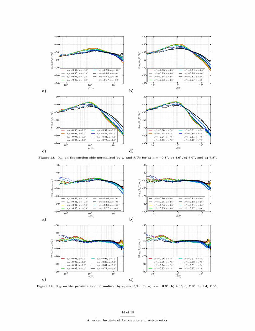
Another way to normalize Φpp is using the local dynamic pressure qe as shown in figures 13 and 14. Theoverlap collapses well with qe for moderate adverse pressure gradients. The maximum of the normalizedsuction side Φpp is −36dB± 1dB for α ≥ 7.0◦ in the vicinity of the trailing edge.

The peak of the pressure side Φpp do not collapse with the normalizing parameters in agreement withthe argument in the previous section that the pressure side Φpp is affected by the scattering of the suctionside hydrodynamic pressure field.

III.E. Evaluation of empirical models of surface pressure power spectrum density

Figure 15 shows Φpp for α = −0.8◦ and 4.6◦. Both figures show x/c = 0.96, 0.88, 0.77 from top to bottom.In these figures, the absolute levels of the Goody model are increased by 3.5 dB and by 7.5 dB for the CFASmodel. These increments were selected based on arbitrary fitting of the model spectrum to the measured

12 of 18


10-2 10-1 100

ωδ ∗ /Ue

30

20

10

0

10

20

30

40

10l

og 1

0(ΦppUe/δ∗(τw

)2)

x/c=0.96, α=−0.8 ◦

x/c=0.95, α=−0.8 ◦

x/c=0.94, α=−0.8 ◦

x/c=0.93, α=−0.8 ◦

x/c=0.91, α=−0.8 ◦

x/c=0.88, α=−0.8 ◦

x/c=0.81, α=−0.8 ◦

x/c=0.77, α=−0.8 ◦

10-2 10-1 100

ωδ ∗ /Ue

30

20

10

0

10

20

30

40

10l

og 1

0(ΦppUe/δ∗(τw

)2)

x/c=0.96, α=3.2 ◦

x/c=0.95, α=3.2 ◦

x/c=0.94, α=3.2 ◦

x/c=0.93, α=3.2 ◦

x/c=0.91, α=3.2 ◦

x/c=0.88, α=3.2 ◦

x/c=0.81, α=3.2 ◦

x/c=0.77, α=3.2 ◦

10-2 10-1 100

ωδ ∗ /Ue

30

20

10

0

10

20

30

40

10l

og 1

0(ΦppUe/δ∗(τw

)2)

x/c=0.96, α=4.6 ◦

x/c=0.95, α=4.6 ◦

x/c=0.94, α=4.6 ◦

x/c=0.93, α=4.6 ◦

x/c=0.91, α=4.6 ◦

x/c=0.88, α=4.6 ◦

x/c=0.81, α=4.6 ◦

x/c=0.77, α=4.6 ◦

Figure 11. Pressure spectra on the suction side normalized by τw and δ∗/Ue for α= −0.8◦, 3.2◦, 4.6◦

a)

10-2 10-1 100

ωδ ∗ /Ue

30

20

10

0

10

20

30

40

10lo

g 10(

ΦppUe/δ

∗(τw

)2)

x/c=0.96, α=−0.8 ◦

x/c=0.95, α=−0.8 ◦

x/c=0.94, α=−0.8 ◦

x/c=0.93, α=−0.8 ◦

x/c=0.91, α=−0.8 ◦

x/c=0.88, α=−0.8 ◦

x/c=0.81, α=−0.8 ◦

x/c=0.77, α=−0.8 ◦

b)

10-2 10-1 100

ωδ ∗ /Ue

30

20

10

0

10

20

30

40

10lo

g 10(

ΦppUe/δ

∗(τw

)2)

x/c=0.96, α=4.6 ◦

x/c=0.95, α=4.6 ◦

x/c=0.94, α=4.6 ◦

x/c=0.93, α=4.6 ◦

x/c=0.91, α=4.6 ◦

x/c=0.88, α=4.6 ◦

x/c=0.81, α=4.6 ◦

x/c=0.77, α=4.6 ◦

c)

10-2 10-1 100

ωδ ∗ /Ue

30

20

10

0

10

20

30

40

10lo

g 10(Φ

ppUe/δ

∗(τw

)2)

x/c=0.96, α=7.0 ◦

x/c=0.95, α=7.0 ◦

x/c=0.94, α=7.0 ◦

x/c=0.93, α=7.0 ◦

x/c=0.91, α=7.0 ◦

x/c=0.88, α=7.0 ◦

x/c=0.81, α=7.0 ◦

x/c=0.77, α=7.0 ◦

d)

10-2 10-1 100

ωδ ∗ /Ue

30

20

10

0

10

20

30

40

10lo

g 10(Φ

ppUe/δ

∗(τw

)2)

x/c=0.96, α=7.8 ◦

x/c=0.95, α=7.8 ◦

x/c=0.94, α=7.8 ◦

x/c=0.93, α=7.8 ◦

x/c=0.91, α=7.8 ◦

x/c=0.88, α=7.8 ◦

x/c=0.81, α=7.8 ◦

x/c=0.77, α=7.8 ◦

Figure 12. Pressure spectra on the pressure side normalized by τw and δ∗/Ue for a) α= −0.8◦, b) 4.6◦, c) 7.0◦, and d)7.8◦.

13 of 18


a)10-1 100 101

ωδ/Ue

90

80

70

60

50

40

30

10lo

g 10(

ΦppUe/δq

2 e)

x/c=0.96, α=−0.8 ◦

x/c=0.95, α=−0.8 ◦

x/c=0.94, α=−0.8 ◦

x/c=0.93, α=−0.8 ◦

x/c=0.91, α=−0.8 ◦

x/c=0.88, α=−0.8 ◦

x/c=0.81, α=−0.8 ◦

x/c=0.77, α=−0.8 ◦

b)10-1 100 101

ωδ/Ue

90

80

70

60

50

40

30

10lo

g 10(

ΦppUe/δq

2 e)

x/c=0.96, α=4.6 ◦

x/c=0.95, α=4.6 ◦

x/c=0.94, α=4.6 ◦

x/c=0.93, α=4.6 ◦

x/c=0.91, α=4.6 ◦

x/c=0.88, α=4.6 ◦

x/c=0.81, α=4.6 ◦

x/c=0.77, α=4.6 ◦

c)10-1 100 101

ωδ/Ue

90

80

70

60

50

40

30

10lo

g 10(

ΦppUe/δq

2 e)

x/c=0.96, α=7.0 ◦

x/c=0.95, α=7.0 ◦

x/c=0.94, α=7.0 ◦

x/c=0.93, α=7.0 ◦

x/c=0.91, α=7.0 ◦

x/c=0.88, α=7.0 ◦

x/c=0.81, α=7.0 ◦

x/c=0.77, α=7.0 ◦

d)10-1 100 101

ωδ/Ue

90

80

70

60

50

40

30

10lo

g 10(

ΦppUe/δq

2 e)

x/c=0.96, α=7.8 ◦

x/c=0.95, α=7.8 ◦

x/c=0.94, α=7.8 ◦

x/c=0.93, α=7.8 ◦

x/c=0.91, α=7.8 ◦

x/c=0.88, α=7.8 ◦

x/c=0.81, α=7.8 ◦

x/c=0.77, α=7.8 ◦

Figure 13. Φpp on the suction side normalized by qe and δ/Ue for a) α = −0.8◦, b) 4.6◦, c) 7.0◦, and d) 7.8◦.

a)10-1 100 101

ωδ/Ue

90

80

70

60

50

40

30

10lo

g 10(

ΦppUe/δq

2 e)

x/c=0.96, α=−0.8 ◦

x/c=0.95, α=−0.8 ◦

x/c=0.94, α=−0.8 ◦

x/c=0.93, α=−0.8 ◦

x/c=0.91, α=−0.8 ◦

x/c=0.88, α=−0.8 ◦

x/c=0.81, α=−0.8 ◦

x/c=0.77, α=−0.8 ◦

b)10-1 100 101

ωδ/Ue

90

80

70

60

50

40

30

10lo

g 10(

ΦppUe/δq

2 e)

x/c=0.96, α=4.6 ◦

x/c=0.95, α=4.6 ◦

x/c=0.94, α=4.6 ◦

x/c=0.93, α=4.6 ◦

x/c=0.91, α=4.6 ◦

x/c=0.88, α=4.6 ◦

x/c=0.81, α=4.6 ◦

x/c=0.77, α=4.6 ◦

c)10-1 100 101

ωδ/Ue

90

80

70

60

50

40

30

10lo

g 10(

ΦppUe/δq

2 e)

x/c=0.96, α=7.0 ◦

x/c=0.95, α=7.0 ◦

x/c=0.94, α=7.0 ◦

x/c=0.93, α=7.0 ◦

x/c=0.91, α=7.0 ◦

x/c=0.88, α=7.0 ◦

x/c=0.81, α=7.0 ◦

x/c=0.77, α=7.0 ◦

d)10-1 100 101

ωδ/Ue

90

80

70

60

50

40

30

10lo

g 10(

ΦppUe/δq

2 e)

x/c=0.96, α=7.8 ◦

x/c=0.95, α=7.8 ◦

x/c=0.94, α=7.8 ◦

x/c=0.93, α=7.8 ◦

x/c=0.91, α=7.8 ◦

x/c=0.88, α=7.8 ◦

x/c=0.81, α=7.8 ◦

x/c=0.77, α=7.8 ◦

Figure 14. Φpp on the pressure side normalized by qe and δ/Ue for a) α = −0.8◦, b) 4.6◦, c) 7.0◦, and d) 7.8◦..

14 of 18


x/c

=0.

96

103 104 105

ω[rad/s]

40

50

60

70

80

90

100

10lo

g 10(

Φpp/(

2×1

05)2

)[dB·s]

βc =7.06

du96, experiment

Goody, 2004

Rozenberg et al.,2012

Catlett et al., 2014

103 104 105

ω[rad/s]

40

50

60

70

80

90

100

10lo

g 10(

Φpp/(

2×1

05)2

)[dB·s]

βc =17.44

du96, experiment

Goody, 2004



x/c

=0.

88

103 104 105

ω[rad/s]

40

50

60

70

80

90

100

10lo

g 10(

Φpp/(

2×1

05)2

)[dB·s]

βc =1.34

du96, experiment

Goody, 2004



103 104 105

ω[rad/s]

40

50

60

70

80

90

100

10lo

g 10(

Φpp/(

2×1

05)2

)[dB·s]

βc =3.42

du96, experiment

Goody, 2004



x/c

=0.

76

103 104 105

ω[rad/s]

40

50

60

70

80

90

100

10lo

g 10(

Φpp/(

2×1

05)2

)[dB·s]

βc =0.99

du96, experiment

Goody, 2004



103 104 105

ω[rad/s]

40

50

60

70

80

90

100

10lo

g 10(

Φpp/(

2×1

05)2

)[dB·s]

βc =2.38

du96, experiment

Goody, 2004



a) b)

Figure 15. Surface pressure spectra on the suction side along the chordwise positions from top to bottomx/c= 0.96, 0.88, 0.76 mm for a) α= −0.8◦ and b) α= 4.6◦.

spectrum. In figure 15 a) Φpp(f ;x = 0.96) behaves according to the CFAS model but deviation starts as βcdecreases and Φpp(ω;x/c = 0.77) follows the spectral shape given by the Goody model. Here, the differenceof power level from the zero pressure gradient spectrum of Goody can be attributed to the pressure gradient.A similar increase can also be observed in Ref. 12. For all configurations, the RRM model fails to predict thetransition location from the overlap to high frequency region. Issues with the RRM model were discussedin Ref. 5. In figure 15 b), similar trends to the previous figure can also be observed; Φpp is influenced bythe increase of βc. However, at x/c ≥ 0.88 the CFAS spectra fail to capture the spectral trend because atα = 4.6◦ the boundary layer near the trailing edge has separated.

III.F. Prediction of surface pressure power spectrum density with modified Blake-TNO model

The pressure autospectral density was predicted using Eq. 6. In this study and also in Ref. 14, a discussionabout the convective velocity is focused whether Uc(y) = 0.7U(y)10 or Uc(y) = U(y). The reason for thelatter ratio is that the turbulent eddy is expected to travel with the local velocity. To establish the proper

15 of 18


102 103 104 105

ω [rad/s]

20

40

60

80

100

Φpp [d

B·s]

measured, x/c=0.96

Blake-TNO model Uc (y) =0.7U(y)

Blake-TNO model Uc (y) =U(y)

Figure 16. Pressure autospectra for the trailing edge position for α = −0.8◦.

a)102 103 104 105

ω [rad/s]

20

40

60

80

100

Φpp [d

B·s]

measured, x/c=0.96

Blake-TNO model

SR Blake-TNO model

present Blake-TNO model

b)102 103 104 105

ω [rad/s]

20

40

60

80

100

Φpp [d

B·s]

measured, x/c=0.96

Blake - TNO model

SR Blake - TNO model


c)102 103 104 105

ω [rad/s]

20

40

60

80

100

Φpp [d

B·s]

measured, x/c=0.96

Blake-TNO model

SR Blake-TNO model


d)102 103 104 105

ω [rad/s]

20

40

60

80

100

Φpp [d

B·s]

measured, x/c=0.96

Blake-TNO model

SR Blake-TNO model


Figure 17. Surface pressure autospectra at x/c= 0.96 for a) α= 7.0◦, b) α= 7.8◦, c) α= 8.7◦, and d) α= 10.3◦.

relationship, Φpp(ω;α = −0.8◦) was calculated and it was found that Uc(y) = U(y) provided the correctlevels as shown in Fig. 16. In the integration of Eq. (6) the measured chord-normal distributions 0 ≤ y ≤ δof dU/dy and v′v′ were used.

Figure 17 shows Φpp(ω; 7.0◦ ≤ α ≤ 10.3◦). Here, the integration with respect to y was defined froma certain height from the surface to the edge of the boundary layer because of the presence of reversedflow. This range is listed in table 4. The modifications of Uc and Ly as proposed in Ref. 14 (SR, Uc(y) =0.7U(y), Ly = 2.5`mix/κ) over-predict the magnitude of the power spectrum and provide a roll off thatstarts too early. The original Blake-TNO model (Uc(y) = 0.7U(y), Ly = `mix/κ) is shown as the green line

16 of 18


a)

102 103 104 105

ω [rad/s]

10-7

10-6

10-5

10-4

10-3

Φvv

b)

102 103 104 105

ω [rad/s]

10-7

10-6

10-5

10-4

10-3

Φvv

Figure 18. Vertical velocity spectrum, Φvv(ω) at α= 10.3◦ a) Original Blake-TNO model and b) present Blake-TNOmodel with c1= 1.3, c2= 1.6.

in figure 17 and it under-predicts the power spectrum. The present prediction was done by modifying themoving axis spectrum .

Φm(ω − c1Uc(y)kx) =1

αGauss√π

exp[− (ω − c1Uc(y)kx)2

α2Gauss

](9)

and Ly = c2`mix/κ, where c1 and c2 are determined heuristically and given in Table 4. These modifications

Table 4. y Range of integration in y and moving axis modifier c1, c2.

α y[mm] c1 c2

7.0◦ 7 ≤ y ≤ 20 1.3 1.67.8◦ 8 ≤ y ≤ 24 1.3 1.69.4◦ 8 ≤ y ≤ 30 1.5 1.6

10.3◦ 16 ≤ y ≤ 40 1.6 1.7

are analogous to a change in the correlation length scales Lx, Ly for a separated boundary layer. Thechordwise length scale Lx decreases and the chord normal length scale Ly increases for α ≥ 7.0◦. Thesmaller value of Lx can be directly attributed to the increase rate of dissipation as seen in the measuredΦpp(ω).

The vertical velocity spectrum was modeled using the von Karman isotropic spectrum model and shownas dashed line in figure 18. This spectral curve is an integration of

Φvv(ω; y) =∫ ∞

0

∫ ∞0

Φpp(kx, kz)Φm(ω − c1Uc(y)kx) dkxdkz (10)

The dashed line color varies from black to blue indicating positions of increasing distance from the surface.The isotropic model under-predicts the measured spectra significantly, in particular at positions far from thesurface it does not represent the spectral hump as shown in figure 18. With the proposed modifications theprediction of Φvv is worse. However, increasing the integrand Ly in Eq. (6) with a factor of c2 compensatesfor the magnitudes of Φvv.

IV. Conclusions

The goal of this project is to develop a model for the prediction of far-field trailing edge noise induced bya separated turbulent boundary layer. In part of this, a DU-96-W-180 airfoil was equipped with miniaturesurface pressure sensors to measure the local surface pressure fluctuations. In this communication themeasured surface pressure autospectral density is compared with that given by empirical and semi-empiricalmodels.

The mean velocity profile was measured at 1%c behind the trailing edge. The velocity profile wascompared with CFD simulation results, where for sufficiently two-dimensional flow (i.e. α ≤ 7.0◦) the velocity

17 of 18


profiles agree reasonably. The boundary layer properties were evaluated by XFOIL simulation, where alsofor sufficiently two-dimensional flows (i.e. α ≤ 7.8◦) the boundary layer properties agree well.

Flow separation affects the suction side surface pressure spectra as an increase of power level in the lowfrequency region. Downstream of the point of separation of the turbulent boundary layer, the surface pressurespectrum is independent of the chordwise positions. This suggests that the turbulent boundary layer insidethe separation region can be approximated as a chordwise homogeneous flow. On the pressure side favorablepressure gradient condition is met, which in effect flattens the surface pressure spectra at the high frequencyrange. Near-field trailing edge noise contributions can be observed on the pressure side at frequencies thatcorrespond to the suction side hydrodynamical pressure spectral peaks, due to the hydrodynamical pressureon the pressure side is dominated by smaller wavelengths with lower levels compared to the suction sidehydrodynamic pressure field.

The SR modifications of the correlation length scale and convective velocity are found to produce incorrectlevels and earlier spectral roll off. A modification to the moving axis spectra is proposed to fit the measuredsurface pressure power spectral density. A physical analogy is proposed that the modifying parametersshortened the chordwise correlation length scale and lengthened the chord-normal one. Measured data forthe chord-normal correlation length scale are currently under evaluation to validate the present modificationsof the Blake-TNO model and the frequency-wavenumber spectra are to be analyzed for the prediction of thefar-field noise.

Acknowledgments

This work was sponsored by GE Wind Energy, GmbH, Salzbergen, Germany.

References

1Bertagnolio, F., Trailing edge noise model applied to wind turbine airfoils, Risø-R-1633(EN), RisøNational Laboratory,Technical University of Denmark, Denmark, 2008.

2Blake, W.K., Mechanics of Flow-Induced Sound and Vibration, Academic Press, London, 1986.3Brooks, T.F., and Hodgson, T.H., Trailing edge noise prediction from measured surface pressures, Journal of Sound and

Vibration, vol. 78, no. 1, 1981.4Brooks, T.F., Pope, D.S., and Marcolini, M.A., Airfoil self-noise and prediction, NASA Reference Publication 1218,

1989.5Catlett, M.R., Forest, J.B., Anderson, J.M., and Stewart, D.O., Empirical spectral model of surface pressure fluctuations

beneath adverse pressure gradients, Proceedings of the 20th AIAA/CEAS Aeroacoustic Conference, Atlanta, GA, AIAA paper2014-2910, 2014.

6Corcos, G.M., The structure of the turbulent pressure field in boundary-layer flows, Journal of Fluid Mechanics, vol. 18,no. 3, 1964.

7Drela, M., XFOIL: An analysis and design system for low Reynolds number airfoils, in Low Reynolds number aerody-namics, Mueller, T.J. (ed), Lecture Notes in Engineering, vol. 54, Springer-Verlag, Berlin 1989.

8Goody, M., Empirical spectral model of surface pressure fluctuations, AIAA Journal, vol. 42, no. 9, 2004.9Howe, M.S., Trailing edge noise at low Mach numbers, part 2: Attached and separated edge flows, Journal of Sound

Vibration, vol. 234, no. 5, 2000.10Parchen, R., Progress report DRAW: A prediction scheme for trailing-edge noise based on detailed boundary-layer char-

acteristics, TNO report HAG-RPT-980023, TNO Institute of Applied Sciences, The Netherlands, 1998.11Rozenberg, Y., Gilles, R., and Moreau, S., Wall-pressure spectral model including the adverse pressure gradient effects,

AIAA Journal, vol. 50, no. 10, 2012.12Schloemer, H.H.: Effects of pressure gradient on turbulent-boundary-layer surface-pressure fluctuations, The Journal of

the Acoustical Society of America, vol. 42, no. 1, 196713Schule C.Y., First milestone meeting: Flow separation study, DLR Internal report, 201214Schule, C.Y., and Rossignol, K.S., Trailing edge noise modeling and validation for separated flow conditions, Proceedings

of the 19th AIAA/CEAS Aeroacoustic conference, Berlin, Germany, AIAA paper 2013-2008, 2013.

18 of 18


Documents

Wall pressure spectra on a DU96-W-180 pro le from low to