Water Temperature

Modeling Review Central Valley

September 2000

Sponsored by the

Bay Delta Modeling Forum

Michael L. Deas

Cindy L. Lowney

_____________________________________________________________________________

I I

1. INTRODUCTION .............................................................................................................2 1.1. PURPOSE...................................................................................................................2 1.2. IMPORTANCE OF WATER TEMPERATURE IN AQUATIC SYSTEMS ...........................................3 1.3. MATHEMATICAL MODELS ..............................................................................................4 1.4. HISTORY OF TEMPERATURE MODELING IN THE CENTRAL VALLEY ........................................4

1.4.1 U.S. Bureau of Reclamation ................................................................................5 1.4.2 US Army Corps of Engineers ...............................................................................6 1.4.3 Other Modeling Studies .......................................................................................6

1.5. EXTENT OF REVIEW .....................................................................................................9 1.5.1 Model Classifications ........................................................................................11 1.5.2 Hydrodynamic Representation ...........................................................................11 1.5.3 Numerical Solution Schemes .............................................................................11 1.5.4 Central Valley Systems .....................................................................................12 1.5.5 Model Dimensions ............................................................................................12 1.5.6 Model Domain: Near- and Far-Field Problems ....................................................12 1.5.7 Units ................................................................................................................13

1.6. LITERATURE .............................................................................................................13 1.7. REPORT OUTLINE AND ACKNOWLEDGEMENTS ................................................................13

1.7.1 Report Outline ..................................................................................................13 1.7.2 Acknowledgements...........................................................................................14

2. THEORETICAL CONSIDERATIONS ..............................................................................15 2.1. HEAT AND TEMPERATURE ...........................................................................................15

2.1.1 Temperature.....................................................................................................15 2.1.2 Heat Energy .....................................................................................................16 2.1.3 Density.............................................................................................................16 2.1.4 Specific Heat ....................................................................................................17

2.2. THE ENERGY BUDGET ................................................................................................18 2.2.1 Solar Radiation ( swq ).......................................................................................19 2.2.1.1 Riparian Shading.............................................................................................................................23 2.2.2 Longwave Radiation (qatm and qb) .....................................................................24 2.2.2.1 Downwelling Longwave Radiation................................................................................................25 2.2.2.2 Upwelling Longwave Radiation.....................................................................................................25 2.2.3 Latent Heat Flux (qL) .........................................................................................25 2.2.3.1 Basic Expressions of Atmospheric Moisture Content................................................................25 2.2.3.2 Evaporative Heat Loss ...................................................................................................................27 2.2.4 Sensible Heat Flux ( hq )....................................................................................29 2.2.5 Ground Heat Conduction...................................................................................29

2.3. EQUILIBRIUM TEMPERATURE .......................................................................................30 2.4. MODELING LAKES AND RESERVOIRS .............................................................................30

2.4.1 Lake and Reservoir Heat Budgets......................................................................31 2.4.2 Internal Temperature Dynamics.........................................................................31 2.4.3 Inflows and Outflows .........................................................................................33 2.4.3.1 Outflow Dynamics ...........................................................................................................................34 2.4.3.2 Spatial Representation ...................................................................................................................35

2.5. MODELING STREAMS AND RIVERS ................................................................................36 2.5.1 Transport Mechanisms......................................................................................36 2.5.2 Analytical Models..............................................................................................38 2.5.3 Thermal Regimes of Regulated Rivers ...............................................................39 2.5.3.1 Formation of Nodes and Anti-Nodes in the Sacramento River................................................41

3. WATER TEMPERATURE STUDIES ...............................................................................45

I I I

3.1. TYPES OF WATER TEMPERATURE MODELING STUDIES ....................................................45 3.1.1 Baseline Studies ...............................................................................................45 3.1.2 Impact Analyses ...............................................................................................46 3.1.3 Operations .......................................................................................................46 3.1.4 Research .........................................................................................................46 3.1.5 Other Applications ............................................................................................46

3.2. PRELIMINARY SYSTEM CHARACTERIZATION ...................................................................47 3.2.1 Study Area and Study Period.............................................................................47 3.2.2 System Boundaries, Components, and Attributes................................................47 3.2.3 Space and Time Scales ....................................................................................47

3.3. MODEL OUTPUT ........................................................................................................48 3.4. MODEL PERFORMANCE TARGETS.................................................................................50 3.5. DATA SYNTHESIS ......................................................................................................50

3.5.1 Data Terminology .............................................................................................51 3.5.1.1 Boundary Conditions.......................................................................................................................51 3.5.1.2 Initial Conditions ..............................................................................................................................52 3.5.1.3 Calibration and Validation Data ....................................................................................................52 3.5.2 Meteorological Information ................................................................................53 3.5.2.1 Meteorological Data Sources ........................................................................................................53 3.5.2.2 Other Meteorological Data Issues ................................................................................................54 3.5.3 Rivers and Streams ..........................................................................................55 3.5.3.1 Geometric Data................................................................................................................................55 3.5.3.2 Flow Information..............................................................................................................................56 3.5.3.3 Water Temperature.........................................................................................................................58 3.5.3.4 Other Data ........................................................................................................................................60 3.5.4 Reservoirs and Lakes .......................................................................................60 3.5.4.1 Geometric Data................................................................................................................................60 3.5.4.2 Flow Information..............................................................................................................................60 3.5.4.3 Water Temperature.........................................................................................................................62 3.5.5 Non-physical System Constraints for Rivers and Reservoirs ................................63 3.5.6 Need for Additional Data ...................................................................................63 3.5.6.1 Field Monitoring ...............................................................................................................................63 3.5.6.2 Data Estimation...............................................................................................................................64

3.6. MODEL SELECTION ....................................................................................................64 3.6.1 Model Capability...............................................................................................65 3.6.2 Data Requirements and Availability....................................................................66 3.6.3 Computer Model Availability and Status .............................................................66 3.6.4 Model Training, Documentation, and Support .....................................................67 3.6.5 Computational Issues........................................................................................67 3.6.5.1 Hardware..........................................................................................................................................67 3.6.5.2 Software and Code Modifications .................................................................................................67 3.6.5.3 Numerical Solution Techniques ....................................................................................................67 3.6.6 Available Resources .........................................................................................70

3.7. SUMMARY ................................................................................................................70 4. MODEL IMPLEMENTATION, CALIBRATION/VALIDATION, AND APPLICATION ...........72

4.1. INTRODUCTION..........................................................................................................72 4.2. MODEL IMPLEMENTATION............................................................................................72

4.2.1 Model Test Cases .............................................................................................72 4.2.2 Mathematical Description of the System .............................................................72 4.2.3 Loading Data and Selecting Default Parameters .................................................72 4.2.4 Trial Simulations ...............................................................................................73 4.2.5 Formulating Initial Conditions .............................................................................73

4.3. CALIBRATION AND VALIDATION.....................................................................................74 4.3.1 Uncertainty.......................................................................................................74 4.3.2 Calibration Parameters......................................................................................74

IV

4.3.3 Model Performance...........................................................................................75 4.3.3.1 Statistical Measures ........................................................................................................................75 4.3.3.2 Calibration and Validation Locations for Rivers and Reservoirs..............................................77 4.3.4 Range of Model Applicability..............................................................................77 4.3.5 Calibration and Validation and Mo del Performance .............................................78

4.4. SENSITIVITY ANALYSIS ...............................................................................................78 4.5. MODEL USE..............................................................................................................80

5. CONCLUSIONS AND RECOMMENDATIONS ................................................................81 5.1. THEORETICAL CONSIDERATIONS ..................................................................................81 5.2. WATER TEMPERATURE STUDIES ...................................................................................81 5.3. MODEL IMPLEMENTATION, CALIBRATION/VALIDATION, AND USE ........................................82 5.4. STATE OF THE F IELD ..................................................................................................82 5.5. FINDINGS AND RECOMMENDATIONS ..............................................................................83

5.5.1 Technical Issues ...............................................................................................83 5.5.1.1 Heat Budget Formulation ...............................................................................................................84 5.5.1.2 Reservoir Inflow and Withdrawal Envelope Formulations ........................................................85 5.5.2 Modeling Mechanics .........................................................................................85 5.5.2.1 Computer Language and Code.....................................................................................................85 5.5.2.2 Improved Model Interfaces ............................................................................................................85 5.5.3 Data Considerations .........................................................................................86 5.5.3.1 General .............................................................................................................................................86 5.5.3.2 Monitoring.........................................................................................................................................86 5.5.3.3 Meteorological Data........................................................................................................................87 5.5.4 Interdisciplinary Efforts......................................................................................87 5.5.5 Education and Training .....................................................................................88 5.5.6 Concluding Comment........................................................................................89

6. REFERENCES ..............................................................................................................90

7. GLOSSARY ..................................................................................................................97

APPENDIX A. PUBLICLY AVAILABLE MODELS................................................................ 104 A.1 RIVER MODELS.......................................................................................................... 104 A.1.1 CEQUAL-RIV1...................................................................................................... 104 A.1.2 HSPF, HYDROLOGICAL SIMULATION PROGRAM—FORTRAN........................................... 104 A.1.3 QUAL2E ............................................................................................................... 106 A.1.4 SNTEMP............................................................................................................... 107 A.1.5 WQRRS ................................................................................................................ 108 A.1.6 HEC5-Q ................................................................................................................ 108 A.1.7 CE-QUALW-2 ....................................................................................................... 109 A.2 RESERVOIR MODELS .................................................................................................. 109 A.2.1 CEQUAL-R1 ......................................................................................................... 109 A.2.2 CE-QUALW-2 ....................................................................................................... 110 A.2.3 HEC5-Q ................................................................................................................ 111 A.2.4 WQRRS ................................................................................................................ 111

APPENDIX B. DATA SOURCES ......................................................................................... 112 B.1 STREAM FLOW ........................................................................................................... 112 B.2 WATER TEMPERATURE................................................................................................ 112 B.3 METEOROLOGICAL DATA ............................................................................................. 112

1

Dedication

This report is dedicated to two dear friends and colleagues, Gerald Orlob and

the late Ray Krone. It would be difficult to name two individuals whose research contributions in the field of water resources have lead to a greater

understanding of the Bay, Delta, and Central Valley systems. We are privileged to take this opportunity to identify these two individuals who

worked so diligently to lay the foundation that we stand upon each day.

2

1. INTRODUCTION “Temperature, a catalyst, a depressant, an activator, a restrictor, a stimulator, a controller, a killer, is one of the most important and influential water quality characteristics to life in water”

Federal Water Pollution Control Administration (1967)

1.1. PURPOSE

The Central Valley watershed provides an important environmental, social, and economic resource. Its streams, lakes, reservoirs, and estuary provide critical habitat for fish and wildlife, recreation, water supply, hydropower, flood control, navigation, and other uses that support California’s vast economy. However, extensive water resources development has affected aquatic environments in most of the Central Valley watershed. Construction of dams on the Sacramento and San Joaquin River, as well as on most major tributaries to these rivers, has blocked passage for anadromous fishes that historically spawned in these watersheds. Additionally, the impoundment of waters and operation of reservoirs has altered both the flow regime and water quality in downstream river reaches. Downstream river reaches are further impacted by diversions and return flows. Of particular concern is the effect that impoundments and water resources development along river reaches have on water temperature.

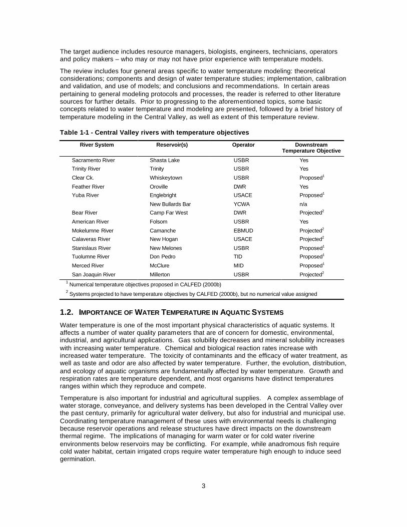
The influence of water temperature on native Central Valley fishes is of importance, particularly for anadromous chinook salmon and steelhead. In response to concerns over the effects of reservoirs on downstream water temperature, regulators have established water temperature requirements or objectives that significantly restrict the operation of upstream reservoirs, as shown in Table 1-1. In addition, major activities and expenditures are being contemplated for re-operation of reservoirs, modification of dams, restoration of riparian habitat, management of drainage flows, and modification of channel geometry, in part to improve stream water temperature conditions for these fish. Mathematical modeling of stream and reservoir temperature has become important for operation of system reservoirs, and is also valuable for simulating effectiveness of proposed strategies that utilize passive (e.g., non-operational) approaches to water temperature control.

As modeling techniques, monitoring equipment, and computing power improve, more sophisticated mathematical tools for evaluation of reservoir operations and watershed restoration efforts have become available. There is increasing interest over how temperature modeling is, can, and should be used for reservoir system operations to meet existing down stream temperature standards. Yet concern also exists over the ability of temperature modeling to adequately simulate the effectiveness of non-reservoir management activities. Topics of interest include assessment of reservoir carryover storage for cold water supplies, reservoir releases from selected depths, and riparian shading of streams and rivers to control/maintain water temperature. In response to the interest and concern associated with selection and application of temperature models and the biological and ecological effects of temperature regimes, the Bay Delta Modeling Forum (BDMF) sponsored two preliminary assessments: this review of temperature modeling for Central Valley water management and a review of temperature effects on anadromous Central Valley salmonids. As such, the report objective is:

To provide an overview of stream and reservoir water temperature modeling, review historic and current temperature modeling work in the Central Valley, identify basic temperature prediction concepts, present the required field and other physical data, and define the role of temperature modeling in addressing current biological problems.

3

The target audience includes resource managers, biologists, engineers, technicians, operators and policy makers – who may or may not have prior experience with temperature models.

The review includes four general areas specific to water temperature modeling: theoretical considerations; components and design of water temperature studies; implementation, calibration and validation, and use of models; and conclusions and recommendations. In certain areas pertaining to general modeling protocols and processes, the reader is referred to other literature sources for further details. Prior to progressing to the aforementioned topics, some basic concepts related to water temperature and modeling are presented, followed by a brief history of temperature modeling in the Central Valley, as well as extent of this temperature review.

Table 1-1 - Central Valley rivers with temperature objectives

River System Reservoir(s) Operator Downstream Temperature Objective

Sacramento River Shasta Lake USBR Yes

Trinity River Trinity USBR Yes

Clear Ck. Whiskeytown USBR Proposed1

Feather River Oroville DWR Yes

Yuba River Englebright

New Bullards Bar

USACE

YCWA

Proposed1

n/a

Bear River Camp Far West DWR Projected2

American River Folsom USBR Yes

Mokelumne River Camanche EBMUD Projected2

Calaveras River New Hogan USACE Projected2

Stanislaus River New Melones USBR Proposed1

Tuolumne River Don Pedro TID Proposed1

Merced River McClure MID Proposed1

San Joaquin River Millerton USBR Projected2 1 Numerical temperature objectives proposed in CALFED (2000b) 2 Systems projected to have temperature objectives by CALFED (2000b), but no numerical value assigned

1.2. IMPORTANCE OF WATER TEMPERATURE IN AQUATIC SYSTEMS

Water temperature is one of the most important physical characteristics of aquatic systems. It affects a number of water quality parameters that are of concern for domestic, environmental, industrial, and agricultural applications. Gas solubility decreases and mineral solubility increases with increasing water temperature. Chemical and biological reaction rates increase with increased water temperature. The toxicity of contaminants and the efficacy of water treatment, as well as taste and odor are also affected by water temperature. Further, the evolution, distribution, and ecology of aquatic organisms are fundamentally affected by water temperature. Growth and respiration rates are temperature dependent, and most organisms have distinct temperatures ranges within which they reproduce and compete.

Temperature is also important for industrial and agricultural supplies. A complex assemblage of water storage, conveyance, and delivery systems has been developed in the Central Valley over the past century, primarily for agricultural water delivery, but also for industrial and municipal use. Coordinating temperature management of these uses with environmental needs is challenging because reservoir operations and release structures have direct impacts on the downstream thermal regime. The implications of managing for warm water or for cold water riverine environments below reservoirs may be conflicting. For example, while anadromous fish require cold water habitat, certain irrigated crops require water temperature high enough to induce seed germination.

4

In addition to these more fundamental concerns, in recent years there has been an increasing interest in the potential impact of global warming on the thermal structure of aquatic systems. Such impacts may have far reaching implications on water resources development, operation, and management in the future.

1.3. MATHEMATICAL MODELS

With increasing frequency we use “models” to predict the future. Models typically include a set of relationships that, either through correlation or through cause and effect functions, aim to yield an increased understanding of a process or processes. To various degrees, models provide representations of complex natural systems. Although all predictive models have their basis in mathematics, for the purpose of this report, mathematical models refers to the use of computers to solve the governing equations of fluid flow, heat exchange and transport in water bodies.

Through the wide availability of mathematical models as well as the increase of computational power and data storage capabilities, models are becoming more practical and popular for assessing stream and reservoir water temperature conditions. The number of models, modeling approaches, and assumptions are increasing. The need for predictive water temperature modeling in the Central Valley has arisen largely due to the cumulative effects of water resources development over the past century, as noted above.

The governing equations of fluid motion (flow) and of heat conservation (temperature) constitute the basis of a mathematical model for water temperature simulation. An important limitation in mathematical modeling results from the fact that the governing equations are second-order partial differential equations in space and time. Solution of these equations is possible through analytical or numerical methods; however, simplifications (or approximations) are often required. For example, the governing fluid flow equations may be reduced from the full three-dimensional representation to a two-or one-dimensional form. At times, secondary terms may be dropped from these equations to simplify the formulations. In general, these simplifications decrease the degree of difficulty of model implementation; however, they may also reduce the range of problems that can be assessed with a particular model.

Notwithstanding the inherent simplifications, the main advantage of mathematical modeling lies in the fact that it is a general tool applicable to different field conditions. Many of today’s mathematical models can be applied to large, complex reservoir and river systems requiring high spatial and temporal resolution. These powerful tools can be used to simulate and assess cause and effect relationships between water resources management, physical processes, and aquatic system response. However, model complexity does not guarantee accuracy. For certain types of applications, a simplified model may be more accurate or reliable than a more complex one.

Finally, mathematical models are valuable tools for assessment and management of aquatic systems; however, a single model is rarely capable of representing an entire system from headwaters to sea. The diversity in slope and channel geometry of steep mountain streams, the presence of reservoirs and low gradient valley rivers often requires “multiple” model approaches to capture the necessary water temperature characteristics of a system. Thus, consideration of the type of system, availability of data, and the problem objective usually guides model review and selection. In certain cases, model modification may be necessary in order to fulfill project objectives.

1.4. HISTORY OF TEMPERATURE MODELING IN THE CENTRAL VALLEY Temperature modeling has a long history in the Central Valley. The first mathematical model, a manual technique, was employed in the Central Valley in the 1960’s. As reported by Water Resources Engineering (WRE, 1977)

5

“Raphael (1962) applied a manual technique for calculation of the thermal energy budget for proposed reservoirs which he successfully applied to Oroville Reservoir on California’s Feather River and to several other reservoirs on the Columbia River system. The method allowed reasonable estimation of downstream temperatures from these projects but failed to provide a description of the vertical distribution of heat within the impoundment.”

The first effort to computerize the energy budget calculations for rivers and reservoirs, such as those implemented by Raphael, appear to have been initiated in the mid-1960’s by two independent groups, one a private consulting organization and the other an academic institution. WRE, under contract with the California Department of Fish and Game, developed the fundamental concepts for predicting thermal energy distribution in streams and reservoirs (WRE, 1967) and Parson’s Hydraulic Lab at the Massachusetts Institute of Technology under a grant from the US Envi ronmental Protection Agency produced a working model for simulation of deep reservoirs (Huber et al., 1972). Critical to the development of these computer models was the comprehensive study of heat exchange in impoundments completed by the Tennessee Valley Authority (TVA, 1972).

One of the earliest studies in the Central Valley was completed by WRE in the Feather River basin during the late 1960’s, wherein a computer model was used to predict water temperature for a proposed reservoir – the Marysville project (Rowell, 1998; Orlob pers. comm.). By the early-1970’s the US Bureau of Reclamation (USBR) had adopted and was actively applying computer simulation of water temperature in several mainstem reservoirs in the Sacramento River basin. Nearly all of the early computer model applications addressed water temperature conditions below mainstem reservoirs for anadromous fish restoration and/or maintenance – the same issue that continues to motivate temperature modeling today.

Two major agencies have dominated water temperature (and in some cases water quality) modeling in the Central Valley over the past 30 years, the USBR and the U.S. Army Corps of Engineers (USACE). The application of USBR and USACE temperature models has not been independent, with models evolving to accommodate new findings and utilizing advances in computer technology. In addition, other models and modeling efforts occurred throughout the past several decades in the Central Valley.

1.4.1 U.S. Bureau of Reclamation In the early 1970’s the USBR applied the USACE - Hydrologic Engineering Center (HEC) Reservoir Temperature Stratification (RTS) model (Beard and Willey, 1972) to Shasta and Folsom Reservoirs to simulate monthly thermal conditions/response. This initial model was a one-dimensional, vertical characterization of reservoirs, exploiting the thermal stratification features of most large, deep reservoirs. Soon thereafter, the USBR modified the RTS to accommodate their needs, and utilized the heat budget logic to formulate a stream temperature model for predicting the thermal response of river reaches downstream of reservoirs. Subsequently, Rowell (1972) completed river temperature simulations on the Sacramento River upstream of Red Bluff. In an extension of these models, Rowell (1975) adapted the stream model to the Truckee River water temperature prediction studies to identify minimum flows to maintain suitable water temperature for Lahontan Cutthroat Trout. Christiansen and Orlob (1989) applied USBR models for Shasta, Trinity, Whiskeytown, and Folsom Reservoirs, and the associated river models for the Trinity, Sacramento, and American Rivers to assess their predictive temperature and flow performance. These models have been maintained by USBR and, as necessary, modified to address other reservoirs and river reaches. They are the most widely applied and continuously used temperature models in the Central Valley, and possibly in the United States. Although they operate on a monthly time step the models continue to assist USBR in planning and operation of USBR Central Valley facilities for identifying the effects of alternative operating scenarios on reservoir and downstream river water temperatures for anadromous fish.

6

1.4.2 U.S. Army Corps of Engineers The USACE-HEC produced two models that have been widely applied to Central Valley systems: Water Quality for River-Reservoir Systems (WQRRS) and Water Quality Simulation Module HEC5-Q (HEC-5Q). WQRRS (USACE-HEC, 1986) and HEC-5Q (USACE -HEC, 1987c) evolved from work completed by WRE (1969), Chen and Orlob (1972), and Beard and Willey (1972) as well as other earlier models. Both models assess reservoir-river systems, characterizing reservoirs with vertical one-dimensional representations and rivers as one-dimensional longitudinal reaches. Th ese physically-based models are multi-purpose water quality models capable of simulating water temperature over large portions of river basins. WQRRS provides a broader range of water quality and ecological processes than HEC5-Q, but reservoir and river simulations must be processed individually. Further, HEC-5Q includes more comprehensive operations logic to accommodate operating rules (e.g. flood control and hydropower production) and reservoir-river systems can be simulated in a single model run. Water temperature simulation can occur with the full heat budget or the equilibrium approach in WQRRS, but only the latter in HEC-5Q (see Chapter 2 for details on these approaches). Neither program is actively supported by the USACE-HEC, rather they are termed “developmental.” WQRRS and HEC-5Q have been widely applied in temperature analyses in the Central Valley.

A modified version of WQRRS was applied by Smith (1981) on the North Fork of the Stanislaus River to assess potential water temperature effects of proposed hydroelectric development. More recently, Shasta and Trinity Reservoirs have been modeled with WQRRS. Orlob et al. (1993) and Meyer and Orlob (1994) used WQRRS to investigate effects of climate change on water quality, including water temperature. Deas et al. (1997) applied the models developed by Meyer and Orlob to simulate water temperature response for alternative operations for anadromous fish restoration in the Sacramento River downstream of Keswick Reservoir. Deas (1998) applied WQRRS to Trinity Reservoir examining selective withdrawal and carryover storage issues for water temperature control in the Trinity River below Lewiston Dam.

The USACE-HEC applied HEC-5Q to the Sacramento Valley reservoir system to illustrate the application of this river-reservoir model to water quality analysis (USACE-HEC, 1987b). The model domain included Shasta and Keswick Reservoirs, the Sacramento River from Keswick Dam to below Sacramento near Hood; Oroville Reservoir and the Feather River from Oroville Dam to the confluence with the Sacramento River; and Folsom Reservoir and the American River to the confluence with the Sacramento River. In 1988 Smith applied HEC-5Q to a similar set of reservoir-river components, but did not include Oroville Reservoir (Smith pers. comm.). HEC-5Q was applied to the lower Yuba River (Salmon et al., 1992). More recently, HEC-5Q has been applied to New Melones and Tulloch Reservoirs, and the Stanislaus River from Tulloch Reservoir to the confluence with the San Joaquin River to develop relationships between operations at upstream reservoirs and downstream Stanislaus River temperatures. For application to New Melones, the model was modified to accommodate both vertical and longitudinal variations in reservoir temperature due to the existence of Old Melones Dam, as well as to accommodate other unique features of that system of reservoirs and river reaches (Smith pers. comm.).

1.4.3 Other Modeling Studies In addition to the aforementioned models, several other reservoir and river modeling efforts have taken place in the Central Valley over the last twenty years. Outlined below is a brief summary of other studies. This synopsis is by no means all-inclusive, but an effort has been made to collect a representative sample.

QUAL2E: QUAL2E is a steady-state flow, one-dimensional (longitudinal), physically-based, stream water quality model developed by EPA that is capable of simulating diurnal variations in water temperature. QUAL2E has been applied to the American and Feather River simulating hourly water temperature (Rowell, 1998).

7

RMA: Resource Management Associates, Inc. (RMA) models, although requiring a fee for the computer programs, are treated as public domain models for the purposes of this report for two reasons. First, the models have been widely applied in the Central Valley and are available through the University of California, Davis, Department of Civil and Environmental Engineering. Second, unlike many proprietary codes that are available for purchase, the source code is supplied with the purchase.

RMA models have been applied to several river and reservoir systems. RMA-2 and RMA-11 have been used to model flow and temperature, respectively, in the Sacramento and Feather Rivers, Keswick Reservoir, as well as Clear Creek (Deas et al., 1997, Jensen et al., 1999). RMA-10 has been used to model flow and temperature on the Sacramento River and explore the impact of riparian vegetation on water temperature (Lowney, 2000). RMA-6, a two-dimensional laterally-averaged model was applied to Keswick Reservoir by Anderson (1994). Jensen et al. (1999) implemented RMA-10 and RMA-11 to characterize the complex hydrodynamic and thermal regime of Whiskeytown Reservoir in three dimensions.

SNTEMP: SNTEMP is a steady-flow, physically-based, one-dimensional heat transport model that predicts the daily mean and maximum water temperatures as a function of stream distance and environmental heat flux. The model was developed by Theurer et al. (1984) and has been used in several locations in the Central Valley and associated basins including the Trinity River (Zedonis, 1997), Battle Creek (J. Icanberry and H. Rectenwald, pers. comm.), and the Tuolumne River (T. Ford, pers. comm.). SNTEMP has been used for preliminary (informal) simulations of the Sacramento River water temperature as well.

CE-QUAL-R1: the USACE-WES model CE-QUAL-R1 is a one-dimensional vertical reservoir model that was an extension of WQRRS. New Bullards Bar Reservoir on the Yuba River was modeled with CE-QUAL-R1 by Bookman-Edmonston (1991).

BETTER: The Box Exchange Transport Temperature and Ecology of Reservoirs (BETTER) model is a two-dimensional reservoir temperature and water quality model (TVA 1990). BETTER was applied by Jones and Stokes Associates (1992) to simulate flow and temperature for assessing operational impacts on the thermal regime of Lewiston Reservoir and subsequent diversions to Whiskeytown Reservoir and releases to the Trinity River.

CE-QUAL-W2: CE-QUAL-W2 is a two-dimensional (vertical and longitudinal), laterally-averaged, hydrodynamic and water quality model. Hanna et al. (1999) have applied this model to investigate the effect operations of a temperature control device on the reservoir thermal regime.

There are many other models that have not been applied in the Central Valley (to the authors’ knowledge) but that have been applied in other regions of the country. For example, the USACE -WES model CEQUAL-RIV1 for dynamic analysis of streams and rivers, or the TVA models RQUAL and ADYN, also a set of dynamic stream and water quality models.

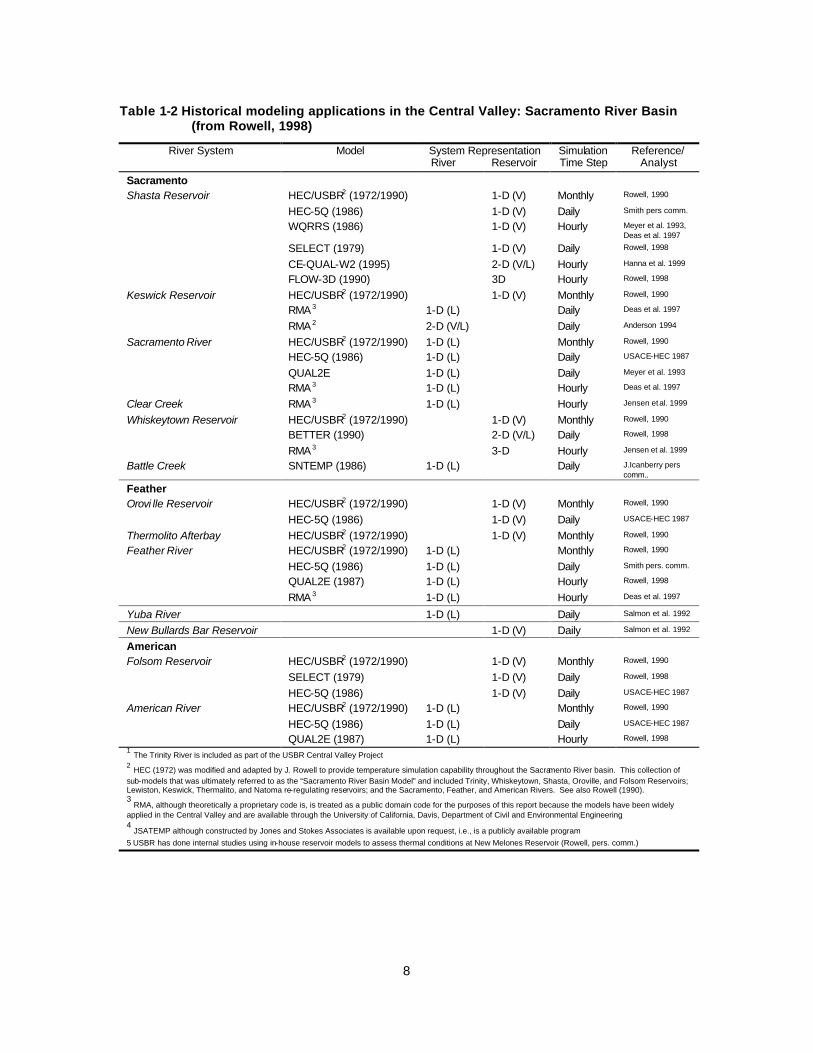
In addition to these modeling efforts and models, other tools have been used to assess water temperature in river systems of the Central Valley. JSATEMP is a spreadsheet model solving the heat budget for mean daily water temperature for steady-flow conditions on the Merced River, as well as Putah Creek (R. Brown, pers. comm.). Lowney et al. (1998) and Lowney (2000) also utilized spreadsheet software to construct an optimization model assessing power plant operations and instream temperature targets on Battle Creek. These are just two examples of many less formal, but often quite useful, modeling efforts. Table 1-2, Table 1-3, and Table 1-4, summarize several Central Valley water temperature modeling efforts over the past three decades, denoting the system, model and year the model was constructed, system representation, and simulation time step. More comprehensive explanations of selected models are summarized in Appendix A.

8

Table 1-2 Historical modeling applications in the Central Valley: Sacramento River Basin (from Rowell, 1998)

River System Model System Representation River Reservoir

Simulation Time Step

Reference/ Analyst

Sacramento

Shasta Reservoir HEC/USBR2 (1972/1990) 1-D (V) Monthly Rowell, 1990

HEC-5Q (1986) 1-D (V) Daily Smith pers comm.

WQRRS (1986) 1-D (V) Hourly Meyer et al. 1993, Deas et al. 1997

SELECT (1979) 1-D (V) Daily Rowell, 1998

CE-QUAL-W2 (1995) 2-D (V/L) Hourly Hanna et al. 1999

FLOW-3D (1990) 3D Hourly Rowell, 1998

Keswick Reservoir HEC/USBR2 (1972/1990) 1-D (V) Monthly Rowell, 1990

RMA 3 1-D (L) Daily Deas et al. 1997

RMA 2 2-D (V/L) Daily Anderson 1994

Sacramento River HEC/USBR2 (1972/1990) 1-D (L) Monthly Rowell, 1990

HEC-5Q (1986) 1-D (L) Daily USACE-HEC 1987

QUAL2E 1-D (L) Daily Meyer et al. 1993

RMA 3 1-D (L) Hourly Deas et al. 1997

Clear Creek RMA 3 1-D (L) Hourly Jensen et al. 1999

Whiskeytown Reservoir HEC/USBR2 (1972/1990) 1-D (V) Monthly Rowell, 1990

BETTER (1990) 2-D (V/L) Daily Rowell, 1998

RMA 3 3-D Hourly Jensen et al. 1999

Battle Creek SNTEMP (1986) 1-D (L) Daily J.Icanberry pers comm..

Feather

Orovi lle Reservoir HEC/USBR2 (1972/1990) 1-D (V) Monthly Rowell, 1990

HEC-5Q (1986) 1-D (V) Daily USACE-HEC 1987

Thermolito Afterbay HEC/USBR2 (1972/1990) 1-D (V) Monthly Rowell, 1990

Feather River HEC/USBR2 (1972/1990) 1-D (L) Monthly Rowell, 1990

HEC-5Q (1986) 1-D (L) Daily Smith pers. comm.

QUAL2E (1987) 1-D (L) Hourly Rowell, 1998

RMA 3 1-D (L) Hourly Deas et al. 1997

Yuba River 1-D (L) Daily Salmon et al. 1992

New Bullards Bar Reservoir 1-D (V) Daily Salmon et al. 1992

American

Folsom Reservoir HEC/USBR2 (1972/1990) 1-D (V) Monthly Rowell, 1990

SELECT (1979) 1-D (V) Daily Rowell, 1998

HEC-5Q (1986) 1-D (V) Daily USACE-HEC 1987

American River HEC/USBR2 (1972/1990) 1-D (L) Monthly Rowell, 1990

HEC-5Q (1986) 1-D (L) Daily USACE-HEC 1987

QUAL2E (1987) 1-D (L) Hourly Rowell, 1998 1 The Trinity River is included as part of the USBR Central Valley Project

2 HEC (1972) was modified and adapted by J. Rowell to provide temperature simulation capability throughout the Sacramento River basin. This collection of sub-models that was ultimately referred to as the “Sacramento River Basin Model” and included Trinity, Whiskeytown, Shasta, Oroville, and Folsom Reservoirs; Lewiston, Keswick, Thermalito, and Natoma re-regulating reservoirs; and the Sacramento, Feather, and American Rivers. See also Rowell (1990). 3 RMA, although theoretically a proprietary code is, is treated as a public domain code for the purposes of this report because the models have been widely applied in the Central Valley and are available through the University of California, Davis, Department of Civil and Environmental Engineering 4 JSATEMP although constructed by Jones and Stokes Associates is available upon request, i.e., is a publicly available program 5 USBR has done internal studies using in-house reservoir models to assess thermal conditions at New Melones Reservoir (Rowell, pers. comm.)

9

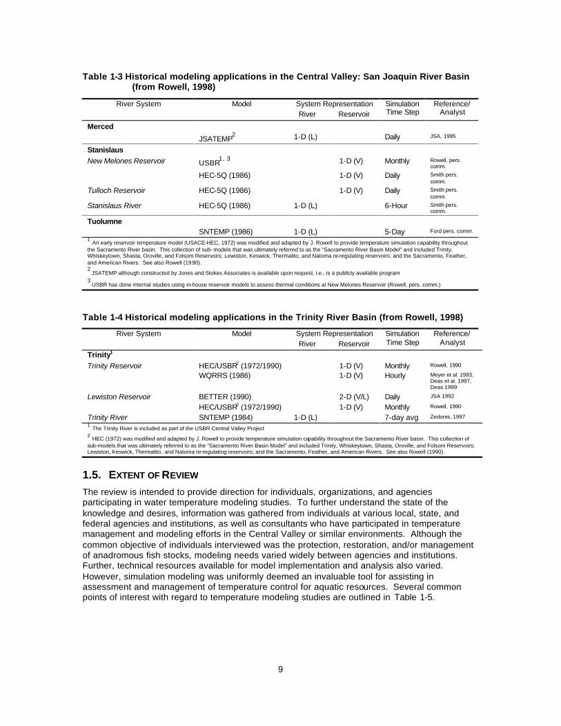
Table 1-3 Historical modeling applications in the Central Valley: San Joaquin River Basin (from Rowell, 1998)

River System Model System Representation River Reservoir

Simulation Time Step

Reference/ Analyst

Merced

JSATEMP2 1-D (L) Daily JSA, 1995

Stanislaus

New Melones Reservoir USBR1, 3

1-D (V) Monthly Rowell, pers. comm.

HEC-5Q (1986) 1-D (V) Daily Smith pers. comm.

Tulloch Reservoir HEC-5Q (1986) 1-D (V) Daily Smith pers. comm.

Stanislaus River HEC-5Q (1986) 1-D (L) 6-Hour Smith pers. comm.

Tuolumne

SNTEMP (1986) 1-D (L) 5-Day Ford pers. comm. 1 An early reservoir temperature model (USACE-HEC, 1972) was modified and adapted by J. Rowell to provide temperature simulation capability throughout the Sacramento River basin. This collection of sub- models that was ultimately referred to as the “Sacramento River Basin Model” and included Trinity, Whiskeytown, Shasta, Oroville, and Folsom Reservoirs; Lewiston, Keswick, Thermalito, and Natoma re-regulating reservoirs; and the Sacramento, Feather, and American Rivers. See also Rowell (1990). 2

JSATEMP although constructed by Jones and Stokes Associates is available upon request, i.e., is a publicly available program 3 USBR has done internal studies using in-house reservoir models to assess thermal conditions at New Melones Reservoir (Rowell, pers. comm.)

Table 1-4 Historical modeling applications in the Trinity River Basin (from Rowell, 1998)

River System Model System Representation River Reservoir

Simulation Time Step

Reference/ Analyst

Trinity1

Trinity Reservoir HEC/USBR2 (1972/1990) 1-D (V) Monthly Rowell, 1990

WQRRS (1986) 1-D (V) Hourly Meyer et al. 1993, Deas et al. 1997, Deas 1999

Lewiston Reservoir BETTER (1990) 2-D (V/L) Daily JSA 1992

HEC/USBR2 (1972/1990) 1-D (V) Monthly Rowell, 1990

Trinity River SNTEMP (1984) 1-D (L) 7-day avg Zedonis, 1997 1 The Trinity River is included as part of the USBR Central Valley Project

2 HEC (1972) was modified and adapted by J. Rowell to provide temperature simulation capability throughout the Sacramento River basin. This collection of sub-models that was ultimately referred to as the “Sacramento River Basin Model” and included Trinity, Whiskeytown, Shasta, Oroville, and Folsom Reservoirs; Lewiston, Keswick, Thermalito, and Natoma re-regulating reservoirs; and the Sacramento, Feather, and American Rivers. See also Rowell (1990).

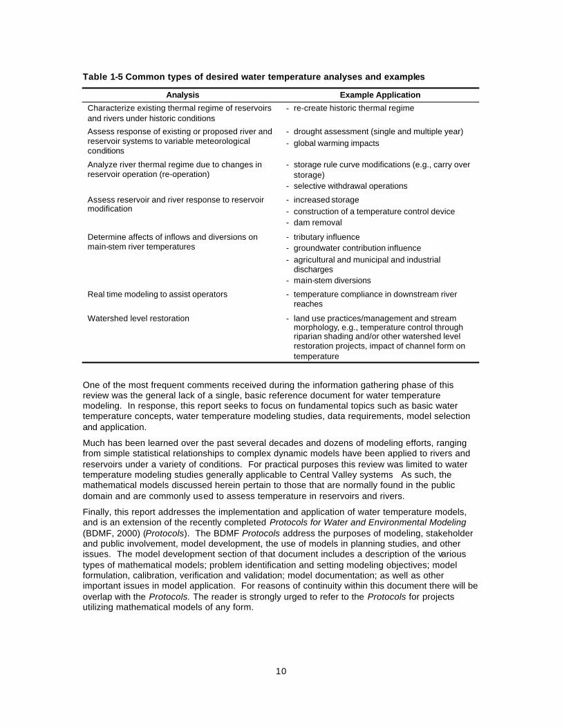
1.5. EXTENT OF REVIEW The review is intended to provide direction for individuals, organizations, and agencies participating in water temperature modeling studies. To further understand the state of the knowledge and desires, information was gathered from individuals at various local, state, and federal agencies and institutions, as well as consultants who have participated in temperature management and modeling efforts in the Central Valley or similar environments. Although the common objective of individuals interviewed was the protection, restoration, and/or management of anadromous fish stocks, modeling needs varied widely between agencies and institutions. Further, technical resources available for model implementation and analysis also varied. However, simulation modeling was uniformly deemed an invaluable tool for assisting in assessment and management of temperature control for aquatic resources. Several common points of interest with regard to temperature modeling studies are outlined in Table 1-5.

10

Table 1-5 Common types of desired water temperature analyses and examples

Analysis Example Application

Characterize existing thermal regime of reservoirs and rivers under historic conditions

- re-create historic thermal regime

Assess response of existing or proposed river and reservoir systems to variable meteorological conditions

- drought assessment (single and multiple year) - global warming impacts

Analyze river thermal regime due to changes in reservoir operation (re-operation)

- storage rule curve modifications (e.g., carry over storage)

- selective withdrawal operations

Assess reservoir and river response to reservoir modification

- increased storage - construction of a temperature control device - dam removal

Determine affects of inflows and diversions on main-stem river temperatures

- tributary influence - groundwater contribution influence - agricultural and municipal and industrial

discharges - main-stem diversions

Real time modeling to assist operators - temperature compliance in downstream river reaches

Watershed level restoration - land use practices/management and stream morphology, e.g., temperature control through riparian shading and/or other watershed level restoration projects, impact of channel form on temperature

One of the most frequent comments received during the information gathering phase of this review was the general lack of a single, basic reference document for water temperature modeling. In response, this report seeks to focus on fundamental topics such as basic water temperature concepts, water temperature modeling studies, data requirements, model selection and application.

Much has been learned over the past several decades and dozens of modeling efforts, ranging from simple statistical relationships to complex dynamic models have been applied to rivers and reservoirs under a variety of conditions. For practical purposes this review was limited to water temperature modeling studies generally applicable to Central Valley systems As such, the mathematical models discussed herein pertain to those that are normally found in the public domain and are commonly used to assess temperature in reservoirs and rivers.

Finally, this report addresses the implementation and application of water temperature models, and is an extension of the recently completed Protocols for Water and Environmental Modeling (BDMF, 2000) (Protocols). The BDMF Protocols address the purposes of modeling, stakeholder and public involvement, model development, the use of models in planning studies, and other issues. The model development section of that document includes a description of the various types of mathematical models; problem identification and setting modeling objectives; model formulation, calibration, verification and validation; model documentation; as well as other important issues in model application. For reasons of continuity within this document there will be overlap with the Protocols. The reader is strongly urged to refer to the Protocols for projects utilizing mathematical models of any form.

11

1.5.1 Model Classifications Mathematical models for stream and reservoir applications can be broadly classified as physically-based, empirical, or “mixed” (BDMF, 2000). Physically-based models utilize governing equations for heat transport and fluid flow to simulate water temperature based upon user described system geometry (e.g. channel shape, slope), flow, and climatic conditions. Theoretically, a physically-based model is applicable to a wide range of systems, and is capable of simulating water temperature under a variety of circumstances that may not be present in the existing system, such as simulating extreme flow and climate, or the impact of reservoir re-operation.

In contrast, empirical models are statistical relationships between two or more observed characteristics of a particular system. The simplest example of this type of model is a linear regression relationship between observed flow and temperature. Obvious limitations to this type of model include the inability for the model to simulate response under conditions that were not observed during data collection (e.g. changes in weather, channel changes that affect travel time through the reach, riparian reforestation).

Although most models include a mix of empirical and physical based approaches, mixed models are defined herein as those that include the dominant physical processes but are formulated for strongly idealized conditions. There is no general rule that separates empirical, mixed, and physically-based models. Typically model user manuals, reports, reviews, or other literature discuss the model representation. It is important to match the level of sophistication of the model (i.e. the degree to which it is physically-based) to the objectives of the study. This review focuses on those models that would generally be termed physically-based.

1.5.2 Hydrodynamic Representation Water temperature models have two primary components: (1) a hydrodynamic or hydrologic (flow) component, and (2) a water temperature (heat flux and transport) component. Both components are critical to effectively represent the thermal regime of reservoirs and rivers. For rivers, flow simulation provides stream flow velocity, depth, air-water and bed-water surface area: necessary parameters to calculate heat transfer at the air- and bed-water interfaces as well as transport downstream. The reservoir models addressed herein are similarly represented with flow or volume being determined first (as well as depth and surface area) and subsequently temperature. However, temperature (density) effects are directly or indirectly taken into account to address the influence of stratification as well as the simulation of the temperature of release waters. Hydrodynamic and hydrologic models are not the subjects of this review; however, their role in temperature simulation is critical and to that extent they are occasionally discussed.

1.5.3 Numerical Solution Schemes The governing equations employed in physically-based hydrodynamics and water temperature models are complex partial differential equations that, for all but the simplest cases, cannot be solved directly using classical mathematics. Numerical methods are used to approximate the partial derivative terms of the governing equations with algebraic expressions for solution by computer. These methods are efficient and reliable, but not without their limitations. Specifically, temporal and spatial restrictions, numerical dispersion, and accuracy are important considerations associated with model selection and application. Where pertinent, issues of numerical solution scheme are noted; however, the details of mathematical formulation and computational representation of the governing equations and their solution are beyond the scope of this report.

12

1.5.4 Central Valley Systems As noted above, many Central Valley river systems originate as steep mountain streams, pass through large and small reservoirs, and flow as lowland rivers into tidally influenced estuaries. The temperature modeling review focuses on river and reservoir systems that are associated with Central Valley water resources on a regional level where temperature control is possible. This subset primarily includes main-stem operational reservoirs, rivers and streams. Intermittent streams, farm ponds, and small reservoirs are not applicable systems. Estuary regions and tidally affected systems are not included (and there is limited potential for temperature control within the Delta proper). Nonetheless, many of the concepts of water temperature modeling can be applied to these other systems.

1.5.5 Model Dimensions Most temperature modeling projects in reservoirs and lakes, and river and streams can be adequately assessed with one-dimensional representations along their principle axis of variation. That is, many of the large reservoirs and lakes stratify and experience appreciable vertical temperature gradients, but are laterally uniform (i.e., horizontal stratification). Meanwhile, rivers and streams typically experience modest vertical and transverse temperature gradients (i.e., well mixed) compared to temperature variations along the stream flow axis.

Certain reservoir or river analyses may require a second dimension to accommodate important vertical or lateral temperature gradients. However, sufficient justification for the additional dimension should be provided because analyses will require substantially more data collection and more complex models. Three-dimensional models are rarely applied, especially for far-field problems (see below). If such models are required, experts in the field must develop and apply them.

Because of the limited use of two- and three-dimensional models, this report only addresses one-dimensional temperature model representations. For reservoirs and lakes the principal axis of variation is vertical, whereas for rivers and streams it is longitudinal (along the stream flow axis). Exceptions are noted.

1.5.6 Model Domain: Near- and Far-Field Problems Problems concerning temperature prediction can generally be reduced to near-field and far-field regions. Near-field problems typically focus on the mixing zone of inflowing waters (e.g., tributary, drains, outfalls) where the properties of the discharge fluid have a significant impact on the mixing and resulting dilution of the discharged fluid by the receiving water. Important properties of the inflowing water include relative density to the receiving water and initial momentum of the inflowing water, (i.e., modeling the local thermal effects of warm wastewater discharge to a cool river or reservoir). In extreme cases, the domain is represented in three dimensions and extends only a few tens of meters, while the simulation time step may be on the order of minutes or seconds with a total simulation period of hours. Near-field problems often require effectively representing temperature-dependent density differences because the density affects flow, requiring simultaneous determination of both fluid motion and heat distribution within a water body.

Beyond the near-field region exists a larger far-field region where mixing processes are no longer a function of the type of discharge and initial properties of the inflowing water. In the far-field, the mixing processes are dominated by turbulence within the receiving water and the variability of the velocity field. Thus, far-field problems are usually defined by larger spatial domains and diminished local detail.

The distribution of heat in far-field representation is primarily governed by

13

§ heat exchange across the air-water interface: provides for fluxes of heat at the water surface.

§ advection transport of heat in the direction of flow, e.g., river flow, wind driven currents, tidal currents

§ buoyancy induced convection: horizontal density and/or vertical gradients induce buoyant convection. These gradients may be superimposed upon advection by ambient currents. The importance of this mechanism is primarily related to the magnitude of the gradient.

§ dispersion: due to shear dispersion (mixing due to variations in the fluid velocity at different positions in the water body) and diffusion (molecular and turbulent)

§ depth: heat flux at the air- and bed- water interface is distributed through the depth of the water column.

These processes, temporally unsteady and spatially non-uniform, will be discussed in greater detail in Chapter 2. Consistent with these primary processes describing the distribution of heat in aquatic systems, this review focuses on far-field problems.

1.5.7 Units Units consistent with the Système Internationale (SI) are used in this report. SI base units and their accepted symbols are meter (m) for length, kilogram (kg) for mass, Kelvin (K) or degree Celsius (°C) for temperature, and second (s) for time. Joules is the unit of heat expressed as (J = Nm = kg m3 s-2), while heat flux is expressed in Watts (W).

1.6. LITERATURE Primary references addressing water temperature modeling or concepts related to water temperature modeling include Edinger et al. (1968), Fisher et al. (1979), Chapra (1983), Orlob (1983), Thomann and Mueller (1987), McCutcheon (1989), Chapra (1997) and Martin and McCutcheon (1999). A seminal treatment of heat exchange relationships at the air-water interface is presented by TVA (1972), and revisited by Lowney (2000). A standard reference for general energy budget concepts is provided by Oke (1984). Several computer model user manuals include heat budget formulations, forming a valuable reference for the modeler. There are countless journal articles, too numerous to mention, that reproduce heat budget formulations, discuss particular components of the heat budget, or present temperature model applications. Using these literature sources and discussions with scientists, technicians, academics, managers, and other interested and involved parties, this document aims to present a concise source of water temperature modeling information.

1.7. REPORT OUTLINE AND ACKNOWLEDGEMENTS

1.7.1 Report Outline The water temperature modeling review report consists of five chapters. Chapter 1 introduces the topic of temperature modeling and defines the objective of the report, scope of review, and acknowledgements. Chapter 2 outlines the theoretical considerations of mathematically modeling water temperature in reservoirs and rivers. Chapter 3 presents components and a framework for water temperature studies, including data requirements, monitoring and synthesis, and model selection. Chapter 4 discusses model implementation, calibration and validation, and use. Chapter 5 presents conclusions and recommendations. References and personal communications, as well as a glossary, conclude the main report. Two appendices are included: Appendix A summarizes selected publicly available models, and Appendix B lists sources for data required for water temperature modeling.

14

1.7.2 Acknowledgements The Water Temperature Modeling Review was prepared for the BDMF under contract number 254-99, and was administered by the San Francisco Estuary Institute. Technical oversight for this report was provided by Mr. John Williams, Executive Director of the Bay Delta Modeling Forum; Dr. Jay Lund, Professor of Civil and Environmental Engineering at the University of California, Davis; Mr. John Bartholow, Ecologist at U.S. Geological Service Biological Resource Division – Midcontinent Ecological Science Center. Dr. Steve McCord provided additional review.

Finally, we wish to acknowledge several people who contributed through interviews, emails, phone calls and other communications: Mike Aceituno and Dennis Smith of the National Marine Fisheries Service; Meri Miles, Jack Rowell, Russ Yaworski, Chet Boling, Paul Fujitani, Tom Morstein-Marx, and Dave Reed of the U.S. Bureau of Reclamation; Jerry Johns of the SWRCB; Dan Castleberry, Craig Fleming, John Icanberry, Tricia Parker, and Scott Spaulding of the U.S. Fish and Wildlife Service; John Nelson and Harry Rectenwald of the California Department of Fish and Game; Russ Brown of Jones and Stokes Associates, Inc.: Don Smith of Resource Management Associates, Inc., as well as the many individuals representing over a dozen agencies and organizations whom directly or indirectly provided insight and discussion that ultimately assisted in formulating this report.

15

2. THEORETICAL CONSIDERATIONS Biological activity is strongly affected by temperature. Of all the water quality constituents (e.g., water temperature, dissolved oxygen, suspended sediment, pH, nutrients, metals), water temperature is the easiest and often least costly to monitor in field conditions. Thus, water quality investigations with a biological focus often begin with a monitoring campaign designed to characterize temperature conditions. Water temperature models range in objective and sophistication of approach. One modeling objective may be to improve understanding of an existing system, another may be to develop a management tool to determine the effect of flow changes on temperature. Research applications may be designed to answer such questions as the effect of temperature control devices on reservoir temperature dynamics. This chapter describes the fundamental principals of most water temperature models: heat transfer and transport.

2.1. HEAT AND TEMPERATURE This short section provides an introduction to physical relationships between heat and temperature, and commonly used units.

2.1.1 Temperature Throughout this report, temperature is expressed in degrees Celsius (°C), or in Kelvin (K). The Celsius scale is defined according to the boiling and freezing points of water. A one degree Celsius rise in temperature is equivalent to a one Kelvin rise in temperature. The two scales are offset by 273.16 K. That is, 0 °C is equivalent to 273.16K. Temperature may also be reported in units of Fahrenheit or Rankine, although Rankine is no longer a commonly used unit. Celsius and Fahrenheit degrees are not equivalent. A one degree rise measured in Celsius is equivalent to a 1.8 degree rise measured in Fahrenheit. The Fahrenheit - Rankine relationship is mathematically analogous to the Celsius – Kelvin relationship. Conversions are provided in Table 2-1.

Table 2-1 Temperature conversions

Degree Fahrenheit (TF) to Degree Celsius (TC) CT

T oFF

c o )32(95

−=

Kelvin (TK) to Degree Celsius (TC) CT

T oKk

c )15.273( −=

Degree Rankine (TR) to Fahrenheit (TF) FT

TRank

RF

o)67.459( −=

The range of water temperatures found on the earth encompasses both the freezing point (0°C for fresh water and –1.9°C for seawat er) and the boiling point (100°C for freshwater, 102°C for seawater). Much of the earth’s free water is contained in the oceans at temperatures toward the low end of this range, remaining nearly frozen at an average annual temperature of approximately 1°C (Domenico and Schwartz, 1990). Very warm waters are found at a few locations on the earth’s surface such as geysers and hot springs, where water is naturally heated to its boiling point. A small amount of the earth’s water, around 0.5%, is contained in groundwater, with typical temperatures similar to local average annual air temperatures. Lakes and rivers, containing only around 0.01% of the earth’s free water have temperature ranges between 0 and 40°C, in which most biological activity occurs. Shallow lakes and rivers in warm climates can reach temperatures of 40°C; however, maximum temperatures of most lakes and streams are somewhat less than this extreme (Denny, 1993).

16

2.1.2 Heat Energy Most water temperature models utilize equations of conservation of energy to compute surface temperatures. These equations express energy as the rate of energy flow, or flux, in units of Joules per second (J s-1) or Watts (W), into the water’s surface at a perpendicular angle. Energy entering the surface is typically normalized for area so that the units of energy flux density (W m-

2), rather than Watts are used. Other units for energy include Calories (cal) and British Thermal Units (BTU). Conversions are provided in Table 2-2 below.

Table 2-2 Energy conversions

Calories (Cal) to Joules (J) 1 Cal = 4.187J

British Thermal Unit (BTU) to Joules (J) 1 BTU = 1055J

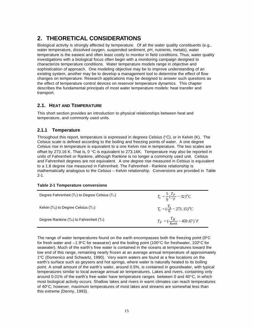
2.1.3 Density Density is defined as the mass of a substance per unit volume. Unlike most fluids, density of water is not a monotonic function of temperature. Density of water may be calculated using equation (2-1),

55

44

33

2210 TaTaTaTaTaao +++++=ρ (2-1)

where ρo is density of fresh water (kg m-3), and the constants are

a0 = 999.842594 a1 = 6.793952 x 10-2

a2 = -9.09529 x 10-3 a3 = 1.001685 x 10-4 a4 = -1.120083 x 10-6 a5 = 6.536332 x 10-9

The temperature – density relationship is shown graphically in Figure 2-1 below.

992

994

996

998

1000

0 5 10 15 20 25 30 35 40

Temperature (oC)

Den

sity

of

Wat

er (

kg

m-3

)

Figure 2-1 Density of pure water as function of temperature

This temperature-density relationship has a profound affect on temperature regimes of aquatic systems, explaining why ice floats, and the water at the bottom of a lake is typically around 4°C. Water reaches its maximum density at 3.98°C, as shown in Figure 2-1 above.

Density of seawater differs slightly from that of pure water, its freezing point as well as its maximum density point are lowered by dissolved salt. Density as a function of salinity S, is given by equation (2-2),

2*

2/3** SCSBSAow +++= ρρ (2-2)

where ρo is density of fresh water (kg m-3), and

17

4937

2531*

103875.5102467.8

106438.7100899.41024493.8

TxTx

TxTxxA−−

−−−

+−

+−=

(2-3)

2643* 106546.1100227.11072466.5 TxTxxB −−− −+−= (2-4)

4

* 108314.4 −= xC (2-5)

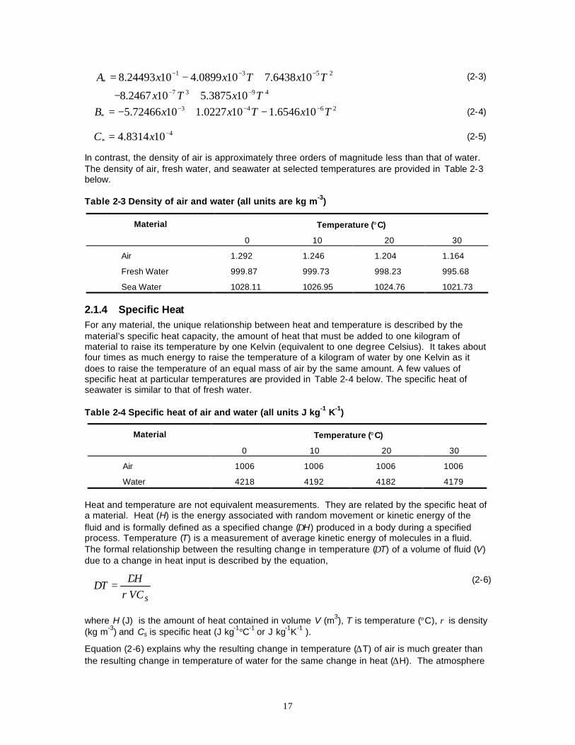
In contrast, the density of air is approximately three orders of magnitude less than that of water. The density of air, fresh water, and seawater at selected temperatures are provided in Table 2-3 below.

Table 2-3 Density of air and water (all units are kg m-3)

Material Temperature (°C)

0 10 20 30

Air 1.292 1.246 1.204 1.164

Fresh Water 999.87 999.73 998.23 995.68

Sea Water 1028.11 1026.95 1024.76 1021.73

2.1.4 Specific Heat For any material, the unique relationship between heat and temperature is described by the material’s specific heat capacity, the amount of heat that must be added to one kilogram of material to raise its temperature by one Kelvin (equivalent to one degree Celsius). It takes about four times as much energy to raise the temperature of a kilogram of water by one Kelvin as it does to raise the temperature of an equal mass of air by the same amount. A few values of specific heat at particular temperatures are provided in Table 2-4 below. The specific heat of seawater is similar to that of fresh water.

Table 2-4 Specific heat of air and water (all units J kg-1 K-1)

Material Temperature (°C)

0 10 20 30

Air 1006 1006 1006 1006

Water 4218 4192 4182 4179 Heat and temperature are not equivalent measurements. They are related by the specific heat of a material. Heat (H) is the energy associated with random movement or kinetic energy of the fluid and is formally defined as a specified change (∆H) produced in a body during a specified process. Temperature (T) is a measurement of average kinetic energy of molecules in a fluid. The formal relationship between the resulting change in temperature (∆T) of a volume of fluid (V) due to a change in heat input is described by the equation,

sVCH

Tρ

∆∆ =

(2-6)

where H (J) is the amount of heat contained in volume V (m3), T is temperature (°C), ρ is density (kg m-3) and Cs is specific heat (J kg-1°C-1 or J kg-1K-1 ).

Equation (2-6) explains why the resulting change in temperature (∆T) of air is much greater than the resulting change in temperature of water for the same change in heat (∆H). The atmosphere

18

responds relatively quickly to changes in heat input. Water bodies respond comparatively slowly, due to the difference between their specific heats.

2.2. THE ENERGY BUDGET

Most water temperature models are based on the laws of conservation of energy. For the purposes of water temperature modeling, energy input is typically normalized for surface area, so that units of energy flux density (W m-2), rather than units of energy flux (W or J s-1) are used to describe energy exchange at the air-water and bed-water interfaces. The sign convention used herein is positive (+) for heat entering the water’s surface, and negative (-) for heat leaving the water’s surface.

The first law of thermodynamics (conservation of energy) states that energy cannot be created nor destroyed, only converted from one form to another. The exchange between water (i.e., a lake or river) and its surroundings (i.e., the overlying atmosphere and channel bed) may be expressed as conservation of energy,

outenergyheatinenergyheatfluxheatnetstorageheatinchange −==

(2-7)

For a lake or river, net heat flux is typically expressed as,

ghbatmswnet qqqqqqq +++++= l (2-8)

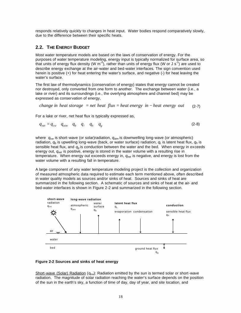
where qsw is short-wave (or solar)radiation, qatm is downwelling long-wave (or atmospheric) radiation, qb is upwelling long-wave (back, or water surface) radiation, qL is latent heat flux, qh is sensible heat flux, and qg is conduction between the water and the bed. When energy in exceeds energy out, qnet is positive, energy is stored in the water volume with a resulting rise in temperature. When energy out exceeds energy in, qnet is negative, and energy is lost from the water volume with a resulting fall in temperature. A large component of any water temperature modeling project is the collection and organization of measured atmospheric data required to estimate each term mentioned above, often described in water quality models as sources and/or sinks of heat. Sources and sinks of heat are summarized in the following section. A schematic of sources and sinks of heat at the air- and bed-water interfaces is shown in Figure 2-2 and summarized in the following section.

short-waveradiationqsw atmospheric

qatm

long-wave radiationwatersurfaceqb evaporation

latent heat fluxqL

condensation

conduction

sensible heat fluxqh

ground heat fluxqg

air

water

bed

Figure 2-2 Sources and sinks of heat energy

Short-wave (Solar) Radiation (qsw): Radiation emitted by the sun is termed solar or short-wave radiation. The magnitude of solar radiation reaching the water’s surface depends on the position of the sun in the earth’s sky, a function of time of day, day of year, and site location, and

19

attenuation of the solar beam due to atmospheric particles and cloud cover. Solar radiation is always positive in sign during the day, zero during nighttime hours, and typically varies from around 50 to 500 Wm-2.

Long-wave Radiation (qatm and qb): Radiation emitted by terrestrial objects and the earth’s atmosphere is termed long-wave radiation. The magnitude of long-wave radiation is a strong function of the surface temperature of the emitting object. Radiation emitted by the earth’s atmosphere toward the water’s surface is positive in sign, is a strong function of air temperature, and generally varies from around 30 to 450 Wm-2. Radiation emitted by the water’s surface is negative in sign, is a strong function of water temperature, and generally varies from around 300 to 500 Wm-2.

Latent Heat Flux (qL): A gain (or loss) of energy occurs as a result of a change in phase such as condensation or evaporation. The magnitude of latent heat flux is a function of water temperature and atmospheric conditions including vapor pressure and atmospheric turbulence. For example, evaporation proceeds most quickly on a day when relative humidity is low and wind speed is high. Evaporation is negative in sign. Condensation is positive in sign. Evaporative heat loss typically varies from around 100 to 600 Wm-2 if water temperature is at or near equilibrium.

Sensible Heat Flux (qh): Heat conduction occurs when two fluids of different temperature come in contact with each other, in this case, air and water. Sensible heat is conduction between the water surface and the atmosphere. The magnitude of sensible heat flux is a function of water temperature and atmospheric conditions such as air temperature and atmospheric turbulence. Sensible heat is positive in sign when air temperature is greater than water temperature and negative in sign when water temperature is greater than air temperature. Sensible heat typically varies from around 100 to 600 Wm-2, if water temperature is at or near equilibrium.

Ground Heat Conduction (qg): Ground heat conduction occurs between water and the bed, and is a function of water temperature, bed temperature, heat storage capacity of bed material, and thermal diffusivity of bed material. Ground heat conduction is positive in sign when bed temperature is greater than water temperature and negative in sign when water temperature is greater than bed temperature.

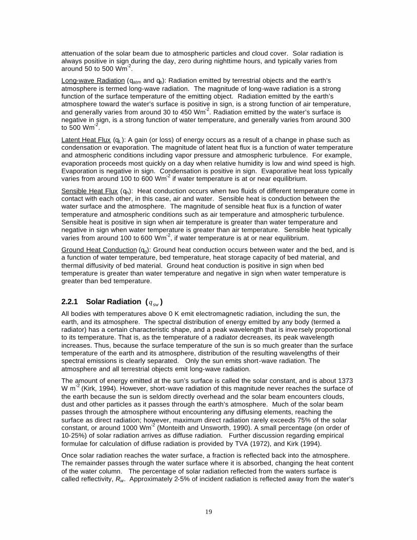
2.2.1 Solar Radiation ( swq )

All bodies with temperatures above 0 K emit electromagnetic radiation, including the sun, the earth, and its atmosphere. The spectral distribution of energy emitted by any body (termed a radiator) has a certain characteristic shape, and a peak wavelength that is inve rsely proportional to its temperature. That is, as the temperature of a radiator decreases, its peak wavelength increases. Thus, because the surface temperature of the sun is so much greater than the surface temperature of the earth and its atmosphere, distribution of the resulting wavelengths of their spectral emissions is clearly separated. Only the sun emits short-wave radiation. The atmosphere and all terrestrial objects emit long-wave radiation.

The amount of energy emitted at the sun’s surface is called the solar constant, and is about 1373 W m-2 (Kirk, 1994). However, short-wave radiation of this magnitude never reaches the surface of the earth because the sun is seldom directly overhead and the solar beam encounters clouds, dust and other particles as it passes through the earth’s atmosphere. Much of the solar beam passes through the atmosphere without encountering any diffusing elements, reaching the surface as direct radiation; however, maximum direct radiation rarely exceeds 75% of the solar constant, or around 1000 Wm-2 (Monteith and Unsworth, 1990). A small percentage (on order of 10-25%) of solar radiation arrives as diffuse radiation. Further discussion regarding empirical formulae for calculation of diffuse radiation is provided by TVA (1972), and Kirk (1994).

Once solar radiation reaches the water surface, a fraction is reflected back into the atmosphere. The remainder passes through the water surface where it is absorbed, changing the heat content of the water column. The percentage of solar radiation reflected from the waters surface is called reflectivity, Rw. Approximately 2-5% of incident radiation is reflected away from the water’s

20

surface at most solar altitudes; however, at sunrise and sunset, when solar altitude (α) is nearly zero, reflectivity increases rapidly toward 100%. These processes are illustrated schematically in Figure 2-3.

α

absoption and scatteringby clouds and particles

Top of Atmosphere

reflection at water surface

Qo Solar Constant

Figure 2-3 Attenuation of the solar beam by the earth’s atmosphere.

Solar radiation may be measured relatively inexpensively, and is reported by some weather stations. If measured solar radiation is not available, solar radiation reaching the earth’s surface may be estimated by,

asosw CRaHq )1( −= τ (2-9)

where Ho the amount of solar radiation reaching the earth’s outer atmosphere, Rs is albedo or the reflection coefficient, aτ is atmospheric attenuation (unitless), and Ca is the fraction of solar radiation not absorbed by clouds. The fraction of radiation passing through clouds is given by,

265.01 La CC −= (2-10)

where LC is the fraction of sky covered by clouds.

Extraterrestrial Radiation

The flux of short-wave radiation reaching the earth’s outer atmosphere may be estimated by

( ) ( )[ ] Γ

−+= be

sco hh

rH

H sinsincoscos12

sinsin2 δφπ

δφ (2-11)

where Hsc is the solar constant (1390 W m-2), r is the relative distance between the earth and sun, φ is latitude of the local meridian (radians), δ is declination in radians, and he is solar hour angle (radians) at the end of the time period and hb is solar angle (radians) at the beginning of the time period over which Ho is being calculated, and Γ is a correction factor for diurnal radiation flux (0 between sunset and sunrise, 1 between sunrise and sunset). The relative earth sun distance may be estimated by,

( )

−+= JDr 1853652

cos017.00.1π

(2-12)

where JD is Julian Day (1 on January 1).

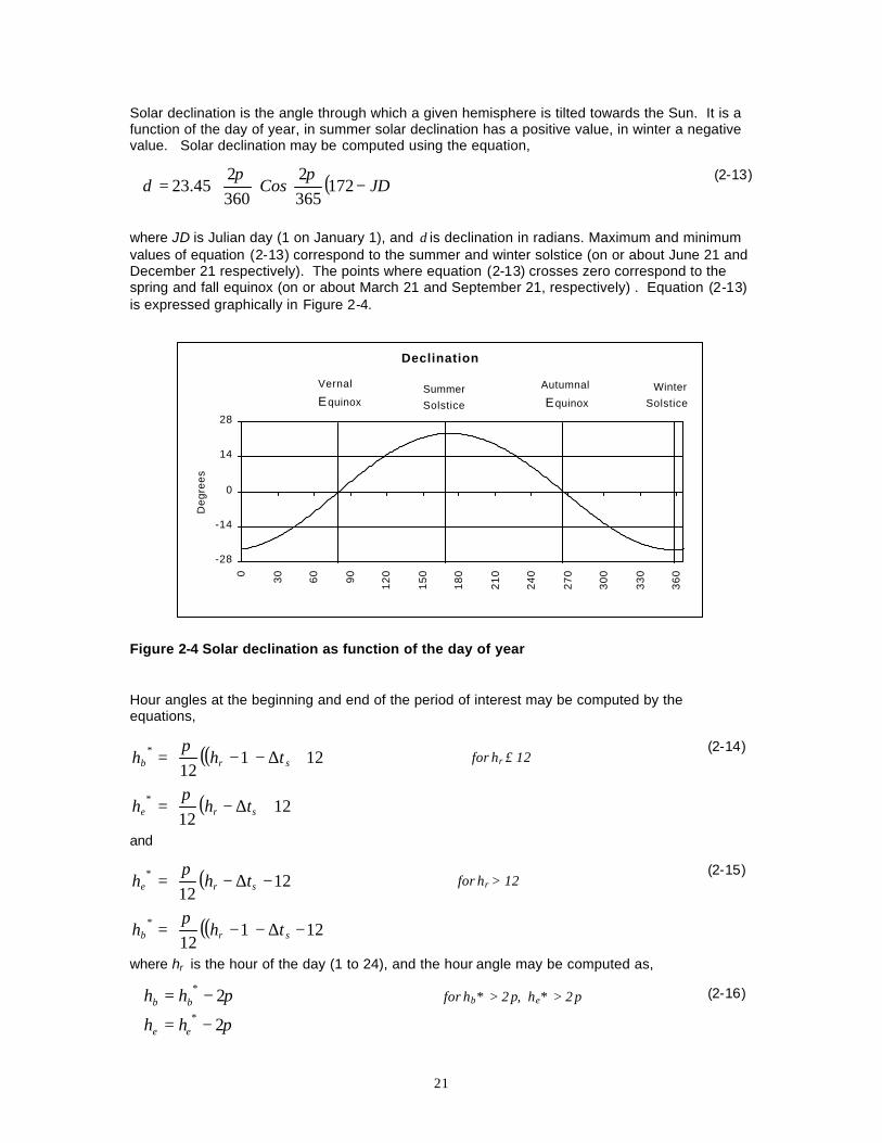
21

Solar declination is the angle through which a given hemisphere is tilted towards the Sun. It is a function of the day of year, in summer solar declination has a positive value, in winter a negative value. Solar declination may be computed using the equation,

( )

−

= JDCos 172

3652

3602

45.23ππ

δ (2-13)

where JD is Julian day (1 on January 1), and δ is declination in radians. Maximum and minimum values of equation (2-13) correspond to the summer and winter solstice (on or about June 21 and December 21 respectively). The points where equation (2-13) crosses zero correspond to the spring and fall equinox (on or about March 21 and September 21, respectively) . Equation (2-13) is expressed graphically in Figure 2-4.

Declination

-28

-14

0

14

28

0

30

60

90

12

0

15

0

18

0

21

0

24

0

27

0

30

0

33

0

36

0

Deg

rees

Vernal

EquinoxSummer

Solstice

Autumnal

Equinox

Winter

Solstice

Figure 2-4 Solar declination as function of the day of year

Hour angles at the beginning and end of the period of interest may be computed by the equations,

( )( )

+∆−−= 12112

*srb thh

π for hr ≤ 12

( )

+∆−= 1212

*sre thh

π

(2-14)

and

( )

−∆−= 1212

*sre thh

π for hr > 12

( )( )

−∆−−= 12112

*srb thh

π

(2-15)

where hr is the hour of the day (1 to 24), and the hour angle may be computed as,

π2* −= bb hh for hb* > 2 π, he* > 2 π

π2* −= ee hh

(2-16)

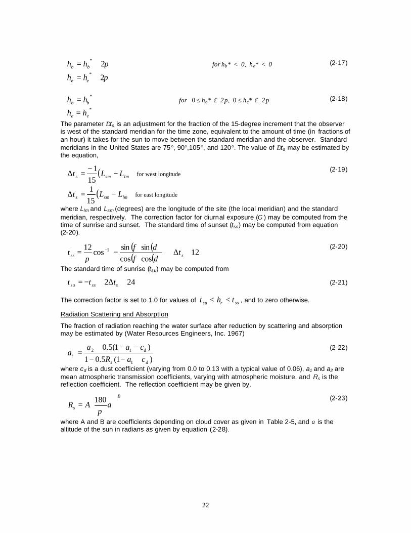
22

π2* += bb hh for hb* < 0, he* < 0

π2* += ee hh

(2-17)

*

bb hh = for 0 ≤ hb* ≤ 2π, 0 ≤ he* ≤ 2π *

ee hh =

(2-18)

The parameter ∆ts is an adjustment for the fraction of the 15-degree increment that the observer is west of the standard meridian for the time zone, equivalent to the amount of time (in fractions of an hour) it takes for the sun to move between the standard meridian and the observer. Standard meridians in the United States are 75°, 90°,105°, and 120°. The value of ∆ts may be estimated by the equation,

( )lmsms LLt −−

=∆15

1 for west longitude

( )lmsms LLt −=∆151

for east longitude

(2-19)

where Llm and Lsm (degrees) are the longitude of the site (the local meridian) and the standard meridian, respectively. The correction factor for diurnal exposure (Γ ) may be computed from the time of sunrise and sunset. The standard time of sunset (tss) may be computed from equation (2-20).

( ) ( )( ) ( ) 12

coscossinsin

cos12 1 +∆+

−= −

sss ttδφδφ

π

(2-20)

The standard time of sunrise (tsu) may be computed from

242 +∆+−= ssssu ttt (2-21)

The correction factor is set to 1.0 for values of ssrsu tht << , and to zero otherwise.

Radiation Scattering and Absorption

The fraction of radiation reaching the water surface after reduction by scattering and absorption may be estimated by (Water Resources Engineers, Inc. 1967)

)1(5.01)1(5.0

1

12

ds

d

caRcaa

a+−−−−+

=τ (2-22)

where cd is a dust coefficient (varying from 0.0 to 0.13 with a typical value of 0.06), a1 and a2 are mean atmospheric transmission coefficients, varying with atmospheric moisture, and Rs is the reflection coefficient. The reflection coefficient may be given by,

B

s AR

= α

π180

(2-23)

where A and B are coefficients depending on cloud cover as given in Table 2-5, and α is the altitude of the sun in radians as given by equation (2-28).

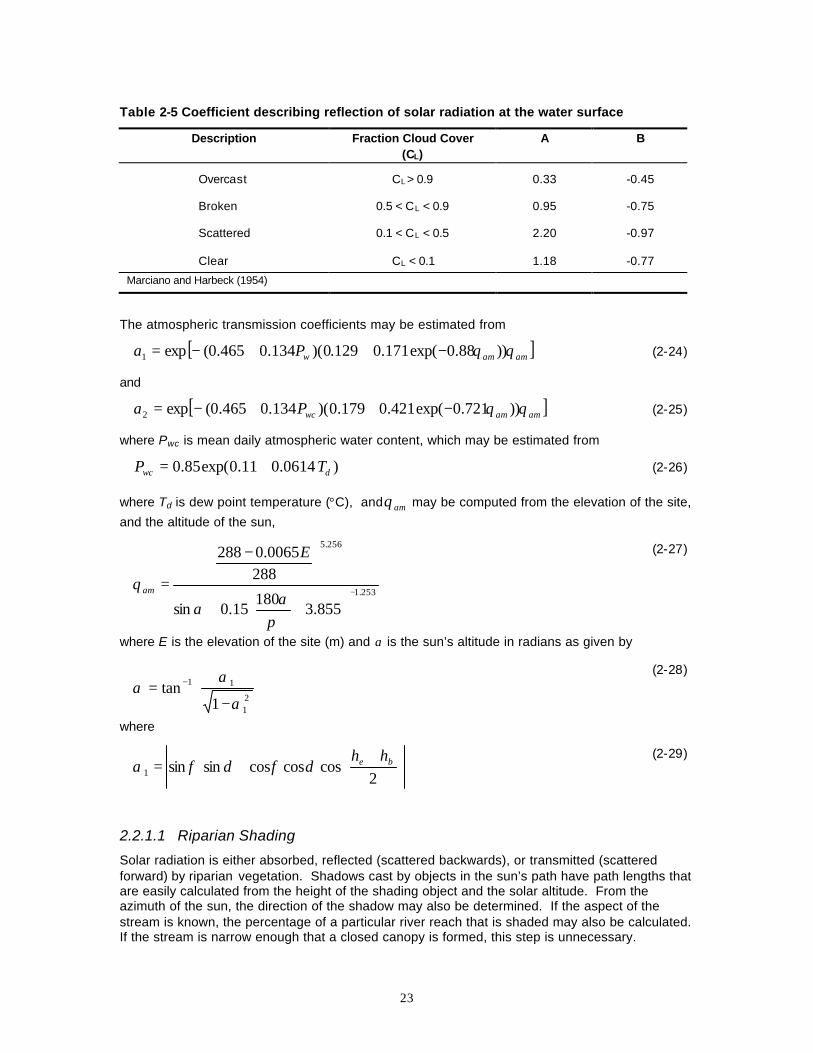
23

Table 2-5 Coefficient describing reflection of solar radiation at the water surface

Description Fraction Cloud Cover (CL)

A B

Overcast CL > 0.9 0.33 -0.45

Broken 0.5 < CL < 0.9 0.95 -0.75

Scattered 0.1 < CL < 0.5 2.20 -0.97

Clear CL < 0.1 1.18 -0.77

Marciano and Harbeck (1954)

The atmospheric transmission coefficients may be estimated from

[ ]amamwPa θθ ))88.0exp(171.0129.0)(134.0465.0(exp1 −++−= (2-24)

and

[ ]amamwcPa θθ ))721.0exp(421.0179.0)(134.0465.0(exp2 −++−= (2-25)

where Pwc is mean daily atmospheric water content, which may be estimated from

)0614.011.0exp(85.0 dwc TP += (2-26)

where Td is dew point temperature (°C), and amθ may be computed from the elevation of the site,

and the altitude of the sun,

253.1

256.5

855.3180

15.0sin

2880065.0288

−

++

−

=

πα

α

θ

E

am

(2-27)

where E is the elevation of the site (m) and α is the sun’s altitude in radians as given by

−= −

21

11

1tan

α

αα

(2-28)

where

++=

2coscoscossinsin1

be hhδφδφα

(2-29)

2.2.1.1 Riparian Shading

Solar radiation is either absorbed, reflected (scattered backwards), or transmitted (scattered forward) by riparian vegetation. Shadows cast by objects in the sun’s path have path lengths that are easily calculated from the height of the shading object and the solar altitude. From the azimuth of the sun, the direction of the shadow may also be determined. If the aspect of the stream is known, the percentage of a particular river reach that is shaded may also be calculated. If the stream is narrow enough that a closed canopy is formed, this step is unnecessary.

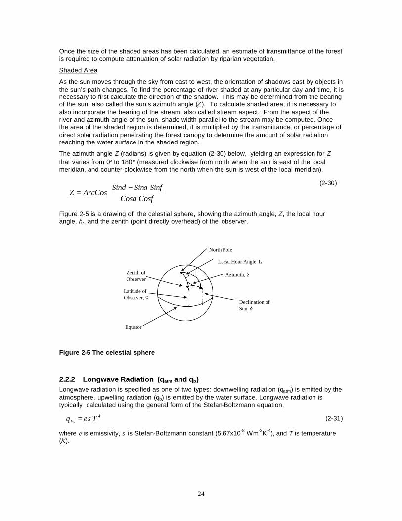
24

Once the size of the shaded areas has been calculated, an estimate of transmittance of the forest is required to compute attenuation of solar radiation by riparian vegetation.

Shaded Area

As the sun moves through the sky from east to west, the orientation of shadows cast by objects in the sun’s path changes. To find the percentage of river shaded at any particular day and time, it is necessary to first calculate the direction of the shadow. This may be determined from the bearing of the sun, also called the sun’s azimuth angle (Z). To calculate shaded area, it is necessary to also incorporate the bearing of the stream, also called stream aspect. From the aspect of the river and azimuth angle of the sun, shade width parallel to the stream may be computed. Once the area of the shaded region is determined, it is multiplied by the transmittance, or percentage of direct solar radiation penetrating the forest canopy to determine the amount of solar radiation reaching the water surface in the shaded region.

The azimuth angle Z (radians) is given by equation (2-30) below, yielding an expression for Z that varies from 0° to 180° (measured clockwise from north when the sun is east of the local meridian, and counter-clockwise from the north when the sun is west of the local meridian),

−=

φαφαδ

CosCosSinSinSin

ArcCosZ

(2-30)

Figure 2-5 is a drawing of the celestial sphere, showing the azimuth angle, Z, the local hour angle, hr, and the zenith (point directly overhead) of the observer.

North Pole

Declination ofSun, δ

Local Hour Angle, hr

Azimuth, ZZenith ofObserver

Latitude ofObserver, φ

Equator

Figure 2-5 The celestial sphere

2.2.2 Longwave Radiation (qatm and qb) Longwave radiation is specified as one of two types: downwelling radiation (qatm) is emitted by the atmosphere, upwelling radiation (qb) is emitted by the water surface. Longwave radiation is typically calculated using the general form of the Stefan-Boltzmann equation,

4Tq lw εσ= (2-31)

where ε is emissivity, σ is Stefan-Boltzmann constant (5.67x10-8 Wm-2K-4), and T is temperature (K).

25

2.2.2.1 Downwelling Longwave Radiation

The emissivity of a clear atmosphere can be much lower than the assumed emissivity of objects on the earth’s surface. Clouds increase emissivity, as do particles in the atmosphere. Many empirical formulae are available for computing atmospheric emissivities, most assume a strong dependence on atmospheric vapor content. A commonly used expression is based on work by Wunderlich (1968, 1972),

6)17.01(97.0 aLoatm TCq += ασ (2-32)

where Ta is air temperature (K), and αo is a proportionality constant,

510937.0 −= xoα (2-33)

Longwave radiation is relatively easy to measure directly; however, it is not routinely reported by standard weather stations, and is typically computed using an equation similar to (2-32).

2.2.2.2 Upwelling Longwave Radiation

For most objects on the earth’s surface, emissivity is assumed to be around 0.97. Using the Stefan-Boltzmann equation, long-wave radiation emitted by the water’s surface may be computed as

4)16.273(97.0 +−= wb Tq σ (2-34)

where Tw is water temperature (oC), and the negative sign indicates heat flux away from the water surface.

2.2.3 Latent Heat Flux (qL) Water is unique in that it exists in all three phases (ice, liquid and vapor) at temperatures and pressures found on the earth’s surface. Energy associated with a phase change is termed latent heat because energy is essentially locked up in liquid, gaseous or frozen water and is not transferred until the phase change occurs. For evaporation and condensation, the amount of energy associated with a phase change can be quite large. The energy required to evaporate one kilogram of water is roughly equivalent to the amount of energy required to raise the temperature of six kilograms of water from 0°C to 100°C (Oke, 1984). Latent heat for various phase changes as a function of temperature is given in Table 2-6 below.

2.2.3.1 Basic Expressions of Atmospheric Moisture Content

Most expressions for latent heat flux used in water temperature modeling are mass transfer type or relationships which describe latent heat flux as a function of vapor pressure of the overlying air mass (an expression of moisture content), wind speed, and water temperature. Vapor pressure may be derived from relative humidity, wet bulb, or dew point data. Important definitions and conversions for latent heat flux calculations follow.

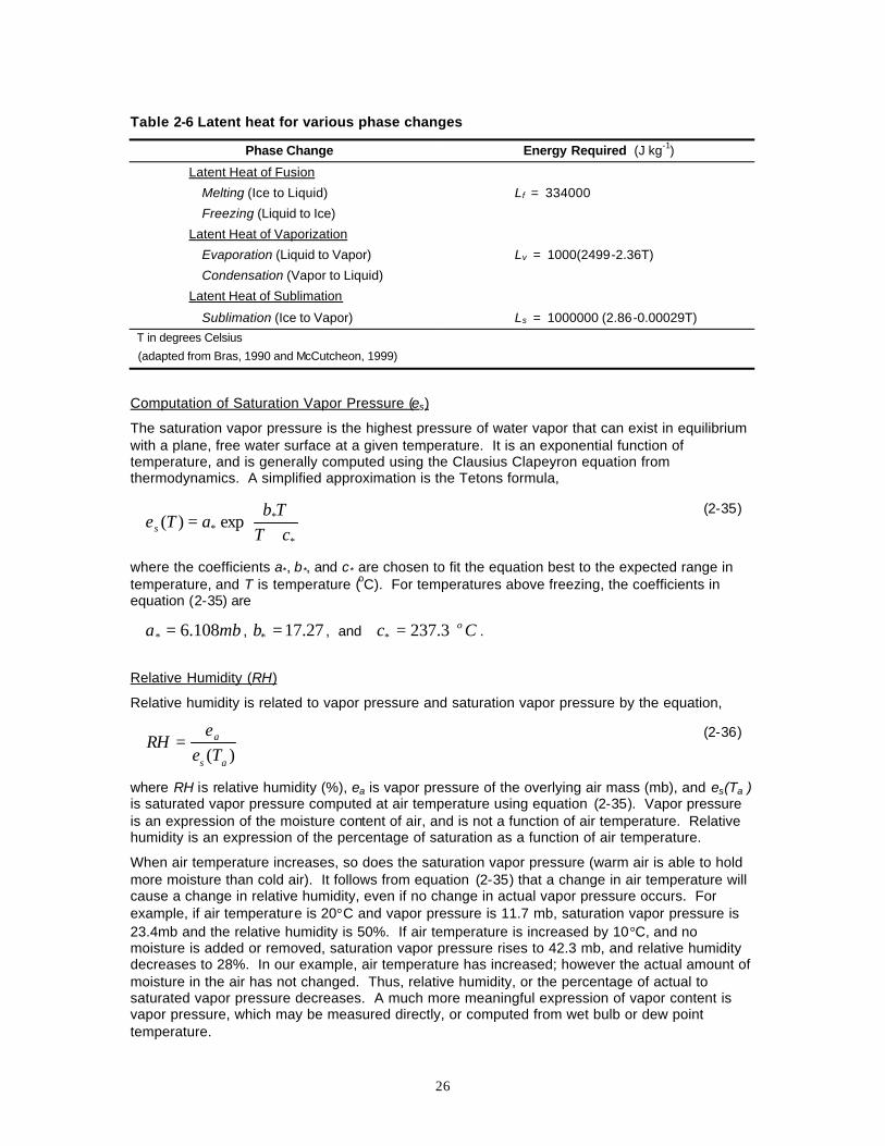
26

Table 2-6 Latent heat for various phase changes

Phase Change Energy Required (J kg-1)

Latent Heat of Fusion

Melting (Ice to Liquid)

Freezing (Liquid to Ice)

Lf = 334000

Latent Heat of Vaporization

Evaporation (Liquid to Vapor)

Condensation (Vapor to Liquid)

Lv = 1000(2499-2.36T)

Latent Heat of Sublimation

Sublimation (Ice to Vapor)

Ls = 1000000 (2.86-0.00029T) T in degrees Celsius

(adapted from Bras, 1990 and McCutcheon, 1999)

Computation of Saturation Vapor Pressure (e s)

The saturation vapor pressure is the highest pressure of water vapor that can exist in equilibrium with a plane, free water surface at a given temperature. It is an exponential function of temperature, and is generally computed using the Clausius Clapeyron equation from thermodynamics. A simplified approximation is the Tetons formula,

+

=*

** exp)(

cTTb

aTes (2-35)

where the coefficients a*, b*, and c* are chosen to fit the equation best to the expected range in temperature, and T is temperature (oC). For temperatures above freezing, the coefficients in equation (2-35) are

mba 108.6* = , 27.17* =b , and Cc o3.237* = .

Relative Humidity (RH)

Relative humidity is related to vapor pressure and saturation vapor pressure by the equation,

)( as

a

Tee

RH = (2-36)

where RH is relative humidity (%), ea is vapor pressure of the overlying air mass (mb), and es(Ta ) is saturated vapor pressure computed at air temperature using equation (2-35). Vapor pressure is an expression of the moisture content of air, and is not a function of air temperature. Relative humidity is an expression of the percentage of saturation as a function of air temperature.

When air temperature increases, so does the saturation vapor pressure (warm air is able to hold more moisture than cold air). It follows from equation (2-35) that a change in air temperature will cause a change in relative humidity, even if no change in actual vapor pressure occurs. For example, if air temperature is 20°C and vapor pressure is 11.7 mb, saturation vapor pressure is 23.4mb and the relative humidity is 50%. If air temperature is increased by 10°C, and no moisture is added or removed, saturation vapor pressure rises to 42.3 mb, and relative humidity decreases to 28%. In our example, air temperature has increased; however the actual amount of moisture in the air has not changed. Thus, relative humidity, or the percentage of actual to saturated vapor pressure decreases. A much more meaningful expression of vapor content is vapor pressure, which may be measured directly, or computed from wet bulb or dew point temperature.

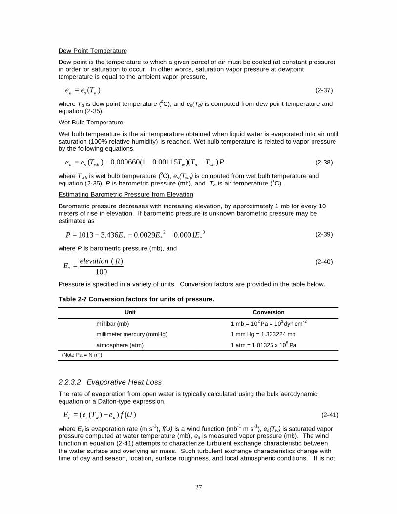
27

Dew Point Temperature

Dew point is the temperature to which a given parcel of air must be cooled (at constant pressure) in order for saturation to occur. In other words, saturation vapor pressure at dewpoint temperature is equal to the ambient vapor pressure,

)( dsa Tee = (2-37)

where Td is dew point temperature (oC), and es(Td) is computed from dew point temperature and equation (2-35).

Wet Bulb Temperature

Wet bulb temperature is the air temperature obtained when liquid water is evaporated into air until saturation (100% relative humidity) is reached. Wet bulb temperature is related to vapor pressure by the following equations,

PTTTTee wbawwbsa ))(00115.01(000660.0)( −+−= (2-38)

where Twb is wet bulb temperature (oC), es(Twb) is computed from wet bulb temperature and equation (2-35), P is barometric pressure (mb), and Ta is air temperature (oC).

Estimating Barometric Pressure from Elevation

Barometric pressure decreases with increasing elevation, by approximately 1 mb for every 10 meters of rise in elevation. If barometric pressure is unknown barometric pressure may be estimated as

3*

2** 0001.00029.0436.31013 EEEP +−−= (2-39)

where P is barometric pressure (mb), and

100)(

*ftelevation

E = (2-40)

Pressure is specified in a variety of units. Conversion factors are provided in the table below.

Table 2-7 Conversion factors for units of pressure.

Unit Conversion

millibar (mb) 1 mb = 102 Pa = 103 dyn cm -2

millimeter mercury (mmHg) 1 mm Hg = 1.333224 mb

atmosphere (atm) 1 atm = 1.01325 x 105 Pa

(Note Pa = N m-2)

2.2.3.2 Evaporative Heat Loss

The rate of evaporation from open water is typically calculated using the bulk aerodynamic equation or a Dalton-type expression,

)())(( UfeTeE awsr −= (2-41)

where Er is evaporation rate (m s-1), f(U) is a wind function (mb-1 m s-1), es(Tw) is saturated vapor

pressure computed at water temperature (mb), ea is measured vapor pressure (mb). The wind function in equation (2-41) attempts to characterize turbulent exchange characteristic between the water surface and overlying air mass. Such turbulent exchange characteristics change with time of day and season, location, surface roughness, and local atmospheric conditions. It is not

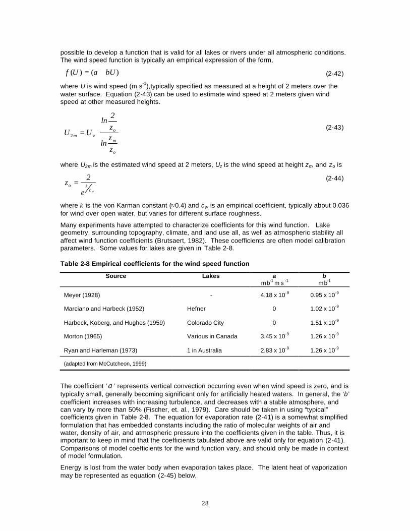
28

possible to develop a function that is valid for all lakes or rivers under all atmospheric conditions. The wind speed function is typically an empirical expression of the form,

)()( bUaUf += (2-42)

where U is wind speed (m s-1),typically specified as measured at a height of 2 meters over the water surface. Equation (2-43) can be used to estimate wind speed at 2 meters given wind speed at other measured heights.

=

o

m

ozm

zz

ln

z2

lnUU 2

(2-43)

where U2m is the estimated wind speed at 2 meters, Uz is the wind speed at height zm, and zo is

wco

e

2z

κ=

(2-44)

where κ is the von Karman constant (≈0.4) and cw is an empirical coefficient, typically about 0.036 for wind over open water, but varies for different surface roughness.

Many experiments have attempted to characterize coefficients for this wind function. Lake geometry, surrounding topography, climate, and land use all, as well as atmospheric stability all affect wind function coefficients (Brutsaert, 1982). These coefficients are often model calibration parameters. Some values for lakes are given in Table 2-8.

Table 2-8 Empirical coefficients for the wind speed function

Source Lakes a mb-1 m s -1

b mb-1

Meyer (1928) - 4.18 x 10-9 0.95 x 10-9

Marciano and Harbeck (1952) Hefner 0 1.02 x 10-9

Harbeck, Koberg, and Hughes (1959) Colorado City 0 1.51 x 10-9

Morton (1965) Various in Canada 3.45 x 10-9 1.26 x 10-9

Ryan and Harleman (1973) 1 in Australia 2.83 x 10-9 1.26 x 10-9

(adapted from McCutcheon, 1999)

The coefficient ‘ a ’ represents vertical convection occurring even when wind speed is zero, and is typically small, generally becoming significant only for artificially heated waters. In general, the ‘b’ coefficient increases with increasing turbulence, and decreases with a stable atmosphere, and can vary by more than 50% (Fischer, et. al., 1979). Care should be taken in using “typical” coefficients given in Table 2-8. The equation for evaporation rate (2-41) is a somewhat simplified formulation that has embedded constants including the ratio of molecular weights of air and water, density of air, and atmospheric pressure into the coefficients given in the table. Thus, it is important to keep in mind that the coefficients tabulated above are valid only for equation (2-41). Comparisons of model coefficients for the wind function vary, and should only be made in context of model formulation.

Energy is lost from the water body when evaporation takes place. The latent heat of vaporization may be represented as equation (2-45) below,

29

rvw ELq ρ=l (2-45)

where Er is evaporation rate is given by equation (2-41), ρw is density of the water (kg m-3) being evaporated as given by equation (2-2), and Lv is latent heat of vaporization (J kg-1), as given in Table 2-6 above.

2.2.4 Sensible Heat Flux ( hq )

Sensible heat describes the flux of heat through molecular or turbulent transfer between the air and water surface. The amount of heat gained or lost through sensible heat depends on the gradient of temperature in the vertical direction. The most widely applied formulation for takes advantage of the analogy between vapor and heat transport. The Bowen Ratio describes the relationship between heat and vapor transport, which has been observed to be valid over varying conditions. The Bowen Ratio is described by the equation,

−

−==

aws

aw

refB

h

eTeTT

PP

Cqq

B)(l

(2-46)

where the coefficient CB is equal to approximately 0.61 mb, P is atmospheric pressure (mb), and Pref is a reference pressure at mean sea level, Tw is water surface temperature (oC), Ta is air temperature (oC), es is saturated vapor pressure computed at water surface temperature (mb), and ea is vapor pressure of the air (mb). An expression for sensible heat is obtained by substituting equation (2-45) into equation (2-46), and rearranging to obtain the expression for sensible heat transfer below,

)()( waref

Bvwh TTPP

CUfLq −= ρ (2-47)

where f(U) is the wind function (mb-1 m s-1) given as equation(2-42), ρw is density of water, Lw is latent heat of vaporization (J kg-1). The wind function varies slightly for sensible and latent heat; however, the same wind function may be used for most water temperature applications.

2.2.5 Ground Heat Conduction Heat flux through soil is governed by thermal conductivity, heat capacity and thermal diffusivity. Thermal conductivity is a measure of the ability of the bed to conduct heat and has units (W m-1 K-1). Thermal conductivity is not a simple constant for a particular bed. It varies both in depth and time, depending upon soil porosity and moisture content. Heat capacity relates the temperature changed produced as a result of a gain or loss of heat. The value of heat capacity for a given soil is strongly dependent on the soil moisture content. Thermal diffusivity of a soil describes its ability to diffuse thermal influences, essentially controlling the speed at which temperature waves move downward into the soil. Thermal diffusivity is related to thermal conductivity and heat capacity by the equation,

b

bb C

k=κ

(2-48)

where κb is thermal diffusivity of the bed (m2 s-1), kb is thermal conductivity (W m-1K-1) of bed material, and Cb is heat capacity of the bed(J m-3 K-1). Heat flux between the water and the streambed may be described by

0=∂∂

−=z

bbb z

Tkq

(2-49)

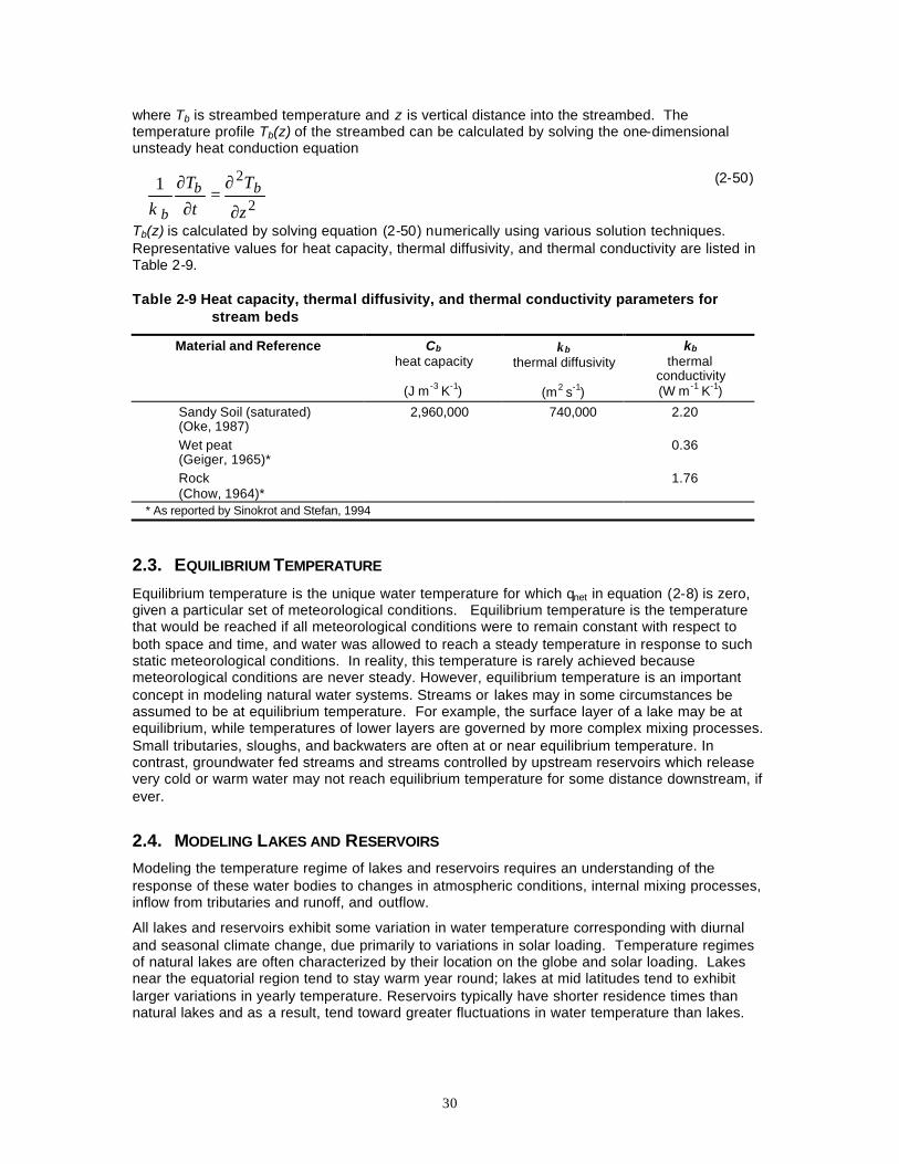
30

where Tb is streambed temperature and z is vertical distance into the streambed. The temperature profile Tb(z) of the streambed can be calculated by solving the one-dimensional unsteady heat conduction equation

2

21

z

Tt

T bb

b ∂

∂=

∂∂

κ

(2-50)

Tb(z) is calculated by solving equation (2-50) numerically using various solution techniques. Representative values for heat capacity, thermal diffusivity, and thermal conductivity are listed in Table 2-9.

Table 2-9 Heat capacity, thermal diffusivity, and thermal conductivity parameters for stream beds

Material and Reference Cb

heat capacity

(J m -3 K-1)

κb thermal diffusivity

(m2 s-1)

kb

thermal conductivity (W m -1 K-1)

Sandy Soil (saturated) (Oke, 1987)

2,960,000 740,000 2.20

Wet peat (Geiger, 1965)*

0.36

Rock (Chow, 1964)*

1.76

* As reported by Sinokrot and Stefan, 1994

2.3. EQUILIBRIUM TEMPERATURE

Equilibrium temperature is the unique water temperature for which qnet in equation (2-8) is zero, given a particular set of meteorological conditions. Equilibrium temperature is the temperature that would be reached if all meteorological conditions were to remain constant with respect to both space and time, and water was allowed to reach a steady temperature in response to such static meteorological conditions. In reality, this temperature is rarely achieved because meteorological conditions are never steady. However, equilibrium temperature is an important concept in modeling natural water systems. Streams or lakes may in some circumstances be assumed to be at equilibrium temperature. For example, the surface layer of a lake may be at equilibrium, while temperatures of lower layers are governed by more complex mixing processes. Small tributaries, sloughs, and backwaters are often at or near equilibrium temperature. In contrast, groundwater fed streams and streams controlled by upstream reservoirs which release very cold or warm water may not reach equilibrium temperature for some distance downstream, if ever.

2.4. MODELING LAKES AND RESERVOIRS Modeling the temperature regime of lakes and reservoirs requires an understanding of the response of these water bodies to changes in atmospheric conditions, internal mixing processes, inflow from tributaries and runoff, and outflow.

All lakes and reservoirs exhibit some variation in water temperature corresponding with diurnal and seasonal climate change, due primarily to variations in solar loading. Temperature regimes of natural lakes are often characterized by their location on the globe and solar loading. Lakes near the equatorial region tend to stay warm year round; lakes at mid latitudes tend to exhibit larger variations in yearly temperature. Reservoirs typically have shorter residence times than natural lakes and as a result, tend toward greater fluctuations in water temperature than lakes.

31

2.4.1 Lake and Reservoir Heat Budgets The rate of change of heat content in a lake or reservoir is determined by the rate of heat transport into and out of the water body at the air- and bed-water interfaces, as well as transport of heat from inflows and outflows. The surface of most lakes can be assumed to be at or near equilibrium temperature. However, water temperature beneath the surface is seldom at equilibrium temperature, and only sometimes isothermal. With the exception of solar radiation, energy exchange takes place at the surface of the reservoir. Solar radiation passes through the water surface, and is attenuated by absorption and scattering in the water column; nearly all radiation outside the visible range is absorbed within the first meter or so of the water column, only visible light may penetrate to deeper layers of the impoundment. After this initial absorption, attenuation of visible light follows the relationship described by Beer’s Law

zswsz eqq ηβ −−= )1( (2-51)

where β is the ratio of radiation absorbed at the surface to net incoming radiation, z is depth below the water surface, η is bulk extinction coefficient, and qsw is net solar radiation penetrating the waters surface. Both β and η exhibit large ranges, depending upon the presence of suspended particles. For an extensive review of this topic, see Kirk (1994).

Heat conduction between the bed and its overlying water is typically small except in very clear, shallow lakes, where solar radiation passes through the water column with minimum extinction, heating underlying sediments. In such cases, sediments generally act as a source of heat during the fall and winter, and a sink for heat during the summer.

2.4.2 Internal Temperature Dynamics While energy flux (i.e., solar radiation, longwave radiation, latent and sensible heat flux) determines heat load into a lake or reservoir, fluid movement within the water body determine heat distribution within the lake itself. Deep impoundments tend to exhibit a characteristic cycle of vertical stratification. In the spring, the reservoir may be isothermal throughout (temperature is vertically uniform). In cold climates, this uniform temperature tends toward the that of the maximum density of water (i.e. 4°C). As summer approaches, surface layers of the reservoir begin to warm in response to increasing intensity of solar radiation. Solar radiation decreases exponentially with depth. In deep lakes, solar radiation eventually reaches extinction at some depth, so that deep in the lake, no warming occurs and water temperature does not change from fully mixed conditions. Wind acts to mix water near the top of the lake, gradually mixing warm surface water with layers of cooler water beneath, to distribute heat downward. The result of this combination forces is a layer of warm, less dense water overlying layers of colder, denser water below. The thickness of this zone of mixing is a function of solar intensity and the wind regime, along with other factors which affect mixing and solar extinction such as turbidity and lake geometry. Throughout the summer, continued input of solar radiation accompanied by wind mixing continue to warm the surface layer, making it increasingly less dense than cool water below. This process results in stratification, a common occurrence in deep temperate lakes during summer months. A sharp temperature gradient called a thermocline forms in the metalimnion, the region that separates the top layer (epilimnion) from the bottom layer (hypolimnion). Water motion in the epilimnion is dominated by wind mixing, while motion in the hypolimnion, protected from wind induced mixing by the thermocline, tends to be sluggish or quiescent. Figure 2-6 shows a schematic of these mixing layers.

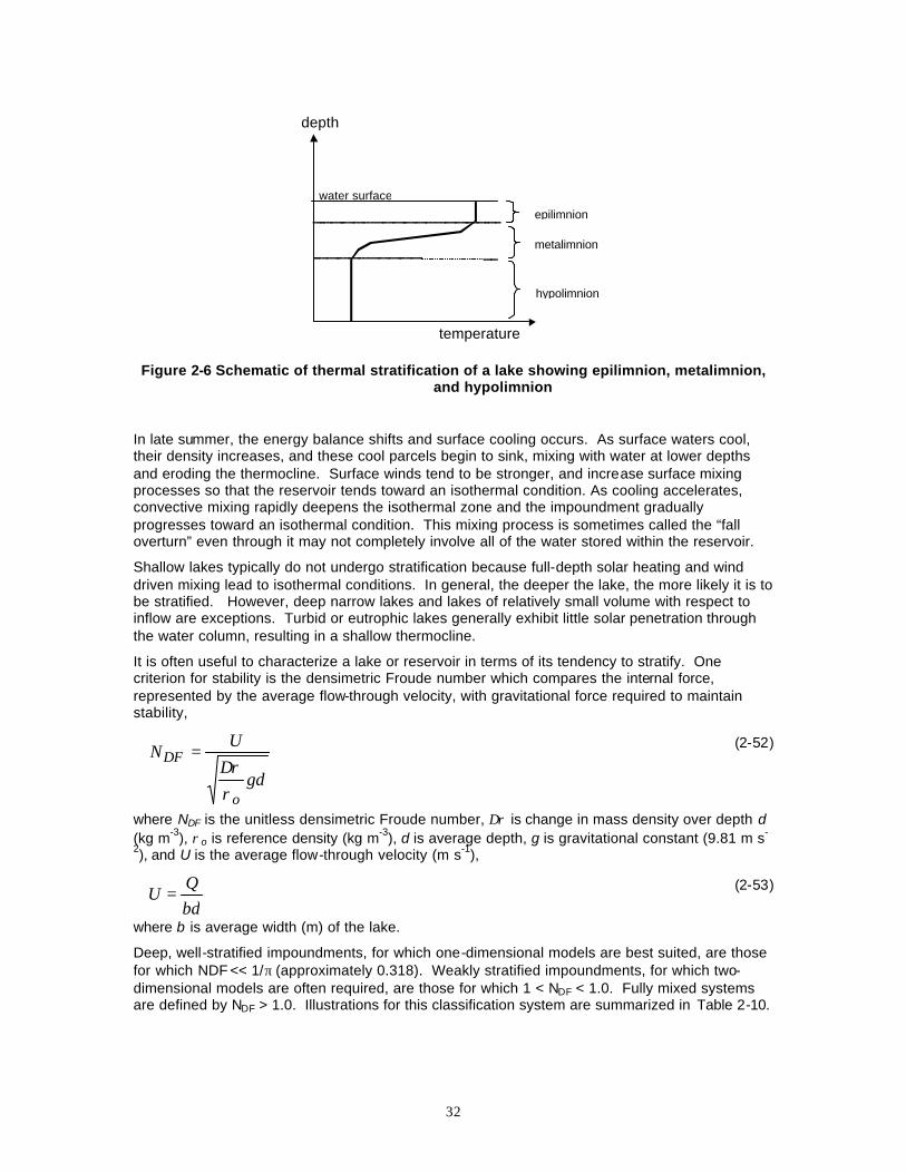
32

temperature

depth

water surface

epilimnion

metalimnion

hypolimnion

Figure 2-6 Schematic of thermal stratification of a lake showing epilimnion, metalimnion,

and hypolimnion

In late summer, the energy balance shifts and surface cooling occurs. As surface waters cool, their density increases, and these cool parcels begin to sink, mixing with water at lower depths and eroding the thermocline. Surface winds tend to be stronger, and increase surface mixing processes so that the reservoir tends toward an isothermal condition. As cooling accelerates, convective mixing rapidly deepens the isothermal zone and the impoundment gradually progresses toward an isothermal condition. This mixing process is sometimes called the “fall overturn” even through it may not completely involve all of the water stored within the reservoir.

Shallow lakes typically do not undergo stratification because full-depth solar heating and wind driven mixing lead to isothermal conditions. In general, the deeper the lake, the more likely it is to be stratified. However, deep narrow lakes and lakes of relatively small volume with respect to inflow are exceptions. Turbid or eutrophic lakes generally exhibit little solar penetration through the water column, resulting in a shallow thermocline.

It is often useful to characterize a lake or reservoir in terms of its tendency to stratify. One criterion for stability is the densimetric Froude number which compares the internal force, represented by the average flow-through velocity, with gravitational force required to maintain stability,

gd

UN

o

DF

ρρ∆

= (2-52)

where NDF is the unitless densimetric Froude number, ∆ρ is change in mass density over depth d (kg m-3), ρo is reference density (kg m-3), d is average depth, g is gravitational constant (9.81 m s-

2), and U is the average flow-through velocity (m s-1),

bdQ

U = (2-53)

where b is average width (m) of the lake.

Deep, well-stratified impoundments, for which one-dimensional models are best suited, are those for which NDF << 1/π (approximately 0.318). Weakly stratified impoundments, for which two-dimensional models are often required, are those for which 1 < NDF < 1.0. Fully mixed systems are defined by NDF > 1.0. Illustrations for this classification system are summarized in Table 2-10.

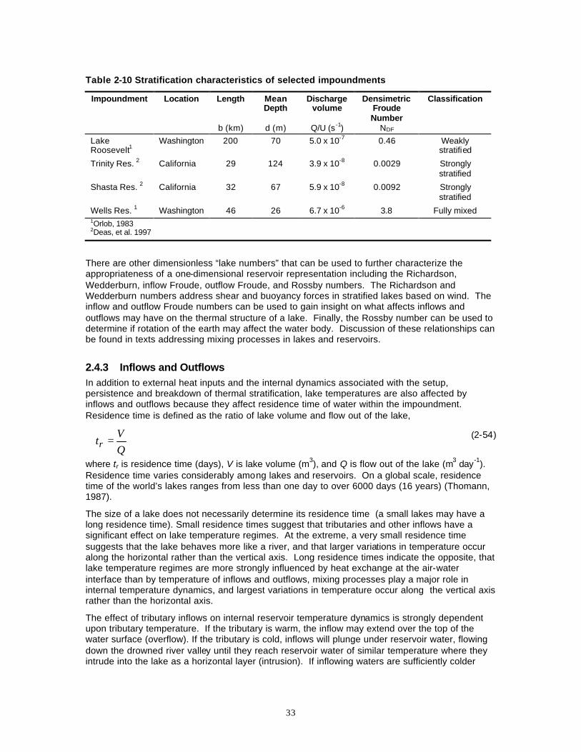
33

Table 2-10 Stratification characteristics of selected impoundments

Impoundment Location Length

b (km)

Mean Depth

d (m)

Discharge volume

Q/U (s -1)

Densimetric Froude Number

NDF

Classification

Lake Roosevelt1

Washington 200 70 5.0 x 10-7 0.46 Weakly stratified

Trinity Res. 2 California 29 124 3.9 x 10-8 0.0029 Strongly stratified

Shasta Res. 2 California 32 67 5.9 x 10-8 0.0092 Strongly stratified

Wells Res. 1 Washington 46 26 6.7 x 10-6 3.8 Fully mixed 1Orlob, 1983 2Deas, et al. 1997

There are other dimensionless “lake numbers” that can be used to further characterize the appropriateness of a one-dimensional reservoir representation including the Richardson, Wedderburn, inflow Froude, outflow Froude, and Rossby numbers. The Richardson and Wedderburn numbers address shear and buoyancy forces in stratified lakes based on wind. The inflow and outflow Froude numbers can be used to gain insight on what affects inflows and outflows may have on the thermal structure of a lake. Finally, the Rossby number can be used to determine if rotation of the earth may affect the water body. Discussion of these relationships can be found in texts addressing mixing processes in lakes and reservoirs.

2.4.3 Inflows and Outflows In addition to external heat inputs and the internal dynamics associated with the setup, persistence and breakdown of thermal stratification, lake temperatures are also affected by inflows and outflows because they affect residence time of water within the impoundment. Residence time is defined as the ratio of lake volume and flow out of the lake,

QV

tr = (2-54)

where tr is residence time (days), V is lake volume (m3), and Q is flow out of the lake (m3 day-1). Residence time varies considerably among lakes and reservoirs. On a global scale, residence time of the world’s lakes ranges from less than one day to over 6000 days (16 years) (Thomann, 1987).

The size of a lake does not necessarily determine its residence time (a small lakes may have a long residence time). Small residence times suggest that tributaries and other inflows have a significant effect on lake temperature regimes. At the extreme, a very small residence time suggests that the lake behaves more like a river, and that larger variations in temperature occur along the horizontal rather than the vertical axis. Long residence times indicate the opposite, that lake temperature regimes are more strongly influenced by heat exchange at the air-water interface than by temperature of inflows and outflows, mixing processes play a major role in internal temperature dynamics, and largest variations in temperature occur along the vertical axis rather than the horizontal axis.

The effect of tributary inflows on internal reservoir temperature dynamics is strongly dependent upon tributary temperature. If the tributary is warm, the inflow may extend over the top of the water surface (overflow). If the tributary is cold, inflows will plunge under reservoir water, flowing down the drowned river valley until they reach reservoir water of similar temperature where they intrude into the lake as a horizontal layer (intrusion). If inflowing waters are sufficiently colder

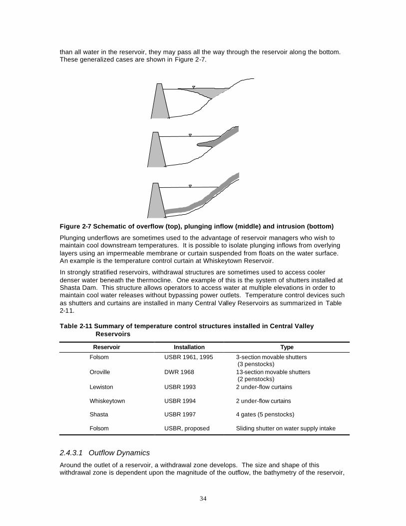
34

than all water in the reservoir, they may pass all the way through the reservoir along the bottom. These generalized cases are shown in Figure 2-7.

Figure 2-7 Schematic of overflow (top), plunging inflow (middle) and intrusion (bottom)

Plunging underflows are sometimes used to the advantage of reservoir managers who wish to maintain cool downstream temperatures. It is possible to isolate plunging inflows from overlying layers using an impermeable membrane or curtain suspended from floats on the water surface. An example is the temperature control curtain at Whiskeytown Reservoir.

In strongly stratified reservoirs, withdrawal structures are sometimes used to access cooler denser water beneath the thermocline. One example of this is the system of shutters installed at Shasta Dam. This structure allows operators to access water at multiple elevations in order to maintain cool water releases without bypassing power outlets. Temperature control devices such as shutters and curtains are installed in many Central Valley Reservoirs as summarized in Table 2-11.

Table 2-11 Summary of temperature control structures installed in Central Valley Reservoirs

Reservoir Installation Type

Folsom USBR 1961, 1995 3-section movable shutters (3 penstocks)

Oroville DWR 1968 13-section movable shutters (2 penstocks)

Lewiston USBR 1993 2 under-flow curtains

Whiskeytown USBR 1994 2 under-flow curtains

Shasta USBR 1997 4 gates (5 penstocks)

Folsom USBR, proposed Sliding shutter on water supply intake

2.4.3.1 Outflow Dynamics

Around the outlet of a reservoir, a withdrawal zone develops. The size and shape of this withdrawal zone is dependent upon the magnitude of the outflow, the bathymetry of the reservoir,

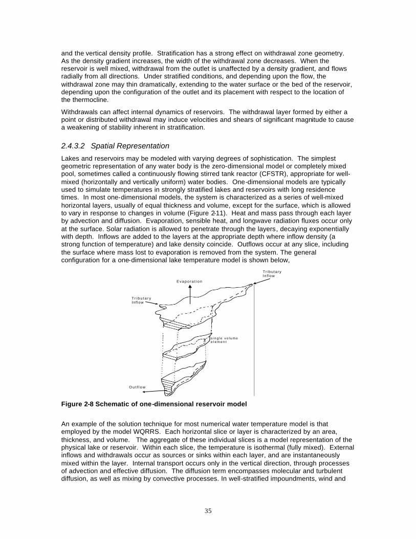
35

and the vertical density profile. Stratification has a strong effect on withdrawal zone geometry. As the density gradient increases, the width of the withdrawal zone decreases. When the reservoir is well mixed, withdrawal from the outlet is unaffected by a density gradient, and flows radially from all directions. Under stratified conditions, and depending upon the flow, the withdrawal zone may thin dramatically, extending to the water surface or the bed of the reservoir, depending upon the configuration of the outlet and its placement with respect to the location of the thermocline.

Withdrawals can affect internal dynamics of reservoirs. The withdrawal layer formed by either a point or distributed withdrawal may induce velocities and shears of significant magnitude to cause a weakening of stability inherent in stratification.

2.4.3.2 Spatial Representation

Lakes and reservoirs may be modeled with varying degrees of sophistication. The simplest geometric representation of any water body is the zero-dimensional model or completely mixed pool, sometimes called a continuously flowing stirred tank reactor (CFSTR), appropriate for well-mixed (horizontally and vertically uniform) water bodies. One-dimensional models are typically used to simulate temperatures in strongly stratified lakes and reservoirs with long residence times. In most one-dimensional models, the system is characterized as a series of well-mixed horizontal layers, usually of equal thickness and volume, except for the surface, which is allowed to vary in response to changes in volume (Figure 2-11). Heat and mass pass through each layer by advection and diffusion. Evaporation, sensible heat, and longwave radiation fluxes occur only at the surface. Solar radiation is allowed to penetrate through the layers, decaying exponentially with depth. Inflows are added to the layers at the appropriate depth where inflow density (a strong function of temperature) and lake density coincide. Outflows occur at any slice, including the surface where mass lost to evaporation is removed from the system. The general configuration for a one-dimensional lake temperature model is shown below,

E v a p o r a t i o n

T r i bu ta ryIn f low

T r i b u t a r yIn f low

O u t f l o w

s i n g l e v o l u m ee l e m e n t

Figure 2-8 Schematic of one-dimensional reservoir model

An example of the solution technique for most numerical water temperature model is that employed by the model WQRRS. Each horizontal slice or layer is characterized by an area, thickness, and volume. The aggregate of these individual slices is a model representation of the physical lake or reservoir. Within each slice, the temperature is isothermal (fully mixed). External inflows and withdrawals occur as sources or sinks within each layer, and are instantaneously mixed within the layer. Internal transport occurs only in the vertical direction, through processes of advection and effective diffusion. The diffusion term encompasses molecular and turbulent diffusion, as well as mixing by convective processes. In well-stratified impoundments, wind and

36

convective mixing are the dominant mixing processes in the epilimnion; however, molecular diffusion may be the dominant mechanism in the hypolimnion. In weakly stratified reservoirs, wind-induced turbulent diffusion is the dominant mechanism throughout the lake. The one-dimensional equation for transport of heat in a reservoir may be written as,

yx

Cq

zT

Dz

zAzT

VzT

zQsw

netzzz

∆∆+

∂∂

∂∂

∆=∂∂

+∂∂

∆ρ

(2-55)

where T is laterally averaged temperature (°C), z is space coordinate in the vertical direction (m), Qz is vertical advection (m3 s-1), Az is surface layer of a particular element normal to direction of flow (m2), Dz is effective diffusion coefficient (m2 s-1), ρw is density of water (kg m-3), qnet is net heat flux at the air water interface for the surface layer, solar radiation penetrating to the appropriate depth in middle layers, and bed conduction in the bottom layer (W m-2), Cs is specific heat of water (kg °C J-1). Reservoirs with short residence times sometimes stratify longitudinally. An example of this is Keswick Reservoir, the re-regulating afterbay downstream of Shasta Dam. Such reservoirs are often modeled as one-dimensional longitudinal systems, essentially as slow, deep rivers. In some cases, two-dimensional laterally averaged models are applied to reservoirs that exhibit both longitudinal and vertical stratification characteristics simultaneously. For shallow impoundments, two-dimensional laterally-averaged models are sometimes appropriate. Three-dimensional models are sometimes appropriate for near-field problems; however, their application is beyond the scope of this report.

2.5. MODELING STREAMS AND RIVERS Many types of pollutants are discharged to rivers and streams. Water quality models have their origin in simulation of fate and transport of pollutants downstream from waste discharges. Transport of heat through a river system is a similar problem. While the equations and concepts are similar for both types of water quality applications, water temperature modeling in rivers presents some unique challenges. Thermal energy may energy and depart a stream or river at tributaries, drains and other inflows, heat exchange also takes place along the entire course of the river. Heat flux is a true distributed source, proposing a somewhat different modeling problem than a point source pollutant.

2.5.1 Transport Mechanisms To illustrate heat transport mechanisms, consider a tracer such as dye released into a river. Two basic transport mechanisms may be observed. Immediately, the tracer moves downstream. This bulk movement of the tracer with the main flow is termed advection. As the tracer moves downstream it simultaneously spreads in all directions due to diffusion and dispersion. Figure 2-9 is a schematic drawing that illustrates bulk movement of a tracer from point A to point B by advection, as well as simultaneous spreading of the tracer by dispersion and diffusion. For purposes of this discussion, we define downstream or longitudinal transport as movement in the x-direction, lateral, side-to-side, or transverse transport as movement in the y-direction, and vertical transport as movement in the z-direction. Figure 2-9 illustrates bulk movement of a tracer from point A to point B by advection, as well as simultaneous spreading of the tracer by dispersion and diffusion.

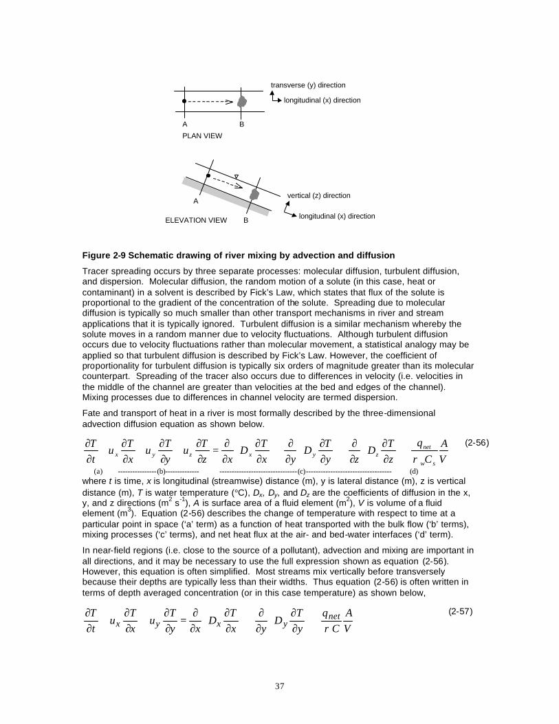
37

longitudinal (x) direction

transverse (y) direction

A B

PLAN VIEW

longitudinal (x) direction

vertical (z) directionA

BELEVATION VIEW

Figure 2-9 Schematic drawing of river mixing by advection and diffusion

Tracer spreading occurs by three separate processes: molecular diffusion, turbulent diffusion, and dispersion. Molecular diffusion, the random motion of a solute (in this case, heat or contaminant) in a solvent is described by Fick’s Law, which states that flux of the solute is proportional to the gradient of the concentration of the solute. Spreading due to molecular diffusion is typically so much smaller than other transport mechanisms in river and stream applications that it is typically ignored. Turbulent diffusion is a similar mechanism whereby the solute moves in a random manner due to velocity fluctuations. Although turbulent diffusion occurs due to velocity fluctuations rather than molecular movement, a statistical analogy may be applied so that turbulent diffusion is described by Fick’s Law. However, the coefficient of proportionality for turbulent diffusion is typically six orders of magnitude greater than its molecular counterpart. Spreading of the tracer also occurs due to differences in velocity (i.e. velocities in the middle of the channel are greater than velocities at the bed and edges of the channel). Mixing processes due to differences in channel velocity are termed dispersion.

Fate and transport of heat in a river is most formally described by the three-dimensional advection diffusion equation as shown below.

VA

Cq

zT

Dzy

TD

yxT

Dxz

Tu

yT

uxT

utT

sw

netzyxzyx ρ

+

∂∂

∂∂

+

∂∂

∂∂

+

∂∂

∂∂

=∂∂

+∂∂

+∂∂

+∂∂

(a) ----------------(b)-------------- --------------------------------(c)----------------------------------- (d)

(2-56)

where t is time, x is longitudinal (streamwise) distance (m), y is lateral distance (m), z is vertical distance (m), T is water temperature (°C), Dx, Dy, and Dz are the coefficients of diffusion in the x, y, and z directions (m2 s-1), A is surface area of a fluid element (m2), V is volume of a fluid element (m3). Equation (2-56) describes the change of temperature with respect to time at a particular point in space (‘a’ term) as a function of heat transported with the bulk flow (‘b’ terms), mixing processes (‘c’ terms), and net heat flux at the air- and bed-water interfaces (‘d’ term).

In near-field regions (i.e. close to the source of a pollutant), advection and mixing are important in all directions, and it may be necessary to use the full expression shown as equation (2-56). However, this equation is often simplified. Most streams mix vertically before transversely because their depths are typically less than their widths. Thus equation (2-56) is often written in terms of depth averaged concentration (or in this case temperature) as shown below,

VA

Cq

yT

Dyx

TD

xyT

uxT

utT net

yxyx ρ+

∂∂

∂∂

+

∂∂

∂∂

=∂∂

+∂∂

+∂∂

(2-57)

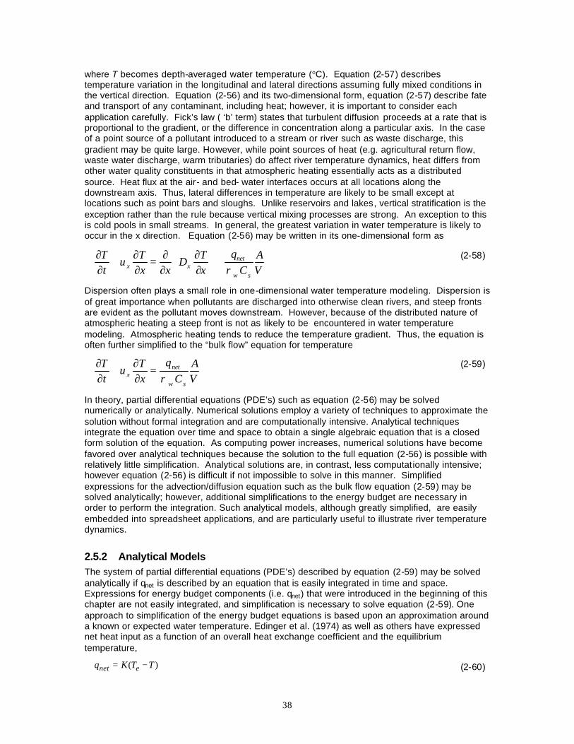
38

where T becomes depth-averaged water temperature (°C). Equation (2-57) describes temperature variation in the longitudinal and lateral directions assuming fully mixed conditions in the vertical direction. Equation (2-56) and its two-dimensional form, equation (2-57) describe fate and transport of any contaminant, including heat; however, it is important to consider each application carefully. Fick’s law ( ‘b’ term) states that turbulent diffusion proceeds at a rate that is proportional to the gradient, or the difference in concentration along a particular axis. In the case of a point source of a pollutant introduced to a stream or river such as waste discharge, this gradient may be quite large. However, while point sources of heat (e.g. agricultural return flow, waste water discharge, warm tributaries) do affect river temperature dynamics, heat differs from other water quality constituents in that atmospheric heating essentially acts as a distributed source. Heat flux at the air- and bed- water interfaces occurs at all locations along the downstream axis. Thus, lateral differences in temperature are likely to be small except at locations such as point bars and sloughs. Unlike reservoirs and lakes, vertical stratification is the exception rather than the rule because vertical mixing processes are strong. An exception to this is cold pools in small streams. In general, the greatest variation in water temperature is likely to occur in the x direction. Equation (2-56) may be written in its one-dimensional form as

VA

Cq

xT

Dxx

Tu

tT

sw

netxx ρ

+

∂∂

∂∂

=∂∂

+∂∂

(2-58)

Dispersion often plays a small role in one-dimensional water temperature modeling. Dispersion is of great importance when pollutants are discharged into otherwise clean rivers, and steep fronts are evident as the pollutant moves downstream. However, because of the distributed nature of atmospheric heating a steep front is not as likely to be encountered in water temperature modeling. Atmospheric heating tends to reduce the temperature gradient. Thus, the equation is often further simplified to the “bulk flow” equation for temperature

VA

Cq

xT

utT

sw

netx ρ

=∂∂

+∂∂

(2-59)

In theory, partial differential equations (PDE’s) such as equation (2-56) may be solved numerically or analytically. Numerical solutions employ a variety of techniques to approximate the solution without formal integration and are computationally intensive. Analytical techniques integrate the equation over time and space to obtain a single algebraic equation that is a closed form solution of the equation. As computing power increases, numerical solutions have become favored over analytical techniques because the solution to the full equation (2-56) is possible with relatively little simplification. Analytical solutions are, in contrast, less computationally intensive; however equation (2-56) is difficult if not impossible to solve in this manner. Simplified expressions for the advection/diffusion equation such as the bulk flow equation (2-59) may be solved analytically; however, additional simplifications to the energy budget are necessary in order to perform the integration. Such analytical models, although greatly simplified, are easily embedded into spreadsheet applications, and are particularly useful to illustrate river temperature dynamics.

2.5.2 Analytical Models The system of partial differential equations (PDE’s) described by equation (2-59) may be solved analytically if qnet is described by an equation that is easily integrated in time and space. Expressions for energy budget components (i.e. qnet) that were introduced in the beginning of this chapter are not easily integrated, and simplification is necessary to solve equation (2-59). One approach to simplification of the energy budget equations is based upon an approximation around a known or expected water temperature. Edinger et al. (1974) as well as others have expressed net heat input as a function of an overall heat exchange coefficient and the equilibrium temperature,

)( TTKq enet −= (2-60)

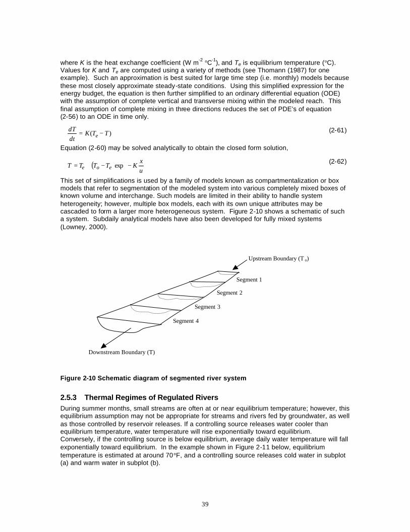
39

where K is the heat exchange coefficient (W m-2 °C-1), and Te is equilibrium temperature (°C). Values for K and Te are computed using a variety of methods (see Thomann (1987) for one example). Such an approximation is best suited for large time step (i.e. monthly) models because these most closely approximate steady-state conditions. Using this simplified expression for the energy budget, the equation is then further simplified to an ordinary differential equation (ODE) with the assumption of complete vertical and transverse mixing within the modeled reach. This final assumption of complete mixing in three directions reduces the set of PDE’s of equation (2-56) to an ODE in time only.

)( TTKdtdT

e −= (2-61)

Equation (2-60) may be solved analytically to obtain the closed form solution,

( )

−−+=

ux

KTTTT eoe exp (2-62)

This set of simplifications is used by a family of models known as compartmentalization or box models that refer to segmentation of the modeled system into various completely mixed boxes of known volume and interchange. Such models are limited in their ability to handle system heterogeneity; however, multiple box models, each with its own unique attributes may be cascaded to form a larger more heterogeneous system. Figure 2-10 shows a schematic of such a system. Subdaily analytical models have also been developed for fully mixed systems (Lowney, 2000).

Figure 2-10 Schematic diagram of segmented river system

2.5.3 Thermal Regimes of Regulated Rivers During summer months, small streams are often at or near equilibrium temperature; however, this equilibrium assumption may not be appropriate for streams and rivers fed by groundwater, as well as those controlled by reservoir releases. If a controlling source releases water cooler than equilibrium temperature, water temperature will rise exponentially toward equilibrium. Conversely, if the controlling source is below equilibrium, average daily water temperature will fall exponentially toward equilibrium. In the example shown in Figure 2-11 below, equilibrium temperature is estimated at around 70°F, and a controlling source releases cold water in subplot (a) and warm water in subplot (b).

Segment 1

Segment 2

Segment 3

Segment 4

Upstream Boundary (T o)

Downstream Boundary (T)

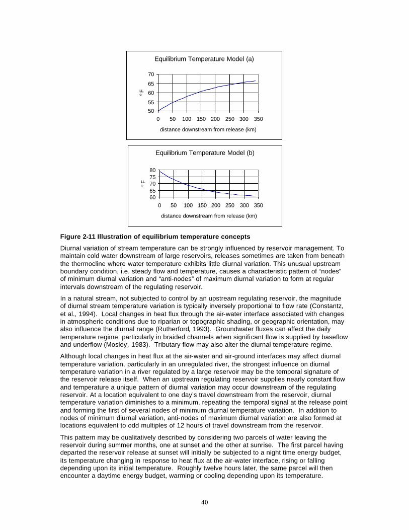
40

Equilibrium Temperature Model (a)

50

55

60

65

70

0 50 100 150 200 250 300 350

distance downstream from release (km)

o F

Equilibrium Temperature Model (b)

6065707580

0 50 100 150 200 250 300 350

distance downstream from release (km)

o F

Figure 2-11 Illustration of equilibrium temperature concepts

Diurnal variation of stream temperature can be strongly influenced by reservoir management. To maintain cold water downstream of large reservoirs, releases sometimes are taken from beneath the thermocline where water temperature exhibits little diurnal variation. This unusual upstream boundary condition, i.e. steady flow and temperature, causes a characteristic pattern of “nodes” of minimum diurnal variation and “anti-nodes” of maximum diurnal variation to form at regular intervals downstream of the regulating reservoir.

In a natural stream, not subjected to control by an upstream regulating reservoir, the magnitude of diurnal stream temperature variation is typically inversely proportional to flow rate (Constantz, et al., 1994). Local changes in heat flux through the air-water interface associated with changes in atmospheric conditions due to riparian or topographic shading, or geographic orientation, may also influence the diurnal range (Rutherford, 1993). Groundwater fluxes can affect the daily temperature regime, particularly in braided channels when significant flow is supplied by baseflow and underflow (Mosley, 1983). Tributary flow may also alter the diurnal temperature regime.

Although local changes in heat flux at the air-water and air-ground interfaces may affect diurnal temperature variation, particularly in an unregulated river, the strongest influence on diurnal temperature variation in a river regulated by a large reservoir may be the temporal signature of the reservoir release itself. When an upstream regulating reservoir supplies nearly constant flow and temperature a unique pattern of diurnal variation may occur downstream of the regulating reservoir. At a location equivalent to one day’s travel downstream from the reservoir, diurnal temperature variation diminishes to a minimum, repeating the temporal signal at the release point and forming the first of several nodes of minimum diurnal temperature variation. In addition to nodes of minimum diurnal variation, anti-nodes of maximum diurnal variation are also formed at locations equivalent to odd multiples of 12 hours of travel downstream from the reservoir.

This pattern may be qualitatively described by considering two parcels of water leaving the reservoir during summer months, one at sunset and the other at sunrise. The first parcel having departed the reservoir release at sunset will initially be subjected to a night time energy budget, its temperature changing in response to heat flux at the air-water interface, rising or falling depending upon its initial temperature. Roughly twelve hours later, the same parcel will then encounter a daytime energy budget, warming or cooling depending upon its temperature.

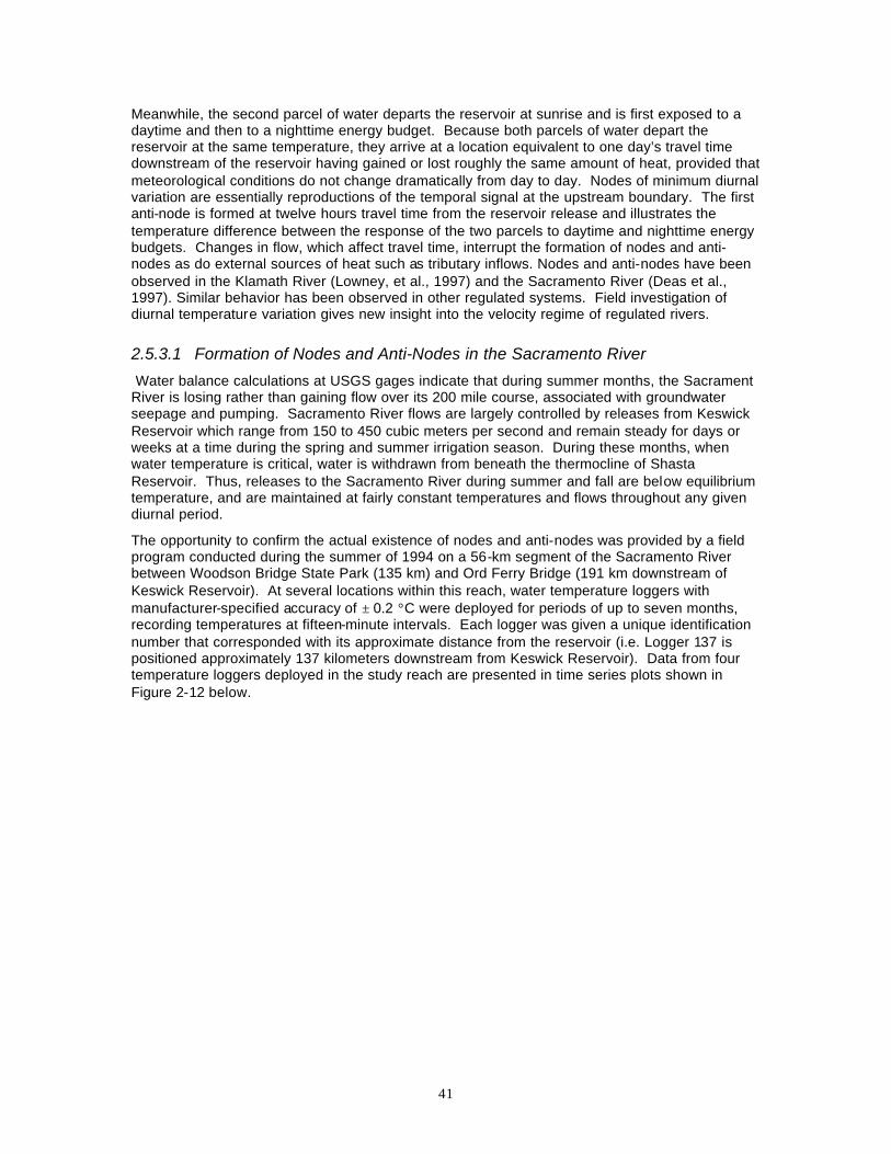
41

Meanwhile, the second parcel of water departs the reservoir at sunrise and is first exposed to a daytime and then to a nighttime energy budget. Because both parcels of water depart the reservoir at the same temperature, they arrive at a location equivalent to one day’s travel time downstream of the reservoir having gained or lost roughly the same amount of heat, provided that meteorological conditions do not change dramatically from day to day. Nodes of minimum diurnal variation are essentially reproductions of the temporal signal at the upstream boundary. The first anti-node is formed at twelve hours travel time from the reservoir release and illustrates the temperature difference between the response of the two parcels to daytime and nighttime energy budgets. Changes in flow, which affect travel time, interrupt the formation of nodes and anti-nodes as do external sources of heat such as tributary inflows. Nodes and anti-nodes have been observed in the Klamath River (Lowney, et al., 1997) and the Sacramento River (Deas et al., 1997). Similar behavior has been observed in other regulated systems. Field investigation of diurnal temperature variation gives new insight into the velocity regime of regulated rivers.

2.5.3.1 Formation of Nodes and Anti-Nodes in the Sacramento River

Water balance calculations at USGS gages indicate that during summer months, the Sacrament River is losing rather than gaining flow over its 200 mile course, associated with groundwater seepage and pumping. Sacramento River flows are largely controlled by releases from Keswick Reservoir which range from 150 to 450 cubic meters per second and remain steady for days or weeks at a time during the spring and summer irrigation season. During these months, when water temperature is critical, water is withdrawn from beneath the thermocline of Shasta Reservoir. Thus, releases to the Sacramento River during summer and fall are below equilibrium temperature, and are maintained at fairly constant temperatures and flows throughout any given diurnal period.

The opportunity to confirm the actual existence of nodes and anti-nodes was provided by a field program conducted during the summer of 1994 on a 56-km segment of the Sacramento River between Woodson Bridge State Park (135 km) and Ord Ferry Bridge (191 km downstream of Keswick Reservoir). At several locations within this reach, water temperature loggers with manufacturer-specified accuracy of ± 0.2 °C were deployed for periods of up to seven months, recording temperatures at fifteen-minute intervals. Each logger was given a unique identification number that corresponded with its approximate distance from the reservoir (i.e. Logger 137 is positioned approximately 137 kilometers downstream from Keswick Reservoir). Data from four temperature loggers deployed in the study reach are presented in time series plots shown in Figure 2-12 below.

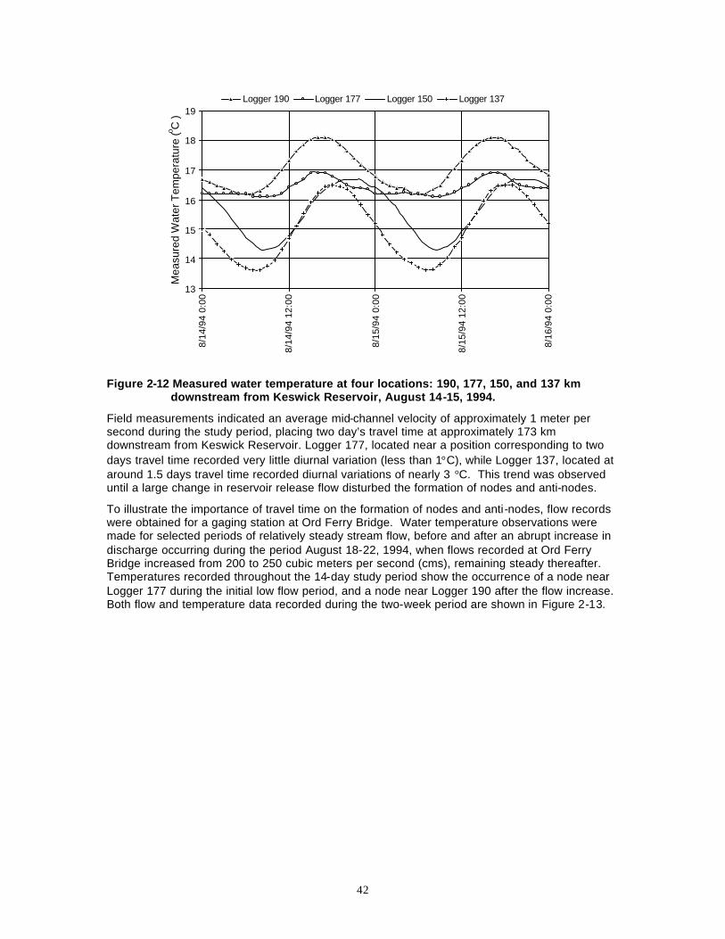
42

13

14

15

16

17

18

19

8/14

/94

0:00

8/14

/94

12:0

0

8/15

/94

0:00

8/15

/94

12:0

0

8/16

/94

0:00

Mea

sure

d W

ater

Tem

pera

ture

( o C )

Logger 190 Logger 177 Logger 150 Logger 137

Figure 2-12 Measured water temperature at four locations: 190, 177, 150, and 137 km

downstream from Keswick Reservoir, August 14-15, 1994.

Field measurements indicated an average mid-channel velocity of approximately 1 meter per second during the study period, placing two day’s travel time at approximately 173 km downstream from Keswick Reservoir. Logger 177, located near a position corresponding to two days travel time recorded very little diurnal variation (less than 1°C), while Logger 137, located at around 1.5 days travel time recorded diurnal variations of nearly 3 °C. This trend was observed until a large change in reservoir release flow disturbed the formation of nodes and anti-nodes.

To illustrate the importance of travel time on the formation of nodes and anti-nodes, flow records were obtained for a gaging station at Ord Ferry Bridge. Water temperature observations were made for selected periods of relatively steady stream flow, before and after an abrupt increase in discharge occurring during the period August 18-22, 1994, when flows recorded at Ord Ferry Bridge increased from 200 to 250 cubic meters per second (cms), remaining steady thereafter. Temperatures recorded throughout the 14-day study period show the occurrence of a node near Logger 177 during the initial low flow period, and a node near Logger 190 after the flow increase. Both flow and temperature data recorded during the two-week period are shown in Figure 2-13.

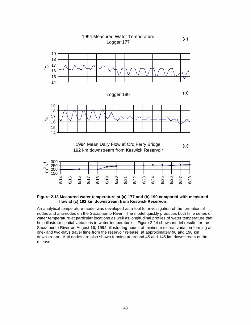
43

1994 Measured Water TemperatureLogger 177

141516171819

o C

(a)

Logger 190

141516171819

oC

(b)

1994 Mean Daily Flow at Ord Ferry Bridge192 km downstream from Keswick Reservoir

150200250300

8/14

8/15

8/16

8/17

8/18

8/19

8/20

8/21

8/22

8/23

8/24

8/25

8/26

8/27

8/28

m3 s-1

(c)

Figure 2-13 Measured water temperature at (a) 177 and (b) 190 compared with measured

flow at (c) 192 km downstream from Keswick Reservoir.

An analytical temperature model was developed as a tool for investigation of the formation of nodes and anti-nodes on the Sacramento River. The model quickly produces both time series of water temperature at particular locations as well as longitudinal profiles of water temperature that help illustrate spatial variations in water temperature. Figure 2-14 shows model results for the Sacramento River on August 16, 1994, illustrating nodes of minimum diurnal variation forming at one- and two-days travel time from the reservoir release, at approximately 90 and 190 km downstream. Anti-nodes are also shown forming at around 45 and 145 km downstream of the release.

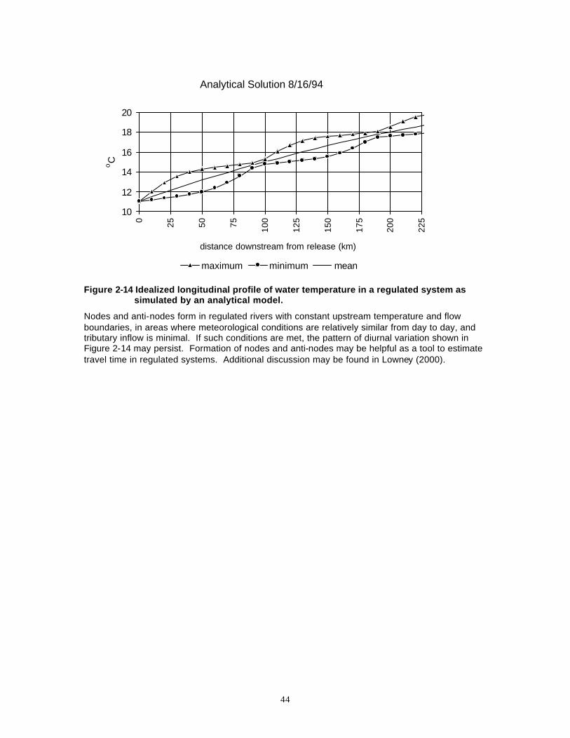
44

Analytical Solution 8/16/94

10

12

14

16

18

20

0 25 50 75 100

125

150

175

200

225

distance downstream from release (km)

oC

maximum minimum mean

Figure 2-14 Idealized longitudinal profile of water temperature in a regulated system as simulated by an analytical model.

Nodes and anti-nodes form in regulated rivers with constant upstream temperature and flow boundaries, in areas where meteorological conditions are relatively similar from day to day, and tributary inflow is minimal. If such conditions are met, the pattern of diurnal variation shown in Figure 2-14 may persist. Formation of nodes and anti-nodes may be helpful as a tool to estimate travel time in regulated systems. Additional discussion may be found in Lowney (2000).

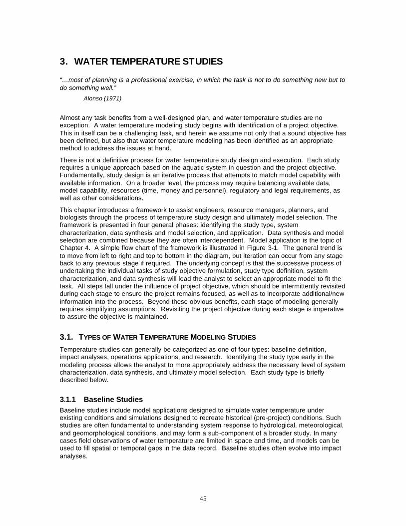
45

3. WATER TEMPERATURE STUDIES “…most of planning is a professional exercise, in which the task is not to do something new but to do something well.”

Alonso (1971)

Almost any task benefits from a well-designed plan, and water temperature studies are no exception. A water temperature modeling study begins with identification of a project objective. This in itself can be a challenging task, and herein we assume not only that a sound objective has been defined, but also that water temperature modeling has been identified as an appropriate method to address the issues at hand.

There is not a definitive process for water temperature study design and execution. Each study requires a unique approach based on the aquatic system in question and the project objective. Fundamentally, study design is an iterative process that attempts to match model capability with available information. On a broader level, the process may require balancing available data, model capability, resources (time, money and personnel), regulatory and legal requirements, as well as other considerations.

This chapter introduces a framework to assist engineers, resource managers, planners, and biologists through the process of temperature study design and ultimately model selection. The framework is presented in four general phases: identifying the study type, system characterization, data synthesis and model selection, and application. Data synthesis and model selection are combined because they are often interdependent. Model application is the topic of Chapter 4. A simple flow chart of the framework is illustrated in Figure 3-1. The general trend is to move from left to right and top to bottom in the diagram, but iteration can occur from any stage back to any previous stage if required. The underlying concept is that the successive process of undertaking the individual tasks of study objective formulation, study type definition, system characterization, and data synthesis will lead the analyst to select an appropriate model to fit the task. All steps fall under the influence of project objective, which should be intermittently revisited during each stage to ensure the project remains focused, as well as to incorporate additional/new information into the process. Beyond these obvious benefits, each stage of modeling generally requires simplifying assumptions. Revisiting the project objective during each stage is imperative to assure the objective is maintained.

3.1. TYPES OF WATER TEMPERATURE MODELING STUDIES Temperature studies can generally be categorized as one of four types: baseline definition, impact analyses, operations applications, and research. Identifying the study type early in the modeling process allows the analyst to more appropriately address the necessary level of system characterization, data synthesis, and ultimately model selection. Each study type is briefly described below.

3.1.1 Baseline Studies Baseline studies include model applications designed to simulate water temperature under existing conditions and simulations designed to recreate historical (pre-project) conditions. Such studies are often fundamental to understanding system response to hydrological, meteorological, and geomorphological conditions, and may form a sub-component of a broader study. In many cases field observations of water temperature are limited in space and time, and models can be used to fill spatial or temporal gaps in the data record. Baseline studies often evolve into impact analyses.

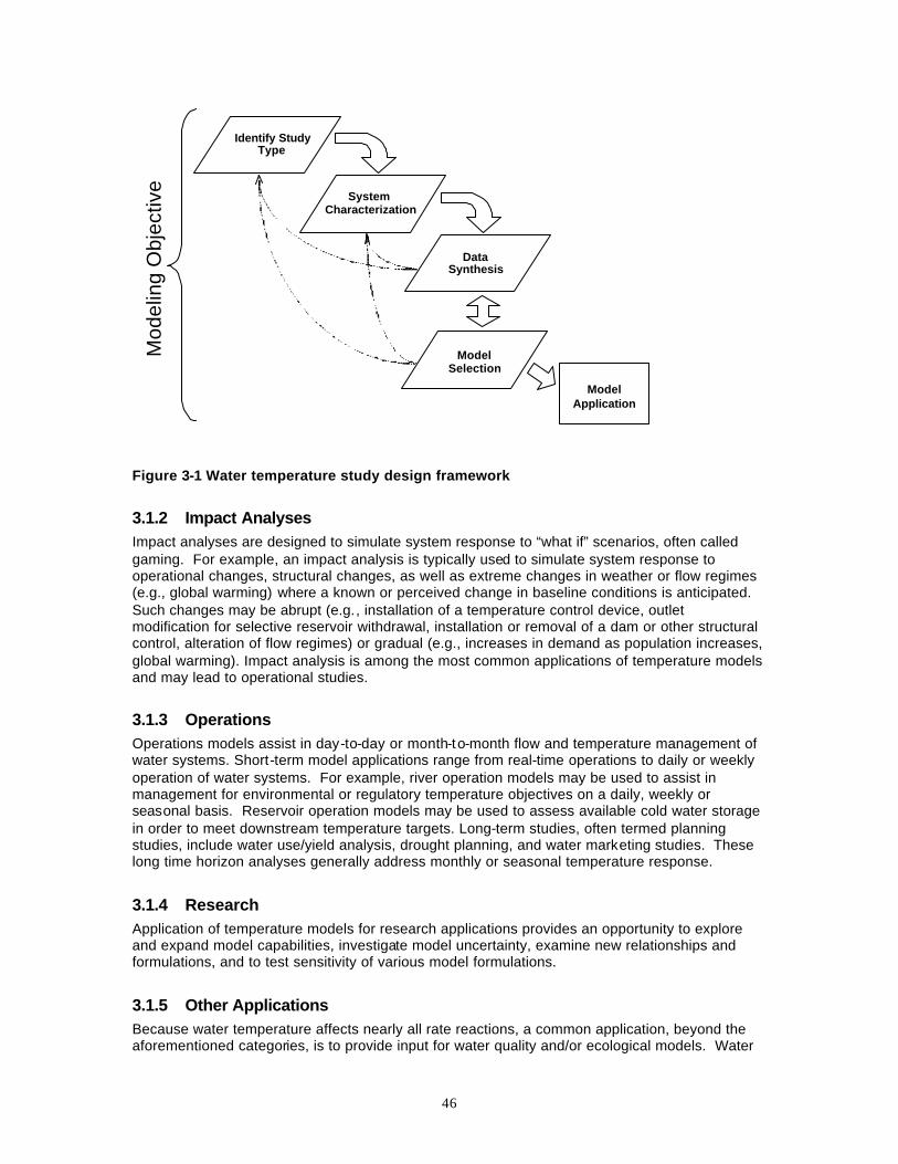
46

Identify StudyType

SystemCharacterization

ModelSelection

DataSynthesis

Mod

elin

g O

bjec

tive

ModelApplication

Figure 3-1 Water temperature study design framework

3.1.2 Impact Analyses Impact analyses are designed to simulate system response to “what if” scenarios, often called gaming. For example, an impact analysis is typically used to simulate system response to operational changes, structural changes, as well as extreme changes in weather or flow regimes (e.g., global warming) where a known or perceived change in baseline conditions is anticipated. Such changes may be abrupt (e.g., installation of a temperature control device, outlet modification for selective reservoir withdrawal, installation or removal of a dam or other structural control, alteration of flow regimes) or gradual (e.g., increases in demand as population increases, global warming). Impact analysis is among the most common applications of temperature models and may lead to operational studies.

3.1.3 Operations Operations models assist in day-to-day or month-to-month flow and temperature management of water systems. Short-term model applications range from real-time operations to daily or weekly operation of water systems. For example, river operation models may be used to assist in management for environmental or regulatory temperature objectives on a daily, weekly or seasonal basis. Reservoir operation models may be used to assess available cold water storage in order to meet downstream temperature targets. Long-term studies, often termed planning studies, include water use/yield analysis, drought planning, and water marketing studies. These long time horizon analyses generally address monthly or seasonal temperature response.

3.1.4 Research Application of temperature models for research applications provides an opportunity to explore and expand model capabilities, investigate model uncertainty, examine new relationships and formulations, and to test sensitivity of various model formulations.

3.1.5 Other Applications Because water temperature affects nearly all rate reactions, a common application, beyond the aforementioned categories, is to provide input for water quality and/or ecological models. Water

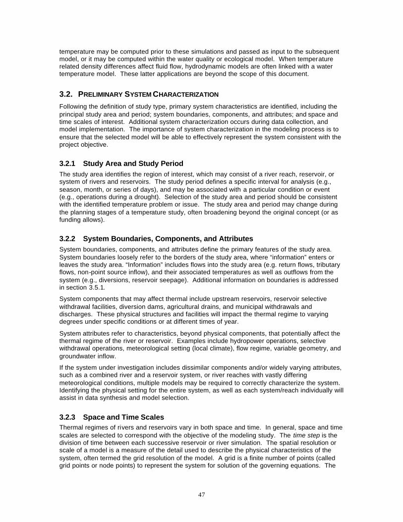
47

temperature may be computed prior to these simulations and passed as input to the subsequent model, or it may be computed within the water quality or ecological model. When temperature related density differences affect fluid flow, hydrodynamic models are often linked with a water temperature model. These latter applications are beyond the scope of this document.

3.2. PRELIMINARY SYSTEM CHARACTERIZATION Following the definition of study type, primary system characteristics are identified, including the principal study area and period; system boundaries, components, and attributes; and space and time scales of interest. Additional system characterization occurs during data collection, and model implementation. The importance of system characterization in the modeling process is to ensure that the selected model will be able to effectively represent the system consistent with the project objective.

3.2.1 Study Area and Study Period The study area identifies the region of interest, which may consist of a river reach, reservoir, or system of rivers and reservoirs. The study period defines a specific interval for analysis (e.g., season, month, or series of days), and may be associated with a particular condition or event (e.g., operations during a drought). Selection of the study area and period should be consistent with the identified temperature problem or issue. The study area and period may change during the planning stages of a temperature study, often broadening beyond the original concept (or as funding allows).

3.2.2 System Boundaries, Components, and Attributes System boundaries, components, and attributes define the primary features of the study area. System boundaries loosely refer to the borders of the study area, where “information” enters or leaves the study area. “Information” includes flows into the study area (e.g. return flows, tributary flows, non-point source inflow), and their associated temperatures as well as outflows from the system (e.g., diversions, reservoir seepage). Additional information on boundaries is addressed in section 3.5.1.

System components that may affect thermal include upstream reservoirs, reservoir selective withdrawal facilities, diversion dams, agricultural drains, and municipal withdrawals and discharges. These physical structures and facilities will impact the thermal regime to varying degrees under specific conditions or at different times of year.

System attributes refer to characteristics, beyond physical components, that potentially affect the thermal regime of the river or reservoir. Examples include hydropower operations, selective withdrawal operations, meteorological setting (local climate), flow regime, variable geometry, and groundwater inflow.

If the system under investigation includes dissimilar components and/or widely varying attributes, such as a combined river and a reservoir system, or river reaches with vastly differing meteorological conditions, multiple models may be required to correctly characterize the system. Identifying the physical setting for the entire system, as well as each system/reach individually will assist in data synthesis and model selection.

3.2.3 Space and Time Scales Thermal regimes of rivers and reservoirs vary in both space and time. In general, space and time scales are selected to correspond with the objective of the modeling study. The time step is the division of time between each successive reservoir or river simulation. The spatial resolution or scale of a model is a measure of the detail used to describe the physical characteristics of the system, often termed the grid resolution of the model. A grid is a finite number of points (called grid points or node points) to represent the system for solution of the governing equations. The

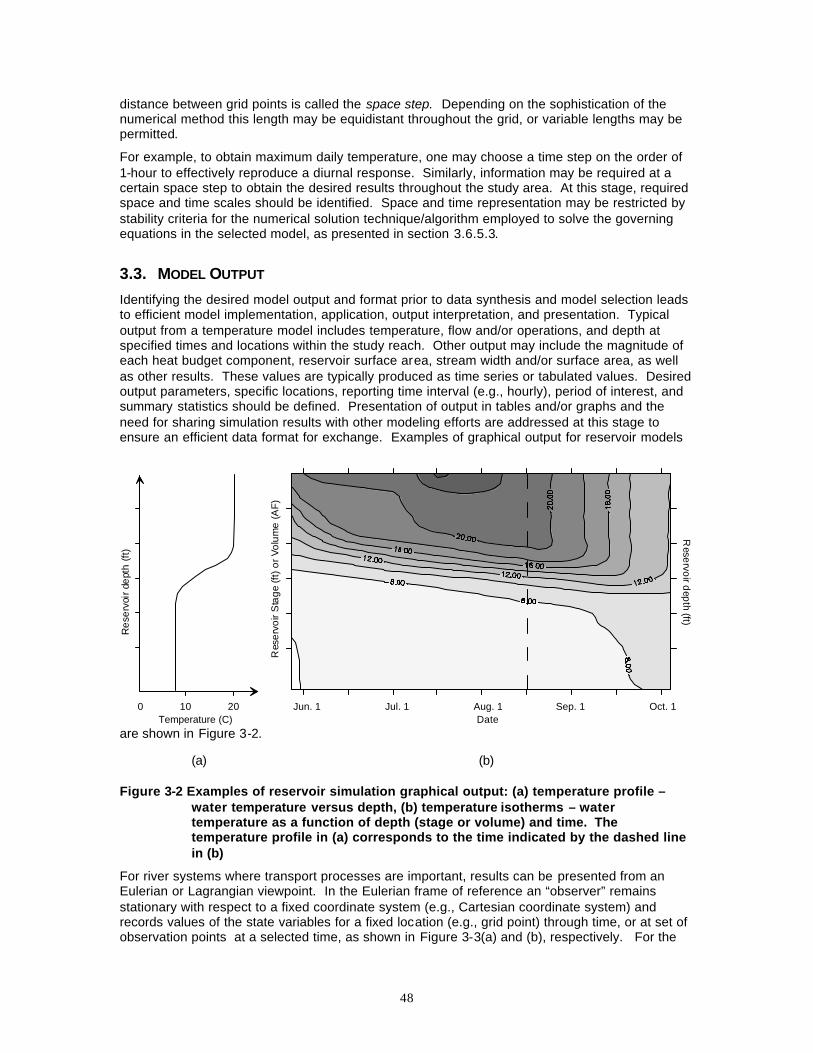
48

distance between grid points is called the space step. Depending on the sophistication of the numerical method this length may be equidistant throughout the grid, or variable lengths may be permitted.

For example, to obtain maximum daily temperature, one may choose a time step on the order of 1-hour to effectively reproduce a diurnal response. Similarly, information may be required at a certain space step to obtain the desired results throughout the study area. At this stage, required space and time scales should be identified. Space and time representation may be restricted by stability criteria for the numerical solution technique/algorithm employed to solve the governing equations in the selected model, as presented in section 3.6.5.3.

3.3. MODEL OUTPUT

Identifying the desired model output and format prior to data synthesis and model selection leads to efficient model implementation, application, output interpretation, and presentation. Typical output from a temperature model includes temperature, flow and/or operations, and depth at specified times and locations within the study reach. Other output may include the magnitude of each heat budget component, reservoir surface area, stream width and/or surface area, as well as other results. These values are typically produced as time series or tabulated values. Desired output parameters, specific locations, reporting time interval (e.g., hourly), period of interest, and summary statistics should be defined. Presentation of output in tables and/or graphs and the need for sharing simulation results with other modeling efforts are addressed at this stage to ensure an efficient data format for exchange. Examples of graphical output for reservoir models

are shown in Figure 3-2.

(a) (b)

Figure 3-2 Examples of reservoir simulation graphical output: (a) temperature profile – water temperature versus depth, (b) temperature isotherms – water temperature as a function of depth (stage or volume) and time. The temperature profile in (a) corresponds to the time indicated by the dashed line in (b)

For river systems where transport processes are important, results can be presented from an Eulerian or Lagrangian viewpoint. In the Eulerian frame of reference an “observer” remains stationary with respect to a fixed coordinate system (e.g., Cartesian coordinate system) and records values of the state variables for a fixed location (e.g., grid point) through time, or at set of observation points at a selected time, as shown in Figure 3-3(a) and (b), respectively. For the

Jun. 1 Jul. 1 Aug. 1 Sep. 1 Oct. 1

Res

ervo

ir S

tage

(ft)

or V

olum

e (A

F)

Reservoir depth (ft)

Res

ervo

ir de

pth

(ft)

Temperature (C)0 10 20

Date

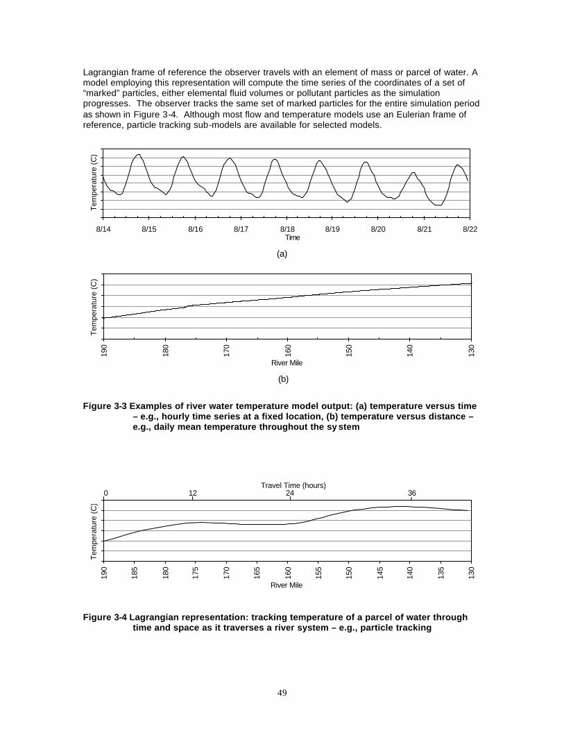
49

Lagrangian frame of reference the observer travels with an element of mass or parcel of water. A model employing this representation will compute the time series of the coordinates of a set of “marked” particles, either elemental fluid volumes or pollutant particles as the simulation progresses. The observer tracks the same set of marked particles for the entire simulation period as shown in Figure 3-4. Although most flow and temperature models use an Eulerian frame of reference, particle tracking sub-models are available for selected models.

(a)

(b)

Figure 3-3 Examples of river water temperature model output: (a) temperature versus time – e.g., hourly time series at a fixed location, (b) temperature versus distance – e.g., daily mean temperature throughout the sy stem

Figure 3-4 Lagrangian representation: tracking temperature of a parcel of water through time and space as it traverses a river system – e.g., particle tracking

8/14 8/15 8/16 8/17 8/18 8/19 8/20 8/21 8/22Time

Tem

pera

ture

(C

)

130

140

150

160

170

180

190

River Mile

Tem

pera

ture

(C

)

130

135

140

145

150

155

160

165

170

175

180

185

190

River Mile

Tem

pera

ture

(C

)

Travel Time (hours) 0 12 24 36

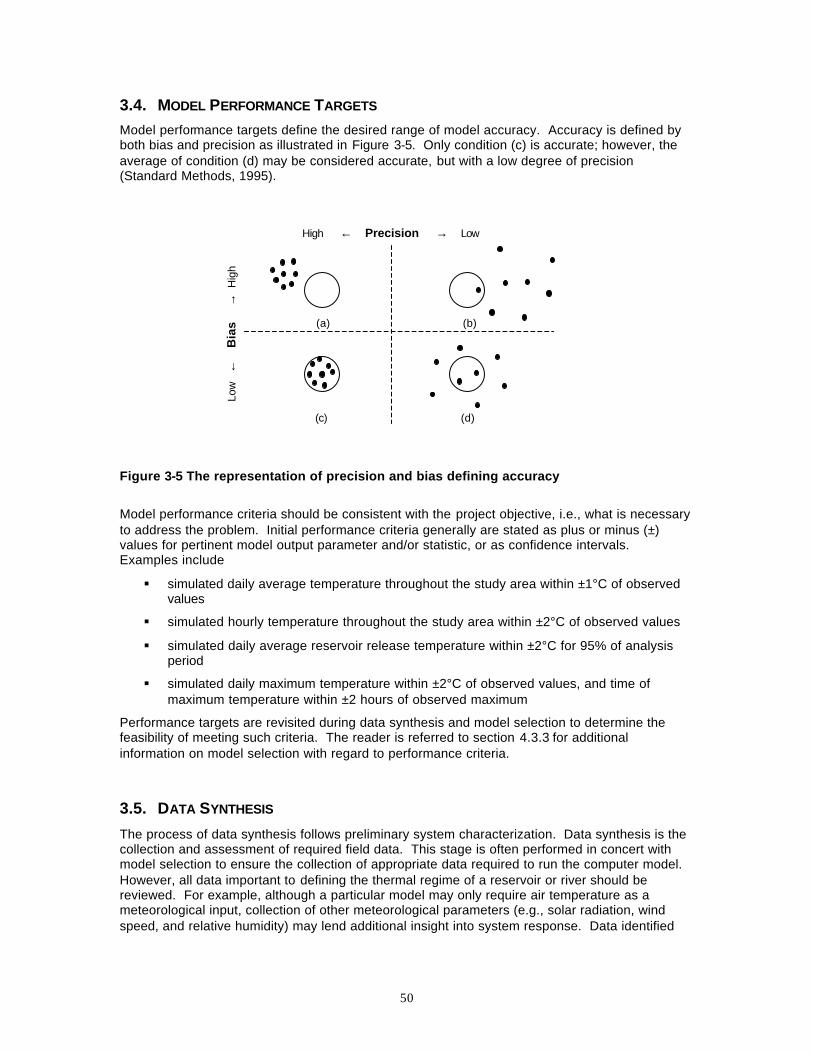
50

3.4. MODEL PERFORMANCE TARGETS Model performance targets define the desired range of model accuracy. Accuracy is defined by both bias and precision as illustrated in Figure 3-5. Only condition (c) is accurate; however, the average of condition (d) may be considered accurate, but with a low degree of precision (Standard Methods, 1995).

Figure 3-5 The representation of precision and bias defining accuracy

Model performance criteria should be consistent with the project objective, i.e., what is necessary to address the problem. Initial performance criteria generally are stated as plus or minus (±) values for pertinent model output parameter and/or statistic, or as confidence intervals. Examples include

§ simulated daily average temperature throughout the study area within ±1°C of observed values

§ simulated hourly temperature throughout the study area within ±2°C of observed values

§ simulated daily average reservoir release temperature within ±2°C for 95% of analysis period

§ simulated daily maximum temperature within ±2°C of observed values, and time of maximum temperature within ±2 hours of observed maximum

Performance targets are revisited during data synthesis and model selection to determine the feasibility of meeting such criteria. The reader is referred to section 4.3.3 for additional information on model selection with regard to performance criteria.

3.5. DATA SYNTHESIS

The process of data synthesis follows preliminary system characterization. Data synthesis is the collection and assessment of required field data. This stage is often performed in concert with model selection to ensure the collection of appropriate data required to run the computer model. However, all data important to defining the thermal regime of a reservoir or river should be reviewed. For example, although a particular model may only require air temperature as a meteorological input, collection of other meteorological parameters (e.g., solar radiation, wind speed, and relative humidity) may lend additional insight into system response. Data identified

(a)

High ← Precision → Low Lo

w

←

Bia

s

→ H

igh

(b)

(c) (d)

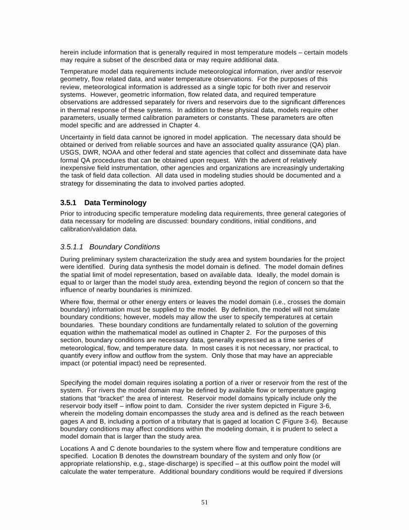
51

herein include information that is generally required in most temperature models – certain models may require a subset of the described data or may require additional data.

Temperature model data requirements include meteorological information, river and/or reservoir geometry, flow related data, and water temperature observations. For the purposes of this review, meteorological information is addressed as a single topic for both river and reservoir systems. However, geometric information, flow related data, and required temperature observations are addressed separately for rivers and reservoirs due to the significant differences in thermal response of these systems. In addition to these physical data, models require other parameters, usually termed calibration parameters or constants. These parameters are often model specific and are addressed in Chapter 4.

Uncertainty in field data cannot be ignored in model application. The necessary data should be obtained or derived from reliable sources and have an associated quality assurance (QA) plan. USGS, DWR, NOAA and other federal and state agencies that collect and disseminate data have formal QA procedures that can be obtained upon request. With the advent of relatively inexpensive field instrumentation, other agencies and organizations are increasingly undertaking the task of field data collection. All data used in modeling studies should be documented and a strategy for disseminating the data to involved parties adopted.

3.5.1 Data Terminology Prior to introducing specific temperature modeling data requirements, three general categories of data necessary for modeling are discussed: boundary conditions, initial conditions, and calibration/validation data.

3.5.1.1 Boundary Conditions

During preliminary system characterization the study area and system boundaries for the project were identified. During data synthesis the model domain is defined. The model domain defines the spatial limit of model representation, based on available data. Ideally, the model domain is equal to or larger than the model study area, extending beyond the region of concern so that the influence of nearby boundaries is minimized.

Where flow, thermal or other energy enters or leaves the model domain (i.e., crosses the domain boundary) information must be supplied to the model. By definition, the model will not simulate boundary conditions; however, models may allow the user to specify temperatures at certain boundaries. These boundary conditions are fundamentally related to solution of the governing equation within the mathematical model as outlined in Chapter 2. For the purposes of this section, boundary conditions are necessary data, generally expressed as a time series of meteorological, flow, and temperature data. In most cases it is not necessary, nor practical, to quantify every inflow and outflow from the system. Only those that may have an appreciable impact (or potential impact) need be represented.

Specifying the model domain requires isolating a portion of a river or reservoir from the rest of the system. For rivers the model domain may be defined by available flow or temperature gaging stations that “bracket” the area of interest. Reservoir model domains typically include only the reservoir body itself – inflow point to dam. Consider the river system depicted in Figure 3-6, wherein the modeling domain encompasses the study area and is defined as the reach between gages A and B, including a portion of a tributary that is gaged at location C (Figure 3-6). Because boundary conditions may affect conditions within the modeling domain, it is prudent to select a model domain that is larger than the study area.

Locations A and C denote boundaries to the system where flow and temperature conditions are specified. Location B denotes the downstream boundary of the system and only flow (or appropriate relationship, e.g., stage-discharge) is specified – at this outflow point the model will calculate the water temperature. Additional boundary conditions would be required if diversions

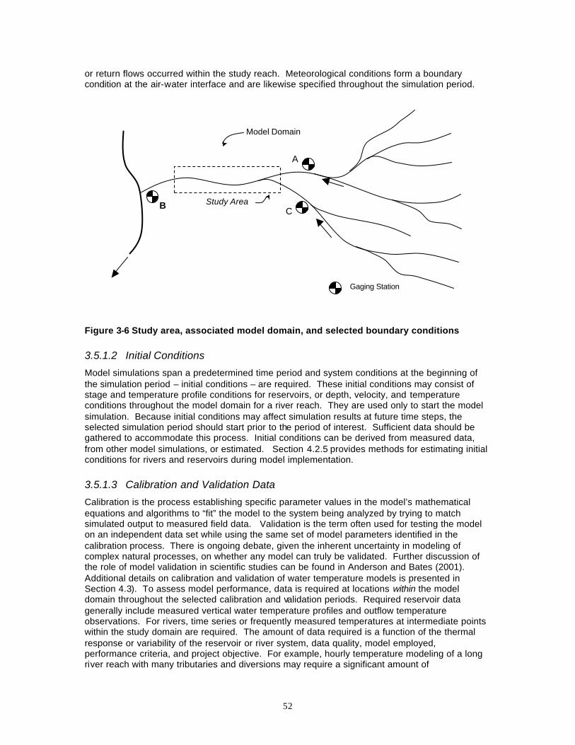
52

Gaging Station

A

B C

Model Domain

Study Area

or return flows occurred within the study reach. Meteorological conditions form a boundary condition at the air-water interface and are likewise specified throughout the simulation period.

Figure 3-6 Study area, associated model domain, and selected boundary conditions

3.5.1.2 Initial Conditions

Model simulations span a predetermined time period and system conditions at the beginning of the simulation period – initial conditions – are required. These initial conditions may consist of stage and temperature profile conditions for reservoirs, or depth, velocity, and temperature conditions throughout the model domain for a river reach. They are used only to start the model simulation. Because initial conditions may affect simulation results at future time steps, the selected simulation period should start prior to the period of interest. Sufficient data should be gathered to accommodate this process. Initial conditions can be derived from measured data, from other model simulations, or estimated. Section 4.2.5 provides methods for estimating initial conditions for rivers and reservoirs during model implementation.

3.5.1.3 Calibration and Validation Data

Calibration is the process establishing specific parameter values in the model’s mathematical equations and algorithms to “fit” the model to the system being analyzed by trying to match simulated output to measured field data. Validation is the term often used for testing the model on an independent data set while using the same set of model parameters identified in the calibration process. There is ongoing debate, given the inherent uncertainty in modeling of complex natural processes, on whether any model can truly be validated. Further discussion of the role of model validation in scientific studies can be found in Anderson and Bates (2001). Additional details on calibration and validation of water temperature models is presented in Section 4.3). To assess model performance, data is required at locations within the model domain throughout the selected calibration and validation periods. Required reservoir data generally include measured vertical water temperature profiles and outflow temperature observations. For rivers, time series or frequently measured temperatures at intermediate points within the study domain are required. The amount of data required is a function of the thermal response or variability of the reservoir or river system, data quality, model employed, performance criteria, and project objective. For example, hourly temperature modeling of a long river reach with many tributaries and diversions may require a significant amount of

53

calibration/validation data if performance targets are narrow, while a monthly reservoir model to address general planning questions may only require a few monthly temperature profiles for adequate representation. If insufficient calibration and validation measurements are available, confidence in model output will be compromised.

3.5.2 Meteorological Information Water temperature models use meteorological information to determine heat exchange at the air-water interface. As such, it forms an important boundary condition for water temperature models. This boundary condition is different than the flow and water temperature boundary conditions where the mass (flow) and thermal energy (water temperature) are assumed conserved. For heat transfer at the air-water interface, commonly measured meteorological parameters are used as proxy variables to estimate/represent energy budget terms. Solution of the energy budget estimates the transfer of short and long-wave radiation as well as heat fluxes across the air-water interface (equation (2-8)). This result is used in equation (2-51) through (2-54) to calculate fate and transport of thermal energy as represented by water temperature in rivers and reservoirs, respectively.

Typical meteorological parameters required for water temperature modeling include

§ air temperature

§ humidity

§ solar radiation

§ wind speed

§ atmospheric pressure

Meteorological observations commonly used to represent the energy budget terms are outlined in Table 3-1. Not all parameters are used in all water temperature models. Certain parameters, such as vapor pressure, can be derived from other meteorological observations.

The resolution of meteorological data required for water temperature modeling is defined by the project objective. If diurnal variation in water temperature is desired, sub-daily meteorological data are necessary. Hourly and three-hour meteorological observations are commonly available and are suitable to reproduce diurnal variations in water temperature modeling. For longer time step modeling efforts daily, monthly, and annual weather summaries can be used.

3.5.2.1 Meteorological Data Sources

Sources of data include international and municipal airports; California Irrigation Management Information System (CIMIS) stations; ranger, forestry, and fire stations; coast guard, naval, and army installations; universities and colleges; and city and county facilities. Those monitoring locations that are part of a larger overall framework, such as CIMIS or those airports that are part of the National Oceanic and Atmospheric Administration (NOAA) climate network, generally have the most complete records, i.e., having the most measured parameters as well as long historic records. Several agencies provide long-term meteorological data for selected stations throughout the Unites States. Appendix B, provides a partial list of agencies that archive and disseminate data.

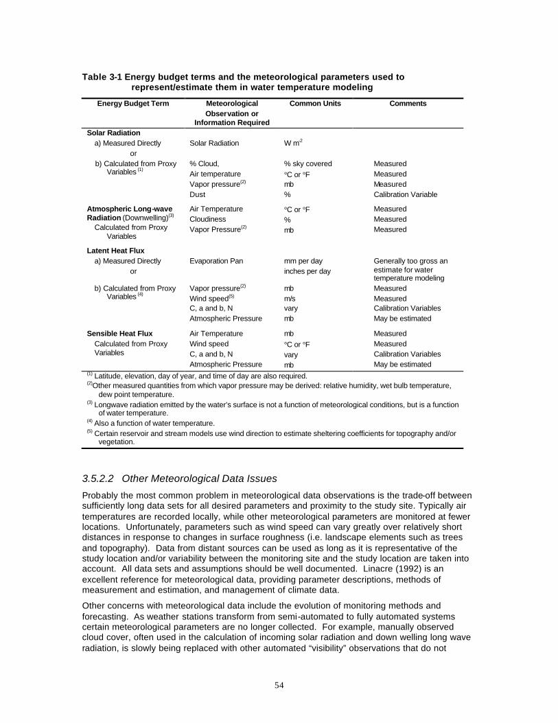
54

Table 3-1 Energy budget terms and the meteorological parameters used to represent/estimate them in water temperature modeling

Energy Budget Term Meteorological Observation or

Information Required

Common Units Comments

Solar Radiation a) Measured Directly

or

Solar Radiation

W m-2

b) Calculated from Proxy Variables (1)

% Cloud, Air temperature Vapor pressure(2) Dust

% sky covered °C or °F mb %

Measured Measured Measured Calibration Variable

Atmospheric Long-wave Radiation (Downwelling)(3)

Calculated from Proxy Variables

Air Temperature Cloudiness Vapor Pressure(2)

°C or °F % mb

Measured Measured Measured

Latent Heat Flux a) Measured Directly

or

Evaporation Pan

mm per day inches per day

Generally too gross an estimate for water temperature modeling

b) Calculated from Proxy Variables (4)

Vapor pressure(2) Wind speed(5) C, a and b, N Atmospheric Pressure

mb m/s vary mb

Measured Measured Calibration Variables May be estimated

Sensible Heat Flux Calculated from Proxy Variables

Air Temperature Wind speed C, a and b, N Atmospheric Pressure

mb °C or °F vary mb

Measured Measured Calibration Variables May be estimated

(1) Latitude, elevation, day of year, and time of day are also required. (2)Other measured quantities from which vapor pressure may be derived: relative humidity, wet bulb temperature,

dew point temperature. (3) Longwave radiation emitted by the water’s surface is not a function of meteorological conditions, but is a function

of water temperature. (4) Also a function of water temperature. (5) Certain reservoir and stream models use wind direction to estimate sheltering coefficients for topography and/or

vegetation.

3.5.2.2 Other Meteorological Data Issues

Probably the most common problem in meteorological data observations is the trade-off between sufficiently long data sets for all desired parameters and proximity to the study site. Typically air temperatures are recorded locally, while other meteorological parameters are monitored at fewer locations. Unfortunately, parameters such as wind speed can vary greatly over relatively short distances in response to changes in surface roughness (i.e. landscape elements such as trees and topography). Data from distant sources can be used as long as it is representative of the study location and/or variability between the monitoring site and the study location are taken into account. All data sets and assumptions should be well documented. Linacre (1992) is an excellent reference for meteorological data, providing parameter descriptions, methods of measurement and estimation, and management of climate data.

Other concerns with meteorological data include the evolution of monitoring methods and forecasting. As weather stations transform from semi-automated to fully automated systems certain meteorological parameters are no longer collected. For example, manually observed cloud cover, often used in the calculation of incoming solar radiation and down welling long wave radiation, is slowly being replaced with other automated “visibility” observations that do not

55

necessarily reflect cloud cover conditions. In most instances changes in monitoring methods do not accommodate the information required in temperature modeling, e.g., when cloud cover is dropped from a monitoring program, solar radiation observations are not added.

Another potential temperature modeling limitation concerning meteorological data is short-term planning (days to weeks) and/or real-time operations where weather forecasts are required. The National Weather Service and NOAA produce short- and intermediate-term weather forecasts that are useful in temperature models. However, forecasts are only provided for select weather stations, thus further reducing the number of locations where appropriate data can be obtained and used. Also, the uncertainty in forecasts directly affects model results.

3.5.3 Rivers and Streams In addition to meteorological data, river water temperature models require three principal types of data to effectively characterize river system response within the range of desired analysis: a geometric description of the physical system, flow data, and water temperature data. Data requirements addressed herein primarily address one-dimensional models representing longitudinal variations in rivers and streams. Multi-dimensional models require additional data and/or different data representation.

3.5.3.1 Geometric Data

Required river geometric data varies from model to model, but generally includes a description of the river location, channel slope, stream cross section, stage-discharge relationships, and bed type. Typical sources of these data include federal and state agencies, as well as data from other instream flow studies (e.g., fish habitat studies).

3.5.3.1.1 River Location and Length River location refers to the physical setting of the stream on the landscape. This may consist of a latitude – longitude (or UTM coordinate) description of the river. Implicit in this data set is river length and orientation/direction (aspect). Certain models do not require this detailed description and only require distance or reach length. Most models will require at a minimum the local latitude (and possibly longitude) for solar radiation calculations. Locations of tributaries, diversions, return flow, and other pertinent features should be identified.

3.5.3.1.2 Channel Slope Channel or bed slope is required for flow simulation and can be derived from elevations along the river reach (i.e., from a river profile). Several rivers in the western United States have been surveyed and have well defined elevation profiles, while other systems have little or no available data. In these cases, river profiles, and thus channel slope, can be approximated from digital elevation models (DEM), USGS topographic maps, gaging station datums, surveyed bridge crossings, and water resources development projects. Graphical Information System (GIS) representations are often used to define the river course and distance. However, care should be exercised to ensure that the representation is consistent with the physical system, i.e., that river length is correctly specified. Similar discretion should be used when a DEM is used to estimate elevations, and subsequently channel slopes.

3.5.3.1.3 Stream Cross Section Surveys Modeling flow and temperature requires a description of stream morphology to compute flow, and stream depth, width, and water surface area. When steady-state flow models are used in temperature modeling, flow is often represented with a Manning or Chézy formulation. Certain models estimate flow using a set of stage-discharge relationships throughout the modeling domain, typically using a set of discharge coefficients of the form d=αQβ and W=δQφ; where d is depth, W is width, and α, β, γ, and φ are empirical constants determined from stage-discharge rating curves.

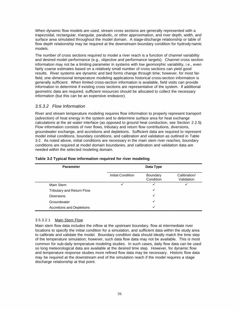
56

When dynamic flow models are used, stream cross sections are generally represented with a trapezoidal, rectangular, triangular, parabolic, or other approximation, and river depth, width, and surface area simulated throughout the model domain. A stage-discharge relationship or table of flow depth relationship may be required at the downstream boundary condition for hydrody namic models.

The number of cross sections required to model a river reach is a function of channel variability and desired model performance (e.g., objective and performance targets). Channel cross section information may not be a limiting parameter in systems with low geomorphic variability, i.e., even fairly coarse estimates based on a relatively small number of cross sections can yield good results. River systems are dynamic and bed forms change through time; however, for most far-field, one-dimensional temperature modeling applications historical cross-section information is generally sufficient. When limited cross-section information is available, field visits can provide information to determine if existing cross sections are representative of the system. If additional geometric data are required, sufficient resources should be allocated to collect the necessary information (but this can be an expensive endeavor).

3.5.3.2 Flow Information

River and stream temperature modeling requires flow information to properly represent transport (advection) of heat energy in the system and to determine surface area for heat exchange calculations at the air-water interface (as opposed to ground heat conduction, see Section 2.2.5). Flow information consists of river flows, tributary and return flow contributions, diversions, groundwater exchange, and accretions and depletions. Sufficient data are required to represent model initial conditions, boundary conditions, and calibration and validation as outlined in Table 3-2. As noted above, initial conditions are necessary in the main stem river reaches, boundary conditions are required at model domain boundaries, and calibration and validation data are needed within the selected modeling domain.

Table 3-2 Typical flow information required for river modeling

Data Type Parameter

Initial Condition Boundary Condition

Calibration/ Validation

Main Stem ü ü ü

Tributary and Return Flow ü

Diversions ü

Groundwater ü

Accretions and Depletions ü

3.5.3.2.1 Main Stem Flow Main stem flow data includes the inflow at the upstream boundary, flow at intermediate river locations to specify the initial condition for a simulation, and sufficient data within the study area to calibrate and validate the model. Boundary condition data should ideally match the time step of the temperature simulation; however, such data flow data may not be available. This is most common for sub-daily temperature modeling studies. In such cases, daily flow data can be used so long meteorological data are available at the desired time step. However, for dynamic flow and temperature response studies more refined flow data may be necessary. Historic flow data may be required at the downstream end of the simulation reach if the model requires a stage discharge relationship at that point.

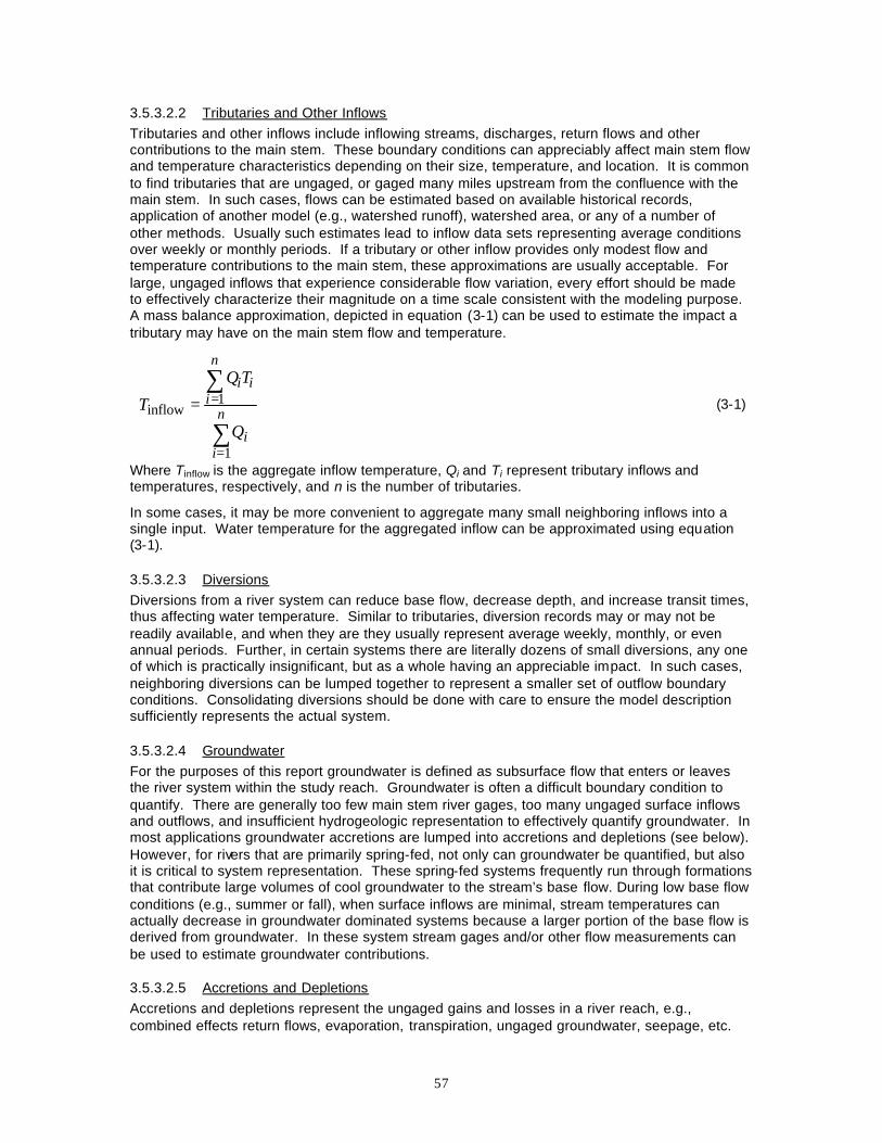
57

3.5.3.2.2 Tributaries and Other Inflows Tributaries and other inflows include inflowing streams, discharges, return flows and other contributions to the main stem. These boundary conditions can appreciably affect main stem flow and temperature characteristics depending on their size, temperature, and location. It is common to find tributaries that are ungaged, or gaged many miles upstream from the confluence with the main stem. In such cases, flows can be estimated based on available historical records, application of another model (e.g., watershed runoff), watershed area, or any of a number of other methods. Usually such estimates lead to inflow data sets representing average conditions over weekly or monthly periods. If a tributary or other inflow provides only modest flow and temperature contributions to the main stem, these approximations are usually acceptable. For large, ungaged inflows that experience considerable flow variation, every effort should be made to effectively characterize their magnitude on a time scale consistent with the modeling purpose. A mass balance approximation, depicted in equation (3-1) can be used to estimate the impact a tributary may have on the main stem flow and temperature.

∑

∑

=

== n

ii

n

iii

Q

TQ

T

1

1inflow

(3-1)

Where Tinflow is the aggregate inflow temperature, Qi and Ti represent tributary inflows and temperatures, respectively, and n is the number of tributaries.

In some cases, it may be more convenient to aggregate many small neighboring inflows into a single input. Water temperature for the aggregated inflow can be approximated using equation (3-1).

3.5.3.2.3 Diversions Diversions from a river system can reduce base flow, decrease depth, and increase transit times, thus affecting water temperature. Similar to tributaries, diversion records may or may not be readily available, and when they are they usually represent average weekly, monthly, or even annual periods. Further, in certain systems there are literally dozens of small diversions, any one of which is practically insignificant, but as a whole having an appreciable impact. In such cases, neighboring diversions can be lumped together to represent a smaller set of outflow boundary conditions. Consolidating diversions should be done with care to ensure the model description sufficiently represents the actual system.

3.5.3.2.4 Groundwater For the purposes of this report groundwater is defined as subsurface flow that enters or leaves the river system within the study reach. Groundwater is often a difficult boundary condition to quantify. There are generally too few main stem river gages, too many ungaged surface inflows and outflows, and insufficient hydrogeologic representation to effectively quantify groundwater. In most applications groundwater accretions are lumped into accretions and depletions (see below). However, for rivers that are primarily spring-fed, not only can groundwater be quantified, but also it is critical to system representation. These spring-fed systems frequently run through formations that contribute large volumes of cool groundwater to the stream’s base flow. During low base flow conditions (e.g., summer or fall), when surface inflows are minimal, stream temperatures can actually decrease in groundwater dominated systems because a larger portion of the base flow is derived from groundwater. In these system stream gages and/or other flow measurements can be used to estimate groundwater contributions.

3.5.3.2.5 Accretions and Depletions Accretions and depletions represent the ungaged gains and losses in a river reach, e.g., combined effects return flows, evaporation, transpiration, ungaged groundwater, seepage, etc.

58

Such inputs and outputs may be as basic as a single ungaged tributary or diversion, or as complex as dozens of inputs and outputs spread over many miles of river reach. In the simplest sense accretions/depletions are estimated using a water budget: measured inflows are subtracted from measured outflows and, assuming no storage in the study reach, the difference is an accretion if the value is positive and a depletion if the value is negative. This calculation is often completed between main stem stream gages, while accounting for any gaged tributary contributions or measured withdrawals. If the accretion/depletions are significant it may be necessary to explicitly include them to properly represent river velocity and depth – both critical parameters in temperature modeling. If the value is small relative to the total inflow (or outflow) it can be neglected.

Locating accretion/depletion points in the model domain is not an arbitrary process. To maintain proper hydrodynamic river representation requires identifying where and when water enters and leaves the system. For example, accretions and depletions are often associated with an ungaged tributary or diversion and can be placed accordingly. Land use, water resources development, and geology can further assist in this effort. If the reach is long and there are multiple main stem gages, accretions and depletions can be estimated for each sub-reach, i.e., between flow gages.

The previous discussion holds strictly for steady-state flow conditions/simulations, but is not necessarily applicable for non-steady-state flow conditions. If the travel time through the study reach is appreciably longer than the simulation time step then a simple water balance may not be applicable. Consider a model domain for a 200 mile river reach, where gages are located at the upstream and downstream boundaries. Further, assume the transit time through the reach is several days and the model time step is daily. Under steady-state conditions a simple daily water balance is applicable; however, if flow is unsteady, an increase or decrease in flow rate introduced at the upstream boundary will take several days to reach the downstream boundary and a simple daily water balance will not be applicable. There are several alternatives to estimating accretions and depletions when unsteady flow conditions exist:

§ Average flow data over a longer time period (e.g., weekly) to form approximate accretions and depletions,

§ Use a hydrodynamic or hydrologic1 model to route flows through the system and use these time series data to form time series of accretions/depletions, or

§ Use intermediate gages, if available, to estimate accretions for sub-reaches of the system using either of the above two options.

If the model is to be used to for impact analyses or operational studies, where presumed conditions may differ considerably from observed conditions, the estimated accretions/depletions may or may not be representative. In certain cases the estimates may need to be modified to reflect the intent or purpose of a proposed alternative or operation.

3.5.3.3 Water Temperature

Obtaining sufficient measured water temperature data is paramount to effectively characterize the river or stream thermal regime. Temperature data requirements are similar to those of flow data: main stem river reach, tributary contributions (including return flows), and, if available, groundwater temperatures. Diversions need not be assigned a water temperature because they are leaving the system. Accretions and depletions require special care, as outlined below. Table 3-3 presents typical water temperature data required for river modeling. Section 4.2.5 provides additional information on formulating initial conditions with limited water temperature data.

1 Hydrologic routing may not fully represent highly dynamic flow regimes. Hydrodynamic models are recommended to support temperature simulations under such conditions.

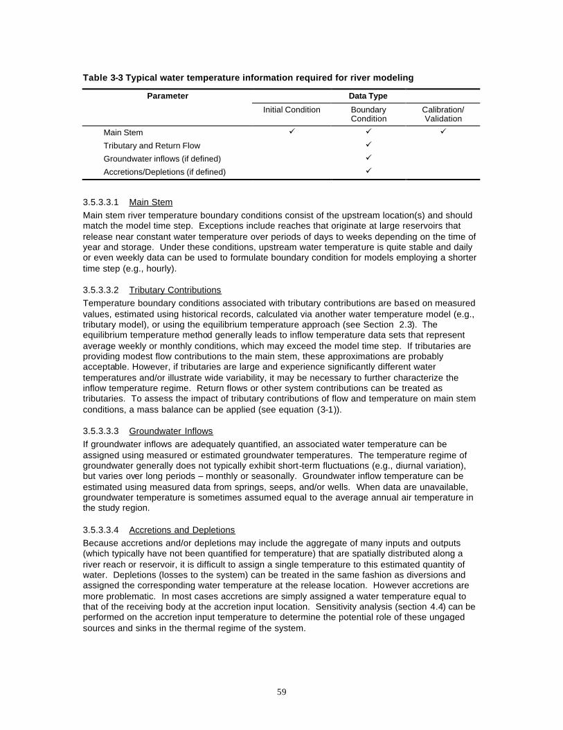
59

Table 3-3 Typical water temperature information required for river modeling

Parameter Data Type

Initial Condition Boundary Condition

Calibration/ Validation

Main Stem ü ü ü

Tributary and Return Flow ü

Groundwater inflows (if defined) ü

Accretions/Depletions (if defined) ü

3.5.3.3.1 Main Stem Main stem river temperature boundary conditions consist of the upstream location(s) and should match the model time step. Exceptions include reaches that originate at large reservoirs that release near constant water temperature over periods of days to weeks depending on the time of year and storage. Under these conditions, upstream water temperature is quite stable and daily or even weekly data can be used to formulate boundary condition for models employing a shorter time step (e.g., hourly).

3.5.3.3.2 Tributary Contributions Temperature boundary conditions associated with tributary contributions are based on measured values, estimated using historical records, calculated via another water temperature model (e.g., tributary model), or using the equilibrium temperature approach (see Section 2.3). The equilibrium temperature method generally leads to inflow temperature data sets that represent average weekly or monthly conditions, which may exceed the model time step. If tributaries are providing modest flow contributions to the main stem, these approximations are probably acceptable. However, if tributaries are large and experience significantly different water temperatures and/or illustrate wide variability, it may be necessary to further characterize the inflow temperature regime. Return flows or other system contributions can be treated as tributaries. To assess the impact of tributary contributions of flow and temperature on main stem conditions, a mass balance can be applied (see equation (3-1)).

3.5.3.3.3 Groundwater Inflows If groundwater inflows are adequately quantified, an associated water temperature can be assigned using measured or estimated groundwater temperatures. The temperature regime of groundwater generally does not typically exhibit short-term fluctuations (e.g., diurnal variation), but varies over long periods – monthly or seasonally. Groundwater inflow temperature can be estimated using measured data from springs, seeps, and/or wells. When data are unavailable, groundwater temperature is sometimes assumed equal to the average annual air temperature in the study region.

3.5.3.3.4 Accretions and Depletions Because accretions and/or depletions may include the aggregate of many inputs and outputs (which typically have not been quantified for temperature) that are spatially distributed along a river reach or reservoir, it is difficult to assign a single temperature to this estimated quantity of water. Depletions (losses to the system) can be treated in the same fashion as diversions and assigned the corresponding water temperature at the release location. However accretions are more problematic. In most cases accretions are simply assigned a water temperature equal to that of the receiving body at the accretion input location. Sensitivity analysis (section 4.4) can be performed on the accretion input temperature to determine the potential role of these ungaged sources and sinks in the thermal regime of the system.

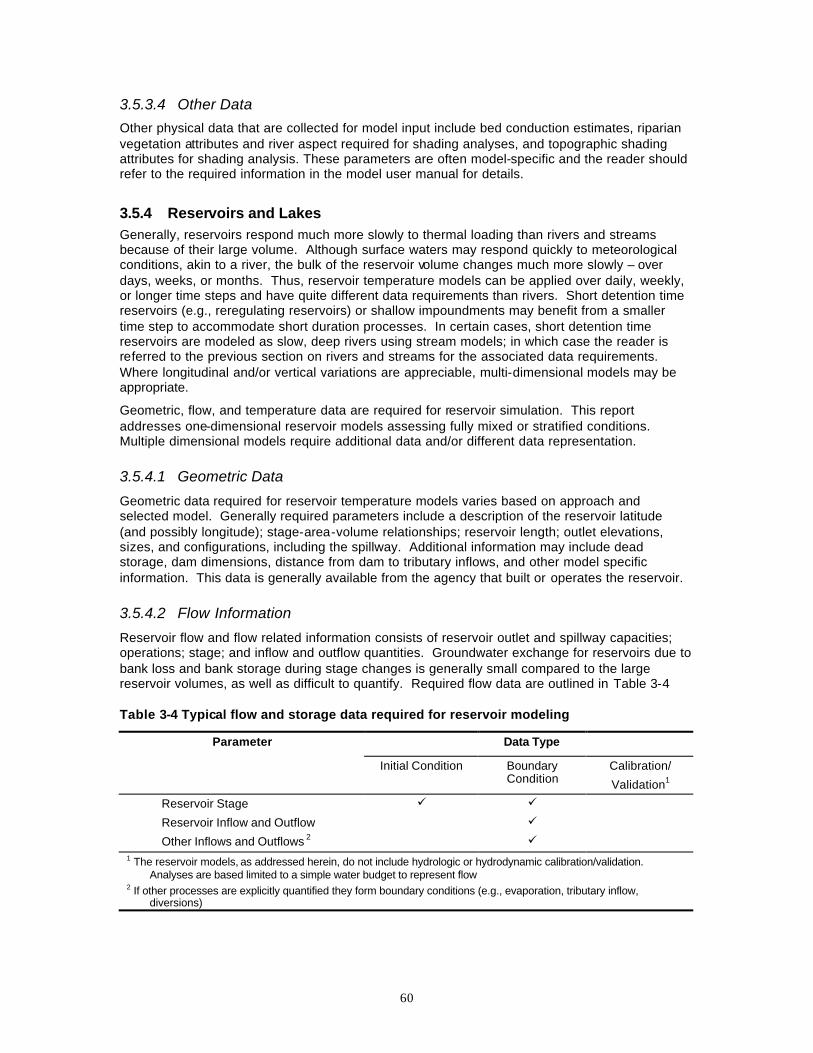
60

3.5.3.4 Other Data

Other physical data that are collected for model input include bed conduction estimates, riparian vegetation attributes and river aspect required for shading analyses, and topographic shading attributes for shading analysis. These parameters are often model-specific and the reader should refer to the required information in the model user manual for details.

3.5.4 Reservoirs and Lakes Generally, reservoirs respond much more slowly to thermal loading than rivers and streams because of their large volume. Although surface waters may respond quickly to meteorological conditions, akin to a river, the bulk of the reservoir volume changes much more slowly – over days, weeks, or months. Thus, reservoir temperature models can be applied over daily, weekly, or longer time steps and have quite different data requirements than rivers. Short detention time reservoirs (e.g., reregulating reservoirs) or shallow impoundments may benefit from a smaller time step to accommodate short duration processes. In certain cases, short detention time reservoirs are modeled as slow, deep rivers using stream models; in which case the reader is referred to the previous section on rivers and streams for the associated data requirements. Where longitudinal and/or vertical variations are appreciable, multi-dimensional models may be appropriate.

Geometric, flow, and temperature data are required for reservoir simulation. This report addresses one-dimensional reservoir models assessing fully mixed or stratified conditions. Multiple dimensional models require additional data and/or different data representation.

3.5.4.1 Geometric Data

Geometric data required for reservoir temperature models varies based on approach and selected model. Generally required parameters include a description of the reservoir latitude (and possibly longitude); stage-area-volume relationships; reservoir length; outlet elevations, sizes, and configurations, including the spillway. Additional information may include dead storage, dam dimensions, distance from dam to tributary inflows, and other model specific information. This data is generally available from the agency that built or operates the reservoir.

3.5.4.2 Flow Information

Reservoir flow and flow related information consists of reservoir outlet and spillway capacities; operations; stage; and inflow and outflow quantities. Groundwater exchange for reservoirs due to bank loss and bank storage during stage changes is generally small compared to the large reservoir volumes, as well as difficult to quantify. Required flow data are outlined in Table 3-4

Table 3-4 Typical flow and storage data required for reservoir modeling

Data Type Parameter

Initial Condition Boundary Condition

Calibration/

Validation1

Reservoir Stage ü ü

Reservoir Inflow and Outflow ü

Other Inflows and Outflows 2 ü 1 The reservoir models, as addressed herein, do not include hydrologic or hydrodynamic calibration/validation.

Analyses are based limited to a simple water budget to represent flow 2 If other processes are explicitly quantified they form boundary conditions (e.g., evaporation, tributary inflow,

diversions)

61

3.5.4.2.1 Reservoir Outlet and Spillway Capacities Theoretical outlet and spillway capacities are generally used in model application. For all reservoirs outlet and spillway capacities are a function of reservoir storage (stage or elevation), and are often represented through stage-discharge relationships. Many models do not incorporate stage-discharge relationships directly into simulations, thus it is important to have these data in-hand to ensure that simulated releases and results are feasible.

3.5.4.2.2 Reservoir Operations

Reservoirs support multiple purposes including hydropower, water supply, flood control, and in stream uses. Determining reservoir operations or proposed operations is necessary. Many reservoirs have rule curves and outlet schedules that reflect operations on a seasonal basis. Further, certain reservoirs have multi-level outlets to accommodate the wide variety of reservoir demands and purposes. In almost all cases, the operators of the facility can provide additional, valuable information.

3.5.4.2.3 Reservoir Stage Reservoir stage is used to determine storage and surface area via reservoir stage-volume-area relationships. All models will require reservoir stage for an initial condition. However, stage data (or storage data) should be collected throughout the analysis period to compare with simulated volume to ensure proper model representation.

3.5.4.2.4 Reservoir Inflow and Outflow

Daily inflow and outflow records are available for most reservoirs. Outflow is measured directly at the dam as the sum of the outlet releases plus spills or at a gaging station immediately downstream. Daily data is typically available, but hydropower operators at many dams can provide hourly information if required. Inflow may be gaged for each tributary; however, in many cases the gross reservoir inflow is estimated via a water balance calculation using storage (i.e., measured stage) and outflow. More specifically,

I-O = ∆S or I = ∆S – O (3-2)

Where I is gross inflow, O is measured total reservoir release (outflow), ∆S is measured change in storage based on a stage-volume relationship. Values may be calculated at daily, weekly, monthly or other interval averages; however for daily or shorter time intervals, the simple water balance may not represent flood waves, or other disturbances traversing larger reservoirs. When gross inflow is calculated in this manner it includes evaporation as well as other inputs and outputs such as diversions, ungaged and gaged stream flow, etc. Care should be used when representing reservoir inflow because temperature models commonly calculate and subtract evaporation losses from reservoirs. If gross inflow were employed in this type of model evaporation would be double counted. In such cases, evaporation can be estimated and added to the gross inflow, or the model can be modified to neglect evaporation losses.

Calculating gross inflow is straightforward when reservoirs have a single primary inflow. However, if multiple inflows exist and have different temperature regimes, explicit determination of the inflows is recommended (see water temperature, below). To complete this exercise several water balance components are required, including reservoir evaporation, diversions, gaged inflows, outflows, and stage data. It is important to realistically represent the water balance and reproduce reservoir stage (i.e., volume) throughout the analysis period (termed “closing” the water balance). If storage volume is poorly represented, model results will suffer.

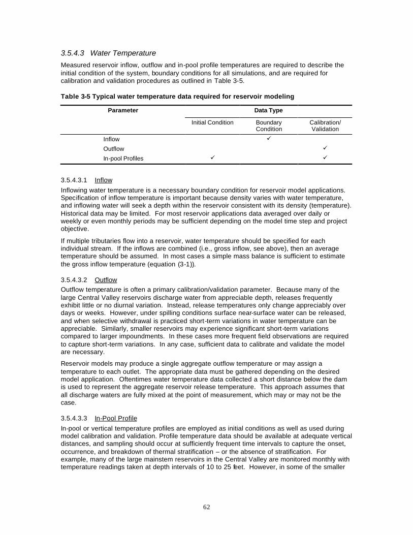
62

3.5.4.3 Water Temperature

Measured reservoir inflow, outflow and in-pool profile temperatures are required to describe the initial condition of the system, boundary conditions for all simulations, and are required for calibration and validation procedures as outlined in Table 3-5.

Table 3-5 Typical water temperature data required for reservoir modeling

Data Type Parameter

Initial Condition Boundary Condition

Calibration/ Validation

Inflow ü

Outflow ü

In-pool Profiles ü ü

3.5.4.3.1 Inflow

Inflowing water temperature is a necessary boundary condition for reservoir model applications. Specification of inflow temperature is important because density varies with water temperature, and inflowing water will seek a depth within the reservoir consistent with its density (temperature). Historical data may be limited. For most reservoir applications data averaged over daily or weekly or even monthly periods may be sufficient depending on the model time step and project objective.

If multiple tributaries flow into a reservoir, water temperature should be specified for each individual stream. If the inflows are combined (i.e., gross inflow, see above), then an average temperature should be assumed. In most cases a simple mass balance is sufficient to estimate the gross inflow temperature (equation (3-1)).

3.5.4.3.2 Outflow Outflow temperature is often a primary calibration/validation parameter. Because many of the large Central Valley reservoirs discharge water from appreciable depth, releases frequently exhibit little or no diurnal variation. Instead, release temperatures only change appreciably over days or weeks. However, under spilling conditions surface near-surface water can be released, and when selective withdrawal is practiced short-term variations in water temperature can be appreciable. Similarly, smaller reservoirs may experience significant short-term variations compared to larger impoundments. In these cases more frequent field observations are required to capture short-term variations. In any case, sufficient data to calibrate and validate the model are necessary.

Reservoir models may produce a single aggregate outflow temperature or may assign a temperature to each outlet. The appropriate data must be gathered depending on the desired model application. Oftentimes water temperature data collected a short distance below the dam is used to represent the aggregate reservoir release temperature. This approach assumes that all discharge waters are fully mixed at the point of measurement, which may or may not be the case.

3.5.4.3.3 In-Pool Profile

In-pool or vertical temperature profiles are employed as initial conditions as well as used during model calibration and validation. Profile temperature data should be available at adequate vertical distances, and sampling should occur at sufficiently frequent time intervals to capture the onset, occurrence, and breakdown of thermal stratification – or the absence of stratification. For example, many of the large mainstem reservoirs in the Central Valley are monitored monthly with temperature readings taken at depth intervals of 10 to 25 feet. However, in some of the smaller

63

reservoirs, especially the reregulating reservoirs, monitoring on a daily basis may be required to adequately represent the thermal response.

Initial conditions can be based on measured data or, if reservoir simulations commence in winter months, isothermal conditions can be assumed. Care must be used in estimating initial conditions for larger reservoirs that may experience significant carry-over storage because the initial estimate may affect reservoir thermal structure well into and through the summer period. For reservoir simulations that start during a period when signs of thermal stratification are present it is best to employ a measured temperature profile.

The number of measured temperature profiles required for calibration and validation is dependent on many factors including typical reservoir thermal response, degree and rate of stratification, thermal loading, simulation period length, inflow and outflow conditions (quantity, quality, and timing), changes in storage throughout the simulation period, as well as other factors. If reservoir conditions change rapidly and/or significantly, more profiles may be required.

3.5.5 Non-physical System Constraints for Rivers and Reservoirs Non-physical system constraints as defined herein apply to limitations or restrictions above and beyond physical capacities identified for rivers and reservoirs (e.g., maximum penstock capacity, diversion or canal capacity). Non-physical system constraints for both quantity and quality are also important in many modeling efforts and should be identified and characterized. Many of these constraints take the form of state water rights, federal legislative restrictions, agency codes and stipulations, judicial rulings, memorandums of understanding or agreement, and many other forms. Some constraints are simply guidelines that the reservoir operator chooses to implement while others are legal requirements.

Common reservoir constraints include reservoir operating rules, maximum allowable storage, minimum releases, hydropower generation targets, and rate of change of release (ramping). Quality constraints may include selective withdrawal or power plant bypass operations to meet downstream temperature objectives. Rivers, especially regulated systems, have similar constraints. Diversion rights, minimum instream flows, rate of change of flows, temperature compliance, maximum temperature impacts and other restrictions are often important to modeling studies.

Somewhat separate from these day-to-day constraints are emergency measures. Under sever drought conditions, floods, reservoir spilling conditions, post-earthquakes response and other anomalous conditions, other constraints may take effect, augmenting or superceding day-to-day constraints. If temperature studies are completed for these conditions, special care should be taken to ensure non-physical constraints are addressed.

3.5.6 Need for Additional Data In many cases temperature modeling data is unavailable or insufficient to effectively characterize the system and/or meet model input requirements. Further, for long-term modeling efforts, continued data collection may be desired. To obtain the requisite information, field data can be collected (monitoring) or records can be estimated. Both methods have their strengths and weaknesses.

3.5.6.1 Field Monitoring

Field monitoring requires direct measurement of physical parameters within the study area. There are several benefits of direct field measurements. Foremost is collecting data that is specific to the modeling project. Sampling can be carried out at the desired frequency, locations, and periods. Additional monitoring can be added for calibration and validation periods. If field monitoring produces new information, the monitoring program can be adapted to more effectively capture system dynamics. Finally, monitoring captures current conditions, while historical data

64

may represent conditions under different circumstances, e.g., a different level of water resources development.

The downside of monitoring is that it is expensive and time consuming. Further, there is the question of representative sampling periods – system variability is difficult to ascertain from a short monitoring period. Finally, if a model or modeling results are proposed for long-term applications or solutions, it is often necessary to maintain monitoring efforts as well; a costly endeavor. Monitoring can play a valuable role if limited information needs to be collected, especially information that is not time sensitive. For example, current geometric data can be utilized with historic meteorological, hydrologic, and temperature data. Also, it is often quite effective to monitor tributaries, return flows, and other required parameters for short periods to provide insight on potential range of values and for estimating data. In all cases a quality assurance plan should be developed to ensure effective collection and documentation of required data.

3.5.6.2 Data Estimation

Data estimation for temperature model applications may consist of simply filling in a few missing points in a time series to recreating an entire record. Methods range from employing a simple average to using a separate model to reproduce the desired data. Data estimation and synthesis techniques and approaches are too numerous to include herein. However, it is important to note that simple methods are often sufficient, such as using historic values, interpolation, first differences, average values, regression equations, empirical relationships, and correlating data from nearby stations. Model sensitivity can aid in assessing the impact of data estimates on model results (see Chapter 4). Techniques and assumptions should be substantiated and documented when estimating data.

3.6. MODEL SELECTION Many factors are considered in the selection of a water temperature model for a river or reservoir. To be consistent with the temperature modeling study framework proposed herein, all models should initially be considered. Subsequently, a final model should be selected based on theoretical representation of the flow and temperature dynamics, data requirements, model availability and status, computational issues, and available resources.

One guideline in model selection is to simulate system response at a resolution approximately one time step lower than your desired results and then average output over the desired time period. For example, to more effectively represent annual conditions a monthly time step model is used and results averaged over the annual cycle. Similarly for monthly conditions a weekly model is used; to assess weekly system responses a daily model is used; for daily analysis an hourly model is used, and so on. Such an approach provides system response at a more refined level that can assist in output interpretation. A useful reference is Winter (1981), who provides examples of how temporal and areal averaging of input data affect uncertainty in water balance models. The opposite approach, disaggregation, requires taking longer interval data and attempting to reduce it to shorter time periods (e.g., reducing monthly values to daily values, or daily values to hourly values). Disaggregation, by its very nature, typically introduces appreciable uncertainty into an analysis. Nonetheless, time and resources often constrain modeling efforts.

The following questions may assist the modeler in selecting a model consistent with the project objective and other primary project goals:

§ Is the model capable of addressing the problem identified in the project objective?

§ What are the data requirements, and are the data available?

§ Is the model public domain or a proprietary code?

§ Is peer review desired or required?

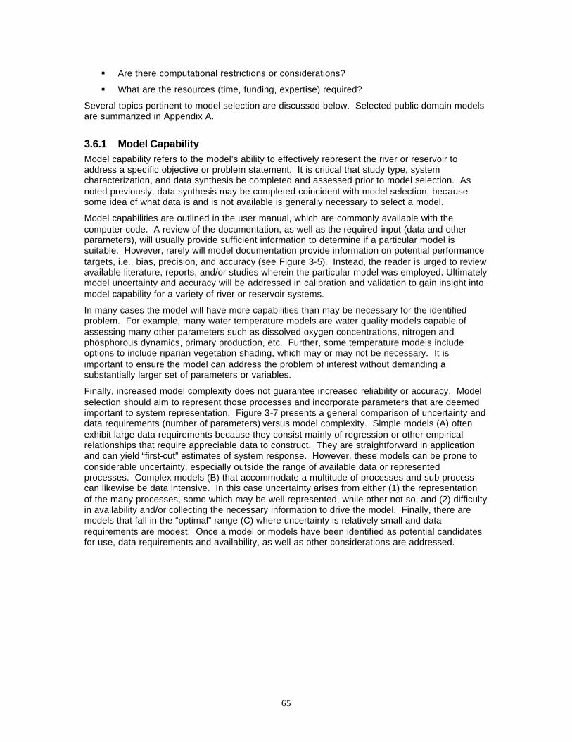
65

§ Are there computational restrictions or considerations?

§ What are the resources (time, funding, expertise) required?

Several topics pertinent to model selection are discussed below. Selected public domain models are summarized in Appendix A.

3.6.1 Model Capability Model capability refers to the model’s ability to effectively represent the river or reservoir to address a specific objective or problem statement. It is critical that study type, system characterization, and data synthesis be completed and assessed prior to model selection. As noted previously, data synthesis may be completed coincident with model selection, because some idea of what data is and is not available is generally necessary to select a model.

Model capabilities are outlined in the user manual, which are commonly available with the computer code. A review of the documentation, as well as the required input (data and other parameters), will usually provide sufficient information to determine if a particular model is suitable. However, rarely will model documentation provide information on potential performance targets, i.e., bias, precision, and accuracy (see Figure 3-5). Instead, the reader is urged to review available literature, reports, and/or studies wherein the particular model was employed. Ultimately model uncertainty and accuracy will be addressed in calibration and validation to gain insight into model capability for a variety of river or reservoir systems.

In many cases the model will have more capabilities than may be necessary for the identified problem. For example, many water temperature models are water quality models capable of assessing many other parameters such as dissolved oxygen concentrations, nitrogen and phosphorous dynamics, primary production, etc. Further, some temperature models include options to include riparian vegetation shading, which may or may not be necessary. It is important to ensure the model can address the problem of interest without demanding a substantially larger set of parameters or variables.

Finally, increased model complexity does not guarantee increased reliability or accuracy. Model selection should aim to represent those processes and incorporate parameters that are deemed important to system representation. Figure 3-7 presents a general comparison of uncertainty and data requirements (number of parameters) versus model complexity. Simple models (A) often exhibit large data requirements because they consist mainly of regression or other empirical relationships that require appreciable data to construct. They are straightforward in application and can yield “first-cut” estimates of system response. However, these models can be prone to considerable uncertainty, especially outside the range of available data or represented processes. Complex models (B) that accommodate a multitude of processes and sub-process can likewise be data intensive. In this case uncertainty arises from either (1) the representation of the many processes, some which may be well represented, while other not so, and (2) difficulty in availability and/or collecting the necessary information to drive the model. Finally, there are models that fall in the “optimal” range (C) where uncertainty is relatively small and data requirements are modest. Once a model or models have been identified as potential candidates for use, data requirements and availability, as well as other considerations are addressed.

66

Figure 3-7 Model uncertainty and data requirements as a function of model complexity (adapted from Martin and McCutcheon (1999))

3.6.2 Data Requirements and Availability Data requirements play a role in model selection and as noted can be completed coincident with model selection. Data requirements and availability do not usually limit modeling effort where appreciable geometry, meteorological, hydrologic, and water temperature are available. If highly complex models are employed this may not be the case. It is prudent to utilize the data synthesis phase to improve and expand the understanding of river or reservoir flow regime and thermal response (as well as other attributes) and to use this information to identify potentially applicable models.

3.6.3 Computer Model Availability and Status Water temperature models are widely available both in the public domain as well as from private vendors. Some important considerations when selecting a model include cost, documentation, available support, ease of use, level of peer review, and whether the model resides in the public domain.

Temperature model costs vary from free for many public domain computer codes, to tens of thousands of dollars for proprietary codes. Generally public domain codes are readily available for little or no cost: several models can be downloaded from the internet or obtained for a modest handling charge from Universities or other agencies. Although proprietary codes are significantly more expensive, the associated documentation and technical support is superior in most cases. Further, proprietary codes may offer graphical user interfaces (GUI) that can ease model application and allow efficient input and output examination and interpretation. Ease of use is a difficult topic to assess because it is user dependent. The current expansion of GUI for public domain codes has increased the cost as well as restricted access to the source code in some cases. Even with a well-designed GUI, first-time temperature model users will face what seems like a daunting task, while experienced model users may be able to use a wide range of models with ease and efficiency.

Probably the two most critical differences, besides cost, is that (1) public domain models either have undergone peer review and/or their code is readily accessible for peer review, and (2) if model modification is necessary, public domain model source code is readily available. During the model selection process issues of peer review and potential model modification should be

Simple

Unr

elia

ble

Rel

iabl

e M

any Few

Complex

Model Complexity

Unc

erta

inty

D

ata Requirem

ents A

C

B

67

considered. With regard to model modification, certain companies and institutions will modify the code at the user’s request; however time constraints and access to the computer code algorithms may remain restricted.

3.6.4 Model Training, Documentation, and Support If water temperature modeling studies are to be completed in-house, model training, documentation, and support can be important factors to consider in model selection. The project objective, level of in-house staff expertise, access to “outside” assistance, as well as time and budget determine the level of training and support required.

Training is available for a small set of public domain models capable of temperature simulation, while it is widely available for proprietary codes. There are consulting firms that provide training for those public domain codes where there is no training offered from the agency that maintains the computer code. Documentation and support for models range on a relative scale from “good” to “none.” As noted above, proprietary codes generally have better documentation and support. Often support is based on an annual fee basis, but many options for fee-based support exist.

3.6.5 Computational Issues Although there are many computational issues, for the purposes of this report three are presented: hardware limitations, software limitations associated with code modification, and space and time resolution limitations placed on the numerical solution methods of the governing equations. Each is briefly described below.

3.6.5.1 Hardware

Computer hardware constraints are of limited concern for most available models. Nearly all readily available models in either the public or private domain will run on a standard PC, although memory requirements (RAM and hard disk space) and processor speed may be of interest for larger applications. If water temperature models are to be used as a sub-component of a larger framework that includes a GUI, data management program, other ecological or water quality models, and/or geographical information systems (GIS) there may be some computational requirements that need to be addressed, but nearly all issues can be overcome through hardware upgrades.

3.6.5.2 Software and Code Modifications

A second point with respect to computational issues is the ability to modify the code. Code modification is a common practice in many modeling projects to incorporate components or processes that are unavailable in the original program (e.g., different riparian shading, heat budget, and/or bed conduction formulations). More commonly input or output logic is modified to improve data management and to provide output in a format consistent with another use such as input to another model. If computer code modifications are necessary, the appropriate software is required, e.g., program compiler. Although many of today’s temperature models are written in FORTRAN, certain models, as well as GUIs, are written in other computer languages. If code modification is desired, personnel familiar with the necessary computer language are required.

3.6.5.3 Numerical Solution Techniques

Thermal regimes of rivers and reservoirs vary in both space and time. In space, a river or reservoir system is divided into discrete volumes (sometimes termed elements, segments, or links), for which mass balance and energy balance equations are written (Chapter 2). Temperature changes in each of these volumes take place over a defined period of time, e.g., hours or days. Model resolution describes the spatial and temporal detail of a model, where space and time increments are represented as ∆x and ∆t, respectively. In general, time and

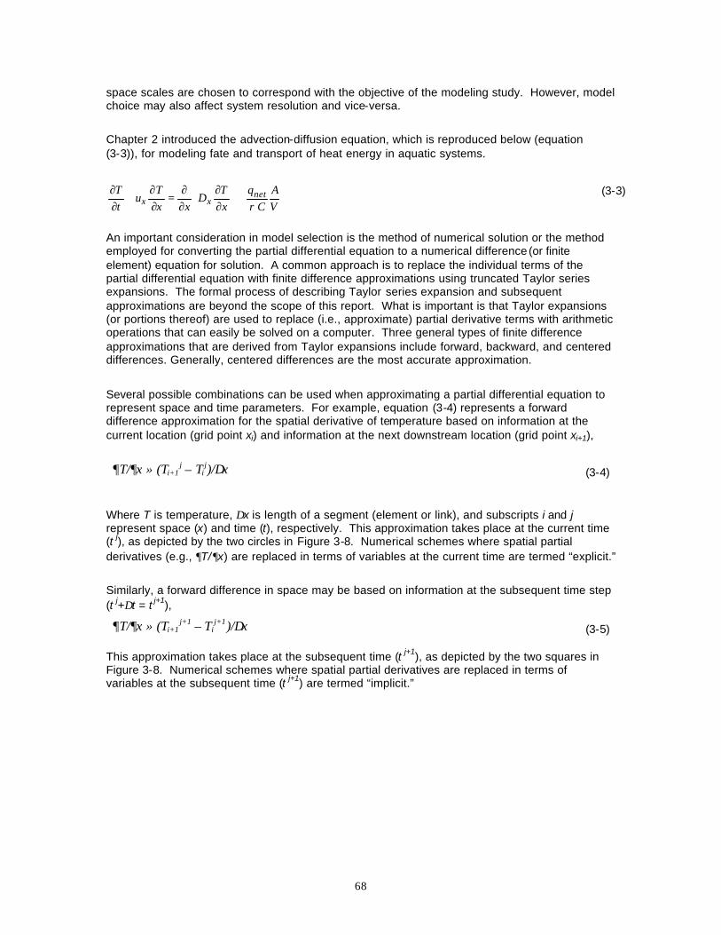
68

space scales are chosen to correspond with the objective of the modeling study. However, model choice may also affect system resolution and vice-versa.

Chapter 2 introduced the advection-diffusion equation, which is reproduced below (equation (3-3)), for modeling fate and transport of heat energy in aquatic systems.

VA

Cq

xT

Dxx

Tu

tT net

xx ρ+

∂∂

∂∂

=∂∂

+∂∂

(3-3)

An important consideration in model selection is the method of numerical solution or the method employed for converting the partial differential equation to a numerical difference (or finite element) equation for solution. A common approach is to replace the individual terms of the partial differential equation with finite difference approximations using truncated Taylor series expansions. The formal process of describing Taylor series expansion and subsequent approximations are beyond the scope of this report. What is important is that Taylor expansions (or portions thereof) are used to replace (i.e., approximate) partial derivative terms with arithmetic operations that can easily be solved on a computer. Three general types of finite difference approximations that are derived from Taylor expansions include forward, backward, and centered differences. Generally, centered differences are the most accurate approximation.

Several possible combinations can be used when approximating a partial differential equation to represent space and time parameters. For example, equation (3-4) represents a forward difference approximation for the spatial derivative of temperature based on information at the current location (grid point xi) and information at the next downstream location (grid point xi+1),

∂T/∂x ≈ (Ti+1

j – Tij)/∆x

(3-4)

Where T is temperature, ∆x is length of a segment (element or link), and subscripts i and j represent space (x) and time (t), respectively. This approximation takes place at the current time (t j), as depicted by the two circles in Figure 3-8. Numerical schemes where spatial partial derivatives (e.g., ∂T/∂x) are replaced in terms of variables at the current time are termed “explicit.”

Similarly, a forward difference in space may be based on information at the subsequent time step (t j+∆t = t j+1),

∂T/∂x ≈ (Ti+1j+1 – Ti

j+1)/∆x (3-5) This approximation takes place at the subsequent time (t j+1), as depicted by the two squares in Figure 3-8. Numerical schemes where spatial partial derivatives are replaced in terms of variables at the subsequent time (t j+1) are termed “implicit.”

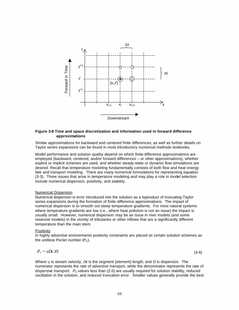
69

Figure 3-8 Time and space discretization and information used in forward difference approximations

Similar approximations for backward and centered finite differences, as well as further details on Taylor series expansions can be found in most introductory numerical methods textbooks.

Model performance and solution quality depend on which finite difference approximations are employed (backward, centered, and/or forward differences – or other approximations), whether explicit or implicit schemes are used, and whether steady-state or dynamic flow simulations are desired. Recall that temperature modeling fundamentally consists of both flow and heat energy fate and transport modeling. There are many numerical formulations for representing equation (3-3). Three issues that arise in temperature modeling and may play a role in model selection include numerical dispersion, positivity, and stability.

Numerical Dispersion Numerical dispersion is error introduced into the solution as a byproduct of truncating Taylor series expansions during the formation of finite difference approximations. The impact of numerical dispersion is to smooth out steep temperature gradients. For most natural systems where temperature gradients are low (i.e., where heat pollution is not an issue) the impact is usually small. However, numerical dispersion may be an issue in river models (and some reservoir models) in the vicinity of tributaries or other inflows that are a significantly different temperature than the main stem.

Positivity In highly advective environments positivity constraints are placed on certain solution schemes as the unitless Peclet number (Pe),

Pe = u∆x /D (3-6)

Where u is stream velocity, ∆x is the segment (element) length, and D is dispersion. The numerator represents the rate of advective transport, while the denominator represents the rate of dispersive transport. Pe values less than (2.0) are usually required for solution stability, reduced oscillation in the solution, and reduced truncation error. Smaller values generally provide the best

x

t

xi-1 xi+1 xi

tj

tj+1

tj-1

∆t

∆x

For

war

d in

Tim

e

Downstream

(xi,tj)

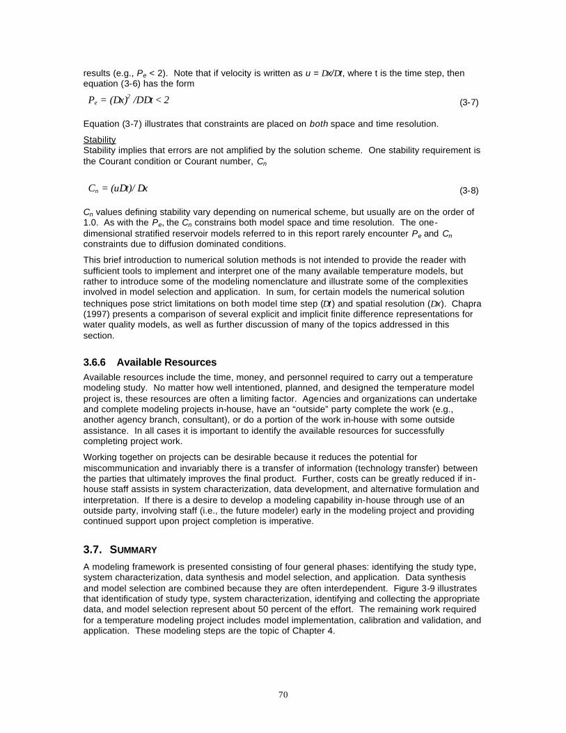
70

results (e.g., Pe < 2). Note that if velocity is written as u = ∆x/∆t, where t is the time step, then equation (3-6) has the form

Pe = (∆x)2 /D∆t < 2 (3-7) Equation (3-7) illustrates that constraints are placed on both space and time resolution.

Stability Stability implies that errors are not amplified by the solution scheme. One stability requirement is the Courant condition or Courant number, Cn

Cn = (u∆t)/ ∆x (3-8)

Cn values defining stability vary depending on numerical scheme, but usually are on the order of 1.0. As with the Pe, the Cn constrains both model space and time resolution. The one-dimensional stratified reservoir models referred to in this report rarely encounter Pe and Cn constraints due to diffusion dominated conditions.

This brief introduction to numerical solution methods is not intended to provide the reader with sufficient tools to implement and interpret one of the many available temperature models, but rather to introduce some of the modeling nomenclature and illustrate some of the complexities involved in model selection and application. In sum, for certain models the numerical solution techniques pose strict limitations on both model time step (∆t ) and spatial resolution (∆x). Chapra (1997) presents a comparison of several explicit and implicit finite difference representations for water quality models, as well as further discussion of many of the topics addressed in this section.

3.6.6 Available Resources Available resources include the time, money, and personnel required to carry out a temperature modeling study. No matter how well intentioned, planned, and designed the temperature model project is, these resources are often a limiting factor. Agencies and organizations can undertake and complete modeling projects in-house, have an “outside” party complete the work (e.g., another agency branch, consultant), or do a portion of the work in-house with some outside assistance. In all cases it is important to identify the available resources for successfully completing project work.

Working together on projects can be desirable because it reduces the potential for miscommunication and invariably there is a transfer of information (technology transfer) between the parties that ultimately improves the final product. Further, costs can be greatly reduced if in-house staff assists in system characterization, data development, and alternative formulation and interpretation. If there is a desire to develop a modeling capability in-house through use of an outside party, involving staff (i.e., the future modeler) early in the modeling project and providing continued support upon project completion is imperative.

3.7. SUMMARY A modeling framework is presented consisting of four general phases: identifying the study type, system characterization, data synthesis and model selection, and application. Data synthesis and model selection are combined because they are often interdependent. Figure 3-9 illustrates that identification of study type, system characterization, identifying and collecting the appropriate data, and model selection represent about 50 percent of the effort. The remaining work required for a temperature modeling project includes model implementation, calibration and validation, and application. These modeling steps are the topic of Chapter 4.

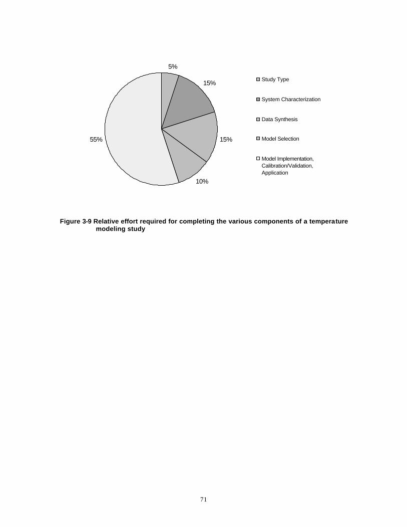
71

Figure 3-9 Relative effort required for completing the various components of a temperature modeling study

5%

15%

15%

10%

55%

Study Type

System Characterization

Data Synthesis

Model Selection

Model Implementation,Calibration/Validation,Application

72

4. MODEL IMPLEMENTATION, CALIBRATION/VALIDATION, AND APPLICATION

4.1. INTRODUCTION

Following system characterization, identification and assembling of required data, and model selection, the processes of model implementation, calibration and validation, and application are carried out. These are discrete phases of model development constituting a large part of a water temperature study. Sensitivity analysis is an additional process commonly used in water temperature modeling to identify important parameters and the role they play in simulated system response. Each topic is briefly outlined below.

4.2. MODEL IMPLEMENTATION Model implementation includes testing the software, loading model data and selecting default parameters, formulating initial conditions, and completing trial simulations. The end result is a functioning, but uncalibrated model.

4.2.1 Model Test Cases Most model software includes a set of test cases or test input and output files that can be used to ensure proper model function. Upon successful installation of the selected model on a computer, the first task is running these test cases and comparing results to those supplied in the model documentation. This is a fairly straightforward task, but it is not uncommon to find discrepancies between the two. If differences occur, the model distributor or author should be contacted to determine the origin of the discrepancy.

4.2.2 Mathematical Description of the System One of the first steps in model implementation is transferring the physical description of the river or reservoir into a mathematical description. For rivers this requires reducing the river to individual reaches (often called elements, segments, or links), separated by “nodes” or “grid points.” Bed slope and cross section information are specified for each reach at the associated nodes. Reservoirs generally require the user to specify the vertical resolution of the model, e.g., a layer thickness. Stage-volume-area data are necessary to approximate the morphology of the reservoir, as well as outlet size, capacity, and elevation.

4.2.3 Loading Data and Selecting Default Parameters Once the basic test cases have been successfully implemented and the physical data are properly represented, the model is further adapted to the system of interest by applying the appropriate system specific data and selecting default model parameters. System data include flow information (e.g., flow at the upstream boundary, tributary boundary flows, diversions), meteorological information (e.g., air temperature, wind speed, solar radiation, relative humidity), and water temperature information (e.g., tributary temperatures, water temperature at the upstream boundary). It is often useful to start with a simplified version of the system being modeled, and gradually add complexity. Attempting to employ all the necessary data for long simulations of a complicated system often leads to long and tedious investigations of input file format and model errors.

In addition to formatting required input information, it is also necessary to specify default values for model parameters (i.e., constants and coefficients). Many of these values are assessed during model calibration and once determined are rarely changed during model application. However, prior to calibration, or as a first estimate, default values for model specific parameters

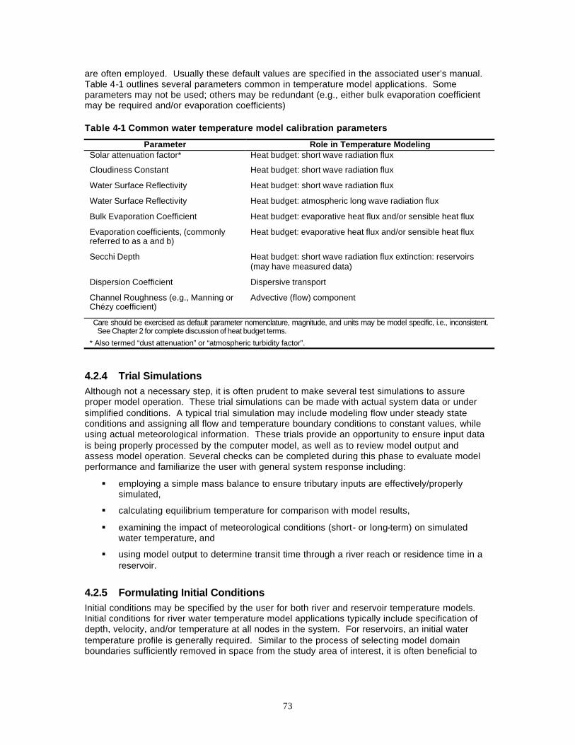
73

are often employed. Usually these default values are specified in the associated user’s manual. Table 4-1 outlines several parameters common in temperature model applications. Some parameters may not be used; others may be redundant (e.g., either bulk evaporation coefficient may be required and/or evaporation coefficients)

Table 4-1 Common water temperature model calibration parameters

Parameter Role in Temperature Modeling Solar attenuation factor* Heat budget: short wave radiation flux

Cloudiness Constant Heat budget: short wave radiation flux

Water Surface Reflectivity Heat budget: short wave radiation flux

Water Surface Reflectivity Heat budget: atmospheric long wave radiation flux

Bulk Evaporation Coefficient Heat budget: evaporative heat flux and/or sensible heat flux

Evaporation coefficients, (commonly referred to as a and b)

Heat budget: evaporative heat flux and/or sensible heat flux

Secchi Depth Heat budget: short wave radiation flux extinction: reservoirs (may have measured data)

Dispersion Coefficient Dispersive transport

Channel Roughness (e.g., Manning or Chézy coefficient)

Advective (flow) component

Care should be exercised as default parameter nomenclature, magnitude, and units may be model specific, i.e., inconsistent. See Chapter 2 for complete discussion of heat budget terms.

* Also termed “dust attenuation” or “atmospheric turbidity factor”.

4.2.4 Trial Simulations Although not a necessary step, it is often prudent to make several test simulations to assure proper model operation. These trial simulations can be made with actual system data or under simplified conditions. A typical trial simulation may include modeling flow under steady state conditions and assigning all flow and temperature boundary conditions to constant values, while using actual meteorological information. These trials provide an opportunity to ensure input data is being properly processed by the computer model, as well as to review model output and assess model operation. Several checks can be completed during this phase to evaluate model performance and familiarize the user with general system response including:

§ employing a simple mass balance to ensure tributary inputs are effectively/properly simulated,

§ calculating equilibrium temperature for comparison with model results,

§ examining the impact of meteorological conditions (short- or long-term) on simulated water temperature, and

§ using model output to determine transit time through a river reach or residence time in a reservoir.

4.2.5 Formulating Initial Conditions Initial conditions may be specified by the user for both river and reservoir temperature models. Initial conditions for river water temperature model applications typically include specification of depth, velocity, and/or temperature at all nodes in the system. For reservoirs, an initial water temperature profile is generally required. Similar to the process of selecting model domain boundaries sufficiently removed in space from the study area of interest, it is often beneficial to

74

start model simulations well in advance of the time period of interest such that initial conditions do not adversely affect the solution.

For river systems, specifying realistic initial water temperature and flow (i.e., depth and velocity) conditions at all locations in the model domain may not be feasible or possible. However, the model can be used to create an initial condition based on information leading up to the desired analysis period. Specifically, the model can be run using flow and meteorological data starting several days, weeks, or longer (based on the simulation time step and length of river modeled) prior to the desired simulation period. This process is often called “warm up.” Because the effects of initial conditions can persist in a river system for some time, a rough rule of thumb is to provide a warm up period of at least two complete transit times through the system.

Fewer data are typically required to specify initial conditions for reservoirs. In most cases, only a single profile of temperature observations is required. If profile data are unavailable they can be estimated from available data. Simulations can be started in winter months when profile temperatures are equal throughout the reservoir depth (i.e., isothermal conditions). If initial conditions are estimated, the simulation period should start well in advance of the desired analysis period. Caution should be used in estimating initial water temperature profiles in large reservoirs because modest errors in initial estimates can affect simulated temperatures well into summer months – an important consideration when analyzing reservoir carryover storage and cold water supplies for downstream temperature control.

4.3. CALIBRATION AND VALIDATION As introduced in Chapter 3, calibration is the process of selecting model parameters to “fit” the model to the system and validation is testing those parameters on an independent data set. There is no definitive set of tests available to evaluate water temperature models. For specific computer modeling calibration and validation procedures and processes the reader is referred to BDMF (2000), Martin and McCutcheon (1998), Chapra (1997), and Thomann (1987). However, several points pertinent to calibration and validation of river and reservoir water temperature modeling are addressed herein, including model uncertainty, calibration parameters, model performance, and range of model applicability.

4.3.1 Uncertainty Because calibration and validation are often used to measure model performance it is useful to briefly discuss model uncertainty. The challenges of representing natural systems with mathematical models are numerous, but three general categories include the randomness of driving variables, sampling or monitoring error, and an incorrect understanding or representation of the physical (or chemical or biological) processes. The randomness of driving variables in water temperature modeling is illustrated in the non-recurring, highly variable pattern of hydrologic and meteorological events. As such, it is impossible to “predict” the future temperature in a stream when the flow and meteorological conditions are unknown. Additional uncertainty is introduced in the field sampling or monitoring effort. Instrument resolution, malfunction, and human error introduce further uncertainty into the data used in the models. Also, the monitoring programs, due to economic and other resource factors, can only sample a limited portion of the system. Finally, the understanding of physical processes is well quantified, but uncertainty remains, and mathematical representations of those processes are imperfect.

Nonetheless, modeling plays a valuable role in water resources management. Methods to reduce uncertainty through various measures, e.g., improved forecasts, quality assurance plans, and ongoing research continue to advance the field of water temperature modeling.

4.3.2 Calibration Parameters During the calibration stage of model development the default parameters identified in Table 4-1 are adjusted to improve model performance, as measured by comparing simulation results with

75

field observations. Model formulation varies between computer codes, i.e., individual river models may use different calibration parameters, employ varying units, and may represent processes using different formulations. Further, river and reservoir models often use similar terminology, but the fundamental processes represented in the computer code may be quite different. The user’s manual is a valuable reference when selecting calibration parameter values.

4.3.3 Model Performance There are many approaches to assessing model performance during calibration and validation. Regardless of approach, some method of comparing simulated values with measured data should be defined to measure performance. Customarily some statistical measure is used to assess model performance, ranging from simple to complex statistical analyses, but other methods are available (see BDMF, 2000). Representative statistical measures are presented as well as where to apply these methods in river and reservoir calibration.

4.3.3.1 Statistical Measures

Model performance is usually examined by comparing simulated results with field observations, as well as analyzing the difference (bias or error, in linear regression referred to as “residuals”) between simulated results and field observations. Further, observations as well as bias can be correlated with time of year, stream flow, selected meteorological values, as well as other parameters to assess model performance. A wide array of methods can be employed and beyond direct comparison (e.g., graphical), with statistical methods commonly employed to quantify model performance.

Frequently, an array of summary statistics is computed for the simulated results and field observations, as well as a suite of basic statistics applied to the bias. Table 4-2 outlines representative statistics used to assess model performance, a description of the result and a mathematical representation. Additional techniques for examining paired comparisons can be useful when comparing simulated results to measured data. Maidment (1992) presents two tests for paired comparisons based upon bias, the signed-rank test and the paired t-test, providing descriptions of each method and their strengths and weaknesses. Martin and McCutcheon (1998) provide a detailed discussion of statistical tests of paired comparisons focusing on comparing model simulations and field observations. The power of most of these statistical tests is limited by issues of independence, equivalent variances, and distribution type. Events are considered independent if the one event cannot be determined, deduced or derived from other events in the set under consideration, e.g., the roll of a die will not assist in determining the outcome of a coin flip. Equivalent variances examines whether the mean of one population is different than the mean of another (e.g., is the mean of the simulated temperatures statistically different than the mean of the observed data). Finally, certain statistical results require that the sample set be normally distributed, e.g., symmetrically distributed about the mean with a classic “bell” shaped curve. Standard statistical textbooks present fundamental information concerning these more advanced methods, and the reader is encouraged to research techniques prior to embarking on extensive analysis.

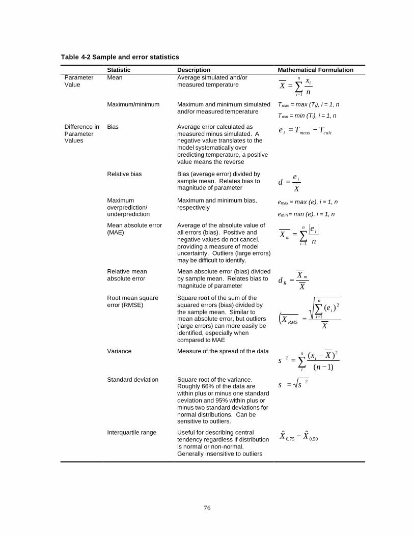
76

Table 4-2 Sample and error statistics

Statistic Description Mathematical Formulation Parameter Value

Mean Average simulated and/or measured temperature ∑

=

=n

i

i

nx

X1

Maximum/minimum Maximum and minimum simulated and/or measured temperature

Tmax = max (Ti), i = 1, n

Tmin = min (Ti), i = 1, n

Difference in Parameter Values

Bias

Average error calculated as measured minus simulated. A negative value translates to the model systematically over predicting temperature, a positive value means the reverse

calcmeasi TT −=ε

Relative bias Bias (average error) divided by sample mean. Relates bias to magnitude of parameter X

iεδ =

Maximum overprediction/ underprediction

Maximum and minimum bias, respectively

εmax = max (εi), i = 1, n

εmin = min (εi), i = 1, n

Mean absolute error (MAE)

Average of the absolute value of all errors (bias). Positive and negative values do not cancel, providing a measure of model uncertainty. Outliers (large errors) may be difficult to identify.

∑=

=n

i

im n

X1

ε

Relative mean absolute error

Mean absolute error (bias) divided by sample mean. Relates bias to magnitude of parameter X

X mR =δ

Root mean square error (RMSE)

Square root of the sum of the squared errors (bias) divided by the sample mean. Similar to mean absolute error, but outliers (large errors) can more easily be identified, especially when compared to MAE

( )X

X

n

ii

RMS

∑== 1

2)(ε

Variance Measure of the spread of the data

∑ −−

=n

i

i

nXx

)1()( 2

2σ

Standard deviation Square root of the variance. Roughly 66% of the data are within plus or minus one standard deviation and 95% within plus or minus two standard deviations for normal distributions. Can be sensitive to outliers.

2σσ =

Interquartile range Useful for describing central tendency regardless if distribution is normal or non-normal. Generally insensitive to outliers

50.075.0ˆˆ XX −

77

4.3.3.2 Calibration and Validation Locations for Rivers and Reservoirs

Each river and reservoir system has unique attributes that should be sufficiently represented with field data to allow satisfactory calibration and validation. Further, the model(s) should be tested at multiple locations and over sufficiently representative time periods.

For river systems, calibration and validation data are usually collected at multiple locations throughout the model domain. The analyst can focus on the study area, but securing data for the entire model domain provides additional field information and generally leads to improved model performance. There is no definitive rule on the amount of data required for this exercise, but generally several locations are desired to fully characterize the river and provide confidence in model calibration. Simulation results and field observations are compared at each location using graphical methods or statistical procedures. Information can be averaged over periods longer than the model time step for interpretation and presentation. For example, daily average values can be calculated from hourly data for both simulation results and field observations and compared directly. In certain cases the model time step is shorter than the available data and this process is necessary. However, aggregating information at multiple locations (e.g., averaging the error at all locations at a particular time) for calibration and validation is discouraged, or should be done with care, because it is difficult to discern model performance through spac e. That is, a model may perform well in certain reaches of river, but perform poorly in others, and averaging information at multiple locations can obscure these conditions.

Reservoir calibration and validation usually involves examining both in-pool reservoir profiles and reservoir outflow temperature. Typically when analyzing reservoir profiles, the onset and breakdown of thermal stratification, the location of the thermocline, and hypolimnion and epilimnion water temperatures are of primary concern. Calibration and validation assessment can include all measured data in the vertical profile or selected locations. Comparison of near-surface water temperatures is sometimes neglected in modeling large reservoirs because surface waters tend to respond to short-term meteorological conditions, while deeper waters respond to long-term (seasonal) variations. If temperature control operations include reservoir spill as an option, such an approach may not be acceptable. When selective withdrawal is important, those elevations in the region of withdrawal elevation, as well as the thermocline location, may warrant additional attention.

Reservoir releases may occur from a single outlet or multiple outlets. Calibration and validation comparisons can be made for each outlet individually or the outflow aggregated into a single value. Analyzing individual outlets requires measured data at each reservoir release location/elevation (e.g., each penstock), which is often unavailable. Aggregated release temperature is commonly used, assuming that all releases mix completely and instantaneously below the dam and that measured river temperature is representative of aggregate reservoir outflow temperature.

4.3.4 Range of Model Applicability Range of model applicability is generally tied to the range of conditions used to calibrate, validate and/or test the model. Thus, calibration and validation data sets should be independent and examine a river and/or reservoir model over the full range of expected conditions, e.g., low, average and high flows/storage; cooler, hotter, drier and wetter conditions. However, data availability and resources are often limiting. One method to improve the range of model validity when data are limited is to select a validation period or periods that are markedly different than the calibration period. In rare cases, a model may have two unique sets of calibration parameters to represent dramatically different conditions (e.g., low reservoir storage conditions and high storage conditions). Upon successful validation some modelers combine the calibration and validation data and re-calibrate to improve model performance. The final calibrated model, ready for analysis, should have well defined limits for flow, depth, temperature, and meteorological conditions. This does not mean that the model cannot be used outside of these limits. On the contrary, one of the most important uses of models is to examine management alternatives that are infeasible to test in the physical system (e.g., implementing selective withdrawal, extreme

78

droughts, dam removal). Thus, models are often applied outside of their calibration and validation range. Comparative analysis, where alternatives (simulations) are compared relative to one another versus a baseline condition, is often employed under these conditions. The concept of comparative analysis is that uncertainty associated with one simulation is similar to the uncertainty associated with another – thus allowing direct comparison. However, if the alternatives simulated are vastly different this assumption may be invalid. Involving personnel with expertise and experience in temperature modeling can aid in interpretation of alternatives well outside the calibration and validation range.

4.3.5 Calibration and Validation and Model Performance Model performance is primarily defined by calibration and validation. That is, the desired performance targets defined in the system characterization (and possibly refined in data synthesis and model selection) should be achieved through model calibration and validation. If the performance targets are not met, or only met under certain circumstances, the modeling project can proceed, but the performance targets should be redefined to reflect the model capabilities and limitations. When modeling regulatory requirements or compliance, performance targets may not be sufficiently flexible to simply allow redefining the target. Under such circumstances it may be necessary to revisit a previous stage in the water temperature study design framework (Figure 3-1). Ideally, appropriate application of the framework should minimize the possibility of reaching model calibration and validation and encountering such problems.

In addition to calibration and validation, model performance can further assessed through sensitivity analysis. Sensitivity analysis will not usually improve model performance, but provides insight into model behavior and uncertainty – thus supporting model performance criteria.

4.4. SENSITIVITY ANALYSIS

A second measure of model performance or reliability is sensitivity analysis. Sensitivity analysis is a method to determine the response of a state variable to variations in parameters, initial conditions, or boundary conditions. Although some refer to sensitivity analysis as a calibration method, it is generally defined as a separate process to further understand or define model behavior. Many variables may influence model output; however, usually a model is most sensitive to only a few variables or parameters. When working with a limited budget, sensitivity analysis can identify parameters that have the greatest impact on model predictions, and resources can be directed towards defining and refining these parameters.

When carrying out sensitivity analysis, typically one model parameter or input data type is varied at a time, usually by a fixed percentage or through an accepted range of values while all other values remain unchanged. The parameter may be a calibration parameter (e.g., evaporation coefficient) or a model input (e.g., wind speed, flow). Model sensitivity can be defined as

S = ∂T / ∂P (4-1) Where S is sensitivity, T represents simulated temperature and P is the parameter being assessed for sensitivity. Sensitivity, as defined in equation (4-1) has units of temperature divided by the units of the parameter P, whatever they may be. In this form, comparing the relative sensitivity of each parameter is more difficult because of inconsistent units. Thus, relative sensitivity (unit less) is defined as

Sr = (∂T/∂P) (P/T) (4-2) Relative sensitivity can provide insight to model performance by providing a basis to compare various parameters and determine which play the largest role. For example, heat budget calculations (and thus model simulated water temperature) are generally insensitive to atmospheric pressure values (a proxy variable used as a boundary condition for calculating vapor pressure in latent heat flux and sensible heat flux). Thus, if measured data are unavailable for

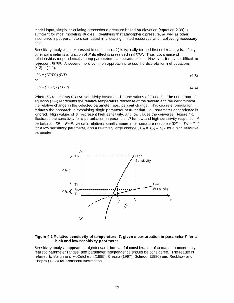
79

model input, simply calculating atmospheric pressure based on elevation (equation 2-39) is sufficient for most modeling studies. Identifying that atmospheric pressure, as well as other insensitive input parameters can assist in allocating limited resources when collecting necessary data.

Sensitivity analysis as expressed in equation (4-2) is typically termed first order analysis. If any other parameter is a function of P its effect is preserved in ∂T/∂P. Thus, covariance of relationships (dependence) among parameters can be addressed. However, it may be difficult to represent ∂T/∂P. A second more common approach is to use the discrete form of equations (4-3)or (4-4).

S’r = (∆T/∆P) (P/T) (4-3) or

S’r = (∆T/T) / (∆P/P) (4-4) Where S’r represents relative sensitivity based on discrete values of T and P. The numerator of equation (4-4) represents the relative temperature response of the system and the denominator the relative change in the selected parameter, e.g., percent change. This discrete formulation reduces the approach to examining single parameter perturbation, i.e., parameter dependence is ignored. High values of S’r represent high sensitivity, and low values the converse. Figure 4-1 illustrates the sensitivity for a perturbation in parameter P for low and high sensitivity response. A perturbation ∆P = P2-P1 yields a relatively small change in temperature response (∆TL = T2L – T1L) for a low sensitivity parameter, and a relatively large change (∆TH = T2H – T1H) for a high sensitive parameter.

Figure 4-1 Relative sensitivity of temperature, T, given a perturbation in parameter P for a high and low sensitivity parameter

Sensitivity analysis appears straightforward, but careful consideration of actual data uncertainty, realistic parameter ranges, and parameter independence should be considered. The reader is referred to Martin and McCutcheon (1998), Chapra (1997), Schnoor (1996) and Reckhow and Chapra (1983) for additional information.

T

Low Sensitivity

High Sensitivity

P P2 P1

T2L T1H

T2H

T1L

∆TH

∆TL

∆P

80

4.5. MODEL USE Upon completion of calibration and validation a model can be used to assess remedial actions and predict their changes in water temperature. Important considerations in model use include providing supporting documentation, modeling assistance, and model management. Additional details on model use can be found in BDMF (2000).

Supporting documentation provides a means for reproducible results – a fundamental premise of any scientific study. Calibration, validation, sensitivity, and other model tests should be well documented, along with model data and parameter values. Likewise, it is important to document model applications, often termed “reporting.” Documentation is time consuming, and should be explicitly included in a modeling project budget.

Formal assistance from computer model authors or software suppliers is available, as well as third party support from consultants or contractors. For example, although the USACE -HEC temperature models are readily available from the National Technological Information Service for a small cost, the user must contact an approved vendor for technical support. Identifying the potential need for model assistance should be made early in the study design process.

Model management is primarily a concern for agencies and organizations interested in incorporating models into ongoing planning and management activities. A formal framework should be defined to address the many factors associated with maintaining a computer model. Several factors are outlined in Table 4-3.

Table 4-3 Long-term model management considerations

Consideration Description

Model management protocols Identify “original” source code; model metadata*; code archives; code dissemination, personnel responsible for codes; etc.

Testing and documenting Procedures/requirements for modification, testing and documentation, and constructing and archiving test cases and calibration/validation runs

Training Long-term model management structure for notifying staff of modifications, as well as training of new staff

Ongoing data collection Identify need and process to collect data to support continued model application

Peer Review Identify need for initial peer review as well as “re-review” if substantial code modifications occur

Funding Secure funding to maintain models and support staff

* model metadata includes a description of the model, contact personnel, model status (ongoing development or completed), computer environment (programming language, hardware requirements, and operating system), access instructions, security information, documentation of algorithms (e.g., citations) and other supplemental information

81

5. CONCLUSIONS AND RECOMMENDATIONS Because of a continued interest in water temperature as a critical parameter for aquatic health, temperature modeling remains an important issue in planning and management of Central Valley aquatic systems. There is a wide body of literature on water temperature and water temperature modeling, as well as an array of mathematical tools and analysis techniques available to individuals, organizations, and agencies that wish to undertake water temperature studies. The purpose of this Bay Delta Modeling Forum water temperature model review is to provide an overview of stream and reservoir water temperature models and modeling techniques, identify historic and current temperature modeling efforts in the Central Valley, define basic temperature prediction concepts, present required field and other physical data, and summarize the role of temperature modeling in addressing water resources and biological problems.

Summarized below are the three main topic areas covered in Chapters 2, 3, and 4: theoretical considerations; water temperature studies; and model implementation, calibration/validation, and use. Subsequently the “state of the field” of water temperature modeling is presented. Based on these findings, as well as discussions with users and experience from model applications, several recommendations for improvements in water temperature models and their applications are presented.

5.1. THEORETICAL CONSIDERATIONS

Physically-based models are the focus of this report. A common component of these models is the heat budget, which describes energy exchange at the air-water interface. Although formulations differ slightly, the heat budget consists of five terms representing short wave radiation, incoming or atmospheric long wave radiation, upwelling long wave radiation, latent heat flux, and sensible heat flux. Certain models include energy exchange at the stream bed-water interface explicitly through an additional bed conduction term.

Generally, models are appropriate for application to either rivers or reservoirs, but not to both. In certain instances river models may be applicable to reservoirs and vice versa, but these are exceptions. River models vary from simple reach models that predict temperatures in short reaches of a stream to more complex basin models that can simulate temperature response in river networks. Reservoir models vary similarly. Reservoir modeling is somewhat different than river modeling because thermal stratification of lakes plays an important role in both in-pool water temperature (and quality) as well as downstream releases. Reservoir and lake temperature dynamics have been modeled extensively for decades. Similar to river temperature models, many reservoir models that simulate water temperature also simulate other water quality constituents. There are models that focus solely on temperature. In all cases temperature modeling requires both flow and heat energy models.

5.2. WATER TEMPERATURE STUDIES

Water temperature studies, as with any scientific assessment, require planning and design for successful implementation and completion. A framework consisting of discrete stages is introduced to assist engineers, resource managers, planners, and biologists through the process of temperature study design and, ultimately, model application. The phases include investigation of study type, system characterization, data synthesis, model selection, and model application. Data collection and assessment and model selection are included as a combined phase because they are often inter-dependent with available data affecting model selection and model selection driving data collection. All phases fall under the influence of project objective. Although presented as a primarily serial process, iteration is common within the modeling framework because new information often becomes available during the study, or more likely the process of modeling helps to more fully define the project objective. The underlying concept is that completing the stages of study objective, study definition, study type, system characterization,

82

and data collection and assessment lead the analyst to select the appropriate model to fit the task. Even upon final selection and application, the modeling process should not be static. System characterization and model application may lead to an increase in information concerning the thermal response of a river or reservoir to hydrologic, meteorological, or other conditions. If the existing model is perceived to be insufficient (e.g., either excessive or insufficient detail), it may be necessary to modify the model or select a new model.

The four study types identified in the first phase include baseline definition, impact analyses, operations applications, and research studies. Water temperature is often not the final parameter of interest. Often water temperature is modeled as a necessary prelude to water quality or ecological modeling.

Once the type of study has been defined, primary system characteristics are identified. Such characteristics include study area and system boundaries primary system components and attributes, and space and time scales of interest. Model output and performance targets are also defined at this time. Most of the information that is gathered during this phase is elementary, ideally identifying critical components and areas where additional data is required. Detailed system characterization occurs during the data collection and assessment phase.

The subsequent phase is a detailed data collection and assessment. As noted above, this step is often performed in concert with model selection. In many cases identification of key data are necessary to make a final model selection. The data types identified in this report include information that is generally required in most temperature models – certain models may not require all described data or may require additional data. Such data include meteorological information, river and reservoir geometry, flow, and water temperature observations. Data can be characterized as being one of three basic types: boundary conditions, initial conditions, and calibration/validation data. Boundary and initial conditions are required for all model applications, while calibration/validation data are only required to test the model prior to application. Data quality cannot be ignored as it directly affects simulation quality. Further, if insufficient data are available or for long-term modeling efforts it may be necessary to implement a field monitoring program.

Model selection, although often carried out coincident with data assessment (model requirements and availability of the necessary data), includes several other key components, including model capability, model availability and status, computational issues, and available resources.

5.3. MODEL IMPLEMENTATION, CALIBRATION/VALIDATION, AND USE Critical steps in the modeling process prior to application include implementation and calibration and validation. Model implementation is the process of loading data, testing, and estimation of model parameters, resulting in a functioning but uncalibrated model. Following implementation the formal process of calibration and validation may begin. Procedures for calibration and validation are well documented. Thus, the focus of this report was to identify a limited number of issues that may play a role in modeling projects including data quality, calibration parameters, methods for comparing simulated output to measured data, and the applicable range of calibration and validation. Once the model is implemented and calibrated, models are often subject to sensitivity analysis to further characterize system response and improve user confidence in model output.

The end product of these preparatory steps is a tested, calibrated, and validated model ready for use. Completion of these steps, although necessary, does not provide the user free reign over any and all analysis. Model use is often restricted to the range of calibration and validation conditions, and when applied outside of these bounds the appropriate limitations should be noted.

5.4. STATE OF THE FIELD Identifying the historical need for temperature prediction illustrates how the field of temperature modeling has evolved. With respect to rivers, much of the concern in early temperature modeling

83

focused on heat pollution, e.g., cooling water or other waste discharge. In the 1980’s stream temperature models to examine heat transfer in relatively short river reaches became popular as fish and wildlife issues became more prominent. These models were generally limited in space and time, that is, they assessed small reaches of a few thousand meters for a short period of time, for example a day or a week. When extensive portions of river systems were investigated or when long periods were examined, models with long time steps were employed (e.g., weekly or monthly). During this same period, more comprehensive models to assess river system water quality became popular. Thus, the driving force was rarely temperature alone, but also the concomitant need for temperature simulation in water quality analyses. Today’s models are either the same or are only slightly different versions than these earlier models. As such, most of the more robust water temperature models that are currently available are components of more extensive water quality models.

Temperature model logic has been fairly static over the past several years, experiencing broader application not necessarily through improvements to the codes, but through advances in computer hardware. Thus the current state of temperature modeling techniques and knowledge is based largely on work that was completed decades ago. Representation of the governing equations of flow and transport is well studied and documented. Although there have been minor reformulations and reinterpretations, the fundamental concepts of heat transfer at the air-water interface have remained unchanged as well. However, unlike the governing equations of flow and transport, which are fairly well represented, the heat budget formulations are based on limited studies and should be revisited.

There have been many successful temperature modeling applications over the past several decades, both within the Central Valley and outside the basin. This has led to the perception that temperature modeling is a “complete” science – that scientists have mastered the basic concepts and moved on to bigger and better problems. However, many of the formulations are dated, models are being applied at finer levels of detail (shorter time and space scales), and technology has changed dramatically since the first models came to fruition. Thus, although there has been favorable success there is still work to do. Several of these areas are addressed in the subsequent section.

5.5. FINDINGS AND RECOMMENDATIONS

Water temperature modeling studies have been carried out for decades. Through time these studies have continually expanded to include larger areas and smaller time steps. Results have generally been acceptable and have proven useful in water resources planning and management. However, through these applications as well as other efforts, additional areas for research and improvement are apparent. Five general categories of findings and recommendations are:

§ Technical Issues

§ Modeling Mechanics

§ Data Considerations

§ Interdisciplinary Efforts

§ Training and Education

The list of recommendations is not exhaustive, but provides a starting point for continued improvement of temperature models and their applications to water resources planning and management

5.5.1 Technical Issues The principal technical issues associated with water temperature modeling include mathematical formulation and numerical solution of the governing equations as well as the heat budget representation. Generally, hydrodynamic and advection-diffusion representation for flow and heat

84

energy transport is appropriate and sufficient. There is the ever-present caution that hydrodynamic representation is an integral part of temperature modeling and that proper flow representation is critical to effective water temperature simulation. Likewise, there are the numerical considerations and limitations associated with certain model formulations that must be accommodated. The primary technical issues addressed herein are associated with the heat budget formulation. A second technical issue of interest is the representation of withdrawal envelopes or the zone of influence associated with outlets in one-dimensional reservoir models and these influences on simulated reservoir thermal structure.

5.5.1.1 Heat Budget Formulation

Examination of the heat budget formulations included within many mainstream models illustrates that the fundamental heat budget formulations have changed little in the past fifteen to twenty years or longer. Largely borne out of TVA (1972) they remain in use with little or no modification in many models. Review of published “updates” to water temperature models generally yields only modest changes to the logic, i.e., addition of a bed conduction term or modification of short wave radiation to accommodate riparian shading.

Advances in atmospheric science and other fields, coupled with improved instrumentation, reduced costs, and increased computing capabilities, provide an opportunity to revisit the heat budget formulations. The relatively high success rate of temperature model applications to many reservoirs and rivers has not provided the impetus for change – the argument being that the models are “good enough.” However, there are three fundamental issues of concern.

First, although TVA (1972) is a seminal document in the field of temperature modeling, many of the formulations presented therein were based on limited data at a limited number of sites under conditions that, in many cases, may not translate easily to other locations. In some cases studies intended for other purposes have been utilized in the heat budget formulations, e.g., Lake Hefner evaporation studies (see Anderson, 1954).

Second, many heat budget formulations in existing models are based on lake formulations with large fetch systems. That is they simulate heat flux at the air water interface for a fully formed boundary layer over the water surface. Although reservoirs are large enough for such a boundary layer to develop, rivers are typically not so geometrically convenient. Further research into the surface fluxes in limited fetch systems is necessary.

Finally, to accommodate computational limitations, early computer models often utilized a simplified equilibrium temperature approach (see Section 2.5.2). Several models still incorporate this method. Where longer time steps are used (e.g., reservoirs) and water temperatures are near equilibrium, these models generally perform well. However, in many regulated rivers of the Central Valley, reservoir release temperatures during critical summer and fall months are far below equilibrium temperature. Given current computational capabilities the full heat budget formulation should be represented when modeling river reaches below large mainstem reservoirs with short time steps.

Recommendation: It is recommended that agencies and organizations responsible for water temperature control and management fund research in the field of meteorology as it affects heat exchange with water bodies in systems typical to the Central Valley. Specific studies include revisiting the seminal work in water temperature modeling (e.g., TVA, 1972) as well as recent advances, identifying improvements in monitoring equipment and data analysis, and formulating up to date research plans for advancing the state of the field. There is an opportunity to contribute to the field of water temperature modeling through revision of dated computer codes with new, more comprehensive representations. The Bay Delta Modeling Forum, through its member agencies, associates, and affiliations can provide the motivation and can assist in identifying funding for this important work.

85

5.5.1.2 Reservoir Inflow and Withdrawal Envelope Formulations

The one- and two-dimensional reservoir representations require several approximations. Although not discussed heretofore, of particular interest is the determination of vertical and lateral extent or influence of reservoir outlets, often termed withdrawal envelopes. The representations of withdrawal envelope extent are generally empirical relationships based on intake location and size, release rate, thermal structure of the reservoir, and reservoir geometry (e.g., surface and bottom). In most models this logic may be presented in the user’s manual, but there is typically only one or two withdrawal envelope formulations available. Thus the modeler is restricted to what is in the computer code, and often these formulations were developed twenty to thirty years ago. Because the withdrawal envelope affects hydrodynamics in a region (depth and width) that is significantly larger than the intake diameter, proper representation is critical when analyzing temperature control such as selective withdrawal from multiple depths and/or outlets.

Recommendation: Complete a review of past and current research in the formulation of reservoir inflow allocation and withdrawal envelope relationships. Determine if sufficient information is available to validate (or invalidate) existing formulations. If invalid, seek funding to complete necessary research to revise and/or define new relationships, or at a minimum quantify limitations of existing formulations. Recent improvements in flow measurement (e.g., acoustic Doppler current profiler) and temperature monitoring can provide considerable insight into system response that was unavailable during the determination of many currently available formulations. In addition, advances in computational hydrodynamics can provide a means to further assess near-field conditions and, coupled with high precision field monitoring, can be used to formulate improved withdrawal relationships.

5.5.2 Modeling Mechanics Modeling mechanics involves use and operation of the computer code and the interface between the modeler and the model. Two topics of interest are identified: (1) the primary computer language used in most temperature models is FORTRAN and (2) improved model interfaces can improve temperature model applications.

5.5.2.1 Computer Language and Code

Historically, civil and mechanical engineers constructed the majority of flow and water quality models. Because the most common engineering computing language from the late 1960’s to the 1990’s was FORTRAN, almost all water temperature models are coded in FORTRAN. Even with the increased availability and popularity of new computer languages, few of the models have been converted to new/different languages. Examination of any of several computer codes illustrates that much of the original logic remains, including formatted input and output, measures to maximize use of storage space and computer memory, and procedures to reduce computational effort. Although documentation exists for many of the public domain codes, the programs themselves are generally poorly commented and can be difficult to modify or update.

Recommendation: It most cases it is not economically feasible to update and document existing model codes. Nonetheless, opportunities may present themselves to improve model formulation and documentation. When such opportunities occur, codes should be updated and the benefits of employing languages other than FORTRAN explored.

5.5.2.2 Improved Model Interfaces

With the proliferation of models and the wider use of models for regulatory compliance there is an increasing need to improve the interface between the computer model and technician – a graphical user-interface (GUI). Many of the original computer codes have cumbersome, formatted input and output files (flat files). Input is difficult to manage in this form, especially for larger applications. In many cases modelers construct elaborate pre-processing programs (a separate computer program) or spreadsheets where the data is input and manipulated,

86

subsequently this information is transferred to a text file for use by the computer model. Although output is often in tabular form with some level of description, these files are similarly cumbersome to use in text form and generally are post processed or imported into another program (e.g., a spreadsheet) for analysis and graphing. Management of these flat files is at best inefficient; at worst it is a potential source of input error and erroneous model results. Improved GUI can ease model implementation, calibration and validation, and use. Further, well-designed interfaces can aid interpretation of input and output through improved data management, assist in training staff, and provide a valuable means venue for presenting results.

There is the concern that making models easier to use may result in non-qualified or untrained users to misapply models. This concern should promote managers to ensure modelers receive adequate training. In all cases the primary model source code should remain readily accessible for peer review and potential modification. If the model undergoes continuous modification, modification and maintenance of the interface (which is typically not written in FORTRAN) is likewise required.

Recommendation: It is recommended that interface development be encouraged and adopted by agencies and organizations modeling in the Central Valley. Interface development should extend beyond simply passing flat file information back and forth between the user and model. Investigation into data management, model interaction, and input and output interpretation to improve efficiency and flexibility should be incorporated to the highest degree possible. Documentation should accompany any interface development.

5.5.3 Data Considerations Paramount to reliable and responsible temperature modeling is the collection, analysis, and maintenance of high quality data. Likewise, the management of both input and output data is important. Data quality considerations, consistent monitoring, as well as specific recommendations for meteorological data are discussed.

5.5.3.1 General

Currently there are few standards for collection and maintenance of temperature data in the Central Valley, particularly time series observations. For selected local systems, watershed groups, state, federal and other agencies have developed temperature monitoring protocols; however, such protocols are the exception rather than the rule. Further, water temperature modeling requires more than just water temperature data; meteorological, flow, and geometric data are also necessary. Meteorological and flow time series are customarily overseen by state and federal agencies, with associated protocols and quality assurance measures.

As noted above, model interfaces can assist in input and output data interpretation, but they can also play a valuable role in data management. Identifying appropriate data management tools such as the HEC data storage system (HEC-DSS) or other software with or without a GUI will provide analytical and economical benefits.

Recommendation: Available temperature data collection methods should be inventoried and assessed. Collect available temperature monitoring protocols and formulate a range of quality assurance program levels to accommodate river and reservoir analyses typical to the Central Valley. Identify and review flow and meteorological monitoring programs to provide a level of data quality for consideration in temperature modeling. Review available data management software and report on capabilities, costs, and availability.

5.5.3.2 Monitoring

Although water temperature monitoring has increased dramatically, there is inconsistent representation throughout the Central Valley. Certain systems have significant networks of temperature devices deployed throughout their length and/or depth, while other rivers or reservoirs have infrequent and inconsistent monitoring.

87

Recommendation: The BDMF member agencies should identify representative organizations from which to solicit input for individual river and reservoir systems regarding existing water temperature monitoring. Reservoir profile and intake temperature monitoring should be assessed to determine adequacy given in-pool and downstream requirements – both regulatory and non-regulatory. Critical river reaches should be identified and monitoring efficacy reviewed. Long-term stations should be identified and funding secured to maintain key stations.

5.5.3.3 Meteorological Data

The National Weather Service (NWS) is updating meteorological stations throughout the United States. Automated weather observations systems (AWOS) are rapidly replacing less sophisticated meteorological stations and manual observations systems. As a result, cloud cover is being phased out of the weather observation data set; however, an appropriate replacement – ideally measured short wave radiation monitoring – is rarely added to the weather stations. To some degree there is a level of redundancy with the NWS in the Central Valley because the California Irrigation Management Information System (CIMIS) monitors all necessary meteorological parameters for water temperature modeling (including solar radiation) at several locations. Certain models may not have the option to input solar radiation directly, but the modification is fairly straightforward.

Another challenge facing certain agencies is the near-real time operation of project facilities to meet temperature requirements in river reaches below large reservoirs. Mathematical models are used to estimate the rate of water temperature increase and water temperatures based on reservoir release, release water temperature, and meteorological forecasts. Meteorological forecasts are only available at selected locations in the Central Valley that are supported and maintained by the NWS. Not only does this limit the available meteorological data that is used in model simulation, but introduces uncertainty associated with forecasts into the modeling analysis.

Recommendation: Identify critical stations in the Central Valley (e.g., Sacramento Metropolitan Airport) and determine if the conversion to AWOS has compromised the required data for temperature modeling. Determine potential funding sources to augment monitoring as necessary. Inventory meteorological stations that are used or potentially may be used by agencies forecasting short-term operating conditions for temperature control in downstream river reaches and assess limitations (proximity to water body, appropriate observations, etc.). Develop a probabilistic methodology to incorporate uncertainty in short-term meteorological forecasting for agencies that are regulating water temperatures downstream of main stem reservoirs.

5.5.4 Interdisciplinary Efforts As the scope and scale of environmental studies expands, the need for interdisciplinary studies including scientists, engineers, biologists and other specialists has become apparent. In most cases Central Valley water temperate modeling applications and monitoring efforts provide information for ecological or biological applications. For example, carry-over cold water supplies in main stem reservoirs and temperature studies in most of the major river systems are associated with anadromous fish restoration measures. Not only are inter-disciplinary projects necessary, they often provide a broader contribution to problem assessment due to integrated perspectives, more complete system representation, and improved overall understanding of system dynamics. Further, because both water temperature (and flow), ecological, and biological studies are often costly, a well planned, interdisciplinary project can be more cost effective through efficient integration of project objectives, plans, field monitoring, and analyses.

Incorporating a temperature model into an inter-disciplinary process may not be straightforward. Distinctive perspectives; technical nuances of model development, application, and data sharing; as well as project management requirements present unique challenges to such projects. Water temperature and ecological models may operate at different time and space scales, and computational times may vary considerably. For example, a temperature model may take hours

88

to complete a simulation and an ecological model may operate for a few seconds, or vice versa. Required data quality and quantity may differ between studies.

Some considerations for integrating water temperature modeling into inter-disciplinary studies include:

§ Define common objectives

§ Identify and define technical terminology to provide effective methods of communication among participants

§ Involve stakeholders (and recognize that stakeholders must receive some benefit from their interaction)

§ Create a project management plan and allocate sufficient resources (e.g., time, funding, and administrative support)

§ Provide well defined leadership and lines of communication

§ Identify study design that accommodates all project components (e.g., temperature modeling, ecological modeling) and personnel

§ Define data requirements for all project components

§ Create a cooperative monitoring program to collect common data

§ Accept that model domains may not be coincident

§ Provide an “interface” or “link” between the temperature and other models to ensure proper data output and data format

§ Include comprehensive documentation

The primary goal is to identify common ground and accommodate potential model differences.

Recommendation: The BDMF should sponsor a one-day workshop addressing the challenges and approaches to interdisciplinary projects and research. The workshop should focus on developing a matrix of critical considerations for inter-disciplinary efforts involving water temperature modeling with ecological and biological studies. Input and participation from appropriate agencies, organizations, and stakeholders is requisite to the success of such a workshop.

5.5.5 Education and Training Agency personnel, scientists, and the public need to be better informed about the rationales, goals, and methods of water temperature modeling. For example, computer models tend to give a false sense of certainty to environmental studies. Natural systems are notoriously complex and water temperature prediction includes a level of uncertainty. Uncertainty is a difficult concept to incorporate into regulatory compliance. Thus, there is a need to maintain an appropriate level of training and education within agencies and organizations to ensure capable and useful model analyses are completed. Technology transfer to agencies from third party interests (universities, consultants, other agencies) should be encouraged where appropriate. By and large federal, state, and local agencies control our water resources or have a direct role in regulation of water bodies. Often considerable expertise resides within these agencies as institutional knowledge. Thus, developing and maintaining modeling capabilities, or at least modeling familiarity within these institutions, will be useful in water resources management.

Education and training can occur through formal means such as enrollment at Universities, colleges, and extension courses. Informal methods include modeling workshops, self-training/on the job training, the formation of technical groups to meet and discuss pertinent topics, invitation of speakers, and forming cooperative arrangements with other organizations to share technical

89

support services. Fundamental to all education and training is a commitment from management to encourage and support employee development.

Recommendation: Available education and training opportunities should be identified and disseminated to interested parties. The Bay Delta Modeling Forum should sponsor a technical group to assist in common aspects of temperature modeling, e.g., development, implementation, calibration and validation, and application. The group should enlist the local expertise and interest of state and federal agencies participating in activities where water temperature plays a key role.

5.5.6 Concluding Comment The intent of this report is to advance the level of knowledge in the field of water temperature modeling and promote continued research in the field. No single document can address all possible circumstances that may be encountered in the process of conducting temperature studies. The reader is encouraged to explore resources beyond this document and to keep abreast of the field through organizations such as the Bay Delta Modeling Forum.

90

6. REFERENCES Alonso, W. 1971. “Beyond the interdisciplinary approach to planning,” Journal of the American

Institute of Planners. May.

Anderson, J.A. 1994. Modeling Impacts of Temperature on Salmon. Unpublished Master’s Thesis, University of California, Davi s.

Anderson, M.G. and P.D. Bates (2001) “Hydrologic Science: Credibility and Scientific Integrity”, in Model Validation: perspectives in hydrologic sciences . Ed. M.G. Anderson and P.D. Bates. John Wiley and Sons Ltd. New York. 500 pp.

Bartholow, J.M. 1989. Stream temperature investigations: field and analytic methods . Instream Flow Information Paper No. 13. U.S. Fish and Wildlife Service. Biological Report 89(17) 139 pp.

Bay Delta Modeling Forum (BDMF). 2000. Protocols for Water and Environmental Modeling. Prepared by the Ad hoc Modeling Protocols Committee. January. (Posted at www.sfei.org/modelingforum)

Beard, L.R. and R.G. Willey. 1972. Reservoir Temperature Stratification. Generalized computer program no. 723-410. User’s Manual. U.S. Army Corps of Engineers Hydrologic Engineering Center. Davis, CA

Bestchta, R.L. 1984. A computer model for predicting stream temperature results from the management of streamside vegetation. USDA Forest Service. WSDG Report, WSDG-AD-00009. July.

Bicknell, B.R., J.C. Imhoff, J.L. Kittle, Jr., T.H. Jobes, A.S. Donigian, Jr. 2001. Hydrologic Simulation Program – FORTRAN. HSPF, Version 12, User’s Manual. Prepared by Aqua Terra Consultants in cooperation with U.S. Geological Survey, Hydrologic Analysis Software Support Program for the U.S. Environmental Protection Agency. Contract No. 68-C-98-010.

Bowen, I.S. 1926. “The ratio of heat losses by conduction and by evaporation from any water surface”. Physical Review. Vol. 27. pp 779-787.

Bowie, G.L., W.B. Mills, D.B. Porcella, C.L. Campbell, J.R. Pagenkopf, G.L. Rupp, K.M. Johnson, P.W. Chan, and S.A. Gherini. 1985. Rates, constants and kinetics formulations in surface water quality modeling. 2nd Ed. EPA/600/3-85/040 U.S. Environmental Protection Agency, Environmental Research Laboratory, Athens GA.

Brown, L.C. and T.O. Barnwell, Jr. 1987. The enhanced stream water quality models QUAL2E and QUAL2E-UNCAS: documentation and user’s manual. EPA/600/3-87/700. U.S. Environmental Protection Agency, Environmental Research Laboratory, Athens GA. May.

Brutsaert, W. 1982. Evaporation into the atmosphere. Kluwer Academic Publishers, Dordrecht, The Netherlands.

CALFED Bay Delta Program (CALFED). 2000a. Final Programmatic EIS/EIR. Sacramento. June.

CALFED Bay Delta Program (CALFED). 2000b. Ecosystem Restoration Program: Volumes I, II, and Strategic Plan for Ecosystem Restoration. Sacramento. June.

Campbell, G.S., and J.M. Norman, 1998. An Introduction to Environmental Biophysics, Second Edition. Springer-Verlag. New York, NY.

Central Valley Regional Water Quality Control Board (CVRWQCB). 1998. A Compilation of Water Quality Goals. Prepared by J.B. Marshack. Prepared in cooperation with the California Environmental Protection Agency. Sacramento, CA. March.

Chapra, S. C. 1997. Surface Water Quality Modeling. McGraw-Hill. New York.

91

Chen, C.W. and G.T. Orlob. 1972. Ecological Simulation for Aquatic Environments, WRE 1-0500, Water Resources Engineers, Inc., Walnut Creek, CA.

Christiansen, C.L. and G.T. Orlob. 1989. Temperature Modeling of the Sacramento and American Rivers. Project report prepared for the California Department of Fish and Game by the University of California, Davis.

Cook, C.B. and G.T.Orlob. 2000. Numerical Estimation of Dynamic Water Temperature Fluctuations at Compliance Point Robinson Riffle (DRAFT). Prepared for the California Department of Water Resources by the Water Resources and Environmental Modeling Group, Department of Civil and Environmental Engineering, University of California, Davis. May.

Deas, M.L. 1998. Trinity Reservoir Water Temperature Simulation Model. Prepared for Trinity County, Agreement No. TFG 97-10. M.L. Deas, P.E. August.

Deas, M.L. 1998a. Trinity Reservoir Carryover Analysis. Prepared for Trinity County, Agreement No. TFG 97-10A. M.L. Deas, P.E. August.

Deas, M.L. and G.T. Orlob. 1997. Iterative calibration of hydrodynamic and water temperature models – application to the Sacramento River.” Proceedings Water for a Changing Global Community. 27th Congress of the International Association for Hydraulic Research and hosted by the American Society of Civil Engineers Water Resources Division, August 10-15, San Francisco, CA, 1997.

Deas, M.L., Meyer, G.K, Lowney, C.L., Orlob, G.T., and King, I.P. (1997) Sacramento River Temperature Modeling Project Report. Center for Environmental and Water Resources Engineering University of California, Davis, Report Number 97-01.

Denny, M.W. 1993. Air and Water: the biology and physics of life’s media. Princeton University Press. Princeton, New Jersey.

Domenico, P.S. and F.W. Schwartz. 1990. Physical and Chemical Hydrogeology. John Wiley and Sons. New York. 824 pp.

Edinger, J.E., D.W. Dutweiler, and J.C. Geyer. 1968. Heat Exchange in the Environment, Cooling Water Discharge Project Report no. 2, Publication 65-902, Edison Electric Institute, New York, NY.

Environmental Laboratory. 1995. CE-QUAL-RIV1: A dynamic, one-dimensional (longitudinal) water quality model for streams: User’s Manual, Instructional report EL-95-2, U.S. Army Corps of Engineer Waterways Experiment Station, Vicksburg, MS.

Environmental Laboratory. 1986. CE-QUAL-R1: A numerical, one-dimensional model of reservoir water quality; User’s Manual, Instructional report EL-82-1 (Revised Edition), U.S. Army Corps of Engineer Waterways Experiment Station, Vicksburg, MS.

Federal Water Pollution Control Administration. 1967. Temperature and Aquatic Life. Laboratory Investigations No. 6, Technical Advisories and Investigations Branch, Cincinnati, Ohio.

Fisher, H.B., E.J. List, R.C.Y. Koh, J. Imberger, and N.H. Brooks. 1979. Mixing in inland and coastal waters. Academic Press, New York, NY.

Hanna, R.B., L.Saito, J.M. Bartholow, and J. Sandelin. 1999. “Results of Simulated Temperature Control Device Operations on In-Reservoir and Discharge Water Temperatures Using CE -QUAL-W2.” North American Lake Management Society. Vol. 15, No. 2. pp 87-102. June

Holmes, R.M. 2000. The Importance of Groundwater to Stream Ecosystem Function. Streams and Groundwaters. Ed. J.B. Jones and P.J. Mulholland. Academic Press, London.

Hondzo, M. and H.G. Stefan, 1994. “Riverbed heat conduction prediction” Water Resources Research. Vol. 30, No. 5 pp 1503-1513. May.

92

Horne, A.J., and C.R. Goldman, 1994. Limnology, Second Edition. McGraw-Hill, Inc. New York, NY.

Huber, W.C., D.R.F. Harleman, and P.J. Ryan. 1972. “Temperature prediction in stratified reservoirs,” ASCE, Journal of the Hydraulics Division. Vol. 98, HY4, pp 645-666, April.

Humphrey, J.H. 1987. American River Water Temperature Modeling. Ott Water Engineers, Inc. Redding, CA.

Hutchinson, G.E., 1975. A Treatise on Limnology, John Wiley & Sons, Inc., New York.

Hydroscience, Inc. 1971. Simplified mathematical modeling of water quality. 444-368/392. U.S. Environmental Protection Agency, Office of Water Programs, Washington D.C.

Imberger, J. 1985. “Thermal characteristics of standing waters: an illustration of dynamic processes.” Hydrobiologia, Vol 125, pp 7-29.

Imberger, J., and J.C. Patterson. 1990. “Physical Limnology.” Advances in Applied Mechanics, Vol 27, pp 303-475.

Jacquet, J. 1983. Simulation of Thermal Regimes in Rivers, in Mathematical Modeling of Water Quality: Streams, Lakes, and Reservoirs, Ed. G.T. Orlob. International Institute for Applied Systems Analysis (IIASA). John Wiley and Sons. New York.

Jenson, M. X. Wang, J.J Fellos, and G.T. Orlob. 1999. Temperature Regulation through Whiskeytown Reservoir. Prepared for the US Bureau of Reclamation. by the Water Resources and Environmental Modeling Group, Department of Civil and Environmental Engineering, University of California, Davis. November.

Jirka, G.H., G. Abraham, and D.R.F. Harleman, 1975. An Assessment of Techniques for Hydrothermal Prediction. Ralph M. Parsons Laboratory for Water Resources and Hydrodynamics, Department of Civil Engineering, Massachusetts Institute of Technology. Report No. 203. July.

Jobson, H.E., 1977. Bed Conduction Computation for Thermal Models Journal of the Hydraulics Division, ASCE, Vol. 103 pp 1213-1217.

Johnson, W.K. 1988. Introduction to Civil Engineering Planning. University of California, Davis.

Jones, F.E. 1992. Evaporation of water: with emphasis on applications and measurements. Lewis Publishers, Inc., Chelsea, Michigan.

Jones, J.B. and P.J. Mulholland. 2000. Streams and Ground Waters. Academic Press.

Jones and Stokes Associates (JSA). 1995. Temperature and Gravel Investigations for Fisheries Enhancement on the Lower Merced River, Merced County, CA. Prepared for California Department of Fish and Game.

Jones and Stokes Associates, Inc. (JSA). 1992. Temperature Modeling of Lewiston Lake with the BETTER Two-Dimensional Reservoir Flow Mixing and Heat Exchange Model. Prepared for County of Trinity, Department of Transportation and Planning. June.

King, I.P. 1994. RMA-2; A Two-Dimensional Finite Element Model for Flow in Estuaries and Streams, Version 5.1. Department of Civil and Environmental Engineering, University of California, Davis.

King, I.P. 1997. RMA-11 A Three Dimensional Finite Element Model for Water Quality in Estuaries and Streams – Documentation Version 2.5. Department of Civil and Environmental Engineering, University of California, Davis.

Kirk, J.T.O., 1994. Light and Photosynthesis in Aquatic Ecosystems. Cambridge University Press, Great Britain.

Linacre, E., 1992. Climate Data and Resources. Routledge, London.

93

Lowney, C.L. 2000. River Temperature Dynamics in the Sacramento River: Measurement and Modeling. Ph.D. Dissertation, University of California, Davis. March.

Lowney, Cynthia, L. 2000. Stream temperature variation in regulated rivers: Evidence for a spatial pattern in daily minimum and maximum magnitudes. Water Resources Research Vol. 36, No.10, 2947-2955.

Lowney, C.L., J.R. Lund, M.L. Deas. 1998. Optimization Modeling for River Restoration. Proceedings: Water Resources Planning and Environmental Regulations: Improving Coordination, American Society of Civil Engineers.

Martin, J.L. and S.C. McCutcheon. 1999. Hydrodynamics and Transport for Water Quality Models. Lewis Publishers, London.

McCutcheon, S.C. 1989. Water Quality Modeling, Volume I Transport and Surface Exchange in Rivers. CRC Press, Boca Raton, Florida.

Meyer, G.K., G.T. Orlob, and C. Jokiel. 1993. “Chapter 13: Climate Change Effects on Water Quality, Central Valley, California,” in Monograph on Water Resources Management in the Phase of Climatic/Hydrologic Uncertainties, Z. Kaczmarek (Ed.), International Institute for Applied Systems Analysis (IIASA).

Meyer, G. and G.T. Orlob. 1994 Impacts of Global Warming on the Quality of Surface Waters . Department of Civil and Environmental Engineering, University of California, Davis.

Monteith, J.L., and M. Unsworth. 1990. Principles of Environmental Physics, 2nd Edition. Edward Arnold, New York.

Oke, T.R., 1987. Boundary Layer Climates. Second Edition. Routledge, New York, NY.

Orlob, G.T., 1983. “One-Dimensional Models for Simulation of Water Quality in Lakes and Reservoirs” in Mathematical Modeling of Water Quality in Lakes and Reservoirs, edited by G.T. Orlob, Wiley Interscience, New York.

Orlob, G.T., 1981. “Models for Stratified Impoundments” in Models for Water Quality Management, edited by A.K. Biswas, McGraw Hill, New York.

Purkey, D.R., G.A. Thomas, D. K. Fullerton, M. Moench, L. Axelrad. 1998. Feasibility Study of a Maximal Program of Groundwater Banking. Prepared by the Natural Heritage Institute. December.

Raphael, J.M. 1962. “Prediction of temperatures in rivers and reservoirs,” ASCE Journal of the Power Division, Vol. 88 (PO2) pp 157-181.

Rowell, J.H. 1998. “A history of temperature modeling in the Central Valley.” Presentation at the Bay Delta Modeling Forum, Temperature Modeling Workshop, October 22, Sacramento.

Rowell, J.H. 1990. Mathematical Model Investigations: Trinity Dam Multilevel Outlet Evaluation – Trinity River Temperature Prediction Study. Trinity River Basin Fish and Wildlife Task Force; Interim Action Program. U.S. Bureau of Reclamation, Sacramento, CA.

Rowell, J.H. 1980. Mathematical Model Investigation of Auburn Dam Multilevel Intakes for Downstream Temperature Control. U.S. Bureau of Reclamation, Sacramento, CA.

Rowell, J.H. Truckee River Temperature Prediction Study. U.S. Bureau of Reclamation, Sacramento. 1975.

Rowell, J.H. 1972. Reservoir and Stream Predictions in the Upper Sacramento River Basin. M. S. Thesis, California State University, Sacramento, July.

Rutherford, J.C. 1994. River Mixing. John Wiley & Sons, Inc., New York.

Salmon, M.E., M.A. Breitenbach, and D.B. Steiner. 1992. Report on Water Temperature Modeling on the Yuba River. Prepared for the Yuba County Water Agency. Prepared by Bookman-Edmonston Engineering, Inc., Sacramento, CA.

94

Saviz, C.M., J.F. DeGeorge, G. T. Orlob, and I.P. King. 1995. Modeling the Fate of Metamsodium and MITC in the Upper Sacramento River: The Cantara Southern Pacific Spill. Department of Civil and Environmental Engineering. Center for Environmental and Water Resources Engineering, University of California, Davis. Report 95-2.

Schnoor, J.L. 1996. Environmental Modeling. John Wiley and Sons, Inc.

Sinokrot, B.A. and H.G. Stefan. 1993. “Stream temperature dynamics: measurements and modeling.” Water Resources Research, Vol 29, No. 7, pp 2299-2312. July.

Smith, D. J. 1988. Calibration Report – Sacramento River System – Temperature and EC Model. Draft report to US Bureau of Reclamation contractor: CH2Mhill. Resource Management Associates. May.

Smith, D.J. 1981 Effects of the Proposed North Fork Stanislaus River Hydroelectric Development Project on Water Temperature. Prepared by Resource Management Associates (RMA) for Calaveras County. March.

Stull, R.B., 1988. An Introduction to Boundary Layer Meteorology. Kluwer Academic Publishers, Dordrecht.

Tchobanoglous, G. and E.D. Schroeder. 1985. Water quality. Addison-Wesley, Menlo Park, CA.

Tennessee Valley Authority (TVA). 2001. TVA River Modeling System. Report No. WR28-1-590-64. Prepared by G. Hauser. TN.

Tennessee Valley Authority (TVA). 1990. BETTER: A two -dimensional reservoir water quality model, technical reference manual and user’s guide. Water Resources Research Laboratory, Report No. WR28-2-590-152. TN.

Tennessee Valley Authority (TVA). 1972. Heat and mass transfer between a water surface and the atmosphere. Report No. 14. April.

Thomann, R.V. and J.A. Mueller. 1987. Principles of Surface Water Quality Modeling. HarperCollins Publishers, Inc. New York.

Theurer, F.D., K.A. Voos, W.J. Miller. 1984. Instream Water Temperature Model. Instream Flow Information paper 16. U.S. Fish and Wildlife Service FWS/OBS-84/15

Tsay, T., G.J. Ruggaber, S.W. Effler, and C.T. Driscoll. 1992. “Thermal Stratification modeling of Lakes with Sediment Heat Flux.” Journal of Hydraulic Engineering, Vol. 118, No. 3, March.

United States Army Corp of Engineers (USACE). 1995. CE-QUAL-W2: A Two -Dimensional, Laterally Averaged, Hydrodynamic and Water Quality Model, Version 2.0, User Manual. Instructional Report EL-95-1. Prepare by T.M. Cole and E.M. Buchak. June.

United States Army Corp of Engineers (USACE). 1994. Computer Models for Water Resources Planning and Management. Prepared by Ralph Wurbs. IWR Report 94-NDS-7. July

United States Army Corps of Engineers – Hydrologic Engineering Center (USACE -HEC). 1991. “Stream and Reservoir Routing.” Chapter 9 of Document EM1110-2-9021. September 30.

United States Army Corp of Engineers – Hydrologic Engineering Center (USACE-HEC). 1987a. Water Quality Modeling of Reservoir System Operations Using HEC-5Q. Training Document No 24 (TD-24)Hydrologic Engineering Center. September.

United States Army Corps of Engineers – Hydrologic Engineering Center (USACE -HEC). 1987b. Water Quality Modeling of Reservoir System Operations Using HEC-5. Training Document No. 24. September.

United States Army Corps of Engineers – Hydrologic Engineering Center (USACE -HEC). 1987c. Simulation of Flood Control and Conservation Systems: appendix on Water Quality Analysis. September.

95

United States Army Corp of Engineers – Hydrologic Engineering Center (USACE-HEC). 1986. WQRRS Water Quality for River-Reservoir Systems, User’s manual. Hydrologic Engineering Center. October 1978, revised 1986.

United States Environmental Protection Agency (EPA). 1979. Quality Criteria for Water (Red Book). Washington D.C. July.

United States Environmental Protection Agency (EPA). 1987. Selection Criteria for Mathematical Models Used in Exposure Assessments: Surface Water Models. EPA/600/8-87/042. July.

University of California, Davis (UC Davis) 1997. Sacramento River Temperature Modeling Project. Center for Environmental and Water Resources Engineering. Report No. 97-01. Sponsored by the State Water Resources Control Board 205(j) Clean Water Act Grant Program, Trinity County Planning Department, and California Department of Fish and Game Proposition 70 Salmon Stream Restoration Fund. January.

Walker, W.W. 1999. Simplified Procedures for Eutrophication Assessment and Prediction: User Manual. U.S. Army Corps of Engineers, Waterways Experiment Station. April.

Walling, D.E. and B.W. Webb. 1996. Water Quality, I. Physical Characteristics. River Flow and Channel Forms. Ed. G. Petts and P. Calow. Blackwell Sciences Limited, Australia.

Water Resources Engineers. (WRE). 1969. Mathematical Models for the Prediction of Thermal Energy Changes in Impoundments. Report to the U.S. Environmental Protection Agency, Project # 16130 EXT. December.

Water Resources Engineers. (WRE). 1967. Prediction of Thermal Energy Distribution in Streams and Rivers. Prepared for the Department of Fish and Game, State of California. June.

Water Resources Engineers (WRE). 1977 Mathematical Modeling of Surface Impoundments, Vol I, II. RMA 6080. Prepared by G.T. Orlob. Lafayette, CA. June.

Wetzel, R.G. 1983. Limnology, 2nd Ed. Saunders College Publishing. Harcourt Brace College Publishers. Fort Worth, TX.

Winter, T.C. 1981. “Uncertainties in Estimating the Water Balance of Lakes .” Water Resources Bulletin, American Water Resources Association. Vol. 17, No. 1, February.

Zedonis, P. 1997. A Water Temperature Model of the Trinity River. Prepared for US Bureau of Reclamation, Sacramento, CA by US fish and Wildlife.

96

Personal Communications

Personal communications includes all people contacted via phone, email, and through meetings. Their involvement ranges widely, from providing additional contacts to reviewing the draft document. Regardless, their assistance is appreciated.

Mike Aceituno, National Marine Fisheries Service Chet Boling, US Bureau of Reclamation Russ Brown, Jones and Stokes Associates Dan Castleberry, United States Fish and Wildlife Service Dick Daniels, CALFED Peter Dileanis, United States Geologic Survey Steve Edmonston, National Marine Fisheries Service John Engbring, United States Fish and Wildlife Service Craig Fleming, United States Fish and Wildlife Service Tim Ford, Turlock Irrigation District Paul Fujitani, US Bureau of Reclamation Andy Hamilton, U.S. Fish and Wildlife Service Steve Herrera, State Water Resources Control Board Paul Hutton, Department of Water Resources John Icanberry, United States Fish and Wildlife Service Jerry Johns, State Water Resources Control Board Debbie McEwan, Department of Water Resources James McKevitt, United States Fish and Wildlife Service Meri Moore, US Bureau of Reclamation Tom Morstein-Marx, US Bureau of Reclamation Parvis Nadir, Department of Water Resources John Nelson, California Department of Fish and Game Gerald Orlob, University of California, Davis Tricia Parker, United States Fish and Wildlife Service Lloyd Peterson, US Bureau of Reclamation Harry Rectenwald, California Department of Fish and Game Dave Reed, US Bureau of Reclamation Jack Rowell, US Bureau of Reclamation Rich Satkowski, State Water Resources Control Board Camilla Saviz, University of the Pacific Dennis Smith, National Marine Fisheries Service Don Smith, RMA Inc. Ted Sommer, Department of Water Resources Scott Spaulding, United States Fish and Wildlife Service Michael Tansey, US Bureau of Reclamation Dave Vogel, Natural Resources Scientists, Inc. Nick Wilcox, State Water Resources Control Board Sam Williamson, United States Geologic Survey Russ Yaworsky, US Bureau of Reclamation Paul Zedonis, United States Fish and Wildlife Service

97

7. GLOSSARY Accretions Ungaged flows into a river or reservoir. Often determined through a

water balance or flow routing exercise.

Accuracy A measure of model performance whereby simulated values are compared with field observations (or other measured data). A function of both bias and precision.

Advection Transport of heat or other water quality constituent along with the movement of a mass of water (bulk flow). Transport by an imposed current system.

Albedo Ratio of amount of solar radiation reflected by a body to the amount incident upon it.

Analysis Period

Specific period of interest for a modeling study. Typically less than or equal to model simulation period.

Analytical Solution Those solutions where the unknown variable is given as a mathematical expression in terms of the independent variables and parameters of the system.

Anemometer An instrument for measuring the speed of the wind.

Atmospheric Pressure Pressure exerted on the surface of the earth due to the weight of the air.

Bathymetry Topographic map showing depth contour lines, typically in a reservoir.

Beer’s Law Change in radiation intensity due to absorption of radiation. Describes attenuation where radiation of a single wavelength is absorbed but not scattered when it passes through a homogeneous medium.

Bias The difference between observed (field measurements) and simulated values. Often termed error, and may be represented by an average.

Boundary Condition Data required by the model at each time step at all locations where flow, thermal energy, or other energy enters or leaves the system. Mathematically, A pre-determined criterion that the solution to a differential equation must always satisfy, such as a zero flow condition at a fluid boundary.

Bowen Ratio Ratio of sensible to latent heat. lqqB h /= .

Calibration The process of establishing specific values for parameters in the model’s mathematical equations and algorithms. A statistically acceptable comparison between model results and field measurements; adjustment of model parameters is allowed within the range of experimentally determined values reported in the literature.

Cloud Cover The amount of cloud cover given in the fraction of the sky that contains clouds.

Comparative Analysis Alternatives (simulations) are compared relative to one another or versus a baseline condition. The assumption is that uncertainty associated with one simulation is similar to the uncertainty associated with another – which may or may not be true.

Condensation Process by which vapor becomes liquid.

Continuity Also referred to as conservation of mass, it is one of two fundamental conservation laws representing the equations of motion in open channel

98

conservation laws representing the equations of motion in open channel flow (the other being the conservation of momentum).

Convection The transfer of heat through conveyance within a fluid (e.g., air or water).

Courant Number Cn = (u∆t)/ ∆x: where u is stream velocity, ∆t is the time step, and ∆x is the segment (element) length. Cn values defining stability vary depending on numerical scheme, but usually are on the order of 1.0. As with the Pe, the Cn constrains both model space and time resolution.

Data Logger

An electronic instrument that records measurements over time. Typically, data loggers are small, battery-powered devices that are equipped with a microprocessor, data storage and sensor. Most data loggers utilize software on an external computer to initiate the logger and view collected data.

Declination The angle through which a given hemisphere is tilted towards the Sun.

Depletions Ungaged losses. Often determined through a water balance or flow routing exercise.

Dew-point Temperature Temperature at which a parcel of air would become saturated (100% relative humidity) when cooled at constant pressure.

Diffusion (molecular) Scattering of a constituent by random molecular motions described by Fick’s law.

Diffusion (turbulent)

Scattering of a constituent by turbulent motion, considered to be statistically similar to molecular diffusion, roughly analogous but with “eddy” diffusion coefficients (that are larger than molecular diffusion coefficients). Sometimes called mixing coefficient. One for each principal direction.

Dispersion Scattering of a constituent by effect of shear and transverse diffusion.

Diurnal Having a daily cycle.

Dynamic

State variable or variables that vary through time at a fixed location. Compare with “steady-state.”

Element Term often used to describe spatial discretization of the model domain. Defined by two or more nodes.

Emissivity Ratio of total radiant energy emitted per unit time per unit area of a surface at a specified wavelength and temperature to that of a black body under the same conditions (Oke, 1987).

Energy Budget Relation between fluxes of heat into and out of a given region or body and the heat stored by the system. In general, this budget includes advective, evaporative, and other terms as well as radiation terms.

Epilimnion The warm less dense layer of water in a stratified lake lying above the thermocline and in contact with the atmosphere. The epilimnion exhibits a fairly uniform temperature due to surface mixing processes.

Equilibrium Temperature Water temperature at which the rate of heat leaving the fluid is exactly equal to the rate of heat entering the fluid.

Evaporation Process by which a liquid is transformed into a gas (e.g. water changing to water vapor).

Explicit Explicit finite difference schemes represent spatial derivatives with known information (i.e. at the current time step). Efficient numerical solution (often termed “marching schemes”, fast computational times,

99

solution (often termed “marching schemes”, fast computational times, and easy to code. Lower order formulations subject to numerical dispersion. Both explicit and implicit schemes have numerical restrictions (see Courant and Peclet Numbers).

Far-Field Region beyond the near-field where mixing processes are no longer a function of the type of discharge and the initial properties of the inflowing water.

Fetch Distance, measured in the upwind direction.

Finite Element A numerical method to solve the complex governing equations of flow and fate and transport. The method required that the domain be divided into a number of finite elements that are assumed joined at a discrete number of points (nodes) along their boundaries. A functional form is then chosen to represent the variation of the desired quantity over each element in terms of the values of this quantity at the nodes of the element. By using the physical properties of the system and the appropriate physical laws a set of simultaneous equations in the unknown quantities at the element boundaries is formed. The result is a large banded matrix, readily solved on a computer.

First Differences As stated in Linacre (1992): “Consider a series of numbers with one missing which has to be estimated. To do this, form another series consisting of the differences between adjacent pairs in the original series. The second set will have a double gap. Estimate the left hand number in that gap by continuing rightwards the part of the left of the gap. Add this estimated value to the number just to the left of the single gap in the original series. Likewise on the right to obtain a second estimate for the original missing number. Then take the mean of these two estimates as the wanted figure in the original series.”

Flux Rate of flow of some quantity (e.g. energy).

Flux Density The flux of any quantity through unit surface area.

Gradient Change in some quantity per unit distance.

Grid Point See “node.”

GUI Graphical User Interface.

Heat Capacity See “specific heat”.

Hydrodynamic

Hydrodynamic or hydraulic models are based on the solution of the partial differential equations of unsteady open channel flow. These equations are often referred to as the St. Venant equations or dynamic wave equations, and include the continuity equation and conservation of momentum.

Hydrologic

Hydrologic routing employs the continuity equation and a simplification of the momentum equation, either as an analytical or empirical relationship between storage within a river/reservoir reach and discharge at the outlet.

Hypolimnion A cool less dense layer of water at the bottom of the lake. Beneath the thermocline.

Implicit Implicit finite difference schemes represent spatial derivatives at the future time step. Implicit schemes simultaneously solved a system of equations at each time step, making them more cumbersome to code and less computationally efficient. However, they are generally more accurate – perform better – than explicit schemes. Both implicit and explicit schemes have numerical restrictions (see Courant and Peclet

100

explicit schemes have numerical restrictions (see Courant and Peclet Numbers).

Initial Condition Conditions specified for or determined by the model to represent the initial state of the system at the beginning of the simulation.

Isotherm Lines connecting points of equal temperature.

Isothermal Condition Often used in reservoir modeling when water temperature is constant through depth, i.e., top to bottom. Often used in reference to reservoir modeling.

Kelvin The SI unit of thermodynamic temperature. The temperature interval of 1 Kelvin (K) equals that of 1°C (degree Celsius).

Latent Heat of Vaporization Heat that is required to change the state of unit mass of a substance from liquid to gas without change of temperature.

Lateral Direction In streams, bank to bank.

Longitudinal Direction In streams, same direction as bulk flow.

Mathematical Model A quantitative formulation of physical processes that simulates the actual system.

Metalimnion

In a stratified lake, the layer between the hypolimnion and the epilimnion. Also called the thermocline, marked by a high density (temperature) gradient.

Model Domain Area or region represented by the model, often defined by available data. See also “study area.”

Model Implementation The process of loading data into the models, selecting default parameters and testing. The end result of model implementation is a functioning, but uncalibrated model.

Model Inputs Forcing functions or constants required to run the model (e.g. flow, meteorological conditions).

Model Parameters Coefficients in the model that are used to formulate equations (e.g. coefficient of dispersion, Manning’s n).

Near-Field

The region that includes the mixing zone of inflowing waters where the properties of the inflowing waters have significant impact on the missing and resulting dilution of the discharged fluid by the receiving waters.

Nodes

Associated with spatial discretization of the governing equations for solution by numerical methods or other means. Nodes are separated by a given distance (which may be variable). Inter-nodal distance often termed space step or element length.

Non-uniform Flow Velocity in a given length of channel at a time varies with respect to distance.

Numerical Dispersion Numerical dispersion is error introduced into the solution as a byproduct of truncating Taylor series expansions during the formation of finite difference approximations. The impact of numerical dispersion is to smooth out steep concentration (e.g., temperature) gradients.

Numerical Solution/Method A method used to solve the governing equations (e.g. partial differential equations) by replacing the differential equation with an approximation and solving with the finite difference or finite element. Typically the approximations are amenable to efficient solution on a computer. Numerical methods are capable of handling non-linear equations, complex geometries, and large systems of coupled equations.

101

complex geometries, and large systems of coupled equations.

Operational Model final calibrated and validated model.

Partial Derivative Differential equation where the unknown function depends on several variables, e.g., temperature is a function of space and time. As compared with an ordinary differential equation where the unknown function depends on one variable.

Peclet Number

Pe = u∆x /E: where u is stream velocity, ∆x is the segment (element) length, and E is dispersion. Pe less than (2.0) are usually required to for solution stability, unwarranted oscillation in the solution, and truncation error. Smaller values generally provide the best results (e.g., Pe < 1). The numerator represents the rate of advective transport, while the denominator represents the rate of dispersive transport. As with the Cn, the Pe constrains both model space and time resolution (u = ∆x/∆t).

Precision How closely individual computed values agree with each other, e.g., “scattered” values represent low precision, “clustered” values represent high precision.

Profile Graph of a constituent (e.g. temperature) versus a horizontal or vertical distance scale. Typically refers to vertical representation in reservoirs and a longitudinal representation in rivers (1-D models).

Pyranometer Instrument for measuring either the diffuse or total solar radiation.

Relative Humidity Ratio of weight of water in air at a given temperature to weight of water in saturated air at same temperature (%).

Residence Time The approximate time it that a parcel a parcel to flow from the inflow to the outflow point in a reservoir (θ = volume/flow through rate).

Return Flow Water entering a river or reservoir system after utilization. Examples include tailwater from agricultural fields, cooling water discharge from industrial applications, and wastewater discharge.

Richardson Number Dimensionless ratio of the shear forces to the buoyant forces acting on a portion of stratified fluid. If the Richardson number is less than unity, the fluid is stable, greater than unity it is unstable, and at unity the fluid is neutral.

Saturation Vapor Pressure The maximum partial pressure that water vapor molecules would exert if the air were saturated with vapor at a given temperature.

Sensitivity Analysis Determination of the effect of a small change in model parameters on the results (state variable) either by numerical simulation or mathematical techniques.

Shear Advection of fluid at different velocities at different positions; may be as simple as reduced velocities at banks of the river, or changes in velocity with depth in complex flows such as estuaries.

Shortwave Radiation The radiation received from the sun and emitted in the spectral wavelengths less than 4 microns. Also called “solar radiation.”

Simulation Use of the model with an input data set (even hypothetical) and not requiring calibration or verification with fi eld data.

Simulation Period Simulation period: the time period or periods over which the model simulation occurs. Typically greater than or equal to the analysis period.

Space Step The spatial discretization of the model domain. Certain numerical methods place limitations no the space and time step.

102

methods place limitations no the space and time step.

Solar Altitude Vertical direction of the Sun above the horizon expressed in degrees (Oke, 1987).

Solar Azimuth Horizontal direction of the Sun relative to a reference direction (usually true north) expressed in degrees.

Solar Radiation See “shortwave radiation.”

Solar Zenith Vertical direction of the Sun relative to the Zenith expressed in degrees.

Specific Heat Amount of heat absorbed (or released) by a unit mass for a corresponding rise or fall of 1°C.

State Variable The dependent variable that is being modeled.

Steady State A mathematical constraint that the variable in question does not change with time.

Stratification The vertical segregation of reservoir and lake waters, wherein seasonal thermal loading leads to warming of surface waters forming a distinct density (temperature) profile with cool (dense) waters occupying the hypolimnion of reservoirs/lakes, and warm (less dense) waters occupying the epilimnion. The transition between the epilimnion and hypolimnion is marked by a sharp density gradient. In short residence time reservoirs such as afterbays below large mainstem impoundments, longitudinal stratification may occur. Under these conditions longitudinal variations in temperature is greater than vertical variations.

Temperature Logger Term for a continuously recording temperature device. Generally consists of a battery, microprocessor, and memory in a waterproof housing with a thermistor or similar type of probe attached.

Temperature Profile In a reservoir, typically a vertical description of temperature with depth. If longitudinal variations are present in a reservoir or river the profile may refer to a description of temperature along the principal axis of variation.

Thermistor Abbreviation for thermal resistor, semiconductor, mixture of cobalt, nickel and manganese oxides with finely divided copper, of which the resistance is very sensitive to temperature.

Thermistor String Thermistors bundled so that a vertical temperature profile may be monitored.

Thermocline In lakes, a region of rapidly changing temperature found between the epilimnion and the hypolimnion. Sometimes defined as the region where temperature changes are greater than 1oC per meter of depth.

Time Step The temporal discretization of the study period, e.g., hourly, daily, monthly time step. Certain model formulations may place limitations on the space and time steps.

Transverse Direction In streams, bank to bank.

Uniform Flow flow velocity at a given instant in time does not change within a given length of channel.

Validation A statistically acceptable comparison between model results and a second (independent) set of field data for another period or at an alternate site; model parameters are fixed and no further adjustment is allowed after the calibration step. Verification and validation are often

103

used interchangeably.

Vapor Pressure Partial pressure in the atmosphere due to water vapor.

Verification The process of determining whether the underlying principles employed in the model are representative. Methods include sign test, ordinal test and others identified in BDMF (2000). Verification and validation are often used interchangeably.

Water Budget A model where conservation of mass is represented by the equation: Inflow – Outflow = Change in Storage. Momentum is neglected.

Zenith Point in the celestial sphere surrounding an observer that lies directly above the observer.

104

APPENDIX A. PUBLICLY AVAILABLE MODELS Several models are available in the public domain. The models are generally free or have a modest handling charge associated with their distribution. Most of the models addressed herein are water quality models that also incorporate water temperature simulation. Models often have multiple versions and care should be used when reviewing results.

Outlined herein are selected river and reservoir models that include water temperature modeling logic. The summaries have been derived from the model documentation and/or the descriptions provided on the web sites. The authors do not endorse these models with respect to their suitability for any particular purpose, and their inclusion herein should not be construed as such. There are multitudes of mathematical models available that simulate water temperature both in the public and private domain. The reader is encouraged to examine all available models when considering a water temperature study.

A.1 RIVER MODELS

A.1.1 CEQUAL-RIV1 Sponsor: US Army Corps of Engineers Dimension: 1- dimensional Hydrodynamics/hydraulics: dynamic Time Step: sub-daily Heat Budget Formulation: full heat budget and equilibrium temperature method Model Availability: generally available on request

http://www.wes.army.mil/el/elmodels/index.html#wqmodels Documentation:

Environmental Laboratory. 1995. CE-QUAL-RIV1: A dynamic, one-dimensional (longitudinal) water quality model for streams: User’s Manual, Instructional report EL-95-2, U.S. Army Corps of Engineer Waterways Experiment Station, Vicksburg, MS.

Capabilities: CE-QUAL-RIV 1 is a one-dimensional (longitudinal) fully dynamic hydraulic and water quality simulation model intended for modeling highly unsteady streamflow conditions, such as associated with peaking hydroelectric tailwaters. The model also allows simulation of branched river systems with multiple control structures such as reregulation dams and navigation locks and dams. The model has two parts, hydrodynamics and water quality. Output from the hydrodynamic model is used to drive the water quality model. Temperature is a primary constituent that can be modeled, but other water quality constituents include, dissolved oxygen, biochemical oxygen demand, nitrogen and phosphorous species and transforms, coliform bacteria, dissolved iron and manganese, and the effects of algae and macrophytes. The model was originally developed at the Ohio State University for the US Environmental Protection Agency for predicting water quality associated with storm water runoff. The model was revised during the 1980’s by Ohio State University and he USACE Waterways Experiment Station (WES). He current version has been tested and applied in several studies at WES.

A.1.2 HSPF, HYDROLOGICAL SIMULATION PROGRAM—FORTRAN

Enhanced Stream Water Quality Model Sponsor: USGS

105

Dimension: 1- dimensional Hydrodynamics/hydraulics: channel routing Time Step: sub-daily Heat Budget Formulation: full heat budget Model Availability:

Operation and Distribution: 1. U.S. Geological Survey

Hydrologic Analysis Software Support Program 437 National Center Reston, VA 20192 h2osoft@usgs.gov

2. U.S. Environmental Protection Agency (http://www.epa.gov/ceampubl) USGS Official versions of U.S. Geological Survey water-resources analysis software are available for electronic retrieval via the World Wide Web (WWW) at:

http://water.usgs.gov/software/ and via anonymous File Transfer Protocol (FTP) from:

water.usgs.gov (path: /pub/software). The WWW page and anonymous FTP directory from which the HSPF software can be retrieved are, respectively:

http://water.usgs.gov/software/hspf.html and

/pub/software/surface_water/hspf

EPA EPA versions are available at:

http://www.epa.gov/ceampubl/hspf.htm Documentation: Bicknell, B.R., Imhoff, J.C., Kittle, J.L., Jr., Donigian, A.S., Jr., and Johanson, R.C., 2001, Hydrological Simulation Program--Fortran: User's manual for version 12: U.S. Environmental Protection Agency, National Exposure Research Laboratory, Athens, Ga., EPA/600/R-97/080, 831 pp. Related Documentation: Flynn, K.M., Hummel, P.R., Lumb, A.M., and Kittle, J.L., Jr., 1995, User's manual for ANNIE, version 2, a computer program for interactive hydrologic data management. U.S. Geological Survey Water-Resources Investigations Report 95-4085, 211 p.

Capabilities: HSPF simulates the hydrologic, and associated water quality, processes on pervious and impervious surfaces and in streams and well-mixed impoundments for extended periods of time. HSPF uses continuous rainfall and other meteorological records to compute streamflow hydrographs and pollutographs. HSPF simulates interception soil moisture, surface runoff, interflow, base flow, snowpack depth and water content, snowmelt, evapotranspiration, ground-water recharge, temperature, as well as a host of other water quality parameters (e.g., dissolved oxygen, biochemical oxygen demand (BOD), pesticides, conservatives, fecal coliforms, sediment transport, pH, nutrients, phytoplankton, and zooplankton). Program can simulate one or many pervious or impervious unit areas discharging to one or many river reaches or reservoirs. Frequency-duration analysis can be done for any time series. Any time step from 1 minute to 1 day that divides equally into 1 day can be used. Any period from a few minutes to hundreds of years may be simulated. HSPF is generally used to assess the

106

effects of land-use change, reservoir operations, point or nonpoint source treatment alternatives, flow diversions, etc. Programs, available separately, support data preprocessing and postprocessing for statistical and graphical analysis of data saved to the Watershed Data Management (WDM) file.

A.1.3 QUAL2E

Enhanced Stream Water Quality Model Sponsor: USEPA Dimension: 1- dimensional Hydrodynamics/hydraulics: steady-state Time Step: sub-daily Heat Budget Formulation: full heat budget Model Availability:

QUAL2E Model (DOS): Center for Exposure Assessment Modeling 960 College Station Road Athens, Georgia 30605-2700 706-355-8400 ceam@epamail.epa.gov Download: http://www.epa.gov/ceampubl/softwdos.htm (DOS version) Diskette Excha nge: at above address

Via ftp: ftp.epa.gov (see website for ins tructions)

QUAL2E Windows Interface: Exposure Assessment Branch (4305) 401 M Street, S.W. Washington, DC 20460 Download: http://www.epa.gov/OST/BASINS/bsnsdocs.html (interface runs under Windows Version 3.1, Windows 95, or Windows 98. It does not run under Windows-NT)

Documentation: L.C. Brown and T.O. Barnwell. 1987. The Enhanced Stream Water Quality Models

QUAL2E and QUAL2E-UNCAS: Documentation and User’s Manual. EPA/600/3-87/007, EPA Environmental Research Laboratory. MAY (NTIS PB87-202-156). (available via the Web)

Capabilities: QUAL2E permits simulation of several water quality constituents in a branching stream system using a finite difference solution to the one-dimensional advective-dispersive mass transport and reaction equation. It is intended as a water quality planning tool for developing total maximum daily loads (TMDLs) and can also be used in conjunction with field sampling for identifying the magnitude and quality characteristics of nonpoint sources. The QUAL2E Windows interface was developed to make the model more user friendly. The interface provides input screens to facilitate preparing model input, executing the model, and graphical viewing of both input data and model results. Help screens are provided. The conceptual representation of a stream used in the QUAL2E formulation is a stream reach that has been divided into a number of subreaches or computational elements equivalent to finite difference elements. For each computational element, a hydrologic balance in terms of flow, a heat balance in terms of temperature, and a materials balance in terms of concentration is written. Both advective and dispersive

107

transport are considered in the materials balance. Mass can be gained or lost from each element by transport processes, external sources and sinks (e.g., waste discharges or withdrawals) or by internal sources and sinks (e.g., benthic sources or biological transformations). These equations are then solved for the steady flow, steady state condition in a classical implicit backwards difference method. Mass transport in the QUAL2E computer program is handled in a relatively simple manner. The forcing function used for estimating transport is the streamflow rate, which, as mentioned above, is assumed to be constant. Stream velocity, cross-sectional area, and depth are computed from streamflow. QUAL2E-UNCAS is an enhancement allowing users to perform three types of uncertainty analyses: sensitivity analysis, first order error analysis, and Monte Carlo simulation. The computer program uses pre- and post-processing algorithms to select the input variables and/or parameters to be altered without the user having to manually restructure the input data set and to store and manipulate only the output of interest. The modeler is free to select the important variables and locations in the stream network where uncertainty effects are desired. QUAL2E requires some degree of modeling sophistication and expertise on the part of a user. The user must supply more than 100 individual inputs, some of which require considerable judgment to estimate. The uncertainty analysis procedures incorporated in the computer program serve both to guide the user in the calibration process as well as to provide information about the uncertainty associated with the calibrated model.

Remarks:

QUAL-2E is one of the most widely used general stream water quality models in the United States. Used in a wide range of regulatory and water quality management applications for rivers, lakes, and estuaries.

A.1.4 SNTEMP

Sponsor: MESC, Biological Resources Division, USGS Dimension: 1- dimensional Hydrodynamics/hydraulics: Steady-state Time Step: Daily to monthly Heat Budget Formulation: Equilibrium temperature method Model Availability:

Johnson Controls World Services P.O. Box 270308 Fort Collins, CO 80527 970-226-9413

or download at http://www.mesc.usgs.gov/rsm/more_temp.html

Documentation: U.S. Fish and Wildlife Service. 1984. Instream Water Temperature Model. Instream Flow Information Paper: No. 16. In cooperation with the U.S> Soil Conservation Service. FWS/OBS-84/15. September. Available at http://www.mesc.usgs.gov/rsm/more_temp.html Model Capabilities: SNTEMP is a mechanistic, one-dimensional heat transport model that predicts the daily mean and maximum water temperatures as a function of stream distance and environmental heat flux. Net heat flux is calculated as the sum of heat to or from long-

108

wave atmospheric radiation, direct short-wave solar radiation, convection, conduction, evaporation, streamside vegetation (shading), streambed fluid friction, and the water's back radiation (Figure 1). The heat flux model includes the incorporation of groundwater influx. The heat transport model is based on the dynamic temperature-steady flow equation and assumes that all input data, including meteorological and hydrological variables, can be represented by 24-hour averages.

A.1.5 WQRRS Sponsor: US Army Corps of Engineers Dimension: 1- dimensional Hydrodynamics/hydraulics: dynamic (see “Capabilities” below) Time Step: sub-daily Heat Budget Formulation: full heat budget (upwelling long wave, evaporation, and

conduction terms are linearized) or equilibrium temperature approach Model Availability:

Hydrologic Engineering Center US Army Corps of Engineers 609 Second Street Davis, CA 95616 http://www.wrc-hec.usace.army.mil/software/index.html

Documentation: United States Army Corp of Engineers – Hydrologic Engineering Center (USACE-

HEC). 1986. WQRRS Water Quality for River-Reservoir Systems, User’s manual. Hydrologic Engineering Center. October 1978, revised 1986.

Capabilities: The WQRRS package consists of the programs SHP, WQRRSQ, and WQRRSR that interface with each other. The Stream Hydraulics Package (SHP) and the Stream Water Quality (WQRRSQ) programs simulate flow and quality conditions for stream networks that can include branching channels and islands. The Reservoir Water Quality (WQRRSR) program is a one-dimensional model wise to evaluate the vertical stratification of physical, chemical and biological parameters in a reservoir. The SHP provides a range of optional methods for computing discharges, velocities and depths as a function of time and location in a stream system. The hydraulic computations can be performed optionally using input stage discharge relationships, hydrologic routing, kinematic routing, steady-flow equations, of the full unsteady flow St. Venant equations (finite element method). The WQRRSR and the WQRRSQ programs provide capabilities for analyzing temperature and over a dozen chemical, physical, biological and organic constituents.

Remarks: The US Army Corps of Engineers Hydrologic Engineering Center does not formally support WQRRS at this time.

A.1.6 HEC5-Q Sponsor: US Army Corps of Engineers Dimension: 1- dimensional Hydrodynamics/hydraulics: hydrologic routing Time Step: sub-daily Heat Budget Formulation: equilibrium temperature approach Model Availability:

Hydrologic Engineering Center US Army Corps of Engineers 609 Second Street

109

Davis, CA 95616 http://www.wrc-hec.usace.army.mil/software/index.html

Documentation: The HEC-5Q water quality features are documented by an appendix to the HEC-5 users manual. A training document and several papers on specific application of the water quality model are also available from the Hydrologic Engineering Center. HEC-5 Simulation of Flood Control and Conservation Systems, Appendix on Water

Quality Analysis. US Army Corps of Engineers – Hydrologic Engineering Center, Draft 1987

Capabilities: HEC-5Q utilizes the flow simulation capabilities of HEC-5. HEC-5 simulates multiple-purpose multiple reservoir systems in essentially any stream tributary configuration using a variable computational interval. The water quality simulation module (HEC-5Q) computed the vertical distribution of temperature, as well as other constituents, in the reservoirs and the water quality in the associated downstream reaches. The model also determines the gate openings got reservoir selective withdrawal structures to meet user specified water quality objectives at downstream control points. If the downstream quality objectives cannot be satisfied by selective withdrawal, the model will determine if the objectives can be satisfied by an increase in flow quantity.

Remarks: HEC-5 is widely used; however HEC-5Q has been applied in relatively few studies. At this time HEC-5Q is being updated by the US Army Corps of Engineers and in the interim there is no formal support for the model. No timeline is provided for completion

A.1.7 CE-QUALW-2

See discussion under “Reservoirs,” below

A.2 RESERVOIR MODELS

A.2.1 CEQUAL-R1

Sponsor: US Army Corps of Engineers Dimension: 1- dimensional Hydrodynamics/hydraulics: water balance Time Step: sub-daily Heat Budget Formulation: full heat budget (upwelling long wave radiation and water

surface saturation vapor pressure terms are linearized) Model Availability:

Water Quality and Contaminant Modeling Branch Environmental Laboratory U.S. Army Engineer Waterways Experiment Station 3909 Halls Ferry Road Vicksburg, MI 39180 http://www.wes.army.mil/el/elmodels/index.html#wqmodels

Documentation: CEQUAL-R1: A Numerical One-Dimensional Model of Reservoir Water Quality,

User’s Manual, Instruction Report E-82-1, Environmental Laboratory, U.S. Army Engineer Waterways Experiment Station, Vicksburg, MI. July 1986.

110

Capabilities: CE-QUAL-R1 simulated the vertical distribution of thermal energy and chemical and biological materials in a reservoir through time. The models us used to study water quality problems and the effects of reservoir operations on water quality. A reservoir is conceptualizes as a vertical sequence of horizontal layers with thermal energy and materials uniformly distributed in each later. The distribution of inflows among the horizontal layers is based on density differences. Vertical transport of thermal energy and materials occurs through entrainment and turbulent diffusion. The interactions of numerous biological and chemical factors are reflected in the model. The model simulates the dynamics of over two dozen water quality variables, computing both in-pool and downstream release magnitudes. Materials in the sediments can also be represented. Reservoir outflows may occur in the model according to a specified schedule of port releases. Alternatively the model may select port releases based on user specification of total release and desired release temperatures. Water quality conditions that can be addressed include prediction and analysis of thermal stratification, location of withdrawal ports required to meet downstream temperature objectives, analysis of storm events, upstream land use changes, or reservoir operational changes on in-pool release water quality.

Remarks: The model is an extension/outgrowth of WQRRS

A.2.2 CE-QUALW-2

Sponsor: US Army Corps of Engineers Dimension: 2-dimensional Hydrodynamics/hydraulics: dynamic Time Step: sub-daily Heat Budget: equilibrium temperature method Model Availability:

Water Quality and Contaminant Modeling Branch Environmental Laboratory U.S. Army Engineer Waterways Experiment Station 3909 Halls Ferry Road Vicksburg, MI 39180 http://www.wes.army.mil/el/elmodels/w2info.html

Documentation: CE-QUAL-W2: A Two-Dimensional Laterally Averaged, Hydrodynamic and Water

Quality Model, Version 2.0, User Manual. Instructional Report NE-86-5, Environmental Laboratory, U.S. Army Engineer Waterways Experiment Station, Vicksburg, MI. June 1995.

Capabilities: CE-QUAL-W2 was developed for reservoirs but has also be applied to rivers and estuaries. The two-dimensional model determines the vertical and longitudinal distributions of thermal energy and selected biological and chemical materials in a system through time. The models provides capabilities for assessing the impact of reservoir design and operations on the water quality variables. The model determines in-pool water volumes, surface elevations, densities, vertical and longitudinal velocities, temperatures, constituent concentrations as well as downstream release concentrations. The unsteady hydrodynamic model accommodates variable density effects on the flow field. The water quality model simulated the dynamics of up to 20 constituents in addition to temperature.

Remarks: An updated version (V 3.0) will be available soon

111

A.2.3 HEC5-Q

(See HEC-5Q under “River Models,” above)

A.2.4 WQRRS Sponsor: US Army Corps of Engineers Dimension: 1-dimensional Hydrodynamics/hydraulics: water balance, hydrologic flood routing Time Step: sub-daily Heat Budget: full heat budget (upwelling long wave, evaporation, and conduction terms

are linearized) or equilibrium temperature approach Model Availability:

Hydrologic Engineering Center US Army Corps of Engineers 609 Second Street Davis, CA 95616 http://www.wrc-hec.usace.army.mil/software/index.html

Documentation: United States Army Corp of Engineers – Hydrologic Engineering Center (USACE-

HEC). 1986. WQRRS Water Quality for River-Reservoir Systems, User’s manual. Hydrologic Engineering Center. October 1978, revised 1986.

Capabilities: WQRRS (similar to CE-QUAL-R1) simulates the vertical distribution of thermal energy and chemical and biological materials in a reservoir through time. The models us used to study water quality problems and the effects of reservoir operations on water quality. A reservoir is conceptualizes as a vertical sequence of horizontal layers with thermal energy and materials uniformly distributed in each later. The distribution of inflows among the horizontal layers is based on density differences. Vertical transport of thermal energy and materials occurs through entrainment and turbulent diffusion. The interactions of numerous biological and chemical factors are reflected in the model. The model simulates the dynamics of over a dozen water quality variables, computing both in-pool and downstream release magnitudes. Reservoir outflows may occur in the model according to a specified schedule of port releases. Alternatively the model may select port releases through a sub-optimization procedure based on user specification of total release and desired release temperatures. Water quality conditions that can be addressed include prediction and analysis of thermal stratification, location of withdrawal ports required to meet downstream temperature objectives, analysis of storm events, upstream land use changes, or reservoir operational changes on in-pool release water quality. Reservoirs can be represented as two formulations: well mixed or prone to stratification – defined by a densimetric Froude number.

Remarks: The US Army Corps of Engineers Hydrologic Engineering Center does not formally support WQRRS at this time.

112

APPENDIX B. DATA SOURCES Primary sources of data include state and federal agencies. Outlined herein are a few of the more common sources of flow, temperature, and meteorological data. There are many additional sources of information. Improved monitoring equipment and lower costs have allowed other agencies and organizations to collect data. Information may be available at county and city facilities, as well as watershed groups, resource conservation districts, etc. It is important to inquire about quality assurance plans and standard operating procedures from these agencies and organizations to ensure the data is of sufficient quality for its intended purpose. Most of the sites listed below provide data for free or charge a modest fee to cover shipping and handling. Data can be purchased from any one of several private companies. Often these products are packaged with software allowing the user to carry out a basic search and tabulate the data in a variety of formats.

B.1 STREAM FLOW Stream flow data is readily available from many sources. Historic data sets are generally daily; however in recent years many agencies are reporting data at significantly shorter time intervals (e.g., fifteen-minute intervals). California Department of Water Resources

California Data Exchange Center – CDEC (http://cdec.water.ca.gov/) United States Geological Survey

Water Resources Division (http://water.usgs.gov/data.html)

B.2 WATER TEMPERATURE Historic water temperature data are limited to infrequent grab samples at most locations. A few locations do provide daily readings. Within the last few years “real-time” (e.g., fifteen-minute sampling) water temperature observations have been implemented at selected stations. Thus, several stations include water temperature time series. California Department of Water Resources

California Data Exchange Center – CDEC (http://cdec.water.ca.gov/) United States Geological Survey

Water Resources Division (http://water.usgs.gov/data.html)

B.3 METEOROLOGICAL DATA Meteorological data is available from several sources and many of the agencies may have the same information. Limited data is available through the California Department of Water Resources (CDEC) compared to the other agencies. CIMIS data is free, but the user must sign up for and use a password for access. The National Weather Service and National Oceanic and Atmospheric Administration provide data through the National Data Exchange Center (NCDC) for a fee. Similarly, the Western Regional Climate Center (WRCC) provides a modest fee for data requests. It is prudent to contact several agencies when searching for meteorological data because costs and processing and shipping time may vary considerably. California Department of Water Resources

California Data Exchange Center – CDEC (http://cdec.water.ca.gov/ ) California Irrigation Management Information System (CIMIS)

http://wwwdpla.water.ca.gov/cimis/cimis/hq/

113

National Weather Service/National Oceanic and Atmospheric Administration National Climatic Data Center (http://www.ncdc.noaa.gov/)

Western Regional Climate Center (http://www.wrcc.dri.edu/)