Embed Size (px)
Citation preview

ADVANCES IN MODELING HIGH TEMPERATURE PARTICLE FLOWS IN
THE FIELD OF CONCENTRATING SOLAR POWER
A THESIS SUBMITTED TO
THE GRADUATE SCHOOL OF NATURAL AND APPLIED SCIENCES
OF
MIDDLE EAST TECHNICAL UNIVERSITY
BY
EVAN F JOHNSON
IN PARTIAL FULFILLMENT OF THE REQUIREMENTS
FOR
THE DEGREE OF DOCTOR OF PHILOSOPHY
IN
MECHANICAL ENGINEERING
FEBRUARY 2021


Approval of the thesis:
ADVANCES IN MODELING HIGH TEMPERATURE PARTICLE FLOWS
IN THE FIELD OF CONCENTRATING SOLAR POWER
submitted by EVAN FAIR JOHNSON in partial fulfillment of the requirements
for the degree of Doctor of Philosophy in Mechanical Engineering, Middle East
Technical University by,
Prof. Dr. Halil Kalıpçılar
Dean, Graduate School of Natural and Applied Sciences
Prof. Dr. M. A. Sahir Arıkan
Head of the Department, Mechanical Engineering
Prof. Dr. İlker Tarı
Supervisor, Mechanical Engineering, METU
Prof. Dr. Derek Baker
Co-Supervisor, Mechanical Engineering, METU
Examining Committee Members:
Prof. Dr. M. Metin Yavuz
Mechanical Engineering, METU
Prof. Dr. İlker Tarı
Mechanical Engineering, METU
Prof. Dr. Murat Köksal
Mechanical Engineering, Hacettepe University
Asst. Prof. Dr. Mehdi Mehrtash
Energy Systems Engineering, Atilim University
Asst. Prof. Dr. Çağla Meral Akgül
Civil Engineering, METU
Date: 08.02.2021

iv
I hereby declare that all information in this document has been obtained and
presented in accordance with academic rules and ethical conduct. I also
declare that, as required by these rules and conduct, I have fully cited and
referenced all material and results that are not original to this work.
Name, Last name : Evan F Johnson
Signature :
v
ABSTRACT
ADVANCES IN MODELING HIGH TEMPERATURE PARTICLE FLOWS
IN THE FIELD OF CONCENTRATING SOLAR POWER
Johnson, Evan F
Doctor of Philosophy, Mechanical Engineering
Supervisor : Prof. Dr. İlker Tarı
Co-Supervisor: Prof. Dr. Derek Baker
February 2021, 224 pages
Within the field of concentrating solar power (CSP), central receiver (“tower”) type
systems are capable of achieving temperatures reaching or exceeding 1000 ⁰C. To
utilize this heat efficiently, a growing body of research points to the benefits of
using solid, sand-like particles as a heat storage medium in CSP plants. Modeling
capabilities for flowing groups of particles at high temperatures are lacking in
several aspects, and thermal radiation in particle groups has received relatively
little attention in research. This thesis focuses on developing the modeling
capabilities needed to simulate heat transfer in solid particle solar receivers and
heat exchangers using the Discrete Element Method (DEM), where particle
mechanics and heat transfer are modeled at the particle scale. Several original
contributions are made in this thesis: A) a 3D Monte Carlo Ray Tracing code is
developed for modeling radiation for gray, uniformly sized particles, B) an
expression for the effective thermal conductivity due to radiation is derived from
Monte Carlo simulations, C) the “Distance Based Approximation” (DBA) model
for radiative heat transfer in particle groups is developed, which can be
implemented directly into DEM codes, D) an open source heat transfer code is
developed for dense granular flows, named Dense Particle Heat Transfer (DPHT),

vi
which uses the DBA radiation model and several previously proposed heat
conduction models to form a code which is readily usable for particle-based heat
exchange devices, and E) the DPHT code is used to model a solar receiver for
preheating of lime particles for calcination. In addition to modeling, experimental
work on dense granular flows is carried out under a high-flux solar simulator, with
particle temperatures reaching 750 ⁰C. Results show a relatively close match
between experimental results and the newly developed DPHT heat transfer code.
Keywords: Particle radiation, Discrete Element Method heat transfer, Monte Carlo
radiation, Concentrating Solar Power, Dense granular flow heat transfer

vii
ÖZ
KONSANTRE GÜNEŞ ENERJİSİ ALANINDA YÜKSEK SICAKLIKLI
PARTİKÜL AKIŞLARINI MODELLEMEDEKİ GELİŞMELER
Johnson, Evan F
Doktora, Makina Mühendisliği
Tez Yöneticisi: Prof. Dr. İlker Tarı
Ortak Tez Yöneticisi: Doç. Dr. Derek Baker
Şubat 2021, 224 sayfa
Konsantre güneş enerjisi (CSP) alanında, merkezi alıcı ("kule") tipi sistemler 1000
⁰C'ye ulaşan veya bu sıcaklığı aşan sıcaklıklara ulaşabilir. Bu ısıyı verimli bir
şekilde kullanmak için, büyüyen bir araştırma grubu, CSP tesislerinde ısı depolama
ortamı olarak katı, kum benzeri partiküllerin kullanılmasının faydalarına işaret
ediyor. Yüksek sıcaklıkta akan partikül grupları için modelleme yetenekleri, çeşitli
yönlerden eksiktir ve partikül gruplarındaki termal radyasyon, araştırmada nispeten
az ilgi görmüştür. Bu tez, parçacık mekaniğinin ve ısı transferinin parçacık
ölçeğinde modellendiği Ayrık Eleman Yöntemi (DEM) kullanılarak katı parçacık
güneş alıcılarında ve ısı değiştiricilerinde ısı transferini simüle etmek için gereken
modelleme yeteneklerini geliştirmeye odaklanmaktadır. Bu tezde birkaç orijinal
katkı yapılmıştır: A) gri, tek tip boyutlu parçacıklar için radyasyonu modellemek
için bir 3D Monte Carlo Işını İzleme kodu geliştirilmiştir, B) Radyasyona bağlı
etkili termal iletkenlik için bir ifade, Monte Carlo simülasyonlarından türetilmiştir,
C ) Parçacık gruplarında ışınımla ısı transferi için doğrudan DEM kodlarına
uygulanabilen "Mesafe Tabanlı Yaklaşım" (DBA) modeli geliştirildi, D) DBA
radyasyonunu kullanan yoğun taneli akışlar için açık kaynaklı bir ısı aktarım kodu
geliştirildi model ve daha önce önerilen birkaç ısı iletim modeli, partikül bazlı ısı

viii
değişim cihazları için kolaylıkla kullanılabilen bir kod oluşturmak için ve E)
geliştirilen ısı transfer kodu kireçleme için kireç partiküllerinin ön ısıtması için bir
güneş alıcısı modellemek için kullanılır. Modellemeye ek olarak, partikül
sıcaklıkları 750 ⁰C'ye ulaşan yüksek akılı güneş simülatörü altında yoğun granül
akışlar üzerinde deneysel çalışma yürütülmektedir.
Anahtar Kelimeler: Parçacık radyasyonu, Ayrık Eleman Yöntemi ısı transferi,
Monte Carlo radyasyonu, Konsantre Güneş Enerjisi, Yoğun granüler akışlı ısı
transferi

ix
ACKNOWLEDGMENTS
I would like to express my deepest gratitude to my advisors İlker Tarı and Derek
Baker for their help, guidance, and encouragement. In the laboratory, Mustafa
Yalçın was a constant source of ideas and knowledge, and I appreciate all the hard
work he undertook to ensure a positive outcome of the experiments.
Throughout this work, I have had an ongoing collaboration with Serdar Hiçdurmaz,
who has been working on the centrifugal solar receiver at the German Aerospace
Center. This collaboration led to many important developments and a joint
conference paper at SolarPaces conference, 2020. The heat conduction sub-models
in Chapter 5 were explored and implemented in collaboration with Serdar. The
collaboration has been both fruitful and enjoyable, and Serdar has my gratitude for
all of the ideas and input he has given over the span of this thesis.

x
TABLE OF CONTENTS
ABSTRACT ................................................................................................................ v
ÖZ .............................................................................................................................. vii
ACKNOWLEDGMENTS .......................................................................................... ix
TABLE OF CONTENTS ............................................................................................ x
LIST OF TABLES .................................................................................................. xvii
LIST OF FIGURES .................................................................................................. xix
LIST OF ABBREVIATIONS ............................................................................... xxvii
CHAPTERS
1 INTRODUCTION .............................................................................................. 1
1.1 Background ....................................................................................................... 2
1.2 Preview of Research Contributions .................................................................. 4
1.3 CSP with Solid Particles ................................................................................... 6
1.4 Effective Thermal Conductivity in Particle Beds ............................................. 9
1.5 Modeling Heat Transfer in Particle Flows ..................................................... 13
1.6 Experimental Studies of Dense Particle Flows .............................................. 17
2 AN OPEN SOURCE MONTE CARLO CODE FOR THERMAL
RADIATION IN GROUPS OF PARTICLES .......................................................... 19
2.1 Model Details ................................................................................................. 20
2.2 Validation ....................................................................................................... 23
2.2.1 Two Touching Spheres ............................................................................... 23
2.2.2 Two Separated Spheres ............................................................................... 24
2.2.3 Randomly Packed 50-Sphere Domain ........................................................ 25

xi
2.2.4 Particle-Wall Validation .............................................................................. 27
2.3 File Structure ................................................................................................... 28
2.4 Particle-Particle RDF Example ....................................................................... 29
2.5 Particle-Wall RDF Example ........................................................................... 32
2.6 MCRT Conclusion .......................................................................................... 34
3 EFFECTIVE THERMAL CONDUCTIVITY DUE TO RADIATION ............ 35
3.1 Method for finding krad ................................................................................... 36
3.1.1 Generating the Particle Domain with DEM ................................................ 38
3.1.2 Simulating Photons with Monte Carlo Ray Tracing ................................... 40
3.1.3 Particle-Particle Heat Exchange Simulation ............................................... 40
3.1.4 Calculating krad from the Temperature Profile ............................................ 43
3.1.5 Finding the Exchange Factor ....................................................................... 45
3.2 Validation ........................................................................................................ 45
3.3 Results and Discussion ................................................................................... 47
3.3.1 Near-Edge Effects ....................................................................................... 47
3.3.2 Number of Photons ...................................................................................... 48
3.3.3 Thickness of the Particle Wall .................................................................... 49
3.3.4 Independence of FE with Respect to Temperature ...................................... 50
3.3.5 Reproducibility with Different Particle Positions ....................................... 51
3.3.6 Exchange Factor Results ............................................................................. 51
3.3.7 Comparisons with Previous Research ......................................................... 53
3.3.8 Total Effective Thermal Conductivity ........................................................ 56
3.4 Conclusions for krad ......................................................................................... 57

xii
4 PARTICLE-SCALE RADIATION: THE DISTANCE BASED
APPROXIMATION MODEL ................................................................................... 59
4.1 Introduction of the Distance Based Approximation Model ........................... 59
4.2 Methods .......................................................................................................... 61
4.2.1 PP Radiation: Generation of Particle Domains ........................................... 61
4.2.2 PP Radiation: Monte Carlo Ray Tracing .................................................... 63
4.2.3 PP Radiation: RDF Tables .......................................................................... 64
4.2.4 PP Radiation: Calculating Heat Exchange in DEM .................................... 65
4.2.5 PW Radiation: Generation of Particle-Wall Domains ................................ 66
4.2.6 PW Radiation: Monte Carlo Ray Tracing ................................................... 68
4.2.7 PW Radiation: RDF Tables ........................................................................ 68
4.2.8 PW Radiation: Calculating Heat Exchange in DEM .................................. 69
4.3 Model Validation ............................................................................................ 69
4.3.1 Validation of Particle-Particle DBA Model ................................................ 69
4.3.2 Validation of Particle-Wall DBA Model .................................................... 73
4.4 Results and Discussion ................................................................................... 74
4.4.1 Particle-Particle Results and Discussion ..................................................... 74
4.4.2 Particle-Wall Results and Discussion ......................................................... 78
4.5 Modeling Radiation in a Dense Granular Flow .............................................. 80
4.6 Conclusions and Future Work for DBA Model ............................................. 87
5 AN OPEN SOURCE CODE FOR DENSE PARTICLE HEAT TRANSFER 89
5.1 Motivation ...................................................................................................... 90
5.2 Applications and Assumptions ....................................................................... 91
5.3 Software Notes ............................................................................................... 92
xiii
5.4 Heat Transfer Models...................................................................................... 93
5.4.1 Particle-Particle Conduction ....................................................................... 94
5.4.2 Particle-Wall Conduction ............................................................................ 96
5.4.3 Particle-Fluid-Particle Conduction .............................................................. 97
5.4.4 Particle-Fluid-Wall Conduction ................................................................ 105
5.4.5 Particle-Particle and Particle-Wall Radiation............................................ 107
5.5 Boundary Conditions .................................................................................... 108
5.6 File Structure ................................................................................................. 109
5.6.1 DPHT_code ............................................................................................... 110
5.6.2 Mesh .......................................................................................................... 115
5.6.3 PFP_PFW_conduction .............................................................................. 115
5.6.4 Post ............................................................................................................ 115
5.6.5 PP_RDF_tables ......................................................................................... 115
5.6.6 PW_RDF_tables ........................................................................................ 116
5.6.7 Results_to_save ......................................................................................... 116
5.7 Example Simulation with DPHT: Flow Through a Heated Tube ................. 116
5.7.1 Geometry Creation .................................................................................... 117
5.7.2 Mesh Generation ....................................................................................... 117
5.7.3 Mesh Extraction ........................................................................................ 118
5.7.4 DEM Modeling ......................................................................................... 119
5.7.5 DPHT Modeling ........................................................................................ 120
5.7.6 Post-Processing ......................................................................................... 121
5.8 Comparison with ZBS Model ....................................................................... 123
5.9 Solving Conjugate Heat Transfer Problems ................................................. 126

xiv
5.9.1 Matching the Interface of the Two Domains ............................................ 127
5.9.2 Overall Heat Transfer Coefficient ............................................................ 127
5.10 Conclusions for DPHT ................................................................................. 129
6 EXPERIMENTAL INVESTIGATION OF A DENSE GRANULAR FLOW
AT HIGH TEMPERATURES ................................................................................ 131
6.1 Experiment Design ....................................................................................... 132
6.1.1 Overall Setup ............................................................................................ 132
6.1.2 Hopper ...................................................................................................... 135
6.1.3 Shutoff Valve ............................................................................................ 137
6.1.4 Test Section ............................................................................................... 137
6.1.5 Inlet and Outlet Measurement Blocks ...................................................... 139
6.1.6 Orifice Plates, Overflow Channels, Mixing Devices ................................ 140
6.1.7 Data Acquisition ....................................................................................... 142
6.2 Testing and Results ....................................................................................... 142
6.2.1 Particle Materials Tested .......................................................................... 142
6.2.2 Procedure .................................................................................................. 143
6.2.3 Results ....................................................................................................... 144
6.2.4 Summary and Discussion .......................................................................... 150
6.3 Discussion of Practical Lessons Learned ..................................................... 152
6.3.1 Particle Filtration ...................................................................................... 152
6.3.2 Minimizing Heat Loss .............................................................................. 153
6.3.3 Heated Hopper Design .............................................................................. 155
6.3.4 Mixing the Particle Stream ....................................................................... 157
6.4 Conclusions for Experimental Investigation ................................................ 161
xv
7 COMPARISON OF EXPERIMENTAL AND DPHT MODEL RESULTS ... 163
7.1 DEM Simulation ........................................................................................... 163
7.2 DPHT Simulation .......................................................................................... 166
7.2.1 Modified PFP Heat Transfer Model .......................................................... 166
7.2.2 Thermal Properties .................................................................................... 168
7.2.3 Thermal Boundary Conditions .................................................................. 169
7.3 Results and Discussion ................................................................................. 173
7.3.1 Test 2 Results ............................................................................................ 173
7.3.2 Test 3 Results ............................................................................................ 176
7.3.3 Uncertainty and Repeatability ................................................................... 177
7.4 Conclusions for Comparison of Experimental and DPHT Model Results ... 179
8 A SOLAR RECEIVER FOR PREHEATING LIME PARTICLES ................ 181
8.1 Receiver Design ............................................................................................ 182
8.2 Modeling Methods ........................................................................................ 183
8.2.1 Ray Tracing of the CSP System ................................................................ 183
8.2.2 Particle-Scale Heat Transfer Modeling with DPHT ................................. 185
8.2.3 Overall Receiver Heat Transfer Model ..................................................... 190
8.3 Conclusions for Solar Receiver Model ......................................................... 195
9 CONCLUSIONS AND RECOMMENDED FUTURE WORK ...................... 197
REFERENCES ........................................................................................................ 201
APPENDICES
A. Particle-Particle RDF Tables ........................................................................... 215
B. Particle-Wall RDF Tables ................................................................................ 217
CURRICULUM VITAE .......................................................................................... 223

xvi

xvii
LIST OF TABLES
TABLES
Table 2.1. View factor validation between two spheres separated by various
distances. ................................................................................................................. 24
Table 2.2 Input parameters for PW validation of MCRT code. .............................. 27
Table 2.3. Total heat transfer calculated with Fluent and MCRT code. ................. 28
Table 2.4 Data in the all_RDF output file, showing the RDF from each particle to
each other particle. .................................................................................................. 32
Table 2.5 The dist_vs_RDF output file, with table truncated to 12 rows. .............. 32
Table 2.6 Data output in the PW_RDF file. ............................................................ 34
Table 3.1. Exchange Factor calculated at various temperatures for a solid fraction
of 0.45 and an emissivity of 0.7. ............................................................................. 51
Table 3.2 Exchange Factor results for various solid fractions and emissivity (ε)
values. ..................................................................................................................... 52
Table 4.1. Mean of the total PP RDF over 100 particles, for the ten PP RDF cases
studied. .................................................................................................................... 70
Table 4.2. Total heat transfer from the hot core, comparing results from the DBA
model with a full Monte Carlo ray tracing simulation. ........................................... 72
Table 4.3. Total heat transfer rate (W) from the wall to the red particles in the
hemispherical volume, comparing Monte Carlo and DBA results for each PW RDF
curve presented in Appendix B. .............................................................................. 74
Table 4.4. PP center-to-center cutoff distance based on 99.9% of photons absorbed.
................................................................................................................................. 77
Table 4.5. PW cutoff distance based on 99.9% of photons absorbed. .................... 79
Table 4.6. Properties and boundary conditions used in the DEM and heat transfer
simulations. ............................................................................................................. 82
Table 6.1 Steady state temperature conditions from each test. ............................. 150
Table 7.1. DEM parameters used in simulation of experimental setup. ............... 164

xviii
Table 7.2. Thermal parameters used in simulation of experimental setup. ........... 168
Table 7.3. Measured temperatures in center of wall, and calculated temperatures at
interior surface. ...................................................................................................... 171
Table 7.4. Steady state heat transfer rate from wall to particles, Test 2. ............... 174
Table 7.5. Steady state heat transfer rate from wall to particles, Test 3. ............... 176
Table 8.1 Properties used in DEM and DPHT modeling. ..................................... 186

xix
LIST OF FIGURES
FIGURES
Figure 1.1. Main components of a concentrating solar power plant for electricity
generation. ................................................................................................................. 7
Figure 1.2. Heat transfer modes in a particle-fluid-wall domain. ........................... 14
Figure 2.1. (a) Sphere with random photon emission location, (b) random emission
direction in temporary axes, and (c) emission direction vector passing through
several neighboring spheres, in XYZ axes. ............................................................ 22
Figure 2.2. View factors calculated with various numbers of photons emitted per
particle, for two touching spheres. .......................................................................... 24
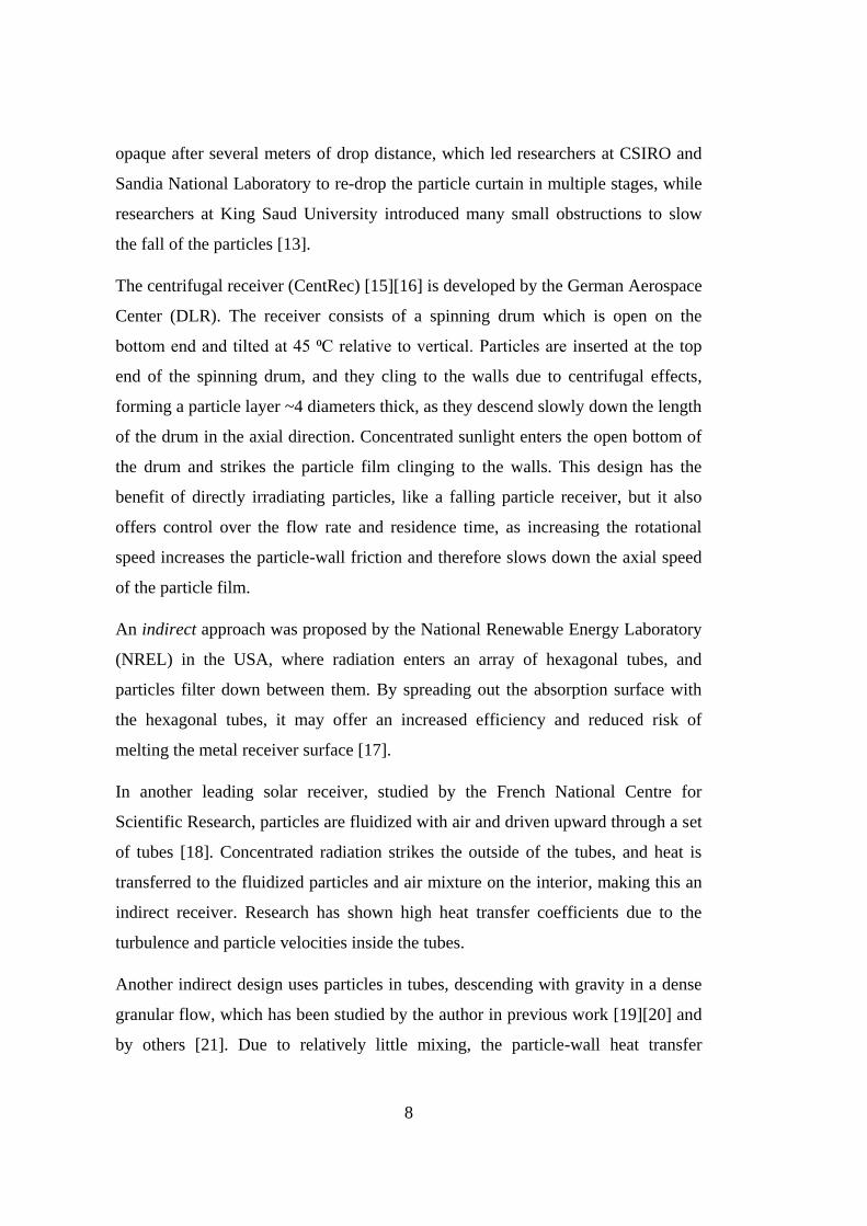
Figure 2.3. (a) The 50-sphere domain and surrounding sphere used for Fluent
validation, (b) view factors between the central sphere and all neighboring spheres.
................................................................................................................................. 26
Figure 2.4. The 3-sphere domain and walls used for PW validation against a Fluent
Surface-to-Surface radiation simulation. ................................................................ 27
Figure 2.5. File structure of the MCRT code. ......................................................... 28
Figure 2.6. Eight-particle simulation domain. ........................................................ 30
Figure 2.7. Parameters input to initiate MRCT code. ............................................. 31
Figure 2.8. Particle and wall positions used in the example simulation. ................ 33
Figure 2.9. Parameters for the particle-wall simulation. ......................................... 33
Figure 3.1. Close-up view of a domain with a solid fraction of (a) 0.64, and (b)
0.25. ......................................................................................................................... 39
Figure 3.2. (a) Initial cubic shaped domain, (b) the final spherical shaped domain
after removing the necessary spheres, and (c) a cut-away view to show the central
sphere. ..................................................................................................................... 40
Figure 3.3. Particle temperatures over time, with initial temperatures shown in red
and steady state temperatures shown in purple, and (b) steady state particle
temperatures of a slice of the domain. .................................................................... 42
Figure 3.4. Steady state particle temperatures and curve fit equation of form T=C1/r
+ C2 for a solid fraction of 0.45 and emissivity 0.5. ............................................... 44

xx
Figure 3.5. Steady state temperatures of spheres of particle domain shown in Figure
2.3, with results from both Fluent and the MCRT plus particle-particle heat
exchange simulation. ............................................................................................... 47
Figure 3.6. Exchange Factor found at various radial positions throughout the
particle wall, for a solid fraction of 0.64 and an emissivity of 1. ............................ 48
Figure 3.7. Exchange Factor at various radial positions for a solid fraction of 0.45
and an emissivity of 0.7, with 102, 10
3, 10
4, and 10
5 photons used in the Monte
Carlo simulation. ..................................................................................................... 49
Figure 3.8. Exchange Factor measured at various radial positions, showing
simulations with different numbers of particles. ..................................................... 50
Figure 3.9. Exchange Factor results, with points representing data from Table 3.2,
and lines representing the surface fit of Eq. (3.11). ................................................. 53
Figure 3.10. Exchange Factor comparison to previous models and experimental
work, for a solid fraction of 0.60 [37][29][28][42]. ................................................ 54
Figure 3.11. Comparison of Exchange Factors between present study and models
by Zehner, Bauer, and Schlünder (ZBS), and Breitbach and Barthels (BB). .......... 55
Figure 4.1. Group of 50,000 particles with a solid fraction of 0.45. ....................... 62
Figure 4.2. Particle-particle RDF at various distances between particles, for εp =
0.86 and SF = 0.55, showing individual data points and a smoothing spline fit. .... 64
Figure 4.3. (a) Particle-wall domain with a SFbulk = 0.64, (b) domain with SFbulk
= 0.25, and (c) local solid fraction at various distances from the wall, showing
various bulk solid fractions. .................................................................................... 67
Figure 4.4. Particle-wall RDF at various distances, for a εp = 0.86, εw = 0.80, and
SFbulk = 0.45. ......................................................................................................... 68
Figure 4.5. Mean cumulative RDF (fraction of photos absorbed) at various
distances from the emitting particle, calculated with Monte Carlo and the DBA
models, for εp = 0.65 and various solid fractions. ................................................... 71
Figure 4.6. Cross section of the spherical domain used for validating the DBA
model, with 10,000 particles and a solid fraction of 0.45. ...................................... 72

xxi
Figure 4.7. Particle-wall domain with a SFbulk of 0.45. Half of the domain is semi-
transparent to show the red particles included in the PW heat transfer calculation.73
Figure 4.8. PP RDF as a function of distance for (a) εp = 0.65, (b) εp = 0.86, and (c)
the extreme values of SF and εp. ............................................................................. 76
Figure 4.9. (a) Particle-particle RDF data and three proposed curves for SF = 0.64
and εp = 0.65, and (b) Cumulative PP RDF at various distances from the emitting
particle. .................................................................................................................... 77
Figure 4.10. Particle-wall RDF for (a) εp = 0.65, εw = 0.8, and various bulk solid
fractions, and (b) εp = 0.86, SFbulk = 0.45, and various wall emissivities. .............. 78
Figure 4.11. Simulation domain of a heated channel in dense granular flow. ........ 81
Figure 4.12. (a) Total PW heat transfer over time, (b) steady state particle
temperatures, and (c) steady state PW heat transfer per particle. ........................... 85
Figure 4.13. Steady state heat transfer rate from the wall, comparing results with
various radiation time step sizes. ............................................................................ 86
Figure 4.14. (a) Mean PP heat transfer per particle, and (b) mean PW heat transfer
per particle, both as a function of distance from the wall. ...................................... 87
Figure 5.1. The six heat transfer modes included in DPHT. ................................... 93
Figure 5.2. (a) The three particle-particle heat transfer modes, and (b) the three
particle-wall heat transfer modes (blue = fluid, red = wall). .................................. 94
Figure 5.3. Geometry of two contacting spheres used to calculate PP conduction..
................................................................................................................................. 95
Figure 5.4. Dimensions relevant to Eq. (5.9) for calculating PFP conduction,
showing (a) non-contacting and (b) contacting spheres. Outline of the double cone
volume is shown in orange. .................................................................................... 98
Figure 5.5. PFP conduction as a function of distance, for ksi=ksj=2.0, kf=0.0702, αs
= 0.60, and R=0.0005 m, showing (a) heat flux as a function of radial position, for
various particle distances, and (b) heat transfer coefficient as a functions of particle
distance (dij). ......................................................................................................... 102
Figure 5.6. PFP heat transfer coefficient solved for various particle distances and
temperatures (same parameters as Figure 5.5). ..................................................... 103
xxii
Figure 5.7. Particle-fluid-wall geometry. .............................................................. 105
Figure 5.8. Particle-wall HTC values found for ksi=2.0, αs = 0.60, R=0.0005. ..... 107
Figure 5.9. Particle and wall element geometry used for applying boundary
conditions. ............................................................................................................. 109
Figure 5.10. DPHT file structure. .......................................................................... 110
Figure 5.11. (a) Surface of tube with nozzle, drawn with Onshape, and (b) meshed
surface using Gmsh. .............................................................................................. 117
Figure 5.12. ParaView settings for exporting the vertices. ................................... 118
Figure 5.13. ParaView settings for exporting the relations between cell IDs and
vertices. .................................................................................................................. 118
Figure 5.14. ParaView settings for exporting the cell centers. .............................. 119
Figure 5.15. Commands to run the DPHT code from the Julia terminal. .............. 121
Figure 5.16. Particle temperatures at the outlet, showing (a) view from the outside,
and (b) cross section view. .................................................................................... 122
Figure 5.17. Total PW heat transfer over time, separated by heat transfer mode. 123
Figure 5.18. Simulation domain for finding keff from a DPHT simulation. .......... 124
Figure 5.19. Results for keff calculated using the DPHT simulation, also showing
the values predicted using the ZBS model for solid-fluid conduction [29] plus the
radiative portion calculated with ZBS, Breitbach and Barthels [28], and the krad
model from Chapter 3. ........................................................................................... 125
Figure 5.20. keff with radiation eliminated, comparing ZS and DPHT simulation
results. .................................................................................................................... 126
Figure 6.1. (a) Experimental setup in front of high flux solar simulator, and (b)
front view of lamps. ............................................................................................... 133
Figure 6.2. Main components of the experimental setup. ..................................... 133
Figure 6.3. Close-up of measurement test section. ................................................ 134
Figure 6.4. Diagram of the components and flow regimes in the setup. ............... 135
Figure 6.5. Hopper, with insulation removed to expose ends of the heating tubes.
............................................................................................................................... 136
Figure 6.6. Shutoff valve used to stop the particle flow. ....................................... 137

xxiii
Figure 6.7. (a) Hopper and test section, with holes for thermocouple probes visible,
circled in red, (b) front view of test section with thermocouples installed at
locations circled in red, and (c) extra insulation installed in front test section. .... 138
Figure 6.8. Inlet temperature measurement block with grooves cut for
thermocouples wires. ............................................................................................ 139
Figure 6.9. Paddle wheel mixing device showing (a) paddle wheel installed inside
the insulation block, and (b) 9V DC motor mounted on the exterior, connected to
stainless steel shaft. ............................................................................................... 140
Figure 6.10. Top overflow channel shown (a) on full setup, and (b) close-up where
it attaches to the insulation blocks. ....................................................................... 142
Figure 6.11. Temperature data from Test 1. ......................................................... 145
Figure 6.12. Mass of particles accumulated over time during Test 1. .................. 145
Figure 6.13. Sintered bauxite particles can be seen glowing at the exit, where (a) a
gradient can be seen before while mixer is off, and (b) the gradient is eliminated
once mixer is turned on. ........................................................................................ 146
Figure 6.14. Stream of sintered bauxite radiating visible red light at ~750 ⁰C. .... 147
Figure 6.15. Temperature data from Test 2. ......................................................... 148
Figure 6.16. Mass of particles accumulated over time during Test 2. .................. 148
Figure 6.17. Temperature data from Test 3. ......................................................... 149
Figure 6.18. Mass of particles accumulated over time during Test 3. .................. 150
Figure 6.19. Test section, well-insulated on three sides with ceramic insulation. 154
Figure 6.20. Top view of the hopper, where U-shaped steel rods are placed over the
heating tubes to promote conduction inside the hopper and reduce temperature
gradients. ............................................................................................................... 157
Figure 6.21. Three prototype passive mixing devices, none of which were found to
completely mix the particle stream. ...................................................................... 158
Figure 6.22. Paddle wheel mixing device used to achieve a uniform stream
temperature. .......................................................................................................... 160
Figure 6.23. Three frames of video showing the high-speed and chaotic particle
flow imparted by the paddle wheel, leading to a high degree of mixing. ............. 160

xxiv
Figure 7.1. Square tube test section and orifice plate used in modeling the
experimental setup. ................................................................................................ 164
Figure 7.2. Mass accumulation over time, and equation for mass flow rate. ........ 165
Figure 7.3. Particle group used for evaluation of keff, leading to a correction factor
value of 1.28 in Eq. (7.2). ...................................................................................... 167
Figure 7.4. Keff at several temperatures, showing the ZS model, the original PFP
model, and the PFP model modified with a correction factor of 1.28 in Eq. (7.2).
............................................................................................................................... 168
Figure 7.5. Specific heat as a function of temperature. ......................................... 169
Figure 7.6. Temperature locations shown in red (a) on the front of the square tube,
and (b) on all surfaces of the unfolded surface, subdivided into 16 panels. .......... 170
Figure 7.7. Temperature map of right half of square tube test section, found from
polynomial surface fitting of eight known temperature locations. ........................ 172
Figure 7.8. Temperature boundary condition applied to inner surface of square
tube. ....................................................................................................................... 173
Figure 7.10. Steady state particle temperatures, showing (a) entire particle stream,
and (b) section view to show interior particles, and (c) close-up section view to
show particles near the outlet. ............................................................................... 175
Figure 7.11. Heat flux of test section at steady state. ............................................ 176
Figure 8.1. Receiver design and 1-mm diameter particles descending between
parallel plates. ........................................................................................................ 182
Figure 8.2. Secondary reflector used to further concentrate rays onto the receiver
surface (image of secondary reflector supplied by Canavarro [107]). ................. 184
Figure 8.3. Configuration of heliostat field and solar receiver (supplied by
Canavarro [107]). .................................................................................................. 184
Figure 8.4. Incident radiative flux on the receiver surface. ................................... 185
Figure 8.5. (a) Parallel plates with diamond-shaped obstruction, and (b) particles in
between the 8-mm by 8-mm parallel plate strip studied. ...................................... 186
Figure 8.6. Overall heat transfer from wall to particles, separated by heat transfer
mode. ..................................................................................................................... 187

xxv
Figure 8.7. Particles at the outlet, colored by temperature. .................................. 188
Figure 8.8. Outputs from DPHT simulation analyzed to show (a) bulk temperature,
and (b) overall heat transfer coefficient, both as a function of distance from the
inlet. ...................................................................................................................... 189
Figure 8.9. One element of the metal receiver surface and the adjoining cell
containing the particle-air mixture. ....................................................................... 191
Figure 8.10. Receiver surface showing (a) external surface temperature, and (b)
absorbed heat flux. ................................................................................................ 194


xxvii
LIST OF ABBREVIATIONS
BB Breitbach and Barthels model for radiative effective thermal
conductivity
CentRec Centrifugal Receiver, a solar receiver design pursued by the German
Aerospace Center (DLR)
CFD Computational Fluid Dynamics
CSP Concentrating Solar Power
DBA Distance Based Approximation radiation model developed in this
thesis
DEM Discrete Element Method
DLR German Aerospace Center
DPHT Dense Particle Heat Transfer, a DEM-based heat transfer code
developed in this thesis
LRM Long Range Model, a particle-scale radiation model
MCRT Monte Carlo Ray Tracing
MPI Message Passing Interface
NREL National Renewable Energy Laboratory
PFP Particle-Fluid-Particle, a heat conduction model
PFW Particle-Fluid-Wall, a heat conduction model
PP Particle-Particle
PV Photovoltaic solar panels
PW Particle-Wall
RDF Radiation Distribution Factor
SF Solid Fraction, or particle volume fraction
SLE Special Limit of Error, a high accuracy thermocouple
SRM Short Range Model, a particle-scale radiation model
TRL Technology Readiness Level
ZBS The Zehner, Bauer, and Schlünder model for effective thermal
conductivity, which builds upon the original ZS model to include
numerous parameters, including radiation
ZS The continuum model for effective thermal conductivity by Zehner
and Schlünder, which accounts for heat transfer in packed particle
beds

1
CHAPTER 1
1 INTRODUCTION
Within the field of concentrating solar power (CSP), central receiver (“power
tower”) type systems are capable of achieving high solar concentration ratios and
therefore very high temperatures. A growing body of research points to the
efficiency and cost benefits of switching from a liquid heat transfer fluid to using
solid sand-like particles as a heat transfer medium in CSP plants [1]. Unfortunately,
our understanding of the mechanics and heat transfer of granular materials lags far
behind that of the closely related field of fluid mechanics. According to the authors
of Granular Materials; Fundamentals and Applications:
Despite wide interest and more than five decades of experimental and
theoretical investigations many aspects of the behavior of flowing granular
materials are not well understood. At this stage, there is still no complete
understanding of the constitutive relations that govern the flow of granular
materials. The general field is very much in a stage of development
comparable to that of fluid mechanics before the advent of the Navier-
Stokes relations. [2]
The Navier-Stokes (fluid momentum) equations are fundamental to solving fluid
mechanics problems both analytically and with Computational Fluid Dynamics
(CFD), so this passage clearly states that there is still much to learn in this field. To
help address the challenges facing CSP with solid particles, the overarching goal of
this thesis is to improve the modeling capabilities regarding heat transfer in flowing
groups of particles, with special focus on thermal radiation.
2
1.1 Background
In the past decades, CSP systems have been installed for electricity generation,
where the heat collected is used to run a steam Rankine cycle. In addition to
electricity generation, research and demonstration projects are currently underway
for supplying heat directly to industrial processes (without converting to
electricity), such as cement, metallurgy, melting of aluminum for recycling, waste
treatment, and formation of liquid fuels [3].
When used for electricity production, the key advantage of CSP over other
renewable energies is the low cost of integrating energy storage. By storing heated
materials in large, insulated tanks, the heat can be converted to electricity as
needed, providing a predictable electricity output to the power grid all 24 hours per
day, or as required by the grid operator. Electricity from photovoltaic (PV) panels
has become the least expensive power available in some electricity markets in
recent years, but it is rarely coupled with energy storage, resulting in large amounts
of curtailed electricity and even negative wholesale energy prices due to
overproduction in areas of high PV deployment [4]. Thus, instead of competing
with other inexpensive renewables, CSP with storage actually enables using more
of them by providing the reliability and flexibility needed to smoothly operate an
electricity grid with a high proportion of renewable energy. Specifically, CSP
plants can store all the collected energy during the daytime when inexpensive PV
electricity is available, and then thermal storage can be dispatched during the
nighttime when PV electricity is not available. Electric battery storage technology
has made great advances in recent years, but installations have remained small
compared to CSP systems such as the NOOR III in Morocco, in operation since
2018, with ~1 GWhe of storage capacity [5].
Decarbonizing the electricity sector is well under way, largely due to falling costs
of solar and wind power in recent years. However, industrial processes, such as
cement production, steel production, and manufacturing, are responsible for ~24%
of the overall carbon dioxide emissions worldwide [6]. Much of the emissions from

3
these processes come not from electricity use, but instead come from burning fossil
fuels to bring raw materials to high temperatures. Unfortunately, there are very few
current solutions available to stop the use of fossil fuels in these processes. CSP
can supply very high temperatures and heat fluxes, so coupling CSP with high
temperature industrial processes could provide a pathway to decarbonize these
industries, which is a growing area of research [3][6]. Like CSP for electricity, CSP
plants which supply heat to industrial processes likely also need thermal storage,
enabling them to supply a steady stream of heat at all hours of the day.
State-of-the-art central receiver systems for electricity production use molten salt
as the heat transfer and storage medium, which is a mixture of sodium nitrate and
potassium nitrate and is a liquid above ~200 ⁰C. Numerous researchers in recent
years have studied the benefits of switching from a molten salt (liquid) heat transfer
and storage medium to using solid particles, such as sand or sintered bauxite, for
the same role [1]. One benefit is the improvement in cycle efficiency. Molten salt
chemically breaks down above ~600 ⁰C, imposing a temperature limit on the entire
system, whereas solid particles can work even above 1000 ⁰C, with no chemical or
phase changes. Increasing the working temperature would increase the Carnot
efficiency and the actual thermal efficiency of the steam Rankine cycle typically
used in these power plants. Furthermore, the power cycle could be changed to a
higher temperature cycle such as supercritical CO2 or air Brayton, which both
promise a large increase in efficiency [1][7]. Another benefit is the low cost of
these materials as a heat storage medium, which is important because many tons
are required for a large system. Sand is widely available and very inexpensive, and
sintered bauxite is produced in large quantities for the hydraulic fracturing
industry, making it slightly more expensive, but still much cheaper than using
molten salt to store the same quantity of heat. Lastly, molten salt changes to a solid
if it drops below 200 ⁰C, so steps must be taken to avoid this, adding to the cost and
complexity of a molten salt power plant. Each of these benefits of a particle-based
system decreases the price of the overall plant and therefore the energy output.

4
Switching from a liquid to a solid particle based CSP plant requires reengineering
several components, with the heat exchange devices being the chief components
under research. However, solving for heat transfer in flowing groups of solid
particles can be quite complex. Unlike fluids, particles do not form a continuum,
and the Eulerian or continuum equations of motion are not generally applicable.
Heat transfer mechanisms in particle flows are also completely different from those
of fluids, as particles transfer heat through direct contact, through the fluid gap in
between particles, and through radiation. Because the field is much less developed
than fluid mechanics, there are far fewer modeling capabilities available, making it
more difficult to design heat exchange devices in the proposed particle-based CSP
systems.
The overall goal of this thesis is to improve the modeling capabilities for heat
transfer in flowing groups of particles, especially heat transfer through thermal
radiation, which has been omitted from many analyses due to its complexity and its
negligible effect at temperatures below ~400 ⁰C. However, at the high temperatures
of CSP, radiation is an important heat transfer mechanism and must be modeled to
accurately predict the performance of a heat exchange device.
1.2 Preview of Research Contributions
Each chapter builds on the previous chapters, with Chapter 1 serving as the
introduction. Specific contributions of this thesis beyond the current state of
research include:
Chapter 2: A Monte Carlo Ray Tracing (MCRT) code is developed to
model radiation in large groups of particles. This is a useful code for others
to use in their research, and it will be posted in an online repository as an
open source C++ code. This MCRT code is used as a tool throughout the
thesis and is required for all of the subsequent chapters.

5
Chapter 3: The MCRT code is used to solve for the effective thermal
conductivity using a new method which is more fundamental and physically
realistic than previous methods. It also covers a wider range than the current
models and is likely more accurate.
Chapter 4: A model for calculating radiative heat transfer at the particle
level is developed for use in Discrete Element Method (DEM) simulations.
In this method the distance between two particles is used to estimate
radiative transfer, which is shown to have a high accuracy but a very low
computational cost compared to other particle-scale radiation models. This
is termed the Distance Based Approximation (DBA) model in this thesis.
Chapter 5: The DBA radiation model is implemented, along with the
relevant heat conduction modes, into a new open source code for heat
transfer in dense granular flows, termed Dense Particle Heat Transfer
(DPHT). An example simulation is given, along with an in-depth
explanation of how the code functions, so it can be easily modified to
simulate devices by other researchers. Though the focus of this thesis is on
radiation, several improvements to the existing heat conduction models are
implemented as well.
Chapter 6: An experimental investigation is run to study heat transfer in a
dense granular flow inside a square tube heated under highly concentrated
radiation. This is used both for validation of the DPHT code and for
studying dense granular flows for CSP heat exchangers.
Chapter 8: The DPHT code (from Chapter 5) is used to study a solar
receiver for heating particles to 700 ⁰C, with final results including the
overall heat gain and thermal efficiency of the solar receiver. The receiver
envisioned is for preheating of sandstone particles for lime calcination in
the production of cement.
Though chapters are all related and build upon each other, each chapter in this
thesis forms a distinct research effort. Therefore, detailed conclusions are

6
included within each chapter, and only broad conclusions are presented in the
final chapter.
This thesis spans several fields of research, including particle-based CSP power
plants, packed particle beds, DEM modeling, and experimental studies of heat
transfer in particle flows. Therefore, the literature review spans several diverse
fields as well, so it is divided into these sub-topics in the following sections.
1.3 CSP with Solid Particles
The main components of a CSP plant for electricity generation are shown in Figure
1.1. The sun’s rays strike the heliostats (individually actuated, highly reflective
mirrors) which reflect sunlight toward the top of the tower, where the solar receiver
is positioned. The solar receiver receives radiation which has been concentrated
several hundred times, and it transfers the energy to the heat transfer medium (solid
particles in this case) which can reach temperatures of 700 to 1000 ⁰C. The
particles then descend to the well-insulated hot particle storage tank. When they are
needed for electricity production, the particles are passed through the particle-fluid
heat exchanger to deliver their heat to the working fluid of the power cycle, such as
a steam Rankine cycle, a Brayton cycle, or a supercritical CO2 cycle [7].
Alternatively, heat from particles can be transferred to a fluid stream such as air to
be used directly in an industrial process. Particles are then stored in a “cold”
particle storage tank with a temperature in the range of 400 to 600 ⁰C until sunlight
is available, when they are transported to the top of the tower to be reheated in the
solar receiver. At the time of publication, there is only one fully functional power
plant utilizing solid particles, a research plant at King Saud University where heat
from stored particles is used to preheat the air stream in a 100 kWe gas turbine
system, to reduce fuel consumption [8].
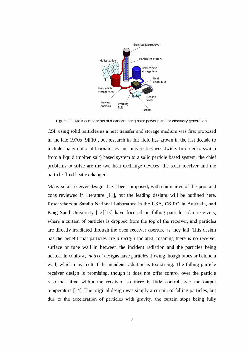
7
Figure 1.1. Main components of a concentrating solar power plant for electricity generation.
CSP using solid particles as a heat transfer and storage medium was first proposed
in the late 1970s [9][10], but research in this field has grown in the last decade to
include many national laboratories and universities worldwide. In order to switch
from a liquid (molten salt) based system to a solid particle based system, the chief
problems to solve are the two heat exchange devices: the solar receiver and the
particle-fluid heat exchanger.
Many solar receiver designs have been proposed, with summaries of the pros and
cons reviewed in literature [11], but the leading designs will be outlined here.
Researchers at Sandia National Laboratory in the USA, CSIRO in Australia, and
King Saud University [12][13] have focused on falling particle solar receivers,
where a curtain of particles is dropped from the top of the receiver, and particles
are directly irradiated through the open receiver aperture as they fall. This design
has the benefit that particles are directly irradiated, meaning there is no receiver
surface or tube wall in between the incident radiation and the particles being
heated. In contrast, indirect designs have particles flowing though tubes or behind a
wall, which may melt if the incident radiation is too strong. The falling particle
receiver design is promising, though it does not offer control over the particle
residence time within the receiver, so there is little control over the output
temperature [14]. The original design was simply a curtain of falling particles, but
due to the acceleration of particles with gravity, the curtain stops being fully
8
opaque after several meters of drop distance, which led researchers at CSIRO and
Sandia National Laboratory to re-drop the particle curtain in multiple stages, while
researchers at King Saud University introduced many small obstructions to slow
the fall of the particles [13].
The centrifugal receiver (CentRec) [15][16] is developed by the German Aerospace
Center (DLR). The receiver consists of a spinning drum which is open on the
bottom end and tilted at 45 ⁰C relative to vertical. Particles are inserted at the top
end of the spinning drum, and they cling to the walls due to centrifugal effects,
forming a particle layer ~4 diameters thick, as they descend slowly down the length
of the drum in the axial direction. Concentrated sunlight enters the open bottom of
the drum and strikes the particle film clinging to the walls. This design has the
benefit of directly irradiating particles, like a falling particle receiver, but it also
offers control over the flow rate and residence time, as increasing the rotational
speed increases the particle-wall friction and therefore slows down the axial speed
of the particle film.
An indirect approach was proposed by the National Renewable Energy Laboratory
(NREL) in the USA, where radiation enters an array of hexagonal tubes, and
particles filter down between them. By spreading out the absorption surface with
the hexagonal tubes, it may offer an increased efficiency and reduced risk of
melting the metal receiver surface [17].
In another leading solar receiver, studied by the French National Centre for
Scientific Research, particles are fluidized with air and driven upward through a set
of tubes [18]. Concentrated radiation strikes the outside of the tubes, and heat is
transferred to the fluidized particles and air mixture on the interior, making this an
indirect receiver. Research has shown high heat transfer coefficients due to the
turbulence and particle velocities inside the tubes.
Another indirect design uses particles in tubes, descending with gravity in a dense
granular flow, which has been studied by the author in previous work [19][20] and
by others [21]. Due to relatively little mixing, the particle-wall heat transfer

9
coefficient in such a system is low compared to a fluidized flow. However, the
benefits are that it is very simple, and the flow rate is adjustable with a valve, so the
particle residence time and output temperature can be easily controlled over a wide
range. This design is revisited in this thesis, in Chapter 8.
Particle-fluid heat exchangers have also been studied by numerous researchers. A
“moving bed heat exchanger” has been studied by DLR, which consists of a bank
of horizontal tubes, through which runs the working fluid of the power plant (such
as steam), and particles flow vertically downward through the tube bank [22].
Researchers at METU have also worked on particle-fluid heat exchange, where a
concept was developed to transfer heat from particles to air directly, by using the
air to fluidize stored particles [23]. Flat plate heat exchanger designs have been
recently tested by Sandia National Laboratory, consisting of a gravity-driven dense
granular flow in between parallel plates, with supercritical CO2 as the working
fluid [24].
This is a thriving area of research where numerous devices have been proposed for
both solar receivers and particle-fluid heat exchangers, and though several
prominent designs exist, there is not yet a single clear design that is best for all
applications. After examining the research on these devices, it is clear that some
designs use diffuse or dispersed flows (such as falling or fluidized particles), while
others use dense granular flows, and some exhibit both types of flow in one device.
1.4 Effective Thermal Conductivity in Particle Beds
The effective thermal conductivity (keff) of a group of particles is the thermal
conductivity of the bulk material taken as if it were a continuous medium instead of
a collection of individual particles. It is an important parameter for thermal design
in many industries, including packed bed nuclear reactors [25], drying processes
[26], and particle-based CSP [24]. Using keff is a convenient way to combine the
various modes of heat transfer in the particle-fluid domain into a single thermal

10
conductivity value which is representative of the bulk. In the center of the domain,
far from walls, heat is transferred through A) the solid contact where two particles
touch, B) the fluid gap between particles, and C) radiation between particles [26],
assuming a transparent fluid which does not participate in radiation. The effective
thermal conductivity of each heat transfer mode can be found independently,
denoted as ksolid, kfluid, and krad respectively, and later they can be summed to find
the total effective thermal conductivity, keff [27]. This thesis focuses only on the
radiative portion, krad, which is the least studied component. It also focuses on
randomly distributed particle groups typical of most natural and industrial systems,
as opposed to an ordered packing structure studied by some previous researchers.
At low temperatures, radiation has a small effect and krad is neglected in many
applications, but for high temperature industries (above ~400 ⁰C) krad can play an
important or even dominant role in the overall heat transfer.
A variety of correlations have been proposed to express krad as a function of the
particle emissivity and the solid fraction, which is the proportion of solid particle
volume to the whole volume. The solid fraction is known by other names,
including volume fraction, solid volume fraction, particle fraction, particle volume
fraction, and packing fraction, and it sums to one with the porosity or void fraction.
One method to determine krad is to adopt and analyze a representative unit cell
which is assumed to be repeated throughout the domain [28]. Among the keff
models, the Zehner, Bauer, and Schlünder unit cell model (commonly referred to as
the “ZBS” model) [29][30][31] is perhaps the most commonly used, which is
derived based on two opposing non-spherical particles with heat flux contours
assumed to be parallel across the unit cell. (Note: the so-called ZBS model consists
of the original model by Zehner and Schlünder from 1970 [30], which only
accounts for heat transfer through the fluid gap between spheres, plus
improvements by the same authors in 1972 [29] and by Bauer and Schlünder in
1978 [31]. The later studies add effects such as radiation, gas pressure, and non-
spherical particles. Because the original papers are written in German, English
speakers are directed to [32][33].) Although the radiative portion of the ZBS model

11
could be considered rudimentary compared to more recent research methods, the
ZBS model has become widely used, as the portion regarding heat conduction
through the fluid and solid has been extensively studied.
Another method to find krad is to first find the absorption and scattering coefficients
corresponding to the Radiative Transfer Equation, and then krad can be calculated
with one of several proposed equations [34]. Chen and Churchill [35] found the
scattering and absorption coefficients experimentally, while others [36][37] have
found these numerically. Singh and Kaviany [38] used a Monte Carlo approach but
only studied simple cubic packed particle beds.
Experimental validation of krad over a wide range of parameters is challenging, and
experiments have only been attempted by few researchers. To isolate krad, heat
transfer experiments must be performed under vacuum conditions to eliminate any
heat transfer through the fluid, and conduction through the particle-particle contacts
must also be either eliminated or quantified. De Beer et al. [39] were able to
separate the radiative portion of keff by using experimental data along with a
calibrated numerical model for packed beds of 6-cm diameter graphite spheres.
Similar experiments for packed beds with graphite spheres have been performed by
Breitbach and Barthels [28], Rousseau et al. [40], and Robold [41]. Kasparek and
Vortmeyer [42] eliminated particle-particle conduction by mechanically separating
rows of steel spheres in place, with tests also run under vacuum conditions. Slavin
et al. [43] also ran experiments with 1-mm diameter alumina spheres.
Because many industries use static, packed beds, the majority of research has been
focused on this condition. When the particle bed is less than fully packed, as found
in fluidized beds or some particle-fluid heat exchangers [17], static experiments
would be exceptionally difficult, as particles would have to be suspended in place
while experiments are run. Furthermore, only certain emissivity values have been
tested due to the limited number of particle materials available for high temperature
experiments, and in addition the emissivity of each material is often a function of

12
temperature. All of these difficulties explain why very few experimental results
have been reported, covering only a limited set of parameters.
In both experimental and computational research, krad has received relatively little
focus in situations where the solid fraction is less than packed. With the
advancement of computational modeling techniques of multi-phase heat transfer,
the less than packed condition can be studied using the Discrete Element Method
(DEM). The krad results presented in this study may be especially useful when used
in conjunction with DEM, either by incorporating the results directly into a DEM
model or for validation of particle-scale radiation models such as the model
developed in Chapter 4 [44], or those studied by Qi and Wright [45], Wu et al.
[46], and Pitso [47].
With very little experimental data available, the current body of research has yet to
prove definitively if one of the proposed krad models is accurate over a range of
independent variables, most importantly the emissivity and solid fraction. In light
of this lack of certainty, a fundamental approach is taken in this research to
evaluate krad over a wide range of emissivity and solid fractions. In the method
developed in this thesis, particle positions are generated using DEM in the shape of
a thick spherical wall consisting of uniformly sized spheres, radiation is modeled
with a 3D Monte Carlo ray tracing code, a particle-particle heat transfer simulation
is run to find the steady state temperature profile of the particle group, and finally
krad is found with a comparison to heat conduction in an isotropic solid of the same
geometry.
Monte Carlo methods are well developed and documented in literature
[48][49][50], but there has been no study which uses a Monte Carlo simulation to
systematically find krad over a range of solid fractions and emissivity values for
gray, diffuse, monodisperse particle beds. The Monte Carlo code written is
described in detail in Chapter 2. The method developed to calculate krad is
described in Chapter 3, and the results culminate in an equation for krad over the
entire range of emissivity values from 0.3 to 1 and solid fractions from 0.25 to the

13
fully packed state of 0.64. This equation for krad is combined with the Zehner and
Schlünder model [30] for ksolid and kfluid to give an equation to calculate the full keff
value.
1.5 Modeling Heat Transfer in Particle Flows
Modeling of particle flows can be separated broadly into Eulerian approaches,
where the bulk of particles is modeled assuming the particles form a continuum as
if they were a fluid, and Lagrangian approaches, where particles are modeled
individually [51]. Eulerian approaches ignore frictional and collisional effects
between particles and along walls, which dominate the motion in granular flows
[52], making the overall flow patterns much different from fluids. The Discrete
Element Method (DEM) is the leading Lagrangian approach, where each particle is
modeled as a sphere, and each collision is modeled with solid mechanics, allowing
for detailed calculations of normal and tangential frictional effects to be
incorporated at the particle scale. The strength of DEM is that because particles are
modeled at the individual particle level, it is in theory possible to accurately
replicate all the physical phenomena of both particle mechanics and heat transfer
[51]. In contrast, Eulerian approaches always strive to approximate particle flows
as a fluid, though the physical mechanisms that govern the flow are fundamentally
different. Until the last decade, the Lagrangian approach was not a viable option for
modeling actual devices, as the chief drawback is the high computational burden.
Even with the computation power currently on a PC workstation, simulations larger
than a million particles may take weeks of computation time. However, with the
continuous enhancement in computer processing speeds, this approach promises to
become even more advantageous in the coming decades.
Most often, particles are surrounded by an “interstitial” fluid (such as air) which
must be modeled as well, and together they comprise a two-phase system. In some
circumstances the “Euler-Euler” model (also known as the “Two-Fluid” model)
can be used, where the particle phase is modeled as a second fluid which is

14
intermixed with the actual interstitial fluid, and a solution is found using a modified
version of the Navier-Stokes equations and CFD. Solutions using the Euler-Euler
model have been applied to fluidized beds, as well as some dense flow problems
[22]. With a Euler-Lagrange approach, the fluid is modeled by simulating the
interstitial fluid with CFD, and a “coupled CFD-DEM” simulation is run by
alternating between the DEM and CFD models and accounting for momentum and
heat transfer between the two phases [53]. With a coupled model, both frictional
effects of the particles as well as the hydrodynamic and thermal effects of the fluid
are simulated, which is not possible with a DEM or CFD model alone. The leading
software combination for coupled CFD-DEM simulations is the open source code
LIGGGHTS for DEM modeling and OpenFOAM for CFD. The software CFDEM
provides the coupling by passing heat transfer and momentum information back
and forth between the solid and fluid phase models [53][54].
Figure 1.2. Heat transfer modes in a particle-fluid-wall domain.
Figure 1.2 shows the six relevant heat transfer modes in a generic domain
consisting of particles, fluid, and a wall, where the interstitial fluid is assumed to be
non-participating in radiation. The conduction and convection heat transfer modes
have been studied previously, with models available in
LIGGGHTS/OpenFOAM/CFDEM. However, there are currently no sub-models
for particle-particle or particle-wall radiation in LIGGGHTS or commercial DEM
codes, and there is relatively little analysis in literature. This is likely because it is

15
often neglected at the moderate temperatures of many industrial processes. In high
temperature particle systems (above ~400 ⁰C [55]) such as those found in CSP [56],
nuclear pebble bed reactors [57], lime calcination [58][59], and biomass pyrolysis
[45], particle-particle and particle-wall radiation cannot be neglected without a
substantial under-prediction of heat transfer. Several previous attempts to include
PP and PW radiation have been described in literature, as detailed below.
In an approach studied by Cheng and Yu [60], Wu et al. [61], and others
[57][45][62][46], a “Voronoi” polyhedron is created around each particle, and the
polyhedral face geometry is used to approximate radiation using what is referred to
as the Short Range Model (SRM) or the Long Range Model (LRM). The SRM
accounts for heat transfer only between directly contacting polyhedra, whereas the
LRM accounts for heat transfer to all neighboring polyhedra [57][46]. The authors
note that because the SRM neglects any radiation to polyhedra which are not in
direct contact, it substantially underestimates radiative transfer, with the total view
factor from one particle adding up to only 0.83 in a packed bed [46], substantially
less than the theoretical value of 1. When the particle thermal conductivity is low,
neglecting the conduction resistance within particles can cause an overestimation in
heat transfer, and according to the authors, the SRM is accurate because these two
errors may compensate for each other [57][46][63]. While this may happen to be
true in some cases it is certainly not a rigorous method in all circumstances. These
approaches have focused on the conditions in a packed bed where the solid fraction
is ~0.61, and they are generally not applicable for lower solid fractions.
In addition to the SRM and LRM, Wu et al. [46] outline several other models for
consideration. The Black Model is only valid for an emissivity of 1, limiting its
utility. The Uniform Radiation Model, according to the authors, is also not
appropriate for modeling gray particles because it is built upon an assumption of
uniform radiosity on the particle surface, which eliminates the effect of the
emissivity and is therefore not physically realistic. The authors also describe a
Local Radiation Model, where each particle surface is divided into many surface
elements, and the radiative transfer is calculated between each element

16
combination. This improves upon the Uniform Radiation Model because radiosity
is allowed to vary over the particle surface, but the high computational cost of
calculating radiation element-by-element makes this unsuitable for simulations
with thousands of particles. Finally, Wu et al. [46] derive a Particle Scale Radiation
Model which uses several functions to approximate the effects of particle and wall
emissivities as well as the solid fraction, though it includes many approximations
and has not been validated to a great extent.
Several approaches have been described where the surrounding particles are
lumped together or averaged. A model based on the “local environment
temperature” of each particle has been described by Yang et al. [64] and Krause et
al. [58], though this only accounts for neighboring particles within a distance of 1.5
particle diameters and suffers similar limitations to the SRM. Another approach is
the Spherical Unit Nodalization model described by Pitso [47] where view factors
are lumped into several concentric shells surrounding each particle. Work by Pitso
also forms the basis for the Multi-sphere Unit Cell model described by Van
Antwerpen et al. [25], where long range radiation (radiation between non-
contacting particles) is estimated by averaging the view factors of all nearby
spheres using a pre-computed distribution curve of view factors in a packed bed.
These approaches offer a simple estimation of radiation, but they are tailored to
packed beds and have not been developed for lower solid fractions where long
range radiation becomes very important.
Several Monte Carlo approaches have also been studied. Amberger et al. [65]
implemented a Monte Carlo ray tracing code directly into the DEM code
LIGGGHTS [51], which could be very accurate if enough rays are traced, but the
Monte Carlo method carries a very high computational cost making it unsuitable
for large simulations. Liu et al. [66] used a Monte Carlo approach to solve for
radiation distribution factors in randomly and regularly packed domains, but only
PP radiation was studied at very low solid fractions, and results were not applied in
the DEM context. Radiation in beds of packed, black particles have been studied in

17
previous work by the current author [67], and similar conditions have been studied
by Malinouski and Rabinovich [68].
Given the shortcomings of the previously proposed models, a method to solve for
radiation in large particle systems with acceptable accuracy and low computational
cost is still sought [63]. For situations with static beds, low computation time is
desired but not critical because the necessary view factors must only be calculated
once. In contrast, for dynamic simulations such as particles flowing through
concentrating solar power receivers or lime kilns, radiation must be recalculated
continuously throughout a simulation, making a computationally efficient model
for radiation an absolute requirement. In Chapter 4, a radiation model that can be
implemented in DEM or CFD-DEM codes is developed to address these
shortcomings. The central challenge is to calculate radiation at the particle scale in
systems containing hundreds of thousands of particles, while adding a minimal
amount of computational time to the already high computational burden of DEM
and CFD-DEM.
1.6 Experimental Studies of Dense Particle Flows
Very few experimental studies exist for heated dense granular flows, especially at
the high temperatures relevant to CSP devices where radiation plays a prominent
role in the overall heat transfer. Natarajan and Hunt [69] studied heat transfer to
glass spheres between heated, vertically-oriented parallel plates. Their experiments
showed the heat transfer coefficient increases significantly with flow rate until a
peak is reached around 12 cm s-1
and then falls off slightly at higher flow rates.
They attributed this peak to two opposing factors. Increasing the flow rate increases
the particle motion and mixing and therefore heat transport, but at higher velocities
the low-conductivity air gap along the wall increases in thickness, reducing heat
transfer. The second important conclusion drawn by Natarajan and Hunt is that
inclined chutes heated on the bottom face (as opposed to vertical chutes) have
higher heat transfer, and their peak heat transfer occurs at much higher velocities.

18
This is attributed to gravity forcing particles towards the wall and reducing the air
gap between wall and particles. Similar work was undertaken by Sullivan [70]. In
both studies the heated section is short, so flows did not become thermally fully
developed. Furthermore, they are not directly applicable to the radiation modeling
developed because they are performed at low temperatures where heat transfer via
radiation is likely negligible. Still, understanding interplay between the bulk
velocity, the near-wall air gap, and inclination angle is useful for envisioning the
particle receiver in Chapter 8. Watkins [21] gives perhaps the only applicable
experimental results for dense granular flows of sand-like materials at high
temperatures, where zirconia-silica particles flow downward with gravity through
an electrically heated Inconel tube, reaching temperatures around 1000 ⁰C.

19
CHAPTER 2
2 AN OPEN SOURCE MONTE CARLO CODE FOR THERMAL RADIATION IN
GROUPS OF PARTICLES
Some of the content in this chapter has already been published by the author:
E. Johnson, İ. Tarı, D. Baker, A Monte Carlo method to solve for radiative effective
thermal conductivity for particle beds of various solid fractions and emissivities,
Journal of Quantitative and Spectroscopic Radiative Transfer. 250 (2020).
doi:https://doi.org/10.1016/j.jqsrt.2020.107014.
All of the work that follows in this thesis builds upon the Monte Carlo Ray Tracing
(MCRT) code presented in this chapter. The code is used to solve for thermal
radiation in beds of particles and to the walls, which is used in Chapter 3 to find the
effective thermal conductivity of particle beds and again in Chapter 4 to develop a
particle-scale radiation model which can be implemented into DEM. This code will
be placed on the GitHub repository to make it available for others to use and
modify (https://github.com/ef-johnson/Ray-Tracing-Many-Spheres).
A 3D MCRT code is needed to simulate the radiative transfer in beds of thousands
to hundreds-of-thousands of spheres. While MCRT codes have been well-studied
in general [48][49], no open source code was found for this specific application.
The code developed has several notable attributes:
A) The code works seamlessly with DEM by reading the xyz particle positions
from the output files, allowing ray tracing to be done for realistic groups of
particles, as opposed to ordered packing structures like Kaviany [38] or less
physically realistic methods for placing particles randomly in the domain
[71].

20
B) It is written in C++ using parallel “message passing interface” (MPI)
programming, allowing for simultaneous computations on many cores of a
workstation or cluster. Speedup is nearly linear with the number of
processors.
C) The particles which emit photons (rays) are specified by the user with an
input text file, allowing a user to specify a certain particle or group of
particles, from which photons will be emitted.
D) Reflections and absorptions are modeled, leading to the Radiation
Distribution Factor (RDF), which allows for a simpler and more accurate
calculation of heat transfer compared to approaches using the more typical
radiative view factor.
The Ubuntu (Linux) operating system is recommended to run the MCRT code, as
LIGGGHTS is typically run in this operating system as well. The code is written in
C++. OpenMPI must be installed to enable parallel processing, which most users
will already have installed as it is a prerequisite for LIGGGHTS as well. For ray
tracing in systems of tens to hundreds of thousands of particles, running
simulations in parallel is a necessity; for the simulations of 50,000 particles run in
Chapter 4, parallel computing reduced run time from months to several days.
2.1 Model Details
The MCRT code was developed under the assumptions of monodisperse (uniform-
diameter) spheres, no light transmission through spheres, and a non-participating
fluid phase. All reflections and emissions are modeled as gray and diffuse,
implying that emissivity and absorptivity are equal according to Kirchhoff’s law
[72]. The particle absorptivity is chosen by the user at the beginning of the
simulation. The goal of the MCRT code is to simulate the rays or photons emitted
from each sphere by following the photon path through any reflections until it is
absorbed by a neighboring sphere. Often, the goal of ray tracing is to find the
radiative view factor from one surface to another, which is the fraction of photons

21
emitted from one surface that strike a second surface [72]. However, in this study
the output of the MCRT code is the radiation distribution factor (RDF), the portion
of photons emitted from one particle which are eventually absorbed by the second
particle after any number of reflections off neighboring particles [48][50]. This has
also been termed the exchange factor [49], but because that exact term is already
used Chapter 3 to mean something unrelated, the term RDF will be adopted here to
reduce confusion.
The Monte Carlo code is initiated by identifying the “emitting” particles (the
particles from which photons will be released) from a user-input text file. These are
also referred to as “home” particles in the code. For each of the emitting particles,
the ray tracing is started by finding a random emission location on the surface of
the emitting particle, represented by the red dot in Figure 2.1(a). This requires
determining an elevation angle (ø) where , and the azimuth angle ( )
where . These are found by drawing random numbers ( and )
between 0 and 1 along with the probability density functions for ø and in
Equations (2.1) and (2.2) [73], which give a uniform distribution of emission
locations on the sphere surface. Next, the emission direction (Figure 2.1 (b)), with
respect to the temporary x’y’z’ axes, is chosen using the probability density
functions in Equations (2.3) and (2.4), which are applicable under the gray, diffuse
emission assumption [74] and give a uniform distribution of photon directions in
the outward facing hemisphere from the emission location. In this case the
emission direction is defined by the elevation angle γ, where
, and the
azimuth angle β, where . With the emission direction determined, an
arbitrary length is assumed to form a vector within the x’y’z’ axes ( ). In Figure
2.1(c), an Euler transformation is applied to find the vector with respect to the
XYZ axes, which are aligned to the original xyz axes but with the origin at the
emission location.
(2.1)

22
(2.2)
(√ * (2.3)
(2.4)
Figure 2.1. (a) Sphere with random photon emission location, (b) random emission direction in
temporary axes, and (c) emission direction vector passing through several neighboring spheres, in
XYZ axes.
Using vector algebra, all other spheres are checked to see if the vector would
pass through their surface. The closest sphere to be hit is chosen as the true incident
sphere, and the actual incident location is calculated. The photon can then either be
reflected or absorbed, since no transmission through the particles is assumed.
Whether the photon is absorbed or reflected is determined by choosing a random
number, Rα, between 0 and 1. If , where α is the surface absorptivity, the
photon is reflected and the path continues; the location of the reflection is fixed, but
because reflections are assumed to be diffuse, a random reflection direction is
(a) (b)
(c)

23
found by generating new γ and β angles. The definition of the photon path is
continued in this way until the photon strikes a sphere and a random number
is found, representing the photon finally being absorbed. After simulating
many photons emitted from one sphere, the number of photons absorbed by each
neighboring sphere is divided by the total number of photons emitted, which results
in the RDF between the emitting sphere and each other sphere. Next, this process is
repeated by starting with a new emitting sphere until all emitting spheres have been
simulated.
If all of the spheres in the domain are specified as emitting spheres (as done in
Chapter 2), the output of the MCRT simulation is a square matrix containing the
RDF from each sphere to every other sphere in the domain. If the Monte Carlo
simulation were perfectly accurate in predicting RDFs, the matrix would be
symmetrical. The diagonals of the matrix, representing the RDF of a particle to
itself, are generally not zero due to photons reflected back on to the original
emitting particle.
2.2 Validation
Several validation steps have been performed to ensure the MCRT code produces
accurate and reliable results, which are detailed in the following subsections.
2.2.1 Two Touching Spheres
For the simplest validation configuration, the MCRT code was used to calculate the
view factor between two touching spheres. An analytical solution is available [75],
computed by Feng and Han [76] to be 0.0755868. The MCRT simulation was run
with an increasing number of photons, and as shown in Figure 2.2, the ray tracing
code matches the analytical solution to a high degree when ~105 or more photons
are used. The output of the MCRT code in general is the RDF, so in this case the

24
absorptivity was set to 1 to make the output the same as the more common
radiative view factor.
Figure 2.2. View factors calculated with various numbers of photons emitted per particle, for two touching spheres.
2.2.2 Two Separated Spheres
Next, the configuration was studied where the spheres are spaced at various
distances apart. Results match closely with Feng and Han [76] as shown in Table
2.1, who found the view factors by evaluating the integral equation from Tanaka
[75]. In this case, the number of photons traced by the MCRT code was very high,
107, to maximize accuracy.
Table 2.1. View factor validation between two spheres separated by various distances.
0.064
0.066
0.068
0.070
0.072
0.074
0.076
0.078
1E+2 1E+3 1E+4 1E+5 1E+6 1E+7
Vie
w F
acto
r
Number of Photons
Monte Carlo Code
Analytical Solution
Center-Center Distance (radii)
View Factor, Monte Carlo, Present Study
View Factor, Feng and Han [76]
Difference
2.00 0.07578 0.07559 0.25%
2.01 0.07450 0.07455 -0.06%
2.05 0.07073 0.07074 0.00%
2.10 0.06641 0.06650 -0.14%
2.50 0.04422 0.04412 0.23%
3.00 0.02956 0.02959 -0.09%
5.00 0.01020 0.01021 -0.10%
10.00 0.00251 0.00251 -0.04%

25
2.2.3 Randomly Packed 50-Sphere Domain
The CFD software package Fluent was used for validation of view factors and heat
transfer in a 50-sphere domain. While this small-scale validation is possible in
Fluent, both the manual effort to load spheres with specific positions as well as
actual code run time make the simulation process extremely time-intensive, even
for a domain of only 50 spheres. Simulating a domain of 10,000 particles in Fluent
is certainly not feasible, whereas the Monte Carlo and subsequent particle-particle
heat transfer simulations can be run with over 10,000 particles with minimal
manual effort and manageable code execution times.
For the randomly packed 50-sphere domain, shown in Figure 2.3(a), Fluent was
used to find the view factors between the central particle and all surrounding
particles using the Surface-to-Surface Ray Tracing model. The particles, with
radius 3 cm, were meshed and refined until decreasing the mesh size did not
change the resulting view factors, and modeling proceeded with a mesh sizing
parameter of 0.002 m. This is a rigorous test of the Monte Carlo code because the
spheres experience a high degree of shading. A very good agreement is still shown
for each sphere in Figure 2.3(b), demonstrating the high accuracy of the MCRT
code developed in this research. Because Fluent only calculates view factors, not
RDFs, the absorptivity was set to 1 in the MCRT code, as the RDF and view factor
are identical when no photons are reflected.
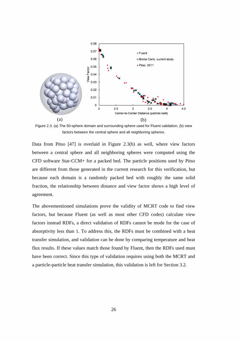
26
Figure 2.3. (a) The 50-sphere domain and surrounding sphere used for Fluent validation, (b) view
factors between the central sphere and all neighboring spheres.
Data from Pitso [47] is overlaid in Figure 2.3(b) as well, where view factors
between a central sphere and all neighboring spheres were computed using the
CFD software Star-CCM+ for a packed bed. The particle positions used by Pitso
are different from those generated in the current research for this verification, but
because each domain is a randomly packed bed with roughly the same solid
fraction, the relationship between distance and view factor shows a high level of
agreement.
The abovementioned simulations prove the validity of MCRT code to find view
factors, but because Fluent (as well as most other CFD codes) calculate view
factors instead RDFs, a direct validation of RDFs cannot be mode for the case of
absorptivity less than 1. To address this, the RDFs must be combined with a heat
transfer simulation, and validation can be done by comparing temperature and heat
flux results. If these values match those found by Fluent, then the RDFs used must
have been correct. Since this type of validation requires using both the MCRT and
a particle-particle heat transfer simulation, this validation is left for Section 3.2.
(a) (b)

27
2.2.4 Particle-Wall Validation
A validation for the PW calculations was performed in Fluent on the geometry
shown in Figure 2.4, consisting of three 0.02 m diameter particles contained inside
a bounding box, with properties listed in Table 2.2. The MCRT code is equipped to
handle only a single wall, so the bottom wall is given an emissivity (and
absorptivity) of 0.5, while all other walls are considered black surroundings. The
random particle positions and emissivities less than 1 mean there will be a high
number of photons reflected between the wall and all three particles, providing an
adequately challenging test case for the MCRT code.
Figure 2.4. The 3-sphere domain and walls used for PW validation against a Fluent Surface-to-
Surface radiation simulation.
Table 2.2 Input parameters for PW validation of MCRT code.
After running the MCRT code, the RDF from each particle to all other surfaces is
known, and the heat transfer between the particles and walls is calculated with
, where is the heat transfer, is the particle
emissivity, is the particle surface area, and is the Stefan-Boltzmann constant
(more details on this equation are given in Section 3.1.3). The total heat transfer
Surface x y z Temperature (K) Emissivity
Sphere 1 0 0 0.011 700 0.7
Sphere 2 0 0.006 0.032 800 0.7
Sphere 3 0.019 0.015 0.030 900 0.7
Bottom wall (z=0) - - - 600 0.5
Black surroundings (other walls) - - - 500 1.0

28
leaving each particle is found so that the results can be compared with results from
Fluent.
The exact same geometry was modeled in Fluent, with a mesh element size of
0.00001 m and radiation simulated with the Surface-to-Surface model. Heat
transfer rates from the spheres are compared in Table 2.3, with nearly identical
results shown between Fluent and the MCRT code. With this validation method,
the RDFs (or view factors) are not compared directly, but they must be correct to
arrive at the same heat transfer values as found by Fluent.
Table 2.3. Total heat transfer calculated with Fluent and MCRT code.
Surface Heat Transfer (W)
Fluent Heat Transfer (W)
MCRT Difference
Sphere 1 6.333 6.340 0.11%
Sphere 2 14.973 15.016 0.28%
Sphere 3 27.964 28.022 0.21%
2.3 File Structure
The file structure used by the MCRT code is shown in Figure 2.5.
Figure 2.5. File structure of the MCRT code.

29
In the pos folder there must be two files:
1. pos_[number of particles]_[solid fraction]_[LIGGGHTS time step
number].txt: this file contains the xyz position of the center of each
particle, one particle per line, in a space delimited format.
2. home_id_[number of particles]_[solid fraction]_[LIGGGHTS time step
number].txt: this file contains a list of 0’s and 1’s, with one value for
each particle. A 1 indicates the particle will be an “emitting” particle
(“home” particle), and 0 indicates the particle will not.
The RDF_files folder begins empty, and it is filled with the output files at
the end of the simulation.
The tmp_data folder begins empty, and it is used to temporarily store the
data output from each processor, before the end of the simulation when data
is gathered and consolidated into a single output file in the RDF_files
folder. The contents can be deleted routinely.
The text file containing the source code, such as PW_MCRT_1.6.cpp.
The compiled executable, PW_MCRT_1.6, is present after the source code
has been compiled.
2.4 Particle-Particle RDF Example
This example shows how the RDFs are calculated for the 8-particle domain shown
in Figure 2.6, with the geometry defined by the particle center coordinates found in
the file pos_8_0.50_100.txt. In the file home_id, there are eight rows containing a
1, so each of the particles is designated as an emitting particle (“home” particle).
The home_id file in this case was simple to make manually, but for simulations
with thousands of particles, it is recommended to create this file with Matlab or a
similar program, as this gives the user full flexibility over which will be designated
as home particles. For example, by reading in the particle position file, the particles
in a certain region can be designated (e.g. all particles with -0.1 < x < 0.1), or as

30
done in Chapter 4, the home particles are designated as a random subset of the
particles in a specified region.
From the file names, it can be seen that there are 8 particles, a solid fraction of
0.50, and a LIGGGHTS time step ID of 100. When naming the files this simple
example, the solid fraction is not actually calculated, so a value of 0.50 is chosen
arbitrarily. Likewise, the particle domain was created manually, so the LIGGGHTS
time step is simply assigned a value of 100. These parameters are only used in the
naming of the input and output files, but when working with many different
LIGGGHTS time steps and solid fraction files, maintaining these naming
conventions is essential to keep the inputs and outputs organized. In contrast, the
number of particles in the file name must match the actual number of particles to be
simulated.
Figure 2.6. Eight-particle simulation domain.
To compile the code, a terminal window is opened in the main folder, and the
command is issued: mpicxx -std=c++11 PW_MCRT_1.6.cpp -o PW_MCRT_1.6,
which compiles the code in the text file PW_MCRT_1.6.cpp into the executable,
called PW_MCRT_1.6. Next, the simulation is started either in serial with the
command ./PW_MCRT_1.6, or in parallel with mpirun -np 4 PW_MCRT_1.6,
where 4 is the number of processors specified. As shown in Figure 2.7, the program
asks for simulation parameters, including the number of photons, the volume
fraction (solid fraction), the absorptivity (emissivity), the particle radius, and the

31
outputs desired. It then asks if the wall should be modeled, which will be covered
in the next section.
Figure 2.7. Parameters input to initiate MRCT code.
After the run, two output files appear in folder RDF_files. The all_RDF output
style is necessary when the RDF from every particle to every other particle in the
domain is needed, such as when finding the effective thermal conductivity in
Chapter 3. In contrast, the dist_vs_RDF output style is more convenient when
building the distance vs. RDF curves in Chapter 4. The output files are:
1) all_RDF_0.50_8_1e6_0.75_0.00_100.txt: This file contains a square matrix of
RDFs from each particle to each other particle. The naming convention is (in
order) solid fraction, number of particles, number of photons, particle
absorptivity, wall absorptivity, and LIGGGHTS time step number. In this case
the wall emissivity is zero since the wall is not modeled. For the eight-particle
system the all_RDF file is shown in Table 2.4, where headers are added for
clarity. As expected, the matrix is symmetric, with small differences due to the
inherent errors in the MCRT which diminish with increasing numbers of
photons. There is one extra column for the wall, which is not modeled, so it is
simply left as a column of zeros.

32
Table 2.4 Data in the all_RDF output file, showing the RDF from each particle to each other particle.
2) dist_vs_RDF_0.50_8_1e6_0.75_0.00_100.txt: This file contains columns for
the emitting particle ID, the absorbing particle ID, the distance between the
particle centers, and the RDF between the two (Table 2.5). The first line shows
both emitting and receiving IDs are 0, a PP distance of 0.0000, and an RDF of
0.011975. This indicates that 1.1975% of the photons emitted from the surface
of particle 0 were reflected back and absorbed by the same particle. RDFs from
particle 0 to the others are shown in the next seven lines. A receiving ID of -1
indicates the wall, which in this case is not modeled so it is left as zero.
Table 2.5 The dist_vs_RDF output file, with table truncated to 12 rows.
Emitting ID Absorbing ID Distance (m) RDF
0 0 0.0000000 0.011975
0 1 0.0200000 0.060233
0 2 0.0223607 0.045472
0 3 0.0300000 0.021374
0 4 0.0374166 0.014346
0 5 0.0424264 0.007688
0 6 0.0512348 0.005390
0 7 0.0438748 0.008687
0 -1 0.0100000 0.000000
1 0 0.0200000 0.059895
1 1 0.0000000 0.014824
1 2 0.0223607 0.044933
(table continues with more rows)
2.5 Particle-Wall RDF Example
The same particle positions are used, but this time a wall on the plane is
modeled, which extends over and , as shown
in Figure 2.8. In the MCRT code, the wall must be on the plane. Photons are
Particle j Wall
Particle i
1 2 3 4 5 6 7 8
1
0.011975 0.060233 0.045472 0.021374 0.014346 0.007688 0.00539 0.008687 0
2
0.059895 0.014824 0.044933 0.045351 0.002983 0.000937 0.000166 0.018380 0
3
0.045612 0.045622 0.011462 0.036811 0.015029 0.022761 0.013724 0.020551 0
4
0.020964 0.044701 0.036431 0.006866 0.007684 0.009880 0.002730 0.007548 0
5
0.014388 0.002772 0.015116 0.008005 0.001919 0.165793 0.011853 0.002311 0
6
0.007697 0.000999 0.022712 0.009745 0.165081 0.005542 0.089800 0.004596 0
7
0.005349 0.000151 0.013608 0.002727 0.011647 0.089601 0.004403 0.006626 0
8
0.008798 0.018454 0.020660 0.007444 0.002173 0.004470 0.006838 0.001280 0
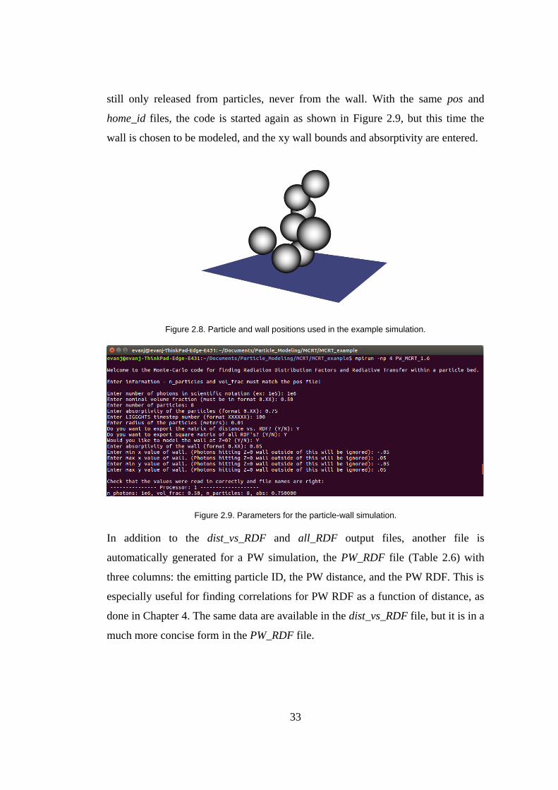
33
still only released from particles, never from the wall. With the same pos and
home_id files, the code is started again as shown in Figure 2.9, but this time the
wall is chosen to be modeled, and the xy wall bounds and absorptivity are entered.
Figure 2.8. Particle and wall positions used in the example simulation.
Figure 2.9. Parameters for the particle-wall simulation.
In addition to the dist_vs_RDF and all_RDF output files, another file is
automatically generated for a PW simulation, the PW_RDF file (Table 2.6) with
three columns: the emitting particle ID, the PW distance, and the PW RDF. This is
especially useful for finding correlations for PW RDF as a function of distance, as
done in Chapter 4. The same data are available in the dist_vs_RDF file, but it is in a
much more concise form in the PW_RDF file.

34
Table 2.6 Data output in the PW_RDF file.
Emitting ID PW Distance (m) PW RDF
0 0.01 0.348029
1 0.01 0.334898
2 0.03 0.120732
3 0.02 0.216053
4 0.04 0.139871
5 0.05 0.058603
6 0.06 0.063357
7 0.03 0.150329
2.6 MCRT Conclusion
In this chapter, a MCRT code was developed which is built to be used directly after
modeling the particle positions with a DEM code such as LIGGGHTS. The output
files give the RDF values either as a square matrix or alongside the distance
between the particle-particle or particle-wall pair. It can be used to easily find the
RDF (or view factor, if absorptivity is set to 1) between spheres numbering in the
hundreds of thousands. This code can be used by others to simulate radiative heat
transfer in static beds of small, conductive particles (see the uniform particle
temperature assumption in Section 3.1), and it can be used to develop or validate
particle-scale radiation models such as those used in DEM simulations.

35
CHAPTER 3
3 EFFECTIVE THERMAL CONDUCTIVITY DUE TO RADIATION
Some of the content in this chapter has already been published by the author:
E. Johnson, İ. Tarı, D. Baker, A Monte Carlo method to solve for radiative effective
thermal conductivity for particle beds of various solid fractions and emissivities,
Journal of Quantitative and Spectroscopic Radiative Transfer. 250 (2020).
doi:https://doi.org/10.1016/j.jqsrt.2020.107014.
An accurate model to estimate the effective thermal conductivity (keff) of groups of
particles is vital for simulating particle-based CSP devices, such as the parallel
plate heat exchangers developed by Sandia National Laboratory [24] and the in
dense flow through tubes [21]. It is also used in other industries using static beds,
such as nuclear pebble bed reactors [25] and laser sintering [71]. The radiation
component (krad) is the least studied component of the overall keff, but it is
responsible for a significant portion of the overall heat transfer at the high
temperatures of CSP. A method is developed to find krad over a wider range of
parameters (solid fraction and emissivity) than previous models, and given the
fundamental approach used, results should have a higher accuracy.
The resulting krad model can be combined with the other modes of heat transfer to
find the total keff, or it can be used on its own to validate particle-scale radiation
models, such as the Distance Based Approximation model (developed in Chapter
4) or the previously proposed models described in Section 1.5. In fact, the krad
model was developed exactly for this reason; any valid particle-scale radiation
model implemented in DEM must match the continuum krad model in predicting
overall heat transfer through the bulk, yet there are currently no models for krad
covering a wide range of solid fraction and emissivity.

36
Unlike most previous studies, the method does not rely on the assumption of a unit
cell or absorption and scattering coefficients to derive krad. In this method, a
realistic group of particles is generated by DEM modeling, and radiation between
particles is modeled with the MCRT code, leading to a calculation of krad and the
dimensionless Exchange Factor (FE). The key result is a model for FE over the
entire range of emissivities from 0.3 to 1 and solid fractions from 0.25 to the fully
packed state of 0.64. FE results are compared to previous models, with agreement
shown in some cases but a large disagreement found for low solid fractions. The
krad results are combined with the Zehner and Schlünder model [30] for solid and
fluid conduction, providing an equation for the total keff.
3.1 Method for finding krad
There are several important assumptions regarding the applicability of the
following method. Particles are assumed to be uniform in temperature, which is a
valid assumption under two circumstances. First, when particles are small and
conductive, the resistance to heat flow due to solid conduction within the particle
becomes negligible, so there is essentially no temperature gradient across the
particle. This is the case when the dimensionless solid conductivity ( ) is greater
than 10, where
, and is the thermal conductivity of the solid material
in W m-1
K-1
, dp is the particle diameter in meters, σ is the Stefan-Boltzmann
constant of 5.67x10⁻⁸
W m-2
K-4
, and T is the absolute temperature in Kelvin or
Rankine [77]. The second case where the uniform particle temperature assumption
is valid is in dynamic DEM simulations where particles are continuously and
quickly colliding and rotating. In this case a significant temperature gradient does
not form across each particle, even if is low, because the particles rotate before a
significant temperature gradient can develop. Thus, the model presented is well
suited for static beds of small metallic particles or for integration into dynamic
DEM simulations. However, the model in its current state is not well suited for
other applications such as static pebble bed reactors [40] because the relatively

37
large (~6 cm diameter) graphite spheres have a low thermal conductivity and are
known to exhibit a temperature gradient across each particle.
Similar to previous Monte Carlo studies of particle beds [34][78][36], the modeling
in this study relies on geometric optics where diffraction and near-field effects are
neglected, which is a valid assumption for particles greater than 75 μm [36][79],
and therefore the results are not applicable for smaller particles. Additionally, the
krad correlations presented here, as with most other published correlations, are only
valid for the bulk region, as the packing structure changes near the walls [26].
Finally, this study assumes gray and diffuse reflecting spheres of equal radius.
The uniform particle temperature assumption is valid for the case of sintered
bauxite particles used in particle-based CSP systems: with a solid conductivity of
~2 W m-1
K-1
, a particle diameter of ~300 μm, and temperatures in the range of 500
to 1000 ⁰C, is much greater than 10, and the diamter is larger than 75 μm, so it
meets both criteria.
The method developed in this chapter follows the sequence detailed in the sections
below. First, a domain of particles is generated using the DEM. Second, a Monte
Carlo ray tracing simulation is used to solve for the Radiation Distribution Factor
(RDF) between each particle and every other particle. Third, a heat transfer
simulation is run where the center of a spherical group of particles is heated and the
outside is cooled. Fourth, the resulting steady state temperature profile is plotted
and fitted with an applicable curve, leading to a calculation of krad. Finally, krad is
used to find the dimensionless Exchange Factor (FE), which depends only on
emissivity and solid fraction [26] (as opposed to krad, which also depends upon the
temperature and particle radius). The key outcome is FE, which is found for a range
of emissivity and solid fractions. Using FE, krad can be readily calculated for any
desired temperature and particle radius.

38
3.1.1 Generating the Particle Domain with DEM
The open source DEM software LIGGGHTS [51] is used to generate the particle
domain because it gives a realistic distribution of particle positions as they collide
with each other. A Hertz force model is used with a Young’s modulus of 109
Pa to
simulate hard particles such as stone or metals. For the special case of a packed
bed, particles are inserted into the domain and allowed to come to rest in the
presence of gravity. For beds which are not fully packed (solid fraction < 0.64), a
random yet realistic domain of particles is generated using the following procedure:
A. A single spherical particle is inserted at the center of a walled, cubic
domain, and it is fixed to that location throughout the DEM simulation.
B. Around 50,000 particles are then inserted into the domain in random
positions. The exact number of particles to insert depends on the desired
solid fraction and domain size.
C. Gravity is turned upside down for a short period of time to give particles
some kinetic energy, and then it is turned off completely.
D. The boundary condition is changed to periodic, allowing particles to leave
one side of the domain and enter on the opposite side. The goal is to create
a packing distribution representing the bulk region, without any effects
from the walls, so the more common fixed wall boundary condition is
avoided.
E. The particle coefficient of restitution is set to 1, and particles continue to
collide and travel around the domain indefinitely.
F. The particle positions at a time step of choice are then analyzed, and the
solid fraction of the group is determined. The solid fraction is actually
calculated in numerous concentric spherical shells to ensure the solid
fraction remains consistent throughout the domain. Domains with a solid
fraction of 0.64 and 0.25 are shown in Figure 3.1.

39
Figure 3.1. Close-up view of a domain with a solid fraction of (a) 0.64, and (b) 0.25.
G. For the heat transfer simulation, a spherical wall shaped domain was chosen
to ensure no heat is lost due to end effects, as opposed to a rectangular or
cylindrical domain which may have this problem. As will be described in
Section 2.3, the single central sphere (from step A, above) will act as a high
temperature heat source, the surroundings will be kept at a cold
temperature, and the spheres in between will be allowed to change
temperature. A gap is created between the central sphere and the others
(Figure 3.2(c)). If this gap is not created, the exact positions of the nearest
several neighbors of the central sphere can have an effect on the total heat
transfer from the central sphere due to its very high temperature. This can
lead to a different heat transfer from the central sphere when simulating a
different set of random particle positions, which is not desired for
consistency, though it would also not lead to an error in krad as long as
enough particles are included in the simulation. Using the gap eliminates
this effect by spreading out the heat transfer from the central sphere to
many particles instead of heavily weighted towards several neighbors.
Various gap sizes were studied, and it was determined that eliminating 500
of the closest particles results in consistent heat transfer from the central
sphere when considering various sets of random particle positions.
Therefore, starting with the initial cubic shaped domain shown in Figure
3.2(a), the desired spherical wall shaped domain is created by removing 500
(a) (b)

40
spheres from the interior and removing all the external spheres, leaving
10,000 spheres to make up the spherical wall. The original particle positions
are shown in Figure 3.2(a), the reduced, final group is shown in Figure
3.2(b), and a cut-away view is shown in Figure 3.2(c) to show the central
sphere and the gap created.
Figure 3.2. (a) Initial cubic shaped domain, (b) the final spherical shaped domain after removing the
necessary spheres, and (c) a cut-away view to show the central sphere.
3.1.2 Simulating Photons with Monte Carlo Ray Tracing
The MCRT code described in Chapter 2 is used here. The output of the MCRT
simulation is a square matrix containing the RDF from each sphere to every other
sphere in the domain, which for the current simulation size is stored in a text file
with 10,000 rows and columns. If the MCRT simulation were perfectly accurate in
predicting RDFs, the matrix would be symmetrical. The diagonals of the matrix,
representing the RDF of a particle to itself, are generally not zero due to photons
reflected back on to the original emitting particle.
3.1.3 Particle-Particle Heat Exchange Simulation
The particle-particle heat exchange simulation was written in the Julia programing
language [80] because it has many embedded functions, and it can manipulate large
data sets such as the RDF matrix. A heat transfer code was written where the
central sphere is specified with a surface temperature of Thot, the surroundings are
(a) (b) (c)

41
specified with a temperature of Tcold, and the intermediate 9,999 particles are
allowed to exchange heat until a steady state is reached. Initial temperatures are
assigned to each particle, with the central particle at Thot and all others at Tcold. The
heat transfer rate (qij) between any two spheres i and j is found with Eq. (3.1) [74],
where is the surface emissivity, is the sphere surface area, is the Stefan-
Boltzmann constant, T is the temperature of each sphere, and is the RDF
between particles i and j. In Eq. (3.1), instead of using directly, the average of
and is used, which enforces RDF reciprocity and improves accuracy by
effectively doubling the number of photons used to find in the Monte Carlo
simulation.
(3.1)
Similarly, the heat transferred from one sphere to the surroundings ( ),
maintained at Tcold is found with Eq. (3.2), and is the RDF from particle i
to the surroundings.
(3.2)
is found with Eq. (3.3), where n_particles is the total number of particles
in the simulation domain. This is simply a statement of energy conservation; any
photon not absorbed by a particle must be absorbed by the black surroundings.
∑
(3.3)
With these values known, the net heat transfer rate from each i particle ) can
be found with Eq. (3.4).
∑
(3.4)
After specifying the particle mass (m), specific heat (Cp), and an sufficiently small
time step ( ), the first law of thermodynamics can be written in the form of Eq.
(3.5), which solves for the final temperature of each sphere, Ti,final, based on the
initial temperature, Ti,initial, after a duration of one time step. The new temperature

42
of each sphere i is found and adjusted after each time step, except the central
heated sphere which is always maintained at Thot.
(3.5)
The sequence is repeated for many time steps, and after an initial transient phase, a
steady state is eventually reached when the total heat transfer from the central
sphere equals the total heat transfer to the surroundings, and these values, as well
as all particle temperatures, remain constant with successive time steps. Figure
3.3(a) shows the evolution of particle temperatures over time for a domain with a
solid fraction of 0.45 and an emissivity of 0.5. Steady state particle temperatures
are shown in Figure 3.3(b), where only a slice of the domain is shown so the inner
particles can be seen. In both figures, the temperature scale covers the particle wall,
and the central sphere at Thot, 1098 K in this case, has been omitted because
including it would reduce visibility of the other data points. The output from this
simulation is the steady state temperature and xyz position of each particle, along
with the overall heat transfer rate from the central heated sphere.
Figure 3.3. Particle temperatures over time, with initial temperatures shown in red and steady state
temperatures shown in purple, and (b) steady state particle temperatures of a slice of the domain.
998.0
998.5
999.0
999.5
1,000.0
1,000.5
0.10 0.15 0.20 0.25 0.30 0.35
Part
icle
Tem
pera
ture
(K
)
Radial Position (m)
Initial Condition
Time step 10
Time step 20
Time step 40
Time step 100
Time step 782 (Steady State)
(a) (b)
43
The small temperature difference across the spherical wall, around 2 K in Figure
3.3, is used because krad is temperature dependent; using a large temperature
difference would lead to a krad that varies in the radial direction, making it difficult
to determine krad at a specific temperature. In Figure 3, krad would be found for
roughly 999 K, the average particle temperature of the group.
3.1.4 Calculating krad from the Temperature Profile
The xyz position of each particle is converted to a radial distance from the central
heated sphere, and these are plotted against the steady state temperatures, as shown
in Figure 3.4. The result is a radial temperature profile, similar to that of a spherical
wall. From heat conduction theory, the temperature profile of a spherical wall of an
isotropic solid has the general format of Eq. (3.6), where T is the temperature, r is
the radial location, and C1 and C2 are constants which depend on the boundary
conditions [72].
(3.6)
From the definition of the effective thermal conductivity, the group of particles can
be represented by an analogous isotropic solid with the same radial heat transfer
and temperature profile. Therefore, a curve fit is found for the data, and C1 and C2
are determined, as shown in Figure 3.4. The change in curvature seen at the lower
end of the radial position is addressed in Section 3.3.1.

44
Figure 3.4. Steady state particle temperatures and curve fit equation of form T=C1/r + C2 for a solid
fraction of 0.45 and emissivity 0.5.
Starting again with the general temperature profile (Eq. (3.6)) and taking a
derivative with respect to the radius gives the slope in the radial direction:
(3.7)
From Fourier’s law of conduction in spherical coordinates, where q is the heat
transfer rate, k is the thermal conductivity, and A is the area of heat transfer:
(3.8)
Combining Equations (3.7) and (3.8) by eliminating dT/dr, using the surface area
of a sphere as A , and rearranging to solve for k gives Eq. (3.9), which
relates the thermal conductivity, the heat transfer rate, and constant .
(3.9)
The total heat transfer rate (q) from the central sphere is known from the
simulation, and is known from the curve fitting method above. Thus, the
effective thermal conductivity of the bulk of particles, or krad, is finally found.
998.0
998.5
999.0
999.5
1000.0
1000.5
0.10 0.15 0.20 0.25 0.30
Tem
pera
ture
(K
)
Radial Position (m)
Particle Temperatures
Curve Fit: T = 0.3738572/r + 996.7193

45
3.1.5 Finding the Exchange Factor
With krad determined, the dimensionless Exchange Factor (FE) can now be
calculated as described by Van Antwerpen et al. [26] using Eq. (3.10), which is
valid when the temperature change across the wall-shaped domain is much less
than the average temperature of the wall, or
. The Exchange Factor is
useful because it eliminates the temperature and particle radius variables. While
krad is a function of solid fraction, emissivity, radius, and temperature, FE is only a
function of solid fraction and emissivity, making it much simpler to express in a
table or equation.
For a particular application, krad can be found with Eq. (3.10), as long as FE is
known along with the temperature and particle radius. After running this entire
modeling sequence for various solid fraction and emissivity combinations, the FE
results from this research are given in Section 3.3.6. In Eq. (3.10), σ is the Stefan-
Boltzmann constant, is the particle diameter, and T is the absolute temperature.
In these simulations, T is taken as the mean temperature of the group of spheres.
(3.10)
3.2 Validation
The MCRT code presented in Chapter 2 has been validated to accurately calculate
PP and PW RDF values as long as a sufficiently high number of photons has been
simulated. A second validation step is shown here to simultaneously validate the
particle-particle heat exchange simulation as well as the RDF values found by the
MCRT code for the case when absorptivity is less than 1. Using the same 50-
particle domain used in the MCRT code validation (Section 2.2.3, Figure 2.3(a)), a
heat transfer simulation was run in Fluent, and results were compared to the Monte
Carlo plus particle-particle heat exchange simulation results. The surface of the

46
central particle was specified with a boundary condition of 1000 K, and the
surroundings were comprised of the large bounding sphere encompassing all the
particles with a boundary condition of 900 K and an absorptivity of 1. Spheres
were modeled as a solid phase with near-infinite thermal conductivity and a surface
emissivity of 0.8, and the space in between the particles was modeled as a fluid
transparent to radiation and having near-zero thermal conductivity. Any conduction
between spheres was eliminated by ensuring neighboring spheres were very close
but not actually touching.
With the boundary conditions specified for the surface of the central sphere and the
surrounding enclosure, a transient simulation was run, and the other spheres were
allowed to change temperature until a steady state was reached. The steady state
sphere temperatures from Fluent and from the current study are presented in Figure
3.5, showing nearly identical results. The temperature of the central particle is not
included in the figure, as the y-axis would have to be extended to 1000 K, and the
detail of the other particle temperatures would not be discernable. In Fluent, the
steady state heat transfer from the central sphere was found to be 146.01 W, while
heat transfer to the surroundings was 144.76 W, with this small discrepancy in the
conservation of energy likely due to truncation errors within Fluent. In contrast, the
Monte Carlo plus particle-particle heat exchange simulation method converges to a
very high precision; heat transfer from the central sphere and heat transfer to the
surroundings both yield a value of 145.30 W, closely aligned with results found
with Fluent. Thus, the Monte Carlo plus particle-particle heat transfer simulation
calculates accurate results in terms of steady state particle temperatures and heat
transfer, and it is therefore validated to a high degree.

47
Figure 3.5. Steady state temperatures of spheres of particle domain shown in Figure 2.3, with results
from both Fluent and the MCRT plus particle-particle heat exchange simulation.
3.3 Results and Discussion
Before presenting final results for FE, several factors are examined to ensure the
simulation domain and parameters chosen give accurate and reproducible krad
results. These include near-edge effects, the number of photons used in the MCRT
simulation, the thickness of the spherical particle wall, the independence of FE with
respect to temperature, and reproducibility with different particle positions.
3.3.1 Near-Edge Effects
As shown in Figure 3.6, the radial temperature gradient at the edges of the particle
wall is less than in bulk region, and therefore a higher krad value is expected at the
edge. To observe and eliminate this edge effect, the spherical particle wall is
subdivided into multiple thinner spherical walls, allowing FE to be found locally at
various radial positions using Equations (3.9) and (3.10). FE at each radial position
was found by considering the particles within 0.02 m above and below each data
point indicated in Figure 3.6. The plot shows FE is higher near the edges but stable
in the bulk region from radial position 0.14 to 0.22 m. Therefore to eliminate near-
900
902
904
906
908
910
912
914
916
2.0 2.5 3.0 3.5 4.0 4.5
Tem
pera
ture
(K
)
Center-to-Center Distance (particle radii)
Fluent
Monte Carlo, current study
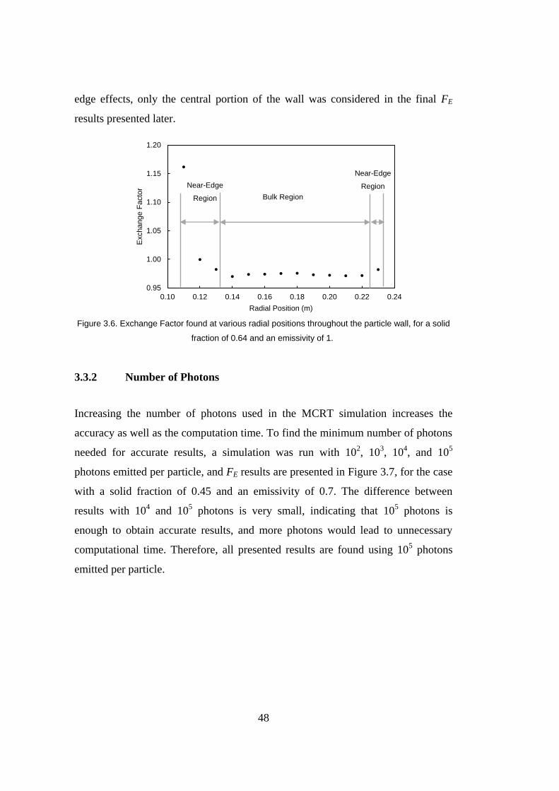
48
edge effects, only the central portion of the wall was considered in the final FE
results presented later.
Figure 3.6. Exchange Factor found at various radial positions throughout the particle wall, for a solid
fraction of 0.64 and an emissivity of 1.
3.3.2 Number of Photons
Increasing the number of photons used in the MCRT simulation increases the
accuracy as well as the computation time. To find the minimum number of photons
needed for accurate results, a simulation was run with 102, 10
3, 10
4, and 10
5
photons emitted per particle, and FE results are presented in Figure 3.7, for the case
with a solid fraction of 0.45 and an emissivity of 0.7. The difference between
results with 104 and 10
5 photons is very small, indicating that 10
5 photons is
enough to obtain accurate results, and more photons would lead to unnecessary
computational time. Therefore, all presented results are found using 105 photons
emitted per particle.
0.95
1.00
1.05
1.10
1.15
1.20
0.10 0.12 0.14 0.16 0.18 0.20 0.22 0.24
Exchan
ge F
acto
r
Radial Position (m)
Bulk Region
Near-Edge
Region
Near-Edge
Region

49
Figure 3.7. Exchange Factor at various radial positions for a solid fraction of 0.45 and an emissivity
of 0.7, with 102, 10
3, 10
4, and 10
5 photons used in the Monte Carlo simulation.
3.3.3 Thickness of the Particle Wall
The Exchange Factor should be a function of the solid fraction and emissivity, but
the results should be consistent for different thicknesses of the spherical particle
wall chosen for the simulation. It is important to choose a thick enough particle
wall so any edge effects can be identified and eliminated. To demonstrate this,
simulations were run with three different wall thicknesses, for the case with a solid
fraction of 0.45, an emissivity of 0.5, and a particle radius of 0.01 m. Each of the
three domains has an inner radius of 0.104 m, and they extend to an outer radius of
0.266, 0.286, and 0.307 m, with the domains containing 8,000, 10,000, and 12,500
particles respectively. As shown in Figure 3.8, the bulk region can be seen between
0.17 and 0.23 m, and consistent FE results are shown between all of the three
simulations as long as the near-edge regions can be identified and eliminated in
each case. If a thinner particle wall were chosen extending up to only 0.18 m, the
lower and upper near-edge regions would meet, and the bulk region would be
eliminated; the domain chosen would be too small to accurately calculate FE. A
smaller domain requires less computational time, so in the case of Figure 3.8 the
10,000 and 12,500 particle simulations are unnecessarily large. However, a
0.12 0.14 0.16 0.18 0.20 0.22 0.24 0.26
0.85
0.90
0.95
1.00
1.05
Radial Position (m)
Exchan
ge F
acto
r
1e2 photons
1e3 photons
1e4 photons
1e5 photons

50
simulation of 10,000 particles was chosen because it is large enough to clearly
identify the bulk region and eliminate the near-edge effects in all cases run.
Figure 3.8. Exchange Factor measured at various radial positions, showing simulations with different numbers of particles.
3.3.4 Independence of FE with Respect to Temperature
The Exchange Factor is a dimensionless quantity which can be used to calculate
krad at any temperature using Eq. (3.10). Therefore, FE should not depend on the
temperature chosen for the simulation. To verify this independence, the particle-
particle heat transfer simulation was run using a range of temperature conditions
for the case of a solid fraction of 0.45 and an emissivity of 0.7. In a sequence of
simulations, the temperature of the central heated particle and the surroundings
were increased in increments of 100 K, while the temperature difference between
the two values remained constant. As shown in Table 3.1, an increase in
temperature leads to a higher krad value, but the FE value calculated with Eq. (3.10)
is nearly identical for each simulation. With a maximum deviation of 0.02%
between the lowest and highest values, FE is shown to be independent of the
simulation temperature.
0.10 0.15 0.20 0.25 0.30
0.74
0.76
0.78
0.80
0.82
0.84
0.86
Radial Location (m)
Exchan
ge F
acto
r
8000 particles, upper radius 0.266 m
10000 particles, upper radius 0.286 m
12500 particles, upper radius 0.307 m

51
Table 3.1. Exchange Factor calculated at various temperatures for a solid fraction of 0.45 and an
emissivity of 0.7.
Central Sphere Temperature
(K)
Surroundings Temperature
(K)
Average Steady State Particle
Temperature in Bulk Region (K)
krad (W m
-1 k
-1)
Exchange Factor
798 698 698.65 1.514 0.97847
898 798 798.63 2.261 0.97840
998 898 898.62 3.220 0.97835
1098 998 998.61 4.419 0.97831
1198 1098 1098.60 5.884 0.97828
3.3.5 Reproducibility with Different Particle Positions
At the beginning of this simulation sequence, a DEM simulation was run to
generate a random domain of particles with the output being a static “snapshot” of
the particle positions, for each solid fraction simulated. These particle positions are
inputs to the Monte Carlo and particle-particle heat exchange simulation sequence.
The final FE results should be reproducible for any different set of random particle
positions, so to ensure this, a second set of particle positions was generated with
the DEM simulation, and all simulation cases were run to find FE a second time.
The FE results from the two sets of simulations are very close, differing by no more
than 1.1% in each case. The FE results presented below are the average of the two
sets of simulations.
3.3.6 Exchange Factor Results
The simulation sequence was run to find FE at five values of emissivity and five
values of solid fraction. All results were found using a domain of 10,000 particles
with a particle radius of 0.01 m, and the Monte Carlo simulation was run with 105
photons emitted per particle. All particle-particle heat transfer simulations were run
using a central sphere temperature of 1098 K and a surroundings temperature of
998 K, leading to a spherical particle wall with an average temperature of roughly
998.5 K, though the exact average temperature depends on the steady state particle
temperatures. After eliminating the near-edge regions from the temperature profile,

52
krad was found for the bulk region with the curve fitting method and Eq. (3.9). FE
values were then calculated using Eq. (3.10), where the average particle
temperature in the bulk region was used for T. This procedure was used to calculate
FE for each of the 25 combinations of emissivity and solid fraction. As noted in
Section 3.3.5, this entire process was repeated for a second set of random particle
positions, and the FE results were averaged between the two simulations. In total,
50 simulations were run, leading to the 25 values found in Table 3.2.
Table 3.2 Exchange Factor results for various solid fractions and emissivity (ε) values.
Solid fraction ε = 0.3 ε = 0.5 ε = 0.7 ε = 0.9 ε = 1
0.25 1.5609 1.8497 2.1757 2.5572 2.7753
0.35 0.8926 1.1140 1.3675 1.6647 1.8282
0.45 0.5717 0.7602 0.9770 1.2305 1.3706
0.55 0.3897 0.5574 0.7503 0.9777 1.1060
0.64 0.2983 0.4570 0.6394 0.8527 0.9770
A polynomial surface has been fitted to these data points and the equation of the
surface is presented in Eq. (3.11). With this equation, FE can be found for any
combination of solid fraction ( ) and emissivity (ε) within the range of
and . Over the 25 data points the surface fit gives an average
error of 1.1%, and the highest error is 4.8% for the case where solid fraction is 0.55
and emissivity is 0.3.
(3.11)
The FE data points from Table 3.2 and the polynomial surface fit from Eq. (3.11)
are plotted as a function of solid fraction and emissivity in Figure 3.9. It is expected
that a lower solid fraction leads to higher value for FE due to the increased distance
photons can penetrate into the group of spheres, as seen in the figure. FE increases
with emissivity due to the higher radiative emission from each sphere.

53
Figure 3.9. Exchange Factor results, with points representing data from Table 3.2, and lines
representing the surface fit of Eq. (3.11).
3.3.7 Comparisons with Previous Research
The leading models for FE in packed beds are compared in Figure 3.10 for a solid
fraction of 0.60 and a range of emissivities, as published by Kaviany [37], ZBS
[32] and Breitbach and Barthels (BB) [28], with experimental work by Kasparek
and Vortmeyer [42]. Nearly all of these models are in relative agreement under
these conditions, with the exception of the Kaviany Two-Flux model, which does
not accurately account for the particle emissivity [37]. Results from the current
study are slightly below the Kaviany Monte Carlo study and the Kasparek and
Vortmeyer experimental work, which is likely because both of these studies used a
simple cubic packing instead of a random packing structure. The Kasparek and
Vortmeyer experiment studied a solid fraction of 0.60 using 1-cm steel spheres,
with both a polished steel surface (emissivity of 0.35 and specular) and chromium
oxide coated surface (emissivity of 0.85 and diffuse). In the experiment, rows of
spheres were fixed in place to prevent conduction between layers, and tests were
run under vacuum conditions, forcing both ksolid and kfluid to zero. It is also
important to note that due to the conductive steel particles Λ has a very high value,
and therefore the uniform particle temperature assumption is valid, allowing for a
useful comparison with the current work. Other experimental work has focused on
0.00
0.50
1.00
1.50
2.00
2.50
3.00
0.25 0.35 0.45 0.55 0.65
Exchan
ge F
acto
r
Solid fraction
ε = 0.3
ε = 0.5
ε = 0.7
ε = 0.9
ε = 1.0

54
packed beds of larger graphite spheres, [28][41] but because Λ is low the results
cannot be compared directly with the current study.
Figure 3.10. Exchange Factor comparison to previous models and experimental work, for a solid
fraction of 0.60 [37][29][28][42].
There are a large number of proposed FE models for the packed bed condition as
shown in Figure 3.10, but with the exception of the ZBS and BB models, the other
models shown do not account for various solid fractions. While the ZBS and BB
models do include a term to account for a lower solid fraction, they are derived
assuming a unit cell consisting of two touching particles. In particle beds where the
solid fraction is less than ~0.52 very few particles are touching, so the applicability
of the resulting ZBS and BB models is questionable in this range. Still, to see the
difference in predicted values, the FE results from the current study are compared
to the values predicted by the radiation models of ZBS and BB in Figure 3.11,
where Λ > 10 is assumed. Under certain conditions, such as for an emissivity of 0.7
and a packed bed with solid fraction above 0.55, results are nearly identical. In
contrast, for an emissivity of 1 and a solid fraction of 0.64, the ZBS and BB models
overestimate FE by 24% compared to the current study. While trends are generally
similar, at low solid fractions the current study shows a much higher FE than the
0
0.2
0.4
0.6
0.8
1
1.2
1.4
0.20 0.30 0.40 0.50 0.60 0.70 0.80 0.90 1.00
Exchan
ge F
acto
r
Emissivity
Kaviany, Monte Carlo
Kaviany, Two-Flux model
Argo and Smith
Vortmeyer
Kasparek and Vortmeyer, Exp.
ZBS
BB
Current Study

55
ZBS or BB models predict. (Note: The ZBS and BB models are identical for an
emissivity of 1, so these lines overlap exactly in the figure.)
Figure 3.11. Comparison of Exchange Factors between present study and models by Zehner, Bauer,
and Schlünder (ZBS), and Breitbach and Barthels (BB).
With a large disagreement in results found between the models under some
conditions, ideally experiments would show which model is valid. However,
experimental data is available only at the fully packed condition, as experiments
with low solid fractions are very difficult to run; particles would have to be secured
in a suspended state throughout the experiment while heat transfer data is collected.
The method presented in this study aims to simulate such an experiment
numerically by tracing each ray through a large group of randomly distributed
particles, making it a close approximation to reality. In contrast, the ZBS and BB
models use a single idealized unit cell based on two touching non-spherical
particles to derive a relation that accounts for a lower fraction of particles in the
domain. The method presented starts with relatively few assumptions and provides
a close approximation to these hypothetical experiments, and therefore the results
are expected to be valid and more physically realistic than the results of the ZBS or
BB models, especially where particles have a solid fraction of less than 0.52.
0.25 0.35 0.45 0.55 0.65
0.0
0.5
1.0
1.5
2.0
2.5
3.0
Solid fraction
Exchan
ge F
acto
r
Current Study, ε = 1
ZBS, ε = 1
BB, ε = 1
Current Study, ε = 0.7
ZBS, ε = 0.7
BB, ε = 0.7
Current Study, ε = 0.3
ZBS, ε = 0.3
BB, ε = 0.3

56
3.3.8 Total Effective Thermal Conductivity
In addition to radiative transfer, most engineering applications require the full
effective thermal conductivity including heat conduction through the fluid and
solid phases as well. The model for krad given in this study can be combined with
the models for the other modes of heat transfer by summing them to find the total
effective thermal conductivity, which has been done to form Eq. (3.12). The first
two terms represent heat that conducts from one particle to the next particle across
the fluid gap, using the commonly cited Zehner and Schlünder model [30], and the
third term is the radiation component from the current study. The Zehner and
Schlünder model neglects the direct conduction between contacting particles, as
this is typically much smaller than the heat conducted across the fluid gap. In this
equation, is the effective thermal conductivity of the bed including all modes
of heat transfer, and are the thermal conductivities of the fluid and particle
phases respectively, is the solid fraction, and is a function of the solid fraction
given in Eq. (3.13). is the exchange factor found with Eq. (3.10), is the
Stefan-Boltzmann constant, is the particle diameter, and is the temperature in
Kelvin. Eq. (3.12) presents a convenient way to calculate the effective thermal
conductivity for a randomly distributed particle bed, relying upon the Zehner and
Schlünder model for solid and fluid conduction and the model presented in the
current study for radiation. Because the unit cell used by Zehner and Schlünder is
derived based upon two touching particles, Eq. (3.12) should be regarded as valid
for .
( √ ) √ [
] {
( *
( *
(
*
}
(3.12)
(
*
(3.13)

57
3.4 Conclusions for krad
Numerous modeling approaches in particle-based CSP involve the use of keff, so
having a known and trusted model is essential, yet the krad values predicted by the
leading previously published models do not match the results from this study under
all emissivity and solid fraction combinations. The model in this study captures the
complex phenomena involved, by modeling realistic “random” distributions of
particles and taking into account radiation heat transfer that may include multiple
diffuse reflections. Compared to the approaches based on an idealized unit cell or
those based on the Radiative Transfer Equation, this is a much more physically
realistic approach, making it likely that it is of higher accuracy. Moreover, unlike
many other models, the method described is valid for nearly any solid fraction and
emissivity combination.
Exchange Factors for 25 combinations of emissivity and solid fraction are
presented, and a polynomial equation is given to find FE for solid fractions from
0.25 to 0.64 and emissivities from 0.30 to 1. To find krad for a certain application,
Eq. (3.10) can be used along with the particle diameter, the temperature, and FE.
Like many previous models, the Exchange Factors presented are only valid for
particles that are sufficiently small and conductive that their temperature can be
considered uniform. In future work, the model can be expanded to account for
temperature gradients within particles.


59
CHAPTER 4
4 PARTICLE-SCALE RADIATION:
THE DISTANCE BASED APPROXIMATION MODEL
Some of the content in this chapter has already been published by the author:
E.F. Johnson, İ. Tarı, D. Baker, Radiative heat transfer in the discrete element
method by distance based approximations, Powder Technology (2020).
doi:10.1016/j.powtec.2020.11.050.
4.1 Introduction of the Distance Based Approximation Model
In this chapter, a new model is described to calculate particle-particle (PP) and
particle-wall (PW) radiation, which is computationally efficient enough to embed
in a dynamic DEM or CFD-DEM simulation and fixes several shortcomings of the
existing models. To develop the model, a particle domain is generated using the
DEM code LIGGGHTS, and the MCRT code is used to find the Radiation
Distribution Factor (RDF) between PP and PW pairs. The RDF is plotted against
distance for many PP and PW pairs, and a relationship is established, taking the
form of an equation or table expressing the average RDF as a function of distance.
With this curve established, it can be implemented in the DEM code, and the RDF
can be approximated based on the distance between particles alone. The PP or PW
heat transfer can then be immediately determined with a single equation. Thus, the
MCRT simulation only has to be run initially to find the RDF-distance curves for a
certain set of parameters, namely the solid fraction (SF), particle emissivity (εp),
and wall emissivity (εw). In this chapter, the method to find these RDF-distance
curves is described, and the RDF-distance curves are presented for various sets of
parameters, which others can implement directly into their DEM codes. This
approach, referred to herein as the Distance Based Approximation (DBA) model, is
computationally efficient, simple to implement into any DEM code, and
60
sufficiently accurate for many engineering applications. Furthermore, it is
applicable for both packed beds and diffuse flows such as fluidized beds or falling
particles.
It offer several benefits compared to the previously proposed models. The DBA
model does not suffer from the same radiosity errors as the Uniform Radiation
Model [46] because all reflections are accurately simulated in the initial Monte
Carlo model. Unlike the Black Model [46], the particle emissivity is taken into
account in a physically realistic manner. In contrast to the SRM and the local
environment temperature approaches, the DBA model accounts for radiative
transfer to all nearby particles including those that are not direct neighbors, which
is especially important for particles with a low solid fraction such as fluidized or
falling particles. The DBA model has a very low computational cost, especially
compared to the high cost of a direct Monte Carlo implementation [65] or
subdividing particles with the Local Radiation Model [46].
The central premise of the DBA approach is that the RDF can be estimated instead
of calculated explicitly, and any overestimation or underestimation of the RDF due
to the random positions and shading of particles will balance out when large groups
of particles are considered. This hypothesis is verified through several validation
simulations, and results confirm that a sufficient accuracy for many engineering
applications is achieved.
The key contributions of this research are the description of the DBA methodology
and the RDF-distance curves for two particle emissivities, four wall emissivities,
and a range of solid fractions. While results are only presented for the particle
emissivities of sand and sintered bauxite due to their immediate relevance in the
field of CSP, the method to develop and implement the tables is applicable for
situations with other emissivities or solid fractions. Implementation of the DBA
model alongside a DEM simulation is demonstrated for a heat exchanger with a
dense granular flow, and numerous important implementation details are discussed.
To the knowledge of the author, the DBA model is novel; no similar RDF-distance
61
tables have been published, and the implementation of those tables to calculate the
radiative transfer in a domain of particles and walls has not been introduced in the
literature or in commercial DEM software.
4.2 Methods
The DBA model is applicable under the same assumptions as the MCRT and
particle-particle heat transfer model described in Section 3.1. Specifically, particles
are assumed to be opaque, gray-diffuse emitting and reflecting, monodisperse
spheres. Furthermore, each particle is assumed to have a uniform temperature,
which is a valid assumption for or for particles that are rotating fast enough
that no temperature gradients can develop. Thus, the DBA model is well-suited for
static beds of small metallic particles or for integration into dynamic DEM
simulations.
4.2.1 PP Radiation: Generation of Particle Domains
A spherical group of 50,000 particles was generated using the DEM software
LIGGGHTS following a procedure similar to that of Chapter 3. For packed beds,
the procedure is simple: particles are allowed to settle at the bottom of the domain
against a hard wall in the presence of gravity, and particles far from the bottom
wall are analyzed to eliminate any effect of the wall on the packing structure. For
non-packed beds (solid fraction of less than ~0.60), the following procedure is
used. Many particles (roughly 100,000) are inserted into a cube-shaped domain,
given a small initial velocity, and allowed to travel around the domain and collide
with neighboring particles without gravity or other body forces. To eliminate any
effects from walls on the distribution of particles, all edges of the domain are not
modeled as hard walls but are instead given periodic boundary conditions, where
any particle leaving one boundary of the domain reappears at the same place and
with the same velocity on the opposite boundary. The PP coefficient of restitution
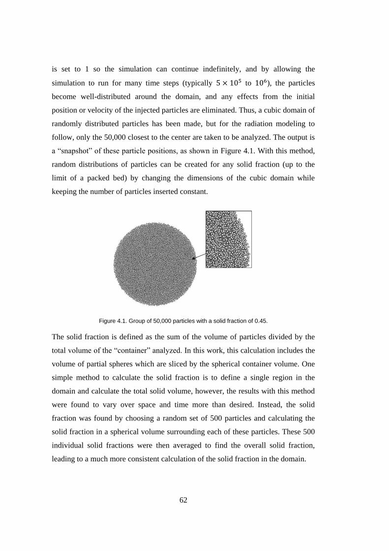
62
is set to 1 so the simulation can continue indefinitely, and by allowing the
simulation to run for many time steps (typically to ), the particles
become well-distributed around the domain, and any effects from the initial
position or velocity of the injected particles are eliminated. Thus, a cubic domain of
randomly distributed particles has been made, but for the radiation modeling to
follow, only the 50,000 closest to the center are taken to be analyzed. The output is
a “snapshot” of these particle positions, as shown in Figure 4.1. With this method,
random distributions of particles can be created for any solid fraction (up to the
limit of a packed bed) by changing the dimensions of the cubic domain while
keeping the number of particles inserted constant.
Figure 4.1. Group of 50,000 particles with a solid fraction of 0.45.
The solid fraction is defined as the sum of the volume of particles divided by the
total volume of the “container” analyzed. In this work, this calculation includes the
volume of partial spheres which are sliced by the spherical container volume. One
simple method to calculate the solid fraction is to define a single region in the
domain and calculate the total solid volume, however, the results with this method
were found to vary over space and time more than desired. Instead, the solid
fraction was found by choosing a random set of 500 particles and calculating the
solid fraction in a spherical volume surrounding each of these particles. These 500
individual solid fractions were then averaged to find the overall solid fraction,
leading to a much more consistent calculation of the solid fraction in the domain.

63
4.2.2 PP Radiation: Monte Carlo Ray Tracing
A randomly selected sample of 500 emitting particles were specified near the
center of the domain, and the MCRT code was used to find the RDF from each of
these emitting spheres to every other sphere in the domain. Each emitting sphere
was far from the edges of the particle group to ensure that all photons were
eventually absorbed by a particle and none were lost to the surroundings.
Results are shown in Figure 4.2 for all 500 emitting spheres, giving PP RDF as a
function of the center-to-center distance between each particle pair, and a
smoothing spline curve fit applied. There is a clear relationship between the
distance and the PP RDF, though the data is somewhat scattered due to the random
positions and shading of particles. It is noteworthy that the RDF prediction is
relatively accurate for close particles at a distance of 2 to 3 radii, where the highest
portion of the radiative transfer occurs, and there is more scatter between 3 and 5
radii. This is because when a pair of particles is close together (e.g. 2-3 radii) there
is little room in between for other neighboring particles which would intercept
radiation. In contrast, for particles further apart (e.g. 3-5 radii), there may be
several neighboring particles in between the two particles of interest, so the degree
of shading varies depending on the exact position of the particles in between,
leading to the higher spread in the RDF data shown. However, while any specific
pair of particles may have an RDF slightly higher or lower than the curve, the
correct amount of heat transfer can still be calculated for a group of particles with
reasonable accuracy due to the high number of particle-particle radiation
interactions, as demonstrated in Section 4.3.

64
Figure 4.2. Particle-particle RDF at various distances between particles, for εp = 0.86 and SF = 0.55, showing individual data points and a smoothing spline fit.
4.2.3 PP Radiation: RDF Tables
Within a DEM code the RDF between any two particles is approximated using a
tabulated form of the smoothing spline curve, such as the one shown in Figure 4.2.
Many attempts were made to fit the data to an equation such as polynomial,
exponential, power function, and the fit suggested by Liu et al. [66], however, each
of these failed to follow the RDF data to an adequate degree. Even a small
deviation from the spline curve can lead to a model which fails in terms of heat
transfer in the validation steps. Therefore, to maximize accuracy, the RDF at
discrete PP distances is tabulated instead of given as an equation of a curve. The
tables, found in Appendix A, give RDF as a function of distance, which is
normalized by the particle radius so it is applicable for particles of any size. At
short PP distances, a spacing of 0.2 radii is used to capture the high curvature, and
at greater PP distances the spacing is increased to minimize the table length. Within
a DEM simulation, the RDF for a pair of particles is calculated by interpolating
between the tabulated data based on the exact distance between the particles.

65
The previous steps were used to generate a single RDF-distance table which is only
valid for a specific solid fraction and particle emissivity. Different particle domains
were generated with DEM to achieve different solid fractions (0.25, 0.35, 0.45,
0.55, and 0.64), and the MCRT modeling was performed using two particle
emissivities (0.65 and 0.86), resulting in an RDF-distance table for each
combination of solid fraction and particle emissivity, which are presented in
Appendix A. The first application of the DBA model is intended for particle-based
CSP devices, so the tables are given specifically for the emissivities of silica sand
and sintered bauxite in the range of 700 to 800 ⁰C (taken to be 0.65 and 0.86
respectively), as these are the top candidates for heat storage materials in this
industry [56][7][81]. Though tables for only two particle emissivities are given
here, the method can be followed to generate tables for particles of any emissivity
and solid fraction with the procedure outlined along with the DEM and Monte
Carlo simulations.
4.2.4 PP Radiation: Calculating Heat Exchange in DEM
Within the DEM code, the rate of radiative heat exchange (qij) between any two
spheres i and j is found using Eq. (3.1) (Section 3.1). All of these variables are
typically known in a DEM simulation except . To find , values for the PP
distance and the solid fraction must be calculated within the DEM code. Then, with
the RDF tables, two linear interpolations are used (or more directly, a bilinear
interpolation [82]) to calculate the actual RDF at the distance and solid fraction of
interest.
In the typical “soft-sphere” DEM approach [53] the deformation of contacting
spheres is modeled by allowing them to overlap slightly, making the center-to-
center distance just less than 2 radii. Since real particles cannot overlap and the
deformation of small, hard particles is very slight, any deformation will not
measurably change the RDF for the conditions of interest. Therefore, in the DBA

66
model the center-to-center distance of any slightly overlapping pair of particles is
taken to be exactly 2 radii when using the tables to calculate the RDF.
4.2.5 PW Radiation: Generation of Particle-Wall Domains
Particle-wall domains with bulk solid fractions of 0.25, 0.35, 0.45, 0.55 and 0.64
were created in LIGGGHTS using a procedure similar to the PP domains, for
groups of 24,000 spheres. For the cases of packed beds with a bulk solid fraction of
0.55 and 0.64, particles were inserted into the domain and allowed to come to rest
on top of the wall in the presence of gravity, as shown in Figure 4.3(a). To generate
domains with lower solid fractions, particles were inserted in between the top and
bottom walls (Figure 4.3(b)) with some velocity, gravity was turned off, the
coefficient of restitution was set to 1, and particles were allowed to collide and
travel around the domain until a snapshot of the xyz particle locations was taken. In
both cases, the vertical edges of the domain were given periodic boundary
conditions, allowing particles to exert contact forces across the boundary and to
leave one side of the domain and enter on the opposite side, eliminating any effects
from side walls. The snapshot of particle locations was taken after a duration long
enough such that particles were well-distributed throughout the domain, without
any effect from the original position and velocity of the injected particles.
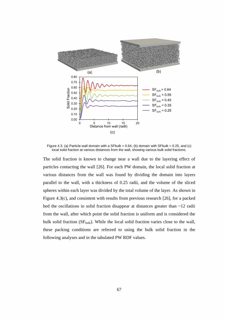
67
Figure 4.3. (a) Particle-wall domain with a SFbulk = 0.64, (b) domain with SFbulk = 0.25, and (c) local solid fraction at various distances from the wall, showing various bulk solid fractions.
The solid fraction is known to change near a wall due to the layering effect of
particles contacting the wall [26]. For each PW domain, the local solid fraction at
various distances from the wall was found by dividing the domain into layers
parallel to the wall, with a thickness of 0.25 radii, and the volume of the sliced
spheres within each layer was divided by the total volume of the layer. As shown in
Figure 4.3(c), and consistent with results from previous research [26], for a packed
bed the oscillations in solid fraction disappear at distances greater than ~12 radii
from the wall, after which point the solid fraction is uniform and is considered the
bulk solid fraction (SFbulk). While the local solid fraction varies close to the wall,
these packing conditions are referred to using the bulk solid fraction in the
following analyses and in the tabulated PW RDF values.

68
4.2.6 PW Radiation: Monte Carlo Ray Tracing
Simulations were run with the MCRT code to find the RDF between particles and
the wall for the five bulk solid fractions. During each simulation, photons were
emitted from 4000 randomly-selected particles far from the sides of the domain to
ensure negligible loss of photons to the surroundings. Sample PW RDF results for
the case of a εp = 0.86, εw = 0.60, and SFbulk = 0.45 are shown in Figure 4.4 along
with a smoothing spline fit of the data. The layering of particles against the wall
causes the concentration of particles at distances of one radius and three radii from
the wall with few particles in between, which is consistent with the peaks in the
solid fraction shown in Figure 4.3(c).
Figure 4.4. Particle-wall RDF at various distances, for a εp = 0.86, εw = 0.80, and SFbulk = 0.45.
4.2.7 PW Radiation: RDF Tables
A set of PW RDF tables was generated and is given in Appendix B, with the wall
emissivity being a third parameter affecting the PW RDF. The tables cover particle
emissivities of 0.65 and 0.86, wall emissivities of 0.4, 0.6, 0.8, and 1.0, and bulk
solid fractions of 0.25, 0.35, 0.45, 0.55, and 0.64. With the additional variable of
the wall emissivity, the number of tables to cover all circumstances can become

69
high, but within any particular DEM simulation the wall and particle emissivities
are typically constant, so only a single table with various bulk solid fractions and
PW distances must be implemented.
4.2.8 PW Radiation: Calculating Heat Exchange in DEM
Radiative heat transfer from particle to the wall is calculated with Eq. (4.1),
where is the particle emissivity, is the particle surface area, is the absolute
temperature, is the Stefan-Boltzmann constant, and is the RDF from particle
to the wall. Similar to the calculation of the PP RDF, requires a bilinear
interpolation based on the PW distance and bulk solid fraction.
(4.1)
4.3 Model Validation
The MCRT code has been validated to find RDFs to a high degree of accuracy for
both PP and PW domains. Therefore, the DBA model was validated by comparing
results in the simulations that follow, where the RDFs were found both with the
highly accurate Monte Carlo code and by approximating RDFs using the tables in
the appendices.
4.3.1 Validation of Particle-Particle DBA Model
According to the first law of thermodynamics all emitted photons must eventually
be absorbed, so the sum of the RDFs from one particle to all particles (including
the emitting particle) must be 1. While this is not enforced in the DBA model, if a
valid PP RDF-distance curve is used, then the sum of all RDFs should, on average,
be equal to 1. This fundamental property was tested for each of the ten proposed PP
RDF curves. A new domain of particles was generated (i.e. a different snapshot of

70
particle positions was taken) for each of the solid fractions studied, and 100
particles were randomly selected near the center of the domain. The total RDF was
calculated using the DBA model for each of these 100 particles, and the mean was
found, leading to the results shown in Table 4.1. In all cases the mean total RDF is
very close to 1, indicating that for any different set of particle positions having the
solid fractions studied, this fundamental criterion is met by applying the proposed
curves (in contrast, particles have a total view factor of only ~0.83 using the Short
Range Model [46]). It should be noted that while the total PP RDF may be slightly
more or less than 1, the first law of thermodynamics will not be violated in a DEM
simulation because the same quantity of heat is removed from one particle and
delivered to the second particle, keeping the total energy in the simulation
unchanged.
Table 4.1. Mean of the total PP RDF over 100 particles, for the ten PP RDF cases studied.
Solid Fraction
εp = 0.65 εp = 0.86
0.64 0.9979 0.9990
0.55 1.0025 1.0032
0.45 1.0019 1.0023
0.35 1.0022 1.0025
0.25 1.0020 1.0024
The results in Table 4.1 show that the sum of the RDFs is very close to 1 using
with the proposed PP RDF curves, however, it does not show that the RDFs are
distributed correctly based on the distance from the emitting particle. An invalid PP
RDF curve could, for example, overestimate the RDF for closely neighboring
particles and underestimate the RDF for particles at a greater distance, and it is
possible for the total RDF to still equal 1. To ensure the RDFs are correctly
estimated based on distance, the cumulative RDF (i.e. the fraction of photons
absorbed) is plotted as a function of distance from the emitting particle.
For each of the ten cases, a new particle domain was generated again, and the
cumulative RDF curve was found and averaged over 100 randomly-selected
particles using both the proposed PP RDF curves and the highly accurate RDFs
found with the Monte Carlo model. Results are shown in Figure 4.5 for a particle
emissivity of 0.65 and each of the solid fractions studied, and an extremely close

71
match is shown between the Monte Carlo (MC) and DBA results in each case. This
comparison shows that by using the proposed RDF curves, the distribution of
photons absorbed as a function of the distance from each particle can be accurately
predicted for any domain of particles that has one of the solid fractions studied.
Similarly close results were also found for an emissivity of 0.86, so all of the ten
proposed RDF curves provide a valid estimate for the RDF as a function of
distance from the emitting particle. In the figure, the RDF starts at a value above
zero due to the photons reflected back onto and absorbed by the emitting particle,
and the immediate rise at a distance of 2.0 is due to photons absorbed by particles
in contact with the emitting particle.
Figure 4.5. Mean cumulative RDF (fraction of photos absorbed) at various distances from the emitting particle, calculated with Monte Carlo and the DBA models, for εp = 0.65 and various solid
fractions.
Finally, each of the cases was validated using a heat transfer simulation, where the
heat transfer rate between each particle and every other particle was calculated with
Eq. (3.1). A spherical domain of 10,000 particles (Figure 4.6) of radius 0.01 m was
generated for each of the five solid fractions, and a hot core with a radius of 0.07 m
was designated where particles have a temperature of 1010 K, with all other
particles having a temperature of 1000 K. The PP RDF values were found using
both a full MCRT simulation and by using the tables to estimate the RDFs. The

72
total heat transfer rate leaving the hot core was then calculated to compare the two
methods, and results are shown in Table 4.2 for each of the ten cases studied.
Figure 4.6. Cross section of the spherical domain used for validating the DBA model, with 10,000 particles and a solid fraction of 0.45.
Table 4.2. Total heat transfer from the hot core, comparing results from the DBA model with a full
Monte Carlo ray tracing simulation.
# of particles in hot core
Total heat transfer from core (W)
SF εp Monte Carlo DBA Error
0.25 0.65 83 83.59 85.07 1.77%
0.25 0.86 83 107.68 111.00 3.09%
0.35 0.65 116 89.62 90.64 1.14%
0.35 0.86 116 116.78 118.84 1.76%
0.45 0.65 153 94.73 93.70 -1.09%
0.45 0.86 153 125.90 125.13 -0.61%
0.55 0.65 195 96.22 98.23 2.08%
0.55 0.86 195 131.05 134.03 2.27%
0.64 0.65 219 95.10 95.63 0.56%
0.64 0.86 219 131.99 133.00 0.76%
The lowest error is for the packed bed case of SF = 0.64, which is likely due to the
dense and consistent packing compared to the lower solid fractions. The SF = 0.25
case shows the highest error, where the relatively larger space in between particles
leads to more variation in particle positions and shading effects. Overall, the results
predicted by the DBA model are shown to vary up to 3.09% when compared to the
Monte Carlo simulation, which indicates the DBA model is accurate enough for
many engineering applications. The number of particles in the heated core ranges
from 83 to 219 particles depending on the solid fraction, but if a simulation is run
with very few particles the accuracy is expected to decrease due to less radiation
interactions included in the summation of the total heat transfer from the core.

73
However, since most DEM simulations are typically run with tens of thousands to
hundreds of thousands of particles, this is not foreseen as a major constraint for the
DBA model once it is implemented in a DEM code.
4.3.2 Validation of Particle-Wall DBA Model
To validate the PW portion of the DBA model, the domains studied consisted of
24,000 particles with a radius of 0.01 m, as shown in Figure 4.7. All particles were
assigned a temperature of 1000 K, and the wall temperature was specified at 1010
K. The total heat transfer was calculated from the wall to a hemispherical-shaped
group of 500 particles using Eq. (4.1). These particles are shown in red in Figure
4.7, where half of the domain is made semi-transparent to expose this region. The
particle group is in the center of the domain to eliminate photons lost to the
surroundings.
Figure 4.7. Particle-wall domain with a SFbulk of 0.45. Half of the domain is semi-transparent to show the red particles included in the PW heat transfer calculation.
Total heat transfer from the wall to the red particle group was calculated, with PW
RDF values found using both the Monte Carlo code and the DBA model. With two
particle emissivities, four wall emissivities, and five bulk solid fractions, a total of
40 PW RDF-distance curves are given in Appendix B. A validation simulation was
run for each of the 40 cases, and the total PW heat transfer is shown in Table 4.3.
In all cases, the total heat transfer from the wall to the group of particles has a
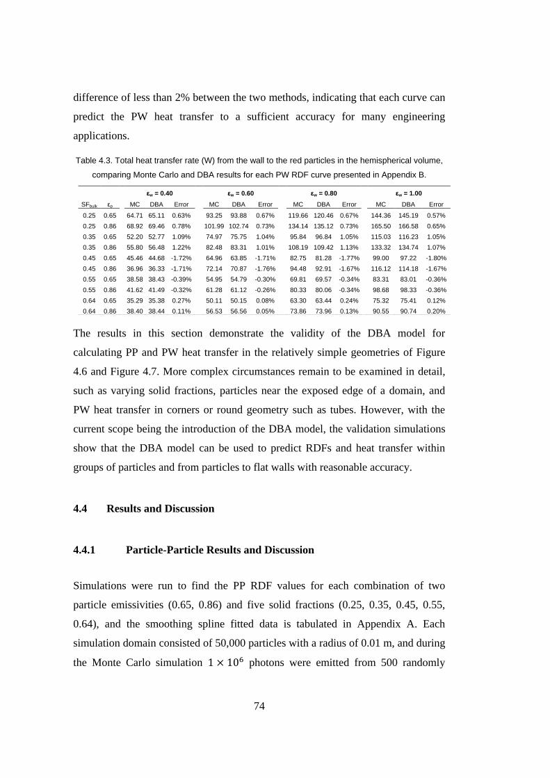
74
difference of less than 2% between the two methods, indicating that each curve can
predict the PW heat transfer to a sufficient accuracy for many engineering
applications.
Table 4.3. Total heat transfer rate (W) from the wall to the red particles in the hemispherical volume,
comparing Monte Carlo and DBA results for each PW RDF curve presented in Appendix B.
The results in this section demonstrate the validity of the DBA model for
calculating PP and PW heat transfer in the relatively simple geometries of Figure
4.6 and Figure 4.7. More complex circumstances remain to be examined in detail,
such as varying solid fractions, particles near the exposed edge of a domain, and
PW heat transfer in corners or round geometry such as tubes. However, with the
current scope being the introduction of the DBA model, the validation simulations
show that the DBA model can be used to predict RDFs and heat transfer within
groups of particles and from particles to flat walls with reasonable accuracy.
4.4 Results and Discussion
4.4.1 Particle-Particle Results and Discussion
Simulations were run to find the PP RDF values for each combination of two
particle emissivities (0.65, 0.86) and five solid fractions (0.25, 0.35, 0.45, 0.55,
0.64), and the smoothing spline fitted data is tabulated in Appendix A. Each
simulation domain consisted of 50,000 particles with a radius of 0.01 m, and during
the Monte Carlo simulation photons were emitted from 500 randomly
SFbulk εp
εw = 0.40
εw = 0.60
εw = 0.80
εw = 1.00
MC DBA Error
MC DBA Error
MC DBA Error
MC DBA Error
0.25 0.65
64.71 65.11 0.63%
93.25 93.88 0.67%
119.66 120.46 0.67%
144.36 145.19 0.57%
0.25 0.86
68.92 69.46 0.78%
101.99 102.74 0.73%
134.14 135.12 0.73%
165.50 166.58 0.65%
0.35 0.65
52.20 52.77 1.09%
74.97 75.75 1.04%
95.84 96.84 1.05%
115.03 116.23 1.05%
0.35 0.86
55.80 56.48 1.22%
82.48 83.31 1.01%
108.19 109.42 1.13%
133.32 134.74 1.07%
0.45 0.65
45.46 44.68 -1.72%
64.96 63.85 -1.71%
82.75 81.28 -1.77%
99.00 97.22 -1.80%
0.45 0.86
36.96 36.33 -1.71%
72.14 70.87 -1.76%
94.48 92.91 -1.67%
116.12 114.18 -1.67%
0.55 0.65
38.58 38.43 -0.39%
54.95 54.79 -0.30%
69.81 69.57 -0.34%
83.31 83.01 -0.36%
0.55 0.86
41.62 41.49 -0.32%
61.28 61.12 -0.26%
80.33 80.06 -0.34%
98.68 98.33 -0.36%
0.64 0.65
35.29 35.38 0.27%
50.11 50.15 0.08%
63.30 63.44 0.24%
75.32 75.41 0.12%
0.64 0.86
38.40 38.44 0.11%
56.53 56.56 0.05%
73.86 73.96 0.13%
90.55 90.74 0.20%

75
selected particles to build each table. The high number of emitting particles was
used to find a very accurate average PP RDF-distance curve, with any local particle
position or solid fraction variations balanced out.
The PP RDF tables are plotted for particle emissivities of 0.65 and 0.86 in Figure
4.8 (a) and (b), showing each solid fraction studied. In both cases, the lowest curve
is for a solid fraction of 0.64 because it has the densest packing, which stops
photons from penetrating far through the particle group. Several interesting
phenomena can be seen in Figure 4.8(c), where particle emissivities of 0.65 and
0.86 are shown for the highest (0.64) and lowest (0.25) solid fractions. For both
solid fractions, the curve for εp = 0.65 is lower than for εp = 0.86, a difference that
is especially pronounced at close range and for touching particles. With a lower
emissivity, and therefore a higher reflectivity, a higher number of rays reflect off
neighboring particles and are absorbed by the original emitting particle. This
reduces the rays absorbed by the neighboring particles and results in a lower RDF.
Also shown in Figure 4.8(c), the RDF for touching particles (distance of 2 radii) is
actually less for low solid fractions (red curves) than for packed beds (blue curves),
for the same emissivity. While at first it may seem that two touching particles
should have the same RDF regardless of the packing of the surrounding particles,
the difference again is due to the reflections. For two touching particles with many
close neighbors, rays emitted from one particle may reflect off other neighbors
before being absorbed by the particle touching the emitting particle. For a sparsely
packed group of particles, the emitting particle has fewer neighbors in close
proximity, so the likelihood of a photon reflecting off a neighbor towards the
touching particle is low. Due to the difference in reflectivities, this trend is visible
in the case of εp = 0.65, but it is hardly visible for εp = 0.86.

76
Figure 4.8. PP RDF as a function of distance for (a) εp = 0.65, (b) εp = 0.86, and (c) the extreme values of SF and εp.
Instead of presenting RDF-distance tables, expressing the RDF with an equation as
function of distance would be more concise and easier to implement into a DEM
code. However, no equation could be found to accurately represent the data in all
cases because the mechanics of contacting particles often does not lead to a smooth
curve. An example is shown in Figure 4.9(a) for SF = 0.64 and εp = 0.65, where the
data points make a distinct change in the curvature at ~3.25 and again at ~4 radii.
The smoothing spline follows this change in curvature, whereas the curve fits of
the form and (suggested by Liu et al. [66]) cannot
follow these distinct changes in curvature. In the cumulative RDF graph in Figure
4.9(b) (similar to those shown in Section 4.3.1), the proposed equations do not
match well with the MCRT results, and they each have a total PP RDF well above
1.00. In contrast, the cumulative RDF curve found by interpolating the points of the

77
smoothing spline matches the Monte Carlo results very closely, showing the higher
accuracy of this method.
Figure 4.9. (a) Particle-particle RDF data and three proposed curves for SF = 0.64 and εp = 0.65, and (b) Cumulative PP RDF at various distances from the emitting particle.
Another point of comparison is to the Short Range Model [46]. The total view
factor, which is the same as the RDF for black particles, is calculated by the SRM
as only 0.83 for a packed bed [46], which would lead to a large error in radiative
transfer. Furthermore, the deviation of the total view factor from 1 only increases
when particles are not tightly packed.
In a large DEM simulation, calculating the RDF between very distant particles is
an unnecessary computational expense, since above a certain distance the RDF is
negligible. To find the “cutoff” distance above which the PP radiative transfer can
be omitted with negligible loss of accuracy, the cumulative PP RDF curve from the
Monte Carlo simulation was analyzed to find the distance at which 99.9% of the
photons had been absorbed. These distances are given in Table 4.4, and the tables
in Appendix A are truncated to zero above these values as well.
Table 4.4. PP center-to-center cutoff distance based on 99.9% of photons absorbed.
PP Cutoff Distance (radii)
Solid Fraction εp = 0.65 εp = 0.86
0.25 29.9 28.2
0.35 18.4 17.8
0.45 12.5 12.1
0.55 8.9 8.7
0.64 6.7 6.6

78
4.4.2 Particle-Wall Results and Discussion
PW RDF curves are found for each combination of two particle emissivities (0.65,
0.86), four wall emissivities (0.4, 0.6, 0.8, 1.0), and five bulk solid fractions (0.25,
0.35, 0.45, 0.55, 0.64), and tabulated results are found in Appendix B. Each domain
consisted of 24,000 particles with a radius of 0.01 m, and during the Monte Carlo
simulations photons were emitted from 4000 particles. While there are 40 PW
curves in total, several examples are shown in Figure 4.10. Results are plotted in
Figure 4.10(a) for the case of εp = 0.65, εw = 0.80, and bulk solid fractions ranging
from 0.25 to 0.64. The PW RDF is lowest for densely packed domains due to the
many neighboring particles which intercept emitted rays, even for particles in
contact with the wall (distance of 1 radius). The change in curvature around 3 radii
is caused by the layering effect, as there are many particles with their centers in this
region and very few with centers between 1 and 3 radii. Results are shown in
Figure 4.10(b) for εp = 0.86, SF = 0.45, and various wall emissivities, where low
wall emissivities lead to low PW RDF values due to a higher portion of photons
being reflected from the wall.
Figure 4.10. Particle-wall RDF for (a) εp = 0.65, εw = 0.8, and various bulk solid fractions, and (b) εp = 0.86, SFbulk = 0.45, and various wall emissivities.
Similar to the method applied to find the PP cutoff distance, cumulative PW RDF
curves were constructed for each of the 40 cases using the Monte Carlo data, and
the PW cutoff was determined as the point at which 99.9% of the total cumulative

79
PW RDF was reached. These values are given in Table 4.5 and the PW RDF tables
are truncated above these values.
Table 4.5. PW cutoff distance based on 99.9% of photons absorbed.
Bulk Solid
Fraction
εp = 0.65 εw = 0.40
εp = 0.65 εw = 0.60
εp = 0.65 εw = 0.80
εp = 0.65 εw = 1.00
εp = 0.86 εw = 0.40
εp = 0.86 εw = 0.60
εp = 0.86 εw = 0.80
εp = 0.86 εw = 1.00
0.25 22.2 22.2 22.2 22.2 21.7 21.7 21.7 21.7
0.35 14.1 14.1 14.1 14.1 13.7 13.7 13.7 13.7
0.45 9.2 9.2 9.2 9.2 8.9 8.9 8.9 8.9
0.55 6.8 6.8 6.8 6.9 6.6 6.6 6.6 6.6
0.64 4.7 4.7 4.8 4.8 4.6 4.6 4.6 4.6
The Monte Carlo code, and therefore the tables in Appendix B, gives the PW RDF
values from one emitting particle to the entire wall. Therefore, when using the PW
RDF values to calculate the heat transfer using Eq. (4.1), the entire wall must have
a uniform temperature for the equation to be applied correctly. However, if a non-
uniform temperature boundary condition is used by dividing the wall into surface
mesh elements, as is common in CFD-DEM simulations, Eq. (4.1) can still be
implemented by considering to be the temperature of the closest wall element,
and all heat transfer can be assumed to be to that element. Using Eq. (4.1) in this
way is a valid approximation as long as temperature gradients along the wall are
small over a length scale of several particle diameters, as the majority of PW heat
transfer occurs close to the particle. This is true in almost all “unresolved” CFD-
DEM simulations (when the particle size is smaller than the CFD mesh elements)
[53] because the particle diameter must be several times smaller than the length of
the element.
For highly reflective walls, the wall reflections can actually affect the RDF values
between particle pairs. For example, in the extreme case of a wall with a
reflectivity of 1, a pair of particles has a higher PP RDF if they are both touching
the wall than they would in the center of a group of particles, due to the photons
that are emitted from one particle which are reflected off the wall and then strike
the second particle. However, this effect is relatively minor because it only affects
particle pairs that are touching or nearly touching the wall. Furthermore, in many
circumstances, such as the heat transfer simulation in Figure 4.11, the direction of

80
the heat flux is largely perpendicular to the wall, so two neighboring particles
which are both touching the wall have very similar temperatures, and an error in
the PP RDF due to wall reflections will contribute little to the error in actual heat
transfer. Special near-wall PP RDF values could be investigated, but for the initial
implementation of the DBA model this effect was neglected.
4.5 Modeling Radiation in a Dense Granular Flow
The initial implementation of the DBA model in a dynamic DEM simulation was
performed for particles descending with gravity through a channel which is heated
on one side, representing the conditions present in a particle heat exchanger or
solar receiver with a dense granular flow [20][21][24]. The purpose is to
demonstrate and discuss the DBA model implementation and to examine the
radiative transfer in detail, so radiation was the only heat transfer mode considered.
The channel, shown in Figure 4.11, has widths in the x and z directions of 10 mm,
and the heated section is between y = 20 mm and y = 40 mm. The current
implementation includes a DEM modeling step and a subsequent heat transfer
modeling step, which are executed by separate codes.

81
Figure 4.11. Simulation domain of a heated channel in dense granular flow.
First, LIGGGHTS was used to model the particle positions over time as they flow
downward and drain through the nozzle. A group of 5000 particles with a radius of
500 μm was inserted into the domain, and after every 1000 DEM time steps the xyz
positions of all particles were saved to a text file output. Boundaries on the z-planes
at 0 and 10 mm were modeled as walls, while the boundaries on the x-planes at 0
and 10 mm were periodic, meaning particles could pass through one plane and
reappear on the other. This was done to make the packing in the x-direction
uniform by avoiding any layering effects, therefore making the simulation
represent a channel of infinite length in the x-direction. The boundaries in the y-
direction were also periodic, so as particles flowed out through the nozzle they
reappeared with the same x-z position and velocity at the top of the domain. Thus,
the total number of particles was always maintained at 5000, and the fill level at the
top of the dense granular flow remained relatively constant over time at roughly y
= 48 mm, above the heated section of the wall. Parameters used in the simulation
are found in Table 4.6, with particle properties representing sintered bauxite
[56][83][84]. However, the density and specific heat capacity values were
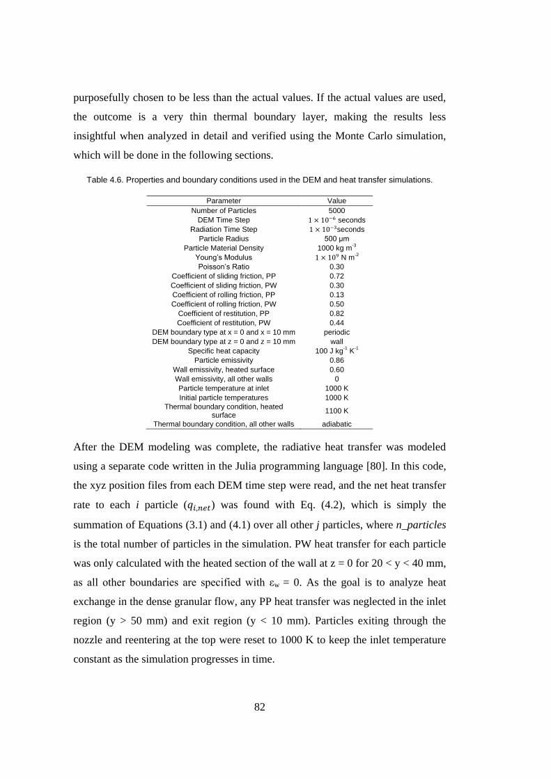
82
purposefully chosen to be less than the actual values. If the actual values are used,
the outcome is a very thin thermal boundary layer, making the results less
insightful when analyzed in detail and verified using the Monte Carlo simulation,
which will be done in the following sections.
Table 4.6. Properties and boundary conditions used in the DEM and heat transfer simulations.
Parameter Value
Number of Particles 5000
DEM Time Step seconds
Radiation Time Step seconds
Particle Radius 500 μm
Particle Material Density 1000 kg m-3
Young’s Modulus N m-2
Poisson’s Ratio 0.30
Coefficient of sliding friction, PP 0.72
Coefficient of sliding friction, PW 0.30
Coefficient of rolling friction, PP 0.13
Coefficient of rolling friction, PW 0.50
Coefficient of restitution, PP 0.82
Coefficient of restitution, PW 0.44
DEM boundary type at x = 0 and x = 10 mm periodic
DEM boundary type at z = 0 and z = 10 mm wall
Specific heat capacity 100 J kg-1
K-1
Particle emissivity 0.86
Wall emissivity, heated surface 0.60
Wall emissivity, all other walls 0
Particle temperature at inlet 1000 K
Initial particle temperatures 1000 K
Thermal boundary condition, heated surface
1100 K
Thermal boundary condition, all other walls adiabatic
After the DEM modeling was complete, the radiative heat transfer was modeled
using a separate code written in the Julia programming language [80]. In this code,
the xyz position files from each DEM time step were read, and the net heat transfer
rate to each i particle ( ) was found with Eq. (4.2), which is simply the
summation of Equations (3.1) and (4.1) over all other j particles, where n_particles
is the total number of particles in the simulation. PW heat transfer for each particle
was only calculated with the heated section of the wall at z = 0 for 20 < y < 40 mm,
as all other boundaries are specified with εw = 0. As the goal is to analyze heat
exchange in the dense granular flow, any PP heat transfer was neglected in the inlet
region (y > 50 mm) and exit region (y < 10 mm). Particles exiting through the
nozzle and reentering at the top were reset to 1000 K to keep the inlet temperature
constant as the simulation progresses in time.

83
(
) ∑
(4.2)
After calculating for each particle using Eq. (4.2(4.2), Eq. (4.3) was used to
find the temperature ( ) of each sphere i at the time step based on the
temperature at the previous time step ( ), after a duration of one radiation time
step ( ). The DEM time step size ( ) must be extremely small due to
limitations in the equations governing the collision mechanics [85], but changes in
radiative transfer are more gradual and can therefore be recalculated much less
frequently to save computation time, meaning the value of chosen can be
many times that of without loss of accuracy. The choice of will be
examined in detail later in this section. Using Eq. (4.3), with being the mass of
one particle and being the specific heat capacity of the particles, the temperature
of each sphere i is found at time step n, and the heat transfer simulation can then
proceed to the next time step.
(4.3)
The RDFs and require interpolating within the tabulated data based on
both the distance and the solid fraction. In general, for simulations where the bulk
solid fraction is not uniform in space or time, the solid fraction must be calculated
locally and at each radiation time step. However, in this simulation a simplification
was made to use a single bulk solid fraction value because it was found to change
minimally across all time steps and for all y-positions within the dense flow region
of the domain. Therefore, the bulk solid fraction for the region adjacent to the
heated wall (20 < y < 40 mm) was calculated to be 0.6278 at a time of 1.35
seconds, which is after a steady state is established, as will be shown later in this
section. This bulk solid fraction value was used throughout the radiative transfer
code for all time steps.
One important adjustment to the solid fraction was necessary to implement the PP
RDF tables for particles near a wall. The PP RDF tables were developed assuming

84
a large group of particles with a nearly uniform solid fraction, but in the current
simulation the local solid fraction varied due to layering effects against the wall (as
shown in Figure 4.3(c) in Section 4.2.5). A separate near-wall region was
implemented to account for this difference, taken to be between 0 and 5 radii in this
simulation. The near-wall solid fraction in this region was calculated to be 0.5728,
somewhat lower than the bulk value of 0.6278. In the heat transfer simulation, if
both particles i and j were within 5 radii of the wall, then the near-wall solid
fraction was used for determining the PP RDF from the tables, and if not, the bulk
solid fraction was used. Accounting for the lower near-wall solid fraction in this
way increases the accuracy of the current simulation in the near-wall region, but
additional research is necessary to investigate if this approach can be generalized
for various conditions, such as flow over more complex geometries, low solid
fractions, and in different flow regimes. This type of adjustment is not necessary
for the PW RDF tables because they were developed using domains of particles
adjacent to a wall, so the varying solid fraction is already incorporated into the
RDF-distance curve.
Several results relevant to the design or optimization of a particle heat exchanger
are shown in Figure 4.12. The total heat transfer rate from the wall to the particles
is likely the key metric for a heat exchanger, which is shown as a function of time
in Figure 4.12(a). There is an initial transient phase with high heat transfer due to
the initial particle temperatures of 1000 K coming in contact with the heated
surface at 1100 K, and after a thermal boundary layer has developed, a steady state
is achieved after roughly 1.35 seconds where heat transfer from the wall remains
relatively constant at ~2.11 W. There is some variation even after reaching this
steady state due to slight changes in the bulk particle velocity caused by frictional
effects and bridging through the nozzle. Particle temperatures at 1.35 seconds are
shown in Figure 4.12(b), where a thin thermal boundary layer forms and particle
temperatures increase towards the lower edge of the heated surface. PW heat
transfer for each particle is shown in Figure 4.12(c), where heat transfer is highest
near the inlet and declines in the direction of flow.
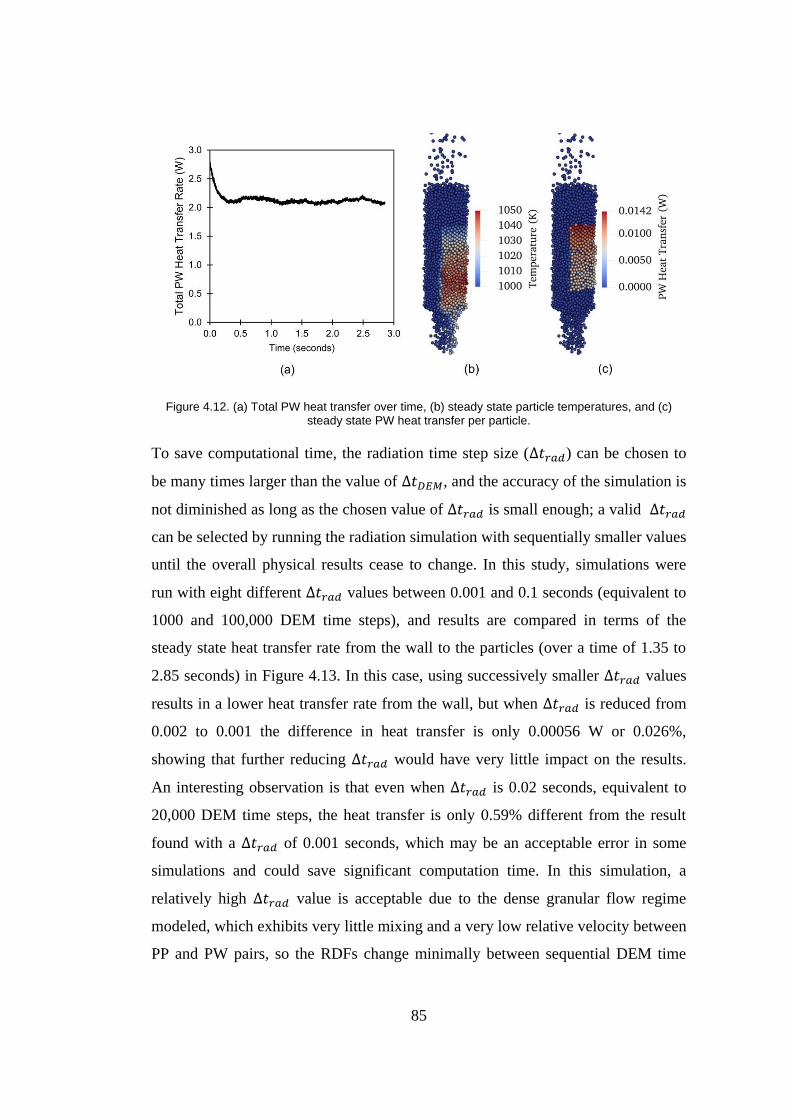
85
Figure 4.12. (a) Total PW heat transfer over time, (b) steady state particle temperatures, and (c) steady state PW heat transfer per particle.
To save computational time, the radiation time step size ( ) can be chosen to
be many times larger than the value of , and the accuracy of the simulation is
not diminished as long as the chosen value of is small enough; a valid
can be selected by running the radiation simulation with sequentially smaller values
until the overall physical results cease to change. In this study, simulations were
run with eight different values between 0.001 and 0.1 seconds (equivalent to
1000 and 100,000 DEM time steps), and results are compared in terms of the
steady state heat transfer rate from the wall to the particles (over a time of 1.35 to
2.85 seconds) in Figure 4.13. In this case, using successively smaller values
results in a lower heat transfer rate from the wall, but when is reduced from
0.002 to 0.001 the difference in heat transfer is only 0.00056 W or 0.026%,
showing that further reducing would have very little impact on the results.
An interesting observation is that even when is 0.02 seconds, equivalent to
20,000 DEM time steps, the heat transfer is only 0.59% different from the result
found with a of 0.001 seconds, which may be an acceptable error in some
simulations and could save significant computation time. In this simulation, a
relatively high value is acceptable due to the dense granular flow regime
modeled, which exhibits very little mixing and a very low relative velocity between
PP and PW pairs, so the RDFs change minimally between sequential DEM time

86
steps, and therefore the estimated RDF values remain accurate for a relatively long
time. In contrast, for simulations with a high relative velocity between particles
such as fluidized beds, the RDF values change much more between each DEM
time step, and the value required would be much lower. In the following
results and analyses a value of 0.001 is used to maximize accuracy.
Figure 4.13. Steady state heat transfer rate from the wall, comparing results with various radiation time step sizes.
With 5000 particles and a simulation with hundreds of time steps, running a
validation simulation using the Monte Carlo code to find the accurate RDF values
at every time step is computationally unreasonable. However, a comparison can
still be made by analyzing a single time step in detail using both a Monte Carlo
simulation and the DBA model. The time step chosen to analyze is at 1.35 seconds,
after a steady state has been established. For the xyz particle positions at this time
step, the RDFs from each particle to every other particle and the wall were
calculated with the Monte Carlo code and estimated with the DBA model. The net
PP and PW heat transfer rate to each particle was then found using Eq. (4.2), and
the mean PP and PW heat transfer per particle is plotted as a function of distance
from the wall in Figure 4.14. The mean PP heat transfer is shown in Figure 4.14(a),
where the particles against the wall (at a distance of 1 radius from the wall) have
the highest temperature, and these particles transfer heat to the cooler particles on
the interior of the domain, resulting in a large, negative PP heat transfer per

87
particle. The cooler interior particles receive this heat, resulting in the positive heat
transfer per particle above 2 radii from the wall, which diminishes until a distance
of 10 radii from the wall, after which almost no heat is transferred between
particles. Similarly, the mean PW heat transfer is shown at various distances from
the wall in Figure 4.14(b). As expected, the PW heat transfer is highest for particles
in contact with the wall, and it quickly reduces with increasing PW distance. The
chart shows that the PW heat transfer is negligible for distances greater than ~5.5
radii, which agrees with the PW cutoff distance range given in Table 4.5.
Comparing the trends and values in Figure 4.14, a close match is shown between
the DBA and Monte Carlo results for both PP and PW heat transfer. The overall
PW heat transfer is calculated to be 2.025 W and 2.028 W with the Monte Carlo
simulation and DBA models respectively, a difference of 0.14%, indicating the
validity of the DBA model in the simulation.
Figure 4.14. (a) Mean PP heat transfer per particle, and (b) mean PW heat transfer per particle, both as a function of distance from the wall.
4.6 Conclusions and Future Work for DBA Model
A method is presented to estimate the particle-particle and particle-wall radiative
transfer by using a Distance Based Approximation (DBA) of the RDF between PP
and PW pairs. Once the RDF-distance curve is established, the DBA model is both
simple to implement and has a low computational cost in a DEM code, requiring

88
only two equations and an evaluation of the RDF with a lookup table. RDF tables
are provided for solid fractions of 0.25, 0.35, 0.45, 0.55 and 0.64, particle
emissivities of 0.65 and 0.86, and wall emissivities of 0.4, 0.6, 0.8 and 1.0, and
these can be copied and directly implemented into DEM codes by other
researchers. Several simulations have demonstrated the validity of both the DBA
methodology and the actual curves provided, with errors typically less than ~2-3%
in overall heat transfer between two groups of particles or between a group of
particles and an adjacent wall.
An initial implementation of the DBA model in a dense granular flow shows it can
accurately predict overall radiative transfer, by showing a high level of agreement
with a full Monte Carlo solution for a time step analyzed in detail. It was
demonstrated that a radiation time step in the range of 0.001 to 0.02 seconds
(equivalent to 1000 to 20,000 DEM time steps) or less would be acceptable for the
current simulation, but a lower radiation time step would likely be required in
situations with higher particle velocities such as fluidized beds or falling particles.
The DBA model can potentially be used in many applications, but carefully
analyzing the validity in more challenging situations is left for future work. For
situations where the solid fraction varies in space and time such as in groups of
fluidized or falling particles, the solid fraction must be recalculated locally and at
each radiation time step. For modeling internal or external particle flow in contact
with round tubes, the PW RDF tables provided are valid as long as the tube radius
is much larger than the particle radius, though the degree of the size difference
required has not yet been investigated. Particles in very thin channels, particles
near two or more walls, and particles on the edge of the domain should be treated
and verified with care, as these situations diverge from the original assumptions
under which the RDF tables were developed. Additional suggested future work is
to implement the DBA model directly into DEM software such as the open source
code LIGGGHTS, commercial software, or the in-house codes developed by many
research institutions.

89
CHAPTER 5
5 AN OPEN SOURCE CODE FOR
DENSE PARTICLE HEAT TRANSFER
Throughout this research, codes were developed to model heat transfer in dense
particulate flows. Initially, a rudimentary form of the DBA model [67] was
implemented directly in LIGGGHTS, but due to the challenges of working within
the confines of that code, the approach was adopted where particle mechanics are
modeled with LIGGGHTS, and heat transfer is calculated afterwards using a
separate code. This code, which has been refined and annotated for others to use, is
referred to as the Dense Particle Heat Transfer (DPHT) code. More information as
well as the code itself can be found on the GitHub repository found at
https://github.com/ef-johnson/Dense-Particle-Heat-Transfer.
The combination of DEM and DPHT can be considered a “one-way” coupling,
where information only flows from the DEM model to the DPHT model, and not in
the other direction. The benefit is that after running the DEM simulation once to
find the particle positions over time, multiple thermal simulations can be run to
investigate the different thermal variables (e.g. temperature boundary conditions,
particle thermal conductivity, etc.), without having to re-run the DEM simulation
(which often takes the majority of the simulation time). The disadvantage of one-
way coupling is that the mechanics cannot be modified based on thermal
information, such as having temperature-dependent particle friction properties.
In the DPHT code, heat conduction models from literature are implemented, and
several of them are modified to be more physically realistic. The DBA model is
used for radiation, similar to the implementation shown in Section 4.5. While
previous researchers have implemented similar codes for their own use, there is no
open source code for heat transfer in dense granular flows that has been published
and explained in detail for others to use and build upon.

90
5.1 Motivation
There are numerous industrial applications of dense granular flows with heat
transfer, including many in CSP research. Modeling these processes at the particle
level is still relatively new, and when models are described in literature, they are
often performed with in-house codes. The current options for researchers or
students are to develop their own code, which may take months or years, or to use
an available DEM code such as LIGGGHTS.
While LIGGGHTS has some basic models for heat transfer, the features present are
not nearly robust enough to simulate most industrial processes. Numerous heat
transfer mechanisms are absent which are important in a dense flow, including
particle-fluid-particle and particle-fluid-wall conduction, and PP and PW radiation.
In addition, any mesh used as a boundary can only be given a single wall
temperature, whereas it is much more useful to specify the wall temperature as a
function or to assign various wall elements different temperatures. Within
LIGGGHTS, the PP and PW conduction model for contacting particles has been
implemented, but it appears to overestimate heat transfer by a factor of √ (see
Section 5.4.1). Additionally, heat transfer does not require recalculations nearly as
frequently as the DEM simulation requires, which would save an enormous amount
of computation time compared with executing heat transfer calculations at every
DEM time step. Finally, for researchers interested in implementing their own
model, modifying or adding to LIGGGHTS is cumbersome due to the many
dependent functions and source files, and relatively little notation is provided in the
C++ source code.
The aim of developing DPHT is to provide other researchers with a code that A)
has all of the main heat transfer modes already implemented; B) has been validated
under a basic set of circumstances; and C) is flexible enough so it can be easily
adapted for similar work. Furthermore, to make it easier for others to adopt, the full
workflow using all open source software is described here, starting from geometry
generation and ending in heat transfer modeling with DPHT.

91
5.2 Applications and Assumptions
The DPHT code is valid for the special case of dense granular flows, as the
interstitial fluid can be considered stationary with respect to the particles. Because
the relative movement between the air and particles is negligible, no heat is
transported away from the particles by convection. Heat transfer across the small
fluid gap between particles is still modeled, but only as conduction through the
stagnant fluid. This simplifies the model greatly because the fluid is not modeled
explicitly as a separate phase, so only the particle phase must be modeled, and the
more complex and computationally intense coupled CFD-DEM method is avoided.
This approach has been taken previously by Qi and Wright [45] who studied a
screw reactor and Chaudhuri et al. [86] who studied rotary calciners.
In addition, this approach neglects the heat absorbed by the fluid phase, which is
almost always a valid assumption in CSP devices, as the heat capacity of the solid
particles is much greater than the interstitial air. The assumptions of the radiation
model follow those in Section 3.1, including uniform particle temperatures and
geometric optics, with all spheres having gray, diffuse emissions and reflections.
The DPHT code could be directly useful for other CSP researchers who study
devices with dense granular flows. For example:
Watkins [21] studied dense granular flow through gravity-fed tubes as a
solar receiver concept, but the “two-layer” model developed is not general;
it is valid for only vertical tubes. If there were any mixing geometry or an
orifice introduced, which are potential ways to significantly increase heat
transfer, the two-layer model would not be valid.
Albrecht and Ho [24] studied a particles-to-sCO2 heat exchanger consisting
of parallel plates with particles in a gravity-driven dense granular flow. An
Eulerian approach was taken, and heat transfer equations were solved with
effective properties. This approach works for the parallel plates geometry
studied, but similar to work by Watkins described above, if the geometry is

92
varied by adding features to mix the flow, such a simple approach is
invalid. Also, radiation was neglected.
Baumann and Zunft [22][87] studied a “moving bed heat exchanger” for
CSP where particles flow with gravity over a bank of horizontal tubes to
heat the fluid (steam) flowing on the interior of the tubes. The authors point
out discrepancies between the flow field in the experimental setup (taken
with particle image velocimetry), and the Euler-Euler model. Particles form
a stagnant region above (upstream of) each tube and an empty pocket below
(downstream). This behavior is quite different from that of a fluid, so some
disagreement between the experiment and model can be expected due to the
continuum assumption inherent to Eulerian models.
Numerous other devices have been studied which could use DPHT either directly
or with some additions or modifications, such as the CentRec receiver [16], the
recently-proposed transparent tubular receiver [88], and the hexagonal tube
receiver by NREL [17]. The DPHT code can also be used for other industrial
processes, such as static powder beds used for laser sintering [71] and rotating kilns
[89]. In contrast, DPHT is not applicable for particles falling through air or in
fluidized beds.
5.3 Software Notes
DPHT is intended for use in Ubuntu (Linux) because it has been developed using
tools such as LIGGGHTS and ParaView, which are most often run on Linux-based
operating systems. DPHT is written in the Julia language because it is free to use,
and it is nearly as simple as programming with Matlab (including many functions
which are nearly identical). Simultaneously, it offers very fast computation speeds
due to its “just-in-time” compilation scheme. Almost all other languages are either
easy to program but slow (interpreted languages, e.g. Matlab, Python, Perl, Ruby),
or more difficult to program but fast (compiled languages, e.g. C++, C, Fortran).
Julia was built specifically to address the need for both speed and usability. Data

93
from benchmark tests [90] shows that Julia is comparable in speed to C, and it may
be an order of magnitude faster than Matlab, depending on the nature of the code.
Unlike Matlab, performing operations in vectors is not needed for speed, as for
loops are generally faster than vector operations in Julia, making the programming
more straightforward in many circumstances. The DPHT code takes advantage of
parallel processing in Julia by using multi-threaded for loops for the bulk of the
operations, leading to a large decrease in the run time over a serial code.
In addition to the DPHT code, a DEM code such as LIGGGHTS is needed to solve
for the particle positions before DPHT can be run. As described in Section 5.7,
several additional programs are needed for modeling, including a CAD drawing
program (such as Onshape), surface meshing software (such as Gmsh or Ansys),
and visualization software (ParaView), all of which can be obtained at no cost.
5.4 Heat Transfer Models
Each heat transfer mode is shown in Figure 5.1 and described in the following
sections, which can be found in the code files PP_ht.jl and PW_ht.jl.
Figure 5.1. The six heat transfer modes included in DPHT.

94
The heat transfer modes are shown in more detail in Figure 5.2. The models for
particle-fluid-particle (PFP) and particle-fluid-wall (PFW) heat transfer can be
visualized with the sequence of red and purple arrows.
Figure 5.2. (a) The three particle-particle heat transfer modes, and (b) the three particle-wall heat transfer modes (blue = fluid, red = wall).
One note should be made about terminology: many of the studies referenced below,
as well as the LIGGGHTS documentation, use the term heat flux to refer to the heat
transfer rate between two particles (in units of Watts). Technically, this is not
correct, since a heat flux must have units of power per area. To be clear, each of the
heat transfer modes below solves for the heat transfer rate in Watts.
5.4.1 Particle-Particle Conduction
A model for conduction between two particles has been suggested by Batchelor
and O’Brien [91] in 1976, given in Eq. (5.1). The thermal conductivity of the solid
particle is ks, and Ti and Tj are the temperatures of the two particles. In DEM
models, two contacting spheres are allowed to overlap slightly, and rc is the radius
of contact of the overlapping lens, as shown in Figure 5.3. The degree of overlap is
exaggerated in the figure for clarity, but it is very slight in an actual DEM
simulation.
(a) (b)

95
Figure 5.3. Geometry of two contacting spheres used to calculate PP conduction..
(5.1)
This equation was originally derived for particles in static contact, though it has
been used widely for dynamic calculations as well [86][92][93][94]. In the DPHT
model, the PP distance is known, and the contact radius is found with Eq. (5.2),
coming from the geometry of Figure 5.3.
√ (
)
(5.2)
Since Eq. (5.1) was published by Batchelor and O’Brien, numerous researchers
have modified it. In DEM modeling, typical practice is to use a Young’s modulus
several orders of magnitude lower than the actual material. This saves significant
computation time by allowing for a larger DEM time step size, as this is limited by
the Rayleigh and Hertz time step sizes, which are both functions of the Young’s
modulus. By reducing the Young’s modulus, the particles become softer, leading to
the undesired side effect of an increased overlap area between two colliding
spheres in DEM, which in turn results in an overestimation of heat transfer when
using Eq. (5.1). According to Zhou et al. [95] multiplying Eq. (5.1) by the factor c
corrects this overestimation, where and are the DEM-modeled and true
Young’s moduli, respectively.

96
(
* ⁄
(5.3)
The equation implemented in the LIGGGHTS code is given in Eq. (5.4). The
equation is similar, but not identical to, the Batchelor and O’Brien equation. The
first term in parentheses represents an effective conductivity in case the particles
have different thermal conductivities. If the two particles have the same thermal
conductivity, this term becomes simply ks and the equation is nearly identical to
Eq. (5.1) by Batchelor and O’Brien.
(
) √ (5.4)
The only difference between the LIGGGHTS version and the Batchelor and
O’Brien version is the term √ , instead of rc, where is the contact area and rc
the contact radius. Though the makers of LIGGGHTS cite Chaudhuri et al. [89],
that paper cites the original Batchelor and O’Brien equation, so the equations
should all be the same. Substituting into Eq. (5.4), it is clear that heat
transfer is overpredicted by a factor of √ or 1.77 in LIGGGHTS, compared to the
cited paper. It appears to be a mistake in the LIGGGHTS implementation which
may have implications for any researchers who have used or plan to use
LIGGGHTS for heat transfer calculations.
5.4.2 Particle-Wall Conduction
The PW conduction model is essentially the same as the PP conduction model of
Eq. (5.1), with several modifications. The contact radius rc is found with Eq. (5.5),
where R is the particle radius and diw is the particle-center to wall distance.
√ (5.5)

97
The particle and wall thermal conductivities are combined to form an effective
conductivity (kp,w) from the particle conductivity (ksi) and wall conductivity (ksw),
following the method from Cheng et al. [94].
(5.6)
The c factor is calculated with Eq. (5.7), which is interpreted from Zhou et al. [95]
for the case where particles have different properties. The Poisson’s ratios are νi
and νj respectively, and are the Young’s moduli used in the DEM
simulation, and and are the Young’s moduli of the actual materials. In
this case, the particle j is taken to be the wall.
(
(
) (
)
(
) (
))
⁄
(5.7)
5.4.3 Particle-Fluid-Particle Conduction
The heat conducted across the stagnant fluid gap between two nearby particles is
modeled with the particle-fluid-particle (PFP) conduction mode, for both
contacting and non-contacting particles. In the DPHT code, this is often referred to
as q_conv for ease of nomenclature, but technically the heat transfer is due to
conduction instead of convection, as the fluid is stagnant.
The model implemented comes from Cheng et al. [94]. The derivation starts by
building a “Voronoi” polyhedron around each particle, and a “double pyramid” is
defined, where the base of each pyramid is the Voronoi polyhedron between the
two spheres, and the pyramid edges are defined by connecting lines between each
vertex of the Voronoi polyhedron and the center of the particle, forming the point
of the pyramid. There is no analytical solution for such an arbitrary geometric
pyramid, so a similar, simpler geometry is adopted consisting of two opposing
cones, for which an analytical solution is possible. The cone bases lie on the center-

98
plane between the particles, the cone points are at the particle centers, and the
volume of the cone is the same as the original double pyramid formed with the
Voronoi polyhedron. A diagram showing the cone geometry is shown in Figure
5.4(a) for non-contacting particles and in Figure 5.4(b) for contacting particles,
where orange lines designate the outline of the double cone.
Figure 5.4. Dimensions relevant to Eq. (5.9) for calculating PFP conduction, showing (a) non-
contacting and (b) contacting spheres. Outline of the double cone volume is shown in orange.
This treatment allows for an analytical calculation of heat transfer to particle i from
particle j. The original form presented by Cheng et al. is shown for reference in Eq.
(5.8). However, a mathematically identical form is shown in Equations (5.9)-
(5.11), which is much more intuitive because, along with Figure 5.4, it reveals how
the equation was derived.
( ) ∫
[√
](
* [ √ ] ⁄
(5.8)
(a) (b)

99
In the geometry shown in Figure 5.4, the cone surfaces are considered isothermal at
and . From Eq. (5.9), it is clear that the heat flux is assumed to be 1D and
parallel to the vector between the particle centers. This equation uses resistances to
heat conduction in a series configuration, where (referring Figure 5.4) at a certain
radius r, heat first conducts through the solid in particle i a distance of , then it
conducts across the fluid gap a distance of , and finally it conducts through
particle j until it reaches the cone surface, after a distance of . In Eq. (5.9), ,
, and are the thermal conductivities of particle , particle , and the fluid,
respectively. Because particles are assumed to be monodisperse in the current
work, the distance traveled through the solid is the same for each sphere ( ).
These distances are solved with Equations (5.10) and (5.11) for a certain radial
location (r) in terms of the particle radius ( , the cone base radius ( ), and the
distance from the center plane to the closest “tip” of the particle (h). This distance h
is found with Eq. (5.14). The lower integration limit ( ) is taken as zero for non-
contacting particles, or the contact radius ( ) for overlapping particles. The upper
integration limit ( ) represents the intersection of the cone and the sphere,
calculated with Eq. (5.12).
( ) ∫
(
*
(5.9)
√
(5.10)
[ √ ] (5.11)
√
(5.12)
√
(5.13)

100
(5.14)
Unfortunately, in the original formulation of these equations, the cone base radius
( ) term must be calculated from the double pyramid volume ( ), which
requires building the Voronoi polyhedra around all particles at each time step, a
very computationally expensive process. To eliminate this requirement, Zhou et al.
[93] interpreted the results from Yang et al. [96] to express the cone base radius as
a function of only the particle radius and solid fraction ( ). With this
advancement, is much simpler to find using Eq. (5.15), and this eliminates the
need to build the Voronoi polyhedra or use Eq. (5.13).
(5.15)
Instead of solving Eq. (5.9) within the main code at each time step, it is much more
computationally efficient to use pre-calculated heat transfer coefficients as follows.
Within the main function go, the function PFP_conduction is called once at the
beginning of the simulation, which takes arguments of the solid fraction, the
particle thermal conductivity, and the particle radius. This function computes the
heat transfer coefficient (HTC) between two particles, where
( ). This is done by numerically solving the integral in Eq. (5.9) using the
trapezoid rule. These computations are repeated for many values of the particle
distance ( ) and numerous temperatures, until a matrix of HTC values has been
created, which is saved in the file htc_values.txt. Temperature must be included as
a parameter because it affects the thermal conductivity of the fluid; the current
implementation contains the values for air, which changes thermal conductivity by
a factor of ~2.5 between room temperature and 750 ⁰C. Within the code, the
temperature for evaluating PFP conduction is chosen as the mean of the two
particle temperatures. With the matrix of pre-calculated HTC values, the HTC for
any two particles is found with a bilinear interpolation and multiplied by ( )
to find the PFP conduction in Watts. Thus, the computationally expensive

101
numerical integration must only be performed once, at the beginning of the
simulation, making the calculation of heat transfer between particle pairs is very
fast.
To verify the output of the function matches physical expectations, the quantity
which will be integrated over 2πrdr (specifically, [
]
) is first plotted
for numerous radial locations (r) in Figure 5.5(a). Each curve shows the heat flux at
that radial location divided by the temperature difference between the two particles,
and each curve represents a different particle pair separated by distance dij. When
particles are overlapping, there is no PFP conduction at radial locations less than
the contact radius, so the lines start at radial positions greater than zero in the
figure. As expected, heat flux is highest at low radial locations, due to the ease of
heat transfer through the thin fluid gap near the circle of contact.

102
Figure 5.5. PFP conduction as a function of distance, for ksi=ksj=2.0, kf=0.0702, αs = 0.60, and
R=0.0005 m, showing (a) heat flux as a function of radial position, for various particle distances, and
(b) heat transfer coefficient as a functions of particle distance (dij).
dij = 0.0010 (just touching)
(b)
(a)

103
Next, the curves in Figure 5.5(a) are numerically integrated over 2πrdr with the
trapezoid rule to calculate the integral in Eq. (5.9), thus solving for the HTC at each
PP distance, with results shown in Figure 5.5(b). According to Zhou et al. [93],
heat transfer becomes negligible for
, or equivalently, . This
recommendation is followed in the DPHT code with PFP conduction neglected for
particles at a distance greater than 3 radii. The integration is repeated for a range of
temperatures to account for varying fluid thermal conductivity with temperature,
leading to the curves in Figure 5.6. These values are saved in PFP_htc_values.txt
and used to look up the HTC as a function of distance and temperature using the
function bilin_interp.jl.
Figure 5.6. PFP heat transfer coefficient solved for various particle distances and temperatures
(same parameters as Figure 5.5).
Similar to PP and PW conduction, because of the artificially low Young’s modulus,
the true distance between two contacting particles is less than it is in the DEM
simulation. The relevant literature did not show a correction factor for PFP
conduction, so one is derived here. The center-to-center distance between two
particles within the DEM simulation ( ) is known, but to calculate the PFP
conduction with the bilinear interpolation, the actual distance is desired ( )
0.00E+00
5.00E-05
1.00E-04
1.50E-04
2.00E-04
2.50E-04
3.00E-04
1.5 2 2.5 3
Heat
transfe
r coeff
icie
nt
(W /K
)
Particle center-to-center distance (radii)
T = 273
T = 373
T = 473
T = 573
T = 673
T = 773
T = 873
T = 973
T = 1073
T = 1173
T = 1273

104
after taking into account the reduced Young’s modulus. From the geometry of two
overlapping spheres, Equations (5.16) and (5.17) relate the particle radius (R), the
distance (dij), and contact radius of overlap (rc) for both the real and DEM cases.
Eq. (5.18) is another expression of the same c factor used previously (known from
Eq. (5.3)) which relates the true and DEM-modeled contact radii.
( ⁄ )
(5.16)
( ⁄ )
(5.17)
(5.18)
Substituting and rearranging these three equations, the actual distance can be found
in terms of the DEM-modeled distance, the radius, and c, to form Eq. (5.19). This
corrected distance can then be used in the bilinear interpolation of to find
the HTC in PFP conduction. Using instead of has the effect of
making contacting particles further away from each other, thus reducing PFP heat
transfer. For non-contacting particles, this does not apply, and .
Initial tests were run to show the effect of this modification in terms of overall heat
flow through the domain of particles found in Section 5.8. Results with the
corrected and uncorrected differed by only a very small amount, showing this
correction may not be needed in all cases. However, in this simulation the particles
modeled were relatively hard, with a DEM Young’s modulus of . A larger
difference is expected if softer particles are used in the DEM model, such as the
minimum value allowable in LIGGGHTS ( Pa) which is used by others
[97]. Since the adjusted distance should be more physically realistic in all cases, it
is used in the DPHT code in all modeling that follows.
√ [ ( ⁄ ) ] (5.19)

105
5.4.4 Particle-Fluid-Wall Conduction
Qi and Wright [45] extended the PFP conduction model described above
(originally from Cheng et al. [94]) to account for particle-fluid-wall (PFW)
conduction. Their adaptation assumes that there is still a conduction resistance due
to the wall. However, if the boundary condition is specified as Tw on the surface of
the wall (as shown in Figure 5.7), there should be no heat transfer resistance due to
the wall (i.e. heat does not have to conduct into the wall any distance to reach the
specified Tw). Thus, there should only be two conduction resistances, as shown in
Figure 5.7. This re-formulation of PFW conduction is given in Equations (5.20)-
(5.22), and is thought to be more realistic. Note that now is half of the value used
in PFP conduction.
Figure 5.7. Particle-fluid-wall geometry.
∫
(
*
(5.20)
√
(5.21)
√ (5.22)
When a particle overlaps the wall, we again must compensate for the artificially
low Young’s modulus for both the particles and the wall. Equations (5.23) to (5.25)

106
give the relations between particle radius (R), the particle-wall distance ( ), and
contact radius (rc) for both the DEM and real cases. The two cases are related
through the factor c using Eq. (5.7). After substitutions, the real PW distance
( ) is found from the other known variables with Eq. (5.26).
(5.23)
(5.24)
(5.25)
√ [ ] (5.26)
Similar to in the PFP conduction case, this adjustment makes the particle center
further away from the wall, reducing PFW heat transfer. This adjustment is only
used for particles touching the wall.
Similar to PFP conduction, at the beginning of the DPHT simulation, the PW HTC
is found for many temperatures and PW distances and saved in
PFW_htc_values.txt. During the simulation, the bilinear interpolation is used to
look up the correct HTC based on the PW distance and the temperature, where the
temperature used is the mean of the particle and the nearest wall element. Example
PW HTC curves are shown in Figure 5.8.

107
Figure 5.8. Particle-wall HTC values found for ksi=2.0, αs = 0.60, R=0.0005.
5.4.5 Particle-Particle and Particle-Wall Radiation
The Distance Based Approximation (DBA) model developed in Chapter 4 is
implemented for both PP and PW radiation. The RDF tables are interpolated with
the function bilin_interp using the PP or PW distance and the solid fraction. In the
current DPHT code, separate solid fractions for the near wall region and for the
bulk region have been used, as discussed in Section 4.5. These solid fractions must
be calculated externally before the simulation is run and specified with the
variables VlF_near_wall and VlF_bulk. The RDF tables must have the format of
the first column being the PP or PW distance (in units of radii) and the first row
being the solid fractions. Currently, RDF tables are available for solid fractions of
0.25, 0.35, 0.45, 0.55, and 0.64, for particle emissivities of 0.65 and 0.86, and for
wall emissivities of 0.4, 0.6, 0.8, and 1.0. If different conditions are desired, these
tables must be generated by finding the RDF as a function of distance as described
in Chapter 4 or interpolated between the known curves. With the RDF estimated,
0.0E+00
1.0E-04
2.0E-04
3.0E-04
4.0E-04
5.0E-04
6.0E-04
0.8 0.9 1 1.1 1.2 1.3 1.4 1.5
Hea
t tr
ansfe
r co
eff
icie
nt
(W /K
)
Particle center-to-wall distance (radii)
T = 273
T = 373
T = 473
T = 573
T = 673
T = 773
T = 873
T = 973
T = 1073
T = 1173
T = 1273
108
the PP and PW radiative transfer can be found with Equations (5.27) and (5.28),
where is the radiative transfer rate to particle i from particle j, is the
radiative transfer rate to particle i from the wall, is the particle emissivity, is
the surface area of the particle, is the Stefan-Boltzmann constant, and
represents the temperatures, where is the temperature of the closest wall
element.
(5.27)
(5.28)
5.5 Boundary Conditions
Boundary conditions are specified in DPHT by assigning a temperature to each
triangular wall element. Unlike in CFD, a heat flux boundary condition cannot be
easily specified, as this would require distributing the specified heat transfer among
the nearby particles, likely requiring iterations.
Before specifying the wall element temperatures, the walls must first be drawn and
meshed, and the mesh information must be saved as three text files (vertices.txt,
centers.txt, and relations.txt). This is demonstrated in Section 5.7.
At the beginning of the DPHT simulation the function create_BCs is run. The
temperature of each element is assigned, which can be specified as a function of the
centroid coordinates. With the three vertex locations of each wall element defined
in vertices.txt, the equation of a plane is found for each wall element. The
coefficients of each element’s plane equation are saved in the file bdry_data.txt and
will be used later to find the perpendicular distance to nearby particles. With this
information, a matrix is built which has all of the wall element centroid locations,
temperatures, and coefficients defining the plane of the element. An arbitrary
geometry of wall elements is shown in Figure 5.9, and more details on the coding
are given in Section 5.6.1.

109
The simulation iterates through each particle to calculate the PP heat transfer to
nearby particles and PW heat transfer to the nearest wall element. While iterating
through each particle, the closest wall element is identified by finding the minimum
distance between the particle and the centroid of each wall element. In Figure 5.9,
the closest centroid belongs to the element shown in red. The plane equation for the
closest element (which has been pre-computed and saved in bdry_data.txt) is then
used to calculate the perpendicular distance between the wall element and the
particle center, shown as diw in the figure. A correct calculation of this distance is
critical, as it is used in all three PW heat transfer models.
Figure 5.9. Particle and wall element geometry used for applying boundary conditions.
5.6 File Structure
Within the main DPHT folder, there are numerous folders and files, with the
structure shown in Figure 5.10, and each is discussed below.

110
Figure 5.10. DPHT file structure.
5.6.1 DPHT_code
This folder contains all of the Julia functions required to run DPHT. The details of
each file are described below:

111
a. The file DPH_tube.jl contains the main function, which is simply called go.
Several actions are taken at the start of the run. First, the user can select if
the boundary condition file and the PFP and PFW conduction HTC matrices
should be rebuilt or not, which is controlled by setting the booleans
rebuild_BCs and rebuild_PFP_cond to true or false. The DEM time step
size is set, which should match the timestep variable in the LIGGGHTS
input file (in this case the file in.fill_lattice). The variable LTS_stamp_delta
specifies the number of LIGGGHTS time steps in between each heat
transfer calculation by DPHT, and the LIGGGHTS time steps to start and
end are also specified. The number of threads for parallel processing is read
in from an environment variable, which can be set by pasting the command
export JULIA_NUM_THREADS=4 (where 4 is the number of processors
specified) into the ~.bashrc file, or by typing this command directly into the
terminal window before starting Julia. Next, various physical parameters
and properties are set, such as the particle radius and particle thermal
conductivity. Next, data is read in from several text files, including the RDF
tables, PFP conduction HTC tables, and the boundary conditions
corresponding to each wall element.
The next portion of the code executes at each time step, as specified by the
variables LTS_stamp_start, LTS_stamp_delta, and LTS_stamp_end. At the
current time step, the xyz position file and the temperature (in Kelvin) from
the previously solved time step are read and stored in the vectors xPos,
yPos, zPos, and T. The row number of these vectors can be thought of as
the ID value for each particle, as the IDs remain unchanged throughout the
simulation (this is because the command “dump_modify dmpPos sort id” is
given in the LIGGGHTS input file, which orders the output file according
to the particle ID). The functions PP_ht and PW_ht are called, where the
actual heat transfer calculations are performed. These are included as
functions, instead of keeping the functions in go, because the multi-
threaded for loops work faster in their own functions. The outputs of these
112
functions are the vectors q_PP and q_PW, which contain the net heat
transfer rate to each particle, in Watts. The function PW_ht also modifies
the vectors q_cond_wall, q_conv_wall, and q_rad_wall which contain the
heat transfer rates from each heat transfer mode to each wall element.
Finally, the new temperature (T_next) of each particle is calculated based
on heat transfer rates q_PP, q_PW, the thermal time step, and the heat
capacity of the particle. Several output files are saved to the post folder,
including the position and temperature of each particle at each time step,
saved in the xyzT file. In addition to being a useful output to visualize
particle temperatures over time (with a visualization program such as
ParaView), the xyzT file is also used to save the temperature information for
use in the next time step.
b. The PP_ht.jl file contains the function PP_ht, where the PP heat transfer
models are located. One key optimization step is found at the beginning of
this function. The heat transfer must be evaluated from one particle to every
other particle in the domain, though many are zero due to being far apart. In
the code, this means calculating the heat transfer from each i particle to
each other j particle, so if using a simple nested for loop, this would mean
heat transfer computations, where is the
number of particles in the simulation. However, the heat transferred from i
to j is the same in magnitude but opposite in sign as from j to i, so iterating
from 1 to over both i and j is duplicative, and iterating j from 1 to
i would suffice. For the specific case of , this represents heat transfer
from a particle to itself, which is clearly zero. Therefore, as implemented,
the code iterates over all i particles (from to ), but it only iterates
over j particles from to . After calculating the heat transfer from i
to j, this value is added to the total for the i particle and subtracted from the
total of the j particle, which is stored in the q_PP vector. By switching to
this iteration scheme, only half of the heat transfer calculations must be
made, but multithreading in Julia presents one problem with this approach.

113
When using the threaded for loop with the @threads command, the iterators
(i values) are split up by processors, with the first chunk given to the first
processor, the second chunk given to the second processor, and so on (e.g.
if there are three processors and i ranges from 1 to 9, processor 1 executes
on i values from 1 to 3, processor 2 executes on i from 4 to 6, and processor
3 executes on i from 7 to 9). Unfortunately, with the for loop scheme
described above, the iterations are extremely unbalanced in computation
time; high i values must iterate through many j values, whereas low i values
must iterate through fewer, so the lower numbered processors finish first
and must wait for the higher numbered processors to finish, leading to a less
than optimal run time. To fix this, a vector (interleaved_ids) is built which
alternatively counts up and down (e.g. for n_particles = 100,
interleaved_ids is: [1, 100, 2, 99, 3, 98… 49, 51, 50]). Then, the multi-
threaded for loop is initiated with a variable k, but the actual i values for
each processor to evaluate are found from the interleaved_ids vector. The
outcome is that each processor gets an equal distribution of short jobs (low i
values) and long jobs (high i values), and all should finish at roughly the
same time, meaning the process has been optimized.
c. The file PW_ht.jl contains the function PW_ht. Here, PW heat transfer is
calculated between each i particle and each wall element. To find the PW
distance, which is needed for the PW heat transfer models, the closest wall
element center is identified, named wall_id_closest. The equation of the
plane formed by each wall element in the form of ,
has already been pre-calculated at the beginning of the function go in the
function create_BCs, and the coefficients a to d are stored in the matrix
found in mesh/bdry_data.txt. The perpendicular distance from the particle-
center to the plane of the nearest wall element is then calculated using these
coefficients [98]. The temperature of the nearest wall element is found in
the vector T_wall, and the heat transfer to the wall is then computed.
114
d. The file bilin_interp.jl contains the function bilin_interp, which does the
bilinear interpolations required in several places.
e. The file create_BCs.jl contains the function create_BCs. It is called
optionally at the beginning of go. It reads in three sets of data which define
the surface mesh: the vertices.txt file contains the xyz locations of the
vertices of the mesh, the centers.txt file contains the xyz locations of the
centroid of each wall element, relations.txt contains the three vertex IDs
corresponding to each wall element ID. The coefficients a, b, c, and d
defining the plane of each wall element are calculated and output to the file
bdry_data. The function create_BCs is also where the boundary conditions
for each wall element are set, by iterating through the wall elements and
setting the variables Temp and BC_type. The variables xCell, yCell, and
zCell can be used to set the element temperatures in any desired way, such
as uniform temperature for all elements, or a linear variation in one
direction (e.g. ). In addition to Temp, the
BC_type must also be set for each element: type 1 is a fixed wall
temperature boundary condition, whereas type 2 is adiabatic, meaning any
heat transfer interaction between this wall element and the nearby particles
is ignored. This is useful in a scenario where, for example, one would like
to neglect any heat transfer to the walls at the inlet section of a heat
exchanger. These values are added to the bdry_data matrix and saved in
mesh/bdry_data.txt.
f. The file PFP_conduction.jl contains the function PFP_conduction. It is
optionally called at the beginning of go, and it builds the matrix of HTC
values needed for the PFP conduction heat transfer mode. The first row
contains the temperature, the first column contains the PP distance (in
meters) and the HTC values fill the matrix.
g. The file PFW_conduction.jl behaves the same as PFP_conduction.jl, except
the first column contains the PW distance.

115
5.6.2 Mesh
The mesh folder contains the files that define the triangular surface mesh, including
vertices.txt, centers.txt, and relations.txt. The STL mesh file must also be stored in
the mesh folder, as LIGGGHTS searches for the mesh used in the DEM simulation.
Once the function create_BCs has been run, the file bdry_data.txt is also stored
here.
5.6.3 PFP_PFW_conduction
This folder contains the heat transfer coefficients needed for the PFP and PFW
conduction heat transfer modes, which are output to the files PFP_htc_values.txt
and PFW_htc_values.txt by the functions PFP_conduction and PFW_conduction.
5.6.4 Post
This folder contains the simulation outputs. The files in post/xyzT contain the xyz
position and temperature of each particle, with one file exported at each time step.
This is useful for visualization of the particles and their temperatures in ParaView.
The file post/q_PW_tot/q_PW_tot.txt contains one line for each time step. The
columns show the time step, the total PW heat transfer rate at that time step (in W),
and the individual contributions from PW conduction, PFW conduction, and PW
radiation modes. Last, the post/q_PW_cells folder contains a file for each time step,
with the xyz position of the cell center, the total PW heat transfer rate (in W), and
the contributions from each PW heat transfer mode.
5.6.5 PP_RDF_tables
This folder contains the RDF tables for PP radiation. Each file has the format
where the first column is the particle center-to-center distances (in radii) and the

116
first row is the solid fraction. The naming convention is
PP_RDF_table_ep_[particle emissivity].txt, which must be followed so the correct
table is chosen in the function go. Only PP RDF files for emissivities of 0.65 and
0.86 are currently available.
5.6.6 PW_RDF_tables
This folder contains the RDF tables for PW radiation. The format of the tables is
the same as the PP RDF tables, but the distance column represents particle-center
to wall distance, in units of radii. The naming convention used is
PW_RDF_table_ep_[particle_emissivity]_ew_[wall_emissivity].txt, which again
must be correct so the proper table can be chosen based on the emissivity values
specified in the particle properties section of go. Currently, RDF tables for wall
emissivity values of 0.4, 0.6, 0.8, and 1.0 are available.
5.6.7 Results_to_save
This folder, originally empty, can be used for storing the outputs from past runs. By
default, the post folder is deleted (along with all data inside it) at the beginning of
each simulation. To save the data, copy any outputs to the results_to_save folder.
5.7 Example Simulation with DPHT: Flow Through a Heated Tube
The following example shows how to model the heat transfer in a dense granular
flow using DPHT, which requires several steps, including geometry creation, mesh
generation, mesh element data extraction, DEM modeling, DPHT modeling, and
post-processing. The software used below is all freely available.

117
5.7.1 Geometry Creation
This can be done in various software, such as SolidWorks, Onshape, or in Ansys.
Onshape is free to use for non-commercial uses, and it has the benefit of being run
fully within a web browser, so it can be run on any operating system. For this
example, Onshape is used, and the tube and nozzle shown in Figure 5.11 are
generated as surfaces with no thickness. This surface is exported in STEP format.
Figure 5.11. (a) Surface of tube with nozzle, drawn with Onshape, and (b) meshed surface using
Gmsh.
5.7.2 Mesh Generation
Gmsh is used for this mesh generation (Figure 5.11 (b)), though there are many
programs for mesh generation, including Ansys. The elements must be triangular
for DPHT. In this instance, the dimensions have to be adjusted down using a factor
of 0.001, which can be set using Tools > Options > Geometry > General > Global
Model Scaling. The mesh can be adjusted by toggling between 2D and “refine by

118
splitting”, or by using many other more complex methods. The mesh is saved as
file type STL.
5.7.3 Mesh Extraction
ParaView (version 5.8.0) is used to get the vertices, element centers, and relations
into a usable file format for DPHT. It is also a time to check the mesh to ensure it is
the expected size (in meters). After opening the STL file in ParaView, open a
“spreadsheet view” to save the three necessary files:
vertices.txt: as shown in Figure 5.12, make sure the STL file is selected,
Attribute is set to Point Data, toggle the button with the “10” icon to ensure
scientific notation is used, and Precision may be increased as needed. Use
File>Export Scene to save the data as it is shown in the spreadsheet view,
and name the file vertices.txt.
Figure 5.12. ParaView settings for exporting the vertices.
relations.txt: Switch Attribute to Cell Data, toggle the “{...}” icon to turn on
the cell connectivity, and File>Export Scene, saving as relations.txt.
Figure 5.13. ParaView settings for exporting the relations between cell IDs and vertices.
centers.txt: Choose the “Cell Centers” filter, choose Point Data, and then
File>Export Scene, saving as centers.txt.

119
Figure 5.14. ParaView settings for exporting the cell centers.
5.7.4 DEM Modeling
The LIGGGHTS input file (in.fill_lattice) is found in the DEM folder. The STL
mesh file created in Gmsh should be used in the mesh/surface command. The
lattice filling method used in this file quickly inserts many particles into the
domain. The simulation is periodic in the y-direction (vertical), so particles flowing
out through the nozzle are re-inserted with the same x-z position and velocity, but
at the top of the simulation domain. In this way, particles recirculate continuously
from the bottom to the top, and the same number of particles is always present
throughout the simulation. In the DPHT code the particle temperature will be reset
to the inlet temperature each time the particle crosses the periodic boundary.
Open a terminal window within the DEM folder, and run LIGGGHTS with the
command such as: mpirun -np 3 ~/LIGGGHTS-PUBLIC/src/lmp_auto <
in.fill_lattice. Note: One change to LIGGGHTS can make working with the xyz
position files easier. In the src folder, the source file dump_custom.cpp contains the
function void DumpCustom::header_item(bigint ndump). By commenting out all
the lines of code contained in this function and recompiling LIGGGHTS (by
issuing a “make auto” command in the src folder), the dump/custom command in
the input file no longer include the ~9 lines of header information, making it easier
to read and manipulate in Julia as well as other post-processing software such as
Matlab or ParaView. In the function go of the DPHT code, particle positions are
read using a CSV.read command where it is assumed this step has been done and
there are no header lines in the xyz position file.

120
5.7.5 DPHT Modeling
To set up Julia to run DPHT for the first time, several steps are required. First, set
the number of threads Julia will use for multithreading by adding a line such as
“JULIA_NUM_THREADS=20” (where 20 is the number of threads you wish to
specify) at the end of the hidden .bashrc file (found in the home folder). Second, it
is easiest to open Julia using an alias, which can be done by adding another line in
the .bashrc file such as “alias julia='~/julia-1.5.2/bin/julia'”. Then, Julia can be
easily opened from any terminal by simply typing “julia”. Next, the DPHT code
requires several downloadable packages, which can be installed by opening Julia,
issuing the command “using Pkg” (to load the package management tool), and then
using the following commands to add the necessary packages: “Pkg.add(“CSV”)”,
“Pkg.add(“DelimitedFiles”)”, “Pkg.add(“Formatting”)”, “Pkg.add(“Dierckx”)”,
and “Pkg.add(“Printf”)”.
After navigating to the DPHT_code folder and opening a terminal window, open
Julia. Issue the command include(“DPHT_tube.jl”), and then use the command
go() to run the code. As shown in Figure 5.15, some information will be displayed
including a report from the functions PFP_conduction and create_BCs at the
beginning, and then at each time step the total PW heat transfer and execution
times are given.

121
Figure 5.15. Commands to run the DPHT code from the Julia terminal.
5.7.6 Post-Processing
After, or even during, the DPHT simulation, the results can be viewed with
ParaView. Open the xyzT data, deselect the “Have Headers” box in the “Properties”
section, and change the “Field Delimiter Characters” to a space instead of a
comma, as the output files from DPHT are space delimited. Choose the “Table to
Points” filter, and in the Properties section, choose “X Column” as “Field 0”, “Y
Column” as “Field 1”, and “Z Column” as “Field 2”. Change the “Representation”
to “Point Gaussian” and change the “Gaussian Radius” to 0.0005 to match the
particle diameter of 1 mm in the simulation. Change the coloring to be “Field 3”,
and outputs can be seen such as Figure 5.16(a), which shows the view from the
outside, and Figure 5.16(b) after it has been clipped at the X=0 plane to reveal a
cross section.

122
Figure 5.16. Particle temperatures at the outlet, showing (a) view from the outside, and (b) cross
section view.
The overall PW heat transfer over time by each mode can be found in the output
file q_PW_tot.txt, as shown in Figure 5.17. At the end of the simulation a steady
state is nearly reached, and at this point the overall heat transfer to the particles is
~616 W, of which 2.8% is due to PW conduction, 80.9% is due to PFP conduction,
and 16.4% is from PW radiation.
(a) (b)

123
Figure 5.17. Total PW heat transfer over time, separated by heat transfer mode.
5.8 Comparison with ZBS Model
A simulation was run to compare the results of a DPHT simulation against the
effective thermal conductivity (keff) predicted by the Zehner, Bauer, and Schlünder
(ZBS) [31][32] model, which accounts for conduction through the fluid gap and via
radiation. The simulation domain consisted of the rectangular prism shaped group
of particles shown in Figure 5.18. The domain was created in LIGGGHTS by
allowing particles to come to rest on top of a surface in the presence of gravity, and
then the near-wall portions were removed to leave the particle group shown, so any
influence from the walls on the packing structure was eliminated. The solid fraction
was calculated to be 0.5924.
0
100
200
300
400
500
600
700
800
900
1 51 101 151 201 251 301 351 401 451
Part
icle
-Wall
Heat
Tra
nsfe
r (W
)
Time Step Number
PW Radiation
PW Conduction
PFW Conduction

124
Figure 5.18. Simulation domain for finding keff from a DPHT simulation.
With the left and right sides of the region kept at 1068 K and 1078 K, the central
particles were allowed to exchange heat until a steady state was reached. The linear
temperature profile at steady state was plotted, and the slope of the line (i.e. the
temperature gradient,
) was found, along with the total heat transfer from the hot
to cold region (q) and cross sectional area ( ). keff was then found with Eqn.
(5.29). Because keff is temperature-dependent, using a large temperature difference
between the hot and cold regions would cause keff to vary significantly from the hot
to the cold region, and a non-linear temperature profile would result. Therefore, a
small (10 K) temperature difference was used.
(5.29)
This allows for the direct comparison to the continuum models of keff, such as the
original ZS model [30] which only accounts for the heat conducted across the fluid
gap between spherical particles, or the later ZBS model [31][32], which includes
radiation. Results are shown in Figure 5.19, where the DPHT simulation results are
compared to several models at four different temperatures. In the figure, the
original ZS model [29] is used for the solid-fluid portion of keff, and the radiative
portion is calculated with ZBS [31], Breitbach and Barthels (BB) [28], and the krad
equation from Chapter 3.
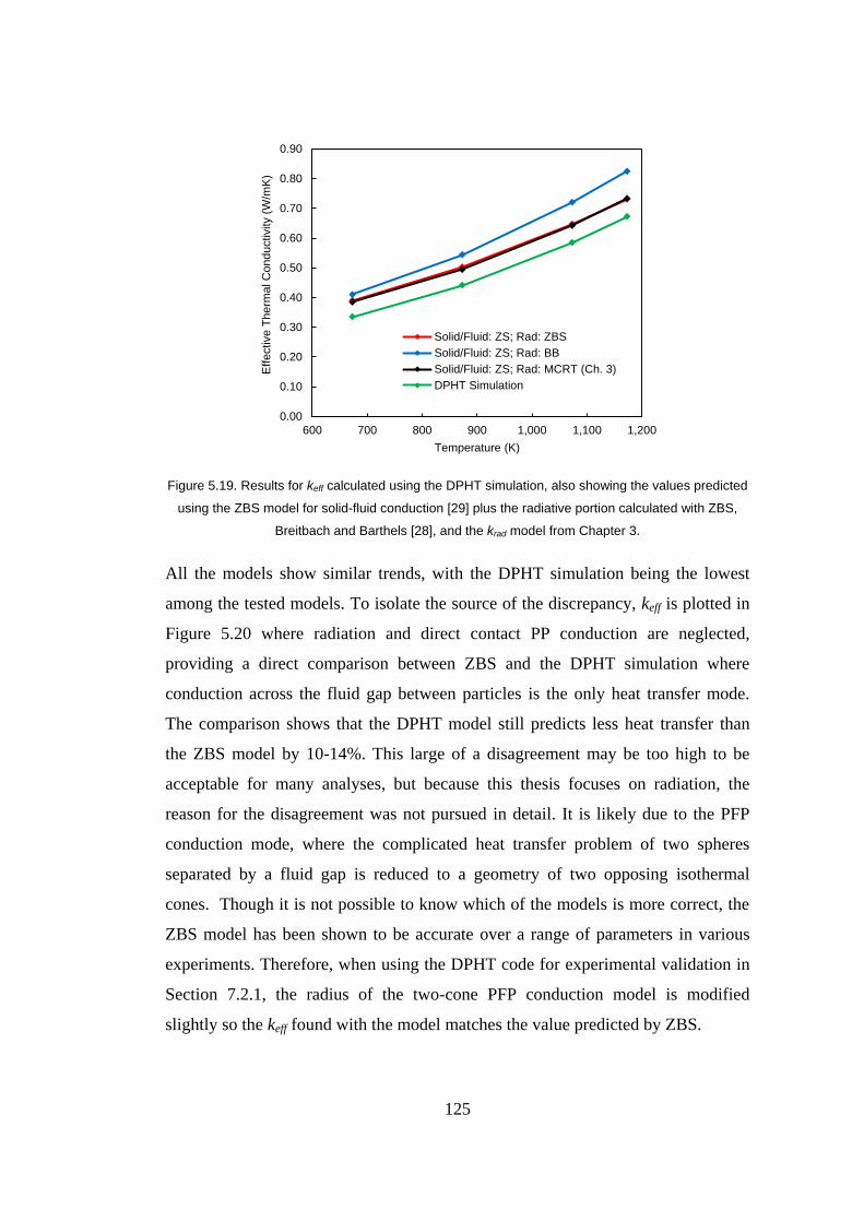
125
Figure 5.19. Results for keff calculated using the DPHT simulation, also showing the values predicted
using the ZBS model for solid-fluid conduction [29] plus the radiative portion calculated with ZBS,
Breitbach and Barthels [28], and the krad model from Chapter 3.
All the models show similar trends, with the DPHT simulation being the lowest
among the tested models. To isolate the source of the discrepancy, keff is plotted in
Figure 5.20 where radiation and direct contact PP conduction are neglected,
providing a direct comparison between ZBS and the DPHT simulation where
conduction across the fluid gap between particles is the only heat transfer mode.
The comparison shows that the DPHT model still predicts less heat transfer than
the ZBS model by 10-14%. This large of a disagreement may be too high to be
acceptable for many analyses, but because this thesis focuses on radiation, the
reason for the disagreement was not pursued in detail. It is likely due to the PFP
conduction mode, where the complicated heat transfer problem of two spheres
separated by a fluid gap is reduced to a geometry of two opposing isothermal
cones. Though it is not possible to know which of the models is more correct, the
ZBS model has been shown to be accurate over a range of parameters in various
experiments. Therefore, when using the DPHT code for experimental validation in
Section 7.2.1, the radius of the two-cone PFP conduction model is modified
slightly so the keff found with the model matches the value predicted by ZBS.
0.00
0.10
0.20
0.30
0.40
0.50
0.60
0.70
0.80
0.90
600 700 800 900 1,000 1,100 1,200
Effective T
herm
al C
onductivity (
W/m
K)
Temperature (K)
Solid/Fluid: ZS; Rad: ZBS
Solid/Fluid: ZS; Rad: BB
Solid/Fluid: ZS; Rad: MCRT (Ch. 3)
DPHT Simulation

126
Figure 5.20. keff with radiation eliminated, comparing ZS and DPHT simulation results.
5.9 Solving Conjugate Heat Transfer Problems
For many actual devices, the boundary condition is known on the outside of the
solid part, not on the boundary of the particle domain. For example, if cool
particles flow downward through a thick-walled metal tube that is heated from the
outside, the boundary condition is likely known on the outside surface of the tube.
The interior surface of the tube forms the boundary of the particle/fluid domain, but
the temperature there is typically unknown. The temperature of the interface
changes based upon both the thermal properties of the tube and the characteristics
of the particle/fluid domain. Such a problem is an example of conjugate heat
transfer.
It is possible in some cases to incorporate the heat conduction through the solid
directly into the model, but solvers in CFD often take a coupled approach. The
fluid and solid domains are solved separately and then compared at the boundary.
This allows for using the optimal solver in each domain, and meshes do not have to
match at the boundary [99]. A similar approach adapted for a DEM+DPHT
simulation is described in the following section. Then, an approach using the
overall heat transfer coefficient is detailed in Section 5.9.2.
0.00
0.05
0.10
0.15
0.20
0.25
0.30
0.35
0.40
0.45
600 700 800 900 1,000 1,100 1,200
Effective T
herm
al C
onductivity (
W/m
K)
Temperature (K)
Solid/Fluid: ZS; no Rad.
Solid/Fluid: DPHT; no Rad.

127
5.9.1 Matching the Interface of the Two Domains
This method requires starting with an estimate of the temperature distribution at the
interface. This is used as a boundary condition in a DEM+DPHT simulation of the
particle/fluid domain. Then, conduction heat transfer is simulated in the solid
domain, which can be done with many CFD codes. The known boundary condition
is used on the outside, and the assumed boundary condition is used at the interface
boundary. After both simulations are at a steady state, they are compared in terms
of heat transfer along the interface. If the heat transfer matches at each location on
the boundary (within some desired accuracy), then the temperature estimate is
correct. If not, a better estimate for the interface temperature must be made, and
both the particle/fluid and solid domains must be re-modeled until a match is
found. Commercial CFD software can solve similar problems consisting of a solid
and fluid domain, and the iterative process is automated. With the recently
developed DPHT code, these iterations would have to be performed manually or by
developing the code further.
This type of iteration may become quite burdensome given the already high
computational cost of DEM+DPHT modeling. However, often times the DPHT
part of the simulation requires only a small amount of time compared to the DEM
portion, and the DEM part would not have to be re-run in these iterations. No
conjugate heat transfer simulations were run in this research, but the methodology
was studied and considered, and the DPHT code could be used for this in the
future. While computationally intense, this method can eventually lead to a solution
with high accuracy with enough iterations.
5.9.2 Overall Heat Transfer Coefficient
Another approach is to find the overall heat transfer coefficient from the wall to the
particle/fluid mixture for a representative sub-section of the domain, and then this
is used in a simplified heat transfer model of the entire domain. This can

128
dramatically reduce the computational time, especially for large domains with
millions of particles. However, the accuracy is likely not as high as the two-domain
approach described in the previous section.
The overall heat transfer coefficient approach is used in Chapter 8 to model an
entire solar receiver. In this case, a flat metal plate with a thickness of 4 mm forms
the solar receiver surface. The boundary condition is known on the outside of the
metal plate, which is a combination of incident heat flux and losses from reflection,
convection, and emission. The temperature on the interior surface (facing the
particle/fluid mixture) is unknown, making a straightforward DEM+DPHT
simulation not possible. Furthermore, due to the large size, modeling the receiver
would require ~450 million particles and would take perhaps years of computation
time.
In the method used, the DPHT simulation was run using an estimate for the
temperature boundary condition at the interface between the particle/fluid and solid
domains. After reaching a steady state, the overall heat transfer coefficient from the
wall to the particle/fluid mixture was calculated, which encompasses all of the
complex effects due to the six particle-scale heat transfer models as well as the
mixing characteristics and particle mechanics. In this case the heat transfer
coefficient was found as a function of distance from the inlet, as it varies
significantly in the flow direction. With the heat transfer coefficient known, a
simple 1D heat transfer model can be used, where the heat flux to the particle/fluid
mixture at each location is calculated by multiplying the heat transfer coefficient by
the temperature difference between the wall and the particle mixture. More details
on this model are given in Chapter 8.
One key for accurate results is to ensure that the temperature boundary condition
used in the DPHT simulation is close to the interface temperature in the 1D
simulation. The overall heat transfer coefficient is only valid under the exact
conditions under which it was derived. For the case studied, the heat transfer
129
coefficient increases at higher temperatures due to radiative effects and the
increased thermal conductivity of air.
5.10 Conclusions for DPHT
With the DBA radiation model developed, the goal was to implement it in a DEM-
based heat transfer code for dense flows so it could be used to model CSP devices.
However, no such software is publically available, so the entire modeling scheme
had to be developed, resulting in the DPHT code. By assuming that the interstitial
fluid is stagnant relative to the particles, heat transfer is only via conduction where
particles touch, conduction across the thin fluid gap between particles, and
radiation. Sub-models for both conduction modes were found in literature, though
several modifications were made so they are more physically realistic than the
originally published models.
In a DPHT simulation where only the PFP model was enabled, total heat transfer
through a group of particles was found to be 10-14% less than the Zehner-
Schlünder model predicts. This may reveal an underprediction by the PFP model,
at least for the current case, pointing to the need for additional verification of the
PFP model. In the experimental validation in Section 7.2.1, the PFP model will be
tuned for the current conditions by increasing the radii of the two opposing cones,
making the results match the more trusted ZS model.
The example simulation given in this chapter should provide enough detail that a
newcomer to this type of modeling can understand, execute, and begin to modify
the code to simulate a new device. Finally, several strategies are discussed to model
more complicated boundary conditions.


131
CHAPTER 6
6 EXPERIMENTAL INVESTIGATION OF A DENSE GRANULAR FLOW AT
HIGH TEMPERATURES
DEM and CFD-DEM are relatively new modeling methods which are still being
developed by various research groups, and these models have been experimentally
validated much less than other computational techniques such as CFD. To be
accurate, these models require many parameters which must be either known or
calibrated experimentally. As for the particle mechanics side of DEM, the
properties (such as coefficient of restitution, Poisson’s ratio, Young’s modulus, PP
and PW friction coefficients) can be experimentally calibrated using a series of lab
tests, and they have been studied previously [84]. In contrast, the heat transfer side
of DEM has been has been much less studied.
Given DEM heat transfer models are in need of validation but few relevant
experiments in this research area exist, experimental results are pursued in this
thesis. The specific aims are to:
A. Provide the experimental results so particle-scale heat transfer models,
including the DBA radiation model, can be validated under the high
temperature conditions of CSP.
B. Document practical lessons learned in the design and execution of experiments
in dense granular flows at high temperatures for others in research or industry
working on similar experiments or devices.
C. Increase the technology readiness level (TRL) of the dense granular flow
receiver [19][21] concept from TRL 3 (experimental proof of concept) to TRL
4 (technology validated in lab) by running experiments using highly
concentrated light in a solar simulator facility.
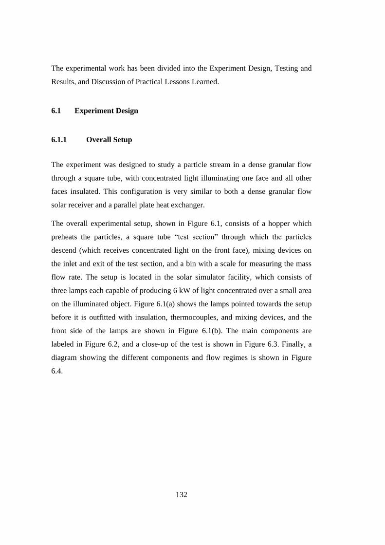
132
The experimental work has been divided into the Experiment Design, Testing and
Results, and Discussion of Practical Lessons Learned.
6.1 Experiment Design
6.1.1 Overall Setup
The experiment was designed to study a particle stream in a dense granular flow
through a square tube, with concentrated light illuminating one face and all other
faces insulated. This configuration is very similar to both a dense granular flow
solar receiver and a parallel plate heat exchanger.
The overall experimental setup, shown in Figure 6.1, consists of a hopper which
preheats the particles, a square tube “test section” through which the particles
descend (which receives concentrated light on the front face), mixing devices on
the inlet and exit of the test section, and a bin with a scale for measuring the mass
flow rate. The setup is located in the solar simulator facility, which consists of
three lamps each capable of producing 6 kW of light concentrated over a small area
on the illuminated object. Figure 6.1(a) shows the lamps pointed towards the setup
before it is outfitted with insulation, thermocouples, and mixing devices, and the
front side of the lamps are shown in Figure 6.1(b). The main components are
labeled in Figure 6.2, and a close-up of the test is shown in Figure 6.3. Finally, a
diagram showing the different components and flow regimes is shown in Figure
6.4.
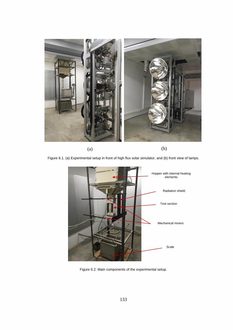
133
Figure 6.1. (a) Experimental setup in front of high flux solar simulator, and (b) front view of lamps.
Figure 6.2. Main components of the experimental setup.
(a) (b)
Hopper with internal heating elements
Radiation shield
Test section
Scale
Mechanical mixers

134
Figure 6.3. Close-up of measurement test section.
9V DC motors for mixers
Inlet temperature measurement block
Outlet temperature measurement block
Test section
Eight thermocouple probes embedded in walls

135
Figure 6.4. Diagram of the components and flow regimes in the setup.
6.1.2 Hopper
The hopper, along with all other metal components subject to high temperatures in
this setup, is constructed from Stainless Steel 310, chosen for its strength at high
temperatures. With only 18 kW of power available from the lamps, if particles
were to enter the test section at room temperature, the outlet temperature would not
reach the desired high temperatures of above 400 ⁰C. Thus, particles are heated to a
high temperature in the hopper, and then particles are heated a second time as they
flow through the illuminated test section. This not only achieves the high

136
temperatures desired, but it mimics the conditions in a CSP solar receiver or
particle heat exchanger where the inlet temperature is in the 500 to 600 ⁰C
temperature range. In this setup, particles are manually transported up to the hopper
with a bucket before each test is run.
As shown in Figure 6.5 (insulation removed for photo), the preheaters were
constructed of 24 Stainless Steel 310 tubes placed across the hopper. Only one side
of each tube was welded in place, and the other side passes through a hole in the
side of the hopper, allowing for thermal expansion of the tubes in the axial
direction. Ceramic tubes were used for electrical insulation, and molybdenum wire
coils were used for electrical resistance heating. The ends of these tubes can be
seen in the figure, where the ceramic insulation tubes are white. They can output a
combined power of up to 27.8 kW and were used to heat particles to over 750 ⁰C.
Figure 6.5. Hopper, with insulation removed to expose ends of the heating tubes.

137
6.1.3 Shutoff Valve
A shutoff valve (Figure 6.6) is located directly below the hopper, where particles
flow through the square opening and flow is shut off by inserting the long plate
shown on the left. The four holes are for bolts to hold it in place. It is located just
below the hopper so flow can be shut off with particles stored in the hopper while
work is performed on the test section and any components below it. During tests,
the flat plate is removed completely so it does not conduct heat out of the setup,
and insulation is placed over the opening. The valve offers the advantage of
simplicity, with no moving parts having close tolerances that could jam with
particles. It also works well at high temperatures and does not leak particles.
Figure 6.6. Shutoff valve used to stop the particle flow.
6.1.4 Test Section
The test section (the actual section portion used to characterize the heat transfer)
consists of a square tube of Stainless Steel 310 with an interior cross section of 20
x 20 mm where particles flow, and a wall thickness of 8 mm. The length of the tube
is 250 mm. The thick wall was chosen to allow for 3 mm diameter thermocouple
probes to be inserted into the wall itself from the side. This was done by drilling
four holes in the front (illuminated) side and four holes in the back (insulated) side
of the test section. The holes are drilled deep enough such that the thermocouples
are centered horizontally on the face (i.e. centered in the right-left direction in
Figure 6.7(b), as shown by the red circles). The holes are sized to make a very tight
fit with the thermocouple probes, ensuring good thermal contact. The test section

138
with holes drilled is shown from the side in Figure 6.7(a), before applying
insulation. Thermocouple probes were inserted through insulation blocks, shown in
Figure 6.7(b). Once installed, extra insulation was added to shield radiation from
striking the thermocouple probes, as shown in Figure 6.7(c). Embedding the
thermocouple probes in the wall was chosen as the most accurate method to
measure the wall temperature, as a thermocouple placed on the inside of the wall
would be affected by the temperature of the flowing particles and may also disturb
the flow, and a thermocouple attached to the outside of the wall would likely melt
under the high heat flux of the concentrated light. Measuring the front face
temperature with an infrared camera was also considered, but this was not feasible
because (without a detailed calibration) the camera cannot distinguish between
radiation emitted from the test section and the radiation which is emitted from the
lamps and reflected back to the camera.
Figure 6.7. (a) Hopper and test section, with holes for thermocouple probes visible, circled in red, (b)
front view of test section with thermocouples installed at locations circled in red, and (c) extra
insulation installed in front test section.
(a) (b) (c)

139
6.1.5 Inlet and Outlet Measurement Blocks
The overall heat absorbed by the particle stream is calculated using the inlet and
outlet temperatures of the test section. For this calculation to be valid, the particle
stream at the inlet and outlet must be uniform in temperature, which is why the
paddle wheel mixing devices are used, as described in the following section and
discussed in more detail in Section 6.3.4. After mixing, the particle stream
temperature is measured with several K-type thermocouples, with thermocouples
placed specifically in the dense granular flow region, as opposed to in a dispersed
flow (e.g. downstream from an orifice plate). This is done to avoid any effects of
the air temperature, in case it is not perfectly mixed and identical to the particle
temperature. The block where the inlet thermocouples are placed is shown in
Figure 6.8, with the 14 mm diameter flow channel in the center, two thin grooves
cut into the block where the thermocouples wires are placed, and four holes for
mounting bolts. Each thermocouple is arranged such that it lies in a straight line,
with the junction in the center of the flow channel and one wire exiting out
opposing sides. This secures the thermocouple in place while allowing for manual
adjustments of the location of the thermocouple junction in the flow channel. The
two perpendicular grooves are used to allow for two thermocouples placed at
different heights. Similar blocks are used to measure both the inlet and outlet
temperatures.
Figure 6.8. Inlet temperature measurement block with grooves cut for thermocouples wires.
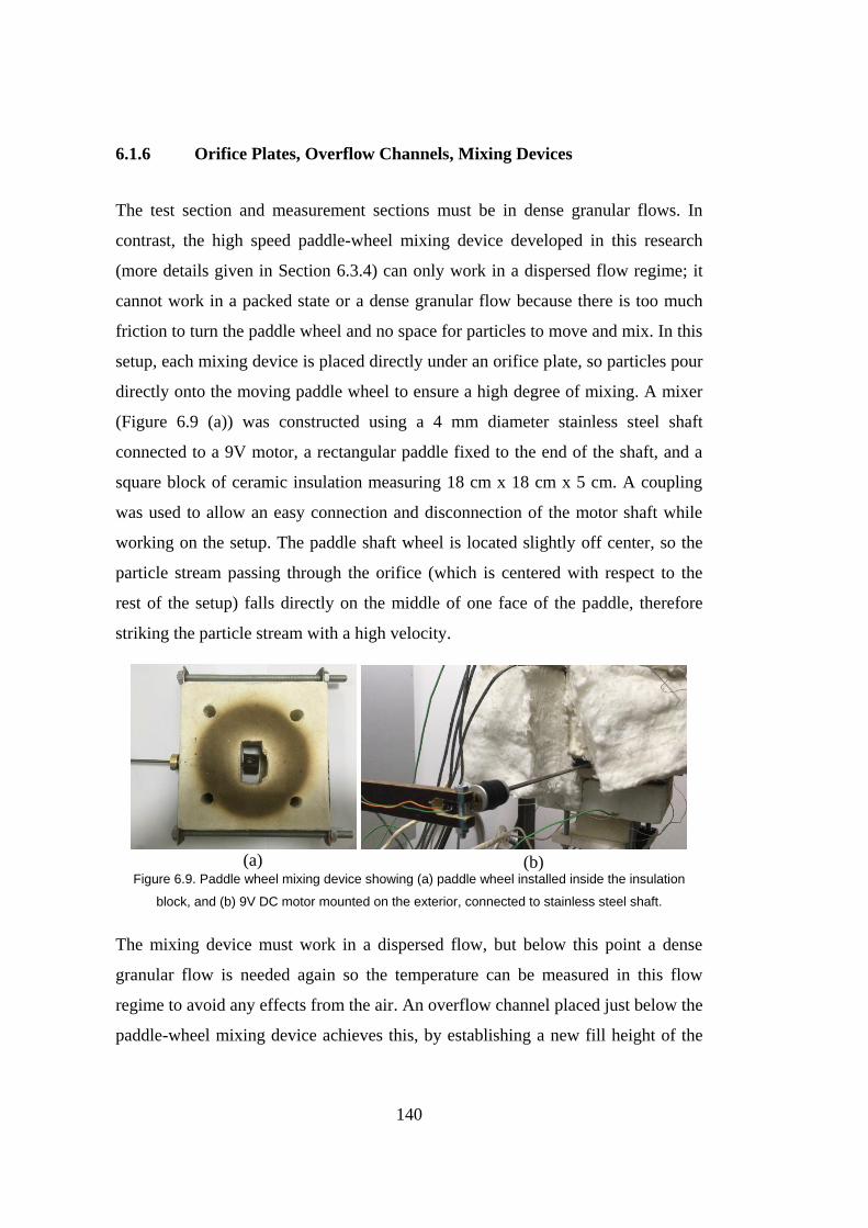
140
6.1.6 Orifice Plates, Overflow Channels, Mixing Devices
The test section and measurement sections must be in dense granular flows. In
contrast, the high speed paddle-wheel mixing device developed in this research
(more details given in Section 6.3.4) can only work in a dispersed flow regime; it
cannot work in a packed state or a dense granular flow because there is too much
friction to turn the paddle wheel and no space for particles to move and mix. In this
setup, each mixing device is placed directly under an orifice plate, so particles pour
directly onto the moving paddle wheel to ensure a high degree of mixing. A mixer
(Figure 6.9 (a)) was constructed using a 4 mm diameter stainless steel shaft
connected to a 9V motor, a rectangular paddle fixed to the end of the shaft, and a
square block of ceramic insulation measuring 18 cm x 18 cm x 5 cm. A coupling
was used to allow an easy connection and disconnection of the motor shaft while
working on the setup. The paddle shaft wheel is located slightly off center, so the
particle stream passing through the orifice (which is centered with respect to the
rest of the setup) falls directly on the middle of one face of the paddle, therefore
striking the particle stream with a high velocity.
Figure 6.9. Paddle wheel mixing device showing (a) paddle wheel installed inside the insulation
block, and (b) 9V DC motor mounted on the exterior, connected to stainless steel shaft.
The mixing device must work in a dispersed flow, but below this point a dense
granular flow is needed again so the temperature can be measured in this flow
regime to avoid any effects from the air. An overflow channel placed just below the
paddle-wheel mixing device achieves this, by establishing a new fill height of the
(a) (b)

141
dense flow; the dense granular flow cannot fill any higher than the overflow
channel, as any particles at a higher level immediately descend through the
overflow channel. This “trick” is done twice; once for each mixing device. For the
top mixing device, the top orifice (8.5 mm diameter) is sized just larger than the
orifice at the outlet of the test section (8.0 mm diameter), so there is always a slight
excess flow of particles exiting through the overflow channel. These excess
particles are routed out through a tube and not included in the mass flow rate
calculation, which only includes particles flowing through the test section.
A similar configuration is used at the outlet as well, where a dense granular flow is
needed after the outlet mixing device so that the thermocouple can be placed in a
dense granular flow to eliminate any temperature effects from the air. Below the
outlet mixer, a third orifice plate (with a 6.5 mm diameter orifice) is used to
reestablish a dense granular flow, and a second overflow channel is used to release
excess particles. In this case both streams are sent to the scale because both flow
through the test section.
This scheme is extremely useful as it allows for establishing a dispersed flow and
reestablishing a dense granular flow to meet the needs of different components. In
the process, a small stream of excess particles must be rejected from the main
stream, but by making the top orifice only slightly larger in size, the “lost” flow
rate of these unused particles is minimal. To minimize any air intrusion from the
outside, these overflow channels are sized such that the excess particle stream
roughly fills the channel, so any air flow will be outward with the particles. The top
overflow channel is shown in Figure 6.10, where particles are routed out through a
tube to an external collection bin. The bottom overflow channel opens near the
bottom, so particles drop straight into the weighing bin.

142
Figure 6.10. Top overflow channel shown (a) on full setup, and (b) close-up where it attaches to the
insulation blocks.
6.1.7 Data Acquisition
For mass flow rate measurements a CAS brand DH-LED scale was used, with a
maximum capacity of 300 kg and a sensitivity of 50 g, which is connected to a
computer using a serial connection. The mass flow rate is calculated by fitting a
straight line to the mass accumulation vs. time curve over the duration of each test.
Temperature measurements from the thermocouples (all K-type) are recorded at an
interval of 10 seconds, using a Keysight 34972A data acquisition system.
6.2 Testing and Results
6.2.1 Particle Materials Tested
Tests were run with both sand and sintered bauxite, chosen for their relevance as
heat transfer materials in CSP. The sintered bauxite is Carbo HSP 40/70, which
was chosen because many of its thermophysical properties have been previously
(a) (b)
top overflow
channel

143
determined by others in the CSP field. The size distribution of both materials was
analyzed with a Mastersizer 2000 laser diffraction analyzer. The Sauter mean
diameter (also known as the surface weighted mean and abbreviated as d32) for the
Carbo HSP and sand is found to be 371.15 μm and 722.50 μm respectively.
Following similar studies [97], the monodisperse spheres modeled with DEM and
DPHT will use the Sauter mean diameter.
6.2.2 Procedure
The following sequence was used for each of the tests:
a. All particles to be tested were filtered to ensure no debris would be
introduced to the experiment.
b. Particles were manually transported up to the hopper with a bucket, filling
the hopper enough to cover all of the preheater tubes.
c. Particles were preheated for 1-2 hours depending on the desired
temperature.
d. Particles were allowed to rest for at least one hour to reduce temperature
gradients inside the hopper.
e. The flow was started by opening the shutoff valve.
f. Paddle wheel mixers were turned on.
g. The flow was temporarily stopped by placing a block over the outlet for
roughly 25 seconds, until particles start to pour out from the top overflow
channel, indicating the dense fill level has reached that point. Because the
flow rate through the top orifice (8.5 mm) is greater than the middle orifice
(8 mm), with enough time the dense fill level would slowly rise from the
middle orifice plate to the overflow channel, but temporarily blocking the
exit quickly establishes the correct flow regimes.
h. Each of the three lamps was turned on.
i. Temperatures of the inlet, outlet, and walls of the test section were
monitored until the system arrived at a steady state.

144
6.2.3 Results
Experiments were run under three conditions; (1) particles of silica sand preheated
to 420 ⁰C, (2) particles of sintered bauxite preheated to 620 ⁰C, and (3) particles of
sintered bauxite starting at room temperature. The data from each of these
experiments are given below, where the thermocouples on the front (illuminated)
and back (insulated) walls are referred to with numbers from 1 to 4, with 1 being
the top thermocouple and 4 being the bottom thermocouple.
6.2.3.1 Test 1: Sand Preheated to 420 ⁰C
In this test, sand was preheated to 420 ⁰C, and the mixers were started at around a
time of 200 seconds in Figure 6.11 below. The three lamps were turned on and
adjusted, causing several inflections in the wall temperatures before temperatures
stabilize, and the lamps were switched off at 1070 seconds. Due to heat loss from
the hopper, the inlet temperature slowly decreased throughout the test, and
therefore the other temperatures slowly declined as well. However, the difference
between the temperatures is constant, so the condition can be considered quasi-
static, and each time step can be considered a steady state for the purposes of
validating with DEM. The temperatures at the steady state condition are taken as
the average temperature between 1000 and 1070 seconds, which are reported in the
summary of results in Table 6.1.

145
Figure 6.11. Temperature data from Test 1.
The mass accumulated in the weighing bin was measured over time at an interval
of 10 s, with a nearly linear relationship shown in Figure 6.12 and therefore a very
constant flow rate in the range of 500 to 1000 seconds. With linear curve fit, a flow
rate of 0.0112 kg s-1
is found.
Figure 6.12. Mass of particles accumulated over time during Test 1.

146
6.2.3.2 Test 2: Sintered Bauxite Preheated to 620 ⁰C
In Test 2, the sintered bauxite was heated to around 750 ⁰C when the photos in
Figure 6.13 were taken. In Figure 6.13(a), the mixer was not running, and the right
half of the particle exit stream glows red, while it is black (not glowing) on the left
side. The illuminated front face of the test section corresponds to the right side of
this picture, so it matches expectations that the illuminated side of the particle
stream is at a much higher temperature than the insulated side. This visually shows
the extreme temperature gradient caused by the high heat flux from the illuminated
surface. In Figure 6.13(b) the mixer has been turned on, and the temperature
gradient can no longer be seen, and only a faint glow was visible. Note: the smaller
particle stream on the right side of the main exit stream is from the lower overflow
channel.
Figure 6.13. Sintered bauxite particles can be seen glowing at the exit, where (a) a gradient can be
seen before while mixer is off, and (b) the gradient is eliminated once mixer is turned on.
With the room lights and lamps turned off, the particle stream glows red, as shown
in Figure 6.14(a), and in (b) the lamps have been recently turned off but are still
radiating a small amount of light as they cool.
(a) (b)

147
Figure 6.14. Stream of sintered bauxite radiating visible red light at ~750 ⁰C.
As shown in Figure 6.15, temperatures fluctuate at the beginning of the test before
becoming relatively constant after a time of 1200 seconds. The inlet temperature
shows a significant dip between the times of 700 and 1000 seconds, likely due to
the stream being drawn from a relatively colder place in the hopper. The dip can be
seen to temporarily decrease all the other temperatures as well. The inlet
temperature stabilizes again at around 1100 seconds, though it does drop again
slightly at 1400 seconds. The most stable conditions are beyond this point, so the
steady state mean temperatures are taken as the time steps between 1630 to 1760
seconds.
(a) (b)

148
Figure 6.15. Temperature data from Test 2.
The mass accumulated by the weighing bin was measured over time, and plotted
for the range of 1000 to 1800 seconds in Figure 6.16, showing, a mass flow rate of
0.0206 kg s-1
.
Figure 6.16. Mass of particles accumulated over time during Test 2.
6.2.3.3 Test 3: Sintered bauxite with no preheating
In this test the sintered bauxite particles were not preheated, though a small amount
of heat remained in the hopper from tests on the previous days, making the inlet

149
temperature roughly 46 ⁰C. As shown in Figure 6.17, most of the temperature
readings appear to reach steady state values, though some of the thermocouples in
the back wall still show a slight increase in temperature even at the end of the test,
meaning they may not have quite reached a steady state. Without running the
experiment longer, the values reported in Table 6.1 are taken to be the mean
temperature, between 1170 and 1270 seconds.
Figure 6.17. Temperature data from Test 3.
The mass of particles over time is plotted in Figure 6.18, and a mass flow rate of
0.0202 kg s-1
is found.

150
Figure 6.18. Mass of particles accumulated over time during Test 3.
6.2.4 Summary and Discussion
A summary of the steady state temperatures and flow rates from each of the three
tests is shown in Table 6.1. This is one of the central outputs of this experimental
research, as these data can be used to compare against results predicted by DEM
modeling. Ideally, measurements should be taken under steady state conditions,
and the inlet and outlet particle streams must be completely uniform in
temperature. Many efforts were made to be as close to these ideal conditions as
possible, but several shortcomings are discussed below.
Table 6.1 Steady state temperature conditions from each test.
Parameter Units Test 1 Test 2 Test 3
Material - Sand Carbo HSP Carbo HSP
Mass Flow Rate kg s-1
0.0112 0.0206 0.0202
Inlet ⁰C 422.7 621.7 46.5
Outlet ⁰C 455.1 652.5 110.2
Front Wall 1 (top) ⁰C 485.7 725.1 253.2
Front Wall 2 ⁰C 574.0 886.2 500.0
Front Wall 3 ⁰C 618.7 916.3 596.3
Front Wall 4 (bottom) ⁰C 600.6 762.5 367.7
Back Wall 1 (top) ⁰C 437.7 631.0 108.1
Back Wall 2 ⁰C 476.8 690.7 200.1
Back Wall 3 ⁰C 505.7 724.4 262.8
Back Wall 4 (bottom) ⁰C 509.8 702.2 245.0
In the inlet and outlet test sections, two to three thermocouples were immersed in
the flow to measure the temperature simultaneously. Of these, the high temperature
151
caused numerous outages, especially with the thinnest of the thermocouple wires
used. Efforts were made to ensure the thermocouple wire was centered in the
tubular shaped flow channel, but in some cases a thermocouple may have been off
center. Thus, the inlet and outlet temperature data presented in Table 6.1 are the
best available results taken from the collected data.
Testing was done to check the temperature uniformity of the particle stream by
manually moving the thermocouple junction back and forth across the flow
channel. With the paddle wheel mixers running, no temperature gradient due to the
illuminated front wall could be found. However, the temperature measurement in
the center of the stream appeared to be several degrees higher than the temperature
next to the wall, which may indicate some heat loss through the insulation. Heat
loss was minimized by constructing the channels from insulation blocks, with a
minimum of 8.5 cm of insulation around the flow channel, plus more insulation
blankets wrapping around the whole setup. Furthermore, the vertical distance that
the particles must descend between the actual outlet of the test section and the
thermocouples was kept to a minimum, only ~8 cm, so the residence time during
which the particles could lose heat is very low. These measures were taken to
ensure very little heat is lost before the temperature is measured, but still a small
amount of deviation was noticed between the center of the flow and the edges. If
there is indeed a significant radial temperature profile, quantifying it is complicated
by the fact that the inlet temperature to the test section can also fluctuate in the
range of several degrees over several minutes, due to the hopper output temperature
being not quite constant. The experimental setup was not constructed to accurately
investigate such a temperature profile, so studying this phenomenon is left for
future experiments.
Thermocouples embedded in the walls of the test section are 3 mm in diameter, and
the walls are 8 mm thick. The holes where the thermocouples are embedded are
sized extremely close to the diameter of the thermocouple probes themselves;
installing them was done by hand, but it required holding the probe with pliers
while pushing with a high degree of manual force. Thus, the thermal contact

152
between the wall and the probe is thought to be extremely good, and the
thermocouple readings should be an accurate representation of the wall
temperature.
For each test, a time period was selected as the best representation of a steady state
condition. In Test 2, the inlet temperature varied at several points throughout the
test, though a fairly good approximation to a steady state was achieved near the
end. This is likely due to an inherent deficiency in the hopper design, as will be
discussed in Section 6.3.3. In Test 3, the test was stopped when the inlet and outlet
temperatures reached steady values, but some of the wall temperatures were still
slowly climbing and would in reality reach a steady state at a slightly higher value.
Still, the last data points provide a relatively accurate approximation of steady state
temperatures.
6.3 Discussion of Practical Lessons Learned
The setup shown is the result of an original design which evolved to the present
state after numerous experimental trials and improvements. Through this process
many practical insights were learned in the laboratory which can be used by other
researchers in this field who are designing similar experimental setups or industrial
systems.
6.3.1 Particle Filtration
Care should be taken to not introduce any foreign debris into the particles, such as
small pieces of ceramic insulation that fall into the weighing bin. Several
experimental runs were interrupted by a clogged flow from a small piece of
insulation being stuck in an orifice plate. Thereafter, between each heated test run,
the particles were filtered through a mesh of roughly 3.5 mm to strain out any small
pieces of insulation or debris. It adds significant manual effort and time, but it is
necessary to ensure the system runs smoothly. In the current setup the filtration is

153
performed outside of the system, but in future work a filter may be added in the
flow just below the shutoff valve to ensure no foreign particles enter the test
section.
6.3.2 Minimizing Heat Loss
At temperatures nearing 1000 ⁰C, every component must be designed around
minimizing heat loss. The inlet and outlet flow sections are made out of insulation
blocks to minimize heat loss, and the test section is also insulated with tightly
fitting insulation blocks on three sides. Steel bolts are used to connect the test
section to the hopper and to connect the outlet mixing section to the test section,
but in both cases these are isolated using hard insulation sheets to ensure there was
no metal-to-metal thermal bridge between the test section and the other sections.
Finally, the whole setup is insulated once more with several 5 mm thick insulation
blankets, as shown in Figure 6.19, though the insulation integrity is reduced due to
the penetration of the thermocouple wires. At these temperatures a significant
amount of heat loss is essentially unavoidable, however, this does not limit the
accuracy of the data; as long as the inlet, outlet, and wall temperatures are known,
this can provide data to compare with DEM modeling.

154
Figure 6.19. Test section, well-insulated on three sides with ceramic insulation.
A high temperature rise from inlet to outlet is desired in order to minimize any
inaccuracy in the inlet or outlet temperature measurements. However, if the lamps
are off, the outlet temperature is actually much less than the inlet temperature due
to the high heat loss to the surroundings, even with the extreme efforts taken to
insulate the setup. Therefore, it takes a large portion of the incident energy from the
lamps to simply compensate for the losses and bring the outlet temperature above
the inlet temperature. The problem is exacerbated at high temperatures; the
temperature rise from inlet to outlet is ~110 ⁰C in Test 3 (starting at room
temperature), whereas the temperature rise in Test 2 (starting at 621.7 ⁰C) is only
~30 ⁰C. The temperature on the outside of the insulation (measured with an infrared
thermometer) is low, roughly 55 ⁰C, so it can be concluded that the heat loss is
predominantly from the exposed front side, and adding additional insulation would
not significantly reduce the heat loss.
The temperature rise could be increased in the future in several ways. The surface
of the test section is left uncoated with a dull reflective finish, so a large portion of
155
the incident radiation is reflected. High temperature black paint could be applied to
increase radiation absorption, such as Pyromark paint with an absorptivity of ~0.96
[100], as done on actual solar receivers. Heat losses from the front face are also
exacerbated by the ventilation system in the solar simulator facility, which has a
strong air intake just above the setup, creating an updraft to suck up any smoke or
material off-gassing. This air current likely promotes high convective losses from
the front of the test section, which could be minimized by creating a cavity or hood
around the setup, similar to actual solar receivers.
6.3.3 Heated Hopper Design
The hopper was successfully used to heat particles up to as high as 750 ⁰C, but the
main drawback is that the temperature of the particle stream leaving the hopper
varies slightly with time, due to particles being drawn from hotter or colder regions
of the hopper. During preheating, the molybdenum coils output a very high heat
flux, which heats the particles directly around the tubes to a very high temperature
but leaves the particles in between the tubes relatively colder. To minimize this
effect, after preheating for several hours, the heating elements are turned off and
the particles in the hopper are left to rest, but because the particle bed has a
relatively low thermal conductivity, it takes a long time to reduce or eliminate the
temperature variation in the hopper. Meanwhile, heat is lost out the sides of the
hopper. The hopper is well insulated, but because it weighs several hundred
kilograms, it is attached directly to the steel frame, making a thermal bridge to the
outside air. With this construction, waiting long enough for the internal particle
temperatures to fully equilibrate (which may take 24 hours or more) was not
possible, as the heat loss to the surroundings is high enough that the overall
temperature drops too quickly to maintain the desired temperature of ~600 to 700
⁰C. To help reduce the temperature gradients inside the hopper more quickly, 16
steel rods were bent into a “U” shape and inserted from the top, which hang over

156
the preheater tubes (Figure 6.20), which appeared to reduce, but not eliminate, this
problem.
The hopper design could be improved by eliminating the thermal bridge between
the hopper and the frame, increasing the insulation thickness, and adding many
more conductive rods to promote equilibration of temperature. However, in
practice it is hard to entirely eliminate these temperature gradients and to ensure a
perfectly constant particle temperature supplied to the test section using such a
hopper. A flow-through type design was also considered, where particles start in an
unheated hopper, and the particle stream descends through a preheating section to
raise the temperature by ~700 ⁰C as the particles flow through. Such a design could
create a constant temperature particle stream and would also eliminate time spent
on preheating and waiting for the temperature in the hopper to equilibrate. The
heated hopper design was chosen for its simplicity and because a flow-through
style heater may take significant vertical length to raise the temperature more than
700 ⁰C, but the overall vertical height of the current setup is limited by the ceiling
of the facility to ~3.5 m. Originally, it was also thought that a flow-through heater
would have the disadvantage of high temperature gradients across the particle
stream, as some portions of the stream would be close to the heated walls of the
device, while other particles would be further away from the walls. However, the
paddle wheel mixing device developed during this research can effectively mix the
particle stream completely, so it is no longer a problem if the particle stream
leaving the preheater has large temperature gradients. Given these points, a flow-
through style heater may be a better choice to achieve a constant output
temperature for similar setups or for modifying this setup in the future.
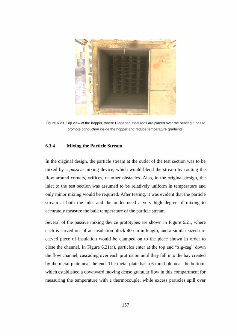
157
Figure 6.20. Top view of the hopper, where U-shaped steel rods are placed over the heating tubes to
promote conduction inside the hopper and reduce temperature gradients.
6.3.4 Mixing the Particle Stream
In the original design, the particle stream at the outlet of the test section was to be
mixed by a passive mixing device, which would blend the stream by routing the
flow around corners, orifices, or other obstacles. Also, in the original design, the
inlet to the test section was assumed to be relatively uniform in temperature and
only minor mixing would be required. After testing, it was evident that the particle
stream at both the inlet and the outlet need a very high degree of mixing to
accurately measure the bulk temperature of the particle stream.
Several of the passive mixing device prototypes are shown in Figure 6.21, where
each is carved out of an insulation block 40 cm in length, and a similar sized un-
carved piece of insulation would be clamped on to the piece shown in order to
close the channel. In Figure 6.21(a), particles enter at the top and “zig-zag” down
the flow channel, cascading over each protrusion until they fall into the bay created
by the metal plate near the end. The metal plate has a 6 mm hole near the bottom,
which established a downward moving dense granular flow in this compartment for
measuring the temperature with a thermocouple, while excess particles spill over

158
the top and fall directly towards the exit. Another design, in Figure 6.21(b), uses
two similar bays for measuring the particle temperature, along with a dispersed
flow through a field of many small screws which enhances random collisions and
therefore mixing. A third design is shown in Figure 6.21(c) where the mixing
section is clamped against a piece of Plexiglas to show the flow pattern. This
design has five bays, each with a 6 mm orifice to create a downward moving dense
granular flow where thermocouples were installed.
Figure 6.21. Three prototype passive mixing devices, none of which were found to completely mix
the particle stream.
While the setup is running with the lamps turned on, the outlet stream has a very
large temperature gradient, with particles near the illuminated front face being
much higher in temperature than particles in the back. The designs shown in Figure
6.21 were tested by placing five to ten thermocouples in multiple locations, with
some placed in the bays with a dense granular flow and some in the dispersed flow.
If the particle stream is well mixed, readings from thermocouples near the end of
the mixing section should become uniform as all the particles and the air should be
(a) (b) (c)

159
essentially equal in temperature at that point. However, this was generally not
observed. For example, in the design of Figure 6.21(c), one test (no preheating and
only one lamp on) showed steady state temperatures in the five bays from top to
bottom of 45.9, 48.5, 41.6, 44.4, and 40.5 ⁰C, which indicates particles are not well
mixed. Of these three designs tested, the dispersed flow design in Figure 6.21(b)
seemed to achieve the most mixing, though after many tests, it was clear that full
mixing of the stream to completely destroy this temperature gradient was not
possible with these passive designs, and much more aggressive mechanical mixing
would be required.
Similarly, the temperature of particle stream at the inlet of the test section (that is,
at the outlet of the hopper) was measured in three locations, each with the same
axial (vertical) location but at different radial positions in the flow channel. In an
initial test, with no mixer after the hopper, the temperature was found to vary by
over 100 ⁰C between these two thermocouples, even though the two thermocouples
were less than 1 cm apart, apparently because one portion of the stream is drawn
from a hot region of the hopper and another portion of the stream is drawn from a
cold region. This clearly shows that the particle steam leaving the hopper must be
mixed aggressively so an accurate bulk temperature measurement can be found.
The mechanical paddle wheel mixer described in Section 6.1.6 was designed to fix
these problems and achieve a very high degree of mixing. Particles descend
through the orifice plate above the mixer, dropping onto the center of the upward
moving half of the paddle wheel, as shown in Figure 6.22. This ensures that the
upward stroke of the paddle wheel collides with the downward motion of the
particles, resulting in a high speed collision which sends particles in random
directions with high velocity. Testing showed that if the stream collides with the
downward moving half of the paddle, particles simply move along with the paddle,
resulting in few collisions and little mixing. Even a particle stream centered on the
paddle is not desired, as the half of the stream striking the upward moving part of
the paddle is well mixed but the other half of the stream is not. The mixer behavior
was observed outside of the setup and recorded with a slow motion camera,

160
revealing a particle flow which is extremely chaotic, with many high-velocity
collisions and an extremely high degree of mixing. Several frames from the video
footage are shown in Figure 6.23, where the stream is poured on the upward
moving side of the paddle, and even from these still photographs the high degree of
random collisions can be seen. Mixing was validated quantitatively as well by
placing multiple thermocouples in the flow channel and comparing the readings,
and unlike the passive mixing devices, the paddle wheel mixer eliminated any
noticeable temperature gradient present in the incoming particle stream.
Figure 6.22. Paddle wheel mixing device used to achieve a uniform stream temperature.
Figure 6.23. Three frames of video showing the high-speed and chaotic particle flow imparted by the
paddle wheel, leading to a high degree of mixing.
(a) (b) (c)

161
6.4 Conclusions for Experimental Investigation
More experiments such the one described in this chapter are needed for validation
of DEM based heat transfer models, but achieving trusted results at these high
temperatures is extremely challenging. Through this process, several key concepts
for obtaining trusted results were identified and addressed. To completely mix the
particle stream, it was found that a high speed paddle-wheel type mixing device is
needed, and the passive mixing devices originally designed were not adequate. To
actually implement such a paddle-wheel device, the key development is to use a
second orifice plate and an overflow channel to create a vacant pocket where the
mixer can spin freely and mix particles at high velocity. With this combination of
mixer, orifice plate, and overflow channel, various experimental setups could be
devised for similar studies. The hopper type preheater was found to give a non-
constant temperature output, and for future work a flow-through type heater is
recommended. Future tests should aim for a much higher temperature rise, which
would minimize the impact of any error in the bulk particle temperature
measurements at the inlet and exit.
Data sets from three tests are presented, covering both sand and sintered bauxite at
high, medium, and low temperatures. Given the many experimental challenges in
obtaining these measurements, an uncertainty analysis was not performed, as the
inaccuracy due to measurement errors is assumed to be larger than the contribution
from the thermocouples and scale. Still, the three tests presented are the best results
obtained during the experiment, so the data sets can be compared against DEM-
based heat transfer models such as DPHT. This is the subject of Chapter 7.


163
CHAPTER 7
7 COMPARISON OF EXPERIMENTAL AND DPHT MODEL RESULTS
In this section, a comparison is made between the experimental results and the
DEM+DPHT simulation, with the goal being to validate the methods, models, and
assumptions described in the previous chapters. Comparisons are performed with
data from the “Test 2” and “Test 3” experiments because the mechanical and
thermal properties for sintered bauxite are available in literature, whereas
properties are not known with high accuracy for the sand used in the experiment.
7.1 DEM Simulation
A DEM simulation was run in LIGGGHTS where the particles descend through the
square tube and orifice plate shown in Figure 7.1. The surface shown has zero wall
thickness and is made to replicate the dimensions of the inner surface of the square
tube (test section). The lower and upper boundaries are periodic, so particles
leaving the bottom are reinserted at the top. A total of 3.2 million particles were
inserted, creating a dense flow where the fill level is above what will be the heated
section. Files with the xyz particle positions were output every 2000 DEM time
steps. A total of 48 seconds of real time were simulated, which took 20 days of run
time, using 54 processors on a HP Z840 workstation with a clock speed of 2.8
GHz. DEM parameters are shown in Table 7.1.
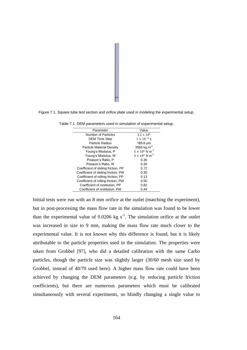
164
Figure 7.1. Square tube test section and orifice plate used in modeling the experimental setup.
Table 7.1. DEM parameters used in simulation of experimental setup.
Parameter Value
Number of Particles DEM Time Step s
Particle Radius 185.6 μm
Particle Material Density 3560 kg m-3
Young’s Modulus, P N m-2
Young’s Modulus, W N m-2
Poisson’s Ratio, P 0.30
Poisson’s Ratio, W 0.30
Coefficient of sliding friction, PP 0.72
Coefficient of sliding friction, PW 0.30
Coefficient of rolling friction, PP 0.13
Coefficient of rolling friction, PW 0.50
Coefficient of restitution, PP 0.82
Coefficient of restitution, PW 0.44
Initial tests were run with an 8 mm orifice at the outlet (matching the experiment),
but in post-processing the mass flow rate in the simulation was found to be lower
than the experimental value of 0.0206 kg s-1
. The simulation orifice at the outlet
was increased in size to 9 mm, making the mass flow rate much closer to the
experimental value. It is not known why this difference is found, but it is likely
attributable to the particle properties used in the simulation. The properties were
taken from Grobbel [97], who did a detailed calibration with the same Carbo
particles, though the particle size was slightly larger (30/60 mesh size used by
Grobbel, instead of 40/70 used here). A higher mass flow rate could have been
achieved by changing the DEM parameters (e.g. by reducing particle friction
coefficients), but there are numerous parameters which must be calibrated
simultaneously with several experiments, so blindly changing a single value to

165
match the current experiment may influence the mechanics in undesired or non-
physically realistic ways. Therefore, to proceed, the orifice diameter was increased
until the average mass flow rate was close to the experimental value of 0.0206 kg s-
1. The total mass passing a horizontal plane over time is shown in Figure 7.2,
leading to the linear curve fit shown and an average mass flow rate of 0.020277 kg
s-1
, close to the experimental value. To more exactly align the conditions in the
simulation and experiment, the DEM time step is modified ( ) when
proceeding with the heat transfer simulation using Eq. (7.1). This results in a
modified time step of s, which ensures that the mass flow rate in
the thermal simulation exactly matches that of the experiment. Effectively, this
increases the velocity of all of the particles a small amount, which is a reasonable
way to increase the flow rate slightly. Alternatively, the orifice plate could have
been adjusted iteratively until the simulation matched the experimental mass flow
rate, but iterating many times is not feasible due to the high computation time of
the simulations.
*
+ (7.1)
Figure 7.2. Mass accumulation over time, and equation for mass flow rate.
y = 0.0202774x - 1E-07
0.E+00
2.E-05
4.E-05
6.E-05
8.E-05
1.E-04
1.E-04
0.000 0.002 0.004 0.006
Accum
ula
ted M
ass (
kg)
Time (s)

166
7.2 DPHT Simulation
Since the mass flow rates in Test 2 and Test 3 are nearly identical, the same DEM
simulation was used to run both DPHT simulations. Section 7.2 describes how the
heat transfer simulation was run using DPHT for Test 2, the high-temperature
experiment. The same procedure was followed for Test 3, the lower temperature
experiment. Details for Test 3 are not shown but results are presented.
7.2.1 Modified PFP Heat Transfer Model
As described in Section 5.8, the particle-scale model for PFP heat transfer by
Cheng et al. [94] underpredicts the overall heat transfer through a packed bed
compared to the keff model of Zehner and Schlünder (ZS) [30] by around 10-15%.
Both the particle-scale PFP model and the continuum ZS model account for only
the heat transferred through the fluid gap between particles, so this is a direct
comparison. While it is not possible to know for certain which is more correct, the
validity of the ZS model has been shown under many conditions with experimental
data, while the PFP model from Cheng et al. has been implemented in several
research studies but with less experimental validation. The PFP model takes the
complicated heat transfer problem of two spheres with non-isothermal surfaces and
reduces it down to a two-cone configuration with isothermal surfaces, so it may not
lead to accurate results under all conditions, such as different particle radii,
temperatures, thermal conductivities, and solid fractions. The cone radius was
originally found by drawing Voronoi polyhedra around each sphere, but later the
cone radius was found as a function of the solid fraction by Zhou et al. [93].
To make the results of the PFP model match more closely with the ZS model under
the conditions relevant to the experiment of this thesis, the equation for the cone
radius by Zhou et al. was multiplied by the correction factor to form Eq. (7.2)
The keff for the domain shown in Figure 7.3 was found using different values of ,
until a match was found with the ZS model. In these simulations, the thermal

167
conductivity and the radius of the spheres were those of the sintered bauxite
particles (2.0 W m-1
K-1
and 0.1856 mm). The evaluation of keff was carried out at
873 K, leading to a value of 1.28.
(7.2)
Figure 7.3. Particle group used for evaluation of keff, leading to a correction factor value of 1.28 in Eq.
(7.2).
As shown in Figure 7.4, the keff found with the simulation using the original PFP
model by Cheng et al. [94] was much lower than the value predicted by the ZS
model. After applying the correction factor of 1.28 to the cone radius, a much
closer match was found. The match is nearly perfect at 878 K because was
determined at that point, but a close match is also seen at the other temperatures.
This value is expected to increase accuracy for the current conditions, but it is
probably not widely transferrable to other applications because it is tailored to the
conditions of this experiment. In the DPHT simulation, an value of 1.28 was
applied in both the PFP and PFW conduction models.

168
Figure 7.4. Keff at several temperatures, showing the ZS model, the original PFP model, and the PFP
model modified with a correction factor of 1.28 in Eq. (7.2).
7.2.2 Thermal Properties
The thermal simulation was run with the DPHT code using the parameters shown
in Table 7.2.
Table 7.2. Thermal parameters used in simulation of experimental setup.
Parameter Value
Thermal conductivity, P 2.0 W m-1
K-1
Thermal conductivity, W 16.6 W m-1
K-1
Emissivity, P 0.86
Emissivity, W 0.60
Particle temperature at inlet 621.7 ⁰C
Initial particle temperature 621.7 ⁰C
Young’s Modulus, DEM, P N m-2
Young’s Modulus DEM, W N m-2
Young’s Modulus, real, P N m-2
Young’s Modulus, real, W (stainless steel)
N m-2
Solid Fraction, bulk 0.5791
Solid Fraction, near wall 0.5284
Specific heat capacity, P 0.74857*T[K] + 560.768 J kg-1
K-1
Siegel et al. [56]presented specific heat capacity values for Carbo HSP particles,
which were found experimentally as a function of temperature. Data points in the
temperature range of interest were given a linear fit as shown in Figure 7.5, and the
corresponding equation gives specific heat as a function of temperature, where
units are in Kelvin.
0.00
0.05
0.10
0.15
0.20
0.25
0.30
0.35
0.40
0.45
600 700 800 900 1,000 1,100 1,200
Effective T
herm
al C
onductivity
(W/m
K)
Temperature (K)
ZS model
Original PFP (Cheng et al.)
Modified PFP, fc = 1.28

169
Figure 7.5. Specific heat as a function of temperature.
7.2.3 Thermal Boundary Conditions
With wall temperatures known only at eight locations, boundary conditions must
be estimated for the entire surface. To do this, the square tube was “unfolded” to
make a flat surface for which a temperature map can be found with curve fitting.
However, the thermocouple probes measure the temperature at the center of the 8
mm thick wall, whereas the thermal boundary condition is desired at the interior
surface, with a slightly lower temperature. This presents a challenge; the
temperature at the interior surface could be found with Fourier’s law of conduction,
Eq. (7.3), but this would require knowing the heat flux through the wall at each
location, which is not known at the beginning of the simulation.
(7.3)
This problem was solved by estimating the heat flux at each location using the
experimental data. First, the total heat transfer in the experiment was estimated
using the inlet and outlet temperatures, mass flow rate, and an assumed constant
specific heat of 1200 J kg-1
K-1
, resulting in 761 W. Next, the temperatures on the
sides of the square tube (still in the center of the wall) were estimated by linearly
interpolating between the front and back measurements at the same height,
Cp = 0.74857*T + 560.768
1000
1100
1200
1300
1400
1500
1600
700 900 1100 1300
Specific
Heat
(J /(k
g K
))
Temperature (K)

170
resulting in temperature values at a total of 16 locations. Figure 7.6 shows the
measurement locations on the square tube as well as on the unfolded surface. The
surface of the tube was broken up into 16 rectangular panels, with one temperature
measurement for each panel. The key is to estimate how the total heat transfer (761
W) is distributed among the different panels.
Figure 7.6. Temperature locations shown in red (a) on the front of the square tube, and (b) on all surfaces of the unfolded surface, subdivided into 16 panels.
To make this estimation, the heat transfer through each panel was assumed to be A)
uniform, and B) proportional to the difference between the wall temperature and
the inlet particle temperature. These should be reasonable approximations for a
small temperature range, where variation in the T4 radiative effects and any
variation in thermal properties are minimal. Under this assumption, the temperature
excess with respect to the inlet temperature (621.7 ⁰C) was found at each of the 16
temperature locations, and this was divided by the total temperature excess from all
temperature locations combined (2129.6 ⁰C). The total of 761 W was then divided
among the panels based on this proportion. The heat flux was then calculated for
each panel, as not all panels have the same area due to the location of the drilled
holes for the thermocouple probes. The temperature on the interior surface of the
square tube was then found for each of the locations using Eq. (7.3), where the
temperature at the center of the wall and the heat flux ( ) are known, the distance
(a) (b)

171
from the center to the surface ( ) is 4 mm, and the thermal conductivity (k) is
16.6 W m-1
K-1
for stainless steel. As shown in Table 7.3, the surface temperatures
are reduced slightly (~6 ⁰C) on the back side, and up to 18 ⁰C on the front side
where the highest temperatures and heat flux are found. However, in all cases this
is a fairly modest temperature adjustment, roughly 6% at each point, in comparison
to the temperature difference between the wall and the particles, so the accuracy of
this estimation was acceptable.
Table 7.3. Measured temperatures in center of wall, and calculated temperatures at interior surface.
Thermocouple Location
Measured temperature, center of wall (⁰C)
Adjusted temperature, interior surface (⁰C)
Front Wall 1 (top) 725.1 718.0
Front Wall 2 886.2 869.9
Front Wall 3 916.3 898.2
Front Wall 4 (bottom) 762.5 752.9
Back Wall 1 (top) 631.0 630.4
Back Wall 2 690.7 686.5
Back Wall 3 724.4 718.1
Back Wall 4 (bottom) 702.2 696.7
With the surface temperature at each of the original eight temperature locations
calculated, a polynomial surface fit was found. This resulted in the temperature
map shown in Figure 7.7, representing the right half of the square tube. A linear fit
in the x-direction was used, as a higher order fit is not possible with only two
points. A 3rd
order fit in the y-direction was selected because it is the lowest order
that conformed well to the known data points. In the figure, the vertical black lines
represent the corners of the square tube, and white circles represent measurement
locations. The left half of the receiver is the same but symmetrical around the
center line (x=0).

172
Figure 7.7. Temperature map of right half of square tube test section, found from polynomial surface fitting of eight known temperature locations.
The equation for this surface fit is given in Eq. (7.4), which is applied as a
boundary condition in the DPHT code. In this equation, T is the temperature in K,
and the xy coordinates relate to Figure 7.7, with units of meters.
(7.4)
This boundary condition is then “folded” around the 3D geometry of the square
tube, and the result is shown in Figure 7.8.

173
Figure 7.8. Temperature boundary condition applied to inner surface of square tube.
7.3 Results and Discussion
7.3.1 Test 2 Results
Results from the thermal simulation of Test 2 are shown in Figure 7.9, where the
total heat transfer over time is separated by the three PW heat transfer modes. A
steady state is established after roughly 10 seconds.
Figure 7.9. Total heat transfer from wall to particles over time, showing all three PW heat transfer modes.
0
200
400
600
800
1000
1200
1400
1600
0 2 4 6 8 10 12 14 16 18
Heat
Tra
nsfe
r fr
om
Wall
to P
art
icle
s (
W)
Time (s)
PW Conduction
PW Radiation
PFW Conduction
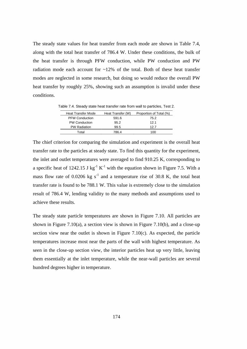
174
The steady state values for heat transfer from each mode are shown in Table 7.4,
along with the total heat transfer of 786.4 W. Under these conditions, the bulk of
the heat transfer is through PFW conduction, while PW conduction and PW
radiation mode each account for ~12% of the total. Both of these heat transfer
modes are neglected in some research, but doing so would reduce the overall PW
heat transfer by roughly 25%, showing such an assumption is invalid under these
conditions.
Table 7.4. Steady state heat transfer rate from wall to particles, Test 2.
Heat Transfer Mode Heat Transfer (W) Proportion of Total (%)
PFW Conduction 591.6 75.2
PW Conduction 95.2 12.1
PW Radiation 99.5 12.7
Total 786.4 100
The chief criterion for comparing the simulation and experiment is the overall heat
transfer rate to the particles at steady state. To find this quantity for the experiment,
the inlet and outlet temperatures were averaged to find 910.25 K, corresponding to
a specific heat of 1242.15 J kg-1
K-1
with the equation shown in Figure 7.5. With a
mass flow rate of 0.0206 kg s-1
and a temperature rise of 30.8 K, the total heat
transfer rate is found to be 788.1 W. This value is extremely close to the simulation
result of 786.4 W, lending validity to the many methods and assumptions used to
achieve these results.
The steady state particle temperatures are shown in Figure 7.10. All particles are
shown in Figure 7.10(a), a section view is shown in Figure 7.10(b), and a close-up
section view near the outlet is shown in Figure 7.10(c). As expected, the particle
temperatures increase most near the parts of the wall with highest temperature. As
seen in the close-up section view, the interior particles heat up very little, leaving
them essentially at the inlet temperature, while the near-wall particles are several
hundred degrees higher in temperature.

175
Figure 7.10. Steady state particle temperatures, showing (a) entire particle stream, and (b) section view to show interior particles, and (c) close-up section view to show particles near the outlet.
The steady state heat flux at the boundary is shown in Figure 7.11. As expected, the
heat flux peaks at the front and center, where the incident radiation is the highest.
An interesting and perhaps unexpected result is the negative heat flux shown at the
lower portion of the tube, meaning heat is transferred from the particles to the wall.
If the particle temperatures in Figure 7.10(a) are compared to the wall temperatures
in Figure 7.8 this is logical; the hottest (red) particles are heated to ~1119 K before
descending further to the part of the wall which is cooler at around 1000 K (shown
in light blue), so heat is transferred from the particles to the wall.
(a) (b) (c)

176
Figure 7.11. Heat flux of test section at steady state.
7.3.2 Test 3 Results
Steady state heat transfer rates from the wall to the particles, for Test 3, are shown
in Table 7.5. Unlike at the higher temperatures of Test 2, radiation plays an almost
negligible role, contributing only 3.2% to the overall PW heat transfer. This shows
the need for the heated hopper in the experiments, as starting tests at room
temperature largely misses any contributions from radiation, making it a less useful
test for validation of all the implemented heat transfer models. The overall heat
transfer to the particles was predicted to be 1167.2 W by the DPHT simulation.
Table 7.5. Steady state heat transfer rate from wall to particles, Test 3.
Heat Transfer Mode Heat Transfer (W) Proportion of Total (%)
PFW Conduction 938.9 80.4
PW Conduction 191.2 16.4
PW Radiation 37.1 3.2
Total 1167.2 100
The overall heat gain in the experiment was found from the temperature rise (63.7
K), a mass flow rate of 0.0202 kg s-1
, and an average specific heat of 825.7 J kg-1
K-1
. The specific heat was found with a method similar to that shown in Figure 7.5,
but the fit was found for the lower temperature range for Test 3. This yielded a total

177
heat transfer rate for the experiment of 1062.5 W, roughly 9% less than the value
predicted by the DPHT simulation.
7.3.3 Uncertainty and Repeatability
There results show a close match between the simulation and the experiment for
Test 2, and a difference of 9% for Test 3. Under the conditions of Test 3, radiation
plays a very small part in the overall heat transfer, which points towards either
experimental uncertainty/error, or a deficiency in the PFP conduction model as the
root cause of the discrepancy. Nevertheless, the results from the two tests give
some indication as to the accuracy that can be expected. Clearly, more comparisons
with experiments must be run before the six heat transfer models in DPHT can be
considered truly validated for high accuracy simulations.
An uncertainty analysis was run for the total heat gain in the experiment, which
was found using Eq. (7.5). The mass flow rate was found with a linear curve fit
using many (roughly 130) measurements of the mass on the scale over time, so the
uncertainty in the mass flow rate is not considered in this analysis. In addition, the
uncertainty in the specific heat is not considered, as it was taken from previously
published data, and no uncertainty information is known. Thus, only the
uncertainties in the thermocouple measurements were considered. For best
accuracy, “Special Limit of Error” (SLE) K-type thermocouples were generally
used for the inlet and outlet temperature measurements, as they offer higher
accuracy than typical thermocouples. The stated accuracy is ±1.1 ⁰C or 0.004%,
whichever is greater. Normal K-type thermocouples have an accuracy of ±2.2 ⁰C or
0.0075%, whichever is greater. During Test 2, the SLE thermocouple broke, so the
reading was taken with a backup thermocouple, which was a normal K-type.
(7.5)

178
For Test 2, an uncertainty of ±17.3% was found. The relatively high uncertainty is
due both to the high temperature, and due to the normal K-type thermocouple used
at the inlet. Thus, even though a very close match was found between the
simulation and experimental results, the closeness of the match may not be
repeatable, as the uncertainty in the experiment is quite high.
In Test 3, a low uncertainty of only 2.3% was found due to the low temperatures
and SLE thermocouples used. Thus, the 9% difference between simulation and
experimental results cannot simply be attributed to experimental uncertainty; there
must be an error either in the measurement or in the model.
The comparisons shown represent a culmination of work to develop both new
modeling and experimental techniques, so there are potential sources of error in
both areas. In the model, perhaps the largest source of potential error is in the PFP
and PFW conduction models because they account for the largest portion of heat
transfer overall. The direct conduction and radiation models each have a lesser
impact on the overall results. The DBA radiation model is expected to have a high
accuracy given the rigorous numerical validations conducted under very similar
conditions in Chapter 4.
The properties used in these models may also have a large effect on the results. The
thermal conductivity of air is a main factor in the PFP conduction model, and for
this reason it was found as a function of temperature instead of assuming a constant
value. In contrast, the thermal conductivity of sintered bauxite was taken as a
constant value of 2.0 W m-2
K-1
, as no temperature dependent properties were
available. However, the solid conductivity has a relatively minor impact on the
overall heat transfer because in the PFP model, which is the leading mode of heat
transfer, by far the largest resistance to heat transfer is due to the air gap between
particles. Thus, any error in the solid thermal conductivity value likely contributes
relatively little to the overall error. An error in the particle specific heat would be a
large contributor to the overall error due to its direct effect on the temperature rise
of the particles. The values used to find specific heat as a function of temperature

179
were taken from an experimental data set used widely by researchers in this field,
so they are thought to be accurate. The emissivity of the stainless steel wall has a
strong effect on the PW radiative transfer in the DBA model; 0.60 was chosen,
though there is a wide variety of values found in literature but few at high
temperatures, and the value strongly depends on the surface treatment. Radiation
accounts for 12.7% of the total heat transfer from the wall in Test 2, so any
inaccuracy in the wall emissivity could lead to several percent error overall.
In the experiment, perhaps the largest source of potential error is from the inlet and
outlet temperature values measured, since the particle streams may not be perfectly
uniform both spatially (across the stream) and in time, as noted in Section 6.2.4.
Given the temperature rise (30.8 ⁰C in Test 2, and 63.7 ⁰C in Test 3), a small
experimental error in the inlet or outlet temperature readings would lead to a large
error in the computed overall heat gain. In future experiments, a much higher
temperature rise is desired to minimize this effect.
7.4 Conclusions for Comparison of Experimental and DPHT Model
Results
When comparing the experimental and DPHT simulation results in terms of overall
heat transfer, an extremely close match was found for Test 2 (high temperature),
while a difference of ~9% was found for Test 3 (low temperature). This level of
agreement indicates that, at a minimum, the model can predict with relative
accuracy the behavior of a real system. With only these two tests for comparison, it
is not clear how repeatable this is. There may be multiple errors in the model which
have the effect of cancelling each other out under certain circumstances, leading to
the close agreement shown in Test 2. This has to be addressed in future work, with
more experimental studies performed until a repeatable pattern of high accuracy
results can confirm the validity of the model.

181
CHAPTER 8
8 A SOLAR RECEIVER FOR PREHEATING LIME PARTICLES
Cement production is responsible for 5-7% of the annual CO2 emissions globally
[101], making it an industry which is critical to decarbonize in the coming decades
to address climate change. Calcination of limestone is the key step in cement
production, where limestone, predominantly CaCO3, is converted to CaO and CO2
through an endothermic reaction in the temperature range of 900 to 1500 ⁰C.
Carbon dioxide is released due to both the chemical reaction, shown in Eq. (8.1), as
well as in the burning of fossil fuels to reach the high temperatures of the reaction.
(8.1)
Supplying heat from CSP may provide a solution to calcinate limestone without
fossil fuels [102]. It can also be applied to other high-temperature and energy-
intensive industrial processes such as metallurgy, waste incineration, and metals
recycling [3]. In this research, a solar receiver is envisioned for preheating lime
particles from ambient temperatures to roughly 700 ⁰C, which would save a large
portion of CO2 in the heating step before calcination occurs. At temperatures above
700 ⁰C the calcination reaction begins, where heating and off-gassing of the
reaction products must be tightly controlled, so this initial receiver design is
focused on preheating the particles only. Furthermore, by designing a receiver to
preheat particles, the modeling method and results may be transferrable to other
industrial heating processes which require a similar heating of granular material to
high temperatures.

182
8.1 Receiver Design
The receiver designed uses a dense granular flow of particles which descend due to
gravity in between parallel plates. One of these plates forms the heated surface of
the receiver, shown in red in Figure 8.1, and the other plate is insulated. The overall
dimensions of this receiver follow the designs of cavity receivers which circulate
molten salt as a heat transfer fluid for electricity generation [103]. The receiver
surface is 12 m wide by 6 m high, with a 5 m deep cavity (or hood), and a 2.5 m
lip. The entire receiver and cavity is tilted towards the front at 12.5⁰. The cavity is
critical, as it substantially reduces emissive and convective losses from the hot
receiver surface, leading to a much higher efficiency than an “open” receiver
without the cavity. Lime particles of diameter 1 mm descend between the parallel
plates, which are spaced at a distance of 8 mm, as shown in the close-up in Figure
8.1. A thin channel is desired for the best heat transfer, but reducing it further may
cause blockages in the flow due to clogging and bridging at the outlet. These
dimensions all play a role in the final efficiency and heat gain of the receiver, and
they can be adjusted to optimize the design in future work.
Figure 8.1. Receiver design and 1-mm diameter particles descending between parallel plates.
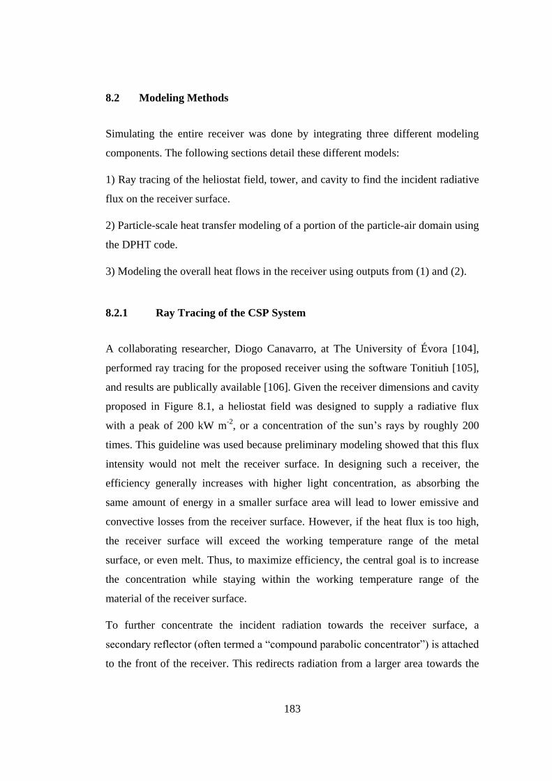
183
8.2 Modeling Methods
Simulating the entire receiver was done by integrating three different modeling
components. The following sections detail these different models:
1) Ray tracing of the heliostat field, tower, and cavity to find the incident radiative
flux on the receiver surface.
2) Particle-scale heat transfer modeling of a portion of the particle-air domain using
the DPHT code.
3) Modeling the overall heat flows in the receiver using outputs from (1) and (2).
8.2.1 Ray Tracing of the CSP System
A collaborating researcher, Diogo Canavarro, at The University of Évora [104],
performed ray tracing for the proposed receiver using the software Tonitiuh [105],
and results are publically available [106]. Given the receiver dimensions and cavity
proposed in Figure 8.1, a heliostat field was designed to supply a radiative flux
with a peak of 200 kW m-2
, or a concentration of the sun’s rays by roughly 200
times. This guideline was used because preliminary modeling showed that this flux
intensity would not melt the receiver surface. In designing such a receiver, the
efficiency generally increases with higher light concentration, as absorbing the
same amount of energy in a smaller surface area will lead to lower emissive and
convective losses from the receiver surface. However, if the heat flux is too high,
the receiver surface will exceed the working temperature range of the metal
surface, or even melt. Thus, to maximize efficiency, the central goal is to increase
the concentration while staying within the working temperature range of the
material of the receiver surface.
To further concentrate the incident radiation towards the receiver surface, a
secondary reflector (often termed a “compound parabolic concentrator”) is attached
to the front of the receiver. This redirects radiation from a larger area towards the
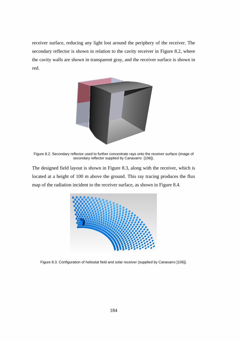
184
receiver surface, reducing any light lost around the periphery of the receiver. The
secondary reflector is shown in relation to the cavity receiver in Figure 8.2, where
the cavity walls are shown in transparent gray, and the receiver surface is shown in
red.
Figure 8.2. Secondary reflector used to further concentrate rays onto the receiver surface (image of secondary reflector supplied by Canavarro [106]).
The designed field layout is shown in Figure 8.3, along with the receiver, which is
located at a height of 100 m above the ground. This ray tracing produces the flux
map of the radiation incident to the receiver surface, as shown in Figure 8.4.
Figure 8.3. Configuration of heliostat field and solar receiver (supplied by Canavarro [106]).

185
Figure 8.4. Incident radiative flux on the receiver surface.
8.2.2 Particle-Scale Heat Transfer Modeling with DPHT
Modeling the entire receiver with DPHT was not feasible due to the very large
number of particles, which would number in the hundreds of millions. Therefore,
the overall heat transfer coefficient method was followed, as described in Section
5.9.2. First, a DPHT simulation was used to find the overall heat transfer
coefficient from the wall to the particles under the relevant conditions. This lumps
all of the detailed and complex heat transfer effects of the particle-air mixture into
a single parameter, which simplifies the next modeling step, the heat transfer model
of the entire receiver. Thus, the DPHT simulation acts as a bridge between the
complex heat transfer phenomena at the particle scale and the large dimensions of
an actual receiver. This is conceptually similar to using experimental work, where
the heat transfer coefficient might be found under the relevant conditions and then
used afterwards for modeling an actual device.
The geometry modeled is a set of parallel plates separated by 8 mm and also 8 mm
in width, as shown in Figure 8.5. Because the simulation domain must be long
enough to establish a thermally fully developed flow, the plates are 6 m in length,
with a static fill level of roughly 4.8 m, containing 329,376 particles. At the outlet,
a diamond shaped obstruction (Figure 8.5(a)) is added to ensure the flow above it
stays in a packed state (instead of in free-fall), but the constriction is very slight to

186
maintain a high flow rate. By setting the DEM boundary condition in the y-
direction (vertical) to be periodic, particles exiting through the nozzle reappear at
the top of the domain, making the number of particles constant throughout the
simulation. When particles transit this periodic boundary, their temperatures are
reset to the inlet temperature of 300 K in DPHT. A uniform temperature boundary
condition of 1173 K is given to one plate, and an adiabatic boundary condition is
given to the other. Simulation parameters are given in Table 8.1.
Figure 8.5. (a) Parallel plates with diamond-shaped obstruction, and (b) particles in between the 8-
mm by 8-mm parallel plate strip studied.
Table 8.1 Properties used in DEM and DPHT modeling.
Property Value Units
Radius, P 0.0005 m
Density, P [VDI, p612] 2200 kg m-3
Young's modulus, DEM, P 1e8 Pa
Young's modulus, DEM, W 1e8 Pa
Young's modulus, real, P 5.20e10 Pa
Young's modulus, real, W 1.80e11 Pa
Poisson's ratio, P 0.25 -
Poisson's ratio, W 0.30 -
Coeff. of restitution, PP 0.44 -
Coeff. of restitution, PW 0.825 -
Coeff of friction, PP 0.40 -
Coeff of friction, PW 0.30 -
Coeff of rolling friction, PP 0.40 -
Coeff of rolling friction, PW 0.50 -
Thermal conductivity, P 2.0 W m-2
K-1
Thermal conductivity, W 16.6 W m-2
K-1
Emissivity, P 0.86 -
Emissivity, W 0.60 -
(a) (b)

187
The LIGGGHTS and DPHT codes are each run, for a total of 7 million DEM time
steps and 3500 thermal time steps. The LIGGGHTS and DPHT runs took roughly 6
days and 1 day, respectively, using 50 processors on a Hewlett-Packard Z840
Workstation. The DPHT code has been refined and optimized for performance, and
for the current simulation it takes ~24 seconds per thermal time step for the domain
of 329,376 particles.
The three components of PW heat transfer are shown in Figure 8.6, which shows a
steady state has been reached after ~60 seconds. At steady state, the heat transfer
from the wall to the particles is separated by each mode and shown in Figure 8.6.
Similar to examples in the previous chapters, direct PW conduction contributes the
least to the overall heat transfer, and PFW conduction contributes the most.
Figure 8.6. Overall heat transfer from wall to particles, separated by heat transfer mode.
The steady state particle temperatures at the outlet are shown in Figure 8.7, which
indicates particles near the heated wall reach ~1124 K, while particles near the
insulated wall are substantially cooler, down to 740 K. This temperature difference
of nearly 400 degrees over a distance of only 8 mm is due to the low effective
thermal conductivity and very little mixing in this geometry. The particles form a
layer on the hot wall, which is enhanced by the fact that the parallel plates are tilted
downward at 12.5 ⁰C to match the receiver tilt. This is accomplished in
LIGGGHTS by turning the gravity vector at a 12.5 degree angle. This actually
0
2000
4000
6000
8000
10000
12000
14000
16000
0
10
20
30
40
50
60
70
80
90
10
0
11
0
12
0
13
0
14
0
15
0
Wall-
to-P
art
icle
Heat
Tra
nsfe
r (W
)
Time (s)
PW Radiation
PW Conduction
PFW Conduction

188
increases the PW heat transfer slightly, as noted by Natarajan and Hunt [69],
because the gravity vector in the direction of the wall increases the solid fraction
along the wall.
Figure 8.7. Particles at the outlet, colored by temperature.
For post-processing, the domain is subdivided into many different sections in the y-
direction. The mean particle temperature in each section is plotted in Figure 8.8(a)
as a function of the distance from the heated inlet, and the heat transfer coefficient
is shown in Figure 8.8(b). Both plots show the averaged values over 100 time steps,
after a steady state has been established. The heat transfer coefficient (h) in each
section is found with Eq. (8.2), where Tbulk is the mean particle temperature in the
section, and qPW for the section is known from the DPHT outputs. The mass flow
rate is analyzed over the same time period, with an average mass flow rate of
0.0056 kg s-1
found.

189
(8.2)
Similar to heat transfer in pipe flow, the heat transfer coefficient is highest near the
inlet and decreases until it reaches a thermally developed state, in this case taken to
be at a distance 1.5 m. The heat transfer coefficient is approximated with a fourth-
order polynomial curve for the entrance region and a constant value in the fully
developed region, and shown in Figure 8.8(b) and in Equations (8.3) and (8.4).
After the particles were inserted, they reduced down due to compaction and
established a fill level of ~4.8 m, so the x axis in this figure only extends to this
distance. Nevertheless, the heat transfer coefficient value is expected to remain
relatively unchanged between 4.8 m and the outlet at 6 m.
Figure 8.8. Outputs from DPHT simulation analyzed to show (a) bulk temperature, and (b) overall
heat transfer coefficient, both as a function of distance from the inlet.
(8.3)
(8.4)
The heat transfer coefficient is the output of the DPHT simulation which will be
used in the overall receiver heat transfer model. It is important to note that this heat
transfer coefficient is found for a very specific set of conditions, and it depends on
the particle properties, the mass flow rate, and the temperature range. The heat
transfer coefficient would change based on the wall temperature modeled. A wall
0
100
200
300
400
500
600
700
800
900
1,000
0 1 2 3 4 5
Bulk
Tem
pera
ture
(K
)
Distance from Inlet (m)
0
50
100
150
200
250
300
350
400
450
0 1 2 3 4 5
Overa
ll H
eat
Tra
nsfe
r C
oeffic
ient
(W/m
2K
)
Distance from Inlet (m)
(a) (b)

190
temperature of 1173 K was chosen, as the wall temperature of the receiver when in
operation is expected to be roughly this value. To pursue a more accurate model,
the DPHT model could be run for multiple wall temperatures and particle inlet
temperatures, so a heat transfer coefficient could be even more tailored to the
conditions.
The proposed parallel plate geometry is clearly not an optimal design; as shown in
Figure 8.7, the flow exhibits very little mixing, leading to the hottest particles
remaining in constant contact with the wall, while the interior particles receive
much less heat. If some geometry were placed in the flow to enhance mixing, such
as orifice plates, ridges, or diagonal plates, this could bring cold particles towards
the hot surface and enhance the heat transfer coefficient and the overall efficiency
of the receiver.
8.2.3 Overall Receiver Heat Transfer Model
To model the overall receiver, the 12 m by 6 m surface is subdivided into 1800
square elements, each 20 cm x 20 cm. Each element is assumed to have a uniform
temperature across its surface, and no heat is conducted to the neighboring
elements. A set of seven heat transfer equations is solved simultaneously for each
element, which is given in Equations (8.5) to (8.11). Figure 8.9 shows the geometry
of a single wall element and the adjoining particle-air cell, along with the heat
inflows and outflows. The key that enables the use of this simplified 1D model is
that the overall heat transfer coefficient from the wall to the particles has already
been found with the detailed DEM+DPHT simulation.

191
Figure 8.9. One element of the metal receiver surface and the adjoining cell containing the particle-
air mixture.
(8.5)
(
*
(8.6)
( ) (8.7)
( ) (8.8)
( ) (8.9)
(8.10)
(
) (8.11)
Equation (8.5) is an energy balance of the plane where the incident radiation
initially strikes the metal receiver surface. The incident radiation striking that
element (qinc) with area A is found according to the flux map supplied by the ray
tracing simulation described in Section 8.2.1. The heat passing into the metal
192
receiver wall, and eventually to the particle-air mixture, is qabs, and losses due to
reflection, convection, and emission are denoted as qL,refl, qL,conv, and qL,emiss.
Equation (8.6) solves for the absorbed energy by the particle-air stream in the
volume directly behind the surface element. It uses the heat transfer coefficient
(hparticles) from Equations (8.3) and (8.4), which were found with the DPHT heat
transfer simulation. The temperature of the surface ( ) and the
temperature of the particle-air mixture are related with the log mean temperature
difference. Equation (8.7) relates the heat gain to the temperature rise in the
particle-air mixture, where is the mass flow rate, Cp is the specific heat of the
particles, and the bulk temperatures are and . Equation (8.8)
calculates heat conduction across the metal receiver wall, by relating the exposed
surface temperature ( ) to the internal surface facing the particles-air
cell ( ). Equation (8.9) is for the convective loss, where hext is the
convection coefficient to the outside, which is taken to be 6 W m-2
K-1
[107]. The
ambient temperature ( is taken as 300 K. The variable Bconv is either 0 or 1
according to the work of Clausing [107], where it is assumed that convection loss is
negligible anywhere above the level of the lip due to a stagnant zone in the upper
part of the receiver. Reflection loss is calculated with Eq. (8.10), which uses the
reflectivity ( ) and the diffuse view factor from the surface element to the aperture
( ). The calculation of emissive loss in Eq. (8.11) uses the same diffuse view
factor, and the emissivity (ε) of Pyromark paint common to solar receivers. An
emissivity value of 0.87 was used in this model, though values reported in literature
vary to a small degree [14][100].
For each surface element, this set of equations was solved simultaneously using a
non-linear solver. The top row of surface elements was solved first, as the inlet
temperature ( ) must be specified, which was set to 300 K. When solving the
next row down, the bulk inlet temperature is taken as the bulk outlet temperature
( ) of the element directly above.

193
The interior walls of the cavity (the bottom, top, and side walls) are not explicitly
modeled with these equations. Due to convective and radiative transfer they will
reach equilibrium somewhere between the receiver surface temperature and the
ambient temperature. Studies that focus only on the heat transfer in cavity receivers
[103] actually model these surfaces as adiabatic panels, but doing so requires
solving Equations (8.5)-(8.11) over all surface elements simultaneously, due to the
radiative interactions between surface elements. This would lead to a set of
hundreds of non-linear equations to be solved simultaneously, a problem that
cannot be readily solved by most non-linear solvers.
To reduce the complexity while still providing a valid estimate of the overall heat
gain and receiver efficiency, the following approach is used. The solution is first
found by solving Equations (8.5)-(8.11) for each element of the receiver surface.
This underestimates the loss, since it includes no emissive or convective losses
from the internal walls of the receiver cavity. The losses are calculated from the
bottom, top, and side walls of the receiver by assuming the temperature of these
surfaces is the mean of the solved receiver surface and ambient temperatures. For
convective loss, the guidelines from Clausing [107] are followed again, where
convection from the walls anywhere above the receiver lip is negligible. For the
emissive losses, the diffuse view factors are calculated from each wall to the
aperture. Therefore, while the original model is run without a detailed analysis of
the interior cavity surfaces, these “extra” loss calculations are performed afterwards
to compensate, providing an improved estimate of the receiver efficiency.

194
Figure 8.10. Receiver surface showing (a) external surface temperature, and (b) absorbed heat flux.
When solved by the original simulation (before extra cavity losses are subtracted),
the outer temperature of the receiver surface ( ) is shown in Figure
8.10(a), and the absorbed heat flux is shown in Figure 8.10(b). Of the total 7.94
MW of radiation incident to the receiver, 5.65 MW were found to absorb before the
“extra” cavity losses are subtracted. After the cavity losses are calculated, the total
energy absorbed is reduced to 4.80 MW, representing a thermal efficiency of
60.5%. This neglects any “spillage” losses from light missing the receiver entirely.
The average outlet temperature of the original simulation is 1092 K, but after
reducing the temperature based on the extra cavity losses, the bulk outlet
temperature is estimated to be 973 K, or 700 ⁰C. This matches the output
temperature originally designed, which was achieved by adjusting the mass flow
rate through the receiver until an outlet temperature of 700 ⁰C was found. The mass
(a)
(b)

195
flow rate in the 8 mm x 8 mm section studied with DPHT was 0.0056 kg s-1
,
compared to a value of 0.0042 kg s-1
used in the final receiver simulation. The
overall heat transfer coefficient is not expected to vary a high amount due to the
lowered flow rate, but for best accuracy the DEM+DPHT simulations could be run
again at a lower flow rate. However, such iterations may weeks of computation
time, so the accuracy achieved with the current method is deemed high enough for
this initial investigation. The maximum temperature reached on the surface of the
receiver was 1228 ⁰C, which may be acceptable for Ni-based superalloys (e.g.
Inconel), but this would exceed the temperature limit of stainless steels.
8.3 Conclusions for Solar Receiver Model
A dense granular flow receiver was modeled in this chapter, and the overall heat
transfer coefficient provided a bridge between the detailed particle-scale model and
the large-scale model of an entire solar receiver.
The receiver studied uses particles flowing downward through parallel plates. The
receiver chosen, with a thermal efficiency of 60.5% under the conditions modeled,
represents a base-case scenario for similar receivers. Adding either fins or some
type of orifice plates to mix the particles would reduce the surface temperature and
increase the overall thermal efficiency.


197
CHAPTER 9
9 CONCLUSIONS AND RECOMMENDED FUTURE WORK
As noted in the introduction, specific conclusions are included in each chapter.
Therefore, this chapter contains only broad conclusions that span multiple chapters.
The goal of this work has been to improve the ability to model heat exchange
devices for CSP systems, and several related areas were studied in pursuit of that
goal. This research has added to the knowledge of the field in several ways,
including the major contributions of an open source Monte Carlo code to calculate
radiative transfer in groups of thousands of particles and an improved method to
find the effective thermal conductivity due to radiation (krad). The effective thermal
conductivity of packed beds has been studied by researchers in many fields, and the
Monte Carlo code as well as the krad model can be used by researchers far beyond
the field of CSP. The Monte Carlo method is widely regarded as an accurate and
reliable way to simulate radiation in particles, so a model for krad that is built
directly upon Monte Carlo simulation results should also yield a high accuracy.
Modeling particle flows with DEM provides detailed results for researchers in
many fields, and in recent years industry has begun to adopt it. Within the field of
CSP, DEM could be used to model many proposed heat exchange devices.
Unfortunately, the commercial and open source software options for performing
the DEM simulations with heat transfer are lacking in numerous aspects, so
researchers have often turned to other, often less rigorous modeling methods
instead. For simple geometries continuum models often suffice, but for more
complex designs (e.g. particles flowing over a bank of tubes, or through an orifice)
continuum models diverge from reality, as the bulk of particles does not flow as a
fluid flows. This calls for a DEM approach. The modeling method developed to
address this gap includes an initial DEM modeling step and a subsequent heat

198
transfer modeling step with DPHT. This is applicable for dense granular flows, an
important flow regime used in many CSP heat exchange devices. The DPHT model
is described in detail in this thesis and is posted as an open source code, with the
hope that others can use it and improve it as new sub-models are developed. The
DPHT code is currently only for uniform-sized spheres, but in future work the sub-
models could be expanded to work for multi-sized spheres to reflect more realistic
particle beds.
The Distance Based Approximation model was developed to estimate radiative
transfer between particles and particle-wall pairs in DEM-based simulations. The
method has been shown to accurately predict bulk heat transfer in large groups of
particles by comparing results from the DBA model against detailed ray tracing
calculations. Though there are several previous models in literature, these have
numerous problems, ranging from the particle emissivity not being correctly
incorporated, to the view factors not summing to 1, to simply adding an
unreasonable computational burden. The DBA model does not have these
shortcomings, and it is extremely easy to implement in a code, requiring only an
equation and a lookup table. The DBA model was implemented in DPHT, but it
has been described with sufficient detail for others to implement it into their own
codes as well.
With little experimental work reported in literature under the conditions relevant to
CSP, experiments were conducted to provide the data needed to start validating
models such as DPHT. Numerous practical findings were made throughout the
process, with a key development being the method to mix and measure the bulk
temperature of the particle stream. The mechanical paddle-wheel mixer was
determined to mix the particle stream to a high degree, and an air pocket where the
paddle-wheel could spin at high speed was created by adding a secondary orifice
plate and an overflow channel. This same method can be used by others needing to
measure the bulk temperature in particle flows. Three successful experimental runs
are described, covering two particle materials and temperature ranges up to ~650
⁰C. The geometry studied was a square tube heated on one face with a high flux

199
solar simulator. In the future, experiments should include more complex
geometries for mixing particles to increase the overall heat transfer, both because
that is the eventual goal and also because it would provide a more robust test case
for the DPHT code.
With experimental results obtained and the DPHT model developed, a comparison
was made between the two. An excellent match was found in terms of the overall
heat gain at the high temperature range, with a difference of only 0.2% between the
simulation and the experiment. In the lower temperature range, a difference of ~9%
was found. This indicates the DPHT code calculates heat transfer that is in the right
range, though with only these two points of comparison it is not clear if results are
repeatable and if similarly accurate results would be found under different
conditions. Future work should include further validation simulations until
repeatability is shown under various circumstances, with special attention needed
in the PFP and PFW conduction models. Having a DEM-based code that is easy to
use, flexible, and validated to give reliable results would be a large step forward in
the field of CSP, and it would lead to greater adoption of DEM-based models for
heat transfer in numerous fields.
One of the original goals was to model a solar receiver with a DEM code. After
developing the DBA model for radiation, developing the DPHT code to incorporate
the other modes of heat transfer, and producing promising initial validation results,
a solar receiver was modeled in Chapter 8. A dense granular flow receiver was
modeled with DEM+DPHT, where a thin strip of the receiver was used to
characterize the heat transfer in terms of a heat transfer coefficient. Results were
then used in an overall heat transfer model of the receiver, which accounted for
incident concentrated light from a heliostat field and heat losses from the receiver
surface. This serves as an example of how the heat transfer between particles at the
micron scale can be linked to an actual device at the length scale of several meters.
For particle-based CSP to play a role in addressing climate change, modeling tools
are needed to evaluate and design the heat exchange devices that will be required.

200
Models must be both accurate and simple enough that researchers, students, and
industry professionals can readily use them. With the developments in this thesis,
DEM-based heat transfer modeling has been improved in several meaningful ways,
allowing for the development of better particle-based CSP devices by researchers
in the future.
201
REFERENCES
[1] Z. Ma, M. Mehos, G. Glatzmaier, B.B. Sakadjian, Development of a
Concentrating Solar Power System Using Fluidized-bed Technology for
Thermal Energy Conversion and Solid Particles for Thermal Energy
Storage, Energy Procedia. 69 (2015) 1349–1359.
doi:10.1016/j.egypro.2015.03.136.
[2] S.J. Antony, W. Hoyle, Y. Ding, Granular Materials; Fundamentals and
Applications, 2004. doi:10.1017/CBO9781107415324.004.
[3] E. Alonso, A. Gallo, M.I. Roldán, C.A. Pérez-rábago, E. Fuentealba, Use of
rotary kilns for solar thermal applications : Review of developed studies and
analysis of their potential, Sol. Energy. 144 (2017) 90–104.
doi:10.1016/j.solener.2017.01.004.
[4] E. O’Shaughnessy, J.R. Cruce, K. Xu, Too much of a good thing? Global
trends in the curtailment of solar PV, Sol. Energy. 208 (2020) 1068–1077.
doi:10.1016/j.solener.2020.08.075.
[5] O. of E.E. and R.E. US Department of Energy, NOOR III | Concentrating
Solar Power Projects, (2020). https://solarpaces.nrel.gov/noor-iii (accessed
November 24, 2020).
[6] C.A. Schoeneberger, C.A. McMillan, P. Kurup, S. Akar, R. Margolis, E.
Masanet, Solar for industrial process heat: A review of technologies,
analysis approaches, and potential applications in the United States, Energy.
206 (2020) 118083. doi:10.1016/j.energy.2020.118083.
[7] N. Siegel, M. Gross, C. Ho, T. Phan, J. Yuan, Physical Properties of Solid
Particle Thermal Energy Storage Media for Concentrating Solar Power
Applications, Energy Procedia. 49 (2014) 1015–1023.
doi:10.1016/j.egypro.2014.03.109.
[8] H. Al-Ansary, A. El-Leathy, S. Jeter, E. Djajadiwinata, S. Alaqel, M. Golob,
C. Nguyen, R. Saad, T. Shafiq, S. Danish, S. Abdel-Khalik, Z. Al-Suhaibani,

202
N. Abu-Shikhah, M.I. Haq, A. Al-Balawi, F. Al-Harthi, On-sun experiments
on a particle heating receiver with red sand as the working medium, AIP
Conf. Proc. 2033 (2018) 1–8. doi:10.1063/1.5067038.
[9] G. Flamant, D. Hernandez, C. Bonet, J.P. Traverse, Experimental aspects of
the thermochemical conversion of solar energy; Decarbonation of CaCO3,
Sol. Energy. 24 (1980) 385–395. doi:10.1016/0038-092X(80)90301-1.
[10] J. Hruby, R. Steeper, G. Evans, C. Crowe, An Experimental and Numerical
Study of Flow and Convective Heat Transfer in a Freely Falling Curtain of
Particles, J. Fluids Eng. 110 (1988) 172. doi:10.1115/1.3243531.
[11] C.K. Ho, A new generation of solid particle and other high-performance
receiver designs for concentrating solar thermal (CST) central tower
systems, Adv. Conc. Sol. Therm. Res. Technol. (2017) 107–128.
doi:10.1016/B978-0-08-100516-3.00006-X.
[12] J. Christian, C. Ho, System Design of a 1 MW North-facing, Solid Particle
Receiver, Energy Procedia. 69 (2015) 340–349.
doi:10.1016/j.egypro.2015.03.038.
[13] C.K. Ho, J.M. Christian, J. Yellowhair, N. Siegel, S. Jeter, M. Golob, S.I.
Abdel-Khalik, C. Nguyen, H. Al-Ansary, On-sun testing of an advanced
falling particle receiver system, AIP Conf. Proc. 1734 (2016).
doi:10.1063/1.4949074.
[14] C. Ho, J. Christian, D. Gill, A. Moya, S. Jeter, S. Abdel-Khalik, D.
Sadowski, N. Siegel, H. Al-Ansary, L. Amsbeck, B. Gobereit, R. Buck,
Technology Advancements for Next Generation Falling Particle Receivers,
Energy Procedia. 49 (2014) 398–407. doi:10.1016/j.egypro.2014.03.043.
[15] W. Wu, D. Trebing, L. Amsbeck, R. Buck, R. Pitz-Paal, Prototype Testing
of a Centrifugal Particle Receiver for High-Temperature Concentrating Solar
Applications, J. Sol. Energy Eng. 137 (2015) 041011–041011.
doi:10.1115/1.4030657.

203
[16] S. Hicdurmaz, E. Johnson, J. Grobbel, L. Amsbeck, R. Buck, B.
Hoffschmidt, Numerical Heat Transfer Modelling of a Centrifugal Solar
Particle Receiver, (n.d.).
[17] A.B. Morris, Z. Ma, S. Pannala, C.M. Hrenya, Simulations of heat transfer
to solid particles flowing through an array of heated tubes, Sol. Energy. 130
(2016) 101–115. doi:10.1016/j.solener.2016.01.033.
[18] I.P. Lopez, H. Benoit, D. Gauthier, J.L. Sans, E. Guillot, G. Mazza, G.
Flamant, On-sun first operation of a 150 kWth pilot solar receiver using
dense particle suspension as heat transfer fluid, AIP Conf. Proc. 137 (2016)
463–476. doi:10.1063/1.4949080.
[19] E. Johnson, D. Baker, I. Tari, Proposal of a Novel Gravity-Fed , Particle-
Filled Solar Receiver, AIP Conf. Proc. 1850 (2017). doi:10.1063/1.4984371.
[20] E. Johnson, Conceptual Design and Heat Transfer Investigation of a Dense
Granular Flow Solar Receiver, Middle East Technical University, 2017.
[21] M.F. Watkins, A Heat Transfer Analysis of Vertical Dense Granular Flows,
North Carolina State University, 2018.
[22] P. Bartsch, T. Baumann, S. Zunft, Granular Flow Field in Moving Bed Heat
Exchangers: A Continuous Model Approach, Energy Procedia. 99 (2016)
72–79. doi:10.1016/j.egypro.2016.10.099.
[23] S. Hicdurmaz, I. Tari, Numerical Investigaton of Bubbling Fluidized Bed to
e Used as Thermal Energy Storage Integrated to High-Temperature
Concentrated Solar Power, Multiph. Sci. Technol. 30 (2018).
[24] K.J. Albrecht, C.K. Ho, Heat Transfer Models of Moving Packed-Bed
Particle-to-sCO2 Heat Exchangers, J. Sol. Energy Eng. Trans. ASME. 141
(2019) 1–10. doi:10.1115/1.4041546.
[25] W. Van Antwerpen, P.G. Rousseau, C.G. Du Toit, Multi-sphere Unit Cell
model to calculate the effective thermal conductivity in packed pebble beds
of mono-sized spheres, Nucl. Eng. Des. 247 (2012) 183–201.

204
doi:10.1016/j.nucengdes.2012.03.012.
[26] W. Van Antwerpen, C.G. Du Toit, P.G. Rousseau, A review of correlations
to model the packing structure and effective thermal conductivity in packed
beds of mono-sized spherical particles, Nucl. Eng. Des. 240 (2010) 1803–
1818. doi:10.1016/j.nucengdes.2010.03.009.
[27] X. Wang, J. Zheng, H. Chen, A prediction model for the effective thermal
conductivity of mono-sized pebble beds, Fusion Eng. Des. 103 (2016) 136–
151. doi:10.1016/j.fusengdes.2015.12.051.
[28] G. Breitbach, H. Barthels, The Radiant Heat Transfer in the High
Temperature Reactor Core after Failure of the Afterheat Removal Systems,
Nucl. Technol. 49 (1980) 392–399. doi:10.13182/nt80-a17687.
[29] P. Zehner, E.U. Schlünder, Einfluß der Wärmestrahlung und des Druckes
auf den Wärmetransport in nicht durchströmten Schüttungen, Chemie Ing.
Tech. 44 (1972) 1303–1308. doi:10.1002/cite.330442305.
[30] P. Zehner, E.U. Schlünder, Warmeleitfahigkeit von Schuttungen bei
mässigen Temperaturen, Chemie Ing. Tech. 42 (1970) 933–941.
[31] R. Bauer, E.U. Schlunder, Effective radial thermal conductivity of packings
in gas flow. Part II thermal conductivity of the packing fraction without gas
flow, Int. Chem. Eng. 18 (1978) 189–204.
[32] E. Tsotsas, D6.3 Thermal Conductivity of Packed Beds. In: VDI Heat Atlas,
2nd ed., Springer, Berlin, Heidelberg, 2010. doi:10.1007/978-3-540-77877-
6.
[33] C.T. Hsu, P. Cheng, K.W. Wong, Modified Zehner-Schlunder models for
stagnant thermal conductivity of porous media, Int. J. Heat Mass Transf. 37
(1994) 2751–2759. doi:10.1016/0017-9310(94)90392-1.
[34] Y.S. Yang, J.R. Howell, D.E. Klein, Radiative Heat Transfer Through a
Randomly Packed Bed of Spheres by the Monte Carlo Method, J. Heat
Transfer. 105 (1983) 325. doi:10.1115/1.3245582.

205
[35] J.C. Chen, S.W. Churchill, Radiant heat transfer in packed beds, AIChE J. 9
(1963) 35–41. doi:10.1002/aic.690090108.
[36] D. Bouvard, C. Argento, A ray tracing method for evaluating the radiative
heat transfer in porous media, 39 (1996) 3175–3180.
[37] M. Kaviany, Principles of Heat Transfer in Porous Media, 1999.
[38] B.P. Singh, M. Kaviany, Effect of solid conductivity on radiative heat
transfer in packed beds, Int. J. Heat Mass Transf. 37 (1994) 2579–2583.
doi:10.1016/0017-9310(94)90295-X.
[39] M. De Beer, C.G. Du Toit, P.G. Rousseau, A methodology to investigate the
contribution of conduction and radiation heat transfer to the effective
thermal conductivity of packed graphite pebble beds, including the wall
effect, Nucl. Eng. Des. 314 (2017) 67–81.
doi:10.1016/j.nucengdes.2017.01.010.
[40] P.G. Rousseau, C.G. Du Toit, W. Van Antwerpen, H.J. Van Antwerpen,
Separate effects tests to determine the effective thermal conductivity in the
PBMR HTTU test facility, Nucl. Eng. Des. 271 (2014) 444–458.
doi:10.1016/j.nucengdes.2013.12.015.
[41] K. Robold, Wärmetransport im inneren und in der Randzone von
Kugeischüttungen, 1982.
[42] G. Kasparek, D. Vortmeyer, Wärmestrahlung in Schüttungen aus Kugeln mit
vernachlässigbarem Wärmeleitwiderstand, Wärme- Und Stoffübertragung. 9
(1976) 117–128. doi:10.1007/BF01589465.
[43] A.J. Slavin, F.A. Londry, J. Harrison, A new model for the effective thermal
conductivity of packed beds of solid spheroids: alumina in helium between
100 and 500°C, Int. J. Heat Mass Transf. 43 (2000) 2059–2073.
doi:10.1016/s0017-9310(00)00208-8.
[44] E.F. Johnson, İ. Tarı, D. Baker, Radiative heat transfer in the discrete
element method by distance based approximations of radiation distribution
206
factors, Powder Technol. (2020). doi:10.1016/j.powtec.2020.11.050.
[45] F. Qi, M.M. Wright, Particle scale modeling of heat transfer in granular
flows in a double screw reactor, Powder Technol. 335 (2018) 18–34.
doi:10.1016/j.powtec.2018.04.068.
[46] H. Wu, N. Gui, X. Yang, J. Tu, S. Jiang, Analysis and evaluations of four
models of thermal radiation for densely packed granular systems, Chem.
Eng. Sci. 211 (2020) 115309. doi:10.1016/j.ces.2019.115309.
[47] M.L. Pitso, Characterisation of long range radiation heat transfer in packed
pebble beds, North-West University, 2011.
http://dspace.nwu.ac.za/bitstream/handle/10394/8435/Pitso_ML.pdf;sequenc
e=1.
[48] J.R. Mahan, The Monte Carlo Ray-Trace Method in Radiation Heat Transfer
and Applied Optics, Wiley-ASME Press, 2019.
doi:10.1002/9781119518471.
[49] J.R. Howell, The Monte Carlo Method in Radiative Heat Transfer, Mech.
Eng. J. Heat Transf. 120 (1998) 547–560.
[50] B.K. Liu, J.M. Zhao, L.H. Liu, Radiative heat transfer in densely packed
spherical particle system by Monte Carlo method, Int. Heat Transf. Conf.
2018-Augus (2018) 8439–8446. doi:10.1615/ihtc16.rti.024195.
[51] C. Goniva, C. Kloss, A. Hager, S. Pirker, An open source CFD-DEM
perspective, Proc. OpenFOAM Work. (2010) 1–10.
ftp://ftp.heanet.ie/disk1/sourceforge/o/op/openfoam-
extend/OpenFOAM_Workshops/OFW5_2010_Gothenburg/Papers/Christop
hGonivaPaperOFWS5.pdf.
[52] C. Brennen, Fundamentals of Multiphase Flow, Cambridge University Press,
2002.
[53] C. Kloss, C. Goniva, A. Hager, S. Amberger, S. Pirker, Models , algorithms
and validation for opensource DEM and CFD-DEM, Prog. Comput. Fluid

207
Dyn. 12 (2012) 140–152. doi:10.1504/PCFD.2012.047457.
[54] H.R. Norouzi, R. Zarghami, R. Sotudeh-gharebagh, N. Mostoufi, Coupled
CFD ‐ DEM Modeling Coupled CFD ‐ DEM Modeling and Application to
Multiphase Flows, n.d.
[55] J. Marti, A. Haselbacher, A. Steinfeld, A numerical investigation of gas-
particle suspensions as heat transfer media for high-temperature
concentrated solar power, Int. J. Heat Mass Transf. 90 (2015) 1056–1070.
doi:10.1016/j.ijheatmasstransfer.2015.07.033.
[56] N.P. Siegel, M.D. Gross, R. Coury, The Development of Direct Absorption
and Storage Media for Falling Particle Solar Central Receivers, 137 (2018)
1–7. doi:10.1115/1.4030069.
[57] H. Wu, N. Gui, X. Yang, J. Tu, S. Jiang, Numerical simulation of heat
transfer in packed pebble beds: CFD-DEM coupled with particle thermal
radiation, Int. J. Heat Mass Transf. 110 (2017) 393–405.
doi:10.1016/j.ijheatmasstransfer.2017.03.035.
[58] B. Krause, B. Liedmann, J. Wiese, P. Bucher, S. Wirtz, H. Piringer, V.
Scherer, 3D-DEM-CFD simulation of heat and mass transfer, gas
combustion and calcination in an intermittent operating lime shaft kiln, Int.
J. Therm. Sci. 117 (2017) 121–135. doi:10.1016/j.ijthermalsci.2017.03.017.
[59] H. Komossa, S. Wirtz, V. Scherer, F. Herz, E. Specht, Heat transfer in
indirect heated rotary drums filled with monodisperse spheres: Comparison
of experiments with DEM simulations, Powder Technol. 286 (2015) 722–
731. doi:10.1016/j.powtec.2015.07.022.
[60] G.J. Cheng, A.B. Yu, Particle scale evaluation of the effective thermal
conductivity from the structure of a packed bed: Radiation heat transfer, Ind.
Eng. Chem. Res. 52 (2013) 12202–12211. doi:10.1021/ie3033137.
[61] H. Wu, N. Gui, X. Yang, J. Tu, S. Jiang, Effect of scale on the modeling of
radiation heat transfer in packed pebble beds, Int. J. Heat Mass Transf. 101

208
(2016) 562–569. doi:10.1016/j.ijheatmasstransfer.2016.05.090.
[62] L. Chen, C. Wang, M. Moscardini, M. Kamlah, S. Liu, A DEM-based heat
transfer model for the evaluation of effective thermal conductivity of packed
beds filled with stagnant fluid: Thermal contact theory and numerical
simulation, Int. J. Heat Mass Transf. 132 (2019) 331–346.
doi:10.1016/j.ijheatmasstransfer.2018.12.005.
[63] G. Ruiz, N. Ripoll, N. Fedorova, A. Zbogar-Rasic, V. Jovicic, A. Delgado,
M. Toledo, Experimental and numerical analysis of the heat transfer in a
packed bed exposed to the high thermal radiation flux, Int. J. Heat Mass
Transf. 136 (2019) 383–392. doi:10.1016/j.ijheatmasstransfer.2019.03.009.
[64] W.J. Yang, Z.Y. Zhou, A.B. Yu, Particle scale studies of heat transfer in a
moving bed, Powder Technol. 281 (2015) 99–111.
doi:10.1016/j.powtec.2015.04.071.
[65] S. Amberger, S. Pirker, C. Kloss, Thermal Radiation Modeling Using Ray
Tracing in LIGGGHTS, in: DEM6 Conf., 2013.
[66] B. Liu, J. Zhao, L. Liu, Continuum approach based on radiation distribution
function for radiative heat transfer in densely packed particulate system,
(2019) 1–37. http://arxiv.org/abs/1910.06905.
[67] E. Johnson, D. Baker, I. Tari, Development of view factor correlations for
modeling thermal radiation in solid particle solar receivers using CFD-DEM,
in: AIP Conf. Proc., 2019. doi:10.1063/1.5117540.
[68] A. Malinouski, O. Rabinovich, Evaluation of particle-scale radiative heat
transfer in polydisperse beds, in: CFDEM Conf., Linz, Austria, 2017.
[69] V.V.R. Natarajan, M.L. Hunt, Heat Transfer in Vertical Granular Flows,
Exp. Heat Transf. 10 (1997) 89–107. doi:10.1080/08916159708946536.
[70] W.N. Sullivan, Heat Transfer to Flowing Granular Media, California
Institute of Technology, 1973.

209
[71] A. V. Gusarov, Radiative transfer, absorption, and reflection by metal
powder beds in laser powder-bed processing, J. Quant. Spectrosc. Radiat.
Transf. 257 (2020) 107366. doi:10.1016/j.jqsrt.2020.107366.
[72] T.L. Bergman, A.S. Lavine, F.P. Incropera, D.P. DeWitt, Introduction to
Heat Transfer, 6th ed., John Wiley & Sons, 2011.
[73] R. Siegel, J.R. Howell, Thermal Radiation Heat Transfer, NASA, 1971.
[74] J.R. Howell, R. Siegel, Thermal Radiation Heat Transfer, NASA, 1969.
[75] S. Tanaka, Exact view-factor analysis for radiation from a sphere to another
sphere linked with a coaxial cylinder, Rev. Fac. Marit. Sci. Kobe Univ.
(2008) 85–92. http://www.lib.kobe-
u.ac.jp/repository/thesis/d1/D1002621.pdf.
[76] Y.T. Feng, K. Han, An accurate evaluation of geometric view factors for
modelling radiative heat transfer in randomly packed beds of equally sized
spheres, Int. J. Heat Mass Transf. 55 (2012) 6374–6383.
doi:10.1016/j.ijheatmasstransfer.2012.06.025.
[77] H. Wu, N. Gui, X. Yang, J. Tu, S. Jiang, Numerical simulation of heat
transfer in packed pebble beds: CFD-DEM coupled with particle thermal
radiation, Int. J. Heat Mass Transf. 110 (2017) 393–405.
doi:10.1016/j.ijheatmasstransfer.2017.03.035.
[78] B.P. Singh, M. Kaviany, Independent theory versus direct simulation of
radiation heat transfer in packed beds, Int. J. Heat Mass Transf. 34 (1991)
2869–2882. doi:10.1016/0017-9310(91)90247-C.
[79] C.L. Tien, Thermal Radiation in Packed and Fluidized Beds, J. Heat
Transfer. 110 (1988) 1230. doi:10.1115/1.3250623.
[80] J. Bezanson, A. Edelman, S. Karpinski, V.B. Shah, Julia: A fresh approach
to numerical computing, SIAM Rev. 59 (2017) 65–98.
doi:10.1137/141000671.

210
[81] M. Diago, A.C. Iniesta, A. Soum-Glaude, N. Calvet, Characterization of
desert sand to be used as a high-temperature thermal energy storage medium
in particle solar receiver technology, Appl. Energy. 216 (2018) 402–413.
doi:10.1016/j.apenergy.2018.02.106.
[82] W.H. Press, S.A. Teukolsky, W.T. Vetterling, B.P. Flannery, Numerical
Recipes in C: The Art of Scientific Computing, 3rd ed., Cambridge
University Press, Cambridge, UK, 2007.
[83] K. Kim, N. Siegel, G. Kolb, V. Rangaswamy, S.F. Moujaes, A study of solid
particle flow characterization in solar particle receiver, Sol. Energy. 83
(2009) 1784–1793. doi:10.1016/j.solener.2009.06.011.
[84] J. Grobbel, S. Brendelberger, M. Henninger, C. Sattler, R. Pitz-Paal,
Calibration of parameters for DEM simulations of solar particle receivers by
bulk experiments and surrogate functions, Powder Technol. 364 (2020) 831–
844. doi:10.1016/j.powtec.2019.11.028.
[85] C. Kloss, C. Goniva, G. Aichinger, S. Pirker, Comprehensive DEM-DPM-
CFD Simulations-Model Synthesis, Experimental Validation and Scalability,
Seventh Int. Conf. CFD Miner. Process Ind. (2009) 1–7.
http://www.cfd.com.au/cfd_conf09/PDFs/090KLO.pdf.
[86] B. Chaudhuri, F.J. Muzzio, M.S. Tomassone, Experimentally validated
computations of heat transfer in granular materials in rotary calciners,
Powder Technol. 198 (2010) 6–15. doi:10.1016/j.powtec.2009.09.024.
[87] T. Baumann, S. Zunft, Development and Performance Assessment of a
Moving Bed Heat Exchanger for Solar Central Receiver Power Plants,
Energy Procedia. 69 (2015) 748–757. doi:10.1016/j.egypro.2015.03.085.
[88] S. Niederwestberg, F. Schneider, C. Boura, U. Herrmann, Introduction to a
Direct Irradiated Transparent Tube Particle Receiver, in: (Currently under
Rev., 2020.
[89] B. Chaudhuri, F.J. Muzzio, M.S. Tomassone, Modeling of heat transfer in

211
granular flow in rotating vessels, Chem. Eng. Sci. 61 (2006) 6348–6360.
doi:10.1016/j.ces.2006.05.034.
[90] Julia Micro-Benchmarks, (2020). https://julialang.org/benchmarks/
(accessed November 29, 2020).
[91] G.K. Batchelor, R.W. O’Brien, Thermal or Electrical Conduction Through a
Granular Material, Proc R Soc London Ser A. 355 (1977) 313–333.
doi:10.1098/rspa.1977.0100.
[92] T. Oschmann, M. Schiemann, H. Kruggel-Emden, Development and
verification of a resolved 3D inner particle heat transfer model for the
Discrete Element Method (DEM), Powder Technol. 291 (2016) 392–407.
doi:10.1016/j.powtec.2015.12.008.
[93] Z.Y. Zhou, A.B. Yu, P. Zulli, Particle Scale Study of Heat Transfer in
Packed and Bubbling Fluidized Beds, AIChE J. 55 (2009) 868–884.
doi:10.1002/aic.
[94] G.J. Cheng, A.B. Yu, P. Zulli, Evaluation of effective thermal conductivity
from the structure of a packed bed, Chem. Eng. Sci. 54 (1999) 4199–4209.
doi:10.1016/S0009-2509(99)00125-6.
[95] Z.Y. Zhou, A.B. Yu, P. Zulli, A new computational method for studying
heat transfer in fluid bed reactors, Powder Technol. 197 (2010) 102–110.
doi:10.1016/j.powtec.2009.09.002.
[96] R.Y. Yang, R.P. Zou, A.B. Yu, Voronoi tessellation of the packing of fine
uniform spheres, Phys. Rev. E - Stat. Physics, Plasmas, Fluids, Relat.
Interdiscip. Top. 65 (2002) 8. doi:10.1103/PhysRevE.65.041302.
[97] J. Grobbel, Modeling Solar Particle Receivers with the Discrete Element
Method, (2019).
[98] E.W. Weisstein, Point-Plane Distance, (n.d.).
https://mathworld.wolfram.com/Point-PlaneDistance.html (accessed
December 11, 2020).

212
[99] L.C. Yau, Conjugate Heat Transfer with the Multiphysics Coupling Library
preCICE, Technische Universitat Munchen, 2016.
[100] M. López-Herraiz, A.B. Fernández, N. Martinez, M. Gallas, Effect of the
optical properties of the coating of a concentrated solar power central
receiver on its thermal efficiency, Sol. Energy Mater. Sol. Cells. 159 (2017)
66–72. doi:10.1016/j.solmat.2016.08.031.
[101] E. Benhelal, G. Zahedi, E. Shamsaei, A. Bahadori, Global strategies and
potentials to curb CO2 emissions in cement industry, J. Clean. Prod. 51
(2013) 142–161. doi:10.1016/j.jclepro.2012.10.049.
[102] T. Esence, E. Guillot, M. Tessonneaud, J.L. Sans, G. Flamant, Solar
calcination at pilot scale in a continuous flow multistage horizontal fluidized
bed, Sol. Energy. 207 (2020) 367–378. doi:10.1016/j.solener.2020.06.098.
[103] P. Schöttl, G. Bern, D.W. van Rooyen, J.A. Fernández Pretel, T. Fluri, P.
Nitz, Optimization of Solar Tower molten salt cavity receivers for maximum
yield based on annual performance assessment, Sol. Energy. 199 (2020)
278–294. doi:10.1016/j.solener.2020.02.007.
[104] D. Canavarro, J. Chaves, M. Collares-Pereira, New dual asymmetric CEC
linear Fresnel concentrator for evacuated tubular receivers, in: AIP Conf.
Proc., 2017. doi:10.1063/1.4984397.
[105] M.J. Blanco, J.M. Amieva, A. Mancilla, The tonatiuh software development
project: AN open source approach to the simulation of solar concentrating
systems, Am. Soc. Mech. Eng. Comput. Inf. Eng. Div. CED. 10 (2005) 157–
164. doi:10.1115/IMECE2005-81859.
[106] INSHIP DELIVERABLE 4.4, (n.d.). http://www.inship.eu/deliverables.php
(accessed January 6, 2021).

213
[107] A.M. Clausing, Convective Losses From Cavity Solar Receivers -
Comparisons Between Analytical Predictions and Experimental Results., J.
Sol. Energy Eng. Trans. ASME. 105 (1983) 29–33. doi:10.1115/1.3266342.


215
APPENDICES
A. Particle-Particle RDF Tables
Table A. Particle-particle RDF at various center-to-center distances, for εp = 0.65 and 0.86, and solid
fractions of 0.25, 0.35, 0.45, 0.55, and 0.64.
Distance εp = 0.65 εp = 0.86
(radii) 0.25 0.35 0.45 0.55 0.64 0.25 0.35 0.45 0.55 0.64
2.0 5.9648E-2 6.2474E-2 6.4735E-2 6.6076E-2 6.4606E-2 6.8927E-2 7.0160E-2 7.0970E-2 7.1238E-2 6.9641E-2
2.2 4.7897E-2 5.0344E-2 5.2083E-2 5.2931E-2 5.0158E-2 5.5013E-2 5.5901E-2 5.6380E-2 5.6331E-2 5.3533E-2
2.4 3.9789E-2 4.1856E-2 4.3041E-2 4.3481E-2 3.9354E-2 4.5201E-2 4.5913E-2 4.6042E-2 4.5814E-2 4.1730E-2
2.6 3.3854E-2 3.5363E-2 3.5840E-2 3.5481E-2 3.0555E-2 3.7956E-2 3.8331E-2 3.8025E-2 3.7267E-2 3.2344E-2
2.8 2.9062E-2 3.0067E-2 2.9904E-2 2.6513E-2 2.2903E-2 3.2338E-2 3.2321E-2 3.1534E-2 2.8125E-2 2.4196E-2
3.0 2.5198E-2 2.5529E-2 2.4453E-2 2.0015E-2 1.5843E-2 2.7762E-2 2.7265E-2 2.5717E-2 2.1370E-2 1.6743E-2
3.2 2.1915E-2 2.1576E-2 1.9645E-2 1.6067E-2 1.0061E-2 2.3979E-2 2.2903E-2 2.0601E-2 1.7166E-2 1.0540E-2
3.4 1.8891E-2 1.7936E-2 1.5113E-2 1.1366E-2 5.2250E-3 2.0533E-2 1.8941E-2 1.5753E-2 1.1924E-2 5.3138E-3
3.6 1.6129E-2 1.4600E-2 1.1083E-2 6.4577E-3 3.3830E-3 1.7399E-2 1.5264E-2 1.1396E-2 6.4791E-3 3.3448E-3
3.8 1.3816E-2 1.1707E-2 8.1696E-3 4.6578E-3 2.0798E-3 1.4771E-2 1.2080E-2 8.2259E-3 4.5877E-3 1.9698E-3
4.0 1.1636E-2 8.9337E-3 6.0044E-3 3.5683E-3 1.0051E-3 1.2282E-2 9.0278E-3 5.8775E-3 3.4518E-3 8.7552E-4
4.2 9.8468E-3 7.3030E-3 4.6600E-3 1.9322E-3 1.0476E-3 1.0282E-2 7.2489E-3 4.4503E-3 1.6681E-3 9.8179E-4
4.4 8.4606E-3 6.3324E-3 3.7760E-3 1.1816E-3 8.0026E-4 8.7580E-3 6.2506E-3 3.5748E-3 8.9625E-4 7.5712E-4
4.6 7.4786E-3 5.3876E-3 3.2824E-3 1.2132E-3 5.9882E-4 7.6698E-3 5.2572E-3 3.1055E-3 1.0592E-3 5.7076E-4
4.8 6.5021E-3 4.6876E-3 2.6610E-3 1.0849E-3 4.0616E-4 6.6111E-3 4.5667E-3 2.4987E-3 1.0487E-3 3.8731E-4
5.0 5.7356E-3 3.9691E-3 2.2920E-3 9.0910E-4 2.8432E-4 5.7881E-3 3.8353E-3 2.1765E-3 8.9368E-4 2.6972E-4
5.4 4.4995E-3 2.9725E-3 1.5063E-3 5.9693E-4 1.2178E-4 4.4834E-3 2.8480E-3 1.4110E-3 5.8799E-4 1.0961E-4
5.8 3.5797E-3 2.1475E-3 9.6895E-4 2.3504E-4 6.1086E-5 3.5222E-3 2.0235E-3 8.8790E-4 1.9564E-4 5.4136E-5
6.2 2.8999E-3 1.6569E-3 6.4512E-4 1.4960E-4 3.5927E-5 2.8376E-3 1.5563E-3 5.7508E-4 1.2283E-4 3.4894E-5
6.6 2.3261E-3 1.1886E-3 4.5699E-4 9.1014E-5 1.8705E-5 2.2431E-3 1.0892E-3 4.0798E-4 7.9711E-5 1.9997E-5
7.0 1.8745E-3 9.3542E-4 3.2362E-4 6.4764E-5 1.0969E-5 1.7853E-3 8.5755E-4 2.8839E-4 5.9783E-5 1.3190E-5
7.4 1.5235E-3 7.0323E-4 2.1988E-4 4.1793E-5 0.0 1.4393E-3 6.3656E-4 1.9246E-4 3.8822E-5 0.0
7.8 1.2564E-3 5.4257E-4 1.4966E-4 2.1862E-5 0.0 1.1789E-3 4.8487E-4 1.2877E-4 1.9580E-5 0.0
8.2 1.0223E-3 4.0782E-4 1.0852E-4 1.5259E-5 0.0 9.5046E-4 3.5959E-4 9.3396E-5 1.4860E-5 0.0
8.6 8.4470E-4 3.1355E-4 7.6371E-5 9.3283E-6 0.0 7.7777E-4 2.7465E-4 6.5820E-5 1.0459E-5 0.0
9.0 7.0175E-4 2.4964E-4 5.2881E-5 7.7623E-6 0.0 6.3875E-4 2.1809E-4 4.5487E-5 8.7663E-6 0.0
9.4 5.8807E-4 1.9845E-4 3.8785E-5 0.0 0.0 5.3335E-4 1.7292E-4 3.3995E-5 0.0 0.0
9.8 4.9488E-4 1.5217E-4 2.7558E-5 0.0 0.0 4.4692E-4 1.3131E-4 2.4637E-5 0.0 0.0
10.2 4.0727E-4 1.1911E-4 2.0244E-5 0.0 0.0 3.6279E-4 1.0219E-4 1.9162E-5 0.0 0.0
10.6 3.4034E-4 9.2135E-5 1.4268E-5 0.0 0.0 3.0099E-4 7.8245E-5 1.4025E-5 0.0 0.0
11.0 2.9145E-4 7.3511E-5 1.0215E-5 0.0 0.0 2.5674E-4 6.2131E-5 1.0788E-5 0.0 0.0
11.4 2.4757E-4 5.8778E-5 8.1796E-6 0.0 0.0 2.1742E-4 4.9817E-5 9.3684E-6 0.0 0.0
11.8 2.0680E-4 4.6697E-5 6.5213E-6 0.0 0.0 1.8025E-4 3.9494E-5 7.9478E-6 0.0 0.0
12.2 1.7088E-4 3.6652E-5 5.2818E-6 0.0 0.0 1.4726E-4 3.1200E-5 6.9363E-6 0.0 0.0
12.6 1.4753E-4 2.8899E-5 4.2857E-6 0.0 0.0 1.2631E-4 2.4862E-5 0.0 0.0 0.0
13.0 1.2740E-4 2.3567E-5 0.0 0.0 0.0 1.0905E-4 2.1067E-5 0.0 0.0 0.0
13.4 1.0933E-4 1.8458E-5 0.0 0.0 0.0 9.3663E-5 1.6886E-5 0.0 0.0 0.0
13.8 9.2009E-5 1.5066E-5 0.0 0.0 0.0 7.7938E-5 1.4556E-5 0.0 0.0 0.0
14.2 7.7104E-5 1.2016E-5 0.0 0.0 0.0 6.4710E-5 1.1786E-5 0.0 0.0 0.0
14.6 6.6746E-5 9.8062E-6 0.0 0.0 0.0 5.5806E-5 1.0180E-5 0.0 0.0 0.0
15.0 5.8855E-5 8.4398E-6 0.0 0.0 0.0 4.9283E-5 9.3326E-6 0.0 0.0 0.0
16.0 3.9422E-5 5.3513E-6 0.0 0.0 0.0 3.3041E-5 6.5248E-6 0.0 0.0 0.0
17.0 2.7131E-5 3.8105E-6 0.0 0.0 0.0 2.2890E-5 5.0481E-6 0.0 0.0 0.0
18.0 1.8940E-5 3.0957E-6 0.0 0.0 0.0 1.6703E-5 4.4253E-6 0.0 0.0 0.0
19.0 1.3345E-5 2.3721E-6 0.0 0.0 0.0 1.2463E-5 0.0 0.0 0.0 0.0

216
20.0 9.5900E-6 0.0 0.0 0.0 0.0 9.7688E-6 0.0 0.0 0.0 0.0
21.0 7.2078E-6 0.0 0.0 0.0 0.0 7.8921E-6 0.0 0.0 0.0 0.0
22.0 5.3667E-6 0.0 0.0 0.0 0.0 6.2811E-6 0.0 0.0 0.0 0.0
23.0 4.2484E-6 0.0 0.0 0.0 0.0 5.3729E-6 0.0 0.0 0.0 0.0
24.0 3.4265E-6 0.0 0.0 0.0 0.0 4.5571E-6 0.0 0.0 0.0 0.0
25.0 2.9827E-6 0.0 0.0 0.0 0.0 4.2433E-6 0.0 0.0 0.0 0.0
26.0 2.5433E-6 0.0 0.0 0.0 0.0 3.7209E-6 0.0 0.0 0.0 0.0
27.0 2.2955E-6 0.0 0.0 0.0 0.0 3.3674E-6 0.0 0.0 0.0 0.0
28.0 2.1426E-6 0.0 0.0 0.0 0.0 3.1938E-6 0.0 0.0 0.0 0.0
29.0 1.9656E-6 0.0 0.0 0.0 0.0 3.0204E-6 0.0 0.0 0.0 0.0
30.0 1.7255E-6 0.0 0.0 0.0 0.0 0.0 0.0 0.0 0.0 0.0

217
B. Particle-Wall RDF Tables
Table B1. Particle-wall RDF at various particle center-to-wall distances, for εp = 0.65, εw = 0.4 and
0.6, and bulk solid fractions of 0.25, 0.35, 0.45, 0.55, and 0.64.
Distance εp = 0.65, εw = 0.4 εp = 0.65, εw = 0.6
(radii) 0.25 0.35 0.45 0.55 0.64
0.25 0.35 0.45 0.55 0.64
1.0 2.2417E-1 2.1267E-1 1.9396E-1 1.7567E-1 1.5871E-1 3.2158E-1 3.0387E-1 2.7678E-1 2.5012E-1 2.2481E-1
1.2 2.1357E-1 1.9733E-1 1.7554E-1 1.4853E-1 1.3619E-1 3.0709E-1 2.8273E-1 2.5046E-1 2.1129E-1 1.9364E-1
1.4 2.0220E-1 1.8236E-1 1.5631E-1 1.2690E-1 1.1429E-1 2.9122E-1 2.6144E-1 2.2375E-1 1.8050E-1 1.6301E-1
1.6 1.9001E-1 1.6793E-1 1.3765E-1 1.0821E-1 9.3588E-2 2.7383E-1 2.4135E-1 1.9723E-1 1.5429E-1 1.3361E-1
1.8 1.7668E-1 1.5372E-1 1.2049E-1 9.1001E-2 7.4453E-2 2.5490E-1 2.2102E-1 1.7263E-1 1.3029E-1 1.0627E-1
2.0 1.6449E-1 1.3625E-1 1.0295E-1 7.2008E-2 5.6784E-2 2.3756E-1 1.9569E-1 1.4745E-1 1.0333E-1 8.1042E-2
2.2 1.5307E-1 1.1764E-1 8.6265E-2 5.4756E-2 3.8950E-2 2.2085E-1 1.6911E-1 1.2314E-1 7.8481E-2 5.5636E-2
2.4 1.4129E-1 1.0368E-1 6.8619E-2 3.8924E-2 2.2999E-2 2.0405E-1 1.4896E-1 9.7917E-2 5.5656E-2 3.2787E-2
2.6 1.2794E-1 9.0049E-2 5.1641E-2 2.7301E-2 1.0688E-2 1.8491E-1 1.2946E-1 7.4153E-2 3.9179E-2 1.5194E-2
2.8 1.1794E-1 7.5649E-2 4.0595E-2 2.1067E-2 8.0888E-3 1.7021E-1 1.0884E-1 5.8427E-2 3.0181E-2 1.1582E-2
3.0 1.0694E-1 6.4803E-2 3.3881E-2 1.8543E-2 7.9484E-3 1.5420E-1 9.3284E-2 4.8550E-2 2.6606E-2 1.1337E-2
3.2 9.8977E-2 5.8155E-2 2.9577E-2 1.6031E-2 6.9887E-3 1.4289E-1 8.3904E-2 4.2221E-2 2.3144E-2 9.9634E-3
3.4 9.0808E-2 5.2815E-2 2.6936E-2 1.4372E-2 5.0752E-3 1.3134E-1 7.6122E-2 3.8561E-2 2.0799E-2 7.2526E-3
3.6 8.0463E-2 4.7872E-2 2.3963E-2 1.1059E-2 3.7683E-3 1.1640E-1 6.8894E-2 3.4242E-2 1.5877E-2 5.3907E-3
3.8 7.3815E-2 4.3094E-2 2.0620E-2 8.1950E-3 2.6505E-3 1.0644E-1 6.2188E-2 2.9635E-2 1.1673E-2 3.7970E-3
4.0 6.9430E-2 4.0536E-2 1.6594E-2 6.0444E-3 1.4976E-3 1.0016E-1 5.8516E-2 2.3870E-2 8.6595E-3 2.1391E-3
4.2 6.7613E-2 3.6366E-2 1.3555E-2 4.8187E-3 1.0460E-3 9.7701E-2 5.2341E-2 1.9377E-2 6.9247E-3 1.4952E-3
4.4 6.4247E-2 3.1613E-2 1.1545E-2 3.9136E-3 7.6399E-4 9.2758E-2 4.5298E-2 1.6477E-2 5.6263E-3 1.1210E-3
4.6 6.0056E-2 2.8209E-2 9.8947E-3 3.0007E-3 6.5636E-4 8.6825E-2 4.0563E-2 1.4142E-2 4.3029E-3 9.8431E-4
4.8 5.5771E-2 2.5385E-2 8.5348E-3 2.6620E-3 0.0 8.0788E-2 3.6650E-2 1.2253E-2 3.8123E-3 0.0
5.0 5.1026E-2 2.3564E-2 7.3468E-3 2.4193E-3 0.0 7.3703E-2 3.4062E-2 1.0547E-2 3.4475E-3 0.0
5.4 4.2659E-2 1.7818E-2 5.6914E-3 1.4133E-3 0.0 6.1689E-2 2.5635E-2 8.1619E-3 1.9902E-3 0.0
5.8 3.6444E-2 1.4906E-2 3.9832E-3 9.1745E-4 0.0 5.2697E-2 2.1444E-2 5.7636E-3 1.3181E-3 0.0
6.2 3.2606E-2 1.1852E-2 3.2523E-3 6.9073E-4 0.0 4.6969E-2 1.6947E-2 4.7022E-3 9.7941E-4 0.0
6.6 2.8517E-2 9.7582E-3 2.1235E-3 4.1384E-4 0.0 4.1321E-2 1.4157E-2 3.0700E-3 5.7473E-4 0.0
7.0 2.4149E-2 7.8113E-3 1.6216E-3 0.0 0.0 3.4949E-2 1.1158E-2 2.3618E-3 0.0 0.0
7.4 2.1909E-2 6.5990E-3 1.3182E-3 0.0 0.0 3.1758E-2 9.5122E-3 1.8645E-3 0.0 0.0
7.8 1.9476E-2 5.3345E-3 9.7363E-4 0.0 0.0 2.8128E-2 7.6137E-3 1.3621E-3 0.0 0.0
8.2 1.7097E-2 4.4308E-3 6.2535E-4 0.0 0.0 2.4683E-2 6.4523E-3 8.8199E-4 0.0 0.0
8.6 1.4751E-2 3.4017E-3 5.0335E-4 0.0 0.0 2.1326E-2 4.9811E-3 7.1637E-4 0.0 0.0
9.0 1.3477E-2 2.8354E-3 4.0343E-4 0.0 0.0 1.9457E-2 4.1383E-3 5.5986E-4 0.0 0.0
9.4 1.1451E-2 2.4802E-3 0.0 0.0 0.0 1.6515E-2 3.5406E-3 0.0 0.0 0.0
9.8 1.0391E-2 1.9645E-3 0.0 0.0 0.0 1.4962E-2 2.8261E-3 0.0 0.0 0.0
10.2 9.1511E-3 1.6394E-3 0.0 0.0 0.0 1.3285E-2 2.3712E-3 0.0 0.0 0.0
10.6 7.4557E-3 1.2914E-3 0.0 0.0 0.0 1.0830E-2 1.8406E-3 0.0 0.0 0.0
11.0 6.9788E-3 1.0191E-3 0.0 0.0 0.0 1.0242E-2 1.4957E-3 0.0 0.0 0.0
11.4 6.2711E-3 9.7901E-4 0.0 0.0 0.0 9.1237E-3 1.4299E-3 0.0 0.0 0.0
11.8 5.6095E-3 7.8197E-4 0.0 0.0 0.0 8.0287E-3 1.1318E-3 0.0 0.0 0.0
12.2 4.7413E-3 6.6092E-4 0.0 0.0 0.0 6.8434E-3 9.2881E-4 0.0 0.0 0.0
12.6 4.2546E-3 4.7828E-4 0.0 0.0 0.0 6.2286E-3 6.9601E-4 0.0 0.0 0.0
13.0 3.8149E-3 4.3633E-4 0.0 0.0 0.0 5.4676E-3 6.2421E-4 0.0 0.0 0.0
13.4 3.3267E-3 3.6126E-4 0.0 0.0 0.0 4.7976E-3 5.4559E-4 0.0 0.0 0.0
13.8 3.0184E-3 3.0261E-4 0.0 0.0 0.0 4.3400E-3 4.5009E-4 0.0 0.0 0.0
14.2 2.5551E-3 0.0 0.0 0.0 0.0 3.7163E-3 0.0 0.0 0.0 0.0
14.6 2.3201E-3 0.0 0.0 0.0 0.0 3.3511E-3 0.0 0.0 0.0 0.0
15.0 2.1186E-3 0.0 0.0 0.0 0.0 3.0433E-3 0.0 0.0 0.0 0.0
15.4 1.9917E-3 0.0 0.0 0.0 0.0 2.8603E-3 0.0 0.0 0.0 0.0
15.8 1.6944E-3 0.0 0.0 0.0 0.0 2.4621E-3 0.0 0.0 0.0 0.0

218
16.2 1.4750E-3 0.0 0.0 0.0 0.0 2.1801E-3 0.0 0.0 0.0 0.0
16.6 1.2370E-3 0.0 0.0 0.0 0.0 1.8112E-3 0.0 0.0 0.0 0.0
17.0 1.1584E-3 0.0 0.0 0.0 0.0 1.6765E-3 0.0 0.0 0.0 0.0
17.4 1.0361E-3 0.0 0.0 0.0 0.0 1.4884E-3 0.0 0.0 0.0 0.0
17.8 9.4419E-4 0.0 0.0 0.0 0.0 1.4117E-3 0.0 0.0 0.0 0.0
18.2 8.9235E-4 0.0 0.0 0.0 0.0 1.2882E-3 0.0 0.0 0.0 0.0
18.6 7.0752E-4 0.0 0.0 0.0 0.0 1.0129E-3 0.0 0.0 0.0 0.0
19.0 6.5728E-4 0.0 0.0 0.0 0.0 9.4971E-4 0.0 0.0 0.0 0.0
19.4 5.8784E-4 0.0 0.0 0.0 0.0 8.1932E-4 0.0 0.0 0.0 0.0
19.8 5.0871E-4 0.0 0.0 0.0 0.0 7.2663E-4 0.0 0.0 0.0 0.0
20.2 4.9343E-4 0.0 0.0 0.0 0.0 7.3143E-4 0.0 0.0 0.0 0.0
20.6 4.2924E-4 0.0 0.0 0.0 0.0 6.1457E-4 0.0 0.0 0.0 0.0
21.0 4.1687E-4 0.0 0.0 0.0 0.0 5.9133E-4 0.0 0.0 0.0 0.0
21.4 3.5807E-4 0.0 0.0 0.0 0.0 4.9505E-4 0.0 0.0 0.0 0.0
21.8 3.3874E-4 0.0 0.0 0.0 0.0 4.9459E-4 0.0 0.0 0.0 0.0
22.2 2.8176E-4 0.0 0.0 0.0 0.0 4.1359E-4 0.0 0.0 0.0 0.0
Table B2. Particle-wall RDF at various center-to-wall distances, for εp = 0.65, εw =0.8 and 1.0, and
bulk solid fractions of 0.25, 0.35, 0.45, 0.55, and 0.64.
Distance εp = 0.65, εw = 0.8 εp = 0.65, εw = 1.0
(radii) 0.25 0.35 0.45 0.55 0.64 0.25 0.35 0.45 0.55 0.64
1.0 4.1057E-1 3.8722E-1 3.5131E-1 3.1709E-1 2.8413E-1 4.9287E-1 4.6273E-1 4.1914E-1 3.7762E-1 3.3754E-1
1.2 3.9308E-1 3.6071E-1 3.1882E-1 2.6803E-1 2.4443E-1 4.7247E-1 4.3229E-1 3.8106E-1 3.2031E-1 2.9098E-1
1.4 3.7333E-1 3.3408E-1 2.8505E-1 2.2930E-1 2.0581E-1 4.4942E-1 4.0096E-1 3.4077E-1 2.7491E-1 2.4547E-1
1.6 3.5117E-1 3.0837E-1 2.5111E-1 1.9622E-1 1.6917E-1 4.2335E-1 3.7084E-1 3.0073E-1 2.3561E-1 2.0200E-1
1.8 3.2674E-1 2.8269E-1 2.1940E-1 1.6591E-1 1.3512E-1 3.9405E-1 3.3997E-1 2.6353E-1 1.9912E-1 1.6152E-1
2.0 3.0477E-1 2.5096E-1 1.8768E-1 1.3185E-1 1.0335E-1 3.6755E-1 3.0177E-1 2.2570E-1 1.5784E-1 1.2375E-1
2.2 2.8402E-1 2.1694E-1 1.5774E-1 1.0041E-1 7.0990E-2 3.4247E-1 2.6112E-1 1.8930E-1 1.2019E-1 8.4972E-2
2.4 2.6237E-1 1.9072E-1 1.2549E-1 7.1301E-2 4.1868E-2 3.1670E-1 2.2985E-1 1.5047E-1 8.5508E-2 4.9994E-2
2.6 2.3772E-1 1.6558E-1 9.4701E-2 4.9961E-2 1.9488E-2 2.8717E-1 1.9944E-1 1.1369E-1 6.0073E-2 2.3169E-2
2.8 2.1891E-1 1.3951E-1 7.4587E-2 3.8600E-2 1.4666E-2 2.6421E-1 1.6772E-1 8.9460E-2 4.6422E-2 1.7628E-2
3.0 1.9817E-1 1.1960E-1 6.2009E-2 3.3923E-2 1.4456E-2 2.3912E-1 1.4359E-1 7.4498E-2 4.0903E-2 1.7315E-2
3.2 1.8367E-1 1.0741E-1 5.4090E-2 2.9429E-2 1.2725E-2 2.2179E-1 1.2908E-1 6.4924E-2 3.5449E-2 1.5199E-2
3.4 1.6903E-1 9.7383E-2 4.9392E-2 2.6558E-2 9.1901E-3 2.0407E-1 1.1740E-1 5.9299E-2 3.1903E-2 1.1032E-2
3.6 1.4954E-1 8.8157E-2 4.3978E-2 2.0479E-2 6.8413E-3 1.8048E-1 1.0629E-1 5.2756E-2 2.4582E-2 8.1795E-3
3.8 1.3682E-1 7.9564E-2 3.7884E-2 1.5074E-2 4.8731E-3 1.6514E-1 9.5726E-2 4.5562E-2 1.8197E-2 5.7966E-3
4.0 1.2879E-1 7.4890E-2 3.0450E-2 1.1123E-2 2.7215E-3 1.5531E-1 8.9929E-2 3.6592E-2 1.3393E-2 3.2963E-3
4.2 1.2538E-1 6.7141E-2 2.4846E-2 8.8451E-3 1.8916E-3 1.5122E-1 8.0596E-2 2.9787E-2 1.0614E-2 2.2972E-3
4.4 1.1908E-1 5.8301E-2 2.1122E-2 7.1324E-3 1.3994E-3 1.4407E-1 7.0056E-2 2.5536E-2 8.5848E-3 1.6771E-3
4.6 1.1159E-1 5.2105E-2 1.8219E-2 5.5069E-3 1.2392E-3 1.3502E-1 6.2642E-2 2.1929E-2 6.6356E-3 1.4782E-3
4.8 1.0373E-1 4.7032E-2 1.5703E-2 4.8422E-3 0.0 1.2531E-1 5.6469E-2 1.8870E-2 5.8922E-3 0.0
5.0 9.4795E-2 4.3648E-2 1.3454E-2 4.4142E-3 0.0 1.1444E-1 5.2427E-2 1.6269E-2 5.3140E-3 0.0
5.4 7.9212E-2 3.2891E-2 1.0366E-2 2.5298E-3 0.0 9.5927E-2 3.9707E-2 1.2468E-2 3.0543E-3 0.0
5.8 6.7895E-2 2.7581E-2 7.2873E-3 1.7016E-3 0.0 8.1940E-2 3.3166E-2 8.7691E-3 2.0531E-3 0.0
6.2 6.0298E-2 2.1884E-2 5.9887E-3 1.2600E-3 0.0 7.2925E-2 2.6228E-2 7.2305E-3 1.5216E-3 0.0
6.6 5.3264E-2 1.8133E-2 3.8537E-3 7.4399E-4 0.0 6.4225E-2 2.1782E-2 4.6597E-3 8.9942E-4 0.0
7.0 4.5121E-2 1.4350E-2 3.0042E-3 0.0 0.0 5.4324E-2 1.7200E-2 3.6043E-3 0.0 0.0
7.4 4.0785E-2 1.2249E-2 2.4569E-3 0.0 0.0 4.9060E-2 1.4641E-2 2.8942E-3 0.0 0.0
7.8 3.6291E-2 9.7825E-3 1.7564E-3 0.0 0.0 4.3785E-2 1.1812E-2 2.1071E-3 0.0 0.0
8.2 3.1810E-2 8.2308E-3 1.1569E-3 0.0 0.0 3.8483E-2 9.9863E-3 1.3734E-3 0.0 0.0
8.6 2.7459E-2 6.3686E-3 9.1441E-4 0.0 0.0 3.3238E-2 7.6235E-3 1.0908E-3 0.0 0.0
9.0 2.5109E-2 5.3340E-3 7.1638E-4 0.0 0.0 3.0371E-2 6.3710E-3 8.6769E-4 0.0 0.0
9.4 2.1292E-2 4.5559E-3 0.0 0.0 0.0 2.5622E-2 5.4621E-3 0.0 0.0 0.0
9.8 1.9188E-2 3.6789E-3 0.0 0.0 0.0 2.3213E-2 4.3343E-3 0.0 0.0 0.0
10.2 1.7036E-2 3.0485E-3 0.0 0.0 0.0 2.0606E-2 3.6790E-3 0.0 0.0 0.0

219
10.6 1.3905E-2 2.3624E-3 0.0 0.0 0.0 1.6826E-2 2.8552E-3 0.0 0.0 0.0
11.0 1.3075E-2 1.8918E-3 0.0 0.0 0.0 1.5697E-2 2.3029E-3 0.0 0.0 0.0
11.4 1.1771E-2 1.8536E-3 0.0 0.0 0.0 1.4090E-2 2.2265E-3 0.0 0.0 0.0
11.8 1.0272E-2 1.4593E-3 0.0 0.0 0.0 1.2569E-2 1.7495E-3 0.0 0.0 0.0
12.2 8.8016E-3 1.2043E-3 0.0 0.0 0.0 1.0660E-2 1.4553E-3 0.0 0.0 0.0
12.6 7.9383E-3 8.8823E-4 0.0 0.0 0.0 9.6574E-3 1.1043E-3 0.0 0.0 0.0
13.0 7.0230E-3 8.0851E-4 0.0 0.0 0.0 8.5017E-3 9.6594E-4 0.0 0.0 0.0
13.4 6.1577E-3 6.8999E-4 0.0 0.0 0.0 7.4978E-3 8.6088E-4 0.0 0.0 0.0
13.8 5.6144E-3 5.6393E-4 0.0 0.0 0.0 6.7782E-3 6.8072E-4 0.0 0.0 0.0
14.2 4.6954E-3 0.0 0.0 0.0 0.0 5.7467E-3 0.0 0.0 0.0 0.0
14.6 4.3315E-3 0.0 0.0 0.0 0.0 5.2421E-3 0.0 0.0 0.0 0.0
15.0 3.9215E-3 0.0 0.0 0.0 0.0 4.7655E-3 0.0 0.0 0.0 0.0
15.4 3.7233E-3 0.0 0.0 0.0 0.0 4.4966E-3 0.0 0.0 0.0 0.0
15.8 3.1620E-3 0.0 0.0 0.0 0.0 3.8251E-3 0.0 0.0 0.0 0.0
16.2 2.7298E-3 0.0 0.0 0.0 0.0 3.3397E-3 0.0 0.0 0.0 0.0
16.6 2.3145E-3 0.0 0.0 0.0 0.0 2.8329E-3 0.0 0.0 0.0 0.0
17.0 2.1337E-3 0.0 0.0 0.0 0.0 2.5776E-3 0.0 0.0 0.0 0.0
17.4 1.9389E-3 0.0 0.0 0.0 0.0 2.2840E-3 0.0 0.0 0.0 0.0
17.8 1.7971E-3 0.0 0.0 0.0 0.0 2.1987E-3 0.0 0.0 0.0 0.0
18.2 1.6668E-3 0.0 0.0 0.0 0.0 2.0045E-3 0.0 0.0 0.0 0.0
18.6 1.3027E-3 0.0 0.0 0.0 0.0 1.5792E-3 0.0 0.0 0.0 0.0
19.0 1.2554E-3 0.0 0.0 0.0 0.0 1.5035E-3 0.0 0.0 0.0 0.0
19.4 1.0828E-3 0.0 0.0 0.0 0.0 1.3380E-3 0.0 0.0 0.0 0.0
19.8 9.5382E-4 0.0 0.0 0.0 0.0 1.1127E-3 0.0 0.0 0.0 0.0
20.2 9.2287E-4 0.0 0.0 0.0 0.0 1.1116E-3 0.0 0.0 0.0 0.0
20.6 7.9606E-4 0.0 0.0 0.0 0.0 9.4957E-4 0.0 0.0 0.0 0.0
21.0 7.5978E-4 0.0 0.0 0.0 0.0 9.4345E-4 0.0 0.0 0.0 0.0
21.4 6.7251E-4 0.0 0.0 0.0 0.0 7.8938E-4 0.0 0.0 0.0 0.0
21.8 6.3575E-4 0.0 0.0 0.0 0.0 7.4414E-4 0.0 0.0 0.0 0.0
22.2 5.1895E-4 0.0 0.0 0.0 0.0 0.0 0.0 0.0 0.0 0.0
Table B3. Particle-wall RDF at various center-to-wall distances, for εp = 0.86, εw = 0.4 and 0.6, and
bulk solid fractions of 0.25, 0.35, 0.45, 0.55, and 0.64.
Distance εp = 0.86, εw = 0.4 εp = 0.86, εw = 0.6
(radii)
0.25 0.35 0.45 0.55 0.64
0.25 0.35 0.45 0.55 0.64
1.0 1.8843E-1 1.7781E-1 1.6101E-1 1.4528E-1 1.3118E-1 2.7784E-1 2.6170E-1 2.3722E-1 2.1398E-1 1.9296E-1
1.2 1.7969E-1 1.6467E-1 1.4564E-1 1.2263E-1 1.1213E-1 2.6533E-1 2.4273E-1 2.1485E-1 1.8011E-1 1.6548E-1
1.4 1.6993E-1 1.5174E-1 1.2947E-1 1.0431E-1 9.3600E-2 2.5115E-1 2.2397E-1 1.9079E-1 1.5324E-1 1.3856E-1
1.6 1.5903E-1 1.3946E-1 1.1337E-1 8.8419E-2 7.6078E-2 2.3540E-1 2.0583E-1 1.6692E-1 1.3024E-1 1.1286E-1
1.8 1.4704E-1 1.2696E-1 9.8420E-2 7.3802E-2 6.0037E-2 2.1799E-1 1.8703E-1 1.4505E-1 1.0901E-1 8.9065E-2
2.0 1.3627E-1 1.1129E-1 8.3249E-2 5.7744E-2 4.5539E-2 2.0177E-1 1.6441E-1 1.2288E-1 8.5295E-2 6.7287E-2
2.2 1.2604E-1 9.5312E-2 6.8917E-2 4.3341E-2 3.1051E-2 1.8634E-1 1.4089E-1 1.0173E-1 6.4030E-2 4.5630E-2
2.4 1.1564E-1 8.3339E-2 5.4010E-2 3.0337E-2 1.7954E-2 1.7086E-1 1.2291E-1 7.9656E-2 4.4762E-2 2.6420E-2
2.6 1.0368E-1 7.1659E-2 3.9931E-2 2.0915E-2 8.0347E-3 1.5354E-1 1.0556E-1 5.8970E-2 3.0716E-2 1.1836E-2
2.8 9.4634E-2 5.9164E-2 3.0984E-2 1.5860E-2 5.9851E-3 1.4013E-1 8.7426E-2 4.5715E-2 2.3342E-2 8.8303E-3
3.0 8.5017E-2 4.9949E-2 2.5413E-2 1.3861E-2 5.9636E-3 1.2556E-1 7.3842E-2 3.7525E-2 2.0649E-2 8.8122E-3
3.2 7.8336E-2 4.4741E-2 2.2046E-2 1.2103E-2 5.2964E-3 1.1582E-1 6.5950E-2 3.2649E-2 1.7988E-2 7.7921E-3
3.4 7.1494E-2 4.0434E-2 2.0137E-2 1.0937E-2 3.8168E-3 1.0604E-1 5.9724E-2 2.9742E-2 1.6179E-2 5.5771E-3
3.6 6.2641E-2 3.6451E-2 1.7911E-2 8.3106E-3 2.7971E-3 9.2712E-2 5.3908E-2 2.6317E-2 1.2267E-2 4.0913E-3
3.8 5.6967E-2 3.2653E-2 1.5348E-2 6.0201E-3 1.9439E-3 8.4139E-2 4.8280E-2 2.2562E-2 8.9184E-3 2.8740E-3
4.0 5.3388E-2 3.0763E-2 1.2215E-2 4.4273E-3 1.0624E-3 7.8931E-2 4.5264E-2 1.7942E-2 6.5003E-3 1.5867E-3
4.2 5.2054E-2 2.7452E-2 9.8469E-3 3.4989E-3 7.4653E-4 7.7209E-2 4.0378E-2 1.4409E-2 5.1833E-3 1.1115E-3

220
4.4 4.9460E-2 2.3497E-2 8.3210E-3 2.8110E-3 5.4555E-4 7.3277E-2 3.4744E-2 1.2220E-2 4.1394E-3 8.0948E-4
4.6 4.6103E-2 2.0905E-2 7.1581E-3 2.1493E-3 0.0 6.8387E-2 3.1005E-2 1.0573E-2 3.1694E-3 0.0
4.8 4.2624E-2 1.8792E-2 6.1244E-3 1.8958E-3 0.0 6.3420E-2 2.7861E-2 9.0436E-3 2.8090E-3 0.0
5.0 3.8678E-2 1.7440E-2 5.2071E-3 1.7557E-3 0.0 5.7553E-2 2.5837E-2 7.6892E-3 2.5522E-3 0.0
5.4 3.2031E-2 1.2886E-2 4.0125E-3 9.7357E-4 0.0 4.7461E-2 1.9054E-2 5.8968E-3 1.4649E-3 0.0
5.8 2.7137E-2 1.0787E-2 2.8138E-3 6.5123E-4 0.0 4.0039E-2 1.5856E-2 4.1173E-3 9.5783E-4 0.0
6.2 2.4072E-2 8.4312E-3 2.2605E-3 4.7303E-4 0.0 3.5486E-2 1.2515E-2 3.3559E-3 7.1441E-4 0.0
6.6 2.0965E-2 6.9572E-3 1.4536E-3 0.0 0.0 3.1117E-2 1.0267E-2 2.1507E-3 0.0 0.0
7.0 1.7532E-2 5.3943E-3 1.1065E-3 0.0 0.0 2.6044E-2 8.0355E-3 1.6142E-3 0.0 0.0
7.4 1.5824E-2 4.6450E-3 9.1184E-4 0.0 0.0 2.3424E-2 6.8246E-3 1.3402E-3 0.0 0.0
7.8 1.4069E-2 3.6901E-3 6.5221E-4 0.0 0.0 2.0753E-2 5.4352E-3 9.6853E-4 0.0 0.0
8.2 1.2221E-2 3.1425E-3 3.9139E-4 0.0 0.0 1.8177E-2 4.6334E-3 6.0726E-4 0.0 0.0
8.6 1.0542E-2 2.3188E-3 3.3764E-4 0.0 0.0 1.5601E-2 3.4454E-3 5.1714E-4 0.0 0.0
9.0 9.5561E-3 1.9618E-3 0.0 0.0 0.0 1.4233E-2 2.8649E-3 0.0 0.0 0.0
9.4 8.1038E-3 1.6834E-3 0.0 0.0 0.0 1.1949E-2 2.4899E-3 0.0 0.0 0.0
9.8 7.3343E-3 1.3360E-3 0.0 0.0 0.0 1.0775E-2 1.9774E-3 0.0 0.0 0.0
10.2 6.4326E-3 1.1044E-3 0.0 0.0 0.0 9.4440E-3 1.6422E-3 0.0 0.0 0.0
10.6 5.1633E-3 8.8002E-4 0.0 0.0 0.0 7.7083E-3 1.2904E-3 0.0 0.0 0.0
11.0 4.9044E-3 6.5830E-4 0.0 0.0 0.0 7.2388E-3 9.7972E-4 0.0 0.0 0.0
11.4 4.3400E-3 6.8708E-4 0.0 0.0 0.0 6.4487E-3 9.8881E-4 0.0 0.0 0.0
11.8 3.8758E-3 5.1790E-4 0.0 0.0 0.0 5.7226E-3 7.6476E-4 0.0 0.0 0.0
12.2 3.2265E-3 4.1899E-4 0.0 0.0 0.0 4.7232E-3 6.3256E-4 0.0 0.0 0.0
12.6 2.9066E-3 3.1655E-4 0.0 0.0 0.0 4.3673E-3 4.6095E-4 0.0 0.0 0.0
13.0 2.5422E-3 2.8303E-4 0.0 0.0 0.0 3.7624E-3 4.1044E-4 0.0 0.0 0.0
13.4 2.2149E-3 2.4603E-4 0.0 0.0 0.0 3.3268E-3 3.6451E-4 0.0 0.0 0.0
13.8 2.0301E-3 0.0 0.0 0.0 0.0 3.0412E-3 0.0 0.0 0.0 0.0
14.2 1.7261E-3 0.0 0.0 0.0 0.0 2.5096E-3 0.0 0.0 0.0 0.0
14.6 1.5355E-3 0.0 0.0 0.0 0.0 2.2887E-3 0.0 0.0 0.0 0.0
15.0 1.4089E-3 0.0 0.0 0.0 0.0 2.1103E-3 0.0 0.0 0.0 0.0
15.4 1.3422E-3 0.0 0.0 0.0 0.0 1.9767E-3 0.0 0.0 0.0 0.0
15.8 1.1269E-3 0.0 0.0 0.0 0.0 1.6854E-3 0.0 0.0 0.0 0.0
16.2 9.8476E-4 0.0 0.0 0.0 0.0 1.4564E-3 0.0 0.0 0.0 0.0
16.6 8.4342E-4 0.0 0.0 0.0 0.0 1.1980E-3 0.0 0.0 0.0 0.0
17.0 7.6683E-4 0.0 0.0 0.0 0.0 1.1343E-3 0.0 0.0 0.0 0.0
17.4 6.7033E-4 0.0 0.0 0.0 0.0 1.0009E-3 0.0 0.0 0.0 0.0
17.8 6.5334E-4 0.0 0.0 0.0 0.0 9.4223E-4 0.0 0.0 0.0 0.0
18.2 5.8696E-4 0.0 0.0 0.0 0.0 8.5933E-4 0.0 0.0 0.0 0.0
18.6 4.5459E-4 0.0 0.0 0.0 0.0 6.7962E-4 0.0 0.0 0.0 0.0
19.0 4.3977E-4 0.0 0.0 0.0 0.0 6.3632E-4 0.0 0.0 0.0 0.0
19.4 3.7111E-4 0.0 0.0 0.0 0.0 5.3649E-4 0.0 0.0 0.0 0.0
19.8 3.1067E-4 0.0 0.0 0.0 0.0 4.8788E-4 0.0 0.0 0.0 0.0
20.2 3.3007E-4 0.0 0.0 0.0 0.0 4.7712E-4 0.0 0.0 0.0 0.0
20.6 2.7182E-4 0.0 0.0 0.0 0.0 3.8634E-4 0.0 0.0 0.0 0.0
21.0 2.7543E-4 0.0 0.0 0.0 0.0 3.9673E-4 0.0 0.0 0.0 0.0
21.4 2.3159E-4 0.0 0.0 0.0 0.0 3.4236E-4 0.0 0.0 0.0 0.0

221
Table B4. Particle-wall RDF at various center-to-wall distances, for εp = 0.86, εw = 0.8 and 1.0, and
bulk solid fractions of 0.25, 0.35, 0.45, 0.55, and 0.64.
Distance εp = 0.86, εw = 0.8 εp = 0.86, εw = 1.0
(radii)
0.25 0.35 0.45 0.55 0.64
0.25 0.35 0.45 0.55 0.64
1.0
3.6482E-1 3.4311E-1 3.1094E-1 2.8013E-1 2.5223E-1
4.4912E-1 4.2175E-1 3.8176E-1 3.4387E-1 3.0941E-1
1.2 3.4867E-1 3.1855E-1 2.8143E-1 2.3595E-1 2.1562E-1
4.2949E-1 3.9217E-1 3.4564E-1 2.8956E-1 2.6525E-1
1.4
3.3023E-1 2.9391E-1 2.5002E-1 2.0083E-1 1.8019E-1
4.0683E-1 3.6207E-1 3.0747E-1 2.4655E-1 2.2219E-1
1.6 3.0914E-1 2.7025E-1 2.1886E-1 1.7073E-1 1.4690E-1
3.8117E-1 3.3315E-1 2.6957E-1 2.0991E-1 1.8125E-1
1.8
2.8607E-1 2.4586E-1 1.9017E-1 1.4304E-1 1.1629E-1
3.5282E-1 3.0321E-1 2.3423E-1 1.7595E-1 1.4342E-1
2.0 2.6539E-1 2.1599E-1 1.6122E-1 1.1209E-1 8.8167E-2
3.2722E-1 2.6661E-1 1.9830E-1 1.3790E-1 1.0867E-1
2.2
2.4541E-1 1.8533E-1 1.3356E-1 8.4203E-2 5.9968E-2
3.0241E-1 2.2819E-1 1.6413E-1 1.0354E-1 7.3753E-2
2.4 2.2488E-1 1.6186E-1 1.0467E-1 5.8759E-2 3.4759E-2
2.7718E-1 1.9874E-1 1.2870E-1 7.2275E-2 4.2671E-2
2.6
2.0223E-1 1.3895E-1 7.7311E-2 4.0306E-2 1.5539E-2
2.4918E-1 1.7077E-1 9.5454E-2 4.9665E-2 1.9100E-2
2.8 1.8477E-1 1.1478E-1 5.9865E-2 3.0712E-2 1.1626E-2
2.2765E-1 1.4154E-1 7.3928E-2 3.7786E-2 1.4242E-2
3.0
1.6564E-1 9.7127E-2 4.9324E-2 2.7039E-2 1.1524E-2
2.0427E-1 1.1986E-1 6.0642E-2 3.3293E-2 1.4218E-2
3.2 1.5258E-1 8.6909E-2 4.2797E-2 2.3516E-2 1.0147E-2
1.8844E-1 1.0705E-1 5.2744E-2 2.8973E-2 1.2571E-2
3.4
1.3942E-1 7.8533E-2 3.9051E-2 2.1146E-2 7.3430E-3
1.7206E-1 9.6612E-2 4.8084E-2 2.6080E-2 9.0095E-3
3.6 1.2208E-1 7.0615E-2 3.4635E-2 1.6102E-2 5.4206E-3
1.5044E-1 8.7172E-2 4.2527E-2 1.9898E-2 6.5771E-3
3.8
1.1107E-1 6.3279E-2 2.9612E-2 1.1676E-2 3.7735E-3
1.3681E-1 7.8180E-2 3.6467E-2 1.4493E-2 4.5893E-3
4.0 1.0406E-1 5.9692E-2 2.3672E-2 8.5098E-3 2.0535E-3
1.2842E-1 7.3503E-2 2.9035E-2 1.0501E-2 2.5376E-3
4.2
1.0161E-1 5.3207E-2 1.9142E-2 6.7173E-3 1.4485E-3
1.2531E-1 6.5593E-2 2.3455E-2 8.3222E-3 1.7864E-3
4.4 9.6479E-2 4.5743E-2 1.6225E-2 5.3904E-3 1.0612E-3
1.1900E-1 5.6313E-2 1.9905E-2 6.6816E-3 1.3115E-3
4.6
9.0141E-2 4.0747E-2 1.3879E-2 4.1545E-3 0.0
1.1107E-1 5.0027E-2 1.7098E-2 5.0836E-3 0.0
4.8 8.3293E-2 3.6591E-2 1.1854E-2 3.6969E-3 0.0
1.0271E-1 4.5083E-2 1.4643E-2 4.5113E-3 0.0
5.0
7.5572E-2 3.3915E-2 1.0129E-2 3.3858E-3 0.0
9.3098E-2 4.1831E-2 1.2459E-2 4.1231E-3 0.0
5.4 6.2268E-2 2.5210E-2 7.7128E-3 1.9143E-3 0.0
7.6901E-2 3.0929E-2 9.5066E-3 2.3672E-3 0.0
5.8
5.2677E-2 2.0941E-2 5.3825E-3 1.2727E-3 0.0
6.5361E-2 2.5701E-2 6.5965E-3 1.5357E-3 0.0
6.2 4.6820E-2 1.6508E-2 4.4636E-3 9.2125E-4 0.0
5.7840E-2 2.0279E-2 5.4671E-3 1.1221E-3 0.0
6.6
4.0835E-2 1.3487E-2 2.8511E-3 0.0 0.0
5.0458E-2 1.6677E-2 3.5193E-3 6.3980E-4 0.0
7.0 3.4181E-2 1.0547E-2 2.1404E-3 0.0 0.0
4.2330E-2 1.3107E-2 2.6601E-3 0.0 0.0
7.4
3.0981E-2 8.9904E-3 1.7594E-3 0.0 0.0
3.8212E-2 1.1127E-2 2.1573E-3 0.0 0.0
7.8 2.7335E-2 7.1661E-3 1.2662E-3 0.0 0.0
3.3875E-2 8.7938E-3 1.5477E-3 0.0 0.0
8.2
2.3770E-2 6.0447E-3 8.1037E-4 0.0 0.0
2.9380E-2 7.5061E-3 9.6927E-4 0.0 0.0
8.6 2.0500E-2 4.6009E-3 6.5476E-4 0.0 0.0
2.5410E-2 5.6141E-3 8.0150E-4 0.0 0.0
9.0
1.8697E-2 3.7983E-3 0.0 0.0 0.0
2.3055E-2 4.6585E-3 0.0 0.0 0.0
9.4 1.5892E-2 3.2659E-3 0.0 0.0 0.0
1.9514E-2 4.0364E-3 0.0 0.0 0.0
9.8
1.4233E-2 2.5753E-3 0.0 0.0 0.0
1.7615E-2 3.1805E-3 0.0 0.0 0.0
10.2 1.2548E-2 2.1485E-3 0.0 0.0 0.0
1.5564E-2 2.6670E-3 0.0 0.0 0.0
10.6
1.0096E-2 1.6527E-3 0.0 0.0 0.0
1.2493E-2 2.0419E-3 0.0 0.0 0.0
11.0 9.5407E-3 1.3071E-3 0.0 0.0 0.0
1.1682E-2 1.6306E-3 0.0 0.0 0.0
11.4
8.5348E-3 1.2976E-3 0.0 0.0 0.0
1.0497E-2 1.6054E-3 0.0 0.0 0.0
11.8 7.5291E-3 1.0029E-3 0.0 0.0 0.0
9.3219E-3 1.2791E-3 0.0 0.0 0.0
12.2
6.2484E-3 8.3033E-4 0.0 0.0 0.0
7.8054E-3 1.0066E-3 0.0 0.0 0.0
12.6 5.7433E-3 6.1281E-4 0.0 0.0 0.0
7.0719E-3 7.5825E-4 0.0 0.0 0.0
13.0
4.9909E-3 5.6862E-4 0.0 0.0 0.0
6.1742E-3 6.7798E-4 0.0 0.0 0.0
13.4 4.3378E-3 4.8134E-4 0.0 0.0 0.0
5.3786E-3 5.9859E-4 0.0 0.0 0.0
13.8
3.9886E-3 0.0 0.0 0.0 0.0
4.9715E-3 0.0 0.0 0.0 0.0
14.2 3.3167E-3 0.0 0.0 0.0 0.0
4.1117E-3 0.0 0.0 0.0 0.0
14.6
3.0149E-3 0.0 0.0 0.0 0.0
3.7269E-3 0.0 0.0 0.0 0.0
15.0 2.7487E-3 0.0 0.0 0.0 0.0
3.3715E-3 0.0 0.0 0.0 0.0
15.4
2.6232E-3 0.0 0.0 0.0 0.0
3.1809E-3 0.0 0.0 0.0 0.0
15.8 2.1970E-3 0.0 0.0 0.0 0.0
2.6985E-3 0.0 0.0 0.0 0.0
16.2
1.8907E-3 0.0 0.0 0.0 0.0
2.3541E-3 0.0 0.0 0.0 0.0
16.6 1.6097E-3 0.0 0.0 0.0 0.0
1.9697E-3 0.0 0.0 0.0 0.0
17.0
1.5055E-3 0.0 0.0 0.0 0.0
1.8607E-3 0.0 0.0 0.0 0.0
222
17.4 1.2891E-3 0.0 0.0 0.0 0.0
1.5939E-3 0.0 0.0 0.0 0.0
17.8
1.2128E-3 0.0 0.0 0.0 0.0
1.5539E-3 0.0 0.0 0.0 0.0
18.2 1.1451E-3 0.0 0.0 0.0 0.0
1.4124E-3 0.0 0.0 0.0 0.0
18.6
8.8705E-4 0.0 0.0 0.0 0.0
1.1134E-3 0.0 0.0 0.0 0.0
19.0 8.2700E-4 0.0 0.0 0.0 0.0
1.0295E-3 0.0 0.0 0.0 0.0
19.4
7.3170E-4 0.0 0.0 0.0 0.0
8.9618E-4 0.0 0.0 0.0 0.0
19.8 6.3366E-4 0.0 0.0 0.0 0.0
7.6251E-4 0.0 0.0 0.0 0.0
20.2
6.4708E-4 0.0 0.0 0.0 0.0
7.7417E-4 0.0 0.0 0.0 0.0
20.6 5.3813E-4 0.0 0.0 0.0 0.0
6.5023E-4 0.0 0.0 0.0 0.0
21.0
5.2513E-4 0.0 0.0 0.0 0.0
6.6582E-4 0.0 0.0 0.0 0.0
21.4 4.3954E-4 0.0 0.0 0.0 0.0
5.3931E-4 0.0 0.0 0.0 0.0

223
CURRICULUM VITAE
PERSONAL INFORMATION
Surname, Name: Johnson, Evan
Nationality: United States of America
EDUCATION
Degree Institution Year of
Graduation
MS METU 2017
BS California Polytechnic State University,
San Luis Obispo
2009
High School Newport High School, Oregon, USA 2004
PUBLICATIONS
[1] E.F. Johnson, İ. Tarı, D. Baker, Radiative heat transfer in the discrete
element method by distance based approximations, Powder Technol. (2020).
doi:10.1016/j.powtec.2020.11.050.
[2] S. Hicdurmaz, E. Johnson, J. Grobbel, L. Amsbeck, R. Buck, B.
Hoffschmidt, Numerical Heat Transfer Modelling of a Centrifugal Solar Particle
Receiver, (n.d.).
[3] E. Johnson, İ. Tarı, D. Baker, A Monte Carlo method to solve for radiative
effective thermal conductivity for particle beds of various solid fractions and
emissivities, J. Quant. Spectrosc. Radiat. Transf. 250 (2020).
doi:https://doi.org/10.1016/j.jqsrt.2020.107014.
[4] E. Johnson, D. Baker, I. Tari, Development of View Factor Correlations for
Modeling Thermal Radiation in Solid Particle Solar Receivers Using CFD-DEM,
AIP Conf. Proc. (2018).
[5] N. Bonyadi, E. Johnson, D. Baker, Technoeconomic and exergy analysis of
a solar geothermal hybrid electric power plant using a novel combined cycle,
Energy Convers. Manag. 156 (2018). doi:10.1016/j.enconman.2017.11.052.
[6] E. Johnson, Conceptual Design and Heat Transfer Investigation of a Dense
Granular Flow Solar Receiver, Middle East Technical University, 2017.

224
[7] E. Johnson, D. Baker, I. Tari, Proposal of a Novel Gravity-Fed , Particle-
Filled Solar Receiver, AIP Conf. Proc. 1850 (2017). doi:10.1063/1.4984371.