SCRS/2017/037 Collect. Vol. Sci. Pap. ICCAT, 74(6): 2809-2831 (2018)

2809

VPA-2BOX MODEL DIAGNOSTICS USED IN THE 2014

ASSESSMENT OF EASTERN ATLANTIC BLUEFIN TUNA

R. Zarrad1, J.F. Walter2, M.V. Lauretta 2

SUMMARY

This report documents model diagnostics of the Eastern Atlantic and Mediterranean Bluefin

stock assessment VPA model and projections. Diagnostics include model convergence criteria,

sensitivity analyses of abundance indices, retrospective analyses and likelihood profiling of key

parameters, bootstrap analysis to evaluate model robustness. In particular, we consider the F-

ratio specifications which are a key uncertainty in the model. The objectives of these analyses

are to diagnose model performance and to recommend parameter settings and approaches for

updating the EBFT VPA in the future.

RÉSUMÉ

Ce rapport documente les diagnostics du modèle VPA et des projections de l’évaluation du

stock de thon rouge de l’Atlantique Est et de la Méditerranée. Les diagnostics incluent les

critères de convergence du modèle, des analyses de sensibilité des indices d’abondance, des

analyses rétrospectives et le profilage de vraisemblance des paramètres clés, ainsi que les

analyses bootstrap pour évaluer la robustesse du modèle. En particulier, nous considérons les

spécifications de F-ratio qui sont la principale incertitude dans le modèle. Les objectifs de ces

analyses visent à diagnostiquer les performances du modèle et à recommander des

spécifications des paramètres et des approches pour la mise à jour de la VPA del’EBFT à

l’avenir.

RESUMEN

Este informe documenta los diagnósticos del modelo del VPA de la evaluación del stock de atún

rojo del Atlántico este y Mediterráneo y las proyecciones. Los diagnósticos incluyen los

criterios de convergencia del modelo, los análisis de sensibilidad de los índices de abundancia,

los análisis retrospectivos y el perfil de verosimilitud de los parámetros clave, así como análisis

de bootstrap para evaluar la robustez del modelo. En particular, se consideran las

especificaciones de la ratio de F, que es una incertidumbre clave del modelo. Los objetivos de

estos análisis son diagnosticar el rendimiento del modelo y recomendar especificaciones de

parámetros y enfoques para actualizar el VPA del atún rojo del este en el futuro.

KEYWORDS

Bluefin tuna, VPA2Box, stock assessment, diagnostics

1 Institut National des Sciences et Technologies de la Mer (INSTM-Mahdia), BP 138 Mahdia 5199, E-mail : rafik.zarrad@instm.rnrt.tn 2 U.S. National Marine Fisheries Service, Southeast Fisheries Center, Sustainable Fisheries Division, 75 Virginia Beach Drive, Miami, FL,

33149-1099, USA.

2810

1. Introduction

A prerequisite to providing advice from stock assessment models is to consider a suite of model diagnostics.

These diagnostics evaluate the quality of the assessment model and its ability to provide management advice.

These evaluations can be particularly valuable for determining appropriate parameterizations of models given the

information in the input data.

The 2014 ICCAT Atlantic Bluefin tuna stock assessment (Anon 2014) used VPA2Box (Porch 1999) as the

primary assessment model and Pro2Box (Porch 1999) to conduct projections. As the model was an update of the

2012 stock assessment, the format of the model and many parameter assumptions and specifications remained

unchanged from 2012. In particular, one key assumption of the VPA was the F ratio (ratio of Fage10/Fage9) that has

been input as a fixed vector. This ratio is a particularly critical parameter as it largely determines the potential for

domed versus asymptotic selectivity of the entire fishery. This vector was originally estimated from a separable

VPA conducted many years ago and the recent F-ratio values of 1 have been retained for several years. In

addition to substantial added years of data, the many improvements to the catch at age (CAA) and indices now

require that the F-ratio assumptions be re-evaluated for the VPA. Furthermore, it is also important to consider

multiple options for estimating the F-ratio such as expanding the plus-group age.

In anticipation of a future assessment, it is informative to reconsider many of the parameterizations of the VPA

model and to conduct a full suite of diagnostic evaluations. The objective of this paper is to conduct a full

diagnostic evaluation of the 2014 EBFT VPA with a focus on the F-ratio. We also provide recommendations on

key parameter settings and model configurations.

2. Methods

In this paper we evaluate basic VPA model convergence to the 2014 VPA run 5, reported catch. We chose this

model run as it was one of the models chosen for advice in the 2014 assessment. We evaluate the input CAA and

PCAA for empirical evidence that might facilitate making modeling decisions for the upcoming 2017 stock

assessment.

2.1. A suite of diagnostics are available for VPA2Box

2.1.1. Basic VPA model convergence.

These diagnostics are critical to determine whether the model has converged to a stable solution, whether the

parameters are well estimated and whether major model mis-specifications may be present.

1. Starting seed: Vary seed starting values until the objective function is minimized and stable.

2. Chi-squared discrepancy statistic statistic (df = Ndata – Nparms, chi-squared critical value is chi-

squared discrepancy statistic from report file). Calculate the p-value for standard chi-squared table. The

idea here is to assess whether the observed discrepancies between the observed and predicted CPUE

could have arisen by chance under the model assumptions. Major failures of the model would lead to

either very high p-values (>0.99, in which case the model probably has too many parameters) or very

low p-values (less than 0.01, in which case the model is inconsistent with the data). The chi-square

statistic can also be used to identify changes in the model, other than error structure, that augment its

performance and bring the p-values to a reasonable range. For instance, assume that the Chi-squared

value is 109.81, the df is 177-18=159, then the chi-squared p value is 0.998930686

=CHISQ.DIST.RT(109.81,159) in excel) so the model probably has too many parameters. This tests the

hypothesis of whether the probability of the chi-sq test statistic is greater than what would be expected

under the distribution with the given degrees of freedom.

3. Evaluate the first derivative test in the VPA-2BOX.Log file and also look at the correlation matrix of

parameters. This test gives a good indication of whether a true minimum has been reached for a

parameter if the central value is close to zero while (-h) is slightly negative and (+h) is slightly

positive.” The three statistics should be plotted to determine if there are some parameters that are not

well estimated. The correlation matrix provides an indication of whether parameters are correlated and

may be combined (if correlations are >0.9) or eliminated from model fitting entirely.

2811

4. Jitter starting values on terminal F or terminal N in the parameter file. Look at the log-likelihood which

should be similar across starting seed values. If it changes this is an indication of model instability. In

any case one want to find the lowest log likelihood solution so use the seed that gives this solution. Also

check for parameter bounding in the estimate file.

5. Estimate the variances of the indices to determine if they are compatible with the input variances. If not,

consider reweighting.

6. Likelihood profiling on key parameters, focusing on the F-ratio and terminal year F assumptions.

7. Retrospective analysis peels of a successive year of data and estimates the model. Look for

retrospective bias, i.e., the model estimates of SSB, recruitment or F for the completed years changing

in a directional manner as years of data are added to the model. For instance, one might look at the

recruitment to see if adding a year of data changes the recruitment estimates for the overlapping years.

To create retrospective runs in VPA2BOX, change the number of retrospective runs in the control file

to a number greater than 0:

# RETROSPECTIVE ANALYSES (CANNOT DO RETROSPECTIVE ANALYSES AND

BOOTSTRAPS AT SAME TIME)

#-----------------------------------------------------------------------------

6

8. Evaluate fits and residual patterns in indices.

9. Bootstrapping. Always run bootstraps of a model to evaluate convergence. The presence of many BAD

boots in the BAD.out file is indicative of a poorly determined model. Check for bias between the

bootstrap and the MLE, also indicative of problems.

2.1.2. Higher level diagnostics. These evaluations are necessary to determine whether there is substantial

1. Jacknife of indices. Sequentially remove one index at a time to evaluate model sensitivity to divergent

indices. The goal here is to determine where there are conflicting indices and to then identify whether

there are discrepancies between indices that can be resolved.

2. Jackknife of data

3. Likelihood profiling by component

2.2. Reconsideration of the F-ratio

2.2.1. Examine empirical evidence for F ratio changes

a) Examine PCAA for PS, trap, LL and BB fleets (did they target older or younger fish during these times)

b) Examine overall CAA over time.

c) Determine whether the estimated F ratios ‘match’ observations, e.g. did the fishery change its targeting

during the time period estimated by the F-ratio

2.2.2. Potential methods of re-estimating the F-ratio

1. Fix as in 2014

2. Estimate as free parameters

3. Estimate as free parameters but in 5 year blocks

4. estimate an offset from a previous parameter in 5 year blocks

5. Random walk

6. Random walk in 5 year blocks

2.2.3. Calculate Effect on VPA

d) Calculate Mohn statistic to determine improvement in retrospective bias.

2812

We use the 2014 EBFT VPA model run 5, reported catch and model 7 (split Japan longline in 2010) for analyses

here. We run the VPA with 5 retrospective peels using the 6 different methods of treating the F-ration and then

evaluate retrospective error using the Mohn statistic (Mohn 1999).

Several derivations of the Mohn statistic (Mohn 1999) have been proposed (Legault 2009, Hanselman 2013). We

use a derivation of the mean of the absolute percentage difference between the values for the full time series and

the retrospective peel for the terminal year of the retrospective peel, as below.

𝜌 =∑ 𝑎𝑏𝑠(𝑋𝑦,𝑝 − 𝑋𝑦,0)𝑃𝑝=1

𝑃⁄

where P is the number of retrospective peels, y is the terminal year of each retrospective peel and 𝑋𝑦,0 is the full

time series.

Use of the terminal year follows the derivation of Parma (1993) and weights each retrospective peel equally, e.g.

each ‘peel’ has a single absolute percent difference. The use of the absolute (rather than the real value) weights

departures above or below the full model equally and is more of a measure of retrospective error rather than

retrospective bias. For our purposes we are interested in the extreme variability in retrospective patterns and any

bias can be readily observed in the plots.

e) Evaluate methods from 2.2.2 by improvement in the Mohn statistic.

3. Results

3.1.1. Basic VPA model convergence

These diagnostics are critical to determine whether the model has converged to a stable solution, whether the

parameters are well estimated and whether major model mis-specifications may be present.

1. Jitter starting seed: Here there are two different solutions (Figure 1A), with a lower objective function

obtained most of the time (0.240). One would want to use a starting seed that gives the lower objective

function, though the results are almost exactly the same (Figure 1B).

2. The chi-squared p value is CHISQ.DIST.RT(112.32,162)= 0.998925 so the model probably has too

many parameters, or there is too much flexibility to fit the CPUE data. We may want to see if some

intervention in the modeling improves this statistic.

3. Evaluate the first derivative test in the VPA-2BOX.Log file (Figure 2). Plotting the three statistics for

the 10 estimated parameters indicates that several of the F parameters for ages 4-9 may not be well

estimated. In particular the first derivative of F on age 6, 7 and 9 is not close to 0 indicating that these

may not be well estimated and it may be necessary to alter model parameterization. According to the

VPA-2Box manual (Porch 2002), such failures may occur if (1) one or more parameters are estimated

near the boundary constraints, (2) the simplex search has not found a true minimum and (3) surface of

objective function is not approximately quadratic near the minimum (either very flat or very jagged).

The first possibility can easily be checked by inspection of the parameter estimate file to look for

bounding. The second possibility can be addressed by the jittering process, above. In this case, the third

possibility is most likely which suggests that the data are either too noisy, conflicting or sparse to

provide useful parameter estimates. This is a key problem for the Eastern Atlantic VPA given the

decline in informative CPUE time series in recent years and the substantive changes that have occurred

in the fishery. There are several options for proceeding; these are to reduce the number of estimated

parameters such as combining F-estimates across ages.

The correlation matrix of parameters indicates that few parameters are highly correlated (none>0.9).

4. Jitter starting values on terminal F or terminal N in the parameter file and also check for parameter

bounding in the estimate file. In the VPA-2BOX.txt document, no parameters hit bounds. We have not

jittered the starting values but this should be done for any assessment.

2813

5. Estimate the variances of the indices to determine if they are compatible with the input variances. The

variance scaling parameter was estimated to be 0.6687. This variance scaling parameter is multiplied by

the input CVs in the data file. In the VPA.dat file the variability in the indices was input as a coefficient

of variation. The values in the 2014 dat file should be reconsidered, particularly as some of the input

values range between 20-400 which would indicate extremely high CVs. Also there are many instances

in the input where the values range from 0.4 to 400 for the same index indicating that they are likely in

different units.

6. Likelihood profiling on key parameters, focusing on the F-ratio and terminal year F assumptions.

Likelihood profiles for the F-ratio for the last 6 years indicates that it is reasonably well estimated but

also less than the assumed value of 1 (Figure 3). The initial F-ratio (1950-1955) is estimated to be 0.5

(Figure 3)

7. Retrospective analysis indicates a fairly substantial retrospective pattern in the recruitment and SSB

(Figure 4). Note that the final 3 years or recruits are removed from the recruitment time series. The

retrospective error or Mohn statistic for recruitment is 62% indicating that, on average, the absolute

percent deviation of the terminal year estimate of recruitment is substantially different than that of the

full time series. Retrospective error is less for spawning biomass, on average, however there is also a

noteworthy shift between the minus 0 and minus 1 retrospectives and the minus 2-minus 5. This

substantial retrospective error, and in the case of the shift, retrospective bias indicates that the model is

extremely poorly determined, and the exceptionally higher recruitments for 2004-2007 estimated by

minus 0 and minus 1 retrospectives relative to the other years indicates that something in the addition of

the 2012 and 2013 data is responsible for the VPA estimating these as recruitments many years prior. In

other words, none of the data going into the VPA up until 2011 indicates the presence and strength of

these recruitment events. Additionally, in the terminal years of most recruitment time series, the

recruitment drops towards exceptionally, and likely, unrealistically low levels which is also indicative

of severe instability in the model. Overall, the high level of retrospective error, which influences

recruitment estimates going back 12 years indicates that the recent status of the stock is particularly

poorly estimated by the current configuration of the VPA.

8. Evaluate fits and residual patterns in indices. Overall the fits to the indices are quite poor with evidence

of substantially autocorrelated residuals (Figure 5). In particular, there is a lack of fit to the indices in

some of the recent years which may be indicative of problems related to changing selectivity due to

regulations or other effects. Further examination of the pCAA (Section 3.2.1) may be helpful. For other

indices the presence of clearly conflicting trends at the same time for indices that track the same ages of

fish (EspMarTrap) and JLLEMed and their completely opposite residual patterns (Figure 5) likely

creates substantial conflict in the model. It might be good to carefully examine whether these conflicts

can be resolved. It should also be noted that correlation in the residuals will lead to very bad

bootstrapping performance as noted (Kell et al 2015).

9. Bootstrapping. In the 2014 VPA a substantial number of the bootstraps were removed as the objective

function for those runs clearly an outlier. While we have not conducted additional bootstrapping for this

document the previous results are indicative of poor model performance.

3.1.2. Higher level diagnostics related to (1-3) above are standard part of diagnostic outputs (Kell et al) and not

presented here. Likelihood profiling of the F-ratio in the most recent years indicates that it is relatively well

determined but also substantially lower than the assumed value of 1.

3.1.3. Examine empirical evidence for F ratio or selectivity changes

a) Examine PCAA for PS, trap, LL and BB fleets (did they target older or younger fish during these

times)

The Spanish and Moroccan traps catch since 2002 older fish (age > 5 years) (Figure 6). Fish younger than 5

years were scarce to absent in the catch. The older fish 10+ were so important in the catch since 2008 with a

proportion from 60 to 90%.

2814

The Japanese LL in the east Mediterranean target older fish since 1980 and the proportions of age 10+ were

from 60 to 70% reaching values of 90% in some years. However, the Japanese LL in the East Atlantic the older

fish (10+) were at the proportion of 10 % to 45%, during the period 1992 to 2011. In the recent years (2012-

2013) the Japanese LL targeted older fish and the 10+ groups were more present (60 to 70%). The Japan longline

NEA fleet also shows a clear break point in the pCAA between 2009 and 2010 where all fish younger than age 6

drop out of the CAA (Figure 6) yet the selectivity of this fleet includes 4 and 5 year old fish. Also the index is

full selected on age 9 fish with a substantial drop on age 10, yet the pCAA since 2012 is mostly age 10+ fish.

This shift could contribute the retrospective patterns observed in the VPA as the model has to create large

numbers of recruits to try to fit the index, given that the VPA assumes that the JPLL NEA is only 50% selected

for age 10+ fish. If it was allowed to select more for these old fish, it might not to create a lot of recruits to fit the

index.

For the BB fleets, older fish (9 and 10+) were absent in the catch for the period 1952 to 1962. During the year

1963 to 2012 the fishes 10+ were so scarce (0 to 5%). However, in 2013 the older fish (10+) represented more

than 60% of the catches. Spanish BB1 clearly has substantial change in the PCCA over the time series. The

resulting pattern in the CPUE residuals may be a result of the shifting of the SP BB1 age composition between

1957-1962. It may be necessary to further split this index or consider a more flexible (Powers and Restrepo)

method of estimating selectivity for this fleet. Similarly, the SPBB3 shows a complete absence of fish at age 2

and some clear changes in the pCAA. The index selectivity is only applied to ages 3-6, however these are less

represented in the PCAA for this fleet, particularly as age 10+ is very high in 2013. It is clear that the pCAA

should be revisited for this fleet, as it is the only indicator for small fish and slight changes in the selectivity of

the fleet may substantially alter the estimation of recruits.

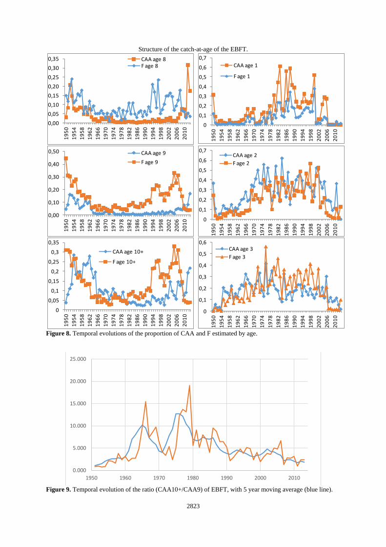
b) Examine overall CAA over time.

The analysis of the CAA of E-BFT (Figures 7) showed four different periods of target fishes. From 1954 to

1965, older fish (10+) represent 20 to 30% of the caches. After, from 1966 to 1980 older fish were around 10%.

The last proportion decreased from 1980 to 1994 with values lower than 10%. Since 1995 the catch of older fish

increased and reached value of 20% in 2013.

c) Determine whether the estimated F ratios ‘match’ observations, e.g. did the fishery change its

targeting during the time period estimated by the F-ratio

The analysis of F (estimated over time showed a decrease during recent years. For the young fish age 1 to 3, this

index matches with the CAA. However, in 2013 CAA was equal to 0 but the F for the age 2 and 3 increased to

reach values around 0.1. For the older fish (age 8, 9 and 10+) CAA and F showed different patterns with

opposite evolution in the year 1950s and 2010s.

The analysis of the ratio (CAA10+/CAA9) by time (Figure 8) showed two break points over time: the years

1965 and 1978. This ratio had reached the values of 15 in 1965 and 19 in 1978. For the periods 1950 to1963 and

from 2006 to 2013 this ratio was lower than 5.

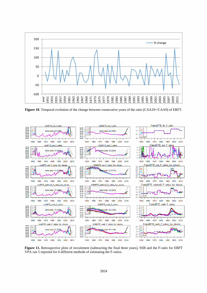
The temporal evolution of change pattern of the ratio ((Change= Ry+1-Ry)/Ry)*100), from 1950 to 2013 (Figure

9), showed a high irregularity between negative and positive changes. We can see the most important variations

between the year 1983 (Change= - 43%) and the year 1984 (Change= +140%) and the year 2009 (Change = -

69%) and the year 2010 (change = 146%).

This analysis does not really provide strong evidence for empirically-derived time blocks for estimating the F-

ratio (Figure 10). The changes in the ratio of CAA10+/CAA9 over time are quite severe and do not clearly lend

themselves to the visual identification of time blocks longer than 5 years, as there is still substantial variation

even for a 5 year moving average.

3.1.4. Potential methods of re-estimating the F-ratio

All 6 methods retain a substantial retrospective error in recruitment (31-62%) and SSB (17-28%) however there

is some substantial improvement offered by some methods (Figure 11). One of the clear patterns is that the

assumption of an F-ratio of 1 in recent years is not supported by the data. For each method that allows the F-ratio

to change in recent years, it is now estimated to be below 1 (Figure 12) indicating that whatever method is

chosen it needs to be flexible to a changing F-ratio. This is similar to the results obtained from profiling the F-

ratio for the last 6 years (Figure 6). While the exact method of estimating the F-ratio, either random walk or as

2815

an offset from previous parameters seems to have a minor impact, it appears that 5 year blocks at a minimum are

necessary to allow for model convergence. For estimation as free parameters or as a random walk in all years,

the model convergence was often poor and run times much longer.

Given the substantial changes in the pCAA in the JLLNEA fishery (Figure 6) that almost requires splitting this

index we evaluated the retrospective performance of the same 6 F-ratio treatments for this run (Figure 13).

Retrospective performance was similar to run 5 with the fixed F-ratio but substantially improved when the F-

ratio was allowed to vary, with retrospective error dropping in half for some treatments. This improvement in

retrospective performance was largely due to a reduction in the strength of the 2004-2007 recruitment estimates,

indicating that their appearance and magnitude is substantially driven by assumptions regarding the F-ratio and

the increase in the JLLNEA index.

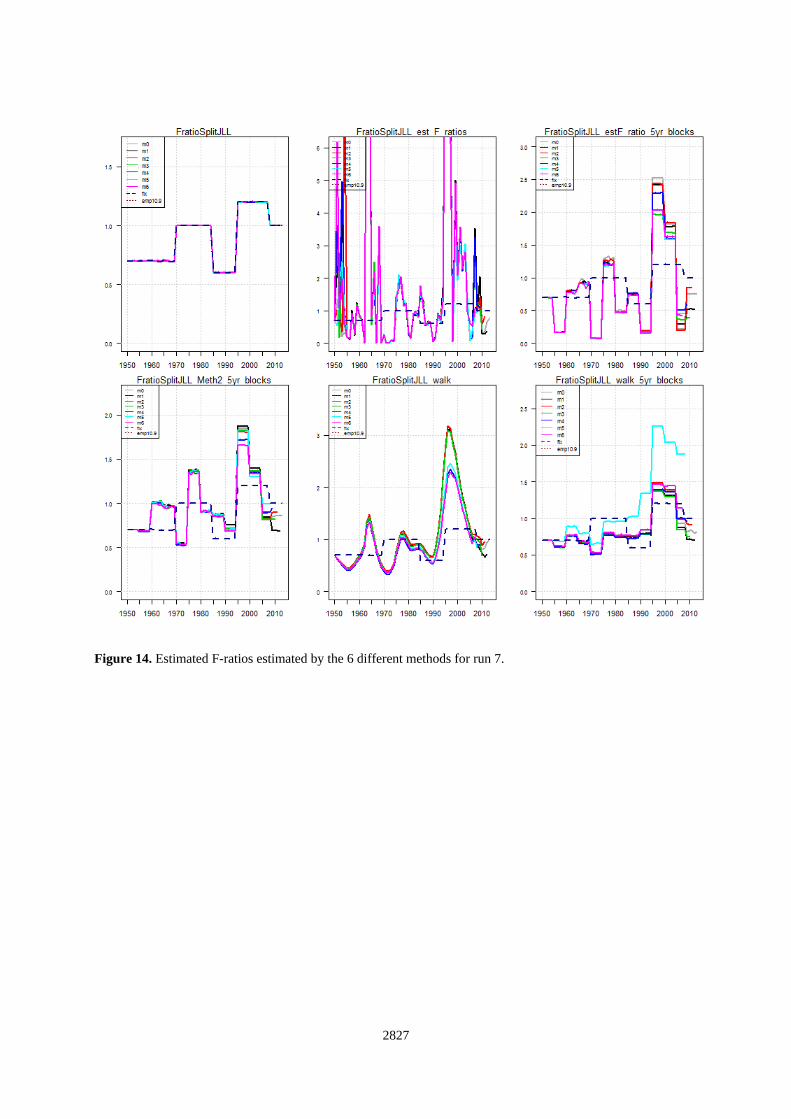
It is informative that the recent F-ratio is, while quite variable and poorly determined from one retrospective to

another, almost always below 1 in the most recent 5-10 years in all treatments (Figure 14) for run 7.

1. Are there logical ‘break points’ in the F-ratio treatment

From the above analysis in section 3.2.1 clear break points were not evident in the time series. Hence we 5 year

break points may be a necessary compromise.

2. Can we extend the plus group age to avoid making an F-ratio assumption?

It would be desirable to avoid estimating the F-ratio entirely and potentially it is possible to extend the plus-

group modeling out to older ages and allowing the F-ratio of the plus group to the age before the plus group to

equal 1. In most cases the estimated pattern in recruitment for the time series is very similar except for the spike

in recruitment seen around 1964-1967. This indicates that extending the plus group does not dramatically smear

the estimate recruitment patterns. However, extending the plus group does not substantially correct the

retrospective error, which remains high and variable across the plus group treatments for either model 5 (Figure

15) or model 7 (Figure 16). What is affected by the plus group extension is the absolute magnitude of the stock

because the assumption of an F ratio of 1 is a relatively strong assumption that overall selectivity is flat-topped.

In most years, the estimated selectivity pattern in the extended plus group models is asymptotic or with

increasing selectivity on the oldest fish. Furthermore, the ratio of F10/F9 (plotted in Figs 15 and 16) is almost

always estimated to be higher than the assumed fixed vector, except in the most recent years, indicating that the

original F-ratio assumptions of an F-ratio less than 1 for much of the time series should be reconsidered. There is

also a clear pattern of a shift in the F10/F9 ratio (plotted in Figures 15-16) from very high levels up to 2005 to a

sharp decline between 2005 and 2006. This was also the time of substantial under-reporting of catch and the fact

that the F-ratio is highly variable at this time makes re-evaluation of the construction of the Inflated catch at age

of particular need. It is not clear from this analysis that extending the plus group solves the retrospective error

but it does highlight that the assumption of an F-ratio less than 1 (and the implied dome-shaped selectivity)

should be evaluated.

3. What are appropriate levels of the random walk flexibility?

The stiffness of the random walk can be specified to allow for greater or less flexibility in the change in F-ratio

over time. Using the 5year blocks we evaluated increasing flexibility in the RW parameter (Figure 17) which

indicated that a more flexible value (0.5) appear to give the best retrospective performance.

5. Discussion

Splitting the Japan longline NEA index, while allowing the F-ratio to vary in the recent years results in

substantial reductions in retrospective error in both SSB and recruitment (Figure 18). The appearance of the

2004-2007 cohorts is driven entirely by the addition of two years of data (2012 and 2013) which only has one

year of ESPMOR trap and two years of JLLNEA and SPBB3 index values. The addition of these data points

seem to cause this retrospective pattern which is substantially mitigated by breaking the Japan longline index and

allowing the F-ratio to vary. Nonetheless the retrospective error on recruitment remains very high, and

particularly the recent F-ratio remains very uncertain and prone to change substantially with each retrospective

peel.

2816

One of the potential causes of this retrospective variability in the F-ratio could be the following of the 2003

cohort by the indices, which are assumed to have constant selectivity over the time period that they are modeled.

The 2003 cohort is clearly seen in the JLL pCAA and appears to move through (Figure 6). It might be necessary

to allow for more flexible selectivity in the pCAA modeling.

Some outstanding issues remain. First the initial F-ratio in 1950 should be profiled. Here in all analyses it was

assumed to be 0.7, however this assumption should be checked. Initial exploration of the catch at age in 1950

indicates that it is very different than the CAA in 1951, potentially indicative of some strange patterns in the

data. It may be desirable to start the model in 1951 if the 1950 CAA is questionable. It should have little bearing

on the VPA results but should help to estimate the initial F-ratios, given the divergence between the CAA in

1950 and 1951.

Recommendations for 2017 VPA

1. Re-evaluate index weighting scenarios, paying particular attention the units and whether they are CVs

or standard errors

2. Re-run this diagnostic analysis on the new CAA and updated VPAs

3. Evaluate the assumption of an initial F-ratio of 0.7 in the starting year, particularly as profiling indicates

a value close to 0.5.

4. Replace fixed F-ratio vector with a random walk in 5 year blocks. Allow that uncertainty in the F-ratio

may be a key modeling uncertainty due to its effect upon scaling the population and its impact on recent

recruitment estimates.

5. Start VPA in 1951 or slightly later. The age composition in 1950 is very different than in 1951, creating

initial instability, potentially not allowing the model to estimate intitial F-ratios, or violating

assumptions of constant F-ratios. Starting the model then should stablize methods that attempt to

estimate the F-ratio.

6. Split indices where dramatic changes in PCAA (Japan longline at 2010) were observed and where

regulatory impacts may have changed the index, Spain Morocco trap after 2009 due to impacts of

Resolution 08-05. One could use the Powers and Restrepo (1992) approach to allow variable selectivity

but if catchability also changes (which is likely) then splitting the index may be best approach.

7. Revise the Inflated CAA, paying particular attention to the mosy likely age composition of unreported

fish due its affect on the F-ratio

References

Legault, C.M., Chair. 2009. Report of the Retrospective Working Group, January 14‐16, 2008, Woods Hole,

Massachusetts. US Dept Commer, Northeast Fish Sci Cent Ref Doc. 09‐01; 30 p. Available from: National

Marine Fisheries Service, 166 Water Street, Woods Hole, MA 02543‐1026, or online at

http://www.nefsc.noaa.gov/nefsc/publications/

Mohn, R. 1999. The retrospective problem in sequential population analysis: An investigation using cod fishery

and simulated data. ICES J. Mar. Sci. 56: 473‐488.

Parma, A. N. 1993. Retrospective catch‐at‐age analysis of pacific halibut: implications on assessment of

harvesting policies. In Proceedings of the International Symposium on Management Strategies for

Exploited Fish Populations, pp. 247–265. Ed. by G. Kruse, D. M. Eggers, C. Pautzke, R. J. Marasco, and T.

J. Quinn II. Alaska Sea Grant College Program.

Powers, J. E., and V. R. Restrepo. 1992. Additional options for age-sequenced analysis. ICCAT Col. Vol. Sci.

Pap. 39(3):540-553.

2817

Figure 1. A. Results of jittering starting seed. B. SSB with the different values of the objective function

indicating that both solutions are almost the same.

2818

Figure 2. First derivative test for EBFT 2014 Run 5 report.

Figure 3. Likelihood profiling of the Fratio in the initial years (1950-1955) and the F-ratio in the last 6 years.

Note the difference between estimation with and without constraints. The constraints are applied which constrain

the change in the F-ratio for 1956.

2819

Figure 4. Retrospective plots of recruitment (subtracting the final three years), SSB and the F-ratio for EBFT

VPA run 5 reported. The F-ratio plot also shows the empirical ratio of catch of 10/catch 9 year old fish plotted as

dashed lines.

2820

Figure 5. Fits to CPUE indices and residual patterns.

2821

Figure 5, continued. Fits to CPUE indices and residual patterns.

2822

Figure 6. Structure of the partial catch-at-age of the EBFT.

Figure 7. Structure of the catch-at-age of the EBFT.

0%

10%

20%

30%

40%

50%

60%

70%

80%

90%

100%

1970

1973

1976

1979

1982

1985

1988

1991

1994

1997

2000

2003

2006

2009

2012

'ESPMarTrap'

age 10+

age 9

age 8

age 7

age 6

age 5

age 4

age 3

age 2

age 10%

10%

20%

30%

40%

50%

60%

70%

80%

90%

100%

1970

1973

1976

1979

1982

1985

1988

1991

1994

1997

2000

2003

2006

2009

'JLL EastMed'age 10+

age 9

age 8

age 7

age 6

age 5

age 4

age 3

age 2

age 1

0%

10%

20%

30%

40%

50%

60%

70%

80%

90%

100% 'JPLL'

age 10+

age 9

age 8

age 7

age 6

age 5

age 4

age 3

age 2

age 1

0%

10%

20%

30%

40%

50%

60%

70%

80%

90%

100%

19521953195419551956195719581959196019611962

'SP BB1'age 10+

age 9

age 8

age 7

age 6

age 5

age 4

age 3

age 2

age 1

0%

10%

20%

30%

40%

50%

60%

70%

80%

90%

100%

1963

1966

1969

1972

1975

1978

1981

1984

1987

1990

1993

1996

1999

2002

2005

'SP BB2'age 10+

age 9

age 8

age 7

age 6

age 5

age 4

age 3

age 2

age 10%

10%

20%

30%

40%

50%

60%

70%

80%

90%

100%

2007 2008 2009 2010 2011 2012 2013

'SP BB3'age 10+

age 9

age 8

age 7

age 6

age 5

age 4

age 3

age 2

age 1

2823

Structure of the catch-at-age of the EBFT.

Figure 8. Temporal evolutions of the proportion of CAA and F estimated by age.

Figure 9. Temporal evolution of the ratio (CAA10+/CAA9) of EBFT, with 5 year moving average (blue line).

0,00

0,05

0,10

0,15

0,20

0,25

0,30

0,351

95

0

19

54

19

58

19

62

19

66

19

70

19

74

19

78

19

82

19

86

19

90

19

94

19

98

20

02

20

06

20

10

CAA age 8F age 8

0

0,1

0,2

0,3

0,4

0,5

0,6

0,7

19

50

19

54

19

58

19

62

19

66

19

70

19

74

19

78

19

82

19

86

19

90

19

94

19

98

20

02

20

06

20

10

CAA age 1

F age 1

0,00

0,10

0,20

0,30

0,40

0,50

19

50

19

54

19

58

19

62

19

66

19

70

19

74

19

78

19

82

19

86

19

90

19

94

19

98

20

02

20

06

20

10

CAA age 9

F age 9

0

0,1

0,2

0,3

0,4

0,5

0,6

0,7

19

50

19

54

19

58

19

62

19

66

19

70

19

74

19

78

19

82

19

86

19

90

19

94

19

98

20

02

20

06

20

10

CAA age 2

F age 2

0

0,05

0,1

0,15

0,2

0,25

0,3

0,35

19

50

19

54

19

58

19

62

19

66

19

70

19

74

19

78

19

82

19

86

19

90

19

94

19

98

20

02

20

06

20

10

CAA age 10+

F age 10+

0

0,1

0,2

0,3

0,4

0,5

0,6

19

50

19

54

19

58

19

62

19

66

19

70

19

74

19

78

19

82

19

86

19

90

19

94

19

98

20

02

20

06

20

10

CAA age 3

F age 3

0.000

5.000

10.000

15.000

20.000

25.000

1950 1960 1970 1980 1990 2000 2010

2824

Figure 10. Temporal evolution of the change between consecutive years of the ratio (CAA10+/CAA9) of EBFT.

Figure 11. Retrospective plots of recruitment (subtracting the final three years), SSB and the F-ratio for EBFT

VPA run 5 reported for 6 different methods of estimating the F-ratios.

-100

-50

0

50

100

150

200ye

ar

19

51

19

53

19

55

19

57

19

59

19

61

19

63

19

65

19

67

19

69

19

71

19

73

19

75

19

77

19

79

19

81

19

83

19

85

19

87

19

89

19

91

19

93

19

95

19

97

19

99

20

01

20

03

20

05

20

07

20

09

20

11

% change

2825

Figure 12. Estimated F-ratios estimated by the 6 different methods for run 5.

2826

Figure 13. Retrospective plots of recruitment (subtracting the final three years), SSB and the F-ratio for EBFT

VPA run 7 (split JLL NEA) reported for 6 different methods of estimating the F-ratios.

2827

Figure 14. Estimated F-ratios estimated by the 6 different methods for run 7.

2828

Figure 15. Extending the plus group from 10-16, for run 5.

2829

Figure 16. Extending the plus group from 10-16, for run 7.

2830

Figure 17. Evaluation of how stiff to penalize the random walk departures. Increasing sigma values from 0.1,

0.2, 0.3, 0.4 and 0.5 increases flexibility of the random walk.

2831

Figure 18. Recommended treatment of random walk in 5 year time blocks for the F-ratio.