Visual Models of Plants Interacting with TheirEnvironmentRadomir Mech and Przemyslaw PrusinkiewiczDepartment of Computer ScienceUniversity of CalgaryCalgary, Alberta, Canada T2N 1N4e−mail: mech|pwp@cpsc.ucalgary.ca

Abstract

Interaction with the environment is a key factor affecting the development of plants and plantecosystems. In this paper we introduce a modeling framework that makes it possible tosimulate and visualize a wide range of interactions at the level of plant architecture. Thisframework extends the formalism of Lindenmayer systems with constructs needed to modelbi−directional information exchange between plants and their environment. We illustrate theproposed framework with models and simulations that capture the development of treebranches limited by collisions, the colonizing growth of clonal plants competing for space infavorable areas, the interaction between roots competing for water in the soil, and thecompetition within and between trees for access to light. Computer animation andvisualization techniques make it possible to better understand the modeled processes and leadto realistic images of plants within their environmental context.

Keywords: scientific visualization, realistic image synthesis, software design, L−system,modeling, simulation, ecosystem, plant development, clonal plant, root, tree.

Reference

Radomir Mech and Przemyslaw Prusinkiewicz. Visual Models of Plants Interacting with Their Environment.Proceedings of SIGGRAPH 96 (New Orleans, Louisiana, August 4−9, 1996). In Computer GraphicsProceedings, Annual Conference Series, 1996, ACM SIGGRAPH, pp. 397−410.

Visual Models of PlantsInteracting with Their Environment

Radomır Mech and Przemyslaw Prusinkiewicz1

University of Calgary

ABSTRACT

Interaction with the environment is a key factor affecting the devel-opment of plants and plant ecosystems. In this paper we introduce amodeling framework that makes it possible to simulate and visualizea wide range of interactions at the level of plant architecture. Thisframework extends the formalism of Lindenmayer systems withconstructs needed to model bi-directional information exchange be-tween plants and their environment. We illustrate the proposedframework with models and simulations that capture the develop-ment of tree branches limited by collisions, the colonizing growth ofclonal plants competing for space in favorable areas, the interactionbetween roots competing for water in the soil, and the competitionwithin and between trees for access to light. Computer animationand visualization techniques make it possible to better understandthe modeled processes and lead to realistic images of plants withintheir environmental context.

CR categories: F.4.2 [Mathematical Logic and Formal Lan-guages]: Grammars and Other Rewriting Systems: Parallel rewrit-ing systems, I.3.7 [Computer Graphics]: Three-DimensionalGraphics and Realism, I.6.3 [Simulation and Modeling]: Appli-cations, J.3 [Life and Medical Sciences]: Biology.

Keywords: scientific visualization, realistic image synthesis, soft-ware design, L-system, modeling, simulation, ecosystem, plant de-velopment, clonal plant, root, tree.

1 INTRODUCTION

Computer modeling and visualization of plant development can betraced back to 1962, when Ulam applied cellular automata to sim-ulate the development of branching patterns, thought of as an ab-stract representation of plants [53]. Subsequently, Cohen presenteda more realistic model operating in continuous space [13], Linden-

1Department of Computer Science, University of Calgary, Cal-gary, Alberta, Canada T2N 1N4 (mechjpwp@cpsc.ucalgary.ca)

mayer proposed the formalism of L-systems as a general frameworkfor plant modeling [38, 39], and Honda introduced the first computermodel of tree structures [32]. From these origins, plant modelingemerged as a vibrant area of interdisciplinary research, attracting theefforts of biologists, applied plant scientists, mathematicians, andcomputer scientists. Computer graphics, in particular, contributeda wide range of models and methods for synthesizing images ofplants. See [18, 48, 54] for recent reviews of the main results.

One aspect of plant structure and behavior neglected by most modelsis the interaction between plants and their environment (includingother plants). Indeed, the incorporation of interactions has beenidentified as one of the main outstanding problems in the domain ofplant modeling [48] (see also [15, 18, 50]). Its solution is needed toconstruct predictive models suitable for applications ranging fromcomputer-assisted landscape and garden design to the determinationof crop and lumber yields in agriculture and forestry.

Using the information flow between a plant and its environment asthe classification key, we can distinguish three forms of interactionand the associated models of plant-environment systems devised todate:

1. The plant is affected by global properties of the environment,such as day length controlling the initiation of flowering [23]and daily minimum and maximum temperatures modulating thegrowth rate [28].

2. The plant is affected by local properties of the environment, suchas the presence of obstacles controlling the spread of grass [2]and directing the growth of tree roots [26], geometry of supportfor climbing plants [2, 25], soil resistance and temperature invarious soil layers [16], and predefined geometry of surfaces towhich plant branches are pruned [45].

3. The plant interacts with the environment in an information feed-back loop, where the environment affects the plant and the plantreciprocally affects the environment. This type of interaction isrelated to sighted [4] or exogenous [42] mechanisms controllingplant development, in which parts of a plant influence the devel-opment of other parts of the same or a different plant through thespace in which they grow. Specific models capture:

� competition for space (including collision detection and ac-cess to light) between segments of essentially two-dimensionalschematic branching structures [4, 13, 21, 22, 33, 34, 36];

� competition between root tips for nutrients and water trans-ported in soil [12, 37] (this mechanism is related to competitionbetween growing branches of corals and sponges for nutrientsdiffusing in water [34]);

� competition for light between three-dimensional shoots ofherbaceous plants [25] and branches of trees [9, 10, 11, 15,33, 35, 52].

Models of exogenous phenomena require a comprehensive repre-sentation of both the developing plant and the environment. Con-sequently, they are the most difficult to formulate, implement, anddocument. Programs addressed to the biological audience are oftenlimited to narrow groups of plants (for example, poplars [9] or treesin the pine family [21]), and present the results in a rudimentarygraphical form. On the other hand, models addressed to the com-puter graphics audience use more advanced techniques for realisticimage synthesis, but put little emphasis on the faithful reproductionof physiological mechanisms characteristic to specific plants.

In this paper we propose a general framework (defined as a mod-eling methodology supported by appropriate software) for mod-eling, simulating, and visualizing the development of plants thatbi-directionally interact with their environment. The usefulness ofmodeling frameworks for simulation studies of models with com-plex (emergent) behavior is manifested by previous work in the-oretical biology, artificial life, and computer graphics. Examplesinclude cellular automata [51], systems for simulating behavior ofcellular structures in discrete [1] and continuous [20] spaces, andL-system-based frameworks for modeling plants [36, 46]. Frame-works may have the form of a general-purpose simulation programthat accepts models described in a suitable mini-language as in-put, e.g. [36, 46], or a set of library programs [27]. Compared tospecial-purpose programs, they offer the following benefits:

� At the conceptual level, they facilitate the design, specification,documentation, and comparison of models.

� At the level of model implementation, they make it possible to de-velop software that can be reused in various models. Specifically,graphical capabilities needed to visualize the models become apart of the modeling framework, and do not have to be reimple-mented.

� Finally, flexible conceptual and software frameworks facilitateinteractive experimentation with the models [46, Appendix A].

Our framework is intended both for purpose of image synthesis andas a research and visualization tool for model studies in plant mor-phogenesis and ecology. These goals are addressed at the levels ofthe simulation system and the modeling language design. The un-derlying paradigm of plant-environment interaction is described inSection 2. The resulting design of the simulation software is outlinedin Section 3. The language for specifying plant models is presentedin Section 4. It extends the concept of environmentally-sensitive L-systems [45] with constructs for bi-directional communication withthe environment. The following sections illustrate the proposedframework with concrete models of plants interacting with theirenvironment. The examples include: the development of planarbranching systems controlled by the crowding of apices (Section 5),the development of clonal plants controlled by both the crowdingof ramets and the quality of terrain (Section 6), the developmentof roots controlled by the concentration of water transported in thesoil (Section 7), and the development of tree crowns affected by thelocal distribution of light (Section 8) The paper concludes with anevaluation of the results and a list of open problems (Section 9).

Plant Environment

Internal processes

Reception

Response

Internal processes

Reception

Response

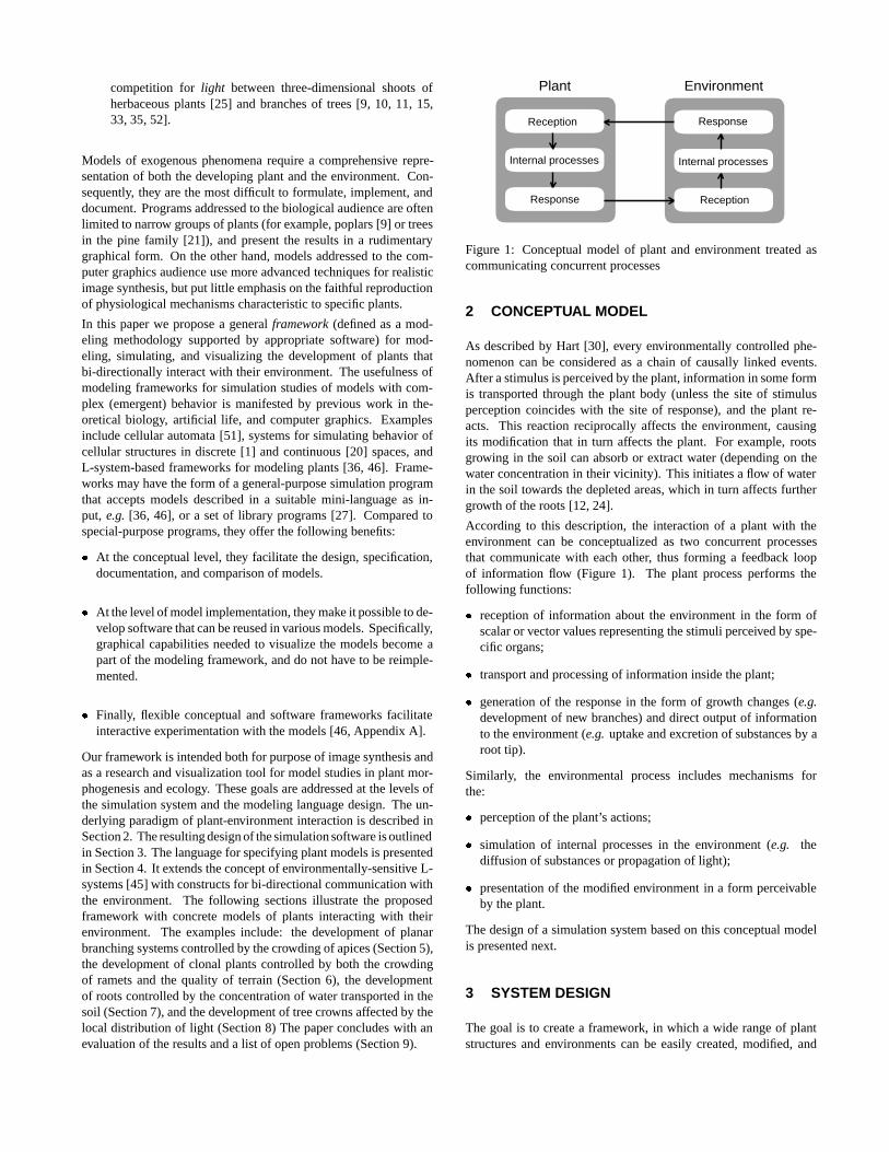
Figure 1: Conceptual model of plant and environment treated ascommunicating concurrent processes

2 CONCEPTUAL MODEL

As described by Hart [30], every environmentally controlled phe-nomenon can be considered as a chain of causally linked events.After a stimulus is perceived by the plant, information in some formis transported through the plant body (unless the site of stimulusperception coincides with the site of response), and the plant re-acts. This reaction reciprocally affects the environment, causingits modification that in turn affects the plant. For example, rootsgrowing in the soil can absorb or extract water (depending on thewater concentration in their vicinity). This initiates a flow of waterin the soil towards the depleted areas, which in turn affects furthergrowth of the roots [12, 24].

According to this description, the interaction of a plant with theenvironment can be conceptualized as two concurrent processesthat communicate with each other, thus forming a feedback loopof information flow (Figure 1). The plant process performs thefollowing functions:

� reception of information about the environment in the form ofscalar or vector values representing the stimuli perceived by spe-cific organs;

� transport and processing of information inside the plant;

� generation of the response in the form of growth changes (e.g.development of new branches) and direct output of informationto the environment (e.g. uptake and excretion of substances by aroot tip).

Similarly, the environmental process includes mechanisms forthe:

� perception of the plant’s actions;

� simulation of internal processes in the environment (e.g. thediffusion of substances or propagation of light);

� presentation of the modified environment in a form perceivableby the plant.

The design of a simulation system based on this conceptual modelis presented next.

3 SYSTEM DESIGN

The goal is to create a framework, in which a wide range of plantstructures and environments can be easily created, modified, and

used for experimentation. This requirement led us to the followingdesign decisions:

� The plant and the environment should be modeled by separateprograms and run as two communicating processes. This designis:

� compatible with the assumed conceptual model of plant-envi-ronment interaction (Figure 1);

� consistent with the principles of structured design (moduleswith clearly specified functions jointly contribute to the solu-tion of a problem by communicating through a well definedinterface; information local to each module is hidden fromother modules);

� appropriate for interactive experimentation with the models;in particular, changes in the plant program can be implementedwithout affecting the environmental program, and vice versa;

� extensible to distributed computing environments, where dif-ferent components of a large ecosystem may be simulatedusing separate computers.

� The user should have control over the type and amount of infor-mation exchanged between the processes representing the plantand the environment, so that all the needed but no superfluousinformation is transferred.

� Plant models should be specified in a language based on L-systems, equipped with constructs for bi-directional communi-cation between the plant and the environment. This decision hasthe following rationale:

� A succinct description of the models in an interpreted lan-guage facilitates experimentation involving modifications tothe models;

� L-systems capture two fundamental mechanisms that controldevelopment, namely flow of information from a mother mod-ule to its offspring (cellular descent) and flow of informationbetween coexisting modules (endogenous interaction) [38].The latter mechanism plays an essential role in transmittinginformation from the site of stimulus perception to the siteof the response. Moreover, L-systems have been extendedto allow for input of information from the environment (seeSection 4);

� Modeling of plants using L-systems has reached a relativelyadvanced state, manifested by models ranging from algae toherbaceous plants and trees [43, 46].

� Given the variety of processes that may take place in the environ-ment, they should be modeled using special-purpose programs.

� Generic aspects of modeling, not specific to particular models,should be supported by the modeling system. This includes:

� an L-system-based plant modeling program, which interpretsL-systems supplied as its input and visualizes the results, and

� the support for communication and synchronization of pro-cesses simulating the modeled plant and the environment.

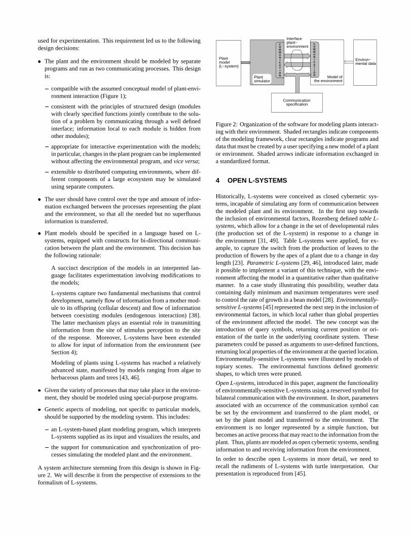
A system architecture stemming from this design is shown in Fig-ure 2. We will describe it from the perspective of extensions to theformalism of L-systems.

Plantmodel(L−system)

Plantsimulator

Model of the environment

Interfaceplant−environment

Environ−mental data

COMMUNICATION

COMMUNICATION

Communicationspecification

Figure 2: Organization of the software for modeling plants interact-ing with their environment. Shaded rectangles indicate componentsof the modeling framework, clear rectangles indicate programs anddata that must be created by a user specifying a new model of a plantor environment. Shaded arrows indicate information exchanged ina standardized format.

4 OPEN L-SYSTEMS

Historically, L-systems were conceived as closed cybernetic sys-tems, incapable of simulating any form of communication betweenthe modeled plant and its environment. In the first step towardsthe inclusion of environmental factors, Rozenberg defined table L-systems, which allow for a change in the set of developmental rules(the production set of the L-system) in response to a change inthe environment [31, 49]. Table L-systems were applied, for ex-ample, to capture the switch from the production of leaves to theproduction of flowers by the apex of a plant due to a change in daylength [23]. Parametric L-systems [29, 46], introduced later, madeit possible to implement a variant of this technique, with the envi-ronment affecting the model in a quantitative rather than qualitativemanner. In a case study illustrating this possibility, weather datacontaining daily minimum and maximum temperatures were usedto control the rate of growth in a bean model [28]. Environmentally-sensitive L-systems [45] represented the next step in the inclusion ofenvironmental factors, in which local rather than global propertiesof the environment affected the model. The new concept was theintroduction of query symbols, returning current position or ori-entation of the turtle in the underlying coordinate system. Theseparameters could be passed as arguments to user-defined functions,returning local properties of the environment at the queried location.Environmentally-sensitive L-systems were illustrated by models oftopiary scenes. The environmental functions defined geometricshapes, to which trees were pruned.

Open L-systems, introduced in this paper, augment the functionalityof environmentally-sensitive L-systems using a reserved symbol forbilateral communication with the environment. In short, parametersassociated with an occurrence of the communication symbol canbe set by the environment and transferred to the plant model, orset by the plant model and transferred to the environment. Theenvironment is no longer represented by a simple function, butbecomes an active process that may react to the information from theplant. Thus, plants are modeled as open cybernetic systems, sendinginformation to and receiving information from the environment.

In order to describe open L-systems in more detail, we need torecall the rudiments of L-systems with turtle interpretation. Ourpresentation is reproduced from [45].

An L-system is a parallel rewriting system operating on branchingstructures represented as bracketed strings of symbols with asso-ciated numerical parameters, called modules. Matching pairs ofsquare brackets enclose branches. Simulation begins with an ini-tial string called the axiom, and proceeds in a sequence of discretederivation steps. In each step, rewriting rules or productions replaceall modules in the predecessor string by successor modules. Theapplicability of a production depends on a predecessor’s context(in context-sensitive L-systems), values of parameters (in produc-tions guarded by conditions), and on random factors (in stochasticL-systems). Typically, a production has the format:

id : lc < pred > rc : cond! succ : prob

where id is the production identifier (label), lc, pred, and rc arethe left context, the strict predecessor, and the right context, cond isthe condition, succ is the successor, and prob is the probability ofproduction application. The strict predecessor and the successor arethe only mandatory fields. For example, the L-system given belowconsists of axiom ! and three productions p1, p2, and p3.

!: A(1)B(3)A(5)p1: A(x) !A(x+1) : 0.4p2: A(x) !B(x–1) : 0.6p3: A(x) < B(y) > A(z) : y < 4!B(x+z)[A(y)]

The stochastic productions p1 and p2 replace module A(x) by ei-ther A(x + 1) or B(x � 1), with probabilities equal to 0.4 and0.6, respectively. The context-sensitive production p3 replaces amodule B(y) with left context A(x) and right context A(z) bymodule B(x+ z) supporting branch A(y). The application of thisproduction is guarded by condition y < 4. Consequently, the firstderivation step may have the form:

A(1)B(3)A(5) ) A(2)B(6)[A(3)]B(4)

It was assumed that, as a result of random choice, production p1

was applied to the module A(1), and production p2 to the moduleA(5). Production p3 was applied to the module B(3), because itoccurred with the required left and right context, and the condition3 < 4 was true.

In the L-systems presented as examples we also use several addi-tional constructs (cf. [29, 44]):

� Productions may include statements assigning values to localvariables. These statements are enclosed in curly braces andseparated by semicolons.

� The L-systems may also include arrays. References to arrayelements follow the syntax of C; for example, MaxLen[order].

� The list of productions is ordered. In the deterministic case, thefirst matching production applies. In the stochastic case, the setof all matching productions is established, and one of them ischosen according to the specified probabilities.

For details of the L-system syntax see [29, 43, 46].

H\→

/L

−+

U→

→

^

&

Figure 3: Controlling theturtle in three dimensions

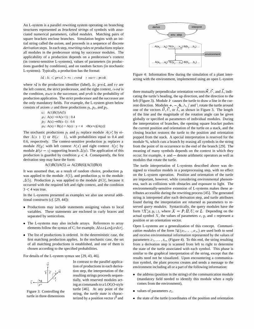
In contrast to the parallel applica-tion of productions in each deriva-tion step, the interpretation of theresulting strings proceeds sequen-tially, with reserved modules act-ing as commands to a LOGO-styleturtle [46]. At any point of thestring, the turtle state is charac-terized by a position vector ~P and

derive

env. step

interpret

... A(a1,...,ak) ?E(x1,...,xm) B(b1,...,bn) ...

... A(a1,...,ak) ?E(y1,...,ym) B(b1,...,bn) ...

environment

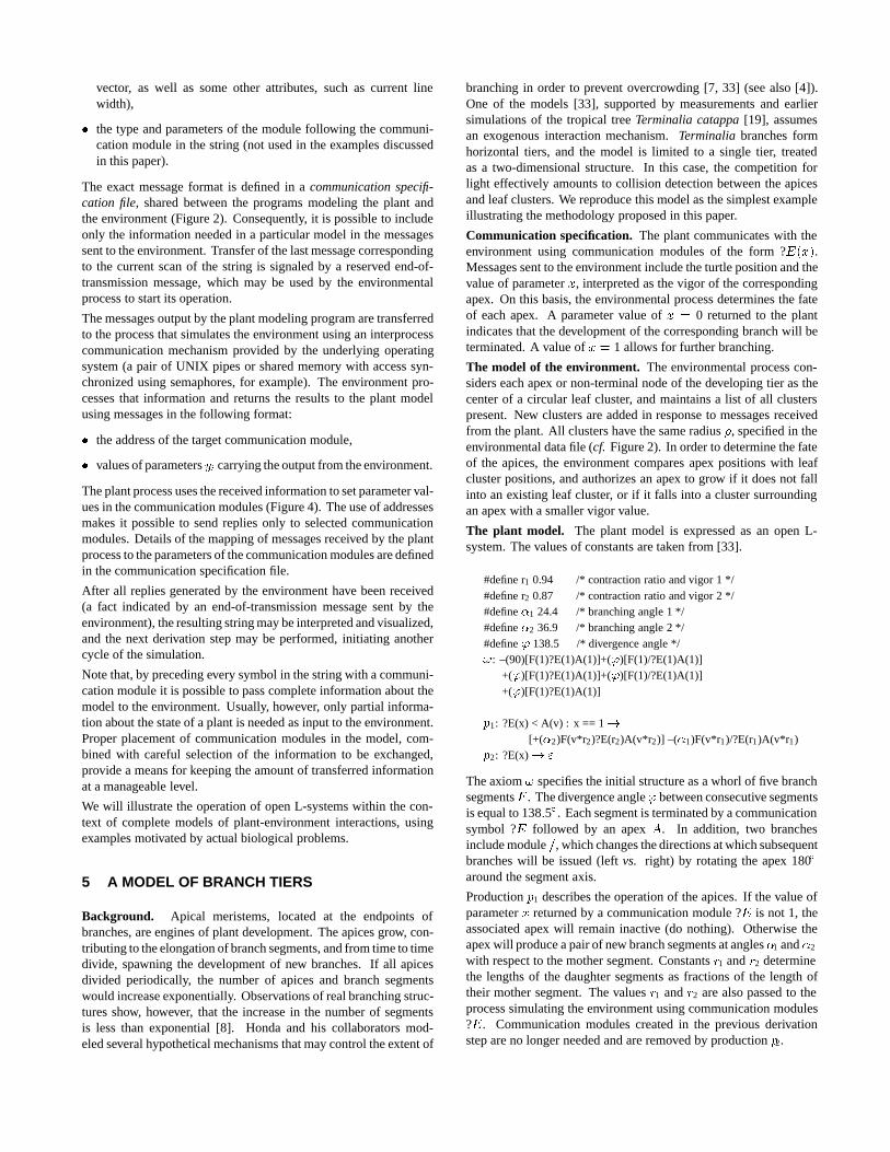
Figure 4: Information flow during the simulation of a plant inter-acting with the environment, implemented using an open L-system

three mutually perpendicular orientation vectors ~H, ~U , and ~L, indi-cating the turtle’s heading, the up direction, and the direction to theleft (Figure 3). Module F causes the turtle to draw a line in the cur-rent direction. Modules +,�, &, ^, = and n rotate the turtle aroundone of the vectors ~H; ~U , or ~L, as shown in Figure 3. The lengthof the line and the magnitude of the rotation angle can be givenglobally or specified as parameters of individual modules. Duringthe interpretation of branches, the opening square bracket pushesthe current position and orientation of the turtle on a stack, and theclosing bracket restores the turtle to the position and orientationpopped from the stack. A special interpretation is reserved for themodule %, which cuts a branch by erasing all symbols in the stringfrom the point of its occurrence to the end of the branch [29]. Themeaning of many symbols depends on the context in which theyoccur; for example, + and � denote arithmetic operators as well asmodules that rotate the turtle.

The turtle interpretation of L-systems described above was de-signed to visualize models in a postprocessing step, with no effecton the L-system operation. Position and orientation of the turtleare important, however, while considering environmental phenom-ena, such as collisions with obstacles and exposure to light. Theenvironmentally-sensitive extension of L-systems makes these at-tributes accessible during the rewriting process [45]. The generatedstring is interpreted after each derivation step, and turtle attributesfound during the interpretation are returned as parameters to re-served query modules. Syntactically, the query modules have theform ?X(x; y; z), where X = P;H;U; or L. Depending on theactual symbol X , the values of parameters x, y, and z represent aposition or an orientation vector.

Open L-systems are a generalization of this concept. Communi-cation modules of the form ?E(x1; : : : ; xm) are used both to sendand receive environmental information represented by the values ofparameters x1; : : : ; xm (Figure 4). To this end, the string resultingfrom a derivation step is scanned from left to right to determinethe state of the turtle associated with each symbol. This phase issimilar to the graphical interpretation of the string, except that theresults need not be visualized. Upon encountering a communica-tion symbol, the plant process creates and sends a message to theenvironment including all or a part of the following information:

� the address (position in the string) of the communication module(mandatory field needed to identify this module when a replycomes from the environment),

� values of parameters xi,

� the state of the turtle (coordinates of the position and orientation

vector, as well as some other attributes, such as current linewidth),

� the type and parameters of the module following the communi-cation module in the string (not used in the examples discussedin this paper).

The exact message format is defined in a communication specifi-cation file, shared between the programs modeling the plant andthe environment (Figure 2). Consequently, it is possible to includeonly the information needed in a particular model in the messagessent to the environment. Transfer of the last message correspondingto the current scan of the string is signaled by a reserved end-of-transmission message, which may be used by the environmentalprocess to start its operation.

The messages output by the plant modeling program are transferredto the process that simulates the environment using an interprocesscommunication mechanism provided by the underlying operatingsystem (a pair of UNIX pipes or shared memory with access syn-chronized using semaphores, for example). The environment pro-cesses that information and returns the results to the plant modelusing messages in the following format:

� the address of the target communication module,

� values of parameters yi carrying the output from the environment.

The plant process uses the received information to set parameter val-ues in the communication modules (Figure 4). The use of addressesmakes it possible to send replies only to selected communicationmodules. Details of the mapping of messages received by the plantprocess to the parameters of the communication modules are definedin the communication specification file.

After all replies generated by the environment have been received(a fact indicated by an end-of-transmission message sent by theenvironment), the resulting string may be interpreted and visualized,and the next derivation step may be performed, initiating anothercycle of the simulation.

Note that, by preceding every symbol in the string with a communi-cation module it is possible to pass complete information about themodel to the environment. Usually, however, only partial informa-tion about the state of a plant is needed as input to the environment.Proper placement of communication modules in the model, com-bined with careful selection of the information to be exchanged,provide a means for keeping the amount of transferred informationat a manageable level.

We will illustrate the operation of open L-systems within the con-text of complete models of plant-environment interactions, usingexamples motivated by actual biological problems.

5 A MODEL OF BRANCH TIERS

Background. Apical meristems, located at the endpoints ofbranches, are engines of plant development. The apices grow, con-tributing to the elongation of branch segments, and from time to timedivide, spawning the development of new branches. If all apicesdivided periodically, the number of apices and branch segmentswould increase exponentially. Observations of real branching struc-tures show, however, that the increase in the number of segmentsis less than exponential [8]. Honda and his collaborators mod-eled several hypothetical mechanisms that may control the extent of

branching in order to prevent overcrowding [7, 33] (see also [4]).One of the models [33], supported by measurements and earliersimulations of the tropical tree Terminalia catappa [19], assumesan exogenous interaction mechanism. Terminalia branches formhorizontal tiers, and the model is limited to a single tier, treatedas a two-dimensional structure. In this case, the competition forlight effectively amounts to collision detection between the apicesand leaf clusters. We reproduce this model as the simplest exampleillustrating the methodology proposed in this paper.

Communication specification. The plant communicates with theenvironment using communication modules of the form ?E(x).Messages sent to the environment include the turtle position and thevalue of parameter x, interpreted as the vigor of the correspondingapex. On this basis, the environmental process determines the fateof each apex. A parameter value of x = 0 returned to the plantindicates that the development of the corresponding branch will beterminated. A value of x = 1 allows for further branching.

The model of the environment. The environmental process con-siders each apex or non-terminal node of the developing tier as thecenter of a circular leaf cluster, and maintains a list of all clusterspresent. New clusters are added in response to messages receivedfrom the plant. All clusters have the same radius �, specified in theenvironmental data file (cf. Figure 2). In order to determine the fateof the apices, the environment compares apex positions with leafcluster positions, and authorizes an apex to grow if it does not fallinto an existing leaf cluster, or if it falls into a cluster surroundingan apex with a smaller vigor value.

The plant model. The plant model is expressed as an open L-system. The values of constants are taken from [33].

#define r1 0.94 /* contraction ratio and vigor 1 */#define r2 0.87 /* contraction ratio and vigor 2 */#define �1 24.4 /* branching angle 1 */#define �2 36.9 /* branching angle 2 */#define ' 138.5 /* divergence angle */!: –(90)[F(1)?E(1)A(1)]+(')[F(1)/?E(1)A(1)]

+(')[F(1)?E(1)A(1)]+(')[F(1)/?E(1)A(1)]+(')[F(1)?E(1)A(1)]

p1: ?E(x) < A(v) : x == 1 ![+(�2)F(v*r2)?E(r2)A(v*r2)] –(�1)F(v*r1)/?E(r1)A(v*r1)

p2: ?E(x) ! "

The axiom ! specifies the initial structure as a whorl of five branchsegmentsF . The divergence angle' between consecutive segmentsis equal to 138:5�. Each segment is terminated by a communicationsymbol ?E followed by an apex A. In addition, two branchesinclude module =, which changes the directions at which subsequentbranches will be issued (left vs. right) by rotating the apex 180�

around the segment axis.

Production p1 describes the operation of the apices. If the value ofparameter x returned by a communication module ?E is not 1, theassociated apex will remain inactive (do nothing). Otherwise theapex will produce a pair of new branch segments at angles �1 and �2

with respect to the mother segment. Constants r1 and r2 determinethe lengths of the daughter segments as fractions of the length oftheir mother segment. The values r1 and r2 are also passed to theprocess simulating the environment using communication modules?E. Communication modules created in the previous derivationstep are no longer needed and are removed by production p2.

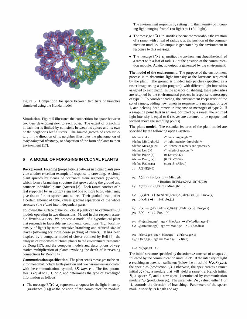
Figure 5: Competition for space between two tiers of branchessimulated using the Honda model

Simulation. Figure 5 illustrates the competition for space betweentwo tiers developing next to each other. The extent of branchingin each tier is limited by collisions between its apices and its ownor the neighbor’s leaf clusters. The limited growth of each struc-ture in the direction of its neighbor illustrates the phenomenon ofmorphological plasticity, or adaptation of the form of plants to theirenvironment [17].

6 A MODEL OF FORAGING IN CLONAL PLANTS

Background. Foraging (propagation) patterns in clonal plants pro-vide another excellent example of response to crowding. A clonalplant spreads by means of horizontal stem segments (spacers),which form a branching structure that grows along the ground andconnects individual plants (ramets) [3]. Each ramet consists of aleaf supported by an upright stem and one or more buds, which maygive rise to further spacers and ramets. Their gradual death, aftera certain amount of time, causes gradual separation of the wholestructure (the clone) into independent parts.

Following the surface of the soil, clonal plants can be captured usingmodels operating in two dimensions [5], and in that respect resem-ble Terminalia tiers. We propose a model of a hypothetical plantthat responds to favorable environmental conditions (high local in-tensity of light) by more extensive branching and reduced size ofleaves (allowing for more dense packing of ramets). It has beeninspired by a computer model of clover outlined by Bell [4], theanalysis of responses of clonal plants to the environment presentedby Dong [17], and the computer models and descriptions of veg-etative multiplication of plants involving the death of interveningconnections by Room [47].

Communication specification. The plant sends messages to the en-vironment that include turtle position and two parameters associatedwith the communications symbol, ?E(type; x). The first param-eter is equal to 0, 1, or 2, and determines the type of exchangedinformation as follows:

� The message ?E(0; x) represents a request for the light intensity(irradiance [14]) at the position of the communication module.

The environment responds by setting x to the intensity of incom-ing light, ranging from 0 (no light) to 1 (full light).

� The message ?E(1; x) notifies the environment about the creationof a ramet with a leaf of radius x at the position of the commu-nication module. No output is generated by the environment inresponse to this message.

� The message ?E(2; x) notifies the environment about the death ofa ramet with a leaf of radius x at the position of the communica-tion module. Again, no output is generated by the environment.

The model of the environment. The purpose of the environmentprocess is to determine light intensity at the locations requestedby the plant. The ground is divided into patches (specified as araster image using a paint program), with different light intensitiesassigned to each patch. In the absence of shading, these intensitiesare returned by the environmental process in response to messagesof type 0. To consider shading, the environment keeps track of theset of ramets, adding new ramets in response to a messages of type1, and deleting dead ramets in response to messages of type 2. Ifa sampling point falls in an area occupied by a ramet, the returnedlight intensity is equal to 0 (leaves are assumed to be opaque, andlocated above the sampling points).

The plant model. The essential features of the plant model arespecified by the following open L-system.

#define � 45 /* branching angle */#define MinLight 0.1 /* light intensity threshold */#define MaxAge 20 /* lifetime of ramets and spacers */#define Len 2.0 /* length of spacers */#define ProbB (x) (0.12+x*0.42)#define ProbR(x) (0.03+x*0.54)#define Radius(x) (sqrt(15–x*5)/�)

!: A(1)?E(0,0)

p1: A(dir) > ?E(0,x) : x >= MinLight! R(x)B(x,dir)F(Len,0)A(–dir)?E(0,0)

p2: A(dir) > ?E(0,x) : x < MinLight ! "

p3: B(x,dir) ! [+(�*dir)F(Len,0)A(–dir)?E(0,0)] : ProbB (x)p4: B(x,dir) ! " : 1–ProbB (x)

p5: R(x) ! [@o(Radius(x),0)?E(1,Radius(x))] : ProbR(x)p6: R(x) ! " : 1–ProbR(x)

p7: @o(radius,age): age < MaxAge !@o(radius,age+1)p8: @o(radius,age): age == MaxAge ! ?E(2,radius)

p9: F(len,age): age < MaxAge ! F(len,age+1)p10: F(len,age): age == MaxAge ! f(len)

p11: ?E(type,x) ! "

The initial structure specified by the axiom ! consists of an apex Afollowed by the communication module ?E. If the intensity of lightx reaching an apex is insufficient (below the threshold MinLight),the apex dies (production p2). Otherwise, the apex creates a rametinitial R (i.e., a module that will yield a ramet), a branch initialB, a spacer F , and a new apex A terminated by communicationmodule ?E (production p1). The parameter dir, valued either 1 or-1, controls the direction of branching. Parameters of the spacermodule specify its length and age.

A branch initial B may create a lateral branch with its own apexA and communication module ?E (production p3), or it may dieand disappear from the system (production p4). The probability ofsurvival is an increasing linear function ProbB of the light intensityx that has reached the mother apex A in the previous derivationstep. A similar stochastic mechanism describes the production ofa ramet by the ramet initial R (productions p5 and p6), with theprobability of ramet formation controlled by an increasing linearfunction ProbR. The ramet is represented as a circle @o; its radiusis a decreasing function Radius of the light intensity x. As in thecase of spacers, the second parameter of a ramet indicates its age,initially set to 0. The environment is notified about the creation ofthe ramet using a communication module ?E.

The subsequent productions describe the aging of spacers (p7) andramets (p9). Upon reaching the maximum age MaxAge, a ramet isremoved from the system and a message notifying the environmentabout this fact is sent by the plant (p8). The death of the spacersis simulated by replacing spacer modules F with invisible line seg-ments f of the same length. This replacement maintains the relativeposition of the remaining elements of the structure. Finally, produc-tion p11 removes communication modules after they have performedtheir tasks.

1.0

0.0

0.60.2

0.2

I

IIIII

IV

V

Figure 6: Division ofthe ground into patches

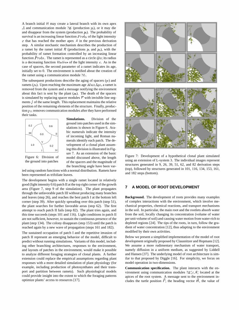
Simulations. Division of theground into patches used in the sim-ulations is shown in Figure 6. Ara-bic numerals indicate the intensityof incoming light, and Roman nu-merals identify each patch. The de-velopment of a clonal plant assum-ing this division is illustrated in Fig-ure 7. As an extension of the basicmodel discussed above, the lengthof the spacers and the magnitude ofthe branching angle have been var-

ied using random functions with a normal distribution. Ramets havebeen represented as trifoliate leaves.

The development begins with a single ramet located in relativelygood (light intensity 0.6) patch II at the top right corner of the growtharea (Figure 7, step 9 of the simulation). The plant propagatesthrough the unfavorable patch III without producing many branchesand leaves (step 26), and reaches the best patch I at the bottom leftcorner (step 39). After quickly spreading over this patch (step 51),the plant searches for further favorable areas (step 62). The firstattempt to reach patch II fails (step 82). The plant tries again, andthis time succeeds (steps 101 and 116). Light conditions in patch IIare not sufficient, however, to sustain the continuous presence of theplant (step 134). The colony disappears (step 153) until the patch isreached again by a new wave of propagation (steps 161 and 182).

The sustained occupation of patch I and the repetitive invasion ofpatch II represent an emerging behavior of the model, difficult topredict without running simulations. Variants of this model, includ-ing other branching architectures, responses to the environment,and layouts of patches in the environment, would make it possibleto analyze different foraging strategies of clonal plants. A furtherextension could replace the empirical assumptions regarding plantresponses with a more detailed simulation of plant physiology (forexample, including production of photosynthates and their trans-port and partition between ramets). Such physiological modelscould provide insight into the extent to which the foraging patternsoptimize plants’ access to resources [17].

Figure 7: Development of a hypothetical clonal plant simulatedusing an extension of L-system 3. The individual images representstructures generated in 9, 26, 39, 51, 62, and 82 derivation steps(top), followed by structures generated in 101, 116, 134, 153, 161,and 182 steps (bottom).

7 A MODEL OF ROOT DEVELOPMENT

Background. The development of roots provides many examplesof complex interactions with the environment, which involve me-chanical properties, chemical reactions, and transport mechanismsin the soil. In particular, the main root and the rootlets absorb waterfrom the soil, locally changing its concentration (volume of waterper unit volume of soil) and causing water motion from water-rich todepleted regions [24]. The tips of the roots, in turn, follow the gra-dient of water concentration [12], thus adapting to the environmentmodified by their own activities.

Below we present a simplified implementation of the model of rootdevelopment originally proposed by Clausnitzer and Hopmans [12].We assume a more rudimentary mechanism of water transport,namely diffusion in a uniform medium, as suggested by Liddelland Hansen [37]. The underlying model of root architecture is sim-ilar to that proposed by Diggle [16]. For simplicity, we focus onmodel operation in two-dimensions.

Communication specification. The plant interacts with the en-vironment using communication modules ?E(c; �) located at theapices of the root system. A message sent to the environment in-cludes the turtle position ~P , the heading vector ~H, the value of

parameter c representing the requested (optimal) water uptake, andthe value of parameter � representing the tendency of the apex tofollow the gradient of water concentration. A message returned tothe plant specifies the amount of water actually received by the apexas the value of parameter c, and the angle biasing direction of furthergrowth as the value of �.

H

θin∇C

∇C

θout

→

T →

Figure 8: Definition ofthe biasing angle �out

The model of the environment.The environment maintains a fieldC of water concentrations, repre-sented as an array of the amountsof water in square sampling areas.Water is transported by diffusion,simulated numerically using finitedifferencing [41]. The environ-ment responds to a request for wa-ter from an apex located in an area(i; j) by granting the lesser of the

values requested and available at that location. The amount of waterin the sampled area is then decreased by the amount received by theapex. The environment also calculates a linear combination ~T ofthe turtle heading vector ~H and the gradient of water concentrationrC (estimated numerically from the water concentrations in thesampled area and its neighbors), and returns an angle � between thevectors ~T and ~H (Figure 8). This angle is used by the plant modelto bias turtle heading in the direction of high water concentration.

The root model. The open L-system representing the root modelmakes use of arrays that specify parameters for each branching order(main axis, its daughter axes, etc.). The parameter values are looselybased on those reported by Clausnitzer and Hopmans [12].

#define N 3 /* max. branching order + 1 */Define: f arrayReq[N] = f0.1, 0.4, 0.05g, /* requested nutrient intake */MinReq[N] = f0.01, 0.06, 0.01g, /* minimum nutrient intake */ElRate[N] = f0.55, 0.25, 0.55g, /* maximum elongation rate */MaxLen[N] = f200, 5, 0.8g, /* maximum branch length */Sens[N] = f10, 0, 0g, /* sensitivity to gradient */Dev[N] = f30, 75, 75g, /* deviation in heading */Del[N–1] = f30, 60g, /* delay in branch growth */BrAngle[N–1] = f90, 90g, /* branching angle */BrSpace[N–1] = f1, 0.5g /* distance between branches */g

!: A(0,0,0)?E(Req[0],Sens[0])

p1: A(n,s,b) > ?E(c,�) : (s > MaxLen[n]) || (c < MinReq[n]) ! "

p2: A(n,s,b) > ?E(c,�) :(n >= N–1) || (b < BrSpace[n]) fh=c/Req[n]*ElRate[n];g! +(nran(�,Dev[n]))F(h) A(n,s+h,b+h)?E(Req[n],Sens[n])

p3: A(n,s,b) > ?E(c,�) :(n < N–1) && (b >= BrSpace[n]) fh=c/Req[n]*ElRate[n];g! +(nran(�,Dev[n]))B(n,0)F(h)

/(180)A(n,s+h,h)?E(Req[n],Sens[n])

p4: B(n,t) : t < Del[n] ! B(n,t+1)p5: B(n,t) : t >= Del[n]

! [+(BrAngle[n])A(n+1,0,0)?E(Req[n+1],Sens[n+1])]p6: ?E(c,�) ! "

The development starts with an apex A followed by a communica-tion module ?E. The parameters of the apex represent the branchorder (0 for the main axis, 1 for its daughter axes, etc.), current axislength, and distance (along the axis) to the nearest branching point.

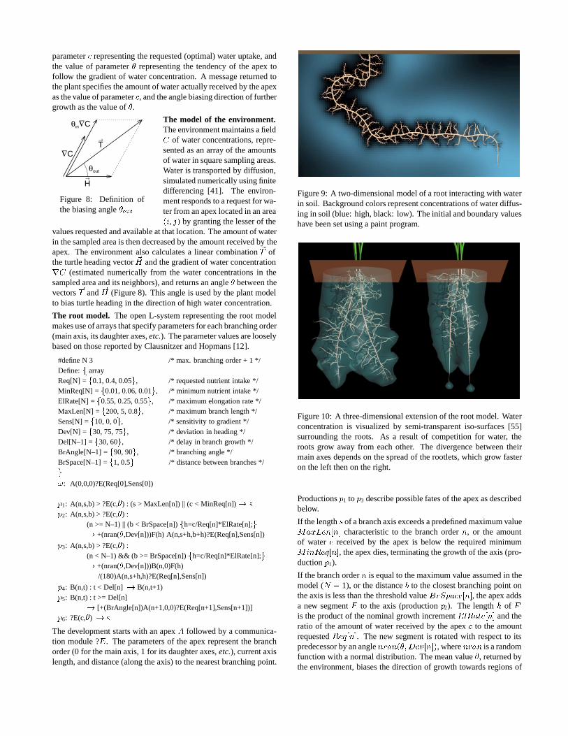
Figure 9: A two-dimensional model of a root interacting with waterin soil. Background colors represent concentrations of water diffus-ing in soil (blue: high, black: low). The initial and boundary valueshave been set using a paint program.

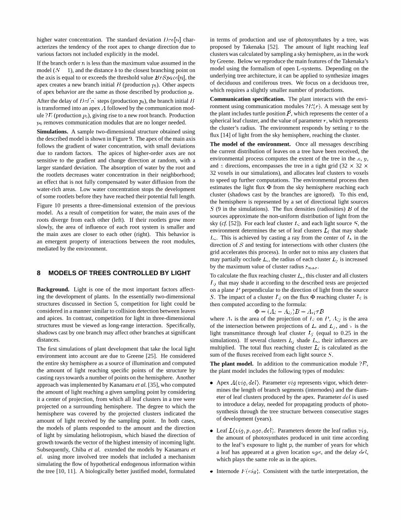
Figure 10: A three-dimensional extension of the root model. Waterconcentration is visualized by semi-transparent iso-surfaces [55]surrounding the roots. As a result of competition for water, theroots grow away from each other. The divergence between theirmain axes depends on the spread of the rootlets, which grow fasteron the left then on the right.

Productions p1 to p3 describe possible fates of the apex as describedbelow.

If the length s of a branch axis exceeds a predefined maximum valueMaxLen[n] characteristic to the branch order n, or the amountof water c received by the apex is below the required minimumMinReq[n], the apex dies, terminating the growth of the axis (pro-duction p1).

If the branch order n is equal to the maximum value assumed in themodel (N � 1), or the distance b to the closest branching point onthe axis is less than the threshold value BrSpace[n], the apex addsa new segment F to the axis (production p2). The length h of Fis the product of the nominal growth increment ElRate[n] and theratio of the amount of water received by the apex c to the amountrequested Req[n]. The new segment is rotated with respect to itspredecessor by an angle nran(�;Dev[n]), where nran is a randomfunction with a normal distribution. The mean value �, returned bythe environment, biases the direction of growth towards regions of

higher water concentration. The standard deviation Dev[n] char-acterizes the tendency of the root apex to change direction due tovarious factors not included explicitly in the model.

If the branch order n is less than the maximum value assumed in themodel (N � 1), and the distance b to the closest branching point onthe axis is equal to or exceeds the threshold value BrSpace[n], theapex creates a new branch initial B (production p3). Other aspectsof apex behavior are the same as those described by production p2.

After the delay of Del[n] steps (production p4), the branch initialBis transformed into an apex A followed by the communication mod-ule ?E (production p5), giving rise to a new root branch. Productionp6 removes communication modules that are no longer needed.

Simulations. A sample two-dimensional structure obtained usingthe described model is shown in Figure 9. The apex of the main axisfollows the gradient of water concentration, with small deviationsdue to random factors. The apices of higher-order axes are notsensitive to the gradient and change direction at random, with alarger standard deviation. The absorption of water by the root andthe rootlets decreases water concentration in their neighborhood;an effect that is not fully compensated by water diffusion from thewater-rich areas. Low water concentration stops the developmentof some rootlets before they have reached their potential full length.

Figure 10 presents a three-dimensional extension of the previousmodel. As a result of competition for water, the main axes of theroots diverge from each other (left). If their rootlets grow moreslowly, the area of influence of each root system is smaller andthe main axes are closer to each other (right). This behavior isan emergent property of interactions between the root modules,mediated by the environment.

8 MODELS OF TREES CONTROLLED BY LIGHT

Background. Light is one of the most important factors affect-ing the development of plants. In the essentially two-dimensionalstructures discussed in Section 5, competition for light could beconsidered in a manner similar to collision detection between leavesand apices. In contrast, competition for light in three-dimensionalstructures must be viewed as long-range interaction. Specifically,shadows cast by one branch may affect other branches at significantdistances.

The first simulations of plant development that take the local lightenvironment into account are due to Greene [25]. He consideredthe entire sky hemisphere as a source of illumination and computedthe amount of light reaching specific points of the structure bycasting rays towards a number of points on the hemisphere. Anotherapproach was implemented by Kanamaru et al. [35], who computedthe amount of light reaching a given sampling point by consideringit a center of projection, from which all leaf clusters in a tree wereprojected on a surrounding hemisphere. The degree to which thehemisphere was covered by the projected clusters indicated theamount of light received by the sampling point. In both cases,the models of plants responded to the amount and the directionof light by simulating heliotropism, which biased the direction ofgrowth towards the vector of the highest intensity of incoming light.Subsequently, Chiba et al. extended the models by Kanamaru etal. using more involved tree models that included a mechanismsimulating the flow of hypothetical endogenous information withinthe tree [10, 11]. A biologically better justified model, formulated

in terms of production and use of photosynthates by a tree, wasproposed by Takenaka [52]. The amount of light reaching leafclusters was calculated by sampling a sky hemisphere, as in the workby Greene. Below we reproduce the main features of the Takenaka’smodel using the formalism of open L-systems. Depending on theunderlying tree architecture, it can be applied to synthesize imagesof deciduous and coniferous trees. We focus on a deciduous tree,which requires a slightly smaller number of productions.

Communication specification. The plant interacts with the envi-ronment using communication modules ?E(r). A message sent bythe plant includes turtle position ~P , which represents the center of aspherical leaf cluster, and the value of parameter r, which representsthe cluster’s radius. The environment responds by setting r to theflux [14] of light from the sky hemisphere, reaching the cluster.

The model of the environment. Once all messages describingthe current distribution of leaves on a tree have been received, theenvironmental process computes the extent of the tree in the x, y,and z directions, encompasses the tree in a tight grid (32 � 32 �32 voxels in our simulations), and allocates leaf clusters to voxelsto speed up further computations. The environmental process thenestimates the light flux Φ from the sky hemisphere reaching eachcluster (shadows cast by the branches are ignored). To this end,the hemisphere is represented by a set of directional light sourcesS (9 in the simulations). The flux densities (radiosities) B of thesources approximate the non-uniform distribution of light from thesky (cf. [52]). For each leaf cluster Li and each light source S, theenvironment determines the set of leaf clusters Lj that may shadeLi. This is achieved by casting a ray from the center of Li in thedirection of S and testing for intersections with other clusters (thegrid accelerates this process). In order not to miss any clusters thatmay partially occlude Li, the radius of each cluster Lj is increasedby the maximum value of cluster radius rmax.

To calculate the flux reaching cluster Li, this cluster and all clustersLj that may shade it according to the described tests are projectedon a plane P perpendicular to the direction of light from the sourceS. The impact of a cluster Lj on the flux Φ reaching cluster Li isthen computed according to the formula:

Φ = (Ai �Aij)B +Aij�B

where Ai is the area of the projection of Li on P , Aij is the areaof the intersection between projections of Li and Lj , and � is thelight transmittance through leaf cluster Lj (equal to 0.25 in thesimulations). If several clusters Lj shade Li, their influences aremultiplied. The total flux reaching cluster Li is calculated as thesum of the fluxes received from each light source S.

The plant model. In addition to the communication module ?E,the plant model includes the following types of modules:

� Apex A(vig; del). Parameter vig represents vigor, which deter-mines the length of branch segments (internodes) and the diam-eter of leaf clusters produced by the apex. Parameter del is usedto introduce a delay, needed for propagating products of photo-synthesis through the tree structure between consecutive stagesof development (years).

� Leaf L(vig; p; age; del). Parameters denote the leaf radius vig,the amount of photosynthates produced in unit time accordingto the leaf’s exposure to light p, the number of years for whicha leaf has appeared at a given location age, and the delay del,which plays the same role as in the apices.

� Internode F (vig). Consistent with the turtle interpretation, the

parameter vig indicates the internode length.

� Branch width symbol !(w; p; n), also used to carry the endoge-nous information flow. The parameters determine: the width ofthe following internode w, the amount of photosynthates reach-ing the symbol’s location p, and the number of terminal branchsegments above this location n.

The corresponding L-system is given below.

#define ' 137.5 /* divergence angle */#define �0 5 /* direction change - no branching */#define �1 20 /* branching angle - main axis */#define �2 32 /* branching angle - lateral axis */#define W 0.02 /* initial branch width */#define VD 0.95 /* apex vigor decrement */#define Del 30 /* delay */#define LS 5 /* how long a leaf stays */#define LP 8 /* full photosynthate production */#define LM 2 /* leaf maintenance */#define PB 0.8 /* photosynthates needed for branching */#define PG 0.4 /* photosynthates needed for growth */#define BM 0.32 /* branch maintenance coefficient */#define BE 1.5 /* branch maintenance exponent */#define Nmin 25 /* threshold for shedding */Consider: ?E[]!L /* for context matching */

!: !(W,1,1)F(2)L(1,LP,0,0)A(1,0)[!(0,0,0)]!(W,0,1)

p1: A(vig,del) : del<Del ! A(vig,del+1)p2: L(vig,p,age,del) : (age<LS)&&(del<Del–1) ! L(vig,p,age,del+1)p3: L(vig,p,age,del) : (age<LS)&&(del==Del–1)

! L(vig,p,age,del+1)?E(vig*0.5)p4: L(vig,p,age,del) > ?E(r) : (age<LS) && (r*LP>=LM)

&& (del == Del) ! L(vig,LP*r–LM,age+1,0)p5: L(vig,p,age,del) > ?E(r) : ((age == LS)||(r*LP<=LM))

&& (del == Del) ! L(0,0,LS,0)

p6: ?E(r) < A(vig,del) : r*LP–LM>PB fvig=vig*VD;g! /(')[+(�2)!(W,–PB,1)F(vig)L(vig,LP,0,0)A(vig,0)

[!(0,0,0)]!(W,0,1)]–(�1)!(W,0,1)F(vig)L(vig,LP,0,0)/A(vig,0)

p7: ?E(r) < A(vig,del) : r*LP–LM > PG fvig=vig*VD;g! /(')–(�0)[!(0,0,0)]

!(W,–PG,1)F(vig)L(vig,LP,0,0)A(vig,0)p8: ?E(r) < A(vig,del) : r*LP–LM <= PG ! A(vig,0)p9: ?E(r) ! "

p10: !(w0,p0,n0) > L(vig,pL,age,del) [!(w1,p1,n1)]!(w2,p2,n2) :fw=(w1ˆ2+w2ˆ2)ˆ0.5; p=p1+p2+pL–BM*(w/W)ˆBE;g(p>0) || (n1+n2 >=Nmin) ! !(w,p,n1+n2)

p11: !(w0,p0,n0) > L(vig,pL,age,del) [!(w1,p1,n1)]!(w2,p2,n2)! !(w0,0,0)L%

The simulation starts with a structure consisting of a branch segmentF , supporting a leaf L and an apex A (axiom !). The first branchwidth symbol ! defines the segment width. Two additional symbols! following the apex create “virtual branches," needed to provideproper context for productions p10 and p11. The tree grows in stages,with the delay of Del + 1 derivation steps between consecutivestages introduced by production p1 for the apices and p2 for theleaves. Immediately before each new growth stage, communicationsymbols are introduced to inform the environment about the locationand size of the leaf clusters (p3). If the flux r returned by theenvironment results in the production of photosynthates r � LP

0 4 8 1612 20 240

8

128

512

32768

2

32

2048

8192

year

num

ber

of te

rmin

als

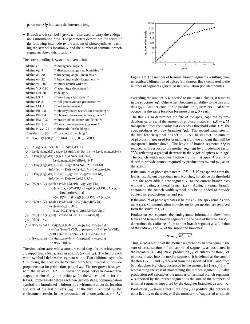
Figure 11: The number of terminal branch segments resulting fromunrestricted bifurcation of apices (continuous line), compared to thenumber of segments generated in a simulation (isolated points)

exceeding the amount LM needed to maintain a cluster, it remainsin the structure (p4). Otherwise it becomes a liability to the tree anddies (p5). Another condition to production p5 prevents a leaf fromoccupying the same location for more than LS years.

The flux r also determines the fate of the apex, captured by pro-ductions p6 to p8. If the amount of photosynthates r � LP � LM

transported from the nearby leaf exceeds a threshold value PB, theapex produces two new branches (p6). The second parameter inthe first branch symbol ! is set to �PB, to subtract the amountof photosynthates used for branching from the amount that will betransported further down. The length of branch segments vig isreduced with respect to the mother segment by a predefined factorV D, reflecting a gradual decrease in the vigor of apices with age.The branch width modules ! following the first apex A are intro-duced to provide context required by productions p10 and p11, as inthe axiom.

If the amount of photosynthates r �LP �LM transported from theleaf is insufficient to produce new branches, but above the thresholdPG, the apex adds a new segment F to the current branch axiswithout creating a lateral branch (p7). Again, a virtual branchcontaining the branch width symbol ! is being added to providecontext for productions p10 and p11.

If the amount of photosynthates is below PG, the apex remains dor-mant (p8). Communication modules no longer needed are removedfrom the structure (p9).

Production p10 captures the endogenous information flow fromleaves and terminal branch segments to the base of the tree. First, itdetermines the radius w of the mother branch segment as a functionof the radii w1 and w2 of the supported branches:

w =pw2

1 + w22:

Thus, a cross section of the mother segment has an area equal to thesum of cross sections of the supported segments, as postulated inthe literature [40, 46]. Next, production p10 calculates the flow p ofphotosynthates into the mother segment. It is defined as the sum ofthe flows pL, p1 and p2 received from the associated leafL and fromboth daughter branches, decreased by the amountBM �(w=W )BE

representing the cost of maintaining the mother segment. Finally,production p10 calculates the number of terminal branch segmentsn supported by the mother segment as the sum of the numbers ofterminal segments supported by the daughter branches, n1 and n2.

Production p10 takes effect if the flow p is positive (the branch isnot a liability to the tree), or if the number n of supported terminals

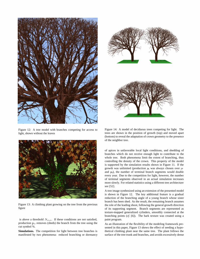
Figure 12: A tree model with branches competing for access tolight, shown without the leaves

Figure 13: A climbing plant growing on the tree from the previousfigure

is above a threshold Nmin. If these conditions are not satisfied,production p11 removes (sheds) the branch from the tree using thecut symbol %.

Simulations. The competition for light between tree branches ismanifested by two phenomena: reduced branching or dormancy

Figure 14: A model of deciduous trees competing for light. Thetrees are shown in the position of growth (top) and moved apart(bottom) to reveal the adaptation of crown geometry to the presenceof the neighbor tree.

of apices in unfavorable local light conditions, and shedding ofbranches which do not receive enough light to contribute to thewhole tree. Both phenomena limit the extent of branching, thuscontrolling the density of the crown. This property of the modelis supported by the simulation results shown in Figure 11. If thegrowth was unlimited (production p6 was always chosen over p7

and p8), the number of terminal branch segments would doubleevery year. Due to the competition for light, however, the numberof terminal segments observed in an actual simulation increasesmore slowly. For related statistics using a different tree architecturesee [52].

A tree image synthesized using an extension of the presented modelis shown in Figure 12. The key additional feature is a gradualreduction of the branching angle of a young branch whose sisterbranch has been shed. As the result, the remaining branch assumesthe role of the leading shoot, following the general growth directionof its supporting segment. Branch segments are represented astexture-mapped generalized cylinders, smoothly connected at thebranching points (cf. [6]). The bark texture was created using apaint program.

As an illustration of the flexibility of the modeling framework pre-sented in this paper, Figure 13 shows the effect of seeding a hypo-thetical climbing plant near the same tree. The plant follows thesurface of the tree trunk and branches, and avoids excessively dense

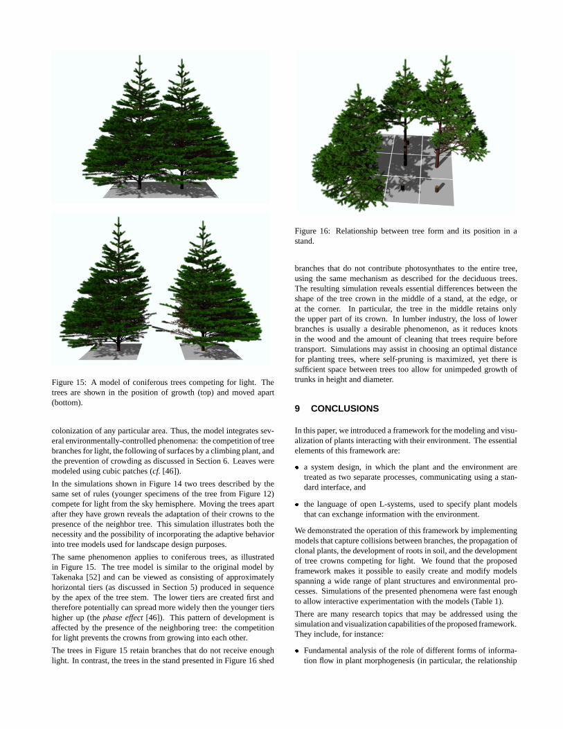
Figure 15: A model of coniferous trees competing for light. Thetrees are shown in the position of growth (top) and moved apart(bottom).

colonization of any particular area. Thus, the model integrates sev-eral environmentally-controlled phenomena: the competition of treebranches for light, the following of surfaces by a climbing plant, andthe prevention of crowding as discussed in Section 6. Leaves weremodeled using cubic patches (cf. [46]).

In the simulations shown in Figure 14 two trees described by thesame set of rules (younger specimens of the tree from Figure 12)compete for light from the sky hemisphere. Moving the trees apartafter they have grown reveals the adaptation of their crowns to thepresence of the neighbor tree. This simulation illustrates both thenecessity and the possibility of incorporating the adaptive behaviorinto tree models used for landscape design purposes.

The same phenomenon applies to coniferous trees, as illustratedin Figure 15. The tree model is similar to the original model byTakenaka [52] and can be viewed as consisting of approximatelyhorizontal tiers (as discussed in Section 5) produced in sequenceby the apex of the tree stem. The lower tiers are created first andtherefore potentially can spread more widely then the younger tiershigher up (the phase effect [46]). This pattern of development isaffected by the presence of the neighboring tree: the competitionfor light prevents the crowns from growing into each other.

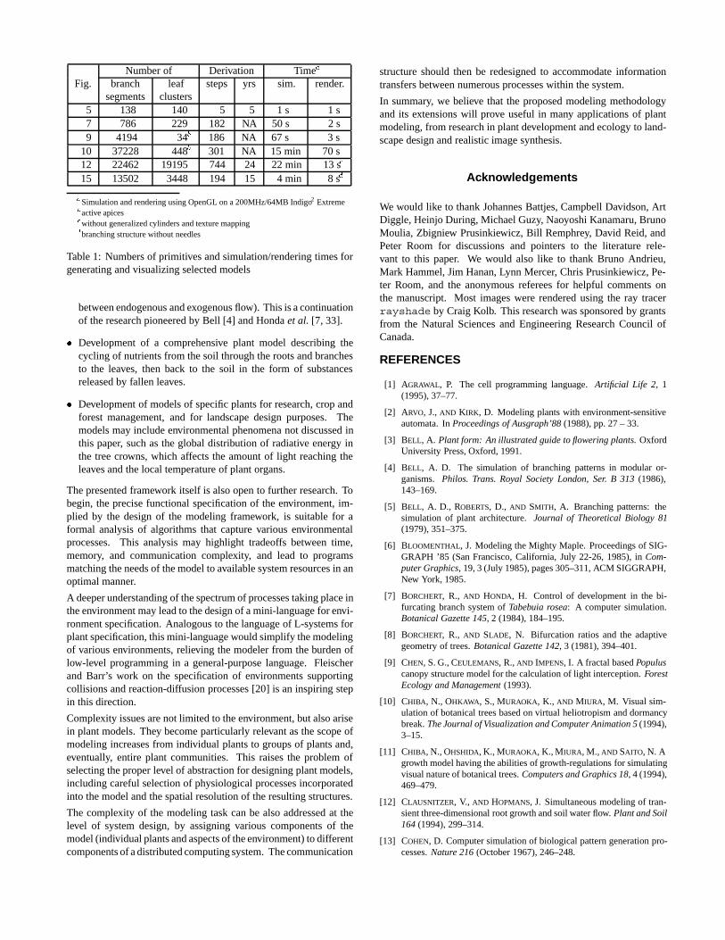
The trees in Figure 15 retain branches that do not receive enoughlight. In contrast, the trees in the stand presented in Figure 16 shed

Figure 16: Relationship between tree form and its position in astand.

branches that do not contribute photosynthates to the entire tree,using the same mechanism as described for the deciduous trees.The resulting simulation reveals essential differences between theshape of the tree crown in the middle of a stand, at the edge, orat the corner. In particular, the tree in the middle retains onlythe upper part of its crown. In lumber industry, the loss of lowerbranches is usually a desirable phenomenon, as it reduces knotsin the wood and the amount of cleaning that trees require beforetransport. Simulations may assist in choosing an optimal distancefor planting trees, where self-pruning is maximized, yet there issufficient space between trees too allow for unimpeded growth oftrunks in height and diameter.

9 CONCLUSIONS

In this paper, we introduced a framework for the modeling and visu-alization of plants interacting with their environment. The essentialelements of this framework are:

� a system design, in which the plant and the environment aretreated as two separate processes, communicating using a stan-dard interface, and

� the language of open L-systems, used to specify plant modelsthat can exchange information with the environment.

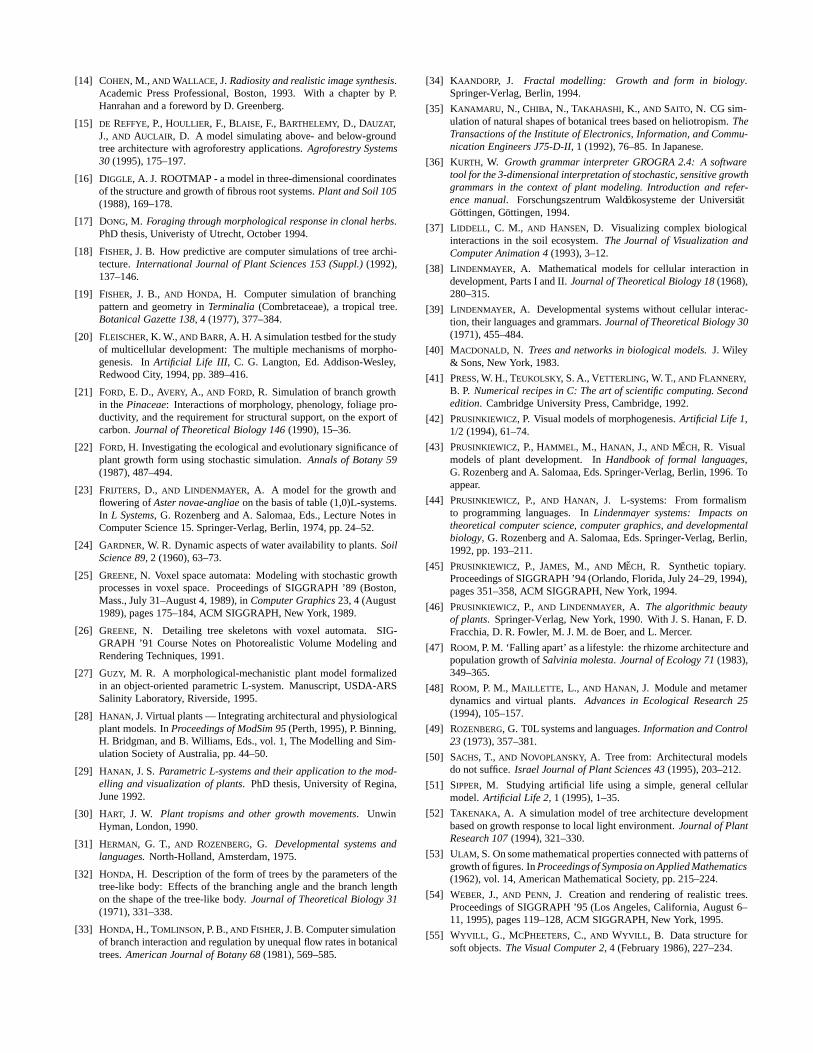
We demonstrated the operation of this framework by implementingmodels that capture collisions between branches, the propagation ofclonal plants, the development of roots in soil, and the developmentof tree crowns competing for light. We found that the proposedframework makes it possible to easily create and modify modelsspanning a wide range of plant structures and environmental pro-cesses. Simulations of the presented phenomena were fast enoughto allow interactive experimentation with the models (Table 1).

There are many research topics that may be addressed using thesimulation and visualization capabilities of the proposed framework.They include, for instance:

� Fundamental analysis of the role of different forms of informa-tion flow in plant morphogenesis (in particular, the relationship

Number of Derivation Timea

Fig. branch leaf steps yrs sim. render.segments clusters

5 138 140 5 5 1 s 1 s7 786 229 182 NA 50 s 2 s9 4194 34b 186 NA 67 s 3 s

10 37228 448b 301 NA 15 min 70 s12 22462 19195 744 24 22 min 13 sc

15 13502 3448 194 15 4 min 8 sd

aSimulation and rendering using OpenGL on a 200MHz/64MB Indigo2 Extremebactive apicescwithout generalized cylinders and texture mappingdbranching structure without needles

Table 1: Numbers of primitives and simulation/rendering times forgenerating and visualizing selected models

between endogenous and exogenous flow). This is a continuationof the research pioneered by Bell [4] and Honda et al. [7, 33].

� Development of a comprehensive plant model describing thecycling of nutrients from the soil through the roots and branchesto the leaves, then back to the soil in the form of substancesreleased by fallen leaves.

� Development of models of specific plants for research, crop andforest management, and for landscape design purposes. Themodels may include environmental phenomena not discussed inthis paper, such as the global distribution of radiative energy inthe tree crowns, which affects the amount of light reaching theleaves and the local temperature of plant organs.

The presented framework itself is also open to further research. Tobegin, the precise functional specification of the environment, im-plied by the design of the modeling framework, is suitable for aformal analysis of algorithms that capture various environmentalprocesses. This analysis may highlight tradeoffs between time,memory, and communication complexity, and lead to programsmatching the needs of the model to available system resources in anoptimal manner.

A deeper understanding of the spectrum of processes taking place inthe environment may lead to the design of a mini-language for envi-ronment specification. Analogous to the language of L-systems forplant specification, this mini-language would simplify the modelingof various environments, relieving the modeler from the burden oflow-level programming in a general-purpose language. Fleischerand Barr’s work on the specification of environments supportingcollisions and reaction-diffusion processes [20] is an inspiring stepin this direction.

Complexity issues are not limited to the environment, but also arisein plant models. They become particularly relevant as the scope ofmodeling increases from individual plants to groups of plants and,eventually, entire plant communities. This raises the problem ofselecting the proper level of abstraction for designing plant models,including careful selection of physiological processes incorporatedinto the model and the spatial resolution of the resulting structures.

The complexity of the modeling task can be also addressed at thelevel of system design, by assigning various components of themodel (individual plants and aspects of the environment) to differentcomponents of a distributed computing system. The communication

structure should then be redesigned to accommodate informationtransfers between numerous processes within the system.

In summary, we believe that the proposed modeling methodologyand its extensions will prove useful in many applications of plantmodeling, from research in plant development and ecology to land-scape design and realistic image synthesis.

Acknowledgements

We would like to thank Johannes Battjes, Campbell Davidson, ArtDiggle, Heinjo During, Michael Guzy, Naoyoshi Kanamaru, BrunoMoulia, Zbigniew Prusinkiewicz, Bill Remphrey, David Reid, andPeter Room for discussions and pointers to the literature rele-vant to this paper. We would also like to thank Bruno Andrieu,Mark Hammel, Jim Hanan, Lynn Mercer, Chris Prusinkiewicz, Pe-ter Room, and the anonymous referees for helpful comments onthe manuscript. Most images were rendered using the ray tracerrayshade by Craig Kolb. This research was sponsored by grantsfrom the Natural Sciences and Engineering Research Council ofCanada.

REFERENCES

[1] AGRAWAL, P. The cell programming language. Artificial Life 2, 1(1995), 37–77.

[2] ARVO, J., AND KIRK, D. Modeling plants with environment-sensitiveautomata. In Proceedings of Ausgraph’88 (1988), pp. 27 – 33.

[3] BELL, A. Plant form: An illustrated guide to flowering plants. OxfordUniversity Press, Oxford, 1991.

[4] BELL, A. D. The simulation of branching patterns in modular or-ganisms. Philos. Trans. Royal Society London, Ser. B 313 (1986),143–169.

[5] BELL, A. D., ROBERTS, D., AND SMITH, A. Branching patterns: thesimulation of plant architecture. Journal of Theoretical Biology 81(1979), 351–375.

[6] BLOOMENTHAL, J. Modeling the Mighty Maple. Proceedings of SIG-GRAPH ’85 (San Francisco, California, July 22-26, 1985), in Com-puter Graphics, 19, 3 (July 1985), pages 305–311, ACM SIGGRAPH,New York, 1985.

[7] BORCHERT, R., AND HONDA, H. Control of development in the bi-furcating branch system of Tabebuia rosea: A computer simulation.Botanical Gazette 145, 2 (1984), 184–195.

[8] BORCHERT, R., AND SLADE, N. Bifurcation ratios and the adaptivegeometry of trees. Botanical Gazette 142, 3 (1981), 394–401.

[9] CHEN, S. G., CEULEMANS, R., AND IMPENS, I. A fractal based Populuscanopy structure model for the calculation of light interception. ForestEcology and Management (1993).

[10] CHIBA, N., OHKAWA, S., MURAOKA, K., AND MIURA, M. Visual sim-ulation of botanical trees based on virtual heliotropism and dormancybreak. The Journal of Visualization and Computer Animation 5 (1994),3–15.

[11] CHIBA, N., OHSHIDA, K., MURAOKA, K., MIURA, M., AND SAITO, N. Agrowth model having the abilities of growth-regulations for simulatingvisual nature of botanical trees. Computers and Graphics 18, 4 (1994),469–479.

[12] CLAUSNITZER, V., AND HOPMANS, J. Simultaneous modeling of tran-sient three-dimensional root growth and soil water flow. Plant and Soil164 (1994), 299–314.

[13] COHEN, D. Computer simulation of biological pattern generation pro-cesses. Nature 216 (October 1967), 246–248.

[14] COHEN, M., AND WALLACE, J. Radiosity and realistic image synthesis.Academic Press Professional, Boston, 1993. With a chapter by P.Hanrahan and a foreword by D. Greenberg.

[15] DE REFFYE, P., HOULLIER, F., BLAISE, F., BARTHELEMY, D., DAUZAT,J., AND AUCLAIR, D. A model simulating above- and below-groundtree architecture with agroforestry applications. Agroforestry Systems30 (1995), 175–197.

[16] DIGGLE, A. J. ROOTMAP - a model in three-dimensional coordinatesof the structure and growth of fibrous root systems. Plant and Soil 105(1988), 169–178.

[17] DONG, M. Foraging through morphological response in clonal herbs.PhD thesis, Univeristy of Utrecht, October 1994.

[18] FISHER, J. B. How predictive are computer simulations of tree archi-tecture. International Journal of Plant Sciences 153 (Suppl.) (1992),137–146.

[19] FISHER, J. B., AND HONDA, H. Computer simulation of branchingpattern and geometry in Terminalia (Combretaceae), a tropical tree.Botanical Gazette 138, 4 (1977), 377–384.

[20] FLEISCHER, K. W., AND BARR, A. H. A simulation testbed for the studyof multicellular development: The multiple mechanisms of morpho-genesis. In Artificial Life III, C. G. Langton, Ed. Addison-Wesley,Redwood City, 1994, pp. 389–416.

[21] FORD, E. D., AVERY, A., AND FORD, R. Simulation of branch growthin the Pinaceae: Interactions of morphology, phenology, foliage pro-ductivity, and the requirement for structural support, on the export ofcarbon. Journal of Theoretical Biology 146 (1990), 15–36.

[22] FORD, H. Investigating the ecological and evolutionary significance ofplant growth form using stochastic simulation. Annals of Botany 59(1987), 487–494.

[23] FRIJTERS, D., AND LINDENMAYER, A. A model for the growth andflowering of Aster novae-angliae on the basis of table (1,0)L-systems.In L Systems, G. Rozenberg and A. Salomaa, Eds., Lecture Notes inComputer Science 15. Springer-Verlag, Berlin, 1974, pp. 24–52.

[24] GARDNER, W. R. Dynamic aspects of water availability to plants. SoilScience 89, 2 (1960), 63–73.

[25] GREENE, N. Voxel space automata: Modeling with stochastic growthprocesses in voxel space. Proceedings of SIGGRAPH ’89 (Boston,Mass., July 31–August 4, 1989), in Computer Graphics 23, 4 (August1989), pages 175–184, ACM SIGGRAPH, New York, 1989.

[26] GREENE, N. Detailing tree skeletons with voxel automata. SIG-GRAPH ’91 Course Notes on Photorealistic Volume Modeling andRendering Techniques, 1991.

[27] GUZY, M. R. A morphological-mechanistic plant model formalizedin an object-oriented parametric L-system. Manuscript, USDA-ARSSalinity Laboratory, Riverside, 1995.

[28] HANAN, J. Virtual plants — Integrating architectural and physiologicalplant models. In Proceedings of ModSim 95 (Perth, 1995), P. Binning,H. Bridgman, and B. Williams, Eds., vol. 1, The Modelling and Sim-ulation Society of Australia, pp. 44–50.

[29] HANAN, J. S. Parametric L-systems and their application to the mod-elling and visualization of plants. PhD thesis, University of Regina,June 1992.

[30] HART, J. W. Plant tropisms and other growth movements. UnwinHyman, London, 1990.

[31] HERMAN, G. T., AND ROZENBERG, G. Developmental systems andlanguages. North-Holland, Amsterdam, 1975.

[32] HONDA, H. Description of the form of trees by the parameters of thetree-like body: Effects of the branching angle and the branch lengthon the shape of the tree-like body. Journal of Theoretical Biology 31(1971), 331–338.

[33] HONDA, H., TOMLINSON, P. B., AND FISHER, J. B. Computer simulationof branch interaction and regulation by unequal flow rates in botanicaltrees. American Journal of Botany 68 (1981), 569–585.

[34] KAANDORP, J. Fractal modelling: Growth and form in biology.Springer-Verlag, Berlin, 1994.

[35] KANAMARU, N., CHIBA, N., TAKAHASHI, K., AND SAITO, N. CG sim-ulation of natural shapes of botanical trees based on heliotropism. TheTransactions of the Institute of Electronics, Information, and Commu-nication Engineers J75-D-II, 1 (1992), 76–85. In Japanese.

[36] KURTH, W. Growth grammar interpreter GROGRA 2.4: A softwaretool for the 3-dimensional interpretation of stochastic, sensitive growthgrammars in the context of plant modeling. Introduction and refer-ence manual. Forschungszentrum Waldokosysteme der UniversitatGottingen, Gottingen, 1994.

[37] LIDDELL, C. M., AND HANSEN, D. Visualizing complex biologicalinteractions in the soil ecosystem. The Journal of Visualization andComputer Animation 4 (1993), 3–12.

[38] LINDENMAYER, A. Mathematical models for cellular interaction indevelopment, Parts I and II. Journal of Theoretical Biology 18 (1968),280–315.

[39] LINDENMAYER, A. Developmental systems without cellular interac-tion, their languages and grammars. Journal of Theoretical Biology 30(1971), 455–484.

[40] MACDONALD, N. Trees and networks in biological models. J. Wiley& Sons, New York, 1983.

[41] PRESS, W. H., TEUKOLSKY, S. A., VETTERLING, W. T., AND FLANNERY,B. P. Numerical recipes in C: The art of scientific computing. Secondedition. Cambridge University Press, Cambridge, 1992.

[42] PRUSINKIEWICZ, P. Visual models of morphogenesis. Artificial Life 1,1/2 (1994), 61–74.

[43] PRUSINKIEWICZ, P., HAMMEL, M., HANAN, J., AND MECH, R. Visualmodels of plant development. In Handbook of formal languages,G. Rozenberg and A. Salomaa, Eds. Springer-Verlag, Berlin, 1996. Toappear.

[44] PRUSINKIEWICZ, P., AND HANAN, J. L-systems: From formalismto programming languages. In Lindenmayer systems: Impacts ontheoretical computer science, computer graphics, and developmentalbiology, G. Rozenberg and A. Salomaa, Eds. Springer-Verlag, Berlin,1992, pp. 193–211.

[45] PRUSINKIEWICZ, P., JAMES, M., AND MECH, R. Synthetic topiary.Proceedings of SIGGRAPH ’94 (Orlando, Florida, July 24–29, 1994),pages 351–358, ACM SIGGRAPH, New York, 1994.

[46] PRUSINKIEWICZ, P., AND LINDENMAYER, A. The algorithmic beautyof plants. Springer-Verlag, New York, 1990. With J. S. Hanan, F. D.Fracchia, D. R. Fowler, M. J. M. de Boer, and L. Mercer.

[47] ROOM, P. M. ‘Falling apart’ as a lifestyle: the rhizome architecture andpopulation growth of Salvinia molesta. Journal of Ecology 71 (1983),349–365.

[48] ROOM, P. M., MAILLETTE, L., AND HANAN, J. Module and metamerdynamics and virtual plants. Advances in Ecological Research 25(1994), 105–157.

[49] ROZENBERG, G. T0L systems and languages. Information and Control23 (1973), 357–381.

[50] SACHS, T., AND NOVOPLANSKY, A. Tree from: Architectural modelsdo not suffice. Israel Journal of Plant Sciences 43 (1995), 203–212.

[51] SIPPER, M. Studying artificial life using a simple, general cellularmodel. Artificial Life 2, 1 (1995), 1–35.

[52] TAKENAKA, A. A simulation model of tree architecture developmentbased on growth response to local light environment. Journal of PlantResearch 107 (1994), 321–330.

[53] ULAM, S. On some mathematical properties connected with patterns ofgrowth of figures. In Proceedings of Symposia on Applied Mathematics(1962), vol. 14, American Mathematical Society, pp. 215–224.

[54] WEBER, J., AND PENN, J. Creation and rendering of realistic trees.Proceedings of SIGGRAPH ’95 (Los Angeles, California, August 6–11, 1995), pages 119–128, ACM SIGGRAPH, New York, 1995.

[55] WYVILL, G., MCPHEETERS, C., AND WYVILL, B. Data structure forsoft objects. The Visual Computer 2, 4 (February 1986), 227–234.