Regional Impacts of State jobs in Denmark

The General Interregional Quantity Model

Bjarne Madsen

CRT, Centre for Regional and Tourism Research

Stenbrudsvej 55, DK-3730 Nexø

Tel.: +45 5644 1144 Fax: +45 5649 4624

E-mail: bma@crt.dk

Abstract

LINE is an interregional model for Danish municipalities, which now is used by regional planning authorities and labor market body to analyze and forecast regional economic development.

The paper commences with an overview of regional modeling in Denmark, involving the development of LINE. The structure of LINE is examined, taking the Leontief and Miyazawa formulations of the interregional economic quantity model as the point of departure. In the core of LINE is the general interregional static quantity model, which essentially is local rather than regional and incorporates a number of conceptual and theoretical changes, which have become necessary as economies become more diverse and differentiated. There is a need to integrate essentially subregional and local/urban activities covering such areas as commuting, shopping, tourism and trade into a general interregional modeling framework. The theoretical changes examined include a set of new geographical concepts and in the context of an interregional SAM the development of the two-by-two-by-two approach, involving two sets of actors (production units and institutional units), two types of markets (commodities and factors) and two locations (origin and destination). The equations of the general interregional quantity model are presented together with the solution of the model. Comparisons are made with the Danish interregional static CGE-model LINE and a typology of regions is proposed using the general model as a conceptual foundation.

Finally, LINE is used to examine regional impacts of state jobs for Danish municipalities. In the empirical analysis the direct state jobs by municipality is measured using SAM-K, which is a national account for Danish municipalities. On the basis of the direct state jobs the total effects of state jobs, including both the indirect and the derived effects are analyzed using LINE. In the analysis only the quantity model of LINE has been used measuring the effects on production, income and employment in quantities, whereas the impacts of state jobs on the labor market and productivity involving the cost and price model in LINE have not been included in this analysis.

The analysis conclude that there are substantial differences in direct as well total effects of state jobs: For the metropolitan area as well as the bigger cities state activities is at a relative high level due to location of the universities, hospitals and the state administration. For rural municipalities with military installations state jobs also have an above average share. The analysis also finds, that impacts are geographically propagated by commuting and shopping and tourism, implying that the impacts on residential

employment as well as local demand are much more smoothly distributed. Anyhow, it is concluded that the location of state jobs activities is one of the most important and effective instruments in regional policy.

Keywords: Interregional quantity models, Interregional SAM, Subregional models, Urban models, Regional typology, State jobs.

Background

In Denmark research based upon regional data, models and analysis began in the late 70s. Relatively high unemployment rates especially in peripheral areas and the introduction of an active labor market and education policy put forward the regional economic activity agenda: How would regional labor market develop? What would be the impacts of activities within important sectors such as food production and tourism? And what is the competitiveness of the regional export? Especially changes in the EU Common Agricultural Policy (CAP) were of major interest. At the same time there were a growing interest to study the impacts great infrastructure projects developed (in the 90s and the 00s Denmark were geographically connected with 3 major bridges and tunnels) ?

1.1National data, accounts and models

The development of regional data and analytical tools in Denmark has been closely connected to the development at the national level, although with a lag of 5-10 years. This was on one hand a push forward, but it also represented a step in a wrong direction. National technical solutions were taken over without rethinking whether regional models could do better finding its own form:In the beginning of the eighties national accounts for the Danish economy had been compiled for almost 10 years (Danmark Statistik 1973, Thage 1981, Thage & Thomsen 2004) on the basis of supply and use tables. However, multipliers based upon sector by sector input output tables were used. As such it followed the Leontief tradition, where the institutional form was chosen because of computational and data capacity problems in the 30s and the 40s. At the national level a model for Danish economy, called ADAM (Andersen 1975, Dam 1995) was developed in the mid 70’es ADAM was also – and is still today - based upon sector by sector input-output tables. Other macro-economic models at the national level (MONA - the macro economic model developed by the national Bank of Denmark (Danmarks Nationalbank (2004), SMEC - the model for the Economic Council (Det Økonomisk Råds Sekretariat 2007) as well as the DREAM-model being which is a CGE-model (DREAM-group 2008)) were developed still using a sector by sector approach. The potential in extending the structural analysis to include changes in supply and demand by commodity has not been exploited.At least as analytically important models based upon micro level data to analyze distributional topics were developed. The most important was the “law model” (Danish Ministry of Finance 2003), which was used to analyze distributional consequences of major changes in legislation such as the tax legislation. This model was a simple micro simulation

model calculating the disposable income by type of person, household, region etc. This type of analysis was not integrated into macro economic analysis, the macro-economic models only including structural analysis by sector – and not structural analysis by type of factor, type of family / institution etc.

1.2Regional data, accounts and models

The development of regional models followed the national path – with inspiration from regional models from other countries: The first model was for Sønderjylland County called SØREN building on the first regional national account in the form of regional sector by sector input-output tables and including a Keynesian income multiplier model (Groes 1982b). This was followed by the IRIS-model based upon the 2 regional accounts for Greater Copenhagen and the rest of Denmark. The IRIS-model (Holm 1984) had basically the same structure as SØREN, but with an interregional sector by sector input-output model in its core. Both models were inspired Dutch experiences (Oosterhaven 1981).In these models the distinctions between place of production and place of residence was made as a net transformation. It was assumed that people worked the same place as they lived. Similarly it was assumed that private consumption was bought and consumed at the place of residence not taking shopping and tourism into account. Furthermore, in these models only activity by sector was analyzed leaving outside the analysis the factor market (employment and income by type of labor such as by gender, age and education). Also the distribution into type of households (married/non married with and without children) was not considered. Finally, the commodities were not included in the frame work.In the EMIL- and AIDA-models (Jensen-Butler & Madsen 2002 and Madsen 1992a & b) some of these inherent problems were considered. A major inspiration came from Portugal was an interregional model, where Chris Jensen-Butler together with Portuguese researchers developed for Portugal (Jensen-Butler, Gaspar?????)……. Still the models were based upon the institutional approach and a net transfer of employment and income from place of production to place of residence (commuting) and a net transfer of consumption from place of residence to place of commodity market (shopping and tourism). But the process of finding solutions to inadequate data and model structures for local economies began:Firstly, number of regions was increased to 12 for AIDA, which included a (complex) interregional sector by sector model, and to 16 for EMIL, which was one region models such as SØREN.Secondly, distinctions between place of production and place of residence were introduced using a net coefficient between income and employment by “night and day

population”. Similarly, a net coefficient for consumption transformation of the private consumption from place of residence to the place of commodity markets was introduced. Especially the private consumption were divided into tourism and local private consumption, with a net coefficient transforming demand from place of residence to tourist destination or to the shopping center. Thirdly, the commodities were introduced as for foreign exports and imports following the tradition in the national account, still keeping the interregional trade in sectors and divided into intermediate and private consumption.Fourthly, the first steps to introduce the dual model to the quantity model began: Export was assumed to depend upon the relative price on export commodities at the place of production and at the place of export commodity market. In an analysis of the impacts of the fixed Great Belt link on prices of commodities it was assumed that improved access reduced the production cost of the production and shipping of the commodities (Groes (1982b), Jensen-Butler & Madsen (2002)).

1.3SAM-K and LINE

In 1995 a long term research project on the rural areas development opened for basic development both in regional data, national accounts as well as models.In the field of data, the use of register data based upon social security numbers for person and production identification for firms / production units was introduced. For persons very detailed tables showing population, labor force, employment and income, income transfers and taxes by the place of production and the place of residence, by producing sectors, type of labor (such as gender, age and education) and type of family changed the accounts for production and income. It also introduced the transformation from

a. income by sector to income by type of labor (factor)b. type of labor by place of production to place of residence (gross commuting) andc. type of labor at the place of residence to the type of family in terms of income,

taxes etc.Secondly, the access to elaborated surveys in the area of tourism and transport improved the description of the regional and local economy. It became possible to measure tourism consumption by place of residence (nationality for foreign tourist) and by place of commodity market (tourist destination) as well as it became possible to introduce distinctions between type of tourist / nights as well as a division of local private consumption at the place of residence and the place of commodity market and by commodity.

Thirdly, access to the basic supply and use tables in the national accounts instead of the conventional sector by sector tables opened for at new structure of the input output and trade structure of the local and regional economies. As something new, also regional supply and demand balance were established in interregional commodity balances: The regional supply now include the gross output, the imports from abroad as well as the imports from other regions and are accounted in commodities. Correspondingly, the regional demand, which consist of local demand (intermediate, private governmental consumption as well as investment), export abroad and exports to other regions, are accounted in commodities. Instead – and as a consequence - the conventional sector by sector input output tables was replaced by the supply (make) and use tables together with the international and interregional trade flows measured in commodities.Fourthly, regional economic activity was measured both in fixed price (leading to the “general interregional quantity model”) and in current prices (leading to the introduction of the ”general interregional cost and price model”, which is not examined in depth in this article). This opened for new descriptions of regional economic activity both in quantities and in current prices. This made it possible to model impacts of changes in wages and prices involving changes in the price of transportation of commodities (trade with products) and of persons (trade with service) and commuting and shopping / tourism.Fifthly, the distinction between income and commodity prices with or without taxes and subsidies both for commodities, for producers, for production factors and for institutions/families are introduced: firstly, the distinction for commodity market reflects the difference between market and basic prices, secondly, the distinction between income before and after tax at the place of residence for households imply introduction of concepts such as earned income and disposable income, thirdly, the distinction for production factors implies the difference between factor income and wage before and after tax and fourthly, for production income it involves the distinction between incomes with and without taxes or the distinction between Gross Value Added and Gross Factor Income.

2. The two by two by two principle

The development in Danish regional models took place on the basis of the two by two by two principle, which will be presented in this section. Firstly, the sector by sector input-output model will be introduced. Then it will be transformed into the “general interregional quantity model” based upon commodity demand and supply. Finally, the interregional quantity being a part of LINE will be compared with the general interregional quantity model.

2.1The single region Leontief quantity model

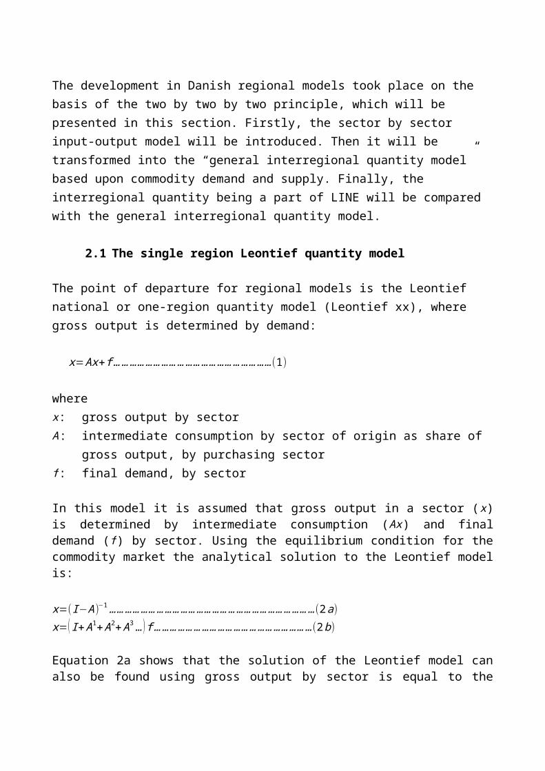
The point of departure for regional models is the Leontief national or one-region quantity model (Leontief xx), where gross output is determined by demand:

x=Ax+ f …………………………………………………… (1)

wherex: gross output by sectorA: intermediate consumption by sector of origin as share of gross output, by purchasing

sectorf : final demand, by sector

In this model it is assumed that gross output in a sector (x) is determined by intermediate consumption (Ax) and final demand (f ) by sector. Using the equilibrium condition for the commodity market the analytical solution to the Leontief model is:

x=(I−A )−1……………………………………………………………………(2a)x=( I+A1+A2+A3…) f ……………………………………………………(2b)

Equation 2a shows that the solution of the Leontief model can also be found using gross output by sector is equal to the product of the Leontief inverse and the vector of final demand. Equation 2b shows that the solution of the Leontief quantity model can be found sequentially using the power series approximation of the spill over and feedback effects between and within sectors. Each term expresses the effects of an extra round of intermediate consumption.

This model is a single region model as economic activities take place in one region without interaction with other regions. The model is based upon sectors (industries) and does not include explicit transformations from sectors to commodities (output) or transformations from commodities to sectors (input). The Leontief quantity model is therefore a reduced form model with underlying transformations, which appear when the model is applied to local and urban economies.

2.2The interregional Leontief quantity model

Setting up an interregional quantity model (Leontief xx) involves extensions of the reduced form Leontief quantity model. The interregional quantity model includes intra- and interregional trade, which in spatial terms leads to a distinction between place of production and place of commodity market. The interregional quantity model establishes a link

between place of commodity market, where intermediate consumption or final demand originates and place of production, where production takes place.

The Isard model (Isard 1951) is often described as the ideal interregional quantity model, which establishes a direct link between the intermediate consumption by purchasing sector in region S and gross output in the producing sector in region P. In the Isard model the A-matrix is simply extended, so that the same sector in two regions is defined as two different sectors. This in turn gives the same solution as in equation 2.

The Chenery-Moses model (Chenery 1953, Moses 1955) uses a pool approach, where intermediate consumption and final demand by region and sector are added together. Aggregate demand by sector enters into a demand pool. In simple models demand is met by production from other regions, which supply the pool. Both supply and demand are by sector. In more complex models a trade model establishes a link between economic activity at place of commodity market and at place of production. In some of the models it is simply assumed that supply is distributed amongst the supplying regions in proportion to the region’s share of supply to the pool. In other approaches it is assumed that transport cost is an impediment to trade. Interregional trade can be modelled using a gravity model or an entropy maximising model.

However, both types of model involve the problem as they establish intra- and interregional trade in sectors using a methodology which relies on the assumption that the make matrix for the region of demand can be used as the make matrix for the region of production. It seems more straight forward to use a commodity approach in trade assuming that demand by place of commodity market is transformed into commodity demand, then being transformed from place of commodity market to place of production still in commodity form and finally at the place of production being transformed from production in commodities to production in sectors (Greenstreet 1987).

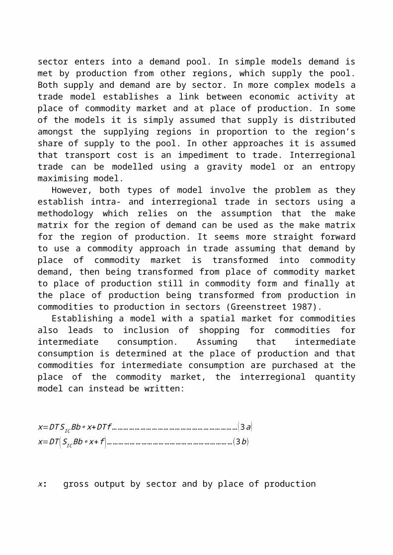
Establishing a model with a spatial market for commodities also leads to inclusion of shopping for commodities for intermediate consumption. Assuming that intermediate consumption is determined at the place of production and that commodities for intermediate consumption are purchased at the place of the commodity market, the interregional quantity model can instead be written:

x=DT S ICBb∘ x+DTf ………………………………………………………… (3a )x=DT (SICBb ∘x+f )…………………………………………………………(3b)

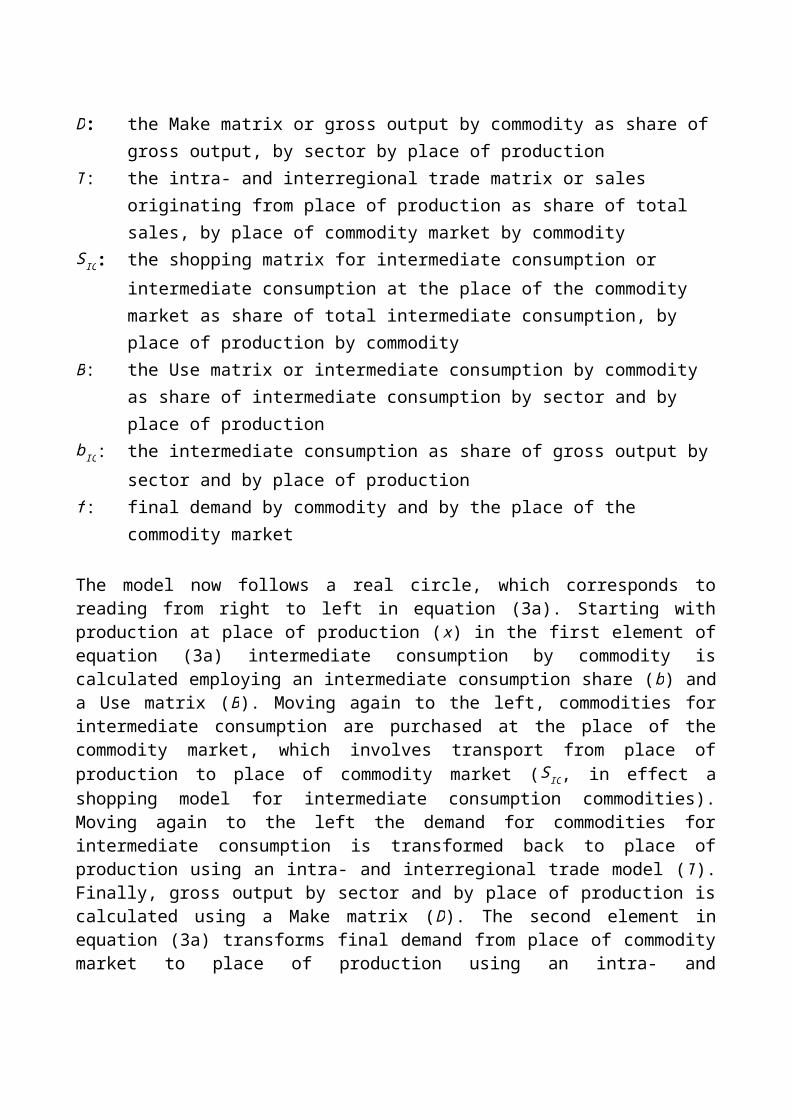
x: gross output by sector and by place of productionD: the Make matrix or gross output by commodity as share of gross output, by sector

by place of production

T : the intra- and interregional trade matrix or sales originating from place of production as share of total sales, by place of commodity market by commodity

S IC: the shopping matrix for intermediate consumption or intermediate consumption at the place of the commodity market as share of total intermediate consumption, by place of production by commodity

B: the Use matrix or intermediate consumption by commodity as share of intermediate consumption by sector and by place of production

b IC: the intermediate consumption as share of gross output by sector and by place of production

f : final demand by commodity and by the place of the commodity market

The model now follows a real circle, which corresponds to reading from right to left in equation (3a). Starting with production at place of production (x) in the first element of equation (3a) intermediate consumption by commodity is calculated employing an intermediate consumption share (b) and a Use matrix (B). Moving again to the left, commodities for intermediate consumption are purchased at the place of the commodity market, which involves transport from place of production to place of commodity market (S IC, in effect a shopping model for intermediate consumption commodities). Moving again to the left the demand for commodities for intermediate consumption is transformed back to place of production using an intra- and interregional trade model (T ). Finally, gross output by sector and by place of production is calculated using a Make matrix (D). The second element in equation (3a) transforms final demand from place of commodity market to place of production using an intra- and interregional trade model (T ) and further from production in commodities to production by sector using a make matrix (D).

Assuming that the interregional trade structure (T ) and the make matrix (D) for intermediate and final consumption goods are identical, T and D can be set outside the parentheses (equation 3b).

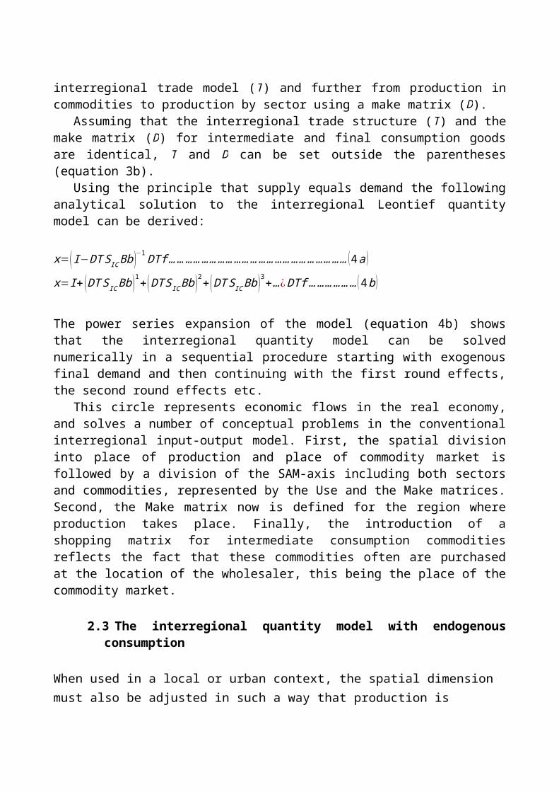
Using the principle that supply equals demand the following analytical solution to the interregional Leontief quantity model can be derived:

x=( I−DT SICBb )−1DTf ………………………………………………………… (4 a )

x=I+(DT S IC Bb )1+(DT SICBb )2+(DT S ICBb )3+…¿DTf ……………… ( 4b )

The power series expansion of the model (equation 4b) shows that the interregional quantity model can be solved numerically in a sequential procedure starting with exogenous final demand and then continuing with the first round effects, the second round effects etc.

This circle represents economic flows in the real economy, and solves a number of conceptual problems in the conventional interregional input-output model. First, the spatial division into place of production and place of commodity market is followed by a division of the SAM-axis including both sectors and commodities, represented by the Use and the Make

matrices. Second, the Make matrix now is defined for the region where production takes place. Finally, the introduction of a shopping matrix for intermediate consumption commodities reflects the fact that these commodities often are purchased at the location of the wholesaler, this being the place of the commodity market.

2.3The interregional quantity model with endogenous consumption

When used in a local or urban context, the spatial dimension must also be adjusted in such a way that production is located at the place of production whereas the institution is located at the place of residence of the institution. Private consumption is derived from demand originating at the place of residence and is purchased at the place of production. Introducing the real circle into the interregional quantity model involves a geographical transformation in 2 steps: i) commuting, which transforms employment from place of production to place of residence (and from sectors to types of institutions); ii) combined shopping and trade, which transforms private consumption from place of residence to place of production (and from type of institution back to sector). Further, a kind of activity transformation in two steps is involved: from sectors to production factors and from production factors to commodities. Transforming the interregional Leontief model into a local or an urban input-output model involves introduction of three spatial dimensions and three SAM-dimensions into the modelling framework.

In this 3 dimensional version of the interregional quantity model the following spatial transformations are included: from place of production to place of residence corresponding to a transformation from

sectors to type of production factors from place of residence to place of commodity market corresponding to a

transformation from type of production factors to commodities from place of commodity market back to place of production corresponding to a

transformation from commodities to sectors

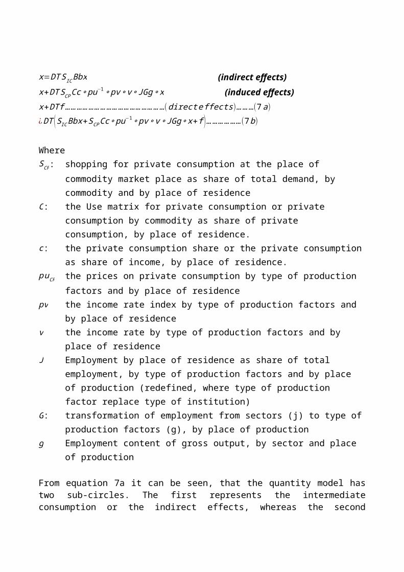
The model assumes that intermediate consumption and final demand are added before entering into the intra- and interregional trade systemi. Gross output can now be expressed as follows:

x=DT S ICBbx (indirect effects)x+DT SCPCc∘ pu−1∘ pv∘ v ∘ JGg∘ x (induced effects)x+DTf …………………………………………… (direct e ffects)………(7 a)¿DT (S ICBbx+SCPCc∘ pu−1∘ pv∘ v ∘ JGg∘ x+ f )………………(7b)

WhereSCP: shopping for private consumption at the place of commodity market place as share

of total demand, by commodity and by place of residenceC: the Use matrix for private consumption or private consumption by commodity as

share of private consumption, by place of residence.c: the private consumption share or the private consumption as share of income, by

place of residence.puCP the prices on private consumption by type of production factors and by place of

residence pv the income rate index by type of production factors and by place of residence v the income rate by type of production factors and by place of residence J Employment by place of residence as share of total employment, by type of

production factors and by place of production (redefined, where type of production factor replace type of institution)

G: transformation of employment from sectors (j) to type of production factors (g), by place of production

g Employment content of gross output, by sector and place of production

From equation 7a it can be seen, that the quantity model has two sub-circles. The first represents the intermediate consumption or the indirect effects, whereas the second includes the private consumption (induced) effects. The third ‘appendix’ is the exogenous demand or the direct effects.

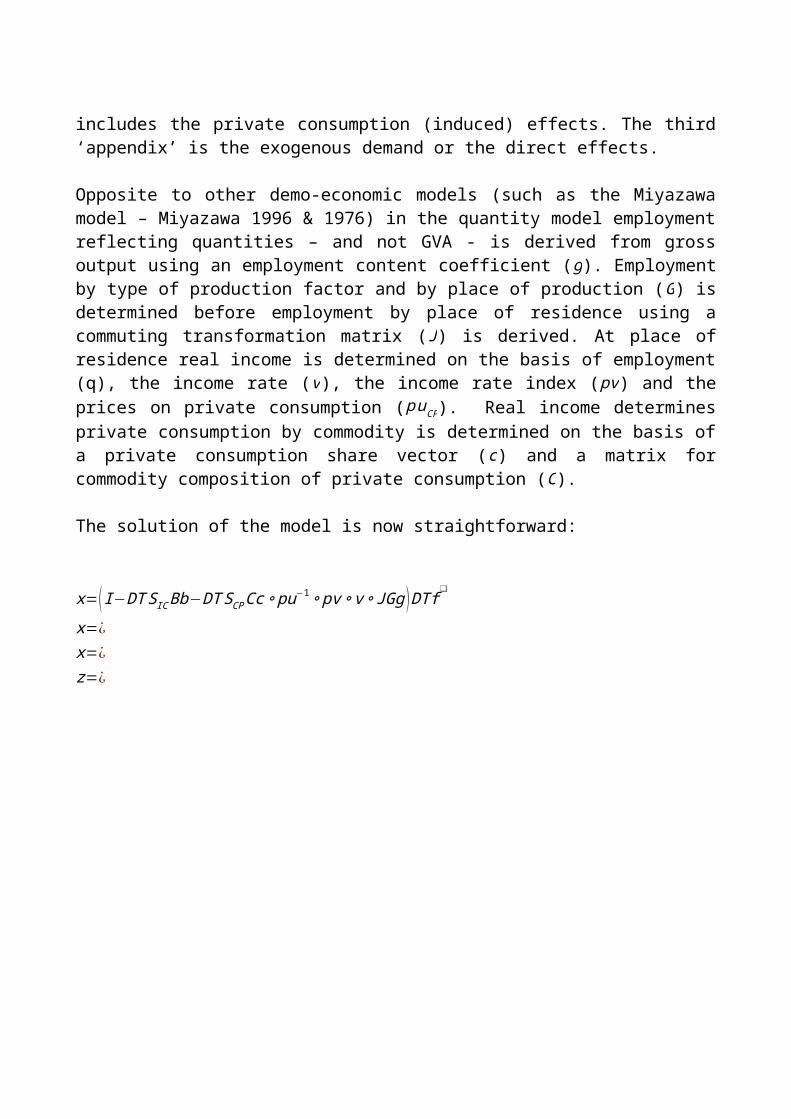
Opposite to other demo-economic models (such as the Miyazawa model – Miyazawa 1996 & 1976) in the quantity model employment reflecting quantities – and not GVA - is derived from gross output using an employment content coefficient (g). Employment by type of production factor and by place of production (G) is determined before employment by place of residence using a commuting transformation matrix (J) is derived. At place of residence real income is determined on the basis of employment (q), the income rate (v), the income rate index (pv) and the prices on private consumption ( puCP). Real income determines private consumption by commodity is determined on the basis of a private consumption share vector (c) and a matrix for commodity composition of private consumption (C). The solution of the model is now straightforward:

x=(I−DT S ICBb−DT SCPCc∘ pu−1∘ pv∘v ∘JGg )DTf❑

x=¿x=¿

z=¿

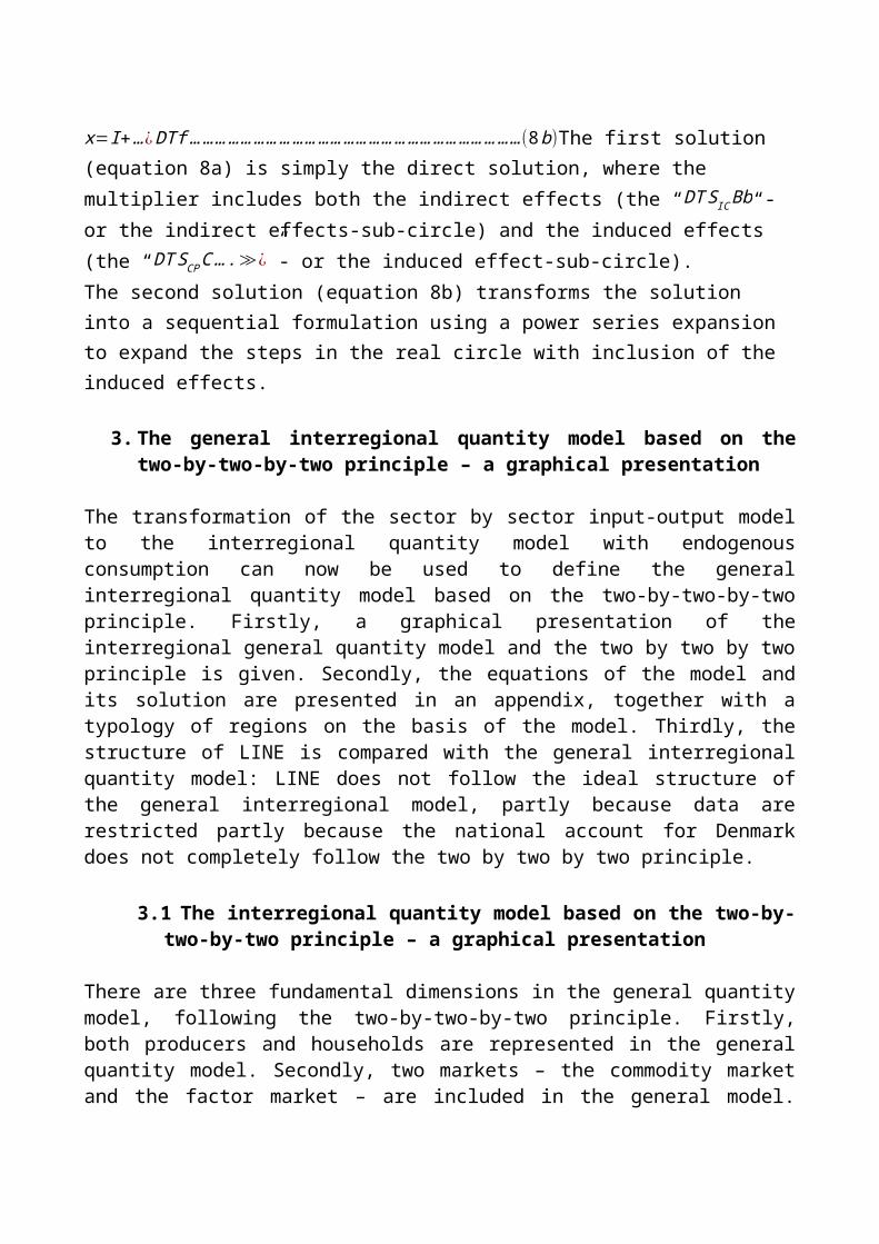
x=I+…¿DTf ……………………………………………………………………(8b)The first solution (equation 8a) is simply the direct solution, where the multiplier includes both the indirect effects (the “DT S IC Bb“- or the indirect effects-sub-circle) and the induced effects (the “DT SCPC….≫¿”- or the induced effect-sub-circle).The second solution (equation 8b) transforms the solution into a sequential formulation using a power series expansion to expand the steps in the real circle with inclusion of the induced effects.

3. The general interregional quantity model based on the two-by-two-by-two principle – a graphical presentation

The transformation of the sector by sector input-output model to the interregional quantity model with endogenous consumption can now be used to define the general interregional quantity model based on the two-by-two-by-two principle. Firstly, a graphical presentation of the interregional general quantity model and the two by two by two principle is given. Secondly, the equations of the model and its solution are presented in an appendix, together with a typology of regions on the basis of the model. Thirdly, the structure of LINE is compared with the general interregional quantity model: LINE does not follow the ideal structure of the general interregional model, partly because data are restricted partly because the national account for Denmark does not completely follow the two by two by two principle.

3.1The interregional quantity model based on the two-by-two-by-two principle – a graphical presentation

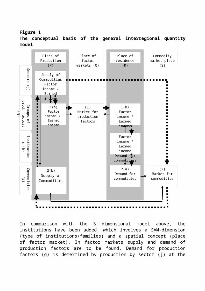
There are three fundamental dimensions in the general quantity model, following the two-by-two-by-two principle. Firstly, both producers and households are represented in the general quantity model. Secondly, two markets – the commodity market and the factor market – are included in the general model. Thirdly, interaction between markets and actors include information on origins and destinations. For both actors and markets basic geographical concepts have been used as well as social accounting concepts for activities. The model structure is presented in figure 1.

Place of Production (P)

Place of factor markets (Q)

Place of residence (R)

Commodity market place (S)

Sectors (j)

Groups of

prod. factors (g)Institutions (h)

Com

modities (i)

Supply of Commodities

Factor income / Earned income

1(a)Factor

income / Earnedincome

(1)Market for production

factors

1(b)Factor income / Earned income

Factor income / Earned income

Demand for commodities

2(a)Demand for commodities

(2)Market for

commodities

2(b)Supply of

Commodities

Figure 1The conceptual basis of the general interregional quantity model

In comparison with the 3 dimensional model above, the institutions have been added, which involves a SAM-dimension (type of institutions/families) and a spatial concept (place of factor market). In factor markets supply and demand of production factors are to be found. Demand for production factors (g) is determined by production by sector (j) at the place of production (p). In figure 1 factor demand by sector is transformed into factor demand by type of production factor (g). On the supply side, supply of production factors by type of institution (h) is transformed into supply by type of production factor (g). Supply of a production factor is related to the place of residence of the institution (r). The factor market is geographically assigned to the market place for factors (q).

Completing the presentation of the general model based on the two-by-two-by-two principle, in figure 1 in the commodity market there is a distinction between place of residence (r), the market place for commodities (s) and place of production (p). The market place for commodities links the demand for the commodity (from place of residence to the market place for commodities) to the supply of the commodity (from place of production to the market place for commodities). Before the transformation to the market place for commodities, the demand for commodities is transformed from institutional group (h) to commodity (i). On the supply side, production by sector (j) is transformed into production by commodity (i) and then supply is related geographically to the market place for commodities (s).

Second, in the general model both domestic and foreign sectors are represented in all markets. This involves not only international trade in commodities, but also other types of international interaction, such as cross border commuting (income flows to and from abroad through commuting), border shopping, which includes one-day tourist expenditure in both directions, and tourism, again in both directions. This extension is included to make the general model more applicable as most regional systems do not encompass the world, but are surrounded by »the rest of the world«.

3.2 The model and typology of regions

In appendix 1 the equations of the general local/urban quantity model are presented. The model can be treated as a national model (including an input-output model and a Keynesian income multiplier model), where a spatial dimension and a social accounting dimension has been included. The equations in the real circle are presented in structural form together with their partial solutions.

The analytical solution can be used to refine and document a) the multiplier effects of the economic activity in a local area on the local area itself and b) the spill-over effects from economic activities in other local areas on the local area. The general a priori result is that the multiplier becomes smaller the smaller the area, but also that the local area becomes increasingly dependent upon economic activity in other local areas, especially the neighbouring areas. The extreme example is of course the case where a local area only consists of one production unit. In this case the internal multiplier effect on demand from the production unit itself becomes small, whereas the economic dependency on economic activity in all other local areas becomes very important.

Another aspect is that the analytical solution shown in equation 9 is determined from the perspective of the place of production and industrial sector. If the subject was instead effects on income by place of residence (,which is relevant from a place of residence and type of institution perspective), the impacts arising from changes in exogenous demand would be smaller. Alternatively, if the perspective was the effects on economic activity at the place of commodity market (such as retailing activities), then the impacts would be even smaller.

Using the analytical solution, a list of factors determining the level of production at the place of production can be drawn up, the sign in brackets showing the expected impacts on gross output of positive change in the factor: Intermediate consumption

– Share of gross output (?)– Purchases abroad (-)– Purchases in other local areas (-)– Purchases from other local areas (+)– Purchases from abroad (+)

Commuting– Place of residence abroad (-)– Place of residence in other local areas (-)– Place of production in other areas (+)– Place of production abroad (+)

Local private consumption (shopping) – Propensity to consume (+)– Private consumption abroad, such as tourism abroad (-)– Shopping in other local areas, including domestic tourism (-)– Shopping from other local areas, including domestic tourism (+)– Private consumption from abroad, such as one-day tourism and conventional

tourism (+) Trade

– Import from abroad (-)– Import from other local areas (-)– Export to other local areas (+)– Export broad (+)

As can be seen the above list includes factors which involve interaction between the local area itself, other regions and abroad. Other exogenous variables affecting the composition of demand and supply in the commodity market and in the market for production factors also influence economic activity in the local area. Impacts of such changes should be modelled with other types of interregional models, which include impacts from changes in costs and prices.

The list can be used to identify different ideal types of local area. Each group is a pure type, whilst in reality a local area is a mix of different types. The definition relies upon the interaction balance, net areas based upon local production

– primary products (trade balance and intermediate commodity-purchasing surplus in primary products)

– secondary products (trade balance and intermediate commodity - purchasing surplus in secondary products)

– advanced services (trade balance and intermediate commodity -purchasing surplus in tertiary products)

residential areas– high level of outward commuting and low level of inward commuting

areas based upon shopping– high level retailing services (local private consumption: shopping surplus)– conventional tourist areas (surplus in conventional tourist balance)

urban (surplus in conventional tourist balance) rural (surplus in conventional tourist balance) ecological (surplus in conventional tourist balance for ecological tourist type)

– one day tourist areas cultural (surplus in one-day tourist balance) retailing (surplus in one-day tourist balance)

3.3 The LINE model and the general interregional quantity model

LINE is an interregional general equilibrium model constructed for Danish municipalities (Madsen et al 2001 and Madsen & Jensen-Butler (2004)). The spatial two-by-two-by-two principle described above has been the guiding principle for the construction of the model and the interregional social accounting matrix, SAM-K (Madsen et al 2002a & 2002b and Madsen & Jensen-Butler (2004)), which serves as the database for LINE. Both LINE and SAM-K are designed on the basis of the structure shown in figure 1, using the double spatial entry principle or extended regional accounts (two-by-two-by-two), rather than non-spatial regional accounting principles (two-by-two).

The structure of LINE follows the basic interregional general equilibrium model shown in figure 5.1 with: Factor markets and commodity markets Demand and supply in both markets Origins and destinations in all interactions

However, there are some differences between LINE and a model based upon a pure two-by-two-by-two principle. Some simplifications and some extensions are incorporated. The general model is adjusted in order to take into account the nature of the available data and the structure of the regional economy. In some respects the model is developed, whilst in other respects it is simplified.

First, the concept of the market place for factors does not correspond in general to reality. In practice, the place of residence of the production factor (such as labour) can be interpreted as both place of residence and the market place for factors. Only in very few

cases does a geographically defined factor market exist. From a data collection point of view, only registration of place of residence and place of production in the factor market is possible. Therefore, the market place for factors has been excluded from LINE.

Second, only factor income from labour receives a full treatment. Regional data on capital income only exist by place of production in Denmark. Data on interregional commuting of capital income is still lacking, which makes a comparable treatment to commuting flows of labour income impossible and identification of a market place for capital income difficult to develop. In the present version of LINE capital income enters exogenously at the place of residence without any information on its spatial origin. Future developments with respect to savings and investments and identification of market places for these could include the use of pooling methods or identification of gross flows, referred to above.

Third, there is a need to keep track of economic interactions at the place of residence between factor groups and between institutions. Interaction between households and the governmental sector is important in order to describe the economic strength of households, for example measured by disposable income of households including income transfers from government and the subtraction of taxes. Interactions between factor groups, household and governmental sectors are therefore included in LINE.

Fourth, consumption by institutions (households) both from a decision-making or a behavioural point of view must be divided into two nested steps. First, at the place of residence consumption is determined at a high level of aggregation, for example food, clothing, transport etc. and in market prices. In the next step, at the place of commodity market the consumption bundles are further divided into specific commodities, transformed into basic prices, and distributed into domestic and foreign markets and among producing regions. From a decision-making point of view both the first and second steps are a part of the household decision problem, the sellers (the retailing sector) reflecting the demand from the households. The same is the case for intermediate consumption and for other types of final demand, such as governmental consumption and gross capital formation, where decisions are taken in two steps: First, at the place of residence deciding expenditure on aggregate commodity, such as expenditure on schools and second in the institution at the place of commodity market and the place of production, where decisions on type of commodity, by domestic and foreign market and by supplying regions are taken.

Fifth, private consumption has been divided into local private consumption and domestic tourism. This division has been relevant in studies of tourism impacts, where in LINE it is possible to distinguish between tourism by foreigners, domestic tourism and tourism abroad, all divided into either one-day visits or visits involving overnight stays.

Sixth, different price concepts are included in the model, reflecting the fact that different variables for economic activity use different price concepts. For goods and services, total expenditures at the place of commodity market are measured in market prices. Supply of commodities entering the goods and services market is modelled in basic prices. Basic prices are defined as the value of production at the factory, not including net commodity taxes paid by the producer. Going from market/buyers prices to basic prices involves subtraction of commodity taxes and trade margins, where trade margins also are part of the commodity

account. Interregional trade is measured in basic prices both seen from at the place of production and place of commodity market point of view. At the place of commodity market commodity prices are transformed from basic prices to market prices.

Finally, LINE is based upon two interrelated circles: a real circuit described above and a dual cost-price circuit. Figure 1 shows the general model structure, based upon the real circle employed in LINE. The two circles are linked together with a link from real economic activities to formation of cost and prices (mainly a weighting system for determining costs and prices) and from the costs and prices to real economic activity. This last link includes the effects of cost and price changes on demand, the transformation of disposable income in current prices to fixed prices and the effects on exports and imports prices in turn determining exports and imports. Part of the model uses fixed prices (the demand and supply of commodities) and part of the model uses current prices (earned income, taxes, transfer incomes and disposable income).

Here only a brief comparison of LINE and the general interregional quantity model is made. The full LINE model and its equations are described in Madsen et al. (2001) and Madsen & Jensen-Butler (2004). LINE has been constructed as a flexible on a number of key dimensions. For any application of LINE the model and the associated database are aggregated in order to capture the special requirements of each case. Thus in any version of LINE the model configuration is specific. One example of such an application is the basis version of SAM-K and LINE, which Danish regions and labour market regions use in monitoring economic activity and where the following dimensions were used:

Sectors37 sectors aggregated from the 130 sectors used in the national accounts.

Factors10 age, 2 sex and 20 education groups.

Households4 types, based upon household composition.

NeedsFor private consumption and governmental individual consumption 13 components, aggregated from the 72 components in the detailed national accounts. For governmental consumption, 8 groups. For gross fixed capital formation, 10 components.

Commodities37 commodities, aggregated from app. 2800 commodities used in the national accounts.

Regions

99 municipalities, including one state-owned island and one unit for extra-regional activities, this being the lowest level of spatial disaggregation. Regions are defined either as place of production, place of residence or as place of commodity market.

4. Impact studies with LINE.To illustrate the new description of local economy a set of multiplier experiments for 98 Danish municipalities with the local economic model LINE are presented: The case chosen is state activities in Danish municipalities. Firstly, the case is of major interest in regional policy. Seen from the local economy point of view state jobs can be seen as export jobs financed from the “rest of the world”. Secondly, state activities are present in all municipalities, which makes it possible to sort out factors explaining the share of state activities (direct effects) and influencing the multiplier process working through the geographical and kind of activity transformations recorded in LINE (direct and derived effects).

4.1. State activities definition and volume of activityIn this analysis state activities are defined on the basis of ownership code for production units: In the SAM, ownership is recorded as sectors and at the place of production (Pj). The owner ship code is aggregated into the following 4 types:

- Private- Municipality- County- State

To evaluate the impacts of state jobs, employment in state activities is set to zero in each municipality successively and LINE then calculates the direct (negative) effects and the derived effects in 98 multiplier experiments.

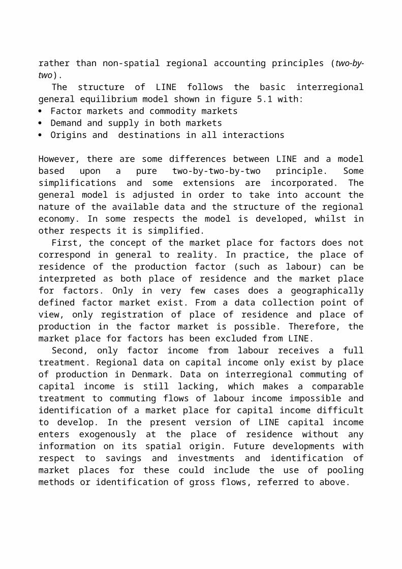
4.2 Regional direct impacts on jobs from state activitiesThe number of state jobs and their impacts on employment by 98 Danish municipalities by place of production can be seen in table 1 and in appendix 2, table 1 and by place of residence in table 2 and in appendix 2, table 2.In table 1, column 1 the results for the 10 municipalities with highest and the 10 municipalities with the lowest shares in direct employment by place of production are shown. Table 1 in appendix 1 shows the results for all 98 municipalities.

Table 1. The 10 municipalities with the highest and the 10 municipalities with the lowest share of employment by place of production in state jobs in Denmark in 2008

Direct Total Multiplier

Share Rank Share Rank Index Rank

1 2 3 4 5 610 highest ranked:Frederiksberg 15,6 1 17,9 2 114,8 76København/Copenhagen 13,7 2 18,5 1 134,6 8Lyngby-Taarbæk 11,9 3 13,4 6 112,6 89Slagelse 11,9 4 15,3 3 128,9 16Viborg 11,0 5 13,6 5 123,9 30Allerød 10,4 6 13,7 4 132,5 11Haderslev 10,4 7 12,8 7 123,2 37Roskilde 10,2 8 12,0 8 117,3 64Frederikshavn 9,5 9 11,8 9 123,8 32Aalborg 9,0 10 10,8 12 119,8 50

10 lowest ranked:Jammerbugt 3,0 89 3,4 90 114,9 74Vallensbæk 2,9 90 3,5 89 121,0 46Greve 2,8 91 3,4 91 121,4 44Brønderslev 2,6 92 3,0 92 115,0 73Herlev 2,5 93 2,9 93 118,5 55Stevns 2,2 94 2,8 94 124,4 28Egedal 1,8 95 2,4 96 129,8 13Glostrup 1,8 96 2,4 95 134,2 9Kerteminde 1,5 97 1,9 97 123,3 36Læsø 1,4 98 1,8 98 124,5 27

From the column 1 in table 1 it can be seen, that Frederiksberg (neighbor to the municipality of Copenhagen), Copenhagen and Aalborg (city number 4) are members of the top-ten group. Other municipalities in the top-ten group are municipalities with military barracks, such as Slagelse, Viborg, Allerød, Haderslev and Frederikshavn. Finally, municipalities with universities and hospitals such as Lyngby-Taarbæk and Roskilde are also included in the top-ten group.The bottom-ten municipalities are peripheral municipalities without military barracks, such as Jammerbugt, Brønderslev, Stevns, Kerteminde, Læsø municipalities and sub-urban municipalities in Copenhagen, such as Vallensbæk, Greve, Herlev, Egedal and Glostrup.

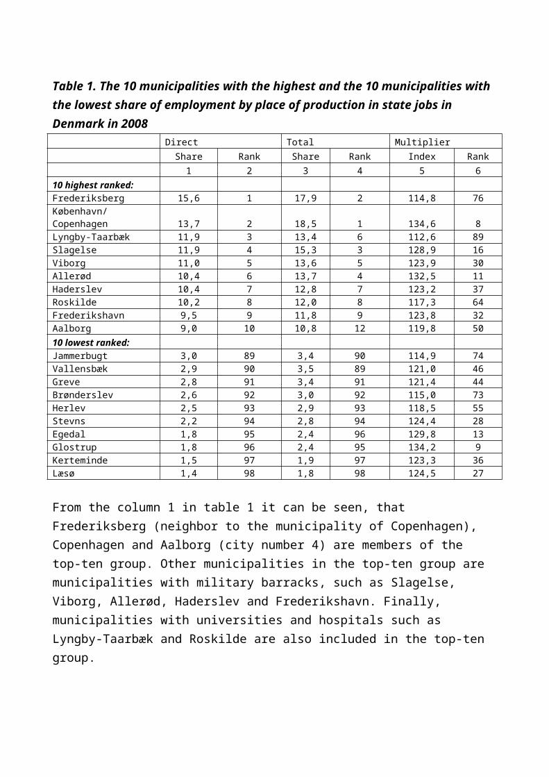
Table 2. The 10 municipalities with the highest and the 10 municipalities with the lowest share of employment by place of residence in state jobs in Denmark in 2008

Direct Total Multiplier

Share Rank Share Rank Index Rank

1 2 3 4 5 610 highest ranked:Bornholm 12,1 1 13,3 3 109,7 65Viborg 11,4 2 13,3 2 116,4 21Aalborg 11,3 3 12,5 5 110,6 57København/Copenhagen 11,2 4 13,9 1 123,4 7Frederikshavn 10,8 5 12,4 6 115,6 26Slagelse 10,6 6 12,7 4 120,3 13Haderslev 9,8 7 11,3 7 115,2 29Århus 9,8 8 10,6 8 108,6 77Svendborg 9,0 9 9,3 12 103,8 98Samsø 8,9 10 9,9 9 112,1 46

10 lowest ranked:Stevns 1,7 89 1,9 90 112,9 41Ishøj 1,6 90 1,9 88 118,4 18Hvidovre 1,5 91 1,7 91 114,7 31Greve 1,4 92 1,6 92 112,5 45Rødovre 1,2 93 1,4 93 122,7 11Solrød 1,2 94 1,3 94 113,2 37Herlev 1,1 95 1,2 95 111,0 54Vallensbæk 0,8 96 0,9 96 114,7 33Egedal 0,8 97 0,9 97 118,5 17Glostrup 0,7 98 0,8 98 122,9 10

Looking table 2, column 1 and 2, the impacts by place of residence as well as the ranking the pattern is changed, although the results still are mainly a result of the location of state jobs: Bornholm (the biggest of the islands municipalities) now enter into the top-ten group: The island has it military barrachs, but the share of permanent personnel, who both work and live on the island is high, because in-commuting is limited. Therefore, although that ranking according to place of production is 14, due to very low in-commuting the total impacts are ranked as 1. Frederiksberg disappears from the top-ten group having a rank as 54 from a place of residence point of view. The ranking of Copenhagen also falls although less. These changes are also explained by substantial in-commuting from Greater Copenhagen sub-urban.

For the 10 lowest ranked municipalities this group now consists exclusively of sub-urban municipalities in Greater Copenhagen area. The reason for this is the leakage in the form of commuting: A substantial part of state jobs in the municipality themselves are transferred

to other municipalities (in the Greater Copenhagen area) and very few of the jobs in the municipality itself return as extra derived jobs, all due to the high level of commuting.

4.3 Regional total impacts within the municipality on jobs from state activities As can be seen changes in rankings are very close related to the leakages on labor market and the size of multipliers, which is examined more in detail in the section. In general impacts within the municipalities are 23% higher than the direct effects – the share of employment at national level is 7,2% of total employment. Impacts within the municipalities is 8,8%, whereas the total impacts including jobs in other municipalities making the total domestic impacts 35% higher effects than the direct jobs involving 9,7% of employment as direct and derived jobs from state activities. This means that for every time 100 state jobs are established, 23 jobs within the municipality and 35 jobs including 12 jobs in other municipalities are created.The impacts from state jobs depend on leakages, such as commuting, shopping/tourism and trade. At the place of production all directs effects are related to the place of production. At the place of residence some of the state jobs remain in the municipality whereas other are transferred other municipalities or even to the rest of the world. Looking at the place of commodity market even more of the direct effects are transferred to other municipalities and the rest of the world.Looking at total impacts the spill over, but also the feed-back processes are continued. The following table illustrates the process at the place of production for jobs and at the place of production for the employment:

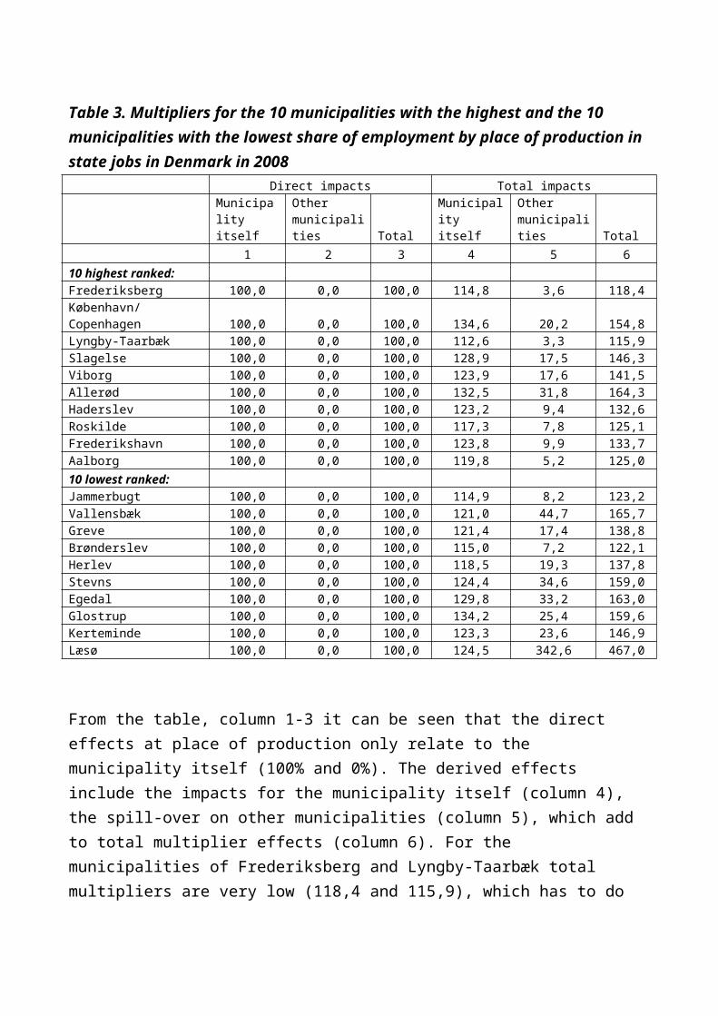
Table 3. Multipliers for the 10 municipalities with the highest and the 10 municipalities with the lowest share of employment by place of production in state jobs in Denmark in 2008

Direct impacts Total impactsMunicipality itself

Other municipalities Total

Municipality itself

Other municipalities Total

1 2 3 4 5 610 highest ranked:Frederiksberg 100,0 0,0 100,0 114,8 3,6 118,4København/Copenhagen 100,0 0,0 100,0 134,6 20,2 154,8Lyngby-Taarbæk 100,0 0,0 100,0 112,6 3,3 115,9Slagelse 100,0 0,0 100,0 128,9 17,5 146,3Viborg 100,0 0,0 100,0 123,9 17,6 141,5Allerød 100,0 0,0 100,0 132,5 31,8 164,3Haderslev 100,0 0,0 100,0 123,2 9,4 132,6Roskilde 100,0 0,0 100,0 117,3 7,8 125,1Frederikshavn 100,0 0,0 100,0 123,8 9,9 133,7Aalborg 100,0 0,0 100,0 119,8 5,2 125,0

10 lowest ranked:Jammerbugt 100,0 0,0 100,0 114,9 8,2 123,2Vallensbæk 100,0 0,0 100,0 121,0 44,7 165,7Greve 100,0 0,0 100,0 121,4 17,4 138,8Brønderslev 100,0 0,0 100,0 115,0 7,2 122,1Herlev 100,0 0,0 100,0 118,5 19,3 137,8Stevns 100,0 0,0 100,0 124,4 34,6 159,0Egedal 100,0 0,0 100,0 129,8 33,2 163,0Glostrup 100,0 0,0 100,0 134,2 25,4 159,6Kerteminde 100,0 0,0 100,0 123,3 23,6 146,9Læsø 100,0 0,0 100,0 124,5 342,6 467,0

From the table, column 1-3 it can be seen that the direct effects at place of production only relate to the municipality itself (100% and 0%). The derived effects include the impacts for the municipality itself (column 4), the spill-over on other municipalities (column 5), which add to total multiplier effects (column 6). For the municipalities of Frederiksberg and Lyngby-Taarbæk total multipliers are very low (118,4 and 115,9), which has to do with low derived effects in university sectors. From column 4 and 5 it can be seen, that the low multiplier originates from low internal feed-back effects on the municipality itself (column 5). Opposite for the municipality of Copenhagen, which due to size have high internal and external multipliers. This is also the case for municipalities in Jutland.

Table 4. Multipliers for the 10 municipalities with the highest and the 10 municipalities with the lowest share of employment by place of residence in state jobs in Denmark in 2008

Direct impacts Total impactsMunicipality itself

Other municipalities Total

Municipality itself

Other municipalities Total

1 2 3 4 5 610 highest ranked:Bornholm 94,6 5,4 100,0 103,8 14,5 118,3Viborg 65,3 34,7 100,0 76,0 50,3 126,2Aalborg 76,8 23,2 100,0 84,9 29,0 113,9København/Copenhagen 47,0 53,0 100,0 58,0 76,1 134,0Frederikshavn 77,8 22,2 100,0 89,8 31,6 121,4Slagelse 67,9 32,1 100,0 81,7 48,6 130,3Haderslev 70,3 29,7 100,0 81,0 39,8 120,8Århus 73,5 26,5 100,0 79,8 30,4 110,3Svendborg 79,0 21,0 100,0 82,0 24,0 106,0Samsø 92,1 7,9 100,0 103,3 37,0 140,3

10 lowest ranked:Stevns 71,9 28,1 100,0 81,3 49,3 130,5Ishøj 24,3 75,7 100,0 28,7 96,3 125,1Hvidovre 25,7 74,3 100,0 29,5 91,4 120,9Greve 40,7 59,3 100,0 45,9 74,8 120,6Rødovre 23,0 77,0 100,0 28,3 99,3 127,5Solrød 39,1 60,9 100,0 44,3 82,1 126,4Herlev 20,0 80,0 100,0 22,2 99,8 122,0Vallensbæk 23,0 77,0 100,0 26,3 105,5 131,9Egedal 42,1 57,9 100,0 49,9 83,5 133,4Glostrup 12,5 87,5 100,0 15,3 120,7 136,0

From a place of residence point of view, islands such as Bornholm and Samsø have very small out-commuting. The direct impacts are more than 90%, due to low out-commuting, whereas municipalities of Copenhagen only keep 47% of the state jobs inside the municipality, reducing the impacts from state jobs. This increases the rankings of state jobs for islands and decreases the impacts for urban municipalities with high share of state jobs. These effects can also be studied for the 10 lowest ranked municipalities, which now are sub-urban municipalities in the greater Copenhagen area

5. ConclusionsIn the article it is argued that local economies have become more complex and that local economic models must reflect this reality. Based upon the two by two by two principle this involve a set of new geographical concepts and in the context of an interregional SAM the development of the two-by-two-by-two approach, involving two sets of actors (production

units and institutional units), two types of markets (commodities and factors) and two locations (origin and destination). From these four geographical concepts – the place of production, the place of factor market, the place of residence and the commodity market place – are introduced as well as 4 different SAM-actors, which are sectors, factor types, institutional or family types and commodities. The equations of the general interregional quantity model are presented together with the solution of the model. Comparisons are made with the Danish interregional static CGE-model LINE and a typology of regions is proposed using the general model as a conceptual foundation. Finally, results of analysis on data wit LINE to assess the impacts of state jobs are presented: Direct state jobs are 7,2% of total employment. Adding to this the multiplier effects the impacts of state jobs are explained by the size of geographical and kind of activity transformations included in LINE (the two by two by two principle). Impacts within the municipalities is 8,8%, whereas the total impacts including jobs in other municipalities making the total domestic impacts 35% higher effects than the direct jobs involving 9,7% concentrated in cities and metropolitan area and in area where military barracks are located. The impacts also depend upon whether the variable is related to place of production, where state jobs have the full impact on economic activity, whereas residential employment and market place demand only are partly reduced according to the pattern of commuting and pattern of shopping and tourism.

Litterature

Andersen, E (1975): En model for Danmark 1949-1965- Københavns Universitets Økonomiske Studier nr. 21. København: Forlag, Denmark

Chenery, H.B. (1953): Regional Analysis. In: Chenery, H.B.; P.G. Clark and V.C. Pinna (eds.):The Structure and Growth of the Italian Economy, U.S. Mutual Security Agency, Rome: 97-129.

Dam, P.U. (Ed.) (1995): ADAM—En model for dansk økonomi, Statistics Denmark, Denmark

Danish Ministry of Finance (2003) Lovmodellen, maj 2003, Finansministeriet, Copenhagen, Denmark

Danmarks Nationalbank (2004): MONA – Model for the Danish Economy, Danmarks Nationalbank, Denmark

Danmarks Statistik (1973): Input-output tabeller for Danmark 1966. Statistiske Undersøgelser nr. 30 og 31. København, Denmark

Det Økonomiske Råds sekretariat (2007) SMEC - Modelbeskrivelse og -egenskaber, 2006, Arbejdspapir (2007:1), Det Økonomiske Råds sekretariat, Denmark

DREAM-group (2008) Danish Rational Economic Agents Model, Statistics Denmark, Denmark

Greenstreet, D. (1987): Constructing an interregional commodity-by-industry input -quantitymodel. Research Paper 8713, Regional Research Institute, West Virginia University.

Groes, N (1982a): En fast forbindelse - oplæg til debat om konsekvenser af en fast Store-bæltsforbindelse - på landsplan og regionalt, Department of Border Region Studies, Denmark.

Groes, N (1982b): En regionalmodel for Sønderjylland, Department of Border Region Studies, Denmark.

Holm, K. (1984): Hovedstadsregionens økonomi – en modelbeskrivelse.AKF Forlaget, Copenhagen.

Isard, W. (1951): Interregional and Regional Input-quantity Analysis: A Model of a SpaceEconomy. Review of Economics and Statistics 33(4): 318-328.

Jensen-Butler, C & B Madsen (2002): Modelling the Regional Economic Effect of the Danish Great Belt Link. In: Classics in Transport Studies. Edward Elgar, UK

Jensen-Butler, C; Gaspar...????

Leontief, W xx A og I-a

Leontief, W xx Interregional A og I-a

Madsen, B (1992a): Report on the AIDA Model, AKF, Copenhagen, Denmark

Madsen, B (1992b): Report on the EMIL Model, AKF, Copenhagen, Denmark

Madsen, B; C Jensen-Butler & PU Dam (2002a): The Line-model. AKF forlaget, Copenhagen, Denmark.

Madsen, B; C Jensen-Butler & PU Dam (2002b): A Social Accounting Matrix for Danish Municipalities (SAM-K). AKF forlaget, Copenhagen, Denmark.

B Madsen & C Jensen-Butler (2004): Theoretical and operational issues in sub-regional modelling, illustrated through the development and application of the LINE model, Economic Modelling, Volume 21, Issue 3, p. 471-508.

Miyazawa, K. (1966): Internal and external matrix multipliers in the input-output model.Hitotsubashi Journal of Economics 7: 38-55.

Miyazawa, K. (1976): Input-output Analysis and the Structure of Income Distribution.Springer-Verlag, New York.

Moses, L.N. (1955): The Stability of Interregional Trading Patterns and Input-quantityAnalysis. American Economic Review 45(5): 803-32.

Jan Oosterhaven (1981) Interregional input-output analysis and dutch regional policy problems, Ph.d.-dissertation University of Groningen, the Netherlands

Thage, B (1981): Techniques in the Compilation of Danish Input-Output Tables: A New Approach to the Treatment of Imports, Danmarks Statistik 6.kt. København, Denmark

Thage, B & A Thomsen (2004): Nationalregnskabet, Serien Erhverv og samfund, Handelshøjskolen Forlag, Denmark

Appendix 1 The equations for the general interregional quantity model for local and urban economies in structural form

In this appendix the general interregional quantity model is documented in detail, including the equations in the model. Firstly, the notation in the mathematical documentation is explained. Secondly, the equations are presented followed by a verbal explanation of the model based upon the two-by-two-by-two principle and the graphical presentation of the model in figure 1. Thirdly, the mathematical solution to the model is presented and discussed. Fourthly, the four approaches to measuring the impacts of tourism is defined in mathematical terms following the structure and equations of the model.

A 2.1The model – notation

The notation includes such information as variable names, sub-script, superscripts and mathematical operators. In general, the equations in the model involve tensor algebra, which is multi-dimensional matrix algebra. However, most of the notation from two-dimensional matrix algebra can be used in tensor algebra without further explanation.

The upgrading from matrix to tensor algebra is necessary, because most variables involve one or two regional specifications. For example commuting, which is employment at the place of production and the place of residence by age group, is 3-dimensional. If also age and education and the time axis are included, the tensors will be 6 dimensional.

Variables in the quantity modelThe variables in the general interregional quantity model are denoted in the following way:

Variablesx: Gross outputD: Make coefficient matrixq: EmploymentT: Trade coefficient matrixb: Use coefficient vector of demandz: Trade vectorB: Use coefficient matrix of demandpu: Price index vector for demandG, H, J: Employment transformation coefficient matricespv: Income index vectorv: Income rate h: Income vectors

SuperscriptsP: Place of production (regional axes)Q: Place of factor market (regional axes)R: Place of residence (regional axes)S: Place of commodity market (regional axes)D: DomesticF: Rest of the worldf: Fixed prices

SubscriptsSAM-axesj: Sector (SAM-axis)g: Groups of factors (SAM-axis)h: Type of institution (SAM-axis)i: Commodity (SAM-axis)IC: Intermediate consumptionCP: private consumptionCO: Governmental consumptionIR: Investments

A.2 The equations in structural form

A.3 The general interregional quantity model for local and urban economies – the quations in words

The equations follow the real circle as illustrated in figure 1. Starting in the upper left hand corner at place of production by sector (cell Pj) in equation 1 intermediate consumption u j , ICP , f

is determined using a intermediate consumption share of gross output . u is demand. The subscript IC indicates intermediate consumption by sector j. The superscript shows, that intermediate consumption is determined at the place of production P and in fixed

prices f. Intermediate consumption is a function of gross output X jP , f

(by sector j, by place of

production P in fixed prices f) and intermediate consumption’s share of production B j , ICP

(by sector j by place of production R in fixed prices f). In equations 2-6 intermediate consumption is determined in the following sequencei) transformation from sectors to commodities (equation 2),ii) commodities for intermediate consumption purchased abroad are derived and

subtracted (equation 3 and 4),iii) transformation from place of production to place of commodity market (equation 5)

andiv) commodities for foreign intermediate consumption purchased at the place of the

commodity market are added (equation 6)

The sequential structure of the equations of the real circle shown in appendix 1 is clear and follows the graphical presentation in figure 1. The real circle corresponds to a straightforward, but extended version of the Leontief and Miyazawa interregional quantity model and moves clockwise in figure 1. Continuing in the upper left corner (cell Pj), production generates employment using a employment content coefficient (equation 7). Employment is transformed from sectors j to factor groups g and includes employment hired from abroad (equations 8 to 10). Then employment is transformed from place of production P to place of factor market Q and further to the place of residence R through a commuting model (from cell Pg to cell Rg, going through the factor market, cell Qg, equations 10-11) and including employment abroad (equation 12). Employment together with exogenously income rates determines GVA, which in turn is the basis for determination of private consumption in market prices, by place of residence (cell Rg). First, GVA is transferred to groups of households (cell Rh), transformed from current prices to fixed prices and used in the determination of private consumption (equations 13-14).

The remaining equations 15-24 reflect the following overall path: Private consumption is divided into tourism (domestic and international) and local private consumption (cell Ri) and is assigned to the place of the commodity market (cell Si) using a shopping model for local private consumption. Private consumption, together with intermediate consumption, public consumption and investment constitute the total local demand for commodities (cell Si). Local demand is met by imports from other regions and abroad in addition to local production (cell Si). Through a trade model exports to other regions and production for the region itself is determined. Adding export abroad, gross output by commodity is determined (cell Pi). Through a reverse Make matrix the cycle returns to production by sector (cell Pj).

A.4 The analytical solution to the general interregional quantity modelThe model can now be solved by straightforward insertion. By inserting equation (24) into equation (25), and equation (23) into the modified equation (25) and so on, gross output by sector is a function of itself multiplied by two coefficient matrices, one of which reflects the indirect effects and the other the induced effects (see equation 1 in appendix 2). By using the Leontief and Miyazawa solution techniques, the following result is obtained:

The solution includes a multiplier (the first 3 lines in the expression) and the exogenous demand in line 4-6. The multiplier can be decomposed into a line showing the indirect effects (line 1) and the induced effects (line 2-3). The exogenous demand can be divided into impacts from foreign exports (line 4), from commodities for intermediate consumption sold to abroad, foreign tourist consumption, governmental consumption and investment (line 5). And the impacts through income earned abroad from cross border commuting (line 6).

i .In principle, the model could be formulated with separate trade models for intermediate consumption and final demand. But because this information is not normally available and because problems with differences in trade patterns can be solved by further disaggregation of commodities, combining intermediate consumption and final demand as total demand at the place of commodity market is proposed.