1

Upstream Urbanization Exacerbates Urban Heat Island Effects

Da-Lin Zhang*, Yi-Xuan Shou, & Russell R. Dickerson

Department of Atmospheric and Oceanic Science, University of Maryland, College Park,

Maryland 20742

Email: dalin@atmos.umd.edu

The adverse impacts of urbanization on climate and weather through urban

heat island (UHI) effects and greenhouse emissions are issues of growing concern1-4

.

Previous studies have attributed UHI effects or heat waves to localized, surface

processes1-5

. Based on an observational and modeling study of an extreme UHI

episode in the Baltimore-Washington corridor, we find that upstream urbanization

exacerbates UHI effects and that meteorological consequences of extra-urban

development can cascade well downwind. Under the influence of southwesterly flow,

Baltimore, Maryland, experienced a higher peak surface temperature and higher

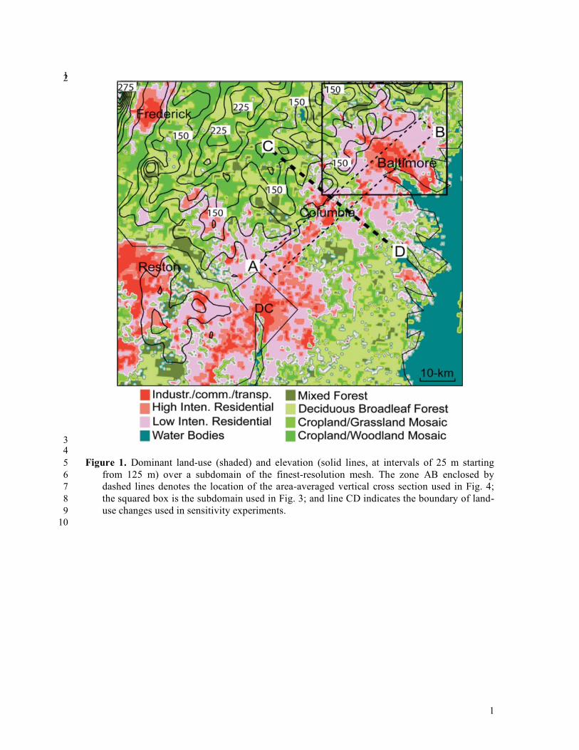
pollution concentrations than did the larger urban area of Washington, DC (Fig. 1).

Ultra-high resolution (500 m) numerical simulations show a nonlocal, dynamical

contribution to UHI effects – replacing (in the model) upstream development with

natural vegetation reduces the warming by >25%. These findings suggest that

judicious land-use and urban planning, especially in rapidly developing cities, could

help alleviate extreme UHI consequences including heat stress, haze, and smog4.

There is considerable evidence that changes in land use, especially urbanization,

can change local climate1-7

. Artificial surfaces increase runoff, inhibit evapotranspiration,

and increase absorption of solar radiation, in addition to the heat directly emitted by fuel

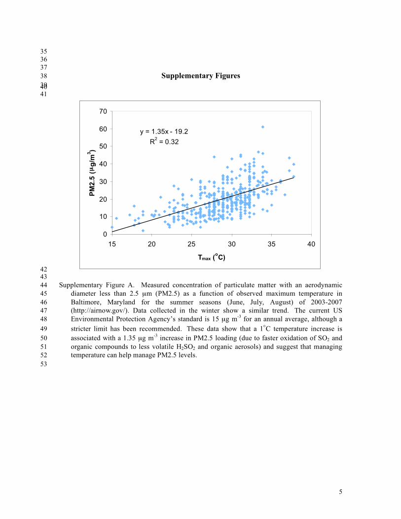
combustion and air conditioning. These UHI effects lead to heat stress in the summer

and increased concentrations of the air pollutants ozone4,8-11

and fine particulate matter

2

throughout the year (see Supplementary Fig. A). The heavier aerosol loading affects

cloud microphysics, rain patterns, and radiative balance4 leading to possible temperature-

pollution feedback effects. The heat wave of 2003 is blamed for hundreds of excess

deaths in England and thousands in other European countries12,13

. Here we show that

some heat wave events may be exacerbated by a dynamical impact that cascades from

upwind urbanization. This will be achieved by numerically simulating the extreme UHI

(heat wave) episode of 7-10 July 2007 in the Mid-Atlantic region of the eastern United

States. This UHI episode exhibited a peak surface temperature (Tsfc, measured at 2 m) of

37.5°C with a maximum 8-h average ozone concentration of 125 ppb and a maximum 24-

h average particulate matter concentration of 40 μg m-3

in Baltimore (the current

standards are 75 ppb and 35 μg m-3

), but concentrations were 85 ppb and 29 μg m-3

in

Washington where the peak Tsfc was 36.5°C. The contrast in UHI effects can not be

explained by the previous finding that the larger the metropolitan area, the greater is the

UHI effect1-7,15

, since Baltimore has a smaller urban area than Washington (Fig. 1).

During this study period, the larger-scale circulation was dominated by weak, westerly

flows until the late morning hours of July 9 when the surface winds backed to the

southwest (see Fig. 2b, and Supplementary Fig. B1). These are the two typical

summertime flow regimes under the influence of the Bermuda high.

A multi-nested version of the Weather Research and Forecast (WRF) model14

coupled with a sophisticated single-layer urban canopy model (UCM)15,16

was run at

resolution as fine as 500 m. We will first verify the model-simulated surface features

before using the model results to examine the impact of upstream urbanization on the

3

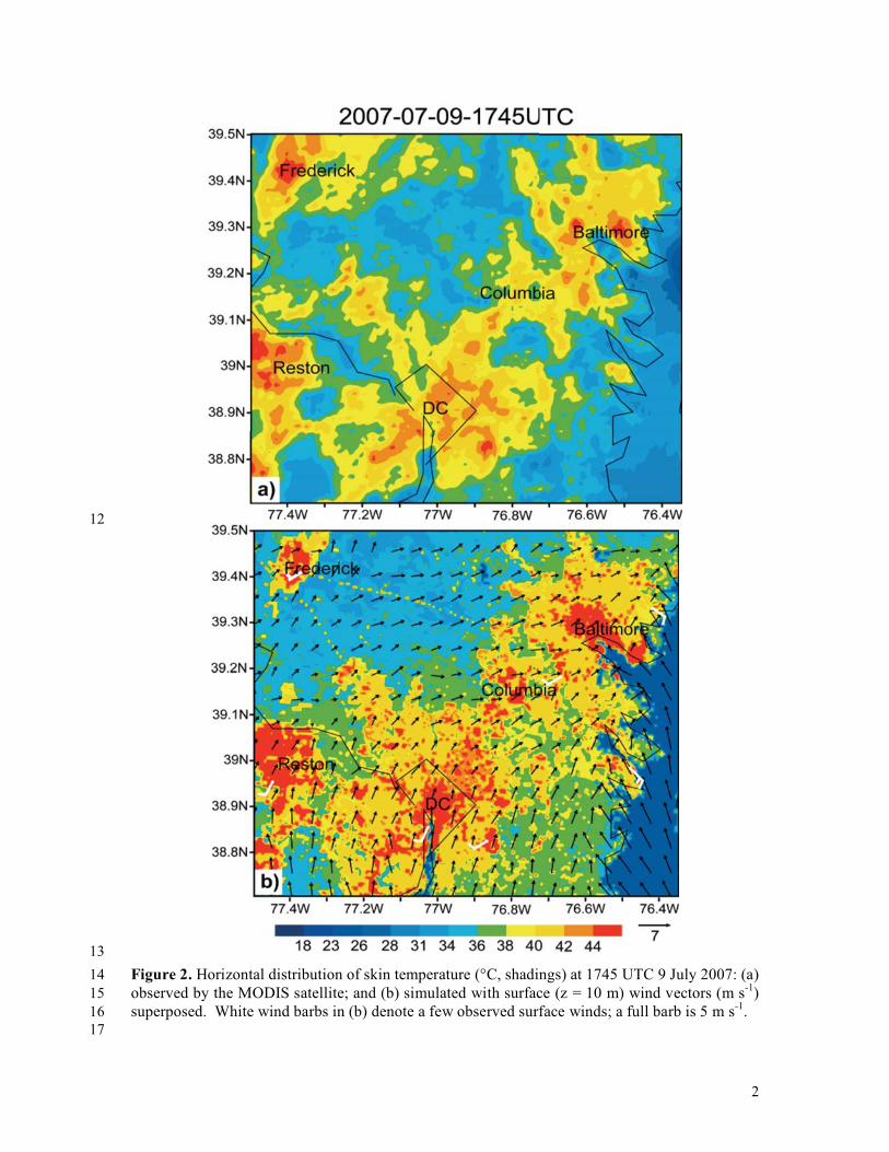
extreme UHI and associated urban boundary layer (UBL). Skin temperature1 (Tskin)

observed by the MODIS satellite instrument at 1745 UTC (1245 LST) 9 July 2007 shows

pronounced contrast between urban and rural areas (Fig. 2a), in agreement with

contrasting land-cover categories (Fig. 1). Minor differences in Tskin, e.g., over Columbia

and Frederick, Maryland, are likely due to rapid urbanization since 2001. The satellite

observations highlight UHI effects over Washington, Columbia, Baltimore, Reston, and

Frederick as well as many small towns. The hottest Tskin (> 46°C) occurred at the heart of

these cities in areas of high intensity residential buildings and commercial/industrial

activity; they were more than 10°C higher than rural regions even at this early afternoon

hour.

The coupled model reproduces well the observed UHI effects, especially the sharp

contrast between urban, suburban and rural areas (compare Figs. 2a,b), despite the use of

large-scale initial conditions. The model even captures the UHI effects of Interstate

highways such as I-70 between Frederick and Baltimore, and I-270 between Frederick

and Washington. In contrast, I-295, the Baltimore-Washington Parkway running NE/SW

between these two cities has tree cover in the median and off the shoulders – it does not

have a heat signature. The simulated UHI patterns resemble those of the land-cover map

even better than the satellite observations (compare Figs. 1 and 2b), because of the

specified Year-2001 land-cover data in the model. The model slightly overestimates the

area of maximum Tskin and misses the UHI effects over some towns, but this could again

1 Tskin is the radiometric temperature (assuming an ideal black body) derived from the thermal

emission of the earth surface as some temperature average between various canopy and soil

surfaces. Without any vegetation, it is the temperature of a molecular boundary or skin layer

between soil and a turbulent air layer.

4

be attributed to land-use changes since 2001.

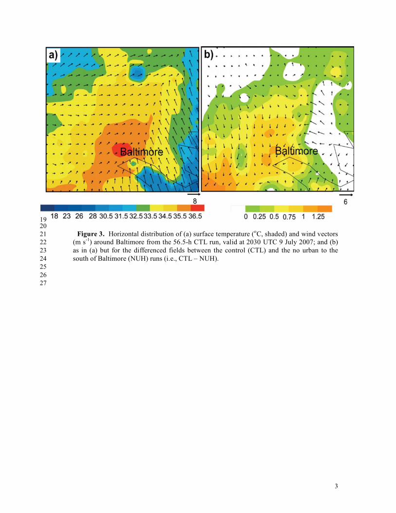
The urban area Tsfc, like Tskin, exhibits substantially more warming (> 5°C) than that

over the rural area in the mid-afternoon (i.e., 1530 LST), and the commercial-industrial-

transportation areas, often located near a city’s center, are 3-4°C warmer than the suburbs

(see Fig. 3a and Supplementary Fig. B1). The simulated peak Tsfc at Baltimore and

Washington are 36.5 and 35.5°C, respectively, as compared to the observed 37.5 and

36.5°C. This 1°C negative bias is not detrimental to the present study, since Tsfc is a

diagnostic variable between Tskin and the model surface layer (centered at z = 12 m)

temperatures, but the 1°C Tsfc difference between Baltimore and Washington is

significant.

Figure 2b also shows general agreement between the simulated surface winds and

the few observations available. We see the convergence of southwesterly synoptic flows

with the Chesapeake Bay breeze, with urban surface winds 2-3 m s-1

weaker than those

over rural areas due to the presence of high roughness elements. Convergence leads to an

area of stagnant winds and locally high pollution concentrations. The southwesterly

flows began to intrude the study area near noon 9 July, progressed into Columbia by 1245

LST (Fig. 2b), and passed over Baltimore 3 h later (Fig. 3a).

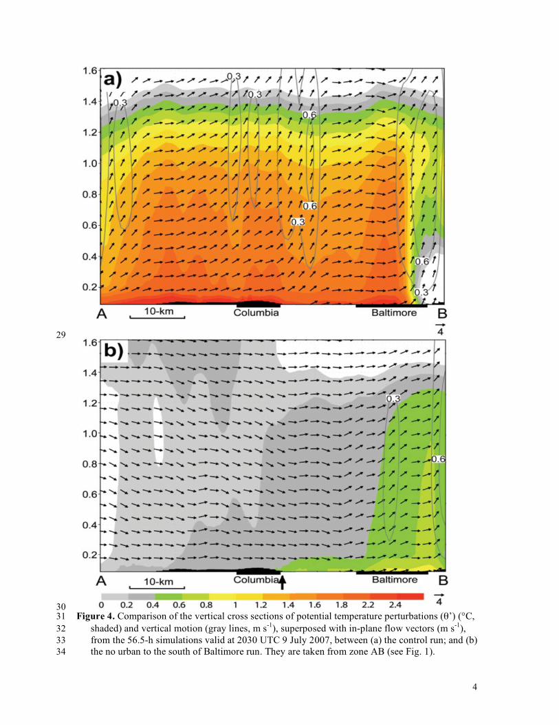
To reveal how the upstream urbanization (i.e., in Columbia and Washington) could

exacerbate the UHI effects over Baltimore, the southwesterly flows are superimposed on

the urban distribution of the Washington-Baltimore corridor. Figure 4a shows an along-

wind vertical cross section of in-plane flow vectors and the perturbation potential

temperature, �’, (potential temperature is the temperature a parcel of air would have if

brought to the 1000 hPa pressure level in an adiabatic process) through Columbia and

5

Baltimore in the mid-afternoon of July 9, where �’ is obtained by subtracting the mean

potential temperature profile in the rural environment to the west of Baltimore. The

upward extension of the UHI effects with different intensity layers extend up to ~1.4 km

altitude, the approximate depth of the well-mixed UBL at this time. The stratified UBLs

appear as layered “hot towers” (columns of rising air) corresponding to individual local

towns along the Washington-Baltimore corridor (compare Figs. 4a and 1). To our

knowledge, previous studies have examined the local UHI effects mostly in the context of

Tsfc and Tskin, but with little attention to such vertical UHI structures due to the lack of

high-resolution data. Moreover, deep rising motions on the scale of 10 - 20 km and as

strong as 0.6 m s-1

occur in the well-mixed UBL. These are unlikely due to gravity waves

associated with the nearby topography (compare Figs. 4a and 1) because of the near

neutral lapse rates in the mixed boundary layer and their absence over the rural areas (Fig.

4b). The upward motion of this magnitude could affect urban weather conditions such as

triggering cumulus clouds near the top of the UBL or the urban-rural boundaries3.

Each layer of the surface-rooted “hot tower” over Baltimore (e.g., �’= 2 ~1.5°C) is

generally deeper and more robust than those upstream, i.e., Columbia (Fig. 4a). Because

of the southwesterly advection of the warm air from the upstream UBL, little additional

heat from the surface is needed to maintain the warm column above Baltimore. Instead,

most of the local surface heat flux is used to heat the column and increase the depth of the

mixed UBL. Entrainment into the potentially warmer air aloft helps further increase the

temperature in the mixed UBL7,17

, leading to the generation of robust hot towers over the

city of Baltimore.

To supplement the above results, we conducted a numerical sensitivity experiment in

6

which the urban areas to the southwest of Baltimore are replaced by a vegetated surface

(NUH), as indicated by line CD in Fig. 1, while holding all the other parameters identical

to the control simulation (CTL) shown in Figs. 2 and 3. The differenced fields of Tsfc and

surface winds between the CTL and NUH simulations (Fig. 3b) show a city-wide

reduction in Tsfc in experiment NUH, with 1.25 – 1.5°C peak differences or more than

25% reduction of the UHI effects. Based on observations11

(see also Supplementary Fig.

A), 1.25 – 1.5°C cooling corresponds to a reduction of 3-4 ppb ozone and ~2 μg m-3

particulate matter in the summer. In addition, the well-mixed UBL in the NUH

experiment is about 200 m shallower and the hot tower over Baltimore is weaker than

that in CTL (compare Figs. 4a and 4b). Vertical motion to the south of Baltimore is

mostly downward due to the Bermuda high, confirming further the importance of the

urban-surface-rooted hot towers in generating the pronounced upward motion. Upstream

urbanization also appears to cause (Figs. 3 and 4) enhanced convergence along the Bay

and greater intrusion of the Bay breeze into the city of Baltimore.

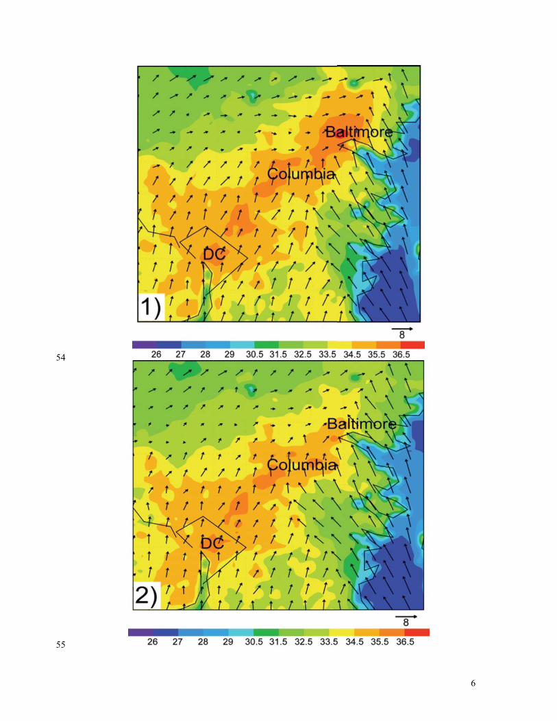
In another sensitivity simulation, Baltimore is treated as a rural area (the area to the

northeast of line CD in Fig. 1) while holding the other conditions identical to the control

simulation. Although there is little change in Tsfc over Washington, and Columbia (see

Supplementary Figs. B1 and B2), Baltimore’s Tsfc is higher than expected for a “rural”

area, offering additional evidence for a non-local UHI effect involving advection of

warmer air from upstream.

While individual urban areas on their own can do little to diminish the harmful

impacts of global climate change, our study shows that they can take action to mitigate

changes in local climate. By taking into consideration the interaction of surface

7

properties with atmospheric physics, chemistry and dynamics, informed choices in land

use can help lessen heat waves, smog episodes, and adverse impacts on regional weather.

This could be an especially powerful tool in the developing world where urbanization is

proceeding rapidly and adverse impacts on the environment and human health are

substantial.

Model description

The quadruply nested domains of the coupled WRF-UCM model14-16

have (x, y)

dimensions of 181 � 151, 244 � 196, 280 � 247, and 349 � 349 with the grid length of

13.5, 4.5, 1.5, and 0.5 km, respectively. The innermost domain covers an area that is

about 60% greater than that shown in Fig. 1. All the domains use 30 layers in the vertical

with 20 layers in the lowest 2 km in order to better resolve the evolution of the UBL.

The model is initialized at 1200 UTC (or 0700 LST) 7 July 2007 and integrated for

72 h until 1200 UTC 10 July 2007. The model initial conditions and its outermost lateral

boundary conditions as well as the soil moisture field are taken from the National Centers

for Environmental Prediction’s (NCEP) 1° resolution Final Global Analyses.

The model physics used include: (i) a three-class microphysical parameterization18

;

(ii) a boundary-layer parameterization19

; (iii) a land-surface parameterization in which

four soil layers and one canopy with 24 land-use categories are incorporated16

; and (iv)

an ensemble cumulus scheme20

as an additional procedure to treat convective instability

for the first two coarsest–resolution domains.

The UCM15

includes 3-category 30-m resolution urban surfaces (i.e., low-intensity

residential, high-intensity residential, and commercial/industrial/transportation), based on

the US Environmental Protection Agency’s National Land Cover Data of year 2001, the

8

most recent year for which high-resolution land-cover data are available. The dynamic

and thermodynamic properties of roofs, walls and roads as well as some anthropogenic

effects are used to determine roughness length, albedo, emissivity and the other surface

parameters influencing the surface energy budget.

Acknowledgements

We wish to thank Dr. Fei Chen of the National Center for Atmospheric Research

for his helpful advice. This work was funded by Maryland’s Department of the

Environment.

9

References

1. IPCC Intergovernmental Panel on Climate Change: Fourth Assessment Report (2007).

2. Kalnay, E. & Cai, M.: Impact of urbanization and land-use change on climate. Nature

423, 528-531 (2003).

3. Bornstein, R. & Q. L. Lin: Urban heat islands and summertime convective

thunderstorms in Atlanta: three case studies. Atmos. Environ. 34, 507-516 (2000).

4. Crutzen, P. J.: New Directions: The growing urban heat and pollution island effect -

impact on chemistry and climate. Atmos. Environ., 38, 3539-3540 (2004).

5. Rotach, M. W., et al.: BUBBLE - an Urban Boundary Layer Meteorology Project,

Theor. Appl. Climatol. 81, 231-261 (2005).

6. Grossman-Clarke, S. et al.: Simulations of the urban planetary boundary layer in an

arid metropolitan area. J. Appl., Meteor. Climatol. 47, 752-768 (2008).

7. Oke, T.R.: Boundary layer Climate. Routledge, 435 pp (1987).

8. Cheng, Y. Y. & D. W. Byun: Application of high resolution land use and land cover

data for atmospheric modeling in the Houston-Galveston metropolitan area, Part I:

Meteorological simulation results. Atmos. Environ. 42, 7795-7811 (2008).

9. Jacob, D. J. & D. A. Winner: Effect of climate change on air quality. Atmos. Environ.

43, 51-63 (2009).

10. Banta, R. M. et al.: Daytime buildup and nighttime transport of urban ozone in the

boundary layer during a stagnation episode. J. Geophys. Res. 103, 22519-22544

(1998).

11. Bloomer, B. J., et al.: A climate change penalty in ozone air pollution observed over

the eastern United States. Geophys. Res. Lett. In press (2009).

10

12. Fischer, P. H. et al.: Air pollution related deaths during the 2003 heat wave in the

Netherlands. Atmos. Environ. 38, 1083-1085 (2003).

13. Stedman J. R.: The predicted number of air pollution related deaths in the UK during

the August 2003 heat wave. Atmos. Environ. 38, 1087-1090 (2004).

14. Skamarock, W. C., et al: A description of the Advanced Research WRF Version 2,

NCAR, 100pp (2005).

15. Kusaka, H., et al.: A simple single-layer urban canopy model for atmospheric models:

Comparison with multi-layer and slab models, Bound.-Layer Meteor. 101,329-358

(2001).

16. Chen, F., & J. Dudhia: Coupling an advanced land-surface-hydrology model with the

Penn State-NCAR MM5 modeling system. Part I: Model implementation and

sensitivity, Mon. Wea. Rev. 129, 569-585 (2001).

17. Zhang, D.-L., & R. A. Anthes: A high-resolution model of the planetary boundary-

layer-sensitivity tests and comparisons with SESAME-79 data, J. Appl. Meteor. 21,

1594-1609 (1982).

18. Hong, S.Y. et al.: A revised approach to ice microphysical processes for the bulk

parameterization of clouds and precipitation, Mon. Wea. Rev. 132, 103–120 (2004).

19. Janji�, Z. I.: The step-mountain Eta coordinate model: Further development of the

convection, viscous sublayer and turbulent closure schemes. Mon. Wea. Rev. 122,

927–945 (1994).

20. Grell, G. A. & D. Devenyi: A generalized approach to parameterizing convection

combining ensemble and data assimilation techniques, Geophys. Res. Lett. 29(14),

1693, doi:10.1029/2002GL015311 (2002).

11

Figure Captions

Figure 1. Dominant land-use (shaded) and elevation (solid lines, at intervals of 25 m

starting from 120 m) over a subdomain of the finest-resolution mesh. The zone AB

enclosed by dashed lines denotes the location of the area-averaged vertical cross

section used in Fig. 4; the squared box is the subdomain used in Fig. 3; and line CD

indicates the boundary of land-use changes used in sensitivity experiments.

Figure 2. Horizontal distribution of skin temperature (shadings) at 1745 UTC 9 July

2007: (a) observed by the MODIS satellite; and (b) simulated with surface wind

vectors superposed. White wind barbs in (b) denote a few observed surface winds;

a full barb is 5 m s-1

.

Figure 3. Horizontal distribution of (a) surface temperature (°C, shaded) and wind

vectors (m s-1

) around Baltimore from the 56.5-h CTL run, valid at 2030 UTC 9

July 2007; and (b) as in (a) but for the differenced fields between the CTL and

NUH (no urban to the south of Baltimore) runs (i.e., CTL – NUH).

Figure 4. A comparison of the vertical cross sections of potential temperature

perturbations (�’ in °C, shaded) and vertical motion (gray lines, m s-1

), superposed

with in-plane flow vectors (m s-1), from the 56.5-h simulations valid at 2030 UTC 9

July 2007, between (a) the control run and (b) the no urban to the south of

Baltimore run. They are taken from zone AB (see Fig. 1).

1

1 2

3 4

Figure 1. Dominant land-use (shaded) and elevation (solid lines, at intervals of 25 m starting 5

from 125 m) over a subdomain of the finest-resolution mesh. The zone AB enclosed by 6

dashed lines denotes the location of the area-averaged vertical cross section used in Fig. 4; 7

the squared box is the subdomain used in Fig. 3; and line CD indicates the boundary of land-8

use changes used in sensitivity experiments. 9

10

2

12

13

Figure 2. Horizontal distribution of skin temperature (°C, shadings) at 1745 UTC 9 July 2007: (a) 14

observed by the MODIS satellite; and (b) simulated with surface (z = 10 m) wind vectors (m s-1

) 15

superposed. White wind barbs in (b) denote a few observed surface winds; a full barb is 5 m s-1

. 16

17

3

19 20

Figure 3. Horizontal distribution of (a) surface temperature (oC, shaded) and wind vectors 21

(m s-1

) around Baltimore from the 56.5-h CTL run, valid at 2030 UTC 9 July 2007; and (b) 22

as in (a) but for the differenced fields between the control (CTL) and the no urban to the 23

south of Baltimore (NUH) runs (i.e., CTL – NUH). 24

25

26

27

4

29

30 Figure 4. Comparison of the vertical cross sections of potential temperature perturbations (�’) (°C, 31

shaded) and vertical motion (gray lines, m s-1

), superposed with in-plane flow vectors (m s-1

), 32

from the 56.5-h simulations valid at 2030 UTC 9 July 2007, between (a) the control run; and (b) 33

the no urban to the south of Baltimore run. They are taken from zone AB (see Fig. 1). 34

5

35

36

37

Supplementary Figures 38

39 40 41

y = 1.35x - 19.2

R2 = 0.32

0

10

20

30

40

50

60

70

15 20 25 30 35 40

Tmax (oC)

PM

2.5

(μ μ

g/m

3)

42 43

Supplementary Figure A. Measured concentration of particulate matter with an aerodynamic 44

diameter less than 2.5 μm (PM2.5) as a function of observed maximum temperature in 45

Baltimore, Maryland for the summer seasons (June, July, August) of 2003-2007 46

(http://airnow.gov/). Data collected in the winter show a similar trend. The current US 47

Environmental Protection Agency’s standard is 15 μg m-3

for an annual average, although a 48

stricter limit has been recommended. These data show that a 1 C temperature increase is 49

associated with a 1.35 μg m-3

increase in PM2.5 loading (due to faster oxidation of SO2 and 50

organic compounds to less volatile H2SO2 and organic aerosols) and suggest that managing 51

temperature can help manage PM2.5 levels. 52

53

6

54

55

7

56

Supplementary Fig. B. Horizontal distribution of surface temperatures (°C , shaded) and surface 57

wind vectors (m s-1

) over the Washington-Baltimore metropolitan region from the 56.5-h 58

simulation, valid at 2030 UTC 9 July 2007: (1) the control simulation; and (2) a sensitivity 59

simulation in which Baltimore is treated as a rural area. 60 61 62 63 64 65