Embed Size (px)
Citation preview
UNIVERSITA’ DEGLI STUDI DI PADOVA
NATIONAL TECHNICAL UNIVERSITY OF ATHENS
DIPARTIMENTO DI INGEGNERIA INDUSTRIALE
CORSO DI LAUREA MAGISTRALE IN INGEGNERIA
ENERGETICA
TESI DI LAUREA
DESIGN AND PERFORMANCE EVALUATION OF AN ORC
SYSTEM EXPLOITING THE WASTE HEAT OF THE MAIN ENGINE
OF A TANKER
Relatori: Proff. CHRISTOS A. FRANGOPOULOS, ANDREA LAZZARETTO
Correlatore: Ing. GIOVANNI MANENTE
Laureando: STEFANO MANCINI
Matr.n. 1020442
Anno accademico 2012/2013


Δεν υπάρχει εξορία μόνο μια καινούργια πατρίδα

I
Contents
Nomenclature .......................................................................................................................... V
List of Figures .......................................................................................................................... IX
List of Tables ........................................................................................................................... XI
Acknowledgement ................................................................................................................ XIII
Abstract .................................................................................................................................... 1
Introduction ............................................................................................................................. 3
1. Review of the Literature on ORC Working fluid ............................................................. 5
1.1. Introduction............................................................................................................ 5
1.2. Working Fluid Properties ........................................................................................ 5
1.2.1. Effectiveness of superheating ............................................................................ 6
1.2.2. Critical points of the working fluids ................................................................... 7
1.2.3. Stability of the fluid and compatibility with materials in contact ...................... 8
1.2.4. Environmental aspects ....................................................................................... 8
1.2.5. Safety .................................................................................................................. 9
1.2.6. Size of the system ............................................................................................. 10
1.3. Fluid Selection and Parametric Optimization for Basic Rankine Cycle ................. 11
1.4. Fluid Selection and Parametric Optimization for Transcritical Rankine Cycles .... 18
1.5. Conclusions based on the Literature Review ....................................................... 19
2. Literature Review of Various ORC Systems .................................................................. 23
2.1. Introduction.......................................................................................................... 23
2.2. Thermal efficiency and total heat recovery efficiency. ........................................ 23
2.3. Simple ORC ........................................................................................................... 25
2.4. ORC with Use of Heat Available from the Engine Cooling System ....................... 26
2.5. Dual loop system .................................................................................................. 27
2.6. Recovery system by Yue et al. (2012) .................................................................. 28
2.7. Regenerated ORC ................................................................................................. 29
2.8. Two-stage Organic Rankine Cycle ........................................................................ 32
2.9. Effect of using Diathermic Oil ............................................................................... 33
3. Energy Balance of the Main Engine.............................................................................. 35
3.1. Introduction.......................................................................................................... 35

II
3.2. Main Engine System ............................................................................................. 35
3.3. Explanation of the Main Components of the Main Engine System. .................... 37
3.3.1. Main Engine ...................................................................................................... 37
3.3.2. Turbocharger .................................................................................................... 37
3.3.3. Lubricating oil cooler and jacket water cooler ................................................. 37
3.3.4. Fresh water generator ...................................................................................... 38
3.3.5. Scavenge Air cooler .......................................................................................... 39
3.3.6. Exhaust gas Boiler ............................................................................................. 40
3.3.7. Central Fresh Water Cooler .............................................................................. 41
3.4. Operating Profile of the Main Engine .................................................................. 43
3.5. Model of the Main Engine Balance ...................................................................... 44
3.6. Data and Assumptions ......................................................................................... 48
3.7. Energy Balance at 100% Engine Load ................................................................... 58
3.8. Operating data and results at 100%, 80%, 70% and 55% Load ............................ 59
4. Hot Composite Curves .................................................................................................. 65
5. ORC model .................................................................................................................... 69
5.1. Introduction.......................................................................................................... 69
5.2. Thermodynamic Model of ORC ............................................................................ 69
5.3. Optimization Function .......................................................................................... 71
5.4. Simulation Procedure ........................................................................................... 73
6. Selection of Alternative Systems for an Performance Evaluation ............................... 77
6.1. Introduction.......................................................................................................... 77
6.2. Optimization with Ideal System ORC ................................................................... 77
6.3. First ORCs configuration proposed ...................................................................... 82
6.4. Second configuration of ORCs with two heat exchangers: air cooler and jacket
water 89
6.5. Third configuration: Regenerated ORC ................................................................ 94
6.6. Fourth configuration: Simple ORCs with three heat exchanges: air cooler, jacket
water and lubricating oil. ............................................................................................................. 99
6.7. Fifth Configuration: Only Air Heat Exchanger .................................................... 104
6.8. Sixth configuration: Two Stage ORC System ...................................................... 109
6.9. Conclusion .......................................................................................................... 114
7. Output Power Evaluation of the ORC Systems at 70% and 55% of the Engine Load . 117
7.1. Introduction........................................................................................................ 117
7.2. Model and Results .............................................................................................. 117
III
8. Annual Energy Savings ............................................................................................... 121
8.1. Introduction........................................................................................................ 121
8.2. Calculation of Annual Energy Savings ................................................................ 121
9. Economic Feasibility ................................................................................................... 123
9.1. Introduction........................................................................................................ 123
9.2. Parameters of Economic Feasibility ................................................................... 123
9.3. Economic Feasibility of dual Stage ORC ............................................................. 125
9.4. Conclusion .......................................................................................................... 129
10. Conclusion .................................................................................................................. 131
11. Suggestions for further work ..................................................................................... 135
Bibliography ......................................................................................................................... 137

IV
V
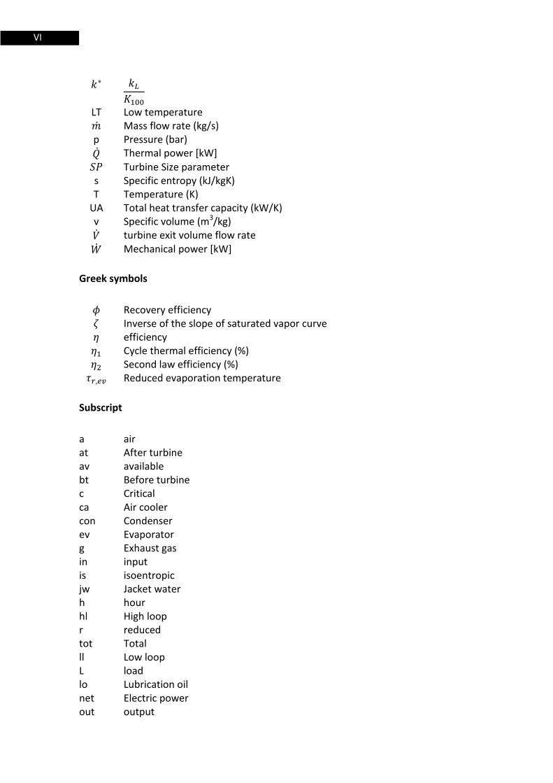
Nomenclature
Abbreviations
DPP Dynamic payback period ECO Economizer EGB Exhaust gas boiler EVA Evaporator FW Fresh Water FWG Fresh water generator HFO Heavy Fuel Oil IRR Internal rate of return HCC Hot composite curve CCC Cold composite curve JWC Jacket water cooler L.O. Lubrication oil M/E Main engine MDO Marine Diesel oil NPV Net Present value ORC Organic Rankine cycle ORCs Organic Rankine cycle system PP Payback period SH Super heater SW Sea water
Symbols
A Exchange Surface (m2) C cost cp Isobaric specific heat (kJ/kg K)
∆hfg Enthalpy of vaporization (kJ/kg) Isentropic enthalpy change in turbine (kJ/kg) Entropy different (kJ/kgK) E Annual energy savings (kWh) n 0.375-0.38 f Optimization function h Specific enthalpy (kJ/kg) Lower calorific Value HT High temperature k
∑
VI
LT Low temperature Mass flow rate (kg/s) p Pressure (bar)
Thermal power [kW] Turbine Size parameter s Specific entropy (kJ/kgK) T Temperature (K)
UA Total heat transfer capacity (kW/K) v Specific volume (m3/kg)
turbine exit volume flow rate
Mechanical power [kW]
Greek symbols
Recovery efficiency Inverse of the slope of saturated vapor curve efficiency Cycle thermal efficiency (%) Second law efficiency (%) Reduced evaporation temperature
Subscript
a air at After turbine av available bt Before turbine c Critical ca Air cooler con Condenser ev Evaporator g Exhaust gas in input is isoentropic jw Jacket water h hour hl High loop r reduced tot Total ll Low loop L load lo Lubrication oil net Electric power out output

VII
R regenerator r radiation R Rankine s steam T Total heat recovey TH Rankine efficiency y year

VIII

IX
List of Figures
FIGURE 2-1 FLOW DIAGRAM OF SIMPLE ORC. ................................................................................ 25
FIGURE 2-2 DIAGRAM T-S SIMPLE ORC. ....................................................................................... 25
FIGURE 2-3 FLOW DIAGRAM OF ORC WITH ENGINE COOLING SYSTEM. ................................................ 26
FIGURE 2-4 FLOW DIAGRAM DUAL LOOP SYSTEM. ............................................................................ 27
FIGURE 2-5 T-S PLOTS OF THE HT AND LT LOOPS. ........................................................................... 28
FIGURE 2-6 FLOW DIAGRAM OF SYSTEM BY YUE ET AL. (2012). ......................................................... 29
FIGURE 2-7 FLOW DIAGRAM OF REGENERATED ORC. ....................................................................... 30
FIGURE 2-8 BENZENE REGENERATED CYCLE, T-S DIAGRAM. ............................................................... 31
FIGURE 2-9 FLOW DIAGRAM FOR A TWO STAGE ORC SYSTEM. .......................................................... 32
FIGURE 2-10 TWO-STAGE ORC PROCESS IN FORM OF A T-S DIAGRAM. .............................................. 33
FIGURE 3-1 ARRANGEMENT OF THE MAIN ENGINE IN SHIPS OF RELATIVELY LOW POWER WITHOUT STEAM
TURBINE. ......................................................................................................................... 36
FIGURE 3-2 FRESH WATER GENERATOR. ....................................................................................... 39
FIGURE 3-3 ARRANGEMENT OF THE MAIN ENGINE IN SHIPS OF RELATIVELY LOW POWER WITH STEAM TURBINE.
THE TEMPERATURE OF FRESH WATER COOLER ARE SHOWN IN PARENTHETICAL. .............................. 42
FIGURE 3-4 ARRANGEMENT OF THE MAIN ENGINE IN SHIPS OF RELATIVELY LOW POWER WITHOUT STEAM
TURBINE. THE BOUNDARY CONTROL IS SHOWN WITH A RED DASHED LINE. .................................... 47
FIGURE 3-5 OUTLET TEMPERATURE OF JACKET WATER FROM M/E AS A FUNCTION OF ENGINE LOAD. ........ 50
FIGURE 3-6 INLET TEMPERATURE OF JACKET WATER TO THE M/E AS A FUNCTION OF LOAD. ..................... 50
FIGURE 3-7 INLET TEMPERATURE OF LUBRICATING OIL TO THE M/E AS A FUNCTION OF LOAD. .................. 50
FIGURE 3-8 OUTLET TEMPERATURE OF LUBRICATING OIL AS A FUNCTION OF LOAD. ................................ 51
FIGURE 3-9 AIR INLET TEMPERATURE TO THE SUPERCHARGING AIR COOLER. ......................................... 51
FIGURE 3-10 AIR OUTLET TEMPERATURE FROM THE SUPERCHARGING AIR COOLER. ................................ 51
FIGURE 3-11 EXHAUST GAS TEMPERATURE FROM TURBOCHARGER. .................................................... 52
FIGURE 3-12 C* AS FUNCTION OF ENGINE LOAD.............................................................................. 53
FIGURE 3-13 JACKET WATER TREND. ............................................................................................ 54
FIGURE 3-14 LUBRICATING OIL TREND. ......................................................................................... 56
FIGURE 3-15 AIR COOLER TREND................................................................................................. 57
FIGURE 3-16 ENERGY BALANCE AT 80% ENGINE LOAD. .................................................................... 62
FIGURE 3-17 ENERGY BALANCE AT 70% ENGINE LOAD. ................................................................... 63
FIGURE 3-18 ENERGY BALANCE AT 55% ENGINE LOAD. ................................................................... 64
FIGURE 4-1 THREE HOT UTILITIES CHOSEN. .................................................................................... 66
FIGURE 4-2 HOT COMPOSITE CURVE: A) 80% ENGINE LOAD, B) 70% ENGINE LOAD, C) 55% ENGINE LOAD.
..................................................................................................................................... 68
FIGURE 5-1 MODEL OF THE ORCS. .............................................................................................. 69
FIGURE 5-2 CIRCUIT OF ORC. ..................................................................................................... 73

X
FIGURE 5-3 SIMULATION PROCEDURE. ......................................................................................... 75
FIGURE 6-1 IDEAL SYSTEM ORC. ................................................................................................. 77
FIGURE 6-2 COMPOSITE CURVES OF R134A, R227EA, R245FA, R236FA (SEE FIGURE 6-1). ................. 81
FIGURE 6-3 ORC SYSTEM AS THE ONE PROPOSED BY YUE ET AL. (2012). ............................................ 82
FIGURE 6-4 COMPOSITE CURVE OF FIRST CONFIGURATION (SEE FIGURE 6-3). ....................................... 88
FIGURE 6-5 ORCS WITH TWO HEAT EXCHANGER (AIR/ORC AND WATER/ORC). ............................... 89
FIGURE 6-6 COMPOSITE CURVES FOR THE SECOND CONFIGURATION (SEE FIGURE 6-5). .......................... 93
FIGURE 6-7 REGENERATED ORC. ................................................................................................ 94
FIGURE 6-8 COMPOSITE CURVES OF REGENERATED SYSTEM (SEE FIGURE 6-7). ..................................... 98
FIGURE 6-9 FOURTH CONFIGURATION OF SYSTEM. .......................................................................... 99
FIGURE 6-10 COMPOSITE CURVE OF FOURTH CONFIGURATION (SEE FIGURE 6-9)................................ 103
FIGURE 6-11 FIFTH CONFIGURATION OF THE SYSTEM. .................................................................... 104
FIGURE 6-12 COMPOSITE CURVES OF THE FIFTH CONFIGURATION (SEE FIGURE 6-11). ........................ 108
FIGURE 6-13 TWO STAGE ORC SYSTEM. ..................................................................................... 109
FIGURE 6-14 COMPOSITE CURVE OF SIXTH CONFIGURATION (SEE FIGURE 6-13). ................................ 113
FIGURE 7-1 TWO STAGE ORC SYSTEM. ....................................................................................... 117
FIGURE 7-2 COMPOSITE CURVE OF R236FA AT 70% AND 55% ENGINE LOAD. ................................. 120
FIGURE 9-1 NET PRESENT VALUE AS A FUNCTION OF THE FUEL COST AND OF THE SPECIFIC COST OF THE
INITIAL INVESTMENT ........................................................................................................ 128
FIGURE 9-2 PAYBACK PERIOD AS A FUNCTION OF THE FUEL COST AND OF THE SPECIFIC COST OF THE INITIAL
INVESTMENT. ................................................................................................................. 128
FIGURE 9-3 INTERNAL RATE OF THE RETURN AS A FUNCTION OF THE FUEL COST AND OF A SPECIFIC COST OF A
INITIAL INVESTMENT. ....................................................................................................... 129
XI
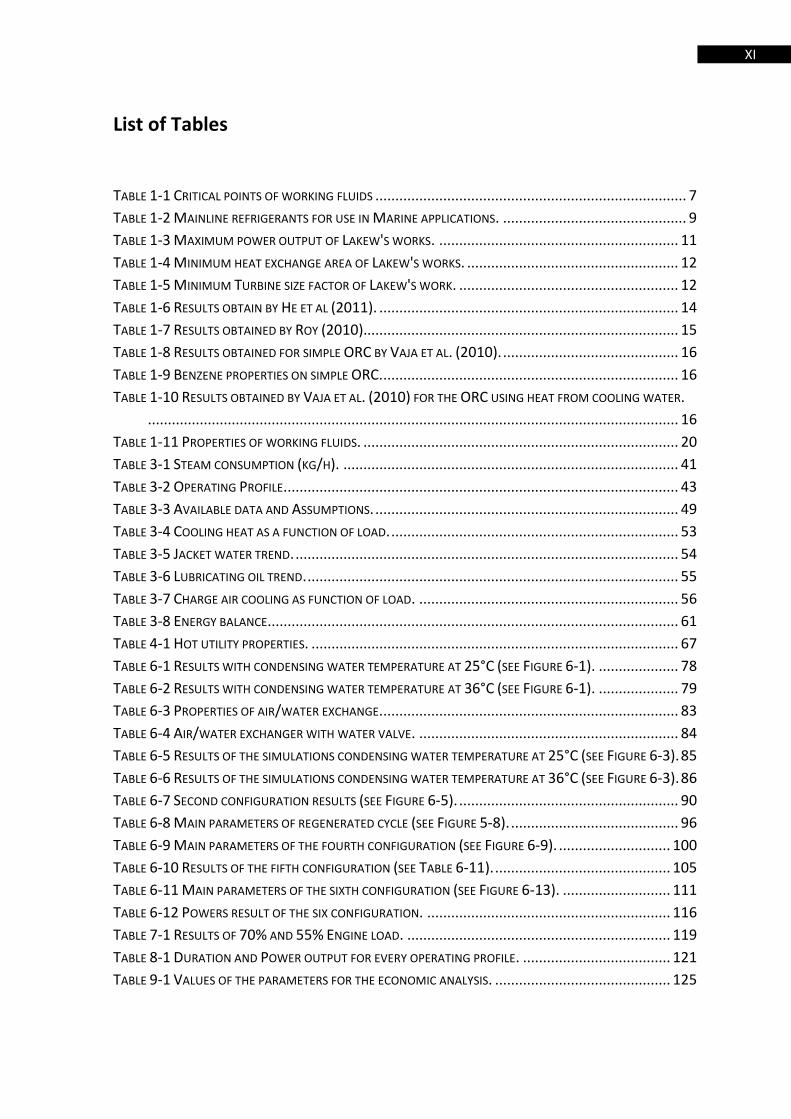
List of Tables
TABLE 1-1 CRITICAL POINTS OF WORKING FLUIDS .............................................................................. 7
TABLE 1-2 MAINLINE REFRIGERANTS FOR USE IN MARINE APPLICATIONS. .............................................. 9
TABLE 1-3 MAXIMUM POWER OUTPUT OF LAKEW'S WORKS. ............................................................ 11
TABLE 1-4 MINIMUM HEAT EXCHANGE AREA OF LAKEW'S WORKS. ..................................................... 12
TABLE 1-5 MINIMUM TURBINE SIZE FACTOR OF LAKEW'S WORK. ....................................................... 12
TABLE 1-6 RESULTS OBTAIN BY HE ET AL (2011). ........................................................................... 14
TABLE 1-7 RESULTS OBTAINED BY ROY (2010)............................................................................... 15
TABLE 1-8 RESULTS OBTAINED FOR SIMPLE ORC BY VAJA ET AL. (2010). ............................................ 16
TABLE 1-9 BENZENE PROPERTIES ON SIMPLE ORC. .......................................................................... 16
TABLE 1-10 RESULTS OBTAINED BY VAJA ET AL. (2010) FOR THE ORC USING HEAT FROM COOLING WATER.
..................................................................................................................................... 16
TABLE 1-11 PROPERTIES OF WORKING FLUIDS. ............................................................................... 20
TABLE 3-1 STEAM CONSUMPTION (KG/H). .................................................................................... 41
TABLE 3-2 OPERATING PROFILE. .................................................................................................. 43
TABLE 3-3 AVAILABLE DATA AND ASSUMPTIONS. ............................................................................ 49
TABLE 3-4 COOLING HEAT AS A FUNCTION OF LOAD. ........................................................................ 53
TABLE 3-5 JACKET WATER TREND. ................................................................................................ 54
TABLE 3-6 LUBRICATING OIL TREND. ............................................................................................. 55
TABLE 3-7 CHARGE AIR COOLING AS FUNCTION OF LOAD. ................................................................. 56
TABLE 3-8 ENERGY BALANCE....................................................................................................... 61
TABLE 4-1 HOT UTILITY PROPERTIES. ............................................................................................ 67
TABLE 6-1 RESULTS WITH CONDENSING WATER TEMPERATURE AT 25°C (SEE FIGURE 6-1). .................... 78
TABLE 6-2 RESULTS WITH CONDENSING WATER TEMPERATURE AT 36°C (SEE FIGURE 6-1). .................... 79
TABLE 6-3 PROPERTIES OF AIR/WATER EXCHANGE. .......................................................................... 83
TABLE 6-4 AIR/WATER EXCHANGER WITH WATER VALVE. ................................................................. 84
TABLE 6-5 RESULTS OF THE SIMULATIONS CONDENSING WATER TEMPERATURE AT 25°C (SEE FIGURE 6-3). 85
TABLE 6-6 RESULTS OF THE SIMULATIONS CONDENSING WATER TEMPERATURE AT 36°C (SEE FIGURE 6-3). 86
TABLE 6-7 SECOND CONFIGURATION RESULTS (SEE FIGURE 6-5). ....................................................... 90
TABLE 6-8 MAIN PARAMETERS OF REGENERATED CYCLE (SEE FIGURE 5-8). .......................................... 96
TABLE 6-9 MAIN PARAMETERS OF THE FOURTH CONFIGURATION (SEE FIGURE 6-9). ............................ 100
TABLE 6-10 RESULTS OF THE FIFTH CONFIGURATION (SEE TABLE 6-11). ............................................ 105
TABLE 6-11 MAIN PARAMETERS OF THE SIXTH CONFIGURATION (SEE FIGURE 6-13). ........................... 111
TABLE 6-12 POWERS RESULT OF THE SIX CONFIGURATION. ............................................................. 116
TABLE 7-1 RESULTS OF 70% AND 55% ENGINE LOAD. .................................................................. 119
TABLE 8-1 DURATION AND POWER OUTPUT FOR EVERY OPERATING PROFILE. ..................................... 121
TABLE 9-1 VALUES OF THE PARAMETERS FOR THE ECONOMIC ANALYSIS. ............................................ 125

XII
TABLE 9-2 INITIAL INVESTMENT AND NET PRESENT VALUE. ............................................................ 127
TABLE 9-3 PAYBACK PERIOD AS A FUNCTION OF THE FUEL COST AND OF THE SPECIFIC COST OF THE INITIAL
INVESTMENT. ................................................................................................................. 127
TABLE 9-4 INTERNAL RATE OF RETURN AS A FUNCTION OF THE FUEL COST AND OF THE SPECIFIC COST OF THE
INITIAL INVESTMENT. ....................................................................................................... 127

XIII
Acknowledgement
I would like to thank all the people who supported me in developing this thesis, in
particular:
Christos A. Frangopoulos at the School of Naval Architecture and Marine Engineering of
NTUA Athens. Nikolaos Kakalis, George Dimopoulos, DET NORSKE VERITAS (DNV). Andrea
Lazzaretto, Giovanni Manente, Marco Soffiato and Sergio Rech, University of Padova.
Raymond Genesse and Alberto Schiavon, Zeno Rama, Claudia Marino for my English
writing.
I desire to thank my family who supported me in all these years of study from all
points of view.

1 Abstract
Abstract
The vast majority of the world’s trade is conducted across water. Ships remain one
of the best means of transport. Cleaner technologies are inevitable in this field as well.
Solutions for this new request are developing by some shipping companies. One solution
is the reduction of the fuel consumption keeping the equivalent performance of the ship
without fuel reduction. An ORC may be an answer of this problem. In this work an ORC
system applied to cooling system of the Main Engine of a Tanker is investigated. The
energy balance is calculated for the main operating loads. Three main operating loads are
taken into consideration for the ORC system (80%, 70%, 55%). Four working fluids R134a,
R245fa, R236fa, R227ea have been considered. At first the best match between the
choice of working fluid and ORC configuration is carried out at design point (80% engine
load). Then, using the ORC system at design point, the maximum electric power is
evaluated in the three main loads. After that, the annual energy saving is calculated using
the output power and the duration for each operating load. An economic analysis is
carried out through three parameters: net present value (NPV), dynamic payback period
(DPP), internal rate of the return (IRR).

2
3 Introduction
Introduction
Energy conservation and environmental protection have become more important
with the rapid development of global industrialization and urbanization. The
industrialization has risen to a level never reached before, releasing in the same process
large quantities of CO2 into the atmosphere. Current concerns over climate change call for
measures to reduce greenhouse gases. Some modification could be a decrease in the
energy intensity of buildings and industry, use clean power generation by renewable
energies, a shift from fossil fuels for transportation and heating. Organic Rankine cycle
(ORC) technology can play a non-negligible role in these proposed solutions. It can have a
beneficial effect on the energy intensity of industrial processes mainly recovering waste
heat for electricity production or it can be used to convert renewable heat sources ( as
geothermal, biomass and solar sources) into electricity.
Environmental pollution of the ocean has become increasingly serious owing to
shipping. Total CO2 emissions generated in the domestic and overseas shipping industries
reached a record of about 1 billion tons in 2007, constituting 3.3% of global CO2
emissions. The MEPC (Marine Environmental Protection Committee) of the IMO
(International Maritime Organization) under the umbrella of the UN (United Nations) has
modified its marine pollution prevention convention, i.e. the MARPOL (International
Convention for the Prevention of Pollution From Ships) Annex VI, in order to lower the
CO2 emitted from newly built ships and existing ships [Choi and Kim (2013)].
The amount of CO2 emitted from a ship is directly related to the amount of fuel
consumed by the internal combustion engine propelling the ship. Therefore a power
generation system that makes use of the waste heat from its main engine (a waste heat
recovery system) could be a principal technology to reduce CO2 emissions on boat. There
are several waste heat recovery power generation systems: a power turbine scheme, in
which the kinetic energy of the gas is utilized to directly drive the turbines, a steam
turbine scheme, or a combination of both these schemes. If the ship needs vapor for
internal utility, an exhaust gas boiler (system to produce steam by exhaust gas) could be
installed. New studies proved the advantages of ORC technology against steam
technology. It is possible to substitute the steam turbine with an ORC. Conceptually the
ORC is similar to a steam Rankine Cycle. The ORC involves some components as a
conventional steam power plant (a boiler, a work-producing expansion device, a
condenser and a pump). However the working fluid is an organic compound characterized
by a lower boiling temperature than water and allowing power generation from low
temperature heat sources. Another advantage is that ORC requires less space than the
steam technology given the same conditions.
4 Introduction
When designing an ORC, special attention must be paid to the choice of the
appropriate working fluid based on heat source temperature. Chen et al (2011)
considered 35 pure working fluids. They analyzed the working fluids selection criteria for
ORC such the types of working fluids, density, specific heat, latent heat critical
point, thermal conductivity. Lakew and Bolland (2010) concluded that R227ea produces
the highest power for heat source temperature range considered (80-160°C), while
R245fa gives higher power for heat source temperature higher than 160°C.
Many researches have also investigated ORC system design and parametric
optimization. Roy et al (2010) conducted a parametric optimization and performance
analysis of a waste heat recovery system based on an organic Rankine cycle using R12,
R123, R134a as the working fluid for power generation. Schuster et al. (2010) presented a
simulation study of an ORC when using supercritical parameters and various working
fluids. Vaja and Gambarotta (2010) described a specific thermodynamic analysis in order
to efficiently match an ORC to an internal combustion engine.
In the present study, it was investigated a heat recovery power generation system
applied to the cooling system of the main engine of a Tanker ship that is actually in
operation. At the beginning the literature on working fluids and ORC system was
reviewed. The energy balance was then evaluated using a combination of various source:
documentation available, and engine software available on the website of the
manufacture. Air cooler, lubricating oil and jacket water heat are available for ORC cycle.
Waste heat from exhaust gas is already recovered by the exhaust gas boiler. The three
main operating condition are 80%, 70%, 55% of the engine load. Operation at 80% engine
load is chosen as design point of ORCs Four organic fluids, R134a, R245fa, R227ea and
R236fa have been considered as working fluids for the ORCs after the literature review in
Chapter 1. Several configurations are studied to find the one that gives the maximal
power. After that the dual stage system and the R236fa are selected as the best mach.
They lead to the higher net power output. An approximate evaluation is carried out
(without using a detailed off-design model) to evaluate the power output at 70% and 55%
of the engine load. Using the output power and the duration for each operating load, the
annual energy saving was calculated. In conclusion an economic analysis is made by three
parameters: net present value (NPV), payback period (PP) and internal rate return (IRR).
5 Review of the Literature on ORC Working fluids
1. Review of the Literature on ORC Working fluid
1.1. Introduction
The literature on ORC presents extensive analyses and comparisons among
different thermodynamic cycles and working fluids. However, most of the comparisons
were conducted under certain predefined temperature conditions and used only a few
working fluids. The claims for best working fluids and the cycle with highest efficiencies
may not hold true under other operating conditions and with other working fluids. In this
chapter, the pertinent properties of the fluids are first described and then the criteria and
the procedure for selecting appropriate fluids for a particular application are presented.
1.2. Working Fluid Properties
The thermodynamic and physical properties, stability, environmental impacts,
safety and compatibility with the materials and size of heat exchangers and turbine, are
among the important properties that have to be considered when selecting a working
fluid for an ORC system.
The properties of organic fluids are different from those of water [Stine et al.
(1985)]. The slope of the vapor-side saturation curve of a working fluid in a T–s diagram
can be positive (e.g. isopentane), negative (e.g. R22) or vertical (e.g. R142b), and the fluid
is accordingly called ‘‘wet’’, ‘‘dry’’ or ‘‘isentropic’’. Wet fluids like water usually need to be
superheated, while many organic fluids, which may be dry or isentropic, do not need
superheating. Another advantage of organic working fluids is that ORCs typically require
only a single-stage expander, resulting in a simpler, more economical system in terms of
capital costs and maintenance [Andersen et al. (2005)].
There is no best fluid that meets all the criteria discussed for heat sources with
different temperatures. Compromise must be made when selecting the fluids. Among all
the criteria and concerns, the critical temperature and the ζ value (see Eq. (1.1)) are
important parameters that suggest which type of cycle a fluid may serve and the
applicable operating temperature of the fluid. The ζ parameter is in fact the
aforementioned slope of the vapor-side saturation curve of a fluid and it is defined by the
equation
(
)
(1.1)

6 Review of the Literature on ORC Working fluids
The type of working fluid can be classified by the value of ζ: if ζ>0 it is a dry fluid
(e.g. pentane), if ζ=0 it is an isentropic fluid (e.g. R143a), and if ζ < 0 it is a wet fluid (e.g.
water). τr,ev (=TH/TC) denotes the reduced evaporation temperature.
Isentropic or dry fluids were suggested for organic Rankine cycles to avoid liquid
droplet impingent on the turbine blades during the expansion. However, if the fluid is
‘‘too dry,’’ the expanded vapor will leave the turbine with substantial ‘‘superheat’’, which
is a waste and adds to the cooling load in the condenser. The cycle efficiency can be
increased using this superheat to preheat the liquid after it leaves the feed pump and
before it enters the boiler. There is still a great need to find proper working fluids for
supercritical Rankine cycles. Anyway dry fluids may serve better than wet fluids in
supercritical states, because the dry fluid can still leave the turbine at superheated state,
without decreasing the performance of turbine; moreover the heating process of a
supercritical Rankine cycle, resulting in a better thermal match in the boiler, with less
irreversibility. As a working fluid for supercritical Rankine cycle, carbon dioxide has
desirable qualities such as moderate critical point, stability, little environmental impact
and low cost. However, the low critical temperature of carbon dioxide, 31.1 °C, might be a
disadvantage for the condensation process; carbon dioxide has to be cooled below the
critical point (31.1 °C), preferably to around 20 °C in order to condense, which is quite a
challenge for the design of a cooling system for many cases.
1.2.1. Effectiveness of superheating
Superheating contributes negatively to the cycle efficiency for dry fluids, and is not
recommended. For wet fluids, superheating is mostly necessary for turbine expansion
safety and improvement of the cycle efficiency.
Propyne, HC-270, R-152a, R-22 and R-1270 are wet fluids and superheating is
usually needed for this group of fluids. They might be applied in supercritical Rankine
cycles if the temperature profile of the heat source meets the requirements. However,
propyne, HC-270 (cyclopropane) and R-1270 (propene) are not normally used in their
supercritical state due to the stability concerns. Propyne, HC-270 and R-1270 have
relatively low molecular weight. Applying these fluids implies a larger system size
compared to those fluids with higher molecular weight.
Among these fluids, R-141b, R-142b (isentropic fluids), R-123, R-245ca, R-245fa (dry
fluids) and R21 (wet fluid) have critical temperature above 400 K, making them more
likely to be used in organic Rankine cycle than in supercritical cycle for low temperature
heat sources. Fluids R-601, R-600, R-600a, FC-4-1-12, R-C318, R-3-1-10 are considered dry
fluids, they may be used in supercritical Rankine cycles and organic Rankine cycles. Since
superheat has a negative effect on the cycle efficiency when dry fluids are used in organic
Rankine cycle, superheating is not recommended.
7 Review of the Literature on ORC Working fluids
1.2.2. Critical points of the working fluids
Condensation is a necessary process in the organic Rankine cycle. The design
condensation temperature is normally above 300 K in order to reject heat to the ambient;
therefore, fluids like methane with critical temperatures far below 300 K are out of
consideration because of the difficulty in condensing. On the other hand, the critical point
of a fluid considered as the working fluid of a supercritical Rankine cycle should not be
too high to overpass. The critical point of a working fluid, being the peak point of the fluid
saturation line in a T–s diagram, suggests the proper operating temperature range for the
working fluid of liquid and vapor forms, and the critical temperature is an important data
for fluid selection. Another important thermodynamic property is the freezing point of
the fluid, which must be below the lowest operating temperature in the cycle. The fluid
must also work in an acceptable pressure range. Very high pressure or high vacuum has a
tendency to impact the reliability of the cycle or increase the cost.
Fluids R-170, R-744, R-41, R- 23, R-116, R-32, R-125 and R-143a are wet fluids with
low critical temperatures and reasonable critical pressures; which are desirable
characteristics for supercritical Rankine cycles. Among these fluids, R-170, R-744, R-41, R-
23 and R-116 have critical temperatures below 320 K, which require low condensing
temperatures, not achievable under many circumstances. The critical temperatures of R-
32, R-125 and R-143a are above 320 K, so the design of condensers for these fluids is not
a big concern. Provided other aspects are satisfied, R-32, R-125 and R-143a could be
promising working fluids for supercritical Rankine cycles.
Table 1-1 Critical points of working fluids
Working Fluids Tc [K] Pc [bar] Properties
R170 305.33 48.7 Critical
temperature below 320 K
Complicated
design condenser
R744 304.13 73.8
R41 317.28 59
R23 299.29 48.3
R116 293.03 30.5
R32 351.26 57.8 Critical temperature above 320 K
Promising working fluids
for supercritical R125 339.17 36.2
R143a 374.21 37.6
8 Review of the Literature on ORC Working fluids
1.2.3. Stability of the fluid and compatibility with materials in contact
Unlike water, organic fluids usually suffer chemical deterioration and
decomposition at high temperatures. The maximum operating temperature is thus
limited by the chemical stability of the working fluid. Additionally, the working fluid
should be noncorrosive and compatible with engine materials and lubricating oil.
Calderazziet al (1997) studied the thermal stability of R-134a, R-141b, R-13I1, R-7146 and
R-125 associated with stainless steel as the container material. Ammonia as a deep wet
fluid, needs superheating when used in an organic Rankine cycles. Ammonia is not
recommended in supercritical Rankine cycles, since the critical pressure (11.33 MPa) is
relatively high. Meanwhile ammonia is highly hydrophilic and ammonia-water solution is
corrosive, limiting the materials that may be used [Huijuan (2010)]. For example it is not
possible to use ammonia with copper.
1.2.4. Environmental aspects
As to the environmental aspects, the main concerns include:
ODP: the ozone depletion potential
GWP: global warming potential
ALT: atmospheric lifetime.
The ODP of a chemical compound is the relative amount of degradation to the
“ozone layer” it can cause, with trichlorofluoromethane (R-11 or CFC-11) being fixed at an
ODP of 1.0. Chlorodifluoromethane (R-22), for example, has an ODP of 0.055. CFC 11, or
R-11 has the maximum potential amongst chlorocarbons because of the presence of
three chlorine atoms in the molecule.
The GWP is a relative measure of how much heat a greenhouse gas traps in the
atmosphere. It compares the amount of heat trapped by a certain mass of the gas in
question to the amount of heat trapped by a similar mass of carbon dioxide. A GWP is
calculated over a specific time interval, commonly 20, 100 or 500 years. GWP is expressed
as a factor of carbon dioxide (whose GWP is standardized to 1).
The ODP and GWP represent substance’s potential to contribute to ozone
degradation and global warming. Due to environmental concerns, some working fluids
have been phased out, such as R-11, R-12, R-113, R-114, and R-115, while some others
will be phased out in 2020 (such as R-21, R-22, R-123, R-124, R-141b and R-142b). Those
phased-out substances are not included in the following discussion of potential working
fluids. Alternative fluids are being found and applied. The alternatives are expected to
retain the attractive properties and avoid their adverse environmental impact. The most
promising candidates are still found among fluids containing fluorine and carbon atoms.
9 Review of the Literature on ORC Working fluids
The inclusion of one or more hydrogen atoms in the molecule, results in it being largely
destroyed in the lower atmosphere by naturally occurring hydroxyl radical, ensuring that
little of the fluid survives to enter the stratosphere.
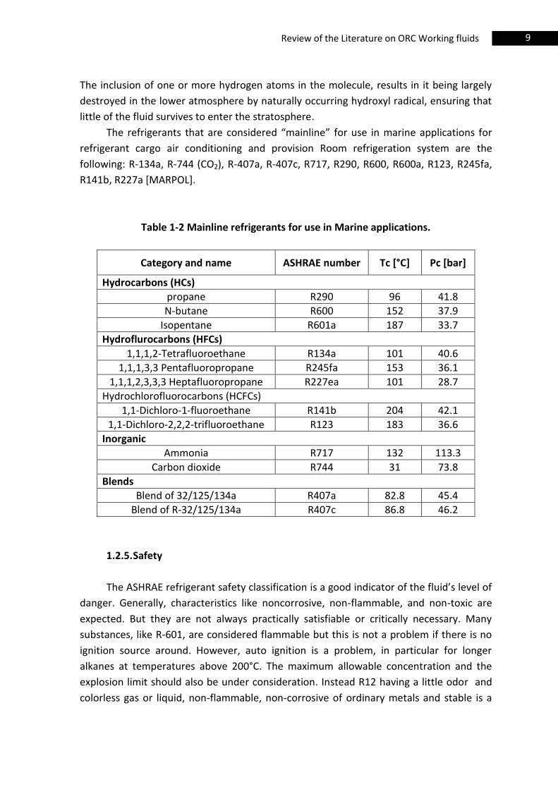
The refrigerants that are considered “mainline” for use in marine applications for
refrigerant cargo air conditioning and provision Room refrigeration system are the
following: R-134a, R-744 (CO2), R-407a, R-407c, R717, R290, R600, R600a, R123, R245fa,
R141b, R227a [MARPOL].
Table 1-2 Mainline refrigerants for use in Marine applications.
Category and name ASHRAE number Tc [°C] Pc [bar]
Hydrocarbons (HCs)
propane R290 96 41.8
N-butane R600 152 37.9
Isopentane R601a 187 33.7
Hydroflurocarbons (HFCs)
1,1,1,2-Tetrafluoroethane R134a 101 40.6
1,1,1,3,3 Pentafluoropropane R245fa 153 36.1
1,1,1,2,3,3,3 Heptafluoropropane R227ea 101 28.7
Hydrochlorofluorocarbons (HCFCs)
1,1-Dichloro-1-fluoroethane R141b 204 42.1
1,1-Dichloro-2,2,2-trifluoroethane R123 183 36.6
Inorganic
Ammonia R717 132 113.3
Carbon dioxide R744 31 73.8
Blends
Blend of 32/125/134a R407a 82.8 45.4
Blend of R-32/125/134a R407c 86.8 46.2
1.2.5. Safety
The ASHRAE refrigerant safety classification is a good indicator of the fluid’s level of
danger. Generally, characteristics like noncorrosive, non-flammable, and non-toxic are
expected. But they are not always practically satisfiable or critically necessary. Many
substances, like R-601, are considered flammable but this is not a problem if there is no
ignition source around. However, auto ignition is a problem, in particular for longer
alkanes at temperatures above 200°C. The maximum allowable concentration and the
explosion limit should also be under consideration. Instead R12 having a little odor and
colorless gas or liquid, non-flammable, non-corrosive of ordinary metals and stable is a
10 Review of the Literature on ORC Working fluids
CFC refrigerant Roy (2010). The ASHRAE refrigerant safety classification is a good
indicator of the fluid’s level of danger. Generally, characteristics like non-corrosive, non-
flammable, and non-toxic are expected, but the most essential requirement is chemical
stability.
A refrigeration system is expected to operate many years, and all other properties
would be useless if the refrigerant decomposed or reacted to form something else.
The next most important criterion relates to health and safety; the ideal refrigerant
would have low toxicity and be nonflammable.
ASHRAE classifies refrigerants according to their toxicity (with “A” being a “lower
degree of toxicity” as indicated by a “permissible exposure limit” of 400 ppm or greater,
while “B” refrigerants have a “higher degree of toxicity” and flammability (ranging from
“1” for nonflammable fluids to “3” for highly flammable fluids, such as the hydrocarbons).
Flammability class “2” has a further subclass (“2L”) for refrigerants of very low
flammability, as defined by a burning velocity of less than 10 cm/s. Thus, an ideal
refrigerant would be class “A1,” and such refrigerants can be used with minimal health
and safety restrictions. Other classes are restricted, such as maximum limits on the
system charge or restriction to use in dedicated machine rooms.
Manente (2011) describe some examples: alkanes that are non-toxic but flammable
are class A3. They require safety devices. R152a is classified A2 (lower flammability and
non-toxic). R134a is of class A1 (non-flammable and non-toxic). R123 is B1 (non-
flammable but toxic). Ammonia classified B2 (toxic and lower flammability) could be used
in an open space with lesser precaution compared with alkanes. Shengjun (2011)
provides the ASHRAE coefficient of several fluids. R227ea and R236fa are of class A1 and
R245fa is of class B1.
1.2.6. Size of the system
There are two indicators to describe the ORC size: one of those is the total area of
heat exchangers and the other one is the turbine size.
The evaporator contributes more area to the total area required for two reasons;
more heat is exchanged in the evaporator than in the condenser and air side heat transfer
coefficient is the dominant. It is known that air or exhaust gas have lower heat transfer
coefficient than water (which is the heat sink in this case).
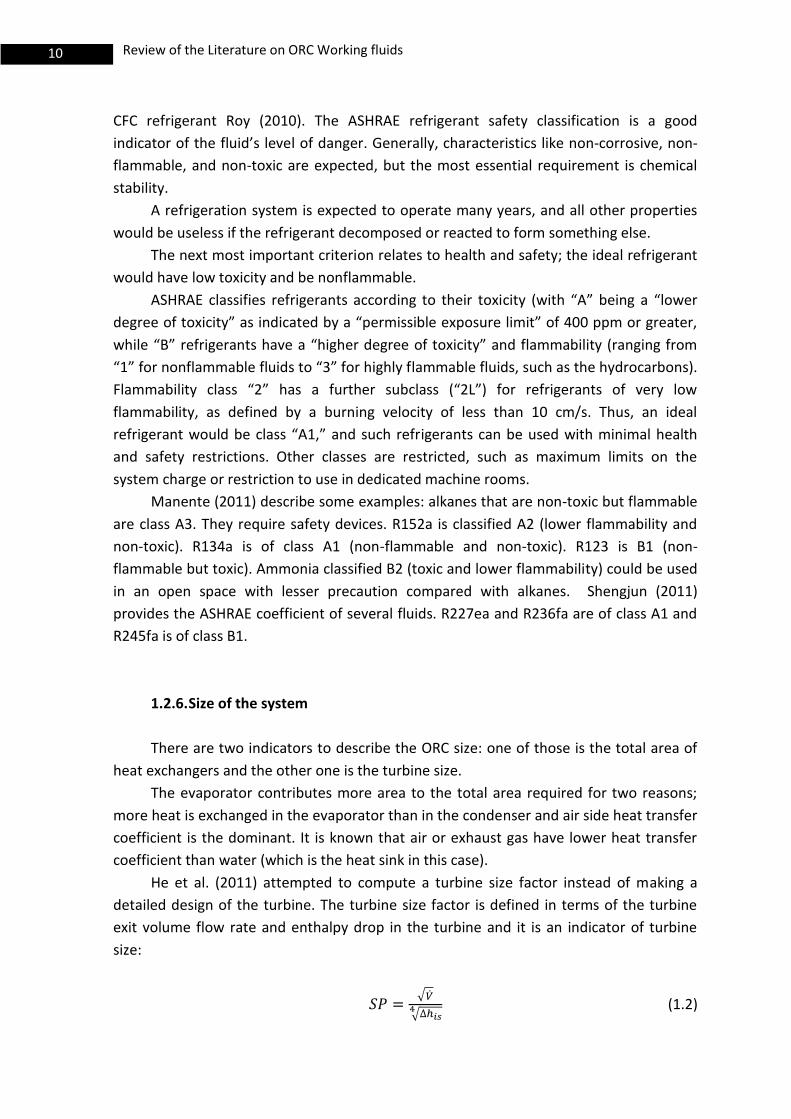
He et al. (2011) attempted to compute a turbine size factor instead of making a
detailed design of the turbine. The turbine size factor is defined in terms of the turbine
exit volume flow rate and enthalpy drop in the turbine and it is an indicator of turbine
size:
√
√ (1.2)
11 Review of the Literature on ORC Working fluids
The size parameter is proportional to actual turbine size.
In the work by He et al (2012) described in Section 1.3, they discovered that working
fluids R717, methanol, R600a, R142b, R114, R600, R245fa, R123, R601a, n-pentane, R11,
R141b and R113 have the lower size factor; instead, Lakew et al. (2010) from a selection
of working fluids concluded that R134a has the lowest turbine size factor.
1.3. Fluid Selection and Parametric Optimization for Basic Rankine Cycle
Lakew et al. (2010) presented the performance of different working fluids to
recover low temperature heat source. Working fluid considered are R-134a R-123, R-
227ea, R-245fa, R-290 N-pentane. A simple Rankine cycle with subcritical configuration is
considered, which consists of a pump, evaporator, turbine and condenser. The working
fluid is saturated liquid at the exit of the condenser, then it gains heat from the heat
source, later at the exit of the evaporator, the fluid is saturated vapor. Pump and turbine
efficiency is 80%, and generator efficiency is 90%, the condensation temperature is fixed
at 20°C, minimum approach temperature of 10°C in the evaporator and 5°C in condenser.
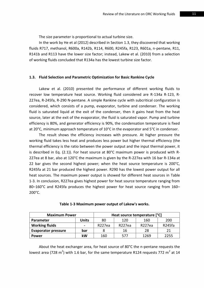
The result shows the efficiency increases with pressure. At higher pressure the
working fluid takes less heat and produces less power but higher thermal efficiency (the
thermal efficiency is the ratio between the power output and the input thermal power, it
is described in Eq. (2.1)). For heat source at 80°C maximum power is produced with R-
227ea at 8 bar, also at 120°C the maximum is given by the R-227ea with 16 bar R-134a at
22 bar gives the second highest power; when the heat source temperature is 200°C,
R245fa at 21 bar produced the highest power. R290 has the lowest power output for all
heat sources. The maximum power output is showed for different heat sources in Table
1-3. In conclusion, R227ea gives highest power for heat source temperature ranging from
80–160°C and R245fa produces the highest power for heat source ranging from 160–
200°C.
Table 1-3 Maximum power output of Lakew's works.
Maximum Power Heat source temperature [°C]
Parameter Units 80 120 160 200
Working fluids - R227ea R227ea R227ea R245fa
Evaporator pressure bar 8 16 28 21
Power kW 160 577 1269 2255
About the heat exchanger area, for heat source of 80°C the n-pentane requests the
lowest area (728 m2) with 1.6 bar, for the same temperature R124 requests 772 m2 at 14
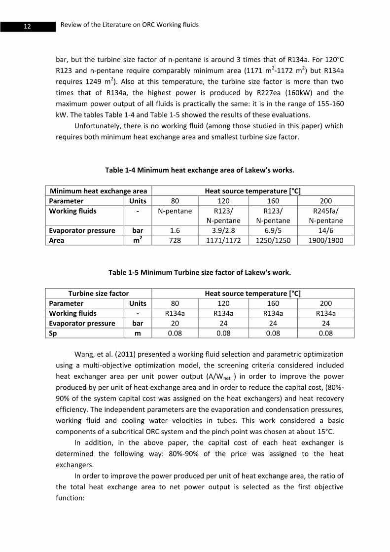
12 Review of the Literature on ORC Working fluids
bar, but the turbine size factor of n-pentane is around 3 times that of R134a. For 120°C
R123 and n-pentane require comparably minimum area (1171 m2-1172 m2) but R134a
requires 1249 m2). Also at this temperature, the turbine size factor is more than two
times that of R134a, the highest power is produced by R227ea (160kW) and the
maximum power output of all fluids is practically the same: it is in the range of 155-160
kW. The tables Table 1-4 and Table 1-5 showed the results of these evaluations.
Unfortunately, there is no working fluid (among those studied in this paper) which
requires both minimum heat exchange area and smallest turbine size factor.
Table 1-4 Minimum heat exchange area of Lakew's works.
Minimum heat exchange area Heat source temperature [°C]
Parameter Units 80 120 160 200
Working fluids - N-pentane R123/ N-pentane
R123/ N-pentane
R245fa/ N-pentane
Evaporator pressure bar 1.6 3.9/2.8 6.9/5 14/6
Area m2 728 1171/1172 1250/1250 1900/1900
Table 1-5 Minimum Turbine size factor of Lakew's work.
Turbine size factor Heat source temperature [°C]
Parameter Units 80 120 160 200
Working fluids - R134a R134a R134a R134a
Evaporator pressure bar 20 24 24 24
Sp m 0.08 0.08 0.08 0.08
Wang, et al. (2011) presented a working fluid selection and parametric optimization
using a multi-objective optimization model, the screening criteria considered included
heat exchanger area per unit power output (A/Wnet ) in order to improve the power
produced by per unit of heat exchange area and in order to reduce the capital cost, (80%-
90% of the system capital cost was assigned on the heat exchangers) and heat recovery
efficiency. The independent parameters are the evaporation and condensation pressures,
working fluid and cooling water velocities in tubes. This work considered a basic
components of a subcritical ORC system and the pinch point was chosen at about 15°C.
In addition, in the above paper, the capital cost of each heat exchanger is
determined the following way: 80%-90% of the price was assigned to the heat
exchangers.
In order to improve the power produced per unit of heat exchange area, the ratio of
the total heat exchange area to net power output is selected as the first objective
function:
13 Review of the Literature on ORC Working fluids
min f1(x) =
(1.3)
On the other hand, higher heat recovery efficiency means more energy recovered
from wasted heat and more net power. Therefore, the second objective function is the
heat recovery efficiency
min f2(x) =
(1.4)
The evaluation function for the optimization is expressed by:
F(x)=w1f1(x)+w2f2(x) (1.5)
The authors suggest the values: w1 = 0.6 and w2 = 0.4.
With this model Eq.(1.5) and with a comparison of optimized results for 13 working
fluids the following results are obtained:
a) The evaporating pressure in the cycle increases with the decrease of the boiling
temperature of working fluids.
b) The value of objective function of R-123 is the lowest for the temperature ranges
from 100°C to 180°C, and R141b is the optimal working fluid when the
temperature higher than 180°C.
c) When the heat source temperature is 140°C, the payback period for R-123 is 3.68
years. Compared to R123 the payback period of R134a increases by 59.8%, when
the temperature is higher than 180°C, R-141b is the best, when the temperature
is 120°C the payback period of R-123 is 5.25 years.
d) The optimal pinch point for ORC system is about 15°C.
e) When the heat source temperature is lower than 100°C, the ORC technology is
inappropriate and the payback rises to 9.35 years with the R123, too long for the
ORC system.
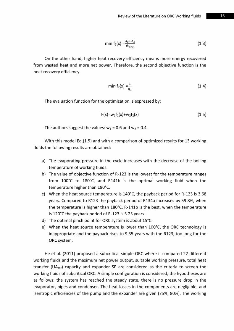
He et al. (2011) proposed a subcritical simple ORC where it compared 22 different
working fluids and the maximum net power output, suitable working pressure, total heat
transfer (UAtot) capacity and expander SP are considered as the criteria to screen the
working fluids of subcritical ORC. A simple configuration is considered, the hypotheses are
as follows: the system has reached the steady state, there is no pressure drop in the
evaporator, pipes and condenser. The heat losses in the components are negligible, and
isentropic efficiencies of the pump and the expander are given (75%, 80%). The working
14 Review of the Literature on ORC Working fluids
fluid at the expander inlet and condenser outlet is saturated vapor and saturated liquid,
respectively. The waste heat source temperature is 150°C and the mass source flow rate
is 1 kg/s, the pinch temperature difference in the evaporator is 5 K and the pinch point
temperature difference in condenser is 5 K.
Table 1-6 Results obtain by He et al (2011).
Working
fluids
Power output
[kW]
Pressure
[kPa]
UAtot
[kW/K]
SP
[m]
R114 9.61 1206 6.2-7.5 0.03
R142b 9.58 1835 8-12 0.03
R600a 9.54 1714 8-12 0.03
R245fa 9.52 1040 6.2-7.5 0.03
R600 9.43 1307 6.2-7.5 0.03
The results from this paper show that the maximal net power output values vary
with the different working fluids like R600a, R142b, R114, R600, R245fa; there is highest
net power of ORC when R114 is adopted, and the smallest with R245fa between the fluid
shown before. The lowest net power outputs of ORC is with methanol and toluene.
In this work it can be deduced that the larger net power output will be produced
when the critical temperature of working fluid approaches the temperature of the waste
heat source.
The working pressure at the maximal net power output are shown in Table 1-6, for
some working fluids like toluene, n-heptane and n-octane the pressure could be much
lower than atmospheric pressure and it means the system need a perfect sealing and
extra cost.
For working fluids like R600a, R142b the total heat transfer capacity could change
from 8 kW/K to 12 kW/K, for working fluids R141b, R600, R144, R245fa, R113, R123,
R600a, toluene the heat transfer capacity is between 6,2 kW/K-7,5 kW/K. For the
remaining fluids like n-heptane, n-octane, the total heat transfer capacity is less than 6
kW/K. Usually higher total heat transfer capacity means more costs of the heat
exchanger, but for the last two fluids, the power output and working pressure are not
ideal for these working fluids.
As regards the turbine size, for working fluids R600a, R142b, R114, R600, R245fa,
R123, R600a the expander SP is smaller than 0.03 m.
At the end the authors suggest working fluids such a R114, R245fa, R123, R600a,n-
pentane, R141b and R113 are better ones under the given conditions in their paper.
15 Review of the Literature on ORC Working fluids
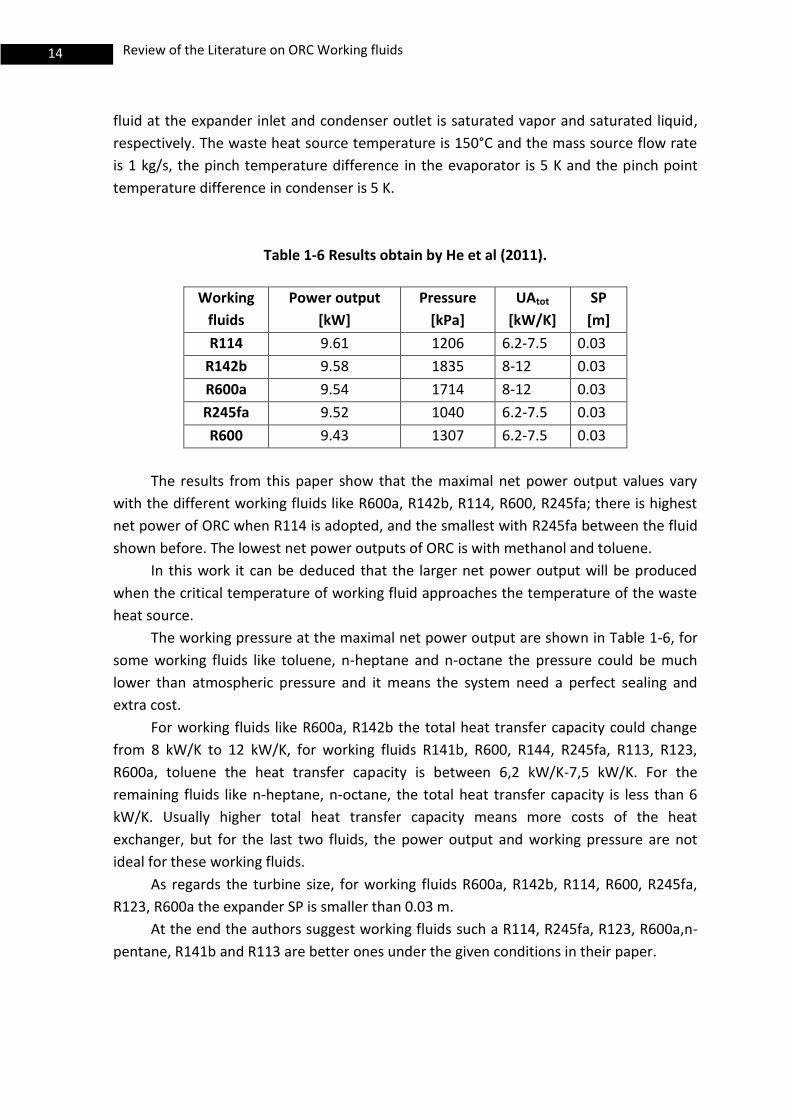
Roy (2010) presented an analysis of an ORC using R12, R123, R134a. The
assumptions are Ideal Rankine cycle, isentropic expansion in the turbine, and the pump
work is neglected during the optimization study. The heat source is exhaust gas with
temperature of 140°C and the mass flow rate of 312 kg/s. A parametric optimization of
turbine inlet pressure was performed to obtain the maximum system efficiency, at each
inlet pressure during TIT (turbine inlet temperature) optimization W, , were
calculated and the improvements in performance on superheating were investigated up
to the available waste heat temperature under this study.
The results show that for R12 the optimum work of 16.84 kJ/kg with an efficiency
value of 12.09%, the superheating is required at moderate pressure to keep the turbine
outlet vapor quality within acceptable limit.
R123 as the working fluid appears to be a better choice, a turbine inlet pressure
value at 1.945 MPa with 55.56 kJ/kg and 25.30% efficiency. The superheating for this fluid
is not suggested.
For R134a the optimum work of 28.03 kJ/kg with an efficiency of 15.53% is obtained
at the pressure 3.533 MPa, with a turbine outlet vapor quality of 0.866. If the pressure is
increased, the outlet vapor quality is further reduced to value 0.7872 then the
superheating is not at all beneficial.
Table 1-7 Results obtained by Roy (2010).
Parameters/output R12 R123 R134a
Turbine inlet pressure (MPa) 3.332 1.945 3.533
Optimum work (kJ/kg) 16.84 55.56 28.03
First law efficiency (%) 12.09 25.30 15.53
Second low efficiency (%) 30.01 64.40 37.80
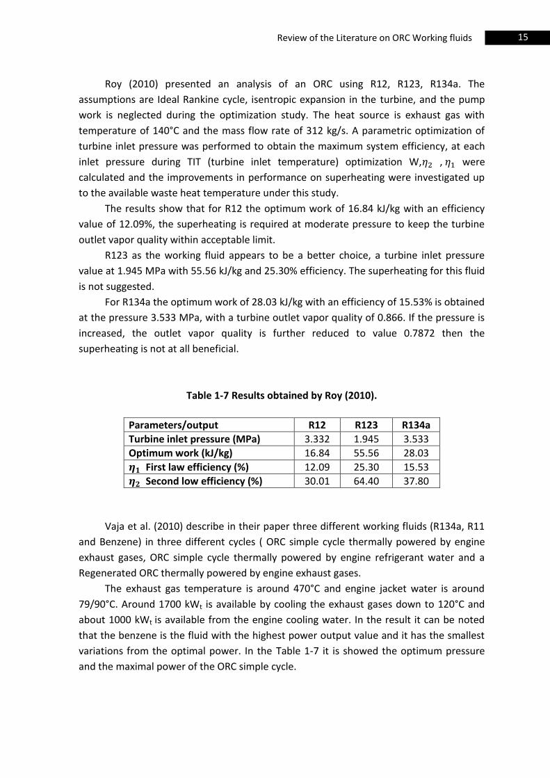
Vaja et al. (2010) describe in their paper three different working fluids (R134a, R11
and Benzene) in three different cycles ( ORC simple cycle thermally powered by engine
exhaust gases, ORC simple cycle thermally powered by engine refrigerant water and a
Regenerated ORC thermally powered by engine exhaust gases.
The exhaust gas temperature is around 470°C and engine jacket water is around
79/90°C. Around 1700 kWt is available by cooling the exhaust gases down to 120°C and
about 1000 kWt is available from the engine cooling water. In the result it can be noted
that the benzene is the fluid with the highest power output value and it has the smallest
variations from the optimal power. In the Table 1-7 it is showed the optimum pressure
and the maximal power of the ORC simple cycle.
16 Review of the Literature on ORC Working fluids
Table 1-8 Results obtained for simple ORC by Vaja et al. (2010).
Working fluids Power output
[kW] Pressure
[kPa] vat/vbt
R134a 147 3723 0.085 5
R11 290 3835 0.165 32
Benzene 376 4470 0.215 374
The parameter vat/vbt (the ratio between specific volume after and before the
turbine) is particularly significant as it shows how much the fluid volume increases
through the expansion, and the benzene has the highest value. Considerations regarding
the power curve for benzene suggest that a lower evaporating pressure would allow a
reduction of turbine outlet/inlet volume flow ratios; for this reason a new optimal value
of evaporating pressure for benzene is selected at 2000 kPa.
Table 1-9 Benzene properties on simple ORC.
Working fluids Power output
[kW] Pressure
[kPa] vat/vbt
Benzene 349.3 2000 0.198 107
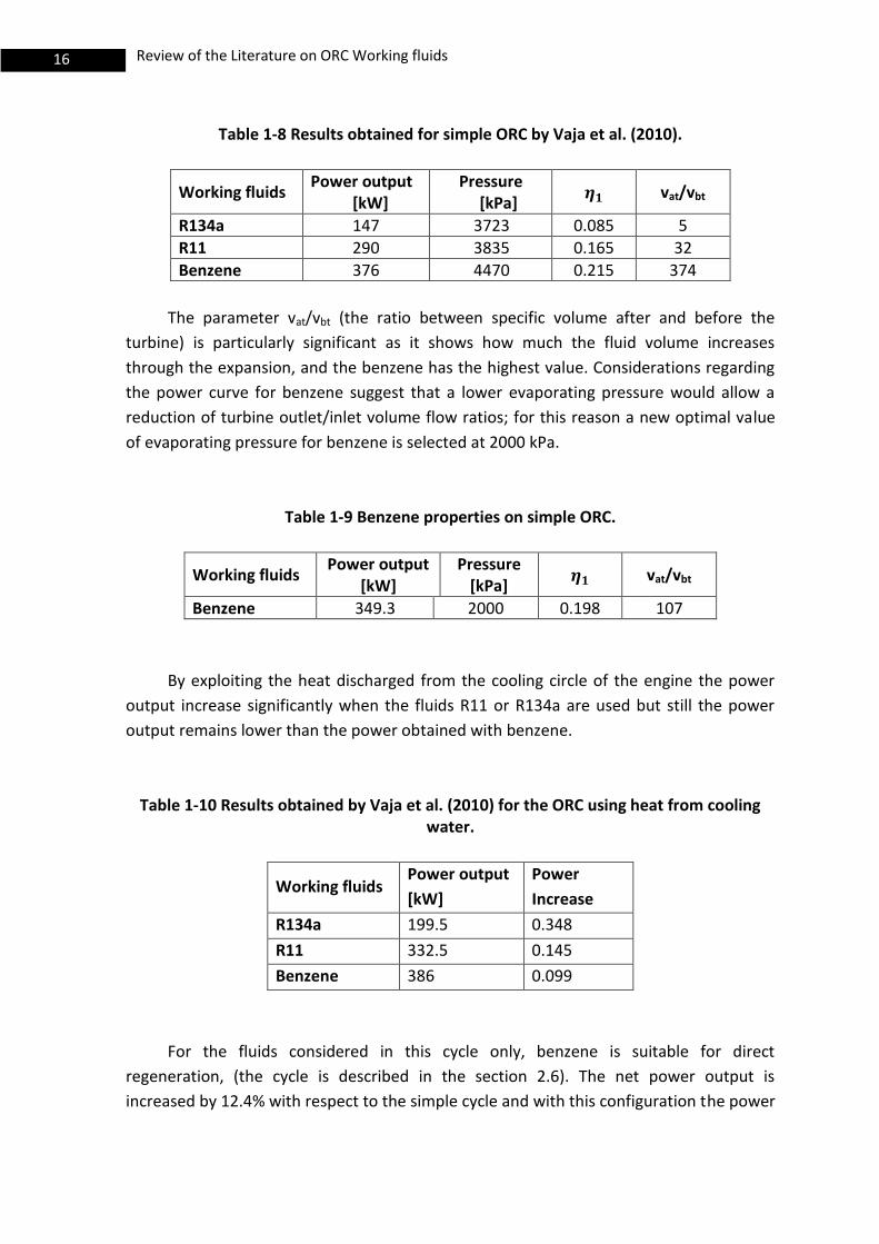
By exploiting the heat discharged from the cooling circle of the engine the power
output increase significantly when the fluids R11 or R134a are used but still the power
output remains lower than the power obtained with benzene.
Table 1-10 Results obtained by Vaja et al. (2010) for the ORC using heat from cooling water.
Working fluids Power output
[kW]
Power
Increase
R134a 199.5 0.348
R11 332.5 0.145
Benzene 386 0.099
For the fluids considered in this cycle only, benzene is suitable for direct
regeneration, (the cycle is described in the section 2.6). The net power output is
increased by 12.4% with respect to the simple cycle and with this configuration the power
17 Review of the Literature on ORC Working fluids
is 392.6 kW with a cycle efficiency of 22.3%. But the benzene is not recommended for
installation on board because it is flammable.
Wang et al. (2012) propose a novel system combining a gasoline engine with a dual
loop ORC (the description of the cycle in 2.5, R245fa is selected as the working fluid for
the HT (high temperature 353.15-404.59 K) and R134a is selected for the LT (low
temperature 304.15-348.15 K) loop. R245fa was chosen because of its good safety and
environmental properties, and R134a was selected because it is environmental friendly
refrigerant widely used in automotive air conditioners.
Borsukiewicz-Gozdur (2010) proposed hybrid power plant to increase the utilization
of geothermal resource supposed available at 80–120 °C, i.e. to reduce the temperature
of the returned geothermal water. The author proposed two solutions, a dual-fluid hybrid
power plant and an hybrid power plant. The proposed dual-fluid power plant consists of
an upper Hirn cycle, in which water is vapourized in a biomass boiler and is then
condensed in a condenser–vapourizer exchanger, which is the thermal link between the
upper and lower cycles. The lower cycle is an ORC where the organic liquid is preheated
by the geothermal resource. Thus, in this dual-fluid power plant, the low-pressure part of
the classical steam–water power plant (i.e. condenser) is replaced by a ORC. The
geothermal water could also be used for preheating of the working fluid (water or
another substance) in a single cycle power plant. Borsukiewicz-Gozdur (2010)called this
cycle simply hybrid plant, and chose a biomass boiler for the upper part of the cycle, while
the working fluid selected is cyclohexane. In the calculation, Borsukiewicz-Gozdur (2010)
supposed to reject the geothermal water down to a very low temperature, i.e. 35 °C. The
author found out that, with the scope to use the least share of energy from other sources
than geothermal, the best option would be a dualfluid-hybrid power plant with R236fa as
a working fluid for the ORC cycle.
18 Review of the Literature on ORC Working fluids
1.4. Fluid Selection and Parametric Optimization for Transcritical Rankine Cycles
Organic Rankine cycles are reviewed for low grades of heat conversion into power.
If a working fluid with subcritical Organic Rankine cycles does not have a good thermal
match with its heat sources, the same working fluid, can be compressed directly to its
supercritical pressures and heated to its supercritical state before expansion, so as to
obtain a better thermal match with the heat source. Unfortunately a supercritical Rankine
cycle normally needs higher operating pressures.
Chen et al. (2010) indicates that a review of the literature shows that a transcritical
Rankine cycle can achieve higher efficiency than the conventional ORC, and they conduct
a rigorous comparative study between a CO2-based, R32-based, and transcritical Rankine
cycles for the conservation of low-grade heat. The results show that the R32-based
transcritical Rankine cycle has many advantages over the CO2-based transcritical Rankine
cycle.
One problem with CO2 is that it has a much lower critical temperature (304.13K,
31°C) and the design of a condenser for CO2 could be hard to achieve economically and
effectively, because in the summer condition the temperature of the sea water is 32°C
and it is not possible to remove the heat from the condenser. Instead, R32 has a much
higher critical temperature (351.26K), making it much easier to condense. Also, R32 has a
higher thermal conductivity in both liquid and vapor phases, which may indicate a smaller
heat exchanger for R32.
In this paper energetic and exergetic analyses of transcritical Rankine cycles
show that:
I. The thermal efficiency of R32-based transcritical Rankine cycle is higher that CO2-
based cycle for the cycle high temperature of 393-453K and R32 works at much
lower pressures.
II. R32 has higher exergy density and lower mass flow rate.
III. With a high temperature of 433 K the exergy efficiencies of CO2 and R32 based
transcritical Rankine cycles are in the range of 0.15-0.51 and 0.56-0.61
respectively, over a wide range of the cycle high pressure.
If we compare the pressure between He et al. (2011) work and the result of the
work of Chen et al (2011), we discover that the working pressure at the maximal net
power output for the CO2 is 22 MPa, for the R23 is around 11 MPa, instead of 1.2 MPa
with R114 He et al. (2011) like according to the paper Chen H. et al (2010).
19 Review of the Literature on ORC Working fluids
Schuster et al. (2010) evaluated the performance of ORCs operating at supercritical
pressures. They compared different fluids using both the thermal efficiency and the total
heat-recovery efficiency. They showed that the advantage in adopting a supercritical
pressure compared to a subcritical operation are: lower exergy destruction in the
evaporator and lower exergy losses in the exhausts, it means a low temperature
differences between the heat source and the working fluid, thus it require larger U·A
values for the heat exchangers.
High pressure and larger U·A are two reasons that render difficult the installation on
board.
1.5. Conclusions based on the Literature Review
The brief review presented above clearly shows that the selection of an appropriate
working fluid is very important for maximum waste heat recovery in actual output electric
power. Amlaku et al. (2010) suggest R227ea for heat source temperature ranging from
80°C-160°C and R245fa for that ranging from 160-200°C. Moreover he stated that the
R134a has the lowest turbine size. Instead Wang et al. (2011) wrote that the best choice
for the range from 100°C to 180°C is R123 (in agreement with Roy (2010) and R141b
when the temperature is higher than 180°C. Chao et al. (2011) took heat transfer capacity
and the turbine size for working fluids in consideration and they suggested fluids like
R114, R113, R245fa, R123, R600a, n-pentane, R141b. Boursukiewiciz-Gozdur (2010)
suggest R236fa as working fluid for ORC cycle. Huijuon et al. (2010) indicated that the
supercritical ORC gives higher efficiency than simple ORC but in the same time high
working pressure. As indicated in Section 1.2.4 like R113, R114 are phased out and others
like R21, R22, R123, R124, R141b, R142b will be phased out in 2020 or 2030. Considering
all this information, the possible fluids are R227ea, R245fa, R134a, R236fa.
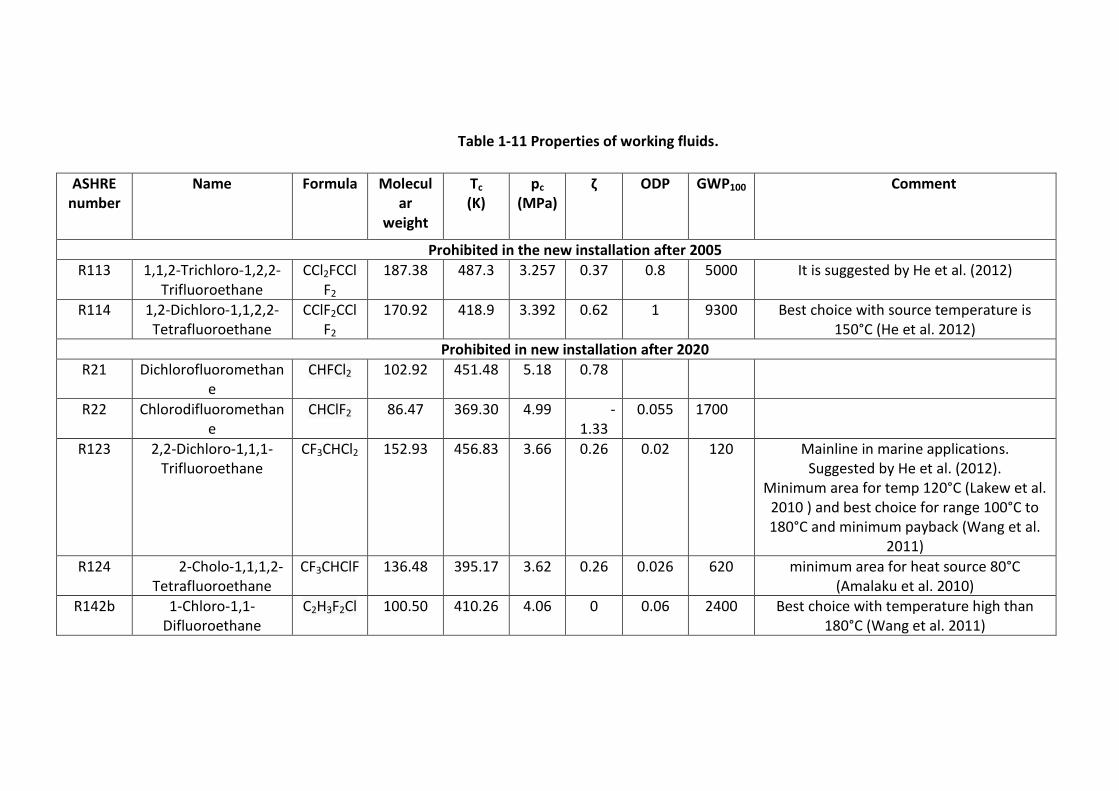
20 Review of the Literature on ORC Working fluids
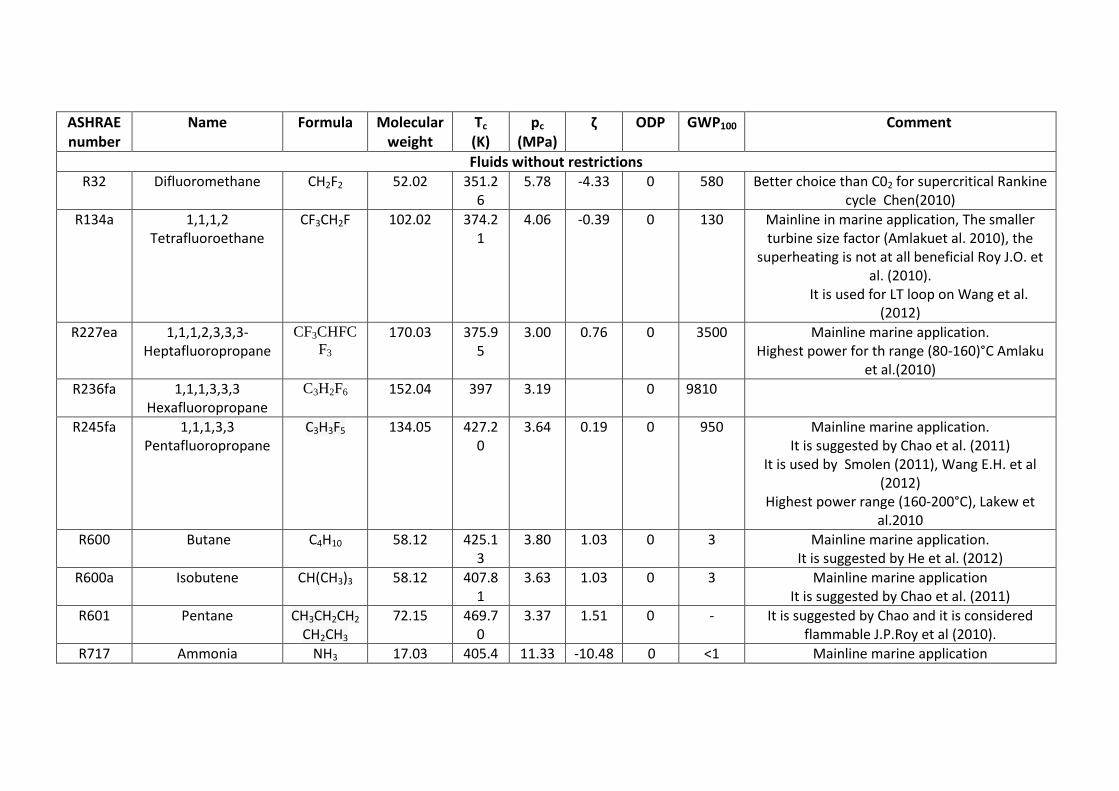
Table 1-11 Properties of working fluids.
ASHRE number
Name Formula Molecular
weight
Tc (K)
pc (MPa)
ζ ODP GWP100 Comment
Prohibited in the new installation after 2005
R113 1,1,2-Trichloro-1,2,2-Trifluoroethane
CCl2FCClF2
187.38 487.3 3.257 0.37 0.8 5000 It is suggested by He et al. (2012)
R114 1,2-Dichloro-1,1,2,2-Tetrafluoroethane
CClF2CClF2
170.92 418.9 3.392 0.62 1 9300 Best choice with source temperature is 150°C (He et al. 2012)
Prohibited in new installation after 2020
R21 Dichlorofluoromethane
CHFCl2 102.92 451.48 5.18 0.78
R22 Chlorodifluoromethane
CHClF2 86.47 369.30 4.99 -1.33
0.055 1700
R123 2,2-Dichloro-1,1,1-Trifluoroethane
CF3CHCl2 152.93 456.83 3.66 0.26 0.02 120 Mainline in marine applications. Suggested by He et al. (2012).
Minimum area for temp 120°C (Lakew et al. 2010 ) and best choice for range 100°C to 180°C and minimum payback (Wang et al.
2011)
R124 2-Cholo-1,1,1,2-Tetrafluoroethane
CF3CHClF 136.48 395.17 3.62 0.26 0.026 620 minimum area for heat source 80°C (Amalaku et al. 2010)
R142b 1-Chloro-1,1-Difluoroethane
C2H3F2Cl 100.50 410.26 4.06 0 0.06 2400 Best choice with temperature high than 180°C (Wang et al. 2011)
21 Review of the Literature on ORC Working fluids
ASHRAE number
Name Formula Molecular weight
Tc (K)
pc (MPa)
ζ ODP GWP100 Comment
Fluids without restrictions R32 Difluoromethane CH2F2 52.02 351.2
6 5.78 -4.33 0 580 Better choice than C02 for supercritical Rankine
cycle Chen(2010)
R134a 1,1,1,2 Tetrafluoroethane
CF3CH2F 102.02 374.21
4.06 -0.39 0 130 Mainline in marine application, The smaller turbine size factor (Amlakuet al. 2010), the
superheating is not at all beneficial Roy J.O. et al. (2010).
It is used for LT loop on Wang et al. (2012)
R227ea 1,1,1,2,3,3,3-Heptafluoropropane
CF3CHFC
F3 170.03 375.9
5 3.00 0.76 0 3500 Mainline marine application.
Highest power for th range (80-160)°C Amlaku et al.(2010)
R236fa 1,1,1,3,3,3 Hexafluoropropane
C3H2F6 152.04 397 3.19 0 9810
R245fa 1,1,1,3,3 Pentafluoropropane
C3H3F5 134.05 427.20
3.64 0.19 0 950 Mainline marine application. It is suggested by Chao et al. (2011)
It is used by Smolen (2011), Wang E.H. et al (2012)
Highest power range (160-200°C), Lakew et al.2010
R600 Butane C4H10 58.12 425.13
3.80 1.03 0 3 Mainline marine application. It is suggested by He et al. (2012)
R600a Isobutene CH(CH3)3 58.12 407.81
3.63 1.03 0 3 Mainline marine application It is suggested by Chao et al. (2011)
R601 Pentane CH3CH2CH2
CH2CH3 72.15 469.7
0 3.37 1.51 0 - It is suggested by Chao and it is considered
flammable J.P.Roy et al (2010).
R717 Ammonia NH3 17.03 405.4 11.33 -10.48 0 <1 Mainline marine application
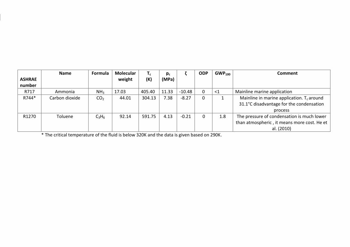
22 Review of the Literature on ORC Working fluids
ASHRAE number
Name Formula Molecular weight
Tc (K)
pc (MPa)
ζ ODP GWP100 Comment
R717 Ammonia NH3 17.03 405.40 11.33 -10.48 0 <1 Mainline marine application
R744* Carbon dioxide CO2 44.01 304.13 7.38 -8.27 0 1 Mainline in marine application. Tc around 31.1°C disadvantage for the condensation
process
R1270 Toluene C3H6 92.14 591.75 4.13 -0.21 0 1.8 The pressure of condensation is much lower than atmospheric , it means more cost. He et
al. (2010)
* The critical temperature of the fluid is below 320K and the data is given based on 290K.
23 Literature Review of Various ORC Systems
2. Literature Review of Various ORC Systems
2.1. Introduction
The aim of this chapter is to describe various ORC cycles that they are found in
literature in order to find the best choice or suggest a plant design to apply in the ship
that is studied.
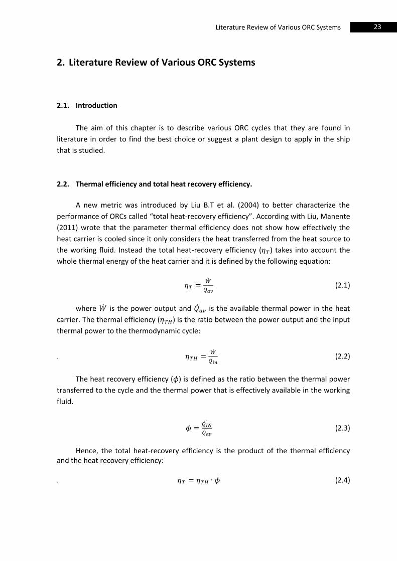
2.2. Thermal efficiency and total heat recovery efficiency.
A new metric was introduced by Liu B.T et al. (2004) to better characterize the
performance of ORCs called “total heat-recovery efficiency”. According with Liu, Manente
(2011) wrote that the parameter thermal efficiency does not show how effectively the
heat carrier is cooled since it only considers the heat transferred from the heat source to
the working fluid. Instead the total heat-recovery efficiency ( ) takes into account the
whole thermal energy of the heat carrier and it is defined by the following equation:
(2.1)
where is the power output and is the available thermal power in the heat
carrier. The thermal efficiency ( ) is the ratio between the power output and the input
thermal power to the thermodynamic cycle:
.
(2.2)
The heat recovery efficiency ( ) is defined as the ratio between the thermal power
transferred to the cycle and the thermal power that is effectively available in the working
fluid.
(2.3)
Hence, the total heat-recovery efficiency is the product of the thermal efficiency
and the heat recovery efficiency: . (2.4)

24 Literature Review of Various ORC Systems
The analysis of total heat recovery is different from the conventional analysis which
focused on thermal efficiency. In general, the maximum value of total heat-recovery
efficiency occurs at the appropriate evaporating temperature that is between the inlet
temperature of waste heat and the condensing temperature. The maximum value of total
heat recovery efficiency increases with the increase of the inlet temperature of the waste
heat and decreases it by using working fluids of the lower critical temperature.
Analysis using a constant waste heat temperature, or based on thermal efficiency
may result in considerable deviation regarding the system design of the varying
temperature conditions of the actual waste heat recovery.
25 Literature Review of Various ORC Systems
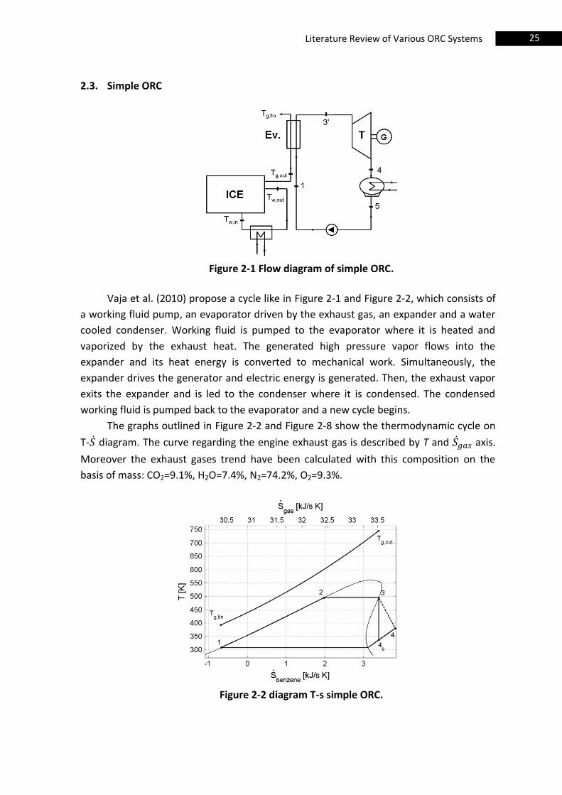
2.3. Simple ORC
Figure 2-1 Flow diagram of simple ORC.
Vaja et al. (2010) propose a cycle like in Figure 2-1 and Figure 2-2, which consists of
a working fluid pump, an evaporator driven by the exhaust gas, an expander and a water
cooled condenser. Working fluid is pumped to the evaporator where it is heated and
vaporized by the exhaust heat. The generated high pressure vapor flows into the
expander and its heat energy is converted to mechanical work. Simultaneously, the
expander drives the generator and electric energy is generated. Then, the exhaust vapor
exits the expander and is led to the condenser where it is condensed. The condensed
working fluid is pumped back to the evaporator and a new cycle begins.
The graphs outlined in Figure 2-2 and Figure 2-8 show the thermodynamic cycle on
T- diagram. The curve regarding the engine exhaust gas is described by T and axis.
Moreover the exhaust gases trend have been calculated with this composition on the
basis of mass: CO2=9.1%, H2O=7.4%, N2=74.2%, O2=9.3%.
Figure 2-2 diagram T-s simple ORC.
26 Literature Review of Various ORC Systems
The heat source includes 1700 kWt from exhaust gas (from 340°C to 120°C). If the
simple ORC configuration in Figure 2-2 is used, the power output is 376 kW for benzene,
290 kW for R11, and 147 kW for R134. With regard to the cycle efficiencies, the maximum
value of 0.215 is achieved with benzene, 0.165 with R11 and 0.085 with R134a.
The temperature difference between gases and organic fluid induces irreversibility,
that is the main cause for low thermodynamic efficiencies with R11 and R134a. Benzene
has a critical temperature of 288.9°C and it is closer to inlet exhaust gas temperature than
the other two fluids.
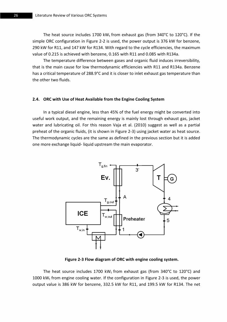
2.4. ORC with Use of Heat Available from the Engine Cooling System
In a typical diesel engine, less than 45% of the fuel energy might be converted into
useful work output, and the remaining energy is mainly lost through exhaust gas, jacket
water and lubricating oil. For this reason Vaja et al. (2010) suggest as well as a partial
preheat of the organic fluids, (it is shown in Figure 2-3) using jacket water as heat source.
The thermodynamic cycles are the same as defined in the previous section but it is added
one more exchange liquid- liquid upstream the main evaporator.
Figure 2-3 Flow diagram of ORC with engine cooling system.
The heat source includes 1700 kWt from exhaust gas (from 340°C to 120°C) and
1000 kWt from engine cooling water. If the configuration in Figure 2-3 is used, the power
output value is 386 kW for benzene, 332.5 kW for R11, and 199.5 kW for R134. The net
27 Literature Review of Various ORC Systems
power output compared to the simple ORC increases by 9.9% with benzene, 14.5% with
R11 and 34.8% with R134a.
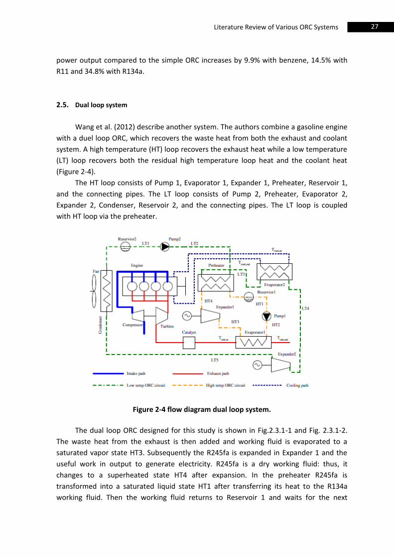
2.5. Dual loop system
Wang et al. (2012) describe another system. The authors combine a gasoline engine
with a duel loop ORC, which recovers the waste heat from both the exhaust and coolant
system. A high temperature (HT) loop recovers the exhaust heat while a low temperature
(LT) loop recovers both the residual high temperature loop heat and the coolant heat
(Figure 2-4).
The HT loop consists of Pump 1, Evaporator 1, Expander 1, Preheater, Reservoir 1,
and the connecting pipes. The LT loop consists of Pump 2, Preheater, Evaporator 2,
Expander 2, Condenser, Reservoir 2, and the connecting pipes. The LT loop is coupled
with HT loop via the preheater.
Figure 2-4 flow diagram dual loop system.
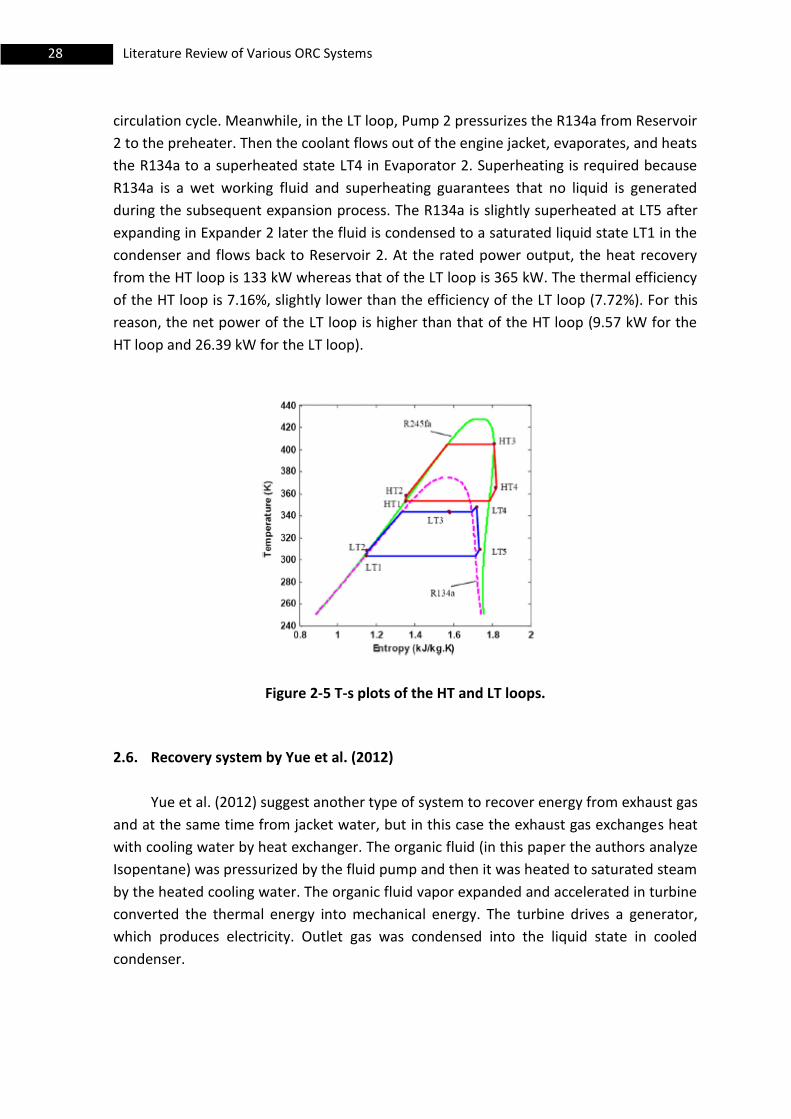
The dual loop ORC designed for this study is shown in Fig.2.3.1-1 and Fig. 2.3.1-2.
The waste heat from the exhaust is then added and working fluid is evaporated to a
saturated vapor state HT3. Subsequently the R245fa is expanded in Expander 1 and the
useful work in output to generate electricity. R245fa is a dry working fluid: thus, it
changes to a superheated state HT4 after expansion. In the preheater R245fa is
transformed into a saturated liquid state HT1 after transferring its heat to the R134a
working fluid. Then the working fluid returns to Reservoir 1 and waits for the next
28 Literature Review of Various ORC Systems
circulation cycle. Meanwhile, in the LT loop, Pump 2 pressurizes the R134a from Reservoir
2 to the preheater. Then the coolant flows out of the engine jacket, evaporates, and heats
the R134a to a superheated state LT4 in Evaporator 2. Superheating is required because
R134a is a wet working fluid and superheating guarantees that no liquid is generated
during the subsequent expansion process. The R134a is slightly superheated at LT5 after
expanding in Expander 2 later the fluid is condensed to a saturated liquid state LT1 in the
condenser and flows back to Reservoir 2. At the rated power output, the heat recovery
from the HT loop is 133 kW whereas that of the LT loop is 365 kW. The thermal efficiency
of the HT loop is 7.16%, slightly lower than the efficiency of the LT loop (7.72%). For this
reason, the net power of the LT loop is higher than that of the HT loop (9.57 kW for the
HT loop and 26.39 kW for the LT loop).
Figure 2-5 T-s plots of the HT and LT loops.
2.6. Recovery system by Yue et al. (2012)
Yue et al. (2012) suggest another type of system to recover energy from exhaust gas
and at the same time from jacket water, but in this case the exhaust gas exchanges heat
with cooling water by heat exchanger. The organic fluid (in this paper the authors analyze
Isopentane) was pressurized by the fluid pump and then it was heated to saturated steam
by the heated cooling water. The organic fluid vapor expanded and accelerated in turbine
converted the thermal energy into mechanical energy. The turbine drives a generator,
which produces electricity. Outlet gas was condensed into the liquid state in cooled
condenser.
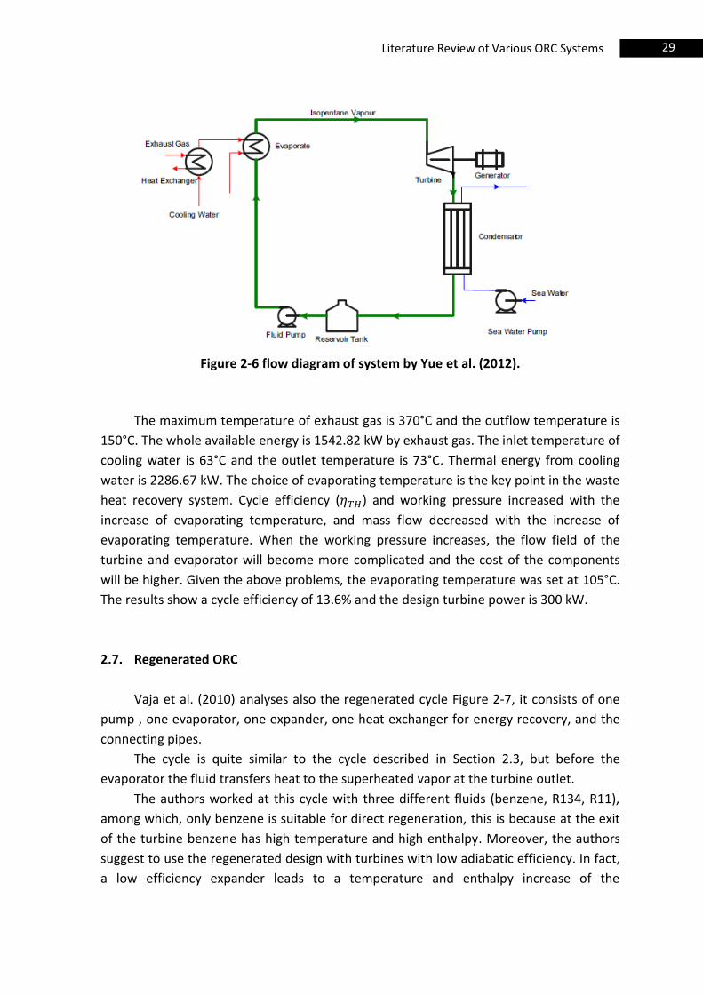
29 Literature Review of Various ORC Systems
Figure 2-6 flow diagram of system by Yue et al. (2012).
The maximum temperature of exhaust gas is 370°C and the outflow temperature is
150°C. The whole available energy is 1542.82 kW by exhaust gas. The inlet temperature of
cooling water is 63°C and the outlet temperature is 73°C. Thermal energy from cooling
water is 2286.67 kW. The choice of evaporating temperature is the key point in the waste
heat recovery system. Cycle efficiency ( ) and working pressure increased with the
increase of evaporating temperature, and mass flow decreased with the increase of
evaporating temperature. When the working pressure increases, the flow field of the
turbine and evaporator will become more complicated and the cost of the components
will be higher. Given the above problems, the evaporating temperature was set at 105°C.
The results show a cycle efficiency of 13.6% and the design turbine power is 300 kW.
2.7. Regenerated ORC
Vaja et al. (2010) analyses also the regenerated cycle Figure 2-7, it consists of one
pump , one evaporator, one expander, one heat exchanger for energy recovery, and the
connecting pipes.
The cycle is quite similar to the cycle described in Section 2.3, but before the
evaporator the fluid transfers heat to the superheated vapor at the turbine outlet.
The authors worked at this cycle with three different fluids (benzene, R134, R11),
among which, only benzene is suitable for direct regeneration, this is because at the exit
of the turbine benzene has high temperature and high enthalpy. Moreover, the authors
suggest to use the regenerated design with turbines with low adiabatic efficiency. In fact,
a low efficiency expander leads to a temperature and enthalpy increase of the

30 Literature Review of Various ORC Systems
superheated vapor at the turbine outlet and this energy is partly recovered in the
exchange.
The regenerate heat exchange requires a liquid-gas, it is not simple than the heat
exchange liquid-liquid. Vaja et al. (2010) shows in the Section 1.3 that the increase power
output from the regenerated cycle and from simple cycle with preheat is the same, so it is
suggested the second choice, thus simplifying the design of the heat exchanger required.
The heat source includes 1700 kWt from exhaust gas (from 340°C to 120°C). If the
configuration in Figure 2 8 is used, the power output is 392.6 kW for benzene, and the net
power increases with respect to the simple ORC by 12.4 %.
Figure 2-7 flow diagram of regenerated ORC.

31 Literature Review of Various ORC Systems
Figure 2-8 benzene regenerated cycle, T-s diagram.
Vaja consider that the recuperator is a counterflow type heat exchanger and it
required a . Under these hypotheses the temperature of the vapor at the
heat exchanger outlet can be evaluated.
(2.5)
In Figure 2-8 the two dotted lines are referred to the internal heat exchange process.
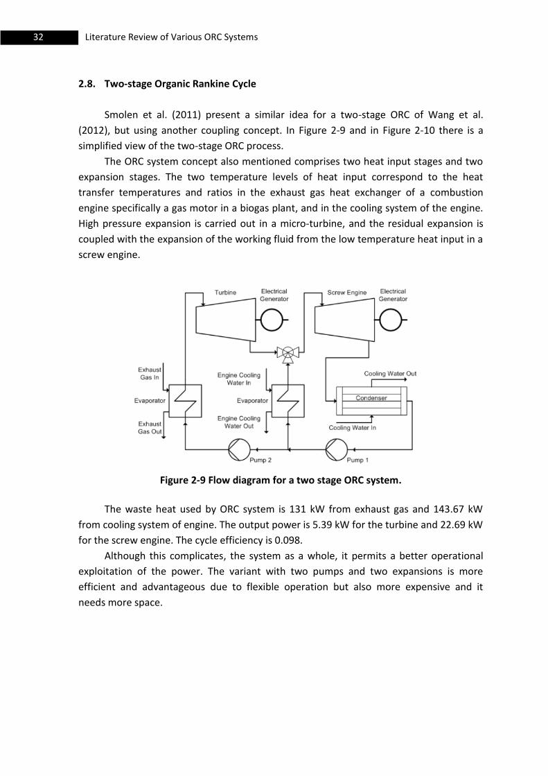
32 Literature Review of Various ORC Systems
2.8. Two-stage Organic Rankine Cycle
Smolen et al. (2011) present a similar idea for a two-stage ORC of Wang et al.
(2012), but using another coupling concept. In Figure 2-9 and in Figure 2-10 there is a
simplified view of the two-stage ORC process.
The ORC system concept also mentioned comprises two heat input stages and two
expansion stages. The two temperature levels of heat input correspond to the heat
transfer temperatures and ratios in the exhaust gas heat exchanger of a combustion
engine specifically a gas motor in a biogas plant, and in the cooling system of the engine.
High pressure expansion is carried out in a micro-turbine, and the residual expansion is
coupled with the expansion of the working fluid from the low temperature heat input in a
screw engine.
Figure 2-9 Flow diagram for a two stage ORC system.
The waste heat used by ORC system is 131 kW from exhaust gas and 143.67 kW
from cooling system of engine. The output power is 5.39 kW for the turbine and 22.69 kW
for the screw engine. The cycle efficiency is 0.098.
Although this complicates, the system as a whole, it permits a better operational
exploitation of the power. The variant with two pumps and two expansions is more
efficient and advantageous due to flexible operation but also more expensive and it
needs more space.
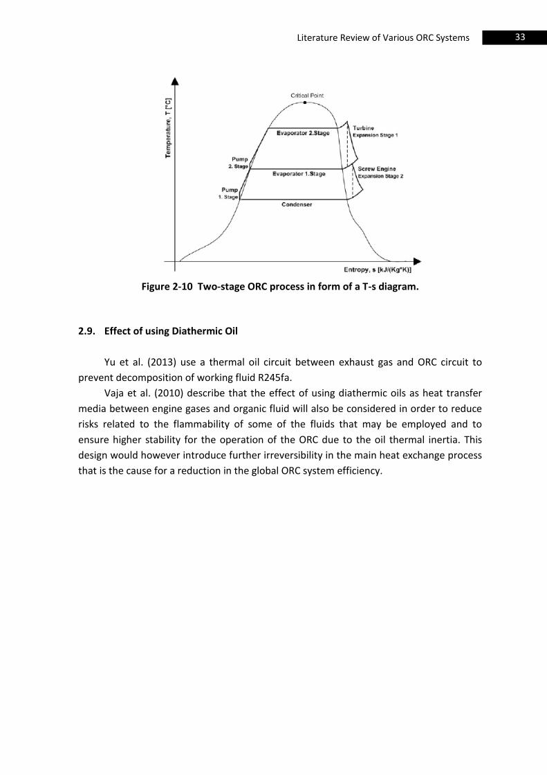
33 Literature Review of Various ORC Systems
Figure 2-10 Two-stage ORC process in form of a T-s diagram.
2.9. Effect of using Diathermic Oil
Yu et al. (2013) use a thermal oil circuit between exhaust gas and ORC circuit to
prevent decomposition of working fluid R245fa.
Vaja et al. (2010) describe that the effect of using diathermic oils as heat transfer
media between engine gases and organic fluid will also be considered in order to reduce
risks related to the flammability of some of the fluids that may be employed and to
ensure higher stability for the operation of the ORC due to the oil thermal inertia. This
design would however introduce further irreversibility in the main heat exchange process
that is the cause for a reduction in the global ORC system efficiency.

34 Literature Review of Various ORC Systems
35 Energy Balance of the Main Engine
3. Energy Balance of the Main Engine
3.1. Introduction
The aim of this chapter is to explain the whole method that was used to evaluate
the energy balance of the main engine (M/E) for a Tanker. The results are obtained
combining information from various sources: official shop test results for Main Engine
(there are data for 110%, 100%, 90%, 75%, 50%, 25% engine load), results of sea trials,
F.W (fresh water)/S.W (sea water) heating balance calculation, and steam balance. In
addition, the values of several operating parameters at various loads (not given in the
aforementioned documents) have been obtained using software available on the website
of the manufacturer. Thus, using the available data and formulating some assumptions
the energy balances for the main engine loads are evaluated.
3.2. Main Engine System
In Figure 3-1, the Main Engine system is shown. Within main engine (box number 1)
the fuel thermal power is converted into useful mechanical power ( ). The remaining
fuel thermal power is lost through lubricating oil (box number 3), jacket water (box
number 4), air cooling (box number 6), radiation losses ( ) and exhaust gas (point g1).
Part of the exhaust gas heat is actually recovered in the turbocharger (box number 2) and
in the exhaust gas boiler (box number 7). The turbocharger’s compressor draws in
ambient air (point a1) and compresses it (point a2) before it enters into the air cooler
system (box number 6). Using part of the thermal power from the jacket water, fresh
water generator (box number 5) produces fresh water (water used for steam production,
domestic consumption). Cooling system is composed by a water loop which extracts heat
from lubricating oil, jacket water and supercharging air and then reject it to seawater in a
central cooler (box number 8).
.

36 Energy Balance of the Main Engine
Main Engine
FWG
Central F. W. cooler
Fuel
Exhaust Gas
s1
s2
g2
Air
a1
a2a3
⑦
lo1lo2 w2
w1 w3
w4
w5
①
⑥
④
⑤
②
③
g1
cw1 cw2 cw3
cw4 cw5
⑧
g3
Ẇ
f
Legend:
1 Main Engine a=air
2 Turbocharger eg=exhaust gas 3 Lubricating oil exchanger w=water
4 Jacket water exchanger lo=lubricating oil
5 Fresh water generator s=water / steam
6 Supercharging air cooler cw=cooling water
7 Exhaust gas boiler
8 Central fresh water cooler
Qr=radiation power
=mechanical power
Figure 3-1 Arrangement of the main engine in ships of relatively low power without steam turbine.
37 Energy Balance of the Main Engine
3.3. Explanation of the Main Components of the Main Engine System.
Figure 3-1 shows eight main components (eight boxes). They are: main Engine,
Turbocharger, Lubricating oil cooler, jacket water cooler, fresh water generator,
supercharging air cooler, exhaust gas boiler and central fresh water cooler. Using the
available documents (official shop test results for Main Engine, results of sea trials,
heating balance calculation and steam balance, and fresh water generator manual), this
paragraph explains in detail all these main components.
3.3.1. Main Engine
Information of the Main Engine are: type 6S60MC, number of cylinders 6, diameter
of the cylinder (bore) 600 mm; power 15400 BHP (11325 kW) at 97 RPM. The engine
(Diesel Engine) is fed with Marine Diesel Oil (MDO). The fuel consumption rate as
measured is 2169 l/hr, if the fuel has the following features: density of 0.962 kg/l, low
calorific value of 9609 kcal/kg and the engine load is 92.84% (10516 kW).
3.3.2. Turbocharger
Supercharging air is supplied to the engine by one or more turbochargers, located
on the exhaust side of the engine (see Figure 3-1). There are two turbochargers equipping
the Main Engine having the following features: maximum speeds (20400 RPM and 19380
RPM) and maximum exhaust gas inlet temperatures (550°C and 520°C, respectively).
The compressor of each turbocharger draws air from the engine room, through an
air filter, and the compressed air is cooled in the supercharging air cooler (box number 6).
The supercharging air cooler is provided with a water mist eliminator, which prevents
condensate water from being carried with the air into the supercharging air receiver and
to the combustion chamber.
3.3.3. Lubricating oil cooler and jacket water cooler
The cooling water is pumped through the heat exchanger with the lubricating oil
and then in the heat exchanger with the jacket water (see Figure 3-1). At 100% engine
load, the inlet temperature of the lubricating oil to the Main Engine (point lo2) is 46°C and
the outlet temperature is 50.8°C (point lo1), the inlet temperature of the jacket water to
the Main Engine (point w1) is 70°C and the outlet temperature (point w2) is 79.3°C. The
inlet temperature of the cooling water coming from the central cooler is 36°C (point cw1
38 Energy Balance of the Main Engine
in Figure 3-1 ); after the heat exchanger with the lubricating oil the temperature reaches
42.5°C (point cw2). Through the heat exchanger with the jacket water the temperature
increases further until 53.7°C (point cw3). All these data are for the 100% engine load.
Mass flow rate and thermal power for all these hot streams are not given in the available
documentation.
3.3.4. Fresh water generator
Fresh water generator is an important equipment on board. Fresh water (i.e.,
desalinated water) produced by the fresh water generator is used for steam production,
cooling circuits, as well as for domestic consumption .
The fresh water is produced by heating and evaporation of the sea water. The heat
exchanger in the freshwater generator is connected to the jacket cooling water system of
the Diesel engine, and it, therefore, works as an extra cooler (see box 5 in Figure 3-1 ).
Looking at Figure 3-2, the jacket cooling water, which may reach a temperature
around 80°C, flows outside the tubes of the heat exchanger. During this passage the
temperature will drop between 4 to 10°C depending on the amount of jacket cooling
water that is used. The controlled amount of sea feed water flows within the heat
exchanger tubes, where it is heated under vacuum (-0.085 MPa) and evaporates by rising
film evaporation, meaning that optimum conditions are achieved and scale formation is
minimized. The vacuum required is obtained by means of a water ejector which
automatically ensures correct conditions.
The generated vapor passes through the separator, in which the sea water droplets
are separated. The brine is discharged by means of a water ejector.
The saturated vapor reaches the sea water heat exchanger, it cools off, and it is
condensed outside the tubes into fresh water, which is collected in a shell and discharged
by the freshwater pump, (see FigureFigure 3-2).
The model of fresh water generator is KE25 of Sakura Engineering, the capacity of
distillate is 25 t/day, and the heat balance is described in Figure 3-2. It requires 704.5 kW
from jacket water thermal power.

39 Energy Balance of the Main Engine
Figure 3-2 Fresh Water Generator.
3.3.5. Scavenge Air cooler
The Turbocharger increases charge air density, and intake manifold temperature as
well. High temperature can lead to reduced charge density and higher combustion
temperature, which can affect torque, power and emissions. If intake manifold
temperature could be reduced, the intake density could be further increased and more
air could be supplied to the engine without necessarily increasing the intake manifold
pressure. By cooling the air with a heat exchanger, the temperature will be low and the
density will be higher. While this would require a compressor capable of higher flow, the
cost would be considerably less than a compressor that was also capable of higher
pressures. Cooling the air with a heat exchanger as soon as it leaves the compressor, is a
common way to achieve this supercharging air cooling. At 100% engine load, the cooler

40 Energy Balance of the Main Engine
system (see box 6 Figure 3-1) uses water directly from central cooler, thus the inlet
temperature is 36°C (point cw4) and the outlet temperature is around 60°C (point cw5).
3.3.6. Exhaust gas Boiler
The steam consumers in this vessel consist of steam driven pumps, oil heaters for
E/R machinery, steam heated F.O tanks, slop tanks (cleaning tanker), domestic
consumers, etc.. The steam consumption is divided into three different pressure levels: 16
kg/cm2G (16.7 bar), 10 kg/cm2G (9.8 bar) and 6 kg/cm2G (5.88 bar). Three different steam
generators supply these demands. Two of them are auxiliary boilers fed with heavy fuel
oil: each of them produces 25000 kg/h of saturated steam at two pressure levels at 16
kg/m2G (16.7 bar) and 6 kg/m2G (5.88 bar). The other one is an Exhaust gas boiler (box 7
in Figure 3-1 ) which recovers heat from exhaust gas of the engine and produces 1400
Kg/h of saturated vapor at 6 kg/m2G (5.88 bar). In all cases the feed water temperature is
60°C (point s1) because it comes from the fresh water generator.
According to the available information, there are three different pressure levels of
steam, in four different operating modes. These modes are “normal voyage”, “tank
heating”, “tank cleaning” and “cargo unloading”. Each of these operating modes is
associated with different steam demands. “Tank heating” is a normal practice to heat up
cargo for 2-3 days before arriving at the discharge port. “Tank cleaning” is the preparation
of ship for dry docking. The tanks must be fully and thoroughly cleaned to avoid
hydrocarbon release when the ship is in the repair yard, (otherwise the vessel will not
receive the gas free certificate). The duration but also the temperature and hence steam
consumption will depend not only on internal tank geometry but also on the type of
cargo, the viscosity and the existence of any constituents which cling on the internal
structure and is difficult to be removed. This operation takes place only once a year or
every two years. “Cargo unloading” is the process of moving oil off a tanker: the transfer
starts at low pressure to ensure that equipment is working correctly and that connections
are secure. Then a steady pressure is achieved and held during all the operation.
To complete the energy balance the ISO conditions are taken into consideration and
only the exhaust gas boiler is considered, because it operates with heat from exhaust
gases of the main engine.
The steam consumption at 6 kg/m2G (5.88 bar) is 767 kg/h during the normal
voyage, 1105 kg/h during tank cleaning, 1149 kg/h during tank heating, 43292 kg/h during
cargo unloading. Using 1400 kg/h of steam, produced by the exhaust gas boiler, it is
possible to cover the steam demand for all of the three operating conditions.
Nevertheless, in “normal voyage”, exhaust gas heat is only partially used and a part of it
would be used for ORC system.
In this study “cargo unloading” is not considered, because in this operating mode
the engine does not operate.
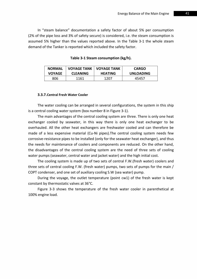
41 Energy Balance of the Main Engine
In “steam balance” documentation a safety factor of about 5% per consumption
(2% of the pipe loss and 3% of safety secure) is considered, i.e. the steam consumption is
assumed 5% higher than the values reported above. In the Table 3-1 the whole steam
demand of the Tanker is reported which included the safety factor.
Table 3-1 Steam consumption (kg/h).
NORMAL VOYAGE
VOYAGE TANK CLEANING
VOYAGE TANK HEATING
CARGO UNLOADING
806 1161 1207 45457
3.3.7. Central Fresh Water Cooler
The water cooling can be arranged in several configurations, the system in this ship
is a central cooling water system (box number 8 in Figure 3-1).
The main advantages of the central cooling system are three. There is only one heat
exchanger cooled by seawater, in this way there is only one heat exchanger to be
overhauled. All the other heat exchangers are freshwater cooled and can therefore be
made of a less expensive material (Cu-Ni pipes).The central cooling system needs few
corrosive-resistance pipes to be installed (only for the seawater heat exchanger), and thus
the needs for maintenance of coolers and components are reduced. On the other hand,
the disadvantages of the central cooling system are the need of three sets of cooling
water pumps (seawater, central water and jacket water) and the high initial cost.
The cooling system is made up of two sets of central F.W.(fresh water) coolers and
three sets of central cooling F.W. (fresh water) pumps, two sets of pumps for the main /
COPT condenser, and one set of auxiliary cooling S.W (sea water) pump.
During the voyage, the outlet temperature (point cw1) of the fresh water is kept
constant by thermostatic valves at 36°C.
Figure 3-3 shows the temperature of the fresh water cooler in parenthetical at
100% engine load.
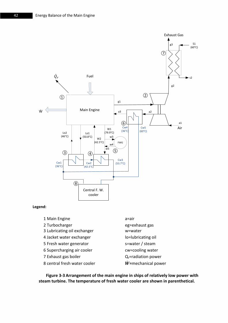
42 Energy Balance of the Main Engine
Main Engine
FWG
Central F. W. cooler
Fuel
Exhaust Gas
S1(60°C)
s2
g2
Air
a1
a2a3
⑦
Lo1(50.8°C)
Lo2(46°C)
W2(42.5°C)
W1(79.9°C)
w3
w4
w5
①
⑥
④⑤
②
③
g1
Cw1(36°C)
Cw2(42.5°C)
Cw3 (53.7°C)
Cw4(36°C)
Cw5(60°C)
⑧
g3
Ẇ
Legend:
1 Main Engine a=air
2 Turbocharger eg=exhaust gas 3 Lubricating oil exchanger w=water
4 Jacket water exchanger lo=lubricating oil
5 Fresh water generator s=water / steam
6 Supercharging air cooler cw=cooling water
7 Exhaust gas boiler Qr=radiation power
8 central fresh water cooler =mechanical power
Figure 3-3 Arrangement of the main engine in ships of relatively low power with steam turbine. The temperature of fresh water cooler are shown in parenthetical.
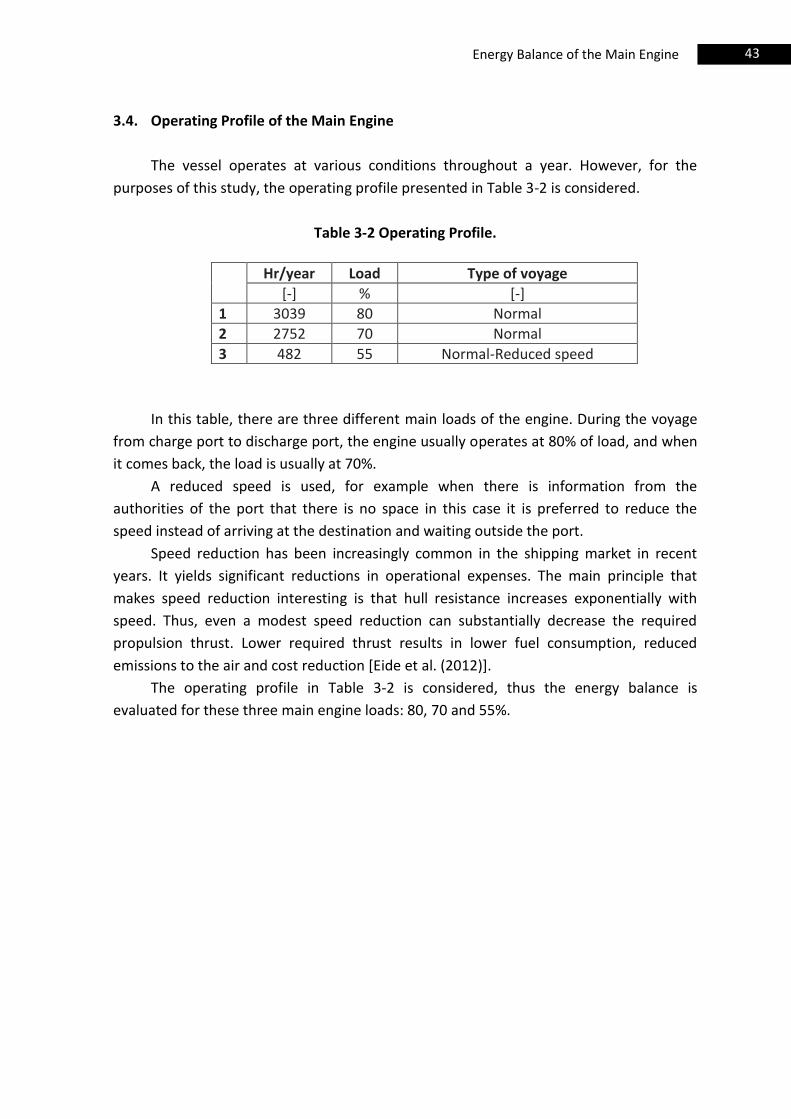
43 Energy Balance of the Main Engine
3.4. Operating Profile of the Main Engine
The vessel operates at various conditions throughout a year. However, for the
purposes of this study, the operating profile presented in Table 3-2 is considered.
Table 3-2 Operating Profile.
Hr/year Load Type of voyage
[-] % [-]
1 3039 80 Normal
2 2752 70 Normal
3 482 55 Normal-Reduced speed
In this table, there are three different main loads of the engine. During the voyage
from charge port to discharge port, the engine usually operates at 80% of load, and when
it comes back, the load is usually at 70%.
A reduced speed is used, for example when there is information from the
authorities of the port that there is no space in this case it is preferred to reduce the
speed instead of arriving at the destination and waiting outside the port.
Speed reduction has been increasingly common in the shipping market in recent
years. It yields significant reductions in operational expenses. The main principle that
makes speed reduction interesting is that hull resistance increases exponentially with
speed. Thus, even a modest speed reduction can substantially decrease the required
propulsion thrust. Lower required thrust results in lower fuel consumption, reduced
emissions to the air and cost reduction [Eide et al. (2012)].
The operating profile in Table 3-2 is considered, thus the energy balance is
evaluated for these three main engine loads: 80, 70 and 55%.

44 Energy Balance of the Main Engine
3.5. Model of the Main Engine Balance
In Figure 3-4 the red line is the boundary control of the Engine assumed for the
energy balance calculations. The temperatures of the cooling loop are known from
Section 3.3. In the points cw1, cw2, cw3, cw4, cw5 the temperatures are 36, 42.5, 53.7, 36
60°C, respectively. According to Wang et al. (2012) when the heat source temperature is
lower than 100°C, ORC-technology is uneconomical. Thus, the evaluated ship does not
allow a convenient heat recovery from the cooling circuit because the working fluid
cannot reach temperature higher than 100°C (maximum temperature of the cooling loop
is 60 °C, point cw5 in Figure 3-1). For this reason, the component boundary does not
include the three heat exchangers (air cooler, lubricating oil, jacket water). The possibility
to recover directly heat from these hot streams is examined in study, so the working fluid
could reach higher temperature than 100°C.
The energy balance of the main engine is expressed as follows
[ ( )] ( ) (3.1)
(3.2)
Then:
[ ( )] ( ) (3.3)
where:
fuel mass flow rate
Lower calorific value
Isobaric specific heat of the fuel
Inlet fuel temperature
Reference temperature
Air mass flow rate
Isobaric specific heat of the air
Inlet air temperature
Mechanical Power
Cooling power
Exhaust gas power
Radiation power
jacket water power at the exit of the main engine
lubricating oil power
Air cooler power
45 Energy Balance of the Main Engine
where:
( ) (3.4)
( ) (3.5)
( ) (3.6)
( ) (3.7)
: approximately 1% of the fuel energy. (3.8)
Note that , as defined by Eq. (3.7), is the thermal energy contained in exhaust
gas measured above the reference temperature . The actual available heat from
exhaust gas is given by the equation:
( ) (3.9)
where is the lowest allowed temperature for the exhaust gases at the exit of the
boiler (the value used here is 180°C). Part of this thermal energy (down Tg3 in Figure 3-4)
is recovered in the exhaust gas boiler to generate low pressure steam and the useful heat
of the exhaust gas boiler is given by the equation:
( ) (3.10)
or
( ) (3.11)
The heat that would be available for the ORC from the exhaust gas boiler is given by the
following equation
(3.16)
where is given by Eq.(3.11). Practically, the required mass flow rate of steam in various
modes of operation is given in Table 3-1. In order to use the whole available thermal
power contained in exhaust gas for the production of the steam, Qs is equal to 975 kW,
which is the power required for the production of 1400 Kg/h of steam, that is the maximal
capacity of the exhaust gas boiler when the main engine is operating.
The thermal energy required by the fresh water generation is:
( ) (3.17)
46 Energy Balance of the Main Engine
The thermal energy that remains to be rejected through the jacket water cooler (box number
4):
( ) (3.18)
All the points, symbols described in section 3.5 are showed in Figure 3-4.
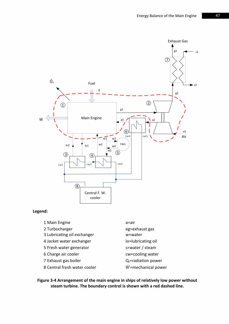
47 Energy Balance of the Main Engine
Main Engine
FWG
Central F. W. cooler
Fuel
Exhaust Gas
s1
s2
g2
Air
a1
a2a3
⑦
lo1lo2 w2
w1 w3
w4
w5
①
⑥
④⑤
②
③
g1
cw1 cw2 cw3
cw4 cw5
⑧
g3
Ẇ
f
Legend:
1 Main Engine a=air
2 Turbocharger eg=exhaust gas 3 Lubricating oil exchanger w=water
4 Jacket water exchanger lo=lubricating oil
5 Fresh water generator s=water / steam
6 Charge air cooler cw=cooling water
7 Exhaust gas boiler Qr=radiation power
8 Central fresh water cooler =mechanical power
Figure 3-4 Arrangement of the main engine in ships of relatively low power without steam turbine. The boundary control is shown with a red dashed line.
48 Energy Balance of the Main Engine
3.6. Data and Assumptions
This section explains the data and the assumptions needed to evaluate the energy
balance referring to Figure 3-4 . Mechanical power ( ), fuel consumption ( ), low
calorific value of the fuel ( ), mechanical efficiency ( ), thermal power required by
the fresh water generation ( ), isobaric specific heat of the fuel ( ), inlet
temperature of the fuel ( ), temperatures , of the jacket water, temperatures
, of lubricating oil, temperatures , of the air, and the temperature of the
exhaust gas at point g2 are given from the documentation available at 100, 90, 75, 50,
25% engine loads. These data will be used to find out the temperatures at 80, 70, 55%
engine loads, which are the most frequent engine loads (see Table 3-2). Efficiency ( )
of the exhaust gas boiler, reference temperature ( ) and inlet temperature of the air
( ), are assumptions made for this work. Efficiency ( ) is equal to 0.95, the
reference temperature and the air temperature are equal to 25°C. According to
Marindagen and Potentialer (2011) the condensation of sulfuric acid is avoided when the
exhaust gas outlet temperature is kept higher than 180°C. Table 3-3 summarizes all these
data for five engine load (100, 90, 75, 50, 25%).
Table 3-3 shows that on varying of engine load, the air temperature ( ) varies in a
wide range (from 189.5°C at 100% engine load to 43.5°C at 25% engine load), instead of
jacket water and lubricating oil. The outlet temperature of the lubricating oil from the
Main Engine ( ,) varies from 50.8°C at 100% engine load to 48°C at 25% engine load.
The range of the outlet temperature of jacket water from Main Engine ( ) is from 70°C
at 100% engine load to 60°C at 25% engine load. There is the maximum engine efficiency
at 75% engine load where is equal to 0.481. At the 75% engine load the exhaust
gas temperature ( ) is the lowest (229°C) of other engine loads. Lower exhaust gas
temperature means lower exhaust gas power, thus less fuel thermal power lost and more
mechanical efficiency ( ). In detail, Figure 3-11 shows that there is the minimum
exhaust gas temperature (Tg2) at 80% engine load. For this reason, the Main engine
operates at 80% engine load from charge port to discharge port and at 70% engine load
when the tanker comes back to the charge port (when the mechanical efficiency reaches
the highest values).
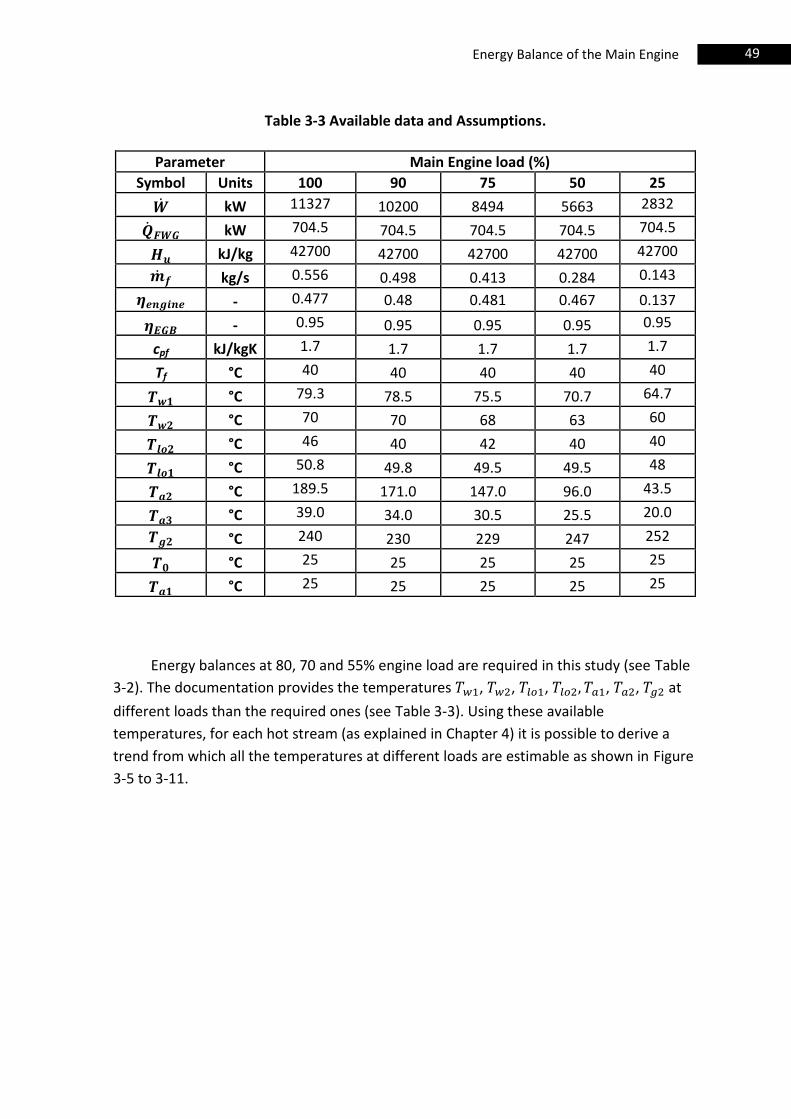
49 Energy Balance of the Main Engine
Table 3-3 Available data and Assumptions.
Parameter Main Engine load (%)
Symbol Units 100 90 75 50 25
kW 11327 10200 8494 5663 2832
kW 704.5 704.5 704.5 704.5 704.5
kJ/kg 42700 42700 42700 42700 42700
kg/s 0.556 0.498 0.413 0.284 0.143
- 0.477 0.48 0.481 0.467 0.137
- 0.95 0.95 0.95 0.95 0.95
cpf kJ/kgK 1.7 1.7 1.7 1.7 1.7
Tf °C 40 40 40 40 40
°C 79.3 78.5 75.5 70.7 64.7
°C 70 70 68 63 60
°C 46 40 42 40 40
°C 50.8 49.8 49.5 49.5 48
°C 189.5 171.0 147.0 96.0 43.5
°C 39.0 34.0 30.5 25.5 20.0
°C 240 230 229 247 252
°C 25 25 25 25 25
°C 25 25 25 25 25
Energy balances at 80, 70 and 55% engine load are required in this study (see Table
3-2). The documentation provides the temperatures , , , , , at
different loads than the required ones (see Table 3-3). Using these available
temperatures, for each hot stream (as explained in Chapter 4) it is possible to derive a
trend from which all the temperatures at different loads are estimable as shown in Figure
3-5 to 3-11.
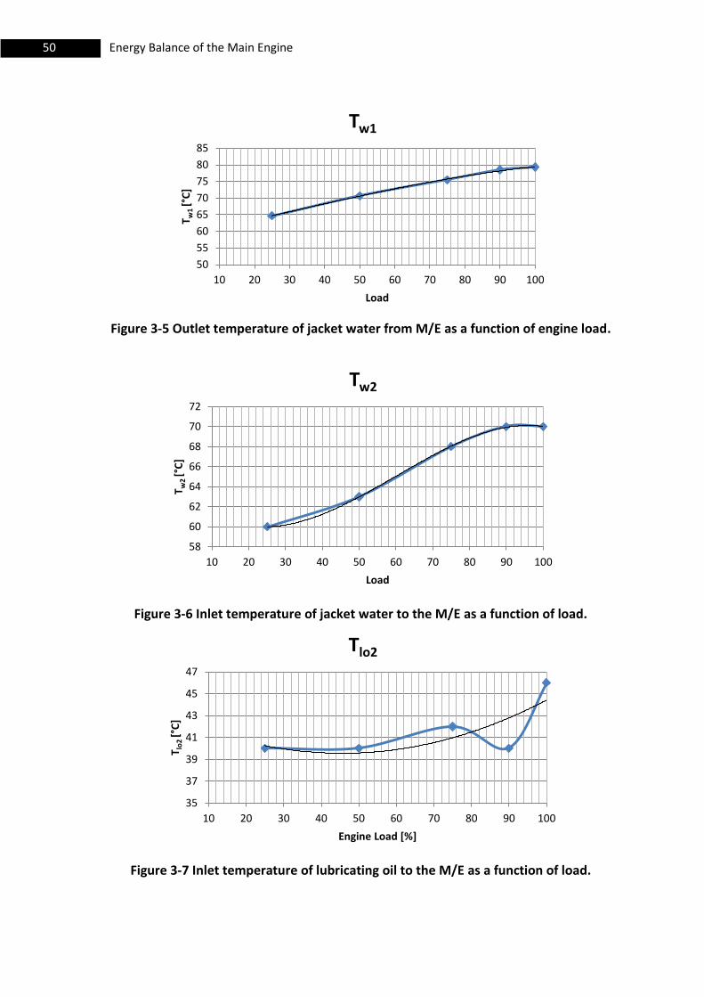
50 Energy Balance of the Main Engine
Figure 3-5 Outlet temperature of jacket water from M/E as a function of engine load.
Figure 3-6 Inlet temperature of jacket water to the M/E as a function of load.
Figure 3-7 Inlet temperature of lubricating oil to the M/E as a function of load.
50
55
60
65
70
75
80
85
10 20 30 40 50 60 70 80 90 100
T w1
[°C
]
Load
Tw1
58
60
62
64
66
68
70
72
10 20 30 40 50 60 70 80 90 100
T w2
[°C
]
Load
Tw2
35
37
39
41
43
45
47
10 20 30 40 50 60 70 80 90 100
T lo
2 [°
C]
Engine Load [%]
Tlo2
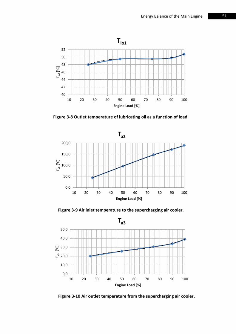
51 Energy Balance of the Main Engine
Figure 3-8 Outlet temperature of lubricating oil as a function of load.
Figure 3-9 Air inlet temperature to the supercharging air cooler.
Figure 3-10 Air outlet temperature from the supercharging air cooler.
40
42
44
46
48
50
52
10 20 30 40 50 60 70 80 90 100
T lo
1 [°
C]
Engine Load [%]
Tlo1
0,0
50,0
100,0
150,0
200,0
10 20 30 40 50 60 70 80 90 100
T a2
[°C
]
Engine Load [%]
Ta2
0,0
10,0
20,0
30,0
40,0
50,0
10 20 30 40 50 60 70 80 90 100
T a3
[°C
]
Engine Load [%]
Ta3
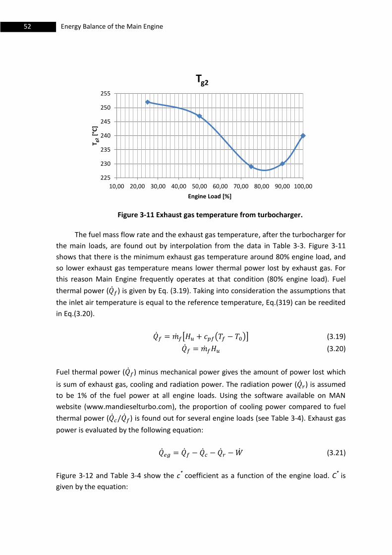
52 Energy Balance of the Main Engine
Figure 3-11 Exhaust gas temperature from turbocharger.
The fuel mass flow rate and the exhaust gas temperature, after the turbocharger for
the main loads, are found out by interpolation from the data in Table 3-3. Figure 3-11
shows that there is the minimum exhaust gas temperature around 80% engine load, and
so lower exhaust gas temperature means lower thermal power lost by exhaust gas. For
this reason Main Engine frequently operates at that condition (80% engine load). Fuel
thermal power ( ) is given by Eq. (3.19). Taking into consideration the assumptions that
the inlet air temperature is equal to the reference temperature, Eq.(319) can be reedited
in Eq.(3.20).
[ ( )] (3.19)
(3.20)
Fuel thermal power ( ) minus mechanical power gives the amount of power lost which
is sum of exhaust gas, cooling and radiation power. The radiation power ( ) is assumed
to be 1% of the fuel power at all engine loads. Using the software available on MAN
website (www.mandieselturbo.com), the proportion of cooling power compared to fuel
thermal power ( ) is found out for several engine loads (see Table 3-4). Exhaust gas
power is evaluated by the following equation:
(3.21)
Figure 3-12 and Table 3-4 show the c* coefficient as a function of the engine load. C* is
given by the equation:
225
230
235
240
245
250
255
10,00 20,00 30,00 40,00 50,00 60,00 70,00 80,00 90,00 100,00
T g2
[°C
]
Engine Load [%]
Tg2

53 Energy Balance of the Main Engine
( )
( )
(3.22)
Eq.(3.22) describes the ratio between cooling power and the thermal fuel power at
generic engine load (L) compared to the ratio between the cooling power and the fuel
power at 100% engine load. Eq. (3.23) describes c* as a function of the engine load.
Table 3-4 Cooling heat as a function of load.
Load
[%] [kW] [kW] [-] [-]
100 6790 26420 0.257 1.000
90 6070 23619 0.259 1.006
80 5350 20693 0.258 1.002
70 4590 17824 0.251 0.977
60 3850 15333 0.243 0.945
50 3110 12805 0.231 0.900
40 2400 10376 0.218 0.850
25 1520 6958 0.208 0.810
Figure 3-12 c* as function of engine load.
Eq. (3.23):
0,000
0,200
0,400
0,600
0,800
1,000
1,200
0 20 40 60 80 100 120
c*
Engine Load [%]
Cooling Heat
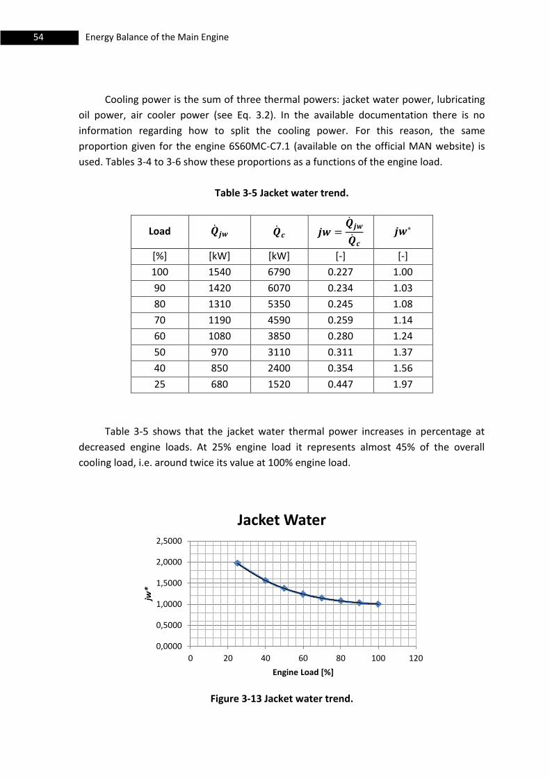
54 Energy Balance of the Main Engine
Cooling power is the sum of three thermal powers: jacket water power, lubricating
oil power, air cooler power (see Eq. 3.2). In the available documentation there is no
information regarding how to split the cooling power. For this reason, the same
proportion given for the engine 6S60MC-C7.1 (available on the official MAN website) is
used. Tables 3-4 to 3-6 show these proportions as a functions of the engine load.
Table 3-5 Jacket water trend.
Load
[%] [kW] [kW] [-] [-]
100 1540 6790 0.227 1.00
90 1420 6070 0.234 1.03
80 1310 5350 0.245 1.08
70 1190 4590 0.259 1.14
60 1080 3850 0.280 1.24
50 970 3110 0.311 1.37
40 850 2400 0.354 1.56
25 680 1520 0.447 1.97
Table 3-5 shows that the jacket water thermal power increases in percentage at
decreased engine loads. At 25% engine load it represents almost 45% of the overall
cooling load, i.e. around twice its value at 100% engine load.
Figure 3-13 Jacket water trend.
0,0000
0,5000
1,0000
1,5000
2,0000
2,5000
0 20 40 60 80 100 120
jw*
Engine Load [%]
Jacket Water

55 Energy Balance of the Main Engine
Eq. (3.24):
Figure 3-13 and Eq. (3.24) describe jw*: the ratio between jacket water power and
the cooling power at certain engine load L compared to the ratio between the jacket
water power and the cooling power at 100% engine load as a function of the engine load.
Table 3-6 Lubricating oil trend.
Load
[%] [kW] [kW] [-] [-]
100 850 6790 0.125 1.000
90 830 6070 0.137 1.092
80 800 5350 0.150 1.195
70 760 4590 0.166 1.323
60 720 3850 0.187 1.494
50 660 3110 0.212 1.695
40 600 2400 0.250 1.997
25 480 1520 0.316 2.523
Table 3-6 shows that the lubricating oil thermal power increases in percentage at
decreased engine loads as the jacket water thermal power in percentage (see Table 3-5).
At 25% engine load it represents almost 31% of the overall cooling load, i.e. around twice
and a half its value at 100% engine load.
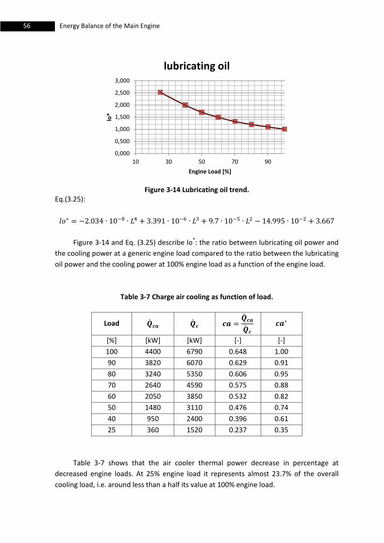
56 Energy Balance of the Main Engine
Figure 3-14 Lubricating oil trend.
Eq.(3.25):
Figure 3-14 and Eq. (3.25) describe lo*: the ratio between lubricating oil power and
the cooling power at a generic engine load compared to the ratio between the lubricating
oil power and the cooling power at 100% engine load as a function of the engine load.
Table 3-7 Charge air cooling as function of load.
Load
[%] [kW] [kW] [-] [-]
100 4400 6790 0.648 1.00
90 3820 6070 0.629 0.91
80 3240 5350 0.606 0.95
70 2640 4590 0.575 0.88
60 2050 3850 0.532 0.82
50 1480 3110 0.476 0.74
40 950 2400 0.396 0.61
25 360 1520 0.237 0.35
Table 3-7 shows that the air cooler thermal power decrease in percentage at
decreased engine loads. At 25% engine load it represents almost 23.7% of the overall
cooling load, i.e. around less than a half its value at 100% engine load.
0,000
0,500
1,000
1,500
2,000
2,500
3,000
10 30 50 70 90
lo*
Engine Load [%]
lubricating oil
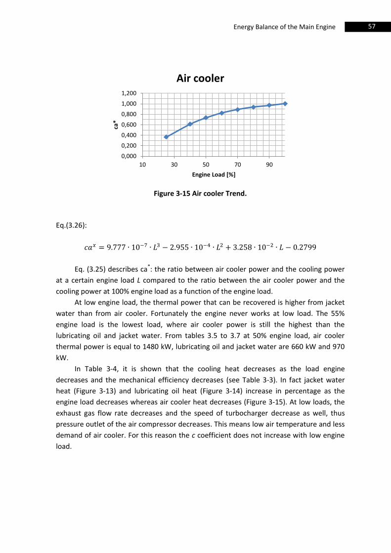
57 Energy Balance of the Main Engine
Figure 3-15 Air cooler Trend.
Eq.(3.26):
Eq. (3.25) describes ca*: the ratio between air cooler power and the cooling power
at a certain engine load L compared to the ratio between the air cooler power and the
cooling power at 100% engine load as a function of the engine load.
At low engine load, the thermal power that can be recovered is higher from jacket
water than from air cooler. Fortunately the engine never works at low load. The 55%
engine load is the lowest load, where air cooler power is still the highest than the
lubricating oil and jacket water. From tables 3.5 to 3.7 at 50% engine load, air cooler
thermal power is equal to 1480 kW, lubricating oil and jacket water are 660 kW and 970
kW.
In Table 3-4, it is shown that the cooling heat decreases as the load engine
decreases and the mechanical efficiency decreases (see Table 3-3). In fact jacket water
heat (Figure 3-13) and lubricating oil heat (Figure 3-14) increase in percentage as the
engine load decreases whereas air cooler heat decreases (Figure 3-15). At low loads, the
exhaust gas flow rate decreases and the speed of turbocharger decrease as well, thus
pressure outlet of the air compressor decreases. This means low air temperature and less
demand of air cooler. For this reason the c coefficient does not increase with low engine
load.
0,000
0,200
0,400
0,600
0,800
1,000
1,200
10 30 50 70 90
ca*
Engine Load [%]
Air cooler
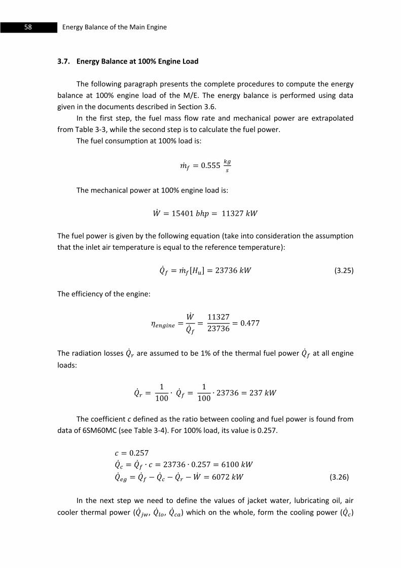
58 Energy Balance of the Main Engine
3.7. Energy Balance at 100% Engine Load
The following paragraph presents the complete procedures to compute the energy
balance at 100% engine load of the M/E. The energy balance is performed using data
given in the documents described in Section 3.6.
In the first step, the fuel mass flow rate and mechanical power are extrapolated
from Table 3-3, while the second step is to calculate the fuel power.
The fuel consumption at 100% load is:
The mechanical power at 100% engine load is:
The fuel power is given by the following equation (take into consideration the assumption
that the inlet air temperature is equal to the reference temperature):
[ ] (3.25)
The efficiency of the engine:
The radiation losses are assumed to be 1% of the thermal fuel power at all engine
loads:
The coefficient c defined as the ratio between cooling and fuel power is found from
data of 6SM60MC (see Table 3-4). For 100% load, its value is 0.257.
(3.26)
In the next step we need to define the values of jacket water, lubricating oil, air
cooler thermal power ( , , ) which on the whole, form the cooling power ( )

59 Energy Balance of the Main Engine
see Eq. (3.2). As already seen in the previous section for different engine loads, the value
of is known but no information is available regarding how to split the cooling power.
So the proportions for the engine 6S60MC-C7.1 are applied. At 100% engine load the
coefficients: jw, lo, a are 0.227, 0.125, 0.648, respectively (see Table 3-5, Table 3-6, Table
3-7), then:
The energy balance of the main engine is expressed as follows (the left side of the
equation depicts input power, the right side the output power):
[ ( )]
From the previous finding, the energy balance is satisfied. The input power is equal
to the output power in the composite boundary in Figure 3-4.
3.8. Operating data and results at 100%, 80%, 70% and 55% Load
In the previous sections: the method, the component boundary (see the red line
Figure 3-4), available data, assumptions and the energy balance at 100% engine load were
explained. Using previous information and procedure (Section 3.7), it is possible to fill
Table 3-8. It summarizes the results of the energy balances and the properties observed
at various points as shown in Fig. 3-4 at 100% engine load and at 80%, 70%, 55% engine
load which on the whole, form the operating profile .
Due to the lack of sufficient information and because of inconsistencies in some
data of the available documents the product of the mass flow rate and isobaric specific
heat is evaluated instead of the mass flow rate of the same stream, using the following
equation:
(3.27)
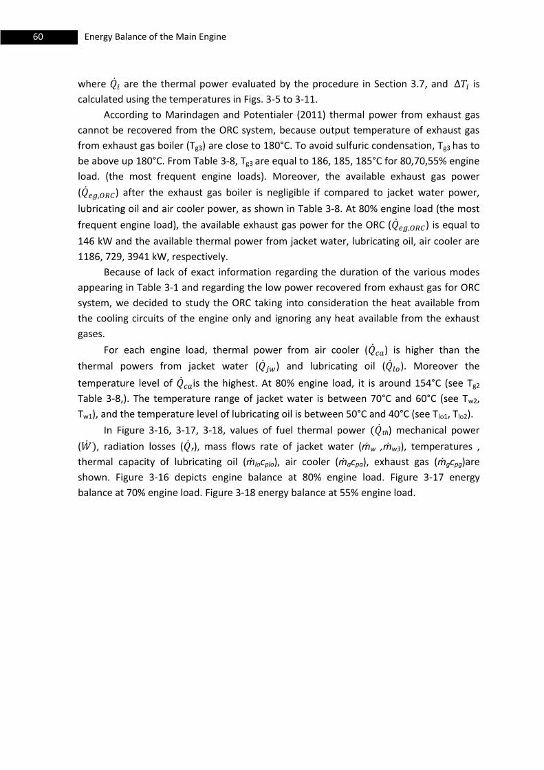
60 Energy Balance of the Main Engine
where are the thermal power evaluated by the procedure in Section 3.7, and is
calculated using the temperatures in Figs. 3-5 to 3-11.
According to Marindagen and Potentialer (2011) thermal power from exhaust gas
cannot be recovered from the ORC system, because output temperature of exhaust gas
from exhaust gas boiler (Tg3) are close to 180°C. To avoid sulfuric condensation, Tg3 has to
be above up 180°C. From Table 3-8, Tg3 are equal to 186, 185, 185°C for 80,70,55% engine
load. (the most frequent engine loads). Moreover, the available exhaust gas power
( ) after the exhaust gas boiler is negligible if compared to jacket water power,
lubricating oil and air cooler power, as shown in Table 3-8. At 80% engine load (the most
frequent engine load), the available exhaust gas power for the ORC ( ) is equal to
146 kW and the available thermal power from jacket water, lubricating oil, air cooler are
1186, 729, 3941 kW, respectively.
Because of lack of exact information regarding the duration of the various modes
appearing in Table 3-1 and regarding the low power recovered from exhaust gas for ORC
system, we decided to study the ORC taking into consideration the heat available from
the cooling circuits of the engine only and ignoring any heat available from the exhaust
gases.
For each engine load, thermal power from air cooler ( ) is higher than the
thermal powers from jacket water ( ) and lubricating oil ( ). Moreover the
temperature level of is the highest. At 80% engine load, it is around 154°C (see Tg2
Table 3-8,). The temperature range of jacket water is between 70°C and 60°C (see Tw2,
Tw1), and the temperature level of lubricating oil is between 50°C and 40°C (see Tlo1, Tlo2).
In Figure 3-16, 3-17, 3-18, values of fuel thermal power ( th) mechanical power
( ), radiation losses ( r), mass flows rate of jacket water (ṁw ,ṁw3), temperatures ,
thermal capacity of lubricating oil (ṁlocplo), air cooler (ṁacpa), exhaust gas (ṁgcpg)are
shown. Figure 3-16 depicts engine balance at 80% engine load. Figure 3-17 energy
balance at 70% engine load. Figure 3-18 energy balance at 55% engine load.

61 Energy Balance of the Main Engine
Table 3-8 Energy balance.
Parameter Main Engine load (%)
Symbol Units 100 80 70 55
Hu kJ/kg 42700 42700 42700 42700
th kW 23736 18842 16577 13245
kW 11327 9062 7929 6230
eg kW 6072 4736 4306 3729
r kW 237 188 166 132
jw kW 1385 1186 1081 929
lo kW 762 729 693 627
ca kW 3953 2941 2402 1598
ṁf kg/s 0.555 0.441 0.388 0.310
ṁs kg/s 0.39 0.39 0.39 0.39
ṁw kg/s 35.6 36.8 33.1 28.8
ṁw3 kg/s 18.1 21.8 21.6 21.8
ṁlocplo kW/K 158.7 82.84 103.4 78.4
ṁacpa kW/K 26.3 23.81 22.53 19.98
ṁgcpg kW/K 27.6 23.35 21 17
T0 °C 25 25 25 25
Ta1 °C 25 25 25 25
Tf °C 40 40 40 40
Tw1 °C 79.3 76.6 74.8 71.7
Tw2 °C 70 68.9 67.0 64.0
Tw3 °C 79.3 76.6 74.8 71.7
Tw4 °C 70 68.9 67.0 64.0
Tw5 °C 74.5 72 70 66
Tlo1 °C 50.8 49.5 49.5 49.6
Tlo2 °C 46 40.7 42.8 41.6
Ta2 °C 189.5 154.9 136.3 106.7
Ta3 °C 39 31.4 29.7 26.7
Tg1 °C 436 390 381 372
Tg2 °C 240 228 232 243
Tg3 °C 205 186 185 185
hs1 kJ/kg 251 251 251 251
hs2 kJ/kg 2762 2762 2762 2762
kW 975 975 975 975
kW 1656 1121 1092 1071
kW 681 146 117 96
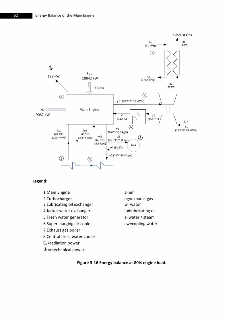
62 Energy Balance of the Main Engine
Main Engine
FWG
Fuel18842 kW
Exhaust Gas
hS1
(251 kJ/kg)
hs2
(2762 kJ/kg)
g2(228°C)
Aira1
(25°C-23.81 kW/K)
a2 (154.9°C)
a3(31.4°C)
⑦
lo1(49.5°C-
82.84 kW/K)
lo2(40.7°C-
82.84 kW/k) w2(68.9°C-
35.6 kg/s)
w1(76.6°C-35.6 kg/s)
w3 (76.6°C-21.8 kg/s)
w4 (68.9°C)
w5 (72°C-36.8 kg/s)
①
⑥
④
⑤
②
③
g1 (390°C-23.35 kW/K)
g3(186°C)
Ẇ 9062 kW
188 kW
f (40°C)
Legend:
1 Main Engine a=air
2 Turbocharger eg=exhaust gas 3 Lubricating oil exchanger w=water
4 Jacket water exchanger lo=lubricating oil
5 Fresh water generator s=water / steam
6 Supercharging air cooler cw=cooling water
7 Exhaust gas boiler
8 Central fresh water cooler
Qr=radiation power
=mechanical power
Figure 3-16 Energy balance at 80% engine load.

63 Energy Balance of the Main Engine
Main Engine
FWG
Fuel16577 kW
Exhaust Gas
hS1
(251 kJ/kg)
hs2
(2762 kJ/kg)
g2(232°C)
Aira1
(25°C-22.53 kW/K)
a2 (136.3°C)
a3(29.7°C)
⑦
lo1(49.5°C-
103.4 kW/K)
lo2(42.8°C-
103.4 kW/k) w2(67°C-
33.1 kg/s)
w1(74.8°C-33.1 kg/s)
w3 (74.8°C-21.6 kg/s)
w4 (67°C)
w5 (70°C-33.1 kg/s)
①
⑥
④
⑤
②
③
g1 (381°C-21 kW/k)
g3(185°C)
Ẇ 7929 kW
166 kW
f (40°C)
Legend:
1 Main Engine a=air
2 Turbocharger eg=exhaust gas 3 Lubricating oil exchanger w=water
4 Jacket water exchanger lo=lubricating oil
5 Fresh water generator s=water / steam
6 Supercharging air cooler cw=cooling water
7 Exhaust gas boiler
8 Central fresh water cooler
Qr=radiation power
=mechanical power
Figure 3-17 Energy Balance at 70% Engine load.
64 Energy Balance of the Main Engine
Main Engine
FWG
Fuel13245 kW
Exhaust Gas
hS1
(251 kJ/kg)
hs2
(2762 kJ/kg)
g2(243°C)
Aira1
(25°C-19.98 kW/K)
a2 (106.7°C)
a3(26.7°C)
⑦
lo1(49.6°C-
78.4 kW/K)
lo2(41.6°C-
78.4 kW/k) w2(64°C-
28.8 kg/s)
w1(71.7°C-28.8 kg/s)
w3 (71.7°C-21.8 kg/s)
w4 (64°C)
w5 (66°C-28.8 kg/s)
①
⑥
④
⑤
②
③
g1 (372°C-17 kW/k)
g3(185°C)
Ẇ 6230 kW
132 kW
f (40°C)
Legend:
1 Main Engine a=air
2 Turbocharger eg=exhaust gas 3 Lubricating oil exchanger w=water
4 Jacket water exchanger lo=lubricating oil
5 Fresh water generator s=water / steam
6 Supercharging air cooler cw=cooling water
7 Exhaust gas boiler
8 Central fresh water cooler
Qr=radiation power
=mechanical power
Figure 3-18 Energy Balance at 55% Engine load.
65 Hot Composite Curve
4. Hot Composite Curves
In Chapter 3, energy balances for main engine loads were evaluated. Table 3-8 and
Figure 3-4 show the four hot streams of the main engine: exhaust gas, jacket water, air
cooler, lubricating oil. As previously stated (Section 3.5), the temperatures of the cooling
circuit are known. Looking at Figure 3-4, the temperatures , , ,
are 36, 42.5, 53.7, 36, 60°C respectively. The possibility to recover heat from the cooling
circuit is not convenient. According to Wang et al. (2012) when heat source temperature
is lower than 100°C ORC technology is uneconomical. Also the possibility to recover
power from the exhaust gas is not considered here, for reason explained in the preceding,
even if the exhaust gas temperature ( ) is higher than 100°C. Indeed the 100°C
temperature is not a reference temperature for what concern the exhaust gas of the
Main Engine due to the formation of sulfuric acid below 180°C. In this case it is not
possible to extract power because the temperature is close to 180°C, see Table 3-8.
Moreover, the available exhaust gas power after the exhaust gas boiler is negligible if
compared to jacket water power, lubricating oil and air cooler power, as shown in Table
3-8. At 80% engine load (the most frequent engine load), the available exhaust gas power
for the ORC ( ) is equal to 146 kW and the available thermal power from jacket
water, lubricating oil, air cooler are 1186, 729, 3941 kW, respectively.
Because of the lack of exact information regarding the duration of the fresh water
generator operation, the fresh water generator is considered in steady working condition.
After these preliminary considerations, it was decided to use as feasible ORC system
hot streams, the thermal power rejected through the jacket water cooler , from the
scavenge air cooler and from the lubricating oil cooler . Thus these hot streams
change heat directly with working fluid of the ORC system. The three thermal powers are
shown in Figure 4-1.
Table 4-1 summarizes the properties of three hot streams: (and Table
3-8) for the three main operating loads.
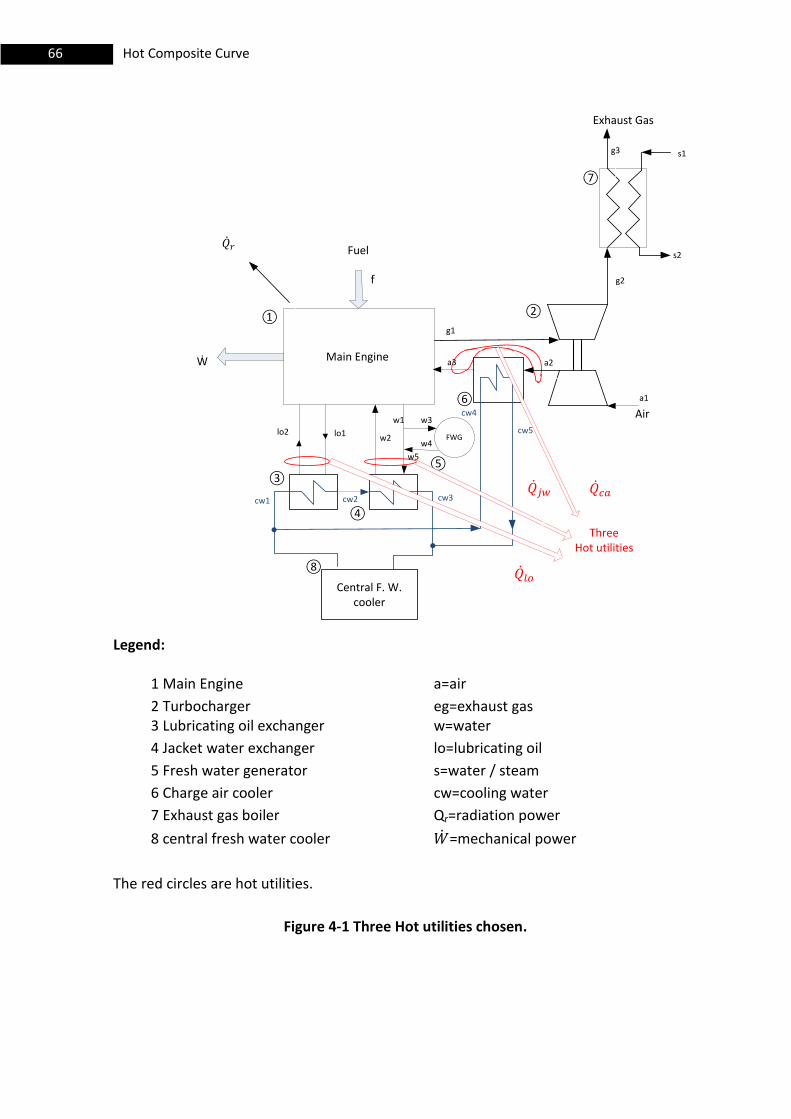
66 Hot Composite Curve
Legend:
1 Main Engine a=air
2 Turbocharger eg=exhaust gas 3 Lubricating oil exchanger w=water
4 Jacket water exchanger lo=lubricating oil
5 Fresh water generator s=water / steam
6 Charge air cooler cw=cooling water
7 Exhaust gas boiler Qr=radiation power
8 central fresh water cooler =mechanical power
The red circles are hot utilities.
Figure 4-1 Three Hot utilities chosen.
Main Engine
FWG
Central F. W. cooler
Fuel
Exhaust Gas
s1
s2
g2
Air
a1
a2a3
⑦
lo1lo2w2
w1 w3
w4
w5
①
⑥
④
⑤
②
③
g1
cw1 cw2 cw3
cw4
cw5
⑧
g3
Ẇ
ThreeHot utilities
f
𝑐𝑎 𝑗𝑤
𝑙𝑜

67 Hot Composite Curve
Table 4-1 Hot utility properties.
Parameter Main Engine load (%)
Symbol Units 80 70 55
ca kW 2941 2402 1598
jw kW 477.5 415 241
lo kW 729 693 627
Ta2 °C 154.9 136.3 106.7
Ta3 °C 31.4 29.7 26.7
Tw5 °C 72 70 66
Tw2 °C 68.9 67.0 64.0
Tlo1 °C 49.5 49.5 49.6
Tlo2 °C 40.7 42.8 41.6
ṁacpa kW/K 23.81 22.53 19.98
ṁlocplo kW/K 82.84 103.4 78.4 kW/k 154 138 120
To build the hot composite curves is necessary to combine the temperature
characteristics of all hot streams into a single hot composite curve.
Each of The following three graphs shows the hot composite curves at three main
engine loads, in the order: 80-70-55%, where for each segment the sources are shown.
Thermal power available for the ORC system is 4147 kW at 80% engine load, 3510
kW at 70% engine load and 2466 kW at 55% engine load. In each graphs, thermal power
from air cooler covers all temperature range. At 80% engine load, ca covers the
temperature range from 154.9°C to 31.4°C. HCC is made by the combination of two
streams, supercharging air and jacket water between 72°C and 68.9°C . and by lubricating
oil and supercharging air from 49.5°C to 40.7°C . There is the same situation also at 70%
and 55% of engine load. In each HCC, the temperature range can be divided in three
parts, top, middle and bottom. In the top part, thermal power is supplied by air cooler, in
the middle part by air cooler combine jacket water (range from 70°C to 64°C), and in the
bottom part, thermal power is supplied by the combination of lubricating oil and air
cooler (range between 50°C and 40°C)
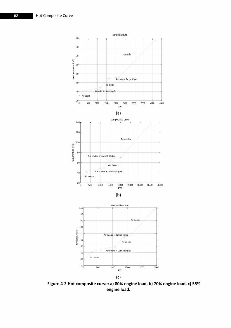
68 Hot Composite Curve
(a)
(b)
(c)
Figure 4-2 Hot composite curve: a) 80% engine load, b) 70% engine load, c) 55% engine load.
0 500 1000 1500 2000 2500 3000 3500 4000 450020
40
60
80
100
120
140
160compositive curve
kW
tem
perature [°C
]
Air cooler
Air cooler
Air cooler + Lubricating Oil
Air cooler
Air cooler + Jacket Water
0 500 1000 1500 2000 2500 3000 3500 400020
40
60
80
100
120
140compositive curve
kW
tem
pera
ture
[°C
]
Air cooler
Air cooler + Jacket Water
Air cooler + Lubricating oil
Air cooler
Air cooler
0 500 1000 1500 2000 250020
30
40
50
60
70
80
90
100
110compositive curve
kW
tem
pera
ture
[°C
]
Air cooler
Air cooler + Jacket water
Air cooler
Air cooler + Lubricating oil
Air cooler
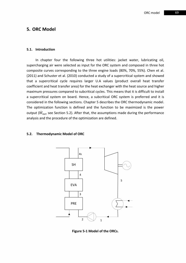
69 ORC model
5. ORC Model
5.1. Introduction
In chapter four the following three hot utilities: jacket water, lubricating oil,
supercharging air were selected as input for the ORC system and composed in three hot
composite curves corresponding to the three engine loads (80%, 70%, 55%). Chen et al.
(2011) and Schuster et al. (2010) conducted a study of a supercritical system and showed
that a supercritical cycle requires larger U.A values (product overall heat transfer
coefficient and heat transfer area) for the heat exchanger with the heat source and higher
maximum pressures compared to subcritical cycles. This means that it is difficult to install
a supercritical system on board. Hence, a subcritical ORC system is preferred and it is
considered in the following sections. Chapter 5 describes the ORC thermodynamic model.
The optimization function is defined and the function to be maximized is the power
output ( see Section 5.2). After that, the assumptions made during the performance
analysis and the procedure of the optimization are defined.
5.2. Thermodynamic Model of ORC
12
4
3
EVA
SH
PRE
5
4s
Figure 5-1 Model of the ORCs.
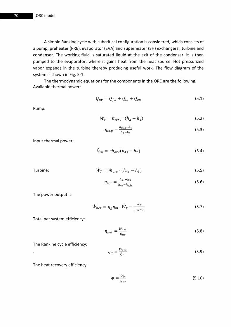
70 ORC model
A simple Rankine cycle with subcritical configuration is considered, which consists of
a pump, preheater (PRE), evaporator (EVA) and superheater (SH) exchangers , turbine and
condenser. The working fluid is saturated liquid at the exit of the condenser; it is then
pumped to the evaporator, where it gains heat from the heat source. Hot pressurized
vapor expands in the turbine thereby producing useful work. The flow diagram of the
system is shown in Fig. 5-1.
The thermodynamic equations for the components in the ORC are the following. Available thermal power:
(5.1)
Pump:
( ) (5.2)
(5.3)
Input thermal power:
( ) (5.4)
Turbine: ( ) (5.5)
(5.6)
The power output is:
(5.7)
Total net system efficiency:
(5.8)
The Rankine cycle efficiency:
.
(5.9)
The heat recovery efficiency:
(5.10)
71 ORC model
5.3. Optimization Function
The objective function to be maximized is the power output:
( ( )) (5.11)
where: [ ] (5.12)
We consider the following as independent variables for the system optimization: mass flow rate of the organic fluid.
cycle maximum pressure.
According to Toffolo et al. (2010), the degree of superheating is measured in
terms of entropy. The degree of superheating is measured from the entropy
of the point on saturated vapor curve for subcritical cycle.
In addition the following bounds are specified for the three independent variables:
(5.13)
(5.14)
(5.15)
The model of the basic plant configuration was built in the Matlab/Simulink
environment and the working fluid properties are calculated with REFPROP.
In this work the following assumptions are made during the optimization and
performance analysis. The values of isentropic ( ) and mechanical ( ) efficiency of
pump (indicated by p subscript) and turbine (indicated by t subscript), generator
efficiency ( ) and motor efficiency of the pump ( ) are fixed:
(5.13)
(5.14)
(5.15)
(5.16)
(5.18)
Sea water at 25°C (ISO conditions) is used as cold utility in the condenser; and also
the possibility to use water from cooling system at 36°C is investigated. The minimum

72 ORC model
approach temperature ( ) is set at 10°C in the evaporator and 5°C in the condenser
in accordance with Lakew and Bolland (2010).
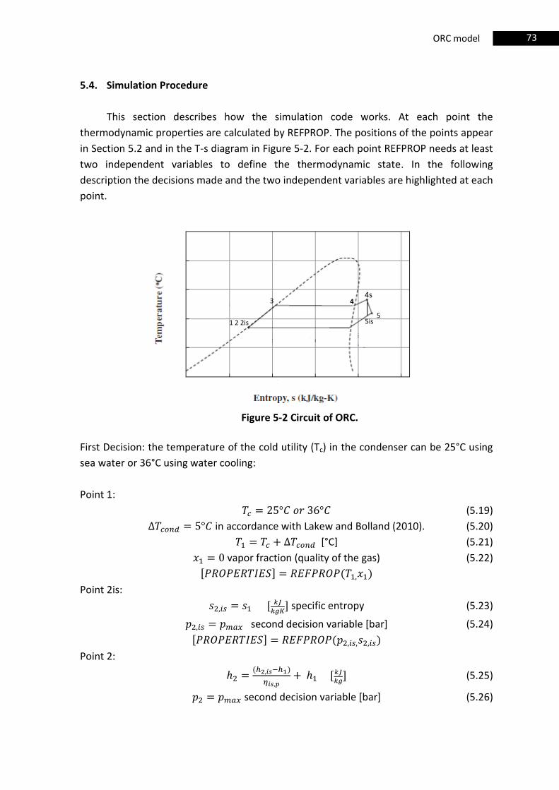
73 ORC model
5.4. Simulation Procedure
This section describes how the simulation code works. At each point the
thermodynamic properties are calculated by REFPROP. The positions of the points appear
in Section 5.2 and in the T-s diagram in Figure 5-2. For each point REFPROP needs at least
two independent variables to define the thermodynamic state. In the following
description the decisions made and the two independent variables are highlighted at each
point.
3 4
55is
4s
1 2 2is
Figure 5-2 Circuit of ORC.
First Decision: the temperature of the cold utility (Tc) in the condenser can be 25°C using
sea water or 36°C using water cooling:
Point 1:
(5.19)
in accordance with Lakew and Bolland (2010). (5.20)
[°C] (5.21)
vapor fraction (quality of the gas) (5.22)
[ ] ( )
Point 2is:
[
] specific entropy (5.23)
second decision variable [bar] (5.24)
[ ] ( )
Point 2:
( )
[
] (5.25)
second decision variable [bar] (5.26)
74 ORC model
[ ] ( )
assumption from Section 5.2
Point 3:
(5.27)
second decision variable [bar] (5.28)
[ ] ( )
Point 4:
(5.29)
second decision variable [bar] (5.30)
[ ] ( )
Point 4s:
[
] ( is the third decision variable) (5.31)
second decision variable [bar] (5.32)
[ ] ( )
Point 5is:
[
] specific entropy (5.33)
[bar] (5.34)
[ ] ( )
Point 5:
( ) [
] (5.35)
[bar] (5.36)
[ ] ( )
assumption from section 5.3.
A hc vector with all the specific enthalpies of the cold composite curve (C.C.C) is created:
[ ] (5.37)
The hc vector is multiplied by mass flow rate (first decision variable):
(5.38)
Hc describes the x-axis value (enthalpy multiplied mass flow rate) of the cold composite
curve.
Another vector with temperatures is made of the cold composite curve
[ ] (5.39)
Tc vector represent the y-axis value of the cold composite curve.
:
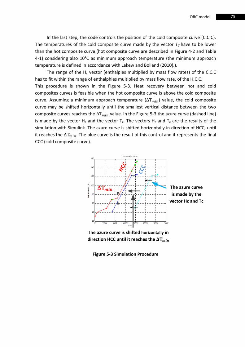
75 ORC model
In the last step, the code controls the position of the cold composite curve (C.C.C).
The temperatures of the cold composite curve made by the vector TC have to be lower
than the hot composite curve (hot composite curve are described in Figure 4-2 and Table
4-1) considering also 10°C as minimum approach temperature (the minimum approach
temperature is defined in accordance with Lakew and Bolland (2010).).
The range of the Hc vector (enthalpies multiplied by mass flow rates) of the C.C.C
has to fit within the range of enthalphies multiplied by mass flow rate. of the H.C.C.
This procedure is shown in the Figure 5-3. Heat recovery between hot and cold
composites curves is feasible when the hot composite curve is above the cold composite
curve. Assuming a minimum approach temperature ( ) value, the cold composite
curve may be shifted horizontally until the smallest vertical distance between the two
composite curves reaches the value. In the Figure 5-3 the azure curve (dashed line)
is made by the vector Hc and the vector Tc. The vectors Hc and Tc are the results of the
simulation with Simulink. The azure curve is shifted horizontally in direction of HCC, until
it reaches the . The blue curve is the result of this control and it represents the final
CCC (cold composite curve).
Figure 5-3 Simulation Procedure
𝚫𝐓𝒎𝒊𝒏
.
The azure curve is shifted horizontally in
direction HCC until it reaches the 𝚫𝐓𝒎𝒊𝒏
The azure curve
is made by the
vector Hc and Tc

76 ORC model
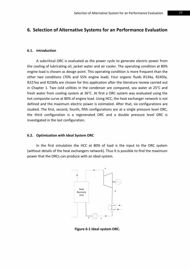
77 Selection of Alternative System for an Performance Evaluation
6. Selection of Alternative Systems for an Performance Evaluation
6.1. Introduction
A subcritical ORC is evaluated as the power cycle to generate electric power from
the cooling of lubricating oil, jacket water and air cooler. The operating condition at 80%
engine load is chosen as design point. This operating condition is more frequent than the
other two conditions (70% and 55% engine load). Four organic fluids R134a, R245fa,
R227ea and R236fa are chosen for this application after the literature review carried out
in Chapter 1. Two cold utilities in the condenser are compared, sea water at 25°C and
fresh water from cooling system at 36°C. At first a ORC system was evaluated using the
hot composite curve at 80% of engine load. Using HCC, the heat exchanger network is not
defined and the maximum electric power is estimated. After that, six configurations are
studied. The first, second, fourth, fifth configurations are at a single pressure level ORC,
the third configuration is a regenerated ORC and a double pressure level ORC is
investigated in the last configuration.
6.2. Optimization with Ideal System ORC
In the first simulation the HCC at 80% of load is the input to the ORC system
(without details of the heat exchangers network). Thus it is possible to find the maximum
power that the ORCs can produce with an ideal system.
12
4Heat
Recovery Unit
3
Figure 6-1 Ideal system ORC.
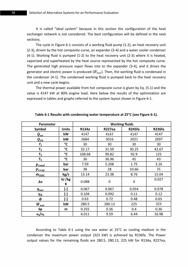
78 Selection of Alternative Systems for an Performance Evaluation
It is called “ideal system” because in this section the configuration of the heat
exchanger network is not considered. The best configuration will be defined in the next
sections.
The cycle in Figure 6-1 consists of a working fluid pump (1-2), an heat recovery unit
(2-3), driven by the hot composite curve, an expander (3-4) and a water cooler condenser
(4-1). Working fluid is pumped (1-2) to the heat recovery unit (2-3) where it is heated,
vaporized and superheated by the heat source represented by the hot composite curve.
The generated high pressure vapor flows into to the expander (3-4), and it drives the
generator and electric power is produced ( ). Then, the working fluid is condensed in
the condenser (4-1). The condensed working fluid is pumped back to the heat recovery
unit and a new cycle begins.
The thermal power available from hot composite curve is given by Eq. (5.1) and the
value is 4147 kW at 80% engine load. Here below the results of the optimization are
expressed in tables and graphs referred to the system layout shown in Figure 6-1.
Table 6-1 Results with condensing water temperature at 25°C (see Figure 6-1).
Parameter Working fluids
Symbol Units R134a R227ea R245fa R236fa
kW 4147 4147 4147 4147
kW 2684 3016 2021 2697
T1 °C 30 30 30 30
T2 °C 32.17 31.59 30.25 42.67
T3 °C 108.68 99.82 92.9 125
T4 °C 36 36.96 45 43
bar 7.59 5.208 1.75 3.16
bar 38 28 10.66 31
kg/s 13.14 23.38 8.76 15.04
kJ /kg
K 0.088 0 0
0.027
[-] 0.067 0.067 0.054 0.078
[-] 0.104 0.092 0.11 0.12
[-] 0.63 0.72 0.48 0.65
kW 280.5 280.13 225 323
Sp m 0.255 0.36 0.4 0.36
v4/v3 6.011 9.59 6.44 16.98
According to Table 6-1 using the sea water at 25°C as cooling medium in the
condenser the maximum power output (323 kW) is achieved by R236fa. The Power
output values for the remaining fluids are 280.5, 280.13, 225 kW for R134a, R227ea,
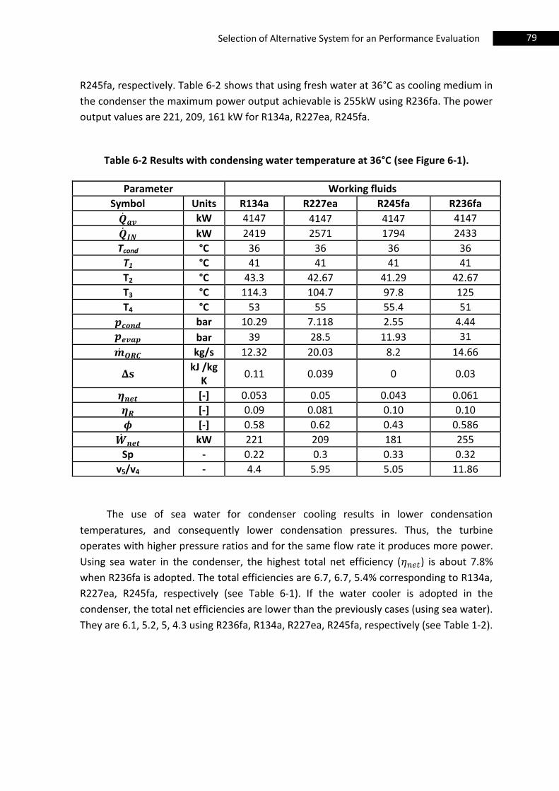
79 Selection of Alternative System for an Performance Evaluation
R245fa, respectively. Table 6-2 shows that using fresh water at 36°C as cooling medium in
the condenser the maximum power output achievable is 255kW using R236fa. The power
output values are 221, 209, 161 kW for R134a, R227ea, R245fa.
Table 6-2 Results with condensing water temperature at 36°C (see Figure 6-1).
Parameter Working fluids
Symbol Units R134a R227ea R245fa R236fa
kW 4147 4147 4147 4147
kW 2419 2571 1794 2433
Tcond °C 36 36 36 36
T1 °C 41 41 41 41
T2 °C 43.3 42.67 41.29 42.67
T3 °C 114.3 104.7 97.8 125
T4 °C 53 55 55.4 51
bar 10.29 7.118 2.55 4.44
bar 39 28.5 11.93 31
kg/s 12.32 20.03 8.2 14.66
kJ /kg
K 0.11 0.039 0 0.03
[-] 0.053 0.05 0.043 0.061
[-] 0.09 0.081 0.10 0.10
[-] 0.58 0.62 0.43 0.586
kW 221 209 181 255
Sp - 0.22 0.3 0.33 0.32
v5/v4 - 4.4 5.95 5.05 11.86
The use of sea water for condenser cooling results in lower condensation
temperatures, and consequently lower condensation pressures. Thus, the turbine
operates with higher pressure ratios and for the same flow rate it produces more power.
Using sea water in the condenser, the highest total net efficiency ( ) is about 7.8%
when R236fa is adopted. The total efficiencies are 6.7, 6.7, 5.4% corresponding to R134a,
R227ea, R245fa, respectively (see Table 6-1). If the water cooler is adopted in the
condenser, the total net efficiencies are lower than the previously cases (using sea water).
They are 6.1, 5.2, 5, 4.3 using R236fa, R134a, R227ea, R245fa, respectively (see Table 1-2).

80 Selection of Alternative Systems for an Performance Evaluation
Sea water (25°C) Water cooling (36°C)
R134a
R227ea
R245fa
0 1000 2000 3000 4000 5000 600020
40
60
80
100
120
140
160composite curve
kW
tem
pera
ture
[°C
]
0 1000 2000 3000 4000 5000 600020
40
60
80
100
120
140
160
kW
tem
pera
ture
[°C
]
0 1000 2000 3000 4000 5000 6000 7000 8000 900020
40
60
80
100
120
140
160composite curve
kW
tem
pera
ture
[°C
]
0 1000 2000 3000 4000 5000 6000 7000 800020
40
60
80
100
120
140
160composite curve
kW
tem
pera
ture
[°C
]
0 500 1000 1500 2000 2500 3000 3500 4000 450020
40
60
80
100
120
140
160composite curve
kW
tem
pera
ture
[°C
]
0 500 1000 1500 2000 2500 3000 3500 4000 450020
40
60
80
100
120
140
160composite curve
kW
tem
pera
ture
[°C
]
Air
Air + Jacket Water
Air+ lubricating oil Air
Air
Air
Air + Jacket Water
Air + lubricating oil
Air
Air
Air
Air + Jacket Water
Air + lubricating oil
Air
Air
Air
Air + Jacket Water
Air + lubricating oil
Air
Air
Air
Air + Jacket Water
Air + lubricating oil
Air
Air
Air
Air + Jacket Water
Air + lubricating oil Air
Air
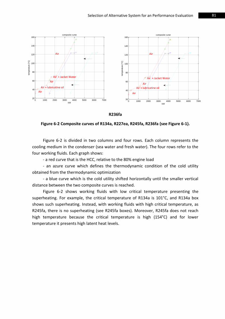
81 Selection of Alternative System for an Performance Evaluation
R236fa
Figure 6-2 Composite curves of R134a, R227ea, R245fa, R236fa (see Figure 6-1).
Figure 6-2 is divided in two columns and four rows. Each column represents the
cooling medium in the condenser (sea water and fresh water). The four rows refer to the
four working fluids. Each graph shows:
- a red curve that is the HCC, relative to the 80% engine load
- an azure curve which defines the thermodynamic condition of the cold utility
obtained from the thermodynamic optimization
- a blue curve which is the cold utility shifted horizontally until the smaller vertical
distance between the two composite curves is reached.
Figure 6-2 shows working fluids with low critical temperature presenting the
superheating. For example, the critical temperature of R134a is 101°C, and R134a box
shows such superheating. Instead, with working fluids with high critical temperature, as
R245fa, there is no superheating (see R245fa boxes). Moreover, R245fa does not reach
high temperature because the critical temperature is high (154°C) and for lower
temperature it presents high latent heat levels.
0 1000 2000 3000 4000 5000 6000 700020
40
60
80
100
120
140
160composite curve
kW
tem
pera
ture
[°C
]
0 1000 2000 3000 4000 5000 6000 700020
40
60
80
100
120
140
160composite curve
kW
tem
pera
ture
[°C
]
Air
Air + Jacket Water
Air + lubricating oil
Air
Air
Air
Air + Jacket Water
Air + lubricating oil
Air
Air
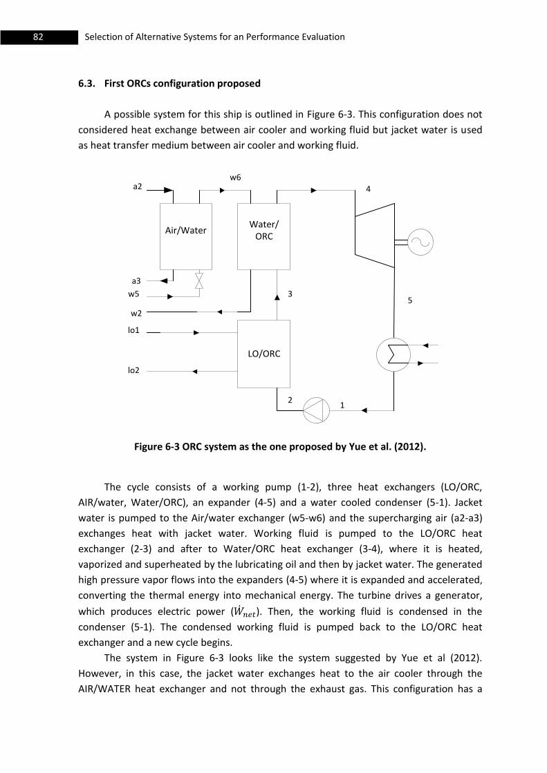
82 Selection of Alternative Systems for an Performance Evaluation
6.3. First ORCs configuration proposed
A possible system for this ship is outlined in Figure 6-3. This configuration does not
considered heat exchange between air cooler and working fluid but jacket water is used
as heat transfer medium between air cooler and working fluid.
Air/Water
LO/ORC
Water/ORC
a2
a3
w5
w2
lo1
lo2
12
4
3
w6
5
Figure 6-3 ORC system as the one proposed by Yue et al. (2012). The cycle consists of a working pump (1-2), three heat exchangers (LO/ORC,
AIR/water, Water/ORC), an expander (4-5) and a water cooled condenser (5-1). Jacket
water is pumped to the Air/water exchanger (w5-w6) and the supercharging air (a2-a3)
exchanges heat with jacket water. Working fluid is pumped to the LO/ORC heat
exchanger (2-3) and after to Water/ORC heat exchanger (3-4), where it is heated,
vaporized and superheated by the lubricating oil and then by jacket water. The generated
high pressure vapor flows into the expanders (4-5) where it is expanded and accelerated,
converting the thermal energy into mechanical energy. The turbine drives a generator,
which produces electric power ( ). Then, the working fluid is condensed in the
condenser (5-1). The condensed working fluid is pumped back to the LO/ORC heat
exchanger and a new cycle begins.
The system in Figure 6-3 looks like the system suggested by Yue et al (2012).
However, in this case, the jacket water exchanges heat to the air cooler through the
AIR/WATER heat exchanger and not through the exhaust gas. This configuration has a

83 Selection of Alternative System for an Performance Evaluation
number of advantages which are missing in the first configuration (Section 6.2). The water
is pumped in the pipes instead of air and carried around the ship, thus It permits a more
compact ORC system.
One problem is that the air temperature outlet cannot be lower than the inlet
temperature of the water, thus the air cooling needs two heat exchangers, one for the
ORCs and the other one for the cooling system. Air cooler is not used as heat source at
low temperature for ORC system, because working fluid is already warm up by lubricating
oil.
Thus, if in the Air/Water heat exchanger, the product ṁacpa is kept constant and the
air outlet temperature (Ta3) is supposed to be equal to the water inlet temperature (Tw5)
plus 5°C, the thermal power available from air cooler decreases if compared to the value
in Table 3-8 . At 80% engine load, ṁacpa is equal to 23.81 kg/s (see Table 4-1) and Ta3 is
equal to 77°C. The thermal power rejected through Air/Water heat exchanger is 1855 kW
(Table 6-3) and the thermal power available from air cooler is 2941 kW (see Table 4-1).
This system needs one heat exchanger to cool down the air from 77°C to 31.4°C, which
means a thermal power equal to 1086 kW which cannot used for ORCs.
Table 6-3 shows the properties of AIR/WATER exchange.
Table 6-3 Properties of air/water exchange.
Parameter Main Engine load (%)
Symbol Units 100 80 70 55
kW 2893 1855 1385 713
cpH20 kJ/kgK 4.186 4.186 4.186 4.186
Tw5 °C 74.5 72 70 66
Tw6 °C 94 84 79 71
Tevap °C 133 133 133 133
PH2O Bar 2.94 2.94 2.94 2.94
kg/s 35.6 36.8 33.1 28.8
If the whole water flow rate is used in the Air/Water exchanger, the outlet
temperature is low (Tw6), and the working fluids cannot reach a high temperature at the
outlet of the Water/ORC exchanger (see Table 6-3).
In this section it is proposed to add to the system a valve which can select the
quantity of water flow rate at the entry of the AIR/WATER heat exchanger, in order to
increase the temperature of the water at the outlet. Indeed, the rest of quantity of jacket
water flows in the central fresh water cooler.
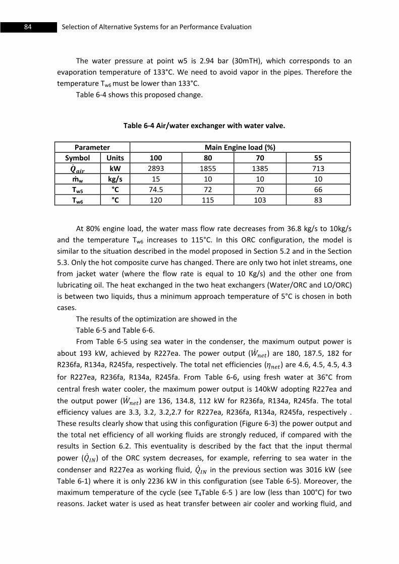
84 Selection of Alternative Systems for an Performance Evaluation
The water pressure at point w5 is 2.94 bar (30mTH), which corresponds to an
evaporation temperature of 133°C. We need to avoid vapor in the pipes. Therefore the
temperature Tw6 must be lower than 133°C.
Table 6-4 shows this proposed change.
Table 6-4 Air/water exchanger with water valve.
Parameter Main Engine load (%)
Symbol Units 100 80 70 55
kW 2893 1855 1385 713
ṁw kg/s 15 10 10 10
Tw5 °C 74.5 72 70 66
Tw6 °C 120 115 103 83
At 80% engine load, the water mass flow rate decreases from 36.8 kg/s to 10kg/s
and the temperature Tw6 increases to 115°C. In this ORC configuration, the model is
similar to the situation described in the model proposed in Section 5.2 and in the Section
5.3. Only the hot composite curve has changed. There are only two hot inlet streams, one
from jacket water (where the flow rate is equal to 10 Kg/s) and the other one from
lubricating oil. The heat exchanged in the two heat exchangers (Water/ORC and LO/ORC)
is between two liquids, thus a minimum approach temperature of 5°C is chosen in both
cases.
The results of the optimization are showed in the
Table 6-5 and Table 6-6.
From Table 6-5 using sea water in the condenser, the maximum output power is
about 193 kW, achieved by R227ea. The power output ( ) are 180, 187.5, 182 for
R236fa, R134a, R245fa, respectively. The total net efficiencies ( ) are 4.6, 4.5, 4.5, 4.3
for R227ea, R236fa, R134a, R245fa. From Table 6-6, using fresh water at 36°C from
central fresh water cooler, the maximum power output is 140kW adopting R227ea and
the output power ( ) are 136, 134.8, 112 kW for R236fa, R134a, R245fa. The total
efficiency values are 3.3, 3.2, 3.2,2.7 for R227ea, R236fa, R134a, R245fa, respectively .
These results clearly show that using this configuration (Figure 6-3) the power output and
the total net efficiency of all working fluids are strongly reduced, if compared with the
results in Section 6.2. This eventuality is described by the fact that the input thermal
power ( ) of the ORC system decreases, for example, referring to sea water in the
condenser and R227ea as working fluid, in the previous section was 3016 kW (see
Table 6-1) where it is only 2236 kW in this configuration (see Table 6-5). Moreover, the
maximum temperature of the cycle (see T4Table 6-5 ) are low (less than 100°C) for two
reasons. Jacket water is used as heat transfer between air cooler and working fluid, and
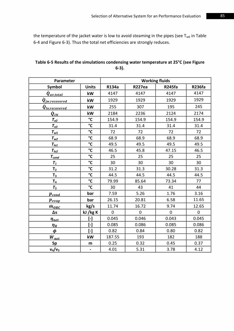
85 Selection of Alternative System for an Performance Evaluation
the temperature of the jacket water is low to avoid steaming in the pipes (see Tw6 in Table
6-4 and Figure 6-3). Thus the total net efficiencies are strongly reduces.
Table 6-5 Results of the simulations condensing water temperature at 25°C (see Figure 6-3).
Parameter Working fluids
Symbol Units R134a R227ea R245fa R236fa
kW 4147 4147 4147 4147
kW 1929 1929 1929 1929
kW 255 307 195 245
kW 2184 2236 2124 2174
Ta2 °C 154.9 154.9 154.9 154.9
Ta3 °C 31.4 31.4 31.4 31.4
Tw5 °C 72 72 72 72
Tw2 °C 68.9 68.9 68.9 68.9
Tlo1 °C 49.5 49.5 49.5 49.5
Tlo2 °C 46.5 45.8 47.15 46.5
Tcond °C 25 25 25 25
T1 °C 30 30 30 30
T2 °C 31.2 31.3 30.28 31.3
T3 °C 44.5 44.5 44.5 44.5
T4 °C 79.99 85.64 73.34 77
T5 °C 30 43 41 44
bar 7.59 5.26 1.76 3.16
bar 26.15 20.81 6.58 11.65
kg/s 11.74 16.72 9.74 12.65
kJ /kg K 0 0 0 0
[-] 0.045 0.046 0.043 0.045
[-] 0.085 0.086 0.085 0.086
[-] 0.82 0.84 0.80 0.82
kW 187.55 193 182 188
Sp m 0.25 0.32 0.45 0.37
v4/v3 - 4.01 5.31 3.78 4.12

86 Selection of Alternative Systems for an Performance Evaluation
Table 6-6 Results of the simulations condensing water temperature at 36°C (see Figure
6-3).
Parameter Working fluids
Symbol Units R134a R227ea R245fa R236fa
kW 4147 4147 4147 4147
kW 1929 1929 1678 1929
kW 48 59 0 40
kW 1977 1988 1678 1969
Ta2 °C 154.9 154.9 154.9 154.9
Ta3 °C 31.4 31.4 31.4 31.4
Tw5 °C 72 72 72 72
Tw2 °C 68.9 68.9 75 68.9
Tlo1 °C 49.5 49.5 49.5 49.5
Tlo2 °C 48.9 48.8 49.5 40.7
T1 °C 41 41 41 41
T2 °C 42.16 42.35 41.26 42
T3 °C 44 44.5 41.26 44.5
T4 °C 80.67 86.44 74.2 77
T5 °C 41 50 49 51
bar 10.29 7.19 2.57 4.44
bar 26.52 21.17 8.23 11.85
kg/s 11.63 16.5 6.73 12.44
kJ /kg K 0 0 0 0
[-] 0.032 0.033 0.027 0.032
[-] 0.068 0.07 0.066 0.07
[-] 0.47 0.48 0.40 0.47
kW 134.8 140 112 136
Sp - 0.23 0.29 0.375 0.34
v4/v3 - 2.98 3.89 2.67 2.97
As previous states, the power output and the total net efficiency of all working
fluids are reduced, compared to the results in Section 6.2. Also the maximum
temperature of the ORC cycle is reduced. Using R227ea as working fluid, the value of T4,
which is the inlet temperature of the expansion is 86°C (see Table 6-6) instead, in the
previous section, the value of inlet temperature of the expansion is 104.7°C (see T3 in
Table 6-2 ). In both situations of this configuration (using sea water and water fresh as
cooling medium in the condenser) there is no working fluid superheating ( =0 see Table
6-5 and Table 6-6).
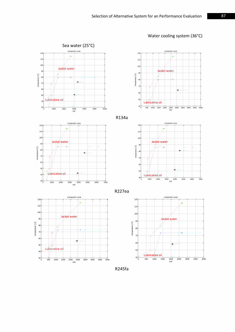
87 Selection of Alternative System for an Performance Evaluation
Sea water (25°C)
Water cooling system (36°C)
R134a
R227ea
R245fa
0 1000 2000 3000 4000 5000 600030
40
50
60
70
80
90
100
110
120composite curve
kW
tem
pera
ture
[°C
]
0 500 1000 1500 2000 2500 3000 3500 4000 4500 500040
50
60
70
80
90
100
110
120composite curve
kW
tem
pera
ture
[°C
]
0 1000 2000 3000 4000 5000 6000 700030
40
50
60
70
80
90
100
110
120composite curve
kW
tem
pera
ture
[°C
]
0 1000 2000 3000 4000 5000 6000 700040
50
60
70
80
90
100
110
120composite curve
kW
tem
pera
ture
[°C
]
0 500 1000 1500 2000 2500 3000 3500 4000 450030
40
50
60
70
80
90
100
110
120composite curve
kW
tem
pera
ture
[°C
]
0 500 1000 1500 2000 2500 3000 3500 400040
50
60
70
80
90
100
110
120composite curve
kW
tem
pera
ture
[°C
]
Jacket water Jacket water
Jacket water Jacket water
Jacket water Jacket water
Lubricating oil Lubricating oil
Lubricating oil Lubricating oil
Lubricating oil
Lubricating oil
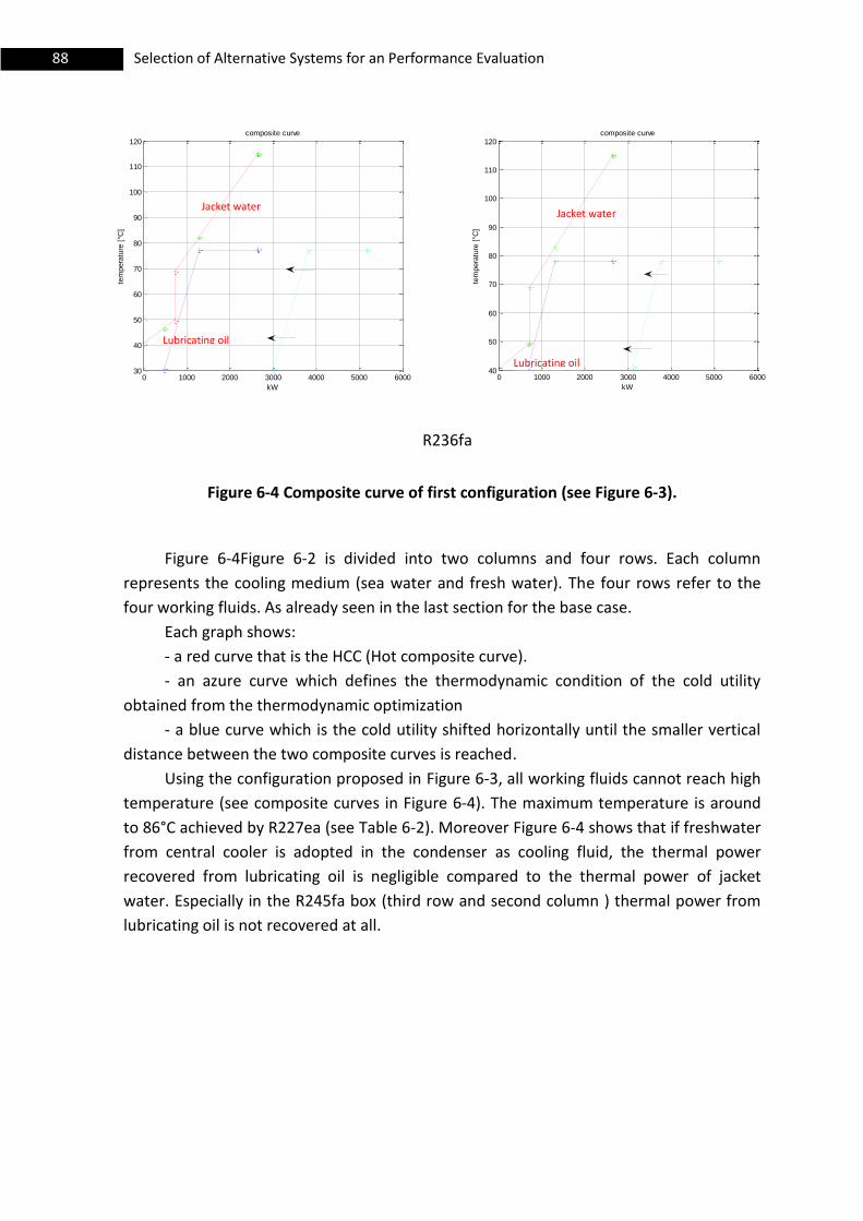
88 Selection of Alternative Systems for an Performance Evaluation
R236fa
Figure 6-4 Composite curve of first configuration (see Figure 6-3).
Figure 6-4Figure 6-2 is divided into two columns and four rows. Each column
represents the cooling medium (sea water and fresh water). The four rows refer to the
four working fluids. As already seen in the last section for the base case.
Each graph shows:
- a red curve that is the HCC (Hot composite curve).
- an azure curve which defines the thermodynamic condition of the cold utility
obtained from the thermodynamic optimization
- a blue curve which is the cold utility shifted horizontally until the smaller vertical
distance between the two composite curves is reached.
Using the configuration proposed in Figure 6-3, all working fluids cannot reach high
temperature (see composite curves in Figure 6-4). The maximum temperature is around
to 86°C achieved by R227ea (see Table 6-2). Moreover Figure 6-4 shows that if freshwater
from central cooler is adopted in the condenser as cooling fluid, the thermal power
recovered from lubricating oil is negligible compared to the thermal power of jacket
water. Especially in the R245fa box (third row and second column ) thermal power from
lubricating oil is not recovered at all.
0 1000 2000 3000 4000 5000 600030
40
50
60
70
80
90
100
110
120composite curve
kW
tem
pera
ture
[°C
]
0 1000 2000 3000 4000 5000 600040
50
60
70
80
90
100
110
120composite curve
kW
tem
pera
ture
[°C
]
Jacket water Jacket water
Lubricating oil
Lubricating oil
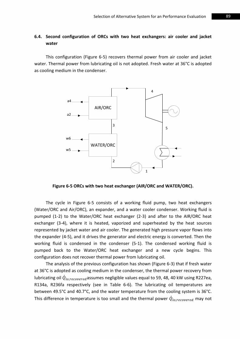
89 Selection of Alternative System for an Performance Evaluation
6.4. Second configuration of ORCs with two heat exchangers: air cooler and jacket
water
This configuration (Figure 6-5) recovers thermal power from air cooler and jacket
water. Thermal power from lubricating oil is not adopted. Fresh water at 36°C is adopted
as cooling medium in the condenser.
1
2
4
35
w5
w6
a2
a4
AIR/ORC
WATER/ORC
Figure 6-5 ORCs with two heat exchanger (AIR/ORC and WATER/ORC).
The cycle in Figure 6-5 consists of a working fluid pump, two heat exchangers
(Water/ORC and Air/ORC), an expander, and a water cooler condenser. Working fluid is
pumped (1-2) to the Water/ORC heat exchanger (2-3) and after to the AIR/ORC heat
exchanger (3-4), where it is heated, vaporized and superheated by the heat sources
represented by jacket water and air cooler. The generated high pressure vapor flows into
the expander (4-5), and it drives the generator and electric energy is converted. Then the
working fluid is condensed in the condenser (5-1). The condensed working fluid is
pumped back to the Water/ORC heat exchanger and a new cycle begins. This
configuration does not recover thermal power from lubricating oil.
The analysis of the previous configuration has shown (Figure 6-3) that if fresh water
at 36°C is adopted as cooling medium in the condenser, the thermal power recovery from
lubricating oil assumes negligible values equal to 59, 48, 40 kW using R227ea,
R134a, R236fa respectively (see in Table 6-6). The lubricating oil temperatures are
between 49.5°C and 40.7°C, and the water temperature from the cooling system is 36°C.
This difference in temperature is too small and the thermal power may not
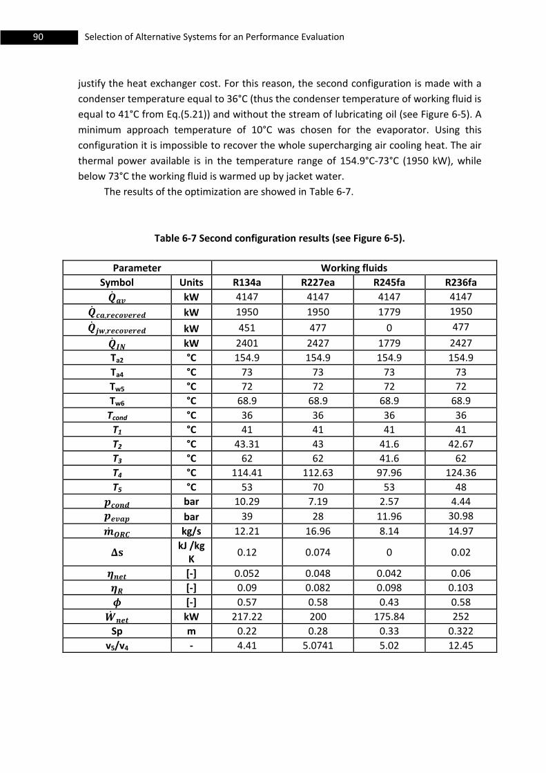
90 Selection of Alternative Systems for an Performance Evaluation
justify the heat exchanger cost. For this reason, the second configuration is made with a
condenser temperature equal to 36°C (thus the condenser temperature of working fluid is
equal to 41°C from Eq.(5.21)) and without the stream of lubricating oil (see Figure 6-5). A
minimum approach temperature of 10°C was chosen for the evaporator. Using this
configuration it is impossible to recover the whole supercharging air cooling heat. The air
thermal power available is in the temperature range of 154.9°C-73°C (1950 kW), while
below 73°C the working fluid is warmed up by jacket water.
The results of the optimization are showed in Table 6-7.
Table 6-7 Second configuration results (see Figure 6-5).
Parameter Working fluids
Symbol Units R134a R227ea R245fa R236fa
kW 4147 4147 4147 4147
kW 1950 1950 1779 1950
kW 451 477 0 477
kW 2401 2427 1779 2427
Ta2 °C 154.9 154.9 154.9 154.9
Ta4 °C 73 73 73 73
Tw5 °C 72 72 72 72
Tw6 °C 68.9 68.9 68.9 68.9
Tcond °C 36 36 36 36
T1 °C 41 41 41 41
T2 °C 43.31 43 41.6 42.67
T3 °C 62 62 41.6 62
T4 °C 114.41 112.63 97.96 124.36
T5 °C 53 70 53 48
bar 10.29 7.19 2.57 4.44
bar 39 28 11.96 30.98
kg/s 12.21 16.96 8.14 14.97
kJ /kg
K 0.12 0.074 0 0.02
[-] 0.052 0.048 0.042 0.06
[-] 0.09 0.082 0.098 0.103
[-] 0.57 0.58 0.43 0.58
kW 217.22 200 175.84 252
Sp m 0.22 0.28 0.33 0.322
v5/v4 - 4.41 5.0741 5.02 12.45
91 Selection of Alternative System for an Performance Evaluation
From Table 6-7, the maximum output power is about 252 kW, reached by R236fa.
The power outputs ( ) are 217.22, 200, 175.84 for R134a, R227ea, R245fa,
respectively. The total net efficiencies ( ) are 6.0, 5.2, 4.8, 4.2 for R236fa, R134a,
R227ea, R245fa.
With this configuration (Figure 6-5) the power output and the total net efficiency of
all working fluids are higher than those presented in Section 6.3. This result is explained
by the fact that there is not the jacket water as heat transfer medium between air cooler
and working fluid (see the Air/water heat exchanger in Figure 6-3) which in the first
configuration limited the maximum temperatures achievable by the working fluid.
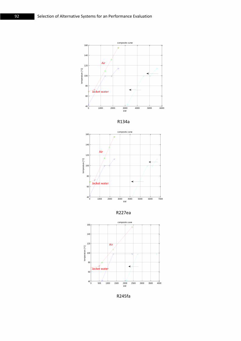
92 Selection of Alternative Systems for an Performance Evaluation
R134a
R227ea
R245fa
0 1000 2000 3000 4000 5000 600040
60
80
100
120
140
160composite curve
kW
tem
pera
ture
[°C
]
0 1000 2000 3000 4000 5000 6000 700040
60
80
100
120
140
160composite curve
kW
tem
pera
ture
[°C
]
0 500 1000 1500 2000 2500 3000 3500 400040
60
80
100
120
140
160composite curve
kW
tem
pera
ture
[°C
]
Air
Jacket water
Jacket water
Air
Air
Jacket water
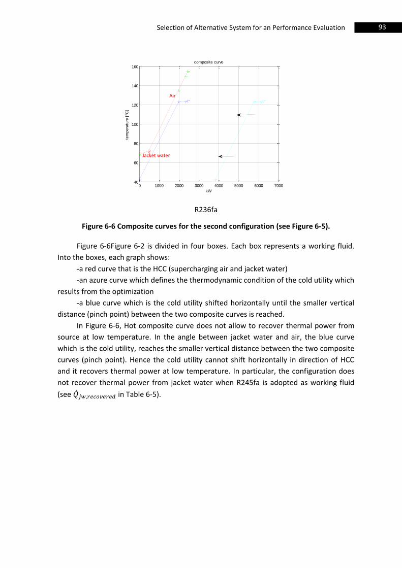
93 Selection of Alternative System for an Performance Evaluation
R236fa
Figure 6-6 Composite curves for the second configuration (see Figure 6-5).
Figure 6-6Figure 6-2 is divided in four boxes. Each box represents a working fluid.
Into the boxes, each graph shows:
-a red curve that is the HCC (supercharging air and jacket water)
-an azure curve which defines the thermodynamic condition of the cold utility which
results from the optimization
-a blue curve which is the cold utility shifted horizontally until the smaller vertical
distance (pinch point) between the two composite curves is reached.
In Figure 6-6, Hot composite curve does not allow to recover thermal power from
source at low temperature. In the angle between jacket water and air, the blue curve
which is the cold utility, reaches the smaller vertical distance between the two composite
curves (pinch point). Hence the cold utility cannot shift horizontally in direction of HCC
and it recovers thermal power at low temperature. In particular, the configuration does
not recover thermal power from jacket water when R245fa is adopted as working fluid
(see in Table 6-5).
0 1000 2000 3000 4000 5000 6000 700040
60
80
100
120
140
160composite curve
kW
tem
pera
ture
[°C
]
Air
Jacket water
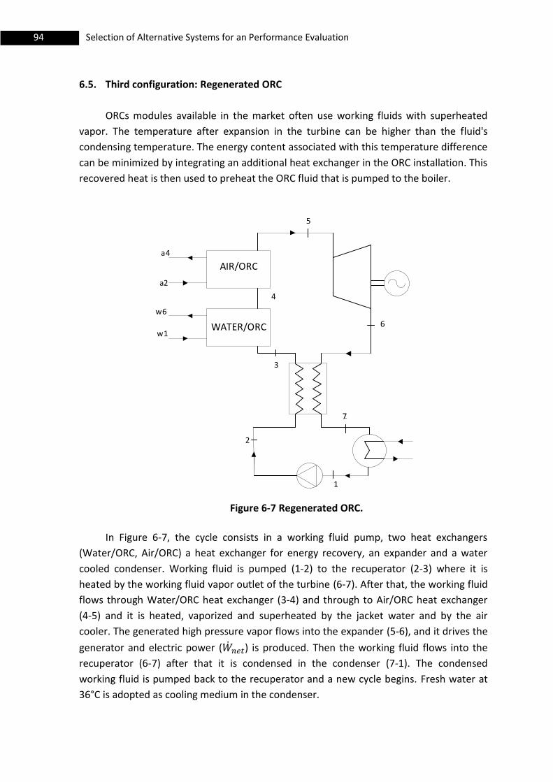
94 Selection of Alternative Systems for an Performance Evaluation
6.5. Third configuration: Regenerated ORC
ORCs modules available in the market often use working fluids with superheated
vapor. The temperature after expansion in the turbine can be higher than the fluid's
condensing temperature. The energy content associated with this temperature difference
can be minimized by integrating an additional heat exchanger in the ORC installation. This
recovered heat is then used to preheat the ORC fluid that is pumped to the boiler.
4
1
2
4
3
5w1
w6
a2
a4
AIR/ORC
WATER/ORC
6
5
6
7
Figure 6-7 Regenerated ORC.
In Figure 6-7, the cycle consists in a working fluid pump, two heat exchangers
(Water/ORC, Air/ORC) a heat exchanger for energy recovery, an expander and a water
cooled condenser. Working fluid is pumped (1-2) to the recuperator (2-3) where it is
heated by the working fluid vapor outlet of the turbine (6-7). After that, the working fluid
flows through Water/ORC heat exchanger (3-4) and through to Air/ORC heat exchanger
(4-5) and it is heated, vaporized and superheated by the jacket water and by the air
cooler. The generated high pressure vapor flows into the expander (5-6), and it drives the
generator and electric power ( ) is produced. Then the working fluid flows into the
recuperator (6-7) after that it is condensed in the condenser (7-1). The condensed
working fluid is pumped back to the recuperator and a new cycle begins. Fresh water at
36°C is adopted as cooling medium in the condenser.
95 Selection of Alternative System for an Performance Evaluation
In the present configuration it is considered that the recuperator is a counter flow
type heat exchanger in which is equal to 10°C. Under this hypothesis the
temperature of the vapor at the heat exchanger outlet can be evaluated, as well as the
available energy for the internal heat exchange process ( ):
(6.1)
( ) (6.2)
The state of the liquid at the regenerator outlet can be determined, since:
(6.3)
Vaja and Gambarotta (2010) used this method, but they considered a
equal to 15°C. In the previous configuration (see Section 6.5) for all working fluids, the
output temperatures of turbine (T5) are not high (the maximum output temperature is
70°C with R227ea, 53°C for R134a and R245fa, 48°C for R236fa, see Table 6-7). As
previously stated, fresh water is used in the condenser, thus T2 is close to 36°C (fresh
water temperature) plus 5°C (minimum approach temperature in the condenser see Eq.
(5.21) ). If the is equal to 15°C, from Eq.(6.1) T7 would be 56°C, it is higher than
almost all output temperatures vapor of expansion found in Section 6.5, which means
that the heat exchange is impossible from Eq. (6.2). Thus, in this work equal to
10°C is chosen, so the heat exchange is possible between liquid working fluid and vapor at
the end of turbine expansion.
In this simulation one more constraint is added. T6 has to be equal or higher than T7.
Table 6-8 shows that the regenerated heat exchanger is useless for R134a and
R236fa. The outlet turbine temperatures (T7) are 53°C for both working fluids, T7 is equal
to T6, and (available thermal power for the internal heat exchange process) found
from Eq. (5.41) is zero. Using R227ea and R245fa as a working fluids, is 79.22 and, 33
kW, respectively. The output power is 246, 217.16, 202, 177 kW for R236fa, R134a,
R227ea, R245fa, respectively. If these output powers are compared to the output powers
found in Section 6.4, there is an slight improvements for R227ea (from 200 kW to 202
kW) and for R245fa (from 175.84 kW to 177 kW). There is a worsening adopting R236fa
(from 252 kW to 246 kW) and using R134a (from 217.22 kW to 217.16 kW) because there
is a constraint that T6 has to be equal or higher than T7 (using the second configuration
the output power is higher because the output temperature of the expansion is lower.)
The total net efficiencies ( ) are 5.9, 5.2, 4.8, 4.2% for R236fa, R134a, R227ea,
R245fa. They are almost equal to the total net efficiencies found in section 6.4. In
conclusion, using a recuperator, there is not a great improvement.
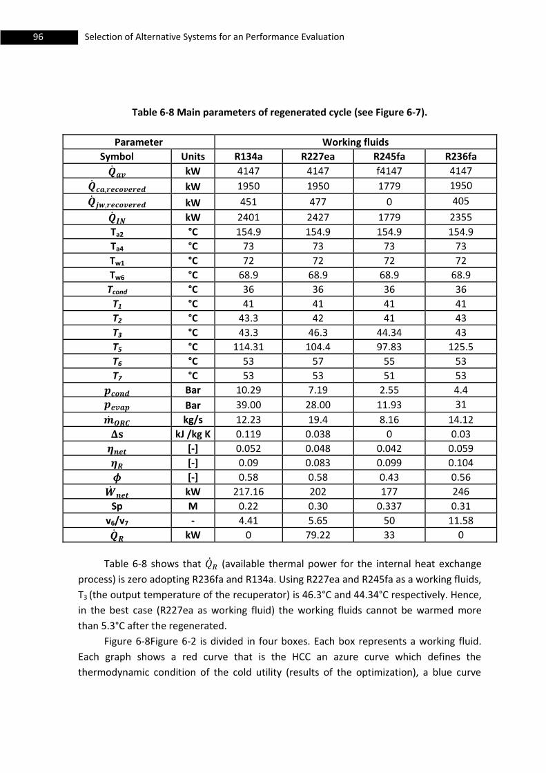
96 Selection of Alternative Systems for an Performance Evaluation
Table 6-8 Main parameters of regenerated cycle (see Figure 6-7).
Parameter Working fluids
Symbol Units R134a R227ea R245fa R236fa
kW 4147 4147 f4147 4147
kW 1950 1950 1779 1950
kW 451 477 0 405
kW 2401 2427 1779 2355
Ta2 °C 154.9 154.9 154.9 154.9
Ta4 °C 73 73 73 73
Tw1 °C 72 72 72 72
Tw6 °C 68.9 68.9 68.9 68.9
Tcond °C 36 36 36 36
T1 °C 41 41 41 41
T2 °C 43.3 42 41 43
T3 °C 43.3 46.3 44.34 43
T5 °C 114.31 104.4 97.83 125.5
T6 °C 53 57 55 53
T7 °C 53 53 51 53
Bar 10.29 7.19 2.55 4.4
Bar 39.00 28.00 11.93 31
kg/s 12.23 19.4 8.16 14.12
kJ /kg K 0.119 0.038 0 0.03
[-] 0.052 0.048 0.042 0.059
[-] 0.09 0.083 0.099 0.104
[-] 0.58 0.58 0.43 0.56
kW 217.16 202 177 246
Sp M 0.22 0.30 0.337 0.31
v6/v7 - 4.41 5.65 50 11.58
kW 0 79.22 33 0
Table 6-8 shows that (available thermal power for the internal heat exchange
process) is zero adopting R236fa and R134a. Using R227ea and R245fa as a working fluids,
T3 (the output temperature of the recuperator) is 46.3°C and 44.34°C respectively. Hence,
in the best case (R227ea as working fluid) the working fluids cannot be warmed more
than 5.3°C after the regenerated.
Figure 6-8Figure 6-2 is divided in four boxes. Each box represents a working fluid.
Each graph shows a red curve that is the HCC an azure curve which defines the
thermodynamic condition of the cold utility (results of the optimization), a blue curve

97 Selection of Alternative System for an Performance Evaluation
which is the cold utility shifted horizontally until the smaller vertical distance (pinch point)
between the two composite curves is reached.
R134a
R227ea
0 1000 2000 3000 4000 5000 600040
60
80
100
120
140
160composite curve
kW
tem
pera
ture
[°C
]
0 1000 2000 3000 4000 5000 6000 7000 800040
60
80
100
120
140
160composite curve
kW
tem
pera
ture
[°C
]
Jacket water
Jacket water
Air
Air
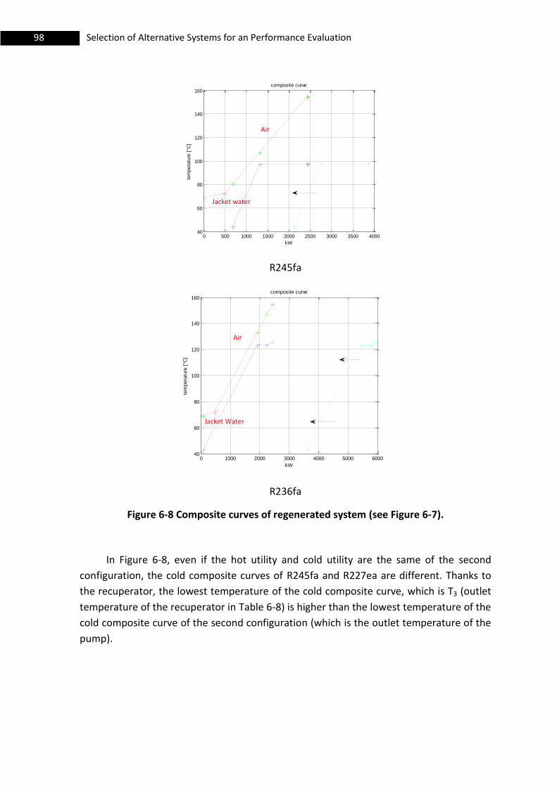
98 Selection of Alternative Systems for an Performance Evaluation
R245fa
R236fa
Figure 6-8 Composite curves of regenerated system (see Figure 6-7).
In Figure 6-8, even if the hot utility and cold utility are the same of the second
configuration, the cold composite curves of R245fa and R227ea are different. Thanks to
the recuperator, the lowest temperature of the cold composite curve, which is T3 (outlet
temperature of the recuperator in Table 6-8) is higher than the lowest temperature of the
cold composite curve of the second configuration (which is the outlet temperature of the
pump).
0 500 1000 1500 2000 2500 3000 3500 400040
60
80
100
120
140
160composite curve
kW
tem
pera
ture
[°C
]
0 1000 2000 3000 4000 5000 600040
60
80
100
120
140
160composite curve
kW
tem
pera
ture
[°C
]
Jacket water
Air
Air
Jacket Water
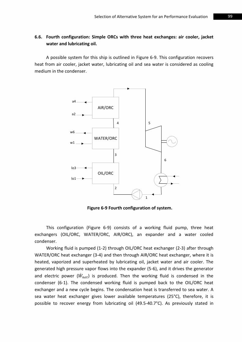
99 Selection of Alternative System for an Performance Evaluation
6.6. Fourth configuration: Simple ORCs with three heat exchanges: air cooler, jacket
water and lubricating oil.
A possible system for this ship is outlined in Figure 6-9. This configuration recovers
heat from air cooler, jacket water, lubricating oil and sea water is considered as cooling
medium in the condenser.
1
2
4
3
5
w1
w6
a2
a4
AIR/ORC
WATER/ORC
6
OIL/ORClo3
lo1
Figure 6-9 Fourth configuration of system.
This configuration (Figure 6-9) consists of a working fluid pump, three heat
exchangers (OIL/ORC, WATER/ORC, AIR/ORC), an expander and a water cooled
condenser.
Working fluid is pumped (1-2) through OIL/ORC heat exchanger (2-3) after through
WATER/ORC heat exchanger (3-4) and then through AIR/ORC heat exchanger, where it is
heated, vaporized and superheated by lubricating oil, jacket water and air cooler. The
generated high pressure vapor flows into the expander (5-6), and it drives the generator
and electric power ( ) is produced. Then the working fluid is condensed in the
condenser (6-1). The condensed working fluid is pumped back to the OIL/ORC heat
exchanger and a new cycle begins. The condensation heat is transferred to sea water. A
sea water heat exchanger gives lower available temperatures (25°C), therefore, it is
possible to recover energy from lubricating oil (49.5-40.7°C). As previously stated in
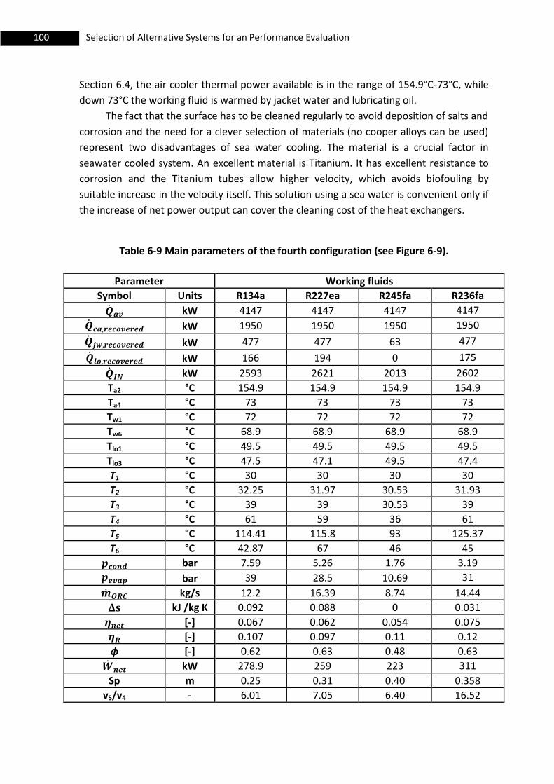
100 Selection of Alternative Systems for an Performance Evaluation
Section 6.4, the air cooler thermal power available is in the range of 154.9°C-73°C, while
down 73°C the working fluid is warmed by jacket water and lubricating oil.
The fact that the surface has to be cleaned regularly to avoid deposition of salts and
corrosion and the need for a clever selection of materials (no cooper alloys can be used)
represent two disadvantages of sea water cooling. The material is a crucial factor in
seawater cooled system. An excellent material is Titanium. It has excellent resistance to
corrosion and the Titanium tubes allow higher velocity, which avoids biofouling by
suitable increase in the velocity itself. This solution using a sea water is convenient only if
the increase of net power output can cover the cleaning cost of the heat exchangers.
Table 6-9 Main parameters of the fourth configuration (see Figure 6-9).
Parameter Working fluids
Symbol Units R134a R227ea R245fa R236fa
kW 4147 4147 4147 4147
kW 1950 1950 1950 1950
kW 477 477 63 477
kW 166 194 0 175
kW 2593 2621 2013 2602
Ta2 °C 154.9 154.9 154.9 154.9
Ta4 °C 73 73 73 73
Tw1 °C 72 72 72 72
Tw6 °C 68.9 68.9 68.9 68.9
Tlo1 °C 49.5 49.5 49.5 49.5
Tlo3 °C 47.5 47.1 49.5 47.4
T1 °C 30 30 30 30
T2 °C 32.25 31.97 30.53 31.93
T3 °C 39 39 30.53 39
T4 °C 61 59 36 61
T5 °C 114.41 115.8 93 125.37
T6 °C 42.87 67 46 45
bar 7.59 5.26 1.76 3.19
bar 39 28.5 10.69 31
kg/s 12.2 16.39 8.74 14.44
kJ /kg K 0.092 0.088 0 0.031
[-] 0.067 0.062 0.054 0.075
[-] 0.107 0.097 0.11 0.12
[-] 0.62 0.63 0.48 0.63
kW 278.9 259 223 311
Sp m 0.25 0.31 0.40 0.358
v5/v4 - 6.01 7.05 6.40 16.52
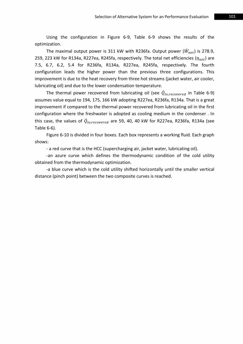
101 Selection of Alternative System for an Performance Evaluation
Using the configuration in Figure 6-9, Table 6-9 shows the results of the
optimization.
The maximal output power is 311 kW with R236fa. Output power ( ) is 278.9,
259, 223 kW for R134a, R227ea, R245fa, respectively. The total net efficiencies ( ) are
7.5, 6.7, 6.2, 5.4 for R236fa, R134a, R227ea, R245fa, respectively. The fourth
configuration leads the higher power than the previous three configurations. This
improvement is due to the heat recovery from three hot streams (jacket water, air cooler,
lubricating oil) and due to the lower condensation temperature.
The thermal power recovered from lubricating oil (see in Table 6-9)
assumes value equal to 194, 175, 166 kW adopting R227ea, R236fa, R134a. That is a great
improvement if compared to the thermal power recovered from lubricating oil in the first
configuration where the freshwater is adopted as cooling medium in the condenser . In
this case, the values of are 59, 40, 40 kW for R227ea, R236fa, R134a (see
Table 6-6).
Figure 6-10 is divided in four boxes. Each box represents a working fluid. Each graph
shows:
- a red curve that is the HCC (supercharging air, jacket water, lubricating oil).
-an azure curve which defines the thermodynamic condition of the cold utility
obtained from the thermodynamic optimization.
-a blue curve which is the cold utility shifted horizontally until the smaller vertical
distance (pinch point) between the two composite curves is reached.
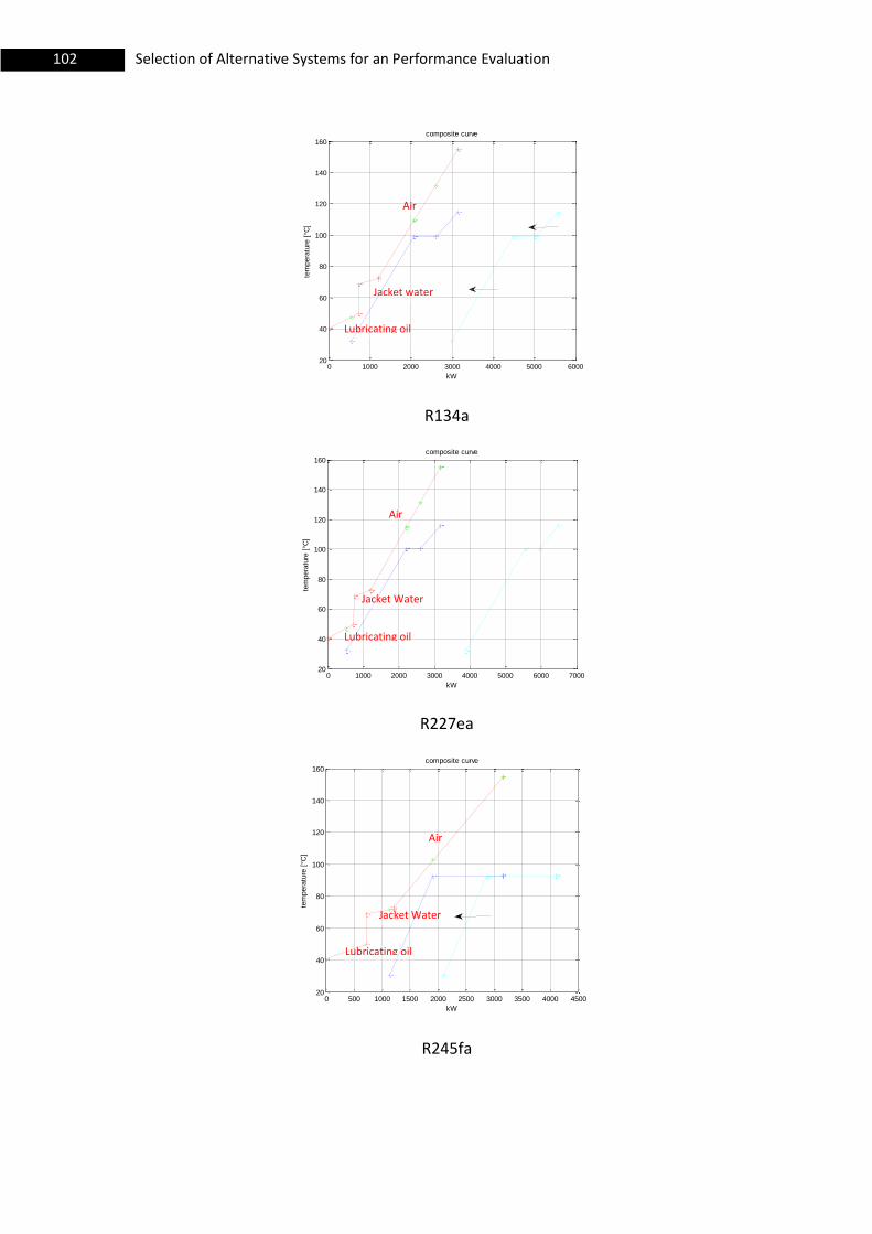
102 Selection of Alternative Systems for an Performance Evaluation
R134a
R227ea
R245fa
0 1000 2000 3000 4000 5000 600020
40
60
80
100
120
140
160composite curve
kW
tem
pera
ture
[°C
]
0 1000 2000 3000 4000 5000 6000 700020
40
60
80
100
120
140
160composite curve
kW
tem
pera
ture
[°C
]
0 500 1000 1500 2000 2500 3000 3500 4000 450020
40
60
80
100
120
140
160composite curve
kW
tem
pera
ture
[°C
]
Air
Air
Air
Jacket water
Lubricating oil
Lubricating oil
Lubricating oil
Jacket Water
Jacket Water
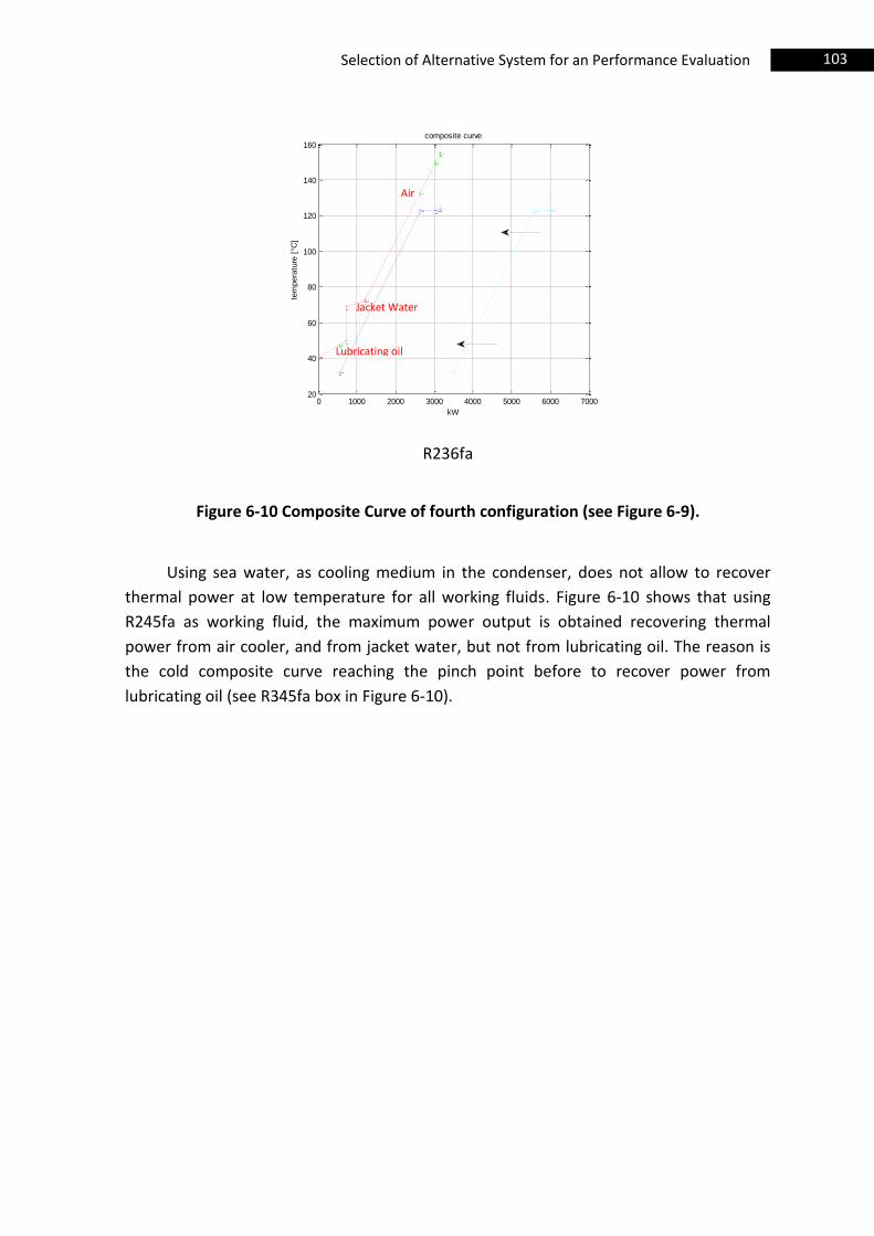
103 Selection of Alternative System for an Performance Evaluation
R236fa
Figure 6-10 Composite Curve of fourth configuration (see Figure 6-9).
Using sea water, as cooling medium in the condenser, does not allow to recover
thermal power at low temperature for all working fluids. Figure 6-10 shows that using
R245fa as working fluid, the maximum power output is obtained recovering thermal
power from air cooler, and from jacket water, but not from lubricating oil. The reason is
the cold composite curve reaching the pinch point before to recover power from
lubricating oil (see R345fa box in Figure 6-10).
0 1000 2000 3000 4000 5000 6000 700020
40
60
80
100
120
140
160composite curve
kW
tem
pera
ture
[°C
]
Air
Jacket Water
Lubricating oil
104 Selection of Alternative Systems for an Performance Evaluation
6.7. Fifth Configuration: Only Air Heat Exchanger
The fifth configuration explores the possibility to recover energy only from air
cooler (Figure 6-11) and sea water at 25°C is adopted as cooling medium in the
condenser.
12
4
3
a2
a4
Air cooler/ORC
Figure 6-11 Fifth configuration of the system.
The cycle in Figure 6-11 consists of a working fluid pump, one heat exchanger
(AIR/ORC), an expander and a water cooled condenser. Working fluid is pumped (1-2) to
the AIR/ORC heat exchanger (2-3), where it is heated, vaporized and superheated by air
cooler. The generated high pressure vapor flows into the expander (3-4), and it drives the
generator and electric power is produced. Then the working fluid is condensed in the
condenser (4-1). The condensed working fluid is pumped back to the AIR/ORC heat
exchanger and a new cycle begins. The condensation heat is transferred to sea water.
The temperature range is higher than with the other heat sources. The fourth
configuration (the best of the previous four configuration studied) in Section 6.6 required
several heat exchangers as it is shown in Figure 6-10. For examples, the R236fa needs
three preheaters (one for jacket water, one for lubricating oil, and another one for air
cooler), one evaporator and one superheater, it means five heat exchangers in total.
Instead, using one heat source (supercharging air) only one economizer, one evaporator
and one superheater are needed.
Table 6-11 shows the results of the optimization.
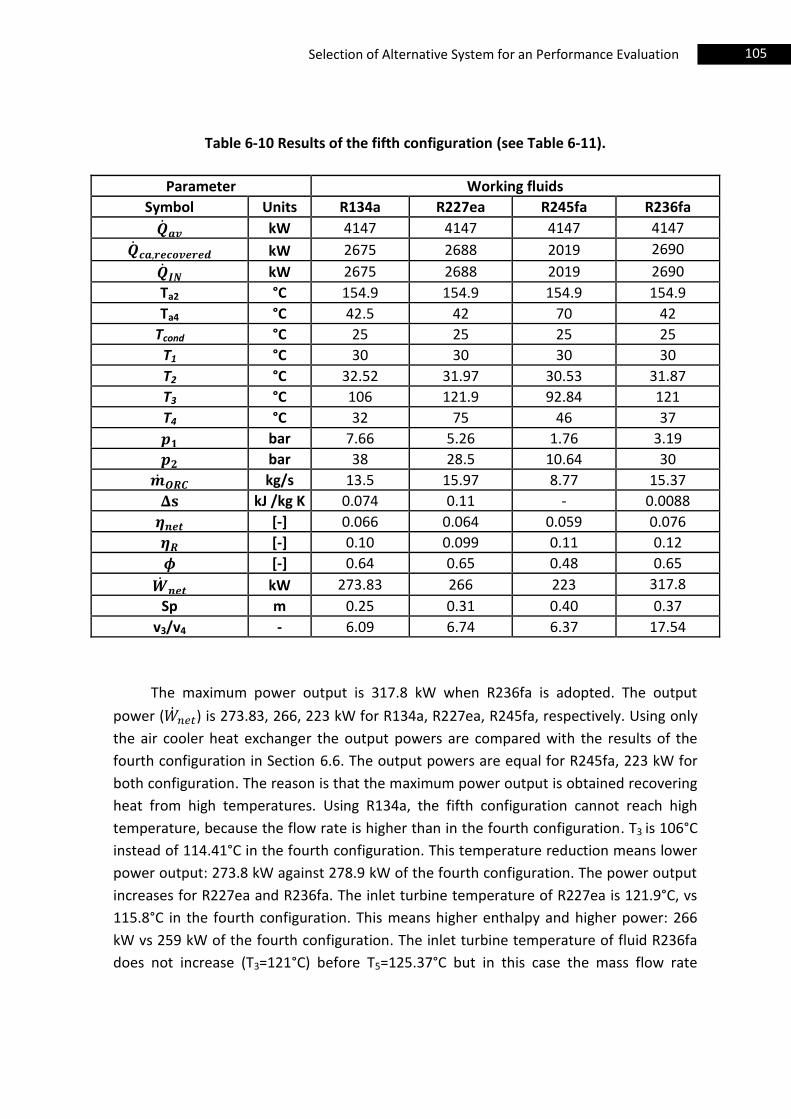
105 Selection of Alternative System for an Performance Evaluation
Table 6-10 Results of the fifth configuration (see Table 6-11).
Parameter Working fluids
Symbol Units R134a R227ea R245fa R236fa
kW 4147 4147 4147 4147
kW 2675 2688 2019 2690
kW 2675 2688 2019 2690
Ta2 °C 154.9 154.9 154.9 154.9
Ta4 °C 42.5 42 70 42
Tcond °C 25 25 25 25
T1 °C 30 30 30 30
T2 °C 32.52 31.97 30.53 31.87
T3 °C 106 121.9 92.84 121
T4 °C 32 75 46 37
bar 7.66 5.26 1.76 3.19
bar 38 28.5 10.64 30
kg/s 13.5 15.97 8.77 15.37
kJ /kg K 0.074 0.11 - 0.0088
[-] 0.066 0.064 0.059 0.076
[-] 0.10 0.099 0.11 0.12
[-] 0.64 0.65 0.48 0.65
kW 273.83 266 223 317.8
Sp m 0.25 0.31 0.40 0.37
v3/v4 - 6.09 6.74 6.37 17.54
The maximum power output is 317.8 kW when R236fa is adopted. The output
power ( ) is 273.83, 266, 223 kW for R134a, R227ea, R245fa, respectively. Using only
the air cooler heat exchanger the output powers are compared with the results of the
fourth configuration in Section 6.6. The output powers are equal for R245fa, 223 kW for
both configuration. The reason is that the maximum power output is obtained recovering
heat from high temperatures. Using R134a, the fifth configuration cannot reach high
temperature, because the flow rate is higher than in the fourth configuration. T3 is 106°C
instead of 114.41°C in the fourth configuration. This temperature reduction means lower
power output: 273.8 kW against 278.9 kW of the fourth configuration. The power output
increases for R227ea and R236fa. The inlet turbine temperature of R227ea is 121.9°C, vs
115.8°C in the fourth configuration. This means higher enthalpy and higher power: 266
kW vs 259 kW of the fourth configuration. The inlet turbine temperature of fluid R236fa
does not increase (T3=121°C) before T5=125.37°C but in this case the mass flow rate
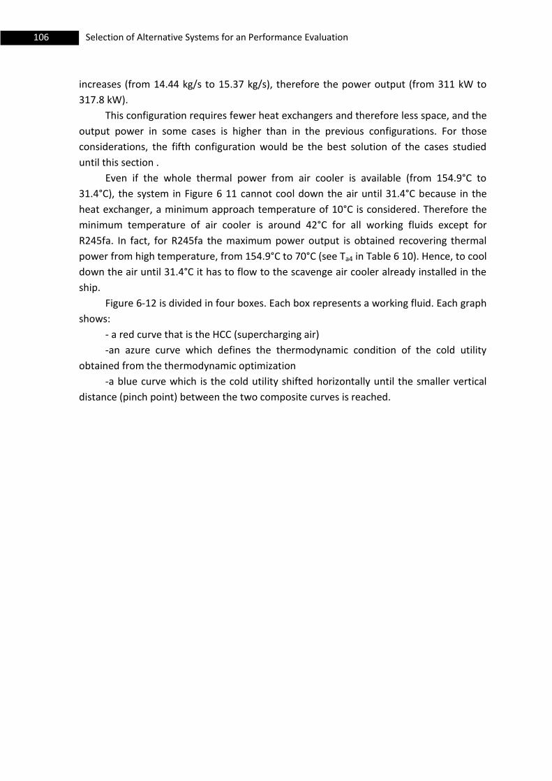
106 Selection of Alternative Systems for an Performance Evaluation
increases (from 14.44 kg/s to 15.37 kg/s), therefore the power output (from 311 kW to
317.8 kW).
This configuration requires fewer heat exchangers and therefore less space, and the
output power in some cases is higher than in the previous configurations. For those
considerations, the fifth configuration would be the best solution of the cases studied
until this section .
Even if the whole thermal power from air cooler is available (from 154.9°C to
31.4°C), the system in Figure 6 11 cannot cool down the air until 31.4°C because in the
heat exchanger, a minimum approach temperature of 10°C is considered. Therefore the
minimum temperature of air cooler is around 42°C for all working fluids except for
R245fa. In fact, for R245fa the maximum power output is obtained recovering thermal
power from high temperature, from 154.9°C to 70°C (see Ta4 in Table 6 10). Hence, to cool
down the air until 31.4°C it has to flow to the scavenge air cooler already installed in the
ship.
Figure 6-12 is divided in four boxes. Each box represents a working fluid. Each graph
shows:
- a red curve that is the HCC (supercharging air)
-an azure curve which defines the thermodynamic condition of the cold utility
obtained from the thermodynamic optimization
-a blue curve which is the cold utility shifted horizontally until the smaller vertical
distance (pinch point) between the two composite curves is reached.
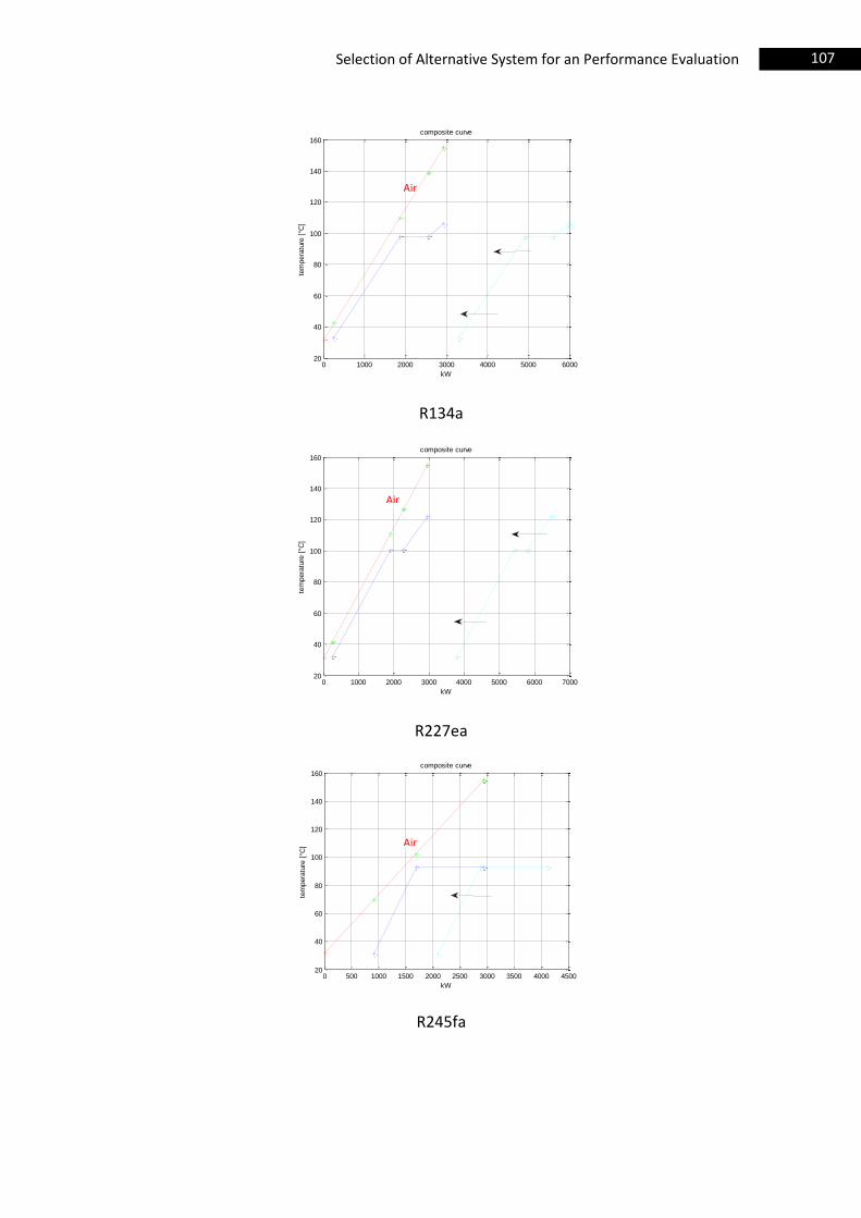
107 Selection of Alternative System for an Performance Evaluation
R134a
R227ea
R245fa
0 1000 2000 3000 4000 5000 600020
40
60
80
100
120
140
160composite curve
kW
tem
pera
ture
[°C
]
0 1000 2000 3000 4000 5000 6000 700020
40
60
80
100
120
140
160composite curve
kW
tem
pera
ture
[°C
]
0 500 1000 1500 2000 2500 3000 3500 4000 450020
40
60
80
100
120
140
160composite curve
kW
tem
pera
ture
[°C
]
Air
Air
Air
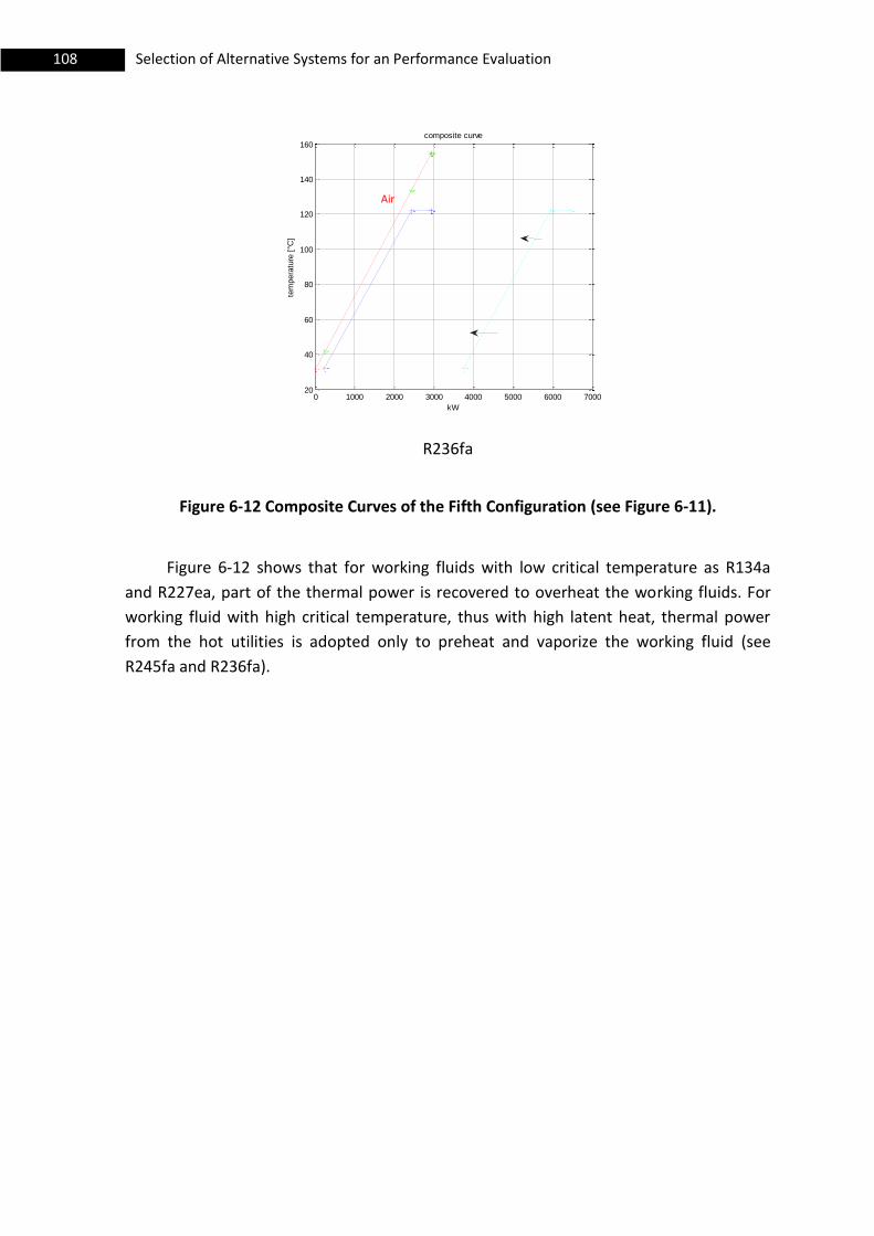
108 Selection of Alternative Systems for an Performance Evaluation
R236fa
Figure 6-12 Composite Curves of the Fifth Configuration (see Figure 6-11).
Figure 6-12 shows that for working fluids with low critical temperature as R134a
and R227ea, part of the thermal power is recovered to overheat the working fluids. For
working fluid with high critical temperature, thus with high latent heat, thermal power
from the hot utilities is adopted only to preheat and vaporize the working fluid (see
R245fa and R236fa).
0 1000 2000 3000 4000 5000 6000 700020
40
60
80
100
120
140
160composite curve
kW
tem
pera
ture
[°C
]
Air

109 Selection of Alternative System for an Performance Evaluation
6.8. Sixth configuration: Two Stage ORC System
In Section 6.7, the advantages of the fifth configuration (Figure 6-11) compared with
the other four configurations previously studied are explained. Using only the whole air
cooler thermal power, the output powers with two working fluids (R227ea and R236fa)
are the highest compared to the previous four configurations. But jacket water and oil
lubricating sources are still available, so in this section the system proposed (dual stage
system) in Section 2.8 is considered (Figure 6-13). Thus thermal power of jacket water and
lubricating oil are recovered as well.
1
2
4
3
5
w5
w2
a2
a4
6
9
8
7
lo1
lo3
Air cooler/ORC
Water/ORC
Oil/ORC
10
11
valve 1
valve 2
Turbine 1 Turbine 2
HIGH PRESSURE
STAGE
LOW PRESSURE
STAGE
Figure 6-13 Two stage ORC system.
Two stage ORC system comprises two working fluid pump, three heat exchangers,
two valves, two expansions and a water cooled condenser.
The working fluid is pumped (1-2) to the valve 1, where it is divided into two mass
flow rates. Mass flow rate is pumped (3-4) to the evaporator at high pressure (Air
cooler/ORC heat exchanger 4-5) where it is heated, vaporized and overheated by air
cooler. The generated high pressure vapor flows into Turbine 1 (5-6), and it drives the
generator and electric power ( ) is produced. Then the working fluid mass flow rate
is mixed to mass flow rate in valve 2. At the same time, after valve 1, mass flow
110 Selection of Alternative Systems for an Performance Evaluation
rate flows through Lubricating oil/ORC heat exchanger (9-10), and Jacket Water/ORC
heat exchanger (10-11) where it is heated, vaporized and overheated by lubricating oil
and jacket water. After the valve 2, the vapor working fluid flows into Turbine 2 (7-8)
where mechanical power is produced and in the generator it is converted in electric
power ( ). Then the working fluid is condensed in the condenser (8-1). The condensed
working fluid is pumped back to valve 1 and a new cycle begins. The condensation heat is
transferred to sea water.
The thermodynamic equations and the assumptions for the components are the
same as described in Section 5.2. Two more equations are introduced.
Mass balance at valve 1:
(6.4)
Energy balance at valve 2:
(6.5)
The low pressure stage in Figure 6-14 clearly suggests that it is difficult to have a
good match between composite curves, because most of the power from lubricating oil is
not recovered. The maximum power for the low pressure loop is obtained only for high
pressure (p2) and low mass flow rate ( ). Even if, the cooler temperature is 25°C of sea
water, Table 6-11 and Figure 6-14 show the thermal power recovered from lubricating oil
is 37, 50, 32, 41 kW for the working fluids: R134a, R227ea, R245fa, R236fa, respectively
and their values in proportional of the thermal power recovered from jacket water (There
is this comparison because both of them are the sources of the low pressure stage) are
10.5, 8.6, 7.7, 6.5 % for R134a, R227ea, R245fa and R236fa, respectively
The advantages using two stage system is the possibility to recover more thermal
power from the three heat sources (jacket water, lubricating oil, air cooler) than the other
five configuration studied. Table 6-11 shows that heat recovery efficiencies ( ) are about
77% for R236fa, R134a, R227ea and 48.7% for R245fa, the highest coefficient found
between the six configurations studied. Thus, the two stage ORC configuration produces
the highest power: 311 kW for R134a, 302.5 kW for R227ea, 260.26 kW for R245fa and
354.13 kW for R236fa. The highest total net efficiency ( ) is about 8.5% when R236fa is
adopted. The total efficiencies are 7.5, 7.2, 6.2% corresponding to R134a, R227ea, R245fa,
respectively (see Table 6-1). In comparison to the fifth configuration (the best solution of
the previous five configurations) the relative improvement in power is 13%, 14%, 16.7%
and 11.4% for fluids R134a, R227ea, R245fa and R236fa, respectively. R245fa has the
maximal improvement and R236fa has the minimum advantage, but its power is still the
highest.

111 Selection of Alternative System for an Performance Evaluation
Table 6-11 Main parameters of the sixth configuration (see Figure 6-13).
Parameter Working fluids
Symbol Units R134a R227ea R245fa R236fa
kW 4147 4147 4147 4147
kW 2677 2687 2020 2690
kW 477 477 477 477
kW 37 50 32 41
kW 3191 3214 2529 3208
Ta2 °C 154.9 154.9 154.9 154.9
Ta4 °C 43 41.97 70 41.9
Tw5 °C 72 72 72 72
Tw2 °C 68.9 68.9 68.9 68.9
Tlo1 °C 49.5 49.5 49.5 49.5
Tlo3 °C 49.1 48.9 49.12 49.03
T1 °C 30 30 30 30
T2 °C 30.74 30.54 31.16 30.30
T3 °C 30.74 30.54 31.16 30.30
T4 °C 32.52 31.97 31.53 31.86
T5 °C 106 122 92.82 122
T6 °C 62 93 68 60.8
T7 °C 62 85.9 66 60.6
T8 °C 32.1 67 44 39.89
T9 °C 30.74 30.54 30.54 30.30
T10 °C 39.4 39.5 39.5 39.5
T11 °C 62 59.86 59.6 59.74
bar 7.66 5.26 1.76 3.19
bar 16.53 11.59 4.51 7.5
bar 38 28.5 10.64 30
kg/s 16.25 20.18 11.21 18.57
kg/s 2.75 4.21 2.44 3.2
kg/s 15.97 15.97 8.77 15.37
hl kJ /kg K 0.11 0.11 0 0.0088
ll kJ /kg K 0 0 0 0
[-] 0.075 0.072 0.062 0.085
[-] 0.097 0.094 0.128 0.11
[-] 0.77 0.77 0.487 0.77
kW 311 302.5 260.26 354.13
Sp1 m 0.20 0.24 0.30 0.27
Sp2 m 0.33 0.41 0.53 0.50
v6/v5 - 2.69 2.93 2.50 6.83
v8/v7 - 2.25 2.32 2.54 2.46
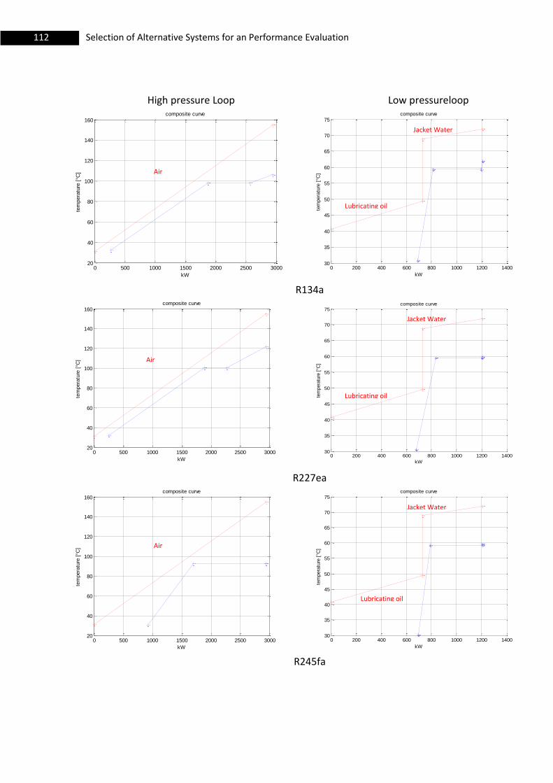
112 Selection of Alternative Systems for an Performance Evaluation
High pressure Loop Low pressureloop
R134a
R227ea
R245fa
0 500 1000 1500 2000 2500 300020
40
60
80
100
120
140
160composite curve
kW
tem
pera
ture
[°C
]
0 200 400 600 800 1000 1200 140030
35
40
45
50
55
60
65
70
75composite curve
kW
tem
pera
ture
[°C
]
0 500 1000 1500 2000 2500 300020
40
60
80
100
120
140
160composite curve
kW
tem
pera
ture
[°C
]
0 200 400 600 800 1000 1200 140030
35
40
45
50
55
60
65
70
75composite curve
kW
tem
pera
ture
[°C
]
0 500 1000 1500 2000 2500 300020
40
60
80
100
120
140
160composite curve
kW
tem
pera
ture
[°C
]
0 200 400 600 800 1000 1200 140030
35
40
45
50
55
60
65
70
75composite curve
kW
tem
pera
ture
[°C
]
Air
Air
Air
Jacket Water
Lubricating oil
Lubricating oil
Lubricating oil
Jacket Water
Jacket Water
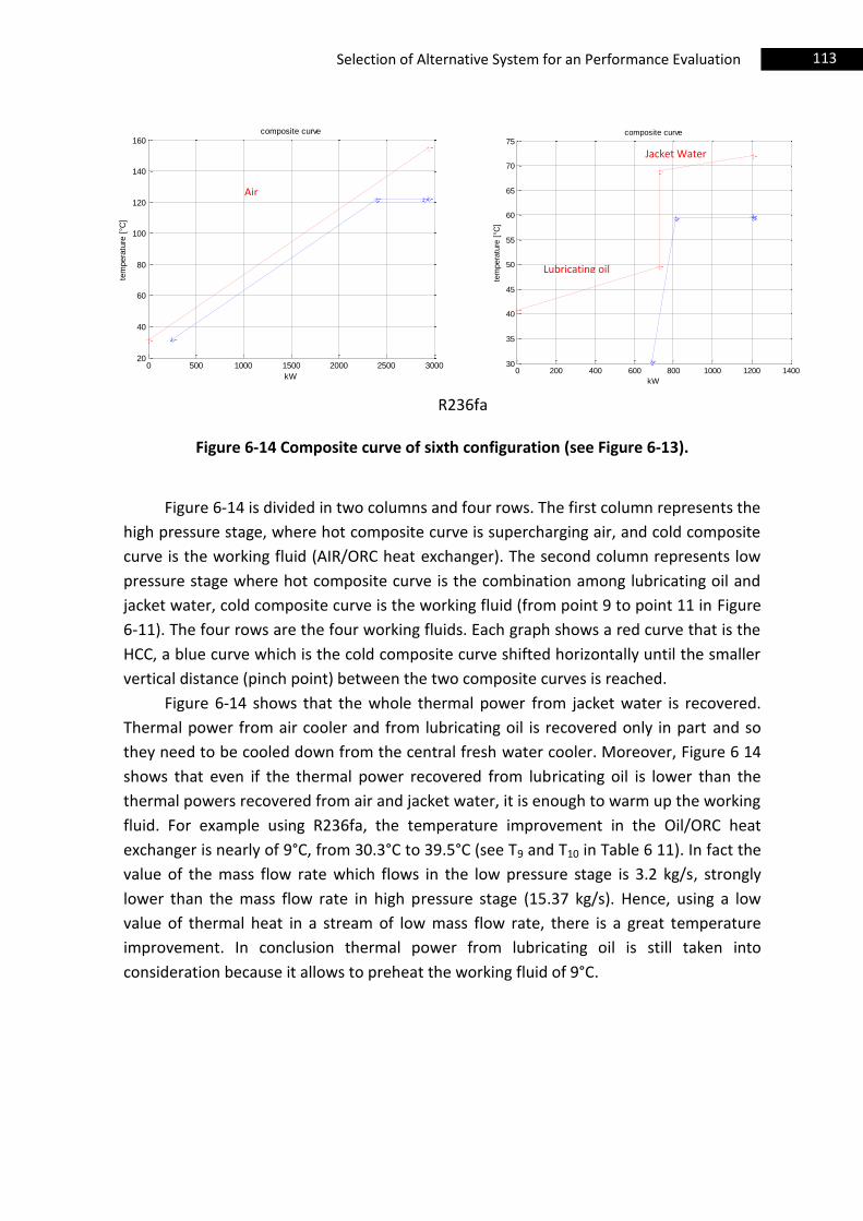
113 Selection of Alternative System for an Performance Evaluation
R236fa
Figure 6-14 Composite curve of sixth configuration (see Figure 6-13).
Figure 6-14 is divided in two columns and four rows. The first column represents the
high pressure stage, where hot composite curve is supercharging air, and cold composite
curve is the working fluid (AIR/ORC heat exchanger). The second column represents low
pressure stage where hot composite curve is the combination among lubricating oil and
jacket water, cold composite curve is the working fluid (from point 9 to point 11 in Figure
6-11). The four rows are the four working fluids. Each graph shows a red curve that is the
HCC, a blue curve which is the cold composite curve shifted horizontally until the smaller
vertical distance (pinch point) between the two composite curves is reached.
Figure 6-14 shows that the whole thermal power from jacket water is recovered.
Thermal power from air cooler and from lubricating oil is recovered only in part and so
they need to be cooled down from the central fresh water cooler. Moreover, Figure 6 14
shows that even if the thermal power recovered from lubricating oil is lower than the
thermal powers recovered from air and jacket water, it is enough to warm up the working
fluid. For example using R236fa, the temperature improvement in the Oil/ORC heat
exchanger is nearly of 9°C, from 30.3°C to 39.5°C (see T9 and T10 in Table 6 11). In fact the
value of the mass flow rate which flows in the low pressure stage is 3.2 kg/s, strongly
lower than the mass flow rate in high pressure stage (15.37 kg/s). Hence, using a low
value of thermal heat in a stream of low mass flow rate, there is a great temperature
improvement. In conclusion thermal power from lubricating oil is still taken into
consideration because it allows to preheat the working fluid of 9°C.
0 500 1000 1500 2000 2500 300020
40
60
80
100
120
140
160composite curve
kW
tem
pera
ture
[°C
]
0 200 400 600 800 1000 1200 140030
35
40
45
50
55
60
65
70
75composite curve
kW
tem
pera
ture
[°C
]
Air
Jacket Water
Lubricating oil
114 Selection of Alternative Systems for an Performance Evaluation
6.9. Conclusion
In this chapter an evaluation of ORC systems is described. Engine load of 80% was
considered as the design point for all ORC systems being considered. Several
configurations were investigated: five simple Rankine cycles, a regenerated system, and a
two-stages of ORC.
At first an ORC system was evaluated using the Hot Composite Curve at 80% of
engine load. This is an “ideal configuration” because the task to define the heat
exchanger network is not taken into consideration and the maximum output power is
estimated.
The first proposed configuration is similar to the cycle proposed by Yue et al. (2012),
with three sources: air cooler, jacket water and lubricating oil and with two different
condenser sources, sea water at 25°C and fresh water from the cooling system at 36°C.
The second configuration is a simple ORC with two heat sources (air cooler and
jacket water), and the condenser source is fresh water from the cooling system. It was
decided to investigate this system, because from the first configuration, when the fresh
water was used in the condenser, the maximum output power was obtained without the
lubricating oil heat. The second and third configurations have the same hot utility
(supercharging air and jacket water) and fresh water in the condenser, but in the third
configuration it is studied a regenerative ORC system. A condenser with fresh water at
36°C does not allow energy recovery from vapor outside of the expansion because the
difference temperature between the output of turbine and the output of the pump is too
low to have an heat exchange (see Table 6-8). On the other hand, a condenser with sea
water at 25°C allows to energy recovery from lubricating oil because the oil temperature
range is within 49.5°C and 42.7°C and the power obtained from this different
temperatures can be used to warm up the working fluid. Thus, the fourth configuration
has the three hot utilities (jacket water, lubricating oil, supercharging air), and sea wateris
adopted in the condenser. The fourth configuration needs several heat exchangers: three
preaheater, one evaporator and one superheater for the simple cycle (see R236fa
example in section 6.6 ). The fifth configuration was proposed to avoid this problem. Air
cooler thermal power is considered as the only one hot utility, so that only three heat
exchangers are required. The results of fifth configuration are close to the results of the
fourth configuration. This configuration suggests the possibility to have more power
realizing a dual stage system.
The sixth configuration proposes a two stage ORC system and sea water as a cold
utility. Supercharging air is the source of the high pressure stage and jacket water plus
lubricating oil are the heat sources of the low pressure stage.
In the first configuration, using fresh water as a cold utility the output powers
( ) are 140, 136, 134.8, 112 kW for R227ea, R236fa, R134a, R245fa but using sea
water as a cold utility, powers output ( ) are 180, 187.5, 182 for R236fa, R134a,
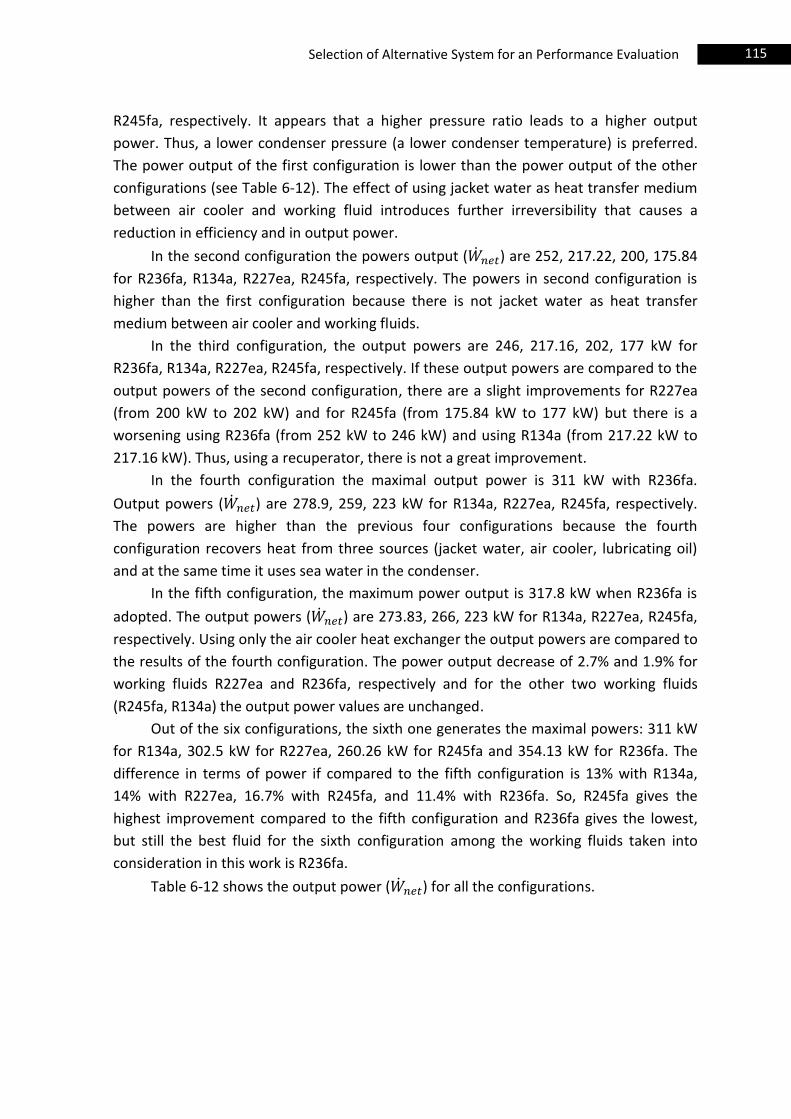
115 Selection of Alternative System for an Performance Evaluation
R245fa, respectively. It appears that a higher pressure ratio leads to a higher output
power. Thus, a lower condenser pressure (a lower condenser temperature) is preferred.
The power output of the first configuration is lower than the power output of the other
configurations (see Table 6-12). The effect of using jacket water as heat transfer medium
between air cooler and working fluid introduces further irreversibility that causes a
reduction in efficiency and in output power.
In the second configuration the powers output ( ) are 252, 217.22, 200, 175.84
for R236fa, R134a, R227ea, R245fa, respectively. The powers in second configuration is
higher than the first configuration because there is not jacket water as heat transfer
medium between air cooler and working fluids.
In the third configuration, the output powers are 246, 217.16, 202, 177 kW for
R236fa, R134a, R227ea, R245fa, respectively. If these output powers are compared to the
output powers of the second configuration, there are a slight improvements for R227ea
(from 200 kW to 202 kW) and for R245fa (from 175.84 kW to 177 kW) but there is a
worsening using R236fa (from 252 kW to 246 kW) and using R134a (from 217.22 kW to
217.16 kW). Thus, using a recuperator, there is not a great improvement.
In the fourth configuration the maximal output power is 311 kW with R236fa.
Output powers ( ) are 278.9, 259, 223 kW for R134a, R227ea, R245fa, respectively.
The powers are higher than the previous four configurations because the fourth
configuration recovers heat from three sources (jacket water, air cooler, lubricating oil)
and at the same time it uses sea water in the condenser.
In the fifth configuration, the maximum power output is 317.8 kW when R236fa is
adopted. The output powers ( ) are 273.83, 266, 223 kW for R134a, R227ea, R245fa,
respectively. Using only the air cooler heat exchanger the output powers are compared to
the results of the fourth configuration. The power output decrease of 2.7% and 1.9% for
working fluids R227ea and R236fa, respectively and for the other two working fluids
(R245fa, R134a) the output power values are unchanged.
Out of the six configurations, the sixth one generates the maximal powers: 311 kW
for R134a, 302.5 kW for R227ea, 260.26 kW for R245fa and 354.13 kW for R236fa. The
difference in terms of power if compared to the fifth configuration is 13% with R134a,
14% with R227ea, 16.7% with R245fa, and 11.4% with R236fa. So, R245fa gives the
highest improvement compared to the fifth configuration and R236fa gives the lowest,
but still the best fluid for the sixth configuration among the working fluids taken into
consideration in this work is R236fa.
Table 6-12 shows the output power ( ) for all the configurations.
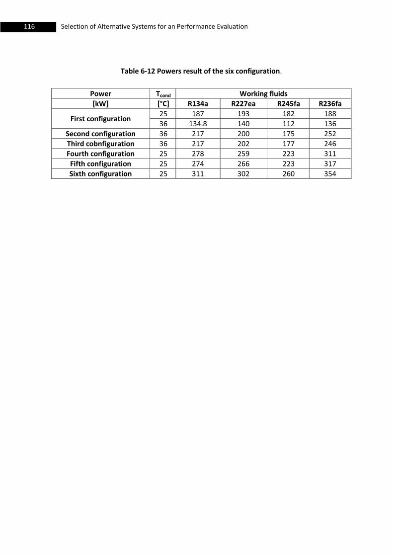
116 Selection of Alternative Systems for an Performance Evaluation
Table 6-12 Powers result of the six configuration.
Power Tcond Working fluids
[kW] [°C] R134a R227ea R245fa R236fa
First configuration 25 187 193 182 188
36 134.8 140 112 136
Second configuration 36 217 200 175 252
Third cobnfiguration 36 217 202 177 246
Fourth configuration 25 278 259 223 311
Fifth configuration 25 274 266 223 317
Sixth configuration 25 311 302 260 354
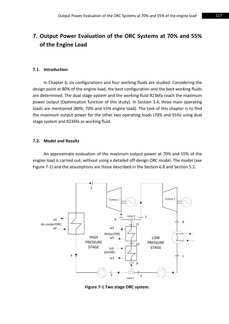
117 Output Power Evaluation of the ORC Systems at 70% and 55% of the engine load
7. Output Power Evaluation of the ORC Systems at 70% and 55%
of the Engine Load
7.1. Introduction
In Chapter 6, six configurations and four working fluids are studied. Considering the
design point at 80% of the engine load, the best configuration and the best working fluids
are determined. The dual stage system and the working fluid R236fa reach the maximum
power output (Optimization function of this study). In Section 3.4, three main operating
loads are mentioned (80%, 70% and 55% engine load). The task of this chapter is to find
the maximum output power for the other two operating loads (70% and 55%) using dual
stage system and R236fa as working fluid.
7.2. Model and Results
An approximate evaluation of the maximum output power at 70% and 55% of the
engine load is carried out, without using a detailed off-design ORC model. The model (see
Figure 7-1) and the assumptions are those described in the Section 6.8 and Section 5.2.
1
2
4
3
5
w5
w2
a2
a4
6
9
8
7
lo1
lo3
Air cooler/ORC
Water/ORC
Oil/ORC
10
11
valve 1
valve 2
Turbine 1 Turbine 2
HIGH PRESSURE
STAGE
LOW PRESSURE
STAGE
Figure 7-1 Two stage ORC system.
118
Output Power Evaluation of the ORC Systems at 70% and 55% of the engine load
Mass flow rate and pressure are supposed variable and efficiency of pumps and
turbines are kept constant. Two more constraints are included in these simulations. Mass
flow rate and pressure of both stages cannot reach higher values than those at 80% of the
engine load.
The minimum approach temperature is set at 10°C in the evaporator and 5°C in the
condenser in accordance with Lakew and Bolland (2010). Seawater at 25°C (ISO condition)
is adopted as a cooling medium in the condenser. The values of the three hot utilities are
2402 kW from the air cooler, 693 kW from lubricating oil and 415 kW from jacket water at
70% of the main engine load. At 55% main engine load the thermal powers are 1598 kW,
241 kW, 627 kW from air cooler, jacket water and lubricating oil, respectively. The
amount of heat available at 70% of the engine load is 3510 kW, whereas at 55% engine
load is 2466 kW.
Table 7-1 summarizes the main parameters described in Figure 6-13. At 70% engine
load, output power ( ) is equal to 182.44 kW and the net efficiency system ( ) is
equal to 5.2%. At 55% engine load, output power ( ) is equal to 75 kW and the net
efficiency system ( ) is equal to 3%.
From Table 7-1 and Table 6-11, it is possible to see that in the high pressure stage
the evaporation pressure varies in a wide range from 30 bar (80% engine load) to 8.65 bar
(55% engine load), while in the low pressure stage the evaporation pressure is lower from
7.5 bar (80% engine load) to 6.53 bar (55% engine load). These two different pressure
ranges can be explained with the fact that jacket water and lubricating oil do not vary
much in the different engine loads, but the power of the air cooler is reduced by 55% at
55% engine load, decreasing the performance of the high pressure stage and
consequently of the ORC.
Figure 7-2 is divided in two rows and two columns. Rows depict engine loads, first
row 70% engine load, second row 55% engine load. First column represents high pressure
stage where hot composite curve is supercharging air, and cold composite curve is the
working fluid (AIR/ORC heat exchanger in Figure 7-1). Second column represents low
pressure stage where hot composite curve is the combination among lubricating oil and
jacket water, cold composite curve is the working fluid (from point 9 to point 11 in Figure
7-1). Each graph shows a red curve that is the HCC, a blue curve which is the cold
composite curve shifted horizontally until the smaller vertical distance (pinch point)
between the two composite curves is reached.
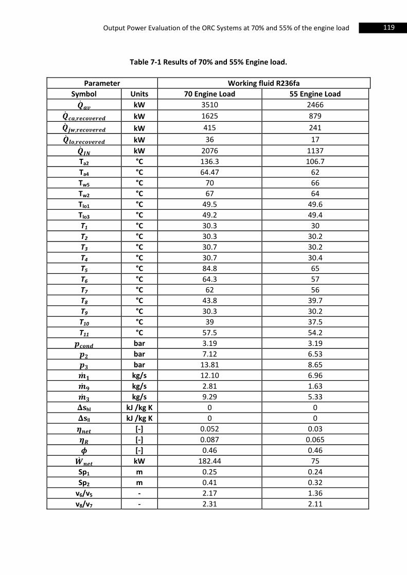
119 Output Power Evaluation of the ORC Systems at 70% and 55% of the engine load
Table 7-1 Results of 70% and 55% Engine load.
Parameter Working fluid R236fa
Symbol Units 70 Engine Load 55 Engine Load
kW 3510 2466
kW 1625 879
kW 415 241
kW 36 17
kW 2076 1137
Ta2 °C 136.3 106.7
Ta4 °C 64.47 62
Tw5 °C 70 66
Tw2 °C 67 64
Tlo1 °C 49.5 49.6
Tlo3 °C 49.2 49.4
T1 °C 30.3 30
T2 °C 30.3 30.2
T3 °C 30.7 30.2
T4 °C 30.7 30.4
T5 °C 84.8 65
T6 °C 64.3 57
T7 °C 62 56
T8 °C 43.8 39.7
T9 °C 30.3 30.2
T10 °C 39 37.5
T11 °C 57.5 54.2
bar 3.19 3.19
bar 7.12 6.53
bar 13.81 8.65
kg/s 12.10 6.96
kg/s 2.81 1.63
kg/s 9.29 5.33
hl kJ /kg K 0 0
ll kJ /kg K 0 0
[-] 0.052 0.03
[-] 0.087 0.065
[-] 0.46 0.46
kW 182.44 75
Sp1 m 0.25 0.24
Sp2 m 0.41 0.32
v6/v5 - 2.17 1.36
v8/v7 - 2.31 2.11
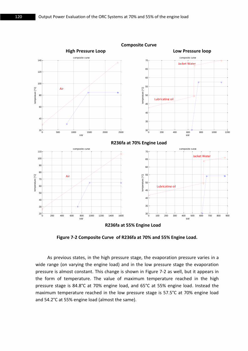
120
Output Power Evaluation of the ORC Systems at 70% and 55% of the engine load
Composite Curve High Pressure Loop Low Pressure loop
R236fa at 70% Engine Load
R236fa at 55% Engine Load
Figure 7-2 Composite Curve of R236fa at 70% and 55% Engine Load.
As previous states, in the high pressure stage, the evaporation pressure varies in a
wide range (on varying the engine load) and in the low pressure stage the evaporation
pressure is almost constant. This change is shown in Figure 7-2 as well, but it appears in
the form of temperature. The value of maximum temperature reached in the high
pressure stage is 84.8°C at 70% engine load, and 65°C at 55% engine load. Instead the
maximum temperature reached in the low pressure stage is 57.5°C at 70% engine load
and 54.2°C at 55% engine load (almost the same).
0 500 1000 1500 2000 250020
40
60
80
100
120
140composite curve
kW
tem
pera
ture
[°C
]
0 200 400 600 800 1000 120030
35
40
45
50
55
60
65
70composite curve
kW
tem
pera
ture
[°C
]
0 200 400 600 800 1000 1200 1400 160020
30
40
50
60
70
80
90
100
110composite curve
kW
tem
pera
ture
[°C
]
0 100 200 300 400 500 600 700 800 90030
35
40
45
50
55
60
65
70composite curve
kW
tem
pera
ture
[°C
]
Jacket Water
Jacket Water
Lubricating oil
Lubricating oil
Air
Air
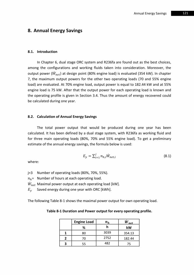
121 Annual Energy Savings
8. Annual Energy Savings
8.1. Introduction
In Chapter 6, dual stage ORC system and R236fa are found out as the best choices,
among the configurations and working fluids taken into consideration. Moreover, the
output power ( ) at design point (80% engine load) is evaluated (354 kW). In chapter
7, the maximum output powers for the other two operating loads (70 and 55% engine
load) are evaluated. At 70% engine load, output power is equal to 182.44 kW and at 55%
engine load is 75 kW. After that the output power for each operating load is known and
the operating profile is given in Section 3.4. Thus the amount of energy recovered could
be calculated during one year.
8.2. Calculation of Annual Energy Savings
The total power output that would be produced during one year has been
calculated. It has been defined by a dual stage system, with R236fa as working fluid and
for three main operating loads (80%, 70% and 55% engine load). To get a preliminary
estimate of the annual energy savings, the formula below is used:
∑ (8.1)
where:
j=3 Number of operating loads (80%, 70%, 55%).
= Number of hours at each operating load.
Maximal power output at each operating load [kW].
Saved energy during one year with ORC [kWh].
The following Table 8-1 shows the maximal power output for own operating load.
Table 8-1 Duration and Power output for every operating profile.
Engine Load
% h kW
1 80 3039 354.13
2 70 2752 182.44
3 55 482 75
122 Annual Energy Savings
After this information (Table 8-1 and Eq(8.1)), the value of annual energy savings
( ) is 1614 MWh per year, as given by Eq.(8.2):
(8.2)
The average power during a year is:
(8.3)
where:
Total hours number of the operating main engine (6273 h).
ORC Power output if ORC operates at constant power.
is equal to 257 kW, that means 72% of the ORC design power. The electricity
on board is supplied by three Diesel generator sets. The type of all Diesel generators is
L23/30H of the MAN B &W. One of them works during the “voyage”, the second works
only during the cargo unloading (the ship needs more electric power for the operation)
and the third is on reserve. The specific fuel consumption is 191.3 g/kWh in reference
condition (ISO 3046) for the diesel generator sets. Under this assumption (the specific fuel
consumption) and with the annual energy savings, a saving of 308.7 tons of fuel (Marine
Diesel oil) per year is achieved, as derived by the following equation
[ ] [
] (8.4)
where:
fuel savings.
annual energy savings.
specific fuel consumption of the engine generator sets (191.3 g/kWh).
123 Economic Feasibility
9. Economic Feasibility
9.1. Introduction
The two stage ORC system is analyzed from an economic point of view. During one
year the energy savings is 1614 MWh (using dual stage system and R236fa as working
fluid) and 308.7 tons of fuel (Marine Diesel Oil) are saved, see Chapter 8. The economic
feasibility of the two stage ORC system is assessed by three parameters: Net Present
Value (NPV), Dynamic Payback Period (DPP) and Internal Rate of Return (IRR). In Chapter
9, at first Economic Feasibility model is explained and then it will be used for the
configuration chosen in Chapter 6.
9.2. Parameters of Economic Feasibility
NPV (net present value) is defined as the sum of discounted cash inflows and
outflows, in order to compare the present value of an investment to the value of saving
that will be obtained in well-defined period. NPV is describe by Eq. (9.1):
∑
( )
(9.1)
where
i considered year
Fi net annual cash flow for year i
a market discount rate
ny economic analysis period
The net annual cash flow rate for the year I (Fi) is given by Eq. (9.2) and Eq. (9.3):
Fi=-C (first year i=0) (9.2)
Fi= Cfs,i-Com,i (i=1,2... ny) (9.3)
Com,i= Com,ORC,i-Com,EG,I (i=1,2... ny) (9.4)
(9.5)
where
C initial investment
Cfs,i cost of fuel saved
Com,ORC,i cost of operating and maintenance of the ORC
124 Economic Feasibility
Com,EG,i savings of operation and maintenance of the diesel-generator sets
Com sum of operating and maintenance cost between the ORC and the Diesel-
generator sets
Ey energy saved
bf specific fuel energy consumption of the engine-generator sets
unit cost of the fuel
The energy annual saving (Ey) and the cost of the fuel (cf) are considered constant so
the Eq. (9.1) can be rewrite:
∑
( )
(9.6)
Also the market discount rate (a) is considered constant during the period studied.
Based on this, Eq. (9.6) can be reedited in this form:
( )
(9.7)
Dynamic Payback Period (DPP), which is defined by the Eq. (9.8) evaluates how long
a given ORC system will pay for itself.
( )
(9.8)
Under the specific assumptions (market discount rate, cost of the fuel, annual
saving are considered constant), DPP is evaluated by Eq. (9.9).
(
)
( ) (9.9)
If it is:
(9.10)
Eq. (9.9) does not have a solution, and the configuration considered will require an infinitive number of years, in order to recover the initial investment.
The internal rate of return (IRR) is the interest that makes the Net Present Value equal to zero at the end of the period studied:
( )
(9.11)
125 Economic Feasibility
( )
(9.12)
( )
(9.13)
Thus IRR is given by Eq. (9.13). 9.3. Economic Feasibility of dual Stage ORC
The model described in Section 9.2 is used on the dual stage ORC. The energy
annual saving (Ey) and the cost of the fuel (cf) are considered constant. The initial
investment (C) is considered proportional to the maximal net power of the system. The
range of the initial investment is chosen from 2000 US$/kW to 8000 US$/kW. The value
Com (sum of the operation and maintenance cost of the ORC and diesel-generator sets) is
considered proportional to the MWh produced by ORC system in the first year, moreover
Com is kept constant during the whole period taken into account (20 years). The specific
fuel consumption (bf) is 191.3 g/kWh in reference condition (ISO 3046) for the diesel
generators. The range of the Marine Diesel Oil is chosen between 500 US$/ton and 1000
US$/ton.
These assumptions for the calculations are reported in Table 9-1.
Table 9-1 Values of the parameters for the economic analysis.
Parameter Value
Symbol Units [-]
ny years 20
a % 8
bf g/kWh 191.3
kW 354.13
Ey kWh 1614
Com US$/MWh 3
cf US$ 500-1000
The results are summarized in the following table and graphs.
126 Economic Feasibility
Table 9-2 is divided in two parts: on the top the initial investment is presented, and
on the bottom the net present value (NPV) is calculated as a function of the initial
investment and of the fuel cost. In the white cells the investment can be economically
attractive. In the cells with a pink background the investment is not profitable, because
the NPV value is negative and with those two conditions (fuel cost and initial investment),
the ORC system will not pay for itself. Table 9-3 shows the dynamic payback period as a
function of the initial investment and of the fuel cost. In the white cells the investment
can be profitable, and in the pink cells the dynamic payback period is longer than twenty
years (period of the economic analysis). In the red boxes, Eq. (9.9) does not have a
solution because the argument of the logarithm is not positive number. The meaning is
that, if the market discount is considered 0.08 (assumption of this study), the
configuration will never recover the initial investment under the specific data. In order to
recover the initial investment, the market discount has to be lower than the market
discount considered in the study. Table 9-4 reports the internal rate of return (the
interest that makes the Net Present Value equal to zero at the end of the period studied)
as a function of the fuel cost and initial investment. Under the same specific data of the
red boxes in Table 9-3, the internal rate of return is lower than the market discount
considered (8%). Moreover, net present value, payback period, internal rate of return are
described in Figure 9-1, Figure 9-2 and Figure 9-3, respectively as functions of the fuel
cost and of the specific cost of the initial investment. In the graphs, the x-axis are the
initial investment, the ordinate represents NPV in Figure 9-1, dynamic Payback period in
Figure 9-2, and internal rate of return in Figure 9-3. Moreover in each graph there are five
curves, each one considers a different fuel (Marine Diesel Oil) cost from 500 to 1000
US$/ton.
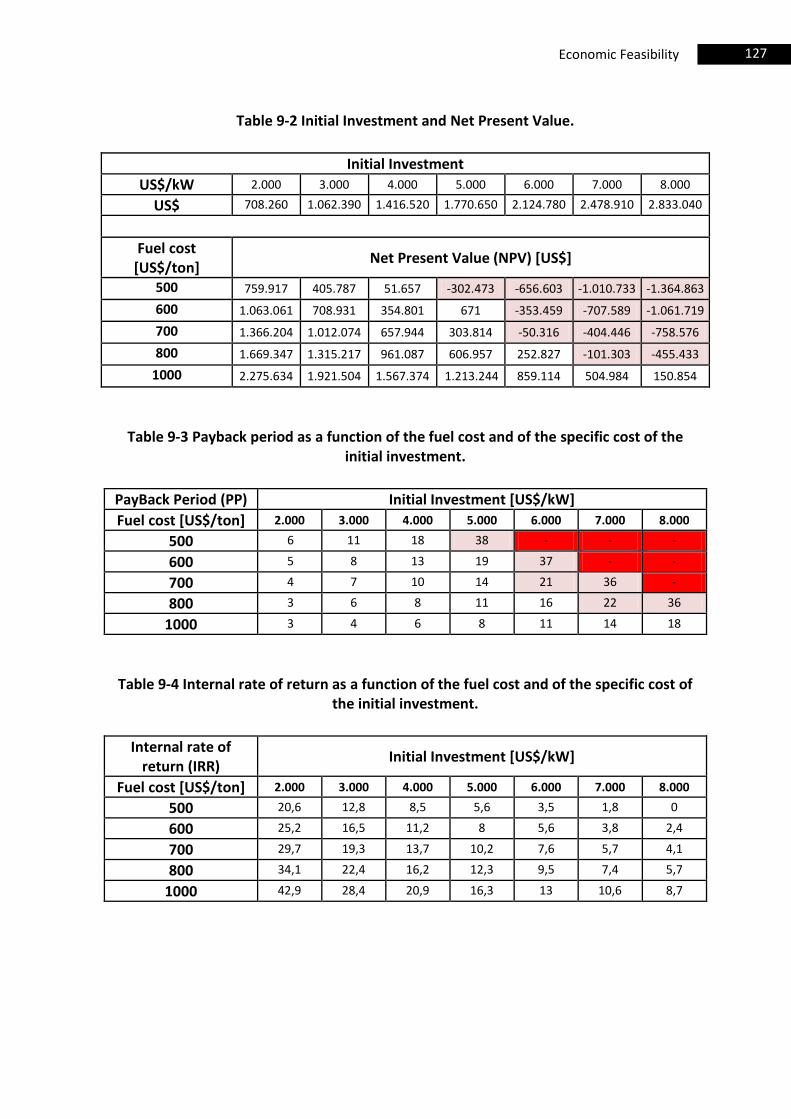
127 Economic Feasibility
Table 9-2 Initial Investment and Net Present Value.
Initial Investment
US$/kW 2.000 3.000 4.000 5.000 6.000 7.000 8.000
US$ 708.260 1.062.390 1.416.520 1.770.650 2.124.780 2.478.910 2.833.040
Fuel cost [US$/ton]
Net Present Value (NPV) [US$]
500 759.917 405.787 51.657 -302.473 -656.603 -1.010.733 -1.364.863
600 1.063.061 708.931 354.801 671 -353.459 -707.589 -1.061.719
700 1.366.204 1.012.074 657.944 303.814 -50.316 -404.446 -758.576
800 1.669.347 1.315.217 961.087 606.957 252.827 -101.303 -455.433
1000 2.275.634 1.921.504 1.567.374 1.213.244 859.114 504.984 150.854
Table 9-3 Payback period as a function of the fuel cost and of the specific cost of the initial investment.
PayBack Period (PP) Initial Investment [US$/kW]
Fuel cost [US$/ton] 2.000 3.000 4.000 5.000 6.000 7.000 8.000
500 6 11 18 38 - - -
600 5 8 13 19 37 - -
700 4 7 10 14 21 36 -
800 3 6 8 11 16 22 36
1000 3 4 6 8 11 14 18
Table 9-4 Internal rate of return as a function of the fuel cost and of the specific cost of the initial investment.
Internal rate of return (IRR)
Initial Investment [US$/kW]
Fuel cost [US$/ton] 2.000 3.000 4.000 5.000 6.000 7.000 8.000
500 20,6 12,8 8,5 5,6 3,5 1,8 0
600 25,2 16,5 11,2 8 5,6 3,8 2,4
700 29,7 19,3 13,7 10,2 7,6 5,7 4,1
800 34,1 22,4 16,2 12,3 9,5 7,4 5,7
1000 42,9 28,4 20,9 16,3 13 10,6 8,7
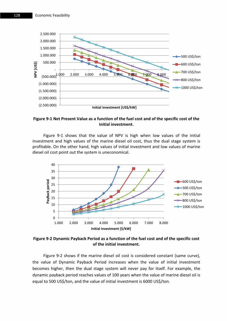
128 Economic Feasibility
Figure 9-1 Net Present Value as a function of the fuel cost and of the specific cost of the initial investment.
Figure 9-1 shows that the value of NPV is high when low values of the initial
investment and high values of the marine diesel oil cost, thus the dual stage system is profitable. On the other hand, high values of initial investment and low values of marine diesel oil cost point out the system is uneconomical.
Figure 9-2 Dynamic Payback Period as a function of the fuel cost and of the specific cost
of the initial investment.
Figure 9-2 shows if the marine diesel oil cost is considered constant (same curve),
the value of Dynamic Payback Period increases when the value of initial investment
becomes higher, then the dual stage system will never pay for itself. For example, the
dynamic payback period reaches values of 100 years when the value of marine diesel oil is
equal to 500 US$/ton, and the value of initial investment is 6000 US$/ton.
(2.500.000)
(2.000.000)
(1.500.000)
(1.000.000)
(500.000)
-
500.000
1.000.000
1.500.000
2.000.000
2.500.000
1.000 2.000 3.000 4.000 5.000 6.000 7.000 8.000
NP
V [
US$
]
Initial investment [US$/kW]
500 US$/ton
600 US$/ton
700 US$/ton
800 US$/ton
1000 US$/ton
0
5
10
15
20
25
30
35
40
1.000 2.000 3.000 4.000 5.000 6.000 7.000 8.000
Pay
Bac
k p
eri
od
Initial investment [$/kW]
600 US$/ton
500 US$/ton
700 US$/ton
800 US$/ton
1000 US$/ton
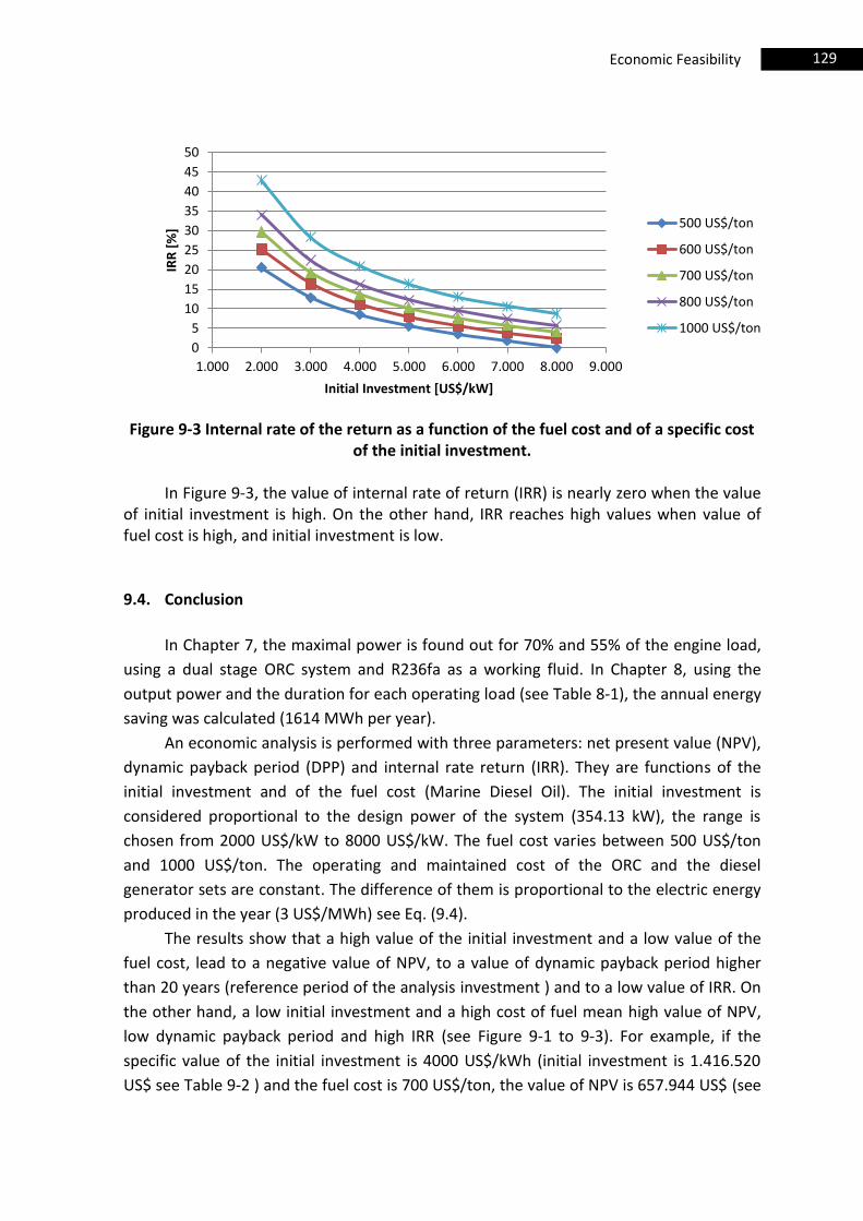
129 Economic Feasibility
Figure 9-3 Internal rate of the return as a function of the fuel cost and of a specific cost
of the initial investment.
In Figure 9-3, the value of internal rate of return (IRR) is nearly zero when the value of initial investment is high. On the other hand, IRR reaches high values when value of fuel cost is high, and initial investment is low. 9.4. Conclusion
In Chapter 7, the maximal power is found out for 70% and 55% of the engine load,
using a dual stage ORC system and R236fa as a working fluid. In Chapter 8, using the
output power and the duration for each operating load (see Table 8-1), the annual energy
saving was calculated (1614 MWh per year).
An economic analysis is performed with three parameters: net present value (NPV),
dynamic payback period (DPP) and internal rate return (IRR). They are functions of the
initial investment and of the fuel cost (Marine Diesel Oil). The initial investment is
considered proportional to the design power of the system (354.13 kW), the range is
chosen from 2000 US$/kW to 8000 US$/kW. The fuel cost varies between 500 US$/ton
and 1000 US$/ton. The operating and maintained cost of the ORC and the diesel
generator sets are constant. The difference of them is proportional to the electric energy
produced in the year (3 US$/MWh) see Eq. (9.4).
The results show that a high value of the initial investment and a low value of the
fuel cost, lead to a negative value of NPV, to a value of dynamic payback period higher
than 20 years (reference period of the analysis investment ) and to a low value of IRR. On
the other hand, a low initial investment and a high cost of fuel mean high value of NPV,
low dynamic payback period and high IRR (see Figure 9-1 to 9-3). For example, if the
specific value of the initial investment is 4000 US$/kWh (initial investment is 1.416.520
US$ see Table 9-2 ) and the fuel cost is 700 US$/ton, the value of NPV is 657.944 US$ (see
0
5
10
15
20
25
30
35
40
45
50
1.000 2.000 3.000 4.000 5.000 6.000 7.000 8.000 9.000
IRR
[%
]
Initial Investment [US$/kW]
500 US$/ton
600 US$/ton
700 US$/ton
800 US$/ton
1000 US$/ton

130 Economic Feasibility
Table 9-3Table 9-2), the dynamic payback period is equal to 10 years (see Table 9-3), and
the IRR is equal to 13.7% (see Table 9-4).
131 Conclusion
10. Conclusion
In the present study, heat recovery power generation system applied to the cooling
system of the main engine of a tanker ship was investigated. In the literature review,
R227ea, R134a, R245fa, R236fa are supposed to be the best working fluids for this
project. In chapter 3, the energy balance is evaluated. Air cooler, jacket water, lubricating
oil heats are available for ORC cycle. Waste heat from exhaust gas is already recovered by
the exhaust gas boiler. The energy balance is evaluated for the three main operating
loads: 80%, 70% and 55% of the main engine (see Table 3-8). The hot composite curves
for each operating load are built in Chapter 4 (see Figure 4-2). The operating load at 80%
of the main engine is chosen as a design point for the ORC system. Several configurations
were studied in Chapter 6.
At first a simple ORC system was evaluated, using the HCC at 80% engine load. Note
that, according to this approach, the heat exchanger network within the ORC system
remains undefined and can be found by applying Pinch Analysis rules. Two cold utilities in
the condenser are compared, sea water at 25°C and fresh water from cooling system at
36°C.Using the sea water at 25°C as cooling medium in the condenser, the maximum
power output (323 kW) is achieved by R236fa. The Power output values for the remaining
fluids are 280.5, 280.13, 225 kW for R134a, R227ea, R245fa, respectively. Using fresh
water at 36°C as cooling medium in the condenser, the maximum power output
achievable is 255kW using R236fa. The power output values for the remaining fluids are
221, 209, 181 kW for R134a, R227ea, R245fa, respectively. The use of sea water for
condenser cooling results in lower condensation temperatures, and consequently lower
condensation pressures. The turbine operates with higher pressure ratios and it produces
more power for the same mass flow rate .
The first proposed configuration recovers heat from the three heat source:
supercharging air, jacket water, lubricating oil but it does not consider heat exchange
between air cooler and working fluid. Jacket water is used as heat transfer medium
between air cooler and working fluid. Thus working fluid exchanges heat with jacket
water and lubricating oil in a simple Rankine cycle. Also in this configuration two cold
utilities in the condenser are compared (sea water and fresh water). Using sea water as
cooling medium in the condenser, the maximum output power is about 193 kW, achieved
by R227ea. The power output for the remaining fluids is 180, 187.5, 182 for R236fa,
R134a, R245fa, respectively. Using fresh water at 36°C, the maximum power output is
140kW adopting R227ea and the output powers for the remaining fluids are 136, 134.8,
112 kW for R236fa, R134a, R245fa. These results clearly show that using this
132 Conclusion
configuration the power output of all working fluids is strongly reduced. This eventuality
is described by the fact that input thermal power of the simple ORC system is low,
because Jack water is used as heat transfer between air cooler and working fluid, and the
temperature of the jacket water is kept low to avoid steam in the pipes.
The second configuration is a simple ORC with two heat sources (from air cooler
and jacket water), and fresh water as cooling medium in the condenser. It was decided to
investigate this system, because from the first configuration, when the fresh water was
used in the condenser, the maximum output power was obtained without the lubricating
oil heat. In the second configuration the power output values are 252, 217.22, 200,
175.84 for R236fa, R134a, R227ea, R245fa, respectively. In second configuration the
power is higher than in the first configuration because there is not jacket water as heat
transfer medium between air cooler and working fluids.
The third configuration is a regenerated ORC system with two heat sources (from
air cooler and jacket water) and fresh water (36°C) as cold utility. The output power
values are 246, 217.16, 202, 177 kW for R236fa, R134a, R227ea, R245fa, respectively. If
these output powers are compared to the output power values of the second
configuration, there is a slight improvement for R227ea (from 200 kW to 202 kW) and for
R245fa (from 175.84 kW to 177 kW) but there is a worsening using R236fa (from 252 kW
to 246 kW) and using R134a (from 217.22 kW to 217.16 kW). Thus, using a recuperator,
there is not a great improvement. A condenser with fresh water at 36°C does not allow
energy recovery from vapor after the expansion because the difference of temperature
between the output of the turbine and the output of the pump is too low to have an heat
exchange. On the other hand, a condenser with sea water at 25°C allows energy recovery
from lubricating oil because the oil temperature range is within 49.5°C and 42.7°C and the
power obtained from this temperature difference can be used to warm up the working
fluid.
Thus, the fourth configuration recovers heat from the three hot utilities, and sea
water is adopted as cold utility in the condenser. Maximal output power is 311 kW
reached by R236fa. Output powers for the remaining fluids are 278.9, 259, 223 kW for
R134a, R227ea, R245fa, respectively. The powers are higher than the previous
configurations because the fourth configuration recovers heat from the three sources and
at the same time it uses sea water in the condenser. The fact that the surface has to be
cleaned regularly to avoid deposition of salts and corrosion and the need for a clever
selection of materials (no copper alloys can be used) represent two disadvantages of sea
water cooling. On the other hand, if the increase of net power output can cover the
cleaning cost of the heat exchanger, this solution is convenient.
The fifth configuration explores the possibility to recover energy only from air
cooler, and sea water is used as cooling medium in the condenser. The maximum power
output is 317.8 kW achieved by R236fa. The output powers for the remaining fluids are
273.83, 266, 223 kW for R134a, R227ea, R245fa, respectively. Using only the thermal
133 Conclusion
power from supercharging air the output powers are close to the results obtained from
the fourth configuration, even if jacket water and lubricating oil sources are still available.
Thus the sixth configuration proposes a two stage ORC system and sea water as a
cooling medium in the condenser. Supercharging air is the source of the high pressure
stage. Jacket water plus lubricating oil are the heat sources of the low pressure stage. Out
of the six configurations, the sixth one generates the maximal powers: 311 kW for R134a,
302.5 kW for R227ea, 260.26 kW for R245fa and 354.13 kW for R236fa. If compared to
the fifth configuration, the improvement in terms of power is 13% with R134a, 14% with
R227ea, 16.7% with R245fa, and 11.4% with R236fa. So, R245fa gives the highest
improvement compared to the fifth configuration and R236fa gives the lowest, but
R236fa is still the best fluid for the sixth configuration among the working fluids taken
into consideration in this work.
The dual stage ORC system with R236fa as a working fluid leads the maximum net
power output (354.13 kW); the thermodynamic properties are listed in (Table 6-11). Using
the same configuration and the same working fluid the net power outputs are 182.44 kW
and 75 kW for 70% and 55% of the engine load, respectively. These powers are found
without a detailed off-design ORC model. The annual energy saving was calculated (1614
MWh per year), and it leads to 308 tons of marine diesel oil saved (Section 8.2) using the
output power and the duration for each operating load (see Table 8-1),
An economic analysis is performed with three parameters: net present value (NPV),
dynamic payback period (DPP) and internal rate return (IRR). They are functions of the
initial investment and of the fuel cost (Marine Diesel Oil). The initial investment is
considered proportional to the design power of the system and the range is chosen from
2000 US$/kW to 8000 US$/kW. The fuel cost varies between 500 US$/ton and 1000
US$/ton. The sum of operating and maintenance cost of the ORC and the diesel generator
sets are considered constant. The difference of them (see Eq. (9.4)) is proportional to the
electric energy produced in the year (3 US$/MWh). The parameters NPV, DPP, IRR are
showed in Tables 9.2, 9.3, 9.4 and in Figures 9.1, 9.2, 9.3. The results show that a high
value of the initial investment and a low value of the fuel cost, lead to a negative value of
NPV, to a value of dynamic payback period higher than 20 years (reference period of the
analysis investment) and to a low value of IRR. The dual stage system is not convenient.
On the other hand, a low initial investment and an high cost of fuel mean a high value of
NPV, low dynamic payback period and high IRR. Therefore the dual stage system could be
profitable.
Nowadays, the cost of fuel is around of 600 US$/ton. It means that the dual stage
ORC system (using the assumption and the economic model in chapter 8) is profitable, if
the cost of the initial investment is below 5000 US$/kW (see section 9.3). In fact, if 5000
US$/kW is taken into consideration, net present value (NPV) is equal to 671 US$, dynamic
payback period is nearly to 20 years and the internal rate of return (IRR) is 8% (same value
considered in the model in Section 9.3).

134 Conclusion
135 Suggestions for further work
11. Suggestions for further work
In order to improve and to continue the present work, I suggest to develop an off-
design model. To investigate the exact amount of electrical power produced (therefore
the energy saved in one year) at 70% and 55% engine load, it could be used a dual stage
system (sixth configuration, which reaches highest value of electric output power), and
also simple ORC (fourth and fifth configurations which need less space than the sixth
configuration). In this way two objectives could be investigated: the maximal output
power produced and the space occupied. After that, the work requires a study of
economic feasibility: the cost for each component, the cost for the installation of the ORC
system on board, and all the issues which concern marine application must be taken into
account.

136 Bibliography
137 Bibliography
Bibliography
Andersen W.C., Bruno T.J. (2005), “Rapid screening of fluids for chemical stability in
Organic Rankine Cycles applications,” Industrial and Engineering Chemistry
Research, Vol. 44, pp. 5560-5566.
Angelino G., Gaia M., Macchi M. (1984), “A review of Italian activity in the field of Organic
rankine cycle,”, Proceedings of the international VDI-Seminar held, Zürich, 10-12
September.
Bao Junjiang, Zhao Li (2013), “A review of working fluid and expander selections for
Organic Rankine cycle,”, Renewable and Sustainable Energy Reviews, Vol. 24 pp.
325-342.
Bejan A., Tsatsaronis G., Moran M. (1996), “Thermal Design and Optimization,” John
Wiley & Sons, New York.
Borsukiewicz-Gozdur (2010), “A. Dual-fluid-hybrid power plant co-powered by low temperature geothermal water” Geothermics, Vol. 39, pp. 170–6.
Calderazzi L., Di Paliano P.C. (1997), “Thermal stability of R-134, R-141b, R-131, R-7146, R-
125 associated with stainless steel as a containing material,” International Journal of
Refrigerant, Vol. 20, pp. 381-389.
Chen H., Yogi Goswami D., Stefanakos E.K, (2010), “A review of thermodynamic cycles and
working fluids for the conversion of low-grade heat”, Renewable and Sustainable
Energy Reviews, Vol. 34, pp. 3059-3067.
Chen H., Goswami Y.D., Rahman M.M., Stefanakos E.K. (2011), “Energetic and exergetic
analysis of CO2- and R32-based transcritical Rankine cycles for low-grade heat
conversion,” Applied Energy, Vol. 88, pp. 2802-2808.
Choi C. B., Kim Min Y. (2013), “Thermodynamic analysis of a dual loop heat recovery
system with trilateral cycle applied to exhaust gases of internal combustion engine
for propulsion of the 6800 TEU container ship”, Energy, Vol.1 pp. 1-13.
Eide M., Chryssakis C., Alvik S., Endresen ∅, (2012) “Pathways to low carbon shipping-
abatement potential towards 2050”, Det Norske Veritas, Hoevik, Norway.
He C., Liu C., Gao H., Xie H., Li Y., Wu S., Xu J. (2012), “The optimal evaporation
temperature and working fluids for subcritical organic Rankine cycle”, Energy, Vol.
38, pp 136-143.
Lakew A.A, Bolland O. (2010), “Working fluids for low-temperature heat source”, Applied
Thermal Engineering, Vol. 30, pp. 1262-1258.
Liu B.T., Chen K.H. and Wang C.C (2004), “Effect of working fluids on organic Rankine cycle for waste heat recovery”, Energy , Vol 29 pp.1207-1217.
MAN B&M (2009), “MAN B&W S60MC6 project guide”, 7th Edition, January.
Manente G, (2011), “Analysis and development of innovative binary cycle power plants
for geothermal and combined geo-solar thermal resources ”, Ph.D. Thesis,
University of Padova, Italy.
138 Bibliography
Marindagen S., Haraldson L. (2011), “Potentialer f r verkningsgrasf rb ttringar”,
Wartsila, 4 May.
MARPOL (2002) Act, Annex VI, Regulation No. 12, “Ozone depleting substances”.
Marechal F., “Exergy, Energy system analysis and optimization-Vol. I Pinch Analysis”, Ecole
Polytechnique Fédérale de Lausanne (EPFL), Switzerland.
Pugh S.J., Hewitt G.F., H. Mülle-Steinhagen (2003), “ Fouling during the use of seawater as
coolant the development of a “User Guide””, ESDU International, London, UK.
Roy J.P., Mishra M.K., Misra A. (2010), “Parametric optimization and performance analysis
of a waste heat recovery system using Rankine Cycle”, Energy, Vol 35, pp.5049-
5062.
Schuster A., Karellas S., Aumann R., (2010) “Efficiency optimization potential in
supercritical organic rankine cycles”, Energy, vol. 35, pp. 1033-1039.
Smolen S. (2011), “Simulation and thermodynamic analysis of a two-stage organic
Rankine cycle for utilization of waste heat at medium and Low temperature levels,”
Energy Science and Technology, Vol. 1, pp. 64-78.
Stine W.B., Harrigan R.W. (1985), “Solar Energy Fundamentals and Design,” Wiley.
Tempesti D., Manfrida G., Fiaschi D. (2012), “Thermodinamic analysis of two micro CHP
systems operating with geothermal and solar energy”, Applied Energy, Vol. 97,pp.
609-617.
Toffolo A., Lazzaretto A., Manente G., Rossi N. (2010), “Synthesis/Design Optimization of
Organic Rankine Cycles for Low Temperature Geothermal Sources with HEATSEP
Method,”23rd international Conference on Efficiency, Cost, Optimization, Simulation
and Environmental Impact of Energy Systems, ECOS 2010, Lausanne, Switzerland,
14-17 June.
Vaja I., Gambarotta A. (2010), “Internal combustion engine (ICE) bottoming with organic
Rankine cycles (ORCs),” Energy, Vol 35, pp. 1084-1093.
Wang E.H., Zhang H.G., Yhao Y., Fan B.Y., Wu Y.T., Mu Q.H. (2012), “Performance analysis
of a novel system combining a dual loop organic Rankine cycle (ORC) with a gasoline
engine,” Energy, Vol. 43, pp. 385-395.
Wang Z.Q., Zhou N.J., Guo J., Wang X.Y. (2011), “Fluid selection and parametric
optimization of organic Rankine cycle using low temperature waste heat”, Energy,
Vol. 40, pp 107-115.
Walter W.F. et al. “ASHRAE (2012) Position Document on Refrigerants and their
Responsible Use”, Atlanta ASHRAE.
Yu G., Shu G., Tian H., Wei H., Liu L. (2013), “Simulation and thermodynamic analysis of a
bottoming Organic Rankine Cycle (ORC) of a diesel engine (DE),” Energy, Vol. 51, pp.
281-290.
Yue G., Dong S., Zheng Q. and Li J. (2012), “Design of Marine Diesel Engine Waste Heat
Recovery System with Organic Rankine Cycle” Applied Mechanics and Materials,
Vols. 148-149 pp 1264-1270.


![universita' degli studi di padova - [email protected] - Universit](https://img.pdfslide.us/doc/110x75/620619ec8c2f7b1730049ab8/universita-degli-studi-di-padova-emailprotected-universit.jpg)