Embed Size (px)
Citation preview
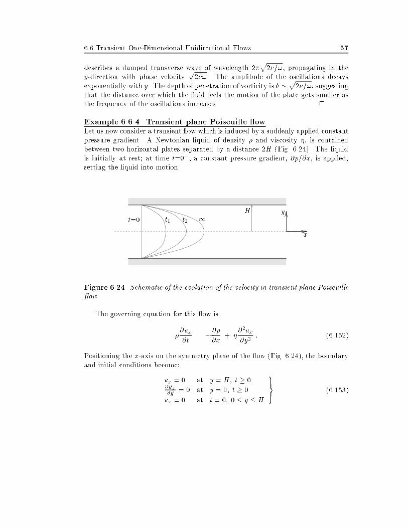
Contents
� UNIDIRECTIONAL FLOWS �
��� Steady� One�Dimensional Rectilinear Flows �
��� Steady� Axisymmetric Rectilinear Flows ��
��� Steady� Axisymmetric Torsional Flows �
�� Steady� Axisymmetric Radial Flows �
��� Steady� Spherically Symmetric Radial Flows �
��� Transient One�Dimensional Unidirectional Flows �
�� Steady Two�Dimensional Rectilinear Flows ��
�� Problems
��� References �
i
ii CONTENTS
Chapter �
UNIDIRECTIONAL FLOWS
Isothermal� laminar� incompressible Newtonian �ow is governed by a system of fourscalar partial di�erential equations �PDEs�� these are the continuity equation andthe three components of the Navier�Stokes equation� The pressure and the threevelocity components are the primary unknowns� which are� in general� functions oftime and of spatial coordinates� This system of PDEs is amenable to analyticalsolution for limited classes of �ow� Even in the case of relatively simple �ows inregular geometries� the nonlinearities introduced by the convective terms rule outthe possibility of �nding analytical solutions� This explains the extensive use ofnumerical methods in Fluid Mechanics ���� Computational Fluid Dynamics �CFD�is certainly the fastest growing branch of �uid mechanics� largely as a result of theincreasing availability and power of computers� and the parallel advancement ofversatile numerical techniques�
In this chapter� we study certain classes of incompressible �ows� in which theNavier�Stokes equations are simpli�ed signi�cantly to lead to analytical solutions�These classes concern unidirectional �ows� that is� �ows which have only one nonzerovelocity component� ui� Hence� the number of the primary unknowns is reduced totwo� the velocity component� ui� and pressure� p� In many �ows of interest� the PDEscorresponding to the two unknown �elds are decoupled� As a result� one can �rst �ndui� by solving the corresponding component of the Navier�Stokes equation� and thencalculate the pressure� Another consequence of the unidirectionality assumption� isthat ui is a function of at most two spatial variables and time� Therefore� in theworst case scenario of incompressible� unidirectional �ow one has to solve a PDEwith three independent variables� one of which is time�
The number of independent variables is reduced to two in
�a� transient one�dimensional ��D� unidirectional �ows in which ui is a function ofone spatial independent variable and time� and
�b� steady two�dimensional ��D� unidirectional �ows in which ui is a function oftwo spatial independent variables�
�
� Chapter �� Unidirectional Flows
The resulting PDEs in the above two cases can often be solved using various tech�niques� such as the separation of variables ��� and similarity methods ����
In steady� one�dimensional unidirectional �ows� the number of independent vari�ables is reduced to one� In these �ows� the governing equation for the nonzero ve�locity component is just a linear� second�order ordinary di�erential equation �ODE�which can be solved easily using well�known formulas and techniques� Such �ows arestudied in the �rst three sections of this chapter� In particular� in Sections � and ��we study �ows in which the streamlines are straight lines� i�e�� one�dimensional recti�linear �ows with ux�ux�y� and uy�uz�� �Section ����� and axisymmetric rectilinear�ows with uz�uz�r� and ur�u��� �Section ����� In Section ���� we study axisym�metric torsional �or swirling� �ows� with u��u��r� and uz�ur��� In this case� thestreamlines are circles centered at the axis of symmetry�
In Sections �� and ���� we discuss brie�y steady radial �ows� with axial andspherical symmetry� respectively� An interesting feature of radial �ows is that thenonzero radial velocity component� ur�ur�r�� is determined from the continuityequation rather than from the radial component of the Navier�Stokes equation� InSection ���� we study transient� one�dimensional unidirectional �ows� Finally� inSection �� � we consider examples of steady� two�dimensional unidirectional �ows�
Unidirectional �ows� although simple� are important in a diversity of �uid trans�ferring and processing applications� As demonstrated in examples in the followingsections� once the velocity and the pressure are known� the nonzero componentsof the stress tensor� such as the shear stress� as well as other useful macroscopicquantities� such as the volumetric �ow rate and the shear force �or drag� on solidboundaries in contact with the �uid� can be easily determined�
Let us point out that analytical solutions can also be found for a limited class oftwo�dimensional almost unidirectional or bidirectional �ows by means of the potentialfunction and�or the stream function� as demonstrated in Chapters to ��� Approx�imate solutions for limiting values of the involved parameters can be constructedby asymptotic and perturbation analyses� which are the topics of Chapters and ��with the most profound examples being the lubrication� thin��lm� and boundary�layer approximations�
��� Steady� One�Dimensional RectilinearFlows
Rectilinear �ows� i�e�� �ows in which the streamlines are straight lines� are usuallydescribed in Cartesian coordinates� with one of the axes being parallel to the �owdirection� If the �ow is axisymmetric� a cylindrical coordinate system with the z�axis
��� Steady� One�Dimensional Rectilinear Flows �
coinciding with the axis of symmetry of the �ow is usually used�Let us assume that a Cartesian coordinate system is chosen to describe a rec�
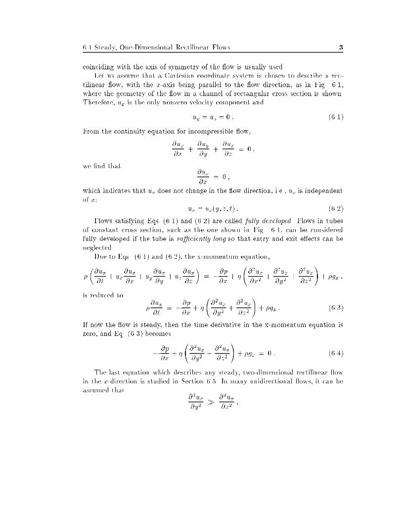
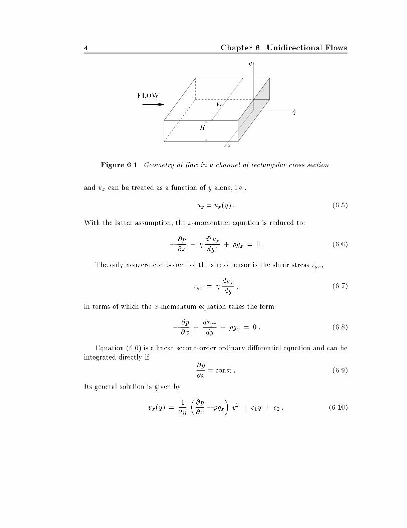
tilinear �ow� with the x�axis being parallel to the �ow direction� as in Fig� ����where the geometry of the �ow in a channel of rectangular cross section is shown�Therefore� ux is the only nonzero velocity component and
uy � uz � � � �����
From the continuity equation for incompressible �ow�
�ux�x
��uy�y
��uz�z
� � �
we �nd that�ux�x
� � �
which indicates that ux does not change in the �ow direction� i�e�� ux is independentof x�
ux � ux�y� z� t� � �����
Flows satisfying Eqs� ����� and ����� are called fully developed� Flows in tubesof constant cross section� such as the one shown in Fig� ���� can be consideredfully developed if the tube is su�ciently long so that entry and exit e�ects can beneglected�
Due to Eqs� ����� and ������ the x�momentum equation�
�
��ux�t
� ux�ux�x
� uy�ux�y
� uz�ux�z
�� ��p
�x� �
���ux�x�
���ux�y�
���ux�z�
�� �gx �
is reduced to
��ux�t
� ��p
�x� �
���ux�y�
���ux�z�
�� �gx � �����
If now the �ow is steady� then the time derivative in the x�momentum equation iszero� and Eq� ����� becomes
� �p
�x� �
���ux�y�
���ux�z�
�� �gx � � � ����
The last equation which describes any steady� two�dimensional rectilinear �owin the x�direction is studied in Section ���� In many unidirectional �ows� it can beassumed that
��ux�y�
� ��ux�z�
�
� Chapter �� Unidirectional Flows
x
y
z
H
WFLOW
Figure ���� Geometry of �ow in a channel of rectangular cross section
and ux can be treated as a function of y alone� i�e��
ux � ux�y� � �����
With the latter assumption� the x�momentum equation is reduced to�
� �p
�x� �
d�uxdy�
� �gx � � � �����
The only nonzero component of the stress tensor is the shear stress �yx�
�yx � �duxdy
� ��� �
in terms of which the x�momentum equation takes the form
� �p
�x�
d�yxdy
� �gx � � � ����
Equation ����� is a linear second�order ordinary di�erential equation and can beintegrated directly if
�p
�x� const � �����
Its general solution is given by
ux�y� ��
��
��p
�x� �gx
�y� � c�y � c� � ������
��� Steady� One�Dimensional Rectilinear Flows �
�����������������������������������
�����������������������������������
�y
�x
�V
ux�VH y
�������
���
�
�
H
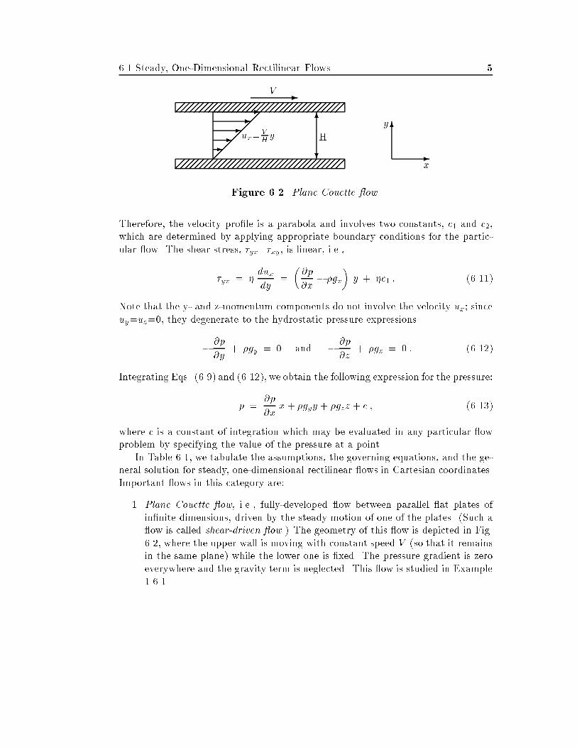
Figure ���� Plane Couette �ow
Therefore� the velocity pro�le is a parabola and involves two constants� c� and c��which are determined by applying appropriate boundary conditions for the partic�ular �ow� The shear stress� �yx��xy � is linear� i�e��
�yx � �duxdy
�
��p
�x� �gx
�y � �c� � ������
Note that the y� and z�momentum components do not involve the velocity ux� sinceuy�uz��� they degenerate to the hydrostatic pressure expressions
� �p
�y� �gy � � and � �p
�z� �gz � � � ������
Integrating Eqs� ����� and ������� we obtain the following expression for the pressure�
p ��p
�xx� �gyy � �gzz � c � ������
where c is a constant of integration which may be evaluated in any particular �owproblem by specifying the value of the pressure at a point�
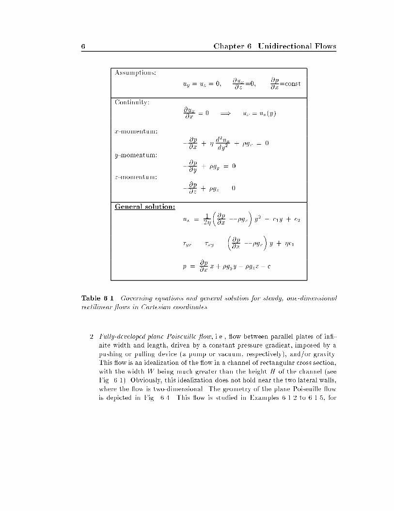
In Table ���� we tabulate the assumptions� the governing equations� and the ge�neral solution for steady� one�dimensional rectilinear �ows in Cartesian coordinates�Important �ows in this category are�
�� Plane Couette �ow� i�e�� fully�developed �ow between parallel �at plates ofin�nite dimensions� driven by the steady motion of one of the plates� �Such a�ow is called shear�driven �ow�� The geometry of this �ow is depicted in Fig����� where the upper wall is moving with constant speed V �so that it remainsin the same plane� while the lower one is �xed� The pressure gradient is zeroeverywhere and the gravity term is neglected� This �ow is studied in Example������
� Chapter �� Unidirectional Flows
Assumptions�
uy � uz � �� �ux�z
����p�x
�const�
Continuity��ux�x � � �� ux � ux�y�
x�momentum�
��p�x
� � d�uxdy�
� �gx � �
y�momentum�
��p�y
� �gy � �
z�momentum�
��p�z � �gz � �
General solution�
ux � ���
��p�x
� �gx
�y� � c�y � c�
�yx � �xy �
��p�x
� �gx
�y � �c�
p � �p�x
x� �gyy � �gzz � c
Table ���� Governing equations and general solution for steady� one�dimensionalrectilinear �ows in Cartesian coordinates
�� Fully�developed plane Poiseuille �ow� i�e�� �ow between parallel plates of in��nite width and length� driven by a constant pressure gradient� imposed by apushing or pulling device �a pump or vacuum� respectively�� and�or gravity�This �ow is an idealization of the �ow in a channel of rectangular cross section�with the width W being much greater than the height H of the channel �seeFig� ����� Obviously� this idealization does not hold near the two lateral walls�where the �ow is two�dimensional� The geometry of the plane Poiseuille �owis depicted in Fig� ��� This �ow is studied in Examples ����� to ������ for
��� Steady� One�Dimensional Rectilinear Flows
di�erent boundary conditions�
�� Thin �lm �ow down an inclined plane� driven by gravity �i�e�� elevation di�er�ences�� under the absence of surface tension� The pressure gradient is usuallyassumed to be everywhere zero� Such a �ow is illustrated in Fig� ��� and isstudied in Example ������
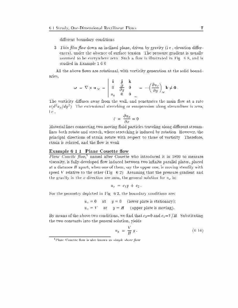
All the above �ows are rotational� with vorticity generation at the solid bound�aries�
� � r� ujw �
��������i j k
� ��y
�
ux � �
��������w
� ���ux�y
�w
k �� �
The vorticity di�uses away from the wall� and penetrates the main �ow at a rate��d�ux�dy
��� The extensional stretching or compression along streamlines is zero�i�e��
� ��ux�x
� �
Material lines connecting two moving �uid particles traveling along di�erent stream�lines both rotate and stretch� where stretching is induced by rotation� However� theprincipal directions of strain rotate with respect to those of vorticity� Therefore�strain is relaxed� and the �ow is weak�
Example ������ Plane Couette �owPlane Couette �ow�� named after Couette who introduced it in ��� to measureviscosity� is fully�developed �ow induced between two in�nite parallel plates� placedat a distance H apart� when one of them� say the upper one� is moving steadily withspeed V relative to the other �Fig� ����� Assuming that the pressure gradient andthe gravity in the x�direction are zero� the general solution for ux is�
ux � c�y � c� �
For the geometry depicted in Fig� ���� the boundary conditions are�
ux � � at y � � �lower plate is stationary��
ux � V at y � H �upper plate is moving��
By means of the above two conditions� we �nd that c��� and c��V�H � Substitutingthe two constants into the general solution� yields
ux �V
Hy � �����
�Plane Couette �ow is also known as simple shear �ow�
� Chapter �� Unidirectional Flows
The velocity ux then varies linearly across the gap� The corresponding shear stressis constant�
�yx � �V
H� ������
A number of macroscopic quantities� such as the volumetric �ow rate and theshear stress at the wall� can be calculated� The volumetric �ow rate per unit widthis calculated by integrating ux along the gap�
Q
W�
Z H
�ux dy �
Z H
�
V
Hy dy ��
Q
W�
�
�HV � ������
The shear stress �w exerted by the �uid on the upper plate is
�w � ��yxjy�H � �� V
H� ���� �
The minus sign accounts for the upper wall facing the negative y�direction of thechosen system of coordinates� The shear force per unit width required to move theupper plate is then
F
W� �
Z L
��w dx � �
V
HL �
where L is the length of the plate�
�����������������������������������
�����������������������������������
�y
�x
�V
ux�V
�V
������ �
�
H
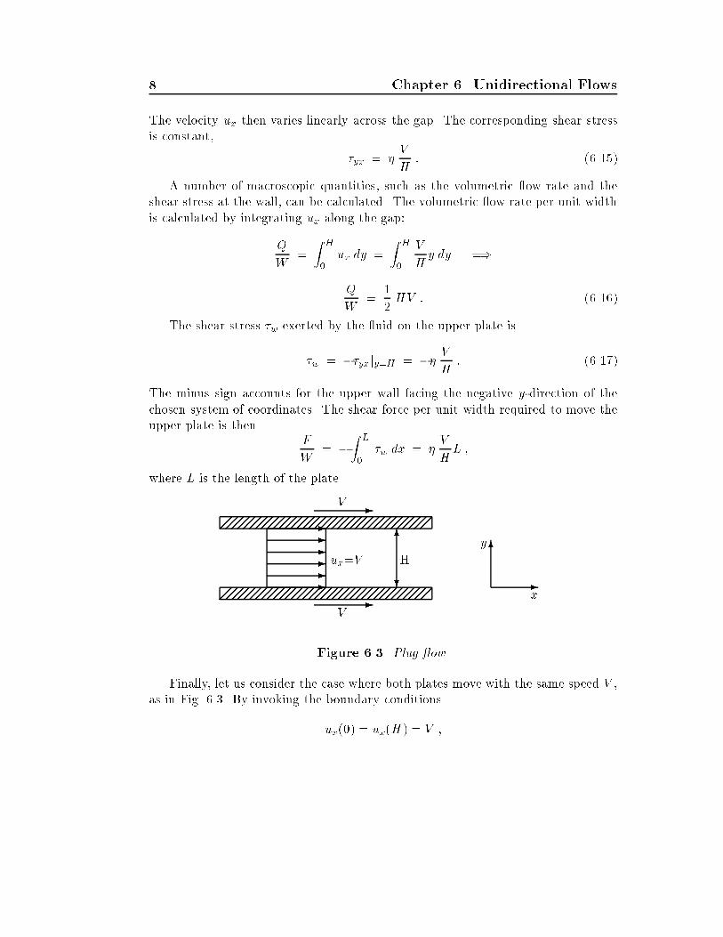
Figure ���� Plug �ow
Finally� let us consider the case where both plates move with the same speed V �as in Fig� ���� By invoking the boundary conditions
ux��� � ux�H� � V �
��� Steady� One�Dimensional Rectilinear Flows �
we �nd that c��� and c��V � and� therefore�
ux � V �
Thus� in this case� plane Couette �ow degenerates into plug �ow� �
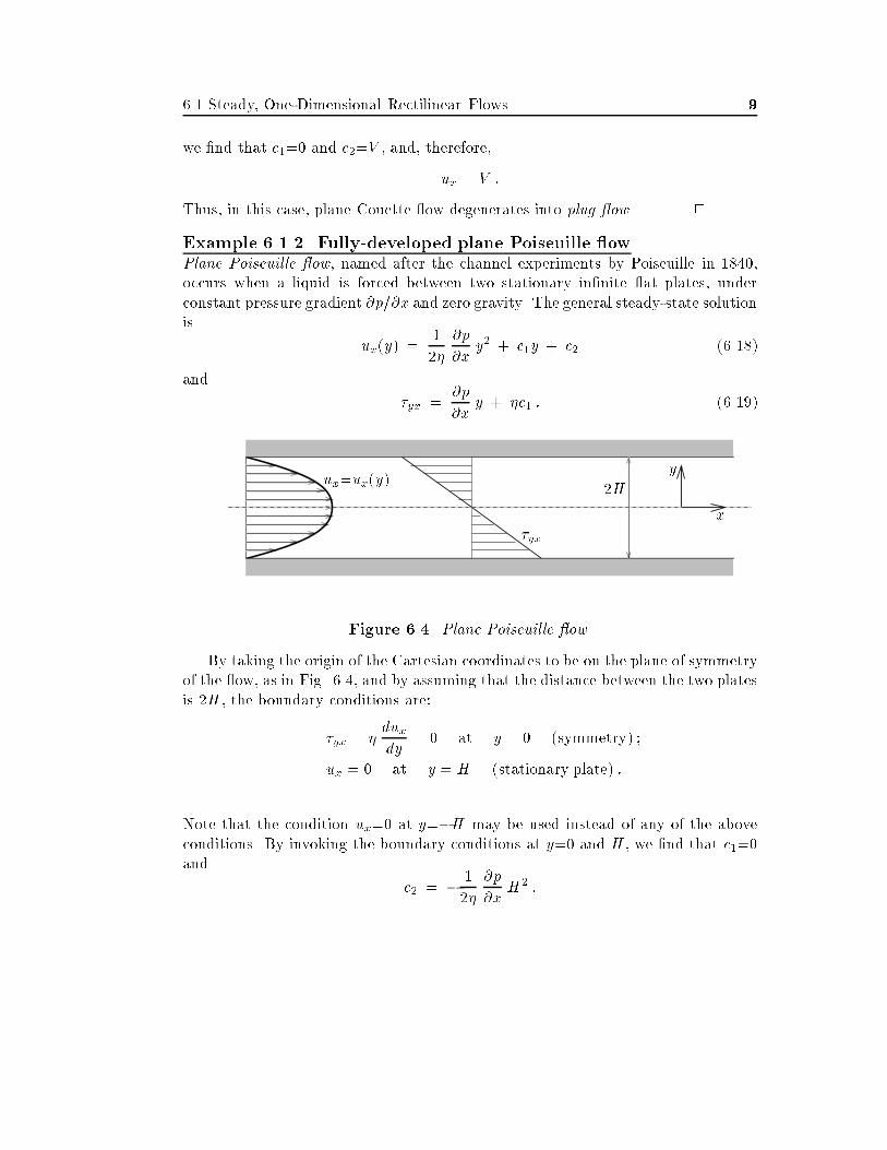
Example ������ Fully�developed plane Poiseuille �owPlane Poiseuille �ow� named after the channel experiments by Poiseuille in ���occurs when a liquid is forced between two stationary in�nite �at plates� underconstant pressure gradient �p��x and zero gravity� The general steady�state solutionis
ux�y� ��
��
�p
�xy� � c�y � c� �����
and
�yx ��p
�xy � �c� � ������
x
y
�Hux�ux�y�
�yx
Figure ���� Plane Poiseuille �ow
By taking the origin of the Cartesian coordinates to be on the plane of symmetryof the �ow� as in Fig� ��� and by assuming that the distance between the two platesis �H � the boundary conditions are�
�yx � �duxdy
� � at y � � �symmetry� �
ux � � at y � H �stationary plate� �
Note that the condition ux�� at y��H may be used instead of any of the aboveconditions� By invoking the boundary conditions at y�� and H � we �nd that c���and
c� � � �
��
�p
�xH� �
� Chapter �� Unidirectional Flows
The two constants are substituted into the general solution to obtain the followingparabolic velocity pro�le�
ux � � �
��
�p
�x�H� � y�� � ������
If the pressure gradient is negative� then the �ow is in the positive direction� as inFig� ��� Obviously� the velocity ux attains its maximum value at the centerline�y����
ux�max � � �
��
�p
�xH� �
The volumetric �ow rate per unit width is
Q
W�
Z H
�Hux dy � �
Z H
�� �
��
�p
�x�H� � y�� dy ��
Q � � �
��
�p
�xH�W � ������
As expected� Eq� ������ indicates that the volumetric �ow rate Q is proportionalto the pressure gradient� �p��x� and inversely proportional to the viscosity �� Notealso that� since �p��x is negative� Q is positive� The average velocity� �ux� in thechannel is�
�ux �Q
WH� � �
��
�p
�xH� �
The shear stress distribution is given by
�yx ��p
�xy � ������
i�e�� �yx varies linearly from y�� to H � being zero at the centerline and attaining itsmaximum absolute value at the wall� The shear stress exerted by the �uid on thewall at y�H is
�w � ��yxjy�H � ��p
�xH �
�
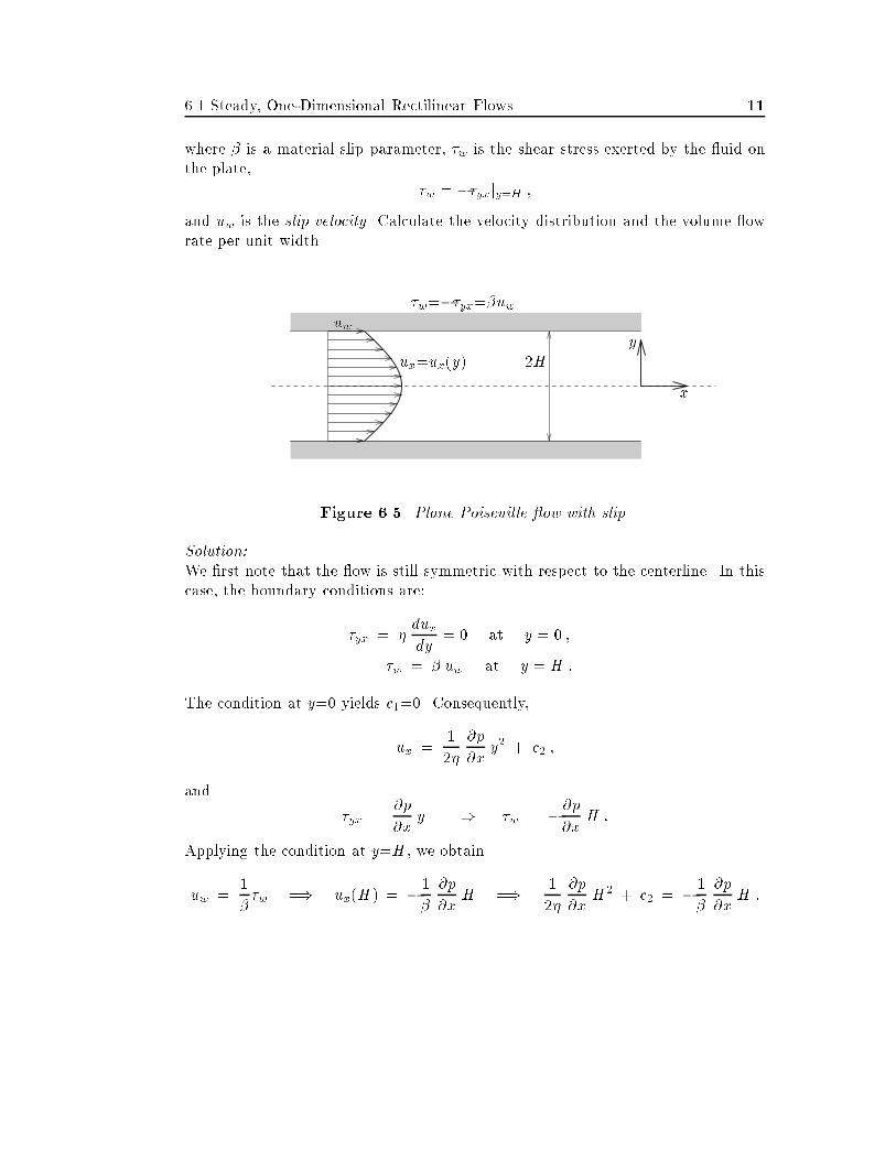
Example ������ Plane Poiseuille �ow with slipConsider again the fully�developed plane Poiseuille �ow of the previous example�and assume that slip occurs along the two plates according to the slip law
�w � uw at y � H �
��� Steady� One�Dimensional Rectilinear Flows ��
where is a material slip parameter� �w is the shear stress exerted by the �uid onthe plate�
�w � ��yxjy�H �
and uw is the slip velocity� Calculate the velocity distribution and the volume �owrate per unit width�
x
y
�Hux�ux�y�
uw
�w���yx�uw
Figure ���� Plane Poiseuille �ow with slip
SolutionWe �rst note that the �ow is still symmetric with respect to the centerline� In thiscase� the boundary conditions are�
�yx � �duxdy
� � at y � � �
�w � uw at y � H �
The condition at y�� yields c���� Consequently�
ux ��
��
�p
�xy� � c� �
and
�yx ��p
�xy �� �w � ��p
�xH �
Applying the condition at y�H � we obtain
uw ��
�w �� ux�H� � � �
�p
�xH �� �
��
�p
�xH� � c� � � �
�p
�xH �
�� Chapter �� Unidirectional Flows
Consequently�
c� � � �
��
�p
�x
�H� �
��H
��
and
ux � � �
��
�p
�x
�H� �
��H
� y�
�� ������
Note that this expression reduces to the standard Poiseuille �ow pro�le when ���Since the slip velocity is inversely proportional to the slip coe�cient � the standardno�slip condition is recovered�
An alternative expression of the velocity distribution is
ux � uw � �
��
�p
�x
�H� � y�
��
which indicates that ux is just the superposition of the slip velocity uw to the velocitydistribution of the previous example�
For the volumetric �ow rate per unit width� we obtain�
Q
W� �
Z H
�ux dy � �uwH � �
��
�p
�xH� ��
Q � � �
��
�p
�xH�
�� �
��
H
�W � �����
�
Example ������ Plane Couette�Poiseuille �owConsider again fully�developed plane Poiseuille �ow with the upper plate movingwith constant speed� V �Fig� ����� This �ow is called plane Couette�Poiseuille �owor general Couette �ow� In contrast to the previous two examples� this �ow is notsymmetric with respect to the centerline of the channel� and� therefore� having theorigin of the Cartesian coordinates on the centerline is not convenient� Therefore�the origin is moved to the lower plate�
The boundary conditions for this �ow are�
ux � � at y � � �
ux � V at y � a �
where a is the distance between the two plates� Applying the two conditions� weget c��� and
V ��
��
�p
�xa� � c�a �� c� �
V
a� �
��
�p
�xa �
��� Steady� One�Dimensional Rectilinear Flows ��
x
ya
ux�ux�y�
V
V
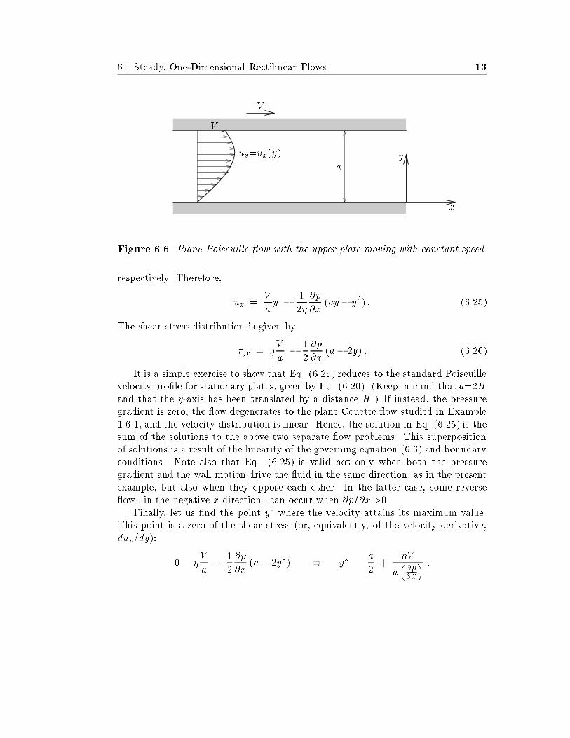
Figure ���� Plane Poiseuille �ow with the upper plate moving with constant speed
respectively� Therefore�
ux �V
ay � �
��
�p
�x�ay � y�� � ������
The shear stress distribution is given by
�yx � �V
a� �
�
�p
�x�a� �y� � ������
It is a simple exercise to show that Eq� ������ reduces to the standard Poiseuillevelocity pro�le for stationary plates� given by Eq� ������� �Keep in mind that a��Hand that the y�axis has been translated by a distance H �� If instead� the pressuregradient is zero� the �ow degenerates to the plane Couette �ow studied in Example������ and the velocity distribution is linear� Hence� the solution in Eq� ������ is thesum of the solutions to the above two separate �ow problems� This superpositionof solutions is a result of the linearity of the governing equation ����� and boundaryconditions� Note also that Eq� ������ is valid not only when both the pressuregradient and the wall motion drive the �uid in the same direction� as in the presentexample� but also when they oppose each other� In the latter case� some reverse�ow �in the negative x direction� can occur when �p��x ���
Finally� let us �nd the point y� where the velocity attains its maximum value�This point is a zero of the shear stress �or� equivalently� of the velocity derivative�dux�dy��
� � �V
a� �
�
�p
�x�a� �y�� �� y� �
a
��
�V
a��p�x
� �
�� Chapter �� Unidirectional Flows
The �ow is symmetric with respect to the centerline� if y��a��� i�e�� when V���The maximum velocity ux�max is determined by substituting y� into Eq� �������
�
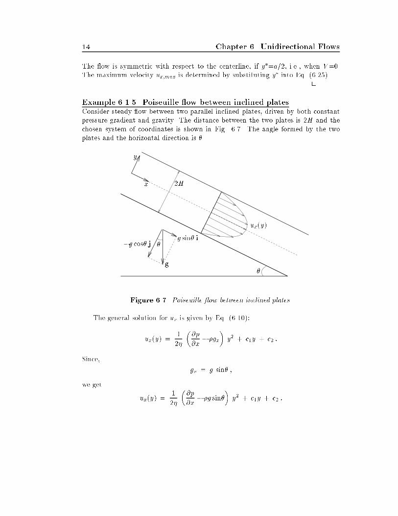
Example ����� Poiseuille �ow between inclined platesConsider steady �ow between two parallel inclined plates� driven by both constantpressure gradient and gravity� The distance between the two plates is �H and thechosen system of coordinates is shown in Fig� �� � The angle formed by the twoplates and the horizontal direction is ��
x
y
�H
ux�y�
�
�
g
g sin� i�g cos� j
Figure ��� Poiseuille �ow between inclined plates
The general solution for ux is given by Eq� �������
ux�y� ��
��
��p
�x� �gx
�y� � c�y � c� �
Since�
gx � g sin� �
we get
ux�y� ��
��
��p
�x� �g sin�
�y� � c�y � c� �
��� Steady� One�Dimensional Rectilinear Flows ��
Integration of this equation with respect to y and application of the boundary con�ditions� dux�dy�� at y�� and ux�� at y�H � give
ux�y� ��
��
���p
�x� �g sin�
��H� � y�� � ���� �
The pressure is obtained from Eq� ������ as
p ��p
�xx � �gy y � c ��
p ��p
�xx � �g cos� y � c �����
�
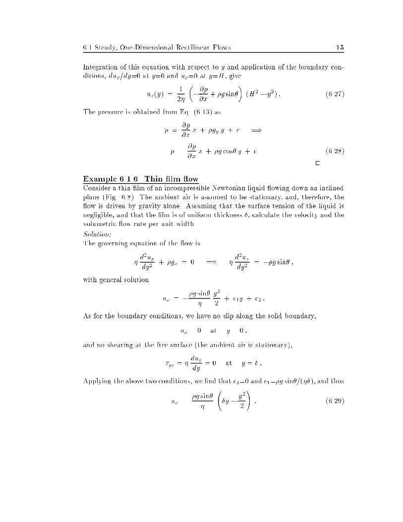
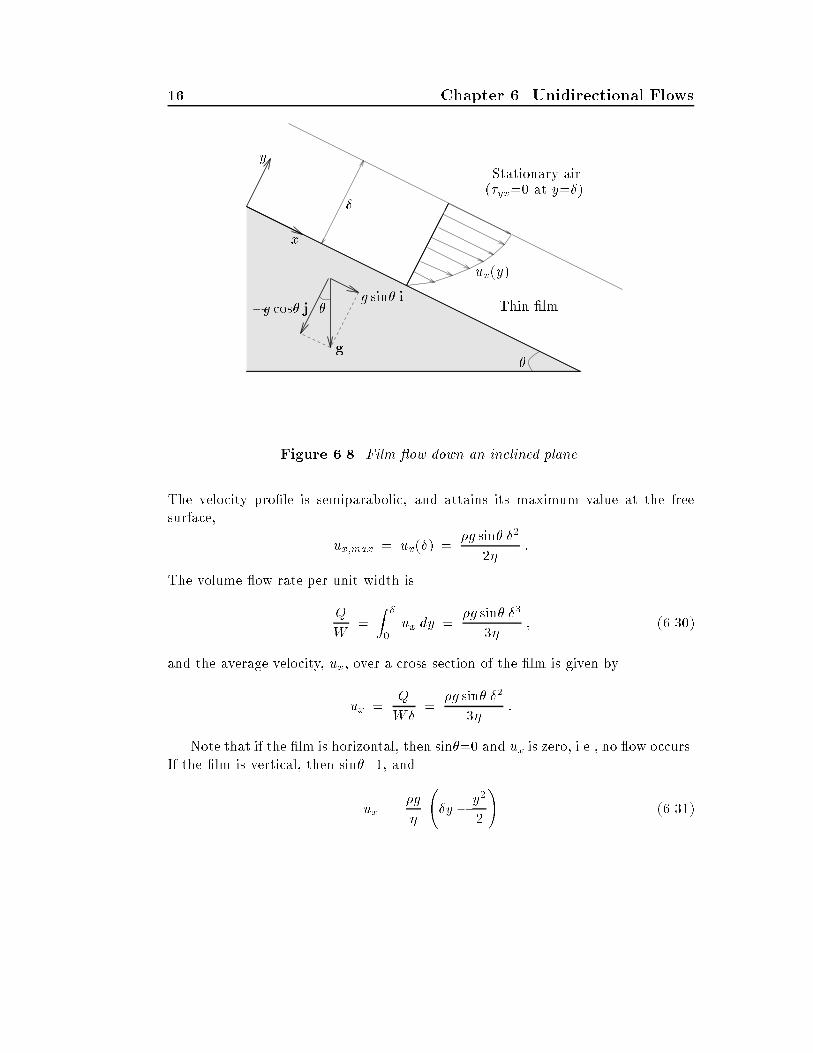
Example ������ Thin lm �owConsider a thin �lm of an incompressible Newtonian liquid �owing down an inclinedplane �Fig� ���� The ambient air is assumed to be stationary� and� therefore� the�ow is driven by gravity alone� Assuming that the surface tension of the liquid isnegligible� and that the �lm is of uniform thickness � calculate the velocity and thevolumetric �ow rate per unit width�
SolutionThe governing equation of the �ow is
�d�uxdy�
� �gx � � �� �d�uxdy�
� ��g sin� �
with general solution
ux � ��g sin��
y�
�� c�y � c� �
As for the boundary conditions� we have no slip along the solid boundary�
ux � � at y � � �
and no shearing at the free surface �the ambient air is stationary��
�yx � �duxdy
� � at y � �
Applying the above two conditions� we �nd that c��� and c���g sin���� �� and thus
ux ��g sin�
�
� y � y�
�
�� ������
�� Chapter �� Unidirectional Flows
x
y
ux�y�
Stationary air
Thin �lm
��yx�� at y� �
�
�
g
g sin� i�g cos� j
Figure ���� Film �ow down an inclined plane
The velocity pro�le is semiparabolic� and attains its maximum value at the freesurface�
ux�max � ux� � ��g sin� �
���
The volume �ow rate per unit width is
Q
W�
Z �
�ux dy �
�g sin� �
��� ������
and the average velocity� �ux� over a cross section of the �lm is given by
�ux �Q
W �
�g sin� �
���
Note that if the �lm is horizontal� then sin��� and ux is zero� i�e�� no �ow occurs�If the �lm is vertical� then sin���� and
ux ��g
�
� y � y�
�
�������
��� Steady� One�Dimensional Rectilinear Flows �
andQ
W�
�g �
��� ������
By virtue of Eq� ������� the pressure is given by
p � �gy y � c � ��g cos� y � c �
At the free surface� the pressure must be equal to the atmospheric pressure� p�� so
p� � ��g cos� � c
and
p � p� � �g � � y� cos� � ������
�
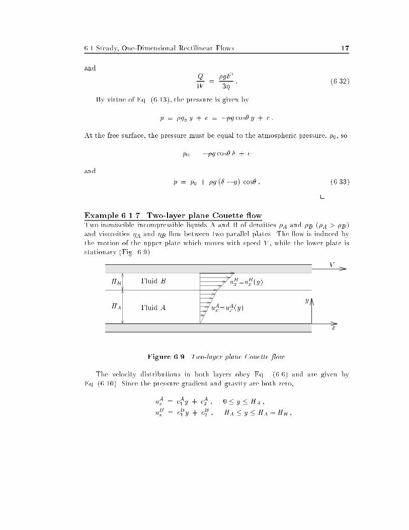
Example ������ Two�layer plane Couette �owTwo immiscible incompressible liquids A and B of densities �A and �B ��A � �B�and viscosities �A and �B �ow between two parallel plates� The �ow is induced bythe motion of the upper plate which moves with speed V � while the lower plate isstationary �Fig� �����
x
y
V
uAx�uAx �y�
uBx�uBx �y�
HA
HB
Fluid A
Fluid B
Figure ���� Two�layer plane Couette �ow
The velocity distributions in both layers obey Eq� ����� and are given byEq� ������� Since the pressure gradient and gravity are both zero�
uAx � cA� y � cA� � � � y � HA �
uBx � cB� y � cB� � HA � y � HA �HB �
�� Chapter �� Unidirectional Flows
where cA� � cA� � c
B� and cB� are integration constants determined by conditions at the
solid boundaries and the interface of the two layers� The no�slip boundary conditionsat the two plates are applied �rst� At y��� uAx��� therefore�
cA� � � �
At y�HA �HB� uBx�V � therefore�
cB� � V � CB� �HA �HB� �
The two velocity distributions become
uAx � cA� y � � � y � HA �
uBx � V � cB� �HA �HB � y� � HA � y � HA �HB �
At the interface �y�HA�� we have two additional conditions��a� the velocity distribution is continuous� i�e��
uAx � uBx at y � HA �
�b� momentum transfer through the interface is continuous� i�e��
�Ayx � �Byx at y � HA ��
�AduAxdy
� �BduBxdy
at y � HA �
From the interface conditions� we �nd that
cA� ��BV
�AHB � �BHAand cB� �
�AV
�AHB � �BHA�
Hence� the velocity pro�les in the two layers are
uAx ��BV
�AHB � �BHAy � � � y � HA � �����
uBx � V � �AV
�AHB � �BHA�HA �HB � y� � HA � y � HA �HB � ������
If the two liquids are of the same viscosity� �A��B��� then the two velocitypro�les are the same� and the results simplify to the linear velocity pro�le for one�layer Couette �ow�
uAx � uBx �V
HA �HBy �
�
Sec� ���� Steady� Axisymmetric Rectilinear Flows ��
��� Steady� Axisymmetric Rectilinear Flows
Axisymmetric �ows are conveniently studied in a cylindrical coordinate system��r� �� z�� with the z�axis coinciding with the axis of symmetry of the �ow� Axisym�metry means that there is no variation of the velocity with the angle ��
�u
��� � ������
There are three important classes of axisymmetric unidirectional �ows �i�e�� �owsin which only one of the three velocity components� ur� u� and uz � is nonzero��
�� Axisymmetric rectilinear �ows� in which only the axial velocity component�uz � is nonzero� The streamlines are straight lines� Typical �ows are fully�developed pressure�driven �ows in cylindrical tubes and annuli� and open �lm�ows down cylinders or conical pipes�
�� Axisymmetric torsional �ows� in which only the azimuthal velocity component�u�� is nonzero� The streamlines are circles centered on the axis of symmetry�These �ows� studied in Section ���� are good prototypes of rigid�body rotation��ow in rotating mixing devices� and swirling �ows� such as tornados�
�� Axisymmetric radial �ows� in which only the radial velocity component� ur�is nonzero� These �ows� studied in Section ��� are typical models for radial�ows through porous media� migration of oil towards drilling wells� and suction�ows from porous pipes and annuli�
As already mentioned� in axisymmetric rectilinear �ows�
ur � u� � � � ���� �
The continuity equation for incompressible �ow�
�
r
�
�r�rur� �
�
r
�u���
��uz�z
� � �
becomes�uz�z
� � �
From the above equation and the axisymmetry condition ������� we deduce that
uz � uz�r� t� � �����
� Chapter �� Unidirectional Flows
Due to Eqs� ������������� the z�momentum equation�
�
��uz
�t� ur
�uz
�r�
u�
r
�uz
��� uz
�uz
�z
�� �
�p
�z��
��
r
�
�r
�r�uz
�r
���
r���uz
����
��uz
�z�
��gz �
is simpli�ed to
��uz�t
� ��p�z
� ��
r
�
�r
�r�uz�r
�� �gz � ������
For steady �ow� uz�uz�r� and Eq� ������ becomes an ordinary di�erential equation�
� �p
�z� �
�
r
d
dr
�rduzdr
�� �gz � � � �����
The only nonzero components of the stress tensor are the shear stresses �rz and�zr �
�rz � �zr � �duzdr
� �����
for which we have
� �p
�z�
�
r
d
dr�r�rz� � �gz � � � �����
When the pressure gradient �p��z is constant� the general solution of Eq� ������is
uz ��
�
��p
�z� �gz
�r� � c� ln r � c� � �����
For �rz� we get
�rz ��
�
��p
�z� �gz
�r � �
c�r� ����
The constants c� and c� are determined from the boundary conditions of the �ow�The assumptions� the governing equations and the general solution for steady� ax�isymmetric rectilinear �ows are summarized in Table ����
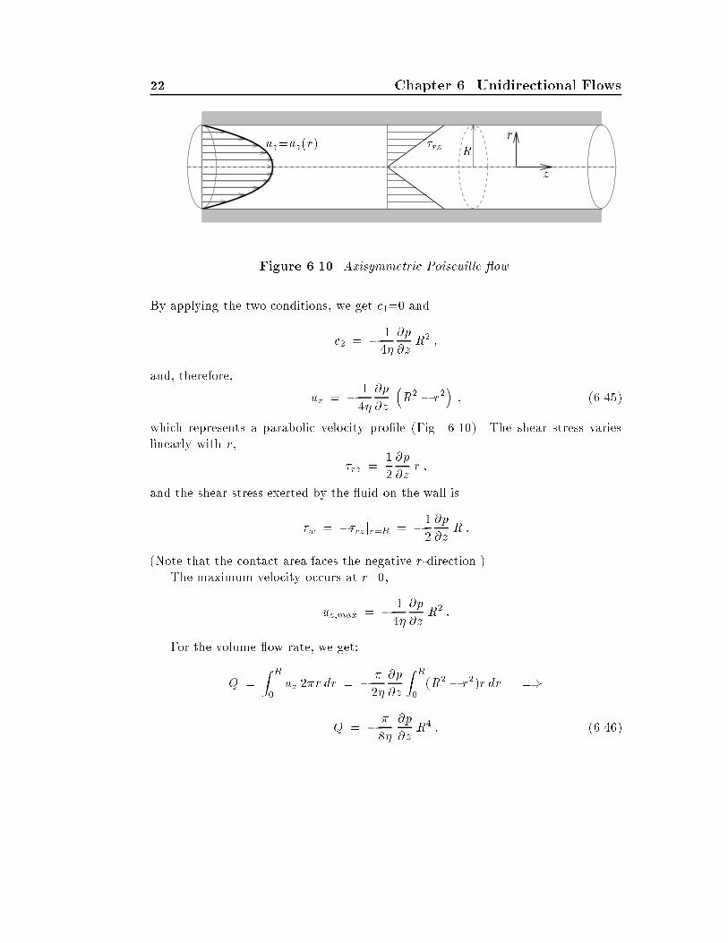
Example ������ Hagen�Poiseuille �owFully�developed axisymmetric Poiseuille �ow� or Hagen�Poiseuille �ow� studied ex�perimentally by Hagen in ��� and Poiseuille in ��� is the pressure�driven �ow inin�nitely long cylindrical tubes� The geometry of the �ow is shown in Fig� �����
Assuming that gravity is zero� the general solution for uz is
uz ��
�
�p
�zr� � c� ln r � c� �
��� Steady� Axisymmetric Rectilinear Flows ��
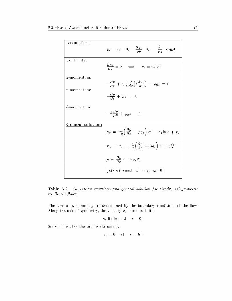
Assumptions�
ur � u� � �� �uz��
����p�z
�const�
Continuity��uz�z � � �� uz � uz�r�
z�momentum�
��p�z � � �rddr
�rduzdr
�� �gz � �
r�momentum�
��p�r
� �gr � �
��momentum�
��r�p��
� �g� � �
General solution�
uz � ��
��p�z � �gz
�r� � c� ln r � c�
�rz � �zr � ��
��p�z � �gz
�r � � c�r
p ��p�z z � c�r� ��
� c�r� ���const� when gr�g��� �
Table ���� Governing equations and general solution for steady� axisymmetricrectilinear �ows
The constants c� and c� are determined by the boundary conditions of the �ow�Along the axis of symmetry� the velocity uz must be �nite�
uz �nite at r � � �
Since the wall of the tube is stationary�
uz � � at r � R �
�� Chapter �� Unidirectional Flows
z
r
Ruz�uz�r� �rz
Figure ���� Axisymmetric Poiseuille �ow
By applying the two conditions� we get c��� and
c� � � �
�
�p
�zR� �
and� therefore�
uz � � �
�
�p
�z
�R� � r�
�� �����
which represents a parabolic velocity pro�le �Fig� ������ The shear stress varieslinearly with r�
�rz ��
�
�p
�zr �
and the shear stress exerted by the �uid on the wall is
�w � ��rz jr�R � ��
�
�p
�zR �
�Note that the contact area faces the negative r�direction��The maximum velocity occurs at r���
uz�max � � �
�
�p
�zR� �
For the volume �ow rate� we get�
Q �Z R
�uz ��r dr � � �
��
�p
�z
Z R
��R� � r��r dr ��
Q � � �
�
�p
�zR� � �����
��� Steady� Axisymmetric Rectilinear Flows ��
Note that� since the pressure gradient �p��z is negative� Q is positive� Equation����� is the famous experimental result of Hagen and Poiseuille� also known asthe fourth�power law� This basic equation is used to determine the viscosity fromcapillary viscometer data after taking into account the so�called Bagley correctionfor the inlet and exit pressure losses�
The average velocity� �uz � in the tube is
�uz �Q
�R�� � �
�
�p
�zR� �
�
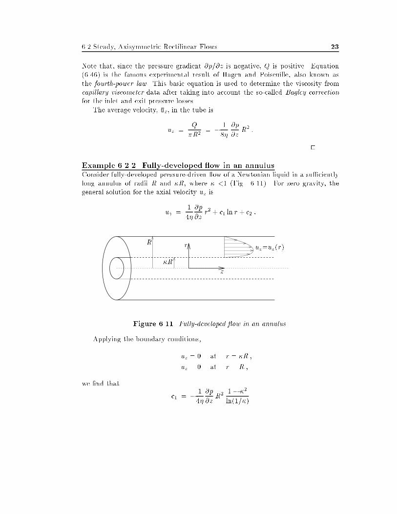
Example ������ Fully�developed �ow in an annulusConsider fully�developed pressure�driven �ow of a Newtonian liquid in a su�cientlylong annulus of radii R and �R� where � �� �Fig� ������ For zero gravity� thegeneral solution for the axial velocity uz is
uz ��
�
�p
�zr� � c� ln r � c� �
z
rR
�R
uz�uz�r�
Figure ����� Fully�developed �ow in an annulus
Applying the boundary conditions�
uz � � at r � �R �
uz � � at r � R �
we �nd that
c� � � �
�
�p
�zR� �� ��
ln�����
�� Chapter �� Unidirectional Flows
and
c� � � �
�
�p
�zR� � c� lnR �
Substituting c� and c� into the general solution we obtain�
uz � � �
�
�p
�zR�
��
�r
R
���
�� ��
ln�����ln
r
R
�� ��� �
The shear stress is given by
�rz ��
�p
�zR
�
�r
R
�� �� ��
ln�����
�R
r
��� ����
The maximum velocity occurs at the point where �rz�� �which is equivalent toduz�dr���� i�e�� at
r� � R
�� ��
� ln�����
�����
Substituting into Eq� ��� �� we get
uz�max � � �
�
�p
�zR�
�� � �� ��
� ln�����
�� ln
�� ��
� ln�����
� �
For the volume �ow rate� we have
Q �
Z R
�uz ��r dr � � �
��
�p
�zR�
Z R
�
��
�r
R
���
�� ��
ln�����ln
r
R
�r dr ��
Q � � �
�
�p
�zR�
��� ��
����� ��
��ln�����
�� �����
The average velocity� �uz � in the annulus is
�uz �Q
�R� � ���R��� � �
�
�p
�zR�
�� � ��
����� ��
�ln�����
��
�
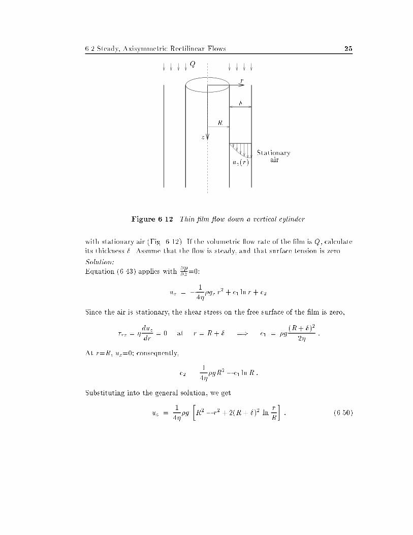
Example ������ Film �ow down a vertical cylinderA Newtonian liquid is falling vertically on the outside surface of an in�nitely longcylinder of radius R� in the form of a thin uniform axisymmetric �lm� in contact
��� Steady� Axisymmetric Rectilinear Flows ��
z
r
Q
R
uz�r�Stationary
air
Figure ����� Thin �lm �ow down a vertical cylinder
with stationary air �Fig� ������ If the volumetric �ow rate of the �lm is Q� calculateits thickness � Assume that the �ow is steady� and that surface tension is zero�
SolutionEquation ����� applies with �p
�z���
uz � � �
��gz r
� � c� ln r � c�
Since the air is stationary� the shear stress on the free surface of the �lm is zero�
�rz � �duzdr
� � at r � R� �� c� � �g�R� ��
���
At r�R� uz��� consequently�
c� ��
��gR� � c� lnR �
Substituting into the general solution� we get
uz ��
��g
�R� � r� � ��R� �� ln
r
R
� ������
�� Chapter �� Unidirectional Flows
For the volume �ow rate� Q� we have�
Q �
Z R��
Ruz ��r dr �
�
���g
Z R��
R
�R� � r� � ��R� �� ln
r
R
r dr �
After integration and some algebraic manipulations� we �nd that
Q ��
��gR�
�
�� �
R
��ln
�� �
R
��
R
�� �
R
��
�� �
R
��� �
� � ������
When the annular �lm is very thin� it can be approximated as a thin planar �lm�We will show that this is indeed the case� by proving that for
R � �
Eq� ������ reduces to the expression found in Example ����� for a thin verticalplanar �lm� Letting
�
R
leads to the following expression for Q�
Q ��
��gR�
n �� � �� ln �� � � � �� � �
h� �� � �� � �
io�
Expanding ln�� � � into Taylor series� we get
ln�� � � � � �
���
�� �
� O��� �
Thus
�� � �� ln�� � � � �� � � �� � � � ��
� �
���
�� �
�O���
�
� �
�� �
��
�� �
��
��� � O���
Consequently�
Q ��
��gR�
�
��
�� �
��
�� �
��
��� � O���
� �� �� � ��� � ���
��
or
Q ��
��gR�
���
�� � ��
��� � O���
�
��� Steady� Axisymmetric Rectilinear Flows �
Keeping only the third�order term� we get
Q ��
��gR� ��
�
�
R
���� Q
��R�
�g �
���
By setting ��R equal to W � the last equation becomes identical to Eq� ������� �
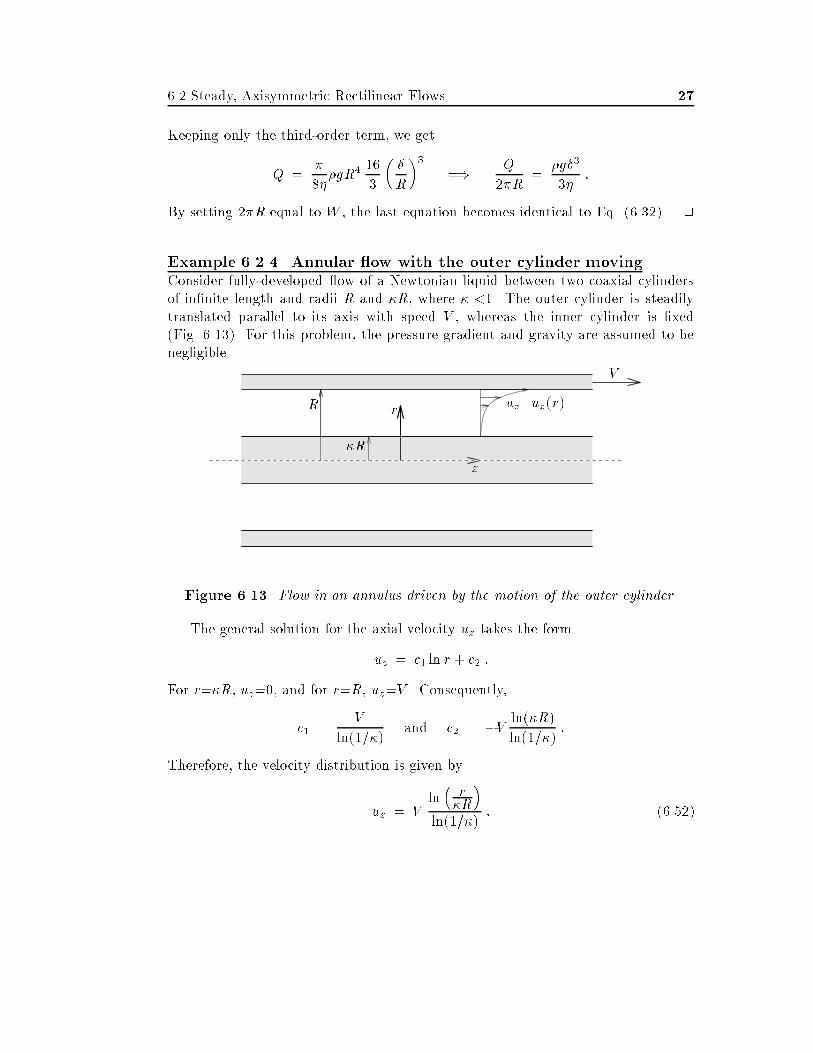
Example ������ Annular �ow with the outer cylinder movingConsider fully�developed �ow of a Newtonian liquid between two coaxial cylindersof in�nite length and radii R and �R� where � ��� The outer cylinder is steadilytranslated parallel to its axis with speed V � whereas the inner cylinder is �xed�Fig� ������ For this problem� the pressure gradient and gravity are assumed to benegligible�
z
rR
�R
uz�uz�r�
V
Figure ����� Flow in an annulus driven by the motion of the outer cylinder
The general solution for the axial velocity uz takes the form
uz � c� ln r � c� �
For r��R� uz��� and for r�R� uz�V � Consequently�
c� �V
ln�����and c� � �V ln��R�
ln������
Therefore� the velocity distribution is given by
uz � Vln�r�R
�ln�����
� ������
�� Chapter �� Unidirectional Flows
Let us now examine two limiting cases of this �ow��a� For ���� the annular �ow degenerates to �ow in a tube� From Eq� ������� wehave
uz � lim���
Vln�
r�R
�ln�����
� V lim���
�� �
ln rR
ln�����
� V �
In other words� we have plug �ow �solid�body translation� in a tube��b� For ���� the annular �ow is approximately a plane Couette �ow� To demon�strate this� let
��
�� � �
�� �
�
and
�R � R� �R � ��� ��R �� �R ��R
�
Introducing Cartesian coordinates� �y� z�� with the origin on the surface of the innercylinder� we have
y � r � �R �� r
�R� ��
y
�R�
Substituting into Eq� ������� we get
uz � Vln�� � y
R
�ln�� � �
� ������
Using L�H opital�s rule� we �nd that
lim���
Vln�� � y
R
�ln�� � �
� lim���
Vy
�R
� �
� � yR
� Vy
�R�
Therefore� for small values of � that is for ���� we obtain a linear velocity dis�tribution which corresponds to plane Couette �ow between plates separated by adistance �R� �
��� Steady� Axisymmetric Torsional Flows
In axisymmetric torsional �ows� also referred to as swirling �ows�
ur � uz � � � �����
and the streamlines are circles centered at the axis of symmetry� Such �ows usuallyoccur when rigid cylindrical boundaries �concentric to the symmetry axis of the
��� Steady� Axisymmetric Torsional Flows ��
�ow� are rotating about their axis� Due to the axisymmetry condition� �u�������the continuity equation for incompressible �ow�
�
r
�
�r�rur� �
�
r
�u���
��uz�z
� � �
is automatically satis�ed�Assuming that the gravitational acceleration is parallel to the symmetry axis of
the �ow�g � �g ez � ������
the r� and z�momentum equations are simpli�ed as follows�
�u��r
��p
�r� ������
�p
�z� �g � � � ���� �
Equation ������ suggests that the centrifugal force on an element of �uid balancesthe force produced by the radial pressure gradient� Equation ���� � represents thestandard hydrostatic expression� Note also that Eq� ������ provides an examplein which the nonlinear convective terms are not vanishing� In the present case�however� this nonlinearity poses no di�culties in obtaining the analytical solutionfor u� � As explained below� u� is determined from the ��momentum equation whichis decoupled from Eq� �������
By assuming that�p
��� �
and by integrating Eq� ���� �� we get
p � ��g z � c�r� t� �
consequently� �p��r is not a function of z� Then� from Eq� ������ we deduce that
u� � u��r� t� � �����
Due to the above assumptions� the ��momentum equation reduces to
��u��t
� ��
�r
��
r
�
�r�ru��
�� ������
For steady �ow� we obtain the linear ordinary di�erential equation
d
dr
��
r
d
dr�ru��
�� � � ������
� Chapter �� Unidirectional Flows
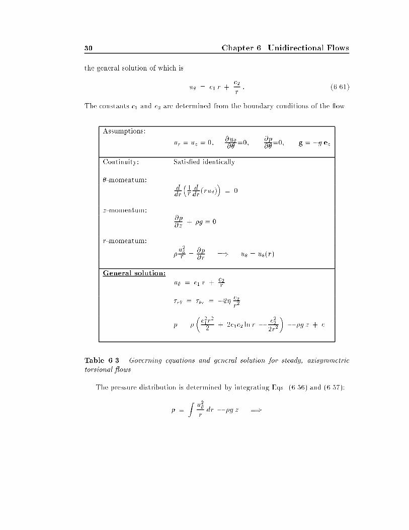
the general solution of which is
u� � c� r �c�r� ������
The constants c� and c� are determined from the boundary conditions of the �ow�
Assumptions�
ur � uz � �� �u���
��� �p��
��� g � �g ez
Continuity� Satis�ed identically
��momentum�ddr
��rddr
�ru���
� �
z�momentum��p�z
� �g � �
r�momentum�
�u��r �
�p�r �� u� � u��r�
General solution�
u� � c� r � c�r
�r� � ��r � ��� c�r�
p � �
�c��r
�
� � �c�c� ln r � c���r�
�� �g z � c
Table ���� Governing equations and general solution for steady� axisymmetrictorsional �ows
The pressure distribution is determined by integrating Eqs� ������ and ���� ��
p �
Zu��rdr � �g z ��
��� Steady� Axisymmetric Torsional Flows ��
p � �
�c��r
�
�� �c�c� ln r � c��
�r�
�� �g z � c � ������
where c is a constant of integration� evaluated in any particular problem by speci�fying the value of the pressure at a reference point�
Note that� under the above assumptions� the only nonzero components of thestress tensor are the shear stresses�
�r� � ��r � � rd
dr
�u�r
�� ������
in terms of which the ��momentum equation takes the form
d
dr�r��r�� � � � �����
The general solution for �r� is
�r� � �� � c�r�
� ������
The assumptions� the governing equations and the general solution for steady�axisymmetric torsional �ows are summarized in Table ����
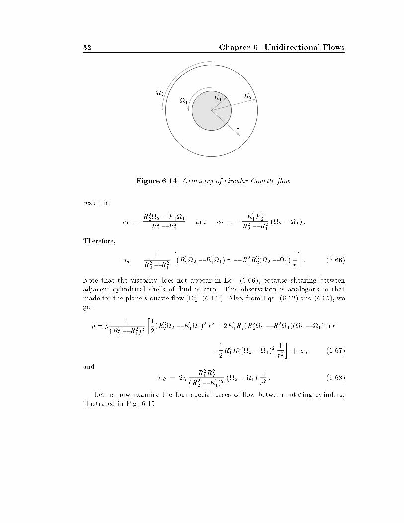
Example ������ Steady �ow between rotating cylindersThe �ow between rotating coaxial cylinders is known as the circular Couette �ow�and is the basis for Couette rotational�type viscometers� Consider the steady �owof an incompressible Newtonian liquid between two vertical coaxial cylinders ofin�nite length and radii R� and R�� respectively� occurring when the two cylindersare rotating about their common axis with angular velocities !� and !�� in theabsence of gravity �Fig� ������
The general form of the angular velocity u� is given by Eq� �������
u� � c� r �c�r�
The boundary conditions�
u� � !�R� at r � R� �
u� � !�R� at r � R� �
�The time�dependent �ow between rotating cylinders is much more interesting� especially themanner in which it destabilizes for large values of ��� leading to the generation of axisymmetricTaylor vortices ����
�� Chapter �� Unidirectional Flows
!�
!�R�
R�
r
Figure ����� Geometry of circular Couette �ow
result in
c� �R��!� � R�
�!�
R�� � R�
�
and c� � � R��R
��
R�� � R�
�
�!� � !�� �
Therefore�
u� ��
R�� � R�
�
��R�
�!� �R��!�� r � R�
�R���!� � !��
�
r
� ������
Note that the viscosity does not appear in Eq� ������� because shearing betweenadjacent cylindrical shells of �uid is zero� This observation is analogous to thatmade for the plane Couette �ow �Eq� ������� Also� from Eqs� ������ and ������� weget
p � ��
�R��� R�
���
��
��R�
�!� �R��!��
� r� � �R��R
���R
��!� �R�
�!���!� � !�� ln r
� �
�R��R
���!� � !��
� �
r�
� c � ���� �
and
�r� � ��R��R
��
�R�� � R�
����!� � !��
�
r�� �����
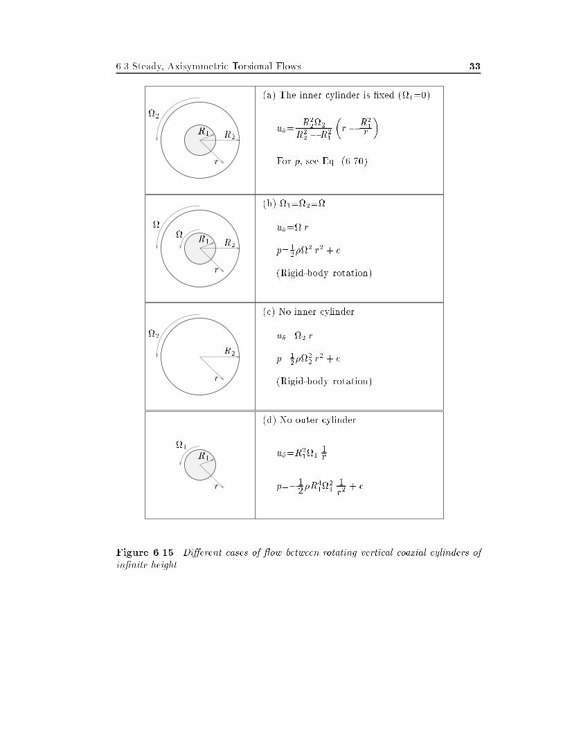
Let us now examine the four special cases of �ow between rotating cylinders�illustrated in Fig� �����
��� Steady� Axisymmetric Torsional Flows ��
!�
R� R�
r
�a� The inner cylinder is �xed �!����
u��R��!�
R�� �R�
�
�r � R�
�r
�
For p� see Eq� ��� ��
!!
R� R�
r
�b� !��!��!
u��! r
p����!
� r� � c
�Rigid�body rotation�
!�
R�
r
�c� No inner cylinder
u��!� r
p����!
�� r
� � c
�Rigid�body rotation�
!�
R�
r
�d� No outer cylinder
u��R��!�
�r
p�����R
��!
���r�
� c
Figure ����� Di�erent cases of �ow between rotating vertical coaxial cylinders ofin�nite height
�� Chapter �� Unidirectional Flows
�a� The inner cylinder is �xed� i�e�� !���� In this case�
u� �R��!�
R�� �R�
�
�r � R�
�
r
�������
and
p � �R��!
��
�R�� �R�
���
�r�
�� �R�
� ln r �R��
�r�
�� c � ��� ��
The constant c can be determined by setting p�p� at r�R�� accordingly�
p � �R��!
��
�R��� R�
���
r� � R�
�
�� �R�
� lnr
R�� R�
�
�
��
r�� �
R��
��� p� � ��� ��
For the shear stress� �r�� we get
�r� � ��R��R
��
R�� �R�
�
!��
r�� ��� ��
The shear stress exerted by the liquid to the outer cylinder is
�w � ��r�jr�R�� ��� R�
�
R�� �R�
�
!� � ��� ��
In viscosity measurements� one measures the torque T per unit height L� at theouter cylinder�
T
L� �� R�
� ���w� ��
T
L� ��
R��R
��
R�� �R�
�
!� � ��� �
The unknown viscosity of a liquid can be determined using the above relation�When the gap between the two cylinders is very small� circular Couette �ow can
be approximated as a plane Couette �ow� Indeed� letting r�R���r� we get fromEq� ������
u� �R��!�
R�� �R�
�
� � rR�
� � rR�
�r �
When R�� R�� �r�R�� and� therefore�
u� �R�!�
��R� �R����r �
R�!�
R� �R��r �
��� Steady� Axisymmetric Torsional Flows ��
which is a linear velocity distribution corresponding to plane Couette �ow betweenplates separated by a distance R��R�� with the upper plate moving with velocityR�!��
�b� The two cylinders rotate with the same angular velocity� i�e��
!� � !� � ! �
In thic case� c��! and c���� Consequently�
u� � ! r � ��� ��
which corresponds to rigid�body rotation� This is also indicated by the zero tangen�tial stress�
�r� � ��� c�r�
� � �
For the pressure� we get
p ��
��!� r� � c � ��� ��
�c� The inner cylinder is removed� In thic case� c��!� and c���� since u� �and �r��are �nite at r��� This �ow is the limiting case of the previous one for R����
u� � !� r � �r� � � and p ��
��!�
� r� � c �
�d� The outer cylinder is removed� i�e�� the inner cylinder is rotating in an in�nitepool of liquid� In this case� u��� as r��� and� therefore� c���� At r�R�� u��!�R�
which gives
c� � R��!� �
Consequently�
u� � R��!�
�
r� ��� �
�r� � ��� R��!�
�
r�� ��� �
and
p � ��
�� R�
�!���
r�� c � ��� ��
The shear stress exerted by the liquid to the cylinder is
�w � �r�jr�R�� ��� !� � �����
�� Chapter �� Unidirectional Flows
The torque per unit height required to rotate the cylinder is
T
L� ��R�
� ���w� � �� R��!� � �����
�
In the previous example� we studied �ows between vertical coaxial cylinders ofin�nite height ignoring the gravitational acceleration� As indicated by Eq� �������gravity has no in�uence on the velocity and a�ects only the pressure� In case ofrotating liquids with a free surface� the gravity term should be included if the toppart of the �ow and the shape of the free surface were of interest� If surface tensione�ects are neglected� the pressure on the free surface is constant� Therefore� thelocus of the free surface can be determined using Eq� �������
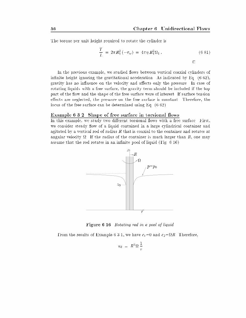
Example ������ Shape of free surface in torsional �owsIn this example� we study two di�erent torsional �ows with a free surface� First�we consider steady �ow of a liquid contained in a large cylindrical container andagitated by a vertical rod of radius R that is coaxial to the container and rotates atangular velocity !� If the radius of the container is much larger than R� one mayassume that the rod rotates in an in�nite pool of liquid �Fig� ������
z
r
!
R
z�
p�p�
Figure ����� Rotating rod in a pool of liquid
From the results of Example ������ we have c��� and c��!R� Therefore�
u� � R�!�
r
��� Steady� Axisymmetric Torsional Flows �
and
p � ��
��R�!� �
r�� �g z � c �
With the surface tension e�ects neglected� the pressure on the free surface is equalto the atmospheric pressure� p�� To determine the constant c� we assume that thefree surface contacts the rod at z�z�� Thus� we obtain
c � p� ��
��R�!� �
R�� �g z�
and
p ��
��R�!�
��
R�� �
r�
�� �g �z � z�� � p� � �����
Since the pressure is constant along the free surface� the equation of the latter is
� � p� p� ��
��R�!�
��
R�� �
r�
�� �g �z � z�� ��
z � z� �R�!�
�g
��� R�
r�
�� �����
The elevation of the free surface increases with the radial distance r and approachesasymptotically the value
z� � z� �R�!�
�g�
This �ow behavior� known as rod dipping� is a characteristic of generalized�Newtonianliquids� whereas viscoelastic liquids exhibit rod climbing �i�e�� they climb the rotatingrod� ����
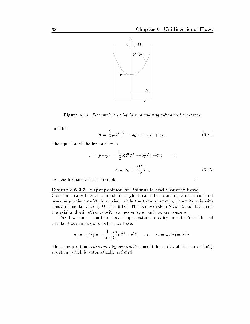
Consider now steady �ow of a liquid contained in a cylindrical container of radiusR rotating at angular velocity ! �Fig� ��� �� From Example ������ we know thatthis �ow corresponds to rigid�body rotation� i�e��
u� � ! r �
The pressure is given by
p ��
��!� r� � �g z � c �
Letting z� be the elevation of the free surface at r��� and p� be the atmosphericpressure� we get
c � p� � �g z� �
�� Chapter �� Unidirectional Flows
z
r
!
R
z�
p�p�
Figure ���� Free surface of liquid in a rotating cylindrical container
and thus
p ��
��!� r� � �g �z � z�� � p� � ����
The equation of the free surface is
� � p� p� ��
��!� r� � �g �z � z�� ��
z � z� �!�
�gr� � �����
i�e�� the free surface is a parabola� �
Example ������ Superposition of Poiseuille and Couette �owsConsider steady �ow of a liquid in a cylindrical tube occurring when a constantpressure gradient �p��z is applied� while the tube is rotating about its axis withconstant angular velocity ! �Fig� ����� This is obviously a bidirectional �ow� sincethe axial and azimuthal velocity components� uz and u�� are nonzero�
The �ow can be considered as a superposition of axisymmetric Poiseuille andcircular Couette �ows� for which we have�
uz � uz�r� � � �
�
�p
�z�R� � r�� and u� � u��r� � ! r �
This superposition is dynamically admissible� since it does not violate the continuityequation� which is automatically satis�ed�
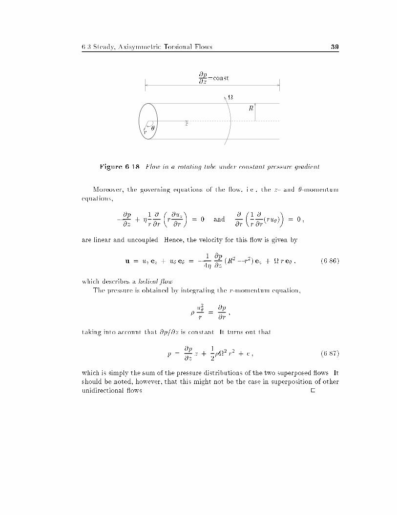
��� Steady� Axisymmetric Torsional Flows ��
zr�
!
R
�p�z
�const�
Figure ����� Flow in a rotating tube under constant pressure gradient
Moreover� the governing equations of the �ow� i�e�� the z� and ��momentumequations�
��p�z
� ��
r
�
�r
�r�uz�r
�� � and
�
�r
��
r
�
�r�ru��
�� � �
are linear and uncoupled� Hence� the velocity for this �ow is given by
u � uz ez � u� e� � � �
�
�p
�z�R� � r�� ez � ! r e� � �����
which describes a helical �ow�The pressure is obtained by integrating the r�momentum equation�
�u��r
��p
�r�
taking into account that �p��z is constant� It turns out that
p ��p
�zz �
�
��!� r� � c � ��� �
which is simply the sum of the pressure distributions of the two superposed �ows� Itshould be noted� however� that this might not be the case in superposition of otherunidirectional �ows� �
� Chapter �� Unidirectional Flows
��� Steady� Axisymmetric Radial Flows
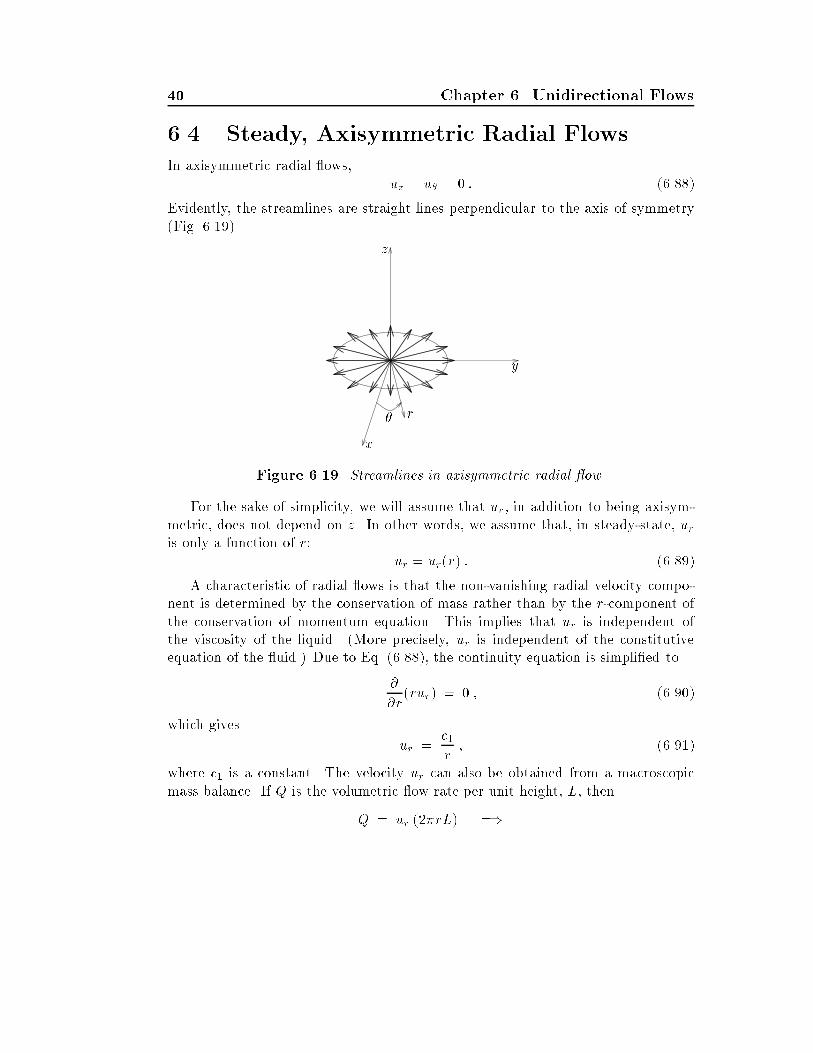
In axisymmetric radial �ows�uz � u� � � � ����
Evidently� the streamlines are straight lines perpendicular to the axis of symmetry�Fig� ������
x
y
z
r�
Figure ����� Streamlines in axisymmetric radial �ow
For the sake of simplicity� we will assume that ur� in addition to being axisym�metric� does not depend on z� In other words� we assume that� in steady�state� uris only a function of r�
ur � ur�r� � �����
A characteristic of radial �ows is that the non�vanishing radial velocity compo�nent is determined by the conservation of mass rather than by the r�component ofthe conservation of momentum equation� This implies that ur is independent ofthe viscosity of the liquid� �More precisely� ur is independent of the constitutiveequation of the �uid�� Due to Eq� ����� the continuity equation is simpli�ed to
�
�r�rur� � � � ������
which gives
ur �c�r� ������
where c� is a constant� The velocity ur can also be obtained from a macroscopicmass balance� If Q is the volumetric �ow rate per unit height� L� then
Q � ur ���rL� ��
�� Steady� Axisymmetric Radial Flows ��
ur �Q
��L r� ������
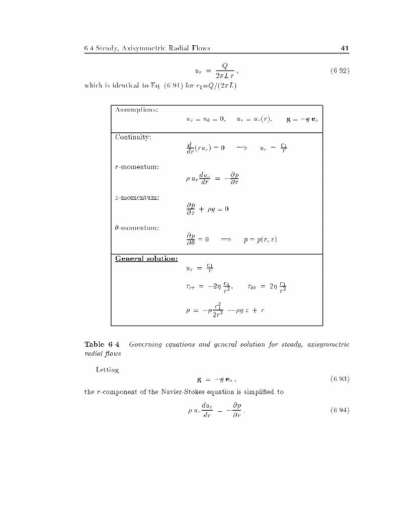
which is identical to Eq� ������ for c��Q����L��
Assumptions�uz � u� � �� ur � ur�r�� g � �g ez
Continuity�ddr
�rur� � � �� ur � c�r
r�momentum�
� urdurdr
� ��p�r
z�momentum��p�z
� �g � �
��momentum��p��
� � �� p � p�r� z�
General solution�
ur � c�r
�rr � ��� c�r�� ��� � �� c�
r�
p � �� c���r�
� �g z � c
Table ���� Governing equations and general solution for steady� axisymmetricradial �ows
Lettingg � �g ez � ������
the r�component of the Navier�Stokes equation is simpli�ed to
� urdurdr
� ��p�r
� �����
�� Chapter �� Unidirectional Flows
Note that the above equation contains a non�vanishing nonlinear convective term�The z� and ��components of the Navier�Stokes equation are reduced to the standardhydrostatic expression�
�p
�z� �g � � � ������
and to�p
��� � � ������
respectively� The latter equation dictates that p�p�r� z�� Integration of Eqs� �����and ������ gives
p�r� z� � ��Zurdurdr
dr � �g z � c
� � c��
Z�
r�dr � �g z � c ��
p�r� z� � �� c���r�
� �g z � c � ���� �
where the integration constant c is determined by specifying the value of the pressureat a point�
In axisymmetric radial �ows� there are two non�vanishing stress components�
�rr � ��durdr
� ��� c�r�
� �����
��� � ��urr
� ��c�r�
� ������
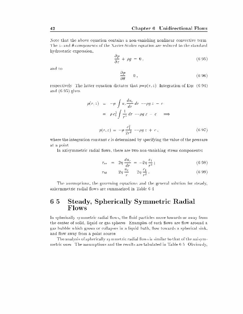
The assumptions� the governing equations and the general solution for steady�axisymmetric radial �ows are summarized in Table ���
�� Steady� Spherically Symmetric RadialFlows
In spherically symmetric radial �ows� the �uid particles move towards or away fromthe center of solid� liquid or gas spheres� Examples of such �ows are �ow around agas bubble which grows or collapses in a liquid bath� �ow towards a spherical sink�and �ow away from a point source�
The analysis of spherically symmetric radial �ows is similar to that of the axisym�metric ones� The assumptions and the results are tabulated in Table ���� Obviously�
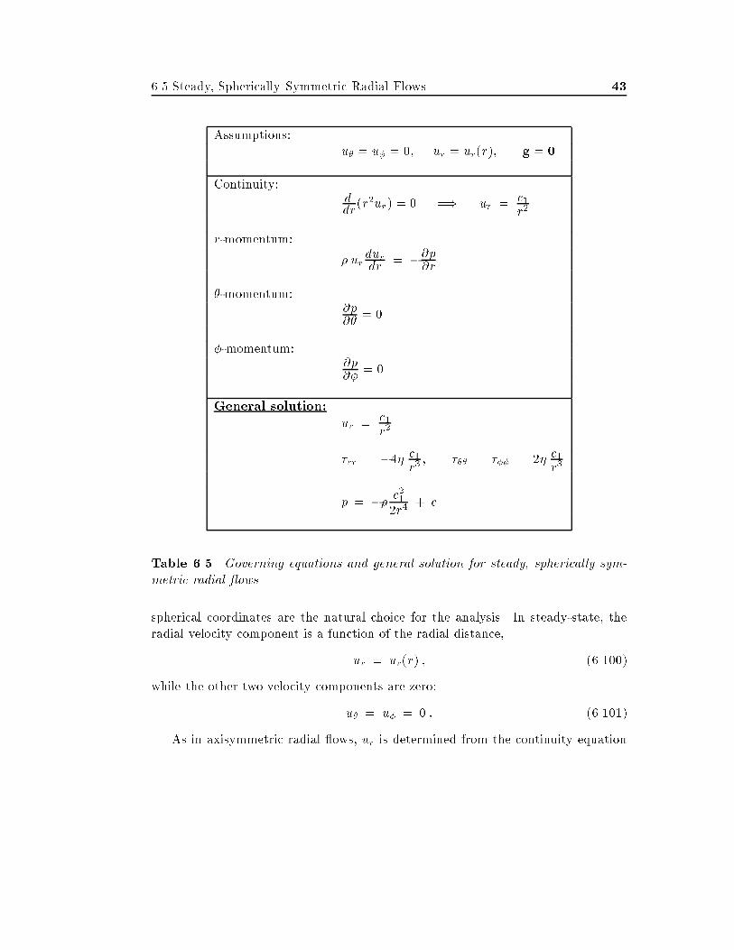
��� Steady� Spherically Symmetric Radial Flows ��
Assumptions�u� � u� � �� ur � ur�r�� g �
Continuity�ddr
�r�ur� � � �� ur � c�r�
r�momentum�
� urdurdr � ��p�r
��momentum��p��
� �
��momentum��p��
� �
General solution�
ur � c�r�
�rr � �� c�r�� ��� � ��� � �� c�
r�
p � �� c���r�
� c
Table ���� Governing equations and general solution for steady� spherically sym�metric radial �ows
spherical coordinates are the natural choice for the analysis� In steady�state� theradial velocity component is a function of the radial distance�
ur � ur�r� � �������
while the other two velocity components are zero�
u� � u� � � � �������
As in axisymmetric radial �ows� ur is determined from the continuity equation
�� Chapter �� Unidirectional Flows
asur �
c�r�
� �������
or
ur �Q
� r�� �������
where Q is the volumetric �ow rate�The pressure is given by
p�r� � �� c���r�
� c � ������
�Note that� in spherically symmetric �ows� gravity is neglected�� Finally� there arenow three non�vanishing stress components�
�rr � ��durdr
� �� c�r�
� �������
��� � ��� � ��urr
� ��c�r�
� �������
Example ����� Bubble growth in a Newtonian liquidBoiling of a liquid often originates from small air bubbles which grow radially in theliquid� Consider a spherical bubble of radius R�t� in a pool of liquid� growing at arate
dR
dt� k �
The velocity� ur� and the pressure� p� can be calculated using Eqs� �������and ������� respectively� At �rst� we calculate the constant c�� At r�R� ur�dR�dt�kor
c�R�
� k �� c� � kR� �
Substituting c� into Eqs� ������� and ������� we get
ur � kR�
r�
and
p � ��k� R�
�r�� c �
Note that the pressure near the surface of the bubble may attain small or evennegative values� which favor evaporation of the liquid and expansion of the bubble�
�
Sec� ���� Transient One�Dimensional Unidirectional Flows ��
��� Transient One�Dimensional UnidirectionalFlows
In Sections ��� to ���� we studied three classes of steady�state unidirectional �ows�where the dependent variable� i�e�� the nonzero velocity component� was assumedto be a function of a single spatial independent variable� The governing equationfor such a �ow is a linear second�order ordinary di�erential equation which is inte�grated to arrive at a general solution� The general solution contains two integrationconstants which are determined by the boundary conditions at the endpoints of theone�dimensional domain over which the analytical solution is sought�
In the present section� we consider one�dimensional� transient unidirectional�ows� Hence� the dependent variable is now a function of two independent vari�ables� one of which is time� t� The governing equations for these �ows are partialdi�erential equations� In fact� we have already encountered some of these PDEsin Sections �������� while simplifying the corresponding components of the Navier�Stokes equation� For the sake of convenience� these are listed below�
�a� For transient one�dimensional rectilinear �ow in Cartesian coordinates withuy�uz�� and ux�ux�y� t��
��ux�t
� ��p
�x� �
��ux�y�
� �gx � ����� �
�b� For transient axisymmetric rectilinear �ow with ur�u��� and uz�uz�r� t��
��uz�t
� ��p�z
� ��
r
�
�r
�r�uz�r
�� �gz �
or
��uz�t
� ��p�z
� �
���uz�r�
��
r
�uz�r
�� �gz � ������
�c� For transient axisymmetric torsional �ow with uz�ur�� and u��u��r� t��
��u��t
� ��
�r
��
r
�
�r�ru��
��
or
��u��t
� �
���u��r�
��
r
�u��r
� �
r�u�
�� �������
�� Chapter �� Unidirectional Flows
The above equations are all parabolic PDEs� For any particular �ow� they aresupplemented by appropriate boundary conditions at the two endpoints of the one�dimensional �ow domain� and by an initial condition for the entire �ow domain� Notethat the pressure gradients in Eqs� ����� � and ������ may be functions of time�These two equations are inhomogeneous due to the presence of the pressure gradientand gravity terms� The inhomogeneous terms can be eliminated by decomposing thedependent variable into a properly chosen steady�state component �satisfying thecorresponding steady�state problem and the boundary conditions� and a transientone which satis�es the homogeneous problem� A similar decomposition is oftenused for transforming inhomogeneous boundary conditions into homogeneous ones�Separation of variables ��� and the similarity solution method ����� are the standardmethods for solving Eq� ������� and the homogeneous counterparts of Eqs� ����� �and �������
In homogeneous problems admitting separable solutions� the dependent variableu�xi� t� is expressed in the form
u�xi� t� � X�xi� T �t� � �������
Substitution of the above expression into the governing equation leads to the equiv�alent problem of solving two ordinary di�erential equations with X and T as thedependent variables�
In similarity methods� the two independent variables� xi and t� are combinedinto the similarity variable
� � ��xi� t� � �������
If a similarity solution does exist� then the original partial di�erential equation foru�xi� t� is reduced to an ordinary di�erential equation for u����
Similarity solutions exist for problems involving parabolic PDEs in two indepen�dent variables where external length and time scales are absent� A typical problemis �ow of a semi�in�nite �uid above a plate suddenly set in motion with a constantvelocity �Example ������� Length and time scales do exist in transient plane Couette�ow� and in �ow of a semi�in�nite �uid above a plate oscillating along its own plane�In the former �ow� the length scale is the distance between the two plates� whereasin the latter case� the length scale is the period of oscillations� These two �ows aregoverned by Eq� ����� �� with the pressure�gradient and gravity terms neglected�they are solved in Examples ����� and ������ using separation of variables� In Exam�ple ����� we solve the problem of transient plane Poiseuille �ow� due to the suddenapplication of a constant pressure gradient�
Finally� in the last two examples� we solve transient axisymmetric rectilinearand torsional �ow problems� governed� respectively� by Eqs� ������ and �������� In
��� Transient One�Dimensional Unidirectional Flows �
Example ������ we consider transient axisymmetric Poiseuille �ow� and in Exam�ple ������ we consider �ow inside an in�nite long cylinder which is suddenly rotated�
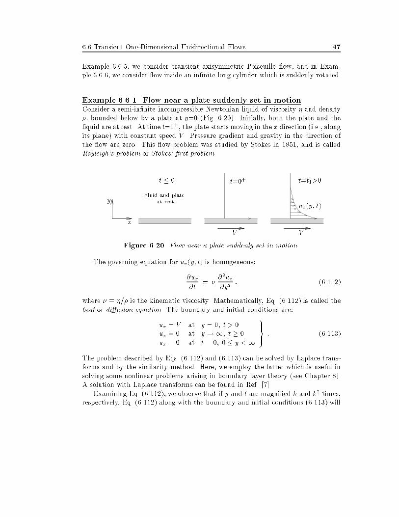
Example ������ Flow near a plate suddenly set in motionConsider a semi�in�nite incompressible Newtonian liquid of viscosity � and density�� bounded below by a plate at y�� �Fig� ������ Initially� both the plate and theliquid are at rest� At time t���� the plate starts moving in the x direction �i�e�� alongits plane� with constant speed V � Pressure gradient and gravity in the direction ofthe �ow are zero� This �ow problem was studied by Stokes in ���� and is calledRayleigh�s problem or Stokes� �rst problem�
x
y
t � � t��� t�t���
Fluid and plateat rest
ux�y� t�
V V
Figure ���� Flow near a plate suddenly set in motion
The governing equation for ux�y� t� is homogeneous�
�ux�t
� ���ux�y�
� �������
where � ��� is the kinematic viscosity� Mathematically� Eq� ������� is called theheat or di�usion equation� The boundary and initial conditions are�
ux � V at y � �� t � �ux � � at y ��� t � �ux � � at t � �� � � y ��
����� � �������
The problem described by Eqs� ������� and ������� can be solved by Laplace trans�forms and by the similarity method� Here� we employ the latter which is useful insolving some nonlinear problems arising in boundary layer theory �see Chapter ��A solution with Laplace transforms can be found in Ref� � ��
Examining Eq� �������� we observe that if y and t are magni�ed k and k� times�respectively� Eq� ������� along with the boundary and initial conditions ������� will
�� Chapter �� Unidirectional Flows
still be satis�ed� This clearly suggests that ux depends on a combination of y and tof the form y�
pt� The same conclusion is reached by noting that the dimensionless
velocity ux�V must be a function of the remaining kinematic quantities of this �owproblem� �� t and y� From these three quantities� only one dimensionless group canbe formed� ��y�
p�t�
Let us� however� assume that the existence of a similarity solution and the propercombination of y and t are not known a priori� and assume that the solution is ofthe form
ux�y� t� � V f��� � ������
where
� � ay
tn� with n � � � �������
Here ��y� t� is the similarity variable� a is a constant to be determined later so that� is dimensionless� and n is a positive number to be chosen so that the originalpartial di�erential equation ������� can be transformed into an ordinary di�erentialequation with f as the dependent variable and � as the independent one� Note thata precondition for the existence of a similarity solution is that � is of such a formthat the original boundary and initial conditions are combined into two boundaryconditions for the new dependent variable f � This is easily veri�ed in the present�ow� The boundary condition at y�� is equivalent to
f � � at � � � � �������
whereas the boundary condition at y�� and the initial condition collapse to asingle boundary condition for f �
f � � at � �� � ����� �
Di�erentiation of Eq� ������ using the chain rule gives
�ux�t
� �V nay
tn��f � � �V n
�
tf � �
�ux�y
� Va
tnf � and
��ux�y�
� Va�
t�nf �� �
where primes denote di�erentiation with respect to �� Substitution of the abovederivatives into Eq� ������� gives the following equation�
f �� �n�
�a�t�n�� f � � � �
��� Transient One�Dimensional Unidirectional Flows ��
By setting n����� time is eliminated and the above expression becomes a second�order ordinary di�erential equation�
f �� ��
��a�f � � � with � � a
ypt�
Taking a equal to ��p� makes the similarity variable dimensionless� For convenience
in the solution of the di�erential equation� we set a�����p��� Hence�
� �y
�p� t
� ������
whereas the resulting ordinary di�erential equation is
f �� � �� f � � � � �������
This equation is subject to the boundary conditions ������� and ����� �� By straight�forward integration� we obtain
f��� � c�
Z
�e�z
�
dz � c� �
where z is a dummy variable of integration� At ���� f��� consequently� c���� At���� f��� therefore�
c�
Z�
�e�z
�
dz � � � � or c� � � �p��
and
f��� � � � �p�
Z
�e�z
�
dz � � � erf��� � �������
where erf is the error function� de�ned as
erf��� �p�
Z
�e�z
�
dz � �������
Values of the error function are tabulated in several math textbooks� It is a mono�tone increasing function with
erf��� � � and lim��
erf��� � � �
Note that the second expression was used when calculating the constant c�� Substi�tuting into Eq� ������� we obtain the solution
ux�y� t� � V
�� � erf
�y
�p� t
�� �������
� Chapter �� Unidirectional Flows
0
0.2
0.4
0.6
0.8
1
-0.2 0 0.2 0.4 0.6 0.8 1 1.2
ux�V
y��
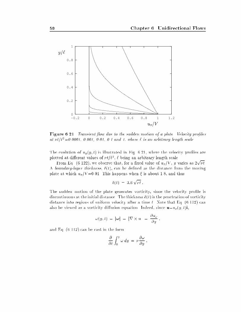
Figure ����� Transient �ow due to the sudden motion of a plate Velocity pro�lesat �t���� �� �� �� � and �� where � is an arbitrary length scale
The evolution of ux�y� t� is illustrated in Fig� ����� where the velocity pro�les areplotted at di�erent values of �t���� � being an arbitrary length scale�
From Eq� �������� we observe that� for a �xed value of ux�V � y varies as �p�t�
A boundary�layer thickness� �t�� can be de�ned as the distance from the movingplate at which ux�V������ This happens when � is about ��� and thus
�t� � ���p�t �
The sudden motion of the plate generates vorticity� since the velocity pro�le isdiscontinuous at the initial distance� The thickness �t� is the penetration of vorticitydistance into regions of uniform velocity after a time t� Note that Eq� ������� canalso be viewed as a vorticity di�usion equation� Indeed� since u�ux�y� t�i�
��y� t� � j�j � jr� uj � �ux�y
�
and Eq� ������� can be cast in the form
�
�t
Z y
�� dy � �
��
�y�
��� Transient One�Dimensional Unidirectional Flows ��
or� equivalently���
�t� �
���
�y�� �������
The above expression is a vorticity conservation equation and highlights the roleof kinematic viscosity� which acts as a vorticity di�usion coe�cient� in a manneranalogous to that of thermal di�usivity in heat di�usion�
The shear stress on the plate is given by
�w � �yxjy�� � ��ux�y
����y��
� ��V �erf���
��
������
��
�y
����y��
� � �Vp��t
� ������
which suggests that the stress is singular at the instant the plate starts moving� anddecreases as ��
pt�
The physics of this example are similar to those of boundary layer �ow� which isexamined in detail in Chapter � In fact� the same similarity variable was invokedby Rayleigh to calculate skin�friction over a plate moving with velocity V througha stationary liquid which leads to ��
�w ��Vp��
sV
x�
by simply replacing t by x�V in Eq� ������� This situation arises in free stream�ows overtaking submerged bodies� giving rise to boundary layers ����
�
In the following example� we demonstrate the use of separation of variables bysolving a transient plane Couette �ow problem�
Example ������ Transient plane Couette �owConsider a Newtonian liquid of density � and viscosity � bounded by two in�niteparallel plates separated by a distance H � as shown in Fig� ����� The liquid and thetwo plates are initially at rest� At time t���� the lower plate is suddenly broughtto a steady velocity V in its own plane� while the upper plate is held stationary�
The governing equation is the same as in the previous example�
�ux�t
� ���ux�y�
� �������
with the following boundary and initial conditions�
ux � V at y � �� t � �ux � � at y � H� t � �ux � � at t � �� � � y � H
����� �������
�� Chapter �� Unidirectional Flows
x
y
H
V
t�
t�t�
�
ux���V��� y
H
�
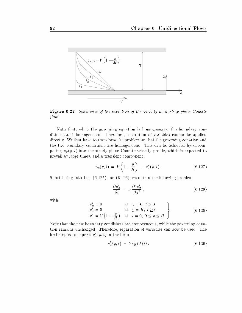
Figure ����� Schematic of the evolution of the velocity in start�up plane Couette�ow
Note that� while the governing equation is homogeneous� the boundary con�ditions are inhomogeneous� Therefore� separation of variables cannot be applieddirectly� We �rst have to transform the problem so that the governing equation andthe two boundary conditions are homogeneous� This can be achieved by decom�posing ux�y� t� into the steady plane Couette velocity pro�le� which is expected toprevail at large times� and a transient component�
ux�y� t� � V
��� y
H
�� u�x�y� t� � ����� �
Substituting into Eqs� ������� and �������� we obtain the following problem
�u�x�t
� ���u�x�y�
� ������
withu�x � � at y � �� t � �u�x � � at y � H� t � �
u�x � V��� y
H
�at t � �� � � y � H
����� �������
Note that the new boundary conditions are homogeneous� while the governing equa�tion remains unchanged� Therefore� separation of variables can now be used� The�rst step is to express u�x�y� t� in the form
u�x�y� t� � Y �y� T �t� � �������
��� Transient One�Dimensional Unidirectional Flows ��
Substituting into Eq� ������ and separating the functions Y and T � we get
�
�T
dT
dt�
�
Y
d�Y
dY ��
The only way a function of t can be equal to a function of y is for both functionsto be equal to the same constant� For convenience� we choose this constant to be����H�� �One advantage of this choice is that � is dimensionless�� We thus obtaintwo ordinary di�erential equations�
dT
dt�
���
H�T � � � �������
d�Y
dy��
��
H�Y � � � �������
The solution to Eq� ������� is
T � c� e����H� t � �������
where c� is an integration constant to be determined�Equation ������� is a homogeneous second�order ODE with constant coe�cients�
and its general solution is
Y �y� � c� sin��y
H� � c� cos�
�y
H� � ������
The form of the general solution justi�es the choice we made earlier for the constant����H�� The constants c� and c� are determined by the boundary conditions�Applying Eq� ������� to the boundary conditions at y�� and H� we obtain
Y ��� T �t� � � and Y �H� T �t� � � �
The case of T �t��� is excluded� since this corresponds to the steady�state problem�Hence� we get the following boundary conditions for Y �
Y ��� � � and Y �H� � � � �������
Note that in order to get the boundary conditions on Y � it is essential that theboundary conditions are homogeneous�
Applying the boundary condition at y��� we get c���� Thus�
Y �y� � c� sin��y
H� � �������
�� Chapter �� Unidirectional Flows
Applying now the boundary condition at y�H � we get
sin��� � � � ����� �
which has in�nitely many roots�
�k � k� � k � �� �� � � � ������
To each of these roots correspond solutions Yk and Tk� These in�nitely many solu�tions are superimposed by de�ning
u�x�y� t� ��Xk��
Bk sin��ky
H� e���
�k
H� t ��Xk��
Bk sin�k� y
H� e�k���
H� �t� �������
where the constants Bk�c�kc�k are determined from the initial condition� For t���we get
�Xk��
Bk sin�k� y
H� � V
��� y
H
�� ������
To isolate Bk� we will take advantage of the orthogonality property
Z �
�sin�k�x� sin�n�x� dx �
�����
�� � k � n
� � k �� n
������
BY multiplying both sides of Eq� ������ by sin�n�y�H�dy� and by integrating from� to H � we have�
�Xk��
Bk
Z H
�sin�
k� y
H� sin�
n� y
H� dy � V
Z H
�
��� y
H
�sin�
n� y
H� dy �
Setting ��y�H � we get
�Xk��
Bk
Z �
�sin�k��� sin�n��� d� � V
Z �
���� �� sin�n��� d� �
Due to the orthogonality property ������� the only nonzero term on the left handside is that for k�n� hence�
Bk�
�� V
Z �
���� �� sin�k��� d� � V
�
k���
��� Transient One�Dimensional Unidirectional Flows ��
Bk ��V
k�� ������
Substituting into Eq� ������� gives
u�x�y� t� ��V
�
�Xk��
�
ksin�
k� y
H� e�k���
H� �t� ������
0
0.2
0.4
0.6
0.8
1
-0.2 0 0.2 0.4 0.6 0.8 1 1.2
ux�V
y�H
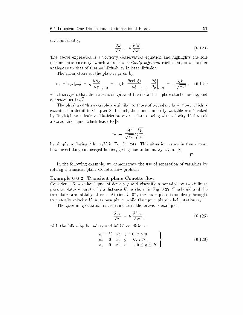
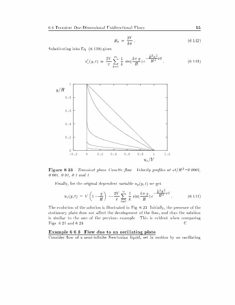
Figure ����� Transient plane Couette �ow Velocity pro�les at �t�H�� �� �� �� � and �
Finally� for the original dependent variable ux�y� t� we get
ux�y� t� � V
��� y
H
�� �V
�
�Xk��
�
ksin�
k� y
H� e�k���
H� �t� �����
The evolution of the solution is illustrated in Fig� ����� Initially� the presence of thestationary plate does not a�ect the development of the �ow� and thus the solutionis similar to the one of the previous example� This is evident when comparingFigs� ���� and ����� �
Example ������ Flow due to an oscillating plateConsider �ow of a semi�in�nite Newtonian liquid� set in motion by an oscillating
�� Chapter �� Unidirectional Flows
plate of velocityV � V� cos�t � t � � � ������
The governing equation� the initial condition and the boundary condition at y��are the same as those of Example ������ At y��� ux is now equal to V� cos�t� Hence�we have the following problem�
�ux�t
� ���ux�y�
� ������
withux � V� cos�t at y � �� t � �ux � � at y ��� t � �ux � � at t � �� � � y � �
����� � ���� �
This is known as Stokes problem or Stokes� second problem� �rst studied by Stokesin ���
Since the period of the oscillations of the plate introduces a time scale� no simi�larity solution exists to this problem� By virtue of Eq� ������� it may be expectedthat ux will also oscillate in time with the same frequency� but possibly with a phaseshift relative to the oscillations of the plate� Thus� we separate the two independentvariables by representing the velocity as
ux�y� t� � RehY �y� eit
i� �����
where Re denotes the real part of the expression within the brackets� i is the imagi�nary unit� and Y �y� is a complex function� Substituting into the governing equation�we have
d�Y
dy�� i�
�Y � � � ������
The general solution of the above equation is
Y �y� � c� exp
��r
�
���� � i� y
�� c� exp
�r�
���� � i� y
��
The fact that ux�� at y��� dictates that c� be zero� Then� the boundary conditionat y�� requires that c��V�� Thus�
ux�y� t� � V� Re�exp
��r
�
���� � i� y
�eit
� �������
The resulting solution�
ux�y� t� � V� exp
��r
�
��y
�cos
��t�
r�
��y
�� �������
��� Transient One�Dimensional Unidirectional Flows �
describes a damped transverse wave of wavelength ��p����� propagating in the
y�direction with phase velocityp���� The amplitude of the oscillations decays
exponentially with y� The depth of penetration of vorticity is p����� suggesting
that the distance over which the �uid feels the motion of the plate gets smaller asthe frequency of the oscillations increases� �
Example ������ Transient plane Poiseuille �owLet us now consider a transient �ow which is induced by a suddenly applied constantpressure gradient� A Newtonian liquid of density � and viscosity �� is containedbetween two horizontal plates separated by a distance �H �Fig� ����� The liquidis initially at rest� at time t���� a constant pressure gradient� �p��x� is applied�setting the liquid into motion�
x
yHt�� t� t� �
Figure ����� Schematic of the evolution of the velocity in transient plane Poiseuille�ow
The governing equation for this �ow is
��ux�t
� ��p
�x� �
��ux�y�
� �������
Positioning the x�axis on the symmetry plane of the �ow �Fig� ����� the boundaryand initial conditions become�
ux � � at y � H� t � ��ux�y � � at y � �� t � �
ux � � at t � �� � � y � H
����� �������
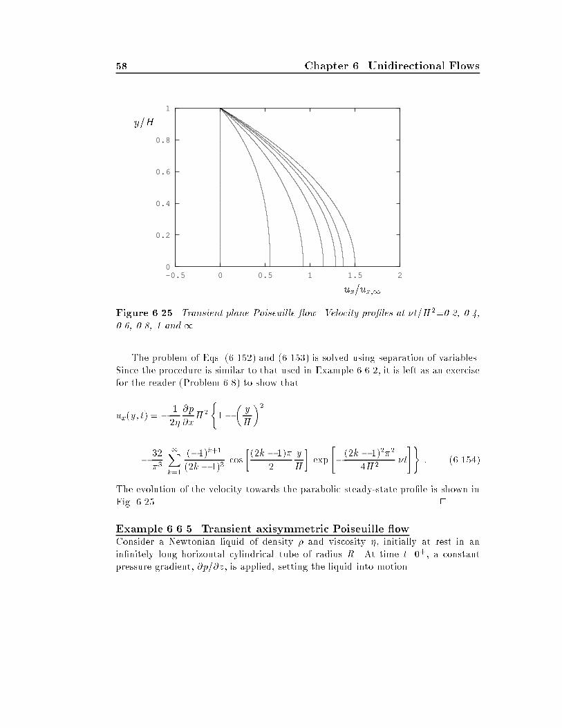
�� Chapter �� Unidirectional Flows
0
0.2
0.4
0.6
0.8
1
-0.5 0 0.5 1 1.5 2
ux��ux��
y�H
Figure ����� Transient plane Poiseuille �ow Velocity pro�les at �t�H�� �� �� �� �� � and �
The problem of Eqs� ������� and ������� is solved using separation of variables�Since the procedure is similar to that used in Example ������ it is left as an exercisefor the reader �Problem ��� to show that
ux�y� t� � � �
��
�p
�xH�
���
�y
H
��
� ��
��
�Xk��
����k����k � ���
cos
���k � ���
�
y
H
exp
���k � �����
H��t
� � ������
The evolution of the velocity towards the parabolic steady�state pro�le is shown inFig� ����� �
Example ����� Transient axisymmetric Poiseuille �owConsider a Newtonian liquid of density � and viscosity �� initially at rest in anin�nitely long horizontal cylindrical tube of radius R� At time t���� a constantpressure gradient� �p��z� is applied� setting the liquid into motion�
��� Transient One�Dimensional Unidirectional Flows ��
This is obviously a transient axisymmetric rectilinear �ow� Since gravity is zero�the governing equation is
��uz�t
� ��p�z
� �
���uz�r�
��
r
�uz�r
�� �������
subject to the following boundary conditions�
uz � � at r � R� t � �uz �nite at r � �� t � �uz � � at t � �� � � r � R
����� �������
By decomposing uz�r� t� into the steady�state Poiseuille �ow component �ex�pected to prevail at large times� and a new dependent variable�
uz�r� t� � � �
�
�p
�z�R� � r�� � u�z�r� t� � ����� �
the inhomogeneous pressure�gradient term in Eq� ������� is eliminated� and thefollowing homogeneous problem is obtained�
�u�z�t
� �
���u�z�r�
��
r
�u�z�r
�������
withu�z � � at r � R� t � �u�z �nite at r � �� t � �
u�z � � ��
�p�z �R� � r�� at t � �� � � r � R
����� �������
Using separation of variables� we express u�z�r� t� in the form
u�z�r� t� � X�r� T �t� � �������
Substituting into Eq� ������ and separating the functions X and T � we get
�
�T
dT
dt�
�
X
�d�X
dr��
�
r
dX
dr
��
Equating both sides of the above expression to ����R�� where � is a dimensionlessconstant� we obtain two ordinary di�erential equations�
dT
dt�
���
R�T � � � �������
� Chapter �� Unidirectional Flows
d�X
dr��
�
r
dX
dr�
��
R�X � � � �������
The solution to Eq� ������� is
T � c� e����R� t � �������
where c� is an integration constant�Equation ������� is a Bessel�s di�erential equation� whose general solution is
given by
X�r� � c� J���r
R� � c� Y��
�r
R� � ������
where J� and Y� are the zeroth�order Bessel functions of the �rst and second kind�respectively� From the theory of Bessel functions� we know that Y��x� and its �rstderivative are unbounded at x��� Since u�z and thus X must be �nite at r��� weget c����
Di�erentiating Eq� ������ and noting that
dJ�dx
�x� � �J��x� �
where J� is the �rst�order Bessel function of the �rst kind� we obtain�
dX
dr�r� � �c� �
RJ��
�r
R� � c�
�
R
dY�dr
��r
R� �
Given that J������� we �nd again that c� must be zero so that dX�dr�� at r���Thus�
X�r� � c�J���r
R� � �������
Applying the boundary condition at r�R� we get
J���� � � � �������
Note that J��x� is an oscillating function with in�nitely many roots�
�k � k � �� �� � � �
Therefore� u�z�r� t� is expressed as an in�nite sum of the form
u�z�r� t� ��Xk��
Bk J���kr
R� e���
�k
R� t � ����� �
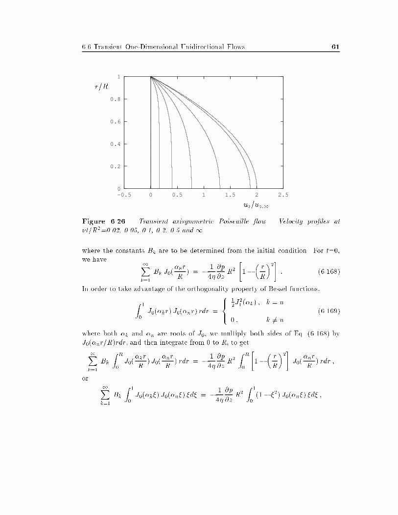
��� Transient One�Dimensional Unidirectional Flows ��
0
0.2
0.4
0.6
0.8
1
-0.5 0 0.5 1 1.5 2 2.5
uz��uz��
r�R
Figure ����� Transient axisymmetric Poiseuille �ow Velocity pro�les at�t�R�� �� �� �� �� � and �
where the constants Bk are to be determined from the initial condition� For t���we have
�Xk��
Bk J���kr
R� � � �
�
�p
�zR�
��
�r
R
���� ������
In order to take advantage of the orthogonality property of Bessel functions�
Z �
�J���kr� J���nr� rdr �
�����
��J
�� ��k� � k � n
� � k �� n�������
where both �k and �n are roots of J�� we multiply both sides of Eq� ������ byJ���nr�R�rdr� and then integrate from � to R� to get
�Xk��
Bk
Z R
�J��
�kr
R� J��
�nr
R� rdr � � �
�
�p
�zR�
Z R
�
��
�r
R
���J��
�nr
R� rdr �
or�Xk��
Bk
Z �
�J���k�� J���n�� �d� � � �
�
�p
�zR�
Z �
���� ��� J���n�� �d� �
�� Chapter �� Unidirectional Flows
where ��r�R� The only nonzero term on the left hand side corresponds to k�n�Hence�
Bk�
�J�� ��k� � � �
�
�p
�zR�
Z �
���� ��� J���k�� �d� � ���� ��
Using standard relations for Bessel functions� we �nd that
Z �
���� ��� J���k�� �d� �
J���k�
��k�
Therefore�
Bk � � �
�
�p
�z
��k J���k��
and
u�z � � �
�
�p
�z�R��
�Xk��
J���krR
���k J���k�
e���
�k
R� t � ���� ��
Substituting into Eq� ����� � gives
uz�r� t� � � �
�
�p
�zR�
����� � r
R
���
�Xk��
J���krR
���k J���k�
e���
�k
R� t
��� � ���� ��
The evolution of the velocity is shown in Fig� ����� �
Example ������ Flow inside a cylinder that is suddenly rotatedA Newtonian liquid of density � and viscosity � is initially at rest in a vertical�in�nitely long cylinder of radius R� At time t���� the cylinder starts rotatingabout its axis with constant angular velocity !� setting the liquid into motion�
This is a transient axisymmetric torsional �ow� governed by
�u��t
� �
���u��r�
��
r
�u��r
� �
r�u�
�� ���� ��
subject to the following conditions�
u� � !R at r � R� t � �u� �nite at r � �� t � �u� � � at t � �� � � r � R
����� ���� �
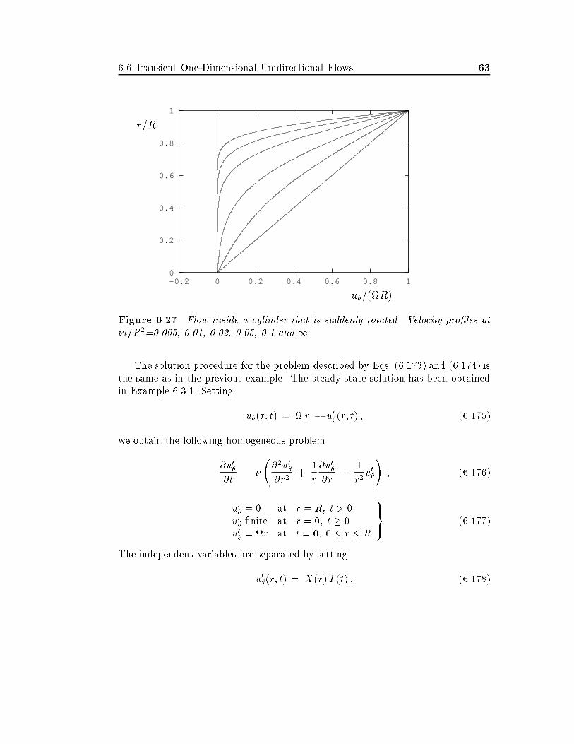
��� Transient One�Dimensional Unidirectional Flows ��
0
0.2
0.4
0.6
0.8
1
-0.2 0 0.2 0.4 0.6 0.8 1
u����R�
r�R
Figure ���� Flow inside a cylinder that is suddenly rotated Velocity pro�les at�t�R�� �� �� �� �� � and �
The solution procedure for the problem described by Eqs� ���� �� and ���� � isthe same as in the previous example� The steady�state solution has been obtainedin Example ������ Setting
u��r� t� � ! r � u���r� t� � ���� ��
we obtain the following homogeneous problem
�u���t
� �
���u���r�
��
r
�u���r
� �
r�u��
�� ���� ��
u�� � � at r � R� t � �u�� �nite at r � �� t � �u�� � !r at t � �� � � r � R
����� ���� �
The independent variables are separated by setting
u���r� t� � X�r�T �t� � ���� �
�� Chapter �� Unidirectional Flows
which leads to two ordinary di�erential equations�
dT
dt�
���
R�T � � � ���� ��
andd�X
dr��
�
r
dX
dr�
���
R�� �
r�
�X � � � ������
Equation ���� �� is identical to Eq� ������� of the previous example� whose generalsolution is
T � c� e����R� t � ������
The general solution of Eq� ������ is
X�r� � c� J���r
R� � c� Y��
�r
R� � ������
where J� and Y� are the �rst�order Bessel functions of the �rst and second kind�respectively� Since Y��x� is unbounded at x��� c� must be zero� Therefore�
X�r� � c�J���r
R� � ������
The boundary condition at r�R requires that
J���� � � � �����
which has in�nitely many roots� Therefore� u���r� t� is expressed as an in�nite sumof the form
u���r� t� ��Xk��
Bk J���kr
R� e���
�k
R� t � ������
where the constants Bk are to be determined from the initial condition� For t���we have
�Xk��
Bk J���kr
R� � ! r � ������
The constants Bk are determined by using the orthogonality property of Besselfunctions� Z �
�J���kr� J���nr� rdr �
�����
��J
�� ��k� � k � n
� � k �� n���� �
Sec� ���� Steady Two�Dimensional Rectilinear Flows ��
where both �k and �n are roots of J�� Multiplying both sides of Eq� ������ byJ���nr�R�rdr� and integrating from � to R� we get
�Xk��
Bk
Z R
�J��
�kr
R� J��
�nr
R� rdr � !
Z R
�J��
�nr
R� r� dr �
or�Xk��
Bk
Z �
�J���k�� J���n�� �d� � !R
Z �
�J���n�� �
� d� �
where ��r�R� Invoking Eq� ���� �� we get
Bk�
�J�� ��k� � !R
Z �
�J���k�� �
�d� � �!RJ���k�
�k��
Bk � � �!R
�k J���k��
Therefore�
u�� � ��!R�Xk��
J���krR
��k J���k�
e���
�k
R� t �����
and
u��r� t� � ! r � �!R�Xk��
J���krR
��k J���k�
e���
�k
R� t � ������
The evolution of the u� is shown in Fig� ��� � �
�� Steady Two�Dimensional RectilinearFlows
As explained in Section ���� in steady� rectilinear �ows in the x direction� ux�ux�y� z�and the x�momentum equation is reduced to a Poisson equation�
��ux�y�
���ux�z�
��
�
�p
�x� �
�gx � �������
Equation ������� is an elliptic PDE� Since �p��x is a function of x alone and uxis a function of y and z� Eq� ������� can be satis�ed only when �p��x is constant�Therefore� the right hand side term of Eq� ������� is a constant� This inhomogeneousterm can be eliminated by introducing a new dependent variable which satis�es theLaplace equation�
Two classes of �ows governed by Eq� ������� are�
�� Chapter �� Unidirectional Flows
�a� Poiseuille �ows in tubes of arbitrary but constant cross section� and
�b� gravity�driven rectilinear �lm �ows�
One�dimensional Poiseuille �ows have been encountered in Sections ��� and ����The most important of them� i�e�� plane� round and annular Poiseuille �ows� aresummarized in Fig� ���� In the following� we will discuss two�dimensional Poiseuille�ows in tubes of elliptical� rectangular and triangular cross sections� illustrated inFig� ����� In these rather simple geometries� Eq� ������� can be solved analytically�Analytical solutions for other cross sectional shapes are given in Refs� ���� and �����
Example ������ Poiseuille �ow in a tube of elliptical cross sectionConsider fully�developed �ow of an incompressible Newtonian liquid in an in�nitelylong tube of elliptical cross section� under constant pressure gradient �p��x� Gravityis neglected� and thus Eq� ������� becomes
��ux�y�
���ux�z�
��
�
�p
�xin
y�
a��z�
b�� � � �������
where a and b are the semi�axes of the elliptical cross section� as shown in Fig� ����a�The velocity is zero at the wall� and thus the boundary condition is�
ux � � ony�
a��z�
b�� � � �������
Let us now introduce a new dependent variable u�x� such that
ux�y� z� � u�x�y� z� � c�y� � c�z
� � �������
where c� and c� are non zero constants to be determined so that �a� u�x satis�es theLaplace equation� and �b� u�x is constant on the wall� Substituting Eq� ������� intoEq� �������� we get
��u�x�y�
���u�x�z�
� �c� � �c� ��
�
�p
�x� ������
Evidently� u�x satis�es the Laplace equation�
��u�x�y�
���u�x�z�
� � � �������
if
�c� � �c� ��
�
�p
�x� �������
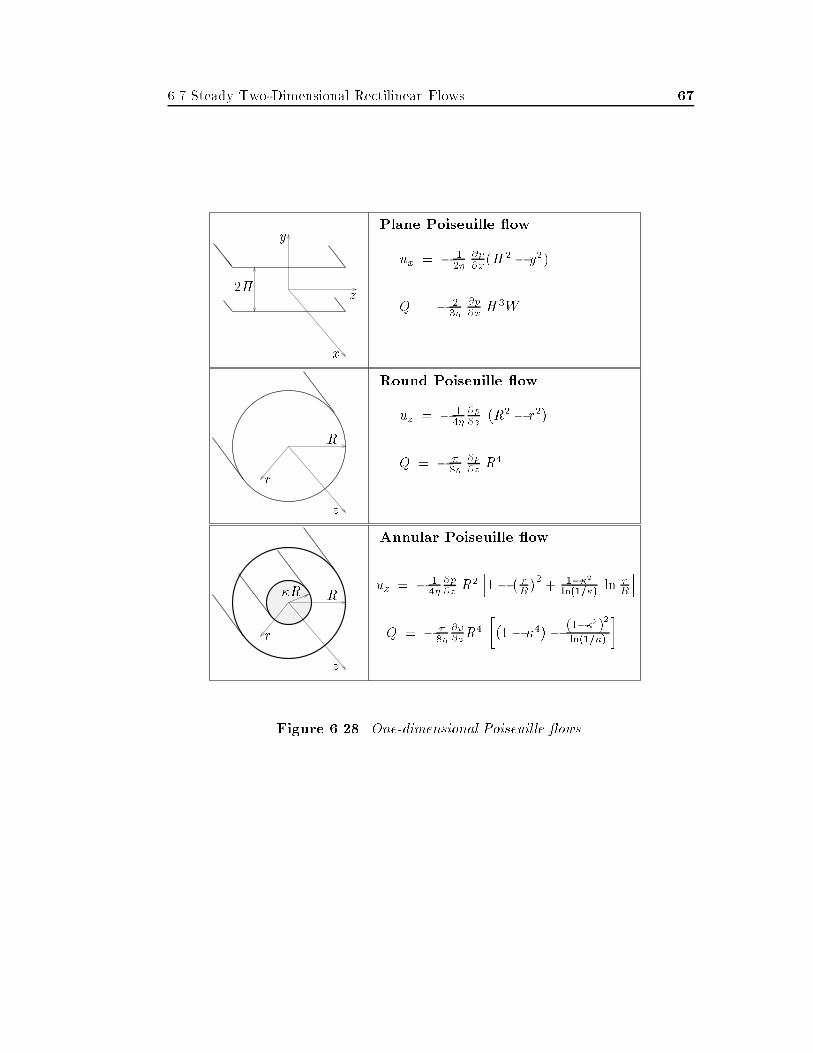
�� Steady Two�Dimensional Rectilinear Flows �
�H
x
y
z
Plane Poiseuille ow
ux � � ���
�p�x�H
� � y��
Q � � ���
�p�x H
�W
z
R
r
Round Poiseuille ow
uz � � ���
�p�z
�R� � r�
�
Q � � ��
�p�z R
�
z
R�R
r
Annular Poiseuille ow
uz � � ���
�p�z R
�h�� � rR�� � ����
ln����� ln rR
i
Q � � ��
�p�zR
�
���� ��
�� �������
ln�����
Figure ����� One�dimensional Poiseuille �ows
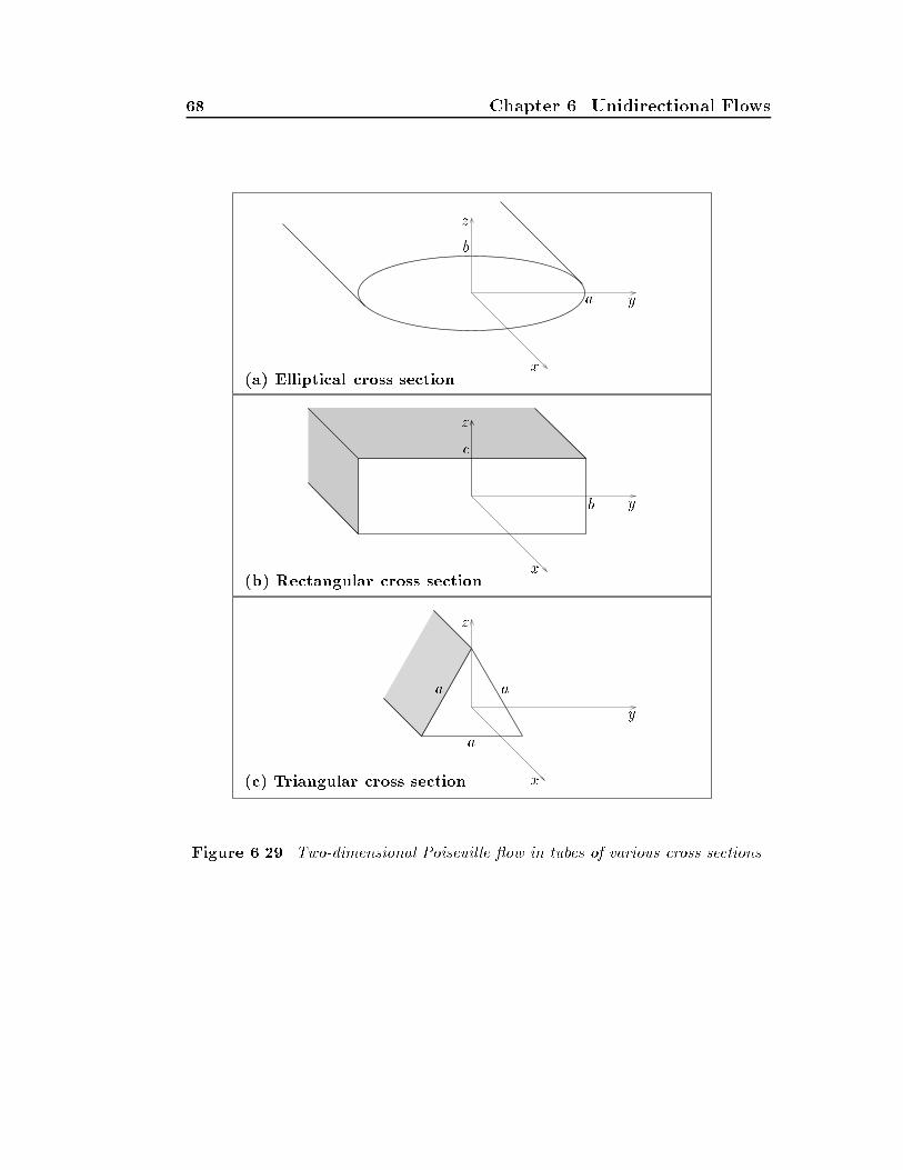
�� Chapter �� Unidirectional Flows
�a� Elliptical cross sectionx
y
z
a
b
�b� Rectangular cross sectionx
y
z
b
c
�c� Triangular cross section x
y
z
aa
a
Figure ����� Two�dimensional Poiseuille �ow in tubes of various cross sections
�� Steady Two�Dimensional Rectilinear Flows ��
From boundary condition �������� we have
u�x�y� z� � �c�y� � c�z� � �c�
�y� �
c�c�z�
ony�
a��z�
b�� � �
Settingc�c�
�a�
b�� ����� �
u�x becomes constant on the boundary�
u�x�y� z� � �c�a� ony�
a��z�
b�� � � ������
The maximum principle for the Laplace equation states that u�x has both itsminimum and maximum values on the boundary of the domain ����� Therefore� u�xis constant over the whole domain�
u�x�y� z� � �c�a� � �������
Substituting into Eq� ������� and using Eq� ����� �� we get
ux�y� z� � �c�a� � c�y� � c�z
� � �c�a�� � y�
a�� c�
c�
z�
a�
���
ux�y� z� � �c�a�� � y�
a�� z�
b�
�� �������
The constant c� is determined from Eqs� ������� and ����� ��
c� ��
��
�p
�x
b�
a� � b�� �������
consequently�
ux�y� z� � � �
��
�p
�x
a�b�
a� � b�
� � y�
a�� z�
b�
�� �������
Obviously� the maximum velocity occurs at the origin� Integration of the velocitypro�le ������� over the elliptical cross section yields the volumetric �ow rate
Q � � �
�
�p
�x
a�b�
a� � b�� �������
Chapter �� Unidirectional Flows
Equation ������� degenerates to the circular Poiseuille �ow velocity pro�le whena�b�R�
ux�y� z� � � �
�
�p
�xR�
� � y� � z�
R�
��
Setting r��y��z�� and switching to cylindrical coordinates� we get
uz�r� � � �
�
�p
�z�R� � r�� � ������
If now a�H and b� H � Eq� ������� yields the plane Poiseuille �ow velocity pro�le�
ux�y� � � �
��
�p
�x�H� � y�� � �������
Note that� due to symmetry� the shear stress is zero along symmetry planes� Thezero shear stress condition along such a plane applies also in gravity�driven �ow of a�lm of semielliptical cross section� Therefore� the velocity pro�le for the latter �owcan be obtained by replacing ��p��x by �gx� Similarly� Eqs� ������ and �������can be modi�ed to describe the gravity�driven �ow of semicircular and planar �lms�respectively� �
Example ������ Poiseuille �ow in a tube of rectangular cross sectionConsider steady pressure�driven �ow of an incompressible Newtonian liquid in anin�nitely long tube of rectangular cross section of width �b and height �c� as shownin Fig� ����b� The �ow is governed by the Poisson equation
��ux�y�
���ux�z�
��
�
�p
�x� �������
Taking into account the symmetry with respect to the planes y�� and z��� the �owcan be studied only in the �rst quadrant �Fig� ������ The boundary conditions canthen be written as follows�
�ux�y
� � on y � �
ux � � on y � b
�ux�z
� � on z � �
ux � � on z � c
�������������������������
� ����� �
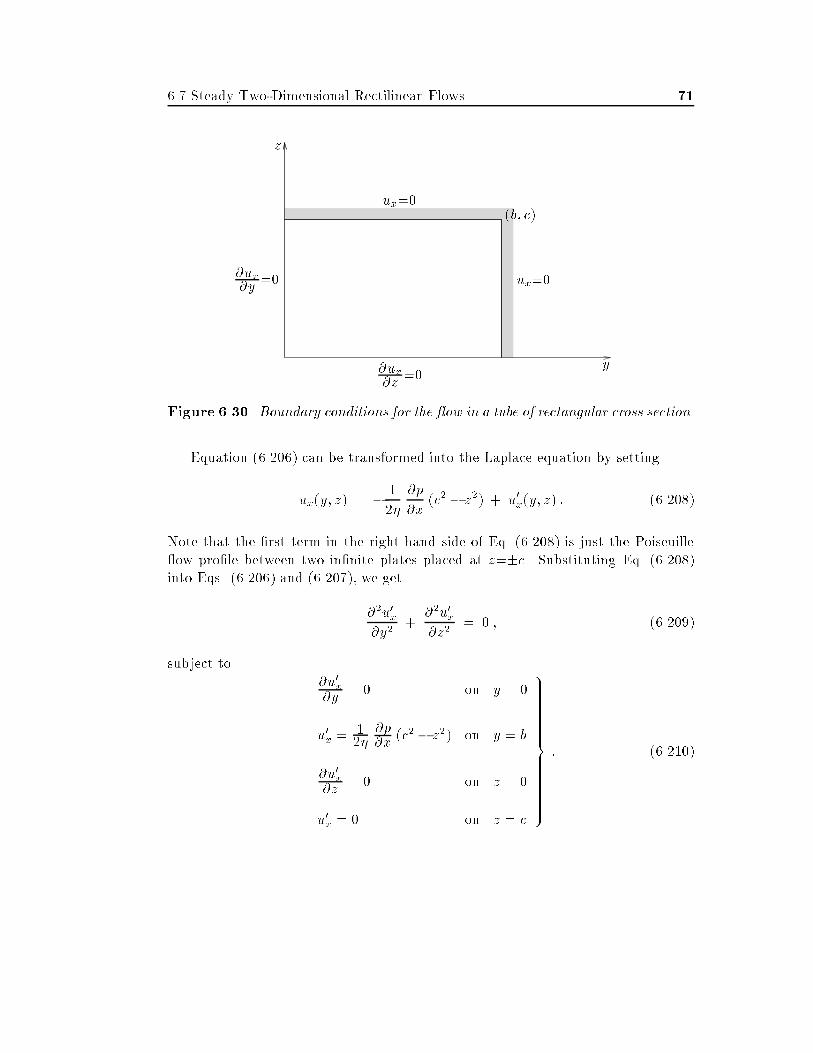
�� Steady Two�Dimensional Rectilinear Flows �
y
z
�b� c�ux��
ux���ux�y ��
�ux�z
��
Figure ���� Boundary conditions for the �ow in a tube of rectangular cross section
Equation ������� can be transformed into the Laplace equation by setting
ux�y� z� � � �
��
�p
�x�c� � z�� � u�x�y� z� � ������
Note that the �rst term in the right hand side of Eq� ������ is just the Poiseuille�ow pro�le between two in�nite plates placed at z��c� Substituting Eq� ������into Eqs� ������� and ����� �� we get
��u�x�y�
���u�x�z�
� � � �������
subject to�u�x�y
� � on y � �
u�x � ���
�p�x
�c� � z�� on y � b
�u�x�z
� � on z � �
u�x � � on z � c
�����������������������������
� �������
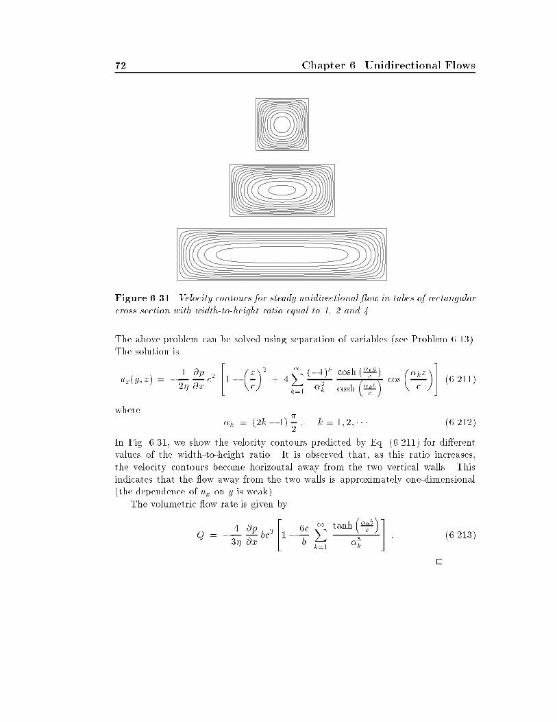
� Chapter �� Unidirectional Flows
Figure ����� Velocity contours for steady unidirectional �ow in tubes of rectangularcross section with width�to�height ratio equal to �� � and �
The above problem can be solved using separation of variables �see Problem ������The solution is
ux�y� z� � � �
��
�p
�xc�
���� �z
c
���
�Xk��
����k��k
cosh� ky
c
�cosh
� kbc
� cos
��kz
c
��� �������
where�k � ��k� ��
�
�� k � �� �� � � � �������
In Fig� ����� we show the velocity contours predicted by Eq� ������� for di�erentvalues of the width�to�height ratio� It is observed that� as this ratio increases�the velocity contours become horizontal away from the two vertical walls� Thisindicates that the �ow away from the two walls is approximately one�dimensional�the dependence of ux on y is weak��
The volumetric �ow rate is given by
Q � �
��
�p
�xbc�
���� �c
b
�Xk��
tanh� kbc
���k
�� � �������
�
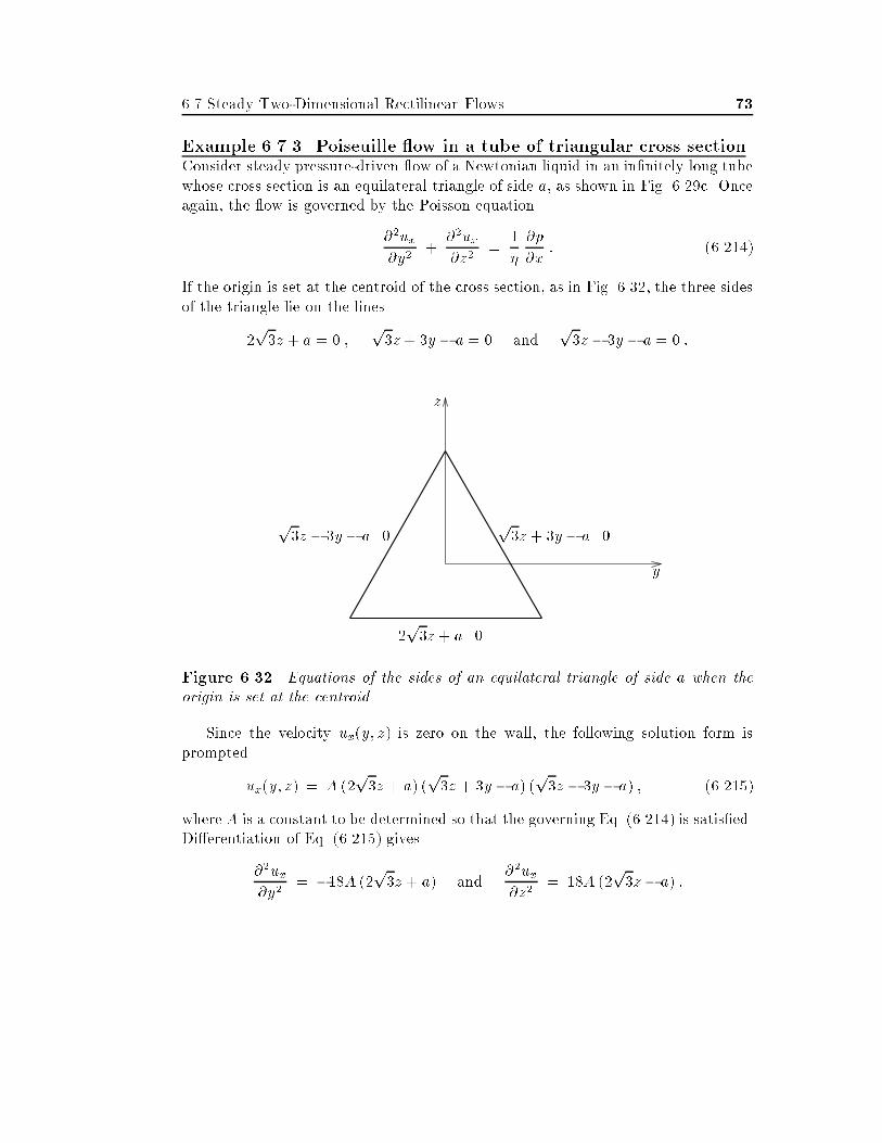
�� Steady Two�Dimensional Rectilinear Flows �
Example ������ Poiseuille �ow in a tube of triangular cross sectionConsider steady pressure�driven �ow of a Newtonian liquid in an in�nitely long tubewhose cross section is an equilateral triangle of side a� as shown in Fig� ����c� Onceagain� the �ow is governed by the Poisson equation
��ux�y�
���ux�z�
��
�
�p
�x� ������
If the origin is set at the centroid of the cross section� as in Fig� ����� the three sidesof the triangle lie on the lines
�p�z � a � � �
p�z � �y � a � � and
p�z � �y � a � � �
y
z
p�z � �y � a��
p�z � �y � a��
�p�z � a��
Figure ����� Equations of the sides of an equilateral triangle of side a when theorigin is set at the centroid
Since the velocity ux�y� z� is zero on the wall� the following solution form isprompted
ux�y� z� � A ��p�z � a� �
p�z � �y � a� �
p�z � �y � a� � �������
where A is a constant to be determined so that the governing Eq� ������ is satis�ed�Di�erentiation of Eq� ������� gives
��ux�y�
� ��A ��p�z � a� and
��ux�z�
� �A ��p�z � a� �
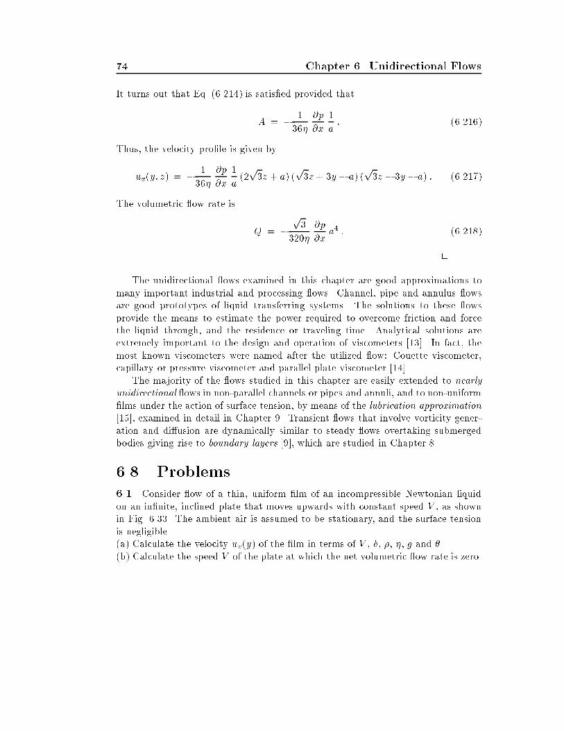
� Chapter �� Unidirectional Flows
It turns out that Eq� ������ is satis�ed provided that
A � � �
���
�p
�x
�
a� �������
Thus� the velocity pro�le is given by
ux�y� z� � � �
���
�p
�x
�
a��p�z � a� �
p�z � �y � a� �
p�z � �y � a� � ����� �
The volumetric �ow rate is
Q � �p�
����
�p
�xa� � ������
�
The unidirectional �ows examined in this chapter are good approximations tomany important industrial and processing �ows� Channel� pipe and annulus �owsare good prototypes of liquid transferring systems� The solutions to these �owsprovide the means to estimate the power required to overcome friction and forcethe liquid through� and the residence or traveling time� Analytical solutions areextremely important to the design and operation of viscometers ����� In fact� themost known viscometers were named after the utilized �ow� Couette viscometer�capillary or pressure viscometer and parallel plate viscometer ����
The majority of the �ows studied in this chapter are easily extended to nearlyunidirectional �ows in non�parallel channels or pipes and annuli� and to non�uniform�lms under the action of surface tension� by means of the lubrication approximation����� examined in detail in Chapter �� Transient �ows that involve vorticity gener�ation and di�usion are dynamically similar to steady �ows overtaking submergedbodies giving rise to boundary layers ���� which are studied in Chapter �
��� Problems
���� Consider �ow of a thin� uniform �lm of an incompressible Newtonian liquidon an in�nite� inclined plate that moves upwards with constant speed V � as shownin Fig� ����� The ambient air is assumed to be stationary� and the surface tensionis negligible��a� Calculate the velocity ux�y� of the �lm in terms of V � � �� �� g and ���b� Calculate the speed V of the plate at which the net volumetric �ow rate is zero�
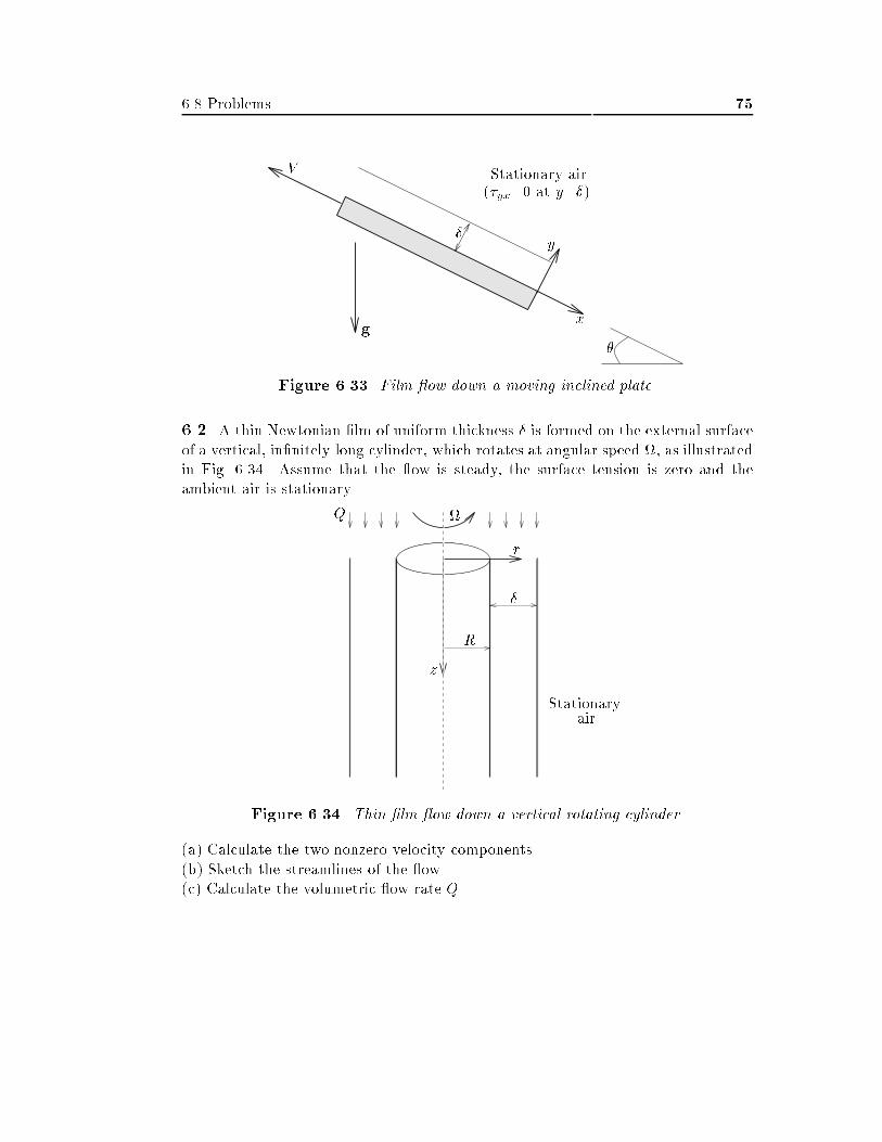
�� Problems �
x
y
V
Stationary air��yx�� at y� �
�g
Figure ����� Film �ow down a moving inclined plate
���� A thin Newtonian �lm of uniform thickness is formed on the external surfaceof a vertical� in�nitely long cylinder� which rotates at angular speed !� as illustratedin Fig� ���� Assume that the �ow is steady� the surface tension is zero and theambient air is stationary�
z
r
Q !
R
Stationaryair
Figure ����� Thin �lm �ow down a vertical rotating cylinder
�a� Calculate the two nonzero velocity components��b� Sketch the streamlines of the �ow��c� Calculate the volumetric �ow rate Q�
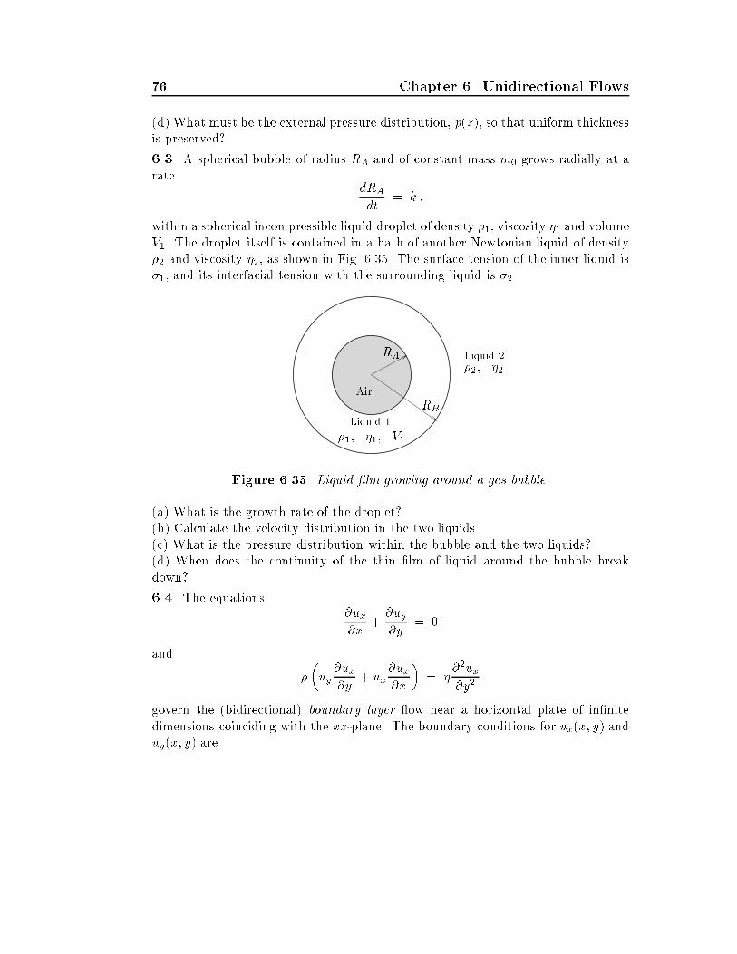
� Chapter �� Unidirectional Flows
�d� What must be the external pressure distribution� p�z�� so that uniform thicknessis preserved"
���� A spherical bubble of radius RA and of constant mass m� grows radially at arate
dRA
dt� k �
within a spherical incompressible liquid droplet of density ��� viscosity �� and volumeV�� The droplet itself is contained in a bath of another Newtonian liquid of density�� and viscosity ��� as shown in Fig� ����� The surface tension of the inner liquid is��� and its interfacial tension with the surrounding liquid is ���
RA
RB
��� ��� V�
��� ��
Air
Liquid
Liquid
Figure ����� Liquid �lm growing around a gas bubble
�a� What is the growth rate of the droplet"�b� Calculate the velocity distribution in the two liquids��c� What is the pressure distribution within the bubble and the two liquids"�d� When does the continuity of the thin �lm of liquid around the bubble breakdown"
���� The equations�ux�x
��uy�y
� �
and
�
�uy
�ux�y
� ux�ux�x
�� �
��ux�y�
govern the �bidirectional� boundary layer �ow near a horizontal plate of in�nitedimensions coinciding with the xz�plane� The boundary conditions for ux�x� y� anduy�x� y� are
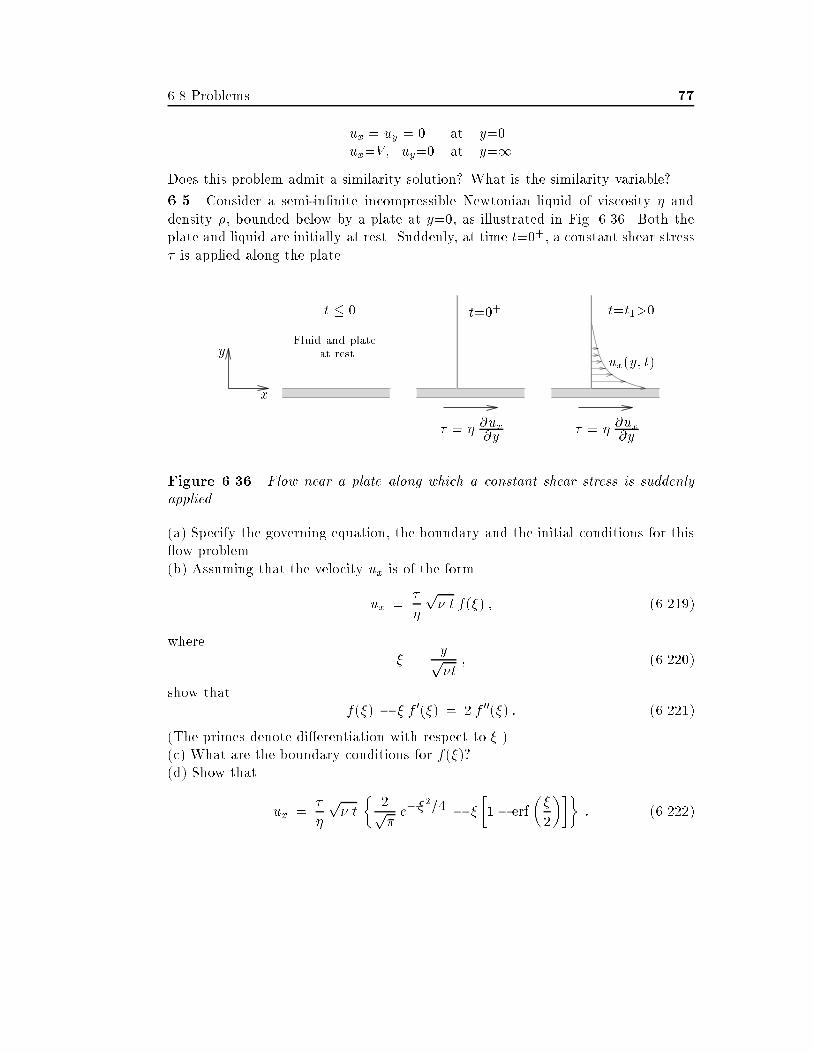
�� Problems
ux � uy � � at y��ux�V� uy�� at y��
Does this problem admit a similarity solution" What is the similarity variable"
��� Consider a semi�in�nite incompressible Newtonian liquid of viscosity � anddensity �� bounded below by a plate at y��� as illustrated in Fig� ����� Both theplate and liquid are initially at rest� Suddenly� at time t���� a constant shear stress� is applied along the plate�
x
y
t � � t��� t�t���
Fluid and plateat rest
ux�y� t�
� � � �ux�y
� � � �ux�y
Figure ����� Flow near a plate along which a constant shear stress is suddenlyapplied
�a� Specify the governing equation� the boundary and the initial conditions for this�ow problem��b� Assuming that the velocity ux is of the form
ux ��
�
p� t f��� � �������
where� �
yp�t
� �������
show thatf��� � � f ���� � � f ����� � �������
�The primes denote di�erentiation with respect to ����c� What are the boundary conditions for f���"�d� Show that
ux ��
�
p� t
��p�e���� � �
��� erf
��
�
��� �������
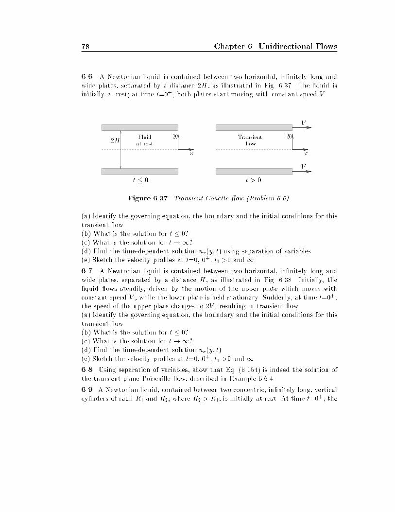
� Chapter �� Unidirectional Flows
���� A Newtonian liquid is contained between two horizontal� in�nitely long andwide plates� separated by a distance �H � as illustrated in Fig� ��� � The liquid isinitially at rest� at time t���� both plates start moving with constant speed V �
x
y
x
y�H
t � � t � �
V
V
Fluidat rest
Transient�ow
Figure ���� Transient Couette �ow �Problem ���
�a� Identify the governing equation� the boundary and the initial conditions for thistransient �ow��b� What is the solution for t � �"�c� What is the solution for t��"�d� Find the time�dependent solution ux�y� t� using separation of variables��e� Sketch the velocity pro�les at t��� ��� t� �� and ��
���� A Newtonian liquid is contained between two horizontal� in�nitely long andwide plates� separated by a distance H � as illustrated in Fig� ���� Initially� theliquid �ows steadily� driven by the motion of the upper plate which moves withconstant speed V � while the lower plate is held stationary� Suddenly� at time t����the speed of the upper plate changes to �V � resulting in transient �ow��a� Identify the governing equation� the boundary and the initial conditions for thistransient �ow��b� What is the solution for t � �"�c� What is the solution for t��"�d� Find the time�dependent solution ux�y� t���e� Sketch the velocity pro�les at t��� ��� t� �� and ��
�� � Using separation of variables� show that Eq� ������ is indeed the solution ofthe transient plane Poiseuille �ow� described in Example �����
���� A Newtonian liquid� contained between two concentric� in�nitely long� verticalcylinders of radii R� and R�� where R� � R�� is initially at rest� At time t���� the
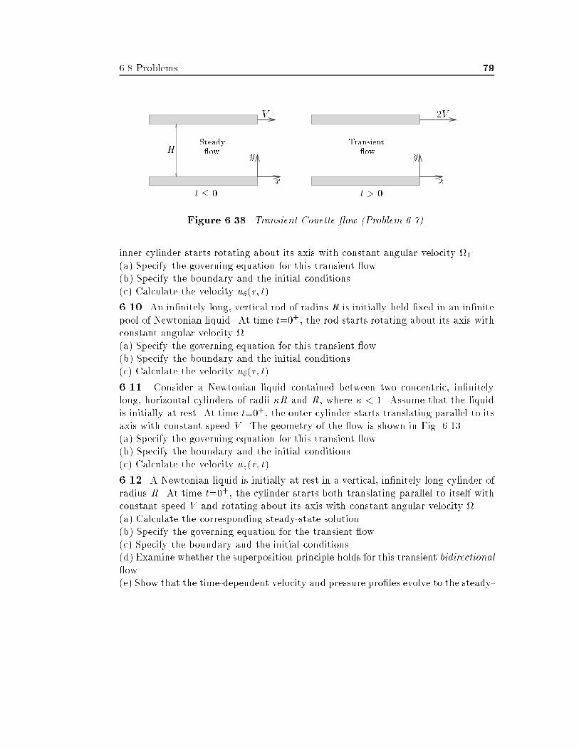
�� Problems �
x
y
x
yH
t � � t � �
V �V
Steady�ow
Transient�ow
Figure ����� Transient Couette �ow �Problem ���
inner cylinder starts rotating about its axis with constant angular velocity !���a� Specify the governing equation for this transient �ow��b� Specify the boundary and the initial conditions��c� Calculate the velocity u��r� t��
����� An in�nitely long� vertical rod of radius R is initially held �xed in an in�nitepool of Newtonian liquid� At time t���� the rod starts rotating about its axis withconstant angular velocity !��a� Specify the governing equation for this transient �ow��b� Specify the boundary and the initial conditions��c� Calculate the velocity u��r� t��
����� Consider a Newtonian liquid contained between two concentric� in�nitelylong� horizontal cylinders of radii �R and R� where � � �� Assume that the liquidis initially at rest� At time t���� the outer cylinder starts translating parallel to itsaxis with constant speed V � The geometry of the �ow is shown in Fig� ������a� Specify the governing equation for this transient �ow��b� Specify the boundary and the initial conditions��c� Calculate the velocity uz�r� t��
����� A Newtonian liquid is initially at rest in a vertical� in�nitely long cylinder ofradius R� At time t���� the cylinder starts both translating parallel to itself withconstant speed V and rotating about its axis with constant angular velocity !��a� Calculate the corresponding steady�state solution��b� Specify the governing equation for the transient �ow��c� Specify the boundary and the initial conditions��d� Examine whether the superposition principle holds for this transient bidirectional�ow��e� Show that the time�dependent velocity and pressure pro�les evolve to the steady�
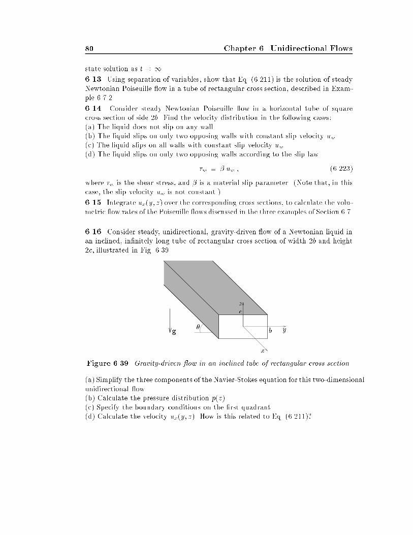
� Chapter �� Unidirectional Flows
state solution as t���
����� Using separation of variables� show that Eq� ������� is the solution of steadyNewtonian Poiseuille �ow in a tube of rectangular cross section� described in Exam�ple �� ���
����� Consider steady Newtonian Poiseuille �ow in a horizontal tube of squarecross section of side �b� Find the velocity distribution in the following cases��a� The liquid does not slip on any wall��b� The liquid slips on only two opposing walls with constant slip velocity uw��c� The liquid slips on all walls with constant slip velocity uw ��d� The liquid slips on only two opposing walls according to the slip law
�w � uw � �������
where �w is the shear stress� and is a material slip parameter� �Note that� in thiscase� the slip velocity uw is not constant��
���� Integrate ux�y� z� over the corresponding cross sections� to calculate the volu�metric �ow rates of the Poiseuille �ows discussed in the three examples of Section �� �
����� Consider steady� unidirectional� gravity�driven �ow of a Newtonian liquid inan inclined� in�nitely long tube of rectangular cross section of width �b and height�c� illustrated in Fig� �����
x
y
z
b
c
g�
Figure ����� Gravity�driven �ow in an inclined tube of rectangular cross section
�a� Simplify the three components of the Navier�Stokes equation for this two�dimensionalunidirectional �ow��b� Calculate the pressure distribution p�z���c� Specify the boundary conditions on the �rst quadrant��d� Calculate the velocity ux�y� z�� How is this related to Eq� �������"
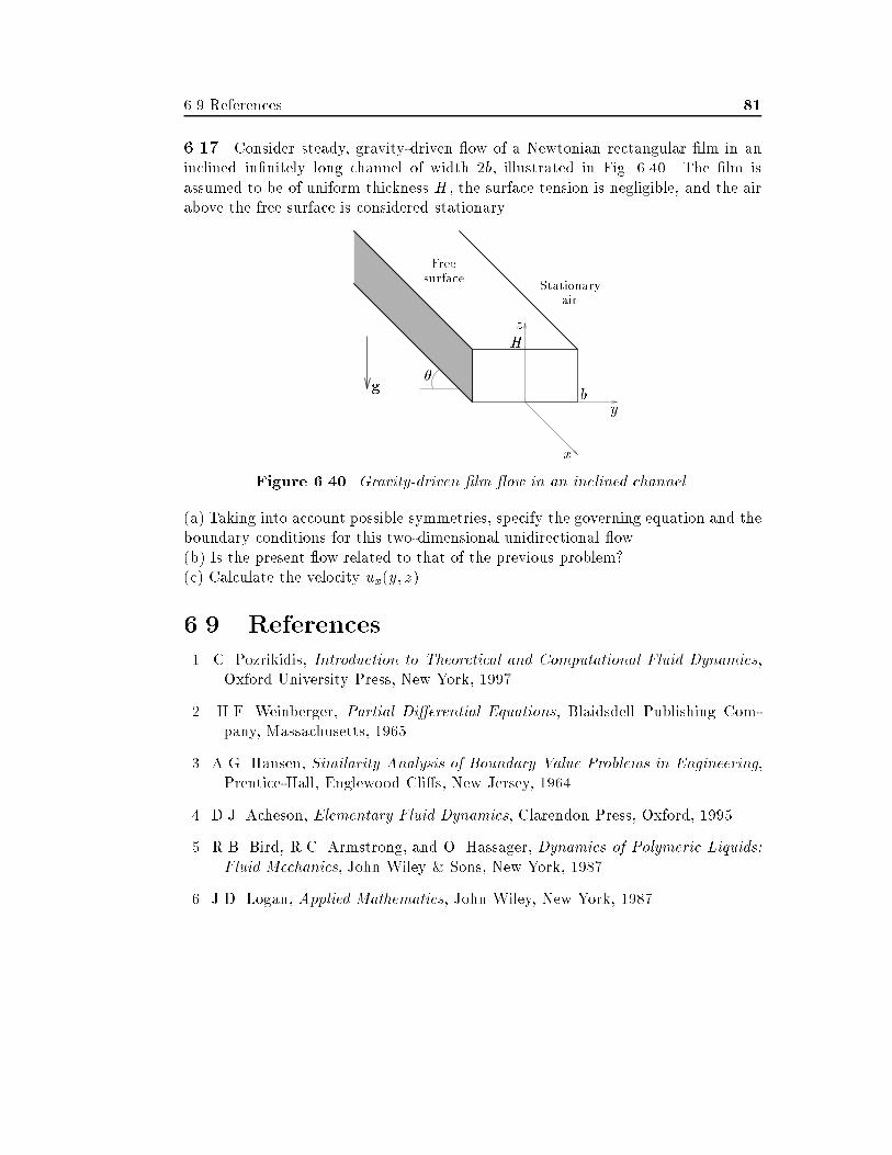
��� References ��
����� Consider steady� gravity�driven �ow of a Newtonian rectangular �lm in aninclined in�nitely long channel of width �b� illustrated in Fig� ���� The �lm isassumed to be of uniform thickness H � the surface tension is negligible� and the airabove the free surface is considered stationary�
x
y
z
b
H
g�
Freesurface
Stationaryair
Figure ���� Gravity�driven �lm �ow in an inclined channel
�a� Taking into account possible symmetries� specify the governing equation and theboundary conditions for this two�dimensional unidirectional �ow��b� Is the present �ow related to that of the previous problem"�c� Calculate the velocity ux�y� z��
��� References
�� C� Pozrikidis� Introduction to Theoretical and Computational Fluid Dynamics�Oxford University Press� New York� ��� �
�� H�F� Weinberger� Partial Di�erential Equations� Blaidsdell Publishing Com�pany� Massachusetts� �����
�� A�G� Hansen� Similarity Analysis of Boundary Value Problems in Engineering�Prentice�Hall� Englewood Cli�s� New Jersey� ����
� D�J� Acheson� Elementary Fluid Dynamics� Clarendon Press� Oxford� �����
�� R�B� Bird� R�C� Armstrong� and O� Hassager� Dynamics of Polymeric LiquidsFluid Mechanics� John Wiley # Sons� New York� �� �
�� J�D� Logan� Applied Mathematics� John Wiley� New York� �� �
��
� R�S� Brodkey� The Phenomena of Fluid Motions� Addison�Wesley Series inChemical Engineering� ��� �
� Lord Rayleigh� Scienti�c Papers� Dover� ����
�� H� Schlichting� Boundary Layer Theory� McGraw�Hill� New York� ����
��� R� Berger� $Int%egration des %equations du mouvement d�un �uide visqueuxincompressible�& in Handbuch der Physik ����� Springer� Berlin� ��� �������
��� R�K� Shah� and A�L� London� Laminar Flow Forced Convection in Ducts�Academic� �� �
��� M�H� Protter and H�F� Weinberger� Maximum Principles in Di�erential Equa�tions� Prentice�Hall� Englewood Cli�s� New Jersey� ��� �
��� H�A� Barnes� J�F� Hutton and K� Walters� An Introduction to Rheology� Else�vier� Amsterdam� ����
�� J�M� Dealy� Rheometers for Molten Plastics� Van Nostrand Rheinhold� ����
��� O� Reynolds� $Papers on Mechanical and Physical Aspects�& Phil Trans RoySoc �� �� �����
Index
annular �ow� ��� � axisymmetric �ow� �� ��� �axisymmetric Poiseuille �ow� ��axisymmetric radial �ow� �� ��axisymmetric rectilinear �ow� �� ��axisymmetric torsional �ow� �� ��� �axisymmetry� ��
Bagley correction� ��
capillary viscometer� ��circular Couette �ow� ��� �Couette �ow� �� � ��� �
�lm �ow� ���ow
axisymmetric �ow� �� ��� �Couette �ow� �� � ��� �fully developed �ows� �in an annulus� ��� � plug �ow� Poiseuille �ow� �� �� ��� ��� �� ��radial �ow� �� ��rectilinear �ow� �� ��spherically symmetric �ow� �spherically symmetric radial �ow�
�torsional �ow� �� ��� �unidirectional �ows� �
fully developed �ows� �
Hagen�Poiseuille �ow� ��helical �ow� ��
L�H opital�s rule� �
plane Couette �ow� �� � �plane Poiseuille �ow� �� ��� ��� �plug �ow� Poiseuille �ow� �� �� ��� ��� �� ��
radial �ow� �� ��rectilinear �ow� �rod climbing� � rod dipping� �
separation of variables� �shear�driven �ow� �similarity transformation� �slip� ��slip velocity� ��spherically symmetric �ow� �spherically symmetric radial �ow� �swirling �ow� �
Taylor series� ��Taylor vortices� ��torsional �ow� �� ��� �
unidirectional �ows� �
��


![small - GOEDOCwebdoc.sub.gwdg.de/ebook/diss/2003/fu-berlin/2001/93/gesamt.pdf · ompkins (G. Gamo w[Gam65]) Historically, statistical mec hanics (or thermostatistics) has b een dev](https://img.pdfslide.us/doc/110x75/5e04475a2fb0247e091a34a4/small-ompkins-g-gamo-wgam65-historically-statistical-mec-hanics-or-thermostatistics.jpg)