1

I-campus project

School-wide Program on Fluid Mechanics

Modules on Waves in uids

T. R. Akylas & C. C. Mei

CHAPTER SIX

FORCED DISPERSIVE WAVES ALONG A NARROW CHANNEL

Linear surface gravity w aves propagating along a narrow c hannel display i n teresting

phenomena. At � r s t w e consider free waves propagating along an in�nite narrow c hannel.

We g i v e the solution for this problem as a superposition of wave modes and we illustrate

concepts like the notion of cut-o� frequency. Second, we consider a semi-in�nite channel

with forced waves excited by a wave maker located at one end of the channel. As in

the previous case, the wave �eld generated by the wave maker can b e described as a

superposition of wave modes. As the wave maker starts exciting the uid, a w ave front

develop and starts propagating along the channel if the excitation frequency is above t h e

cut-o� frequency for the �rst channel wave mode. If the excitation frequency is below

the cut-o� frequency for the �rst channel mode, the wave disturbance stays localized

close to the wave maker, and for the particular case where the excitation frequency

matches the natural frequency of a particular channel wave modes, there is resonance

b e t ween this particular wave mode and the wave m a k er, and the wave amplitude at the

wave maker grows with time.

E�ects of non-linearity and dissipation are not taken into account. In this chapter

we obtain and illustrate through animations the free-surface displacement evolution in

time along a semi-in�nite narrow c hannel excited by a w ave maker at one of its ends.

1 Free Wave Propagation Along a Narrow Waveg-

uide.

We consider free waves propagating along an in�nite channel of depth h and width 2b.

We adopt a coordinate system x; y; z, where x and z are in the horizontal plane and y is

the vertical coordinate. The x axis is along the channel, the lateral walls are located at

2

z = �b and the bottom is the plane y = �h. The free surface is located at y = �(x; z; t),

which is unknown. We assume irrotational ow and incompressible uid such that the

velocity �eld can be given as the gradient of a potential function �(x; y; z; t), where t is

the time parameterization. The linearized boundary value problem for propagation of

free waves is given by the set of equations

r2�(x; y; z; t) =0 for �1 < x <1;�h < y < 0 and � b < z < b; (1.1)

@2�

@t2+ g

@�

@y=0 at y = 0; (1.2)

@�

@y=0 at y = �h; (1.3)

@�

@z=0 at z = �b; (1.4)

and appropriate radiation conditions. This is an homogeneous boundary value problem

that can be solved by the technique of separation of variables. First we assume that the

free waves propagating along the channel are given as a superposition of plane mono-

chromatic waves. Due to the linearity of the boundary value problem, we need only

to solve it for a single nono-chromatic plane wave with wave frequency !. The time

dependence is

exp(�i!t);

and now we can write the potential function �(x; y; z; t) and the free-surface displacement

�(x; z; t) in the form

�(x; y; z; t) = �(x; y; z) exp(�i!t); (1.5)

�(x; z; t) = �(x; z) exp(�i!t): (1.6)

Now the boundary value problem given by equations (1.1) to (1.4) assume the form

3

r2�(x; y; z) =0 for �1 < x <1;�h < y < 0 and � b < z < b; (1.7)

�!2�+ g@�

@y=0 at y = 0; (1.8)

@�

@y=0 at y = �h; (1.9)

@�

@z=0 at z = �b; (1.10)

where we eliminated the free surface displacement �(x; z) and reduced the boundary

value problem to a boundary value problem in one dependent variable, �(x; y; z). Next,

we apply the technique of separation of variables to solve the boundary value problem

given by equations (1.7) to (1.10). We assume the potential function �(x; y; z) given as

�(x; y; z) � exp(�ikx)

0@ sin(kzz)

cos(kzz)

1AH(y); (1.11)

where the possible values kz is determined by the boundary condition at the channel

walls located at z = �b, and the possible values of the constant k are discussed below. If

we substitute the expression given by equation (1.11) into the boundary value problem

given by equations (1.7) to (1.10), we obtain a Sturm-Liouville problem (one-dimensional

boundary value problem with a second order di�erential equation) for the functionH(y),

which is given by the equations

Hyy + �H(y) = 0; (1.12)

�!2H(y) + gHy = 0 at y = 0; (1.13)

Hy = 0 at y = �h; (1.14)

where �2 = �k2z+k2. The constant � represents a set of eigenvalues, which are functions

of the wave frequency !, of the gravity acceleration g and of the depth h.

If we apply the boundary conditions given by equation (1.10) to the potential function

�(x; y; z), we realize that we can use either cos(kzz) or sin(kzz) in the expression for

�(x; y; z) given by equation (1.11), but with di�erent set of possible values for the

4

constant kz

. The set of values for kz

are determined by the boundary condition (1.10)

and the choice b e t ween cos(kz

z) and sin(kz

z). If we consider the z dependence of the

potential �(x; y; z) given in terms of cos(kz

z), the constant kz

has to assume the values

� n�

� with n as a natural number. (1.15)kzn

=

2b b

If we consider the z dependence of the potential �(x; y; z) g iv en in terms of sin(kz

z), the

constant kz

has to assume the values

m�

kzm

= � with m as a natural number. (1.16)

b

The general form of the solution for the equation (1.12) is

H(y) = A cosh(�(y + h)) + B sinh(�(y + h)); (1.17)

but the boundary condition on the bottom given by the equation (1.14) implies that

B = 0 . The boundary condition at the free-surface (y = 0 ) g i v es the eigenvalue equation

or dispersion relation

!2 = g� tanh(�h) (1.18)

for the constant �. This implicit eigenvalue equation has one real solutions �0

and an

in�nite countable set of pure imaginary eigenvalues i�l

; l = 1; 2; : : : . Associated with

these eigenvalues we have the eigenfunctions

cosh(�0(y + h))

H0(y) = ; (1.19)

cosh(�0

h)

cos(�l(y + h))

Hl

(y) = ; with l = 1 ; 2; : : : (1.20)

cos(�l

h)

The term exp(ikx)(exp(�ikx)) in the equation (1.11) above for �(x; y; z) represents a

wave propagating to the right (left) if the constant k is real, or a right (left) evanescent

5

wave if k is a pure imaginary number, or a combination of both if k is complex. We

label the constant k as the wavenumber. Since, we are interested in free propagating

waves, we need the constant k to be a real number. The value of this constant is given

in terms of the constants � and kz

, according to the equation

k2 2 � k2= � z

; (1.21)

where the possible values of kz

are given by the equations (1.15) and (1.16). The possible

values of � are solutions of the dispersion relation given by the equation (1.18). Since

we w ant k as a real number, this excludes the imaginary solutions of the equation (1.18),

so we can write the equation above in the form

kn

=�2 � kz

2 ; (1.22)0 n

km

=�2 � kz

2 ; (1.23)0 m

where we appended the indexes n and m to the constant k to make clear its dependence

on the eigenvalues kzn

and kzm

.

Now we can write the potential function �(x; y; z) in th e form

� �+1 X cosh(�0(y + h))

�(x; y; z) = [Am

exp(ikmx) + Bm

exp(�ikm

x)] sin(kzm

z)

cosh(�0h)

m=�1

1

� � X cosh(�0(y + h))

+ [An

exp(iknx) + Bn

exp(�iknx)] cos(kzn

z) ;

cosh(�0h)

n=�1

(1.24)

and the free-surface displacement �(x; z) is given by the equation

( � �+1

i!

X cosh(�0(y + h))

�(x; z) = � (Am

exp(ikmx) + Bm

exp(�ikm

x)) sin(kzm

z)

g cosh(�0h)

m=�1 ) � �1 X cosh(�0(y + h))

+ (An

exp(iknx) + Bn

exp(�iknx)) cos(kzn

z) ;

cosh(�0h)

n=�1

(1.25)

6

where the value of the constants Am

; A n; B m

and Bn

are speci�ed by the appropriate

radiation conditions.

k

�

According to the value of kzm

or kzn

, the constants km

and kn

in the equations (1.24)

and (1.25) may be real (propagating wave mode) or pure imaginary numbers (evanescent

wave m ode). If we �x the value of kzm

or kzn

(�x the value of m or n), for a given depth

h, we can vary the wave frequency ! such that �0

> kzm

(kzn

) or �0

< kzm

(kzn

). When

0

> kzm

(kzn

), km(kn) is a real numb e r and we have a propagating wave mode, but

when �0

< kzm

(kzn

) we have that km(kn) is a pure imaginary numb e r and the wave

mode associated with this value of k is evanescent. So, the wave frequency value where

zm

= � 0(kzn

= � 0

) is called the cut-o� frequency for the mth (nth) wave mode.

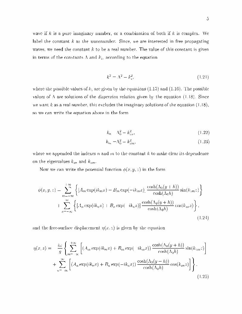
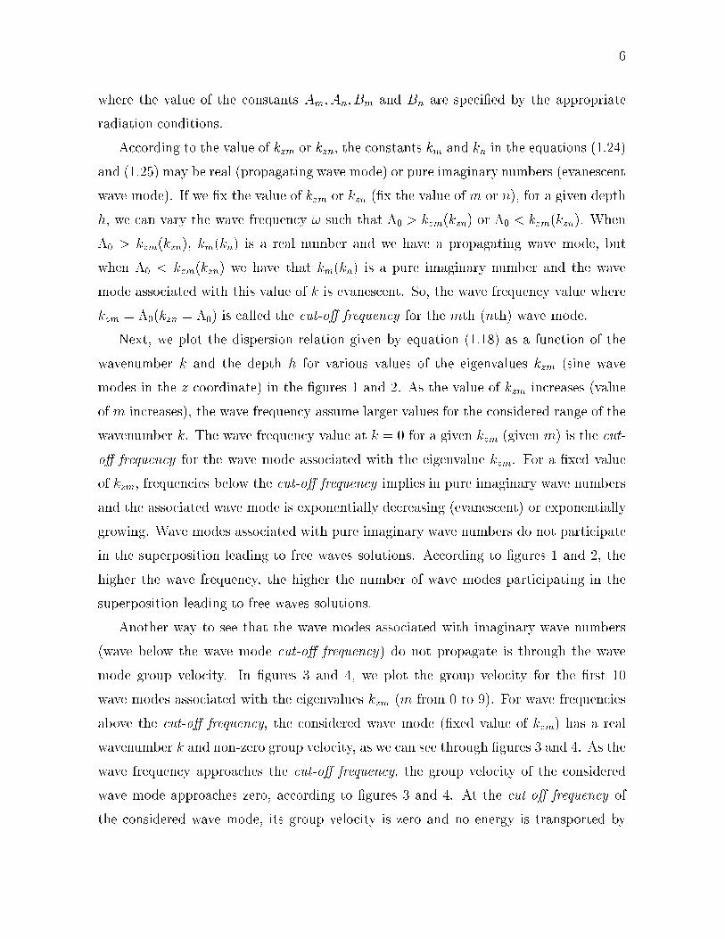
Next, we plot the dispersion relation given by equation (1.18) as a function of the

wavenumb e r k and the depth h for various values of the eigenvalues kzm

(sine wave

modes in the z coordinate) in the �gures 1 and 2. As the value of kzm

increases (value

of m increases), the wave frequency assume larger values for the considered range of the

wavenumb e r k. The wave frequency value at k = 0 for a given kzm

(given m) is the cut-

o� frequency for the wave mode associated with the eigenvalue kzm

. For a �xed value

of kzm

, frequencies below t h e cut-o� frequency implies in pure imaginary wave n umb e r s

and the associated wave mode is exponentially decreasing (evanescent) or exponentially

growing. Wave modes associated with pure imaginary wave n umbers do not participate

in the superposition leading to free waves solutions. According to �gures 1 and 2, the

higher the wave frequency, the higher the numb e r of wave modes participating in the

superposition leading to free waves solutions.

Another way to see that the wave modes associated with imaginary wave numb e r s

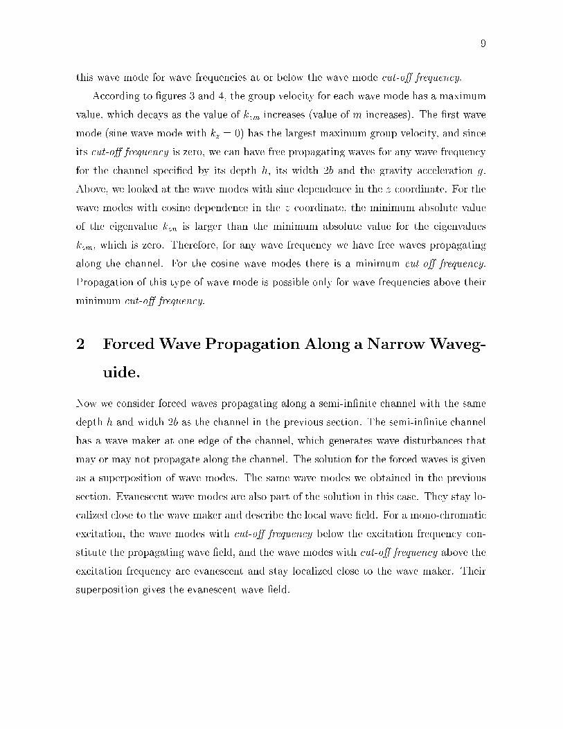
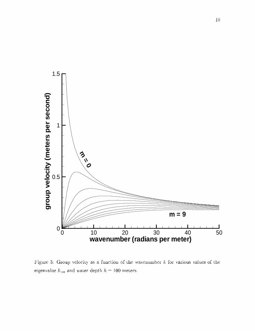
(wave b e lo w the wave mode cut-o� frequency ) do not propagate is through the wave

mode group velocity. In �gures 3 and 4, we plot the group velocity for the �rst 10

wave modes associated with the eigenvalues kzm

(m from 0 to 9). For wave frequencies

above the cut-o� frequency, the considered wave mode (�xed value of kzm

) has a real

wavenumb e r k and non-zero group velocity, a s w e can see through �gures 3 and 4. As the

wave frequency approaches the cut-o� frequency, the group velocity of the considered

wave mode approaches zero, according to �gures 3 and 4. At the cut-o� frequency of

the considered wave mode, its group velocity is zero and no energy is transported by

7

wa

ve f

req

ue

ncy

(ra

dia

ns

pe

r se

con

d)

22

20

18

16

14

12

10

8

6

4

2

m = 9

m=

0

0 10 20 30 40 wavenumber (radians per meter)

Figure 1: Wave frequency as a function of the wavenumb e r k for various values of the

eigenvalue kzm

and water depth h = 100 meters.

50

24

8

wa

ve f

req

ue

ncy

(ra

dia

ns

pe

r se

con

d) 22

20

18

16

14

12

10

8

6

4

2

m = 9 m

=0

0 10 20 30 40 wavenumber (radians per meter)

Figure 2: Wave frequency as a function of the wavenumb e r k for various values of the

eigenvalue kzm

and water depth h = 0 :1 meters.

50

9

this wave mode for wave frequencies at or b e l o w the wave mode cut-o� frequency.

k

According to �gures 3 and 4, the group velocity f o r e a c h w ave mode has a maximum

value, which decays as the value of kzm

increases (value of m increases). The �rst wave

mode (sine wave mode with kz

= 0) has the largest maximum group velocity, and since

its cut-o� frequency is zero, we c a n h a ve free propagating waves for any w ave frequency

for the channel speci�ed by its depth h, its width 2b and the gravity acceleration g.

Above, we l o o k ed at the wave modes with sine dependence in the z coordinate. For the

wave modes with cosine dependence in the z coordinate, the minimum absolute value

of the eigenvalue kzn

is larger than the minimum absolute value for the eigenvalues

zm

, which is zero. Therefore, for any wave frequency we have free waves propagating

along the channel. For the cosine wave modes there is a minimum cut-o� frequency.

Propagation of this type of wave mode is possible only for wave frequencies above their

minimum cut-o� frequency.

2 Forced Wave Propagation Along a Narrow Waveg-

uide.

Now we consider forced waves propagating along a semi-in�nite channel with the same

depth h and width 2b as the channel in the previous section. The semi-in�nite channel

has a wave maker at one edge of the channel, which generates wave disturbances that

may o r m a y not propagate along the channel. The solution for the forced waves is given

as a superposition of wave modes. The same wave modes we obtained in the previous

section. Evanescent wave modes are also part of the solution in this case. They stay lo-

calized close to the wave m a k er and describe the local wave � e l d . For a mono-chromatic

excitation, the wave modes with cut-o� frequency b e l o w the excitation frequency con-

stitute the propagating wave �eld, and the wave modes with cut-o� frequency above th e

excitation frequency are evanescent and stay localized close to the wave maker. Their

superposition gives the evanescent wave �eld.

1.5

10

gro

up

ve

loci

ty (

me

ters

pe

r se

con

d)

1

0.5

0

m=

0

m = 9

0 10 20 30 40 50 wavenumber (radians per meter)

Figure 3: Group velocity as a function of the wavenumb e r k for various values of the

eigenvalue kzm

and water depth h = 100 meters.

1

11

gro

up

ve

loci

ty (

me

ters

pe

r se

con

d) 0.9

0.8

0.7

0.6

0.5

0.4

0.3

0.2

0.1

0

m=

0

m = 9

0 10 20 30 40 wavenumber (radians per meter)

Figure 4: Group velocity as a function of the wavenumb e r k for various values of the

eigenvalue kzm

and water depth h = 0 :1 meters.

50

12

3 Initial Boundary Value Problem.

We consider the same coordinate system used in the previous section. The wave maker is

located at x = 0 and the channel lays at x > 0. The linearized boundary value problem

for the forced waves is similar to the boundary value problem for the free waves problem.

The di�erence is the boundary condition describing the e�ect of the wave maker and

the fact that the channel is now semi-in�nite. The linear boundary value problem for

forced waves is given by the set of equations

r2�(x; y; z; t) =0 for 0 < x <1;�h < y < 0 and � b < z < b; (3.26)

@2�

@t2+ g

@�

@y=0 at y = 0; (3.27)

@�

@y=0 at y = �h; (3.28)

@�

@z=0 at z = �b; (3.29)

@�

@x=!A

bF (z)G(y)f(t) on x = 0; (3.30)

and the free surface displacement �(x; z; t) is related to the potential function �(x; y; z; t)

according to the equation

�(x; z; t) = �1

g

@�

@t(x; 0; z; t): (3.31)

The function f(t) is a known function of time. Actually, we chose an harmonic excita-

tion, so we have

f(t) = cos(!t); (3.32)

where ! is the excitation frequency. We need also to consider initial conditions for the

boundary value problem above. They are given by the equations

�(x; y; z; 0) =0; (3.33)

�t(x; y; z; 0) =0; (3.34)

13

where the initial condition (3.34) is equivalent to have a still free surface at t =

0 (�(x; z; 0) = 0). Next, we solve the initial boundary value problem, which is dis-

cussed in the next section.

3.1 Solution of the Initial Boundary Value Problem.

The �rst step to solve the initial boundary value problem given by equations (3.26)

to (3.30) is to apply the cosine transform in the x variable. This results in a non-

homogeneous Helmholtz-like equation for the potential function under homogeneous

boundary conditions. Since the resulting equation is non-homogeneous, the solution

is given as the superposition of the solution for the homogeneous part of the problem

plus a particular solution that handles the non-homogeneity. To solve the associated

homogeneous problem, we use the method of separation of variables as in the previ-

ous section. The solution of the homogeneous problem is given as a superposition of

modes in the y and z variables. The particular solution is obtained using the homo-

geneous solution through the method of variation of the parameters. The constants of

the homogeneous solution are obtained by applying the boundary conditions to the full

solution (homogeneous plus particular solutions). Next, we discuss in detail the steps

outlined above.

We consider the cosine transform pair

f(k) =

Z1

0

f(x) cos(kx)dx (3.35)

and

f(x) =1

2�

Z1

0

f(k) cos(kx)dk: (3.36)

If we apply the cosine transform (3.36) to the second partial derivative of the potential

function �(x; y; z; t) with respect to the x variable, we have that

Z1

0

�xx cos(kx)dx = ��x(0; y; z; t)� k2�(k; y; z; t); (3.37)

14

since we assumed that �x

! 0 and � ! 0 as x !1 . The term �x(0; y ; z; t ) is speci�ed

by the boundary condition at x = 0 and given by equation (3.30). Next, we apply

the cosine transform to the initial boundary value problem given by equations (3.26) to

(3.30). This results in the set of equations

+ ^�yy

�zz

� k2 � = �x(0; y ; z; t ) =

A!F (z)G(y) cos(!t ); (3.38)

b

�tt

+ g� y

=0 on y = 0 ; (3.39)

�y

=0 on y = �h; (3.40)

�z

=0 on z = �b; (3.41)

with the initial conditions given by equations (3.33) and (3.34) written in the form

�(k ; y ; z; 0) =0; (3.42)

�t(k ; y ; z; 0) =0: (3.43)

This is a non-homogeneous initial boundary value problem for the function �(k ; y ; z; t )

(cosine transform of �(x; y; z; t)). Our strategy to solve this initial boundary value

problem is to �nd the general form of the solution of the homogeneous part of the

initial boundary value problem given by equations (3.38) to (3.41) plus a particular

solution for the non-homogeneous part of this initial boundary value problem. To �nd

the value of the constants of the homogeneous part of the solution, we apply the initial

and boundary conditions to the full solution (homogeneous plus particular). Next, we

consider the homogeneous part of the initial b o u n d a r y value problem for �, which is

given as the superposition of wave modes obtained in the previous section. So, the

solution of the homogeneous problem is similar to the one given by equation (1.24).

The solution for the homogeneous problem is

+1 X

�H

= f[An(k ; t ) cosh(�n(y + h)) + Bn(k ; t ) sinh(�n(y + h))] cos(kzn

z)g

n=�1

+1 X

+ f[Cm

(k ; t ) cosh(�m(y + h)) + Dm(k ; t ) sin h (� m(y + h))] sin(kzm

z)g ;

m=�1

15

where �2 = k2 + kz

2 ; �2 = k2 + kz

2 , and kzn

and kzm

are given respectively, in equations m m n n

(1.16) and (1.15). As we mentioned before, the general solution is given as a superpo-

sition of the homogeneous solution �H

plus a particular solution. We assume that the

particular solution has the form

+1 nh i o X

�P

= An(k ; y ; t ) cosh(�n(y + h)) +

~^ ~ Bn(k ; y ; t ) sinh(�n(y + h)) cos(kzn

z)

n=�1

+1 nh i o X

+ Cm

(k ; y ; t ) cosh(�m(y + h)) +

~~ Dm

(k ; y ; t ) sin h (�m(y + h)) sin(kzm

z) :

m=�1

We substitute the potential �P

in the non-homogeneous Helmholtz equation (3.38) in

the y and z variables. We also impose that

+1 n h i o X@�P ~= �n

An

sinh(�n(y + h)) +

~Bn

cosh(�n(y + h)) cos(kzn

z)

@y

n=�1

(3.44)

+1 n h i o X

+ �m

Cm

sinh(�m(y + h)) +

~~ Dm

cosh(�m

(y + h)) sin(kzm

z) :

m=�1

~ Bn;

~The procedure above results in the set of equations for the amplitudes An;

~ Cm

and

~Dm.

An)y

cosh(�n(y + h)) + (

~( ~ Bn)y

sinh(�n(y + h)) =0; (3.45)

Cm)y

cosh(�m(y + h)) + (

~( ~ Dm)y

sinh(�m(y + h)) =0; (3.46) n o

An)y

sinh(�n(y + h)) + (

~�n

( ~ Bn

)y

cosh(�n(y + h)) =

A!G(y) cos( !t )Fn; (3.47)

b2 n o

�m

( ~A!~Cm)y

sinh(�m(y + h)) + ( Dm

)y

cosh(�m(y + h)) = G(y) cos( !t )Fm; (3.48)

b2

where

Z b

Fm

= F (z) sin (kzm

z)dz; (3.49)

�b Z b

Fn

= F (z) cos(kzn

z)dz: (3.50)

�b

16

If we solve the set of equations above and integrate with respect to the y variable

from �h to 0, we obtain the following expressions for the amplitudes ~An; ~Bn; ~Cn and

~Dn, which follows:

~An =�A!

b2�n

cos(!t)FnGn(y); (3.51)

~Bn =A!

b2�n

cos(!t)FnHn(y); (3.52)

~Cm =�A!

b2�m

cos(!t)FmGm(y); (3.53)

~Dm =A!

b2�m

cos(!t)FmHm(y); (3.54)

where the functions Gn(y); Hn(y); Gm(y) and Hm(y) are given by the equations

Gn(y) =

Z y

�h

G(p) sinh(�n(p+ h))dp; (3.55)

Hn(y) =

Z y

�h

G(p) cosh(�n(p+ h))dp; (3.56)

Gm(y) =

Z y

�h

G(p) sinh(�m(p+ h))dp; (3.57)

Hm(y) =

Z y

�h

G(p) cosh(�m(p+ h))dp: (3.58)

Now, the total solution �(k; y; z) can written in the form

� =1X

n=�1

���An �

A!

b2�n

cos(!t)FnGn(y)

�cosh(�n(y + h))

+

�Bn +

A!

b2�n

cos(!t)FnHn(y)

�sinh(�n(y + h))

�cos(kznz)

�

+1X

m=�1

���Cm �

A!

b2�m

cos(!t)FmGm(y)

�cosh(�m(y + h))

+

�Dm +

A!

b2�m

cos(!t)FmHm(y)

�sinh(�m(y + h))

�sin(kzmz)

�:

(3.59)

In the expression above we still need to obtain the constants Am; Bm; Cn and Dn of the

homogeneous part of the solution. To do so, we apply the boundary conditions (3.39)

17

at y = 0 and (3.40) at y = �h. The b o u n d a r y condition at y = �h, given by the

equation (3.40), implies that Dm

= 0 ( Bn

= 0). The boundary condition at y = 0 gives

the equation

A Fn

�

(An)tt

+ g�n

tanh(�nh)An

= !3 cos(!t ) [ Hn(0) tanh(�nh) � Gn(0)]

b2 �n (3.60)

+g�n! cos(!t ) [ Gn(0) tanh(�nh) � Hn(0)]g :

We also obtain a similar equation for Cm. This is a non-homogeneous second order dif-

ferential equation in time for the amplitude An. Its solution is given as the superposition

of the solution of the homogeneous part of the equation plus a particular solution which

satis�es the non-homogeneous term in the equation (3.60). The homogeneous solution

is given as

^ ^(An(t))H

= A cos(n

t) + B sin(n

t) (3.61)

with 2 = g�n

tanh(�nh). We assume the particular solution given in the form n

^(An(t))P

= A(t)P

cos(t) + B(t)P

sin(t): (3.62)

We impose that

n od ^(An(t))P

= n

� A(t)P

sin(t) + B(t)P

cos(t) : (3.63)

dt

If we substitute the form of the particular solution, given by equation (3.62) into the

governing equation (3.61) and take i n to account the assumed form for

d (An(t))P

, givendt

^ ^by equation (3.63), we obtain for the amplitudes A(t)P

and B(t)P

the expressions

� �

^ 1 (!; n; h ) cos[(n

� !)t] cos[(n

+ !)t]

A(t)P

= + ; (3.64)

2 n

n

� ! n

+ ! � �

^ 1 (!; n; h ) sin[(n

� !)t] sin[(n

+ !)t]

B(t)P

= + ; (3.65)

2 n

n

� ! n

+ !

18

where

A Fn

�

(!; n; h ) = !3 [Hn(0) tanh(�nh) � Gn(0)]

b2 �n (3.66)

+g�n! [Gn(0) tanh(�nh) � Hn(0)]g

A(t)P

and

^If we substitute these expressions for the amplitudes

^ B(t)P

in the assumed

form of the particular solution, we obtain

(!; n; h )

(An(t))P

= � cos(!t ): (3.67)

!2 � 2

n

As a result, we obtain for An(t) the following expression:

(!; �; h )^ ^An(t) = An

cos(nt) + Bn

sin(nt) � cos(!t ) (3.68)

(!2 � 2 )

For the amplitude Cm

we obtain the same expression as above for An

(t), but with

the index m instead of the index n. Now the potential function can b e written in the

form

���+1 X

^ ^ ^ (!; �n; h )

� = An

cos(n

t) + Bn

sin(n

t) � cos(!t )

(!2 � 2 )

n=�1 � � �

A Fn

A Fn� ! cos(!t ) Gn(y) cosh(�n(y + h)) + ! cos(!t ) Hn(y) sinh(�n(y + h)) cos(kzn

z)

b2 b2�n

�n ���+1 X

^ ^ (!; �m; h )

+ Cm

cos(m

t) + Dm

sin(m

t) � cos(!t )

(!2 � 2 )

m=�1

m � � �

A Fn

A Fm� ! cos(!t ) Gm(y) cosh(�m(y + h)) + ! cos(!t ) Hm(y) sin h (�m(y + h)) sin(kzm

z) ;

b2 b2�m

�m

(3.69)

^ Bn;

^ ^which is a function of the unknown constants An;

^ Cm

and Dm

. To obtain these

constants we use the initial conditions for �(k ; y ; z; t ) given by equations (3.42) and

(3.43). We obtain

19

^ (!; �n; h ) A ! F n

A ! F nAn

= + Gn(0) � Hn(0) tanh(�nh); (3.70)

!2 � 2 b2 b2�n

�n

^

n

Bn

=0; (3.71)

^ (!; �m; h ) A ! F m

A ! F mCm

= + Gm(0) � Hm(0) tanh(�m

h); (3.72)

!2 � 2 b2 b2�m

�m

^

m

Dm

=0: (3.73)

The �nal form of the potential function �(k ; y ; z; t ) is g iv en by the equation

� �+1

^X AFn

!3 cos(nt) � cos(!t ) cosh(�nh)

� = � + ! (cos(n

t) � cos(!t ))

b2 �2 (!2 � 2 ) cosh(�nh) �2

n=�1

n n � �

! sinh2(�nh) A sinh2(�n(y + h))

� cos(n

t) cosh(�n(y + h)) + !F n

cos(!t ) cos(kzn

z)

�2 cosh(�nh) b2 �2

n n � �+1 X AFm

!3 cos(m

t) � cos(!t ) cosh(�m

h)

+ � + ! (cos(m

t) � cos(!t ))

b2 �2 (!2 � 2 ) cosh(�mh) �2

m=�1

m m � �

! sinh2(�m

h) A sinh2(�m

(y + h))

� cos(m

t) cosh(�m(y + h)) + !F m

cos(!t ) sin(kzm

z):

�2 cosh(�mh) b2 �2

m m

(3.74)

We are interested in the displacement of the free-surface �(k ; z; t ), which is given

in terms of the p o t e n tial function �(k ; y ; z; t ) according to the equation (3.31). Then

the cosine transform of the free-surface displacement is given in terms of the Fourier

transform of the potential according to the equation

1 @��(k ; z; t ) = � (x; 0; z; t ): (3.75)

g @ t

If we apply this equation to the expression for �(k ; y ; z; t ) given by equation (3.74),

we obtain

20

�� � �1 X AFn

!n�(k ; z; t ) = (! sin(!t ) � n

sin(n

t)) cos(kzn

z)

gb

2 �2 (!2 � 2 )

n=�1

n n

1

�� � � X AFm

!m+ (! sin(!t ) � m

sin(m

t)) cos(kzm

z) :

gb

2 �2 (!2 � 2 )

m=�1

m m

(3.76)

3.2 Fourier Integral Solution.

Here we apply the inverse cosine transform to the expression above for the cosine trans-

form of the free-surface displacement. The inverse cosine transform is given by equation

(3.36), and we apply it to the equation (3.76) to obtain the free-surface displacement

� � � � Z1 X AFn

1

1 !n�(x; z; t) = (! sin(!t ) � n

sin(nt)) cos(kx )dk cos(kzn

z)

gb

2 2� 0

�2 (!2 � 2 )

n=�1

n n

1

� � � � Z X AFm

1

1 !m+ (! sin(!t ) � m

sin(m

t)) cos(kx )dk sin(kzm

z)

gb

2 2� 0

�2 (!2 � 2 )

m=�1

m m

(3.77)

The integrands in the integrals above apparently have p o l e s i n t h e complex k plane

for wave numbers solutions of !2 � 2 (k) = 0. As n(k) approaches �!, we have thatn

n(k) sin(!t ) approaches ! sin(!t ) in the same fashion, so there is no singularity in

the integrand and the integral is well behaved. To obtain the free-surface displacement

we evaluated numerically the inverse cosine transforms appearing in equation (3.77).

Results from these simulations were used to generate animations of the evolution of the

free-surface displacement due to the action of the wave maker over the uid. These

animations are discussed in the next section.

3.3 Numerical Results.

Here we s h o w results from the numerical evaluation of the inverse cosine transforms ap-

pearing in the equation (3.77) for the free-surface displacement. We d i s p l a y t h e e v olution

of the free-surface displacement in time through the numerical evaluation of equation

(3.77). We generated animations for the evolution of the free-surface displacement due

21

to the action of the wave maker at x = 0. Here we discuss the examples and we give

links for the movies associated with these examples.

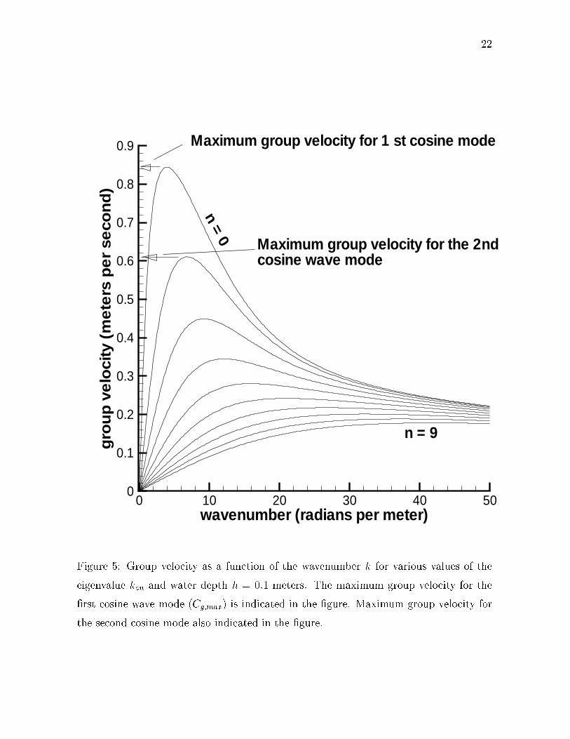
� We consider that the displacement of the wave maker coincides with the �rst

cosine wave mode in the z direction. The excitation frequency is above the cut-

o� frequency for the �rst cosine wave mode. With this type of excitation, the

only wave mode taking part in the solution is the �rst cosine wave mode. Since

the wave maker starts from rest to the harmonic motion, it excites initially all

wave frequencies and generates a transient which propagates along the channel

and is followed by a nono-chromatic wave train (the cosine wave mode) with

frequency equals to the excitation frequency. The transient h a s a w ave f r o n t which

propagates with the maximum group velocity possible for this cosine wave mode.

For the depth h = 0 :1 meters, �gure 5 illustrates the maximum group velocity f o r

the cosine wave modes. The maximum group velocity possible Cg;max

is the group

velocity of the cosine wave mode with kzn

=

� (n = 0). Then, for a given time

2b

instant t, there is no wave disturbance at positions x > Cg;maxt. The transient

for a given instant t stays in the region Cg;maxt > x > C g

(!)t, where Cg

(!) is the

group velocity of the excited cosine wave mode at the excitation frequency !. To

see the animation associated with this example, click here.

� We consider that the displacement of the wave maker coincides with the second

cosine wave mode in the z direction. The excitation frequency is above t h e cut-o�

frequency for the �rst cosine mode but below the cut-o� frequency for the second

cosine mode. Again, the wave maker starts from rest to the harmonic motion.

All wave frequencies are excited initially and a transient develops. The transient

propagates along the channel, and behind it we are left with only the second cosine

wave m ode, w hich decays exponentially as we go away from the wave m aker, since

at this excitation frequency the second cosine wave mode is evanescent. Again,

the transient has a wave front w h i c h propagates with the maximum group velocity

possible for the second cosine wave mode. To see the animation associated with

this example, click here.

� We consider that the displacement of the wave maker coincides with the �rst

0.9

22

gro

up

ve

loci

ty (

me

ters

pe

r se

con

d)

Maximum group velocity for 1 st cosine mode

0.8

0.7

0.6

0.5

0.4

0.3

0.2

0.1

0

n=

0 l

n = 9

Maximum group ve ocity for the 2nd cosine wave mode

0 10 20 30 40 wavenumber (radians per meter)

Figure 5: Group velocity as a function of the wavenumb e r k for various values of the

eigenvalue kzn

and water depth h = 0:1 meters. The maximum group velocity for the

�rst cosine wave mode (Cg;max) is indicated in the �gure. Maximum group velocity for

the second cosine mode also indicated in the �gure.

50

23

cosine mode in the z direction. The excitation frequency is exactly at the cut-o�

frequency. Again, the wave maker starts from rest to the harmonic motion, and

initially all wave frequencies are excited. A transient develops and propagates

along the channel. The transient has a wave front which propagates with the

maximum group velocity possible Cg;max

for the �rst cosine wave mode. Behind

the transient w e are left with the �rst cosine wave mode, since it is the only wave

mode excited by the wave maker. The group velocity of this wave mode at its

cut-o� frequency is zero, so there is no energy propagation along the channel after

the transient part of the solution is already far from the wave maker. Since the

energy cannot be radiated away from the wave maker, we see the wave amplitude

growing with time close to the wave maker. The cosine wave mode resonates with

the wave maker in this case. To see the animation associated with this example,

click here.

� Now the wave m a k er is a liner function in the z direction (F (z) = z). We show the

evolution of the disturbance due to the action of the wave maker. We consider all

modes that take part in the solution. We actually consider only a �nite numb e r

of sine and cosine wave modes. As the wavenumb e r kzm

or kzn

associated with

a wave mode increases, its amplitude decreases, so only a �nite numb e r of wave

modes are signi�cant. Again, the wave maker starts from rest to the harmonic

motion. We h a ve initially a transient w h i c h propagates along the channel. It has a

wave front which propagates with the maximum possible group velocity, which is

the maximum group velocity for the �rst sine wave m o d e . Ahead of the wave front

(x > Cg;maxt for a given instant t, where Cg;max

is the maximum group velocity

for the �rst sine wave mode) we h a ve n o w aves disturbance. For a given instant t,

the transient stays in the region Cg;maxt > x > C g

(!)t, where Cg

(!) is the group

velocity of the �rst sine wave mode at the excitation frequency !. Behind this

region we have the steady state solution. To see the animation associated with

this example, click here.