1

I-campus project

School-wide Program on Fluid Mechanics

Modules on Waves in uids

T. R. Akylas & C. C. Mei

CHAPTER SEVEN

INTERNAL WAVES IN A STRATIFIED FLUID

1 Introduction.

The atmosphere and ocean are continuously strati�ed due to change in temperature,

composition and pressure. These changes in the ocean and atmosphere can lead to

signi�cant variations of density of the uid in the vertical direction. As an example,

fresh water from rivers can rest on top of sea water, and due to the small di�usivity, the

density contrast remains for a long time. The density strati�cation allows oscillation of

the uid to happen. The restoring force that produces the oscillation is the buoyancy

force. The wave phenomena associated with these oscillations are called internal waves

and are discussed in this chapter.

2 Governing Equations for Incompressible Density-

strati�ed Fluid.

We are going to derive the system of equations governing wave motion of an incompress-

ible uid with continuous density strati�cation. Cartesian coordinates x; y and z will

be used, with z measured vertically upward. The velocity components in the directions

of increasing x; y and z will be denoted as u; v and w. The uid particle has to satisfy

the continuity equation

1

�

D�

Dt+

@u

@x+

@v

@y+

@w

@z= 0 (2.1)

and the momentum equations

2

�@u

@t+ u

@u

@x= �@p

@x; (2.2)

�@v

@t+ v

@v

@y= �@p

@y; (2.3)

�@w

@t+ w

@w

@z= �@p

@z� g�; (2.4)

where � and p are, respectively, the uid density and pressure. The uid is taken to

be such that the density depends only on entropy and on composition, i.e., � depends

only on the potential temperature � and on the concentrations of constituents, e.g., the

salinity s or humidity q. Then for �xed � and q (or s), � is independent of pressure:

� = �(�; q): (2.5)

The motion that takes place is assumed to be isentropic and without change of phase,

so that � and q are constant for a material element. Therefore

D�

Dt=

@�

@�

D�

Dt+

@�

@q

Dq

Dt= 0: (2.6)

In other words, � is constant for a material element because � and q are, and � depends

only on � and q. Such a uid is said to be incompressible, and because of (2.6) the

continuity equation (2.1) becomes

@u

@x+

@v

@y+

@w

@z= 0: (2.7)

For an incompressible uid, the density � satis�es the density equation

1

�

D�

Dt= 0: (2.8)

Assuming that the velocities are small, we can linearize the momentum equations to

obtain

3

�@u

@t= �@p

@x; (2.9)

�@v

@t= �@p

@y; (2.10)

�@w

@t= �@p

@z� g�: (2.11)

Next, we consider that the wave motion results from the perturbation of a state of

equilibrium, which is the state of rest. So the distribution of density and pressure is the

hydrostatic equilibrium distribution given by

@�p

@z= �g��: (2.12)

When the motion develops, the pressure and density changes to

p =�p(z) + p0; (2.13)

� =��(z) + �0; (2.14)

where p0 and �0 are, respectively, the pressure and density perturbations of the \back-

ground" state in which the density �� and the pressure �p are in hydrostatic balance. The

density equation now assume the form

@�0

@t+ u

@�0

@x+ v

@�0

@y+ w

@��

@z+ w

@�0

@z= 0: (2.15)

The nonlinear terms u(@�0=@x), v(@�0=@y) and w(@�0=@z) are negligible for small am-

plitude motion, so the equation (2.15) simpli�es to

@�0

@t+ w

@��

@z= 0; (2.16)

which states that the density perturbation at a point is generated by a vertical advection

of the background density distribution. The continuity equation (2.7) for incompressible

uid stays the same, but the momentum equations (2.9) to (2.11) assume the form

4

��@u

@t= �@p0

@x; (2.17)

��@v

@t= �@p0

@y; (2.18)

��@w

@t= �@p0

@z� g�0: (2.19)

We would like to reduce the systems of equations (2.7), (2.16) and (2.17) to (2.19) to a

single partial di�erential equation. This can be achieved as follows. First, we take the

time derivative of the continuity equation to obtain

@2u

@t@x+

@2v

@t@y+

@2w

@t@z= 0: (2.20)

Second, we take the x; y and t derivatives, respectively, of the equations (2.17) to (2.19),

and we obtain

��@2u

@x@t= �@2p0

@x2; (2.21)

��@2v

@y@t= �@2p0

@y2; (2.22)

��@2w

@t2= � @2p0

@t@z� g

@�0

@t: (2.23)

If we substitute equations (2.21) and (2.22) into equation (2.20), we obtain

�1

��

�@2p0

@x2+

@2p0

@y2

�+

@2w

@t@z= 0: (2.24)

We can eliminate �0 from (2.23) by using equation (2.16) to obtain

��@2w

@t2= � @2p0

@t@z+ g

@��

@zw: (2.25)

Third, we apply the operator @2

@x2+ @2

@y2to equation (2.25) to obtain

��@2

@t2

�@2w

@x2+

@2w

@y2

�= � @2

@t@z

�@2p0

@x2+

@2p0

@y2

�+ g

@��

@z

�@2w

@x2+

@2w

@y2

�: (2.26)

5

Next, we use equation (2.24) to eliminate p0 from equation (2.26), which gives the

following partial di�erential equation for w:

@2

@t2

�@2w

@x2+

@2w

@y2+

1

��

@

@z

���@w

@z

��+N2

�@2w

@x2+

@2w

@y2

�= 0; (2.27)

where we de�ne

N2(z) = �g

�

@��

@z; (2.28)

which has the units of frequency (rad/sec) and is called the Brunt-V�ais�al�a frequency or

buoyancy frequency. If we assume that w varies with z much more rapidly than ��(z),

then

1

��

@

@z

���@

@z

�w � @2w

@z2; (2.29)

and (2.27) can be approximated by the equation

@2

@t2

�@2w

@x2+

@2w

@y2+

@2w

@z2

�+N2

�@2w

@x2+

@2w

@y2

�= 0: (2.30)

The assumption above is equivalent to the Boussinesq approximation, which applies

when the motion has vertical scale small compared with the scale of the background

density. It consists in taking the density to be constant in computing rates of change

of momentum from accelerations, but taking full account of the density variations when

they give rise to buoyancy forces, i.e., when there is a multiplying factor g in the ver-

tical component of the momentum equations. The Boussinesq approximation leads to

equation (2.30) for the vertical velocity w.

3 The Buoyancy Frequency (Brunt-V�ais�al�a frequency).

Consider a calm strati�ed uid with a static density distribution ��(z) which decreases

with height z. If a uid parcel is moved from the level z upward to z+�, it is surrounded

by lighter uid of density ��(z + �). The upward buoyancy force per unit volume is

6

g [��(z + �)� ��(z)] � gd��

dz�; (3.31)

and it is negative. Applying Newton's law to the uid parcel of unit volume, we have

��@2�

@t2= g

d��

dz� (3.32)

or

@2�

@t2+N2� = 0; (3.33)

where

N2(z) = �g

��

d��

dz; (3.34)

which is called the buoyancy frequency or the Brunt V�as�al�a frequency. This elementary

consideration shows that once a uid is displaced from its equilibrium position, gravity

and density gradient provide restoring force to enable oscillations.

4 Internal Gravity Waves in Unbounded Strati�ed

Fluid.

Consider the case in which the buoyancy (Brunt-V�ais�al�a) frequency N is constant

throughout the uid. Traveling wave solutions of (2.30) can be found of the form

w = w0 cos(kx+ ly +mz � !t); (4.35)

where w0 is the vertical velocity amplitude and�!k = (k; l;m) is the wavenumber of the

disturbance, and ! is the frequency. In order for (4.35) to satisfy the governing equation

(2.30) for the vertical perturbation velocity, ! and�!k must be related by the dispersion

relation

7

!2 =(k2 + l2)N2

k2 + l2 +m2: (4.36)

Thus internal waves can have any frequency between zero and a maximum value of

N . The dispersion relation for internal waves is of quite a di�erent character compared

to that for surface waves. In particular, the frequency of surface waves depends only

on the magnitude j�!k j of the wavenumber, whereas the frequency of internal waves is

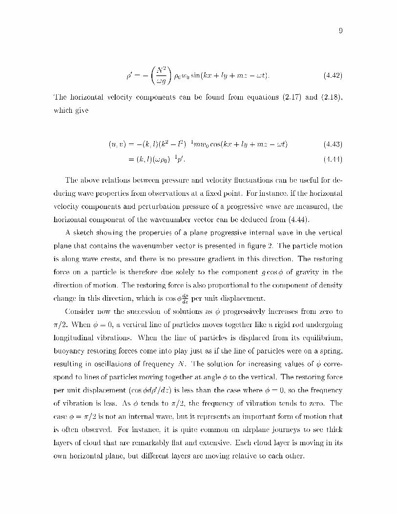
independent of the magnitude of the wavenumber and depends only on the angle � that

the wavenumber vector makes with the horizontal. To illustrate this, we consider the

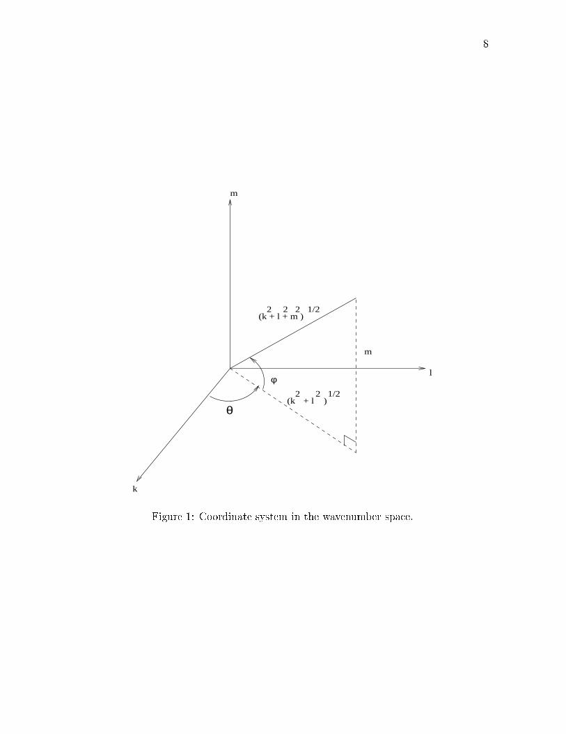
spherical system of coordinates in the wavenumber space, namely,

k =j�!k j cos(�) cos(�) (4.37)

l =j�!k j cos(�) sin(�) (4.38)

m =j�!k j sin(�) (4.39)

The coordinate system in the wavenumber space is given in the �gure 1.

The dispersion relation given by equation (4.36) reduces to

!2 = N cos(�): (4.40)

Now we can write expressions for the quantities p0; �0; u and v. From equation (2.20) we

can write

� 1

�0

�@2p0

@x2+

@2p0

@y2

�=

@2w

@t@z= !mw0 cos(kx + ly +mz � !t);

which implies that the perturbation pressure p0 is given by

p0 = � !mw0�0(k2 + l2)1=2

cos(kx + ly +mz � !t): (4.41)

From equation (2.16) we have the perturbation density �0 given by

8

m

l

k

m

φ

(k 2

+ l2

)1/2

(k + l + m )2 2 2 1/2

θ

Figure 1: Coordinate system in the wavenumber space.

9

�0 = ��N2

!g

��0w0 sin(kx+ ly +mz � !t): (4.42)

The horizontal velocity components can be found from equations (2.17) and (2.18),

which give

(u; v) = �(k; l)(k2 + l2)�1mw0 cos(kx + ly +mz � !t) (4.43)

= (k; l)(!�0)�1p0: (4.44)

The above relations between pressure and velocity uctuations can be useful for de-

ducing wave properties from observations at a �xed point. For instance, if the horizontal

velocity components and perturbation pressure of a progressive wave are measured, the

horizontal component of the wavenumber vector can be deduced from (4.44).

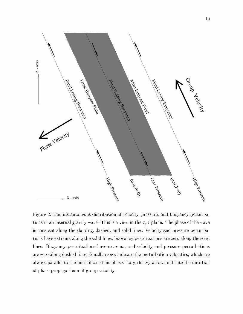
A sketch showing the properties of a plane progressive internal wave in the vertical

plane that contains the wavenumber vector is presented in �gure 2. The particle motion

is along wave crests, and there is no pressure gradient in this direction. The restoring

force on a particle is therefore due solely to the component g cos� of gravity in the

direction of motion. The restoring force is also proportional to the component of density

change in this direction, which is cos�d�dz

per unit displacement.

Consider now the succession of solutions as � progressively increases from zero to

�=2. When � = 0, a vertical line of particles moves together like a rigid rod undergoing

longitudinal vibrations. When the line of particles is displaced from its equilibrium,

buoyancy restoring forces come into play just as if the line of particles were on a spring,

resulting in oscillations of frequency N . The solution for increasing values of � corre-

spond to lines of particles moving together at angle � to the vertical. The restoring force

per unit displacement (cos�d�0=dz) is less than the case where � = 0, so the frequency

of vibration is less. As � tends to �=2, the frequency of vibration tends to zero. The

case � = �=2 is not an internal wave, but it represents an important form of motion that

is often observed. For instance, it is quite common on airplane journeys to see thick

layers of cloud that are remarkably at and extensive. Each cloud layer is moving in its

own horizontal plane, but di�erent layers are moving relative to each other.

10

Fluid Losing B

uoyancy

Fluid Losing B

uoyancy

Most B

uoyant Fluid

Least B

uoyant Fluid

Fluid Gaining B

uoyancy

High Pressure

Low

Pressure

High Pressure

(u,w,P=0)

(u,w,P=0)

Group V

elocity

Phase Velocity

X - axis

Z -

axi

s

Figure 2: The instantaneous distribution of velocity, pressure, and buoyancy perturba-

tions in an internal gravity wave. This is a view in the x; z plane. The phase of the wave

is constant along the slanting, dashed, and solid lines. Velocity and pressure perturba-

tions have extrema along the solid lines; buoyancy perturbations are zero along the solid

lines. Buoyancy perturbations have extrema, and velocity and pressure perturbations

are zero along dashed lines. Small arrows indicate the perturbation velocities, which are

always parallel to the lines of constant phase. Large heavy arrows indicate the direction

of phase propagation and group velocity.

11

4.1 Dispersion E�ects.

In practice, internal gravity waves never have the form of the exact plane wave given

by equation (4.35), so it is necessary to consider superposition of such waves. As a

consequence, dispersion e�ects become evident, since waves with di�erent frequencies

have di�erent phase and group velocities as we are going to show in this section. For

internal waves, surfaces of constant frequency in the wavenumber space are the cones

� = constant. The phase velocity is parallel to the wavenumber vector and it lies on a

cone of constant phase. Its magnitude is

!

j�!k j =

N

j�!k j

!cos �: (4.45)

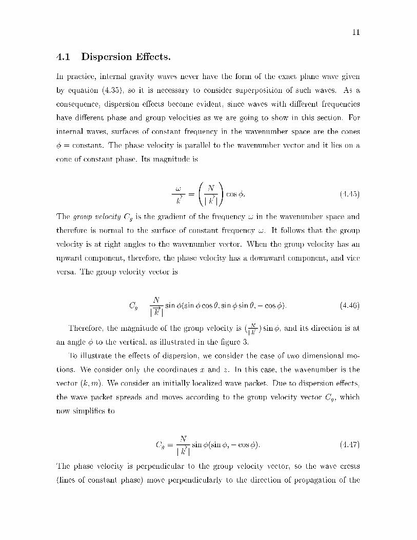
The group velocity Cg is the gradient of the frequency ! in the wavenumber space and

therefore is normal to the surface of constant frequency !. It follows that the group

velocity is at right angles to the wavenumber vector. When the group velocity has an

upward component, therefore, the phase velocity has a downward component, and vice

versa. The group velocity vector is

Cg =N

j�!k j sin�(sin� cos �; sin� sin �;� cos�): (4.46)

Therefore, the magnitude of the group velocity is ( Nj�!k j) sin�, and its direction is at

an angle � to the vertical, as illustrated in the �gure 3.

To illustrate the e�ects of dispersion, we consider the case of two dimensional mo-

tions. We consider only the coordinates x and z. In this case, the wavenumber is the

vector (k;m). We consider an initially localized wave packet. Due to dispersion e�ects,

the wave packet spreads and moves according to the group velocity vector Cg, which

now simpli�es to

Cg =N

j�!k j sin�(sin�;� cos�): (4.47)

The phase velocity is perpendicular to the group velocity vector, so the wave crests

(lines of constant phase) move perpendicularly to the direction of propagation of the

12

l

k

m

(k 2

+ l2

)1/2

(k + l + m )2 2 2 1/2

θ

φC g

φ

m

Figure 3: Wavenumber vector and group velocity vector.

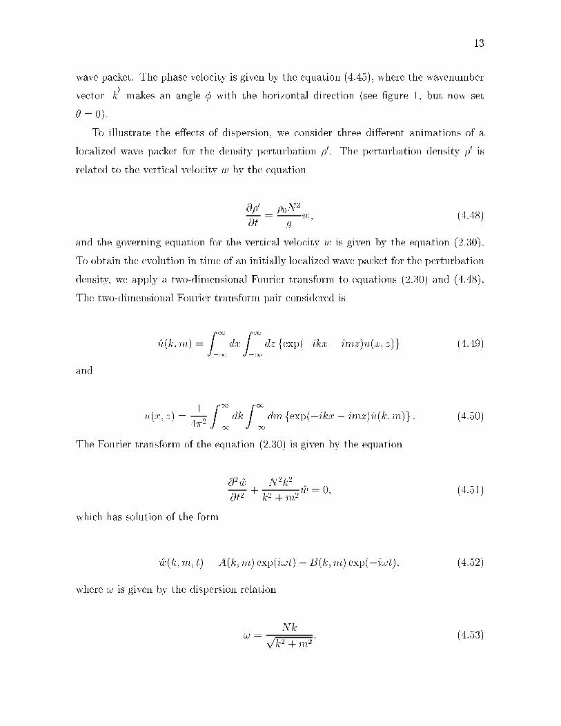
13

wave packet. The phase velocity is given by the equation (4.45), where the wavenumber

vector�!k makes an angle � with the horizontal direction (see �gure 1, but now set

� = 0).

To illustrate the e�ects of dispersion, we consider three di�erent animations of a

localized wave packet for the density perturbation �0. The perturbation density �0 is

related to the vertical velocity w by the equation

@�0

@t=

�0N2

gw; (4.48)

and the governing equation for the vertical velocity w is given by the equation (2.30).

To obtain the evolution in time of an initially localized wave packet for the perturbation

density, we apply a two-dimensional Fourier transform to equations (2.30) and (4.48).

The two-dimensional Fourier transform pair considered is

u(k;m) =

Z 1

�1

dx

Z 1

�1

dz fexp(�ikx� imz)u(x; z)g (4.49)

and

u(x; z) =1

4�2

Z 1

�1

dk

Z 1

�1

dm fexp(�ikx� imz)u(k;m)g : (4.50)

The Fourier transform of the equation (2.30) is given by the equation

@2w

@t2+

N2k2

k2 +m2w = 0; (4.51)

which has solution of the form

w(k;m; t) = A(k;m) exp(i!t) +B(k;m) exp(�i!t); (4.52)

where ! is given by the dispersion relation

! =Nkp

k2 +m2: (4.53)

14

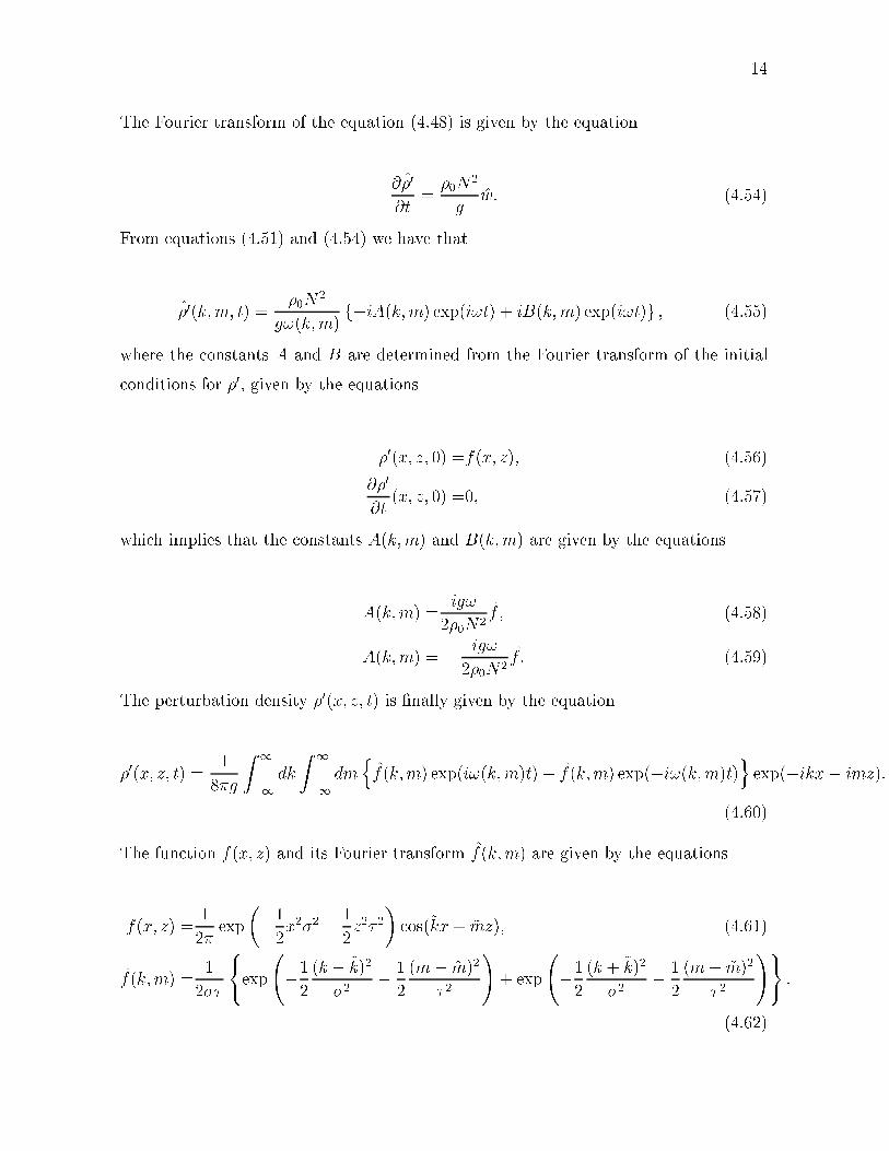
The Fourier transform of the equation (4.48) is given by the equation

@�0

@t=

�0N2

gw: (4.54)

From equations (4.51) and (4.54) we have that

�0(k;m; t) =�0N

2

g!(k;m)f�iA(k;m) exp(i!t) + iB(k;m) exp(i!t)g ; (4.55)

where the constants A and B are determined from the Fourier transform of the initial

conditions for �0, given by the equations

�0(x; z; 0) =f(x; z); (4.56)

@�0

@t(x; z; 0) =0; (4.57)

which implies that the constants A(k;m) and B(k;m) are given by the equations

A(k;m) =ig!

2�0N2f ; (4.58)

A(k;m) =� ig!

2�0N2f : (4.59)

The perturbation density �0(x; z; t) is �nally given by the equation

�0(x; z; t) =1

8�g

Z 1

�1

dk

Z 1

�1

dmnf(k;m) exp(i!(k;m)t) + f(k;m) exp(�i!(k;m)t)

oexp(�ikx� imz):

(4.60)

The function f(x; z) and its Fourier transform f(k;m) are given by the equations

f(x; z) =1

2�exp

��1

2x2�2 � 1

2z2� 2

�cos(~kx+ ~mz); (4.61)

f(k;m) =1

2��

(exp

�1

2

(k � ~k)2

�2� 1

2

(m� ~m)2

� 2

!+ exp

�1

2

(k + ~k)2

�2� 1

2

(m+ ~m)2

� 2

!):

(4.62)

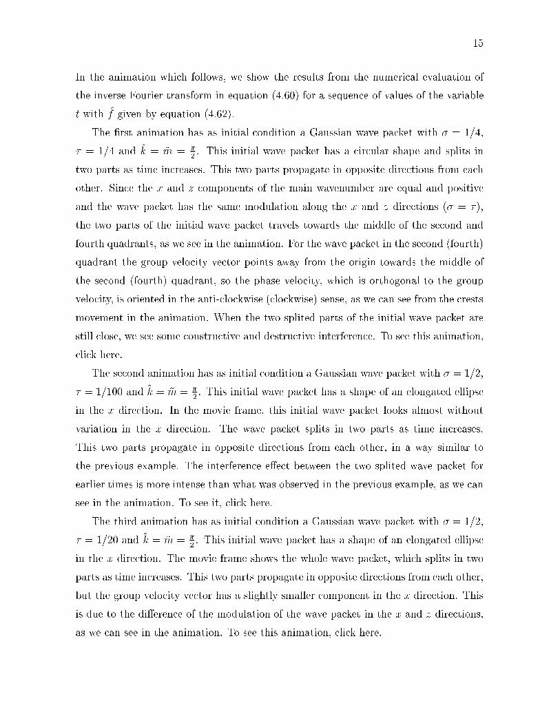
15

In the animation which follows, we show the results from the numerical evaluation of

the inverse Fourier transform in equation (4.60) for a sequence of values of the variable

t with f given by equation (4.62).

The �rst animation has as initial condition a Gaussian wave packet with � = 1=4,

� = 1=4 and ~k = ~m = �2. This initial wave packet has a circular shape and splits in

two parts as time increases. This two parts propagate in opposite directions from each

other. Since the x and z components of the main wavenumber are equal and positive

and the wave packet has the same modulation along the x and z directions (� = �),

the two parts of the initial wave packet travels towards the middle of the second and

fourth quadrants, as we see in the animation. For the wave packet in the second (fourth)

quadrant the group velocity vector points away from the origin towards the middle of

the second (fourth) quadrant, so the phase velocity, which is orthogonal to the group

velocity, is oriented in the anti-clockwise (clockwise) sense, as we can see from the crests

movement in the animation. When the two splited parts of the initial wave packet are

still close, we see some constructive and destructive interference. To see this animation,

click here.

The second animation has as initial condition a Gaussian wave packet with � = 1=2,

� = 1=100 and ~k = ~m = �2. This initial wave packet has a shape of an elongated ellipse

in the x direction. In the movie frame, this initial wave packet looks almost without

variation in the x direction. The wave packet splits in two parts as time increases.

This two parts propagate in opposite directions from each other, in a way similar to

the previous example. The interference e�ect between the two splited wave packet for

earlier times is more intense than what was observed in the previous example, as we can

see in the animation. To see it, click here.

The third animation has as initial condition a Gaussian wave packet with � = 1=2,

� = 1=20 and ~k = ~m = �2. This initial wave packet has a shape of an elongated ellipse

in the x direction. The movie frame shows the whole wave packet, which splits in two

parts as time increases. This two parts propagate in opposite directions from each other,

but the group velocity vector has a slightly smaller component in the x direction. This

is due to the di�erence of the modulation of the wave packet in the x and z directions,

as we can see in the animation. To see this animation, click here.

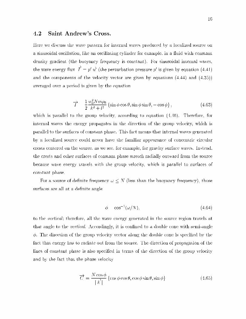
16

4.2 Saint Andrew's Cross.

Here we discuss the wave pattern for internal waves produced by a localized source on

a sinusoidal oscillation, like an oscillating cylinder for example, in a uid with constant

density gradient (the buoyancy frequency is constant). For sinusoidal internal waves,

the wave energy ux�!I = p0�!u (the perturbation pressure p0 is given by equation (4.41)

and the components of the velocity vector are given by equations (4.44) and (4.35))

averaged over a period is given by the equation

�!I =

1

2

w2

0Nm�0

k2 + l2fsin� cos �; sin� sin �;� cos�g ; (4.63)

which is parallel to the group velocity, according to equation (4.46). Therefore, for

internal waves the energy propagates in the direction of the group velocity, which is

parallel to the surfaces of constant phase. This fact means that internal waves generated

by a localized source could never have the familiar appearance of concentric circular

crests centered on the source, as we see, for example, for gravity surface waves. Instead,

the crests and other surfaces of constant phase stretch radially outward from the source

because wave energy travels with the group velocity, which is parallel to surfaces of

constant phase.

For a source of de�nite frequency ! � N (less than the buoyancy frequency), those

surfaces are all at a de�nite angle

� = cos�1(!=N); (4.64)

to the vertical ; therefore, all the wave energy generated in the source region travels at

that angle to the vertical. Accordingly, it is con�ned to a double cone with semi-angle

�. The direction of the group velocity vector along the double cone is speci�ed by the

fact that energy has to radiate out from the source. The direction of propagation of the

lines of constant phase is also speci�ed in terms of the direction of the group velocity

and by the fact that the phase velocity

�!C =

N cos�

j�!k jfcos � cos �; cos� sin �; sin�g (4.65)

17

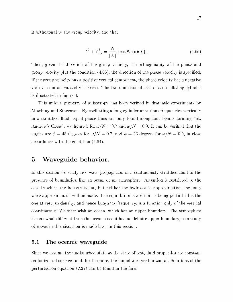
is orthogonal to the group velocity, and that

�!C +

�!C g =

N

j�!k j fcos �; sin �; 0g : (4.66)

Then, given the direction of the group velocity, the orthogonality of the phase and

group velocity plus the condition (4.66), the direction of the phase velocity is speci�ed.

If the group velocity has a positive vertical component, the phase velocity has a negative

vertical component and vice-versa. The two-dimensional case of an oscillating cylinder

is illustrated in �gure 4.

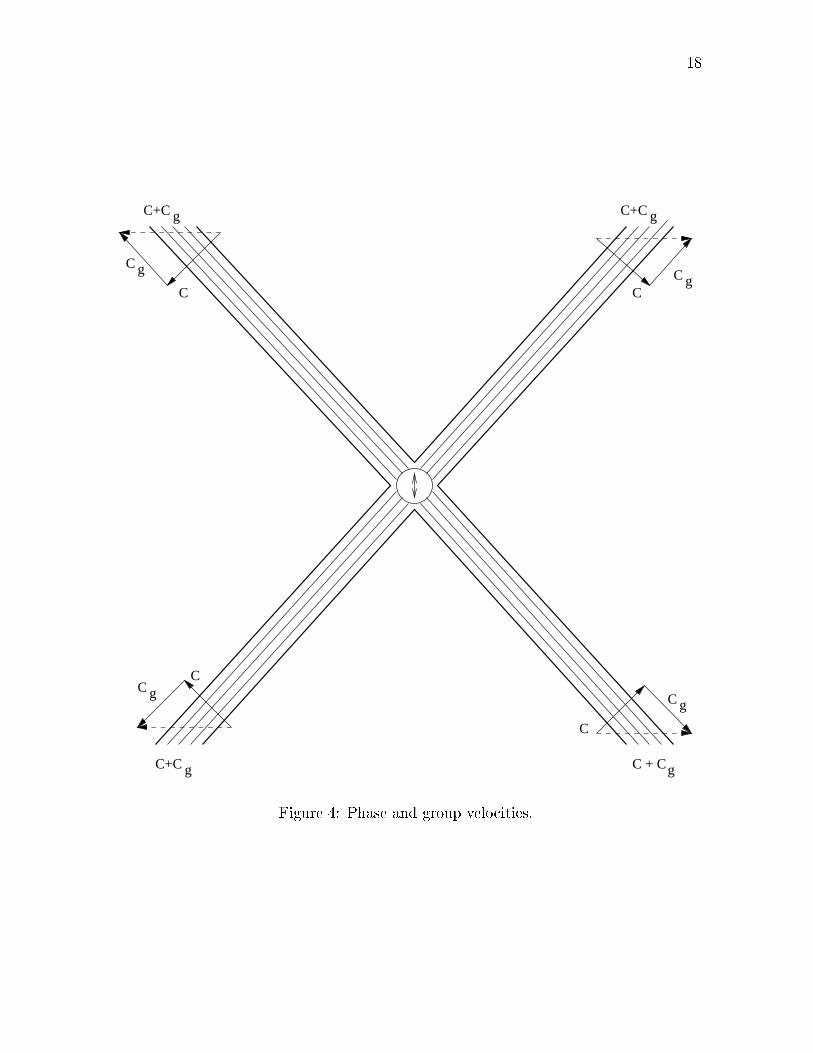
This unique property of anisotropy has been veri�ed in dramatic experiments by

Mowbray and Stevenson. By oscillating a long cylinder at various frequencies vertically

in a strati�ed uid, equal phase lines are only found along four beams forming \St.

Andrew's Cross", see �gure 5 for !=N = 0:7 and !=N = 0:9. It can be veri�ed that the

angles are � = 45 degrees for !=N = 0:7, and � = 26 degrees for !=N = 0:9, in close

accordance with the condition (4.64).

5 Waveguide behavior.

In this section we study free wave propagation in a continuously strati�ed uid in the

presence of boundaries, like an ocean or an atmosphere. Attention is restricted to the

case in which the bottom is at, but neither the hydrostatic approximation nor long-

wave approximation will be made. The equilibrium state that is being perturbed is the

one at rest, so density, and hence buoyancy frequency, is a function only of the vertical

coordinate z. We start with an ocean, which has an upper boundary. The atmosphere

is somewhat di�erent from the ocean since it has no de�nite upper boundary, so a study

of waves in this situation is made later in this section.

5.1 The oceanic waveguide

Since we assume the undisturbed state as the state of rest, uid properties are constant

on horizontal surfaces and, furthermore, the boundaries are horizontal. Solutions of the

perturbation equation (2.27) can be found in the form

18

C

C g

C + Cg

CC g

C

C g

CC g

C+C g

C+C g C+C g

Figure 4: Phase and group velocities.

19

Figure 5: St Andrew's Cross in a strati�ed uid. In the top �gure !=N = 0:9 and in

the left bottom �gure !=N = 0:7.

20

w(x; y; z; t) = w(z) exp[i(kx + ly � !t)] (5.67)

The equation for w(z) can be found by substitution of equation (5.67) into the governing

equation (2.27). We obtain

1

��

@

@z

���@w

@z

�+

(N2 � !2)

!2(k2 + l2)w(z) = 0 (5.68)

The boundary conditions for this equation are the bottom condition of no ux across

it, given by the equation

w(z) = 0 at z = �H; (5.69)

and at the free-surface we have the linearized condition

@p0

@t= ��gw(z) at z = 0; (5.70)

where p0 is the perturbation pressure. From this equation we can obtain a free-surface

boundary condition for w(z). We apply the operator @@t

to the equation (2.24), and then

we substitute equation (5.70) into the resulting equation. As a result, we obtain the

equation

@3w

@t2@z= g

�@2w

@x2+

@2w

@y2

�at z = 0 (5.71)

Now, if we substitute equation (5.67) into the equation (5.71), we obtain the free-surface

boundary condition for w(z), which follows

@2w

@z2+

(N2 � !2)

!2(k2 + l2)w(z) = 0 at z = 0: (5.72)

To simplify the governing equation for w(z), we make the Boussinesq approximation,

such that equation (5.68) simpli�es to

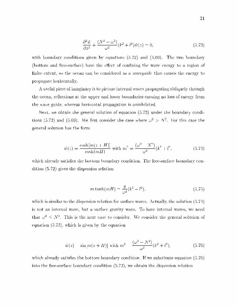
21

@2w

@z2+

(N2 � !2)

!2(k2 + l2)w(z) = 0; (5.73)

with boundary conditions given by equations (5.72) and (5.69). The two boundary

(bottom and free-surface) have the e�ect of con�ning the wave energy to a region of

�nite extent, so the ocean can be considered as a waveguide that causes the energy to

propagate horizontally.

A useful piece of imaginary is to picture internal waves propagating obliquely through

the ocean, re ections at the upper and lower boundaries ensuing no loss of energy from

the wave guide, whereas horizontal propagation is uninhibited.

Next, we obtain the general solution of equation (5.73) under the boundary condi-

tions (5.72) and (5.69). We �rst consider the case where !2 > N2. For this case the

general solution has the form

w(z) =cosh[m(z +H)]

cosh(mH)with m2 =

(!2 �N2)

!2(k2 + l2; (5.74)

which already satis�es the bottom boundary condition. The free-surface boundary con-

dition (5.72) gives the dispersion relation

m tanh(mH) =g

!2(k2 + l2); (5.75)

which is similar to the dispersion relation for surface waves. Actually, the solution (5.74)

is not an internal wave, but a surface gravity wave. To have internal waves, we need

that !2 � N2. This is the next case to consider. We consider the general solution of

equation (5.73), which is given by the equation

w(z) = sin[m(z +H)] with m2 =(!2 �N2)

!2(k2 + l2); (5.76)

which already satis�es the bottom boundary condition. If we substitute equation (5.76)

into the free-surface boundary condition (5.72), we obtain the dispersion relation

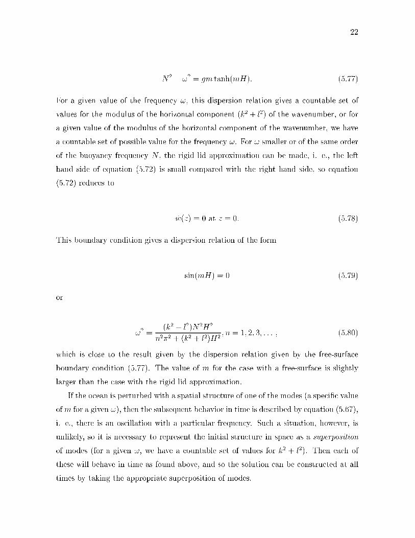
22

N2 � !2 = gm tanh(mH): (5.77)

For a given value of the frequency !, this dispersion relation gives a countable set of

values for the modulus of the horizontal component (k2 + l2) of the wavenumber, or for

a given value of the modulus of the horizontal component of the wavenumber, we have

a countable set of possible value for the frequency !. For ! smaller or of the same order

of the buoyancy frequency N , the rigid lid approximation can be made, i. e., the left

hand side of equation (5.72) is small compared with the right hand side, so equation

(5.72) reduces to

w(z) = 0 at z = 0: (5.78)

This boundary condition gives a dispersion relation of the form

sin(mH) = 0 (5.79)

or

!2 =(k2 + l2)N2H2

n2�2 + (k2 + l2)H2; n = 1; 2; 3; : : : ; (5.80)

which is close to the result given by the dispersion relation given by the free-surface

boundary condition (5.77). The value of m for the case with a free-surface is slightly

larger than the case with the rigid lid approximation.

If the ocean is perturbed with a spatial structure of one of the modes (a speci�c value

ofm for a given !), then the subsequent behavior in time is described by equation (5.67),

i. e., there is an oscillation with a particular frequency. Such a situation, however, is

unlikely, so it is necessary to represent the initial structure in space as a superposition

of modes (for a given !, we have a countable set of values for k2 + l2). Then each of

these will behave in time as found above, and so the solution can be constructed at all

times by taking the appropriate superposition of modes.

23

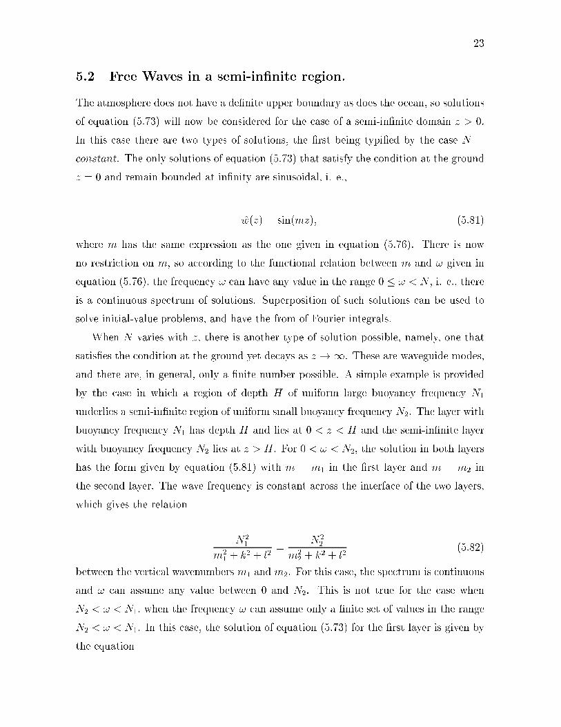
5.2 Free Waves in a semi-in�nite region.

The atmosphere does not have a de�nite upper boundary as does the ocean, so solutions

of equation (5.73) will now be considered for the case of a semi-in�nite domain z > 0.

In this case there are two types of solutions, the �rst being typi�ed by the case N =

constant. The only solutions of equation (5.73) that satisfy the condition at the ground

z = 0 and remain bounded at in�nity are sinusoidal, i. e.,

w(z) = sin(mz); (5.81)

where m has the same expression as the one given in equation (5.76). There is now

no restriction on m, so according to the functional relation between m and ! given in

equation (5.76), the frequency ! can have any value in the range 0 � ! < N , i. e., there

is a continuous spectrum of solutions. Superposition of such solutions can be used to

solve initial-value problems, and have the from of Fourier integrals.

When N varies with z, there is another type of solution possible, namely, one that

satis�es the condition at the ground yet decays as z !1. These are waveguide modes,

and there are, in general, only a �nite number possible. A simple example is provided

by the case in which a region of depth H of uniform large buoyancy frequency N1

underlies a semi-in�nite region of uniform small buoyancy frequency N2. The layer with

buoyancy frequency N1 has depth H and lies at 0 < z < H and the semi-in�nite layer

with buoyancy frequency N2 lies at z > H. For 0 < ! < N2, the solution in both layers

has the form given by equation (5.81) with m = m1 in the �rst layer and m = m2 in

the second layer. The wave frequency is constant across the interface of the two layers,

which gives the relation

N2

1

m2

1+ k2 + l2

=N2

2

m2

2+ k2 + l2

(5.82)

between the vertical wavenumbers m1 and m2. For this case, the spectrum is continuous

and ! can assume any value between 0 and N2. This is not true for the case when

N2 < ! < N1, when the frequency ! can assume only a �nite set of values in the range

N2 < ! < N1. In this case, the solution of equation (5.73) for the �rst layer is given by

the equation

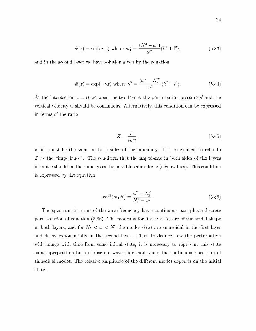
24

w(z) = sin(m1z) where m2

1=

(N2

1� !2)

!2(k2 + l2); (5.83)

and in the second layer we have solution given by the equation

w(z) = exp(� z) where 2 = (!2 �N2

2)

!2(k2 + l2): (5.84)

At the intersection z = H between the two layers, the perturbation pressure p0 and the

vertical velocity w should be continuous. Alternatively, this condition can be expressed

in terms of the ratio

Z =p0

�0w; (5.85)

which must be the same on both sides of the boundary. It is convenient to refer to

Z as the \impedance". The condition that the impedance in both sides of the layers

interface should be the same gives the possible values for ! (eigenvalues). This condition

is expressed by the equation

cot2(m1H) =!2 �N2

2

N2

1� !2

: (5.86)

The spectrum in terms of the wave frequency has a continuous part plus a discrete

part, solution of equation (5.86). The modes w for 0 < ! < N2 are of sinusoidal shape

in both layers, and for N2 < ! < N1 the modes w(z) are sinusoidal in the �rst layer

and decay exponentially in the second layer. Thus, to deduce how the perturbation

will change with time from some initial state, it is necessary to represent this state

as a superposition both of discrete waveguide modes and the continuous spectrum of

sinusoidal modes. The relative amplitude of the di�erent modes depends on the initial

state.