Underwater localization based on grid computation and its

This is a repository copy of Underwater localization based on grid computation and its application to transmit beamforming in multiuser UWA communications.

White Rose Research Online URL for this paper:http://eprints.whiterose.ac.uk/127319/

Version: Accepted Version

Article:

Liao, Li, Zakharov, Yuriy orcid.org/0000-0002-2193-4334 and Mitchell, Paul Daniel orcid.org/0000-0003-0714-2581 (2018) Underwater localization based on grid computationand its application to transmit beamforming in multiuser UWA communications. IEEE Access. pp. 4297-4307. ISSN 2169-3536

https://doi.org/10.1109/ACCESS.2018.2793962

[email protected]://eprints.whiterose.ac.uk/

Reuse

Items deposited in White Rose Research Online are protected by copyright, with all rights reserved unless indicated otherwise. They may be downloaded and/or printed for private study, or other acts as permitted by national copyright laws. The publisher or other rights holders may allow further reproduction and re-use of the full text version. This is indicated by the licence information on the White Rose Research Online record for the item.

Takedown

If you consider content in White Rose Research Online to be in breach of UK law, please notify us by emailing [email protected] including the URL of the record and the reason for the withdrawal request.

IEEE ACCESS, NOVEMBER 2017 1

Underwater Localization Based on Grid

Computation and its Application to Transmit

Beamforming in Multiuser UWA Communications

Li Liao†, Student Member, IEEE, Yuriy Zakharov†, Senior Member, IEEE,

Paul D. Mitchell†, Senior Member, IEEE

Abstract—Underwater localization is a challenging problemand established technologies for terrestrial systems cannot beused, notably the Global Positioning System (GPS). In this paper,we propose an underwater localization technique and demon-strate how it can be effectively used for transmit beamformingin multiuser underwater acoustic (UWA) communications. Thelocalization is based on pre-computation of acoustic channel pa-rameters between a transmitter-receiver pair on a grid of pointscovering the area of interest. This is similar to the localizationprocess using matched field processing, which is often based onprocessing a priori unknown signals received by an array ofhydrophones. However, in our case, every receiver is assumed tohave a single hydrophone, while an array of transducers transmit(pilot) signals known at a receiver. The receiver processes thereceived pilot signal to estimate the Channel State Information(CSI) and compares it with the CSI pre-computed on the grid; thebest match indicates the location estimate. The proposed local-ization technique also enables an efficient solution to the inherentproblem of informing a transmitter about the CSI available at thereceiver for the purpose of transmit beamforming. The receiveronly needs to send a grid point index to enable the transmitter toobtain the pre-computed CSI corresponding to the particular gridpoint, thereby significantly reducing transmission overheads. Weapply this approach to a multiuser communication scenario withorthogonal frequency-division multiplexing (OFDM) and showthat the proposed approach results in accurate localization ofreceivers and multiuser communications with a high detectionperformance.

Keywords—Localization, multiuser communication, SDMA,transmit beamforming

I. INTRODUCTION

In recent years, there has been a growing interest in un-

derwater acoustic communications (UAC) in various applica-

tion areas such as telemetry, remote control, speech/image

transmission, etc. [1]. The investigation of UAC has met

many challenges since, in particular, the underwater acoustic

(UWA) channels are characterized by limited bandwidth, long

propagation delays, and multipath interference [2]. The clas-

sical multiple access communication strategies, such as time

division multiple access (TDMA), frequency division multi-

ple access (FDMA), code division multiple access (CDMA),

as well as spatial division multiple access (SDMA) have

been widely used in terrestrial radio communication systems,

†Dept. of Electronic Eng., University of York, UK; [email protected],[email protected], [email protected]. The work of Y. Za-kharov and P. Mitchell is partly supported by the UK Engineering and PhysicalSciences Research Council (EPSRC) through the USMART Project underGrant EP/P017975/1.

with users separated in time, frequency, code domains, or in

space [3]–[7]. FDMA is not well suited for UAC due to the

narrow bandwidth of the UAW channel. TDMA can be useful,

but it is challenging to make efficient use of channel time

in highly dynamic scenarios, since long propagation delays

inhibit the ability to allocate capacity in response to time

varying needs. CDMA may suffer from the severe multipath

interference that leads to degradation of the code correlation

properties, resulting in smaller codeword distances [5]. These

three multiple access schemes have to divide the available

time-frequency resources among the multiple users. On the

other hand, with SDMA, the same time-frequency resources

can be independently used by every user. With simultaneous

transmission to multiple users in multi-antenna broadcast

channels, SDMA is capable of achieving a much higher

throughput than other multiple-access schemes [6], and it is a

viable choice in UAC.

In this paper, we consider SDMA systems with multi-

ple transmit antennas (transducers) and multiple receivers

equipped with a single antenna (hydrophone) each. In such

a system, in order to design the transmit beamformer, the

transmitter requires knowledge of the Channel State Informa-

tion (CSI) between every transducer and every receiver hy-

drophone [8]. This information can be estimated at the receiver

by processing pilot signals. The estimated CSI then needs to

be sent back to the transmitter, which can be problematic in

narrowband UWA channels due to the large amount of data

comprising the CSI and low data throughput capability.

This problem can be resolved if both the transmitter and

receiver have a pre-computed dictionary of possible CSIs. In

this case, the receiver only needs to send back the index of

the CSI from the dictionary that provides the best match to

the CSI estimate. In UWA channels, such a dictionary can

be built based upon acoustic field computation for a specific

environment, where the communication system is installed.

More specifically, the dictionary can be computed for a grid

of points in space (grid of range/depth points), thus also

solving the localization problem (estimation of position of

the receiver with respect to the position of the transducers),

which is required in many applications [9]–[11]. Underwater

localization is a difficult problem, and in many cases it cannot

rely on traditional terrestrial localisation technologies, such as

the Global Positioning System (GPS) [2].

The approach based on pre-computing the acoustic field

using a wave equation is similar to localization using matched


20

0 m

500 m 100 m

Area of interest

Receiver

80 m

50 m

Sea surface

Sea bottom

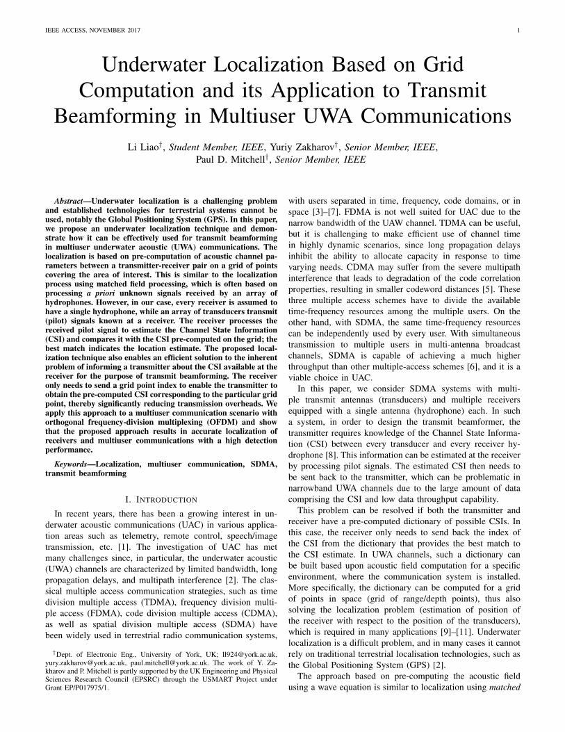
Fig. 1: The receiver is located in an area of interest

200 m × 500 m. The sea depth is 220 m. The transducers

are equally spaced from a depth of 50 m to 80 m.

field processing (MFP) often based on processing of a priori

unknown signals received by an array of hydrophones. There

have been a number of studies and experiments related to

MFP [12]–[16] and the general idea is to search over a

parameter space for the unknown parameters of the signal

source [17], [18]. As a development of MFP, the environmental

focalization technique was proposed [19], [20], which is based

on adjustement of environmental parameters within a search

space which, after being optimized under a particular objective

function, generates physical parameters that correspond to the

acoustic field replica best matching the observed acoustic field.

In the recent work [21], the focalization technique was used

to improve the channel estimation in UAC.

The design of a transmit beamformer in multiuser channels

is an important problem in modern wireless communication

systems with SDMA. The main difficulty in such systems is

that coordinated receive processing is not possible and that

all the signal processing must be employed at the transmitter

side [8]. Linear precoding schemes provide a promising trade-

off between performance and complexity [22]–[25]. The zero-

forcing (ZF) beamforming is the most common linear precod-

ing scheme, which decouples the multiuser channel into multi-

ple independent subchannels [26]–[32]. Orthogonal frequency-

division multiplexing (OFDM) communication is considered

as a promising technology for high data-rate communications

in UAC [33]–[36]. It can be efficiently combined with SDMA

to improve the system throughput [33], [37]–[39]. In this

paper, we will be investigating transmit beamforming based

on linear precoding in an OFDM communication system.

One of the significant problems with numerical investigation

of signal processing algorithms in UWA systems is the model-

ing of the signal transmission that takes into consideration the

specific acoustic environment, and consequently the specific

multipath propagation. For such virtual signal transmission,

i.e., transmission that mimics a real sea trial, the VirTEX

simulator was developed [40] and used [41]; the model relies

on the Bellhop ray/beam tracing approach [42] to compute

the channel response in defined acoustic environments. A

similar approach is used in the Waymark simulator [43]–

[46] developed to investigate UWA signal transmission in

long communication sessions. We use the Waymark model

to investigate the localization and communication techniques.

In this paper:

• a receiver localization technique is proposed, based on

matching the CSI estimated at the receiver to the CSI

pre-computed at grid points in an area of interest (over

depth and range);

• we propose to apply this localization technique in UAC

with SDMA to inform the transmitter of the CSI when

designing the transmit beamformer, thus greatly reducing

the size of the feedback message from the receiver to the

transmitter;

• a transmit beamformer is proposed, that exploits multiple

channel estimates for the same user to improve the

detection performance;

• the accuracy of the proposed localization technique and

the detection performance of multiuser UAC with OFDM

signals and proposed transmit beamforming are investi-

gated using the virtual signal transmission.

This paper is organized as follows. Section II describes

the proposed localization technique. Section III describes

the proposed transmit beamformer based on the localization

technique. Section IV presents numerical results demonstrating

that the proposed localization technique is effective in terms

of accuracy of localization and that the proposed transmit

beamformer achieves a high detection performance. Section V

gives some concluding remarks.

II. RECEIVER LOCALIZATION

Consider a (geographical) area of interest, for example as

shown in Fig. 1. The Channel State Information (CSI) between

a transducer and a receiver hydrophone located within this

area can be pre-computed, e.g., using standard acoustic field

computation programs. This computation can be repeated for

every grid point as illustrated in Fig. 1, thus producing a grid

map. The receiver can estimate the CSI using a pilot signal

transmitted from the transducer. By comparing the estimated

CSI with the CSI in the grid map, the best match can be

identified and the position of the corresponding grid point can

be treated as an estimate of the receiver position.

Let gm be a K × 1 channel frequency response vector

representing the CSI for the mth grid point; the vector length

K is the number of (subcarrier) frequencies at which the

frequency response is defined. UAC typically operates at

relatively high frequencies, for which ray tracing is an efficient

method to solve the wave equation and thus compute the

vector gm. For our numerical examples, we use the ray-

tracing program Bellhop [42]. Based on the knowledge of

the acoustic environment, such as the sound-speed profile

(SSP) and acoustic parameters of the sea bottom, the depth

of the transducer, and the (range-depth) position of the grid

point, the program computes the complex-valued amplitudes

Am,i and delays τm,i for multiple (Lm) rays (eigenpaths),

i = 0, . . . , Lm−1, connecting the transducer and hydrophone

at the mth grid point. Based on these channel parameters, the

channel frequency response can be computed as

gm(f) =

Lm−1∑

i=0

Am,iexp(−j2πfτm,i), (1)


where the computations are made at subcarrier frequencies

f = f0, ..., fK−1 covering the frequency range of the commu-

nication system; the values gm(f) are elements of the vector

gm = [gm(f0), ..., gm(fK−1)]T .

Let h be a K × 1 vector representing the channel estimate

at the same frequencies. In the frequency domain, at a fre-

quency f , the received signal is given by

y(f) = h(f)p(f) + n(f), (2)

where h(f), p(f) and n(f) are the channel frequency re-

sponse, transmitted signal and noise, respectively. The least-

square channel estimate is then given by [47]:

h(f) =y(f)

p(f), f = f0, ..., fK−1. (3)

Thus, elements of the K × 1 vector h are the values h(fk),k = 1, . . . ,K, i.e. h = [h(f0), ..., h(fK−1)]

T .

The vector gm represents a ‘signature’ of the mth grid point,

and h is a ‘signature’ measured at the receiver. By comparing

h with the M signatures in the dictionary {gm}Mm=1, we can

find the best match resulting in an estimate of the receiver

location.

We could find the best match between the vector h and Mvectors {gm}Mm=1 representing the grid map by computing the

normalised covariance

cm =

∣

∣

∣gHmh

∣

∣

∣

2

||gm||22 ||h||22, m = 1, . . . ,M, (4)

where ||h||22 = hH h, and finding the maximum amongst all

the covariances:

mbest = arg maxm=1,...,M

cm. (5)

However, since the pilot transmission and reception are

not synchronized, there is an unknown delay between the

channel impulse responses estimated at the receiver and those

pre-computed using the wave equation. In application to the

channel frequency responses, this is equivalent to replacing

h with Λτ h, where Λτ is an K × K diagonal matrix with

diagonal elements

Λτ = diag[

e−j2πf0τ , . . . , e−j2πfK−1τ]

,

and τ is the unknown propagation delay. Therefore, the

covariance computed according (4) cannot be directly used

to identify the best match. This can be modified by searching

for the maximum over a delay range as given by


maxτ∈[τmin,τmax]

∣

∣

∣gHmΛτ h

∣

∣

∣

2

||gm||22 ||h||22, (6)

where we use the fact that ||Λτ h||22 = ||h||22, and [τmin, τmax] is

an interval of possible delays. Note that the quantities gHmΛτ h

in (6) can be efficiently computed for a range of delays using

the fast Fourier transform (FFT).

With multiple transducers, the localization performance

can be improved by combining the coherence coefficients

for all (NT ) transducers. More specifically, NT grid maps

{gt,m}Mm=1, t = 1, . . . , NT , are pre-computed, one for every

transducer, NT channel estimates ht, t = 1, . . . , NT , are

obtained at the receiver, one for each transducer, and the grid

point with the best match is found as


NT∑

t=1

maxτ∈[τmin,τmax]

∣

∣

∣gHt,mΛτ ht

∣

∣

∣

2

||gt,m||22 ||ht||22. (7)

Geographical coordinates of the grid point mbest are con-

sidered as an estimate of the receiver location. The accuracy

of this localization method is investigated in Section IV.

In the following section, Section III, we show how this

localization technique can be used for transmit beamforming

in a multiuser communication system.

III. TRANSMIT BEAMFORMING

We consider a scenario with a transmitter using multiple

transmit antennas and multiple receivers using single receive

antennas. The transmission technique is OFDM with a trans-

mitted signal described by a set of subcarriers at frequencies

f ∈ {f0, ..., fK−1}. A broadcast channel with NR users can

be described in the frequency domain as

yn(f) = hTn (f)x(f) + nn(f), n = 1, . . . , NR, (8)

where yn(f) is the signal received by the nth receiver at sub-

carrier f , hn(f) = [hn,1(f), ..., hn,NT(f)]T is the frequency

response of the channel between the transmit antennas and

nth receiver at frequency f , x(f) is the NT × 1 transmitted

signal vector and nn(f) is Gaussian noise with zero mean

and variance σ2n(f). We also introduce the NR ×NT channel

matrix H(f) = [h1(f), ...,hNR(f)]T . Then the model in (8)

can be rewritten as

y(f) = H(f)x(f) + n(f), (9)

where y(f) = [y1(f), . . . , yNR(f)]T are signals received by

the NR receivers and n(f) = [n1(f), . . . , nNR(f)]T is the

noise vector.

In linear precoding (transmit beamforming) methods, the

transmitted signal vector x(f) is a linear transformation of

the information symbols s(f) = [s1(f), . . . , sNR(f)] [32]:

x(f) = T(f)s(f), f = f0, ..., fK−1, (10)

where T(f) is an NT ×NR precoding matrix (beamformer).

To design T(f) achieving zero interference between users,

the product H(f)T(f) should be a diagonal matrix [32] of

size NR ×NR, e.g., the identity matrix INR:

H(f)T(f) = INR. (11)

Such a precoder is known as the zero-forcing (ZF) beamformer

and it is given by

T(f) = HH(f)[

H(f)HH(f)]−1

. (12)

The detection performance of the receivers can be improved

using the diagonal loading:

T(f) = HH(f)[

H(f)HH(f) + αINR

]−1, (13)


where α > 0 is associated with different beamforming

designs [48]–[50]; for the design of ZF beamforming, α = 0.

When designing the beamformer, the true channel parameters

are unavailable and therefore their estimates are used instead.

Every column T(n)(f) of the matrix T(f) is an NT × 1beamformer vector dedicated to a single receiver. The trans-

mitted OFDM signal for the nth user after beamforming is

given by

xn(f) = T(n)(f)sn(f), f = f0, ...fK−1, (14)

where sn(f) is the information symbol for the nth user at

subcarrier f .

The design of the transmit beamformer requires the channel

frequency response from each transmit antenna to be known by

the transmitter. A classical method to obtain this knowledge is

to send back the estimated channel frequency response from

each receiver to the transmitter. Such feedback represents a

significant overhead, however, and can comprise a substantial

portion of the overall capacity for data throughput. With the

proposed localization technique using the grid map, the only

information that needs to be sent back to the transmitter is the

index number of the grid point where the receiver is located.

To obtain more accurate localization and better detection

performance, the resolution of the grid map can be improved;

the influence of the map resolution on the localization and

detection performance is investigated in Section IV.

Another approach is based on increasing the number of grid

points transmission to which is cancelled by the beamformer,

as proposed below. With our localization technique, based on

grid computation, the full set of position estimates is finite.

Therefore, we can find, instead of one location estimate,

several estimates, e.g., by finding several (two or three, as

in our numerical investigation) grid points with the highest

covariances. In this case, the feedback message should contain

indices of these grid points. When designing the transmit

beamformer, the additional channel estimates can be used to

improve the detection performance by cancelling interference

in the extra grid points.

To explain the proposed approach in detail, consider an

example with NT = 4 transmit antennas and NR = 2 users.

When only one location estimate for each user is received at

the transmitter in the feedback message, the 2 × 4 channel

matrix is given by H(f) = [h1(f),h2(f)]T and the 4 × 2

matrix T(f) is found from (13). Here, the vectors h1(f) and

h2(f) are the frequency responses for the best grid points of

user 1 and user 2, respectively, as found by using (7).

With two location estimates for each user, the beamformer

vectors for user 1 and user 2 are found by solving, respectively,

the following equations:

H1(f)T(1)(f) = [1, 0, 0]T , (15)

H2(f)T(2)(f) = [0, 0, 1]T , (16)

where H1(f) = [h1,1(f),h2,1(f),h2,2(f)]T , H2(f) =

[h1,1(f),h1,2(f),h2,1(f)]T , and hp,q is the channel response

vector corresponding to the qth location estimate of the pth

user. The beamformer found by solving the equation (15) will

be focusing the beam towards the best location estimate of

user 1, while focusing zeros to the two location estimates for

user 2. The beamformer found by solving the equation (16)

will be focusing the beam towards the best location estimate of

user 2, while focusing zeros to the two location estimates for

user 1. This can significantly reduce the multiuser interference

in the case of the best location estimates to be incorrect.

With three location estimates for each user, the beamformer

vectors for user 1 and user 2 are found by solving, respectively,

the following equations:

H1(f)T(1)(f) = [1, 0, 0, 0]T , (17)

H2(f)T(2)(f) = [0, 0, 0, 1]T , (18)

where H1(f) = [h1,1(f),h2,1(f),h2,2(f),h2,3(f)]T and

H2(f) = [h1,1(f),h1,2(f),h1,3(f),h2,1(f)]T . In the case of

two and three location estimates, the beamforming vectors are

found as

T(1)(f) =[

HH1 (f)[H1(f)H

H1 (f) + αINR

]−1](1)

, (19)

T(2)(f) =[

HH2 (f)[H2(f)H

H2 (f) + αINR

]−1](2)

. (20)

With the location of the receiver estimated using the pro-

posed grid map technique, there is no need to have a long

feedback message sent back to the transmitter to design the

beamformer. Assuming that the total number of grid points in

the area of interest (see Fig. 1) is 201× 501 < 217 (with the

1 m resolution grid map), only 17 bits are required to represent

the receiver position on the grid. For two users, the feedback

messages contain 34 bits. This is significantly less compared to

the case when the CSI estimate is transmitted. Indeed, to trans-

mit frequency responses for K = 1024 subcarriers, NT = 4transducers and NR = 2 users, and with 16 bits representing

a complex-valued sample of frequency response, a feedback

message comprising 16KNTNR = 16×1024×4×2 = 217 bits

is required. This requires UAC with a very high throughput,

and such transmission would be impractical. The proposed

approach allows the feedback messages to be reduced in size

by 217/34 ≈ 4000 times. For the grid map with a 0.5-meter

resolution, 38 bits (only slightly higher than 34 bits in the case

of 1-m resolution) are required for the feedback messages.

Thus, UAC with the proposed transmit beamforming allows

significant reduction of the feedback messages.

IV. NUMERICAL RESULTS

In this section, numerical examples are presented to illus-

trate the performance of the proposed receiver localization

and transmit beamforming techniques. In the investigation, we

use the Waymark simulator [43]–[46] for the virtual signal

transmission in scenarios with NT transducers are investigated.

The sea depth is 220 m, and the transducers are equally

spaced from a depth of 50 m to 80 m (for NT = 4) or to

100 m (for NT = 6). The transducers emit acoustic signals

in the interval of vertical angles [−50◦,+50◦]. The area of

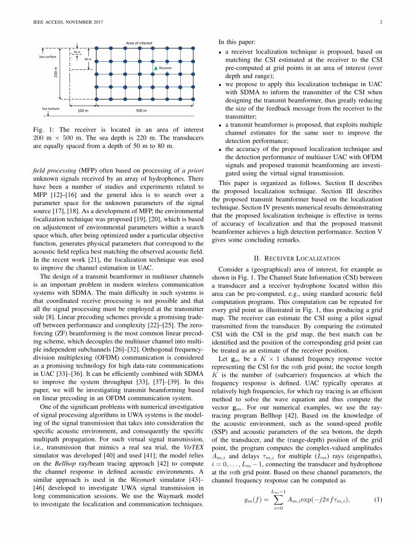
interest is shown in Fig. 1. The SSP and sea bottom parameters

are taken from [51] and shown in Fig. 2. Every receiver

is equipped with a single receive antenna. The signals are

transmitted at the carrier frequency 3072 Hz with a frequency

bandwidth of 1024 Hz, so that the frequency band is from


Fig. 2: The SSP and the layered sea bottom parameters.

2560 Hz to 3584 Hz. The pilot and data transmission are

performed using OFDM signals with K = 1024 subcarriers,

an orthogonality interval of 1 s, and subcarrier spacing of

1 Hz. The cyclic prefix (CP) of the OFDM symbols is 1 s

long to avoid the intersymbol interference due to long channel

delays (see Fig. 3). When searching over delays τ in (7),

the search interval [τmin, τmax] is set to OFDM orthogonality

interval [−0.5, 0.5] s. The pilot and data symbols used for

modulation of OFDM subcarriers are BPSK symbols.

In the experiments, a grid map, with 1 m or 0.5 m resolution,

is generated and stored in memory for every transducer. The

grid maps are pre-computed in Matlab (version R2013a) under

the Windows 7 operating system with a 3.4 GHz Intel Core i7

CPU and 8 GB of RAM. The 1 m resolution grid map with

201 × 501 ≈ 105 grid points is computed within 5 min, and

it requires a storage memory of 37 MB. The 0.5 m resolution

grid map with about 4 × 105 grid points is computed within

20 min, and it requires a storage memory of 148 MB. The

average computation time and storage memory for one grid

point is approximately 3 ms and 370 bytes, respectively.

A. Localization Experiments

To investigate the performance of the localization technique,

a pilot signal is transmitted from each of the four transmit

antennas sequentially in time. The pilot signal is a single

OFDM symbol with a predefined BPSK sequence modulating

the subcarriers. At the receiver, channel estimation is carried

out as described by (3). Using the channel estimates, the

best combined coherence of the channel frequency responses

estimated at the receiver and those computed at the grid points

is calculated using equation (7). The position of this best grid

point is treated as an estimate of the receiver position. The

grid map is computed with a resolution of either 1 m or 0.5 m

in both the depth and range.

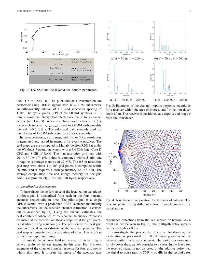
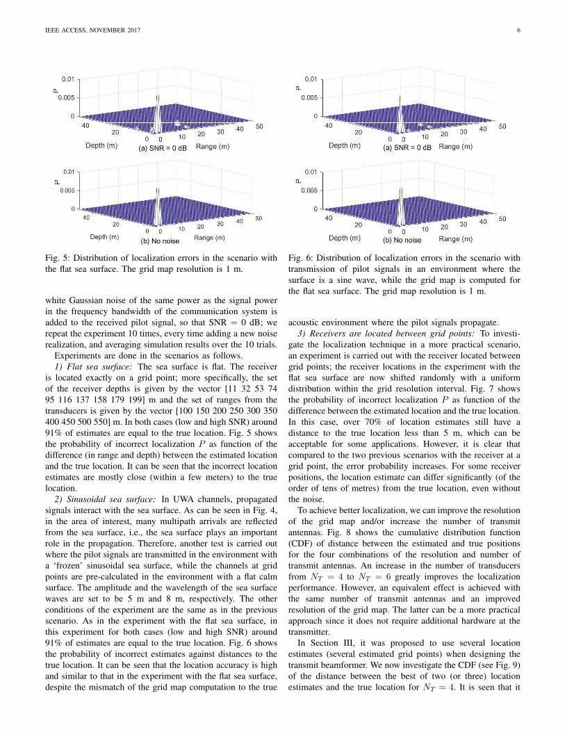
To illustrate the acoustic field in the area of interest, Fig. 4

shows results of the ray tracing in this area. Fig. 3 shows

examples of the channel impulse response for four grid points

within this area. It is seen that most of the acoustic rays

0 100 200 300 400 500 600

Delay (ms)

0

0.2

0.4

0.6

0.8

1

Magnitude

(a) d = 50 m, r = 200 m.

0 100 200 300 400 500 600

Delay (ms)

0

0.2

0.4

0.6

0.8

1

Magnitude

(b) d = 50 m, r = 500 m.

0 100 200 300 400 500 600

Delay (ms)

0

0.2

0.4

0.6

0.8

1

Magnitude

(c) d = 150 m, r = 200 m.

0 100 200 300 400 500 600

Delay (ms)

0

0.2

0.4

0.6

0.8

1

Magnitude

(d) d = 150 m, r = 500 m.

Fig. 3: Examples of the channel impulse response magnitude

for a receiver within the area of interest and for the transducer

depth 80 m. The receiver is positioned at a depth d and range rfrom the transducer.

Fig. 4: Ray tracing computation for the area of interest. The

rays are plotted using different colors to simply improve the

visualization.

experience reflections from the sea surface or bottom. As a

result (as can be seen in Fig. 3), the multipath delay spreads

can be as high as 0.5 s.

To investigate the probability of correct localization, the

localization is performed for 100 different positions of the

receiver within the area of interest. The tested positions uni-

formly cover the area. We consider two cases. In the first case,

the received signal is not distorted by the additive noise, i.e.,

the signal-to-noise ratio is SNR = ∞ dB. In the second case,


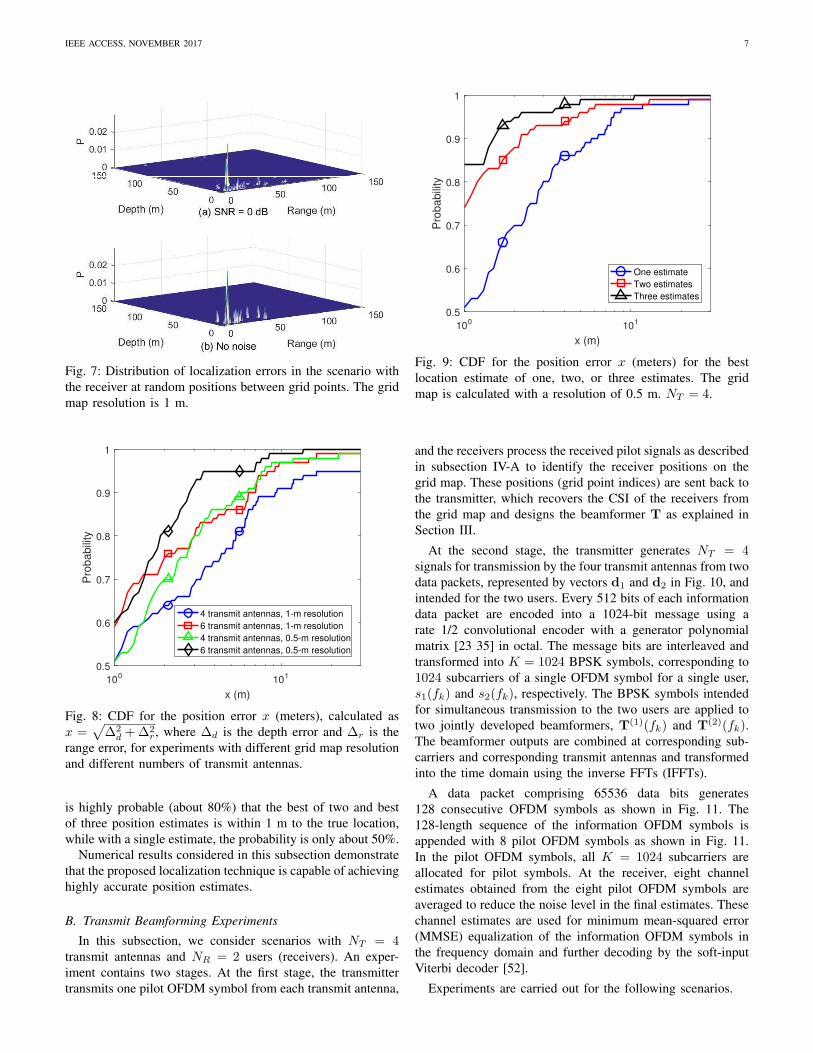
Fig. 5: Distribution of localization errors in the scenario with

the flat sea surface. The grid map resolution is 1 m.

white Gaussian noise of the same power as the signal power

in the frequency bandwidth of the communication system is

added to the received pilot signal, so that SNR = 0 dB; we

repeat the experiment 10 times, every time adding a new noise

realization, and averaging simulation results over the 10 trials.

Experiments are done in the scenarios as follows.

1) Flat sea surface: The sea surface is flat. The receiver

is located exactly on a grid point; more specifically, the set

of the receiver depths is given by the vector [11 32 53 74

95 116 137 158 179 199] m and the set of ranges from the

transducers is given by the vector [100 150 200 250 300 350

400 450 500 550] m. In both cases (low and high SNR) around

91% of estimates are equal to the true location. Fig. 5 shows

the probability of incorrect localization P as function of the

difference (in range and depth) between the estimated location

and the true location. It can be seen that the incorrect location

estimates are mostly close (within a few meters) to the true

location.

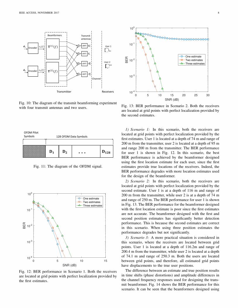
2) Sinusoidal sea surface: In UWA channels, propagated

signals interact with the sea surface. As can be seen in Fig. 4,

in the area of interest, many multipath arrivals are reflected

from the sea surface, i.e., the sea surface plays an important

role in the propagation. Therefore, another test is carried out

where the pilot signals are transmitted in the environment with

a ‘frozen’ sinusoidal sea surface, while the channels at grid

points are pre-calculated in the environment with a flat calm

surface. The amplitude and the wavelength of the sea surface

waves are set to be 5 m and 8 m, respectively. The other

conditions of the experiment are the same as in the previous

scenario. As in the experiment with the flat sea surface, in

this experiment for both cases (low and high SNR) around

91% of estimates are equal to the true location. Fig. 6 shows

the probability of incorrect estimates against distances to the

true location. It can be seen that the location accuracy is high

and similar to that in the experiment with the flat sea surface,

despite the mismatch of the grid map computation to the true


transmission of pilot signals in an environment where the

surface is a sine wave, while the grid map is computed for

the flat sea surface. The grid map resolution is 1 m.

acoustic environment where the pilot signals propagate.

3) Receivers are located between grid points: To investi-

gate the localization technique in a more practical scenario,

an experiment is carried out with the receiver located between

grid points; the receiver locations in the experiment with the

flat sea surface are now shifted randomly with a uniform

distribution within the grid resolution interval. Fig. 7 shows

the probability of incorrect localization P as function of the

difference between the estimated location and the true location.

In this case, over 70% of location estimates still have a

distance to the true location less than 5 m, which can be

acceptable for some applications. However, it is clear that

compared to the two previous scenarios with the receiver at a

grid point, the error probability increases. For some receiver

positions, the location estimate can differ significantly (of the

order of tens of metres) from the true location, even without

the noise.

To achieve better localization, we can improve the resolution

of the grid map and/or increase the number of transmit

antennas. Fig. 8 shows the cumulative distribution function

(CDF) of distance between the estimated and true positions

for the four combinations of the resolution and number of

transmit antennas. An increase in the number of transducers

from NT = 4 to NT = 6 greatly improves the localization

performance. However, an equivalent effect is achieved with

the same number of transmit antennas and an improved

resolution of the grid map. The latter can be a more practical

approach since it does not require additional hardware at the

transmitter.

In Section III, it was proposed to use several location

estimates (several estimated grid points) when designing the

transmit beamformer. We now investigate the CDF (see Fig. 9)

of the distance between the best of two (or three) location

estimates and the true location for NT = 4. It is seen that it



the receiver at random positions between grid points. The grid

map resolution is 1 m.

100 101

x (m)

0.5

0.6

0.7

0.8

0.9

1

Pro

babili

ty

4 transmit antennas, 1-m resolution

6 transmit antennas, 1-m resolution

4 transmit antennas, 0.5-m resolution

6 transmit antennas, 0.5-m resolution

Fig. 8: CDF for the position error x (meters), calculated as

x =√

∆2d +∆2

r , where ∆d is the depth error and ∆r is the

range error, for experiments with different grid map resolution

and different numbers of transmit antennas.

is highly probable (about 80%) that the best of two and best

of three position estimates is within 1 m to the true location,

while with a single estimate, the probability is only about 50%.

Numerical results considered in this subsection demonstrate

that the proposed localization technique is capable of achieving

highly accurate position estimates.

B. Transmit Beamforming Experiments

In this subsection, we consider scenarios with NT = 4transmit antennas and NR = 2 users (receivers). An exper-

iment contains two stages. At the first stage, the transmitter

transmits one pilot OFDM symbol from each transmit antenna,

100 101

x (m)

0.5

0.6

0.7

0.8

0.9

1

Pro

babili

ty

One estimate

Two estimates

Three estimates

Fig. 9: CDF for the position error x (meters) for the best

location estimate of one, two, or three estimates. The grid

map is calculated with a resolution of 0.5 m. NT = 4.

and the receivers process the received pilot signals as described

in subsection IV-A to identify the receiver positions on the

grid map. These positions (grid point indices) are sent back to

the transmitter, which recovers the CSI of the receivers from

the grid map and designs the beamformer T as explained in

Section III.

At the second stage, the transmitter generates NT = 4signals for transmission by the four transmit antennas from two

data packets, represented by vectors d1 and d2 in Fig. 10, and

intended for the two users. Every 512 bits of each information

data packet are encoded into a 1024-bit message using a

rate 1/2 convolutional encoder with a generator polynomial

matrix [23 35] in octal. The message bits are interleaved and

transformed into K = 1024 BPSK symbols, corresponding to

1024 subcarriers of a single OFDM symbol for a single user,

s1(fk) and s2(fk), respectively. The BPSK symbols intended

for simultaneous transmission to the two users are applied to

two jointly developed beamformers, T(1)(fk) and T(2)(fk).The beamformer outputs are combined at corresponding sub-

carriers and corresponding transmit antennas and transformed

into the time domain using the inverse FFTs (IFFTs).

A data packet comprising 65536 data bits generates

128 consecutive OFDM symbols as shown in Fig. 11. The

128-length sequence of the information OFDM symbols is

appended with 8 pilot OFDM symbols as shown in Fig. 11.

In the pilot OFDM symbols, all K = 1024 subcarriers are

allocated for pilot symbols. At the receiver, eight channel

estimates obtained from the eight pilot OFDM symbols are

averaged to reduce the noise level in the final estimates. These

channel estimates are used for minimum mean-squared error

(MMSE) equalization of the information OFDM symbols in

the frequency domain and further decoding by the soft-input

Viterbi decoder [52].

Experiments are carried out for the following scenarios.


𝐓 1 (𝑓)

𝐓(2)(𝑓)

𝐝1 User 1

User 2

Transmit

antennas

Beamformers

𝐝2

Transmitter Receivers

Encoder

Encoder

𝑠1(𝑓)

𝑠2(𝑓)

IFFT

IFFT

IFFT

IFFT

Channel

Fig. 10: The diagram of the transmit beamforming experiment

with four transmit antennas and two users.

OFDM Pilot

Symbols 128 OFDM Data Symbols

𝐃𝟏 𝐃𝟐 𝐃𝟏𝟐𝟖 . . .

Fig. 11: The diagram of the OFDM signal.

0 5 10 15

SNR (dB)

10-4

10-3

10-2

10-1

100

BE

R

One estimate

Two estimates

Three estimates

Fig. 12: BER performance in Scenario 1. Both the receivers

are located at grid points with perfect localization provided by

the first estimates.

0 5 10 15 20 25 30

SNR (dB)

10-4

10-3

10-2

10-1

100

BE

R One estimate

Two estimates

Three estimates

Fig. 13: BER performance in Scenario 2. Both the receivers

are located at grid points with perfect localization provided by

the second estimates.

1) Scenario 1: In this scenario, both the receivers are

located at grid points with perfect localization provided by the

first estimates. User 1 is located at a depth of 74 m and range of

200 m from the transmitter, user 2 is located at a depth of 95 m

and range 200 m from the transmitter. The BER performance

for user 1 is shown in Fig. 12. In this scenario, the best

BER performance is achieved by the beamformer designed

using the first location estimate for each user, since the first

estimates provide true locations of the receivers. Indeed, the

BER performance degrades with more location estimates used

for the design of the beamformer.

2) Scenario 2: In this scenario, both the receivers are

located at grid points with perfect localization provided by the

second estimate. User 1 is at a depth of 116 m and range of

200 m from the transmitter, while user 2 is at a depth of 74 m

and range of 250 m. The BER performance for user 1 is shown

in Fig. 13. The BER performance for the beamformer designed

with the first location estimate is poor since the first estimates

are not accurate. The beamformer designed with the first and

second position estimates has significantly better detection

performance. This is because the second estimates are correct

in this scenario. When using three position estimates the

performance degrades but not significantly.

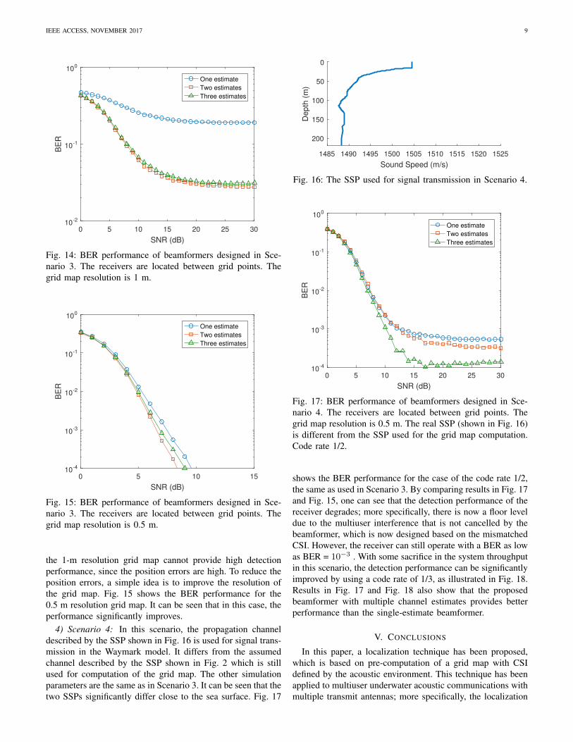
3) Scenario 3: A more practical situation is considered in

this scenario, where the receivers are located between grid

points. User 1 is located at a depth of 116.2m and range of

200.4 m from the transmitter, while user 2 is located at a depth

of 74.1 m and range of 250.3 m. Both the users are located

between grid points, and therefore, all estimated grid points

have displacements to the true user positions.

The difference between an estimate and true position results

in time shifts (phase distortions) and amplitude differences in

the channel frequency responses used for designing the trans-

mit beamformer. Fig. 14 shows the BER performance for this

scenario. It can be seen that the beamformers designed using


0 5 10 15 20 25 30

SNR (dB)

10-2

10-1

100

BE

R

One estimate

Two estimates

Three estimates

Fig. 14: BER performance of beamformers designed in Sce-

nario 3. The receivers are located between grid points. The

grid map resolution is 1 m.

0 5 10 15

SNR (dB)

10-4

10-3

10-2

10-1

100

BE

R

One estimate

Two estimates

Three estimates



grid map resolution is 0.5 m.

the 1-m resolution grid map cannot provide high detection

performance, since the position errors are high. To reduce the

position errors, a simple idea is to improve the resolution of

the grid map. Fig. 15 shows the BER performance for the

0.5 m resolution grid map. It can be seen that in this case, the

performance significantly improves.

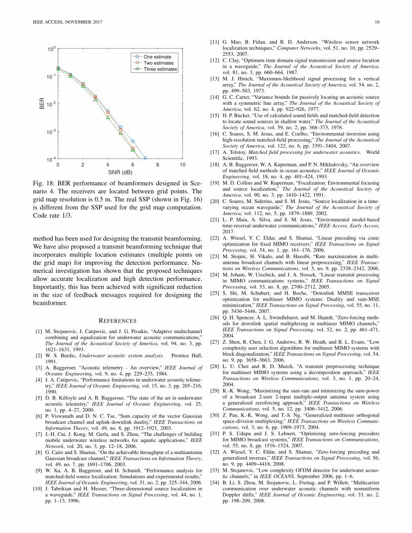
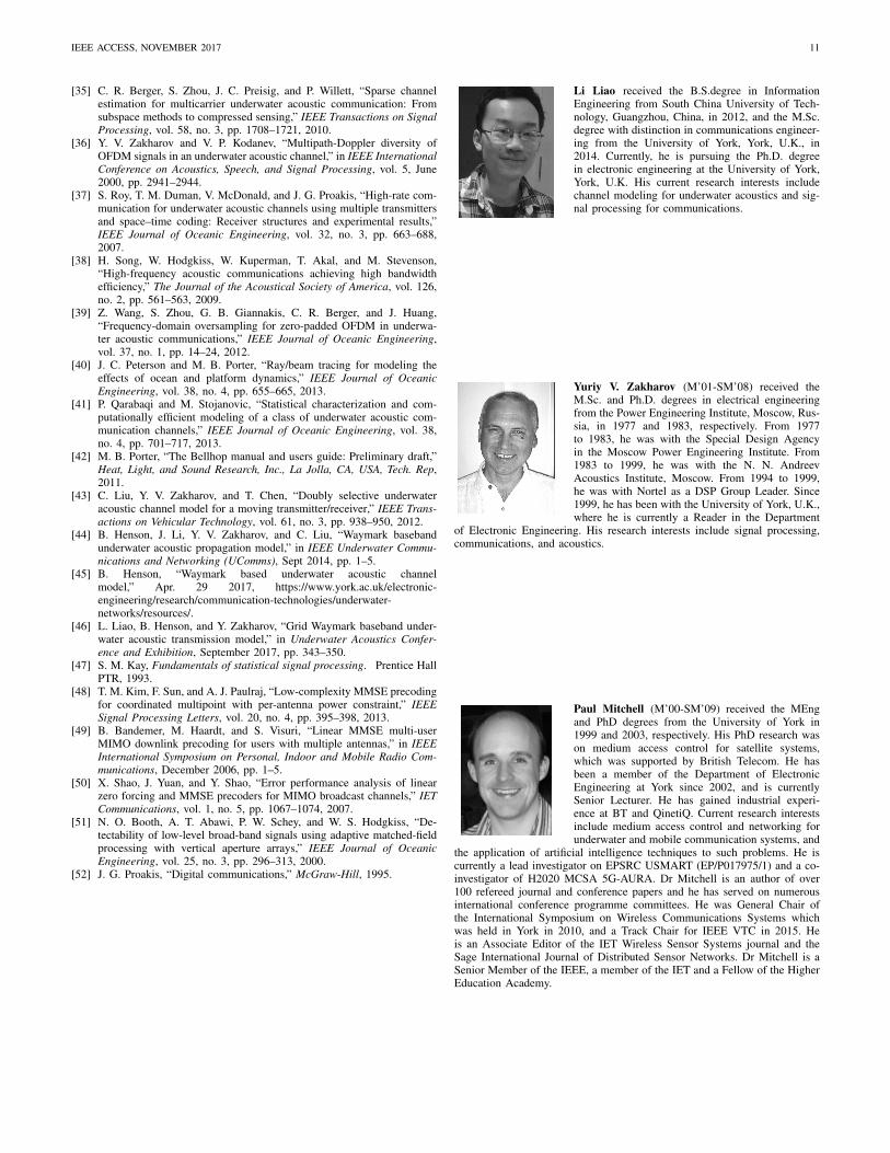
4) Scenario 4: In this scenario, the propagation channel

described by the SSP shown in Fig. 16 is used for signal trans-

mission in the Waymark model. It differs from the assumed

channel described by the SSP shown in Fig. 2 which is still

used for computation of the grid map. The other simulation

parameters are the same as in Scenario 3. It can be seen that the

two SSPs significantly differ close to the sea surface. Fig. 17

1485 1490 1495 1500 1505 1510 1515 1520 1525

Sound Speed (m/s)

0

50

100

150

200

Depth

(m

)

Fig. 16: The SSP used for signal transmission in Scenario 4.

0 5 10 15 20 25 30

SNR (dB)

10-4

10-3

10-2

10-1

100

BE

R

One estimate

Two estimates

Three estimates



grid map resolution is 0.5 m. The real SSP (shown in Fig. 16)

is different from the SSP used for the grid map computation.

Code rate 1/2.

shows the BER performance for the case of the code rate 1/2,

the same as used in Scenario 3. By comparing results in Fig. 17

and Fig. 15, one can see that the detection performance of the

receiver degrades; more specifically, there is now a floor level

due to the multiuser interference that is not cancelled by the

beamformer, which is now designed based on the mismatched

CSI. However, the receiver can still operate with a BER as low

as BER = 10−3 . With some sacrifice in the system throughput

in this scenario, the detection performance can be significantly

improved by using a code rate of 1/3, as illustrated in Fig. 18.

Results in Fig. 17 and Fig. 18 also show that the proposed

beamformer with multiple channel estimates provides better

performance than the single-estimate beamformer.

V. CONCLUSIONS

In this paper, a localization technique has been proposed,

which is based on pre-computation of a grid map with CSI

defined by the acoustic environment. This technique has been

applied to multiuser underwater acoustic communications with

multiple transmit antennas; more specifically, the localization


0 2 4 6 8 10

SNR (dB)

10-4

10-3

10-2

10-1

100

BE

R

One estimate

Two estimates

Three estimates



grid map resolution is 0.5 m. The real SSP (shown in Fig. 16)

is different from the SSP used for the grid map computation.

Code rate 1/3.

method has been used for designing the transmit beamforming.

We have also proposed a transmit beamforming technique that

incorporates multiple location estimates (multiple points on

the grid map) for improving the detection performance. Nu-

merical investigation has shown that the proposed techniques

allow accurate localization and high detection performance.

Importantly, this has been achieved with significant reduction

in the size of feedback messages required for designing the

beamformer.

REFERENCES

[1] M. Stojanovic, J. Catipovic, and J. G. Proakis, “Adaptive multichannelcombining and equalization for underwater acoustic communications,”The Journal of the Acoustical Society of America, vol. 94, no. 3, pp.1621–1631, 1993.

[2] W. S. Burdic, Underwater acoustic system analysis. Prentice Hall,1991.

[3] A. Baggeroer, “Acoustic telemetry - An overview,” IEEE Journal of

Oceanic Engineering, vol. 9, no. 4, pp. 229–235, 1984.[4] J. A. Catipovic, “Performance limitations in underwater acoustic teleme-

try,” IEEE Journal of Oceanic Engineering, vol. 15, no. 3, pp. 205–216,1990.

[5] D. B. Kilfoyle and A. B. Baggeroer, “The state of the art in underwateracoustic telemetry,” IEEE Journal of Oceanic Engineering, vol. 25,no. 1, pp. 4–27, 2000.

[6] P. Viswanath and D. N. C. Tse, “Sum capacity of the vector Gaussianbroadcast channel and uplink-downlink duality,” IEEE Transactions on

Information Theory, vol. 49, no. 8, pp. 1912–1921, 2003.[7] J.-H. Cui, J. Kong, M. Gerla, and S. Zhou, “The challenges of building

mobile underwater wireless networks for aquatic applications,” IEEE

Network, vol. 20, no. 3, pp. 12–18, 2006.[8] G. Caire and S. Shamai, “On the achievable throughput of a multiantenna

Gaussian broadcast channel,” IEEE Transactions on Information Theory,vol. 49, no. 7, pp. 1691–1706, 2003.

[9] W. Xu, A. B. Baggeroer, and H. Schmidt, “Performance analysis formatched-field source localization: Simulations and experimental results,”IEEE Journal of Oceanic Engineering, vol. 31, no. 2, pp. 325–344, 2006.

[10] J. Tabrikian and H. Messer, “Three-dimensional source localization ina waveguide,” IEEE Transactions on Signal Processing, vol. 44, no. 1,pp. 1–13, 1996.

[11] G. Mao, B. Fidan, and B. D. Anderson, “Wireless sensor networklocalization techniques,” Computer Networks, vol. 51, no. 10, pp. 2529–2553, 2007.

[12] C. Clay, “Optimum time domain signal transmission and source locationin a waveguide,” The Journal of the Acoustical Society of America,vol. 81, no. 3, pp. 660–664, 1987.

[13] M. J. Hinich, “Maximum-likelihood signal processing for a verticalarray,” The Journal of the Acoustical Society of America, vol. 54, no. 2,pp. 499–503, 1973.

[14] G. C. Carter, “Variance bounds for passively locating an acoustic sourcewith a symmetric line array,” The Journal of the Acoustical Society of

America, vol. 62, no. 4, pp. 922–926, 1977.

[15] H. P. Bucker, “Use of calculated sound fields and matched-field detectionto locate sound sources in shallow water,” The Journal of the Acoustical

Society of America, vol. 59, no. 2, pp. 368–373, 1976.

[16] C. Soares, S. M. Jesus, and E. Coelho, “Environmental inversion usinghigh-resolution matched-field processing,” The Journal of the Acoustical

Society of America, vol. 122, no. 6, pp. 3391–3404, 2007.

[17] A. Tolstoy, Matched field processing for underwater acoustics. WorldScientific, 1993.

[18] A. B. Baggeroer, W. A. Kuperman, and P. N. Mikhalevsky, “An overviewof matched field methods in ocean acoustics,” IEEE Journal of Oceanic

Engineering, vol. 18, no. 4, pp. 401–424, 1993.

[19] M. D. Collins and W. Kuperman, “Focalization: Environmental focusingand source localization,” The Journal of the Acoustical Society of

America, vol. 90, no. 3, pp. 1410–1422, 1991.

[20] C. Soares, M. Siderius, and S. M. Jesus, “Source localization in a time-varying ocean waveguide,” The Journal of the Acoustical Society of

America, vol. 112, no. 5, pp. 1879–1889, 2002.

[21] L. P. Maia, A. Silva, and S. M. Jesus, “Environmental model-basedtime-reversal underwater communications,” IEEE Access, Early Access,2017.

[22] A. Wiesel, Y. C. Eldar, and S. Shamai, “Linear precoding via conicoptimization for fixed MIMO receivers,” IEEE Transactions on Signal

Processing, vol. 54, no. 1, pp. 161–176, 2006.

[23] M. Stojnic, H. Vikalo, and B. Hassibi, “Rate maximization in multi-antenna broadcast channels with linear preprocessing,” IEEE Transac-

tions on Wireless Communications, vol. 5, no. 9, pp. 2338–2342, 2006.

[24] M. Joham, W. Utschick, and J. A. Nossek, “Linear transmit processingin MIMO communications systems,” IEEE Transactions on Signal

Processing, vol. 53, no. 8, pp. 2700–2712, 2005.

[25] S. Shi, M. Schubert, and H. Boche, “Downlink MMSE transceiveroptimization for multiuser MIMO systems: Duality and sum-MSEminimization,” IEEE Transactions on Signal Processing, vol. 55, no. 11,pp. 5436–5446, 2007.

[26] Q. H. Spencer, A. L. Swindlehurst, and M. Haardt, “Zero-forcing meth-ods for downlink spatial multiplexing in multiuser MIMO channels,”IEEE Transactions on Signal Processing, vol. 52, no. 2, pp. 461–471,2004.

[27] Z. Shen, R. Chen, J. G. Andrews, R. W. Heath, and B. L. Evans, “Lowcomplexity user selection algorithms for multiuser MIMO systems withblock diagonalization,” IEEE Transactions on Signal Processing, vol. 54,no. 9, pp. 3658–3663, 2006.

[28] L. U. Choi and R. D. Murch, “A transmit preprocessing techniquefor multiuser MIMO systems using a decomposition approach,” IEEE

Transactions on Wireless Communications, vol. 3, no. 1, pp. 20–24,2004.

[29] K.-K. Wong, “Maximizing the sum-rate and minimizing the sum-powerof a broadcast 2-user 2-input multiple-output antenna system usinga generalized zeroforcing approach,” IEEE Transactions on Wireless

Communications, vol. 5, no. 12, pp. 3406–3412, 2006.

[30] Z. Pan, K.-K. Wong, and T.-S. Ng, “Generalized multiuser orthogonalspace-division multiplexing,” IEEE Transactions on Wireless Communi-

cations, vol. 3, no. 6, pp. 1969–1973, 2004.

[31] P. S. Udupa and J. S. Lehnert, “Optimizing zero-forcing precodersfor MIMO broadcast systems,” IEEE Transactions on Communications,vol. 55, no. 8, pp. 1516–1524, 2007.

[32] A. Wiesel, Y. C. Eldar, and S. Shamai, “Zero-forcing precoding andgeneralized inverses,” IEEE Transactions on Signal Processing, vol. 56,no. 9, pp. 4409–4418, 2008.

[33] M. Stojanovic, “Low complexity OFDM detector for underwater acous-tic channels,” in IEEE OCEANS, September 2006, pp. 1–6.

[34] B. Li, S. Zhou, M. Stojanovic, L. Freitag, and P. Willett, “Multicarriercommunication over underwater acoustic channels with nonuniformDoppler shifts,” IEEE Journal of Oceanic Engineering, vol. 33, no. 2,pp. 198–209, 2008.


[35] C. R. Berger, S. Zhou, J. C. Preisig, and P. Willett, “Sparse channelestimation for multicarrier underwater acoustic communication: Fromsubspace methods to compressed sensing,” IEEE Transactions on Signal

Processing, vol. 58, no. 3, pp. 1708–1721, 2010.[36] Y. V. Zakharov and V. P. Kodanev, “Multipath-Doppler diversity of

OFDM signals in an underwater acoustic channel,” in IEEE International

Conference on Acoustics, Speech, and Signal Processing, vol. 5, June2000, pp. 2941–2944.

[37] S. Roy, T. M. Duman, V. McDonald, and J. G. Proakis, “High-rate com-munication for underwater acoustic channels using multiple transmittersand space–time coding: Receiver structures and experimental results,”IEEE Journal of Oceanic Engineering, vol. 32, no. 3, pp. 663–688,2007.

[38] H. Song, W. Hodgkiss, W. Kuperman, T. Akal, and M. Stevenson,“High-frequency acoustic communications achieving high bandwidthefficiency,” The Journal of the Acoustical Society of America, vol. 126,no. 2, pp. 561–563, 2009.

[39] Z. Wang, S. Zhou, G. B. Giannakis, C. R. Berger, and J. Huang,“Frequency-domain oversampling for zero-padded OFDM in underwa-ter acoustic communications,” IEEE Journal of Oceanic Engineering,vol. 37, no. 1, pp. 14–24, 2012.

[40] J. C. Peterson and M. B. Porter, “Ray/beam tracing for modeling theeffects of ocean and platform dynamics,” IEEE Journal of Oceanic

Engineering, vol. 38, no. 4, pp. 655–665, 2013.[41] P. Qarabaqi and M. Stojanovic, “Statistical characterization and com-

putationally efficient modeling of a class of underwater acoustic com-munication channels,” IEEE Journal of Oceanic Engineering, vol. 38,no. 4, pp. 701–717, 2013.

[42] M. B. Porter, “The Bellhop manual and users guide: Preliminary draft,”Heat, Light, and Sound Research, Inc., La Jolla, CA, USA, Tech. Rep,2011.

[43] C. Liu, Y. V. Zakharov, and T. Chen, “Doubly selective underwateracoustic channel model for a moving transmitter/receiver,” IEEE Trans-

actions on Vehicular Technology, vol. 61, no. 3, pp. 938–950, 2012.[44] B. Henson, J. Li, Y. V. Zakharov, and C. Liu, “Waymark baseband

underwater acoustic propagation model,” in IEEE Underwater Commu-

nications and Networking (UComms), Sept 2014, pp. 1–5.[45] B. Henson, “Waymark based underwater acoustic channel

model,” Apr. 29 2017, https://www.york.ac.uk/electronic-engineering/research/communication-technologies/underwater-networks/resources/.

[46] L. Liao, B. Henson, and Y. Zakharov, “Grid Waymark baseband under-water acoustic transmission model,” in Underwater Acoustics Confer-

ence and Exhibition, September 2017, pp. 343–350.[47] S. M. Kay, Fundamentals of statistical signal processing. Prentice Hall

PTR, 1993.[48] T. M. Kim, F. Sun, and A. J. Paulraj, “Low-complexity MMSE precoding

for coordinated multipoint with per-antenna power constraint,” IEEE

Signal Processing Letters, vol. 20, no. 4, pp. 395–398, 2013.[49] B. Bandemer, M. Haardt, and S. Visuri, “Linear MMSE multi-user

MIMO downlink precoding for users with multiple antennas,” in IEEE

International Symposium on Personal, Indoor and Mobile Radio Com-

munications, December 2006, pp. 1–5.[50] X. Shao, J. Yuan, and Y. Shao, “Error performance analysis of linear

zero forcing and MMSE precoders for MIMO broadcast channels,” IET

Communications, vol. 1, no. 5, pp. 1067–1074, 2007.[51] N. O. Booth, A. T. Abawi, P. W. Schey, and W. S. Hodgkiss, “De-

tectability of low-level broad-band signals using adaptive matched-fieldprocessing with vertical aperture arrays,” IEEE Journal of Oceanic

Engineering, vol. 25, no. 3, pp. 296–313, 2000.[52] J. G. Proakis, “Digital communications,” McGraw-Hill, 1995.

Li Liao received the B.S.degree in InformationEngineering from South China University of Tech-nology, Guangzhou, China, in 2012, and the M.Sc.degree with distinction in communications engineer-ing from the University of York, York, U.K., in2014. Currently, he is pursuing the Ph.D. degreein electronic engineering at the University of York,York, U.K. His current research interests includechannel modeling for underwater acoustics and sig-nal processing for communications.

Yuriy V. Zakharov (M’01-SM’08) received theM.Sc. and Ph.D. degrees in electrical engineeringfrom the Power Engineering Institute, Moscow, Rus-sia, in 1977 and 1983, respectively. From 1977to 1983, he was with the Special Design Agencyin the Moscow Power Engineering Institute. From1983 to 1999, he was with the N. N. AndreevAcoustics Institute, Moscow. From 1994 to 1999,he was with Nortel as a DSP Group Leader. Since1999, he has been with the University of York, U.K.,where he is currently a Reader in the Department

of Electronic Engineering. His research interests include signal processing,communications, and acoustics.

Paul Mitchell (M’00-SM’09) received the MEngand PhD degrees from the University of York in1999 and 2003, respectively. His PhD research wason medium access control for satellite systems,which was supported by British Telecom. He hasbeen a member of the Department of ElectronicEngineering at York since 2002, and is currentlySenior Lecturer. He has gained industrial experi-ence at BT and QinetiQ. Current research interestsinclude medium access control and networking forunderwater and mobile communication systems, and

the application of artificial intelligence techniques to such problems. He iscurrently a lead investigator on EPSRC USMART (EP/P017975/1) and a co-investigator of H2020 MCSA 5G-AURA. Dr Mitchell is an author of over100 refereed journal and conference papers and he has served on numerousinternational conference programme committees. He was General Chair ofthe International Symposium on Wireless Communications Systems whichwas held in York in 2010, and a Track Chair for IEEE VTC in 2015. Heis an Associate Editor of the IET Wireless Sensor Systems journal and theSage International Journal of Distributed Sensor Networks. Dr Mitchell is aSenior Member of the IEEE, a member of the IET and a Fellow of the HigherEducation Academy.

Documents

Underwater localization based on grid computation and its