Embed Size (px)
Citation preview
Autonomous, Localization-Free UnderwaterData Muling using Acoustic and OpticalCommunication
Marek Doniec, Iulian Topor, Mandar Chitre, Daniela Rus
Abstract We present a fully autonomous data muling system consisting of hardwareand algorithms. The system allows a robot to autonomously find a sensor node anduse high bandwidth, short range optical communication to download 1.2 MB of datafrom the sensor node and then transport the data back to a base station. The hardwareof the system consists of an autonomous underwater vehicle (AUV) paired with anunderwater sensor node. The robot and the sensor node use two modes of communi-cation - acousic for long range communication and and optical for high bandwidthcommunication. No positioning system is required. Acoustic ranging is used be-tween the sensor node and the AUV. The AUV uses the ranging information to findthe sensor node by means of either stochastic gradient descent, or a particle filter.Once it comes close enough to the sensor node where it can use the optical channelit switches to position keeping by means of stochastic gradient descent on the signalquality of the optical link. During this time the optical link is used to download data.Fountain codes are used for data transfer to maximize throughput while minimiz-ing protocol requirements. The system is evaluated in three separate experimentsusing our Autonomous Modular Optical Underwater Robot (AMOUR), a PANDAsensor node, the UNET acoustic modem, and the AquaOptical modem. In the firstexperiment AMOUR uses acoustic gradient descent to find the PANDA node start-ing from a distance of at least 25m and then switches to optical position keepingduring which it downloads a 1.2 MB large file. This experiment is completed 10times successfully. In the second experiment AMOUR is manually steered abovethe PANDA node and then autonomously maintains position using the quality of theoptical link as a measurement. This experiment is performed two times for 10 min-utes. The final experiment does not make use of the optical modems and evaluatethe performance of the particle filter in finding the PANDA node. This experimentis performed 5 times successfully.
Marek Doniec, Daniela RusComputer Science and Artificial Intelligence LaboratoryMassachusetts Institute of Technology - Cambridge, MassachusettsIulian Topor, Mandar ChitreARL, Tropical Marine Science InstituteNational University of Singapore - Singaporee-mail: [email protected], [email protected], [email protected], [email protected]
1
2 Marek Doniec, Iulian Topor, Mandar Chitre, Daniela Rus
1 Introduction
Our goal is to develop technologies that enable users to interact with ocean obser-vatories. In an ocean observatory robots and and in-situ sensors collect informa-tion about the underwater environment and deliver this information to remote users,much like a web-cam delivers remote data to users on the ground. In this paper wefocus on developing effective technologies for wireless data transmission underwa-ter. When the amount of data from an ocean observatory is large (for example inthe case of image feeds), low-bandwidth acoustic communication is not adequate.We instead propose using optical data muling with a robot equipped with an opticalmodem that can retrieve data fast from underwater nodes with line-of-site connec-tion to the robot. An important problem is locating the underwater sensor node.When distances between the robot and the nodes are large, and their locations areunknown, positioning the data muling robot within optical communication range ischallenging. In this paper we present a solution to autonomous data muling under-water, where the node’s location is unknown. The algorithm has three phases. In thefirst phase, acoustic communication is used to bring the data muling robot withinsome close range of the desired sensor where it can detect the optical signal. Inthe second phase, the robot does a local search using the optical signal strength toprecisely locate the sensor and position itself within communication range. In thethird phase the robot uses optical communication to collect the data from the sensor.In practice, phase two and three overlap once the signal strength becomes strongenough to transmit data.
Previous work has looked at the theoretical performance of data muling [10] andthe optimization of the path taken between nodes [7]. In both cases the locationsof the nodes are assumed known. Data muling with an underwater robot has beenpreviously shown in [5]. The nodes were found using a spiral search that looked fora valid optical signal. A method for homing to a single beacon using acoustic rangemeasurements based on an Extended Kalman Filter with a fixed robot maneouverfor initialization is presented and evaluated in simulation in [13]. In [9] the authorspresent an Extended Kalman Filter approach to localizing a moving vehicle usingrange-only measurements to a group of beacons. They use particle filters to initializethe beacons location. In [1] a high-frequency acoustic network is suggested, thatoffers range and bandwidth performance between conventional acoustic and opticalrates.
We implemented and experimentally evaluated the data muling system describedin this paper. This work uses a new version of the Pop-up Ambient Noise DataAcquisition sensor node called UNET-PANDA, which is presented, along with theacoustic modem used, in [2]. For simplicity UNET-PANDA is referred to as PANDAin the remainder of the paper. The optical modem has been described in [3]. TheAutonomous Modular Optical Underwater Robot (AMOUR) was presented in [4].Our implementation of the data muling system was repeatably able to acousticallylocate the sensor node from distances of 25m and 100m and to download a 1.2 MBdata file optically once the node was found.
Autonomous, Loc.-Free Underwater Data Muling using Acoustic & Optical Comms 3
2 Problem Statement
We consider a sensor node that is deployed at a fixed location on the seafloor. Weassume that the sensor node is equipped with an acoustic modem and an opticalmodem. We use the acoustic modem for low data rate (≤ 1 Kbps) and long range (≥100 m) communications. We use the optical modem for high data rate (≥ 1 Mbps)and short range (≤ 100 m) communications. We do not require a precise externalpositioning system but we assume that a coarse location estimate of the node exists.By coarse we mean that the margin of error for this position estimate is within theacoustic communication range. This is usually on the order of hundreds of metersto a few kilometers, though acoustic communication ranges of over 100 km arepossible [11]. Examples in which such a situation can arise are (1) when a node isdeployed in deep waters from a boat and drifts before it finally reaches the oceanfloor; (2) when a node is deployed by an autonomous underwater vehicle usingdead reckoning the placement can have a large error; (3) when a node is not rigidlymoored and its position changes with time because of water currents.
Further, we assume that an autonomous hovering underwater vehicle (AUV) isequipped with identical acoustic and optical modems and capable of communicatingthrough these with the sensor node when in range. Hovering enables the vehicleto hold its attitude and depth statically and to execute surge (forward / backward)velocity commands.
Our problem statement concerns the case in which the sensor node is collectingdata at rates in excess of what can be transmitted using the long distance acousticchannel. Kilfoyle et al. show empirically that the product of acoustic communi-cation rate and bandwidth rarely exceeds 40 km-Kbps for state of the art acousticmodems [6]. For a single sensor separated by 5 km from the user this would result ina communication rate of 8 Kbps. If we consider an application that collects ambientacoustic signals or even video our data stream will far exceed the available acousticchannel capacity.
3 Technical Approach
Algorithm 1 Acoustic Stochastic Gra-dient Descent1: YAWrobot ⇐ π ∗Random(−1.0...1.0)2: SPEEDrobot ⇐ 0.25 Knots forward3: RANGEth⇐ inf4: while No optical link available do5: Receive RANGEm6: if RANGEm > RANGEth +1m then7: YAWrobot ⇐ YAWrobot + π + π ∗
Random(−0.5...0.5)8: RANGEth⇐ RANGEm9: end if
10: if RANGEm < RANGEth then11: RANGEth⇐ RANGEm12: end if13: end while14: Begin Optical Gradient Descent
Algorithm 2 Optical Stochastic Gradi-ent Descent1: Retain YAWrobot from Algorithm I.2: Retain SPEEDrobot from Algorithm I.3: SSIth⇐ 04: while Optical Link Established do5: Wait 0.25 Seconds. Measure SSIm6: if SSIm 6 0.9∗SSIth then7: YAWrobot ⇐ YAWrobot + π + π ∗
Random(−0.5...0.5)8: SSIth⇐ SSIm9: end if
10: if SSIm > SSIth then11: SSIth⇐ SSIm12: end if13: end while14: Switch back to Acoustic Gradient Descent
4 Marek Doniec, Iulian Topor, Mandar Chitre, Daniela Rus
We developed a combined acousto-optical communication network capable oflarge scale data recovery that does not require precise localization of the robot northe sensor node. The robot uses acoustic communication and ranging to come closeto the sensor node. High bandwidth optical channel allows the robot to downloadthe payload data. More specifically, our approach to data muling is as follows:
1. We use acoustic ranging between the robot and the PANDA sensor node. Theacoustic modems use a carrier frequency of 27 kHz, transmitting at a bandwidthof 18 kHz with a power level of 180 dB measured at 1m. We use OrthogonalFrequency Division Multiplexing together with a 12/23 Golay code and 1/3 rateconvolution code. The acoustic modem on the PANDA transmitts a 18 byte longranging beacon every 6 seconds that is received by the acoustic modem on therobot and provides it with a range measurement. The robot uses the stochasticgradient descent algorithm shown in Algorithm 1 to travel close to the PANDA.
2. At all times the PANDA is streaming the payload data using the optical mo-dem and random linear rateless erasure codes known as Luby transform (LT)codes [8]. Each optical packet transmitted contained 576 bytes payload data plus32 bytes of configuration data (i.e. source and destination address, packet size,32 bit CRC checksum, degree and seed used for the LT-Codes). The test file is arandom data file consisting of 2048 blocks of 576 bytes. The LT-Codes requireon average an overhead of 3%, so about 2109 packets have to be received by therobot to decode the entire file. Because of the nature of the LT-Codes it does notmatter which packets are received.
3. Once the robot is close enough to the sensor node to receive an error-free packet itswitches from acoustic gradient descent to maintaining position using the opticalgradient descent algorithm described in Algorithm 2. If the optical connectionbreaks at any point in time we return to step 1.
4. While AMOUR is in optical communication range every packet is used to (a)measure the signal strength and (b) decode the payload data if the CRC matches.
5. The experiment is considered to have completed successfully once the entire 1.2MB file has been received and decoded by the robot. In a real world scenario therobot would now continue on the approximate location of the next sensor nodeto begin acoustic gradient descent there.
4 Performance Improvement with a Particle Filter
The stochastic gradient descent approach described in Section 3 has no memoryof previous decisions. The only state variables are the current heading and a rangethreshold used to make the decision whether to keep going straight or to turn. Whenthe algorithm encounters an increasing range it changes the direction of the robotin a random direction at least 90 degrees different from the current direction oftravel. This new choice of direction takes into account only the most recent fewmeasurements as reflected in the threshold stored. Because so little information is
Autonomous, Loc.-Free Underwater Data Muling using Acoustic & Optical Comms 5
taken into account, bad choices are made frequently. Further, even when the robotis moving in the right direction a single spurious measurement caused by noise canmake it veer of the correct course. The algorithm will recover from this mistake withhigh probability as the ranges will keep increasing from here on, but this comes atthe cost of time and energy. It also causes a large variance in the time that it takes tofind the target sensor node.
A more effective algorithm should keep a belief of where the robot is relativeto the sensor node and update this belief with every measurement. An ExtendedKalman Filter (EKF) delivers such a behavior. It represents the current belief of therobot’s location as a mean and covariance. Because of this it needs to be initialized,for example by performing a circular maneuver such as in [13]. Further, becausewe are representing the robot’s state with a multidimensional Gaussian, we cannotrepresent multimodal distributions, for example when we have a baseline ambiguitybecause our vehicle has been traveling straight.
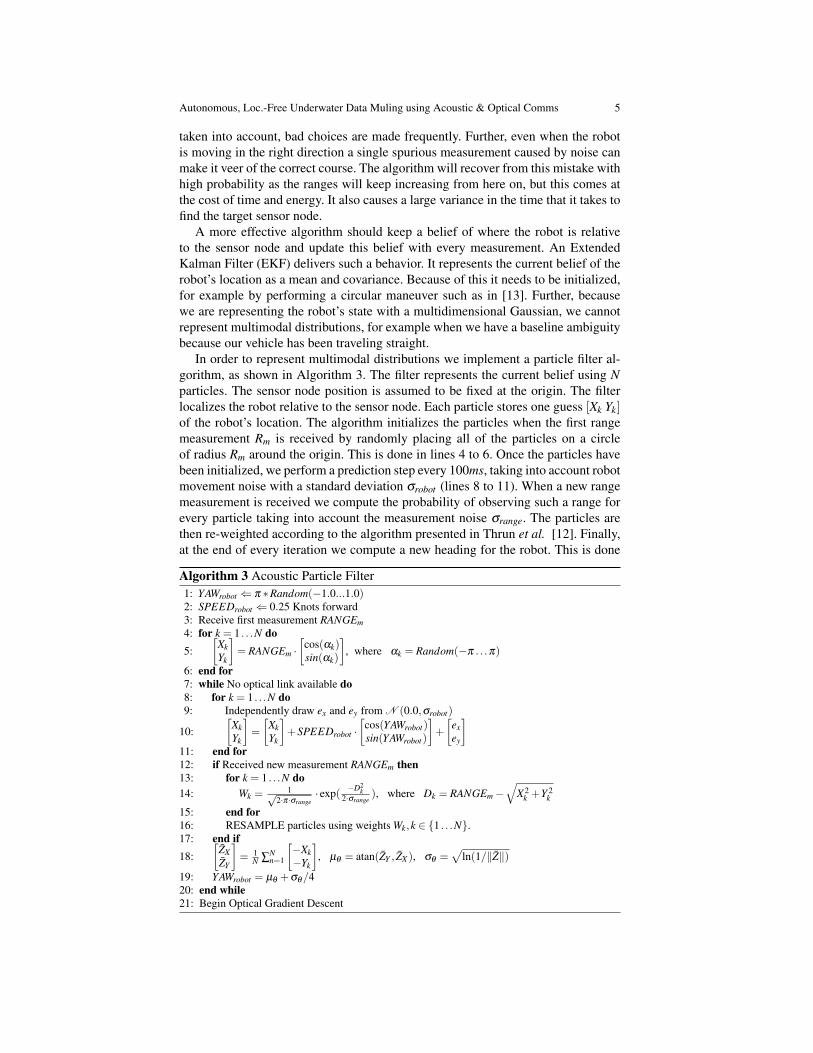
In order to represent multimodal distributions we implement a particle filter al-gorithm, as shown in Algorithm 3. The filter represents the current belief using Nparticles. The sensor node position is assumed to be fixed at the origin. The filterlocalizes the robot relative to the sensor node. Each particle stores one guess [Xk Yk]of the robot’s location. The algorithm initializes the particles when the first rangemeasurement Rm is received by randomly placing all of the particles on a circleof radius Rm around the origin. This is done in lines 4 to 6. Once the particles havebeen initialized, we perform a prediction step every 100ms, taking into account robotmovement noise with a standard deviation σrobot (lines 8 to 11). When a new rangemeasurement is received we compute the probability of observing such a range forevery particle taking into account the measurement noise σrange. The particles arethen re-weighted according to the algorithm presented in Thrun et al. [12]. Finally,at the end of every iteration we compute a new heading for the robot. This is done
Algorithm 3 Acoustic Particle Filter1: YAWrobot ⇐ π ∗Random(−1.0...1.0)2: SPEEDrobot ⇐ 0.25 Knots forward3: Receive first measurement RANGEm4: for k = 1 . . .N do5:
[XkYk
]= RANGEm ·
[cos(αk)sin(αk)
], where αk = Random(−π . . .π)
6: end for7: while No optical link available do8: for k = 1 . . .N do9: Independently draw ex and ey from N (0.0,σrobot)
10:[
XkYk
]=
[XkYk
]+SPEEDrobot ·
[cos(YAWrobot)sin(YAWrobot)
]+
[exey
]11: end for12: if Received new measurement RANGEm then13: for k = 1 . . .N do14: Wk =
1√2·π·σrange
· exp( −D2k
2·σrange), where Dk = RANGEm−
√X2
k +Y 2k
15: end for16: RESAMPLE particles using weights Wk,k ∈ {1 . . .N}.17: end if18:
[Z̄XZ̄Y
]= 1
N ∑Nn=1
[−Xk−Yk
], µθ = atan(Z̄Y , Z̄X ), σθ =
√ln(1/‖Z̄‖)
19: YAWrobot = µθ +σθ/420: end while21: Begin Optical Gradient Descent
6 Marek Doniec, Iulian Topor, Mandar Chitre, Daniela Rus
by computing the heading required for every particle to travel towards the node.We assume these headings form a wrapped normal distribution and we compute themean and standard deviation in line 18. Setting the robot heading to the mean wouldresult in the particles traveling directly towards the node and can create a baselineambiguity. Thus, we chose to set the new headings as the mean plus the standard de-viation divided by a factor of 4. The more uncertain the particle filter is, the more therobot will deviate from the straight path, and this in turn helps resolve the baselineambiguity.
5 Theoretical Performance
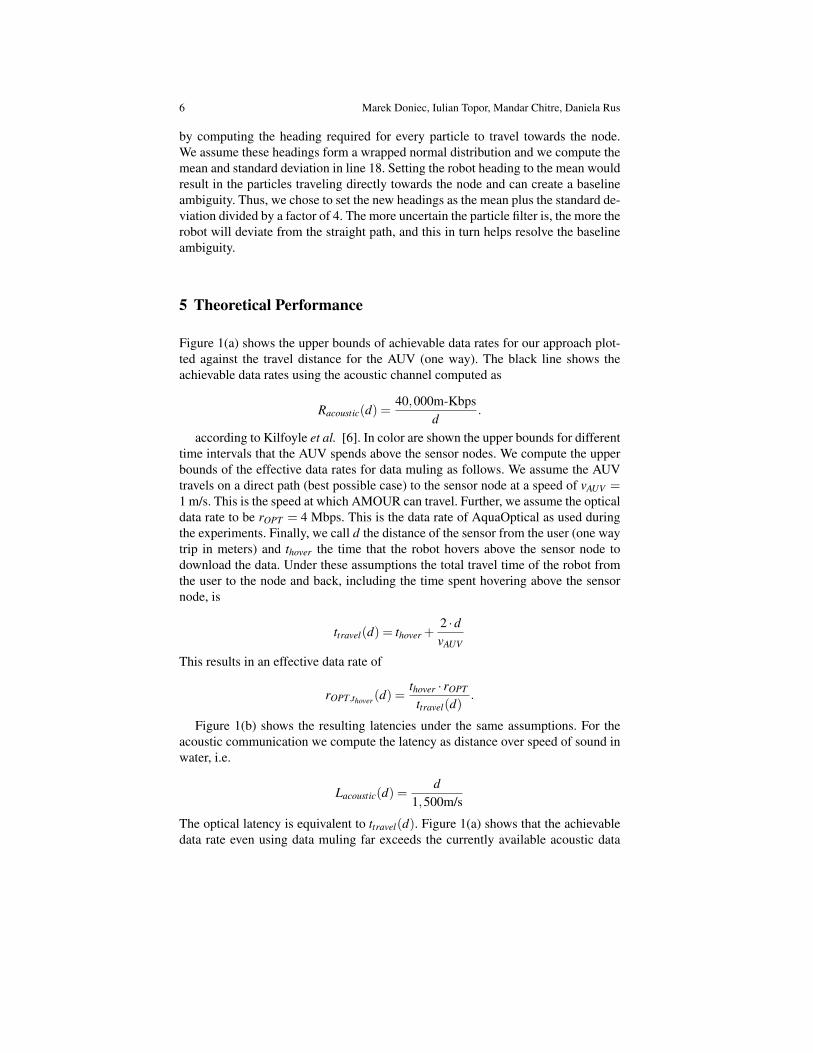
Figure 1(a) shows the upper bounds of achievable data rates for our approach plot-ted against the travel distance for the AUV (one way). The black line shows theachievable data rates using the acoustic channel computed as
Racoustic(d) =40,000m-Kbps
d.
according to Kilfoyle et al. [6]. In color are shown the upper bounds for differenttime intervals that the AUV spends above the sensor nodes. We compute the upperbounds of the effective data rates for data muling as follows. We assume the AUVtravels on a direct path (best possible case) to the sensor node at a speed of vAUV =1 m/s. This is the speed at which AMOUR can travel. Further, we assume the opticaldata rate to be rOPT = 4 Mbps. This is the data rate of AquaOptical as used duringthe experiments. Finally, we call d the distance of the sensor from the user (one waytrip in meters) and thover the time that the robot hovers above the sensor node todownload the data. Under these assumptions the total travel time of the robot fromthe user to the node and back, including the time spent hovering above the sensornode, is
ttravel(d) = thover +2 ·dvAUV
This results in an effective data rate of
rOPT,thover(d) =thover · rOPT
ttravel(d).
Figure 1(b) shows the resulting latencies under the same assumptions. For theacoustic communication we compute the latency as distance over speed of sound inwater, i.e.
Lacoustic(d) =d
1,500m/s
The optical latency is equivalent to ttravel(d). Figure 1(a) shows that the achievabledata rate even using data muling far exceeds the currently available acoustic data
Autonomous, Loc.-Free Underwater Data Muling using Acoustic & Optical Comms 7
0 1 2 3 4 5 6 7 8 9 1010
0
101
102
103
104
distance [km]
effe
ctiv
e da
ta r
ate
[kbp
s/s]
RACOUSTIC
ROPT
, 5 min hover, 150 MB capacity
ROPT
, 20 min hover, 600 MB capacity
ROPT
, 60 min hover, 1800 MB capacity
(a) Effective data rates over distance.
0 1 2 3 4 5 6 7 8 9 1010
−2
10−1
100
101
102
103
104
105
distance [km]
effe
ctiv
e la
tenc
y [s
]
LACOUSTIC
LOPT
, 5 min hover, 150 MB capacity
LOPT
, 20 min hover, 600 MB capacity
LOPT
, 60 min hover, 1800 MB capacity
(b) Effective latencies over distance.
Fig. 1 The left graph shows effective data rates for given distances between the sensor node andthe user. The x axis shows the distance in km and the y axis the data rate. Black shows data ratesfor acoustic communication. The colored lines show data rates for data muling with different timesspent hovering above the sensor to download the data. The right graph shows effective latencies forthe same theoretical cases as in the left figure. The x axis shows the distance in km and the y axisthe resulting latency in seconds. The latencies are reported as worst-case latencies for data mulling(i.e. the entire trip time).
rates. This effect can even be amplified by using multiple AUVs which can travel inparallel to either a single or multiple sensor nodes. Using acoustic communicationneighboring nodes often have to share the medium further reducing the effectivedata rate per node. The disadvantage of data mulling is its higher latency as seen inFigure 1(b).
6 Simulations
We evaluated both the acoustic stochastic gradient descent algorithm (Algorithm 1),and the acoustic particle filter algorithm (Algorithm 3) in simulation. In each simu-lation the robot state was represented as [Xrobot Yrobot YAWrobot ]. The robot was sim-ulated with a constant speed of SPEEDrobot = 1m/s. Independent white Gaussiannoise with a standard deviation σrobot in meters was added to the robot’s position ev-ery second to simulate movement errors. Thus, every second the new robot positionwas computed as[
Xrobot(t +1)Yrobot(t +1)
]=
[Xrobot(t)Yrobot(t)
]+SPEEDrobot ·
[cos(YAWrobot)sin(YAWrobot)
]+
[exey
]where ex and ey are independently drawn from N (0.0,σrobot). Measurements
were simulated every second with added Gaussian noise with a standard deviationσrange. Each new measurement RANGEm is computed as
RANGEm =√
X2robot +Y 2
robot + er
where er is drawn from N (0.0,σrange).
8 Marek Doniec, Iulian Topor, Mandar Chitre, Daniela Rus
(a) Picture of AMOUR 6 [4].
(b) Picture of experimental site.
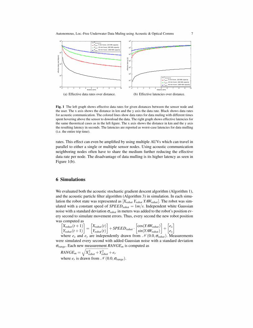
(c) Picture of PANDA with Optical Mo-dem.Fig. 2 (a) AMOUR 6 in the water withacoustic and optical modems attached. (b)Experimental site. The PANDA was de-ployed in the middle of the basin enclosedthe dock. (c) PANDA node (white cylinderon tripod) with Optical Modem attachedon the left.
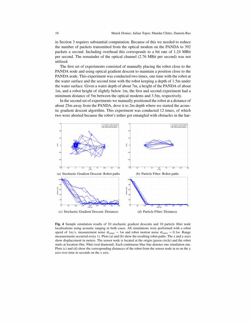
Figure 4 shows two sets of 10 simulated paths taken by the robot using stochasticgradient descent (Fig. 4(a)) and a particle filter (Fig. 4(b)). The simulations wereperformed using Algorithm 1 and Algorithm 3. The parameters for these simula-tions were σrange = 1m and σrobot = 0.1m. These plots visualize the characteristicdifference in paths generated by the stochastic gradient descent and the particle fil-ter. When the stochastic gradient descent encounters an increasing range, it picksa new direction almost entirely at random. The particle filter, on the other hand,continuously merges all gathered information about the sensor node location andcontinuously updates the robot’s heading resulting in a more direct path. Plotted inFigures 4(c) and 4(d) are the corresponding distances of the robot to the sensor nodeover time.
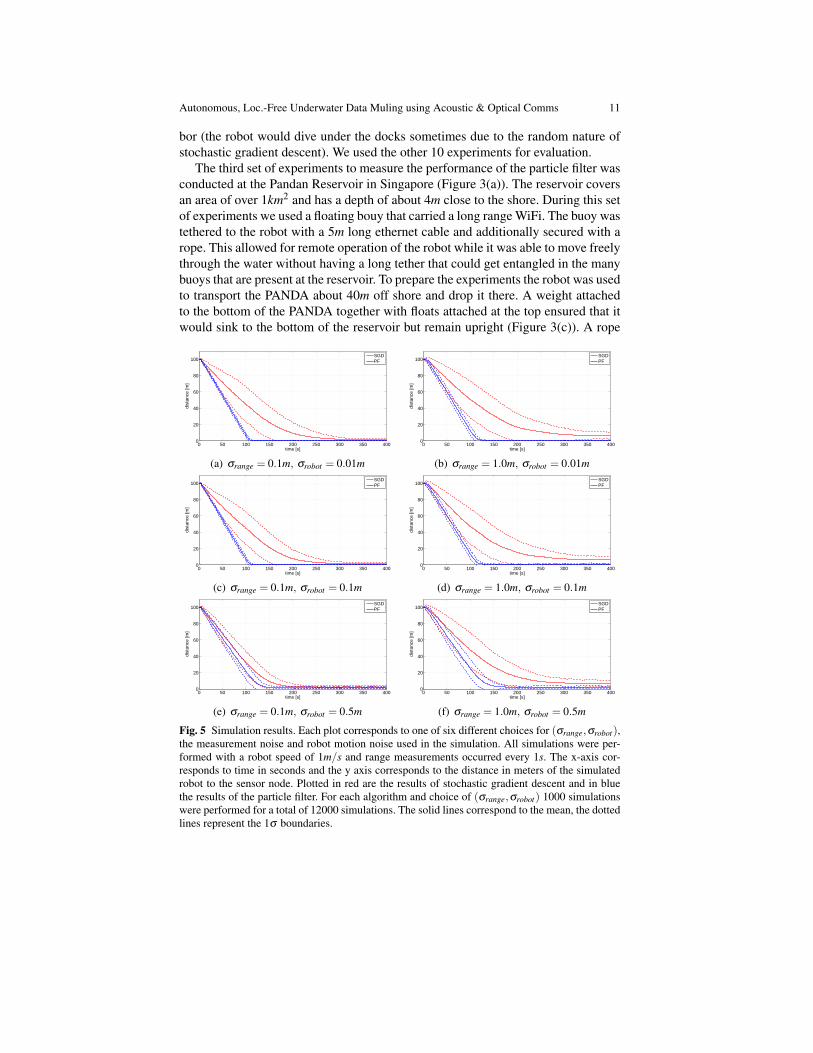
Finally we conducted six sets of simulation runs with parameters chosen as(σrange,σrobot) ∈ {0.1m,1.0m}× {0.01m,0.1m,1.0m}. For each set we simulated1000 runs using the stochastic gradient descent algorithm and 1000 runs using theparticle filter. Figure 5 shows the results for all these runs grouped in six plots ac-cording to parameter choices. Each plot shows the mean distance over time (solidline) with 1σ boundaries (dashed lines). The stochastic gradient descent results areplotted in red, the particle filter results are plotted in blue. In all six cases the par-ticle filter outperforms the stochastic gradient descent. When the noise is low (Fig-
Autonomous, Loc.-Free Underwater Data Muling using Acoustic & Optical Comms 9
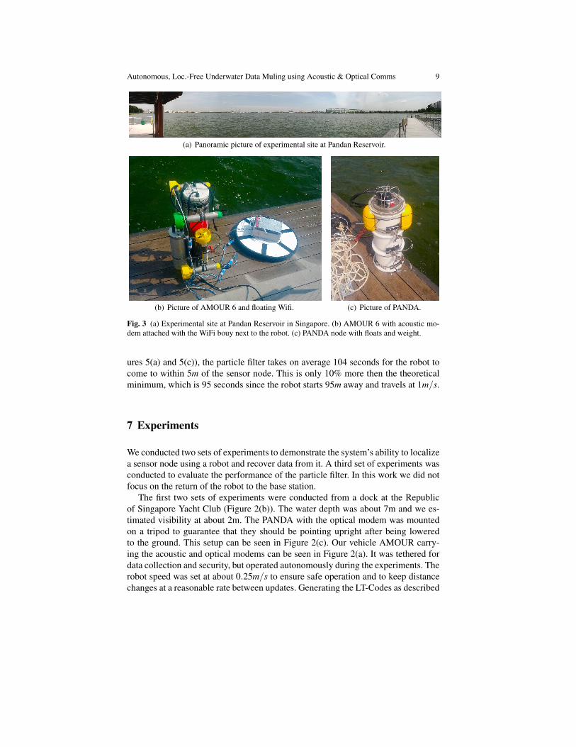
(a) Panoramic picture of experimental site at Pandan Reservoir.
(b) Picture of AMOUR 6 and floating Wifi. (c) Picture of PANDA.
Fig. 3 (a) Experimental site at Pandan Reservoir in Singapore. (b) AMOUR 6 with acoustic mo-dem attached with the WiFi bouy next to the robot. (c) PANDA node with floats and weight.
ures 5(a) and 5(c)), the particle filter takes on average 104 seconds for the robot tocome to within 5m of the sensor node. This is only 10% more then the theoreticalminimum, which is 95 seconds since the robot starts 95m away and travels at 1m/s.
7 Experiments
We conducted two sets of experiments to demonstrate the system’s ability to localizea sensor node using a robot and recover data from it. A third set of experiments wasconducted to evaluate the performance of the particle filter. In this work we did notfocus on the return of the robot to the base station.
The first two sets of experiments were conducted from a dock at the Republicof Singapore Yacht Club (Figure 2(b)). The water depth was about 7m and we es-timated visibility at about 2m. The PANDA with the optical modem was mountedon a tripod to guarantee that they should be pointing upright after being loweredto the ground. This setup can be seen in Figure 2(c). Our vehicle AMOUR carry-ing the acoustic and optical modems can be seen in Figure 2(a). It was tethered fordata collection and security, but operated autonomously during the experiments. Therobot speed was set at about 0.25m/s to ensure safe operation and to keep distancechanges at a reasonable rate between updates. Generating the LT-Codes as described
10 Marek Doniec, Iulian Topor, Mandar Chitre, Daniela Rus
in Section 3 requires substantial computation. Because of this we needed to reducethe number of packets transmitted from the optical modem on the PANDA to 392packets a second. Including overhead this corresponds to a bit rate of 1.24 MBitper second. The remainder of the optical channel (2.76 MBit per second) was notutilized.
The first set of experiments consisted of manually placing the robot close to thePANDA node and using optical gradient descent to maintain a position close to thePANDA node. This experiment was conducted two times, one time with the robot atthe water surface and the second time with the robot keeping a depth of 1.5m underthe water surface. Given a water depth of about 7m, a height of the PANDA of about1m, and a robot height of slightly below 1m, the first and second experiment had aminimum distance of 5m between the optical modems and 3.5m, respectively.
In the second set of experiments we manually positioned the robot at a distance ofabout 25m away from the PANDA, dove it to 2m depth where we started the acous-tic gradient descent algorithm. This experiment was conducted 12 times, of whichtwo were aborted because the robot’s tether got entangled with obstacles in the har-
−50 −25 0 25 50 75 100 125 150−75
−50
−25
0
25
50
75
x [m]
y [m
]
Sensor node locationRobot start location
(a) Stochastic Gradient Descent: Robot paths
−50 −25 0 25 50 75 100 125 150−75
−50
−25
0
25
50
75
x [m]
y [m
]
Sensor node locationRobot start location
(b) Particle Filter: Robot paths
0 50 100 150 200 250 300 350 4000
20
40
60
80
100
time [s]
dist
ance
[m]
(c) Stochastic Gradient Descent: Distances
0 50 100 150 200 250 300 350 4000
20
40
60
80
100
time [s]
dist
ance
[m]
(d) Particle Filter: Distances
Fig. 4 Sample simulation results of 10 stochastic gradient descents and 10 particle filter nodelocalizations using acoustic ranging in both cases. All simulations were performed with a robotspeed of 1m/s, measurement noise σrange = 1m and robot motion noise σrobot = 0.1m. Rangemeasurements occurred every 1s. Plots (a) and (b) show the resulting robot paths. The x and y-axesshow displacement in meters. The sensor node is located at the origin (green circle) and the robotstarts at location (0m, 50m) (red diamond). Each continuous blue line denotes one simulation run.Plots (c) and (d) show the corresponding distances of the robot from the sensor node in m on the yaxis over time in seconds on the x axis.
Autonomous, Loc.-Free Underwater Data Muling using Acoustic & Optical Comms 11
bor (the robot would dive under the docks sometimes due to the random nature ofstochastic gradient descent). We used the other 10 experiments for evaluation.
The third set of experiments to measure the performance of the particle filter wasconducted at the Pandan Reservoir in Singapore (Figure 3(a)). The reservoir coversan area of over 1km2 and has a depth of about 4m close to the shore. During this setof experiments we used a floating bouy that carried a long range WiFi. The buoy wastethered to the robot with a 5m long ethernet cable and additionally secured with arope. This allowed for remote operation of the robot while it was able to move freelythrough the water without having a long tether that could get entangled in the manybuoys that are present at the reservoir. To prepare the experiments the robot was usedto transport the PANDA about 40m off shore and drop it there. A weight attachedto the bottom of the PANDA together with floats attached at the top ensured that itwould sink to the bottom of the reservoir but remain upright (Figure 3(c)). A rope
0 50 100 150 200 250 300 350 4000
20
40
60
80
100
time [s]
dist
ance
[m]
SGDPF
(a) σrange = 0.1m, σrobot = 0.01m
0 50 100 150 200 250 300 350 4000
20
40
60
80
100
time [s]
dist
ance
[m]
SGDPF
(b) σrange = 1.0m, σrobot = 0.01m
0 50 100 150 200 250 300 350 4000
20
40
60
80
100
time [s]
dist
ance
[m]
SGDPF
(c) σrange = 0.1m, σrobot = 0.1m
0 50 100 150 200 250 300 350 4000
20
40
60
80
100
time [s]
dist
ance
[m]
SGDPF
(d) σrange = 1.0m, σrobot = 0.1m
0 50 100 150 200 250 300 350 4000
20
40
60
80
100
time [s]
dist
ance
[m]
SGDPF
(e) σrange = 0.1m, σrobot = 0.5m
0 50 100 150 200 250 300 350 4000
20
40
60
80
100
time [s]
dist
ance
[m]
SGDPF
(f) σrange = 1.0m, σrobot = 0.5m
Fig. 5 Simulation results. Each plot corresponds to one of six different choices for (σrange,σrobot),the measurement noise and robot motion noise used in the simulation. All simulations were per-formed with a robot speed of 1m/s and range measurements occurred every 1s. The x-axis cor-responds to time in seconds and the y axis corresponds to the distance in meters of the simulatedrobot to the sensor node. Plotted in red are the results of stochastic gradient descent and in bluethe results of the particle filter. For each algorithm and choice of (σrange,σrobot) 1000 simulationswere performed for a total of 12000 simulations. The solid lines correspond to the mean, the dottedlines represent the 1σ boundaries.
12 Marek Doniec, Iulian Topor, Mandar Chitre, Daniela Rus
was permanently attached to the PANDA that allowed us to recover it manuallyafter the experiments. During each experiment the robot was manually positionedat a distance of at least 100m away from the PANDA and the node localizationalgorithm based on a particle filter was started. At all times the robot traveled witha speed of 0.5m/s at a depth of 1m. The experiment was conducted 5 times, all ofwhich were used for evaluation.
8 Results
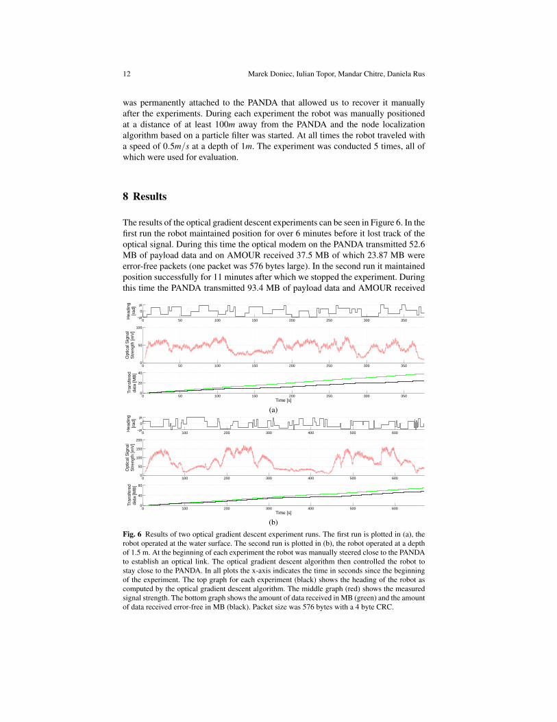
The results of the optical gradient descent experiments can be seen in Figure 6. In thefirst run the robot maintained position for over 6 minutes before it lost track of theoptical signal. During this time the optical modem on the PANDA transmitted 52.6MB of payload data and on AMOUR received 37.5 MB of which 23.87 MB wereerror-free packets (one packet was 576 bytes large). In the second run it maintainedposition successfully for 11 minutes after which we stopped the experiment. Duringthis time the PANDA transmitted 93.4 MB of payload data and AMOUR received
0 50 100 150 200 250 300 350−pi
0
pi
Hea
ding
[rad
]
0 50 100 150 200 250 300 3500
20
40
Time [s]
Tra
nsfe
red
data
[MB
]
0 50 100 150 200 250 300 3500
50
100
Opt
ical
Sig
nal
Str
engt
h [m
V]
(a)
0 100 200 300 400 500 600−pi
0
pi
Hea
ding
[rad
]
0 100 200 300 400 500 6000
40
80
Time [s]
Tra
nsfe
red
data
[MB
]
0 100 200 300 400 500 6000
50
100
150
200
Opt
ical
Sig
nal
Str
engt
h [m
V]
(b)
Fig. 6 Results of two optical gradient descent experiment runs. The first run is plotted in (a), therobot operated at the water surface. The second run is plotted in (b), the robot operated at a depthof 1.5 m. At the beginning of each experiment the robot was manually steered close to the PANDAto establish an optical link. The optical gradient descent algorithm then controlled the robot tostay close to the PANDA. In all plots the x-axis indicates the time in seconds since the beginningof the experiment. The top graph for each experiment (black) shows the heading of the robot ascomputed by the optical gradient descent algorithm. The middle graph (red) shows the measuredsignal strength. The bottom graph shows the amount of data received in MB (green) and the amountof data received error-free in MB (black). Packet size was 576 bytes with a 4 byte CRC.
Autonomous, Loc.-Free Underwater Data Muling using Acoustic & Optical Comms 13
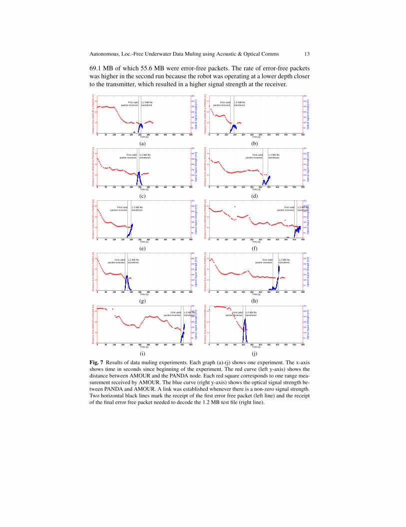
69.1 MB of which 55.6 MB were error-free packets. The rate of error-free packetswas higher in the second run because the robot was operating at a lower depth closerto the transmitter, which resulted in a higher signal strength at the receiver.
0 50 100 150 200 250 300 350 400 450 500 5500
10
20
30First valid
packet received.1.2 MB filetransfered.
Time [s]
Dis
tanc
e fr
om A
MO
UR
to P
AN
DA
[m]
0 50 100 150 200 250 300 350 400 450 500 5500
50
100
150
200
250
300
350
Opt
ical
Sig
nal S
tren
gth
[mV
]
(a)
0 50 100 150 200 250 300 350 400 450 500 5500
10
20
30First valid
packet received.1.2 MB filetransfered.
Time [s]
Dis
tanc
e fr
om A
MO
UR
to P
AN
DA
[m]
0 50 100 150 200 250 300 350 400 450 500 5500
50
100
150
200
250
300
350
Opt
ical
Sig
nal S
tren
gth
[mV
]
(b)
0 50 100 150 200 250 300 350 400 450 500 5500
10
20
30First valid
packet received.1.2 MB filetransfered.
Time [s]
Dis
tanc
e fr
om A
MO
UR
to P
AN
DA
[m]
0 50 100 150 200 250 300 350 400 450 500 5500
50
100
150
200
250
300
350
Opt
ical
Sig
nal S
tren
gth
[mV
](c)
0 50 100 150 200 250 300 350 400 450 500 5500
10
20
30First valid
packet received.1.2 MB filetransfered.
Time [s]
Dis
tanc
e fr
om A
MO
UR
to P
AN
DA
[m]
0 50 100 150 200 250 300 350 400 450 500 5500
50
100
150
200
250
300
350
Opt
ical
Sig
nal S
tren
gth
[mV
]
(d)
0 50 100 150 200 250 300 350 400 450 500 5500
10
20
30First valid
packet received.1.2 MB filetransfered.
Time [s]
Dis
tanc
e fr
om A
MO
UR
to P
AN
DA
[m]
0 50 100 150 200 250 300 350 400 450 500 5500
50
100
150
200
250
300
350
Opt
ical
Sig
nal S
tren
gth
[mV
]
(e)
0 50 100 150 200 250 300 350 400 450 500 5500
10
20
30First valid
packet received.1.2 MB filetransfered.
Time [s]
Dis
tanc
e fr
om A
MO
UR
to P
AN
DA
[m]
0 50 100 150 200 250 300 350 400 450 500 5500
50
100
150
200
250
300
350
Opt
ical
Sig
nal S
tren
gth
[mV
]
(f)
0 50 100 150 200 250 300 350 400 450 500 5500
10
20
30First valid
packet received.1.2 MB filetransfered.
Time [s]
Dis
tanc
e fr
om A
MO
UR
to P
AN
DA
[m]
0 50 100 150 200 250 300 350 400 450 500 5500
50
100
150
200
250
300
350
Opt
ical
Sig
nal S
tren
gth
[mV
]
(g)
0 50 100 150 200 250 300 350 400 450 500 5500
10
20
30First valid
packet received.1.2 MB filetransfered.
Time [s]
Dis
tanc
e fr
om A
MO
UR
to P
AN
DA
[m]
0 50 100 150 200 250 300 350 400 450 500 5500
50
100
150
200
250
300
350
Opt
ical
Sig
nal S
tren
gth
[mV
]
(h)
0 50 100 150 200 250 300 350 400 450 500 5500
10
20
30First valid
packet received.1.2 MB filetransfered.
Time [s]
Dis
tanc
e fr
om A
MO
UR
to P
AN
DA
[m]
0 50 100 150 200 250 300 350 400 450 500 5500
50
100
150
200
250
300
350
Opt
ical
Sig
nal S
tren
gth
[mV
]
(i)
0 50 100 150 200 250 300 350 400 450 500 5500
10
20
30First valid
packet received.1.2 MB filetransfered.
Time [s]
Dis
tanc
e fr
om A
MO
UR
to P
AN
DA
[m]
0 50 100 150 200 250 300 350 400 450 500 5500
50
100
150
200
250
300
350O
ptic
al S
igna
l Str
engt
h [m
V]
(j)
Fig. 7 Results of data muling experiments. Each graph (a)-(j) shows one experiment. The x-axisshows time in seconds since beginning of the experiment. The red curve (left y-axis) shows thedistance between AMOUR and the PANDA node. Each red square corresponds to one range mea-surement received by AMOUR. The blue curve (right y-axis) shows the optical signal strength be-tween PANDA and AMOUR. A link was established whenever there is a non-zero signal strength.Two horizontal black lines mark the receipt of the first error free packet (left line) and the receiptof the final error free packet needed to decode the 1.2 MB test file (right line).
14 Marek Doniec, Iulian Topor, Mandar Chitre, Daniela Rus
The results of the second set of experiments can be seen in Figure 7. In all 10experiments the robot successfully found the PANDA within 2.5 to 8 minutes andproceeded to download the 1.2 MB file within an additional 10 to 35 seconds.
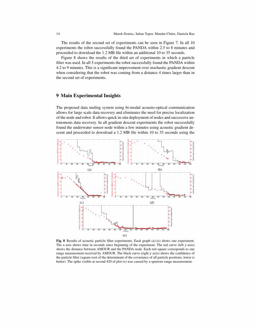
Figure 8 shows the results of the third set of experiments in which a particlefilter was used. In all 5 experiments the robot successfully found the PANDA within4.2 to 9 minutes. This is a significant improvement over stochastic gradient descentwhen considering that the robot was coming from a distance 4 times larger than inthe second set of experiments.
9 Main Experimental Insights
The proposed data muling system using bi-modal acousto-optical communicationallows for large scale data recovery and eliminates the need for precise localizationof the node and robot. It allows quick in-situ deployment of nodes and successive au-tonomous data recovery. In all gradient descent experiments the robot successfullyfound the underwater sensor node within a few minutes using acoustic gradient de-scent and proceeded to download a 1.2 MB file within 10 to 35 seconds using the
0 50 100 150 200 250 300 350 400 450 500 5500
20
40
60
80
100
120
Time [s]
Dis
tanc
e fr
om A
MO
UR
to P
AN
DA
[m]
0 50 100 150 200 250 300 350 400 450 500 5500
20
40
60
80
100
120
Par
ticle
Filt
er C
onfid
ence
[m]
(a)
0 50 100 150 200 250 300 350 400 450 500 5500
20
40
60
80
100
120
Time [s]
Dis
tanc
e fr
om A
MO
UR
to P
AN
DA
[m]
0 50 100 150 200 250 300 350 400 450 500 5500
20
40
60
80
100
120
Par
ticle
Filt
er C
onfid
ence
[m]
(b)
0 50 100 150 200 250 300 350 4000
20
40
60
80
100
120
Time [s]
Dis
tanc
e fr
om A
MO
UR
to P
AN
DA
[m]
0 50 100 150 200 250 300 350 4000
20
40
60
80
100
120
Par
ticle
Filt
er C
onfid
ence
[m]
(c)
0 50 100 150 200 250 300 350 400 450 500 550 600 650 7000
20
40
60
80
100
120
Time [s]
Dis
tanc
e fr
om A
MO
UR
to P
AN
DA
[m]
0 50 100 150 200 250 300 350 400 450 500 550 600 650 7000
20
40
60
80
100
120
Par
ticle
Filt
er C
onfid
ence
[m]
(d)
0 50 100 150 200 250 300 350 400 450 500 550 600 650 700 750 8000
20
40
60
80
100
120
Time [s]
Dis
tanc
e fr
om A
MO
UR
to P
AN
DA
[m]
0 50 100 150 200 250 300 350 400 450 500 550 600 650 700 750 8000
20
40
60
80
100
120
Par
ticle
Filt
er C
onfid
ence
[m]
(e)
Fig. 8 Results of acoustic particle filter experiments. Each graph (a)-(e) shows one experiment.The x-axis shows time in seconds since beginning of the experiment. The red curve (left y-axis)shows the distance between AMOUR and the PANDA node. Each red square corresponds to onerange measurement received by AMOUR. The black curve (right y-axis) shows the confidence ofthe particle filter (square root of the determinant of the covariance of all particle positions, lower isbetter). The spike visible at second 420 of plot (e) was caused by a spurious range measurement.
Autonomous, Loc.-Free Underwater Data Muling using Acoustic & Optical Comms 15
optical link. Further we demonstrated that we can use the optical signal strength tomaintain the robot’s position close to the position of the sensor node. We also exper-imentally evaluated the use of a particle filter to locate the node using only acousticranging. Both in simulation and experimentally the particle filter performed betterthan stochatic gradient descent.
If the PANDA had been able to generate LT-Codes at the full rate of 4 MBit/secthen our throughput would have been 3.2 times higher than measured. It should benoted that this was purely a limitation on the computational side and not a limitationof the optical or acoustic modem itself. Also, since we do not use error coding andcorrection, all packets with a single bit error were discarded. This amounted to 13.6MB of 37.5 MB and 13.5 MB of 69.1 MB in payload data lost. With the expense ofmore computational resources this bandwidth can be almost entirely utilized.
Future improvements of the system include the usage of the acoustic link to turnon and off both the optical modem and the acoustic beacons (or at least reducingtheir frequency) to save battery life while the robot is not in range. We also planto extend the presented data muling system to three dimensions which will allowfor the nodes to be deployed at greater depths. The gradient descent algorithm canbe extended to include state in order to speed up the robot’s successful approachtowards the node. Further, we plan to extend experiments into the open ocean wherethe algorithm can be tested at distances of multiple kilometers.
Acknowledgments
The authors would like to acknowledge the help of Mohan Panayamadam, AndyMarchese, TeongBeng Koay, and Puthenpurayil Unnikrishnan Saneesh.
References
1. Benson, C., Dunbar, R., Ryan, M., Huntington, E., Frater, M.: Towards a dense high-capacityunderwater acoustic network. In: Communication Systems (ICCS), 2010 IEEE InternationalConference on, pp. 386 –389 (2010). DOI 10.1109/ICCS.2010.5686512
2. Chitre, M., Topor, I.: The unet-2 modem - an extensible tool for underwater networking re-search. In: OCEANS 2012 - Yeosu, pp. 1 –9 (2012)
3. Doniec, M., Rus, D.: Bidirectional optical communication with aquaoptical ii. In: Communi-cation Systems (ICCS), 2010 IEEE International Conference on, pp. 390 –394 (2010). DOI10.1109/ICCS.2010.5686513
4. Doniec, M., Vasilescu, I., Detweiler, C., Rus, D.: Complete se(3) underwater robot controlwith arbitrary thruster configurations. In: In Proc. of the International Conference on Roboticsand Automation. Anchorage, Alaska (2010)
5. Dunbabin, M., Corke, P., Vasilescu, I., Rus, D.: Data muling over underwater wireless sensornetworks using an autonomous underwater vehicle. In: Proc. IEEE ICRA 2006, pp. 2091–2098. Orlando, Florida (2006)
6. Kilfoyle, D., Baggeroer, A.: The state of the art in underwater acoustic telemetry. OceanicEngineering, IEEE Journal of 25(1), 4 –27 (2000). DOI 10.1109/48.820733
16 Marek Doniec, Iulian Topor, Mandar Chitre, Daniela Rus
7. Li, K., Shen, C.C., Chen, G.: Energy-constrained bi-objective data muling in underwater wire-less sensor networks. In: Mobile Adhoc and Sensor Systems (MASS), 2010 IEEE 7th Inter-national Conference on, pp. 332 –341 (2010). DOI 10.1109/MASS.2010.5664026
8. Luby, M.: Lt codes. In: Foundations of Computer Science, 2002. Proceedings. The 43rdAnnual IEEE Symposium on, pp. 271 – 280 (2002). DOI 10.1109/SFCS.2002.1181950
9. Olson, E., Leonard, J., Teller, S.: Robust range-only beacon localization. In: Proceedings ofAutonomous Underwater Vehicles, 2004 (2004)
10. Shah, R., Roy, S., Jain, S., Brunette, W.: Data mules: modeling a three-tier architecture forsparse sensor networks. In: Sensor Network Protocols and Applications, 2003. Proceed-ings of the First IEEE. 2003 IEEE International Workshop on, pp. 30 – 41 (2003). DOI10.1109/SNPA.2003.1203354
11. Stojanovic, M.: Recent advances in high-speed underwater acoustic communications. OceanicEngineering, IEEE Journal of 21(2), 125 –136 (1996). DOI 10.1109/48.486787
12. Thrun, S.: Probabilistic robotics. Commun. ACM 45(3), 52–57 (2002). DOI10.1145/504729.504754. URL http://doi.acm.org/10.1145/504729.504754
13. Vaganay, J., Baccou, P., Jouvencel, B.: Homing by acoustic ranging to a single beacon. In:OCEANS 2000, vol. 2, pp. 1457 – 1462 (2000)