Experiments with Underwater Robot Localization and Tracking

Peter Corke†, Carrick Detweiler∗, Matthew Dunbabin†, Michael Hamilton◦,Daniela Rus∗ and Iuliu Vasilescu∗

†Autonomous Systems Lab ∗Computer Science & Artificial Intelligence Lab ◦University of CaliforniaCSIRO ICT Centre Massachusetts Institute of Technology James San Jacinto Mountains ReserveBrisbane, Australia Cambridge, MA 02139, USA Idyllwild, CA 92549, USA

Abstract— This paper describes a novel experiment in whichtwo very different methods of underwater robot localization arecompared. The first method is based on a geometric approach inwhich a mobile node moves within a field of static nodes, and allnodes are capable of estimating the range to their neighboursacoustically. The second method uses visual odometry, fromstereo cameras, by integrating scaled optical flow. The fun-damental algorithmic principles of each localization techniqueis described. We also present experimental results comparingacoustic localization with GPS for surface operation, and acomparison of acoustic and visual methods for underwateroperation.

I. INTRODUCTION

Performing reliable localization and navigation withinhighly unstructured underwater environments is a difficulttask. Knowing the position and distance an AutonomousUnderwater Vehicle (AUV) has moved is critical to ensurethat correct and repeatable measurements are being takenfor reef surveying and other applications. A number oftechniques are used, or proposed, to estimate vehicle motionwhich can be categorized as either acoustic or vision-based.

Leonard et al. [1] provide a good survey of underwaterlocalization methods. Acoustic sensors such as Dopplervelocity logs are a common means of obtaining accuratemotion information, measuring speed with respect to thesea floor. Position can be estimated by integration but willbe subject to unbounded growth in error. Long Base Line(LBL) systems employ transponder beacons whose positionis known from survey, or GPS if they are on the surface. Thevehicle periodically pings the transponders and estimates itsposition based on the round trip delay. Ultra Short Base Line(USBL) systems determine the angle as well as distance toa beacon. The largest source of uncertainty with this classof methods is the speed of sound underwater which is acomplex function of temperature, pressure and salinity.

A number of authors have investigated localization usingvision as a primary navigation sensor for robots moving in6DOF, for example Amidi [2] provides an early and detailedinvestigation into feature tracking for visual odometry foran autonomous helicopter, and Corke [3] describes the usevision for helicopter hover stabilization. The use of visionunderwater has been explored for navigation [4] and stationkeeping [5], [6]. Dagleish presents a survey of vision-basedunderwater vehicle navigation for the tracking of cables,pipes and fish [7], and for station-keeping and position-ing [8]. Of critical importance in these systems is the long-term stability of the motion estimate. Current research is

thus focusing on reducing motion estimation drift in longimage sequences through techniques such as mosaicing andSLAM. Many examples are presented, but most algorithmswere only applied to recorded data sets or implemented onan ROV allowing significant computing power, not on anenergy-constrained AUV.

Each method above has different advantages and disad-vantages. Visual odometry, by its nature integrates perceivedmotion and is subject to long-term drift, and requires occa-sional “position fixes” to keep error in check. The acousticlocalization system involves the creation of infrastructurewhich must be powered, but provides absolute position es-timates. Complementary or hybrid systems could be createdthat would exploit the advantages of each method, but arenot the subject of this paper.

In this paper we compare, for the first time, these twoquite different underwater localization methods. Our acousticlocalization system is able to self calibrate the location ofthe static nodes, and then provide location information tothe underwater vehicle. We compare the vehicle locationsmeasured by the acoustic system with GPS during surfaceoperations. In previous work it has been difficult to groundtruth the visual odometry system since it requires closeproximity to the sea floor, whereas as GPS requires operationat the surface. In this work we compare the dead reckonedlocation, from visual odometry, with the estimate from theacoustic localization system. We present experimental resultsfrom a recent ocean trial.

The remainder of the paper is organized as follows. Wedescribe the experimental platforms and procedures, and thenpresent results for the acoustic and vision systems. Finallywe compare the two methods and conclude.

II. EXPERIMENTAL STUDY

A. Experimental Platforms

1) Sensor Nodes: The sensor nodes shown in Figure 1were developed at MIT. These nodes package communica-tion, sensing, and computation in a cylindrical water-tightcontainer of 6in diameter and 10in height. Each unit includesan acoustic modem we designed and developed. The systemof sensor nodes is self-synchronizing and uses a distributedtime division multiple access (TDMA) communications pro-tocol. The system is capable of ranging and has a data rate of300 b/s verified up to 300 m in fresh water and in the ocean.Each unit also includes an optical modem implemented using

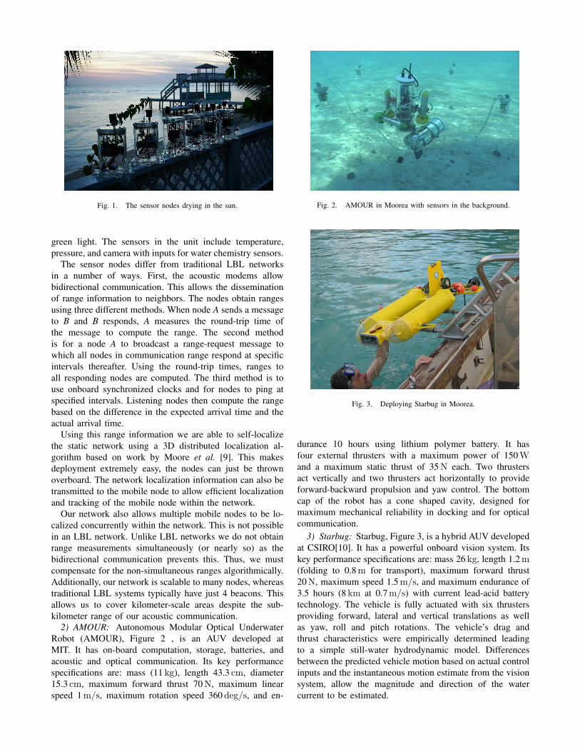
Fig. 1. The sensor nodes drying in the sun.

green light. The sensors in the unit include temperature,pressure, and camera with inputs for water chemistry sensors.

The sensor nodes differ from traditional LBL networksin a number of ways. First, the acoustic modems allowbidirectional communication. This allows the disseminationof range information to neighbors. The nodes obtain rangesusing three different methods. When node A sends a messageto B and B responds, A measures the round-trip time ofthe message to compute the range. The second methodis for a node A to broadcast a range-request message towhich all nodes in communication range respond at specificintervals thereafter. Using the round-trip times, ranges toall responding nodes are computed. The third method is touse onboard synchronized clocks and for nodes to ping atspecified intervals. Listening nodes then compute the rangebased on the difference in the expected arrival time and theactual arrival time.

Using this range information we are able to self-localizethe static network using a 3D distributed localization al-gorithm based on work by Moore et al. [9]. This makesdeployment extremely easy, the nodes can just be thrownoverboard. The network localization information can also betransmitted to the mobile node to allow efficient localizationand tracking of the mobile node within the network.

Our network also allows multiple mobile nodes to be lo-calized concurrently within the network. This is not possiblein an LBL network. Unlike LBL networks we do not obtainrange measurements simultaneously (or nearly so) as thebidirectional communication prevents this. Thus, we mustcompensate for the non-simultaneous ranges algorithmically.Additionally, our network is scalable to many nodes, whereastraditional LBL systems typically have just 4 beacons. Thisallows us to cover kilometer-scale areas despite the sub-kilometer range of our acoustic communication.

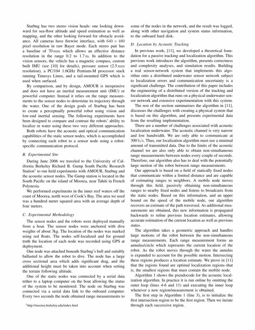
2) AMOUR: Autonomous Modular Optical UnderwaterRobot (AMOUR), Figure 2 , is an AUV developed atMIT. It has on-board computation, storage, batteries, andacoustic and optical communication. Its key performancespecifications are: mass (11 kg), length 43.3 cm, diameter15.3 cm, maximum forward thrust 70 N, maximum linearspeed 1 m/s, maximum rotation speed 360 deg/s, and en-

Fig. 2. AMOUR in Moorea with sensors in the background.

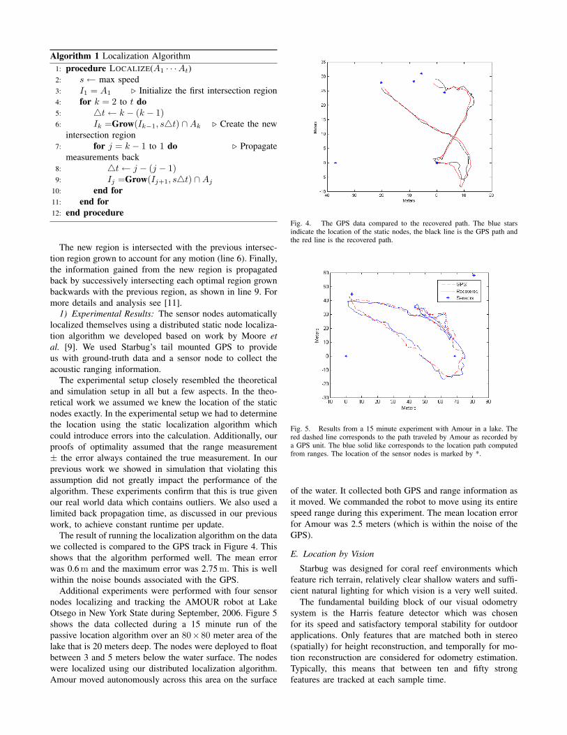
Fig. 3. Deploying Starbug in Moorea.

durance 10 hours using lithium polymer battery. It hasfour external thrusters with a maximum power of 150 Wand a maximum static thrust of 35 N each. Two thrustersact vertically and two thrusters act horizontally to provideforward-backward propulsion and yaw control. The bottomcap of the robot has a cone shaped cavity, designed formaximum mechanical reliability in docking and for opticalcommunication.

3) Starbug: Starbug, Figure 3, is a hybrid AUV developedat CSIRO[10]. It has a powerful onboard vision system. Itskey performance specifications are: mass 26 kg, length 1.2 m(folding to 0.8 m for transport), maximum forward thrust20 N, maximum speed 1.5 m/s, and maximum endurance of3.5 hours (8 km at 0.7 m/s) with current lead-acid batterytechnology. The vehicle is fully actuated with six thrustersproviding forward, lateral and vertical translations as wellas yaw, roll and pitch rotations. The vehicle’s drag andthrust characteristics were empirically determined leadingto a simple still-water hydrodynamic model. Differencesbetween the predicted vehicle motion based on actual controlinputs and the instantaneous motion estimate from the visionsystem, allow the magnitude and direction of the watercurrent to be estimated.

Starbug has two stereo vision heads: one looking down-ward for sea-floor altitude and speed estimation as well asmapping, and the other looking forward for obstacle avoid-ance. All cameras have firewire interface, with 640 × 480pixel resolution in raw Bayer mode. Each stereo pair hasa baseline of 70 mm which allows an effective distanceresolution in the range 0.2 to 1.7 m. In addition to thevision sensors, the vehicle has a magnetic compass, custombuilt IMU (see [10] for details), pressure sensor (2.5 mmresolution), a PC/104 1.6GHz Pentium-M processor stackrunning Timesys Linux, and a tail-mounted GPS which isused when surfaced.

By comparison, and by design, AMOUR is inexpensiveand does not have an inertial measurement unit (IMU) orpowerful computer. Instead it relies on the range measure-ments to the sensor nodes to determine its trajectory throughthe water. One of the design goals of Starbug has beento create a perceptually powerful robot using vision andlow-end inertial sensing. The following experiments havebeen designed to compare and contrast the robots’ ability tolocalize in water using these two very different approaches.

Both robots have the acoustic and optical communicationcapabilities of the static sensor nodes, which is accomplishedby connecting each robot to a sensor node using a robot-specific communication protocol.

B. Experimental Site

During June 2006 we traveled to the University of Cal-ifornia Berkeley Richard B. Gump South Pacific ResearchStation1 to run field experiments with AMOUR, Starbug andthe acoustic sensor nodes. The Gump station is located in theSouth Pacific on the island of Moorea, near Tahiti in FrenchPolynesia.

We performed experiments in the inner reef waters off thecoast of Moorea, north west of Cook’s Bay. The area we usedwas a hundred meter squared area with an average depth offour meters.

C. Experimental Methodology

The sensor nodes and the robots were deployed manuallyfrom a boat. The sensor nodes were anchored with diveweights of about 3kg. The location of the nodes was markedusing red floats. The nodes self-localized and for groundtruth the location of each node was recorded using GPS atdeployment.

One node was attached beneath Starbug’s hull and suitablyballasted to allow the robot to dive. The node has a largecross sectional area which adds significant drag, and theadditional height must be taken into account when settingthe terrain following altitude.

One of the static nodes was connected by a serial datatether to a laptop computer on the boat allowing the statusof the system to be monitored. The node on Starbug wasconnected via a serial data link to the onboard computer.Every two seconds the node obtained range measurements to

1http://moorea.berkeley.edu/index.html

some of the nodes in the network, and the result was logged,along with other navigation and system status information,to the onboard hard disk.

D. Location by Acoustic Tracking

In previous work, [11], we developed a theoretical foun-dation for a passive tracking and localization algorithm. Thisprevious work introduces the algorithm, presents correctnessand complexity analyses, and simulation results. Buildinga real sensor-network system that implements this algo-rithm onto a distributed underwater sensor network subjectto localization errors and communication uncertainty is asignificant challenge. The contribution of this paper includesthe engineering of a distributed version of the tracking andlocalization algorithm that runs on a physical underwater sen-sor network and extensive experimentation with this system.

The rest of the section summarizes the algorithm in [11],discusses the challenges with creating a physical system thatis based on this algorithm, and presents experimental datafrom the resulting implementation.

There are a number of challenges associated with acousticlocalization underwater. The acoustic channel is very narrowand low bandwidth. We are only able to communicate at300 b/s. Thus, our localization algorithm must use a minimalamount of transmitted data. Due to the limits of the acousticchannel we are also only able to obtain non-simultaneousrange measurements between nodes every couple of seconds.Therefore, our algorithm also has to deal with the potentiallylarge motion of the robot between range measurements.

Our approach is based on a field of statically fixed nodesthat communicate within a limited distance and are capableof estimating ranges to neighbors. A mobile node movesthrough this field, passively obtaining non-simultaneousranges to nearby fixed nodes and listens to broadcasts fromthe static nodes. Based on this information, and an upperbound on the speed of the mobile node, our algorithmrecovers an estimate of the path traversed. As additional mea-surements are obtained, this new information is propagatedbackwards to refine previous location estimates, allowingaccurate estimation of the current location as well as previousstates.

The algorithm takes a geometric approach and handleslarge motions of the robot between the non-simultaneousrange measurements. Each range measurement forms anannulus/circle which represents the current location of therobot. As the robot moves through the water the annulusis expanded to account for the possible motion. Intersectingthese regions produces a location estimate. We prove in [11]that the regions found are optimal localization regions–thatis, the smallest regions that must contain the mobile node.

Algorithm 1 shows the pseudocode for the acoustic local-ization algorithm. In practice it is run online by omitting theouter loop (lines 4-6 and 11) and executing the inner loopwhenever a new region/measurement is obtained.

The first step in Algorithm 1 (line 3), is to initialize thefirst intersection region to be the first region. Then we iteratethrough each successive region.

Algorithm 1 Localization Algorithm1: procedure LOCALIZE(A1 · · ·At)2: s← max speed3: I1 = A1 . Initialize the first intersection region4: for k = 2 to t do5: 4t← k − (k − 1)6: Ik =Grow(Ik−1, s4t) ∩Ak . Create the new

intersection region7: for j = k − 1 to 1 do . Propagate

measurements back8: 4t← j − (j − 1)9: Ij =Grow(Ij+1, s4t) ∩Aj

10: end for11: end for12: end procedure

The new region is intersected with the previous intersec-tion region grown to account for any motion (line 6). Finally,the information gained from the new region is propagatedback by successively intersecting each optimal region grownbackwards with the previous region, as shown in line 9. Formore details and analysis see [11].

1) Experimental Results: The sensor nodes automaticallylocalized themselves using a distributed static node localiza-tion algorithm we developed based on work by Moore etal. [9]. We used Starbug’s tail mounted GPS to provideus with ground-truth data and a sensor node to collect theacoustic ranging information.

The experimental setup closely resembled the theoreticaland simulation setup in all but a few aspects. In the theo-retical work we assumed we knew the location of the staticnodes exactly. In the experimental setup we had to determinethe location using the static localization algorithm whichcould introduce errors into the calculation. Additionally, ourproofs of optimality assumed that the range measurement± the error always contained the true measurement. In ourprevious work we showed in simulation that violating thisassumption did not greatly impact the performance of thealgorithm. These experiments confirm that this is true givenour real world data which contains outliers. We also used alimited back propagation time, as discussed in our previouswork, to achieve constant runtime per update.

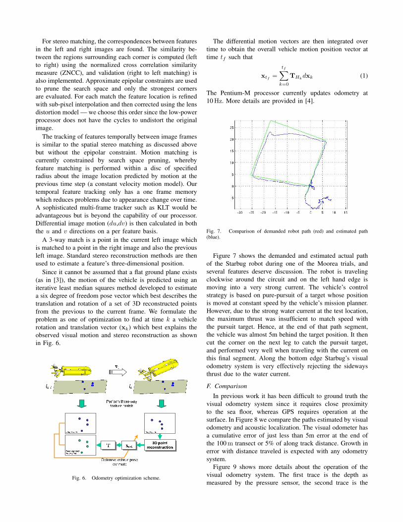
The result of running the localization algorithm on the datawe collected is compared to the GPS track in Figure 4. Thisshows that the algorithm performed well. The mean errorwas 0.6 m and the maximum error was 2.75 m. This is wellwithin the noise bounds associated with the GPS.

Additional experiments were performed with four sensornodes localizing and tracking the AMOUR robot at LakeOtsego in New York State during September, 2006. Figure 5shows the data collected during a 15 minute run of thepassive location algorithm over an 80×80 meter area of thelake that is 20 meters deep. The nodes were deployed to floatbetween 3 and 5 meters below the water surface. The nodeswere localized using our distributed localization algorithm.Amour moved autonomously across this area on the surface

Fig. 4. The GPS data compared to the recovered path. The blue starsindicate the location of the static nodes, the black line is the GPS path andthe red line is the recovered path.

Fig. 5. Results from a 15 minute experiment with Amour in a lake. Thered dashed line corresponds to the path traveled by Amour as recorded bya GPS unit. The blue solid like corresponds to the location path computedfrom ranges. The location of the sensor nodes is marked by *.

of the water. It collected both GPS and range information asit moved. We commanded the robot to move using its entirespeed range during this experiment. The mean location errorfor Amour was 2.5 meters (which is within the noise of theGPS).

E. Location by Vision

Starbug was designed for coral reef environments whichfeature rich terrain, relatively clear shallow waters and suffi-cient natural lighting for which vision is a very well suited.

The fundamental building block of our visual odometrysystem is the Harris feature detector which was chosenfor its speed and satisfactory temporal stability for outdoorapplications. Only features that are matched both in stereo(spatially) for height reconstruction, and temporally for mo-tion reconstruction are considered for odometry estimation.Typically, this means that between ten and fifty strongfeatures are tracked at each sample time.

For stereo matching, the correspondences between featuresin the left and right images are found. The similarity be-tween the regions surrounding each corner is computed (leftto right) using the normalized cross correlation similaritymeasure (ZNCC), and validation (right to left matching) isalso implemented. Approximate epipolar constraints are usedto prune the search space and only the strongest cornersare evaluated. For each match the feature location is refinedwith sub-pixel interpolation and then corrected using the lensdistortion model — we choose this order since the low-powerprocessor does not have the cycles to undistort the originalimage.

The tracking of features temporally between image framesis similar to the spatial stereo matching as discussed abovebut without the epipolar constraint. Motion matching iscurrently constrained by search space pruning, wherebyfeature matching is performed within a disc of specifiedradius about the image location predicted by motion at theprevious time step (a constant velocity motion model). Ourtemporal feature tracking only has a one frame memorywhich reduces problems due to appearance change over time.A sophisticated multi-frame tracker such as KLT would beadvantageous but is beyond the capability of our processor.Differential image motion (du,dv) is then calculated in boththe u and v directions on a per feature basis.

A 3-way match is a point in the current left image whichis matched to a point in the right image and also the previousleft image. Standard stereo reconstruction methods are thenused to estimate a feature’s three-dimensional position.

Since it cannot be assumed that a flat ground plane exists(as in [3]), the motion of the vehicle is predicted using aniterative least median squares method developed to estimatea six degree of freedom pose vector which best describes thetranslation and rotation of a set of 3D reconstructed pointsfrom the previous to the current frame. We formulate theproblem as one of optimization to find at time k a vehiclerotation and translation vector (xk) which best explains theobserved visual motion and stereo reconstruction as shownin Fig. 6.

Fig. 6. Odometry optimization scheme.

The differential motion vectors are then integrated overtime to obtain the overall vehicle motion position vector attime tf such that

xtf=

tf∑k=0

THkdxk (1)

The Pentium-M processor currently updates odometry at10 Hz. More details are provided in [4].

Fig. 7. Comparison of demanded robot path (red) and estimated path(blue).

Figure 7 shows the demanded and estimated actual pathof the Starbug robot during one of the Moorea trials, andseveral features deserve discussion. The robot is travelingclockwise around the circuit and on the left hand edge ismoving into a very strong current. The vehicle’s controlstrategy is based on pure-pursuit of a target whose positionis moved at constant speed by the vehicle’s mission planner.However, due to the strong water current at the test location,the maximum thrust was insufficient to match speed withthe pursuit target. Hence, at the end of that path segment,the vehicle was almost 5m behind the target position. It thencut the corner on the next leg to catch the pursuit target,and performed very well when traveling with the current onthis final segment. Along the bottom edge Starbug’s visualodometry system is very effectively rejecting the sidewaysthrust due to the water current.

F. Comparison

In previous work it has been difficult to ground truth thevisual odometry system since it requires close proximityto the sea floor, whereas GPS requires operation at thesurface. In Figure 8 we compare the paths estimated by visualodometry and acoustic localization. The visual odometer hasa cumulative error of just less than 5m error at the end ofthe 100 m transect or 5% of along track distance. Growth inerror with distance traveled is expected with any odometrysystem.

Figure 9 shows more details about the operation of thevisual odometry system. The first trace is the depth asmeasured by the pressure sensor, the second trace is the

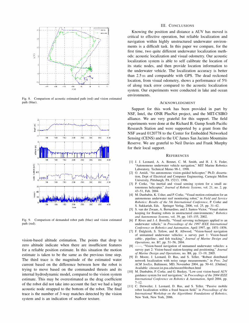
Fig. 8. Comparison of acoustic estimated path (red) and vision estimatedpath (blue).

Fig. 9. Comparison of demanded robot path (blue) and vision estimatedpath (red).

vision-based altitude estimation. The points that drop tozero altitude indicate when there are insufficient featuresfor a reliable position estimate. In this situation the motionestimate is taken to be the same as the previous time step.The third trace is the magnitude of the estimated watercurrent based on the difference between how the robot istrying to move based on the commanded thrusts and itsinternal hydrodynamic model, compared to the vision systemestimate. This may be overestimated as the drag coefficientof the robot did not take into account the fact we had a largeacoustic node strapped to the bottom of the robot. The finaltrace is the number of 3-way matches detected by the visionsystem and is an indication of seafloor texture.

III. CONCLUSIONS

Knowing the position and distance a AUV has moved iscritical to effective operation, but reliable localization andnavigation within highly unstructured underwater environ-ments is a difficult task. In this paper we compare, for thefirst time, two quite different underwater localization meth-ods: acoustic localization and visual odometry. Our acousticlocalization system is able to self calibrate the location ofits static nodes, and then provide location information tothe underwater vehicle. The localization accuracy is betterthan 2.5 m and comparable with GPS. The dead reckonedlocation, from visual odometry, shows a performance of 5%of along track error compared to the acoustic localizationsystem. Our experiments were conducted in lake and oceanenvironments.

ACKNOWLEDGMENT

Support for this work has been provided in part byNSF, Intel, the ONR PlusNet project, and the MIT-CSIROalliance. We are very grateful for this support. The fieldexperiments were done at the Richard B. Gump South PacificResearch Station and were supported by a grant from theNSF award 0120778 to the Center for Embedded NetworkedSensing (CENS) and to the UC James San Jacinto MountainsReserve. We are grateful to Neil Davies and Frank Murphyfor their local support.

REFERENCES

[1] J. J. Leonard, A. A. Bennet, C. M. Smith, and H. J. S. Feder,“Autonomous underwater vehicle navigation,” MIT Marine RoboticsLaboratory, Technical Memo 98-1, 1998.

[2] O. Amidi, “An autonomous vision-guided helicopter,” Ph.D. disserta-tion, Dept of Electrical and Computer Engineering, Carnegie MellonUniversity, Pittsburgh, PA 15213, 1996.

[3] P. Corke, “An inertial and visual sensing system for a small au-tonomous helicopter,” Journal of Robotic Systems, vol. 21, no. 2, pp.43–51, Feb. 2004.

[4] M. Dunbabin, K. Usher, and P. Corke, “Visual motion estimation for anautonomous underwater reef monitoring robot,” in Field and ServiceRobotics: Results of the 5th International Conference, P. Corke andS. Sukkariah, Eds. Springer Verlag, 2006, vol. 25, pp. 31–42.

[5] S. van der Zwaan, A. Bernardino, and J. Santos-Victor, “Visual stationkeeping for floating robots in unstructured ennvironments,” Roboticsand Autonomous Systems, vol. 39, pp. 145–155, 2002.

[6] P. Rives and J.-J. Borrelly, “Visual servoing techniques applied to anunderwater vehicle,” in Proceedings of the 1997 IEEE InternationalConference on Robotics and Automation, April 1997, pp. 1851–1856.

[7] F. Dalgleish, S. Tetlow, and R. Allwood, “Vision-based navigationof unmanned underwater vehicles: a survey part 1: Vision-basedcable-, pipeline-, and fish tracking,” Journal of Marine Design andOperations, no. B7, pp. 51–56, 2004.

[8] ——, “Vision-based navigation of unmanned underwater vehicles: asurvey part 2: Vision-based station-keeping and positioning,” Journalof Marine Design and Operations, no. B8, pp. 13–19, 2005.

[9] D. Moore, J. Leonard, D. Rus, and S. Teller, “Robust distributednetwork localization with noisy range measurements,” in Proc. 2ndACM SenSys, Baltimore, MD, November 2004, pp. 50–61. [Online].Available: citeseer.ist.psu.edu/moore04robust.html

[10] M. Dunbabin, P. Corke, and G. Buskey, “Low-cost vision-based AUVguidance system for reef navigation,” in Proceedings of the 2004 IEEEInternational Conference on Robotics & Automation, April 2004, pp.7–12.

[11] C. Detweiler, J. Leonard, D. Rus, and S. Teller, “Passive mobilerobot localization within a fixed beacon field,” in Proceedings of theInternational Workshop on the Algorithmic Foundations of Robotics,New York, New York, 2006.