NBER WORKING PAPER SERIES

UNCOVERING THE AMERICAN DREAM:INEQUALITY AND MOBILITY IN SOCIAL SECURITY EARNINGS DATA SINCE 1937

Wojciech KopczukEmmanuel Saez

Jae Song

Working Paper 13345http://www.nber.org/papers/w13345

NATIONAL BUREAU OF ECONOMIC RESEARCH1050 Massachusetts Avenue

Cambridge, MA 02138August 2007

We thank Clair Brown, David Card, Jessica Guillory, Russ Hudson, Jennifer Hunt, Larry Katz, AlanKrueger, Thomas Lemieux, Michael Leonesio, Joyce Manchester, Robert Margo, David Pattison, MichaelReich, and many seminar participants for helpful comments and discussions. We also thank Ed DeMarcoand Linda Maxfield for their support, Bill Kearns, Joel Packman, Russ Hudson, Shirley Piazza, GregDiez, Fred Galeas, Bert Kestenbaum, William Piet, Jay Rossi, Thomas Mattson for help with the data,and Thomas Solomon and Barbara Tyler for computing support. Financial support from the SloanFoundation and NSF Grant SES-0617737 is gratefully acknowledged. The views expressed hereinare those of the author(s) and do not necessarily reflect the views of the National Bureau of EconomicResearch.

© 2007 by Wojciech Kopczuk, Emmanuel Saez, and Jae Song. All rights reserved. Short sectionsof text, not to exceed two paragraphs, may be quoted without explicit permission provided that fullcredit, including © notice, is given to the source.

Uncovering the American Dream: Inequality and Mobility in Social Security Earnings Datasince 1937Wojciech Kopczuk, Emmanuel Saez, and Jae SongNBER Working Paper No. 13345August 2007JEL No. D3,J3

ABSTRACT

This paper uses Social Security Administration longitudinal earnings micro data since 1937 to analyzethe evolution of inequality and mobility in the United States. Earnings inequality follows a U-shapepattern, decreasing sharply up to 1953 and increasing steadily afterwards. We find that short-termand long-term (rank based) mobility among all workers has been quite stable since 1950 (after a temporarysurge during World War II). Therefore, the pattern of annual earnings inequality is very close to thepattern of inequality of longer term earnings. Mobility at the top has also been very stable and hasnot mitigated the dramatic increase in annual earnings concentration since the 1970s. However, thestability in long-term earnings mobility among all workers masks substantial heterogeneity acrossdemographic groups. The decrease in the gender earnings gap and the substantial increase in upwardmobility over a career for women is the driving force behind the relative stability of overall mobilitymeasures which mask declines in mobility among men. In contrast, overall inequality and mobilitypatterns are not significantly influenced by the changing size and structure of immigration nor by changesin the black/white earnings gaps.

Wojciech KopczukColumbia University420 West 118th Street, Rm. 1022 IABMC 3323New York, NY 10027and NBERwk2110@columbia.edu

Emmanuel SaezUniversity of California549 Evans Hall #3880Berkeley, CA 94720and NBERsaez@econ.berkeley.edu

Jae SongSocial Security AdministrationOffice of Research, Evaluation and Statistics500 E Street, SW, 9th FloorWashington, DC 20254jae.song@ssa.gov

1 Introduction

One of America’s most celebrated values is giving its people the opportunity to move up theeconomic ladder over their lifetimes. This opportunity, often summarized by the “AmericanDream” expression, is considered as a key building block of the U.S. social fabric. It is seenas the best antidote against the high levels of annual earnings inequality which the free marketAmerican economy generates. It also carries the promise that economically disadvantaged groupssuch as women, ethnic minorities, or immigrants can achieve economic success within theirlifetime.1 Although the concept of the “American Dream” is hotly debated in the press andamong policy makers and the broader public, it has never been rigorously measured over longperiods of time due to lack of suitable data. In order to understand fully the evolution ofeconomic disparity and opportunity in the United States, it is therefore crucial to combine theanalysis of earnings inequality with the analysis of long-term mobility.

A large body of academic work has analyzed earnings inequality and mobility in the UnitedStates. A number of key facts on earnings inequality from the pre-World War II years tothe present have been established:2 (1) Earnings inequality decreased substantially during the“Great Compression” of the 1940s (Goldin and Margo, 1992) and remained low over the nexttwo decades, (2) Earnings inequality has increased substantially since the 1970s and especiallyduring the 1980s (Katz and Murphy, 1992; Katz and Autor, 1999), (3) the top of the earningsdistribution experienced enormous gains over the last 25 years (Piketty and Saez, 2003), (4)short-term rank-based mobility has remained fairly stable (Gottschalk, 1997) since the 1970s, (5)the gender gap has narrowed substantially since the 1970s (Goldin, 1990; O’Neill and Polachek,1993; Blau, 1998; Goldin, 2006a). There are, however, important questions that remain opendue primarily to lack of homogenous and longitudinal earnings data covering a long period oftime.

First, no annual earnings survey data covering most of the US workforce are available beforethe 1960s so that it is difficult to measure overall earnings inequality on a consistent basis beforethe 1960s and in particular analyze the mechanisms of the Great Compression during the WorldWar II decade. Second and as mentioned above, studies of mobility have focused primarilyon short term mobility measures due to lack of long and large longitudinal data. Therefore,little is known about earnings mobility across a full career such as the likelihood that a workerstarting in the bottom quintiles ends up in the top quintile by the end of his/her career. Weknow even less about the evolution of such long-term mobility over time, and how mobilityover a career has contributed to reducing economic disparity across gender and ethnic groups.

1The American Dream expression is also used for intergenerational upward mobility. Our paper focuses only

on mobility within a life-time. See Solon (1999) for a survey on intergenerational earnings mobility.2A number of studies have also analyzed inequality in America in earlier periods (see Lindert, 2000, for a

survey)

1

Third and related, there is a controversial debate on whether the increase in inequality sincethe 1970s have been offset by increases in earnings mobility. To the extent that individualscan smooth transitory shocks in earnings using savings and credit markets, inequality based onlonger periods than a year is a better measure of true economic disparity. Two recent findingsin the literature suggest that mobility might have mitigated inequality increases. Krueger andPerri (2006) and Slesnick (2001) argue that consumption inequality has not increased despite anincrease in income inequality.3 Kopczuk and Saez (2004), Kennickell (2006) and Scholz (2003)find no major increase in wealth concentration in the 1980s and 1990s in spite of the surge intop income shares.4

The goal of this paper is to use the large Social Security Administration (SSA) micro dataavailable since 1937 to make progress on those questions. The SSA data we use combine fourkey advantages relative to the data that have been used in previous studies on inequality andmobility in the United States. First, the SSA data we use for our research purposes are verylarge: a 1% sample of the full US population is available since 1957, and a 0.1% sample since1937. Second, the SSA data are annual and cover a very long time period of almost 70 years.Third, the SSA data are longitudinal as samples are selected based on the same Social SecurityNumbers every year. Finally, the earnings data have very little measurement error and are fullyuncapped (with no top code) since 1978.

Although Social Security earnings data have been used in a number of previous studies5 (oftenmatched to survey data such as the Current Population Survey), the data we have assembled forthis study overcome three important previous limitations. First, from 1951 to 1977, quarterlyearnings information can be used to extrapolate earnings up to 4 times the Social Securityannual cap, allowing us to study groups up to the top percentile of the earnings distribution.6

Second, we can match the data to employers and industry information starting in 1957 allowingus to control for expansions in Social Security coverage which started in the 1950s. Finally, andperhaps surprisingly, the Social Security annual earnings data before 1951 have never been used

3Those results are challenged by Attanasio et al. (2007) who question the quality of the Consumer Expenditure

Survey (CEX) data used in those studies. The earlier study by Cutler and Katz (1991) found an increase in

consumption inequality in CEX data.4Edlund and Kopczuk (2007) argue that an increase in intergenerational mobility at the top of the distribution

explains this pattern.5For example, Leonesio and Del Bene (2006) have recently used SSA data since 1951 to analyze life-time

inequality. They use, however, top-coded earnings data. Congressional Budget Office (2007) use uncapped SSA

earnings data since 1981 and focus on short-term mobility and earnings instability.6Previous work using SSA data before the 1980s has almost always used data capped at the Social Security

annual maximum (which was around the median in the 1960s) making it impossible to study the top half of the

distribution. To our knowledge, the quarterly earnings information is not stored in the main administrative SSA

database and it seems to have been retained only in the 1% sample since 1957 and in the 0.1% sample since 1951

that we are using in this study.

2

outside SSA for research purposes.7

As most administrative data, the main drawback is that few socio-demographic variablesare available relative to standard survey data. Date of birth, gender, place of birth (including aforeign birth indicator), and race are available since 1937. Furthermore, employer information(such as geographic location, industry and size) is available since 1957. Because we do not haveinformation on important variables such as family structure, education, and hours of work, ouranalysis will focus only on earnings rather than wage rates and will not attempt to explainthe links between family structure, education, labor supply and earnings, as many previousstudies have done. In contrast to studies relying on income tax returns and official CensusBureau inequality measures, the whole analysis is also based on individual rather than family-level data. We also focus only of wage earnings and hence exclude self-employment earningsas well as all other forms of income such as capital income, business income, and transfers.Because of expansion in social security coverage, we focus exclusively on employment earningsfrom commerce and industry workers (representing about 70% of all US employees) which is thecore group always covered since 1937.

We construct continuous and homogeneous series of employment earnings inequality andmobility for the period 1937-2004 for commerce and industry workers.8 First, we constructinequality measures such as Gini coefficients, and income shares of various groups such as quin-tiles, and smaller upper income groups. We construct these measures based on annual incomesbut also based on longer measures such as 3 or 5 year earnings averages. Second, we constructmeasures of group gaps such as the fraction of Women, Blacks, or foreign born in quintiles andsmaller upper groups of the earnings distribution relative to population ratios. Third, we con-struct short-term mobility series showing the probability of moving from one quantile to anotherquantile after 1, 3, or 5 years. Fourth, we construct two types of long-term mobility series. Thefirst type measures mobility of long term 11 year earnings spans after 10, 15 or 20 years relativeto the full work force. The second type measures mobility within one’s birth cohort: we dividefull careers from age 25 to age 60 into three stages of 12 years each (early, middle, and late). Wethen compute probabilities of moving from one quintile group to another quintile group acrossstages. Finally, we compute cohort-level measures of career long earnings inequality.

Our series allow us to uncover three main findings. First, our annual series confirm the U-shape pattern of earnings inequality since the 1930s, decreasing sharply up to 1953 and increasingsteadily and continuously afterwards. The U-shape pattern of inequality is also present within

7The only study we found was Leimer (2003). The existence of the pre-1951 electronic micro data seems to be

unknown to academic researchers. Social Security Administration (1937-1952) provided detailed annual statistical

reports on reported earnings before the data were put in electronic format.8Some of the series are constructed for sub-periods, due to top coding before 1978, the lack of quarterly earnings

before 1951 (which affects our imputation procedure) and smaller sample size before 1957.

3

each gender group and is more pronounced for men. The Great Compression in earnings from1938 to 1953 took place in two distinct phases. Inequality decreased sharply during the waryears. This process is clear at the top of the distribution, and present but masked by changesin the composition of the labor force during World War II at the bottom. Inequality reboundedpartially in 1945-1946 and then decreased again, especially at the bottom, but more slowly tillthe early 1950s. Uncapped earnings data since 1978 show that earnings shares of all groupsexcept the top 5% have decreased over the last 25 years. Furthermore, the increases withinthe top 5% have been concentrated among the top 1% and especially the top 0.1%. Thereforethe pattern of individual top earnings shares is very close to the family top earnings sharesconstructed with tax return data in Piketty and Saez (2003).

Second, we find that short-term and long-term mobility among all workers has been quitestable since the 1950s.9 Therefore, the pattern of annual earnings inequality is very close to thepattern of inequality of longer term earnings. Those findings cast some doubts on consumptionbased studies ((Krueger and Perri, 2006), (Slesnick, 2001)) claiming that increases in annualearnings inequality overstate increases in economic welfare inequality. Furthermore, mobility atthe top of the earnings distribution, measured by the probability of staying in a top group after1, 3, or 5 years has also been very stable since 1978 and therefore has not mitigated the dramaticincrease in annual earnings concentration. Long term career mobility measures for all workersare also quite stable since 1951 either when measured unconditionally or when measured withincohorts.

Third, we find that the stability in long-term earnings mobility among all workers maskssubstantial heterogeneity across demographic groups. The decrease of the gender gap in earnings,which started in the late 1960s, has taken place throughout the distribution, including the verytop, and has contributed greatly to reducing long-term inequality and increasing long-termmobility across all workers. Upward mobility over a career was much lower for women than formen but this mobility gap has also been reduced significantly in recent decades. This is thereforethe driving force behind relative stability of overall mobility measures which mask declines inmobility among men. We also find that while the closing of the gender gap in career earnings wasevident for all cohorts in the labor force at the time, it nevertheless displays a sharp break startingwith the 1941 cohort suggesting that changes taking place in the 1960s made a large difference inwomen career choices and achievement.10 In contrast, overall inequality and mobility patternsare not significantly influenced by the changing size and structure of immigration nor by changesin the black/white earnings gaps. Consistent with previous work (e.g., Smith and Welch, 1989;Donohue and Heckman, 1991; Chandra, 2000), we find a sharp narrowing of the Black vs. White

9Mobility was unsurprisingly higher during the World War II decade but this was a temporary increase due

to the large turnover in the labor market generated by the War.10Those findings are consistent with the analysis presented in Goldin (2004, 2006a) emphasizing breaks in a

number of gender gaps series.

4

gap exactly during World War II and resuming in the early 1960s but ending abruptly in thelate 1970s except within the top percentile of the earnings distribution.

The paper is organized as follows. Section 2 describes the data and our estimation methods.Section 3 presents inequality results based on annual earnings. Section 4 focuses on short-term mobility and its effects on inequality while Section 5 focuses on long-term career mobilityand inequality. Section 6 explains how the evolution of gender and ethnic gaps has affectedoverall patterns of long-term mobility and inequality. Finally, Section 7 offers some concludingremarks. The complete details on the data and our methodology, as well as sensitivity analysisare presented in appendix. Complete tabulated results in electronic format are posted online.

2 Data, Methodology, and Previous Work

2.1 Social Security Administration Data

• Data

We will rely on datasets constructed in the Social Security Administration for analyticalpurposes known as the Continuous Work History Sample (CWHS) system. Detailed documen-tation of these datasets can be found in Panis et al. (2000). These datasets are derived from theadministrative-level data and their primary purpose is to support research and statistical anal-ysis. The annual samples are selected based on a fixed subset of digits of the transformation ofthe Social Security Number. The same digits are used every year and the sample can be treatedas a random sample of the data (see, Harte, 1986, for the algorithm and more discussion). Wewill use three main datasets from SSA.11

(1) The 1% CWHS file contains information about taxable social security earnings from 1951to date (2004), basic demographic characteristics such as year of birth, sex and race, type ofwork (farm or non-farm, wage or self-employment), self-employment taxable income, insurancestatus for the Social Security Programs, and several other variables. Because Social Securitytaxes apply up to a maximum level of annual earnings, however, earnings in this dataset areeffectively top-coded at the annual cap before 1978. Starting in 1978, the dataset also containsinformation about full compensation from the W-2 forms, and hence earnings are no longer topcoded. W-2 wage forms report the full wage income compensation including all salaries, bonuses,and exercised stock-options exactly as wage income reported on individual income tax returns.

(2) The second file is known as the Employee-Employer file (EE-ER) and we will rely on its11As explained in the appendix we also make a very limited use of the 1% extract from the Master Earnings

File. Furthermore, we derive the foreign place of birth indicator from the Numident dataset — the administrative

database of information about each assigned SSN.

5

longitudinal version (LEED) that covers 1957 to date. While the sampling approach based onthe SSN is the same as the 1% CWHS, individual earnings are reported at the employer levelso that there is a record for each employer a worker is employed by in a year. This datasetcontains basic demographic characteristics, compensation information subject to top-coding atthe employer-employee record level (and with no top code after 1978), and information aboutthe employer including geographic information and industry at the three digit (major group andindustry group) level.

Importantly, the LEED (and EE-ER) dataset also includes imputed wages above the taxablemaximum from 1957 to 1977. The imputation procedure is based on the quarter in which aperson reached the taxable maximum and is discussed in more detail in Kestenbaum (1976, hismethod II). The idea is to use earnings for quarters when they are observed to impute earnings inquarters that are not observed (because the annual taxable maximum has been reached) and torely on a Pareto interpolation when the taxable maximum is reached in the first quarter. Taxablemaximums varied over time and before 1978, depending on the year, between less than 20% (inthe late 1970s) to more than 40% (in the mid-1960s) of individuals are affected. The numberof individuals who were top-coded in the first quarter and whose earnings are imputed basedon the Pareto imputation is less than 1% of the sample for almost all years.12 Consequently,high-quality earnings information is available for more than 99% of the sample allowing us tostudy both inequality and mobility up to the top percentile.

(3) Third, we also have access to the so-called .1% CWHS file (one tenth of one percent) thatis constructed as a subset of the 1% file but covers 1937-1977. This is of course a smaller sampleand the data in this file also suffers from the top-coding issue, but it is unique in its covering the1940s which is the period when most of the drop in earnings inequality documented by Goldinand Margo (1992) and Piketty and Saez (2003) took place. The .1% file contains quarterlyearnings information starting with 1951 (and quarter at which the top code was reached for1946-1950), thereby extending our ability to deal with top-coding problems.

The combination of the 1% CWHS, .1% CWHS and LEED allows for constructing a con-sistent longitudinal dataset covering the period from 1951 to 2004, and it allows for studyingmobility and inequality up to the top percentile throughout this period and within the toppercentile starting in 1978. The .1% CWHS allows us to study the distribution up to the topquintile from 1937 to 1950.

• Top Coding Issues

Earnings above the top code (from 1937 to 1945) and above 4 times the top code (from 1946to 1977) are imputed based on Pareto distributions from wage income tax statistics published by

12The exceptions are 1964 (1.08%) and 1965 (1.17%)

6

the Internal Revenue Service and the wage income series estimated in Piketty and Saez (2003).13

From 1937 to 1945, the fraction of workers top coded increased from about 3% in 1937 to 19.4%in 1944 and 17.3% in 1945. The number of top-coded observations increased to 33% by 1950,but the quarter when a person reached taxable maximum helps in classifying people into broadincome categories. This implies that we cannot study groups smaller than the top 1% from 1951on and we cannot study groups smaller than the top quintile from 1937 to 1950.

It is important to keep in mind therefore that annual earnings shares in top groups before1978 are imputed from wage income tax statistics and hence are by definition calibrated to theestimates of Piketty and Saez (2003). Hence, we will restrict our mobility series and multi-annualincome shares to groups and years where those imputations do not have a significant impact onour series.

• Changing Coverage Issues

Initially, Social Security covered only commerce and industry employees defined as mostprivate for-profit sector employees and excluding farm and domestic employees as well as self-employed workers. Over time, there has been an expansion in the workers covered by SocialSecurity and hence included in the data. An important expansion took place in 1951 whenself-employed workers, farm and domestic employees were included. This reform also expandedcoverage to some government and non-profit employees (including large parts of education andhealth care industries), with coverage further significantly increasing in 1954 and then slowlyexpanding since then. In order to focus on a consistent definition of workers, we include in oursample only commerce and industry employment earnings. In 2004, commerce and industryemployees are about 70% of all employees and this proportion has declined only very modestlysince 1937.14

• Sample Selection

For our primary analysis, we are restricting the sample to adult individuals aged 18 and above(by January 1st of the corresponding year) up to age 70 (by January 1st of the correspondingyear). This top age restriction allows us to concentrate on the working-age population, whilerecognizing that some high-income individuals may continue making very high incomes evenbeyond the standard retirement age. Second, we consider for our main sample only workers withannual (commerce and industry) employment earnings above a minimum threshold presentlydefined as one-fourth of a full year-full time minimum wage in 2004 ($2575 in 2004), and then

13For 1946-1950, the imputation procedure preserves the rank order based on the quarter when the taxable

maximum was reached.14We provide in appendix some sensitivity analysis of extending our sample to all covered workers and show

that the key results for recent decades are robust to including all covered workers.

7

indexed by nominal average wage growth for earlier years.15 From now on, we denote this samplethe “core sample”.

Figure 0 presents (on the left axis) the average and median real annual earnings for oursample of interest (age 18 to 70 and earnings above the minimum threshold). The figure showsthat average earnings (expressed in 2004 dollar using the standard CPI deflator) have increasedfrom $15,000 in 1937 to $39,200 in 2004. As is well known, median earnings grew quickly from1938 to 1973 and have hardly increased over the last 30 years. Figure 0 also displays (on theright axis) the number of workers in our sample. The number of adult covered workers hasincreased from 27 million to 95 millions over the period (130 million without the commerce andindustry restriction).

2.2 Constructing Inequality and Mobility Series

• Dividing Individuals into Groups

The first step of the analysis is to divide individuals into various income groups. For thispurpose, for each year t from 1937 to 2004, all commerce and industry earnings records ofindividuals in the sample with earnings above the minimum threshold are divided into 10 groupsfrom the bottom quintile P0-20 to the top 0.1% (P99.9-100). The rest of the records for year t

(those not yet 18, those above 70, those who are deceased and those who have earnings below theminimum threshold) form an 11th group called the Missing group. Such groups are in generaldefined relative to the full population of interest. Sometimes, we will restrict the population ofinterest to men or women only, or smaller age or cohort groups. Table 1 displays the level ofearnings for each of the groups we consider in 2004.16

We will refer to P0-20 and P20-40 (the bottom two quintile) as the bottom groups. Themedian quintile P40-60 with average earnings of $26,715 will be referred as the moderate incomegroup. P60-80 and P80-90 with average earnings of $41,869 and $63,114 are considered as themiddle-class groups. P90-95 and P95-99 with average earnings of $85,304 and $134,639 areconsidered as upper middle class. Groups within the top percentile (earnings above $219,000)are considered as top groups.

In order to focus on longer term measures of inequality, we also divide individuals basedon earnings averaged over 3, 5, or 11 years. In that case, zeros will be included in the averageand the minimum threshold is imposed on earnings in the middle year.17 The age restriction is

15We show in appendix that virtually all of our results are unaffected if we choose alternative minimum thresh-

olds.16Table A1 in appendix shows analogous figures for the full sample without the commerce-and-industry restric-

tion.17This is to keep the sample criteria the same for annual earnings and earnings over a number of years. The

8

imposed so that individuals are alive and aged 18 or more and 70 or less in all years included inthe average.

• Inequality Series

We compute several types of inequality series. Those inequality series are always definedrelative to our sample of interest and including only individuals earning at least the minimumearnings threshold on average. We estimate Gini coefficients. We compute shares of totalearnings accruing to the income groups we have defined.

For gender and Black-White gaps, we compute the fraction of Women, Black, and immigrantsin various earnings groups relative to adult population ratios. This measure has the greatadvantage of being a final outcome measure which is of direct interest without requiring acorrection for labor force participation selection issues (see our discussion below). We alsocompute the fraction of Women and Blacks in quantiles cohort by cohort and based on longerterm measures of earnings.

• Mobility Series

For each year from 1937 to present, we estimate a mobility matrix showing in each cell (a,b)the number of individuals falling in group a in year t and in group b in year t + 1. Groups aredefined as 11 earnings groups (or an aggregated subset of them) above. Conditional mobilityseries are then estimated as the fraction of individuals in group a in year t who are in group b inyear t + 1 conditional on not being missing in year t + 1 (due to any reason such as age over 70,earnings below the minimum threshold, or death). We then repeat the same procedure but formobility between year t and year t+3, and t+5. Some of those mobility series are computed forspecific demographic groups but quantiles are defined relative to the full population of workers(unless otherwise stated).

We estimates two types of long term mobility series. The first type is unconditional. We use11 year earnings spans and estimate mobility matrices between year t and year t + 10, t + 15,t + 20. The sample is selected conditional on having earnings in the middle year t above theminimum threshold (other years can be zero) and meeting the age restriction 18-70 in all years ofthe 11 year span. The second is conditional on birth cohort. We estimate mobility matrices fromthe early career to middle career, middle to late career, and early to late career. Early career isdefined as the calendar year the person reaches 25 to the calendar year the person reaches 36.Middle and later careers are defined similarly from age 37 to 48 and age 49 to 60 respectively.For example, for a person born in 1944, the early career is calendar years 1969-1980, middlecareer is 1981-1992, and late career is 1993-2004. Those long-term career mobility matrices are

only source of the difference between samples averaged over different number of years is due to the age restriction.

9

always computed conditional on having average earnings in each career stage above the minimumthreshold. Those mobility matrices are based on cohorts (so that we always compare individualsrelative to the individuals born in the same year) and hence will always be presented by year ofbirth.

2.3 Previous Work

As we discussed in introduction, there is a very large body of work on inequality, mobility, andgender gaps in the United States. Therefore, it is important to provide a very brief summaryof the key studies so that we can place our own study in its proper context and understand theprecise value added of the data we use and series we present.

• Inequality

Most studies of wage and earnings inequality in the United States have focused on surveydata, primarily CPS micro-data available annually since 1961.18 Before the 1960s, the onlysurvey data covering most of the US workforce is the decennial Census which contains earningssince in 1940. Katz and Autor (1999) provide an extensive summary of the literature on theUS earnings inequality using CPS and Census data.19 The Census studies (e.g. Goldin andMargo, 1992; Murphy and Welch, 1993; Juhn, 1999) find a sharp narrowing of inequality from1939 to 1949 (called the Great Compression by Goldin and Margo) followed by a slow reversalwhich accelerates in the 1970s and especially the 1980s. The CPS based studies also find asharp increase in inequality especially during the 1980s and among men. There is, however,a controversial debate about the explanation for the widening of inequality since 1970. Someauthors emphasize secular shifts in the supply of and demand for skills (see e.g. Katz andMurphy, 1992; Acemoglu, 2002; Autor et al., 2007), while others emphasize the erosion in the1980s of labor market institutions such labor unions and the minimum wage favoring low wageworkers (Lee, 1999; Card and DiNardo, 2002; Lemieux, 2006). Key to this debate is the exacttiming on the widening in inequality and different survey datasets point to somewhat differentpatterns.20 Finally, tax return data show a dramatic increase in the concentration of familywage income starting in the 1970s and accelerating in the 1980s and 1990s (Piketty and Saez,2003).

18This is the data that is used for the official Census Bureau inequality series produced annually by the US

government. The CPS started in 1940 but unfortunately the micro-data before 1961 are lost and only some

tabulations are available.19Before 1940, the literature has relied on annual series of wages for given occupations to construct occupational

wage ratios.20The March CPS surveys show continuous increases of residual wage inequality since the 1970s while the May

CPS and outgoing CPS rotation groups show that increases in residual wage inequality happened primarily in

the 1980s.

10

The SSA data have the advantage of being annual, starting in 1937, and contain littlemeasurement error.21 A number of studies have used matched SSA earnings records from theMEF (from 1951 on) to survey data. However, such matched data are always top coded at theSocial Security cap before 1978 because the MEF is top-coded.22

• Mobility

There are many different ways to measure mobility and different mobility measures can some-time evolve in different ways (see e.g., Fields and Ok, 1999; Fields et al., 2003, for a theoreticaldiscussion and a US application using PSID data from 1970 to 1995). In this paper, we focusonly on rank based measures of mobility such as transition matrices across quantiles because thismeasure fits naturally with our analysis of inequality based on quantile shares. Another conceptoften used is “directional income movement”, which indicates whether the earnings changes arepositive or negative and by how much earnings have changed.23 Finally, other authors havebeen concerned with the variability or uncertainty of incomes. This later approach is in generalmore structural and aims at estimating earnings dynamics processes using variance-covarianceregression analysis. Authors have been particularly interested in decomposing changes in earn-ings inequality into its persistent and transitory components. This approach has often beenpreferred to the non-parametric approaches previously described because it can provide moreprecise estimates with relatively small survey samples. Baker and Solon (2003), however, usea large longitudinal administrative earnings data from Canada and show that the Canadiandata rejects a number of restrictions often imposed in the U.S. literature (such as homogeneityof initial conditions across cohorts). Furthermore, this approach is also much less transparentand harder to interpret than the non-parametric measures. As the large SSA data allow us toobtain fairly precise non-parametric estimates, we do not attempt the parametric approach inthis paper.24

Earnings mobility may be considered as welfare enhancing because high levels of mobilityreduce long-term earnings inequality (relative to short-term earnings inequality). Long-termearnings inequality is more relevant for economic welfare than short-term inequality if house-holds can use credit markets to smooth consumption. However, increased mobility also implieshigher earnings instability and hence higher likelihood of earnings losses. Earnings instability is

21A number of studies have compared survey data matched to administrative data in order to assess measure-

ment error in survey data. See Bound et al. (2001) for a survey and Bound and Krueger (1991), Bollinger (1998)

for CPS data matched to SSA earnings and Abowd and Stinson (2005) for SIPP data matched to SSA earnings.22As discussed above, only the 1% LEED file at SSA contains imputed earnings above the cap using the

quarterly earnings structure.23The recent study by Congressional Budget Office (2007) based on SSA data since 1981 uses such concepts

and reports probabilities of earnings increases (or drops) by over 25%, 50% from one year to the next.24It would, however, be methodologically valuable to repeat the Baker and Solon (2003) exercise using U.S.

data.

11

welfare reducing if households cannot use credit markets (or other insurance devices) to smoothconsumption.

There is a large literature on earnings mobility in the United States25 based mostly on PSIDdata, which is the longest longitudinal US survey data. As a result, the literature has onlybeen able to study mobility since the 1970s and has focused primarily on short-term mobility.26

Gottschalk (1997) mentions: “Only a few studies have looked at changes in earnings mobility.Some have found declines, most have found no change, and none has found any increase.” Indeed,Buchinsky and Hunt (1999) use NLSY data and find that mobility declined from 1979 to 1991,especially at the lower end of the earnings distribution. Moffitt and Gottschalk (1995), usingPSID, find that five-year mobility rates have been stable from 1969 to 1987 but that year-to-yearmobility began falling in the late 1970s. Gittleman and Joyce (1995) and Gittleman and Joyce(1996) using the short 2-year panel structure of the March CPS from 1967 to 1991 find stableyear to year mobility in the 1970s and 1980s. Congressional Budget Office (2007) using SSAdata finds stability in measures of absolute increases or decreases in earnings.

A number of studies have estimated the earnings variance structure and concluded thatthe increase in inequality since 1970s is due to increases in both the permanent and transitorycomponents of earnings inequality. Haider (2001) uses PSID data from 1967-1991 and findsincreases in earnings variability mostly in the 1970s. Gottschalk and Moffitt (1994) use PSIDdata from 1970 to 1987 and find that transitory variance increased from the 1970s to the 1980s.Moffitt and Gottschalk (2002) use PSID data from 1969-1996 and find that the variance oftransitory earnings rose slightly in the 1980s but declined in the 1990s. Finally, Shin and Solon(2007), using PSID data from 1969 to 2004, find that earnings volatility increased in the 1970swith no clear trend afterwards (with a slight increase since 1998). If inequality increases and rankbased mobility (such as the quantile mobility matrix) remains stable, then earnings instabilitywill necessarily increase as well. This reconciles the stability of quantile mobility matrices withthe increase in earnings instability documented in the United States since 1970.

As we pointed out, survey data contain significant measurement error that might affect mo-bility measures. Several studies (Pischke, 1995; Gottschalk and Huynh, 2006; Dragoset andFields, 2006) compare mobility measures reported in the SIPP or PSID versus matched ad-ministrative data (SSA or tax records) and do not find systematic biases in a given directionacross the two datasets although the measures of mobility can be quite different across the twodatasets.

Finally, a number of studies have analyzed family income mobility (instead of individual wageearnings mobility). Hungerford (1993) uses PSID data and finds similar levels of family incomemobility (rank based) in the 1970s and 1980s. Hacker (2006) and Dynan et al. (2007) using

25Atkinson et al. (1992) summarize the international literature on mobility.26Ferrie (2005) used Census data matched by name from 1850 on to study occupational mobility over the

life-time.

12

PSID data since 1974 find substantial increases in family income instability (using a variancedecomposition) especially in the 1990s. Auten and Gee (2007) and Carroll et al. (2007) haveused tax return data to examine family income mobility in the 1980s and 1990s and find that(rank based) mobility has slightly declined over time. The difference between those two sets offamily income studies could be due to data (survey vs. administrative) and volatility vs. rankbased mobility measures.

3 Cross Sectional Inequality

3.1 General Trends

Figure 1 plots the Gini coefficient from 1937 to 2004 for all workers and for men and womenseparately. The Gini series for all workers follows a U-shape. It displays a sharp decrease from0.45 in 1938 down to 0.38 in 1953 (the Great Compression) followed by a steady and continuousincrease since 1953. The figure shows close to a linear increase in the Gini coefficient over the fivedecades from 1953 to 2004 which suggests a slow moving phenomenon rather than an episodicevent concentrated primarily in the 1980s. The Gini coefficient surpassed the pre-war level in theearly 1980s and is highest in 2004 at almost 0.5. Figure 1 also shows that the pattern for malesand females separately displays the same U-shape pattern. Interestingly, the upward trend ininequality is even more pronounced for men than for all workers. This shows that the rise inthe Gini coefficient since 1970 cannot be attributed to gender composition changes. Figure 1also shows that the Great Compression was much more pronounced for men than for womenand took place in two steps. The Gini coefficient decreased sharply during the war from 1941 to1944, rebounded partly from 1944 to 1946 and then declined again from 1946 to 1953. The Ginifor men shows a sharp increase from 1979 to 1988 which is consistent with the CPS evidencedescribed above. On the other hand, stability of the Gini coefficients for men and for womenfrom the late 1950s through 1960s highlights that the overall increase in the Gini coefficient inthat period has been driven by the changes in the relative earnings of men and women. Thisprovides the first hint of the importance of changes in women’s labor market behavior andoutcomes, the topic we are going to return to later in the paper.

In order to understand better the mechanisms behind this inverted U-shape pattern, Figure 2plots the earnings shares for various groups of the earnings distribution. Figure 2A plots theshares of P20-40, P60-80, and P80-90.27 The bottom group P20-40 first increases and peaks in1953. After 1953, a slow decline starts which accelerates in the 1970s and 1980s. By the early1980s, all the gains in relative incomes from the “Great Compression” are lost but the dropstabilizes in the late 1980s. By 2004, the P20-40 share is at its historical minimum, down by

27The patterns for P0-20 and P40-60 are very similar to the pattern for P20-40 and not shown graphically.

They are reported in appendix Table A3

13

about 30% from its peak levels in 1953. Figure 2A also displays the fourth quintile and theninth decile earnings shares. As mentioned earlier, those groups earn on average $42,000 and$63,000 in 2004 and hence perhaps best represent the “middle-class”. In contrast to the bottomquintiles, those two groups gain during the War but actually lose ground in the post-war years.Both groups’ shares increase slightly from 1950 to 1970. Those two groups lose ground in the1980s and especially the 1990s.

Figure 2B focuses on upper middle class groups (P90-95 and P95-99 with average earningsof $85,000 and $135,000 respectively in 2004) and the top percentile (all those with earningsabove $219,000 in 2004). The upper middle class groups lose in relative terms during both thewar and the post war period (except for a jump upward from 1945 to 1946 for P95-99 share)and increase slowly starting in the 1950s.

The top percentile decreases sharply during the war28 and then decreases more slowly in thepost war period and does not start to increase before the 1960s. The top percentile more thandoubles from about 6% in the 1960s to almost 14% at the peak in 2000. Interestingly, P90-95peaks in the early 1980s and is about flat over the last 2 decades. This shows that the increasein earnings concentration since 1970 is limited to the top 5% and that most of the gains actuallyaccrue to the top percentile, and that not only the bottom quintiles but also the middle classand upper middle class (up to P95) has indeed be squeezed in relative terms by the gains at thetop since 1970.

Finally, Figure 2C uses the uncapped data since 1978 to plot earnings shares at the top. Itbreaks the top percentile into three groups: the top 0.1% (P99.9-100), the next 0.4% (P99.9-99.9), and the bottom half of the top percentile (P99-99.5). It confirms the finding of Pikettyand Saez (2003) that the gains have been extremely concentrated even within the top 1%. Thecloseness of our SSA based (individual-level) results and the tax return based (family level)results of Piketty and Saez show that changes in assortative mating played at best a minor rolein the surge of top wage incomes.

3.2 The Great Compression

No other annual data on the full distribution of earnings are available between census years 1939and 1949.29 Previous studies (Williamson and Lindert, 1980; Goldin and Margo, 1992; Goldinand Katz, 1999) have supplemented census data with occupational ratios and distribution ofwages within industries (from BLS reports) available at a higher frequency. However, no studyhas been able to analyze earnings inequality in general based on annual data. The SSA data

28This result is of course consistent with the Piketty and Saez (2003) series because our imputations are based

on the wage income shares estimated by Piketty and Saez (2003).29Tax returns data analyzed in Kuznets (1953) and Piketty and Saez (2003) cover only the top 10% of the

income distribution during this period.

14

allow us to cast further light on this key episode.Figure 3A plots the (log) P90/P50 and P50/P10 ratios from 1937 to 1956 for white males

reporting earnings at least equal to a full-time full-year 2004 minimum wage ($10,300 in 2004 de-flated using average wage income for earlier years) in order to be roughly comparable with Goldinand Margo (1992) Census based analysis. The compression in the upper half of the distribution(P90/P50) happened during early part of the period from 1938 to 1945 and is concentratedprimarily in the War years. This evidence extends Piketty and Saez (2003) who showed usingtax statistics on wage income that the large reduction in the top decile wage income share tookplace almost entirely during the War years of the Great Compression decade. P90/P50 remainsstable during the full decade following the war and is virtually identical in 1945 and 1955. Incontrast, P50/P10 actually increases slightly from 1938 to 1945 and does not change much dur-ing the wars year. P50/P10 does decline in the decade following the war but relatively modestly.P50/P10 is only slightly lower in 1956 than in 1937.

One difficulty is that the composition of the commerce and industry workforce changesdrastically during the war as workers are drafted into the military and older workers re-enterthe labor force, and after the war as veterans return to the work force. Although this movementout and back cannot erase the Great Compression, which is evident from comparing post-warand pre-war data as done in Goldin and Margo (1992), it might have affected significantly itstiming. The magnitude of the movements in and out of the labor force is illustrated in Figure 3B.It shows share of the labor forced entering in each year and staying for at least two years, shareof the labor force exiting following each year after having been in the sample for at least twoyears and share of the labor force present in a given year but not in the previous or the next.Some findings are expected: over 25% of the (white male) labor force in 1946 was not there in1945. There is also clear evidence of increased draft-related exit from the labor force in 1942-1945. On the other hand, there are massive flows into the labor force (or flows from non-coveredsectors to commerce and industry) between 1939 and 1941. Much of these inflows correspondsto older workers and to very young workers. The latter is reflected, for example in the largenumber of workers present just in 1942: the number of individuals born in 1923 in the labor forcealmost doubled between 1941 and 1942 and fell by 60% in 1943 reflecting the draft. The olderworkers flows are responsible for increased exits in 1945 and much of the entry in 1939-1943:the representation of each of the single-year cohorts born between 1880 and 1900 increased byover 20% between 1939 and 1944.

In order to eliminate the effect of changing composition of the labor force during the war, werecomputed the P90/P50 and P50/P10 ratios on sub-samples less affected by the war exit andentry effects: those in the sample every year from 1937 to 1956,30 those who did not exit/enterduring the war31 and those who are over 40. We show the P50 to P10 ratio for these three

30When they are between 21 and 60. The sample includes those between 21 and 60 in a given year.31War exits are defined as being present in 1937-1939, but missing for at least one year in 1941-1945. War

15

samples in Figure 3C. For the two samples that explicitly eliminate entry/exit during the war,there is a clear pattern of compression starting from 1938. Compression does not occur forthose over 40 until about 1943. However the composition of this group is not constant: itevolves during the war as older workers are joining the labor force. Thus, we conclude thatGreat Compression at the bottom of the distribution is masked by compositional problems inour baseline data and in fact began taking place in the late 1930s, at about the same time ascompression at the top. Compression beginning as early as late 1930s suggests that wartimeregulations are unlikely to be the full explanation, and instead suggests that increased demandfor less skilled labor occurring during the military build-up and as a consequence of continuingindustrialization played an important role.

In Figure 3D, we show that the compositional effects during the war worked through theireffect at the bottom of the distribution. The figure shows 10th, 50th and 90th quantiles of boththe baseline sample including all white males with income above the minimum wage and thesample of those who were present in all years i.e. excluding wartime entries and exits.32 P50and P90 move in parallel, with a little bit of a level difference reflecting positive selection of the“always in” subsample. On the other hand, P10 for the two samples diverges: P10 in the fullsample does not increase nearly as much in the early 1940s as P10 in the “always in” sub-sample.The gap between the two series decreases and then remains roughly constant after 1945. Hence,the net effect of entries and exits excluded from the “always in” sample was to disproportionatelyadd to the sample below or remove above the 10th percentile, thereby keeping the P10 artificiallylow.

Interestingly, the compression in the upper part of the distribution lasts for several decadesafter the war (see Figure 2B). In contrast, the compression in the lower part of the distri-bution starts to unravel by the mid 1950s (Figure 2A). The different timings of these laterchanges suggests that different mechanisms took place in the upper versus the lower part of thedistribution.

4 Short Term Mobility and Multi-Year Income Shares

4.1 Mobility at the Top

As discussed above, one of the most striking changes in the U.S. earnings distribution hasbeen the surge in the share of total earnings going to top groups such as the top percentile.The SSA data allow us to make progress in understanding the surge in top earnings by usingthe longitudinal property of the SSA data to analyze whether this surge in top incomes been

entries are defined as missing between 1937 and 1939, but present in at least one year in 1941-1945. The sample

is restricted to those 30 or over to make the definition based on 1937-1939 labor force participation meaningful.32The quantiles are normalized by the average wage index.

16

mitigated by an increase in mobility for the high income groups.Figure 4A shows the probability of staying in the top 0.1% of earnings after 1, 3, 5 and 10

years (conditional on staying in our core sample) starting in 1978. The one-year probability isbetween 60% and 70% and it shows no overall trend. This pattern gives little hope for attributingany part of the increase in earnings share of the top 0.1% over this period to increased short-termfluctuations of incomes at the top. Longer term mobility measures are largely consistent withthis conclusion, showing no overall trend in the 1980s and 1990s.

Figure 4B further reinforces this point. It compares the share of earnings of the top 0.1%based on annual data with shares of the top 0.1% defined based on earnings averaged on theindividual level over 3 and 5 years. These longer-term measures naturally smooth short-termfluctuations but show the same pattern of robust increase as annual measures do.

Figure 4C analyzes the transition from middle and upper middle class to the top 1%.33 Weconsider top 1% income earners in a given year t and estimate in which group did those top 1%income earners belong to 10 years earlier (conditional on being in our core sample). The figureshows that, for top 1% earners in 2004, 38% belonged to the top 1% 10 years earlier (in 1994),about 36% belonged to P95-99, only 15% belonged to the “middle-class” groups P80-95, and amere 11% belonged to the bottom four quintiles P0-80. Overall, the graph displays an overallrelative stability over the last 50 years. The graph shows that the fraction coming from the top(P99-100 or P95-99) has increased slightly since the mid 1970s. At the same time, the fractioncoming from the “middle-class” has slightly declined. This is a reverse of the earlier pattern fromthe 1960s and 1970s where the odds of coming from middle class groups was actually increasing.

These findings suggest that while persistence of staying in the top of the distribution hasremained stable, the very top is harder to reach unless you start very to close it. This graphprovides some support for the notion of the “middle class” squeeze from the popular press:income earners in P90-95 (which earn about $80,000 in 2004) have not done much better thanthe average since 1970 (see also Figure 2B). Meanwhile, top 1% incomes have doubled (relativeto the average). Thus, at the same time as the gap in earnings between the upper middle classand the top percentile was drastically widening, it was becoming less likely that an upper middleclass earner could reach the top percentile within 10 years.

4.2 Mobility in the rest of the distribution

Figures 5A and 5B display income shares averaged over 5 year (or 11 year) periods and comparethe pattern with the annual earnings shares analyzed above. In order to make the comparisonthe simplest, we have computed the 5 year and 11 year shares using a very similar sample as

33Because our data prior to 1978 is top-coded, the top 1% is the smallest group for which we can show longer

term patterns.

17

in the the case of 1 year shares.34 The patterns of annual inequality are virtually identical tothe 5 and 11 year patterns. In particular, the surge in the top 1% income share for earningsaveraged over 5 or 11 years is virtually the same as the surge for annual earnings. Those resultsshow that year to year mobility has modest effects on the pattern of economic inequality. Asa result, annual earnings inequality provide a very good proxy for the level and evolution oflonger term earnings inequality in the United States. Those findings cast doubts on the findingsfrom Krueger and Perri (2006) and Slesnick (2001) arguing that consumption inequality has notincreased. It is difficult to understand how the dispersion of consumption could be stable whenlong-term earnings (averaged over a 11 year period) dispersion display such a dramatic increase,especially given lack of evidence of significant increases in wealth concentration.

Figure 6A reports the probability of staying in the bottom two quintiles P0-40 or top twoquintiles P60-100 after 1 year. Two basic findings should be noted from those figures. First,the probability of staying in the top quintiles is higher than the probability of staying in thebottom quintiles, showing that being in the bottom of the distribution in any one year is more atransitory state (on average) than being in the upper part of the distribution. This differentialeffect is consistent with the standard view that earnings increase over the career (making theprobability of upward mobility higher than the probability of downward mobility) until theperson retires and leaves our sample. Second, there is certainly no secular increase in mobilityover the 70 year period we analyze. After a temporary dip during the War period, mobility hasbeen fairly stable since 1950 and if anything has declined slightly. Mobility is at its lowest inrecent years. Hence, and perhaps in contrast to popular beliefs, the idea that, in the long run,economic progress and new technologies increase relative mobility is certainly not borne out bythe data.

Figure 6B examines the probability of downward mobility from P60-100 down to P0-40and the upward mobility from P0-40 to P60-100. Comparing Figures 6A and 6B shows thatdownward and upward mobility is unsurprisingly much less likely than stability. Downwardmobility captures the notion of earnings instability. It is closely correlated with the businesscycle and spikes in downward mobility are clearly visible during recessions but there is no long-term trend. Upward mobility was significantly higher in the 1940s and has declined slowly andsteadily since the 1950s and appears also to be around its lowest in recent years.

In sum, the movements in short-term mobility appear to be much smaller than changesin inequality. As a result, changes in short-term mobility have had no significant impact oninequality patterns in the United States. Those findings are consistent with previous studies forrecent decades based on PSID data (see e.g., Gottschalk, 1997, for a summary) as well as the

34Specifically, we include individuals who have earnings above the minimum earnings threshold in the middle

year of the five-year (or 11-year) average (earnings can be zero outside the middle year). We continue to impose

the restrictions that the person is between 18 and 70 and alive in each year used in analysis.

18

most recent SSA data based analysis of Congressional Budget Office (2007) and the tax returnbased analysis of Carroll et al. (2007). They are more difficult to reconcile, however, with thefindings of Hacker (2006) showing great increases in family income variability in recent decades.

5 Long-term mobility and Life Time Inequality

The very long span of our data allows us to estimate long-term mobility. Such mobility measuresgo beyond the issue of transitory earnings analyzed above and describe instead mobility acrossa full career. Such estimates have not been produced for the United States in any systematicway because of the lack of very long and large panels. Hence, our data can address some ofthe central questions on the issue of career mobility: what is the probability of getting towardthe top when starting from the bottom within a lifetime? Has this social mobility grown ordecreased in the United States over the last 6 decades? How does long-term mobility affectlong-term inequality measures such as earnings averaged over a full career?

• Unconditional Long-Term Mobility

We begin with the simplest extension of our previous analysis to a longer-term horizon. Weestimate 11 year long average individual earnings. For year t, that means earnings from year t−5to year t + 5 and classify individuals in quintiles based on those averages.35 Figure 7 displaysupward mobility probabilities from P0-40 to P80-100 after 10, 15, and 20 years. If earningsafter 10, 15, or 20 years were independent of base earnings, the probability of moving up to thetop quintile would be 20%. The probability is substantially lower than this although it reachesabout 10% for the 20 year mobility graph for the most recent years. After a temporary surge inupward mobility due to the World War II episode, the graph shows increases in upward long-term mobility (especially after 20 years) since the 1950s, with some indication of stabilizationor decline toward the end of the period. This graph suggests that, in contrast to short-termmobility, there was a noticeable increase in long-term upward mobility.

• Cohort based Long-Term Mobility

The analysis so far ignored changes in the age structure of the population as well as changesin the wage profiles over a career. To address those shortcomings we turn to cohort-level analysis.Figure 8 displays long-run mobility series.36 Figure 8A focuses on the probability of staying in

35As above, the sample is selected conditional on the middle year t earnings above the minimum threshold and

conditional on being aged 18 to 70 during the full 11 year window.36Due to top-coding problems, we restrict attention to quintiles of the distribution and observations that can

be constructed using data starting with 1951. Imputations do not have an effect on our results as long as they do

not lead to mis-classifying individuals. Since we assign earnings randomly only within the top 1% (in 1951-1977),

we can construct longer-term quintiles as long as all individuals in the top 1% stay in top quintile of a longer-term

19

the top quintile (P80-100), Figure 8B focuses on the probability of staying in the bottom 2quintiles (P0-40), Figure 8C focuses on upward mobility and reports the probability of movingto the top quintile conditional on being in the bottom two quintiles. Finally, Figure 8D focuseson downward mobility (the probability of moving down to P0-40 when starting from P80-100).Each panel reports 3 mobility series: from the early part of the career (age 25 to 36) to themiddle career (age 37 to 48), from middle to late career (age 49 to 60), and from early to late.We have also extrapolated in lighter grey the series up to six years.37

Two important results should be noted. First, mobility over a life-time is relatively modest.For example, Figure 8A shows that for the cohort born in 1940 (corresponding to a workingcareer from 1965 to 2000), the probability of staying in the top quintile from early to middle is68% and is still 54% from early to late. If there were no correlation, those probabilities should be20%. This shows that there is a quite substantial but not deterministic relationship in earningsacross those broad lifetime episodes. Figure 8B shows the probability of staying in the bottomtwo quintiles is also significantly higher than in the no correlation case.

Second, the pattern of mobility over the period displays modest increases in mobility overthe period we analyze. Those changes are most visible in the mobility from early to late career.For example, Figure 8C shows that upward mobility from early to late career increased fromless than 6% for cohorts born before the Great Depression to over 8% for cohorts born just afterWorld War II. Symmetrically, Figure 8D shows that the probability of downward mobility alsoincreased from less than 10% to over 13%.

Those results are consistent with the unconditional long-term mobility results from the pre-vious section and suggest that, in contrast to the annual inequality and short-term mobilityseries described above which point to increasing economic disparity, long-term mobility seriesappear to show modest increases in mobility.

• Long-Term Inequality

Figure 9 reports the top quintile (Figure 9A) and bottom two quintiles (Figure 9B) earningsshare in early, middle, and late career. The top quintile earnings shares are consistent withannual inequality and the long-term mobility pattern we have uncovered. Interestingly, theseries also show that there is much more income concentration in late career than in middlecareer, and in middle career than in early career. Coupled with an increasing pattern at allstages, it suggests that overall inequality may further increase as currently young cohorts age.

In contrast, Figure 9B shows that the share of P0-40 has declined for early cohorts buthas then increased for cohorts born after 1940. Hence, bottom quintiles are actually doing

distribution. This is true with probability close to one.37As explained in detail in appendix, those extrapolations are based on series using truncated parts of each

career stage.

20

better when we consider a longer term perspective, especially in the early part of the career.Those results are striking in light of our results from previous sections showing a worsening ofthe share going to bottom groups either in annual cross-sections or in averages across 5 years.Those results can actually be reconciled once compositional gender effects are understood. Weturn to those effects in the next section.

6 The Role of Gender, Racial and Native-Immigrant Gaps

Economic disparity across groups such as gender, ethnic, and native vs. foreign born groupsis widely perceived as a central issue in American society, and one that has attracted a lot ofattention from scholars. In the context of the analysis of overall inequality and mobility in thispaper, we want to examine to what extent the closing (or widening) of economic gaps acrossthose groups has contributed to shaping the patterns we have documented earlier.

6.1 Annual Earnings Gaps

We first document the broad facts on annual earnings gaps, pointing out which facts werepreviously known and where the SSA data casts new light.

Figure 10 shows the fraction of women, Blacks, and foreign born workers in our commerceand industry core sample. As is well known, the fraction of women in the workforce has increasedsteadily since 1937 from around 27% to about 45% today. World War II generated a temporarysurge in women labor force participation, two thirds of which was reversed immediately afterthe war.38 Women labor force participation has been steadily increasing since the mid 1950sand seems to have reached an asymptote around 45% by 1990. Those slow and continuous gainsin women labor force participation are consistent with previous work based on CPS and Censusdata (Goldin, 1991; Blau et al., 2006). In contrast, the fraction Black increased steadily exactlyduring World War II with little reversal after the War and stability afterwards.39 Finally, thefraction foreign born displays a sharp U-shape: it decreases from over 11% in 1937 to a lowbelow 6% around 1950 and then increases up to around 15% today. Increases since the 1980shave been particularly rapid.40

Figure 11 displays average earnings for each of those three groups, as well as for all workers.It shows that Black earnings caught up with Women earnings in the years just preceding WorldWar II. From 1942 to 1961, Women and Black average earnings remained very close. Blacks’

38This is fully consistent with the analysis of Goldin (1991) which uses a unique micro survey data covering

women workforce history from 1940 to 1951. Acemoglu et al. (2004) use the war induced changes in female labor

supply to estimate its effects on the wage structure.39This is consistent with previous Census analysis of Smith and Welch (1989), Donohue and Heckman (1991),

and Chandra (2000).40Note that our data captures only workers who use a valid Social Security Number (SSN).

21

earnings increased significantly more than women’s from 1961 to the mid 1970s. From 1980 on,women’s earnings grew faster than Black’s earnings and overtook them in 1994.

Average earnings of foreign-born are close to the overall average, exceeding it somewhatprior to mid-1960s and falling behind afterward. This pattern is consistent with the shift to-ward immigration from less-developed countries after liberalization of immigration policies in1965 (Borjas et al., 1997), alternatively it may be driven by an increase in the relative numberof less-experienced and therefore low-earning immigrants driven by the overall increase in inflowof immigrants. Because our data excludes the informal sector, in particular immigrants withouta valid SSN, the gap between overall and immigrant average earnings is likely to be somewhatunderstated.41

As is well known, the direct comparison of earnings or wage gaps among workers acrossdifferent groups can be biased by composition effects such as differential changes in labor forceparticipation42, or differential changes in the wage structure.43

A simple way to get around those composition effects with our data is to consider the fractionof women (or Blacks) in each earnings group relative to the fraction of women (or Blacks) in theadult population. Those fractions with no adjustment capture the total realized gaps includinglabor supply decisions.44 As a result, they combine not only the traditional wage gap amongworkers but also the labor force participation gap. Such measures have rarely been used whenanalyzing the gender or Black-White gaps45 because economists have traditionally started byanalyzing average wage ratios and then extended that analysis by looking at percentile wageratios (such as the ratio of medians). However, we believe that the measure of the fractionfemale in a given group has several advantages over wage ratio measures.

First, it is a very transparent measure that is easy to understand and interpret. Second, itis neutral with respect to changes in the wage structure. Indeed, a change in the wage structure

41The number of foreign-born individuals in our data is close to CPS-based estimates. For example, the U.S.

Census Bureau (2001) estimate for 2000 shows that 12.4% of the labor force was foreign-born (page 38), while the

corresponding estimate for our commerce-industry sample is 13.4%. While undercounting of illegal immigrants

biases CPS figures downwards, underestimates are believed to be in the range of 10-25% Hanson (2006) and with

illegal immigrants constituting less than 1/3 of the total foreign-born population (Congressional Budget Office,

2004), the CPS-based estimates of the share of foreign-born in the labor force are unlikely to be biased by more

than 10%. It appears therefore that our data captures great majority of foreign-born population.42For example, if unskilled women start working, this will automatically increase the gender wage gap. Cor-

recting for such selection issues is discussed in the case of the gender gap by Blau (1998).43For example, if Blacks are less skilled than Whites on average, an increase in the skill premium will increase

the overall Black-White gap, even in the absence of changes in black-white gaps by skill levels. Juhn et al. (1991)

make this point and propose a decomposition. Blau and Kahn (1997) apply this to the gender gap.44Labor supply decisions include participation and hours of work but also the decision to work in the commerce

and industry sector (rather than other sectors or self-employment).45Such measures have often been used to measure occupational gaps. See Bertrand and Hallock (2002) in the

case of women among CEOs and Blau (1998); Blau et al. (2006) for a summary of the literature on such gender

occupational gaps.

22

can be defined as gender neutral if it leaves the fraction of women in each quantile unchanged.Third, such measures could easily lend themselves to traditional decompositions in order toanalyze the relative contribution of different factors (such as increased education, fertility ormarriage decisions, etc.) as this is commonly done in the case of average wage ratios.46

• Gender Gap

Figures 12A and 12B plots the fraction of women overall in our core sample and in variousupper income groups. As adult women aged 18 to 70 are about half of the adult population aged18 to 70, with no gender differences in earnings, those fractions should be approximately 0.5.For comparison purposes, we report on the right y-axis the traditional gender gap measured asaverage women earnings divided by average men earnings (without any adjustment).

The gender gap series shows that the representation of women in upper earnings groupshas increased significantly over the last four decades and in a staggered fashion across uppergroups.47 The fraction of women in P60-80 starts to increase in 1965 from around 13% andreaches about 38% in the early 1990s and has remained about stable since then. The fraction ofwomen in the top decile (P90-100) does not really start to increase before 1973 from around 2%to almost 22% in 2004 and is still quickly increasing. Figure 12B shows that the representationof women in the top percentile did not really start to increase before the late 1970s. In 2004,the representation of women is still sharply declining as one moves up the earnings distribution.The representation at the top is clearly still increasing.48,49

This staggered pattern could be explained by career effects (Goldin, 2004, 2006a): startingin the 1960s, women started entering new careers but it took time before those women were ableto reach the top of the ladders in their professions. Our findings are consistent with the previousliterature (see e.g., Goldin, 1990; Blau and Kahn, 1997; Blau, 1998; Goldin, 2004; Blau and Kahn,2006; Goldin, 2006b), which finds a narrowing of the gender gap especially during the 1970s and1980s. It is useful to note that the (uncorrected) ratio of women to men earnings decreases from1950 to the early 1970s. Hence, the early gains of women at the top are masked by increased

46The econometrics would be simpler than in the case of percentile wage ratios as the left-hand-side variable is

simply a dummy for belonging to a given quintile. We leave such an analysis for future work.47There was a surge in women in P60-80 during World War II but this was entirely reversed by 1948. As discussed

above, the increase in women labor force participation during the War was only partly reversed afterwards.48This is consistent with the CEO findings of Bertrand and Hallock (2002).49It should be noted that, before the 1970s, a very large fraction of all college educated women were teach-

ers (Goldin et al., 2006, Table 5) who are not included in our commerce and industry core sample. Indeed, in

the full sample including all industrial groups, the fraction women in the top 10% would double to 4% (instead

of 2% in commerce and industry) in 1970. The fraction women in the top 10% in 2004 is 25% (when including

all industries) instead of 22% in the commerce and industry core sample. The fraction of women in the top 1% is

very close in both 1970 and 2004 in the core sample and in the full sample as very few non commerce and industry

workers are in the top 1%. This suggests that the dramatic trend upward in the representation of women at the

top should be robust to including all employees.

23

labor force participation of women with low earnings.50 The analysis of the representation ofwomen by quantile groups has the virtue of showing very saliently where gains for women aretaking place and where gains have stopped.

In contrast to the influential study by Albrecht et al. (2003) which does not find an increase inthe ratio of percentiles of the distribution of men to those of women toward the top of the earningsdistribution using CPS data, our results based on administrative data show that the fraction ofwomen decreases continuously as one moves up the earnings distribution. Correspondingly, inour core sample in 2004 the percentile ratios of men to women increase in the top 10% as well:the log ratio is approximately 0.40 between P40 and P90, increases to 0.44 at P95, 0.75 at P99and 1.04 at P99.9.51 Under the standard assumption of both distributions being approximatelyPareto, this implies that the upper tail of the men’s distribution is thicker than the upper tailof the women’s distribution.

• Black-White Gap

Figures 13A and 13B plot the fraction of Black in our full sample and in various upper incomegroups relative to the Black share in the adult population. With no Black-White differences inthe distribution of earnings, those fractions should be around one. For comparison purposes,we also report on the right y-axis the traditional Black-White gap measured as average Blackearnings divided by average earnings (without any adjustment).

Figures 13A and 13B show that the Black-White gap has followed a different pattern fromthe gender gap. Blacks have made progress in the middle class and upper middle class groupsduring World War II. The average Black to White (defined as non-Black) wage ratio display astriking step pattern: it increases sharply exactly during the war years from 1941 to 1945 andis flat afterwards. This is consistent with the census based analysis of Smith and Welch (1989),Donohue and Heckman (1991), and Margo (1995). Such a step pattern can best be explainedby economic migration of Blacks from the South to the North due to labor shortages duringthe war, and where Blacks remain in their better paid Northern industrial occupations after thewar. Unfortunately, the SSA data before 1957 do not provide geographical information (beyondstate of birth) allowing us to test this hypothesis in more detail.52 Such a sudden pattern is

50The jump in the ratio from 2000 to 2002 is entirely due to the big drop in top earnings following the 2001

recession (as top earners are overwhelmingly male) and illustrates the impact of changes in inequality on the

uncorrected traditional earnings gap ratio.51Albrecht et al. (2003) do find increasing percentile ratios in the case of Sweden using administrative data. We

suspect that the difference between CPS and SSA data is due to top coding and measurement error in the CPS

data. Hence, this “Glass Ceiling” phenomenon uncovered by Albrecht et al. (2003) in the case of Sweden seems

also to be present in the United States. Such a pattern of increasing percentile ratios could be due to many other

factors than “Glass Ceiling” (if “Glass Ceiling” is understood as discrimination preventing women from going

above certain positions in their careers).52Tabulations produced by SSA in Social Security Administration (1937-1952) show indeed a doubling of the

24

harder to reconcile with slow improvement in Blacks’ education.After stability in the Black-White gap from the end of World War II to 1960, Blacks made

significant progress from the early 1960s. Virtually all of our series on Figure 13A display aclear break starting in the early 1960s, arguably in 1961.53 It is striking to note, however,that Black progress during the 1960s and the 1970s was actually smaller (and certainly muchslower) than progress during World War II. Black progress stops around 1980 and is followedby a reversal except at the top of the distribution.54 Indeed, while the representation of Blacksdropped significantly overall and in P60-80 since 1980, it was stable for P80-90 and P90-95, andactually increased significantly in the top percentile. It is also striking to see that, in contrastto women, the fraction Black in top 1% is actually lower than in the top 0.1%. This suggeststhat the composition of characteristics (such as occupation) of blacks in the top 1% is likely verydifferent for blacks than for the rest of the population or that the labor market environmentthat blacks face is different from women.

• Immigrant-Native Gap

The gap between earnings of foreign-born and natives can be analyzed in a similar way.Figures 14A and 14B confirm that the distribution of the immigrant population shifted towardthe bottom of the distribution in the 1960s and 1970s, but this pattern has stabilized afterwards.Foreign-born workers are nowadays somewhat under-represented at the top of the distribution,but the gap is much smaller than for women or Blacks. This is consistent with previous workbased on Census data since 1960: Borjas (1999) shows that immigrants are much more likelyto fall in the bottom deciles of the wage distribution in 1990 than in 1960 (Table 3, p. 1726).Butcher and DiNardo (2002) show that this increasing wage gap between immigrants and nativesis in large part due to the widening of the overall wage structure.55 By definition, our represen-

fraction Black among covered workers from 1939 to 1945 outside the South while the fraction Black remained

constant in the South. Those tables also show that average wages are much higher in the North than in the South

both in 1939 and 1945 and that Black workers were also paid much more on average in the North than the South

in 1939. Unfortunately, no tabulations by state and race are available in 1945 to verify that Blacks in the North

were also paid much more than in the South after the war. Consistent with the migration explanation, the SSA

micro data show that relative earnings gains of Blacks were indeed concentrated among South born Blacks with

no change in relative earnings of North born Blacks.53Dating exactly the beginning of Black’s earnings gains is important to determine the causes. Donohue and

Heckman (1991) emphasize this issue and the difficulty of dating the break point using survey data. Vroman

(1991) shows using top coded SSA earnings data that Black earnings made progress relative to whites’ primarily

from 1965 to 1975. Card and Krueger (1993) using matched CPS-SSA earnings data also date most of the

reduction in earnings gap starting after 1965.54A number of studies have tried to account for the lack of progress of Blacks’ relative earnings since 1980.

See in particular Bound and Freeman (1989), Bound and Freeman (1992), Card and Lemieux (1994), Juhn et al.

(1991).55A number of studies, including Borjas (1995), Borjas (2000), LaLonde and Topel (1992), and Jasso et al.

25

tativeness ratios should not be affected by changes in the overall wage structure as long as theskill composition of new immigrants stays constant. Given the size and changes of immigrationover the 1990s, this assumption is unlikely to be correct, though. The declining pattern of theratios for the top 1% and top .1% visible on Figure 14B corresponds to a slightly increasingshare of immigrants in the top 1% (from approximately 11% in 1990 and 13.6% in 2004) and aflat pattern in the top .1% (fluctuating between 10.5 and 12.5% from 1990 to 2004).

The patterns we find do not indicate that accounting for immigration is likely to make animportant difference to measures of overall income distribution and in fact we have verified thatearnings shares and the Gini coefficient for the native population are extremely close to thosebased on overall population (see Figure A2B in appendix).

The evidence for women and blacks shows that they have in part shared the extraordinarygains at the top of the earnings distribution. While both groups are still under-represented atthe top of the distribution, the period of widening earnings distribution was also a period ofreduction in gender and racial gap at the very top of the distribution.

6.2 Long-Term Earnings Gaps

Figure 15A displays the long-term upward mobility from P0-40 to P80-100 after 20 years for11 year averages for various groups: all (as in Figure 7), men, women, Blacks and foreign-born.The figure shows a striking heterogeneity across groups. First, men have significantly higherlevels of upward mobility than women and Blacks. Thus, in addition to the annual earnings gapwe documented, there is an upward mobility gap as well across groups. Second, the mobility gaphas also been closing overtime: the probability of upward mobility among men has been stableoverall since World War II with a slight increase up to the 1960s and declines after the 1970s. Incontrast, the probability of upward mobility of women has continuously increased from less than0.5% in the 1940s to about 7% in the 1980. The probability of upward mobility for Blacks alsostarted very low but increased earlier and more sharply than for women. It has however slightlydeclined since 1965. There is no major difference between upward mobility of foreign-born andthe rest of the population. The increase in upward mobility for women and Blacks compensatefor the stagnation or slight decline in mobility for men so that the overall upward mobility forall workers is slightly increasing. It is conceivable that upward mobility is lower for women (orBlacks) because even within P0-40, they are more likely to be in the bottom half of P0-40 thanmen. We recompute those upward mobility series controlling for such differences in Figure A6Ain appendix. Our results are virtually unchanged showing that the mobility gap we describe is

(2000), have focused on the relative wages of immigrants and natives and analyzed how it evolves with experience

in the US labor market. Lubotsky (2001) and Lubotsky (2007) used CPS and SIPP data matched to SSA earnings

records and showed that using actual longitudinal data shows that convergence of immigrants wages is much slower

than in Census based repeated cross section analysis.

26

robust to controlling for base earnings.Figure 15A also suggests that the gains in annual earnings made by women and Black were

in part due to women and Blacks already in the labor force making earnings gains rather thangains entirely due to the entry of new cohorts of women and Blacks with higher earnings.

Figure 15B focuses on career mobility within cohorts (as Figure 8). It displays upwardmobility probabilities from early career (age 25-36) to late career (age 49-60) for men, women,and all workers. Similar to Figure 15A, it shows a large upward mobility gap that closesovertime: men upward mobility is stable at around 12% while women mobility increases from1-2% to around 7%. This shows again that the reason for the slight increase in upward careermobility for all workers is entirely due to the gains made by women.56

Figure 16 shows that the share P0-40 over various career stages has actually declined sharplywhen the sample is restricted to men (rather than all workers as in Figure 9B). Interestingly,the drop starts in the early 1970s for each career stage which shows that the worsening of theeconomic condition for male low earners since the 1970s was a widespread phenomenon thatis clearly visible from a long-run perspective. Furthermore, it is possible to show that thisworsening economic situation for low earning men was even more pronounced among those menwith strong attachment in the labor force (i.e., men working at least 10 years over the 12 yearcareer stages we are considering).

Therefore, the gains of P0-40 displayed on Figure 9B for recent cohorts are due primarily tothe increased attachment of women into the labor force. P0-40 used to include a large numberof women with very weak labor force attachment and hence very low earnings making the P0-40share low. The increased labor force attachment of women since the 1960s reduced the numberof very low earners in P0-40 and hence drove the P0-40 share up. This effect was actually sostrong that it can entirely mask the worsening economic situation of low earning men displayedon Figure 9B.

Thus, one can say that low income earners have gained modestly in recent cohorts. However,those modest gains are the net effect of great gains experienced by women who work moreregularly than before and earn more than before when they work combined with great lossesexperienced by low earning men. Hence, it appears that women gains were at least partly men’slosses, the point that has previously been suggested by Fortin and Lemieux (1998).

Figure 17 displays the fraction of women (Figure 17A) and Blacks (relative to Black adultpopulation) (Figure 17B) in the top quintile from a long-term perspective by cohorts at eachstage of the career.

Figure 17A shows three important things. First, it shows that the period starting after themid-1960s was favorable to all women (and not only young women): the share of women in the

56Those results are also robust to controlling for differences in the distribution of base earnings for men and

women within P0-40. See appendix Figure A6B.

27

top quintile increases around the 1920 cohort for late career women (aged 49-60), around the1930 cohort for mid career women (aged 37-48), and around the 1941 cohort for early careerwomen (aged 25-36). This demonstrates that women’s progress cannot be entirely due to achange in education, fertility or marriage status, or career decisions of young women. Second,Figure 17A also shows a sharp break in the early and middle career situation starting with the1941 cohort. This means that there was also an additional positive effect on women born startingwith the 1941 cohort. This is consistent with the sharp breaks found by Goldin (2004, 2006a) invarious series such as college graduation of women, fraction women in professional schools, ageof first marriage of educated women, or employment expectations of young women.57 Third,young women representation in the top quintile seems to have stopped growing for cohorts 1965-1974 and the representation of women at the top in mid career is no longer higher than in earlycareer (after the 1960 cohort). This suggests that economic progress of women might well reachan asymptote well before parity is attained.58 The lack of changes in the top two quintiles foryoung women born after 1965 is striking in light of the continuous and rapid progress of womenrelative college graduation rates for cohorts 1965 to 1975 (see (Goldin et al., 2006)).

Figure 17B shows that the progress in representation of Blacks at the top shows also verysharp gains followed by a clear downturn at all career stages starting with the 1950 cohort.

7 Conclusion and Future Work

Our paper has used U.S. Social Security earnings administrative data to construct series ofinequality and mobility in the United States since 1937. The analysis of these data has allowed usto start exploring the evolution of mobility and inequality over a full career as well as complementthe more standard analysis of annual inequality and short term mobility in several ways. Wefound that changes in mobility have not substantially affected the evolution of inequality, sothat annual snapshots of the distribution provide a good approximation of the evolution of thelonger term measures of inequality.

However, our key finding is that while the overall measures of mobility are fairly stable,they hide heterogeneity by gender groups. Inequality and opportunity among male workershas worsened along almost any dimension since the 1950s: our series display sharp increasesin annual earnings inequality, slight reductions in short-term mobility, large increases in long-

57Goldin and Katz (2002) demonstrate that availability of birth control pills for single women, starting in the

late 1960s, had strong effects on marital and educational choices of women. The SSA data shows that women

start gaining with the 1941 cohort suggesting that factors happening earlier than the pill for single women also

had a positive impact on women’s earnings.58A similar figure for P60-80 shows that the fraction of women in the second to top quintile has stopped growing

for early career women born after 1958 and is around 0.39 for cohorts 1958-1974. The fraction of women among

all early careers is around 0.45 for those cohorts (see appendix Figure A7).

28

term career wide inequality with slight reduction or stability of long-term mobility. Againstthose developments stand the very large earning gains achieved by women since the 1950s, dueto increases in labor force attachment as well as increases in earnings conditional on working.Those gains have been so great that they more than compensate for the increase in inequalityfor males when focusing on the bottom of the distribution.

Thus, the weakening of social norms and labor market institutions inherited from the post-war years which favored low skilled white male workers59 at the expense of women, Blacks, andtop talent has had two important and conflicting consequences for earnings inequality in recentdecades. It has allowed women to close a large part of the gender gap, hence improving theposition of low earners (especially from a lifetime and upward mobility perspective). However,it may have also strengthened pure market forces which have contributed to increasing sharplythe pay of top earners in the US economy.

We would like to develop the present analysis in several ways in future work. First, we planon investigating in more detail the mechanisms of the surge in top earnings using employee-employer data. This will allow us to examine the industrial composition of top earnings and itsevolution. We will also be able to analyze the evolution of the labor market for top earners (suchas tenure, turn-over, and earnings changes within jobs and across jobs). Second, our analysis hasremained largely descriptive without trying to test formally specific hypotheses or decomposepatterns into various factors. Even though the administrative SSA data have relatively fewcovariates, it should be possible to expand the analysis in that direction.

More importantly, our analysis has lead us to assemble various SSA data that had notbeen systematically used for research purposes previously. We hope that our broad analysisof inequality and mobility, as well as the new opportunities for joint research projects betweenSSA and outside academic researchers, will encourage further research with these extraordinarySSA earnings data which can cast new light on many different aspects of labor economics in theUnited States.

59Levy and Temin (2007) describe the earlier set of institutions as the “Treaty of Detroit” and characterize it

by strong unions, very progressive taxes, and high minimum wages, and argue that those institutions have been

replaced by the Washington consensus favoring free markets and deregulation.

29

Appendix

A.1 Data Sample and Organization

• Covered Workers

Table 2.A1 of the Annual Statistical Supplement of SSA (2005) presents the evolution ofcovered employment and self-employment provisions from 1937 to date. At the start in 1937,only employees in commerce and industry were covered. There have been a number of expansionsin coverage since 1937.

In 1951 most self-employed workers and all regularly employed farm and domestic employeesbecame covered. The coverage has also been (in some cases electively or for new hires) extendedto non-profit organizations and some state and local government employees. A further expansionto state and local employees covered under a state or local retirement system took place in 1954,followed by many smaller change expanding coverage to additional categories of state, local andfederal government employees. For this reason, we eliminate from our main sample (referredto as “commerce and industry”) workers that fall into categories that have not always beencovered. Quantitatively, other than directly obvious categories of public administration, self-employed, farm workers and household employees, these expansions brought into the system alarge number of workers in education and health care.

Self-employment and farm earnings do not correspond to W-2 forms, instead SSA obtains thisinformation from the IRS as reported on tax returns. As a result, self-employment earnings wereeffectively top-coded at the taxable maximum until 1993 (when the cap for Medicare tax waseliminated) and are never present in the data on a quarterly basis. All of it makes it impossibleto pursue any reasonable imputation strategy for top incomes in that group. Additionally, thepresence of self-employment earnings may potentially interact with withholding and reporting ofother types of income. Hence, we exclude individuals with other than occasional self-employmentincome, i.e. those who have self-employment income in two subsequent years (the number ofobservations affected is very small). Imputations above maximum taxable earnings from 1951to 1977 (either our own imputations from 1951 to 1956 or the LEED imputations from 1957 to1977) are also based solely on employment earnings excluding farm wages. Therefore, excludingself-employment earnings and farm employment earnings has no repercussions for imputationsabove the top code.

To exclude non-always covered industry categories, we rely on industry codes present in theLEED (starting with 1957). We exclude workers with main source of earnings in the followingcategories (using SIC classification): agriculture, forestry and fishing (01-09), hospitals (8060-8069), educational services (82), social service (83), religious organizations and non-classifiedmembership organizations (8660-8699), private households (88), public administration (91-97).

30

These categories were selected by looking at the fraction of individuals in each industry in 1957who were present in the data in 1950, i.e. prior to expansions (when industry codes are notavailable). We selected categories with over 60% of newly covered workers (the average for thewhole sample was 29%, with no large remaining categories exceeding 40%).

Between 1951 and 1956 no industry codes are present. Hence, we apply a heuristic to correctfor the expansion of coverage during that period. We eliminate earnings in 1951-1956 for workerswho worked in one of the excluded industries in 1957 or 1958 (if there are no earnings in 1957)and who did not have any covered earnings in 1949-1950. We also eliminate 1951-1956 earningsfor workers with no earnings in 1947-1950 and 1957-1960. For the remaining workers working inthe excluded industries as of 1957 (who were by construction working in a covered occupationin 1949 or 1950), we randomly assign the date of joining that industry drawn from the uniformdistribution on (1950,1957) and erase earnings in 1951-1956 preceding this imputed date. Weverified that this procedure brings us close to matching the pattern of employment dynamics inthe 1950s.

Figure A1 shows the numbers of workers in our full sample (already excluding self-employedand farm workers) and in the commerce-industry sample that underlies most of the estimatespresented in the paper. By construction, the series coincide prior to 1951 and diverge afterwards.We also show how the number of observation relates to employment from the NIPA tables. Thecommerce and industry sample constitutes between 70 and 90% of overall employment, with aslight downward trend. We also compare our estimate of the number of commerce and industryworkers to employment in the same industries constructed using the NIPA tables and find thatthis relationship is quite stable.

• Top Coding and Imputations Before 1978

The general idea is to use earnings for quarters when they are observed to impute earningsin quarters that are not observed (because the annual taxable maximum has been reached)and to rely on a Pareto interpolations when the taxable maximum is reached in the first quar-ter. Pareto parameters are obtained from income tax statistics tabulations (published in U.S.Treasury Department: Internal Revenue Service (1916-2004) by size of wage income combinedwith the Piketty and Saez (2003) homogeneous series estimated based on the same tax statisticssource. The important point to note is that we do a Pareto interpolation by brackets because thelocation of the top code (or 4 times the top code) changes overtime and the Pareto parameteris somewhat sensitive to the threshold of earnings defining the top tail. Each individual*yearobservation who reaches the annual taxable maximum is assigned a random iid uniformly dis-tributed variable uit. We describe our imputations from 1937 to 1977 by reverse chronologicalorder as the complexity of the imputations is greater in the earlier years.

From 1957 to 1977, the 1% LEED file provides imputed earnings above the top code. This

31

imputation was originally done using quarterly earnings information and Method II describedbelow. The imputation was based on employment earnings (and excluding farm wages and self-employment earnings). Unfortunately, the quarterly earnings information has not been retainedin the LEED file and hence we cannot replicate directly ourselves the imputation. The originalMethod II imputation for those above 4 times the top code was set equal to a given constant(which only varied by year and gender). From 1957 to 1977, we replace this LEED imputationfor observations above 4 times the top code with a single Pareto interpolation:

zit = (4 · taxmax) · u−1/at

it ,

where at is the Pareto parameter estimated from the Piketty and Saez (2003) wage income series.at is estimated as b/(b− 1) where b is average earnings above the threshold (4 · taxmax) dividedby the threshold. We pick as the threshold for the Pareto interpolation the percentile (P95,P99, P99.5 or P99.9) threshold from the Piketty and Saez (2003) series closest to the 4 · taxmax

threshold.From 1951 to 1956, the 0.1% CWHS also reports the earnings by quarter (up to point where

the taxable maximum is reached). This information allows us to apply Method II (described inKestenbaum, 1976). If the taxable maximum is reached in quarter 1, we do a Pareto interpolationas described above. If the taxable maximum is reached in quarter T (T = 2, 3, 4), then earningsin quarters T, .., 4 are estimated as earnings in the most recent quarter with earnings exceedingearnings in quarter T or as earnings in quarter T if there is no earlier quarter with higherearnings.

From 1946 to 1950, the 0.1% CWHS reports the quarter in which the taxable maximumis reached (but does not report the amount of earnings in each quarter before the tax codeis reached). This allows us to apply Method I to impute earnings. Method I is describedin Kestenbaum (1976). Method I assumes that earnings are evenly distributed over the year.Hence, if the taxable maximum X is reached in quarter 1, we assume that annual earnings areabove 4 ·X. If the taxable maximum is reached in quarter 2, we assume that annual earnings arebetween 2 ·X (when the taxable max is reached at the very end of quarter 2) and 4 ·X (whenthe taxable max is reach at the very beginning of quarter 2). Similarly, if the taxable maximumis reached in quarter 3, we assume that annual earnings are between 4

3 ·X and 2 ·X and if thetaxable maximum is reached in quarter 3, we assume that annual earnings are between X and43 · X. We assume that the distribution of earnings in each of those brackets follows a Paretodistribution estimated bracket by bracket from the wage income tax statistics. The formula forimputed earnings zit in the bracket [z1, z2) is:

zit = z1 ·(

uit + (1− uit) ·z1

z2

)− 1a

,

32

where a is the Pareto parameter which is specific to each year and bracket.60 For the top bracket,the Pareto parameter is estimated as b/(b− 1) where b is average earnings above the threshold(4 · taxmax) divided by the threshold.

For each year b is obtained from the Piketty and Saez (2003) series. For brackets below thetop, the Pareto parameter a is obtained from the tax statistics using the formula:

a =log(p2/p1)log(z1/z2)

, (1)

where pi is the fraction of earners above zi and zi are the cap thresholds X, 43 ×X, 2×X, and

4×X.From 1937 to 1945, the 0.1% CWHS reports only earnings up to the top code with no

additional information on quarterly earnings for those who reach the annual top code. Hence,the data are effectively top coded up to the social security taxable maximum of $3,000 forthose years. The number of top coded individuals in our main sample grows from about 3% in1937-1939 to almost 20% in 1944 and 1945 (see Table A2). Because the relative location of thetop code changes so much during these years, a single standard Pareto interpolation would notreproduce accurately the wage income distribution from the tax statistics.

Therefore, for that period, we have imputed earnings above the top code using a Paretointerpolation by brackets in order to replicate the top wage income shares from Piketty andSaez (2003). More precisely, we replicate the Piketty and Saez (2003) wage income shares forP90-95, P95-99, and P99-100 up to a multiplicative factor (constant across years) in order topaste our series in 1951.

From 1937 to 1956, the 0.1% CWHS contains relatively few observations at the top, hencethe Pareto imputation for the top bracket can sometimes generate extreme values which canhave a large impact on top income shares. In order to remedy this noise issue in the imputation,we randomly order top-coded observations and space them equally in the corresponding c.d.f.underlying the Pareto imputation. This method guarantees that we match the top income shareexactly without sampling noise.

Note that imputations in various years are independent and that imputations are independentof any earnings information in other years that we may know. In other words, we do not tryto impute the mobility patterns for top-coded observations. This procedure is innocuous forthe annual income shares of groups bigger than the top-coded group because by construction itmatches those share exactly. It is important to note that it also provides an unbiased estimateof top income share based on averages over a number of years if all individuals with imputedincome remain in the top income group. Because in 1951-1977 imputations apply to at most 1%of the sample and, empirically, the likelihood of an observation falling out from the top quintilefor reason other than death or retirement is extremely low, this procedure is expected to provide

60The same formula applies for the top bracket where z2 =∞.

33

a good approximation of the income share of the top quintile of distribution averaged over anumber of years.

• Data cleaning

As pointed out by (Utendorf, 2001/2002), there are a number of errors in the uncappedearnings for year 1978 to 1980 that are due to errors in the coding of the data and which biasseverely top income shares and mobility measures if not corrected for. There are also someerroneous observations in some years after 1978 (although much less common).

We first explain the nature of these problems, and then describe our procedure. We alsodescribe the procedure that to use in our ongoing work that deals with the problems moreprecisely and explain why it is not applied in this paper. The problems are already present inthe administrative database (Master Earnings File, MEF) from which CWHS and LEED arederived. Among other things, the MEF contains information on total compensation (starting in1978) and Social Security covered earnings derived from W-2. Each W-2 corresponds to one ormore records in the database. A single W-2 may correspond to multiple records, either to accom-modate multiple boxes on W-2 or to split large numbers. A single employment relationship maycorrespond to multiple W-2s, for example when the W-2 was later amended. Subsequent correc-tions of errors are also recorded as additional records in the MEF. The research databases areobtained from the MEF by aggregating information to the employer level (LEED) or individuallevel (CWHS). Any problems in the underlying MEF records are then potentially confoundedand hence hard to detect due to aggregating them with other information. The problems in theadministrative data take a variety of forms: some records are duplicated, adjustments may bemade to FICA earnings but not to total compensation, typos are present and so on. Problemsin the MEF are common in 1978-1980, the dominant (but not the sole) one being omission ofthe decimal point in total compensation figure.61 The documentation for the MEF indicatesthat the total compensation in 1978 and soon after may reflect the decimal point as being in thewrong position but does not provide a way to identify affected observations. These problemsaffect total compensation. The (top-coded) FICA earnings are of very high quality, presumablybecause they are the critical input in computing benefits.

Using the MEF, these problems are hard but not impossible to identify and address bycomparing FICA and total compensation, searching for duplicates, checking for the lack ofadjustments to total compensation when adjustments to FICA are present and so on. An idealcorrection routine would work directly on the MEF. In our ongoing work, we follow this path

61Another important type of problem arises when corrections to W-2 were made: they are implemented by

adding two new records — one showing the amended income and another with negative income equal to the old

value so that it gets offset when aggregating. In practice, these negative numbers are correctly included in the

FICA field but sometimes missing from the total compensation field making aggregation of total compensation

less reliable.

34

and work directly with extracts from the MEF. However, estimates presented in this paper relyon our earlier and more heuristic data cleaning procedure that incorporates information on totalcompensation and FICA earnings present in 1% CWHS and LEED. The main reason for thisapproach is our desire to retain consistency of pre- and post-1978 data. CWHS and LEED arederived from the MEF after about a year and are not subsequently updated to reflect any futureadjustments and undergo some additional processing. Starting with 1978, CWHS and LEEDcan be thought of as (processed) extracts from the MEF, however prior to 1978 these datasetscontain some information that is not present in the modern MEF.62 Since MEF does not containdetail information for years prior to 1978, data cleaning procedure relying on the MEF wouldrequire replicating the process of creating LEED and CWHS in order to retain consistency withpre-1978 data, we did not attempt to do so. However, we rely on the 1% MEF in 1978-2004to address another deficiency of the data. In some years a substantial number of observationsis missing from CWHS but present in the MEF.63 We investigated carefully the patterns ofentry/exit from the sample and did not find evidence that such problems were present prior to1978. Not addressing this issue would result in discrete changes in the number of observationsused driven by factors other than Social Security coverage.

We proceed as follows to construct earnings variables in 1978-2004. We construct correctedtotal compensation for everyone as described below. However, we use FICA-covered earningsfor individuals with earnings below taxable maximum and use the corrected total compensationonly for those with earnings above the taxable maximum.

Our objective is to obtain a dataset that preserves information for high-income individualsand does not distort mobility patterns. In designing the data cleaning procedure, we comparedincome distributions, mobility patterns and joint distributions of incomes from all availablesources with those for years that are not affected by these issues and with earnings distributionbased on income tax records. The procedure was designed to be as conservative as possible sothat we do not correct observations that need not be adjusted.

Unless otherwise indicated, the procedure is applied to all years starting with 1978 (but inpractice affects few observations after 1980). We first supplement CWHS earnings by earningsfrom the MEF (using the same definition as one used for earnings in the CWHS to maintainconsistency) if CWHS is missing. Next, we verified that virtually all 1978-1979 observationsthat are missing in LEED but present in the CWHS and that have total earnings greater than$100,000 have FICA earnings (when below taxable max) and earnings in adjacent years smaller

62Obviously, how earnings histories are recorded and stored by the SSA evolved over time and the CWHS has

not always been a simple extract from the administrative database. In fact, the CWHS predates the computer

technology: it started in 1940, with information originally recorded on punch cards (Perlman and Mandel, 1944).63The worst case in that respect is 1981, when 50,000 out of 900,000 observations are missing. The extent of

this last problem generally falls over time, by 1987 it applies to less than 2% of observations and by the end of

our sample it falls below 1%.

35

by the factor of the order 100. In many cases, FICA earnings are exactly 1/100th of totalearnings. Consequently, we divide CWHS earnings in such cases by 100. There are 2400 casesof this nature in 1978 and about 1400 in 1979. We are confident that over-correction here, ifany, is limited to a handful of cases.

In other cases, we use CWHS total earnings if (1) LEED earnings are missing (2) CWHSearnings are greater than 50 and smaller than 5 times LEED earnings or (3) (in 1978-1979) whenCWHS earnings exceed LEED earnings by a multiple of 100,000 with CWHS above taxable maxand earnings in at least one of the three following years equal to at least a half of CWHSearnings.64 If none of these is the case, we start with LEED earnings.

We compare Social Security earnings with total compensation and if the latter is 100 timesgreater than the former (plus or minus $100), we use Social Security earnings. For other obser-vations we proceed with a more heuristic algorithm. Candidates to be corrected are defined asfollows: an observations must have FICA earnings higher than taxable max minus 10 or totalearnings must exceed FICA earnings by a factor of at least 5, with FICA earnings positive. Wemake adjustments only to those observations among the ones identified above that have earningsin adjacent years that are very much out of line. We use income in the three following years(fewer years in 2002-2004) and income in two preceding years with the exception of 1978-1980when we use instead income in 1977. Starting with the last year, we correct by dividing by 100or reverting to LEED in cases where LEED and CWHS were different by a multiple of 100,000if and only if the following three conditions hold: (1) income in any of the adjacent years asspecified above is not zero, (2) income in all the adjacent years is less than 20 of income in theyear considered and (3) if 1977 income is used, it is not at the taxable max. We repeat thisstep one more time for 1979 and 1980 so that some additional corrections take place based onalready corrected observations.

In our final dataset, in 1978, 50,000 out of approximately 870,000 observations have theirorigin in LEED and in 1979 this is the case for 100,000 of approximately 900,000. In otheryears, earnings have their source only in CWHS or MEF.65 Due to the multitude of tests thatwe apply before an observation gets corrected, the number of observations that are affectedby our correction procedure is small (and the numbers below are overestimates because weconstruct the corrected earnings measure for all observations, including those with earningsbelow the taxable maximum for which we end up using FICA earnings anyway). Other than theaccurate adjustment of observations missing from LEED mentioned above, we end up correctingabout 6900 observations in 1978, 5600 in 1979 and 800 in 1980. Afterwards, this procedureusually affects 500 or fewer observations, with the exception of 1982, 1987, 2002, 2003 and 2004when it affects approximately 1000 cases. Although the number of affected observations is very

64We verified that W2-level earnings data in 1978-1979 in LEED never exceed 100,000 and in fact include only

the last five digits (and decimal part).65In 1978-1980, few observations from MEF need to be used.

36

small relative to the sample size, their pre-corrected values were heavily concentrated at thetop and both mobility and inequality patterns at the top were obviously and very significantlyincorrect. These adjustments bring earnings shares in line with tax statistics and generatemobility patterns that do not exhibit significant discontinuities.

A.2 Series Estimation

• Sample Selection

We use as the base year t sample individuals aged at least 18 by the end of year t and agedat most 70 by the beginning of year t.

Our base sample is also defined for individuals whose annual earnings are least equal to aminimum threshold X(t). X(t) is defined at $2, 575 in 2004 which is 1/4 of a full time fullyear minimum wage (500 hours times $5.15). X(t) is defined for earlier years using the AverageWage Index (AWI) estimated by SSA from 1951 to present. For years 1937 to 1950, the SSAdoes not compute an AWI. We have estimated the AWI based on the nominal annual averagewage and salaries from National Income and Product Accounts. This annual average wage andsalaries is directly estimated as total wages and salaries divided by the number of employees(which includes both full time and part time employees).

• Earnings Shares and Gini

For each year t, we divide our sample of interest into 10 groups P0-20, P20-40, P40-60, P60-80, P80-90, P90-95, P95-99, P99-99.5, P99.5-99.9, P99.9-100. We then obtain earnings sharesby dividing earnings accruing in each of those groups by total earnings for our sample of interest(denoted by P0-100). Individuals excluded from the sample of interest (either because of theirage, or because their earnings are below X(t)) is called the out group and forms the 11th group.

Gini coefficients are estimated using the standard exact formula of computing the correlationbetween earnings and rank in the distribution.

• Multi-Year Earnings Shares

We also compute earnings shares based on multi-year averages (such as 3 or 5 years). In thatcase, we average earnings over a 3 or 5 year period using the AWI. Our year t sample is definedas individuals with earnings in year t above X(t) and aged 18 to 70 over the 3 or 5 year period.We impose the minimum threshold on year t so that our sample is directly comparable to theannual earnings share samples. We then rank individuals based on their multi-year averagesand compute corresponding multi-year earnings shares.

• Short-Term Mobility

37

We consider again our 10 earnings groups plus the out group.For each year from 1937 to present, we estimate an 11x11 mobility matrix showing in each

cell (a, b) the number of individuals falling in group a in year t and in group b in year t + 1. Wethen repeat the same procedure but for mobility between year t and year t+3, t+5, t+10. Foryears prior to 1978, because of top coding, we limit the cells up to the top 1%. For years 1937to 1945, we have to further limit our mobility computations at the top because of top codinglimitations for those years. The smallest group we can consider is the top decile and even thetop quintile for 1943-1945.

The mobility series presented are always conditional on staying in our sample of interest.For example, the probability of staying in the top quintile after 1 year is defined as the ratio ofindividuals in top quintile in both years t and t+1 divided by the individuals in the top quintilein year t who are still in our sample of interest in year t + 1 (age 18 to 70 and earnings abovethe minimum threshold). We present in the sensitivity analysis section some comparison resultsbased on unconditional mobility.

• Gender, Black-White and Immigrant gaps

For gender, Black-White and Immigrant gaps, we compute the fraction of Women, Black andImmigrants in various earnings groups. We express the fraction Black and Immigrant relativeto the overall share of population in these groups. We estimate the Black and Immigrant adultpopulation share using decennial Census estimates from 1930 to 2000 and using the StatisticalAbstract of the US (2006 edition) for year 2004. Those sources provide the fraction of Blacksand Immigrants in the population aged 20-64. We do not correct for the fact that our populationof interest is 18-70. We use cubic splines to interpolate between those years.

• Career Mobility and Inequality

For long term mobility and inequality series, we divide one’s career into three stages. Earlycareer is defined as the calendar year the person reaches 25 to the calendar year the personreaches 36. Middle and later careers are defined similarly from age 37 to 48 and age 49 to 60respectively. For example, for a person born in 1944, the early career is calendar years 1969-1980, middle career is 1981-1992, and late career is 1993-2004. Hence the cohort born in 1944is the latest for which our data can capture the full career. Symmetrically, the cohort born in1912 is earliest for which our data can capture the full career.

We estimate average individual earnings at each stage of the career for each individual.Averages are always performed using the AWI. Our sample of interest is defined as individualswhose average earnings in a given stage of the career is above the minimum indexed threshold.We then rank individuals within their cohort of birth into quintiles at each stage of their career.We cannot consider groups smaller than quintiles because of top coding imputations.

38

We compute earnings shares for each quintile by cohort and career stage. We estimate theprobability of moving from quintile a to quintile b from the early career to middle career, middleto late career, and early to late career. Those long-term mobility matrices are always computedconditional on having average earnings in each career stage above the minimum threshold. Thosemobility matrices are based on cohorts (so that we always compare individuals relative to theindividuals born in the same year) and hence are always be presented by year of birth.

We have extended our career mobility and long-term gender and Black-White gaps estimatesto later cohorts for which we do not have complete earnings information. To do so, we computethe average of earnings over the first six years of any given stage of the career (25-30, 37-42,49-54) and scale the resulting series to match the full 12-year period value for the last cohortthat we can observe for 12 years. This provides as with six extra data points for the youngercohorts that are displayed on our figures in gray. In the sensitivity analysis section we show thatseries based on such six-year averages track reasonably well the full 12-year series.

A.3 Sensitivity Analysis

Figure A2 compares estimates of the Gini coefficient for our commerce-industry core sampleand various alternative samples. Figure A2A displays the Gini coefficient for a broader sampleincluding all industrial groups. The overall trend and pattern is the same. The Gini includingall industries is lower today than the commerce and industry sample while the Gini for the twosamples was almost identical in 1970. This is consistent with Katz and Krueger (1991) whoshow that inequality within the public sector has increased much less than in the private sectorin the 1980s. We cannot document changes in inequality outside the commerce and industrysector during the Great Compression. However, Margo and Finegan (2002), using census data,showed that a similar compression took place within the public sector as well. This suggeststhat the overall U-shape pattern for the Gini should be robust to including all sectors.

Figure A2A also displays the Gini coefficient when increasing the minimum threshold by afactor 4 (so that it is equal to a full-time full-year minimum wage $10,300 in 2004). Unsur-prisingly, the Gini is lower for that sample. However, the overall U-shape pattern and the keyinflection points remain identical. Figure A2A also displays the Gini coefficient when excludingthe top 1% earner. The figure shows that the increase in the Gini in the 1980s and especiallythe 1990s is noticeably smaller when excluding the top 1%. This is not surprising that the top1% share has increased dramatically and the share going to the top affects significantly the Gini(this can be easily seen by drawing the Lorenz curve). This shows that Gini estimates based ontop coded data such as the CPS are likely to be severely biased relative to administrative datawith no top code and good coverage at the top. Finally, Figure A2A shows that the U-shapepattern is also robust to limiting the sample to workers aged 25-60 (inequality is unsurprisinglylower for that narrower age group).

39

Figure A2B displays the Gini coefficient for various demographic groups. The Gini coeffi-cients white and those born in the U.S. is almost distinguishable from the series based on the fullpopulation, which is not surprising given that those groups constitute the great majority of thepopulation. The Gini coefficient for the blacks is much lower than overall. It follows a differentpattern than the overall Gini until the early 1970s, peaking during the WWII and stabilizingafterwards. Forces affecting inequality since the 1970s influenced Blacks as well, as the inequal-ity among them grew in line with the overall trend. The Gini coefficient for immigrants followssimilar pattern as the overall for most of the period, with the exception of the early 1940s andthe 1990s. The Gini coefficient among immigrants stabilized in the 1990s, presumably reflectingan increase in low-income immigration during that period.

Figure A3 shows that restricting the sample to commerce and industry does not have animportant effect on our mobility figures. On the other hand, there is evidence that, contrary toour baseline sample, mobility for men has been declining suggesting that the overall stability ofmobility patterns has to do with the difference in changes experienced by men and women.

All mobility figures in the paper present probabilities of moving between groups conditionalon staying in the sample (i.e., excluding retirements, disability, unemployment and deaths).Figure A4 shows the alternative unconditional probability. By construction, the unconditionalprobabilities are lower than conditional ones but their time patterns are very similar.

Figure A5 illustrates how we construct imputations for cohorts for which we have less thantwelve years of data at a given stage of a career. We show in gray the probability of stayingin P80-100 based on average earnings over the first six years of a career and in black thecorresponding regular series. These series extend for six more years. Our imputation scales thelast seven years of the 6-year series so that it matches the 12-year one; we show the extension inthe graph as well. The figure illustrates that 6-year and 12-year based series are close to parallelsuggesting that this out-of-sample imputation is likely to be informative.

Figure A6A and A6B explore how our long-term upward mobility results are affected whenwe control for the distribution of base earnings within P0-40. More precisely, we re-estimate theupward mobility series by re-weighing the fraction of women (or men, blacks, or foreign-born)in P0-20 versus P20-40 in base year so that they are equal to those in the overall distribution.The graphs show that this has only a minimal effect on the patterns we find suggesting thatfully controlling for base earnings would not change our findings. Table A4 reveals why this isthe case for women: fraction of women in P0-20 and P20-40 is very similar so that reweighingmakes little difference.

Figure A7 displays the fraction of women in the overall sample and in the fourth quintileP60-80 by career stage and birth cohort. The figure shows that women participation increasedslowly overtime (in contrast to the fraction of women in the top quintile). The figure also showsthat the fraction of women in P60-80 increased sharply but has reached an asymptote for recent

40

cohorts suggesting that the long-term gender gap will not close entirely.

41

References

Abowd, John M. and Martha Stinson, “Estimating Measurement Error in SIPP AnnualJob Earnings: A Comparison of Census Survey and SSA Administrative Data,” January 2005.Cornell University, mimeo.

Acemoglu, Daron, “Technical Change, Inequality, and the Labor Market,” Journal of Eco-nomic Literature, March 2002, 90 (1), 7–72.

, David H. Autor, and David Lyle, “Women, War, and Wages: The Effect of FemaleLabor Supply on the Wage Structure at Midcentury,” Journal of Political Economy, June2004, 112 (3), 497–551.

Albrecht, James, Anders Bjorklund, and Susan Vroman, “Is There a Glass Ceiling inSweden?,” Journal of Labor Economics, January 2003, 21 (1), 145–77.

Atkinson, Anthony B., Francois Bourguignon, and Christian Morrisson, EmpiricalStudies of Earnings Mobility, Chur, Switzerland: Harwood Academic, 1992.

Attanasio, Orazio, Erich Battistin, and Hidehiko Ichimura, “What Really Happened toConsumption Inequality in the US?,” in Ernst Berndt and Charles Hulten, eds., MeasurementIssues in Economics - The Paths Ahead. Essays in Honor of Zvi Griliches, Chicago: Universityof Chicago Press, 2007.

Auten, Gerald E. and Geoffrey Gee, “Income Mobility in the U.S.: Evidence from IncomeTax Returns For 1987 and 1996,” OTA Working Paper 99, U.S. Department of Treasury May2007.

Autor, David, Lawrence F. Katz, and Melissa Schettini Kearney, “Trends in U.S.Wage Inequality: Re-Assessing the Revisionists,” Review of Economics and Statistics, 2007.

Baker, Michael and Gary Solon, “Earnings Dynamics and Inequality among Canadian Men,1976-1992: Evidence from Longitudinal Income Tax Records,” Journal of Labor Economics,April 2003, 21 (2), 289–321.

Bertrand, Marianne and Kevin F. Hallock, “The Gender Gap In Top Corporate Jobs,”International Labor Relations Review, October 2002, 55 (1), 3–21.

Blau, Francine D., “Trends in the Well-being of American Women, 1970-1995,” Journal ofEconomic Literature, March 1998, 36 (1), 112–165.

and Lawrence M. Kahn, “Swimming Upstream: Trends in the Gender Wage Differentialin 1980s,” Journal of Labor Economics, 1997, 15 (1), 1–42.

42

and , “The Gender Pay Gap: Going, Going ... But Not Gone,” in Francine D. Blau,Mary C. Brinton, and David B. Grusky, eds., The Declining Significance of Gender?, NewYork: Rusell Sage Foundation, 2006, 37–66.

, Marianne Ferber, and Anne Winkler, The Economics of Women, Men and Work, 4th

ed., Prentice-Hall, 2006.

Bollinger, Christopher R., “Measurement Error in the Current Population Survey: A Non-parametric Look,” Journal of Labor Economics, 1998, 16 (3), 576–594.

Borjas, George J., “Assimilation and Changes in Cohort Quality Revisited: What Happenedto Immigrant Earnings in the 1980s?,” Journal of Labor Economics, April 1995, 13 (2), 201–45.

, “The Economic Analysis of Immigration,” in Orley Ashenfelter and David Card, eds., Hand-book of Labor Economics, Amsterdam; New York: Elsevier/North Holland, 1999, 1697–1760.

, “The Economic Progress of Immigrants,” in George J. Borjas, ed., Issues in the Economicsof Immigration, Chicago: University of Chicago Press, 2000, 15–49.

, Richard B. Freeman, and Lawrence F. Katz, “How Much Do Immigration and TradeAffect Labor Market Outcomes?,” Brookings Papers on Economic Activity, 1997, (1), 1–90.

Bound, John and Alan B. Krueger, “The Extent of Measurement Error in LongitudinalEarnings Data: Do Two Wrongs Make a Right?,” Journal of Labor Economics, January 1991,9 (1), 1–24.

and Richard B. Freeman, “Black Economic Progress: Erosion of the Post-1965 Gains inthe 1980s?,” in Steven Shulman and William A. Darity Jr., eds., The Question of Discrimi-nation, Middletown, CT: Wesleyan University Press, 1989.

and , “What Went Wrong? The Erosion of Relative Earnings of and Employment AmongYoung Black Men in the 1980s,” Quarterly Journal of Economics, February 1992, 107 (1),201–232.

, Charles Brown, and Nancy Mathiowitz, “Measurement Error in Survey Data,” inJames J. Heckman and Edward Leamer, eds., Handbook of Econometrics, Amsterdam; Londonand New York: Elsevier Science B.V., 2001, 3707–3745.

Buchinsky, Moshe and Jennifer Hunt, “Wage Mobility in the United States,” Review ofEconomics and Statistics, August 1999, 81, 351–68.

Butcher, Kristin and John DiNardo, “The Immigrant and Native Born Wage Distribu-tions,” Industrial and Labor Relations Review, October 2002, 56 (1), 97–121.

43

Card, David and Alan B. Krueger, “Trends in Relative Black-White Earnings Revisited,”American Economic Review Papers and Proceedings, May 1993, 83 (2), 85–91.

and John E. DiNardo, “Skill-Biased Technological Change and Rising Wage Inequality:Some Problems and Puzzles,” Journal of Labor Economics, 2002, 20 (4), 733–783.

and Thomas Lemieux, “Changing Wage Structure and Black-White Wage Differentials,”American Economic Review Papers and Proceedings, 1994, 84 (2), 29–33.

Carroll, Robert, David Joulfaian, and Mark Rider, “Income Mobility: The Recent Ameri-can Experience,” Working Paper 07-18, Andrew Young School of Policy Studies, Georgia StateUniversity March 2007.

Chandra, Amitabh, “Labor-Market Dropouts and the Racial Wage Gap: 1940-1990,” Amer-ican Economic Review Papers and Proceedings, May 2000, 90 (2), 333–38.

Congressional Budget Office, “A Description of the Immigrant Population,” November 2004.Online at http://www.cbo.gov/ftpdocs/60xx/doc6019/11-23-Immigrant.pdf.

, “Trends in Earnings Variability Over the Past 20 Years,” Letter to the Honorable Charles E.Schumer and the Honorable Jim Webb April 2007. Online at http://www.cbo.gov/ftpdocs/80xx/doc8007/04-17-EarningsVariability.pdf.

Cutler, David and Lawrence Katz, “Macroeconomic Performance and the Disadvantaged,”Brookings Papers on Economic Activity, 1991, 2, 1–74.

Donohue, John J. and James Heckman, “Continuous Versus Episodic Change: The Impactof Civil Rights Policy on the Economic Status of Blacks,” Journal of Economic Literature,December 1991, 29 (4), 1603–1643.

Dragoset, Lisa M. and Gary S. Fields, “U.S. Earnings Mobility: Comparing Survey- Basedand Administrative-Based Estimates,” Working Paper 2006-55, ECINEQ September 2006.

Dynan, Karen E., Douglas W. Elmendorf, and Daniel E. Sichel, “The Evolution ofHousehold Income Volatility,” Working Paper, Brookings Institution June 2007.

Edlund, Lena and Wojciech Kopczuk, “Women, Wealth and Mobility,” Working Paper13162, National Bureau of Economic Research June 2007.

Ferrie, Joseph, “The End of American Exceptionalism? Mobility in the United States Since1850,” Journal of Economic Perspectives, Summer 2005, 19 (3), 199–215.

44

Fields, Gary S. and Efe Ok, “The measurement of income mobility: an introduction tothe literature,” in Jacques Silber, ed., Handbook of Income Inequality Measurement, Boston:Kluwer Academic Publishing, 1999.

, Jesse Leary, and Efe Ok, “Stochastic Dominance in Mobility Analysis,” EconomicsLetters, May 2003, 75 (3), 333–339.

Fortin, Nicole M. and Thomas Lemieux, “Rank Regressions, Wage Distributions, and theGender Gap,” Journal of Human Resources, Summer 1998, 33 (3), 610–643.

Gittleman, Maury and Mary Joyce, “Earnings Mobility in the United States, 1967-91,”Monthly Labor Review, September 1995, 118 (9), 3–13.

and , “Earnings Mobility and Long-Run Inequality: An Analysis Using Matched CPSData,” Industrial Relations, April 1996, 35 (2), 180–196.

Goldin, Claudia, Understanding the gender gap: An economic history of American womenNBER Series on Long-Term Factors in Economic Development, New York; Oxford and Mel-bourne: Oxford University Press, 1990.

, “The Role of World War II in the Rise of Women’s Employment,” American EconomicReview, September 1991, 81 (4), 741–56.

, “From the Valley to the Summit: The Quiet Revolution that Transformed Women’s Work,”Working Paper 10035, National Bureau of Economic Research March 2004.

, “The Quiet Revolution That Transformed Women’s Employment, Education, and Family,”American Economic Review Papers and Proceedings, May 2006, 96 (2), 1–21.

, “The Rising (and then Declining) Significance of Gender,” in Francine D. Blau, Mary C.Brinton, and David B. Grusky, eds., The Declining Significance of Gender?, New York: RusellSage Foundation, 2006, 67–101.

and Lawrence F. Katz, “The Returns to Skill across the Twentieth Century in the UnitedStates,” Working Paper 7126, National Bureau of Economic Research May 1999.

and , “The Power of the Pill: Oral Contraceptives and Women’s Career and MarriageDecisions,” Journal of Political Economy, August 2002, 110 (4), 730–770.

and Robert A. Margo, “The Great Compression: The Wage Structure in the UnitedStates at Mid-Century,” Quarterly Journal of Economics, February 1992, 107 (1), 1–34.

45

, Lawrence F. Katz, and Ilyana Kuziemko, “The Homecoming of American Women:The Reversal of the College Gender Gap,” Journal of Economic Perspectives, Fall 2006, 20(4), 133–156.

Gottschalk, Peter, “Inequality, Income Growth, and Mobility: The Basic Facts,” Journal ofEconomic Perspectives, Spring 1997, 11 (2), 21–40.

and Minh Huynh, “Impact of Non-Classical Measurement Error on Measures of EarningsInequality and Mobility,” Discussion Paper 2327, IZA September 2006.

and Robert Moffitt, “The growth of earnings instability in the U.S. labor market,” Brook-ings Papers on Economic Activity, 1994, (2), 217–54.

Hacker, Jacob S, The Great Risk Shift: The Assault on American Jobs, Families Health Care,and Retirement - And How You Can Fight Back, Oxford University Press, 2006.

Haider, Steven J, “Earnings Instability and Earnings Inequality of Males in the United States:1967-1991,” Journal of Labor Economics, October 2001, 19 (4), 799–836.

Hanson, Gordon H., “Illegal Immigration from Mexico to the United States,” Journal ofEconomic Literature, December 2006, 44 (4), 869–924.

Harte, James M., “Some Mathematical and Statistical Aspects of the Transformed TaxpayerIdentification Number: A Sample Selection Tool Used at IRS,” American Statistical Associa-tion Proceedings, Section on Survey Research Methods, 1986, 603–608.

Hungerford, Thomas L, “U.S. Income Mobility in the Seventies and Eighties,” Review ofIncome and Wealth, December 1993, 39 (4), 403–417.

Jasso, Guillermina, Mark R. Rosenzweig, and James P. Smith, “The Changing Skill ofNew Immigrants to the United States: Recent Trends and Their Determinants,” in George J.Borjas, ed., Issues in the Economics of lmmigration, Chicago: University of Chicago Pressand NBER, 2000.

Juhn, Chinhui, “Wage Inequality and Demand for Skill: Evidence from Five Decades,” In-dustrial and Labor Relations Review, April 1999, 52 (3), 424–443.

, Kevin M. Murphy, and Brooks Pierce, “Accounting for the Slowdown in Black-WhiteWage Convergence,” in Marvin Kosters, ed., Workers and Their Wages, AEI Press, 1991,107–43.

Katz, Lawrence F. and Alan B. Krueger, “Changes in the Structure of Wages in the Publicand Private Sectors,” in Ronald G. Ehrenberg, ed., Research in Labor Economics, Vol. 12,Greenwich, Conn. and London: JAI Press, 1991, 137–172.

46

and David Autor, “Changes in the Wage Structure and Earnings Inequality,” in OrleyAshenfelter and David Card, eds., Handbook of Labor Economics, Amsterdam; New York:Elsevier/North Holland, 1999.

and Kevin M. Murphy, “Changes in Relative Wages, 1963-87: Supply and DemandFactors,” Quarterly Journal of Economics, February 1992, 107 (1), 35–78.

Kennickell, Arthur B., “Currents and Undercurrents: Changes in the Distribution of Wealth,1989-2004,” Discussion Paper 2006-13, Federal Reserve Board 2006.

Kestenbaum, Bert, “Evaluating SSA’s Current Procedure for Estimating Untaxed Wages,”American Statistical Association Proceedings of the Social Statistics Section, 1976, Part 2,461–465.

Kopczuk, Wojciech and Emmanuel Saez, “Top Wealth Shares in the United States, 1916-2000: Evidence from Estate Tax Returns,” National Tax Journal, June 2004, 57 (2 (part 2)),445–488.

Krueger, Dirk and Fabrizio Perri, “Does Income Inequality Lead to Consumption Inequal-ity? Evidence and Theory,” Review of Economic Studies, January 2006, 73 (1), 163–93.

Kuznets, Simon, Shares of Upper Income Groups in Income and Savings, New York: NationalBureau of Economic Research, 1953.

LaLonde, Robert J. and Robert H. Topel, “The Assimilation of Immigrants in the U.S.Labor Market,” in George J. Borjas and Richard B. Freeman, eds., Immigration and the WorkForce: Economic Consequences for the United States and Source Areas, Chicago: Universityof Chicago Press, 1992, 67–92.

Lee, David S, “Wage Inequality in the United States during the 1980s: Rising Dispersion orFalling Minimum Wage?,” Quarterly Journal of Economics, August 1999, 114 (3), 977–1023.

Leimer, Dean R., “Historical Redistribution Under the Social Security Old-Age and SurvivorsInusrance Program,” ORES Working Paper Series 101, Social Security Administration April2003.

Lemieux, Thomas, “Increasing Residual Wage Inequality: Composition Effects, Noisy Data,or Rising Demand for Skill?,” American Economic Review, June 2006, 96 (3), 461–498.

Leonesio, Michael V. and Linda Del Bene, “The Evolution of Lifetime Earnings Patternsin the U.S.: Evidence from Social Security Longitudinal Earnings Records,” Working Paper,Social Security Administration 2006.

47

Levy, Frank and Peter Temin, “Inequality and Institutions in 20th Century America,”Working Paper 13106, National Bureau of Economic Research May 2007.

Lindert, Peter, “Three Centuries of Inequality in Britain and America,” in Anthony B. Atkin-son and Francois Bourguignon, eds., Handbook of Income Distribution, Amsterdam; New York:Elsevier/North Holland, 2000, 167–216.

Lubotsky, Darren, “The Effect of Changes in the U.S. Wage Structure on Recent Immigrants,”2001. University of Illinois at Urbana-Champaign, mimeo.

, “Chutes or Ladders? A Longitudinal Analysis of Immigrant Earnings,” May 2007. Universityof Illinois at Urbana-Champaign, mimeo.

Margo, Robert A., “Explaining Black-White Wage Convergence, 1940-1950,” Industrial andLabor Relations Review, April 1995, 48 (3), 470–481.

and T. Aldrich Finegan, “The Great Compression of the 1940s: The Public versus thePrivate Sector,” Explorations in Economic History, April 2002, 39 (2), 183–203.

Moffitt, Robert A. and Peter Gottschalk, “Trends in the Autocovariance Structure ofEarnings in the U.S.: 1969-1987,” 1995. Johns Hopkins University, mimeo.

and , “Trends in the transitory variance of earnings in the United States,” EconomicJournal, March 2002, 112 (478), C68–C73.

Murphy, Kevin M. and Finis Welch, “Occupational Change and the Demand for Skill,1940-1990,” American Economic Review Papers and Proceedings, May 1993, 83 (2), 122–126.

O’Neill, June and Solomon Polachek, “Why the Gender Gap in Wages Narrowed in the1980s,” Journal of Labor Economics, January 1993, 11 (1, Part 1), 205–28.

Panis, Constantijn, Roald Euller, Cynthia Grant, Melissa Bradley, Christine E.Peterson, Randall Hirscher, and Paul Steinberg, SSA Program Data User’s ManualRAND June 2000. Prepared for the Social Security Administration.

Perlman, Jacob and Benjamin Mandel, “The Continuous Work History Sample UnderOld-Age and Survivors Insurance,” Social Security Bulletin, February 1944, 7 (2), 12–22.

Piketty, Thomas and Emmanuel Saez, “Income Inequality in the United States, 1913-1998,”Quarterly Journal of Economics, February 2003, 118, 1–39.

Pischke, Jorn-Steffen, “Measurement Error and Earnings Dynamics: Some Estimates FromPSID Validation Study,” Journal of Business and Economic Statistics, July 1995, 13 (3),305–314.

48

Scholz, John Karl, “Wealth Inequality and the Wealth of Cohorts,” 2003. University ofWisconsin, mimeo.

Shin, Donggyun and Gary Solon, “Trends in Men’s Earnings Volatility: What Does thePanel Study of Income Dynamics Show?,” July 2007. Working Paper.

Slesnick, Daniel T., Consumption and Social Welfare: Living Standards and Their Distribu-tion in the United States, Cambridge, New York and Melbourne: Cambridge University Press,2001.

Smith, James and Finis Welch, “Black Economic Progress After Myrdal,” Journal of Eco-nomic Literature, June 1989, 27 (2), 519–564.

Social Security Administration, Handbook of Old-Age and Survivors Insurance Statistics(annual), Washington, D.C.: US Government Printing Office, 1937-1952.

Solon, Gary, “Intergenerational Mobility in the Labor Market,” in Orley Ashenfelter and DavidCard, eds., Handbook of Labor Economics, Vol. 3A, Amsterdam; New York: Elsevier/NorthHolland, 1999, 1761–1800.

U.S. Census Bureau, “Profile of the Foreign-Born Population in the United States: 2000,”Current Population Reports, Special Studies P23-2006, U.S. Department of Commerce De-cember 2001. Online at http://www.census.gov/prod/2002pubs/p23-206.pdf.

U.S. Treasury Department: Internal Revenue Service, “Statistics of Income,” 1916-2004.Washington, D.C.

Utendorf, Kevin R., “The Upper Part of the Earnings Distribution in the United States:How Has It Changed?,” Social Security Bulletin, 2001/2002, 64 (3), 1–11.

Vroman, Wayne, “Industrial Change and Black Men’s Relative Earnings,” in Ronald G.Ehrenberg, ed., Research in Labor Economics, Vol. 12, Greenwich, Conn. and London: JAIPress, 1991, 213–44.

Williamson, Jeffrey G. and Peter H. Lindert, American Inequality: A MacroeconomicHistory, New York: Academic Press, 1980.

49

Figures footnotes

Figure 0: Sample is the core sample defined as all employees in Commerce and Industry withearnings above minimum threshold ($2,575 in 2004 and indexed using average wage forearlier years) and aged 18 to 70 (by January 1st of a given year t). Commerce and Industryis defined as all industrial sectors excluding government employees, agriculture, hospitals,educational services, social services, religious and membership organizations, and privatehouseholds. Only commerce and industry earnings are included. Self-employment earningsare fully excluded. See the appendix for details.

Figure 1: Sample is the core sample (see Figure 0 footnote)

Figure 2: Sample is the core sample (see Figure 0 footnote). Earnings above the top code(annual social security cap from 1937-1945 and 4 times the annual cap from 1946-1977)are imputed using Pareto distributions calibrated based on wage income tax statistics.Earnings since 1978 are fully uncapped.

Figure 3: Sample is white males in the core sample with earnings greater than $10,300 in2004, indexed using average wage. An individual is considered present in the sample whenearnings are above the minimum threshold, entry and exit into the sample are definedaccordingly. Series presented in Panel C are constructed based on subsamples that imposeadditional restrictions. The “over 40 years old” sample includes individuals 40 or older inthe given year. The “in sample 1937-1956” group includes those who are 21 and over in agiven year and present in the sample every year between 1937 and 1956 as along as theyare between 21 and 60. The “no entry/exit during war” subsample includes those who are30 or over and excludes individuals with (1) war-related exits defined as being present inthe sample in 1937-1939 and absent for at least one year between 1941 and 1945 or (2)war-related entries defined as not being present in the sample in 1937-1939 but present inat least one year between 1941 and 1945.

Figure 4: Sample is core sample (see Figure 0). Probabilities of staying in top 0.1% groupin Panel A are conditional on being in the top 0.1% group in base year and staying inthe core sample after 1, 3, 5, or 10 years. In Panel B, 3 and 5 year averages in year t

are estimated for individuals with earnings above the minimum threshold in the middleyear t (earnings can be zero in other years) and alive and aged 18 to 70 in the 3 (or 5)year window. Earnings over the 3 or 5 year window are averaged using the average wageindex. Panel C displays the location in year t− 10 of top 1% core sample earners in yeart conditional on being in the core sample in year t− 10.

Figure 5: Sample is core sample (see Figure 0). 5 and 11 year averages in year t are estimatedfor individuals with earnings above the minimum threshold in the middle year t (earnings

50

can be zero in other years) and alive and aged 18 to 70 in the 5 (or 11) year window.Earnings over the 5 or 11 year window are averaged using the average wage index.

Figure 6: Sample is core sample (see Figure 0). Panel A displays the probabilities of stayingin group P0-40 (P60-100) after 1 year conditional on being in group P0-40 (P60-100) inbase year and staying in core sample after 1 year. Panel B displays the probabilities ofmoving from P60-100 to P0-40 (P0-40 to P60-100) after 1 year conditional on being ingroup P60-100 (P0-40) in base year and staying in core sample after 1 year. Shaded areasdenote recession months defined using NBER dates (yearly tick marks correspond to themiddle of the year). Because of small sample size, series before 1957 are smoothed using aweighted 3-year moving average with weight of .5 for cohort t and weights of .25 for t− 1and t + 1 (sample size of SSA data is 0.1% up to 1956 and 1% afterwards).

Figure 7: Sample in year t is core sample (see Figure 0) with additional restriction that indi-vidual is alive and aged 18 to 70 in the 11 window centered around middle year t. Thefigure displays the probability of moving from P0-40 to P80-100 after 10 (15, 20) yearsconditional on being in group P0-40 in base year and staying in core sample (with ad-ditional restriction as in base year) after 10 (15, 20) years. Percentile groups in year t

(t+10, t+15, t+20) are defined based on 11 year earnings averages (centered around mid-dle year t (t+10, t+15, t+20) and using average wage index) and conditional on earningsin middle year being above the minimum threshold and conditional on being alive andaged 18 to 70 in the 11 window around middle year. Because of small sample size, seriesincluding earnings before 1957 are smoothed using a weighted 3-year moving average withweight of .5 for cohort t and weights of .25 for t− 1 and t + 1.

Figure 8: Sample is career sample defined as follows for each career stage and birth cohort: allemployees with average Commerce and Industry earnings (using average wage index) overthe 12-year career stage above the minimum threshold ($2,575 in 2004 and indexed onaverage wage for earlier years). Note that earnings can be zero for some years. Quintilesare then defined within each birth cohort based on average (Commerce and Industry)earnings in each career stage. Probability of moving from quintile q1 to quintile q1 froma career stage s1 to career stage s2 is conditional on being in the career sample in bothcareer stages s1 and s2 and conditional on being in quintile q1 in stage s1. Because ofsmall sample size, series including earnings before 1957 are smoothed using a weighted3-year moving average with weight of .5 for cohort t and weights of .25 for t− 1 and t + 1.Estimates in lighter grey are imputed based on less than 12 year of earnings (as the careerstage is right-censored in 2004), see appendix for details.

Figure 9: Sample is career sample for each given stage and birth cohort (see Figure 8). Quintileshares are defined within each cohort and career stage. Smoothing as in Figure 8.

51

Figure 10: Sample is core sample (see Figure 0).

Figure 11: Sample is core sample (see Figure 0).

Figure 12: Sample is core sample (see Figure 0). Panels A and B display the fraction of womenin various groups. Panel A displays the average earnings ratio of women to men on theright axis.

Figure 13: Sample is core sample (see Figure 0). Panels A and B display the fraction of Blacksin various groups (relative to the fraction of Blacks in the adult population aged 18 to70 estimated from decennial Census data and cubic spline interpolation between censusyears). Panel A displays the average earnings ratio of Blacks to Whites on the right axis.

Figure 14: Sample is core sample (see Figure 0). Panels A and B display the fraction offoreign born individuals in various groups (relative to the fraction foreign born in the adultpopulation aged 18 to 70 estimated from decennial Census data and spline interpolationbetween census years). Panel A displays the average earnings ratio of foreign born tonatives on the right axis.

Figure 15: Sample in Panel A is core sample with same restriction and smoothing as in Figure7. Probabilities for each group (such as women) are also conditional on belonging in thegroup. Sample in Panel B is career sample (as in Figure 8). Probabilities for each group(such as women) are conditional on being in the group (smoothing and imputations beyond2004 is as in Figure 8).

Figure 16: Sample is career sample for each given stage and birth cohort (see Figure 8). Quin-tile shares are defined within each cohort and career stage. Quintile shares for men arecomputed in the career sample restricted to men (smoothing is as in Figure 8).

Figure 17: Sample is career sample for each given stage and birth cohort (see Figure 8). PanelA reports the fraction of women in the top quintile for each career stage and birth cohortgroups (smoothing and imputations beyond 2004 as in Figure 8). Panel B reports thefraction of Black in the top quintile (relative to blacks at the given career stage andbirth cohort) for each career stage and birth cohort groups. Panel B series are smoothedthroughout using a weighted 3-year moving average with weight of .5 for cohort t andweights of .25 for t− 1 and t + 1.

52

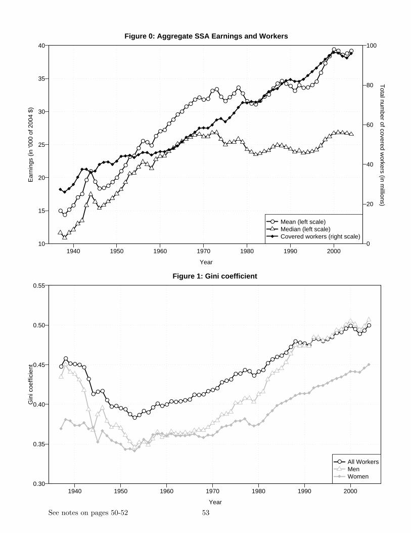
1940 1950 1960 1970 1980 1990 200010

15

20

25

30

35

40

Year

Ear

ning

s (in

'000

of 2

004

$)

●●

●●

●●

●

●

●

● ● ●●

●

●

●

● ●

●

● ●●

●● ●

●●

●●

●●

● ● ● ●

● ●

●●

●●

●

●

●● ●

●● ●

●●

●●

●●

●● ●

●●

●

●

●

● ●● ●

●

0

20

40

60

80

100

Total num

ber of covered workers (in m

illions)

● Mean (left scale)Median (left scale)Covered workers (right scale)

Figure 0: Aggregate SSA Earnings and Workers

1940 1950 1960 1970 1980 1990 20000.30

0.35

0.40

0.45

0.50

0.55

Year

Gin

i coe

ffici

ent

● All WorkersMenWomen

●

●● ● ●

●

●

●● ●

●

● ●● ●

●●

●● ●

●●

● ●● ● ● ● ●

● ● ●● ● ●

● ● ●

● ●● ●

●● ●

●●

● ●●

●

● ● ● ●

● ● ● ● ●● ●

●●

●●

●●

Figure 1: Gini coefficient

See notes on pages 50-52 53

1940 1950 1960 1970 1980 1990 2000

Year

Ear

ning

s S

hare

(%

)

6

10

14

18

22

26

● P20−P40 P60−P80 P80−P90

●●

● ● ●●

●

● ●●

●● ● ● ●

● ● ●● ●

●● ● ● ● ● ● ● ●

● ● ● ● ● ●● ● ● ● ● ● ● ● ● ●

● ● ● ● ● ● ● ● ● ● ● ● ● ● ● ● ● ● ● ● ● ● ●

Figure 2A: Bottom and Middle Earnings Shares

1940 1950 1960 1970 1980 1990 20004

6

8

10

12

14

Year

Ear

ning

s S

hare

(%

)

● P99−P100 P95−P99 P90−P95

●

● ●

●

●

●

●

●●

●●

●●

●●

●

●●

● ●● ●

● ● ●● ●

● ●

● ● ● ● ●●

●●

●●

●

●● ●

● ●

●●

● ●

●

●

●

●●

●

●

●

●

●

●

●●

●

●

●

●●

●

Figure 2B: Upper Earnings Shares

See notes on pages 50-52 54

1980 1985 1990 1995 2000 20050

1

2

3

4

5

6

Year

Ear

ning

s S

hare

(%

)

● P99.9−P100P99.5−P99.9P99−P99.5

● ●● ●

●

●

● ●

●

●

●

●●

●

●

●

●●

●

●

●

●

●

●

●●

●

Figure 2C: Top Earnings Share

1940 1945 1950 19550.4

0.5

0.6

0.7

0.8

0.9

1.0

1.1

Year

Qua

ntile

rat

io (

loga

rithm

ic s

cale

)

●

● ●

●●

●●

●

●

●● ●

● ●●

● ●●

●

●

● log(P50/P10)log(P90/P50)

Figure 3A: Great Compression (White Males)

See notes on pages 50-52 55

1940 1945 1950 19550

5

10

15

20

25

30

Year

Per

cent

●

●●

●

●

●

●

●

●

●

●

●

●

●

● ●

●

●●

● Entry, no exitExit below min wage, no entryBoth entry and exit

Figure 3B: Great Compression: Entry and Exit

1940 1945 1950 19550.5

0.6

0.7

0.8

0.9

1.0

Year

Log(

P50

/P10

)

●

● ●

●

●

●

●

●

●

●● ●

●●

●

● ●●

●

●

● Baseline sampleOver 40 years oldIn sample 1937−1956No entry/exit during war

Figure 3C: Great Compression at the Bottom of the Distribution (White Males) − log(P50/P10)

See notes on pages 50-52 56

1940 1945 1950 19559.5

10.0

10.5

11.0

11.5

12.0

Year

Log

quan

tile

●● ●

● ●●

●

●

●

●● ● ● ●

●●

● ● ● ●

●

Full sampleP10P50P90

Always inP10P50P90

Figure 3D: Great Compression − Quantiles

1980 1985 1990 1995 200030

40

50

60

70

Year

Pro

babi

lity

(%)

● After 1 yearAfter 3 yearsAfter 5 yearsAfter 10 years

●● ●

● ●●

●●

●

●

●

●

●●

●

●●

●●

●● ●

●

●

● ●

Figure 4A: Probability of Staying in Top 0.1%

See notes on pages 50-52 57

1980 1985 1990 1995 2000 20051

2

3

4

5

6

Year

Ear

ning

s S

hare

(%

)

● 1 year3 year average5 year average

● ●● ●

●

●

● ●

●

●

●

●●

●

●

●

●●

●

●

●

●

●

●

●●

●

Figure 4B: Top 0.1% Multi−Year Earnings Share

1960 1970 1980 1990 20000

10

20

30

40

50

Year

Sha

re o

f Top

1%

● Top 1% P95−99 P80−95 P0−80

●

● ●

●

●

● ●

● ●● ● ●

● ● ●●

●

● ●

● ● ●●

●● ●

●

●● ●

● ● ● ● ●●

●

● ●●

●● ● ●

Figure 4C: Source of Top 1% Ten Years Earlier

See notes on pages 50-52 58

1940 1950 1960 1970 1980 1990 200011

12

13

14

15

16

17

18

Year

Ear

ning

s S

hare

(%

)

● 1 year 5 years 11 years

P40−P60

●

●●

● ●●

●

● ● ●

●

● ●●

●

●● ●

● ●

●●

●● ●

● ● ● ●● ●

●● ● ●

●● ●

● ●

●●

●● ●

●●

● ●●

●

● ● ● ●

● ● ●● ●

● ●●

●●

●●

●

P0−P40

●

●

●● ●

●

●

●

●

●

●

● ●●

●

●●

●

●

●

●

●● ●

● ● ● ●●

●● ●

● ●●

●● ●

● ●●

●

●●

●

●

●● ●

●●

● ●● ●

● ●● ● ●

● ●● ● ● ●

●

●

Figure 5A: Bottom Shares (multi−year)

1950 1960 1970 1980 1990 20004

6

8

10

12

14

Year

Ear

ning

s S

hare

(%

)

● 1 year 5 years 11 years

P99−P100●

●

●●

● ●● ●

● ● ●● ●

● ●

● ● ● ● ●●

●●

●●

●

●● ●

● ●

●●

● ●

●

●

●

●●

●

●

●

●

●

●

●●

●

●

●

●●

●

P95−P99

●● ●

● ●●

●●

● ●● ● ● ● ● ●

● ●●

●●

● ●●

● ● ●

●

●● ●

● ● ● ●● ●

● ●● ● ●

● ●● ● ● ● ●

● ● ● ● ●

Figure 5B: Upper Shares (multi−year)

See notes on pages 50-52 59

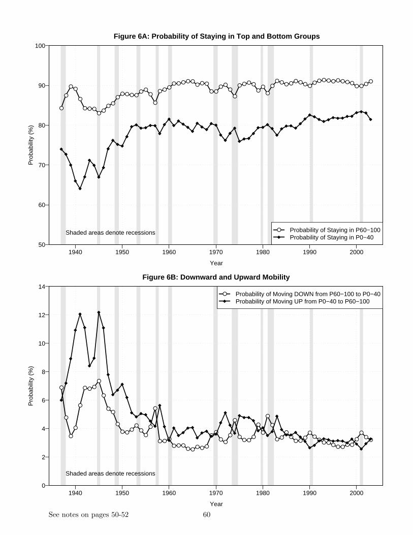
1940 1950 1960 1970 1980 1990 200050

60

70

80

90

100

Year

Pro

babi

lity

(%)

● Probability of Staying in P60−100Probability of Staying in P0−40

●

●

●●

●

● ● ●●

●●

●

●● ● ● ●

● ●●

●

● ● ●● ● ● ● ●

● ● ●

● ●● ●

●

●

● ● ● ●

●●

●

●● ● ● ●

● ● ● ●● ● ● ● ● ● ● ● ●

● ● ●●

Shaded areas denote recessions

Figure 6A: Probability of Staying in Top and Bottom Groups

1940 1950 1960 1970 1980 1990 20000

2

4

6

8

10

12

14

Year

Pro

babi

lity

(%)

● Probability of Moving DOWN from P60−100 to P0−40Probability of Moving UP from P0−40 to P60−100

●

●

●

●

●

● ● ●

●

●

●●

●

● ●●

●●

●

●

●

● ● ●

● ● ●● ●

● ● ●

●●

●●

●

●

●● ●

●

●

●

●

●

● ●●

●● ●

●●

●●

● ●● ● ● ● ●

●

●●

●

Shaded areas denote recessions

Figure 6B: Downward and Upward Mobility

See notes on pages 50-52 60

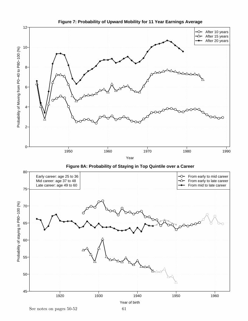
1950 1960 1970 1980 19900

2

4

6

8

10

12

Year

Pro

babi

lity

of M

ovin

g fr

om P

0−40

to P

80−

100

(%)

● After 10 yearsAfter 15 yearsAfter 20 years

●●

●●

●

●

● ●● ●

●●

● ●●

●

● ●●

●● ● ●

●●

● ● ●●

● ● ●● ●

● ● ● ●●

●● ● ● ●

Figure 7: Probability of Upward Mobility for 11 Year Earnings Average

1920 1930 1940 1950 196045

50

55

60

65

70

75

80

Year of birth

Pro

babi

lity

of s

tayi

ng in

P80

−10

0 (%

)

●

●●

●

●

●

● ●

●

●● ●

● ●

●● ●

●

●

● ●●

● ●

● ●● ●

●

●

● ●

●●

● ● ● ●●

● From early to mid careerFrom early to late careerFrom mid to late career

Early career: age 25 to 36Mid career: age 37 to 48Late career: age 49 to 60

Figure 8A: Probability of Staying in Top Quintile over a Career

See notes on pages 50-52 61

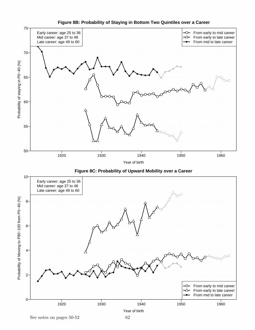
1920 1930 1940 1950 196050

55

60

65

70

75

Year of birth

Pro

babi

lity

of s

tayi

ng in

P0−

40 (

%)

● ●

●●

● ●● ●

●

●

●

●

● ● ● ●

●● ● ●

● ●● ● ● ●

●●

● ●●

●● ●

●

●●

●

●

● From early to mid careerFrom early to late careerFrom mid to late career

Early career: age 25 to 36Mid career: age 37 to 48Late career: age 49 to 60

Figure 8B: Probability of Staying in Bottom Two Quintiles over a Career

1920 1930 1940 1950 19600

2

4

6

8

10

Year of birth

Pro

babi

lity

of M

ovin

g to

P80

−10

0 fr

om P

0−40

(%

)

● From early to mid careerFrom early to late careerFrom mid to late career

Early career: age 25 to 36Mid career: age 37 to 48Late career: age 49 to 60

●

● ●● ● ●

● ●

●●

● ●

●●

●

●

●

●

●●

●

●

●

●●

●●

●

●● ●

●●

●

●

● ●●

●

Figure 8C: Probability of Upward Mobility over a Career

See notes on pages 50-52 62

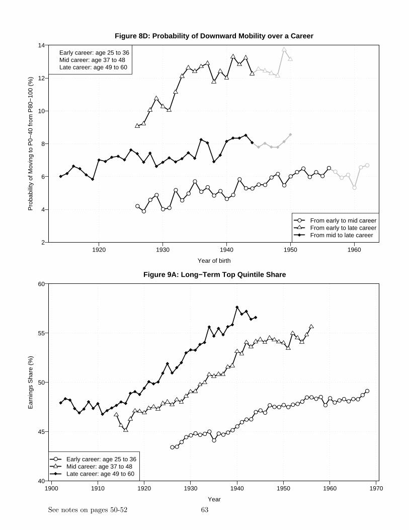
1920 1930 1940 1950 19602

4

6

8

10

12

14

Year of birth

Pro

babi

lity

of M

ovin

g to

P0−

40 fr

om P

80−

100

(%)

● From early to mid careerFrom early to late careerFrom mid to late career

Early career: age 25 to 36Mid career: age 37 to 48Late career: age 49 to 60

●

●●

●●

●

● ●

●●

●●

● ●

●

●

●

●

●●

●●

●●

●

● ●● ●

●●

●

●●

●

●●

●

●

Figure 8D: Probability of Downward Mobility over a Career

1900 1910 1920 1930 1940 1950 1960 197040

45

50

55

60

Year

Ear

ning

s S

hare

(%

)

● Early career: age 25 to 36Mid career: age 37 to 48Late career: age 49 to 60

●

●

● ●●

● ● ● ● ●●

●

● ● ●●

●●

● ●

● ●●

● ● ● ● ●● ●

●● ● ● ●

●

●● ● ●

●● ●

●●

Figure 9A: Long−Term Top Quintile Share

See notes on pages 50-52 63

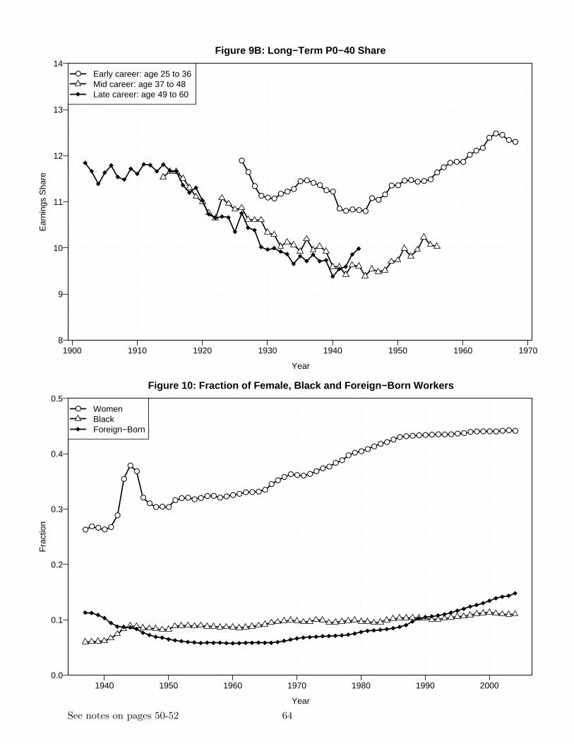
1900 1910 1920 1930 1940 1950 1960 19708

9

10

11

12

13

14

Year

Ear

ning

s S

hare

● Early career: age 25 to 36Mid career: age 37 to 48Late career: age 49 to 60

●

●

●

●

●

● ● ●● ● ●

● ● ● ●● ●

● ● ● ● ●

● ●●

● ●● ● ● ● ●

●●

● ● ●●

● ●

●● ●

● ●

Figure 9B: Long−Term P0−40 Share

1940 1950 1960 1970 1980 1990 20000.0

0.1

0.2

0.3

0.4

0.5

Year

Fra

ctio

n

● WomenBlackForeign−Born

●● ● ● ●

●

●

●●

●●

● ● ●● ● ● ● ● ● ● ● ● ● ● ● ● ● ●

●●

● ● ● ● ● ● ● ●● ●

● ● ● ● ● ● ● ● ● ● ● ● ● ● ● ● ● ● ● ● ● ● ● ● ● ● ●

Figure 10: Fraction of Female, Black and Foreign−Born Workers

See notes on pages 50-52 64

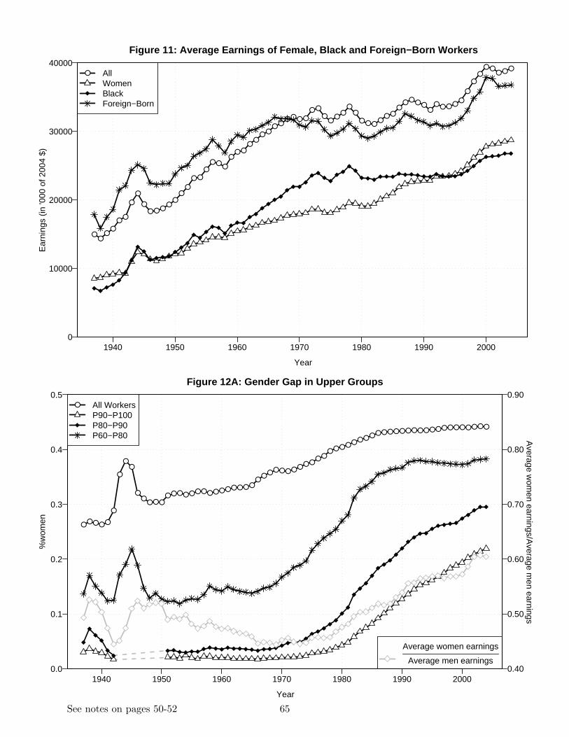
1940 1950 1960 1970 1980 1990 20000

10000

20000

30000

40000

Year

Ear

ning

s (in

'000

of 2

004

$)

● AllWomenBlackForeign−Born

●●

●●

●●

●

●

●● ● ●

●●

●●

● ●

●● ●

●

●● ●

●●

● ●● ●

● ● ● ●

● ●

●●

●●

●●

● ● ●●

● ●●

● ● ● ●●

● ● ● ●●

●

●●

● ●● ● ●

Figure 11: Average Earnings of Female, Black and Foreign−Born Workers

1940 1950 1960 1970 1980 1990 20000.0

0.1

0.2

0.3

0.4

0.5

Year

%w

omen

Average women earnings

Average men earnings

● All WorkersP90−P100P80−P90P60−P80

●● ● ● ●

●

●

●●

●●

● ● ●● ● ● ● ● ● ● ● ● ● ● ● ● ● ●

●●

● ● ● ● ● ● ● ●● ●

● ● ● ● ● ● ● ● ● ● ● ● ● ● ● ● ● ● ● ● ● ● ● ● ● ● ●

0.40

0.50

0.60

0.70

0.80

0.90

Average w

omen earnings/A

verage men earnings

Figure 12A: Gender Gap in Upper Groups

See notes on pages 50-52 65

1950 1960 1970 1980 1990 20000.00

0.05

0.10

0.15

0.20

0.25

Year

%w

omen

● P99.9−P100P99−P100P95−P99P90−P95

● ●● ● ● ●

●

●● ● ●

●

●

● ● ● ●

●

●

●

●

●●

●●

●

●

Figure 12B: Gender Gap in Top Groups

1940 1950 1960 1970 1980 1990 20000.0

0.2

0.4

0.6

0.8

1.0

Year

%bl

ack/

%bl

ack

in p

opul

atio

n

Average black earnings

Average white earnings

● All WorkersP90−P100P80−P90P60−P80

●● ● ●

●

●

●

● ●

● ● ●● ●

● ● ●● ●

● ●● ● ●

● ● ●●

●

● ●●

●●

● ●●

●

● ● ● ● ●●

●● ●

●● ● ● ●

● ●● ● ● ● ● ●

●● ● ●

●● ● ●

0.40

0.50

0.60

0.70

0.80

0.90

Average black earnings/A

verage white earnings

Figure 13A: Black−White Gap in Upper Groups

See notes on pages 50-52 66

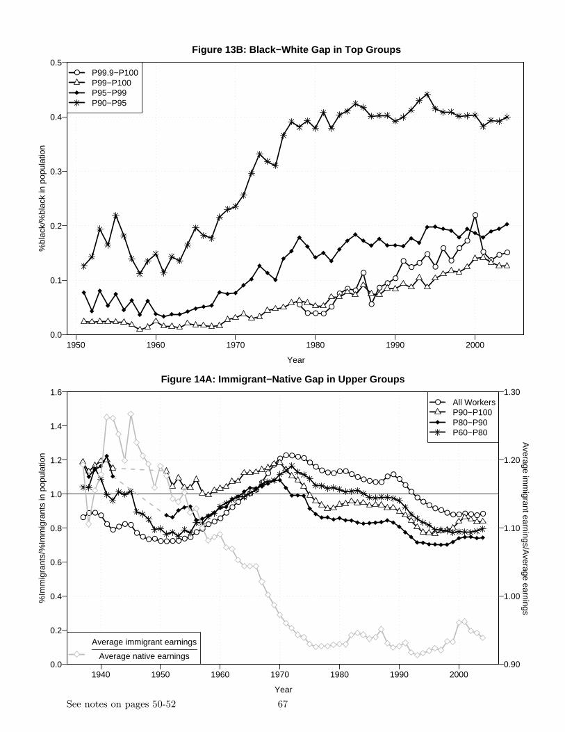
1950 1960 1970 1980 1990 20000.0

0.1

0.2

0.3

0.4

0.5

Year

%bl

ack/

%bl

ack

in p

opul

atio

n

● P99.9−P100P99−P100P95−P99P90−P95

●

● ● ●●

●● ●

●

●

●●

●

●●

●

●

●

●

●

●●

●

●

●● ●

Figure 13B: Black−White Gap in Top Groups

1940 1950 1960 1970 1980 1990 2000

Year

%Im

mig

rant

s/%

Imm

igra

nts

in p

opul

atio

n

0.0

0.2

0.4

0.6

0.8

1.0

1.2

1.4

1.6

Average immigrant earnings

Average native earnings

● All WorkersP90−P100P80−P90P60−P80

●● ● ●

●●

● ● ●

●● ● ● ● ● ● ● ● ●

●●

● ●●

●●

●●

●●

●

●

●●

● ● ● ●●

●● ● ● ● ● ● ● ● ● ● ●

● ●●

●●

●●

●● ● ● ● ● ● ● ● ●

0.90

1.00

1.10

1.20

1.30

Average im

migrant earnings/A

verage earnings

Figure 14A: Immigrant−Native Gap in Upper Groups

See notes on pages 50-52 67

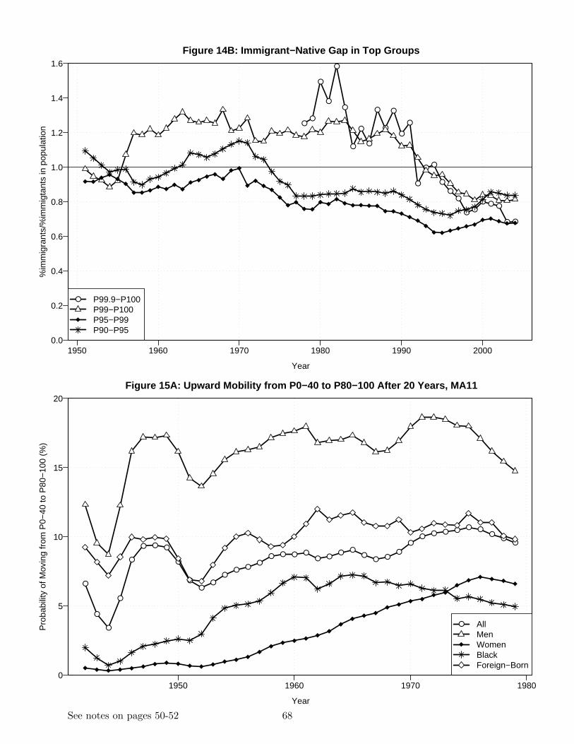
1950 1960 1970 1980 1990 2000

Year

%im

mig

rant

s/%

imm

igta

nts

in p

opul

atio

n

0.0

0.2

0.4

0.6

0.8

1.0

1.2

1.4

1.6

● P99.9−P100P99−P100P95−P99P90−P95

●●

●

●

●

●

●

●

●

●

●

●

●

●

●

● ●

●

●●

● ●

● ● ●

● ●

Figure 14B: Immigrant−Native Gap in Top Groups

1950 1960 1970 19800

5

10

15

20

Year

Pro

babi

lity

of M

ovin

g fr

om P

0−40

to P

80−

100

(%)

● AllMenWomenBlackForeign−Born

●

●

●

●

●

● ● ●

●

●●

●●

● ●●

● ● ● ●● ●

● ●●

● ●●

●●

● ● ● ● ●●

●●

Figure 15A: Upward Mobility from P0−40 to P80−100 After 20 Years, MA11

See notes on pages 50-52 68

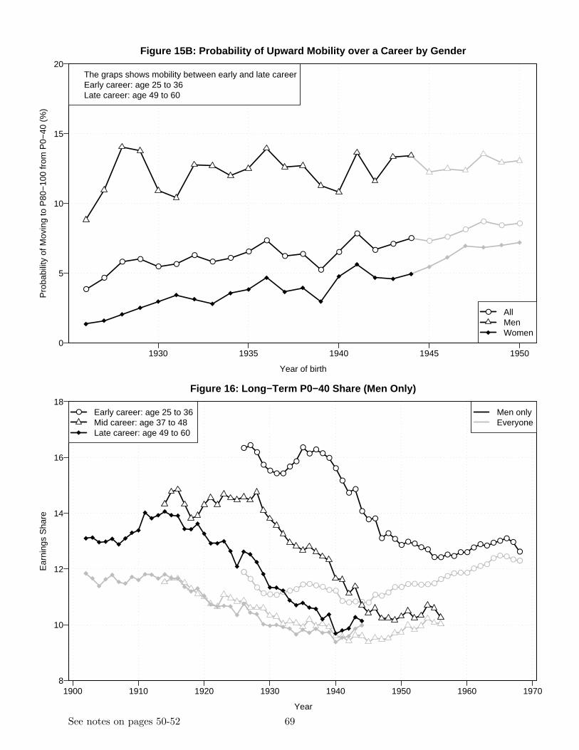
1930 1935 1940 1945 19500

5

10

15

20

Year of birth

Pro

babi

lity

of M

ovin

g to

P80

−10

0 fr

om P

0−40

(%

)

● AllMenWomen

The graps shows mobility between early and late careerEarly career: age 25 to 36Late career: age 49 to 60

●

● ●●

●

●● ●

●

●

● ●● ●

●●

●●

●

● ●

●

●

●

●●

●

Figure 15B: Probability of Upward Mobility over a Career by Gender

1900 1910 1920 1930 1940 1950 1960 19708

10

12

14

16

18

Year

Ear

ning

s S

hare

● Early career: age 25 to 36Mid career: age 37 to 48Late career: age 49 to 60

Men onlyEveryone

●

●

●●

●● ● ● ● ● ●

● ● ● ● ● ●

● ● ● ● ●

● ●●

● ● ● ● ● ● ●●

● ● ● ●● ● ●

● ● ● ● ●

●

●

● ●●

●● ● ●

●●

●●

●●

●

●

●

●●

●

● ●

●●

●●

● ●● ●

● ● ● ●● ●

●● ● ● ● ●

●

●

Figure 16: Long−Term P0−40 Share (Men Only)

See notes on pages 50-52 69

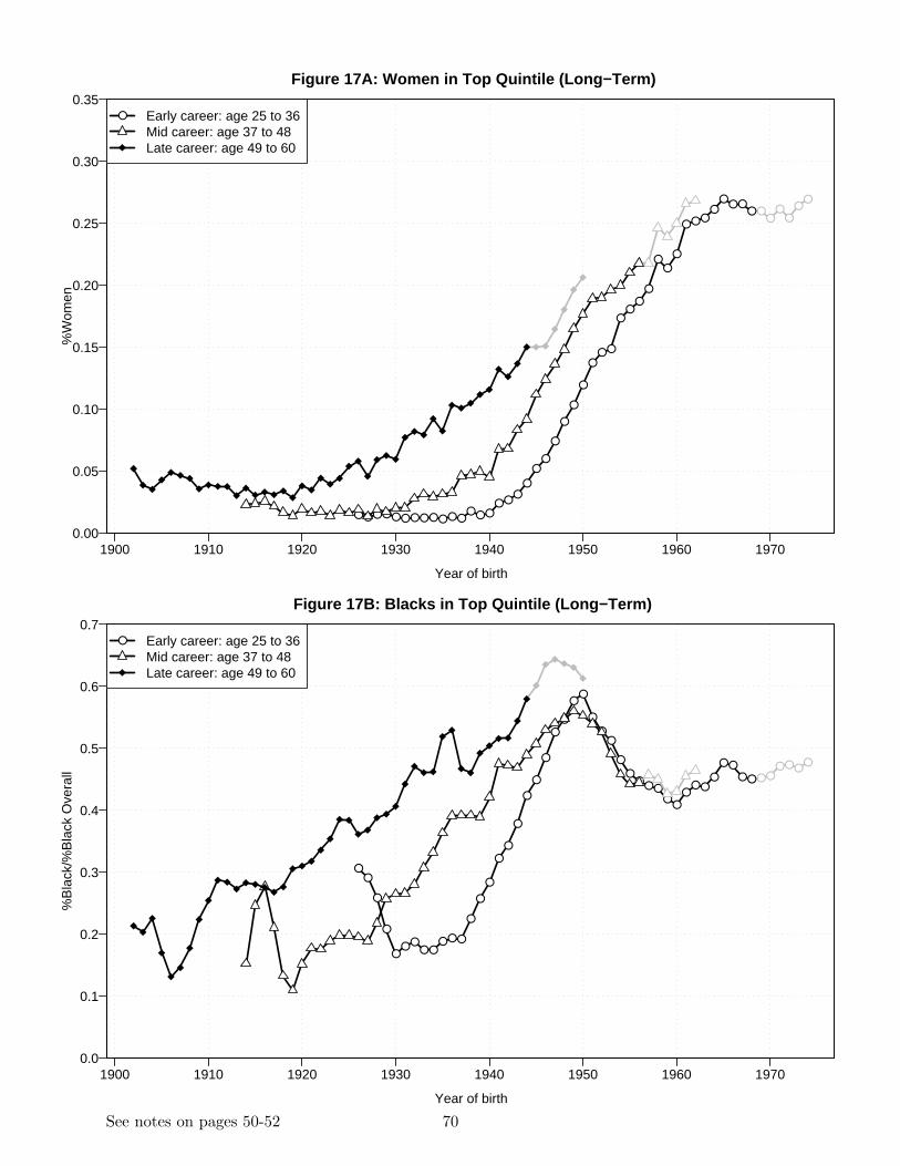
1900 1910 1920 1930 1940 1950 1960 19700.00

0.05

0.10

0.15

0.20

0.25

0.30

0.35

Year of birth

%W

omen

● Early career: age 25 to 36Mid career: age 37 to 48Late career: age 49 to 60

●

● ●●

●●

●●

● ● ● ● ● ● ● ● ● ● ● ●● ● ●

● ●●

●

●●

●

●

●

●

●● ●

●●

●

●

●●

●

● ● ●●

●● ●

●

Figure 17A: Women in Top Quintile (Long−Term)

1900 1910 1920 1930 1940 1950 1960 19700.0

0.1

0.2

0.3

0.4

0.5

0.6

0.7

Year of birth

%B

lack

/%B

lack

Ove

rall

● Early career: age 25 to 36Mid career: age 37 to 48Late career: age 49 to 60

●

● ● ●● ● ●

●

●●

●

●

●● ●

● ●● ● ●

●

●

●

●

●

●

●

●

●

●

●

●●

●

●●

●

●● ● ●

●●

●● ●

●

● ●● ●

Figure 17B: Blacks in Top Quintile (Long−Term)

See notes on pages 50-52 70

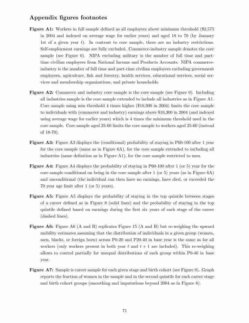
Appendix figures footnotes

Figure A1: Workers in full sample defined as all employees above minimum threshold ($2,575in 2004 and indexed on average wage for earlier years) and aged 18 to 70 (by January1st of a given year t). In contrast to core sample, there are no industry restrictions.Self-employment earnings are fully excluded. Commerce-industry sample denotes the coresample (see Figure 0). NIPA excluding military is the number of full time and part-time civilian employees from National Income and Products Accounts. NIPA commerce-industry is the number of full time and part-time civilian employees excluding governmentemployees, agriculture, fish and forestry, health services, educational services, social ser-vices and membership organizations, and private households.

Figure A2: Commerce and industry core sample is the core sample (see Figure 0). Includingall industries sample is the core sample extended to include all industries as in Figure A1.Core sample using min threshold 4 times higher ($10,300 in 2004) limits the core sampleto individuals with (commerce and industry) earnings above $10,300 in 2004 (and indexedusing average wage for earlier years) which is 4 times the minimum threshold used in thecore sample. Core sample aged 25-60 limits the core sample to workers aged 25-60 (insteadof 18-70).

Figure A3: Figure A3 displays the (conditional) probability of staying in P60-100 after 1 yearfor the core sample (same as in Figure 6A), for the core sample extended to including allindustries (same definition as in Figure A1), for the core sample restricted to men.

Figure A4: Figure A4 displays the probability of staying in P60-100 after 1 (or 5) year for thecore sample conditional on being in the core sample after 1 (or 5) years (as in Figure 6A)and unconditional (the individual can then have no earnings, have died, or exceeded the70 year age limit after 1 (or 5) years).

Figure A5: Figure A5 displays the probability of staying in the top quintile between stagesof a career defined as in Figure 8 (solid lines) and the probability of staying in the topquintile defined based on earnings during the first six years of each stage of the career(dashed lines).

Figure A6: Figure A6 (A and B) replicates Figure 15 (A and B) but re-weighing the upwardmobility estimates assuming that the distribution of individuals in a given group (women,men, blacks, or foreign born) across P0-20 and P20-40 in base year is the same as for allworkers (only workers present in both year t and t + 1 are included). This re-weighingallows to control partially for unequal distributions of each group within P0-40 in baseyear.

Figure A7: Sample is career sample for each given stage and birth cohort (see Figure 8). Graphreports the fraction of women in the sample and in the second quintile for each career stageand birth cohort groups (smoothing and imputations beyond 2004 as in Figure 8).

71

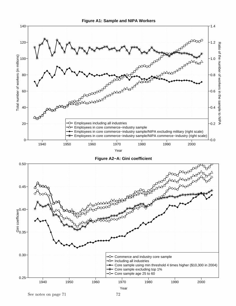
1940 1950 1960 1970 1980 1990 2000

Year

Tot

al n

umbe

r of

wor

kers

(in

mill

ions

)

0

20

40

60

80

100

120

140

● ●●

●●

● ●● ●

● ● ● ●●

● ● ● ●●

●● ● ● ● ● ● ●

●●

●●

●● ● ●

●● ● ●

●●

●● ● ● ● ●

●● ●

●●

● ● ● ● ●●

●●

●●

●● ● ● ●

●

0.0

0.2

0.4

0.6

0.8

1.0

1.2

1.4

Ratio of the num

ber of workers in the sam

ple to NIP

A

● Employees including all industriesEmployees in core commerce−industry sampleEmployees in core commerce−industry sample/NIPA excluding military (right scale)Employees in core commerce−industry sample/NIPA commerce−industry (right scale)

Figure A1: Sample and NIPA Workers

1940 1950 1960 1970 1980 1990 20000.25

0.30

0.35

0.40

0.45

0.50

Year

Gin

i coe

ffici

ent

● Commerce and industry core sampleIncluding all industriesCore sample using min threshold 4 times higher ($10,300 in 2004)Core sample excluding top 1%Core sample age 25 to 60

●

●● ● ●

●

●

●● ●

●

● ●● ●

●●

●● ●

●●

● ●● ● ● ● ●

● ● ●● ● ●

● ● ●

● ●● ●

●● ●

●●

● ●●

●

● ● ● ●

● ● ● ● ●● ●

●●

●●

●●

Figure A2−A: Gini coefficient

See notes on page 71 72

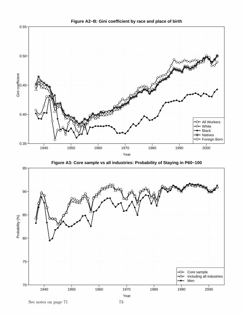
1940 1950 1960 1970 1980 1990 20000.35

0.40

0.45

0.50

0.55

Year

Gin

i coe

ffici

ent

●

●

● ● ●●

●

●● ●

●

● ●● ●

●●

●● ●

●●

● ●● ● ● ● ●

● ● ●● ● ●

● ● ●

● ●● ●

●● ●

●●

● ●●

●

● ● ● ●

● ●●

●●

● ●●

●●

●●

●

● All WorkersWhiteBlackNativesForeign Born

Figure A2−B: Gini coefficient by race and place of birth

1940 1950 1960 1970 1980 1990 200070

75

80

85

90

95

Year

Pro

babi

lity

(%)

● Core sampleIncluding all industriesMen

●

●

●●

●

● ● ●

●●

●●

●

● ●● ●

●●

●

●

●●

●

● ●●

● ●

● ●●

● ●

●●

●

●

●●

●●

●●

●

●

●●

●●

● ●●

●

●● ● ● ● ● ● ● ●

● ●●

●

Figure A3: Core sample vs all industries: Probability of Staying in P60−100

See notes on page 71 73

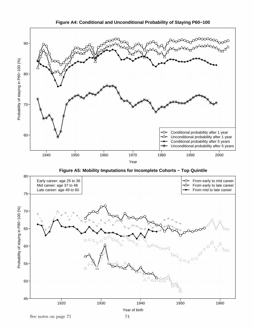
1940 1950 1960 1970 1980 1990 2000

60

70

80

90

Year

Pro

babi

lity

of s

tayi

ng in

P60

−10

0 (%

)

● Conditional probability after 1 yearUnconditional probability after 1 yearConditional probability after 5 yearsUnconditional probability after 5 years

●

●

●●

●

● ● ●●

●

●●

●

● ● ● ●●

●●

●

●●

●● ● ● ● ●

● ● ●

● ●

● ●●

●

● ● ●●

●●

●

●● ● ● ● ● ● ● ●

● ● ● ● ● ● ● ● ●● ● ● ●

Figure A4: Conditional and Unconditional Probability of Staying P60−100

1920 1930 1940 1950 196045

50

55

60

65

70

75

80

Year of birth

Pro

babi

lity

of s

tayi

ng in

P80

−10

0 (%

)

●

●●

●

●

●

● ●

●

●● ●

● ●

●● ●

●

●

● ●●

● ●

● ●● ●

●

●

● ●

●●

● ● ● ●●

●● ● ●●

●●

●● ●

●

●

●●

●

●●

●● ●

● ● ●

● ●

● ● ●● ●

●

●●

●

●

●

● ●

● From early to mid careerFrom early to late careerFrom mid to late career

Early career: age 25 to 36Mid career: age 37 to 48Late career: age 49 to 60

Figure A5: Mobility Imputations for Incomplete Cohorts − Top Quintile

See notes on page 71 74

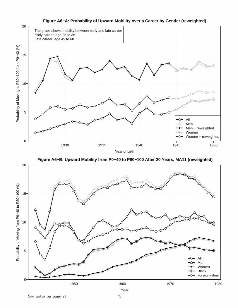
1930 1935 1940 1945 19500

5

10

15

20

Year of birth

Pro

babi

lity

of M

ovin

g to

P80

−10

0 fr

om P

0−40

(%

)

● AllMenMen − reweightedWomenWomen − reweighted

The graps shows mobility between early and late careerEarly career: age 25 to 36Late career: age 49 to 60

●

● ●●

●

●● ●

●

●

● ●● ●

●●

●●

●

● ●

●

●

●

●●

●

Figure A6−A: Probability of Upward Mobility over a Career by Gender (reweighted)

1950 1960 1970 19800

5

10

15

20

Year

Pro

babi

lity

of M

ovin

g fr

om P

0−40

to P

80−

100

(%)

● AllMenWomenBlackForeign−Born

●

●

●

●

●

● ● ●

●

●●

●●

● ●●

● ● ● ●● ●

● ●●

● ●●

●●

● ● ● ● ●●

●●

Figure A6−B: Upward Mobility from P0−40 to P80−100 After 20 Years, MA11 (reweighted)

See notes on page 71 75

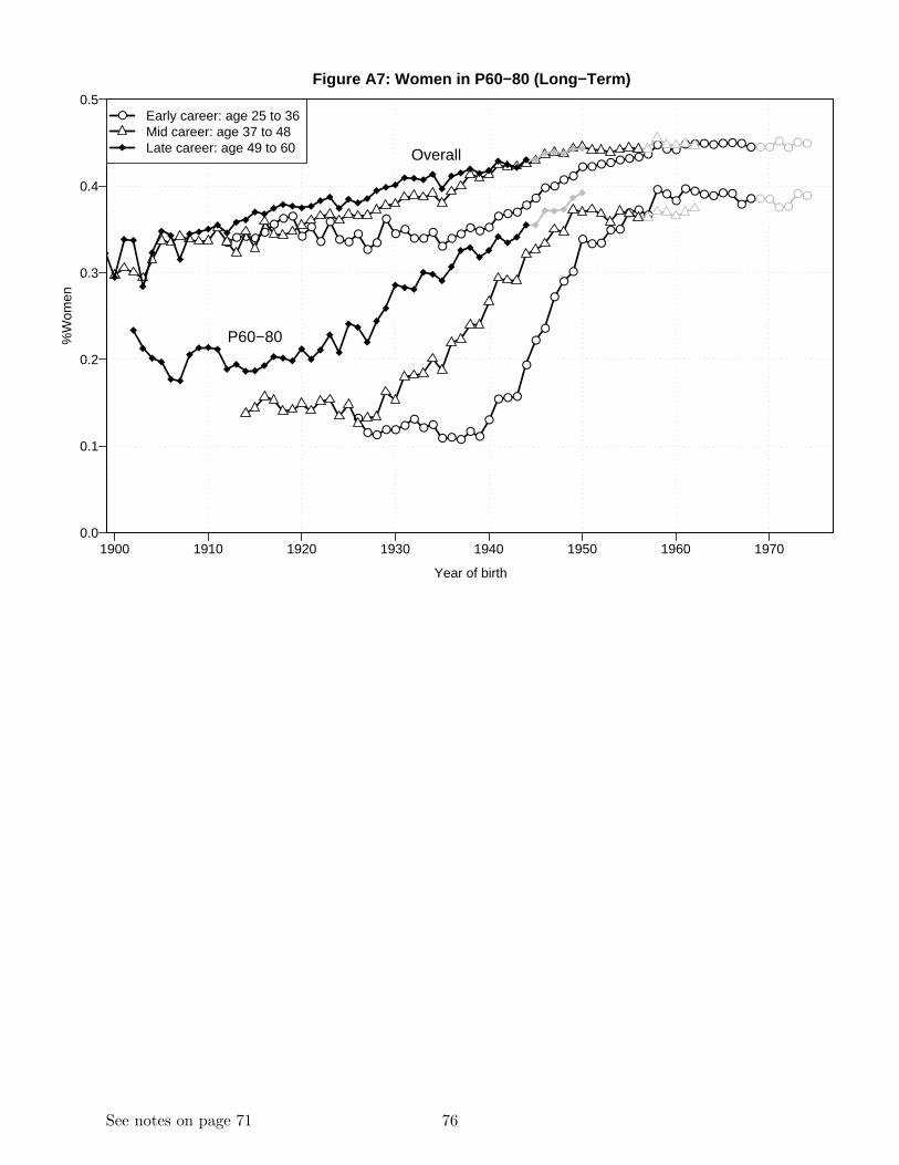
1900 1910 1920 1930 1940 1950 1960 19700.0

0.1

0.2

0.3

0.4

0.5

Year of birth

%W

omen

● Early career: age 25 to 36Mid career: age 37 to 48Late career: age 49 to 60

●

● ● ●●

●● ●

●● ● ●

●●

● ●

●●

●

●

● ●●

●●

●

● ●● ●

●

●● ●

● ● ●● ● ●

●●

● ●● ●

● ● ● ● ● ● ● ●● ● ●

● ● ● ● ● ● ● ●Overall

●

● ● ●● ●

● ●

●

● ●● ● ●

●● ●

● ● ●●

●

●

● ● ●

●

●●

●

●●

● ● ●

● ●

● ●●

● ●●

● ● ● ● ● ●●

●

P60−80

Figure A7: Women in P60−80 (Long−Term)

See notes on page 71 76

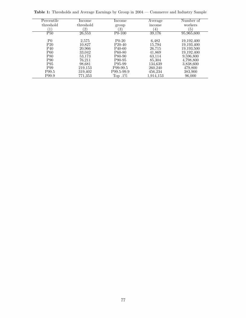
Table 1: Thresholds and Average Earnings by Group in 2004 — Commerce and Industry Sample

Percentilethreshold

Incomethreshold

Incomegroup

Averageincome

Number ofworkers

(1) (2) (3) (4) (5)P50 26,553 P0-100 39,176 95,965,600

P0 2,575 P0-20 6,482 19,192,400P20 10,827 P20-40 15,794 19,193,400P40 20,966 P40-60 26,715 19,193,500P60 33,042 P60-80 41,869 19,192,400P80 53,173 P80-90 63,114 9,596,800P90 76,211 P90-95 85,304 4,798,800P95 98,681 P95-99 134,639 3,838,600P99 219,153 P99-99.5 260,240 479,800

P99.5 319,402 P99.5-99.9 456,234 383,900P99.9 771,353 Top .1% 1,914,153 96,000

77

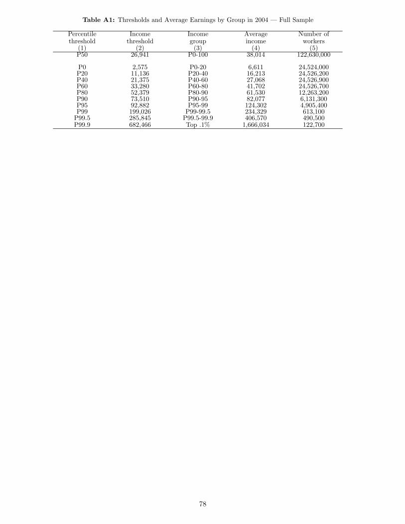
Table A1: Thresholds and Average Earnings by Group in 2004 — Full Sample

Percentilethreshold

Incomethreshold

Incomegroup

Averageincome

Number ofworkers

(1) (2) (3) (4) (5)P50 26,941 P0-100 38,014 122,630,000

P0 2,575 P0-20 6,611 24,524,000P20 11,136 P20-40 16,213 24,526,200P40 21,375 P40-60 27,068 24,526,900P60 33,280 P60-80 41,702 24,526,700P80 52,379 P80-90 61,530 12,263,200P90 73,510 P90-95 82,077 6,131,300P95 92,882 P95-99 124,302 4,905,400P99 199,026 P99-99.5 234,329 613,100

P99.5 285,845 P99.5-99.9 406,570 490,500P99.9 682,466 Top .1% 1,666,034 122,700

78

Table A2: Aggregate Statistics and the Number of Observations

Year workers(core, no

min)

workers(all in-

dustries)

workers(core

sample)

Average(2004 $)

Median(2004 $)

GiniMA1

GiniMA5

Tax max(nominal

$)

%Abovetax max

%Above4*taxmax

(1) (2) (3) (4) (5) (6) (7) (8) (9) (10) (11)1937 30,850 27,395 27,395 14,968 11,656 0.448 3,000 3.611938 29,840 26,031 26,031 14,354 10,874 0.458 3,000 3.521939 31,661 27,771 27,771 15,136 11,642 0.451 0.441 3,000 3.631940 34,041 29,885 29,885 15,789 12,133 0.451 0.437 3,000 4.021941 37,782 33,531 33,531 17,000 13,032 0.450 0.444 3,000 5.441942 42,480 37,524 37,524 17,514 13,477 0.447 0.444 3,000 9.561943 42,618 37,575 37,575 19,629 15,785 0.432 0.433 3,000 15.741944 40,675 36,008 36,008 20,942 17,468 0.413 0.416 3,000 19.481945 42,013 36,630 36,630 19,369 16,339 0.416 0.412 3,000 17.351946 45,058 39,975 39,975 18,336 15,388 0.417 0.408 3,000 16.06 0.481947 45,534 41,028 41,028 18,427 15,830 0.405 0.401 3,000 23.15 0.611948 45,579 41,226 41,226 18,755 16,358 0.397 0.397 3,000 28.75 0.651949 44,213 39,976 39,976 19,313 16,851 0.398 0.382 3,000 28.97 0.711950 45,766 41,604 41,604 19,977 17,553 0.395 0.384 3,000 32.88 0.691951 47,817 45,808 44,052 20,965 18,210 0.394 0.392 3,600 28.94 0.641952 47,853 46,716 44,273 21,872 19,272 0.388 0.387 3,600 33.26 0.701953 48,064 47,675 44,567 23,170 20,582 0.383 0.384 3,600 37.64 0.781954 47,102 46,964 43,469 23,288 20,683 0.387 0.376 3,600 38.34 0.941955 48,493 49,721 44,864 24,445 21,577 0.392 0.384 4,200 31.77 0.611956 49,661 52,043 46,021 25,526 22,392 0.390 0.392 4,200 34.99 0.731957 49,998 55,115 45,985 25,348 21,989 0.396 0.393 4,200 36.46 0.781958 48,999 54,336 44,740 24,861 21,398 0.401 0.389 4,200 36.68 0.841959 49,936 55,831 45,876 26,274 22,759 0.398 0.396 4,800 32.36 0.671960 50,544 56,882 46,475 27,012 23,230 0.400 0.398 4,800 34.86 0.781961 50,540 57,359 46,388 27,204 23,284 0.404 0.395 4,800 36.08 0.821962 51,521 58,892 47,377 28,148 23,962 0.403 0.399 4,800 38.38 0.881963 52,313 59,946 48,072 28,760 24,457 0.404 0.399 4,800 40.14 0.961964 53,711 61,529 49,320 29,552 25,094 0.405 0.398 4,800 42.18 1.081965 55,888 64,043 51,370 29,982 25,436 0.406 0.401 4,800 43.89 1.171966 58,259 67,247 53,668 30,745 25,779 0.412 0.406 6,600 29.46 0.631967 59,294 69,253 54,699 31,163 26,088 0.412 0.406 6,600 31.51 0.701968 60,979 71,359 56,262 31,798 26,460 0.413 0.410 7,800 25.54 0.531969 63,144 73,746 58,298 32,109 26,574 0.417 0.415 7,800 29.05 0.651970 63,595 74,250 58,449 31,789 26,227 0.418 0.412 7,800 31.13 0.751971 63,797 74,283 58,327 31,908 26,223 0.420 0.410 7,800 33.82 0.831972 65,673 76,031 59,919 33,124 26,801 0.428 0.417 9,000 29.79 0.741973 68,251 78,549 62,428 33,369 26,824 0.430 0.428 10,800 24.12 0.581974 68,996 79,982 63,131 32,217 25,806 0.431 0.429 13,200 17.62 0.441975 67,668 79,177 61,520 31,576 24,981 0.438 0.422 14,100 17.80 0.501976 69,660 81,467 63,560 32,148 25,325 0.439 0.430 15,300 17.90 0.461977 72,047 84,131 65,900 32,712 25,350 0.443 0.434 16,500 18.15 0.501978 74,186 87,318 68,732 33,611 25,820 0.442 0.438 17,700 18.81 0.511979 76,554 89,947 71,194 32,723 25,378 0.436 0.439 22,900 12.02 0.321980 76,701 90,574 71,038 31,552 24,249 0.441 0.437 25,900 10.91 0.331981 77,513 91,133 71,721 31,194 23,888 0.443 0.440 29,700 9.50 0.291982 77,639 90,022 71,408 31,076 23,497 0.452 0.442 32,400 8.74 0.311983 78,310 90,571 71,882 31,618 23,655 0.457 0.445 35,700 7.77 0.281984 81,227 93,570 74,612 32,245 23,946 0.460 0.456 37,800 7.71 0.301985 83,662 96,018 76,722 32,559 24,113 0.461 0.461 39,600 7.71 0.301986 84,893 97,422 77,768 33,470 24,666 0.465 0.465 42,000 7.26 0.321987 85,362 99,485 78,234 34,228 24,932 0.472 0.466 43,800 7.25 0.401988 87,996 102,741 80,702 34,613 24,837 0.479 0.472 45,000 7.56 0.451989 89,644 104,982 82,278 34,212 24,596 0.478 0.475 48,000 7.09 0.431990 90,078 106,169 82,828 33,858 24,334 0.477 0.476 51,300 6.50 0.411991 89,294 105,707 81,884 33,130 23,865 0.475 0.474 53,400 6.40 0.371992 89,414 105,952 81,828 33,973 24,052 0.483 0.474 55,500 6.48 0.421993 90,827 107,215 82,933 33,587 23,734 0.482 0.476 57,600 6.29 0.391994 92,748 109,400 84,825 33,646 23,852 0.480 0.479 60,600 6.08 0.361995 94,842 111,329 86,804 33,995 23,941 0.482 0.480 61,200 6.48 0.401996 96,703 113,146 88,624 34,520 24,201 0.485 0.481 62,700 6.77 0.431997 99,006 115,584 90,976 35,865 24,816 0.490 0.485 65,400 6.91 0.451998 101,077 117,980 93,064 37,290 25,750 0.491 0.488 68,400 7.04 0.471999 102,992 120,005 94,897 38,375 26,237 0.496 0.490 72,600 6.85 0.472000 104,735 121,912 96,481 39,400 26,720 0.499 0.491 76,200 7.76 0.542001 104,766 122,082 96,164 39,177 26,811 0.495 0.490 80,400 6.68 0.442002 103,500 121,076 94,600 38,564 26,776 0.489 0.489 84,900 5.98 0.372003 102,780 120,880 93,695 38,787 26,707 0.493 87,000 6.14 0.382004 105,637 122,630 95,966 39,176 26,553 0.500 87,900 6.48 0.42

0.1% sample from 1937 to 1956, 1% from 1957 to 2004. Number of workers in thousands.

79

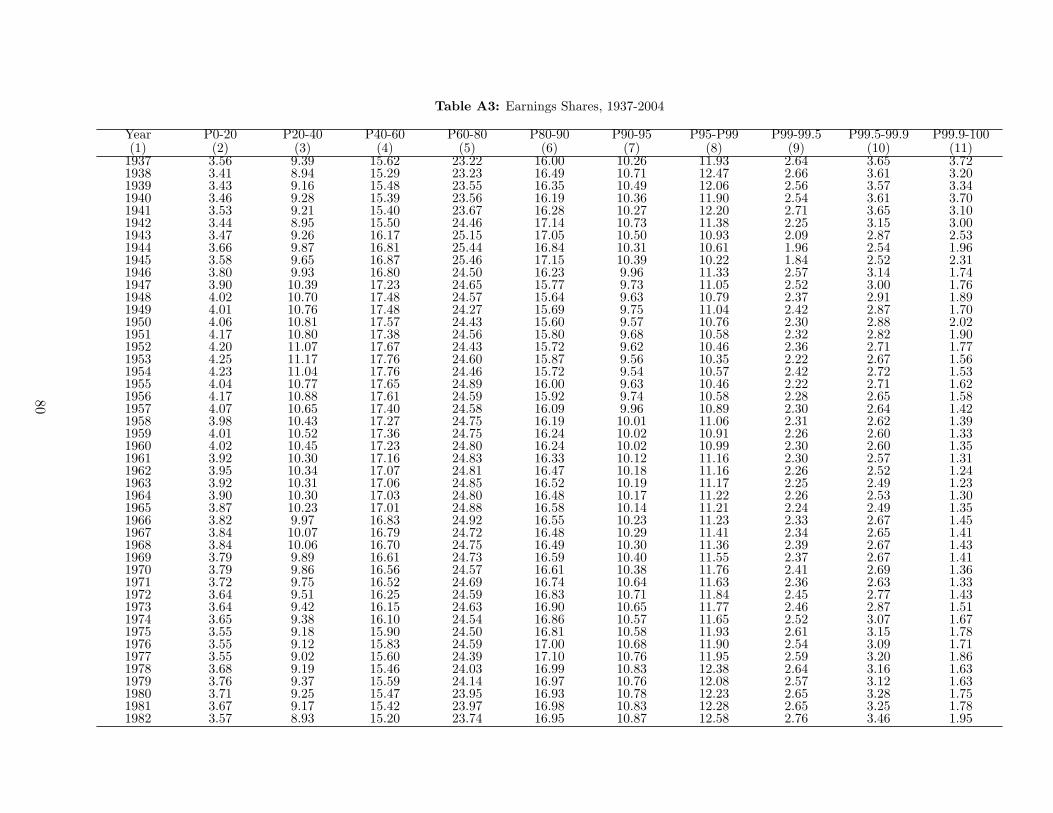
Table A3: Earnings Shares, 1937-2004

Year P0-20 P20-40 P40-60 P60-80 P80-90 P90-95 P95-P99 P99-99.5 P99.5-99.9 P99.9-100(1) (2) (3) (4) (5) (6) (7) (8) (9) (10) (11)

1937 3.56 9.39 15.62 23.22 16.00 10.26 11.93 2.64 3.65 3.721938 3.41 8.94 15.29 23.23 16.49 10.71 12.47 2.66 3.61 3.201939 3.43 9.16 15.48 23.55 16.35 10.49 12.06 2.56 3.57 3.341940 3.46 9.28 15.39 23.56 16.19 10.36 11.90 2.54 3.61 3.701941 3.53 9.21 15.40 23.67 16.28 10.27 12.20 2.71 3.65 3.101942 3.44 8.95 15.50 24.46 17.14 10.73 11.38 2.25 3.15 3.001943 3.47 9.26 16.17 25.15 17.05 10.50 10.93 2.09 2.87 2.531944 3.66 9.87 16.81 25.44 16.84 10.31 10.61 1.96 2.54 1.961945 3.58 9.65 16.87 25.46 17.15 10.39 10.22 1.84 2.52 2.311946 3.80 9.93 16.80 24.50 16.23 9.96 11.33 2.57 3.14 1.741947 3.90 10.39 17.23 24.65 15.77 9.73 11.05 2.52 3.00 1.761948 4.02 10.70 17.48 24.57 15.64 9.63 10.79 2.37 2.91 1.891949 4.01 10.76 17.48 24.27 15.69 9.75 11.04 2.42 2.87 1.701950 4.06 10.81 17.57 24.43 15.60 9.57 10.76 2.30 2.88 2.021951 4.17 10.80 17.38 24.56 15.80 9.68 10.58 2.32 2.82 1.901952 4.20 11.07 17.67 24.43 15.72 9.62 10.46 2.36 2.71 1.771953 4.25 11.17 17.76 24.60 15.87 9.56 10.35 2.22 2.67 1.561954 4.23 11.04 17.76 24.46 15.72 9.54 10.57 2.42 2.72 1.531955 4.04 10.77 17.65 24.89 16.00 9.63 10.46 2.22 2.71 1.621956 4.17 10.88 17.61 24.59 15.92 9.74 10.58 2.28 2.65 1.581957 4.07 10.65 17.40 24.58 16.09 9.96 10.89 2.30 2.64 1.421958 3.98 10.43 17.27 24.75 16.19 10.01 11.06 2.31 2.62 1.391959 4.01 10.52 17.36 24.75 16.24 10.02 10.91 2.26 2.60 1.331960 4.02 10.45 17.23 24.80 16.24 10.02 10.99 2.30 2.60 1.351961 3.92 10.30 17.16 24.83 16.33 10.12 11.16 2.30 2.57 1.311962 3.95 10.34 17.07 24.81 16.47 10.18 11.16 2.26 2.52 1.241963 3.92 10.31 17.06 24.85 16.52 10.19 11.17 2.25 2.49 1.231964 3.90 10.30 17.03 24.80 16.48 10.17 11.22 2.26 2.53 1.301965 3.87 10.23 17.01 24.88 16.58 10.14 11.21 2.24 2.49 1.351966 3.82 9.97 16.83 24.92 16.55 10.23 11.23 2.33 2.67 1.451967 3.84 10.07 16.79 24.72 16.48 10.29 11.41 2.34 2.65 1.411968 3.84 10.06 16.70 24.75 16.49 10.30 11.36 2.39 2.67 1.431969 3.79 9.89 16.61 24.73 16.59 10.40 11.55 2.37 2.67 1.411970 3.79 9.86 16.56 24.57 16.61 10.38 11.76 2.41 2.69 1.361971 3.72 9.75 16.52 24.69 16.74 10.64 11.63 2.36 2.63 1.331972 3.64 9.51 16.25 24.59 16.83 10.71 11.84 2.45 2.77 1.431973 3.64 9.42 16.15 24.63 16.90 10.65 11.77 2.46 2.87 1.511974 3.65 9.38 16.10 24.54 16.86 10.57 11.65 2.52 3.07 1.671975 3.55 9.18 15.90 24.50 16.81 10.58 11.93 2.61 3.15 1.781976 3.55 9.12 15.83 24.59 17.00 10.68 11.90 2.54 3.09 1.711977 3.55 9.02 15.60 24.39 17.10 10.76 11.95 2.59 3.20 1.861978 3.68 9.19 15.46 24.03 16.99 10.83 12.38 2.64 3.16 1.631979 3.76 9.37 15.59 24.14 16.97 10.76 12.08 2.57 3.12 1.631980 3.71 9.25 15.47 23.95 16.93 10.78 12.23 2.65 3.28 1.751981 3.67 9.17 15.42 23.97 16.98 10.83 12.28 2.65 3.25 1.781982 3.57 8.93 15.20 23.74 16.95 10.87 12.58 2.76 3.46 1.95

80

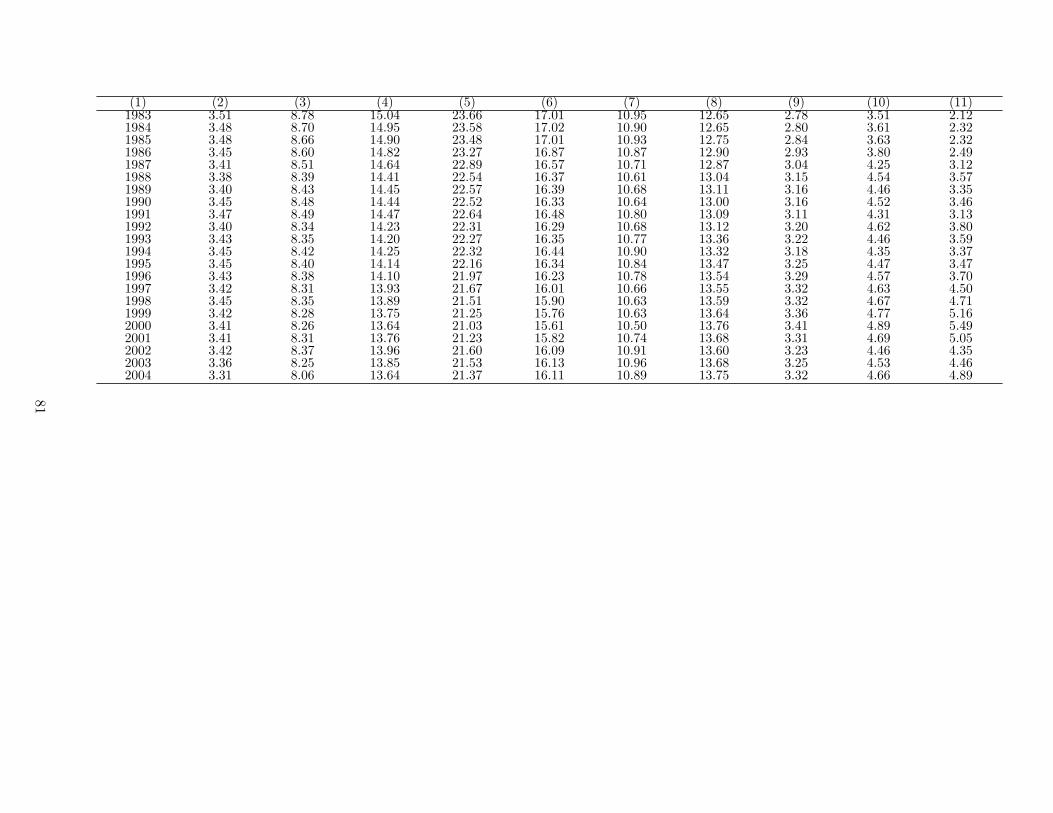
(1) (2) (3) (4) (5) (6) (7) (8) (9) (10) (11)1983 3.51 8.78 15.04 23.66 17.01 10.95 12.65 2.78 3.51 2.121984 3.48 8.70 14.95 23.58 17.02 10.90 12.65 2.80 3.61 2.321985 3.48 8.66 14.90 23.48 17.01 10.93 12.75 2.84 3.63 2.321986 3.45 8.60 14.82 23.27 16.87 10.87 12.90 2.93 3.80 2.491987 3.41 8.51 14.64 22.89 16.57 10.71 12.87 3.04 4.25 3.121988 3.38 8.39 14.41 22.54 16.37 10.61 13.04 3.15 4.54 3.571989 3.40 8.43 14.45 22.57 16.39 10.68 13.11 3.16 4.46 3.351990 3.45 8.48 14.44 22.52 16.33 10.64 13.00 3.16 4.52 3.461991 3.47 8.49 14.47 22.64 16.48 10.80 13.09 3.11 4.31 3.131992 3.40 8.34 14.23 22.31 16.29 10.68 13.12 3.20 4.62 3.801993 3.43 8.35 14.20 22.27 16.35 10.77 13.36 3.22 4.46 3.591994 3.45 8.42 14.25 22.32 16.44 10.90 13.32 3.18 4.35 3.371995 3.45 8.40 14.14 22.16 16.34 10.84 13.47 3.25 4.47 3.471996 3.43 8.38 14.10 21.97 16.23 10.78 13.54 3.29 4.57 3.701997 3.42 8.31 13.93 21.67 16.01 10.66 13.55 3.32 4.63 4.501998 3.45 8.35 13.89 21.51 15.90 10.63 13.59 3.32 4.67 4.711999 3.42 8.28 13.75 21.25 15.76 10.63 13.64 3.36 4.77 5.162000 3.41 8.26 13.64 21.03 15.61 10.50 13.76 3.41 4.89 5.492001 3.41 8.31 13.76 21.23 15.82 10.74 13.68 3.31 4.69 5.052002 3.42 8.37 13.96 21.60 16.09 10.91 13.60 3.23 4.46 4.352003 3.36 8.25 13.85 21.53 16.13 10.96 13.68 3.25 4.53 4.462004 3.31 8.06 13.64 21.37 16.11 10.89 13.75 3.32 4.66 4.89

81

Table A4: Gender Gap: %women

Year %Women inSample

P0-20 P20-40 P40-60 P60-80 P80-90 P90-95 P95-P99 P99-99.5 P99.5-99.9 P99.9-100

(1) (2) (3) (4) (5) (6) (7) (8) (9) (10) (11) (12)1937 26.297 0.394 0.419 0.326 0.0881938 26.864 0.369 0.396 0.354 0.1131939 26.618 0.370 0.402 0.361 0.0991940 26.311 0.378 0.412 0.347 0.0891941 26.739 0.413 0.426 0.346 0.0761942 28.867 0.469 0.436 0.394 0.0731943 35.449 0.540 0.559 0.475 0.1001944 37.880 0.582 0.594 0.491 0.1141945 36.830 0.486 0.569 0.533 0.1271946 32.083 0.474 0.476 0.415 0.1201947 31.050 0.490 0.468 0.407 0.0941948 30.362 0.484 0.468 0.395 0.0851949 30.441 0.475 0.478 0.387 0.0921950 30.367 0.476 0.481 0.392 0.0851951 31.608 0.516 0.518 0.397 0.0751952 31.970 0.531 0.527 0.389 0.124 0.034 0.022 0.020 0.0241953 32.044 0.536 0.534 0.389 0.119 0.031 0.018 0.019 0.0251954 31.765 0.530 0.519 0.387 0.125 0.030 0.023 0.025 0.0251955 31.997 0.542 0.520 0.383 0.128 0.031 0.018 0.025 0.0181956 32.355 0.559 0.530 0.377 0.126 0.031 0.019 0.019 0.0111957 32.377 0.555 0.520 0.379 0.135 0.036 0.021 0.025 0.0231958 32.068 0.532 0.504 0.386 0.151 0.039 0.023 0.021 0.0241959 32.297 0.553 0.512 0.378 0.144 0.037 0.020 0.019 0.0221960 32.522 0.552 0.520 0.385 0.142 0.035 0.021 0.019 0.0201961 32.755 0.545 0.521 0.394 0.149 0.038 0.021 0.019 0.0191962 33.042 0.555 0.526 0.399 0.145 0.037 0.018 0.019 0.0171963 33.067 0.556 0.533 0.396 0.141 0.037 0.020 0.017 0.0161964 33.150 0.555 0.537 0.399 0.140 0.036 0.018 0.017 0.0191965 33.479 0.561 0.544 0.405 0.137 0.035 0.018 0.018 0.0201966 34.515 0.576 0.564 0.420 0.141 0.033 0.019 0.016 0.0161967 35.210 0.580 0.578 0.429 0.147 0.036 0.021 0.017 0.0181968 35.793 0.587 0.583 0.443 0.149 0.036 0.022 0.017 0.0161969 36.293 0.591 0.587 0.452 0.156 0.038 0.022 0.018 0.0171970 36.148 0.578 0.579 0.452 0.167 0.042 0.023 0.018 0.0201971 36.041 0.571 0.570 0.452 0.175 0.047 0.023 0.019 0.0191972 36.344 0.578 0.566 0.452 0.185 0.048 0.025 0.019 0.0171973 36.827 0.587 0.570 0.459 0.189 0.049 0.026 0.019 0.0181974 37.362 0.589 0.579 0.464 0.197 0.055 0.027 0.022 0.0191975 37.662 0.576 0.572 0.473 0.216 0.064 0.033 0.025 0.0191976 38.345 0.580 0.577 0.483 0.229 0.068 0.035 0.026 0.0201977 38.823 0.584 0.579 0.487 0.238 0.074 0.038 0.027 0.0221978 39.715 0.596 0.593 0.493 0.246 0.081 0.041 0.030 0.024 0.019 0.0101979 40.191 0.596 0.599 0.497 0.254 0.088 0.047 0.033 0.027 0.019 0.0131980 40.451 0.583 0.593 0.505 0.270 0.101 0.053 0.036 0.030 0.019 0.010

82

(1) (2) (3) (4) (5) (6) (7) (8) (9) (10) (11) (12)1981 40.832 0.583 0.588 0.509 0.281 0.112 0.060 0.039 0.028 0.022 0.0131982 41.325 0.571 0.577 0.510 0.312 0.135 0.073 0.047 0.033 0.023 0.0141983 41.791 0.565 0.571 0.519 0.328 0.146 0.085 0.056 0.036 0.030 0.0151984 42.102 0.576 0.568 0.513 0.333 0.156 0.094 0.062 0.036 0.029 0.0251985 42.554 0.576 0.570 0.513 0.342 0.170 0.104 0.068 0.041 0.036 0.0181986 43.009 0.574 0.569 0.515 0.355 0.184 0.114 0.077 0.050 0.042 0.0221987 43.155 0.574 0.567 0.514 0.357 0.190 0.124 0.085 0.062 0.043 0.0241988 43.247 0.569 0.565 0.511 0.363 0.198 0.133 0.096 0.069 0.046 0.0261989 43.326 0.566 0.563 0.508 0.365 0.208 0.145 0.104 0.069 0.049 0.0381990 43.381 0.563 0.560 0.505 0.367 0.220 0.151 0.114 0.070 0.062 0.0281991 43.445 0.553 0.553 0.506 0.376 0.232 0.163 0.121 0.077 0.057 0.0391992 43.510 0.550 0.549 0.505 0.380 0.240 0.172 0.129 0.093 0.069 0.0391993 43.480 0.550 0.545 0.500 0.380 0.247 0.179 0.138 0.096 0.070 0.0391994 43.509 0.556 0.545 0.494 0.378 0.247 0.186 0.140 0.098 0.068 0.0401995 43.633 0.557 0.548 0.490 0.378 0.255 0.192 0.145 0.098 0.074 0.0581996 43.732 0.560 0.549 0.488 0.376 0.261 0.195 0.152 0.104 0.086 0.0481997 43.947 0.562 0.552 0.490 0.375 0.263 0.204 0.159 0.111 0.093 0.0601998 44.023 0.565 0.553 0.486 0.374 0.265 0.212 0.166 0.122 0.095 0.0701999 44.039 0.562 0.555 0.485 0.373 0.266 0.217 0.173 0.122 0.102 0.0852000 44.052 0.559 0.556 0.481 0.372 0.274 0.219 0.180 0.138 0.109 0.0892001 44.017 0.553 0.550 0.482 0.374 0.281 0.233 0.185 0.144 0.110 0.0822002 44.140 0.546 0.546 0.485 0.381 0.289 0.240 0.190 0.158 0.114 0.0762003 44.240 0.546 0.544 0.486 0.382 0.295 0.244 0.197 0.152 0.121 0.0892004 44.141 0.542 0.541 0.484 0.383 0.295 0.250 0.202 0.148 0.125 0.07883

Table A5: Short-Term Mobility: Probability of Staying in the Same Group after One Year

Year P0-20 P20-40 P40-60 P60-80 P80-100 P90-100 P99-100 P99.9-100(1) (2) (3) (4) (5) (6) (7) (8) (9)

1937 52.59 46.79 49.54 56.43 79.26 78.761938 46.22 48.45 56.66 66.65 86.87 86.461939 45.70 50.28 58.48 68.34 86.68 85.921940 38.51 43.47 53.01 63.41 86.07 83.431941 38.51 39.06 49.00 57.50 79.93 74.851942 39.10 40.51 48.64 54.72 76.03 53.931943 49.52 48.04 54.44 58.13 76.54 41.831944 45.67 45.81 51.01 55.81 77.00 41.761945 37.59 40.67 47.79 51.60 76.02 48.231946 45.95 41.63 47.34 52.92 74.81 65.741947 50.98 48.45 54.07 52.33 69.97 67.741948 54.34 49.64 53.18 49.91 66.86 64.601949 50.27 50.94 56.18 54.26 71.10 64.191950 47.89 48.94 55.30 55.98 73.92 63.491951 55.97 52.77 56.96 62.90 79.98 74.22 76.171952 57.71 55.25 59.24 63.98 80.60 74.37 72.081953 61.05 55.75 58.68 63.34 79.09 71.92 71.891954 55.45 56.10 59.83 65.74 82.66 77.36 76.511955 58.31 55.89 60.81 65.95 82.53 76.88 81.861956 60.24 54.09 58.87 65.63 80.61 74.79 83.521957 60.09 53.74 56.36 62.97 79.63 75.15 77.051958 55.74 53.88 58.24 65.93 83.14 78.84 78.541959 59.18 55.67 59.77 66.98 83.40 79.26 78.141960 60.46 57.24 61.92 68.94 84.28 78.94 77.951961 58.00 56.61 62.56 69.10 84.56 80.90 78.191962 60.01 57.23 62.93 69.52 84.37 80.84 78.161963 58.52 57.22 63.04 69.47 84.73 81.22 76.311964 57.03 56.87 62.77 68.84 84.87 81.56 70.461965 55.38 55.82 61.45 66.77 83.58 80.40 71.491966 58.25 56.28 61.42 68.17 84.24 79.34 77.281967 57.70 55.59 61.10 68.41 84.80 79.66 76.891968 57.52 54.63 60.22 67.97 84.93 80.41 73.361969 59.71 54.35 58.45 66.07 83.15 78.54 71.521970 58.87 54.46 59.25 66.83 83.46 78.58 72.961971 55.05 52.65 59.12 67.58 84.59 80.04 73.021972 53.36 51.27 58.60 67.70 85.30 80.41 74.731973 55.84 51.50 58.05 65.67 83.66 78.31 73.571974 57.52 52.25 57.58 64.92 82.46 78.50 70.321975 52.67 50.69 59.00 67.97 86.02 81.70 73.671976 53.36 51.25 59.66 68.73 86.58 81.71 73.571977 51.96 51.56 60.38 69.55 87.52 82.27 63.831978 54.59 52.70 60.61 69.60 87.10 83.38 74.33 64.781979 56.97 53.18 59.98 68.15 85.19 81.76 76.23 65.481980 56.53 54.44 61.47 69.76 86.44 83.20 77.41 65.081981 57.42 54.22 60.11 67.40 84.47 81.58 75.17 64.161982 54.95 54.66 62.73 71.22 86.94 83.69 76.00 64.571983 52.17 53.71 62.93 72.02 88.63 85.62 78.43 65.571984 54.86 54.37 62.64 71.92 88.40 85.41 77.61 67.301985 56.13 55.00 62.83 71.52 87.84 85.03 75.66 66.441986 56.26 55.39 63.24 72.14 88.09 85.03 73.40 60.821987 55.93 55.00 62.95 72.44 89.03 85.95 74.90 59.291988 57.59 55.72 63.32 72.52 88.79 86.00 75.17 62.101989 59.44 56.66 63.58 72.09 88.15 85.90 75.23 63.931990 60.83 57.05 63.78 72.33 87.77 85.59 76.47 65.391991 59.54 57.71 65.09 73.65 88.53 86.34 78.18 64.701992 58.58 57.69 65.16 73.91 89.20 87.07 78.37 68.541993 57.68 57.33 64.81 73.76 89.47 87.28 78.33 66.421994 58.94 57.22 64.62 73.81 89.49 87.09 78.75 67.241995 59.59 57.77 64.81 73.56 89.37 87.05 78.07 66.671996 59.58 58.01 64.69 73.40 89.26 86.83 77.88 67.131997 59.71 57.90 64.27 72.80 88.88 86.17 76.48 63.351998 60.87 58.41 64.50 72.71 88.73 86.11 75.22 62.791999 61.31 58.33 64.16 72.25 88.51 85.56 74.47 62.622000 63.18 58.39 63.64 71.62 87.63 84.77 72.80 61.442001 62.89 58.89 64.55 72.40 87.81 86.18 75.20 65.212002 61.79 59.22 65.70 73.79 88.49 86.68 76.55 66.592003 59.52 57.84 64.94 73.75 89.38 87.39 77.55 66.63

84