Embed Size (px)
Citation preview

INFORMATION TO USERS
This manuscript has been reproduced from the microfilm master. UMI films the text directly from the original or copy submitted. Thus, some thesis and dissertation copies are in typewriter face, while others may be from any type of computer printer.
The quality of this reproduction is dependent upon the quality of the copy submitted. Broken or indistinct print, colored or poor quality illustrations and photographs, print bleedthrough, substandard margins, and improper alignment can adversely affect reproduction.
In the unlikely event that the author did not send UMI a complete manuscript and there are missing pages, these will be noted. Also, if unauthorized copyright material had to be removed, a note will indicate the deletion.
Oversize materials (e.g., maps, drawings, charts) are reproduced by sectioning the original, beginning at the upper left-hand corner and continuing from left to right in equal sections with small overlaps. Each original is also photographed in one exposure and is included in reduced form at the back of the book.
Photographs included in the original manuscript have been reproduced xerographically in this copy. Higher quality 6" x 9" black and white photographic prints are available for any photographs or illustrations appearing in this copy for an additional charge. Contact UMI directly to order.
UMI University Microfilms International
A Bell & Howell Information Company 300 North Zeeb Road, Ann Arbor. Ml 48106-1346 USA
313/761-4700 800/521-0600


Order Number 9225068
Phase separation kinetics of binary liquid crystal-polymer mixtures
Kim, Jae Yon, Ph.D.
Kent State University, 1992
UMI 300N.ZeebRd. Ann Arbor, MI 48106

V

PHASE SEPARATION KINETICS OF BINARY LIQUID CRYSTAL-POLYMER MIXTURES
A dissertation submitted to the Kent State University Graduate College in partial fulfillment of the requirements for the degree of Doctor of Philosophy
by
Jae Yon Kim
May, 1992

Dissertation written by
Jae Yon Kim
B.A., Jeonbuk National University, 1985
Ph.D., Kent State University, 1992
\
(Mr**- JHU+At
rf/tc^m. D<
QasJI itf.
Approved by
Chair, Doctoral Dissertation Committee
Members, Doctoral Dissertation Committee
ed by
Chair, Department of Physics
Dean, Graduate College
ii

Table of Contents
List of Figures * v
Acknowledgements viii
Chapter I — Introduction 1
1.1 Liquid crystals 1
1.2 Polymer dispersed liquid crystal (PDLC) materials 11
1.3 Binary mixtures 14
1.4 Studies of phase separation 15
Chapter II — Phase Separation 18
2.1 Overview 18
2.2 Phase separation in thermally quenched binary mixtures 29
2.2.1 Nucleation theories 29
2.2.2 Early stage theories of spinodal decomposition 30
2.2.3 Late stage growth theories 36
2.2.4 Scaling theories for structure factors 44
2.3 Polymerization induced phase separation (PIPS) 46
2.3.1 Flory-Huggins model - binary systems 46
2.3.2 Complex multicomponent systems 47
Chapter III — Light Scattering 55
3.1 Light scattering theory 55
3.2 Dynamic light scattering 58
3.2.1 Photon correlation 58
3.2.2 Director fluctuation in PDLC materials 59
Chapter IV — Experimental Details and Results 63
4.1 Experimental details 63
4.1.1 Sample preparation 63
4.1.2 Experimental setup 67
4.2 Experimental results 80
4.2.1 Resistance and capacitance measurements 80
iii .

4.2.2 Light scattering 84
4.2.3 Morphology of PDLC materials 100
4.2.4 Cascade phenomena 103
4.2.5 Effect of shear during phase separation I l l
4.2.6 Director fluctuations 113
Chapter V — Some Applications 119
5.1 Overview - Optical power limiting and bistability 119
5.2 Experimental details 120
5.3 Experimental results 122
Chapter VI — Conclusions 132
Appendix I — The Size Distribution in Multicomponent Systems 134
Appendix II — The Gibbs-Thomson Relation 139
Appendix III — The First Order Freedericksz Transition with Linear
Feedback 141
References 147
iv

List of Figures
Figure page
1. Schematics of liquid crystalline phases 2
2. Canonical deformations of a nematic liquid crystal 6
3. Schematic illustration concerning the refractive index of a nematic liquid
crystal for an obliquely incident light 10
4. Schematic illustration of optoelectronic response of a PDLC film 13
5. Fre£ energy and corresponding phase diagram of a two component
mixture 22
6. The free energy changes during phase separation of a metastable phase of
concentration <j>0 24
7. Spontaneous disappearance of concentration fluctuations and diffusion
towards a nucleus in a sytem undergoing nucleation and growth 25
8. The free energy changes during phase separation of an unstable phase of
concentration <f>0 26
9. Temporal change in concentration profile in a system undergoing spinodal
decomposition 28
10. The growth rate in the early stage predicted by the Cahn-Hilliard
theory 33
11. Four different stages of spinodal decomposition 38
12. n-mer distribution as function of time and size 50
13. Schematic of the scattering geometry 56
14. Illustration of the droplet director of an elongated cavity in the presence
of an electric field 60
15. The chemical structures of the components of the nematic liquid crystal
E7 64
16. Molecular structures of Epon 828 and Capcure 3-800 65
17. Refractive indices of the pure liquid crystal E7 and the pure polymer as
function of temperature 68
18. Experimental setup for resistance measurement during curing process 69
v

19. Capacitance and resistance measurement by a GenRad capacitance
bridge 71
20. Light scattering setup 1 73
21. Light scattering setup II 74
22. Schematic of a microscope and a VCR arrangement to study phase
separation while curing 76
23. Schematic of the experimental arrangement to see the effect of shear
during phase separation 77
24. Experimental arrangement for detecting the fluctuating scattered light
from the PDLC film 79
25. Resistance of a sample as a function of time during phase separation I. ... 81
26. Resistance of a sample as a function of time during phase separation II. .. 82
27. Capacitance and resistance during phase separation 83
28. Onset time of phase separation as a function of composition 85
29. Temporal evolution of the diffraction pattern 86
30. Scattered intensity as functions of angle and time 87
31. Variation of -M— I and KM with time 88 Of
32. Typical scattered intensity from a diffraction grating 89
33. Graph of intensity vs. time 91
34. Scttered intensity vs. q = ^ sin(f) a* different times 1 92
35. Scttered intensity vs. q = ^ sinf^J at different times II 93
36. Plot of the scaled structure factor Inor • qmax3 vs. the scaled wavevector
q/qmax 94
37. Log-log plot of the scaled structure factor F(q/qmax) vs. the scaled
wavevector q/q„iax 1 95
38. Log-log plot of the scaled structure factor F(q/qmax) vs. the scaled
wavevector q/qmax II 97
39. In q ^ vs. In (t-t0) 98
40. In Imax vs. In (t-t0) 99
41. Scanning electron micrograph (SEM) of the cured PDLC material. It
consists of 33% liquid crystal E7 by weight 101
42. Scanning electron micrograph (SEM) of the cured PDLC material. It
consists of 45% liquid crystal E7 by weight 102
43. Micrographs of cascade phenomena while curing at 45°C 104
vi

44. Illustration of Gibbs-Thomson effect 110
45. SEM micrographs of the sample in the presence of shear during phase
separation 112
46. Autocorrelation function of the scattered light with time. The
polarization is Vy and no electric field is applied 114
47. Autocorrelation function of the scattered light with time. The
polarization is YH and no electric field is applied 115
48. Autocorrelation function of the scattered light with time. The
polarization is Vy and the applied electric field is 10 volt at 1 KHz 116
49. Autocorrelation function of the scattered light with time. The
polarization is V# and the applied electric field is 10 volt at 1 KHz 117
50. Autocorrelation function of the scattered light with time. The
polarization is VH and the applied electric field is 10 volt at 1 KHz.
Sample time and experimental duration are longer than those of
Fig. 50 118
51. Schematic diagram of the experimental setup and the feedback circuit.
121
52. Sample transmittances as a function of applied voltage 123
53. Measured response of the system with negative feedback 125
54. Calculated response of the system with negative feedback 126
55. Measured response of the system with positive feedback 127
56. Calculated response of the system with positive feedback 128
57. Sketch showing the intersection of the sample transmittance and
feedback response curves to determine the operating point 130
A.l . Schematic of Freedericksz transition due to an electric field applied
perpendicular to the cell 142
vii

Acknowledgements
It has been a great pleasure and tremendous opportunity for me to study at Kent
for the last six years. I have met many distinguished scholars and friends who have
opened new horizons in my life and gave me a new way of thinking. I need hardly
mention that one of them is my supervisor, Peter Palffy-Muhoray, who has always
helped me through tough problems which I have confronted during my study. His
eagerness for science gave me a taste of the true scientific world. Without his patient
guidance, this dissertation can not exist today.
Part of works have been done in Professor Thein Kyu's laboratory at the
Institute of Polymer Engineering located at The University of Akron. I am pleased to
express my appreciation to him for helpful discussions and his permission for use of his
light scattering equipment.
I can never forget my parents' self-sacrificing support throughout my life. With
their continuous encouragement, I have enjoyed my school life and finished my doctoral
study. I am in debt to my sisters who made sacrifices to educate me.
I should not forget Drs. Kee Bang Lee, Hyung Jae Lee, Jung Hong Kim, and
Young Hee Lee's guidance and teachings through my undergraduate school life in
Jeonbuk National University back Korea. Friends, staff, and faculty's kind help from
the Liquid Crystal Institute and Department of Physics are gratefully acknowledged.
viii

Chapter I
Introduction
1.1 Liquid crystals
Liquid crystals exhibit intermediate phases (also known as imesophases')
between the crystalline solid and the isotropic liquid [de Gennes, 1974]. Oridary
liquids are characterized by fluidity and isotropy while crystals possesses long
range positional order. The key characteristic of liquid crystals is the
orientational order of the constituent molecules. Liquid crystals are typically
composed of organic molecules with anisotropic properties which are manifest in
the diamagnetic and dielectric susceptibilities and the optical birefringence.
Generally, two types of liquid crystalline material are distinguished;
thermotropic and lyotropic. Thermotropic liquid crystalline materials show
mesomorphic phases as the temperature is changed. Lyotropic liquid crystalline
materials exhibit mesophases depending on the relative concentrations of the
constituent components. Liquid crystals in thermotropic and lyotropic materials
can be made up of molecules with a rod-like or a disk-like structure.
There are several types of liquid crystalline phase and they are classified
mainly into three categories: nematic, cholesteric, and smectic. Schematics of a
few common phases are shown in Fig. 1. The nematic phase is the least ordered
liquid crystalline phase. This type of mesophase is usually formed by elongated
molecules which have a long range orientational order. The direction of the long
1

2
/ /v/V. \
M 7 ^ ' - ' ' '^.-v \
(a) isotropic (b) nematic
\ ' / in \ / i i i / / \ i / \ / i \ i i / / | \ i n / l i / l / / /H/ l \ >\>ii\/\\/\\n\/
/
\
(c) smectic A (d) cholesteric
Fig. 1. Schematics of liquid crystalline phases.

3
range orientational order is denoted by the unit vector n and called the director.
The parallel and perpendicular components of the macroscopic properties of the
nematic with respect to the director exhibit different values. If the values of two
components perpendicular to each other as well as to the director are the same,
then the nematic is called a uniaxial phase. Otherwise, it is called a biaxial phase.
The exhibition of either a uniaxial or a biaxial phase depends on the shape of the
constituent molecules. Either rod-like (uniaxial) or book-like (biaxial) shapes can
be considered. Theoretical considerations of book-like molecules lead to
predictions of biaxial phases [Straley, 1974]. Biaxial nematic phases in lyotropic
liquid crystals were found experimentally by Yu and Saupe [1980], in
thermotropic polymer by Hessel and Finkelmann [1986] and in thermotropic
monomeric systems by Malthete et al. [1986]. The cholesteric is very similar to
the nematic in which the mesophase exhibit helical structure along the preferred
direction. Smectic phases are characterized by a one-dimensional positional order
as well as a long range orientational order.
The orientational order of nematic liquid crystalls can be defined
considering a cylindrically symmetric molecule in an external magnetic field H.
The induced molecular magnetic moment p can be expressed as
/ I = K | , ( H . 1 ) 1 + « ± { H - ( H . 1 ) 1 } (1.1)
where 1 is a unit vector along the symmetry axis of the molecule and K ,, and K X
are components of the molecular magnetic susceptibility parallel and
perpendicular to the long axis of the molecule, respectively. Extracting the
isotropic part of the molecular magnetic susceptibility,

4
Ai=«H + | 4« l{3 (H. l ) l -H} (1.2)
where the molecular susceptibility anisotropy and the average molecular
susceptibility are defined as
K II + ZK J_
AK=K II — K x a n c ^ ~*= o • (1.3)
The bulk diamagnetic susceptibility can be written as
2A^.Ai Xap=PnK 6
a^Pn^<2^Xp-6ap> (1.4)
where pn is the number density and the brackets < > denote the ensemble
average. The orientational order parameter is defined as
QaP=<U3l^-6a/3>- (1.5)
In the principal axis frame, the order parameter is diagonalized, and can be
written as
Qa/?~
i(S-P)
0
0
0
-J(S + P)
0
0
0
S
(1.6)
where S and P are called the uniaxial and the biaxial order parameter,

5
respectively. Both order parameters depend on the temperature. In this frame,
the unit vector of the axis associated with the eigenvalue S is called the director n.
It represents the direction of average alignment of molecules.
For a uniaxial nematic liquid crystal, the biaxial order parameter, P,
vanishes and molecules tend to align parallel to each other with partial ordering of
their long molecular axes. In this case,
Qa/3 = S.±(3nanp-6a/3) (1.7)
where S is the local orientational order of the rod-like molecules and n a is the
components of the director n. The directions n and - n are physically equivalent.
From Eq. (1.5), the molecular order parameter is represented by
S = Q z z = i <3 cos20 - 1> (1.8)
In some systems, the director varies with positions. The notation of < P 2 > is
sometimes used for the order parameter instead of S since the second order
Legendre polynomial, P2(cos0), is equal to (3cos20-l)/2. Note that by tradition,
the order parameter in an order-disorder transition is usually defined such that
S= l in the perfectly ordered system and S=0 for the completely disordered
system.
Three canonical elastic deformations commonly found in nematic liquid
crystals are illustrated in Fig. 2; (a) undeformed state, (b) splay mode, (c) twist
mode and (d) bend mode. Each mode is associated with an elastic constant; the
splay constant, K1} the twist constant, K2, and the bend constant, K3. The elastic

I ) I I I I1 ' I ' I I I I l< l l ' I
»\ V . ' i11 i « i 'a i ,w
Fig. 2. Canonical deformations of a nematic liquid crystal.

7
free energy [Frank, 1958] associated with the deformations is expressed by
F = J [[K^ V -n)2 + K2(n- V xn)2 + K3(nx V xn)2] dr. (1.9)
A model describing the nematic-isotropic phase transition was established
by Maier and Saupe [Maier and Saupe, 1958; 1959; I960]. In the theory, the
molecules are assumed to be nonpolar and to have intermolecular interactions.
However, this mean field approach ignores fluctuations in the short range order so
that the results of the theory is approximate. The single particle pseudopotential
is given by
e(cos 0)= -USP2(cos 0) + ±US2 (1.10)
where 9 is the angle between the symmetry axis of the molecule and the nematic
director and U is a measure of the strength of the average anisotropic pair
interaction [Palffy-Muhoray and Dunmur, 1982]. The second term arises from the
reguirement that the average potential energy per molecule equals one half of the
average potential energy per a pair of molecules. The orientational partition
function for one molecule is
z=y\-^cose^nede (l.li)
where /?=(k B T) _ 1 . The orientational free energy per molecule F = - (kgT/U) In z
becomes

8
F=IS 2 - I In y eaSP^COS ' ) sin* d9 (1.12)
where a=U/k B T. Extremal values of F are obtained when 5F/dS=0, that is,
when
/ * P2(cos ,) e « S P =( c o s «) sin« d« s=^r7^UT' (L13)
J o
The solution of the self-consistent Eq. (1.13) gives the values of the temperature
dependent order parameter.
The dielectric tensor has the same form as the magnetic susceptibility
tensor (Eq. (1.4)):
£ap=£<£6ap +§£(AS2( 3 nan / 3 - *o/j) (I-1 4)
where _ en +2ex
Ae—e»-eL and e=—-—5 (1-15)
and en and eL are components of the dielectric constants parallel and
perpendicular to the director, repectively. Choosing z-axis along the director, eaQ
can be diagonalized and the parallel and perpendicular components of the
refractive indices, n M and n x , with repect to the nematic director have the
following relationship.
n=>|£, (1.16)
n f ^ (1-17)

9
and
n ± = ^ = f w (1-18)
nn is the extraordinary refractive index ( also represented by ne) and n x the
ordinary refractive index (also represented by n0) of the uniaxial nematic liquid
crystal. The mean refractive index n of the liquid crystal is given by
n=s\ (2n02 + n e
2) /3. (1.19)
When the principal direction of molecular orientation (or director) n makes
an angle 0 with the propagation vector k, the refractive index nejy=nn for light
linearly polarized parallel to the (n, k) plane varies with 0 and is given by Fig. 3.
^ ^ ( . • ^ • r t ) ^ (1-20)
The refractive index n ± for light linearly polarized perpendicular to the (n, k)
plane shows no dependence on the angle 9 and is given by
n ± = n 0 (1.21)
It can be understood that in the above situation, for an incident light beam
perpendicular to the director, the linearly polarized light perpendicular to both
the director of the liquid crystal and the propogation vector k will not be
scattered since there is no refractive index variation along its path. The other

10
• n.
n
m1
V / ' v ' / / i > v •/; \ i
V l\\i
n
e.
/» \ ' l \ / | \ l
Fig. 3 Schematic illustration of the refractive index of a nematic liquid crystal for
an obliquely incident light.

11
component of the light will be scattered strongly due to large variation of
refractive index along its path. For 0=0°, n n =n 0 and 0=90°, n n =n e .
1.2 Polymer dispersed liquid crystal (PDLC) materials
Polymer dispersed liquid crystal (PDLC) materials have received
considerable attention recently for fundamental scientific reasons as well as for
their potential in display applications [Doane et al., 1986 and 1989; Drzaic, 1986;
Vaz et al., 1987; Montgomery and Vaz, 1987]. They are composite materials
consisting of micron-sized liquid crystal droplets in a polymer matrix, formed by
phase separation of the initial homogeneous liquid crystal-polymer mixture. They
can be used as light shutters, switchable windows, color projectors and so on.
PDLC films have some advantages over conventional twisted nematic displays
(also called 'TN cell') in that one can make large size and flexible displays since
no polarizer is required and it is much easier to fabricate them.
In 1976 Hilsum patented a light shutter device in which micron-size soda
glass spheres are dispersed in a nematic liquid crystal confined between two glass
plates with transparent conducting electrodes [Hilsum, 1976]. The surface of the
soda glass spheres orient the liquid crystal. The incident light is then scattered
due to the mismatch between the refractive index of the liquid crystal and that of
the soda glass spheres. Upon application of an electric field to the device the
electric field aligns the nematic to match its refractive index with that of the soda
glass spheres. Thus less light is scattered for normally incident light and the
device becomes transparent.
In 1982 Craighead et al. at Bell Laboratories patented a device where the

12
micron-size pores in a microporous filter were filled with a nematic liquid crystal
of positive dielectric anisotropy [Craighead et al., 1982]. This electro-optic device
was also not developed further.
In 1983 Fergason developed a liquid crystal based electro-optic device
formed by an encapsulation method [Fergason, 1985]. In this method, an
emulsion is formed of liquid crystal in water and later a water soluble polymer,
polyvinyl alchol (PVA) is added. As the water is evaporated, liquid crystal
droplets are entrapped in the polymer. The material is referred to nematic
curvilinearly aligned phase (NCAP) and commercialized by Taliq.
In 1984 researchers at the Liquid Crystal Institute of Kent State University
developed phase separation methods to obtain a polymer dispersed liquid crystal
(PDLC) material [Doane, 1986]. Phase separation procedures greatly improved
the electro-optic display fabrication methods.
The PDLC film sandwiched between two conductive indium tin oxide
(ITO) thin film coated glasses may be switched from an opaque scattering state to
a clear transparent state by application of electric field because of the dielectric
anisotropics of the film. The mismatch of the refractive indices between the
liquid crystal droplets and the polymer induces the film to an opaque state (Fig.
4-a). The applied electric field can cause the symmetrical axes of liquid crystal
molecules in the droplets to align parallel to the electric field, so that the ordinary
refractive index of the nematic liquid crystal can be matched with that of the
polymer and the film becomes transparent (Fig. 4-b). The refractive indices
typically for the nematic liquid crystal E7 are known to be n0=1.521 and
ne=1.746. The refractive index for epoxy polymer is 1.55.

13
(a)
nn \
n„
( O ) • (N>; nr
, -'/1 \ • <r~ ' i v --->
l£ U v
(b)
V
A
V
Fig. 4. Schematic illustration of opto-electric response of a PDLC film.

14
1.3 Binary mixtures
Mixtures consist of different chemical species. Let us consider a binary
system which has two components with the total number of Nx and N2 particles,
respectively. The free energy density, T= '« - Ts, of the binary system has two
contributions: the energy and the entropy. These contribution arise when the
system is mixed. The average energy density of the mixture, u, may be larger or
smaller than for the separated constituents. The energy difference is called the
energy of mixing. The entropy of the mixture also changes when two different
species interchange their positions. The change is called the entropy of mixing.
Usually, the same species of molecules prefer to interact. If the entropy
term in the free energy density is negligible, as at T=0, the mixture is not stable
because of the excessive mixing energy. Such a mixture will then separate into
two phases. But at a finite temperature the - Ts term in the free energy of the
homogeneous mixture always tends to lower the free energy.
If the entropy term dominates, the system remains a homogeneous single
phase. If, however, the energy term dominates, the system phase separates. In
general, competition between the energy and the entropy always exist.
The simple statistical model of the binary mixture called the 'regular
solution model' was proposed by Becker [1938]. The free energy density of the
mixture, based on the model, is expressed in terms of the volume fraction <j> and
the molecular volume v of each constituent as
/=v7el+V^e2 + k B i l v 7 l n V7 +V£ i n V^l (1.22)
15
Here the system has two different species respectively with Nx and N2 particles N-v-
and et- is the average energy, the total volume of the system is V, and <f>~ -h l.
If we quench the homogeneous system into lower temperature, the effect of
entropy is reduced and the mixture phase separates. The entropy can also be
reduced by polymerization, which leads to phase separation. Eq. (1.22) and the
entropy decrease by polymerization will be derived and discussed in detail in
Chapter II.
1.4 Studies of phase separation
Phase separation kinetics has been the subject of vivid theoretical and
experimental investigation in various fields, such as metallic alloys and binary
fluid mixtures [Gunton et al., 1983]. The phase separation of polymer blends has
also become the subject of recent studies [Nishi et al., 1975; de Gennes, 1980;
Pincus, 1981; Hashimoto et al., 1983; Snyder and Meakin, 1983]. Phase separation
provides us with the characteristic PDLC materials of current interest for optical
device application. Three mechanisms have been known to form PDLC materials;
thermal quenching induced phase separation (TIPS), polymerization induced
phase separation (PIPS), and solvent evaporation induced phase separation
(SIPS). Most of the work has been mainly on thermal quench induced phase
separation. However, little work has been done to date on the kinetics of phase
separation due to polymerization [Kim and Palffy-Muhoray, 1991; Visconti and
Marchessault, 1974; Kim and Kim, 1991].
Phase separation by polymerization in PDLC systems is usually achieved
by either a condensation reaction or photo initiated polymerization. An example

16
for the former case is a solution formed by a thermoset epoxy Epon 828 mixed
with the eutectic liquid crystal mixture E7 and the curing agent Capcure 3-800 in
a 1:1:1 ratio by weight. An ultraviolet-curable polymer (e.g., Norland optical
adhesive) mixed with the liquid crystal E7 can be the latter case.
The solution of a thermoplastic epoxy (e.g., Polymethyl methacrylate with
an average molecular weight 12,000 by Aldrich Chemical Co., Inc.) mixed with
the liquid crystal E7 can form a PDLC material by the thermal quench induced
phase separation. It is usually mixed at a temperature higher than the melting
temperature of the thermoplastics and cooled into the miscibility gap of the
system, which causes phase separation of the liquid crystal. The droplet size
distribution may be controlled by the rate of cooling.
A homogeneous solution in the solvent evaporation induced phase
separation is formed in a common solvent. As the solvent is evaporated, the
system is induced into the miscibility gap and the liquid crystal phase separated.
The droplet size distribution depends on the rate of solvent removal.
The application of the PDLC materials to a display is in need of
understanding the kinetics of phase separation of the liquid crystal-polymer
mixtures since its characteristic electro-optic properties are affected by the droplet
morphology. The focus of this dissertation is on the kinetics of phase separation.
The studies associated with phase separation have been carried out in the
following areas.
- simple fluids (gas-liquid transitions)
- binary fluids
- binary alloys

17
- superfluids and superconductors
- physisorption and chemisorption
- polymer blends
- gels
- chemically reacting systems
- glasses and crystalline ceramics
Chapter II
Phase Separation
2.1 Overview
Let us consider a binary mixture which is composed of two different species
of molecules. When the individual molecules are indistinguishable, the total
configurational partition function is given in the mean field approximations as
Ni
1 »'•
where i indicates one of the molecular species, q?- is the partition function of one
molecule, and N,- is the total number of one of the components of molecules. We
assume that
q i=ye-^d3r=Cj.e-^K (2.2)
where T is the potential energy for the i molecule, e- the average energy, V the
volume of the system, and ci the integral constant. From the relationships of
F=-k B TlnQ, Q=Qa-Q2, and Stirling's formula (In N!~N In N - N ) , the free
energy of the system is
P=e1N1 + e2N2 + ̂ T ^ l n N i + N2lnN2 - (Nx + N2) - {N1\nc1 V+ N2lnc2 V)}. (2.3)
18

19
The free energy density is then
j=F/y
=e1P1 + e2p2 + kBT(p! In px + p2 In p2) - kBT(pa In cx + p2 In c2 + p) (2.4)
where / ^ = T T is the number density of species i, p=px + p2, and p=§j.
In the model,
- el=/>l7ll + ?27l2
and
- s2=p2722 + pa72i (2.5)
where 7-- is the strength of interaction between molecules. Assuming the
geometric-mean interaction between constituents which is valid for London-van
der Waals interaction between spherical molecules,
7i2=72i=S|7n722 . (2-6)
By substituting Eqs. (2.5) and (2.6) into Eq. (2.4), the free energy density of the
mixture can then be rewritten as
f= ~ {Pxffn + />2^) 2 + k B T (p i l n Pi + Piln P2) ~ M ^ i ^ i + />2C2) (2.7)
where C ^ l n cx + 1 and C2=ln c2 + 1 .
20
When we put
V = N lVl + N2v2 (2.8)
and v i N i J. ylPi=-y^-=<Pi
V 2 N 2 , V 2 / ? 2 = ^ V _ = ^ 2
(2.9)
where N4 and v,- are respectively the number of molecules of species i and the
molecular volume and fy is the volume fraction of each species, the free energy
density is given by
^-{vi>[7lT + v f ^ i } 2 + kBT(vIln ^i + vf1* t2)-kBT(^C1+^C2\ (2.10)
Since the strength coupling constant 7.. between molecules in the van der Waals
interaction is proportional to the multiplication of each molecular polarizability,
api and the molecular polarizability is proportional to the molecular volume, i.e.,
a- ~ v?-, we can write
"I; „• ~ oi-a • 'ij 1 J
=(afv i).(a jv i). (2.11)
where at- is the proportional constant. Terms in the free energy and linear in ^. do
not contribute to making the free energy unstable and hence we neglect them.

21
Thus the free energy density can be rewritten as
> = - ( a ^ 1 + a2^2)2 + k B T ( | l l n | l + | | l n | | ) (2.12)
The free energy / and the phase diagram of the binary mixture are shown
in Fig. 5. The free energy of the homogeneous mixture usually exhibits a double
well form as a function of one of the constituents (e.g., component 2) at a
temperature below the critical temperature, Tc , of the system, which results in a
miscibility gap. The points of common tangency to the top curve in Fig. 5 define
the concentration of the coexisting phases at the temperature. The curve which
consists of the locus of the points is called 'binodal'. The locus of two inflection
d2f points satisfying the condition of -r-4=0 in the curve is termed 'spinodal'. Gibbs is
recognized as the first to classify the two different regimes [Cahn, 1968].
When the system is quenched into the metastable region from a
homogeneous single phase, the free energy change due to the concentration
fluctuations, <£-<£0, exists as shown in Fig. 6. We consider the change Af in / for
the system when one mole of concentration <j> is formed from the mixture of
concentration <j>0. We will assume that the amount of mixture is large enough so
that its compositional change may be neglected. At the original mixture of
concentration <j>0, the partial molar free energy are /i(<£0) and /2(<£0). The free
energy change arises from the transfer of <j> mole of component 2 from the original
mixture of concentration <£0 and from the analogous transfer of component 1. The
change is given by

22
concentration
Fig. 5. Free energy and corresponding phase diagram of a two component
mixture.
23
4/H/2M -/3(4,)}*+{fM) -/i(^0)}(i - *)
=Ati-fo)-(!$h(*-*J ' (2-13)
Suppose that there is an infinitesimal fluctuation 6<j>=4> - <j>0. Expanding the
free energy in a Taylor's series about <t>0,
M=Ato) + (* - *o)(g)^0 + fa ~ ̂ f($)^0 + • • • (2-14)
Substituting in Eq. (2.13) we get
, Q 2 X .
(—2)<&=̂ ^S Positive in Fig. 6. When there is a small separation by
thermal fluctuation, the free energy is increased and the system is therefore
metastable. In the region, if the fluctuation is small, then it will spontaneously
disappear (Fig. 7-a). In order to get the decrease in the free energy, the
fluctuation should exceed <j>a. The fluctuation can then form tiny 'nuclei' of the
minor phase (Fig. 7-b). These small 'nuclei' grow by attracting the same species
of the component from the mixture (Fig. 7-c). The growing nuclei will finally
reach two separate concentrations <j>a and 4>p (Fig. 7-d). This process is called
nucleation and growth (NG). fd2f\ As in Fig. 8, [-r^u—s is negative which means that any small fluctuations

24
E> 0 C CD Q) CD
fiW
metastable
* fk)(0-0o)
f2(0o)
0o 0 0.
concentration
Fig. 6. The free energy changes during phase separation of a metastable phase of
concentration <f>0.

25
0, <k
0o
0
0o
0«
0
0o
0.
0o
0.
0o
r 0. (a)
nucleus nucleus
7/ \N| \y M f / \N
(b)
(c)
(d)
Fig. 7. Spontaneous disappearance of concentration fluctuations and diffusion
towards a nucleus in a system undergoing nucleation and growth.

26
5* E> CD C CD CD CD
Wo)
unstable
* f'(0oW-«u
f2(0o)
0« 0S1 0o 0 0S2
concentration 0,
Fig. 8. The free energy changes during phase separation of an unstable phase of
concentration <j>0.

27
can decrease the free energy of the system spontaneously, as indicated by the
successive lines, until the lowest free energy is achieved which is a two phase
mixture. Thus the system is unstable. The system evolves through the
nonlocalized fluctuations with characteristic wavelengths, which forms
interconnected domains of the minor phase. In the initial state, the system has
negative diffusion constant (D<0), which Cahn first called 'uphill diffusion' (Fig.
9-a). The state of D=0 is then followed by, where the two concentrations reach
<j>Bl and <j>s2 (Fig. 9-b). Finally the system enters into metastable region (D>0)
(Fig.9-c). This is termed spinodal decomposition (SD).
Although this classical model can be used to distinguish between
metastable and unstable states, recent studies suggest that there is no sharp
distinction between them. In addition, Langer [1974] has shown that the
transition between the two mechanism is intrinsically smooth, i.e. that no sharp
spinodal line exists. Experimental evidence of the transitional region was carried
out by Tanaka et al. [1990].
To distinguish the qualitative features of the dynamical properties of
metastable and unstable phases, microscopic observations may be used. Usually
interconnected domains are observed in spinodal decompositions and droplet-like
domains in nucleation and growth. However, it has been pointed out that
morphology alone can not be used to determine whether the phase separation is
driven by the process of spinodal decomposition or nucleation and growth. In
fact, we can hardly distinguish in determining the difference at late s tage- this
stage will be discussed later.

28
0.
0o
0 _0>0si_ ex
~0<0S s2
(a)
0ft 0=0E s2
0o
0_ 0=0si
0.
0o
0.
(b)
0>0 • * & . -
0<& a t .
4 \-
(c)
Fig. 9. Temporal change in concentration profile in a system undergoing spinodal
decomposition.

29
2.2 Phase separation in thermally quenched binary mixtures
2.2.1 Nucleation theories
Let us consider a simple situation in which a droplet with radius R is
formed from a mixture. The free energy densities of the mixture and the droplet
are Tj and «F2, respectively. The free energy density of the droplet can be
represented as
F= | ; rR% 2 + 4tfR2<T (2.16)
The first term denotes the bulk free energy and the second the surface free energy.
The free energy density before phase separation is originally
F0=|TTR3=F1 (2.17)
so that the energy excess is given as
^F=|,rR3(=F2-=F1)+47rR2o- (2.18)
But it should be noticed that this would be true only for an open system in which
substance could be exchanged with an external source reservoir.
The critical radius of the nucleus, Rc=c, a , is obtained from the Jl~ J2
condition of <j^-=0. In this case, the energy excess is
AFc=^Rc2a. (2.19)

30
If the radius R of the nucleus is larger than the critical size, then the droplet will
grow. Otherwise, the droplet shrinks and disappears. This is the basis of the
nucleation theory.
2.2.2 Early stage theories of spinodal decomposition
(i) Cahn-Hilliard theory
The theory of Cahn and Hilliard describes the early stage of spinodal
decomposition [Cahn and Hilliard, 1958 and 1959; Cahn, 1959]. It is based on the
assumption that an inhomogeneous binary mixture (consisted of components 'A'
and 'B') can be described by a free energy.
F=/L/ fa ) + « ( V ^ ) 2 + . . . ] d r (2.20)
where j{^>) is the Helmholz free energy density of the homogeneous system of
concentration cf> of one component (component 'A') and K( V<£)2 is the second term
of the expansion of 7[^(r)] in a Taylor series in r. The term is associated with the
interfacial energy. When the variational derivative of Eq. (2.20) is taken, we
obtain
fJ=g-2«V»*+...=„ (2.21)
where p is a chemical potential of component A. The interdiffusional flux
( J=3 A = - JB) is related to the gradient of chemical potential difference which is
the thermodynamic driving force for the phase separation. That is,

31
J=-MV/< (2.22)
where M is the mobility. By substituting Eq. (2.22) into the continuity equation
d4>/dt + V • J=0, the concentration diffusion is described by
^ = M V . [ V { | - 2 K V M r ) } ] (2.23)
Cahn linearized this nonlinear equation about the concentration <£0, to
obtain
^r=M v 20*o-2"v 2 ]* ( t ) ' (224)
where
tf(r)=rf(r)-4,. (2.25)
This theory based on the linearization approximation has been called linear
theory. One would expect this linearization to be valid for the early time
following a quench, since the concentration fluctuations should be small. The
Fourier transform of Eq. (2.24) yields
The scattered intensity I(q,t) is proportional to | rp(q) | 2 and
I(q,t) = I ( q , 0 ) e 2 R ^ (2.27)
where

32
R(q)=Mq2[-(0)^-2«q2]. (2.28)
is the growth rate. Each sinusoidal component will grow or shrink exponentially in
time according to the corresponding value of R(q). As long as the effects of
multiple scattering are neglected, the scattered intensity is proportional to the
structure factor, which is called Rayleigh-Gans approximation [Van de Hulst,
1957]. In the spinodal decomposition region, (—fQ is negative and R(q) thus can
be either positive or negative, since K is positive. That is, it is positive for q
smaller than qc and negative for q larger than qc. In the nucleation and growth
region, (—^) is positive leading to negative R(q) (Fig.10).
As we mentioned above, this linear theory applies only to the early stage spinodal
decomposition.
(ii) Langer, Bar-on, and Miller (LBM) theory
The theory developed by Langer, Bar-on, and Miller for the spinodal
decomposition is the best of the various attempts made so far [Langer et al.,
1975]. The statistical model for the kinetics of spinodal decomposition starts with
the Helmholtz free energy funcctional as in Eq. (2.20). Before discussing the
theory, we need to understand how to establish the free energy functional. Here,
<j>(i) is constructed by dividing the system into small cells whose size is
comparable to the cube of the equlibrium correlation length £, so that it can be
assumed to be a smooth function on the scale of the correlation length. The free

33
unstable
Fig. 10. The growth rate in the early stage predicted by the Cahn-Hilliard theory.

34
energy functional F(<£) constructed by the suitable choice of the cells is termed a
'coarse-grained' free energy functional of the system. Based on this functional
F(<£), the phase transformation of the system can be interpreted.
The model is described by a continuity equation with a Langevin force
term,
* £ * L - V . j + C(r,t). (2.30)
The mean value of the Langevin force term, <C(r,t)>, vanishes and its correlation
<C(r,t)C(r',t')>=-2kBTMV25(r-r')«(t-t') (2.31)
satsfies the fluctuation-dissipation theorem. By considering the distribution
function p(<j>) defined on the space of < (̂r), Langer et al. have derived a functional
continuity equation:
dP(*)_ f^W1) -Tr~j*m < 2 - 3 2 )
and
J M = - M v 2 ( i § ) ' + k * T 4 ) ) (2'33)
where J(r) is the probability current. The complete statistical description of the
binary system is described by eqs. (2.20), (2.32), and (2.33).
The theory involves an equation for the fluctuation correlation function,
S(|r-r0|,t)=<u(r,t)u(r0,t)>, (2.34)
35
where u is the deviation of the concentration from <j>0, i.e., u(r)=^(r) -<j>0. The
Fourier transform of Eq. (2.34) is
S(q, t )=/e i«»- rS(r , t )dr (2.35)
The equation of motion for S obtained by Langer et al. is
«s(q) dt
= -2Mq^+(^))S(q)+l(0)S3(q)+^)S4(q) + ...}
+ 2MkBTq2 (2.36)
where the quantities Sn are the Fourier transforms of the higher-order two-point
correlation function:
S„( | r - r 0 | )^<u"- 1 ( r )u(r 0 )> (2.37)
Neglecting all the Sn(q) (n>2) and the noise term (2MkBTq2), we obtain the
Cahn-Hilliard theory.
When we assume that p(<£) is a Gaussian distribution on the function u(r),
centered at u=0, then all odd correlation functions vanish, and
S4(q) ~ 3<u2>S(q) (2.38)
with
< u 2 > = ^ _ | d q S ( q ) (2.39)

36
The resulting equation of motion for S(q) has the same form as that in the linear
theory, but the previ
dependent expression
o2f theory, but the previously constant quantity -§-k- is now replaced by the time-
d<p 0
w-^m,<At)> {2M)
Because <u 2 > is a positive, increasing function of time, the characteristic wave
number qc must decrease. That is, the mean-square fluctuations, via the
nonlinear part of I-T, cause a qualitatively correct coarsening of the precipitation
pattern.
Binder [1977] has pointed out that the LBM theory is inconsistent with the
Lifshitz-Slyozov t1'3 law [Lifshitz and Slyozov, 1961] which will be discussed in the
next section. The theory can not correctly describe the late stage coarsening. It
is thus considered an early time theory.
2.2.3 Late stage growth theories
(i) Overview
As a quenched system evolves toward the stable equilibrium state, the
average domain (or droplet) size becomes large and the interfacial thickness of
domain boundary becomes vanishingly small compared with the average domain
size R. This stage is usually known as the late stage of the phase separatien. As
one can see, Eqs. (2.27) and (2.28) predict that the concentration variations will
continue to grow indefinitely at an ever increasing rate. This physically
impossible result is due to the assumption of a constant (-^-Ita..^ and the neglect

37
of the higher order derivatives in the Cahn-Hilliard theory. The system can thus
apparently continue to decrease its free energy indefinitely. This implies that the
linearized Cahn-Hilliard theory is not appropriate to explain the late stages of the
phase separation. The stage may be further categorized into distinct regimes as
follows.
Four different stages of the spinodal decomposition process was suggested
by Hashimoto et al. [1986] and Bates and Wiltzius later [1989] while they
analyzed their polymer binary mixtures; early, intermediate, transition, and final
stages. The temporal development of the concentration undulations during each
of these four distinct stages are shown in Fig. 11.
The early stage is dominently characterized by the single wavelength Lm(0)
which leads to the development of a peak in the scattering structure factor at
qm(0). It is noticed that in this stage, the amplitude of the concentration
fluctuations increases with time and the position of qm does not change as shown
in Fig. 11 (a). It is in this stage that the linearized Cahn-Hilliard theory may be
applicable.
In the intermediate stage, the wavelength of fluctuations and the
amplitude of the fluctuations grow with time as shown in Fig. 11 (b). Thus the
linearized Cahn-Hilliard theory may not be applicable to the stage.
The transition stage begins when the amplitude of the concentration
fluctuations profile reaches its equilibrium values. The stage is characterized by
two time-dependent length scales as indicated in Fig. 11 (c). As the heterogeneity
length Lm(t) increases, the interfacial breadth A(t) decreases with increasing time,
until the latter reaches its equilibrium value A = A(oo).

38
<o) EARLY STAGE • r
Lm=2TT/qm
(b)INTERMEDIATE STAGE - r
*i
* D * C
«
-Lm(t<)--Lm ( t 2 ) -
(C) TRANSITION STAGE -»r
* '
*o *c
« 1 |A(t2)«
L m ( t 2 ) H -Lm(t4). • '
—77 Y"^
A(t<)«Lm
(d) FINAL STAGE
Fig. 11. Four different stages of spinodal decomposition.

39
A single time-dependent length scale Lm(t) » A exhibits the final stage
which is depicted in Fig. 11 (d).
The experimental results based on the different stages will be discussed
later. However, some stages may not be observed.
(ii) Lifshitz-Slyozov coalescence
Lifshitz and Slyozov [Lifshitz and Slyozov, 1961; Wagner, 1961] calculated
the asymptotic behavior of the droplet distribution function /(R,t) an^ *ne
asymptotic growth of droplets of a minority phase in a small initial
supersaturation. Since the growth occurs only after a nearly equilibrium volume
fraction of the new phase of droplets has formed, the concentration gradients are
very small. Therefore, we can assume that ^r - 0. The diffusional flux j of one of
the components into a droplet is given by
& + V -j =0 (2.41)
From j=DV<£ where D is the diffusion coefficient and a steady state diffusional
condition,
^ = D V M r ) = ^ ! ( r * f ! ) = 0 <2'42>
With the boundary conditions (j>(r=R)=<j>a and <£(r=oo)=0 (the overall composition
of the system), we obtain
^ ( r ) = ^ _ ( i z ^ M (2.43)
40
On the surface of a droplet, j ~ ^ and %|-~j-y4 where V and A denote the
volume and the area of the droplet respectively. From the relationship,
d ( ^ R 3 ) , R 2
-J- i p^=cons t an t , (2.44)
we obtain that R3 ~ t which is one of the results of the Lifshitz-Slyozov
calculations.
The basic mechanism of the theory is that diffusional flow due to the
concentration gradient between two domains (or droplets) having different sizes
cause the larger droplet to grow at the expense of the smaller one. This is
explained by the Gibbs-Thomson effect [Appendix II]. At the curved surface of a
domain (Eq. A.II.6),
*R=+OO exp(2V<7/kJ3TR)
~0 o o( l + 2t»/kBTR) (2.45)
where <I>R is the matrix concentration in equlibrium with a droplet of radius R (or
with a local radius of curvature R), i.e., the saturation concentration above a
spherical droplet surface with radius R, ^ the concentration of the saturated
solution above a plane surface of the minority phase ( that is, when R—»oo), v the
molar volume of the minority phase, and a the surface tension.
For two particles with radius xx and r2 and from Eq. (2.45),
41
*„(ri) -*.(r2)=*a(~) g f r & " £ ) (2-46)
A concentration gradient exsiting in the matrix between two particles of different
sizes will cause diffusion flow. Thus the larger droplet can grow at the expense of
the smaller one.
(iii) Hydrodynamic effects and power laws
Siggia [1979] has focused on the late stages of spinodal decomposition in a
binary fluid and analyzed them with several different mechanisms. These
mechanisms depend on the volume fraction v occupied by the drops. One possible
growth is the coalescence of spherical droplets of radius R. The resulting growth
law is given as
R3=12DRvt (2.47)
Experimetal observations of Siggia's theory were done in critical binary mixtures
of isobutric acid-water and 2,6-lutidine-water by Chou and Goldburg [1979] and of
isobutric acid-water Wong and Knobler [1981]. Wong and Knobler have
interpreted their experimental light scattering results in terms of Siggia's theory.
For this purpose they use the estimate R=qm_1, where qm denotes the
wavenumber corresponding to the maximum in the intensity of the scattered
light. In this case Eq. (2.47) can be written approximately as
k m - 3 ^12 W (2.48)

42
where k and r are the scaled variables with the correlation length £ near the
critical temperature Tc:
km=qm£ (2-49)
and
r=Dt/£ 2 (2.50)
Hydrodynamic interactions between the drops modifies Eq. (2.48). Namely, as
the drops diffuse toward each other, the intervening fluid must be squeezed out
from between them. An estimate of this effect leads to
km"3~ln(0.557km) (2'51)
Another growth mechanism is due to evaporation and condensation. This
occurs for small supersaturations, i.e., v is small, and leads to the Lifshitz-Slyozov
law
km-3=0.053D£r (2.52)
It should be noted that the amplitude of this r1 '3 growth law is independent of v,
unlike Eq. (2.48) and Eq. (2.51).
Siggia also discussed several growth mechanisms, unique to fluids, which
result from a critical quench. If the volume fraction exceeds the percolation limit
whose estimated value is ~ 15%, one has connected minority phase (droplets) and
can have growth driven by surface tension. The basic idea of so-called a capilary

43
flow model is to imagine a long tube of fluid of radius R with a radial undulation
of wavelength Z» R. The undulations lead to a presure gradient ~ <r/RZ along the
axis. The net effect of this gradient is to drive fluid from the necks to the bulges.
An estimate of the growth rate leads to
k r a-1=R=i0.1d;/ i j , (2.53)
where <r and 77 are the surface tension and the viscosity. This then leads to the
approximate result
k m - x ~ 0 . 3 r (2.54)
[Wong and Knobler, 1981].
To summarize, for concentrated mixtures (critical mixtures) one should
first observe diffusive growth, with km ~ r"1'3, followed by a crossover to the r'1
behavior given by Eq. (2.54). However, the behavior of the dilute mixtures (off-
critical mixtures) will be dependent on the relative quench A T . / A T ^ (Fig. 5).
When AT,- < 0.35ATy, the volume fraction exceeds the percolation limit and some
region of r"1 may be exhibited. Quenches for which 0 .35AT^ < AT,- < 0.9ATy
should initially exhibit T'1?3 growth with v. After the supersaturation has been
reduced, a crossover to a v indepndent Lifshitz-Slyozov growth can be observed.
Only Lifshitz-Slyozov growth should be observed when AT,- > 0 .9ATJ .
For the late stage of SD, Langer et al. [1975], Binder and Stauffer [1974],
and Siggia [1979] have considered power-law relationship between qmax and t and
Imax and t:

44
q ^ - r ^ a n d l ^ - t f 3 (2.55)
Langer et al. predicted a=0.21. Binder and Stauffer argued, based on cluster
dynamics, that a=l /3 , /?=l , and /3=3a. Siggia predicted for mixtures of the
critical composition that the initial growth is diffusional where a = l / 3 , and at long
times the domain growth proceeds by coalescence due to surface tension where
«=1 .
2.2.4 Scaling theories for structure factors
For the various systems in which phase separation is observed the structure
factor is a fundamental measure of the nonequilibrium properties of the system.
The structure factor S of the decomposing seems to exhibit a simple scaling
behavior analogous to the scaling behavior observed in critical phenomena.
Although some theoretical work has been done to this nonequilibrium scaling, the
subject is not yet well understood.
The basic idea of the scaling of S(q,t) is that after some initial transient
time following a quench, a time-dependent characteristic scaling length R(t) is
established. Various choices of choosing this length exist. Furukawa's approach
calls for the use of l/qma* where q,,,^ is the wavevector corresponding to the
maximum of the intensity peak, whereas Lebowitz and coworkers choose q1? the
first moment of the structure factor. One can choose the length as qm a x~1(t)i ^ n e
position of the maximum in S(q,t). The structure factor of the decomposing
system, which is proportional to the scattering intensity, may be related to a
scaled factor such that

45
S(q,t)=b(t)-F(qR(t)) (2.56)
where F(qR(t)) is the time-independent scaling factor [Marro et al., 1979]. As the
system reaches at the equilibrium phases after quenching, the mean-square
concentration fluctuation can be obtained from the requirement that
j^J S (q,t) dq= < <? > - < 4> > 2 (2.57)
which is independent of time. The normalized structure factor is given by
S = . S ( q ' t } (2.58)
/ q 2 S(q,t)dq
From Eqs. (2.56) and (2.57), we must have
S (q,t)=R(t)3 • F(qR(t)). (2.59)
Theoretical and computer simulation approaches [Furukawa, 1984; Marro et al. ,
1979; Lebowitz et al. 1982] have been attempted to investigate the dynamical
scaling behavior. It is known that F(qR(t)) depends on quenches and is weakly
time-dependent. It was noticed by Wong and Knobler that the identification of
R ( t ) = q m_ 1 is not clear for their binary fluids.
Furukawa proposed a series of dynamical scaling expressions for F(x) for
the late stage of SD [Furukawa, 1984]:

46
F ( a : ) - 7 / 2 + 0̂ + ^ ( 2 ' 6 0 )
where F(x) is the scaled structure factor and a^q/qmax- The constant 7=d + 1 for
an off-critical mixture and 7=2d for a critical mixture; d is the dimensionality.
For three dimensional growth, F(a;) ~ x2 for a?< 1, and for x> 1 F(x) ~ x~6 for a
critical mixture and F(x) ~ x~4 for an off-critical mixture. Furukawa [1986, 1989]
subsequently also proposed the following modifications for the late stage of phase
separation in three dimensions:
F W ~2T? (2,61)
F « ~ p ^ <2-62>
For large q, Porod's law S(q) ~ q 4 is expected to hold, provided that the
boundaries of the domains are sharp [Porod, 1982].
2.3 Polymerization induced phase separation
2.3.1 Flory-Huggins model-binary systems
We focus on the liquid crystal (component 1) and the polymer mixture
(component 2). In fact, the system consists of three components which are the
liquid crystal, the polymer, and the curing agent. We treat the polymer and the
curing agent as one species and furthermore assume that the system is
monodisperse, even though it consists of different sized n-mers. During
polymerization, <j>x , v1? and <^2=1-^1 remain constants and v2=n2vp increases
where n2 is called the 'degree of polymerization' of component 2 (the degree of

47
polymerization of the liquid crystal is 1, that is, n2=l) and vp is the monomer
volume. If we neglect terms independent of fy and linear in 4>i which do not
contribute to making the system unstable and assume that wx ~ vp, the normalized
free energy density in terms of <f>x, after some manipulation of Eq. (2.12), becomes
3 _ / v i kBT~kBT
= ^ l n ^ 1 + i i = A l l n ( l - ^ ) + x^i( l-^i) . (2.63)
v (a - a )2
This is the Flory-Huggins free energy [Flory, 1971]. x= I _ T *S *ke
interaction parameter and favors separation. kBT
Initially, n2=l, the second derivative of the free energy with respect to
composition,
frMfc+saiV** w
is positive, and a homogeneous mixture is stable. As the polymerization proceeds,
n2 increases with time, the second derivative becomes negative at a certain time,
and the free energy takes on a double well form which favors phase separation for
certain concentrations.
2.3.2 Complex multicomponent systems
(i) Size distribution
The size of a linear polymer molecule can be expressed in terms of the
degree of polymerization, i.e., the number of repeating units along the chain. In a

48
polymerizing system, the size distribution of the polymer molecules changes with
time. To make the discussion simple, we consider only linear polymers which are
long, flexible and have two active parts in the end of each monomer molecule.
Let />(n,t) represent the number of molecules of size n at time t and let N
be the total number of the monomers [Rogers, 1977]. A change in the number of
size n of the polymer molecules at time t is due to an increase of size n from the
connection of size m and size n-m molecules and a decrease of size n from the
connection of size n + m molecules where m=l, 2, 3, •••.
dofn t) 1 °° V =5 Y, <Wm p(m,t)p(n - m,t) - p(n,t) £ a ^ p(m,t) (2.65) U b * m = l m=l
where n=l,2,3---. If we assume that the rate constants amn.m are the same, then
with the substitutions «„,„.,„= a=constant and r = ^ , Eq. (2.65) can be written as
^ f c l L £ P(m,rMn - m,r) - 2p(n,r) £ ,(m,r). (2.66) u r m=l m=l
The solution of this equation is given in more detail in Appendix I and is
, , N(Nr) n _ 1 / f t „ ,
If we regard x=n/N as a continuous variable since N is very big number
(typically, N> 105),
P ( x , r ) = ^ ( n , r ) = ^ e - ^ . (2.68)

49
As shown in Fig. 12, the function shows that only monomers initially exist. As
time passes, the molecules react with each other and the size distribution becomes
broader.
In an Epon-Capcure system, the Epon and the Capcure has respectively
three and two reactive parts. Eq. (2.65) can be modified to the system as
^ L £ (2m - l)p(m,r){2(n - m ) - l}p(n - m,r) m = l
-2/>(n,r)£(2m-l) , (m,r) . (2.69) m = l
The weighted quantities 2 m - 1 and 2 ( n - m ) - l are associated with the number of
the reactive part of the epoxy. However, the solution has not been achieved yet.
(ii) Free energy and stability
Let us consider a situation in which small phase separation in a local region
is induced by the concentration fluctuations of the multicomponent system.
When the two separated phases are represented by A and B, yiA and yt-B denote
the concentrations of size i in the phase separated mixture and yj0 is the average
value. V^ and VB are the volumes of the phases. We assume that in the system
the total number of molecules, N= J2 N,-, is consisted of the number of Nt of size i i
where i=l,2,3,--.. The free energy density is then given by
J^fAn)+^AfB) (2-70)
where f{yA)=J[y1A, y2A, y3A,—), AYB)=f{yiB, Y2B> YSB.—) a n d v i s t h e t o t a l

50
Fig. 12. n-mer distribution as function of time and size.

51
volume of the system. The following relationship holds between the different size
molecules in two phases:
YiA^\f + YiB-y^-^if-—Yio \*-tl)
When we expand f(yA) in Taylor's series around j(y0),
AYA)=AYO) + YidyiyiA ~y.o) + lY, 52dy~by(yiA ~yio)(YjA -Yjo) (2.72)
where yo=(yio> Y2C» y3o •••)• It is noted that the same form holds for ,/(yB). When
we put -r£=x and-^p=l - a;,
.Yio-YiB *=m=9rB <2-73>
for any i. The free energy of Eq. (2.70) is then given by
Vf„ , M , l ^ r d2f J=AYO) + 52 -dfiYiB - Yio) +152 52 -dfJfiYiB ~ Yio) (YJB - Yjo)
I i J J
-(YiB-YioXYjB-Yjo))} (2-74)
When we put xiA=yiA - y,0 and after some calculation, we are end up with
H y o ) + ^ ( l - ^ 52dy%^-yiB)(YjA-YjB) (2-75)

52
When we assume the geometric-mean interaction between different-size
molecules, we can generalize the free energy / of Eq. (2.12) for two component
system to the multicomponent system:
*i n A i=0 i=0
(2.76)
FT-where a ^ ^ 1 [Kehlen et al., 1986]. For the liquid crystal-polymer mixture, if we
represents the concentration of the liquid crystal as <j)Q, considering that £<£,•=1
and <j>0=l - ]C ;̂> the free energy density is i=0
i = i
j= -{ao(l - 52^) + E 4 2 + ^ L ^ m L - ^ + k B T £ ! i ln|i. (2.77) i = l i = l
The stability of the system can be investigated by finding the eigenvalues of the
second derivative of the free energy:
d2f dS ̂
= - 2 ( a 0 - a , . ) ( a 0 - a j ) - f k B T ( ^ - + ^ - ) (2.78)
If all the a,- for i=l, 2, 3, •••, n are assumed to be the same, i.e., a,=a, the second
derivative can be represented in a matrix form as
d2f _ HiH-
bx 0 0 6,
0 • • • 0 6„
— £
1 1 1 1
(2.79)
k R T, where both of the matrices are n-by-n orthogonal matrices, &i="^~z~^ij and

53
2 , k B T £ = 2 ( a 0 - a ) 2
+ V o ^ .
The eigenvalue problem of the above type of a matrix is well known [Golub
and Van Loan, 1989]. Suppose that the diagonal entries satisfy bx>--->bn and
e ^ 0. If the eigenvalues of the matrix is such that \x > • • • > Xn, then
(a) The A,- are the zeros of f(A)=l + e52T-U~'
(b) If e > 0 then bx > \x > b2 > • • • > b„ > Xn.
If e < 0 then Xx > bx > \2 > ••• > A„ > bn. (2.80)
In the liquid crystal-polymer system, the limit of stability of the system
can be determined by the relationship:
iW=X0)+ / ' ( * ) • (2-81)
The smallest eigenvalue, Amjn, is then proportional to
- 2 ( a 0 - a p ) ^ k B T ( ^ - + r L - ) (2.82)
where o and i indicate 'liquid crystal molecules' and 'polymer molecules with size
z' respectively. As Sv»^t increases due to polymerization, Amjn decreases and the
system phase separates.
(iii) Cascadgj>henomena
In the beginning of the curing process of the liquid crystal-epon mixture
d2f under study, „, i, is assumed to be positive so that any small fluctuation
increases the free energy of the system. As the curing process proceeds, the

54
number of size i increases and hence so does </>-. Thus the second terms of Eq.
d2f (2.78) becomes smaller due to the term of ^v,-. Finally, », i, becomes negative
so that the system becomes unstable. The second derivative changes continuously
with time. This continuing change of free energy beyond the limit of stability
induces the system to a multiple phase separation. We term this phenomena
'cascade'. The phenomena will be discussed with optical micrographs.

Chapter III
Light Scattering
3.1 Light scattering theory
In a light scattering experiment, an incident electric field is scattered by
induced dipoles. The scattered field at a point far from the scattering medium is
the superposition of the scattered fields from scatterers in the medium. If the
medium is homogeneous, there will be no scattered light except the forward
direction because in other direction scattered light from a pair of scatterers is
identical in amplitude but opposite in phase, and thus cancel each other. In
condensed matter, light scattering originates from the inhomogeneity of the
dielectric constant.
Let us consider a plane wave with polarization vector ni5
E i ( r )=n ,E ,e*«- r , (3.1)
incident upon a medium as shown in Fig. 13. The wave propagates through the
scattering medium where E,- is the incident amplitude and k,' is the incident wave
vector. The scattered wave vector q is defined as q=k , -ky . Considering the
scattering geometry and assuming quasi-elastic scattering, that is, | k,-1 ~ | kf | ,
q=4f sin(|). (3.2)
55

56
detector
©n,
k,
Fig. 13. Schematic of the scattering geometry.

57
where n is the refractive index of the medium, A the wavelength of the incident
light and 0 the scattered angle from the direction of the incident wave vector k,-.
The scattered electric field with polarization vector ng at r is approximately
E ^k2 E, e * r
* 4TIT y d r ' e - * * , r V e ( r ' ) - n , . (3.3)
where c(r')=e06fJ- + fc(r') is the dielectric constant fluctuation tensor of the medium
and the integral is carried out over the scattering volume [Jackson, 1975]. The
equation can be expressed in terms of the spatial Fourier transform of the
dielectric constant
u2 pi ik-r Eg= X na.e(q).n,. (3.4)
PDLC materials during the curing process consist of the liquid crystal
molecules, the Epon monomers, the Capcure monomers, and compounds of Epon
and Capcure. This is multicomponent system since the polymerization between
the Epon and the Capcure creates many different size compound molecules.
However, we consider this sytem as a pseudo-binary mixture. In other words, the
system can be thought of as the binary mixture of the liquid crystal (A species)
and the rest of components (B species), where polymerization between the latter
components drives phase separation. The structure factor of the complex mixture
may then be considered as the Fourier transform of the correlation function of the
concentration of the liquid crystal (A species):
S(q,t)= J < <£(O,t)0(r,t) > e ' q - r dr. (3.5)

58
where <f> is the concentration of the liquid crystal.
The scattered light intensity is proportional to the spatial Fourier
transform of the correlation function of the dielectric constant of the pseudo-
binary mixture:
I(q,t) ~ / < e(0,t)e(r,t) > e ' q ' r dr (3.6)
Since e~ eA<f> + eB(l -<j>), the scattered intensity is proportional to the structure
factor:
I(q, t)~S(q, t) . (3.7)
From light scattering measurements we can get the structure factor of the pseudo
binary mixture during phase separation process.
3.2 Dynamic light scattering
3.2.1 Photon correlation
Correlation function is a measure of the degree of similarity or regularity
between two signals in time or space. The mathematical expresion for the time-
correlation function between two periodic scattered light intensity Ix(t) and
I2(t + r) is given by
C^rHHmJ^211(t)I2(t + r)dt (3.8)

59
where C12(r) refers to the cross-correlation function. The process of correlation
between a signal and its delayed version, i.e., C n ( r ) , is termed auto-correlation
function. By using a correlator, we can get a correlation function which include
dynamical information of the system.
3.2.2 Director fluctuation in PDLC films
Several different director configurations in nematic droplets of PDLC films
are known[Golemme et al., 1988]. The molecules in spherical droplets typically
exhibit the bipolar configuration in which the cylindrically sysmmetric axes of
molecules are aligned parallel to the surface of the droplets except near two
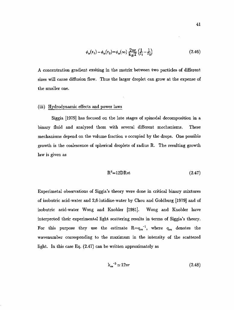
singular points. We define droplet director as the direction of average orientation
of the symmetry axis of the molecules in the droplet. Assuming that the droplet
is a prolate ellipsoid, the droplet director is represented by N^ and L is a unit
vector along the symmetry axis of the ellipsoid (Fig. 14). An alternating electric
field E is applied to a thin PDLC film layer perpendicular to the substrate planes,
the droplet director oscillates according to the electric field. From the
measurement of the correlation function of the scattered light we interpret the
dynamics of director fluctuations.
By using a droplet order parameter and a film order parameter in PDLC
film, Kelly and Palffy-Muhoray [1991] have established a simple model which can
explain a variety of PDLC phenomena, such as optical transmittance and
dielectric response. In this model, the free energy density of a nematic droplet
under an applied electric field E can be written as
S = - ^ ( N d . L ) 2 - | ( N d . E ) 2 (3.9)
60
Fig. 14. Illustration of the droplet director of an elongated cavity in the presence
of an electric field.

61
where the first is the elastic energy term and the second term is due to the
electric field. A and B are the proportional constants and K is the elastic
constant. If 0 is the angle between N^ and L and 0O between E and L, the free
energy is given by
V= _ AKcos20 - |E2cos2(0 -0O) (3.10)
The equation of motion of the director is
7 80
= - AK cosS sine - BE2 cos(0 - 0O) sin(<9 - 0O) (3.11)
where j is the viscousity. When we assume that 0 and 0O are small, i.e., N^ and E
do not deviate from L, and Langevin force F(t) is involved, the equation of motion
can be linearized in 0 and 0O:
j9(t)= - AK0 + BE2 cos0o sin0o + F(t) (3.12)
where the electric field is given by E(t)=E0 cos(w0t).
Taking the Fourier transform of Eq. (3.12) in frequency space, we can
transform F(t) into a constant, D, in respect that the random force exhibits a
white noise. Simple calculations show from the transform that
* ( " ) = ^ 7 - U K ( D + 2U^ + b(*(2w° " W) + 5(2W° + W))}- ( 3 1 3 )

62
where b=4(BE2 cos0o sin0o) and 6(u) is a delta function. Now, doing the reverse
transform of 0(w)0*(u)=9(u)0(-u), the correlation function C(t) of the director
fluctuation can be written as
C(t)= /0(u)0*(u>) e iu>i du
^ . - « ^ + ( ff y « ( » * ) + ~ (3.H)
The correlation function has three contributions. The first term is due to thermal
fluctuation and the second the applied electric field. The infinity term is the
contribution from the constant background field, which can be ignored. There is a
competition between first two terms. This simple understanding of the director
dynamics will be discussed with experimental results of the correlation function.
The study for the director fluctuation has not been completed yet.

Chapter IV
Experimental Details and Results
4.1 Experimental details
4.1.1 Sample preparation
PDLC samples were prepared using the polymerization induced phase
separation method. The materials used consisted of the nematic liquid crystal E7,
the epoxy Epon 828, and the curing agent Capcure 3-800. The epoxy resin Epon
828 (from Miller Stephenson Company) is the reaction product of epichlorohydrin
and bisphenol A. The curing agent Capcure 3-800 (from Miller Stephenson
Company) is a trifunctional mercaptan. E7 (EM industries, Inc.) is a eutectic
liquid crystal mixture of cyanobiphenyls and triphenyls. It is composed of 5 CB,
7 CB, 8 OCB, and 5 CT.
The molecular structure and components of E7 are given in Fig. 15. The
structures of Epon 828 and Capcure 3-800 are shown in Fig. 16. The Epon 828
has two epoxide group which are the reactive groups. The Capcure has three
reactive groups which are indicated as R in Fig. 16. Equal weights of Epon 828
and Capcure 3-800 result in almost exact mole fraction ratio of 3:2. The physical
properties of E7 is shown in Table 1.
Typical samples studied were ternary mixtures with a 0.45 weight fraction
of E7, 0.275 weight fraction of Epon, and 0.275 weight fraction of Capcure. The
63

64
5CB R=CH3(CH2)4-7CB R=CH3(CH2)6-
8 OCB R=CH2(CH2)70-
(EK><X>cs N 5CT R=CH3(CH2)4-
BDH E7 composition
/ 5 C B 51%
7 CB 25%
8OCB 16%
\ 5 CT 8%
Fig. 15. The chemical structures of the components of the nematic liquid crystal
E7.

65
i
! A |CH2-CH
epoxide group
CH3
CH2-oi^-C^3t°-CH5 CH3
Bisphenol A
(Epon 828)
.. J
CH \
C /
CH2
sV w
CH3
R=-0(CH2CH-0)
CH /
k
\ CH
nCH£
It
2
V.
OH I 1
>CHCH2SH
(Capcure 3-800)
Fig. 16. Molecular structures of Epon 828 and Capcure 3-800.

66
Table I. Some physical properties of the liquid crystal mixture E7
Properties
Melting point
Clearing point
Kinematic viscosity
Dielectric constant
Refractive indices
Elastic constants ratio (bend/splay)
Physical values
-10 °C
60.5 °C
3 9 x l 0 - 6 m 2 / s e c at 20 °C
1 8 1 x l O - 6 m 7 s e c at 0 °C
t-y =19.0
e x =5 . 2
AC=13.8 at 20 °C (lKHz)
ne=1.746
n0=1.522
An=0.224 at 20 °C (589nm)
K3/Ka=1.54 at 20 °C

67
components - 200 mg of E7, 122.2 mg of Epon, and 122.2 mg of Capcure-were
mixed and stirred mechanically to form a clear homogeneous solution from which
dissolved air was removed by centrifuging. The solution was then placed between
two glasses (2.54cm x 2.54cm x lmm) with a transparent layer of conducting
indium tin oxide (ITO). 30^m thick mylar spacers were put on the corners
between the glasses.
The schematic variation of refractive indices of the nematic liquid crystal
E7 and the polymer mixture with temperature are shown in Fig. 17.
4.1.2 Experimental setup
(i) Resistance and capacitance measurements
The polymerization induced phase separation process for epoxy PDLC
materials begins with a homogeneous mixture of prepolymer, curing agent, and
liquid crystal. As the prepolymer Epon and the curing agent Capcure react with
each other and form the high molecular weight polymer, the liquid crystal
becomes immiscible and phase separation takes place. In order to study the
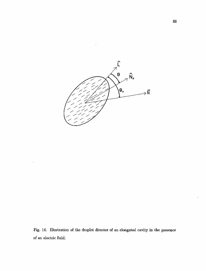
kinetics of the curing process both to determine the onset time of phase separation
and to look at long term behavior, an electric circuit was designed to measure the
sample resistance (Fig. 18). By increasing the gain of the circuit, the small
change in the resistance of the sample during the long term can be detected and
in that point an ohmmeter can not be used.
To protect the circuit from external noise, coaxial cables were used
between the sample holder and other devices. The electric circuit and sample

68
— liquid crystal
— polymer
Isotropic
Temperature
Fig. 17. Refractive indices of the pure liquid crystal E7 and the pure polymer as
function of temperature.

69
i — —
sample
Stepdown Transformer
Surge Protector
120 Volt 60 Hz
Temperature Controller
A: PMI OP EP B : MA 741 TC
Soltec Chart recorder
D.C Keithly 197Autoranging
Multimeter
Fig. 18. Experimental setup for resistance measurement during curing process.

70
holder were housed in an aluminum box which are grounded. The power
conditioner was also used as a surge protection. In the circuit of Fig. 18, the part
'A' is a follower which has unit gain and the part 'B ' is an amplifier whose gain
can be adjusted by the variable resistance 'R'. The maximum value of the
resistance is 10 Kohm so that the maximum gain through the amplifier can be
14.7 which is calculated from G=Rmax/ .679 Kohm.
The output of the circuit is connected to the Keithly 197 autoranging
multimeter which ultimately convert the input A.C. voltage to the output D.C.
voltage which is proportional to the input. Finally, the D.C. output was recorded
on the Soltec Chart Recorder. The temperature was kept at 62±0.02°C by a
temperature controller (Instec, Inc.).
The capacitance and resistance were also measured simultaneously during
the curing process using a GenRad 1615-A capacitance bridge which is capable of
capacitance measurements with ~ 1x10" 3pF accuracy. Fig. 19 shows the
schematic diagram of the measurement. Changes in the environment and in the
connections can vary the terminal capacitances, CG. However, the direct
capacitance, C^, are not affected from the changes. An EG&G 5102 lock-in
amplifier was used to detect the null. Measurements were made at lOKHz with
1.00 rms volt across the sample. A Tektronix 501A function generator was the
signal generator for the bridge. The Instec temperature controller was used to
keep at 62±0.02°C.
(ii) Light scattering
The preliminary light scattering experiment, (hereafter called I), was

71
Instec Thermostat
Tektronix 501-A Function Generator
GenRad
1615-A
Capacitance Bridge
EG&G5102
Lock-In Amplifier
Fig. 19. Capacitance and resistance measurement by a GenRad capacitance
bridge.

72
carried with a setup as shown in Fig. 20. The homogeneous mixture was placed
between two glasses separated by a 27/im thick mylar spacer. The cell then
immersed in glycerol in a thermosttated cylindrical cell housing. The refractive
index of the glycerol used is 1.5 which is very close to that of glass so that we can
avoid the experimental error due to the light deflection on the glass surface of the
sample. The sample temperature was kept at 62°C, above the nematic-isotropic
transition of the pure liquid crystal. An 8 mW He-Ne laser (Photochemical
Research Associates Inc.) was used as the light source. The data was collected by
using a photomultiplier tube (PMT). The detected light intensity was then read
from AT&T PC 6300 computer.
In order to detect the scattered light during a short period of phase
separation, the computer-controlled experimental setup was required as shown in
Fig. 21. The scattered intensity was detected by a photomultiplier under V„
polarization conditions. The output of the photomultiplier was converted to
digitals and stored in RAM of IBM personal computer. The scanning of the PMT
is driven back and forth by a stepping motor which is monitored by the computer
as well. The equipments in this part were used in conjunction with T. Kyu at the
Institute of Polymer Engineering, The University of Akron. The scanning rate of
the rotator was 5.5°/sec which can sample 17.45 data points/sec. The resolution
angle of the photomultiplier was less than 2.2°. The temperature of the sample
holder was kept at 62±0.2°C by a temperature controller (Omega Engineering,
Inc.), above the 58°C nematic-isotropic transition temperature of the liquid crystal
E7. This experiment will be represented by II.

to o
irt-
ere
Sample spatial pin lens Pol. lens holder filter hole ~"
Laser
Temp. Controller
diaphragm
lens
analyzer
neutral density filter
lens diaphragm
line filter
Computer

74
High Voltage Power Supply
Rotary Stage
IBM PC
Motion Controller
Stepping Motor
He-Ne Laser
Fig. 21. Light scattering setup II.

75
(iii) Morphology of PDLC materials
Most of morphologies of the PDLC materials were investigated mainly by
using a JEOL scanning electron microscope (SEM).
(iv) Cascade phenomena
Phase separation at 45°C below the nematic-isotropic phase transition
temperature was investigated. At this temperature, phase separation was slower
than that at higher temperatures so that we may expect to observe phase
separation more precisely. The experiment was monitored by a color video
camera and recorded by a videocassette recorder as shown in Fig. 22.
Magnification of the Nikon microscope was 100 times.
(v) Effect of shear measurement
Fig. 23 shows the experimental arrangement. A Nikon microscope and a
mechanical puller was used while the temperature was fixed at 62°C by a
temperature controller (Instec, Inc.). The speed of the mechanical puller was
~ 3.4 mm/hr.
The sample was formed by mixing the liquid crystal E7, the epoxy Epon
828, and the curing agent Capcure 3-800 in a 1:1:1 ratio by weight.
(vi) Director fluctuations
The sample used was the same type as that made in light scattering
measurement. That is, it consists of 0.45 weight fraction of E7, 0.275 weight
fraction of Epon, 0.275 weight fraction of Capcure.

76
TV Monitor o
VCR
Instec
Temperature
Controller
VCR Camera
Nikon Microscope
Fig. 22. Schematic of a microscope and a VCR arrangement to study phase
separation.
77
VCR Camera
Nikon Microscope
Instec Temperature
Controller
Fig. 23. Schematic of the experimental arrangement to see the effect of shear
during phase separation.

78
The autocorrelation fuction of the scattered intensity at a fixed angle was
measured with an electric field applied to the sample from a Tektronix 501A
function generator amplified by a Kepco BOP 72-5 operational amplifier. A
schematic diagram of the experimental system is shown in Fig. 24.
A PRA (Photochemical Research Associates Inc.) He-Ne laser used has 8
mW maximum output. Hamamatsu R464 photomultiplier tube and C1050
photon count unit which contain a pre-amplifier, main amplifier, discriminator
and waveform shaping circuit along with a photomultiplier tube socket, and power
supply (Bertan Associates, Inc. ) were used. The ± 12V low power supply
designed and built in the lababoratory was also used for the preamplifier of the
photo counting unit. A Malvern K7032 CE 8 bit digital correlator was used to
determine the autocorrelation of light intensity. The correlator was used in
conjunction with AT&T PC 6300 computer. The scattered light was detected at
30° from the direction of the incident light. A line filter (Oriel) used has the
maximum transmittance of 62% for A=634.05 nm with the half peak bandwidth of
10.1 nm.

I-S O
O f O
era
to
H x • a (D
CD
p
era
0
o a-e-f-<D O I - . .
era
& (3 o c* P e-t-!-»• P
era CO
o 0) a
era 13*
lens
He-Ne Laser
IZ7-
Spatial
Filter f™™^ A
Polarizer
PDLC Sample
E
z v
Tektronix 501A2MHZ
Function Generator
Diaphragm
Analyzer
Diaphragm
Une Filter
Kepco BOP Amplifier
Photomultiplier
Printer AT&TPC6300
Computer
Malvern K7032CE
Multi-8Correlator
- a to

80
4.2 Experimental results
4.2.1 Resistance and capacitance measurements
Resistance of the sample was measured over a long period. Results for
about 40 hours are shown in Fig. 25. Fig. 26 shows the measurement for about 6
days. The gain of the circuit was 7.535 for both of Fig. 25 and Fig.26. Even
though the curing process is assumed to start right after the components are
mixed, the phase separation takes place only after certain time which we call the
'induction time'. This is the elapsed time between the insertion of the mixture
into the thermostat and the time when phase separation, as determined by both
changes in resistance and light scattering measurements, begins. Further
discussion will be given later with light scattering measurement. For the mixture
of 0.45 weight fraction of E7, the induction time was usually 31 minutes (which
corresponds to 3.449 on the horizontal axis of Fig. 26).
We see that the curing process persisted for a long time. Surprisingly,
after about 7 hours, resistance curve exhibits a different trend as shown in both of
Figs. 25 and 26. As shown in Fig. 26, the trend showed the second change after
four and half days (106.7 hours).
In the measurements of capacitance and resistance at the same time, the
capacitance of the sample decreases with time and the resistance increases as
shown in Fig. 27. The size of the sample was 2.1cm x 1.7cm x 30pm. The applied
frequency and voltage were respectively lOKHz and 1 volt.

81
? o
«
fl 1—1
D -
5-
4-
3-
2-
i i
imHPn 1 x
^ ~ X
X
X
X
X X
X X
X X
X v x X *
X X *
1 1 1 1 1 , . , . 1
L 2 3 4 5 6
E7 Epon 828 Capcure 3 -800 t=30 /xm 62°C
r | i , . | . ,
7 8 9 10
In t (min.)
Fig. 25. Resistance of a sample as a function of time during phase separation I.

82
6 rS O
6-1
5-
4-
3-
2-
1 l
X X
1 1 L 2
x X
X
X
X
X X
X X
x**
1 ' 1 • 1
3 4 5 1 6
E7 Epon 828 Capcure 3-800 t = 3 0 jLim 62°C
i • i • i • i 7 8 9 10
In t (min.)
Fig. 26. Resistance of a sample as a function of time during phase separation II.

** cm to -a
O •S p> o
o m
H a> CD !-<« GO
6 o (X
o-0 1-1
p P* 9J
ai
s. o p
1100
1080
1060-
O 1040-
1020-
1000 0 20 40 60 80 100 120 140 160 180
Curing Time (min.)
oo co
84
4.2.2 Light scattering
The time when the abrupt change in the scattered intensity occurs is
recognized as the onset time of phase separation. Fig. 28 shows that the higher
the curing temperature, the shorter the onset time of phase separation, tc. Fig. 29
shows the temporal evolution of the diffraction pattern; the elapsed time between
photographs is 30 seconds. The decrease in the radius of the ring in the
diffraction pattern indicates that q^x is decreasing with time. The structure
factor can be more accurately determined by detailed measurements of the
intensity of the scattered light as a function of angle. Fig. 30 shows typical
scattered intensity at a fixed angle as function of time.
The scattered data was analyzed based on Eq. (2.20) and the assumption
that the shape of the free energy changes with time during the polymerization
d2f process. The convexity of the free energy —4 , the mobility M of the liquid
0<p
crystal and the coefficient K are all expected to vary with time. On the basis of
Eq. (2.21), we have extracted values of M-f—^) and KM as functions of time from
the results of our light scattering measurements. Values of these quantities are
shown in Fig. 31; the solid lines in the figure are mearely to guide the eye. We d2f
expect that —-r\ a n ( - K both increase with time as the degree of polymerization
N B increases. Assuming that the mobility M is a weak function of NB, this is
consistent with our observations. The observed decrease of qmax2 = _ ^ { x 4 ) "with.
time indicates that K increases more rapidly than the curvature of the free energy.
In order to know the corresponding scattered angles, a diffraction grating
was used which has three diffrent ranges of spacings; 100 lines/mm, 300 lines/mm,
and 600 lines/mm. Fig. 32 is a typical plot of the scattered intensity for a

85
700-,
•
a o
E-« CD
fcl
CO
O
600-
500-
400-•
300-
200-
100-
Curing Temperature
10 20 30 40 50 60 70 80 90 100
Liquid Crystal Concentration (%)
Fig. 28. Onset time of phase separation as function of composition.

86
A,.4"3»«-l
S3
&V$*S $m%
Vu,> ,lJSr
WMM: RVP;
KSHSfc^iSl
S T ; ' - -
retf&sra
Sfv
':-.'v ;••'"•' $CT?«
iffi
3fl s w i K&S
ftOra/S
Fig. 29. Temporal evolution of the diffraction pattern.
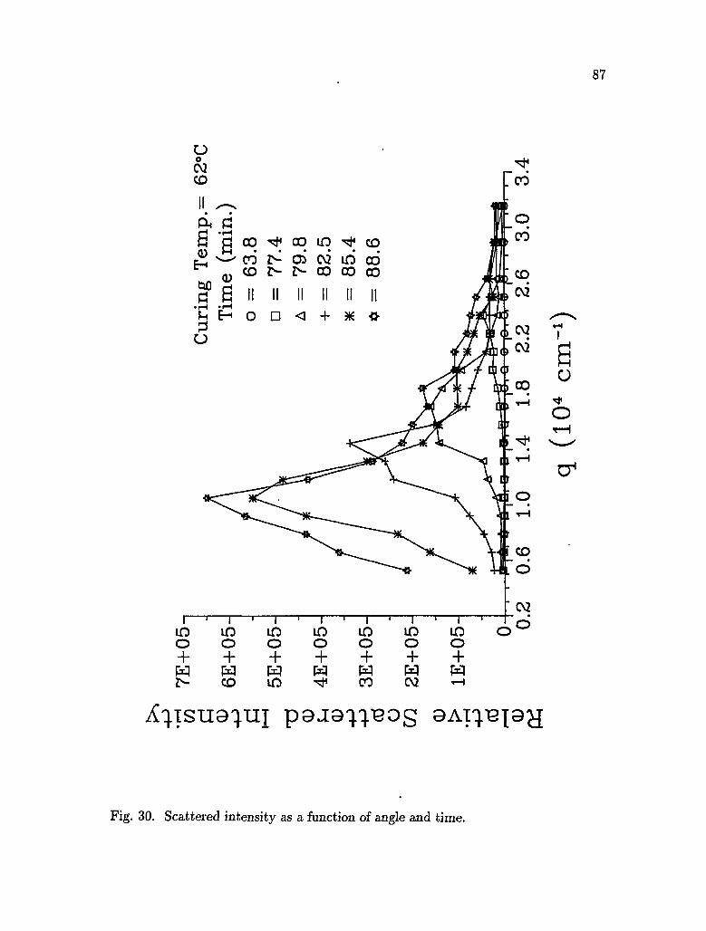
I > ""tf1
1 LO o + H zs
1 1 LO o + w CD
1 1 LO o + W LO
1 1 LO o + H <tf
i LO O + w CO
1 LO
o + w C\2
\ «
-^ V
' 1 ' LO C O + w 1-i
I *H
t i co - • •
L O
" C\2 3°
X^isu9q.ui p9J8^q.iaos 9Ai^X9jj
Fig. 30. Scattered intensity as a function of angle and time.

88
KM (min. - 1)
4>e (-.-•mm 3mo 8_0l) y§n
d2f Fig. 31. Variation of - M — and «M with time.

89
5-,
• iH £.
* *x x *
x x X
3-X
tie
1-
%f
x%
V
* &
X X
tf X X
%
#
V X X X
V x X
X* *
X w w^
3 4 T 1 2
Number corresponding to angles
Fig. 32. Typical scattered intensity from a diffraction grating.

90
diffraction grating in air. Distinct peaks in the scattered intensity were observed.
There are 100 lines/mm in the diffraction grating, so that d=10 pm. Fig. 33
shows typical scattered intensity at a fixed angle as function of time. 3.449 on the
time-axis in Fig. 33 corresponds to 31.5 minutes. The onset time is functions of
the curing temperature and the liquid crystal concentration.
The scattered intensity profile I(q,t) is shown in Fig. 34 and Fig. 35 at
different times. The scattered intensity is proportional to the structure factor of
the sample which is isotropic with a broad peak at a wave vector qmax- As time
increases, the maximum scattered intensity increases while qmax shifts towards
smaller q. The peak position characterizes the wavelength of the spatial periodic
concentration variation. The first point on the q-axis in Fig. 34 corresponds to
the angle of 0.984° and the last one 31.6°.
Fig. 36 shows the plots of Inor-qmax3 against q/qmax- All the curves for
various time scale are superposed suggesting that self-similarity has been attained.
This observation is consistent with the results of other studies such as in polymer
blends and alloys.
The exponent of the scaled vector x for x < l in Fig. 37 takes on values
between 2 and 4, in agreement with the prediction of Furukawa [Ohta and
Nozaki, 1989]. The exponent for x > l is -6 near ~ 1, and -4 for x > > l . The slope
- 4 is associated with Porod's law to the case of small angle x-ray scattering [G.
Porod, 1982] where the law is valid not only for single particles, but also densely
packed systems and for non-particulate structures provided that the boundaries of
the domains of the systems are well defined or sharp. This is because only the
structure near the surface is responsible for the slope of S(q). One can imagine

91
>> -p • iH CO
0) - p tf
HH
T * Q) (H
- P - P cd o
CO
0.6n •
0.5-•
0.4-.
0.3-•
0.2-
0.1-
H5 0.0-f r
scattering angle=2°
X
X —1 • T • - T - ' ' 1 « 1 • 1
10 20 30 40 50 60 t (min.)
Fig. 33. Graph of intensity vs. time

92
- p • i-H CO Pi 0)
- p PI
1—1
-a CD
- P - P
o CO (1)
.£; -P cd i -H CD K
4.0-1
-
3.0-
-
2.0-
1.0-
0.0-
A
1
M K
IK
T L
+ " * + + #
+ +
* * + * , * • *
+ « V
+* /V* + X * & _
* * X ^ f t t
A x S*****&L
45wt% E7 62 °C
t (min.) o= 37.5 D= 38.1 A= 38.7 o= 39.3 x= 40.0 *= 40.6 += 41.2 *= 41.9
q (10< cm -v
Fig. 34. Scattered intensity vs. q=% sm(f) a* different times I.

93
fc» 3.0- ,
CO PI
-3
*H 0)
• p -p (0 O
CO
is -p cd
I—I 0)
«
q ( 10+4 cm-1 )
Fig. 35. Scattered intensity vs. q=^f- sm(f) a t different times II.

94
8.E-03-,
6.E-03-
09
o" 4.E-03 a
2.E-03-
q/q,
time(min.) n= 38.1 A= 38.7 «= 39.3 x= 40.0 *= 40.6 o= 41.2
max
Fig. 36. Plot of the scled structure factor Inor-<lmax3 v s- *^e scaled wavevector
q/qmax-
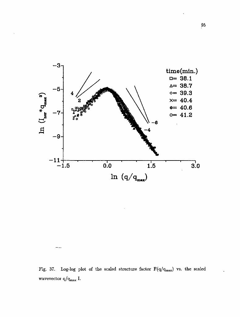
95
" s
.Ft
- 3 - ,
- 5 -
• 7 -
•9-
- 1 1 - 1 . 5
T 1 1 1 1
0.0 1.5
In (q/qmJ
t ime (min.) • = 38.1 A= 38.7 o= 39.3 x= 40.4 *= 40.6 o= 41.2
• i
3.0
Fig. 37. Log-log plot of the scaled structure factor F(q/qmax) vs. the scaled
wavevector q /q , ^ I.

96
that the interfacial thickness becomes thinner in the final stage of the phase
separation.
The slope - 6 is typical for a critical quench in a thermally quenched
binary system. In our system it may arise if, during the polymerization, the
convex (unstable) point of the free energy occurs for compositions near the initial
composition of the mixture. We have also observed a second maximum of the
structure factor (Fig. 38), which has been previously observed in thermally
quenched near critical binary system [Bates and Wiltzius, 1989], and in
homogeneously nucleated systems [Cumming and Wiltzius, 1990]. We believe this
to be a signature of long range structural periodicity.
Fig. 39 and Fig. 40 show the power law dependence of q ^ , and Imax on
time t, respectively. For small t - t 0 , the predicted exponent is - i , which is
reasonably consistent with the results as shown in Fig. 39. However, in this
regime, the exponent is sensitively dependent on the value of t0, and thus more
data is required for its unambiguous determination. Tanaka et al. [1990] have
shown experimentally that there exists a crossover region between the metastable
and unstable regions where the exponent a changes its value as a function of the
quench depth. In the unstable region, they found that the exponent a was
roughly equal to 4, which is characteristic of the intermediate stage of phase
separation in a system with conserved order parameter. In the metastable region,
on the other hand, their exponent was very small (~iTr), reflecting very slow
coarsening. In the transitional region, NG and SD can proceed simultaneously,
which suggest both process can be thermally activated.
At later times, the exponent is clearly - 1 . Binder and Stauffer [1974]

97
" a
-4 - ,
-5-
- 6
-7-
- 8
-9-
10 - 2
I - 1
T 0
T 1
In ( q / O
time(min.) o«31.8
•=32.6
A = 3 3 . 3
o=33.9
7=34.7
x=35.4
•=38.9
•=40.5
2 3
Fig. 38. Log-log plot of the scaled structure factor F(q/qmax) vs. the scaled
wavevector q/qmax II.

98
l l . O - i
10.6-- 1 / 3
45 wt% E7 62 °C
10.2-
£ 9.8-1
9.4-
9.0-xxxxxxxxx
- 3 1 ' 1 • 1 ' 1 « 1 ' 1
- 2 - 1 0 1 2 3 In (t-t0)
Fig. 39. In q ^ vs. In ( t - t 0 ) .
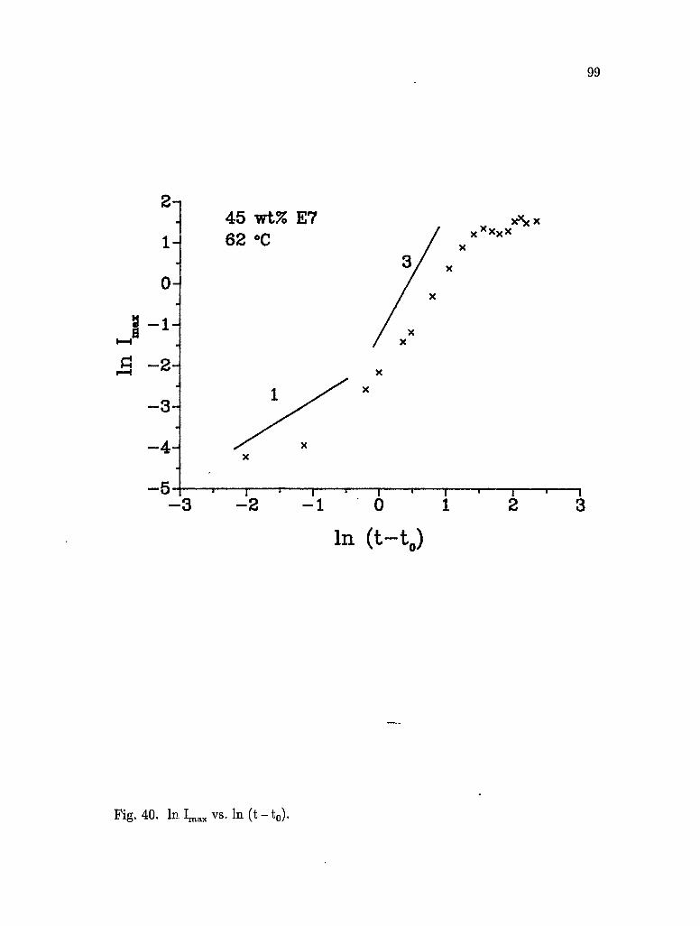
99
2-i
1-
0-
I - 1 " t-r
« - 2 -
- 3 -
45 wt% E7 62 °C
1 ^
- 4 -
: x x x x x*xx
- 3 - 2 - I r
0 T 1
In (t-t0)
Fig. 40. ln l m a x vs. l n ( t - t 0 ) .
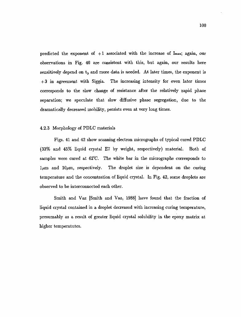
100
predicted the exponent of + 1 associated with the increase of Imax; again, our
observations in Fig. 40 are consistent with this, but again, our results here
sensitively depend on t0 and more data is needed. At later times, the exponent is
+ 3 in agreement with Siggia. The increasing intensity for even later times
corresponds to the slow change of resistance after the relatively rapid phase
separation; we speculate that slow diffusive phase segregation, due to the
dramatically decreased mobility, persists even at very long times.
4.2.3 Morphology of PDLC materials
Figs. 41 and 42 show scanning electron micrographs of typical cured PDLC
(33% and 45% liquid crystal E7 by weight, respectively) material. Both of
samples were cured at 62°C. The white bar in the micrographs corresponds to
1/xm and 10//m, respectively. The droplet size is dependent on the curing
temperature and the concentration of liquid crystal. In Fig. 42, some droplets are
observed to be interconnected each other.
Smith and Vaz [Smith and Vaz, 1988] have found that the fraction of
liquid crystal contained in a droplet decreased with increasing curing temperature,
presumably as a result of greater liquid crystal solubility in the epoxy matrix at
higher temperatutes.

101
Fig. 41 Scanning electron micrograph (SEM) of the cured PDLC material. It
consists of 33% liquid crystal E7 by weight.

102
Fig. 42 Scanning electron micrograph (SEM) of the cured PDLC material. It
consists of 45% liquid crystal E7 by weight.

103
4.2.4 Cascade phenomena
The micrographs are shown in Fig. 43 (a)-(f). The picture were taken from
the TV monitor. The elapsed time after mixing are shown on the pictures. After
2 hours and 14 minutes, a pattern with a characteristic wave length which has a
periodic pattern occurs. The pattern starts from a region and spread out to other
regions and grows. This early periodic pattern reminds us of the early stage
spinodal decomposition in a mixture. The periodic pattern phase separates and
keep growing (Fig. 43 (a)). It is thought that small domains are polymer-rich
areas.
In Fig. 43 (b)-(c), we can observe the direct coalescence of the domains.
The system still exhibits phase separation. This is a so-called later stage of
spinodal decomposition which is different from the early process.
We can observe in Fig. 43 (d)-(e) that the second phase separation takes
place in each regions. We also observe that smaller domains become smaller and
finally dissappear and that larger ones become larger. That is, smaller domains
diffuse and larger ones enlarge at the expense of smaller ones, which is similar to
the Lifshitz-Slyozov mechanism usually observed in a solid alloys. These are due
to the Gibbs-Thomson effect [Appendix II]. There is a concentration gradient
which arises from the different curvatures of the domains between domains of
different size (Fig. 44).
Finally, mobility of the system becomes small as the curing goes on7~"This
prevents the domains from moving so that the mixture can not flow any more
(Fig. 43 (f)). However, the curing process persists for a long time as shown in
resistance measurement, especially about one week for the sample cured at 62°C.

104
Fig. 43-(a). Micrographs of cascade phenomena while curing at 45°C.

105
Fig. 43-(b). Micrographs of cascade phenomena while curing at 45°C.

106
Fig. 43-(c). Micrographs of cascade phenomena while curing at 45°C.

107
Fig. 43-(d). Micrographs of cascade phenomena while curing at 45°C.

108
Fig. 43-(e). Micrographs of cascade phenomena while curing at 45°C.
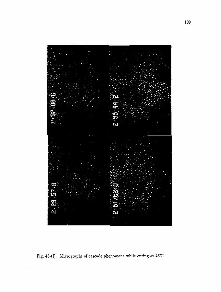
109
Fig. 43-(f). Micrographs of cascade phenomena while curing at 45°C.

110
• •
Fig. 44. Illustration of Gibbs-Thomson effect.
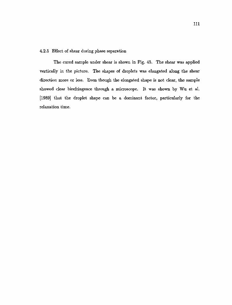
I l l
4.2.5 Effect of shear during phase separation
The cured sample under shear is shown in Fig. 45. The shear was applied
vertically in the picture. The shapes of droplets was elongated along the shear
direction more or less. Even though the elongated shape is not clear, the sample
showed clear birefringence through a microscope. It was shown by Wu et al.
[1989] that the droplet shape can be a dominant factor, particularly for the
relaxation time.

112
, y r. ,<• ,,**> ,' t
,v r.'v
/ > '
15KU X 3 0 0 0 , ' 1 0 0 1 , . 1 0 . 0 U h+ECTCn
Fig. 45. SEM micrographs of the sample in the presence of shear during phase
separation.

113
4.2.6 Director fluctuations
Without an applied electric field, the director fluctuation is due to thermal
motion of the molecules in droplets. Figs. 46 and 47 show the autocorrelation
functions of the scattered light at the scattering angle of 30° under Vy and VH
polarization conditions respectively. Here V indicates vertical direction and H
horizontal direction. In figures, ST and ED indicate 'sample time' and
'experimental duration' of the correlator. The figures show the exponential decay
of the function with ~ 1 m second of a correlation time.
When 10 r.m.s. volt with 1 KHz frequency is applied to the sample, the
autocorrelation function shows two contributions due to the applied electric field
and thermal fluctuation (Figs. 48 and 49). Specially, under VH polarization, the
function showed the period function which has IKHz and 2KHz components which
is not observed under Vy polarization. This is more clearly shown in Fig. 50 when
the sample time and the experimental duration are increased.

114
5.73E+08-
5.72E+08-
o • I - I
CO r—t V f-i
o o o 5.71E+08-
5.70E+08-
ST=40 jLtSec ED=20 Sec
v •Hie %c
A.
"^^"^"SIWA *W'$? , ,B ,V«»I0*
— i 1 j 1 1 1 1 1 1 , 1 , ,
20 40 60 80 100 120 140
channel number
Fig. 46. Autocorrelation function of the scattered light with time. The
polarization is Vy and no electric field was applied.

115
8.45E+08H
.2 8.44E+08-cti
r—I O U £ 8.43E+08-o
3 8.42E+08-
8.41E+08-
ST=40 fjSec ED=20 Sec
- i — ] — i — | — i — i — i — | — i — | — i — | — , — ,
20 40 60 80 100 120 140
channel number
Fig. 47. Autocorrelation function of the scattered light with time. The
polarization is VH and no electric field was applied.

116
PJ O
• iH
03 I — I V U t-t O O I o
3
2.10E+09-
2.10E+09-
2.09E+09-
ST=40 fjSec ED=30 Sec 10 V 1 KHz
w .
•v« „ * *
" &> »ti« w*
V * % jft A •Jlrf
rf^Hi * „ " K
—) 1 1 1 1 r
20 40 60 —, , , , , , , 80 100 120 140
channel number
Fig. 48. Autocorrelation function of the scattered light with time. The
polarization is Vy and the applied electric field was 10 V with 1 KHz.

117
PJ O
• FH •+->
cd i—I 0)
o o
3
o. roci-r-uo-
8.74E+08-
8.73E+08-
8.72E+08-
K
X
X
X
X
vs. MX
X " * *-
X x *>!* x A x \
W x x * X, > *" x * \ „*
l l j l " " *f *,x
X
'• • 1 ' 1 •' 1 — • >
ST=40 /zSec ED=30 Sec 10 V 1 KHz
K Ml X* * „
X* M X * i f " * X? * *
1 ' i ' i - - « — i
20 40 60 80 100 120 140
channel number
Fig. 49. Autocorrelation function of the scattered light with time. The
polarization is VH and the applied electric field was 10 V with 1 KHz.

118
O • r-t •+->
cd I—I Q) *H o o
2.32E+10-,
2.31E+10-
6 2.31E+10--P
5
2.31E+10-
ST=250 /*Sec ED=120 Sec 10 V 1 KHz
X x
X X * X
X X x x * V x
"»_ * X X X
K * X x x x „ „ XX X
xx„_, " x x K - " " " " X K - -""""««»«««",,»" * » x „ „ M " * " « * * x
" * « * « * « * « « , « x ' x ' x ' x ' x * X, x -* * » X X X X
20 - T -
40 80 60 80 100
channel number 120 140
Fig. 50. Autocorrelation function of the scattered light with time. The
polarization is V# and the applied electric field was 10 V with 1 KHz. Sample
time and experimental duration are longer than those of Fig. 48.

Chapter V
Some Applications
5.1 Overview - Optical power limiting and bistability
It has been shown that the liquid-crystal droplets in PDLC films can
undergo a transition to an elastically deformed state under the influence of static
magnetic fields [Kelly et al., 1989] and optical fields [Palffy-Muhoray and West,
1988]. This transition was first observed in a nematic liquid crystal by
Freedericksz and Zolina [1933].
Wang et al. [1987] studied the Freedericksz transition in a nematic cell,
with feedback. A cell with planar alignment at the cell walls was placed between
crossed polarizers, and illuminated with a light source. The output voltage of the
detector measuring the transmitted light intensity was used as the feedback signal
which modulated the voltage applied to the cell. It was found that, for certain
feedback parameters, the normally second-order transition became first order.
In this chapter, the behavior of a PDLC film with feedback is considered,
where the voltage applied across the film depends on the intensity of light
transmitted by the film. The effects of both positive and negative feedback were
studied. Bistable and optical power limiting behavior was observed and these can
be simply explained in terms of the optical transmittance characteristics of the
film.
119
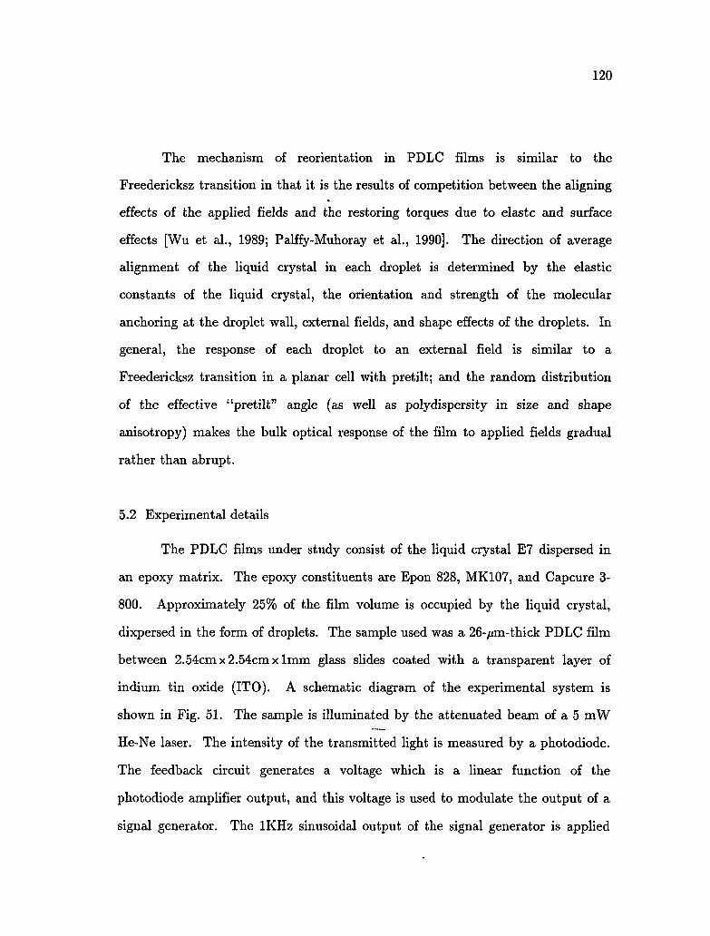
120
The mechanism of reorientation in PDLC films is similar to the
Freedericksz transition in that it is the results of competition between the aligning
effects of the applied fields and the restoring torques due to elastc and surface
effects [Wu et al., 1989; Palffy-Muhoray et al., 1990]. The direction of average
alignment of the liquid crystal in each droplet is determined by the elastic
constants of the liquid crystal, the orientation and strength of the molecular
anchoring at the droplet wall, external fields, and shape effects of the droplets. In
general, the response of each droplet to an external field is similar to a
Freedericksz transition in a planar cell with pretilt; and the random distribution
of the effective "pretilt" angle (as well as polydispersity in size and shape
anisotropy) makes the bulk optical response of the film to applied fields gradual
rather than abrupt.
5.2 Experimental details
The PDLC films under study consist of the liquid crystal E7 dispersed in
an epoxy matrix. The epoxy constituents are Epon 828, MK107, and Capcure 3-
800. Approximately 25% of the film volume is occupied by the liquid crystal,
dixpersed in the form of droplets. The sample used was a 26-/mi-thick PDLC film
between 2.54cm x 2.54cm x 1mm glass slides coated with a transparent layer of
indium tin oxide (ITO). A schematic diagram of the experimental system is
shown in Fig. 51. The sample is illuminated by the attenuated beam of a 5 mW
He-Ne laser. The intensity of the transmitted light is measured by a photodiode.
The feedback circuit generates a voltage which is a linear function of the
photodiode amplifier output, and this voltage is used to modulate the output of a
signal generator. The IKHz sinusoidal output of the signal generator is applied

50-50 beam splitter
attenuator
sample PDLC film
He-Ne Laser
*P-
detector 1
detector 2
out
vr
linear feedback
Vr
Fig. 51. Schematic diagram of the experimental setup and the feedback circuit.

122
to the sample cell via a step-up transformer.
5.3 Experimental results
In the analysis of the planar nematic cell with feedback [Wang et al., 1987],
an expression for the response of the cell to an applied voltage is obtained by
minimizing a free energy, and keeping only the lowest-order term describing the
distortion [Appendix III]. This description cannot be accurate for large distortions
which occur, for example, if the transition is strongly first order. Although we
have obtained closed form expressions for the orientational order and
transmittance of PDLC films as a function of applied voltage from a free-energy
minimization procedure, we find it more useful here to simply characterize the
film by its experimentally determined response. In Fig. 52, the transmittance of
the sample is shown at A=632.8 nm as a function of the applied voltage Vc.
Although there is some hysteresis, for these samples it is a small effect, and will
not be considered further here.
The nonlinear dependence of the transmittance on the applied Vc is
responsible for the characteristic nonlinear response of the system in the presence
of linear feedback. The power transmitted by the sample is
Pout = <Pi„, (4.1)
where t is the transmittance and P;n is the incident power. The output voltage of
detector 2 is proportional to Po u t , and the voltage across the cell is a linear
function of the detector output so that

123
0.8-,
0.6H
£ 0.4H
0.2H
t j •K3
s~ 4j«»aott*n«DB Dfl-BBDCa-DKH- O-D
i D
H0
a
X = 632.8 nm T = 22°C
•n
"T"
10 —i r
20 —T r
40 30 40 50
Applied Voltage Vc (V r m s)
• • — i 60
Fig. 52. Sample transmittances as a function fo applied voltage.

124
Vc = V0 + GiP in, (4.2)
where V0 is the offset and G is the gain of the feedback circuit. The
transmittance t is a function is a function of Vc, as indicated in Fig. 52. The
response of the system with negative feedback (G<0) is shown in Fig. 53. For low
incident intensities, Vc decreases, reducing the transmittance and giving rise to
optical power limiting behavior. By varying the feedback parameters, the
characteristic of this behavior may be modified. For example, increasing VD
increases the range where P o u t is proportional to P i n , while changing G simply
scales P i n and P o u t , leaving the response otherwise unchanged. The expected
response of the system calculated by choosing a value of Vc, obtaining the
corresponding P i n and P o u t is shown in Fig. 54.
For positive feedback (G>0), the response of the system is shown in Fig.
55. At high incident intensities, Vc is large, t is essentially constant, and P o u t is
proportional to P i n . As the incident power is decreased, Vc decreases, reducing
the film transmittance which further reduces Vc. This instability can lead to an
abrupt change in P o u t as the incident power is varied; however, the value of P i n
where this jump takes place depends on whether the incident power is increasing
or decreasing. This gives rise to hysteresis, and to the existence of two stable
states with different transmittance for some range of incident power. Increasing
the offset V0 causes the width of the hysteresis region to be reduced, and above a
critical value of V0, no hysteresis can be observed. Changing the gain again
simply scales the power. The expected response of the system calculated by
choosing a value of Vc, obtaining the corresponding P i n and P o u t is shown in Fig.

£= 0.024-,
O 0.018-1 D D
ft ffi a oo a * D D a a a DD
0.012-
• a
0.006-a
D
•
0.000-^
G = -1040 V/mW
VQ = 28.9 V
0.0 0.1 0.2
Incident Power P;n (mW) 0.3
Fig. 53. Measured response of the system with negative feedback.

0.024-1
0.018-
0.012-
0.006-D
D
G = -1040 V/mW V0 = 28.9 V
0.000-0.0 0.1 0.2 0.3
Incident Power P m (mW)
Fig. 54. Calculated response of the system with negative feedback.

% ° ^ o 0.18-
PL,
O PL,
GO PI CO U
0.12-
0.06-
G = 198 V/mW
VQ = 5.23 V
0.00-*
KM- P +B •» P O -D-, B D, 13 » r
0.0 0.1 0.2
Incident Power P m (mW) 0.3
Fig. 55. Measured response of the system with positive feedback.
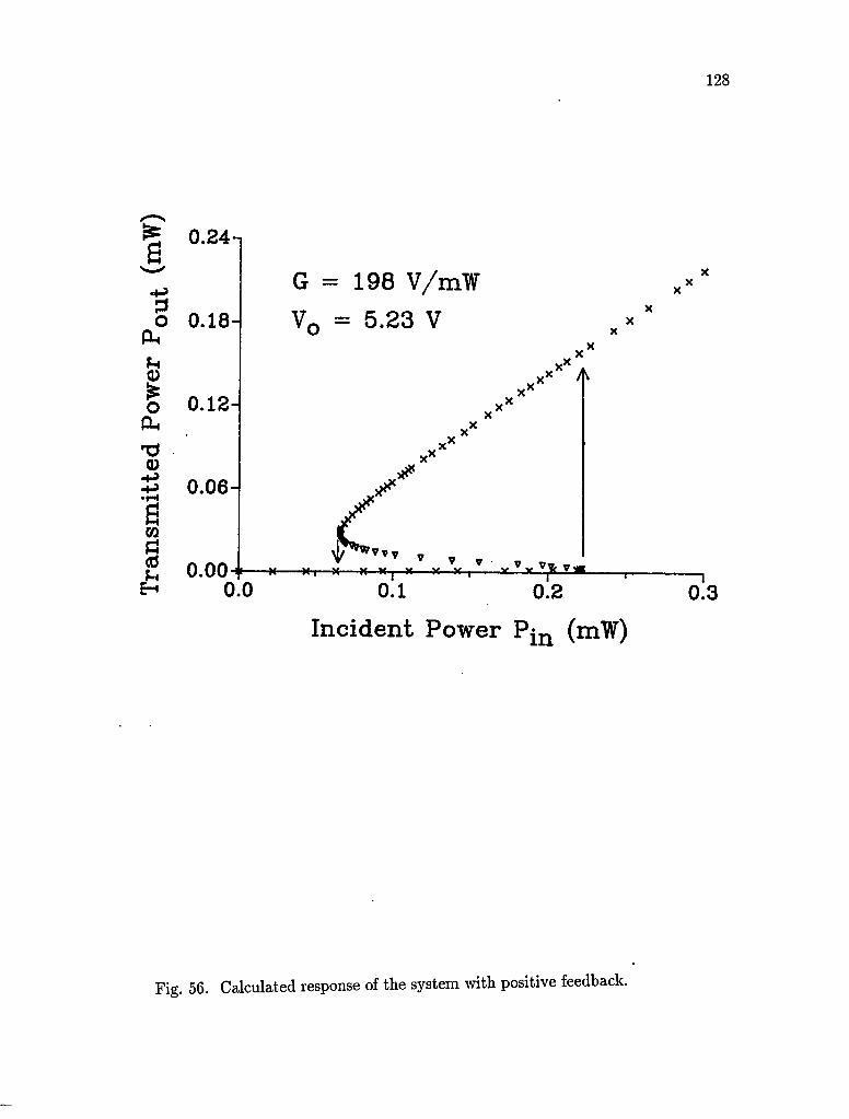
0.24-,
0.18
0.12J
0.06
G = 198 V/mW
V0 = 5.23 V X
x *
0.004 * **—*—x X| x—x x , v x v y v f t v * 0.0 0.1 0.2
Incident Power P m (mW) 0.3
56. Calculated response of the system with positive feedback.

129
55.
The behavior of the system may be simply understood by rearranging Eq.
(4.2) to read
< = ( V c - V 0 ) / G P l n , (4.3)
and noting that transmittance of the cell is given by the intersection of the cell
response curve of Fig. 52 and the straight line through V0 with slope l / (GP i n)
given by Eq. (4.3), as illustrated in Fig. 57.
For G<0, there is only a single intersection, and hence there is no
hysteresis or bistability. If, instead of the gradual increase in the cell
transmittance with Vc, the cell response was a step function at some voltage Vstep,
then the output power Po u t would be exactly proportional to P i n for
P i n<(V 0 -V 8 t e p ) / ( -G<) , and have the constant value (V0 - V8tep)/( - G) for all
values of Pin greater than this. In the case of linear feedback, therefore, ideal
power limiting behavior is obtained if the cell response is a step function. It is
worth noting that, by decreasing G, the limiting value of the output power may
be readly increased up to the (large) optical damage threshold of the PDLC
material.
For G>0 and for sufficiently small values of V0, there may be three
intersections of the straight line of Eq. (4.3) and the cell response curve for some
range of incident power P i n . The state of the system here is determined by its
history; however, as P i n is varied, the intersection corresponding to the state of
the system may be vanish, giving rise to a discontinuous jump in t and hence in

130
0
Fig. 57. Sketch showing the intersection of the sample transmittance and
feedback response curves to determine the operating point.

131
P o u t . In the regime where there are three intersections, the stste corresponding to
the intermediate one is unstable. That is, any peturbation in Vc will grow, and
take the system to one of the other ststes, which are both stable. Hysteresis and
bistability exist in this regime. It is interesting to note that if the cell response is
a step function, although a large multiple intersection regime exists, it is not
possible to switch into more transparent state by varying P i n only.
It is interesting to consider the behavior of a system where transmittance
of the film as a function of applied voltage shows strong hysteresis. Here we
expect bistability even in the case of negative feedback, and a broadening of the
bistable region in the case of positive feedback.

Chapter VI
Conclusions
Phase separation in a liquid crystal and polymer mixture has been
observed where the phase separation is induced by polymerization. The
polymerization process observed by resistance and capacitance of the sample
persists for long times compared to the onset time of the phase separation. The
structure factors show that the behavior of this system is similar to thermally
quenched binary system. However, the induction time is needed to initiate the
phase separation which is not observed in thermally quenched binary system.
Typically, the induction time is 31.5 minutes for the mixture of 0.45 liquid crystal
weight fraction and it is a function of the curing temperature and the
concentration of the liquid crystal. The scaling behavior of the structure factor of
the late stage of spinodal decomposition is in reasonable agreement with
Furukawa's proposition. A second maximum at higher wavenumber was found in
the scaled structure factor. The crossover of q ^ from i - 1 ' 3 to t~l predicted by
Siggia was observed.
It was observed that phase separation takes place twice at 45°C. This is
due to the continuing change of the free energy of the system. After the second
phase separation, no process can be observed because the increased viscosity due
to polymerization prevents the system from further process.
132
133
The effect of shear during the polymerization process was investigated.
The SEM picture of the sheared sample revealed the elongated shape of the
nematic droplets.
The autocorrelation function observed from scattered light intensity gives
useful information of director dynamics inside the droplets. Two contributions
due to thermal fluctuation and external electric field were observed. The results
were understood based on the simple model for the droplet director fluctuation.
Quantitative explanation is an objective for future work.
The behavior of PDLC films with linear feedback was examined. Both
optical power limiting and bistable behavior were observed and the experimental
results showed good agreement with predicted values. These results suggest that
PDLC films with feedback may be useful in optical protection and in optical
memory applications.

Appendix I
The Size Distribution in Multicomponent Systems
We derive here the size distribution function of polymer molecules due to
polymerization. The similar derivation was carried out by Rogers [1977] in his
mathematical model of the phenomena of multiple clustering of like embryonic
cells. Helpful discussion with R.G. Petschek is acknowledged in the derivation.
The distribution of the system consisted of initially linear monomers is
characterized by Eq. (2.63):
^ d = 52 P(m,r)p(n -m,r) - 2,(n,r) £ p(m,r). (A.I.I) U T m = l m = l
We define a new function as follows.
p(Z,r)=52p(m,r)z"'-\ (A.I.2) m = l
Substituting Eq. (A.I.2) into Eq. (A.I.I), we get
¥ ^ ' = E H M zn-V(n-m,r)-2,(n,r) ^ ' ^ ( m , r ) (A.I.3) u r m=l m = l
Summing Eq. (A.I.3) over a large number n (we can choose it as an infinite
134

135
number),
g d p ^ r ) z „ - i = z g g p ( m ) r ) z m - l p ( n _ m r ) z „ - m - i
OO OO
-252p(n,T)z"-*52p(m,r) (A.I.4)
n=l ~' n=lm=l
n=l m=l
This reduces to
^ M = z p 2 ( z , r ) - 2p(z,r)p(l,r) (A.I.5)
and we have
d/»(V)_ n2( -P2(l,r) (A.I.6)
The solution of Eq. (A.I.6) gives
P ( l , r ) = ^ r (A.I.7)
From Eqs. (A.I.6) and (A.I.7),
M^r) 2( x 2P(z,r) dr -ZPW> T + T ^
^ d 1 _ z 2 /A j o\ drp(z,r) p(z,r) (r + r0)
Let us define a new relationship and substitute it into Eq. (A.1.8):

where u is a function of time. Substituting (A.I.9) into (A.1.8), we get
2 9u_„ - 2u(r + r0) - (r + r0)2 g = B - 2u(r + r0)
U = ^ + C
- ^ = z ( r + r0) + c(r + r0)2 (A.I.10)
The constant c is calculated from the condition of p0(l)=Y~ at r=0.
c = p » ( 1 ) ^ - z ) < A ' U 1 )
Therefore,
p ( z ' r ) = - 7 — n tea) if—rv (A-L12)
0(1)
If p(l)=N and p(n)=0 at r=0 where n £ 0, p0(z)=N and />0(1)=N. Thus,
p(z,r)= i i 1— (A.I.13) «(r4)+N(l-8)(r+^
Considering the following relationship,
,(z)=p(l) + p(2)z + p(3)z2 + ..-,

137
and
we have
and
Now,
P(Z)),=P(1),
dp{%=p(2), dz
-£8—21,(3),
P(l)= N(- + ^ ) 2
1 & , n - l ^ n ' T ) = ( n ^ T ) ! ^ r T ^ M
(A.I.14)
(A.I.15)
and
P ( Z 'TKu. , ^2 N(r+i)2 + Z{r + l-N(r+^)2}
- 1 1 KNrfl) {,_!__!.}
^ i l l Y = -1 ( - I f " ^ k! 0Zk >=° rCNr + l j ' ^ J i + ^ l r ( N r + l){l+IJ_l dz1
1 d"-1
(A.I.16)
.k+l
(n-lJlte-^^KcNr + ljIH-^
,(n,r)= N N(Nr) n-1
Nr(Nr + l ){ l+ i} n (Nr+1)^1 (A.I.17)
The final result is that

138
Pfn A nPM_ n(Nr)"-1
P ( n , r ) - — j p - ^ ( N r + 1)„+i (A.I.18)
Since N is very large number, ^=x can be regarded as a continuous variable. By
the relationship between P(a;,r) and P(n,r),
P(x,r)#=P(n,r)dn (A.I.19) 'N
and
P(x,r)=NP(n,r)
_ nN(Nr)"-1
Nr
Since lim (l+£)N=e*, N->ooV N 7 '
(Nr+l) n + 1
= ^ I T X } N ) ' * • (A-L2°)
P H - ^ e " (A.I.21) T
Therefore, we have finally
P M ^ e " , (A.I.22) T

Appendix II
The Gibbs-Thomson Relation
The Gibbs-Thomson equation expresses the effect of the curved interface
between two phases on its solubility in an adjacent phase. As an example, we
consider a solution in which there exist a precipatate particle with the radius R
and thus two phases are separated by the curved interface. Imagine that dn
molecules are brought into the particle from the surrounding phase. If pR is the
chemical potential of the particle and p. is the corresponding quantity of the
solution with a planar surface, the work (pR - p)dn in this process is done. This is
the same as if dn molecules had been used in enlarging the surface of the drop. It
is, in turn, equal to ad A, where <r is the surface tension and A the area of the
surface of the particle:
(pR-p)dn=(rdA=8irRadR (A.II.l)
From the relationship of V=t;rR3, we obtain
fldn=dV=47rR2dR (A.II.2)
By eliminating dn and dR,
139

140
which is the general form of the Kelvin equation.
The chemical potential is respectively given for the two phases as
p=P0 + kBT \n <j>
| (A.II.4)
^R=^0 + + k B T m <I>R
where <j> is the concentration of dissolved material in the mixture in contact with a
plane interface, and <j>R that of the particle [Landau and Lifshitz, 1986]. From the
above equation, we have
pR-p=kBTln(+£) (A.II.5)
From equations (A.II.4) and (A.II.5) one obtains
"•GfhSfe <A-n-6>
This is the Gibbs-Thomson solubility relationship.

Appendix III
The First Order Freedericksz Transition with Linear Feedback
Let us consider a planar parallel-aligned nematic liquid crystal cell of
thickness d. The z-axis is perpendicular to the plates of the cell and the x-axis
along the direction of the molecules at the surfaces. In the presence of an electric
field, the molecules will be tilted by an angle 0 relative to the plates due to the
dielectric anisotropy (Fig. A.l). The Frank free energy is
F = i jd[kx( V -n)2 + k2(n- V xn)2 + k3(nx V xn)3 + D-E]dz (A.III.l)
where 0=9(z) and n=(cos 0, 0, sin 0).
From the requirement that V • D=0, the z component is independent of z
and
D - E = D , - E z ( z ) = ^ (A.III.2)
Let us assume that ezz=e n sin2^ + e x cos20 [Deuling, 1972 and 1974]. Then,
D - E = — r ^ o- (A.III.3) e ,, Sin^fl + e x C O S ^
Therfore,
141

/
/ /
/ /
/ /
/ / e
/ /
/ /
/ /
/ /
. / /
/ / /
- " / /
/ / - " / /
/ / / / /
/ / / / /
/ / / / /
Fig. A.l . Schematic of Freedericksz transition due to an electric
perpendicular to the cell.

143
F = i /1(k1cos20 + k 3 s in 2 0)#) 2 + — ^ j-ldz (A.III.4) 2 7 o L V 1 3 Adzy
e || sin20 + e ± cosV v ;
By appling an Euler-Lagrange equation, we obtain
AD „ AD „ D,2(e M - £ , )sin0 • COS0 (klCos20 + k3sin20)(^)2 + (k3 - kx)sin* • cos<? (M)2 + , ' 5 - ^ = 0 v * 3 Adzy v 3 1J W (£ | |sin2e-|-£±cos2e)2
o ^ [ ( k ^ o s ^ + kas in 2 ^)^) 2 — ^ „-]=0 d0LV 1 3 y W e||Sin2^ + e x c o s V
<* (klCos20 + k 3 s in 2 0)#) 2 r J ^ 5-=constant (A.III.5) v * 3 A d z ; £||Sin26/ + e±cos26i v '
Considering the boundary and symmetry condition, i.e., 4 ^ L _ d / 2 = 0 and
0(z=d/2) = 0m,
X^D*{ , „ * -2 ,}1,2-L S i n 2tm"S i n 2 g- , J 1 / 2 (A.IIL6) dz Hcxk1(l+^sm26im)- ' <-(l + z\sin2fii)(l + /csin2e)J v '
£M — £ j_ k — k i where ^ 1 = - ^ - and K=—.—- . Finally, the solution of (A.III.6) is
J- kx
1 r £ x k x ( l + W Q , 1 / 2 f0 r (l + 4sin20)(l+«sin20) | 1 / 2 ^ D2 I 4 J Jo"* sin20m-sin26> J v '
By using the above results, the potential applied across the cell is
V = / o E * d Z
y o «

144
=2D, fd,2p. J o "
= 2 D , / ' " ^ Jo zz
dz d0
=2D (6ml {tikiii + As^mhmlil + Asintyjl + Ksmtyyu dfl (Am8) ZJ o DTI /* J I sin20 -sin20 J c " V ;
When we let £„=£ „ sin20+£ x cos20=£ x (l+z\sin20) and sin20m • sin2e*=sin20,
V=2 k i ( 1 + / * s i n O [6m ( l + «sin2g )i/2d6, N e J. ^ 7 0 Hsin20m - sin20)(1 + A3in20y
- 9 E I n - ^ 0 2\ [*l2i l + «sin2gm-sin2a i1 /2
^ . ^ ^ ^ • " " • V o Vl + Ann20 .sin2a)(l-sin20 -sin2aV
Approximately,
V ~ , ki ^ ( l + f O / ^ l + f J - s i n ^ - ^ - s i n ^ + ^ - s i n M d a
=V0-(l+|O{l + (f-| + ^ 4
=Vo-{l + (f + f + i)C} (A.III.9)
That is,
V-¥o=l(l + K + A)0n (A.III.10)
We can also derive the voltage from the free energy.

145
F = i fd Ukxcos29 + k3sin2fl)(ffi2 + „ D ' 2 . „ ,}dz 2 y o l . v l 3 A d z ; e±(l + Asm20y
=ydo{kx(l + K92)(^r + ̂ f(l-A92
+ ̂ + A204)}dz
=I/od {k1(l + ^m
2-sin2(f ) -^-cos 2 ( f )
+ ? f (l-^m2sm2(f ) + A(A + l)0m
i.sm\f )}dz (A.III.ll)
By taking the derivative of the free energy,
§ = 0 = ^ ( 1 + 1*0J) + »i{-A + lA(A + l)-9m2} (A.III.12)
The applied voltage is
V = D 2 / d | k J o zz
= D fd dz ZJ o £ x ( l + /lsin20)
= ^ | ' d z ( l - ^ 2 + ^ + z \ 2 e 4 + - )
*^{l-J^4 (A-III.13)
Therefore,

V2 =^( l + « ^ ) ( 1 _ Mm2){1 + §*„,» + J O (A.m. 14)
When 0m=O, V„=,
That is,
k* % x 4
1^=1(1+ K + A)0r> (A.III.15)
This is the same result as Eq. (A.III.IO). This is different from Eq. (4) of Wang
et al.'s paper [1987] and is believed to be the correct expression.

References
F.S. Bates k P. Wiltzius, J. Chem. Phys., 91, 3258 (1989).
R. Becker, Ann. Phys., 32, 128 (1938).
B.J. Berne k R. Pecora, Dynamic Light Scattering, (John Wiley k Sons, Inc.,
1976).
K. Binder, Phys. Rev. B 15, 4425 (1977).
K. Binder and D. Stauffer, Phys. Rev. Lett, 33, 1006 (1974).
J.W. Cahn k J.E. Hilliard, J. Chem. Phys., 28, 258 (1958); ibid., 31, 688 (1959).
J.W. Cahn, J. Chem. Phys., 30, 1121 (1959).
J.W. Cahn, Transactions of the Metallurgical Society of AIME, 242, 166 (1968)
and references therein.
Y.C. Chou k W.I. Goldburg, Phys. Rev. A, 20, 2105 (1979).
H.G. Craighead, J. Cheng k S. Hackwood, Appl. Phys. Lett, 40, 22 (1982).
A. Cumming k P. Wiltzius, Phys. Rev. Lett, 65, 863 (1990).
P.G. de Gennes, The Physics of Liquid Crystals, Oxford University Press, Oxford,
(1974).
P.G. de Gennes, J. Chem. Phys., 72, 4756 (1980).
H.J. Deuling, Mol. Cryst Liq. Cryst, 19, 123 (1972).
H.J. Deuling k W. Helfrich, App. Phys. Lett, 25, 129 (1974).
J.W. Doane, N.A. Vaz, B.-G. Wu k S. Zumer, Appl. Phys. Lett 48(4), 269 (1986)
and references therein.
J.W. Doane, A. Golemme, J.L. West, J.B. Whitehead,Jr. k B.-G. Wu, Mol.
Cryst. Liq. Cryst, 165, 511 (1989).
P.S. Drzaic, J. Appl. Phys., 60, 2142 (1986).
F.C. Frank, Discuss. Faraday Soc. 25, 19 (1958)
J.L. Fergason, SID Digest of Technical Papers, 16, 68 (1985).
P. Flory, Principles of Polymer Chemistry, (Cornell University Press, Ithaca, N.Y.
1971).
V. Freedericksz k V. Zolina, Trans. Faraday Soc. , 29, 919 (1933).
H. Furukawa, Physica, A123, 497 (1984) also refer to Progr. Theor.Phys., 59, 1072
147

148
(1978); Phys. Rev. Lett, 43, 136 (1979).
H. Furukawa, Phys. Rev. B, Rapid Commun.,33, 638 (1986).
H. Furukawa, J. Phys. Soc. Jpn., 58, 216 (1989).
J.W. Gibbs, in The Scientific Papers of J. Williard Gibbs, reprinted version
(Dover, New York, 1961).
A. Golemme, S. Zumer, J.W. Doane k M.E. Neubert, Phys. Rev. A, 37, 559
(1988).
N.M. Golovataya, M.V. Kurik k O.D. Lavrentovich, Liquid Crystals, 7, 287
(1990).
G.H. Golub k C.F. Van Loan, Matrix Computations, 2nd ed. John Hopkins
University Press (1989). See Theorem 8.6.2 in § 8.6 A Divide and Conquer
Method. I am pleased to express my appreciation to E.C. Gartland and L.
Reichel for helpful discussions.
J.D. Gunton, M. San Miguel k P. S. Sahni, Phase Transition and Critical
Phenomena, edited by C. Domb k J.L. Lebowitz (Academic Press, New
York, 1983) Vol. 8
T. Hashimoto, M. Itakura k H. Hasegawa, J. Chem. Phys., 85, 6118 (1986).
T. Hashimoto, J. Kumaki k H. Kawai, Macromolecules, 16, 641 (1983).
F. Hessel and H. Finkelmann, Polymer Bulletin, 15, 349 (1986).
C. Hilsum, U.K. Patent #1,442,360 (1976).
Y. Hirai, S. Niiyama, H. Kumai k T. Gunjima, in Liquid Crystal Displays and
Applications, SPIE Proc. 1257, 2 (1990).
J.D. Jackson, Classical Electrodynamics, 2nd edition, John Wiley k Sons, N.Y.,
1975, P.418-421.
H. Kehlen, M.T. Ratzsch k J. Bergmann, Z. Chem., 26(1), 1-6 (1986).
J. Kelly, D.W. Allender, P. Palffy-Muhoray k C. Rosenblatt, Am. Phys. Soc.
Bull. 34, 496 (1989).
J.R. Kelly k P. Palffy-Muhoray, in Technical Reports of ALCOM (NSF Center
on Advanced Liquid Crystalline Optical Materials) symposium, Cuyahoga
Falls, Ohio, (1991).
D.H. Kim and S.C. Kim, Pol. Eng. Sci., 31, 289 (1991).
J.Y. Kim and P. Palffy-Muhoray, J. Appl. Phys., 66(1), 362(1989).
J.Y. Kim and P. Palffy-Muhoray, Mol. Cryst. Liq. Cryst, 203, 93(1991).
J.Y. Kim, C H . Cho, P. Palffy-Muhoray, M. Mustafa k T. Kyu, Phys. Rev. A,
submitteded (1992).

149
E.M. Landau and E.M. Lifshitz, Statistical Physics, 3rd ed., p. 267 (Pergamon
Press, Oxford, 1986).
J.S. Langer, Physica 73, 61 (1974).
J.S. Langer, M. Bar-on k H.D. Miller, Phys. Rev. A, 11, 1417 (1975).
J.L. Lebowitz, J. Marro k M.H. Kalos, Acta. Metall., 30, 297 (1982).
I.M. Lifshitz k V.V. Slyozov, J. Chem. Phys. Solids, 19, 35 (1961) and C.
Wagner, Z. Electrochem., 65, 581 (1961). See E.M. Lifshitz k L.P. Pitaevski,
Physical Kinetics, Chapter XII, Pergamon Press (1981).
W. Maier and A. Saupe, Z. Naturforsch. 13 a, 564 (1958).
W. Maier and A. Saupe, Z. Naturforsch. 14 a, 882 (1959).
W. Maier and A. Saupe, Z. Naturforsch. 15 a, 287 (1960).
J. Malthete, L. Liebert, A.M. Lovelut and Y. Galerne, C.R. Acad. Sc. Paris, 303,
n , 1073 (1986).
J. Marro, J.L. Lebowitz k M.H. Kalos, Phys. Rev. Lett, 43, 282 (1979).
G.P. Montgomery,Jr. k N.A. Vaz, Appl. Opt, 26, 738 (1987).
T. Nishi, T.T. Wang k T.K. Kwei, Macromolecules, 8, 227 (1975).
T. Ohta k H. Nozaki in Space-Time Organization in Macromolecular Fluids,
edited by F. Tanaka, M. Doi k T. Ohta, Springer Series in Chemical
Physics. Vol. 51, (Springer-Verlag Berlin, Heidelberg, 1989), p. 51.
P . Palffy-Muhoray k D.A. Dunmur, Phys. Lett, 91A, No. 3, 121 (1982).
P. Palffy-Muhoray k J.L. West, in Wave Propagation in Varied Media, edited by
V.K. Varadan and V.V. Varadan, SPIE Proc. 927 (1988).
P . Palffy-Muhoray, M.A. Lee k J.L. West, Mol. Cryst Liq. Cryst, 179, 445
(1990).
P. Pincus, J. Chem. Phys., 75, 1996 (1981).
G. Porod, in Small Angle X-ray,Scattering, edited by 0 . Glatter k O. Kratky,
(Academic Press, New York, 1982).
T.D. Rogers, Bulletin of Mathematical Biology, vol. 39, 23-42 (1977).
E.D. Siggia, Phys. Rev. A, 20, 595 (1979).
G.W. Smith k N.A. Vaz, Liq. Cryst, 3, No. 5, 543 (1988).
H.L. Snyder k P. Meakin, J. Chem. Phys., 79, 5588 (1983).
J.P. Straley, Phys. Rev. A, 10, 1881(1974).
H. Tanaka, T. Yokokawa, H. Abe, T. Hayashi k T. Nishi, Phys. Rev. Lett, 65,
3136 (1990).
H.C. van de Hulst, Light Scattering in Small Particles, (republished by Dover

Publications, Inc., N.Y., 1981).
N.A. Vaz, G.W. Smith k G.P. Montgomery,Jr., Mol. Cryst. Liq. Cryst, 146, 1
(1987); ibid., 146, 17 (1987).
S. Visconti and R.H. Marchessault, Macromolecules, 7, 913 (1974).
C. Wagner, Z. Electrochem., 65, 581 (1961).
P.-y. Wang, H.-j. Zhang k J.-h. Dai, Opt. Lett, 12, 654 (1987).
P. Wiltzius k A. Cumming, Phys. Rev. Lett, 66, 3000 (1991).
P. Wiltzius, 1991 APS Meeting Bulletin, p.946., Cincinnati, Ohio
N.C. Wong k C M . Knobler, Phys. Rev. A, 24, 3205 (1981).
B.-G. Wu, J. Erdmann k J.W.Doane, Liq Cryst, 5, 1453 (1989).
L.J. Yu k A. Saupe, Phys. Rev. Lett, 45, 1000(1980).