Embed Size (px)
Citation preview
1
1
ABSTRACT 2
The current design of offshore wind turbines follows mainly the IEC 61400-3 standard. The list 3
of Design Load Cases (DLCs) implied for this standard is comprehensive and the resulting 4
number of time domain simulations is computationally prohibitive. The aim of this paper is to 5
systematically analyse a subset of ultimate limit state load cases proposed by the IEC 61400-3, 6
and understand the relative severity among the load cases to identify the most critical among 7
them. For this study, attention is focused on power production and parked load cases. The 8
analysis is based on the NREL 5 MW prototype turbine model, mounted on a monopile with a 9
rigid foundation. The mudline overturning moment, as well as the blade-root in-plane and out-10
of-plane moments are taken as metrics to compare among the load cases. The simulations are 11
carried out using the aero-hydro-servo-elastic simulator, FAST, and the key observations are 12
thoroughly discussed. The DLC 1.6a is shown to be the most onerous load case. Although the 13
considered load cases are limited to power production and idling regimes, the obtained results 14
will be extremely useful for the substructure (monopile) design and for efficient reliability 15
analysis subsequently, as is also shown partially by some previous studies. 16
Keywords: 17
Offshore wind turbine; Design load case; Monopile; Response analysis; Support structure; Ultimate 18 load 19
1. INTRODUCTION 20
Depleting fossil fuel reserves and ever-increasing demand for energy have resulted in rapid 21
development of renewable energy sources. Offshore wind energy presents huge potential in this 22
regard. The combination of the hydrodynamic loading from waves and current, the 23
aerodynamic effects of wind, structural dynamics of the support structure, and the nonlinear 24
effects of the controller together make the design of Offshore Wind turbines a very challenging 25
exercise. From a structural design perspective, several factors have to be considered in the 26
Ultimate loads and response analysis of a monopile supported offshore wind turbine using fully coupled simulation
A. Morató & S. Sriramula LRF Centre for Safety and Reliability Engineering, Aberdeen, United Kingdom
N. Krishnan Lloyd’s Register EMEA, Aberdeen, United Kingdom
J. Nichols Lloyd’s Register, London, United Kingdom
*Corresponding author: Srinivas Sriramula Lloyd’s Register Foundation (LRF) Centre for Safety & Reliability Engineering, School of Engineering, University of Aberdeen Aberdeen, AB24 3UE, UK. Phone: +44 (0)1224 272778, Fax: +44 (0) 1224‐272497
Email: [email protected]
2
design of Offshore Wind Turbine (OWT) support structures, which are absent in their onshore 27
counterparts. 28
The current design of OWT support structures is performed largely following the IEC 61400-3 29
standard [1], which proposes a number of design situations representing the various modes of 30
operation of the turbine, with each design situation leading to a number of Design Load Cases 31
(DLCs). The IEC standard distinguishes two types of load cases, namely ultimate and fatigue 32
load cases, with a further subdivision of Ultimate Limit State (ULS) cases as Normal, Abnormal 33
and Transportation cases. The design standard recommends appropriate load factors to be 34
associated with these load cases and also offers guidance on methods of evaluating the DLCs in 35
order to check the structural integrity of the offshore wind turbine. The background work that 36
forms the basis of the DLCs is proposed in [1, 2] and is summarized in technical reports [3]. 37
The DLCs listed in the IEC standard are comprehensive and require thousands of time domain 38
simulations. There have been efforts to study various DLCs in detail. RECOFF [3] was the first 39
project that addressed the complexity of the combination of the Oil&Gas offshore standards and 40
the existing onshore wind energy standards, proposing a series of recommendations for the 41
design of OWT [4], it also led to the elaboration of the IEC 61400-3 [1]. Other authors such as 42
Tarp-Johansen applied the design standards to the design of OWT in the US and also studied the 43
partial safety factors and characteristic values for extreme load effects [5, 6]. More recently 44
NREL did a lot of work related to floating OWTs, studying the influence of the simulation length 45
of the DLC on the uncertainties in ultimate and fatigue loads [7] and structural response of 46
different OWT concepts, while also comparing the results with the onshore structures. Agarwal 47
[8, 9] studied the DLC 1.2 (normal operation in turbulent wind and stochastic waves) in detail 48
and the implications of nonlinear wave loading on the load extrapolation procedure. Moriarty et 49
al [10] studied the DLC 1.1/1.2 and outlined a method of statistical extrapolation procedure. 50
Cheng [11] performed a thorough analysis on the effect of the number of wind and wave seeds 51
and simulation length on the maximum response distribution and concluded that 50 52
simulations of 40mins can be considered sufficient for studying the chosen responses. 53
A number of relevant DLCs proposed by the IEC standard were studied in the UPWind project 54
[12, 13]. In the preliminary design phase of UpWind 4.2.5 [12] the wind loads were studied 55
through the fatigue DLCs 1.2 and 6.4 and the extreme cases 1.3, 1.4, and 6.2a in a calm sea for a 56
jacket substructure. For the final design phase, the considered DLCs were 2.2 and 2.3 which 57
include system faults, and 1.6a, 6.1a and 6.2a. However, these studies were based on the 58
assumptions such as 1-min turbulent wind and a positive small yaw misalignment. The fault 59
cases were found not to be influencing the support structure, whereas DLC 6.1 showed the 60
severest load condition. In addition, UpWind 4.2.8 [13] considered a reference support 61
structure for monopile and jacket and applied a subset of DLCs on these structures. This work 62
considered the fault load cases among other ULS load cases. The results of the ULS checks for 63
the substructure (yield and buckling) showed that DLCs 6.1a and 6.2a appear to be governing 64
for the monopile, whereas fault DLCs were again not influencing the loading at the seabed level. 65
The fault cases were found to be relevant to the tower. It is to be noted that, in these studies [12, 66
13] the DLCs were not studied in detail to understand the causes of the maximum values and 67
the parameters affecting them, only the results at different locations of the structure were 68
shown. 69
3
Kim et al. [14] focused on identifying the effect of the substructure type on the load 70
characteristics of the superstructure such as the blade, hub or tower under ULS DLCs 1.6a, 6.1a 71
and 6.2a and fault DLCs 2.1 and 2.2. The latter were not found to be design driving in any case 72
for the monopile. It is to be noted that the focus on substructure was limited in this study, as the 73
emphasis was more on blades and tower-top interface. Cordle et al. [15] studied the design 74
drivers for OWTs using jacket support structures and investigated the fatigue DLCs 1.2 and 6.4, 75
in addition to a previously considered set of extreme DLCs. It was observed that the severest 76
extreme loading combination was given by DLC 6.1a. A clear understanding of the significance 77
of parameters affecting the extreme values of different DLCs provides an opportunity to study 78
the reliability of OWT substructures efficiently [16]. More recently, Galinosa et al. [17] 79
presented a detailed load case analysis for onshore Vertical Axis Wind Turbines (VAWT) and 80
compared with corresponding loads for Horizontal Axis Wind Turbines (HAWT). However, as 81
the focus was on onshore turbines, it is not directly relevant for the present work. 82
To conclude, despite the extensive literature sampled above, to the authors’ knowledge, there 83
exists no work that systematically compares all the potentially relevant design load cases for 84
substructure design, and ranks them in order to offer useful starting points for designers and 85
researchers. This work aims to fulfil this gap by developing a comprehensive analysis of the 86
most relevant Ultimate Limit State DLCs that a designer has to go through to assure that the 87
OWT will perform satisfactorily for the entire design life. The DLCs studied are taken from the 88
IEC 61400-3 [1] standard. The focus is on power production and parked/idling load case subset, 89
specifically on DLCs 1.1, 1.3, 1.4, 1.5, 1.6a, 6.1a and 6.2a. The cases considered in this study were 90
limited to those driving the design loads for the pile and being dominated by wave and wind 91
loading during normal operation. This choice is partially justified based on the results of 92
previous literature and industrial experience. Fault cases were not considered as they are more 93
sensitive to the details of the wind turbine supervisory control and it was considered that this 94
would produce less universally applicable conclusions. The loads arising from start-up and 95
shut-down cases are quite specific to the controller adopted, and hence those load cases are not 96
chosen for our study (see also [17]). 97
This study compares the key parameters for the design of both the rotor/nacelle assembly and 98
the support structure such as: flapwise (out-of-plane) and edgewise (in-plane) moment at the 99
root of the blade and the overturning moment at the seabed (mudline moment). The 100
simulations are carried out using FAST 8 [18], an aero-hydro-servo-elastic simulator developed 101
by the National Renewable Energy Laboratory (NREL). The turbulent wind is generated by 102
TurbSim [19] and coupled with FAST. All the DLCs are applied to a benchmark which 103
corresponds to the monopile structure model of the phase I of the Offshore Code Comparison 104
Collaboration (OC3) [20]. It is to be noted that the present study is limited to a prototype wind 105
turbine structure with a rigid foundation. The metocean data used is site-specific and the 106
attention is restricted to the power production and parked load cases. 107
2. BENCHMARK AND METOCEAN DATA 108
2.1 Benchmark 109
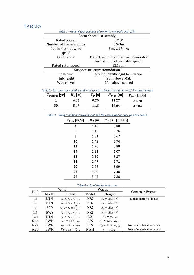
The structure used for the study is the 5MW monopile OWT model from the OC3 project [20]. 110
The main characteristics are described in Table 1. The platform has a constant thickness of 111
0.06m with a diameter of 6m whereas the tower diameter and thickness decrease linearly, the 112
4
diameter from 6 to 3.87m and thickness from 0.027 to 0.019m, further information can be 113
found in [21]. 114
2.2 Metocean data 115
The location chosen for this study is based on the Ijmuiden Shallow Water Site from the Upwind 116
design basis [22]. The site is found in the Dutch North Sea, the coordinates of Ijmuiden site are 117
52º33’00” east and 4º03’30” north. The metocean data is presented as 3-hour average values 118
for a period of 22 years. This location has been chosen in order to work with a realistic, 119
consistent and reasonable metocean dataset as the corresponding water depth and hub height 120
of this site matches well with the chosen benchmark monopile and water depth. 121
The main variables used in the following sections are shown next. The water levels used are the 122
Highest Still Water Level (HSWL) and Highest Astronautical Tide (HAT) which are 2.4 and 1.4m 123
above the Mean Sea Level (MSL). For normal current loads an average value of 0.6m/s at surface 124
level is taken and for the extreme case a value of 1.2m/s is considered. 125
The values for the extreme wave conditions were found to follow Equation (1) resulting in the 126
extreme wave height values shown in Table 2 [22]. A factor of 1.86 can be used to obtain the 127
maximum wave height in equation (2) as the water depth is relatively shallow [1]. 128
𝐻𝑆,3ℎ(𝑇𝑟𝑒𝑡𝑢𝑟𝑛) = 0.479 · ln(𝑇𝑟𝑒𝑡𝑢𝑟𝑛) + 6.0626 (1) 𝐻𝑚𝑎𝑥 = 1.86 · 𝐻𝑆,3ℎ (2)
where 𝐻𝑆,3ℎ is the significant wave height for a 3-hour reference period, 𝑇𝑟𝑒𝑡𝑢𝑟𝑛is the return 129
period corresponding to 𝐻𝑆,3ℎ and, 𝐻𝑚𝑎𝑥 is the Extreme Wave Height (EWH). 130
Moreover, the extreme wind values are determined from the measured data using a 10 minute 131
reference period. The measured data is fitted to a Weibull distribution with parameters A= 132
10.61m/s and k=2.08. The extreme wind speed is defined as the maximum wind speed that 133
occurs with a certain return period, resulting in Equation (3). The common return periods used 134
for the wind speed and their results can be seen in Table 2 [22]. 135
𝑉ℎ𝑢𝑏,10 𝑚𝑖𝑛(𝑇𝑟𝑒𝑡𝑢𝑟𝑛) = 2.6446 · ln(𝑇𝑟𝑒𝑡𝑢𝑟𝑛) + 31.695 (3)
where 𝑉ℎ𝑢𝑏,10 𝑚𝑖𝑛(𝑥) is the wind speed at the hub. 136
Power production DLCs, among others, use the significant wave height conditioned on wind 137
speed. Table 3 shows eleven wind speed bins of 2m/s size, from the cut-in to cut-out wind 138
speeds. The table also lists the significant wave height and peak spectral periods associated with 139
the wind speed [22]. 140
2.3 Modeling assumptions 141
For this study many simulations need to be performed to cover all the studied DLCs and thus 142
some assumptions and simplifications need to be applied to facilitate and optimise the 143
procedure. These are given in the following paragraphs: 144
• Writing and reading the turbulent wind field created by TurbSim [19] is very time-145
consuming, therefore the grid size is set to 13x13 points comprising an area of 146
155x155m2. 147
5
• The wind turbine uses a conventional variable-speed, blade-pitch-to-feather 148
configuration. The method for controlling power-production operation relies on the 149
design of two primary control loops: a generator-torque controller and a full-span rotor-150
collective blade-pitch controller. The goal of the generator-torque controller is to 151
maximize power capture below the rated operation point. On the other hand, blade-152
pitch controller aims to regulate the generator speed above the rated operation point. 153
NREL developed the NREL offshore 5-MW wind turbine’s baseline control system as an 154
external Dynamic Link Library (DLL) which is called by ServoDyn. Further information 155
about this routine can be found in [21]. 156
• It is also assumed that the wind turbine is class II within the framework found in IEC [2] 157
as it fits with wind data. The turbulence reference intensity is chosen as B (0.14) as class 158
A is unlikely to be found offshore, unless the spacing within the wind farm is lower than 159
typically found, and hence quite conservative. 160
• HydroDyn uses Morison’s equation to model the hydrodynamic loading; it uses Airy’s 161
theory to define the inertia and drag loading, both containing two empirical 162
hydrodynamic coefficients—an inertia coefficient and a drag coefficient. 163
• The current is modeled as a near-surface current, the model follows a linear relationship 164
down to a reference depth, further information can be found in the FAST user guide 165
[18]. 166
• The time span for each simulation is increased by 30 seconds, and the simulation results 167
for the initial 30 seconds were ignored to discount the start-up transients. 168
• For the DLCs which include deterministic wind transient changes spanning 10-12 169
seconds, the initial results spanning 30 seconds are deleted. Also, the start time for the 170
event is set at 80 seconds and the simulation time span is fixed as 120 seconds. This 171
combination gives enough time to analyse the DLC before and after the transient phase 172
dies out. 173
3. DESIGN LOAD CASES 174
This section goes through the subset of the IEC [1] DLCs considered in our study. As mentioned 175
earlier, attention is hereby restricted to the power production and parked load cases. More 176
specifically, the load cases considered are; 1.1, 1.3, 1.4, 1.5, 1.6a, 6.1a and 6.2a. A brief summary 177
of these DLCs is given in Table 4. 178
Each DLC is analysed separately highlighting the main characteristics of the environment-179
structure interaction. Three response variables are chosen as metrics for comparison among the 180
DLCs; the flapwise (out-of-plane) moment and edgewise (in-plane) moment at the root of the 181
blade and the overturning moment at the seabed. The first two are widely used for the design of 182
blades whereas the third drives the support structure design. The flapwise moment is the cause 183
of the out-of-plane blade tip deflection whereas edgewise moment creates an in-plane blade tip 184
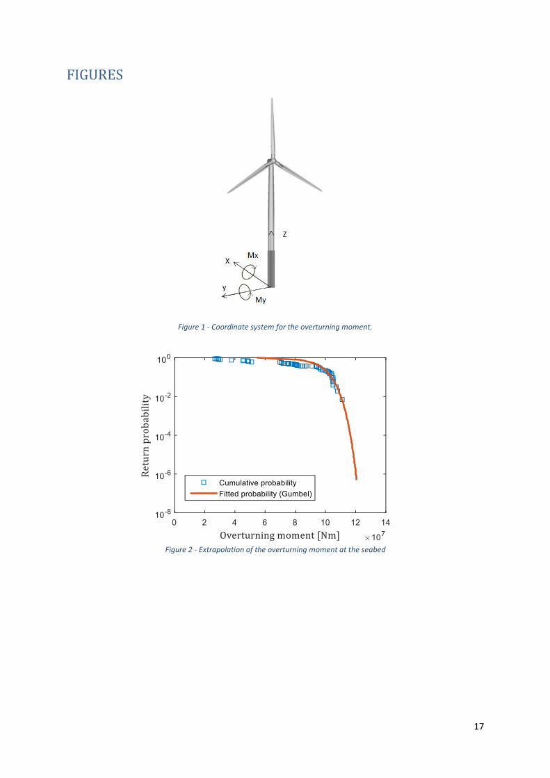
deflection. Considering the directional nature of loading, Equation (4) defines the overturning 185
moment at the mudline following the coordinate system shown in Figure 1. 186
𝑀𝑂𝑣𝑒𝑟𝑡𝑢𝑟𝑛𝑖𝑛𝑔 = √𝑀𝑥2 + 𝑀𝑦
2 (4)
3.1 Power production DLCs 187
This design situation simulates an OWT which is running and connected to the grid and hence 188
the turbine is producing electricity within the cut-in and cut-out range of wind speed. The DLCs 189
6
simulated corresponding to this design situation are 1.1, 1.3, 1.4, 1.5 and 1.6a. DLC 1.6b is not 190
included in current common practices for being not design driving and therefore it is omitted in 191
this section. 192
In these conditions the turbine is considered to use a torque and pitch controller implemented 193
in GH Bladed-style DLL format. The DLL (i.e., DISCON.dll) is supplied with the NREL 5-MW 194
models [21]. Pitch control will twist the blades by linking the angle of attack to wind speed 195
fluctuation whereas the variable-speed torque controller controls the rotor speed in order to 196
capture as much power as possible when the wind speed is below rated. This turbine does not 197
use a yaw controller; to account for the lack of it, some DLCs are simulated in this paper with 198
small yaw misalignments representing the possible yaw control delay. For heavily-loaded rotors 199
(i.e. at low wind speeds) the Generalized-Dynamic Wake (GDW) option (DYNIN) of AeroDyn is 200
numerically unstable [23] and hence the EQUIL model is set in AeroDyn instead of DYNIN for all 201
the simulations within the power production DLCs. 202
3.1.1 DLC 1.1 203
As the OWT does not include a yaw controller, the simulations are also performed with a yaw 204
misalignment of 0° and ±8° in order to account for the small delay that a yaw controller could 205
have. The IEC standard states that the number of simulations carried out for each mean wind 206
speed and sea state combination shall be sufficient to determine a reliable long term probability 207
distribution of extreme values for extrapolation to the characteristic load effect. The present 208
study considers six 10-minute simulations which result in a total of 198 simulations if seeds, 209
wind bins and yaw misalignment are taken into account (6 seeds x 11 wind speed bins x 3 yaw 210
angles). The purpose of this DLC is not to provide instantaneous histories for loads at desired 211
sections, but to statistically extrapolate the load response results of all multiple stochastic 212
simulations in order to achieve the structural response for a 50 year return period. 213
To do that, all the simulations corresponding to all the wind speed bins and yaw misalignment 214
angles are performed. For each wind bin, the mean of the 6 maximums (6 seeds) of the 215
overturning moment is taken, in this case corresponding to a yaw misalignment of 0°. Then all 216
the values of the time-series are sorted from smallest to largest and the Cumulative Distribution 217
Function (CDF) is obtained. After that a Gumbel distribution is fitted to the CDF by minimising 218
the least squares error corresponding to the distribution parameters. In order to not 219
overestimate the tail of the distribution a method which weights the error by the load 220
prediction difference between the two points is used. Therefore, in the tail region, where there 221
are fewer points, each point has relatively more importance. The result can be seen for the 222
overturning moment at the seabed in Figure 2, the same procedure is applied for the flapwise 223
and edgewise moments at the root of the blade. 224
The probability of exceedance related to a 50 year event is taken as 3.8E-07 [1] and it is found 225
using Equation (5), where N corresponds to the total number of independent 10-minute 226
intervals in 50 years. 227
A load factor of 1.25 is applied to the results after the extrapolation. These extrapolated values 228
are used to calibrate DLC 1.3, the extreme values derived from DLC 1.3 need to be equal or 229
higher than the extrapolated ones assuring this way that the structural response is related to a 230
50 year event. If the results from DLC 1.3 turn out to be lower than the extrapolated value from 231
𝑃𝐸𝑥𝑐𝑒𝑒𝑑𝑎𝑛𝑐𝑒 = 1/𝑁 (5)
7
DLC 1.1, then the Extreme Turbulence Model (ETM) in DLC 1.3 is re-calibrated by increasing the 232
c value, until the results from DLC 1.3 approach or exceed the extreme load computed in DLC 233
1.1. 234
3.1.2 DLC 1.3 235
This power production DLC has the same features as DLC 1.1 except for the wind model; DLC 236
1.3 uses the ETM instead of the Normal Turbulence Model (NTM). It is also simulated with a 237
slight misalignment to account for the lack of a yaw controller. The length and number of 238
simulations are the same as in DLC 1.1 (198), although there is no requirement to perform 239
extrapolation in this case. The wind, wave and current loading corresponding to the DLC are 240
applied to the model, and Figure 3 shows how the maximum values of each seed of the 241
overturning moment and rotor thrust evolve over the wind speed bins, for the case 242
corresponding to a yaw misalignment of -8°. 243
As the rotor thrust is measured along the shaft and it rotates with the nacelle-yaw angle, it 244
would be expected that thrust and tower-top loads should be very similar between onshore and 245
offshore monopile configurations. Generally, in pitch controlled OWT, higher loads are achieved 246
when wind speed is around rated wind speed, although a small yaw misalignment deforms the 247
trend at higher wind bins giving higher maximums for 20 and 22m/s, for a -8° and 8° yaw 248
misalignment, respectively. Furthermore, the characteristic load, the highest mean value of the 249
overturning moment maxima (dashed line in Figure 3), derived from this DLC is 1,167E+08Nm 250
for a mean wind speed of 16m/s and a yaw misalignment of 0°. 251
Two seeds are further investigated in Figure 4 to analyse the variability observed for wind 252
speed bins of 18m/s and 22m/s. The overturning moment maxima occur at different times, but 253
the cause seems to be the same; a decrease and increase of the wind speed causing a trough in 254
the pitch angle. This rotation towards 0° of the blade pitch angle creates a significant resistance 255
to the wind force and hence a peak in the overturning moment, the closer to 0° the trough gets, 256
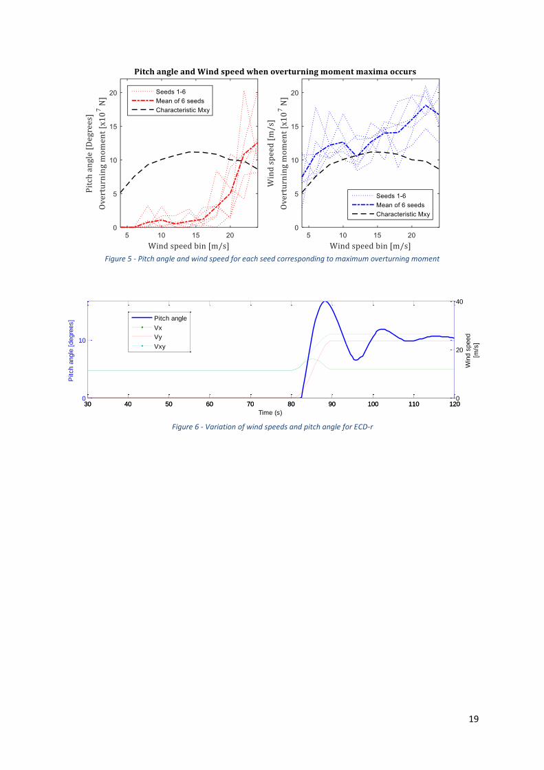
the higher the overturning moment becomes. Figure 5 helps in order to study this phenomena 257
further, it shows the pitch angle and the wind speed when the overturning moment maxima 258
occurs. The mean of the 6 seeds shows a rising trend over the wind bins, but interestingly, 259
higher pitch angle and wind speeds when maxima occurs mean lower overturning moments. To 260
summarise, it can be seen that the fluctuation of the wind speed causes pitch angle troughs, if 261
this happens close to the rated wind speed a higher overturning moment is to be expected. In 262
addition, larger fluctuations (turbulence) increase the chances of the wind speed decreasing 263
close to rated wind speed, creating deeper pitch angle troughs, and therefore higher 264
overturning moments. This also explains that, since we are using the ETM, the location of the 265
peak area in Figure 3 falls in the range of 14-18m/s, whereas if the same graph was plotted 266
using NTM, the peak would correspond to a lower range of wind speed bins, 12-14m/s, and the 267
tail would go lower. The short-term wave height seems not to have a significant influence on the 268
timing of the maximum loads. In Figure 4, the edgewise moment fluctuates with the wind speed, 269
but as there is no wind direction change this parameter is not that affected. On the other hand, 270
the flapwise moment at the root of the blade is more dependent on the wind oscillation and it is 271
also greatly affected by the pitch angle actuator delay, therefore both maxima come when pitch 272
angle approaches 0°, the same situation as for the maximum overturning moment. 273
As explained in the case of DLC 1.1, the design load from DLC 1.3 needs to be equal to or exceed 274
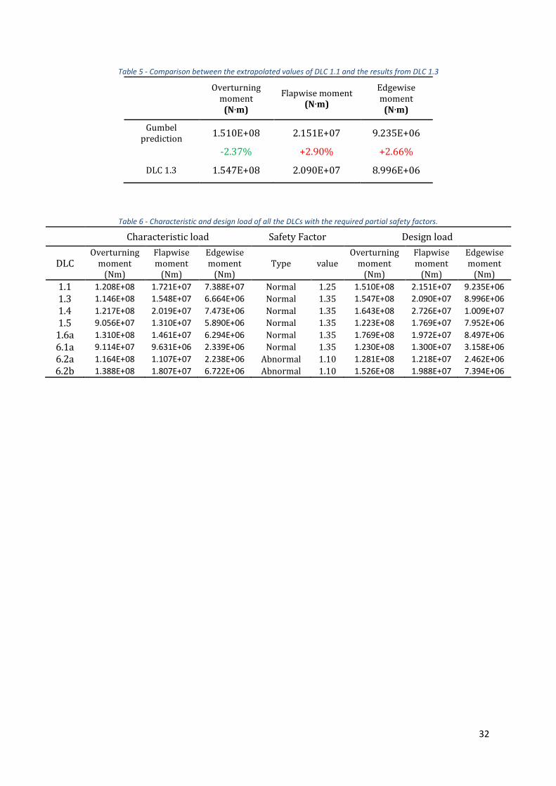
the extrapolated values from DLC 1.1. It is seen from Table 5 that only the design overturning 275
8
moment exceeds the results from DLC 1.1, for the purposes of this study, these small differences 276
are acceptable and therefore simulations are not performed again by increasing the value c. 277
3.1.3 DLC 1.4 278
This DLC might be quite sensitive to the initial azimuth angle of the blades, therefore it is 279
studied for 4 different initial azimuth angles of blade 1: 0°, 30°, 60° and 90°, and for the same 280
reason as for previous DLCs the simulations are also carried out for a yaw misalignment of 0° 281
and ±8°. Although a stochastic Normal Sea State (NSS) with a significant wave height 282
conditioned on rated wind speed is used, no seeds are used for this DLC, leading to a total of 72 283
simulations (6 wind types (ECD±r±2) x 4 azimuth angles x 3 yaw angles). 284
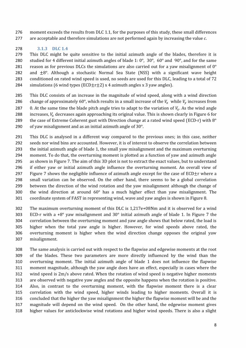
This DLC consists of an increase in the magnitude of wind speed, along with a wind direction 285
change of approximately 60°, which results in a small increase of the 𝑉𝑥 while 𝑉𝑦 increases from 286
0. At the same time the blade pitch angle tries to adapt to the variation of 𝑉𝑥 . As the wind angle 287
increases, 𝑉𝑥 decreases again approaching its original value. This is shown clearly in Figure 6 for 288
the case of Extreme Coherent gust with Direction change at a rated wind speed (ECD-r) with 8° 289
of yaw misalignment and as an initial azimuth angle of 30°. 290
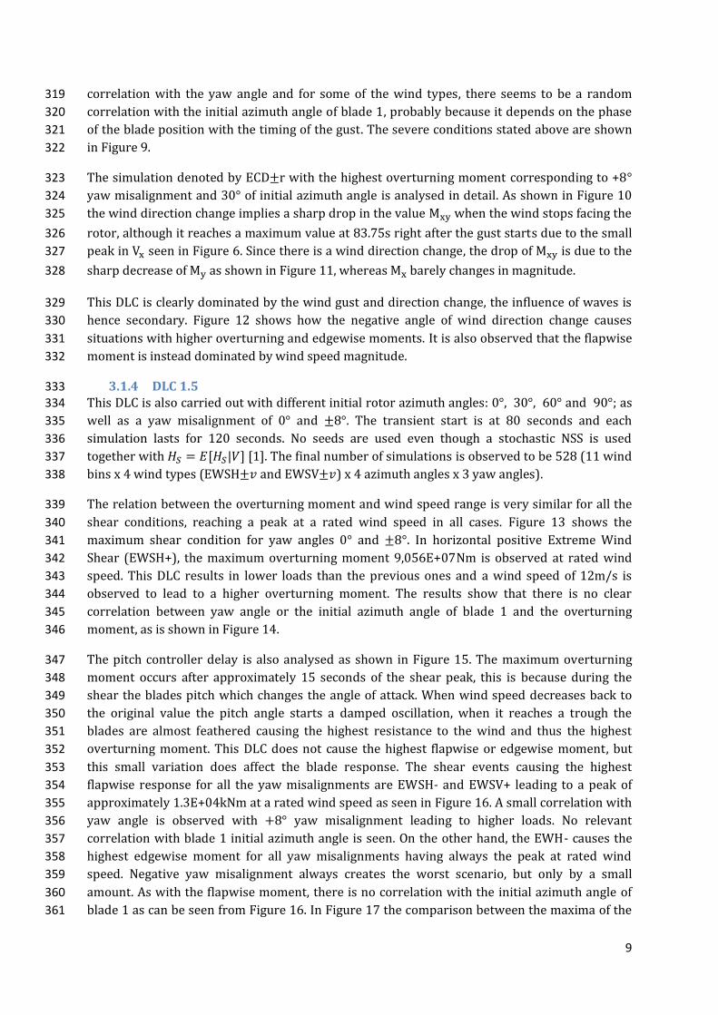
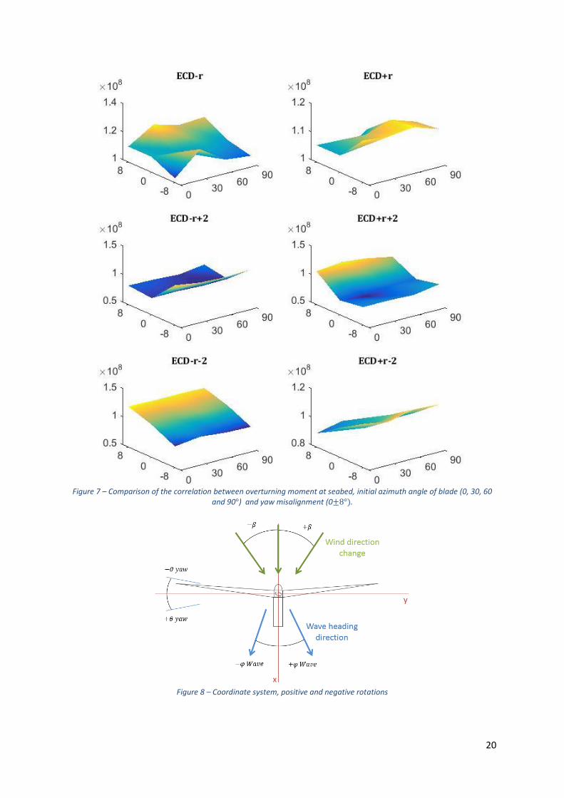
This DLC is analysed in a different way compared to the previous ones; in this case, neither 291
seeds nor wind bins are accounted. However, it is of interest to observe the correlation between 292
the initial azimuth angle of blade 1, the small yaw misalignment and the maximum overturning 293
moment. To do that, the overturning moment is plotted as a function of yaw and azimuth angle 294
as shown in Figure 7. The aim of this 3D plot is not to extract the exact values, but to understand 295
if either yaw or initial azimuth angle influence the overturning moment. An overall view of 296
Figure 7 shows the negligible influence of azimuth angle except for the case of ECD±r where a 297
small variation can be observed. On the other hand, there seems to be a global correlation 298
between the direction of the wind rotation and the yaw misalignment although the change of 299
the wind direction at around 60° has a much higher effect than yaw misalignment. The 300
coordinate system of FAST in representing wind, wave and yaw angles is shown in Figure 8. 301
The maximum overturning moment of this DLC is 1,217e+08Nm and it is observed for a wind 302
ECD-r with a +8° yaw misalignment and 30° initial azimuth angle of blade 1. In Figure 7 the 303
correlation between the overturning moment and yaw angle shows that below rated, the load is 304
higher when the total yaw angle is higher. However, for wind speeds above rated, the 305
overturning moment is higher when the wind direction change opposes the original yaw 306
misalignment. 307
The same analysis is carried out with respect to the flapwise and edgewise moments at the root 308
of the blades. These two parameters are more directly influenced by the wind than the 309
overturning moment. The initial azimuth angle of blade 1 does not influence the flapwise 310
moment magnitude, although the yaw angle does have an effect, especially in cases where the 311
wind speed is 2m/s above rated. When the rotation of wind speed is negative higher moments 312
are observed with negative yaw angles and the opposite happens when the rotation is positive. 313
Also, in contrast to the overturning moment, with the flapwise moment there is a clear 314
correlation with the wind speed, higher winds leading to higher moments. Overall it is 315
concluded that the higher the yaw misalignment the higher the flapwise moment will be and the 316
magnitude will depend on the wind speed. On the other hand, the edgewise moment gives 317
higher values for anticlockwise wind rotations and higher wind speeds. There is also a slight 318
9
correlation with the yaw angle and for some of the wind types, there seems to be a random 319
correlation with the initial azimuth angle of blade 1, probably because it depends on the phase 320
of the blade position with the timing of the gust. The severe conditions stated above are shown 321
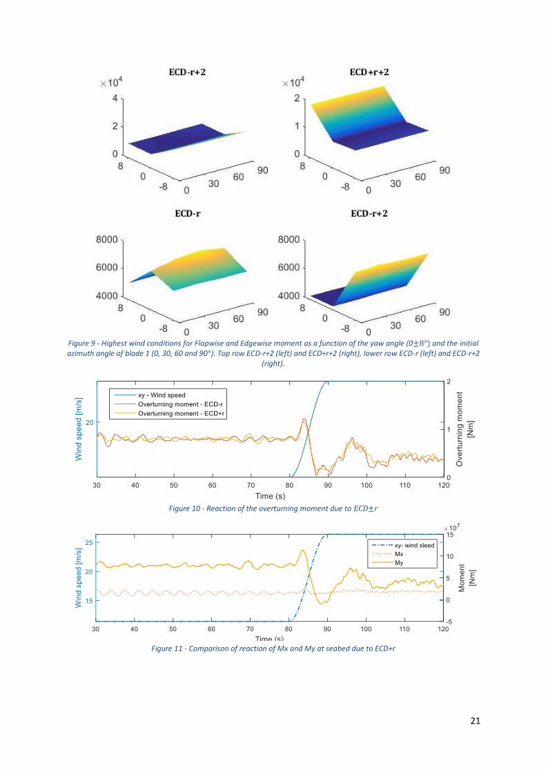
in Figure 9. 322
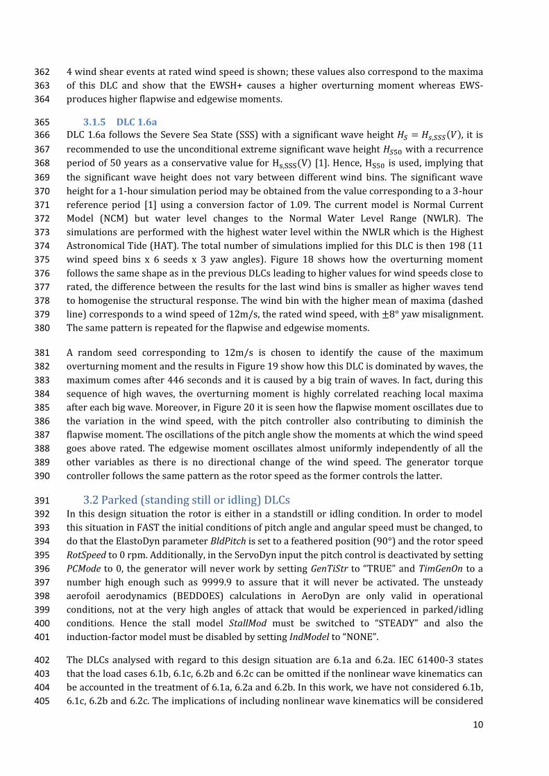
The simulation denoted by ECD±r with the highest overturning moment corresponding to +8° 323
yaw misalignment and 30° of initial azimuth angle is analysed in detail. As shown in Figure 10 324
the wind direction change implies a sharp drop in the value Mxy when the wind stops facing the 325
rotor, although it reaches a maximum value at 83.75s right after the gust starts due to the small 326
peak in Vx seen in Figure 6. Since there is a wind direction change, the drop of Mxy is due to the 327
sharp decrease of My as shown in Figure 11, whereas Mx barely changes in magnitude. 328
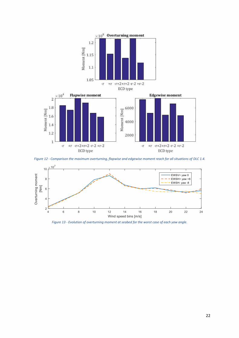
This DLC is clearly dominated by the wind gust and direction change, the influence of waves is 329
hence secondary. Figure 12 shows how the negative angle of wind direction change causes 330
situations with higher overturning and edgewise moments. It is also observed that the flapwise 331
moment is instead dominated by wind speed magnitude. 332
3.1.4 DLC 1.5 333 This DLC is also carried out with different initial rotor azimuth angles: 0°, 30°, 60° and 90°; as 334
well as a yaw misalignment of 0° and ±8°. The transient start is at 80 seconds and each 335
simulation lasts for 120 seconds. No seeds are used even though a stochastic NSS is used 336
together with 𝐻𝑆 = 𝐸[𝐻𝑆|𝑉] [1]. The final number of simulations is observed to be 528 (11 wind 337
bins x 4 wind types (EWSH±𝑣 and EWSV±𝑣) x 4 azimuth angles x 3 yaw angles). 338
The relation between the overturning moment and wind speed range is very similar for all the 339
shear conditions, reaching a peak at a rated wind speed in all cases. Figure 13 shows the 340
maximum shear condition for yaw angles 0° and ±8°. In horizontal positive Extreme Wind 341
Shear (EWSH+), the maximum overturning moment 9,056E+07Nm is observed at rated wind 342
speed. This DLC results in lower loads than the previous ones and a wind speed of 12m/s is 343
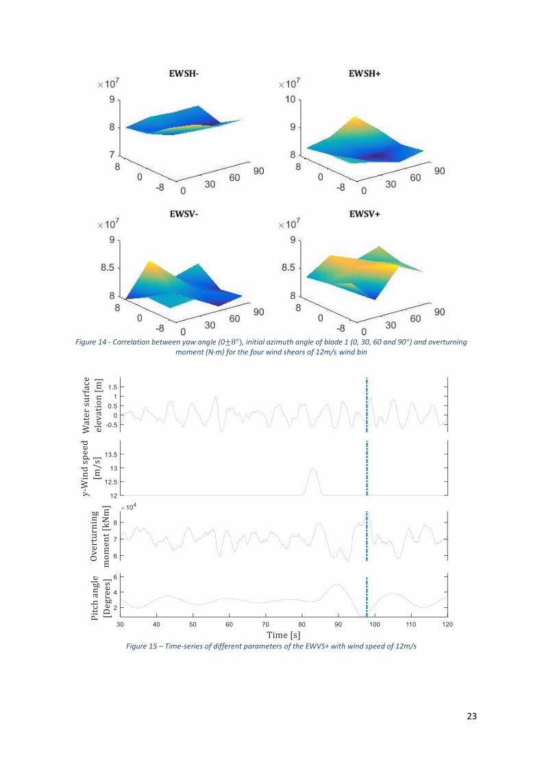
observed to lead to a higher overturning moment. The results show that there is no clear 344
correlation between yaw angle or the initial azimuth angle of blade 1 and the overturning 345
moment, as is shown in Figure 14. 346
The pitch controller delay is also analysed as shown in Figure 15. The maximum overturning 347
moment occurs after approximately 15 seconds of the shear peak, this is because during the 348
shear the blades pitch which changes the angle of attack. When wind speed decreases back to 349
the original value the pitch angle starts a damped oscillation, when it reaches a trough the 350
blades are almost feathered causing the highest resistance to the wind and thus the highest 351
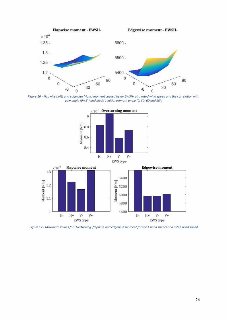
overturning moment. This DLC does not cause the highest flapwise or edgewise moment, but 352
this small variation does affect the blade response. The shear events causing the highest 353
flapwise response for all the yaw misalignments are EWSH- and EWSV+ leading to a peak of 354
approximately 1.3E+04kNm at a rated wind speed as seen in Figure 16. A small correlation with 355
yaw angle is observed with +8° yaw misalignment leading to higher loads. No relevant 356
correlation with blade 1 initial azimuth angle is seen. On the other hand, the EWH- causes the 357
highest edgewise moment for all yaw misalignments having always the peak at rated wind 358
speed. Negative yaw misalignment always creates the worst scenario, but only by a small 359
amount. As with the flapwise moment, there is no correlation with the initial azimuth angle of 360
blade 1 as can be seen from Figure 16. In Figure 17 the comparison between the maxima of the 361
10
4 wind shear events at rated wind speed is shown; these values also correspond to the maxima 362
of this DLC and show that the EWSH+ causes a higher overturning moment whereas EWS- 363
produces higher flapwise and edgewise moments. 364
3.1.5 DLC 1.6a 365 DLC 1.6a follows the Severe Sea State (SSS) with a significant wave height 𝐻𝑆 = 𝐻𝑠,𝑆𝑆𝑆(𝑉), it is 366
recommended to use the unconditional extreme significant wave height 𝐻𝑆50 with a recurrence 367
period of 50 years as a conservative value for Hs,SSS(V) [1]. Hence, HS50 is used, implying that 368
the significant wave height does not vary between different wind bins. The significant wave 369
height for a 1-hour simulation period may be obtained from the value corresponding to a 3-hour 370
reference period [1] using a conversion factor of 1.09. The current model is Normal Current 371
Model (NCM) but water level changes to the Normal Water Level Range (NWLR). The 372
simulations are performed with the highest water level within the NWLR which is the Highest 373
Astronomical Tide (HAT). The total number of simulations implied for this DLC is then 198 (11 374
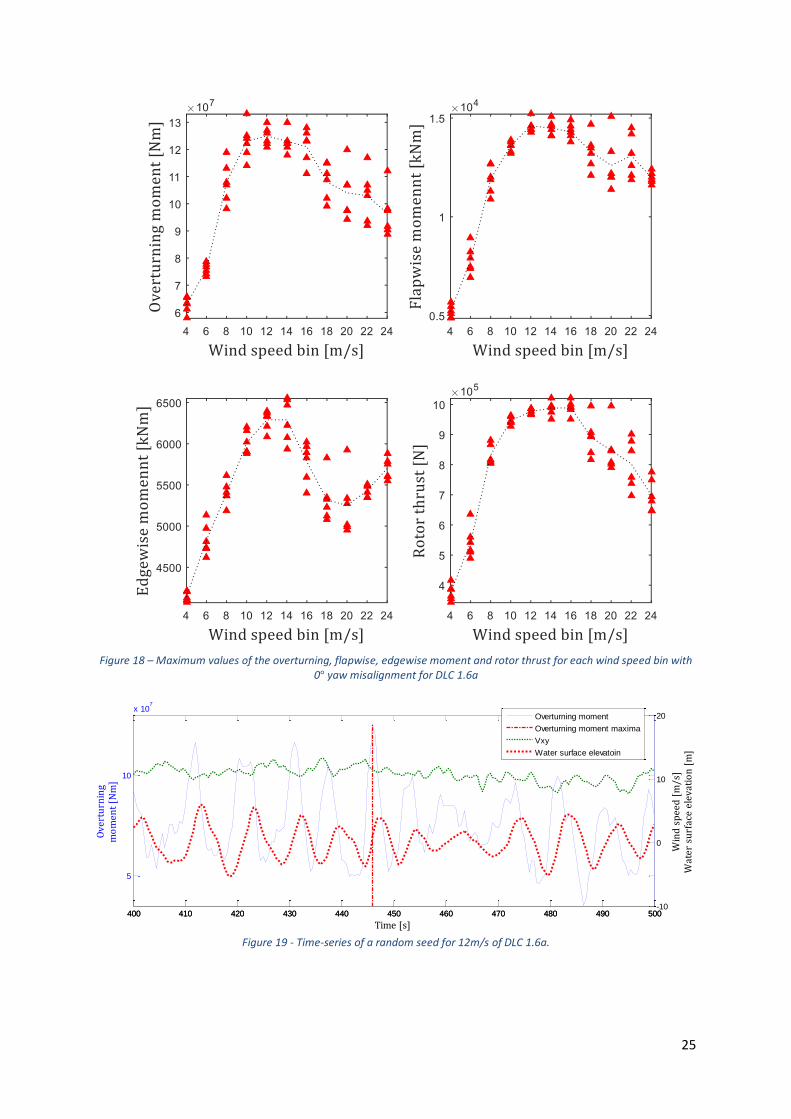
wind speed bins x 6 seeds x 3 yaw angles). Figure 18 shows how the overturning moment 375
follows the same shape as in the previous DLCs leading to higher values for wind speeds close to 376
rated, the difference between the results for the last wind bins is smaller as higher waves tend 377
to homogenise the structural response. The wind bin with the higher mean of maxima (dashed 378
line) corresponds to a wind speed of 12m/s, the rated wind speed, with ±8° yaw misalignment. 379
The same pattern is repeated for the flapwise and edgewise moments. 380
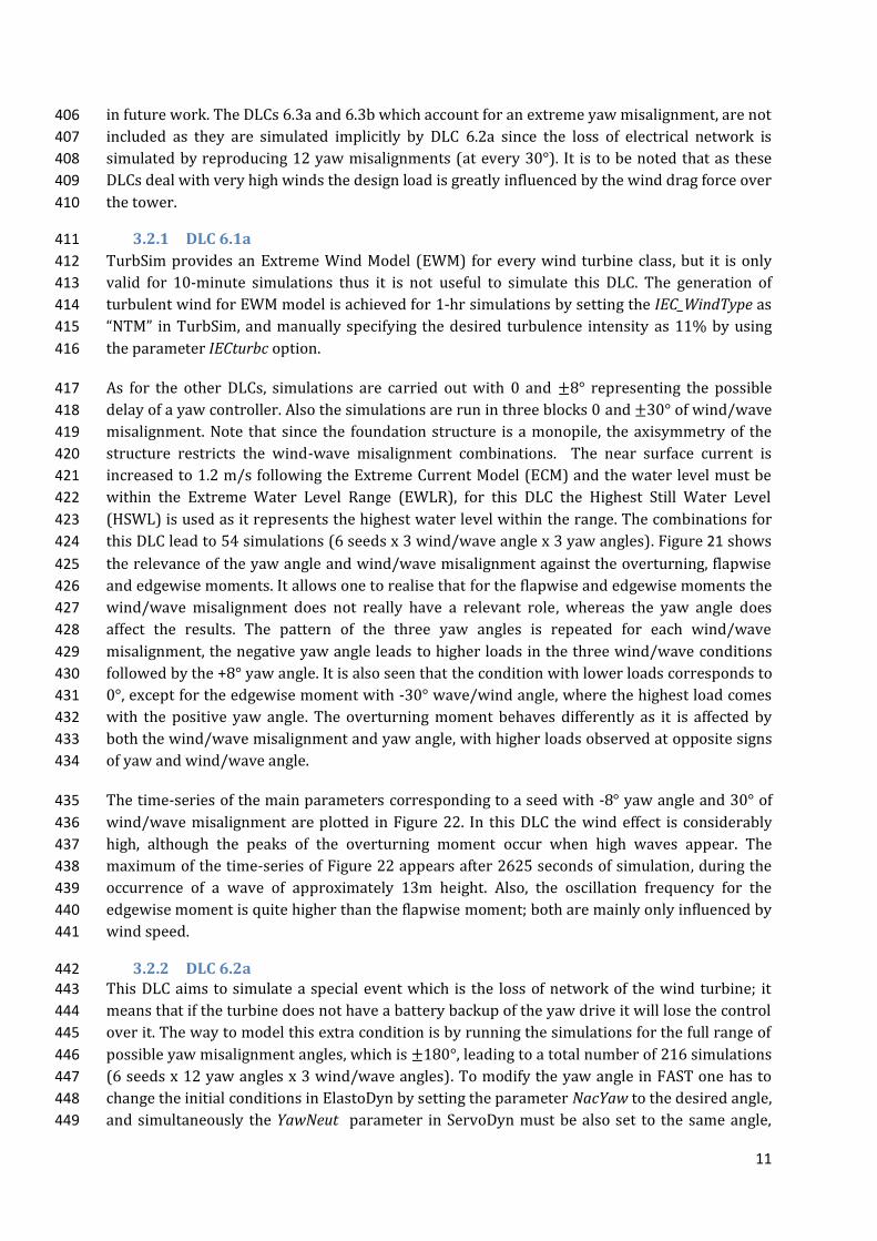
A random seed corresponding to 12m/s is chosen to identify the cause of the maximum 381
overturning moment and the results in Figure 19 show how this DLC is dominated by waves, the 382
maximum comes after 446 seconds and it is caused by a big train of waves. In fact, during this 383
sequence of high waves, the overturning moment is highly correlated reaching local maxima 384
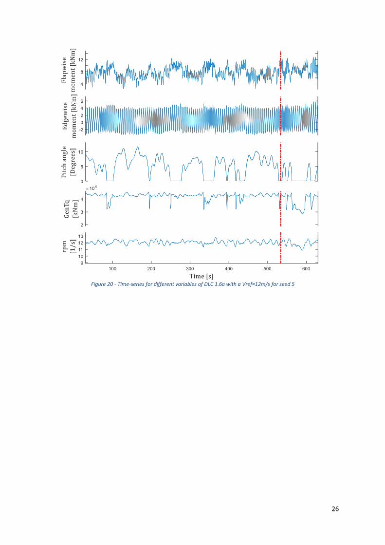
after each big wave. Moreover, in Figure 20 it is seen how the flapwise moment oscillates due to 385
the variation in the wind speed, with the pitch controller also contributing to diminish the 386
flapwise moment. The oscillations of the pitch angle show the moments at which the wind speed 387
goes above rated. The edgewise moment oscillates almost uniformly independently of all the 388
other variables as there is no directional change of the wind speed. The generator torque 389
controller follows the same pattern as the rotor speed as the former controls the latter. 390
3.2 Parked (standing still or idling) DLCs 391
In this design situation the rotor is either in a standstill or idling condition. In order to model 392
this situation in FAST the initial conditions of pitch angle and angular speed must be changed, to 393
do that the ElastoDyn parameter BldPitch is set to a feathered position (90°) and the rotor speed 394
RotSpeed to 0 rpm. Additionally, in the ServoDyn input the pitch control is deactivated by setting 395
PCMode to 0, the generator will never work by setting GenTiStr to “TRUE” and TimGenOn to a 396
number high enough such as 9999.9 to assure that it will never be activated. The unsteady 397
aerofoil aerodynamics (BEDDOES) calculations in AeroDyn are only valid in operational 398
conditions, not at the very high angles of attack that would be experienced in parked/idling 399
conditions. Hence the stall model StallMod must be switched to “STEADY” and also the 400
induction-factor model must be disabled by setting IndModel to “NONE”. 401
The DLCs analysed with regard to this design situation are 6.1a and 6.2a. IEC 61400-3 states 402
that the load cases 6.1b, 6.1c, 6.2b and 6.2c can be omitted if the nonlinear wave kinematics can 403
be accounted in the treatment of 6.1a, 6.2a and 6.2b. In this work, we have not considered 6.1b, 404
6.1c, 6.2b and 6.2c. The implications of including nonlinear wave kinematics will be considered 405
11
in future work. The DLCs 6.3a and 6.3b which account for an extreme yaw misalignment, are not 406
included as they are simulated implicitly by DLC 6.2a since the loss of electrical network is 407
simulated by reproducing 12 yaw misalignments (at every 30°). It is to be noted that as these 408
DLCs deal with very high winds the design load is greatly influenced by the wind drag force over 409
the tower. 410
3.2.1 DLC 6.1a 411
TurbSim provides an Extreme Wind Model (EWM) for every wind turbine class, but it is only 412
valid for 10-minute simulations thus it is not useful to simulate this DLC. The generation of 413
turbulent wind for EWM model is achieved for 1-hr simulations by setting the IEC_WindType as 414
“NTM” in TurbSim, and manually specifying the desired turbulence intensity as 11% by using 415
the parameter IECturbc option. 416
As for the other DLCs, simulations are carried out with 0 and ±8° representing the possible 417
delay of a yaw controller. Also the simulations are run in three blocks 0 and ±30° of wind/wave 418
misalignment. Note that since the foundation structure is a monopile, the axisymmetry of the 419
structure restricts the wind-wave misalignment combinations. The near surface current is 420
increased to 1.2 m/s following the Extreme Current Model (ECM) and the water level must be 421
within the Extreme Water Level Range (EWLR), for this DLC the Highest Still Water Level 422
(HSWL) is used as it represents the highest water level within the range. The combinations for 423
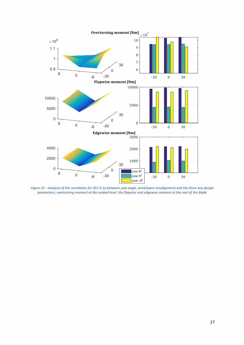
this DLC lead to 54 simulations (6 seeds x 3 wind/wave angle x 3 yaw angles). Figure 21 shows 424
the relevance of the yaw angle and wind/wave misalignment against the overturning, flapwise 425
and edgewise moments. It allows one to realise that for the flapwise and edgewise moments the 426
wind/wave misalignment does not really have a relevant role, whereas the yaw angle does 427
affect the results. The pattern of the three yaw angles is repeated for each wind/wave 428
misalignment, the negative yaw angle leads to higher loads in the three wind/wave conditions 429
followed by the +8° yaw angle. It is also seen that the condition with lower loads corresponds to 430
0°, except for the edgewise moment with -30° wave/wind angle, where the highest load comes 431
with the positive yaw angle. The overturning moment behaves differently as it is affected by 432
both the wind/wave misalignment and yaw angle, with higher loads observed at opposite signs 433
of yaw and wind/wave angle. 434
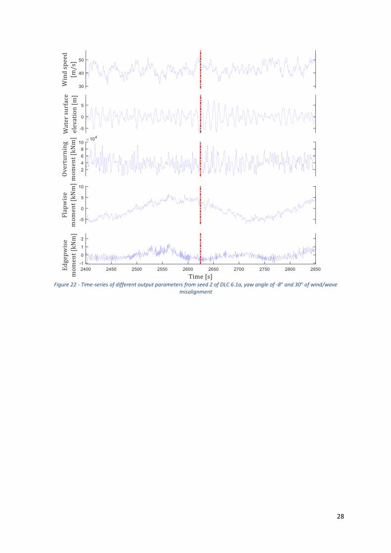
The time-series of the main parameters corresponding to a seed with -8° yaw angle and 30° of 435
wind/wave misalignment are plotted in Figure 22. In this DLC the wind effect is considerably 436
high, although the peaks of the overturning moment occur when high waves appear. The 437
maximum of the time-series of Figure 22 appears after 2625 seconds of simulation, during the 438
occurrence of a wave of approximately 13m height. Also, the oscillation frequency for the 439
edgewise moment is quite higher than the flapwise moment; both are mainly only influenced by 440
wind speed. 441
3.2.2 DLC 6.2a 442 This DLC aims to simulate a special event which is the loss of network of the wind turbine; it 443
means that if the turbine does not have a battery backup of the yaw drive it will lose the control 444
over it. The way to model this extra condition is by running the simulations for the full range of 445
possible yaw misalignment angles, which is ±180°, leading to a total number of 216 simulations 446
(6 seeds x 12 yaw angles x 3 wind/wave angles). To modify the yaw angle in FAST one has to 447
change the initial conditions in ElastoDyn by setting the parameter NacYaw to the desired angle, 448
and simultaneously the YawNeut parameter in ServoDyn must be also set to the same angle, 449
12
otherwise the restoring spring would be acting to rotate the rotor and nacelle towards the 450
neutral angle. 451
It is important to highlight that when using FAST there is an instability that occurs for the NREL 452
baseline turbine at around ±30° degrees. This is described as an "aero-elastic interaction 453
causing negative damping in a mode that couples rotor azimuth with platform yaw" [24]. The 454
current approach by the industry to deal with this problem is either to bypass it by choosing 455
yaw errors that do not result in the instability or increase the structural damping in the blade 456
edge/tower side-to-side mode until the instability disappears. In the present work, the first 457
option is considered by ignoring the case that causes the instability. 458
The 30° wind/wave misalignment seems to create a slightly higher overturning moment for 60° 459
yaw angle and therefore a random seed of this combination is used to study this DLC. The 460
overturning moment at the seabed, the flapwise and edgewise moments at the root of blade 1, 461
rotor thrust (in the direction of the mean wind, regardless of the yaw error) and shear force at 462
the top of the tower are plotted in Figure 23 for 30° wind/wave misalignment, all yaw angles 463
with corresponding maxima for all the 6 seeds. The instability commented before is reflected in 464
the variability of these three parameters at ±30° of yaw angle, although some of these values 465
are not plotted here. The minima and maxima of the shear force values include structural 466
oscillations of the rotor-nacelle weight/inertia, but the weight/inertia should not impact the 467
mean values much. As expected, the maximum tower shear occurs for 90° yaw error, where the 468
incoming wind is normal to the chord when the blades are pitched to 90°. FAST calculates the 469
rotor loads for these cases; however a bigger part of the load is the direct wind load on the 470
tower, which dominates the rotor loads during this condition for most yaw errors. The effect of 471
tower drag loading is seen on the overturning moment at the seabed level. From Figure 24, it is 472
seen that the behaviour is similar to DLC 6.1a as large wave trains seem to dominate local 473
maxima of the overturning moment, although the highest value occurs when a large wave and a 474
wind speed peak occur simultaneously. 475
4. DISCUSSION OF RESULTS 476
4.1 Safety factors 477
This section aims to compare the results obtained in the previous sections, with a view to rank 478
the considered DLCs, and hence identify the most severe DLC in terms of its effect on the 479
support structure. For each DLC, the design load is deduced by applying recommended factors 480
of safety on the characteristic loads obtained from the simulations. As specified in IEC 61400-3 481
for DLCs with deterministic wind field and wave events, the characteristic value of the load 482
effect shall be the worst case computed transient value. If turbulent inflow is used together with 483
irregular sea states, the mean value among the worst case computed load effects for different 484
stochastic realisations shall be taken. If this is applied to the DLCs analysed within this report, 485
DLCs 1.4 and 1.5 are included in the first group, whereas for DLCs 1.1, 1.3, 1.6a, 6.1a and 6.2a 486
the characteristic load is obtained as the highest average (over 6 seeds) of all cases. Table 6 487
indicates the partial safety factors required for each DLC, stated in IEC 61400-3. For the ULS 488
DLCs within power production situation the normal partial safety factor of 1.35 is assigned, 489
except for DLC 1.1 in which 1.25 must be used as the loads are determined using statistical 490
extrapolation. In the case of ULS parked DLCs a normal safety factor of 1.35 is required except 491
for DLCs 6.2 in which the loss of electrical network is combined with the 50-year return wind 492
and wave conditions. As this combined event has a lower probability of occurrence, an 493
13
abnormal partial safety factor of 1.1 is assigned. Table 6 shows the obtained design values for 494
the overturning moment at the mudline and flapwise moment at the root of the blade. 495
4.2 Structural response 496
The set of values of the overturning moment at the seabed level, flapwise and edgewise 497
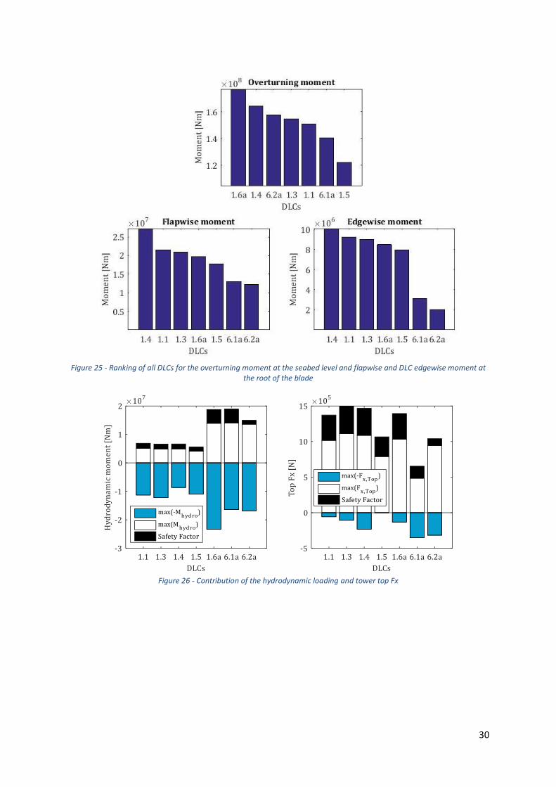
moments for all DLCs was created, sorted from the largest to the smallest and shown in Figure 498
25. It is observed that DLC 1.6a leads to the highest design overturning moment of 1.77E+08Nm, 499
followed by DLC 1.4 in which the result is 7.34% lower. The least demanding DLC is 1.5. For the 500
edgewise and flapwise moments the ranking follows a very similar pattern, the DLC causing the 501
highest design loads is 1.4 followed by 1.1 and 1.3, although for the flapwise moment the 502
difference between 1.4 and the others is much bigger (21.25%) than for the edgewise moment, 503
where the difference is only 8.6%. 504
It is useful to understand and compare the real influence and contribution of the hydrodynamic 505
loading and the tower top Fx force to the overall structure response, as shown in Figure 26. 506
Firstly, it is interesting to see how the largest negative values of the hydrodynamic moment at 507
the seabed level are larger than the positive ones. However, this effect is rather positive for the 508
structure as it opposes the main x-positive loading and helps damping the structure and 509
reducing the overturning moment. On the other hand, it can be seen that DLCs 1.6a, 6.1a and 510
6.2a are more hydrodynamically loaded than the others, and despite having lesser tower top 511
loading two of them (1.6a and 6.2a) are in the top 3 of the ranking. Therefore, the design of this 512
structure is driven by the hydrodynamic loading. 513
Also, the position of DLC 1.4 for the 3 studied parameters is remarkable, as the use of 514
deterministic wind field captures two negative effects at same time. First, the wind gust 515
together with the delay on the pitch controller creates a large overturning and flapwise 516
moment, and secondly, it shows how the wind rotation leads to the severest response of the 517
edgewise moment. In addition, the effect of the pitch controller on the structural response and 518
its role in driving the design loads must be carefully noted. The overturning and flapwise 519
moments show a significant high correlation with the pitch angle in power production DLCs, 520
meaning that sharp variations in the latter lead to critical design situations. Hence, 521
improvements in the pitch controller such as individual pitch control [25, 26] or anticipating the 522
wind troughs [27, 28] would directly diminish the design loads. 523
5. Conclusions 524
We have conducted a systematic comparative study of the power production and parked load 525
cases proposed by the IEC 61400-3 as those load cases are most likely to cause design driving 526
loads for OWT support structures. The analysis is conducted on a prototypical turbine mounted 527
on a monopile structure. The metocean parameters are extracted from a well-known database. 528
The key parameter for the design of the support structure is identified as the overturning 529
moment at the mudline level, and for the blade design, the flapwise and edgewise moments at 530
the blade root. The simulations are carried out using FAST. The structural response to different 531
ultimate limit states is analysed and the DLCs are ranked based on these three parameters to 532
provide guidance to other researchers and industry for designing these structures. The 533
hydrodynamic loading is proven as the design driving load for the support structure as 534
maximum overturning moment is reached in DLC 1.6a, whereas a wind gust together with a 535
wind direction change is the situation causing both the highest flapwise and edgewise moments. 536
14
Some complications derived from the code instabilities are addressed and solutions are 537
proposed. The results of our work will be useful as starting points for detailed study of the 538
relevant load cases, as well as to conduct reliability analyses for various limit states for the 539
substructure. While we believe that the considered load cases in this study are comprehensive 540
to cover substructure design, future work will address the transient load cases (faults, startup 541
and shutdown). Future work will also shed light on the sensitivity of the conclusions of the 542
present work to metocean conditions, water depths and monopile geometry. 543
Acknowledgments 544
This PhD research is funded by Lloyd’s Register Group Services Ltd., Aberdeen. Sriramula’s 545
work within the Lloyd’s Register Foundation Centre for Safety and Reliability Engineering at the 546
University of Aberdeen is supported by Lloyd’s Register Foundation. The Foundation helps to 547
protect life and property by supporting engineering-related education, public engagement and 548
the application of research. We would also like to acknowledge the constant assistance provided 549
by Jason Jonkman on using FAST. 550
551
Abbreviations 552
CDF Cumulative Distribution Function
DLC Design Load Case
DLL Dynamic Link Library
ECD Extreme Coherent gust with direction Change
ECM Extreme Current Model
ESS Extreme Sea State
ETM Extreme Turbulence Model
EWM Extreme Wind Model
EWS Extreme Wind Shear
GDW Generalized-Dynamic Wake
HAT Highest Astronautical Tide
HSWL Highest Still Water Level
MSL Mean Sea Level
NCM Normal Current Model
NREL National Renewable Energy Laboratory
NSS Normal Sea State
NTM Normal Turbulence Model
OC3 Offshore Code Comparison Collaboration
OWT Offshore Wind Turbine
RECOFF Recommendations for Offshore wind turbines design
SSS Severe Sea State
ULS Ultimate Limit State
15
References 553
[1] IEC, (2009). IEC 61400-3: Wind Turbines–Part 3: Design Requirements for offshore wind turbines, 554 International Electrotechnical Commission, Geneva. 555
[2] IEC, (2005). IEC 61400-1: Wind Turbines–Part 1: Design Requirements, International Electrotechnical 556 Commission, Geneva. 557
[3] Frandsen, S., Tarp-Johansen, N.J., Norton, E., Argyriadis, K., Bulder, B. and Rossis, K., (2005). 558 Recommendations for design of offshore wind turbines, Report No. Final Technical Report, Risø National 559 Laboratory, Roskilde, Denmark. 560
[4] Norton, E. and Quarton, D., (2003). Recommendations for design of offshore wind tubines (RECOFF), D3 561 Deliverable-Collated Sensitivity Studies, Document No, 2762. 562
[5] Tarp-Johansen, N.J., (2005). Partial Safety Factors and Characteristic Values for Combined Extreme Wind 563 and Wave Load Effects, Journal of Solar Energy Engineering, 127 (2), pp.242-252. 564
[6] Tarp-Johansen, N., Manwell, J. and McGowan, J., (2006). Application of design standards to the design of 565 offshore wind turbines in the US, Offshore Technology Conference, Houston, Texas. 566
[7] Stewart, G., Lackner, M., Haid, L., Matha, D., Jonkman, J. and Robertson, A., (2013). Assessing fatigue and 567 ultimate load uncertainty in floating offshore wind turbines due to varying simulation length, 11th 568 International Conference on Structural Safety and Reliability; Columbia University, New York, New York; 569 June 16-20, 2013. 570
[8] Agarwal, P. and Manuel, L., (2007). Simulation of offshore wind turbine response for extreme limit states, 571 ASME 2007 26th International Conference on Offshore Mechanics and Arctic Engineering, pp. 219-228. 572
[9] Agarwal, P., (2008). Structural Reliability of Offshore Wind Turbines, B.Tech., M.S. The University of Texas at 573 Austin. 574
[10] Moriarty, P.J., Holley, W. and Butterfield, C.P., (2004). Extrapolation of extreme and fatigue loads using 575 probabilistic methods, Report No. NREL/TP-500-34421, Cole Boulevard, Golden, Colorado: Citeseer. 576
[11] Cheng, P.W., (2002). A reliability based design methodology for extreme responses of offshore wind 577 turbines, TU Delft, Delft University of Technology. 578
[12] Vermula, N.K., (2010). Deliverable D4.2.5 - WP4.2: Offshore foundations and support structures, UpWind 579 project. 580
[13] De Vries, W., (2011). Deliverable D4.2.8 - WP4.2: Offshore foundations and support structures, UpWind 581 project. 582
[14] Kim, B., Jin, J., Bitkina, O. and Kang, K., (2015). Ultimate load characteristics of NREL 5‐MW offshore wind 583 turbines with different substructures, International Journal of Energy Research. 584
[15] Cordle, A., McCann, G. and de Vries, W., (2011). Design drivers for offshore wind turbine jacket support 585 structures, ASME 2011 30th International Conference on Ocean, Offshore and Arctic Engineering, pp. 419-586 428. 587
[16] Morató Casademunt, A., Sriramula, S. and Krishnan, N., (Sept 2016). Reliability analysis of offshore wind 588 turbine support structures using kriging models, Safety and Reliability of Complex Engineered Systems, 589 ESREL 2016, Glasgow, UK. 590
16
[17] Galinosa, C., Larsena, T.J., Madsena, H.A. and Paulsena, U.S., (January 2016). Vertical axis wind turbine 591 design load cases investigation and comparison with horizontal axis wind turbine, Deep Sea Offshore 592 Wind R&D Conference. DeepWind' 2016, Trondheim, Norway. 593
[18] Jonkman, J.M. and Buhl, M.L.J., (Updated August 2005). FAST user's guide - Technical report NREL/EL-500-594 38230 national renewable energy laboratory, Report No. 144 pp, Colorado, USA. 595
[19] Jonkman, B.J., (2009). TurbSim User's Guide: Version 1.50. National Renewable Energy Laboratory Golden, 596 CO, USA. 597
[20] Jonkman, J. and Musial, W., (2010). Offshore Code Comparison Collaboration (OC3) for IEA Wind Task 23 598 Offshore Wind Technology and Deployment. National Renewable Energy Laboratory (NREL), Golden, CO. 599
[21] Jonkman, J.M., Butterfield, S., Musial, W. and Scott, G., (2009). Definition of a 5-MW reference wind 600 turbine for offshore system development, Report No. NREL/TP-500-38060, Colorado, USA: National 601 Renewable Energy Laboratory. 602
[22] Fischer, T., De Vries, W. and Schmidt, B., (2010). UpWind design basis (WP4: Offshore foundations and 603 support structures), Project UpWind. 604
[23] Moriarty, P.J. and Hansen, A.C., (2005). AeroDyn theory manual, Report No. NREL/TP-500-36881, 1617 605 Cole Boulevard, Golden, Colorado 80401-3393: National Renewable Energy Laboratory. 606
[24] Skrzypiński, W., (2012). Analysis and modeling of unsteady aerodynamics with application to wind turbine 607 blade vibration at standstill conditions. 608
[25] Bossanyi, E., (2003). Individual blade pitch control for load reduction, Wind Energy, 6 (2), pp.119-128. 609
[26] Liu, H., Wang, Y., Tang, Q. and Yuan, X., (2015). Individual pitch control strategy of wind turbine to reduce 610 load fluctuations and torque ripples, International Conference on Renewable Power Generation (RPG 611 2015), pp. 1-5. 612
[27] Dunne, F., Simley, E. and Pao, L., (2011). LIDAR wind speed measurement analysis and feed-forward blade 613 pitch control for load mitigation in wind turbines, National Renewable Energy Laboratory, Golden, CO. 614
[28] Schlipf, D., Kapp, S., Anger, J., Bischoff, O., Hofsäß, M., Rettenmeier, A. and Kühn, M., (14-17 March 2011). 615 Prospects of optimization of energy production by lidar assisted control of wind turbines, EWEA 2011 616 Conference Proceedings, Brussels, Belgium. 617
618
17
FIGURES
Figure 1 - Coordinate system for the overturning moment.
Figure 2 - Extrapolation of the overturning moment at the seabed

18
Figure 3 - Maximum values of the 6-seed-maxima for each wind speed bin: overturning moment on the left and Rotor thrust on the right. The dashed line corresponds to the mean of the characteristic load for each wind bin. These values relate to
DLC 1.3 and a yaw misalignment of 8°.
Figure 4 – DLC 1.3 time-series of wind speed, water surface elevation, overturning moment, edgewise and flapwise moment and pitch angle of blade 1 for the seed 4 of wind bin 18m/s and seed 3 of wind bin 22m/s, both with -8° yaw misalignment.
19
Figure 5 - Pitch angle and wind speed for each seed corresponding to maximum overturning moment
Figure 6 - Variation of wind speeds and pitch angle for ECD-r
30 40 50 60 70 80 90 100 110 1200
10
Time (s)
Pitch a
ngle
[degre
es]
30 40 50 60 70 80 90 100 110 1200
20
40
Win
d s
peed
[m/s
]
Pitch angle
Vx
Vy
Vxy
20
Figure 7 – Comparison of the correlation between overturning moment at seabed, initial azimuth angle of blade (0, 30, 60
and 90°) and yaw misalignment (0±8°).
Figure 8 – Coordinate system, positive and negative rotations
21
Figure 9 - Highest wind conditions for Flapwise and Edgewise moment as a function of the yaw angle (0±8°) and the initial azimuth angle of blade 1 (0, 30, 60 and 90°). Top row ECD-r+2 (left) and ECD+r+2 (right), lower row ECD-r (left) and ECD-r+2
(right).
Figure 10 - Reaction of the overturning moment due to ECD±r
Figure 11 - Comparison of reaction of Mx and My at seabed due to ECD+r
22
Figure 12 - Comparison the maximum overturning, flapwise and edgewise moment reach for all situations of DLC 1.4.
Figure 13 - Evolution of overturning moment at seabed for the worst case of each yaw angle.
23
Figure 14 - Correlation between yaw angle (0±8°), initial azimuth angle of blade 1 (0, 30, 60 and 90°) and overturning
moment (N·m) for the four wind shears of 12m/s wind bin
Figure 15 – Time-series of different parameters of the EWVS+ with wind speed of 12m/s
24
Figure 16 - Flapwise (left) and edgewise (right) moment caused by an EWSH- at a rated wind speed and the correlation with
yaw angle (0±8°) and blade 1 initial azimuth angle (0, 30, 60 and 90°)
Figure 17 - Maximum values for Overturning, flapwise and edgewise moment for the 4 wind shears at a rated wind speed
25
Figure 18 – Maximum values of the overturning, flapwise, edgewise moment and rotor thrust for each wind speed bin with
0° yaw misalignment for DLC 1.6a
Figure 19 - Time-series of a random seed for 12m/s of DLC 1.6a.
400 410 420 430 440 450 460 470 480 490 500
5
10
x 107
Time [s]
Ove
rtu
rnin
gm
om
ent
[Nm
]
400 410 420 430 440 450 460 470 480 490 500-10
0
10
20
Win
d s
pee
d [
m/s
]W
ater
su
rfac
e el
evat
ion
[m
]
Overturning moment
Overturning moment maxima
Vxy
Water surface elevatoin
26
Figure 20 - Time-series for different variables of DLC 1.6a with a Vref=12m/s for seed 5
27
Figure 21 – Analysis of the correlation for DLC 6.1a between yaw angle, wind/wave misalignment and the three key-design
parameters; overturning moment at the seabed level, the flapwise and edgewise moment at the root of the blade
28
Figure 22 - Time-series of different output parameters from seed 2 of DLC 6.1a, yaw angle of -8° and 30° of wind/wave
misalignment
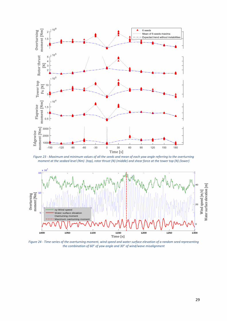
29
Figure 23 - Maximum and minimum values of all the seeds and mean of each yaw angle referring to the overturning
moment at the seabed level (Nm) (top), rotor thrust (N) (middle) and shear force at the tower top (N) (lower)
Figure 24 - Time-series of the overturning moment, wind speed and water surface elevation of a random seed representing
the combination of 60° of yaw angle and 30° of wind/wave misalignment
1000 1050 1100 1150 1200 1250 1300
5
10
15x 10
4
Time [s]
Ove
rtur
ning
mom
ent [
Nm
]
1000 1050 1100 1150 1200 1250 1300
0
20
40
Win
d sp
eed
[m/s
]W
ater
sur
face
ele
vatio
n [m
]
xy-Wind speed
Water surface elevation
Overturning moment
Maximum overturning moment
30
Figure 25 - Ranking of all DLCs for the overturning moment at the seabed level and flapwise and DLC edgewise moment at
the root of the blade
Figure 26 - Contribution of the hydrodynamic loading and tower top Fx
31
TABLES Table 1 – General specifications of the 5MW monopile OWT [19]
Rotor/Nacelle assembly Rated power 5MW
Number of blades/radius 3/63m Cut-in, Cut-out wind
speed 3m/s, 25m/s
Controllers Collective pitch control and generator torque control (variable speed)
Rated rotor speed 12.1rpm Support structure/foundation
Structure Monopile with rigid foundation Hub height 90m above MSL Water level 20m above seabed
Table 2 - Extreme wave heights and wind speed at the hub as a function of the return period
𝑻𝒓𝒆𝒕𝒖𝒓𝒏 [yr] 𝑯𝑺 [m] 𝑻𝑷 [s] 𝑯𝒎𝒂𝒙 [m] 𝑽𝒉𝒖𝒃 [m/s]
1 6.06 9.70 11.27 31.70
50 8.07 11.3 15.64 42.04
Table 3 – Wind-conditioned wave height and the corresponding spectral peak period
𝑽𝒉𝒖𝒃 [m/s] 𝑯𝑺 [m] 𝑻𝑷 [s] (mean)
4 1,10 5,88
6 1,18 5,76
8 1,31 5,67
10 1,48 5,74
12 1,70 5,88
14 1,91 6,07
16 2,19 6,37
18 2,47 6,71
20 2,76 6,99
22 3,09 7,40
24 3,42 7,80
Table 4 – List of design load cases
DLC Wind Waves
Control / Events Model Speed Model Height
1.1 NTM 𝑉𝑖𝑛 < 𝑉ℎ𝑢𝑏 < 𝑉𝑜𝑢𝑡 NSS 𝐻𝑆 = 𝐸[𝐻𝑆|𝑉] Extrapolation of loads
1.3 ETM 𝑉𝑖𝑛 < 𝑉ℎ𝑢𝑏 < 𝑉𝑜𝑢𝑡 NSS 𝐻𝑆 = 𝐸[𝐻𝑆|𝑉]
1.4 ECD 𝑉ℎ𝑢𝑏 = 𝑉𝑟 ± 2𝑚
𝑠, 𝑉𝑟 NSS 𝐻𝑆 = 𝐸[𝐻𝑆|𝑉]
1.5 EWS 𝑉𝑖𝑛 < 𝑉ℎ𝑢𝑏 < 𝑉𝑜𝑢𝑡 NSS 𝐻𝑆 = 𝐸[𝐻𝑆|𝑉]
1.6a NTM 𝑉𝑖𝑛 < 𝑉ℎ𝑢𝑏 < 𝑉𝑜𝑢𝑡 SSS 𝐻𝑆 = 𝐻𝑠,𝑆𝑆𝑆
6.1a EWM 𝑉ℎ𝑢𝑏 = 0.95 ∙ 𝑉𝑟𝑒𝑓 ESS 𝐻𝑆 = 1.09 ∙ 𝐻𝑆,50
6.2a EWM 𝑉ℎ𝑢𝑏 = 0.95 ∙ 𝑉𝑟𝑒𝑓 ESS 𝐻𝑆 = 1.09 ∙ 𝐻𝑆,50 Loss of electrical network
6.2b EWM 𝑉(𝑧ℎ𝑢𝑏) = 𝑉𝑒50 RWH 𝐻𝑆 = 𝐻𝑟𝑒𝑑50 Loss of electrical network
32
Table 5 - Comparison between the extrapolated values of DLC 1.1 and the results from DLC 1.3
Overturning
moment (N∙m)
Flapwise moment (N∙m)
Edgewise moment
(N∙m)
Gumbel prediction
1.510E+08 2.151E+07 9.235E+06
-2.37% +2.90% +2.66%
DLC 1.3 1.547E+08 2.090E+07 8.996E+06
Table 6 - Characteristic and design load of all the DLCs with the required partial safety factors.
Characteristic load Safety Factor Design load
DLC Overturning
moment (Nm)
Flapwise moment
(Nm)
Edgewise moment
(Nm) Type value
Overturning moment
(Nm)
Flapwise moment
(Nm)
Edgewise moment
(Nm) 1.1 1.208E+08 1.721E+07 7.388E+07 Normal 1.25 1.510E+08 2.151E+07 9.235E+06
1.3 1.146E+08 1.548E+07 6.664E+06 Normal 1.35 1.547E+08 2.090E+07 8.996E+06
1.4 1.217E+08 2.019E+07 7.473E+06 Normal 1.35 1.643E+08 2.726E+07 1.009E+07
1.5 9.056E+07 1.310E+07 5.890E+06 Normal 1.35 1.223E+08 1.769E+07 7.952E+06
1.6a 1.310E+08 1.461E+07 6.294E+06 Normal 1.35 1.769E+08 1.972E+07 8.497E+06
6.1a 9.114E+07 9.631E+06 2.339E+06 Normal 1.35 1.230E+08 1.300E+07 3.158E+06
6.2a 1.164E+08 1.107E+07 2.238E+06 Abnormal 1.10 1.281E+08 1.218E+07 2.462E+06
6.2b 1.388E+08 1.807E+07 6.722E+06 Abnormal 1.10 1.526E+08 1.988E+07 7.394E+06