Embed Size (px)
Citation preview
Twistor Inspired Methods in Perturbative Field
Theory and Fuzzy Funnels
Simon McNamara
Thesis submitted for the degree of
Doctor of Philosophy (PhD)
of the University of London
Thesis Supervisor
Prof. Bill Spence
Department of Physics,
Queen Mary, University of London,
Mile End Road,
London, E1 4NS
August 2006

Abstract
The first part of this thesis contains two new techniques for the calculation of scatteringamplitudes in quantum field theories. These methods were inspired by the recent proposalof a correspondence between the weakly coupled regime of the maximally supersymmetricfour dimensional gauge theory and a string theory in twistor space.
We show how generalised unitarity cuts in D=4− 2ε dimensions can be used to calcu-late efficiently complete one-loop scattering amplitudes in non-supersymmetric Yang-Millstheory. This approach naturally generates the rational terms in the amplitudes, as well asthe cut-constructible parts. We then show that the ideas of the Britto, Cachazo, Feng andWitten tree-level on-shell recursion relation can also be applied to the calculation of finiteone-loop amplitudes in pure Einstein gravity.
The second part of this thesis is a study of the nonabelian phenomena associated withD-branes. Specifically we study the nonabelian bionic brane intersection in which a stackof many coincident D1-branes expand via a non-commutative spherical configuration intoa collection of higher dimensional D-branes orthogonal to the original stack of D1-branes.
We suggest a construction of monopoles in dimension 2k+1 from fuzzy funnels. We thenperform two charge calculations related to this construction. This leads to a new formulafor the symmetrised trace quantity. This new formula for the symmetrised trace is thenused to study the collapse of a spherical bound state of D0-branes.
2

Declaration
I declare that the work in this thesis is my own, unless otherwise stated and resulted fromcollaborations with Andreas Brandhuber, Costis Papageorgakis, Sanjaye Ramgoolam, BillSpence and Gabriele Travaglini. Some of the content of this thesis has been published inthe papers [1] and [2].
Simon McNamara
3

Acknowledgements
It is a pleasure to thank my inspirational supervisor Bill Spence and collaborators AndreasBrandhuber, Costis Papageorgakis, Sanjaye Ramgoolam, and Gabriele Travaglini. Thankyou for so many fun hours of doing research. You have taught me a huge number offascinating things. Thank you for all your help.
A big thank you to my friends James Bedford, Samantha Bidwell, John Booth, PeterBrooks, Micheal Coad, Will Creedy, Aneta Dybek, Jannick Guillome, Paul Hafner, DavidHerbert, Xuan Kroeger, Fanny Lessous, Richard Lewis, Caroline Middleton-Hockin, DavidMulryne, Simon Nickerson, Ronald Reid-Edwards, John Richards, John Ward, and MarkWesker. Thanks also to all the members of Harpenden Cricket Club and the choir of StMartin-in-the-Fields.
Finally thank you Mum, Dad and Sarah for looking after me.
4
Table of contents
ABSTRACT 2
DECLARATION 3
ACKNOWLEDGEMENTS 4
INTRODUCTION 12
1 PERTURBATIVE FIELD THEORY AND TWISTORS 14
1.1 Introduction . . . . . . . . . . . . . . . . . . . . . . . . . . . . . . . . . . . . 14
1.2 Amplitudes in perturbative field theory . . . . . . . . . . . . . . . . . . . . 17
1.2.1 Feynman rules . . . . . . . . . . . . . . . . . . . . . . . . . . . . . . 17
1.2.2 Colour stripped amplitudes . . . . . . . . . . . . . . . . . . . . . . . 18
1.2.3 The spinor helicity formalism . . . . . . . . . . . . . . . . . . . . . . 19
1.3 Twistors . . . . . . . . . . . . . . . . . . . . . . . . . . . . . . . . . . . . . . 22
1.3.1 The twistor transform . . . . . . . . . . . . . . . . . . . . . . . . . . 22
1.3.2 The MHV amplitude in twistor space . . . . . . . . . . . . . . . . . 23
1.3.3 Twistor string theory . . . . . . . . . . . . . . . . . . . . . . . . . . 26
1.4 Field theoretic MHV rules . . . . . . . . . . . . . . . . . . . . . . . . . . . . 27
1.4.1 The tree level CSW rules. . . . . . . . . . . . . . . . . . . . . . . . . 27
1.4.2 The one loop BST rules . . . . . . . . . . . . . . . . . . . . . . . . . 29
1.4.3 Mansfield’s proof of the CSW rules . . . . . . . . . . . . . . . . . . . 30
1.5 BDDK’s two-particle unitarity cuts . . . . . . . . . . . . . . . . . . . . . . . 31
1.6 Generalised Unitarity . . . . . . . . . . . . . . . . . . . . . . . . . . . . . . 34
1.6.1 Quadruple cuts in N =4 Super Yang-Mills . . . . . . . . . . . . . . . 35
5

1.6.2 Triple cuts in N =1 Super Yang-Mills . . . . . . . . . . . . . . . . . 37
1.7 The BCFW recursion relation . . . . . . . . . . . . . . . . . . . . . . . . . . 39
1.7.1 A four-point example . . . . . . . . . . . . . . . . . . . . . . . . . . 40
1.7.2 Generalisations of BCFW recursion . . . . . . . . . . . . . . . . . . 42
1.7.3 Risager’s proof of the CSW rules . . . . . . . . . . . . . . . . . . . . 43
2 GENERALISED UNITARITY FOR PURE YANG-MILLS 45
2.1 Generalised Unitarity in D = 4−2ε Dimensions . . . . . . . . . . . . . . . . 45
2.2 The one-loop ++++ amplitude . . . . . . . . . . . . . . . . . . . . . . . . . 49
2.3 The one-loop −+++ amplitude . . . . . . . . . . . . . . . . . . . . . . . . . 52
2.4 The one-loop −−++ amplitude . . . . . . . . . . . . . . . . . . . . . . . . . 58
2.5 The one-loop −+−+ amplitude . . . . . . . . . . . . . . . . . . . . . . . . . 61
2.6 The one-loop +++++ amplitude . . . . . . . . . . . . . . . . . . . . . . . . 66
2.7 Future directions . . . . . . . . . . . . . . . . . . . . . . . . . . . . . . . . . 69
2.7.1 Higher point QCD amplitudes . . . . . . . . . . . . . . . . . . . . . 69
2.7.2 Higher loops, integrability and the AdS/CFT correspondence . . . . 70
3 ON-SHELL RECURSION RELATIONS FOR ONE-LOOP GRAVITY 73
3.1 Introduction . . . . . . . . . . . . . . . . . . . . . . . . . . . . . . . . . . . . 73
3.2 The all-plus amplitude . . . . . . . . . . . . . . . . . . . . . . . . . . . . . . 76
3.2.1 The five-point all-plus amplitude . . . . . . . . . . . . . . . . . . . . 77
3.2.2 The six-point all-plus amplitude . . . . . . . . . . . . . . . . . . . . 80
3.3 The one-loop −+ ++ amplitude . . . . . . . . . . . . . . . . . . . . . . . . 84
3.3.1 −+ ++ in Yang-Mills . . . . . . . . . . . . . . . . . . . . . . . . . . 84
3.3.2 −+ ++ in Gravity . . . . . . . . . . . . . . . . . . . . . . . . . . . . 85
3.4 The one-loop −+ + + + Gravity amplitude . . . . . . . . . . . . . . . . . . 88
3.5 The description of nonstandard factorisations . . . . . . . . . . . . . . . . . 93
3.5.1 −+ + + + in Yang-Mills with |1], |3〉 shifts . . . . . . . . . . . . . . 93
3.5.2 −+ ++ in gravity with |1], |2〉, |3〉, |4〉 shifts . . . . . . . . . . . . . . 95
3.6 Avoiding nonstandard factorisations . . . . . . . . . . . . . . . . . . . . . . 96
3.6.1 The −+ + + + Yang-Mills amplitude . . . . . . . . . . . . . . . . . 97
6

4 THE ADHM CONSTRUCTION AND D-BRANE CHARGES 100
4.1 Introduction . . . . . . . . . . . . . . . . . . . . . . . . . . . . . . . . . . . . 100
4.2 The ADHM construction . . . . . . . . . . . . . . . . . . . . . . . . . . . . . 106
4.2.1 Review of Nahm’s construction for D1 ⊥ D3 . . . . . . . . . . . . . 106
4.2.2 Generalisation to higher dimensions . . . . . . . . . . . . . . . . . . 109
4.2.3 Construction of the Monopole . . . . . . . . . . . . . . . . . . . . . . 110
4.3 Charge calculations . . . . . . . . . . . . . . . . . . . . . . . . . . . . . . . . 111
4.3.1 Monopole charge calculation . . . . . . . . . . . . . . . . . . . . . . 111
4.3.2 Proof of the identity involving N(k, n) and N(k − 1, n+ 1) . . . . . 112
4.3.3 Fuzzy funnel charge calculation. . . . . . . . . . . . . . . . . . . . . 113
4.4 Symmetrised trace calculations . . . . . . . . . . . . . . . . . . . . . . . . . 115
4.4.1 Chord diagram calculations . . . . . . . . . . . . . . . . . . . . . . . 117
4.4.2 The large n expansion of Str(XiXi)m . . . . . . . . . . . . . . . . . . 121
4.4.3 An exact formula for the symmetrised trace . . . . . . . . . . . . . . 124
5 FINITE N EFFECTS ON THE COLLAPSE OF FUZZY SPHERES 126
5.1 Introduction . . . . . . . . . . . . . . . . . . . . . . . . . . . . . . . . . . . . 126
5.2 Lorentz invariance and the physical radius . . . . . . . . . . . . . . . . . . 127
5.3 The fuzzy S2 at finite n . . . . . . . . . . . . . . . . . . . . . . . . . . . . . 129
5.3.1 The D1 ⊥ D3 intersection at finite-n . . . . . . . . . . . . . . . . . . 131
5.3.2 Finite N dynamics as a quotient of free multi-particle dynamics . . 132
5.4 Physical properties of the finite N solutions . . . . . . . . . . . . . . . . . . 133
5.4.1 Special limits where finite n and large n formulae agree . . . . . . . 133
5.4.2 Finite N effects . . . . . . . . . . . . . . . . . . . . . . . . . . . . . . 135
5.4.3 Distance to blow-up in D1 ⊥ D3 . . . . . . . . . . . . . . . . . . . . 138
5.5 Towards a generalisation to higher even-dimensional fuzzy-spheres . . . . . 139
5.6 Summary and Outlook . . . . . . . . . . . . . . . . . . . . . . . . . . . . . . 141
A INTEGRAL IDENTITIES 143
A.1 Scalar box, triangle and bubble integrals . . . . . . . . . . . . . . . . . . . . 143
A.2 Scalar Integral Identities . . . . . . . . . . . . . . . . . . . . . . . . . . . . . 144
A.3 PV reduction . . . . . . . . . . . . . . . . . . . . . . . . . . . . . . . . . . . 145
7

B GRAVITY AMPLITUDE CHECKS 148
B.1 The VegasShift[n] Mathematica command . . . . . . . . . . . . . . . . . . . 148
B.2 Other shifts of the −+ + + + gravity amplitude . . . . . . . . . . . . . . . 149
B.2.1 The |4], |5〉 shifts . . . . . . . . . . . . . . . . . . . . . . . . . . . . . 149
B.2.2 The |2], |1〉 shifts . . . . . . . . . . . . . . . . . . . . . . . . . . . . . 151
C STR CALCULATIONS USING THE HIGHEST WEIGHT METHOD 152
C.1 Review of spin half for SO(3) . . . . . . . . . . . . . . . . . . . . . . . . . . 153
C.2 Derivation of symmetrised trace for minimal SO(2l + 1) representation . . . 154
C.3 Derivation of spin one symmetrised trace for SO(3) . . . . . . . . . . . . . . 155
C.4 Derivation of next-to-minimal representation for SO(2l + 1) . . . . . . . . . 156
8

List of Figures
1.1 The result that MHV amplitudes are supported on degree one, genus zerocurves in twistor space is equivalent to the fact that the MHV amplitude is afunction of only the λs and not of the λs. . . . . . . . . . . . . . . . . . . . 24
1.2 The twistor space localisation of tree amplitudes. Diagram (a) shows thelocalisation of an amplitude with three negative helicity gluons and diagram(b) an amplitude with four negative helicity gluons. . . . . . . . . . . . . . . 25
1.3 The MHV diagrams associated with the CSW construction of the simplestnext-to-MHV tree-level amplitude A(1−, 2−, 3−, 4+, 5+). It is conventional toconsider amplitudes where all the momenta are outgoing, so an internal legjoining two amplitudes will have different helicities labels at each end. . . . 28
1.4 The BST construction of the MHV one-loop amplitude in N =4 super Yang-Mills by sewing two tree-level MHV amplitudes together. . . . . . . . . . . . 29
1.5 The s channel cut of a one-loop amplitude. . . . . . . . . . . . . . . . . . . 32
1.6 A simple quadruple cut to evaluate the coefficient of a one-mass box in thefive-point MHV amplitude in N =4 Super Yang-Mills. . . . . . . . . . . . . 35
1.7 The diagrams in the triple cut of the one-loop MHV amplitude for N = 1Super-Yang Mills. . . . . . . . . . . . . . . . . . . . . . . . . . . . . . . . . . 38
1.8 A diagrammatic representation of the BCFW recursion relation. The sum isover all factorisations into pairs of amplitudes and the possible helicity of theintermediate state. . . . . . . . . . . . . . . . . . . . . . . . . . . . . . . . . 40
1.9 The recursive diagram in the BCFW construction of A(1−, 2+, 3−, 4+). . . . 41
2.1 One of the two quadruple-cut diagrams for the amplitude 1+2+3+4+. This di-agram is obtained by sewing tree amplitudes (represented by the blue bubbles)with an external positive-helicity gluon and two internal scalars of opposite‘helicities’. There are two such diagrams, which are obtained one from theother by flipping all the internal helicities. These diagrams are equal so thatthe full result is obtained by doubling the contribution from the diagram inthis Figure. The same remark applies to all the other diagrams considered inthis chapter. . . . . . . . . . . . . . . . . . . . . . . . . . . . . . . . . . . . 50
9
2.2 One of the possible three-particle cut diagrams for the amplitude 1+2+3+4+.The others are obtained from this one by cyclic relabelling of the externalparticles. . . . . . . . . . . . . . . . . . . . . . . . . . . . . . . . . . . . . . 51
2.3 The quadruple cut for the amplitude 1−2+3+4+. . . . . . . . . . . . . . . . 53
2.4 The two inequivalent triple cuts for the amplitude 1−2+3+4+. . . . . . . . 55
2.5 The quadruple cut for the amplitude 1−2−3+4+. . . . . . . . . . . . . . . . 59
2.6 The two inequivalent triple cuts for the amplitude 1−2−3+4+. . . . . . . . 60
2.7 The quadruple cut for the amplitude 1−2+3−4+. . . . . . . . . . . . . . . . . 62
2.8 The only independent triple cut for the amplitude 1−2+3−4+ (the others areobtained from this one by cyclic relabelling of the external gluons). . . . . . 63
2.9 One of the quadruple cuts for the amplitude 1+2+3+4+5+. . . . . . . . . . . 66
2.10 A puzzling quadruple cut of the six point all-plus amplitude. . . . . . . . . . 69
3.1 The diagram in the recursive expression for M (1)5 (1+, 2+, 3+, 4+, 5+) associ-
ated with the pole 〈12〉 = 0. The amplitude labelled by a T is a tree-levelamplitude and the one labelled by L is a one-loop amplitude. . . . . . . . . . 78
3.2 The diagram in the recursive expression for M (1)5 (1+, 2+, 3+, 4+, 5+) associ-
ated with the pole 〈15〉 = 0. . . . . . . . . . . . . . . . . . . . . . . . . . . . 79
3.3 The diagram in the recursive expression for M (1)5 (1+, 2+, 3+, 4+, 5+, 6+) as-
sociated with the pole 〈23〉 = 0. . . . . . . . . . . . . . . . . . . . . . . . . . 81
3.4 The diagram in the recursive expression for M (1)5 (1+, 2+, 3+, 4+, 5+, 6+) as-
sociated with the pole 〈16〉 = 0. . . . . . . . . . . . . . . . . . . . . . . . . . 82
3.5 The recursive construction of A(1)4 (1−, 2+, 3+, 4+) via shifting |1] and |2〉 in-
volves this nonstandard factorisation diagram. . . . . . . . . . . . . . . . . . 85
3.6 The recursive construction of M (1)4 (1−, 2+, 3+, 4+) via shifting |1] and |2〉
involves these two nonstandard factorisation diagrams. . . . . . . . . . . . . 87
3.7 The diagram in the recursive expression for M (1)5 (1−, 2+, 3+, 4+, 5+) corre-
sponding to a simple-pole associated with [15]=0. . . . . . . . . . . . . . . . 89
3.8 The diagram in the recursive expression for M (1)5 (1−, 2+, 3+, 4+, 5+) corre-
sponding to a simple-pole associated with 〈23〉=0. . . . . . . . . . . . . . . . 90
3.9 The diagram in the recursive expression for M (1)5 (1−, 2+, 3+, 4+, 5+) corre-
sponding to the double-pole associated with 〈23〉=0. . . . . . . . . . . . . . . 91
3.10 The diagrams in the recursive expression for A(1)5 (1−, 2+, 3+, 4+, 5+) with
shifts on |1] and |3〉. . . . . . . . . . . . . . . . . . . . . . . . . . . . . . . . 94
3.11 The diagrams in the |1] |2〉 shift of A(1)5 (1−, 2+, 3+, 4+, 5+). . . . . . . . . . 97
3.12 The diagram in the |4] |5〉 shift of A(1)5 (1−, 2+, 3+, 4+, 5+). . . . . . . . . . . 98
10

A.1 Kinematics of the bubble and triangle integral functions studied in this Ap-pendix. . . . . . . . . . . . . . . . . . . . . . . . . . . . . . . . . . . . . . . 145
B.1 The diagram associated with 〈15〉 = 0, with shifts on |4], |5〉. . . . . . . . . 149
B.2 The diagram associated with [14] = 0, with shifts on |4], |5〉. . . . . . . . . . 149
B.3 The standard factorisation diagram associated with 〈25〉 = 0, with shifts on|4], |5〉. . . . . . . . . . . . . . . . . . . . . . . . . . . . . . . . . . . . . . . 150
B.4 The nonstandard factorisation diagram associated with 〈25〉 = 0, with shiftson |4], |5〉. . . . . . . . . . . . . . . . . . . . . . . . . . . . . . . . . . . . . . 150
B.5 The diagram associated with 〈15〉 = 0 with shifts on |2], |1〉. . . . . . . . . . 151
11

Introduction
The first three chapters of this thesis are concerned with twistor inspired methods in pertur-bative quantum field theory. Chapter 1 contains an introduction to this subject. Chapter2 shows that generalised unitarity in D-dimensions can be used to compute amplitudes inone-loop QCD. Chapter 3 shows that finite one-loop gravity amplitudes can be computedusing on-shell recursion. The remaining two chapters are about fuzzy funnels. Chapter 4contains a study of the duality between monopoles and fuzzy funnels. In Chapter 5 weconsider finite n effects on the collapse of fuzzy spheres.
Chapter 1 provides an introduction to the remarkable recent progress in understandingperturbative quantum field theory which was initiated by Witten’s proposal of a dualitybetween weakly coupled N =4 Super Yang-Mills and a string theory in twistor space CP3|4.This duality explains the remarkable simplicity of certain amplitudes which is hidden bystandard Feynman diagram calculations. The unexpected beauty of scattering amplitudes isexposed by writing colour stripped amplitudes in the spinor helicity formalism. The notionof a twistor and the twistor transform of the maximally helicity violating amplitude (MHV)are then reviewed. We then summarise the twistor space localisation of general amplitudesand describe the string theoretic proposal. The twistor string theory has inspired manynew and efficient field theory techniques for the calculation of amplitudes. We review theremarkable new insight that tree and loop level amplitudes can be built by joining multipleMHV amplitudes together. Finally we review the twistor inspired field theory techniquesof generalised unitarity and on-shell recursion.
In chapter 2 we show how generalised unitarity cuts in D= 4 − 2ε dimensions can beused to calculate efficiently complete one-loop scattering amplitudes in non-supersymmetricYang-Mills theory. This approach naturally generates the rational terms in the amplitudes,as well as the cut-constructible parts. We test the validity of our method by re-derivingthe one-loop ++++, −+++, −−++, −+−+ and +++++ gluon scattering amplitudesusing generalised quadruple cuts and triple cuts in D dimensions. We observe that triplecuts are sufficient to compute complete amplitudes. Thus we can avoid the calculation oftwo-particle cuts which are the most technically challenging to evaluate. In principle thisnew method can be applied to more complicated and currently unknown amplitudes whichare important for the experimental programmes at hadron colliders.
12

In chapter 3 we show that the ideas of the Britto, Cachazo, Feng and Witten tree-level on-shell recursion relation can also be applied to the calculation of finite one-loopamplitudes in pure Einstein gravity. We show how to compute the five and six point all-plus one-loop gravity amplitudes without having to consider boundary terms. We thenconsider the recursive construction of the known one-loop −+++ gravity amplitude andobserve that the factorisation properties in complex momenta of this gravity amplitude aresimilar to those of the one-loop −+++ amplitude in Yang-Mills. The new issue that arisesfor the amplitude with a single negative helicity is the appearance of the one-loop three-point all-plus nonstandard factorisation which gives single and double pole contributionsto the amplitude. We then attempt to calculate the unknown one-loop −++++ gravityamplitude using on-shell recursion. Unfortunately we do not understand the single poleunder the double pole contributions of the three-point one-loop all-plus factorisation in thisamplitude so are unable to calculate the full answer. We review an unsuccessful proposalfor this missing term, and an unsuccessful attempt to avoid the nonstandard factorisationsusing auxiliary recursion relations.
In chapter 4 we consider the nonabelian bionic brane intersection in which a stack ofmany coincident D1-branes expand via a non-commutative spherical configuration into acollection of higher dimensional D-branes orthogonal to the original stack of D1-branes. Wesuggest a construction of monopoles in dimension 2k+1 from fuzzy funnels. For k = 1 thisconstruction coincides with Nahm’s construction of monopoles, which is an adaptation ofthe Atiyah, Drinfeld, Hitchin and Manin construction of instantons. For k = 1, 2, 3 this givesa finite n realisation of the duality between D1-brane and D(2k + 1)-brane world-volumepictures of the non-commutative bionic brane intersection. We then perform two chargecalculations related to this construction. First we calculate the charge of the monopoleand get an answer in precise agreement with the size of the matrices in the fuzzy funnel.Secondly we calculate the charge of the fuzzy funnel. To get this charge to agree with thesize of the matrices in the monopole beyond leading orders in 1/n, we propose a speculativeuse of the symmetrised trace. A matching of the terms of the symmetrised trace with thenumber of branes expected from the charge calculation then leads to a new and surprisinglysimple formula for the symmetrised trace quantity.
In chapter 5 we consider finite n effects on the time evolution of fuzzy 2-spheres movingin flat space-time. We use the new formula for the symmetrised trace found in chapter 4 toshow that exotic bounces of the kind seen in the 1/n expansion do not exist at finite n.
13

CHAPTER 1
PERTURBATIVE FIELD THEORY AND
TWISTORS
1.1 Introduction
There are many interesting things yet to be understood about four-dimensional quantumgauge theories like QCD. It has long been thought that phenomena such as quark con-finement were related to strings. In 1974 ’t Hooft [3] presented a purely diagrammaticargument suggesting that a gauge theory should have a dual description as a string theory.This proposal did not identify which string theory is equivalent to four-dimensional gaugetheory and little progress was made until in 1997 Maldacena [4] proposed that the maxi-mally supersymmetric gauge theory N =4 Super Yang-Mills was equivalent in the ’t Hooftsense to Type IIB superstring theory on the target space AdS5 × S5.
The ’t Hooft expansion relates the strongly-coupled regime of a gauge theory to a weakly-coupled string theory. The Maldacena correspondence therefore provides a perturbativewindow into non-perturbative physics. Other dualities including mirror symmetry andMontonen-Olive duality have demonstrated that the character of quantum field theories isradically different in different parameter regimes. It would therefore be fascinating boththeoretically and phenomenologically to find a duality complementary to Maldacena’s, giv-ing a weakly-coupled string theoretic description of the weakly-coupled gauge theory. A keystep in this direction was made in 2003 by Witten [5]. He suggested a remarkable dualitybetween weakly-coupled N =4 super Yang Mills and a weakly-coupled B-model topologicalstring theory on the super Calabi-Yau manifold CP3|4. Intriguingly, the target space CP3|4
has six bosonic real dimensions which are related to the usual four dimensional space-timeof the quantum field theory by the twistor construction of Penrose [6].
In principle the perturbative analysis of a gauge theory in terms of Feynman diagramsis under control, but in practice the number of such diagrams grows very rapidly with thenumber of external legs and the number of loops. Strikingly, after simplifying the hugenumber of Feynman diagrams, the final answer is often simple and elegant. This stronglyhints at the existence of an underlying dual string theoretic description and was the challengeset by Parke and Taylor in 1986 [7] when they discovered the expression for the tree-levelmaximally helicity violating (MHV) amplitude. An MHV amplitude is one where all but
14

CHAPTER 1. PERTURBATIVE FIELD THEORY AND TWISTORS
two of the external gluons have the same helicity. When the MHV amplitude is written inthe spinor helicity formalism, it is given by a simple holomorphic function of just one ofthe two spinors needed to describe the massless particles. Witten observed that all tree-level gauge theory amplitudes, after a Fourier transform to twistor space, are supported onholomorphically embedded algebraic curves. For the case of MHV amplitudes these curvesare simply straight lines. This beautiful geometrical localisation is totally hidden by theFeynman diagram expansion and led to the string theoretic proposal that gauge theoryamplitudes could be obtained by integrating over the moduli space of D1-brane instantons.
Witten’s insight has motivated a revolution in our understanding of perturbative gaugetheory. Some of the most fruitful advances inspired by twistor string theory have beenpowerful new diagrammatic rules for field theory calculations. In March 2004, Cachazo,Svrcek and Witten (CSW) [8] proposed elevating the MHV amplitude to an effective vertexin a new perturbative expansion of the tree-level Yang-Mills theory. They observed thatamplitudes with more than two negative helicity gluons could be computed by joiningthese effective vertices together with scalar propagators. In twistor string theory thereare several different prescriptions for integrating over curves. When calculating tree levelgauge theory amplitudes, one can either use a single instanton of degree d, or alternativelyd completely disconnected curves each of degree one connected by twistor propagators.The disconnected prescription gives the remarkably efficient MHV diagram construction.For example, the amplitude with three negative helicity and three positive helicity gluonsinvolves 220 Feynman diagrams [9, 10], but can be reconstructed from just 6 diagrams inCSW’s diagrammatic approach.
Despite its many successful achievements, twistor string theory leaves us with manyinteresting open questions. It is clear that the twistor string theory proposed by Wittenfails at loop level because amplitudes receive contributions from closed string, conformalsupergravity states [11]. Surprisingly, a formalism which glues tree-level MHV verticestogether to form loops has been proposed by Brandhuber, Spence and Travaglini (BST) [12]and used to correctly reproduce the one-loop MHV amplitude in supersymmetric Yang-Mills. The twistor space localisation of gauge theory amplitudes therefore persists beyondtree level to the quantum theory. Their method unified the MHV vertex constructionwith the celebrated unitarity-based, cut-constructibility approach of Bern, Dixon, Dunbarand Kosower (BDDK) [13, 14]. This strongly suggests that there may be a version oftwistor string theory dual to pure N = 4 super Yang-Mills at loop level. Another openproblem associated with the duality at loop level is how the infrared singularities of thegauge theory amplitudes arise in the string theory. In the one-loop amplitude the infra-red divergent terms are those where one of the MHV vertices is a four-particle vertex. Intwistor space this corresponds to a localisation on a disjoint union of lines. So it is possiblethat the transformation to twistor space also disentangles the infra-red divergences of theamplitudes.
15
CHAPTER 1. PERTURBATIVE FIELD THEORY AND TWISTORS
The rest of this chapter provides an introduction to the recent progress in understandingperturbative field theory. In the next section we define amplitudes via the Feynman rules.In sections 1.2.2 and 1.2.3 we introduce colour stripping and the spinor helicity formalism,which are two notational techniques that expose the hidden beauty of scattering amplitudes.The notion of a twistor and the twistor transform of the MHV amplitude are reviewed insection 1.3. We then summarise the twistor space localisation of amplitudes with morethan two negative helicity gluons and briefly describe the string theoretic proposal thatprovides a natural framework for the twistor space properties of amplitudes. In section1.4 we review the twistor string inspired MHV rules, which calculate tree-level amplitudeswith more than two negative helicity gluons by sewing MHV amplitudes together and alsocorrectly compute the one-loop MHV amplitude in supersymmetric theories by joining apair of tree-level MHV amplitudes together to form a loop.
In addition to the MHV rules, the twistor string has inspired many new and efficientmethods for the calculation of scattering amplitudes. One of these new techniques is thenotion of generalised four-dimensional unitarity [15]. We review the background to thispowerful tool in section 1.6. In Chapter 2 we present the new technique of D = 4 − 2εgeneralised unitarity. We show how generalised unitarity cuts inD=4−2ε dimensions can beused to calculate efficiently complete one-loop scattering amplitudes in non-supersymmetricYang-Mills theory. This approach naturally generates the rational terms in the amplitudes,as well as the cut-constructible parts. Chapter 2 is based on the work [1].
The recursion relation of Britto, Cachazo, Feng and Witten (BCFW) [16,17] is anotherelegant and systematic method for the computation of tree-level Yang-Mills amplitudes.In section 1.7 we review the proof of this recursion relation and some of its applications.In chapter 3 we show that the ideas of BCFW recursion extend with many complicationsto the finite amplitudes of one-loop pure Einstein gravity. This generalisation has a closeconnection with the use of recursion relations in the calculation of the rational parts of one-loop QCD amplitudes by Bern, Dixon and Kosower (BDK) [18]. This idea is remarkablebecause it enables one to calculate very efficiently at one-loop without really performingany loop integrals.
The calculation and understanding of scattering amplitudes is interesting because as wellas uncovering the hidden beauty of field theory and linking gauge theory to string theory, ithas also allowed us to calculate more efficiently in realistic theories of nature. Asymptoticfreedom [19, 20] allows us to calculate scattering amplitudes as a perturbative expansionin the strong coupling constant αs(µ), evaluated at a large momentum scale µ where thetheory is weakly coupled. However, at hadron colliders the leading order tree-amplitudesdo not suffice to get a reasonable uncertainty and corrections from next to leading orderare important. A precise knowledge of QCD backgrounds for events involving several jetsis needed for maximising the potential for the discovery of physics beyond the StandardModel at colliders like the Large Hadron Collider.
16

CHAPTER 1. PERTURBATIVE FIELD THEORY AND TWISTORS
1.2 Amplitudes in perturbative field theory
1.2.1 Feynman rules
The Lagrangian for a non-abelian gauge theory is
L = ψ(iγµ∂µ −m)ψ − 14(∂µA
aν − ∂νA
aµ)2 + gAa
µψγµtaψ
−gfabc(∂µAaν)A
µbAνc − 14g2(feabAa
µAbν)(f
ecdAµaAνd) (1.1)
Observable quantities are then calculated using perturbation theory. The textbook tech-nique for performing this procedure is to draw and then compute Feynman diagrams. TheFeynman diagrams for a non-abelian gauge theory in Feynman gauge are given by:
Fermion vertex:
= igγµta
Three-point gluon vertex:
=
gfabc[gµν(k − p)ρ
+gνρ(p− q)µ
+gρµ(p− k)ν ]
Four-point gluon vertex:
=
−ig2[fabef cde(gµρgνσ − gµσgνρ)
+facef bde(gµνgρσ − gµσgνρ)
+fadef bce(gµνgρσ − gµρgνσ)]
Ghost vertex:
= −gfabcpµ
Fermion propagator Gluon propagator
=i(γµpµ +m)δab
p2 −m2 + iε=−igµνδab
p2 + iε
The first part of this thesis is about the calculation of amplitudes, however we will not usethe Lagrangian or the Feynman rules very much at all. One of the themes of the thesis
17

CHAPTER 1. PERTURBATIVE FIELD THEORY AND TWISTORS
is that the Feynman rules hide the simplicity of scattering amplitudes. In the next twosections we introduce colour stripping and the spinor helicity formalism. These are theformalisms which originally exposed the surprising simplicity of scattering amplitudes.
1.2.2 Colour stripped amplitudes
In pure Yang-Mills an n-point amplitude is a function of the ith gluon’s momentum vectorpi, polarisation vector εi and colour index ai. At tree level, the interactions are planar, soa gluon amplitude can be written as a sum of single trace terms. This observation leads tothe colour decomposition of the gluon tree amplitude [9, 10,21].
Atreen (pi, εi, ai) = gn−2
∑
σ∈Sn/Zn
Tr(T aσ(1) . . . T aσ(n))An(σ(p1, ε1), . . . , σ(pn, εn)) (1.2)
where g is the gauge coupling and the An(pi, εi) are called colour-ordered partial amplitudes.These partial amplitudes do not carry any colour structure, but contain all the kinematicinformation of the amplitude. Sn is the group of permutations of n objects and Zn is thesubgroup of cyclic permutations, which preserve the cyclic orderings in the trace.
It is simpler to study these partial amplitudes than the full amplitude because they onlyreceive contributions from diagrams with cyclically ordered gluons. This is called colourordering. In colour ordered amplitudes, the poles and cuts can only occur in momentumchannels made out of sums of cyclically adjacent gluons. Hence the analytic structure ofpartial amplitudes is simpler than that of the full amplitude.
At one-loop both single trace and double trace structures are generated. The colourdecomposition of the n-gluon one-loop amplitude is given by [22]:
Aone-loopn (pi, εi, ai) = gn
[ ∑
σ∈Sn/Zn
Nc Tr(T aσ(1) . . . T aσ(n))An;1(σ(p1, ε1), . . . , σ(pn, εn))
+bn/2c+1∑
c=2
∑
σ∈Sn/Sn;c
Tr(T aσ(1) . . . T aσ(c−1))(T aσ(c) . . . T aσ(n))
×An;c(σ(p1, ε1), . . . , σ(pn, εn))]
(1.3)
where An;c(pi, εi) are the partial amplitudes. Zn and Sn;c are the subgroups of Sn whichpreserve the single and double trace structures. The An;1 are called primitive amplitudes.Just like the tree-level partial amplitudes the An;1 are colour ordered. The An;c for c > 1can be written as sums of permutations of the primitive An;1 amplitudes1. For the restof this thesis, when studying Yang-Mills amplitudes, we will ignore colour structure andconsider colour ordered amplitudes.
1See section 7 and appendix III of [13] for more details.
18

CHAPTER 1. PERTURBATIVE FIELD THEORY AND TWISTORS
1.2.3 The spinor helicity formalism
In this section we review the spinor helicity formalism [23] for the description of quantitiesinvolving massless particles. This formalism is responsible for the existence of compactexpressions for tree and loop amplitudes. It introduces a new set of kinematic objects,spinor products, which neatly capture the collinear behaviour of these amplitudes.
The complexified Lorentz group is locally isomorphic to
SO(3, 1,C) ∼= Sl(2,C)× Sl(2,C) (1.4)
so finite dimensional representations of the Lorentz group are classified by (p, q) where p andq are integer or half-integer valued. We write λa, a = 1, 2 for a spinor transforming in the(12 , 0) representation and λa, a = 1, 2 for a spinor transforming in the (0, 1
2) representation.The spinor indices of type (1
2 , 0) are raised and lowered using the antisymmetric tensorsεab and εab which satisfy ε12 = 1 and εacεcb = δa
b. The λ spinors transforming in therepresentation (0, 1
2) are analogously raised and lowered using the antisymmetric tensor εab
and its inverse εab.
λa = εabλb , λa = εabλb and λa = εabλb , λa = εabλ
b (1.5)
There is a scalar product for two spinors λ and λ′ in the (12 , 0) representation and an
analogous scalar product for two spinors λ and λ′ in the (0, 12) representation
〈λλ′〉 = εab λaλ′ b and [λ λ′ ] = εab λ
aλ′ b (1.6)
These scalar products are antisymmetric in their two variables. Vanishing of the scalarproduct 〈λλ′〉 = 0 implies λ ∝ λ′ and similarly [λ λ′ ] = 0 implies λ ∝ λ′. All the λs and λsin this formalism are commuting spinors. Note that they are not Grassmann variables.
The vector representation of SO(3, 1,C) is the (12 ,
12) representation. So a momentum
vector pµ, µ = 0, . . . , 3 can be represented as a bi-spinor paa with two spinor indices a anda transforming in the different spinor representations. More explicitly any four-vector pµ
can be written as a 2×2 matrix,paa = pµσ
µaa (1.7)
where σµ = (1, ~σ) and ~σ are the usual 2×2 Pauli matrices. In this new notation we have
pµpµ = det(paa) (1.8)
If we now impose that the four-vector pµ is massless, p2 = 0, then the determinant of theassociated 2×2 matrix is zero and the rank of this matrix is less than or equal to one. Soa four-momentum pµ being massless is equivalent to the fact that it can be written as the
19

CHAPTER 1. PERTURBATIVE FIELD THEORY AND TWISTORS
product of two (commuting) spinors
paa = λaλa (1.9)
For a given massless vector pµ the spinors λa and λa are unique up to a scaling.
(λ, λ) → (tλ, t−1λ) for t ∈ C , t 6= 0 (1.10)
For real momenta in Minkowski space
λ = ±λ (1.11)
where the ± depends on whether the four-vector is future or past pointing. Thus the spinorsλ are usually called ‘holomorphic’ and the spinors λ ‘anti-holomorphic’. If we use complexmomenta then the spinors λ and λ are independent.
It is customary, when writing amplitudes, to shorten the spinor helicity notation fordifferent particles i and j to 〈λiλj〉 = 〈ij〉 and [λi λj ] = [ij]. It is common to shorten thespinor helicity formalism further using 〈ij〉[jk] = 〈i|j|k].
We now introduce some useful identities for manipulating quantities written in the spinorhelicity formalism. First we have the Schouten identity
〈ij〉〈kl〉 = 〈ik〉〈jl〉 − 〈il〉〈jk〉 (1.12)
Amplitudes are often written in terms of traces of Dirac γ matrices.
〈ij〉[ji] = tr(12(1 + γ5)k/ik/j) = 2ki.kj (1.13)
〈ij〉[jl]〈lm〉[mi] = tr(12(1 + γ5)k/ik/jk/lk/m) (1.14)
〈ij〉[jl]〈lm〉[mn]〈np〉[pi] = tr(12(1 + γ5)k/ik/jk/lk/mk/nk/p) (1.15)
The Fierz rearrangement is:〈i|γµ|j]〈k|γµ|l] = 2〈ik〉[lj] (1.16)
Given a spinor helicity decomposition of the momentum paa = λaλa, we have enoughinformation to determine the polarisation vector, up to a gauge transformation, of a gluonof specific helicity. For a positive helicity gluon we have the polarisation vector:
ε+aa =ρaλa
〈ρ λ〉 (1.17)
where ρ is a negative chirality spinor that is not a multiple of λ. For a negative helicity
20

CHAPTER 1. PERTURBATIVE FIELD THEORY AND TWISTORS
gluon we have the polarisation vector:
ε−aa =λaρa
[λ, ρ](1.18)
where ρ is any positive chirality spinor that is not a multiple of λ. With these definitionsthe polarisation vectors have no unphysical longitudinal modes as they obey the constraintpµε
µ =0. The gauge invariance εµ → εµ + wpµ of the polarisation vector is manifest in thisdescription since ε+ is independent of ρ up to a gauge transformation. To see this noticethat the ρ lives in a two dimensional space spanned by λ and ρ, so a change in ρ is of theform δρ = αρ + βλ. The polarisation vector ε+ is invariant under the α term and the βterm corresponds to a gauge transformation of the polarisation vector:
δe+aa = βλaλa
〈ρ λ〉 (1.19)
Finally, calculating the linearised field strength Fµν = ∂µAν−∂νAµ for a particle of helicity+1 with Aaa = ε+aaexp(ixc cλ
cλc) gives the answer:
Faabb = εabλaλbexp(ixc cλcλc) (1.20)
In bi-spinor notation the field strength is Faabb = εabfab + εabfab where fab and fab are re-spectively the self-dual and anti-self-dual parts of F . So the polarisation vector ε+ correctlygives an anti-self-dual field strength.
When an amplitude is written in the spinor helicity formalism it often takes a verysimple form. The most famous example of this is the MHV amplitude. The tree-level Yang-Mills scattering amplitude with all outgoing gluons having positive helicity vanishes. Theamplitudes with one negative helicity gluon and all the rest positive helicity also vanishes. Inany supersymmetric Yang-Mills theory the vanishing of these amplitudes can be seen from asupersymmetric Ward identity [24,25]. The tree-level gluon amplitudes of a supersymmetrictheory and a non-supersymmetric theory are, of course, the same, so these amplitudes alsovanish in pure Yang-Mills. The first nonzero amplitude is called the maximally helicityviolating (MHV) amplitude and has two negative helicity gluons with all the rest havingpositive helicity. Once the momentum conserving delta function has been stripped off theMHV amplitude it is a very simple function of only the holomorphic spinors λi.
A(1+, 2+, . . . , n− 1+, n+) = 0 (1.21)
A(1+, 2+, . . . , i−, . . . , n− 1+, n+) = 0 (1.22)
A(1+, 2+, . . . , i−, . . . , j−, . . . , n− 1+, n+) = i〈ij〉4
〈12〉〈23〉 . . . 〈n− 1n〉〈n 1〉 (1.23)
21

CHAPTER 1. PERTURBATIVE FIELD THEORY AND TWISTORS
1.3 Twistors
1.3.1 The twistor transform
We define a twistor in the same way as Witten [5]. The spinor variables (λ,λ) are relatedto the twistor variables (λ,µ) by the following half Fourier transform:
λa → i∂
∂µa
∂
∂λa→ iµa (1.24)
The choice to Fourier transform λ rather than λ is an arbitrary one. Writing things in twistorvariables breaks the symmetry between positive and negative helicities. Later we will seethat the holomorphicity of the MHV amplitude has a natural geometrical interpretation intwistor space. However with this choice of Fourier transform, the antiholomorphicity of theamplitude with two positive helicity gluons and all the rest negative helicity will be hidden.These anti-MHV amplitudes are usually called ‘googly’2.
This asymmetry will also be manifest in twistor inspired constructions such as theCSW rules which we will review in section 1.4.1. In this method the construction of MHVamplitudes is trivial, but the googly amplitudes are each constructed differently dependingon the number of negative helicity gluons they contain. For example the five-point googlyamplitude −−−+ + has one more negative helicity gluon than an MHV amplitude and isconstructed by joining two MHV amplitudes together. The six-point googly amplitude isnext-to, next-to MHV and constructed by sewing three MHV amplitudes together.
We now consider the effect of the transformation (1.24) on the representation of theLorentz and conformal symmetry generators. In spinor variables the Lorentz generators arefirst order differential operators:
Jab =i
2
(λa
∂
∂λb+ λb
∂
∂λa
), Jab =
i
2
(λa
∂
∂λb+ λb
∂
∂λa
)(1.25)
In twistor variables these generators remain first order:
Jab =i
2
(λa
∂
∂λb+ λb
∂
∂λa
), Jab =
i
2
(µa
∂
∂µb+ µb
∂
∂µa
)(1.26)
In spinor variables the momentum and special conformal transformation generators arerespectively a multiplication operator and a second order differential operator. In twistor
2The term googly is borrowed from cricket where it refers to the ball bowled out of the back of the handby a leg spin bowler which spins the opposite way to the stock delivery.
22

CHAPTER 1. PERTURBATIVE FIELD THEORY AND TWISTORS
variables, however, these generators take a more standard form both becoming first order:
Pas = λaλa , Kaa =∂2
∂λa∂λa(1.27)
Pas = iλa∂
∂µa, Kaa = iµa
∂
∂λa(1.28)
Finally, the dilatation operator is an inhomogeneous operator in the spinor variables:
D =i
2
(λa
∂
∂λa+ λa
∂
∂λa+ 2
)(1.29)
In twistor variables the operator is homogeneous:
D =i
2
(λa
∂
∂λa− µa
∂
∂µa
)(1.30)
This simple representation of the four dimensional conformal group in twistor variables iseasy to understand. The conformal group of Minkowski space is SO(4, 2) which is the sameas SU(2, 2). The complexification of this group to Sl(4,C), has an obvious four dimensionalrepresentation acting on the twistor Z = (λ1, λ2, µ1, µ2). Twistor space is thus C4.
Tree amplitudes of gluons and more generally the quantum observables of N =4 superYang-Mills are conformally invariant quantities. So it is natural to hope that they will havea simple description in twistor variables.
1.3.2 The MHV amplitude in twistor space
Following Witten [5], we now consider the properties of amplitudes after they have beenhalf Fourier transformed to twistor space.
A(λi, λi) → A(λi, µi) ≡ 1(2π)2n
∫ n∏
i=1
d2λiexp
(i
n∑
i=1
µi aλai
)A(λi, λi) (1.31)
The simplest case is the MHV amplitude (1.23). The MHV amplitude only contains an-gle brackets and thus only has dependence on the space of λi spinors through the usualmomentum-conserving δ-function which multiplies the amplitude. Now recall the followingidentity for the Dirac delta function
δ(x) =12π
∫ ∞
−∞dk eikx (1.32)
We can use this to write the usual momentum conserving delta function as:
δ4
(n∑
i=1
pi
)=
1(2π)4
∫d4xaaexp
ixbb
n∑
j=1
λbj λ
bj
(1.33)
23

CHAPTER 1. PERTURBATIVE FIELD THEORY AND TWISTORS
where the integral is over the ordinary four dimensional space time. Thus the twistortransform A(λi, µi) of the MHV amplitude is:
=1
(2π)2n+4
∫ n∏
i=1
d2 λiexp
(i
n∑
i=1
µi aλai
)∫d4xaaexp
ixbb
n∑
j=1
λbj λ
bj
AMHV
n (λi)
=1
(2π)2n+4
∫d4xaaAMHV
n (λi)∫ n∏
i=1
d2λi exp
i
n∑
i=1
µi aλai + ixbb
n∑
j=1
λbj λ
bj
= AMHVn (λi)
1(2π)4
∫d4x
n∏
i=1
δ2(µi a + xaaλai ) (1.34)
So we are led to consider the following equation:
µa + xaaλa = 0 (1.35)
This equation is familiar from the twistor literature, where it plays a central role and isknown as the incidence relation. Traditionally the equation (1.35) is the definition of atwistor. For a given x the equation (1.35) is regarded as an equation for λ and µ whichdefines a degree one, genus zero curve. Complexified Minkowski space is the moduli spaceof such curves. The transformed amplitude (1.34) will vanish unless (1.35) is satisfied for allthe gluons. So all n points (λi,µi) in an MHV amplitude must lie on a degree one, genus zerocurve determined by xaa. See Figure 1.1. Alternatively, if λ and µ are given, then equation(1.35) is an equation for x. The set of solutions is a two complex dimensional subspaceof complexified Minkowski space that is null and self-dual. In the twistor literature thissubspace is called an α-plane. Twistor space is the moduli space of these α-planes. Anα-plane being null means that any tangent vector to the α-plane is null. An α-plane beingself-dual means that the tangent bi-vector is self-dual.
Figure 1.1: The result that MHV amplitudes are supported on degree one, genus zero curvesin twistor space is equivalent to the fact that the MHV amplitude is a function of only theλs and not of the λs.
At this point we should be more precise about what we mean by twistor space. Thespace called twistor space in the last paragraph is in fact projective twistor space CP3 and
24

CHAPTER 1. PERTURBATIVE FIELD THEORY AND TWISTORS
not the full twistor space C4. The wave function of a massless particle with helicity h scalesunder (λ, λ) → (tλ, t−1λ) as t−2h. For example (1.20) describes a particle of helicity +1and scales like t−2. So a scattering amplitude will obey the following differential equationfor every particle i of helicity hi:
(λa
i
∂
∂λai
− λai
∂
∂λai
)A(λi, λi, hi) = −2hiA(λi, λi, hi) (1.36)
Rewriting this equation in twistor variables it becomes:
(λa
i
∂
∂λai
+ µai
∂
∂µai
)A(λi, µi, hi) = −(2hi + 2)A(λi, µi, hi) (1.37)
The operator on the left hand side of (1.37) is ZI ∂∂ZI where ZI
i = (λ1i , λ
2i , µ
1i , µ
2i ) is the
twistor. So under ZIi → tZI
i amplitudes transform like t−(2hi+2). Since amplitudes arehomogeneous functions of degree −(2hi + 2) in the twistor variable ZI
i we can identifypoints of twistor space C4 projectively and consider projective twistor space CP3.
Witten [5] proposed that the localisation of the tree-level MHV amplitudes extendsnaturally to general amplitudes with q negative helicity gluons and l loops by suggestingthat in twistor space they are supported on holomorphic curves of the degree d and genusg. Where d and g are given in terms of q and l by:
d = q − 1 + l
g ≤ l (1.38)
The tree-level MHV amplitude is the case q = 2 and l = 0 corresponding to d = 1 andg = 0.
Figure 1.2: The twistor space localisation of tree amplitudes. Diagram (a) shows the local-isation of an amplitude with three negative helicity gluons and diagram (b) an amplitudewith four negative helicity gluons.
In general it is difficult to explicitly half Fourier transform amplitudes as was done forthe MHV amplitude in (1.34). However the collinear and coplanar conditions on a set of
25

CHAPTER 1. PERTURBATIVE FIELD THEORY AND TWISTORS
points in twistor space correspond via the twistor transform (1.24) to differential equationsin the usual spinor variables [5]. For example the condition on three points ZI
i , ZIj , Z
Ik in
CP3 to be collinear is that:
0 = FijkL = εIJKLZKi Z
Kj Z
Kk , L = 1, . . . , 4 (1.39)
After twistor transforming this becomes a differential operator. For L = 4 we have:
Fijk = 〈ij〉 ∂
∂λ1k
+ 〈ki〉 ∂
∂λ1j
+ 〈jk〉 ∂
∂λ1i
(1.40)
Given a known amplitude differential operators can be applied to find the support of theamplitude in twistor space. This confirmed the picture in Figure (1.2).
1.3.3 Twistor string theory
In [5] Witten proposed that the weakly coupled N = 4 gauge theory was dual to a stringtheory with the super twistor space CP3|4 as the target manifold. The target spaces CP3|4
and AdS5×S5 both have the symmetry group PSU(2, 2|4) of N =4 super Yang-Mills. Thespace CP3|N is also a Calabi-Yau super manifold if and only if N =4. This enables one todefine a topological B-model with target CP3|4. The topological string is quite different tothe usual super string theory of Maldacena’s duality [4] between strongly coupled N = 4super Yang-Mills and type IIB super strings on AdS5×S5. The B-model has fewer dynamicaldegrees of freedom than the full super string theories, having only massless states ratherthan a full tower of massive ones.
With space filling branes, the open strings on CP3|4 reproduce the spectrum of N = 4super Yang-Mills. However, the topological B-model does not give the full set of interactionsof the gauge theory. While the + + − vertex is present, the − − + vertex is absent andone has to add D1-instantons to get this interaction. The closed strings of the B-modeldescribe the variations of the complex structure in the target manifold. These closed stringsgive conformal supergravity [11], which is a non-unitary theory. It also appears that thisgravitational theory cannot be decoupled from the gauge theory and thus the twistor stringdoes not describe N = 4 gauge theory at loop level. Recently twistor strings involvingEinstein gravity, rather than conformal supergravity, have been constructed [26]. It mayalso be possible to decouple the closed strings in these new models.
Despite these unsatisfactory elements of the duality, Rioban, Spradlin and Volovich haveextracted tree amplitudes with many negative helicities from the B-model by integratingover connected curves [27–29]. It was shown that integrating over connected curves isequivalent to integrating over disconnected curves in [30]. The analysis of these disconnectedcurves led to the efficient CSW rules which are reviewed in the next section.
26

CHAPTER 1. PERTURBATIVE FIELD THEORY AND TWISTORS
1.4 Field theoretic MHV rules
1.4.1 The tree level CSW rules.
The geometrical structure in twistor space of the amplitudes, drawn in Figure (1.2), was alsothe root of a further important development. In [8], Cachazo, Svrcek and Witten (CSW)proposed a novel perturbative expansion for on-shell amplitudes in Yang-Mills, where theMHV amplitudes are lifted to vertices, joined by simple scalar propagators i/P 2 in order toform amplitudes with an increasing number of negative helicities. It is natural to think ofan MHV amplitude as a local interaction, since the line in twistor space on which an MHVamplitude localises corresponds to a point in Minkowski space via the incidence relation.All possible diagrams made of MHV amplitudes with a cyclic ordering of external legs haveto be summed. Applications at tree level confirmed the validity of the method and led tothe derivation of various new amplitudes in gauge theory [8, 31–37].
To generalise the MHV amplitude to a vertex we need to explain what is meant byλa when paa is not massless, as is the case for all the internal legs that join the MHVamplitudes together. The CSW ‘off-shell’ prescription defining the λa for internal linescarrying momentum paa is to use:
λa = paaηa (1.41)
where ηa is an arbitrary negative chirality spinor. The same η is used for all ‘off-shell’ linesin all diagrams contributing to a given amplitude.
As an example of the CSW construction we now consider the five point − − − + +amplitude. This amplitude is googly, so the amplitude is given by (1.23), but using λ
spinors in place of the λ spinors:
A(1−, 2−, 3−, 4+, 5+) = i[45]3
[12][23][34][51](1.42)
In the twistor picture the −−−+ + amplitude is viewed as a next-to-MHV amplitude. InCSW’s construction, next-to-MHV amplitudes are made by joining two MHV amplitudestogether. The diagrams in the CSW construction of this five-point next-to-MHV amplitudeare given in Figure 1.3. The diagram in Figure 1.3a gives the following product of two treeamplitudes and a scalar propagator:
(i
〈12〉3〈2k〉〈k5〉〈51〉
)i
〈34〉[43]
(i〈k3〉3〈34〉〈4k〉
)(1.43)
We now use the CSW ‘off-shell’ prescription (1.41) to define the brackets involving k.
〈2k〉 → 〈2|k|η] = 〈2|3 + 4|η] (1.44)
27

CHAPTER 1. PERTURBATIVE FIELD THEORY AND TWISTORS
Figure 1.3: The MHV diagrams associated with the CSW construction of the simplest next-to-MHV tree-level amplitude A(1−, 2−, 3−, 4+, 5+). It is conventional to consider amplitudeswhere all the momenta are outgoing, so an internal leg joining two amplitudes will havedifferent helicities labels at each end.
The brackets 〈k5〉, 〈k3〉, 〈4k〉 are similarly dealt with yielding the answer for Figure 1.3a:
i〈12〉3〈3|4|η]3
〈15〉〈34〉2[34]〈2|3 + 4|η]〈5|3 + 4|η]〈4|3|η] (1.45)
The remaining three diagrams in Figure 1.3 are given by the three terms:
i〈23〉2〈1|2 + 3|η]3
〈45〉〈51〉[23]〈4|2 + 3|η]〈2|3|η]〈3|2|η] + i〈12〉2〈3|1 + 2|η]3
〈34〉〈45〉[12]〈5|1 + 2|η]〈1|2|η]〈2|1|η]+i
〈23〉3〈1|5|η]3〈34〉〈15〉2[15]〈4|1 + 5|η]〈2|1 + 5|η]〈5|1|η] (1.46)
The sum of the four terms in (1.45) and (1.46) agree with the known answer (1.42). Thiscan be checked numerically by taking the arbitrary spinor to be |η] = |4] + |5] and usingthe VegasShift[n] Mathematica program in Appendix B. It can be also be shown that theconstruction is independent of the arbitrary reference spinor η.
The CSW construction can of course be applied to amplitudes which are neither MHV orgoogly. The first example of this is the next-to-MHV six point amplitude. This amplitudeis constructed from six CSW diagrams, where as a Feynman rules calculation involves 220diagrams [9, 10]. The efficient CSW construction including the ‘off-shell’ prescription forthe internal legs can be proved simply and directly by realising that the CSW rules are anexample of BCFW on shell recursion [38]. This will be reviewed in section 1.7.3.
28

CHAPTER 1. PERTURBATIVE FIELD THEORY AND TWISTORS
1.4.2 The one loop BST rules
In [8], a heuristic derivation of the CSW method was given from the twistor string theory.Rather unfortunately, the latter only appears to describe the scattering amplitudes of Yang-Mills at tree level [11], as at one loop states of conformal supergravity enter the game,and cannot be decoupled in any known limit. The duality between gauge theory andtwistor string theory is thus spoilt by quantum corrections. Surprisingly, it was found byBrandhuber, Spence and Travaglini (BST) that the MHV method does succeed in correctlyreproducing the one-loop MHV scattering amplitude [12].
Figure 1.4: The BST construction of the MHV one-loop amplitude in N = 4 super Yang-Mills by sewing two tree-level MHV amplitudes together.
The BST method is given schematically by the diagram in Figure 1.4. The one-loopMHV amplitude is computed from:
A =∑
m1 m2
∫dMAL(−l1,m1, . . . ,m2, l2)AR(−l2,m2 + 1, . . . ,m1 − 1, l1) (1.47)
where the full N =4 multiplet can run in the loop. AL and AR are MHV amplitudes withthe CSW ‘off shell’ prescription Li = li + ziη. The measure dM is given by
dM = (2π)4δ(4)(L2 − l1 + Pl)d4L1
L21
d4L2
L22
(1.48)
Using the decomposition d4LL = dz
z d4l δ(+)(l2), BST showed that the measure dM can bewritten as the product of two parts. The first part is a dispersive integral, which reconstructsthe amplitude from its discontinuities. The second part is a Lorentz-invariant phase-spacemeasure that computes the discontinuity of the diagram across the branch cut in the sameway as the two-particle unitarity cuts method of BDDK [13, 14]. This method will bereviewed in section 1.5. The calculation of BST has many similarities to the unitarity basedapproach of BDDK. The main practical difference is that the MHV rules reproduce the cut-constructible parts of an amplitude directly without having to worry about over counting.In this sense the BST construction is a diagrammatic method.
29

CHAPTER 1. PERTURBATIVE FIELD THEORY AND TWISTORS
The twistor space picture of one-loop amplitudes is now in complete agreement withthat emerging from these MHV methods, which suggests that the amplitudes at one loophave localisation properties on unions of lines in twistor space in agreement with (1.38).An initial puzzle [39] was indeed clarified and explained in terms of a certain ‘holomorphicanomaly’, introduced in [40], and further analysed in [41–45]. A proof of the MHV methodat tree level was given in [17] and more directly in [38]. At loop level it remains a (well-supported) conjecture. Further understanding of the loop level MHV construction via theFeynman tree theorem was gained in [46].
The initial successful application of the MHV method toN =4 SYM [12] was followed bycalculations of MHV amplitudes in N =1 SYM [47,48], and in pure Yang-Mills [49], wherethe four-dimensional cut-constructible part of the infinite sequence of MHV amplitudes wasderived. However, amplitudes in non-supersymmetric Yang-Mills theory also have rationalterms which escape analyses based on MHV diagrams at one loop [49] or four-dimensionalunitarity [13,14]. It would be interesting to extend the MHV construction to higher loops.
1.4.3 Mansfield’s proof of the CSW rules
It is possible to construct a canonical transformation that takes the usual Yang-Mills actioninto one whose Feynman diagram expansion generates the CSW rules. This transformationwas found by Mansfield [50]. The light-front quantisation of Yang-Mills leads to a formu-lation of Yang-Mills in terms of only the physical degrees of freedom. There are no ghosts.If one chooses the gauge A0 = 0 in light-front coordinates and integrates out the remainingunphysical degree of freedom, one is left with a simple action:
S =4g2
∫dx0 d3x tr
(Az∂0∂0Az − [Dz, ∂0Az]∂−2
0[Dz, ∂0Az]
)(1.49)
This Lagrangian can be written as a sum of four terms L2 +L++−+L−−+ +L−−++ whereL2 is a kinetic term corresponding to a scalar propagator and the other three terms areinteraction vertices labelled by their helicity content. Mansfield showed that it was possibleto perform a transformation that eliminates the googly vertex L++− and at the same timegenerate the missing MHV vertices of the CSW rules. This transformation writes the kineticterm and the three point googly interaction of the old field A, as the kinetic term of a newfield B:
L2[A] + L++−[A] = L2[B] (1.50)
The transformation used by Mansfield is a canonical transformation in which B+ is a func-tional of Az on the quantisation surface, but not Az. The remaining two terms of theLagrangian L−−+[A] + L−−++[A] when written in terms of B± give the infinite series ofMHV vertices that occur in the CSW rules. Further developments in this area can be foundin the papers [51,52]. In principle this idea should generalise to the quantum theory.
30

CHAPTER 1. PERTURBATIVE FIELD THEORY AND TWISTORS
1.5 BDDK’s two-particle unitarity cuts
Unitarity is a well known and useful tool in quantum field theory. Unitarity applied at thelevel of Feynman diagrams usually goes under the name of the ‘Optical Theorem’. See forexample [53–57]. If we write the S-matrix as S = 1 + iA then unitarity of the S-matriximplies, for example, that the imaginary part of a one loop amplitude can be found byconsidering the product of two tree amplitudes.
S†S = 1 ⇒ Im(A) ∼ A†A (1.51)
Each Feynman diagram contributing to an S-matrix element is real unless some de-nominator vanishes, so that the iε prescription for treating poles becomes relevant. ThusFeynman diagrams have an imaginary part only when the virtual particles in the diagramgo on shell. Let F (s) be a Feynman diagram, where s is a momentum invariant. Wenow consider F (s) as an analytic function of the complex variable s, even though we areonly interested in the result for external particles with real momentum. Let s0 be thethreshold energy for the production of the lightest multi-particle state. For real s < s0 theintermediate state cannot go on shell, so F (s) is real:
F (s) =(F (s∗)
)∗ (1.52)
Both sides of this equation are analytic functions of s, so we can analytically continue tothe entire complex s plane. For s > s0 this implies:
ReF (s+ iε) = ReF (s− iε) , ImF (s+ iε) = −ImF (s− iε) (1.53)
Thus, there is a branch cut across the real axis for s > s0. The iε prescription in theFeynman propagator means that the physical scattering amplitude should be evaluatedabove the cut at s+ iε.
The simplicity of tree-level amplitudes in Yang-Mills was exploited by Bern, Dixon,Dunbar and Kosower (BDDK) in order to build one-loop scattering amplitudes [13,14]. Byapplying unitarity at the level of amplitudes, rather than Feynman diagrams, these authorswere able to construct many one-loop amplitudes in supersymmetric theories, such as theinfinite sequence of MHV amplitudes in N = 4 and in N = 1 super Yang-Mills (SYM).The unitarity method of BDDK by-passes the use of Feynman diagrams and its relatedcomplications, and generates results of an unexpectedly simple form. For instance, the one-loop MHV amplitude in N =4 SYM is simply given by the tree-level expression multipliedby a sum of ‘two-mass easy’ box functions, all with coefficient one.
Amplitudes in supersymmetric theories are of course special. They do contain ratio-nal terms, but these are uniquely linked to terms which have cuts in four dimensions.
31

CHAPTER 1. PERTURBATIVE FIELD THEORY AND TWISTORS
In other words, these amplitudes can be reconstructed uniquely from their cuts in four-dimensions [13, 14] - a remarkable result. These cuts are of course four-dimensional tree-level amplitudes, whose simplicity is instrumental in allowing the derivation of analytic,closed-form expressions for the one-loop amplitudes.
Figure 1.5: The s channel cut of a one-loop amplitude.
We now illustrate the computation of branch cut containing terms via the cutting pro-cedure by considering the s-channel cut of a four point amplitude drawn in Figure 1.5.
ImAone-loop(1, 2, 3, 4)∣∣∣s-cut
=∫d4−2εl δ(+)(l24)δ
(+)(l22)
×Atree(−l4, 1, 2, l2)Atree(−l2, 3, 4, l4) (1.54)
Now suppose the amplitude has the form Aone-loop = c log(−s) + · · · = c(log|s| − iπ) + · · ·The phase-space integral (1.54) computes the iπ term. We want both terms, so we replacethe phase-space integral by an unrestricted loop integral in which the the delta functionshave been replaced with propagators. This procedure is usually called ‘reconstruction ofthe Feynman integral’:
A(1, 2, 3, 4)∣∣∣s-cut
=∫d4−2εl
i
l24
i
l22Atree(−l4, 1, 2, l2)Atree(−l2, 3, 4, l4)
∣∣∣s-cut
(1.55)
Equation (1.54) involves only the imaginary part, but equation (1.55) contains both thereal and imaginary parts. This process of ‘reconstructing the Feynman integral’ will bepushed further in chapter 2 to understand the new D-dimensional generalised unitaritycuts. Equation (1.55) is only valid for terms with an s-channel branch cut. A similar cutmust be performed to compute the terms with a t-channel cut. In this way all terms withcuts can be found. Combining the two cuts into a single function in a way that avoids overcounting gives the complete amplitude.
32

CHAPTER 1. PERTURBATIVE FIELD THEORY AND TWISTORS
In non-supersymmetric theories, amplitudes can still be reconstructed from their cuts,but on the condition of working in 4−2ε dimensions, with ε 6= 0 [58–60]. This is a powerfulstatement, but it also implies the rather unpleasant fact that one should in principle workwith tree-level amplitudes involving gluons continued to 4 − 2ε dimensions, which are notsimple.
An important simplification is offered by the well-known supersymmetric decompositionof one-loop amplitudes of gluons in pure Yang-Mills. Given a one-loop amplitude Ag withgluons running the loop, one can re-cast it as
Ag = (Ag + 4Af + 3As) − 4(Af +As) + As . (1.56)
Here Af (As) is the amplitude with the same external particles as Ag but with a Weylfermion (complex scalar) in the adjoint of the gauge group running in the loop.
This decomposition is useful because the first two terms on the right hand side of (1.56)are contributions coming from an N = 4 multiplet and (minus four times) a chiral N = 1multiplet, respectively; therefore, these terms are four-dimensional cut-constructible, whichsimplifies their calculation enormously. The last term in (1.56), As, is the contributioncoming from a scalar running in the loop. The key point here is that the calculation ofthis term is much easier than that of the original amplitude Ag. It is this last contributionwhich is the focus of chapter 2 of this thesis.
The root of the simplification lies in the fact that a massless scalar in 4− 2ε dimensionscan equivalently be described as a massive scalar in four dimensions [59, 60]. Indeed, if Lis the (4 − 2ε)-dimensional momentum of the massless scalar (L2 = 0), decomposed into afour-dimensional component l(4) and a −2ε-dimensional component l(−2ε), L := l(4) + l(−2ε),one has L2 := l2(4) + l2(−2ε) = l2(4) − µ2, where l2(−2ε) := −µ2 and the four-dimensional and−2ε-dimensional subspaces are taken to be orthogonal.
The tree-level amplitudes entering the (4−2ε)-dimensional cuts of a one-loop amplitudewith a scalar in the loop are therefore those involving a pair of massive scalars and gluons.Crucially, these amplitudes have a rather simple form. Some of these amplitudes appear in[59,60]; furthermore, a recent paper [61] describes how to efficiently derive such amplitudesusing a recursion relation similar to that of BCFW. This recursion relation will be reviewedin section 1.7.2.
Using two-particle cuts in 4− 2ε dimensions, together with the supersymmetric decom-position mentioned above, various amplitudes in pure Yang-Mills were derived in recentyears, starting with the pioneering works [59, 60]. In chapter 2 we show that this analy-sis can be performed with the help of an additional tool: generalised (4− 2ε)-dimensionalunitarity.
33

CHAPTER 1. PERTURBATIVE FIELD THEORY AND TWISTORS
1.6 Generalised Unitarity
The twistor string proposal of Witten [5] has inspired many new techniques for the calcu-lation of scattering amplitudes in gauge theory and gravity. As reviewed in section 1.2.3it is efficient to write amplitudes in the spinor-helicity formalism and many of these newtechniques make use of an analytic continuation of these spinors to complex momenta atintermediate steps. For example the use of complex momenta allows for the use of on-shellthree-point amplitudes at intermediate steps. For a three-point on shell amplitude we havethe following kinematic constraints
0 = P 21 = 2P2.P3 = 〈23〉[32]
0 = P 22 = 2P3.P1 = 〈31〉[13]
0 = P 31 = 2P1.P2 = 〈12〉[21]
For real momenta in Minkowski space, the spinors are also related by the additional con-straint λ = ±λ and so any three-point amplitude must vanish. If we now use complexmomenta the λ and λ are independent and thus only one of the conditions λ1 ∝ λ2 ∝ λ3
and λ1 ∝ λ2 ∝ λ3 could hold and we can use the other non-proportional spinors to formallydefine three-point amplitudes. For example, we can define the three-point on-shell tree-levelYang-Mills amplitudes by
A(tree)3 (1−, 2−, 3+) = i
〈12〉3〈23〉〈31〉 and λ1 ∝ λ2 ∝ λ3
A(tree)3 (1+, 2+, 3−) = i
[12]3
[23] [31]and λ1 ∝ λ2 ∝ λ3 (1.57)
Working with complex momenta has enabled a dramatic generalisation of the two-particle cut constructibility techniques to multiple cuts. [56, 57, 62–64] Constructing anamplitude using two-particle cuts can be quite complicated since there are often many func-tions which share the same branch cut. The various scalar integrals of the final amplitudealso have many different branch cuts so one coefficient appears in multiple cut equations.Two-particle cuts also require complicated Passarino-Veltman reduction to write the tensorintegrals of the cut integrals in terms of the scalar integrals of the final amplitude. Thisreduction results in large expressions for the rational coefficients of the scalar integrals. Of-ten these complicated expressions are equivalent to simple formulae suggesting that thereis a more elegant way of computing them [44].
The idea which realises this goal, is to simply cut more propagators than the two whichare cut in a two-particle cut. This is called generalised unitarity. Just as a two-particle cutreplaces two propagators by two delta functions, a generalised cut replaces more propagatorsby delta functions. Simultaneously cutting more legs reduces the overlap between the
34

CHAPTER 1. PERTURBATIVE FIELD THEORY AND TWISTORS
various cuts, thus making the disentanglement of the coefficients from the various cutsmuch simpler. Since the additional delta functions give more on-shell conditions with whichto manipulate the cut integrand, generalised unitarity also reduces the complexity of therequired Passarino-Veltman reduction. In order to cut these extra legs it is crucial to usethree point vertices and therefore complexified momenta.
1.6.1 Quadruple cuts in N =4 Super Yang-Mills
Generalised cuts most dramatic application is to the one-loop amplitudes of N = 4 SuperYang-Mills [15]. The one-loop amplitudes of N = 4 Super Yang-Mills can be written as alinear combination of only scalar box integrals with rational coefficients [13]. There are notriangle and bubble integrals. The scalar box integrals can be thought of as the basis of avector space. Each one-loop amplitude is then a vector which can be written as a linearcombination of members of this basis. Performing the quadruple cut of an amplitude isthen a way of projecting this vector onto a specific member of the basis computing thecorresponding coefficient. Each scalar box integral is associated with a unique quadruplecut. So for N = 4 Super Yang-Mills quadruple cuts can be thought of as a diagrammaticmethod. Replacing all of the four propagators of a scalar box integral with delta functionscompletely localises the integral onto the two solutions of the four on-shell conditions and noPassarino-Veltman reduction is required. Quadruple cuts have thus reduced the calculationof one-loop amplitudes in N =4 Super Yang-Mills to multiplication of four tree amplitudes.
Figure 1.6: A simple quadruple cut to evaluate the coefficient of a one-mass box in thefive-point MHV amplitude in N =4 Super Yang-Mills.
We now present an explicit example of the use of a quadruple cut in the calculationof the coefficient of a one-mass box integral in a one-loop MHV amplitude of N =4 superYang-Mills. We consider the quadruple cut drawn in Figure 1.6. This particular exampleof a quadruple cut is simple because only gluons propagate in the loop. In general allthe particles in the N = 4 multiplet can run in the loop of a quadruple cut. The helicityassignments of the internal legs in a quadruple cut must be chosen so that the three point
35

CHAPTER 1. PERTURBATIVE FIELD THEORY AND TWISTORS
vertices used do not give rise to unphysical constraints on the external momenta. For theparticular one-mass box in Figure 1.6 the only possible helicity assignment is the one givenin the diagram and with this helicity assignment it is only possible for gluons to propagatein the loop.
To calculate the coefficient of the one-mass box in the amplitude we simply multiplyfour on-shell gluon tree amplitudes together.
A(l+5 , 1−, l+1 )A(l−1 , 2
−, l+2 )A(l−2 , 3+, l+3 )A(l−3 , 4
+, 5+, l−5 )
=(i
[l1l5]3
[l51][1l1]
)(i〈l12〉3
〈2l2〉〈l2l1〉)(
i[3l3]3
[l3l2][l23]
)(i
〈l3l5〉3〈l34〉〈45〉〈5l5〉
)(1.58)
We now use momentum conservation and on-shell conditions to eliminate as many of the lsas possible. The numerator of (1.58) simplifies to:
〈2|l1l5l3|3]3 = 〈2|l1l5(4 + 5)|3]3
= 〈2|l11(4 + 5)|3]3
= −〈2|l112|3]3
= −〈2|l1|1]3〈12〉3[23]3
The denominator of (1.58) simplifies to:
−〈4|l3l2l1|1]〈2|l2|3]〈5|l5|1]〈45〉 = −〈4|32l1|1]〈2|l1|3]〈5|l1|1]〈45〉= −〈2|l1|1]2〈5|l1|3]〈43〉[32]〈45〉
So the quadruple cut (1.58) has the value
〈12〉3[23]2
〈34〉〈45〉〈2|l1|1]〈5|l1|3]
(1.59)
Now recall the conditions (1.57) on three point vertices in complex momenta. The three-point vertices involving the external legs 1 and 2 give the conditions λl1 ∝ λ1 and λl1 ∝ λ2
which can be used to eliminate the remaining dependence on the loop momenta:
〈2|l1|1]〈5|l1|3]
=〈21〉[21]〈51〉[23]
(1.60)
Thus the quadruple cut (1.58) gives the coefficient of the scalar box integral to be:
Atree(1−, 2−, 3+, 4+, 5+)(p1 + p2)2(p2 + p3)2 (1.61)
This answer was originally calculated using two-particle unitarity cuts in [13]. It has alsobeen calculated using loop-level MHV rules in [12]. In general it is not always possible toeliminate the loop momentum from the quadruple cut in such a simple fashion and one
36

CHAPTER 1. PERTURBATIVE FIELD THEORY AND TWISTORS
has to explicitly solve the four on-shell conditions for the loop momentum in terms of theexternal particles [15]. There are generally two solutions to this problem and the amplitudeis given by averaging over these two solutions.
The four dimensional quadruple cuts reviewed above have much in common with the D-dimensional quadruple cuts that are presented in chapter 2. However the four dimensionalcuts only compute amplitudes to the leading orders in ε, where as the D-dimensional cutsthat will be introduced in chapter 2 correctly compute to all orders in ε. For example thequadruple cut considered in Figure 1.6 should contain a pentagon term if true to all ordersin ε, but there is no pentagon term in (1.61). These higher order in ε contributions areimportant in, for example, the study of iterative cross order relations that relate the higherorder in ε terms in the one-loop amplitude to higher loop amplitudes [65–68]. For MHVamplitudes in N = 4 super Yang-Mills the dimension shifting relationship of [60] can beused in conjunction with the D-dimensional generalised unitarity method in chapter 2 tocompute to all orders in ε.
1.6.2 Triple cuts in N =1 Super Yang-Mills
Generalised unitarity was also applied to N =1 SYM, in particular to the calculation of thenext-to-MHV amplitude with adjacent negative-helicity gluons [69]. These amplitudes canbe expressed solely in terms of triangles, and were computed in [69] using triple cuts3.
We now consider the simple example of the triple cut of a the MHV amplitude inN = 1 Super Yang-Mills with the two negative helicity gluons adjacent. This examplewas instrumental in our understanding of the procedure of ‘reconstructing the Feynmanintegral’ which enabled us to understand how to compute the D-dimensional triple cuts ofchapter 2. The MHV amplitude with adjacent negative helicity gluons has been computedusing two particle cuts [59, 60] and MHV rules [47, 48] and is particularly simple as it doesnot contain any box integral terms. The absence of boxes can also be seen immediatelyby considering the quadruple cuts and realising that all helicity assignments result in anunphysical constraint on the external momenta.
The two helicity assignments contributing to this triple cut are given in Figure 1.7. Theamplitudes in this cut involve many positive helicity gluons, a single negative helicity gluonand a pair of fermions f or a pair of scalars s. These amplitudes are related to the usualgluon amplitudes by:
A(. . . g−i . . . f−j . . . f+
k ) =〈ik〉〈ij〉A
gluons (1.62)
A(. . . g−i . . . s−j . . . s
+k ) =
〈ik〉2〈ij〉2A
gluons (1.63)
3A new calculation based on localisation in spinor space was also introduced in [70].
37

CHAPTER 1. PERTURBATIVE FIELD THEORY AND TWISTORS
Figure 1.7: The diagrams in the triple cut of the one-loop MHV amplitude for N =1 Super-Yang Mills.
The triple cut contains four terms corresponding to a fermion and a scalar running in theloop of the two diagrams in Figure 1.7:
triple cut =〈1|ml1|2〉〈1|l2l3|1〉〈2|l1l3|2〉
P 2Q2〈23〉 . . . 〈n 1〉 − 〈2|ml1|2〉〈1|l2l3|1〉〈2|l1l3|1〉P 2Q2〈23〉 . . . 〈n 1〉
+〈1|ml1|2〉〈1|l2l3|1〉〈2|l1l3|2〉
P 2Q2〈23〉 . . . 〈n 1〉 − 〈1|ml1|1〉〈1|l2l3|2〉〈2|l1l3|2〉P 2Q2〈23〉 . . . 〈n 1〉
=Atree
n (1−, 2−, 3+, . . . , n+)(p1 + p2)2
tr+(12 l1m) (1.64)
Unlike the quadruple cuts, which completely localise the integral, triple cuts cut only threeof the propagators and there is still some integration left to do. In this example it appearswe are left with the following integral:
∫d4−2εl δ+(l21)δ
+(l22)δ+(l23) l
µ1 (1.65)
However, calculation of this integral reveals that it is proportional to mµ and therefore thetriple cut (1.64) vanishes. So initially, it appears that triple cuts do not allow us to computethe amplitude. The correct procedure is to ‘reconstruct the Feynman integral’ by replacingthe delta functions in (1.65) by propagators to give the integral:
∫d4−2εl
lµ1l21l
22l
23
(1.66)
Inserting the result of this integral into (1.64) yields an answer in agreement with two-particle cuts [59,60] and MHV rules [47,48].
38

CHAPTER 1. PERTURBATIVE FIELD THEORY AND TWISTORS
1.7 The BCFW recursion relation
Another new technique for calculating amplitudes is the Britto, Cachazo, Feng and Witten(BCFW) recursion relation for tree-level Yang-Mills amplitudes [16,17]. This elegant tech-nique is based on only two very general properties of amplitudes, analyticity [53, 57] andfactorisation on multi-particle poles and hence the idea of BCFW recursion is applicablein many different contexts. Scattering amplitudes can be regarded as analytic functions ofmany complex variables, the (complexified) kinematic invariants they depend on. However,in order to fully use the powerful theorems of complex analysis, it is useful to map scat-tering amplitudes to a function of one complex variable. To this end, BCFW consideredthe following deformation of an amplitude which shifts the spinors of two of the n masslessexternal particles labelled i and j and involves a complex parameter z:
λi → λi
λi → λi − zλj
λj → λj + zλi
λj → λj (1.67)
This deformation does not make sense for real momenta in Minkowski space which satisfyλ = ±λ, but is fine for complex momenta. Under this shift, the shifted momenta pi(z) andpj(z) remain on-shell for all z and pi(z) + pj(z) = pi(0) + pj(0). So the shifted amplitudeA(1, . . . , pi(z), . . . , pj(z), . . . , n) is an on-shell amplitude for all z. In BCFW recursion thedeformed amplitude A(z) proves useful for calculating the undeformed amplitude of physicalinterest A(0). It is possible and often useful to consider more general deformations than(1.67) which still preserve momentum conservation for all z. For example more exotic shiftshave shown that the tree-level CSW rules [38] are an instance of BCFW recursion andmultiple shifts have been used to eliminate boundary terms in a generalisation of BCFWrecursion to one-loop QCD amplitudes [18].
The BCFW recursion relation emerges from considering the following integral where thecontour of the integral C is the circle at infinity,
12πi
∮
CdzA(z)z
(1.68)
Assuming that A(z) → 0 as z →∞ then the Cauchy residue theorem writes the amplitudewe wish to calculate A(0) as a sum of residues of A(z)/z,
A(0) = −∑
poles of A(z)/zexcluding z=0
ResA(z)z
(1.69)
For tree-level Yang-Mills, A(z) has only simple poles. The pole at z = zpole is associated
39

CHAPTER 1. PERTURBATIVE FIELD THEORY AND TWISTORS
with the shifted momentum invariant (pa(z) + · · · + pb(z))2 becoming zero. The residueat this pole is then given by factorising the shifted amplitude on this pole in the shiftedmomentum invariants,
ResA(z)z
=
∑
h
AhL(z=zpole)
i
(pa + · · ·+ pb)2A−h
R (z=zpole) (1.70)
where the sum is over the possible helicity h of the intermediate state. The left and rightshifted amplitudes AL and AR are, of course, only defined for z = zpole when the shiftedmomentum invariant (pa(z)+· · ·+pb(z))2 is zero. The inverse squared momentum associatedwith the pole which appears between the left and right shifted amplitudes, is reminiscent ofa scalar propagator and is evaluated with unshifted kinematics. Since a shifted momentuminvariant involving both (or neither) of the shifted legs i and j will remain unshifted andnot give rise to a pole, the shifted legs i and j will always appear on opposite sides ofthe factorisation. So this procedure constructs an n-point amplitude from amplitudes withfewer legs. The use of complex momenta is essential throughout for the shifts to make senseand also the factorisation onto three point amplitudes.
Figure 1.8: A diagrammatic representation of the BCFW recursion relation. The sum isover all factorisations into pairs of amplitudes and the possible helicity of the intermediatestate.
1.7.1 A four-point example
In this section we review an explicit example of BCFW recursion. We show how to computethe tree-level four-point MHV Yang-Mills amplitude A(1−, 2+, 3−, 4+) from the three-pointamplitudes given in equation (1.57). To do this we use the standard BCFW shifts in (1.67)with i = 1 and j = 2. It is standard to denote the shifted spinors i and j with hats.
The first thing to do is to consider which shifted momentum invariants can vanishcausing the shifted amplitude to develop singularities. In our case there is just one shiftedmomentum invariant which can vanish (1 + 4)2 = (2 + 3)2. In this four-point example thesingularity in the shifted amplitude is caused by individual shifted spinor brackets vanishing.
40

CHAPTER 1. PERTURBATIVE FIELD THEORY AND TWISTORS
The shifted brackets [14] and 〈23〉 both vanish at the same point zpole in the complex z plane.
zpole =[14][24]
= −〈23〉〈13〉 (1.71)
Now we want to understand the factorisation at this pole. Recall the kinematic conditionsfor three point amplitudes in complex momenta given in (1.57). At the pole we have thecondition |1] ∝ |4], which implies that the 1 and 4 legs are part of a three-point A(1−, k−, 4+)amplitude. Similarly, |2〉 ∝ |3〉 at the pole implies that the 2 and 3 legs are part of thethree-point A(3−, k+, 2+) amplitude. So the single recursive diagram in this constructionis the one given in Figure 1.9.
Figure 1.9: The recursive diagram in the BCFW construction of A(1−, 2+, 3−, 4+).
To calculate the four point amplitude A(1−, 2+, 3−, 4+) we simply multiply the twothree-point amplitudes, evaluated with shifted kinematics at z = zpole, by the scalar prop-agator for the diagram,
A(1−, 2+, 3−, 4+) = A(1−, k−, 4+)i
〈23〉[32]A(3−, k+, 2+)
=
(i〈1k〉3〈k4〉〈41〉
)i
〈23〉[32]
(i
[2k]3
[23][3k]
)
=i
〈41〉〈23〉[23]2〈1|k|2]3
〈4|k|3]
=i
〈41〉〈23〉[23]2〈1|3|2]3
〈4|2|3]
= i〈13〉3
〈41〉〈23〉〈24〉 (1.72)
where we have eliminated k using the momentum conservation formula k = 2+3. To removethe remaining hat from this expression we use the value of z at the pole (1.71),
〈24〉 = 〈24〉+ zpole〈14〉= 〈24〉 − 〈23〉〈14〉
〈13〉 = 〈24〉 − 〈21〉〈34〉〈13〉 +
〈24〉〈31〉〈13〉 =
〈12〉〈34〉〈13〉 (1.73)
where the simplification uses the Schouten identity (1.12). Using (1.73) in (1.72) gives a
41

CHAPTER 1. PERTURBATIVE FIELD THEORY AND TWISTORS
result in agreement with (1.23):
A(1−, 2+, 3−, 4+) = i〈13〉4
〈12〉〈23〉〈34〉〈41〉 (1.74)
1.7.2 Generalisations of BCFW recursion
The idea of the BCFW recursion relation has been generalised to many other situationsin perturbative field theory. These include tree-level amplitudes with fermions and scalars[71,72] tree-level gravity amplitudes [73,74] and tree-level amplitudes with massive particles[61]. The recursion relation has been generalised to compute the rational part of one-loopQCD amplitudes [18,75–78]. On-shell recursion has also be used to determine the coefficientsof integral functions appearing in one-loop scattering amplitudes of gauge theories [79].
Once the three-point vertices of a theory in complex momenta have been specified, nofurther information is required to use BCFW recursion to compute all the higher pointtree-amplitudes. The generalisation of BCFW recursion to tree-level gravity [73, 74] usesthe following three-point gravity amplitudes which are just the square of the Yang-Millsamplitudes:
M3(1−, 2−, 3+) =(i〈12〉3〈23〉〈31〉
)2
and λ1 ∝ λ2 ∝ λ3 (1.75)
M3(1+, 2+, 3−) =(i
[12]3
[23] [31]
)2
and λ1 ∝ λ2 ∝ λ3 (1.76)
A complication that arises in the generalisation of BCFW recursion to other field theoriesis understanding the behaviour of the shifted amplitude at large z. In [17] the vanishingat infinity of an appropriately shifted Yang-Mills amplitude was proved by analysing theFeynman diagrams. For tree-level gravity there is no complete proof of the absence ofboundary terms. In the appendix of [74] the KLT relations were used to prove that A(z) → 0as z →∞ for amplitudes with up to eight gravitons. The KLT relations [80] relate tree-levelYang-Mills amplitudes to tree-level gravity amplitudes.
It is also possible to perform BCFW recursion for tree amplitudes with two adjacentmassive scalars and many massless gluons [61]. These tree-level amplitudes will be impor-tant in the next chapter, as they are the building blocks of the new method ofD-dimensionalgeneralised unitarity for the calculation of complete one-loop QCD amplitudes. In this casethe three-point amplitudes are given by:
A3(l+1 , k+, l−2 ) = A3(l−1 , k
+, l+2 ) =〈q1|l1|k]〈q1k〉 (1.77)
A3(l+1 , k−, l−2 ) = A3(l−1 , k
−, l+2 ) =〈k|l1|q2]
[kq2](1.78)
42

CHAPTER 1. PERTURBATIVE FIELD THEORY AND TWISTORS
Where l1 and l2 are the massive scalars and k is a massless gluon. q1 and q2 are arbitraryreference vectors that are not proportional to k. Higher point amplitudes can be builtrecursively from these three-point amplitudes using standard BCFW shifts on the masslessexternal legs. As in the massless case the shifted amplitude has simple poles coming frominternal propagators 1/P (z)2. The only difference in this case is that the propagator is nowa massive one.
In chapter 3 we will present a generalisation of BCFW recursion to the one-loop finiteamplitudes of pure Einstein gravity. This generalisation has much in common with thegeneralisation of BCFW recursion to the rational parts of one-loop QCD amplitudes of [18].
1.7.3 Risager’s proof of the CSW rules
The CSW rules for Yang-Mills tree amplitudes are just one instance of BCFW recursion.This elegant proof of the CSW construction was discovered by Risager [38]. Instead of usingthe standard BCFW shifts (1.67) Risager used more exotic shifts that give precisely theCSW diagrammatics. These shifts were then used to provide a CSW style construction fortree-level gravity [81].
The choice of BCFW shifts that coincide with the CSW rules are those that affect theshifted momentum invariants corresponding to the propagators in the set of CSW diagramsand none of the others. To construct CSW rules for a next-to-MHV amplitude the shiftedmomentum invariants must contain at least one negative helicity gluon and the complimentof the shifted momentum invariants must also contain at least one negative helicity gluon.This set of invariants are affected by a shift on every negative helicity gluon. For thethree-point googly amplitudes not to contribute only the anti-holomorphic spinors must beshifted.
For the CSW construction of a next-to-MHV amplitude, Risager found some explicitshifts. A next-to-MHV amplitude has three negative helicity gluons. These gluons will belabelled 1, 2, 3. We start by considering the following sum of three standard BCFW shifts:
η → η + z1r1λ1 + z2r2λ2 + z3r3λ3
λ1 → λ1 − z1r1η
λ2 → λ2 − z2r2η
λ3 → λ3 − z3r3η (1.79)
This sum of shifts preserves momentum conservation. If we now choose z1 =z2 =z3 =z andr1 =〈23〉, r2 =〈31〉, r3 =〈12〉 then η becomes unshifted. This can be seen by contracting the
43

CHAPTER 1. PERTURBATIVE FIELD THEORY AND TWISTORS
shifted η with an arbitrary spinor a and using the Schouten identity (1.12).
〈ηa〉 = 〈ηa〉+ z(〈23〉〈a1〉+ 〈31〉〈a2〉+ 〈12〉〈a3〉)
= 〈ηa〉+ z(〈2a〉〈31〉 − 〈21〉〈3a〉+ 〈31〉〈a2〉+ 〈12〉〈a3〉)
= 〈ηa〉 (1.80)
Thus we have the shifts that we require to split a next-to-MHV amplitude into a sum ofdiagrams containing all the possible pairs of MHV amplitudes:
λ1 → λ1 − z〈23〉ηλ2 → λ2 − z〈31〉ηλ3 → λ3 − z〈12〉η (1.81)
where η is completely arbitrary spinor. Of course the η in these shifts is the same η asappeared in the CSW ‘off-shell’ prescription (1.41). BCFW recursion gives an on-shellexplanation of CSW’s ‘off-shell’ prescription. The off-shell prescription is just the processof writing the shifted internal legs of the on-shell recursive diagram in terms of the unshiftedexternal legs. For example if one is calculating the − − − + + amplitude using Risager’sshifts, one has the same diagrams as occur in Figure 1.3. Figure 1.3a gives the same algebraas (1.43) where the internal leg k is always on-shell and usually denoted by k. One theneliminates the k from the various brackets like this:
〈2k〉 =〈2|k|η][kη]
=〈2|3 + 4|η]
[kη]
=〈2|3 + 4|η]
[kη](1.82)
where the [kη] in the denominator of (1.82) will cancel overall since the expression (1.43)has the same number of ks in the numerator as the denominator. So (1.82) exactly parallelsthe example of CSW’s ‘off-shell’ prescription in (1.44).
In chapter 3 we will use Risager’s shifts for a different purpose. In chapter 3 we willpresent a generalisation of BCFW recursion to the one-loop finite amplitudes in pure Ein-stein gravity. Using the standard BCFW shifts to calculate the all-plus one-loop amplitudein pure gravity recursively results in a boundary term, however using Risager’s shifts toshift only the holomorphic spinors does not involve a boundary term.
44

CHAPTER 2
GENERALISED UNITARITY FOR PURE
YANG-MILLS
The main point of this chapter is the observation that generalised unitarity is actuallya useful concept also in 4 − 2ε dimensions; in turn this means that generalised (4 − 2ε)-dimensional unitarity is relevant for the calculation of non-supersymmetric amplitudes atone loop. In particular in this chapter we will be able to compute amplitudes in non-supersymmetric Yang-Mills by using quadruple and triple cuts in 4− 2ε dimensions. Thisis advantageous for at least three reasons. First of all, working with multiple cuts simplifiesconsiderably the algebra, because several on-shell conditions can be used at the same time;furthermore, for the case of quadruple cuts the integration is actually completely frozen [15]so that the coefficient of the relevant box functions entering the amplitude can be calculatedwithout performing any integration at all. Lastly, the tree-level sub-amplitudes which aresewn together in order to form the multiple cut of the amplitude are simpler than thoseentering the two-particle cuts of the same amplitude. In principle further progress with thisapproach will not require major new conceptual advances, and the method will be directlyapplicable to more complicated and currently unknown amplitudes.
2.1 Generalised Unitarity in D = 4−2ε Dimensions
Conventional unitarity and generalised unitarity in four dimensions have been shown to beextremely powerful tools for calculating one-loop and higher-loop scattering amplitudes insupersymmetric gauge theories and gravity. At one-loop, conventional unitarity amounts toreconstructing the full amplitude from the knowledge of the discontinuity or imaginary partof the amplitude. In this process the amplitude is cut into two tree-level, on-shell amplitudesdefined in four dimensions, and the two propagators connecting the two sub-amplitudes arereplaced by on-shell delta-functions which reduce the loop integration to a phase spaceintegration. In principle this cutting technique is only sensitive to terms in the amplitudethat have discontinuities, like logarithms and polylogarithms, and in general any cut-free,rational terms are lost. However, in supersymmetric theories all rational terms turn out tobe uniquely linked to terms with discontinuities, and therefore the full amplitudes can bereconstructed in this fashion [13,14].
45

CHAPTER 2. GENERALISED UNITARITY FOR PURE YANG-MILLS
Furthermore, in supersymmetric theories the one-loop amplitudes are known to be linearcombinations of scalar box functions, linear triangle functions and linear bubble functions,with the coefficients being rational functions in spinor products. So the task is really tofind an efficient way to fix those coefficients with as few manipulations and/or integrationsas possible.
The method based on conventional unitarity introduced by BDDK in [13, 14] does notevaluate the phase space integrals explicitly (from which the full amplitude would be ob-tained by performing a dispersion integral), rather it reconstructs the loop integrand fromwhich one is able to read off the coefficients of the various integral functions. In practicethis means that for a given momentum channel the integrand (which is a product of twotree amplitudes) is simplified as much as possible using the condition that the two internallines are on-shell, and only in the last step the two delta-functions are replaced by theappropriate propagators which turn the integral from a phase space integral back to a fully-fledged loop integral. The resulting integral function will have the correct discontinuities inthe particular channel, but, in general, it will also have additional discontinuities in otherchannels. Nevertheless, working channel by channel one can extract linear equations forthe coefficients which allow us in the end to determine the complete amplitude. However,because of the problem of the additional, unwanted discontinuities, this does not provide adiagrammatic method, i.e. one cannot just sum the various integrals for each channel sincedifferent discontinuities might be counted with different weights.
It is natural to contemplate if there exist other complementary, or more efficient methodsto extract the above mentioned rational coefficients of the various integral functions, and ifin particular we can replace more than two propagators by delta functions, so that the loopintegration is further restricted - or even completely localised. The procedure of replacingseveral internal propagators by δ(+)-functions is well known from the study of singularitiesand discontinuities of Feynman integrals, and goes under the name of generalised unitarity[56, 57]. What turns generalised unitarity into a powerful tool is the fact that generalisedcuts of amplitudes can be evaluated with less effort than conventional two-particle cuts.
The most dramatic simplification arises from using quadruple cuts in one-loop ampli-tudes in N = 4 SYM. In this case it is known that the one-loop amplitudes are simply givenby a sum of scalar box functions without triangles or bubbles [13]. Each quadruple cutsingles out a unique box function, and because of the presence of the four δ(+)-functions theloop integration is completely frozen; hence, the coefficient of this particular box is simplygiven by the product of four tree-level scattering amplitudes [15]. An important subtletyarises here because quadruple cuts do not have solutions in real Minkowski space; thereforeat intermediate steps one has to work with complexified momenta.
At this point we can push the analogy with the ‘reconstruction of the Feynman integrand’a step further. Using the on-shell conditions we can pull out the prefactor which is just
46
CHAPTER 2. GENERALISED UNITARITY FOR PURE YANG-MILLS
the product of four tree-level amplitudes in front of the integral, and the integrand of theremaining loop integral becomes just a product of four δ(+)-functions. If we now promotethe integral to a Feynman integral by replacing all δ(+)-functions by the correspondingpropagators 1 we arrive at the integral representation of the appropriate box function. Notethat no over-counting issue arises, because each quadruple cut selects a unique box function,and the final result is obtained by summing over all quadruple cuts. In some sense, one canreally think of this as a true diagrammatic prescription.
As we reduce the amount of supersymmetry to N = 1, life becomes a bit more com-plicated, since the one-loop amplitudes are linear combinations of scalar box, triangle andbubble integral functions. No ambiguities related to rational terms occur however, thanksto supersymmetry. It is therefore natural to attack the problem in two steps: First, usequadruple cuts to fix all the box coefficients as described in the previous paragraph. Second,use triple cuts to fix triangle and bubble coefficients. Note that the triple cuts also havecontributions from the box functions which have been determined in the first step. Thethree δ(+)-functions are not sufficient to freeze the loop integration completely, and it isadvantageous to use again the “reconstruction of the Feynman integrand” method, i.e. usethe on-shell conditions to simplify the integrand as much as possible, and lift the integral toa full loop integral by reinstating three propagators. The resulting integrand can be writtenas a sum of (integrands of) scalar boxes, triangles and bubbles, after standard reductiontechniques, like Passarino-Veltman, have been employed.
At this point it is useful to distinguish three types of triple cuts according to the numberof external lines attached to each of the three tree-level amplitudes. If p of the threeamplitudes have more than one external line attached, we call the cut a p-mass triplecut. Let us start with the 3-mass triple cut. The box terms can be dropped as theyhave been determined using quadruple cuts, the coefficients of three-mass triangles can beread off directly, and the remaining terms, which are bubbles or triangles with a differenttriple cut, are dropped as well. Special care is needed for 1-mass and 2-mass triple cuts.First let us note that any bubble can be written as a linear combination of scalar andlinear 1-mass triangles or scalar and linear 2-mass triangles depending on whether thebubble depends on a two-particle invariant, t[2]
i = (pi + pi+1)2, or on a r-particle invariant,t[r]i = (pi + . . .+pi+r−1)2, with r > 2. Therefore, what we want to argue is that two-particle
cuts are not needed and that 1-mass, 2-mass and bubbles can be determined from the 1-mass and 2-mass triple cuts. Now every 1-mass triple cut is in one-to-one correspondencewith a unique two-particle channel t[2]
i = (pi+pi+1)2 and allows us to extract the coefficientsof 1-mass triangles and bubbles by only keeping terms in the integral depending on thatparticular t[2]
i and dropping all boxes and triangles/bubbles not depending on that particularvariable. The 2-mass triple cut is associated with two momentum invariants, say P 2 and
1We thank David Kosower for discussions on this point.
47

CHAPTER 2. GENERALISED UNITARITY FOR PURE YANG-MILLS
Q2, and we only keep 2-mass triangles and bubbles that depend on those two invariants.
In non-supersymmetric theories we have to face the problem that the amplitudes containadditional rational terms that are not linked to terms with discontinuities. This statement istrue if we only keep terms in the amplitude up to O(ε0). If we work however in D = 4− 2εdimensions and keep higher orders in ε, even rational terms R develop discontinuities ofthe form R(−s)−ε = R − ε log(−s)R + O(ε2) and become cut-constructible2. In practice,this means that, in our procedure, whenever we cut internal lines by replacing propagatorsby δ(+)-functions we have to keep the cut lines in D dimensions, and in order to proceedwe need to know tree-amplitudes with two legs continued to D dimensions. Because ofthe supersymmetric decomposition of one-loop amplitudes in pure Yang-Mills, which wasreviewed in the Introduction, we only need to consider the case of a scalar running in theloop. Furthermore, the massless scalar in D dimensions can be thought of as a massivescalar in four dimensions L2 = l2(4) + l2(−2ε) = l2(4)−µ2 whose mass has to be integratedover [59, 60]. Interestingly, a term in the loop integral with the insertion of “mass” term(µ2)m can be mapped to a higher-dimensional loop integral in 4 + 2m− 2ε dimensions witha massless scalar [59, 60]. Some of the required tree amplitudes with two massive scalarsand all positive helicity gluons have been calculated in [59,60] using Feynman diagrams andrecursive techniques, and more recently all amplitudes with up to four arbitrary helicitygluons and two massive scalars have been presented in [61].
The comments in the last paragraph make it clear that generalised unitarity techniquescan readily be generalised to D dimensions and be used to obtain complete amplitudes inpure Yang-Mills and, more generally, in massless, non-supersymmetric gauge theories. Theintegrands produced by the method described for four dimensional unitarity will now containterms multiplied by (µ2)m and, therefore, the set of integral functions appearing in theamplitudes includes, in addition to the four-dimensional functions, also higher-dimensionalbox, triangle and bubble functions (some explicit examples of higher-dimensional integralfunctions can be found in Appendix A). For example the one-loop ++++ gluon amplitude,which vanishes in SYM, is given by a rational function times a box integral with µ4 inserted,I4[µ4] = (−ε)(1− ε)I8−2ε
4 = −1/6+O(ε). Hence this amplitude is a purely rational functionin spinor variables.
In the following sections we will describe in detail how this procedure is applied inpractice Specifically, using generalised unitarity in 4 − 2ε dimensions we will re-calculatethe all-orders in ε expressions of all one-loop, four gluon scattering amplitudes in non-supersymmetric Yang-Mills, that is ++++, −+++, and the two MHV amplitudes −−++and −+−+; and finally, the five-gluon all-plus helicity amplitude +++++. These am-plitudes have already been computed to all orders in ε in [59], and we find in all casescomplete agreement with the results of that paper. The examples we consider are comple-
2The idea of using unitarity in D = 4− 2ε dimensions goes back to [58], and was used in [59,60].
48

CHAPTER 2. GENERALISED UNITARITY FOR PURE YANG-MILLS
mentary, as they show that this method can be applied to infrared finite amplitudes that arepurely rational (whose supersymmetric counter parts vanish), as well as to infrared diver-gent amplitudes containing both rational and cut-constructible terms. These calculationsare described in Section 3 and Section 4. In Appendix A we have collected some usefuldefinitions and formulae.
2.2 The one-loop ++++ amplitude
The one-loop ++++ amplitude with a complex scalar running in the loop is the simplestof the all-plus gluon amplitudes, and was first derived in [82] using the string-inspiredformalism. The expression in 4− 2ε dimensions, valid to all-orders in ε, is computed in [59]and is given by
Ascalar4 (1+, 2+, 3+, 4+) =
2i(4π)2−ε
[12][34]〈12〉〈34〉 K4 (2.1)
where3
K4 := I4[µ4] = −ε(1− ε)ID=8−2ε4 = −1
6+O(ε) (2.2)
In this chapter we closely follow the conventions of [59], with
ID=4−2εn [f(p, µ2)] := i(−)n+1(4π)2−ε
∫d4l
(2π)4d−2εµ
(2π)−2ε
f(l, µ2)(l2 − µ2) · · · [(l −∑n−1
i=i Ki)2 − µ2](2.3)
where Ki are external momenta (which, in colour-ordered amplitudes, are sums of adja-cent null momenta of the external gluons) and f(l, µ2) is a generic function of the four-dimensional loop momentum l and of µ2.
The amplitude with four positive helicity gluons is part of the infinite sequence of all-plus helicity gluons, for which a closed expression was conjectured in [83,84]. The result forall n is given by
An(+, . . . ,+) = − i
48π2
∑
1≤i1<i2<i3<i4≤n
〈i1i2〉 [i2i3] 〈i3i4〉 [i4i1]〈12〉 〈23〉 · · · 〈n1〉 (2.4)
or alternatively
An = − i
96π2
∑
1≤i1<i2<i3<i4≤n
si1i2si3i4 − si1i3si2i4 + si1i4si2i3 − 4iε(i1i2i3i4)〈12〉 〈23〉 · · · 〈n1〉 (2.5)
where ε(abcd) := εµνρsaµbνcρdσ. As ε→ 0, (2.1) becomes
A4 =i
48π2
s12s23
〈12〉〈23〉〈34〉〈41〉 (2.6)
3Notice also that [12][34]/(〈12〉〈34〉) = −s12s23/(〈12〉〈23〉〈34〉〈41〉).
49

CHAPTER 2. GENERALISED UNITARITY FOR PURE YANG-MILLS
We see that this amplitude (2.1) consists of purely rational terms, which are cut-free in fourdimensions. We now show how to derive (2.1) from quadruple cuts in D=4−2ε dimensions.
Figure 2.1: One of the two quadruple-cut diagrams for the amplitude 1+2+3+4+. Thisdiagram is obtained by sewing tree amplitudes (represented by the blue bubbles) with anexternal positive-helicity gluon and two internal scalars of opposite ‘helicities’. There are twosuch diagrams, which are obtained one from the other by flipping all the internal helicities.These diagrams are equal so that the full result is obtained by doubling the contribution fromthe diagram in this Figure. The same remark applies to all the other diagrams consideredin this chapter.
Consider the quadruple-cut diagram in Figure 2.1, which is obtained by sewing fourthree-point scattering amplitudes4 with one massless gluon and two massive scalars of massµ2. From [61] we take the three-point amplitudes for one positive-helicity gluon and twoscalars:
A(l+1 , k+, l−2 ) = A(l−1 , k
+, l+2 ) =〈q|l1|k]〈qk〉 (2.7)
where l1 + l2 + k = 0. Here |q〉 is an arbitrary reference spinor not proportional to |k〉. Itis easy to see [61] that (2.7) is actually independent of the choice of |q〉.
The D-dimensional quadruple cut of the amplitude ++++ is obtained by combiningfour three-point tree-level amplitudes,
〈q1|l1|1]〈q11〉
〈q2|l2|2]〈q22〉
〈q3|l3|3]〈q33〉
〈q4|l4|4]〈q44〉 (2.8)
The reference momenta qi, i = 1, . . . , 4 in each of the four ratios in this expression may be
4In the following for the purpose of calculating the (generalised) cuts we drop factors of i appearing inthe usual definition of tree-amplitudes and propagators. For quadruple and two-particle cuts this does notaffect the final result, while for triple cuts this introduces an extra (−1) factor which we reinstate at the endof every calculation.
50

CHAPTER 2. GENERALISED UNITARITY FOR PURE YANG-MILLS
chosen arbitrarily. Then, using momentum conservation,
l2 = l1 − k2 , l4 = l3 − k4 (2.9)
the fact that the external momenta are null, and that the internal momenta square to µ2,it is easy to see that
〈q1|l1|1]〈q11〉
〈q2|l2|2]〈q22〉 = −µ2 [12]
〈12〉 (2.10)
and similarly〈q3|l3|3]〈q33〉
〈q4|l4|4]〈q44〉 = −µ2 [34]
〈34〉 (2.11)
so that the above expression (2.8) becomes simply
µ4 [12][34]〈12〉〈34〉 (2.12)
Finally, we lift the quadruple-cut box to a box function by reinstating the appropriateFeynman propagators. These propagators then combine with the additional factor of µ4
in (2.12) to yield the factor iK4/(4π)2−ε which is proportional to the scalar box integraldefined in (2.2). Including an additional factor of 2 due to the fact that there is a complexscalar propagating in the loop, the amplitude (2.1) is reproduced correctly.
Figure 2.2: One of the possible three-particle cut diagrams for the amplitude 1+2+3+4+.The others are obtained from this one by cyclic relabelling of the external particles.
Next we inspect three-particle cuts. One of the three tree-level amplitudes we sew in thetriple-cut amplitude is an amplitude with two positive-helicity gluons and two scalars [60]
A(l+1 , 1+, 2+, l−2 ) = µ2 [12]
〈12〉[(l1 + k1)2 − µ2](2.13)
Consider, for example, the three-particle cut defined by 1+, 2+, (3+, 4+), see Figure 2.2.
51

CHAPTER 2. GENERALISED UNITARITY FOR PURE YANG-MILLS
Using (2.7) and (2.13), the product of the three tree-level amplitudes gives
〈q1|l1|1]〈q11〉
〈q2|l1|2]〈q22〉
µ2[34]〈34〉[(l2 − k3)2 − µ2]
(2.14)
with l2 = l1 − k2. As for the quadruple cut, it is easily seen that, on this triple cut,
〈q1|l1|1]〈q11〉
〈q2|l1|2]〈q22〉 = −µ2 [12]
〈12〉 (2.15)
where we used l21 = l22 = l24 = µ2. The triple-cut integrand then becomes
− [12][34]〈12〉〈34〉
µ4
[(l2 − k3)2 − µ2](2.16)
which, after replacing the three δ(+) functions by propagators, integrates to (2.1), wherewe have included an additional (−1) factor following the comments in footnote 4 of thischapter. The factor of 2 in (2.1) comes from summing over the two ‘scalar helicities’. Thesame result comes from evaluating the remaining triple cuts.
We remark that in the case of the quadruple cut we did not even need to insert thesolutions of the on-shell conditions for the loop momenta into the expression coming fromthe cut. This is not true in general; for example, for the five gluon amplitude discussedbelow the sum over solutions will be essential to obtaining the correct amplitude.
2.3 The one-loop −+++ amplitude
The one-loop four gluon scattering amplitude −+++, with a complex scalar running in theloop, is given to all orders in ε by [59]
Ascalar4 (1−, 2+, 3+, 4+) =
2i(4π)2−ε
[24]2
[12]〈23〉〈34〉[41]st
u
[t(u− s)su
J3(s) +s(u− t)tu
J3(t)
− t− u
s2J2(s)− s− u
t2J2(t) +
st
2uJ4 +K4
](2.17)
We will now show how to derive this result using generalised unitarity cuts.
First consider the quadruple cut (see Figure 2.3). The product of tree amplitudes gives
〈1|l1|q1][1q1]
〈q2|l2|2]〈q22〉
〈q3|l3|3]〈q33〉
〈q4|l4|4]〈q44〉 (2.18)
52

CHAPTER 2. GENERALISED UNITARITY FOR PURE YANG-MILLS
Figure 2.3: The quadruple cut for the amplitude 1−2+3+4+.
It is straightforward to show that, on the quadruple cut,
〈q3|l3|3]〈q33〉
〈q4|l4|4]〈q44〉 = −µ2 [34]
〈34〉〈1|l1|q1]〈1q1〉
〈q2|l2|2]〈q22〉 =
[23][31]
(− µ2 〈31〉
〈23〉 − [2|l1|1〉)
and hence the quadruple cut in Figure 2.3 gives
Q(1+, 2+, 3+, 4−) = µ2 [3 4]〈3 4〉
[2 3][3 1]
[µ2 〈3 1〉〈2 3〉 + [2|l1|1〉
](2.19)
In order to compare with (2.17) it is useful to notice that
[34]〈34〉
[23][31]
〈31〉〈23〉 =
[24]2
[12]〈23〉〈34〉[41]st
u:= N (2.20)
We conclude that the first term in (2.19) generates
i
(4π)2−ε
([24]2
[12]〈23〉〈34〉[41]st
u
)K4 (2.21)
where the prefactor in (2.21) comes from the definition (2.2) and (2.3) for the function K4.
The second term in (2.19) corresponds to a linear box integral, which we examine now.We notice that the quadruple cut freezes the loop integration on the solution for the cut.In the linear box term in (2.19) we will then replace l1 in [2|l1|1〉 by the solutions of thecut, and sum over the different solutions.
53

CHAPTER 2. GENERALISED UNITARITY FOR PURE YANG-MILLS
Specifically, in order to solve for the cut-loop momentum l1 one has to require
l21 = l22 = l23 = l24 = µ2 ,
l1 = l4 − k1 , l2 = l1 − k2 , l3 = l2 − k3 , l4 = l3 − k4 (2.22)
In order to solve these conditions, it proves useful [15] to use the four linearly independentvectors k1, k2, k3 and K, where
Kµ := εµνρσ kν1 k
ρ2 k
σ3 (2.23)
Settingl1 = ak1 + bk2 + ck3 + dK (2.24)
one finds
a =t
2u, b =
12, c = − s
2u, (2.25)
d = ±√−st+ 4µ2u
stu2
wheres = (k1 + k2)2 , t = (k2 + k3)2 , u = (k1 + k3)2 (2.26)
and s+ t+ u = 0. Then one has
[2|l1|1〉 −→ [2| l+1 + l−1
2|1〉 = c · [2|3|1〉 = − s
2u[23]〈31〉 (2.27)
where l±1 denotes the two solutions for the quadruple cut. The square root drops out ofthe calculation (as it should, given that the amplitude is a rational function). We concludethat the second term in (2.19) gives5
i
(4π)2−ε
([24]2
[12]〈23〉〈34〉[41]st
u
)st
2uJ4 (2.28)
whereJn := In[µ2] (2.29)
Again, the prefactor in (2.28) arises from the definition (2.3). In total the quadruple cut(2.19) gives
2i(4π)2−ε
N(K4 +
st
2uJ4
)(2.30)
where we have again included a factor of two for the contribution of a complex scalar. Thisresult matches exactly all the box functions appearing in (2.17).
5Recall that in our conventions t := 〈23〉[32].
54

CHAPTER 2. GENERALISED UNITARITY FOR PURE YANG-MILLS
Figure 2.4: The two inequivalent triple cuts for the amplitude 1−2+3+4+.
We now move on to consider triple cuts. We start by considering the triple cut in Figure2.4(a), which we label as (1−, 2+, (3+, 4+)). It may be shown that this triple cut yields thefollowing expression:
TC(1−, 2+, (3+, 4+)) = µ2 [3 4]〈3 4〉
[2 3][3 1]
(−µ2 〈3 1〉
〈2 3〉 − [2|l1|1〉)
1(l2 − k3)2 − µ2
−µ2 [3 4]〈3 4〉
[2|l1|1〉〈2 3〉[3 1]
(2.31)
The first line in (2.31) clearly contains the (negative of the) term already studied withquadruple cuts – see (2.19) (For an explanation of the relative minus sign see again footnote4 of this chapter).
We now reconsider the linear box term (second term in the first line of (2.31)), andstudy its Passarino-Veltman (PV) reduction. As we shall see, this box appears also in othertriple cuts See (2.43). Let us consider the linear box integral
Aµ :=∫d4l1(2π)4
d−2εµ
(2π)−2ε
µ2 lµ1(l21 − µ2)[(l1 − k2)2 − µ2][(l1 − k2 − k3)2 − µ2][(l1 + k1)2 − µ2]
(2.32)On general grounds the integral is a linear combination of three of the external momenta,
Aµ = αkµ1 + βkµ
2 + γkµ3 (2.33)
55

CHAPTER 2. GENERALISED UNITARITY FOR PURE YANG-MILLS
For the coefficients we find
α = − i
(4π)2−ε
12u
[− tJ4 − 2J3(s) + 2J3(t)
](2.34)
β =i
(4π)2−ε
12J4
γ = − i
(4π)2−ε
12u
[sJ4 − 2J3(s) + 2J3(t)
]
Taken literally, this means that from the linear box in (2.31) we not only get the J4 functionbut, altogether:
iN(4π)2−ε
(st
2uJ4 − t
uJ3(s) +
t
uJ3(t)
)(2.35)
Summarising, the PV reduction of the first line of the triple cut (2.31), lifted to a Feynmanintegral, gives:
iN(4π)2−ε
(K4 +
st
2uJ4 − t
uJ3(s) +
t
uJ3(t)
)(2.36)
The last term in (2.36) is clearly spurious – it does not have the right triple cut, and hasappeared because we lifted the cut-integral to a Feynman integral; hence we will drop it.In conclusion, the triple cut (1−, 2+, (3+, 4+)) in Figure 4a leads to
iN(4π)2−ε
(K4 +
st
2uJ4 − t
uJ3(s)
)(2.37)
We now consider the last term in (2.31), which generates a linear triangle, whose PVreduction we consider now. The linear triangle is proportional to
Bµ :=∫d4l1(2π)4
d−2εµ
(2π)−2ε
µ2 lµ1(l21 − µ2)[(l1 − k2)2 − µ2][(l1 + k1)2 − µ2]
(2.38)
On general grounds,Bµ = θkµ
1 + τkµ2 (2.39)
and hence[2|B |1〉 = 0 (2.40)
We conclude that the second line in (2.31) gives a vanishing contribution, so that the contentof this triple cut is encoded in (2.37).
Next we consider the triple cut labelled by ((1−, 2+), 3+, 4+) and represented in Figure2.4b, which gives
TC((1−, 2+), 3+, 4+) = µ2 [3 4]〈3 4〉
[2 3][3 1]
[−µ2 〈3 1〉
〈2 3〉 +〈1 2〉〈2 3〉 〈3|l2|2]
]1
(l2 + k2)2 − µ2
+µ2 [3 4]〈3 4〉
〈1|3 1 l2 − 2 3 l2|2]〈1 2 〉[1 2] 〈2 3〉 [3 1]
(2.41)
56

CHAPTER 2. GENERALISED UNITARITY FOR PURE YANG-MILLS
The first term of (2.41) clearly corresponds to the functionK4 already fixed using quadruplecuts. The second term can be rewritten as follows. Introducing l1 := l2 + k2, we have
〈12〉〈23〉〈3|l2|2] = − [2|l2|1〉 +
〈13〉〈23〉 [(l2 + k2)2 − µ2] (2.42)
therefore we can rewrite (2.41) as
TC((1−, 2+), 3+, 4+) = µ2 [3 4]〈3 4〉
[2 3][3 1]
(−µ2 〈3 1〉
〈2 3〉 − [2|l1|1〉)
1(l2 + k2)2 − µ2
+ µ2 [3 4]〈3 4〉
( 〈1|3 1 l2 − 2 3 l2|2]〈1 2 〉[1 2] 〈2 3〉 [3 1]
− [23][31]
〈31〉〈23〉
)(2.43)
We know already that the PV reduction of the first line of (2.43) corresponds to (2.36) –with the term containing J3(t) removed – so we now study the second line, which will givenew contributions.
The second term in the second line corresponds to a scalar triangle, more precisely itgives a contribution
− iN(4π)2−ε
J3(s) (2.44)
The first term corresponds to a linear triangle, and now we perform its PV reduction. Therelevant integral is
Cµ :=∫d4l2(2π)4
d−2εµ
(2π)−2ε
µ2 lµ2(l22 − µ2)[(l2 − k3)2 − µ2][(l2 + k1 + k2)2 − µ2]
(2.45)
On general grounds,Cµ = λ kµ
3 + κ (k1 + k2)µ (2.46)
A quick calculation shows that
λ = − i
(4π)2−ε
[J3(s) − 2
sJ2(s)
], κ =
i
(4π)2−ε
1sJ2(s) (2.47)
The first term in the second line of (2.43) gives then
iN(4π)2−ε
(−usJ3(s) +
u− t
sJ2(s)
)(2.48)
where N is defined in (2.20). Altogether, the second line of (2.43) gives
iN(4π)2−ε
(−
(1 +
u
s
)J3(s) +
u− t
sJ2(s)
)(2.49)
57

CHAPTER 2. GENERALISED UNITARITY FOR PURE YANG-MILLS
whereas from the first line of the same equation we get
iN(4π)2−ε
(K4 +
st
2uJ4 − t
uJ3(s)
)(2.50)
where we have dropped the term J3(t) for reasons explained earlier.
We conclude that the function which incorporates all the right cuts in the channelsconsidered so far is equal to the sum of (2.49) and (2.50), which gives
iN(4π)2−ε
(K4 +
st
2uJ4 − t
uJ3(s) −
(1 +
u
s
)J3(s) +
u− t
s2J2(s)
)(2.51)
Using −t/u− 1− u/s = s/u− u/s, (2.51) becomes
iN(4π)2−ε
(K4 +
st
2uJ4 +
( su− u
s
)J3(s) +
u− t
s2J2(s)
)(2.52)
To finish the calculation one has to consider the two remaining triple cuts. The remainingcuts are (4+, 1−, (2+, 3+)) and ((4+, 1−), 2+, 3+). These cuts can be obtained from thepreviously considered cuts by exchanging s with t.
Our conclusion is therefore that the function (including the usual factor of 2) with thecorrect quadruple and triple cuts is:
2iN(4π)2−ε
(K4 +
st
2uJ4 +
( su− u
s
)J3(s) +
u− t
s2J2(s) (2.53)
+( tu− u
t
)J3(t) +
u− s
t2J2(t)
)
This agrees precisely with (2.1) using the identities
t(u− s)su
=s
u− u
s,
s(u− t)tu
=t
u− u
t(2.54)
2.4 The one-loop −−++ amplitude
We now turn our attention to the one-loop four point amplitudes with two negative helicitygluons. We start by considering the one-loop amplitude Ascalar
4 (1−, 2−, 3+, 4+), which isgiven by [59]6
Ascalar4 (1−, 2−, 3+, 4+) = 2
Atree4
(4π)2−ε
(− t
sK4 +
1sJ2(t) +
1tI6−2ε2 (t)
)(2.55)
6Here for simplicity we drop the functions I1 and I2(0), which are zero in the massless case [59]. We alsoinclude a factor of two as we are considering complex scalars.
58

CHAPTER 2. GENERALISED UNITARITY FOR PURE YANG-MILLS
Figure 2.5: The quadruple cut for the amplitude 1−2−3+4+.
To begin with, we consider the quadruple cut of the amplitude in Figure 2.5. It is givenby
〈1|l1|q1][1 q1]
〈2|l1|q2][2 q2]
〈q3|l3|3]〈q3 3〉
〈q4|l4|4]〈q4 4〉 (2.56)
By choosing q1 = 2, q2 = 1, q3 = 4, q4 = 3, (2.56) can be rewritten as
it
sAtree
4 µ4 (2.57)
where
Atree4 = i
〈1 2〉3〈2 3〉〈3 4〉〈4 1〉 (2.58)
Reinstating the four cut propagators and integrating over the loop momentum, (2.57) gives
− Atree4
(4π)2−ε
(t
sK4
)(2.59)
where K4 is defined in (2.2).
Next we consider triple cuts. We begin our analysis with the triple cut in Figure 2.6(a).This yields
µ2[3 4]〈3 4〉2(l2 · 3)
〈1|l1|q1][1 q1]
〈2|l1|q2][2 q2]
= −µ4 〈1 2〉[3 4][1 2]〈3 4〉
12(l2 · 3)
(2.60)
which, upon reinstating the cut propagators and performing the loop momentum integrationgives
− Atree4
(4π)2−ε
(t
sK4
)(2.61)
This function had already been detected with the quadruple cut, as discussed earlier.
59

CHAPTER 2. GENERALISED UNITARITY FOR PURE YANG-MILLS
Figure 2.6: The two inequivalent triple cuts for the amplitude 1−2−3+4+.
Next we move on to consider the triple cut in Figure 2.6(b). This yields
〈1|l3|4]2
2 t (l3 · 4)〈2|l1|q1][2 q1]
〈q2|l2|3]〈q2 3〉 (2.62)
We can re-cast (2.62) as follows. Firstly, we write
〈1|l3|4]〈q2|l3|3]〈q2 3〉 = µ2 〈1|4|3]
〈3 4〉 − 2(l3 · 4)〈1|l3|3]〈3 4〉 (2.63)
and secondly
〈1|l3|4]〈2|l1|q1][2 q1]
= µ2 〈2|1|4][1 2]
− 2(l3 · 4)〈2|1|4][1 2]
+2(l3 · 4)〈2|l3|4]
[1 2](2.64)
The expression (2.62) becomes a sum of six terms Ti, i = 1, . . . , 6, where
T1 =〈1|4|3]〈2|1|4]µ4
t〈3 4〉[1 2]2(l3 · 4)
T2 = −〈1|4|3]〈2|1|4]µ2
t〈3 4〉[1 2]
T3 =〈1|4|3]〈2|l3|4]µ2
t〈3 4〉[1 2]
60

CHAPTER 2. GENERALISED UNITARITY FOR PURE YANG-MILLS
T4 = −〈2|1|4]〈1|l3|3]µ2
t〈3 4〉[1 2]
T5 =〈2|1|4]〈1|l3|3]2(l3 · 4)
t〈3 4〉[1 2]
T6 = −〈1|l3|3]〈2|l3|4]2(l3 · 4)t〈3 4〉[1 2]
(2.65)
Next we replace the delta functions with propagators, and integrate over the loop momen-tum. To evaluate the integrals, we use the linear, quadratic and cubic triangle integrals in4− 2ε dimensions listed in the Appendix. The integration of the expressions gives
T1 → − Atree4
(4π)2−ε
(t
sK4
)
T2 → − Atree4
(4π)2−ε
(− t
sJ3(t)
)
T3 → − Atree4
(4π)2−ε
(t
sJ3(t)− 1
sJ2(t)
)
T4 → − Atree4
(4π)2−ε
(− 1sJ2(t)
)
T5 → − Atree4
(4π)2−ε
(t
2sI2(t) +
u
sI6−2ε3 (t)
)
T6 → − Atree4
(4π)2−ε
(− t
4sI2(t)−
(32s
+1t
)I6−2ε2 (t)− u
sI6−2ε3 (t)
)(2.66)
We now use (A.26) in [59] or (A.7) of this thesis, relating J2(t) to I2(t) and I6−2ε2 (t). This
gives:
T5 + T6 → −Atree4
(1sJ2(t)− 1
tI6−2ε2 (t)
)(2.67)
Adding up the six Ti terms, and including the usual factor of two, we obtain
− 2Atree4
(4π)2−ε
(t
sK4 − 1
sJ2(t)− 1
tI6−2ε2 (t)
)(2.68)
which precisely agrees with (2.55).
2.5 The one-loop −+−+ amplitude
Now we consider the one-loop amplitude with a complex scalar in the loop,Ascalar4 (1−, 2+, 3−, 4+),
which is given by [59]
61

CHAPTER 2. GENERALISED UNITARITY FOR PURE YANG-MILLS
Ascalar4 (1−, 2+, 3−, 4+) = −2
1(4π)2−ε
Atree4
(st
u2K4 − s2t2
u3I6−2ε4 +
st
u2I6−2ε3 (t) (2.69)
+st
u2I6−2ε3 (s)− st(s− t)
u3J3(t)− st(t− s)
u3J3(s) +
s
u2J2(t) +
t
u2J2(s)
+s
tuI6−2ε2 (t) +
t
suI6−2ε2 (s) +
ts2
u3I2(t) +
st2
u3I2(s)
)
Figure 2.7: The quadruple cut for the amplitude 1−2+3−4+.
The relevant quadruple cut is represented in Figure 2.7, and gives:
〈1|l1|q1][1 q1]
〈q2|l2|2]〈q2 2〉
〈3|l3|q3][3 q3]
〈q4|l4|q4]〈q4 4〉
=1
[1 3]〈2 4〉(〈1 3〉µ2 + 〈1 2〉〈3|l1|2]
)([2 4]µ2 − [3 4]〈3|l1|2]
)
= iAtree4
(stµ4
u2+
2s2t〈3|l1|2]µ2
u2〈3|1|2]+s3t〈3|l1|2]2
u2〈3|1|2]2
)(2.70)
where
Atree4 = i
〈13〉4〈12〉〈23〉〈34〉〈41〉 (2.71)
Averaging over the two solutions of the quadruple cut we obtain the following expression:
iAtree4
(st
u2µ4 +
2s2t2
u3µ2 +
s3t3
2u4
)(2.72)
After reinstating the four cut propagators and integrating over the loop momentum, (2.72)
62

CHAPTER 2. GENERALISED UNITARITY FOR PURE YANG-MILLS
gives1
(4π)2−εAtree
4
(− st
u2K4 − 2s2t2
u3J4 − s3t3
2u4I4
)(2.73)
We now use the identity (A.26) in [59] or see (A.5) of this thesis. We ignore all functionsthat do not have a quadruple cut to write this quadruple cut as:
1(4π)2−ε
Atree4
(− st
u2K4 +
s2t2
u3I6−2ε4
)(2.74)
Figure 2.8: The only independent triple cut for the amplitude 1−2+3−4+ (the others areobtained from this one by cyclic relabelling of the external gluons).
We now consider triple cuts. There is only one independent triple cut, and we consider,for instance, the triple cut in Figure 2.8, which gives
〈1|l3|4]2
2 t (l3 · 4)〈3|l3|q2][3 q2]
〈q1|l1|2]〈q1 2〉 (2.75)
Using straightforward spinor manipulations, and taking into account properties of the cutmomenta, one finds that the above expression may be expanded as a product of two sets ofterms. The first is
〈1|l3|4]〈3|l3|q2][3 q2]
=µ2〈3|1|4]
[1 3]− t〈3|l3|4]
[1 3]+
2(l3 · 4)〈3|l3|4][1 3]
(2.76)
whereas the second is
〈1|l3|4]〈q1|l1|2]〈q1 2〉 =
µ2〈1|4|2]〈2 4〉 +
〈4|1|2]〈1|l3|4]〈2 4〉 − 2(l3.4)〈1|l3|2]
〈2 4〉 (2.77)
63

CHAPTER 2. GENERALISED UNITARITY FOR PURE YANG-MILLS
The expression (2.75) becomes then a sum of nine terms Ri, i = 1, . . . , 9, where
R1 =〈1|4|2]〈3|1|4]µ4
t[1 3]〈2 4〉2(l3 · 4)
R2 =〈4|1|2]〈3|1|4]〈1|l3|4]µ2
t[1 3]〈2 4〉2(l3 · 4)
R3 = −〈3|1|4]〈1|l3|2]µ2
t[1 3]〈2 4〉
R4 = − 〈1|4|2]〈3|l3|4]µ2
[1 3]〈2 4〉2(l3 · 4)
R5 = −〈4|1|2]〈3|l3|4]〈1|l3|4][1 3]〈2 4〉2(l3 · 4)
R6 =〈3|l3|4]〈1|l3|2]
[1 3]〈2 4〉
R7 =〈1|4|2]〈3|l3|4]µ2
t[1 3]〈2 4〉
R8 =〈4|1|2]〈3|l3|4]〈1|l3|4]
t[1 3]〈2 4〉
R9 = −〈3|l3|4]〈1|l3|2]2(l3 · 4)t[1 3]〈2 4〉 (2.78)
The term R5 becomes a quadratic box integral when the three delta functions are replacedwith propagators. We can use the properties of the cut momenta to re-write R5 as a sumof terms which will give a box integral, a linear box integral and a linear triangle integralas follows,
R5 = − 〈4|1|2][4|3 1|4]µ2
[1 3]2〈2 4〉2(l3 · 4)+
t〈4|1|2][4|3 l3|4][1 3]2〈2 4〉2(l3 · 4)
− 〈4|1|2][4|3 l3|4][1 3]2〈2 4〉 (2.79)
We now replace the delta functions with propagators and integrate over the cut momenta.Note that one must drop any terms without cuts in the t-channel. This must be used forall the linear box integrals that appear above. Using the results for the linear box and thelinear, quadratic and cubic triangle integrals in 4 − 2ε dimensions listed in the Appendix
64
CHAPTER 2. GENERALISED UNITARITY FOR PURE YANG-MILLS
gives
R1 → − Atree4
(4π)2−ε
(st
u2K4
)
R2 → − Atree4
(4π)2−ε
(s2t2
2u3J4 − s2t
u3J3(t)
)
R3 → − Atree4
(4π)2−ε
(− st
u2J3(t) +
s
u2J2(t)
)
R4 → − Atree4
(4π)2−ε
(s2t2
2u3J4 +
st2
u3J3(t)
)
R5 → − Atree4
(4π)2−ε
(s2t2
u3J4 +
s3t3
2u4I4 +
s2t3
u4I3(t) +
s2t
u3I2(t)
)
R6 → − Atree4
(4π)2−ε
(st
2u2I2(t)
)
R7 → − Atree4
(4π)2−ε
(s
u2J2(t)
)
R8 → − Atree4
(4π)2−ε
(− s2
u2I6−2ε3 (t)
)
R9 → − Atree4
(4π)2−ε
(− st
4u2I2(t) +
(s
2u2− s2
u2t
)I6−2ε2 (t) +
s2
u2I6−2ε3 (t)
)(2.80)
Now we use (A.26) in [59] or see (A.5),(A.6) and (A.7) of this thesis. Ignoring all termswithout cuts in the t-channel, it is easy to show that the sum of these nine terms leads tothe result
At−cut(1−, 2+, 3−, 4+) = − 1(4π)2−ε
Atree4
(st
u2K4 − s2t2
u3I6−2ε4 +
st
u2I6−2ε3 (t)
− st(s− t)u3
J3(t) +s
u2J2(t) +
s
tuI6−2ε2 (t) +
ts2
u3I2(t)
)(2.81)
Next, one must also include the corresponding terms coming from the s-channel versionof the of triple cut in Figure 8. This just yields (2.81) with t replaced by s. Combiningthese two expressions, without double-counting the box contributions (which appear in bothcuts), and including the usual factor of two, one precisely reproduces the amplitude for thisprocess (2.69)
65

CHAPTER 2. GENERALISED UNITARITY FOR PURE YANG-MILLS
2.6 The one-loop +++++ amplitude
The five-gluon all-plus one loop amplitude, with a scalar in the loop, is given by [85]
A5(1+, 2+, 3+, 4+, 5+) =i
96π2C5
[s12s23 + s23s34 + s34s45 + s45s51
+s51s12 + 4iε(1234)]
(2.82)
where C5 := 〈12〉〈23〉〈34〉〈45〉〈51〉 and ε(abcd) := εµνρσ aµbνcρdσ.
An expression for the five-gluon amplitude valid to all orders in ε appears in [60],
Ascalar5;1 (1+, 2+, 3+, 4+, 5+) =
i
C5
ε(1− ε)(4π)2−ε
[s23s34I
(1),8−2ε4 + s34s45I
(2),8−2ε4
+ s45s51I(3),8−2ε4 + s51s12I
(4),8−2ε4 + s12s23I
(5),8−2ε4
+4i(4− 2ε) ε(1234)I10−2ε5
](2.83)
The result (2.82) is obtained from (2.83) by taking the ε→ 0 limit, where [60]
ε(1− ε)I8−2ε4 → 1
6, ε(1− ε)I10−2ε
5 → 124
, ε(1− ε)I10−2ε6 → 0 (2.84)
Figure 2.9: One of the quadruple cuts for the amplitude 1+2+3+4+5+.
Here we will find that we can reproduce the full amplitude using only quadruple cuts in4− 2ε dimensions. Let us start by considering the diagram in Figure 2.9, which representsthe quadruple cut where gluons 4 and 5 enter the same tree amplitude. The momentum
66

CHAPTER 2. GENERALISED UNITARITY FOR PURE YANG-MILLS
constraints on this quadruple cut are given by
l21 = l22 = l23 = l24 = µ2 ,
l1 = l4 − k1 , l2 = l1 − k2 , l3 = l2 − k3 , l4 = l3 − k4 − k5 (2.85)
It will prove convenient to solve for the momentum l3, which we expand in the basis ofvectors k1, k2, k3 and K, where K is defined in (2.23). One finds that the solution of (2.85)is given by7
l3 = ak1 + bk2 + ck3 + dK (2.86)
with
a =t
2u, b = −1
2, c = −1− s
2u, (2.87)
d = ±√−st+ 4µ2u
stu2
where the kinematical invariants s, t, u are again defined by (2.26), but now s + t + u =(k4 + k5)2.
Considering the diagram in Figure 9, the product of tree-level amplitudes entering thequadruple cut can be written as
〈q1|l1|1]〈q11〉
〈q2|l2|2]〈q22〉
〈q3|l3|3]〈q33〉
µ2 [45]〈45〉 [(l3 − k4)2 − µ2]
(2.88)
Using (2.10), and choosing q3 =2, (2.88) can be recast as
− µ4 [12]〈12〉
[45]〈45〉
1〈23〉
〈2|l3|3](l3 − k4)2 − µ2
=µ4
〈12〉〈23〉〈34〉〈45〉〈51〉Tr−(5123l34)
(l3 − k4)2 − µ2
= − µ4
〈12〉〈23〉〈34〉〈45〉〈51〉Tr+(123l343) + Tr+(123l342)
(l3 − k4)2 − µ2(2.89)
Using momentum conservation, and
Tr+(abcd) = 2[(ab)(cd) − (ac)(bd) + (ad)(bc) + iε(abcd)
](2.90)
it is easy to see that
Tr+(123l343) + Tr+(123l342)(l3 · k4)
= 4(12)(23) − 4i(34) ε(12l33) − (12) ε(234l3)
(l3 · k4)(2.91)
7We notice that, had we solved for l1, the solution would have taken the form (2.24) with the samecoefficients a, b, c, d of (2.25) - but with u defined by u = −s− t− (k4 + k5)
2.
67

CHAPTER 2. GENERALISED UNITARITY FOR PURE YANG-MILLS
We setV (l3) = iε(12l33)(3 · 4) − iε(234l3)(1 · 2) (2.92)
Now we wish to sum the expression (2.89) over the solutions (2.87), including a factor of 1/2.Writing these solutions as l±3 = x± y, where y contains the term involving the momentumK, it is straightforward to show that
12
∑
l±3
Tr+(123l343) + Tr+(123l342)(l3 · k4)
= 4 (1 · 2)(2 · 3) − 4V (x)(x · 4) − V (y)(y · 4)
(x · 4)2 − (y · 4)2(2.93)
andV (x)(x · 4) − V (y)(y · 4)
(x · 4)2 − (y · 4)2= − i
2µ2ε(1234)
[1
(l+3 · 4)+
1(l−3 · 4)
](2.94)
Summarising, we have found that
12
∑
l±3
Tr+(123l343) + Tr+(123l342)(l3 · k4)
= 4 (1 · 2)(2 · 3) + 2iµ2ε(1234)[
1(l+3 · 4)
+1
(l−3 · 4)
]
= s12 s23 − 4iµ2ε(1234)[
1(l+3 − k4)2 − µ2
+1
(l−3 − k4)2 − µ2
](2.95)
From (2.89), we see that the full amplitude in the quadruple cut is obtained by multiplying(2.95) by −µ4/C5. Next, we lift the cut integral to a full Feynman integral, and get
− 2µ4
C5
[s12 s23 − 4iµ2ε(1234)
(1
(l+3 − k4)2 − µ2+
1(l−3 − k4)2 − µ2
)]
→ − i
C5(4π)2−ε
[I
(5),4−2ε4 [µ4] s12 s23 + 8iI4−2ε
5 [µ6] ε(1234)]
=i
C5
ε(1− ε)(4π)2−ε
[s12 s23 I
(5),8−2ε4 + 4i (4− 2ε) ε(1234)I10−2ε
5
](2.96)
where the factor of 2 in the first line of (2.96) comes from adding, as usual, the two possiblequadruple cuts of the amplitude (which are equal, since they are obtained one from theother by simply flipping all the internal ‘scalar helicities’).
Let us now discuss the result we have found. The first term in the last line of (2.96)gives the s12s23 term in (2.83). The other quadruple cut diagrams, which come from cyclicrelabelling of the external legs, will similarly generate the other ε(1234)-independent termsin (2.83). Finally, the ε(1234) term in (2.96) – a pentagon integral term – matches theε(1234) term in (2.83).
Thus we have shown that the five gluon amplitude +++++ may be reconstructeddirectly using quadruple cuts in 4− 2ε dimensions.
68

CHAPTER 2. GENERALISED UNITARITY FOR PURE YANG-MILLS
2.7 Future directions
2.7.1 Higher point QCD amplitudes
Recently there has been much interest in techniques which enable efficient calculation ofthe unknown six point gluon amplitudes. See [77,78,86]. It would be useful to understand,at next-to-leading order, events such as the W + 4 jet background to top-quark productionfor the experimental program at the Large Hadron Collider. It is therefore important topush the D-dimensional generalised unitarity technique to higher point amplitudes.
Using D-dimensional generalised unitarity to compute higher point amplitudes involvessome subtleties that it would be interesting to understand. In this section we give a concreteexample which involves the six point all-plus one-loop amplitude. This amplitude has beencalculated using D-dimensional two-particle unitarity cuts in [60].
Ascalar6 (1+, 2+, 3+, 4+, 5+, 6+) =
ε(1− ε)2(4π)2−ε
i
〈12〉〈23〉〈34〉〈45〉〈56〉〈61〉
×−
∑
1≤i1<i2≤6
tr[k/i1k/i1+1,i2−1k/i2k/i2+1,i1−1]I8−2ε4:i1;i2
+ (4− 2ε)6∑
i=1
ε(i+ 1, i+ 2, i+ 3, i+ 4)I(i),10−2ε5
+ (4− 2ε)tr[123456]I10−2ε6
](2.97)
Figure 2.10: A puzzling quadruple cut of the six point all-plus amplitude.
69

CHAPTER 2. GENERALISED UNITARITY FOR PURE YANG-MILLS
The quadruple cut in Figure 2.10 gives the answer:
µ2[12]〈12〉[(l6 − k1)2 − µ2]
µ2[34]〈34〉[(l2 − k3)2 − µ2]
〈q1|l5|5]〈q15〉
〈q2|l6|6]〈q26〉
= µ6 [12][34][56]〈12〉〈34〉〈56〉
1[(l6 − k1)2 − µ2][(l2 − k3)2 − µ2]
(2.98)
It is tempting to interpret the quadruple cut in (2.98) as giving a just hexagon integralterm. At first sight this appears to be different to the known amplitude (2.97), whichgives a different coefficient for the hexagon integral and also involves a pentagon term thatappears to be absent from this quadruple cut. It would be interesting to understand howthe equations (2.98) and (2.97) are consistent with each other.
We have observed in this chapter that full amplitudes can be computed by just consid-ering quadruple cuts and triple cuts and that ordinary two-particle cuts are not needed.This surprising result is very significant, since two-particle cuts are by far the most techni-cally challenging to calculate. It would be very interesting to understand the more generalsystematics of when triple cuts are sufficient.
2.7.2 Higher loops, integrability and the AdS/CFT correspondence
Maldacena’s correspondence [4] relates the seemingly intractable planar limit of N =4 superYang-Mills at strong coupling to free strings in AdS5 × S5. Supersymmetry protects somequantities, but it is less clear how the simplicity of the strongly coupled regime might bemanifested in the perturbative series of unprotected quantities like amplitudes. A stronghint of this simplicity has been observed in iterative cross-order relations in higher-loopamplitudes [65,66]. Remarkably the two-loop four-point amplitude can be written in termsof the one-loop amplitude.
M (2)n (ε) =
12
[M (1)
n
]2+ f (2)(ε)M (1)
n (2ε) + C(2) + E(2)n (ε) (2.99)
whereM (l)n is the n-point l-loop MHV gluon amplitude divided by the tree amplitude. There
is a similar iterative formula which writes the three-loop four-point amplitude in terms ofthe two-loop and one-loop four-point amplitudes [67]. This led to the conjecture that theformula for the all-loop MHV amplitude is the exponential of the one-loop answer:
Mn = exp
[ ∞∑
l=1
alε
(f (l)(ε)M (1)
n (lε) + C(l) +E(l)n (ε)
)](2.100)
These formulae are based on sophisticated four-point and five-point, two-loop and three-loopunitarity computations.
70

CHAPTER 2. GENERALISED UNITARITY FOR PURE YANG-MILLS
These iterative gluon amplitude relations involve the function f (l)(ε). This function isin fact related to the large spin anomalous dimension of the leading-twist operator in thegauge theory:
Tr(DsZ2) + · · · (2.101)
where s is the spin of the operator and the leading-twist refers to the 2. In the limit s→∞this anomalous dimension is expected to scale logarithmically:
∆ = s+ f(g)log(s) +O(s0) (2.102)
The function f(g) is the ε0 term in f (l)(ε) of the iterative gluon amplitude formula. Thefunction f(g) is only a function of the ’t Hooft coupling g2 = g2
YMN . In a remarkablecalculation [87] the anomalous dimension of the leading-twist operator, for arbitrary spin,was calculated to three loops in QCD. It appears that the most transcendental part of thisQCD answer is the N =4 super Yang-Mills result [88]. The large s anomalous dimensionscalculated using the iterative gluon amplitude technique are in agreement with this answer.
The anomalous dimensions of operators in N = 4 super Yang-Mills are believed to beintegrable and can be calculated using the Bethe ansatz. See for example [89]. At one-loop,the leading-twist spin s anomalous dimension is given by:
∆ =s∑
k=1
1u2
k + 14
,
(uk + i
2
uk − i2
)2
=s∏
j=1j 6=k
uk − uj − i
uk − uj + i(2.103)
It is conjectured that the one-loop Bethe ansatz can be extended to all loops via the followingdeformation of the spectral parameter u:
u = x+g2
2x, x± = x(u± i
2) (2.104)
The all loop Bethe ansatz is:
∆ =s∑
k=1
i
x+k
− i
x−k,
(x+
k
x−k
)2
=s∏
j=1j 6=k
uk − uj − i
uk − uj + i(2.105)
Remarkably Eden and Staudacher [90] have managed to write these equations, for large s,in terms of an integral equation. This allows explicit calculation of the f(g) function:
f(g) = 4g2 + 16g4
∫ ∞
0dtJ1(gt)gt
σ(t) (2.106)
where J is a Bessel function and the density of the Bethe roots σ(t) satisfies the integral
71

CHAPTER 2. GENERALISED UNITARITY FOR PURE YANG-MILLS
equation:
σ(t) = − t
et/√
2 − 1
[12J1(gt)gt
+ g2
∫ ∞
0dt′
(J1(gt)J0(gt′)− J0(gt)J1(gt′)
gt− gt′
)σ(t′)
](2.107)
These equations can be easily be solved order by order to a very high number of loops usinga program such as Mathematica. The answer to four loops is:
f(g) = 4g2 − 4ζ(2)g4 + (4ζ(2)2 + 12ζ(4))g6
−(4ζ(2)3 + 24ζ(2)ζ(4) + 4ζ(3)2 + 50ζ(6))g8 + · · · (2.108)
The first three loops are in agreement with the result derived from QCD using the transcen-dentality principle [88]. The four loop result is new and Bern et al. have announced thatthey are currently testing it using unitarity techniques and the iterative gluon amplitudeapproach. If (2.108) breaks down, then BMN scaling and the transcendentality principleboth breakdown at four loops [90]. It would also be very interesting to understand the EdenStaudacher equation for large g to see if it matches the energy of the appropriate spinningstring as predicted by Maldacena’s AdS/CFT correspondence [91]:
energy = f(g) = 2√
2g +3π
log(2) +O(
1g
)(2.109)
The AdS/CFT correspondence tells us that certain field theories reorganise themselvesinto a higher-dimensional dual description, but we do not really understand how this hap-pens. It is thought that the underlying mechanism is open/closed string duality in whichthe stack of D-branes in the open string theory are traded for a warped geometry withonly closed strings. The duality between Chern-Simons gauge theory on S3 and topolog-ical strings on the resolved conifold is an example in which the holes in the open stringdescription explicitly close up to form closed string world-sheets [92]. Unfortunately the’t Hooft expansion of N = 4 super Yang-Mills has not yet been understood explicitly insuch terms. Greater understanding of the twistor string proposal and of open/closed stringduality, along the lines of [93], will perhaps enable us to also view the large N duality ofN =4 super Yang-Mills in a manner close to the well understood topological examples.
72

CHAPTER 3
ON-SHELL RECURSION RELATIONS FOR
ONE-LOOP GRAVITY
3.1 Introduction
The idea of the BCFW recursion relation [16, 17] was introduced in section 1.7. BCFWrecursion exploits a complex deformation of an amplitude and the Cauchy residue theoremto construct an amplitude from a set of factorisations which involve amplitudes with fewerlegs. BCFW recursion was originally considered in the context of tree-level Yang-Millsamplitudes. As BCFW recursion is based on the very general properties of analyticity[53–57] and factorisation on multi-particle poles, it is applicable in many different contexts inperturbative field theory [61,71–74]. In this chapter we consider the generalisation of BCFWrecursion to one-loop finite amplitudes in pure gravity. Pure gravity is renormalisable at one-loop [94]. See the review [95] for what is known about the renormalisability of (super)gravitytheories in various dimensions.
In the last chapter we presented the method of D-dimensional generalised unitarity whichcalculates an amplitude to all orders in ε where the dimensional regularisation parameter isdefined to be 4− 2ε. In the ε→ 0 limit these amplitudes contain two types of term: Thosewhich have a branch cut and those which are purely rational functions, independent of ε.This can be seen explicitly using the formulae in equation (A.4) of appendix A. As reviewedin section 1.5 of the introduction, calculating with four dimensional unitarity cuts onlygives the terms of the nonsupersymmetric amplitude which have cuts in four dimensions,but misses the rational parts of the amplitude (which are not linked to the cut containingterms).
Remarkably, the ideas of BCFW recursion can be applied to the calculation of theserational parts of QCD amplitudes. This has been studied in the series of papers [18,75–78].A low point one-loop amplitude calculated using Feynman rules, unitarity or even the gener-alised unitarity of the last chapter, can be used to compute the rational terms of the higherpoint amplitudes recursively. Calculating the rational terms of an amplitude in this wayavoids many of the complications of D-dimensional unitarity, including the disentanglingof the various cuts, the complicated Passarino-Veltman reduction, and the involvement ofhigher-point integral functions such as pentagons. In this way BCFW recursion offers the
73

CHAPTER 3. ON-SHELL RECURSION RELATIONS FOR ONE-LOOP GRAVITY
remarkable possibility of calculating loop amplitudes without really performing the loopintegrations.
In [18], Bern Dixon and Kosower (BDK) initiated the use of BCFW recursion to calculatethe rational parts of one-loop amplitudes by considering the QCD all-plus amplitude andthe amplitude with a single negative helicity gluon. Since these amplitudes vanish at tree-level, they are infrared finite at one-loop. So these one-loop amplitudes are purely rationalfunctions, as tree-level amplitudes are.
In tree-level Yang-Mills, the structure of multi-particle factorisation means that in gen-eral only simple-poles result from performing shifts on an amplitude [17]. As explainedin [18] the same is almost true for the rational terms of one-loop QCD amplitudes. Thesplitting amplitudes in all helicity configurations except (+ + +) and (−−−) only involvelone powers of spinor products and hence only single-poles. The (+ + +) splitting functionhas the form [ab]/〈ab〉2 [13]. So the three-point one-loop all-plus factorisations will give riseto double poles, when the shifted 〈ab〉 vanishes. These factorisations, along with all theother three-point one-loop factorisations, are called nonstandard factorisations and are themain complicating factor in the extension of BCFW recursion to one-loop.
Since QCD tree-level amplitudes with more than three legs and less than two negativehelicity gluons vanish, the one-loop all-plus amplitude is finite and also has no multi-particlepoles. So the shifted all-plus amplitude only has simple-poles coming from the collinearsingularity of the tree-level (−; ++) splitting amplitude. Once shifts without a boundaryterm have been found, the all-plus amplitudes can be constructed recursively by sewingall-plus loop amplitudes with fewer legs to tree amplitudes [18]. In section 3.2 we show thatthe all-plus one-loop gravity amplitudes behave in a similar way.
Remarkably the ideas of BCFW recursion can be extended to more general QCD one-loop amplitudes such as the amplitude with a single negative-helicity gluon [18]. As can beseen by, for example, performing the BCFW shifts on a known amplitude, there is an addedcomplication in this one-loop recursion as performing a shift results in the appearance of adouble pole. As explained in [18] these double poles are precisely due to the appearance ofthree-point all-plus one-loop vertices. BCFW’s use of the Cauchy residue theorem does, ofcourse, extend to this case since although the double-pole in A(z) does not have a residue,recall that we are integrating A(z)/z which does have a residue
Resz = a
1
z(z − a)2
= − 1
a2(3.1)
Factorisation at a double pole will therefore take the form:
AL1
(P 2
)2AR (3.2)
74

CHAPTER 3. ON-SHELL RECURSION RELATIONS FOR ONE-LOOP GRAVITY
It is clear even on dimensional grounds that AL and AR cannot both be amplitudes. Sothe three-point one-loop all-plus factorisation will involve a vertex with the dimensions ofan amplitude times a momentum squared. As pointed out in [18] this may seem puzzlingat first sight, but it can be understood from the structure of the one-loop three-vertex usedfor obtaining, one-loop splitting amplitudes [13,96,97]:
A(1)3 (1+, 2+, 3+) = −i Np
96π2
[12][23][31]K2
12
(3.3)
So the three-point one-loop all-plus amplitude is either zero or infinite even in complexmomenta as it involves both the λ and λ variables. To compute the recursive double poleterms associated with the three-point all-plus factorisations, BDK propose the use of thefollowing vertex, which has the right dimensions and is only a function of the λ variables:
V(1)3 (1+, 2+, 3+) = − i
96π2[12][23][31] (3.4)
In section 3.3 we will observe that the double poles in the one-loop − + ++ pure gravityamplitude can be understood in an analogous way. For one-loop gravity we use the vertex:
W(1)3 (1+, 2+, 3+) = C([12][23][31])2 (3.5)
where we will fix the numerical coefficient C of this vertex by comparison with the known−+++ gravity amplitude. This amplitude was calculated using D-dimensional two-particleunitarity cuts in [98]. These three-point all-plus gravity factorisations are only double polesin complex momenta. In real momenta the double pole terms in the − + + + + gravityamplitude look like [ab]4/〈ab〉2, so there is no pole at all. The one-loop gravity splittingfunctions vanish.
The three-point one-loop all-plus factorisation also contains a single pole term [18]. Thedescription of this ‘single pole under the double pole term’ is more tricky. In [18] BDKarrived at a candidate single pole under the double pole by proposing that the single polediffered from the double pole by a factor of the form:
S(a1, K+, a2)K2 S(b1,−K−, b2) (3.6)
In this factor, K2 is the propagator that is responsible for the pole in the shifted amplitude.This factor, when multiplying the double pole, cancels one of the two K2 in the double poleterm to give a single-pole term. The legs b1 and b2 are the external legs on the three-pointall-plus vertex. In [18] experimentation revealed that the legs a1 and a2 are to be identifiedwith the external legs of the tree amplitude part of the recursive diagram which are colouradjacent to the propagator. The ‘soft factors’ are given by:
S(a, s+, b) =〈ab〉
〈as〉〈sb〉 , S(a, s−, b) = − [ab][as][sb]
(3.7)
75

CHAPTER 3. ON-SHELL RECURSION RELATIONS FOR ONE-LOOP GRAVITY
In section 3.3.1 we will explicitly review this construction for the simplest case of the four-point one-loop − + ++ Yang-Mills amplitude. We demonstrate in section 3.3.2 that aremarkably similar procedure can also be applied to the single poles in the −+++ one-loopgravity amplitude.
We then attempt to construct the unknown one-loop − + + + + gravity amplitudeusing on shell recursion in section 3.4. Unfortunately our understanding of the three-point all-plus nonstandard factorisations gained from studying the known −+++ one-loopgravity amplitude has not allowed us to generalise to this unknown case yet. We havebeen unable to find ‘single pole under the double pole’ terms which are consistent with thesymmetries and limits of the amplitude. A method for calculating Yang-Mills amplitudesavoiding all nonstandard factorisations was given in [77]. We review this method in section3.6 and calculate the −+ + + + Yang-Mills amplitude using only standard factorisations.Unfortunately, extension of these ideas to the −+ + + + one-loop gravity amplitude doesnot immediately work, but we are hopeful that ideas along these lines will soon enable theconstruction of this amplitude.
3.2 The all-plus amplitude
An ansatz for the n point one-loop amplitude in pure Einstein gravity in which all theexternal gravitons have the same outgoing helicity was presented in [99]. This ansatz agreeswith explicit computations via D-dimensional unitarity cuts for n ≤ 6 [100]. This amplitudecorresponds to self-dual configurations of the field strength. The amplitude is also relatedto the one-loop ‘maximally helicity-violating’ (MHV) amplitude in N =8 supergravity viathe ‘dimension-shifting’ relation of [100]. The explicit expression for this amplitude is:
M (1)n (1+, 2+, . . . , n+) = − i
(4π)21
960
∑
1≤a<b≤nM,N
h(a,M, b)h(b,N, a)tr[k/ak/Mk/bk/N ] (3.8)
In this formula, a and b are massless legs and M and N are two sets forming a distinctnontrivial partition of the remaining n − 2 legs. The first few half soft functions h(a, S, b)are given by
h(a, 1, b) =1
〈a1〉2〈1b〉2
h(a, 1, 2, b) =[12]
〈12〉〈a1〉〈1b〉〈a2〉〈2b〉h(a, 1, 2, 3, b) =
[12][23]〈12〉〈23〉〈a1〉〈1b〉〈a3〉〈3b〉 +
[23][31]〈23〉〈31〉〈a2〉〈2b〉〈a1〉〈1b〉
+[31][12]
〈31〉〈12〉〈a3〉〈3b〉〈a2〉〈2b〉 (3.9)
76

CHAPTER 3. ON-SHELL RECURSION RELATIONS FOR ONE-LOOP GRAVITY
In the following sections we show that the five and six point amplitudes can be con-structed recursively. Inspection of the all-plus amplitude (3.8) shows that the standardBCFW shifts [17] give a boundary term. The following shifts, which first appeared in [38],eliminate a boundary term for suitable choices of η
λ1 = λ1 + z[23]η
λ2 = λ2 + z[31]η
λ3 = λ3 + z[12]η (3.10)
When we construct the five-point all-plus gravity amplitude recursively from the four pointwe use η=λ4 + λ5. For construction of the six-point all-plus amplitude from the five-pointamplitude we use η= λ4 + λ5 + λ6. We choose the shifts (3.10) because they do not giveany boundary term, but these shifts were invented for another purpose. In [38] they wereused to show that the CSW rules [8] for tree-level gauge theory are just a specific instanceof the BCFW [17] recursion relation. See section 1.7.3 of this thesis. These shifts were thenused to obtain a CSW-style formalism for calculating graviton scattering amplitudes in [81].Applying the shifts (3.10) to the all-plus amplitude (3.8) gives a shifted amplitude M (1)
n (z)with only simple-poles. In the next sections we show that the residues at these poles canbe computed from standard recursion relation diagrams.
3.2.1 The five-point all-plus amplitude
In this section we use on-shell one-loop recursion to recompute the known five-point all-plusamplitude from the known four-point all-plus amplitude. The four-point all-plus amplitude(3.8) is given explicitly by
M(1)4 (1+, 2+, 3+, 4+) = − i
(4π)2160
([12] [34]〈12〉〈34〉
)2
(s2 + st+ t2) (3.11)
Where s = (p1 + p2)2 and t = (p2 + p3)2. This four-point all-plus amplitude was firstcomputed using D-dimensional unitarity-cuts in [98].
In the construction of the five-point all-plus amplitude, the shifts (3.10) give rise to ninedifferent diagrams corresponding to the nine different angle brackets that the shifts canmake singular. Using the symmetric choice of η = λ4 +λ5 there are only two distinct typesof diagram to compute and then the remaining diagrams are straight forward permutationsof these two diagrams. All the recursive diagrams contain a four-point one-loop amplitudejoined to a tree-level + +− amplitude. The first type of diagram has two shifted externallegs attached to the tree-level ++− diagram. There are three of these diagrams associatedwith the three simple-poles 〈12〉= 〈23〉= 〈31〉= 0 in the shifted amplitude. The diagramassociated with the pole 〈12〉=0 is given in Figure 3.1. The second type of diagram has a
77

CHAPTER 3. ON-SHELL RECURSION RELATIONS FOR ONE-LOOP GRAVITY
shifted and an unshifted leg attached to the tree-level ++− amplitude. There are six of thistype of diagram associated with the simple-poles 〈14〉= 〈15〉= 〈24〉= 〈25〉= 〈34〉= 〈35〉=0in the shifted amplitude. The diagram associated with 〈15〉=0 is given in Figure 3.2.
Figure 3.1: The diagram in the recursive expression for M (1)5 (1+, 2+, 3+, 4+, 5+) associated
with the pole 〈12〉 = 0. The amplitude labelled by a T is a tree-level amplitude and the onelabelled by L is a one-loop amplitude.
The diagram in Figure 3.1 contributes
M(1)4 (3+, 4+, 5+, K+
12)i
K12M
(0)3 (1+, 2+,−K−
12) (3.12)
Where the three-point tree amplitude is given by
M(0)3 (1+, 2+, 3−) = −i
(i
[12]3
[23][31]
)2
(3.13)
substituting this tree-level amplitude and the one-loop result (3.11) into (3.12) yields
− i
(4π)2160
[34]4[12]5
〈12〉
(〈34〉2[34]2 + 〈34〉[34]〈45〉[45] + 〈45〉2[45]2)
〈5|K|1]2〈5|K|2]2
We can eliminate K12 from this expression using
〈5|K|1]2 = 〈25〉2[12]2 and 〈5|K|2]2 = 〈15〉2[12]2
Figure 3.1 gives 〈12〉=0 which corresponds to a pole in the complex z-plane at
z = − 〈12〉〈η|1 + 2|3]
It is then easy to show that
〈25〉 =[34]〈45〉〈η2〉〈η|1 + 2|3]
〈15〉 =[34]〈45〉〈η1〉〈η|1 + 2|3]
〈34〉 = 〈34〉 − 〈12〉[12]〈η4〉〈η|1 + 2|3]
78

CHAPTER 3. ON-SHELL RECURSION RELATIONS FOR ONE-LOOP GRAVITY
using η = λ4 + λ5 gives the final contribution from Figure 3.1 and (3.12).
− i
(4π)2160
[12]([34]− [35]
)4
〈12〉(〈14〉+ 〈15〉)2(〈24〉+ 〈25〉)2
(〈34〉 − 〈12〉[12]
[34]− [35]
)2
[34]2
+(〈34〉 − 〈12〉[12]
[34]− [35]
)[34]〈45〉[45] + 〈45〉2[45]2
(3.14)
The contributions from the diagrams corresponding to the poles 〈23〉= 0 and 〈31〉= 0 aregiven by cyclically permuting the external legs 1, 2, 3.
Figure 3.2: The diagram in the recursive expression for M (1)5 (1+, 2+, 3+, 4+, 5+) associated
with the pole 〈15〉 = 0.
We now consider the second type of diagram. Figure 3.2 contributes
M(1)4 (2+, 3+, 4+, K+
15)i
K15M
(0)3 (5+, 1+,−K−
15) (3.15)
again using (3.11) this yields
− i
(4π)2160
[23]4[15]5
〈15〉
(〈23〉2[23]2 + 〈23〉[23]〈34〉[34] + 〈34〉2[34]2)
〈4|K|1]2〈4|K|5]2
We can eliminate K15 from this expression using
〈4|K|1]2 = 〈45〉2[15]2 and 〈4|K|5]2 = 〈14〉2[15]2
Figure 3.1 gives 〈15〉 = 0 which corresponds to a pole in the complex z-plane at
z = − 〈15〉[23]〈η5〉
It is then easy to show that
〈14〉 =〈45〉〈η1〉〈η5〉
〈23〉 = 〈23〉 − 〈15〉〈η|2 + 3|1][23]〈η5〉
79

CHAPTER 3. ON-SHELL RECURSION RELATIONS FOR ONE-LOOP GRAVITY
〈34〉 = 〈34〉 − 〈15〉[12]〈η4〉[23]〈η5〉
using η = λ4 + λ5 gives the final contribution from Figure 3.2 and (3.15).
− i
(4π)2160
[15][23]4
〈15〉〈45〉2(〈14〉+ 〈15〉)2
(〈23〉[23] + 〈15〉([14]− [15])
)2
+(〈23〉[23] + 〈15〉([14]− [15])
)(〈34〉[34] +
〈15〉[12][34][23]
)
+(〈34〉[34] +
〈15〉[12][34][23]
)2
(3.16)
The contributions from the diagrams corresponding to the poles 〈25〉= 0 and 〈35〉= 0 areobtained by cyclically permuting the external legs 1, 2, 3. The diagram corresponding tothe pole 〈14〉=0 is obtained from the 〈15〉=0 diagram by interchanging legs 4 and 5. Theremaining diagrams corresponding to the poles 〈24〉=0 and 〈34〉=0 are then obtained bycyclically permuting the external legs 1, 2, 3 of the 〈14〉=0 diagram.
We have checked numerically that each of the terms in the recursion relation agree withthe residues of the shifted known answer (3.8) and so the sum of the nine recursion relationterms are in agreement with the thirty terms of the known answer (3.8).
See Appendix B for a Mathematica program that can be used to compare amplitudesnumerically. The command evalnormal[X] can be used for this purpose. The Appendixalso contains a command, evalshift[X] that can be used to compare the individual residuesof amplitudes under various shifts.
3.2.2 The six-point all-plus amplitude
In this section we recompute the known six-point all-plus amplitude from the five-point all-plus amplitude. We again use Risager shifts (3.10), but now choose η = λ4+λ5+λ6. Just likethe previous five-point case all diagrams contain a one-loop all-plus amplitude and a ++−tree-level amplitude. There are again two types of diagram. The first type of diagramcorresponds to having two shifted legs attached to the three-point tree-level amplitude.There are three of these diagrams associated with the three poles 〈12〉= 〈23〉= 〈31〉= 0.The diagram associated with the pole 〈23〉 = 0 is given in Figure 3.3. The second typeof diagram corresponds to having a shifted and an unshifted leg attached to the three-point tree-level amplitude. There are nine of these diagrams associated with the nine poles〈14〉= 〈15〉= 〈16〉= 〈24〉= 〈25〉= 〈26〉= 〈34〉= 〈35〉= 〈36〉=0. The diagram associated withthe pole 〈16〉=0 is given in Figure 3.4.
80

CHAPTER 3. ON-SHELL RECURSION RELATIONS FOR ONE-LOOP GRAVITY
Figure 3.3: The diagram in the recursive expression for M (1)5 (1+, 2+, 3+, 4+, 5+, 6+) associ-
ated with the pole 〈23〉 = 0.
The first type of recursive diagram is given in Figure 3.3. This contributes:
M(1)5 (4+, 5+, 6+, 1+, K+
23)i
K23M
(0)3 (2+, 3+,−K−
23) (3.17)
The M (1)5 (+ + + + +) amplitude contains thirty terms (3.8). Fortunately the symmetries
in the shifts and the choice for |η〉= |4〉+ |5〉+ |6〉 reduce these thirty terms to the followingten terms plus the two cyclic permutations involving 4, 5, 6 of these ten terms.
8i(4π)2
[− [23]〈46〉[46]3〈56〉[56]3
(〈45〉[45] + 〈56〉[56] + 〈46〉[46])
〈23〉〈14〉〈15〉〈24〉〈25〉
− [23][14]3[15]3〈14〉〈15〉(〈14〉[14] + 〈15〉[15] + 〈45〉[45])
〈23〉〈46〉〈56〉〈24〉〈25〉〈36〉2
− [23][16](〈24〉[24] + 〈34〉[34]
)3(〈25〉[25] + 〈35〉[35])3
〈23〉〈46〉〈56〉〈14〉〈15〉〈16〉〈34〉2〈25〉2
+[23]〈45〉[45]3[15]3〈15〉(〈14〉[14] + 〈15〉[15] + 〈45〉[45]
)
〈23〉〈46〉〈16〉〈24〉〈12〉〈36〉2
+[23]〈46〉[46]3[16]3〈16〉(〈14〉[14] + 〈16〉[16] + 〈46〉[46]
)
〈23〉〈45〉〈15〉〈24〉〈12〉〈35〉2
− [23][56](〈45〉[45] + 〈56〉[56] + 〈46〉[46]
)3(〈24〉[24] + 〈34〉[34])3
〈23〉〈45〉〈46〉〈56〉〈15〉〈16〉〈31〉2〈24〉2
− [23][16]〈45〉[45]3(〈25〉[25] + 〈35〉[35]
)3
〈23〉〈46〉〈14〉〈16〉〈26〉〈12〉〈35〉2
− [23][15]〈46〉[46]3(〈26〉[26] + 〈36〉[36]
)3
〈23〉〈45〉〈14〉〈15〉〈25〉〈12〉〈36〉2
− [23][56][14]3〈14〉(〈45〉[45] + 〈56〉[56]〈46〉[46])3
〈23〉〈45〉〈46〉〈56〉〈25〉〈26〉〈31〉2
− [23][56][14]3〈14〉(〈24〉[24] + 〈34〉[34])3
〈23〉〈56〉〈15〉〈16〉〈25〉〈26〉〈34〉2
](3.18)
81

CHAPTER 3. ON-SHELL RECURSION RELATIONS FOR ONE-LOOP GRAVITY
The diagram in Figure 3.3 is associated with 〈23〉=0 or equivalently with
z = − 〈23〉〈η|2 + 3|1]
(3.19)
using this value for z it is then simple to rewrite the brackets containing hats in (3.18) interms of the external legs. We have checked numerically that the expression (3.18) plus thepermutations agrees with the residue at 〈23〉=0 of the known amplitude (3.8)
Figure 3.4: The diagram in the recursive expression for M (1)5 (1+, 2+, 3+, 4+, 5+, 6+) associ-
ated with the pole 〈16〉 = 0.
The second type of recursive diagram is given in Figure 3.4. This contributes:
M(1)5 (2+, 3+, 4+, 5+, K+
16)i
K16M
(0)3 (6+, 1+,−K−
16) (3.20)
Just like the other term, the M (1)5 (+ + + + +) amplitude contains thirty terms, but the
symmetries of the shifts and the choice of |η〉 = |4〉+ |5〉+ |6〉 reduce these thirty terms tothe following set of terms and permutations:
8i(4π)2
[− [16][23]3[34]3〈23〉〈34〉(〈15〉[15] + 〈56〉[56])
〈16〉〈45〉〈56〉2〈25〉〈12〉〈14〉
+[16][25]3[45]3〈45〉〈25〉(〈31〉[31] + 〈36〉[36])
〈16〉〈23〉〈34〉〈14〉〈12〉〈36〉2
+[16][35][24]3〈24〉(〈14〉[14] + 〈46〉[46])3
〈16〉〈46〉2〈35〉〈25〉〈23〉〈15〉〈31〉
− [16][35][24]3〈24〉(〈12〉[12] + 〈26〉[26])3
〈16〉〈45〉〈34〉〈35〉〈26〉2〈31〉〈15〉
+[16][35](〈14〉[14] + 〈46〉[46])3(〈12〉[12] + 〈26〉[26])3
〈16〉〈45〉〈35〉〈23〉〈25〉〈34〉〈26〉2〈14〉2
](3.21)
We also include three other sets of terms which are the same as (3.21) but with 2, 3 swapped,
82

CHAPTER 3. ON-SHELL RECURSION RELATIONS FOR ONE-LOOP GRAVITY
4, 5 swapped and with 2, 3 and 4, 5 swapped
8i(4π)2
[[16][45][23]3〈23〉(〈31〉[31] + 〈36〉[36])3
〈16〉〈45〉〈24〉〈25〉〈14〉〈15〉〈36〉2
− [16][24]3[25]3〈24〉〈25〉(〈31〉[31] + 〈36〉[36])〈16〉〈34〉〈35〉〈14〉〈15〉〈36〉2
](3.22)
We also include another set of terms which are the same as (3.22) but with 2, 3 swapped.
8i(4π)2
[[16][24]3[34]3〈24〉〈34〉(〈15〉[15] + 〈56〉[56])
〈16〉〈56〉2〈25〉〈35〉〈12〉〈31〉
+[16][23][45]3〈45〉(〈15〉[15] + 〈56〉[56])3
〈16〉〈56〉2〈24〉〈34〉〈23〉〈12〉〈31〉
](3.23)
We also include another set of terms which are the same as (3.23) but with 4, 5 swapped.
8i(4π)2
[[16][45](〈12〉[12] + 〈26〉[26])3(〈31〉[31] + 〈36〉[36])3
〈16〉〈45〉〈24〉〈25〉〈34〉〈35〉〈26〉2〈31〉2
− [16][23](〈14〉[14] + 〈46〉[46])(〈15〉[15] + 〈56〉[56])〈16〉〈46〉2〈24〉〈25〉〈34〉〈35〉〈15〉2〈23〉
](3.24)
So (3.21) plus permutations contributes 20 terms, (3.22) plus permutations contributes 4terms, (3.23) plus permutations contributes 4 terms and (3.24) contributes 2 terms. So wecorrectly have a contribution from all 30 terms in the five-point all-plus amplitude. Thediagram in Figure 3.4 is associated with 〈16〉=0, or equivalently with:
z = − 〈16〉[23]〈η6〉 (3.25)
We have checked numerically that the sum of these terms agrees with the residue of theshifted known amplitude (3.8).
We have shown that the five and six point all-plus amplitudes can be calculated usingon-shell recursion. It would be interesting if it were possible to find some shifts that left thestucture of the all-plus one-loop amplitudes (3.8) written in terms of the half soft functions(3.9) explicit. The half soft functions satisfy the recursion relation [100]:
∑
A⊂CB≡C−A
h(q, A, r)h(q,B, r)〈q|KAKB|q〉〈r|KAKB|r〉 = −K2C h(q, C, r) (3.26)
It would be interesting if it were possible to find some shifts that exploited this recursionrelation in some way. It would be good to use BCFW recursion to calculate the n-pointall-plus gravity amplitude for all n.
83

CHAPTER 3. ON-SHELL RECURSION RELATIONS FOR ONE-LOOP GRAVITY
3.3 The one-loop −+ ++ amplitude
3.3.1 −+ ++ in Yang-Mills
In [18] the five, six and seven-point one-loop Yang-Mills amplitudes with a single negativehelicity gluon were derived from on-shell recursion. Unlike the all-plus amplitude of theprevious section these amplitudes contain the significant complication of the three-pointall-plus nonstandard factorisation from which there is both a double pole and a single polecontribution. In this section we review their construction for the simplest four-point case.The −+ ++ amplitude was first calculated by other methods in [82].
A(1)4 (1−, 2+, 3+, 4+) =
i
96π2
〈24〉[24]3
[12]〈23〉〈34〉[41](3.27)
We will consider recursion based on the standard BCFW shifts on |1] and |2〉:
λ1 → λ1
λ1 → λ1 − zλ2
λ2 → λ2 + zλ1
λ2 → λ2 (3.28)
These shifts applied to the amplitude do not give a boundary term and give a shiftedamplitude which is singular at a single point in the complex z-plane.
〈23〉 = 〈13〉(z − b) , [14] = [42](z − b)
where b = −〈23〉〈13〉 =
[14][24]
(3.29)
So applying the shifts (3.28) to the known amplitude (3.27) yields:
A(1)4 (1−, 2+, 3+, 4+)(z) =
i
96π2
〈12〉[24]〈34〉〈31〉
(1
(z − b)2+〈13〉〈14〉〈34〉〈12〉
1(z − b)
)(3.30)
We can now write the original amplitude A(1)4
(1−, 2+, 3+, 4+
)(0) as a sum of residues of the
poles that occur in the function A(1)4
(1−, 2+, 3+, 4+
)(z)/z. In this case there is only one
pole at z = b. Following [18] this single residue will be explained recursively by splitting itup into two parts. The first part comes from the double pole in (3.30) and the second partcomes from the single pole in (3.30). There will be a one-to-one map between the terms ofthis expansion and the terms of a recursion relation based on the shifts (3.28).
A(1)4 (1−, 2+, 3+, 4+) =
i
96π2
[〈12〉〈13〉[24]〈23〉2〈34〉 +
〈12〉〈13〉[24]〈23〉2〈34〉
〈14〉〈23〉〈12〉〈34〉
](3.31)
84

CHAPTER 3. ON-SHELL RECURSION RELATIONS FOR ONE-LOOP GRAVITY
Figure 3.5: The recursive construction of A(1)4 (1−, 2+, 3+, 4+) via shifting |1] and |2〉 involves
this nonstandard factorisation diagram.
We now review the origin of the two terms in (3.31) from a BCFW recursion relation.Recalling that both terms are associated with 〈23〉 = [14] = 0 the corresponding diagramis in Figure 3.5.
BDK [18] reproduced the double-pole term in (3.31) recursively from Figure 3.5 usingthe one-loop all-plus vertex V (1)
3 (+ + +) which was introduced in (3.4).
A(0)3 (4+, 1+, K−
23)i
(K223)2
V(1)3 (−K+
23, 2+, 3+) =
i
96π2
〈1|K|2]〈1|K|3]〈14〉〈23〉2[23]
〈K1〉〈K4〉
=i
96π2
〈12〉〈13〉[24]〈23〉2〈34〉 (3.32)
The ‘single pole under the double pole’ term in (3.31) differs from the double pole termby the factor:
〈14〉〈23〉〈12〉〈34〉 (3.33)
As reviewed in the introduction, the candidate explanation (3.6) for this factor given in [18]uses the ‘soft factors’ given in equation (3.7) with the following prescription:
S(1, K+23, 4)K2
23 S(2,−K−23, 3) =
〈14〉〈23〉[23]2
〈1|K|3]〈4|K|2]=〈14〉〈23〉〈12〉〈34〉 (3.34)
3.3.2 −+ ++ in Gravity
The −+++ one-loop gravity amplitude was calculated using two-particle unitarity cuts witha D-dimensional scalar running in the loop in [98]. We use the normalisation conventionsof [100].
M(1)4 (1−, 2+, 3+, 4+) =
i
(4π)21
180
( 〈12〉[23][24][12]〈23〉〈24〉
)2
(s2 + st+ t2) (3.35)
Remarkably the recursive procedure for Yang-Mills which was reviewed in the last sectionextends very simply to this gravity case. Just as in the Yang-Mills case we consider thestandard BCFW shifts on |1] and |2〉 given in (3.28). Applying these shifts to the known
85
CHAPTER 3. ON-SHELL RECURSION RELATIONS FOR ONE-LOOP GRAVITY
amplitude does not give a boundary term and introduces singularities at two different pointsin the complex z-plane.
〈24〉 = 〈14〉(z − a) where a = −〈24〉〈14〉 (3.36)
〈23〉 = 〈13〉(z − b) where b = −〈23〉〈13〉 (3.37)
When we later reconstruct this amplitude from a recursion relation the residues at thesetwo points will come from different diagrams. It is not a surprise that there are morerecursive diagrams in gravity than there are in Yang-Mills, because in gravity there is nocyclic ordering of legs like there is for the colour ordered amplitudes of Yang-Mills. Underthe shifts (3.28) the amplitude (3.35) becomes
M(1)4
(1−, 2+, 3+, 4+
)(z) =
i
(4π)21
180
[〈12〉4[23]2[24]2
〈13〉2〈14〉21
(z − a)2(z − b)2
+〈12〉3[23]3[24]2
〈13〉〈14〉2[12]1
(z − a)2(z − b)
+〈12〉2[23]4[24]2
〈14〉2[12]21
(z − a)2
](3.38)
We now separate out the different poles using the following partial fraction expansions:
1(z − a)2(z − b)2
=1
(a− b)2(z − a)2− 2
(a− b)3(z − a)
+1
(a− b)2(z − b)2+
2(a− b)3(z − b)
1(z − a)2(z − b)
=1
(a− b)(z − a)2− 1
(a− b)2(z − a)+
1(a− b)2(z − b)
where a− b can be simplified using the Schouten identity:
a− b = −〈24〉〈14〉 +
〈23〉〈13〉 = −〈12〉〈34〉
〈13〉〈14〉 (3.39)
We can now write the shifted amplitude as a sum of terms associated with the variousdifferent types of pole at different locations.
M(1)4
(1−, 2+, 3+, 4+
)(z) =
i
(4π)21
180
[〈12〉2[23]2[24]2
〈34〉21
(z − a)2
+〈12〉〈13〉〈14〉[23]2[24]2
〈43〉31
z − a
+〈12〉2[23]2[24]2
〈34〉21
(z − b)2
+〈12〉〈13〉〈14〉[23]2[24]2
〈34〉31
z − b
](3.40)
86

CHAPTER 3. ON-SHELL RECURSION RELATIONS FOR ONE-LOOP GRAVITY
Finally we can write the original amplitude M (1)4
(1−, 2+, 3+, 4+
)(0) as a sum of residues
of the function M(1)4
(1−, 2+, 3+, 4+
)(z)/z at the poles of various types and locations in
complex z-plane.
M(1)4 =
i
(4π)21
180
[〈12〉2〈14〉2[23]2[24]2
〈24〉2〈34〉2 double-pole, z = a (3.41)
+〈12〉2〈14〉2[23]2[24]2
〈24〉2〈34〉2(−〈13〉〈24〉〈12〉〈43〉
)single-pole, z = a (3.42)
+〈12〉2〈13〉2[23]2[24]2
〈23〉2〈34〉2 double-pole, z = b (3.43)
+〈12〉2〈13〉2[23]2[24]2
〈23〉2〈34〉2(−〈14〉〈23〉〈12〉〈34〉
)]single-pole, z = b (3.44)
We will now reconstruct these four terms from the diagrams of a recursion relation. Therewill be two diagrams corresponding to the two locations, in the complex z-plane, where thereare poles in the shifted amplitude M (1)
4
(1−, 2+, 3+, 4+
)(z). The pole at z=a is associated
with [13] = 〈24〉= 0 and corresponds to Figure 3.6a. The other pole at z= b is associatedwith [14]=〈23〉=0 and corresponds to Figure 3.6b.
Figure 3.6: The recursive construction of M (1)4 (1−, 2+, 3+, 4+) via shifting |1] and |2〉 in-
volves these two nonstandard factorisation diagrams.
The double-pole term in (3.43) can be reconstructed recursively from Figure 3.6b usingthe new three-point one-loop all-plus gravity vertex W (1)
3 (+ + +) which up to a constant isthe square of the Yang-Mills vertex and was introduced in (3.5)
M(0)3 (1−, K−
23, 4+)
i
(K223)2
W(1)3 (2+, 3+,−K+
23) = −C 〈1|K|3]2〈1|K|2]2
〈23〉2〈41〉2〈1K〉2〈4K〉2 (3.45)
We will later fix the numerical constant C by comparison with the known answer (3.43).We now use the following relations to write the K in terms of the external legs.
〈1|K|3]2 = 〈1|2 + 3|3]2 = 〈12〉2[23]2
〈1|K|2]2 = 〈1|2 + 3|2]2 = 〈13〉2[23]2
〈1K〉2〈4K〉2 =
〈1|K|2]2
〈4|K|2]2=〈1|2 + 3|2]2
〈4|2 + 3|2]2=〈13〉2〈34〉2 (3.46)
87

CHAPTER 3. ON-SHELL RECURSION RELATIONS FOR ONE-LOOP GRAVITY
So (3.45) reproduces the spinor algebra of the known double pole residue at z = b (3.43).
−C 〈12〉2〈13〉2[23]2[24]2
〈23〉2〈34〉2 (3.47)
By comparison with (3.43) we can fix C in the new vertex W (1)3 (+ + +) to be:
C = − i
(4π)21
180(3.48)
The other term (3.44) corresponding to Figure 3.6b is the residue of the single-poleunderneath the double pole at z = b. This single-pole term differs from the double-poleterm (3.43) and (3.45) up to a sign in the same way as in the Yang-Mills amplitude (3.31):
−〈14〉〈23〉〈12〉〈34〉 = −S(1, K+
23, 4)K223S(2,−K−
23, 3) (3.49)
where the ‘soft factors’ are the same as were used for Yang-Mills (3.7). This suggests thefollowing candidate for the single pole under the double pole in gravity:
−M (0)3 (1−, K−
23, 4+)S(1, K+
23, 4)i
K223
S(2,−K−23, 3)W (1)
3 (2+, 3+,−K+23) (3.50)
Figure 3.6a is the same as figure 3.6b, but with the external legs 3 and 4 interchanged. Thetwo terms (3.41) and (3.42), associated with the point z=a, correspond to the Figure 3.6aand are similarly found by interchanging legs 3 and 4.
3.4 The one-loop −+ + + + Gravity amplitude
The − + + + + one-loop gravity amplitude is unknown. We now attempt to construct itusing on-shell recursion. We use the shifts (3.28) on |1] and |2〉 and hope that they will notinvolve a boundary term. In Yang-Mills, shifts of the form [−,+〉 have been observed tobe free of large-parameter contributions [77,101]. This observation extends to the −+ ++gravity amplitude and we hope that it extends further to the −++++ gravity amplitude.
The shifts (3.28) give nine different recursive diagrams. The shifted amplitude hassimple-poles associated with [13]= [14]= [15]=0. The simple pole associated with [15]=0corresponds to the standard recursive diagram in Figure 3.7. The shifted amplitude willalso have simple-pole associated with 〈23〉 = 〈24〉 = 〈25〉 = 0. The simple pole associatedwith 〈23〉=0 corresponds to the standard factorisation diagram in Figure 3.8. Finally thereare also nonstandard factorisations in the shifted amplitude corresponding to the polesassociated with 〈23〉= 〈24〉= 〈25〉=0. These nonstandard factorisations contain a one-loopthree-point all-plus vertex and contribute double poles and also single poles under thesedouble poles. The diagram for the nonstandard factorisation associated with the a pole at
88

CHAPTER 3. ON-SHELL RECURSION RELATIONS FOR ONE-LOOP GRAVITY
〈23〉=0 is given in Figure 3.9. There are just three types of diagram to calculate; Figures3.7, 3.8 and 3.9. The remaining diagrams can be obtained from these by permuting theexternal legs 3, 4, 5.
Figure 3.7: The diagram in the recursive expression for M (1)5 (1−, 2+, 3+, 4+, 5+) correspond-
ing to a simple-pole associated with [15]=0.
First consider Figure 3.7. This contributes:
M(0)3 (1−, K−
15, 5+)
i
K215
M(1)4 (2+, 3+, 4+,−K+
15) (3.51)
where the M (0)3 (−−+) amplitude is given by the square of the Yang-mills amplitude times
−i and the M (1)4 (+ + ++) amplitude was given in (3.11). So (3.51) yields:
− i
(4π)2160
[23]2
〈51〉3[51]〈1|K|4]2
(〈1K〉〈5K〉
〈1K〉〈4K〉
)2 ([23]2 +
[23]〈34〉[34]〈23〉 +
〈34〉2[34]2
〈23〉2)
We now use the following relations to eliminate K15.
〈1|K|4]2 = 〈15〉2[45]2
〈1K〉2〈5K〉2 =
[25]2
[12]2
〈1K〉2〈4K〉2 =
〈15〉2[25]2
〈34〉2[23]2
Figure 3.7 is associated with 0 = [15], or equivalently to a pole located at z = [15]/[25]. Itis then easy to show that:
〈23〉 =〈34〉[45]
[25]
So the final contribution of Figure 3.7 resulting from (3.51) is:
− i
(4π)2160
〈15〉[25]4
〈34〉2[12]2[15]
([23]2[45]2 + [23][34][45][25] + [34]2[25]2
)(3.52)
There is no colour ordering in gravity, so Figure 3.7 is invariant under swapping the externallegs labelled 3 and 4. Use of the Schouten identity shows that the result (3.52) is also
89

CHAPTER 3. ON-SHELL RECURSION RELATIONS FOR ONE-LOOP GRAVITY
invariant under swapping 3 and 4.
Figure 3.8: The diagram in the recursive expression for M (1)5 (1−, 2+, 3+, 4+, 5+) correspond-
ing to a simple-pole associated with 〈23〉=0.
Next we consider Figure 3.8. This contributes:
M(1)4 (1−, 4+, 5+, K+
23)i
K223
M(0)3 (2+, 3+,−K−
23) (3.53)
Where the M (0)3 (+ + −) amplitude is the square of the Yang-Mills one times −i and the
M(1)4 (−+ ++) amplitude was given in (3.35). So (3.53) yields:
i
(4π)21
180〈14〉2[45]2[23]5
〈45〉2〈23〉1
〈4|K|2]2
([4K][3K]
)2 (〈14〉2 +
〈14〉〈45〉[45][14]
+〈45〉2[45]2
[14]2
)(3.54)
We use the following relations to eliminate K23
〈4|K|2]2 = 〈34〉2[23]2
[4K]2
[3K]2=
〈15〉2[45]2
〈12〉2[23]2
Figure 3.8 is associated with 0 = 〈23〉, or equivalently to a pole located at z = −〈23〉/〈13〉.It is then easy to show that:
[14] = −〈35〉[45]〈13〉
So the final contribution of Figure 3.8 resulting from (3.53) is:
i
(4π)21
180〈14〉2〈15〉2[23][45]4
〈12〉2〈23〉〈35〉2〈34〉2〈45〉2(〈14〉2〈35〉2 + 〈14〉〈45〉〈53〉〈13〉+ 〈45〉2〈13〉2
)(3.55)
Figure 3.8 is invariant under swapping the external legs labelled 4 and 5. Use of the Schoutenidentity shows that the result (3.55) is also invariant under swapping 4 and 5.
Finally we consider contributions from the diagram in Figure 3.9. This diagram containsa three-point all-plus vertex so there will be two contributions from this diagram. As wesaw in the four-point example the three-point all-plus vertex gives a single and a double
90

CHAPTER 3. ON-SHELL RECURSION RELATIONS FOR ONE-LOOP GRAVITY
Figure 3.9: The diagram in the recursive expression for M (1)5 (1−, 2+, 3+, 4+, 5+) correspond-
ing to the double-pole associated with 〈23〉=0.
pole term. First consider the double-pole term.
M(0)4 (1−, K−
23, 4+, 5+)
i
(K223)2
W(1)3 (2+, 3+,−K+
23) (3.56)
where the one-loop three-point all-plus vertex W(1)3 (+ + +) is the new vertex which was
introduced in (3.5) and the M (0)4 (−−++) amplitude is given via the following KLT relation:
M(0)4 (1−, 2−, 3+, 4+) = i〈12〉[12]A(0)
4 (1−, 2−, 3+, 4+)A(0)4 (1−, 2−, 4+, 3+)
= −i 〈12〉7[12]〈13〉〈14〉〈23〉〈24〉〈34〉2 (3.57)
So (3.56) yields:
C〈1|K|2]2〈1|K|3]2
〈14〉〈15〉〈23〉2〈45〉2 〈1|K|1]〈1K〉〈1K〉〈4K〉〈5K〉
We now use the following relations to eliminate the hats.
〈1|K|2]2 = 〈13〉2[23]2 , 〈1|K|3]2 = 〈12〉2[23]2 , 〈1|K|1] = 〈45〉[45]
〈1K〉〈4K〉 = −〈13〉
〈34〉 ,〈1K〉〈5K〉 = −〈13〉
〈35〉
So the double-pole contribution (3.56) from Figure 3.9 is:
C〈12〉2〈13〉4[23]4[45]
〈14〉〈15〉〈23〉2〈34〉〈35〉〈45〉 (3.58)
We fixed the coefficient C in (3.48) by comparison with the known −+++ one-loop gravityamplitude. Figure 3.9 is invariant under swapping the external legs labelled 4 and 5. Theresult (3.58) is also invariant under swapping 4 and 5.
The other contribution from Figure 3.9 is from the ‘single-pole underneath the double-pole’ term. Unfortunately this final term posses a problem. Inspired by the correspondingterm (3.44) in the known − + ++ gravity amplitude we might guess that this ‘single-poleunder the double-pole’ term differs from the double-pole term by a now familiar factor of
91

CHAPTER 3. ON-SHELL RECURSION RELATIONS FOR ONE-LOOP GRAVITY
the form introduced in (3.6). Recall that this factor has the form:
S(a1, K+, a2)K2 S(b1,−K−, b2) (3.59)
Experimentation in Yang-Mills [18] led to a1 and a2 being the legs colour adjacent to thepropagator in the tree-level amplitude of the recursive diagram. This prescription cannotextend to gravity since there is no colour ordering of the external legs. If we are to use afactor of this form in gravity we have to choose two of the three external legs attached tothe tree diagram in Figure 3.9 to be a1 and a2. In the −+++ gravity amplitude we did notencounter this decision because the tree amplitude in the recursive diagram only has twoexternal legs. However, since a factor of this form is antisymmetric under swapping a1 anda2, even in the −+++ gravity example, the lack of ordering of the external particles meansthat this factor has an ambiguous sign. For Figure 3.9 there are three possible choices:
S(1, K+23, 4)K2
23S(2,−K−23, 3) = − 〈14〉〈23〉[23]2
〈1|K|3]〈4|K|2]=〈14〉〈23〉〈12〉〈34〉 (3.60)
S(1, K+23, 5)K2
23S(2,−K−23, 3) = − 〈15〉〈23〉[23]2
〈1|K|3]〈5|K|2]=〈15〉〈23〉〈12〉〈35〉 (3.61)
S(5, K+23, 4)K2
23S(2,−K−23, 3) =
〈23〉〈45〉[23]2
〈5|K|2]〈4|K|3]= −〈13〉〈23〉〈45〉
〈12〉〈34〉〈35〉 (3.62)
It is perhaps natural to guess that a sum of these terms might give the correct ‘single poleunder the double pole’ term. Figure 3.9 is symmetric under swapping legs 4 and 5, so werequire a sum of factors which share this symmetry. An appropriate sum of factors is:
±(〈14〉〈23〉〈12〉〈34〉 +
〈15〉〈23〉〈12〉〈35〉
)(3.63)
However this proposal is incorrect as it does not give an amplitude which is symmetricunder the interchange of legs 2 and 3. It is usually believed that an amplitude with thecorrect collinear and soft behaviour is the correct amplitude, but we have been unable tofind a guess of this final term with the correct properties.
There are at least three possible ways that we might be able to calculate the missing‘double pole under single pole’ terms. We could learn how to describe these factorisationsby studying the factorisations of known amplitudes in Yang-Mills and then hope to extendthese ideas to gravity. Some further examples of ‘single pole under double pole’ terms inYang-Mills and gravity can be found in the next section. In section 3.6 we will review anunsuccessful attempt to use auxiliary recursions to completely avoid these problematic non-standard factorisations. Finally we could calculate the amplitude using traditional unitaritybased techniques.
92

CHAPTER 3. ON-SHELL RECURSION RELATIONS FOR ONE-LOOP GRAVITY
3.5 The description of nonstandard factorisations
Any recursive diagram containing a three-point one-loop part is termed a nonstandardfactorisation [77]. Nonstandard factorisations are the complicating feature in the extensionof the BCFW recursion relation from tree level amplitudes to the rational parts of one-loopamplitudes. For example factorisations involving the three-point all-plus amplitude givetwo types of term, a double pole term and a single pole under the double pole term. Whilethe description of the double pole in terms of a three-point all-plus vertex appears to beindependent of the choice of shifts, the description of the ‘single pole under the double pole’as differing from the double pole term by a single factor of the form SP 2S is not universal,even in Yang-Mills. It only seems to work for the simplest BCFW shift on |1] and |2〉.
3.5.1 −+ + + + in Yang-Mills with |1], |3〉 shifts
The −+ + + + Yang-Mills amplitude is given by
A(1)5 (1−, 2+, 3+, 4+, 5+) = i
Np
96π2
1〈34〉2
[− [25]3
[12][51]+〈14〉3[45]〈35〉〈12〉〈23〉〈45〉2 −
〈13〉3[32]〈42〉〈15〉〈54〉〈23〉2
]
(3.64)We now consider the standard BCFW shifts on |1] and |3〉. We apply these shifts to theamplitude and use partial fractions to separate the various poles. If we then put z=0 wehave rewritten the amplitude in a form where there is a one to one correspondence betweenterms in this expansion of the amplitude and the terms of the recursion relation associatedwith the shifts.
A = iNp
96π2
[[35]3
〈24〉2[15][13](3.65)
+[23]3
〈45〉2[12][13](3.66)
+〈25〉〈14〉3[45]
〈13〉〈23〉〈45〉2〈24〉2 (3.67)
− 〈12〉2〈13〉[23]〈45〉〈51〉〈24〉〈23〉2
(1 + 2
〈14〉〈23〉〈13〉〈24〉
)(3.68)
− 〈25〉〈14〉3[25]〈13〉〈34〉〈24〉2〈45〉2 (3.69)
− 〈13〉〈14〉3[43]〈12〉〈51〉〈24〉〈54〉〈34〉2
(1− 2
〈12〉〈34〉〈13〉〈42〉 +
〈15〉〈34〉〈13〉〈45〉
)](3.70)
The terms in this expansion are in one-to-one correspondence with the diagrams in Figure3.10. The term (3.65) corresponds to diagram 3.10(a). The term (3.66) corresponds todiagram 3.10(b). The term (3.67) corresponds to diagram 3.10(c). The term (3.68) cor-responds to diagram 3.10(d). The term (3.69) corresponds to diagram 3.10(e). The term
93

CHAPTER 3. ON-SHELL RECURSION RELATIONS FOR ONE-LOOP GRAVITY
(3.70) corresponds to diagram 3.10(f).
Figure 3.10: The diagrams in the recursive expression for A(1)5 (1−, 2+, 3+, 4+, 5+) with shifts
on |1] and |3〉.
The recursive description of the terms (3.65) to (3.70) is well understood with the excep-tion of the two factors relating the ‘single pole under double pole’ terms to the correspondingdouble pole terms. Thus we require a full explanation of the factors in (3.68) and (3.70).These factors can be explained as a sum of BDK style SP 2S terms.
The ‘single pole under double pole’ factor in the term (3.68) is ‘explained’ in a BDKfashion by looking at the diagram in Figure 3.10(d) and considering the legs colour adjacentto the propagator:
±S(1, k+, 4)K23S(2, k−, 3) = ± 〈14〉〈1k〉〈k4〉〈23〉[23]
[23]
[2k][k3]
= ±〈14〉〈23〉[23]2
〈1|k|2]〈4|k|3]
= ±〈14〉〈23〉〈13〉〈24〉 (3.71)
where ± is included as we are unsure of the correct way to assign a sign to this term. We
94

CHAPTER 3. ON-SHELL RECURSION RELATIONS FOR ONE-LOOP GRAVITY
cannot think of an explanation or rule for the factor of 2 that must appear in (3.68).
The spinor algebra that appears in factors in (3.70) can be similarly ‘explained’, but forthe diagram in Figure 3.10(f) we do not consider the colour adjacent legs to the propagator.The first factor in (3.70) is equal to:
±S(1, k+, 2)K34S(3, k−, 4) = ± 〈12〉〈1k〉〈k2〉〈34〉[34]
[34]
[3k][k4]
= ±〈12〉〈34〉[34]2
〈1|k|4]〈2|k|3]
= ±〈12〉〈34〉〈13〉〈24〉 (3.72)
We cannot think of a sensible explanation for the factor of 2 that appears in front of thisfirst term in (3.70). The second factor in (3.70) is equal to:
±S(1, k+, 5)K34S(3, k−, 4) = ± 〈15〉〈1k〉〈k2〉〈34〉[34]
[34]
[3k][k4]
= ±〈15〉〈34〉[34]2
〈1|k|4]〈5|k|3]
= ±〈15〉〈34〉〈13〉〈45〉 (3.73)
It would be interesting to find an explanation for the factors in (3.68) and (3.70).
3.5.2 −+ ++ in gravity with |1], |2〉, |3〉, |4〉 shifts
In this section we give an example of a set of shifts for which the ‘single pole under thedouble pole’ in the −+ ++ gravity amplitude (3.35) are not of the form SP 2S:
|1] → |1]− z(|2] + |3] + |4])
|a〉 → |a〉+ z|1〉 for a = 2, 3, 4 (3.74)
The ‘single pole under the double pole’ associated with 〈23〉 = 0 differs from the doublepole by a factor of the form:
〈14〉〈23〉〈12〉〈13〉
1〈23〉+ 〈34〉+ 〈42〉
(−2〈13〉〈14〉(〈21〉+ 〈14〉) + (〈21〉+ 〈13〉)
)(3.75)
In these shifts SP 2S is equal to:
S(1, k+, 4)k23S(2, k−, 3) =〈14〉〈23〉〈13〉〈12〉
〈21〉+ 〈13〉〈23〉+ 〈34〉+ 〈42〉 (3.76)
So in these shifts the ‘single pole under the double pole’ does not have the form SP 2S.
95

CHAPTER 3. ON-SHELL RECURSION RELATIONS FOR ONE-LOOP GRAVITY
3.6 Avoiding nonstandard factorisations
It is possible to calculate amplitudes in Yang-Mills without having to consider nonstandardfactorisations [77]. See also the review [101] of this remarkable method. These papers pointout that it is possible to find shifts which avoid non-standard factorisations, but that theseshifts will generically have a boundary term. Using a pair of shifts in two independentcomplex parameters the authors then exploited this fact to calculate complete amplitudesavoiding the consideration of any nonstandard factorisations. We now briefly review theirmethod for the simple case of a purely rational amplitude. The pair of shifts are called theprimary shift and the auxiliary shift:
primary shift: [j, l〉λj → λj − zλl
λl → λl + zλj
(3.77)
auxiliary shift: [a, b〉λa → λa − wλb
λb → λb + wλa
(3.78)
The primary shift is chosen to have no nonstandard factorisations, but it will have a bound-ary term and the auxiliary shift will have no boundary term, but it will include non-standardfactorisations. These two shifts give rise to two recursion relations for the amplitude:
A(1)n (0) = Inf
[j,l〉An +RD,recursive [j, l〉
n (3.79)
A(1)n (0) = RD,recursive [a, b〉
n +RD,non-standard [a, b〉n (3.80)
We now apply the primary shift to the recursion relation for the auxiliary shift (3.80) toextract the large z behaviour of the primary shift:
Inf[j,l〉
An = Inf[j,l〉
RD,recursive [a, b〉n + Inf
[j,l〉RD,non-standard [a, b〉
n (3.81)
where the Inf operation is defined to be the constant term in the expansion of the shiftedterm about z = ∞. We wish to avoid calculating terms involving nonstandard factorisationsso we will assume that the following condition holds.
Inf[j,l〉
RD,non-standard [a, b〉n = 0 (3.82)
Since we do not, in general, know how to calculate the terms involving nonstandard factori-sations it is, of course, difficult to check explicitly if the condition (3.82) holds for a givenpair of shifts. However, if one calculates an amplitude assuming that (3.82) holds and theresulting amplitude has the correct collinear and soft behaviour, then the amplitude is cor-rect and the condition (3.82) must have been true. Thus if we assume the condition (3.82)and use (3.81) to calculate the boundary term in (3.79) we can calculate the amplitude
96

CHAPTER 3. ON-SHELL RECURSION RELATIONS FOR ONE-LOOP GRAVITY
without considering any nonstandard factorisations:
An(0) = Inf[j,l〉
RD,recursive [a, b〉n +RD,recursive [j, l〉
n (3.83)
3.6.1 The −+ + + + Yang-Mills amplitude
The following simple example exhibiting the possibility of calculating an amplitude usingauxiliary recursions to avoid all nonstandard factorisations is not mentioned in [77], but isclosely related to examples that they do consider in their paper. First recall that the knownanswer for the amplitude is
A(1)5 (1−, 2+, 3+, 4+, 5+) = i
Np
96π2
1〈34〉2
[− [25]3
[12][51]+〈14〉3[45]〈35〉〈12〉〈23〉〈45〉2 −
〈13〉3[32]〈42〉〈15〉〈54〉〈23〉2
]
The three terms above will be called term 1, term 2 and term 3 for the purposes of thissection. As shown in [18], if we consider the standard BCFW shifts on |1] and |2〉 thenterm 1 and term 2 come from standard factorisations and term 3 comes from a nonstandardfactorisation. See Figure 3.11. Term 1 comes from the pole associated with [15] = 0. Term2 and term 3 both come from the pole associated with 〈23〉 = 0. Term 2 is a standardfactorisation, but term 3 involves the nonstandard three-point one-loop all-plus vertex.In [18] term 3 was computed by understanding this nonstandard factorisation as a sum oftwo terms called a double pole term and single pole under the double pole term.
Figure 3.11: The diagrams in the |1] |2〉 shift of A(1)5 (1−, 2+, 3+, 4+, 5+).
In this section we show how to use auxiliary recursions to calculate the amplitude withoutconsidering either of the two types of term associated with the three-point one-loop all-plusnonstandard factorisations. We will consider the following pair of shifts. The primary [j, l〉
97

CHAPTER 3. ON-SHELL RECURSION RELATIONS FOR ONE-LOOP GRAVITY
shift is on |4] and |5〉. This shift has no nonstandard factorisations, but does have boundaryterm. The auxiliary [a, b〉 shift is on |1] and |2〉. This shift has no boundary term, but doeshave nonstandard factorisations. From the discussion in the previous paragraph we knowthat
RD,recursive [a, b〉n = term 1 + term 2 (3.84)
RD,non-standard [a, b〉n = term 3 (3.85)
Since we are recalculating a known amplitude we can explicitly check if the condition (3.82)is satisfied. If we perform the [j, l〉 shift on term 3 (put hats on |4] and |5〉) and then considerlarge z then the term is O(1/z) so the condition (3.82) is satisfied:
Inf[j,l〉
RD,non-standard [a, b〉n = Inf
[j,l〉term 3 = 0 (3.86)
So it will be possible to calculate the −+ + + + Yang-Mills amplitude without consideringany nonstandard factorisations using this pair of shifts.
Now we summarise the details of actually calculating the amplitude. First we use (3.84)to calculate the first term in (3.83):
Inf[j,l〉
RD,recursive [a, b〉n = Inf
[j,l〉
(term 1 + term 2
)= term 1 + term 2 (3.87)
As explained in the previous section, this part should be thought of as the boundary termin the primary shift. Finally we have to calculate the recursive diagrams in the primary[j, l〉 shift on |4] and |5〉. There is only one diagram associated with these shifts. This isthe diagram corresponding to a pole at 〈15〉 = 0. See Figure 3.12. Calculating this diagramgives the second term in (3.83).
RD,recursive [j, l〉n = term 3 (3.88)
So putting (3.87) and (3.88) into the equation (3.83) constructs the full amplitude.
An(0) = term 1 + term 2 + term 3 (3.89)
Figure 3.12: The diagram in the |4] |5〉 shift of A(1)5 (1−, 2+, 3+, 4+, 5+).
98

CHAPTER 3. ON-SHELL RECURSION RELATIONS FOR ONE-LOOP GRAVITY
Unfortunately trying to follow this example directly to calculate the one-loop −++++gravity amplitude does not work. In gravity a shift generally involves more factorisationssince in gravity there is no cyclic ordering condition on the external legs like there is inYang-Mills. Using the primary shift on |4] and |5〉 will not work for gravity since someof these extra factorisations are nonstandard. The shift on |4] and |5〉 involves the polesassociated with 〈52〉 = 0 and 〈53〉 = 0. These include contributions from the three-pointone-loop all-plus factorisation.
Despite the fact that the procedure for avoiding nonstandard factorisations in Yang-Mills does not immediately extend to gravity, we are hopeful that the results from variousshifts can be combined in some way to compute the unknown ‘single pole under double pole’terms in −++++ gravity amplitude. The results for the other simple BCFW shifts of the−+ + + + are collected in appendix B.2. Appendix B.2.1 contains the recursive diagramsin the |4], |5〉 shift. Appendix B.2.2 contains the diagram in the |2], |1〉 shift.
Calculating the −++++ amplitude using old methods such as D-dimensional unitarity,or D-dimensional generalised unitarity would tell us the answer for the missing ‘single-poleunderneath the double pole’ terms. Understanding the − + + + + gravity example wouldperhaps shed light on the general description of this type of nonstandard factorisation term.
99

CHAPTER 4
THE ADHM CONSTRUCTION AND D-BRANE
CHARGES
In this chapter we suggest a construction of monopoles in dimension 2k + 1 from fuzzyfunnels. For k = 1 this construction coincides with Nahm’s construction of monopoles [102],which is an adaptation of the Atiyah, Drinfeld, Hitchin and Manin (ADHM) constructionof instantons [103]. For k = 1, 2, 3 this gives a finite n realisation of the duality betweenD1-brane and D(2k+ 1)-brane world-volume pictures of the non-commutative bionic braneintersection [104–106]. We then perform two charge calculations related to this construction.First we calculate the charge of the monopole and get an answer in precise agreement withthe size of the matrices in the fuzzy funnel. Secondly we calculate the charge of the fuzzyfunnel. To get this charge to agree with the size of the matrices in the monopole beyondleading orders in 1/n we propose a speculative use of the symmetrised trace. A matchingof the terms of the symmetrised trace with the number of branes expected from the chargecalculation then leads to a new and surprisingly simple formula for the symmetrised tracequantity.
4.1 Introduction
It is well known that the world-volume theory of N coincident D-branes, arising fromopen strings stretching between the D-branes, is a nonabelian U(N) gauge theory [107].The massless world-volume theory of the D-branes also contains scalar fields describingthe transverse fluctuations of the branes. For many coincident D-branes these coordinatesare matrix-valued in the adjoint of the U(N) gauge group. The matrix-valued coordinatescan be interpreted in terms of non-commutative geometry. The world-volume dynamicsof these D-branes has revealed the phenomena of the dielectric effect [108, 109], where D-branes expand via non-commutative configurations into higher dimensional D-branes. Thefirst example of the dielectric effect was that D0-branes in an external RR four-form fieldexpand into a non-commutative two-sphere. This configuration is interpreted as a boundstate of D0 and D2-branes. For a review of nonabelian phenomena on D-branes see [110].An introduction to the large subject of D-brane physics can be found in [111].
In this chapter we consider the static configurations of many coincident D1-branes ex-panding along their world-line into an orthogonal collection of coincident D(2k+1)-branes.
100

CHAPTER 4. THE ADHM CONSTRUCTION AND D-BRANE CHARGES
In contrast to the dielectric effect this configuration has no nontrivial background fields.There are two different world-volume descriptions of this brane configuration, one comingfrom a solution to the world-volume theory of the D1-branes and the other from a solutionto the world-volume theory of the D(2k+1)-branes. The duality between these different de-scriptions of the same configuration of branes was considered in the limit where the numberof D1-branes is large in the references [104], [105], [106] for the cases k = 1, 2, 3 respectively.
The D1-brane world-volume picture of this configuration is to consider solutions withonly 2k+1 of the transverse scalars Φi(s) turned on, where 0 < s <∞ is the world-volumecoordinate on the set of coincident straight semi-infinite D1-branes. As shown in [104–106]there is a solution called a fuzzy funnel which involves the ansatz
Φi(s) = f(s)Xi(k, n) (4.1)
where the Xi(k, n), with i = 1, . . . , 2k + 1, are the matrix coordinates of the fuzzy S2k
at level n = 1, 2, 3, . . . The Fuzzy two-sphere was first introduced in [112]. Generalisationto the fuzzy four-sphere appeared in [113, 114]. Extension to higher dimensions occurredin [115,116].
For the fuzzy two sphere, the matrix coordinates Xi are simply a representation of thelie algebra of SU(2). The use of non-abelian coordinates rather than the normal commu-tative coordinates reduces the infinite space of functions on the ordinary sphere to a finitedimensional subset defining a fuzzy sphere. The space of functions on the two-sphere can bewritten as a polynomial expansion in the three coordinates on three dimensional flat spacexi, with the additional two-sphere constraint xixi = 1, giving a set of functions of the form:
f(xi) = f (0) + f(1)i1xi1 + f
(2)i1i2
xi1xi2 + · · ·+ f(r)i1...ir
xi1 . . . xir + · · · (4.2)
where the coefficients f (r)i1...ir
are totally symmetric and traceless. Just as the commutativecoordinates satisfy the constraint xixi = 1, the matrices in the representations of SU(2)satisfy a similar condition:
XiXi = n(n+ 2) (4.3)
where the Xi are matrices of dimension n+ 1. If we normalise the Xi so that they satisfyXiXi = 1, then the commutator of the Xi will vanish in the large n limit and we will recoverordinary commuting coordinates. The emergence of the ordinary sphere as the dimensionof the representation of SU(2) increases, can also be seen from the space of functions.The effect of changing the commutative coordinates to noncommutative coordinates is totruncate the set of functions (4.2). For example, if we use the two dimensional representationof SU(2), given by the Pauli matrices, then any polynomial in these matrices which isquadratic or higher degree, can be written in terms of a single Pauli matrix using therelation σiσj = 2δij + iεijkσk. Thus the space of functions is reduced to a set given by
101

CHAPTER 4. THE ADHM CONSTRUCTION AND D-BRANE CHARGES
just the f (0) and f(1)i terms of the expansion (4.2). This space of function has dimension
1 + 3 = 4. In general [112] the n+1 dimensional representation truncates the expansion(4.2) at the nth term. The functions f (r) for r > n will be absent. We now count the size ofthis space of functions. The number of degrees of freedom in the symmetric traceless f (r)
i1...ir
is given by:1r!
r∏
i=1
(i+ 2)− 1(r − 2)!
r−2∏
i=1
(i+ 2) = 2r + 1 (4.4)
We now add up the degrees of freedom in f (0) to f (n) to get dimension of the truncatedspace of functions:
n∑
r=0
(2r + 1) = (n+ 1)2 (4.5)
So the space of functions of the fuzzy two-sphere at level n has dimension N2 = (n + 1)2
which is the same as the size of the matrices in the fuzzy sphere.
The generalisation of the fuzzy two-sphere to the fuzzy 2k-sphere [115, 116] involvesthe matrices Xi, which are related to the representation of SO(2k + 1) with k dimensionalhighest weight state (n
2 ,n2 , . . . ,
n2 ). For n an even integer this representation corresponds to
the Young tableaux which is rectangular with k rows and n2 columns. The dimension of the
representation of SO(2k + 1) with highest weight vector (λ1, . . . , λk) is given by the Weylcharacter formula1:
dim2k+1 =∏
1≤i<j≤k
l2i − l2jm2
i −m2i
k∏
i=1
limi
(4.6)
whereli = λi + k − i+
12
, mi = k − i+12
(4.7)
The fuzzy sphere Xi [115, 116] correspond to the representation with highest weight state(n
2 ,n2 , . . . ,
n2 ) and thus their dimension is given by:
N(k, n) =∏
1≤i<j≤k
n+ 2k − (i+ j) + 12k − (i+ j) + 1
k∏
l=1
n+ 2k − 2l + 12k − 2l + 1
(4.8)
Just like the fuzzy two-sphere case, the use of these noncommutative coordinates truncatesthe space of functions on the classical 2k-sphere to a subset defining the fuzzy sphere. Inthe limit n→∞ the full infinite set of functions on the sphere is recovered, but for n finitethe space of functions has dimension N(k, n)2 [115]. In fact in the large n limit, a space ofhigher dimension than a sphere emerges [118]. Since the size of the fuzzy sphere matricesXi grows like N(k, n) ∼ n
k(k+1)2 , this higher dimensional space is k(k + 1)-dimensional and
given by the coset space2 SO(2k + 1)/U(k) [118]. The generalisation of the relation (4.3)
1See for example page 408 of [117].
2This coset space is actually the twistor space of the 2k-sphere. See for example [119].
102

CHAPTER 4. THE ADHM CONSTRUCTION AND D-BRANE CHARGES
to these higher dimensional spheres takes the form:
Xi(k, n)Xi(k, n) = c(k, n)1N(k,n) , c(k, n) = n(n+ 2k) (4.9)
where the quantity c(k, n) is usually referred to as the quadratic Casmir since:
[Xi, Xj ][Xj , Xi] = 2k c(k, n)1N(k,n) (4.10)
The alternative picture of this brane configuration comes from the D(2k + 1)-braneworld-volume theory and is a monopole solution. This involves turning on a gauge field anda single matrix valued transverse scalar field. The original papers on the D3-brane spikeare [120–122]. For the D5-brane monopole see appendix B of [105]. The generalisationto higher dimensional branes appeared in [123]. It was argued in the papers [104–106]that these different descriptions should agree for large n. The arguments for this appearin, for example, the discussion at the end of [104]. The nature of the agreement is thatthe number of branes in the two descriptions match at large n. The two descriptions arevalid in complimentary regions of the configuration. The solution to the D1-brane world-volume is valid far from the position of the D(2k+ 1)-brane when the radius of the spike issmall. The D(2k+1)-brane solution is a good description in regions of the D(2k+1)-braneworld-volume a long way from the centre of the monopole.
However, there are indications that a more precise relationship should hold. For the D1-branes expanding into a D3-brane (the k = 1 case) there are three excited matrix valuedtransverse scalar fields. The condition for minimum energy, coming from the action of [110],is that they satisfy Nahm’s equation:
∂Φi
∂σ= iεijk[Φj ,Φk] (4.11)
See section 2 of [105]. One can also derive this equation from the requirement that some su-persymmetry is preserved [104]. Since the work of Nahm [102] it has been known that thereis an invertible transform that takes the matrix solutions to Nahm’s equation and constructsa monopole solution in a gauge theory with a precise gauge group and with a precise charge.The charge of the monopole is simply given by the size of the Φi matrices. Nahm’s con-struction of monopoles is an adaption of the ADHM construction of instantons [103]. Thiswas shown to be relevant to D-brane intersections in the papers [124–127]. In [128] Nahm’sadaptation of the ADHM construction was identified with a bound state of D1-branes andD3-branes. The ADHM construction was used to understand the AdS/CFT correspondencein [129–131]. More recently there has been work explaining that the ADHM construction isTachyon condensation [132–134]. D-brane and M theory inspired generalisations of Nahm’sequation have also been considered in [135–138].
In Section 4.2.1 we review Nahm’s construction for the k = 1 configuration, where the
103

CHAPTER 4. THE ADHM CONSTRUCTION AND D-BRANE CHARGES
D1-branes expand into D3-branes. This example of Nahm’s construction is well known. Seefor example section 4.5 of [139]. In this case the Nahm data, or solution to the D1-braneworld-volume theory, is a fuzzy funnel made of fuzzy two-spheres. For the fuzzy two-spherethe Xi are just the lie algebra of SU(2) times a radial profile function:
Φi(s) =1sXi i = 1, 2, 3 (4.12)
Nahm’s construction takes these N by N matrices and constructs of a U(1) Dirac monopolewith charge N = n + 1 from them. The step from Nahm data to the monopole involvesfinding the space of normalisable solutions to a certain Dirac operator which depends on theNahm data. The monopole gauge field is then constructed from this space of normalisablesolutions. For fuzzy two-sphere Nahm data, this Dirac equation has a single normalisablesolution. The single eigenvector means that the monopole will have gauge group U(1) andits charge will be the size of the matrices in the Nahm data which is N=n+ 1.
In this D1 ⊥ D3 example, the single normalisable solution of the Dirac equation corre-sponds to the eigenvector of the following matrix, which has eigenvalue nf − r :
fXi(1, n)⊗Xi(1, 1) + 1N(1,n)×N(1,n) ⊗ xiXi(1, 1) (4.13)
where in this k = 1 case, the xi for i = 1, 2, 3 are the world volume coordinates on the flatorthogonal D3-brane and r =
√(x2
1 + x22 + x2
3). We would now like to guess what to do fork ≥ 2. It is natural that the construction of the monopole in the higher dimensional casesinvolves finding the space of eigenvectors with eigenvalues nf − r of the matrix:
fXi(k, n)⊗Xi(k, 1) + 1N(k,n)×N(k,n) ⊗ xiXi(k, 1) (4.14)
Where the xi for i = 1, . . . , 2k+1 are the world-volume coordinates on the D(2k+1)-braneand now r =
√(x2
1 + · · ·+x22k+1). The D-brane duality studies in [104–106] strongly suggest
that Nahm’s construction for the D1 ⊥ D3 system, which starts from the fuzzy two sphere,should generalise to the higher dimensional cases. That is, monopoles in higher dimensionscan be constructed from higher dimensional fuzzy spheres.
It turns out that the matrix (4.14) does have nf − r as an eigenvalue and the dimensionof the eigenspace is N(k − 1, n + 1). Arguments to show this are given in section 4.2.2.This leads us to construct a monopole from the space of N(k − 1, n+ 1) eigenvectors. Theconstructed gauge field is given by:
Aµ(xi) =1
2r(r + x2k+1)Γµν(k, n)xν , A2k+1(xi) = 0 (4.15)
104
CHAPTER 4. THE ADHM CONSTRUCTION AND D-BRANE CHARGES
where the indices µ, ν = 1, . . . , 2k. The matrices Γµν(k, n) are defined by:
Γab(k, n) = − i2[Xa(k − 1, n+ 1), Xb(k − 1, n+ 1)]
Γc 2k(k, n) = Xc(k − 1, n+ 1) (4.16)
where the indices a, b, c = 1, . . . , 2k − 1. This monopole has appeared in [123], but now itis proposed to be linked precisely with the Nahm data for the fuzzy sphere (4.1).
We then perform two charge calculations as a consistency check of the proposed construc-tion. The first charge calculation is the kth Chern class of the D(2k+1)-brane world-volumemonopole:
1k!
( 12π
)k∫
S2k
Tr(F k) (4.17)
This counts the number of D1-branes in the monopole solution to the D(2k + 1)-branesworld-volume theory since the Ramond-Ramond two-form couples to the kth Chern classin the Chern-Simons part of the world-volume action. As in the usual ADHM construction,consistency requires that the charge of the monopole must equal the size of the Nahm datamatrices Xi from which it was constructed. So the monopole charge should be N(k, n).We show that this is the case in section 4.3.1 using an identity that relates N(k, n) toN(k − 1, n+ 1), which we prove in section 4.3.2.
The other charge calculation we consider is for the fuzzy funnel solution of the D1-branes world-volume theory. This appears in section 4.3.3. We compute the coupling of theN(k, n) D1-branes to the Ramond-Ramond potential C2k+2. This counts the number ofD(2k + 1)-branes in the fuzzy funnel solution to the D1-branes world-volume theory. Therelevant term comes for the Chern-Simons term in the action of [108,109]:
ikλkµ1
k!
∫StrP
[(iΦiΦ)kC2k+2
](4.18)
The consistency of the ADHM construction requires that the number of D(2k+1)-branes isN(k− 1, n+ 1) which in the ADHM construction was the dimension of the eigenspace witheigenvector nf − r. The dimension of this eigenspace is equal to the size of the matrices inthe monopole that gets constructed.
This second charge calculation does not yield precisely N(k − 1, n+ 1), but does agreefor the first two orders in the 1/n expansion. This appears to be a non-trivial check ofthe n + 1 argument in the N(k − 1, n + 1). We then observe a possible mechanism forcorrections to the sub-leading terms of this charge calculation so that there is agreementwith the answer N(k−1, n+1). The details of this suggestion are at the start of section 4.4.The 1/n corrections proposed come from the symmetrised trace and were first calculatedfor the fuzzy two-sphere in [140]. The symmetrised trace quantity first appeared in [141].The observation of a matching between the required corrections and the first few orders of
105

CHAPTER 4. THE ADHM CONSTRUCTION AND D-BRANE CHARGES
the symmetrised trace suggests an all orders prediction for the symmetrised trace quantity.It is surprising that this is possible given the apparent complexity of the symmetrised tracequantity when written in terms of chord diagrams [140]. This prompted a guess of an exactformula for the symmetrised trace. For the fuzzy two-sphere the proposed answer is verysimple:
1N
Str(XiXi)m =
2(2m+ 1)n+ 1
n2∑
i=1
(2i)2m for n even
2(2m+ 1)n+ 1
n+12∑
i=1
(2i− 1)2m for n odd
(4.19)
The existence of a systematic construction of the general term in the symmetrised trace wasanticipated on page 9 of [104]. We have checked that (4.19) is true up to m = 6, but haveno general proof. The dynamics of fuzzy two-spheres will be studied using this formula inchapter 5.
In summary, the proposal is that a fuzzy S2k funnel made of N(k, n) D1-branes expandsinto a collection of precisely N(k − 1, n+ 1) D(2k + 1)-branes. This is an extension of theprevious results that appeared in [104–106] which proposed the leading large n terms of thisrelation.
4.2 The ADHM construction
4.2.1 Review of Nahm’s construction for D1 ⊥ D3
In this section we review Nahm’s construction of Monopoles [102]. A useful review onmonopoles can be found in [142]. We consider the case of the construction that takes arepresentation of SU(2) and constructs a U(1) monopole. This example is well known inthe literature, see for example section 4.5 of [139]. The brane configuration that correspondsto this construction is D1 ⊥ D3 bion [104].
The starting point for Nahm’s construction consists of one dimensional scalar fieldsΦi(s) where i = 1, 2, 3 which satisfy Nahm’s equation (4.11). In D-brane language this isa solution to the world-volume theory of many coincident D1-branes. The construction ofthe Monopole then proceeds in two steps. The first step is to calculate all the normalisablesolutions to the following Dirac equation:
(Φi(s) + xi)⊗Xi(1, 1)|u(xi, s)〉 =∂
∂s|u(xi, s)〉 (4.20)
where we have used the fuzzy sphere notation Xi(1, 1) for the usual Pauli matrices to save
106

CHAPTER 4. THE ADHM CONSTRUCTION AND D-BRANE CHARGES
having multiple notations for the same matrices. The normalisable condition is that:
∫ ∞
0ds〈u(xi, s)|u(xi, s)〉 < ∞ (4.21)
The normalisable solutions to the (4.20) form a vector space with an orthonormal basis|uα(xi, s) > where the index α runs over the elements of the basis. The second step inNahm’s construction is to calculate the fields of the monopole using the formula:
(φ(xi))αβ =∫ ∞
0ds〈uα(xi, s)|s|uβ(xi, s)〉
(Ai(xi))αβ = i
∫ ∞
0ds〈uα(xi, s)| ∂
∂xi|uβ(xi, s)〉 (4.22)
We now consider the D1 ⊥ D3 bion case in which a U(1) monopole is constructed fromthe following Nahm data which is just the fuzzy two sphere representation of SU(2):
Φi(s) =1sXi(1, n) (4.23)
To explicitly construct the monopole corresponding to this Nahm data, we have to firstfind the solutions to the Dirac equation (4.20). As we have already pointed out in theintroduction this amounts to finding the eigenvalues of the matrix (4.13). Recall that thismatrix has the form:
fXi(1, n)⊗Xi(1, 1) + 1N(1,n)×N(1,n) ⊗ xiXi(1, 1)
To calculate the eigenvalues of (4.13), we first use spherical symmetry to rotate this matrixinto the following matrix:
fXi(1, n)⊗Xi(1, 1) + r1⊗X3(1, 1) (4.24)
where r =√
(x21 + x2
2 + x23). The standard way to label the irreducible representations of
SU(2) is in terms of the representations spin j, where 2j = n The states of the spin j
representation are then |j,m〉 where m = j, j − 1, . . . ,−j.
J2|j,m〉 = j(j + 1)|j,m〉J3|j,m〉 = m|j,m〉 (4.25)
The matrix (4.24) is a product of two representations of SU(2) which can be decomposedas a sum of two irreducible representations as follows:
spin(j)⊗ spin(12) = spin(j + 1
2)⊕ spin(j − 12) (4.26)
107

CHAPTER 4. THE ADHM CONSTRUCTION AND D-BRANE CHARGES
Two of the eigenvectors and eigenvalues of the matrix are easily found:
(fXi(1, n)⊗Xi(1, 1) + r1⊗X3(1, 1)
)|j + 1
2 , j + 12〉 = (nf + r)|j + 1
2 , j + 12〉(
fXi(1, n)⊗Xi(1, 1) + r1⊗X3(1, 1))|j + 1
2 ,−j − 12〉 = (nf − r)|j + 1
2 , j + 12〉
The eigenvector with eigenvalue nf − r will be the single normalisable solution to the Diracequation from which we will construct the monopole. The remaining eigenvalues can befound by considering the following pair of vectors:
|j + 12 ,m〉 = a|j,m− 1
2〉|12 , 12〉+ b|j,m+ 1
2〉|12 ,−12〉
|j − 12 ,m〉 = −b|j,m− 1
2〉|12 , 12〉+ a|j,m+ 1
2〉|12 ,−12〉 (4.27)
where
a =
(j +m+ 1
2
2j + 1
) 12
, b =
(j −m+ 1
2
2j + 1
) 12
(4.28)
The second part of the matrix (4.24) acts on these states as follows:
1⊗X3(1, 1)|j + 12 ,m〉 = a|j,m− 1
2〉|12 , 12〉 − b|j,m+ 1
2〉|12 ,−12〉
= (a2 − b2)|j +12,m〉 − 2ab|j − 1
2,m〉
1⊗X3(1, 1)|j − 12 ,m〉 = −b|j,m− 1
2〉|12 , 12〉 − a|j,m+ 1
2〉|12 ,−12〉
= −2ab|j + 12 ,m〉 − (a2 − b2)|j + 1
2 ,m〉 (4.29)
thus the eigenvalue problem has been reduced to finding the eigenvalues of the followingtwo by two matrix:
(2jf + (a2 − b2)r −2abr
−2abr −2(j + 1)f − (a2 − b2)r
)(4.30)
The eigenvalues of this matrix are:
−f ±√((2j + 1)2f2 + r2 + 2(2j + 1)(a2 − b2)fr)
= −f ±√((2j + 1)2f2 + r2 + 4mfr) (4.31)
The only normalisable solution of the Dirac equation is the one corresponding to theeigenvector with eigenvalue nf−r. It is then simple to use this eigenvector and the integrals(4.22) to get the gauge field of a U(1) monopole with charge n+ 1.
108

CHAPTER 4. THE ADHM CONSTRUCTION AND D-BRANE CHARGES
4.2.2 Generalisation to higher dimensions
As explained in the introduction there is a natural generalisation of the D1 ⊥ D3 case tothe higher dimensional D1 ⊥ D(2k+ 1) situation. This involves finding the eigenvectors ofthe matrix (4.14) which has the form:
fXi(k, n)⊗Xi(k, 1) + 1⊗ xiXi(k, 1)
The eigenvalues of this matrix are:
nf − r , nf + r , (−1)pf ±√((n+ p)2f2 + r2 + 2frq) (4.32)
where p = 1, . . . , k and q = n − 1, n − 3, . . . ,−n + 1. This claim is based on the followinggroup representation decomposition. The matrix (4.14) is formed from a product of tworepresentations of SO(2k+ 1) which can be written as a sum of irreducible representationsof SO(2k + 1). This is where the possible values for p in (4.32) come from. Each of theseirreducible representations of SO(2k + 1) can be written as a sum of irreducible represen-tations of SO(2k). This is where the possible values of q in (4.32) come from. Writing thematrix (4.14) with respect to a suitable ordering of this basis of SO(2k) representationsmakes it block diagonal. The largest blocks in this block diagonal form are two by two, sothe eigenvalue problem is reduced to a set of at worst quadratic equations. The two by twoblocks are made from two vectors from copies of the same representation of SO(2k) comingfrom different representations of SO(2k + 1).
We now explain why the eigenspace with eigenvalue nf−r has dimension N(k−1, n+1).To do this we need the Weyl character formula [117] for SO(2k). This formula tells us thedimension of representation of SO(2k) with highest weight vector (λ1, . . . , λk):
dim2k =∏
1≤i<j≤k
l2i − l2jmi −mj
(4.33)
where li = λi + k − i and mi = k − i. The product of the representations of SO(2k + 1)with k dimensional highest weight vectors (n
2 , . . . ,n2 ) and (1
2 , . . . ,12) contains the repre-
sentation with highest weight vector (n+12 , . . . , n+1
2 ). This representation of SO(2k + 1)contains two copies of the representation of SO(2k) with k dimensional highest weightvector (n+1
2 , . . . , n+12 ). The eigenvectors of the matrix (4.14) with eigenvalue nf − r are
precisely one of these representations of SO(2k). The other copy of this representation arethe eigenvectors with eigenvalue nf + r. As can be seen from (4.33) the dimension of therepresentation of SO(2k) with k dimensional highest weight vector (n+1
2 , . . . , n+12 ) is equal
to the dimension of the representation of SO(2k− 1) with k− 1 dimensional highest weightvector (n+1
2 , . . . , n+12 ) which is the definition of N(k − 1, n+ 1).
109

CHAPTER 4. THE ADHM CONSTRUCTION AND D-BRANE CHARGES
4.2.3 Construction of the Monopole
For n = 0, the Nahm data is trivial Φi(s) = 0. It is well known that trivial Nahm dataresults in the construction of a non trivial Monopole [142]. For n = 0 the Dirac equationreduces to:
xiXi(k, 1)|u(xi, s)〉 =∂
∂s|u(xi, s)〉 (4.34)
The matrix xiXi(k, 1) has 2k−1 eigenvectors |v+α (xi)〉 (α = 1, . . . , 2k−1) of eigenvalue r and
2k−1 eigenvectors |v−α (xi)〉 of eigenvalue −r. The vectors |uα(xi, s)〉 = g(xi)e±rs|v±α (xi)〉then solve (4.34) where g(xi) is an arbitrary function of the xi. However, the solutionswith the factor e+rs are not normalisable whilst those with the factor e−rs are. Thus thenormalisable solutions to (4.34) are:
|uα(xi, s)〉 = (2r)12 e−rs|v−α (xi)〉 (4.35)
where g(xi) = (2r)12 was determined by choosing unit normalisation. We now find a explicit
form for the |v−α (xi)〉. The matrix xiXi(k, 1) can be written in terms of Xa(k − 1, 1):
xiXi(k, 1) =
(x2k+112k−1 x2k12k−1 − ixaXa(k − 1, 1)
x2k12k−1 + ixaXa(k − 1, 1) −x2k+112k−1
)(4.36)
Thus an orthonormal set of the 2k−1 eigenvectors of xiXi(k, 1) with eigenvalue −r is givenexplicitly in terms of Xa(k − 1, 1) by:
|v−α (xi)〉 =
−
(1
2r(r+x2k+1)
) 12 (x2k12k−1 − ixaXa(k − 1, 1)
)wα
(r+x2k+1
2r
) 12
wα
(4.37)
where wα are a set of 2k−1 vectors each of dimension 2k−1 with components (wα)β = δαβ.The second step in the construction is to compute the Monopole gauge field from thesenormalised solutions to (4.34)
(φ(xi))αβ =∫ ∞
0ds〈uα(xi, s)|s|uβ(xi, s)〉 =
12rδαβ (4.38)
(Ai(xi))αβ = i
∫ ∞
0ds〈uα(xi, s)| ∂
∂xi|uβ(xi, s)〉 = i〈v−α (xi)| ∂
∂xi|v−β (xi)〉 (4.39)
It is then simple to show that:
Aµ(xi) =1
2r(r + x2k+1)Γµν(k, 0)xν , A2k+1(xi) = 0 (4.40)
Unfortunately we have been unable to find an argument for the construction of the generalcase, but checking a few examples has confirmed (4.15).
110

CHAPTER 4. THE ADHM CONSTRUCTION AND D-BRANE CHARGES
4.3 Charge calculations
4.3.1 Monopole charge calculation
In this section we calculate the kth Chern class of the monopole. We hope the the chargeof the monopole we have constructed (4.15) is equal to the size of the fuzzy sphere matriceswhich provided the starting point for the construction. This is what normally occurs inthe Nahm or ADHM construction. So we hope that the charge of the monopole defined ona stack of N(k − 1, n + 1) D(2k + 1)-branes will yield precisely N(k, n). This calculationextends the work in [123].
1k!
( 12π
)k∫
S2k
Tr(F k) (4.41)
The field strength for the Monopole is given in the appendix of [123]. At the point xµ = 0,x2k+1 = r it has the form:
Fµν =1
4r2Γµν(k, n)
Fµ2k+1 = 0 (4.42)
To calculate the kth Chern class, we first consider the matrix:
M = εµ1...µ2kΓµ1µ2(k, n) . . .Γµ2k−1µ2k
(k, n)
= 2εa1 2k a2a3...a2k−2a2k−1Γa1 2k(k, n)Γa1a2(k, n) . . .Γa2k−2a2k−1
(k, n)
+2εa1a2a3 2k ...a2k−2a2k−1Γa1a2(k, n)Γa3 2k(k, n) . . .Γa2k−2a2k−1
(k, n)
+ · · ·+2εa1a2a3a4...a2k−1 2kΓa1a2(k, n)Γa3a4(k, n) . . .Γa2k−12k(k, n)
= 2k(−i)k−1εa1...a2k−1Xa1(k − 1, n+ 1) . . . Xa2k−1
(k − 1, n+ 1) (4.43)
Now recall an identity from the appendix of [116].
εi1...i2k+1Xi1(k, n) . . . Xi2k+1
(k, n) = C(k, n)Xi(k, n)Xi(k, n) (4.44)
where
C(k, n) = −(2i)kk!k−1∏
l=1
(n+ 2l) (4.45)
Now recalling the fuzzy sphere constraint equation (4.9) from the introduction to this chap-ter, we see that the matrix M is a multiple of the identity matrix:
M = −2kk!k∏
l=1
(n+ 2l − 1)1N(k−1,n+1) (4.46)
111

CHAPTER 4. THE ADHM CONSTRUCTION AND D-BRANE CHARGES
The volume of a 2k-sphere is:
Ω2k = 2k+1πkk∏
l=1
12l − l
(4.47)
Thus the monopole charge is:
− 14kk!
(12π
)k
Ω2kTr(M) = N(k − 1, n+ 1)
(k∏
l=1
n+ 2l − 12l − 1
)21−k (4.48)
It turns out that the right hand side of the above equation is equal to N(k, n), as we hadhoped for. This identity is proved in the next section.
4.3.2 Proof of the identity involving N(k, n) and N(k − 1, n + 1)
In this section we show that the following identity is true.
N(k, n) = N(k − 1, n+ 1)( k∏
l=1
n+ 2l − 12l − 1
)21−k (4.49)
N(k, n) is given by the formula (4.8).
N(k − 1, n+ 1) =∏
1≤i<j≤k−1
n+ 2k − (i+ j)2k − (i+ j)− 1
k−1∏
l=1
n+ 2k − 2l2k − 2l − 1
(4.50)
The first product in N(k − 1, n+ 1) can be written as
∏
1≤i<j≤k−1
n+ 2k − (i+ j + 1) + 12k − (i+ j + 1)
=∏
(i,j)∈S1
n+ 2k − (i+ j) + 12k − (i+ j)
(4.51)
Where S1 = (i, j) | 1 ≤ i < j ≤ k and j− i 6= 1. The second product in N(k−1, n+1)can be written as
k−1∏
l=1
n+ 2k − (l + l + 1) + 12k − (l + l + 1)
=∏
(i,j)∈S2
n+ 2k − (i+ j) + 12k − (i+ j)
(4.52)
Where S2 = (i, j) | 1 ≤ i < j ≤ k and j − i = 1. So we can now write N(k − 1, n+ 1)as a single product
N(k − 1, n+ 1) =∏
1≤i<j≤k
n+ 2k − (i+ j) + 12k − (i+ j)
(4.53)
112

CHAPTER 4. THE ADHM CONSTRUCTION AND D-BRANE CHARGES
This expression has the same numerator as the first product in N(k, n), see (4.8), so we canwrite
N(k, n) = N(k − 1, n+ 1)∏
1≤i<j≤k
2k − (i+ j)2k − (i+ j) + 1
k∏
l=1
n+ 2k − 2l + 12k − 2l + 1
(4.54)
We can evaluate the first product on the right hand side of (4.54)
∏
1≤i<j≤k
2k − (i+ j)2k − (i+ j) + 1
=
k−1k × k
k+1 × k+1k+2 × · · · × 2k−4
2k−3 × 2k−32k−2
×k−2k−3 × k−3
k−4 × k−4k−5 × · · · × 2k−5
2k−4...
......
×23 × 3
4
×12
=(k − 1)(k − 2) . . . 1
(2k − 2)(2k − 4) . . . 2
= 21−k (4.55)
We can rewrite the second product on the right hand side of (4.54)
k∏
l=1
n+ 2k − 2l + 12k − 2l + 1
=k∏
l=1
n+ 2l − 12l − 1
(4.56)
The identity (4.49) now follows from putting (4.55) and (4.56) into (4.54).
4.3.3 Fuzzy funnel charge calculation.
In this section we calculate the number of higher dimensional branes in the stack of D1-branes that form the fuzzy funnel. The suggested monopole construction takes the stackof N(k, n) D1-branes and constructs a monopole defined on a stack of N(k − 1, n + 1)D(2k+ 1)-branes. Recall that the reason for this was based on the fact that the dimensionof the eigenspace of the matrix (4.14) with eigenvalue nf − r was N(k − 1, n + 1). So wehope that the result of this charge calculation will also be N(k−1, n+1). We are interestedin the following Ramond-Ramond coupling [104–106]:
Swz =ikλkµ1
k!
∫tr P
[(iΦiΦ)kC2k+2
]
=ikλk+1µ1
k!
∫dt ds tr
(εi1···i2k+1
Φi1 . . .Φi2k
dΦi2k+1
ds
)C2k+2
0...2k+1 (4.57)
To calculate the charge associated with this coupling, we first consider the matrix:
A = εi1···i2k+1Φi1 . . .Φi2k
dΦi2k+1
ds(4.58)
113

CHAPTER 4. THE ADHM CONSTRUCTION AND D-BRANE CHARGES
where the fuzzy funnel is given by
Φi(s) = f(s)Xi(k, n) (4.59)
the definition of the ‘Physical radius’ F is given by
f =F
λc(k, n)12
(4.60)
where the definition of c(k, n) is in (4.9). Now we use equation (4.44) from the appendixto [116] to give:
A = C(k, n)c(k, n)−k+ 12λ−2k−1F 2k dF
ds1N(k,n) (4.61)
now we useµ1 = (2πλ)kµ2k+1 (4.62)
and the volume of the 2k-sphere from equation (4.47) to write the action Swz as:
ik
2k!C(k, n)c(k, n)−k+ 1
2N(k, n)k∏
l=1
(2l − 1)∫
dtdFF 2kΩ2kC2k+20...2k+1 (4.63)
The integral part of the above equation represents a single D(2k+ 1)-brane, so the numberof branes is give by:
number of branes =ik
2k!C(k, n)c(k, n)−k+ 1
2N(k, n)k∏
l=1
(2l − 1)
= 2k−1N(k, n)( k∏
l=1
(2l − 1))c(k, n)−k+ 1
2
( k−1∏
l=1
(n+ 2l))
= N(k − 1, n+ 1)c(k, n)−k+ 12
2k−1∏
l=1
(n+ l) (4.64)
We had hoped that the number of branes would be precisely N(k − 1, n + 1), but there isonly agreement for large n:
c(k, n)−k+ 12
2k−1∏
l=1
(n+ l) = 1 +[2k
(− k +
12
)+
2k−1∑
l=1
l] 1n
+O( 1n2
)
= 1 +O( 1n2
)(4.65)
Thus, we have agreement with N(k − 1, n+ 1) for the first two orders:
number of branes = N(k − 1, n+ 1)[1 +O
( 1n2
)](4.66)
114

CHAPTER 4. THE ADHM CONSTRUCTION AND D-BRANE CHARGES
4.4 Symmetrised trace calculations
As we have seen, it is possible to view the fuzzy sphere matrices Xi as the transversecoordinates of the world-volume theory of a stack of D1-branes expanding into a stack ofD(2k + 1)-branes. There is also a dual realisation of this system in which the D1-branesappear as a monopole in the world-volume theory of the D(2k + 1)-brane. One can usethe ADHM construction to construct the Monopole dual to the fuzzy sphere transversecoordinates. If one takes the N(k, n)-dimensional fuzzy sphere matrices representing astack of N(k, n) D1-branes as ADHM data for a monopole then one naturally constructs amonopole defined on a stack of N(k − 1, n + 1) D(2k + 1)-branes. Reassuringly when youthen calculate the charge of the monopole you have just constructed you get the answerN(k, n). This is a nice consistency check of the ADHM construction.
As demonstrated in the last section, it is also possible to calculate the charge of thefuzzy sphere transverse coordinates, by looking at the RR coupling, but in this case you donot get N(k − 1, n+ 1) as you would hope,
number of D(2k + 1)-branes = N(k − 1, n+ 1)∏2k−1
i=1 (n+ i)
ck−12
(4.67)
but there is agreement for the first two orders in the large n expansion:
number of D(2k + 1)-branes = N(k − 1, n+ 1)[1 +O
( 1n2
)](4.68)
We now consider this RR charge calculation more carefully. First we consider thek = 1 case. Based on the ADHM construction we expect the number of D3-branes to beN(0, n+ 1)=1. However, equation (4.67) suggests:
number of D3-branes =n+ 1
c12
(4.69)
Suppose that the numerator in the above is correct, but that the denominator is correct onlyat large n and that it receives corrections at lower order to make the number of D3-branesexactly one. Then these corrections need to satisfy:
1 = (n+ 1)(c−12 + x1c
− 32 + x2c
− 52 + · · · ) (4.70)
It is easy to show that we need x1 = −12 and x2 = 3
8 , by Taylor expanding and using thatc = n(n+ 2) for k = 1. Therefore, we would like to have a group theoretic justification forthe series:
c−12 − 1
2c−
32 +
38c−
52 + · · · (4.71)
There exists a formula for the first three terms in the large n expansion of the k = 1
115

CHAPTER 4. THE ADHM CONSTRUCTION AND D-BRANE CHARGES
symmetrised trace operator [140], namely
1N(1, n)
Str(XiXi)m = cm− 23m(m−1)cm−1+
245m(m−1)(m−2)(7m−1)cm−2+ · · · (4.72)
Now, if we make the choice m=−12 in (4.72) we get precisely (4.71). However, this suggests
that if this choice is correct, then we should have an all orders prediction for the action ofthe symmetrised trace operator. Thus, for k=1 we predict that
1N(1, n)
Str(XiXi)m∣∣∣m=− 1
2
' 1(n+ 1)
(4.73)
where for future reference we consider the left hand side to be equal to the symmetrisedtrace in a large-n series expansion, as appeared in [140].
Checking the conjecture (4.73) beyond the first three terms in a straightforward fashion,by techniques similar to those employed in [140], proves difficult. This involves either addingup a large number of chord diagrams, or complicated combinatorics if one uses the highestweight method.
An alternative approach involves first writing down the conjecture based on brane count-ing for general k, since the methods of [140] turn out to generalise from the k = 1 to thegeneral k case. The conjecture for general k, based on the brane counting, follow immedi-ately from (4.67) is:
1N(k, n)
Str(XiXi)m∣∣∣m=−k+ 1
2
'2k−1∏
i=1
1(n+ i)
(4.74)
Note that the right hand side of this equation appears in the factor outside the sum in(4.100) and (4.101). Notice also that the above expression concerns the large n expansionof the symmetrised trace considered at m = −k + 1
2 .
One can then repeat the k = 1 calculation of [140] for general k, to check the firstthree terms of this conjecture. The details of these chord diagram calculations appear inthe next section. We first calculated Str(XiXi)m for m = 2, 3, 4. Then we find the firstthree terms in the symmetrised trace, large n expansion using these results. We can checkthat the conjecture (4.74) is true for the first three terms in the symmetrised trace large nexpansion, for general k as well as for k = 1.
As the first three terms of (4.74) matched for general k, we then performed the longcalculation to check the fourth term in the expansion, for general k. This calculation involvesevaluating Str(XiXi)m for m = 5, 6. The result of this calculation shows that there is alsoagreement for the fourth term in the large n expansion of (4.74).
116

CHAPTER 4. THE ADHM CONSTRUCTION AND D-BRANE CHARGES
4.4.1 Chord diagram calculations
In this section we calculate the Str(XiXi)m quantity for m=1, 2, 3, 4, 5, 6. The fuzzy two-sphere case k = 1 appeared in [140] for m = 1, 2, 3, 4. Just as in [140] it is convenient tosummarise the algebra involved in these calculation using chord diagrams. Chord diagramsare constructed from the following vertex description of a matrix.
(Xi)ab =a b
i
Where i = 1, . . . , 2k+ 1 and a, b = 1, . . . , N . The chord diagrams are then made by joininglegs corresponding to the the summed indices of the matrices. The circle round the outsideof a chord diagram joins up the a, b type indices and the chords across the circle join i, j
type indicies. The simplest example of a chord diagram is the one with a single chord.
&%
'$r
r= tr(XiXi) = cN (4.75)
To calculate Str(XiXi)m we need to calculate the chord diagrams with m chords. Form=2 there are just two of these diagrams. The simplest chord diagram with two chords isgiven by:
&%
'$r
r
r
r= tr (XiXiXjXj) = c2N (4.76)
To evaluate the other chord diagram with two chords the following identity is useful:
[Xi, Xj ]Xj = 4kXi (4.77)
The second chord diagram with two chords is given by:
&%
'$r
rrr = tr (XiXjXiXj)
= tr (XiXi, XjXj)− tr (Xi[Xi, Xj ]Xj)
= c2N − 4k tr (XiXi)
= c2N − 4kcN
= c(c− 4k)N (4.78)
Finally we need to find the multiplicity with which each chord diagram appears in thequantity Str(XiXi)m. Using the cyclic property of the trace we do not have to consider thefull set of (2m)! permutations of 2m objects, but we can just consider strings of numberswhich contain the numbers (1, 1, 2, 2, 3, 3, . . . ,m,m) with a special type of ordering. For agiven m, one writes down strings working from left to right using the rule that one is not
117
CHAPTER 4. THE ADHM CONSTRUCTION AND D-BRANE CHARGES
allowed to write down the first copy of the number j until at least one copy of each of thenumbers less than j has been written down. For m = 2 the set of these strings is:
(1122), (1212), (1221) (4.79)
These strings of numbers are turned into chord diagrams by writing the numbers in thestring round the outer circle of the chord diagram and joining the two copies of each numberwith a chord. The first string (1122) corresponds to the chord diagram (4.76). The secondstring (1212) corresponds to chord diagram (4.78) and the final string (1221) correspondsto another copy of the first chord diagram (4.76). Thus we have
1N
Str(XiXi)2 =1N
(23
&%
'$r
r
r
r+
13
&%
'$r
rrr)
=1N
(23c2N +
13(c− 4k)cN
)
= c2 − 43kc (4.80)
For k = 1 this is in agreement with the calculations of [140].
The calculation of Str(XiXi)m rapidly increases in complexity asm increases. Form = 3there are 5 different chord diagrams.
&%
'$rr
rr
r r,
&%
'$r
r
r
r
r
r,
&%
'$r
r
r
rr
r,
&%
'$rr
r
r
r
r,
&%
'$r
r
rr
""
"" rrb
bbb
(4.81)
The first two diagrams are easily evaluated
&%
'$rr
rr
r r=
&%
'$r
r
r
r
r
r= c3
The third and fourth diagrams are evaluated using the identity (4.77):
&%
'$r
r
r
rr
r= c
&%
'$r
rrr = c2(c− 4k) ,
&%
'$rr
r
r
r
r= (c− 4k)
&%
'$rr
r
r= c(c− 4k)2
To evaluate the final chord diagram we use the identity:
[Xk, [Xi, Xj ]] = 4(δkiXj − δkjXi) (4.82)
We evaluate the final star shaped chord diagram using the string of numbers notation
123123 = [1, 2]3123 + 213123
= [[1, 2], 3]123 + 3[1, 2]123 + 213123
= 4× (1122− 2121) + 312123− 321123 + 213123 (4.83)
118

CHAPTER 4. THE ADHM CONSTRUCTION AND D-BRANE CHARGES
In chord diagram notation the previous relation is:
&%
'$r
r
rr
""
"" rrb
bbb
= 4
&%
'$r
r
r
r− 4
&%
'$rr
r
r+
&%
'$r
r
r
rr
r−
&%
'$r
r
r
r
r
r+
&%
'$r
r
r
rrr
= c3 − 12kc2 + 16k(k + 1)c
We now calculate the multiplicity of these 5 chord diagrams in the Str(XiXi)3. This involvesthe following 15 strings.
(112233), (112323), (112332), (121233), (121323),
(121332), (122133), (122313), (122331), (123123),
(123132), (123231), (123213), (123312), (123321) (4.84)
Putting these calculations together yields the answer to 1N Str(XiXi)3 :
=1N
(215
&%
'$rr
rr
r r+
615
&%
'$r
r
r
rr
r+
315
&%
'$r
r
r
r
r
r+
315
&%
'$rr
r
r
r
r+
115
&%
'$r
r
rr
""
"" rrb
bbb
)
= c3 − 4kc2 +1615k(4k + 1)c (4.85)
For m=4 the calculation is much more tricky as there are 105 different strings and 18different chord diagrams3. 11 of the 18 chord diagrams have one chord which does not crossany of the others. The contribution to Str(XiXi)4 from these diagrams is given by:
=2
105&%
'$r r rrrrr
r+
8105
&%
'$rrr r
r
rr
r+
8105
&%
'$rrr r
r
r
rr +
8105
&%
'$rr
rrr
rrr
+8
105&%
'$rr
rrr
rr
r+
8105
&%
'$rr
r
r
r
rr
r+
8105
&%
'$rr
r
r
r
rr
r+
8105
&%
'$rr
r
r
r
rr
r
+8
105&%
'$rr
r
r r
rr
r +4
105&%
'$rr
r
r
TTTTr
r·
···
rr +
4105
&%
'$rr
r
r
r
r
rr
=14105
c4 +28105
c2
&%
'$r
rrr +
24105
c
&%
'$rr
r
r
r
r+
8105
c
&%
'$r
r
rr
""
"" rrb
bbb
(4.86)
There are 4 chord diagrams in which all the chords cross at least one other chord, butthere is at least one chord that crosses just a single other chord. These 4 diagrams can
3Thanks to Simon Nickerson for a computer program that computes the multiplicities of the variouschord diagrams in the quantity Str(XiXi)
m
119

CHAPTER 4. THE ADHM CONSTRUCTION AND D-BRANE CHARGES
be simplified using the identity (4.77). The contribution to Str(XiXi)4 from these 4 chorddiagrams is given by:
=4
105&%
'$r
rr
r
r
rr
r+
8105
&%
'$r
r
r
rr
r rr+ 8
105&%
'$r
r
r
r
r
rr r+
4105
&%
'$r
r
r
r
r
rr r
= (c− 4k)
(4
105&%
'$r
r
r
rr
r+
8105
&%
'$rr
r
r
r
r+
8105
&%
'$r
rb
bbb
r
rr
r"
"""
+4
105&%
'$rr
r
r
r
r
)(4.87)
The 3 remaining chord diagrams can be evaluated using (4.82)
&%
'$r
r
r
r
rr
bb
bb
rr
""
""= 12314234
= [1, 2]314234 + 21314234
= [[1, 2], 3]14234 + 3[1, 2]14234 + 21314234
= 4× (114224− 214214) + 31214234− 32114234
= 4
&%
'$r
rb
bbb
r
r
rr
""
""− 4
&%
'$r
r
r
r
r
r+
&%
'$r
r
r
rr
r rr−
&%
'$r
r
r
r
r
rr
r+
&%
'$r
r
r
r
r
rr r= 4c3 + (c− 4(k + 1))(c3 − 12kc2 + 16k(k + 1)c)− 4kc(c− 4k)2
&%
'$r
r
r
r
r rr r = 12314324
= [1, 2]314324 + 21314324
= [[1, 2], 3]14324 + 4[1, 2]14324 + 21314324
= 4× (114224− 214124) + 31214324− 32114324 + 21314324
= 4
&%
'$r
r
r
r
r
r− 4
&%
'$r
r
r
rr r+
&%
'$r
r
r
r
r
rr r−
&%
'$r
r
r
r
r
r
r
r+
&%
'$r
r
r
rr
rr
r= 4c3 − 4k(c3 − 12kc2 + 16k(k + 1)c) + c(c− 4(k + 1))(c− 4k)2
&%
'$r
r
TTTT
r
r
r
r
··
··
rr = 12341234
= [1, 2]341234 + 21341234
= [[1, 2], 3]41234 + 3[1, 2]41234 + 21341234
= 4× (141224− 241214) + 31241234− 32141234 + 21341234
= 4
&%
'$r
r
r
rr
r− 4
&%
'$r
r
r
rr r+
&%
'$r
r
r
r
r
r r r−
&%
'$r
r
r
r
r
rr r+
&%
'$r
r
r
r
rr
bb
bbrr
""
""
= 96kc2 − 256ck2 − 24kc3 + c4 + 112c2k2 − 128ck3 − 64ck
These last 3 chord diagrams appear in the quantity Str(XiXi)4 with multiplicity 4105 , 2
105
and 1105 respectively.
120

CHAPTER 4. THE ADHM CONSTRUCTION AND D-BRANE CHARGES
The final answer for m=4 is:
1N
Str(XiXi)4 = c4 − 8kc3 +165k(7k + 2)c2 − 64
105k(34k2 + 24k + 5)c (4.88)
The cases m=5, 6 are very long calculations. Instead of presenting the details we justpresent the answers4. For m = 5 there are 945 different strings and 105 different chorddiagrams.
1N
Str(XiXi)5 = c5
−403kc4
+163
(13k + 4)kc3
−6463
(158k2 + 126k + 31)kc2
+256945
(496k3 + 672k2 + 344k + 63)kc (4.89)
For m=6 there are 10395 different strings and 902 different chord diagrams.
1N
Str(XiXi)6 = c6
−20kc5
+163
(31k + 10)kc4
−6463
(677k2 + 582k + 157)kc3
+256315
(1726k3 + 2616k2 + 1541k + 336)kc2
− 102410395
(11056k4 + 24256k3 + 22046k2 + 9476k + 1575)kc (4.90)
4.4.2 The large n expansion of Str(XiXi)m
In this section we use the results of the previous section for specific values of m to calculatethe first four terms in the large n expansion of Str(XiXi)m for arbitrary m. The first threeterms in the large n expansion of Str(XiXi)m for arbitrary m and k = 1 appeared in [140].The fourth term in the large n expansion and the generalisation of all these terms to k > 1which are calculated here are new results.
We guess that the coefficient of cm−i term in Str(XiXi)m is a polynomial in m of order2i, but we cannot prove this. If this is true, then we have the following simple anzatzinvolving polynomials where there are some known factors and some unknown factors. The
4Thanks to Simon Nickerson for a computer program that writes many of the six chord diagrams in termsof five chord diagrams
121

CHAPTER 4. THE ADHM CONSTRUCTION AND D-BRANE CHARGES
known factors in these polynomials come from the fact that the series has to terminateso that there are never negative powers of c for m = 1, 2, 3, . . . The remaining unknownfunctions of k can then be found using the results from the last section of Str(XiXi)m form = 1, 2, 3, 4, 5, 6.
1NStr(XiXi)m = cm
+y1(k)m(m− 1)cm−1
+(y2(k)m+ y3(k)
)m(m− 1)(m− 2)cm−2
+(y4(k)m2 + y5(k)m+ y6(k)
)m(m− 1)(m− 2)(m− 3)cm−3
+O(cm−4)
We now find the unknown functions y1(k), y2(k) . . . y6(k) using the results of Str(XiXi)m
for m = 2, 3, 4, 5, 6 calculated in the previous section. The answer for Str(XiXi)2 in (4.80)gives an equation for the unknown function y1(k).
y1(k) = −23k (4.91)
The calculations of Str(XiXi)m for m = 3, 4 give 2 equations for the unknowns y2(k) andy3(k).
O(c1) term in (4.85) 3!(3y2 + y3) = 1615k(4k + 1)
O(c2) term in (4.88) 4!(4y2 + y3) = 165 k(7k + 2)
The solution is
(y2
y3
)=
(3 14 1
)−1 (845(4k + 1)k215(7k + 2)k
)
=245
((5k + 2)k(k − 2)k
)(4.92)
The calculation of Str(XiXi)m form = 4, 5, 6 gives 3 equations for the unknowns y4(k), y5(k)and y6(k).
O(c) term in (4.88) 4!(16y24 + 4y5 + y6) = − 64
105(34k2 + 24k + 5)kO(c2) term in (4.89) 5!(25y2
4 + 5y5 + y6) = −6463(158k2 + 126k + 31)k
O(c3) term in (4.90) 6!2 (36y2
4 + 6y5 + y6) = −6463(677k2 + 582k + 157)k
So we need to calculate:
y4
y5
y6
=
16 4 125 5 136 6 1
−1
− 8315(34k2 + 24k + 5)k
− 8945(158k2 + 126k + 31)k
− 82835(677k2 + 582k + 157)k
122

CHAPTER 4. THE ADHM CONSTRUCTION AND D-BRANE CHARGES
The solution is
y4
y5
y6
=
12835
(−140k2 − 168k − 64)k(−84k2 + 216k + 192)k(128k2 + 96k − 104)k
(4.93)
It is now easy to check the original conjecture (4.74). The left hand side of (4.74) involvesthe large n expansion of Str(XiXi)m evaluated at m = −k + 1
2 . Thus, the first three termsin the left had side of (4.74) are:
1N
Str(XiXi)m∣∣∣m=−k+1/2
= c−k+ 12
∞∑
j=0
fj
cj
where the coefficients f1, f2 and f3 are given explicitly by:
f1 = y1(k)m(m− 1)∣∣∣m=−k+ 1
2
= −23k(k − 1
2
)(k +
12
)
f2 =(y2(k)m+ y3(k)
)m(m− 1)(m− 2)
∣∣∣m=−k+ 1
2
=145
(10k2 − 3k + 2)k(k − 1
2
)(k +
12
)(k +
32
)
f3 =(y4(k)m2 + y5(k)m+ y6(k)
)m(m− 1)(m− 2)(m− 3)
∣∣∣m=−k+ 1
2
=1
2835(−24 + 34k − 61k2 + 56k3 − 140k4)
×(k − 1
2
)(k +
12
)(k +
32
)(k +
52
)(4.94)
To check (4.74) we must expand the right hand side of (4.74) as a function of c:
2k−1∏
l=1
1n+ l
=1√
(k2 + c)
k−1∏
l=1
1c+ 2kl − l2
= c−k+ 12
∞∑
j=0
gj
cj(4.95)
where the coefficients gj are easily calculated and given by:
g1 = −23k(k − 1
2
)(k +
12
)
g2 =145
(10k2 − 3k + 2)k(k − 1
2
)(k +
12
)(k +
32
)
g3 =1
2835(−24 + 34k − 61k2 + 56k3 − 140k4)
×k(k − 1
2
)(k +
12
)(k +
32
)(k +
52
)(4.96)
Thus there is precise agreement between the coefficients fj in and gj , so equation (4.74)holds for the first three terms.
123

CHAPTER 4. THE ADHM CONSTRUCTION AND D-BRANE CHARGES
4.4.3 An exact formula for the symmetrised trace
The simple answer for the symmetrised trace in (4.74) is totally hidden by the complexity ofthe chord diagram calculations. This suggested that the general formula for the symmetrisedtrace could also be simple. By looking at the result of Str(XiXi)m for m = 1, 2, 3, 4, 5, 6calculated in the previous section and setting k = 1 it is easy to come up with a simpleguess for the answer:
1N
Str(XiXi)m =
2(2m+ 1)n+ 1
n2∑
i=1
(2i)2m for n even
2(2m+ 1)n+ 1
n+12∑
i=1
(2i− 1)2m for n odd
(4.97)
Unfortunately we have been unable to prove this formula. However, this formula agrees withthe chord diagram calculations from the last chapter which is a good check. The existenceof a systematic construction of the symmetrised trace was anticipated on page 9 of [104].
The formula (4.97) is remarkable because, for example, it reduces the long calculationsof the large n expansion in [140] and the last section of this thesis to a very simple expansionbased on the Euler Maclaurin formula. The Euler Maclarin formula approximates a sumby an integral, plus an infinite series of corrections involving the Bernoulli numbers B2i:
p∑
i=1
f(i) =∫ p+1
0dx f(x)− 1
2
(f(p+ 1) + f(0)
)
+j∑
i=1
1(2i)!
B2i
(f (2i−1)(p+ 1)− f (2i−1)(0)
)
− 1(2j)!
∫ 1
0dxB2j(x)
p∑
ν=0
f (2j)(x+ ν) (4.98)
We now use this formula and the guess (4.97) to calculate the large n expansion of thesymmetrised trace:
1N
Str(XiXi)m =n2m+1
n+ 1
[(1 +
2n
)2m+1− (2m+ 1)
1n
(1 +
2n
)2m
+13(2m+ 1)(2m)
1n2
(1 +
2n
)2m−1
− 145
(2m+ 1)(2m)(2m− 1)(2m− 2)1n4
(1 +
2n
)2m−3+ · · ·
]
(4.99)
This expansion in n can easily be rewritten in terms of c = n(n + 2k) to reproduce the
124

CHAPTER 4. THE ADHM CONSTRUCTION AND D-BRANE CHARGES
functions yi(k), which were calculated in the last section. Calculating the terms of theexpansion in this way is far simpler than performing the chord diagram calculations. Theagreement of the answer (4.99) with the chord diagram answer is convincing evidence thatthe guess (4.97) is true.
This success of the guess (4.97) for the case k = 1 led the following guess for k ≥ 1 .The formula for the symmetrised trace for all m, k and n even is:
1N
Str(XiXi)m =
2k∏k
i1=1(2m− 1 + 2i1)
(k− 1)!∏2k−1
i2=1 (n + i2)
n2∑
i3=1
[ k−1∏
i4=1
((n2
+ i4)2− i23
)(2i3)2m
](4.100)
where the k = 1 case is given above (in this case the product over i4 = 1, . . . , k − 1 is justdefined to be the number 1).
Similarly for all m, k and n odd we have:
1N
Str(XiXi)m =
2k∏k
i1=1(2m− 1 + 2i1)
(k− 1)!∏2k−1
i2=1 (n + i2)
n+12∑
i3=1
[ k−1∏
i4=1
((n2
+ i4)2−
(i3 − 1
2
)2)(2i3 − 1)2m
]
(4.101)
This formula can again be checked against the chord diagram calculations. In the nextchapter we will use the formula (4.97) to study the collapse of a fuzzy spheres.
125

CHAPTER 5
FINITE N EFFECTS ON THE COLLAPSE OF
FUZZY SPHERES
5.1 Introduction
A new formula for the symmetrised trace was presented in the last Chapter. In this chapterwe use this new formula to study the finite n effects on the collapse of a spherical boundstate of D0-branes described by a fuzzy sphere. The symmetrised trace prescription for thenon-Abelian action of multiple D0-branes was proposed in [141] and extended to includebackground RR fluxes in [109]. An interesting time dependent system, in which the needfor an exact prescription arises, is a spherical bound state of N D0-branes with a sphericalD2-brane, for finite values of N . This can be studied both from the point of view of theAbelian D2 DBI action and the non-Abelian D0-DBI action. The latter configuration alsohas an M-theory analogue, that of a time dependent spherical M2-brane, which has beenstudied in the context of matrix theory [143,144]. In [140] it was shown that the D0-braneconstruction, based on the fuzzy 2-sphere, agrees with the Abelian D2-construction at largeN . 1/N corrections coming from the symmetrised trace and a finite N example were alsostudied. Here we develop further the study of finite N . The need for the non-linear DBIaction as opposed to the Yang-Mills limit of the lower dimensional brane was recognised ina spatial D1 ⊥ D3 analog of the D0−D2 system [104].
In this chapter we extend the calculation of symmetrised traces from the spin halfexample of [140] to general representations of SO(3). These results allow us to study indetail the finite N physics of the time-dependent fuzzy two-sphere. We begin our finite Nanalysis with a careful discussion on how to extract the physical radius from the matrices ofthe non-Abelian ansatz. The standard formula used in the Myers effect isR2 = Tr(ΦiΦi)/N .Requiring consistency with a constant speed of light, independent of N , leads us to proposean equation in section 5.2, which agrees with the standard formula in large N commutativelimits, but disagrees in general. Section 5.3 gives finite N formulae for the energy andLagrangian of the time-dependent fuzzy two-sphere. We also give the conserved pressurewhich is relevant for the D1 ⊥ D3 system. In section 4, we study the time of collapse as afunction of N . In the region of large N , for fixed initial radius R0, the time decreases asN decreases. However, at some point there is a turn-around in this trend and the time ofcollapse for spin half is actually larger than at large N . We also investigate the quantity
126

CHAPTER 5. FINITE N EFFECTS ON THE COLLAPSE OF FUZZY SPHERES
E2 − p2, where E is the energy and p the momentum. This quantity is of interest when weview the time-dependent D-brane as a source for space-time fields. E is the T 00 componentof the stress tensor, and p is the T 0r component as we show by a generalisation of argumentspreviously used in the context of BFSS matrix theory. For the large N formulae, E2 − p2
is always positive. At finite N , this can be negative, although the speed of radial motion isless than the speed of light. Given the relation to the stress tensor, we can interpret thisas a violation of the dominant energy condition. The other object of interest is the properacceleration along the trajectory of a collapsing D2-brane. We find analytic and numericalevidence that there are regions of both large R and small R, with small and relativisticvelocities respectively, where the proper accelerations can be small. This is intriguing sincethe introduction of stringy and higher derivative effects in the small velocity region canbe done with an adiabatic approximation, but it is interesting to consider approximationmethods for the relativistic region.
In section 5.5, we discuss the higher fuzzy sphere case [115,116,118,145–149]. We give ageneral formula for STr(XiXi)m, in general irreducible, representations of SO(2k+1). Thisformula is motivated by some considerations surrounding D-brane charges and the ADHMconstruction, which were discussed in more detail in the previous chapter. This allows us apartial discussion of finite N effects for higher fuzzy spheres. We are able to calculate thephysical radius following the argument of section 5.2; however, in general one needs othersymmetrised traces involving elements of the Lie algebra SO(2k + 1).
The symmetrised trace prescription, which we study in detail in this paper, is known tocorrectly match open string calculations up to the first two orders in an α′ expansion, butthe correct answer deviates from the (α′)3 term onwards [150–153]. It is possible howeverthat for certain special symmetric background configurations, it may give the correct physicsto all orders. The D-brane charge computation discussed in the last chapter can perhapsbe viewed as a possible indication in this direction. In any case, it is important to study thecorrections coming from this prescription to all orders, in order to be able to systematicallymodify it, if that becomes necessary when the correct non-Abelian D-brane action is known.Conversely the physics of collapsing D-branes can be used to constrain the form of the non-Abelian Dirac-Born-Infeld action.
5.2 Lorentz invariance and the physical radius
We will study the collapse of a cluster of N D0-branes in the shape of a fuzzy S2k, ina flat background. This configuration is known to have a large-N dual description interms of spherical D(2k) branes with N units of flux. The microscopic D0 descriptioncan be obtained from the non-Abelian action for a number of coincident branes, proposed
127
CHAPTER 5. FINITE N EFFECTS ON THE COLLAPSE OF FUZZY SPHERES
in [109,141]
S0 = − 1gs`s
∫dt STr
√−det(M) , (5.1)
where
M =
(−1 λ∂tΦj
−λ∂tΦi Qij
). (5.2)
Here a, b are world-volume indices, the Φ’s are world-volume scalars, λ = 2π`2s and
Qij = δij + iλ[Φi,Φj ] . (5.3)
We will consider the time dependent ansatz
Φi = R(t)Xi , (5.4)
The Xi are matrices obeying some algebra. The part of the action that depends purely onthe time derivatives and survives when R = 0 is
SD0 =∫dtSTr
√1− λ2(∂tΦi)2 =
∫dtSTr
√1− λ2(∂tR)2XiXi . (5.5)
For the fuzzy S2, the Xi = αi, for i = 1, 2, 3, are generators of the irreducible spin n/2matrix representation of su(2), with matrices of size N = n+ 1. In this case the algebra is
[αi, αj ] = 2iεijkαk (5.6)
and following [140], the action for N D0-branes can be reduced to
S0 = − 1gs`s
∫dt STr
√1 + 4λ2R4αiαi
√1− λ2(∂tR)2αiαi . (5.7)
If we define the physical radius using
R2phys = λ2 lim
m→∞STr(ΦiΦi)m+1
STr(ΦiΦi)m= λ2R2 lim
m→∞STr(αiαi)m+1
STr(αiαi)m, (5.8)
we will find that the Lagrangian will be convergent for speeds between 0 and 1. The radiusof convergence will be exactly one - this follows by applying the ratio test to the seriesexpansion of
STr
√1− λ2 ˙
R2αiαi , (5.9)
where a dot indicates differentiation with respect to time. This leads to
R2phys = λ2R2n2 . (5.10)
128

CHAPTER 5. FINITE N EFFECTS ON THE COLLAPSE OF FUZZY SPHERES
Using explicit formulae for the symmetrised traces we will also see that, with this definitionof the physical radius, the formulae for the Lagrangian and energy will have a first singularityat Rphys = 1. In the large n limit, the definition of physical radius in (5.10) agrees with [109],where Rphys is defined by R2
phys = 1N TrΦiΦi. Note that this definition of the physical
radius will also be valid for the higher dimensional fuzzy spheres, and more generally in anymatrix construction, where the terms in the non-Abelian DBI action depending purely on
the velocity, are of the form√
1− λ2XiXi(∂tR)2.
In what follows, the sums we get in expanding the square root are conveniently writtenin terms of r, s, defined by r4 = 4λ2R4 and s2 = λ2 ˙
R2. It is also useful to define
L2 =λn
2,
r2 =R2
phys
L2= r2n,
s2 = s2n2 . (5.11)
The r and s variables approach the variables called r, s in the large n discussion of [140].Note, using (5.10), that
R2phys = s2n2 = s2 (5.12)
5.3 The fuzzy S2 at finite n
For the fuzzy S2, the relevant algebra is that of su(2), equation (5.6) above. We also havethe Casimir
c = αiαi = (N2 − 1) ,
where the last expression gives the value of the Casimir in the N -dimensional representationwhere N = n+ 1, and n is related to the spin J by n = 2J .
We present here the result of the full evaluation of the symmetrised trace for odd n
C(m,n) ≡ 1n+ 1
STr(αiαi)m =2(2m+ 1)n+ 1
(n+1)/2∑
i=1
(2i− 1)m , (5.13)
whilst for even n
C(m,n) ≡ 1n+ 1
STr(αiαi)m =2(2m+ 1)n+ 1
n/2∑
i=1
(2i)m . (5.14)
For m = 0 the second expression doesn’t have a correct analytic continuation and we willimpose the value STr(αiαi)0 = 1. The expression for C(m, 1) was proved in [140]. Aproof of (5.14) for n = 2 is given in Appendix C. The general formulae given above are
129

CHAPTER 5. FINITE N EFFECTS ON THE COLLAPSE OF FUZZY SPHERES
conjectured on the basis of various examples, together with arguments related to D-branecharges. These were given in the last chapter. There is also a generalisation to the case ofhigher dimensional fuzzy spheres, described in section 5.6.
We will now use the results (5.13), (5.14), to obtain the symmetrised trace correctedenergy for a configuration of N time dependent D0-branes blown up to a fuzzy S2. Thereduced action (5.7) can be expanded to give
L = −STr√
1 + 4λ2R4αiαi
√1− λ2 ˙
R2αiαi
= −STr√
1 + r4αiαi
√1− s2αiαi (5.15)
= −STr∞∑
m=0
∞∑
l=0
s2mr4l(αiαi)m+l
(1/2m
)(1/2l
)(−1)m . (5.16)
The expression for the energy then follows directly -
E = −STr∞∑
m=0
∞∑
l=0
s2mr4l(2m− 1)(αiαi)m+l
(1/2m
)(1/2l
)(−1)m, (5.17)
and after applying the symmetrised trace results given above we get the finite-n correctedenergy for any finite-dimensional irreducible representation of spin-n
2 for the fuzzy S2.
For n = 1, 2 one finds
12En=1(r, s) =
1 + 2r4 − r4s2√1 + r4(1− s2)3/2
, (5.18)
13En=2(r, s) =
23
(1 + 8r4 − 16r4s2)√1 + 4r4(1− 4s2)3/2
+13. (5.19)
We note that both of these expressions provide equations of motion which are solvable bysolutions of the form r = t.
For the case of general n, it can be checked that the energy can be written
En(r, s) =
n+12∑
l=1
2− 2(2l − 1)2r4((2l − 1)2s2 − 2)√1 + (2l − 1)2r4(1− (2l − 1)2s2)3/2
, (5.20)
for n-odd, while for n even
En(r, s) = 1 +
n2∑
l=1
2− 2(2l)2r4((2l)2s2 − 2)√1 + (2l)2r4(1− (2l)2s2)3/2
. (5.21)
130

CHAPTER 5. FINITE N EFFECTS ON THE COLLAPSE OF FUZZY SPHERES
Equivalently, the closed form expression for the Lagrangian for n-odd is
Ln(r, s) = −2
n+12∑
l=1
1− 2(2l − 1)2s2 + (2l − 1)2r4(2− 3(2l − 1)2s2)√1 + (2l − 1)2r4
√1− (2l − 1)2s2
, (5.22)
whilst for n-even
Ln(r, s) = −1− 2
n2∑
l=1
1− 2(2l)2s2 + (2l)2r4(2− 3(2l)2s2)√1 + (2l)2r4
√1− (2l)2s2
. (5.23)
It is clear from these expressions that the equations of motion in the higher spin case willalso admit the r = t solution. Note that, after performing the rescaling to physical variables(5.11) and (5.12), these energy functions and Lagrangians have no singularity for fixed r,in the region 0 ≤ Rphys ≤ 1. As s increases from 0 the first singularity is at s = 1
n , whichcorresponds to s = Rphys = 1. In this sense they are consistent with a fixed speed oflight. However, they do not involve, for fixed r, the form
√dt2 − dr2 and hence do not have
an so(1, 1) symmetry. It will be interesting to see if there are generalisations of so(1, 1),possibly involving non-linear transformations of dt, dr, which can be viewed as symmetries.
5.3.1 The D1 ⊥ D3 intersection at finite-n
The static D1 ⊥ D3 system consists of a set of N D-strings ending on an orthogonalD3 [104]. Far away from the intersection, the valid description is in terms of the non-abelianD1-brane worldvolume action, describing a funnel of increasing fuzzy-S2 cross-section. Theabelian D3 worldvolume picture is valid close to the intersection, describing a BPS magneticmonopole with its Higgs field interpreted as an infinite spike transverse to the brane. Inthe large-N limit the two descriptions overlap significantly.
The relationship between the microscopic descriptions of the time dependent D0−D2system and the static D1 ⊥ D3 intersection was established in [154]. In that paper, thelarge-n behaviour of both systems was described by a genus one Riemann surface, which is afixed orbit in complexified phase space. This was done by considering the conserved energyand pressure and complexifying the variables r and ∂r = s respectively. Conservation ofthe energy-momentum tensor then yielded elliptic curves in r, s, involving a fixed parameterr0, which corresponded to the initial radius of the configuration. The actions for the twosystems were related by a Wick rotation.
We can apply the symmetrised trace formula to also get exact results for the correctedpressure of the fuzzy-S2 funnel configuration at finite-n. For our system we simply display
131
CHAPTER 5. FINITE N EFFECTS ON THE COLLAPSE OF FUZZY SPHERES
the general result and the first two explicit cases
P = STr∞∑
m=0
∞∑
l=0
s2mr4l(2m− 1)(αiαi)m+l
(1/2m
)(1/2l
)(5.24)
12Pn=1(r, s) = − 1 + 2r4 + r4s2√
1 + r4(1 + s2)3/2(5.25)
13Pn=2(r, s) = −2
3(1 + 8r4 + 16r4s2)√1 + 4r4(1 + 4s2)3/2
− 13. (5.26)
Note that the above formulae are related to the energies in (5.18) and (3.7) by a Wickrotation s → is. Similar results to those for the time dependent case hold for the exactexpression of the pressure for the general spin-n
2 representation. Note again that theseexpressions will provide equations of motion which are solved by solutions of the formr = 1/σ, where σ is the spatial D1 worldvolume coordinate. An easy way to see this is tosubstitute s2 = r4 in (5.25), (5.26), to find that the pressures becomes independent of r ands. Since the higher spin results for the pressure are sums of the n = 1 or n = 2 cases, theargument extends.
5.3.2 Finite N dynamics as a quotient of free multi-particle dynamics
Using the formulae above, we can see that the fuzzy S2 energy for general n is determinedby the energy at n = 1. In the odd n case
C(m,n) =2
n+ 1C(m, 1)
n+12∑
i3=1
(2i3 − 1)2m =2
n+ 1(2m+ 1)
n+12∑
i3=1
(2i3 − 1)2m .
Using this form for C(m,n) in the derivation of the energy, we get
En(r, s) =
n+12∑
i3=1
En=1
(r√
(2i3 − 1) , s(2i3 − 1)). (5.27)
Similarly, in the even n case, we find
En(r, s) =
n2∑
i3=1
En=2(r√i3 , s(i3)) . (5.28)
It is also possible to write C(m, 2) in terms of C(m, 1) as (for m 6= 0)
C(m, 2) =22m+1
3C(m, 1) =
22m+1
3(2m+ 1) . (5.29)
132

CHAPTER 5. FINITE N EFFECTS ON THE COLLAPSE OF FUZZY SPHERES
Thus we can write En(r, s), for even n, in terms of the basic En=1(r, s) as
En(r, s) = 1 +
n2∑
i3=1
En=1(r√
(2i3) , s(2i3)) . (5.30)
These expressions for the energy of spin n/2 can be viewed as giving the energy in termsof a quotient of a multi-particle system, where the individual particles are associated withthe spin half system. For example, the energy function for (n+ 1)/2 free particles withdispersion relation determined by En=1 is
∑i En=1(ri, si). By constraining the particles by
ri = r√
2i+ 1, si = s(2i+ 1) we recover precisely (5.27).
We can now use this result to resolve a question raised by [140] on the exotic bouncesseen in the Lagrangians obtained by keeping a finite number of terms in the 1/n expansion.With the first 1/n correction kept, the bounce appeared for a class of paths involving highvelocities with γ = 1√
1−s2∼ c1/4, near the limit of validity of the 1/n expansion. The
bounce disappeared when two orders in the expansion were kept. It was clear that whetherthe bounces actually happened or not could only be determined by finite n calculations.These exotic bounces would be apparent in constant energy contour plots for r, s as a zeroin the first derivative ∂r/∂s. In terms of the energies, this translates into the presence of azero of ∂E/∂s for constant r. It is easy to show from the explicit forms of the energies thatthese quantities are strictly positive for n = 1 and n = 2. Since the energy for every n canbe written in terms of these, we conclude that there are no bounces for any finite n. Thisresolves the question raised in [140] about the fate at finite n of these bounces.
We note that the large-n limit of the formula for the energy provides us with a con-sistency check. In the large n-limit the sums above become integrals. For the odd-n case(even-n can be treated in a similar fashion), define x = 2i3−1
n ∼ 2i3n . Then the sum in (5.27)
goes over to the integral
n
2
∫ 1
0dx
2− 2x2n2r4(x2n2s2 − 2)√1 + x2n2r4(1− x2s2)3/2
=n√
1 + r4n2
√1− s2n2
. (5.31)
By switching to the r, s parameters the energy can be written as n√
1+r4√1−s2
. This matchesexactly the large n limit used in [140].
5.4 Physical properties of the finite N solutions
5.4.1 Special limits where finite n and large n formulae agree
In the above we compared the finite n formula with the large n limit. Here we considerthe comparison between the fixed n formula and the large n one in some other limits. Onphysical grounds we expect some agreement. The D0 − D2 system at large r and small
133
CHAPTER 5. FINITE N EFFECTS ON THE COLLAPSE OF FUZZY SPHERES
velocity s is expected to be correctly described by the D2 equations. These coincide withthe large n limit of the D0. In the D1 ⊥ D3 system, the large r limit with large imaginarys is also described by the D3.
Such an argument should extend to the finite-n case. In [154], these systems were simplydescribed by a genus one Riemann surface. However, in this case the energy functions aremore complicated and the resulting Riemann surfaces are of higher genus. We still expectthe region of the finite n curve, with large r and small, real s, to agree with the same limitof the large n curve. We also expect the region of large r and large imaginary s to agreewith large n.
For concreteness consider odd n. Indeed for large r, small s, (5.20) gives
n+12∑
l=1
4(2l − 1)r2 ∼ n2r2 = nr2 (5.32)
This agrees with the result obtained from the D2-brane Lagrangian [140] using (5.11) and(5.12). In this limit, both the genus one curve and the high genus finite n curves degenerateto a pair of points. Now consider the energy functions in the limit of large r and largeimaginary s. This is the right regime for comparison with the D1 ⊥ D3 system since thisis described, at large n and in the region of large r, by r ∼ 1
σ . This means that r is large atsmall σ, where dr
dσ → is is large. Using the Wick rotation s→ is (which takes us from thetime-dependent system to the space-dependent system)
E → P ∼ nr2
s= n
r2
s, (5.33)
which agrees with the same limit of the large n curve. In this limit, both the large n genusone curve and the finite n curves of large genus degenerate to a genus zero curve.
The agreement in (5.32) between the D0 and D2 pictures is a stringy phenomenon. Itfollows from the fact that there is really one system, a bound state of D0 and D2 branes. Aboundary conformal field theory would have boundary conditions that encode the presenceof both the D0 and D2. In the large N limit, the equations of motion coming from the D0-effective action agree with the D2-effective action description at all Rphys. This is becauseat large N it is possible to specify a DBI-scaling where the regime of validity of both theD0 and D2 effective actions extends for all Rphys. This follows because the DBI scaling has`s → 0 [155]. Indeed it is easy to see that the effective open string metric discussed in [155]
has the property that `2sG−1 =
`2sR2phys
R4phys+L4 goes to zero when N →∞ with L = `s
√πN,Rphys
fixed. This factor `2sG−1 controls higher derivative corrections for the open string degrees
of freedom. At finite N , we can keep `2sG−1 small, either when Rphys ¿ L or Rphys À L.
Therefore, there are two regimes where the stringy description reduces to an effective fieldtheory, where higher derivatives can be neglected. The agreement holds for specified regions
134

CHAPTER 5. FINITE N EFFECTS ON THE COLLAPSE OF FUZZY SPHERES
of Rphys as well as Rphys, because the requirement `2sG−1 ¿ 1 is not the only condition
needed to ensure that higher derivatives can be neglected. We also require that the properacceleration is small. At large Rphys, the magnetic flux density is small (as well as the higherderivatives being small) and theD2-brane without non-commutativity is a good description.This is why the finite N equations derived from the D0-brane effective field theory agreewith the Abelian D2-picture. For small Rphys, small Rphys, we can also neglect higherderivatives. This is the region where the D0-Yang-Mills description is valid, or equivalentlya strongly non-commutative D2-picture.
5.4.2 Finite N effects
We will consider the time of collapse as a function of n using the definition of the physicalradius given in section (2). In order to facilitate comparison with the large n system, wewill be using r, s variables. To begin with, consider the dimensionless acceleration, whichcan be expressed as
−s∂sE|r∂rE|s , (5.34)
with γ = 1/√
(1− s2). As the sphere starts collapsing from r = r0 down to r = 0, thespeed changes from s = 0 to a value less than s = 1. It is easy to see that the accelerationdoes not change sign in this region. Using the basic energy E = E/N from (5.18), we canwrite
∂En=1(r, s)∂s
= s(3(1 + r4) + r4(1− s2))√
(1 + r4)(1− s2)52
,
∂En=1(r, s)∂r
=2r3
(1 + r4)32 (1− s2)
32
((1 + r4) + (1− s2)(2 + r4)
). (5.35)
Neither of the partial derivatives change sign in the range s = 0 to 1. Hence the speed s
increases monotonically. The same result is true for n > 1, since the energy functions forall these cases can be written as a sum of the energies at n = 1.
In the n = 1 case , r = r, s = s. For fixed r0 the speed at r = 0 is given by
(1− s2|n=1) =(1 + r40)
13
(1 + 2r40)23
. (5.36)
Comparing this with the large n formula
(1− s2|n=∞) = (1 + r40)−1, (5.37)
135

CHAPTER 5. FINITE N EFFECTS ON THE COLLAPSE OF FUZZY SPHERES
it is easy to see that ((1− s2)|n=∞(1− s2)|n=1
)3
=(1 + 2r40)
2
(1 + r40)4< 1, (5.38)
which establishes that the speed at r = 0 is larger for n = ∞.
We can strengthen this result to show that the speed of collapse at all r < r0 is smallerfor n = 1 than at n = ∞. For any r < r0 we evaluate this energy function with thespeed of collapse evaluated at s2 = r4
0−r4
r40+1
, which is the speed at the same r in the large n
problem. Let us define F (r, r0) = En=1
(r, s =
√r40−r4
r40+1
). We compare this with En=1(r, s)
for s appropriate for the n = 1 problem, which is just 1+2r40√
1+r40
≡ G(r0) by conservation
of energy. We now use the fact, established above, that ∂En=1∂s is positive for any real r.
This means that we can show s|n=1 <
√r40−r4
r40+1
by showing that F (r, r0) > G(r0). A short
calculation gives
F (r, r0)−G(r0) =r40√
1 + r40(1 + r4)(r40 − r4). (5.39)
It is clear that we have the desired inequality, showing that, at each r, the speed s in then = 1 problem is smaller than the speed in the n = ∞ system. Hence the time of collapseis larger at n = 1. In the n = 2 case, we find that an exactly equivalent treatment provesagain that the collapse is slower than at large n. However, this trend is not a general featurefor all n. In the leading large-N limit, the time of collapse is given by the formula
T
L=
∫dr
√1 + r40√r40 − r4
=K( 1√
2)
√2
√R4 + L4
R(5.40)
For fixed `s, L decreases with decreasing N and as a result T decreases. When we includethe first 1/N correction the time of collapse is [140]
T
L=
∫dr
[ √1 + r40√r40 − r4
+r80
6N2(1 + r40)3/2√r40 − r4
− r40(1 + 3(1 + r40))6N2(1 + r4)
√1 + r40
√r40 − r4
].
(5.41)By performing numerical integration of the above for several values of the parameter r0 andsome large but finite values of N , we see that the time of collapse is smaller for the 1/Ncorrected case. This means that, in the region of large N the time of collapse decreases as Ndecreases, with both the leading large N formula and the 1/N correction being consistentwith this trend. However, as we saw above the time of collapse at n = 1 and n = 2 arelarger than at n = ∞. This means that there are one or more turning points in the time ofcollapse as a function of n.
The deceleration effect that arises in the comparison of n = 1 and n = 2 with large nmay have applications in cosmology. Deceleration mechanisms coming from DBI actionshave been studied in the context of bulk causality in AdS/CFT [156, 157] and applied in
136

CHAPTER 5. FINITE N EFFECTS ON THE COLLAPSE OF FUZZY SPHERES
the problem of satisfying slow roll conditions in stringy inflation [158]. Here we see that thefinite n effects result in a further deceleration in the region of small n.
We turn to the proper acceleration which is important in checking the validity of ouraction. Since the DBI action is valid when higher derivatives are small, it is natural todemand that the proper acceleration, should be small (see for example [156]). The conditionis γ3`s∂
2tRphys ¿ 1. In terms of the dimensionless variables it is γ3(∂2
τ r) ¿√N . If we
want a trajectory with initial radius r0 such that the proper acceleration always remainsless than one through the collapse, then there is an upper bound on r0 (see for examplesection 8 of [140]). The corresponding upper bound on the physical radius goes to infinityas N → ∞, since Rphys ∼ r
√λN . For small r0 we are in the matrix theory limit and the
effective action is valid. For large r0 and r-large, the acceleration is under control, α ∼ 1/rand the velocity will be close to zero. Interestingly, there will also be a class of trajectoriesparametrised by large r0, which admit relativistic motion. Consider for example the n = 1case (where r = r, s = s). The proper acceleration can be written as
α = − 2r3
1 + r4−3 + 2s2 + r4(s2 − 2)√1− s2(r4(s2 − 4)− 3)
. (5.42)
For s ∼ 1 and small r, this becomes
α ' − 2r3
3√
1− s2(5.43)
and√
1− s2 can be found from the energy at the same limits, in which (5.18) becomes
√1− s2 ' 1
(2r20)1/3. (5.44)
Therefore, we can identify a region where the proper acceleration is small by restricting itto be of order 1/r0 for example
α ' 2r3
3(2r20)
1/3 ∼ 1r0. (5.45)
This means that in regions where r ∼ r−5/90 , we will have a relativistic limit described by
the DBI, where stringy corrections can be neglected. This result also holds in the large-Nlimit. It will be interesting to develop a perturbative approximation which systematicallyincludes stringy effects away from this region.
Another quantity of interest is the effective mass squared E2 − p2 , where p = ∂L/∂sis the radial conjugate momentum. It becomes negative for sufficiently large velocities.This includes the above regime of relativistic speeds and small radii. It is straightforwardto see that if our collapsing configuration is considered as a source for spacetime gravity,this implies a violation of the dominant energy condition. In the context of the BFSS
137
CHAPTER 5. FINITE N EFFECTS ON THE COLLAPSE OF FUZZY SPHERES
matrix model, it has been shown that for an action containing a background spacetimeGIJ = ηIJ + hIJ , in the linearised approximation, linear couplings in the fluctuation h0I
correspond to momentum in the XI direction [159]. The same argument can be developedhere for the non-Abelian DBI. We couple a small fluctuation h0r, which in classical geometrywe can write as h0i = h0rxi for the unit sphere. We replace xi by αi/n. The action forD0-branes [109,141] is generalised from (5.1) by replacing R in λ∂tΦi = λ( ˙
R)αi = Rnαi with
(R+h0r). It is then clear that the variation with respect to R, which gives p, is the same asthe variation with respect to h0r, which gives T 0r. Hence, the dominant energy conditionwill be violated, since E < |p| is equivalent to T 00 < T 0r. The violation of this conditionby stringy D-brane matter can have profound consequences. For a discussion of possibleconsequences in cosmology see [160]. In this context, it is noteworthy that the violation canoccur near a region of zero radius, which could be relevant to a near-big-bang region in abraneworld scenario.
5.4.3 Distance to blow-up in D1 ⊥ D3
Comparisons between the finite and large N results can be made in the spatial case usingthe conserved pressure. The arguments are similar to what we used for the time of collapseusing the energy functions. Consider the case n = 1, and let P = P/N . First calculate thederivative of the pressure -
∂P
∂s=
s(4r4 + r4s2 + 3)√1 + r4(1− s2)5/2
. (5.46)
This is clearly always positive. Now evaluate
P
(r, s =
√r4 − r40√1 + r40
)= −(1 + r40)
1/2
1 + r4(1 + r40 + r4). (5.47)
This should be compared with P (r, s), evaluated for the value of s which solves the n = 1equation of motion, which by conservation of pressure is − (1+2r4
0)√1+r4
0
. Take the difference to
find
P
(r, s =
√r4 − r40√1 + r40
)+
(1 + 2r40)√1 + r40
=r40(r
4 − r40)√1 + r40(1 + r4)
. (5.48)
Thus at fixed r0 and r, Pn=1, when evaluated for the value of s which solves the largen problem, is larger than when it is evaluated for the value of s which solves the n = ∞problem. Since P increases monotonically with s for fixed r, this shows that for fixed r0,and any r, s is always larger in the large N problem. Since Σ =
∫dr/s, this means the
distance to blow-up is smaller for n = ∞. Hence for fixed r0, the distance to blow-up islarger at n = 1.
138

CHAPTER 5. FINITE N EFFECTS ON THE COLLAPSE OF FUZZY SPHERES
5.5 Towards a generalisation to higher even-dimensional fuzzy-spheres
For generalisations to higher dimensional brane systems, and to higher dimensional fuzzyspheres [115,118,147,148], it is of interest to derive an extension of the expressions for thesymmetrised traces given above. In the general case, we define N(k, n) to be the dimensionof the irreducible representation of SO(2k+1) with highest weight state (n
2 ,n2 , . . . ,
n2 ) which
contains k entries. We then take C(m, k, n) to be the action of the symmetrised trace onm pairs of matrices Xi, where i = 1, . . . , 2k + 1
C(m, k, n) =1
N(k, n)STr
(XiXi)m. (5.49)
Finding an expression for C(m, k, n) is non-trivial. Investigations based upon intuition fromthe ADHM construction lead us to conjecture that for n odd
C(m, k, n) =2k
∏ki1=1(2m− 1 + 2i1)
(k − 1)!∏2k−1
i2=1 (n+ i2)
n+12∑
i3=1
[ k−1∏
i4=1
((n2
+i4)2−
(i3−1
2
)2)(2i3−1)2m
], (5.50)
while for n even1
C(m, k, n) =2k
∏ki1=1(2m− 1 + 2i1)
(k − 1)!∏2k−1
i2=1 (n+ i2)
n2∑
i3=1
[ k−1∏
i4=1
((n2
+ i4
)2− i23
)(2i3)2m
]. (5.51)
We gave arguments leading to the expressions above in the previous chapter.
For higher even spheres there will be extra complications at finite-n. Consider the caseof the fuzzy S4 for concreteness. The evaluation of the higher dimensional determinant inthe corresponding non-Abelian brane action will give expressions with higher products of∂tΦi and Φij ≡ [Φi,Φj ]
S = −T0
∫dt STr
1 + λ2(∂tΦi)2 + 2λ2ΦijΦji + 2λ4(ΦijΦji)2 − 4λ4ΦijΦjkΦklΦli +
+ 2λ4(∂tΦi)2ΦjkΦkj − 4λ4∂tΦiΦijΦjk∂tΦk +λ6
4(εijklm∂tΦiΦjkΦlm)2
1/2
. (5.52)
The ansatz for the transverse scalars will still be
Φi = R(t)Xi ,
where now i = 1, . . . , 5 and the Xi’s are given by the action of SO(5) gamma matriceson the totally symmetric n-fold tensor product of the basic spinor. After expanding thesquare root, the symmetrisation procedure should take place over all the Xi’s and [Xi, Xj ]’s.
1For m = 0 the value STr(XiXi)0 = 1 is once again imposed.
139

CHAPTER 5. FINITE N EFFECTS ON THE COLLAPSE OF FUZZY SPHERES
However, the commutators of commutators [[X,X], [X,X]] will give a nontrivial contribu-tion, as opposed to what happens in the large-n limit where they are sub-leading and aretaken to be zero. Therefore, in order to uncover the full answer for the finite-n fuzzyS4 it is not enough to just know the result of STr(XiXi)m - we need to know the fullSTr ((X X)m1([X,X][X,X]))m2 with all possible contractions among the above. It wouldbe clearly interesting to have the full answer for the fuzzy S4. A similar story will applyfor the higher even-dimensional fuzzy spheres.
Note, however, that for R = 0 in (5.52) all the commutator terms Φij will vanish, sincethey scale like R2. This reduces the symmetrisation procedure to the one involving XiXi
and yields only one sum for the energy. The same will hold for any even-dimensional S2k,resulting in the following general expression
En,k(0, s) = −STr∞∑
m=0
(−1)ms2m(2m− 1)(XiXi)m
(1/2m
)
= −N(k, n)∞∑
m=0
(−1)ms2m(2m− 1)C(m, k, n)(
1/2m
). (5.53)
Using (5.50), notice that in the odd n case
C(m, k, n) =2k−1∏
i2=1
(1 + i2)(n+ i2)
C(m, k, 1)
n+12∑
i3
fodd(i3, k, n)fodd(1, k, 1)
(2i3 − 1)2m . (5.54)
The factor fodd is
fodd(i3, k, n) =k−1∏
i4=1
((n2
+ i4
)2−
(i3 − 1
2
)2). (5.55)
Inserting this form for C(m, k, n) in terms of C(m, k, 1) we see that
En,k(0, s) = N(n, k)2k−1∏
i2=1
(1 + i2)(n+ i2)
n+12∑
i3=1
fodd(i3, k, n)fodd(1, k, 1)
En=1,k(0, s(2i3 − 1)) (5.56)
Similarly we derive, in the even n case, that
En,k(0, s) = N(n, k)2k−1∏
i2=1
(2 + i2)(n+ i2)
n2∑
i3=1
feven(i3, k, n)feven(1, k, 2)
En=2,k(0, s(i3)) (5.57)
where
feven(i3, k, n) =k−1∏
i4=1
((n2
+ i4
)2− i23
)(5.58)
and E is the energy density, i.e. the energy divided a factor of N(n, k).
140
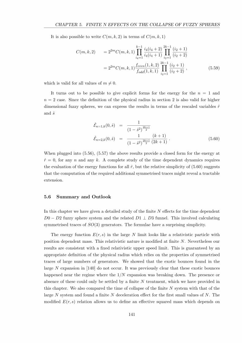
CHAPTER 5. FINITE N EFFECTS ON THE COLLAPSE OF FUZZY SPHERES
It is also possible to write C(m, k, 2) in terms of C(m, k, 1)
C(m, k, 2) = 22mC(m, k, 1)k−1∏
i4=1
i4(i4 + 2)i4(i4 + 1)
2k−1∏
i2=1
(i2 + 1)(i2 + 2)
= 22mC(m, k, 1)feven(1, k, 2)fodd(1, k, 1)
2k−1∏
i2=1
(i2 + 1)(i2 + 2)
, (5.59)
which is valid for all values of m 6= 0.
It turns out to be possible to give explicit forms for the energy for the n = 1 andn = 2 case. Since the definition of the physical radius in section 2 is also valid for higherdimensional fuzzy spheres, we can express the results in terms of the rescaled variables rand s
En=1,k(0, s) =1
(1− s2)2k+1
2
En=2,k(0, s) =1
(1− s2)2k+1
2
(k + 1)(2k + 1)
. (5.60)
When plugged into (5.56), (5.57) the above results provide a closed form for the energy atr = 0, for any n and any k. A complete study of the time dependent dynamics requiresthe evaluation of the energy functions for all r, but the relative simplicity of (5.60) suggeststhat the computation of the required additional symmetrised traces might reveal a tractableextension.
5.6 Summary and Outlook
In this chapter we have given a detailed study of the finite N effects for the time dependentD0 −D2 fuzzy sphere system and the related D1 ⊥ D3 funnel. This involved calculatingsymmetrised traces of SO(3) generators. The formulae have a surprising simplicity.
The energy function E(r, s) in the large N limit looks like a relativistic particle withposition dependent mass. This relativistic nature is modified at finite N . Nevertheless ourresults are consistent with a fixed relativistic upper speed limit. This is guaranteed by anappropriate definition of the physical radius which relies on the properties of symmetrisedtraces of large numbers of generators. We showed that the exotic bounces found in thelarge N expansion in [140] do not occur. It was previously clear that these exotic bounceshappened near the regime where the 1/N expansion was breaking down. The presence orabsence of these could only be settled by a finite N treatment, which we have provided inthis chapter. We also compared the time of collapse of the finite N system with that of thelarge N system and found a finite N deceleration effect for the first small values of N . Themodified E(r, s) relation allows us to define an effective squared mass which depends on
141

CHAPTER 5. FINITE N EFFECTS ON THE COLLAPSE OF FUZZY SPHERES
both r, s. For certain regions in (r, s) space, it can be negative. When the D0−D2 systemis viewed as a source for gravity, a negative sign of this effective mass squared indicates thatthe brane acts as a gravitational source which violates the dominant energy condition.
We have extended some of our discussion to the case of higher even fuzzy spheres withSO(2k + 1) symmetry. The results for symmetrised traces that we obtain can be used in aproposed calculation of charges in the D1 ⊥ D(2k + 1) system. They also provide furtherillustrations of how the correct definition of physical radius using symmetrised traces oflarge powers of Lie algebra generators gives consistency with a constant speed of light. Amore complete discussion of the finite N effects for the higher fuzzy spheres could start fromthese results. Generalisations of the finite N considerations to fuzzy spheres in more generalbackgrounds [161] will be interesting to consider, with a view to possible applications incosmology.
142

APPENDIX A
INTEGRAL IDENTITIES
In this appendix we summarise the tensor bubble, tensor triangle and tensor box integralsused in chapter 2.
A.1 Scalar box, triangle and bubble integrals
The scalar n-point integral functions in D = 4 + 2m− 2ε dimensions are defined as
IDn ≡ ID
n [1] = i(−1)n+1(4π)D/2
∫dDL
(2π)D
1L2(L− p1)2 · · · (L−
∑n−1i=1 pi)2
(A.1)
=i(−1)n+1
π2+m−ε
∫d4+2ml d−2εµ
(l2 − µ2)((l − p1)2 − µ2) · · · ((l −∑n−1i=1 pi)2 − µ2)
The higher dimensional integral functions are related to 4− 2ε dimensional integrals witha factor µ2m inserted in the integrand. For m = 1, 2 one finds
In[µ2] ≡ Jn = (−ε)I6−2εn (A.2)
In[µ4] ≡ Kn = (−ε)(1− ε)I8−2εn (A.3)
In chapter 2 we encounter bubble functions with m = 0, 1, triangles with one massiveexternal line and m = 0, 1, and boxes with four massless external lines and m = 0, 1, 2:
I2(P 2) =rΓ
ε(1− 2ε)(−P 2)−ε , I6−2ε
2 (P 2) = − rΓ2ε(1− 2ε)(3− 2ε)
(−P 2)1−ε ,
I3(P 2) =rΓε2
(−P 2)−1−ε , I6−2ε3 (P 2) =
rΓ2ε(1− ε)(1− 2ε)
(−P 2)−ε ,
I4 = −rΓst
− 1ε2
[(−s)−ε + (−t)−ε
]+
12
log2(st
)+π2
2
+O(ε) ,
(−ε)I6−2ε4 = 0 +O(ε) , (−ε)(1− ε)I8−2ε
4 = −16
+O(ε) . (A.4)
Note that the expressions for the bubbles and triangles are valid to all orders in ε, whereasfor the box functions we have only kept the leading terms which contribute up to O(ε0) inthe amplitudes.
143
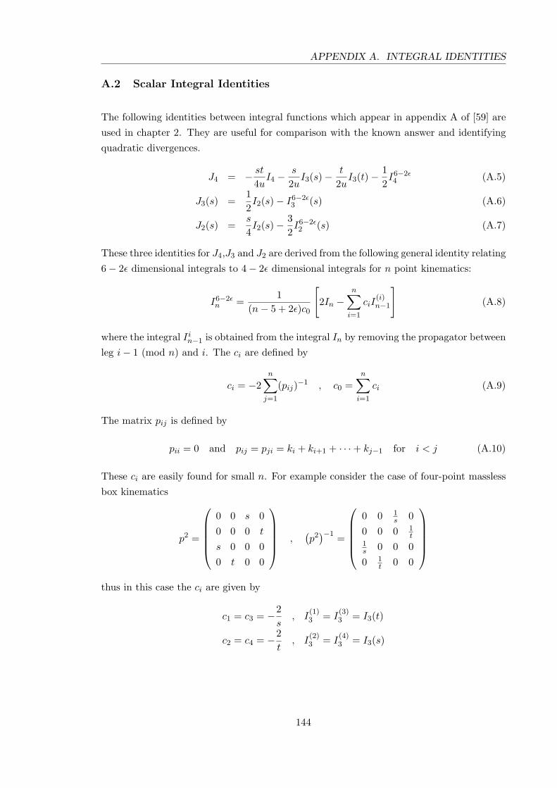
APPENDIX A. INTEGRAL IDENTITIES
A.2 Scalar Integral Identities
The following identities between integral functions which appear in appendix A of [59] areused in chapter 2. They are useful for comparison with the known answer and identifyingquadratic divergences.
J4 = − st
4uI4 − s
2uI3(s)− t
2uI3(t)− 1
2I6−2ε4 (A.5)
J3(s) =12I2(s)− I6−2ε
3 (s) (A.6)
J2(s) =s
4I2(s)− 3
2I6−2ε2 (s) (A.7)
These three identities for J4,J3 and J2 are derived from the following general identity relating6− 2ε dimensional integrals to 4− 2ε dimensional integrals for n point kinematics:
I6−2εn =
1(n− 5 + 2ε)c0
[2In −
n∑
i=1
ciI(i)n−1
](A.8)
where the integral Iin−1 is obtained from the integral In by removing the propagator between
leg i− 1 (mod n) and i. The ci are defined by
ci = −2n∑
j=1
(pij)−1 , c0 =n∑
i=1
ci (A.9)
The matrix pij is defined by
pii = 0 and pij = pji = ki + ki+1 + · · ·+ kj−1 for i < j (A.10)
These ci are easily found for small n. For example consider the case of four-point masslessbox kinematics
p2 =
0 0 s 00 0 0 t
s 0 0 00 t 0 0
,(p2
)−1 =
0 0 1s 0
0 0 0 1t
1s 0 0 00 1
t 0 0
thus in this case the ci are given by
c1 = c3 = −2s
, I(1)3 = I
(3)3 = I3(t)
c2 = c4 = −2t
, I(2)3 = I
(4)3 = I3(s)
144

APPENDIX A. INTEGRAL IDENTITIES
and c0 = 4ust . So finally the identity for J4 is
J4 = (−ε)I6−2ε4
= −12(−1 + 2ε)I6−2ε
4 − 12I6−2ε4
= − 12c0
(2I4 − c1I
(1)3 − c2I
(2)3 − c3I
(3)3
)− 1
2I6−2ε4
= − st
4uI4 − s
2uI3(s)− t
2uI3(t)− 1
2I6−2ε4
which is the identity (A.5) for J4. The identities for J3 and J2 are similar
A.3 PV reduction
In this section we present the result of the Passarino Veltman (PV) reduction for varioustensor integrals which are relevant for the triple cut calculations of the −−++ and −+−+amplitudes in chapter 2.
Figure A.1: Kinematics of the bubble and triangle integral functions studied in this Appendix.
For the linear and two-tensor bubbles we have (see Figure 10a):
I2[Lµ
3
]= −1
2I2(p2 + p3)µ (A.11)
I2[Lµ
3Lν3
]= −1
2I6−2ε2 δµν
[4−2ε] +(
14I2 +
12tI6−2ε2
)(p2 + p3)µ(p2 + p3)ν (A.12)
145

APPENDIX A. INTEGRAL IDENTITIES
For the linear, two- and three-tensor triangles (see Figure 10b):
I3[Lµ
3
]= −1
tI2p
µ2 +
(− I3 +
1tI2
)pµ3 (A.13)
I3[Lµ
3Lν3
]=
12tI2p
µ2p
ν2 +
(1tI6−2ε3 +
12tI2
)(pµ2p
ν3 + pν
2pµ3
)
+(− 3
2tI2 + I3
)pµ3p
ν3 −
12I6−2ε3 δµν
[4−2ε] (A.14)
I3[Lµ
3Lν3L
ρ3
]= −
(14tI2 +
12t2
I6−2ε2
)(pµ2p
ν2p
ρ2
)
−(
14tI2 +
32t2
I6−2ε2
)(pµ2p
ν2p
ρ3 + pµ
2pν3p
ρ2 + pµ
3pν2p
ρ2
)
+(− 1
4tI2 +
32t2
I6−2ε2 − 2
tI6−2ε3
)(pµ2p
ν3p
ρ3 + pµ
3pν3p
ρ2 + pµ
3pν2p
ρ3
)
+(
74tI2 +
12t2
I6−2ε2 − I3
)(pµ3p
ν3p
ρ3
)+
12tI6−2ε2
(δµνpρ
2 + δµρpν2 + δρνpµ
2
)
+(− 1
2tI6−2ε2 +
12I6−2ε3
)(δµνpρ
3 + δµρpν3 + δρνpµ
3
)(A.15)
Finally, for the linear box:
I4[Lµ
3
]=
(t
2uI4 − 1
u
(I3(t)− I3(s)
))pµ1 −
12I4p
µ2
+(t− u
2uI4 − 1
u
(I3(t)− I3(s)
))pµ3 (A.16)
where, as usual, s := (p1 + p2)2, t := (p2 + p3)2, u := (p1 + p3)2.
Note that the above expressions are presented in terms of scalar n-point integral func-tions IDn in various dimensions D, specifically in terms of In, I6−2ε
n and I8−2εn in 4−2ε, 6−2ε
and 8− 2ε dimensions, respectively. The expressions are valid to all orders in ε, if In, I6−2εn
and I8−2εn are evaluated to all orders. In deriving these formulae it is important to remem-
ber that massless bubbles vanish in dimensional regularisation (see page 36 of [14]). Thisis interpreted as the cancelling of a UV and an IR divergence. The PV reductions abovehave been performed in a fashion that naturally leads to coefficients without explicit ε de-pendence. See [96]. We now illustrate this procedure by considering the explicit reductionof the tensor bubble integral
I2[Lµ
3Lν3
]= B1δ
µν[4−2ε] +B2
(p2 + p3
)µ(p2 + p3
)ν (A.17)
146

APPENDIX A. INTEGRAL IDENTITIES
To obtain B1 and B2, the conventional reduction procedure would be to trace over theindices δµν
[4−2ε] and contract with(p2 +p3
)µ(p2 +p3
)ν to obtain the following two equations:
(4− 2ε)B1 + tB2 = 0 , (B1 + tB2) =14I2 (A.18)
Solving these two equations gives
B1 = − 14t
13− 2ε
I2 , B2 =12
2− ε
3− 2εI2 (A.19)
which contain explicit ε dependence. However it is simple to avoid this ε dependence byusing a modified procedure which involves the use of a 6− 2ε dimensional bubble. Insteadof first contracting with δµν
[4−2ε] we contract with δαβ[−2ε]. Recall the following formulae
δ[−2ε]αβ lαlβ = −µ2 and δ
[−2ε]αβ δαβ
[−2ε] = −2ε (A.20)
So contracting with δαβ[−2ε] gives
B1 =12εI2[µ2] = −1
2I6−2ε2 (A.21)
To determine B2 we again use (B1 + tB2) = 14I2 to give
B2 =14I2 +
12tI6−2ε2 (A.22)
See Appendix I of [96] for more details on this particular variant of PV reductions.
147

APPENDIX B
GRAVITY AMPLITUDE CHECKS
B.1 The VegasShift[n] Mathematica command
The following Mathematica code can be used to compare amplitudes numerically. Thereare two different commands evalshift[X] which puts random numbers into the shiftedamplitude and evalnormal[X] which puts random numbers into the unshifted amplitude.evalshift[X] in conjunction with the standard Mathematica command Apart[X] can beused to check the residues of a shifted amplitude one by one.
VegasShift[nn_] := (
rand := Random[Integer, -100, 100]/100;
angle[ii1_,ii2_]:=la[ii1][[1]] la[ii2][[2]]-la[ii1][[2]] la[ii2][[1]];
square[ii1_,ii2_]:=lat[ii1][[1]] lat[ii2][[2]]-lat[ii1][[2]] lat[ii2][[1]];
Do[(la[ii] = rand, rand;
lat[ii] = rand, rand), ii, 1, nn - 2];
P = Sum[Transpose[la[ii]].lat[ii], ii, 1, nn - 2];
la[nn - 1] = 1, 0;
lat[nn - 1] = -P[[1]];
la[nn] = 0, 1;
lat[nn] = -P[[2]];
Sum[Transpose[la[ii]].lat[ii], ii, 1, nn];
lat[1] = lat[1] - z lat[2];
la[2] = la[2] + z la[1];
replist = ;
Do[ replist = Union[replist, ang[xx1, yy1] -> angle[xx1, yy1],
sqr[xx1, yy1] -> square[xx1, yy1]], xx1, 1, nn, yy1, 1, nn];
evalshift[expression_] := expression /. replist;
evalnormal[expression_] := expression /. replist /. z -> 0;)
148

APPENDIX B. GRAVITY AMPLITUDE CHECKS
B.2 Other shifts of the −+ + + + gravity amplitude
B.2.1 The |4], |5〉 shifts
In this section we consider M (1)5 (1−, 2+, 3+, 4+, 5+) with the following shifts which have
both nonstandard factorisations and presumably also have a boundary term.
λ4 → λ4
λ4 → λ4 − zλ5
λ5 → λ5 + zλ4
λ5 → λ5 (B.1)
We will calculate as many terms as we can.
Figure B.1: The diagram associated with 〈15〉 = 0, with shifts on |4], |5〉.
The diagram in Figure B.1 gives:
i
(4π)21
180〈12〉2〈13〉2[23]4[15]
〈23〉2〈24〉2〈45〉2〈34〉2〈15〉(〈12〉2〈34〉2 − 〈12〉〈34〉〈13〉〈24〉+ 〈13〉2〈24〉2) (B.2)
Figure B.2: The diagram associated with [14] = 0, with shifts on |4], |5〉.
The diagram in Figure B.2 gives:
i
(4π)23
180〈14〉[45]6
〈23〉2[14][15]4([23]2[15]2 + [23][12][35][15] + [12]2[35]2
)(B.3)
149

APPENDIX B. GRAVITY AMPLITUDE CHECKS
Figure B.3: The standard factorisation diagram associated with 〈25〉 = 0, with shifts on|4], |5〉.
The diagram in Figure B.3 gives:
i
(4π)21
180〈12〉2〈13〉2〈14〉2[13]4[25]〈23〉2〈24〉4〈34〉2〈25〉〈45〉2
(〈13〉2〈24〉2 + 〈12〉〈24〉〈43〉〈13〉+ 〈34〉2〈12〉2) (B.4)
Figure B.4: The nonstandard factorisation diagram associated with 〈25〉 = 0, with shifts on|4], |5〉.
The diagram in Figure B.4 is a non standard factorisation. The double pole termassociated with this diagram is
i
(4π)21
180〈12〉7〈45〉2[25]4[13]
〈13〉〈14〉〈34〉〈23〉〈25〉2〈24〉4 (B.5)
Just as in the |1], |2〉 shifts the ‘single pole under this double pole’ term is mysterious. Theother two diagrams corresponding to 〈35〉 = 0 can be obtained from the results to FigureB.3 and Figure B.4 by swapping 2 and 3.
It is perhaps interesting to note that if we take some of the above terms in the |4], |5〉shifts, and apply the |1], |2〉 shifts to the answers, and use partial fractions to extract thepole from the term, then there is agreement with the recursive diagrams in section 3.4. Thusthe recursion relation is self consistent. For example, if you apply the |1], |2〉 shifts to (B.3)and extract the 1/[1, 4] pole then this agrees with (3.52) after the legs 4 and 5 have beenswapped. The results (B.4) and (B.5) can similarly be checked against (3.55) and (3.58)respectively.
150
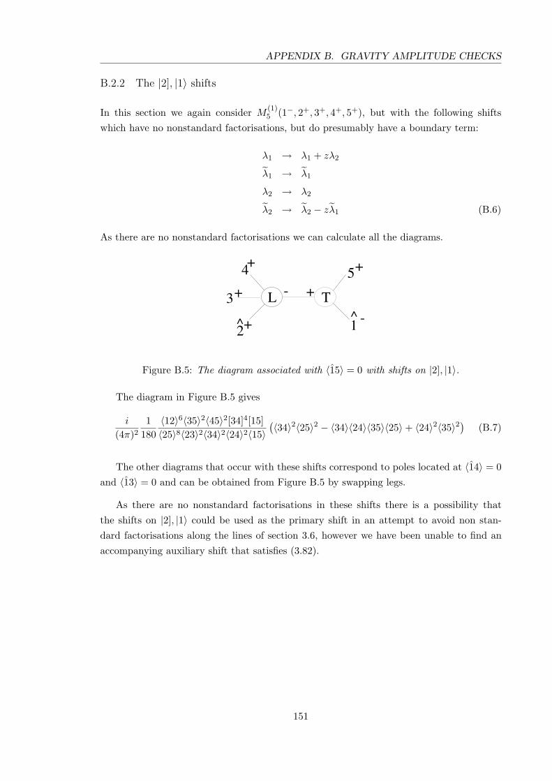
APPENDIX B. GRAVITY AMPLITUDE CHECKS
B.2.2 The |2], |1〉 shifts
In this section we again consider M (1)5 (1−, 2+, 3+, 4+, 5+), but with the following shifts
which have no nonstandard factorisations, but do presumably have a boundary term:
λ1 → λ1 + zλ2
λ1 → λ1
λ2 → λ2
λ2 → λ2 − zλ1 (B.6)
As there are no nonstandard factorisations we can calculate all the diagrams.
Figure B.5: The diagram associated with 〈15〉 = 0 with shifts on |2], |1〉.
The diagram in Figure B.5 gives
i
(4π)21
180〈12〉6〈35〉2〈45〉2[34]4[15]〈25〉8〈23〉2〈34〉2〈24〉2〈15〉
(〈34〉2〈25〉2 − 〈34〉〈24〉〈35〉〈25〉+ 〈24〉2〈35〉2) (B.7)
The other diagrams that occur with these shifts correspond to poles located at 〈14〉 = 0and 〈13〉 = 0 and can be obtained from Figure B.5 by swapping legs.
As there are no nonstandard factorisations in these shifts there is a possibility thatthe shifts on |2], |1〉 could be used as the primary shift in an attempt to avoid non stan-dard factorisations along the lines of section 3.6, however we have been unable to find anaccompanying auxiliary shift that satisfies (3.82).
151
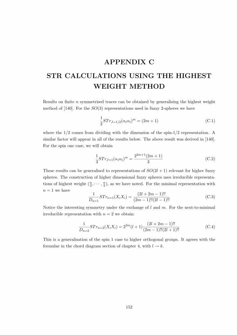
APPENDIX C
STR CALCULATIONS USING THE HIGHEST
WEIGHT METHOD
Results on finite n symmetrised traces can be obtained by generalising the highest weightmethod of [140]. For the SO(3) representations used in fuzzy 2-spheres we have
12STrJ=1/2(αiαi)m = (2m+ 1) (C.1)
where the 1/2 comes from dividing with the dimension of the spin-1/2 representation. Asimilar factor will appear in all of the results below. The above result was derived in [140].For the spin one case, we will obtain
13STrJ=1(αiαi)m =
22m+1(2m+ 1)3
(C.2)
These results can be generalised to representations of SO(2l + 1) relevant for higher fuzzyspheres. The construction of higher dimensional fuzzy spheres uses irreducible representa-tions of highest weight (n
2 , · · · , n2 ), as we have noted. For the minimal representation with
n = 1 we have1
Dn=1STrn=1(XiXi) =
(2l + 2m− 1)!!(2m− 1)!!(2l − 1)!!
(C.3)
Notice the interesting symmetry under the exchange of l and m. For the next-to-minimalirreducible representation with n = 2 we obtain:
1Dn=2
STrn=2(XiXi) = 22m(l + 1)(2l + 2m− 1)!!
(2m− 1)!!(2l + 1)!!(C.4)
This is a generalisation of the spin 1 case to higher orthogonal groups. It agrees with theformulae in the chord diagram section of chapter 4, with l→ k.
152

APPENDIX C. STR CALCULATIONS USING THE HIGHEST WEIGHT METHOD
C.1 Review of spin half for SO(3)
We will begin by recalling some facts about the derivation of the n = 1 case in [140]. Thecommutation relations can be expressed in terms of α3, α±
α± =1√2(α1 ± iα2),
[α3, α±] = 2α±,
[α+, α−] = 2α3,
c = α+α− + α−α+ + α23 (C.5)
With these normalisations, the eigenvalues of α3 in the spin half representation are ±1 andα+α− is 1 on the highest weight state.
It is useful to define a quantity C(p, q) which depends on two natural numbers p, q andcounts the number of ways of separating p identical objects into q parts
C(p, q) =(p+ q − 1)!p!(q − 1)!
(C.6)
We begin by a review of the spin half case, establishing a counting which will be used againin more complicated cases below. This relies on a sum
2k2n−2k∑
i2k
· · ·i3∑
i2=0
i2∑
i1=0
(−1)i1+i2+···i2k = 2k n!(n− k)!k!
Recall that this sum was obtained by evaluating a sequence of generators of SO(3) consistingof k pairs α−α+ and with powers of α3 between these pairs -
α2J2k+1
3 α+α2Jk3 α− · · ·α−αJ3
3 α+αJ23 α−α
J13 (C.7)
We can move the powers of α3 to the left to get factors (α3 − 2)J2+J4+···J2k . Moving the α3
with powers J1, J3.. gives αJ1+J3+···3 . The k powers of α−α+ gives 2k. The above sum can
be rewritten
2k2m−2k∑
J2k+1=0
· · ·2m−2k−J3+..J2k+1∑
J2=0
2m−2k−J2...J2k+1∑
J1=0
(−1)J2+J4···J2k = 2k n!(n− k)!k!
(C.8)
This includes a sum over Je = J2 + J4 + . . . + J2k. The summand does not depend onthe individual J2, J4, . . . only on the sum Je which ranges from 0 to 2m − 2k. The sumover J2, J4, . . . is the combinatoric factor, introduced above, which is the number of ways ofsplitting Je identical objects into k parts, i.e. C(Je, k). The remaining 2m−2k−Je powersof α3 are distributed in k + 1 slots in C(2m − 2k − Je, k + 1) ways. Hence the sum (C.8)
153

APPENDIX C. STR CALCULATIONS USING THE HIGHEST WEIGHT METHOD
can be written more simply as
2k2m−2k∑
Je=0
(−1)JeC(Je, k)C(2m− 2k − Je, k + 1) = 2k m!(m− k)!k!
(C.9)
Then there is a sum over k from 0 to m, with weight
C(k,m) =2kk!(2m− 2k)!m!
(m− k)!(2m)!(C.10)
which gives the final result 2m + 1 [140]. Similar sums arise in the proofs below. In somecases, closed formulae for the sums are obtained experimentally.
C.2 Derivation of symmetrised trace for minimal SO(2l+1) representation
The Casimir of interest here is
XµXµ = X22l+1 +
l∑
i=1
(X
(i)− X
(i)+ +X
(i)+ X
(i)−
)(C.11)
The patterns are similar to those above, with α3 replaced by X2l+1, and noting that herethere are l “colours” of α± which are X(l)
± . All the states in the fundamental spinor areobtained by acting on a vacuum which is annihilated by l species of fermions. Generally wemight expect patterns
. . . Xi12l+1X
(j1)− Xi2
2l+1X(j2)+ . . . (C.12)
In evaluating these, we can commute all the X2l+1 to the left. This results in shifts whichdo not depend on the value of j. It is easy to see that whenever X(1)
+ is followed by X(1)+
we get zero because of the fermionic construction of the gamma matrices. X(1)+ cannot also
be followed by X(2)+ because X(1)
+ X(2)+ +X
(2)+ X
(1)+ = 0. So the pairs have to take the form
X(j)− X
(j)+ for fixed j. The sum we have to evaluate is
m∑
k=0
2m−2k∑
Je=0
(−1)JeC(Je, k)C(2m− 2k − Je, k)C(k, l)2kC(k,m)
=m∑
k=0
(m
k
)2kC(k,m)C(k, l) (C.13)
=(2l + 2m− 1)!!
(2m− 1)!!(2l − 1)!!
154

APPENDIX C. STR CALCULATIONS USING THE HIGHEST WEIGHT METHOD
The factors C(Je, k) and C(2m− 2k − Je, k) have the same origin as in the spin half case.The factor (C.10) is now generalised to an l-colour version
C(k1, k2...kl;m) = 2k (2m− 2k)!(2m)!
m!(m− k)!
k1!k2!...kl! (C.14)
This has to be summed over k1, .., kl. For fixed k = k1 + · · ·+ kl we have
∑
k1..kl
C(k1..kl,m)k!
k1!..kl!=
∑
k1..kl
C(k,m) = C(k,m)C(k, l) (C.15)
The combinatoric factor k!k1!..kl!
in the second line above comes from the different ways ofdistributing the k1..kl pairs of (−+) operators in the k positions along the line of operators.The subsequent sum amounts to calculating the number of ways of separating k objectsinto l parts which is given by C(k, l). The C(k,m) is familiar from (C.10). This sum canbe done for various values of k,m and gives agreement with (C.3).
C.3 Derivation of spin one symmetrised trace for SO(3)
For the spin one case more patterns will arise. After an α− acts on the highest weight, weget a state with α3 = 0 so that we have, for any positive r
αr3α−|J = 1, α3 = 2 >= 0 , ∀ r > 0 (C.16)
Hence any α− can be followed immediately by α+. These neutral pairs of (α+α−) can beseparated by powers of α3. Alternatively an α− can be followed immediately by α−. Theeffect of α2− is to change the highest weight state to a lowest weight state. In describingthe patterns we have written the “vacuum changing operator” on the second line, with thefirst line containing only neutral pairs separated by α3’s. Let there be J1 neutral pairs inthis first line and L1 powers of α3 distributed between them. After the change of vacuum,we can have a sequence of (α−α+) separated by powers of α3. Let there be a total of J2
neutral pairs and L2 α3’s in the second line. At the beginning of the third line we haveanother vacuum changing operator α2
+ which takes us back to the highest weight state. Inthe third line, we have J3 neutral pairs and L3 powers of α3. The equation below describesa general pattern with p pairs of vacuum changing operators. The total number of neutralpairs is 2p+ J where J = J1 + J2 + · · ·+ J2p+1. The general pattern of operators acting on
155

APPENDIX C. STR CALCULATIONS USING THE HIGHEST WEIGHT METHOD
the vacuum is
# (α+α−) # (α+α−) # · · ·# (α+α−) # |J = 1, α3 = 2 >
# (α−α+) # (α−α+) # · · ·# (α−α+) #α2−
# (α+α−) # (α+α−) # · · ·# (α+α−) # α2+
...
# (α−α+) # (α−α+) # · · · # (α−α+) #α2−
# (α+α−) # (α+α−) # · · ·# (α+α−)# α2+ , (C.17)
where in the above the first line of operators acts on the state |J = 1, α3 = 2 > first,then the second line acts, and so on. The symbols # represent powers of α3. We defineJe = J2 + J4 + · · ·J2p which is the total number of (−+) pairs on the even lines above.There is a combinatoric factor C(Je, p) for distributing Je among the p entries, and a similarC(J − Je, p + 1) for the odd lines. The Le = L2 + L4 + · · · + L2p copies of α3 can sit in(J2 + 1) + (J4 + 1) + · · · + (J2p + 1) positions which gives a factor of C(Le, Je + p). TheL1+L3+ · · ·+L2p+1 can sit in (J1+1)+(J3+1)+ · · ·+(J2p+1+1) = J−Je+p+1 positions,giving a factor C(2m− 2J − 4p−Le, J − Je + p+ 1). There is finally a factor C(2p+ J,m)defined in (C.10) which arises from the number of different ways the permutations of 2mindices can be specialised to yield a fixed pattern of α+, α−, α3
[m/2]∑
p=0
m−2p∑
J=0
J∑
Je=0
2m−4p−2J∑
Le=0
C(Je, p) C(J − Je, p+ 1) (−1)Le C(Le, Je + p)×
C(2m− 2J − 4p− Le, J − Je + p+ 1)×22m−2J−4p Q(1, 1)J−Je Q(2, 1)Je Q(2, 2)p C(2p+ J,m)
By doing the sums (using Maple for example) for various values of m we find 22m+1(2m+1)3 .
The factors Q(i, j), denoted in [140] by N(i, j), arise from evaluating the α−, α+ on thehighest weight.
C.4 Derivation of next-to-minimal representation for SO(2l + 1)
The n = 2, general l patterns are again similar to the n = 2, l = 1 case except that theα−, α+ are replaced by coloured objects of l colours, i.e. the X(j)
± . We also have the simplereplacement of α3 by X2l+1.
We define linear combinations of the gamma matrices which are simply related to a set ofl fermionic oscillators: Γ(i)
+ = 1√2(Γ2i−1 + iΓ2i) =
√2a†i and Γ(i)
− = 1√2(Γ2i−1− iΓ2i) =
√2ai.
156

APPENDIX C. STR CALCULATIONS USING THE HIGHEST WEIGHT METHOD
As usual Xi are expressed as operators acting on an n-fold tensor product, and
X(i)± =
∑r
ρr(Γ(i)± ) . (C.18)
Some useful facts are
Xr2l+1X+|0 > = 0, Xr
2l+1X2+|0 > = (−2)rX2
+|0 >,Xr
2l+1X−X+|0 > = X−X+Xr2l+1|0 > = (2)rX−X+|0 >,
X−X+Xr2l+1X
2+|0 > = 0, Y+X
2+ +X2
+Y+|0 > = 0,
X+Y+X+|0 > = 0, X−Y+X+|0 > = 0,
X+X−X2+|0 > = Q(2, 1)X2
+|0 >, X+X−X+Y+|0 > = Q(2, 1)X+Y+|0 >,X2−X
2+|0 > = Q(2, 2)|0 >, Y−X−X+Y+|0 > = Q(2, 2)|0 >
It is significant that the same Q(2, 1), Q(2, 2) factors appear in the different places in theabove equation. In the above X+ stands for any of the l X(i)
+ ’s. Any equation containingX± and Y± stands for any pair X(i)
± and X(j)± for i, j distinct integers from 1 to l.
The general pattern is similar to (C.17) with the only difference that the (α−α+) on thefirst line is replaced by any one (X(i)
− X(i)+ ) for i = 1, . . . , l. The positive vacuum changing
operators can be (X(i)+ X
(j)+ ), where i, j can be identical or different. For every such choice the
allowed neutral pairs following them are X(j)+ X
(i)− and the dual vacuum changing operator
is (X(j)− X
(i)− ).
The summation we have to do is:
[m/2]∑
p=0
m−2p∑
J=0
2m−4p−2J∑
Le=0
J∑
Je=0
(C(2p+ J,m)C(2p+ J, l)C(Je, p) C(J − Je, p+ 1)×
(−1)Le C(Le, Je + p)C(2m− 2J − 4p− Le, J − Je + p+ 1)×
22m−2J−4p Q(1, 1)J−Je Q(2, 1)Je Q(2, 2)p
)
The Q-factors can be easily evaluated on the highest weight and then inserted into theabove
Q(1, 1) = 4 , Q(2, 1) = 4 Q(2, 2) = 16 . (C.19)
By computing this for several values of m, l, we obtain (C.4). Note that both the l = 1 andthe general l case will yield the correct value for m = 0, which is 1.
157

References
[1] A. Brandhuber, S. McNamara, B. J. Spence and G. Travaglini, Loop amplitudes inpure Yang-Mills from generalised unitarity, JHEP 0510, 011 (2005), hep-th/0506068.
[2] S. McNamara, C. Papageorgakis, S. Ramgoolam and B. Spence, Finite N effects onthe collapse of fuzzy spheres, JHEP 0605, 060 (2006), hep-th/0512145.
[3] G. ’t Hooft, A Planar Diagram Theory for Strong Interactions Nucl. Phys. B 72, 461(1974).
[4] J. M. Maldacena, The large N limit of superconformal field theories and supergrav-ity, Adv. Theor. Math. Phys. 2, 231 (1998), [Int. J. Theor. Phys. 38, 1113 (1999)],hep-th/9711200.
[5] E. Witten, Perturbative gauge theory as a string theory in twistor space, Commun.Math. Phys. 252, 189 (2004), hep-th/0312171.
[6] R. Penrose, Twistor algebra, J. Math. Phys. 8, 345 (1967).
[7] S. J. Parke and T. R. Taylor, An Amplitude For N Gluon Scattering, Phys. Rev. Lett.56, 2459 (1986).
[8] F. Cachazo, P. Svrcek and E. Witten, MHV vertices and tree amplitudes in gaugetheory, JHEP 0409, 006 (2004), hep-th/0403047.
[9] F. A. Berends and W. Giele, The Six Gluon Process As An Example Of Weyl-Van DerWaerden Spinor Calculus, Nucl. Phys. B 294, 700 (1987).
[10] M. L. Mangano, S. J. Parke and Z. Xu, Duality and Multi - Gluon Scattering, Nucl.Phys. B 298, 653 (1988).
[11] N. Berkovits and E. Witten, Conformal supergravity in twistor-string theory, JHEP0408, 009 (2004), hep-th/0406051.
[12] A. Brandhuber, B. J. Spence and G. Travaglini, One-loop gauge theory amplitudesin N = 4 super Yang-Mills from MHV vertices, Nucl. Phys. B 706, 150 (2005),hep-th/0407214.
158

REFERENCES
[13] Z. Bern, L. J. Dixon, D. C. Dunbar and D. A. Kosower, One loop n point gaugetheory amplitudes, unitarity and collinear limits, Nucl. Phys. B 425, 217 (1994),hep-ph/9403226.
[14] Z. Bern, L. J. Dixon, D. C. Dunbar and D. A. Kosower, Fusing gauge theory treeamplitudes into loop amplitudes, Nucl. Phys. B 435, 59 (1995), hep-ph/9409265.
[15] R. Britto, F. Cachazo and B. Feng, Generalized unitarity and one-loop amplitudes inN = 4 super-Yang-Mills, Nucl. Phys. B 725, 275 (2005), hep-th/0412103.
[16] R. Britto, F. Cachazo and B. Feng, New recursion relations for tree amplitudes ofgluons, Nucl. Phys. B 715, 499 (2005), hep-th/0412308.
[17] R. Britto, F. Cachazo, B. Feng and E. Witten, Direct proof of tree-level recursionrelation in Yang-Mills theory, Phys. Rev. Lett. 94, 181602 (2005), hep-th/0501052.
[18] Z. Bern, L. J. Dixon and D. A. Kosower, On-shell recurrence relations for one-loopQCD amplitudes, Phys. Rev. D 71, 105013 (2005), hep-th/0501240.
[19] D. J. Gross and F. Wilczek, Ultraviolet Behaviour of Non-Abelian Gauge Theories,Phys. Rev. Lett. 30, 1343 (1973).
[20] H. D. Politzer, Reliable Perturbative Results for Strong Interactions?, Phys. Rev. Lett.30, 1346 (1973).
[21] M. L. Mangano, The Color Structure Of Gluon Emission, Nucl. Phys. B 309, 461(1988).
[22] Z. Bern and D. A. Kosower, Color Decomposition Of One Loop Amplitudes In GaugeTheories, Nucl. Phys. B 362, 389 (1991).
[23] R. Gastmans and T. T. Wu, The Ubiquitous Photon: Helicity Method For QED AndQCD.
[24] M. T. Grisaru, H. N. Pendleton and P. van Nieuwenhuizen, Supergravity And The SMatrix, Phys. Rev. D 15, 996 (1977).
[25] M. T. Grisaru and H. N. Pendleton, Some Properties Of Scattering Amplitudes InSupersymmetric Theories, Nucl. Phys. B 124, 81 (1977).
[26] M. Abou-Zeid, C. M. Hull and L. J. Mason, Einstein supergravity and new twistorstring theories, hep-th/0606272.
[27] R. Roiban, M. Spradlin and A. Volovich, A googly amplitude from the B-model intwistor space, JHEP 0404, 012 (2004), hep-th/0402016.
[28] R. Roiban and A. Volovich, All googly amplitudes from the B-model in twistor space,Phys. Rev. Lett. 93, 131602 (2004), hep-th/0402121.
159

REFERENCES
[29] R. Roiban, M. Spradlin and A. Volovich, On the tree-level S-matrix of Yang-Millstheory, Phys. Rev. D 70, 026009 (2004), hep-th/0403190.
[30] S. Gukov, L. Motl and A. Neitzke, Equivalence of twistor prescriptions for super Yang-Mills, hep-th/0404085.
[31] C. J. Zhu, The googly amplitudes in gauge theory, JHEP 0404, 032 (2004),hep-th/0403115.
[32] G. Georgiou and V. V. Khoze, Tree amplitudes in gauge theory as scalar MHV dia-grams, JHEP 0405, 070 (2004), hep-th/0404072.
[33] J. B. Wu and C. J. Zhu, MHV vertices and scattering amplitudes in gauge theory,JHEP 0407, 032 (2004), hep-th/0406085.
[34] J. B. Wu and C. J. Zhu, MHV vertices and fermionic scattering amplitudes in gaugetheory with quarks and gluinos, JHEP 0409, 063 (2004), hep-th/0406146.
[35] G. Georgiou, E. W. N. Glover and V. V. Khoze, Non-MHV tree amplitudes in gaugetheory, JHEP 0407, 048 (2004), hep-th/0407027.
[36] L. J. Dixon, E. W. N. Glover and V. V. Khoze, MHV rules for Higgs plus multi-gluonamplitudes, JHEP 0412, 015 (2004), hep-th/0411092.
[37] Z. Bern, D. Forde, D. A. Kosower and P. Mastrolia, ‘Twistor-inspired construction ofelectroweak vector boson currents, Phys. Rev. D 72, 025006 (2005), hep-ph/0412167.
[38] K. Risager, A direct proof of the CSW rules, JHEP 0512, 003 (2005), hep-th/0508206.
[39] F. Cachazo, P. Svrcek and E. Witten, Twistor space structure of one-loop amplitudesin gauge theory, JHEP 0410, 074 (2004), hep-th/0406177.
[40] F. Cachazo, P. Svrcek and E. Witten, Gauge theory amplitudes in twistor space andholomorphic anomaly, JHEP 0410, 077 (2004), hep-th/0409245.
[41] I. Bena, Z. Bern, D. A. Kosower and R. Roiban, Loops in twistor space, Phys. Rev. D71, 106010 (2005), hep-th/0410054.
[42] F. Cachazo, Holomorphic anomaly of unitarity cuts and one-loop gauge theory ampli-tudes, hep-th/0410077.
[43] R. Britto, F. Cachazo and B. Feng, Computing one-loop amplitudes from the holomor-phic anomaly of unitarity cuts, Phys. Rev. D 71 (2005) 025012, hep-th/0410179.
[44] Z. Bern, V. Del Duca, L. J. Dixon and D. A. Kosower, All non-maximally-helicity-violating one-loop seven-gluon amplitudes in N = 4 super-Yang-Mills theory, Phys.Rev. D 71 (2005) 045006, hep-th/0410224.
160

REFERENCES
[45] S. J. Bidder, N. E. J. Bjerrum-Bohr, L. J. Dixon and D. C. Dunbar, N = 1 supersym-metric one-loop amplitudes and the holomorphic anomaly of unitarity cuts, Phys. Lett.B 606 (2005) 189, hep-th/0410296.
[46] A. Brandhuber, B. Spence and G. Travaglini, From trees to loops and back, JHEP0601, 142 (2006), hep-th/0510253.
[47] C. Quigley and M. Rozali, ‘One-loop MHV amplitudes in supersymmetric gauge theo-ries, JHEP 0501, 053 (2005), hep-th/0410278.
[48] J. Bedford, A. Brandhuber, B. J. Spence and G. Travaglini, A twistor approach toone-loop amplitudes in N = 1 supersymmetric Yang-Mills theory, Nucl. Phys. B 706,100 (2005), hep-th/0410280.
[49] J. Bedford, A. Brandhuber, B. J. Spence and G. Travaglini, Non-supersymmetric loopamplitudes and MHV vertices, Nucl. Phys. B 712, 59 (2005), hep-th/041210.
[50] P. Mansfield, The Lagrangian origin of MHV rules, JHEP 0603, 037 (2006),hep-th/0511264.
[51] A. Gorsky and A. Rosly, From Yang-Mills Lagrangian to MHV diagrams, JHEP 0601,101 (2006), hep-th/0510111.
[52] J. H. Ettle and T. R. Morris, Structure of the MHV-rules Lagrangian, JHEP 0608,003 (2006), hep-th/0605121.
[53] L. D. Landau, On analytic properties of vertex parts in quantum field theory, Nucl.Phys. 13, 181 (1959).
[54] S. Mandelstam, Determination Of The Pion - Nucleon Scattering Amplitude FromDispersion Relations And Unitarity. General Theory, Phys. Rev. 112, 1344 (1958).
[55] S. Mandelstam, Analytic Properties Of Transition Amplitudes In Perturbation Theory,Phys. Rev. 115, 1741 (1959).
[56] R. E. Cutkosky, Singularities and discontinuities of Feynman amplitudes, J. Math.Phys. 1, 429 (1960).
[57] R.J. Eden, P.V. Landshoff, D.I. Olive, J.C. Polkinghorne, The Analytic S-Matrix. Cam-bridge University Press 1966.
[58] W. L. van Neerven, Dimensional Regularization Of Mass And Infrared Singularities InTwo Loop On-Shell Vertex Functions, Nucl. Phys. B 268 (1986) 453.
[59] Z. Bern and A. G. Morgan, Massive Loop Amplitudes from Unitarity, Nucl. Phys. B467 (1996) 479, hep-ph/9511336.
161

REFERENCES
[60] Z. Bern, L. J. Dixon, D. C. Dunbar and D. A. Kosower, One-loop self-dual and N = 4super Yang-Mills, Phys. Lett. B 394 (1997) 105, hep-th/9611127.
[61] S. D. Badger, E. W. N. Glover, V. V. Khoze and P. Svrcek, Recursion relations for gaugetheory amplitudes with massive particles, JHEP 0507, 025 (2005), hep-th/0504159.
[62] Z. Bern, L. J. Dixon and D. A. Kosower, One-loop amplitudes for e+ e- to four partons,Nucl. Phys. B 513 (1998) 3, hep-ph/9708239.
[63] Z. Bern, L. J. Dixon and D. A. Kosower, A two-loop four-gluon helicity amplitude inQCD, JHEP 0001 (2000) 027, hep-ph/0001001.
[64] Z. Bern, L. J. Dixon and D. A. Kosower, Two-loop g → g g splitting amplitudes inQCD, JHEP 0408 (2004) 012, hep-ph/0404293.
[65] C. Anastasiou, Z. Bern, L. J. Dixon and D. A. Kosower, Planar amplitudes inmaximally supersymmetric Yang-Mills theory, Phys. Rev. Lett. 91, 251602 (2003),hep-th/0309040.
[66] C. Anastasiou, L. J. Dixon, Z. Bern and D. A. Kosower, Cross-order relations in N =4 supersymmetric gauge theories, hep-th/0402053.
[67] Z. Bern, L. J. Dixon and V. A. Smirnov, Iteration of planar amplitudes in maximallysupersymmetric Yang-Mills theory at three loops and beyond, Phys. Rev. D 72, 085001(2005), hep-th/0505205.
[68] Z. Bern, M. Czakon, D. A. Kosower, R. Roiban and V. A. Smirnov, Two-loop iterationof five-point N = 4 super-Yang-Mills amplitudes, hep-th/0604074.
[69] S. J. Bidder, N. E. J. Bjerrum-Bohr, D. C. Dunbar and W. B. Perkins, One-loop gluonscattering amplitudes in theories with N ≤ 4 supersymmetries, Phys. Lett. B 612, 75(2005), hep-th/0502028.
[70] R. Britto, E. Buchbinder, F. Cachazo and B. Feng, One-loop amplitudes of gluons inSQCD, Phys. Rev. D 72, 065012 (2005), hep-ph/0503132.
[71] M. x. Luo and C. k. Wen, Recursion relations for tree amplitudes in super gauge theo-ries, JHEP 0503, 004 (2005), hep-th/0501121.
[72] M. x. Luo and C. k. Wen, Compact formulas for all tree amplitudes of six partons,Phys. Rev. D 71, 091501 (2005), hep-th/0502009.
[73] J. Bedford, A. Brandhuber, B. J. Spence and G. Travaglini, A recursion relation forgravity amplitudes, Nucl. Phys. B 721, 98 (2005), hep-th/0502146.
[74] F. Cachazo and P. Svrcek, Tree level recursion relations in general relativity,hep-th/0502160.
162

REFERENCES
[75] Z. Bern, L. J. Dixon and D. A. Kosower, The last of the finite loop amplitudes in QCD,Phys. Rev. D 72, 125003 (2005), hep-ph/0505055.
[76] Z. Bern, L. J. Dixon and D. A. Kosower, Bootstrapping multi-parton loop amplitudesin QCD, Phys. Rev. D 73, 065013 (2006), hep-ph/0507005.
[77] C. F. Berger, Z. Bern, L. J. Dixon, D. Forde and D. A. Kosower, Bootstrapping one-loopQCD amplitudes with general helicities, hep-ph/0604195.
[78] C. F. Berger, Z. Bern, L. J. Dixon, D. Forde and D. A. Kosower, All one-loop maximallyhelicity violating gluonic amplitudes in QCD, hep-ph/0607014.
[79] Z. Bern, N. E. J. Bjerrum-Bohr, D. C. Dunbar and H. Ita, Recursive calculation ofone-loop QCD integral coefficients, JHEP 0511, 027 (2005), hep-ph/0507019.
[80] H. Kawai, D. C. Lewellen and S. H. H. Tye, A Relation Between Tree Amplitudes OfClosed And Open Strings, Nucl. Phys. B 269, 1 (1986).
[81] N. E. J. Bjerrum-Bohr, D. C. Dunbar, H. Ita, W. B. Perkins and K. Risager, MHV-vertices for gravity amplitudes, JHEP 0601, 009 (2006), hep-th/0509016.
[82] Z. Bern and D. A. Kosower, The Computation of loop amplitudes in gauge theories,Nucl. Phys. B 379, 451 (1992).
[83] Z. Bern, L. J. Dixon and D. A. Kosower, New QCD Results From String Theory,hep-th/9311026.
[84] Z. Bern, G. Chalmers, L. J. Dixon and D. A. Kosower, One loop N gluon amplitudeswith maximal helicity violation via collinear limits, Phys. Rev. Lett. 72, 2134 (1994),hep-ph/9312333.
[85] Z. Bern, L. J. Dixon and D. A. Kosower, One loop corrections to five gluon amplitudes,Phys. Rev. Lett. 70, 2677 (1993), hep-ph/9302280.
[86] Z. G. Xiao, G. Yang and C. J. Zhu, The rational part of QCD amplitude. III: Thesix-gluon, hep-ph/0607017.
[87] S. Moch, J. A. M. Vermaseren and A. Vogt, The three-loop splitting functions in QCD:The non-singlet case, Nucl. Phys. B 688, 101 (2004), hep-ph/0403192.
[88] A. V. Kotikov, L. N. Lipatov, A. I. Onishchenko and V. N. Velizhanin, Three-loop uni-versal anomalous dimension of the Wilson operators in N=4 SUSY Yang-Mills model,Phys. Lett. B 595, 521 (2004), [Erratum-ibid. B 632, 754 (2006)], hep-th/0404092.
[89] N. Beisert, V. Dippel and M. Staudacher, A novel long range spin chain and planar N= 4 super Yang-Mills, JHEP 0407, 075 (2004), hep-th/0405001.
[90] B. Eden and M. Staudacher, Integrability and transcendentality, hep-th/0603157.
163

REFERENCES
[91] S. Frolov and A. A. Tseytlin, Semiclassical quantization of rotating superstring inAdS(5) x S(5), JHEP 0206, 007 (2002), hep-th/0204226.
[92] H. Ooguri and C. Vafa, Worldsheet derivation of a large N duality, Nucl. Phys. B 641,3 (2002), hep-th/0205297.
[93] R. Gopakumar, From free fields to AdS, Phys. Rev. D 70, 025009 (2004),hep-th/0308184.
[94] G. ’t Hooft and M. J. G. Veltman, One Loop Divergences In The Theory Of Gravitation,Annales Poincare Phys. Theor. A 20, 69 (1974).
[95] Z. Bern, Perturbative quantum gravity and its relation to gauge theory, Living Rev.Rel. 5, 5 (2002), gr-qc/0206071.
[96] Z. Bern and G. Chalmers, Factorization in one loop gauge theory, Nucl. Phys. B 447,465 (1995), hep-ph/9503236.
[97] D. A. Kosower and P. Uwer, One-loop splitting amplitudes in gauge theory, Nucl. Phys.B 563, 477 (1999), hep-ph/9903515.
[98] D. C. Dunbar and P. S. Norridge, Calculation of graviton scattering amplitudes usingstring based methods, Nucl. Phys. B 433, 181 (1995), hep-th/9408014.
[99] Z. Bern, L. J. Dixon, M. Perelstein and J. S. Rozowsky, One-loop n-point helicityamplitudes in (self-dual) gravity, Phys. Lett. B 444, 273 (1998), hep-th/9809160.
[100] Z. Bern, L. J. Dixon, M. Perelstein and J. S. Rozowsky, Multi-leg one-loop gravityamplitudes from gauge theory, Nucl. Phys. B 546, 423 (1999), hep-th/9811140.
[101] C. F. Berger, Bootstrapping one-loop QCD amplitudes, hep-ph/0608027.
[102] W. Nahm, A Simple Formalism For The Bps Monopole, Phys. Lett. B 90, 413 (1980),
[103] M. F. Atiyah, N. J. Hitchin, V. G. Drinfeld and Y. I. Manin, Construction Of Instan-tons, Phys. Lett. A 65, 185 (1978),
[104] N. R. Constable, R. C. Myers and O. Tafjord, The noncommutative bion core, Phys.Rev. D 61, 106009 (2000), hep-th/9911136.
[105] N. R. Constable, R. C. Myers and O. Tafjord, Non-Abelian brane intersections, JHEP0106, 023 (2001), hep-th/0102080.
[106] P. Cook, R. de Mello Koch and J. Murugan, Non-Abelian BIonic brane intersections,Phys. Rev. D 68, 126007 (2003), hep-th/0306250.
[107] E. Witten, Bound states of strings and p-branes, Nucl. Phys. B 460, 335 (1996),hep-th/9510135.
164

REFERENCES
[108] W. I. Taylor and M. Van Raamsdonk, Multiple Dp-branes in weak background fields,Nucl. Phys. B 573, 703 (2000), hep-th/9910052.
[109] R. C. Myers, Dielectric-branes, JHEP 9912, 022 (1999), hep-th/9910053.
[110] R. C. Myers, “Nonabelian phenomena on D-branes, Class. Quant. Grav. 20, S347(2003), hep-th/0303072.
[111] C. V. Johnson, D-branes, Cambridge University Press (2003).
[112] J. Madore, The fuzzy sphere, Class. Quant. Grav. 9, 69 (1992).
[113] H. Grosse, C. Klimcik and P. Presnajder, Finite quantum field theory in noncommu-tative geometry, Commun. Math. Phys. 180, 429 (1996), hep-th/9602115.
[114] J. Castelino, S. M. Lee and W. I. Taylor, Longitudinal 5-branes as 4-spheres in matrixtheory, Nucl. Phys. B 526, 334 (1998), hep-th/9712105.
[115] S. Ramgoolam, On spherical harmonics for fuzzy spheres in diverse dimensions, Nucl.Phys. B 610, 461 (2001), hep-th/0105006.
[116] Y. Kimura, On higher dimensional fuzzy spherical branes, Nucl. Phys. B 664, 512(2003), hep-th/0301055.
[117] W. Fulton, J. Harris, Representation theory, Springer (1991).
[118] P. M. Ho and S. Ramgoolam, Higher dimensional geometries from matrix brane con-structions, Nucl. Phys. B 627, 266 (2002), hep-th/0111278.
[119] H. B. Lawson, M. Michelson, Spin Geometry, Princeton University Press.
[120] C. G. Callan and J. M. Maldacena, Brane dynamics from the Born-Infeld action,Nucl. Phys. B 513, 198 (1998), hep-th/9708147.
[121] P. S. Howe, N. D. Lambert and P. C. West, The self-dual string soliton, Nucl. Phys.B 515, 203 (1998), hep-th/9709014.
[122] G. W. Gibbons, Born-Infeld particles and Dirichlet p-branes, Nucl. Phys. B 514, 603(1998), hep-th/9709027.
[123] Y. Kimura, Nonabelian gauge field and dual description of fuzzy sphere, JHEP 0404,058 (2004), hep-th/0402044.
[124] E. Witten, Sigma models and the ADHM construction of instantons, J. Geom. Phys.15, 215 (1995), hep-th/9410052.
[125] E. Witten, Small Instantons in String Theory, Nucl. Phys. B 460, 541 (1996),hep-th/9511030.
165

REFERENCES
[126] M. R. Douglas, Gauge Fields and D-branes, J. Geom. Phys. 28, 255 (1998),hep-th/9604198.
[127] M. R. Douglas and G. W. Moore, D-branes, Quivers, and ALE Instantons,hep-th/9603167.
[128] D. E. Diaconescu, D-branes, monopoles and Nahm equations, Nucl. Phys. B 503, 220(1997), hep-th/9608163.
[129] M. Bianchi, M. B. Green, S. Kovacs and G. Rossi, Instantons in supersymmet-ric Yang-Mills and D-instantons in IIB superstring theory, JHEP 9808, 013 (1998),hep-th/9807033.
[130] N. Dorey, T. J. Hollowood, V. V. Khoze, M. P. Mattis and S. Vandoren, Multi-instanton calculus and the AdS/CFT correspondence in N = 4 superconformal fieldtheory, Nucl. Phys. B 552, 88 (1999), hep-th/9901128.
[131] C. Bachas, J. Hoppe and B. Pioline, Nahm equations, N = 1* domain walls, andD-strings in AdS(5) x S(5), JHEP 0107, 041 (2001), hep-th/0007067.
[132] K. Hashimoto and S. Terashima, Stringy derivation of Nahm construction ofmonopoles, JHEP 0509, 055 (2005), hep-th/0507078.
[133] K. Hashimoto and S. Terashima, ADHM is tachyon condensation, JHEP 0602, 018(2006), hep-th/0511297.
[134] T. Asakawa, S. Matsuura and K. Ohta, Construction of Instantons via Tachyon Con-densation, hep-th/0604104.
[135] N. R. Constable and N. D. Lambert, Calibrations, monopoles and fuzzy funnels, Phys.Rev. D 66, 065016 (2002), hep-th/0206243.
[136] A. Basu and J. A. Harvey, The M2-M5 brane system and a generalized Nahm’s equa-tion, Nucl. Phys. B 713, 136 (2005), hep-th/0412310.
[137] D. S. Berman and N. B. Copland, Five-brane calibrations and fuzzy funnels, Nucl.Phys. B 723, 117 (2005), hep-th/0504044.
[138] D. S. Berman and N. B. Copland, A note on the M2-M5 brane system and fuzzyspheres, hep-th/0605086.
[139] D. J. Gross and N. A. Nekrasov, Monopoles and strings in noncommutative gaugetheory, JHEP 0007, 034 (2000), hep-th/0005204.
[140] S. Ramgoolam, B. J. Spence and S. Thomas, Resolving brane collapse with 1/N cor-rections in non-Abelian DBI, Nucl. Phys. B 703, 236 (2004), hep-th/0405256.
166

REFERENCES
[141] A. A. Tseytlin, Born-Infeld action, supersymmetry and string theory,hep-th/9908105.
[142] P. M. Sutcliffe, BPS monopoles, Int. J. Mod. Phys. A 12, 4663 (1997),hep-th/9707009.
[143] T. Banks, W. Fischler, S. H. Shenker and L. Susskind, M theory as a matrix model:A conjecture, Phys. Rev. D 55 (1997) 5112, hep-th/9610043.
[144] D. Kabat and W. I. Taylor, Spherical membranes in matrix theory, Adv. Theor. Math.Phys. 2 (1998) 181, hep-th/9711078.
[145] H. Grosse, C. Klimcik and P. Presnajder, Finite quantum field theory in noncommu-tative geometry, Commun. Math. Phys. 180 (1996) 429, hep-th/9602115.
[146] J. Castelino, S. M. Lee and W. I. Taylor, Longitudinal 5-branes as 4-spheres in matrixtheory, Nucl. Phys. B 526 (1998) 334, hep-th/9712105.
[147] Y. Kimura, Noncommutative gauge theory on fuzzy four-sphere and matrix model,Nucl. Phys. B 637 (2002) 177, hep-th/0204256.
[148] T. Azuma and M. Bagnoud, Curved-space classical solutions of a massive supermatrixmodel, Nucl. Phys. B 651 (2003) 71, hep-th/0209057.
[149] B. P. Dolan, D. O’Connor and P. Presnajder, Fuzzy Complex Quadrics and Spheres,JHEP 0402 (2004) 055, hep-th/0312190.
[150] A. Hashimoto and W. I. Taylor, Fluctuation spectra of tilted and intersecting D-branesfrom the Born-Infeld action, Nucl. Phys. B 503 (1997) 193, hep-th/9703217.
[151] A. Sevrin, J. Troost and W. Troost, The non-Abelian Born-Infeld action at orderF**6, Nucl. Phys. B 603 (2001) 389, hep-th/0101192.
[152] A. Sevrin and A. Wijns, Higher order terms in the non-Abelian D-brane effectiveaction and magnetic background fields, JHEP 0308 (2003) 059, hep-th/0306260.
[153] D. Oprisa and S. Stieberger, Six gluon open superstring disk amplitude, multiple hy-pergeometric series and Euler-Zagier sums, hep-th/0509042.
[154] C. Papageorgakis and S. Ramgoolam, Large-small dualities between periodic collapsing/ expanding branes and brane funnels, Nucl. Phys. B 731 (2005) 45, hep-th/0504157.
[155] C. Papageorgakis, S. Ramgoolam and N. Toumbas, Noncommutative geometry, quan-tum effects and DBI-scaling in the collapse of D0-D2 bound states, hep-th/0510144.
[156] E. Silverstein and D. Tong, Scalar speed limits and cosmology: Acceleration fromD-cceleration, Phys. Rev. D 70 (2004) 103505, hep-th/0310221.
167

REFERENCES
[157] A. Hamilton, D. Kabat, G. Lifschytz and D. A. Lowe, Local bulk operators inAdS/CFT: A boundary view of horizons and locality, hep-th/0506118.
[158] M. Alishahiha, E. Silverstein and D. Tong, DBI in the sky, Phys. Rev. D 70 (2004)123505, hep-th/0404084.
[159] W. I. Taylor and M. Van Raamsdonk, Supergravity currents and linearized interactionsfor matrix theory configurations with fermionic backgrounds, JHEP 9904 (1999) 013,hep-th/9812239.
[160] G. W. Gibbons, Thoughts on tachyon cosmology, Class. Quant. Grav. 20 (2003) S321,hep-th/0301117.
[161] S. Thomas and J. Ward, Fuzzy sphere dynamics and non-Abelian DBI in curvedbackgrounds, hep-th/0508085.
168


![Taylor - MPP Theory Group - Members...Non-commutative Field Theory on Moyal Plane Twistor Theory Quantum Fields in Twistor Space arXiv:0704.2071 [hep-th] Non-commuting Coordinates](https://img.pdfslide.us/doc/110x75/613597180ad5d2067647792a/taylor-mpp-theory-group-members-non-commutative-field-theory-on-moyal-plane.jpg)


![Twistor theory at fifty: from contour integrals to twistor ... · arXiv:1704.07464v2 [hep-th] 8 Sep 2017 Twistor theory at fifty: from contour integrals to twistor strings Michael](https://img.pdfslide.us/doc/110x75/5af45bab7f8b9a9e598c9549/twistor-theory-at-fty-from-contour-integrals-to-twistor-170407464v2-hep-th.jpg)