Embed Size (px)
Citation preview

Durham E-Theses
Perturbative and non-perturbative studies in low
dimensional quantum �eld theory
Lishman, Anna Rebecca
How to cite:
Lishman, Anna Rebecca (2007) Perturbative and non-perturbative studies in low dimensional quantum �eld
theory, Durham theses, Durham University. Available at Durham E-Theses Online:http://etheses.dur.ac.uk/2485/
Use policy
The full-text may be used and/or reproduced, and given to third parties in any format or medium, without prior permission orcharge, for personal research or study, educational, or not-for-pro�t purposes provided that:
• a full bibliographic reference is made to the original source
• a link is made to the metadata record in Durham E-Theses
• the full-text is not changed in any way
The full-text must not be sold in any format or medium without the formal permission of the copyright holders.
Please consult the full Durham E-Theses policy for further details.

Academic Support O�ce, Durham University, University O�ce, Old Elvet, Durham DH1 3HPe-mail: [email protected] Tel: +44 0191 334 6107
http://etheses.dur.ac.uk
2

Perturbative and Non-Perturbative Studies in Low Dimensional
Quantum Field Theory
Anna Rebecca Lishman
The copyright of this thesis rests with the author or the university to which it was submitted. No quotation from it or info~ation ~erived from it rna; be published Without the prior written cons_ent of t?e author or university, and any mformat10n derived from it should be acknowledged.
A Thesis presented for the degree of
Doctor of Philosophy
• ,, Centre for Particle Theory
Department of Mathematical Sciences University of Durham
England
Septe~007
1 7 APR 2008

Dedicated to Mum and Dad

Perturbative and Non-Perturbative Studies in Low Dimensional Quantum Field Theory
Anna Rebecca Lishman
Submitted for the degree of Doctor of Philosophy
September 2007
Abstract
A relevant perturbation of a conformal field theory (CFT) on the half-plane, by
both a bulk and boundary operator, often leads to a massive theory with a particle
description in terms of the bulk S-matrix and boundary reflection factor R. The
link between the particle basis and the CFT in the bulk is usually made with the
thermodynamic Bethe ansatz effective central charge Ceff· This allows a conjectured
S-matrix to be identified with a specific perturbed CFT. Less is known about the links
between the reflection factors and conformal boundary conditions, but it has been
proposed that an exact, off-critical version of Affleck and Ludwig's g-function could
be used, analogously to Ceff, to identify the physically realised reflection factors and
to match them with the corresponding boundary conditions. In the first part of this
thesis, this exact g-function is tested for the purely elastic scattering theories related
to the AD ET Lie algebras. Minimal reflection factors are given, and a method to
incorporate a boundary parameter is proposed. This enables the prediction of several
new flows between conformal boundary conditions to be made.
The second part of this thesis concerns the three-parameter family of PT-symmetric
Hamiltonians H 111,a,t = p2 - ( ix )2M- a( ix )M-l + l(lx~l). The positions where the eigen
values merge and become complex correspond to quadratic and cubic exceptional
points. The quasi-exact solvability of the models for M = 3 is exploited to explore
the Jordan block structure of the Hamiltonian at these points, and the phase diagram
away from NI = 3 is investigated using both numerical and perturbative approaches.
Declaration
The work in this thesis is based on research carried out at the Department of Mathe
matica.l Sciences, the University of Durham, England. No part of this thesis has been
submitted elsewhere for any other degree or qualification.
Chapters 1, 2, 3 and Sections 4.1, 4.2, and 5.1-5.4 all contain necessary background
material and no claim of originality is made. The remaining work is believed to be
original, unless stated otherwise. The work in Chapter 4, apart from the fina.l section,
is published in collaboration with Patrick Dorey, Chaiho Rim and Roberto Tateo
in [1]. The work in Chapter 5 is done in collaboration with Patrick Dorey, Clare
Dunning and Roberto Tateo, and will form a paper currently in preparation [2].
IV

Acknowledgements
I would like to thank Patrick Dorey for his help and support during my studies.
Thanks also to Clare Dunning and Roberto Tateo for helpful explanations, and to
Daniel Roggenkamp for useful discussions. I thank EPSRC for financial support and
EUCLID for making it possible for me to attend various schools and conferences.
Thanks to my office mates: Mark Goodsell, David Leonard, Lisa Muller, Jen
Richardson and Gina Titchener for our many coffee breaks and lunch trips that
made my time pass a little quicker than it should. Thanks to my parents, Robert
and Jenni, and my sister, Emma, for their support and encouragement over the years.
Finally I thank my husband, James, for keeping me sane and making me laugh.
v

Contents
Abstract
Declaration
Acknowledgements
1 Introduction
2 Techniques in Integrability
2.1 Statistical Mechanics . . .
2.1.1 Critical Phenomena .
2.1.2 Renormalisation Group .
2.1.3 Transfer Matrix .
2.2 Conformal Field Theory
2.2.1 Null states and minimal models
2.2.2 Finite size effects
2.3 Perturbed CFT
2.4 S matrices . . .
2.5 Thermodynamic Bethe Ansatz .
2.6 'ODE/IM' Correspondence ...
2.6.1 Functional relations in Integrable Models
2.6.2 Ordinary differential equations ..... .
3 Boundary Problems
3.1 Boundary CFT .
3.2 Perturbed Boundary CFT
3.3 Reflection factors .....
Vl
iii
iv
v
1
4
4
6
7
10
12
21
25
31
35
44
51
51
55
60
60
65
67

Contents
3.4 Off-Critical g-function
3.4.1 L-channel TBA
3.4.2 R-channel TBA
3.4.3 Cluster Expansion
4 ADET cases
4.1 The ADET family of purely elastic scattering theories .
4.2 Affine Lie algebras and their role in Conformal Field Theories
4.2.1 Affine Lie algebras . . . . . . . .
vii
74
76
81
86
89
89
91
92
4.2.2 WZW models and Coset theories 100
4.3 Minimal reflection factors for purely elastic scattering theories 107
4.4 One-parameter families of reflection factors . . . . . . . . . . 113
4.5 Boundary Tr theories as reductions of boundary sine-Gordon 115
4.6 Some aspects of the off~critical g-functions . . . . . . . . . . 118
4.6.1 The exact g-function for diagonal scattering theories
4.6.2 Models with internal symmetries .....
4.6.3 Further properties of the exact g-function
4. 7 UV values of the g-function
4.7.1 Tr .. · · · · ·
4. 7.2 An Dr and Er .
4.8 Checks in conformal perturbation theory
4.9 One-parameter families and RG flows
4.9.1 The ultraviolet limit .....
119
120
124
127
128
129
134
139
139
4.9.2 On the relationship between the UV and IR parameters . 142
4.10 Boundary bound states of the three-state Potts model .
5 PT symmetry breaking and exceptional points
5.1 PT-symmetric Quantum Mechanics .
5.2 Functional relations .
5.3 Reality proof ....
5.4 Investigating the frontiers of the region of reality .
5.5 TheM= 3 problem revisited- cusps and QES lines
5.6 The Jordan block at an exceptional point .
5.6.1 Basis for ann x n Jordan block ..
146
153
153
156
159
161
168
170
171

Contents viii
5.6.2 A quadratic exceptional point 173
5.6.3 A cubic exceptional point 175
5.7 Numerical results for 1 < M < 3 . 179
5.8 Perturbation theory about M = 1 181
5.8.1 Exceptional points via near-degenerate perturbation theory . 181
5.8.2 Perturbative locations of the exceptional points
6 Conclusion
Appendix
A Perturbative expansion of the matrix elements
A.0.3 Expanding H++
A.0.4 Expanding H __
A.0.5 Expanding H+-
Bibliography
185
191
193
193
195
196
199
201

List of Figures
2.1 A block spin transformation
2.2 Radial quantisation
2.3 The contour C ..
2.4 Crossing symmetry
2.5 The two particle S-matrix
2.6 Cuts in the complex plane
2. 7 The Yang-Baxter equation
2.8 A bound state, shown in the forward and crossed channels
2.9 The mass triangle .
2.10 The bootstrap . . .
2.11 Example of a Landau diagram
2.12 The two periods of a torus ..
3.1 Mapping from the upper half plane into an infinite strip
3.2 L-channel decomposition
3.3 R-channel decomposition
3.4 The reflection factor R~ (B)
3.5 Boundary Yang-Baxter equation .
3.6 The boundary bootstrap constraint
3. 7 The boundary coupling of a bulk bound state
3.8 Boundary bound state . . . . . . . . . . . . .
3.9 The boundary bound state bootstrap constraint
3.10 A boundary independent Coleman-Thun process .
3.11 The 'u-channel' process ............ .
3.12 Boundary dependent Coleman-Thun processes
3.13 The contour for ln 9<I>(JL(b)), from [79] .....
IX
8
17
19
21
36
37
39
40
41
41
42
44
61
61
62
68
69
71
71
71
72
73
73
74
81

List of Figures X
4.1 Dynkin diagrams for the AD ET Lie algebras . 92 ~ ~ ~
4.2 Extended Dynkin diagrams for the affine Lie algebras A, D and E 96
4.3 The 'square root' blocks . . . 109
4.4 The bootstrap equation for A2 110
4.5 The expected RG flow pattern 140
4.6 The poles and zeros of R~o) and R~o)
4. 7 The poles and zeros of R~1 ) and R~1 )
4.8 Coleman-Thun diagrams for poles d and e in R~1 )
4.9 Coleman-Thun process diagram for pole g in R~1 )
4.10 The poles and zeros of R~2) and R~2) . . . . . . . .
4.11 Coleman-Thun diagrams for the double pole h in R~2)=1 3 )
4.12 Coleman-Thun diagram for pole i in R~2 ) .....
4.13 Coleman-Thun diagrams for poles j and kin R~2)
4.14 The boundary spectrum of the three-state Potts mode
5.1 A wavefunction contour for l\1 > 2 . . . . . . . . . . .
5.2 Quantisation contours for the lateral and radial problems
5.3 The approximate 'phase diagram' at fixed M ..... .
5.4 The domain of unreality in the (2>., a) plane for !vi = 3
5.5 The (2>., a) plane for M = 3, showing lines across which further pairs
of complex eigenvalues are formed.
5.6 Surface plot of energy levels in the vicinity of a cusp .
5. 7 The shape of the first cusp for !vi = 3 .
5.8 Cusps for M = 2. .
5.9 Cusps for !vi = 1.5.
5.10 Cusps for M = 1.3.
5.11 Perturbative PT boundary forM= 1.005.
5.12 Perturbative PT boundary for !vi= 1.01. .
5.13 Perturbative PT boundary for !vi= 1.02 ..
5.14 Perturbative PT boundary for M = 1.035.
147
148
149
149
150
151
151
152
152
155
157
161
167
168
169
179
180
180
181
187
187
188
188
List of Tables
2.1 Critical exponents for the two-dimensional Ising model .
2.2 Operator-field correspondence for the critical Ising model
4.1 Perturbed minimal models described by perturbations of the coset the-. ~X~~~
ones 91 91 92 · · · · · · · · · · · · · · · · · · ·
4.2 Outer automorphisms of ADE affine Lie algebras
4.3 Data for the ADET purely elastic scattering theories
4.4 Ar coset fields . . . . . . . . . . . . . . . . . . . .
4.5 A2 coset fields with the corresponding boundary labels and level 2
weight labels from table 4. 7 . . . . . . . . . . . .
4.6 E7 coset fields with the corresponding boundary labels and level 2
weight labels from table 4. 7 . . . . . . . . . . . . . . .
4. 7 Level 2 modular S-matrix elements for A, D and E models
4.8 UV g-function values calculated from the minimal reflection factors for the
A, D and E models . . . . . . . . . . . .
4.9 UV g-function values for A and D models
4.10 UV g-function values for E6, E7 andEs models
7
30
90
106
125
132
133
134
135
136
141
141
5.1 Location of some of the cusps in the ( o:+, o:_ )-plane for M = 3. . 170
5.2 Comparison of data . . . . . . . . . . . . . . . . . . . . . . . . . 190
xi
Chapter 1
Introduction
This thesis is concerned with problems in two areas of low dimensional quantum field
theory which at first sight seem quite disconnected. The aim of this section is to give
a brief outline of the thesis and details of the topics mentioned will be elaborated on
in later chapters
The first part of this thesis looks into two dimensional integrable quantum field
theory. A question one might ask is why should one study quantum field theory
in two dimensions when the real world lives in four? The first reason is that many
interesting quantum field theories can only be solved perturbatively and so some
information is lost. In two dimensions, there is a special class of theories which have
enough symmetry to enable them to be solved exactly (non-perturbatively) and so
there is a trade off: the complete picture in two dimensions versus the incomplete
picture in four. The hope is to gain an insight into the non-perturbative aspects of
the realistic four dimensional theories by studying these exactly solvable (integrable)
two dimensional theories.
The prototypes of two dimensional integrable field theories are the conformal field
theories ( CFTs). These are very interesting theories in their own right as they can
be applied to many areas of physics. In string theory, for example, the strings live
on a two dimensional world sheet which is described by a CFT. The application of
interest in this thesis, however, is statistical lattice models at criticality. Conformal
field theories are scale invariant and hence massless, but by perturbing the theory by
a relevant perturbation a mass can be introduced. This can also be used to study
the statistical models away from the critical point. Far away from this point (in
1
Chapter 1. Introduction 2
the infrared, or IR), the massive theory has a particle description in terms of the
two dimensional scattering matrices, S. These S matrices have a set of constraints
imposed by integrability which can be solved for S, up to some ambiguity known as
the 'CDD factor'. The link between this IR particle description and the UV (short
distance) CFT is often made by the thermodynamic Bethe ansatz (TBA) effective
central charge Ceff, which allows the S-matrix conjecture to be identified with a specific
perturbed CFT. This is all discussed in Chapter 2.
In many cases it is interesting to study integrable theories on a half plane. This
corresponds to open string problems, where different conformal boundary conditions
are thought to correspond to different possible bra.nes. There are also quantum
impurity problems (for example, the Kondo problem) where the quantum defect can
be modelled as a boundary. For statistical models, experimentally it is impossible
to produce an infinite lattice so it is important to know the effects of the boundary.
Chapter 3 discusses the boundary conditions consistent with conformal symmetry.
The discussion of perturbed CFT is then extended to the boundary case, where the
theory can now be perturbed by both a relevant bulk and boundary operator. In
the IR there is once again a particle description, now with both the bulk S-matrices
and the boundary scattering matrices, known as reflection factors R, in play. The
contraints imposed on R by integrability are similar to those on S, however there
are many more ambiguities in the boundary case, which is to be expected since each
bulk theory can have many different integrable boundary conditions. The question,
which the first part of this thesis aims to answer, is which of the infinite number of
possible reflection factors for a given bulk theory are physically realised, and to which
boundary conditions do they correspond?
It is argued, in Chapter 3, that in order to answer this question one needs a
boundary analogue of the TBA effective central charge. It is shown that the obvious
candidate for this is the g-function, defined by Affleck and Ludwig in [3], and the
origin of the exact off-critical version of this, recently proposed in [4], is discussed.
This exact g-function is tested in Chapter 4 for the purely elastic theories related to
the AD ET Lie algebras.
Chapter 5 is concerned with the second main topic of this thesis, namely one di
mensional PT-symmetric quantum mechanics. In conventional quantum mechanics,
the Hamiltonian is Hermitian and it is this property that guarantees the reality of the
Chapter 1. Introduction 3
spectrum. Here, this is weakened to invariance under parity P and time reversal T.
Although this doesn't necessarily lead to an entirely real spectrum, it can be used to
prove that all eigenvalues must either be real or appear in complex conjugate pairs.
The main focus of Chapter 5 is on the three-parameter family of Hamiltonians
. ' . l(l+l) H, = p2 - (zx)2M - o:(zx)M-1 + -'---'--M,a,l x2 (1.0.1)
and in particular, on the exceptional points which occur when complex eigenvalues
are formed in the spectrum.
The connection between these two seemingly very different topics is made with
the ODE/IM correspondence. This provides a link between functional relations in
integrable models and spectral problems in ordinary differential equations and, as
shown in Chapter 5, it can be used to prove the reality of the spectrum of H M,a,l for
certain regions of the parameter space.
Chapter 2
Techniques in Integrability
The integrable quantum field theories of interest in this thesis are given by certain
perturbations of two dimensional conformal field theories. In this chapter, conformal
field theory is introduced and the effect of perturbing the theory by a relevant field
is examined. Such a perturbation can result in a massive integrable theory in certain
cases. These theories have an S matrix description and the method which allows the S
matrix of a perturbed theory to be linked to the original CFT is described. Finally, a
curious link between functional relations of integrable models and spectral problems
of ODEs is presented, which will be used, in the context of spectral problems, in
Chapter 5.
As mentioned in Chapter 1, conformal field theories have applications in many
areas of physics, but it is the area of statistical lattice models, near criticality, that
is particularly relevant here. This chapter therefore begins with a brief overview of
statistical mechanics which follows the presentation given by Di Francesco et. al. in
[5] and Cardy in [6].
2.1 Statistical Mechanics
Statistical mechanics is the study of complex physical systems where the exact states
cannot be specified. The so called macrostate of the system is characterised by
physical observables such as temperature and magnetisation, whereas the microstate
is specified by the quantum numbers of the particles, or spin configuration on the
lattice for discrete models. There will be several microstates corresponding to each
4

2.1. Statistical Mechanics 5
macrostate and the basic idea of statistical mechanics is that any physical property
can be thought of as a statistical average over the relevant collection of microstates.
The statistical models of interest in this thesis are the discrete lattice models, the
most famous of which is the two-dimensional Ising model. This can be defined on an
N site square lattice of spacing a, with a spin O"i, taking the value ±1, assigned to
each site. The energy of a specific configuration of spins is given by the Hamiltonian
H = -J L (Ji(Jj - h L (Ji.
(ij)
(2.1.1)
The notation (ij) indicates that the summation is taken over pairs of nearest-neighbour
lattice sites. The first term, with coupling J, represents a ferromagnetic interaction
between neighbouring spins and the second term represents the interaction with an
external magnetic field h.
The probability of a particular configuration with energy Ei at temperature T is
given by the Boltzmann distribution:
(2.1.2)
where k8 is the Boltzmann constant. The normalisation, Z, is called the partition
function and is given by the sum over all configurations:
(2.1.3)
This is a key function in statistical mechanics as it encodes many of the thermody
namic quantities. For example, the free energy of the system, F, is given by
The magnetisation 1\1, which is the mean value of a single spin, is
1 aF M=--
Noh
(2.1.4)
(2.1.5)
and the magnetic susceptibility, which indicates how the magnetisation responds to
a small external field is
x= ~~~ . h=O
(2.1.6)
The heat capacity at constant volume is also related to the free energy:
(2.1. 7)

2.1. Statistical Mechanics 6
and the specific heat is defined as the heat capacity per unit volume. These properties
will all vary with the Boltzmann distribution, the fluctuations being of order 1/ VN. To avoid any problems that may arise with the finite lattice, the thermodynamic limit,
N ---+ oo will be taken, in which these fluctuations disappear and the quantities above
can be considered as exact variables.
2.1.1 Critical Phenomena
Consider the Ising model with no external magnetic field, I.e. with h = 0. At low
temperatures, it is energetically favourable for the spins to align and so the material
is said to be spontaneously magnetised. The lowest energy configuration, at zero
temperature, will be doubly degenerate: the spins will either all point up ( + 1) or
all point down ( -1). Assume for now that all the spins are pointing up. As the
temperature increases some of the spins will use the additional energy to change
direction so pockets of down spins will occur. The overall dominating spin will still
be up but the spontaneous magnetisation will be reduced. Domains of down spin of
all sizes will occur, up to some maximum size. The average domain size is known as
the correlation length ~·
As the temperature increases the domains of down spin, and hence the correlation
length, continue to grow. At a specific temperature, known as the critical temperature
Tc, the correlation length becomes infinite. At this point, although the magnetisation
is continuous, its derivative with respect to the magnetic field, the susceptibility x, diverges. The system therefore undergoes a second order phase transition at this
point. As the temperature is increased above Tc there will be domains of both up
and down spin, but neither will dominate overall and the spontaneous magnetisation
will be lost.
Close to this critical point, many of the properties of the model simplify greatly.
Instead of depending on the spin configurations they have a power law dependence
on the distance from the critical point in the phase space, i.e. on IT-Tel or h. This is
the case for the magnetisation, susceptibility and heat capacity. The pair correlation
function, r(i- j) = (o-ia-1)- (a-i)(a-J), near this critical temperature, has a power
law dependence on the distance between each pair of spins. The exponents of these
power laws, known as critical exponents, are given in table 2.1.

2.1. Statistical Mechanics 7
Critical Exponent Property Exponent Value
a C ex (T- Tc)-a 0
(J !vf ex (Tc - T)f3 1/8
I X ex (T- Tc)-"~ 7/4
b Mexh 116 15
lJ ~ex (T- Tc)-v 1
7] f(i- j) ex li- jl-77 1/4
Table 2.1: Critical exponents for the two-dimensional Ising model
2.1.2 Renormalisation Group
A remarkable fact in statistical mechanics is that all models fall into relatively few
universality classes, which are characterised by their critical exponents. One of the
main aims is therefore to find the critical exponents of a model and so determine
its universality class. The renormalisation group provides a method of doing this by
exploring the model close to the critical point.
Here the real space, or block-spin, renormalisation of the Ising model will be
discussed, following [6]. The general idea is that the physical properties of the system
described above are long ranging, so if some of the microscopic detail of the model is
lost, through coarse-graining, these properties should remain unchanged.
To implement this coarse-graining one can perform a block spin transformation:
group the lattice into 3 x 3 blocks and assign to each a block spin a' = ±1 to indicate
whether the spins are predominantly up or down, as shown in the figure 2.1. The
resulting lattice must now be rescaled by a factor of 3 so that the blocks are the size
of the original lattice spacing. The result of this is that the correlation length reduces
by a factor of the lattice spacing. At the critical point, since the correlation length
is infinite, no matter how many times this transformation is applied, the physical
properties will remain unchanged. This, however, is not the case away from this
point. For T < Tc, this procedure acts to decrease the size of the domains of down
spin so the system becomes more ordered. Similarly, for T > Tc, this reduces the
domain size of both the up and down spins so neither dominates. This critical point
is therefore an unstable fixed point of the renormalisation group.
This procedure of coarse-graining can be described in a more mathematical way

2.1. Statistical Mechanics
- +··+:·+·;..:_:_·+ ' . '
+:+ + + ' ' ' +:-- +
.. ·--------:·+ :: .. ·;..:_:_ .. +
~
a
+: + + ____; '' ' +:- + +
+ +
+
3a
Figure 2.1: A block spin transformation
using the following operator, defined for each block as
, { 1 if a' Li ai > 0 T(a;a1 , .•. ,a9 ) =
0 otherwise .
After a block spin transformation, the new Hamiltonian is defined by
e-H'(a') = L IT T(a'; ai)e-H(a)
a blocks
++ -+
a
8
(2.1.8)
(2.1.9)
where H is the reduced Hamiltonian, related to the usual Hamiltonian by H =
H/kBT. Since the sum La' T(a'; ai) = 1, the partition function is not altered by this
transformation. The physical properties described above are therefore also left un
changed; the only difference is that they should be expressed in terms of the blocked
spins a', rather than the original a.
Although the original Hamiltonian consists of only nearest neighbour interactions,
this block-spin transformation could generate next-to-nearest neighbour interactions,
denoted by l:i~J), and so on. The most general form of the new Hamiltonian is
therefore
(2) (3)
H'(a') = -J~ L aiaj- J~ L aiaj- J~ L aiaj ... - h' L ai (2.1.10) (ij) (ij) (ij)
and it is useful to think of the couplings, J{ as forming a vector J' = ( J~, J~, ... ) .
The original Hamiltonian H can also be considered to depend on a similar vector
J = ( J 1, J 2 , ... ) , although in this case Ji = 0 for i 2: 2. Since the partition functions
of the two Hamiltonians, H and H', are equal there must be a relation between the
vectors J and J'. The map between the two is given by the renormalisation group

2 .1. Statistical Mechanics 9
transformation:
J'=RJ. (2.1.11)
Successive iterations of this map generate a sequence of points in the space of cou
plings, which is known as an RG trajectory. As mentioned earlier, critical points
which have infinite correlation length correspond to stationary points of an RG tra
jectory, and so are called fixed points of the renormalisation group.
The renormalisation group can be used to find the critical exponents by linearising
the RG transformation at a fixed point. Assuming a fixed point exists at J*, and
that R is differentiable at this point, then the following approximation can be made:
J~- J; ~ LTab(Jb- J;), (2.1.12) b
where Tab == 8J~j8JbiJ=h· The matrix T can be diagonalised, with eigenvalues ,Xi
and corresponding eigenvectors vi, so
L v~Tab = Ail!~. a
These eigenvectors are used to define the scaling variables as ui
which transform multiplicatively near the fixed point:
a a,b
L Aiv~(Jb- J;) = ,\iui. b
(2.1.13)
(2.1.14)
The so called 'renormalisation group eigenvalues', Yi, are defined by ,Xi = aYi,
where a is the lattice spacing. The behaviour of the scaling variable under an RG
transformation depends on the sign of Yi:
• If Yi > 0, ui is relevant: the RG trajectory flows away from the critical point
• If Yi < 0, ui is irrelevant: the RG trajectory flows towards the critical point
• If Yi = 0, ui is marginal: in this case the linear approximation around J* is not
valid.
The Ising model has two relevant scaling variables, Ut and uh, with the respective
RG eigenvalues Yt and Yh. These variables are related to the only two free parameters

2.1. Statistical Mechanics 10
in the model: the reduced temperature t = (T- Tc)/Tc and the external magnetic
field h. Since the partition function is invariant under a RG transformation, the free
energy must also remain the same. To ensure this, the free energy per unit site must
mcrease
f(t', h') = a2 f(t, h). (2.1.15)
Close to the critical point, the scaling variables can be taken to be proportional to
the parameters t and h, so under the renormalisation group, t and h will transform
according to (2.1.14). This leads to the scaling hypothesis
(2.1.16)
which can be used to find relations between the critical exponents. The first observa
tion to make, as mentioned in [5], is that c 21Yt f(t, h) is invariant under the scalings
t ---+ aYt t and h ---+ aYh h and so it must depend only on the scale invariant variable
hjtYh!Yt. The free energy per unit site can therefore be expressed as
(2.1.17)
for some function g. The critical exponents can now be found, in terms of the RG
eigenvalues Yt and Yh, by differentiating f as follows:
• The specific heat C = - T ~1=o = -A t 21Yt-2g"(O) so a= 2- 2/Yt
• The spontaneous magnetisation ]\![ = - !li.l = t( 2-Yh)/Ytg'(O) so f] = 2-Yh Bh h=O Yt
• The susceptibility x = 82 {I = t(2- 2Yh )/Yt g" ( 0) so 1 = 2Yh - 2
Bh h=O ~
Other critical exponents can be found in a similar manner.
2.1.3 Transfer Matrix
The transfer matrix method is the analogue, in statistical mechanics, of the operator
formalism in quantum field theory. It will be described here in terms of the Ising
model, following the discussion presented in [5]. Taking the Ising model on a square
lattice with m rows and n columns, the spin, aiJ at each site is now indexed by two
integers, for the row and column numbers. Imposing periodic boundary conditions
(and so defining the lattice on a torus):
(2.1.18)
2.1. Statistical Mechanics 11
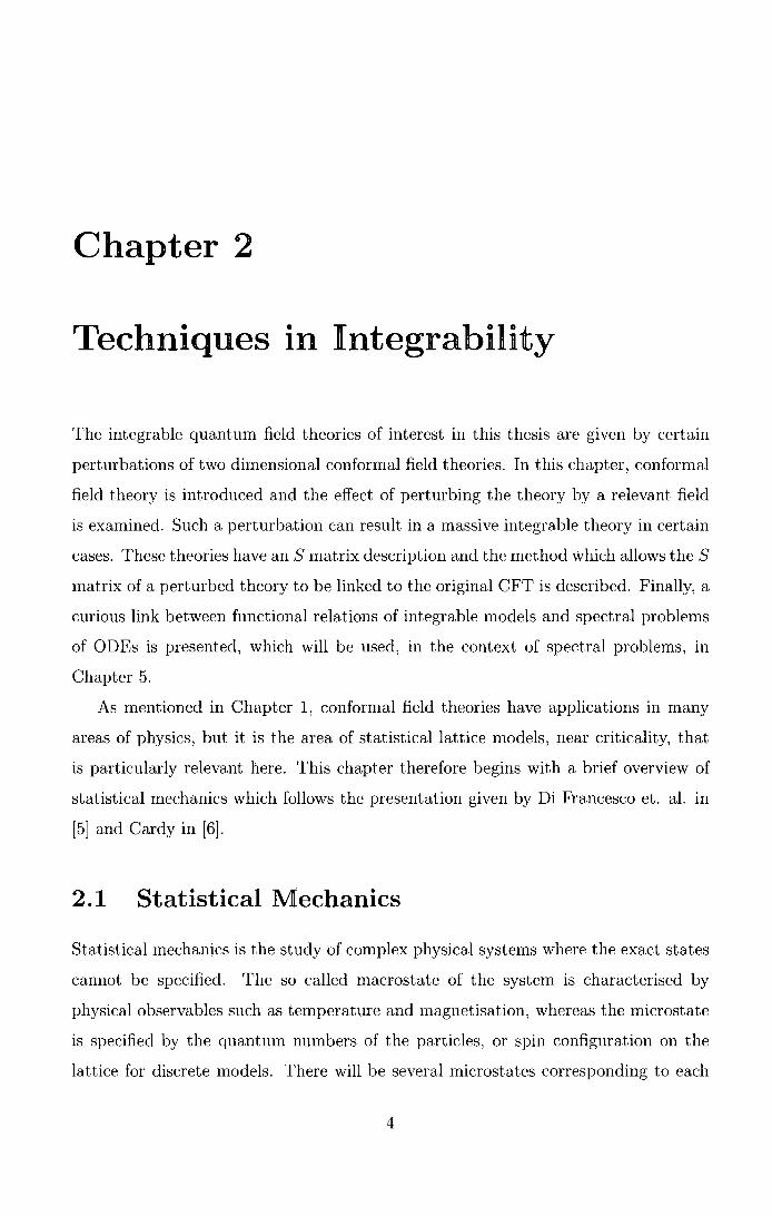
Let /-Li denote the configuration of spins on the ith row: /-Li = {ail, a-i2 , ... , a-in}. Each
row configuration has its own energy
n
E[!-Li] = -J L a-ikai,k+l, k=l
along with an interaction energy with neighbouring rows:
n
E[/-Li, /-Lj] = -J L a-ikajk. k=l
(2.1.19)
(2.1.20)
Now, by defining a formal vector space of row configurations spanned by the states
l!ti), the action of the transfer matrix T can be defined by its matrix elements
(2.1.21)
The partition function has a very simple form in terms of this operator T:
/11 , ... ,/lm (2.1.22)
In Euclidean quantum field theory, the analogue of the partition function 1s the
generating function
Z = J D¢e-S'[¢J, (2.1.23)
where Sis the action which depends on a set of local fields [¢]. To move from this
description to the operator formalism, constant time surfaces are specified and the
operator U(t) = exp( -iHt) evolves states from time t0 tot+ t 0 . The transfer matrix
plays the role of this operator, evolving states over a 'distance of time' equal to the
lattice spacing a, and so one can define a Hamiltonian operator H by
T -aH =e . (2.1.24)
There is also a relation between the correlation length and the mass of the corre
sponding lattice quantum field theory:
1 ~=-.
rna (2.1.25)
Close to a critical point the correlation functions are insensitive to the fine details
of the underlying theory, i.e. to whether it is a discrete statistical model or a lattice

2. 2. Conformal Field Theory 12
quantum field theory. They are also identical to the correlation functions of the
corresponding continuum quantum field theory, so one can describe statistical models,
near criticality, by quantum field theories. At the critical point, ~ -----> oo and the
corresponding quantum field theory is massless.
So far it is clear that a statistical model, at a critical point, is scale invariant.
However, for a system with only local interactions Polyakov showed [7] that it is also
invariant under the larger symmetry of conformal transformations, and so can be
described in terms of a conformal field theory, which will be discussed in the next
section. The idea is that information about all the possible universality classes can
be gained by studying all possible conformal field theories. There are two advan
tages of this description: firstly, conformal invariance in two dimensions puts heavy
constraints on the model, so it should be more tractable than the corresponding sta
tistical model, and secondly, by perturbing the conformal field theory it is possible
to study the statistical model away from criticality. This is of particular interest in
this thesis and will be discussed in more detail in section 2.3.
2.2 Conformal Field Theory
The connection between a statistical model at a critical point and a CFT was first
made by Polykov in [7], but it was some years before the detailed structure of CFT
was studied by Belavin, Polyakov and Zamolodchikov in [8], which paved the way for
the large volume of work which subsequently followed. A brief outline of some of the
main points is presented here, based on the reviews by Di Francesco et. al. [5] and
Ginsparg [9]. More detail can be found in these texts and, for example, in [10].
A theory has conformal symmetry if it is invariant under transformations which
leave the metric unchanged, up to a local scale factor
This means that the angle between vectors is preserved. Under an infinitesimal
coordinate transformation, x 11 -----> x'11 = x 11 + E11 , the metric transforms as
(2.2.2)
For this to be a conformal transformation
(2.2.3)

2.2. Conformal Field Theory 13
where 0 ( x) = 1 - f ( x). Acting with ry11v on both sides, assuming the theory is d
dimensional, f ( x) can be found to be
(2.2.4)
In d ~ 3 dimensions, the possible transformations are given by the Poincare group
x'll
the dilations
and the special conformal transformations
xll + bllx2 x'll == ------=--~ · 1 - 2b.x + b2x 2
(2.2.5)
(2.2.6)
(2.2.7)
(2.2.8)
The two-dimensional case is somewhat special, due to the fact that the global
transformations given here are supplemented by an infinite number of local trans
formations, which provide powerful constraints for the theory. Restricting to two
dimensional Euclidean space, the metric becomes ry11 ,_, = ~11 ,_,, and the constraint in
(2.2.3) reduces to the Cauchy-Riemann equations
(2.2.9)
This provides motivation to introduce the complex coordinates z and z with the
relations
z == x 1 + ix2
1 Oz = 2(81- io2)
(2.2.10)
(2.2.11)
With this change of coordinates the Cauchy-Riemann equations become o2E = 0,
oJ~ = 0, where E = E1 + iE 2 and E = E
1 - iE
2, so in two dimensions, the group of
conformal transformations is isomorphic to the infinite dimensional group of analytic
transformations
z ----t f(z), z ----t ](z). (2.2.12)
The infinitesimal mappings z ----t z + E and z ----t z + E admit the Laurent expansions
00 00
E(z) = L CnZn+l, E(z) = L c~:zn+l (2.2.13) n=-oo n=-oo
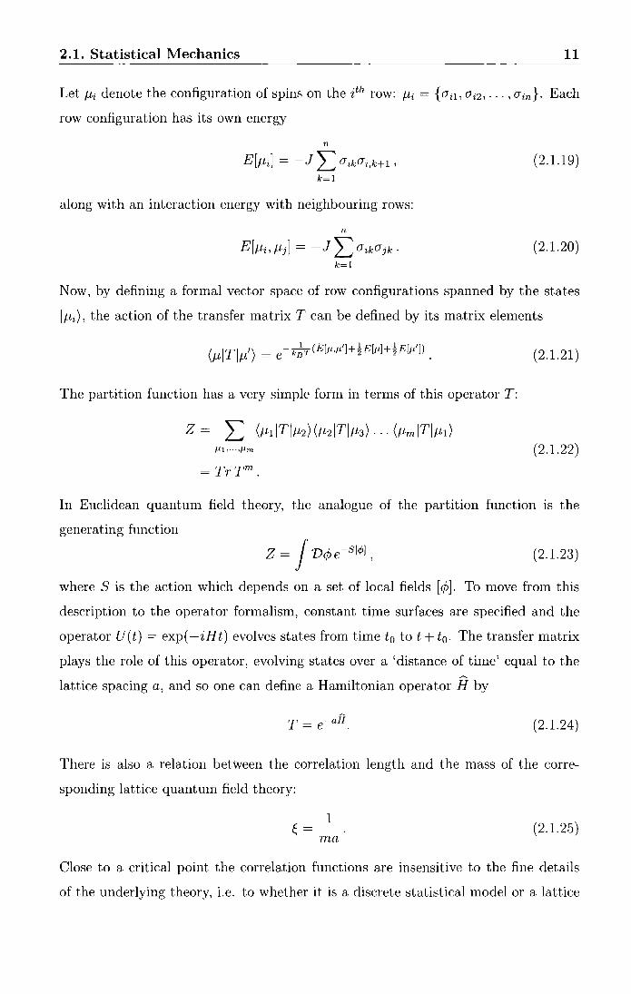
2.2. Conformal Field Theory 14
around z = 0, so the infinitesimal conformal transformations can be locally generated
by
l n+1~ ~- -n+1~ n = -z Uz' n = -z Uz'
which satisfy the commutation relations
[ln, lm]
[fnJm]
(n- m)ln+m
(n- m)ln+m
(2.2.14)
(2.2.15)
This algebra is generally known as the Witt algebra. Following the presentation of
[9], since ln and ~n commute, the algebra splits into a direct sum of two isomorphic
subalgebras, generated by the holomorphic (ln) and anti-holomorphic (ln) generators
respectively. Consequently, z and z can be thought of as independent coordinates,
each taking values over the whole complex plane. Of course, to return to the physical
case one must impose the condition z = z*. The physical theory is therefore invariant
under transformations generated by (ln + ln) and i(ln - ln).
The only infinitesimal generators to be globally well-defined on the Riemann
sphere S 2 = C U oo, are { L 1, l0 , l t} U { L 1 ,[0 ,l1}, and so the subalgebra they generate
is associated with the global conformal group. From the definition above one can see
that L 1 and L 1 generate translations, (l0 + l0 ) and i(l0 - l0 ) generate dilations and
rotations respectively, while h and l1 produce special conformal transformations. The
finite transformations corresponding to the generators { l_ 1 , l 0 , h} form the group of
projective conformal transformations S£(2, C)/'1!..2 , which can be written as
az + b z ----t ' (2.2.16)
cz +d
where a, b, c, d E C and ad - be = 1. The same holds for the anti-holomorphic
generators {f_1 , l0 , fi}. The global conformal algebra can be used to characterise the
physical states. In fact, it will be useful to work in the basis of the eigenstates l0 and
l0 , with the real eigenvalues h and h respectively. Since (l0 + l0 ) generates dilations
and i(l0 - l0 ) rotations, the scaling dimension y and the spin s of the state can be
defined as y = h + 11, and s = h - h,.
The classical action of a field theory, under an infinitesimal conformal transfor
mation xJ.L ----+ x!L + EJ.L ( x), will have variation
(2.2.17)

2.2. Conformal Field Theory 15
where T 1.w = Tv11 is the canonical energy-momentum tensor, which can always be
made symmetric (see [5]). The theory is scale invariant if this tensor is traceless, and
in turn this guarantees conformal invariance since bS = 0. In terms of the complex
coordinates z and z, T/: has the form
(2.2.18)
(2.2.19)
(2.2.20)
the final equality results from the fact that Tj; = 0. Translation and rotation invari
ance requires that 811T 11v = 0, which in terms of the complex coordinates is
(2.2.21)
Since 82Tzz = 0, Tzz is a function of z alone (similarly T22 is a function of z) and
so the energy-momentum tensor splits into an holomorphic and an anti-holomorphic
part, often denoted T(z) = -27rTzz and T(z) = -21rT22 respectively. This property
is assumed to hold when the theory is quantised.
This quantum theory is expected to contain fields known as primary fields, which
transform covariantly under any conformal transformation
(2.2.22)
The real exponents h and h are the conformal weights of the primary field </>j. Quasi
primary fields are those which transform as above for the global conformal trans
formations only. The energy momentum tensor is one example of a quasi-primary
field.
Under the local transformation z ----> z + t:( z), the holomorphic part of a primary
field transforms as
</>(z) ----> [8z(z + t:(z))]h</>(z + t:(z))
(1 + h8zt:(z) + t:(z)az + O(t:(z) 2))¢;(z), (2.2.23)
so the variation of ¢;(z) (ignoring the anti-holomorphic part, which is equivalent) is
b¢;(z) = h82 t:(z)¢;(z) + t:(z)8z</>(z). (2.2.24)

2.2. Conformal Field Theory 16
This transformation can be used to restrict the form taken by the correlation func
tions, as described in [9]. The two-point function G2(z1, Z1, Z2, z2) = (¢(z1, zl), ¢(z2, z2))
must be invariant under conformal transformations, so it must satisfy
0 (2.2.25)
This leads to
(h10z1 E(z!) + E(zi)Oz1 + h20z2 E(z2) + E(z2)0z2 )G2(z1, Z1, Z2, Z2)
+ (h10z1 £(z!) + £(z!)Oz1 + h20z2 E(z2) + £(z2)8zz)G2(z1, Z1, Z2, Z2) = 0. (2.2.26)
Taking the holomorphic part alone, the infinitesimal transformations generated by
L 1, l0 and l1 lead to the following constraints on G2(z1, z2):
=> G2 depends only on Z12 = z1 - z2
E - ?' - ~
The anti-holomorphic part can be examined in the same way. The two-point functions
of primary and quasi-primary fields must therefore have the form
- - 612 G2(z1,z1,z2,z2) = 2h-2h'
Z12 Z12 (2.2.27)
li2 = h, and the normalisation c12 has been set to 612·
The three-point correlation function G3 = (¢1(z1, zl), ¢2(z2, z2), ¢3(z3, z3)) will be
constrained in a similar way, and it can be shown that it must have the form
(2.2.28)
Higher correlation functions are not so simple to determine, and further conditions
must be imposed in order to fix their forms.
For a general field theory, the effect of an infinitesimal transformation on the
correlation functions is given by the Ward identity. In a conformal field theory,

2.2. Conformal Field Theory 17
the three Ward identities corresponding to the translation, rotation and dilation
transformations can be combined into one identity known as the conformal Ward
identity: for the transformation xv ---> xv + Ev ( x) acting on a string of primary fields
¢(xi) ... ¢( X 11 ), denoted here by X, this is given by
6E(X) = { d2x811 (T1-1v(x)Ev(x)X), JM (2.2.29)
where the domain M contains the positions of all the fields in the string X. This can
also be written in terms of the complex variables z, z and T, T as
1 i 1 i -6E,E'(X) = -. dz E(z)(T(z)X)- -. dz E(z)(T(z)X). 2nz c 2m c
(2.2.30)
The integration contour, C, must enclose the positions of all the fields in X.
In order to introduce an operator formalism, following [5], it is necessary to dis
tinguish between the time and space directions. In the statistical mechanics lattice
models described earlier, one direction of the lattice was chosen to be 'space' and
the orthogonal direction was taken as 'time'. In the continuum limit, there is more
freedom in the choice of space and time directions. The usual choice, known as 'ra
dial quantisation' is described here: first, define the theory on an infinite cylinder
of radius L, with the time coordinate x 1 running along the length of the cylinder
and the space coordinate x2 compactified. In Euclidean space this cylinder is de
scribed by a single complex coordinate ~ = x 1 + ix2. Now consider the conformal
map~---> z = exp(2n~/ L). This maps the cylinder to the complex plane, as shown
in figure 2.2. The infinite past and future on the cylinder, x 1 = =foo, are mapped to
Figure 2.2: Radial quantisation. The concentric circles are surfaces of equal time.
the points z = 0, oo on the plane respectively and equal time surfaces, x 1 = const,
become circles of constant radius on the z-plane.
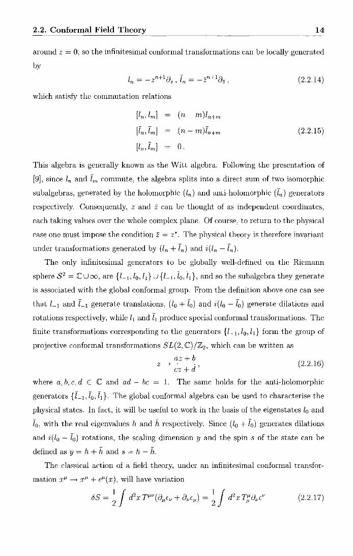
2.2. Conformal Field Theory 18
Concentrating on the holomorphic part of the primary field ¢( w), the conformal
Ward identity for this field, within the radial quantisation scheme is
(5¢(w)) = -.E(z)(T(z)¢(w)). i dz
[z[>[w[ 2m, (2.2.31)
The variation of ¢(w) was found in (2.2.24), and using this in the Ward identity, the
short distance operator product expansion (OPE) of the T(z) with ¢(w) is found to
be h¢(w) az¢(w)
T(z)<P(w) = ( )2 + ( ) + ... z-w z-w (2.2.32)
with the dots representing regular terms. The energy momentum tensor represents an
energy density, so it should have scaling dimension 2 and spin 2. One would therefore
expect T(z) to have conformal weights h = 2, h = 0, and T(z) to have h = 0, h = 2
[5]. The OPE of T(z) with itself will have a similar form to (2.2.32), with h = 2,
but since T(z) is a quasi-primary field, not a primary field, an extra term should be
added: 2T(w) azT(w)
T(z)T(w) = (z _ w) 2 + (z _ w) + f(z, w) + ... (2.2.33)
Now Tis expected to transform as T' = (8zg)- 2T(z) under the global transformation
z-------+ g(z), so the transformation z-------+ w = 1/ z will produce
(2.2.34)
T(O) should always be finite and since T'(1/z) must be just as regular as T(z) this
implies that T(z) must decay as z-4 as z-------+ oo [5]. The extra term in the OPE must
therefore have the form c/2
f(z, w) = (z- w)4'
where c is a constant and the factor 1/2 is just convention.
(2.2.35)
Using the OPE of T(z)T(w) in the conformal Ward identity, the variation ofT
under a local conformal transformation is given by
-~ i dzt(z)T(z)T(w) 27rz c
1 i d ( ) ( 2 T(w) azT(w) c/2 ) -- 7 E Z + +---
2Jri c ~ (z-w)2 (z-w) (z-w)4 c
-2T(w)8wE(w)- E(w)8wT(w)- -8!E(w). 12
(2.2.36)
2.2. Conformal Field Theory 19
As shown in [5], this corresponds to sending T(z)----+ T'(w) under the finite transfor
mation z----+ w(z) where
T'(w) = ( ~: r (T(z)- ;2
{w; z)}, (2.2.37)
and { w; z} is the Schwarzian derivative given by
(2.2.38)
T(z) (equivalently T(z)) admits the mode expansion
T(z) == L z-n-2 Ln, Ln = 2~i f dzzn+lT(z). nEZ
(2.2.39)
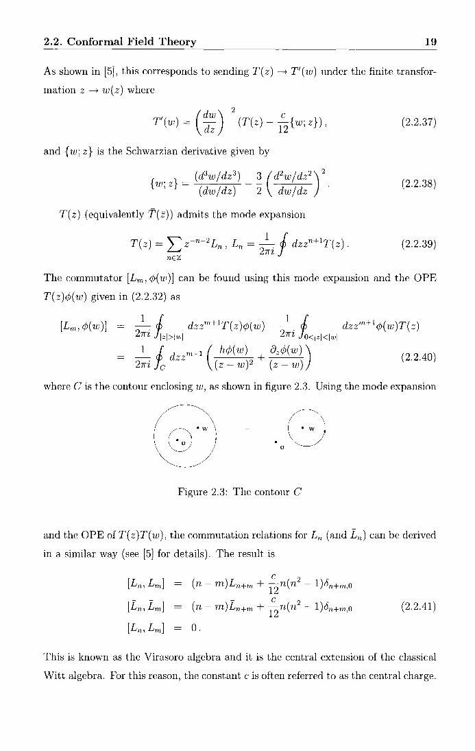
The commutator [Lm, ¢(w)] can be found using this mode expansion and the OPE
T( z )¢( w) given in (2.2.32) as
~ 1 dzzm+ 1T(z)¢(w)- ~ 1 dzzm+ 1¢(w)T(z) 27f'l Jlzl>lwl 2m .fo<lzl<lwl
_1 i dzzm+l ( h<;D(w) + az¢(w)) ( ) ( )
2 ( ) 2.2.40 27fi c z - w z - w
where Cis the contour enclosing w, as shown in figure 2.3. Using the mode expansion
Figure 2.3: The contour C
and the OPE of T(z)T(w), the commutation relations for Ln (and Ln) can be derived
in a similar way (see [5] for details). The result is
[Ln,Lm]
[Ln,Lm]
[Ln,Lm]
c 2 (n- m)Ln+m +
12n(n - 1)5n+m,O
- c 2 -(n- m)Ln+m +
12n(n - 1)6n+m,o
0.
(2.2.41)
This is known as the Virasoro algebra and it is the central extension of the classical
Witt algebra. For this reason, the constant c is often referred to as the central charge.

2.2. Conformal Field Theory 20
Notice that for the global symmetry generators L_ 1 , L0 and £ 1, this central extension
disappears and the algebra reverts to the classical one.
The theory is assumed to have a unique vacuum state, IO), which is invariant
under global symmetries, so
LniO) = 0, n ~ -1. (2.2.42)
A state, I¢), can then be associated to each primary field ¢( z) with the definition
1¢) = limz-.o ¢(z)IO). Using the commutator [L11 , ¢(z)] from (2.2.40) and the relation
(2.2.42) it is easy to show (see [5]) that
Lol¢)
Lnl¢)
limLo¢(z)IO) =hi¢) z--.0
0, n > 0,
(2.2.43)
with equivalent relations holding for L0 I¢) and Ln I¢). This is a highest weight state of
the Virasoro algebra and representations of this algebra can be built from these states
in the following way: acting on 1¢) with the generators L 11 , n < 0, produces an infinite
tower of states L_n1
••• L_nm 1¢), 1 ::; n 1 ::; ... ::; nm, known as left descendants. They
are eigenstates of L0 with eigenvalues h' = h + n 1 + ... + nm = h + l, where l is known
as the level of the descendant. An equivalent tower of right descendants is generated
from 1¢) with the application of L11 , n < 0. The subset of the Hilbert space, spanned
by the primary state 1¢) and its descendants, is closed under the action ofthe Virasoro
generators and so it forms a representation of the Virasoro algebra known as a Verma
module.
The set of fields containing the primary field ¢ and its descendants is called a
conformal family, denoted by [¢]. Since the generators Ln and Ln commute, each
conformal family can be considered as a direct product of the space of left descen
dants, <I>, and right descendants, <I>, so any discussions can be restricted to the 'left'
(holomorphic) sector with the understanding that equivalent statements will hold for
the 'right' (anti-holomorphic) sector.
The objects of interest in these theories are the correlation functions as these are
the physically measurable quantities. Correlation functions between descendant fields
can be expressed in terms of those between the primary fields only, so in order to solve
the theory one needs to know all the correlation functions between the primary fields.
For this it is necessary to know the operator algebra: the complete OPE (including
2.2. Conformal Field Theory 21
all regular terms) of all primary fields with each other. Applying this OPE within a
correlation function reduces it to two-point functions which are known.
By taking the limit as any two fields approach one another in the three-point
correlation function (2.2.28), the OPE for primary fields can be expressed as
The complete operator algebra of primary fields can be obtained from conformal
symmetry once the central charge, c, the conformal dimensions of the primary fields,
and the 3-point function coefficients Cijk are known. Out of these quantities, only
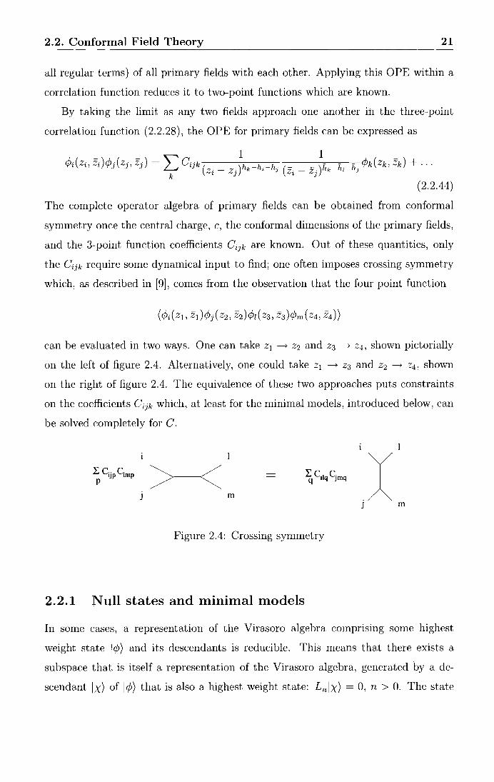
the Cijk require some dynamical input to find; one often imposes crossing symmetry
which, as described in [9], comes from the observation that the four point function
can be evaluated in two ways. One can take z1 -----t z2 and z3 -----t Z4, shown pictorially
on the left of figure 2.4. Alternatively, one could take z1 -----t z3 and z2 -----t Z4, shown
on the right of figure 2.4. The equivalence of these two approaches puts constraints
on the coefficients Cijk which, at least for the minimal models, introduced below, can
be solved completely for C.
LCilqcjmq X q .
J m
Figure 2.4: Crossing symmetry
2.2.1 Null states and minimal models
In some cases, a representation of the Virasoro algebra comprising some highest
weight state 1¢) and its descendants is reducible. This means that there exists a
subspace that is itself a representation of the Virasoro algebra, generated by a de
scendant lx) of 1¢) that is also a highest weight state: Lnlx) = 0, n > 0. The state

2.2. Conformal Field Theory 22
lx) is known as a singular or null vector. It is orthogonal to the whole Verma module
as
(2.2.45)
using Hermitian conjugation, and its norm (xlx) = 0. In fact, all descendants of
lx) also have zero norm and are orthogonal to all states in the Verma module of the
same level. An irreducible representation may be constructed by quotienting out of
the Verma module the null submodule, i.e. by identifying states that differ only by
a state of zero norm.
To each Verma module, one can associate a function X(c,h) ( T) called the character
of the module: ()()
X(c,h) ( T) = Tr qLo-c/24 = L dim( l)ql+h-c/24
1=0
(2.2.46)
where dim(l) is the number of linearly independent states at level l, T is a complex
variable such that (_}m T > 0 and q = e21rir. These characters are generating functions
for the level degeneracy dim(l), so knowing the character amounts to knowing how
many states there are at each level.
Another quantity to determine the number of linearly independent vectors in
the Verma module at level! is the Gram matrix, fi{Ul(c, h), built of inner products
between all basis states:
(2.2.47)
with ni, mi 2: 0 and 2::7= 1 ni = L~=l mi = l. If det fi{Ul(c, h) vanishes then one can
conclude that there are null vectors at level l. If the determinant is negative there
must be states with a negative norm present so the representation is not unitary. A
general formula for this determinant was found by Kac [11] (and proven by Feigin
and Fuchs in [12]):
det M(l) = 0:[ II [h - hr,s]P(l-rs) .
r,s>l rs~l
(2.2.48)
P(l- rs) is the number of partitions of the integer l- rs and o:1 is a positive constant
independent of h and c
O:t = IT [ (2r )s s!]m(r,s)
r,s?.l rs-::;1
(2.2.49)

2.2. Conformal Field Theory 23
with m(r, s) = P(l- rs)- P(l- r(s + 1)). The roots of this determinant can be
expressed by first reparametrising c in terms of the (possibly complex) quantity
(2.2.50)
The hr,s ( m) are then given by
h (m) _ .:_:[(_m_+_1)--,-r_-_m------,--s]_2 _-_1 r,s - 4m(m + 1) ' (2.2.51)
and, in this notation, the central charge becomes
6 c=1-----
m(m + 1) · (2.2.52)
The existence of null states also puts a constraint on the operator algebra which
becomes k=r1 +r2-l
¢(q,si) X ¢(r2,s2) = L l=s1 +s2-l
:I: ¢(k,l)·
k=l+lr1-r2l l=l+ls1-s2l k+r1 +r2=l mod2l+s1 +s2=l mod2
step 2 step 2
(2.2.53)
These are known as fusion rules. This notation means that the OPE of ¢(ri,si) with
¢(r2 ,s2 ) (or their descendant fields) may contain terms belonging to the conformal
families of ¢(k,l) on the RHS. In general, a conformal family [¢(r,s)], with r, s arbitrarily
large, can be generated by repeatedly applying (2.2.53) which implies that there are
an infinite number of conformal families in the theory. However, if the central charge
can be expressed in terms of two coprime integers p, p' as
(p- p')2 c = 1 - 6 ...:..:._______::_---'---
pp'
then the conformal weights become
(pr - p' s) 2 - (p - p') 2 h = ~--~-...:..:.____-~
r,s 4 pp' ,
which has the periodicity properties
hr+p',s+p = hr,s, hr,s = hp'-r,p-s·
(2.2.54)
(2.2.55)
(2.2.56)
The integers p and p' can be taken to be positive and without a loss of generality it
can be assumed that p > p'. They are related to the parameter m by
p' 7n=-
p- p' (2.2.57)
2.2. Conformal Field Theory 24
where the positive branch of m in (2.2.50) has been chosen. It can easily be shown
that hr,s also satisfies the identities:
hr,s + TS hp'+r,p-s = hp'-r,p+s (2.2.58)
hr,s + (p'- T)(p- s) hr,2p-s = h2p'-r,s·
From (2.2.58) it is clear that the null vectors at levels TS and (p' - T) (p - s) are
themselves highest weights of degenerate Verma modules. These two null vectors
will give rise to submodules that also contain null vectors of the same form, and
so on. There will therefore be an infinite number of null vectors within the Verma
module. The existence of each of these null vectors imposes a constraint on the
operator algebra and the result is a Verma module consisting of a finite number of
conformal families. The corresponding conformal weights are hr,s with 1 :S: T :S: p' - 1
and 1 :S: s :S: p - 1, but because of the symmetry hr,s = hp'-r,p-s, there are only
(p-1)(p'-1)/2 fields in the theory with cP(r,s) = cP(p'-r,p-s)· To avoid double counting
one often takes p' s < pT. The pairs ( T, s) are known as Kac labels and Ep,p' denotes
the set of such pairs in the range described here. These theories are the minimal
models, usually denoted by M(p,p')·
The fusion rules given in (2.2.53) can be expressed in the form of the fusion algebm
cPi X cPJ = l::Ni~cPk (2.2.59) k
where the Ni~ are integers. Here the indices i, j, k label the primary fields. For the
minimal models, they can be replaced by the Kac labels ( T, s) but the concept of the
fusion algebra can be applied to more general models which will be discussed later.
This algebra is commutative and associative, with the identity element ¢1 = I the
identity field, so NA = bik· Commutativity implies that Ni~ is symmetric in i and j.
Using this, along with the associativity cPi x ( cP] x cPk) = ( cPi x cPj) x cPk leads to the
expression
L NLj NiT = L Njj N{f: . (2.2.60) I l
By defining a matrix with the entries (Ni)j = Ni~' this condition can be rephrased as
NiNk = L NfkNl l
(2.2.61)

2.2. Conformal Field Theory 25
so the Ni form a matrix representation of the fusion rules. They can be simultaneously
diagonalised and their eigenvalues then form one dimensional representations of the
fusion rules.
The full Hilbert space of the CFT is given by
1t = E9nh,hvh ® vh
h,h
(2.2.62)
where the non-negative integers nh,h specify how many distinct primary fields of
weight (h, h) there are in the CFT. The fusion algebra, shown above, indicates which
values of (h, h) are consistent with the CFT, but not which ones actually occur.
For this one needs the extra constraints imposed when the theory is required to be
modular invariant on the torus. This was first suggested by Cardy in [13].
2.2.2 Finite size effects
Now, consider a CFT on a complex plane and map this to a cylinder of circumference
L with the transformation z ---> w = 2~ ln z. The Schwarzian derivative is { w; z} =
1/2z2 and using (2.2.37), the energy-momentum tensor on the cylinder Tcy1(w) can
be related to that on the plane, Tplane by
T,~1 (w) = c; )' ( Tplane(z)z'- ;4
) (2.2.63)
Assuming that the vacuum energy density (Tplane) vanishes on the plane, taking the
expectation value of the above gives a nonzero vacuum energy density on the cylinder
C7r2
(Tcyl(w)) = -6
L2 . (2.2.64)
The change in energy brought about by imposing these boundary conditions is known
as the Casimir energy. The relation between this and the central charge can now be
used to show that c is also related to the free energy. When the metric tensor is
changed the free energy F varies as
(2.2.65)
In this cylindrical geometry, an infinitesimal scaling of the circumference bL = EL
corresponds to the coordinate variation bz0 = Ez0 and bz1 = 0, where z0 runs around
the cylinder and z1 along it. The metric tensor then varies as bg1w = -2Eb110bvo· Now
00 ) 1 ) 7rC (T ) = (Tzz) + (Tzz = -;(T(z) = 6
£ 2 (2.2.66)

2.2. Conformal Field Theory
so the variation of the free energy is
6F = J d od 1 nc 6L z z 6£2 L .
26
(2.2.67)
The integration over z0 introduces a factor of L, whereas the integration over z1 can
be avoided by considering the free energy per unit length, FL, which varies as
Integrating this then leads to 7fC
FL = --. 6L
(2.2.68)
(2.2.69)
The central charge also appears in the Hamiltonian for the CFT on the cylinder,
where z = exp(x1 + ix2). Here dilations z - eaz become time translations x 1
-----+
x 1 +a therefore the dilation generator on the conformal plane can be regarded as the
Hamiltonian for the system:
27f ( - ) H = L (Lo)cyl + (Lo)cyl (2.2.70)
Substituting the mode expansion Tptane( z) = L z-n-2 Ln into the relation (2.2.63)
gives
where w = 2: lnz. Therefore the translation generator (Lo)cyt on the cylinder, in
terms of the dilation generator L 0 on the plane is
so the Hamiltonian is
c (Lo)cyl = Lo-
24,
27f ( - c ) H = L Lo + Lo -12
,
(2.2. 72)
(2.2. 73)
where the constant term c/12 ensures that the vacuum energy vanishes in the L -----+ oo
limit. The momentum generates translations along the circumference of the cylinder
so this can be written as
2ni ( - ) 2ni ( - ) P = L (Lo)cyl- (Lo)cyl = L Lo- Lo . (2.2.74)
For a CFT on the entire complex plane the holomorphic and anti-holomorphic
sectors completely decouple and can be studied separately. However requiring the
2.2. Conformal Field Theory 27
theory to be consistent on a torus puts useful constraints theory which will now be
discussed. This follows closely the presentation given in [5].
Define a torus by specifying two linearly independent vectors on the complex
plane, and identify points which differ by an integer combination of these vectors.
These vectors can be represented by two complex numbers w1 and w2 , which are the
periods of the torus. Next the space and time directions must be defined. Here space
is taken along the real axis, and time along the imaginary axis. The Hamiltonian,
H, and total momentum, P, of the theory generate translations along the time and
space directions respectively so the operator which translates the system parallel to
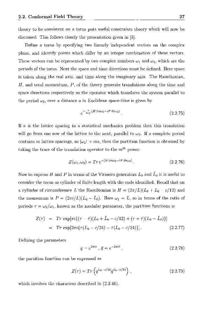
the period w2 , over a distance a in Euclidean space-time is given by
(2.2.75)
If a is the lattice spacing in a statistical mechanics problem then this translation
will go from one row of the lattice to the next, parallel to w2 . If a complete period
contains m lattice spacings, so lw21 = ma, then the partition function is obtained by
taking the trace of the translation operator to the mth power:
(2.2. 76)
Now to express Hand Pin terms of the Virasoro generators £ 0 and L0 it is useful to
consider the torus as cylinder of finite length with the ends identified. Recall that on
a cylinder of circumference L the Hamiltonian isH= (27r/L)(£0 + L0 - c/12) and
the momentum is P = (27ri/ L)(L0 - L0 ). Here w1 = L, so in terms of the ratio of
periods T = w2/w1 , known as the modular parameter, the partition functions is
Z(T) Tr exp[1ri{(T- f)(£0 + L0 - c/12) + (T + f)(£0 - L0 )}]
Tr exp[27ri{ T(L0 - c/24) - f(Lo- c/24)} ].
Defining the parameters
the partition function can be expressed as
which involves the characters described in (2.2.46).
(2.2.77)
(2.2. 78)
(2.2. 79)
2.2. Conformal Field Theory 28
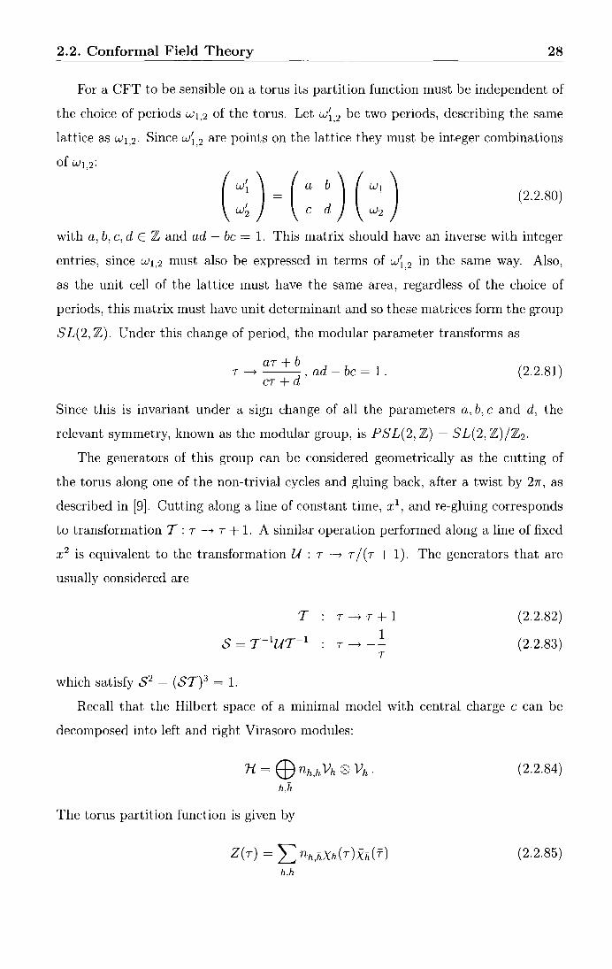
For a CFT to be sensible on a torus its partition function must be independent of
the choice of periods w1,2 of the torus. Let w~.2 be two periods, describing the same
lattice as w1,2 . Since w~.2 are points on the lattice they must be integer combinations
of w1,2 :
( ::) ( : : ) ( :: ) (2.2.80)
with a, b, e, d E Z and ad - be = 1. This matrix should have an inverse with integer
entries, since w1,2 must also be expressed in terms of w~. 2 in the same way. Also,
as the unit cell of the lattice must have the same area, regardless of the choice of
periods, this matrix must have unit determinant and so these matrices form the group
SL(2, Z). Under this change of period, the modular parameter transforms as
aT+b T ----+ , ad - be = 1 .
eT+d (2.2.81)
Since this is invariant under a sign change of all the parameters a, b, e and d, the
relevant symmetry, known as the modular group, is PSL(2, Z) = SL(2, Z)/Z2 .
The generators of this group can be considered geometrically as the cutting of
the torus along one of the non-trivial cycles and gluing back, after a twist by 21r, as
described in [9]. Cutting along a line of constant time, x 1, and re-gluing corresponds
to transformation T : T ----+ T + 1. A similar operation performed along a line of fixed
x 2 is equivalent to the transformation U : T ----+ T / ( T + 1). The generators that are
usually considered are
T
which satisfy 5 2 = (ST) 3 = 1.
T---+T+1 1
T----+ -T
(2.2.82)
(2.2.83)
Recall that the Hilbert space of a minimal model with central charge e can be
decomposed into left and right Virasoro modules:
1{ = E9 nh,h vh ® vii . h,h.
The torus partition function is given by
Z(T) = L nh,JiXh(T)XJi(f) h,h
(2.2.84)
(2.2.85)
2.2. Conformal Field Theory
in terms of the Virasoro characters
Xh(T) = Trvh(qLo-c/24) = qh-c/24 Ld(n)qn. n2':0
The action of T on the minimal characters is
Xr,s(T + 1) = L Trs,paXp,a(T)
(p,a)EEp,p'
where
T. = b b e2in(hr,s -c/24) rs,pa r,p s,a
29
(2.2.86)
(2.2.87)
(2.2.88)
with the conformal dimensions given by the Kac formula (2.2.55). The modular
transformation S acts on the characters as
where
Xr,s( -1/T) = L Srs,paXp,a
(p,a)EEp,p'
Srs,pa = 2 {2 ( -1) l+sp+ra sin (7f P r p) sin (7fp' sa) v Pi' p' p
is known as the modular S matrix [13][14].
(2.2.89)
(2.2.90)
The requirement that the partition function be invariant under the transforma-
tions generated by T and S puts constraints on the multiplicities nh,r, which are
described below following [5]. There is also an additional requirement (at least for a
unitary theory) that the nh,h be non-negative integers, and that the identity operator
appear just once, so n0 ,o = 1.
The T invariance is the weakest condition. This restricts the left-right association
of modules by
h - h = 0 , mod 1 . (2.2.91)
An obvious solution to this is h = h which leads to a 'diagonal' partition function
Z = L 1Xr,sl2
· (2.2.92)
(r,s)EEp,p'
Since S is unitary this is modular invariant. The operator content of this theory can
be read off from the partition function: each field in the Kac table E(p, p') appears
exactly once in the combination <I>(r,s) = c/.>(r,s) ® ~(r,s)· This is known as the minimal
model M(p,p'). The simplest such unitary minimal model is M(4,3), with central

2.2. Conformal Field Theory 30
charge c = 1/2 and this can be shown to correspond to the critical Ising model.
The continuum version of the critical Ising model has three operators: the identity
n with conformal dimension (0, 0), the spin O" (the continuum version of the lattice
spin O"i) and the energy density, or thermal operator, E (the continuum version of the
interaction energy O"iO"i+ I). The exponents rJ and v can be defined in terms of the
critical correlators
(2.2.93)
In table 2.1, these exponents are given as rJ = 1/4 and v = 1 and with the form of
the two point function for primary fields (2.2.27), assuming that the fields O" and E
have no spin ( h = h), their conformal dimensions must be
- ( 1 1) - (1 1) (h,h)a = 16' 16 '(h,h)E: = 2' 2 (2.2.94)
The operator-field correspondence is given in table 2.2 restricting to the holomorphic
part for simplicity.
Kac labels ( 1·, s) Conformal Dimension h Operator
(1,1) or (2,3) 0 n Identity
(2, 2) or (1, 2) 1 O" Spin 16
(2, 1) or (1, 3) 1 E Thermal operator 2
Table 2.2: Operator-field correspondence for the critical Ising model
Minimal models also exist where not all of the possible fields from the Kac table
are present. One example of this is the three-state Potts model. This is related to
the M(6, 5) model, but only the fields ¢cr,s) with s = 1, 3, 5 are present in the theory.
In order to find modular invariants one can group the fields into blocks which have
the required transformation properties. It can be shown that the characters for the
relevant blocks are
Xr,1(T) + Xr,5(T)
Xr,3(T)
(2.2.95)

2.3. Perturbed CFT 31
and the modular invariant partition function [14] is
(2.2.96) r=1,2
L {lxr,l + Xr,51 2 + 2lxr,31 2} .
r=1,2
This shows that only the operators ¢(r,s) with s = 1, 5 and r = 1, 2 are present in the
theory along with two copies of ¢(r,3) with r = 1, 2. This multiplicity 2 indicates that
the three-state Potts model is not a subtheory of the M(6, 5) model but actually has
a larger symmetry algebra, known as the W3 algebra, of which the Virasoro algebra
is a subalgebra. The block-characters given above are the characters with respect
to this extended algebra and the partition function is 'diagonal' when written in
terms of these. Theories of this form are therefore known as block-diagonal. Further
discussion of extended algebras will be given in Section 4.2. The search for these
modular invariant partition functions began in [14]. A full 'ADE' classification for
the minimal models was conjectured by Cappelli, Itzykson and Zuber in [15] , which
was later proved in [16] [17].
There is an important relation between the modular S matrices and the fusion
algebra which was first proposed by Verlinde in [18], and later proven in [19],[20].
This states that S diagonalises the fusion rules, i.e. Ni~ = l:n SjnA;n) Snk. where >..;n)
are the eigenvalues of the matrix Ni· This relation can be used to solve for the Ni~'
in terms of the matrix S: first label the identity by i = 0 so Nij = bj, then the
eigenvalues )..~n) must satisfy )..~n) = Sin/ Son- The Verlinde formula then follows:
This will be of use later on.
Nk. = ""'SinSjnSnk t) L S .
n On
2.3 Perturbed CFT
(2.2.97)
As mentioned earlier, conformal field theories can be used to describe statistical
models at their critical points. One advantage to this description is that it is possible
to perturb a CFT in such a way that it remains integrable, which allows the statistical
model to be studied away from criticality. Such integrable perturbations were first
shown to exist by Zamolodchikov in [21]. This section contains a brief review of this
work.

2.3. Perturbed CFT 32
Integrability of conformal field theory is guaranteed by the existence of an infi
nite number of conserved charges provided by the holomorphic and anti-holomorphic
components of the stress energy tensor and other descendants of the identity. The
identity operator I is the unique primary field with weights (0, 0). Its conformal fam
ily can be split into holomorphic and antiholomorphic sectors and the space of left
descendants of I will be denoted by A. The operator L0 can be used to decompose
this into subspaces As, labelled by spin s
0
(2.3.1)
(2.3.2)
(2.3.3)
Each field Ts E As has conformal weight ( s, 0) and so spin s. Since it is holomorphic
it follows that
(2.3.4)
so an infinite number of conserved charges can be defined:
f Ts(c;)(c;- z)n+s- 1dc;, n = 0, ±1, ±2, ... (2.3.5)
Not all of these conserved charges will be linearly independent as some of the fields
Ts may be total derivatives, but these fields can be avoided by considering the factor
space
which can be decomposed as before
0.
(2.3.6)
(2.3.7)
(2.3.8)
(2.3.9)
Once conformal symmetry is broken one would expect these conserved charges
to no longer exist and integrability to be lost. However, Zamolodchikov [21] has
argued that for certain perturbations of conformal field theory, a sufficient number
of conserved charges remain to allow all the states in the theory to be identified and

2.3. Perturbed CFT 33
hence the theory to still be considered integrable. An outline of his argument is
provided here. Consider a perturbation of a conformal field theory with an action
related to that of the CFT by
(2.3.10)
where¢ is a field in the CFT with conformal weight (h, h), and so scaling dimension
2h. The coupling constant, A, has conformal dimension (1- h, 1- h) (scaling dimen
sion y = 2(1- h)). For a relevant perturbation, y > 0 so¢ is a relevant operator if
h < 1. When A -/:- 0, Ts will no longer satisfy (2.3.4). Instead OzTs can be expanded
in a Taylor series
(2.3.11)
where the R~r:}1 are assumed to be fields belonging to the CFT. The dimensions of
OzTs and A are (s, 1) and (1- h, 1- h) respectively, so by comparing dimensions it
is clear that the fields R~rt]1 must have dimension
[R~r:}1 ] = (s- n(1- h), 1- n(1- h)). (2.3.12)
For n large enough, 1 - n(1 ~ h) < 0. However, all fields in unitary theories have
positive conformal dimensions, so this series must terminate. This argument can
clearly be extended to any non-unitary theories where the conformal dimensions of
the fields are bounded from below. The only possible terms in the series are those
fields in the CFT with conformal dimension
1- n(1- h)=~ (2.3.13)
which are easily identified as the dimensions of all the fields are known. In many
cases, only the first term, with n = 1, is possible in which case
(2.3.14)
where R~~~ has dimension (h + s- 1, h) and so is a left descendant of the perturbing
field ¢. The space, <P, of all left descendants of ¢ can be decomposed in the same
way as A: 00
(2.3.15)

2.3. Perturbed CFT
where
so f}2 can be considered as the linear map
~
For Ts to be non-trivial, it must be non-zero in A
34
(2.3.16)
(2.3.17)
(2.3.18)
A/ L_ 1A and for it to be a
conserved charge, R~~1 must be a. total z-derivative, i.e. it must lie in L_1 <I>. Its
projection onto ii> = <I>/ L_1 <I> must then be zero, so it must therefore lie in the kernel
of the map
(2.3.19)
Conversely, if the kernel of this mapping is nonzero then a conserved charge must
exist. This problem then boils down to checking the dimensions of the spaces As and
<I>s_ 1: the kernel will be nonzero, and so a. conserved charge will exist, provided
~
dim As > dim <I>s-1· (2.3.20)
Using this method, Zamolodchikov demonstrated the existence of a whole series of
conserved charges for the minimal models perturbed by the operators ¢13 , ¢12 and
¢21 and so conjectured that these perturbations are integrable.
The continuity equation 8/LTJ.Lv = 0 for the stress energy tensor, written in coor
dinates z, z is
(2.3.21)
where 8 = -Tzz· This ensures the conservation of momentum of the theory, with IM
(2.3.22)
Following this notation, the higher spin integrals of motion of the perturbed theory
are
Ps = f[Ts+1dz + 8s-1dz]
where the local fields Ts+ 1 and 8s_ 1 satisfy the relation
(2.3.23)
(2.3.24)
A priori there is no reason why one cannot perturb a CFT by two or more relevant
operators simultaneously. However, for the models of interest in this thesis, such a
perturbation will not result in an integrable theory.

2.4. S matrices 35
2.4 S matrices
For many cases, perturbing a CFT will result in a massive theory which, in the in
frared region, can be described in terms of an S-matrix. In this section the constraints
on this S-matrix, due to integrability, will be described and the method of building an
S-matrix using the knowledge of the conserved charges of the theory will be discussed.
Note that this S-matrix approach is naturally described in ( 1 + 1) Minkowski space,
while the CFT description above was given in 2 dimensional Euclidean space. This
discussion is based on the original paper by Zamolodchikov and Zamolodchikov [22],
but mainly follows the review by Dorey [23].
Consider a theory with n particles, each with a different mass ma, a = 1, ... , n.
These particles are on-shell when their light-cone momenta Pa, f5a satisfy the condition
PaPa = m;. It will be convenient to parametrise these momenta in terms of the
rapidity Ba
(2.4.1)
Denoting a particle of type ai, moving with rapidity ei, by AaJei), an n-particle
asymptotic state can be written as
(2.4.2)
An in state, is a state where there are no further interactions as t ---+ -oo so the
particles must be ordered by rapidity, with the fastest on the left and the slowest
on the right. Similarly, if there are no more interactions as t ---+ oo, then the state
is known as an out state, with the order of rapidities reversed. By considering the
Aa;(ei) as non-commuting symbols, the notation can be simplified and the in and out
states can be written as
(2.4.3)
with e1 > e2 > ... en and e1 < e2 < ... en respectively.
The S-matrix is a mapping between the in-state basis and the out-state basis.
Given a 2-particle in state this is
00
Aal (OI)Aaz(e2) = L L s~~~~bn(e1, e2; e~, ... 'en)Abl (e~) ... AbJe~) (2.4.4) n=2 e; < .. <0;,
where a sum on b1 ... bn is implied and the sum on the e~ will, in general, involve a
number of integrals. The rapidities are also constrained by momentum conservation.
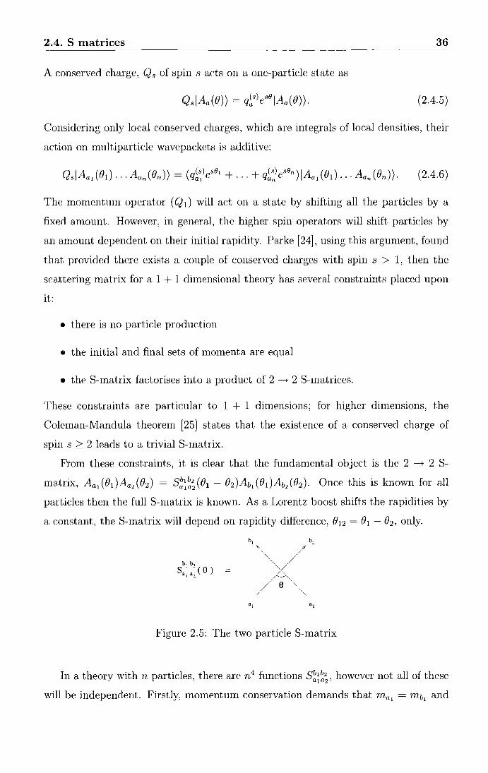
2.4. S matrices 36
A conserved charge, Qs of spin s acts on a one-particle state as
(2.4.5)
Considering only local conserved charges, which are integrals of local densities, their
action on multiparticle wavepackets is additive:
(2.4.6)
The momentum operator ( QI) will act on a state by shifting all the particles by a
fixed amount. However, in general, the higher spin operators will shift particles by
an amount dependent on their initial rapidity. Parke [24], using this argument, found
that provided there exists a couple of conserved charges with spin s > 1, then the
scattering matrix for a 1 + 1 dimensional theory has several constraints placed upon
it:
• there is no particle production
• the initial and final sets of momenta are equal
• the S-matrix factorises into a product of 2 -----+ 2 S-matrices.
These constraints are particular to 1 + 1 dimensions; for higher dimensions, the
Coleman-Mandula theorem [25] states that the existence of a conserved charge of
spin s 2: 2 leads to a trivial S-matrix.
From these constraints, it is clear that the fundamental object is the 2 -----+ 2 S
matrix, Aa1 (8I)Aa2 (82 ) = 5~~~;(81 - 82)Ab1 (8I)Ab2 (82). Once this is known for all
particles then the full S-matrix is known. As a Lorentz boost shifts the rapidities by
a constant, the S-matrix will depend on rapidity difference, 812 = 81 - 82 , only.
Figure 2.5: The two particle S-matrix
In a theory with n particles, there are n4 functions S~~~;, however not all of these
will be independent. Firstly, momentum conservation demands that ma 1 = mh and

2 .4. S matrices 37
ma2 = mb2 , so unless there is a degenerate mass spectrum a 1 = b1 and a2 = b2. It is
also assumed that P, C and T symmetries hold which impose the condition
(2.4.7)
The analytic properties of the S-matrix are most easily understood when described
in terms of the Mandelstam variables
(2.4.8)
where s+t+u = ~:=l mi. Here p1 and p2 are the momenta of the incoming particles
and p3 and p4 that of the outgoers. In 1 + 1 dimensions only one of these variables
is independent, so choosing s and writing it in terms of the rapidities
(2.4.9)
For a physical process, the rapidities are real and so s must be real and s ;::: ( mi +m1 )2
.
Continuing S into the complex plane it is single valued, once suitable cuts, as shown
in figure 2.6, have been made. S(s) is real for real s satisfying (mi - m1)2 ~ s ~
( mi + m1 )2 and physical values occur for s = s+ just above the right hand cut,
as shown in figure 2.6. S(s) is also real-analytic, 1.e. St1(s*) = (Sf}(s))* holds,
cut ~ ====- X X X X
Physical Values
/cut
-===== (m-+m-) 2
I J
Figure 2.6: Cuts in the complex plane
where * denotes complex-conjugate. Unitarity requires that for physical values of s
(s+ = s + iE, E ---+ 0, s > (mi + rn1)2), S(s)St(s) = 1. Since there is no particle
production in this case this corresponds to
(2.4.10)
and using the real-analycity property this becomes
(2.4.11)

2.4. S matrices 38
where s- = s - iE, E ---. 0.
Having so far discussed only the right hand cut, the left hand can be understood
using the relativistic property of crossing. This involves taking particles involved in
an interaction and inverting their paths in time so that incoming particles become
outgoing and vice versa. If one incoming particle and one outgoing particle are
simultaneously "crossed" then the result should be another physical process. Here
this corresponds to looking at the diagram 2.5 from the side, so the forward channel
momenta is t = (p1 - p3 )2
, rather than s. Since p2 = p3 here, there is a simple relation
between s and t
(2.4.12)
The amplitude for this process can be obtained from the previous amplitude by
analytic continuation into a region where t is now physical. This is where t is real
and t 2: (rni + rn1)2 which corresponds to s ::; (rni- rn1)2. Physical amplitudes
correspond to approaching this from above in t, and so from below in s, therefore
they occur on the lower edge of the left hand cut in figure 2.6. So this is just
(2.4.13)
which simplifies when written in terms of the rapidity e, using the transformation
e = (2.4.14)
This maps the physical sheet into the physical strip 0 ::; t.Srn e ::; 1r, with the unphys
ical sheets mapped into the strips n1r ::; t.Srn e ::; ( n + 1 )1r. The cuts open up and the
branch points go to 0 and 1r. Rewriting the constaints in terms of e:
• Real ana.lycity: S(e) is real fore purely imaginary
• Unitarity· snm(e)Sk1 (-e) = <5k<51 · t) nm t J
• Crossing: st1 (e) = S~f ( i1r - e).
The factorisation property also gives rise to the Yang-Baxter equation
(2.4.15)

2.4. S matrices 39
"' e ~ ~
al a, a, al a, a,
Figure 2. 7: The Yang-Baxter equation
shown diagrammatically in figure 2. 7. This constraint, along with the properties
above usually allow the S-matrix to be fixed, up to the "CDD" ambiguity
(2.4.16)
where the CDD factor must satisfy
<I>(O) = <I>(i1r- 0), <I>(O)<I>(-0) = 1. (2.4.17)
Further restrictions come from the bootstrap. The discussion of this will be restricted
to the purely elastic scattering theories (PEST) as they are the only theories of
concern in the remainder of this thesis. These are theories with no degeneracy in the
spectrum so the scattering is diagonal. The S matrix for these theories needs only
two indices and the unitarity condition becomes
(2.4.18)
and the crossing symmetry is
(2.4.19)
Combining these two constraints reveals the periodicity of the S-matrix
(2.4.20)
The Yang-Baxter equation is trivially satisfied for these theories.
Simple poles in the physical strip of an S-matrix element are often associated
with bound states in the spectrum. This is not always the case; exceptions will be
mentioned later. A bound state occurring in the forward (s) channel, with fusing

2.4. S matrices 40
angle Ui~ will correspond to a simple pole in the physical strip, at (}ij = iUi~· Around
this pole the S-matrix can be considered as
CijkCijk
sij(e) ~ ·i e . k -zU.
Z]
(2.4.21)
where Cijk is the three point coupling associated with the bound state. For unitary
theories this three point coupling is real and so this pole will have a positive residue
and will always be paired with another simple pole, at (}ij = 1r - iUi~' with negative
residue, corresponding to the same bound state in the crossed ( t) channel, see fig
ure 2.8. For non-unitary theories, the distinction between the forward and crossed
m
m
forward channel crossed channel
Figure 2.8: A bound state, shown in the forward and crossed channels
channels is not so clear as the residues will not necessarily be positive and negative
respectively since Cijk will not always be real. The intermediate particle k is on-shell,
so should be long-lived, and by the boostrap principle, is expected to be one of the
other asymptotic one-particle states of the model. For the forward channel process,
since the internal particle k is on-shell, s = m% and so
(2.4.22)
This implies that Ui~ is the exterior angle of a 'mass triangle' of sides mi, mj and mko
shown in figure 2.9. Therefore the fusing angles satisfy
(2.4.23)
as one might expect from figure 2.8.
If a third particle interacts with a bound state, this interaction could occur before
or after the bound state is formed. However, the factorisation condition implies that
these cases cannot be distinguished, which leads to the bootstrap equation
(2.4.24)

2.4. S matrices 41
Figure 2.9: The mass triangle
k ~ ~,
Figure 2.10: The bootstrap
where 0 = 1r- U. This is shown pictorially in figure 2.10. There is an equivalent
constraint for the conserved charges which comes about when one considers the action
of one of the conserved charges, given by (2.4.6), on the state before and after fusing.
Equating these leads to the conserved charge bootstrap
(2.4.25)
which can be put into a symmetrical form, using q~s) = ( -1) 8 +1qks)
(s) + (s) isUk + (s) is(Uk +U\) 0 qi qJ e 'J qk e 'J J = . (2.4.26)
So far only simple poles have been discussed, but higher order poles also occur
m S-matrix elements. The explanation for these poles is given by the Coleman
Thun mechanism [26]; the discussion of this presented here follows [27]. For a given
Feynman diagram, if the external momenta are such that one or more of the internal
propagators are on-shell then the loop integrals will give rise to a singularity in
the amplitude. The bound states described here are examples of this, where one
propagator, the bound state particle, is on-shell. In three or more dimensions, all
singularities which do not correspond to bound states appear as branch points, but
in 1 + 1 dimensions they are poles. These poles correspond to more complicated
diagrams composed of entirely on-shell particles (known as Landau diagrams). An
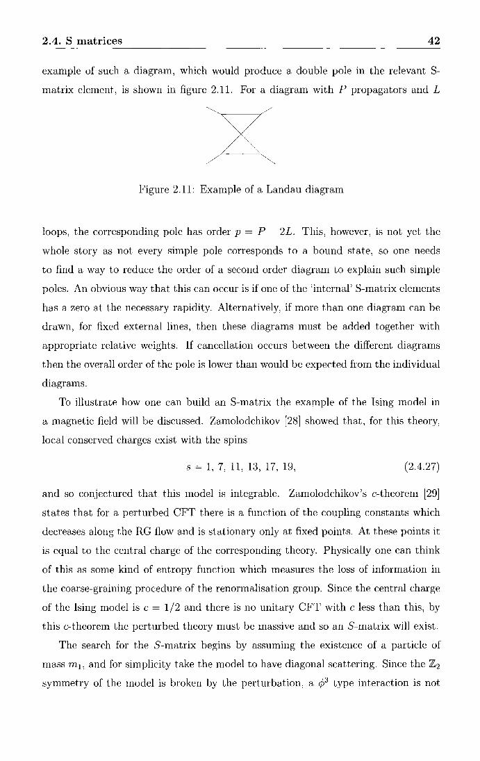
2.4. S matrices 42
example of such a diagram, which would produce a double pole in the relevant S
matrix element, is shown in figure 2.11. For a diagram with P propagators and L
Figure 2.11: Example of a Landau diagram
loops, the corresponding pole has order p = P- 2L. This, however, is not yet the
whole story as not every simple pole corresponds to a bound state, so one needs
to find a way to reduce the order of a second order diagram to explain such simple
poles. An obvious way that this can occur is if one of the 'internal' S-matrix elements
has a zero at the necessary rapidity. Alternatively, if more than one diagram can be
drawn, for fixed external lines, then these diagrams must be added together with
appropriate relative weights. If cancellation occurs between the different diagrams
then the overall order of the pole is lower than would be expected from the individual
diagrams.
To illustrate how one can build an S-matrix the example of the Ising model in
a magnetic field will be discussed. Zamolodchikov [28] showed that, for this theory,
local conserved charges exist with the spins
s = 1, 7, 11, 13, 17, 19, (2.4.27)
and so conjectured that this model is integrable. Zamolodchikov's c-theorem [29]
states that for a perturbed CFT there is a function of the coupling constants which
decreases along the RG flow and is stationary only at fixed points. At these points it
is equal to the central charge of the corresponding theory. Physically one can think
of this as some kind of entropy function which measures the loss of information in
the coarse-graining procedure of the renormalisation group. Since the central charge
of the Ising model is c = 1/2 and there is no unitary CFT with c less than this, by
this c-theorem the perturbed theory must be massive and so an S-matrix will exist.
The search for the S-matrix begins by assuming the existence of a particle of
mass m 1 , and for simplicity take the model to have diagonal scattering. Since the Z 2
symmetry of the model is broken by the perturbation, a q} type interaction is not

2.4. S matrices 43
ruled out so one can assume that the 3-point coupling Cll 1 =/= 0. The mass triangle
is then an equilateral, with all the fusing angles equal to 27r /3. The conserved charge
bootstrap equation is
(2.4.28)
This has a non-trivial solution whenever s has no common divisor with 6
s = 1, 5, 7, 11, 13, 17, ... (2.4.29)
This is close to the spin 'fingerprint' of the model, however there are still too many
spins so Zamolodchikov introduced a second particle with mass m2 and nonzero
coupling Cll2 and C 122 , so A 2 can be interpreted as the 'bound state' A1A1 and vice
versa. Let y1 = exp(iU}1 ) and y2 = exp(iU[2 ) then the conserved charge bootstap
equations are
qis) + q~s)yf + qis)Y~s = 0
q~s) + qis)Y~ + q~s)Y~s = O.
Eliminating qis) and q~s) from the above gives
(2.4.30)
(2.4.31)
(2.4.32)
This is satisfied by y1 = exp(47ri/5) and y2 = exp(37ri/5), for any odds which is not
a multiple of 5, which corresponds to the following set of fusing angles
and the mass ratio
Ul2 = U~1 = 4n-j5
u~l = u;2 = 37f /5
u;l = 21r /5
u~2 = 47f /5
(2.4.33)
(2.4.34)
(2.4.35)
By introducing this second particle the unwanted spins are eliminated and attention
can now be turned to the S-matrix. This will be built from the blocks
· h(() + inx)
(x)(e) = sm 2 60 · h(() inx) sm 2- 60
(2.4.36)
which are unitary, and when combined with the blocks (30 - x), also satisfy the
crossing symmetry property. The choice of 60 here is to ensure that the x is always
an integer. Each block has a single physical-strip pole at iJrx/30 and from the fusing

2.5. Thermodynamic Bethe Ansatz 44
angles Uf1 and U[1 above the positions of the two forward channel poles are known.
Therefore, incorporating these and their crossed channel partners the S-matrix ele
ment 5 11 must contain the blocks (10)(12)(18)(20). However, the bootstrap equation
for the ¢3 interaction 11 ----> 1 requires that 5 11 (()- iJr/3)Sn(() + iJr/3) = 5 11 (()).
For this to be satisfied, an extra factor - (2) (28) must be included. These are
the forward and crossed channel poles corresponding to another particle with mass
m3 = 2m1 cos(Jr/30). This procedure can be repeated for the 11 ----> 2 and 11 ----> 3
fusings, introducing new particles (and more bootstrap constraints) each time a single
pole, with positive residue, and its crossed channel partner are needed to satisfy the
constraints. This system closes on 8 particle types, each with a different mass, mi,
which together form the Perron-Frobenius eigenvector of the Cartan matrix of the
Lie algebra E8 .
2.5 Thermodynamic Bethe Ansatz
The S matrices described above are conjectured to be theIR limit of a perturbed CFT.
However, weight can be added to these conjectures by verifying that the UV limit of
the perturbations are indeed the proposed CFTs. One can do this by implementing
a technique known as the Thermodynamic Bethe Ansatz (TBA) [30].
Begin by considering a relativistic quantum field theory defined on a torus with
the two periods, L and R, as shown in figure 2.12. The aim will be to take the limit
R ----> oo to recover an infinitely long cylinder of circumference L.
Figure 2.12: The two periods of a torus
There are two ways to set up the Hamiltonian description on a torus. On one
hand states can be chosen to lie on the circle L, with time in the R direction, a.s
shown on the right of figure 2.12. These states are evolved by the Hamiltonian HL
and are quantised with momenta 27fn/ L, n E Z. Taking the limit R ----> oo, the
partition function, Z(R,L) = Tr(e-RHL), will be dominated by the ground state of

2.5. Thermodynamic Bethe Ansatz 45
HL with energy Eo(L):
Z(R, L) rv e-REo(L)_ (2.5.1)
Alternatively, one could take the states to lie along R, evolving in the time-like
direction Lunder the Hamiltonian HR. The states are now quantised with momenta
2nn/R and the partition function is Z(R, L) = Tr(e-LHR). Recall from section 2.1
that the free energy of the system can be written in terms of the partition function
as F = - T ln Z, where the temperature T now includes the Boltzmann constant.
Here, the system is considered as a 1-dimensional system at a temperature T = 1/ L.
When the system size is large (so as R ~ oo), the free energy behaves as
F(L) = Rf(L) + O(R- 1) (2.5.2)
where f(L) is known as the bulk free energy per unit volume
f(L) = lim F(L) R~oo R
(2.5.3)
(see, for example, [31] for more details). The partition function, in the limit R ~ oo
therefore behaves as
ln Z(R, L) "'-RLJ(L). (2.5.4)
Equating these two descriptions gives the relation
E0 (L) = Lf(L). (2.5.5)
The Hilbert space 1-lR, is expected to be given by scattering states in the R ~ oo
limit, so one has some control over 1-{R which allows a quantisation condition to be
written down and the limit of Z to be found. The aim is then to evaluate the free
energy using saddle point techniques, i.e. minimising the free energy subject to the
constraint imposed by the quantisation condition. The ground state energy can then
be read off from the result using the relation (2.5.5).
For simplicity, the TBA equations for a purely elastic scattering theory with N
identical particles, each with mass M, with two-particle scattering amplitude S (B)
will be derived. Consider a region of configuration space where the N particles are
all well separated, i.e. the distance between adjacent particles is much larger than
the correlation length 1/ M. The off-mass-shell effects can then be neglected and
the particles treated as if they are free, with on-shell energy and momenta E1 =

2.5. Thermodynamic Bethe Ansatz 46
Nfcosh(OJ) and PJ = .N/sinh(Oj)· This is valid provided R >>11M. In this region
the N-particle state can be described by a Bethe wave function 'lj;(x 1 , ... , XN) =
A(Q) exp(i LjP]Xj) where A(Q) is a function dependent on the configuration of the
particles whose exact form is not important here.
If two particles with initial positions Xj < < xH1 approach one another, interact
and move apart with their positions reversed to the point where xJ+ 1 << Xj, the
situation will again be such that the state can be described by a Bethe wave function
as above. However, as a result of this interaction, the original wave function must
be multiplied by the scattering amplitude S( ej - ej+l). The particle Xj can be sent
around the torus, in the direction R, with the wave function picking up an S-matrix
contribution each time Xj encounters another particle. Of course, when the particle
returns to its original position, the wave function must equal the original. This
periodicity imposes a quantisation condition on the momentum pj, j = 1, ... , N:
eipjR II S(ej- ei) = 1. i#j
Taking the logarithm of this leads to a set of conditions on the rapidities (:}j
.N/Rsinh(Oj)- i LlnS(ej- ei) = 2nnj i#j
with N integer numbers n1.
(2.5.6)
(2.5.7)
This is quite a complicated system of transcendental equations but they become
more tractable in the thermodynamic limit R -----> oo. The limit N -----> oo must also
be taken, where N is the number of particles, so the density N I R remains finite.
In this limit the spectrum of rapidities condenses as the distance between adjacent
rapidities e1 - OH 1 rv 11 NI R so it becomes sensible to introduce a continuous density
of particles, p1• ( 0), which is defined as
(2.5.8)
where d is the number of particles with rapidity between e and e + .6.0. This is
independent of the choice of interval .6._(:}, provided 1 I NI R < < .6.(:} < < 1. The sum in
(2.5. 7) can now be replaced with an integral
(2.5.9)
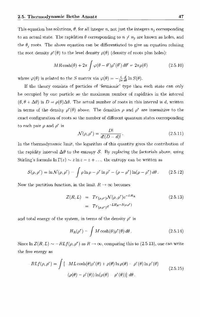
2.5. Thermodynamic Bethe Ansatz 47
This equation has solutions, (), for all integer n, not just the integers n1 corresponding
to an actual state. The rapidities () corresponding to n =1- n1 are known as holes, and
the e1 roots. The above equation can be differentiated to give an equation relating
the root density pr ( ()) to the level density p( ()) (density of roots plus holes):
lvf Rcosh(()) + 21r J tp({)- ()')pr(()') d()' = 27rp(()) (2.5.10)
where tp((}) is related to the S matrix via tp((}) = - 2~J0 lnS(e).
If the theory consists of particles of 'fermionic' type then each state can only
be occupied by one particle so the maximum number of rapidities in the interval
( (), () + .6.()) is D = p( ()) .6,(). The actual number of roots in this interval is d, written
in terms of the density pr ( ()) above. The densities p and pr are insensitive to the
exact configuration of roots so the number of different quantum states corresponding
to each pair p and pr is
N( r) D! p,p = d!(D- d)! (2.5.11)
In the thermodynamic limit, the logarithm of this quantity gives the contribution of
the rapidity interval .6,() to the entropy S. By replacing the factorials above, using
Stirling's formula lnr(z) "'zlnz- z + ... ,the entropy can be written as
Now the partition function, in the limit R-----+ oo becomes
Z(R, L) Tr{p,pr}N(p, pr)e-LHR
TT{p,pr}e-LHR+S(p,pr)
and total energy of the system, in terms of the density pr is
(2.5.12)
(2.5.13)
(2.5.14)
Since ln Z(R, L) "' - RLJ(p, pr) as R-----+ oo, comparing this to (2.5.13), one can write
the free energy as
-RLJ(p, pr) = j [-Jvf Lcosh(())pr(e) + p(()) lnp(())- pr(e) lnpr(e) (2.5.15)
-(p(())- pr(())) ln(p(())- pr(e))] d().

2.5. Thermodynamic Bethe Ansatz 48
The thermal equilibrium configuration can be obtained by minimising the free energy
per unit length, f, with respect top and pr, i.e. set 6(2.5.15)/6pr(O) = 0 where
6(2.5.15) = 8(2.5.15) + J 6p(O') 8(2.5.15) dO' 6pr(O) 3pr(O) 6pr(O) 3p(0') .
(2.5.16)
The constraint (2.5.10) allows p to be treated as a functional of pr and from this it
is clear that
(2.5.17)
and it is also easy to show that
(2.5.18)
and
6 6
pr(O') ((p(O)- pr(O)) ln(p(O)- pr(O))) = (2.5.19)
- (1 + ln(p(O)- pr(O)) 6(0- 0').
The derivatives of (2.5.15) with respect to pr and p depend on these densities only
through the ratio pr / p and since p(O) > pr(O) it is useful to set
(2.5.20)
where c:( 0) is a real function known as the pseudoenergy. In terms of this, the deriva
tives of (2.5.15) are
( pr(O) )
- M L cosh(O) - ln p(O) _ pr(O)
-N!Lcosh(O) + c:(O) (2.5.21)
and
8(2.5.15) = ln ( p(O) ) = ln (1 + e-£(0)) .
3p(O) p(O)- pr(O) (2.5.22)
So setting 6(2.5.15)/6pr(O) = 0 leads to a nonlinear integral equation known as the
TBA equation:
c:(O) = Nf Lcosh(O)- J cp(O- 0') ln(1 + e-£(O)) dO'. (2.5.23)
This TBA equation can now be used to simplify the expression of the free energy
in (2.5.15). Denote the integrand in (2.5.15) by I and writing this in terms of the
pseudoenergy, c:(O), gives
(2.5.24)

2.5. Thermodynamic Bethe Ansatz
The constraint (2.5.10) can be used to replace p(O) here, leaving
1 I=- ]\If L cosh(O)pr(e) + -M Rcosh(O) ln(1 + e-f(O))
2n
+ J cp(O- 0')pr(0') dO' ln(1 + e-E(O)) + pr(0)E(0).
This can be simplified using the TBA equation (2.5.23) to give
1 I=
27r !vi Rcosh(O) ln(1 + e-E(O)),
so the extremal free energy per unit length is then
f(L) = --1- j NI cosh( e) ln(1 + e-E(O)) de.
2nL
49
(2.5.25)
(2.5.26)
(2.5.27)
Recall that the free energy is related to the ground state energy through E0 ( L) =
Lf(L) and so
E0(L) = -~ j 111 cosh( e) ln(1 + e-E(O)) de. 2n
(2.5.28)
The regularisation implicit in the TBA derivation sets the bulk free energy, ££1112,
to zero so E0 ( L) given above is actually the Casimir energy. Comparing this to the
Casimir energy of a CFT, E0 = -ncj6L, one can define the effective central charge,
or ground state scaling function, as
3l J Cetr(l) = n2
de cosh(O) ln(1 + e-E(O)). (2.5.29)
This is dependent on the dimensionless parameter l = 111 L. This will vanish as l ---> oo
which corresponds to the IR limit of the perturbed theory. The UV limit, when the
CFT is recovered, corresponds to l ---> 0. In this case the scaling function is related
to the central charge of the CFT:
lim Cetr(l) = C- ~o. z~o
(2.5.30)
Here ~0 is the lowest scaling dimension of the CFT and since ~0 = 0 for unitary
theories, Cetr(O) = c for those cases. This effective central charge provides a useful tool
to check the validity of conjectured S-matrices for perturbed conformal field theories.
This description was extended to cover the diagonal purely elastic scattering the
ories associated to the ADE type Lie algebras in [32][33]. The number of particles
in these theories corresponds to the rank r of the algebra. The TBA system then
consists of r pseudoenergies, each associated with a particle of mass rna, which satisfy
Ea = maLcosh(O)- t J dO' </Jab(O- 0') ln(1 + e-Eb(O'))
b=l
(2.5.31)

2.5. Thermodynamic Bethe Ansatz
where rPab(()) is related to the scattering amplitude Sab(())
i d rPab(()) = -
27!" d()Sab(()) ·
The Casimir energy can be written in terms of these pseudoenergies as
1 r J E(L) = --L ma d() cosh(()) ln(1 + e-E(O)). 27r
a=l
50
(2.5.32)
(2.5.33)
Zamolodchikov [34] found the following universal form for these TBA equations in
terms of the incidence matrix A~;] of the associated Lie algebra:
Ea(()) =maL cosh(())-~ t J d()' A~;J'Ph(()- ()') ( mbLcosh(()') -ln(l + eEb(O')))
b=l
(2.5.34)
where the universal kernel, 'Ph, now depends only on the Coxeter number, h, of the
Lie algebra
(()) = h 'Ph 2 cosh( ~h())" (2.5.35)
He then remarked that these TBA equations encode one particular solution of a
system of functional equations, known as the Y -system:
r
Ya(() + i7rjh)Ya(()- i1rjh) = rr(l + Yl,(()))A~<;J (2.5.36) b=l
where Ya(()) = exp(ca(())). By successive substitutions of (2.5.36) into itself, it can be
shown (case by case) that these Y -functions are periodic
(2.5.37)
There are also various proofs for this conjecture [35, 36, 37, 38, 39, 40]. This ob
servation has important consequences as it implies that the Y functions admit the
Laurent expansions 00
(2.5.38) k=-oo
and, as L ----t 0, the functions ln(l + e-Ea(O)) acquire the form of a plateau of approx
imately constant height in the central region -ln(1/ Nf L) < < () < < ln(l/.M L ). It
then follows that the function L(E(L)-EL.A12(.>,))/27r = -Ceff(l)/12 can be expanded
as a perturbative series in L 4h/(h+2) [34].
These TBA equations correspond to perturbations resulting in massive quantum
field theories. However, some perturbations of CFTs lead to massless theories in the

2.6. 'ODE/1M' Correspondence 51
IR limit, which are necessarily RG fixed points. These RG flows therefore interpolate
between two conformal field theories. The ¢13 flows between the Virasoro minimal
models are examples of this [29]. In these cases, the derivation of the TBA equa
tions is not so straightforward so Al. Zamolodchikov [41 ][42][43] instead developed a
strategy of making an educated guess of the TBA equations and then testing them
by checking that they correctly reproduced UV data, such as the central charge of
the UV CFT and the dimension of the perturbing operator. Perhaps more inter
estingly, Al. Zamolodchikov [44] also proposed a simple diagonal scattering theory,
known as the 'staircase model', from which the TBA equations follow in the standard
way, shown here. Numerical investigations of the solutions to these equations show
the vacuum energy, which is proportional to the effective central charge, following a
staircase type pattern which suggests there is an underlying theory whose RG flow
passes by a sequence of c < 1, i.e. Virasoro minimal model, fixed points. This was
extended to cover the l¥9 minimal models in [45][ 46][ 4 7], however, a.s this thesis is
concerned with perturbations resulting in massive scattering theories, no more will
be said about these models here.
2.6 'ODE/1M' Correspondence
This section introduces a curious and useful link between functional relations of inte
grable models and spectral problems of ODEs, first found by Dorey and Tateo in [48].
These functional relations can be derived directly in terms of a CFT [49], but as only
the final relations themselves will be of use later, a discussion of this derivation would
deviate unnecessarily from the main point of the thesis. Instead, it will be shown how
these relations arise quite naturally when statistical lattice models are solved using
a particular method. The discussion presented here follows that found in the recent
review [50].
2.6.1 Functional relations in Integrable Models
The specific lattice model used here is the six-vertex model. This is a simple gener
alisation of the Ising model, first solved by Lieb [51 J and Sutherland [52]. Also see
Baxter's book [53]. It can be defined on an N x M lattice with periodic boundary

2.6. 'ODE/1M' Correspondence 52
conditions in both directions. On each link of the lattice a spin 1 or 2 is placed, de
picted here by a right or left arrow, on the horizontal links, and an up or down arrow
on the vertical links. This is often referred to as an 'ice-type' model as each vertex
can be taken to represent an oxygen atom with each link being the bond between
adjacent atoms. The Hydrogen ion, sitting on each bond, will lie closer to one of the
ends, according to the direction of the arrow. The 'ice-rule' states that each oxygen
atom should have two Hydrogen ions close to it and two far away, which translates
to the condition that the flux of arrows through a vertex must be preserved. There
are therefore six options for the spins around each vertex, hence the name 'six-vertex
model'.
For real ice, each possibility is equally likely, but as a generalisation of this one
can allow for different probabilities. The local Boltzmann weights, which assign a
probability to each configuration, are defined here to be:
l¥[-i-] l¥ [-1-] w [- i ~]
and the partition function is
Ml[~l~]=a
w[~i~] =b
w[~l-]=c
Z=2:ITvv[·>J {a} sites
(2.6.1)
(2.6.2)
(2.6.3)
(2.6.4)
where { o-} = { ~, -}. In the thermodynamic limit ( N, M - oo), the overall nor
malisation of a, b and c factors out trivially from all quantities so it is convenient
to reparametrise the two remaining degrees of freedom using the variables v (the
spectral parameter) and 7] (the anisotropy)
a(v,7])
b(v, 77)
c(v,7J)
sin(7J + iv)
sin(77-iv)
sin(27J) .
(2.6.5)
(2.6.6)
(2.6.7)
It is usual to keep the anisotropy fixed in calculations, as different values of 7] will turn
out to correspond to different models. The spectral parameter, on the other hand,
can be varied as it is not a physical parameter, a fact that will become apparent
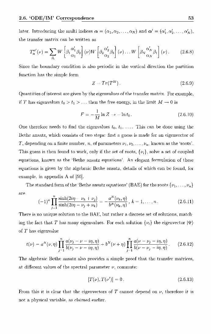
2.6. 'ODE/1M' Correspondence 53
later. Introducing the multi indices a= (a1 , a 2 , ... , aN) and a'= (a~, a;, ... , a~),
the transfer matrix can be written as
(2.6.8)
Since the boundary condition is also periodic in the vertical direction the partition
function has the simple form
(2.6.9)
Quantities of interest are given by the eigenvalues of the transfer matrix. For example,
if T has eigenvalues t 0 > t 1 > ... then the free energy, in the limit M -----+ 0 is
1 F = -- ln Z -----+ - ln t0 .
A1 (2.6.10)
One therefore needs to find the eigenvalues t 0 , t 1 , .... This can be done using the
Bethe ansatz, which consists of two steps: first a guess is made for an eigenvector of
T, depending on a finite number, n, of parameters v1 , v2 , ... , Vn, known as the 'roots'.
This guess is then found to work, only if the set of roots, {vi}, solve a set of coupled
equations, known as the 'Bethe ansatz equations'. An elegant formulation of these
equations is given by the algebraic Bethe ansatz, details of which can be found, for
example, in appendix A of [50].
The standard form of the 'Bethe ansatz equations' (BAE) for the roots {v1 , ... , vn}
are
(- )n rrn sinh(2i7]- Vk + Vj) = _aN (vk, 'lJ) k = 1 . sinh(2i7]- v1· + vk) bN(vk, T/) '
1' · · · 'n ·
J=l
(2.6.11)
There is no unique solution to the BAE, but rather a discrete set of solutions, match-
ing the fact that T has many eigenvalues. For each solution {vJ the eigenvector I'll)
ofT has eigenvalue
( ) N( ) rrn a(vj- V- i'l], 7J) bN( ) rrn a(v- Vj- i'l], 7J)
t v = a v, 17 + v + 17 . j=l b(vj - v- i1], 77) j=l b(v- Vj - i'l], 77)
(2.6.12)
The algebraic Bethe ansatz also provides a simple proof that the transfer matrices,
at different values of the spectral parameter v, commute:
[T(v), T(v')] = 0. (2.6.13)
From this it is clear that the eigenvectors of T cannot depend on v, therefore it is
not a physical variable, as claimed earlier.

2.6. 'ODE/1M' Correspondence 54
Periodic boundary conditions, as imposed here, are not the only boundary condi
tions for which this model is integrable. In fact, integrability is preserved when these
periodic boundary conditions are modified by introducing a 'twist' (see for example,
[54][55][56]). This amounts to adding a phase factor to the Boltzmann weights on
one column of the lattice, say the Nth, so
W [!3N :: ~] (v) ~ e-i¢W [!3N :: ~] (v)
W [f}N :: <---] (v) ~ ei¢HI [f)N :: .-] (v).
(2.6.14)
(2.6.15)
The transfer matrix is then defined as in (2.6.8) and the algebraic Bethe ansatz goes
through almost unchanged. The result is that the generalised transfer matrix T(v, ¢)
has eigenvalues
t(v, ¢) = e-i¢aN (v, TJ) IIn a(vj- v- ~TJ, TJ) + ei¢bN (v + TJ) rrn a(v- Vj- ~TJ, TJ) j=l b(vj- V- ZTJ, TJ) j=l b(v- Vj- ZTJ, TJ)
(2.6.16)
where the set of roots { v1 , ... , v11 } satisfy the modified Bethe ansatz equations
(- )nfln sinh(2iTJ-Vk+vj) __ _ 2i¢aN(VkJTJ) ~-
1 ( )- e N( ),k-1, ... ,n. j=l sinh 2iTJ- v1 + vk b vk, TJ
(2.6.17)
An alternative approach to this is provided by Baxter [57]: since the transfer
matrices T(v) commute for different values of the spectral parameter v, the T(v) can
be simultaneously diagonalised and the eigenvectors W will not depend on v. One can
therefore focus on the individual eigenvalues t0 (v), t 1(v) ... as functions of v. Given
the form of the Boltzmann weights in (2.6.5-2.6. 7) and the claim that the eigenvectors
are v-independent, these functions t(v) are entire and in-periodic. A matrix Q(v)
can now be defined, which commutes with itself and with T:
[Q(v), Q(v')] = [Q(v), T(v')] = 0 (2.6.18)
and satisfies the TQ relation
(2.6.19)
The eigenvalues of Q are also functions of v, denoted q(v), which are also entire
and, at least for the ground state, in-periodic. They satisfy the eigenvaJue relation,
corresponding to (2.6.19)
(2.6.20)

2.6. 'ODE/1M' Correspondence 55
The BAE equations can then be extracted from (2.6.20) as follows: suppose that the
zeros of q(v) are at v1 , ... , Vn. Given the periodicity of q(v), it can be written, up to
an overall normalisation, as n
q(v) =IT sinh(v- v1). (2.6.21) /=1
Now putting v = vi in (2.6.20) gives
(2.6.22)
and using the equation for q(v), (2.6.21), this can be rearranged to
(- )n rrn sinh(2i'1]- Vi+ Vz) __ _ 2iq;aN (vi, 'lJ) . _
1 ( ) - e N( ) , z- 1, ... , n. sinh 2iry - Vf + vi b vi, '1]
1=1
(2.6.23)
This is the BAE from (2.6.17), and t(v), given by (2.6.20), then matches the t(v)
found by the direct calculation. Baxter in fact established this TQ relation (2.6.19)
by an independent argument and then generalised it to the previously unsolved eight
vertex model [57][58]. See his book [53] for more details.
The continuum limit of the six vertex model is a. unitary CFT with central charge
c = 1. The TQ relations, described above, therefore encode information about this
CFT when this limit is taken. Alternatively, these functional relations can also be
constructed directly in terms of a. CFT, as proposed by Ba.zha.nov, Lukya.nov and
Zamolodchikov in [49] and developed further in [59] and [60] . No more will be said
about this approach here as it is not directly used in this thesis.
2.6.2 Ordinary differential equations
In order to make the link between the integrable model above and the theory of
ordinary differential equations, the aim is to find a. functional relation in the ODE
theory which can be directly compared to the TQ relation (2.6.19) above. This link
was first found by Dorey and Ta.teo in [48] where the ODE
d2 - dx
21jJ(x)- (ix) 2M1jJ(x) = E1jJ(x) (2.6.24)
was considered, with x a. complex variable and M > 1. For a. discussion of eigenvalue
problems on a. complex contour see, for example, [61][62][63]. The WKB approxima
tion to the solutions 1/J gives the leading asymptotic
(2.6.25)
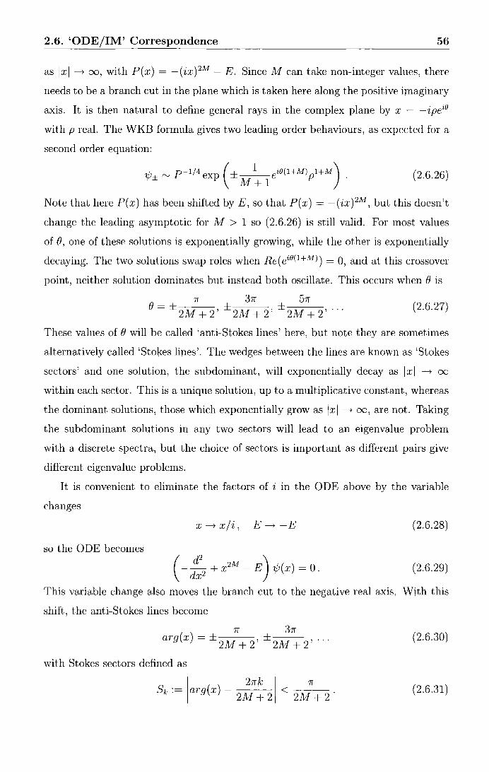
2.6. 'ODE/1M' Correspondence 56
as lxl -----> oo, with P(x) = -(ix)2M- E. Since M can take non-integer values, there
needs to be a branch cut in the plane which is taken here along the positive imaginary
axis. It is then natural to define general rays in the complex plane by x = -ipei0
with p real. The WKB formula gives two leading order behaviours, as expected for a
second order equation:
1/J ""' p-1/4 exp (± 1 eiO(l+M) pl+M) ± A1 + 1
(2.6.26)
Note that here P(x) has been shifted byE, so that P(x) = -(ix) 2M, but this doesn't
change the leading asymptotic for M > 1 so (2.6.26) is still valid. For most values
of(), one of these solutions is exponentially growing, while the other is exponentially
decaying. The two solutions swap roles when Re(eiO(l+M)) = 0, and at this crossover
point, neither solution dominates but instead both oscillate. This occurs when () is
7r 37r 57r () = ± 2111 + 2' ± 2lvf + 2' ± 2111 + 2' ... (2.6.27)
These values of() will be called 'anti-Stokes lines' here, but note they are sometimes
alternatively called 'Stokes lines'. The wedges between the lines are known as 'Stokes
sectors' and one solution, the subdominant, will exponentially decay as lxl ----> oo
within each sector. This is a unique solution, up to a multiplicative constant, whereas
the dominant solutions, those which exponentially grow as lxl -----> oo, are not. Taking
the subdominant solutions in any two sectors will lead to an eigenvalue problem
with a discrete spectra, but the choice of sectors is important as different pairs give
different eigenvalue problems.
It is convenient to eliminate the factors of i in the ODE above by the variable
changes
so the 0 DE becomes
x-----> xji, E-----> -E
(- d2 + x2M - E) 1/J ( x) = 0 .
dx2
(2.6.28)
(2.6.29)
This variable change also moves the branch cut to the negative real axis. With this
shift, the anti-Stokes lines become
7r 37r arg(x) =±2M+ 2' ±2Jvf + 2' · · · (2.6.30)
with Stokes sectors defined as
I 27rk I 7r sk := arg(x)- 111 < Jvf .
2 1 +2 2 +2 (2.6.31)

2.6. 'ODE/1M' Correspondence 57
The ODE (2.6.29) has a so called 'basic' solution y(x, E) which is an entire func
tion on the cut plane. In the limit lxl --+ oo, with iarg(x)i < 2 A~t+- 2 , it has the
asymptotic
y rv -x-2 exp - x" +- 1 1 At [ 1 '!] y'2Z M+1
(2.6.32)
which matches the WKB approximation in the Stokes sectors S_ 1 U S0 u S1 . Note
that this is subdominant in S0 and dominant in S_ 1 and S1. Further solutions to the
ODE can be generated as follows: consider the function fj(x) = y(ax, E) which solves
the differential equation
(- d~2 + a2M+-2x2M - a2 E) fj(x, E) = 0. (2.6.33)
If a2A1+2 = 1 '
fj(x, a- 2 E) is a. solution to the original ODE (2.6.29). By setting
w = e27ri/( 2M+- 2l, one can define a whole set of solutions to (2.6.29)
(2.6.34)
By inspecting the asymptotics of Yk it follows that Yk is subdomina.nt in Sk and
dominant in Sk±1· Furthermore, Yk and Yk+- 1 are linearly independent and so form a
basis of solutions so, for example, y_ 1 can be expanded in the {y0 , yi} basis as
Y-1 (x, E) = C(E)yo(x, E)+ C(E)y1 (x, E). (2.6.35)
This is an example of a Stokes relation and the coefficients, C and C, are the 'Stokes
multipliers'. These multipliers can be expressed in terms of Wronskians, where the
Wronskian of two functions, f(x) and g(x) is
W[f, g] := fg'- f'g · (2.6.36)
By considering the derivative of W, with respect to x, it is easy to show that the
Wronskian of two solutions to a. second order ODE, with no single derivative term, is
independent of x and is zero if and only if the solutions are linearly dependent. Since
y0 and y 1 are linearly independent, expressions can be found for C(E) and C(E) in
terms of Wronskians. First, to simplify notation, let W[y1, Yk] - W1,k and notice,
using (2.6.34), that
(2.6.37)
By considering the asymptotic expressions for y, it also follows that
Wo1 = 1 , (2.6.38)
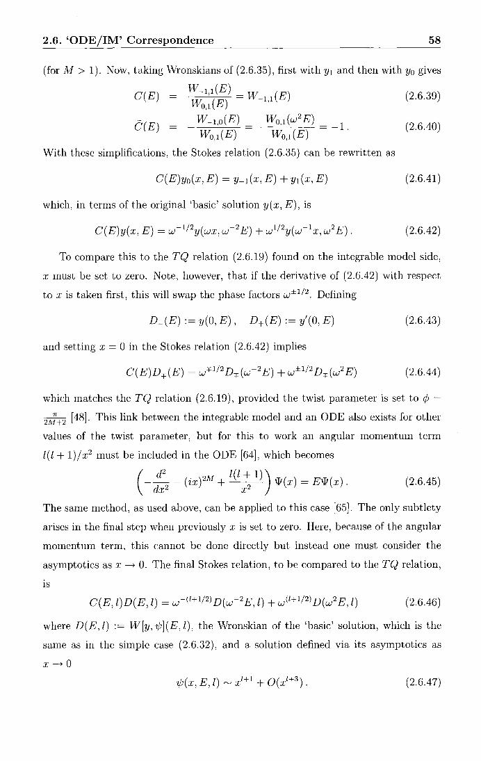
2.6. 'ODE/1M' Correspondence 58
(for Jvf > 1). Now, taking Wronskians of (2.6.35), first with y1 and then with y0 gives
w-1,1(E) W. (E) = W-1,1 (E)
0,1 (2.6.39) C(E)
C(E) w-1,o(E) lVo,1(w2 E) - =- = -1
Wo,1(E) Wo,1(E) · (2.6.40)
With these simplifications, the Stokes relation (2.6.35) can be rewritten as
C(E)yo(x, E)= Y-1(x, E)+ Y1(x, E) (2.6.41)
which, in terms of the original 'basic' solution y(x, E), is
(2.6.42)
To compare this to the TQ relation (2.6.19) found on the integrable model side,
x must be set to zero. Note, however, that if the derivative of (2.6.42) with respect
to x is taken first, this will swap the phase factors w±112. Defining
D_(E) := y(O, E), D+(E) := y'(O, E) (2.6.43)
and setting x = 0 in the Stokes relation (2.6.42) implies
(2.6.44)
which matches the TQ relation (2.6.19), provided the twist parameter is set to ¢ =
211;+2 [48]. This link between the integrable model and an ODE also exists for other
values of the twist parameter, but for this to work an angular momentum term
l(l + 1)/x2 must be included in the ODE [64], which becomes
(-d:2- (ix) 2M + l(l; 1)) w(x) = Ew(x). (2.6.45)
The same method, as used above, can be applied to this case [65]. The only subtlety
arises in the final step when previously x is set to zero. Here, because of the angular
momentum term, this cannot be done directly but instead one must consider the
asymptotics as x ----> 0. The final Stokes relation, to be compared to the TQ relation,
IS
C(E, l)D(E, l) = w-(l+1/ 2l D(w- 2 E, l) + w(1+ 1/ 2l D(w 2 E, l) (2.6.46)
where D(E, l) := W[y, '!j;](E, l), the Wronskian of the 'basic' solution, which is the
same as in the simple case (2.6.32), and a solution defined via its asymptotics as
x---->0
(2.6.47)

2.6. 'ODE/1M' Correspondence 59
This asymptotic fixes 1/J uniquely, provided Re l > -3/2. A second solution can
be found by sending l ---t -1 - l. The differential equation, but not the boundary
condition, is invariant under this transformation so 1/J(x, E, -1 -l) is also a solution
of (2.6.45). Near the origin, this behaves as x-1, so for generic values of l, the
pair of solutions 1/J(x, E, l) and 1/J(x, E, -1- l) are linearly independent. Defining
D_(E) := D(E, l) and D+(E) := D(E, -1- l), then taking land -1 -lin (2.6.46)
gives
(2.6.48)
Comparing this to the TQ relation (2.6.19), it is clear that the twist parameter is
related to the angular momentum l and the degree of the potential of ODE via
(2l + 1)7T ¢ = 2NI + 2
and, in fact, the anisotropy parameter rJ is also related to M:
7T Nf rJ= 21\1+1"
(2.6.49)
(2.6.50)
This 'ODE/IM correspondence' has proved useful, mainly because the properties
of ODEs and their solutions are somewhat better understood than those of the T and
Q functions in integrable quantum field theories. Certain properties, conjectured to
hold for these T and Q functions have been proven using the correspondence [64].
On the other hand, ideas from the theory of integrable models have been employed
to gain insights into the spectral properties of certain ODEs. One example of this,
which will be discussed further in Chapter 5, is the use of this correspondence to
prove the reality of the spectrum, for certain land M, of the PT-symmetric quantum
mechanical problem, with Schrodinger equation (2.6.45) [66].

Chapter 3
Boundary Problems
So far, perturbed conformal field theories have been examined on both an infinite
plane and a torus. An obvious question which now springs to mind is how does this
story change when more general boundary conditions are imposed on the theory?
This chapter aims to answer this by first looking at the effect of the boundary on a
CFT, in particular, which boundary conditions preserve conformal invariance. The
perturbation of this theory, by both bulk and boundary operators, is then discussed
which leads on to the introduction of Reflection factors, or boundary S-matrices. Fi
nally a method is proposed to link the reflection factors to specific conformal boundary
conditions, using the TBA. This is analogous to the effective central charge Ceff which
provides a link between the S-matrix and the central charge of the bulk theory.
3.1 Boundary CFT
In a series of papers [67][68][69][13], Cardy explored the consequence of restricting
a CFT to the upper half plane with the real axis as the boundary. The discussion
presented here follows [68], along with Cardy's review [70]. All conformal transfor
mations acting on the theory must preserve the boundary. This constrains the energy
momentum tensor to satisfy T( z) = T( z) on the real axis. In Cartesian coordinates
this becomes Txylx=O = 0, so physically it corresponds to the requirement that no
energy or momentum must flow across the boundary. The effect of this constraint is
to eliminate half of the conformal generators as the holomorphic and antiholomorphic
sectors are no longer independent.
60
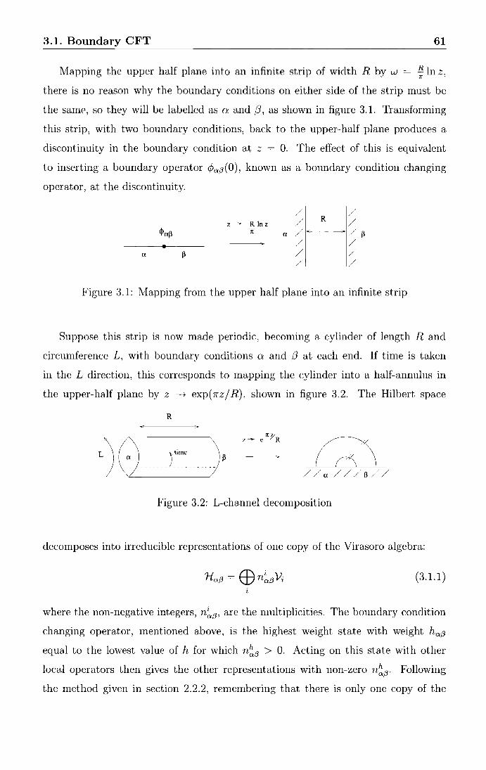
3.1. Boundary CFT 61
Mapping the upper half plane into an infinite strip of width R by w B.ln z. 7r '
there is no reason why the boundary conditions on either side of the strip must be
the same, so they will be labelled as a and (3, as shown in figure 3.1. Transforming
this strip, with two boundary conditions, back to the upper-half plane produces a
discontinuity in the boundary condition at z = 0. The effect of this is equivalent
to inserting a boundary operator ¢o:13 (0), known as a boundary condition changing
operator, at the discontinuity.
/ R
/ z~ R lnz / /
cJ>ap 1[ a / / p / /
a p / / / /
Figure 3.1: Mapping from the upper half plane into an infinite strip
Suppose this strip is now made periodic, becoming a cylinder of length R and
circumference L, with boundary conditions a and (3 at each end. If time is taken
in the L direction, this corresponds to mapping the cylinder into a half-annulus in
the upper-half plane by z ---> exp(7rz/ R), shown in figure 3.2. The Hilbert space
R
Q //a///B//
Figure 3.2: L-channel decomposition
decomposes into irreducible representations of one copy of the Virasoro algebra:
(3.1.1)
where the non-negative integers, n~13 , are the multiplicities. The boundary condition
changing operator, mentioned above, is the highest weight state with weight ho:f3
equal to the lowest value of h for which n~13 > 0. Acting on this state with other
local operators then gives the other representations with non-zero n~13 . Following
the method given in section 2.2.2, remembering that there is only one copy of the
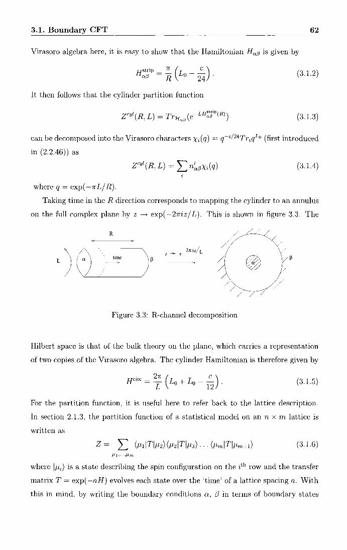
3.1. Boundary CFT 62
Virasoro algebra here, it is easy to show that the Hamiltonian Ho:(3 is given by
Hstrip = !!__ (L _ _5_) o:f3 R 0 24 . (3.1.2)
It then follows that the cylinder partition function
(3.1.3)
can be decomposed into the Virasoro characters Xi(q) = q-c/24TriqLo (first introduced
in (2.2.46)) as
(3.1.4)
where q = exp( -1r L I R).
Taking time in the R direction corresponds to mapping the cylinder to an annulus
on the full complex plane by z --+ exp(- 27fiz I L). This is shown in figure 3.3. The
L C) R
time :~
z ~ c -2niz/L
/ /
Figure 3.3: R-channel decomposition
/
@ /
/
Hilbert space is that of the bulk theory on the plane, which carries a representation
of two copies of the Virasoro algebra. The cylinder Hamiltonian is therefore given by
Hcirc = 2; ( Lo + Lo - lc2) . (3.1.5)
For the partition function, it is useful here to refer back to the lattice description.
In section 2.1.3, the partition function of a statistical model on an n x rn lattice is
written as
(3.1.6) Ill , ... ,jlm
where IJ.Li) is a state describing the spin configuration on the ith row and the transfer
matrix T = exp( -aH) evolves each state over the 'time' of a lattice spacing a. With
this in mind, by writing the boundary conditions a, f3 in terms of boundary states

3.1. Boundary CFT 63
Ia) and I,B) [68] and summing over only those states which satisfy the boundary
conditions, the partitiori function becomes
(3.1. 7)
The condition T(z) = T(z), under the mapping z ~ wexp(-2niz/L), becomes
(3.1.8) '4
which corresponds to the following constraint on these boundary states:
(Ln - L_n) Ia) = 0. (3.1.9)
For diagonal CFTs (i.e. CFTs whose torus partition function can be written as
Z = Li niXi(q)Xi(q)) the solution to this constraint is unique and is given by the
Ishibashi states:
in terms of the highest weight state li) with hi = hi, and conformal vacuum IO) with
h = h = 0. There is one Ishibashi state for each bulk primary state and they can be
normalised so that
(3.1.11)
where q = exp( -4n R/ L ).
States corresponding to physical boundary conditions are not the Ishibashi states
but are certain linear combinations of these, known as Cardy states:
Ia) = L g~lj) ). (3.1.12) j
The coefficients g~ can be assumed to be real as it is always possible to normalise the
fields in such a way that this is true. In this notation (3.1. 7) becomes
Zaf3(q) = L9~9bXJ(ij). j
(3.1.13)
Equating the two partition functions (3.1) and (3.1.13), and using the modular trans
formation property of the characters
Xi(q) = 2:siJXJ(ii) j
(3.1.14)
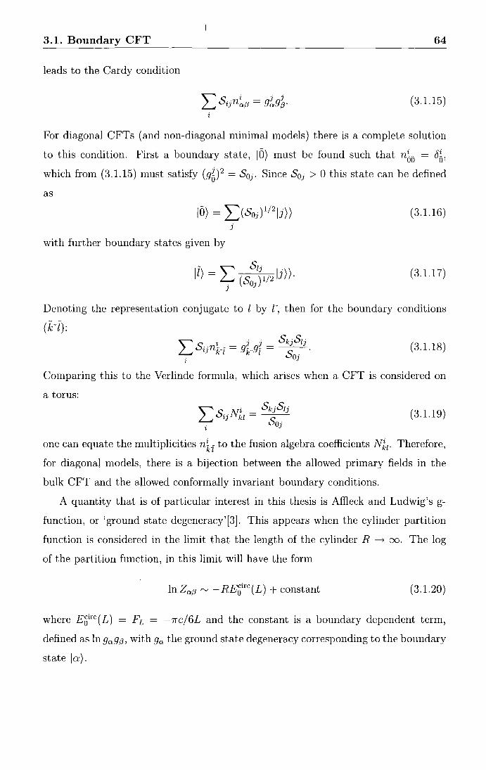
3.1. Boundary CFT 64
leads to the Cardy condition
(3.1.15)
For diagonal CFTs (and non-diagonal minimal models) there is a complete solution
to this condition. First a boundary state, ID) must be found such that n~6 = 6fi, which from (3.1.15) must satisfy (gb) 2 = S01 . Since S01 > 0 this state can be defined
as
ID) = 2:)So1)112 1J))
j
with further boundary states given by
(3.1.16)
(3.1.17)
Denoting the representation conjugate to l by r, then for the boundary conditions
(kd): """ i _ 1 1 _ skjslj ~ sijnjd - gk.gi - ~.
i 0]
(3.1.18)
Comparing this to the Verlinde formula, which arises when a CFT is considered on
a torus:
"""s . Ni - skjslj ~ t) kl- s
i Oj
(3.1.19)
one can equate the multiplicities nki to the fusion algebra coefficients Nkz· Therefore,
for diagonal models, there is a bijection between the allowed primary fields in the
bulk CFT and the allowed conformally invariant boundary conditions.
A quantity that is of particular interest in this thesis is Affleck and Ludwig's g
function, or 'ground state degeneracy'[3]. This appears when the cylinder partition
function is considered in the limit that the length of the cylinder R -t oo. The log
of the partition function, in this limit will have the form
In Za,a '"" - RE~irc ( L) + constant (3.1.20)
where E8irc(L) = FL = -1rcj6L and the constant is a boundary dependent term,
defined a.s ln 9a9f3, with 9a the ground state degeneracy corresponding to the boundary
state Ia).

3.2. Perturbed Boundary CFT 65
Taking time along the cylinder, in the R direction, the partition function has
leading order behaviour
n
(aiD) (DI/3)e-RE8i'c(Ll (3.1.21)
where ID) is the bulk ground state. Taking logs of this gives
ln Zaf3 rv - REgirc ( L) + ln 9a9f3 (3.1.22)
with 9a = (aiD). Now (aiD) = 2::::1 g~( \JID), but since all primary states are orthogo
nal, ((jiD) =((DID). Expandingthelshibashistateas ((DID)= (DID)+(DIL~~1 ID)+
... and using the fact that LniD) = 0 for n > 0, the only non-zero term left in this
expansion is the first. Therefore (aiD)= g~ and so it is clear from (3.1.12), (3.1.16)
and (3.1.17) above that
San 9a = (Son)I/2" go = (Son) 112 (3.1.23)
Affleck and Ludwig also proposed a g-theorem [3], later proven in [71], which is
analogous to Zamolodchikov's c-theorem [29]. It states that the g-function decreases
under renormalisation group flow from a less stable to a more stable critical point in
the same bulk universality class. This means that if a CFT with boundary state Ia)
is perturbed by a boundary perturbation only, while the bulk remains critical, then
the resulting IR theory will be the same CFT with boundary l/3) where 9(3 < 9a· This
no longer necessarily holds when a bulk perturbation is added.
3.2 Perturbed Boundary CFT
The perturbation of a CFT with a boundary was first considered by Ghoshal and
Zamolodchikov in [72] and the discussion here will follow their work. First, consider
a CFT in Euclidean space, with coordinates (x, y) and impose a conformal boundary
condition at x = 0. This theory can be perturbed by both a relevant bulk operator,
rp(x, y), and a relevant boundary operator, ¢(y) with the resulting action taken to be
A= ABCFT + ,\ [~ dx 1: dy rp(x, y) + f-l 1: dy ¢(y). (3.2.1)

3.2. Perturbed Boundary CFT 66
For a boundary CFT the condition Txylx=O = 0 must be satisfied, but for the per
turbed theory this constraint becomes
- d Txyix=O = ( -i)(T- T)ix=O = dy O(y) (3.2.2)
where O(y) is some local boundary field. Of course, in general, even if the bulk
perturbed theory is integrable the boundary conditions could spoil this integrability.
However, if the boundary conditions satisfy
(3.2.3)
for some s E { s }, 08 again being some local boundary field and Ts+l and 8 8 _ 1 being
the local bulk fields described in section 2.3, then an integral of motion for each s
can be found.
There are two ways to introduce the Hamiltonian picture in this theory. The first
is to take y to be the time direction so the boundary is a boundary in space and
the Hilbert space 1-ls is associated to the half-line x E ( -oo, 0]. Alternatively, x can
be taken to be the time direction, in which case the boundary is an initial condition
which can be described by the boundary state IE) which will lie in the Hilbert space
of the bulk theory. In this case the integrals of motion are the same as those for the
bulk theory: Ps = f~oo(Ts+l + Gs_I)dy and Ps = f~(Ts+l + Ss_I)dy. Therefore,
from (3.2.3), for the theory to be integrable the boundary states must satisfy
(3.2.4)
There is no boundary analogue of Zamolodchikov's counting argument to deter
mine the integrable perturbations; instead one must find some integrals of motion
directly. For example, in [72], Ghoshal and Zamolodchikov conjectured that the Vi
rasoro minimal models, perturbed by the bulk and boundary operators 'P(l,3) and
¢(1,3) respectively, are integrable by first setting A = 0, so perturbing at the bound
ary only, and finding solutions to (3.2.3) for s = 1, 3, 5, .... They then argued that by
dimensional analysis, parallel to that used by Zamolodchikov in [21] and described in
section 2.3, these results remain valid for A =/= 0. In general it is expected, although
has never been proven, that adding a boundary perturbation to an integrable bulk
PCFT will result in a.n integrable theory provided the boundary perturbing operator
is the boundary operator corresponding to the bulk perturbing operator. Note that

3.3. Reflection factors 67
as there is only one copy of the Virasoro algebra in the boundary theory, boundary
operators have scaling dimension half that of the corresponding bulk operators. This
expectation is certainly true in every case so far examined and if the boundary oper
ator did not match the bulk operator in this way the situation would, in some sense,
be akin to perturbing a bulk CFT by a combination of two relevant operators which
is also not usually expected to lead to an integrable theory.
Perturbing by a bulk operator, with or without a boundary perturbation, will
clearly alter the boundary conditions and in cases where this perturbation results
in a massive theory with a particle description, it is necessary to understand how
the particles interact with the boundary. The boundary analogue of the S-matrix
elements, known as Reflection factors are therefore needed.
3.3 Reflection factors
In this section the S-matrix approach of section 2.4 is adapted to the semi-infinite
plane. This problem was first treated in papers by Ghoshal and Zamolodchikov [72]
and Fring and Koberle [73], but the discussion presented here follows that given in
[72] and also [27].
Returning to ( 1 + 1) Minkowski space with time taken in the y direction, the
asymptotic states, in parallel to the bulk case, can be considered as particle creation
operators Aa;(Oi) acting on the ground state 10) 8 :
(3.3.5)
For an in state, the rapidities 01 , ... , On are all positive, whereas for an out state they
are aU negative. The boundary can be thought of as an impenetrable particle, B
sitting at x = 0 so formally, the ground state can be written as
(3.3.6)
This description makes the analogy with the S-matrix theory m the bulk quite
straightforward. The asymptotic in and out states become
(3.3.7)
with the rapidities ordered as 01 > 02 > ... On > 0 and 0 < 01 < fh < ... On
respectively. As in the bulk case, the existence of the higher spin integrals of motion

3.3. Reflection factors 68
constrain the in and out momenta to be equal and allow no particle production. The
n particle 8-matrix, which relates the in and out states via
Aa1 ( OI)Aa2 ( 82) · · · Aan (On) IO) B
= R~~~22 .... ba: (81, 82, ... , Bn)Ab1 ( -Ol)Ab2 ( -02) ... Abn ( -Bn)IO)B (3.3.8)
can be expressed in terms of the fundamental 2-particle 8-matrix elements, s~~~~'
and the one particle reflection factors R~, where ma = mb. These reflection factors,
defined by the relations
(3.3.9)
are shown in figure 3.4.
b
Figure 3.4: The reflection factor R~ ( 0)
The amplitudes R~ must satisfy properties, analogous to those for the bulk theory
described earlier. The first of these is the boundary Yang-Baxter equation, which
results from the factorisation property, just as in the bulk case:
(3.3.10)
This is shown in figure 3.5. The boundary unitarity condition is also a generalisation
of the bulk case, coming from the requirement that the reflection factor is analytic
and so (3.3.9) must make sense for negative rapidity. This leads to the constraint
(3.3.11)
The analogue of the bulk crossing symmetry is less obvious and in fact corresponds
to a boundary crossing-unitarity condition found by Ghoshal and Zamolodchikov in
[72]. First, it is necessary to take time in the x direction, i.e. consider the picture
3.4 from the side. The space of states, 'H, is now that of the bulk theory with the

3.3. Reflection factors 69
/
/ .,
.,
Figure 3.5: Boundary Yang-Baxter equation
boundary condition, at x = 0, being an initial condition described by a boundary
state IE). Since IE) E H it must be a superposition of the asymptotic states
Now for a boundary state to be integrable it must satisfy
and since QsiAa(O))
(3.3.12) is n
L 2q~~) sinh(sei)· i=l
(3.3.12)
(3.3.13)
(3.3.14)
Therefore, any particle Aa can only enter the boundary state IE) in a pair Aa(O)Ab( -e)
of equal mass particles with opposite rapidities.
Ghoshal and Zamolodchikov [72] then argued that the relevant boundary state,
written in terms of a 2-particle out state Aa( -O)Ab(O)IO) is
(3.3.15)
where Kab is related to the reflection factor via
(3.3.16)
This boundary state can also be expanded in terms of the in states Aa(O)Ab( -O)IO)
as
(3.3.17)

3.3. Reflection factors 70
Since the in and out states are related by the 8-matrix, this puts a constraint, known
as the boundary crossing-unitarity condition, on ]{ab(O):
(3.3.18)
This allows the boundary state (3.3.15) to be written as
(3.3.19)
The unitarity, Yang-Baxter and crossing constraints described so far allow the reflec
tion factors to be fixed up to R~ ( 0) -----+ R~ ( O)<I> 8 (B), where <I> 8 satisfies
(3.3.20)
which is exactly the bulk CDD ambiguity.
Restricting to the case where the boundary scattering amplitudes are purely elas
tic, the unitarity condition (3.3.11) becomes
(3.3.21)
and crossing-unitarity (3.3.18), written in terms of the reflection factors, is
(3.3.22)
There are also bootstrap constraints, as in the bulk S-matrix theory, which occur
when bound states appear in the spectrum. With the introduction of the boundary
there are now two types of bound states and therefore two bootstrap conditions to
consider. The first of these is the analogue of the bulk bootstrap associated with the
usual bulk bound states: if a particle Ac is interpreted as the bound state of particles
Aa and Ab, i.e. if the bulk three-point coupling cabc is nonzero, then this system
could interact with the boundary before or after the bound state is formed. However,
these two situations are indistinguishable, due to the factorisation condition, which
leads to the bootstrap constraint:
(3.3.23)
shown in figure 3.6. If particle Ac is instead a bound state of Aa with itself then Ra
is expected to have a bound state at () = i1r-j2- U~a/2 as shown in figure 3.7. The
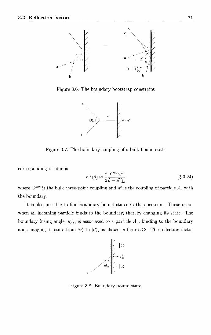
3.3. Reflection factors 71
c
c a
a
b b
Figure 3.6: The boundary bootstrap constraint
a / / /
c / ..,___ gc iU~a / / / /
a /
Figure 3. 7: The boundary coupling of a bulk bound state
corresponding residue is
Ka(e) ~ !_ caa.cg: 2 e- zUaa
(3.3.24)
where caac is the bulk three-point coupling and gc is the coupling of particle Ac with
the boundary.
It is also possible to find boundary bound states in the spectrum. These occur
when an incoming particle binds to the boundary, thereby changing its state. The
boundary fusing angle, u~a' is associated to a particle Aa, binding to the boundary
and changing its state from Ia) to 1;3), as shown in figure 3.8. The reflection factor
a
Figure 3.8: Boundary bound state

3.3. Reflection factors 72
R~ will have an associated pole at iu~a and around this pole it can be considered as
. fJ ao: Ro: (O) ~ '!_ 9ao:9 fJ
a 2() ·fJ - ZUo:a (3.3.25)
in terms of the boundary couplings shown in figure 3.8. This also has an associated
bootstrap condition, shown in figure 3.9, and given by
I a)
b / Ia)
a /
Figure 3.9: The boundary bound state bootstrap constraint
(3.3.26)
The difference in energy of these two boundary states can be written in terms of the
mass of particle a and the boundary fusing angle
(3.3.27)
These bootstrap constraints can be used to construct reflection factors, in much
the same way as the corresponding bulk constraints were used for the 8-matrix. As
suming that all the boundary states can be formed from the vacuum state by binding
a bulk particle to the boundary, once reflection factors for the vacuum boundary state
are known for all bulk particles they can be examined for evidence pointing to fur
ther boundary states. Reflection factors can then be constructed for these boundary
states using (3.3.26) which are then also searched. This is repeated until all poles are
accounted for without the need to introduce any more boundary states.
Some care must be taken here, just as in the bulk case, since not all poles will
correspond to boundary bound states. For example, reflection factors will, in gen
eral, contain simple poles which do not depend on any boundary parameter, although
one would expect boundary bound states to depend on the properties of the bound
ary. These poles must therefore be simple reflections off the boundary given by the
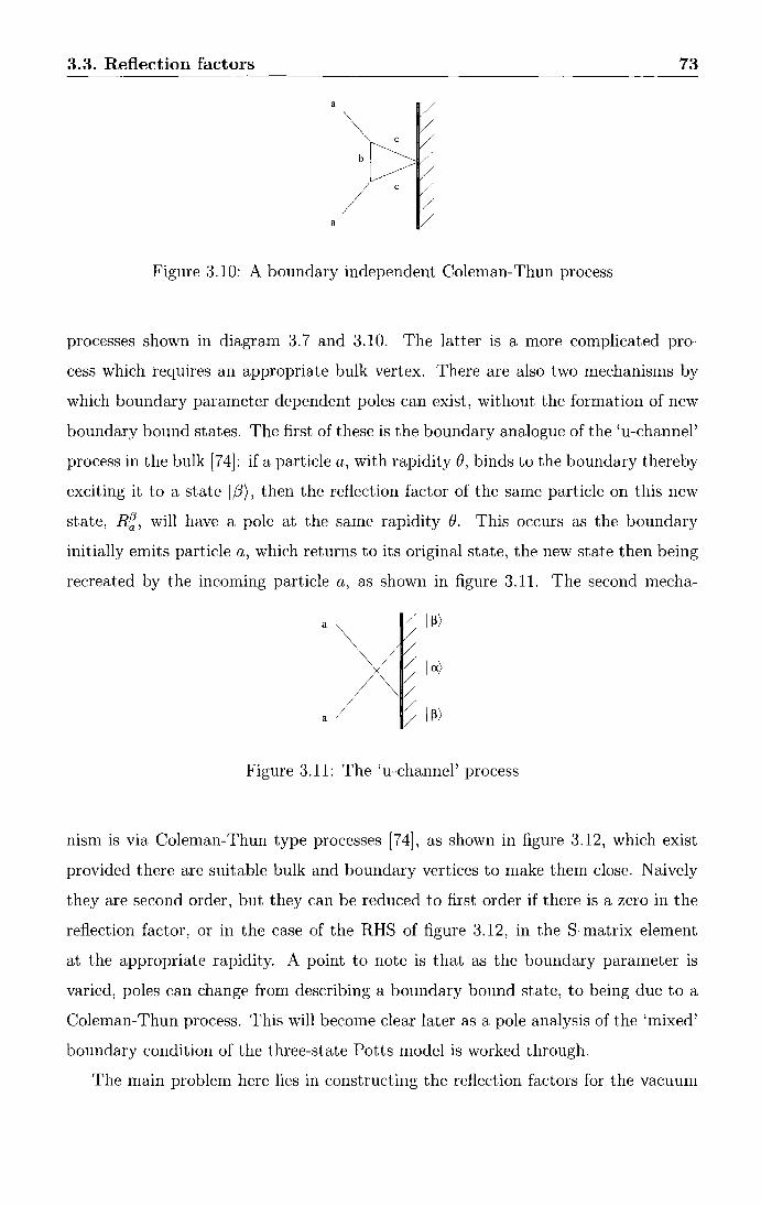
3.3. Reflection factors
a
a
/ /
Figure 3.10: A boundary independent Coleman-Thun process
73
processes shown in diagram 3.7 and 3.10. The latter is a more complicated pro
cess which requires an appropriate bulk vertex. There are also two mechanisms by
which boundary parameter dependent poles can exist, without the formation of new
boundary bound states. The first of these is the boundary analogue of the 'u-channel'
process in the bulk [7 4]: if a particle a, with rapidity e' binds to the boundary thereby
exciting it to a state 1,8), then the reflection factor of the same particle on this new
state, R~, will have a pole at the same rapidity e. This occurs as the boundary
initially emits particle a, which returns to its original state, the new state then being
recreated by the incoming particle a, as shown in figure 3.11. The second mecha-
a , I~>
/ Ia) / /
j I~>
Figure 3.11: The 'u-channel' process
nism is via Coleman-Thun type processes [7 4], as shown in figure 3.12, which exist
provided there are suitable bulk and boundary vertices to make them close. Naively
they are second order, but they can be reduced to first order if there is a zero in the
reflection factor, or in the case of the RHS of figure 3.12, in the S-matrix element
at the appropriate rapidity. A point to note is that as the boundary parameter is
varied, poles can change from describing a boundary bound state, to being due to a
Coleman-Thun process. This will become clear later as a pole analysis of the 'mixed'
boundary condition of the three-state Potts model is worked through.
The main problem here lies in constructing the reflection factors for the vacuum

3.4. Off-Critical g-function
/ / / /
/ /
Figure 3.12: Boundary dependent Coleman-Thun processes
74
boundary state since, for a given bulk S-matrix, there are infinitely-many distinct
sets of reflection factors consistent with these constraints, because any solution can
be multiplied by a solution of the bulk bootstrap, unitarity and crossing equations
to yield another solution [75]. To identify a set of reflection factors as physically
relevant some more information is needed. A common basis for the conjecturing
of bulk scattering amplitudes is a 'minimality hypothesis', that in the absence of
other requirements one should look for solutions of the constraints with the smallest
possible number of poles and zeros. This will be used later to construct a set of
reflection factors for the A, D, E related theories.
Of course, one still needs some way to test these reflection factors, to see if they
are physical and to match them with conformal boundary conditions in the UV limit.
In the bulk case, the S-matrices were matched to specific perturbed conformal field
theories using the TBA Cetr, so what is needed is a boundary analogue of this. An
obvious candidate for this is the g-function, defined by Affleck and Ludwig in [3]. An
off-critical version of this must therefore be constructed.
3.4 Off-Critical g-function
In a massive model, the g-function can be defined m a similar way to the CFT
version [76, 78, 4]. One starts with the partition function Z(ala) [ L, R] for the theory
on a finite cylinder of circumference L, length R and boundary conditions of type
o: at both ends. In the R-channel description, time runs along the length of the
cylinder, and the partition function is represented as a sum over an eigenbasis {l1h)}
of Hcirc(lvf, L), the Hamiltonian which propagates states along the cylinder:
00
Z(ala)[L, R] = ( o:l e-Rwirc(M,L) lo:) = L (QI~?(t))2 e-REI,irc(M,L). (3.4.1) k=O

3.4. Off-Critical g-function 75
Here l = NIL, M is the mass of the lightest particle in the theory, and
(3.4.2)
where Ia) is the (massive) boundary state [72] for the a boundary condition. At finite
values of l any possible infinite-volume vacuum degeneracy is lifted by tunnelling
effects, making the ground state 1'1/Jo) unique. This gives Z(o:lo:) the following leading
and next-to-leading behaviour in the large-R limit:
ln Z(o:lo:) [ L, RJ "' - RE8irc ( NI, L) + 2ln g1~? ( l) . (3.4.3)
It is the second, sub-leading term which characterises the massive g-function. Sub
tracting a linearly-growing piece - flo:)L, the g-function for the boundary condition
a at system size l is defined to be
(3.4.4)
The constant flo:) is equal to the constant (boundary) contribution to the ground
state energy E~trip ( R) of the £-channel Hamiltonian Hstrip ( R) = H(!j1;) ( R), which
propagates states living on a segment of length R and boundary conditions a at both
ends.
An alternative expression for g can be obtained by comparing (3.4.3) with the £
channel representation, a sum over the full set {E~trip(R)} of eigenvalues of Hstrip(R):
00
Z [L RJ = ~ e-LE~trip(M,R)
(o:lo:) ' ~ . (3.4.5) k=O
As R is sent to infinity, this gives the g-function:
lnglo)(l) ~ ~ 1~ [ln (~ e-LE:""IM,R)) + 2fln) L + REg;.c(M, L)l . (3.4.6)
In theories with only massive excitations in the bulk and no infinite-volume vac
uum degeneracy, ln 9io:) ( l) tends exponentially to zero at large l, while in the UV
limit l ---> 0 it reproduces the value of the g-function in the unperturbed boundary
conformal field theory.
In the CFT case, at this point the modular invariance of the partition function
was employed to solve for the g-function, however for massive theories this is not
available and instead the energy, E~trip ( 1\1, R), must be estimated using the particle
basis of states and thermodynamic Bethe Ansatz.

3.4. Off-Critical g-function 76
3.4.1 L-channel TBA
Consider the theory on a cylinder of length R and circumference L with boundary
conditions a and (3 at the ends. There are two TBA descriptions, the L-channel
and the R-channel. The first construction of the off-critical g-function was made,
in [76] (making use of results from [77]), using the L-channel TBA which will now
be described. Taking time evolution along the circumference of length L the Hilbert
space is constructed along the finite length R. In the limit R-----+ oo, the Hilbert space
in this description is given by scattering states and the construction of the TBA
equation and minimisation of the free energy is analogous to the case with periodic
boundary conditions described in section 2.5. The main difference here is that in the
largeR limit, the partition function has a boundary contribution from the g-function,
as shown in (3.4.3), so the TBA method results in an expression for this g-function.
The details of this calculation are presented below.
Assume for convenience that the theory has N particles, all of the same type,
and take them to be sufficiently well spaced to be considered asymptotic. Analogous
to the TBA on the torus, discussed in section 2.5, when one particle moves towards
another, interacts with it and moves past until it can again be taken to be asymptotic,
the wavefunction picks up a factor of the S-matrix. If this particle moves to the
right, bounces off the boundary, where the wavefunction picks up a factor of R(O),
and returns to its original position the resulting wavefunction should be equal to
that obtained when the same particle performs the same operation to the left. This
equality imposes the quantisation condition
ei!IIRsinh(O;) (.IT _S(Oi _OJ)) Rf3(0i) = e-iMRsinh(O;) (.IT. S(-Oi _OJ)) ROi(-Oi)· J=l,rf.z J=l,Jf.z
(3.4. 7)
By unitarity, s- 1(0) = S( -0) and R- 1 (0) = R( -0) so this condition can be rewritten
as
e2iMRsinh(O;) (. ft . S(Oi _ Oj)S(Oi + Oj)) R(3(0i)ROi(Oi) = 1 J=l,Jf.z
with Oi > 0. Taking the logarithm of this
(3.4.8)
(3.4.9)
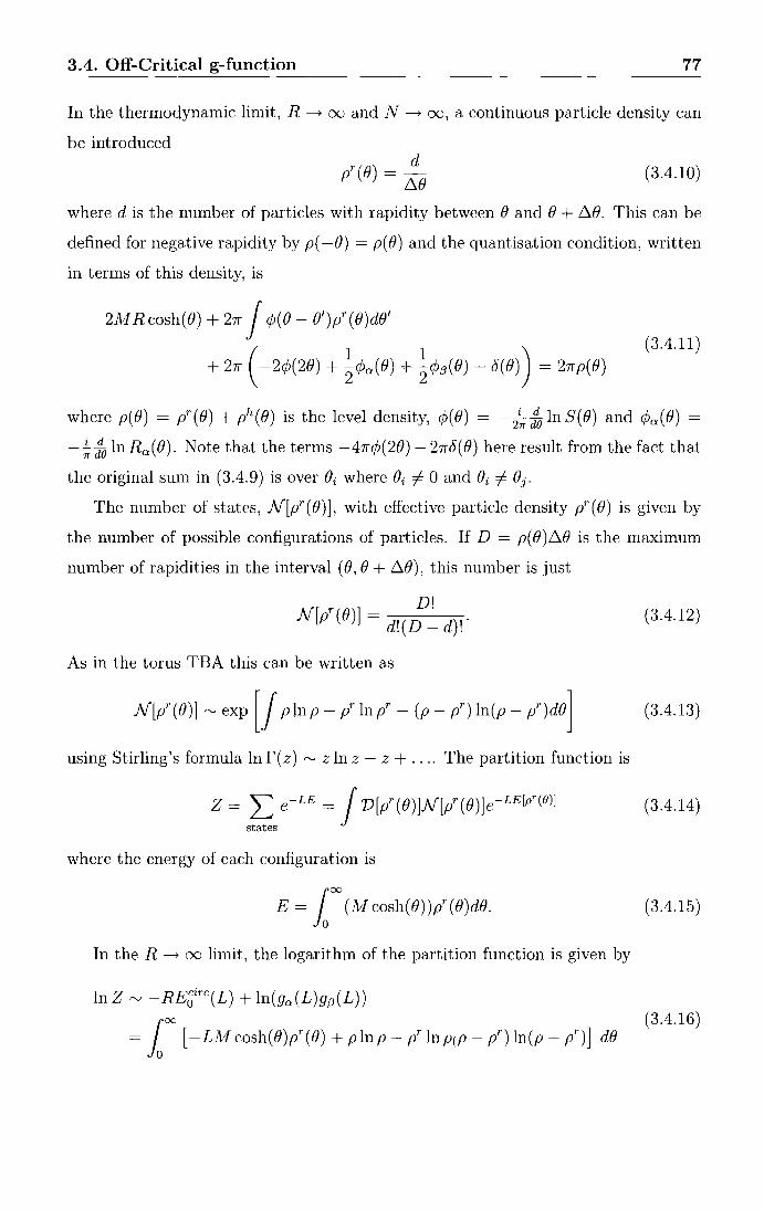
3.4. Off-Critical g-function 77
In the thermodynamic limit, R----? oo and N ----? oo, a continuous particle density can
be introduced
(3.4.10)
where dis the number of particles with rapidity between e and e + t:1e. This can be
defined for negative rapidity by p( -e) = p( e) and the quantisation condition, written
in terms of this density, is
2A1Rcosh(e) + 2n j cp(e- e')pr(e)de'
+ 2n ( -2¢(2e) + tc/Ja(e) + tc/J~(e)- b(e)) = 2np(e) (3.4.11)
where p(e) = pr(e) + ph(e) is the level density, cp(e) = - 2~J0 lnS(e) and c/Ja(e) = -* J0 ln Ra(e). Note that the terms -4n¢(2e)- 2nb(e) here result from the fact that
the original sum in (3.4.9) is over ei where ei =I 0 and ei =I ej.
The number of states, N[pr (e)], with effective particle density pr (e) is given by
the number of possible configurations of particles. If D = p(e)L:1e is the maximum
number of rapidities in the interval ( e' e + £1())' this number is just
(3.4.12)
As in the torus TBA this can be written as
(3.4.13)
using Stirling's formula ln r( z) "' z ln z - z + .... The partition function is
Z = L e-LE = j V[pr(e)]N[pr(e)]e-LE[pr(o)] states
(3.4.14)
where the energy of each configuration is
(3.4.15)
In the R ----? oo limit, the logarithm of the partition function is given by
lnZ"' -REgirc(L) + ln(ga(L)g~(L))
= loa [-L.M cosh( e)pr (e) + p ln p- pr ln P(P- pr) ln(p- p'') J de (3.4.16)

3.4. Off-Critical g-function 78
and this can be minimised, subject to the constraint from (3.4.11), in the same way
as the log of the torus partition function (2.5.15) was treated in section 2.5. First the
TBA equation is found by setting c5(3.4.16)/c5pr(B) = 0 where
(3.4.17)
Notice that the integrand of (3.4.16) is the same as that in (2.5.15), and the con
straint (3.4.11) differs from (2.5.10) by terms independent of pr(B) therefore the TBA
equation here is exactly that of the periodic boundary case
c:(O) = M L cosh( B)- J ¢(0- 0') ln(1 + e-E(O'l) dO' (3.4.18)
where the pseudoenergies are defined by pr (B)/ (p( B) - pr (B)) = e-E(O), as before. The
difference in this case comes when simplifying the integrand, I, of (3.4.16) using this
TBA equation. Writing the integrand in terms of the pseudoenergies:
(3.4.19)
and replacing p( B) here with the constraint ( 3.4.11) gives
1 I=- M L cosh(O)pr(B) + -M R cosh( B) ln(1 + e-E(Ol)
7f
+ J ¢(0- B')p1'(0') dO' ln(1 + e-E(O)) (3.4.20)
+ (~¢a(B) + ~¢~(0)- 2¢(20)- c5(0)) ln(1 + e-E(O)) + pr(O)c:(O).
Using the TBA equation then results in
-JV!Rcosh(B)- 2¢(20) + -¢0 (0) + -¢~(0)- c5(0) ln(1 + e-E(O)) dO. 100
( 1 1 1 ) 0 7f 2 2
(3.4.21)
Once the range of 0 is extended by symmetry, the ground state energy, without the
bulk contribution is given by
(3.4.22)
which is the usual result from the TBA on a torus, and the off-critical g-function is
(3.4.23)

3.4. Off-Critical g-function 79
This result can be extended to a theory with N particle species where
1 N r ln 9a(l) = 4 L }Ill dB 8a(B) ln(1 + e-Ea(lil),
a=l IR
(3.4.24)
8a(B) = (<P~a)(B)- 2¢aa(2B)- b(B)) and now <P~a) = --;Je lnR~a)(B) and cPaa(B) = i d
- 2tr 7i ln sa a (e) .
This was tested extensively for the Yang-Lee model (introduced below) in [79]
using conformal perturbation theory (CPT) and the boundary truncated conformal
space approach (BTCSA). It was shown that for non-zero M, the /~dependence of
(3.4.24) is incorrect, both in the total change in 9a(l) between the UV and IR, and
in the behaviour of the small-/ series expansion. However, the dependence of 9a(l)
on boundary parameters at fixed l, and the ratios of the g functions, 9a(l)fgf3(l)
are in good agreement with the CPT and BTCSA results. The formula for 9a(l),
given in (3.4.24), should therefore be modified by adding some boundary condition
independent terms.
Possible sources of error in this construction of the g-function could be the saddle
point evaluation of the partition function, or corrections from the next-to-leading
term in Stirling's formula [79]. These problems will also exist in the calculation of
the effective central charge, however as this is a leading order term, as opposed to the
next-to-leading order g, the resulting errors are no larger than the numerical errors
in the CPT and TCSA.
One might also think that problems with this equation ought to occur with the
presence of boundary bound states in the spectrum. This was examined in [79], again
for the Yang-Lee model. This is the nonunitary minimal model M 2,5 with central
charge c = -22/5. It has two primary fields ]_ and <p with conformal dimensions
hn = 0 and h'P = -1/5 respectively, and two conformal boundary conditions: ]_ with
no relevant boundary fields and <I> with one relevant boundary field ¢. The bulk
spectrum contains a single particle, with two particle S-matrix [80]
sinh(~ + inx) (x) = 2 6
· h(li inx) · sm 2-6 S(B) = -(1)(2) (3.4.25)
The reflection factors corresponding to the boundary conditions <I>(J.L) (where 1-l is the
boundary coupling) and ]_ are [78]
(3.4.26)
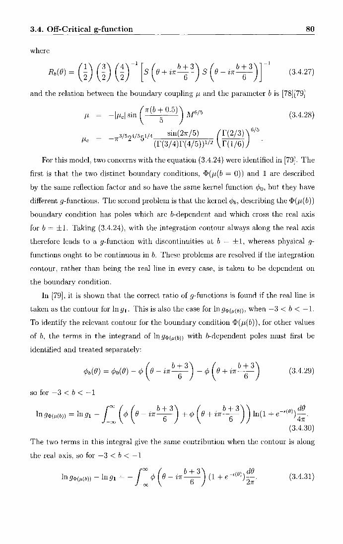
3.4. Off-Critical g-function 80
where
R.(B) ~ m m Gf [s (o +i1rb;3
) s (o- inb; 3
) r (3.4.27)
and the relation between the boundary coupling J-L and the parameter b is [78] [79]
J-L = -IJ-Lcl sin ( 7r(b ~ 0.5)) ]V[6/5 (3.4.28)
-7r3/524/5 1/4 sin(27r/5) (r(2/3)) 6/5 J-Lc = 5
(f(3/4)f(4/5))1/2 r(1/6)
For this model, two concerns with the equation (3.4.24) were identified in [79]. The
first is that the two distinct boundary conditions, ip(J-L( b = 0)) and ]_ are described
by the same reflection factor and so have the same kernel function ¢0 , but they have
different g-functions. The second problem is that the kernel ¢b, describing the ip(J-L( b))
boundary condition has poles which are b-dependent and which cross the real axis
for b = ±1. Taking (3.4.24), with the integration contour always along the real axis
therefore leads to a g-function with discontinuities at b = ±1, whereas physical g
functions ought to be continuous in b. These problems are resolved if the integration
contour, rather than being the real line in every case, is taken to be dependent on
the boundary condition.
In [79], it is shown that the correct ratio of g-functions is found if the real line is
taken as the contour for ln 9ll· This is also the case for ln 9<I>(M(b)), when -3 < b < -1.
To identify the relevant contour for the boundary condition ip(J-L(b)), for other values
of b, the terms in the integrand of ln 9<I>(M(b)) with b-dependent poles must first be
identified and treated separately:
( . b + 3) ( . b + 3) c/Jb(O) = c/Jo(B) - ¢ ()- m-
6- - ¢ () + m-
6- (3.4.29)
so for -3 < b < -1
100
( ( b + 3) ( b + 3) ) EO d() lng<l>(J.l(b)) = lngll- -oo ¢ ()- i1r-6
- + ¢ () + i1r-6
- ln(l + e- ( l) 4
7r.
(3.4.30)
The two terms in this integral give the same contribution when the contour is along
the real axis, so for -3 < b < -1
100
( . b + 3) -<(0) d() ln 9<I>(M(b)) - ln 9ll = - ¢ ()- l7r-- (1 + e )-. -oo 6 27r
(3.4.31)

3.4. Off-Critical g-function 81
NOW ¢( e - in b!3) has poles at
b-5 e = in-6- + 2nni b-l ' e = in-6- + 2nni (3.4.32)
b+1 e = in-6- + 2nni b+5 e = in-6- + 2nni
so when b passes through -1, the contour must deform away from the real axis and
encircle the pole at in(b + 1)/6. This pole is then called 'active'. The same then
happens as b passes through 1, when the pole at in(b- 1)/6 becomes 'active'. This
is shown in figure 3.13, taken from [79].
0 .. , 8== JrrT
(J ,_, 8::::: u 15
X 8= lftb~l
Figure 3.13: The contour for lngq,(J.l(b)), from [79]
In [4], a new expression for the g function was proposed and tested for the Lee
Yang case. The construction avoids the use of the saddle point approximation by
employing an n-particle cluster expansion technique. Before this is discussed, it is
necessary to introduce the R-channel TBA [76] as this will be used later on.
3.4.2 R-channel TBA
Taking time along the length, R, of the cylinder the partition function is
(3.4.33)
where H is the Hamiltonian of the bulk system. The boundary states can be written
as [72]
(3.4.34)
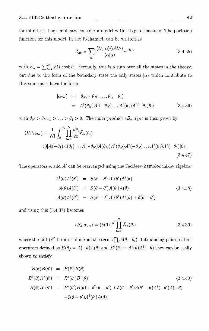
3.4. Off-Critical g-function 82
for infinite L. For simplicity, consider a model with 1 type of particle. The partition
function for this model, in the R-channel, can be written as
(3.4.35)
with Ea = 2..:;:1 2/vf cosh ()i· Formally, this is a sum over all the states in the theory,
but due to the form of the boundary state the only states Ia) which contribute to
this sum must have the form
la2N) = jeN,-eN,···,e1,-e1)
At(eN)At(-eN) ... At(ei)At(-ei)jo) (3.4.36)
with ()N > ()N-1 > ... > ()1 > 0. The inner product (Bala2N) is then given by
1 roo N d()i ~ (Bala2N) = N! Jo IT 271" Ka(()i)
t=l
(OIA( -ei)A(e1) ... A( -eN )A( eN )At (eN )At (-eN) ... At ( ei)A t ( -ei) IO).
(3.4.37)
The operators A and At can be rearranged using the Faddeev-Zamolodchikov algebra:
At (e) At ( ()')
A( e)A( ()')
S( e - ()')At ( e')A t (e)
- S( () - ()')A( ()')A( e) (3.4.38)
and using this (3.4.37) becomes
N
(Bala2N) = (b(O))NII Ka(ei) (3.4.39) i=l
where the ( b(O) )N term results from the terms nib(()- ()i)· Introducing pair creation
operators defined as B(e) = A(-e)A(e) and Bt(e) = At(e)At(-e) they can be easily
shown to satisfy
B(e)B(e')
Bt(())Bt(e')
B(e)Bt (e')
B( ()') B ( ())
Bt(e')Bt(e) (3.4.40)
Bt(e')B(e) +£52 (()-()')+ b(B- B')S(B'- e)At(-e')A(-0)
+b(e- e')At(e')A(e).

3.4. Off-Critical g-function 83
The norm (o:2Nio:2N) can be written in terms of these pair operators
(o:2Nio:2N) = (OIA( -OI)A(OI) ... At(OI)At( -OI)IO)
= (OIB(OI)B(02) ... Bt(o2)Bt(OI)IO) (3.4.41)
and using the algebra above this becomes
(3.4.42)
Therefore the partition function is simply
N
Zab = L II Ka(Oi)Kb(Oi)e-RL~J2Mcosh(O;)_ (3.4.43) Q i=l
Following the method described earlier, the density of pairs of particles is intro
duced, pr(O) = d/ ~0, where dis now the number of pairs of particles with rapidity
in the interval ( 0, 0 + ~0). In terms of this density, the energy becomes an integral:
(3.4.44)
and the partition function is
Zab = J D[pr(O)J exp (1oo [ln(Ka(O)Kb(O))- 2RM cosh(O)] pr(O)dO + S(pr))
(3.4.45)
where S is the entropy of the particle configuration described by the distribution
pr(O), as above.
The momenta are constrained by the quantisation condition on the states lo:2N):
eiMLsinh(li;)S(20i) II S(Oi- Oj)S(Oi + Oj) = 1.
#i
(3.4.46)
This is exactly the same as the quantisation condition found in the periodic case
when each particle of rapidity 0 is accompanied by another with rapidity -0. Taking
logs of this, introducing the level density p = pr + ph, and differentiating gives
21rp = 111 Lcosh(O)- 27f 100
(¢(0- 0') + ¢(0 + 0')) pr(e')de' (3.4.47)
with ¢(e) = - 2~i Jo ln S (e). For large L, the logarithm of the partition function is
ln Zab ~ - LE~trip ( R)
= 100
(ln(Ka(O)Kb(e))- 2RM cosh(e)) pr(e) + S(pr). (3.4.48)
3.4. Off-Critical g-function 84
The TBA equation can be found, using the same method as described earlier: set
5(3.4.48)jc5pr(e) = 0 where
5(3.4.48) = 8(3.4.48) + J 5p(B') 8(3.4.48) dB' 5pr (e) 8pr (e) 5pr ( 0') 8p( 0') .
(3.4.49)
Now from the constraint (3.4.47) it is clear that
(3.4.50)
and the derivative of (3.4.48) with respect to the level density is the same as for the
previous cases 8(3.4.48) =I (1 -E(fJ))
8p(B) n + e ' (3.4.51)
but the derivative with respect to the root density is different
(3.4.52)
which leads to a TBA equation which is different to the £-channel and periodic
boundary condition cases:
E(B) =2Rlvf cosh( B) -ln(Ka(B)Kb(B))
+ 100
(¢(0- e')¢(0 + e')) ln(1 + e-f(fJ')) de'. (3.4.53)
Writing the integrand of (3.4.48), denoted I, in terms of the pseudoenergies gives
and replacing p, using the constraint (3.4.47), leads to
I =(ln(KaKb)- 2RA1cosh(B))pr(e) + 2_A1Lcosh(B)ln(1 + e-E(fJ)) 27r
+ 1oo (¢(0- 0') + ¢(0 + 0')) pr(B') ln(l + e-f(fJ)) dB'+ pr(B)E(B).
Then, with the TBA equation (3.4.53), this simplifies to give
1 I= -A;J Lcosh(B) ln(1 + e-E(fJ)).
27r
(3.4.55)
(3.4.56)
Since K(B) = K( -B), the term Ka(B)Kb(B) is even in e so the domain of the
definition of E( e) can be extended to the whole real axis by E( -e) = E( e). This can

3.4. Off-Critical g-function 85
also be extended to a theory with N particle types, for which the ground state energy
on an interval of length R is
N
E~trip(M, R) = - L 1 d() Ma. cosh(B)La.(B) + £111~ R +fa+ ff3 a.=l IR 4n
(3.4.57)
where £111f R is the bulk contribution to the energy, fa, ff3 are R-independent con
tributions to the energy from the boundaries and La.(B) = ln(1 + e-Ea(0l). The TBA
equation for this theory, written in terms of the reflection factors is
Ea.(B) =2Ma.R cosh(B) -ln ( R~a.) (i% - ()) R~a.) (i% + ()))
N
- L 1 d()'¢a.b(()- ()')Lb(B'). b=l IR
(3.4.58)
In [78], generalisations of these equations are shown to govern the excited state
energies E~trip (!vi, R). The idea is to use analytic continuation to move between
energy levels [81]. In [78], rather than derive the results using the method of [81], the
formulae are conjectured and then checked using the boundary truncated conformal
space approach (BTCSA). In the largeR limit these generalisations reduce to simple
forms. If the nth excited state is made up of rn = 2::=1 rn(a.) particles, rn(a.) being the
number of particles of type a, then
N m(a)
E~trip(lvi, R)- E~trip(M, R) = L L !via cosh(Bia.)) + O(e-RM). a.=l i=l
The rapidities, eia.), satisfy the Bethe ansatz equations
2nn;a.) = 2111a.Rsinh(eia.))- iln(R~a.l(e}a.l)R~a.l(eia.))) N
- LLiln(-Sa.b(e}a.l +Bjbl)) b=l j#i
N
- LLiln(-Sa.b(e}a.l -e)bl)). b=l j#i
(3.4.59)
(3.4.60)
These equations are used in [4] to find an exact IR expansion of the g-function, by
employing a cluster expansion. This will be briefly discussed below for a theory with
only a single particle type.

3.4. Off-Critical g-function 86
3.4.3 Cluster Expansion
In the R -----+ oo limit, the g-function, given in (3.406), becomes
2ln 9a(l) = RE~irc + 2faL - LEgtrip + ln (1 + f e-L(E~trip_E~trip)) + 0( e-Rl\I) k=l
(3.4061)
and since, for R » L » 0, Egtrip = £1112 R + 2fa + O(e-RM), the g-function, to
leading order is
2ln 9a(l) rv R(E~irc- £1112 L) + ln (1 + f e-L(E~trip_E~trip)) k=l
(304062)
The cluster expansion involves letting L-----+ oo, along with R-----+ oo, so that the right
hand side of (3.4062) can be expanded in terms of 1, 2,0 0 0 particle contributions, each
of which can be estimated using the Bethe ansatz approximated levels in (3.4059) and
(3.4060)0 The hope is then to resum this expansion to give an exact expression for
the g-functiono
Taking the large-R equation (3.4062) and truncating at the one-particle level leaves
2lnga rv R(E~irc- £lvf 2 L) + ln (1 + L e-lcosh(Ol(nl)))
rq>O
(3.4063)
and the one-particle Bethe ansatz is essentially that of a free particle
(304064)
In the large-R limit, there is a continuum of possible rapidities so the Bethe ansatz
becomes
~:1 ( 111 R cosh(01 ) - i d~ ln Ra(Ol)) = 1.
The sum in (3.4063) becomes an integral
L e-lcosh(Ol) = ~ ( f e-lcosh(Ol) - e-l)
n1>0 n1=-oo
-----+ ~ f dO (J(ll(e) _ b(O))e-lcosh(8) 2 JJR
(3.4065)
(3.4066)
with the Jacobian, j(ll(e), for the change of variables nl -----+ el = e, from (304065),
being 111R
J(ll(e) = -cosh( e)+ c/Ja(e) 7f
(3.4°67)

3.4. Off-Critical g-function 87
where c/Jo. = - :;i: :fo ln R0 . The cosh term here cancels with the leading order part of
R(E0irc- £M2L), so the one-particle contribution to lng is
2lng =! f dO (c/Jo. _ 6(0))e-tcosh(e). 2 JJR
(3.4.68)
This disagrees with the large-l behaviour of (3.4.24), in particular, there is no ¢(20)
term. However, the hope is that it gives an indication of how to modify the previous
result (3.4.24). The assumption is that the final result will depend, like (3.4.24),
on the single-particle energies only through the TBA pseudoenergies E(O). The first
observation to make, therefore, is that the large-l asymptotic of (3.4.68) also emerges
from
(3.4.69)
which is the resummed, or 'dressed' version of (3.4.68). Numerically, in [4], it is shown
that (3.4.69) is more accurate than (3.4.68) and this is because it actually contains,
not just one-particle contributions, but n > 1 particle contributions also.
The next step is to consider the two-particle contributions. Some of these will be
taken care of by the one-particle resummation, but there are some new terms:
2lng0 =2[lng0]~) + ti
2
d0 1d0 2 cp(0 1 +02)¢(01 - o2)e-lcosh(OI)-Icosh(Oz)
_! { d0¢(20)e-2lcosh(e). 2 JJR
This can then be resummed as
and the final result is given by 2ln go. = 2[ln go.]~) + 2[1n go.]~) + ....
(3.4. 70)
(3.4.71)
The observation made in [4] is that if the first few terms are corrected with
e -I cosh( e) ----t 1 1 + eE(O)
(3.4. 72)
then the only contribution from the next order is of the form
(3.4.73) X e-lcosh(OI) ... e-lcosh(On)

3.4. Off-Critical g-function 88
along with an additional term containing a single integration over ¢(28). The final
conjecture is then to replace l cosh(8) with t:(8) and resum as
1 d8¢(28) ( -~e-2/cosh(O))----> -1 d8¢(28) (ln(1 + e-E(O))-1 +
1eE(O)) (3.4.74)
which leads to the final result
2lngn(l) =~ { d8(¢n(8)- 6(8)- 2¢(28))1n(1 + e-dOl) 2 1&.
~ 1 r d81 d8n + ~ -:;;, }&.n 1 + eE(OJ) ... 1 + eE(On)
(3.4. 75)
with 8n+ 1 = 81. This conjecture was tested numerically for the case of the Lee-Yang
model in [4] and also extended to the purely elastic scattering theories with N particle
species, for which the exact g-function is proposed to be
X rPa1a2(81 + 82)rPa2a3(82- 83) · · · rPanan+! (8n- 8n+d
where 8n+l = 81 and an+l = a1.
(3.4.76)
The derivation of this conjecture avoided some of the problems that could afflict
a more direct calculation, for example, in working in the limit l ---+ oo, the particles
are always well separated so the accuracy of the Bethe ansatz is not in question.
However, a direct approach would be desirable, especially for the generalisation to
more complicated models. There has been an attempt at this by Woynarovich, [82],
who proposed an expression for the 0(1) corrections to the free energy for a one
dimensional Bose gas with repulsive 6-function interaction, obtained by calculating
corrections to the standard saddle point result. Although his expression has some
of the features of the result here there are important differences. In particular, for
the field theory case, the result in [82] is divergent in the UV limit so it cannot be
consistent with the g-function of a CFT. The direct construction of the g-function
therefore remains an open problem.
In [4], only the conjecture (3.4.75) has been tested for the Lee-Yang model, so the
aim of the next chapter is to test the generalisation of this, (3.4.76), for a variety of
purely elastic scattering theories. This work has been published in [1].
Chapter 4
ADET cases
In this chapter the investigations of [4] are extended to a collection of theories for
which boundary UV /IR relations have yet to be found, namely the minimal purely
elastic scattering theories associated with the ADET series of diagrams [83, 32, 84,
85, 86, 87, 88]. The bulk S-matrices of these models have long been known, but less
progress has been made in associating solutions of the boundary bootstrap equations
with specific perturbed boundary conditions. A collection of minimal reflection fac
tors for the ADET theories are presented, and then tested by checking the g-function
flows that they imply. It is also shown how these reflection factors can be modified
to incorporate a free parameter, which generalises a structure previously observed in
the Lee-Yang model [78]. This enables the prediction of a number of new flows to be
made between conformal boundary conditions.
4.1 The ADET family of purely elastic scattering
theories
The purely elastic scattering theories that are treated in this chapter fall into two
classes. The first class associates an S-matrix to each simply-laced Lie algebra g, of
type A, D or E [83, 32, 84, 85]. These S-matrices are minimal, in that they have no
zeros on the physical strip 0 :=::; 2Jm e :=::; 1r, and one-particle unitary, in that all on
shell three-point couplings, as inferred from the residues of forward-channelS-matrix
poles, are real. They describe particle scattering in the perturbations of the coset
conformal field theories g1 x gifg2 by their (1, 1, ad) operators, where g is the affine
89

4.1. The ADET family of purely elastic scattering theories 90
algebra associated with g . More will be said about affine Lie algebras and coset
models below. The unperturbed theories have central charge
2T g
c = (h + 2) ' (4.1.1)
where T 9 is the rank of g, and h is its Coxeter number. These UV central charges can
be recovered directly from the S-matrices, using the thermodynamic Bethe ansatz [30,
32] as described in section 2.5. Some of these theories are also perturbed Virasoro
minimal models. These are listed in table 4.1 along with the corresponding critical
statistical model and relevant perturbing operator.
g Minimal Model Statistical Model Perturbing Operator Conformal weight
c/Jr,s hrs '
A2 M5,6 Three-state Potts ¢21 2/5
energy density
E6 M6,7 Tricritical ¢12 3/8
three-state Potts thermal operator
E1 M4,5 Tricritical Ising ¢12 1/10
energy operator
Es M3,4 Ising ¢13 1/2
magnetic field
Table 4.1: Perturbed minimal models described by perturbations of the coset theories
lJ1 X gJ/g2
The ADE S-matrices describe the diagonal scattering of T 9 particle types, whose
masses together form the Perron-Frobenius eigenvector of the Cartan matrix of g.
This allows the particles to be attached to the nodes of the Dynkin diagram of
g. Each S-matrix element can be conveniently written as a product of elementary
blocks [83]
as
{x}=(x-1)(x+1), sinh (f!. + i1rx)
(x) = 2 2h · h ((} i1rX) sm 2 - 2h
Sab = IT {x}, xEAab
( 4.1.2)
(4.1.3)

4.2. Affine Lie algebras and their role in Conformal Field Theories 91
for some index set Aab· Note that
(0)=1, (h)=-1, (-x)=(x)-1, (x±2h)=(x). (4.1.4)
The notation (4.1.2) has been arranged so that the numbers x are all integers. The
sets Aab are tabulated in [83]; a universal formula expressing them in geometrical
terms was found in [85], and is further discussed in [86, 87].
The S-matrices of the second class [89, 80, 90] are labelled by extending the set
of ADE Dynkin diagrams to include the 'tadpole' Tr. They encode the diagonal
scattering of r particle types, and can be written in terms of the blocks (4.1.2) with
h = 2r+1 [91]: a+b-1
Sab = II {l}{h -l}. l=la-bl+l
step 2
(4.1.5)
These S-matrix elements are again minimal, but they are not one-particle unitary,
reflecting the fact that they describe perturbations of the non-unitary minimal models
M 2,2r+3 , with central charge c = -2T(6r + 5)/(2r + 3). The perturbing operator this
time is ¢ 13 . The Tr S-matrices are quantum group reductions of the sine-Gordon
model at coupling /32 = 167r / (2T+3) [89], a fact that will be relevant later.
A self-contained classification of minimal purely elastic S-matrices is still lacking,
but the results of [88] single out the ADET theories as the only examples having
TBA systems for which all pseudoenergies remain finite in the ultraviolet limit.
The ADET diagrams are shown in figure 4.1, with nodes giving the conventions
employed here for labelling the particles in each theory. For the Dr theories, particles
r-1 and rare sometimes labelled sands', or sands, for r even or odd respectively.
4.2 Affine Lie algebras and their role in Conformal
Field Theories
Before the reflection factors for the AD ET theories are presented it is useful to
digress slightly and discuss CFTs with associated affine Lie algebras g. This serves,
not only to understand the role of these infinite algebras, but also to introduce some
formulae for the modular S matrices, which will be of use later in calculating the

4.2. Affine Lie algebras and their role in Conformal Field Theories 92
... .... ---r I
(a): Ar
2
• • I • • 1 4 I
(d):E6
e • • . .. . <r-1 I r r
(b): Dr
• • • I • • 6
(e): E 1
• • • . . . . e::::J 2 3
(c): Tr
4
• • • • I • • ~ (!
(f): Es
Figure 4. 1: Dynkin diagrams for the AD ET Lie algebras
crit ical (CFT) g-functions for the ADE related theories. The discussion presented
here follows closely that found in chapters 14-18 of DiFrancesco et al. [5] and in the
review by Goddard and Olive [92]. See also the book by Kac [93] for more information.
4.2.1 Affine Lie algebras
Consider the generalisation of a Lie algebra g, with generators Ja , where elements of
the algebra are also Laurent polynomials in some variable t. Denote the set of such
polynomials by C[t, C 1]. This generalisation is called the loop algebra
(4 .2 .1)
generated by J~ = Ja 0 tn; the generators satisfy the commutation relations
[J~ , J~] = L ij~b J~+m · (4.2 .2) c
A central extension of this algebra is obtained by adding a term of the form L i dc:!:niki
where [J~ , ki] = 0. The constants d~ni are constrained by the J acobi ident ity, and
in a basis where the structure constants f~b are totally ant isymmetric, all bar one of
the central terms can be removed by a redefinition of the generators. The extended
algebra is t hen
(4.2.3) c
A convenient basis for the finite-dimensional Lie algebra g consists of a set of
mutually commuting generators, H&, i = 1, ... , r 9 , of the Cartan subalgebra, along
with particular combinations of the generators Ja, denoted Ea , that satisfy
( 4.2.4)

4.2. Affine Lie algebras and their role in Conformal Field Theories 93
The vector a = ( oJ, ... , oh) is called a root and g::x is the corresponding step op
erator. The root components are the non-zero eigenvalues of the H& in a particular
representation, called the adjoint,where the Lie algebra itself serves as the vector
space on which the generators act.
To construct a basis for the extended algebra, following the lines above, one must
first construct the analogue of the Cartan subalgebra (CSA) of the finite Lie algebra.
Starting with this CSA, H~ of g, the central element k can then be added giving an
( r + 1 )-dimensional Abelian subalgebra. In the adjoint representation
ad(H~)E~
ad(k)E~ [k,E~] = 0,
(4.2.5)
(4.2.6)
so each of the roots ( o:l, ... , o:rg, 0) = (a, 0) is infinitely degenerate. To cure this
problem, an extra element La = -tft can be added to the algebra g to distinguish
between the E:;: for different n. This satisfies the commutation relations [La, J~] =
-nJ~, [La, k] = 0. The resulting algebra
( 4.2. 7)
is an affine Lie algebra (also known as a Kac-Moody algebra). The usual basis is
given by the generators of the CSA, fi == {HJ, ... , H~9 , k, La}, along with the step
operators E:;: and H; which correspond to the roots a and nt5 respectively.
The next step is to find an analogue in g of the invariant scalar product, or Killing
form, on g. This must be symmetric and satisfy
([Z, X], Y) + (X, [Z, Y]) = 0, X, Y, Z E g (4.2.8)
which constrains the inner products, up to an overall constant, to be
b b ~ ~ ~
(J~, Jm) = ba bn+m,a, (J~, k) = 0, (k, k) = 0
(J~, La)= 0, (La, k) = -1. (4.2.9)
The only unspecified norm is (La, La) which is often chosen to be zero.
For an arbitrary representation, it is always possible to find a basis, {I~)}, of
simultaneous eigenvectors of the CSA such that
( 4.2.10)
4.2. Affine Lie algebras and their role in Conformal Field Theories 94
~
The vector A of simultaneous eigenvalues is known as an affine weight
............ -- 1 ............ -- ........... A= (,\(H0 ), ... , ,\(H~); ,\(k); ,\( -L0 ))
(4.2.11) = (A;k_x;n)
where A is a weight of g. The weights live in a space dual to the CSA and this can
be encoded using the Killing form: for each element X(H) in the dual space, there
must be an element H.x in the CSA, such that
X( H) = (H.x, H). ( 4.2.12)
The scalar product of two weights is then induced by the Killing form
( 4.2.13)
As in the finite-dimensional case, weights in the adjoint representation are called
roots. Since k commutes with all the generators of g, its eigenvalue on the states of
the adjoint representation is zero. The affine roots, associated with the generators
E;: are therefore
n = (a; 0; n) , n E 12 , a E ~ ( 4.2.14)
where ~ denotes the set of all roots of g. This has the same scalar product as the
finite case: (n, ,6) =(a, j3). The roots associated to H~ are
nl5 = (0; 0; n), n E 12, n =/= 0. (4.2.15)
These have length ( nl5, nt5) = 0 and each one is orthogonal to all other roots so they
are often called imaginary roots, whereas ( 4.2.14) are known as the real roots.
A basis of simple roots must now be identified, in which the expansion coefficients
of any root are either all non-negative or all non-positive. This basis contains the r
finite simple roots ai of g along with one extra simple root
no= ( -,P; 0; 1) ( 4.2.16)
where ,Pis the highest root of g, from which all roots of g can be obtained by repeated
subtraction of simple roots. A positive root is then given by
(a;O;n) > Oifn > 0, or ifn = 0 and a E ~+' (4.2.17)

4.2. Affine Lie algebras and their role in Conformal Field Theories 95
where .6.+ is the set of positive roots of g. The condition, n > 0 and a E .6., for a
positive root is not immediately obvious but by rearranging
a+ nl5 = na0 + (n- 1)1/J + (,P +a) (4.2.18)
the expansion coefficients of the final two factors in terms of finite simple roots are
non-negative. Given a set of affine simple roots and a scalar product, the extended
Cartan matrix is defined in terms of the roots ai and coroots OJ-= 2nJ/InJ 12
cij = (ai, Oj -)' 0::; i,j:::; Tg
2(ai, aj) laj12
(4.2.19)
From this definition it is clear that C is formed from the Cartan matrix C of g
by the addition of an extra row and column given by (a0 , a 0-) = l'l/JI 2 = 2 and
(a0 ,aJ-) = -('ljJ,aJ-)· Note that the expansion coefficients of 'ljJ, when written
in a basis of simple roots, or coroots of g, are known as marks ai and comarks ai
respectively, so -(1/J, aJ -) = - 2::~! 1 ai(ai, aj -). All the information contained in the
extended Cartan matrix can be encoded in the extended Dynkin diagram. This can
be obtained from the Dynkin diagram of g by adding an extra node corresponding to ~ ~
a 0 joined to the other nodes by C0iCw lines. The extended Dynkin diagrams for the
ADE theories are shown in figure 4.2. The nodes are labelled by the ordering of the
roots and the comark. Note that the zeroth comark (and mark) is defined to be 1
so the dual Coxeter number h = 2::~!0 ai- is equal to the Coxeter number h for these
simply laced theories.
-----The affine Weyl group, W, like the finite-dimensional case, is generated by the
reflections
( 4.2.20)
in the hyperplanes normal to the real roots a. This group permutes the real roots,
as
( 4.2.21)
where a= (a; 0; n), a' = (a'; 0; n') and a 0 (a') is the Weyl reflection for the finite
dimensional case. The imaginary roots, on the other hand, are left invariant.
In physical applications, £ 0 is often identified with energy so its spectrum must
be bounded from below. Such a representation is known as a highest weight repre-

4.2. Affine Lie algebras and their role in Conformal Field Theories 96
(0;1)
(I ;I) (2;1) (3; I)
(a): Ar (0;1)
(2;2)
_____. (r-1,1) (r;l)
(1;1) (3;2) (4;3) (3;2) (1;1)
(4;3)
. . . . . I . . (0; I) (I ;2) (3;3) (5;4) (7;5) (8;6) (6;4) (2;2)
(e): Es
(0:1)
~ ~)
(I: I)
(3;2)
(r;l)
/ (r-2;2)~
• (r-1:1)
. . . I . . . (0; I) (2;2) (5;3) (7;4) (6;3) (4;2) (I; I)
~ ~ ~
Figure 4.2: Extended Dynkin diagrams for the affine Lie algebras A, D and E
sentation. Using the commutation relation [La, J~] = -nJ~, if Lal:\) = .:\i:\) then
( 4.2.22)
so the action of J~ on an eigenvector of La with eigenvalue .:\ gives an eigenvector ~
of La with eigenvalue A - n, if it is not annihilated. Since the spectrum of La is
required to be bounded from below there must be some lowest eigenvalue, h>.., with
corresponding eigenvector i:\h) which satisfies
n > 0. (4.2.23)
In such a representation, all states can be built up from the 'vacuum states' which
satisfy ( 4.2.23) by repeated application of the operators jc:_n, n > 0. However, not
a.ll of these representations are unitary. It will be shown below, following [92], that
the unitary representations can be characterised by the vacuum representation of the
corresponding finite algebra g or its highest weight JL, and the value of the central
term k.
The highest weight state, IJ.L), of the vacuum representation of g satisfies
0 if either n > 0 or n = 0 and a E ~+ ( 4.2.24)
0 if n > 0.

4.2. Affine Lie algebras and their role in Conformal Field Theories 97
With respect to the CSA fi = (H, k, L0 ), this state has weight ji = (J.L, k, v) and the
weight ji' = (J.L', k, v') of any state in the representation has the property that ji- ji'
is a sum of positive roots. The representation is usually labelled by the highest weight
ji but v, the lowest eigenvalue of L0 , is often ignored as it is a matter of convention.
For each real root li = (a; 0; n) of g there is an su(2) subalgebra. generated by
2n.fi 2( a.H + nk)
l£il2 a2 (4.2.25)
The states in any unitary representation of g must fall into multiplets of this su(2)
subalgebra. which implies that its set of weights ji' must be mapped into itself by
the Weyl reflections (4.2.20). The weight ji' must therefore satisfy the condition that
ji - iJ(ji') is a sum of positive roots of g for any IJ E W. Applying this to ji' = ji,:
ji- iJO:(fi) = (ji, li~)ii = [(J.L, a~)+ kn](a; 0; n) (4.2.26)
which, for a positive root ii, gives
(4.2.27)
The weights can be expanded, like the roots, in a basis of simple roots, however for
the representations of interest the coefficients of these expansions are not integers.
A more convenient basis is provided by the fundamental weights, which are dual
to the simple coroots. For the finite algebra, g, the fundamental weights .Xi are
defined by (.Xi, a 1 ~) = r5ij for 1 :::::; i, j :::::; r 9 . Any weight in a finite dimensional
irreducible representation can be written in terms of these fundamental weights as
.X' = 2::::~! 1 niAi where the coefficients, ni E Z are known as Dynkin labels. The
highest weight J.L of the representation is the one with all Dynkin labels ni 2: 0. This
is also called a dominant weight.
For the affine algebra g, the fundamental weights Ai are defined in much the same
way
0:::::; i,j:::::; r9 . ( 4.2.28)
The general solution to the condition ( 4.2.27), written in terms of these fundamental
weights is rg
ji = LniAi ( 4.2.29) i=O

4.2. Affine Lie algebras and their role in Conformal Field Theories 98
ignoring the component in the L 0 direction. Using (4.2.13) and the decomposition of
the highest root of g into a sum of coroots: 1/J = L~=l ai ~ai ~, the affine fundamental
weights can be shown to be given by
Ao (0; 1; 0)
( 4.2.30)
( 4.2.31)
in terms of the fundamental weights Ai of g. They are assumed to be eigenstates of
L0 with zero eigenvalue. The Dynkin labels in (4.2.29), fori= 1, ... r 9 are therefore
the same as those in the finite case and the n 0 label is then fixed by the k eigenvalue,
or rather the level l:
( 4.2.32)
Note that for the simply laced theories here l = k. So for the physically interesting
representations, often called integrable representations, the Dynkin labels are all non
negative ni 2 0, i = 0, ... r 9 , and the representation can be specified by the level of
the affine algebra g along with the highest weight of the corresponding representation
of the finite algebra g.
The Verma module of the highest weight state /:\) has the following singular
vectors
Egi /:\)
(Eoa; )-X;+li:\)
g;1/J/:\) = 0
(E~1 )k-(-X,1/Jl+ 1 /:\) = 0, i -:f 0.
(4.2.33)
( 4.2.34)
But when these vectors are quotiented out from the Verma module, the resulting
module is not finite dimensional, unlike the finite Lie algebra case. This is because the
imaginary root can be subtracted from any weight without leaving the representation.
Define the grade to be the L 0 eigenvalue, shifted so that L0 /:\) = 0 for the highest
weight state /:\). At grade zero, all states are obtained from /:\) by applications of the
finite Lie algebra generators, as these are the only generators of g that don't change
the L0 eigenvalue. Therefore, the finite projection of the weights at grade zero are all
the weights in the g irreducible, finite dimensional representation of highest weight ..\.
Weights at grade 1 can be obtained from those at grade zero that have positive zeroth
Dynkin labels, by subtraction of a 0 , followed by all possible subtractions of simple

4.2. Affine Lie algebras and their role in Conformal Field Theories 99
roots, and so on. The important point to note here is that the finite projections of
affine weights at a fixed grade are organised into a direct sum of irreducible finite
dimensional representations of g, so once the L 0 eigenvalue is taken into account, the
multiplicity of weights is finite.
The character of an integrable highest weight representation is defined as
( 4.2.35)
~' ~ The sum here is over all weights A in the representation of highest weight state jA),
........... , _, .......
multx (A ) denotes the multiplicity of the weight A and e>. is a formal exponential.
This satisfies
>..'+-' e IL ( 4.2.36)
(4.2.37)
~
where the e on the RHS of ( 4.2.37) is a genuine exponential function, and ~ is an
arbitrary weight.
The character (4.2.35) can be written in a form known as the Weyl-Kac character
formula: '1\' ~(-1)we -
ch- = emxo L....wEW w(.\+p) >. LwEW(-1)w8wp
( 4.2.38)
where ( -l)w is the signature of w, which is +1 or -1 if w is composed of an even or
an odd number of reflections by simple roots, the Weyl vector pis the weight where
all Dynkin labels are unitary and mx is the modular anomaly
lA + Pi 2 IPI 2
rrz,- = - --- . >. 2(k+h) 2h
( 4.2.39)
The generalised 8 functions, at a specific point~= -27Ti(c;; T; t) are given by
8>._(~) = e-2nikt L e-ni(2k(o:·,.;)+2(.\,.;)-Tkla+>./kl2)
dEQ.
(4.2.40)
where Qv is the coroot lattice of g. The normalised characters are X>.. = e-mx 6chx
and at the point ~ = t = 0 they are known as specialised characters:
X>._(T) = qmx Ld(n)qn = qmXTr>._qLo ( 4.2.41) n20
where d( n) is the number of states at grade n and q = e2niT.
4.2. Affine Lie algebras and their role in Conformal Field Theories 100
Under modular transformations these specialised characters transform as
Xj_( T + 1) L T).jlXil(T) (4.2.42)
jlEP!
X).(-1/T) L s).jlXil( T) . ( 4.2.43)
jlEP!
Note that the sum is over the weights in P!, the set of integrable weights at level
k, which indicates that characters in such representations transform into each other
under the action of the modular group. The transformation T -+ T + 1 induces a
phase change only
rr;__ - ;;_ e2nim5; .l).jl - u>..jl ' ( 4.2.44)
whereas the modular S matrix is given by
Ss,/i = illl+IIP/Qvl-~(k + h,trg/2 L ( -1)we-2ni(w(:A+p),JL+P)/(k+h) ( 4.2.45) wEW
where I~+ I is the number of positive roots in g, P is the weight lattice and for g
simply laced IP/Qvl = IP/QI = det Cij the determinant of the Cartan matrix. The
matrices S and T are both unitary: T-1 = yt, s- 1 = st, and S simplifies to a
product over the positive roots, ~+'of g when jl = kA0 (denoted 0 here):
( 4.2.46)
Note that this is real and positive.
4.2.2 WZW models and Coset theories
The gk Wess-Zumino-Witten (WZW) models are conformal field theories for which
the spectrum generating algebra is the affine Lie algebra g. Unusually for a CFT,
they can be formulated directly in terms of an action, of the form
( 4.2.47)
where k is a positive integer and r is the Wess-Zumino term r = 2ln J83 Tr(g- 1dg) 3
which is an integral over a 3-dimensional space B 3 whose boundary is S 2. The
conserved currents of this theory are asymmetric, a feature first noted by Witten in

4.2. Affine Lie algebras and their role in Conformal Field Theories 101
[94]. They are given by J = Jata "' ogg- 1 and J = Jata "' g- 1[Jg and satisfy the
OPE a b kbab L. Jc(w)
J ( Z) J ( W) rv ( )2 + 1}abc ( ) · z-w z-w c
(4.2.48)
Expanding Ja in terms of modes, using the Laurent expansion
JU(z) = L z-n-1 J~ ( 4.2.49) nEil
and using a similar method to the Virasoro case, as described in section 2.2, these
modes can be shown to satisfy the commutation relations of the gk affine Lie algebra
[J~, J,~] = L ifabcJ~+m + kbabbn+m,O · ( 4.2.50) c
Another copy of this relation holds for the J~ modes and [ J~, J~] = 0 so the two
algebras are independent.
Conformal invariance of this theory can be shown by constructing the energy
momentum tensor with the appropriate algebraic properties using the Sugawara con
struction. This was the culmination of work done by several groups, but details and
further references can be found, for example, in the reviews [5], [92]. Classically,
the energy-momentrum tensor of this theory has the form (1/2k) La JaJa. For the
quantum theory, the currents must be normal ordered to avoid a singularity so T(z)
can be taken to be
T ( z) = I L : Jar : ( z) . ( 4.2.51) a
The constant, /, cannot be fixed from the classical theory as it is renormalised by
quantum effects since the currents are not free fields. Instead it can be fixed by
requiring that the OPE ofT with itself has the form
T(z)T(w) = c/2 + 2T(w) + 8T(w) , (z-w) 4 (z-w) 2 (z-w)
( 4.2.52)
or by requiring Ja to be a Virasoro primary field of dimension 1. The result is that
1 i= -
2(k +h) ( 4.2.53)
where k is the level and h the dual Coxeter number. With this prefactor, the energy
momentum tensor ( 4.2.51) satisfies the OPE ( 4.2.52) with central charge
kdimg c = --------:o-
k+h (4.2.54)

4.2. Affine Lie algebras and their role in Conformal Field Theories 102
T(z) can be written in terms of Virasoro modes
1 Ln = . - L L: J:nJ~-m:
2(k +h) a m . ( 4.2.55)
where the dots represent normal ordering of the modes: J~ and J~-m commute if
n =f 0 so the ordering doesn't matter, but if n = 0 the term with the larger subindex
must be placed to the right. The Ln modes satisfy the Virasoro algebra and from the
OPE of T(z) with Ja(z), which is the usual OPE ofT with a Virasoro primary field
of dimension 1 a Ja ( w) a Ja ( w)
T(z)J(w)=( )2+( )+ ... , z-w z-w ( 4.2.56)
the commutation relation between the Ln and J~ modes can be found. The complete
affine Lie and Virasoro algebra, written here for the holomorphic sector only, is then
[Ln,Lm]
[Ln,J~]
[J~, J~]
(n- rn)Ln+m + 1c2
n(n2- 1)bn+m,o
-rnJ~+m
L ifabcJ~+m + knbabbn+m,O. c
(4.2.57)
Equivalent relations hold for the antiholomorphic sector. Since J0 commutes with
the Virasoro generators, in particular with L 0 , the finite Lie algebra g is a symmetry
algebra of the theory. This is not the case for the affine algebra g, which is the
spectrum generating algebra.
A WZW primary field, ¢ >..,11 , will transform covariantly with respect to the ,\
representation of g in the holomorphic sector, and the !L representation in the anti
holomorphic sector. It satisfies the OPE
JU(z)¢>..Jl(w, w) -t).¢>..Jl ( w, w)
z-w ¢>..Jl(w, w)t~
z-w
(4.2.58)
( 4.2.59)
with t). the matrix t 0 in the ,\ representation. Focusing on the holomorphic sector
only, a state 1¢>..) can be associated to the field¢>.. by ¢>..(0)10) = 1¢>..). Expanding the
currents in terms of modes Ja(z) = Ln(z- w)-n-IJ~(w), from the OPE above it is
clear that the state 1¢>..) must satisfy
0 n > 0.
( 4.2.60)
( 4.2.61)

4.2. Affine Lie algebras and their role in Conformal Field Theories 103
These WZW primary fields are in fact also Virasoro primary. This can be seen by
noticing that for Ln with n > 0, the right most factor I! of ( 4.2.55) has m > 0 so
Ln I<PA) = 0 for n > 0. (4.2.62)
L0 I¢A) also simplifies as only the zero modes 18 contribute
(4.2.63)
This is proportional to the quadratic Casimir operator of g, Q = La Ja ]a. Evaluated
on a highest-weight state 1-X)
QI-X) = (A, A+ 2p)I-X) ( 4.2.64)
where p is the weight where all Dynkin labels are unity, known as the Weyl vector.
Q commutes with all generators of g so its eigenvalue will be the same on all states
of the representation. Therefore, one can associate a conformal weight hA to I<PA),
(4.2.65)
where h = (A,A+2p)
A 2(k +h) . ( 4.2.66)
From (4.2.62) and (4.2.65) <PAis clearly a Virasoro primary field, however the converse
is not necessarily true; a Virasoro primary field can be a WZW descendant. All other
states in the theory are of the form Jr:..n1 J~n2 •• • I¢A) with n 1, n 2 positive integers. The
primary fields correspond to the highest weights of integrable representations of the
affine Lie algebra. Since there are a finite number of such weights for a fixed positive
integer k this means that there are a finite number of primary fields in the lJk WZW
model. Of course, these fields are primary with respect to the affine algebra, but
there are an infinite number of Virasoro primary fields. Theories which are minimal
with respect to either the Virasoro algebra or an extended symmetry algebra, are
often called rational conformal fields theories, or RCFTs.
By analogy with the Virasoro case, the character of the integrable representation
of i:\) is defined as
X~ ( T) = Tr~e2niT(L0 -cj24) ( 4.2.67)
4.2. Affine Lie algebras and their role in Conformal Field Theories 104
with £ 0 given by (4.2.55) and c by (4.2.54). States at level n in the module of i:\) have dimension h;. + n, with h;. given in ( 4.2.66), so the character can be rewritten
as
(4.2.68) n
where d(n) is the number of states at level n. Using the formula
12lpl 2 = h dim g, (4.2.69)
known as the 'Freudenthal-de Vries strange formula', it is easy to check that
h;. - c/24 = m;. (4.2.70)
therefore ( 4.2.68) is just the specialised, and normalised, character of the irreducible
highest weight representation of the affine Lie algebra gkl from ( 4.2.41 ). This iden
tification shows that the characters of the WZW primary fields transform into each
other under the modular transformations with the modular S and T matrices given
in (4.2.45) and (4.2.44) respectively. To obtain physical spectra, a modular invariant
partition function must be constructed. This will not be discussed in detail here, but
like in the Virasoro case, the diagonal theory, in which all primary fields transform
with respect to the same representation in the holomorphic and antiholomorphic sec
tors, with each integrable representation appearing exactly once is modular invariant.
All of these results can be extended to models invariant under tensor products of
Lie groups G 1 ® G2 ® ... , for which the spectrum generating algebra is the direct sum
of the corresponding affine algebras (gi)k1 EB (g2)k2 EB .... The Sugawara construction
can be used to find an energy-momentum tensor for each of these algebras and the
total energy-momentum tensor is then the sum of these. The central charges of these
components also sum to the total central charge c.
Of course, these models will all have c > 1, although all unitary RCFTs, including
the Virasoro minimal models, can be built from WZW models with integer k. This
is done using the coset construction, where a coset is a quotient of direct sums of
WZW models.
To see how this works, consider g and let p be a subalgebra of g. The Sugawara
construction can be applied to both g and p to obtain Virasoro generators £9 and £P
respectively. In general, they will have different prefactors and different c numbers,

4.2. Affine Lie algebras and their role in Conformal Field Theories 105
but they will satisfy the commutation relations
Subtracting gives
[L!, J~]
[L:'n, J~]
J a -n m+n
-nl~.+n
[L~n- L:'n, J~] = 0
a= 1, ... , dimg
a = 1, ... , dim p .
a= 1, ... ,dimp
and a consequence of this is that
[L!- L:'n, L~] = 0.
Defining L (gfp) = Lg - £P leads to m m m
so L~/P) satisfies the Virasoro algebra with central charge
( I ) ~ kg dim g _ kp dim p cgp- - -·
kg+ hg kp + hp
(4.2.71)
( 4.2. 72)
(4.2.73)
(4.2.74)
(4.2.75)
( 4.2.76)
The cosets of interest here are of the form g1 x gifg2 where Qk is the affine algebra
associated to one of the simply-laced algebras A, D or E. The central charge of these
theories simplifies to
. ( 2 2 ) 2rg c = dim 9 1 + h - 2 + h = h + 2 · ( 4.2.77)
In general, to extract the gjp coset conformal theory from the g WZW model, the
representations, ji, of g must be decomposed into a direct sum of representations, v, ofp:
(4.2.78)
This decomposition corresponds to the character identity
(4.2.79)
where Xii and Xv are the characters of the g and p representations ji and D respectively
and the branching function, bp,p( T), is the character of the coset theory. Let II denote
the projection matrix giving the explicit projection of every weight of g onto a weight
of p. Clearly for a coset character to be non zero
II11- v E IIQ ( 4.2.80)
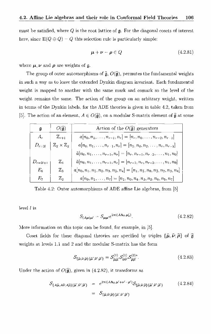
4.2. Affine Lie algebras and their role in Conformal Field Theories 106
must be satisfied, where Q is the root lattice of g. For the diagonal cosets of interest
here, since II ( Q EB Q) = Q this selection rule is particularly simple:
1-L+v-pEQ ( 4.2.81)
where /-L, v and p are weights of g.
The group of outer automorphisms of g, 0 (g), permutes the fundamental weights
in such a way as to leave the extended Dynkin diagram invariant. Each fundamental
weight is mapped to another with the same mark and comark so the level of the
weight remains the same. The action of the group on an arbitrary weight, written
in terms of the Dynkin labels, for the ADE theories is given in table 4.2, taken from
[5]. The action of an element, A E O(g), on a modular S-matrix element of gat some
g O(g) Action of the O(g) generators
Ar Zr+1 a[no, nl, ... 'nr-1, nr] = [nr, no, ... ' nr-2, nr-1]
Dr=2l Z2 x Z2 a[no, n1, ... 'nr-1, nr] = [n1, no, n2, ... 'nr, nr-1]
a[no, n1, ... 'nr-1, nr] = [nn nr-1, nr-2, ... 'n1, no]
Dr=21+1 z4 a[no, n1, ... 'nr-1, nr] = [nr-1, nTl nr-2, ... 'n1, no]
E6 z3 a[no, n 1, ny, n2, n 3, n3, n4] = [n1, ny, no, n3, n 2, n3, n4]
E7 z2 a[n0 , n 1, ... , n 7] = [n1, n0 , n4 , n3, n2, n6, n5 , n7]
Table 4.2: Outer automorphisms of ADE affine Lie algebras, from [5]
level l is
( 4.2.82)
More information on this topic can be found, for example, in [5].
Coset fields for these diagonal theories are specified by triples {/L, v; p} of g
weights at levels 1,1 and 2 and the modular S-matrix has the form
( 4.2.83)
Under the action of O(g), given in ( 4.2.82), it transforms as
( 4.2.84)
S{-- -}{-' _, _,} JL,V;p JL ,V ;p

4.3. Minimal reflection factors for purely elastic scattering theories 107
since J..L1 + v' - p' E Q [95]. This suggests that S is a degenerate matrix, which
cannot be the case since it represents a modular transformation. This degeneracy
must therefore be removed by identifying the fields
{A/L, Av; Ap} = {Jl,, v; p} VA E O(g). ( 4.2.85)
For these diagonal cosets, the orbit of every element A of O(g) has the same order, N,
which is simply the order of the global symmetry group of the model. With this field
identification, every field in the theory will appear with multiplicity N. To remedy
this, the partition function must be divided by this multiplicity, which has the effect
of introducing N into the coset modular S-matrix [96]:
(1) (1) (2) S{, v·p-}{"' v'·-p'} = N s __ ,s __ ,s __ ,_ ,_, , .- , , ILIL vv PP ( 4.2.86)
More information on field identifications can be found, for example, in [97].
4.3 Minimal reflection factors for purely elastic
scattering theories
Returning now to the particle description of the purely elastic scattering theories, it is
useful to note that a common basis for the conjecturing of bulk scattering amplitudes
is a 'minimality hypothesis', that in the absence of other requirements one should
look for solutions of the constraints with the smallest possible number of poles and
zeros. In this section this principle is used to find sets of boundary amplitudes, one
for each purely elastic 8-matrix of type A, D or E. The amplitudes given below were
at first conjectured [98] as a natural generalisation of the minimal versions of the Ar
affine Toda field theory amplitudes found in [99, 100]. The reasoning behind these
conjectures will be explained shortly. More recently, Fateev [101] proposed a set of
reflection factors for the affine Toda. field theories. These were in integral form, and
not all matrix elements were given. However, modulo some overall signs and small
typos, the coupling-independent parts of Fa.teev's conjectures match those presented
here. (This has also been found by Zambon [102], who obtained equivalent formulae
to those recorded below taking Fateev's integral formulae as a. starting point.)
Recall from section 3.3, the unita.rity condition, for a purely elastic scattering

4.3. Minimal reflection factors for purely elastic scattering theories 108
theory, is
( 4.3.1)
and the crossing-unitarity condition is
(4.3.2)
Whenever a bulk three-point coupling cabc is non-zero there IS also a bootstrap
constraint
(4.3.3)
Unitarity and crossing-unitarity together imply that the reflection factors must be 27ri
periodic; unitarity then requires that they be products of the blocks ( x) introduced
in section 4.1: sinh (!l + inx)
(x) = 2 2h · h ( fJ inx) ' Sill 2- 2h
( 4.3.4)
which appear in the ADE S-matrix elements as
Sab = II {X} , {X} = (X - 1) (X + 1) . (4.3.5) xEAab
The crossing-unitarity constraint is then key for the analysis of minimality. Each pole
or zero of Baa (2e) on the right hand side of ( 4.3.2) must be present in one or other
of the factors on the left hand side of that equation. This sets a lower bound on the
number of poles and zeros for the reflection factor Ra (e).
To exploit this observation, it is convenient to work at the level of the larger
blocks { x} = ( x - 1) ( x + 1), the basic units for the bulk bootstrap equations [83, 85].
Define two complementary 'square roots' of these blocks as
(4.3.6)
which have the basic properties
(x)(e) = (i)(e + i1r) (4.3.7)
and
(x)(e) (i)(e) = {x} (2e). (4.3.8)
The crossing-unitarity equation can then be solved, in a minimal fashion, by any
product
(4.3.9) xEAaa

4.3. Minimal reflection factors for purely elastic scattering theories 109
where each factor fx can be freely chosen to be (x) or (x), modulo one subtlety:
since (0) = 1, minimality requires that any factor !I be taken to be (1) rather than
(I). In fact there is always exactly one such factor for the diagonalS-matrix elements
relevant here [86].* Pictorially these 'square root' blocks are shown in figure 4.3. Each
i !t(2h -x)
h {x)(8)
0 i1tx -- ilt 2m
h
i !t(2h -x)_
' 1-1 ' 2h {x)(28) r---. -· -,-~~--1
lltX L~ . 0 Th lit
:X\ ( 8) ~---"-~ '-'---". ·-·--t---,-~~--~--------1
0 ilt
<X: ( 8) 1--~;-:] __ : -~--i 0 ~
Figure 4.3: The 'square root' blocks
block {X}( e) has a pole at e == in( X± 1) I h, depicted in figure 4.3 by the edges of the
block sitting above the horizontal (e) axis. Each of these poles has a corresponding
zero (outside the physical strip); the positions of these zeros are given by the edges
of the block sitting below the axis. Figure 4.3 also shows how the poles and zeros of
each block of S(2e), {x}(2e), are split between the two square roots (x) and (i).
There remains the constraint imposed by the bootstrap equations (4.3.3). To
treat these it is necessary to know how the blocks (x)(e) and (x)(e) transform under
general shifts in e. As in [85, 86], these shifts are best discussed by defining
( e inx) (x)+ (e)= sinh 2 + 2
h ( 4.3.10)
and then
(4.3.11)
*One could also take (x) = (x2 1) (x!1 ), (x) = eh-2x-l)-1
eh-2x+ 1 r1
throughout, but this
would break the pattern previously seen for the Ar theories, and turns out not to fit with the
g-function calculations later.
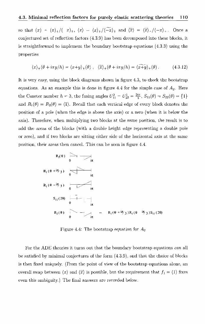
4.3. Minimal reflection factors for purely elastic scattering theories 110
so that (x) = (x)+/( -x )+, (x) = (x)+/ ( ~)+ and (x) = (x)+/ ( -x)+. Once a
conjectured set of reflection factors ( 4.3.9) has been decomposed into these blocks, it
is straightforward to implement the boundary bootstrap equations ( 4.3.3) using the
properties
( 4.3.12)
It is very easy, using the block diagrams shown in figure 4.3, to check the bootstrap
equations. As an example this is done in figure 4.4 for the simple case of A2 . Here
the Coxeter number h = 3, the fusing angles Uf1 = Ui2 = 2;1r, Su (B) = 5 22 (0) = {1}
and R 1 (B) = R 2 (B) = (1). Recall that each vertical edge of every block denotes the
position of a pole (when the edge is above the axis) or a zero (when it is below the
axis). Therefore, when multiplying two blocks at the same position, the result is to
add the areas of the blocks (with a double height edge representing a double pole
or zero), and if two blocks are sitting either side of the horizontal axis at the same
position, their areas then cancel. This can be seen in figure 4.4.
R1(8) PI v.l 0 11[
R1 (8 +i77 3 > I ~I 0~ in
R1 (8 -i77 3 ) I VI~ 0 I1t
s11 c 28) p u 0 in
R2 (8) ~I v.l I
0 11[
Figure 4.4: The bootstrap equation for A2
For the ADE theories it turns out that the boundary bootstrap equations can all
be satisfied by minimal conjectures of the form ( 4.3. 9), and that the choice of blocks
is then fixed uniquely. (From the point of view of the bootstrap equations alone, an
overall swap between (x) and (x) is possible, but the requirement that h = (1) fixes
even this ambiguity.) The final answers are recorded below.

4.3. Minimal reflection factors for purely elastic scattering theories 111
The reflection factors for this case were given in [99]. In the current notation they
are 2a-l
Ra = II (x). x=l
x odd
The reflection factors, Ra, for a = 1, ... , r - 2 are
2a-l 2a-1 2a-5
Ra = II ( x) II ( h - x) II ( h ~ 2) , for a odd x=l x=l x=l
x odd step 4 step 4
2a-l 2a-3
Ra IT (x) IT (~)(h- x- 2), for a even, x=l x=l
x odd step 4
while for a= r- 1 and r
2r-5
Rr = II \x) , for r odd x=l
step 4
2r-3
Rr-l Rr = II (x), for r even, x=l
step 4
R1 = (1)(7)
\1) (5) (7) (li)
R3 R3 = (1) (3)\5)\7) (7) (9)
R4 (1) (3) 2 (5) 2 (5) (7) 2 (7)(9) (9) \11)
( 4.3.13)
(4.3.14)
(4.3.15)
( 4.3.16)

4.3. Minimal reflection factors for purely elastic scattering theories 112
Rl - (1)(9)(17)
R2 (1)(7)(11)(l7)
R3 - (1)(5)(7)(9)(fi)(13)(17)
R4 (1)(3)(7)(9)(9)(11)(15)(17) (4.3.17)
Rs - (1)(3)(5)(7)(7)(9) 2(11)(fi)(13)(i5)(17)
R6 = (1)(3)(5) 2(7)(7)(9) 2 (9)(11)(fi)(13) 2(i5)(17)
R7 - (1)(3) 2(5) 2(5)(7) 3 (7)(9) 2(9) 2(11) 3 (fi)(13)(f3) 2(15) 2 (i7)
Es
Rl (1) (11) (19) (29)
R2 (1)(7)(11)(13)(17)(19)(23)(29)
R3 (1)(3)(9)(11)(fi)(13)(17)(19)(i9)(21)(~7)(29)
R4 - (1)(5)(7)(9)(11)(fi)(13)(15)(l5)(17)(19)(f9)(21)(23)(25)(29)
Rs (1)(3)(5)(7)(9)(9)(11) 2(fi)(13)(i3)(15) 2(17)(i7)(19) 2(i9)(21)(2i)
(23) (25) (27) (29) ( 4.3.18)
R6 = (1)(3)(5)(7)(7)(9) 2(11) 2(fi)(13) 2 (i3)(15)(i5)(17) 2(l7)(19)(i9) 2
(21) 2(23)(23)(25)(27)(29)
R7 - (1)(3)(5) 2(7) 2(7)(9) 2(9)(11) 2(fi) 2 (13) 3(f3)(15) 2(i5) 2(17)3 (i7)(19) 2
(19) 2 (21) 2(21)(23)(23) 2(25) 2(27)(29)
Rs - (1)(3)2 (5) 2 (5)(7)3 (7)(9)3 (9) 2 (11)4 (li) 2(13)3 (l3) 3 (15) 4 (i5) 2 (17) 3 (f7) 3
(19) 4 (19) 2(21) 2(21) 3 (23) 3 (23)(25)(25) 2(27) 2(29)
For the T series the story is different: it is not possible to satisfy the boundary
bootstrap equations with a conjecture of the form ( 4.3.9). This means that the mini
mal reflection factors for these models are forced by the bootstrap to have extra poles
and zeros beyond those required by crossing-unitarity alone. The general proposal
4.4. One-parameter families of reflection factors 113
will be given in eq. (4.5.4) below, but the situation can be understood using the
boundary T1 , or Lee-Yang, model: the minimal reflection factor found in [78] for the
single particle in this model bouncing off the I].) boundary is
( 4.3.19)
The simpler function (~)(~)- 1 would have been enough to satisfy crossing-unitarity,
but then the boundary bootstrap would not have held, and so (4.3.19) really is a
minimal solution. This observation fits nicely with the g-function calculations to
be reported later: had the minimal reflection factors for the Tr theories fallen into
the pattern seen for other models, there would have been a mismatch between the
predicted UV values of the g-functions and the known values from conformal field
theory.
4.4 One-parameter families of reflection factors
The minimal reflection factors introduced in the last section have no free parameters.
However, combined perturbations of a boundary conformal field theory by relevant
bulk and boundary operators involve a dimensionless quantity - the ratio of the
induced bulk and boundary scales- on which the reflection factors would be expected
to depend. To describe such situations, the minimality hypothesis must be dropped
and the conjectures extended.
A first observation, rephrasing that of [75], is that given any two solutions Ra (B)
and R~ (B) of the reflection unitarity, crossing-unitarity and bootstrap relations ( 4.3.1),
(4.3.2) and (4.3.3), their ratios Za(B) = Ra(B)/R~(B) automatically solve one-index
versions of the bulk unitarity, crossing and bootstrap equations (2.4.18), (2.4.19) and
(2.4.24):
Za(B)Za(-B) = 1, Za(B) = Za(i7r- B),
Zc(B) = Za(B- iU~JZb(B + iU:J .
(4.4.1)
( 4.4.2)
The minimal reflection factors Ra (B) can therefore be used as multiplicative 'seeds' for
more general conjectures R~ (B) = Ra (B)/ Za (B), with the parameter-dependent parts
Za(B)- 1 constrained via (4.4.1) and (4.4.2). An immediate solution is zld)(B) = Sda(B)
for any (fixed) particle type d in the theory, where the ket symbol is used here to

4.4. One-parameter families of reflection factors 114
indicate that the label ld) might ultimately refer to one of the possible boundary
states of the theory. However, this does not yet introduce a parameter. Noting that
a symmetrical shift in e preserves all the relevant equations, one possibility is to take
(4.4.3)
with C at this stage arbitrary. This is indeed the solution adopted by the boundary
scaling Lee-Yang example studied in [78]. This model is the r = 1 member of the
Tr series described earlier, and corresponds to the perturbation of the non-unitary
minimal model M 25 by its only relevant bulk operator, cp, of conformal dimensions
fl'P = fl'P = -i· The minimal model has two conformally-invariant boundary con
ditions which were labelled I]_) and I <I>) in [78]. The I]_) boundary has no relevant
boundary fields, and has a minimal reflection factor, given by (4.3.19) above. On the
other hand, the I<I>) boundary has one relevant boundary field, denoted by ¢, and
gives rise to a one-parameter family of reflection factors
(4.4.4)
The factor zlb) (B) has exactly the form mentioned above:
zlb)(e) = s(e + i~(b+3))S(e- i~(b+3)) (4.4.5)
where S( B) is the bulkS-matrix, and the parameter b can be related to the dimension
less ratio J.L2 /).. of the bulk and boundary couplings ).. and fL [78, 79]. (Since there is
only one particle type in the Lee-Yang model, the indices a, d and so on are omitted.
The notation here has also been changed slightly from that of [78] to avoid confusing
the parameter b with a particle label.) t
As an initial attempt to extend ( 4.4.4) to the remaining ADET theories one could
therefore try
( 4.4.6)
with z~d,c\e) as m (4.4.3). This manoeuvre certainly generates mathematically
consistent sets of reflection amplitudes, but in the more general cases it is not the
most economical choice. Consider instead the functions obtained by replacing the
tThere are also boundary-changing operators, but these were not considered in [78, 79].

4.5. Boundary Tr theories as reductions of boundary sine-Gordon 115
blocks {x} in (4.1.3) by the simpler blocks (x) [45]:
s~ = IT (x) . ( 4.4. 7) xEAab
For the Lee-Yang model, SF(()) coincides with S(O), but for other theories it has
fewer poles and zeros. The bootstrap constraints are only satisfied up to signs, but
if SF is used to define a function zid,C) as
( 4.4.8)
then these signs cancel, and so ( 4.4.8) provides a more "minimal" generalisation of the
family of Lee-Yang reflection factors which nevertheless preserves all of its desirable
properties. Setting d equal to the lightest particle in the theory generally gives the
family with the smallest number of additional poles and zeros, but, as will be seen
later, all cases have a role to play.
The normalisation of the shift was changed in passing from ( 4.4.3) to ( 4.4.8); this
is convenient because, as a consequence of the property
(x- C)(O) x (x + C)(O) = (x)(() + i*C) x (x)(()- i*C), (4.4.9)
zld,C) simplifies to
zld,C) = IT (x- C) (x +C) . (4.4.10) xEAad
The factors (zid,C))-1 therefore coincide with the coupling-constant dependent parts
of the affine Toda field theory S-matrices of [83, 32], with C related to the parameter
B of [83] by C = 1- B.
4.5 Boundary Tr theories as reductions of bound
ary sine-Gordon
The reflection factors presented so far are only conjectures, and no evidence has been
given linking them to any physically-realised boundary conditions. The best signal in
this respect will come from the exact g-function calculations to be reported in later
sections. However, for the Tr theories, alternative support for the general scheme
comes from an interesting relation with the reflection factors of the sine-Gordon
model.

4.5. Boundary Tr theories as reductions of boundary sine-Gordon 116
In the bulk, the Tr theories can be found as particularly-simple quantum group
reductions of the sine-Gordon model at certain values of the coupling, in which the
soliton and antisoliton states are deleted leaving only the breathers [89]. Quantum
group reduction in the presence of boundaries has yet to be fully understood, but the
simplifications of the Tr cases allow extra progress to be made. This generalises the
analysis of [78] for T1 , the Lee-Yang model, but has some new features.
The boundary S-matrix for the sine-Gordon solitons was found by Ghoshal and
Zamolodchikov in [72], and extended to the breathers by Ghoshal in [103]. To match
the notation used above for the ADE theories, the sine-Gordon bulk coupling constant
f3 is traded for 167r
h = f32 - 2. (4.5.1)
Ghoshal and Zamolodchikov expressed their matrix solution to the boundary Yang
Baxter equation for the sine-Gordon modelt in terms of two parameters E, and k.
However for the scalar part (which is the whole reflection factor for the breathers)
they found it more convenient to use TJ and fJ, related to E, and k by
1 cos TJ cosh fJ = - k cos E, ,
1 cos2
TJ + cosh2 fJ = 1 + k2 . (4.5.2)
Ghoshal-Zamolodchikov's reflection factor for the ath breather on the !TJ, fJ) boundary
can then be written as
(4.5.3)
where R(a) = (~)(a+ h) arr-
1 (l) (l +h)
o (a+3h) (l+ 3h)2 2 1=1 2
(4.5.4)
is the boundary-parameter-independent part, and
(4.5.5)
with a-1 ( 2v h l)
s(a) (v e) = II -;;:- - 2 + ' (2v +f.!+ [)
l=l-a 1r 2
(4.5.6)
step 2
contains the dependence on TJ and fJ. In these formulae the blocks ( x) are the same as
those defined in (4.1.2) for the minimal ADE theories, with h now given by (4.5.1).
t also found by de Vega and Gonzalez Ruiz [104]

4.5. Boundary Tr theories as reductions of boundary sine-Gordon 117
Now for the quantum group reduction. In the bulk, suppose that {32 is such that
h = 2r + 1, (4.5.7)
At these values of the coupling, Smirnov has shown [89] that a consistent scattering
theory can be obtained by removing all the solitonic states, leaving r breathers with
masses Ma = s~~1(~a~h~) .A11 . The scattering of these breathers is then given by the Tr
S-matrix (4.1.5). In order to explain all poles without recourse to the solitons, extra
three-point couplings must be introduced, some of which are necessarily imaginary,
consistent with the Tr models being perturbations of nonunitary conformal field theo
ries. In the presence of a boundary, these extra couplings give rise to extra boundary
bootstrap equations, which further constrain the boundary reflection factors and im
pose a relation between the parameters 'fl and i). This can be seen by a direct analysis
of the boundary bootstrap equations but it is more interesting to take another route,
as follows.
First recall the observation of [78], that the reflection factors for the boundary
Lee-Yang model match solutions of the boundary Yang-Baxter equation for the sine
Gordon model at
~ ---+ ioo. (4.5.8)
The Lee-Yang case corresponds to r = 1, h = 3, but here it is supposed that the
same constraint should hold more generally (see also [76]). The condition must be
translated into the ( 'fl, iJ) parametrisation. One degree of freedom can be retained by
allowing k to tend to infinity as the limit ( 4.5.8) is taken. The relations ( 4.5.2) then
become
cos 'fl cosh i) = A , cos2 T/ + cosh2 i) = 1 . (4.5.9)
The constant A can be tuned to any value by taking ~ and k to infinity suitably, and
so the first equation in (4.5.9) is not a constraint; solving the second for iiJ,
(4.5.10)
(The shift by r is included for later convenience.) This appears to give a count
able infinity of one-parameter families of reflection factors, but this is not so: the
blocks (x) in (4.5.5) and (4.5.6) depend on the boundary parameters only through
the combination 2iiJ 27] - = - + 2( r-d) + 1 .
7r 7r ( 4.5.11)
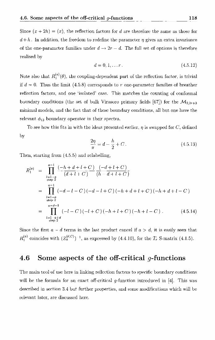
4.6. Some aspects of the off-critical g-functions 118
Since ( x + 2h) = ( x), the reflection factors for d a.re therefore the sa.me a.s those for
d +h. In addition, the freedom to redefine the parameter 7J gives a.n extra. inva.ria.nce
of the one-parameter families under d ----t 2r - d. The full set of options is therefore
realised by
d = 0, 1, ... r. (4.5.12)
Note a.lso tha.t Ria) ( 0), the coupling-dependent pa.rt of the reflection factor, is trivial
if d = 0. Thus the limit ( 4.5.8) corresponds to r one-parameter families of breather
reflection factors, a.nd one 'isolated' ca.se. This matches the counting of conformal
boundary conditions (the set of bulk Virasoro primary fields [67]) for the M 2,2r+3
minimal models, a.nd the fa.ct tha.t of these boundary conditions, a.ll but one ha.ve the
relevant ¢13 boundary operator in their spectra..
To see how this fits in with the ideas presented earlier, 77 is swapped for C, defined
by 2
7] = d - !!_ + c . 7r 2
( 4.5.13)
Then, starting from ( 4.5.5) a.nd relabelling,
R(a) -1 -
a-1
IT (-h+d+l+C) (-d+l+C)
(d + l +c) (h- d + l +c) 1=1-a step 2
a-1
II ( -d- z- c) ( -d -z +c) ( -h + d + z +c) ( -h + d + z- c) 1=1-a step 2
a+d-1
IT ( -z- c) ( -z +c) ( -h + z +c) ( -h + z- c) . 1=1-a+d
step 2
(4.5.14)
Since the first a - d terms in the la.st product cancel if a > d, it is easily seen tha.t
Ria) coincides with (zld,C))- 1, a.s expressed by (4.4.10), for the Tr S-ma.trix (4.1.5).
4.6 Some aspects of the off-critical g-functions
The ma.in tool of use here in linking reflection factors to specific boundary conditions
will be the formula. for a.n exact off-critical g-function introduced in [4]. This wa.s
described in section 3.4 but further properties, a.nd some modifications which will be
relevant later, are discussed here.
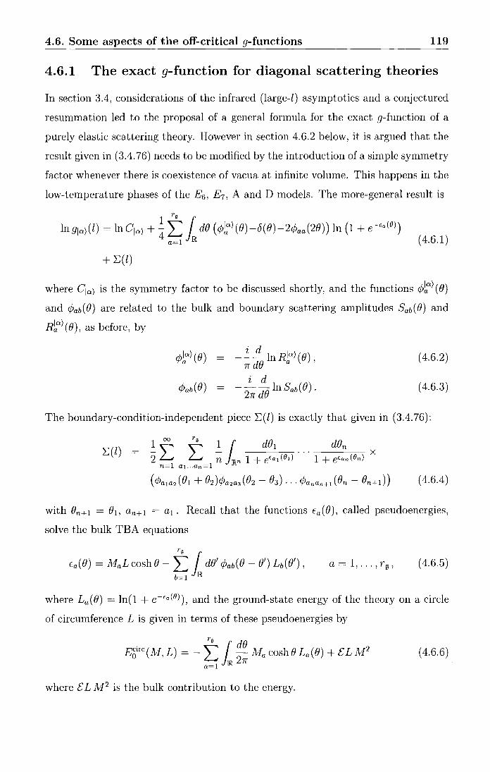
4.6. Some aspects of the off-critical g-functions 119
4.6.1 The exact g-function for diagonal scattering theories
In section 3.4, considerations of the infrared (large-l) asymptotics and a conjectured
resummation led to the proposal of a general formula for the exact g-function of a
purely elastic scattering theory. However in section 4.6.2 below, it is argued that the
result given in (3.4. 76) needs to be modified by the introduction of a simple symmetry
factor whenever there is coexistence of vacua at infinite volume. This happens in the
low-temperature phases of the E6 , E7 , A and D models. The more-general result is
where Cra) is the symmetry factor to be discussed shortly, and the functions ¢':) (B)
and rPab( B) are related to the bulk and boundary scattering amplitudes Sab( B) and
R1a) (B), as before, by
- !:.._ .!}__ ln Ria) (B) 7r d(} a '
( 4.6.2)
i d ---ln S b(O).
27r d(} a ( 4.6.3)
The boundary-condition-independent piece ~( l) is exactly that given in (3.4. 76):
( 4.6.4)
with Bn+l = 01, an+l = a 1 . Recall that the functions Ea(B), called pseudoenergies,
solve the bulk TBA equations
rg
Ea (B) = A1aL cosh(} - ~ 1 dB' rPab( 0 - 0') Lb( 0') , a= 1, . .. ,Tg, ( 4.6.5)
where La (B) = ln( 1 + e-Ea (IJ)), and the ground-state energy of the theory on a circle
of circumference L is given in terms of these pseudoenergies by
( 4.6.6)
where £ L lv/2 is the bulk contribution to the energy.

4.6. Some aspects of the off-critical g-functions 120
As mentioned in section 3.4, the formula ( 4.6.1) has been checked in detail, but
only for the r9 = 1, qll) = 1 case corresponding to the Lee-Yang model [4]. The results
below will confirm that it holds in more general cases, provided qn) is appropriately
chosen.
4.6.2 Models with internal symmetries
The scaling Lee-Yang model, on which the analysis of (4] was mostly concentrated, is
a massive integrable quantum field theory with fully diagonal scattering and a single
vacuum. However many models lack one or both these properties. In this section
this analysis will be extended to models possessing, in infinite volume, N equivalent
vacua but still described by purely elastic scattering theories§. For the ADE-related
theories the N equivalent vacua are related by a global symmetry Z. When these
systems are in their low-temperature phases, the original formula for g(l), as given
in (3.4. 76), should be corrected slightly, by including a 'symmetry factor' qn).
Low-temperature phases are common features of two dimensional magnetic spin
systems below their critical temperatures. A discrete symmetry Z of the Hamiltonian
H is spontaneously broken, and a unique ground state is singled out from a multiplet
of equivalent degenerate vacua. This contrasts with the high-temperature phase,
where the ground state is Z~invariant.
The prototype of two-dimensional spin systems is the Ising model, so this case will
be treated first. The Ising Hamiltonian for zero external magnetic field is invariant
under a global spin reversal transformation (Z = 1:02), and at low temperatures T < Tc
this symmetry is spontaneously broken and there is a doublet {I+), 1-)} of vacuum
states transforming into each other under a global spin-flip:
I±) _, I=F). (4.6.7)
The Z2 symmetry of H is preserved under renormalisation and it also characterises
the continuum field theory version of the model: in the low-temperature phase the
bulk field theory has two degenerate vacua {I+), 1-)} with excitations, the massive
§Integrable models with non-equivalent vacua are typically associated to non-diagonal scattering
like, for example, the ¢ 13 perturbations of the minimal Mp.q models [105].
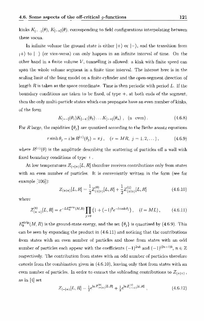
4.6. Some aspects of the off-critical g-functions 121
kinks K[+-J(B), K[-+J(B), corresponding to field configurations interpolating between
these vacua.
In infinite volume the ground state is either I+) or 1-), and the transition from
I+) to 1-) (or vice-versa) can only happen in an infinite interval of time. On the
other hand in a finite volume V, tunnelling is allowed: a kink with finite speed can
span the whole volume segment in a finite time interval. The interest here is in the
scaling limit of the Ising model on a finite cylinder and the open-segment direction of
length R is taken as the space coordinate. Time is then periodic with period L. If the
boundary conditions are taken to be fixed, of type +, at both ends of the segment,
then the only multi-particle states which can propagate have an even number of kinks,
of the form
(4.6.8)
For R large, the rapidities { e J} are quantised according to the Bet he ansatz equations
rsinhBJ- ilnRI+)(BJ) = 1rj, (r = l\1R, j = 1,2, ... ), (4.6.9)
where Rl+) (B) is the amplitude describing the scattering of particles off a wall with
fixed boundary conditions of type + . At low temperatures Z(+l+) [L, R] therefore receives contributions only from states
with an even number of particles. It is conveniently written in the form (see for
example [106]):
where
z~~I+)[L,R] = e-LE~trip(M,R) II (1 + (-1)be-/cosh0j)' (l = l\1L)' j>O
( 4.6.10)
(4.6.11)
E~trip(l\1, R) is the ground-state energy, and the set {OJ} is quantised by (4.6.9). This
can be seen by expanding the product in ( 4.6.11) and noticing that the contributions
from states with an even number of particles and those from states with an odd
number of particles each appear with the coefficients ( -1) 2nb and ( -1)(2n+l)b, n E Z
respectively. The contribution from states with an odd number of particles therefore
cancels from the combination given in (4.6.10), leaving only that from states with an
even number of particles. In order to extract the subleading contributions to Z(+l+) ,
as in [4] set (0) [ (1) J z [L R] = l lnZ(+I+) L,R] + l lnZ(+I+)[L,R
(+I+) ' 2e 2e ' (4.6.12)
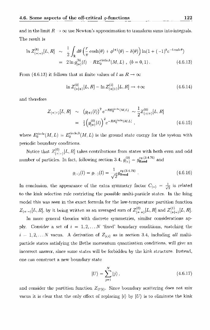
4.6. Some aspects of the off-critical g-functions 122
and in the limit R-----+ oo use Newton's approximation to transform sums into integrals.
The result is
(b) [ l ln Z(+l+) L, R ~ 1 d() (;cosh(B) + ¢1+)(8) _ b({j)) ln(1 + (-1)be-lcosh8)
2lngr!\U)- RE~irc!e,b(M, L), (b = 0, 1). (4.6.13)
From ( 4.6.13) it follows that at finite values of l as R -----+ oo
(0) [ l (1) [ l ln Z(+l+) L, R - ln Z(+l+) L, R -----+ +oo (4.6.14)
and therefore
( (l))2 -RE{Jircle(M,L) ""~z(O) [L R] m+) e 2 (+I+) '
.! ( (0) (l)) 2 -RE{Jircle(M,L)
2 gl+) e ' ( 4.6.15)
where E8ircie(.M, L) = E~ircle,o(M, L) is the ground state energy for the system with
periodic boundary conditions.
Notice that Z~~)l+) [L, R] takes contributions from states with both even and odd
b f . l I f t f ll · t' 3 4 (O) eq.(3.4· 76) d num er o partie es. n ac , o owmg sec 1on . , gi+) = gfixed an
(l) (l) 1 eq.(3.4.76) m+) = gl-) = J2gfixed 0 ( 4.6.16)
In conclusion, the appearance of the extra symmetry factor q+) = ~ is related
to the kink selection rule restricting the possible multi-particle states. In the Ising
model this was seen in the exact formula for the low-temperature partition function
Z(+I+)[L, R], by it being written as an averaged sum of Z~~I+)[L, R] and Z~~I+)[L, R].
In more general theories with discrete symmetries, similar considerations ap
ply. Consider a set of i = 1, 2, ... N 'fixed' boundary conditions, matching the
z = 1, 2, ... N vacua. A derivation of Z(ili) as in section 3.4, including all multi
particle states satisfying the Bethe momentum quantisation conditions, will give an
incorrect answer, since some states will be forbidden by the kink structure. Instead,
one can construct a new boundary state
N
IU) = LIJ)' (4.6.17) j=l
and consider the partition function Z(uji). Since boundary scattering does not mix
vacua it is clear that the only effect of replacing li) by IU) is to eliminate the kink

4.6. Some aspects of the off-critical g-functions 123
condition on allowed multiparticle states. Thus the counting of states on an interval
with U at one end and i at the other is exactly the same as it would be in a high
temperature phase with the reflection factor at both ends being Rli) (e), and the
derivation in section 3.4 goes through to find at large R
( 4.6.18)
Recall, from section 3.4, that Q(0l(t) is the massive g-function, defined by
( 4.6.19)
which is related to the g-function for the boundary condition a by a linearly-growing
piece - ilcl:) L:
ln9ia)(l) = lnQI~?(l) + fla)L. ( 4.6.20)
Q(O) is therefore ~ Up to a linear term ~ given by ( 4.6.1) with q'l~a) (e) = </J~) (e) and
qa) = 1. On the other hand, since all vacua are related by the discrete symmetry Z
and the finite-volume vacuum state /'¢0) must be symmetrical under this symmetry,
( '¢o / i ) = ( '¢o /j ) V i, j, and so
(Q(o)(l))2 = ( U/'¢o )( '¢o/i) = N ( '¢o/i )2
= N (g(o)(t)) 2. ( '¢o /'¢o) ( '¢o /'¢o) It)
( 4.6.21)
Hence
9ii) (l) = )Ng(l) ( 4.6.22)
and 91i)(l) is given by the formula (4.6.1) with qi) = JN. An immediate consequence is that in the infrared, 9li) ( l) does not tend to one.
Instead, 0 1
hm 9ii) ( l) = qi) = 17\T . hoo y N
( 4.6.23)
This perhaps-surprising claim can be justified independently. Recall from section 3.3
that in infinite volume, boundary states can be described using a basis of scattering
states [72]:
( 4.6.24)
where /0) is the bulk vacuum for an infinite line. In finite but large volumes, the same
expression provides a good approximation to the boundary state, the only modifica
tion normally being that the momenta of the multiparticle states must be quantised
by the relevant Bethe ansatz equations. However a subtlety arises when there is a
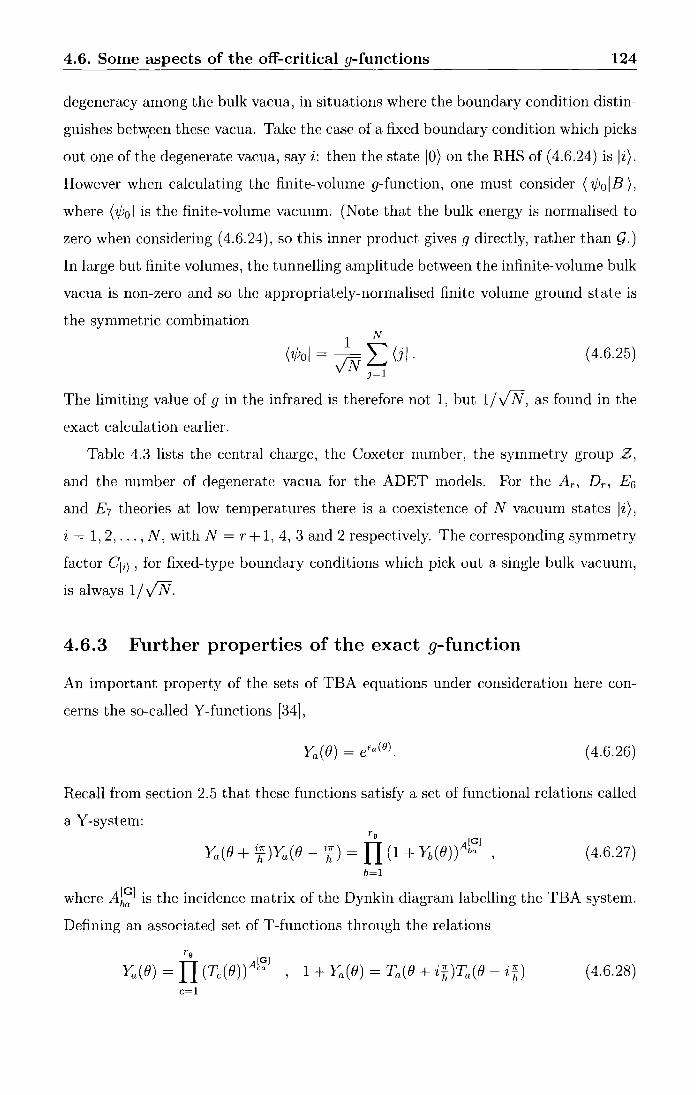
4.6. Some aspects of the off-critical g-functions 124
degeneracy among the bulk vacua, in situations where the boundary condition distin
guishes betw;een these vacua. Take the case of a fixed boundary condition which picks
out one of the degenerate vacua, say i: then the state IO) on the RHS of (4.6.24) is li).
However when calculating the finite-volume g-function, one must consider ( 'l,b0 IB ), where ('l,bol is the finite-volume vacuum. (Note that the bulk energy is normalised to
zero when considering (4.6.24), so this inner product gives g directly, rather than 9.)
In large but finite volumes, the tunnelling amplitude between the infinite-volume bulk
vacua is non~zero and so the appropriately-normalised finite volume ground state is
the symmetric combination 1 N
('l,bol = yiN L (jl. J=l
( 4.6.25)
The limiting value of g in the infrared is therefore not 1, but 1/ v'JV, as found in the
exact calculation earlier.
Table 4.3 lists the central charge, the Coxeter number, the symmetry group Z,
and the number of degenerate vacua for the ADET models. For the Ar, Dr, E6
and E7 theories at low temperatures there is a coexistence of N vacuum states li),
i = 1, 2, ... , N, with N = r + 1, 4, 3 and 2 respectively. The corresponding symmetry
factor qi), for fixed-type boundary conditions which pick out a single bulk vacuum,
is always 1/v'JV.
4.6.3 Further properties of the exact g-function
An important property of the sets of TBA equations under consideration here con
cerns the so-called Y-functions [34],
( 4.6.26)
Recall from section 2.5 that these functions satisfy a set of functional relations called
a Y-system: rg [G]
Ya(B + inYa(B- in= II (1 + Yb(O))Aba , (4.6.27) b=l
where Al;l is the incidence matrix of the Dynkin diagram labelling the TBA system.
Defining an associated set of T -functions through the relations
Tg [Gj
Ya(O) =II (Tc(O))Aca 1 1 + Ya(O) = Ta(O + i*)Ta(O- i*) ( 4.6.28) c=l
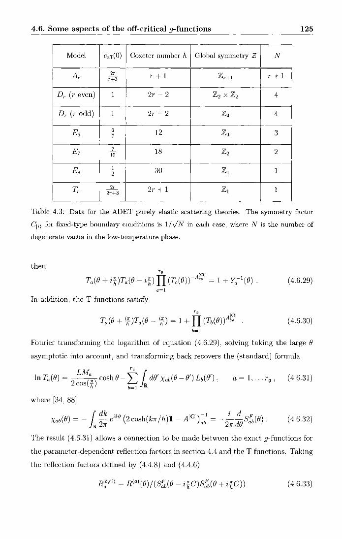
4.6. Some aspects of the off-critical g-functions 125
Model Cetr(O) Coxeter number h Global symmetry Z N
Ar 2r r+1 Zr+l r+1 r+3
Dr (r even) 1 2r- 2 z2 x z2 4
Dr (r odd) 1 2r- 2 z4 4
E6 6 12 z3 3 7
E1 7 18 Z2 2 10
Es 1 30 z1 1 2
Tr 2r 2r + 1 z1 1 2r+3
Table 4.3: Data for the ADET purely elastic scattering theories. The symmetry factor
qi) for fixed-type boundary conditions is 1/ VN in each case, where N is the number of
degenerate vacua in the low-temperature phase.
then
( 4.6.29) c=l
In addition, the T-functions satisfy
rg
Ta(e + i~)Ta(e- i17) = 1 + IJ (n(e))A~': 1 ( 4.6.30)
b=l
Fourier transforming the logarithm of equation ( 4.6.29), solving taking the large ()
asymptotic into account, and transforming back recovers the (standard) formula
a=1, ... r 9 , ( 4.6.31)
where [34, 88]
Xab(()) =- { dk eikB (2cosh(k7r/h)li- A[G]rb1
= _ _!_dd()S~(()). }IW. 2n a 2n
(4.6.32)
The result ( 4.6.31) allows a connection to be made between the exact g-functions for
the parameter-dependent reflection factors in section 4.4 and the T functions. Taking
the reflection factors defined by ( 4.4.8) and ( 4.4.6)
( 4.6.33)

4.6. Some aspects of the off-critical g-functions
and using (4.6.1),
Comparing this result with (4.6.31) and using the property Tb(e) = n( -e),
ln 9ib C) ( l) = ln g( l) + ln Tb (i?!_h c) - Llvfb1r cos (?!_c) ' 2 cosh h
or, subtracting the linear contribution:
126
( 4.6.34)
(4.6.35)
(4.6.36)
Exact relations between g- and T- functions in various situations where the bulk
remains critical were observed in [107, 49, 108]. These were extended off-criticality
to a relation between the 9- and T- function of the Lee-Yang model in [79]. The
generalisation of [79] proposed here relies on the specific forms of the one-parameter
families of reflection factors in section 4.4, and so provides some further motivation
for their introduction.
It is sometimes helpful to have an alternative representation for the infinite sum
~(l) in (4.6.1), the piece of the g-function which does not depend on the specific
boundary condition. It can be checked that, for values of l such that the sum con-
verges, CXl 1 CXl 1
~(l) = L -TrKn- L -TrHn n 2n
n=l n=l
( 4.6.37)
where
K (e e') = ~ 1 (A. (e e') A. (e - e')) 1
ab ' 2 V1 + eEa(O) 'Pab + + 'Pab V1 + eEb(O') ( 4.6.38)
and
H (e e') -1
A. (e - e') 1
ab , - J (n) 'Pab J (n') 1 + eEa u 1 + eEb u
(4.6.39)
The identity CXl 1
ln Det(I- lvf) = Tr ln(I- l\1) = - L -TrM-n n
n=l
( 4.6.40)
then allows ~( l) to be rewritten as
1 ( 1-H) ~(l)= 2 lnDet (I-K)2 . ( 4.6.41)
This formula makes sense even when the original sum diverges, a fact that will be
used in the next section.

4.7. UV values of the g-function 127
4. 7 UV values of the g-function
Taking into account the effect of vacuum degeneracies described above, a first test
of the reflection factors found earlier is to calculate the l ~ 0 limit of ( 4.6.1 ). The
value of 9io:) (0) should match the value of a conformal field theory g-function, either
of a Cardy state or of a superposition of such states.
As l ~ 0, the pseudoenergies Ea(O) tend to constants, which are denoted here by
fa· Their values were tabulated by Klassen and Melzer in [32], who also observed an
elegant formula for the integrals of the logarithmic derivatives of the bulk 8-matrix
elements, later proven in [86] :
1 dO</Yab(O) =-Nab, (4.7.1)
where Nab is related to the Cartan matrix C of the associated Lie algebra by N =
2C~ 1 - 1., The integrals of the logarithmic derivatives of the reflection factors are
also needed. Writing
(4.7.2) xEA
for some set A, the required integrals are
(4.7.3)
with sign[O] = 0. For the minimal ADE reflection factors found in section 4.3 these
evaluate to 1 dO ¢~o:)(O) = 1- Naa,
while for the Tr reflection factors (4.5.4),
To calculate the UV limit of L.(l), define a matrix M whose elements are
M = _ Nab ab 1 + eEa '
2 -1
-1 2 -1
'~~The Cartan matrix for Tr is taken to be
2 -1
-1 1
(4.7.4)
(4.7.5)
(4.7.6)

4.7. UV values of the g-function 128
in terms of which
(4.7.7)
where e1 , ... , er are the eigenvalues of M. When one of these eigenvalues is larger
than 1, the infinite sum does not converge (this is the case for Ar, T 2: 5, Dr, T 2: 4
and Er) but the RHS of ( 4. 7. 7) gives the correct analytic continuation, since it follows
from ( 4.6.41).
4.7.1 Tr
Begin with the Tr theories, whose UV limits are the non-unitary minimal models
M2,2r+3. There are T+ 1 'pure' conformal boundary conditions, and the corresponding
values of the conformal g-functions can be found using the formula
s(l,l+r);(1,l+d) 9(1,l+d) = IS 11/2
(1,l+r),(1,1) d = 0, .. . ,T (4.7.8)
where ( 1, 1 + T) is the ground state of the bulk theory, with lowest conformal weight,
(1, 1) is the 'conformal vacuum' -with conformal weight 0- and S is the modular
S-matrix. Recall from section 2.2.2 that the components of S for a general minimal
model Mp'p are
S 2 /2( 1) 1 +mp+na · ( P ) · ( p' ) (n,m);(p,a) = y PiJ - sm 1f p' np sm 1f p mCJ , (4.7.9)
where 1 :::; n, p :::; p'- 1, 1 :::; m, CJ :::; p- 1 and, to avoid double-counting, m < Jln and p < E,CJ. For the Tr theories, p' = 2 and p = 2T + 3, and so n and p are both p
equal to 1 while m and CJ range from 1 toT+ 1, as in (4.7.8).
The values predicted by ( 4. 7.8) should be compared with the values of 9ia) (0) cal
culated from ( 4.6.1). For the boundary-parameter-independent part of the reflection
factor from (4.5.4), which is the d = 0 case of the 'quantum group reduced' options
(4.5.12), the second term of (4.6.1) evaluates to
1 Lr ( sin2 ( 2r~3) ) = -- a ln 1 + -------'--'----~ 2 · ( a1r ) · ((a+2)7r) a=l Sin 2r+3 Sll1 2r+3
= ln (sin(~) sinr (~)) sinr+l ((r+1)7r) '
2r+3
(4.7.10)
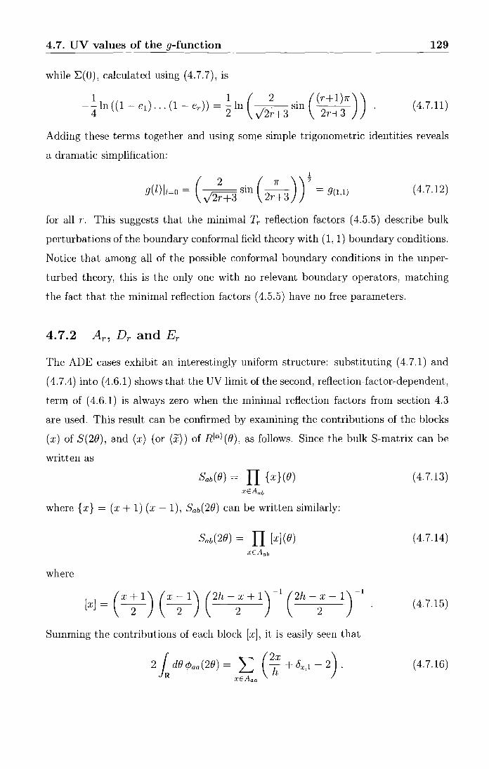
4. 7. UV values of the g-function 129
while ~(0), calculated using (4.7.7), is
1 1 ( 2 . ((r+1)7r)) --ln ((1- el) ... (1- er)) = -ln y'2T+3 sm 4 2 2r+3 2r+3
(4.7.11)
Adding these terms together and using some simple trigonometric identities reveals
a dramatic simplification:
I
g(l)lz=o = (~sin ( 2r:3)) 2
= 9(1,1) (4.7.12)
for all r. This suggests that the minimal Tr reflection factors ( 4.5.5) describe bulk
perturbations of the boundary conformal field theory with ( 1, 1) boundary conditions.
Notice that among all of the possible conformal boundary conditions in the unper
turbed theory, this is the only one with no relevant boundary operators, matching
the fact that the minimal reflection factors ( 4.5.5) have no free parameters.
The ADE cases exhibit an interestingly uniform structure: substituting ( 4. 7.1) and
( 4. 7.4) into ( 4.6.1) shows that the UV limit of the second, reflection-factor-dependent,
term of ( 4.6.1) is always zero when the minimal reflection factors from section 4.3
are used. This result can be confirmed by examining the contributions of the blocks
(x) of S(20), and (x) (or (x)) of Rlal(O), as follows. Since the bulkS-matrix can be
written as
(4.7.13)
where {x} = (x + 1) (x- 1), Sab(20) can be written similarly:
Sab(20) = IT [x](O) (4.7.14) xEAab
where
(4.7.15)
Summing the contributions of each block [x], it is easily seen that
(4.7.16)

4.7. UV values of the g-function 130
The minimal reflection factors discussed in section 4.3 can be written in a similar
way:
(4.7.17) xEAaa
where each fx is either (x) or (x). The contribution to J d() ¢~a) (B) from each (x)
is -2 + 2x/h + 2r5x,l and from each (x) is -2 + 2xjh. Noting that every minimal
reflection factor contains the block (1) exactly once, this integral can be written as
(4.7.18)
and so
(4.7.19)
for every A, D and E theory, as claimed. Working backwards, this gives a general
proof of the formula (4.7.4), given (4.7.1).
With the reflection-factor-dependent term giving zero, the sum of :E(O) and the
symmetry factor should correspond to a conformal g-function value. To find these
values in a uniform way, the diagonal coset description g 1 x gifg2 will be employed,
where g1 is the affine Lie algebra at level l associated to one of the A, D or E Lie
algebras [109]. Recall that coset fields are specified by triples {jt, v; p} ofg weights at
levels 1, 1 and 2, and the g-function for the corresponding conformal boundary condi
tion can be written in terms of the modular S-matrix of the coset model S{o,o;o}{jl,v;p}
as S{O,O;O}{jl,i);p}
9{jl,V;p} = . IS v {0,0;0}{0,0;0}
( 4.7.20)
Once the levell has been specified, the representation of g1 is completely determined
by the Dynkin labels of the corresponding representation of g. For example, the label
0 is given to the vacuum representation, where ni = 0, i = 1, ... , r 9 for both g 1 and
For the level 1 representations of simply laced affine Lie algebras, the characters
have a particularly simple form [110, 111]:
(4.7.21)

4. 7. UV values of the g-function 131
where q = exp(2niT) and the generalised e and Dedekind 'TJ functions are
ep,(q) - L q~(l.t,IL) (4.7.22) ~-tEQ
00
TJ(q) - q~ II (1- qn). (4.7.23) n=l
Under the modular transformation T---+ _.! the theta function transforms as T
(4.7.24)
where P and Q are the weight lattice and root lattice respectively [111, 93], and the
'TJ function becomes 1 1
TJ(--) = (-iT)2TJ(T). T
(4.7.25)
The modular S-matrix for level 1 is therefore
(4.7.26)
For the coset description of the g-function, (4.7.20), one needs to compute S~ti which
is simply
Sbti = 1 JIP/QI
( 4.7.27)
It is important to note that P / Q is isomorphic to the centre of the group under con-
sideration [112, 97]. The group of field identifications of the coset is also isomorphic
to the centre of this group so consequently ( 4. 7.27) becomes
s(ll- _1_ OP,- VN for all /1. (4.7.28)
The g-function can now be written in terms of the level 2 modular S matrices only:
Sb~ /S[fj' 9{P,,v;/J} = 9/J = (4.7.29)
As is clear from (4.7.29), identifying the conformal g-function value will only pin
down the level 2 representation. For E8 , since there is only one possible level 1
representation (with Dynkin labels ni = 0, i = 1, ... , 8), by specifying the level 2
representation the coset field is fixed. However, for other cases, although the coset
selection and identification rules ( 4.2.81), ( 4.2.85) do constrain the possible coset rep
resentations there is still some ambiguity left, in general. For example, for the Ar

4.7. UV values of the g-function 132
cases the selection and identification rules are quite simple and the possible cosets,
given a fixed level 2 weight, are shown in table 4.4. The notation is as follows: jij,
vj are level 1 weights and pj is the level 2 weight with Dynkin labels ni = 1 fori = j
and ni = 0, i = 1, ... , r otherwise. The labels ji0 , v0 and Po now represent 0 with
Dynkin labels ni = 0, i = 1, ... , r.
Fixed level 2 weight Level 1 weight Level 1 weight Number of coset ~ ~
fields {ji, v; p} p J.L v
0 0 0
1-Li Vr+l-i, i = 1, ... r r+1
Pj 1-Li vj-i, i = 0, .. . j
j = 1, ... [(r + 1)/2] I-Lj+k Vr+l-k, k = 1, ... r-j r+1
Table 4.4: Ar coset fields, indicating the number of distinct fields for each level 2 weight;
in the first column, [x] denotes the integer part of x
The coset fields for the A2 (three-state Potts model) and E7 (tricritical Ising
model) cases, along with the corresponding boundary condition labels from [113] and
[114] respectively, are given in tables 4.5 and 4.6 as concrete examples.
It is useful to note that for the Ar, Dn E6 and E7 models, S00 = S0 -p only when
p = AO for some A E O(g) [115] and for each such p there is a unique coset field, so
the number of fields with g-function equal to 9{P,,D,o} is equal to the size of the orbit of
0. On the other hand, E8 has no diagram symmetry, but it is also exceptional in that
S 0o = So-p2
where p2 has Dynkin labels n 2 = 1, all other ni = 0. Physically, this is to
be expected as the two fields correspond to the two fixed boundary conditions (-)
and ( + ), which clearly must have equal g-function values. (This exceptional equality
is discussed from a more mathematical perspective in, for example, [115].)
From ( 4.2.82) it is clear that So(Ap) = S 0 -p is also true for p -:/: 0. For the A and
E models at level 2, these are found to be the only cases where So-p; = S 0 -p1
; for the
Dr models there is more degeneracy.
The modular S matrices, S0 -p can be calculated with ( 4.2.46), alternatively, al
gorithms for computing these matrices are given by Gannon in [116]; Schellekens

4. 7. UV values of the g-function 133
A2
Coset field Boundary label Level 2 weight label
from [113J from table 4. 7
{[1,0,0], [1,0,0J; [2,0,0]} A
{[0, 0, 1], [0, 1, OJ; [2, 0, 0]} B 0
{[0, 1, OJ, [0, 0, 1]; [2, 0, 0]} c
{[1, 0, OJ, [0, 1, OJ; [1, 1, 0]} AB
{[0, 0, 1], [0, 0, 1J; [1, 1, 0]} BC P1
{[0, 1, OJ, [1, 0, OJ; [1, 1, 0]} AC
Table 4.5: A2 coset fields with the corresponding boundary labels and level 2 weight labels
from table 4.7. The weights are given in terms of Dynkin labels [no, n1, n2, ... J
has also produced a useful program for their calculation [117]. The level 2 modular
S-matrix elements for A, D and E theories needed to calculate the UV values of the
g-functions using ( 4. 7.29) are given in table 4. 7. The representations are labelled by
the Dynkin labels, ni, i = 0, ... , r. The number of coset fields corresponding to each
label is equal to the order of the orbit of that level 2 weight, under the outer auto
morphism group O(g). Note for Dr, r even, the weights Pr-l and Pr are in different
orbits, each with order 2, whereas for r odd they are in the same orbit with order 4,
so in both cases there are 4 coset fields with the same g-function value.
For each coset, the possible CFT values of the g-function can now be calculated
using (4.7.29) and the modular S-matrix elements given in table 4.7. Working case
by-case, these numbers can be checked against the sums ln qa) + ~(0), the UV
limits of the off-critical g-functions g(l) for the minimal reflection factors described
in section 4.3. In every case, they are found to be
lng(l)lz=o = lnqa) + ~(0) = lngo ( 4.7.30)
provided that the symmetry factors qa) are assigned as in table 4.3. The explicit
g-function values are given in table 4.8.
For some minimal models, g0 can be compared to the values of the g-function

4.8. Checks in conformal perturbation theory 134
E7
Coset field Boundary label Level 2 weight label
from [114] from table 4. 7
{[1, 0, ... '0], [1, 0, ... '0], [2, 0, ... '0]} (-) 0
{[0, 1, 0, ... ], [0, 1, 0, ... ]; [2, 0, ... '0]} ( +)
{[1, 0, ... '0], [0, 1, 0, ... ]; [1, 1, 0, ... '0]} (d) P1
{[1, 0, ... '0], [1, 0, ... '0]; [0, 0, 1, 0, ... ]} ( -0) P2
{[0, 1, 0, ... ], [0, 1, 0, ... ]; [0, 0, 1, 0, ... ]} (0+)
{[1, 0, ... , OJ, [0, 1, 0, ... ]; [0, 0, 0, 1, 0, ... ]} (0) P3
Table 4.6: E7 coset fields with the corresponding boundary labels and level 2 weight labels
from table 4.7. The weights are given in terms of Dynkin labels [no, n1, n2, ... ]
corresponding to known cases, thereby matching the reflection factors to physical
boundary conditions. For the three-state Potts model (A2 ), the tricritical Ising model
(E7 ) and the Ising model (E8 ) the corresponding boundary condition is the 'fixed'
condition in each case [113, 114, 3]. Note the number of coset fields with g-function
equal to g0 corresponds to the number of degenerate vacua, and hence to the number
of possible 'fixed' boundary conditions for all A, D and E models.
4.8 Checks in conformal perturbation theory
The off-critical g-functions only match boundary conformal field theory values in the
far ultraviolet. Moving away from this point one expects a variety of corrections, some
of which were analysed using conformal perturbation theory in [79]. The expansion
provided by the exact g-function result is instead about the infrared, but convergence
is sufficiently fast that the first few terms of the UV expansion can be extracted
numerically, allowing a comparison with conformal perturbation theory to be made.
In [4] this was done for the boundary Lee-Yang model; in this section the more
general proposals for the case of the three-state Potts model are tested. In [79], the
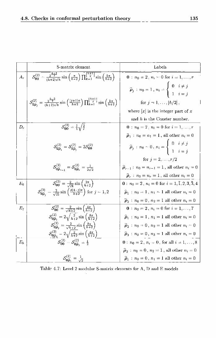
4.8. Checks in conformal perturbation theory 135
S-matrix element Labels
s(2)- .~~ ( ) ·l~+lj ( ) Ar 2 --r- . 7r -2- . kn: 0: no = 2 , ni = 0 for i = 1, ... , r 00- (h+2)Vh Sill h+2 rrk=1 Sill h+2
no=l,n;={ 0 i:f:j
Pj 1 ~=J
h+3 ( ) [h+I] ( ) s(2) - 2--r- . (J+1)n: rr -2- . kn: for j = 1, ... , [h/2], Opj - (h+2)Vh Sill h+2 k=1 Sill h+2
where [x] is the integer part of x
and h is the Coxeter number.
Dr s(2J- lft 00 - 4 T 0 : no = 2 , ni = 0 for i = 1, ... , r
P1 no = n1 = 1, all other ni = 0
s(2l - s(2l - 2S(2l no= 0, n; = { 0 i:f:j
Op1 - Op1
- 00 Pj 1 i=j
for j = 2, ... , r /2
s(2l - s(2J - _1_ ~
no = nr-1 = 1 , all other ni = 0 Opr-1 - Opr - 2V2 Pr-1:
Pr : no = nr = 1 , all other ni = 0
E6 s(2l 2 . ( 2n: ) 00 = y'2I Sill h+2 0 : no = 2, ni = 0 for i = 1, I, 2, 3, 3, 4
s(:J = - 2- sin c(4-j)n:) for j = 1 2 Op1 y'2I h+2 ' P1 no = 1 , n 1 = 1 all other ni = 0
~
no = 0 , n2 = 1 all other ni == 0 P2
E7 5 (2) 2 . ( 4n: ) 00 = V7l+2 Sill h+2 0 no = 2 , ni = 0 for i = 1, ... , 7
s(2
l 2r;!f; · ( sn: ) ~
no = 1 , n 1 = 1 all other ni = 0 Opl = h+2 Slll h+2 P1
s(2l 2 . ( sn: ) ~
no = 0 , n2 = 1 all other ni = 0 Op2 = )h+2 Sill h+2 P2
s(2J 2r;!f;; . .( 4n: ) P3 no = 0 , n3 = 1 all other ni = 0 Op3 = h+2 Slll h+2
Es s(2J - s(2l - 1.
00 - Op2 - 2 0 : no = 2 , ni = 0 , for all i = 1, ... , 8
P2 : no = 0 , n2 = 1 , all other ni = 0
s(2J - _l__ Op1 - 72 P1 : no = 0 , n 1 = 1 all other ni = 0
Table 4. 7: Level 2 modular S-matrix elements for A, D and E models

4.8. Checks in conformal perturbation theory 136
qo:) 90 Number of fields
( h+a [h+l] I) 112 Ar 1 2-----z-- · n -2- • kn r+1 Vr+T (h+2)Vh sm (h+2) nk=1 sm (h+2)
Dr 1 ~(~)1/4 4 2
E6 1 ( 2 . 2n ') 1/2 3 v'3 V2I sm ( h+2)
E7 1 ( 2 · 4n ) 112
2 J2 v'h+2 sm ( h+2)
Es 1 1 2 72
Table 4.8: UV g-function values calculated from the minimal reflection factors for the A,
D and E models
treatment of conformal perturbation theory concentrated on the non-unitary Lee
Yang case whereas here a general discussion of the leading bulk-induced correction
to the g-function in the (simpler to treat) unitary cases will be presented.
Consider a unitary conformal field theory on a circle of circumference L, perturbed
by a bulk spinless primary field r.p with scaling dimension Xcp = ~'P + ~'P . The
perturbed Hamiltonian is then
(4.8.1)
where
27r ( - c) Ha = - La + La - -L 12
(4.8.2)
and
H1 = ( ~) 1-x, f r.p(eiO) d(). (4.8.3)
For ,\real in the ADE models a ,\-A1 relation of the form
( ~)2-x, 1,\(!11)1 = '" ( 4.8.4)
is also expected, with "'" a model-dependent constant.
Leaving the boundary unperturbed, there is a conformal boundary condition a,
with boundary state Ia). Set 9io:) = gfn) = (aiO) and g~) = (alr.p), where IO) and lr.p)
are the states corresponding to the fields 1 and r.p. Since the theory is unitary, IO) is
also the unperturbed ground state; and since r.p is primary, (Oir.piO) = 0.
The aim is to calculate ln91n)(\ L) = ln(al!l) where Ia) is the unperturbed CFT
boundary state, and 1!1) is the PCFT vacuum. This will be a power series in the

4.8. Checks in conformal perturbation theory 137
dimensionless quantity >..L2-x'P; here, the coefficient of the linear term, d~u), will be
found. The calculation follows [79], but is a little different (and in fact simpler)
because the theory is unitary, so that the ground state is the conformal vacuum IO).
First-order perturbation theory implies
(4.8.5) a
where the sum is over all states excluding IO), ('ljla IO) :;::::: 0 and
Da = ('ljlaiHIIO) (OIHoiO) - ('ljlaiHol'ljla) .
(4.8.6)
Since the theory is unitary, (OIHoiO)- ('ljlaiHol'ljla) = -('ljlai 2{(Lo + Lo)l'ljla)· Using
rotational invariance as well,
(4.8.7)
Hence
(4.8.8)
where P = IO) (OI is the projector onto the ground state. Using the formula L 1-L = o+ o
fol qLo+Lo-1 dq,
(4.8.9)
Since (OI<piO) = 0 and qLo+Lo<p(1)IO) = qLo+Lo<p(1)q-Lo-LoiO) = qx'PIO) this last ex
pression simplifies to
( 4.8.10)
Now (o:l<p(q)IO) is a disc amplitude, and by Mobius invariance it is given by
( 4.8.11)
(This is a significant simplification over the nonunitary case discussed in [79], where
the corresponding amplitude had to be expressed in terms of hypergeometric func
tions.)
Taking logarithms,
( 4.8.12)
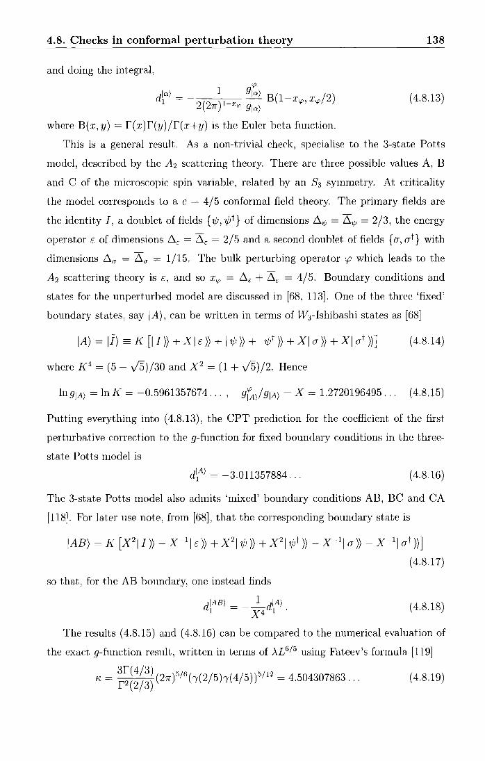
4.8. Checks in conformal perturbation theory
and doing the integral, 'P
In) __ 1 gin) d1 -- - ( )1- - B(1-Xcp, Xcp/2)
2 27r x"' 9in)
where B(x, y) = f(x)r(y)jr(x+y) is the Euler beta function.
138
( 4.8.13)
This is a general result. As a non-trivial check, specialise to the 3-state Potts
model, described by the A2 scattering theory. There are three possible values A, B
and C of the microscopic spin variable, related by an S3 symmetry. At criticality
the model corresponds to a c = 4/5 conformal field theory. The primary fields are
the identity I, a doublet of fields { '1/J, '1/Jt} of dimensions 1:11/J = 1:11/J = 2/3, the energy
operator E of dimensions 1:1c- = 1:1c- = 2/5 and a second doublet of fields {a, at} with
dimensions 1:10" = 1:10" = 1/15. The bulk perturbing operator i.p which leads to the
A2 scattering theory is E, and so Xcp = 1:1c- + 1:1c- = 4/5. Boundary conditions and
states for the unperturbed model are discussed in [68, 113]. One of the three 'fixed'
boundary states, say lA), can be written in terms of W3-Ishibashi states as [68]
(4.8.14)
where K 4 = (5- \1'5)/30 and X 2 = (1 + \1'5)/2. Hence
lngiA) = lnK = -0.5961357674 ... , g~/9iA) =X= 1.2720196495... (4.8.15)
Putting everything into (4.8.13), the CPT prediction for the coefficient of the first
perturbative correction to the g-function for fixed boundary conditions in the three
state Potts model is lA) d1 = -3.011357884 ... ( 4.8.16)
The 3-state Potts model also admits 'mixed' boundary conditions AB, BC and CA
[118]. For later use note, from [68], that the corresponding boundary state is
lAB)= K [X21 I))- x-11 E))+ X 21 '1/J )) + X 217f} )) - x-11 a))- x-11 at))]
(4.8.17)
so that, for the AB boundary, one instead finds
diAB) _____ 1 __ diA) 1 -- X4 1 · (4.8.18)
The results ( 4.8.15) and ( 4.8.16) can be compared to the numerical evaluation of
the exact g-function result, written in terms of )..L615 using Fateev's formula [119]
3r( 4/3) )5/6 ( ( I )5/12 K, = f2(2/3) (27r (r 2/5)1 4 5) = 4.504307863 ... ( 4.8.19)

4.9. One-parameter families and RG flows 139
where r(x) = r(x)/f(1 - x). Setting X = )..£615
(T- Tc) ex ).. < 0) a fit to the numerical data yields
- ( l / r;,) 615 (remembering that
ln g(l) = -0.596135768 - 0.49999991[ - 3.0113570 x
- 0.909937 x2 + 0.3982 x 3 + 1.0 x 4 + ... ( 4.8.20)
which agrees well with (4.8.15) and (4.8.16). The match of the constant term in
(4.8.20) with lngiA) from (4.8.15) is guaranteed by the exact formula, and so serves
as a check on the accuracy of our numerics. A calculation of the coefficient of the
irregular (in x) term, proportional to l, as in [79], predicts the value 0.5, again in
good agreement with the numerical results here.
4.9 One-parameter families and RG flows
Just as the minimal reflection factors were tested in section 4. 7, the same can now be
done with the one-parameter families of reflection factors. These reflection factors,
R1d,C)' depend on the parameter C and are given in (4.4.6) and (4.4.10).
4.9.1 The ultraviolet limit
If the parameter dependent reflection factors are used as input to calculate the g
function, (4.6.1), and the limit l-> 0 is taken then
(4.9.1)
where Td = Td(O) lz=o is a {}-independent constant. From ( 4.6.28) and ( 4.6.26)
(4.9.2)
where the Ed values can be found in [32]. For every AD ET theory, ( 4.9 .1) leads to a
possible CFT g-function value.
For M > 0 there will be many massive bulk flows as the parameter C is varied.
However, it should be possible to tune C, as the limit l -> 0 is taken, so as to give a
massless boundary flow between the conformal g-function gld), corresponding to the
UV limit of the reflection factor R1d,C), and g, corresponding to the UV limit of the
minimal reflection factor. These flows are depicted in figure 4.5. Note that the UV

4.9. One-parameter families and RG flows 140
g-function corresponding to the minimal reflection factors (g0 for the ADE cases and
g( 1,1) for Tr) is the smallest conformal value in all cases so, by Affleck and Ludwig's
g-theorem [3][71], this is a stable fixed point of the boundary RG flow.
Massless
Boundary
Flow
Massive Bulk Flow
1-c:::o
Figure 4.5: The expected RG flow pattern
For the Tr case
gld) = g( 1,d+ 1) for d = 1, ... , r.
This is consistent with a simple pattern of flows
(1, d+1) ----> (1, 1) for d = 1, ... , r.
(4.9.3)
(4.9.4)
The conformal values corresponding to the UV limits of gld) for the A, D and E
cases are given in tables 4.9 and 4.10. Again the boundary flows
(4.9.5)
are expected in each case. Notice that in many cases the UV g-function values are
sums of 'simple' CFT values, corresponding to flows from superpositions of Cardy
boundary conditions, driven by boundary-changing operators.
The conjectured flow for the three-state Potts model (A2 ), g-p1
----> g0 , corresponds
to the 'mixed-to--fixed' flow (AB ----> A) found by Affleck, Oshikawa and Saleur [113],
and by Fredenhagen [120].
Similarly, the flow g-p1
----> g0 in the tricritical Ising model ( E7 ) corresponds to
the 'degenerate-to-fixed' ((d)---->(-) or (d)---->(+)) flows of [121, 120]. Notice that
g0 + g-p2
----> g0 in E7 matches the CFT g values for the flow (-) EB (0+) ----> (-)
conjectured in [120]. However this latter flow is driven by the boundary field with

4.9. One-parameter families and RG flows
gil) = glr) = g/h
gl2) = glr-1) = gPz
g lr/2) = glr/2+1) = g- for r even Prj2
g lh/2 ) = g- for r odd Ph/2
li) - (. + 1) f . - 1 - 2 g - z go or z - , ... , r
glr-1) = glr) = g- = g-Pr-1 Pr
Table 4.9: UV g-function values for A and D models
gil) gil) gPt gP! go+ gp1 gl2) go+ gp2 go+ gp2 2go + gp1 gl3) gl3) gP1 + gPz gPt + gP3 2g0 + 2gfj
1
gl4) go+ gp1 + 2gpz go+ 2gPz 3go + 2giJ1
gl5) go+ 3gPz 5go + 3giJ1 gl6) 2gPt + 2gP3 5g0 + 4g1J1
gl7) 3go + 6giJ2 9go + 6gp1 gl8) 16g0 + 12gp1
Table 4.10: UV g-function values for E6, E7 andEs models
141
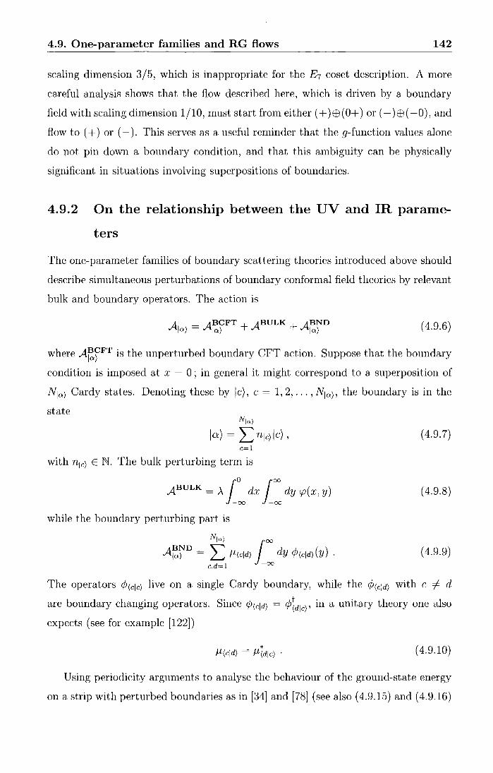
4.9. One-parameter families and RG flows 142
scaling dimension 3/5, which is inappropriate for the E7 coset description. A more
careful analysis shows that the flow described here, which is driven by a boundary
field with scaling dimension 1/10, must start from either ( + )EB(O+) or (- )EB( -0), and
flow to ( +) or (- ). This serves as a useful reminder that the g-function values alone
do not pin down a boundary condition, and that this ambiguity can be physically
significant in situations involving superpositions of boundaries.
4.9.2 On the relationship between the UV and IR parame-
ters
The one-parameter families of boundary scattering theories introduced above should
describe simultaneous perturbations of boundary conformal field theories by relevant
bulk and boundary operators. The action is
A - ABCFT + ABULK + ABND Ia) - Ia) Ia) ( 4.9.6)
where A~)FT is the unperturbed boundary CFT action. Suppose that the boundary
condition is imposed at x = 0; in general it might correspond to a superposition of
Nla) Cardy states. Denoting these by ic), c = 1, 2, ... , Nla), the boundary is in the
state Nlo.)
Ia) = L nlc) I c), c=l
with nlc) E N. The bulk perturbing term is
ABULK =A~~ dx J: dy cp(x, y)
while the boundary perturbing part is
Nlo.) oo
A~fD ~ c~ll'(old) [oo dy ¢1cld}(Y) .
(4.9.7)
(4.9.8)
(4.9.9)
The operators ¢(clc) live on a single Cardy boundary, while the ¢(cld) with c =/= d
are boundary changing operators. Since ¢(cld) = <Ptdlc), in a unitary theory one also
expects (see for example [122])
* J-i(cld) = J-i(dlc) · (4.9.10)
Using periodicity arguments to analyse the behaviour of the ground-state energy
on a strip with perturbed boundaries as in [34] and [78] (see also (4.9.15) and (4.9.16)

4.9. One-parameter families and RG flows 143
below), one can argue that the scaling dimensions of the fields rP(cJd) must, in these
integrable cases, be half that of the bulk perturbing operator cp :
x'P 2 Xq, = 2 = h + 2 (4.9.11)
for the ADE systems and
( 4.9.12)
for the Tr models. The results recorded in ( 4.9.3) and tables 4.9 and 4.10 provide infor
mation about the conformal boundary conditions associated with the one-parameter
families of reflection factors. For Tr and Ar the boundary is always found to be in a
pure Cardy state, while for Dr, E6 and E 7 this is true only in one case per model,
and in the E8-related theories the UV boundary always corresponds to a non-trivial
superposition of the states I±) and jfree). This observation fits nicely with the con
formal field theory results for the Ising model [68]: from (4.9.11) it is clear that for
the E8 coset description the integrable boundary perturbation must have dimension
xq, = 1/16, and indeed the only boundary operators with this dimension in the Ising
model are rP(±Jfree) and rP(freeJ±).
For simplicity, only the cases involving a single Cardy boundary will be discussed
here, where
( 4.9.13)
As in the Ising and Lee-Yang examples of [72, 78], a simple formula is expected to link
the couplings >. and f-i of bulk and boundary fields to the parameter C in the reflection
factors. However, without a precise identification of the operator ¢ it is hard to see
how such a relation can be determined. Even so, a general argument combined with
a numerically-supported conjecture allows the relation formula to be fixed up to a
single overall dimensionless constant. This goes as follows. In section 4.6.3 it was
shown that in all cases
(4.9.14)
where Td is the TEA-related T-function, and Q(o)(Z) is the CPT Q-function corre
sponding to the minimal reflection factor, for which there is no boundary pertur
bation. In addition, Td(B) = Td(B, l) is even in B, Td(B) = Td( -B), and periodic,
Td(() + i1rht2) = Td(B), and so it can be Fourier expanded as
(4.9.15)
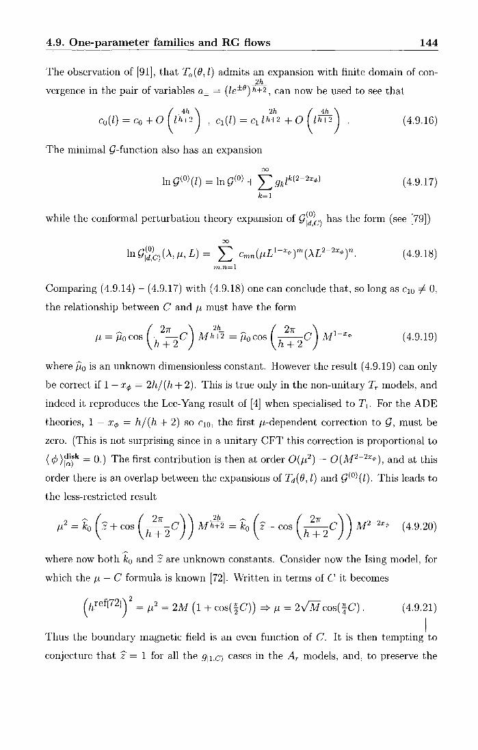
4.9. One-parameter families and RG flows 144
The observation of [91], that Ta(B, l) admits an expansion with finite domain of con-2h
vergence in the pair of variables a± = ( le±e) h+2, can now be used to see that
c0 (l) = c0 + 0 [h+2 , c1 (l) = c1 lh+2 + 0 [h+2 (
4h ) 2h ( 4h ) ( 4.9.16)
The minimal Q-function also has an expansion
00
ln g(o) ( l) = ln g(o) + L 9klk(2-2x¢) (4.9.17) k=l
while the conformal perturbation theory expansion of g 1~?c) has the form (see [79])
00
lnQI~~/\f-t,L) = L Cmn(J-tLl-x<t>)m(>..L2-2x<Pt. (4.9.18) 1n,n=l
Comparing (4.9.14)- (4.9.17) with (4.9.18) one can conclude that, so long as c10 -=1 0,
the relationship between C and f-t must have the form
f-t = /-to cos -- A1 h+2 = /-to cos --C A1 - <t> ~ ( 21r c) _]]!_ ~ ( 21r ) 1 x
h+2 h+2 (4.9.19)
where /10 is an unknown dimensionless constant. However the result ( 4.9.19) can only
be correct if 1-x¢ = 2h/(h+2). This is true only in the non-unitary Tr models, and
indeed it reproduces the Lee-Yang result of [4] when specialised to T1. For the ADE
theories, 1 - X¢ = h / ( h + 2) so c10 , the first f-t-dependent correction to Q, must be
zero. (This is not surprising since in a unitary CFT this correction is proportional to
( ¢ )~)k = 0.) The first contribution is then at order O(f-t2) = O(JvJ2-2x<P ), and at this
order there is an overlap between the expansions of Td( e, l) and g(o) ( l). This leads to
the less-restricted result
~ ( ( 21f ) ) ..1!.!:__ ~ ( ( 21f ) ) f-t 2 = ko z + cos h +
2 C M h+2 = k0 z- cos h +
2 C A12
-2
x<t> ( 4.9.20)
~
where now both k0 and z are unknown constants. Consider now the Ising model, for
which thef-t- C formula is known [72]. Written in terms of Cit becomes
(4.9.21)
I Thus the boundary magnetic field is an even function of C. It is then tempting to
conjecture that z = 1 for all the 9il,C) cases in the Ar models, and, to preserve the
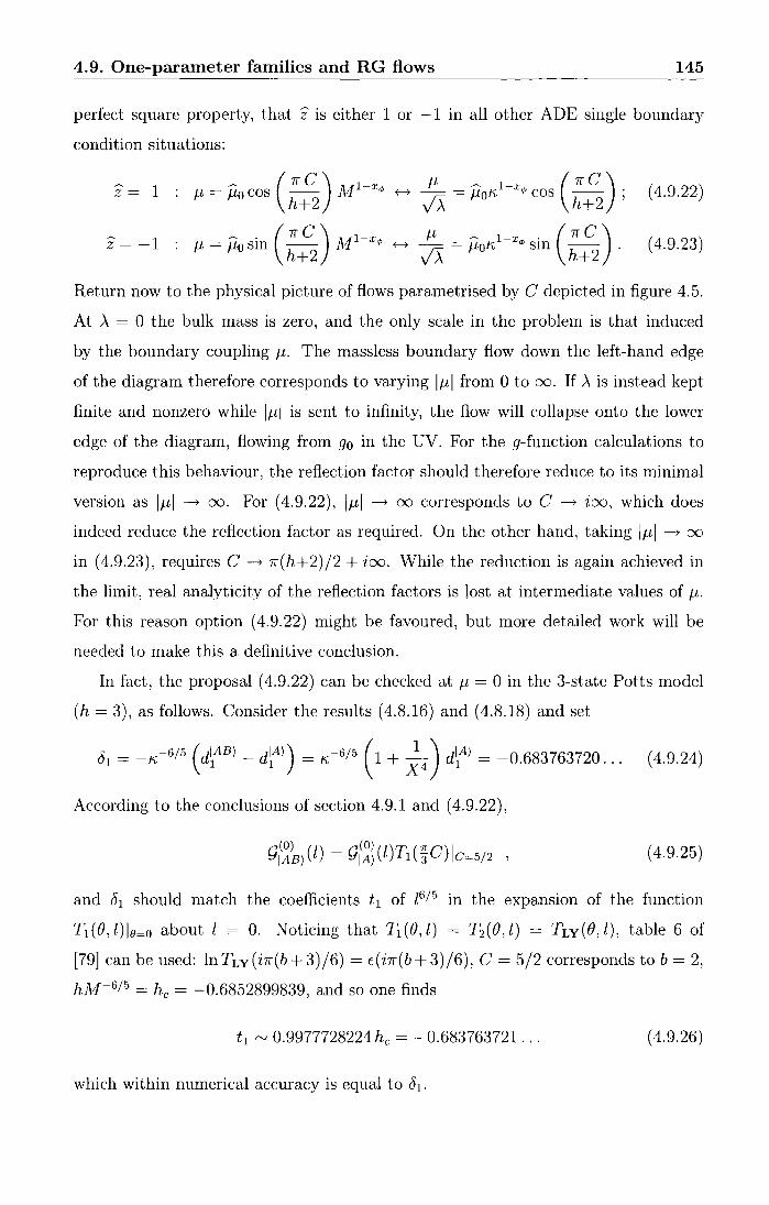
4.9. One-parameter families and RG flows 145
perfect square property, that z is either 1 or -1 in all other ADE single boundary
condition situations:
z= ~ (1rC) 1-x J1 ~ 1-x (1rC) 1 : J1 =!Locos -- .A1 <P +---> - = !LoK, <~>cos -- · h+2 ~ h+2 '
(4.9.22)
~ ~ . (1rC) 1 x J1 ~ 1 x . (1rC) z = -1 : J1 = f-lo sm h+
2 111 - <P +---> ~ = J-loK, - <P sm h+
2 . (4.9.23)
Return now to the physical picture of flows parametrised by C depicted in figure 4.5.
At .\ = 0 the bulk mass is zero, and the only scale in the problem is that induced
by the boundary coupling J-1. The massless boundary flow down the left-hand edge
of the diagram therefore corresponds to varying lf-11 from 0 to oo. If.\ is instead kept
finite and nonzero while lf-11 is sent to infinity, the flow will collapse onto the lower
edge of the diagram, flowing from g0 in the UV. For the g-function calculations to
reproduce this behaviour, the reflection factor should therefore reduce to its minimal
version as lf-11 --> oo. For ( 4.9.22), lf-11 --> oo corresponds to C --> ioo, which does
indeed reduce the reflection factor as required. On the other hand, taking lf-11 --> oo
in (4.9.23), requires C--> 7r(h+2)/2 + ioo. While the reduction is again achieved in
the limit, real analyticity of the reflection factors is lost at intermediate values of J-1.
For this reason option (4.9.22) might be favoured, but more detailed work will be
needed to make this a definitive conclusion.
In fact, the proposal ( 4.9.22) can be checked at J1 = 0 in the 3-state Potts model
(h = 3), as follows. Consider the results (4.8.16) and (4.8.18) and set
J1 = -K,-6/
5 (d~AB)- d~A)) = K,-6/ 5 (1 + ;
4) d~A) = -0.683763720... (4.9.24)
According to the conclusions of section 4.9.1 and (4.9.22),
(4.9.25)
and (h should match the coefficients t 1 of [615 in the expansion of the function
T1 (0, l)lo=o about l = 0. Noticing that T1 (0, l) = T2 (0, l) = TLy(O, l), table 6 of
[79] can be used: lnTLy(i7r(b+3)/6) = E(i7r(b+3)/6), C = 5/2 corresponds to b = 2,
h!VJ-615 = he= -0.6852899839, and so one finds
t1 "' 0.9977728224 he = -0.683763721 ... ( 4.9.26)
which within numerical accuracy is equal to 61 .

4.10. Boundary bound states of the three-state Potts model 146
4.10 Boundary bound states of the three-state Potts
model
Another way to check the proposals made here is to look at the boundary pole
structure of the reflection factors. In this section the boundary parameter dependent
reflection factor for the three-state Potts model will be examined, which extends the
work done for the Yang-Lee model in [74]. Each pole in the physical strip must
correspond to a boundary bound state, unless a 'u-channel' or boundary Coleman
Thun type diagram can be drawn, as described in section 3.3. The boundary bound
state bootstrap condition will be used to construct reflection factors for the excited
state boundaries and the aim is to close the bootrap on a finite number of excited
boundaries, and so conjecture the boundary spectrum.
Recall that the 3-state Potts model has one of 3 possible spins, A, B or C at
each lattice site. It is described by the A2 scattering theory where the two particles
correspond to a kink/ anti-kink pair which interpolate between the spins A -----+ B -----+ C
and A -----+ C -----+ B respectively. Particle 2 can be interpreted as a bound state of
particle 1 with itself, and vice-versa, so the bulk fusing angles are Uf1 = U~2 =
2n/3 and the S-matrix elements are S11 = S22 = (2), S 12 = -(1). The parameter
dependent reflection factors, described in section 4.4 are
(-2)(-1+C)(-1-C)
( ~2)( -2 +C)( -2- C)
(4.10.1)
( 4.10.2)
where IO) denotes the boundary ground state here. In the limit C -----+ ioo, the parame
ter dependent blocks disappear from these reflection factors leaving R 1 = R 2 = ( -2).
There are no poles in the physical strip of these reflection factors, and so no bound
ary bound states as expected since this corresponds to a 'fixed' boundary condition.
When the parameter C = 5/2, the boundary condition is the 'mixed' condition, say
AB, so both spin A or B is allowed at the boundary, but not spin C. The parameter
can therefore be thought of as indicating the preference of the boundary to be either
spin A orB as it moves away from C = 5/2.
The positions of the poles, and zeros, of (4.10.1) and (4.10.2) are shown in fig
ure 4.6 as C is varied. The pole positions are shown as solid lines, the zeros as
dashed lines and the axes are dotted lines. Note that the physical strip for reflection
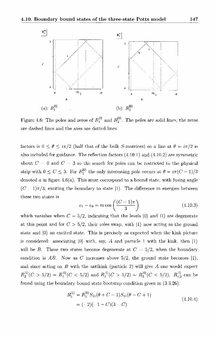
4.10. Boundary bound states of the three-state Potts model 147
3 /·. ~·· ~ : C : 11
' b : . . '
,: I
·.. :"' c " ~-
c
.,
ill
e e
Figure 4.6: The poles and zeros of R~o) and R~o). The poles are solid lines, the zeros
are dashed lines and the axes are dotted lines.
factors is 0 :::; e :::; in/2 (half that of the bulk S-matrices) so a line at e = in /2 is
also included for guidance. The reflection factors ( 4.10.1) and ( 4.10.2) are symmetric
about C = 0 and C = 3 so the search for poles can be restricted to the physical
strip with 0 :::; C :::; 3. For R~o) the only interesting pole occurs at e = i1r(C- 1)/3
denoted a in figure 4.6(a). This must correspond to a bound state, with fusing angle
( C - 1 )n /3, exciting the boundary to state 11). The difference in energies between
these two states is
((C-1)7r) e1 - e0 = m cos
3 (4.10.3)
which vanishes when C = 5/2, indicating that the levels IO) and 11) are degenerate
at this point and for C > 5/2, their roles swap, with 11) now acting as the ground
state and IO) an excited state. This is precisely as expected when the kink picture
is considered: associating IO) with, say, A and particle 1 with the kink, then 11)
will be B. These two states become degenerate at C = 5/2, when the boundary
condition is AB. Now as C increases above 5/2, the ground state becomes 11),
and since acting on B with the antikink (particle 2) will give A one would expect
R~1)(C > 5/2) = R~0)(C < 5/2) and R~1)(C > 5/2) = R~0)(C < 5/2). R~~~ can be
found using the boundary bound state bootsrap condition given in (3.3.26):
Jl) JO) ( ) ( ) R1 = R 1 Su e + C - 1 Su e - C + 1 (4.10.4)
= (-2)( -1 + C)(3- C)

4.10. Boundary bound states of the three-state Potts model 148
c
6 6
Figure 4. 7: The poles and zeros of R~1 ) and R~1 ). The poles are solid lines, the zeros
are dashed lines and the axes are dotted lines.
11) IO) ( ) ( ) R2 = R2 821 B + C - 1 821 B - C + 1
= (-2) (-2 - C) (C) .
Using the property ( x ± 2h) = ( x), where h = 3 here, it is easy to show that
R~0)(C =~-E)
R~O) ( c = ~ - E)
( -2)(~- E)(~+ E)= R~1)(C =~+E)
( -2)(~- E)(~+ E)= R~1)(C =~+E)
(4.10.5)
( 4.10.6)
(4.10.7)
so in fact, one only needs to consider poles in the physical strip for 0 ::; C ::; 5/2 to
get the full picture.
In R~o), there is one such pole at i( C - 2)7r /3, labelled b in figure 4.6. This
corresponds to a bound state, creating the boundary state J2), with energy
((C-2)7r) e2 = e0 + m cos
3 . (4.10.8)
The rapidities of the poles in R~1 ) and R~1 ) are shown in figure 4. 7. The pole, la
belled din figure 4. 7(a) is just the 'u-channel' version of pole a, shown in figure 4.8(a),
whereas pole e corresponds to the Colemann-Thun process shown in figure 4.8(b).
Naively, this ought to represent a double pole, but note that there is a zero in R~o)
at i1r(2 - C) /3, which reduces the order appropriately. Diagram 4.8(b) is only valid
for C < 2, at which point a bound state must form, with fusing angle (3- C)1r /3,
creating a state J3), labelled in 4.7 by f. The pole at i7rC/3 in R~1 ) (gin figure 4.7(b))

4.10. Boundary bound states of the three-state Potts model 149
2
I o) 2
C-1 3-C
(a): poled (b): pole e
Figure 4.8: Coleman-Thun diagrams for poles d and e in R~1 )
2
2 c
Figure 4.9: Coleman-Thun process diagram for pole g in R~1 )
has another Coleman-Thun description, shown in figure 4.9, which again due to the
zero at in(2- C)/3 in R~o) describes a simple, rather than a double pole.
As shown in (4.10.8), the energy of 12) is
((C-2)n) e2 = e0 + m cos
3 ( 4.10.9)
where e0 is the energy of IO) and m is the mass of the kink/anti-kink. For state 13)
the energy is
e3 = eo+ m cos ( ( C ~ 1 )n) + m cos ( (3
-3 C)n)
= eo + m cos ( ( C ~ 2)n) = e2 .
( 4.10.10)
As the states 12) and 13) have the same energy, the minimal assumption is that they
are the same state. This is supported by the fact that the reflection factors R~2) and

4.10. Boundary bound states of the three-state Potts model 150
c c
9 e
Figure 4.10: The poles and zeros of R~2) and R~2). Double poles (and zeros) are shown
by double lines.
Rl3), i = 1, 2 are also equal
R~2) = R~o) S21 (B + C- 2)S2I(B- C + 2)
= ( -2)( -1 + C) 2( -1- C)(3- C)= R~3)
(4.10.11)
R~2 ) = R~o) S22(B + C- 2)S22(B- C + 2)
= (-2)(-2 + C)(-2- C) 2 (C) = R~3) (4.10.12)
and
R~2)(C =~-E)= R~3)(C =~-E)
= (~- E) 2 (~ +E)(~+ E) (4.10.13)
= R~2\ c = ~ + E) = R~3) ( c = ~ + E) .
The poles in Rl2) ( Rl3
)) are shown in figure 4.10 (double poles are shown by double
lines). The double pole at i1r(C- 1)/3 in R~2) (h in figure 4.10(a)), can be described
in two ways: in terms of state 12) by figure 4.11(a), or state 13) by figure 4.11(b). In
these cases there is no zero at i7r(3 - C) /3 in either R~o) or R~o), or at i1r( C - 2) /3
in R~1 ) so these really are second order diagrams. The pole at i7r(3- C)/3 (i in
figure 4.10(a)) cannot be easily described in terms of state 12), but has a simple
description in terms of 13) as the 'u-channel' version of pole j, shown in figure 4.12.
The single pole at i7r(C-2)/3 in R~2) (j in figure 4.10(b)) is the 'u-channel' version
of pole b, as shown in figure 4.13(a), whereas the double pole at i7r(4- C)/3 (k in

4.10. Boundary bound states of the three-state Potts model 151
I~
C-1 •
C-1
(a): pole h, in terms of 12) (b): pole h, in terms of 13)
Figure 4.II: Coleman-Thun diagrams for the double pole h in R~2)=13)
3-C
Figure 4.I2: Coleman-Thun diagram for pole i in R~2)
figure 4.IO) is explained by figure 4.I3(b). Once again there is no zero in R~o) at
in(3- C)/3, so this is indeed second order.
The boundary bound state bootstrap therefore closes on three states I 0), II) and
12). The energies of II) and 12), in terms of e0 , the energy of IO), are
e1 eo + m cos ( ( C ~ I )n) (4.10.I4)
e2 = e0 + m cos ( ( C ~ 2 )n) (4.IO.I5)
They are shown in figure 4.I4, as a function of the boundary parameter C, indicating
at what values they appear in the spectrum. In figure 4.I4(a), the energy of the
ground state e0 is set to zero, and e1 and e2 are given in units of the kink/ antikink mass
m. In order to show the symmetry between e0 and e 1 more clearly, in figure 4.I4(b),
e0 is taken to be e0 = W (1 - cos( (C~l)n)) and again units of the kink/ antikink mass
mare used. The one particle threshold (e0 +m, for C < 5/2 and e1 +m for C > 5/2),
above which the spectrum is continuous, is also shown in bold in figure 4.I4(b). It

4.10. Boundary bound states of the three-state Potts model
:/ 12) 2 '
~ 2
2 12)
lo) lo)
C-2' 12) 2
2 :/ 12)
(a): pole j (b): pole k
Figure 4.13: Coleman-Thun diagrams for poles j and k in R~2 )
0.75
m OS
0.25
oohn~~~~~~~~ 1.0 125 1.5 175 2.0
c
(a): eo= 0
2.5 •n •• 2n 2• Jn 3• 4n
c
(b): eo= T(l- cos((C~l)1r))
152
Figure 4.14: The boundary spectrum of the three-state Potts model, in units of the
kink/ antikink mass m. The bold curve is the one particle threshold.
should be possible to verify the spectrum shown in figure 4.14(b) using the boundary
truncated conformal space approach [78].
Chapter 5
PT symmetry breaking and
exceptional points
This chapter is concerned with the study of a family of PT-symmetric Hamiltonians,
and in particular, in the Jordon block structures which emerge as the PT symmetry
is spontaneously broken. At first sight, this has little in common with the previous
work in this thesis, however the ODE/IM correspondence, described in section 2.6.2,
does have an important role to play. Before this is discussed there will be a brief
introduction to PT-symmetric quantum mechanics, which follows the recent review
[50].
5.1 PT-symmetric Quantum Mechanics
The study of PT-symmetric quantum mechanical theories began in private com
munication between Bessis and Zinn-Justin, who considered the spectrum of the
Hamiltonian H = p2 + ix3, with the corresponding Schrodinger equation
(- d~2 + ix3) 1/J(x) = E'lj;(x), 1/;(x) E L2 (IR). (5.1.1)
Although this Hamiltonian is not Hermitian, and so the usual arguments to show
the reality of the eigenvalues do not apply, numerical studies of this problem led
Bessis and Zinn-Justin to conjecture that the spectrum of H is in fact both real and
positive. Bender and Boettcher [63] suggested that the reality of the spectrum of this
non-Hermitian Hamiltonian is due to it having PT-symmetry, where the parity Pacts
by sending x ----+ -x and p ----+ -p, whereas the time reversal, T, sends p ----+ -p and
153
5.1. PT-symmetric Quantum Mechanics 154
i --+ -i. When the Hamiltonian, H, is PT-symmetric the following commutation
relation holds: [H, PT] = 0. If H and PT are also simultaneously diagonalisable
(which is not necessarily the case as PT is a non-linear operator) it can be shown
that the spectrum of H is real, as follows [123]: working in the basis in which both
Hand PT are simultaneously diagonal, so HI</J) = EI</J) and PTI</J) = ai</J), where a
is a constant, then using (PT) 2 = 1, I<P) = PTPTI<P) = a*ai<P) so a is in fact a pure
phase. It can therefore be absorbed into I<P) with the transformation I<P) --+ a 112 1</J)
so that PTI</J) = 1</J) and HPTI<P) = EI</J). Since H and PT commute, this is also
equal to PT HI¢) = E* I <P) and so E must be real.
Consider now the situation where H and PT are not simultaneously diagonalis
able, so PTI</J) = I~) where I~) =/= al¢). Using the commutation relation of H and
PT, HPTI¢) = PT HI¢), it is clear that HI~)= E*l~) so I~) is an eigenvector of H
with eigenvalue E*. In these cases the PT-symmetry of His said to be spontaneously
broken; the energy eigenvalues are no longer real, but appear in complex-conjugate
pairs. The PT operator acts to interchange the eigenvectors with complex-conjugate
eigenvalues [123].
Bender and Boettcher looked at a generalisation of the Bessis-Zinn-Justin prob
lem, the Hamiltonian HM = p2 - (ix) 2M (M real and > 0), and proposed that the
spectrum of this is real and positive for Jvf 2: 1 [63]. As Jvf decreases below 1, they
found that infinitely-many real eigenvalues pair off and become complex, and as Jvf
reaches 0.5, the last real eigenvalue diverges to infinity. They interpreted this 'phase
transition' at M = 1 as the spontaneous breaking of the PT symmetry of HM.
A further generalisation was made by Dorey and Tateo in [65], where an angular
momentum term was added to the Hamiltonian:
H - 2 (.)2M l(l+1) Ml- p - 'lX + 2 ' , X (M, l real and Jvf > 0). (5.1.2)
The conjecture made in [65], was that the spectrum of H 1d,l is real and positive for
M 2: 1 and l2l + 11 < M + 1. For both of these generalisations, x is no longer
restricted to the real line, so it is important to consider what boundary conditions
to impose, as taking the quantisation contour to tend to infinity in different pairs
of Stokes sectors will lead to different eigenvalue problems, as mentioned in Section
2.6.2. Note that when M = 1 the Hamiltonian H 1 = p2 + x 2 is that of the simple
harmonic oscillator, for which the quantisation contour is the real axis. When the

5.1. PT-symmetric Quantum Mechanics 155
angular momentum term is introduced, this contour must be continued around the
singularity at the origin. In general, Nf can take non-integer values and so to ensure
that the -(ix) 2M term is single valued, a branch cut must be made. This is taken
along the positive imaginary axis here, and so the continuation of the contour around
the origin should be taken through the lower half plane. As M increases above 1, the
resulting eigenvalue problem will be the correct continuation of the the simple har
monic oscillator, provided the quantisation contour tends to infinity in those Stokes
sectors which contain the real axis for M = 1, namely S1 and S_ 1, where
I 27rk I 7r
Sk := arg(x)- 2M+ 2 < 211.1 + 2. (5.1.3)
The Stokes sectors S1 and S_ 1 rotate towards the negative imaginary axis as 11.1
increases, but for Nf < 2, the real axis remains within these sectors and so can be
taken as the quantisation contour (with suitable continuation around the singularity
at the origin). When Nf = 2, the anti-Stokes lines which form the upper boundary
of the sectors S1 and S_ 1 lie along the real axis, so for M 2: 2 the contour must
be deformed from the real axis, down into the lower half plane [63], as shown in
figure 5.1.
' '
Im
' '
' ' ' '
' ' ' '
Re
Figure 5.1: A wavefunction contour for M 2: 2
The spectrum of the following family of PT-symmetric eigenvalue problems, first
studied in detail in [66, 124], are of particular interest in this thesis:
(5.1.4)

5.2. Functional relations 156
For !11 = 1, this also reduces to the simple harmonic oscillator (with energy E +a),
and the addition of the inhomogeneous term (ix)M-1 has no effect on the Stokes
sectors so the contour Cis the same as that described above and shown in figure 5.1.
This problem is invariant under the replacement l -------+ -1 -l , and it will be convenient
in the following to trade l for A := l + !, so that the symmetry is between A and -A.
The first interesting feature of (5.1.4), shared with many PT-symmetric problems,
is the reality of the spectrum for many values of the parameters a and l. More
precisely, for M > 1 and NI, a and A= l+! real, the spectrum of (5.1.4) is
• real if a < M + 1 + 2 I A I ;
• positive if a < M + 1 - 2 I A I .
(5.1.5)
(5.1.6)
This was proved in [66] via the ODE/IM correspondence. This proof will be discussed
shortly, but first it is worth seeing how the functional equations for this ODE differ
from the simpler case described in section 2.6.2 [66] (see also [50]).
5. 2 Functional relations
As a small simplification, the factors of i can be eliminated from ( 5.1.4) by replacing
x with z := x/i and setting <I>(z) := 1/J(x/i), so that the eigenproblem (5.1.4) becomes
(5.2.1)
where £k = -Ek. Note that the quantisation contour has also been rotated by 90°;
the new contour is shown in figure 5.2.
In parallel to the discussion presented in Section 2.6.2, the Stokes relations can
be found by first defining the 'basic' solution, subdominant in the 50 sector, which
in this case is z-111/2-u/2 ZM+l
Y( z £ a A) rv e- 111+1 • ' ' ' V21 From this 'basic' solution the following set of solutions can be generated:
-rri w =eM+!
(5.2.2)
(5.2.3)
for integer k, with each pair of solutions {Yk. Yk+ 1 } forming a basis. Following the
same argument given in section 2.6.2, a Stokes relation can be found, of the form
C(£, a, A)Yo(z, £,a, A) = Y-1 (z, £,a, A)+ Y1 (z, £,a, A) (5.2.4)
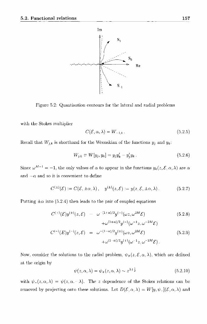
5.2. Functional relations
Im
' ' ' ' ' ' ' ' '
Re
Figure 5.2: Quantisation contours for the lateral and radial problems
with the Stokes multiplier
C(E, o:, .\) = W-1,1.
Recall that Vf!j,k is shorthand for the Wronskian of the functions Y) and yk:
157
(5.2.5)
(5.2.6)
Since w11H 1 = -1, the only values of o: to appear in the functions Yk(z, E, o:, .\)are o:
and -o: and so it is convenient to define
cl±l(E) := C(E, ±o:, .\), yl±l(z, E):= y(z, E, ±o:, .\).
Putting ±o: into (5.2.4) then leads to the pair of coupled equations
c(+)(E)y(+l(z, E) = w-(l+n)/2y(-)(wz, w 2M E)
+w(l+n)/2y(-) (w-1 z, w-2M E)
w-(1-n)/2y(+) (wz, w2M E)
+w(l-n)/2y(+) (w-1 z, w-2M E).
(5.2.7)
(5.2.8)
(5.2.9)
Now, consider the solutions to the radial problem, '1/J±(z, E, o:, .\), which are defined
at the origin by
(5.2.10)
with '1/J_(z, o:, .\) = '1/J(z, o:, -.\). The z dependence of the Stokes relations can be
removed by projecting onto these solutions. Let D(E, o:, .\) = lV[y, '1/J+](E, o:, .\) and
5.2. Functional relations
write D(±l(£) = D(£, ±a, A.). The Stokes relations then become
c(+l(£)D(+l(£) = w-(2A+a)/2 D(-) (w2M £)
+w(2A+a/2) D(-) (w-2/lif £)
w-(2.\-o:)/2 D( +) (w2!vf £)
+w(2.\~a/2) D(+l(w-2M £).
158
(5.2.11)
(5.2.12)
It is worth noting a few features of the multipliers C and D here. C(±) is defined
as the Wronskian of the subdominant solutions in the 5 1 and 5_1 sectors. This
Wronskian is zero if and only if the two solutions are linearly dependent, so in fact
the solution is subdominant in both sectors. Such a solution is an eigenfunction of
this lateral problem and soC(±) is a spectral determinant of this: the zeros of C±(£)
are the eigenvalues of the eigenproblem (5.2.1) with <Pk(z) E L2(iC). D(±l(£) is also
a spectral determinant, but for the radial problem, with boundary conditions set as
x -> 0 and x -> +oo. This is easily seen as D is the Wronskian of two solutions,
one subdominant in the 50 sector, and one which decays as z -> 0. The zeros of
D(£) are therefore the eigenvalues of the radial problem. Note that the quantisation
contour for this problem is along the real axis, as shown in figure 5.2, so this problem
is Hermitian.
Now, for M > 1, vVKB estimates show that the function D(±l(£) has order less
than 1 [65], so Hadamard's factorisation theorem can be applied in its simplest form.
This states that, if D(O, A.) =/= 0 then D(£, A.) can be written as an infinite product
over its zeros. This constraint holds as it can be shown that [66]
D(±l(£)l = = _1_ (M + 1) i;r\';-~ r (Nfh) £ o vl2i 2 r (i~~~c; + D
and so
Di±i(£, .\) ~ Di±l(o, .\) g ( 1- ~) Using (5.2.13) in (5.2.12), along with the identity
r ( ~ + e) r (~ - e) = 7T 2 2 cos(e7T)
and remembering that D(-l(£) = D(£, -a, A.) and w = eA;~~ gives
C(£, a, A.)l£=o = c(+l(£)1£=o
= ( J\1; 1) M"'tl 27T r ( ~ + i~J-:2) r ( ~ - i~;+~a2) ·
(5.2.13)
(5.2.14)
(5.2.15)
(5.2.16)

5.3. Reality proof 159
5.3 Reality proof
The functional relations given above can now be used to reproduce the proof of (5.1.5)
and (5.1.6) [66] (see also [50]), using techniques inspired by the Bethe ansatz.
First, define the zeros of the spectral determinant C(+l(£) = C(£, a, A.) to be
the set { -Ek}, and the zeros of D(±l(£) to be the set {£k±)}. Putting£= -Ek in
(5.2.12) will fix the left of (5.2.12) to zero and so this equation can be rearranged to
D(-l(w2Ek) -2.\-a
D(-l(w-2Ek) = -w ' (5.3.1)
and using the factorised form of D(-) forM> 1, (5.2.14) puts constraints on the Ek:
ft. ( ~~~) + w::k ) = -w-2.\-a, k = 1, 2, ...
n=l En + W Ek (5.3.2)
Each £A-) is an eigenvalue of an Hermitian operator H M,-a,.\ and is therefore real.
Performing a Langer transformation [125] on HM,a,.\, by setting z = ex, y(z) =
ex12¢( x), shows that £A- l solves the following eigenproblem
(5.3.3)
If a < 0, this is an everywhere positive potential and so£(-l is positive. Without loss
of generality, it can be assumed that A. 2 0, since the original problem is invariant
under A.------; -A. and so£(-) will be positive for a < A..
In fact, by considering the value of D(-l(£)1£=0, given in (5.2.13), it is clear that
this first vanishes when a = M + 2..\ + 1, and so all £~-) must be positive up to this
point. Taking the modulus squared of (5.3.2) and writing the eigenvalues of (5.2.1)
as Ek = 1Eklei6k gives
IT (1£~-)1 2 + 1Ekl
2 + 2£A-)1Ekl cos(-ffh + bk)) =
1 n=l I£~-)I 2 +1Ekl 2 +2d-)1Eklcos(J~l-bk) .
(5.3.4)
For a < AJ + 2..\ + 1, all £~-) are positive and so each term in the product is greater
than, less than, or equal to one dependent only on the values of the cosine in the
numerator and denominator, which are independent of the index n. The product
will therefore only be equal to one if each individual term is equal to one, which for
Ek ::/- 0 requires cosCvJ~ 1 + bk) =cos( 1}~ 1 - bk), or equivalently
. ( 27f ) . sm sm(bk) = 0. Jvf + 1
(5.3.5)

5.3. Reality proof 160
As M > 1, this implies that
(5.3.6)
Relaxing the condition on A now, this shows that the eigenvalues of (5.1.4) forM> 1
and a < M + I2AI are real. Note that most of the Ek become complex as Jvf falls
below 1 [63], at least for a = 0. This coincides with the point at which the order of
D(-l(£) is greater than 1, and so the factorised form of D(-l(£) given by Hadamard's
factorisation theorem no longer has such a simple form and this proof breaks down.
To prove the positivity at general values of M > 1, one must first consider the
case of !vi = 1. This is the simple harmonic oscillator with angular momentum term
(where a is absorbed as a shift in £), which is exactly solvable for all A and a in
terms of confluent hypergeometric functions
Now, using the analytic continuation formula, from [126]
U(a b ze21rin) = (1- e- 21ribn) r(1 - b) M(a b z) + e- 21ribnU(a. b z) ' ' r(1 +a- b) ' ' ' '
the Wronskian
W[U(a, b, z), Jvf(a, b, z)] = ~~~~ z-bez
and, for b > 1, the lzl --> 0 asymptotic
r(b- 1) l-b U(a,b,z)rv r(a) z + ...
it can be shown [65] [66] that
21f C(£, a, A)IM=l = r(~ + 2>-+,f-a)r(~ _ 2.x-;+a) ·
(5.3.7)
(5.3.8)
(5.3.9)
(5.3.10)
(5.3.11)
The eigenvalues of (5.1.4), forM= 1, are therefore Ek = 4k+2-a±2A, k = 1, 2, ....
They are all real for all real values of a and A, and are all positive for a< 2- I2AI.
For M > 1, provided a remains less than 1\1 + 1 + I2AI, all eigenvalues Ek will
be confined to the real axis and so the point at which the first eigenvalue becomes
negative will be signalled by the presence of a zero in C (- E, a, A) at E = 0. Recall,
from (5.2.16), that
C(£, a, A)l£=0 = (M; 1) M"'+l 27r r ( ~ + i;~~~) r ( ~ - i:/~~)
(5.3.12)

5.4. Investigating the frontiers of the region of reality 161
and so the first zero when £ = - E = 0 appears when a = M + 1 -I2.AI; the spectrum
is therefore entirely positive for all a < M + 1 - I2.AI and M > 1.
Figure 5.3 shows the regions of parameter space for which the reality and positivity
of the spectrum has been proved. So far, the reality of the spectrum of ( 5.1.4) has
been proven for (a, 2).) E B U CUD, and positivity for (a, 2).) E D. This proof
does not show that the reality of the spectrum breaks down for all, or indeed any, of
the points in A, although this breakdown has been observed numerically for several
points. In [124], Dorey, Dunning and Tateo explored the boundary of A, where they
described a mechanism by which the breakdown of reality occurs. They also showed
numerically that the phase diagram for M = 3 has a much more interesting structure
than is shown in figure 5.3. A discussion of their work is presented below.
a
A
B ,' c
; : M+l ,'
D
Figure 5.3: The approximate 'phase diagram' at fixed !vi. The spectrum is entirely
real in regions B, C and D, and positive in region D.
5.4 Investigating the frontiers of the region of re
ality
It is convenient here to adopt a new set of coordinates in the (2)., a) plane defined
by 1
a± = M [a - M - 1 ± 2.A] . 2 + 2
(5.4.1)
The frontiers of the region (5.1.5) of guaranteed reality are the lines, at ±45° in
the (2)., a) plane, given by a± = 0. In this section, arguments from supersymmetric
quantum mechanics will be used to show that his model has a protected E = 0 energy

5.4. Investigating the frontiers of the region of reality 162
level along these lines, and that level crossing with this protected E = 0 level can be
seen as the mechanism by which the first levels pair-off and become complex as the
region (5.1.5) is left [124]. This argument will also be extended to the lines a±= m,
m E N, for the ./1.1 = 3 case, using the quasi-exact solvability of the model at these
points.
On the line a+= 0, a= .M + 1- 2.\ and the ODE (5.1.4) becomes
( d2 .\2-!) -- + z2M + azM-I + 4 <I>(z) = -E<I>(z). dz2 z2
This factorises as
with
Q d M 2.\- 1
± = ±-+z ----dz 2z '
(5.4.2)
(5.4.3)
(5.4.4)
and such a factorisation usually points to a relationship with supersymmetry. It is
easily seen that (5.4.3) has an E = 0 eigenfunction in L2 (iC):
(5.4.5)
which can be interpreted as having unbroken supersymmetry. All other eigenfunctions ~
are paired with those of the SUSY partner Hamiltonian H = Q_Q+, which can
be found by replacing (a+,a_) = (O,-,vJ~ 1 ) with (Ci+,Ci_) = (-1,-1- ~J~i) =
( -1, cc - ~~ ~i). This problem is symmetric in .\ so sending .\ ---+ -.\ gives the E = 0
eigenfunction on the line a_ = 0. The boundaries between the regions in figure 5.3
coincide with the presence of the ( supersymmetric) zero-energy state in the spectrum.
Ordinarily, this would be expected to be the ground state of the theory, which is the
case on the boundary of D. On the boundary of A, however, this is only true for
a < 1\1 + 3, due to level crossing which is not ruled out here by the usual theory of
SUSY quantum mechanics as this problem is not Hermitian.
To see this level crossing, consider C(£, a, l)IE=O, as given in (5.3.12), which in
the a± coordinates is
(5.4.6)
This is zero when either a+ or a_ vanishes, as expected by the presence of the state
1/J in the spectrum. Level-crossing occurs when a further level passes through zero.

5.4. Investigating the frontiers of the region of reality 163
To find the points where this occurs, consider the SUSY partner potential, which is
isospectral to H except for the elimination of 1/J. Replacing a± in (5.4.6) with D±
( 1\;f + 1 ) (i- ---:-2_1f::---:-
2 r( -&_)
(1\;f + l)(i_ 21f
M-1 . 2 r(M+l-a_)
(5.4.7)
Level-crossings with the state 1/J are indicated by simple zeros of ( 5.4. 7), at (a+, a_) =
(0, n + ~~~i), n = 0, 1, .... Swapping a+ and a_ (using the ,\ ~ -,\ symmetry)
throughout gives level-crossings on the line a_ = 0. Note that these level-crossings
are exact as 1/J is protected by supersymmetry, and cannot mix with any other state.
As soon as this supersymmetric line is left level mixing can occur. In PT-symmetric
systems, eigenvalues are all either real, or occur in complex-conjugate pairs. Com
plex eigenvalues can therefore only be formed via the intermediate coinciding of two
(or more) previously-real eigenvalues. The supersymmetry on the lines a+ = 0 and
a_ = 0 provides a mechanism for this pairing-off to occur, and for the formation of
the associated exceptional points [124]. Exceptional points occur in the spectrum of
an eigenvalue problem whenever the coalescence of two or more eigenvalues is accom
panied by a coalescence of the corresponding eigenvectors; at such points there is a
branching of the spectral Riemann sur'face [127, 128, 129, 130]. For one-dimensional
problems of the sort under discussion here, genuine degeneracies of levels are impossi
ble- since the Wronskian of any two solutions which both decay in some asymptotic
direction must vanish - and so levels in this problem can only coincide at exceptional
points. Quadratic exceptional points must therefore exist at
( M -I) (a+,a_)= O,n+ Nf+I (5.4.8)
for n EN.
There is also a protected zero-energy level along the lines a± = m E N. Exception
ally, for Nf = 3 a similar line of argument can be applied here, using a higher-order
supersymmetry to eliminate this zero energy level along with 2m others [66][124],
which allows the positions of further quadratic exceptional points to be identified.
As will become clear shortly, this is related to the fact that, for M = 3, the model is
quasi-exactly solvable along these lines.

5.4. Investigating the frontiers of the region of reality 164
Specialising now to .1\1 = 3, the eigenproblem (5.2.1) becomes
(- dd:2 + z6 + az2 + A2
z~ ~) <I>k(z) = -Ek<I>k(z), (5.4.9)
If boundary conditions are imposed at z = 0 and z = +oo, the problem (5.4.9)
is quasi-exactly solvable whenever a and A are related by a = - ( 4J + 2A) for some
integer J, and J energy levels can be computed exactly [131]. Bender and Dunne [132]
found an elegant method to find the corresponding wavefunctions, square integrable
along the positive real axis. The solutions to (5.4.9) must have this property along
the contour i C, but with minor modifications the approach of [132] can still be used.
First, look for solutions of the form
(5.4.10)
where
(5.4.11)
The functions ~P± ( z) can be shown to solve ( 5.4. 9) if the coefficients Pn satisfy the
recursion relation
Pn = -EPn-1 + 16(a/4 =f A/2- n + 1)(n- 1)(n- 1 ± A)Pn-2, n 2': 1 (5.4.12)
with the condition that Pm = 0, rn < 0. The normalisation is set by the initial
condition P0 = 1. If a/ 4 =f A/2 = J is a positive integer, then the second term
on the RHS of (5.4.12) vanishes for n = J + 1, and so P1+1(E) is proportional to
P1 (E), as are all subsequent coefficients Pm>J+1 (E). At a zero of P1 (E) the series
therefore terminates and the J QES energy levels are found as those E that satisfy
P1 (E) = 0. Due to the choice of exponential prefactor in (5.4.10) (inverse to that
in [132]), the corresponding 1f)± ( z) will automatically satisfy the revised boundary
conditions. Note, since the boundary conditions are not being imposed at the origin,
both signs of A lead to acceptable solutions.
For simplicity, choose +A in (5.4.10) so a= 4J + 2A (-A can be recovered using
the A -----> -A symmetry) and write Pn, for n 2': J + 1 as
(5.4.13)
The Qn then satisfy the recursion relation
Qn = -EQn-1 + 16(1- n)(n + J- 1)(n + J- 1 + A)Qn-2 (5.4.14)

5.4. Investigating the frontiers of the region of reality 165
with initial condition Q0 = 1. This matches the Pn relation if J ----+ J = -J, or
alternatively, a1 ----+ CXJ = -a1 /2 + 3A and A ----+ ~J = a1 /4 + A/2. Then
(5.4.15)
This has an interesting consequence for the series expansion of (5.4.10), which can
be seen by rewriting it as
[ ... + ~ (-~) n Pn(E, a], A) Z2nl ~ 4 n!r(n+A+1) n=J
[ ... + ~. oo (-~)n+J PJ(E, aJ, A)Qn(E, aJ, A) z2(n+J)l ~ 4 (n + J)! f(n + J +A+ 1)
(5.4.16)
where the dots represent lower order terms. Compare this with the expansion of
·1/;(z, E, a1 , ~1 ):
ol•( E ~ \ ) - ~ 5:+! ~ ( 1)n Pn(z, E, CXJ, ~J) 2n 'f/ z, , a 1, -"J - e 4 z 2 ~ -- ~ z
n=O 4 n!r(n+A+1) (5.4.17)
which, using (5.4.15) and ~J = J +A becomes
/ ( E ~ \ ) = z44 .X+J+~ ~ (-~) n Qn(E, a], A) 2n '1/) z, , a], AJ e Z ~ If( J , ) Z . ·
4 n. n + +-" + 1 n=O
( 5.4.18)
It now follows that '1/;(z, E, a 1, A) is mapped onto a function proportional to '1/;(z, E, 51, ~1 )
by the differential operator
(5.4.19)
It can therefore be shown that Q1 (A) maps the eigenfunctions of H(a 1 , A) to those
of H(a1 , ~1 ), or to zero [66]. The eigenfunctions which are mapped to zero are those
for which P1(E, a1, A) vanishes, which are precisely the QES levels. The operator Q1
is therefore a generalisation of the supersymmetry operator Q + for J > 1.
The argument for the level-crossing along the a± = 0 lines can now be extended
further for the A1 = 3 case [124]. In terms of the a± notation, the QES levels occur at
(a+, a_) = (a+, ~ ( J -1)), for J a positive integer, which in the dual problem (with the

5.4. Investigating the frontiers of the region of reality 166
QES states removed from the spectrum) becomes (ii+, ii_) = (o:+- 1/2, -~(J + 1)).
Substituting this into CIE=O (5.4.6):
~ ~ ( A1 + 1) a+-~ ( 1 -1 l 2n
C(-E,o:+,o:-)iE=o,a_=-~(1+1) = 2 f(-ii+)r(~(J + 1))
( A1 + 1) -~(1 - 1 )+a+ 2n
2 r( -o:+ + ~)r(~(J + 1))
(5.4.20)
which is zero when o:+ = J /2 + n. Recall from above that the protected zero-energy
levels lie on the lines O:± = m E N so if o:+ = m, J must be even and the quadratic
exceptional points occur for
(5.4.21)
Replacing A with -A in the above simply swaps o:±, so there are also quadratic
exceptional points at
(5.4.22)
It is also worth noting that the levels which become complex at these exceptional
points are always in the QES part of the spectrum. This is easy to show once it is
noted that the 'dual' problems, with (ii+, ii_) = (o:+- Jj2, ~(J + 1)), always lie in
regions of the parameter space covered by the reality proof given above [124]. Since
the spectrum of this dual problem is identical to that of the original, minus the QES
levels, it is clear that the non-QES levels must always remain real. It also follows that
the QES eigenvalues are symmetric about zero, i.e. both E and - E are contained in
the QES sector of the spectrum.
Numerical investigations at lv! = 3, reported in [124], showed that the way in
which the spectrum of (5.1.4) becomes complex has considerably more structure than
(5.1.5) might suggest. The curved, cusped line of figure 5.4 is a line of exceptional
points which indicates where the first pair of complex eigenvalues is formed as the
region of reality is left; it only touches the dotted lines c:t± = 0 at the isolated
points given in (5.4.8), but it will be shown that the smooth segments are quadratic
exceptional points, where two levels coalesce, while the cusps themselves are cubic
points.

5.4. Investigating the frontiers of the region of reality 167
20
15
1 0 a
5
0 ~--------~--+-~~-. ----------
,' ·.
- 1 0 0 10
Figure 5.4: The domain of unreality in the (2)., a) plane for NI = 3, with portions of
lines with protected zero-energy levels also shown. The horizontal axis is 2>. = 2l + 1.
The additional dotted lines in figure 5.4 are the lines a ± E N. As mentioned
earlier, the model has a protected zero-energy level, and for M = 3, is also quasi
exactly solvable along these lines. It is worth noting that the cusps in figure 5.4
appear to lie exactly on these lines , to within numerical accuracy.
If one asks when a second pair of complex eigenvalues is formed , and so on,
figure 5.5 is obtained, again for M = 3. This plot is adapted from [50]; the same
pattern was independently found by Sorrell [133] via a complex WKB treatment of
the problem. Note the pattern of cusps is repeated , with the cusps again lying on
lines of protected zero-energy levels , and the curve touching the lines a± = m E N
at the points given in (5.4.21) and (5.4.22).
The analysis of [124] left a number of questions open. While the merging and
subsequent complexification of levels is suggestive of exceptional points and a Jordan
block structure for the Hamiltonian, this has not been demonstrated explicitly. The
apparent siting of the cusps on lines with simultaneous quasi-exact solvability and
protected zero-energy levels has not been proved; in particular, it is not clear whether
this feature should be associated with the zero-energy level (in which case it should
persist for lvf =/=- 3) or with the quasi-exact solvability (in which case it might be lost
for M =/=- 3). Finally, and connected with this last question , the general pattern away
from M = 3 has not been explored.
These issues are addressed in the rest of this chapter. For M = 3 the positions

5.5. TheM= 3 problem revisited- cusps and QES lines 168
20 ,'
15
1 0 a
5
0
-5
-10 0 10
2A.
Figure 5,5: The (2A , a) plane for M = 3, showing lines across which further pairs of
complex eigenvalues are formed,
of the cusps are investigated, and it will be proved that they do indeed lie on QES
lines, The exceptional points in the spectrum will be examined and the Jordan form
at such points found. Finally, the situation for M =1- 3 will be explored numerically,
and the picture that emerges will be verified with a perturbative study near M = 1.
This work can be found in [2]
5.5 TheM 3 problem revisited - cusps and QES
lines
The first question to be addressed is what are the exact locations of the cusps? As
shown above, the levels which become complex at exceptional points are always in
the QES part of the spectrum, so the cubic exceptional points arise when three zero
energy levels appear in the QES sector of the spectrum, Since these eigenvalues are
symmetric about E = 0, this occurs for odd J, and it is precisely this symmetry
that constrains the cusp to lie exactly on QES lines, Figure 5.6 shows a surface plot
of the energy levels for (2A, a) in the vicinity of the cusp at (2A , a) = ( -3, 9) (or
(a+, a_)= (i , 1)), This shows the merging of two energy levels (at the bottom right
and top left of the plot) and then the cusp being formed in the centre of the plot
where three energy levels merge at a single point. The superimposed line indicates

5.5. TheM= 3 problem revisited- cusps and QES lines 169
0.1
Figure 5.6: Surface plot of energy levels in the vicinity of the first cusp at (2A, a) =
( -3, 9), or (a+ , a_) = (~ , 1). The axes are E = a+ - ~, rt = 1 -a_ and E. The
superimposed line indicates the merging of levels.
the merging of levels and the E = 0 line is also included.
The exact locations of the cusps can be found by examining the Bender-Dunne
polynomials P1 (E). For odd values of J, these polynomials split into a polynomial
in E 2 multiplied by an overall factor of E, the first two being
- E(E2 + 96 ± 64A) (5.5.1)
-E(E4 + 320(±A + 5/2)E2 + 2048(8A2 + 40A + 41)) . (5.5.2)
It follows that there will be three zero-energy levels whenever
= 0. (5.5.3) E=O
Swapping to the notation a ±, the cusp positions for positive values of A (which
corresponds to taking -A in (5.4.10)) lie on the lines a+= (J -1)/2 = N+, each line
having precisely a + cusps. Using the Bender-Dunne relation (5.4.12) , the constraint
(5.5.3) is equivalent to Qa:+(a_) = 0 where Qn satisfies the first order recurrence
relation n
IJ(2j- 1)(2j- 2a+- 2)(2j + 2(a_- a+)- 1) j = l

5.6. The Jordan block at an exceptional point
1
2
3
4
5
CL
4 ~±3v'2 4 8
§. §. ± v00 4' 4 8
!._ ± J 86+5Vi90 !._ ± J 86-5Vi90 4 8 '4 ,..---'L-8-=
!:! !:! ± J 170+7v'214 !:! ± J 170-7v'214 4'4 8 '4 8
170
Table 5.1: Location of some of the cusps in the (o:+, o:_)-plane forM= 3.
with Q0 ( o:_) = 1. Solving the recursion relation (5.5.4) gives
Ct+
Qa+(o:_) = 3F2([~, -o:+, ~ + o:_- o:+], [~- o:+, 1 + o:_- o:+], 1) ITU + o:_- o:+), j=l
(5.5.5)
which is a polynomial in o:_ of degree o:+. Mapping back to the variables
(.\, o:) = (±2(o:+- o:_), 4(1 + 0:+ + o:_)) ' (5.5.6)
the zeros of QN+ ( o:_) = 0 match all the cusp positions shown in figure 5.5, to within
the numerical accuracy. Table 5.1 shows the location of the first few cusps. Having
located the exceptional points, the next step if to show their Jordon block explicitly.
5.6 The Jordan block at an exceptional point
At an exceptional point, the Hamiltonian can be arranged so that it contains an
n x n Jordan block, where n is the number of merging levels: two for the quadratic
exceptional points, and three for the cubic ones. In general it is hard to see this
explicitly, since the eigenfunctions of (5.4.9) cannot be found exactly. However for
M = 3, the fact that the model is quasi-exactly solvable (QES) on the lines et± E N
can be exploited. Furthermore, as explained above, any levels which coalesce and
become complex on these lines must lie in the QES sector of the model. Near to the
exceptional points on the QES lines it is therefore a good approximation to truncate
the Hilbert space to that part of the QES sector which contains the coalescing levels.
This will be used to see the Jordan blocks for the first quadratic and cubic exceptional
points.
To do this, begin with the Hamiltonian, H 0 , at the exceptional point, and restrict
to the space of states which merge at this point. Then perturb about this point,

5.6. The Jordan block at an exceptional point 171
along the QES line by writing the full Hamiltonian, Hp as Hp = H0 + V. The aim is
to expand Hp, using the wavefunctions of H0 as a basis, i.e. one needs to calculate
(5.6.1)
where { cPm, cPn} is the basis for the Jordan block form of H o, and { Jm, Jn} is the
appropriate dual basis. The expectation is that the eigenvalues of Hmn, to leading
order, will correspond to the eigenvalues of the the merging QES states. Before Hmn
can be calculated, the appropriate basis for H0 must be found. A general method for
finding such a basis, in cases where a suitable one-parameter family of eigenfunctions
is known exactly as the exceptional point is approached is, outlined below
5.6.1 Basis for an n x n Jordan block
To illustrate a method that can be used to construct the basis of ann x n Jordan block,
which arises when n eigenstates merge, the following toy model will be employed.
Take ann x n matrix L, depending on one parameter t::
1
e(2rrij /n) El/n
e(4rrij/n)E2/n
(5.6.2)
, j = 1 .. . n. (5.6.3)
When E = 0, L(t:) has a Jordan block form, but at this point all n eigenvectors
'1/Jj become equal and so no longer form a basis. A new basis must therefore be
constructed, consisting of the vectors '1/J(k), k = 0 ... n- 1 which satisfy
L(t:)'lj/o) 1€=0
L(t:)!j)kl 1€=0
0
'1/J(k-1) IE=O ' k = 1 ... n- 1.
(5.6.4)
(5.6.5)
5.6. The Jordan block at an exceptional point 172
For simplicity, begin with the eigenvector 'lj;n where
(5.6.6)
Clearly 'lj;(o) = '!j;n(E) satisfies the first condition (5.6.4) above. Choosing 'lj;(o) to be
another 'lj;j here should work equally well but would need a different normalisation
for 'lj;(k) below.
Before the other basis vectors are constructed, it is convenient to introduce some
notation. Let
and
n-1 d D = nEn-
dE
- dL L=- dE.
(5.6.7)
(5.6.8)
Note that L is linear in E so ~: = 0. D and L satisfy the following commutation
relations
Finally, define
[D, Ek/n]
[D,L]
[D,L]
nE(n-l)/n L
0.
(5.6.9)
(5.6.10)
(5.6.11)
(5.6.12)
By induction, it is easy to show that acting with Don (5.6.6) k times for 1 :::; k :::;
n- 1 gives
(5.6.13)
When E = 0 this satisfies (5.6.5), so an appropriate basis is
(5.6.14)
and
(5.6.15)
for k = 1 ... , n -1. Recall that 'lj;n was chosen for simplicity here, but other '1/Jj should
work equally well with some changes to normalisations.

5.6. The Jordan block at an exceptional point 173
5.6.2 A quadratic exceptional point
The method outlined above will now be used to show the existence of a Jordan block
in the Hamiltonian for the first quadratic exceptional point.
Recall that the quadratic exceptional points occur at even values of J so let J = 2,
and take +>. in (5.4.10) so J = a/4- >.j2. Then a = 2>. + 8 and the eigenvalue
problem is now
( d2 ).2 1 )
- dz2 + z6 + (2>. + 8)z2 + z2 4 + E 7/J = 0. (5.6.16)
In the a± notation from (5.4.1), this corresponds to a+ = ~(>.+I) and a_ = 1/2.
Let ). = 2E - 1, then the exceptional point occurs when E = 0. This is the point at
which two levels merge and the Hamiltonian can be written in a Jordan block form.
At this point the recursion relation for F{1 , (5.4.12), becomes
Pn = -EPn-1 + 16(3- n)(n- I)(n + 2E- 2)Pn-2 (5.6.17)
which terminates when n = 3. The energy eigenvalues of the two QES levels are
given by the roots of P2 : E± = ±ivf:32E = ±4~. The corresponding eigenstates,
from (5.4.10), are
(5.6.18)
where W ± = 7/J~q.( 5 . 4 .10) IE± and a is some normalisation constant to be determined
later. The Jordan form of the Hamiltonian can be seen by working with the basis
[129]
(5.6.19)
with b another normalisation constant. The unperturbed Hamiltonian is
d2 3 2 6 Ho = --2 + - 2 + 6z + z (5.6.20)
dz 4z
and in order to satisfy the requirements H0¢(o) = 0 and H0qPl = c/J(o), b is fixed to
be b = - 4~. Note, however, that this basis is not unique as the basis { a¢(o), a¢(ll + ,B¢(0)} also satisfies the Jordan block constraints for any constants a and ,6. The
general Jordan basis, in this case, is therefore given by
(5.6.21)
(5.6.22)

5.6. The Jordan block at an exceptional point 174
The integrals I, ¢m¢n dz, { m, n} E {0, 1 }, must now be calculated in order to fix
these constants and to identify the relevant dual basis { ¢m, ¢n}, which must satisfy
J ¢ 0¢;0 dz = J ¢ 1¢ 1 dz = 1 and J ¢0¢1 dz = J ¢ 1¢0 dz = 0. The contour. here ')' ')' ')' ')' '
and in subsequent calculations, is taken to be 1 = -1-l + /o +/I, where l±(t) =
texp(±in/4), E::; t::; oo, /o = Eeit, -n/4::; t::; n/4 and Eisa small positive number
which avoids any singularities at z = 0. The integrals are given by
~ c/Joc/Jodz
~ c/Joc/J1 dz
~ ¢I¢I dz
-a2 ~ ez4
12z3 dz = 0 (5.6.23)
~ ez4
/2 (-a:z- ia;3z3
) dz =- i~2
V'hr (5.6.24)
~ ez4/2 ( _ 1~: _ ia;z + ;32z3) == ~ (;'JV'hr _ Z~7f) (5.6_25)
Fixing I, ¢ 1¢1 dz = 0 sets ,6 to
;3 = i; {% (5.6.26)
and the requirement that I, ¢0¢ 1 dz = 1 sets a to
( 8) 1/4 a= (1 + i) :; (5.6.27)
- -The basis is now fixed and the dual basis can be taken to be ¢0 == ¢1 and ¢ 1 = ¢0 .
The full Hamiltonian is Hp = H0 + V where V = 4€(;;-1) + 4Ez2, so H mn must now
be calculated, where
(¢miHplc/Jn) (5.6.28)
(¢miHolc/Jn) + 4E(E- 1)(¢mlz-2 lc/Jn) + 4E(¢mlz2 lc/Jn)
with {¢m, ¢n} = {¢0 , ¢1} from above. The aim here is to find the eigenvalues of Hp,
to leading order only. If (¢1IVI¢o) "' a 10 E, for some coefficient a 10 then to leading
order Ep;± ~ ±fo!OE, so no other matrix elements need to be considered. This is the
case here as (¢11VI¢0 ), for V = 4€(;;-1) + 4Ez2 is given by
(5.6.29)
Therefore, to leading order
(5.6.30)
which are equal to the QES eigenvalues E±, as expected.
5.6. The Jordan block at an exceptional point 175
5.6.3 A cubic exceptional point
The first cubic exceptional point occurs when J = 3 and o: = 2,\ + 12. In the o:±
notation, this corresponds to (o:+, o:_) = (1 + .A/2, 1), but in table 5.1 the position of
the first cusp is given as (o:+, o:_) = (1/4, 1) (note o:+ and o:_ have been exchanged
here using the >. ----+ - >. symmetry). If >. = 2E - 3/2, this point then corresponds to
f = 0. The eigenvalue problem, in terms off is
( d2 ( 4f - 2) ( 4f - 4) )
- dz2 + 4z2 + ( 4f + 9)z2 + z6 + E ·1/J = 0 (5.6.31)
and the recursion relation for Pn is
Pn = -EPn-1 + 16(4- n)(n- 1)(n + 2f- 5/2)Pn-2· (5.6.32)
The roots of P3 give the energy eigenvalues of the three QES levels: E0 = 0, E± =
±8v'=2f. The corresponding eigenstates are
\llo ez4j4Z2E-la (1 + 2z4 ) 4f + 1
(5.6.33)
z4/4 2E-l (1 4v'=2fz2 \ll± = e z a =F ----4E ~ 1
2z4
)
4f- 1
where a is some normalisation to be fixed later. Note that when f = 0 the 3 QES
eigenstates above merge and so there is only one known eigenstate at this point,
namely
\llo/E=O =a ez4
/4
( l + 2z3) . (5.6.34)
Moving away from the cusp, along the QES line, the perturbed Hamiltonian would
correspond to a toy model matrix of the form
L(E) ~ c~2 E~2 n (5.6.35)
This is not the form discussed earlier in section 5.6.1 and in fact, to use the method
described there to find the Jordan basis one would need to know the eigenfunctions
of the Hamiltonian along the line perpendicular to this QES line. Unfortunately, as
these functions are not known analytically the basis functions will have to be found
by solving the constraints directly. The relevant basis ¢0 , (PI and ¢2 must satisfy
Ho¢o 0
(5.6.36)

5.6. The Jordan block at an exceptional point 176
where H 0 is the Hamiltonian at the cusp
d2 6 2 2 H0 = -- + z + 9z + -.
dz 2 z2 (5.6.37)
Note that H 0 'lloiE=O = 0 so one can take ¢o = 'llolt=O· Then solving (5.6.36) for ¢ 1
and ¢2 , using maple, gives
(5.6.38)
with a, b and c constants. These are not the most general solutions to (5.6.36) as a
term proportional to e-z4
/ 4 can be added to both but as this term does not satisfy
the boundary conditions it is not included here.
Now that a basis has been constructed, the corresponding dual basis, ¢0 , ¢1 and
¢2 , must be found which satisfies
l ¢i¢i dz 1 , for i = 0, 1, 2
l ¢i¢j dz 0 , for i =/= j. (5.6.39)
From [129] this dual basis is expected to be ¢;0 = ¢2 , ¢;1 = ¢1 and ¢;2 = ¢0 and this is
supported by the fact that J, ¢0¢0 dz = J, ¢0¢ 1 dz = 0 and J, ¢ 1¢ 1 dz ex a 2. Fixing
J, ¢ 2¢ 2 dz = 0 and J, ¢ 1¢2 dz = 0 constrains the coefficients b and c to be
b
c =
a?T
16f(3/4)2
a(37r2 - 8r(3/4)4)
512f(3/4)4
Then requiring J, ¢ 1¢ 1 dz = J, ¢0¢ 2 dz = 1 fixes a2:
Choosing the root with positive real part for a, the basis is fixed to be
¢o = ...:______-====-- e - + 2z (1 - i)27 /8 z4/4 ( 1 3)
y'rill z
(5.6.40)
(5.6.41)
(i- 1)27/8 ez4/4 (~- 8zf (~) 2 + 27rz3) (5.6.42) 16f (~) 5/2 z 4
(1- i)27/8 ez4/4 (24f (~)4 + 37r2- 167Tf (~)2 z + 67T2Z3 -16f (~)4 z3) 512r(~) 912 z 4 4

5.6. The Jordan block at an exceptional point 177
- - -with the dual basis c/Jo = c/J2, cP1 = c/Jl and cP2 = c/Jo.
As in the quadratic case, not all matrix elements need to be calculated in order
to find the eigenvalues to leading order. If (¢2 1VI¢o) ""a20 t: then the eigenvalues are
given by this alone:
Ep;O ~ 0 + O(t:)
Ep;± ~ ±J2a10t: + O(t:).
(5.6.43)
(5.6.44)
(5.6.45)
One should begin, therefore, by calculating (¢2 IVI¢o) which, for V = 4€:;-6€ + 4t:z2 ,
is given by
(¢,1VI</>o) ~ 12~:;: 3f 4
(5.6.46)
Since this is of order t:2, ( ¢11 VI ¢o) = ( ¢21 VI cP1) is also needed:
(5.6.47)
The eigenvalues can now be written down as
Ep;O ~ O(t:)
Ep;± ~ ±8iJ2E + O(t:) (5.6.48)
which for small f correspond to the QES eigenvalues given above.
To investigate the shape of this cusp it is also necessary to perturb away from the
exceptional point in the direction perpendicular to the QES line, i.e. along TJ where
o: = -4TJ + 9 and ,\ = 2TJ- 3/2, or o:+ = 1/4 and o:_ = -TJ + 1. The Hamiltonian is
now d2 (2n- 2)(2TJ- 1)
H ' = - -·- + z6 + ( -4TJ + 9)z2 + -·1------'-----
P dz2 z2 (5.6.49)
which will be considered as a perturbation of H0 , Hp' = H0 + V', with V' = -4rJz2 + 477
:;677
. The matrix element (¢2 IV'I¢0 ) is found to be:
(5.6.50)
5.6. The Jordan block at an exceptional point 178
and since this is of order 'TJ there is no need to calculate any more terms to find the
eigenvalues, which are given by
~ 27r ~ 1/3 2/3 . -( )
1/3
Ep';j~4 -r(3l
4)2 e 3 'TJ +O(ry ),fory-0,1,2. (5.6.51)
A matrix which has eigenvalues (5.6.48) and (5.6.51) in the limits 'TJ -----> 0 and
E -----> 0 respectively, to leading order is
(5.6.52)
This has the characteristic polynomial X 3 + 128t::X + /(;~~)2 = 0. Now the curve of
exceptional points occurs when dX I dE -----> oo (or equivalently dX I dry -----> oo). Since
dX -128X
dt:: 3X2 + 128t:: (5.6.53)
the requirement dX I dt:: -----> oo fixes
X= ±v-1~8t. (5.6.54)
Substituting this into the characteristic polynomial above and restricting to E :::; 0
gives the following relation between 'TJ and t:::
(5.6.55)
For E > 0 the relation (5.6.54) is not real indicating that there are no exceptional
points in this region, which matches with the numerical results. In terms of the a±
notation, a+ = E + 114 and a_ = -ry + 1 so this relation becomes:
(5.6.56)
which is valid for a_ close to 1 and 0 < < a+ :::; 1 I 4.
A comparison between the prediction (5.6.56) and numerical data is shown in
figure 5. 7. A surface plot of the energy levels in the vicinity of this cusp, given by
solutions to the characteristic polynomial above, is shown in figure 5.6, along with
the shape of the cusp given by (5.6.56).

5.7. Numerical results for 1 < M < 3 179
1. 02
0.98
0.2 0.21 0 . 22 0 . 23 0.24 0.25
Figure 5.7: The shape of the cusp forM= 3. The crosses are the prediction (5.6.56)
and the solid line is the numerical result.
5.7 Numerical results for 1 < M < 3
Having established the existence of quadratic and cubic exceptional points at M = 3,
the situation at other values of lvf will now be explored. There is a theorem, due
to Whitney [134] , which states that fold and cusp singularities (corresponding to the
curves of exceptional points seen at M = 3) are the only singularities that are stable
under perturbation, so this pattern of cusped lines must persist, at least while M is
close to 3. Recall also that protected zero-energy levels lie on the lines a± = n for all
values of M. However, away from M = 3 quasi-exact solvability is lost , and so one
of the properties which confined the cusps at M = 3 to the protected lines a± = n ,
namely the symmetry of the set of merging levels under E ~ -E, may no longer
hold.
Figures 5.8 , 5.9 and 5.10 show the cusped lines forM= 2, 1.5 and 1.3. The plots
were obtained by a direct numerical solution of the ODE.
As predicted, the overall pattern remains the same, but the cusps move away from
the protected zero-energy lines. The points where the outermost cusped line touches
the supersymmetric zero-energy lines a± = 0 are known exactly, from (5.4.8). As M
decreases from 3, they move down from the midpoints between a'f = nand a'f = n+ 1
along the lines a± = 0. At the same time, the numerical data appears to show the

5. 7. Numerical results for 1 < M < 3
15 · ..
10
5
or--------------r--~--------~
10
a 5
-10 -5 0
2A.
5
Figure 5.8: Cusps forM= 2.
.·
10
or---------~---r--~--------~
-10 -5 0
2A
·. ·.
5
Figure 5.9: Cusps for M = 1.5.
10
180
cusps moving upwards , at least on the rescaled coordinates of the plots, which keep
the lines of protected zero-energy levels at constant locations. To investigate this
further , the next section explores the pattern of lines for NI = 1 +, exploiting the fact
that for M = 1 the problem can be solved exactly.

5.8. Perturbation theory about M = 1 181
o r-----------~r-~--------~
-5 0 5
Figure 5.10: Cusps for M = 1.3.
5.8 Perturbation theory about M = 1
5.8.1 Exceptional points via near-degenerate perturbation
theory
Return now to the original formulation of the eigenvalue problem, namely
(5.8.1)
where
(5.8.2)
For NI near 1, the contour C can run along the real axis for lxl -t oo, dipping just
below it at the origin. This problem can be solved exactly for M = 1 - it is the
PI-symmetric simple harmonic oscillator [135, 65] and the spectrum is entirely real.
(Note, for ..\2 - ~ =/= 0 the reality of the spectrum is not completely trivial , owing to
the departure of the quantisation contour from the real axis near the origin.) As M
increases above 1, pairs of eigenvalues can become complex; as discussed earlier, this
must be preceded by the coincidence of two real eigenvalues and so the first complex
eigenvalues will be found at points in the (2>., a) plane at which the spectrum had
degeneracies for M = 1. The aim here is to investigate exactly how this occurs.
In [123] , Bender et al. studied the special case of a = ..\2 - ~ = 0, using the
exactly-known M = 1 eigenfunctions In), n = 0, 1, 2... . The full Hilbert space

5.8. Perturbation theory about M = 1 182
was truncated to the subspace spanned by l2n - 1) and l2n), and HM expanded
within that subspace about HM=l· Diagonalising the resulting 2 x 2 matrix allowed
an approximation to the eigenvalues of H M to be found for lvf near to 1. However,
as shown in [136], this approximation predicts level-merging for both signs of the
perturbation rather than the one sign actually observed, and when applied to the
pair of levels l2n) and l2n + 1), it predicts that they too will merge, contrary to the
actual behaviour of the model. These problems can be traced to the fact that the
energy levels at M = 1 and a= .\2- ~ = 0 are equally spaced, making the truncation
to the subspace spanned by l2n- 1) and l2n) unjustified.
For the more general Hamiltonian (5.8.2) the presence of.\ prevents this problem,
as .\ can be tuned so as to make a couple of levels very close to each other relative to
all of the rest. Truncation to these two levels will then yield a good approximation
to their behaviour for M close to 1. To see how a reliable prediction of exceptional
points can emerge from this approach, it is worth examining a simple 2 x 2 example
which illustrates the main features.
Consider the 'unperturbed' Hamiltonian
(5.8.3)
with exactly-known eigenvalues ±27], and add to it the perturbation
(5.8.4)
Here E is the perturbing parameter (corresponding toM -I in the full problem) and
the factors of l/7] capture the fact that nearby levels in the unperturbed problem
interact more strongly as they approach each other. Then Hl+E := H1 + V:, has
eigenvalues
(5.8.5)
and there is an exceptional point for just one sign of the perturbing parameter, at
E = 772. The singular nature of the 7] -----> 0 limit in this presentation of the Hamiltonian
makes it hard to see the emergence of the Jordan block. For this, as in [130], define
a pair of matrices
(5.8.6)

5.8. Perturbation theory about M = 1 183
where q2 = 2iE/TJ. Then Hl+f is similar to
(5.8.7)
which, at TJ = 0, has the expected perturbed Jordan block form.
Returning to the main problem, at !VI= 1 the full Hamiltonian is
(5.8.8)
With the given boundary conditions, H 1 has eigenfunctions
~±(x) = J2Jnf x 112±>-e-x22
L±>-(x2 ), n = 0, 1,.... (5.8.9) 'Pn y'(1-e'f27ri.A)f(±-X+n+1) n
where L~ are the Laguerre polynomials, and the normalisation prefactor is taken
from [137]. The corresponding eigenvalues are
E"/: = -oo + 4n + 2 ± 2,\ . (5.8.10)
A degenerate eigenvalue requires E-:; = E~ for some n and rn, which amounts to
m-n=A. (5.8.11)
Thus the spectrum has degeneracies on the vertical lines ,\ E Z in the (2,\, oo) plane,
and for these values of ,\ infinitely-many pairs of eigenfunctions, ¢~ and ¢-;;1 , are
proportional to one other. For ,\ = q, where q is a non-negative integer, the normali
sation in (5.8.9) is singular. Removing the singular term (1- e±21riq) and writing the
Laguerre polynomials in terms of gamma functions
£f3(x)=~(-1)k r(n+,6+1) xk n ~ r(,B + k + 1)r(n- k + 1)r(k + 1)
0
k=O
(5.8.12)
it is easily shown that ¢;;+q = ( -1 )q¢:, for p any other non-negative integer. Since
¢~ -----t ¢;; when ,\ -----t -,\, it also follows that ¢:+q ex¢;; when ,\ = -q.
In order to find the eigenvalues of H 11I for M = 1 + E, the method of [123] 1s
followed and HM = Hl+f is treated in the basis of eigenfunctions of H 1 by writing it
as
(5.8.13)

5.8. Perturbation theory about !VI= 1 184
where H 1 is given in (5.8.8) and
(5.8.14)
The matrix elements of 1/,o in the truncated basis of H 1 eigenfunctions were found
exactly by Millican-Slater [137]. The results of his calculation are recorded here: The
matrix element (¢~I ( ix) 2M I ¢;t;) is given by
(¢~l(ix) 2MI¢~(x)) =
(cos(Jvhr) + sin(A17r) cot(A7r)) ( -M)n(A + 1)m x Jn!rn!f(A + rn + 1)f(A + n + 1)
(5.8.15)
f(A + M + 1)3F2 ( -rn, A+ A;J + 1, 1 + 111; A+ 1, 1 + A;J- n; 1)
in terms of the hypergeometric function 3 F2 and the Pochhammer symbol (a)n, de
fined for positive integer n as (a)n := a( a+ 1)(a + 2) ... (a+ n- 1) and (a) 0 := 1.
The corresponding matrix element for ¢;; can be found by sending A -----+ -A. Note,
when M = 1 this hypergeometric functions is not defined for all n and rn so the
result for !VI = 1 cannot be read off from the above. This becomes clear when the
hypergeometric function AFB( -rn, a 2 , ... , aA; b1 , b2 , ••• , bE; z) is written in terms of
the Pochhammer symbol
Note that if a is a negative integer, -n, then
( -1)kn! ( -n )k = ( n _ k)! if n 2': k
0 ifn<k
(5.8.16)
(5.8.17)
(5.8.18)
so (5.8.16) is not well defined if one of the bi is negative and -bi < rn. Therefore, the
hypergeometric function in (5.8.15) is undefined forM= 1 and n- 2 < rn. However,
for in- rnl 2': 2 the symmetry of the inner products inn and rn can be used to avoid
this problem. In these cases, when A;J = 1, the (- Jv!)n term in the expressions above
becomes ( -1 )n = 0 so the inner products are zero. For n = rn and n = rn ± 1, by
taking the limit !VI-----+ 1 in (5.8.15) it can be shown [137] that the only non-zero inner
products for A;J = 1 are
(¢~ (x) lx2 1¢~ (x))
(¢~(x)lx21¢~(x))
1 +A+ 2n
1- A+ 2n
(5.8.19)
(5.8.20)
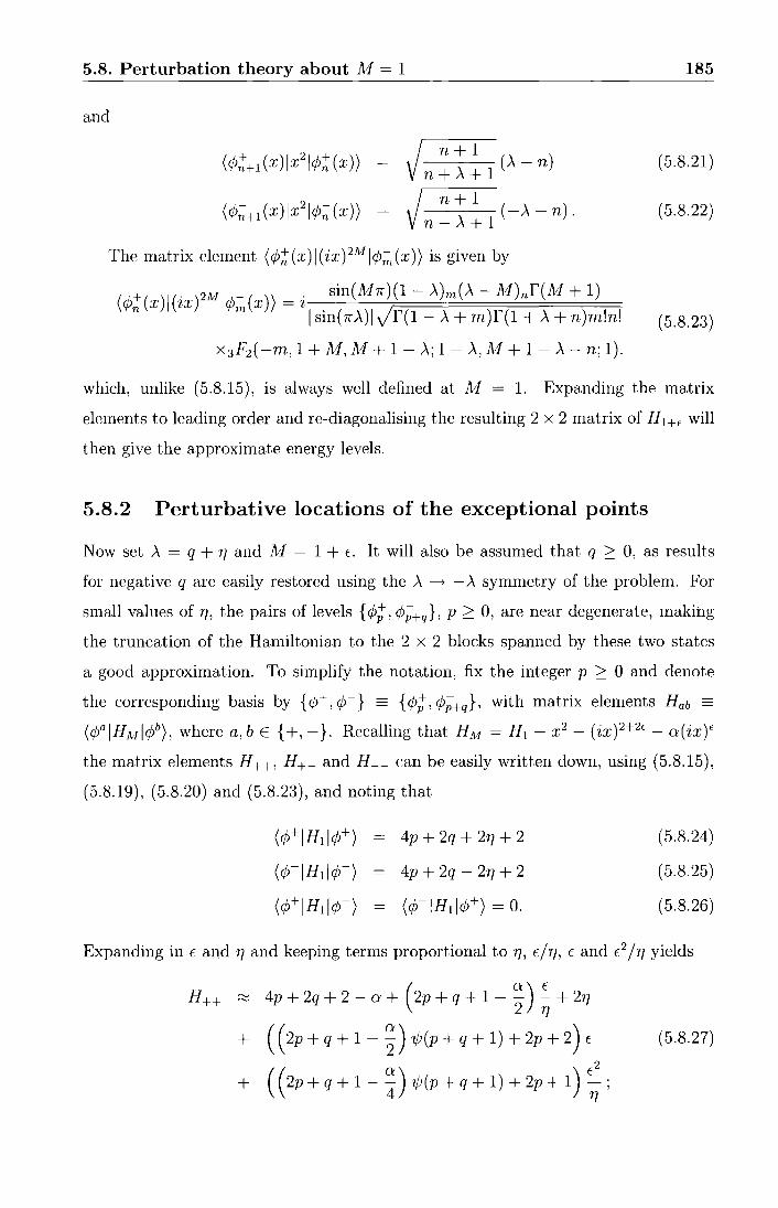
5.8. Perturbation theory about .Af = 1 185
and
I n + 1 (.\- n) Vn+.\+1
(5.8.21)
. I n + 1 v-n---.\-+-1 ( -.\- n). (5.8.22)
The matrix element (¢~(x)J(ix) 2MJ¢~(x)) is given by
(¢~(x)J(ix)2MJ¢~(x)) = i sin(M1r)(1- .\)m(.\- M)nf(M + 1) I sin(7r.\)jJr(1- .\ + m)r(1 + .\ + n)m!n! (5.8.23)
x 3F2 ( -m, 1 + M, !1.1 + 1 - .\; 1 - .\, M + 1 - .\- n; 1).
which, unlike (5.8.15), is always well defined at M = 1. Expanding the matrix
elements to leading order and re-diagonalising the resulting 2 x 2 matrix of Hl+E will
then give the approximate energy levels.
5.8.2 Perturbative locations of the exceptional points
Now set .\ = q + rJ and fvf = 1 + E. It will also be assumed that q :::;:: 0, as results
for negative q are easily restored using the .\ -----+ -.\ symmetry of the problem. For
small values of TJ, the pairs of levels { ¢;, ¢;+q}, p :::;:: 0, are near degenerate, making
the truncation of the Hamiltonian to the 2 x 2 blocks spanned by these two states
a good approximation. To simplify the notation, fix the integer p :::;:: 0 and denote
the corresponding basis by { q,+, q_,-} = { ¢;, ¢;+q}, with matrix elements Hab = (¢0 JHMJ¢b), where a, bE { +,-}. Recalling that HM = H1 - x 2
- (ix)2+2E- o:(ix)E
the matrix elements H++' H+- and H __ can be easily written down, using (5.8.15),
(5.8.19), (5.8.20) and (5.8.23), and noting that
(¢+JHIJ¢+)
(¢-JHIJ¢-)
(¢+ JH1J¢-)
4p + 2q + 2TJ + 2
4p + 2q - 2TJ + 2
(¢-JHIJ¢+) = 0.
(5.8.24)
(5.8.25)
(5.8.26)
Expanding in E and TJ and keeping terms proportional to T}, E/TJ, E and E2 /TJ yields
H ++ ~ 4p + 2q + 2 - a + ( 2p + q + 1 - ~) ~ + 2TJ
+ ( ( 2p + q + 1 - ~) 1/J (p + q + 1) + 2p + 2) E
+ ( ( 2p + q + 1 - ~) 1/J (p + q + 1) + 2p + 1) ~ ; (5.8.27)

5.8. Perturbation theory about M = 1
H _ _ ~ 4p + 2q + 2 - o: - ( 2p + q + 1 - ~) ~ - 2TJ
+ ( ( 2p + q + 1- ~) 1/J(p + 1) + 2p + 2q + 2) E
( ( 2p + q + 1 - ~) 1/J (p + q + 1) + 2p + 1) ~ ;
H+- ~ ~~~ [(2p+q+ 1- ~) E
186
(5.8.28)
+ (~ ( 2p + q + 1- ~) (1/J(p + q + 1) -1/J(p + 1))- q) ETJ (5.8.29)
+ ( ( 2p + q + 1 - ~) 1/J (p + q + 1) + 2p + 1) E2]
where 1/J(z) = f'(z)/f(z). Details of this expansion are given in appendix A. This
matrix can now be diagonalised to find approximations to the eigenvalues E±f> .. =q+ryJ:
~ 4p + 2q + 2 - 0: + ( 2p + q + 2
+ ~(4p+2q+2-o:)(1/J(p+q+1)+'1j;(p+1)))E (5.8.30)
± [(8p + 4q + 4- 2o:)E + ((8p + 4q + 4- o:)'l/J(p + q + 1)
+8p + 4) E2 + ( ( 4p + 2q + 2 - 0:) ( 1/J(p + q + 1) - 1/J(p + 1))
-4q) ETJ + 47]2 ]
1/2
Having obtained the approximate energy levels, exceptional points can be identi
fied as lines on the (2.\, o:) plane where the argument of the square root in (5.8.30)
vanishes. The approximations to these curves for both E±>..=-q-17
and E±>..=q+ry are
plotted in figures 5.11, 5.12, 5.13, and 5.14, for E = 0.005, 0.01, 0.02 and 0.035 re
spectively. Each shows o: against 2.\ for fixed E, taking q = 0, 1, 2 in E±>..=q+ry and
E±>..=-q-ry above, and p = 0, 1 and 2. (The lines of exceptional points for other values
of p and q lie outside the regions shown on the plots.) The dotted lines are the
o:± E z+ lines, as previously.
As M increases from 1, regions of complex eigenvalues open up from the lines
.\ E Z, starting near the bottom of the spectrum. While the cusps cannot be seen
within this approximation (since the truncation is to just two levels), the pictures
are consistent with the numerical evidence in the last section that the cusps should
escape towards o: = +oo as lvf decreases from 3 to 1.

5.8. Perturbation theory about M = 1 187
10 ~1 I rJ ~ 8 I
6
a 4
2
0
-2
- 5 0 5
2A
Figure 5.11: Pert urbative PT boundary forM= 1.005.
10
6
a 4
2 •'·
or---------~-+--~---------
-2
-5 0 5
2A
Figure 5.12: Perturbative PT boundary for M = 1.01.
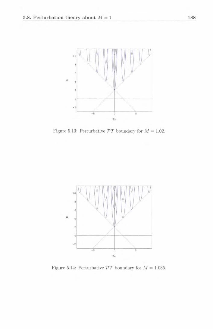
5.8. Perturbation theory about M = 1 188
10
8
6
a 4
2
,· 0~--------.~. --+-~----------
.. ·/ ·. -2
-5 5
Figure 5.13: Perturbative PT boundary for M = 1.02.
a
2
o r---------.~. --+-~.~ ... --------~
-2
-5 0 5
2A.
Figure 5.14: Perturbative PT boundary for M = 1.035.

5.8. Perturbation theory about M = 1 189
A clearer insight into the transitions near M = 1 can be gained by retaining only
the leading terms of the matrix elements for small 77 and E, namely those proportional
to 77 and E/77· For A = q + 77 and M = 1 + E as before, the matrix elements in the
basis { ¢+, ,p-} = { ¢;, ¢;;+q} simplify to
(5.8.31)
where
~ = ~0: - 2p - q - 1 . (5.8.32)
The approximate eigenvalues are then
(5.8.33)
Apart from the overall shift by -2~ and the replacement of E by ~E, (5.8.31) and
(5.8.33) have exactly the same form a.s the toy example (5.8.5). Exceptional points
occur when the argument of the square root vanishes. At fixed E, and using the
A ~ -A symmetry, the curves of exceptional points form the parabolas
1 0: = 4p + 2q + 2 + -(2A ± 2q) 2
2E (5.8.34)
on the (2A, o:) plane, where p and q are non-negative integers. Note the significant
difference between the situations forE> 0 (Jv! > 1) and forE< 0 (M < 1): for given
E > 0 the parabolas open upwards a.s in the figures above, and only a finite number of
eigenvalues are predicted to be imaginary. On the other hand, for E < 0 the parabolas
open downwards, and infinitely-many eigenvalues are imaginary. This provides an
alternative understanding of the transition to infinitely-many complex eigenvalues as
lv! dips below 1, first observed by Bender and Boettcher [63] foro:= 0, 2A = 1.
Finally, in table 5.2 the various approximations used in this section are compared
with numerical data obtained from a direct solution of the ordinary differential equa
tion. The numerical eigenvalues are denoted by Enum so it is against these values
that the approximations are compared. The result using the truncation to two energy
levels, but with no approximation of the matrix elements given in (5.8.15), (5.8.19),
(5.8.20) and (5.8.23), is denoted by E1 and, as shown in table 5.2, this truncation
gives a very good approximation to the numerical result Enum· The initial approxi
mation of this truncated result (including E and E2 /77 terms), given in (5.8.30) from
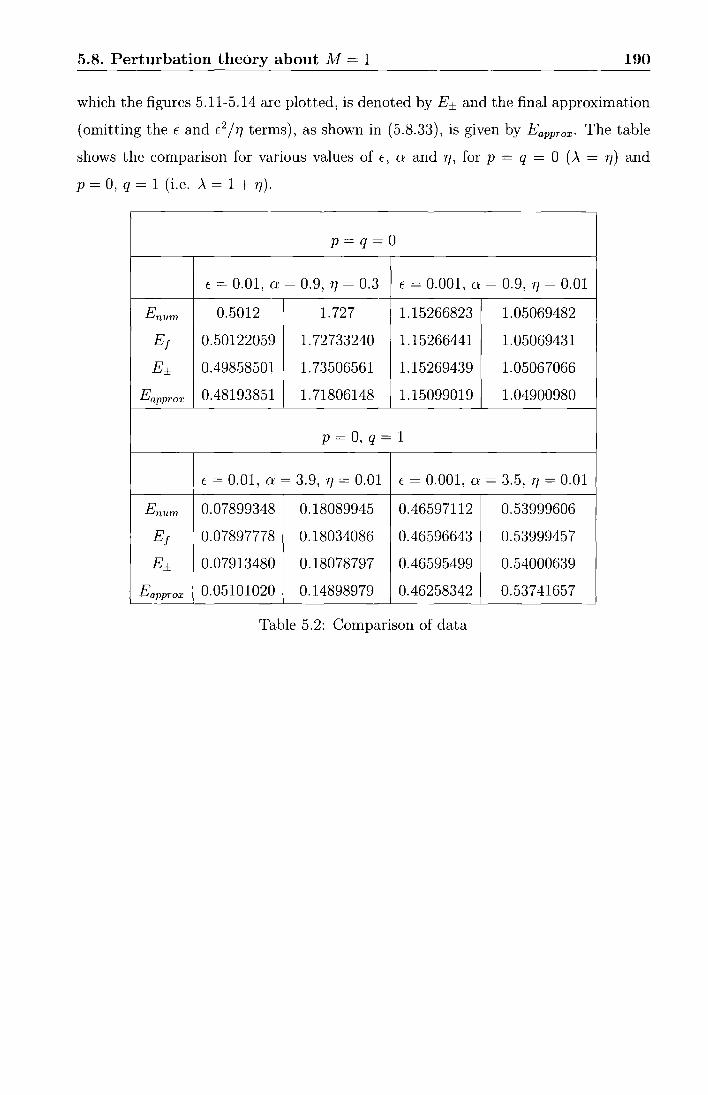
5.8. Perturbation theory about M = 1 190
which the figures 5.11-5.14 are plotted, is denoted byE± and the final approximation
(omitting theE and E2 /TJ terms), as shown in (5.8.33), is given by Eapprox· The table
shows the comparison for various values of E, o: and TJ, for p = q = 0 (.\ = TJ) and
p = 0, q = 1 (i.e. A= 1 + TJ).
p=q=O
E = 0.01, 0: = 0.9, TJ = 0.3 E = 0.001, 0: = 0.9, TJ = 0.01
Enum 0.5012 1.727 1.15266823 1.05069482
Ef 0.50122059 1.72733240 1.15266441 1.05069431
E± 0.49858501 1.73506561 1.15269439 1.05067066
Eapprox 0.48193851 1. 71806148 1.15099019 1.04900980
p = 0, q = 1
E = 0.01, 0: = 3.9, TJ = 0.01 E = 0.001, 0: = 3.5, TJ = 0.01
Enum 0.07899348 0.18089945 0.46597112 0.53999606
Ef 0.07897778 0.18034086 0.46596643 0.53999457
E± 0.07913480 0.18078797 0.46595499 0.54000639
Eapprox 0.05101020 0.14898979 0.46258342 0.53741657
Table 5.2: Comparison of data

Chapter 6
Conclusion
For perturbed boundary conformal field theories, little is known about the link be
tween the reflection factors and the corresponding conformal boundary conditions.
In the bulk, this link can often be made with the TBA effective central charge, which
allows the S matrix to be matched with the perturbed CFT. It has been proposed
that the boundary analogue for this is given by the exact off-critical g-function, and
in Chapter 4, this was tested for the purely elastic scattering theories related to the
ADET Lie algebras. A special class of reflection factors was identified which, in the
ultraviolet limit, were found to describe the reflection of massless particles off a wall
with fixed boundary conditions li), matching the low-temperature vacua.
A set of one-parameter families of reflection amplitudes was also proposed which,
from the g-function calculations, appear to correspond to perturbations of Cardy
boundary states, or of superpositions of such states, by relevant boundary operators,
with each boundary flow ending at a fixed boundary condition li).
While the results presented in Chapter 4 indicate that these models all have in
teresting interpretations as perturbed boundary conformal field theories, the checks
performed so far should be considered as preliminary. In Section 4.10, the bound
ary bound-state spectrum was found for the three-state Potts model but it would
be interesting to check this result using the boundary truncated conformal space ap
proach [78]. It remains an open problem to determine the boundary spectrum for
each of the remaining AD ET models and also to fix completely the boundary UV /IR
relations proposed in Section 4.9.2. Finally, it would be interesting to extend this
work to other models, in particular to the Virasoro minimal models perturbed by the
191

Chapter 6. Conclusion 192
1>13 operator. This perturbation leads to massless flows between the minimal models
and knowledge of the exact g-function should allow conjectures to be made of the
existence of flows between conformal boundary conditions of different minimal mod
els. The exact g-function described in Section 3.4 must be modified for these models
as they are not purely elastic scattering theories. An attempt at this has been made
in [138], but this suffers from the same problems as the original off-critical g-function
and must be modified by some boundary independent terms, as described in Section
3.4.
In Chapter 5, the phase diagram of the three-parameter family of PT symmetric
Hamiltonians HM,a,l was examined. At !vi = 3, this model is quasi-exactly solvable,
which allowed the precise Jordan block structure, at the first quadratic and cubic
points to be shown. The locations of the exceptional points were also explored away
from M = 3, using both numerical and perturbative methods.
These curves of exceptional points, for the !vi = 3 case, have also been found
using the complex WKB method by Sorrell [133]. It would be interesting to see if
this method reproduces the same pictures for other values of !11. It would also be
interesting to investigate the phase diagram of this Hamiltonian when different lateral
boundary conditions are imposed, i.e. when the quantisation contour tends to infinity
in a different pair of Stokes sectors.

Appendix A
Perturbative expansion of the
matrix elements
In this appendix, the matrix elements
sin((E + T7 + q)1r)f(p- 1- E)r(2 + q + T7 +E) H ++ = 2p + q + 1 + T7 + ----'-----. -----'-------------
sm((ry + q)1r)r( -1- E)r(1 + q + ry)p!
H __
x 3F2 ( -p, 2 + E, 2 + q + T7 + E; 1 + q + ry, 2 + E- p; 1) (A.0.1) sin((ry + ~ + q)1r)f(p- ~)r(1 + q + T7 + ~)
- a--~----~----~ sin((ry + q)1r)f( -~)f(1 + q + ry)p!
x 3F2 ( -p, 1 + ~' 1 + q + T7 + ~; 1 + q + ry, 1 + ~- p; 1)
. r(1-ry+p) - Z X
r(1- q- ry)y'r(1- T7 + p)r(1 + q + P + ry)(p + q)!p!
(sin(m)r(p + q- 1 + T7- E)f(2 +E)
I sin((ry + q)1r)lf(q- 1 + T7- E) x 3F2 ( -p- q, 2 + E, 2- q + E- ry; 1- q- ry, 2- q- p + E- ry; 1) (A.0.2) a sin(~)f(p + q + T7- ~)f(1 + ~)
I sin((ry + q)1r)lf(q + T7- ~)
x 3 F2 ( -p- q, 1 + ~' 1- q + ~- ry; 1- q- ry, 1- p- q + ~- ry; 1))
sin((E- '1]- q)1r)f(p + q- 1- E)r(2- q- T7 +E) 2p + q + 1 - T7 - 0
sin ( ( T7 + q) 7f) r( -1 - E) f ( 1 - q - T7 )(p + q)! x 3g( -p- q, 2 + E, 2- q- T7 + E; 1- q- ry, 2 + E- p- q; 1) (A.0.3)
sin((ry- ~ + q)1r)r(p + q- ~)r(1- q- T7 + ~) _ a 2 2 2
sin((ry + q)1r)f( -~)r(1- q- ry)(p + q)!
( E E E ) x 3g -p- q, 1 + 2, 1 - q- T7 + 2; 1 - q- ry, 1 + 2 - p- q; 1
193
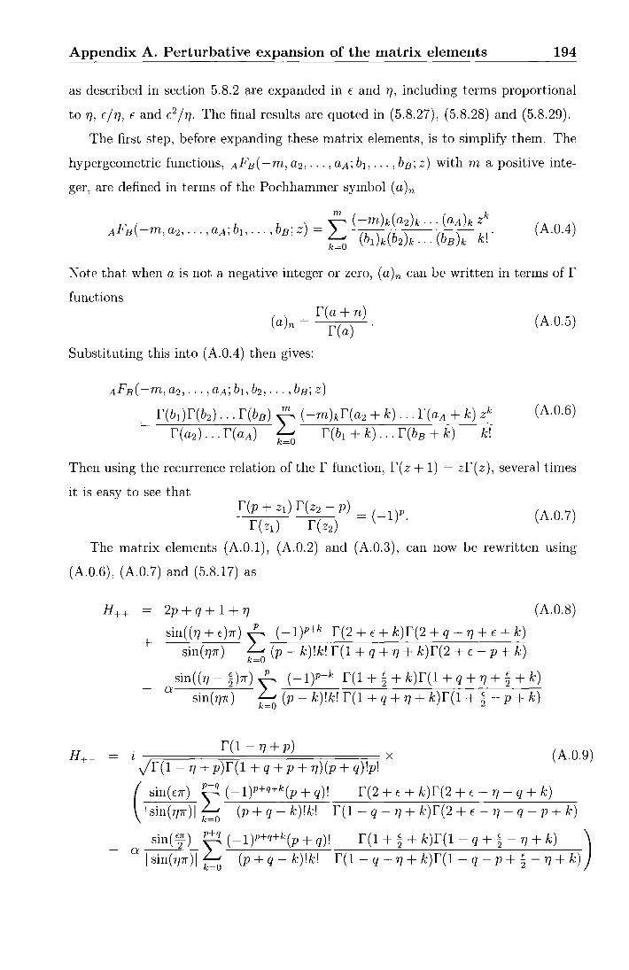
Appendix A. Perturbative expansion of the matrix elements 194
as described in section 5.8.2 are expanded in E and 7], including terms proportional
to TJ, E/TJ, E and E2 /TJ. The final results are quoted in (5.8.27), (5.8.28) and (5.8.29).
The first step, before expanding these matrix elements, is to simplify them. The
hypergeometric functions, AFs( -m, a2, ... , aA; b1, ... , bs; z) with m a positive inte
ger, are defined in terms of the Pochhammer symbol (a) n
(A.0.4)
Note that when a is not a negative integer or zero, (a )n can be written in terms of r
functions
() ~ r(a+n)
a n- r(a)
Substituting this into (A.0.4) then gives:
(A.0.5)
(A.0.6)
Then using the recurrence relation of the r function, f(z + 1) == zf(z), several times
it is easy to see that r(p + z1) r(z2- p) = ( _ 1)P.
r(zi) r(z2) (A.0.7)
The matrix elements (A.0.1), (A.0.2) and (A.0.3), can now be rewritten using
(A.0.6), (A.0.7) and (5.8.17) as
H++ 2p + q + 1 + TJ (A.0.8)
+ sin((TJ+E)7r) ~ (-1)P+k r(2+E+k)r(2+q+T}+E+k) sin(TJ7r) ~ (p- k)!k! f(1 + q + TJ + k)f(2 + E- p + k)
_ asin((TJ-~)n):t (-1)P+k r(1+~+k)f(1+q+TJ+~+k) sin(rJn) k=O (p- k)!k! r(1 + q + TJ + k)f(1 + ~- p + k)
. r(1-TJ+P) 1, X (A.0.9) Jr(1- TJ + p)r(1 + q + p + TJ)(p + q)!p!
( sin(m) I: ( -1)P+q+k(p + q)! r(2 + E + k)f(2 + E- TJ- q + k)
I sin(rJn)l k=O (p + q -k)!k! r(1- q- TJ + k)r(2 + E- TJ- q- p + k)
sin(E;) p+q(-1)P+q+k(p+q)! r(1+~+k)f(1-q+~-TJ+k) )
- a I sin(rJn)l ~ (p + q- k)!k! r(1- q- TJ + k)f(1- q- p + ~- TJ + k)

Appendix A. Perturbative expansion of the matrix elements 195
H__ 2p + q + 1 - 'fJ (A.0.10)
+ sin((TJ- E)1r) ~ ( -1)p+q+k r(2- q + 'f} + E + k)r(2 + E + k) sin(TJ7r) ~ (p + q- k)!k! f(1- q + 'f} + k)f(2- p- q + E + k)
sin((TJ- -"-)7r) p+q ( -1)p+q+k r(1- q- 'f} + .". + k)f(1 + .". + k) -0' 2 ~ . 2 2
sin(TJ7r) ~ (p + q- k)!k! r(1- q- 'fJ + k)r(1- p- q + ~ + k)
A.0.3 Expanding H ++
Begin by expanding H++ (A.0.8), including terms in 'f}, E/TJ, E and E2 /TJ. The Taylor
expansion of r(E +a) and 1/f(E +a) will be needed here:
~ f(a)(1 + '!j;(a)E) 1
~ f(a) (1- 'lj;(a)E) (A.O.ll)
where 'lj;(z) = f'(z)/r(z). It is useful to note that 1j;(1) = -{, where 1 ~ 0.5772 is
Euler's constant, and 'lj;(z+ 1) = '!j;(z) + 1/ z. This is sufficient to expand most terms in
(A.0.8), but more care must be taken over terms of the form f(E+a+k )/f(E+a-p+k)
fork= 0, ... ,panda= 1, ... ,p. Now, fork = p + 1- a, ... ,p the expansion of
these terms can be read off from (A.O.ll) but for k = 0, ... ,p- a this will not be
well defined so a little more work is required. Let j = k + a, then
I: f(E+a+k) t f(E+j) k=O r( E + a + k - p) - j=a r( E + j - p)
p
~ E L ( (j - 2) (j - 3) ... (j - p) + (j - 1) (j - 3) ... (j - p) + ... j=a
+ (j - 1) (j - 2) ... (j - p + 1))
"', t. (r(p + 1- J) ~}}( -I)v+'-\~1 ~ ~)) and using the fact that
fi j _ i = { u- 1)! i=lr(L-j) o
for j = l- 1
otherwise
gives
(A.0.12)
(A.0.13)
(A.0.14)

Appendix A. Perturbative expansion of the matrix elements 196
so, putting this all together, one finds
p ) p-a L r(E+a+k ~Ez=(-1)p-k-a(k+a-1)!(p-k-a)! k=O r( E + a + k - p) k=O
+ ~ ( (k+a-1)!)
1(1+(7P(a+k)-7P(a-p+k))E).
~ k+a-1-p. k=p+l-a
(A.0.15)
Substituting these results into (A.0.8) then gives
H++ ~ 2p+q+1+ry+ (1+~) [(p+1)(p+q+1)(1+(7P(2+p)+I-1)E
+ tP ( 2 + p + q) ( E + 7]) - tP( 1 + p + q) 7]) - p(p + q) ( 1 + ( tP ( 1 + p) + I) E
) ~(k+1)(1+q+k)l
+ 7P(1 + p + q)(E + 77)- tP(P + q)ry + f::o (p _ k)(p _ k _ 1) (A.0.16)
- " ( 1+ 2:,) [ ( 1 +4;( I+ p + q) ~ + ( 1/J(p + 1) + ') ~) - ~ ~ p ~ k l Finally, replacing the sums above with the following
p-1 1
L:p-k = k=O
p-2 1
I: (p - k )(p - k - 1) k=O p-2 k
I: (p - k) (p - k - 1) -k=O
tP(P + 1) +I
1 1-
p
P- 1 - tP(P) - I
p-2 k2
""""' = p2 ~ 1 + (1- 2p)(7P(p) +I) ~ (p- k)(p- k- 1) k=O
and keeping terms in 7], E/7], E and E2 /77 only, (A.0.16) reduces to
H ++ ~ 4p + 2q + 2 - a + ( 2p + q + 1 - ~) ~ + 2ry
+ ( ( 2p + q + 1 - ~) tP (p + q + 1) + 2p + 2) E
+ ((2p+q+1-~)7P(p+q+1)+2p+1) ~ as advertised in (5.8.27).
A.0.4 Expanding H __
(A.0.17)
(A.0.18)
(A.0.19)
(A.0.20)
(A.0.21)
To expand the H __ term (A.0.10), (A.O.ll) and (A.0.15) are used, as above, but now
more attention must also be paid to the r(2- q- 7J + E + k)/r(1- q- 7J + k) and
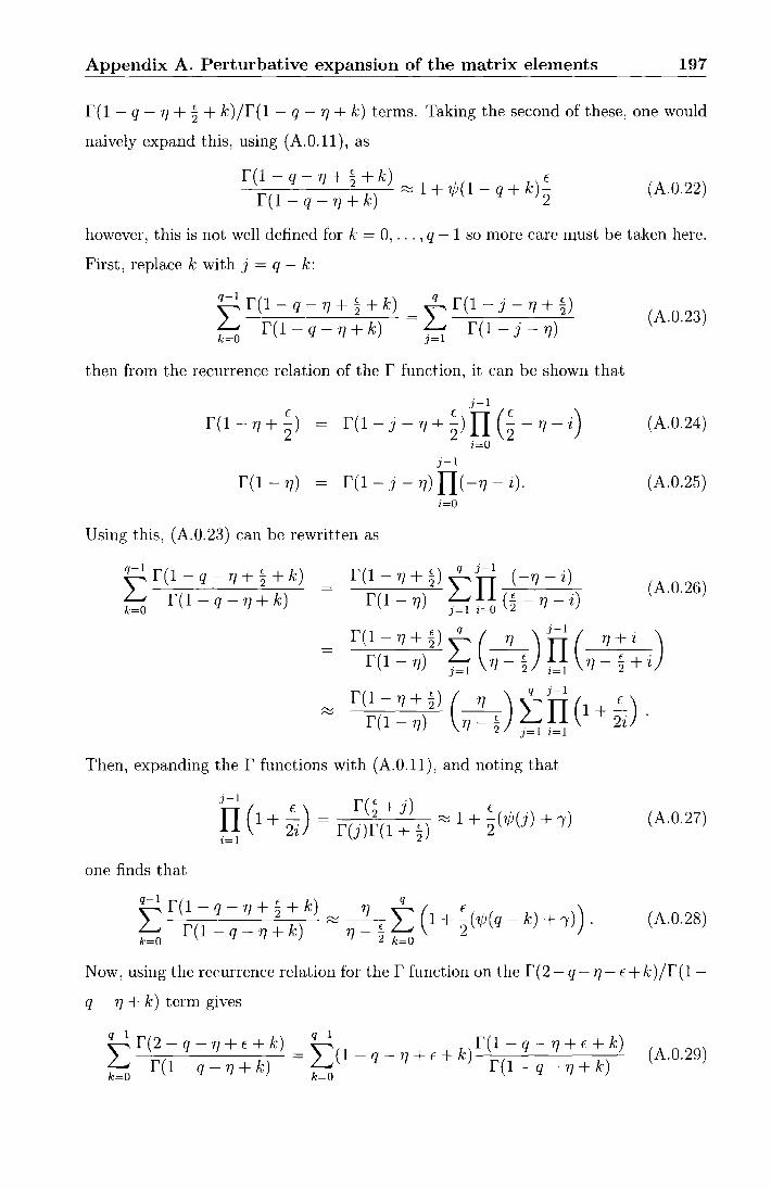
Appendix A. Perturbative expansion of the matrix elements 197
f(1- q- TJ + ~ + k)/f(1- q- TJ + k) terms. Taking the second of these, one would
naively expand this, using (A.O.ll), as
(A.0.22)
however, this is not well defined for k = 0, ... , q -1 so more care must be taken here.
First, replace k with j = q- k:
then from the recurrence relation of the r function, it can be shown that
j-1 E
f(1-TJ+-) 2
r(1- j- TJ +~)II(~- TJ- i) i=O
j-1
r(1-TJ) = r(1-j-TJ)II(-TJ-i).
Using this, (A.0.23) can be rewritten as
q-1 r(1 - q- TJ + ~ + k)
L r(1 - q - TJ + k) k=O
i=O
Then, expanding the r functions with (A.O.ll), and noting that
j-1 ( )
II( E) f~+j E .
i=1 1 + 2i = r(j)f(1 + ~) >=:::;
1 + 2(1/J(J) + !)
one finds that
q-1 f(1- q- TJ + ~ + k) TJ q ( E ) 2:: r(1-q-17~k) >=:::; TJ-~2: 1 +2(1/J(q-k)+,) ·
k=O 2 k=O
(A.0.23)
(A.0.24)
(A.0.25)
(A.0.26)
(A.0.27)
(A.0.28)
Now' using the recurrence relation for the r function on the r ( 2- q- TJ- E + k) ;r ( 1 -
q- TJ + k) term gives
(A.0.29)
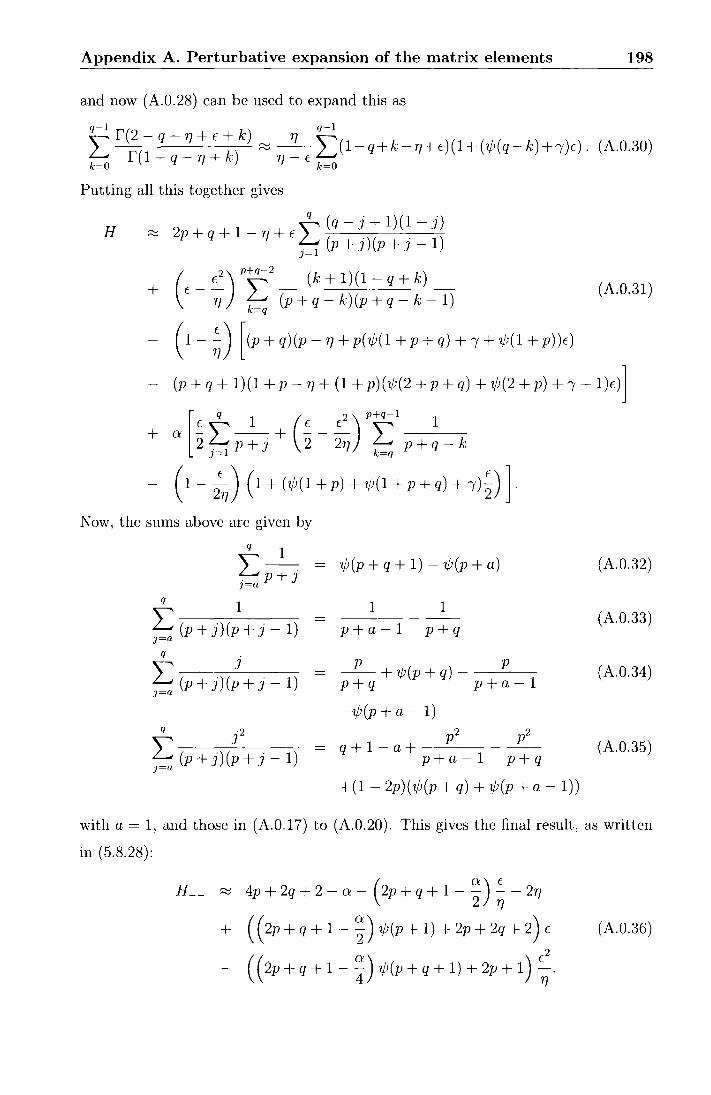
Appendix A. Perturbative expansion of the matrix elements 198
and now (A.0.28) can be used to expand this as
q-l q-l
L r(2 - q - 1] + t + k) 1] I: r( k) :::::::- (1-q+k-7J+t)(1+(1f;(q-k)+1 )t). (A.o.3o)
1-q-1]+ 1]-E k=O k=O
Putting all this together gives
~(q-j+1)(1-j) H__ ::::::: 2p + q + 1 -17 + t ~ ( .)( . 1)
j=l p + J p + J-
(
t 2 )p~2
(k+1)(1-q+k) + t - --:ry (p + q - k) (p + q - k - 1)
k=q
(A.0.31)
- (1-~) [(p+q)(p-1J+p(1f;(1+p+q)+l+1f;(1+p))t)
- (p + q + 1) ( 1 + p - 17 + ( 1 + p) ( 1j; ( 2 + p + q) + 1j; ( 2 + p) + 1 - 1) t)]
[
q 1 ( 2) p+q-l 1
+ ex ~ I: p + j + ~ - ~·ry I: p + q - k J=l k=q
- ( 1 - 2~) ( 1 + ( 1j; ( 1 + p) + 1j; ( 1 + p + q) + I)~) l Now, the sums above are given by
q 1
L:p+j -J=a
q 1
I: (p + j) (p + j - 1) J=a
q '
I: (p + j) (: + j - 1) J=U
'lj;(p + q + 1) -'lj;(p +a)
1 1 ------p+a-1 p+q
p p -- +'1/J(p+q)- -~p+q p+a-1
-'lj;(p +a- 1) p2 p2
q+1-a+ ---p+a-1 p+q
+(1- 2p)(1j;(p + q) + 'lj;(p +a- 1))
(A.0.32)
(A.0.33)
(A.0.34)
(A.0.35)
with a= 1, and those in (A.0.17) to (A.0.20). This gives the final result, as written
in (5.8.28):
H _ _ ::::::: 4p + 2q + 2 - ex - ( 2p + q + 1 - ~) ~ - 21]
+ ( ( 2p + q + 1 - ~ ) 1j; (p + 1) + 2p + 2q + 2) t
- ( ( 2p + q + 1 - ~) 1j; (p + q + 1) + 2p + 1) ~ .
(A.0.36)
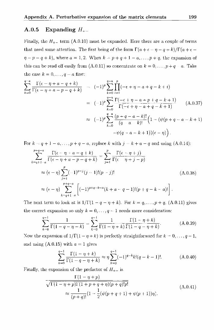
Appendix A. Perturbative expansion of the matrix elements 199
A.0.5 Expanding H +-
Finally, the H+- term (A.0.10) must be expanded. Here there are a couple of terms
that need some attention. The first being of the form f(a + c:- TJ- q + k)jr(a + c:
TJ- p- q + k), where a= 1, 2. When k = p + q + 1- a, ... , p + q, the expansion of
this can be read off easily from (A.0.11) so concentrate on k = 0, ... , p + q- a. Take
the case k = 0, ... , q - a first:
~ r( E - 'T} + a - q + k) q-a P
6r(c:-TJ+a-p-q+k) - (-1)PLI1(-c:+TJ-a+q-k+i) k=O k=O i=l
( _ 1 )P ~ f (- f + TJ - a + p + q - k + 1)
6 ( ) (A.0.37) k=O f - f + TJ - a + q - k + 1
~ ( -1 )P I: (p (; ~ : ~ ~) ~)! ( 1 - ( 'ljJ (p + q - a - k + 1) k=O
-'1/J(q- a- k + 1))(c:- TJ)).
Fork= q + 1- a, ... ,p + q- a, replace k with j = k +a- q and using (A.0.14):
p~a r(c-'T}+a-q+k) ~ r(c:-'T}+j) 6 r(c:- TJ +a- p -q + k) - 6 f(E- TJ + j- p)
k=q+1-a J=l p
~ (c:- TJ) L:(-1)p-j(j -1)!(p- j)! (A.0.38) j=l
p+q-a [ ] ~(c:-ry) L (-1)p+q-k-a(k+a-q-1)!(p+q-k-a)!.
k=q+l-a
The next term to look at is 1/r(1- q- TJ + k). Fork= q, ... ,p + q, (A.O.ll) gives
the correct expansion so only k = 0, ... , q- 1 needs more consideration:
q-l 1 q-l 1 r( 1 - TJ + k)
I: r(1- q- TJ + k) =I: r(1- TJ + k) r(1- q- TJ + k)' k=O k=O
(A.0.39)
Now the expansion of 1/r(1- TJ + k) is perfectly straightforward fork= 0, ... , q- 1,
and using (A.0.15) with a = 1 gives
q-l q-l I: r(1- TJ + k) ~ TJ L:( -1)q-kk!(q- k- 1)!. k=Of( 1 -q-'T}+k) k=O
Finally, the expansion of the prefact.or of H +- is
r(1-TJ+p)
Jr(1- TJ + p)r(1 + P + q + TJ)(p + q)!p! 1 1
~ ( )' (1- -2('1/J(p + q + 1) + '1/J(p + 1))TJ). p+q.
(A.0.40)
(A.0.41)
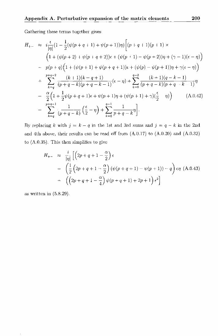
Appendix A. Perturbative expansion of the matrix elements 200
Gathering these terms together gives
H+- ~ i 1~1 (1- ~(?jJ(p + q + 1) + ?jJ(p + 1))17) [(p + q + l)(p + 1) X
( 1 + ( 7jJ (p + 2) + ·1/J (p + q + 2) ) E + ( 7jJ (p + 1) - 7jJ (p + 2) ) 17 + (I - 1 ) ( E - 17))
- p(p + q) ( 1 + (?jJ(p + 1) + ?jJ(p + q + l))E + (?jJ(p) -?jJ(p + 1))17 + I(E -17))
p~2 ( k + 1) ( k - q + 1) ( ) ~ ( k + 1) ( q - k - 1)
+ ~ (p + q - k )(p + q - k - 1) E - 17 + b (p + q -k) (p + q - k - 1) 17
Cl'( 1 E ) - - 1 + -?jJ(p + q + 1 )E + ?jJ(p + 1 )17 + ( ?jJ(p + 1) +I) (- - 17) 2 2 2
(A.0.42)
p+q-1 q-1 l 1 E 1 - --17 + 17 £; (p + q- k) (2 ) £; p + q- k .
By replacing k with j = k - q in the 1st and 3rd sums and j = q- k in the 2nd
and 4th above, their results can be read off from (A.0.17) to (A.0.20) and (A.0.32)
to (A.0.35). This then simplifies to give
H+- ~ ~~~ [(2p+q+ 1- ~) E
+ (~ (2p + q + 1 ~ ~) (?j;(p + q + 1)- ?jJ(p + 1))- q) E17 (A.0.43)
+ ( ( 2p + q + 1 - ~) 7jJ (p + q + 1) + 2p + 1) E2]
as written in (5.8.29).

Bibliography
(1] P. Dorey, A. Lishman, C. Rim and R. Tateo, 'Reflection factors and exact g
functions for purely elastic scattering theories', Nucl. Phys. B 744 (2006) 239
(arXiv:hep-th/0512337].
[2] P. Dorey, C. Dunning, A. Lishman and R. Tateo, 'PT symmetry breaking and
exceptional points for a class of inhomogeneous complex potentials', in prepa
ration.
[3] I. Affleck and A.W.W. Ludwig, 'Universal noninteger 'ground state degeneracy'
in critical quantum systems', Phys. Rev. Lett. 67 (1991) 161.
(4] P. Dorey, D. Fioravanti, C. Rim and R. Tateo, 'Integrable quantum field theory
with boundaries: the exact g-function', Nucl. Phys. B 696 (2004) 445 [arXiv:hep
th/0404014].
[5] P. DiFrancesco, P. Mathieu and D. Senechal, 'Conformal field theory', Springer,
1997.
[ 6] J. Cardy, 'Scaling and Renormalisation in Statistical Physics', Cambridge U ni
versity Press 1996.
[7] A. M. Polyakov, 'Conformal Symmetry Of Critical Fluctuations', JETP Lett.
12 (1970) 381 [Pisma Zh. Eksp. Teor. Fiz. 12 (1970) 538].
[8] A. A. Belavin, A. M. Polyakov and A. B. Zamolodchikov, 'Infinite conformal
symmetry in two-dimensional quantum field theory', Nucl. Phys. B 241 (1984)
333.
[9] P. H. Ginsparg, 'Applied Conformal Field Theory', In Les Houches XLIX -
Fields, Strings and Critical Phenomena, Elsevier 1989 [arXiv:hep-th/9108028].
201
Bibliography 202
[10] J. L. Cardy, 'Conformal Invariance and Statistical Mechanics', In Les Houches
XLIX - Fields, Strings and Critical Phenomena, Elsevier 1989
[11] V.G.Kac, 'Contravariant form for infinite dimensional Lie algebras and super
algebras', Lecture Notes in Physics, vol. 94, Springer-Verlag, Berlin, 1979.
[12] B. L. Feigin and D. B. Fuchs, 'Invariant skew symmetric differential operators
on the line and verma modules over the Virasoro algebra', Funct. Anal. Appl.
16 (1982) 114 [Funkt .. Anal. Pril. 16 (1982) 47].
[13] J. L. Cardy, 'Operator Content Of Two-Dimensional Conformally Invariant
Theories', Nucl. Phys. B 270 (1986) 186.
[14] C. Itzykson and J. B. Zuber, 'Two-Dimensional Conformal Invariant Theories
On A Torus', Nucl. Phys. B 275 (1986) 580.
[15] A. Cappelli, C. Itzykson and J. B. Zuber, 'Modular Invariant Partition Func
tions in Two-Dimensions', Nucl. Phys. B 280 (1987) 445.
[16] A. Cappelli, C. Itzykson and J. B. Zuber, 'The ADE Classification of Minimal
and Al (1) Conformal Invariant Theories', Commun. Math. Phys. 113 (1987)
1.
[17] A. Kato, 'Classification of Modular Invariant Partition Functions in Two
Dimensions', Mod. Phys. Lett. A 2 (1987) 585.
[18] E. P. Verlinde, 'Fusion Rules And Modular Transformations In 2d Conformal
Field Theory', Nucl. Phys. B 300 (1988) 360.
[19] G. W. Moore and N. Seiberg, 'Polynomial Equations for Rational Conformal
Field Theories', Phys. Lett. B 212 ( 1988) 451.
[20] R. Dijkgraaf and E. P. Verlinde, 'Modular Invariance And The Fusion Algebra',
Nucl. Phys. Proc. Suppl. 5B (1988) 87.
[21] A. B. Za.molodchikov, 'Integrable field theory from conformal field theory', Adv.
Stud. Pure Math. 19 (1989) 641.
Bibliography 203
[22] A. B. Zamolodchikov and A. B. Zamolodchikov, 'Factorized S-matrices in two
dimensions as the exact solutions of certain relativistic quantum field models',
Annals Phys. 120 (1979) 253.
[23] P. Dorey, 'Exact S matrices', in the proceedings of the 1996 Eotvos Graduate
School [arXiv:hep-th/9810026].
[24] S. J. Parke, 'Absence of Particle Production and Factorization of the S Matrix
in (1+1)-Dimensional Models', Nucl. Phys. B 174 (1980) 166.
[25] S. R. Coleman and J. Mandula, 'All Possible Symmetries of the S Matrix',
Phys. Rev. 159 (1967) 1251.
[26] S. R. Coleman and H. J. Thun, 'On The Prosaic Origin Of The Double Poles
In The Sine-Gordon S Matrix', Commun. Math. Phys. 61 (1978) 31.
[27] P. A. Mattsson, 'Integrable quantum field theories, in the bulk and with a bound
ary', arXiv:hep-th/0111261.
[28] A.B. Zamolodchikov, 'Integrals of motion and S matrix of the (scaled) T =
T(C) Ising model with magnetic field', Int. J. Mod. Phys. A 4, 4235 (1989).
[29] A. B. Zamolodchikov, 'Irreversibility of the Flux of the Renormalization Group
in a 2D Field Theory', JETP Lett. 43 (1986) 730 [Pisma Zh. Eksp. Teor. Fiz.
43 (1986) 565].
[30] ALB. Zamolodchikov, 'Thermodynamic Bethe ansatz in relativistic models.
Scaling three state Potts and Lee- Yang models', NucL Phys. B 342, 695 (1990).
[31] N. Goldenfeld, 'Lectures on phase transitions and the renormalization group',
Addison-Wesley, Advanced Book Program, 1992.
[32] T.R. Klassen and E. Melzer, 'Purely elastic scattering theories and their ultra
violet limits', NucL Phys. B 338 (1990) 485.
[33] T. R. Klassen and E. Melzer, 'The Thermodynamics of purely elastic scattering
theories and conformal perturbation theory', Nucl. Phys. B 350 (1991) 635.
[34] ALB. Zamolodchikov, 'On the thermodynamic Bethe ansatz equations for re
ftectionless ADE scattering theories', Phys. Lett. B 253 (1991) 391.

Bibliography 204
[35] F. Gliozzi and R. Tateo, 'Thermodynamic Bethe ansatz and threefold triangu
lations', Int. J. Mod. Phys. A 11 (1996) 4051 [a.rXiv:hep-th/9505102).
[36] E. Frenkel and A. Szenes, 'Thermodynamics bethe ansatz and dilogarithm iden
tities. 1 ', arXiv:hep-th/9506215.
[37] R. Caracciolo, F. Gliozzi and R. Tateo, 'A topological invariant of RG flows
in 2D integrable quantum field theories', Int. J. Mod. Phys. B 13 (1999) 2927
[arXiv:hep-th/9902094).
[38] S. Fomin and A. Zelevinsky, 'Y-systems and generalized associahedra ',
arXiv:hep-th/0111053.
[39] A. Y. Volkov, 'On Zamolodchikov 's periodicity conjecture for Y-systems ',
arXiv:hep-th/0606094.
[40] A.Szenes, 'Periodicity of Y-systems and fiat connections', math.RT /0606337.
[41] A. B. Zamolodchikov, 'From tricritical Ising to critical Ising by thermodynamic
Bethe ansatz', Nucl. Phys. B 358 (1991) 524.
[42] A. B. Zamolodchikov, 'Thermodynamic Bethe ansatz for RSOS scattering the
ories', Nucl. Phys. B 358 (1991) 497.
[43] A. B. Zamolodchikov, 'TEA equations for integrable perturbed SU(2)-k x SU(2)
l / SU(2)-k+ l coset models', Nucl. Phys. B 366 (1991) 122.
[44] A. B. Zamolodchikov, 'Resonance factorized scattering and roaming trajecto
ries', J. Phys. A 39 (2006) 12847. Preprint ENS-LPS-335, 1991
[45] P. Dorey and F. Ravanini, 'Staircase models from affine Toda field theory', Int.
J. Mod. Phys. A 8 (1993) 873 [arXiv:hep-th/9206052].
[46] M. J. Martins, 'Exact resonance A-D-ES matrices and their renormalization
group trajectories', Nucl. Phys. B 394 (1993) 339 [a.rXiv:hep-th/9208011].
[47] M. J. Martins, 'Renormalization group trajectories from resonance factorized S
matrices', Phys. Rev. Lett. 69 (1992) 2461 [arXiv:hep-th/9205024].

Bibliography 205
[48] P. Dorey and R. Tateo, 'Anharmonic oscillators, the thermodynamic Bethe
ansatz, and nonlinear integral equations', J. Phys. A 32 (1999) L419 [arXiv:hep
th/9812211].
[49] V.V. Bazhanov, S.L. Lukyanov and A.B. Zamolodchikov, 'Integrable struc
ture of conformal field theory, quantum KdV theory and thermodynamic Bethe
ansatz', Commun. Math. Phys. 177, (1996) 381 [arXiv:hep-th/9412229).
[50] P. Dorey, C. Dunning and R. Tateo, 'The ODE/IM Correspondence', J. Phys.
A 40 (2007) R205 [arXiv:hep-th/0703066].
[51) E. H. Lieb, 'Exact solution of the problem of the entropy of two-dimensional
ice', Phys. Rev. Lett. 18 (1967) 692;
- 'Residual entropy of square ice', Phys. Rev. 162 (1967) 162;
-'Exact solution of the F model of an antiferroelectric ', Phys. Rev. Lett. 18
(1967) 1046;
-'Exact solution of the two-dimensional Slater KDP model of a ferroelectric',
Phys. Rev. Lett. 19 (1967) 108.
[52] B. Sutherland, 'Exact solution of a two-dimensional model for hydrogen-bonded
crystals', Phys. Rev. Lett. 19 (1967) 103.
[53] R. J. Baxter, 'Exactly solved models in statistical mechanics', (Academic Press
1982)
[54] A. Kliimper, M. T. Batchelor and P. A. Pearce, 'Central charges of the 6- and
19-vertex models with twisted boundary conditions', J. Phys. A 24 (1991) 13.
[55] F. C. Alcaraz, M. N. Barber and M. T. Batchelor, 'Conformal invariance,
the X X Z chain and the operator content of two-dimensional critical systems',
Annals Phys. 182 (1988) 280.
[56) C. Korff, 'Auxiliary matrices for the six-vertex model and the algebraic Bethe
ansatz', J. Phys. A 37 (2004) 7227 [arXiv:math-ph/0404028].
[57] R. J. Baxter, 'Eight- Vertex Model in Lattice Statistics', Phys. Rev. Lett. 26
(1971) 832.

Bibliography 206
[58] R. J. Baxter, 'Partition function of the eight-vertex lattice model', Annals Phys.
70 (1972) 193 [Annals Phys. 281 (2000) 187].
[59] V. V. Bazhanov, S. L. Lukyanov and A. B. Zamolodchikov, 'Integrable Structure
of Conformal Field Theory II. Q-operator and DDV equation', Commun. Math.
Phys. 190 (1997) 247 [arXiv:hep-th/9604044].
[60] V. V. Bazhanov, S. L. Lukyanov and A. B. Zamolodchikov, 'Integrable structure
of conformal field theory. III: The Yang-Baxter relation', Commun. Math. Phys.
200 (1999) 297 [arXiv:hep-th/9805008].
[61] Y. Sibuya, 'Global theory of a second-order linear ordinary differential equation
with polynomial coefficient', (Amsterdam: North-Holland 1975).
[62] C. M. Bender and A. Turbiner, 'Analytic Continuation Of Eigenvalue Prob
lems', Phys. Lett. A 173 (1993) 442.
[63] C.M. Bender and S. Boettcher, 'Real spectra in non-hermitian Hamiltonians
having PT symmetry', Phys. Rev. Lett. 80 (1998) 4243, physics/9712001
[64] V. V. Bazhanov, S. L. Lukyanov and A. B. Zamolodchikov, 'Spectral determi
nants for Schrodinger equation and Q-operators of conformal field theory', J.
Statist. Phys. 102 (2001) 567 [arXiv:hep-th/9812247].
[65] P. Dorey and R. Tateo, 'On the relation between Stokes multipliers and the T-Q
systems of conformal field theory', Nucl. Phys. B563 (1999) 573, [arXiv:hep
th/9906219].
[66] P. Dorey, C. Dunning and R. Tateo, 'Spectral equivalences, Bethe Ansatz equa
tions, and reality properties in PT -symmetric quantum mechanics', J. Phys.
A34 (2001) 5679, hep-th/0103051
[67] J.L. Cardy, 'Conformal invariance and surface critical behavior', Nucl. Phys.
B 240 (1984) 514.
[68] J.L. Cardy, 'Boundary conditions, fusion rules and the Verlinde formula', Nucl.
Phys. B 324 (1989) 581.

Bibliography 207
[69] J. L. Cardy, 'Effect Of Boundary Cond·itions On The Operator Content Of
Two-Dimensional Conformally Invariant Theories', Nucl. Phys. B 275 (1986)
200.
[70] J. L. Cardy, 'Boundary conformal field theory', arXiv:hep-th/0411189.
[71] D. Friedan and A. Konechny, 'On the boundary entropy of one-dimensional
quantum systems at low temperature', Phys. Rev. Lett. 93 (2004) 030402
[arXiv:hep-th/0312197].
[72] S. Ghoshal and A.B. Zamolodchikov, 'Boundary S matrix and boundary state
in two-dimensional integrable quantum field theory', Int. J. Mod. Phys. A 9
(1994) 3841 [Erratum-ibid. A 9 (1994) 4353] [arXiv:hep-th/9306002].
[73] A. Fring and R. Koberle, 'Factorized scattering in the presence of reflecting
boundaries', Nucl. Phys. B 421 (1994) 159 [arXiv:hep-th/9304141].
[7 4] P. Dorey, R. Tateo and G. Watts, 'Generalisations of the Coleman- Thun mecha
nism and boundary reflection factors', Phys. Lett. B 448 (1999) 249 [arXiv:hep
th/9810098].
[75] R. Sasaki, 'Reflection bootstrap equations for Toda field theory', in the pro
ceedings of the conference, Interface between physics and mathematics, eds.
W. Nahm and J.-M. Shen [arXiv:hep-th/9311027].
[76] A. LeClair, G. Mussardo, H. Saleur and S. Skorik, 'Boundary energy and bound
ary states in integrable quantum field theories', N ucl. Phys. B 453 ( 1995) 581
[ ar Xiv: hep-th/ 9503227].
[77] P. Fendley and H. Saleur, 'Deriving Boundary S Matrices', Nucl. Phys. B 428
(1994) 681 [arXiv:hep-th/9402045].
[78] P. Dorey, A. Pocklington, R. Tateo and G.M.T. Watts, 'TEA and TCSA
with boundaries and excited states', Nucl. Phys. B 525 (1998) 641 [arXiv:hep
th/9712197].
[79] P. Dorey, I. Runkel, R. Tateo and G.M.T. Watts, 'g-function flow in perturbed
boundary conformal field theories', Nucl. Phys. B 578 (2000) 85 [arXiv:hep
th/9909216].
Bibliography 208
[80] J.L. Cardy and G. Mussardo, 'S matrix of the Yang-Lee edge singularity in
two-dimensions', Phys. Lett. B 225 (1989) 275.
[81] P. Dorey and R. Tateo, 'Excited states by analytic continuation of TEA equa
tions', Nucl. Phys. B 482 (1996) 639 [arXiv:hep-th/9607167].
[82] F. Woynarovich, '0(1) contribution of saddle point fluctuations to the free en
ergy of Bethe Ansatz systems', Nucl. Phys. B 700 (2004) 331 [arXiv:cond
mat/0402129].
[83] H.W. Braden, E. Corrigan, P. Dorey and R. Sasaki, 'Affine Toda field theory
and exactS matrices', Nucl. Phys. B 338 (1990) 689.
[84] V.A. Fateev and A.B. Zamolodchikov, 'Conformal field theory and purely elastic
S matrices', Int. J. Mod. Phys. A 5, 1025 (1990).
[85] P. Dorey, 'Root systems and purely elasticS matrices', Nucl. Phys. B 358 (1991)
654.
[86] P. Dorey, 'Root systems and puTely elastic S matTices. 2', Nucl. Phys. B 374
(1992) 741 [arXiv:hep-th/9110058].
[87] A. Fring and D.I. Olive, 'The fusing TUle and the scattering matTix of affine
Toda theory', Nucl. Phys. B 379 (1992) 429.
[88] F. Ravanini, R. Tateo and A. Valleriani, 'Dynkin TEAs', Int. J. Mod. Phys. A
8 (1993) 1707 [arXiv:hep-th/9207040].
[89] F.A. Smirnov, 'The perturbated c < 1 conformal field theories as reductions of
sine-Gordon model', Int. J. Mod. Phys. A 4 (1989) 4213.
[90] P.G.O. Freund, T.R. Klassen and E. Melzer, 'S matrices for pertuTbations of
certain conformal field theories', Phys. Lett. B 229, 243 (1989).
[91] P. Dorey and R. Tateo, 'Excited states in some simple peTturbed conformal field
theories', Nucl. Phys. B 515 (1998) 575 [arXiv:hep-th/9706140].
[92] P. Goddard and D. I. Olive, 'Kac-Moody And Virasoro Algebras In Relation
To Quantum Physics', Int. J. Mod. Phys. A 1 (1986) 303. (Also in Goddard,

Bibliography 209
P. (ed.), Olive, D. (ed.): Kac-Moody and Virasoro algebras, World Scientific
Publishing Co. 1988)
[93] V.G. Kac, 'Infinite dimensional Lie algebras', Cambridge University Press,
1990.
[94] E. Witten, 'Nonabelian bosonization in two dimensions', Commun. Math. Phys.
92 (1984) 455. (Also in Goddard, P. (ed.), Olive, D. (ed.): Kac-Moody and
Virasoro algebras, World Scientific Publishing Co. 1988)
[95] D. Gepner, 'Field identification in coset conformal field theories', Phys. Lett.
B 222 (1989) 207.
[96] A. N. Schellekens and S. Yankielowicz, 'Field identification fixed points in the
coset construction', Nucl. Phys. B 334 (1990) 67.
[97] C.R. Ahn and M.A. Walton, 'Field identifications in coset conformal theories
from projection matrices', Phys. Rev. D 41 (1990) 2558.
[98] P. Dorey, unpublished.
[99] E. Corrigan, P. Dorey, R.H. Rietdijk and R. Sasaki, 'Affine Toda field theory
on a half line', Phys. Lett. B 333 (1994) 83 [arXiv:hep-th/9404108].
[100] E. Corrigan, P. Dorey and R.H. Rietdijk, 'Aspects of affine Toda field theory on
a half line', Prog. Theor. Phys. Suppl. 118 (1995) 143 [arXiv:hep-th/9407148].
[101] V.A. Fateev, 'Normalization factors, reflection amplitudes and integrable sys
tems', [arXiv:hep-th/0103014].
[102] C. Zambon, York PhD Thesis 2004, unpublished.
[103] S. Ghosha1, 'Bound state boundary S matrix of the sine-Gordon model', Int. J.
Mod. Phys. A 9 (1994) 4801 [arXiv:hep-th/9310188].
[104] H.J. de Vega and A. Gonzalez Ruiz, 'Boundary K matrices for the six vertex
and the n(2n-1) A(n-1) vertex models', J. Phys. A 26 (1993) L519 [arXiv:hep
th/9211114].
Bibliography 210
[105] F.A. Smirnov, 'Reductions of the sine-Gordon model as a perturbation of min
imal models of conformal field theory', Nucl. Phys. B 337 (1990) 156.
[106] R. Chatterjee, 'Exact partition function and boundary state of 2-D massive
Ising field theory with boundary magnetic field', Nucl. Phys. B 468 (1996) 439
[ ar Xiv:hep-th/9509071 J.
[107] P. Fendley, H. Saleur and N.P. Warner, 'Exact solution of a massless scalar field
with a relevant boundary interaction', Nucl. Phys. B 430, (1994) 577 [arXiv:hep
th/9406125].
[108] V.V. Bazhanov, A.N. Hibberd and S.M. Khoroshkin, 'Integrable structure of
W(3) conformal field theory, quantum Boussinesq theory and boundary affine
Toda theory', Nucl. Phys. B 622, (2002)475 [arXiv:hep-th/0105177].
[109] P. Goddard, A. Kent and D.I. Olive, 'Virasoro algebras and coset space models',
Phys. Lett. B 152 (1985) 88.
[110] I.B. Frenkel and V.G. Kac, 'Basic representations of affine Lie algebras and
dual resonance models', Invent. Math. 62 (1980) 23.
[111] V.G. Kac and D.H. Peterson, 'Infinite dimensional Lie algebras, theta functions
and modular forms', Adv. Math. 53 (1984) 125.
[112] D. Bernard, 'String characters from K ac-Moody automorphisms ', N ucl. Phys.
B 288 (1987) 628.
[113] I. Affleck, M. Oshikawa and H. Saleur, 'Boundary critical phenomena in the
three-state Potts model', [arXiv:cond-mat/9804117].
[114] L. Chim, 'Boundary S-matrix for the tricritical Ising model', Int. J. Mod. Phys.
A 11 (1996) 4491 [arXiv:hep-th/9510008].
[115] J. Fuchs, 'Simple WZW currents', Commun. Math. Phys. 136 (1991) 345.
[116] T. Gannon, 'Algorithms for affine Kac-Moody algebras', [arXiv:hep
th/0106123].
[117] B. Schellekens, http:/ jwww. nikhefnlj-t58/kac.html.
Bibliography 211
[118] H. Saleur and M. Bauer, 'On some relations between local height probabilities
and conformal invariance ', Nucl. Phys. B 320 (1989) 591.
[119] V.A. Fateev, 'The exact relations between the coupling constants and the masses
of particles for the integrable perturbed conformal field theories', Phys. Lett. B
324 (1994) 45.
[120] S. Fredenhagen, 'Organizing boundary RG flows', Nucl. Phys. B 660 (2003)
436 [arXiv:hep-th/0301229].
[121] I. Affleck, 'Edge critical behaviour of the 2-dimensional tri-critical Ising model',
J. Phys. A 33 (2000) 6473 [arXiv:cond-mat/0005286].
[122] K. Graham, 'On perturbations of unitary minimal models by boundary condition
changing operators', JHEP 0203, 028 (2002) [arXiv:hep-th/0111205].
[123] C. M. Bender, S. Boettcher and P. Meisinger, 'PT-Symmetric Quantum Me
chanics', J. Math. Phys. 40 (1999) 2201 [arXiv:quant-ph/9809072].
[124] P. Dorey, C. Dunning and R. Tateo, 'Supersymmetry and the spontaneous break
down of PT symmetry', J. Phys. A 34 (2001) L391 [arXiv:hep-th/0104119].
[125] R.E. Langer, 'On the connection formulas and the solutions of the wave equa
tion', Phys. Rev. 51 (1937) 669.
[126] M. Abramowitz M. and I.A. Stegun eds, 'Handbook of Mathematical Functions',
(National Bureau of Standards 1964)
[127] T. Kato, Perturbation theory of linear operators (Springer, Berlin, 1966).
[128] W.D. Heiss, 'Exceptional points of non-Hermitian operators', [arXiv:quant
ph/0304152].
[129] A. V. Sokolov, A. A. Andrianov and F. Cannata, 'Non-Hermitian Quantum
Mechanics of Non-diagonalizable Hamiltonians: puzzles with self-orthogonal
states', [arXiv:quant-ph/0602207].
[130] U. Guenther, I. Rotter and B.F. Samsonov, 'Projective Hilbert space structures
at exceptional points', arXiv:0704.1291 v3 [math-ph].

Bibliography 212
[131] A.V. Turbiner, 'Quasiexactly Solvable Problems and SL(2) Group', Commun.
Math. Phys. 118 (1988) 467.
[132] C. M. Bender and G. V. Dunne, 'Quasi-Exactly Solvable Systems and Orthog
onal Polynomials', J. Math. Phys. 37 (1996) 6 [arXiv:hep-th/9511138].
[133] M. Sorrell, 'Complex WKB analysis of a PT symmetric eigenvalue problem',
arXiv:math-ph/0703030.
[134] H. Whitney, 'On singularities of mappings of Euclidean spaces. I. Mappings of
the plane into the plane\ Ann. Math. 62 (1955) 374
[135] M. Znojil, 'PT-symmetric harmonic oscillators', Phys. Lett. A259 (1999) 220,
[arXiv:quant-ph/9905020].
[136] P. Dorey, A. Millican-Slater and R. Tateo, 'Beyond the WKB approximation
in PT-symmetric quantum mechanics', J. Phys. A 38, 1305 (2005) [arXiv:hep
th/0410013].
[137] A. Millican-Slater 'Aspects of PT-Symmetric Quantum Jl.1echanics ', Ph.D. The
sis 2004.
[138] F. Lesage, H. Saleur and P. Simonetti, 'Boundary flows in minimal models',
Phys. Lett. B 427 (1998) 85 [arXiv:hep-th/9802061].