Embed Size (px)
Citation preview
IntroductionKinematical Structures
Dynamical StructuresConsequences
Quantization and renormalization
From Classical to Quantum Field Theories: Perturbative andNonperturbative Aspects
Romeo Brunetti
Universita di Trento, Dipartimento di Matematica
(Jointly with K. Fredenhagen (Hamburg), M. Dutsch (Gottingen) and P. L. Ribeiro(Sao-Paolo))
Lyon 16.VI.2010
Romeo Brunetti From classical to quantum field theories

IntroductionKinematical Structures
Dynamical StructuresConsequences
Quantization and renormalization
1 Introduction
2 Kinematical StructuresSupport PropertiesRegularity PropertiesResults
3 Dynamical StructuresLagrangiansDynamicsMøller ScatteringPeierls brackets
4 ConsequencesStructural consequencesLocal covariance
5 Quantization and renormalization
Romeo Brunetti From classical to quantum field theories

IntroductionKinematical Structures
Dynamical StructuresConsequences
Quantization and renormalization
Introduction
Typical (rigorous) approaches to Classical Field Theory mainly via geometrictechniques ((multi)symplectic geometry (Kijowski, Marsden et alt.), algebraicgeometry/topology (Vinogradov)) whereas physicists (B. de Witt) like to dealwith (formal) functional methods, tailored to the needs of (path-integral-based)quantum field theory. In this last case we have:
Heuristic infinite-dimensional generalisation of Lagrangian mechanics;
Making it rigorous is possible – usually done in Banach spaces
However, one of our results entails that:
Classical field theory is not as “infinite dimensional” as it appears!
Romeo Brunetti From classical to quantum field theories

IntroductionKinematical Structures
Dynamical StructuresConsequences
Quantization and renormalization
Aims/Bias
Structural Foundations: We wish to give a fresh look, along the algebraicsetting, of interacting classical field theories. From that a “new”quantization procedure for perturbation theory.
pAQFT: Many structures suggested by perturbation theory in the algebraicfashion [Dutsch-Fredenhagen (CMP-2003), Brunetti-Dutsch-Fredenhagen(ATMP-2009) , Brunetti-Fredenhagen (LNP-2009), Keller (JMP-2009)]
Setting
Model: Easiest example, real scalar field ϕ
Geometry: The geometric arena is the following: (M , g) globallyhyperbolic Lorentzian manifold (fixed, but otherwise generic dimensiond ≥ 2), with volume element dµg =
√| det g |dx
Romeo Brunetti From classical to quantum field theories
IntroductionKinematical Structures
Dynamical StructuresConsequences
Quantization and renormalization
States and observables of classical field theory
We mainly need to single out
STATES & OBSERVABLES
Reminder
In classical mechanics, states can be seen as points of a smooth finitedimensional manifold M (configuration space) and observables are taken to bethe smooth functions over it C∞(M). Moreover, we know that it has also aPoisson structure. This is the structure we would like to have;
CONFIGURATION SPACE – OBSERVABLES −→ Kinematics
POISSON STRUCTURE −→ Dynamics
Romeo Brunetti From classical to quantum field theories

IntroductionKinematical Structures
Dynamical StructuresConsequences
Quantization and renormalization
Support PropertiesRegularity PropertiesResults
Configuration Space
We start with the
CONFIGURATION SPACE
Also motivated by the finite-dimensional road map, we choose ϕ ∈ C∞(M ,R)with the usual Frechet topology (simplified notation E ≡ C∞(M ,R))
This choice corresponds to what physicists call
OFF-SHELL SETTING
namely, we do not consider solutions of equations of motion (which haven’t yetbeen considered at all!)
Romeo Brunetti From classical to quantum field theories

IntroductionKinematical Structures
Dynamical StructuresConsequences
Quantization and renormalization
Support PropertiesRegularity PropertiesResults
Observables
As far as observables are concerned, we define them (step-by-step)
F : E −→ R
i.e. real-valued non-linear functionals.
The R-linear space of all functionals is certainly an associative commutativealgebra F00(M ) under the pointwise product defined as
(F .G)(ϕ) = F (ϕ)G(ϕ)
However, in this generality not much can be said. We need to restrict the classof functionals to have good working properties:
Restrictions
Support Properties
Regularity Properties
Romeo Brunetti From classical to quantum field theories

IntroductionKinematical Structures
Dynamical StructuresConsequences
Quantization and renormalization
Support PropertiesRegularity PropertiesResults
Support
Definition: Support
We define the spacetime support of a functional F as
suppF.
= M \{x ∈M : ∃U 3 x open s.t. ∀φ, ψ, suppφ ⊂ U,F (φ+ψ) = F (ψ)}
Lemma: Support properties
Usual properties for the support
Sum: supp(F + G) ⊆ supp(F ) ∪ supp(G)
Product: supp(F .G) ⊆ supp(F ) ∩ supp(G)
We require that all functionals have COMPACT support.
Romeo Brunetti From classical to quantum field theories
IntroductionKinematical Structures
Dynamical StructuresConsequences
Quantization and renormalization
Support PropertiesRegularity PropertiesResults
One further crucial requirement is
Additivity
If for all φ1, φ2, φ3 ∈ E such that suppφ1 ∩ suppφ3 = ∅, then
F (φ1 + φ2 + φ3) = F (φ1 + φ2)− F (φ2) + F (φ2 + φ3);
This replaces sheaf-like properties typical of distributions (in fact, it is a weakreplacement of linearity) and that allows to decompose them into small pieces.Indeed,
Lemma
Any additive and compactly supported functional can be decomposed intofinite sums of such functionals with arbitrarily small supports
Additivity goes back to Kantorovich (1938-1939)!
Romeo Brunetti From classical to quantum field theories

IntroductionKinematical Structures
Dynamical StructuresConsequences
Quantization and renormalization
Support PropertiesRegularity PropertiesResults
Regularity
We would like to choose a subspace of the space of our functionals whichresembles that of the observables in classical mechanics, i.e. smoothobservables. We consider E our manifold but is not even Banach, so one needsa careful definition of differentiability
[Michal (PNAS-USA-1938!), Bastiani (JAM-1964), popularized by Milnor (LesHouches-1984) and Hamilton (BAMS-1982)]
Definition
The derivative of a functional F at ϕ w.r.t. the direction ψ is defined as
dF [ϕ](ψ).
= F (1)[ϕ](ψ).
=d
dλ|λ=0F (ϕ+ λψ)
.= limλ→0
F (ϕ+ λψ)− F (ϕ)
λ
whenever it exists. The functional F is said to be
differentiable at ϕ if dF [ϕ](ψ) exists for any ψ,
continuosly differentiable if it is differentiable for all directions and at allevaluations points, and dF is a jointly continuos map from E × E to R,then F is said to be in C 1(E ,R).
Romeo Brunetti From classical to quantum field theories
IntroductionKinematical Structures
Dynamical StructuresConsequences
Quantization and renormalization
Support PropertiesRegularity PropertiesResults
dF [ϕ](ψ) as a map is typically non-linear at ϕ but certainly linear at ψ.Higher-order derivatives can be defined by iteration. What is important is thatmany of the typical important results of calculus are still valid: Leibniz rule,Chain rule, First Fundamental Theorem of Calculus, Schwarz lemma etc...
So, for our specific task we require
Definition: Smooth Observables
Our observables are all possible functionals F ∈ F00(M ) such that
they are smooth, i.e. F ∈ C∞(E ,R),
k-th order derivatives dkF [ϕ] are distributions of compact support, i.e.dkF [ϕ] ∈ E ′(M k).
Since we want an algebra that possesses, among other things, also a Poissonstructure, the above definition is not enough...we need restrictions on wavefront sets for every derivative!
Romeo Brunetti From classical to quantum field theories
IntroductionKinematical Structures
Dynamical StructuresConsequences
Quantization and renormalization
Support PropertiesRegularity PropertiesResults
Several possibilities, but let us point out the most relevant
Definition: Local Functionals
A smooth functional F is local whenever there hold
1 supp(F (n)[ϕ]) ⊂ ∆n, where ∆n is the small diagonal,
2 WF(F (n)[ϕ]) ⊥ T ∆n.
Example: Ff (ϕ) =∫dµg (x)f (x)P(jx(ϕ)), where f ∈ C∞0 (M ).
However, the space of local functionals Floc(M ) is not an algebra! Hence, weneed some enlargement...
Definition: Microlocal Functionals
A functional F is called microlocal if the following holds (V n± ≡ (M × J±(0))n)
WF(F (n)[ϕ]) ∩ (Vn+ ∪ V
n−) = ∅
One checks that now the derivatives can be safely multiplied (Hormander).Let’s call Γn = T ∗M n \ (V
n+ ∪ V
n−) (warning!!! It is an open cone!), and the
algebra of microlocal functionals as F(M ).
Romeo Brunetti From classical to quantum field theories

IntroductionKinematical Structures
Dynamical StructuresConsequences
Quantization and renormalization
Support PropertiesRegularity PropertiesResults
Results
Two most interesting results:
Lemma: Equivalence
In the smooth case, any local functional is equivalently an additive functional.
Theorem:
F(M ) is a (Haussdorf, locally convex) nuclear and sequentially completetopological algebra.
Sketch:
Initial topology: F −→ F (n)[ϕ], n ∈ N ∪ {0}. Then nuclear if all E ′Γn (M n) aresuch; easy if Γn were closed. Since it is not, one needs to work more.
It is here we see that since the algebra is nuclear then, roughly speaking,classical field theory is not terribly infinite dimensional!
Romeo Brunetti From classical to quantum field theories

IntroductionKinematical Structures
Dynamical StructuresConsequences
Quantization and renormalization
Support PropertiesRegularity PropertiesResults
Summary of Kinematical Structures
Summary1 Configuration space E ≡ C∞(M ) (off-shell formalism);
2 Observables as smooth non-linear functionals (with compact support) overE , with appropriate restrictions on the wave front sets of their derivatives,i.e. WF(F (n)[ϕ]) ⊂ Γn;
3 Notions of smooth additive and local functionals, but actually equivalent;
4 The algebra F(M ) is nuclear and sequentially complete.
Romeo Brunetti From classical to quantum field theories

IntroductionKinematical Structures
Dynamical StructuresConsequences
Quantization and renormalization
LagrangiansDynamicsMøller ScatteringPeierls brackets
Lagrangians
We need to single out the most important object in our study, namely the localfunctional which generalize the notion of Lagrangian[Brunetti-Dutsch-Fredenhagen (ATMP-2009)]
Definition: Lagrangians
A generalized Lagrangian (or Action Functional) is a map
L : D(M ) −→ Floc(M ) ,
such that the following hold;
1 supp(L (f )) ⊆ supp(f ) ;
2 L (f + g + h) = L (f + g)−L (g) + L (g + h), if supp(f )∩ supp(h) = ∅.
Example: Action (linear map)
L (f )(ϕ) =
∫dµg (x)f (x)L ◦ jx(ϕ) with L =
1
2g(dϕ,dϕ)− V (ϕ)
Romeo Brunetti From classical to quantum field theories

IntroductionKinematical Structures
Dynamical StructuresConsequences
Quantization and renormalization
LagrangiansDynamicsMøller ScatteringPeierls brackets
Dynamics
Suppose f ≡ 1 on a relatively compact open subspacetime N ⊂M ,then
Euler-Lagrange equations
L (f )(1) �N [ϕ] =∂L
∂ϕ−∇µ
∂L
∂∇µϕ= −�ϕ− V ′(ϕ) = 0
However, N is arbitrary, and the equation of motions hold everywhere in M .
Linearization
We can linearize the field equations around any arbitrary field configuration ϕ.This means computing the second order derivative of the Lagrangian. Werestrict again to a relatively compact open subspacetime N and determineL (f )(2), f ≡ 1 on N , in our example we get,
L (f )(2)[ϕ]ψ(x) = (−�− V ′′(ϕ))ψ(x)
So we may consider the second derivative as a differential operator, and in thegeneral case, we require that it is a strictly hyperbolic operator, whichpossesses, as known, unique retarded and advanced Green functions ∆ret,adv
L .
Romeo Brunetti From classical to quantum field theories

IntroductionKinematical Structures
Dynamical StructuresConsequences
Quantization and renormalization
LagrangiansDynamicsMøller ScatteringPeierls brackets
Møller Scattering
The off-shell dynamics is defined as a sort of scattering procedure, similar toMøller in quantum mechanics, i.e. consider L (1) as a map from E to E ′, then
Retarded Møller operators
We look for a map rL1,L2 ∈ End(E ), for which
L (1)1 ◦ rL1,L2 = L (1)
2 (∗) intertwining
rL1,L2 (ϕ(x)) = ϕ(x) if x /∈ J+(supp(L1 −L2)) (∗∗) retardation
Our task will be the following:
Main Task
Consider L2 = L and L1 = L + λI (h), then prove existence and uniquenessof rL +λI (h),L , around a general configuration ϕ
Romeo Brunetti From classical to quantum field theories

IntroductionKinematical Structures
Dynamical StructuresConsequences
Quantization and renormalization
LagrangiansDynamicsMøller ScatteringPeierls brackets
Main Result
Main Theorem
rL +λI (h),L exists and is unique in an open nbh of h.
Write down a differential version of (∗)(∗∗), i.e. a flow equation in λ(ϕλ = rL +λI (h),L (ϕ))
〈(L + λI (h))(2)[ϕλ],d
dλϕλ ⊗ h〉+ 〈I (h)(1)[ϕλ], h〉 = 0
By the (∗∗) property and strong hyperbolicity, we use the retardedpropagator to write it in the form
d
dλϕλ = −∆ret
L +λI (h)[ϕλ] ◦I (h)(1)[ϕλ]
Break-up the perturbation part into small pieces (put on Rd) and use thecomposition property rL2,L3 ◦ rL1,L2 = rL1,L3 to go back to spacetime.
Nash-Moser-Hormander Implicit Function Theorem, tame estimates via (apriori) energy estimates for ∆ret
Romeo Brunetti From classical to quantum field theories
IntroductionKinematical Structures
Dynamical StructuresConsequences
Quantization and renormalization
LagrangiansDynamicsMøller ScatteringPeierls brackets
Peierls Brackets
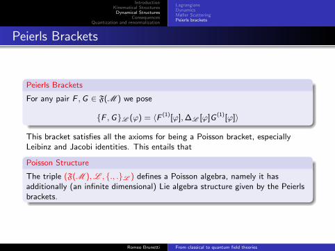
Peierls Brackets
For any pair F ,G ∈ F(M ) we pose
{F ,G}L (ϕ) = 〈F (1)[ϕ],∆L [ϕ]G (1)[ϕ]〉
This bracket satisfies all the axioms for being a Poisson bracket, especiallyLeibinz and Jacobi identities. This entails that
Poisson Structure
The triple (F(M ),L , {., .}L ) defines a Poisson algebra, namely it hasadditionally (an infinite dimensional) Lie algebra structure given by the Peierlsbrackets.
Romeo Brunetti From classical to quantum field theories
IntroductionKinematical Structures
Dynamical StructuresConsequences
Quantization and renormalization
LagrangiansDynamicsMøller ScatteringPeierls brackets
Summary of Dynamical Structures
Summary1 Generalized Lagrangians, hyperbolic equations (linear, semilinear,
quasilinear...)
2 Off-shell dynamics, i.e. Møller intertwiners
3 Off-shell Peierls brackets and Poisson structure
Romeo Brunetti From classical to quantum field theories

IntroductionKinematical Structures
Dynamical StructuresConsequences
Quantization and renormalization
Structural consequencesLocal covariance
Structural consequences
The existence and properties of rL +λI (h),L have fundamental implications forthe underlying Poisson structure of any classical field theory determined by anaction functional L
Darboux
rL +λI (h),L is a canonical transformation, i.e. it intertwines the Poissonstructures associated to L and L + λI (h):
{., .}L +λI (h) ◦ rL +λI (h),L = {., .}L .
In particular, even off-shell does it allow one to put {., .}L +λI (h) in normalform, i.e. to make it locally background-independent (Functional DarbouxTheorem).
Romeo Brunetti From classical to quantum field theories
IntroductionKinematical Structures
Dynamical StructuresConsequences
Quantization and renormalization
Structural consequencesLocal covariance
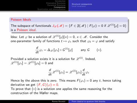
Poisson Ideals
The subspace of functionals JL (M ) = {F ∈ F(M ) | F (ϕ) = 0 if L (1)[ϕ] = 0}is a Poisson ideal.
Idea: Let ϕ be a solution of L (1)[ϕ](x) = 0, x ∈M . Consider theone-parameter family of functions t 7→ ϕt such that ϕ0 = ϕ and satisfy
d
dtϕt = ∆L [ϕt ] ◦ G (1)[ϕ] any G (∗).
Provided a solution exists it is a solution for L (1). Indeed,L (1)[ϕt ] = L (1)[ϕ0] = 0 and
d
dtL (1)[ϕt ] = L (2)[ϕt ]
d
dtϕt
Hence by the above this is zero. This means F (ϕt) = 0 any t, hence takingderivative we get {F ,G}(ϕ) = 0.To prove that (∗) is a solution one applies the same reasoning for theconstruction of the Møller maps.
Romeo Brunetti From classical to quantum field theories

IntroductionKinematical Structures
Dynamical StructuresConsequences
Quantization and renormalization
Structural consequencesLocal covariance
Symplectic-Poisson Structure
We may characterize as well the Casimir functionals Cas(F(M )), namely theelements of the center w.r.t. the Poisson structure, i.e. those F such that{F ,G}L (ϕ) = 0 for any G , ϕ.They are generated by the elements L (1)[ϕ]h(x) and constant functionals.So we may quotient the algebra by the Poisson ideal and/or the Casimir ideal(which is just an ideal for the Lie structure).The quotient represent the (Symplectic-)Poisson algebras for the on-shelltheory, namely
F(M )/JL (M ) , or F(M )/Cas(M )
Since all the ideals are linear subspaces they are nuclear, and since they aresequentially closed, we get that the quotient remains nuclear as well.By restrictions one may get the net structure, instead we shall present it in thelocally covariant form.
Romeo Brunetti From classical to quantum field theories
IntroductionKinematical Structures
Dynamical StructuresConsequences
Quantization and renormalization
Structural consequencesLocal covariance
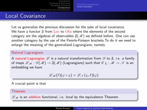
Local Covariance
Let us generalize the previous discussion for the sake of local covariance.We have a functor F from Loc to Obs where the elements of the secondcategory are the algebras of observables F(M ) we defined before. One can useanother category by the use of the Peierls-Poisson brackets.To do it we need toenlarge the meaning of the generalized Lagrangians, namely
Natural Lagrangians
A natural Lagrangian L is a natural transformation from D to F, i.e. a familyof maps LM : D(M )→ F(M ) (Lagrangians) such that if χ : M → N is anembedding we have
LM (f )(ϕ ◦ χ) = LN (χ∗f )(ϕ)
A crucial point is that
Theorem
LM is an additive functional, i.e. local by the equivalence Theorem.
Romeo Brunetti From classical to quantum field theories

IntroductionKinematical Structures
Dynamical StructuresConsequences
Quantization and renormalization
Structural consequencesLocal covariance
Using that L (1)M defines equation of motions ad L (2)
M is a strictly hyperbolicoperator, we endow F(M ) with the Peierls structure of before and we have:
Locally Covariant Classical Field Theory
The functor FL from Loc to the category of (Nuclear) Poisson algebras Poisatisfies the axioms of local covariance
Remarks
1 Actually, one can extend to the case of tensor categories, since nuclearityworks well under tensor products.
2 If one takes the quotient w.r.t. the Poisson ideal, i.e. we pass to theon-shell theory, then the ideals transform as (χ : M → N )
FLχJL (M ) ⊂ JL (N )
The quotient is again a good functor but due to the above (cp. blow-up)the morphisms of the Poisson category are not anymore injectivehomomorphisms! It would be interesting to see if the time-slice axiom issatisfied replacing injectivity by surjectivity.
Romeo Brunetti From classical to quantum field theories

IntroductionKinematical Structures
Dynamical StructuresConsequences
Quantization and renormalization
Deformation Quantization
We restrict our attention to Minkowski spacetime.To quantize one deforms the pointwise product to two different products:Firstly a star product by posing:
Wick’s Theorem
(F ? G)(ϕ) = e〈∆+,
δ2
δϕδϕ′ 〉(F (ϕ)G(ϕ′)) �ϕ=ϕ′
No problem if F and G have smooth functional derivatives.
Vacuum stateω0(F ) = F (0)
Romeo Brunetti From classical to quantum field theories

IntroductionKinematical Structures
Dynamical StructuresConsequences
Quantization and renormalization
Time Ordering Operator
(TF )(ϕ) = e〈∆F ,
δ2
δϕ2 〉F (ϕ) ≡∫
dµ∆F (ψ)F (ϕ− ψ)
where dµ∆F is a gaussian measure with covariance ∆F .
Time Ordered Product
F .TG = T (T−1F .T−1G)
which is not everywhere well defined..., and
(F .TG)(ϕ) = e〈∆F ,
δ2
δϕδϕ′ 〉(F (ϕ)G(ϕ′)) �ϕ=ϕ′
withF ? G = F .TG
whenever supp(F ) is later than supp(G).
Romeo Brunetti From classical to quantum field theories
IntroductionKinematical Structures
Dynamical StructuresConsequences
Quantization and renormalization
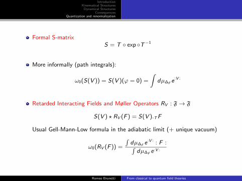
Formal S-matrixS = T ◦ exp ◦T−1
More informally (path integrals):
ω0(S(V )) = S(V )(ϕ = 0) =
∫dµ∆F e :V :
Retarded Interacting Fields and Møller Operators RV : F→ F
S(V ) ? RV (F ) = S(V ).TF
Usual Gell-Mann-Low formula in the adiabatic limit (+ unique vacuum)
ω0(RV (F )) =
∫dµ∆F e :V : : F :∫
dµ∆F e :V :
Romeo Brunetti From classical to quantum field theories

IntroductionKinematical Structures
Dynamical StructuresConsequences
Quantization and renormalization
Up to now we did everything on the case of functionals with smoothderivatives. We wish to extend the construction to the case of localfunctionals, the result of which is the following
Reformulation of Theorem 0 of Epstein-Glaser
?-products for local observables exist and generate an associative ∗-algebra
Time ordered products of local observables exist under conditions ofsupports and generate a partial algebra (Keller-loc. cit.)
What is left is the lift of this result to the case where the restrictions onsupports are not there anymore, which is the essence of renormalization. Inother words we wish to extend the local S-matrix to a map between localfunctionals (observables). The core of the technique is a careful extensionprocedure for distributions. You will hear a lot more on this...(Dutsch,Fredenhagen, Keller)
Romeo Brunetti From classical to quantum field theories