Embed Size (px)
Citation preview
Master Thesis
ONE-LOOP AMPLITUDES IN PERTURBATIVE
QUANTUM FIELD THEORY
Robbert Rietkerk
Supervisor: prof. dr. Eric Laenen
Nikhef Institute for Subatomic Physics
Institute for Theoretical Physics, Utrecht University
August 20, 2012
Thesis submitted for the degree of M.Sc.
Institute for Theoretical Physics, Utrecht University
Nikhef Institute for Subatomic Physics
ii

Abstract
We review methods for calculation of higher order corrections in per-
turbative quantum field theory. After laying the foundation with several
traditional methods we turn to more recent developments. A particular
method, proposed by Ossola, Papadopoulos and Pittau, reduces ten-
sor integrals from one-loop diagrams with many external particles to
known scalar integrals. This is achieved by a highly efficient algebraic
algorithm, thereby opening the window to more precise predictions for
collider processes. We describe the method and present an algebraic
implementation in FORM.
In the field of soft corrections, some spectacular progress has been made
as well. Processes can be calculated to all orders in perturbation theory
through exponentiation of a certain set of diagrams. We investigate
properties of such diagrams by applying the unitarity method.
iii

iv

Acknowledgements
I would like thank my supervisor professor Eric Laenen for guiding me on the journey
that is called research. He inspires me with enthusiastic explanations and manages to
ask just the right questions to push me forward.
Besides my supervisor, a number of other people also deserve thanks for their help.
I thank Ioannis Malamos for giving me an introduction to his research and Domenico
Bonocore for discussing topics of our mutual interest. I’m grateful to Jos Vermaseren
and Jan Kuipers for answering my questions about FORM. Also Pierre Artoisenet and
Damien George are much obliged for their readiness to help out with various problems.
In particular I enjoyed discussions in front of the blackboard.
Thanks to Jory and Philipp for their companionship and help throughout the year
and the rest of the theory group at Nikhef for providing such a pleasant environment.
Also my fellow students in Utrecht provided enjoyable company, mostly during the first
year of the masters. It has been great!
Finally, I thank my family for their love and support.
v

vi
Contents
1. Introduction 3
2. One-Loop Corrections 5
2.1. Vacuum Polarization . . . . . . . . . . . . . . . . . . . . . . . . . . . . . 5
2.2. Electron Self-Energy . . . . . . . . . . . . . . . . . . . . . . . . . . . . . 9
2.3. Vertex Correction . . . . . . . . . . . . . . . . . . . . . . . . . . . . . . . 11
2.4. Renormalization . . . . . . . . . . . . . . . . . . . . . . . . . . . . . . . . 17
3. Unitarity 23
3.1. Unitarity . . . . . . . . . . . . . . . . . . . . . . . . . . . . . . . . . . . . 23
3.2. Cut Feynman Diagrams . . . . . . . . . . . . . . . . . . . . . . . . . . . 24
3.2.1. Largest Time Equation . . . . . . . . . . . . . . . . . . . . . . . . 24
3.2.2. Cutting Equation . . . . . . . . . . . . . . . . . . . . . . . . . . . 26
3.2.3. Connection with Unitarity . . . . . . . . . . . . . . . . . . . . . . 29
3.3. Dispersion Relations . . . . . . . . . . . . . . . . . . . . . . . . . . . . . 30
3.4. Generalized Unitarity . . . . . . . . . . . . . . . . . . . . . . . . . . . . . 32
4. OPP Reduction 35
4.1. Integrand Decomposition . . . . . . . . . . . . . . . . . . . . . . . . . . . 35
4.1.1. Master Formula . . . . . . . . . . . . . . . . . . . . . . . . . . . . 35
4.1.2. The van Neerven-Vermaseren Basis . . . . . . . . . . . . . . . . . 37
4.1.3. Tensor Reduction of One-Loop Integrals . . . . . . . . . . . . . . 40
4.2. Determination of Coefficients . . . . . . . . . . . . . . . . . . . . . . . . 45
4.3. Rational Part . . . . . . . . . . . . . . . . . . . . . . . . . . . . . . . . . 47
4.4. Application of the OPP Method . . . . . . . . . . . . . . . . . . . . . . . 52
4.5. Implementation . . . . . . . . . . . . . . . . . . . . . . . . . . . . . . . . 54
4.5.1. Analytic OPP Reduction in FORM . . . . . . . . . . . . . . . . . 55
4.5.2. Results and Comparison . . . . . . . . . . . . . . . . . . . . . . . 56
vii
viii Contents
5. Eikonal Approximation and Unitarity 61
5.1. Eikonal Propagator . . . . . . . . . . . . . . . . . . . . . . . . . . . . . . 61
5.2. Eikonal Vertex Correction . . . . . . . . . . . . . . . . . . . . . . . . . . 63
5.3. Cutkosky Rule in Eikonal Approximation . . . . . . . . . . . . . . . . . . 66
5.4. Eikonal Vertex Correction by Unitarity . . . . . . . . . . . . . . . . . . . 67
6. Conclusion 71
A. Conventions and Integrals 73
B. Dirac Algebra with FORM 79
C. Analytic OPP Reduction in FORM 81
Bibliography 89

1

2
Chapter 1.
Introduction
One of the main quantities of interest in particle physics is the scattering cross-section,which describes the probability of interaction between particles. Quantum mechanics dic-tates that such probabilities are computed as squares of complex scattering amplitudes.Unfortunately not even the simplest scattering amplitude is known exact. Perturbationtheory has become the established way to approximate results.
A beautiful tool in perturbation theory is the use of Feynman diagrams, a graphicvisualization of terms in the series in powers of the coupling strength between interactingparticles. The largest possible contribution to amplitudes come from tree diagrams.Higher order corrections are given by diagrams with loops.
While the computation of tree diagrams is well established, the one-loop diagramsare notoriously challenging. In the first place, loops give divergent contributions to theamplitude, which need to be properly handled by a renormalization procedure. It hasfirst been shown to produce excellent results in the context of quantum electrodynamics.The correct prediction of the anomalous magnetic moment of the electron [1] is seen asone of the great successes of perturbation theory.
Quantum chromodynamics and the electroweak theory, on the other hand, give rise tomuch more diverse particle interactions. A big step forward was made in the late 1970s,when scalar integrals were computed for arbitrary masses [2] and non-scalar integralswere treated with Passarino-Veltman reduction [3].
In the mean time an alternative calculation method was constructed, which exploitsunitarity of the scattering matrix [4]. This unitarity method allows to determine the ab-sorptive (imaginary) part of an amplitude in a relatively simple manner. The dispersive(real) part of an amplitude can be reconstructed by means of dispersion relations [5].
Some processes, in particular many-particle scattering, remain highly challenging forpractical reasons. The number of Feynman diagrams increases rapidly with the numberof external particles, while the expressions for each of them become more and morelengthy.
One solution is to expand arbitrary one-loop integrals in terms of a basis of scalarone-loop integrals that are known analytically. The existence a finite basis is justified
3
4 Introduction
by explicit tensor reduction and by the theorem that one needs up to four-point scalarintegrals [6], directly related to the number of spacetime dimensions. The problem isthen shifted to the determination of the coefficients in such an expansion.
The generalized unitarity method extracts these coefficients by cutting diagrams andrelating their imaginary part to the discontinuities of scalar integrals from the basis [7].Multiple cuttings are used to determine the coefficients of the box integrals efficiently.Massive virtual particles do pose a difficulty, although some special cases have beenfound [8].
The OPP reduction method is based on a similar expansion, but at the integrandlevel [9]. Determination of the coefficients is performed by evaluating the integrand atdifferent loop momenta. In contrast to generalized unitarity, no information on the ana-lytic structure of the amplitude is needed and it has no problem with massive particles.This feature makes a numerical implementation of the method feasible [10]. It has al-ready been used to give next-to-leading order predictions for many-particle processes atcolliders, such as the LHC [11].
In the area of soft corrections, exponentiation of amplitudes has been established inthe eikonal approximation [12]. This powerful theorem allows the extraction of all-orderinformation on the scattering amplitude from lower-order diagrams in the exponent.We investigate a way to quickly compute contributions to the exponent, making use ofunitarity.
Chapter 2.
One-Loop Corrections
As we mentioned in the introduction, one-loop corrections in perturbation theory arenot calculated without difficulties. Among them are the notorious divergences: infinitecontributions to tree-level amplitudes.
In this chapter we show how to dimensionally regularize expressions in the contextof quantum electrodynamics. The one-loop corrections to the three standard Feynmandiagrams are the vacuum polarization, the electron self-energy and the vertex correction.We give the full results to these diagrams, including in particular the finite parts.
The last section focuses on the renormalization procedure, used to render the theoryfinite. In particular we introduce the renormalization constant Ward identities. Usingour results for the one-loop corrections we show that QED is renormalizable to all orders.
2.1. Vacuum Polarization
The Lagrangian for QED is given by
L = ψ(i/∂ −m)ψ − 14(Fµν)
2 − eAµψγµψ − 1
2λ(∂µA
µ)2 . (2.1)
This Lagrangian gives rise to three Feynman diagrams, namely the propagators for theelectron and photon and the e+e−γ vertex. We use the well-known Feynman rules usedby Peskin and Schroeder in the Feynman gauge [13].
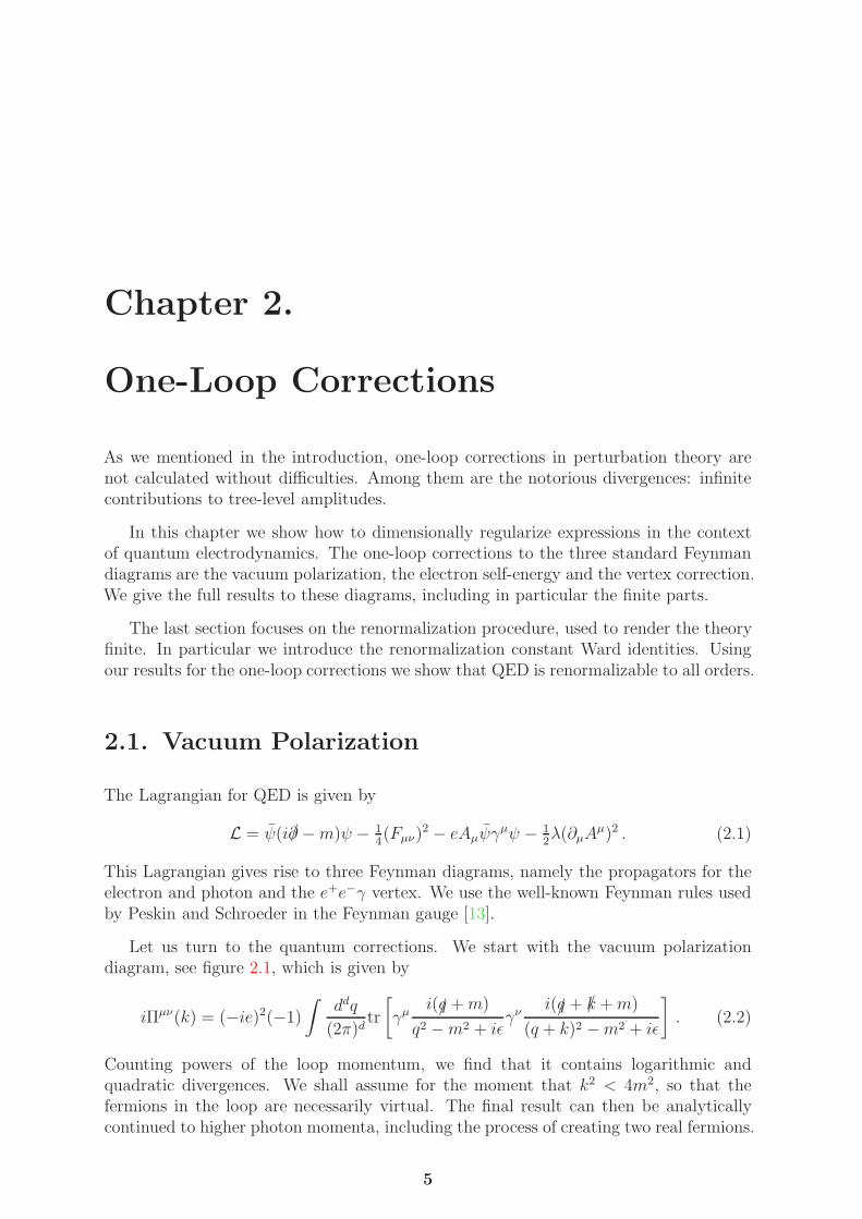
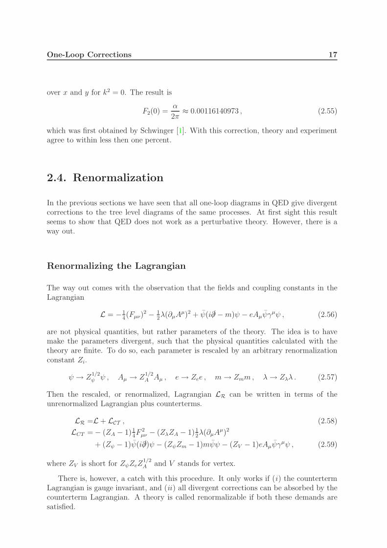
Let us turn to the quantum corrections. We start with the vacuum polarizationdiagram, see figure 2.1, which is given by
iΠµν(k) = (−ie)2(−1)
∫ddq
(2π)dtr
[
γµi(/q +m)
q2 −m2 + iǫγν
i(/q + /k +m)
(q + k)2 −m2 + iǫ
]
. (2.2)
Counting powers of the loop momentum, we find that it contains logarithmic andquadratic divergences. We shall assume for the moment that k2 < 4m2, so that thefermions in the loop are necessarily virtual. The final result can then be analyticallycontinued to higher photon momenta, including the process of creating two real fermions.
5
6 One-Loop Corrections
q + k
q
kk
Figure 2.1.: Vacuum polarization: one-loop correction to the photon propagator.
Calculation of the integral over q is performed in several steps. First, one applies theFeynman parameter trick (A.28) to combine the two denominators. Next, one completesthe square in the denominator, shifts the loop momentum to l = q + xk and definesM2 = m2 − x(1 − x)k2. Taking the trace is done with the aid of (A.8)-(A.10). Theresult contains powers of the loop momentum in the numerator. Terms linear in l vanishaccording to (A.23), while terms containing lµlν become proportional to l2ηµν aftersymmetric integration (A.24). The latter can be further simplified with (A.26). Theresult is remarkably simplified
iΠµν(k) = −8e2∫ 1
0
dx
∫ddl
(2π)dk2ηµν − kµkν
(l2 −M2 + iǫ)2. (2.3)
Let us separate the tensor structure from a scalar prefactor
iΠµν(k) = iΠ(k2)(k2ηµν − kµkν) , (2.4)
thereby defining
Π(k2) = 8ie2∫ 1
0
dx x(1 − x)
∫ddl
(2π)d1
(l2 −M2 + iǫ)2. (2.5)
Observe that the vacuum polarization in this form explicitly satisfies kµΠµν = 0. Ac-
tually this must be true on general grounds. As a direct consequence of the gaugeinvariance of the Lagrangian there exists a Ward identity, which states that a generalamplitude with an external photon carrying momentum k satisfies kµMµ(k) = 0.
The d-dimensional momentum integral in Π(k2) is standard and we plug in the resultfrom (A.21), which is given in terms of d = 4−2 ε. Also we substitute the fine-structureconstant α = e2/(4π).
Π(k2) = −i α3π
(µ2)− ε
[1
ε− γ +
∫ 1
0
dx 6x(x− 1) log
(M2
4πµ2
)]
. (2.6)
Trivial integration over x-independent terms has been carried out. Let us remind thatM2 = m2 − x(1 − x)k2. The factor (µ2)− ε serves to give the expression a correct mass
One-Loop Corrections 7
dimension away from d = 4. We have now found the correct pole structure of the firstorder vacuum polarization. What is left to do is to determine explicitly the finite part.
Feynman Parameter Integral
Consider the last term between the brackets in (2.6),
∫ 1
0
dx 6x(x− 1) log
(m2 − x(1 − x)k2
4πµ2
)
. (2.7)
The integral is well defined because the argument of the logarithm is positive for allvalues of x thanks to our assumption k2 < 4m2. Let’s define the ratio
r :=k2
4m2, (2.8)
and assume further that r 6= 0 so that the logarithm is x-dependent. The trivial caser = 0 will be treated separately. One way to solve the integral is to factorize theargument of the logarithm, split into a sum of logarithms, shift integration variable ifnecessary and finally apply partial integration to terms of the form
∫xn log(x).
Here we go. Factorizing the argument of the logarithm gives k2/(4πµ2) · (x − x+) ·(x− x−), with x± = 1
2(1 ± β) and
β :=√
1 − 1/r . (2.9)
Splitting the logarithm one obtains three terms. The first is simply log(4πµ2/k2). Theother two terms are
∫ 1
0
dx 6x(x− 1) log(x− x+) + {x+ → x−}
=5
6+ 2x+(1 − x+) − log(1 − x+) + (3 − 2x+)x2
+ log
(1 − x+
−x+
)
+ {x+ → x−}
=5
6+ 2x+x− − log(x−) + (1 + 2x−)x2
+ log
(−x−x+
)
+ {x+ ↔ x−}
=5
3+ 4x+x− − log(x+x−) + [(1 + 2x−)x2
+ − (1 + 2x+)x2−] log
(−x−x+
)
=5
3+
1
r+ log(4r) +
(
1 +1
2r
)
β log
(β − 1
β + 1
)
. (2.10)
In the second equality we made use of the observation that 1 − x± = x∓, meaning that(1 − x+) → (1 − x−) and x− → x+ are equivalent substitutions.
8 One-Loop Corrections
In terms of r and β, the final result for the vacuum polarization is
Π(k2) = − α
3π(µ2)− ε
[1
ε− γ − log
(m2
4πµ2
)
+5
3+
1
r+
(
1 +1
2r
)
β log
(β − 1
β + 1
)]
.
(2.11)
together with the tensor structure (2.4).
Analytic Continuation
The above solution was derived under the assumption r < 1 and r 6= 0. Therefor wemust rederive a solution for a photon on mass shell and also see what happens for aphoton with timelike or spacelike momentum. Moreover, we would also like to extendthe solution to r > 1 in order to describe processes such as pair creation.
i) For r = 0 we must go back to the original Feynman parameter integral (2.7) andset k2 = 0. The integral is then trivial and gives − log(m2/(4πµ2)), meaning thatin this case we have only the first three terms of (2.11),
Π(0) = − α
3π(µ2)− ε
[1
ε− γ − log
(m2
4πµ2
)]
. (2.12)
ii) For 0 < r < 1 the argument of the logarithm becomes a complex number ofunit norm exp(iθ(r)), with θ(r) = 2 arctan(
√r/√
1 − r) = 2 arcsin(√r). Both the
square root β and logarithm become purely imaginary. Thus the last term in (2.11)remains real and is written as
−2
(
1 +1
2r
)√1r− 1 arcsin(
√r) for 0 < r < 1 . (2.13)
iii) For r ≥ 1 the argument of the logarithm is negative and real, so it sits on abranch cut. Following the prescription (A.16) for analytic continuation we letM2 → M2 − iǫ and consequently r → r+ iǫ (taking their definitions into account).This puts the logarithm just above the branch cut, which then contributes anadditional +iπ, making the last term equal to
(
1 +1
2r
)
β
[
log
(1 − β
1 + β
)
+ iπ
]
for r ≥ 1 . (2.14)
Only in this regime the vacuum polarization picks up an imaginary part. It happensbecause above the threshold k2 > 4m2 the photon can decay into a real electron-positron pair.
One-Loop Corrections 9
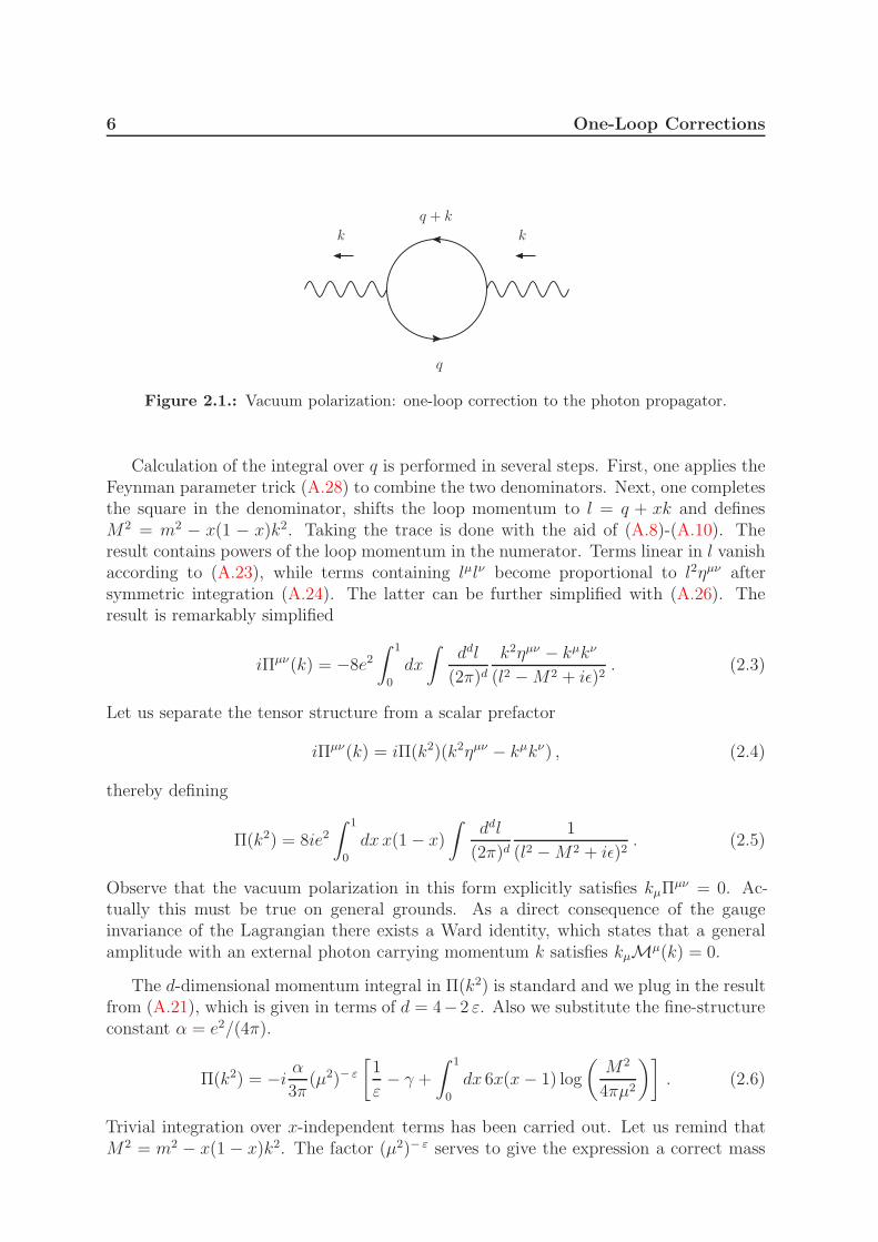
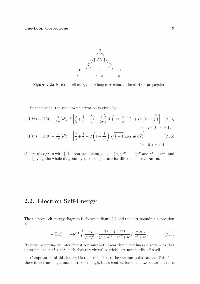
q
pp+ qp
Figure 2.2.: Electron self-energy: one-loop correction to the electron propagator.
In conclusion, the vacuum polarization is given by
Π(k2) = Π(0) − α
3π(µ2)− ε
[5
3+
1
r+
(
1 +1
2r
)
β
(
log
∣∣∣∣
β − 1
β + 1
∣∣∣∣+ iπθ(r − 1)
)]
(2.15)
for r < 0, r ≥ 1 ,
Π(k2) = Π(0) − α
3π(µ2)− ε
[5
3+
1
r− 2
(
1 +1
2r
)√1r− 1 arcsin(
√r)
]
(2.16)
for 0 < r < 1 .
Our result agrees with [14] upon translating ε→ − 12ε, ηµν → −ηµν and γµ → iγµ, and
multiplying the whole diagram by i, to compensate for different normalization.
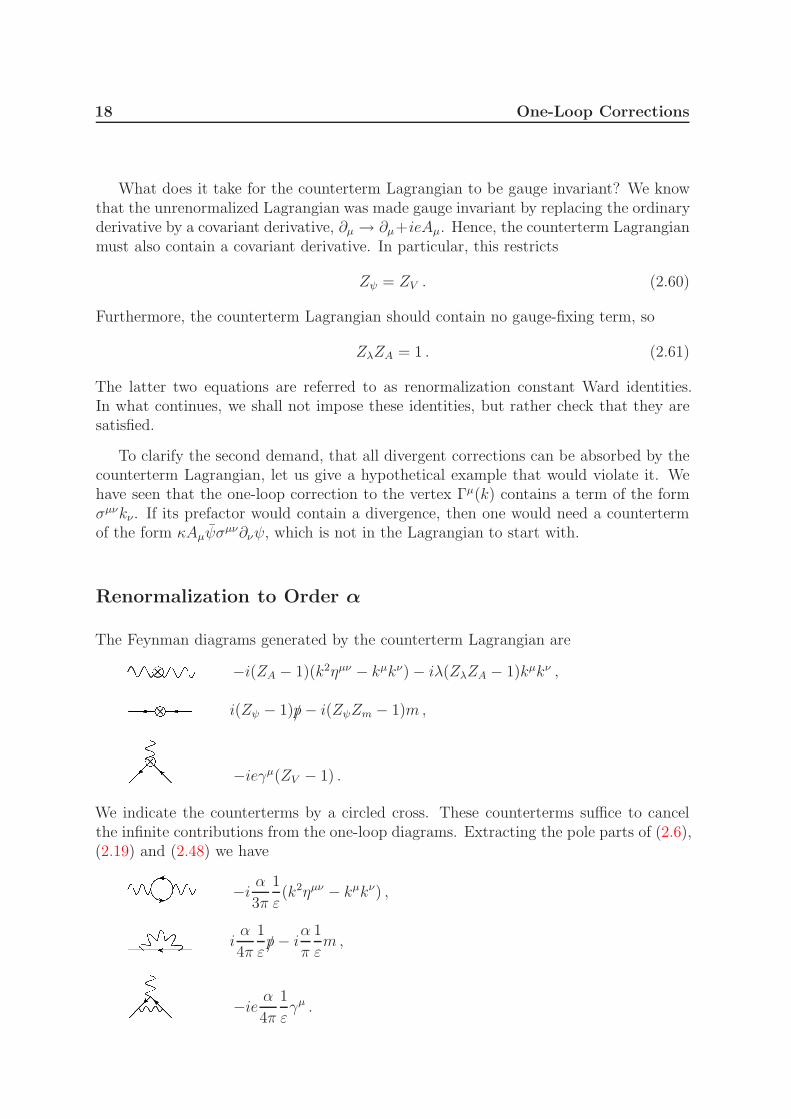
2.2. Electron Self-Energy
The electron self-energy diagram is shown in figure 2.2 and the corresponding expressionis
−iΣ(p) = (−ie)2
∫ddq
(2π)dγµ
i(/p+ /q +m)
(p+ q)2 −m2 + iǫγν
−iηµνq2 + iǫ
. (2.17)
By power counting we infer that it contains both logarithmic and linear divergences. Letus assume that p2 < m2, such that the virtual particles are necessarily off-shell.
Computation of this integral is rather similar to the vacuum polarization. This timethere is no trace of gamma matrices, though, but a contraction of the two outer matrices,
10 One-Loop Corrections
to which we apply (A.11) and (A.11). We compute
−iΣ(p) = −e2∫
ddq
(2π)d(2 − d)(/p+ /q) + dm
((p+ q)2 −m2 + iǫ) (q2 + iǫ)
= −e2∫
ddq
(2π)d
∫ 1
0
dx(2 − d)(/p+ /q) + dm
[(q + xp)2 − x(m2 − (1 − x)p2)) + iǫ]2
= −e2∫ 1
0
dx
∫ddl
(2π)d(2 − d)(/l + (1 − x)/p) + dm
(l2 −M2 + iǫ)2
= −e2∫ 1
0
dx [(2 − d)(1 − x)/p + dm]
∫ddl
(2π)d1
(l2 −M2 + iǫ)2, (2.18)
where M2 = xm2 − x(1 − x)p2. Notice that M2 is positive for all x with p2 < m2. Themomentum integral is now a scalar one and is listed in (A.21). Substituting d = 4− 2 εand α = e2/4π,
−iΣ(p) = iα
4π
[1
ε− γ − 1 − 2
∫ 1
0
dx(1 − x) log
(M2
4πµ2
)]
/p
−iαπ
[1
ε− γ − 1
2−∫ 1
0
dx log
(M2
4πµ2
)]
m. (2.19)
These expressions give the correct divergent parts.
Calculation of the Feynman parameter integrals can be done in the way that wasoutlined in the previous subsection. By introducing the ratio
r :=p2
m2, (2.20)
we have M2 = xm2(1 − (1 − x)r). We quote two intermediate results for r 6= 0,
∫ 1
0
dx log
(M2
4πµ2
)
=
[
−2 + log
(m2
4πµ2
)
+
(
1 − 1
r
)
log(1 − r)
]
, (2.21)
∫ 1
0
dx x log
(M2
4πµ2
)
=1
2
[
−2 + log
(m2
4πµ2
)
+1
r+
(
1 − 1
r
)2
log(1 − r)
]
. (2.22)
The self-energy is now given by
−iΣ(p) = iα
4π
[1
ε− γ − log
(m2
4πµ2
)
+ 1 +1
r−(
1 − 1
r2
)
log(1 − r)
]
/p
−iαπ
[1
ε− γ − log
(m2
4πµ2
)
+3
2−(
1 − 1
r
)
log(1 − r)
]
m. (2.23)
One-Loop Corrections 11
The above solution was derived under the assumptions r < 1 and r 6= 0. We extendit to all r like was done for the vacuum polarization.
i) For r = 0 the integrals in (2.21)-(2.22) are trivial. We find
−iΣ(0) = iα
4π
[1
ε− γ − log
(m2
4πµ2
)
− 1
]
/p− iα
π
[1
ε− γ − log
(m2
4πµ2
)
− 1
2
]
m.
(2.24)
ii) For r > 1 we need to perform analytic continuation of the logarithm. Followingthe the prescription (A.16) we let M2 → M2 − iǫ and consequently r → r + iǫ,which puts the logarithm just below the branch cut. So we replace log(1 − r) bylog |1 − r| − iπθ(r − 1).
Finally, the solution valid for all electron momenta p, is given by
−iΣ(p) = −iΣ(0) + iα
4π
[
2 +1
r−(
1 − 1
r2
)(
log |1 − r| − iπθ(r − 1))]
/p
−iαπ
[
2 −(
1 − 1
r
)(
log |1 − r| − iπθ(r − 1))]
m. (2.25)
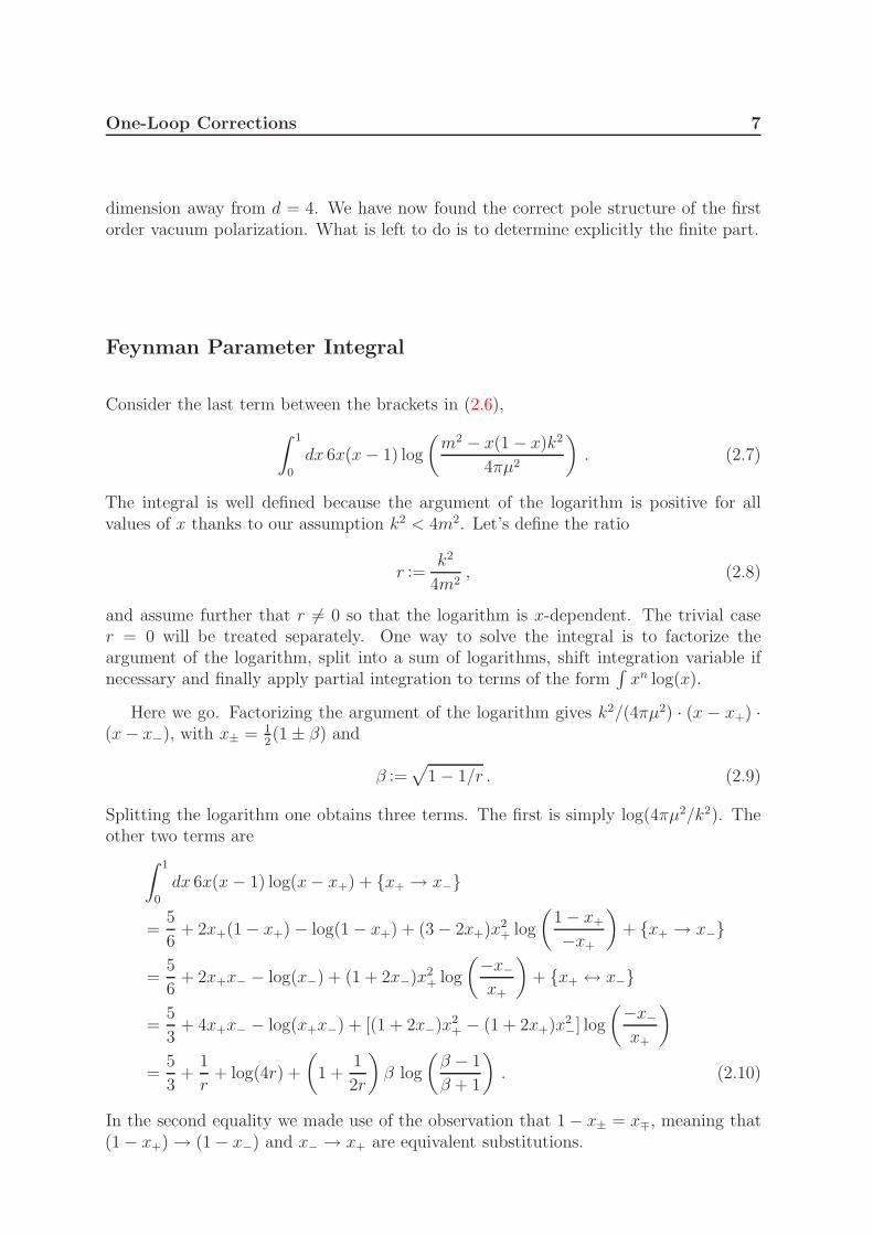
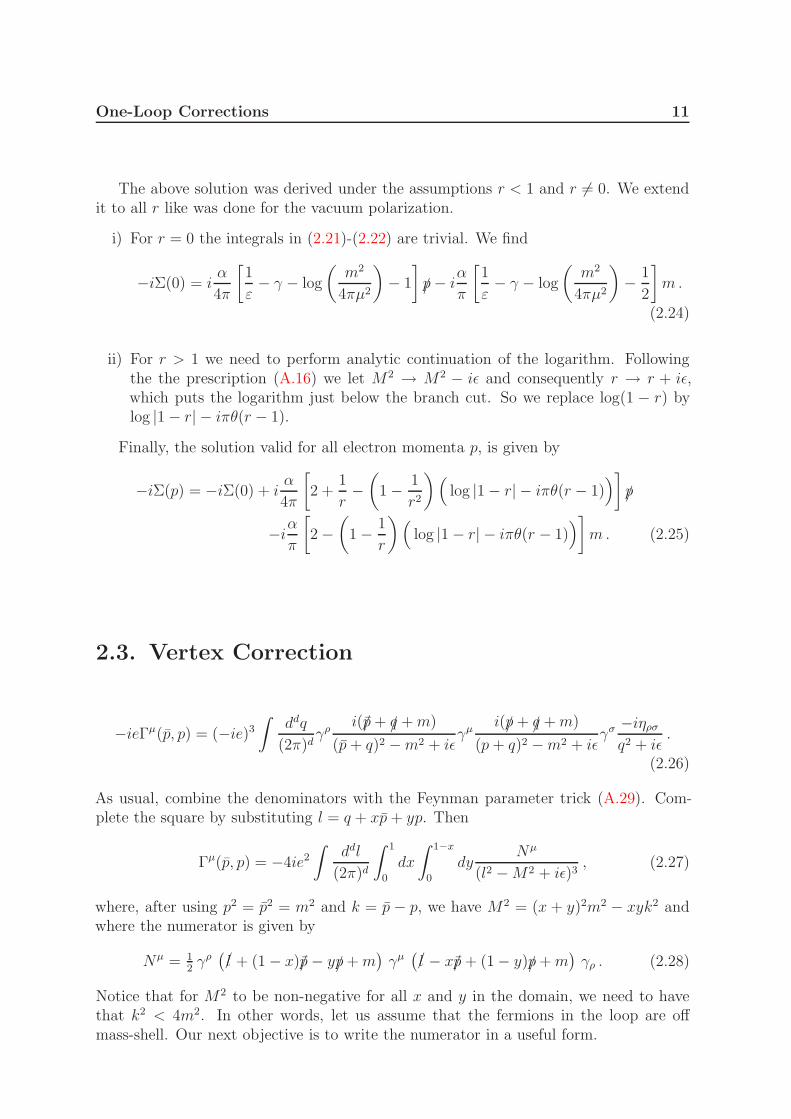
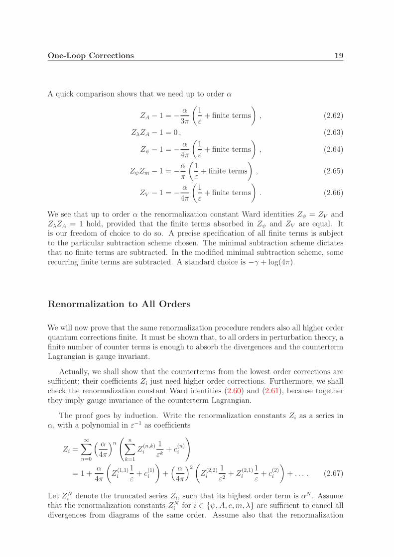
2.3. Vertex Correction
−ieΓµ(p, p) = (−ie)3
∫ddq
(2π)dγρ
i(/p+ /q +m)
(p+ q)2 −m2 + iǫγµ
i(/p+ /q +m)
(p+ q)2 −m2 + iǫγσ
−iηρσq2 + iǫ
.
(2.26)
As usual, combine the denominators with the Feynman parameter trick (A.29). Com-plete the square by substituting l = q + xp + yp. Then
Γµ(p, p) = −4ie2∫
ddl
(2π)d
∫ 1
0
dx
∫ 1−x
0
dyNµ
(l2 −M2 + iǫ)3, (2.27)
where, after using p2 = p2 = m2 and k = p − p, we have M2 = (x + y)2m2 − xyk2 andwhere the numerator is given by
Nµ = 12γρ(/l + (1 − x)/p− y/p+m
)γµ(/l − x/p + (1 − y)/p+m
)γρ . (2.28)
Notice that for M2 to be non-negative for all x and y in the domain, we need to havethat k2 < 4m2. In other words, let us assume that the fermions in the loop are offmass-shell. Our next objective is to write the numerator in a useful form.
12 One-Loop Corrections
p
p+ qp′ + q
p′
q
p′ − p
Figure 2.3.: One-loop vertex correction.
Numerator
There are few steps to simplify the numerator. First, observe that the numerator containsterms with up to two powers of the loop momentum. Applying symmetric integration,linear terms vanish, (A.23), while lµlν can be replaced by l2ηµν/d, (A.24). Second, theindices on the outer two gamma matrices are contracted, so we need the appropriateidentities (A.11)-(A.14). Furthermore, in practice the vertex function gets sandwichedby Dirac spinors u(p) Γµ(p, p) u(p). This means that we can use the Dirac equation(/p−m)u(p) = 0 and u(p)(/p−m) = 0, thereby removing slashed momenta. And finally,there is only one free spacetime index µ, so the numerator can be expressed as
Nµ = C1 γµ + C2p
µ + C3pµ . (2.29)
Bringing the numerator to this form can be quite tedious, making it an excellent taskfor a symbolic computer program. We performed the manipulations in FORM [15], seeappendix B. The coefficients Ci are
C1 = l2 [2d
+ d2− 2] − k2 [1 − x− y + (d
2− 1)xy] +m2 [2 − 4(x+ y) + (d
2− 1)(x+ y)2] ,
C2 = 2m [y − (d2− 1)x(x+ y)] ,
C3 = 2m [x− (d2− 1)y(y + x)] . (2.30)
Inspired by the Ward identity kµΓµ(p, p) = 0, we rewrite the numerator in terms of
the linear combinations (p+p)µ and kµ, giving C1 γµ+ 1
2(C2+C3)(p+p)µ+ 1
2(C2−C3)k
µ.When contracting with kµ, the first two terms vanish by virtue of the Dirac equationand mass-shell condition for the fermion. Since the photon is not constrained to be onmass shell, the contraction as a whole can only vanish (Ward identity) if the coefficientof the third term is zero.
We can also verify explicitly that this must be true. Interchange the dummy variablesx and y. The effect is that C2 becomes C3 and vice versa, hence the coefficient 1
2(C2−C3)
picks up a minus sign. Meanwhile, the domain of integration remains the same, as doesthe denominator. It follows that the coefficient must be zero and the kµ term drops out.
One-Loop Corrections 13
It is conventional to further eliminate (p+p)µ in favor of σµνkν (with σµν = i2[γµ, γν ])
by means of the Gordon identity
u(p)γµu(p) = u(p)
((p+ p)µ
2m+iσµνkν
2m
)
u(p) , (2.31)
after which
Nµ = D1 γµ +D2
iσµνkν2m
, (2.32)
with
D1 = C1 +m(C2 + C3) , (2.33)
D2 = −m(C2 + C3) . (2.34)
Putting numerator (2.32) into the integral (2.27), we can pull the tensor structureoutside the integrals.
Γµ(p, p) = F1(k2)γµ + F2(k
2)iσµνkν
2m, (2.35)
with form factors F1,2 given by
F1,2(k2) = −4ie2
∫ 1
0
dx
∫ 1−x
0
dy
∫ddl
(2π)dD1,2
(l2 −M2 + iǫ)3. (2.36)
These form factors, F1(k2) and F2(k
2), encode the coupling strength of the fermionto an electromagnetic field. In particular, F1(0) is the electric charge of the fermion andF2(0) its anomalous magnetic moment. Of course, to leading order the vertex is simplyΓµ = γµ, in which case F1(0) = 1 and F2(0) = 0. Now let’s find the next-to-leadingorder corrections to these form factors.
First Form Factor
Between the two form factors, F1 is the hardest to compute, because it suffers from bothUV and IR divergences. We shall regulate both divergences by dimensional regulariza-tion. Let us first define once again the ratio of the photon off-shell mass and the squaredmass of two fermions,
r :=k2
4m2. (2.37)
14 One-Loop Corrections
Substituting (2.30) into (2.33) and using this ratio, D1 reads
D1 = l2[
2d
+ d2− 2
]+m2
[(2 − 4r)(1 − x− y) +
(1 − d
2
) ((x+ y)2 + 4rxy
)]. (2.38)
The first term is expected to give a logarithmic UV-divergence by power counting, dueto the factor l2. We apply (A.26), effectively replacing l2 → d/(d− 4)M2, which indeedproduces a ε−1 pole as we take d = 4 − 2 ε. Now
D1 = −M2[
1ε
∣∣UV− 2 + ε
]
+m2[(2 − 4r)(1 − x− y) + (ε−1)
((x+ y)2 + 4rxy
)],
(2.39)
where M2 = m2 ((x+ y)2 − 4rxy) in terms of r as well. Now the momentum integral in(2.36) has attained the standard scalar form and can thus be performed. We take theresult from (A.17) for the case k = 3.
F1(k2) = −4ie2
∫ 1
0
dx
∫ 1−x
0
dy D1−i(µ2)−1−ε
2(4π)3Γ(1 + ε)
(M2
4πµ2
)−1−ε
= −2α (µ2)−1−ε
(4π)2Γ(1 + ε)
∫ 1
0
dx
∫ 1−x
0
dyD1
(M2
4πµ2
)−1−ε. (2.40)
Notice that we did not yet expand any factor around ε = 0. The reason is that there is anIR divergence hidden inside the Feynman parameter integrals. Only after we uncoveredthe divergence in the form of an ε−1 pole, do we start taking to make the expansion.This way we carefully retain ε / ε terms.
The final task is thus to compute the two Feynman parameter integrals. We canexploit the symmetry of the domain of integration and the integrand under x ↔ y.After splitting D1 into terms of zeroth, first and second degree in x and/or y,
D1 = D(0)1 +D
(1)1 +D
(2)1 , (2.41)
we can apply the reparametrization (A.30), that is,
∫ 1
0
dx
∫ 1−x
0
dy f (k)(x, y) =
∫ 1
0
dz z1+k
∫ 1
0
dx f (k)(x, 1 − x) , (2.42)
to the functions
f (j−2−2 ε)(x, y) = D(j)1
(M2
4πµ2
)−1−ε, (2.43)
One-Loop Corrections 15
for j = 0, 1, 2 and
D(0)1 = m2 (2 − 4r) , (2.44)
D(1)1 = −m2 (2 − 4r)(x+ y) , (2.45)
D(2)1 = −M2
(1ε
∣∣
UV− 2 + ε
)
+m2 (−1 + ε)((x+ y)2 + 4rxy) . (2.46)
These functions are symmetric and homogeneous of degree k = j − 2 − 2 ε. Afterreparametrization
F1(k2) = −2α (µ2)−1−ε
(4π)2Γ(1 + ε)
{∫ 1
0
dz z−1−2 ε
∫ 1
0
dx f (−2−2 ε)(x, 1 − x)
+
∫ 1
0
dz z−2 ε
∫ 1
0
dx f (−1−2 ε)(x, 1 − x)
+
∫ 1
0
dz z1−2 ε
∫ 1
0
dx f (−2 ε)(x, 1 − x)
}
. (2.47)
The trivial z-integrals decouple and contribute a factor − 12ε−1, 1
2(2 + ε) and 1
2(1 + ε)
respectively. Observe the emergence of an IR divergence in the form of a ε−1 pole. Itultimately comes from the photon going on mass shell.
At this stage we may expand around ε = 0 using (A.19) and (A.20). The remainingintegrals over x contain f (k)(x, 1 − x), so we plug y = 1 − x into (2.44)-(2.46) and M2.Our final result is
F1(k2) =
α(µ2)− ε
4π
{1
ε
∣∣∣∣UV
− γ − log
(m2
4πµ2
)
− 2 + 2 I1 − I2 + (4r − 2) I3
}
+α(µ2)− ε
4π
{1
ε
∣∣∣∣IR
− γ − log
(m2
4πµ2
)
+ 2
}
(2 − 4r) I1 , (2.48)
with the following integrals for the function f(x) = 1 − x(1 − x)4r,
I1 :=
∫ 1
0
dx1
f(x), I2 :=
∫ 1
0
dx log(f(x)), and I3 :=
∫ 1
0
dxlog(f(x))
f(x). (2.49)
At this point one we verified agreement with the result in [14], by making the usualtranslation of conventions and writing I1 = (1
2I2+1) 1
1−r for the first occurrence in (2.48).They regularize the IR divergence by giving the photon a mass κ1, which leads to a factorlog(κ1) instead of our 1
ε|IR
+ . . . in (2.48). Both diverge as ε and κ1 tend to zero. Inphysical amplitudes this IR divergence is canceled by bremsstrahlung diagrams, that is,tree level vertex diagrams where either the incoming or the outgoing fermion emits asoft photon [13].
16 One-Loop Corrections
Assuming that r 6= 0, factorizing f(x), using partial fractions and (A.35),
I1 =1
2rβlog
(β − 1
β + 1
)
, (2.50)
I2 = −2 − β log
(β − 1
β + 1
)
, (2.51)
I3 =1
4rβ
{
2 log(4r) log
(β − 1
β + 1
)
+ 2 Li2
(1 − β
1 + β
)
− 2 Li2
(1 + β
1 − β
)
− [ log(−1 − β) − log(β − 1) ] ×[
log(−1 − β) + log(−1 + β) + log
(β
β − 1
)
+ log
(β
β + 1
)]
+ [ log(1 − β) − log(β + 1) ] ×[
log(1 + β) + log(1 − β) + log
(β
β − 1
)
+ log
(β
β + 1
)]}
, (2.52)
in terms of β =√
1 − 1/r and the dilogarithm Li2(x), defined in (A.31).
Second Form Factor
The numerator of the second form factor
D2 = 2m2[−(x+ y) + (d2− 1)(x+ y)2] , (2.53)
is independent of the loop momentum. Therefor the momentum integral is UV-convergentin four dimensions. In fact, this form factor does not suffer from an IR divergence either,so we can put d = 4 explicitly.
F2(k2) =
α
π
∫ 1
0
dx
∫ 1−x
0
dy(x+ y)(1 − (x+ y))m2
(x+ y)2m2 − xyk2
=α
π
∫ 1
0
dz
∫ 1
0
dx1 − z
1 − x(1 − x)4r
=α
2π
1
4rβ
∫ 1
0
dx
[1
x− x+
− 1
x− x−
]
=α
π
1
4rβlog
(β − 1
β + 1
)
, (2.54)
where we used the reparametrization (A.30) and x± denote the zeros of x2 − x+ 1/(4r).
The anomalous magnetic moment of the electron, F2(0), is obtained by carefullytaking the limit r → 0 or alternatively by straightforward calculating the original integral
One-Loop Corrections 17
over x and y for k2 = 0. The result is
F2(0) =α
2π≈ 0.00116140973 , (2.55)
which was first obtained by Schwinger [1]. With this correction, theory and experimentagree to within less then one percent.
2.4. Renormalization
In the previous sections we have seen that all one-loop diagrams in QED give divergentcorrections to the tree level diagrams of the same processes. At first sight this resultseems to show that QED does not work as a perturbative theory. However, there is away out.
Renormalizing the Lagrangian
The way out comes with the observation that the fields and coupling constants in theLagrangian
L = −14(Fµν)
2 − 12λ(∂µA
µ)2 + ψ(i/∂ −m)ψ − eAµψγµψ , (2.56)
are not physical quantities, but rather parameters of the theory. The idea is to havemake the parameters divergent, such that the physical quantities calculated with thetheory are finite. To do so, each parameter is rescaled by an arbitrary renormalizationconstant Zi.
ψ → Z1/2ψ ψ , Aµ → Z
1/2A Aµ , e→ Zee , m→ Zmm, λ→ Zλλ . (2.57)
Then the rescaled, or renormalized, Lagrangian LR can be written in terms of theunrenormalized Lagrangian plus counterterms.
LR =L + LCT , (2.58)
LCT = − (ZA − 1)14F 2µν − (ZλZA − 1)1
2λ(∂µA
µ)2
+ (Zψ − 1)ψ(i/∂)ψ − (ZψZm − 1)mψψ − (ZV − 1)eAµψγµψ , (2.59)
where ZV is short for ZψZeZ1/2A and V stands for vertex.
There is, however, a catch with this procedure. It only works if (i) the countertermLagrangian is gauge invariant, and (ii) all divergent corrections can be absorbed by thecounterterm Lagrangian. A theory is called renormalizable if both these demands aresatisfied.
18 One-Loop Corrections
What does it take for the counterterm Lagrangian to be gauge invariant? We knowthat the unrenormalized Lagrangian was made gauge invariant by replacing the ordinaryderivative by a covariant derivative, ∂µ → ∂µ+ieAµ. Hence, the counterterm Lagrangianmust also contain a covariant derivative. In particular, this restricts
Zψ = ZV . (2.60)
Furthermore, the counterterm Lagrangian should contain no gauge-fixing term, so
ZλZA = 1 . (2.61)
The latter two equations are referred to as renormalization constant Ward identities.In what continues, we shall not impose these identities, but rather check that they aresatisfied.
To clarify the second demand, that all divergent corrections can be absorbed by thecounterterm Lagrangian, let us give a hypothetical example that would violate it. Wehave seen that the one-loop correction to the vertex Γµ(k) contains a term of the formσµνkν . If its prefactor would contain a divergence, then one would need a countertermof the form κAµψσ
µν∂νψ, which is not in the Lagrangian to start with.
Renormalization to Order α
The Feynman diagrams generated by the counterterm Lagrangian are
−i(ZA − 1)(k2ηµν − kµkν) − iλ(ZλZA − 1)kµkν ,
i(Zψ − 1)/p− i(ZψZm − 1)m,
−ieγµ(ZV − 1) .
We indicate the counterterms by a circled cross. These counterterms suffice to cancelthe infinite contributions from the one-loop diagrams. Extracting the pole parts of (2.6),(2.19) and (2.48) we have
−i α3π
1
ε(k2ηµν − kµkν) ,
iα
4π
1
ε/p− i
α
π
1
εm ,
−ie α4π
1
εγµ .
One-Loop Corrections 19
A quick comparison shows that we need up to order α
ZA − 1 = − α
3π
(1
ε+ finite terms
)
, (2.62)
ZλZA − 1 = 0 , (2.63)
Zψ − 1 = − α
4π
(1
ε+ finite terms
)
, (2.64)
ZψZm − 1 = −απ
(1
ε+ finite terms
)
, (2.65)
ZV − 1 = − α
4π
(1
ε+ finite terms
)
. (2.66)
We see that up to order α the renormalization constant Ward identities Zψ = ZV andZλZA = 1 hold, provided that the finite terms absorbed in Zψ and ZV are equal. Itis our freedom of choice to do so. A precise specification of all finite terms is subjectto the particular subtraction scheme chosen. The minimal subtraction scheme dictatesthat no finite terms are subtracted. In the modified minimal subtraction scheme, somerecurring finite terms are subtracted. A standard choice is −γ + log(4π).
Renormalization to All Orders
We will now prove that the same renormalization procedure renders also all higher orderquantum corrections finite. It must be shown that, to all orders in perturbation theory, afinite number of counter terms is enough to absorb the divergences and the countertermLagrangian is gauge invariant.
Actually, we shall show that the counterterms from the lowest order corrections aresufficient; their coefficients Zi just need higher order corrections. Furthermore, we shallcheck the renormalization constant Ward identities (2.60) and (2.61), because togetherthey imply gauge invariance of the counterterm Lagrangian.
The proof goes by induction. Write the renormalization constants Zi as a series inα, with a polynomial in ε−1 as coefficients
Zi =
∞∑
n=0
( α
4π
)n(
n∑
k=1
Z(n,k)i
1
εk+ c
(n)i
)
= 1 +α
4π
(
Z(1,1)i
1
ε+ c
(1)i
)
+( α
4π
)2(
Z(2,2)i
1
ε2+ Z
(2,1)i
1
ε+ c
(2)i
)
+ . . . . (2.67)
Let ZNi denote the truncated series Zi, such that its highest order term is αN . Assume
that the renormalization constants ZNi for i ∈ {ψ,A, e,m, λ} are sufficient to cancel all
divergences from diagrams of the same order. Assume also that the renormalization
20 One-Loop Corrections
constant Ward identities hold up to order N ,
ZNψ = ZN
V , ZNλ Z
NA = 1 . (2.68)
The problem is then to show that the latter two statements are valid for N + 1.
The tensor structure of the vacuum polarization is completely fixed at any order.The observation that it can only be a linear combination of ηµν and kµkν , together withthe Ward identity kµΠ
µν(k) = 0, leads to Πµν(k) = Π(k2ηµν − kµkν). Since this holdsin particular at order N + 1, those corrections Π are absorbed into ZN+1
A . The BPHtheorem implies that the counterterm is local.
For the self-energy and vertex correction the story is a bit more involved. As aconsequence of the BPH theorem and Lorentz invariance, the divergent parts can bewritten as
Σ(p) = i/pA− imB , Γµ(p, p+ q) = −ieγµC , (2.69)
with the prefactors A, B and C polynomials in ε−1. Referring to the countertermdiagrams in the previous subsection, we find that the constants A, B and C are absorbedby ZN+1
ψ , ZN+1m and ZN+1
V respectively.
With the gauge invariant Lagrangian up to order N , one can construct the fermionself-energy diagrams of one order higher. Denote the sum of non-amputated self-energydiagrams of order N +1 by ∆(p)Σ(p)∆(p). Now sum over all possible ways of attachinga photon with momentum q to each diagram. Denote this sum by Sµ. The photoncan be attached either to one of the two external fermion propagators, or to one ofthe internal fermion propagators. In the former case we still have a self-energy diagram,with a disconnected tree level vertex. In the latter case the diagram has become a vertexcorrection of order N + 1.
Sµ = ∆(p+ q)(−ie)γµ∆(p)Σ(p)∆(p)
+ ∆(p+ q)Σ(p+ q)∆(p+ q)(−ie)γµ∆(p)
+ ∆(p+ q)(−ie)Γµ(p, p+ q)∆(p) . (2.70)
The Ward identity tells us that the constructed sum, when contracted with qµ, is equalto e times the difference of the self-energy at external momenta p resp. p+ q,
qµSµ = e[∆(p)Σ(p)∆(p) − ∆(p+ q)Σ(p+ q)∆(p+ q)] . (2.71)
Here Σ and Γµ are all of order N + 1, which are of the form
Σ(p) = i/pA− imB , Γµ(p, p+ q) = −ieγµC , (2.72)
as shown before. The expression qµSµ can then be simplified. Using the relations
∆(p+ q)(−i/q)∆(p) = ∆(p) − ∆(p + q) , Σ(p+ q) − Σ(p) = i/qA , (2.73)
One-Loop Corrections 21
the Ward identity (2.71) becomes
A = C . (2.74)
So by choosing the finite terms equal as well, we have ZN+1ψ = ZN+1
V . All correctionswere absorbed without the using the gauge-fixing counterterm. Therefor we can drop itfrom the counterterm Lagrangian by setting ZN+1
λ ZN+1A = 1. We have hereby completed
the induction step. Because the first order corrections were explicitly renormalized, weare led to conclude that all order corrections are renormalizable. In other words, QEDis a renormalizable theory.

22
Chapter 3.
Unitarity
In the previous chapter we computed one-loop diagrams with up to three external parti-cles. There it became clear that the vertex diagrams is the most complicated. Calcula-tion of one-loop n-particle scattering amplitudes is even more involved. Several methodshave been constructed to address this problem.
The unitarity method exploits the unitarity of the scattering matrix to determinethe absorptive (imaginary) part of an amplitude. In certain cases the dispersive (real)part of the amplitude can be recovered from the imaginary part by means of dispersionrelations. This way the amplitude is reconstructed, with the exception of rational terms.
A different approach is to expand arbitrary one-loop integrals in terms of a basisof known scalar one-loop integrals. The generalized unitarity method extracts the coef-ficients in such an expansion by cutting diagrams and relating their discontinuities tothe discontinuities of scalar integrals from the basis. The process of cutting a diagraminvolves putting particles propagating in the loop on shell whenever their propagator iscut.
3.1. Unitarity
The unitarity method is based on unitarity of the scattering matrix, S†S = 1. If wedefine the transition matrix T by the relation S = 1 + iT , then the unitarity of thescattering matrix implies the following identity for the transition matrix
−i(T − T †) = T †T . (3.1)
By definition, the scattering amplitude M is related to the transition matrix by
(2π)4δ(4)(∑
i
pi −∑
j
qj)M(a→ b) = 〈a|T |b〉 , (3.2)
for initial state |a〉 with particle momenta {pi} and final state |b〉 with particle mo-menta {qj}. By understanding that the amplitude is to be multiplied with a momentum
23
24 Unitarity
conserving delta function, we abbreviate
M(a→ b) = 〈b|T |a〉 . (3.3)
Sandwiching (3.1) between states 〈b| . . . |a〉, inserting a complete set of states on theright hand side and using the shorthand notation from (3.3), we obtain the startingequation for the unitarity method
−i [M(a→ b) −M∗(b→ a)] =∑
k
∫
dΠkM∗(b→ k)M(a→ k) . (3.4)
In words, the imaginary part of an amplitude is related to the product of the sum overall possible intermediate states of the partial amplitudes for the scattering (or decay) ofthe initial and final states into such intermediate state.
As an aside we remark that the famous optical theorem is obtained as a special caseof (3.4) by setting the initial and final states equal.
2 Im M(a→ a) =∑
k
∫
dΠk|M(a→ k)|2 ∝ σ(a→ anything) . (3.5)
It states that the imaginary part of the forward scattering amplitude is proportional tothe total cross section.
3.2. Cut Feynman Diagrams
3.2.1. Largest Time Equation
The scalar particle Feynman propagator is given in the spacetime representation by
∆F (x) =
∫d4k
(2π)4
i
k2 −m2 + i εe−ik·x , (3.6)
where the argument x = x2 − x1 is a difference between spacetime points marking theend points of propagation. One can decompose this propagator into contributions frompositive and negative time difference x0,
∆F (x) = θ(x0)∆+(x) + θ(−x0)∆
−(x) , (3.7)
with
∆±(x) ≡∫
d4k
(2π)3θ(±k0)δ(k
2 −m2)e−ik·x . (3.8)
Unitarity 25
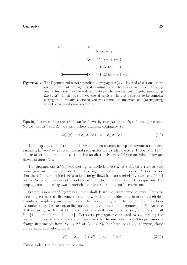
∆F (x2 − x1)
∆+(x2 − x1) (−1)
(−1) ∆−(x2 − x1)
(−1) ∆∗F(x2 − x1) (−1)
x2x1
Figure 3.1.: The Feynman rules corresponding to propagator (3.7). Instead of just one, thereare four different propagators, depending on which vertices are circled. Circlingone vertex fixes the time ordering between the two vertices, thereby simplifying∆F to ∆±. In the case of two circled vertices, the propagator is to be complexconjugated. Finally, a circled vertex is minus an uncircled one (anticipatingcomplex conjugation of a vertex).
Equality between (3.6) and (3.7) can be shown by integrating out k0 in both expressions.Notice that ∆+ and ∆− are each others complex conjugate, so
∆∗F (x) = θ(x0)∆
−(x) + θ(−x0)∆+(x) . (3.9)
The propagator (3.6) results in the well-known momentum space Feynman rule thatassigns i/(k2−m2 + i ε) to an internal propagator for a scalar particle. Propagator (3.7),on the other hand, can be used to define an alternative set of Feynman rules. They areshown in figure 3.1.
The propagators ∆±(x), connecting an uncircled vertex to a circled vertex or viceversa, give an important restriction. Looking back at the definition of ∆±(x), we seethat the θ-function inside is zero unless energy flows from an uncircled vertex to a circledvertex. We shall make use of this observation in the context of the cutting equation. Forpropagators connecting two (un)circled vertices there is no such restriction.
From this new set of Feynman rules we shall derive the largest time equation. Imaginea general connected diagram, containing n vertices of which any number are circled.Denote a completely uncircled diagram by F (x1, . . . , xn) and denote circling of verticesby underlining the corresponding spacetime points xi in the argument of F . Assumethat vertex xm with m ∈ {1, . . . n} has the largest time. That is, (xm)0 > (xi)0 for alli ∈ {1, . . . , m − 1, m + 1, . . . , n}. For every propagator connected to xm, circling thevertex xm gives only a minus sign with respect to the uncircled case. The propagatorschange in principle from ∆F → ∆+ or ∆− → ∆∗
F , but because (xm)0 is largest, thoseare actually equivalent. Thus
F (. . . , xm, . . . ) + F (. . . , xm, . . . ) = 0 . (3.10)
This is called the largest time equation.
26 Unitarity
Consider for a moment the simplest example, F (x1, x2). Assuming that (x2)0 > (x1)0,the largest time equation gives the following two identities
F (x1, x2) + F (x1, x2) = 0 ,
F (x1, x2) + F (x1, x2) = 0 . (3.11)
Diagrammatically this is represented by
= 0
+
+
= 0
Applying the Feynman rules, the above two identities read
∆F (x2 − x1) + ∆+(x2 − x1)(−1) = 0 ,
∆∗F (x2 − x1) + ∆−(x2 − x1)(−1) = 0 , (3.12)
for (x2)0 > (x1)0. Remember that the minus sign between brackets in the second termis due to circling of the vertex x2. One can easily verify this result by looking at theFeynman propagator (3.7) and its complex conjugate (3.9).
3.2.2. Cutting Equation
In general we don’t know which time (xi)0 is largest. Therefor we continue by summingall possible circlings of the vertices in a diagram. The terms in such a sum cancelpairwise.
∑
circlings
F (x1, . . . , xn) = 0 . (3.13)
There are two extreme cases in the sum: no vertices circled and all vertices circled. Fromthe Feynman rules we infer that the diagram with all vertices circled is the complexconjugate of the uncircled diagram: F (x1, . . . , xn) = F ∗(x1, . . . , xn). Singling out thesetwo cases,
F (x1, . . . , xn) + F ∗(x1, . . . , xn) = −∑
circlings\{0,all}F (x1, . . . , xn) . (3.14)
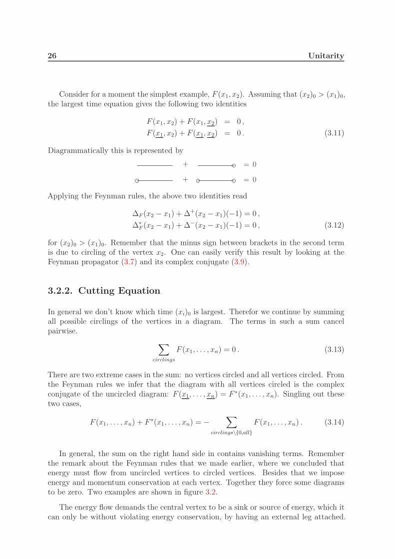
In general, the sum on the right hand side in contains vanishing terms. Rememberthe remark about the Feynman rules that we made earlier, where we concluded thatenergy must flow from uncircled vertices to circled vertices. Besides that we imposeenergy and momentum conservation at each vertex. Together they force some diagramsto be zero. Two examples are shown in figure 3.2.
The energy flow demands the central vertex to be a sink or source of energy, which itcan only be without violating energy conservation, by having an external leg attached.
Unitarity 27
= 0 = 0
Figure 3.2.: Example of two vanishing diagrams on the right hand side of (3.14). Energy mustflow from uncircled vertices to circled vertices, by construction of the Feynmanrules. Imposing energy conservation at the central vertex leads to the conclusionthat both diagrams vanish.
Hence the diagrams vanishes. A more algebraic way of saying the same thing is: aftermultiplying all internal propagators the subspace of the whole momentum space thatsatisfies all θ-functions and δ-functions is empty, so the integrals give zero.
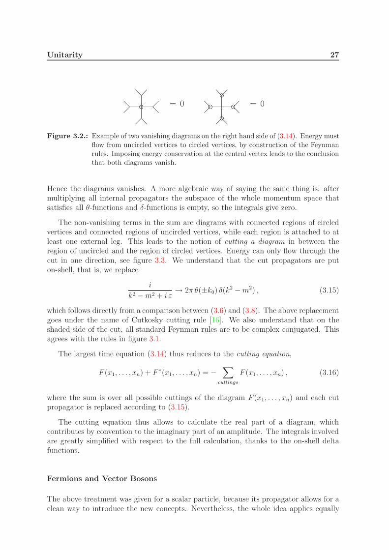
The non-vanishing terms in the sum are diagrams with connected regions of circledvertices and connected regions of uncircled vertices, while each region is attached to atleast one external leg. This leads to the notion of cutting a diagram in between theregion of uncircled and the region of circled vertices. Energy can only flow through thecut in one direction, see figure 3.3. We understand that the cut propagators are puton-shell, that is, we replace
i
k2 −m2 + i ε→ 2π θ(±k0) δ(k
2 −m2) , (3.15)
which follows directly from a comparison between (3.6) and (3.8). The above replacementgoes under the name of Cutkosky cutting rule [16]. We also understand that on theshaded side of the cut, all standard Feynman rules are to be complex conjugated. Thisagrees with the rules in figure 3.1.
The largest time equation (3.14) thus reduces to the cutting equation,
F (x1, . . . , xn) + F ∗(x1, . . . , xn) = −∑
cuttings
F (x1, . . . , xn) , (3.16)
where the sum is over all possible cuttings of the diagram F (x1, . . . , xn) and each cutpropagator is replaced according to (3.15).
The cutting equation thus allows to calculate the real part of a diagram, whichcontributes by convention to the imaginary part of an amplitude. The integrals involvedare greatly simplified with respect to the full calculation, thanks to the on-shell deltafunctions.
Fermions and Vector Bosons
The above treatment was given for a scalar particle, because its propagator allows for aclean way to introduce the new concepts. Nevertheless, the whole idea applies equally
28 Unitarity
=
Figure 3.3.: Translation from circling vertices to cutting propagators. Like energy flowsfrom uncircled to circled vertices, energy only flows through the cut towardsthe shaded side. Furthermore, the Feynman rules in figure 3.1 are replaced bythe simple prescription to put cut propagators on-shell according to (3.15) andeverything on the shaded side is complex conjugated.
well to fermions and vector bosons. However, for those types of particles one findsdifferent expressions for ∆±(x).
For the fermion propagator we can write
SF (x) =
∫d4p
(2π)4
i(/p +m)
p2 −m2 + i εe−ip·x
= (i/∂ +m)∆F (x)
= (i/∂ +m)(θ(x0)∆
+(x) + θ(−x0)∆−(x)
).
The derivative of θ(±x0) gives ±δ(±x0). Upon integrating SF (x) over spacetime thedelta functions put ∆±(x) at the same time x0 = 0, where they are actually equal, sothe two terms cancel. Hence we can define S±(x) ≡ (i/∂ + m)∆±(x), which are eachothers Hermitian conjugate, such that
SF (x) = θ(x0)S+(x) + θ(−x0)S
−(x) , (3.17)
a form suitable for deriving the largest time equation and cutting equation for fermions.One obtains a cutting rule that is like (3.15), multiplied by /p+m,
i(/p+m)
p2 −m2 + i ε→ 2π θ(±p0) δ(p
2 −m2) (/p+m) . (3.18)
Again the sign is chosen such that positive energy flows towards the shaded region.
For vector bosons a similar thing can be done, with the slight complication that wenow get two derivatives acting on ∆F (x). Whereas ∆±(x)|x0=0 are equal, the same doesnot hold for their derivative. Despite the arising ‘contact terms’, it turns out that thelargest time equation can also be maintained in this case [17].
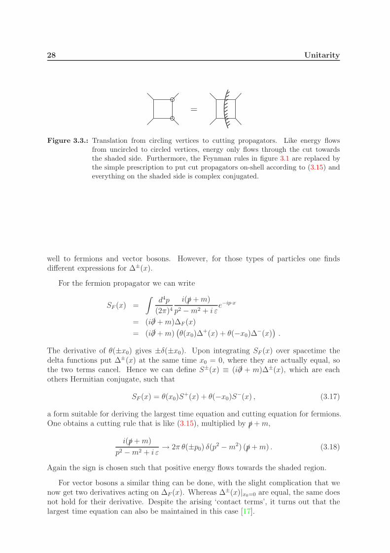
Unitarity 29
q + k
q
kk
Figure 3.4.: The cut vacuum polarization diagram. Both propagators are replaced accordingto (3.18), with a plus sign for the top propagator and a minus sign for the other.The vertex on the right is complex conjugated.
3.2.3. Connection with Unitarity
The cutting equation (3.16) is more stringent than the unitarity equation (3.4). Thereason is that the former holds for individual diagrams, while the latter holds for ascattering amplitude. But even so, for the cutting equation to imply unitarity, twoconditions must be satisfied. First, diagrams in the shaded region must be equal todiagrams obtained from S†, and second, the ∆± must be equal to a summation overintermediate states [4].
The first condition is met if the Lagrangian is its own conjugate. To clarify thesecond condition, it is instructive to verify it for a simple example. Consider the vacuumpolarization from (2.2) contracted with polarization vectors for the external photons. Wecalculate both the cut diagram and the sum over intermediate states. In other words,we verify equivalence of the right hand sides of (3.16) and (3.4).
First the cut diagram. There are two internal fermion propagators which get cutaccording to (3.18). The propagator with momentum q becomes the negative energysolution, while the one with momentum q + k becomes the positive energy solution, seefigure 3.4. The vertex in the shadowed region gets a minus sign, which cancels the overallminus sign for the fermion loop. Hence we find
iΠµνcut(k) = (−ie)2(2π)2
∫d4q
(2π)4θ(−q0)θ(q0 + k0)δ(q
2 −m2)δ((q + k)2 −m2)×
tr[
/ǫ(k) (/q +m) /ǫ(k) (/q + /k +m)]. (3.19)
Next, we consider the sum over intermediate states. The expression is obtained bymultiplying together the S and S† diagrams and summing over spins and integrating
30 Unitarity
over the phase space.
∑
s,s′
∫
dΠ
∣∣∣∣∣
∣∣∣∣∣
2
=∑
s,s′
∫
dΠ[
vs′
(p) (+ie/ǫ(k) ) us(q)] [
us(q) (−ie/ǫ(k) ) vs′
(p)]
= −(−ie)2
∫
dΠ tr[
/ǫ(k) (/q +m) /ǫ(k) (/p−m)]. (3.20)
Notice the minus sign in front of the mass in the antispinor spin sum. The phase spaceintegral is explicitly [13]
∫
dΠ [. . . ] =
∫d3q
(2π)3
1
2q0
∫d3p
(2π)3
1
2p0
(2π)4δ(4)(k − p− q) [. . . ] . (3.21)
Because q0 =√
~q 2 −m2 we have
∫d3q
(2π)3
1
2q0[. . . ] =
∫d4q
(2π)4(2π) θ(p0) δ(p
2 −m2) [. . . ] . (3.22)
Integrating out the four-momentum p, sending q → −q and pulling the overall minussign inside the trace, one obtains precisely (3.19).
We observe that both cases, a different sign for one of the two vertices was canceledby another minus sign. In the cut diagram case that other minus sign was due to thefermion loop, while in the second case it arose from the sum over antispinor spin states.
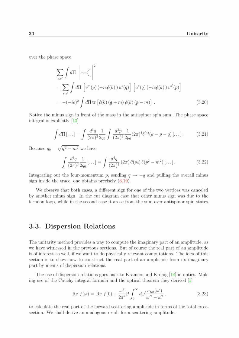
3.3. Dispersion Relations
The unitarity method provides a way to compute the imaginary part of an amplitude, aswe have witnessed in the previous sections. But of course the real part of an amplitudeis of interest as well, if we want to do physically relevant computations. The idea of thissection is to show how to construct the real part of an amplitude from its imaginarypart by means of dispersion relations.
The use of dispersion relations goes back to Kramers and Kronig [18] in optics. Mak-ing use of the Cauchy integral formula and the optical theorem they derived [5]
Re f(ω) = Re f(0) +ω2
2π2P
∫ ∞
0
dω′ σtot(ω′)
ω′2 − ω2, (3.23)
to calculate the real part of the forward scattering amplitude in terms of the total cross-section. We shall derive an analogous result for a scattering amplitude.
Unitarity 31
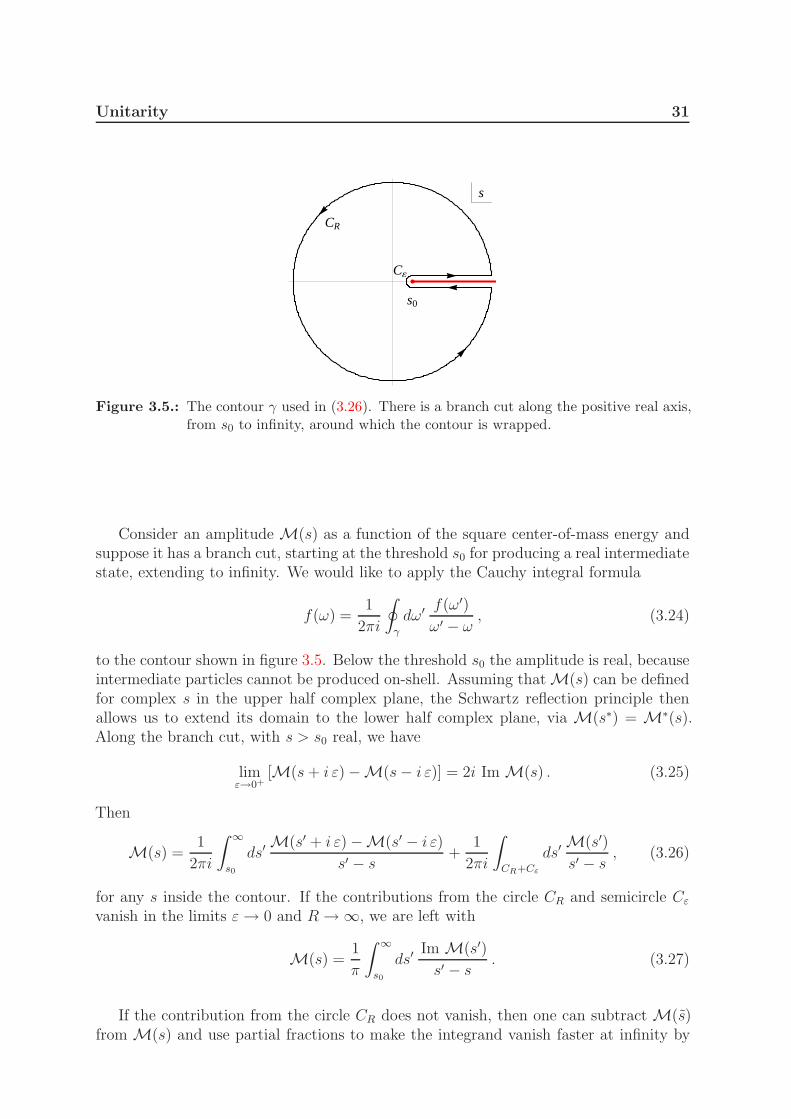
C¶
CR
s0
s
Figure 3.5.: The contour γ used in (3.26). There is a branch cut along the positive real axis,from s0 to infinity, around which the contour is wrapped.
Consider an amplitude M(s) as a function of the square center-of-mass energy andsuppose it has a branch cut, starting at the threshold s0 for producing a real intermediatestate, extending to infinity. We would like to apply the Cauchy integral formula
f(ω) =1
2πi
∮
γ
dω′ f(ω′)
ω′ − ω, (3.24)
to the contour shown in figure 3.5. Below the threshold s0 the amplitude is real, becauseintermediate particles cannot be produced on-shell. Assuming that M(s) can be definedfor complex s in the upper half complex plane, the Schwartz reflection principle thenallows us to extend its domain to the lower half complex plane, via M(s∗) = M∗(s).Along the branch cut, with s > s0 real, we have
limε→0+
[M(s+ i ε) −M(s− i ε)] = 2i Im M(s) . (3.25)
Then
M(s) =1
2πi
∫ ∞
s0
ds′M(s′ + i ε) −M(s′ − i ε)
s′ − s+
1
2πi
∫
CR+Cε
ds′M(s′)
s′ − s, (3.26)
for any s inside the contour. If the contributions from the circle CR and semicircle Cεvanish in the limits ε→ 0 and R→ ∞, we are left with
M(s) =1
π
∫ ∞
s0
ds′Im M(s′)
s′ − s. (3.27)
If the contribution from the circle CR does not vanish, then one can subtract M(s)from M(s) and use partial fractions to make the integrand vanish faster at infinity by
32 Unitarity
a factor 1/s′.
M(s) −M(s) =s− s
2πi
∫ ∞
s0
ds′M(s′ + i ε) −M(s− i ε)
(s′ − s)(s′ − s)
+s− s
2πi
∫
CR+Cε
ds′M(s′)
(s′ − s)(s′ − s). (3.28)
When the contribution from the circle vanishes due to this adjustment, then one is leftwith
M(s) = M(s) +s− s
π
∫ ∞
s0
ds′Im M(s′)
(s′ − s)(s′ − s). (3.29)
As an example, one can apply (3.29) to the imaginary part of the vacuum polarization(2.15). In the current notation, that imaginary part is given by
Im Π(s) = −α3
(
1 +s0
2s
)√
1 − s0
s(3.30)
for s > s0, with s = k2 and s0 = 4m2. A computation of the resulting integral can befound in [19]. The result is precisely (2.16). The precise form of Π(0) is not recoveredin this manner, however. One could say that the result is implicitly renormalized.
In conclusion, the real part of an amplitude can be calculated from the imaginarypart by means of the dispersion relation (3.27) or (3.29).
3.4. Generalized Unitarity
A severe limitation of the unitarity method lies in the application of the dispersionrelations. For more than two external particles the amplitude becomes a function ofmultiple Lorentz invariants. Consequently, the analytic structure is rather complicatedand makes the contour integration a lot harder.
The generalized unitarity method is a way to circumvent the use of dispersion re-lations [7], [20]. A review is given in [21]. The crucial observation is that a generalone-loop amplitude is decomposable into a basis of scalar integrals.
M =∑
i
ciBi . (3.31)
The scalar integrals Bi are up to 4-point integrals and form a finite basis. In chapter4 we demonstrate how to determine the basis explicitly. The derivation makes use ofPassarino-Veltman reduction of tensor integrals and the result [6].
Unitarity 33
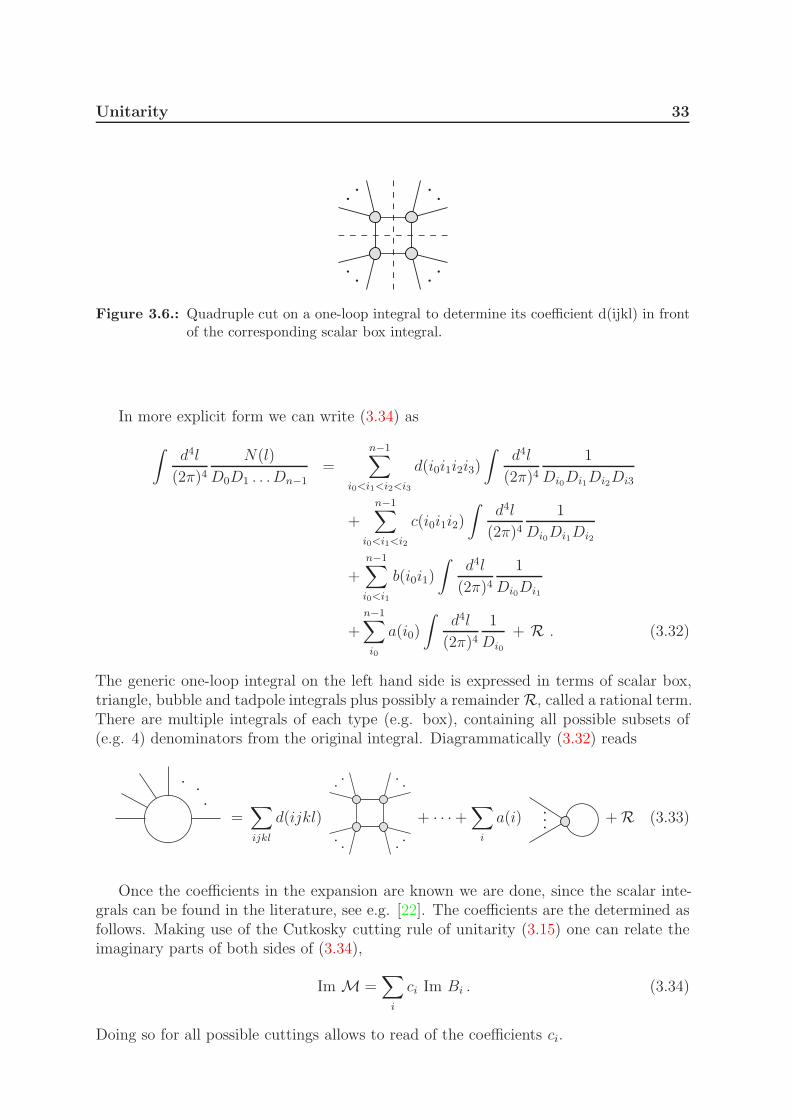
Figure 3.6.: Quadruple cut on a one-loop integral to determine its coefficient d(ijkl) in frontof the corresponding scalar box integral.
In more explicit form we can write (3.34) as
∫d4l
(2π)4
N(l)
D0D1 . . .Dn−1
=n−1∑
i0<i1<i2<i3
d(i0i1i2i3)
∫d4l
(2π)4
1
Di0Di1Di2Di3
+n−1∑
i0<i1<i2
c(i0i1i2)
∫d4l
(2π)4
1
Di0Di1Di2
+n−1∑
i0<i1
b(i0i1)
∫d4l
(2π)4
1
Di0Di1
+n−1∑
i0
a(i0)
∫d4l
(2π)4
1
Di0
+ R . (3.32)
The generic one-loop integral on the left hand side is expressed in terms of scalar box,triangle, bubble and tadpole integrals plus possibly a remainder R, called a rational term.There are multiple integrals of each type (e.g. box), containing all possible subsets of(e.g. 4) denominators from the original integral. Diagrammatically (3.32) reads
=∑
ijkl
d(ijkl) + · · ·+∑
i
a(i) + R (3.33)
Once the coefficients in the expansion are known we are done, since the scalar inte-grals can be found in the literature, see e.g. [22]. The coefficients are the determined asfollows. Making use of the Cutkosky cutting rule of unitarity (3.15) one can relate theimaginary parts of both sides of (3.34),
Im M =∑
i
ci Im Bi . (3.34)
Doing so for all possible cuttings allows to read of the coefficients ci.

34 Unitarity
In addition one performs more cuts than the standard unitarity method. There,cutting one-loop diagrams leads to precisely two cut propagators. Here double cutsare performed as well, see figure 3.6, thereby extending the original unitarity method.Actually, this method is often used the other way around. One-loop amplitudes are thenconstructed by ‘gluing’ tree amplitudes together and promoting the delta function topropagators.
Chapter 4.
OPP Reduction
In the previous chapter we introduced generalized unitarity, where a general one-loopamplitudes is expanded in a basis of known scalar integrals. The coefficients in such abasis are found by applying unitarity cuts and relating imaginary parts on both sides.This process is hard to automate, however, since the precise analytic properties of theamplitude must be known.
In this chapter we determine such coefficients using an idea by Ossola, Papadopoulosand Pittau (OPP), which is basically to expand the integrand rather than the integral.The coefficients are determined by evaluating the integrand at certain loop momenta,which is much easier to implement.
In this chapter we derive the integrand decomposition and explain how the coefficientsare determined in general. We then discuss the construction of rational parts of theamplitude. As an illustration, a manageable problem is worked out in detail. In the lastsection we discuss implementations of the algorithm.
4.1. Integrand Decomposition
The aim of this section is to determine the form of the integrand expansion. We will firstshow the expansion, which is dubbed master formula in the OPP method, and explainsome of its features. After introducing the van Neerven-Vermaseren basis, we are in theposition to derive the master formula by means of tensor reduction.
4.1.1. Master Formula
Consider an amplitude for n-particle scattering at the one-loop level. The amplitudedepends on the external momenta via the Lorentz invariants sij = pi · pj and also on themasses of virtual particles propagating through the loop. Any one-loop (sub)amplitude
35
36 OPP Reduction
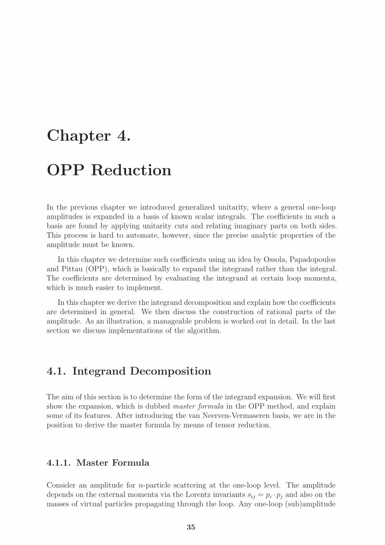
can be written as
Mn(sij, m2i ) =
∫d4l
(2π)4
N(l)
D0D1 . . .Dn−1. (4.1)
Here, the numerator N(l) represents an ‘effective’ numerator generated by the sumof all one-loop Feynman diagrams that contribute to the amplitude. Diagrams withfewer internal propagators are included in N(l) by trivially canceling the appropriatedenominators.
The inverse Feynman propagators appearing in the denominator are given by Di =(l + qi)
2 −m2i . In here the momenta qi are partial sums of external momenta, although
the precise relation between the two is ambiguous. Often, one chooses q0 to be zero,thereby fixing all other qi in terms of the external momenta: qi = p1 + p2 + · · · + pi,as can be verified from figure 4.1. We shall refrain from making such a choice for thetime being, that is, we assume q0 6= 0. In that way all denominators Di are treated onan equal footing. Only at the very end, when a final expression for the amplitude isobtained, do we make such a choice.
It has been shown in [23] that the numerator of the integrand in (4.1) can be decom-posed into
N(l) =
n−1∑
i0<i1<i2<i3
[d(i0i1i2i3) + d(l; i0i1i2i3)]
n−1∏
k 6=i0,i1,i2,i3
Dk +
n−1∑
i0<i1<i2
[c(i0i1i2) + c(l; i0i1i2)]
n−1∏
k 6=i0,i1,i2
Dk +
n−1∑
i0<i1
[b(i0i1) + b(l; i0i1)]
n−1∏
k 6=i0,i1
Dk +
n−1∑
i0
[a(i0) + a(l; i0)]
n−1∏
k 6=i0
Dk +
P (l)
n−1∏
k
Dk . (4.2)
This is the master formula of the OPP reduction method. In the next two subsection weshall explain how this decomposition comes about. For now, let us inspect the contentsof the given formula.
There appear two types of coefficients: the ones with a tilde, d, c, b, a and P , andthe ones without, d, c, b and a. The coefficients with a tilde are called spurious terms.They depend on the loop momentum in such a way that, after substitution of (4.2) into(4.1), they vanish upon integration over the loop momentum. The coefficients a, b, cand d then remain and multiply scalar tadpole, bubble, triangle and box diagrams. In
OPP Reduction 37
p1
pn−1
l + q1
l + q2
l + q0
p2
p3
m0
m1
m2
pnl + qn−1
mn−1
Figure 4.1.: A diagrammatic representation of the one-loop amplitude for n-particle scatter-ing, given in (4.1).
other words, we are lead to the amplitude expansion (3.32) in the generalized unitaritymethod.
On a close inspection, one may observe, that the amplitude expansion is actuallynot entirely reproduced: the rational part is missing. This has to do with the fact thatthe rational part is an artifact of dimensional regularization, while we do not employdimensional regularization at this stage. The problem of the missing rational part shallbe resolved later on in section 4.3.
As a final remark we note that in a renormalizable gauge P (l) is zero. The reasonis that in such a gauge the numerator on the left hand side is at most of order O(|l|n),while the term with P (l) is the only one on the right hand side of order O(|l|2n) or higher.Since the formula holds for any l, we are led conclude that P (l) = 0.
4.1.2. The van Neerven-Vermaseren Basis
In order to derive the master formula we introduce first the van Neerven-Vermaserenbasis. The basis takes its name from the first use by van Neerven and Vermaseren in [6].
In an n-particle scattering there are n−1 linearly independent external momenta dueto momentum conservation. The same holds for the qi in the internal propagators, sincethey are linear combinations of the external momenta. This notion can be expressed byshifting the loop momentum l → l′ − q0 in (4.1) to obtain
Mn =
∫d4l′
(2π)4
N(l′ − q0)
(l′ 2 −m20)((l
′ + k1)2 −m21) . . . ((l
′ + kn−1)2 −m2n−1)
. (4.3)
where we introduced vectors ki defined by
ki := qi − q0 . (4.4)
38 OPP Reduction
Notice that whereas qi are not unambiguously defined in terms of pj, differences betweenthem are. In particular we have ki = p1 + · · ·+ pi for i = 1, . . . , n− 1.
The space that is spanned by the n− 1 vectors ki is referred to as the physical space.It has dimension dP = min(4, n− 1). We define the transverse space as the complementof the physical space in four dimensional spacetime.
For the bases of the physical and transverse space, we use the following notation.The generalized Kronecker symbol is defined as the determinant of a square matrix ofordinary Kronecker deltas,
δµ1µ2...µkν1ν2...νk
:=
δµ1
ν1 δµ1
ν2 . . . δµ1
νk
δµ2
ν1δµ2
ν2. . . δµ2
νk
......
...
δµkν1 δµk
ν2 . . . δµkνk
. (4.5)
We use a compact notation where indices of the generalized Kronecker symbol are re-placed by the label of the vector they are contracted with.
δpµ2...µkν1q...νk
:= δµ1µ2...µkν1ν2...νk
pµ1qν2 . (4.6)
For k = 1 we can generate objects like δµq = qµ and δpq = p · q. For k = 2 we haveδp1p2q1q2 = p1 · q1 p2 · q2 − p1 · q2 p2 · q1 and so on. A special case is when the same set ofvectors appears as upper and lower indices, which gives the Gram determinant
∆(q1, . . . , qk) :=det (qi · qj)k×k = δq1q2...qkq1q2...qk. (4.7)
As a basis for the physical space we could simply use the set of vectors {ki}i=1,...,dP.
However, for reasons that become clear later, we prefer to use its dual basis {vi}i=1,...,dP
defined by the condition ki · vj = δij. Using the introduced notation, we can explicitlyconstruct the dual basis
vµi :=δk1 . . . µ . . . kdP
k1 . . . ki . . . kdP
∆(k1, . . . , kdP). (4.8)
Note that the vectors vµi are not orthogonal, indeed vi · vj = ∆ij/∆(k1, . . . , kdP) where
∆ij is the determinant of the (i, j) cofactor of the matrix (kα · kβ)dP ×dP.
A basis {ni}i=dP +1,...,4 for the transverse space is defined to be orthonormal andorthogonal to the physical space. It can be constructed from the dP vectors ki and from(4 − dP ) vectors ai chosen such that all vectors are linearly independent. Then [24]
nµi :=δk1 . . . kdP
adP +1 . . . µk1 . . . kdP
adP +1 . . . ai√
∆(k1, . . . , kdP, adP +1, . . . , ai−1)
√
∆(k1, . . . , kdP, adP +1, . . . , ai)
, (4.9)
OPP Reduction 39
for i = dP + 1, . . . , 4.
As an overview and reference we record the relevant dot products:
· kj vj nj
ki ki · kj δij 0
vi δij ∆ij/∆ 0
ni 0 0 δij
(4.10)
where the indices on ki and vi run from 1, . . . , dP , while those on the perpendicularvectors ni run from dP + 1, . . . , 4.
These bases are useful to parametrize the loop momentum of the integral (4.3),
l′ µ =
dP∑
i=1
civµi +
4∑
i=dP +1
cinµi . (4.11)
Contracting with kj or nj and using the dot products given in (4.10), we find the coeffi-cients ci = l′ · ki and ci = l′ · ni. Owing to the choice for a dual basis, the ci can now bewritten as a difference of denominators.
2 ci = 2 l′ · ki = (l′ + ki)2 −m2
i − (l′ 2 −m20) − (k2
i −m2i +m2
0)
= (l + qi)2 −m2
i − ((l + q0)2 −m2
0) − (k2i −m2
i +m20)
= Di −D0 − ri . (4.12)
Notice that we reinstated the original loop momentum l = l′−q0 in the second line afterwhich we recognized the denominators Di and D0. In the last line we collected the lastthree term into
ri := k2i −m2
i +m20 . (4.13)
If we further define a vector w as
w := 12
dP∑
i=1
rivi , (4.14)
than the original loop momentum is parametrized as
lµ = −qµ0 − wµ + 12
dP∑
i=1
(Di −D0)vµi +
4∑
i=dP +1
((l + q0) · ni)nµi . (4.15)
This expression will play an important role in the reduction of integrals, a topic we shallnow discuss.
40 OPP Reduction
0 1 2 3 4 5n
0
1
2
3
4
5
r
Figure 4.2.: Overview of the first n-point rank-r integrals in four dimensions. Integrals thatlead to rational terms are represented by red squares, while the blue circlesrepresent cut-constructable integrals: r < max(2, n − 1). Integrals inside theshaded area are UV-finite by power counting: r < 2n − 4
4.1.3. Tensor Reduction of One-Loop Integrals
We now use the van Neerven-Vermaseren basis to reduce tensor integrals to scalar inte-grals and integrals with spurious terms. We start with a five-point integral, after whichthe general case easily follows.
Classification of Integrals
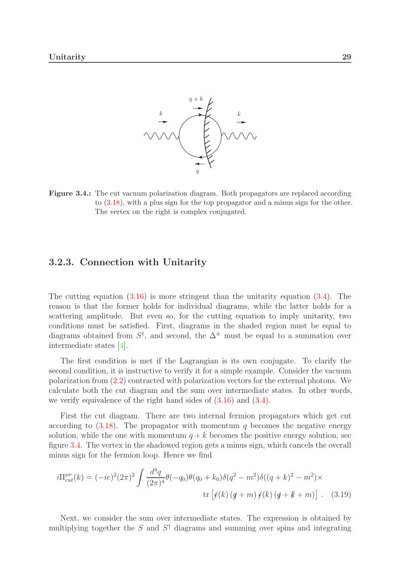
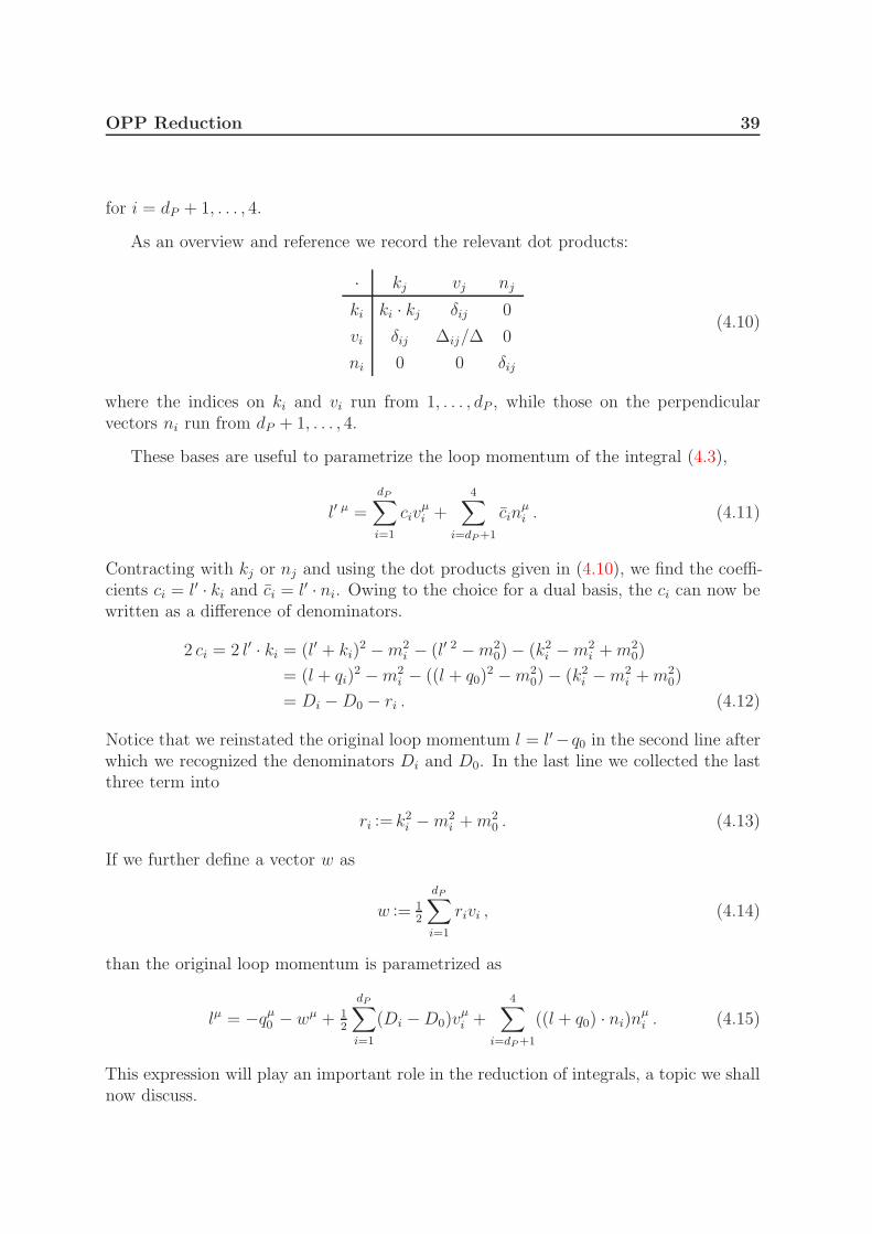
The rank r of the integral in (4.1) is defined as N(λl) ∝ λr for λ → ∞. Together withthe number of denominators n, the rank r distinguishes different types of integrals. Itis convenient to represent them as points in the (n, r)-plane, as is done in figure 4.2.
In a renormalizable gauge the maximal rank of an integral is equal to n, as wementioned before. This is why the integrals shown in figure 4.2 form a triangle on andbelow the line r = n.
The OPP method we describe assumes a four-dimensional loop momentum. Integralsthat do not have a rational part can be calculated by this method and are said to be cut-
constructable. The method does not calculate rational parts of integrals, because thoseare an artifact n-dimensional regularization of UV-divergent integrals. It is however nottrue that all UV-divergent integrals contain rational parts and all other integrals don’t.In order to have a rational part an integral must at least have rank r = 2, which leavesa couple of UV-divergent integrals that certainly have a rational part: (2,2), (3,2), (3,3),(4,4). In the reduction scheme we employ below, we observe furthermore that UV-finiteintegrals can reduce to those UV-divergent integrals by the least steep reduction step(n, r) → (n− 1, r− 1). The condition for an integral to have a rational part (in general)is therefor r ≥ max(2, n− 1) [7],[22]. These facts are summarized in figure 4.2.
OPP Reduction 41
0 1 2 3 4 5n
0
1
2
3
4
5
r
(a)
0 1 2 3 4 5n
0
1
2
3
4
5
r
(b)
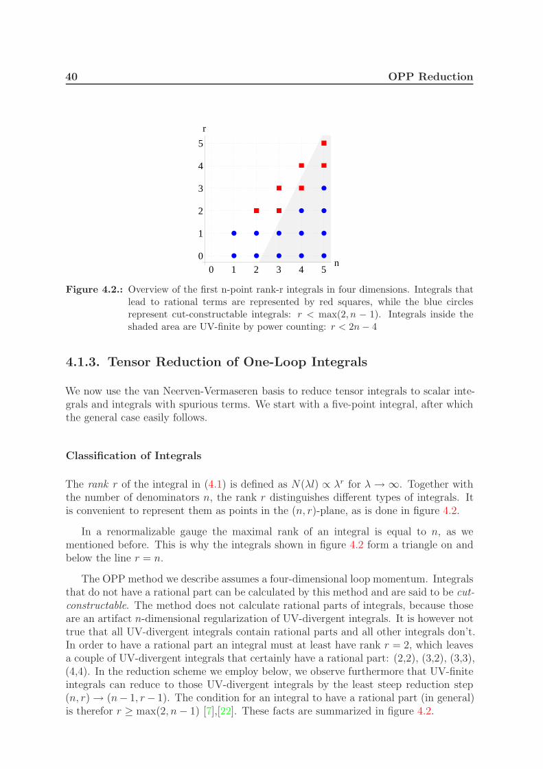
Figure 4.3.: Reduction of a general rank-five five-point integral (star) to lower point and/orrank cut-constructable integrals (blue dots) and integrals with a rational part(red squares). Step (a) is due to (4.16) and step (b) corresponds to (4.18).
Five-Point Integrals
Consider a rank-five five-point integral, that we would like to reduce to known integrals.We follow the same spirit of [25] with the difference that we present the method infour dimensions. The integrand can be written as lµ0 . . . lµ4/D0 . . . D4. There are fourreference momenta k1, . . . , k4, so the physical space has dimension four: dP = 4. Hence,for the integrand of a five-point integral, (4.15) gives us
lµ = −qµ0 − wµ + 12
4∑
i=1
(Di −D0)vµi . (4.16)
By inserting this expression for first factor of l in the numerator of the integrand, the Di
and D0 terms cancel against a denominator, giving rank-four four-point integrals. Thefirst two terms give rise to rank-four five-point integrals. Schematically this is shown asthe top two arrows in figure 4.3a.
The resulting five-point integrals of lower rank can be further in the same way. When-ever D0 is canceled in the process, the loop momentum must be shifted to l−q1 to bringthe integral to the form where the first denominator is l2 −m2
1. Of course, shifting theloop momentum in the numerator generates new terms, but those are all at least onerank lower and can be dealt with in the next reduction steps. It should be clear that inthis way the rank-five five-point integrals can be reduced to a scalar five-point integralsand a collection of four-point integrals of rank one to four, as displayed in figure 4.3a.
The scalar five-point integral can be further reduced to scalar four-point integrals.To this end, square l+ q0 and substitute the van Neerven-Vermaseren basis in two steps,
42 OPP Reduction
such that the result is at most linear in denominators.
(l + q0)2 = (l + q0) ·
(
−w + 12
4∑
i=1
(Di −D0)vi
)
= w2 + 12
4∑
i=1
(Di −D0) (l + q0 − w) · vi . (4.17)
On the other hand (l + q0)2 = D0 +m2
0. Equating and rearranging leads to
m20 − w2 = 1
2
4∑
i=1
(Di −D0)(l + q0 − w) · vi −D0 . (4.18)
The left hand side is independent of the loop momentum, while all terms on the righthand side carry one inverse propagator. Dividing by D0D1 . . .D4 and integrating wefind a relation between a scalar five-point integral and scalar and rank-one four-pointintegrals, as depicted in figure 4.3b.
In fact, the rank-one terms vanish [6] upon integration. We can understand thisin the following way. The Di (l · vi) terms vanish because the denominator with thereference vector ki is removed and kj · vi = 0 for j 6= i. In the D0 (l ·∑i vi) term,one shifts the loop momentum to l → l′ − q1. Then the reference vectors becomeqj−q1 = (qj−q0)−(q1−q0) = kj−k1 for j = 2, 3, 4. Such combinations are perpendicularto the vector
∑
i vi. In other words, the rank-one terms are spurious terms.
In conclusion any five-point integral is fully reducible, that is, reducible exclusivelyto lower-point integrals. It is easy to see that these reduction steps generalize to higherpoint integrals, because the loop momentum decomposition remains the same as dP = 4in all cases [25]. Consequently we consider all integrals with n ≥ 5 fully reducible.
Four-Point Integrals
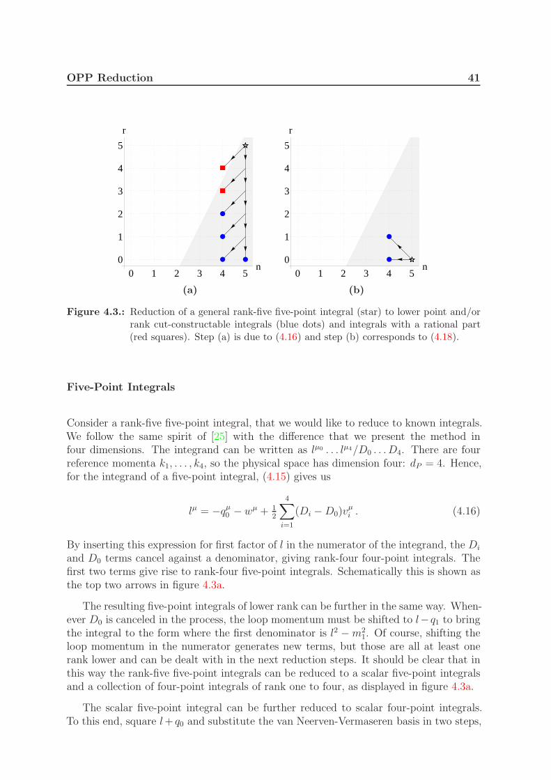
The highest rank integral left from the previous reduction is the four-point rank-fourintegral, with integrand lµ0lµ1 lµ2lµ3/D0D1D2D3. The method of reduction is the sameas before, however we cannot reduce as far because the van Neerven-Vermaseren basisis different. Indeed, now there are only three reference vectors, k1, k2 and k3, so dP = 3and (4.15) gives
lµ = −qµ0 − wµ + 12
3∑
i=1
(Di −D0)vµi + ((l + q0) · n4)n
µ4 . (4.19)
By inserting this expression for lµ0 in the integrand we obtain tree- and four-pointintegrals of one rank lower, but also a term (l + q0) · n4 which is still of rank four. Thisfirst reduction step is shown by the top three arrows in figure 4.4a.
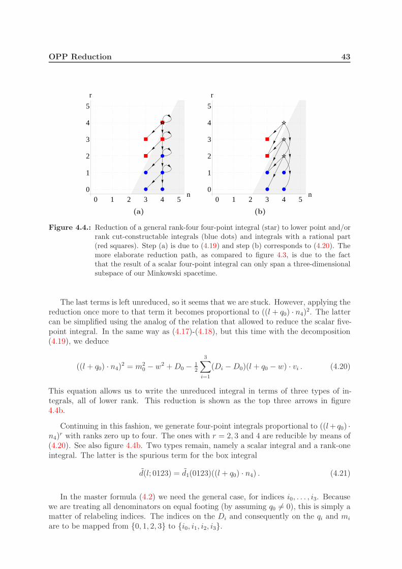
OPP Reduction 43
0 1 2 3 4 5n
0
1
2
3
4
5
r
(a)
0 1 2 3 4 5n
0
1
2
3
4
5
r
(b)
Figure 4.4.: Reduction of a general rank-four four-point integral (star) to lower point and/orrank cut-constructable integrals (blue dots) and integrals with a rational part(red squares). Step (a) is due to (4.19) and step (b) corresponds to (4.20). Themore elaborate reduction path, as compared to figure 4.3, is due to the factthat the result of a scalar four-point integral can only span a three-dimensionalsubspace of our Minkowski spacetime.
The last terms is left unreduced, so it seems that we are stuck. However, applying thereduction once more to that term it becomes proportional to ((l + q0) · n4)
2. The lattercan be simplified using the analog of the relation that allowed to reduce the scalar five-point integral. In the same way as (4.17)-(4.18), but this time with the decomposition(4.19), we deduce
((l + q0) · n4)2 = m2
0 − w2 +D0 − 12
3∑
i=1
(Di −D0)(l + q0 − w) · vi . (4.20)
This equation allows us to write the unreduced integral in terms of three types of in-tegrals, all of lower rank. This reduction is shown as the top three arrows in figure4.4b.
Continuing in this fashion, we generate four-point integrals proportional to ((l+ q0) ·n4)
r with ranks zero up to four. The ones with r = 2, 3 and 4 are reducible by means of(4.20). See also figure 4.4b. Two types remain, namely a scalar integral and a rank-oneintegral. The latter is the spurious term for the box integral
d(l; 0123) = d1(0123)((l + q0) · n4) . (4.21)
In the master formula (4.2) we need the general case, for indices i0, . . . , i3. Becausewe are treating all denominators on equal footing (by assuming q0 6= 0), this is simply amatter of relabeling indices. The indices on the Di and consequently on the qi and mi
are to be mapped from {0, 1, 2, 3} to {i0, i1, i2, i3}.
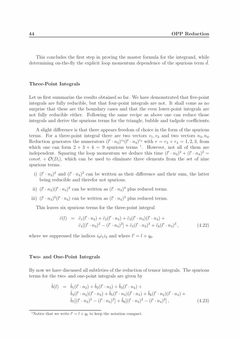
44 OPP Reduction
This concludes the first step in proving the master formula for the integrand, whiledetermining on-the-fly the explicit loop momentum dependence of the spurious term d.
Three-Point Integrals
Let us first summarize the results obtained so far. We have demonstrated that five-pointintegrals are fully reducible, but that four-point integrals are not. It shall come as nosurprise that these are the boundary cases and that the even lower-point integrals arenot fully reducible either. Following the same recipe as above one can reduce thoseintegrals and derive the spurious terms for the triangle, bubble and tadpole coefficients.
A slight difference is that there appears freedom of choice in the form of the spuriousterms. For a three-point integral there are two vectors v1, v2 and two vectors n3, n4.Reduction generates the numerators (l′ · n3)
r3(l′ · n4)r4 with r = r3 + r4 = 1, 2, 3, from
which one can form 2 + 3 + 4 = 9 spurious terms 1. However, not all of them areindependent. Squaring the loop momentum we deduce this time (l′ · n3)
2 + (l′ · n4)2 =
const. + O(Di), which can be used to eliminate three elements from the set of ninespurious terms.
i) (l′ · n3)2 and (l′ · n4)
2 can be written as their difference and their sum, the latterbeing reducible and therefor not spurious.
ii) (l′ · n3)(l′ · n4)
2 can be written as (l′ · n3)3 plus reduced terms.
iii) (l′ · n3)2(l′ · n4) can be written as (l′ · n4)
3 plus reduced terms.
This leaves six spurious terms for the three-point integral
c(l) = c1(l′ · n3) + c2(l
′ · n4) + c3(l′ · n3)(l
′ · n4) +
c4[(l′ · n3)
2 − (l′ · n4)2] + c5(l
′ · n3)3 + c6(l
′ · n4)3 , (4.22)
where we suppressed the indices i0i1i2 and where l′ = l + q0.
Two- and One-Point Integrals
By now we have discussed all subtleties of the reduction of tensor integrals. The spuriousterms for the two- and one-point integrals are given by
b(l) = b1(l′ · n2) + b2(l
′ · n3) + b3(l′ · n4) +
b4(l′ · n2)(l
′ · n3) + b5(l′ · n3)(l
′ · n4) + b6(l′ · n2)(l
′ · n4) +
b7[(l′ · n2)
2 − (l′ · n4)2] + b8[(l
′ · n3)2 − (l′ · n4)
2] , (4.23)
1Notice that we write l′ = l + q0 to keep the notation compact.
OPP Reduction 45
and
a(l) = a1(l′ · n1) + a2(l
′ · n2) + a3(l′ · n3) + a4(l
′ · n4) . (4.24)
4.2. Determination of Coefficients
After establishing the master formula and the explicit l-dependence of the spuriousterms, we are set to further develop the OPP reduction method. The integral (4.1)for a one-loop n-particle scattering amplitude can in general not be calculated directly.Substituting the master formula in place of the numerator, reduces the integral to a setof scalar integrals multiplied by the coefficients a, b, c and d. While the scalar are knownand can be looked up in the literature (see for example [22]), the coefficients are to bedetermined.
The idea is to evaluate both sides of the master formula at different loop momenta toobtain a system of equations that allows one to determine the coefficients. Inverting theresulting system of equations can be highly inefficient when the number of coefficientsis large. For generic n, that number is 2
(n4
)+ 7(n3
)+ 9(n2
)+ 5(n1
). Cases of interest
are typically n = 5, 6, 7, . . . for which the number of coefficients is 195, 335, 539, . . . .Clearly the inversion of such large systems of equations is to be avoided.
A better approach is to construct a triangular system of equations. Assume thatthere exist two loop momenta for which the four denominators Di0 , . . . , Di3 are zero.Evaluating the master formula (4.2) at those loop momenta leaves on the right handside only the coefficients d(i0i1i2i3) and d(1; i0i1i2i3), since only those terms contain noneof the four denominators. This then generates two equations for two unknowns. Doingso for all possible choices i0 < i1 < i2 < i3, one efficiently determine all d-coefficients.
After subtraction of all terms with d-coefficients on both sides of (4.2) one is in theposition to repeat the procedure for the c-coefficients. This time one needs seven loopmomenta, to generate as many equations for the coefficients c(i0i1i2) and c(1; i0i1i2) upto c(6; i0i1i2). Continuing in the same fashion one can also find the b- and a-coefficients.
The advantage is that one has to invert many smaller systems of equations of at most9 × 9. Notice that all coefficients d must be known, including the spurious ones, beforeone can start to determine the c coefficients. Likewise c must be known for b and b mustbe known for a. The spurious terms a don’t need to be found in principle.
As a final remark, we point out that we assumed such a triangular system of equationscan actually be constructed. In particular there must be enough distinct loop momentasatisfying Di0 = · · · = Dik = 0 for k = 0, 1, 2, 3 in order to generate a sufficient number ofindependent equations for the coefficients. We will show that this is the case by explicitconstruction below.
46 OPP Reduction
Box Coefficients
To keep the notation light we consider the determination of a specific box coefficient:d(0123). Coefficients for other box integrals can be found analogously.
We must find loop momenta that satisfy D0 = D1 = D2 = D3 = 0. The loopmomentum for a box diagram is written as defined in (4.15) with dP = 3. Imposing thethree conditions Dk = D0 for k = 1, 2, 3 the third term in (4.15) vanishes. Plugging theresulting loop momentum into the remaining condition, D0 = 0, we find two solutions
lµ± = −qµ0 − wµ ±√
m20 − w2 nµ4 . (4.25)
At these loop momenta, most terms on the right hand side of the master formula vanish,see (4.2) with the explicit spurious terms (4.21)-(4.24). We retain
N(l±) = [d(0123) + d1(0123)((l± + q0) · n4)]
n−1∏
k 6=0,1,2,3
Dk(l±)
= [d(0123) ± d1(0123)√
m20 − w2]
n−1∏
k 6=0,1,2,3
Dk(l±) . (4.26)
In terms of
L(l±) :=N(l±)
∏n−1k 6=0,1,2,3Dk(l±)
, l⊥ :=√
m20 − w2 , (4.27)
the coefficients are elegantly written as
d(0123) =L(l+) + L(l−)
2, d1(0123) =
L(l+) − L(l−)
2 l⊥. (4.28)
Triangle Coefficients
Assuming all d-coefficients are known, one can turn to the determination of the trianglecoefficients. Again, we focus on a specific coefficient c(012), together with the spuriousterms ci(012). Applying the same approach as for the box coefficients, one finds acontinuous set of solutions parametrized by an angle φ ∈ [0, 2π).
lµφ = −qµ0 − wµ +√
m20 − w2 (cos φnµ3 + sinφnµ4) . (4.29)
At these loop momenta the master formula can be written as
L(lφ) = [c(012) + c1(012)((lφ + q0) · n3) + · · · + c6(012)((lφ + q0) · n4)3] , (4.30)
OPP Reduction 47
where
L(lφ) =N(lφ) −
∑n−1i=1 [d(012i) + d1(012i)((lφ + q0) · n4)]
∏n−1k 6=0,1,2,iDk(lφ)
∏n−1k 6=0,1,2Dk(lφ)
. (4.31)
The vector n4 in the numerator of (4.31) is perpendicular to k1, k2 and ki and originatesfrom the determination of the box coefficients. It is different from the vector n4 in (4.30),which is perpendicular to k1, k2 and n3, with n3 some vector perpendicular to k1 and k2.
As there are many vectors lφ, there are many possible systems of equations to gen-erate, thus leaving potential for optimization. In [26] it is suggested to make use of adiscrete Fourier transform. Essentially one writes the right hand side of (4.30) in termsof x = eiφ instead of cos φ and sinφ, which then becomes
∑3k=−3 ckx
k. Performing thesubstitution one easily finds the new coefficients ck in terms of the old ones. The discreteFourier transform then gives
ck =1
7
6∑
n=0
L(lφ=2πn/7)e−2πnk/7 . (4.32)
Connection with Unitarity
At this stage we would like to briefly point out the connection between the OPP methodand unitarity, see chapter 3. The conditions that we impose here, namely Di = Dj =· · · = 0, are nothing other than putting the corresponding particle algebraically on-shell.This is in principle the same, though different in construction, as replacing propagatorsby delta functions according to the Cutkosky cutting rule (3.15). Regarding the numberof conditions, this method extends both unitarity and generalized unitarity. At theone-loop level the latter methods put only two or four virtual particles on-shell.
4.3. Rational Part
As was advocated in the beginning, the rational parts originate from dimensionallyregulated integrals. In this section we explain how they come about and how to calculatethem, originally done in [27].
Since we are ultimately interested in four-dimensional spacetime, we perform theloop momentum integration in d = 4 + ε dimensions. All d-dimensional objects, such asthe loop momentum and functions thereof, are denoted by a bar. The integrand of ann-point amplitude then generalizes to
N(l)
D0D1 . . . Dn−1
, (4.33)
48 OPP Reduction
with Di = (l + qi)2 −m2
i . External momenta are kept four-dimensional. Assuming thatthe ε-dimensional space is orthogonal to the usual four-dimensional spacetime, we cansplit d-dimensional objects into 4- and ε-dimensional parts
lµ = lµ + lµ , (4.34)
γµ = γµ + γµ , (4.35)
gµν = gµν + gµν , (4.36)
where the tilde denotes the ε-dimensional part. The orthogonality implies
l · p = 0 , (4.37)
{γµ, γν} = 0 . (4.38)
This means that the numerator can also be split into N(l) = N(l) + N(l2, l, ε). Theintegrand becomes
N(l)
D0D1 . . . Dn−1︸ ︷︷ ︸
4dim+R1
+N(l2, l, ε)
D0D1 . . . Dn−1︸ ︷︷ ︸
R2
. (4.39)
The first term gives rise to the usual four-dimensional cut constructable part, plus arational part called R1. The R1 part arises from a lack of cancellation between theDi in the denominator and the Di in the numerator expansion (4.2). The second termcontains the ε-dimensional part of the numerator, leading to a rational part R2.
Rational Part R1
The rational part R1 arises from the first term in (4.39),
N(l)
D0D1 . . . Dn−1
, (4.40)
as a result of a mismatch between the different dimensions of the numerator and denom-inator. It is actually closely related to the four-dimensional OPP method, because wecan obtain it from the four-dimensional method by shifting all masses m2
i → m2i − l2
because that puts Di → Di.
The effect of such a mass shift is that all coefficients start to depend on l2. Dueto Lorentz symmetry the spurious terms still vanish upon integration, so they don’tcontribute to R1. The coefficients of the scalar integrals can be written as polynomials
OPP Reduction 49
in l2 with the maximal power of l restricted by the maximal rank of the integral [9].
a(i0; l2) = a(i0i1) , (4.41)
b(i0i1; l2) = b(i0i1) + b(2)(i0i1) l
2 , (4.42)
c(i0i1i2; l2) = c(i0i1i2) + c(2)(i0i1i2) l
2 , (4.43)
d(i0i1i2i3; l2) = d(i0i1i2i3) + d(2)(i0i1i2i3) l
2 + d(4)(i0i1i2i3) l4 . (4.44)
The newly introduced coefficients b(2), c(2), d(2), d(4) are the coefficients of the followingintegrals, which are computed in [23],
∫
ddll2
Di0Di1
= −iπ2
2
[
m2i0
+m2i1− (qi0 − qi1)
2
3
]
+ O(ε) , (4.45)
∫
ddll2
Di0Di1Di2
= −iπ2
2+ O(ε) , (4.46)
∫
dd ll2
Di0Di1Di2Di3
= O(ε) , (4.47)
∫
dd ll4
Di0Di1Di2Di3
= −iπ2
6+ O(ε) . (4.48)
In conclusion, by dividing the integrals by (2π)4, we get an explicit formula for therational part R1, namely
R1 = − i
32π2
n−1∑
i0<i1
b(2)(i0i1)
[
m2i0 +m2
i1 −(qi0 − qi1)
2
3
]
(4.49)
− i
32π2
n−1∑
i0<i1<i2
c(2)(i0i1i2) (4.50)
− i
96π2
n−1∑
i0<i1<i2<i3
d(4)(i0i1i2i3) . (4.51)
The coefficients can be determined either numerically, e.g.
d(4)(i0i1i2i3) = liml2→∞
d(i0i1i2i3; l2)
l4, (4.52)
or as solution to system of equations, e.g.
d(4)(i0i1i2i3) =d(i0i1i2i3; 1) + d(i0i1i2i3;−1) − 2d(i0i1i2i3)
2. (4.53)
50 OPP Reduction
Rational Part R2
The rational part R2 arises from the second term in (4.39), due to the ε-dimensionalnumerator and is defined as
R2 :=
∫ddl
(2π)4
N(l2, l, ε)
D0D1 . . . Dn−1
. (4.54)
In [27] is was proposed to calculate this rational part once and for all for certaindiagrams. The only diagrams that contribute to R2 are the ones with non-negativesuperficial degree of divergence [28]. This limits the number of external particles tofour and hence severely limits the number of processes to be considered. Recording theresults as Feynman rules in the form of effective vertices allows one to simply look upR2 for any process.
The calculation of R2 for a particular diagram goes as follows. Applying the splittingrules (4.34)-(4.38) to the numerator N(l), one finds N(l2, l, ε). This leads to a small setof integrals, all of which can be found in [29]. The integrals range from 2- to 4-point andconsist of two types: finite integrals with powers of l2 in the numerator and UV-divergentintegrals. Of the latter type one needs the pole part, which may give a rational partupon cancellation with terms O(ε) from the numerator.
Let us consider a small example: the fermion self-energy in QED. Its superficialdegree of divergence is 1 and therefor contributes to R2. For this example n = 2,D0 = l2, D1 = (l + p)2 −m2 and the numerator reads
N(l) = −e2 γµ (/l + /p +m) γµ . (4.55)
Applying (4.34)-(4.38), making use of
γµ (. . . ) γµ = 0, γµγµ = 4, γµγ
µ = ε , (4.56)
and dropping terms linear in /l since those vanish upon integration, we find
N(l) = N(l) + ε e2 (/l + /p−m) . (4.57)
The second term is precisely the function N(l2, l, ε) = N(l) − N(l) according to thesplitting performed in (4.39). Plugging it in the integral (4.54) allows to calculate the
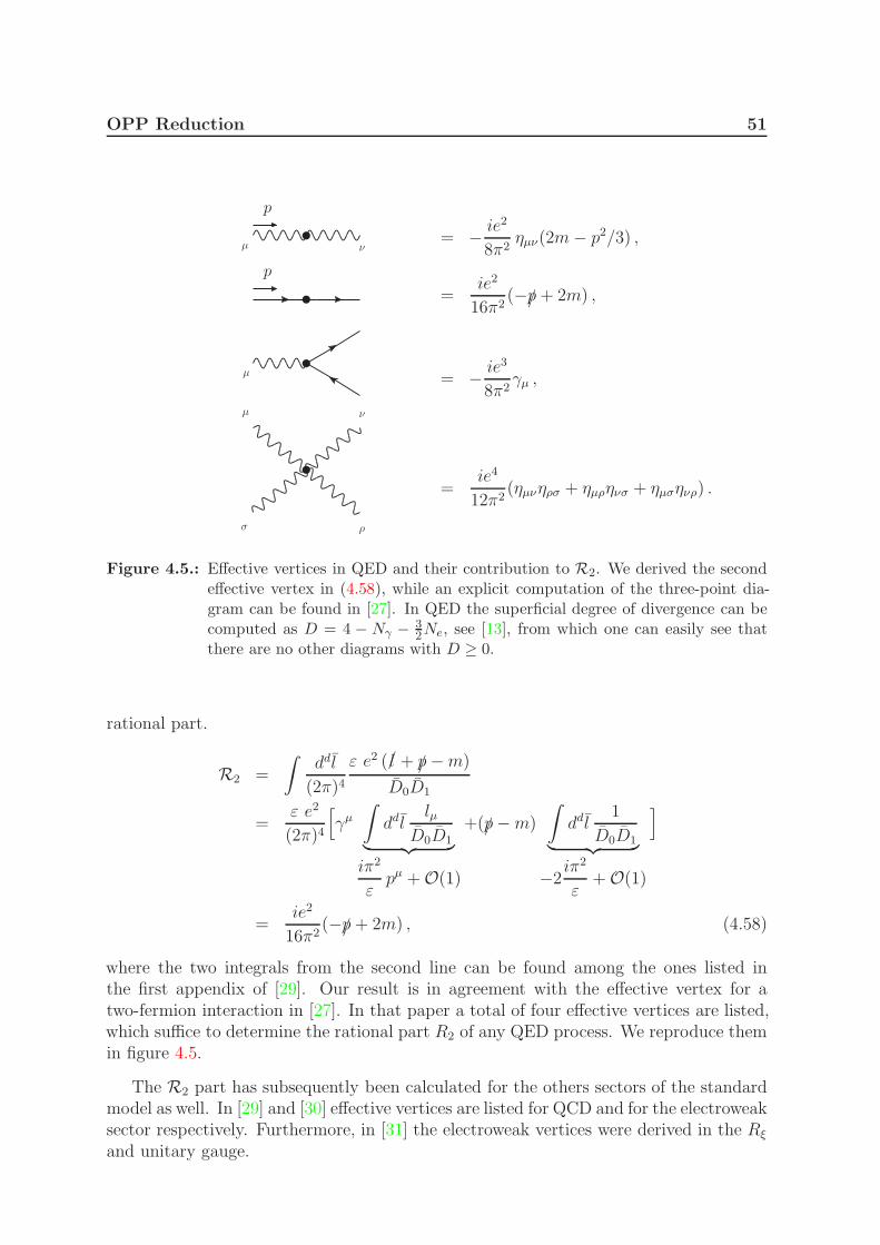
OPP Reduction 51
µ
µ ν
ρσ
νµ
p
p
= − ie2
8π2ηµν(2m− p2/3) ,
=ie2
16π2(−/p+ 2m) ,
= − ie3
8π2γµ ,
=ie4
12π2(ηµνηρσ + ηµρηνσ + ηµσηνρ) .
Figure 4.5.: Effective vertices in QED and their contribution to R2. We derived the secondeffective vertex in (4.58), while an explicit computation of the three-point dia-gram can be found in [27]. In QED the superficial degree of divergence can becomputed as D = 4 − Nγ − 3
2Ne, see [13], from which one can easily see thatthere are no other diagrams with D ≥ 0.
rational part.
R2 =
∫ddl
(2π)4
ε e2 (/l + /p−m)
D0D1
=ε e2
(2π)4
[
γµ∫
ddllµ
D0D1︸ ︷︷ ︸
iπ2
εpµ + O(1)
+(/p−m)
∫
ddl1
D0D1︸ ︷︷ ︸
−2iπ2
ε+ O(1)
]
=ie2
16π2(−/p + 2m) , (4.58)
where the two integrals from the second line can be found among the ones listed inthe first appendix of [29]. Our result is in agreement with the effective vertex for atwo-fermion interaction in [27]. In that paper a total of four effective vertices are listed,which suffice to determine the rational part R2 of any QED process. We reproduce themin figure 4.5.
The R2 part has subsequently been calculated for the others sectors of the standardmodel as well. In [29] and [30] effective vertices are listed for QCD and for the electroweaksector respectively. Furthermore, in [31] the electroweak vertices were derived in the Rξ
and unitary gauge.
52 OPP Reduction
4.4. Application of the OPP Method
At this point we have outlined all concepts involving the OPP reduction method. Letus now apply it to a simple example to see the method in action. We decided to reducea rank-two two-point integral in two spacetime dimensions for two reasons. First of all,the same example is worked out in [25] in a slightly different way, allowing us to compareresults. The second reason is that the coefficients can be derived by hand and given incompact form, which is simply impossible for more realistic examples. We do have tostart with an outline of the method in two dimensions.
Numerator Decomposition
In two dimensions any one-loop amplitude can be decomposed in terms of bubble andtadpole diagrams. This is reflected in the numerator decomposition
N(l) =n−1∑
i<j
[ b(ij) + b(l; ij) ]n−1∏
k 6=i,jDk +
n−1∑
i
[ a(i) + a(l; i) ]n−1∏
k 6=iDk . (4.59)
where a(i) and b(ij) are coefficients of tadpole and bubble scalar integrals respectivelyand n is the number of external particles of a given amplitude. The van Neerven-Vermaseren basis consists of {n1, n2} for tadpoles and {v1, n2} for bubbles. An explicitform of these vectors can be inferred from (4.8) and (4.9). The spurious terms dependon the loop momentum via
a(l; i) = a1(i) ((l + qi) · n1) + a2(i) ((l + qi) · n2) , (4.60)
b(l; ij) = b1(ij) ((l + qi) · n2) . (4.61)
Of course, the same can be derived by making a Passarino-Veltman decomposition of arank-three three-point function, just like we did in four dimensions.
As an illustration we shall now calculate a non-scalar two-point integral by computingits coefficients in terms of a scalar integral basis. That is,
∫d2l
(2π)2
N(l)
D0D1=
∫d2l
(2π)2
b(01)
D0D1+
∫d2l
(2π)2
a(0)
D1+
∫d2l
(2π)2
a(1)
D0+ R1 , (4.62)
for N(l) = (l · n2)2. The bubble coefficient b(01) and the tadpole coefficients a(i) are to
be determined by evaluating the numerator decomposition
(l · n2)2 = [ b(01) + b1(01) ((l + q0) · n2) ]
+ [ a(0) + a1(0) ((l + q0) · n1) + a2(0) ((l + q0) · n2) ] D1
+ [ a(1) + a1(1) ((l + q1) · n1) + a2(1) ((l + q1) · n2) ] D0 , (4.63)
OPP Reduction 53
at different loop momenta. The rational part R1 shall be explicitly found by shiftingthe masses, as was explained in the general four dimensional case. The rational part R2
is absent in d = 2 dimensions.
Bubble Coefficients
Let us first define some convenient variables
k0 = q0 − q1 , r0 = k20 −m2
0 +m21 ,
k1 = q1 − q0 , r1 = k21 −m2
1 +m20 . (4.64)
and basis vectors
vµ1 =kµ1k2
1
, nµ1 =kµ1√
k21
, n2 · k1 = 0 . (4.65)
The loop momentum parametrization for a two-point integral, solving D0 = D1 = 0,is
lµ± = −q0 − wµ ±√
m20 − w2 nµ2 , wµ =
r12vµ1 =
r12k2
1
kµ1 , (4.66)
which is the two-dimensional analog of (4.29). The master formula (4.63), evaluated atthese solutions, reads
(
−q0 · n2 ±√
m20 − w2
)2
= b(01) ± b1(01)√
m20 − w2 . (4.67)
Setting q0 = 0, it immediately follows that
b(01) = m20 − w2 = m2
0 −r21
4q21
,
b1(01) = 0 . (4.68)
Tadpole Coefficients
The loop momentum parametrization for a one-point integral, solvingD0 = 0 andD1 = 0respectively, are
lµ0,φ = −q0 +m0 (cosφnµ1 + sinφnµ2 ) , (4.69)
lµ1,φ = −q1 +m1 (cosφnµ1 + sinφnµ2 ) , (4.70)
54 OPP Reduction
for φ ∈ [0, 2π). Evaluating the master formula at solutions (4.69) and (4.70) respectively,we find
(−q0 · n2 +m0 sinφ)2 − (b(01) + b1(01)m0 sinφ)
= (a(0) + a1(0)m0 cosφ+ a2(0)m0 sin φ) (r1 + 2m0|k1| cosφ) , (4.71)
(−q1 · n2 +m1 sinφ)2 − (b(01) + b1(01)m1 sinφ)
= (a(1) + a1(1)m1 cosφ+ a2(1)m1 sin φ) (r0 − 2m1|k1| cosφ) , (4.72)
where we made use of (4.64) and (4.65) to write kµ1 = |k1|nµ1 = −kµ0 . Now that theequations are written down, we can set q0 = 0, thereby breaking the symmetry in theindices 0 and 1. Evaluating the equations at angles φ = 0, π, π/2 and solving for thecoefficients, we determine
a(0) =r1
4 q21
, a1(0) = − 1
2 |q1|, a2(0) = 0 , (4.73)
a(1) =r0
4 q21
+1
2, a1(1) =
1
2 |q1|, a2(1) = 0 . (4.74)
Rational Part
According to the observation in section 4.3, the rational part R1 is generated by shiftingall masses m2
i → m2i − l2. The variables rj clearly remain invariant under such a shift.
Therefor, only the coefficient b(01) is altered
b(01) → b(01) − l2 , (4.75)
and thus we find the following rational part
R1 = −∫
d2+εl
(2π)2
l2
D0 D1
. (4.76)
The result agrees with [25], where this rational part was derived as an extra coefficientb2 from the start.
4.5. Implementation
The OPP reduction method is currently being used in practice by several frameworks.Among them are MadGraph [32], GoSam [11] and FormCalc [33]. All mentioned frame-works make use of the libraries CutTools [9],[10] and/or Samurai [34]. The latter are thenumerical implementations of the OPP method.
In these programs the reduction is performed for a specific phase space point, thatis, a set numerical values for the momenta of all external particles. Also the masses of
OPP Reduction 55
the internal particles need to be specified numerically. It fits nicely into the frameworks,where cross-sections are calculated by evaluating the amplitude at many phase spacepoints. This means that the reduction is to be performed many times as well, somewhatof a downside. Luckily the numerical OPP reduction can be done quite fast.
We have taken a different and unique approach, by implementing an analytic OPPreduction. By this we mean that the resulting coefficients are analytic functions of thephase space variables. The upside of this approach is that the reduction has to beperformed only once, after which it is simply a matter of evaluation for every phasespace point. Another use could be to compare results with other methods in caseswhere certain limits have been taken, internal or external massless particles for example,to simplify expressions. Unavoidably, the program does not match the speed of thenumerical implementations.
4.5.1. Analytic OPP Reduction in FORM
Let us outline conceptually the working of our implementation in FORM [15], see ap-pendix C.
As input, the program only needs a numerator and the number of denominators. Itstarts by generating a system of equations for the box coefficients. There are only twoequations and two loop momenta, which are fixed. The loop momenta are expressed interms of the van Neerven-Vermaseren basis, which is constructed literally as (4.8) and(4.9). The determinants are constructed from squares of Levi-Civita tensors.
The system of equations is inverted by Gaussian elimination. Upon evaluating de-nominators at the specified loop momenta, we use the following simplification
Dj(l) = (l + qj)2 −m2
j
= (l + q0 + kj)2 −m2
j
= m20 + 2(l + q0) · kj + k2
j −m2j
= 2(l + q0) · kj + rj , (4.77)
in the case D0(l) = (l+ q0)2−m2
0 = 0. The advantage is that no terms quadratic in loopmomentum are left, because the loop momentum is expressed in terms of determinants.
Large expressions occurring multiple times inside the coefficients are replaced by adummy variable and stored away to be calculated only once. They include the 3×3 and4 × 4 Gram determinants for all combinations of external vectors and the length of theloop momentum in the transverse space lp, one for every coefficient. Also coefficientsentering subtraction terms are not substituted. All this contributes to a more compactoutput.
The number of coefficients N , including spurious terms, the number of coefficients ofscalar integrals N0 and the number of Gram determinants as a function of the number
56 OPP Reduction
of external particles, are given by
N(n) =1
12n(n+ 4)(n2 + 4n+ 7) , (4.78)
N0(n) =1
24n(n+ 1)(n2 − 3n+ 14) , (4.79)
Ngram(n) =1
24(n− 2)(n− 1)n(n + 1) . (4.80)
There are Nlp = N expressions lp. The number of expressions in the output is the sumNout(n) = N0 +Ngram +Nlp, since the spurious terms are discarded.
n 5 6 7 . . .
N0 30 56 98
Ngram 15 35 70
Nlp 195 335 539
Nout 240 426 707
(4.81)
For the triangle coefficients and beyond, the choice in loop momentum solutionsincreases. In order to simplify the system of equations, we chose all angles from a setof 16 values, where both the sine and the cosine take on rational values or square roots.Other angles can be chosen, but are likely to result in more dense systems of equations.
The output of the program consists of .mx files, to be imported in Mathematica fornumerical evaluation or further simplification. A possible extension of the program isto generate Fortran code directly from FORM. This would be useful for fast numericalevaluation of amplitudes. A new optimization algorithm in FORM, described in [35],can be particularly useful for producing optimized Fortran code.
4.5.2. Results and Comparison
In this section we describe some results obtained with the FORM program, in the contexta comparison and cross-check with other tools. For a cross-check, it is sufficient tocompare coefficients of scalar integrals. We have performed two independent checks:analytical and numerical. The analytical check is done by comparing our expressionsto the result of explicit Passarino-Veltman reduction. For the numerical comparison wefound CutTools to be a convenient source of numeric values for the coefficients. Belowwe give explicit results for each cross-check on specific examples.
For a comparison with Passarino-Veltman reduction, consider the following integral,as part of the calculation of a five particle interaction,
I :=
∫d4l
(2π)4
l · q3D0D1D2D3D4
(4.82)
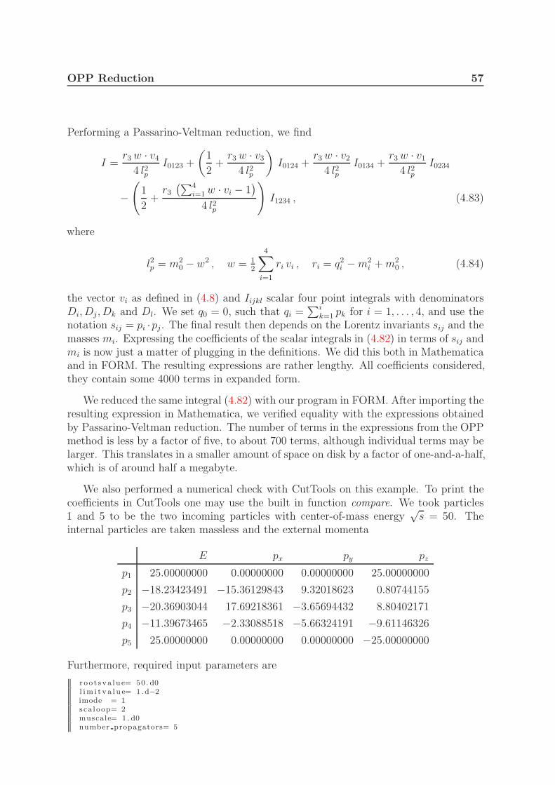
OPP Reduction 57
Performing a Passarino-Veltman reduction, we find
I =r3w · v4
4 l2pI0123 +
(1
2+r3w · v3
4 l2p
)
I0124 +r3w · v2
4 l2pI0134 +
r3w · v1
4 l2pI0234
−(
1
2+r3(∑4
i=1w · vi − 1)
4 l2p
)
I1234 , (4.83)
where
l2p = m20 − w2 , w = 1
2
4∑
i=1
ri vi , ri = q2i −m2
i +m20 , (4.84)
the vector vi as defined in (4.8) and Iijkl scalar four point integrals with denominatorsDi, Dj, Dk and Dl. We set q0 = 0, such that qi =
∑ik=1 pk for i = 1, . . . , 4, and use the
notation sij = pi ·pj. The final result then depends on the Lorentz invariants sij and themasses mi. Expressing the coefficients of the scalar integrals in (4.82) in terms of sij andmi is now just a matter of plugging in the definitions. We did this both in Mathematicaand in FORM. The resulting expressions are rather lengthy. All coefficients considered,they contain some 4000 terms in expanded form.
We reduced the same integral (4.82) with our program in FORM. After importing theresulting expression in Mathematica, we verified equality with the expressions obtainedby Passarino-Veltman reduction. The number of terms in the expressions from the OPPmethod is less by a factor of five, to about 700 terms, although individual terms may belarger. This translates in a smaller amount of space on disk by a factor of one-and-a-half,which is of around half a megabyte.
We also performed a numerical check with CutTools on this example. To print thecoefficients in CutTools one may use the built in function compare. We took particles1 and 5 to be the two incoming particles with center-of-mass energy
√s = 50. The
internal particles are taken massless and the external momenta
E px py pz
p1 25.00000000 0.00000000 0.00000000 25.00000000
p2 −18.23423491 −15.36129843 9.32018623 0.80744155
p3 −20.36903044 17.69218361 −3.65694432 8.80402171
p4 −11.39673465 −2.33088518 −5.66324191 −9.61146326
p5 25.00000000 0.00000000 0.00000000 −25.00000000
Furthermore, required input parameters are
r oo t s va l u e= 50 . d0l im i t v a l u e= 1 . d−2imode = 1sca l oop= 2muscale= 1 . d0number propagators= 5
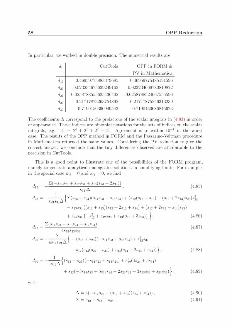
58 OPP Reduction
In particular, we worked in double precision. The numerical results are
di CutTools OPP in FORM &
PV in Mathematica
d15 0.46959773883379685 0.46959775485191596
d23 0.023234675629249163 0.023234669780819872
d27 −0.0258788553625436402 −0.0258788524067555596
d29 0.21717873263754892 0.21717875246313239
d30 −0.7190150390949543 −0.7190150686845623
The coefficients di correspond to the prefactors of the scalar integrals in (4.83) in orderof appearance. These indices are binomial notations for the sets of indices on the scalarintegrals, e.g. 15 = 20 + 21 + 22 + 23. Agreement is to within 10−7 in the worstcase. The results of the OPP method in FORM and the Passarino-Veltman procedurein Mathematica returned the same values. Considering the PV reduction to give thecorrect answer, we conclude that the tiny differences observed are attributable to theprecision in CutTools.
This is a good point to illustrate one of the possibilities of the FORM program,namely to generate analytical manageable solutions in simplifying limits. For example,in the special case mi = 0 and sjj = 0, we find
d15 = −Σ(−s14s23 + s12s34 + s13(s24 + 2s34))
s34 ∆, (4.85)
d23 = − 1
s23s34∆
{
Σ(s23 + s24)(s14s23 − s13s24) + (s12(s12 + s13) − (s12 + 2s13)s23)s234
− s23s34 ((s12 + s13)(s12 + 2s13 + s14) + (s12 + 2s13 − s14)s23)
+ s24s34
(−s2
12 + s12s23 + s13(s13 + 3s23))}
, (4.86)
d27 =Σ(s14s23 − s13s24 + s12s34)
4s12s23s34, (4.87)
d29 = − Σ
4s12s23 ∆
{
− (s13 + s23)(−s14s23 + s13s24) + s212s34
− s12(s13(s24 − s34) + s23(s14 + 2s24 + s34))}
, (4.88)
d30 = − 1
4s12∆
{
(s13 + s23)(−s14s23 + s13s24) + s212(4s24 + 3s34)
+ s12(−3s14s23 + 5s13s24 + 2s23s24 + 3s13s34 + s23s34)}
, (4.89)
with
∆ = 4(−s14s23 + (s12 + s13)(s24 + s34)) , (4.90)
Σ = s12 + s13 + s23 . (4.91)
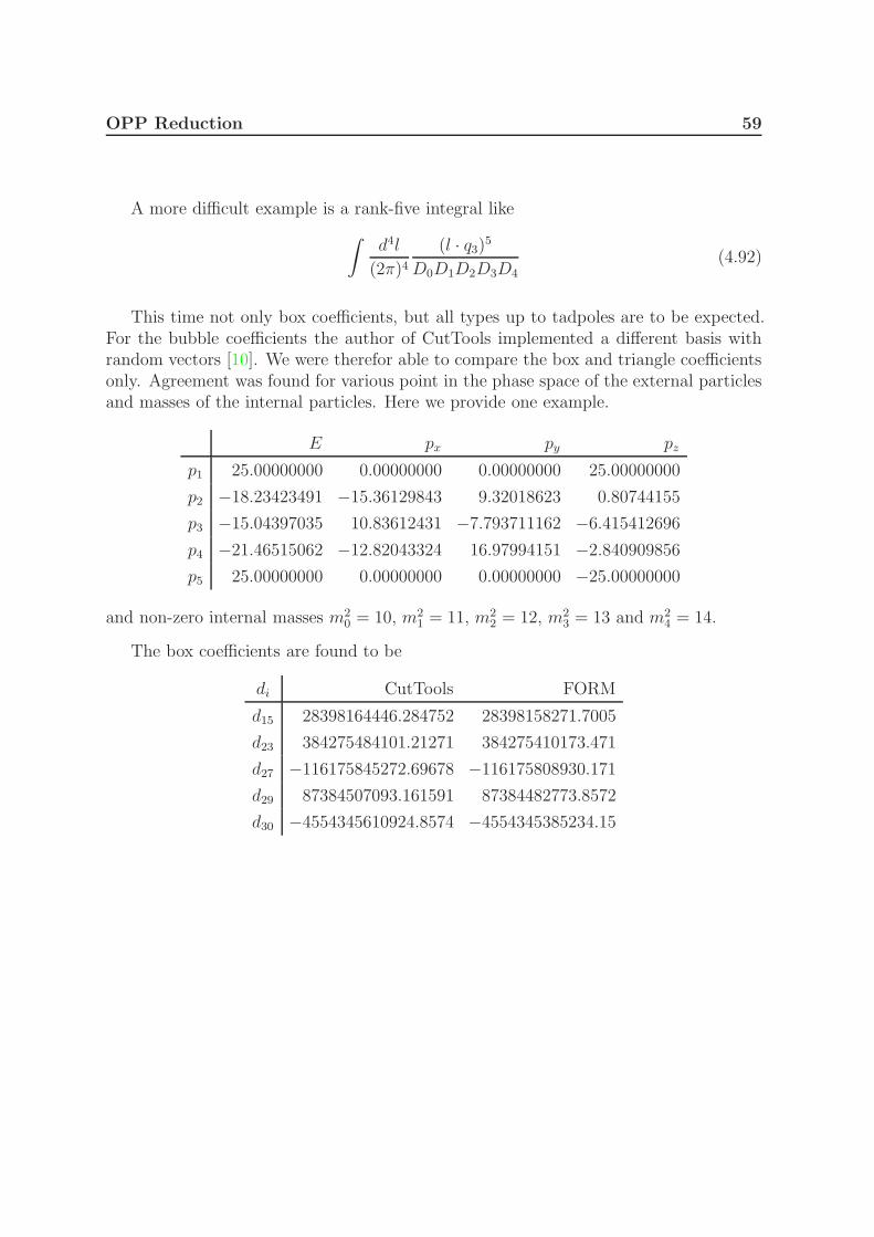
OPP Reduction 59
A more difficult example is a rank-five integral like
∫d4l
(2π)4
(l · q3)5
D0D1D2D3D4(4.92)
This time not only box coefficients, but all types up to tadpoles are to be expected.For the bubble coefficients the author of CutTools implemented a different basis withrandom vectors [10]. We were therefor able to compare the box and triangle coefficientsonly. Agreement was found for various point in the phase space of the external particlesand masses of the internal particles. Here we provide one example.
E px py pz
p1 25.00000000 0.00000000 0.00000000 25.00000000
p2 −18.23423491 −15.36129843 9.32018623 0.80744155
p3 −15.04397035 10.83612431 −7.793711162 −6.415412696
p4 −21.46515062 −12.82043324 16.97994151 −2.840909856
p5 25.00000000 0.00000000 0.00000000 −25.00000000
and non-zero internal masses m20 = 10, m2
1 = 11, m22 = 12, m2
3 = 13 and m24 = 14.
The box coefficients are found to be
di CutTools FORM
d15 28398164446.284752 28398158271.7005
d23 384275484101.21271 384275410173.471
d27 −116175845272.69678 −116175808930.171
d29 87384507093.161591 87384482773.8572
d30 −4554345610924.8574 −4554345385234.15
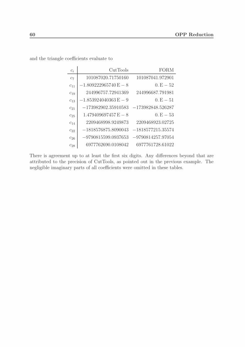
60 OPP Reduction
and the triangle coefficients evaluate to
ci CutTools FORM
c7 101087020.71750160 101087041.972901
c11 −1.809222965740 E− 8 0.E − 52
c19 244996757.72941369 244996687.791981
c13 −1.853924040363 E− 9 0.E − 51
c21 −173982902.35910583 −173982848.526287
c25 1.479409697457 E− 8 0.E − 53
c14 2209468998.9249873 2209468923.02725
c22 −1818576875.8090043 −1818577215.35574
c26 −9790815599.0937653 −9790814257.97054
c28 6977762690.0108042 6977761728.61022
There is agreement up to at least the first six digits. Any differences beyond that areattributed to the precision of CutTools, as pointed out in the previous example. Thenegligible imaginary parts of all coefficients were omitted in these tables.
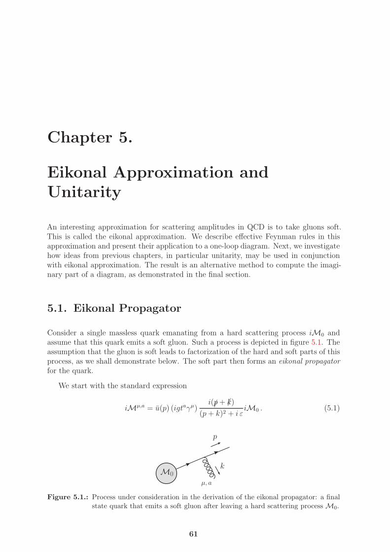
Chapter 5.
Eikonal Approximation and
Unitarity
An interesting approximation for scattering amplitudes in QCD is to take gluons soft.This is called the eikonal approximation. We describe effective Feynman rules in thisapproximation and present their application to a one-loop diagram. Next, we investigatehow ideas from previous chapters, in particular unitarity, may be used in conjunctionwith eikonal approximation. The result is an alternative method to compute the imagi-nary part of a diagram, as demonstrated in the final section.
5.1. Eikonal Propagator
Consider a single massless quark emanating from a hard scattering process iM0 andassume that this quark emits a soft gluon. Such a process is depicted in figure 5.1. Theassumption that the gluon is soft leads to factorization of the hard and soft parts of thisprocess, as we shall demonstrate below. The soft part then forms an eikonal propagator
for the quark.
We start with the standard expression
iMµ,a = u(p) (igtaγµ)i(/p+ /k)
(p+ k)2 + i εiM0 . (5.1)
M0
p
k
µ, a
Figure 5.1.: Process under consideration in the derivation of the eikonal propagator: a finalstate quark that emits a soft gluon after leaving a hard scattering process M0.
61
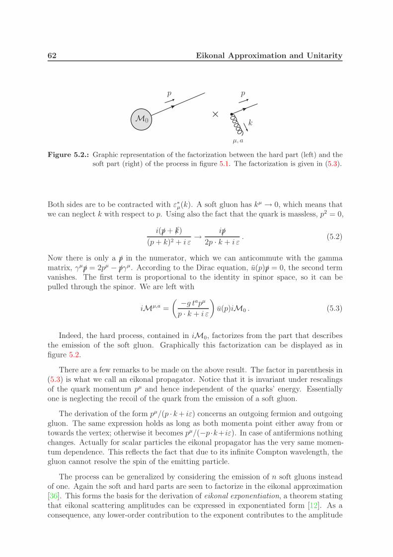
62 Eikonal Approximation and Unitarity
M0
p p
k
µ, a
Figure 5.2.: Graphic representation of the factorization between the hard part (left) and thesoft part (right) of the process in figure 5.1. The factorization is given in (5.3).
Both sides are to be contracted with ε∗µ(k). A soft gluon has kµ → 0, which means thatwe can neglect k with respect to p. Using also the fact that the quark is massless, p2 = 0,
i(/p+ /k)
(p+ k)2 + i ε→
i/p
2p · k + i ε. (5.2)
Now there is only a /p in the numerator, which we can anticommute with the gammamatrix, γµ/p = 2pµ − /pγ
µ. According to the Dirac equation, u(p)/p = 0, the second termvanishes. The first term is proportional to the identity in spinor space, so it can bepulled through the spinor. We are left with
iMµ,a =
( −g tapµp · k + i ε
)
u(p)iM0 . (5.3)
Indeed, the hard process, contained in iM0, factorizes from the part that describesthe emission of the soft gluon. Graphically this factorization can be displayed as infigure 5.2.
There are a few remarks to be made on the above result. The factor in parenthesis in(5.3) is what we call an eikonal propagator. Notice that it is invariant under rescalingsof the quark momentum pµ and hence independent of the quarks’ energy. Essentiallyone is neglecting the recoil of the quark from the emission of a soft gluon.
The derivation of the form pµ/(p · k+ iε) concerns an outgoing fermion and outgoinggluon. The same expression holds as long as both momenta point either away from ortowards the vertex; otherwise it becomes pµ/(−p ·k+iε). In case of antifermions nothingchanges. Actually for scalar particles the eikonal propagator has the very same momen-tum dependence. This reflects the fact that due to its infinite Compton wavelength, thegluon cannot resolve the spin of the emitting particle.
The process can be generalized by considering the emission of n soft gluons insteadof one. Again the soft and hard parts are seen to factorize in the eikonal approximation[36]. This forms the basis for the derivation of eikonal exponentiation, a theorem statingthat eikonal scattering amplitudes can be expressed in exponentiated form [12]. As aconsequence, any lower-order contribution to the exponent contributes to the amplitude
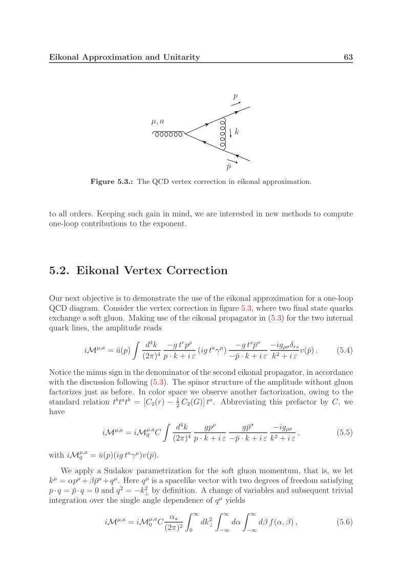
Eikonal Approximation and Unitarity 63
p
k
p
µ, a
Figure 5.3.: The QCD vertex correction in eikonal approximation.
to all orders. Keeping such gain in mind, we are interested in new methods to computeone-loop contributions to the exponent.
5.2. Eikonal Vertex Correction
Our next objective is to demonstrate the use of the eikonal approximation for a one-loopQCD diagram. Consider the vertex correction in figure 5.3, where two final state quarksexchange a soft gluon. Making use of the eikonal propagator in (5.3) for the two internalquark lines, the amplitude reads
iMµ,a = u(p)
∫d4k
(2π)4
−g trpρp · k + i ε
(ig taγµ)−g tspσ
−p · k + i ε
−igρσδrsk2 + i ε
v(p) . (5.4)
Notice the minus sign in the denominator of the second eikonal propagator, in accordancewith the discussion following (5.3). The spinor structure of the amplitude without gluonfactorizes just as before. In color space we observe another factorization, owing to thestandard relation tbtatb = [C2(r) − 1
2C2(G)] ta. Abbreviating this prefactor by C, we
have
iMµ,a = iMµ,a0 C
∫d4k
(2π)4
gpρ
p · k + i ε
gpσ
−p · k + i ε
−igρσk2 + i ε
, (5.5)
with iMµ,a0 = u(p)(ig taγµ)v(p).
We apply a Sudakov parametrization for the soft gluon momentum, that is, we letkµ = αpµ+βpµ+qµ. Here qµ is a spacelike vector with two degrees of freedom satisfyingp · q = p · q = 0 and q2 = −k2
⊥ by definition. A change of variables and subsequent trivialintegration over the single angle dependence of qµ yields
iMµ,a = iMµ,a0 C
αs(2π)2
∫ ∞
0
dk2⊥
∫ ∞
−∞dα
∫ ∞
−∞dβ f(α, β) , (5.6)
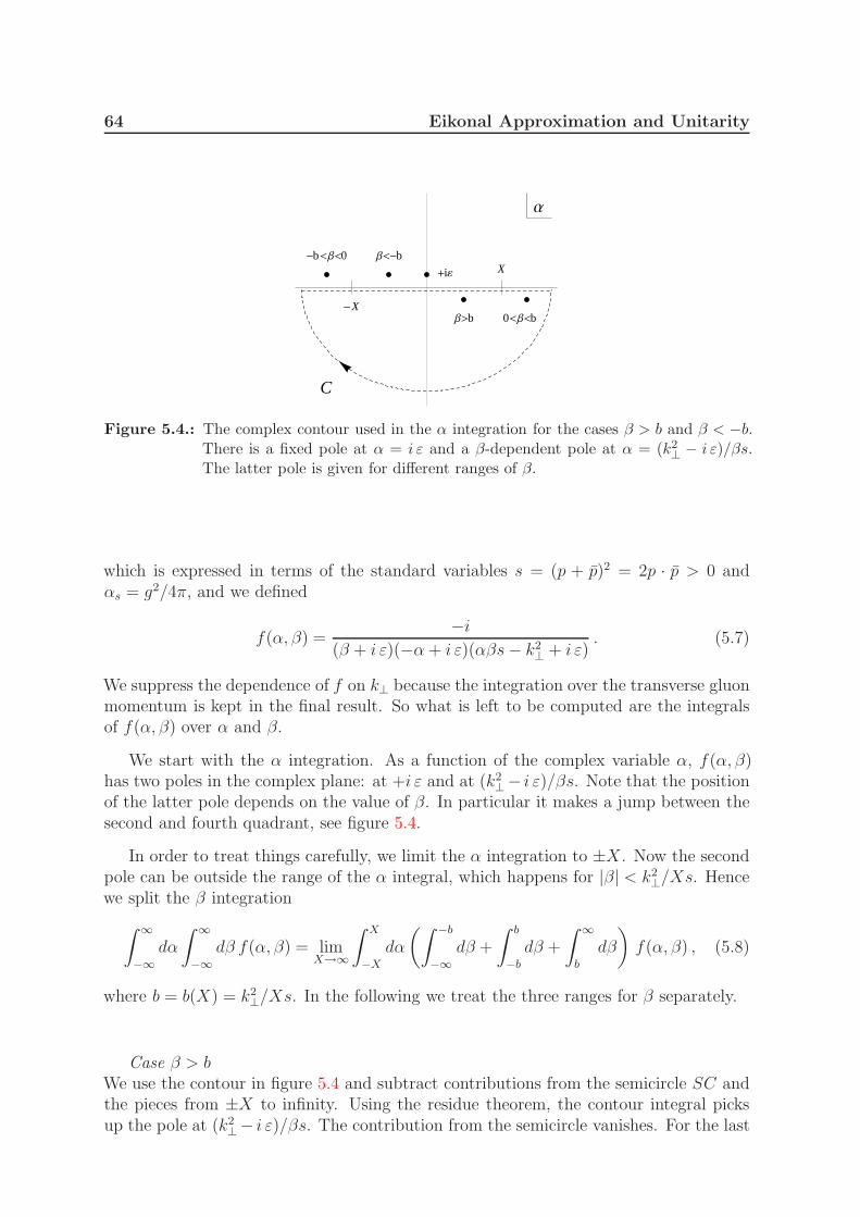
64 Eikonal Approximation and Unitarity
C
-X
X
Α
+i¶
Β<-b-b<Β<0
0<Β<bΒ>b
Figure 5.4.: The complex contour used in the α integration for the cases β > b and β < −b.There is a fixed pole at α = i ε and a β-dependent pole at α = (k2
⊥ − i ε)/βs.The latter pole is given for different ranges of β.
which is expressed in terms of the standard variables s = (p + p)2 = 2p · p > 0 andαs = g2/4π, and we defined
f(α, β) =−i
(β + i ε)(−α + i ε)(αβs− k2⊥ + i ε)
. (5.7)
We suppress the dependence of f on k⊥ because the integration over the transverse gluonmomentum is kept in the final result. So what is left to be computed are the integralsof f(α, β) over α and β.
We start with the α integration. As a function of the complex variable α, f(α, β)has two poles in the complex plane: at +i ε and at (k2
⊥− i ε)/βs. Note that the positionof the latter pole depends on the value of β. In particular it makes a jump between thesecond and fourth quadrant, see figure 5.4.
In order to treat things carefully, we limit the α integration to ±X. Now the secondpole can be outside the range of the α integral, which happens for |β| < k2
⊥/Xs. Hencewe split the β integration
∫ ∞
−∞dα
∫ ∞
−∞dβ f(α, β) = lim
X→∞
∫ X
−Xdα
(∫ −b
−∞dβ +
∫ b
−bdβ +
∫ ∞
b
dβ
)
f(α, β) , (5.8)
where b = b(X) = k2⊥/Xs. In the following we treat the three ranges for β separately.
Case β > bWe use the contour in figure 5.4 and subtract contributions from the semicircle SC andthe pieces from ±X to infinity. Using the residue theorem, the contour integral picksup the pole at (k2
⊥− i ε)/βs. The contribution from the semicircle vanishes. For the last
Eikonal Approximation and Unitarity 65
two α integrals we can drop all i ε’s inside f(α, β) since there are no poles nearby.
limX→∞
∫ ∞
b
dβ
∫ X
−Xdα f(α, β)
= limX→∞
∫ ∞
b
dβ
(∮
C
dα−∫
SC
dα−∫ −X
−∞dα−
∫ ∞
X
dα
)
f(α, β)
= limX→∞
∫ ∞
b
dβ1
β k2⊥
(
2π + i ln(1 − b
β) − i ln(1 +
b
β)
)
= limX→∞
1
k2⊥
(
2π
∫ ln(√s/k2
⊥X)
−∞dy − iLi2(1) + iLi2(−1)
)
=2π
k2⊥
(∫ ∞
−∞dy − i
π
8
)
. (5.9)
The second to last equality needs a bit more explanation. The first term was rewritteninto a rapidity integral, y = 1
2ln α
β= ln k⊥
β√s. The last two terms turned into the defining
integral representation of the dilogarithm upon substitution γ = ± bβ. See (A.31) and
(A.32) for details on the dilogarithm.
Case β < −bUse the contour in figure 5.4 again. This time both poles are above the real axis. Thatmeans no poles are inside the contour and the closed contour integral gives zero. Theconsequence is that there will be no rapidity integral as in the previous case. Theintegrations from ±X to infinity become the same as before upon β → −β. Hence
limX→∞
∫ −b
−∞dβ
∫ X
−Xdα f(α, β) =
2π
k2⊥
(
−iπ8
)
. (5.10)
66 Eikonal Approximation and Unitarity
Case −b < β < bOnly the +iε pole is close to the path of integration. Symmetrize in α.
limX→∞
∫ b
−bdβ
∫ X
−Xdα f(α, β)
= limX→∞
∫ b
−bdβ
∫ X
−Xdα 1
2[f(α, β) + f(−α, β)]
= limX→∞
∫ b
−bdβ
1
β + i ε
∫ X
−Xdα
− ε k2⊥ + iβsα2
(α2 + ε2)(α2β2s2 − k4⊥)
= limX→∞
∫ b
−bdβ
1
β + i ε
∫ X
−Xdα
(
πδ(α)−k2
⊥α2β2s2 − k4
⊥+
iβs
α2β2s2 − k4⊥
)
= limX→∞
∫ b
−bdβ
1
β + i ε
∫ X
−Xdα
1
k2⊥
(
π + i ln(1 − β
b) − i ln(1 +
β
b)
)
. (5.11)
Doing the same for the β integral and recognizing the dilogarithm once again,
limX→∞
∫ b
−bdβ
∫ X
−Xdα f(α, β) =
2π
k2⊥
(
−i3π4
)
. (5.12)
Adding the three contributions (5.9), (5.10) and (5.12) according to (5.8) and plug-ging the result into (5.6), we finally have
iMµ,a = iMµ,a0 C
αs2π
∫ ∞
0
dk2⊥
k2⊥
(∫ ∞
−∞dy − iπ
)
. (5.13)
5.3. Cutkosky Rule in Eikonal Approximation
Looking back at previous section, we learn that computing one-loop corrections is rathertedious, even for a modest example and with the use of eikonal approximation. We stressthat for other diagrams it is only likely to become much more challenging. Thereforwe would like to investigate the possibility of a shortcut in the calculation, using theunitarity principles from chapter 3.
Let us first briefly return to the non-eikonal case. Recall that the imaginary part ofa scattering amplitude can be obtained by summing all possible cuttings of a diagram.Cut propagators are put on shell according to Cutkosky’s rule, see (3.15). For example,for a massless scalar
i
p2 + i ε→ 2π θ(±p0) δ(p
2) . (5.14)
The positive or negative energy solution is chosen such that the energy flows towardsthe shaded side of the cut. The rule for spin one-half particles is obtained by simply
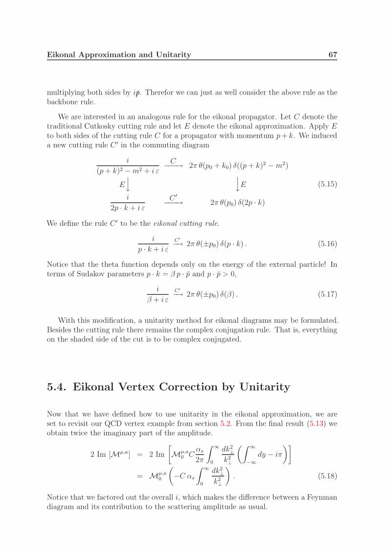
Eikonal Approximation and Unitarity 67
multiplying both sides by i/p. Therefor we can just as well consider the above rule as thebackbone rule.
We are interested in an analogous rule for the eikonal propagator. Let C denote thetraditional Cutkosky cutting rule and let E denote the eikonal approximation. Apply Eto both sides of the cutting rule C for a propagator with momentum p+ k. We induceda new cutting rule C ′ in the commuting diagram
i
(p+ k)2 −m2 + i εC−−−→ 2π θ(p0 + k0) δ((p+ k)2 −m2)
Ey
yE
i
2p · k + i ε
C ′−−−→ 2π θ(p0) δ(2p · k)
(5.15)
We define the rule C ′ to be the eikonal cutting rule.
i
p · k + i ε
C′
−→ 2π θ(±p0) δ(p · k) . (5.16)
Notice that the theta function depends only on the energy of the external particle! Interms of Sudakov parameters p · k = β p · p and p · p > 0,
i
β + i ε
C′
−→ 2π θ(±p0) δ(β) . (5.17)
With this modification, a unitarity method for eikonal diagrams may be formulated.Besides the cutting rule there remains the complex conjugation rule. That is, everythingon the shaded side of the cut is to be complex conjugated.
5.4. Eikonal Vertex Correction by Unitarity
Now that we have defined how to use unitarity in the eikonal approximation, we areset to revisit our QCD vertex example from section 5.2. From the final result (5.13) weobtain twice the imaginary part of the amplitude.
2 Im [Mµ,a] = 2 Im
[
Mµ,a0 C
αs2π
∫ ∞
0
dk2⊥
k2⊥
(∫ ∞
−∞dy − iπ
)]
= Mµ,a0
(
−C αs∫ ∞
0
dk2⊥
k2⊥
)
. (5.18)
Notice that we factored out the overall i, which makes the difference between a Feynmandiagram and its contribution to the scattering amplitude as usual.
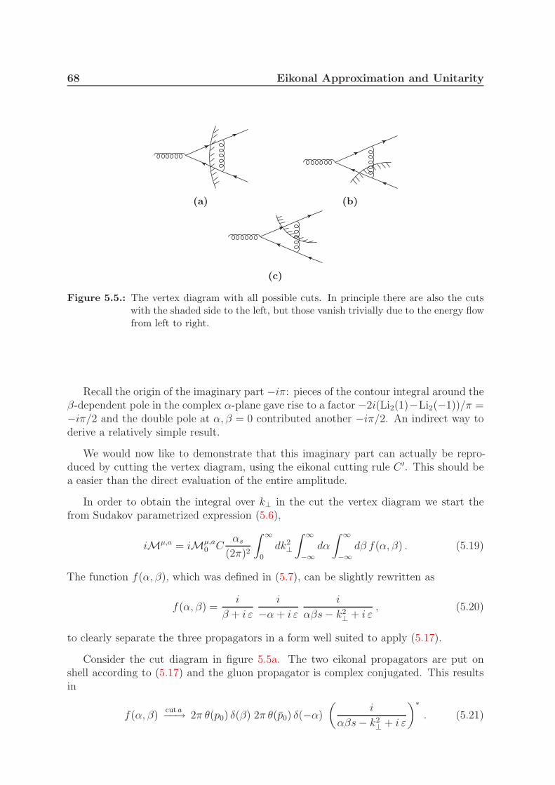
68 Eikonal Approximation and Unitarity
(a) (b)
(c)
Figure 5.5.: The vertex diagram with all possible cuts. In principle there are also the cutswith the shaded side to the left, but those vanish trivially due to the energy flowfrom left to right.
Recall the origin of the imaginary part −iπ: pieces of the contour integral around theβ-dependent pole in the complex α-plane gave rise to a factor −2i(Li2(1)−Li2(−1))/π =−iπ/2 and the double pole at α, β = 0 contributed another −iπ/2. An indirect way toderive a relatively simple result.
We would now like to demonstrate that this imaginary part can actually be repro-duced by cutting the vertex diagram, using the eikonal cutting rule C ′. This should bea easier than the direct evaluation of the entire amplitude.
In order to obtain the integral over k⊥ in the cut the vertex diagram we start thefrom Sudakov parametrized expression (5.6),
iMµ,a = iMµ,a0 C
αs(2π)2
∫ ∞
0
dk2⊥
∫ ∞
−∞dα
∫ ∞
−∞dβ f(α, β) . (5.19)
The function f(α, β), which was defined in (5.7), can be slightly rewritten as
f(α, β) =i
β + i ε
i
−α + i ε
i
αβs− k2⊥ + i ε
, (5.20)
to clearly separate the three propagators in a form well suited to apply (5.17).
Consider the cut diagram in figure 5.5a. The two eikonal propagators are put onshell according to (5.17) and the gluon propagator is complex conjugated. This resultsin
f(α, β)cut a−−→ 2π θ(p0) δ(β) 2π θ(p0) δ(−α)
(i
αβs− k2⊥ + i ε
)∗. (5.21)
Eikonal Approximation and Unitarity 69
The two theta functions are in fact one, because the two quarks are final state particles.Finally, the two vertices in the shaded region give an overall factor of (−1)2 due tocomplex conjugation. With (5.21), the amplitude (5.19) becomes
iMµ,a∣∣cut a
= (−1)2 iMµ,a0 Cαs
∫ ∞
0
dk2⊥
∫ ∞
−∞dα
∫ ∞
−∞dβ δ(β) δ(−α)
−iαβs− k2
⊥ − i ε
= Mµ,a0
(
−C αs∫ ∞
0
dk2⊥
k2⊥
)
. (5.22)
Next, we look at the second cut diagram, the one in figure 5.5b. Here one eikonalpropagator is cut, together with the soft gluon propagator. The gluon momentum is inthe same direction as the shade on the cut, so we pick the positive energy cut.
f(α, β)cut b−−→ i
β + i ε2π θ(p0) δ(−α) 2π θ(αp0 + βp0) δ(αβs− k2
⊥) . (5.23)
Here we used the fact that k0 = αp0 + βp0. The first theta functions is trivial as before.For the single vertex in the shaded region we include a minus sign. So for (5.23), theamplitude (5.19) becomes
iMµ,a∣∣cut b
= (−1) iMµ,a0 Cαs
∫ ∞
0
dk2⊥×
∫ ∞
−∞dα
∫ ∞
−∞dβ
i
β + i εδ(−α) θ(αp0 + βp0) δ(αβs− k2
⊥)
= (−1) iMµ,a0 Cαs
∫ ∞
0
dk2⊥ δ(k
2⊥)
∫ ∞
−∞dβ
i
β + i εθ(βp0) (5.24)
In the first integral we encounter the subtlety whether the delta has support inside thedomain of integration. We argue that the lower bound of the integration over the squaredperpendicular length of the gluon momentum, k2
⊥, should strictly be 0+. If we look backat the result of the full vertex calculation, (5.13), we see that we actually need such alower bound in order to regularize the integral. As a consequence the first integral giveszero and we get iMµ,a|cut b = 0. An analogous computation shows that the diagram withcut c vanishes as well.
The sum of the three cut diagrams is thus equal to the expression in (5.22). Noticethat it is equal to the result (5.18) for twice the imaginary part of the amplitude. Inother words, we have established the cutting equation for this amplitude at order αs:
2 Im [Mµ,a] =∑
cut
iMµ,a∣∣cut. (5.25)

70
Chapter 6.
Conclusion
Theoretical high-energy particle physics aims at describing particles at the most funda-mental level. In order to compare a theory with experiment, one must make definitepredictions about the way particles should interact. The use of perturbation theory hasenabled to make approximate predictions. Our first goal in this thesis was to review tech-niques for making better and better approximations. To be specific, we started by cal-culating one-loop diagrams in the traditional way. Several aspects have been discussed,such as dimensional regularization, Feynman parameter integration and analytic contin-uation. Finally we showed how to renormalize the theory of quantum-electrodynamicsto all orders, by using our explicit calculations. Beyond these examples, calculationstend to become more demanding, suggesting the need for improved techniques.
Unitarity forms the heart of several such techniques. We showed how unitarity of thescattering matrix can be exploited to derive a cutting equation for Feynman diagrams,which allows easy computation of imaginary parts of diagrams. Using unitarity in con-junction with either dispersion relations or with a basis expansion for the amplitude,as in generalized unitarity, one can recover the full amplitude. Still further develop-ments aim at bridging the gap between manual calculations and automated computerprograms.
The OPP method provides the crucial step toward automated calculations. Wedescribed in detail the workings of this method and proved the basis expansion at theintegrand level. In the determination of coefficients in that basis the unitarity principlepops up again, this time in the form of putting virtual particles algebraically on-shell.Particular attention was given to the rational parts of amplitude. We explained theorigin of two kinds of rational part and showed how to compute them. The fact thatthe method works at the integrand level, such that no integration is needed whatsoever,made it suitable for numerical implementations like CutTools.
We presented a complementary program based on the same method, but performingan analytic reduction. In other words, the resulting coefficients are given in closedform in terms of the appropriate Lorentz invariants. Though very large in general,the expressions can take on manageable forms in certain points in phase space. Thiscould provide a comparison for other analytic reduction tools. An extensive comparisonwith CutTools has shown excellent agreement. A possible extension of our program
71

72 Conclusion
includes generating Fortran code, optimized with a new FORM feature, to allow forrapid numerical evaluation.
In the final part of the thesis we discovered still another use of the unitarity principle,this time in the area of soft quantum corrections. The main result was to constructanalogous cutting rules for diagrams in the eikonal approximation. We computed avertex correction diagram in two ways and verified that the imaginary part is reproducedby the sum of all cut diagrams.
Appendix A.
Conventions and Integrals
Conventions
Natural units
c = ~ = 1 (A.1)
Fine-structure constant
α =e2
4π(A.2)
Bjorken-Drell metric
ηµν = diag(1,−1,−1,−1) (A.3)
Number of spacetime dimensions
d = 4 − 2 ε (A.4)
Dirac algebra
{γµ, γν} = 2ηµν 1 (A.5)
The Dirac calculus in d dimensions can be derived from (A.5), together with the
choice to keep gamma matrices 4 × 4. This means that traces are independent of d− 4,
73
74 Conventions and Integrals
while contractions of indices do. For example [13]
tr [1] = 4 (A.6)
tr [γµ] = 0 (A.7)
tr [γµγν ] = 4ηµν (A.8)
tr [γµγνγρ] = 0 (A.9)
tr [γµγνγργσ] = 4(ηµνηρσ − ηµρηνσ + ηµσηνρ) (A.10)
γµγµ = ηµνηµν = δµµ = d (A.11)
γµγργµ = (2 − d)γρ (A.12)
γµγργσγµ = 4ηρσ − (4 − d)γργσ (A.13)
γµγργσγτγµ = −2γτγσγρ + (4 − d)γργσγτ (A.14)
Scalar Integrals
The standard scalar integral is [13]
∫ddl
(2π)d1
(l2 −M2 + iǫ)k=i(−1)k
(4π)d/2Γ(k − d/2)
Γ(k)(M2)d/2−k (A.15)
with integer k > 1, a mass M2 > 0 and iǫ a small but positive imaginary quantity.
Analytic continuation of the above result can be performed following the prescription
M2 →M2 − iǫ (A.16)
Putting d = 4 − 2 ε and introducing arbitrary reference mass µ,
∫ddl
(2π)d1
(l2 −M2 + iǫ)k=i(−1)k
(4π)k(µ2)2−k−εΓ(k − 2 + ε)
Γ(k)
(M2
4πµ2
)2−k−ε. (A.17)
In particular, we need the cases k = 2 and k = 3. Plugging in the following expansions
around ε = 0
Γ(ε) =1
ε− γ + O(ε) , (A.18)
Γ(1 + ε) = 1 − γ ε+O(ε2) , (A.19)(M2
4πµ2
)− ε
= 1 − ε log
(M2
4πµ2
)
+ O(ε2) (A.20)
Conventions and Integrals 75
where γ is the Euler-Mascheroni constant, we find
∫ddl
(2π)d1
(l2 −M2 + iǫ)2=
i(µ2)− ε
(4π)2
(1
ε− γ − log
(M2
4πµ2
)
+ O(ε)
)
, (A.21)
∫ddl
(2π)d1
(l2 −M2 + iǫ)3=
−i(µ2)−1−ε
2(4π)3
(M2
4πµ2
)−1
×(
1 − ε γ − ε log
(M2
4πµ2
)
+ O(ε2)
)
. (A.22)
Tensor Integrals
Symmetric integration [13]
∫ddl
(2π)dlµ
(l2 −M2 + iǫ)k= 0 (A.23)
∫ddl
(2π)dlµlν
(l2 −M2 + iǫ)k=
ηµν
d
∫ddl
(2π)dl2
(l2 −M2 + iǫ)k(A.24)
Application of [14]
0 =
∫ddl
(2π)d∂
∂lµ
(
lµf(l))
= n
∫ddl
(2π)df(l) +
∫ddl
(2π)dlµ
(∂f(l)
∂lµ
)
(A.25)
to f(l) = (l2 +m2 − iǫ)−k leads to
∫ddl
(2π)dl2
(l2 −M2 + iǫ)k+1=
d
d− 2k
∫ddl
(2π)dM2
(l2 −M2 + iǫ)k+1(A.26)
Feynman Parameter Integrals
The general identity is [13]
1∏
iDi=
(∏
i
∫ 1
0
dxi
)
(n− 1)! δ(1 −∑
i xi)
(∑
i xiDi)n, (A.27)
76 Conventions and Integrals
where i runs from 1 to n. We use the cases n = 1 and n = 2,
1
D1D2=
∫ 1
0
dx1
(xD1 + (1 − x)D2)2(A.28)
1
D1D2D3
=
∫ 1
0
dx
∫ 1−x
0
dy2
(xD1 + yD2 + (1 − x− y)D3)3(A.29)
In the latter integral we can exploit the symmetry of the integration domain. Let
f (k)(x, y) be a symmetric homogeneous polynomial of degree k. That is, f (k)(x, y) =
f (k)(y, x) and f (k)(c x, c y) = ckf (k)(x, y). Then [37]
∫ 1
0
dx
∫ 1−x
0
dy f (k)(x, y) =
∫ 1
0
dz z1+k
∫ 1
0
d(xz)
∫ 1
0
d(yz) δ(1 − x
z− y
z)f (k)(x
z, yz)
=
∫ 1
0
dz z1+k
∫ 1
0
dx′ f (k)(x′, 1 − x′) (A.30)
The first equality may be shown by integrating out z on the right hand side. A divergence
(typically IR) arises from the first integral when k < −1.
Dilogarithm
Definition of the dilogarithm for complex argument [38]
Li2(z) :=−∫ z
0
dtlog(1 − t)
tfor z ∈ C\[1,∞) (A.31)
It has very few special values - as far as anyone knows there are eight - including
Li2(0) = 0 , Li2(1) =π2
6, Li2(−1) = −π
2
12(A.32)
The dilogarithm has a branch cut for real z > 1. Making use of the reflection property
Li2(−1/z) + Li2(−z) = 2 Li2(−1) − 12log2(z) (A.33)
we have the following analytic continuation for real r > 1
Li2(r ± i ε) = −Li2(1/r) − 12log2(r) +
π2
3± iπ log(r) (A.34)
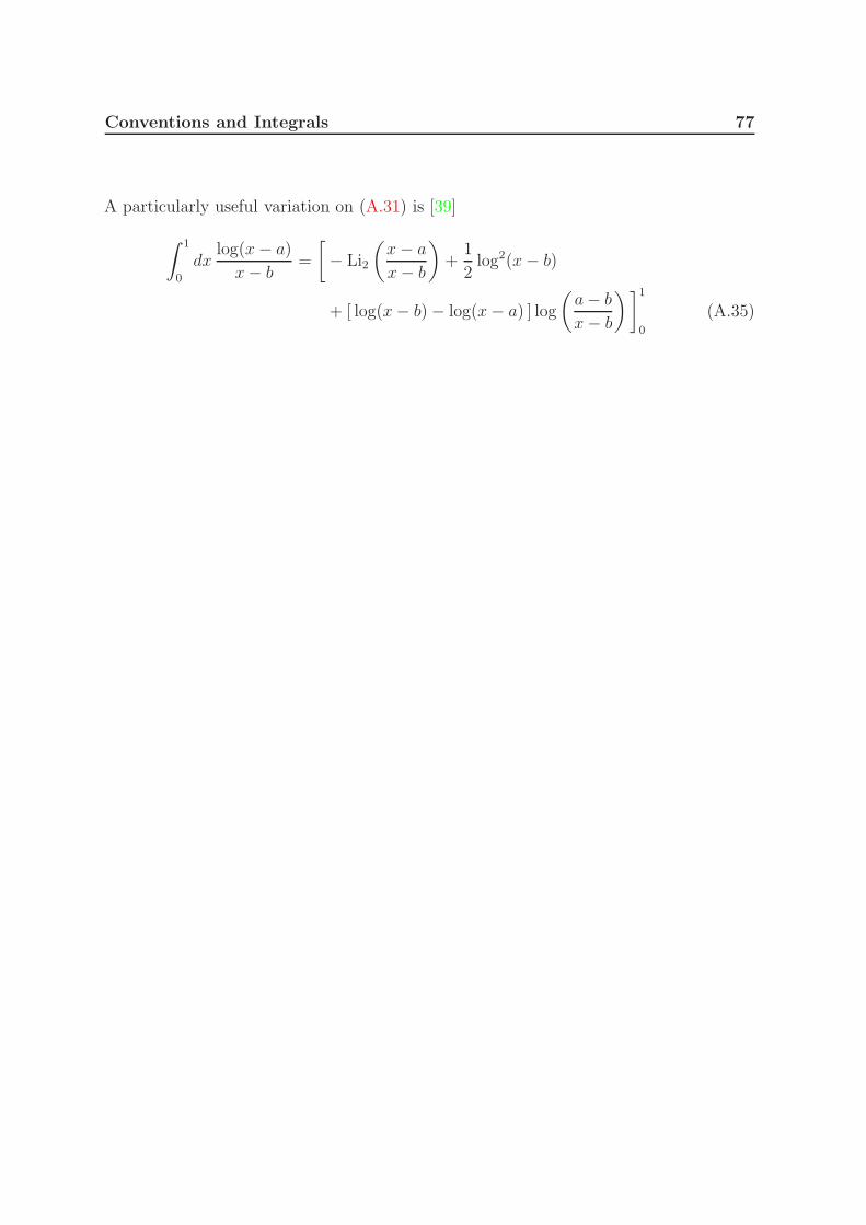
Conventions and Integrals 77
A particularly useful variation on (A.31) is [39]
∫ 1
0
dxlog(x− a)
x− b=
[
− Li2
(x− a
x− b
)
+1
2log2(x− b)
+ [ log(x− b) − log(x− a) ] log
(a− b
x− b
)]1
0
(A.35)

78
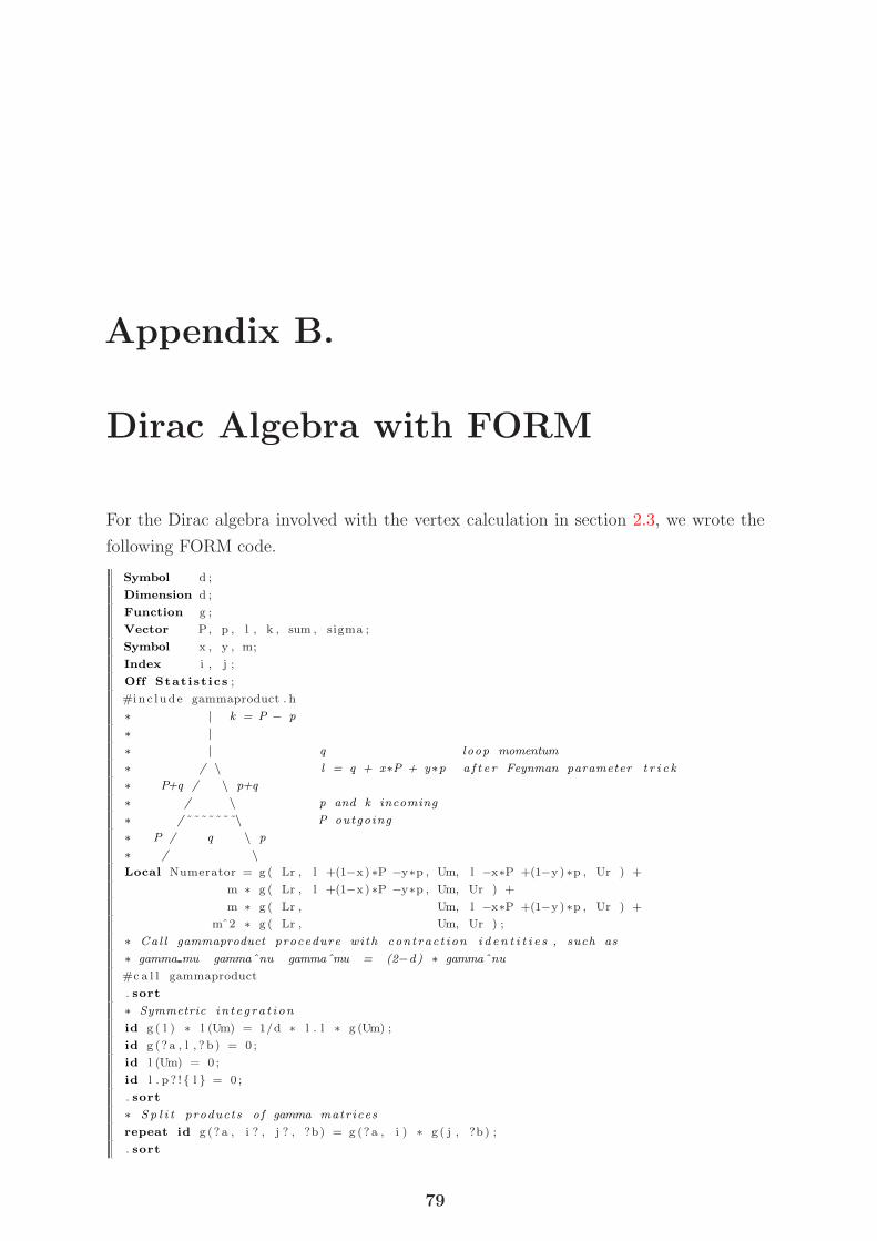
Appendix B.
Dirac Algebra with FORM
For the Dirac algebra involved with the vertex calculation in section 2.3, we wrote the
following FORM code.
Symbol d ;
Dimension d ;
Function g ;
Vector P, p , l , k , sum , sigma ;
Symbol x , y , m;
Index i , j ;
Off Stat i st ics ;
#i nc l ude gammaproduct . h
∗ | k = P − p
∗ |∗ | q loop momentum
∗ / \ l = q + x∗P + y∗p a f t e r Feynman parameter t r i c k
∗ P+q / \ p+q
∗ / \ p and k incoming
∗ /˜˜˜˜˜˜˜\ P outgoing
∗ P / q \ p
∗ / \Local Numerator = g ( Lr , l +(1−x )∗P −y∗p , Um, l −x∗P +(1−y )∗p , Ur ) +
m ∗ g ( Lr , l +(1−x )∗P −y∗p , Um, Ur ) +
m ∗ g ( Lr , Um, l −x∗P +(1−y )∗p , Ur ) +
mˆ2 ∗ g ( Lr , Um, Ur ) ;
∗ Cal l gammaproduct procedure with cont rac t ion i d e n t i t i e s , such as
∗ gamma mu gammaˆnu gammaˆmu = (2−d) ∗ gammaˆnu
#c a l l gammaproduct
. sort
∗ Symmetric i n t e g ra t i on
id g ( l ) ∗ l (Um) = 1/d ∗ l . l ∗ g (Um) ;
id g (? a , l , ? b) = 0 ;
id l (Um) = 0 ;
id l . p ? !{ l } = 0 ;
. sort
∗ S p l i t products o f gamma matrices
repeat id g (? a , i ? , j ? , ?b) = g (? a , i ) ∗ g ( j , ?b) ;
. sort
79
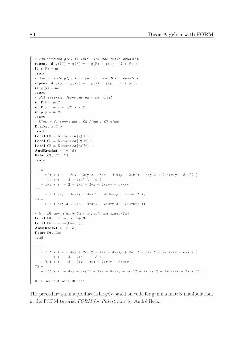
80 Dirac Algebra with FORM
∗ Anticommute g (P) to l e f t , and use Dirac equat ion
repeat id g ( i ?) ∗ g (P) = − g (P) ∗ g ( i ) + 2 ∗ P( i ) ;
id g (P) = m;
. sort
∗ Anticommute g (p ) to r i g h t and use Dirac equat ion
repeat id g (p ) ∗ g ( i ?) = − g ( i ) ∗ g (p) + 2 ∗ p( i ) ;
id g (p) = m;
. sort
∗ Put e x t e rna l fermions on mass s h e l l
id P.P = mˆ2;
id P. p = mˆ2 − 1/2 ∗ k ˆ2 ;
id p . p = mˆ2;
. sort
∗ Nˆmu = C1 gammaˆmu + C2 Pˆmu + C3 pˆmu
Bracket g ,P, p ;
. sort
Local C1 = Numerator [ g (Um) ] ;
Local C2 = Numerator [P(Um) ] ;
Local C3 = Numerator [ p (Um) ] ;
AntiBracket x , y , d ;
Print C1 , C2 , C3 ;
. sort
C1 =
+ mˆ2 ∗ ( 4 − 8∗y − 2∗yˆ2 − 8∗x − 4∗x∗y − 2∗xˆ2 + d∗yˆ2 + 2∗d∗x∗y + d∗xˆ2 )
+ l . l ∗ ( − 4 + 4∗dˆ−1 + d )
+ k∗k ∗ ( − 2 + 2∗y + 2∗x + 2∗x∗y − d∗x∗y ) ;
C2 =
+ m ∗ ( 4∗y + 4∗x∗y + 4∗xˆ2 − 2∗d∗x∗y − 2∗d∗xˆ2 ) ;
C3 =
+ m ∗ ( 4∗yˆ2 + 4∗x + 4∗x∗y − 2∗d∗yˆ2 − 2∗d∗x∗y ) ;
∗ N = D1 gammaˆmu + D2 i sigmaˆmunu k nu /(2m)
Local D1 = C1 + m∗(C2+C3) ;
Local D2 = − m∗(C2+C3) ;
AntiBracket x , y , d ;
Print D1, D2;
. end
D1 =
+ mˆ2 ∗ ( 4 − 4∗y + 2∗yˆ2 − 4∗x + 4∗x∗y + 2∗xˆ2 − d∗yˆ2 − 2∗d∗x∗y − d∗xˆ2 )
+ l . l ∗ ( − 4 + 4∗dˆ−1 + d )
+ k∗k ∗ ( − 2 + 2∗y + 2∗x + 2∗x∗y − d∗x∗y ) ;
D2 =
+ mˆ2 ∗ ( − 4∗y − 4∗yˆ2 − 4∗x − 8∗x∗y − 4∗xˆ2 + 2∗d∗yˆ2 + 4∗d∗x∗y + 2∗d∗xˆ2 ) ;
0 . 00 sec out o f 0 . 00 sec
The procedure gammaproduct is largely based on code for gamma matrix manipulations
in the FORM tutorial FORM for Pedestrians by Andre Heck.
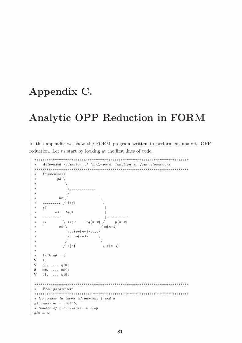
Appendix C.
Analytic OPP Reduction in FORM
In this appendix we show the FORM program written to perform an analytic OPP
reduction. Let us start by looking at the first lines of code.
∗∗∗∗∗∗∗∗∗∗∗∗∗∗∗∗∗∗∗∗∗∗∗∗∗∗∗∗∗∗∗∗∗∗∗∗∗∗∗∗∗∗∗∗∗∗∗∗∗∗∗∗∗∗∗∗∗∗∗∗∗∗∗∗∗∗∗∗∗∗∗∗∗∗∗∗ Automated reduc t ion of (n>4)−poin t func t ion in four dimensions
∗∗∗∗∗∗∗∗∗∗∗∗∗∗∗∗∗∗∗∗∗∗∗∗∗∗∗∗∗∗∗∗∗∗∗∗∗∗∗∗∗∗∗∗∗∗∗∗∗∗∗∗∗∗∗∗∗∗∗∗∗∗∗∗∗∗∗∗∗∗∗∗∗∗∗∗ Conventions
∗ p3 \∗ \∗ \∗ / .
∗ m2 / .
∗ / l+q2 .
∗ p2 | |∗ m1 | l+q1 |∗ | |∗ p1 \ l+q0 l+q{n−2} / p{n−2}∗ m0 \ / m{n−2}∗ \ l+q{n−1} /
∗ / m{n−1} \∗ / \∗ / p{n} \ p{n−1}∗∗ With q0 = 0
V l ;
V q0 , . . . , q10 ;
S m0, . . . , m10 ;
V p1 , . . . , p10 ;
∗∗∗∗∗∗∗∗∗∗∗∗∗∗∗∗∗∗∗∗∗∗∗∗∗∗∗∗∗∗∗∗∗∗∗∗∗∗∗∗∗∗∗∗∗∗∗∗∗∗∗∗∗∗∗∗∗∗∗∗∗∗∗∗∗∗∗∗∗∗∗∗∗∗∗∗ Free parameters
∗∗∗∗∗∗∗∗∗∗∗∗∗∗∗∗∗∗∗∗∗∗∗∗∗∗∗∗∗∗∗∗∗∗∗∗∗∗∗∗∗∗∗∗∗∗∗∗∗∗∗∗∗∗∗∗∗∗∗∗∗∗∗∗∗∗∗∗∗∗∗∗∗∗∗∗ Numerator in terms of momenta l and q
#$numerator = l . q3 ˆ5 ;
∗ Number o f propagators in loop
#$n = 5 ;
81
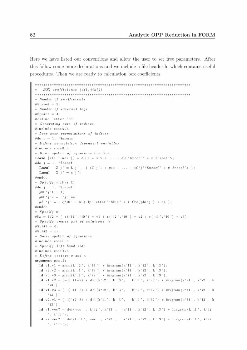
82 Analytic OPP Reduction in FORM
Here we have listed our conventions and allow the user to set free parameters. After
this follow some more declarations and we include a file header.h, which contains useful
procedures. Then we are ready to calculation box coefficients.
∗∗∗∗∗∗∗∗∗∗∗∗∗∗∗∗∗∗∗∗∗∗∗∗∗∗∗∗∗∗∗∗∗∗∗∗∗∗∗∗∗∗∗∗∗∗∗∗∗∗∗∗∗∗∗∗∗∗∗∗∗∗∗∗∗∗∗∗∗∗∗∗∗∗∗ BOX c o e f f i c i e n t s [ d ( l , i j k l ) ]
∗∗∗∗∗∗∗∗∗∗∗∗∗∗∗∗∗∗∗∗∗∗∗∗∗∗∗∗∗∗∗∗∗∗∗∗∗∗∗∗∗∗∗∗∗∗∗∗∗∗∗∗∗∗∗∗∗∗∗∗∗∗∗∗∗∗∗∗∗∗∗∗∗∗∗ Number o f c o e f f i c i e n t s
#$ncoe f = 2 ;
∗ Number o f e x t e r n e l l e g s
#$point = 4 ;
#de f i n e l e t t e r ”d ” ;
∗ Generating s e t s o f i nd i c e s
#inc l ude codeA . h
∗ Loop over permutat ions o f i nd i c e s
#do p = 1 , ‘ $nperm ’
∗ Define permutation dependent v a r i a b l e s
#inc l ude codeB . h
∗ Bui ld system of equat ions L = C. x
Local [ c ( l , ‘ i nd i ’ ) ] = <C11 ∗ x1> + . . . + <C1 ‘ $ncoef ’ ∗ x ‘ $ncoef ’> ;
#do j = 1 , ‘ $ncoef ’
Local Z ‘ j ’ = L ‘ j ’ − ( <C‘ j ’ 1 ∗ x1> + . . . + <C‘ j ’ ‘ $ncoef ’ ∗ x ‘ $ncoef ’> ) ;
Local X‘ j ’ = x ‘ j ’ ;
#enddo
∗ Spec i f y matrix C
#do j = 1 , ‘ $ncoef ’
#$C ‘ j ’ 1 = 1 ;
#$C ‘ j ’ 2 = l ‘ j ’ . n4 ;
#$l ‘ j ’ = − q ‘ i0 ’ − w + lp ‘ l e t t e r ’ ‘ $bin ’ ∗ ( Cos ( phi ‘ j ’ ) ∗ n4 ) ;
#enddo
∗ Spec i f y w
#$w = 1/2 ∗ ( r ( ‘ i1 ’ , ‘ i0 ’ ) ∗ v1 + r ( ‘ i2 ’ , ‘ i0 ’ ) ∗ v2 + r ( ‘ i3 ’ , ‘ i0 ’ ) ∗ v3 ) ;
∗ Spec i f y ang le s phi o f s o l u t i on s l i
#$phi1 = 0 ;
#$phi2 = pi ;
∗ So lve system of equat ions
#inc l ude codeC . h
∗ Spec i f y l e f t hand s i de
#inc l ude codeD . h
∗ Define v e c t o r s v and n
argument pow , 2 ;
id v1 . v1 = gram (k ‘ i2 ’ , k ‘ i3 ’ ) ∗ invgram (k ‘ i1 ’ , k ‘ i2 ’ , k ‘ i3 ’ ) ;
id v2 . v2 = gram (k ‘ i1 ’ , k ‘ i3 ’ ) ∗ invgram (k ‘ i1 ’ , k ‘ i2 ’ , k ‘ i3 ’ ) ;
id v3 . v3 = gram (k ‘ i1 ’ , k ‘ i2 ’ ) ∗ invgram (k ‘ i1 ’ , k ‘ i2 ’ , k ‘ i3 ’ ) ;
id v1 . v2 = (−1) ˆ(1+2) ∗ de l (k ‘ i2 ’ , k ‘ i3 ’ , k ‘ i1 ’ , k ‘ i3 ’ ) ∗ invgram (k ‘ i1 ’ , k ‘ i2 ’ , k
‘ i3 ’ ) ;
id v1 . v3 = (−1) ˆ(1+3) ∗ de l (k ‘ i2 ’ , k ‘ i3 ’ , k ‘ i1 ’ , k ‘ i2 ’ ) ∗ invgram (k ‘ i1 ’ , k ‘ i2 ’ , k
‘ i3 ’ ) ;
id v2 . v3 = (−1) ˆ(2+3) ∗ de l (k ‘ i1 ’ , k ‘ i3 ’ , k ‘ i1 ’ , k ‘ i2 ’ ) ∗ invgram (k ‘ i1 ’ , k ‘ i2 ’ , k
‘ i3 ’ ) ;
id v1 . vec ? = de l ( vec , k ‘ i2 ’ , k ‘ i3 ’ , k ‘ i1 ’ , k ‘ i2 ’ , k ‘ i3 ’ ) ∗ invgram (k ‘ i1 ’ , k ‘ i2
’ , k ‘ i3 ’ ) ;
id v2 . vec ? = de l (k ‘ i1 ’ , vec , k ‘ i3 ’ , k ‘ i1 ’ , k ‘ i2 ’ , k ‘ i3 ’ ) ∗ invgram (k ‘ i1 ’ , k ‘ i2
’ , k ‘ i3 ’ ) ;
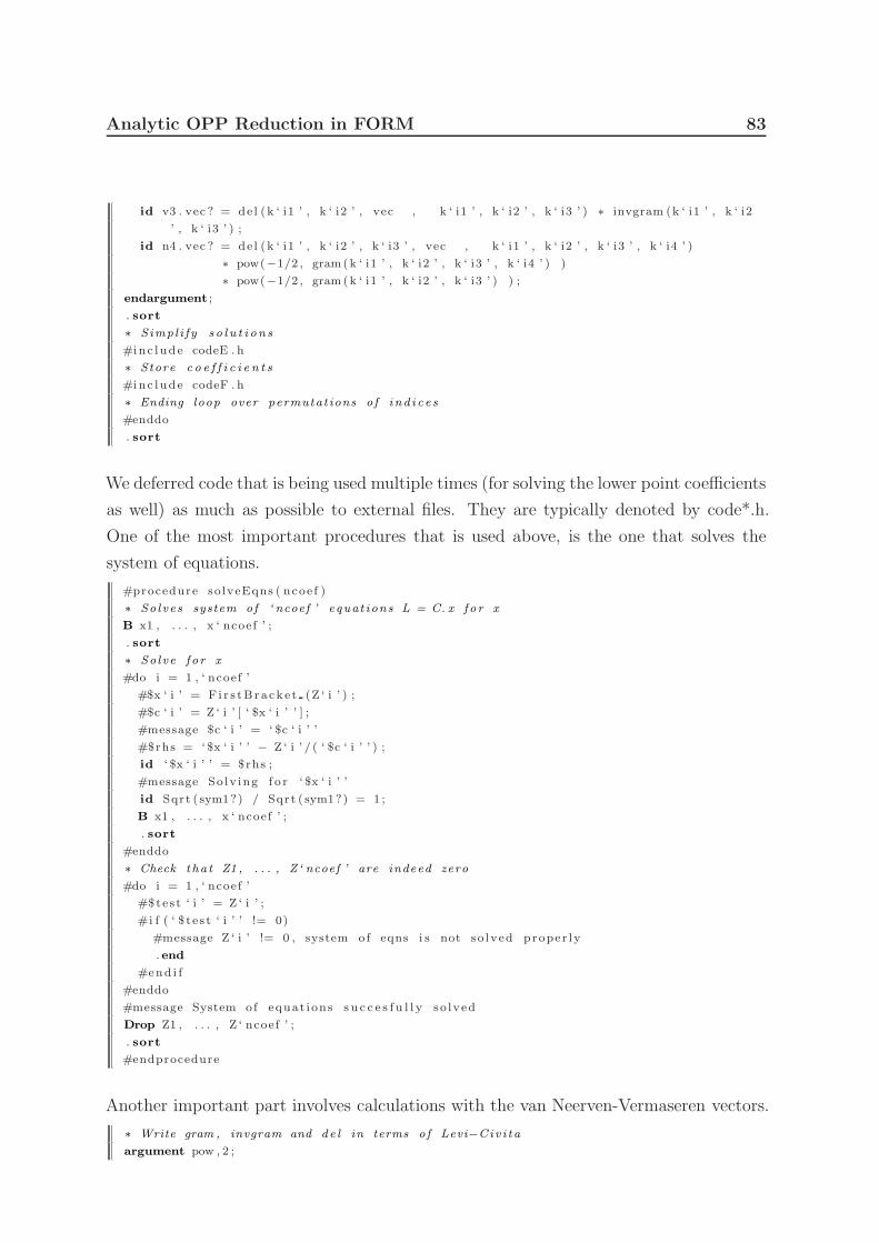
Analytic OPP Reduction in FORM 83
id v3 . vec ? = de l (k ‘ i1 ’ , k ‘ i2 ’ , vec , k ‘ i1 ’ , k ‘ i2 ’ , k ‘ i3 ’ ) ∗ invgram (k ‘ i1 ’ , k ‘ i2
’ , k ‘ i3 ’ ) ;
id n4 . vec ? = de l (k ‘ i1 ’ , k ‘ i2 ’ , k ‘ i3 ’ , vec , k ‘ i1 ’ , k ‘ i2 ’ , k ‘ i3 ’ , k ‘ i4 ’ )
∗ pow(−1/2 , gram (k ‘ i1 ’ , k ‘ i2 ’ , k ‘ i3 ’ , k ‘ i4 ’ ) )
∗ pow(−1/2 , gram (k ‘ i1 ’ , k ‘ i2 ’ , k ‘ i3 ’ ) ) ;
endargument ;
. sort
∗ Simpl i f y s o l u t i on s
#inc l ude codeE . h
∗ Store c o e f f i c i e n t s
#inc l ude codeF . h
∗ Ending loop over permutat ions o f i nd i c e s
#enddo
. sort
We deferred code that is being used multiple times (for solving the lower point coefficients
as well) as much as possible to external files. They are typically denoted by code*.h.
One of the most important procedures that is used above, is the one that solves the
system of equations.
#procedure solveEqns ( ncoe f )
∗ So lve s system of ‘ ncoef ’ equat ions L = C. x f o r x
B x1 , . . . , x ‘ ncoef ’ ;
. sort
∗ So lve f o r x
#do i = 1 , ‘ ncoef ’
#$x ‘ i ’ = F i r s tB r acke t (Z ‘ i ’ ) ;
#$c ‘ i ’ = Z ‘ i ’ [ ‘ $x ‘ i ’ ’ ] ;
#message $c ‘ i ’ = ‘ $c ‘ i ’ ’
#$rhs = ‘ $x ‘ i ’ ’ − Z ‘ i ’ / ( ‘ $c ‘ i ’ ’ ) ;
id ‘ $x ‘ i ’ ’ = $rhs ;
#message So lv ing f o r ‘ $x ‘ i ’ ’
id Sqrt ( sym1?) / Sqrt ( sym1?) = 1 ;
B x1 , . . . , x ‘ ncoef ’ ;
. sort
#enddo
∗ Check t ha t Z1 , . . . , Z ‘ ncoef ’ are indeed zero
#do i = 1 , ‘ ncoef ’
#$tes t ‘ i ’ = Z ‘ i ’ ;
#i f ( ‘ $ tes t ‘ i ’ ’ != 0)
#message Z ‘ i ’ != 0 , system of eqns i s not so lved proper l y
. end
#end i f
#enddo
#message System of equat i ons s u c c e s f u l l y so lved
Drop Z1 , . . . , Z ‘ ncoef ’ ;
. sort
#endprocedure
Another important part involves calculations with the van Neerven-Vermaseren vectors.
∗ Write gram , invgram and de l in terms of Levi−Civ i ta
argument pow , 2 ;
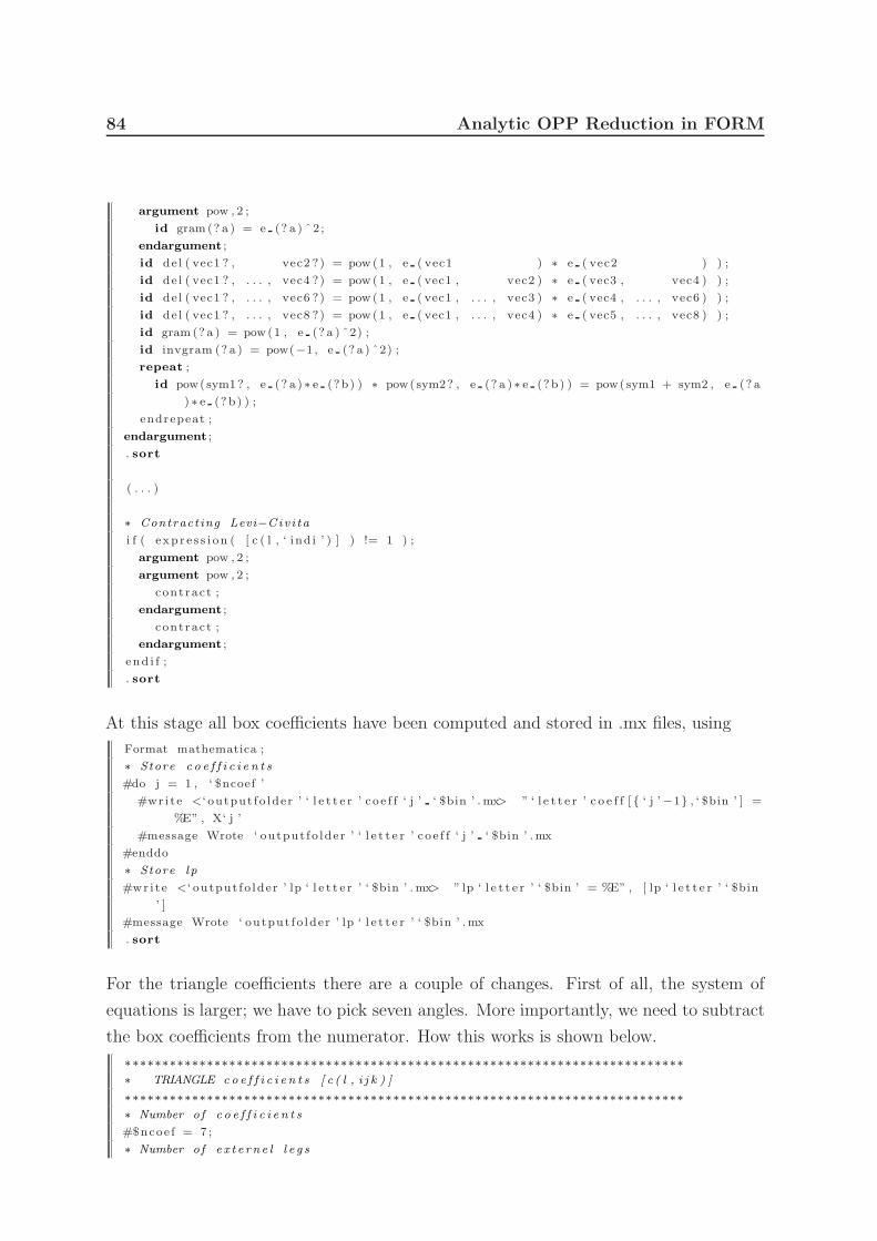
84 Analytic OPP Reduction in FORM
argument pow , 2 ;
id gram (? a ) = e (? a ) ˆ2 ;
endargument ;
id de l ( vec1 ? , vec2 ?) = pow (1 , e ( vec1 ) ∗ e ( vec2 ) ) ;
id de l ( vec1 ? , . . . , vec4 ?) = pow (1 , e ( vec1 , vec2 ) ∗ e ( vec3 , vec4 ) ) ;
id de l ( vec1 ? , . . . , vec6 ?) = pow (1 , e ( vec1 , . . . , vec3 ) ∗ e ( vec4 , . . . , vec6 ) ) ;
id de l ( vec1 ? , . . . , vec8 ?) = pow (1 , e ( vec1 , . . . , vec4 ) ∗ e ( vec5 , . . . , vec8 ) ) ;
id gram (? a ) = pow (1 , e (? a ) ˆ2) ;
id invgram (? a ) = pow(−1 , e (? a ) ˆ2) ;
repeat ;
id pow( sym1? , e (? a ) ∗ e (?b) ) ∗ pow( sym2? , e (? a ) ∗ e (? b) ) = pow(sym1 + sym2 , e (? a
) ∗ e (? b) ) ;
endrepeat ;
endargument ;
. sort
( . . . )
∗ Contract ing Levi−Civ i ta
i f ( exp r e s s i on ( [ c ( l , ‘ i nd i ’ ) ] ) != 1 ) ;
argument pow , 2 ;
argument pow , 2 ;
contract ;
endargument ;
contract ;
endargument ;
end i f ;
. sort
At this stage all box coefficients have been computed and stored in .mx files, using
Format mathematica ;
∗ Store c o e f f i c i e n t s
#do j = 1 , ‘ $ncoef ’
#wr i te <‘ output f o lder ’ ‘ l e t t e r ’ c o e f f ‘ j ’ ‘ $bin ’ . mx> ” ‘ l e t t e r ’ c o e f f [ { ‘ j ’−1} , ‘ $bin ’ ] =
%E” , X‘ j ’
#message Wrote ‘ output f o lder ’ ‘ l e t t e r ’ c o e f f ‘ j ’ ‘ $bin ’ .mx
#enddo
∗ Store l p
#wr i te <‘ output f o lder ’ lp ‘ l e t t e r ’ ‘ $bin ’ . mx> ” lp ‘ l e t t e r ’ ‘ $bin ’ = %E” , [ lp ‘ l e t t e r ’ ‘ $bin
’ ]
#message Wrote ‘ output f o lder ’ lp ‘ l e t t e r ’ ‘ $bin ’ .mx
. sort
For the triangle coefficients there are a couple of changes. First of all, the system of
equations is larger; we have to pick seven angles. More importantly, we need to subtract
the box coefficients from the numerator. How this works is shown below.
∗∗∗∗∗∗∗∗∗∗∗∗∗∗∗∗∗∗∗∗∗∗∗∗∗∗∗∗∗∗∗∗∗∗∗∗∗∗∗∗∗∗∗∗∗∗∗∗∗∗∗∗∗∗∗∗∗∗∗∗∗∗∗∗∗∗∗∗∗∗∗∗∗∗∗∗ TRIANGLE c o e f f i c i e n t s [ c ( l , i j k ) ]
∗∗∗∗∗∗∗∗∗∗∗∗∗∗∗∗∗∗∗∗∗∗∗∗∗∗∗∗∗∗∗∗∗∗∗∗∗∗∗∗∗∗∗∗∗∗∗∗∗∗∗∗∗∗∗∗∗∗∗∗∗∗∗∗∗∗∗∗∗∗∗∗∗∗∗∗ Number o f c o e f f i c i e n t s
#$ncoe f = 7 ;
∗ Number o f e x t e r n e l l e g s
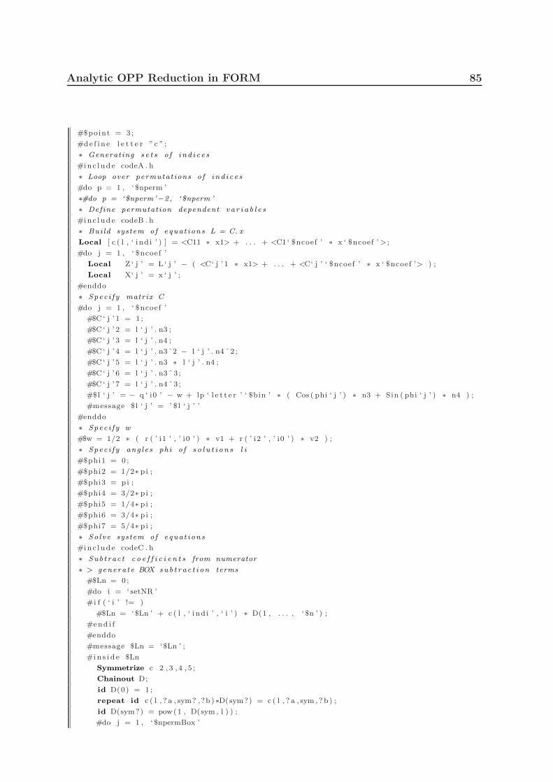
Analytic OPP Reduction in FORM 85
#$point = 3 ;
#de f i n e l e t t e r ” c ” ;
∗ Generating s e t s o f i nd i c e s
#inc l ude codeA . h
∗ Loop over permutat ions o f i nd i c e s
#do p = 1 , ‘ $nperm ’
∗#do p = ‘$nperm’−2 , ‘$nperm ’
∗ Define permutation dependent v a r i a b l e s
#inc l ude codeB . h
∗ Bui ld system of equat ions L = C. x
Local [ c ( l , ‘ i nd i ’ ) ] = <C11 ∗ x1> + . . . + <C1 ‘ $ncoef ’ ∗ x ‘ $ncoef ’> ;
#do j = 1 , ‘ $ncoef ’
Local Z ‘ j ’ = L ‘ j ’ − ( <C‘ j ’ 1 ∗ x1> + . . . + <C‘ j ’ ‘ $ncoef ’ ∗ x ‘ $ncoef ’> ) ;
Local X‘ j ’ = x ‘ j ’ ;
#enddo
∗ Spec i f y matrix C
#do j = 1 , ‘ $ncoef ’
#$C ‘ j ’ 1 = 1 ;
#$C ‘ j ’ 2 = l ‘ j ’ . n3 ;
#$C ‘ j ’ 3 = l ‘ j ’ . n4 ;
#$C ‘ j ’ 4 = l ‘ j ’ . n3ˆ2 − l ‘ j ’ . n4 ˆ2 ;
#$C ‘ j ’ 5 = l ‘ j ’ . n3 ∗ l ‘ j ’ . n4 ;
#$C ‘ j ’ 6 = l ‘ j ’ . n3 ˆ3 ;
#$C ‘ j ’ 7 = l ‘ j ’ . n4 ˆ3 ;
#$l ‘ j ’ = − q ‘ i0 ’ − w + lp ‘ l e t t e r ’ ‘ $bin ’ ∗ ( Cos ( phi ‘ j ’ ) ∗ n3 + Sin ( phi ‘ j ’ ) ∗ n4 ) ;
#message $l ‘ j ’ = ’ $l ‘ j ’ ’
#enddo
∗ Spec i f y w
#$w = 1/2 ∗ ( r ( ’ i1 ’ , ’ i0 ’ ) ∗ v1 + r ( ’ i2 ’ , ’ i0 ’ ) ∗ v2 ) ;
∗ Spec i f y ang le s phi o f s o l u t i on s l i
#$phi1 = 0 ;
#$phi2 = 1/2∗ pi ;
#$phi3 = pi ;
#$phi4 = 3/2∗ pi ;
#$phi5 = 1/4∗ pi ;
#$phi6 = 3/4∗ pi ;
#$phi7 = 5/4∗ pi ;
∗ So lve system of equat ions
#inc l ude codeC . h
∗ Sub t rac t c o e f f i c i e n t s from numerator
∗ > generat e BOX sub t rac t i on terms
#$Ln = 0 ;
#do i = ‘ setNR ’
#i f ( ‘ i ’ != )
#$Ln = ‘$Ln ’ + c ( l , ‘ i nd i ’ , ‘ i ’ ) ∗ D(1 , . . . , ‘ $n ’ ) ;
#end i f
#enddo
#message $Ln = ‘$Ln ’ ;
#i n s i d e $Ln
Symmetrize c 2 , 3 , 4 , 5 ;
Chainout D;
id D(0) = 1 ;
repeat id c ( l , ? a , sym? ,?b ) ∗D(sym?) = c ( l , ? a , sym , ? b) ;
id D(sym?) = pow(1 , D(sym , l ) ) ;
#do j = 1 , ‘ $npermBox ’
86 Analytic OPP Reduction in FORM
id c ( l , ‘ $iBox ‘ j ’ ’ ) = [ c ( l , ‘ $iBox ‘ j ’ ’ ) ] ;
#enddo
#endins ide
#message $Ln = ‘$Ln ’ ;
∗ > sub t r ac t from numerator
id Ln( l ?) = Ln( l ) − ( ‘ $Ln ’ ) ;
. sort
∗ Spec i f y l e f t hand s i de
#inc l ude codeD . h
∗ Define v e c t o r s v and n
argument pow , 2 ;
id v1 . v1 = gram (k ‘ i2 ’ ) ∗ invgram (k ‘ i1 ’ , k ‘ i2 ’ ) ;
id v2 . v2 = gram (k ‘ i1 ’ ) ∗ invgram (k ‘ i1 ’ , k ‘ i2 ’ ) ;
id v1 . v2 = (−1) ˆ(1+2) ∗ de l (k ‘ i2 ’ , k ‘ i1 ’ ) ∗ invgram (k ‘ i1 ’ , k ‘ i2 ’ ) ;
id v1 . vec ? = de l ( vec , k ‘ i2 ’ , k ‘ i1 ’ , k ‘ i2 ’ ) ∗ invgram (k ‘ i1 ’ , k ‘ i2 ’ ) ;
id v2 . vec ? = de l (k ‘ i1 ’ , vec , k ‘ i1 ’ , k ‘ i2 ’ ) ∗ invgram (k ‘ i1 ’ , k ‘ i2 ’ ) ;
id n3 . vec ? = de l (k ‘ i1 ’ , k ‘ i2 ’ , vec , k ‘ i1 ’ , k ‘ i2 ’ , k ‘ i3 ’ )
∗ pow(−1/2 , gram (k ‘ i1 ’ , k ‘ i2 ’ , k ‘ i3 ’ ) )
∗ pow(−1/2 , gram (k ‘ i1 ’ , k ‘ i2 ’ ) ) ;
id n4 . vec ? = de l (k ‘ i1 ’ , k ‘ i2 ’ , k ‘ i3 ’ , vec , k ‘ i1 ’ , k ‘ i2 ’ , k ‘ i3 ’ , k ‘ i4 ’ )
∗ pow(−1/2 , gram (k ‘ i1 ’ , k ‘ i2 ’ , k ‘ i3 ’ , k ‘ i4 ’ ) )
∗ pow(−1/2 , gram (k ‘ i1 ’ , k ‘ i2 ’ , k ‘ i3 ’ ) ) ;
id v1 = de l (k ‘ i2 ’ , k ‘ i2 ’ ) ∗ invgram (k ‘ i1 ’ , k ‘ i2 ’ ) ∗ k ‘ i1 ’ − de l (k ‘ i2 ’ , k ‘ i1 ’ ) ∗invgram (k ‘ i1 ’ , k ‘ i2 ’ ) ∗ k ‘ i2 ’ ;
id v2 = de l (k ‘ i1 ’ , k ‘ i1 ’ ) ∗ invgram (k ‘ i1 ’ , k ‘ i2 ’ ) ∗ k ‘ i2 ’ − de l (k ‘ i1 ’ , k ‘ i2 ’ ) ∗invgram (k ‘ i1 ’ , k ‘ i2 ’ ) ∗ k ‘ i1 ’ ;
id n3 = de l (k ‘ i1 ’ , k ‘ i2 ’ , k ‘ i1 ’ , k ‘ i2 ’ ) ∗ pow(−1/2 , gram (k ‘ i1 ’ , k ‘ i2 ’ , k ‘ i3 ’ ) ) ∗pow(−1/2 , gram (k ‘ i1 ’ , k ‘ i2 ’ ) ) ∗ k ‘ i3 ’
− de l (k ‘ i1 ’ , k ‘ i2 ’ , k ‘ i1 ’ , k ‘ i3 ’ ) ∗ pow(−1/2 , gram (k ‘ i1 ’ , k ‘ i2 ’ , k ‘ i3 ’ ) ) ∗pow(−1/2 , gram (k ‘ i1 ’ , k ‘ i2 ’ ) ) ∗ k ‘ i2 ’
+ de l (k ‘ i1 ’ , k ‘ i2 ’ , k ‘ i2 ’ , k ‘ i3 ’ ) ∗ pow(−1/2 , gram (k ‘ i1 ’ , k ‘ i2 ’ , k ‘ i3 ’ ) ) ∗pow(−1/2 , gram (k ‘ i1 ’ , k ‘ i2 ’ ) ) ∗ k ‘ i1 ’ ;
id n4 = de l (k ‘ i1 ’ , k ‘ i2 ’ , k ‘ i3 ’ , k ‘ i1 ’ , k ‘ i2 ’ , k ‘ i3 ’ ) ∗ pow(−1/2 , gram (k ‘ i1 ’ , k ‘ i2
’ , k ‘ i3 ’ , k ‘ i4 ’ ) ) ∗ pow(−1/2 , gram (k ‘ i1 ’ , k ‘ i2 ’ , k ‘ i3 ’ ) ) ∗ k ‘ i4 ’
− de l (k ‘ i1 ’ , k ‘ i2 ’ , k ‘ i3 ’ , k ‘ i1 ’ , k ‘ i2 ’ , k ‘ i4 ’ ) ∗ pow(−1/2 , gram (k ‘ i1 ’ , k ‘ i2
’ , k ‘ i3 ’ , k ‘ i4 ’ ) ) ∗ pow(−1/2 , gram (k ‘ i1 ’ , k ‘ i2 ’ , k ‘ i3 ’ ) ) ∗ k ‘ i3 ’
+ de l (k ‘ i1 ’ , k ‘ i2 ’ , k ‘ i3 ’ , k ‘ i1 ’ , k ‘ i3 ’ , k ‘ i4 ’ ) ∗ pow(−1/2 , gram (k ‘ i1 ’ , k ‘ i2
’ , k ‘ i3 ’ , k ‘ i4 ’ ) ) ∗ pow(−1/2 , gram (k ‘ i1 ’ , k ‘ i2 ’ , k ‘ i3 ’ ) ) ∗ k ‘ i2 ’
− de l (k ‘ i1 ’ , k ‘ i2 ’ , k ‘ i3 ’ , k ‘ i2 ’ , k ‘ i3 ’ , k ‘ i4 ’ ) ∗ pow(−1/2 , gram (k ‘ i1 ’ , k ‘ i2
’ , k ‘ i3 ’ , k ‘ i4 ’ ) ) ∗ pow(−1/2 , gram (k ‘ i1 ’ , k ‘ i2 ’ , k ‘ i3 ’ ) ) ∗ k ‘ i1 ’ ;
endargument ;
. sort
∗ Simpl i f y s o l u t i on s
#inc l ude codeE . h
∗ Store c o e f f i c i e n t s
#inc l ude codeF . h
∗ Ending loop over permutat ions o f i nd i c e s
#enddo
. sort
Notice also the difference in the van Neerven-Vermaseren vectors, with respect to the
box case. In a similar fashion also the bubble and tadpole coefficients are computed.
Finally we merge the .mx outputfiles into a few files, for importing into Mathematica.
Analytic OPP Reduction in FORM 87
∗∗∗∗∗∗∗∗∗∗∗∗∗∗∗∗∗∗∗∗∗∗∗∗∗∗∗∗∗∗∗∗∗∗∗∗∗∗∗∗∗∗∗∗∗∗∗∗∗∗∗∗∗∗∗∗∗∗∗∗∗∗∗∗∗∗∗∗∗∗∗∗∗∗∗∗ Merge o u t p u t f i l e s
∗∗∗∗∗∗∗∗∗∗∗∗∗∗∗∗∗∗∗∗∗∗∗∗∗∗∗∗∗∗∗∗∗∗∗∗∗∗∗∗∗∗∗∗∗∗∗∗∗∗∗∗∗∗∗∗∗∗∗∗∗∗∗∗∗∗∗∗∗∗∗∗∗∗∗#system . / mergeformoutput ‘ output f o lder ’ gram
#system . / mergeformoutput ‘ output f o lder ’ l p
#system . / mergeformoutput ‘ output f o lder ’ d c o e f f
#system . / mergeformoutput ‘ output f o lder ’ c c o e f f
#system . / mergeformoutput ‘ output f o lder ’ b c o e f f
#system . / mergeformoutput ‘ output f o lder ’ a c o e f f
. end

88
Bibliography
[1] J. Schwinger, On quantum-electrodynamics and the magnetic moment of the
electron, Phys. Rev. 73 (Feb, 1948) 416–417.
[2] G. ’t Hooft and M. Veltman, Scalar One Loop Integrals, Nucl.Phys. B153 (1979)365–401.
[3] G. Passarino and M. Veltman, One Loop Corrections for e+ e- Annihilation Into
mu+ mu- in the Weinberg Model, Nucl.Phys. B160 (1979) 151.
[4] G. ’t Hooft and M. J. G. Veltman, Diagrammar. CERN, Geneva, 1973.
[5] J. Bjorken and S. Drell, Relativistic quantum mechanics. International series inpure and applied physics. McGraw-Hill, 1964.
[6] W. L. van Neerven and J. A. M. Vermaseren, LARGE LOOP INTEGRALS, Phys.
Lett. B137 (1984) 241.
[7] Z. Bern, L. J. Dixon, D. C. Dunbar and D. A. Kosower, Fusing gauge theory tree
amplitudes into loop amplitudes, Nucl.Phys. B435 (1995) 59–101[hep-ph/9409265].
[8] Z. Bern and A. Morgan, Massive loop amplitudes from unitarity, Nucl.Phys. B467
(1996) 479–509 [hep-ph/9511336].
[9] G. Ossola, C. G. Papadopoulos and R. Pittau, Reducing full one-loop amplitudes
to scalar integrals at the integrand level, Nucl.Phys. B763 (2007) 147–169[hep-ph/0609007].
[10] G. Ossola, C. G. Papadopoulos and R. Pittau, CutTools: A Program
implementing the OPP reduction method to compute one-loop amplitudes, JHEP
0803 (2008) 042 [0711.3596].
[11] G. Cullen, N. Greiner, G. Heinrich, G. Luisoni, P. Mastrolia et. al., Automated
One-Loop Calculations with GoSam, Eur.Phys.J. C72 (2012) 1889 [1111.2034].
[12] J. Gatheral, EXPONENTIATION OF EIKONAL CROSS-SECTIONS IN
NONABELIAN GAUGE THEORIES, Phys.Lett. B133 (1983) 90.
[13] M. Peskin and D. Schroeder, Introduction to quantum field theory. AdvancedBook Program. Addison-Wesley Pub. Co., 1995.
[14] B. de Wit and J. Smith, Field theory in particle physics. No. v. 1 in
89
90 Bibliography
North-Holland Personal Library. North-Holland, 1986.
[15] J. Kuipers, T. Ueda, J. A. M. Vermaseren and J. Vollinga, FORM version 4.0,ArXiv e-prints (Mar., 2012) [1203.6543].
[16] R. Cutkosky, Singularities and discontinuities of Feynman amplitudes,J.Math.Phys. 1 (1960) 429–433.
[17] M. Veltman, Diagrammatica: the path to Feynman rules. Cambridge lecture notesin physics. Cambridge University Press, 1994.
[18] R. D. L. KRONIG, On the theory of dispersion of x-rays, J. Opt. Soc. Am. 12
(Jun, 1926) 547–556.
[19] O. Yudilevich, Calculating massive one-loop amplitudes, Master’s thesis, UtrechtUniversity, 2009.
[20] Z. Bern, L. J. Dixon, D. C. Dunbar and D. A. Kosower, One loop n point gauge
theory amplitudes, unitarity and collinear limits, Nucl.Phys. B425 (1994) 217–260[hep-ph/9403226].
[21] Z. Bern, L. J. Dixon and D. A. Kosower, On-Shell Methods in Perturbative QCD,Annals Phys. 322 (2007) 1587–1634 [0704.2798].
[22] R. K. Ellis and G. Zanderighi, Scalar one-loop integrals for QCD, JHEP 0802
(2008) 002 [0712.1851].
[23] F. del Aguila and R. Pittau, Recursive numerical calculus of one-loop tensor
integrals, JHEP 0407 (2004) 017 [hep-ph/0404120].
[24] W. Giele and G. Zanderighi, On the Numerical Evaluation of One-Loop
Amplitudes: The Gluonic Case, JHEP 0806 (2008) 038 [0805.2152].
[25] R. K. Ellis, Z. Kunszt, K. Melnikov and G. Zanderighi, One-loop calculations in
quantum field theory: from Feynman diagrams to unitarity cuts, 1105.4319.
[26] P. Mastrolia, G. Ossola, C. Papadopoulos and R. Pittau, Optimizing the
Reduction of One-Loop Amplitudes, JHEP 0806 (2008) 030 [0803.3964].
[27] G. Ossola, C. G. Papadopoulos and R. Pittau, On the Rational Terms of the
one-loop amplitudes, JHEP 0805 (2008) 004 [0802.1876].
[28] T. Binoth, J. P. Guillet and G. Heinrich, Algebraic evaluation of rational
polynomials in one-loop amplitudes, JHEP 0702 (2007) 013 [hep-ph/0609054].
[29] P. Draggiotis, M. Garzelli, C. Papadopoulos and R. Pittau, Feynman Rules for the
Rational Part of the QCD 1-loop amplitudes, JHEP 0904 (2009) 072 [0903.0356].
[30] M. Garzelli, I. Malamos and R. Pittau, Feynman rules for the rational part of the
Electroweak 1-loop amplitudes, JHEP 1001 (2010) 040 [0910.3130].
[31] M. Garzelli, I. Malamos and R. Pittau, Feynman rules for the rational part of the
Bibliography 91
Electroweak 1-loop amplitudes in the Rxi gauge and in the Unitary gauge, JHEP
1101 (2011) 029 [1009.4302].
[32] J. Alwall, M. Herquet, F. Maltoni, O. Mattelaer and T. Stelzer, MadGraph 5 :
Going Beyond, JHEP 1106 (2011) 128 [1106.0522].
[33] S. Agrawal, T. Hahn and E. Mirabella, FormCalc 7, 1112.0124.
[34] P. Mastrolia, G. Ossola, T. Reiter and F. Tramontano, Scattering AMplitudes
from Unitarity-based Reduction Algorithm at the Integrand-level, JHEP 1008
(2010) 080 [1006.0710].
[35] J. Kuipers, J. A. M. Vermaseren, A. Plaat and H. J. van den Herik, Improving
multivariate Horner schemes with Monte Carlo tree search, ArXiv e-prints (July,2012) [1207.7079].
[36] E. Laenen, L. Magnea, G. Stavenga and C. D. White, Next-to-eikonal corrections
to soft gluon radiation: a diagrammatic approach, JHEP 1101 (2011) 141[1010.1860].
[37] G. Sterman, An introduction to quantum field theory. Cambridge University Press,1993.
[38] L. Lewin, Polylogarithms and associated functions. North Holland, 1981.
[39] W. Beenakker and A. Denner, Infrared divergent scalar box integrals with
applications in the electroweak standard model, Nuclear Physics B 338 (1990),no. 2 349 – 370.


![Loop Quantum Cosmology - Home - Springer...Loop quantum cosmology is based on quantum Riemannian geometry, or loop quantum gravity [172, 22, 195, 174], which is an attempt at a non-perturbative](https://img.pdfslide.us/doc/110x75/60f689d85e1267535167be75/loop-quantum-cosmology-home-springer-loop-quantum-cosmology-is-based-on.jpg)