Embed Size (px)
Citation preview
Path-dependent optionsBlack-Scholes model
dSt
St
= rdt+ σdBt, S0 = s0,
• Barrier option.
• Asian option.
• Lookback option
2
Barrier optionThe price of an down-out option
P (0, s) = E[e−rT
f(ST )1(mT>L)|S0 = s].
where mT is
mT = min0≤t≤T
St
3
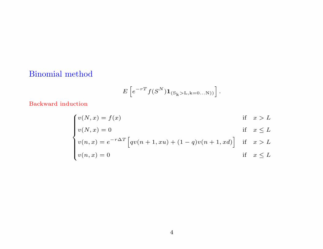
Binomial method
E[e−rT
f(SN )1(Sk>L,k=0...N))
].
Backward induction
v(N, x) = f(x) if x > L
v(N, x) = 0 if x ≤ L
v(n, x) = e−r∆T
[qv(n + 1, xu) + (1 − q)v(n+ 1, xd)
]if x > L
v(n, x) = 0 if x ≤ L
4
DrawbacksThe classical CRR may be problematic when applied to barrier options because the convergence
is very slow compared with that for standard vanilla options. (Boyle and Lau Journal of
Derivatives 94)
The reason is clear: let nL denote the index such that
S0dnL ≥ L > S0d
nL+1
Then the algorithm, N being fixed, yields the same result for any value of the barrier between
S0dnL and S0d
nL+1.
5
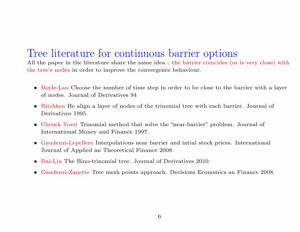
Tree literature for continuous barrier optionsAll the paper in the literature share the same idea : the barrier coincides (or is very close) with
the tree’s nodes in order to improve the convergence behaviour.
• Boyle-Lau Choose the number of time step in order to be close to the barrier with a layer
of nodes. Journal of Derivatives 94
• Ritchken He align a layer of nodes of the trinomial tree with each barrier. Journal of
Derivatives 1995.
• Cheuck Vorst Trinomial method that solve the “near-barrier” problem. Journal of
International Money and Finance 1997.
• Gaudenzi-Lepellere Interpolations near barrier and intial stock prices. International
Journal of Applied an Theoretical Finance 2008.
• Dai-Liu The Bino-trinomial tree. Journal of Derivatives 2010.
• Gaudenzi-Zanette Tree mesh points approach. Decisions Economics an Finance 2008.
6
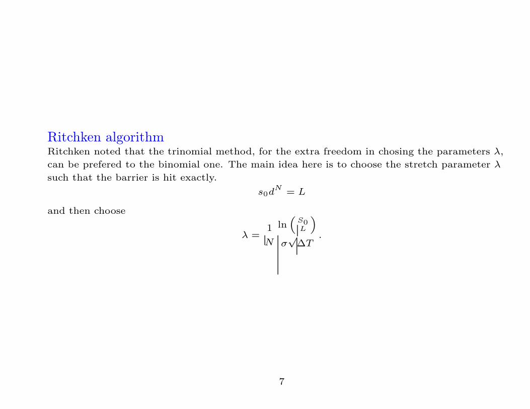
Ritchken algorithmRitchken noted that the trinomial method, for the extra freedom in chosing the parameters λ,
can be prefered to the binomial one. The main idea here is to choose the stretch parameter λ
such that the barrier is hit exactly.
s0dN = L
and then choose
λ =1
N
ln(
S0L
)
σ√∆T
.
7
Tree mesh points method
• As remarked in several previous papers (see Boyle-Lau 94,Cheuk-Vorst 97,
Gaudenzi-Lepellere 06) the price of a barrier option is a ’good approximation’ of the
continuous value when the barrier lies (or it is close) on a line of nodes of the tree.
• We construct a tree where all the tree mesh points are generated by the barrier itself.
• permits us to treat in a natural way and efficiently the ’near-barrier’ problem, that occurs
when the initial asset price is very close to the barrier.
8

Tree mesh points
It is worth to say that the mesh does not seem to be natural in order to describe the evolution of
the asset price.
Nevertheless, this is not important. In fact we only need to set up the state-space of the Markov
chain that we want to approximate the continuous time process.
Finite Difference approach for PDE
9
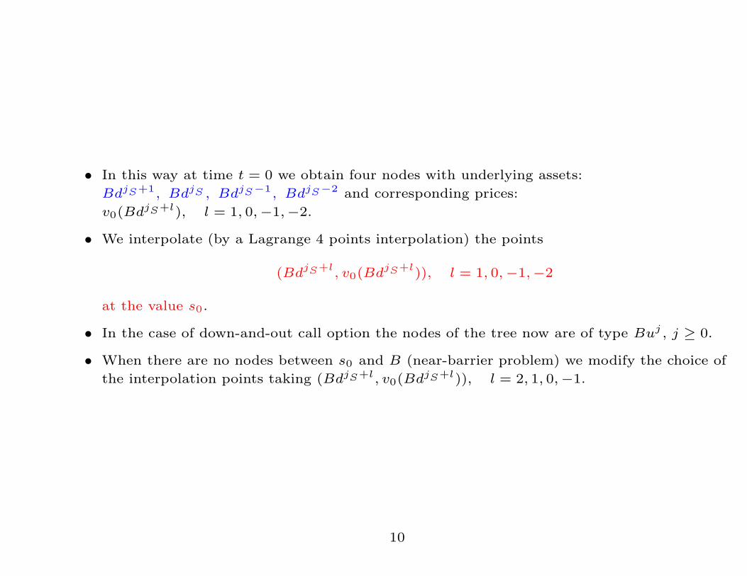
• In this way at time t = 0 we obtain four nodes with underlying assets:
BdjS+1, BdjS , BdjS−1, BdjS−2 and corresponding prices:
v0(BdjS+l), l = 1, 0,−1,−2.
• We interpolate (by a Lagrange 4 points interpolation) the points
(BdjS+l, v0(Bd
jS+l)), l = 1, 0,−1,−2
at the value s0.
• In the case of down-and-out call option the nodes of the tree now are of type Buj , j ≥ 0.
• When there are no nodes between s0 and B (near-barrier problem) we modify the choice of
the interpolation points taking (BdjS+l, v0(BdjS+l)), l = 2, 1, 0,−1.
10
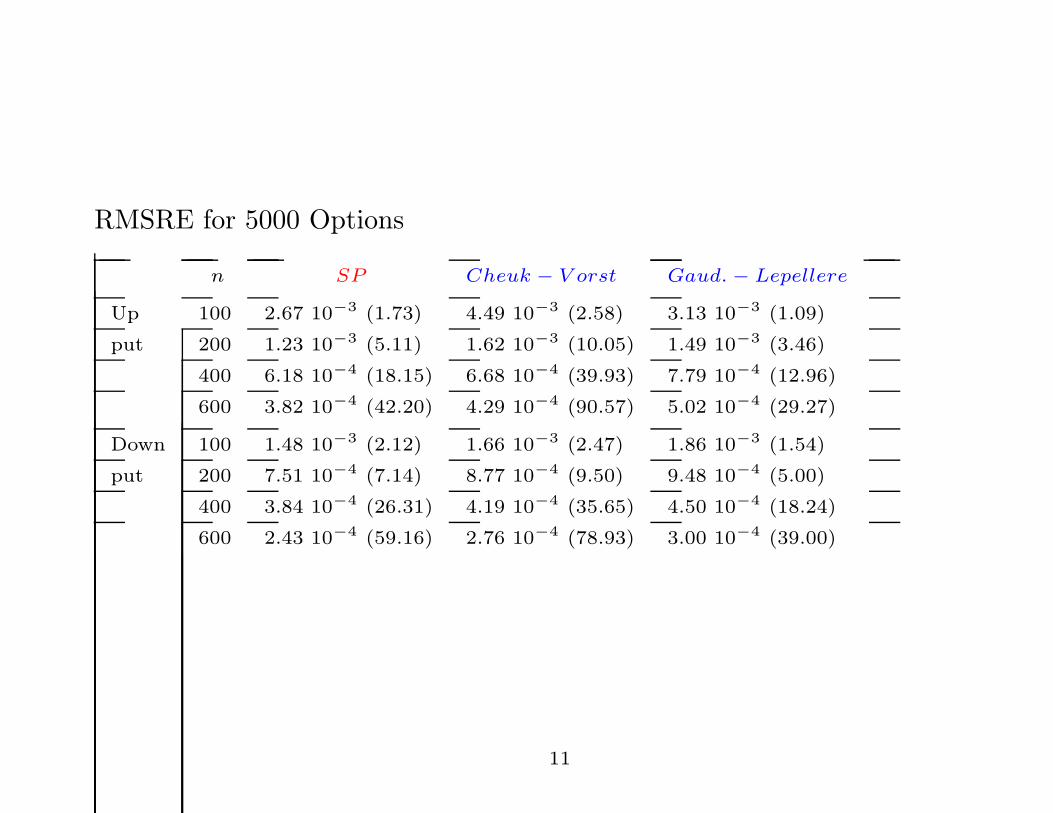
RMSRE for 5000 Options
n SP Cheuk − V orst Gaud.− Lepellere
Up 100 2.67 10−3 (1.73) 4.49 10−3 (2.58) 3.13 10−3 (1.09)
put 200 1.23 10−3 (5.11) 1.62 10−3 (10.05) 1.49 10−3 (3.46)
400 6.18 10−4 (18.15) 6.68 10−4 (39.93) 7.79 10−4 (12.96)
600 3.82 10−4 (42.20) 4.29 10−4 (90.57) 5.02 10−4 (29.27)
Down 100 1.48 10−3 (2.12) 1.66 10−3 (2.47) 1.86 10−3 (1.54)
put 200 7.51 10−4 (7.14) 8.77 10−4 (9.50) 9.48 10−4 (5.00)
400 3.84 10−4 (26.31) 4.19 10−4 (35.65) 4.50 10−4 (18.24)
600 2.43 10−4 (59.16) 2.76 10−4 (78.93) 3.00 10−4 (39.00)
11
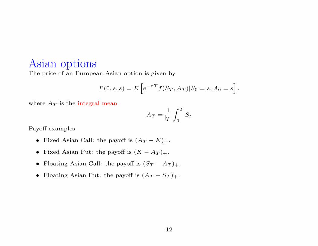
Asian optionsThe price of an European Asian option is given by
P (0, s, s) = E[e−rT
f(ST , AT )|S0 = s,A0 = s].
where AT is the integral mean
AT =1
T
∫T
0
St
Payoff examples
• Fixed Asian Call: the payoff is (AT −K)+.
• Fixed Asian Put: the payoff is (K − AT )+.
• Floating Asian Call: the payoff is (ST − AT )+.
• Floating Asian Put: the payoff is (AT − ST )+.
12
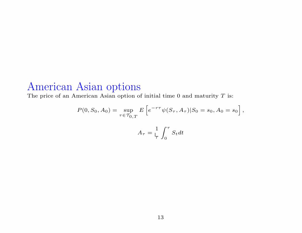
American Asian optionsThe price of an American Asian option of initial time 0 and maturity T is:
P (0, S0, A0) = supτ∈T0,T
E[e−rτ
ψ(Sτ , Aτ )|S0 = s0, A0 = s0
],
Aτ =1
τ
∫τ
0
Stdt
13
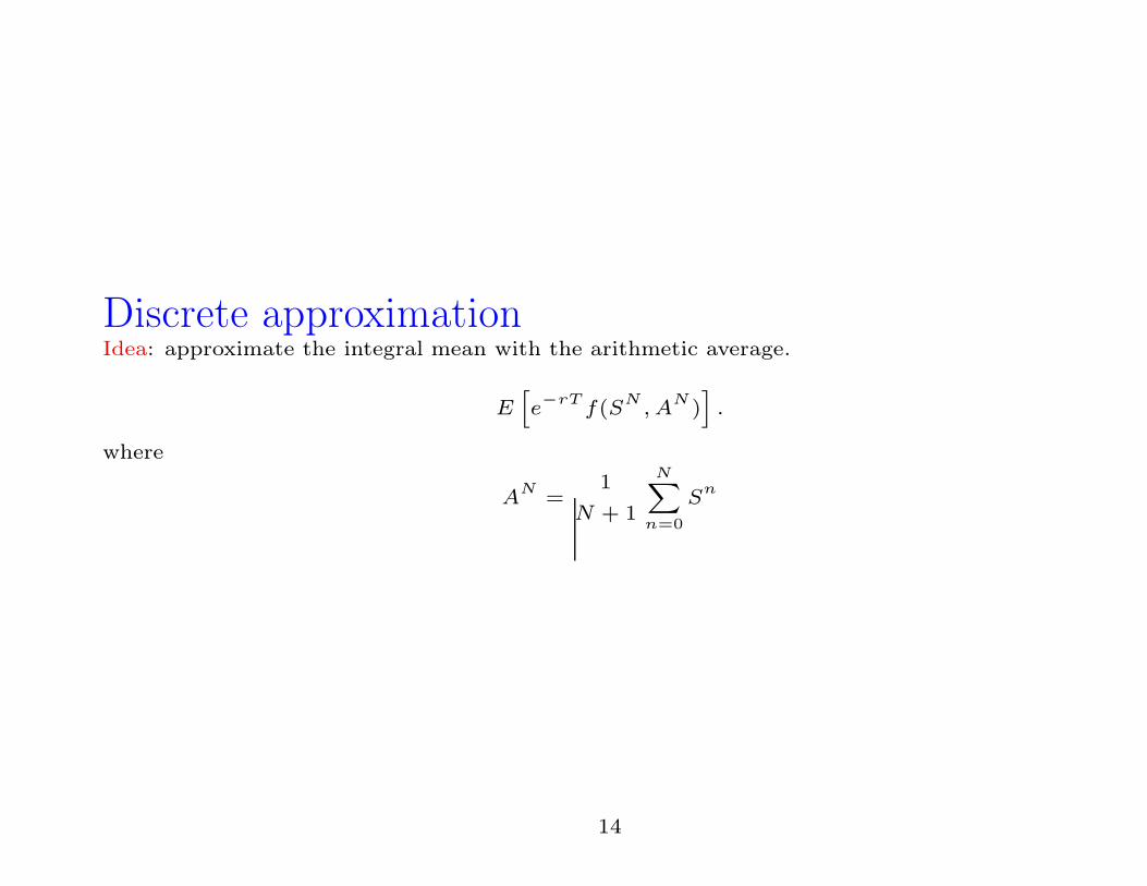
Discrete approximationIdea: approximate the integral mean with the arithmetic average.
E[e−rT
f(SN, A
N)].
where
AN
=1
N + 1
N∑
n=0
Sn
14
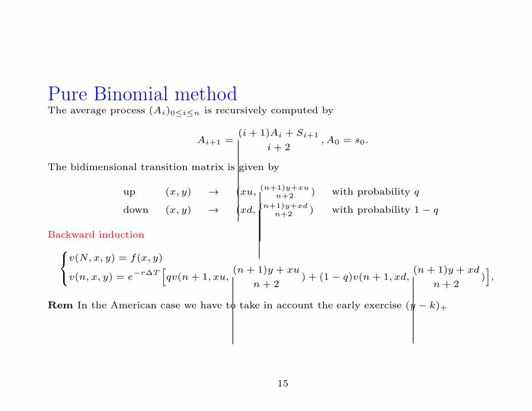
Pure Binomial methodThe average process (Ai)0≤i≤n is recursively computed by
Ai+1 =(i+ 1)Ai + Si+1
i+ 2, A0 = s0.
The bidimensional transition matrix is given by
up (x, y) → (xu,(n+1)y+xu
n+2 ) with probability q
down (x, y) → (xd,(n+1)y+xd
n+2 ) with probability 1 − q
Backward induction
v(N, x, y) = f(x, y)
v(n, x, y) = e−r∆T
[qv(n + 1, xu,
(n+ 1)y + xu
n + 2) + (1 − q)v(n + 1, xd,
(n+ 1)y + xd
n+ 2)],
Rem In the American case we have to take in account the early exercise (y − k)+
15
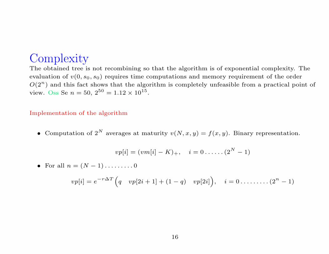
ComplexityThe obtained tree is not recombining so that the algorithm is of exponential complexity. The
evaluation of v(0, s0, s0) requires time computations and memory requirement of the order
O(2n) and this fact shows that the algorithm is completely unfeasible from a practical point of
view. Oss Se n = 50, 250 = 1.12 × 10¹⁵.
Implementation of the algorithm
• Computation of 2N averages at maturity v(N, x, y) = f(x, y). Binary representation.
vp[i] = (vm[i] −K)+, i = 0 . . . . . . (2N − 1)
• For all n = (N − 1) . . . . . . . . . 0
vp[i] = e−r∆T
(q vp[2i+ 1] + (1 − q) vp[2i]
), i = 0 . . . . . . . . . (2
n − 1)
16

Hull-White algoritmIdea: The main idea of this procedure is to restrict the range of the possible arithmetic averages
to a set of some representative values. These values are selected in order to span all the possible
values of the averages reachable at each node of the tree. The price is then computed by a
backward induction procedure where the prices associated to the averages not included in the set
of representative values, are obtained by some suitable interpolation methods.
ANmin = s0
1
N + 1
N∑
k=0
dk= s0
1
N + 1
1 − dN+1
1 − d
ANmax = s0
1
N + 1
N∑
k=0
uk = s0
1
N + 1
uN+1 − 1
u− 1
In particular for every node (n, j)
An,jmin =
1
n + 1s0(1 + d+ . . . . . .+ d
j−1+ d
j+ d
ju+ d
ju2+ . . . . . .+ d
jun−j
) =
1
n+ 1s0
[1 − dj+1
1 − d
]+
1
n+ 1s0d
j[un−j+1 − 1
u− 1− 1
]
An,jmax =
1
n+ 1s0
[un−j+1 − 1
u− 1
]+
1
n+ 1s0u
n−j[ 1 − dj+1
1 − d− 1
]
17
Hull-White algorithm
Discretization mesh of type
Ak,n = s0e
mh
where for a given h, the range of m values is selected to span the possible average at timestep n.
Hull and White suggest that, to ensure accuracy for the algorithm, the value h = 0.005 is
sufficient. Linear interpolation should be performed Complexity of order N3.
18
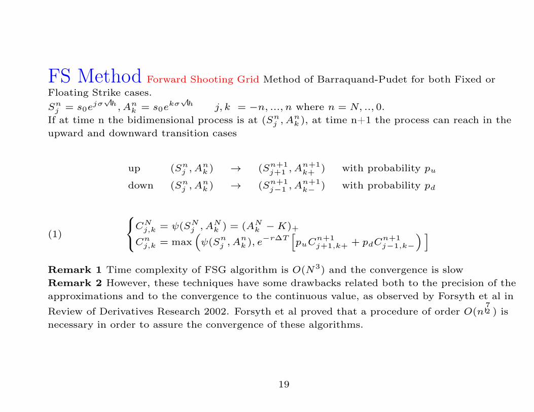
FS Method Forward Shooting Grid Method of Barraquand-Pudet for both Fixed or
Floating Strike cases.
Snj = s0e
jσ√
h, Ank = s0e
kσ√
h j, k = −n, ..., n where n = N, .., 0.
If at time n the bidimensional process is at (Snj , A
nk ), at time n+1 the process can reach in the
upward and downward transition cases
up (Snj , A
nk ) → (Sn+1
j+1 , An+1k+ ) with probability pu
down (Snj , A
nk ) → (Sn+1
j−1 , An+1k− ) with probability pd
(1)
CN
j,k = ψ(SNj , A
Nk ) = (AN
k −K)+
Cnj,k = max
(ψ(Sn
j , Ank ), e
−r∆T[puC
n+1j+1,k+ + pdC
n+1j−1,k−
) ]
Remark 1 Time complexity of FSG algorithm is O(N3) and the convergence is slow
Remark 2 However, these techniques have some drawbacks related both to the precision of the
approximations and to the convergence to the continuous value, as observed by Forsyth et al in
Review of Derivatives Research 2002. Forsyth et al proved that a procedure of order O(n72 ) is
necessary in order to assure the convergence of these algorithms.
19
Singular points methods
• American Asian arithmetic average option
• Binomial algorithm with 200 steps
• Relative error of order 10−4
• Very few requirement of computational time (less than 2 sec) and space
memory.
20
Singular points method• The main idea of our method is to give a continuous representation of the option price
function at every node of the tree as a piecewise linear convex function of the
path-dependent variable (average or maximum/minimum)
• These functions are characterized only by a set of points that we name singular points.
• The property of convexity allows to obtain in a simple way upper and lower bounds of the
price.
21
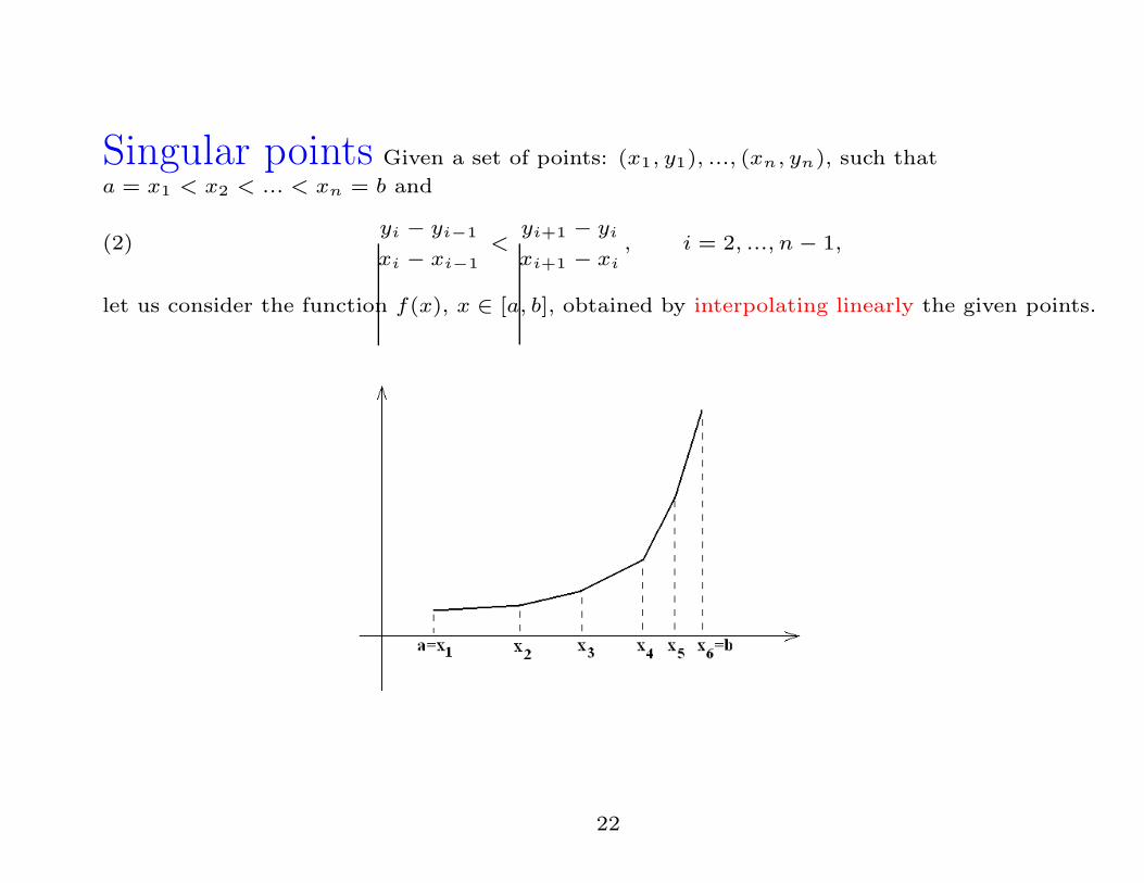
Singular points Given a set of points: (x1, y1), ..., (xn, yn), such that
a = x1 < x2 < ... < xn = b and
(2)yi − yi−1
xi − xi−1
<yi+1 − yi
xi+1 − xi
, i = 2, ..., n− 1,
let us consider the function f(x), x ∈ [a, b], obtained by interpolating linearly the given points.
22
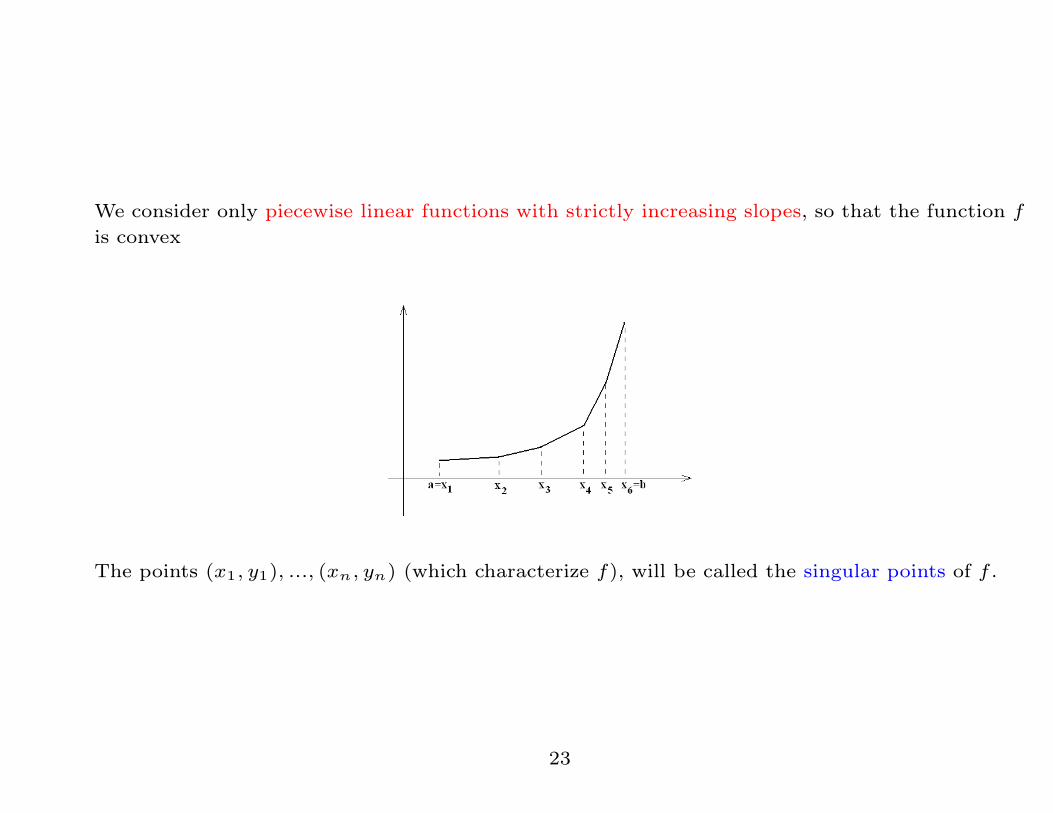
We consider only piecewise linear functions with strictly increasing slopes, so that the function f
is convex
The points (x1, y1), ..., (xn, yn) (which characterize f), will be called the singular points of f .
23
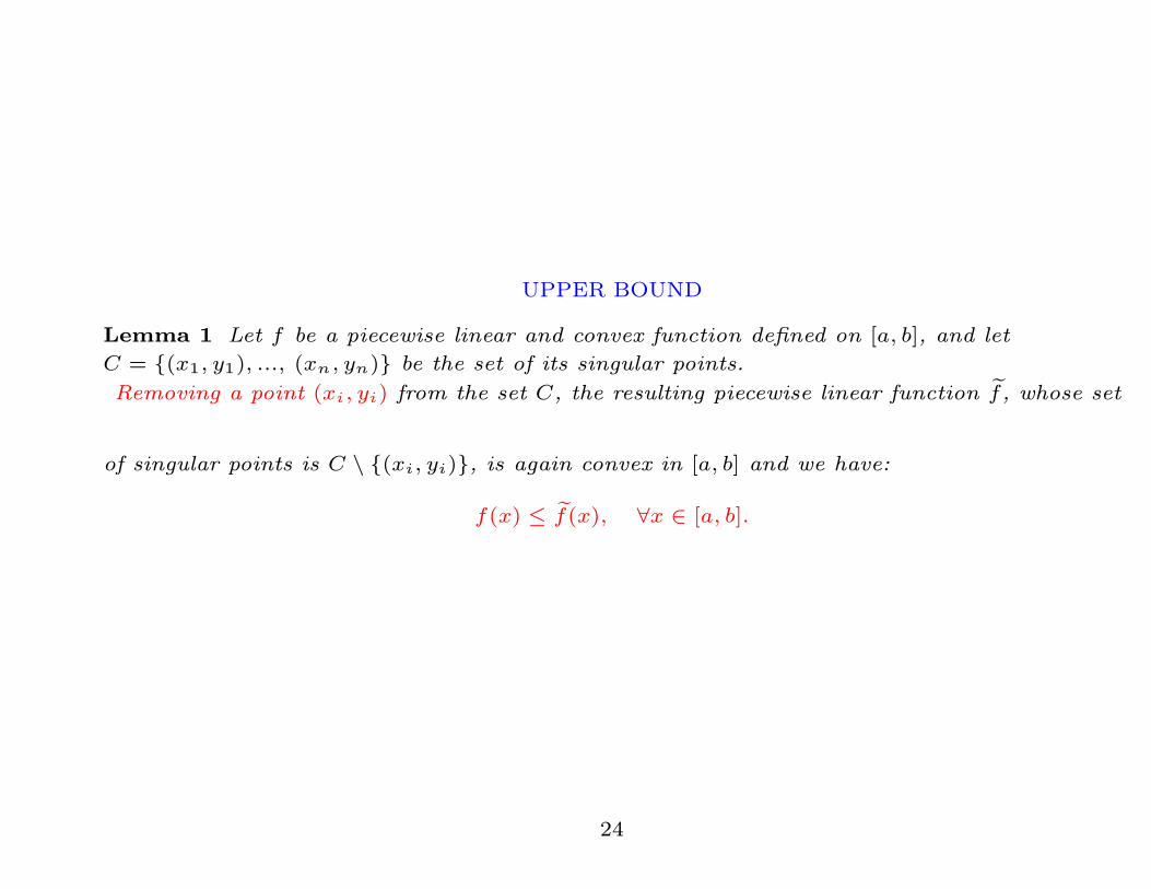
UPPER BOUND
Lemma 1 Let f be a piecewise linear and convex function defined on [a, b], and let
C = {(x1, y1), ..., (xn, yn)} be the set of its singular points.
Removing a point (xi, yi) from the set C, the resulting piecewise linear function f̃, whose set
of singular points is C \ {(xi, yi)}, is again convex in [a, b] and we have:
f(x) ≤ f̃(x), ∀x ∈ [a, b].
24
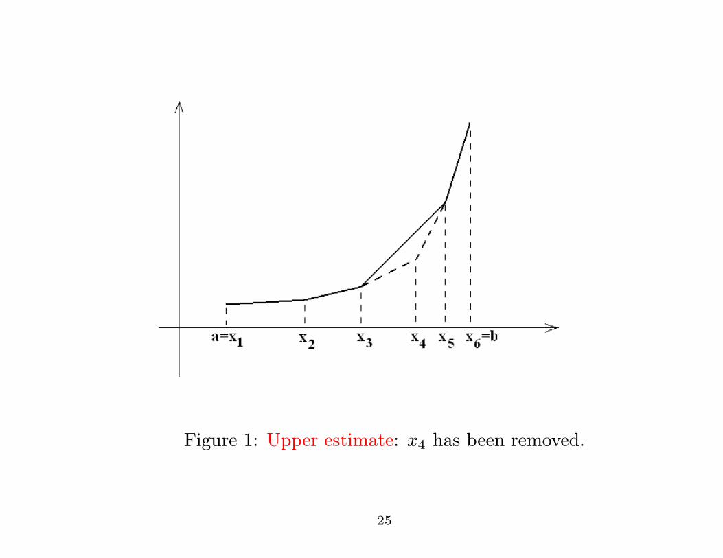
Figure 1: Upper estimate: x4 has been removed.
25
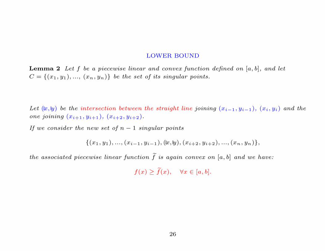
LOWER BOUND
Lemma 2 Let f be a piecewise linear and convex function defined on [a, b], and let
C = {(x1, y1), ..., (xn, yn)} be the set of its singular points.
Let (x, y) be the intersection between the straight line joining (xi−1, yi−1), (xi, yi) and the
one joining (xi+1, yi+1), (xi+2, yi+2).
If we consider the new set of n− 1 singular points
{(x1, y1), ..., (xi−1, yi−1), (x, y), (xi+2, yi+2), ..., (xn, yn)},
the associated piecewise linear function f̃ is again convex on [a, b] and we have:
f(x) ≥ f̃(x), ∀x ∈ [a, b].
26
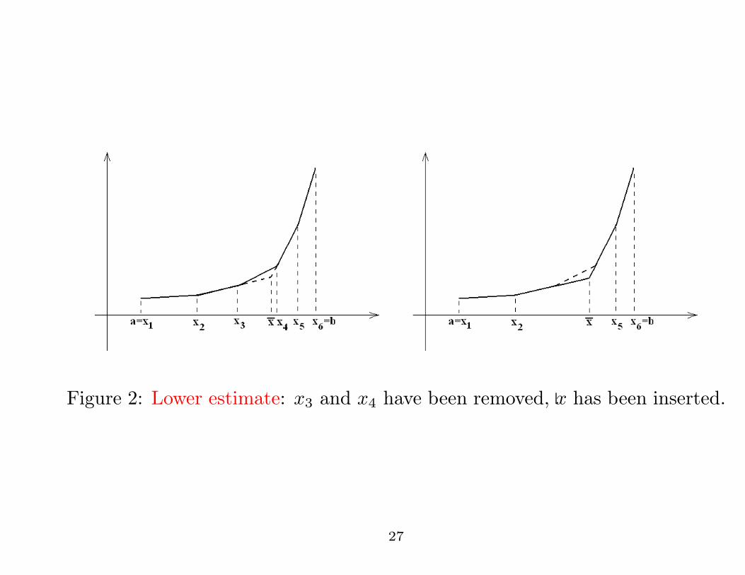
Figure 2: Lower estimate: x3 and x4 have been removed, x has been inserted.
27
Fixed strike European Call Asian options• We will give a continuous representation of the option price function at every node of the
tree as a piecewise linear convex function of the average.
• The price function at every node of the tree is characterized only by its singular points.
• Backward induction algorithm.
28
Notations
• Let us denote by Ni,j the node of the tree whose underlying is Si,j = s0u2j−i, i = 0, ..., n,
j = 0, ..., i.
• We will associate to each node Ni,j a set of singular points, whose number is Li,j . The
singular points will be denoted by
(Ali,j , P
li,j), l = 1, ..., Li,j .
29
Backward algorithm: at maturity n• At every node the average values vary between a minimum average Amin
n,j and a maximum
average Amaxn,j .
• For every A ∈ [Aminn,j , A
maxn,j ] the price of the option can be continuously defined by
vn,j(A) = (A−K)+.
• The function vn,j(A) is a piecewise linear and convex function whose singular points are
easily valuable.
30
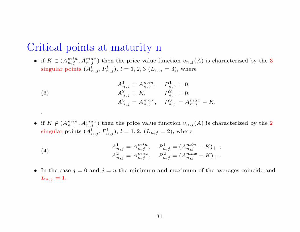
Critical points at maturity n• if K ∈ (Amin
n,j , Amaxn,j ) then the price value function vn,j(A) is characterized by the 3
singular points (Aln,j , P
ln,j), l = 1, 2, 3 (Ln,j = 3), where
(3)
A1n,j = Amin
n,j , P 1n,j = 0;
A2n,j = K, P 2
n,j = 0;
A3n,j = Amax
n,j , P 3n,j = Amax
n,j −K.
.
• if K 6∈ (Aminn,j , A
maxn,j ) then the price value function vn,j(A) is characterized by the 2
singular points (Aln,j , P
ln,j), l = 1, 2, (Ln,j = 2), where
(4)A1
n,j = Aminn,j , P 1
n,j = (Aminn,j −K)+ ;
A2n,j = Amax
n,j , P 2n,j = (Amax
n,j −K)+ .
• In the case j = 0 and j = n the minimum and maximum of the averages coincide and
Ln,j = 1.
31
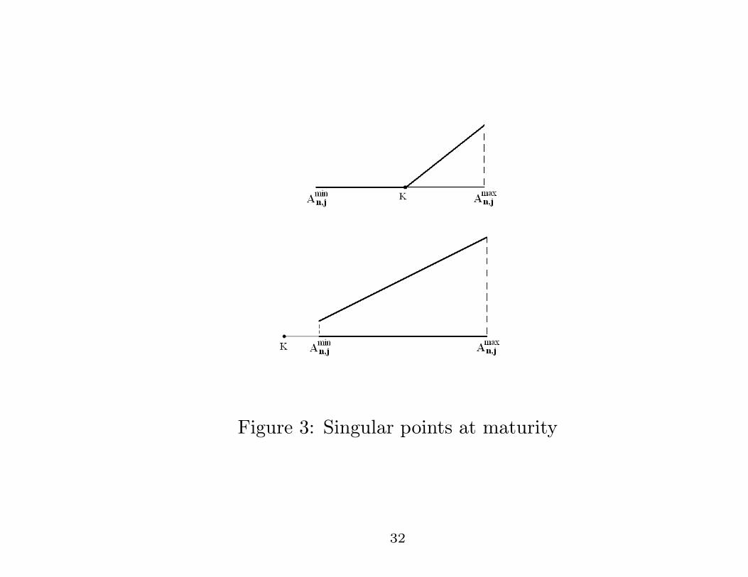
Figure 3: Singular points at maturity
32
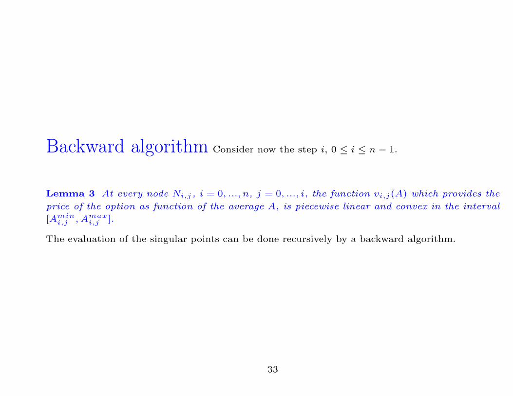
Backward algorithm Consider now the step i, 0 ≤ i ≤ n− 1.
Lemma 3 At every node Ni,j , i = 0, ..., n, j = 0, ..., i, the function vi,j(A) which provides the
price of the option as function of the average A, is piecewise linear and convex in the interval
[Amini,j , Amax
i,j ].
The evaluation of the singular points can be done recursively by a backward algorithm.
33

The claim is true at step i = n (at maturity).
At step i = n− 1, the price function vi,j(A), with A ∈ [Amini,j , Amax
i,j ], is obtained by considering
the discounted expectation value:
(5) vi,j(A) = e−r T
n [πvi+1,j+1(A′) + (1 − π)vi+1,j(A
′′)],
where
(6) A′=
(i+ 1)A+ S0u2j−i+1
i+ 2, A
′′=
(i+ 1)A+ S0u2j−i−1
i+ 2.
As vn,j(A) is piecewise linear and convex in his domain and
h1(A) = vi+1,j+1((i+1)A+S0u2j−i+1
i+2 ) is the composite function of a linear function of A and a
piecewise linear convex one, h1(A) is piecewise linear and convex as function of A.
The same holds true for h2(A) = vi+1,j((i+1)A+S0u2j−i−1
i+2 ). We can conclude that vi,j(A) is
piecewise linear and convex in his domain.
34

Figure 4: Singular points at i=n-1
35
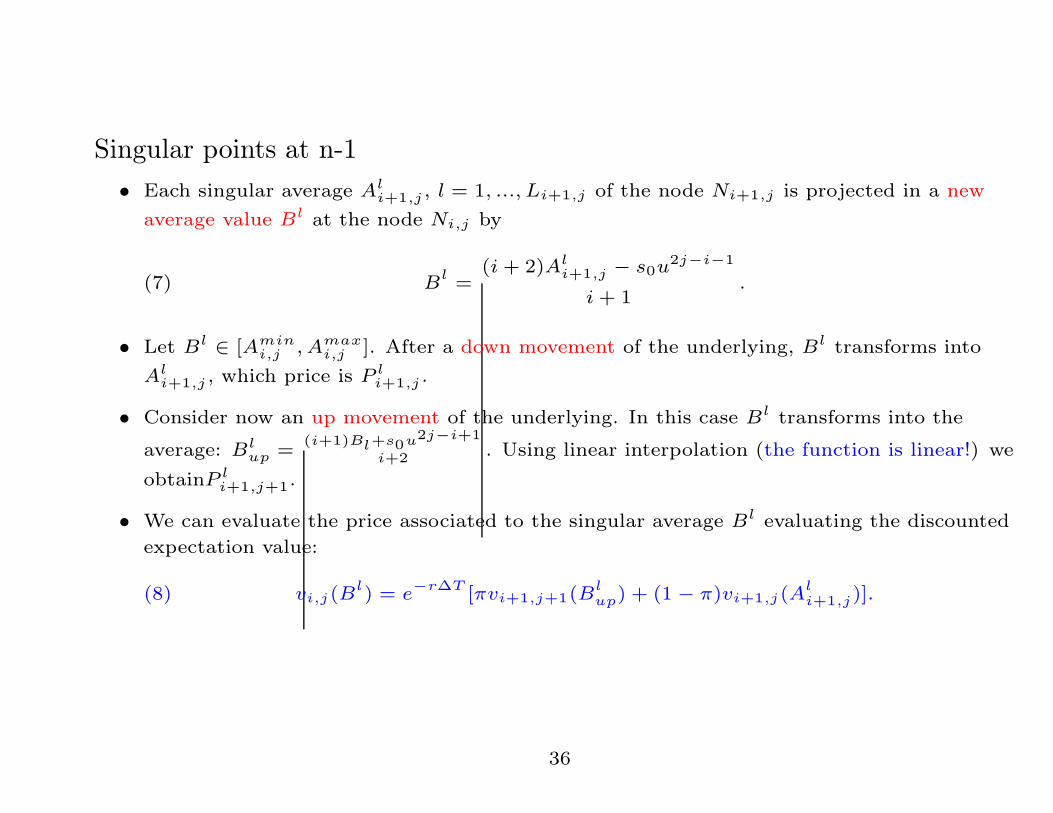
Singular points at n-1
• Each singular average Ali+1,j , l = 1, ..., Li+1,j of the node Ni+1,j is projected in a new
average value Bl at the node Ni,j by
(7) Bl=
(i+ 2)Ali+1,j − s0u
2j−i−1
i+ 1.
• Let Bl ∈ [Amini,j , Amax
i,j ]. After a down movement of the underlying, Bl transforms into
Ali+1,j , which price is P l
i+1,j .
• Consider now an up movement of the underlying. In this case Bl transforms into the
average: Blup =
(i+1)Bl+s0u2j−i+1
i+2 . Using linear interpolation (the function is linear!) we
obtainP li+1,j+1.
• We can evaluate the price associated to the singular average Bl evaluating the discounted
expectation value:
(8) vi,j(Bl) = e
−r∆T [πvi+1,j+1(Blup) + (1 − π)vi+1,j(A
li+1,j)].
36
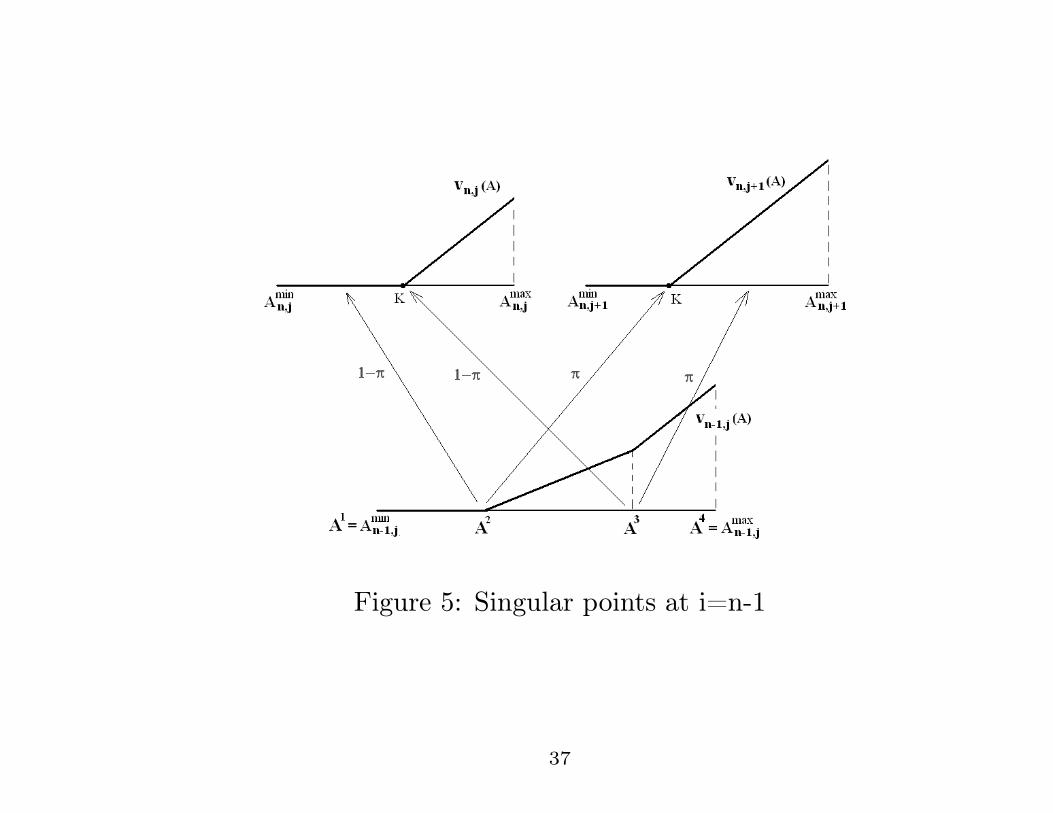
Figure 5: Singular points at i=n-1
37
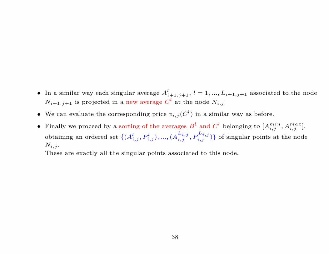
• In a similar way each singular average Ali+1,j+1, l = 1, ..., Li+1,j+1 associated to the node
Ni+1,j+1 is projected in a new average Cl at the node Ni,j
• We can evaluate the corresponding price vi,j(Cl) in a similar way as before.
• Finally we proceed by a sorting of the averages Bl and Cl belonging to [Amini,j , Amax
i,j ],
obtaining an ordered set {(Ali,j , P
li,j), ..., (A
Li,ji,j , P
Li,ji,j )} of singular points at the node
Ni,j .
These are exactly all the singular points associated to this node.
38
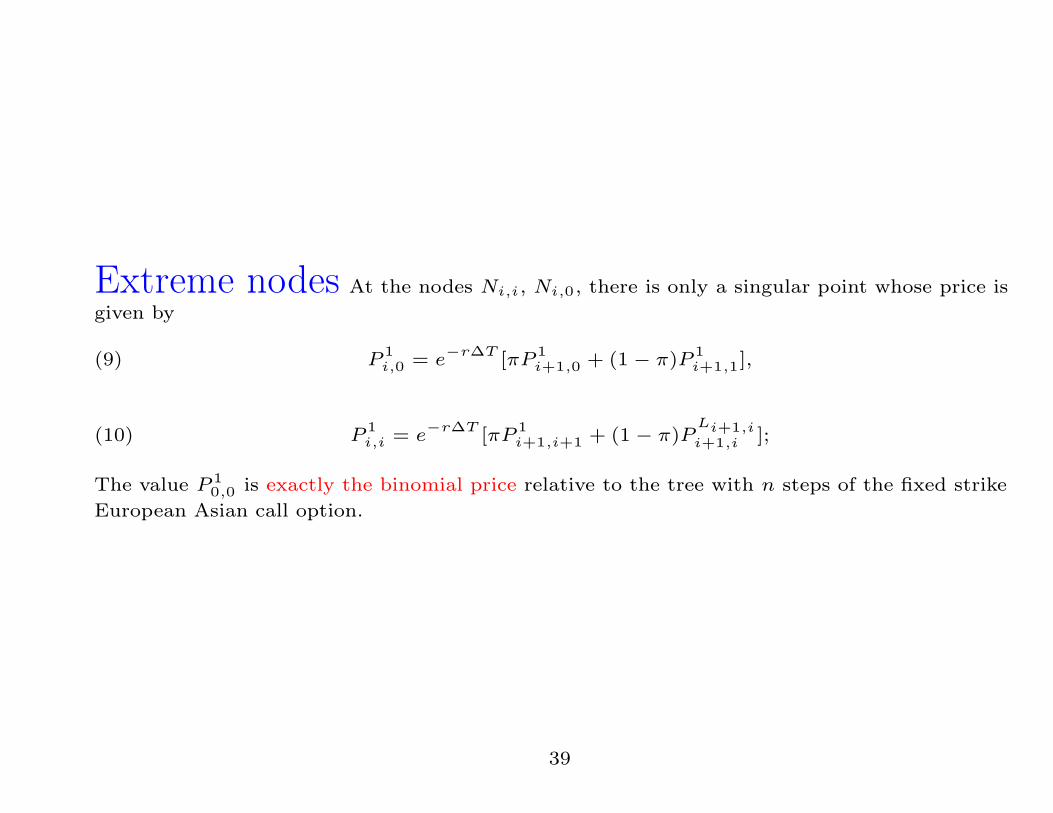
Extreme nodes At the nodes Ni,i, Ni,0, there is only a singular point whose price is
given by
(9) P1i,0 = e
−r∆T [πP 1i+1,0 + (1 − π)P 1
i+1,1],
(10) P1i,i = e
−r∆T [πP 1i+1,i+1 + (1 − π)P
Li+1,ii+1,i ];
The value P 10,0 is exactly the binomial price relative to the tree with n steps of the fixed strike
European Asian call option.
39
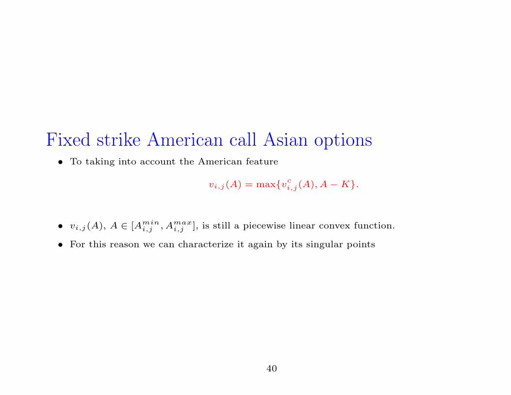
Fixed strike American call Asian options• To taking into account the American feature
vi,j(A) = max{vci,j(A), A−K}.
• vi,j(A), A ∈ [Amini,j , Amax
i,j ], is still a piecewise linear convex function.
• For this reason we can characterize it again by its singular points
40
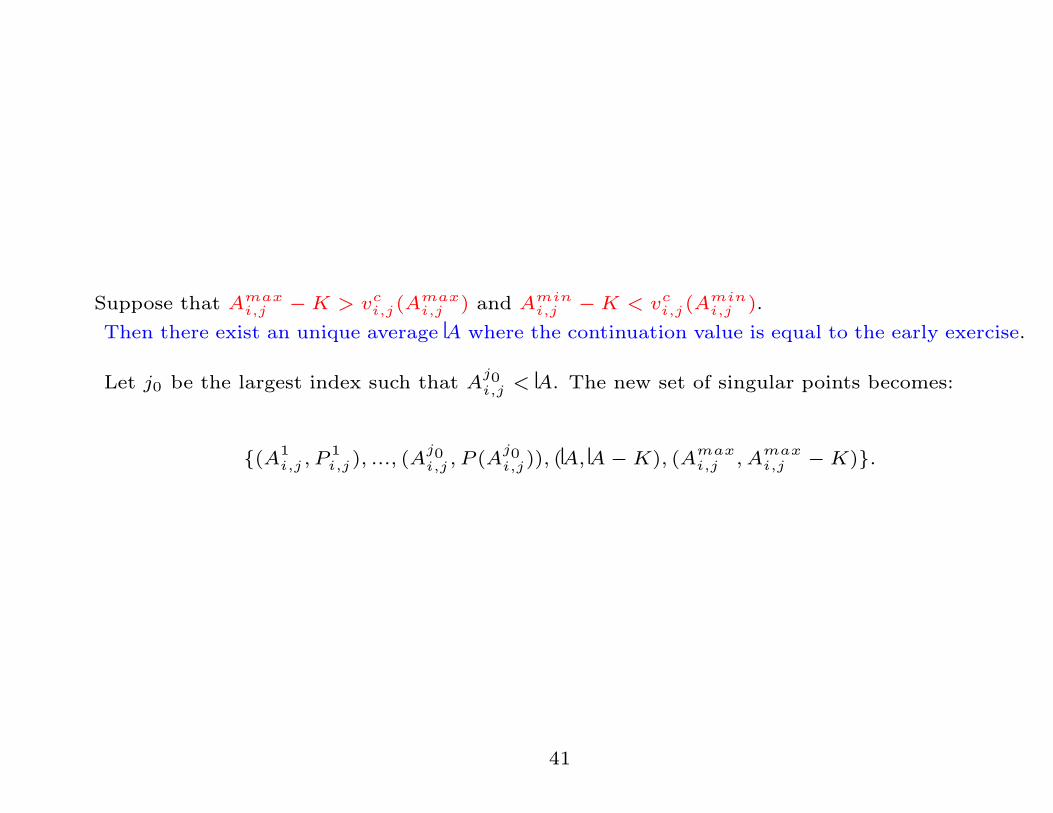
Suppose that Amaxi,j −K > vci,j(A
maxi,j ) and Amin
i,j −K < vci,j(Amini,j ).
Then there exist an unique average A where the continuation value is equal to the early exercise.
Let j0 be the largest index such that Aj0i,j < A. The new set of singular points becomes:
{(A1i,j , P
1i,j), ..., (A
j0i,j , P (A
j0i,j)), (A,A−K), (A
maxi,j , A
maxi,j −K)}.
41
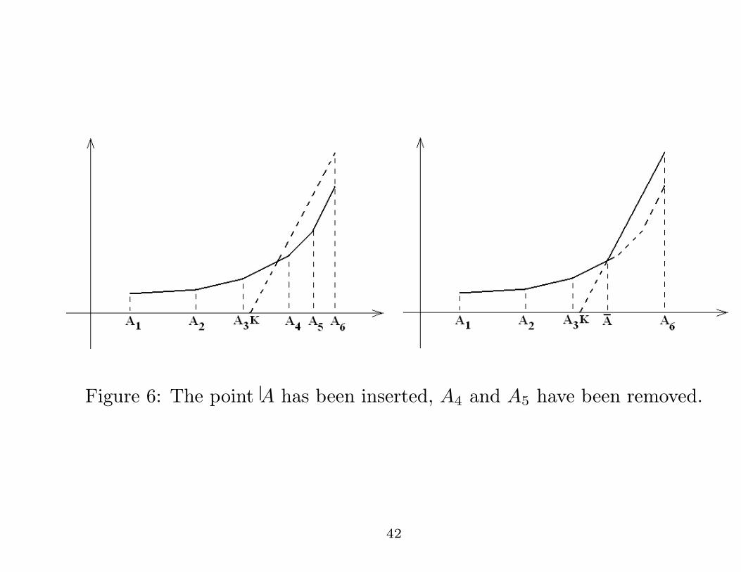
Figure 6: The point A has been inserted, A4 and A5 have been removed.
42
Upper and lower bounds• The resulting algorithm can be of exponential complexity as the standard binomial
technique.
• We are able to compute an upper and a lower bound of the binomial price reducing
drastically the amount of time computation and the memory requirement.
• An a-priori control of the distance of the estimates from the pure binomial price.
43

UPPER BOUND
Remove A4 if ǫ ≤ h
Inductively we get that the obtained upper estimate differs from the binomial value at most for
nh.
44
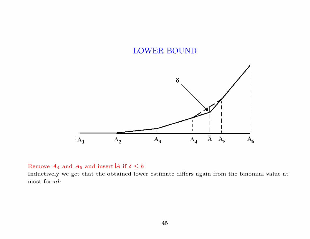
LOWER BOUND
Remove A4 and A5 and insert A if δ ≤ h
Inductively we get that the obtained lower estimate differs again from the binomial value at
most for nh
45
Convergence resultsRemark 1 Jiang and Dai (SIAM Journal on numerical analysis 2005) proved the
convergence of the exact binomial algorithm for European/ American path-dependent options.
In particular they proved that the rate of convergence of the exact binomial algorithm to the
continuous value is O(∆T ).
The possibility of obtaining estimates of the exact binomial price with an error control allows
us to prove easily the convergence of our method to the continuous value. Choosing h
depending on n and so that nh(n) → 0 we have that the corresponding sequences of upper and
lower estimates converge to the continuous price value. Moreover, choosing h(n) = O( 1n2 ), we
are able to guarantee that the order of convergence is O(∆T ).
46
Numerical Results Fixed strike American Call Asian options
• We illustrate numerically the efficiency of singular points method.
• We compare the singular points algorithm with Hull-White,Barraquand-Pudet,Chalasani et
al.
• We assume that the initial value of the stock prices are s0 = 100, the maturity T = 1, the
continuous dividend rates q = 0.03, while the values of the volatility σ = 0.2, 0.4, the
interest rate r = 0.1, and the exercise price K = 90, 100 vary.
• We consider different time steps n = 25, 50, 100, 200, 400, 800
47
1. the pure binomial(PB) model (available only for n = 25),
2. the Hull-White method (HW) with h = 0.005,
3. the forward shooting grid method (FSG) of Barraquand-Pudet with ρ = 0.1,
4. the Chalasani et al. method (CJEV) that provides an upper and a lower bound, (available
only for n = 25, 50, 100),
5. the singular points method providing an upper and a lower bound with error less than nh,
for two different choices of h:
• h = 10−4 (SP1);
• h = 10−5 (SP2).
48
Analysis of convergence1. the PDE-based method of d’Halluin et al. (DFL) available for both the European and the
American Asian options;
2. the PDE-based method of Vecer available in the European Asian option case ;
3. the modified linear interpolation forward shooting grid method (M-FSG) of
Barraquand-Pudet. We chose ρ = 0.1 and n√n grid points in the Asian direction in order
to guarantee the convergence (see the Premia implementation www.premia.fr);
4. the modified FSG algorithm with the Richardson extrapolation (M-FSG-Rich);
5. the singular points method (SP) providing an upper bound with a level of error smaller
than nh with h = 0.1n2 (see Remark 1);
49
In the European case we used the two-points extrapolation 2Pn − Pn2
, whereas in the American
case the three points extrapolation 83Pn − 2Pn
2+ 1
3Pn4
was adopted.
In order to compare the convergence behavior we consider the convergence ratio R
R =Pn
2− Pn
4
Pn − Pn2
50
Lookback optionsThe price of an European lookback option is given by
P (0, s, s) = E[e−rT
f(ST ,MT )|S0 = s,M0 = s].
where MT
MT = max0≤t≤T
St
mT = min0≤t≤T
St
Payoff example:
• Fixed Lookback Call: the payoff is (MT −K)+.
• Fixed Lookback Put: the payoff is (K −mT )+.
• Floating Lookback Call: the payoff is (ST −mT )+.
• Floating Lookback Put: the payoff is (MT − ST )+.
51
Binomial method
E[e−rT
f(SN,M
N)].
where
MN = max
0≤n≤NS
n
52
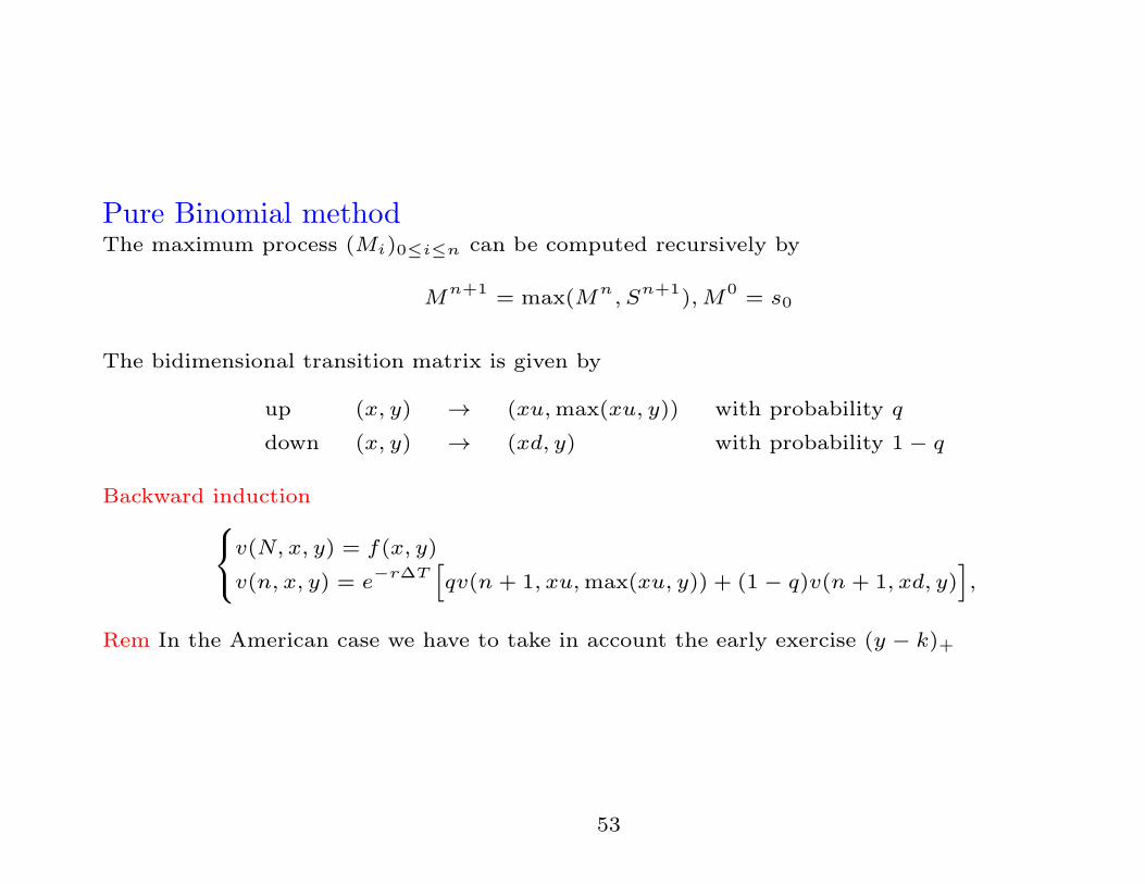
Pure Binomial methodThe maximum process (Mi)0≤i≤n can be computed recursively by
Mn+1 = max(Mn
, Sn+1),M0 = s0
The bidimensional transition matrix is given by
up (x, y) → (xu,max(xu, y)) with probability q
down (x, y) → (xd, y) with probability 1 − q
Backward inductionv(N, x, y) = f(x, y)
v(n, x, y) = e−r∆T
[qv(n + 1, xu,max(xu, y)) + (1 − q)v(n + 1, xd, y)
],
Rem In the American case we have to take in account the early exercise (y − k)+
53
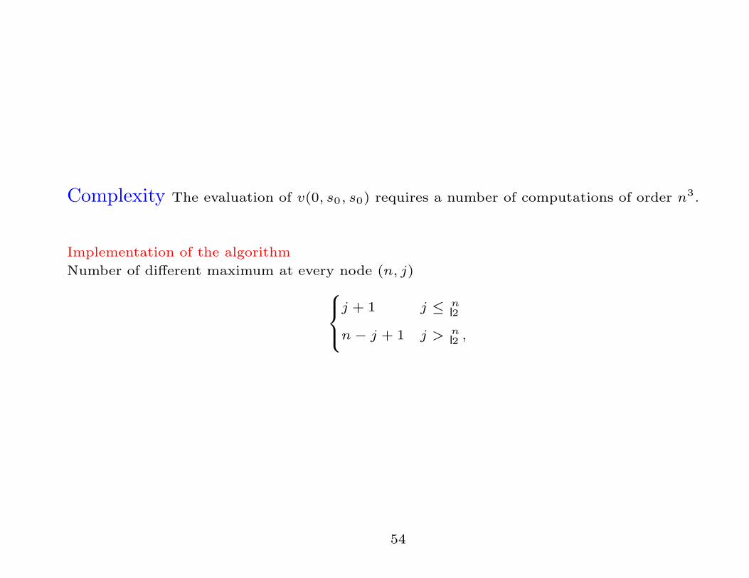
Complexity The evaluation of v(0, s0, s0) requires a number of computations of order n3.
Implementation of the algorithm
Number of different maximum at every node (n, j)
j + 1 j ≤ n2
n− j + 1 j > n2 ,
54
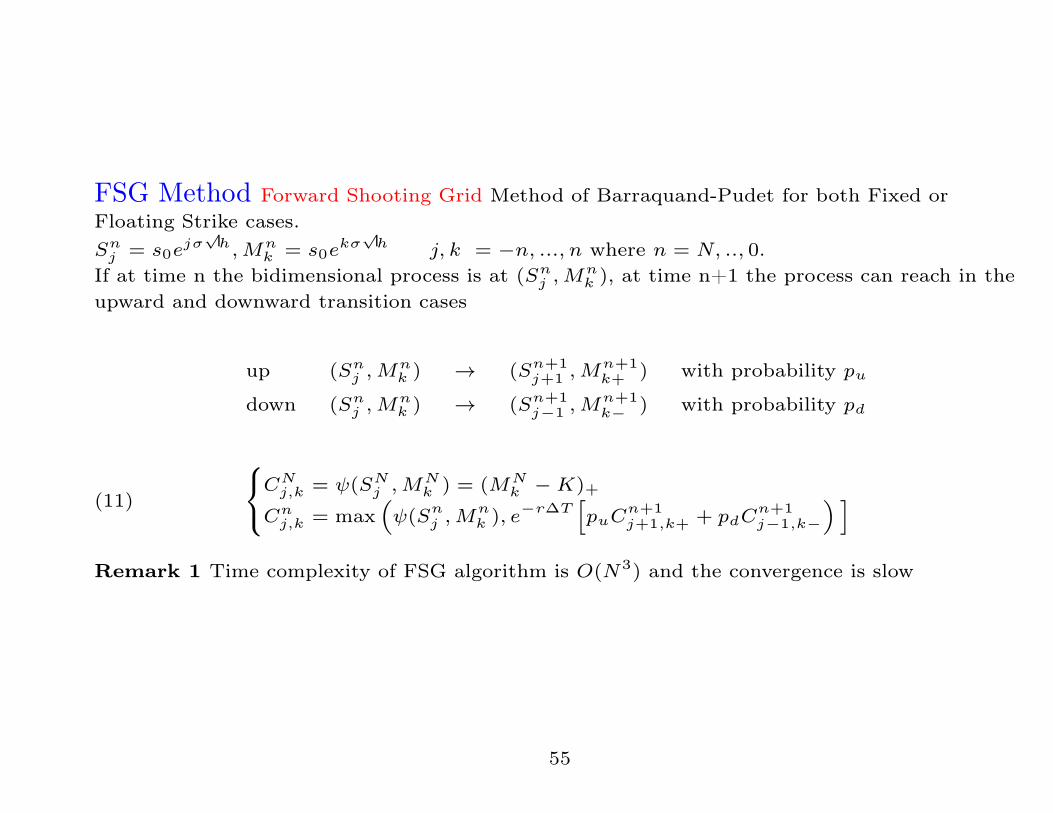
FSG Method Forward Shooting Grid Method of Barraquand-Pudet for both Fixed or
Floating Strike cases.
Snj = s0e
jσ√
h,Mnk = s0e
kσ√
h j, k = −n, ..., n where n = N, .., 0.
If at time n the bidimensional process is at (Snj ,M
nk ), at time n+1 the process can reach in the
upward and downward transition cases
up (Snj ,M
nk ) → (Sn+1
j+1 ,Mn+1k+ ) with probability pu
down (Snj ,M
nk ) → (Sn+1
j−1 ,Mn+1k− ) with probability pd
(11)
CN
j,k = ψ(SNj ,M
Nk ) = (MN
k −K)+
Cnj,k = max
(ψ(Sn
j ,Mnk ), e−r∆T
[puC
n+1j+1,k+ + pdC
n+1j−1,k−
) ]
Remark 1 Time complexity of FSG algorithm is O(N3) and the convergence is slow
55
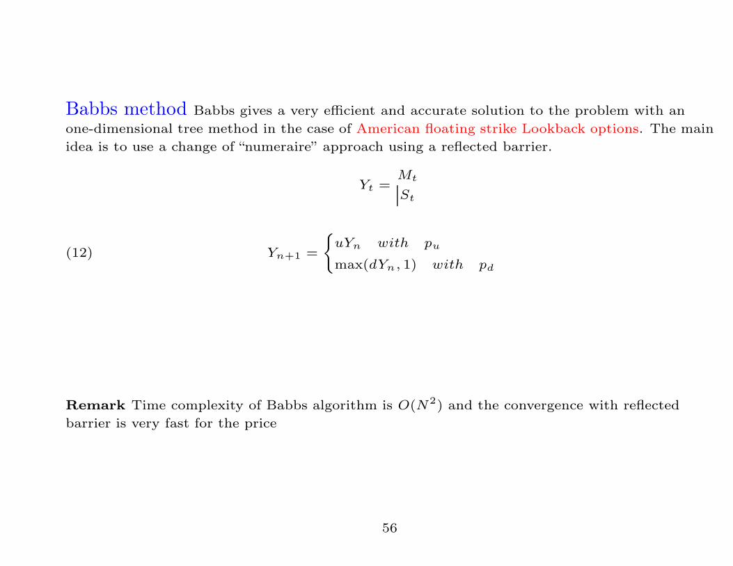
Babbs method Babbs gives a very efficient and accurate solution to the problem with an
one-dimensional tree method in the case of American floating strike Lookback options. The main
idea is to use a change of “numeraire” approach using a reflected barrier.
Yt =Mt
St
(12) Yn+1 =
{uYn with pu
max(dYn, 1) with pd
Remark Time complexity of Babbs algorithm is O(N2) and the convergence with reflected
barrier is very fast for the price
56