Embed Size (px)
Citation preview

A backward Monte Carlo approachto exotic option pricing
Giacomo Bormettia, Giorgia Callegarob, Giulia Livieric,∗,and Andrea Pallavicinid,e
November 4, 2015
a Department of Mathematics, University of Bologna, Piazza di Porta San Donato 5, 40126 Bologna,Italy
b Department of Mathematics, University of Padova, via Trieste 63, 35121 Padova, Italyc Scuola Normale Superiore, Piazza dei Cavalieri 7, 56126 Pisa, Italy
d Department of Mathematics, Imperial College, London SW7 2AZ, United Kingdome Banca IMI, Largo Mattioli 3, 20121 Milano, Italy
Abstract
We propose a novel algorithm which allows to sample paths from an underlying priceprocess in a local volatility model and to achieve a substantial variance reduction whenpricing exotic options. The new algorithm relies on the construction of a discrete multino-mial tree. The crucial feature of our approach is that – in a similar spirit to the BrownianBridge – each random path runs backward from a terminal fixed point to the initial spotprice. We characterize the tree in two alternative ways: in terms of the optimal grids orig-inating from the Recursive Marginal Quantization algorithm and following an approachinspired by the finite difference approximation of the diffusion’s infinitesimal generator.We assess the reliability of the new methodology comparing the performance of bothapproaches and benchmarking them with competitor Monte Carlo methods.
JEL codes: C63, G12, G13Keywords: Monte Carlo, Variance Reduction, Quantization, Markov Generator, Local Volatil-ity, Option Pricing
∗Corresponding author. E-mail address: [email protected]
1
arX
iv:1
511.
0084
8v1
[q-
fin.
CP]
3 N
ov 2
015

Contents
1 Introduction 3
2 The backward Monte Carlo algorithm 5
3 Recoverying the transition probabilities 93.1 A quantization based algorithm . . . . . . . . . . . . . . . . . . . . . . . . . . . . . . . 10
3.1.1 Optimal quantization . . . . . . . . . . . . . . . . . . . . . . . . . . . . . . . . 103.1.2 The Recursive Marginal Quantization Algorithm . . . . . . . . . . . . . . . . . 113.1.3 The Anderson accelerated procedure . . . . . . . . . . . . . . . . . . . . . . . . 13
3.2 The Large Time Step Algorithm . . . . . . . . . . . . . . . . . . . . . . . . . . . . . . 153.2.1 LTSA implementation: more technical details . . . . . . . . . . . . . . . . . . . 18
4 Financial applications 194.1 Model and payoff specifications . . . . . . . . . . . . . . . . . . . . . . . . . . . . . . . 194.2 Numerical results and discussion . . . . . . . . . . . . . . . . . . . . . . . . . . . . . . 21
5 Conclusion 27
A The distortion function and companion parameters 31
B Lloyd I method within the RMQA 32
C Robustness checks 33
D Construction of the Markov generator LΓ 36
2
1 Introduction
Pricing financial derivatives typically requires to solve two main issues. In the first place, thechoice of a flexible model for the stochastic evolution of the underlying asset price. At thispoint, a common trade-off arises as models which describe the historical dynamics of the assetprice with adequate realism are usually unable to precisely match volatility smiles observed inthe option market [1, 2]. Secondly, once a reasonable candidate has been identified, there is theneed to develop fast, accurate, and possibly flexible numerical methods [3, 4, 5]. As regards theformer point, Local Volatility (LV) models have become very popular since their introductionby Dupire [6], and Derman and co-authors [7]. Even though the legitimate use of LV modelsfor the description of the asset dynamics is highly questionable, the ability to self-consistentlyreproduce volatility smiles implied by the market motivates their widespread diffusion amongpractitioners. Since calibration a la Dupire [6] of LV models assumes the unrealistic availabilityof a continuum of vanilla option prices across different strikes and maturities [8], recent yearshave seen the emergence of a growing strand of literature dealing with this problem (see forinstance [8, 9, 10, 11, 12, 13]). In the present paper we fix the calibration following the latestachievements, and we solely focus on the latter issue. Specifically, our goal is to design anovel pricing algorithm based on the Monte Carlo approach able to achieve a sizeable variancereduction with respect to competitor approaches.
The main result of this paper is the development of a flexible and efficient pricing algorithm– termed the backward Monte Carlo algorithm – which runs backward on top of a multinomialtree. The flexibility of this algorithm permits to price generic payoffs without the need ofdesigning tailor-made solutions for each payoff specification. This feature is inherited directlyfrom the Monte Carlo approach (see [14] for an almost exhaustive survey of Monte Carlomethods in finance). The efficiency, instead, is linked primarily to the backward movement onthe multinomial tree. Indeed, our approach combines both advantages of stratified samplingMonte Carlo and the Brownian Bridge construction [14, 15, 16], extending them to more generalfinancial-asset dynamics than the simplistic assumptions of Black, Scholes, and Merton [17,18]. The second purpose of this paper – minor in relative terms with respect to the firstone – is to investigate an alternative scheme for the implementation of the Recursive MarginalQuantization Algorithm (henceforth RMQA ). The RMQA is a recursive algorithm which allowsto approximate a continuous time diffusion by means of a discrete-time Markov Chain definedon a finite grid of points. The alternative scheme, employed at each step of the RMQA , is basedon the Lloyd I method [19] in combination with the Anderson acceleration Algorithm [20, 21]developed to solve fixed-point problems. The accelerated scheme permits to speed up thelinear rate of convergence of the Lloyd I method [19], and besides, to fix some flaws of previousRMQA implementations highlighted in [22].
In more detail, a discrete-time Markov Chain approximation of the asset price dynamics canbe achieved by introducing at each time step two quantities: (i) a grid for the possible values thatthe can take, and (ii) the transition probabilities to propagate from one state to another state.Among the approaches discussed in the literature for computing these quantities, in the present
3

paper we analyse and extend two of them. The first approach quantizes via the RMQA theEuler-Maruyama approximation of the Stochastic Differential Equation (SDE) modelling theunderlying asset price. The RMQA has been introduced in [23] to compute vanilla call and putoptions prices in a pseudo Constant Elasticity of Variance (CEV) LV model. In [22] authorsemploy it to calibrate a Quadratic Normal LV model. The alternative approach, instead,discretises in an appropriate way the infinitesimal Markov generator of the underlying diffusionby means of a finite difference scheme (see [24, 25] for a detailed discussion of theoreticalconvergence results). We name the latter approach Large Time Step Algorithm, henceforthLTSA . In [12] authors implement a modified version of the LTSA to price discrete look-backoptions in a CEV model, whereas in [26] they employ the LTSA idea to price a particularclass of path-dependent payoffs termed Abelian payoffs. More specifically, they incorporate thepath-dependency feature – in the specific case whether or not the underlying asset price hits aspecified level over the life of the option – within the Markov generator. The joint transitionprobability matrix is then recovered as the solution of a payoff specific matrix equation. TheRMQA and LTSA present two major differences which can be summarized as follows: (i) theRMQA permits to recover the optimal – according to a specific criterion [27] – multinomialgrid, whereas the LTSA works on a a priori user-specified grid, (ii) the LTSA necessitates lesscomputational burden than the RMQA when pricing financial derivatives products whose payoffrequires the observation of the underlying on a predefined finite set of dates. Unfortunately,this result holds only for a piecewise time-homogeneous Local Volatility dynamics.
The usage in both equity and foreign exchange (FX) markets of LV models is largely moti-vated by the flexibility of the approach which allows the exact calibration to the whole volatilitysurface. Moreover, the accurate re-pricing of plain vanilla instruments and of most liquid Euro-pean options, together with the stable computation of the option sensitivity to model param-eters and the availability of specific calibration procedures, make the LV modelling approacha popular choice. The LV models are also employed in practice to evaluate Asian options andother path-dependent options, although more sophisticated Stochastic Local Volatility (SLV)models are usually adopted. We refer to [28] for details. The price of path-dependent deriva-tive products is then computed either solving numerically a Partial Differential Equation (PDE)or via Monte Carlo methods. The PDE approach is computationally efficient but it requiresthe definition of a payoff specific pricing equation (see [4] for an extensive survey on PDEapproached in a financial context). Moreover, some options with exotic payoffs and exerciserules are tricky to price even within the Black, Scholes, and Merton framework. On the otherhand, standard Monte Carlo method suffers from some inefficiency – especially when pricingout-of-the-money (OTM) options – since a relevant number of sampled paths does not con-tribute to the option payoff. However, the Monte Carlo approach is extremely flexible andseveral numerical techniques have been introduced to reduce the variance of the Monte Carloestimator [5, 14]. The backward Monte Carlo algorithm pursues this task.
In this paper we consider the FX market, where we can trade spot and forward contractsalong with vanilla and exotic options. In particular, we model the EUR/USD rate using a LVdynamics. The calibration procedure is the one employed in [12] for the equity market and
4

in [13] for the FX market. Specifically, we calibrate the stochastic dynamics for the EUR/USDrate in order to reproduce the observed implied volatilities with a one basis point tolerance whilethe extrapolation to implied volatilities for maturities not quoted by the market is achievedby means of a piecewise time-homogeneous LV model. In order to show the competitive per-formances of the backward Monte Carlo algorithm we compute the price of different kinds ofoptions. We do not price basket options, but we only focus on derivatives written on a single un-derlying asset considering Asian calls, up-out barrier calls, and auto-callable options. We showthat these instruments can be priced more effectively by simulating the discrete-time MarkovChain approximation of the diffusive dynamics from the maturity back to the initial date. Inthese cases, indeed, the backward Monte Carlo algorithm leads to a significant reduction of theMonte Carlo variance. We leave to a future work the extension of our analysis to SLV models.
The rest of the paper is organized as follows. In Section 2 we introduce the key ideas ofthe backward Monte Carlo algorithm on a multinomial tree. Section 3 presents the alterna-tive schemes of implementation based on the RMQA and LTSA , and details the numericalinvestigations testing the performance of both approaches. Section 4 presents a piecewisetime-homogeneous LV model for the FX market and reports the pricing performances of thebackward Monte Carlo algorithm, benchmarking them with different Monte Carlo algorithms.Finally, in Section 5 we conclude and draw possible perspectives.
Notation: we use the symbol “.=” for the definition of new quantities.
2 The backward Monte Carlo algorithm
First of all, let us introduce our working framework. We consider a probability space (Ω,F ,P),a given time horizon T > 0 and a stochastic process X = (Xt)t∈[0,T ] describing the evolution ofthe asset price. We suppose that the market is complete, so that under the unique risk-neutralprobability measure Q, X has a Markovian dynamics described by the following SDE
dXt = b(t,Xt) dt+ σ(t,Xt) dWt ,
X0 = x0 ∈ R+ ,(2.1)
where (Wt)t∈[0,T ] is a standard one-dimensional Q-Brownian motion, and b : [0, T ] × R+ → Rand σ : [0, T ]×R+ → R+ are two measurable functions satisfying the usual conditions ensuringthe existence and uniqueness of a (strong) solution to the SDE (2.1). Besides, we considerdeterministic interest rates. Henceforth, we will always work under the risk-neutral probabilitymeasure Q, since we focus on the pricing of derivative securities written on X. Specifically, weare interested in pricing financial derivative products whose payoff may depend on the wholepath followed by the underlying asset, i.e. path-dependent options.
Let us now motivate the introduction of our novel pricing algorithm. Even in the classicalBlack, Scholes, and Merton [17, 18] framework, when pricing financial derivatives the actualanalytical tractability is limited to plain vanilla call and put options and to few other cases
5
(for instance, see the discussion in [29, 30]). Such circumstances motivate the quest for generaland reliable pricing algorithms able to handle more complex contingent claims in more realisticstochastic market models. In this respect the Monte Carlo (MC) approach represents a naturalcandidate. Nevertheless, a general purpose implementation of the MC method is known to sufferfrom a low rate of convergence. In particular, in order to increase its numerical accuracy, it iseither necessary to draw a large number of paths or to implement tailor-made variance reductiontechniques. Moreover, the standard MC estimator is strongly inefficient when considering out-of-the-money (OTM) options, since a relevant fraction of sampled paths does not contributeto the payoff function. For these reasons, we present a novel MC methodology which allows toeffectively reduce the variance of the estimated price. To this end, we proceed as follows. First
we introduce a discrete-time and discrete-space process X approximating the continuous time(and space) process X in Equation (2.1). Then, we propose a MC approach – the backward
Monte Carlo algorithm – to sample paths from X and to compute derivative prices.
In particular, we first split the time interval [0, T ] into n equally-spaced subintervals [tk, tk+1],k ∈ 0, . . . , n − 1, with t0 = 0, tn = T and we approximate the SDE in Equation (2.1) withan Euler-Maruyama scheme as follows:
Xtk+1
= Xtk + b(tk, Xtk)∆t+ σ(tk, Xtk)√
∆t Zk ,
Xt0 = X0 = x0 ,(2.2)
where (Zk)0≤k≤n−1 is a sequence of i.i.d. standard Normal random variables and ∆t.= tk+1−tk =
T/n. Then, we assume that ∀k ∈ 1, . . . , n each random variable Xtk in Equation (2.2) canbe approximated by a discrete random variable taking values in Γk
.= γk1 , . . . , γkN, whereas for
t0 we have Γ0 = γ0 = x0. We denote by X tk the discrete-valued approximation of the random
variable Xtk . In this way we constrain the discrete-time Markov process ( X tk)1≤k≤n to live ona multinomial tree. Notice that, by definition |Γk| = N , all k ∈ 1, . . . , n. Nevertheless, thisis not the most general setting. For instance, within the RMQA framework authors in [23]perform numerical experiments letting the number of points in the space discretisation gridsvary over time. However, they underline how the complexity in the time varying case becomeshigher as N increases, although the difference in the results is negligible.In order to define our pricing algorithm, we need the transition probabilities from a node attime tk to a node at time tk+1, k ∈ 0, . . . , n − 1, so that in the next section we providea detailed description of two different approaches to consistently approximate them. For themoment, we describe the backward Monte Carlo algorithm assuming the knowledge of both themultinomial tree (Γk)0≤k≤n and the transition probabilities.
As aforementioned, our final target is the computation at time t0 of the fair price of apath-dependent option with maturity T > 0. We denote by F its general discounted payofffunction. In particular, it is a function of a finite number of discrete observations. We are notgoing to make precise F at this point, we only recall here that in this paper we will focus onAsian options, up-and-out barrier options and auto-callable options. According to the arbitrage
6

pricing theory [31], the price is given by the conditional expectation of the discounted payoffunder the risk-neutral measure Q, given the information available at time t0. By means of theEuler-Maruyama discretisation, we can approximate the option price as follows:
Et0[F(x0, Xt1 , . . . , Xtn)
]=
∫
RnF(x0, x1, . . . , xn) p(x0, x1, . . . , xn) dx1 · · · dxn ,
where p(x0, x1, . . . , xn) is the joint probability density function (PDF) of (X0, Xt1 , . . . , Xtn).
The previous expression can be further approximated exploiting the process X and its discretenature (recall that Γk = γk1 , . . . , γkN):
Et0[F(x0, Xt1 , . . . , Xtn)
]' Et0
[F(x0,
X t1 , . . . ,X tn)
]
=N∑
i1=1
· · ·N∑
in=1
F(x0, γ1i1. . . , γnin) P(x0, γ
1i1, . . . , γnin),
(2.3)
whereP(x0, γ
1i1, . . . , γnin)
.= P( X t0 = x0,
X t1 = γ1i1, . . . , X tn = γnin).
Exploiting the Markovian nature of X and using Bayes’ theorem, we rewrite the right handside of Equation (2.3) in the following, equivalent, way:
N∑
i1=1
· · ·N∑
in=1
F(x0, γ1i1, . . . , γnin) P(γ1
i1|x0) · · ·P(γnin|γn−1
in−1), (2.4)
whereP(γk+1
ik+1|γkik)
.= P( X tk+1
= γk+1ik+1| X tk = γkik), (2.5)
all γkik ∈ Γk and all k ∈ 1, . . . , n− 1In order to compute the expression in Equation (2.4), a straightforward application of the
standard MC theory would require the simulation of NMC paths all originating from x0 at timet0 = 0. The same aforementioned arguments about the lack of efficiency of the MC estimatorfor the case of a continuum of state-spaces still hold for the discrete case. However, forcingeach random variable Xtk , 1 ≤ k ≤ n, to take at most N values leads in general to a reductionof the variance of the Monte Carlo estimator.
For each tk ∈ t1, . . . , tn−1 we denote by Πk,k+1 the (N × N)-dimensional matrix whoseelements are the transition probabilities:
Πk,k+1i,j
.= P(γk+1
j |γki ), γki ∈ Γk, γk+1j ∈ Γk+1, and i, j ∈ 1, . . . , N.
7

The key idea behind the backward Monte Carlo algorithm is to express Πk+1,ki,j as a function of
Πk,k+1i,j by applying Bayes’ theorem:
Πk+1,ki,j =
Πk,k+1i,j Pk
i
Pk+1j
(2.6)
where Pki.= P( X tk = γki |Xt0 = x0) and Pk+1
j.= P( X tk+1
= γk+1j |Xt0 = x0). Iteratively, we
recover all the transition probabilities which allow us to go through the multinomial tree ina backward way from each terminal point to the initial node x0. In particular, relation inEquation (2.6) permits to re-write the joint probability appearing in Equation(2.3) and thenin Equation (2.4) as
P(x0, γ1i1, . . . , γnin) = P(γ1
i1|x0) · · ·P(γnin|γn−1
in−1) =
(n−1∏
k=0
Πk+1,kik+1,ik
)Pnin .
Consistently, we obtain the following proposition, containing the core of our pricing algorithm:
Proposition 1. The price of a path-dependent option with discounted payoff F,Et0[F(x0, Xt1 , . . . , Xtn)
], can be approximated by:
Et0[F(x0,
X t1 , . . . ,X tn)
]=
N∑
in=1
Pnin
N∑
i1=1
· · ·N∑
in−1=1
(n−1∏
k=0
Πk+1,kik+1,ik
)F(x0, γ
1i1, . . . , γnin)
.=
N∑
in=1
PninF(x0, γ
nin),
where F(x0, γnin) is the expectation of the payoff function F with respect to all paths starting at
x0 and terminating at γnin.
The expectation F(x0, γnin) can be computed sampling N in
MC MC paths from the conditional
law of ( X t1 , . . . ,X tn−1) given x0 and γnin , thus obtaining, at the same time, the error σin as-
sociated to the MC estimator. By virtue of the Central Limit Theorem the errors scale withthe square root of N in
MC , so that the larger N inMC is, the smaller the error. In particular, if we
indicate with Γn = γn1 , . . . , γnN+, with N+ ≤ N , those points of Γn for which the payoff Fis different from zero, we estimate the boundary values corresponding to the 95% confidenceinterval for the derivative price as
N+∑
in=1
Pnin
F(x0, γnin)± 1.96
√√√√N+∑
in=1
(Pninσin)2 , (2.7)
8

where F(x0, γnin) corresponds to the Monte Carlo estimator of F(x0, γnin). It is worth noticing
that the error in Equation (2.7) does not take into account the effect of finiteness of Γn.A sizeable variance reduction results from having split the n sums in Equation (2.4) into the
external summation over the points of the deterministic grid Γn and the evaluation of anexpectation of the payoff with fixed initial and terminal points. This procedure correspondsto the variance reduction technique known as stratified sampling MC [14]. In particular, in[14] authors prove analytically that the variance of the MC estimator without stratificationis always greater than or equal to that of the stratified one. As pointed out in [14] stratifiedsampling involves consideration of two issues: (i) the choice of the points in Γn and the allocation
N inMC , in ∈ 1, . . . , N, (ii) the generation of samples from X conditional on X tn ∈ Γn and onX t0 = γ0. Our procedure resolves both these points. Precisely, once selected Γn, the Backward
Monte Carlo algorithm allows us to choose the number of paths from all the points in Γn,independently on the value of P n
in .
At this point, two are the main ingredients needed in order to compute the quantities inEquation (2.7): (i) the transition probabilities, (ii) the fast backward simulation of the processX. For both purposes, we introduce ad-hoc numerical procedures. As regards the former point,we analyse and extend two approaches already present in the literature: the first one is based onthe concept of optimal state-partitioning of a random variable (called stratification in [32] andquantization in [33]) and employs the RMQA [23, 22]. The second approach provides a recipeto compute in an effective way the transition probability matrix between any two arbitrarydates for a piecewise time-homogeneous process [12, 34]. More details on these two methodswill be given in Section 3.
For what concerns the backward simulation, we employ the Alias method introduced in [35].
More specifically, for every k from n − 1 to 1, the (backward) simulation of X tk conditional
on X tk+1= γk+1
j is equivalent to sampling at each time tk+1 from a discrete non-uniform
distribution with support Γk and probability mass function equal to the j-th row of Πk+1,k.Given the discrete distribution, a naıve simulation scheme consists in drawing a uniform randomnumber from the interval [0, 1] and recursively search over the cumulative sum of the discreteprobabilities. However, in this case the corresponding computational time grows linearly withthe number N of states. The Alias method, instead, reduces this numerical complexity to O(1)by cleverly pre-computing a table – the Alias table – of size N . We base our implementationon this method, which enables a large reduction of the MC computation time. A more detaileddescription of the Alias method can be found at www.keithschwarz.com.
3 Recoverying the transition probabilities
We present the two approaches used for the approximation of the transition probabilities ofa discrete-time Markov Chain. The RMQA is described and extended in Section 3.1. In
9

particular, we first provide a brief overview on optimal quantization of a random variable andthen we propose an alternative implementation of the RMQA . The LTSA is presented inSection 3.2, where we also provide a brief introduction on Markov processes and generators.
3.1 A quantization based algorithm
The reader who is familiar with quantization can skip the following subsection.
3.1.1 Optimal quantization
We present here the concept of optimal quantization of a random variable by emphasizing itspractical features, without providing all the mathematical details behind it. A more extensivediscussion can be found e.g. in [27, 36, 37, 38].
Let X be a one-dimensional continuous random variable defined on a probability space(Ω,F ,P) and PX the measure induced by it. The quantization of X consists in approximating
it by a one-dimensional discrete random variable X. In particular, this approximation is defined
by means of a quantization function qN of X, that is to say X .= qN(X), defined in such a
way that X takes N ∈ N+ finitely many values in R. The finite set of values for X, denotedby Γ ≡ γ1, . . . , γN, is the quantizer of X, while the image of the function qN is the relatedquantization. The components of Γ can be used as generator points of a Voronoi tessellationCi(Γ)i=1,...,N . In particular, one sets up the following tessellation with respect to the absolutevalue in R
Ci(Γ) ⊂ γ ∈ R : |γ − γi| = min1≤j≤N
|γ − γj| ,
and the associated quantization function qN is defined as follows:
qN(X) =N∑
i=1
γi11Ci(Γ)(X) .
Notice that in our setting, we are going to quantize the random variables (Xtk)0≤k≤n intro-duced in Equation (2.2).
Such a construction rigorously define a probabilistic setting for the random variable X ,by exploiting the probability measure induced by the continuous random variable X. The ap-
proximation of X through X induces an error, whose L2 version – called L2-mean quantizationerror – is defined as
‖X − qN(X)‖2.=
√E[
min1≤i≤N
|X − γi|2]. (3.1)
The expected value in Equation (3.1) is computed with respect to the probability measurewhich characterizes the random variable X. The purpose of the optimal quantization theory
10
is finding a quantizer1 indicated by Γ∗, which minimizes the error in Equation (3.1) over allpossible quantizers with size at most N .From the theory (see, for instance [36]) we know that the mean quantization error vanishesas the grid size N tends to infinity and its rate of convergence is ruled by Zador theorem.However, computationally, finding explicitly Γ∗ can be a challenging task. This has motivatedthe introduction of sub-optimal criteria linked to the notion of stationary quantizer [37]:
Definition A quantizer Γ ≡ γ1, . . . , γN inducing the quantization qN of the random variableX is said to be stationary if
E[X|qN(X)
]= qN(X) . (3.2)
Remark 1. An optimal quantizer is stationary, the vice-versa does not hold true in general(see, for instance [37]).
In order to compute optimal (or sub-optimal) quantizers, one first introduces a notion ofdistance between a random variable X and a quantizer Γ
d(X,Γ).= min
1≤i≤N|X − γi| ,
and then one considers the so called distortion function
D(Γ).= E
[d(X,Γ)2
]= E
[min
1≤i≤N|X − γi|2
]=
N∑
i=1
∫
Ci(Γ)
|ξ − γi|2 dPX(ξ) . (3.3)
It can be shown (see, for instance [37]) that the distortion function is continuously differentiableas a function of Γ. In particular, it turns out that stationary quantizers are critical points ofthe distortion function, that is, a stationary quantizer Γ is such that OD(Γ) = 0.Several numerical approaches have been proposed in order to find stationary quantizers (for areview see [38]). These approaches can be essentially divided into two categories: gradient-basedmethods and fixed-point methods. The former class includes the Newton-Raphson algorithm,whereas the second category includes the Lloyd I algorithm [19]. More specifically, the Newton-Raphson algorithm requires the computation of the gradient, OD(Γ), and of the Hessian matrix,O2D(Γ), of the distortion function. The Lloyd I algorithm, on the other hand, does not requirethe computation of the gradient and Hessian and it consists in a fixed-point algorithm basedon the stationary Equation (3.2).
3.1.2 The Recursive Marginal Quantization Algorithm
The RMQA is a recursive algorithm, which has been recently introduced by G. Pages and A.Sagna in [23]. It consists in quantizing the stochastic process X in Equation (2.1) by working
1In one dimension the uniqueness of the optimal N quantizer is guaranteed if the distribution of X isabsolutely continuous with a log-concave density function [37].
11

on the (marginal) random variables Xtk , all k ∈ 1, . . . , n in (2.2). The key idea behindthe RMQA is that the discrete-time Markov process X = (Xtk)0≤k≤n in Equation (2.2) iscompletely characterized by the initial distribution of Xt0 and by the transition probability
densities. We indicate by X tk the quantization of the random variable Xtk and by D(Γk) theassociated distortion function.
Remark 2. The process X = ( X tk)0≤k≤n is not, in general, a discrete-time Markov Chain.Nevertheless, it is known (see, for instance [38]) that there exists a discrete-time Markov Chain,Xc .
= ( Xc
tk)0≤k≤n, with initial distribution and transition probabilities equal to those of X.
Hence, throughout the rest of the paper, when we will write “discrete-time Markov Chain”within the Recursive Marginal Quantization framework we will refer, by tacit agreement, to the
process Xc
.
Here we give a quick drawing of the RMQA . First of all, one introduces the Euler operatorassociated to the Euler scheme in Equation (2.2):
Ek(x,∆t;Z).= x+ b(tk, x)∆ + σ(tk, x)
√∆t Z
where Z ∼ N (0, 1), so that, from (2.2), Xtk+1= Ek(Xtk ,∆t;Zk).
Lemma 1. Conditionally on the event Xtk = x, the random variable Xtk+1is a Gaussian
random variable with mean mk(x) = x+ b(tk, x)∆ and standard deviation vk(x) =√
∆σ(tk, x),all k = 1, . . . , n− 1.
Proof. It follows immediately from the equality Xtk+1= Ek(Xtk ,∆t;Zk), given that Zk is a
standard normal random variable.
At this point, one writes down the following crucial equalities:
D(Γk+1) = E[d(Xtk+1
,Γk+1)2]
= E[E[d(Xtk+1
,Γk+1)2|Xtk
]]= E
[d(Ek(Xtk ,∆t;Zk),Γk+1)2
],
(3.4)
where (Zk)0≤k≤n is a sequence of i.i.d. one-dimensional standard normal random variables. Assaid, stationary quantizers are zeros of the gradient of the distortion function. By definition,the distortion function D(Γk+1) depends on the distribution of Xtk+1
, which is, in general,unknown. Nevertheless, thanks to Lemma 1, the distortion in Equation (3.4) can be computedexplicitly. Equation (3.4) is the essence of the RMQA . More precisely, one starts setting
the quantization of Xt0 to x0, namely qN(Xt0) = x0. Then, one approximates Xt1 with Xt1.=
E0(x0,∆t;Z1) and the distortion function associated to Xt1 with that associated to Xt1 , namely
D(Γ1) ≈ D(Γ1).= E [d(E0(x0,∆t;Z1),Γ1)2]. Then, one looks for a stationary quantizer Γ1 by
searching for a zero of the gradient of the distortion function, using either Newton-Raphson or
12

Lloyd I method. The procedure is applied iteratively at each time step tk, 1 ≤ k ≤ n, leadingto the following sequence of stationary (marginal) quantizers:
X t0
.= Xt0 ,
X tk = qN(Xtk) and Xtk+1
= Ek( X tk ,∆t;Zk+1) ,
(Zk)1≤k≤n i.i.d. Normal random variables independent from Xt0 .
In [23] the authors give an estimation of the (quadratic) error bound ‖Xtk − X tk‖2, for fixedk = 1, . . . , n.At this point, the approximated transition probabilities (termed companion parameters in [23])are obtained instantaneously given the quantization grids and Lemma 1. In particular:
Πk,k+1i,j = P(γk+1
j |γki ) ≈ P(Xtk+1
∈ Cj(Γk+1)|Xtk ∈ Ci(Γk)). (3.5)
In Appendix A we provide the explicit expressions of the distortion function D(Γk+1) and
of the approximated transition probabilities P(Xtk+1
∈ Cj(Γk+1)|Xtk ∈ Ci(Γk))
.
In order to compute numerically the sequence of stationary quantizers (Γk)1≤k≤n in [22, 23]authors employ the Newton-Raphson algorithm. However, as pointed out in [22], it may becomeunstable when ∆t → 0 due to the ill-condition number of the Hessian matrix O2D(Γ). Analternative approach is based on fixed-point algorithms, such as the Lloyd I method, eventhough such method converges to the optimal solution with a smaller rate of convergence(see [19] for a discussion). For these reason and as original contribution we combine it with aparticular acceleration scheme, called Anderson Acceleration.
3.1.3 The Anderson accelerated procedure
The acceleration scheme, called Anderson acceleration, was originally discussed in Ander-son [20], and outlined in [21] together with some practical considerations for implementations.For completeness, in Appendix B we give some details on how the Lloyd I method works whenemployed in the RMQ setting.
Now, we discuss the major differences between a general fixed-point algorithm – and itsassociated fixed-point iterations – and the same fixed-point method coupled with the Andersonacceleration. We outline the practical features without giving all the technical details concerningthe numerical implementation of the accelerated scheme (please refer to [21] for an extensivediscussion on this issue).
A general fixed-point problem – also known as Picard problem – and its associated fixed-
13

point iteration are defined as follows:
Fixed-point problem : Given g : RN → RN , find Γ ∈ RN s.t. Γ = g(Γ).
Algorithm (Fixed Point Iteration)
Given Γ0,
for l ≥ 0, l ∈ Nset Γl+1 = g(Γl) .
(3.6)
The same problem coupled with the Anderson acceleration scheme is modified as follows:
Algorithm (Anderson acceleration)
Given Γ0 and m ≥ 1 ,m ∈ N,set Γ1 = g(Γ0),
for l ≥ 1, l ∈ Nset ml = min(m, l)
set Fl = (fl−ml , . . . , fl), where fi = g(Γi)− Γi
determine α(l) = (α(l)0 , . . . , α
(l)ml
)T that solves
minαl∈Rml+1
‖Flα(l)‖2 s.t.
ml∑
i=0
α(l)i = 1
set Γl+1 =
ml∑
i=0
α(l)i g(Γl−ml+i).
(3.7)
The Anderson acceleration algorithm stores (at most) m user-specified previous function evalua-tions and computes the new iterate as a linear combination of those evaluations with coefficientsminimising the Euclidean norm of the weighted residuals. In particular, with respect to thegeneral fixed-point iteration, Anderson acceleration exploits more information in order to findthe new iterate.
In Equation (3.7) Anderson acceleration algorithm allows to monitor the conditioning of theleast squares problem. In particular, we follow the strategy used in [21] where the constrainedleast squares problem is first casted in an unconstrained one, and then solved using a QRdecomposition. The usage of the QR decomposition to solve the unconstrained least squareproblem represents a good balance of accuracy and efficiency. Indeed, if we name Fl the leastsquares problem matrix, it is obtained from its predecessor Fl−1 by adding a new column onthe right. The QR decomposition of Fl can be efficiently attained from that of Fl−1 in O(mlN)arithmetic operations using standard QR factor-updating techniques (see [39]).
The Anderson acceleration scheme speeds up the linear rate of convergence of the generalfixed-point problem without increasing its computational complexity. More importantly, itdoes not suffer the extreme sensitivity of the Newton-Raphson method to the choice of theinitial point (grid). We refer to the numerical experiments in Appendix C for an illustration
14

of both the improvement of the Anderson acceleration with respect to the convergence speedof the fixed point iteration and of the over-performance of Lloyd I method with respect tothe stability of the Newton-Raphson algorithm. Appendix C is by no means intended to beexhaustive, since it illustrates the performance of the Anderson acceleration algorithm in someexamples.
3.2 The Large Time Step Algorithm
The LTSA is employed to recover the transition probability matrix associated to a time andspace discretisation of a LV model. We start here by recalling some known results about Markovprocesses, that will be used in what follows. We work under the following assumption:
Assumption 1. The asset price process X follows the dynamics in Equation (2.1), where thedrift and diffusion coefficients b and σ are piecewise-constant functions of time.
Let us consider the Markov process X in Equation (2.1) and let us denote by p(t′, γ′|t, γ),
with 0 ≤ t < t′ ≤ T and γ, γ′ ∈ R, the transition probability density from state γ at time t tostate γ′ at time t′. Under some non stringent assumptions, it is known that p, as a function ofthe backward variables t and γ, satisfies the backward Kolmogorov equation (see [40, 41]):
∂p
∂t(t′, γ′|t, γ) + (Lp)(t′, γ′|t, γ) = 0 for (t, γ) ∈ (0, t′)× R ,
p(t, γ′|t, γ) = δ(γ − γ′) ,(3.8)
where δ is the Dirac delta and L is the infinitesimal operator associated with the SDE (2.1),namely a second order differential operator acting on functions f : R+ × R → R belonging tothe class C1,2 and defined as follows:
(Lf)(t, γ) = b(t, γ)∂f
∂γ(t, γ) +
1
2σ2(t, γ)
∂2f
∂γ2(t, γ) . (3.9)
The solution to Equation (3.8) can be formally written as
p(t′, γ′ |t, γ) = e(t
′−t)Lp(t, γ). (3.10)
The LTSA consists in approximating the transition probabilities relative to a discrete-timefinite-state Markov chain approximation of X using Equation (3.10). We report now a simpleexample to clarify how the LTSA works.
Example 1. Consider for example the case when b and σ in Equation (2.1) are defined as:
b(t,Xt) = b1(Xt)11[0,T1](t) + b2(Xt)11[T1,T2](t) ,
σ(t,Xt) = σ1(Xt)11[0,T1](t) + σ2(Xt)11[T1,T2](t) ,
15

where T1 and T2 = T are two target maturities and b1, b2, σ1, σ2 suitable functions. The transi-tion probabilities in this case are explicitly given. In particular, if we denote by L1
Γ and L2Γ the
infinitesimal Markov generators of the Markov chain approximation of X in [0, T1] and [T1, T2]respectively, the transition probabilities between any two arbitrary dates t and t′ are given by:
e(t′−t)L1Γ for 0 ≤ t ≤ t′ ≤ T1 ,
e(T1−t)L1Γe(t′−T1)L2
Γ for 0 ≤ t ≤ T1 ≤ t′ ≤ T2 ,
e(t′−t)L2Γ for T1 ≤ t ≤ t′ ≤ T2 .
In real market situations the above assumption on b and on σ is not at all restrictive, as we aregoing to see in Section 4.
Let us now give more details on the algorithm. First of all, once a time discretisation gridu0, u1, . . . , um has been chosen (think for example to the calibration pillars or to the expirydates of the calibration dates of vanilla options), we need to obtain the space discretisationgrids Γk, 0 ≤ k ≤ m. Here these grids do not stem from the minimization of any distortionfunction, since they are defined quite flexibly as follows:
Γ0 ≡ x0 and Γk ≡ Γ.= γ1, . . . , γN, k = 1, . . . ,m.
This represents a major difference with respect to the RMQA .Then, the method consists in discretizing, opportunely, the Markov generator L and in
calculating, in an effective and accurate way, the transition probabilities. As regards the dis-cretisation, [25] gives a recipe to construct the discrete counterpart of L – denoted by LΓ – sothat the Markov chain approximation of X converges to the continuous limit process in a weakor distributional sense [24]. In particular, LΓ corresponds to the discretisation of Equation (3.9)through an explicit Euler finite difference approximation of the derivatives [42]. In AppendixD we provide more details on the discretisation of L.
Once LΓ is constructed, one writes a (matrix) Kolmogorov equation for the transition prob-ability matrix. In particular, using operator theory [34], the transition probability matrixbetween any two arbitrary dates uk and uk′ with 0 ≤ uk < uk′ ≤ T can be expressed as amatrix exponential.
Remark 3. The piecewise time-homogeneous feature of the process X plays a crucial role asregards the computational burden required to compute the transition probability matrix. Indeed,in case of time-dependent drift and volatility coefficient, it can no longer be expressed, in astraightforward way, as the exponential of the (time-dependent) Markov generator LΓ (see, forinstance [43]).
The LTSA is computationally convenient with respect to the RMQA when pricing path-dependent derivatives whose payoff specification requires the observation of the asset price ona pre-specified set of dates, for example, u0, u1, . . . , um. Indeed, in this case we first calculate
16

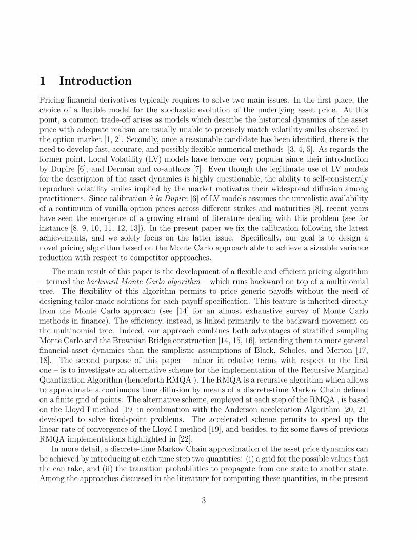
Figure 1: Example of one Monte Carlo path sampled with the LTSA with u1 = t1, u2 = t3, andu3 = t5.
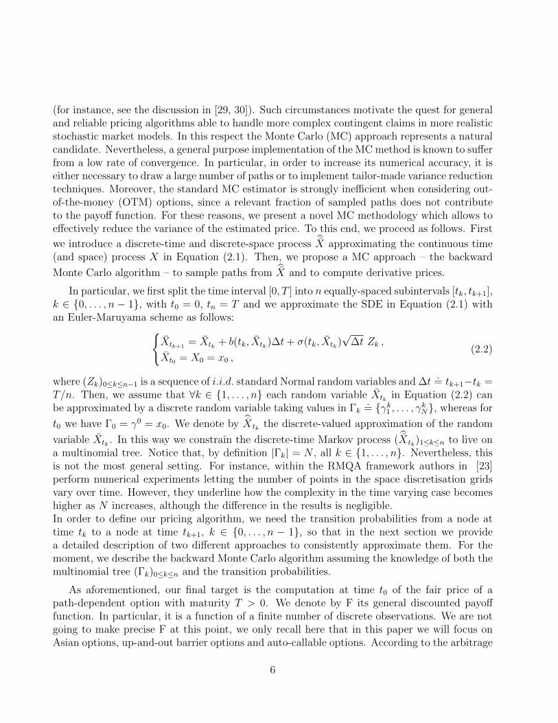
off-line the m transition matrices as in Equation (1), then we price the derivative products viaMonte Carlo with coarse-grained resolution. In Figure 1 we plot an example of a possible pathcorresponding to the case m = 3. This major difference between RMQA and LTSA becomesmore evident looking at Figures 2 and 3, where we plot, respectively, a Monte Carlo simulation
connecting the initial point x0 with a random final point X t5 , and a direct jump to date
simulation to random points X tk with k = 1, . . . , 5, respectively.
Figure 2: Example of one Monte Carlo path sampled with RMQA over a time-grid computedwith six time buckets.
17
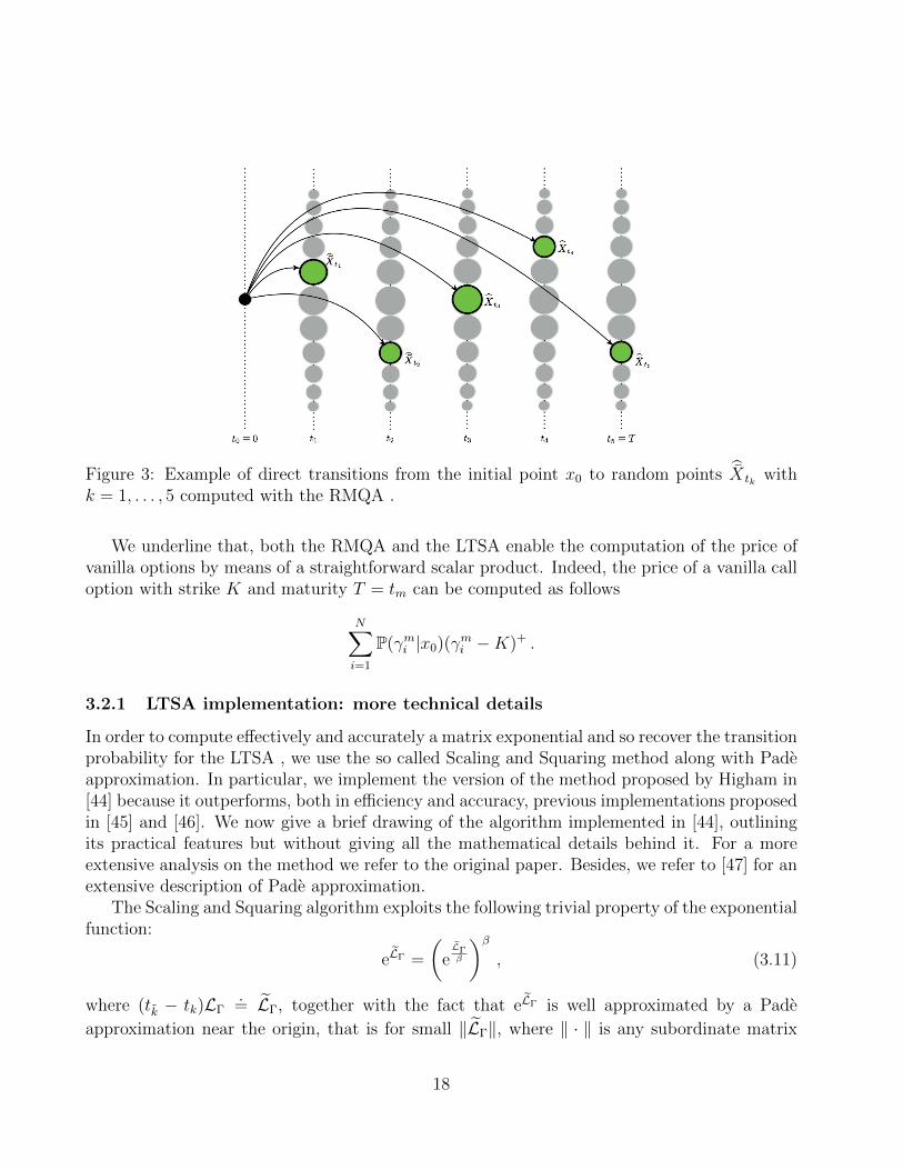
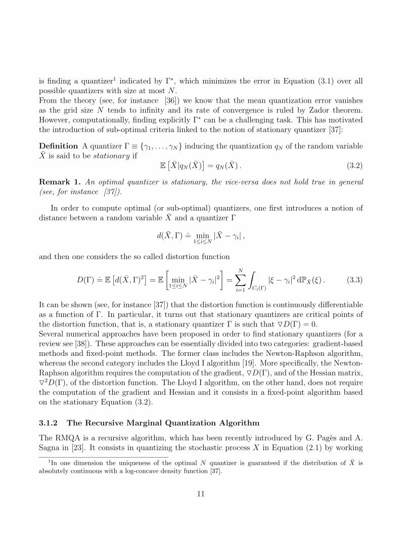
Figure 3: Example of direct transitions from the initial point x0 to random points X tk withk = 1, . . . , 5 computed with the RMQA .
We underline that, both the RMQA and the LTSA enable the computation of the price ofvanilla options by means of a straightforward scalar product. Indeed, the price of a vanilla calloption with strike K and maturity T = tm can be computed as follows
N∑
i=1
P(γmi |x0)(γmi −K)+ .
3.2.1 LTSA implementation: more technical details
In order to compute effectively and accurately a matrix exponential and so recover the transitionprobability for the LTSA , we use the so called Scaling and Squaring method along with Padeapproximation. In particular, we implement the version of the method proposed by Higham in[44] because it outperforms, both in efficiency and accuracy, previous implementations proposedin [45] and [46]. We now give a brief drawing of the algorithm implemented in [44], outliningits practical features but without giving all the mathematical details behind it. For a moreextensive analysis on the method we refer to the original paper. Besides, we refer to [47] for anextensive description of Pade approximation.
The Scaling and Squaring algorithm exploits the following trivial property of the exponentialfunction:
eLΓ =
(eLΓβ
)β, (3.11)
where (tk − tk)LΓ.= LΓ, together with the fact that eLΓ is well approximated by a Pade
approximation near the origin, that is for small ‖LΓ‖, where ‖ · ‖ is any subordinate matrix
18

norm. In particular, Pade approximation estimates eLΓ with the ratio between two (matrix)polynomials of degree 13. The mathematical elegance of the Pade approximation is enhancedby the fact that the two approximating polynomial are known explicitly.The main hint of the Scaling and Squaring method is to choose β in Equation (3.11) as an
integer power of 2, β = 2n say, so that LΓ/β has norm of order 1, to approximate eLΓ/β by a
Pade approximation, and then to compute eLΓ by repeating squaring n times. In particular, wedefine δt
.= (tk′− tk)/2n. We use Pade approximation because of the usage of the explicit Euler
Scheme for the discretisation of L (see Appendix D). Indeed, one needs to impose the so calledCourant condition for the matrix δtLΓ. The Courant condition requires that ‖δLΓ‖∞ < 1. Thistranslates into the following stringent condition for δt
δt <1
2
(∆γ)2
σ(γi), ∀ 1 ≤ i ≤ N .
The usage of the Pade approximation permits to relax the last constraint. In particular, theimplementation in [44] allows ‖δLΓ‖∞ to be much larger.
4 Financial applications
In this final section we present and discuss how results achieved in the previous Sections 2and 3 can be applied to finance, and in particular to option pricing in the FX market, wherespot and forward contracts, along with vanilla and exotic options are traded (see, for instance[48] for a broad overview on FX market). In particular, we consider the following types ofpath-dependent options: (i) Asian calls, (ii) up-and-out barrier calls, (iii) automatic callable(or auto-callabe). We choose two different models for the underlying EUR/USD FX rate: a LVmodel as a benchmark and the Constant Elasticity of Variance model (henceforth CEV) [49],coming from the academic literature.
4.1 Model and payoff specifications
Let us first introduce some notations relative to the LV model and to the CEV model. Recallthat we have assumed in Section 2 deterministic interest rates. Moreover, we indicate byXt the spot price at time t of one EUR expressed in USD and by Xt(T ) the correspondingforward price at time t for delivery at time T . We introduce the so-called normalized spotexchange rate xLVt
.= Xt/X0(t), all t ∈ [0, T ] (where the superscript “LV” clearly stands for
Local Volatility)and we suppose that the process xLV.= (xLVt )t∈[0,T ] follows the SDE
dxLVt = xLVt η(t, xLVt ) dWt ,
xLV0 = 1 .
Hence, in this LV model, xLV corresponds to the underlying process X introduced in Section2, and besides making reference to Equation (2.1) we have b(t, xLVt ) = 0 and σ(t, xLVt ) =
19

η(t, xLVt )xLVt , where η : [0, T ] × R → R+ corresponds to the local volatility function. Specifi-cally, it is a cubic monotone spline for fixed t ∈ [0, T ] (see [50] for an overview on interpolationtechnique) with flat extrapolation. The set of points to be interpolated is determined numer-ically during the calibration procedure2. In particular, this procedure leads to a piecewisetime-homogeneous dynamics for the process xLV .As a second example we consider the CEV, i.e., we assume that the asset price process Xfollows a CEV dynamics
dXt = rXt dt+ σXαt dWt ,
X0 = x0 ∈ R+ ,
where r ∈ R+ is the risk-free interest rate, σ ∈ R+ is the volatility, and α > 0 is a constantparameter.
Then, given a time discretisation grid 0 = t0, t1, . . . , tn = T on [0, T ] as in Section 2 andmaking reference to the Euler-Maruyama scheme in Equation (2.2) we consider the unidimen-sional payoff specifications below. In particular, we compute the price at time t0 = 0.
i) Asian calls. The discounted payoff function of a discretely monitored Asian call optionis
FA(X0, . . . , Xtn).= e−r(tn−t0) max
(1
n+ 1
n∑
i=0
Xti −K, 0),
where K is the strike price and T > 0 the maturity.
ii) Up-and-out barrier calls. We consider barrier options of European style. The dis-counted payoff at maturity T > 0 of an up-and-out barrier call is given by:
e−r(tn−t0) max(XT −K, 0)11τ>T (4.1)
where K is the strike price, τ.= inft ≥ 0 : Xt ≥ B and B is the upper barrier.
It is known – see for instance [15] – that, whenever we discretise the continuous timediscounted payoff in Equation (4.1) by defining
FB(Xt0 , . . . , Xtn).= e−r(tn−t0) max(Xtn −K, 0)
n∏
k=0
11Xtk<B ,
we overestimate the price of the option. Actually, we do not take into account thepossibility that the asset price could have crossed the barrier for some t ∈ (tk, tk+1),0 ≤ k ≤ n−1. In [14, 15] the authors propose a strategy to obtain a better approximation
2We use the calibration procedure proposed in [12] and refined in [13]. This procedure is particularly robust.Indeed, the resulting local volatility surface is ensured to be a smooth function of the spot. The data set isavailable upon requests.
20

of the price of the option in Equation (4.1) when employing MC simulation. It consistsin checking, at each time step tk = k∆t, 0 ≤ k ≤ n − 1, and for all the MC paths l,1 ≤ l ≤ NMC , whether the simulated path X
(l)tk
has reached the barrier B or not. So, firstone computes the probability
p(l)k
.= 1− exp
[− 2
σk∆t(B − X(l)
tk)(B − X(l)
tk+1)
],
with σk the diffusive coefficient of the underlying asset price in (tk, tk+1), then one sim-
ulates a random variable from a Bernoulli distribution with parameter 1 − p(l)k : if the
outcome is favourable the barrier has been reached in the interval (tk, tk+1) and the priceassociated to the l-th path is zero. Otherwise, the simulation is carried on to the step fur-ther. Consistently, the adjusted discounted payoff for a discretely monitored up-and-outcall barrier option reads:
e−r(tn−t0) max(Xtn −K, 0)n−1∏
k=0
pk .
iii) Automatic callable (or auto-callable)3. The discounted payoff of an auto-callableoption with unitary notional is given by
e−r(t
ci−t0)Qi if Xtcj
< X0b ≤ Xtcifor all j < i ,
e−r(tn−t0)XtnX0
if Xtci< X0b for all i = 1, . . . ,m ,
where tc1, . . . , tcm is a set of pre-fixed call dates, b > X0 is a pre-fixed barrier level, andQ1, . . . , Qm is a set of pre-fixed coupons. The set of call dates tc1, . . . , tcm does notcoincide with the set of times of the Euler scheme discretisation t0, . . . , tn. In particular,the latter has finer time resolution grid.
We show in Section 4.2 that all previous payoffs can be priced efficiently by using our novelalgorithm, i.e., by reverting the Monte Carlo paths and simulating them from maturity backto the initial date.
4.2 Numerical results and discussion
Let us introduce some terminology that we will use in the summary Tables of our numericalresults. In particular, we will termed: (i) Euler Scheme prices obtained via a Monte Carloprocedure on the process X, (ii) Forward prices obtained via a forward Monte Carlo procedure
on X from the starting date to the maturity, (iii) Backward prices computed through the
3They were first issued in the U.S. by BNP Paribas in August 2003 as cited for instance in [51].
21

Backward Monte Carlo algorithm, and finally, (iv) the Benchmark price is an Euler Schemeprice (in case of Asian call and up-and-out barrier call options) or a Forward price (in caseof auto-callable option) whose estimation error is negligible respect to the significant digitsreported. Besides, in brackets we will report the numerical estimation error corresponding toone standard deviation.Let us now stress some aspects related to the implementation of the backward Monte Carloalgorithm along with the procedures described in Sections 3.1 and 3.2.In order to have a meaningful comparison between Euler Scheme and Backward prices andbetween Forward and Backward prices, for each of the N+ points γnin ∈ Γn we generate N in
MC
random paths in such a way that N inMC × N+ = NMC , where NMC indicates the number of
simulations employed to compute either Euler Scheme or Forward prices. The choice of thefinal domain of integration Γn depends on the payoff specification. In particular, Γn
.= γni ∈
Γn : K ≤ γni ≤ B when pricing up-and-out call barrier options and Γn = Γn when pricingIn-The-Money (ITM), At-The-Money (ATM), Out-The-Money (OTM) Asian call options andauto-callable options. Concerning the granularity of the state-space discretisation we fix thecardinality of the quantizers Γk, 1 ≤ k ≤ n, to 100. With this value the error on vanilla calloption prices, computed as
|σmkt − σalg| (4.2)
is less than or equal to five basis point (recall that 1 bp = 10−4), where in Equation (4.2),σmkt is the market implied volatility, whereas σalg is the implied volatility computed by thebackward Monte Carlo algorithm.The stopping criteria for the RMQA corresponds to ‖Γl+1
k − Γlk‖ ≤ 10−5, 1 ≤ k ≤ n, whereΓlk is the quantizer computed by the algorithm at time tk ∈ t1, . . . , tn at the l-th iteration.
Moreover, in the Backward Monte Carlo algorithm case, for each point in Γn we generateN inMC = NMC ÷ |N+| = 104 ÷ |Γn| random paths. Let us now come to the discussion of the
numerical results.
In Table 1 we report up-and-out barrier call option prices for both LV and CEV, as wellas their relative estimation errors. In order to test the performances of our algorithm weprice ITM, ATM and OTM options. In particular, for both models the initial spot price isX0 = 1.36. This value corresponds to the value of the EUR/USD exchange rate at pricing date(23-June-2014). Besides, for both dynamics the value of the pair strike-barrier, (K,B), is setto (1.35, 1.39), (1.36, 1.39) and to (1.37, 1.39) for ITM, ATM and OTM up-and-out call barrieroptions respectively. The maturity T is 6 months and the number of Euler steps is n = 51. ForCEV model we fix α = 0.5 and r = 0.32% (the latter corresponds to the value of the 6 monthsdomestic interest rates implied by the forward USD curve at pricing date). Instead, as regardsthe parameter σ we vary it from σ = 5% to σ = 20% with steps ∆σ = 5%.Panel A of Table 1 compares the efficiency of the Euler Scheme Monte Carlo with that ofthe Backward Monte Carlo for the Local Volatility dynamics. Panel B, instead, comparesthe efficiency of the two algorithms for the CEV dynamics. For both models the Backward
22

Monte Carlo algorithm exhibits better performances than the Euler Scheme Monte Carlo. Moreprecisely, for LV the ratio between the estimation error of the Euler Scheme MC and that ofthe Backward MC, henceforth Error ratio, is 2.2, 2.5 and 3.1 for ITM, ATM and OTM optionsrespectively. As regards the CEV model, Figure 4 summarizes the results. In particular, gain inefficiency is more evident if we increase the value of the parameter σ. Intuitively, this happensbecause the probability for the price paths to hit the barrier B over the life of the optionincreases with the increasing of σ. Moreover, for a fixed value of σ gain in efficiency is moreevident when pricing OTM options. This happens because for OTM options a relevant numberof forward paths do not contribute to the payoff and, in order to increase the pricing accuracyof the Euler Scheme MC, it would be necessary to force paths to sample the region in whichthe payoff is different from zero, namely between the strike K and the barrier B.
5% 10% 15% 20%
Parameter σ
1
2
3
4
5
6
7
8
9
10
Err
orra
tio
Up-and-out barrier call optionITM Euler - BacwardATM Euler - BacwardOTM Euler - Bacward
Figure 4: Plot of the Error ratio as a function of the parameter σ for CEV model whenpricing up-and-out barrier call option. The initial spot price is X0 = 1.36, whereas the pairstrike-barrier is set to (1.35, 1.39), (1.36, 1.39), (1.37, 1.39) for ITM, ATM and OTM optionsrespectively.
In Table 2 we compare performances of the Euler Scheme Monte Carlo with those of theBackward Monte Carlo when pricing Asian call options, for both LV and CEV model. We setX0 = 1.36. As done for up-and-out barrier call we test the efficiency of our novel algorithmwhen pricing ITM (K = 1.35), ATM (K = 1.36) and OTM (K = 1.37) options. The maturity
23

Up-and-out barrier call
Algorithm ITM ATM OTM
Panel A Local Volatility model
Euler Scheme 1.063E-3 (3.8E-5) 4.54E-4 (2.2E-5) 1.41E-4( 1E-5)Backward 1.064E-3 (1.7E-5) 4.67E-4 ( 9E-6) 1.45E-4( 3E-5)Benchmark 1.055E-3 4.58E-4 1.44E-4
Panel B CEV model
σ = 5%
Euler Scheme 2.431E-3 (6.7E-5) 1.133E-3 (4.1E-5) 3.11E-4 (1.7E-5)Backward 2.500E-3 (3.1E-5) 1.116E-3 (1.6E-5) 3.49E-4 (6E-6)Benchmark 2.501E-3 1.073E-3 3.49E-4
σ = 10%
Euler Scheme 4.53E-4 (3.0E-5) 1.86E-4 (1.8E-5) 5.31E-5 (7.5E-6)Backward 3.94E-4 (1.0E-5) 1.69E-4 ( 5E-6) 5.39E-5 (1.8E-6)Benchmark 4.03E-4 1.70E-4 5.49E-5
σ = 15%
Euler Scheme 1.32E-4 (1.6E-5) 5.59E-5 (9.1E-6) 1.48E-5 (4.0E-6)Backward 1.28E-4 (5 E-6) 5.57E-5 (2.3E-6) 1.64E-5 ( 8E-7)Benchmark 1.19E-4 5.56E-5 1.64E-5
σ = 20%
Euler Scheme 4.85E-5 (9.3E-6) 2.91E-5 (6.8E-6) 6.2E-7 ( 4.4E-7)Backward 5.80E-5 (2.6E-6) 2.53E-5 (1.2E-6) 8.1E-7 ( 5E-8)Benchmark 5.52E-5 2.43E-5 7.5E-7
Table 1: Numerical values for Euler Scheme and Backward prices for an up-and-out barriercall option for both LV and CEV model. Errors correspond to one standard deviation. Theinitial spot price is X0 = 1.36, whereas the pair strike-barrier is set to (1.35, 1.39), (1.36, 1.39),(1.37, 1.39) for ITM, ATM and OTM options respectively.
T is 6 months and n = 51. Also in this case, for CEV model we fix the value of the risk-free rate r = 0.32% and of α = 0.5, and we vary the value of σ from 5% to 20% with steps∆σ = 5%. Results for the LV dynamics are reported in Panel A of Table 2, whereas Panel Breports the results for the CEV. Table 2 suggests that the strategy of reverting the MC pathsand simulating them from maturity back to starting date is an effective alternative to EulerMC also for Asian call options. In this case the improvement in efficiency derives from thefact that with Backward MC we decide the number of paths to sample from each of the final
24

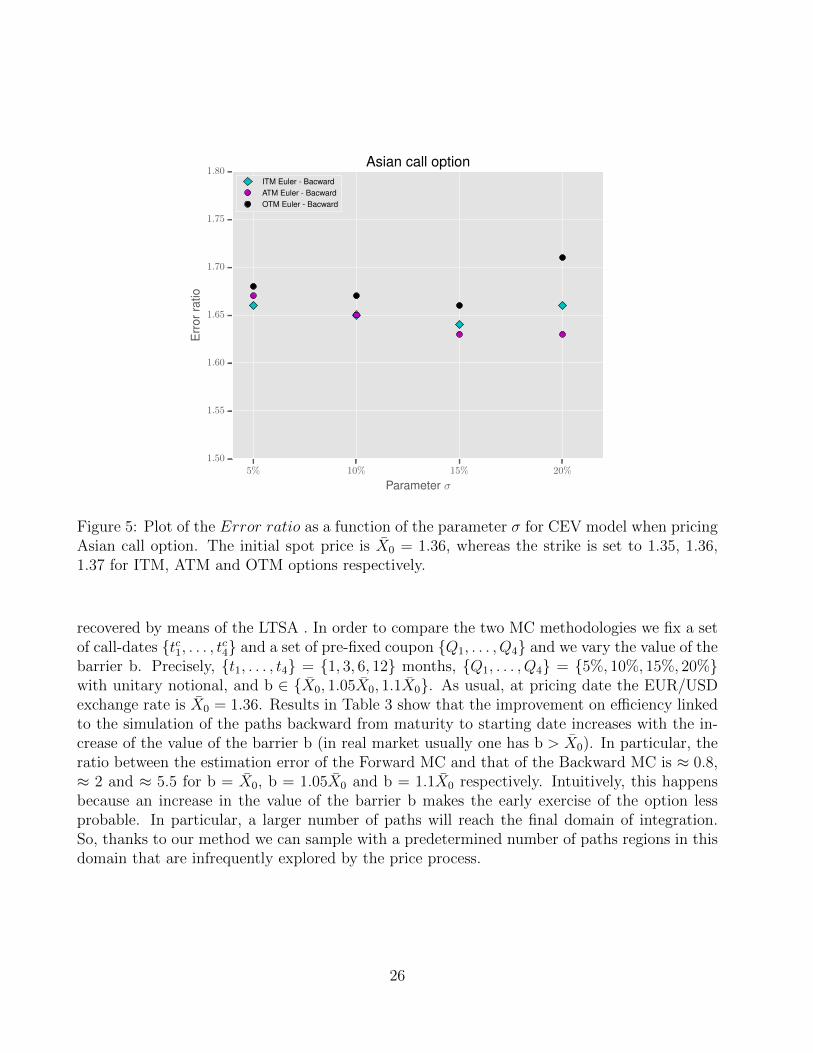
points in Γn, sampling efficiently also those regions that are infrequently explored by the priceprocess because of its diffusive behaviour. Figure 5 suggests that the importance of this featureis more evident when pricing OTM options. Besides, the Error ratio is almost constant acrossthe value of σ for a fixed scenario (ITM, ATM or OTM).
Asian call
Algorithm ITM ATM OTM
Panel A Local Volatility model
Euler Scheme 0.013628 (0.000161) 0.009444 (0.000142) 0.006194 (0.000142)Backward 0.013582 (0.000107) 0.009384 (0.000092) 0.006124 (0.000092)Benchmark 0.013590 0.009398 0.006170
Panel B CEV model
σ = 5%
Euler Scheme 0.015964 (0.000174) 0.009851 (0.000143) 0.005826 (0.000109)Backward 0.015904 (0.000105) 0.010014 (0.000085) 0.005565 (0.000065)Benchmark 0.015989 0.010038 0.005634
σ = 10%
Euler Scheme 0.024682 (0.000321) 0.019681 (0.000288) 0.014780 (0.000251)Backward 0.024709 (0.000190) 0.019164 (0.000171) 0.015021 (0.000150)Benchmark 0.024927 0.019448 0.014921
σ = 15%
Euler Scheme 0.033764 (0.00056) 0.028335 (0.000424) 0.024203 (0.000391)Backward 0.034160 (0.00033) 0.028896 (0.000232) 0.024132 (0.000236)Benchmark 0.033991 0.028867 0.024011
σ = 20%
Euler Scheme 0.043553 (0.000604) 0.037880 (0.000554) 0.033989 (0.000542)Backward 0.043117 (0.000363) 0.037653 (0.000341) 0.033234 (0.000317)Benchmark 0.043276 0.033366 0.033367
Table 2: Numerical values for Euler Scheme and Backward prices for an Asian call option forboth LV and CEV model. Errors correspond to one standard deviation.
In Table 3 we report prices of an auto-callable option for LV. In this case, we compare theBackward MC with the Forward MC. The Euler Scheme MC is ineffective for payoffs specifica-tions which depend on the observation of the underlying on a pre-specified set of dates (such asauto-callable and European). The multinomial tree and the transition probability matrices are
25
5% 10% 15% 20%
Parameter σ
1.50
1.55
1.60
1.65
1.70
1.75
1.80
Err
orra
tio
Asian call optionITM Euler - BacwardATM Euler - BacwardOTM Euler - Bacward
Figure 5: Plot of the Error ratio as a function of the parameter σ for CEV model when pricingAsian call option. The initial spot price is X0 = 1.36, whereas the strike is set to 1.35, 1.36,1.37 for ITM, ATM and OTM options respectively.
recovered by means of the LTSA . In order to compare the two MC methodologies we fix a setof call-dates tc1, . . . , tc4 and a set of pre-fixed coupon Q1, . . . , Q4 and we vary the value of thebarrier b. Precisely, t1, . . . , t4 = 1, 3, 6, 12 months, Q1, . . . , Q4 = 5%, 10%, 15%, 20%with unitary notional, and b ∈ X0, 1.05X0, 1.1X0. As usual, at pricing date the EUR/USDexchange rate is X0 = 1.36. Results in Table 3 show that the improvement on efficiency linkedto the simulation of the paths backward from maturity to starting date increases with the in-crease of the value of the barrier b (in real market usually one has b > X0). In particular, theratio between the estimation error of the Forward MC and that of the Backward MC is ≈ 0.8,≈ 2 and ≈ 5.5 for b = X0, b = 1.05X0 and b = 1.1X0 respectively. Intuitively, this happensbecause an increase in the value of the barrier b makes the early exercise of the option lessprobable. In particular, a larger number of paths will reach the final domain of integration.So, thanks to our method we can sample with a predetermined number of paths regions in thisdomain that are infrequently explored by the price process.
26

Auto-callable options
Barrier b b = X0 b = 1.05X0 b = 1.1X0
Algorithm Local Volatility model
Forward 0.04107 (0.00056) 0.01902 (0.00074) 0.00447 (0.00058)Backward 0.04099 (0.00072) 0.01856 (0.00039) 0.00377 (0.00011)Benchmark 0.04099 0.01820 0.00357
Table 3: Numerical values for Forward and Backward prices for an auto-callable option for LVmodel. Errors correspond to one standard deviation.
5 Conclusion
In this paper, we present a novel approach – termed backward Monte Carlo – to the MonteCarlo simulation of continuous time diffusion processes. We exploit recent advances in thequantization of diffusion processes to approximate the continuous process with a discrete-timeMarkov Chain defined on a finite grid of points. Specifically, we consider the Recursive MarginalQuantization Algorithm and as a first contribution we investigate a fixed-point scheme – termedLloyd I method with Anderson acceleration – to compute the optimal grid in a robust way. Asa complementary approach, we consider the grid associated with the explicit scheme approxi-mation of the Markov generator of a piecewise constant volatility process. The latter approach– termed Large Time Step Algorithm – turns out to be competitive in pricing payoff specifi-cations which require the observation of the price process over a finite number of pre-specifieddates. Both methods – quantization and the explicit scheme – provide us with the marginaland transition probabilities associated with the points of the approximating grid. Samplingfrom the discrete grid backward – from the terminal point to the spot value of the process –we design a simple but effective mechanism to draw Monte Carlo path and achieve a sizeablereduction of the variance associated with Monte Carlo estimators. Our conclusion is extensivelysupported by the numerical results presented in the final section.
References
[1] Jean-Philippe Bouchaud and Marc Potters. Theory of financial risk and derivative pricing:from statistical physics to risk management. Cambridge university press, 2003.
[2] Jim Gatheral. The volatility surface: a practitioner’s guide, volume 357. John Wiley &Sons, 2011.
[3] John C Hull. Options, futures, and other derivatives. Pearson Education India, 2006.
27

[4] Paul Wilmott, Jeff Dewynne, and Sam Howison. Option pricing: mathematical modelsand computation. Oxford financial press, 1993.
[5] Les Clewlow and Chris Strickland. Implementing derivative models (Wiley Series in Fi-nancial Engineering). 1996.
[6] Bruno Dupire. Pricing with a smile. Risk, 7(1):18–20, 1994.
[7] E Derman and I Kani. Riding on a smile risk magazine, 7, 32-39 (1994). Derman E., KaniI., Zou JZ, The Local Volatility Surface: Unlocking the Information in Index OptionsPrices Financial Analysts Journal,(July-Aug 1996), pages 25–36.
[8] Nabil Kahale. An arbitrage-free interpolation of volatilities. Risk, 17(5):102–106, 2004.
[9] Thomas F Coleman, Yuying Li, and Arun Verma. Reconstructing the unknown localvolatility function. Journal of Computational Finance, 2(3):77–102, 1999.
[10] Jesper Andreasen and Brian Huge. Volatility interpolation. Risk, 24(3):76, 2011.
[11] Alex Lipton and Artur Sepp. Filling the gaps. Risk, 24(10):78, 2011.
[12] Adil Reghai, Gilles Boya, and Ghislain Vong. Local volatility: Smooth calibration andfast usage. 2012. ssrn.com/abstract=2008215.
[13] Andrea Pallavicini. A calibration algorithm for the local volatility model. In preparation,2015.
[14] Paul Glasserman. Monte Carlo methods in financial engineering, volume 53. SpringerScience & Business Media, 2003.
[15] Bernard Lapeyre, Agnes Sulem, and Denis Talay. Understanding Numerical Analysis forOption Pricing. Cambridge University Press, 2003.
[16] G Bormetti, G Montagna, N Moreni, and O Nicrosini. Pricing exotic options in a pathintegral approach. Quantitative Finance, 6(1):55–66, 2006.
[17] Fischer Black and Myron Scholes. The pricing of options and corporate liabilities. Thejournal of political economy, pages 637–654, 1973.
[18] Robert C Merton. Theory of rational option pricing. Bell Journal of Economics, 4(1):141–183, 1973.
[19] John B Kieffer. Exponential rate of convergence for lloyd’s method i. Information Theory,IEEE Transactions on, 28(2):205–210, 1982.
[20] Donald G Anderson. Iterative procedures for nonlinear integral equations. Journal of theACM (JACM), 12(4):547–560, 1965.
28

[21] Homer F Walker and Peng Ni. Anderson acceleration for fixed-point iterations. SIAMJournal on Numerical Analysis, 49(4):1715–1735, 2011.
[22] Giorgia Callegaro, Lucio Fiorin, and Martino Grasselli. Pricing and calibration in localvolatility models via fast quantization. Risk Magazine, 2015.
[23] Abass Sagna et al. Recursive marginal quantization of an euler scheme with applicationsto local volatility models. arXiv preprint arXiv:1304.2531, 2013.
[24] Harold Kushner and Paul G Dupuis. Numerical methods for stochastic control problemsin continuous time, volume 24. Springer Science & Business Media, 2013.
[25] Claudio Albanese and Aleksandar Mijatovic. Convergence rates for diffusions oncontinuous-time lattices. SSRN Working Paper Series, 2007.
[26] Claudio Albanese, Harry Lo, and Aleksandar Mijatovic. Spectral methods for volatilityderivatives. Quantitative Finance, 9(6):663–692, 2009.
[27] Jacques Printems et al. Functional quantization for numerics with an application to optionpricing. Monte Carlo Methods and Applications mcma, 11(4):407–446, 2005.
[28] Yong Ren, Dilip Madan, and M Qian Qian. Calibrating and pricing with embedded localvolatility models. RISK-LONDON-RISK MAGAZINE LIMITED-, 20(9):138, 2007.
[29] Cho Hoi Hui, Chi-Fai Lo, and PH Yuen. Comment on pricing double barrier options usinglaplace transforms by antoon pelsser. Finance and Stochastics, 4(1):105–107, 2000.
[30] Jan Vecer and Mingxin Xu. Pricing asian options in a semimartingale model. QuantitativeFinance, 4(2):170–175, 2004.
[31] Tomas Bjork. Arbitrage theory in continuous time. Oxford university press, 2004.
[32] Jerome Barraquand and Didier Martineau. Numerical valuation of high dimensional multi-variate american securities. Journal of financial and quantitative analysis, 30(03):383–405,1995.
[33] Vlad Bally, Gilles Pages, et al. A quantization algorithm for solving multidimensionaldiscrete-time optimal stopping problems. Bernoulli, 9(6):1003–1049, 2003.
[34] Claudio Albanese. Operator methods, abelian processes and dynamic conditioning. AbelianProcesses and Dynamic Conditioning (October 16, 2007), 2007.
[35] Richard A Kronmal and Arthur V Peterson Jr. On the alias method for generating randomvariables from a discrete distribution. The American Statistician, 33(4):214–218, 1979.
29

[36] Siegfried Graf and Harald Luschgy. Foundations of quantization for probability distribu-tions. Springer, 2000.
[37] Gilles Pages et al. Introduction to optimal vector quantization and its applications fornumerics. 2014.
[38] Gilles Pages, Huyen Pham, and Jacques Printems. Optimal quantization methods andapplications to numerical problems in finance. In Handbook of computational and numericalmethods in finance, pages 253–297. Springer, 2004.
[39] Gene H Golub and Charles F Van Loan. Matrix computations, volume 3. JHU Press, 2012.
[40] Ioannis Karatzas and Steven Shreve. Brownian motion and stochastic calculus, volume113. Springer Science & Business Media, 2012.
[41] Masaaki Kijima. Markov processes for stochastic modeling, volume 6. CRC Press, 1997.
[42] Andrew Ronald Mitchell and David Francis Griffiths. The finite difference method inpartial differential equations. John Wiley, 1980.
[43] Sergio Blanes, Fernando Casas, JA Oteo, and Jose Ros. The magnus expansion and someof its applications. Physics Reports, 470(5):151–238, 2009.
[44] Nicholas J Higham. The scaling and squaring method for the matrix exponential revisited.SIAM Journal on Matrix Analysis and Applications, 26(4):1179–1193, 2005.
[45] Roger B Sidje. Expokit: a software package for computing matrix exponentials. ACMTransactions on Mathematical Software (TOMS), 24(1):130–156, 1998.
[46] Robert C Ward. Numerical computation of the matrix exponential with accuracy estimate.SIAM Journal on Numerical Analysis, 14(4):600–610, 1977.
[47] George A Baker and Peter Russell Graves-Morris. Pade approximants, volume 59. Cam-bridge University Press, 1996.
[48] Dimitri Reiswich and Wystup Uwe. Fx volatility smile construction. Wilmott, 2012(60):58–69, 2012.
[49] John Cox. Notes on option pricing i: Constant elasticity of variance diffusions. Unpublishednote, Stanford University, Graduate School of Business, 1975.
[50] Frederick N Fritsch and Ralph E Carlson. Monotone piecewise cubic interpolation. SIAMJournal on Numerical Analysis, 17(2):238–246, 1980.
[51] Geng Deng, Joshua Mallett, and Craig McCann. Modeling autocallable structured prod-ucts. Journal of Derivatives & Hedge Funds, 17(4):326–340, 2011.
30

[52] Rene Carmona, Pierre Del Moral, Peng Hu, and Nadia Oudjane. Numerical Methods inFinance: Bordeaux, June 2010. Springer Science & Business Media, 2012.
[53] Gilles Pages and Jacques Printems. Optimal quadratic quantization for numerics: theGaussian case. Monte Carlo Methods and Applications, 9(2):135–165, 2003.
A The distortion function and companion parameters
We suppose to have access to the quantizer Γk of Xtk and to the related Voronoi tessellations
Ci(Γk)i=1,...,N . We derive an explicit expression for the distortion function D(Γk+1) as follows:
D(Γk+1) = E[d(Ek( X tk ,∆t;Ztk+1
),Γk+1)2
]
=N∑
i=1
E[d(Ek(γki ,∆t;Ztk+1
),Γk+1)2]P(Xtk ∈ Ci(Γk))
=N∑
i=1
N∑
j=1
(mk(γki )− γk+1
j )2(Φ(γk+1,j+(γki ))− Φ(γk+1,j−(γki )))P(Xtk ∈ Ci(Γk))
− 2N∑
i=1
N∑
j=1
(mk(γki )− γk+1
j )vk(γki )(ϕ(γk+1,j+(γki ))− ϕ(γk+1,j−(γki )))P(Xtk ∈ Ci(Γk))
+N∑
i=1
N∑
j=1
vk(γki )2(γk+1,j−(γki )ϕ(γk+1,j−(γki ))− γk+1,j+(γki )ϕ(γk+1,j+(γki )))P(Xtk ∈ Ci(Γk))
+N∑
i=1
N∑
j=1
vk(γki )2(Φ(γk+1,j+(γki ))− Φ(γk+1,j−(γki )))P(Xtk ∈ Ci(Γk)) ,
(A.1)
where Φ and ϕ indicate the cumulative distribution function and the probability density func-tion of a standard Normal random variable, respectively. To simplify notation, in Equation(A.1), we set for all k ∈ 0, . . . , n− 1 and for all j ∈ 1, . . . , N
γk+1,j+(γ).=γk+1j+1/2 −mk(γ)
vk(γ)and γk+1,j−(γ)
.=γk+1j−1/2 −mk(γ)
vk(γ)where
γk+1j−1/2 ≡
γk+1j + γk+1
j−1
2, γk+1
j+1/2 ≡γk+1j + γk+1
j+1
2, γk+1
1/2
.= −∞ , and γk+1
N+1/2
.= +∞ .
31

The so-called companion parameters P(Xtk ∈ Ci(Γk))i=1,...,N and P(Xtk ∈ Cj(Γk)|Xtk−1∈
Ci(Γk))j=1,...,N are computed in a recursive way as follows:
P(Xtk ∈ Ci(Γk)) =N∑
j=1
(Φ(γk,i+(γk−1j ))− Φ(γk,i−(γk−1
j )))P(Xtk−1∈ Cj(Γk−1)) ,
P(Xtk ∈ Ci(Γk)|Xtk−1∈ Cj(Γk−1)) = Φ(γk,i+(γk−1
j ))− Φ(γk,i−(γk−1j )).
B Lloyd I method within the RMQA
We present a brief review of the Lloyd I method within the Recursive Marginal Quantizationframework. Let us fix tk ∈ t1, . . . , tn and suppose we have access to the quantizer Γk of
Xtk and to the associated Voronoi tessellations Ci(Γk)i=1,...,N . We want to quantize Xtk+1=
Ek( X tk ,∆t;Ztk+1) by means of a quantizer Γk+1 ≡ γk+1
1 , . . . , γk+1N of cardinality N . One starts
with an initial guess Γ0k+1 and then one sets recursively a sequence (Γlk+1)l∈N such that
γk+1,l+1j = E
[Xtk+1
|Xtk+1∈ Cj(Γlk+1)
], (B.1)
where l indicates the running iteration number. One can easily check that previous equationimplies that
ql+1N (Xtk+1
) = E[Xtk+1
|qlN(Xtk+1)].=(E[Xtk+1
|Xtk+1∈ Ci(Γlk+1)
])1≤i≤N
,
where qlN is the quantization associated with Γlk+1. It has been proven (see [38, 52])) that
‖Xtk+1− qlN(Xtk+1
)‖2, l ∈ N+ is a non-increasing sequence and that qlN(Xtk+1) converges
towards some random variable taking N values as l tends to infinity. From Equation (B.1) andexploiting the idea of RMQA we have
γk+1,l+1j = E
[Xtk+1
|Xtk+1∈ Cj(Γlk+1)
]
=E[Xtk+1
11X∈Cj(Γlk+1)
]
P(Xtk+1∈ Cj(Γlk+1))
=E[E[Xtk+1
11Xtk+1∈Cj(Γlk+1)|Xtk
]]
E[E[11Xtk+1
∈Cj(Γlk+1)|Xtk
]]
=
∑Ni=1
E[Ek(γki ,∆t;Ztk+1
)11Ek(γki ,∆t;Ztk+1)∈Cj(Γlk+1)
]P(Xtk ∈ Ci(Γk))
∑Ni=1 P(Ek(γki ,∆t;Ztk+1
) ∈ Cj(Γlk+1)P(Xtk ∈ Ci(Γk)).
The last term in previous equation is equivalent to the stationary condition in Equation (3.2)
for the quantization qN(Xtk+1). Then, the stationary condition is equivalent to a fixed point
relation for the quantizer.
32

C Robustness checks
We test the convergence of Lloyd I method with and without Anderson acceleration on thequantization of a standard Normal random variable4 initialised from a distorted quantizer.We indicate by Γ∗N (0,1) the optimal quantizer of a standard Normal random variable and wedistort it through the multiplication by a constant c, that is to say c × Γ∗N (0,1). Then, wemonitor the convergence of both algorithms to Γ∗N (0,1) starting from c × Γ∗N (0,1). The error at
iteration l is defined as ‖Γ∗N (0,1)− ΓlN (0,1)‖2, with ΓlN (0,1) the quantizer found by the algorithms
at the l-th iteration and ‖ · ‖2 the Euclidean norm in RN . The stopping criteria is set to‖Γl+1N (0,1) − ΓlN (0,1)‖2 ≤ 10−7, the level of the quantizer to N = 10, and the constant c to 1.01.
The results of our investigation are summarized in Figure 6. We can graphically assess therate of convergence5 for both algorithms. In case of Lloyd I method without acceleration theconvergence is, as expected, linear. For Lloyd I method with acceleration the rate is not welldefined, but Figure 6 shows the impressive improvement in the convergence towards the knownoptimal quantizer. Figure 7 supports the same conclusion in terms of the number of iterationsnecessary to reach the stopping criterion.
Then, we investigate numerically the sensitivity of Lloyd I method with Anderson accelera-tion and Newton-Raphson algorithm to the initial guess as a function of the distortion c appliedto the optimal quantizer Γ∗N (0,1). The results of our investigation are summarized in Figure 8.
The four panels correspond to different levels of distortion c = 1.10, 1.20, 1.25, 1.35. As be-fore, we set N = 10 whereas on the y axis we report the residual at iteration l, ‖Γl+1 − Γl‖2.For low levels of distortion Newton-Raphson method converges to the optimal solution morequickly than Lloyd I method. This result confirms the theoretical behavior due to the quadraticrate of convergence of the Newton-Raphson algorithm. However, when the initial guess is quitefar from the solution – as it is for the cases of 25% and 35% distortion – the algorithm mayspend many cycles far away from the optimal grid.
Finally, we examine the convergence of Lloyd I and Newton-Raphson algorithms whenconsidering the following Euler-Maruyama discrete scheme
Xtk+1
= Xtk + rXtk∆t+ σXtk
√∆t Ztk ,
X0 = x0 ,
with r, σ, and x0 strictly positive real constants, and ∆t = tk+1 − tk for all k = 1, . . . , n − 1.To enlighten the greater sensitivity of the Newton-Raphson method to the grid initialisation
4At www.quantize.maths-fi.com a database providing quadratic optimal quantizers of the standard uni-variate Gaussian distribution from level N = 1 to N = 1000 is available.
5We recall that a sequence (Γl)l∈N converging to a Γ∗ 6= Γl for all l is said to converge to Γ∗ with order αand asymptotic error constant λ if there exist positive constants α and λ such that
liml→∞
‖Γl+1 − Γ∗‖2‖Γl − Γ∗‖α2
= λ .
33

10−7 10−6 10−5 10−4 10−3 10−2 10−1
Error at iteration l
10−9
10−8
10−7
10−6
10−5
10−4
10−3
10−2
10−1
Err
orat
itera
tionl+
1
Lloyd I with AccelerationLloyd I without Acceleration
Figure 6: Quantization of a standard Normal random variable: Comparison of the convergenceof Lloyd I method with and without Anderson acceleration.
in comparison with the Lloyd I with Anderson acceleration it is sufficient to stop at n = 2with ∆t = 0.01. We set the level of the quantizers Γ1 and Γ2 equal to N = 30 and x0 = 1.By definition the random variable Xt1 ∼ N (m0(x0), v0(x0)) where m0(x0) = x0 + rx0∆t andv0(x0) = σx0. In order to compute the quantizer for Xt1 we initialise the algorithms at time t1 tom0(x0)+v0(x0)Γ∗N (0,1), with Γ∗N (0,1) the optimal quantizer of a standard Normal random variable.
Once we have obtain the optimal quantizer Γ∗1 = γ∗11 , · · · , γ∗301 we set the initialisation of the
quantizer ΓInit2 = γ12 , · · · , γ30
2 at time t2 using one of the following alternatives
i. the optimal quantizer at the previous step
ΓInit2 = Γ∗1 ;
ii. the Euler operatorγi2 = m1(γi1) + v1(γi1)Γ∗,iN (0,1) ,
for i = 1, . . . , 30;
iii. the mid point between Euler operator and the optimal quantizer at the previous step
γi2 = 0.5γi1 + 0.5(m1(γi1) + v1(γi1)Γ∗,iN (0,1)) ,
for i = 1, . . . , 30;
34

0 20 40 60 80 100 120 140
Iteration Number l
10−10
10−9
10−8
10−7
10−6
10−5
10−4
10−3
10−2
10−1
Res
idua
l
Lloyd I with AccelerationLloyd I without Acceleration
Figure 7: Quantization of a standard Normal random variable: Comparison of the number ofiterations necessary to reach the stopping criterion between Lloyd I method with and withoutAnderson acceleration.
iv. the expected valueγi2 = m1(γi1) ,
for i = 1, . . . , 30.
The left panel of Figure 9 shows the four different initial grids which correspond to abovespecifications. In the same panel, on the right side, we also plot the optimal quantizer Γ∗2 towhich both Lloyd I with Anderson acceleration and Newton-Raphson methods should converge.
The right panel report the quantization error – defined as
√D2(Γl2) – as a function of the
iteration number l. We stop the algorithm when the residual falls below 10−5. The numericalinvestigation shows that the Newton-Raphson method converges to the optimal grid faster thanthe Lloyd I method, with the only exception represented by the case Γinit2 equal to the mid point.However, when initialized with the Euler operator or the mid point Newton-Raphson algorithmfails to converge due to the bad condition number of the Hessian matrix (corresponding linesare not reported on the Figure). This result is in line with the findings in [53] where the authorsstress that the Newton-Raphson method may fail even for symmetric initial vectors since theanomalous behavior of some components of the Voronoi tessellation.
In light of above explorations, we finally conclude that the approach based on a fixed-pointalgorithm such as the Lloyd I method with Anderson acceleration is much more robust than aNewton-Raphson approach – which in the present application relies on the computation of theHessian of the matrix.
35

0 2 4 6 8 10 12 14
10−14
10−12
10−10
10−8
10−6
10−4
10−2
100
‖Γ∗ N
(0,1
)−
Γl N
(0,1
)‖ 2
c=1.1 Lloyd I with Acceleration
Newton Raphson
0 2 4 6 8 10 12 14
10−14
10−12
10−10
10−8
10−6
10−4
10−2
100
c=1.20 Lloyd I with Acceleration
Newton Raphson
0 100 200 300 400
Iteration Number l
10−16
10−14
10−12
10−10
10−8
10−6
10−4
10−2
100
‖Γ∗ N
(0,1
)−
Γl N
(0,1
)‖ 2
c=1.25 Lloyd I with Acceleration
Newton Raphson
0 5 10 15 20 25 30 35
Iteration Number l
10−16
10−14
10−12
10−10
10−8
10−6
10−4
10−2
100
c=1.35 Lloyd I with Acceleration
Newton Raphson
Figure 8: Quantization of a standard Normal random variable: Comparison between Lloyd Imethod with Anderson acceleration and Newton-Raphson algorithm.
D Construction of the Markov generator LΓ
We define ∆γ.= γi+1 − γi, 1 ≤ i ≤ N − 1. The finite difference approximation of the first and
second partial derivative in Equation (3.9) is defined as
∂u
∂γ(γ, t) ≈ u(γi + ∆γ, t)− u(γi −∆γ, t)
2∆γ,
∂2u
∂γ2(γ, t) ≈ u(γi + ∆γ, t)− 2u(γi, t) + u(γi −∆γ, t)
(∆γ)2,
36

0.92
0.94
0.96
0.98
1.00
1.02
1.04
1.06
1.08
Qua
ntiz
ers
Γinit2
: Γ∗1
Γinit2
: Euler operator
Γinit2
: mid point
Γinit2
: expected value
Γ∗2
0 5 10 15 20
Iteration Number l
0.7
0.8
0.9
1.0
1.1
1.2
√D
(Γl 2)
×10−3
Lloyd I: Γ∗1
Lloyd I: Euler operatorLloyd I: mid pointLloyd I: expected valueNewton Raphson: Γ∗1
Newton Raphson: expected value
Figure 9: Quantization of the Euler-Maruyama scheme associated to a Geometric Brownianmotion. Left panel: four different initial grids Γinit2 and optimal grid Γ∗2 on the left and rightsides, respectively. Right panel: quantization error as a function of the iteration number.
for all t ∈ [0, T ]. The Markov generator LΓ is the N ×N matrix defined as
LΓ.=
d1 u1 0 0 · · · 0 0l2 d2 u2 0 · · · 0 0
0. . . . . . . . . · · · 0 0
0 0 li di ui 0 0
0 0 0. . . . . . . . . 0
0 0 0 0 lN−1 dN−1 uN−1
0 0 0 0 0 lN dN
,
where the coefficients li, di and ui are given by
li = −b(γi)2∆γ
+1
2
σ(γi)2
(∆γ)2,
di = −σ(γi)2
(∆γ)2,
ui = +b(γi)
2∆γ+
1
2
σ(γi)2
(∆γ)2,
for all 1 ≤ i ≤ N . The coefficients of the first and last row are chosen so that the Markovchain is reflected at the boundaries of the state domain. The choice of the boundary conditionsshould have a negligible effect provided that the range of the state domain is sufficiently large.
37