Embed Size (px)
Citation preview
Imperial College London
Department of Computing
Numerical Methods for Pricing Exotic Options
by
Hardik Dave - 00517958
Supervised by Dr. Daniel Kuhn
Second Marker: Professor Berc Rustem
Submitted in partial fulfilment of the requirements for the MSc Degree in AdvancedComputing of Imperial College London
September 2008

Abstract
Since the introduction of Fischer Black and Myron Scholes’ famous option pricing model [3] in1973, several authors have proposed alternative models and methodologies for pricing optionsaccurately. In this project, we evaluate and extend two such recently proposed methodologies.
In the semi-parametric approach for pricing options, originally proposed by Lo in [22] andsubsequently extended by Bertsimas and Popescu in [1] and [2] and Gotoh and Konno in [9], theoption price is identified with associated semidefinite programming (SDP) problems, the solutionof which provides tight upper and lower bounds, given the first n moments of the distribution ofthe underlying security price. While Gotoh and Konno used their own cutting plane algorithmfor solving the associated SDP problems in [9], we derive and solve such problems with our ownsoftware in this project.
Subsequently, in [21], Lasserre, Prieto-Rumeau and Zervos introduced a new methodology fornumerical pricing of exotic derivatives such as Asian and down-and-out Barrier options. In theirmethodology, the underlying asset price dynamics are modeled by geometric Brownian motionor other mean-reverting processes. For pricing derivatives, they solve a finite dimensional SDPproblem (utilizing their own software GloptiPoly), derived from another infinite dimensionallinear programming problem with moments of appropriate measures.
In this project we investigate and build upon the theory of both of the above approaches.We also extend the theory developed by Lasserre, Prieto-Rumeau and Zervos to model the SDPproblems for pricing European, up-and-out and double Barrier options. Direct implementationof software for solving the associated SDP problems for pricing the European, Asian and (down-and-out, up-and-out and double) Barrier options is given along with detailed analysis of theresults. Secondly, reimplementation of numerical methodology given by Gotoh and Konno is alsogiven, solving the associated SDP problem directly, without using their Cutting Plane algorithm.The efficiency of the above two methods is analysed and compared with other standard optionpricing techniques such as Monte Carlo methods.
i

ii

Acknowledgements
First of all, I would like to acknowledge Dr. Daniel Kuhn who provided me with constantguidance and encouragement through out the project. I am deeply indebted to Dr. Kuhn forembarking with me on this project journey. I could not have wished for better supervisor andcollaborator. Your contributions, insightful comments and awe inspiring conversations have beenof great value to me.
I would also like to acknowledge Professor Berc Rustem for his constructive comments andagreeing to be the second marker for this project.
I also acknowledge my family and friends for their moral and intellectual support during thisproject. Lastly, I would like to thank Nikita for being the indefatigable and untiring source ofstrength for me, when I needed it most.
Contents
List of Figures vi
List of Tables vii
1 Introduction 11.1 Two Recent Methodologies . . . . . . . . . . . . . . . . . . . . . . . . . . . . . . 11.2 Contributions . . . . . . . . . . . . . . . . . . . . . . . . . . . . . . . . . . . . . . 3
2 Options and Valuation Techniques 42.1 Class of Options . . . . . . . . . . . . . . . . . . . . . . . . . . . . . . . . . . . . 4
2.1.1 European Options . . . . . . . . . . . . . . . . . . . . . . . . . . . . . . . 42.1.2 Asian Options . . . . . . . . . . . . . . . . . . . . . . . . . . . . . . . . . 52.1.3 Barrier Options . . . . . . . . . . . . . . . . . . . . . . . . . . . . . . . . . 6
2.2 Models for Underlying Asset Price . . . . . . . . . . . . . . . . . . . . . . . . . . 72.2.1 Geometric Brownian Motion . . . . . . . . . . . . . . . . . . . . . . . . . 72.2.2 Ornstein-Uhlenbeck Process . . . . . . . . . . . . . . . . . . . . . . . . . . 82.2.3 Cox Ingersoll Ross process . . . . . . . . . . . . . . . . . . . . . . . . . . . 9
2.3 Monte Carlo Methods . . . . . . . . . . . . . . . . . . . . . . . . . . . . . . . . . 102.3.1 European Options . . . . . . . . . . . . . . . . . . . . . . . . . . . . . . . 102.3.2 Asian Options . . . . . . . . . . . . . . . . . . . . . . . . . . . . . . . . . 112.3.3 Barrier Options . . . . . . . . . . . . . . . . . . . . . . . . . . . . . . . . . 122.3.4 Advantages and Disadvantages of Monte Carlo Methods . . . . . . . . . . 15
2.4 Black Scholes PDE and Analytical Solution . . . . . . . . . . . . . . . . . . . . . 152.4.1 Analytical Solution for European Options . . . . . . . . . . . . . . . . . . 162.4.2 Analytical Solution for Barrier Options . . . . . . . . . . . . . . . . . . . 162.4.3 Assumptions and Shortcomings of Black Scholes Formula . . . . . . . . . 18
3 Semi-Parametric Approach for Bounding Option Price 203.1 Review of Basic Results . . . . . . . . . . . . . . . . . . . . . . . . . . . . . . . . 203.2 SDP Formulation of the Bounding Problems . . . . . . . . . . . . . . . . . . . . . 253.3 Computing the Moments . . . . . . . . . . . . . . . . . . . . . . . . . . . . . . . . 29
4 Method of Moments and SDP Relaxations 314.1 Introduction . . . . . . . . . . . . . . . . . . . . . . . . . . . . . . . . . . . . . . . 314.2 Deriving Infinite-Dimensional LP Problem . . . . . . . . . . . . . . . . . . . . . . 32
4.2.1 Basic Adjoint Equation . . . . . . . . . . . . . . . . . . . . . . . . . . . . 324.2.2 Martingale Moment Conditions . . . . . . . . . . . . . . . . . . . . . . . . 344.2.3 Using Available Moments . . . . . . . . . . . . . . . . . . . . . . . . . . . 354.2.4 Using Martingale Moments Conditions . . . . . . . . . . . . . . . . . . . . 35
4.3 Polynomial Optimisation and Problem of Moments . . . . . . . . . . . . . . . . . 364.3.1 Notation and Definition . . . . . . . . . . . . . . . . . . . . . . . . . . . . 364.3.2 Necessary Moment conditions . . . . . . . . . . . . . . . . . . . . . . . . . 37
iv
4.3.3 SDP Relaxations . . . . . . . . . . . . . . . . . . . . . . . . . . . . . . . . 384.3.4 Summary . . . . . . . . . . . . . . . . . . . . . . . . . . . . . . . . . . . . 38
4.4 Finite Dimensional Relaxations . . . . . . . . . . . . . . . . . . . . . . . . . . . . 394.5 SDP Relaxations for European Options . . . . . . . . . . . . . . . . . . . . . . . 40
4.5.1 Moments Computation . . . . . . . . . . . . . . . . . . . . . . . . . . . . 424.6 SDP Relaxations for Asian Options . . . . . . . . . . . . . . . . . . . . . . . . . . 43
4.6.1 Moments Computation . . . . . . . . . . . . . . . . . . . . . . . . . . . . 454.7 SDP Relaxations for Barrier Options . . . . . . . . . . . . . . . . . . . . . . . . . 47
4.7.1 Down-and-out Barrier Options . . . . . . . . . . . . . . . . . . . . . . . . 474.7.2 Up-and-out Barrier Options . . . . . . . . . . . . . . . . . . . . . . . . . . 494.7.3 Double Barrier Options . . . . . . . . . . . . . . . . . . . . . . . . . . . . 504.7.4 Evaluating Basic Adjoint Equation . . . . . . . . . . . . . . . . . . . . . . 52
5 Numerical Results and Analysis 555.1 SDP Moment Approach for Pricing Exotic Options . . . . . . . . . . . . . . . . . 55
5.1.1 European Options . . . . . . . . . . . . . . . . . . . . . . . . . . . . . . . 565.1.2 Asian Options . . . . . . . . . . . . . . . . . . . . . . . . . . . . . . . . . 645.1.3 Down-and-out Barrier Options . . . . . . . . . . . . . . . . . . . . . . . . 705.1.4 Up-and-out Barrier Options . . . . . . . . . . . . . . . . . . . . . . . . . . 745.1.5 Double Barrier Options . . . . . . . . . . . . . . . . . . . . . . . . . . . . 78
5.2 Semi-parametric Approach for Pricing European Options . . . . . . . . . . . . . 82
6 Conclusion 866.1 Numerical Remarks . . . . . . . . . . . . . . . . . . . . . . . . . . . . . . . . . . . 866.2 Future Direction of Research . . . . . . . . . . . . . . . . . . . . . . . . . . . . . 87
A Tables and Figures for Numerical Results 89A.1 Semi-parametric Approach for Pricing European Options . . . . . . . . . . . . . 89A.2 SDP Moment Approach for Pricing Exotic Options . . . . . . . . . . . . . . . . . 89
Bibliography 116
v
List of Figures
2.1 Value of European Option at Expiration . . . . . . . . . . . . . . . . . . . . . . . 52.2 Value of Barrier Call Option . . . . . . . . . . . . . . . . . . . . . . . . . . . . . . 7
4.1 Definition of Measures for European Options . . . . . . . . . . . . . . . . . . . . 414.2 Definition of Measures for Asian Options . . . . . . . . . . . . . . . . . . . . . . . 444.3 Definition of Measures for Down-And-Out Barrier Options . . . . . . . . . . . . . 484.4 Definition of Measures for Up-And-Out Barrier Options . . . . . . . . . . . . . . 504.5 Definition of Measures for Double Barrier Options . . . . . . . . . . . . . . . . . 51
5.1 European Call Option: Geometric Brownian Motion . . . . . . . . . . . . . . . . 575.2 European Call Option: Geometric Brownian Motion . . . . . . . . . . . . . . . . 595.3 European Call Option: Ornstein-Uhlenbeck Process . . . . . . . . . . . . . . . . 615.4 European Call Option: Cox Ingersoll Ross Process . . . . . . . . . . . . . . . . . 635.5 Asian Call Option: Geometric Brownian Motion . . . . . . . . . . . . . . . . . . 655.6 Asian Call Option: Ornstein Uhlenbeck Process . . . . . . . . . . . . . . . . . . . 675.7 Asian Call Option: Cox Ingersoll Ross Process . . . . . . . . . . . . . . . . . . . 695.8 Down and Out Barrier Call Option: Ornstein Uhlenbeck Process . . . . . . . . . 715.9 Down and Out Barrier Call Option: Cox Ingersoll Ross Process . . . . . . . . . . 735.10 Up and Out Barrier Call Option: Ornstein Uhlenbeck Process . . . . . . . . . . . 755.11 Up and Out Barrier Call Option: Cox Ingersoll Ross Process . . . . . . . . . . . 775.12 Combined Barrier Call Option: Ornstein Uhlenbeck Process . . . . . . . . . . . . 795.13 Combined Barrier Call Option: Cox Ingersoll Ross Process . . . . . . . . . . . . 815.14 Semi-parametric Approach, European Call Option: Geometric Brownian Motion 835.15 Semi-parametric Approach, European Call Option: Geometric Brownian Motion 85
6.1 Example of Complex Double Barrier Option . . . . . . . . . . . . . . . . . . . . . 87
A.1 Semi-parametric Approach, European Call Option: Geometric Brownian Motion 91A.2 European Call Option: Geometric Brownian Motion . . . . . . . . . . . . . . . . 93A.3 European Call Option: Ornstein-Uhlenbeck Process . . . . . . . . . . . . . . . . 95A.4 European Call Option: Cox Ingersoll Ross Process . . . . . . . . . . . . . . . . . 97A.5 Asian Call Option: Geometric Brownian Motion . . . . . . . . . . . . . . . . . . 99A.6 Asian Call Option: Ornstein Uhlenbeck Process . . . . . . . . . . . . . . . . . . . 101A.7 Asian Call Option: Cox Ingersoll Ross Process . . . . . . . . . . . . . . . . . . . 103A.8 Down and Out Barrier Call Option: Ornstein Uhlenbeck Process . . . . . . . . . 105A.9 Down and Out Barrier Call Option: Cox Ingersoll Ross Process . . . . . . . . . . 107A.10 Up and Out Barrier Call Option: Ornstein Uhlenbeck Process . . . . . . . . . . . 109A.11 Up and Out Barrier Call Option: Cox-Ingersoll-Ross Process . . . . . . . . . . . 111A.12 Double Barrier Call Option: Ornstein Uhlenbeck Process . . . . . . . . . . . . . 113A.13 Double Barrier Call Option: Cox Ingersoll Ross Process . . . . . . . . . . . . . . 115
vi
List of Tables
A.1 European Call Option Values: Geometric Brownian Motion . . . . . . . . . . . . 90A.2 European Call Option Values: Geometric Brownian Motion . . . . . . . . . . . . 92A.3 European Call Option Values: Ornstein-Uhlenbeck Process . . . . . . . . . . . . 94A.4 European Call Option: Cox Ingersoll Ross Process . . . . . . . . . . . . . . . . . 96A.5 Asian Call Option: Geometric Brownian Motion . . . . . . . . . . . . . . . . . . 98A.6 Asian Call Option: Ornstein Uhlenbeck Process . . . . . . . . . . . . . . . . . . . 100A.7 Asian Call Option: Cox Ingersoll Ross Process . . . . . . . . . . . . . . . . . . . 102A.8 Down and Out Barrier Call Option: Ornstein Uhlenbeck Process . . . . . . . . . 104A.9 Down and Out Barrier Call Option: Cox Ingersoll Ross Process . . . . . . . . . . 106A.10 Up and Out Barrier Call Option: Ornstein Uhlenbeck Process . . . . . . . . . . . 108A.11 Up and Out Barrier Call Option: Cox Ingersoll Ross Process . . . . . . . . . . . 110A.12 Double Barrier Call Option: Ornstein Uhlenbeck Process . . . . . . . . . . . . . 112A.13 Double Barrier Call Option: Cox Ingersoll Ross Process . . . . . . . . . . . . . . 114
vii

viii
Chapter 1
Introduction
An option is defined as a financial instrument that gives its holder the right, but not the obliga-tion, to buy (call option) or sell (put option) a predefined underlying security at a set exerciseprice at a specified maturity date. Options are a form of derivative security, as they derivetheir values from their underlying asset. An example of a very common option is a single assetoption which consists of one underlying asset, for example stock option which includes a definednumber of shares in a listed public company.
There are several types of options, differentiated on the basis of maturity date, the methodof pay off calculation, etc. For example, European options can only exercised at the maturitydate, as compared to American option which may be exercised on any trading day on orbefore expiration. Other type of options include Bermudan option which may be exercised onlyon specified dates on or before expiration and Barrier option which depends on underlyingsecurity’s price reaching some barrier before the exercise can occur. Although above type ofoptions are most common, they are not exhaustive. There are several numerical variations onthe basic design of above options for control of risk as perceived by investors and which easesexecution and book keeping.
Based on the concept of risk neutral pricing and using stochastic calculus, variety of numericalmodels and methodologies have been used to determine the theoretical value of an option. Intheir pioneering Noble Prize winning work, Fischer Black and Myron Scholes devised the firstquantitative model (called Black-Scholes option pricing model in [3]) for pricing of a varietyof simple option contracts. The basis if their technique was Black-Scholes partial differentialequation (PDE) which must be satisfied by the price of any derivative dependent on a nondividend paying stock. By creating a risk neutral portfolio that replicates the returns of holdingan option, a closed-form solution for an European option’s theoretical price was obtained.
However, it was discovered that the Black-Scholes model made several assumptions whichlead to non eligible pricing biases. Two important tenets on which Black-Scholes model was builtwere that there were no-arbitrage opportunities, and that the underlying asset (stock) followeda geometric Brownian motion. However, it is well known and proved that stock prices do notfollow geometric Brownian motion(for example, see [14]). Therefore, there has been researchinto pricing models that do not have the underlying log-normal distribution assumption.
1.1 Two Recent Methodologies
Recently, there have been approaches using semidefinite programming to derive bounds basedon the moments of the underlying asset price. An excellent introduction to semidefinite pro-gramming is given by Vandenbergh in [28] and for a detailed reference, reader is encouraged torefer [28]. It has been shown that bounds on the option prices can be derived from only theno-arbitrage assumption(see [22]).
In [22], Lo derived a distribution-free upper bound on single call and put options given the
1
1.1 Two Recent Methodologies
mean and variance of the underlying asset price. These bounds were termed as semi-parametricbecause they depended only on the mean and variance of the terminal asset price and not itsentire distribution. In [4], Boyle and Lin extended Lo’s result to the multi-asset case where theyutilized the correlations between the assets for determining the upper bound of a call option.It is to be noted that in both Lo’s and Boyle and Lin’s approach, the assumption that price ofunderlying asset following a lognormal distribution is not required and hence the upper boundsachieved are distribution-free. Using mean and covariance matrix of the underlying asset prices,Boyle and Lin show that the upper bound can be achieved by solving the associated SDP (solvedby an interior point algorithm).
Extending Boyle and Lin’s work, Bertsimas and Popescu, in [2] and [1], developed a distribution-free tight upper bound on a standard single asset option, given the first n moments of the un-derlying asset price. They also showed that this upper bound can be found by solving it as anSDP problem.
Subsequently, the work of Bertsimas and Popescu was extended by Gotoh and Konno in[9], by finding a tight lower bound for a single asset option by solving another SDP problem.They solved the SDP problem with a cutting plane algorithm which they presented in [8], anapproach similar to what was developed in [11]. The central idea of their algorithm was toview a semidefinite programming problem as a linear program with an infinite number of linearconstraints. They achieved impressive numerical results in real time and derived upper andlower bounds which were extremely close to the actual option price, especially as the number ofmoments became large, i.e. n ≥ 4.
In [10], Han, Li and Sun generalized the above two approaches, to find tight upper bound ofthe price of a multi-asset European call option by solving a sequence of semidefinite programmingproblems. In particular their work generalized Boyle and Lin’s work as they have first n momentsrather than only two moments. Their work also generalized Bertsimas and Popescu’s and Gotohand Konno’s work as they derive the bounds for multi-assets and not single assets. Their resultsshowed that as the dimension of the semidefinite relaxations increases, the bound becomes moreaccurate and converges to the tight bound.
In a related approach, we also choose to extend and reimplement the work done by Lasserre,Prieto-Rumeau and Zervos in [21]. In their original paper, the authors focus on fixed-strike,arithmetic average Asian and down-and-out Barrier options. The underlying asset price dynam-ics in their model is not restricted to geometric Brownian motion, as their model is applicableto number of other diffusions with a special property. Their technique is based on methodologyof moments introduced by Dawson in [7] for solving measure-valued martingale problems whichrepresented geostochastic systems.
In brief, the technique is described as follows. The price of an exotic option has to be iden-tified with a linear combination of moments of appropriately defined probability measures. Inthe next step, an infinite system of linear equations is derived using the martingale property ofassociated stochastic integrals. These infinite linear equations involve the moments of associ-ated measures as its variables. In order to solve this infinite dimensional linear problem, finitedimensional semidefinite relaxations are obtained by involving only finite number or moments.This is done by introducing extra constraints called moment conditions (in form of Moment andLocalizing matrices) which reflect necessary conditions for a set of scalars to be identified withmoments of a measure supported on a given set. The approach of using SDP relaxations andproblem of moments was introduced by Lasserre in [18] for global optimization of polynomials.The authors have given their own reference implementation, a MATLAB software GloptiPolyin [21], which in turn used SeDuMi as the underlying SDP solver developed in [16].
2
1 Introduction
1.2 Contributions
The major contributions and achievements of this project are summarised below.
• We develop and elaborate the theory for the two recently proposed methodologies, specif-ically for semi-parametric approach by Gotoh and Konno in chapter 3 and for method ofmoments and SDP relaxations by Lasserre, Prieto-Rumeau and Zervos in chapter 4.
• The theory of semi-parametric approach is handled with more detailed explanations inchapter 3 than given originally by Gotoh and Konno in [9].
• The theory given by Lasserre, Prieto-Rumeau and Zervos is extended to develop the SDPproblems for pricing European, up-and-out and double Barrier options in chapter 4.
• The theory in chapter 4 also includes explanation for problem of moments and SDP re-laxations for global optimization of polynomials.
• While developing the theory in chapter 4, we also correct several minor errors which werepresent in the original paper [21] by Lasserre, Prieto-Rumeau and Zervos.
• The numerical methodology given by Gotoh and Konno was reimplemented and associatedSDP problems were solved using our own programs directly, without using their CuttingPlane algorithm. The detailed numerical results are analysed in section 5.2 and appendixA.
• The SDP problems obtained in chapter 4 were solved using our own reference implemen-tation for pricing following 5 type of options: European, Asian and (down-and-out, up-and-out and double) Barrier options. The comprehensive numerical results are analysedin section 5.1 and appendix A.
• In chapter 2, we introduce the type of options and the underlying asset price processesconsidered in this project. We also have a look at some of the standard option pricingtechniques such as Monte Carlo methods, and present several analytical formulae basedon Black-Scholes PDE for calculating option prices.
• Finally, we analyse and compare the above two methods for efficiency and accuracy withother standard option pricing techniques such as Monte Carlo methods in detail, in chapter5 and present our conclusions in chapter 6.The comprehensive data obtained from numer-ical experiments done with the two approaches developed in chapters 3 and 4, is listed inAppendix A in tabular and graphical format.
3
Chapter 2
Options and Valuation Techniques
In this section, we present the options on which our analysis focuses in this project. We alsointroduce the standard analytical and numerical techniques used for pricing those options. Weuse these techniques for comparison with the two approaches (semi-parametric approach andmethod of moments with SDP relaxations) which we introduce and implement in later chapters.Specifically, we introduce the type of options in section 2.1 briefly. Then we explain the typeof underlying asset price diffusions in section 2.2 along with analytical solution of geometricBrownian motion and Ornstein Uhlenbeck process. We then introduce the Monte Carlo methodsfor pricing European, Asian and Barrier Options in section 2.3. Finally, the Black-Scholesframework and analytical formulas for pricing call and put versions of European and (down-and-out and up-and-out) Barrier options are explained in section 2.4.
2.1 Class of Options
An option is a contract, or a provision of a contract, that gives one party (the option holder) theright, but not the obligation, to perform a specified transaction with another party (the optionissuer or option writer) according to specified terms. Option contracts are a form of derivativeinstrument and could be linked to a variety of underlying assets, such as bonds, currencies,physical commodities, swaps, or baskets of assets.
Options take many forms. The two most common are:
1. Call options, which provide the holder the right to purchase an underlying asset at aspecified price;
2. Put options, which provide the holder the right to sell an underlying asset at a specifiedprice.
In the next few sections, we introduce the three category of options which we interact within this project: European, Asian and Barrier options.
2.1.1 European Options
The strike price of a call (put) option is the contractual price at which the underlying asset willbe purchased (sold) in the event that the option is exercised. The last date on which an optioncan be exercised is called the expiration date and it can be categorised in two types as below,on the basis of exercise time:
1. With American exercise, the option can be exercised at any time up to the expiration date.
2. With European exercise, the option can be exercised only on the expiration date.
4
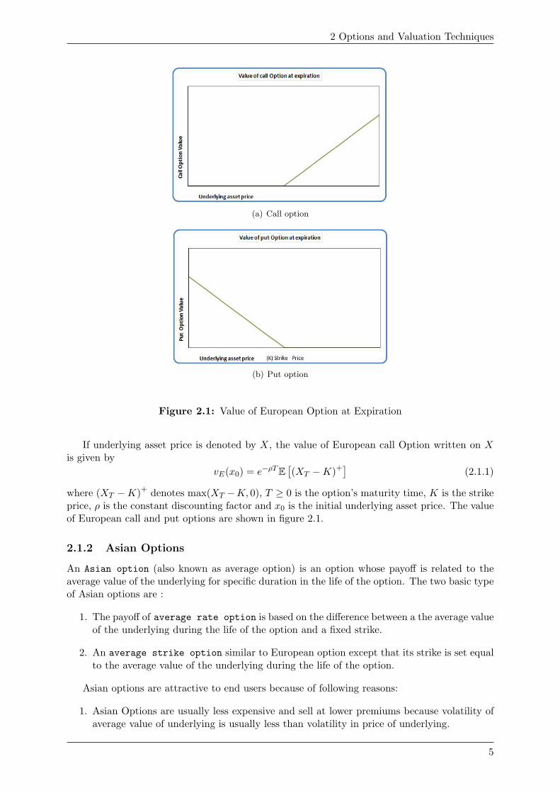
2 Options and Valuation Techniques
(a) Call option
(b) Put option
Figure 2.1: Value of European Option at Expiration
If underlying asset price is denoted by X, the value of European call Option written on Xis given by
vE(x0) = e−ρTE[(XT −K)+
](2.1.1)
where (XT −K)+ denotes max(XT −K, 0), T ≥ 0 is the option’s maturity time, K is the strikeprice, ρ is the constant discounting factor and x0 is the initial underlying asset price. The valueof European call and put options are shown in figure 2.1.
2.1.2 Asian Options
An Asian option (also known as average option) is an option whose payoff is related to theaverage value of the underlying for specific duration in the life of the option. The two basic typeof Asian options are :
1. The payoff of average rate option is based on the difference between a the average valueof the underlying during the life of the option and a fixed strike.
2. An average strike option similar to European option except that its strike is set equalto the average value of the underlying during the life of the option.
Asian options are attractive to end users because of following reasons:
1. Asian Options are usually less expensive and sell at lower premiums because volatility ofaverage value of underlying is usually less than volatility in price of underlying.
5
2.1 Class of Options
2. Asian options offer protection, as manipulation in price of underlying asset is not possibleover prolonged period of time.
3. End users of commodities which tend to be exposed to average prices over time find Asianoptions useful.
If underlying asset price is denoted by X, the value of fixed strike arithmetic-average Asiancall option written on X is given by
vA(x0) = e−ρTE
[(1T
∫ T
0XTdt−K
)+]
(2.1.2)
where (X − Y )+ denotes max(X − Y, 0), T ≥ 0 is the option’s maturity time, K is the strikeprice, ρ is the constant discounting factor and x0 is the initial underlying asset price.
2.1.3 Barrier Options
A barrier option is a path dependent option that has one of the following two features:
1. A knock-out feature causes the option to immediately terminate if the underlying asset’sprice reaches a specified (upper or lower) barrier level, or
2. A knock-in feature causes the option to become effective only if the underlying asset’sprice first reaches a specified (upper or lower) barrier level.
Hence for a simple Barrier option, we can derive eight different flavours, i.e. put and call foreach of the following:
1. Up and in
2. Down and in
3. Up and out
4. Down and out
Due to the contingent nature of the option, they tend to be priced lower than for a correspondingvanilla option.
If underlying asset price is denoted by X, the value of Barrier call option written on X isgiven by
vA(x0) = e−ρTE[(XT −K)+ Iτ=T
](2.1.3)
where (XT −K)+ denotes max(XT −K, 0), T ≥ 0 is the option’s maturity time, K is the strikeprice, ρ is the constant discounting factor, x0 is the initial underlying asset price and τ is the(Ft)-stopping time defined by
τd = inf t ≥ 0|Xt ≤ Hl ∧ Tτu = inf t ≥ 0|Xt ≥ Hu ∧ Tτc = inf t ≥ 0|Xt ≤ Hl ∧Xt ≥ Hu ∧ T
(2.1.4)
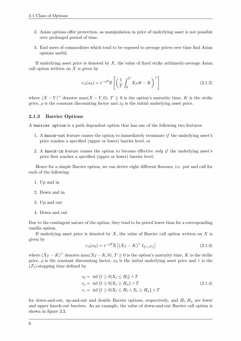
for down-and-out, up-and-out and double Barrier options, respectively, and Hl, Hu are lowerand upper knock-out barriers. As an example, the value of down-and-out Barrier call option isshown in figure 2.2.
6
2 Options and Valuation Techniques
(a) Down-and-Out Call option
Figure 2.2: Value of Barrier Call Option
2.2 Models for Underlying Asset Price
Given the filtered probability space, (Ω,F ,Ft,P), where Ω is given sample space , σ-algebra Fof subsets of Ω, a measure P on (Ω,F), such that P (Ω) = 1 and a filtration Ft on F . For thisproject we will consider that the underlying asset prices of derivatives, which we mentioned inprevious section, would satisfy the stochastic differential equation:
dXt = b (Xt) dt+ σ (Xt) dWt, X0 = x0 ∈ I (2.2.1)
where Wt is the Wiener process, I is either (0,+∞) or R and b, σ : I → I are given functions andwhich enable equation (2.2.1) to have a strong1 solution contained in I, for all t ≥ 0, probabilityalmost surely.
Specifically, for this project, we assume that underlying asset price X is given by three mod-els: geometric Brownian motion, Ornstein-Uhlenbeck process and Cox-Ingersoll-Ross processwhich are termed as Model 1, Model 2 and Model 3, respectively in this project. We describeeach of above diffusions in detail in following sections and give analytical formula for solutionof geometric Brownian motion and Ornstein Uhlenbeck process.
Before proceeding to next section, we note that any diffusions, other than the ones mentionedabove, could be considered aptly for analysis of numerical methodology proposed by Lasserre,Prieto-Rumeau and Zervos in [21] provided that they satisfy this important assumption: theinfinitesimal generator of this diffusion should map polynomials into polynomials of same orsmaller degree.
2.2.1 Geometric Brownian Motion
A continuous-time stochastic process in which the logarithm of the randomly varying quantityfollows a Brownian motion, or a Wiener process is called geometric Brownian motion(GBM).In other words, a stochastic process Xt is said to follow a GBM, if it satisfies the followingstochastic differential equation:
dXt = µXtdt+ σXtdz (2.2.2)
where dz = ε(t)√dt is a Wiener process, ε(t) is a standardized normal random variable, µ is
called as the percentage drift and σ is called the percentage volatility.
1Compared to weak solution which consists of a probability space and a process that satisfies the SDE, astrong solution is a process that satisfies the equation and is defined on a given probability space.
7
2.2 Models for Underlying Asset Price
We will now derive an analytical formula for XT , the price of underlying asset at time T ,when we are given X0 and other parameters of GBM. Now Ito’s Lemma states that for a randomprocess x defined by the Ito process
dx(t) = a(x, t)dt+ b(x, t)dz (2.2.3)
where z is a standard Wiener process, process y(t) defined by y(t) = F (x, t) satisfies the Itoequation
dy(t) =(a∂F
∂x+∂F
∂t+ b2
12∂2F
∂x2
)dt+ b
∂F
∂xdz (2.2.4)
where z is the same Wiener process in (2.2.2).
If we apply Ito’s Lemma to the process F (X(t)) = lnXt, then we identify
a = µX, b = σX,∂F
∂X=
1X, and
∂2F
∂X2= − 1
X2
Substituting these values in (2.2.4), we get
d lnX =(a
X− 1
2b2
X2
)dt+
b
Xdz
=(µ− 1
2σ2
)dt+ σdz
(2.2.5)
Ito-integrating both sides, we get
ln (Xt)− ln (X0) =(µ− 1
2σ2
)(t− 0) + σdz
⇔ Xt = X0e(µ− 1
2σ2)4t+σdz
(2.2.6)
or finally, using the fact that dz = ε(t)√4t for a Wiener process.
Xt = X0e(µ− 1
2σ2)4t+σε(t)
√4t, ε(t) ∼ N(0, 1) (2.2.7)
2.2.2 Ornstein-Uhlenbeck Process
The diffusion Xt governed by following stochastic differential equation,
dXt = γ(θ −Xt)dt+ σdz (2.2.8)
where dz = ε(t)√dt is a Wiener process and ε(t) is a standardized normal random variable, is
known as Ornstein-Uhlenbeck process. The parameters of this diffusion are γ ≥ 0 which isthe rate of mean reversion, θ which is the long term mean of the process and σ is the volatilityor average magnitude, per square-root time, of the random fluctuations that are modelled asBrownian motions. The Vasicek one-factor equilibrium model of interest rates described in [24]is an example which involves Ornstein-Uhlenbeck process.
Ornstein Uhlenbeck process has an important property called mean reversion property. Wecan see thatXt has an overall drift towards the mean value θ, if we ignore the random fluctuationsin the process due to dz. The rate of reversion of diffusion Xt to mean θ is at an exponentialrate γ, and magnitude directly proportional to the distance between the current value of Xt andθ.
8
2 Options and Valuation Techniques
We can also observe that for any fixed T , the random variable XT , conditional upon X0, isnormally distributed with
mean = θ + (X0 − θ)e−γT
variance =σ2
2γ(1− e−2γT )
(2.2.9)
We will now derive an analytical formula for XT , the price of underlying asset at time T , aswe did for geometric Brownian motion, when we are given X0 and other parameters of OrnsteinUhlenbeck process. Introducing the change of variable Yt = Xt−θ, then Yt satisfies the equation
dYt = dXt = −γYtdt+ σdz (2.2.10)
In (2.2.8), Yt shows a drift towards the value zero, at exponential rate γ, hence we introducethe change of variable
Yt = e−γtZt ⇔ Zt = eγtYt (2.2.11)
which eliminates the drift. Now applying the product rule for Ito Integrals we obtain
dZt = γeγtYtdt+ eγtdYt
= γeγtYtdt+ eγt(−γYtdt+ σdz)= 0dt+ σeγtdz
(2.2.12)
Ito-Integrating both sides from 0 to t we get
Zt = Z0 + σ
∫ t
0eγzdz (2.2.13)
Next step would be to reverse the change of variables to obtain
Yt = e−γtZt
= e−γ(t−0)Y0 + σe−γt∫ t
0eγzdz
= e−γtY0 + σ
∫ t
0e−γ(t−z)dz
(2.2.14)
thus we obtain original variable Xt as
Xt = θ + Yt
= θ + e−γt(X0 − θ) + σ
∫ t
0e−γ(t−z)dz
(2.2.15)
which can further be simplified to
Xt ∼ θ + e−γt(X0 − θ) + σ
√1− e−2γt
2γε(t), ε(t) ∼ N(0, 1) (2.2.16)
2.2.3 Cox Ingersoll Ross process
In the Vasicek model which involves Ornstein-Uhlenbeck process (2.2.8), the short term interestrate Xt, can become negative. To overcome this drawback, an alternative one-factor equilibriummodel was proposed by Cox, Ingersoll and Ross in [15] for short term or instantaneous interestrate in which rates would always remain positive.
9
2.3 Monte Carlo Methods
Specifically, a diffusion (short-term or instantaneous interest rate in Cox-Ingersoll-Ross in-terest rate model) which satisfies the following stochastic differential equation
dXt = γ(θ −Xt)dt+ σ√Xtdz (2.2.17)
where dz = ε(t)√dt is a Wiener process and ε(t) is a standardized normal random variable,
is known as Cox-Ingersoll-Ross process. The parameters of this diffusion are same as theones in Ornstein-Uhlenbeck process except the fact that the standard deviation factor, σ
√Xt
does not allow the interest rate Xt to become negative. Hence we observe that, when the valueof Xt is low, the standard deviation becomes close to zero, in turn cancelling the effect of therandom shock on the interest rate. We also note that γθ ≥ 1
2σ2 is necessary and sufficient for
non explosiveness of solution of (2.2.17), or in other words, for instantaneous rate to assume thevalue zero at infinite time with probability 1.
2.3 Monte Carlo Methods
Considering valuation of an option as computing its expected value, we can use repeated randomsampling in order to compute this expected value. Monte Carlo methods are a class of algorithmswhich could be used for such repeated random sampling and thus calculating the expected valueof the derivative price. We describe Monte Carlo algorithms for pricing European options insection 2.3.1, Asian Options in section 2.3.2 and (down-and-out and up-and-out) Barrier optionsin section 2.3.3. Also note that, although the Monte Carlo methods in this section are given forgeometric Brownian motion only, they can be adapted very easily for Ornstein-Uhlenbeck andCox-Ingersoll-Ross diffusions.
2.3.1 European Options
In this section we will give Monte Carlo algorithm for valuation of European put and call options.Pseudo random number generators can be used to compute the estimates of expected values.Consider an European style option with payoff which is some function F of asset price Xt. Nowwe get the model of asset price to be described by geometric Brownian motion (2.2.2), and usingthe risk neutrality approach, option value can be found by calculating e−rTF (XT ), or in otherwords, we intend to calculate
e−rTF (X0e(µ− 1
2σ2)dt+σε(t)
√dt) (2.3.1)
where ε(t) ∼ N(0, 1).The resulting Monte Carlo algorithm can be described as below
10
2 Options and Valuation Techniques
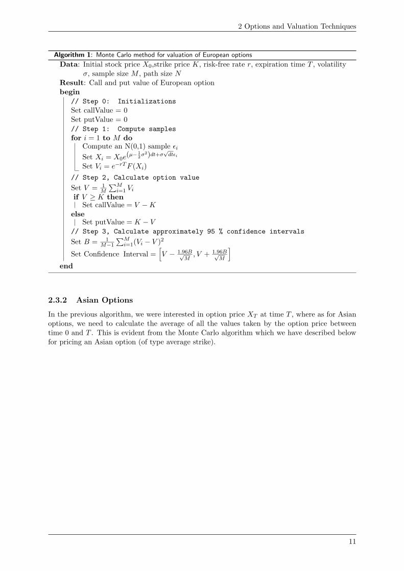
Algorithm 1: Monte Carlo method for valuation of European options
Data: Initial stock price X0,strike price K, risk-free rate r, expiration time T , volatilityσ, sample size M , path size N
Result: Call and put value of European optionbegin
// Step 0: InitializationsSet callValue = 0Set putValue = 0// Step 1: Compute samplesfor i = 1 to M do
Compute an N(0,1) sample εiSet Xi = X0e
(µ− 12σ2)dt+σ
√dtεi
Set Vi = e−rTF (Xi)// Step 2, Calculate option value
Set V = 1M
∑Mi=1 Vi
if V ≥ K thenSet callValue = V −K
elseSet putValue = K − V
// Step 3, Calculate approximately 95 % confidence intervals
Set B = 1M−1
∑Mi=1(Vi − V )2
Set Confidence Interval =[V − 1.96B√
M, V + 1.96B√
M
]end
2.3.2 Asian Options
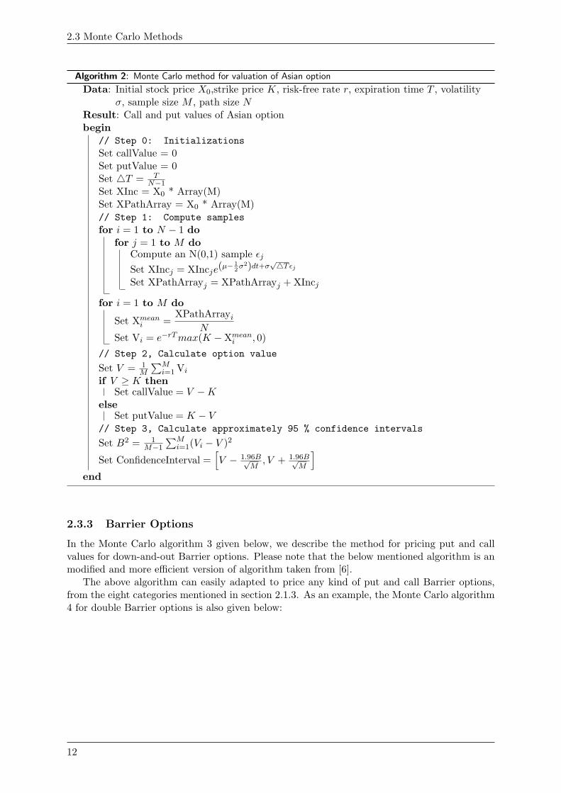
In the previous algorithm, we were interested in option price XT at time T , where as for Asianoptions, we need to calculate the average of all the values taken by the option price betweentime 0 and T . This is evident from the Monte Carlo algorithm which we have described belowfor pricing an Asian option (of type average strike).
11
2.3 Monte Carlo Methods
Algorithm 2: Monte Carlo method for valuation of Asian option
Data: Initial stock price X0,strike price K, risk-free rate r, expiration time T , volatilityσ, sample size M , path size N
Result: Call and put values of Asian optionbegin
// Step 0: InitializationsSet callValue = 0Set putValue = 0Set 4T = T
N−1Set XInc = X0 * Array(M)Set XPathArray = X0 * Array(M)// Step 1: Compute samplesfor i = 1 to N − 1 do
for j = 1 to M doCompute an N(0,1) sample εjSet XIncj = XIncje(µ−
12σ2)dt+σ
√4Tεj
Set XPathArrayj = XPathArrayj + XIncj
for i = 1 to M do
Set Xmeani =
XPathArrayiN
Set Vi = e−rTmax(K −Xmeani , 0)
// Step 2, Calculate option value
Set V = 1M
∑Mi=1 Vi
if V ≥ K thenSet callValue = V −K
elseSet putValue = K − V
// Step 3, Calculate approximately 95 % confidence intervals
Set B2 = 1M−1
∑Mi=1(Vi − V )2
Set ConfidenceInterval =[V − 1.96B√
M, V + 1.96B√
M
]end
2.3.3 Barrier Options
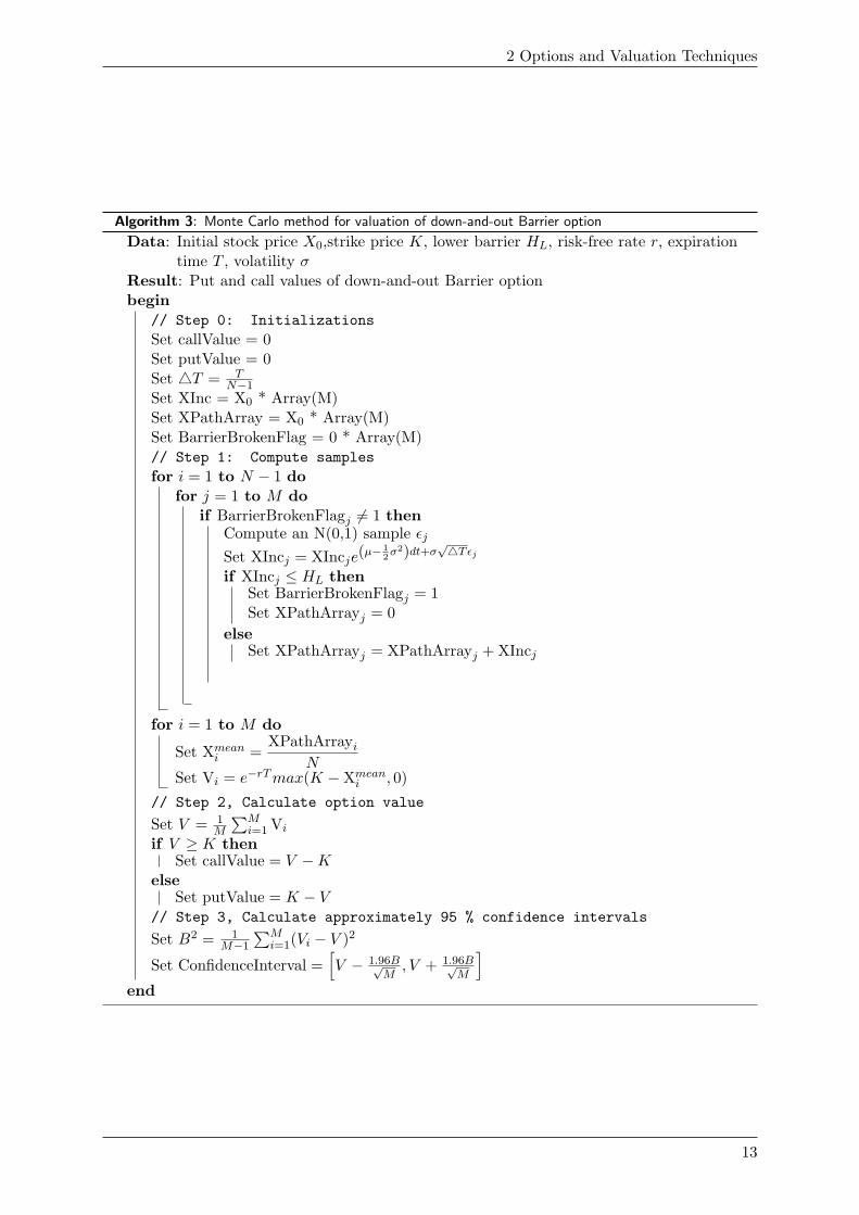
In the Monte Carlo algorithm 3 given below, we describe the method for pricing put and callvalues for down-and-out Barrier options. Please note that the below mentioned algorithm is anmodified and more efficient version of algorithm taken from [6].
The above algorithm can easily adapted to price any kind of put and call Barrier options,from the eight categories mentioned in section 2.1.3. As an example, the Monte Carlo algorithm4 for double Barrier options is also given below:
12
2 Options and Valuation Techniques
Algorithm 3: Monte Carlo method for valuation of down-and-out Barrier option
Data: Initial stock price X0,strike price K, lower barrier HL, risk-free rate r, expirationtime T , volatility σ
Result: Put and call values of down-and-out Barrier optionbegin
// Step 0: InitializationsSet callValue = 0Set putValue = 0Set 4T = T
N−1Set XInc = X0 * Array(M)Set XPathArray = X0 * Array(M)Set BarrierBrokenFlag = 0 * Array(M)// Step 1: Compute samplesfor i = 1 to N − 1 do
for j = 1 to M doif BarrierBrokenFlagj 6= 1 then
Compute an N(0,1) sample εjSet XIncj = XIncje(µ−
12σ2)dt+σ
√4Tεj
if XIncj ≤ HL thenSet BarrierBrokenFlagj = 1Set XPathArrayj = 0
elseSet XPathArrayj = XPathArrayj + XIncj
for i = 1 to M do
Set Xmeani =
XPathArrayiN
Set Vi = e−rTmax(K −Xmeani , 0)
// Step 2, Calculate option value
Set V = 1M
∑Mi=1 Vi
if V ≥ K thenSet callValue = V −K
elseSet putValue = K − V
// Step 3, Calculate approximately 95 % confidence intervals
Set B2 = 1M−1
∑Mi=1(Vi − V )2
Set ConfidenceInterval =[V − 1.96B√
M, V + 1.96B√
M
]end
13

2.3 Monte Carlo Methods
Algorithm 4: Monte Carlo method for valuation of double Barrier options
Data: Initial stock price X0,strike price K, upper barrier HU , lower barrier HL, risk-freerate r, expiration time T , volatility σ
Result: Put and call values of double Barrier Optionbegin
// Step 0: InitializationsSet callValue = 0Set putValue = 0Set 4T = T
N−1Set XInc = X0 * Array(M)Set XPathArray = X0 * Array(M)Set BarrierBrokenFlag = 0 * Array(M)// Step 1: Compute samplesfor i = 1 to N − 1 do
for j = 1 to M doif BarrierBrokenFlagj 6= 1 then
Compute an N(0,1) sample εjSet XIncj = XIncje(µ−
12σ2)dt+σ
√4Tεj
if XIncj ≤ HL OR XIncj ≥ HU thenSet BarrierBrokenFlagj = 1Set XPathArrayj = 0
elseSet XPathArrayj = XPathArrayj + XIncj
for i = 1 to M do
Set Xmeani =
XPathArrayiN
Set Vi = e−rTmax(K −Xmeani , 0)
// Step 2, Calculate option value
Set V = 1M
∑Mi=1 Vi
if V ≥ K thenSet callValue = V −K
elseSet putValue = K − V
// Step 3, Calculate approximately 95 % confidence intervals
Set B2 = 1M−1
∑Mi=1(Vi − V )2
Set ConfidenceInterval =[V − 1.96B√
M, V + 1.96B√
M
]end
14
2 Options and Valuation Techniques
2.3.4 Advantages and Disadvantages of Monte Carlo Methods
Even though Monte Carlo algorithms are simple and elegant to implement, they have certainmerits and demerits of their own, as a class of algorithms which are enlisted below:
Advantages
• The major advantage of Monte Carlo methods is that they are very simple to implementand adapt. Usually an expression of solution or its analytical properties are not requiredfor performing Monte Carlo simulations.
• Owing to their genericity and simplicity in implementation, Monte Carlo methods offerunrestricted choice of functions for implementation.
• As Monte Carlo simulations intrinsically involve certain type of repetitive tasks, they canbe easily parallelized.
Disadvantages
• The most important drawback of Monte Carlo algorithms is that they are slow whenthe dimension of integration is low. We can prove that for Monte Carlo integration theprobabilistic error bound is inversely proportional to the square root of the number ofsamples, hence in order to achieve one more decimal digit of precision, we would require100 times more the number of samples.
• The probabilistic error bound is also dependent on variance. Hence it is not a goodrepresentation of the error when the underlying probability distributions are skewed.
• The error in values computed through Monte Carlo algorithms also depend on the un-derlying probability distributions. As we can consider that Monte Carlo methods tryto estimate the expectation of certain values by sampling, this estimated value may beerroneous, if the underlying probability distribution is heavily skewed or has heavier-than-normal tails. This disadvantage can be taken care of by using appropriate non-randomnumerical methods.
• As Monte-Carlo methods typically follow a Black-box approach, it is difficult to performsensitivity analysis for the input parameters, which would be otherwise possible withcertain types of analytical approximation techniques.
Effects of several of above disadvantages can be decreased there by increasing the accuracyof results in Monte Carlo simulations. For example, there are several techniques for reducingvariance in the sampled values, such as use of antithetic and control variates, importance sam-pling, etc. However, as these topics are not in the scope of this project, we will not elaborate onthem. Interested reader is encouraged to refer [25] for comprehensive treatment of Monte Carlomethods.
2.4 Black Scholes PDE and Analytical Solution
A mathematical model of market for equity was given by Black-Scholes, where the underlying isa stochastic process and the price of derivative on the underlying satisfies a partial differentialequation called Black-Scholes PDE. We briefly summarize the Black Scholes model, PDE andsolution formula obtained by solving the Black-Scholes PDE for European put and call optionsbelow. Suppose that underlying Xt is governed by geometric Brownian motion (2.2.2):
dXt = µXtdt+ σXtdz (2.4.1)
15
2.4 Black Scholes PDE and Analytical Solution
where dz = ε(t)√dt is a Wiener process and ε(t) is a standardized normal random variable.
Now let V be some sort of option on X, or in other words, consider V as a function of Xand t. Hence, V (X, t) is the value of the option at time t if the price of the underlying stock attime t is X. We also assume that V (X, t) is differentiable twice with respect to X and once withrespect to t. Then V (X, t) must satisfy the Black-Scholes partial differential equation:
∂V
∂t+ rX
∂V
∂X+ σ2X2 1
2∂2V
∂X2= rV (2.4.2)
where r is the interest rate.
2.4.1 Analytical Solution for European Options
By solving (2.4.2) for price of European call and put options(for solution techniques and moredetails please refer [14],[6] and [26]), we get
Ct = XtΦ(d1)−Ke−rTΦ(d2)
Pt = Ke−rTΦ(d2)−XtΦ(d1)(2.4.3)
where
d1 =ln
(Xt
K
)+ T
(r + σ2
2
)σ√T
d2 =ln
(Xt
K
)+ T
(r − σ2
2
)σ√T
= d1 − σ√T
Φ(dn) =1√2π
∫ dn
−∞e−
x2
2 dx
(2.4.4)
or in other words, Φ(.) is the standard normal cumulative distribution function.
2.4.2 Analytical Solution for Barrier Options
We present here the analytical formulae used in this project for comparison with bounds obtainedby following the numerical approach given by Lasserre, Prieto-Rumeau and Zervos in [21]. Bysolving (2.4.2) for price of different types of Barrier call and put options (for solution techniquesplease refer [27]), we get the following solutions:
Down-and-out and down-and-in call options:
When H ≤ K, we get
Cdit = X0
(H
X0
)2e1
Φ(e2)−Ke−rT(H
X0
)2e1−2
Φ(e2 − σ√T ) (2.4.5)
16
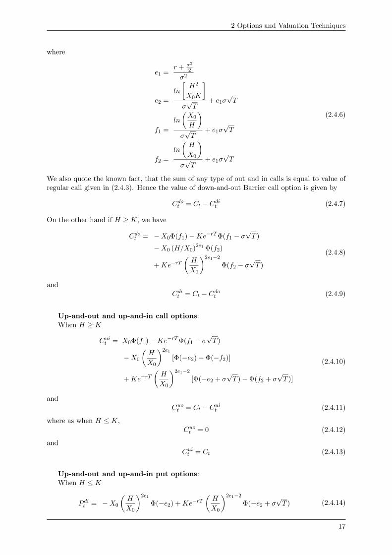
2 Options and Valuation Techniques
where
e1 =r + σ2
2
σ2
e2 =ln
[H2
X0K
]σ√T
+ e1σ√T
f1 =ln
(X0
H
)σ√T
+ e1σ√T
f2 =ln
(H
X0
)σ√T
+ e1σ√T
(2.4.6)
We also quote the known fact, that the sum of any type of out and in calls is equal to value ofregular call given in (2.4.3). Hence the value of down-and-out Barrier call option is given by
Cdot = Ct − Cdit (2.4.7)
On the other hand if H ≥ K, we have
Cdot = −X0Φ(f1)−Ke−rTΦ(f1 − σ√T )
−X0 (H/X0)2e1 Φ(f2)
+Ke−rT(H
X0
)2e1−2
Φ(f2 − σ√T )
(2.4.8)
andCdit = Ct − Cdot (2.4.9)
Up-and-out and up-and-in call options:When H ≥ K
Cuit = X0Φ(f1)−Ke−rTΦ(f1 − σ√T )
−X0
(H
X0
)2e1
[Φ(−e2)− Φ(−f2)]
+Ke−rT(H
X0
)2e1−2
[Φ(−e2 + σ√T )− Φ(f2 + σ
√T )]
(2.4.10)
andCuot = Ct − Cuit (2.4.11)
where as when H ≤ K,Cuot = 0 (2.4.12)
andCuit = Ct (2.4.13)
Up-and-out and up-and-in put options:When H ≤ K
P dit = −X0
(H
X0
)2e1
Φ(−e2) +Ke−rT(H
X0
)2e1−2
Φ(−e2 + σ√T ) (2.4.14)
17
2.4 Black Scholes PDE and Analytical Solution
andP uot = Pt − P uit (2.4.15)
where as when H ≤ K,
P uot = −X0Φ(f1) +Ke−rTΦ(−f1 + σ√T )
+X0
(H
X0
)2e1
Φ(−f2)
−Ke−rT(H
X0
)2e1−2
Φ(−f2 + σ√T )
(2.4.16)
andP uit = Pt − P uit (2.4.17)
Down-and-out and Down-and-in put options:When H ≥ K
P dit = −X0Φ(−f1) +Ke−rTΦ(−f1 + σ√T )
+X0
(H
X0
)2e1
[Φ(e2)− Φ(f2)]
−Ke−rT(H
X0
)2e1−2
[Φ(e2 − σ√T )− Φ(f1 − σ
√T )]
(2.4.18)
andP dot = Pt − P dit (2.4.19)
where as when H ≤ K,P dot = 0 (2.4.20)
andP dit = Pt (2.4.21)
2.4.3 Assumptions and Shortcomings of Black Scholes Formula
There are several assumptions under which above formulation and results were obtained, whichare mentioned as below (for more details, please refer [17], [14], [5] and [6]):
• The price of the underlying asset follows a Wiener process, and the price changes arelog-normally distributed.
• The stock does not pay a dividend and there are no transaction costs or taxes.
• It is possible to short sell the underlying stock and trading in the stock is continuous.Sudden and large changes in stock prices do not occur.
• It is possible to borrow and lend cash at a risk-free interest rate which remains constantover time. Also, there are no arbitrage opportunities.
• The volatility of stock price also remains constant over time.
Some of the assumptions above can be changed, and corresponding Black-Scholes formula can bederived (for example, for extension of Black-Scholes model to price options on dividend payingstocks, please refer to chapter 13 in [14]). On the other hand, certain assumptions cannot becorrected and often lead to an error in the computed option value. For example, it is a wellknown fact that probability distribution of underlying asset is not lognormal which leads to an
18

2 Options and Valuation Techniques
incorrect bias in pricing done by Black-Scholes method. The most prevalent assumption, forexample, when underlying asset is equity, is that equity price has a heavier left tail and lessheavier right tail in comparison with lognormal model.
Many alternative models have been proposed for overcoming the above disadvantages. Inthe next two sections, we give two such methodologies for pricing simple and exotic options.
19
Chapter 3
Semi-Parametric Approach forBounding Option Price
In their original article [1], Bertsimas and Popescu addressed the problem of deriving optimalinequalities for E[φ(X)] for a random variable X when given collection of general momentsE[fi(X)] = qi. Utilizing semidefinite and convex optimization methods in order to derive optimalbounds on the probability that variable X belongs in a given set, given first few moments for therandom variable X, they substantiate their theory by finding optimal upper bounds for optionprices with general payoff. The advantage of their approach is that probability distribution ofunderlying asset price is not required, only the moments are sufficient for deriving the optimalbounds. Later on, Gotoh and Konno [9] extended the above approach to obtain tight lowerbound for the option price with general payoff, given its first few moments.
In this section, we investigate and elaborate the semi-parametric approach for pricing optionsoriginally proposed by Lo in [22] and extended by Bertsimas and Popescu in [2] and [1] andmodified by Gotoh and Konno in [9] for obtaining tighter upper and lower bounds on Europeantype call option price, when we are given the first n moments of the underlying security price.The main idea in this approach is to view a semidefinite programming problem as a linearprogram with an infinite number of linear constraints.
3.1 Review of Basic Results
Introducing the notation: T and K are exercise time and exercise price of European type calloption, respectively. St and r are stock price at time t, and risk-free rate, respectively. Alsoπ is the risk-neutral probability of ST and Eπ[.] denotes the expected value of random variableunder the probability measure π. Then the call option price Ct is given by
Ct = e−r(T−t)Eπ [max(0, ST −K)] (3.1.1)
If we are given the first n moments qi, i = 1, ..., n of π, then the upper and lower bounds of thecall option price can be obtained by solving the following linear programming problems withinfinite number of variables π(ST ):
maximizeπ(ST )
e−rτ∫ ∞
0max(0, ST −K)× π(ST )dST
s.t. e−jrτ∫ ∞
0SjTπ(ST )dST = qj ,
j = 0, 1, ..., n, π(ST ) ≥ 0.
(3.1.2)
20
3 Semi-Parametric Approach for Bounding Option Price
minimizeπ(ST )
e−rτ∫ ∞
0max(0, ST −K)× π(ST )dST
s.t. e−jrτ∫ ∞
0SjTπ(ST )dST = qj ,
j = 0, 1, ..., n, π(ST ) ≥ 0.
(3.1.3)
where q0 = 1 and τ = T − t. Also to be noted is the fact that above problems are feasible. Wenow intend to derive the dual problems of (3.1.2) and (3.1.3). Denoting x = e−rτST and dualvariables as yi, i = 0, 1, ..., n, we can derive their dual problems:
minimizeπ(ST )
n∑i=0
qiyi
s.t.n∑i=0
xiyi ≥ max(0, x− e−rτK),
∀x ∈ R1+.
(3.1.4)
maximizeπ(ST )
n∑i=0
qiyi
s.t.n∑i=0
xiyi ≤ max(0, x− e−rτK),
∀x ∈ R1+.
(3.1.5)
We will now reiterate the propositions given by Bertsimas and Popescu which will assist us toconvert (3.1.4) and (3.1.5) into semidefinite programming problems.
Proposition 1. The polynomial g(x) =∑2k
r=0 yrxr satisfies g(x) ≥ 0 for all x ∈ R1 if and only
if there exists a positive semidefinite matrix X = [xij ] , i, j = 0, ..., k, such that
yr =∑
i,j:i+j=r
xij , r = 0, ..., 2k, X 0. (3.1.6)
Proof. We will first prove the if part, i.e. we assume that (3.1.6) holds, and we need to provethat g(x) =
∑2nr=0 yrx
r satisfies g(x) ≥ 0 for all x ∈ R1. Let x′k = (1, x, x2, ..., xk). Then
g(x) =2k∑r=0
∑i+j=r
xijxr
=k∑i=0
k∑j=0
xijxixj
= x′kXxk
≥ 0
and last step is obtained because we are given that X is positive semidefinite, i.e. X 0. Nowwe will prove the only-if part. We assume that the polynomial g(x) ≥ 0, ∀x ∈ R1 and degreeof g(x) is 2k. Then, we observe the fact that real roots of g(x) should have even multiplicity.This is because if they have odd multiplicity then g(x) would alter sign in an neighborhood of aroot. Denoting λi, i = 1, ..., r as the real roots of g(x) and 2mi as its corresponding multiplicity,its complex roots can then be arranged in conjugate pairs, aj + ibj , aj − ibj , j = 1, ..., h. Hence
g(x) = y2k
r∏i=1
(x− λi)2mih∏j=1
((x− aj)2 + b2j ).
21
3.1 Review of Basic Results
We note the fact that the leading coefficient y2k needs to be positive. Thus, by expanding theterms in the products, we can see that g(x) can be written as a sum of squares of polynomials,of the form
g(x) =k∑i=0
k∑j=0
xijxj
2
= x′kXxk
which proves that X is positive semidefinite, i.e. X 0, as we assumed that g(x) ≥ 0.
Proposition 2. The polynomial g(x) =∑k
r=0 yrxr satisfies g(x) ≥ 0 for all x ∈ R1 if and only
if there exists a positive semidefinite matrix X = [xij ] . i, j = 0, ..., k, such that∑i,j: i+j=2l−1
xij = 0, l = 1, ..., k,
∑i,j: i+j=2l
xij = yl, l = 0, ..., k,
X 0
(3.1.7)
Proof. We observe that g(x) ≥ 0 for all x ≥ 0 if and only if g(t2) ≥ 0, ∀t, which is a directresult of applying Proposition 1. Now in order to prove that g(t2) ≥ 0, ∀t, we evaluate g(t2) asbelow:
g(t2) = y0t0 + y1t
2 + y2t4 + ...+ ykt
2k,
= y0 + 0.t+ y1t2 + 0.t3 + y2t
4 + ...+ 0.t2k−1 + ykt2k,
from which we observe that all terms can be amalgamated into following two terms:
0.t+ 0.t3 + ...+ 0.t2k−1,
and
y0 + y2t4 + ...+ ykt
2k,
hence we obtain
g(t2) =k∑r=0
∑i,j: i+j=2r−1
xijt2r−1 +
k∑r=0
∑i,j: i+j=2r
xijt2r
Now finally we see that g(t2) ≥ 0, ∀ t if and only ifk∑r=0
∑i,j: i+j=2r−1
xijt2r−1+
k∑r=0
∑i,j: i+j=2r
xijt2r ≥ 0
⇔k∑r=0
∑i,j: i+j=2r−1
xijt2r−1 ≥ 0 and
k∑r=0
∑i,j: i+j=2r
xijt2r ≥ 0
⇔k∑r=0
∑i,j: i+j=2r−1
xijt2r−1 = 0 and
k∑r=0
∑i,j: i+j=2r
xijt2r ≥ 0
which proves the proposition, noting the fact that t2 ≥ 0, ∀t ∈ R1.
22
3 Semi-Parametric Approach for Bounding Option Price
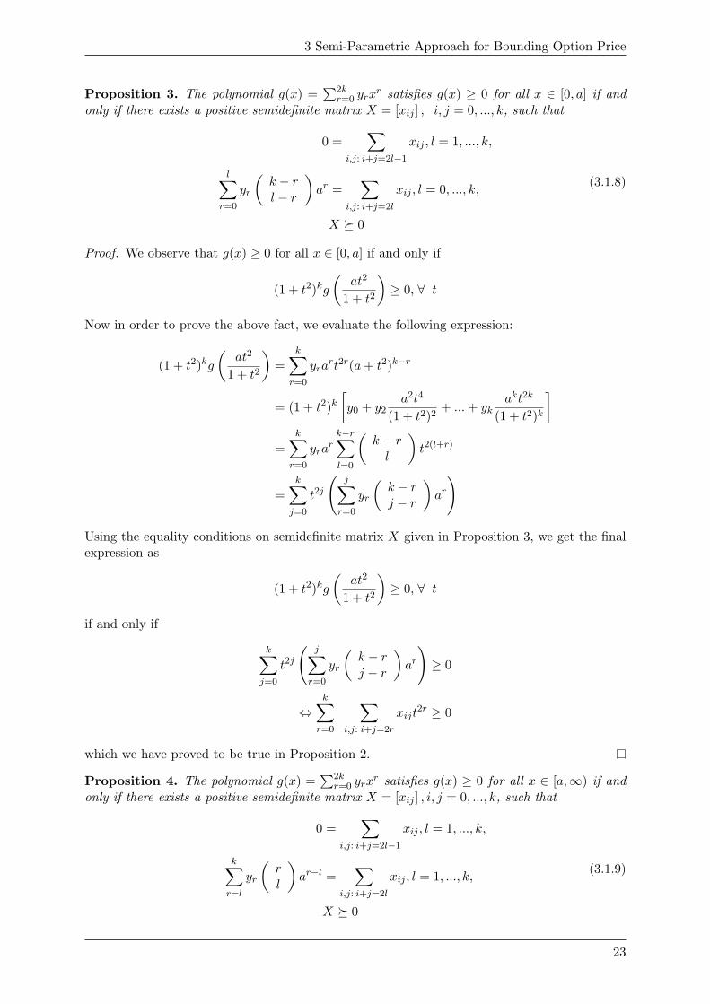
Proposition 3. The polynomial g(x) =∑2k
r=0 yrxr satisfies g(x) ≥ 0 for all x ∈ [0, a] if and
only if there exists a positive semidefinite matrix X = [xij ] , i, j = 0, ..., k, such that
0 =∑
i,j: i+j=2l−1
xij , l = 1, ..., k,
l∑r=0
yr
(k − rl − r
)ar =
∑i,j: i+j=2l
xij , l = 0, ..., k,
X 0
(3.1.8)
Proof. We observe that g(x) ≥ 0 for all x ∈ [0, a] if and only if
(1 + t2)kg(
at2
1 + t2
)≥ 0, ∀ t
Now in order to prove the above fact, we evaluate the following expression:
(1 + t2)kg(
at2
1 + t2
)=
k∑r=0
yrart2r(a+ t2)k−r
= (1 + t2)k[y0 + y2
a2t4
(1 + t2)2+ ...+ yk
akt2k
(1 + t2)k
]=
k∑r=0
yrark−r∑l=0
(k − rl
)t2(l+r)
=k∑j=0
t2j
(j∑r=0
yr
(k − rj − r
)ar
)
Using the equality conditions on semidefinite matrix X given in Proposition 3, we get the finalexpression as
(1 + t2)kg(
at2
1 + t2
)≥ 0, ∀ t
if and only if
k∑j=0
t2j
(j∑r=0
yr
(k − rj − r
)ar
)≥ 0
⇔k∑r=0
∑i,j: i+j=2r
xijt2r ≥ 0
which we have proved to be true in Proposition 2.
Proposition 4. The polynomial g(x) =∑2k
r=0 yrxr satisfies g(x) ≥ 0 for all x ∈ [a,∞) if and
only if there exists a positive semidefinite matrix X = [xij ] , i, j = 0, ..., k, such that
0 =∑
i,j: i+j=2l−1
xij , l = 1, ..., k,
k∑r=l
yr
(rl
)ar−l =
∑i,j: i+j=2l
xij , l = 1, ..., k,
X 0
(3.1.9)
23
3.1 Review of Basic Results
Proof. We observe that g(x) ≥ 0, ∀x ∈ [0, a] if and only if
g(a+ t2) ≥ 0, ∀ t
Now in order to prove that g(a+ t2) ≥ 0 ∀ t, we evaluate g(a+ t2) as below:
g(a+ t2) =k∑r=0
yr(a+ t2)r
=k∑r=0
yr
r∑l=0
(rl
)ar−lt2l
=k∑l=0
t2l
(k∑r=l
yr
(rl
)ar−l
)Using the equality conditions on semidefinite matrix X given in Proposition 4, we get the finalexpression as
g(a+ t2) ≥ 0, ∀ t
if and only if
k∑l=0
t2l
(k∑r=l
yr
(rl
)ar−l
)≥ 0
⇔k∑r=0
∑i,j: i+j=2r
xijt2r ≥ 0
which we have proved to be true in Proposition 2.
Proposition 5. The polynomial g(x) =∑2k
r=0 yrxr satisfies g(x) ≥ 0 for all x ∈ (−∞, a] if and
only if there exists a positive semidefinite matrix X = [xij ] , i, j = 0, ..., k, such that
0 =∑
i,j: i+j=2l−1
xij , l = 1, ..., k,
(−1)lk∑r=l
yr
(rl
)ar−l =
∑i,j: i+j=2l
xij , l = 1, ..., k,
X 0
(3.1.10)
Proof. The proof is similar to that given for Proposition 4, but we just replace t2 by −t2 ing(a+ t2). We observe that g(x) ≥ 0, ∀ x ∈ [0, a] if and only if
g(a− t2) ≥ 0 ∀ t
Now in order to prove that g(a− t2) ≥ 0 ∀ t, we evaluate g(a− t2) as below:
g(a− t2) =k∑r=0
yr(a− t2)r
=k∑r=0
yr
r∑l=0
(rl
)ar−l(−t2)l
=k∑l=0
t2l
((−1)l
k∑r=l
yr
(rl
)ar−l
)we obtain (3.1.10) by applying (3.1.6) in a similar fashion to Proposition 4.
24
3 Semi-Parametric Approach for Bounding Option Price
Proposition 6. The polynomial g(x) =∑2k
r=0 yrxr satisfies g(x) ≥ 0 for all x ∈ [a, b] if and
only if there exists a positive semidefinite matrix X = [xij ] , i, j = 0, ..., k, such that
0 =∑
i,j: i+j=2l−1
xij , l = 1, ..., k,
l∑m=0
k+m−l∑r=m
yr
(rm
)(k − rl −m
)ar−mbm =
∑i,j: i+j=2l
xij , l = 1, ..., k,
X 0
(3.1.11)
Proof. We observe that g(x) ≥ 0, ∀x ∈ [a, b] if and only if
(1 + t2)kg(a+ (b− a)
t2
1 + t2
)≥ 0, ∀ t
Since
(1 + t2)kg(a+ (b− a)
t2
1 + t2
)=
k∑r=0
yr(a+ bt2)r(1 + t2)k−r
=k∑r=0
yr
r∑m=0
(rm
)ar−mbmt2m
k−r∑j=0
(k − rj
)t2j
=k∑l=0
t2l
(l∑
m=0
k+m−l∑r=m
yr
(rm
)(k − rl −m
)ar−mbm
)we obtain (3.1.11) by applying (3.1.6).
3.2 SDP Formulation of the Bounding Problems
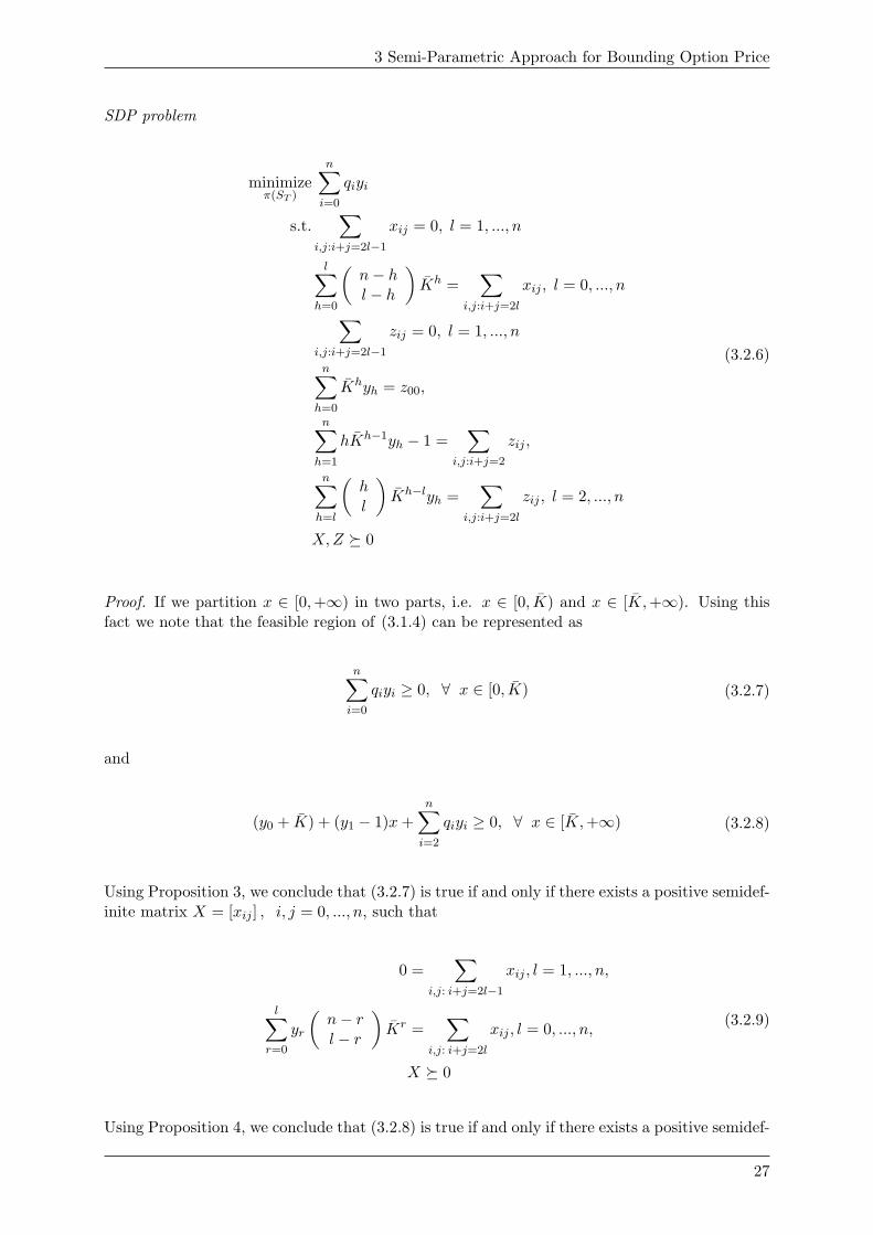
Now that we have seen the basic results we are equipped to convert problems (3.1.4) and (3.1.5)which have infinite constraints, into equivalent SDP problems.
Theroem 1. An optimal solution of problem (3.1.4) can be obtained by solving the followingSDP problem
minimizeπ(ST )
n∑i=0
qiyi
s.t.∑
i,j:i+j=2l−1
xij = 0, l = 1, ..., n
yl −∑
i,j:i+j=2l
xij = 0, l = 0, ..., n
∑i,j:i+j=2l−1
zij = 0, l = 1, ..., n
y0 − z00 = −K,
y1 −∑
i,j:i+j=2
zij = 1
y1 −∑
i,j:i+j=2l
zij = 0, l = 2, ..., n
X,Z 0
(3.2.1)
where X 0, Z 0 denote that X and Y are positive semidefinite and K = e−rτK.
25
3.2 SDP Formulation of the Bounding Problems
Proof. We wish to convert the infinite constraints of problem (3.1.4) in finite constraints, thusobtaining a SDP problem. Representing the feasible region of (3.1.4) as
n∑i=0
qiyi ≥ 0, ∀ x ≥ 0 (3.2.2)
and
(y0 + K) + (y1 − 1)x+n∑i=2
qiyi ≥ 0, ∀ x ≥ 0 (3.2.3)
Using Proposition 2, we conclude that (3.2.2) is true if and only if there exists a positive semidef-inite matrix X = [xij ] . i, j = 0, ..., n, such that
∑i,j: i+j=2l−1
xij = 0, l = 1, ..., n,
∑i,j: i+j=2l
xij = yl, l = 0, ..., n,
X 0
(3.2.4)
Using Proposition 2 again for (3.2.3) we conclude that (3.2.3) is true if and only if there existsa positive semidefinite matrix Z = [zij ] . i, j = 0, ..., n, such that
∑i,j: i+j=2l−1
zij = 0, l = 1, ..., n,
∑i,j: i+j=2l
zij − K = yl, l = 0,
∑i,j: i+j=2l
zij + 1 = yl, l = 1,
∑i,j: i+j=2l
zij = yl, l = 2, ..., n,
X 0
(3.2.5)
Hence we obtain the constraints for our SDP problem by simplifying (3.2.4) and (3.2.5).
Now we will present another way of simplifying the constraints in (3.1.4), for obtaining aSDP problem.
Theroem 2. An optimal solution of problem (3.1.4) can be obtained by solving the following
26
3 Semi-Parametric Approach for Bounding Option Price
SDP problem
minimizeπ(ST )
n∑i=0
qiyi
s.t.∑
i,j:i+j=2l−1
xij = 0, l = 1, ..., n
l∑h=0
(n− hl − h
)Kh =
∑i,j:i+j=2l
xij , l = 0, ..., n
∑i,j:i+j=2l−1
zij = 0, l = 1, ..., n
n∑h=0
Khyh = z00,
n∑h=1
hKh−1yh − 1 =∑
i,j:i+j=2
zij ,
n∑h=l
(hl
)Kh−lyh =
∑i,j:i+j=2l
zij , l = 2, ..., n
X,Z 0
(3.2.6)
Proof. If we partition x ∈ [0,+∞) in two parts, i.e. x ∈ [0, K) and x ∈ [K,+∞). Using thisfact we note that the feasible region of (3.1.4) can be represented as
n∑i=0
qiyi ≥ 0, ∀ x ∈ [0, K) (3.2.7)
and
(y0 + K) + (y1 − 1)x+n∑i=2
qiyi ≥ 0, ∀ x ∈ [K,+∞) (3.2.8)
Using Proposition 3, we conclude that (3.2.7) is true if and only if there exists a positive semidef-inite matrix X = [xij ] , i, j = 0, ..., n, such that
0 =∑
i,j: i+j=2l−1
xij , l = 1, ..., n,
l∑r=0
yr
(n− rl − r
)Kr =
∑i,j: i+j=2l
xij , l = 0, ..., n,
X 0
(3.2.9)
Using Proposition 4, we conclude that (3.2.8) is true if and only if there exists a positive semidef-
27
3.2 SDP Formulation of the Bounding Problems
inite matrix Z = [zij ] , i, j = 0, ..., n, such that∑i,j: i+j=2l−1
zij = 0, l = 1, ..., n,
n∑h=l
yh
(hl
)Kh−l =
∑i,j: i+j=2l
zij , l = 0,
n∑h=l
yh
(hl
)Kh−l − 1 =
∑i,j: i+j=2l
zij , l = 1,
n∑h=l
yh
(hl
)Kh−l =
∑i,j: i+j=2l
zij , l = 2, ...n
Z 0
(3.2.10)
Hence we obtain the constraints for our SDP problem by simplifying (3.2.9) and (3.2.10).
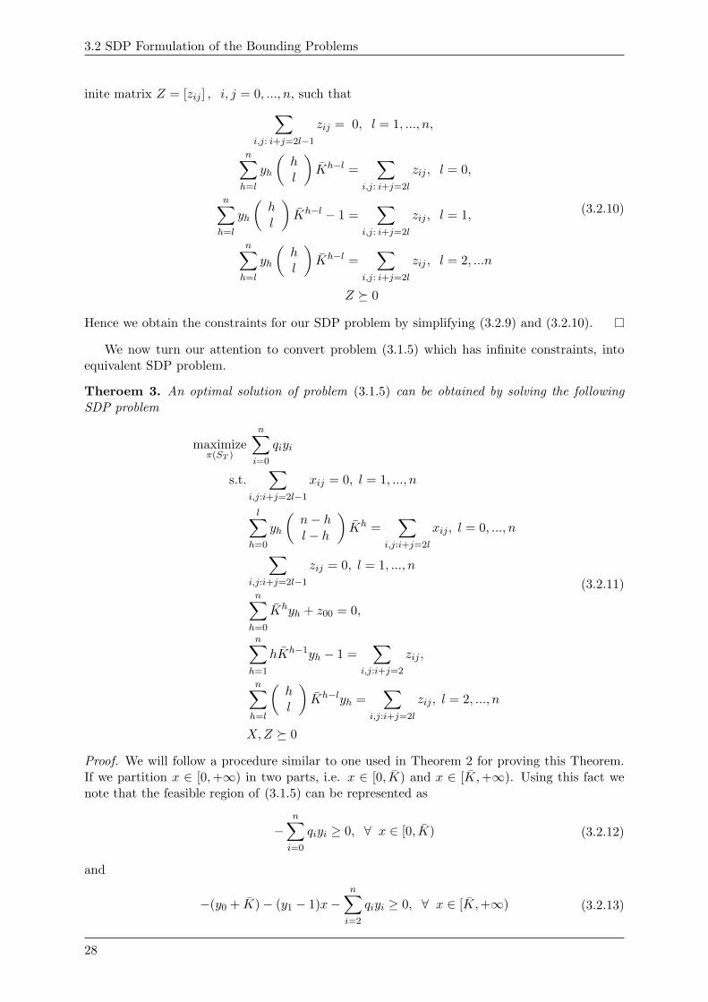
We now turn our attention to convert problem (3.1.5) which has infinite constraints, intoequivalent SDP problem.
Theroem 3. An optimal solution of problem (3.1.5) can be obtained by solving the followingSDP problem
maximizeπ(ST )
n∑i=0
qiyi
s.t.∑
i,j:i+j=2l−1
xij = 0, l = 1, ..., n
l∑h=0
yh
(n− hl − h
)Kh =
∑i,j:i+j=2l
xij , l = 0, ..., n
∑i,j:i+j=2l−1
zij = 0, l = 1, ..., n
n∑h=0
Khyh + z00 = 0,
n∑h=1
hKh−1yh − 1 =∑
i,j:i+j=2
zij ,
n∑h=l
(hl
)Kh−lyh =
∑i,j:i+j=2l
zij , l = 2, ..., n
X,Z 0
(3.2.11)
Proof. We will follow a procedure similar to one used in Theorem 2 for proving this Theorem.If we partition x ∈ [0,+∞) in two parts, i.e. x ∈ [0, K) and x ∈ [K,+∞). Using this fact wenote that the feasible region of (3.1.5) can be represented as
−n∑i=0
qiyi ≥ 0, ∀ x ∈ [0, K) (3.2.12)
and
−(y0 + K)− (y1 − 1)x−n∑i=2
qiyi ≥ 0, ∀ x ∈ [K,+∞) (3.2.13)
28
3 Semi-Parametric Approach for Bounding Option Price
Using Proposition 3, we conclude that (3.2.12) is true if and only if there exists a positivesemidefinite matrix X = [xij ] , i, j = 0, ..., n, such that
0 =∑
i,j: i+j=2l−1
xij , l = 1, ..., n,
l∑r=0
yr
(n− rl − r
)Kr = −
∑i,j: i+j=2l
xij , l = 0, ..., n,
X 0
(3.2.14)
Using Proposition 4, we conclude that (3.2.13) is true if and only if there exists a positivesemidefinite matrix Z = [zij ] , i, j = 0, ..., n, such that∑
i,j: i+j=2l−1
zij = 0, l = 1, ..., n,
n∑h=l
yh
(hl
)Kh−l = −
∑i,j: i+j=2l
zij , l = 0,
n∑h=l
yh
(hl
)Kh−l − 1 = −
∑i,j: i+j=2l
zij , l = 1,
n∑h=l
yh
(hl
)Kh−l = −
∑i,j: i+j=2l
zij , l = 2, ...n
Z 0
(3.2.15)
Hence we obtain the constraints for our SDP problem by simplifying (3.2.14) and (3.2.15).
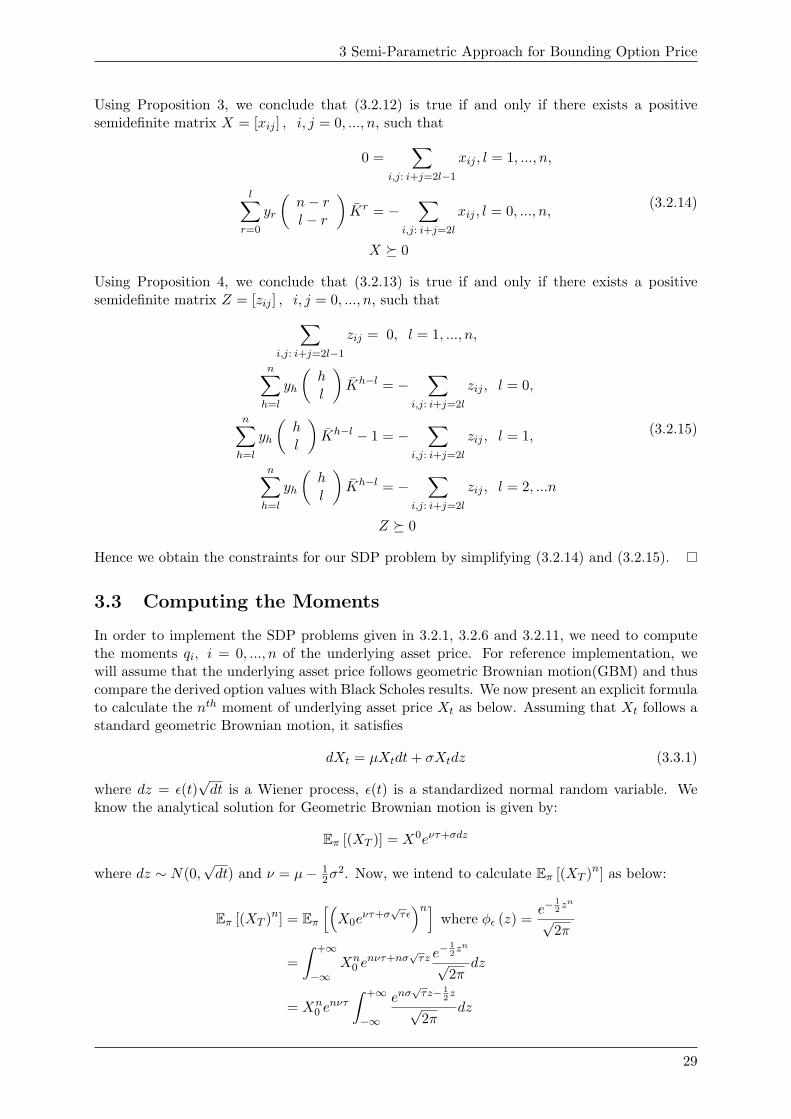
3.3 Computing the Moments
In order to implement the SDP problems given in 3.2.1, 3.2.6 and 3.2.11, we need to computethe moments qi, i = 0, ..., n of the underlying asset price. For reference implementation, wewill assume that the underlying asset price follows geometric Brownian motion(GBM) and thuscompare the derived option values with Black Scholes results. We now present an explicit formulato calculate the nth moment of underlying asset price Xt as below. Assuming that Xt follows astandard geometric Brownian motion, it satisfies
dXt = µXtdt+ σXtdz (3.3.1)
where dz = ε(t)√dt is a Wiener process, ε(t) is a standardized normal random variable. We
know the analytical solution for Geometric Brownian motion is given by:
Eπ [(XT )] = X0eντ+σdz
where dz ∼ N(0,√dt) and ν = µ− 1
2σ2. Now, we intend to calculate Eπ [(XT )n] as below:
Eπ [(XT )n] = Eπ[(X0e
ντ+σ√τε)n]
where φε (z) =e−
12zn
√2π
=∫ +∞
−∞Xn
0 enντ+nσ
√τz e− 1
2zn
√2π
dz
= Xn0 e
nντ
∫ +∞
−∞
enσ√τz− 1
2z
√2π
dz
29
3.3 Computing the Moments
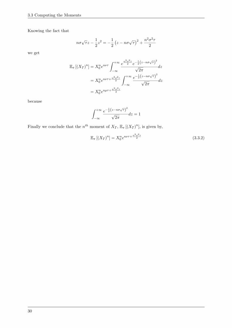
Knowing the fact that
nσ√τz − 1
2z2 = −1
2(z − nσ
√τ)2 +
n2σ2τ
2
we get
Eπ [(XT )n] = Xn0 e
nντ
∫ +∞
−∞
en2σ2τ
2 e−12(z−nσ√τ)2
√2π
dz
= Xn0 e
nντ+n2σ2τ2
∫ +∞
−∞
e−12(z−nσ√τ)2
√2π
dz
= Xn0 e
nµτ+n2σ2τ2
because ∫ +∞
−∞
e−12(z−nσ√τ)2
√2π
dz = 1
Finally we conclude that the nth moment of XT , Eπ [(XT )n], is given by,
Eπ [(XT )n] = Xn0 e
nντ+n2σ2τ2 (3.3.2)
30
Chapter 4
Method of Moments and SDPRelaxations
In this section, we will cover the numerical methods proposed by Lasserre, Prieto-Rumeauand Zervos in [21] for pricing exotic options. These methods are applied to options whereunderlying asset price follows a geometric Brownian motion or other mean-reverting processesof particular interest. The main idea of this method is to identify the derivative price withinfinite-dimensional linear programming problems. These problems involve moments of appro-priate measures. Finally we develop a finite-dimensional relaxation which can be converted toa semidefinite programming(SDP) problem indexed by the number of moments involved.
4.1 Introduction
The whole approach proposed by Lasserre, Prieto-Rumeau and Zervos in [21] can be brieflydescribed as below:
1. The price of a Exotic option has to be identified with a linear combination of moments ofsuitably defined measures.
2. The martingale property of certain associated stochastic integrals is then exploited toderive an infinite system of linear equations involving the moments of the measures con-sidered.
3. Hence the value of an exotic option is characterized with the solution of an infinite-dimensional linear programming (LP) problem. The variables of this LP problem involvesthe moments of certain suitably defined measures.
4. A finite-dimensional relaxation is obtained by restricting the infinite-dimensional LP prob-lem to one that involves only a finite number of moments. Extra constraints called momentconditions are introduced in the LP problem (which thus converts it to a SDP problem) forachieving the finite-dimensional relaxation. These conditions reflect necessary conditionsfor a set of scalars to be identified with moments of a measure supported on a given set.
5. The result is a LP problem or a semidefinite programming (SDP) problem, which dependson the choice of moment conditions. By extremizing the resulting problems, upper andlower bounds for the value of the option under consideration are obtained. Also the qualityof such bounds is enhanced as the number of moments increases.
31
4.2 Deriving Infinite-Dimensional LP Problem
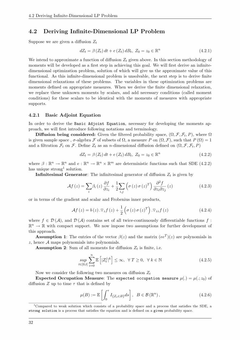
4.2 Deriving Infinite-Dimensional LP Problem
Suppose we are given a diffusion Zt
dZt = β (Zt) dt+ e (Zt) dBt, Z0 = z0 ∈ Rn (4.2.1)
We intend to approximate a function of diffusion Zt given above. In this section methodology ofmoments will be developed as a first step in achieving this goal. We will first derive an infinite-dimensional optimization problem, solution of which will give us the approximate value of thisfunctional. As this infinite-dimensional problem is unsolvable, the next step is to derive finitedimensional relaxations of these problems. The variables in these optimization problems aremoments defined on appropriate measures. When we derive the finite dimensional relaxation,we replace these unknown moments by scalars, and add necessary conditions (called momentconditions) for these scalars to be identical with the moments of measures with appropriatesupports.
4.2.1 Basic Adjoint Equation
In order to derive the Basic Adjoint Equation, necessary for developing the moments ap-proach, we will first introduce following notations and terminology.
Diffusion being considered: Given the filtered probability space, (Ω,F ,Ft,P), where Ωis given sample space , σ-algebra F of subsets of Ω, a measure P on (Ω,F), such that P (Ω) = 1and a filtration Ft on F . Define Zt as an n-dimensional diffusion defined on (Ω,F ,Ft,P)
dZt = β (Zt) dt+ e (Zt) dBt, Z0 = z0 ∈ Rn (4.2.2)
where β : Rn → Rn and e : Rn → Rn × Rm are deterministic functions such that SDE (4.2.2)has unique strong1 solution.
Infinitesimal Generator: The infinitesimal generator of diffusion Zt is given by
Af (z) =∑i
βi (z)∂f
∂zi+
12
∑i,j
(σ (z)σ (z)T
) ∂2f
∂zi∂zj(z) (4.2.3)
or in terms of the gradient and scalar and Frobenius inner products,
Af (z) = b (z) .Ozf (z) +12
(σ (z)σ (z)T
).Ozzf (z) (4.2.4)
where f ∈ D (A), and D (A) contains set of all twice-continuously differentiable functions f :Rn → R with compact support. We now impose two assumptions for further development ofthis approach.
Assumption 1: The entries of the vector β(z) and the matrix (eeT )(z) are polynomials inz, hence A maps polynomials into polynomials.
Assumption 2: Sum of all moments for diffusion Zt is finite, i.e.
supt∈[0,t]
n∑i=0
E[|Zjt |k
]≤ ∞, ∀ T ≥ 0, ∀ k ∈ N (4.2.5)
Now we consider the following two measures on diffusion ZtExpected Occupation Measure: The expected occupation measure µ(.) = µ(.; z0) of
diffusion Z up to time τ that is defined by
µ(B) := E[∫ τ
0IZs∈Bds
], B ∈ B (Rn) , (4.2.6)
1Compared to weak solution which consists of a probability space and a process that satisfies the SDE, astrong solution is a process that satisfies the equation and is defined on a given probability space.
32
4 Method of Moments and SDP Relaxations
where B (Rn) is the Borel σ-algebra on Rn.Exit Location Measure: The exit location measure ν(.) = ν(.; z0) that is defined by
ν(B) := P (Zτ ∈ B) , B ∈ B (Rn) , (4.2.7)
which is nothing but probability distribution of Zτ .
We are now ready to derive the Basic Adjoint Equation given the definitions and assumptionsabove. Specifically, given the Assumptions 1 and 2 above the following process
Mft := f(Zt)− f(z0)−
∫ t
0Af(ZS)ds
=∫ t
0[eTOzf ]T (ZS)dBS , t ≥ 0,
(4.2.8)
where f : Rn → R, f ∈ D (A) as defined above, is a square integrable martingale.
Now, Doob’s optional sampling theorem2 states: For X = Xtt≥0, which is an (Ft,P)martingale, and S, T are stopping times bounded by constant c, with S ≤ T , almost surely, thenEP[XT |FS ] = XS , P almost surely.
Applying Doob’s optional sampling theorem to (4.2.8) at times 0 and T we get,
E[Mft
]= E
[Mf
0
]E[f(Zt)− f(z0)−
∫ t
0Af(ZS)ds
]= E
[f(Z0)− f(z0)−
∫ 0
0Af(ZS)ds
]E [f(Zt)]− f(z0)− E
[∫ t
0Af(ZS)ds
]= f(Z0)− f(z0)− E
[∫ 0
0Af(ZS)ds
] (4.2.9)
and by simple calculations we know that,
f(Z0)− f(z0)− E[∫ 0
0Af(ZS)ds
]= 0 (4.2.10)
hence we get the following result
E [f(Zt)]− f(z0)− E[∫ t
0Af(ZS)ds
]= 0 (4.2.11)
Using the definitions of expected occupation measure µ(.), and exit location measure ν(.) asgiven above, we can rewrite (4.2.11) as below∫
Rnf (z) ν(dz)− f(z0)−
∫RnAf(z)µ(dz) = 0 (4.2.12)
which is called the basic adjoint equation. We can consider this equation as defining therelationship between the measures µ and ν associated with the generator A (for more detailsplease refer to article [12] by Helmes, Rohl and Stockbridge).
2We can roughly interpret Doob’s optional sampling theorem implying that in a Casino in a fair world, wherereturns are martingales and gambler is restricted to quit at stopping times, then there is almost zero probabilityto improve the expected return by judicious choice of stopping time.
33
4.2 Deriving Infinite-Dimensional LP Problem
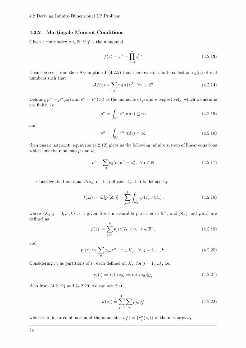
4.2.2 Martingale Moment Conditions
Given a multiindex α ∈ N, if f is the monomial
f(z) = zα =n∏j=1
zαjj (4.2.13)
it can be seen from then Assumption 1 (4.2.5) that there exists a finite collection cβ(α) of realnumbers such that
Af(z) =∑β
cβ(α)zβ, ∀z ∈ Rn (4.2.14)
Defining µα = µα(z0) and να = να(z0) as the moments of µ and ν respectively, which we assumeare finite, i.e.
µα =∫
Rnzαµ(dz) ≤ ∞ (4.2.15)
and
να =∫
Rnzαν(dz) ≤ ∞ (4.2.16)
then basic adjoint equation (4.2.12) gives us the following infinite system of linear equationswhich link the moments µ and ν,
να −∑β
cβ(α)µβ = zα0 , ∀α ∈ N (4.2.17)
Consider the functional J(z0) of the diffusion Zt that is defined by
J(z0) := E [p (Zτ )] =k∑j=1
∫Kj
j (z) ν (dz) , (4.2.18)
where Kj , j = 0, ..., k is a given Borel measurable partition of Rn, and p(z) and pj(z) aredefined as
p(z) :=k∑j=1
pj(z)IKj (z), z ∈ Rn, (4.2.19)
andpj(z) :=
∑α
pjαzα, z ∈ Kj , ∀ j = 1, ..., k, (4.2.20)
Considering νj as partitions of ν, each defined on Kj , for j = 1, ...k, i.e.
νj(.) := νj(.; z0) := νj(.; z0)|Kj (4.2.21)
then from (4.2.19) and (4.2.20) we can see that
J(z0) =k∑j=1
∑α
pjαναj (4.2.22)
which is a linear combination of the moments ναj = ναj (z0) of the measures νj .
34
4 Method of Moments and SDP Relaxations
4.2.3 Using Available Moments
If the moments ναj of the measure να are easily computable (which is the case in European andAsian options as elucidated in subsequent sections), we can bound the functional J(z0) definedin (4.2.18) by obtaining the upper and lower bounds of infinite dimensional LP problem QI(z0)defined by
extremizek∑j=1
∑α
pjαναj ,
subject tok∑j=1
ναj = να, α ∈ Nn
νj ∈M(Kj), j = 1, ..., k,
(4.2.23)
noting that space of all Borel measures with finite moments of all orders that are supported ona given Borel measurable set K ⊆ Rn is denoted by M(Kj). We also note that the constraintsdefining the feasible region of QI(z0) are necessary moment conditions and hence
inf QI(z0) ≤ J(z0) ≤ sup QI(z0) (4.2.24)
When ν is moment-determinate3 then (4.2.24) is satisfied with equality because measure ν(.) isunique.
4.2.4 Using Martingale Moments Conditions
More generally when we cannot compute moments ν easily, we consider the infinite dimensionalLP problem QII(z0) defined by
extremizek∑j=1
∑α
pjαναj ,
subject to να −∑β
cβ(α)µβ = zα0 , ∀α ∈ N
µj ∈M(Rn) νj ∈M(Kj), j = 1, ..., k,
(4.2.25)
where the martingale moment conditions in (4.2.17) are taken into consideration as constraintsfor LP problem QII(z0). Similar to (4.2.23), we again note the fact that the constraints for LPproblem QII(z0) are necessary moment conditions and hence
infQII(z0) ≤ J(z0) ≤ supQII(z0) (4.2.26)
When ν is moment-determinate then (4.2.26) is satisfied with equality and QII is equal to thevalue of J(z0).
Now that we have derived the relevant infinite dimensional LP problem, we would try toaddress the problem of deriving the finite dimensional relaxations of problems (4.2.23) and(4.2.25). For doing that, development of the background material is presented in followingsection is essential.
3Moment determinacy can be defined as equality of ν and µ, for given measure ν on Rn having finite momentsof all orders and whenever
∫zαµ(dz) =
∫zαν(dz). Example of moment determinate probability distributions are
normal and noncentral χ2 distributions, where as lognormal distribution is not moment-determinate.
35
4.3 Polynomial Optimisation and Problem of Moments
4.3 Polynomial Optimisation and Problem of Moments
In [18], Lasserre showed that problem of finding unconstrained global optimum of a real valuedpolynomial, p(x) : Rn → R can be reduced to solving finite sequence of convex Linear MatrixInequalities (LMI) (or semidefinite programming(SDP)) problems. The implementation wasgiven in [19] by Lasserre and Henrion. The same approach can be applied to p(x) over acompact set K defined by polynomial inequalities.
To elaborate, given a real-valued polynomial p(x) : Rn → R, the following problem needs tobe solved
minx∈Rn
p(x) (4.3.1)
Also when K is a compact set(convexity assumption not required) defined by polynomial in-equalities gi(x) ≥ 0, i = 1, ..., r, we obtain the following problem.
minx∈K
p(x) (4.3.2)
The primal LMI relaxation Qi of p(x) given below aims to find the moments of a probabilitymeasure with mass concentrated on some global minimizer of p(x)
Qi := minµ
∫p(x)dµ | µ(K) = 1
(4.3.3)
where minimum is take over all probability measures on the feasible set of p(x), Rn and K for(4.3.1) and (4.3.1) respectively.
4.3.1 Notation and Definition
Let s(r) =(n+ rr
), and
1, x1, x2, ..., xn, x21, x1x2, ..., x1xn, x2x3, ..., x
2n, ..., x
m1 , ..., x
mn (4.3.4)
be the basis for the m-degree real-valued polynomials p(x) : Rn → R , and let s(2m) be itsdimension. We write the polynomial p(x) : Rn → R as below
p(x) =∑α
pαxα
with xα := xα11 xα2
2 ...xαnn
and αi ∈ N,∑i
αi ≤ m, i = 1, ..., n
(4.3.5)
where coefficient vector of p(x) in the basis (4.3.4) has been denoted by p = pα ∈ Rs(m).Moment Matrix:Assuming that we are given a vector y := yα of length s(2m) which
confirms with indexing implied by the basis (4.3.4), we define a matrix of dimensions s(m)×s(m)called moment matrix Mk(y) which has rows and columns labelled by (4.3.4). To be moreprecise, Mk(y) is defined as below:
Mk(y)(1, i) = Mk(y)(i, 1) = yi−1 for i = 1, ..., k + 1Mk(y)(1, j) = yα and Mk(y)(i, 1) = yβ ⇒Mk(y)(i, j) = yα+β
(4.3.6)
In other words we can say that matrix Mk(y) is the block matrix Mk(y)0≤i,j≤2m defined by
Mi,j(y) =
yi+j,0 yi+j−1,1 · · · yi,jyi+j−1,1 yi+j−2,2 · · · yi−1,j+1
......
. . ....
yj,i yi+j−1,1 · · · y0,i+j
(4.3.7)
36
4 Method of Moments and SDP Relaxations
where yi,j represents (i + j)th-order moment∫xiyjµ(d(x, y)) for some probability measure µ.
To understand the concept of moment matrix, we give 3 examples:Example 1: When n = 1, then y = y0, y1, y2, ... and Mk(y) is same as Hankel Matrix
Hk(y)(i, j) = yi+j−2, i, j = 1, ..., k + 1
Example 2:When n = 2 and m = 2, we get
M2(y) =
y0,0 y1,0 y0,1 y2,0 y1,1 y0,2
y1,0 y2,0 y1,1 y3,0 y2,1 y1,2
y0,1 y1,1 y0,2 y2,1 y1,2 y0,3
y2,0 y3,0 y2,1 y4,0 y3,1 y2,2
y1,1 y2,1 y1,2 y3,1 y2,2 y1,3
y0,2 y1,2 y0,3 y2,2 y1,3 y0,4
(4.3.8)
Example 3: For the three-dimensional case, definition ofMk(y) is given via blocks Mi,j,k(y) , 0 ≤i, j, k ≤ 2m as done for the case of n = 2 and m = 2, and so on.
Localizing Matrix: Let q(x) : Rn → R be a real-valued polynomial of degree w withcoefficient vector q ∈ Rs(w). If the entry (i, j) of the matrix Mk(y) is yβ, let β(ij) denote thesubscript β of yβ.Let Mk(q, y) be the matrix defined by
Mk(q, y)(i, j) =∑α
qαyβ(i,j)+α (4.3.9)
For example, given
M1(y) =
y0,0 y1,0 y0,1
y1,0 y2,0 y1,1
y0,1 y1,1 y0,2
and q(x) = ax1 − bx1x2 − cx22, (4.3.10)
we obtain
M1(q, y) =
ay1,0 − by1,1 − cy0,2 ay2,0 − by2,1 − cy1,2 ay1,1 − by1,2 − cy0,3
ay2,0 − by2,1 − cy1,2 ay3,0 − by3,1 − cy2,2 ay2,1 − by2,2 − cy1,3
ay1,1 − by1,2 − cy0,3 ay2,1 − by2,2 − cy1,3 ay1,2 − by1,3 − cy0,4
(4.3.11)
4.3.2 Necessary Moment conditions
Proposition 7. If y = yα(with y0,....,0 = 1) is a vector of moments up to order 2k of someprobability measure µy, then
Mk(q, y) 0 (4.3.12)
Proof. Consider v(x) : Rk → R , a real valued polynomial of degree at most k and a vector ofcoefficients (fα, |α| ≤ k), in the basis (4.3.4). Then we have
〈f,Mk(y)f〉 =∫f2dµ ≥ 0 (4.3.13)
Proposition 8. If y = yα(with y0,....,0 = 1) is a vector of moments up to order 2k of someprobability measure µy, then
Mk(q, y) 0 (4.3.14)
Proof. To prove this consider v(x) : Rk → R , a real valued polynomial of degree at most k anda vector of coefficients (fα, |α| ≤ k), in the basis (4.3.4). Then we have
〈f,Mk(q, y)f〉 =∫f2qdµ ≥ 0 (4.3.15)
37
4.3 Polynomial Optimisation and Problem of Moments
Hence from Proposition 7 (4.3.12) and Proposition 8 (4.3.14), we can say that necessaryconditions for elements of y = yα to be moments of some measure µy on semialgebric set K,i.e. the set of form
K := x ∈ Rn | vi(x) ≥ 0, for all i = 1, ..., l (4.3.16)
where vi, i = 1, ..., l are given polynomials, is given by
Mk(y) 0 and Mk(vi, y) 0, i = 1, ..., l, k = 1, 2, ..., (4.3.17)
We also note that above conditions are necessary conditions but not sufficient conditions forelements of y = yα to be moments of measure µy supported on set K. Before going tothe next section, we note the K-moment problem statement: K-moment problem identifiessequences yα that are moment-sequences of measure µ with support contained in semialgebricset K.
4.3.3 SDP Relaxations
After deriving the necessary conditions for a vector y to be moment of measure µ, we will derivethe SDP relaxations for problems p(x) in (4.3.2) and (4.3.4). For problem p(x) and K, let theassociated feasibility set be defined as
K = x ∈ Rn | qk(x) ≥ 0, k = 0, ...,m (4.3.18)
Also let degree of qk = 2vk + 1 or 2vk, depending on its parity. The vectors qk ∈ Rs(2vk) areextended to vectors of Rs(2i) by appending extra zeros when needed, for any i ≥ maxk∈0,mvk.
Consider the following family of convex positive semidefinite optimization problems Qi,
infy
∑α
pαyα
subject to Mi(y) 0Mi−vk(q, y) 0
(4.3.19)
which are also called Linear Matrix Inequality(LMI) problems.
Assumption 1: Given semialgebric set Kq := x ∈ Rn | q(x) ≥ 0 and a polynomial p(x),strictly positive on Kq, then p(x) can be written as
p(x) =r1∑i=1
qi(x)2 + θ(x)r2∑j=1
tj(x)2, (4.3.20)
for some polynomials qi(x), tj(x), i = 1, ..., r1, j = 1, ..., r2.Under the above Assumption, it was proved in by Lasserre in [18], that
inf Qi ↑ inf p(x), as i →∞ (4.3.21)
or in other words, the problem of obtaining the bounds of p(x) in the original problem (4.3.1) canbe accurately solved with desired accuracy by solving problem of obtaining bounds for convexLMI problem Qi for every i ≥ maxk∈0,mvk.
4.3.4 Summary
To summarise the contents in above section, a result that applies when n = 1 is stated whichwill be useful in the following sections.
38
4 Method of Moments and SDP Relaxations
K-Moment Problem: Given a vector y = (y0, y1, ..., y2r) and a set K ⊆ R, the K-momentproblem investigates necessary and sufficient conditions for y to be identified with the corre-sponding vector of moments of some measure supported on K. This problem is called thetruncated Hausdorff moment problem if K = [a, b], and the truncated Stieltjes moment problemif K = [a,+∞).
Necessary Conditions: Given a vector y = (y0, y1, ..., y2r) ∈ R2r+1, the following state-ments are true:
• Truncated Hausdorff moment problem: Mr(y) 0 and Mr(g, y) 0 with g(x) :=(b− x)(x− a), are necessary and sufficient conditions for the elements of y to be the first2r + 1 moments of a measure supported on [a, b] for the truncated Hausdorff momentproblem.
• Truncated Stieltjes moment problem: Mr(y) 0 and Mr(g, y) 0 with g(x) := x−a,are sufficient conditions for the elements of y to be the first 2r + 1 moments of a measuresupported on [a,+∞) for the truncated Stieltjes moment problem.
4.4 Finite Dimensional Relaxations
We will now derive the finite dimensional relaxations of problems QI(z0) and QII(z0), given by(4.2.23) and (4.2.25). Given a Borel measurable set K ⊆ Rn, let M(K) be the set of all Borelmeasures with support contained in K, and with all moments finite. Consider a set Sr(K) thatis defined by appropriate necessary moment conditions for scalars ηα, |α| ≤ 2r to be momentsof some measure in M(K), as described in section 4.3.4
We define another set Nr(K), such that Sr(K) ⊇ Nr(K) and
Nr(K) :=∫
xαµ(dx)| α ∈ Nn, |α| ≤ 2r µ ∈M(K)
(4.4.1)
where |α| :=∑n
i−1 αi ≤ 2r. Then we consider the finite dimensional relaxations of problemsQI(z0) which was defined in (4.2.23), denoted here as QI
r(z0) as
extremizeη1,...,ηk
k∑j=1
∑α
pjαηαj ,
subject tok∑j=1
ηαj = ηα, |α| ≤ 2r
ηj =ηαj , |α| ≤ 2r
∈ Sr(Kj), j = 1, ..., k
(4.4.2)
and when moments are not known, the finite dimensional relaxation of QII(z0) which was definedin (4.2.23), denoted here as QII
r (z0) as
extremizeη1,...,ηk,ϑ
k∑j=1
∑α
pjαηαj ,
subject tok∑j=1
ηαj −∑β
cβ(α)ϑα = zα0 |α| ≤ 2r
ηj =ηαj , |α| ≤ 2r
∈ Sr(Kj), j = 1, ..., k
ϑj =ϑαj , |α| ≤ 2r
∈ Sr(Rn)
(4.4.3)
We will now specify the sets Sr(K) and Nr(K) in accordance with notation introduced insection 4.3.4 for following three cases:
39
4.5 SDP Relaxations for European Options
• K ⊆ R is the interval [a, b]
• K ⊆ R is the interval [a,+∞)
• K ⊆ R is the interval (−∞, a]
We can clearly see that Sr(K) is given by necessary moment conditions for a vector y ∈ R2n+1
as defined below
• When K = [a, b] the set Sr is given by:
Sr(K) =y ∈ R2r+1 Mr(y) 0 and Mr−1(g, y) 0,
g(x) := (b− x)(x− a)
(4.4.4)
• When K = [a,+∞) the set Sr is given by:
Sr(K) =y ∈ R2r+1 Mr(y) 0 and Mr−1(g, y) 0,
g(x) := (x− a)
(4.4.5)
• When K = (−∞, a] the set Sr is given by:
Sr(K) =y ∈ R2r+1 Mr(y) 0 and Mr−1(g, y) 0,
g(x) := (a− x)
(4.4.6)
and set Nr(K) ⊆ Sr(K) is the set of all vectors that provide the first 2r+1 moments of a measurewith finite moments of all orders and supported on K for any given r ≥ 1.
Before we give the final SDP problems to be solved, we note the relationship between Sr(K)and Nr(K) for following two cases:
• Truncated Hausdorff moment problem: Since K = [a, b] and conditions specified bySr(K) are also sufficient conditions, we note that Sr(K) = Nr(K).
• Truncated Stieltjes moment problem: Define
Tr(K) :=y ∈ R2r+1|Mr(y) 0andMr−1(g, y) 0
(4.4.7)
Hence as per the given definition we observe that ¯Tr(K) = Nr(K) and from section 4.3.4 wesee that Tr(K) ⊆ Nr(K). This results in ¯Nr(K) = Sr(K), for K = [a,∞) or K = (−∞, a].
4.5 SDP Relaxations for European Options
We would now utilize the theory developed in previous sections for solving the problem ofpricing the European options. The case of European options is comparatively simpler becauseit considers measures involving only the process Xt, which are supported on subsets of the realline.
Suppose the underlying asset price process satisfies the following stochastic differential equa-tion
dXt = b(Xt)dt+ σ(Xt)dWt, b, σ : R→ R, X0 = x0 ∈ R (4.5.1)
The value of a European call option written on the underlying X is given by
vE(x0) := e−ρTE[(XT −K)+
](4.5.2)
where (XT−K)+ denotes max(XT−K, 0), T > 0 is the option’s maturity time, K is the option’sstrike price, ρ is a constant discounting factor and x0 is the initial underlying asset price. Under
40
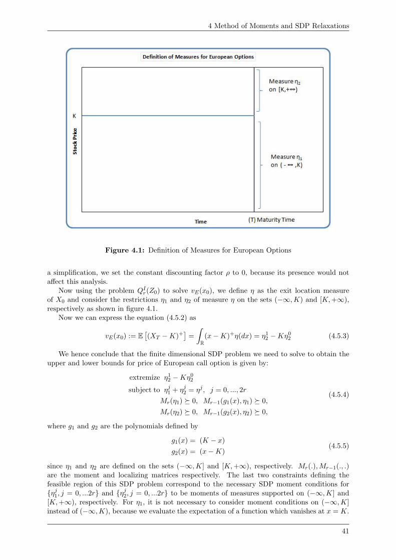
4 Method of Moments and SDP Relaxations
Figure 4.1: Definition of Measures for European Options
a simplification, we set the constant discounting factor ρ to 0, because its presence would notaffect this analysis.
Now using the problem QIr(Z0) to solve vE(x0), we define η as the exit location measureof X0 and consider the restrictions η1 and η2 of measure η on the sets (−∞,K) and [K,+∞),respectively as shown in figure 4.1.
Now we can express the equation (4.5.2) as
vE(x0) := E[(XT −K)+
]=∫
R(x−K)+η(dx) = η1
2 −Kη02 (4.5.3)
We hence conclude that the finite dimensional SDP problem we need to solve to obtain theupper and lower bounds for price of European call option is given by:
extremize η12 −Kη0
2
subject to ηj1 + ηj2 = ηj , j = 0, ..., 2rMr(η1) 0, Mr−1(g1(x), η1) 0,Mr(η2) 0, Mr−1(g2(x), η2) 0,
(4.5.4)
where g1 and g2 are the polynomials defined by
g1(x) = (K − x)g2(x) = (x−K)
(4.5.5)
since η1 and η2 are defined on the sets (−∞,K] and [K,+∞), respectively. Mr(.),Mr−1(., .)are the moment and localizing matrices respectively. The last two constraints defining thefeasible region of this SDP problem correspond to the necessary SDP moment conditions forηj1, j = 0, ...2r and ηj2, j = 0, ...2r to be moments of measures supported on (−∞,K] and[K,+∞), respectively. For η1, it is not necessary to consider moment conditions on (−∞,K]instead of (−∞,K), because we evaluate the expectation of a function which vanishes at x = K.
41
4.5 SDP Relaxations for European Options
The derivation of SDP problem for finding upper and lower bounds for price of Europeanput option is very similar; only the objective function is changed in (4.5.4) which is given byKη0
1 − η11, rest of constraints remain the same.
4.5.1 Moments Computation
We assume that X is the stochastic process defined in previous section. Now we intend tocompute the moment of η, hence we consider the monomial f(X) = Xi which is continuous anddifferentiable, hence we would apply Taylor’s expansion
4f =(df
dx
)4X +
12
(d2f
dx2
)4X2 +
16
(d3f
dx3
)4X3 + ... (4.5.6)
to f(X) for a small change 4X in X. We enlist the following three casesCase 1: Geometric Brownian Motion: Here 4X is given by
4Xt = bXtdt+ σXtdWt (4.5.7)
and hence applying (4.5.6) to (4.5.7), we get
4f = ixi−1(bxdt+ σxdWt)+12i(i− 1)xi−2(bxdt+ σxdWt)2+
16i(i− 1)(i− 2)xi−3(bxdt+ σxdWt)3 + ...
= ibxidt+ iσxidWt +12i(i− 1)σ2xi(dWt)2
(4.5.8)
where step 2 in above equation is obtained by ignoring (4t) terms of order more than 1. Nowtaking the term 1
2 i(i−1)σ2xi(dWt)2, we note the fact that dWt has expected value 0 and variance4t, hence this last term is of order 4t and can’t be ignored. It can be proved that as 4t→ 0,(dWt)2 →4t. Hence moments of η denoted as ηi = E[Xi] can be found by solving the followingsystem of ordinary differential equations
d
dtηi(t) = ibηi(t) +
12i(i− 1)σ2ηi(t), 0 ≤ i ≤ 2r (4.5.9)
with initial conditions ηi(0) = (X0)i and the second term iσxidWt vanishes because E[dWt] = 0.
Case 2: Ornstein-Uhlenbeck Process: Here 4X is given by
4Xt = γ(θ −Xt)dt+ σdWt (4.5.10)
and hence applying (4.5.6) to (4.5.10), we get
4f = ixi−1(γ(θ − x)dt+ σdWt))+12i(i− 1)xi−2(γ(θ − x)dt+ σdWt))2+
16i(i− 1)(i− 2)xi−3(γ(θ − x)dt+ σdWt))3 + ...
= iγθxi−1dt− iγxidt+ iσxi−1dWt +12i(i− 1)(xi−2σ2(dWt)2)
(4.5.11)
where similar analysis applies as we did for Model 1 (geometric Brownian motion). Specifically,step 2 in above equation is obtained by ignoring (4t) terms of order more than 1. Now takingthe fourth term 1
2 i(i − 1)(xi−2σ2(dWt)2), we note the fact that dWt has expected value 0 and
42
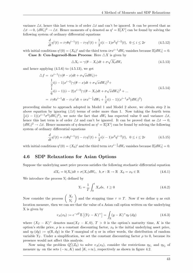
4 Method of Moments and SDP Relaxations
variance 4t, hence this last term is of order 4t and can’t be ignored. It can be proved that as4t→ 0, (dWt)2 →4t. Hence moments of η denoted as ηi = E[Xi] can be found by solving thefollowing system of ordinary differential equations
d
dtηi(t) = iγθηi−1(t)− iγηi(t) +
12i(i− 1)σ2ηi−2(t), 0 ≤ i ≤ 2r (4.5.12)
with initial conditions ηi(0) = (X0)i and the third term iσxi−1dWt vanishes because E[dWt] = 0.Case 3: Cox-Ingersoll-Ross Process: Here 4X is given by
4Xt = γ(θ −Xt)dt+ σ√XtdWt (4.5.13)
and hence applying (4.5.6) to (4.5.13), we get
4f = ixi−1(γ(θ − x)dt+ σ√xdWt)+
12i(i− 1)xi−2(γ(θ − x)dt+ σ
√xdWt)2+
16i(i− 1)(i− 2)xi−3(γ(θ −Xt)dt+ σ
√xdWt)3 + ...
= iγθxi−1dt− iγxidt+ iσxi−12dWt +
12i(i− 1)(xi−1σ2(dWt)2)
(4.5.14)
proceeding similar to approach adopted in Model 1 and Model 2 above, we obtain step 2 inabove equation by ignoring (4t) terms of order more than 1. Now taking the fourth term12 i(i − 1)(xi−1σ2(dWt)2), we note the fact that dWt has expected value 0 and variance 4t,hence this last term is of order 4t and can’t be ignored. It can be proved that as 4t → 0,(dWt)2 →4t. Hence moments of η denoted as ηi = E[Xi] can be found by solving the followingsystem of ordinary differential equations
d
dtηi(t) = iγθηi−1(t)− iγηi(t) +
12i(i− 1)σ2ηi−2(t), 0 ≤ i ≤ 2r (4.5.15)
with initial conditions ηi(0) = (X0)i and the third term iσxi−12dWt vanishes because E[dWt] = 0.
4.6 SDP Relaxations for Asian Options
Suppose the underlying asset price process satisfies the following stochastic differential equation
dXt = b(Xt)dt+ σ(Xt)dWt, b, σ : R→ R X0 = x0 ∈ R (4.6.1)
We introduce the process Yt defined by
Yt =1T
∫ t
0Xsds, t ≥ 0 (4.6.2)
Now consider the process(Xt
Yt
)and the stopping time τ ≡ T . Now if we define η as exit
location measure, then we can see that the value of a Asian call option written on the underlyingX is given by
vA(x0) := e−ρTE[(YT −K)+
]=∫
R(y −K)+ηY (dy) (4.6.3)
where (XT − K)+ denotes max(XT − K, 0), T > 0 is the option’s maturity time, K is theoption’s strike price, ρ is a constant discounting factor, x0 is the initial underlying asset price,and ηY (dy) := η(R, dy) is the Y -marginal of η or in other words, the distribution of randomvariable YT . Under a simplification, we set the constant discounting factor ρ to 0, because itspresence would not affect this analysis.
Now using the problem QIr(Z0) to solve vA(x0), consider the restrictions ηY1 and ηY2 ofmeasure ηY on the sets (−∞,K) and [K,+∞), respectively as shown in figure 4.2.
43
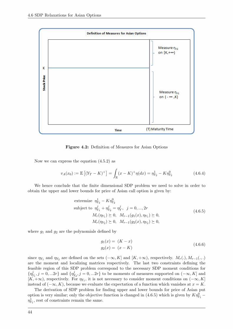
4.6 SDP Relaxations for Asian Options
Figure 4.2: Definition of Measures for Asian Options
Now we can express the equation (4.5.2) as
vA(x0) := E[(YT −K)+
]=∫
R(x−K)+η(dx) = η1
Y2−Kη0
Y2(4.6.4)
We hence conclude that the finite dimensional SDP problem we need to solve in order toobtain the upper and lower bounds for price of Asian call option is given by:
extremize η1Y2−Kη0
Y2
subject to ηjY1+ ηjY2
= ηjY , j = 0, ..., 2r
Mr(ηY1) 0, Mr−1(g1(x), ηY1) 0,Mr(ηY2) 0, Mr−1(g2(x), ηY2) 0,
(4.6.5)
where g1 and g2 are the polynomials defined by
g1(x) = (K − x)g2(x) = (x−K)
(4.6.6)
since ηY1 and ηY2 are defined on the sets (−∞,K] and [K,+∞), respectively. Mr(.),Mr−1(., .)are the moment and localizing matrices respectively. The last two constraints defining thefeasible region of this SDP problem correspond to the necessary SDP moment conditions forηjY1
, j = 0, ...2r and ηjY2, j = 0, ...2r to be moments of measures supported on (−∞,K] and
[K,+∞), respectively. For ηY1 , it is not necessary to consider moment conditions on (−∞,K]instead of (−∞,K), because we evaluate the expectation of a function which vanishes at x = K.
The derivation of SDP problem for finding upper and lower bounds for price of Asian putoption is very similar; only the objective function is changed in (4.6.5) which is given by Kη0
Y1−
η1Y1
, rest of constraints remain the same.
44
4 Method of Moments and SDP Relaxations
4.6.1 Moments Computation
We assume that X and Y are the stochastic processes defined in previous section. Now weintend to compute the moment of η, hence we consider the monomial f(X,Y ) = XiY j which iscontinuous and differentiable, hence we would apply Taylor’s expansion to two variables
4f =(∂f
∂x
)4X +
(∂f
∂y
)4Y
+12
(∂2f
∂x2
)4X2 +
12
(∂2f
∂y2
)4Y 2 +
(∂2f
∂x∂y
)4X4Y + ...
(4.6.7)
to f(X) for a small change 4X in X and 4Y in Y . The change in variable Y , 4Y is given by
4Yt =1tXtdXt (4.6.8)
We will now elaborate on following 3 cases.Case 1: Geometric Brownian Motion: Here 4X is given by
4Xt = bXtdt+ σXtdWt (4.6.9)
and hence applying (4.6.9) to (4.6.7), we get
4f = ixi−1yj(bxdt+ σxdWt)
+ jxiyj−1
(1Txdt
)+
12i(i− 1)xi−2yj(bxdt+ σxdWt)2
+12ijxi−1yj−1(bxdt+ σxdWt)
(1Txdt
)+ j(j − 1)xiyj−2
(1Txdt
)2
+ ...
= ibxiyjdt+ iσxiyjdWt +1Tjxi+1yj−1dt+
12i(i− 1)σ2xiyj(dWt)2
(4.6.10)
where step 2 in above equation is obtained by ignoring (4t) terms of order more than 1. Nowtaking the fourth term 1
2 i(i − 1)σ2xiyj(dWt)2), we note the fact that dWt has expected value0 and variance 4t, hence this last term is of order 4t and can’t be ignored. It can be provedthat as 4t→ 0, (dWt)2 →4t. Hence moments of η denoted as ηi,j = E[XiY j ] can be found bysolving the following system of ordinary differential equations
d
dtηi,j(t) = ibηi,j(t) +
1Tjηi+1,j−1(t) +
12i(i− 1)σ2ηi,j(t), 0 ≤ i ≤ 2r (4.6.11)
with initial conditions η0,j(0) = 0, j 6= 0, η0,0(0) = 1, ηi,0(0) = (X0)i and the second termiσxiyjdWt vanishes because E[dWt] = 0.
Case 2: Ornstein-Uhlenbeck Process: Here 4X is given by
4Xt = γ(θ −Xt)dt+ σdWt (4.6.12)
45
4.6 SDP Relaxations for Asian Options
and hence applying (4.6.9) to (4.6.7), we get
4f = ixi−1yj(γ(θ − x)dt+ σdWt)
+ jxiyj−1
(1Txdt
)+
12i(i− 1)xi−2yj(γ(θ − x)dt+ σdWt)2
+12ijxi−1yj−1(γ(θ − x)dt+ σdWt)
(1Txdt
)+ j(j − 1)xiyj−2
(1Txdt
)2
+ ...
= iγθxi−1yjdt− iγxiyjdt+ iσxi−1yjdWt
+1Tjxi+1yj−1dt+
12i(i− 1)σ2xiyj(dWt)2
(4.6.13)
where similar analysis applies as we did for Model 1 (geometric Brownian motion). Specifically,step 2 in above equation is obtained by ignoring (4t) terms of order more than 1. Now takingthe fifth term 1
2 i(i−1)σ2xiyj(dWt)2, we note the fact that dWt has expected value 0 and variance4t, hence this last term is of order 4t and can’t be ignored. It can be proved that as 4t→ 0,(dWt)2 → 4t. Hence moments of η denoted as ηi,j = E[XiY j ] can be found by solving thefollowing system of ordinary differential equations
d
dtηi,j(t) = iγθηi−1,j(t)− iγηi,j(t) +
1Tjηi+1,j−1(t) +
12i(i− 1)σ2ηi,j(t), 0 ≤ i ≤ 2r (4.6.14)
with initial conditions4 η0,j(0) = 0, j 6= 0, η0,0(0) = 1, ηi,0(0) = (X0)i and the third termiσxi−1yjdWt vanishes because E[dWt] = 0.
Case 3: Cox-Ingersoll-Ross Process: Here 4X is given by
4Xt = γ(θ −Xt)dt+ σ√XtdWt (4.6.15)
and hence applying (4.6.9) to (4.6.7), we get
4f = ixi−1yj(γ(θ − x)dt+ σ√xdWt)
+ jxiyj−1
(1Txdt
)+
12i(i− 1)xi−2yj(γ(θ − x)dt+ σ
√xdWt)2
+12ijxi−1yj−1(γ(θ − x)dt+ σ
√xdWt)
(1Txdt
)+ j(j − 1)xiyj−2
(1Txdt
)2
+ ...
= iγθxi−1yjdt− iγxiyjdt+ iσxi−12 yjdWt
+1Tjxi+1yj−1dt+
12i(i− 1)σ2xi−1yj(dWt)2)
(4.6.16)
proceeding similar to approach adopted in Model 1 and Model 2 above, we obtain step 2 inabove equation by ignoring (4t) terms of order more than 1. Now taking the fifth term 1
2 i(i−1)σ2xi−1yj(dWt)2), we note the fact that dWt has expected value 0 and variance 4t, hence this
4In Lasserre, Prieto-Rumeau and Zervos in [21], there is a minor error in specifying the initial conditions forthis ODE, which we have corrected here.
46
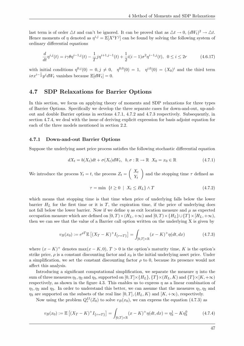
4 Method of Moments and SDP Relaxations
last term is of order 4t and can’t be ignored. It can be proved that as 4t→ 0, (dWt)2 → 4t.Hence moments of η denoted as ηi,j = E[XiY j ] can be found by solving the following system ofordinary differential equations
d
dtηi,j(t) = iγθηi−1,j(t)− 1
Tjηi+1,j−1(t) +
12i(i− 1)σ2ηi−1,j(t), 0 ≤ i ≤ 2r (4.6.17)
with initial conditions η0,j(0) = 0, j 6= 0, η0,0(0) = 1, ηi,0(0) = (X0)i and the third termiσxi−
12 yjdWt vanishes because E[dWt] = 0.
4.7 SDP Relaxations for Barrier Options
In this section, we focus on applying theory of moments and SDP relaxations for three typesof Barrier Options. Specifically we develop the three separate cases for down-and-out, up-and-out and double Barrier options in sections 4.7.1, 4.7.2 and 4.7.3 respectively. Subsequently, insection 4.7.4, we deal with the issue of deriving explicit expression for basis adjoint equation foreach of the three models mentioned in section 2.2.
4.7.1 Down-and-out Barrier Options
Suppose the underlying asset price process satisfies the following stochastic differential equation
dXt = b(Xt)dt+ σ(Xt)dWt, b, σ : R→ R X0 = x0 ∈ R (4.7.1)
We introduce the process Yt = t, the process Zt =(Xt
Yt
)and the stopping time τ defined as
τ = min t ≥ 0 | Xt ≤ HL ∧ T (4.7.2)
which means that stopping time is that time when price of underlying falls below the lowerbarrier HL for the first time or it is T , the expiration time, if the price of underlying doesnot fall below the lower barrier. Now if we define η as exit location measure and µ as expectedoccupation measure which are defined on [0, T )×(HL,+∞) and [0, T )×HL∪T× [HL,+∞),then we can see that the value of a Barrier call option written on the underlying X is given by
vB(x0) := eρTE[(XT −K)+Iτ=T
]=∫
[0,T ]×R(x−K)+η(dt, dx) (4.7.3)
where (x−K)+ denotes max(x−K, 0), T > 0 is the option’s maturity time, K is the option’sstrike price, ρ is a constant discounting factor and x0 is the initial underlying asset price. Undera simplification, we set the constant discounting factor ρ to 0, because its presence would notaffect this analysis.
Introducing a significant computational simplification, we separate the measure η into thesum of three measures η1, η2 and η3, supported on [0, T ]×HL, T×(HL,K) and T×[K,+∞)respectively, as shown in the figure 4.3. This enables us to express η as a linear combination ofη1, η2 and η3. In order to understand this better, we can assume that the measures η1, η2 andη3 are supported on the subsets of the real line [0, T ], (HL,K) and [K,+∞), respectively.
Now using the problem QIIr (Z0) to solve vB(x0), we can express the equation (4.7.3) as
vB(x0) := E[(XT −K)+Iτ=T
]=∫
[0,T ]×R(x−K)+η(dt, dx) = η1
3 −Kη03 (4.7.4)
47
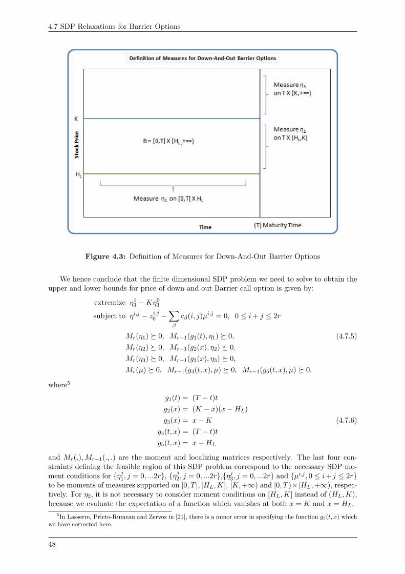
4.7 SDP Relaxations for Barrier Options
Figure 4.3: Definition of Measures for Down-And-Out Barrier Options
We hence conclude that the finite dimensional SDP problem we need to solve to obtain theupper and lower bounds for price of down-and-out Barrier call option is given by:
extremize η13 −Kη0
3
subject to ηi,j − zi,j0 −∑β
cβ(i, j)µi,j = 0, 0 ≤ i+ j ≤ 2r
Mr(η1) 0, Mr−1(g1(t), η1) 0,Mr(η2) 0, Mr−1(g2(x), η2) 0,Mr(η3) 0, Mr−1(g3(x), η3) 0,Mr(µ) 0, Mr−1(g4(t, x), µ) 0, Mr−1(g5(t, x), µ) 0,
(4.7.5)
where5
g1(t) = (T − t)tg2(x) = (K − x)(x−HL)g3(x) = x−K
g4(t, x) = (T − t)tg5(t, x) = x−HL
(4.7.6)
and Mr(.),Mr−1(., .) are the moment and localizing matrices respectively. The last four con-straints defining the feasible region of this SDP problem correspond to the necessary SDP mo-ment conditions for ηj1, j = 0, ...2r, ηj2, j = 0, ...2r,ηj3, j = 0, ...2r and µi,j , 0 ≤ i+ j ≤ 2rto be moments of measures supported on [0, T ], [HL,K], [K,+∞) and [0, T )× [HL,+∞), respec-tively. For η2, it is not necessary to consider moment conditions on [HL,K] instead of (HL,K),because we evaluate the expectation of a function which vanishes at both x = K and x = HL.
5In Lasserre, Prieto-Rumeau and Zervos in [21], there is a minor error in specifying the function g5(t, x) whichwe have corrected here.
48
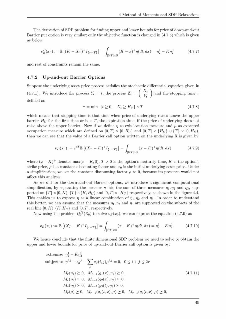
4 Method of Moments and SDP Relaxations
The derivation of SDP problem for finding upper and lower bounds for price of down-and-outBarrier put option is very similar; only the objective function is changed in (4.7.5) which is givenas below:
vPB(x0) := E[(K −XT )+Iτ=T
]=∫
[0,T ]×R(K − x)+η(dt, dx) = η1
2 −Kη02 (4.7.7)
and rest of constraints remain the same.
4.7.2 Up-and-out Barrier Options
Suppose the underlying asset price process satisfies the stochastic differential equation given in
(4.7.1). We introduce the process Yt = t, the process Zt =(Xt
Yt
)and the stopping time τ
defined asτ = min t ≥ 0 | Xt ≥ HU ∧ T (4.7.8)
which means that stopping time is that time when price of underlying raises above the upperbarrier HU for the first time or it is T , the expiration time, if the price of underlying does notraise above the upper barrier. Now if we define η as exit location measure and µ as expectedoccupation measure which are defined on [0, T ) × [0, HU ) and [0, T ] × HU ∪ T × [0, HU ),then we can see that the value of a Barrier call option written on the underlying X is given by
vB(x0) := eρTE[(XT −K)+Iτ=T
]=∫
[0,T ]×R(x−K)+η(dt, dx) (4.7.9)
where (x−K)+ denotes max(x−K, 0), T > 0 is the option’s maturity time, K is the option’sstrike price, ρ is a constant discounting factor and x0 is the initial underlying asset price. Undera simplification, we set the constant discounting factor ρ to 0, because its presence would notaffect this analysis.
As we did for the down-and-out Barrier options, we introduce a significant computationalsimplification, by separating the measure η into the sum of three measures η1, η2 and η3, sup-ported on T× [0,K), T× (K,HU ) and [0, T ]×HU respectively, as shown in the figure 4.4.This enables us to express η as a linear combination of η1, η2 and η3. In order to understandthis better, we can assume that the measures η1, η2 and η3 are supported on the subsets of thereal line [0,K), (K,HU ) and [0, T ], respectively.
Now using the problem QIIr (Z0) to solve vB(x0), we can express the equation (4.7.9) as
vB(x0) := E[(XT −K)+Iτ=T
]=∫
[0,T ]×R(x−K)+η(dt, dx) = η1
2 −Kη02 (4.7.10)
We hence conclude that the finite dimensional SDP problem we need to solve to obtain theupper and lower bounds for price of up-and-out Barrier call option is given by:
extremize η12 −Kη0
2
subject to ηi,j − zi,j0 −∑β
cβ(i, j)µi,j = 0, 0 ≤ i+ j ≤ 2r
Mr(η1) 0, Mr−1(g1(x), η1) 0,Mr(η2) 0, Mr−1(g2(x), η2) 0,Mr(η3) 0, Mr−1(g3(t), η3) 0,Mr(µ) 0, Mr−1(g4(t, x), µ) 0, Mr−1(g5(t, x), µ) 0,
(4.7.11)
49
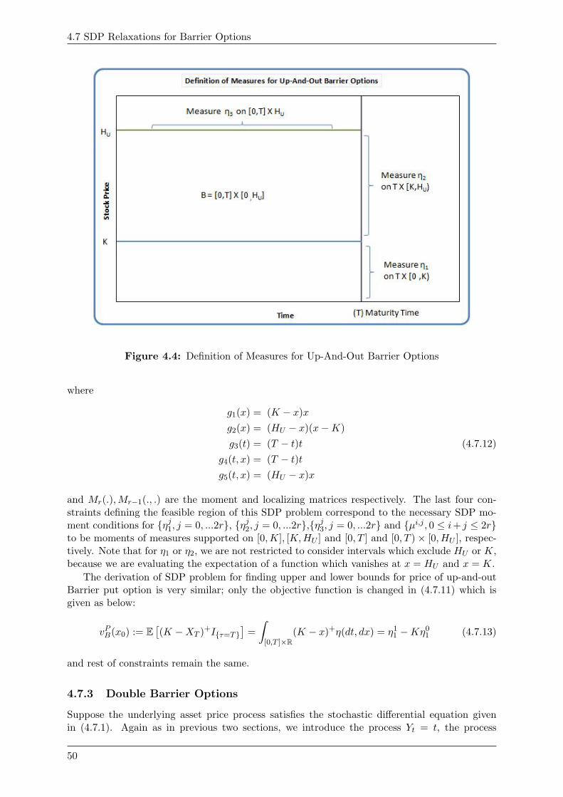
4.7 SDP Relaxations for Barrier Options
Figure 4.4: Definition of Measures for Up-And-Out Barrier Options
where
g1(x) = (K − x)xg2(x) = (HU − x)(x−K)g3(t) = (T − t)t
g4(t, x) = (T − t)tg5(t, x) = (HU − x)x
(4.7.12)
and Mr(.),Mr−1(., .) are the moment and localizing matrices respectively. The last four con-straints defining the feasible region of this SDP problem correspond to the necessary SDP mo-ment conditions for ηj1, j = 0, ...2r, ηj2, j = 0, ...2r,ηj3, j = 0, ...2r and µi,j , 0 ≤ i+ j ≤ 2rto be moments of measures supported on [0,K], [K,HU ] and [0, T ] and [0, T )× [0, HU ], respec-tively. Note that for η1 or η2, we are not restricted to consider intervals which exclude HU or K,because we are evaluating the expectation of a function which vanishes at x = HU and x = K.
The derivation of SDP problem for finding upper and lower bounds for price of up-and-outBarrier put option is very similar; only the objective function is changed in (4.7.11) which isgiven as below:
vPB(x0) := E[(K −XT )+Iτ=T
]=∫
[0,T ]×R(K − x)+η(dt, dx) = η1
1 −Kη01 (4.7.13)
and rest of constraints remain the same.
4.7.3 Double Barrier Options
Suppose the underlying asset price process satisfies the stochastic differential equation givenin (4.7.1). Again as in previous two sections, we introduce the process Yt = t, the process
50
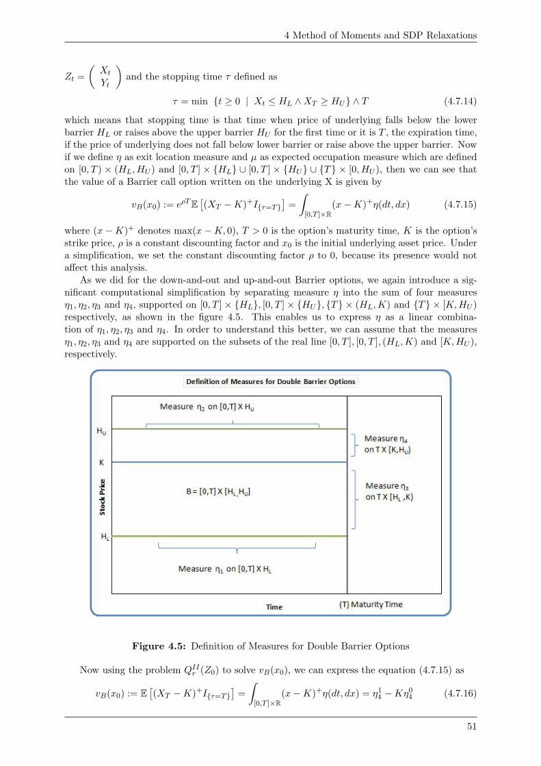
4 Method of Moments and SDP Relaxations
Zt =(Xt
Yt
)and the stopping time τ defined as
τ = min t ≥ 0 | Xt ≤ HL ∧XT ≥ HU ∧ T (4.7.14)
which means that stopping time is that time when price of underlying falls below the lowerbarrier HL or raises above the upper barrier HU for the first time or it is T , the expiration time,if the price of underlying does not fall below lower barrier or raise above the upper barrier. Nowif we define η as exit location measure and µ as expected occupation measure which are definedon [0, T ) × (HL, HU ) and [0, T ] × HL ∪ [0, T ] × HU ∪ T × [0, HU ), then we can see thatthe value of a Barrier call option written on the underlying X is given by
vB(x0) := eρTE[(XT −K)+Iτ=T
]=∫
[0,T ]×R(x−K)+η(dt, dx) (4.7.15)
where (x−K)+ denotes max(x−K, 0), T > 0 is the option’s maturity time, K is the option’sstrike price, ρ is a constant discounting factor and x0 is the initial underlying asset price. Undera simplification, we set the constant discounting factor ρ to 0, because its presence would notaffect this analysis.
As we did for the down-and-out and up-and-out Barrier options, we again introduce a sig-nificant computational simplification by separating measure η into the sum of four measuresη1, η2, η3 and η4, supported on [0, T ]× HL, [0, T ]× HU, T × (HL,K) and T × [K,HU )respectively, as shown in the figure 4.5. This enables us to express η as a linear combina-tion of η1, η2, η3 and η4. In order to understand this better, we can assume that the measuresη1, η2, η3 and η4 are supported on the subsets of the real line [0, T ], [0, T ], (HL,K) and [K,HU ),respectively.
Figure 4.5: Definition of Measures for Double Barrier Options
Now using the problem QIIr (Z0) to solve vB(x0), we can express the equation (4.7.15) as
vB(x0) := E[(XT −K)+Iτ=T
]=∫
[0,T ]×R(x−K)+η(dt, dx) = η1
4 −Kη04 (4.7.16)
51
4.7 SDP Relaxations for Barrier Options
We hence conclude that the finite dimensional SDP problem we need to solve to obtain theupper and lower bounds for price of double Barrier call option is given by:
extremize η14 −Kη0
4
subject to ηi,j − zi,j0 −∑β
cβ(i, j)µi,j = 0, 0 ≤ i+ j ≤ 2r
Mr(η1) 0, Mr−1(g1(t), η1) 0,Mr(η2) 0, Mr−1(g2(t), η2) 0,Mr(η3) 0, Mr−1(g3(x), η3) 0,Mr(η4) 0, Mr−1(g3(x), η3) 0,Mr(µ) 0, Mr−1(g5(t, x), µ) 0, Mr−1(g6(t, x), µ) 0,
(4.7.17)
where
g1(t) = (T − t)tg2(t) = (T − t)tg3(x) = (K − x)(x−HL)g4(x) = (HU − x)(x−K)
g5(t, x) = (T − t)tg6(t, x) = (HU − x)(x−HL)
(4.7.18)
and Mr(.),Mr−1(., .) are the moment and localizing matrices respectively. The last four con-straints defining the feasible region of this SDP problem correspond to the necessary SDPmoment conditions for ηj1, j = 0, ...2r, ηj2, j = 0, ...2r,, ηj3, j = 0, ...2r,ηj4, j = 0, ...2rand µi,j , 0 ≤ i + j ≤ 2r to be moments of measures supported on [0, T ], [0, T ], [HL,K] and[K,HU ] and T × (K,HU ) and [0, T )× (HL, HU ), respectively. Note that for η3 or η4, we arenot restricted to consider intervals which exclude HU , HL or K, because we are evaluating theexpectation of a function which vanishes at all of following values: x = HU , x = HL and x = K.
The derivation of SDP problem for finding upper and lower bounds for price of double Barrieroption is very similar; only the objective function is changed in (4.7.17) which is given as below:
vPB(x0) := E[(K −XT )+Iτ=T
]=∫
[0,T ]×R(K − x)+η(dt, dx) = η1
3 −Kη03 (4.7.19)
and rest of constraints remain the same.
4.7.4 Evaluating Basic Adjoint Equation
We will now derive an explicit expression for evaluating the basis adjoint equation mentioned inSDP problems (4.7.5), (4.7.11) and (4.7.17).
ηi,j − zi,j0 −∑β
cβ(i, j)µi,j = 0, 0 ≤ i+ j ≤ 2r (4.7.20)
To calculate ηi,j for each of down-and-out, up-and-out and double Barrier options, consider themonomial f(t, x) = tixj ,
ηi,j =∫
R2
f(z)η(dz) =∫
R2
f(t, x)η(dt, dx)
=∫
R2
tixjη(dt, dx)(4.7.21)
which can be evaluated as below for each of the three type of Barrier options
52
4 Method of Moments and SDP Relaxations
Case 1: Down-and-out Barrier Options
ηi,j =∫
R2
tixjη(dt, dx)
= HjL
∫ T
0tiη1(dt) + T i
∫ K
HL
xjη2(dx) + T i∫ +∞
Kxjη3(dx)
= HjLη
i1 + T iηj2 + T iηj3
(4.7.22)
Case 2: Up-and-out Barrier Options
ηi,j =∫
R2
tixjη(dt, dx)
= T i∫ K
0xjη1(dx) + T i
∫ HU
Kxjη2(dx) +Hj
U
∫ T
0tiη3(dt)
= T iηj1 + T iηj2 +HjUη
i3
(4.7.23)
Case 3: Double Barrier Options
ηi,j =∫
R2
tixjη(dt, dx)
= HjL
∫ T
0tiη1(dt) +Hj
U
∫ T
0tiη2(dt)
+ T i∫ K
HL
xjη3(dx) + T i∫ HU
Kxjη4(dx)
= HjLη
i1 +Hj
Uηi1 + T iηj3 + T iηj4
(4.7.24)
We now turn our attention to evaluating the following term∑β
cβ(i, j)µi,j =∫
RnAf(z)µ(dz) (4.7.25)
which depends on infinitesimal generator
Af(t, x) := ft(t, x) +12σ2(x)fxx(t, x) + b(x)fx(t, x) (4.7.26)
of particular process. Considering the following three cases:Case 1: Geometric Brownian Motion: Here the underlying Xt satisfies the following
stochastic differential equation:dXt = bXtdt+ σXtdWt (4.7.27)
So the infinitesimal generator can be derived as
Af(t, x) := iti−1xj +12
(σx)2j(j − 1)tixj−2 + bjtixj (4.7.28)
and the coefficients (4.7.25) can be calculated from (4.7.26) as below∑β
cβ(i, j)µi,j = iµi−1,j +12σ2j(j − 1)µi,j + bjµi,j (4.7.29)
Case 2: Ornstein-Uhlenbeck Process: Here the underlying Xt satisfies the followingstochastic differential equation:
dXt = γ(θ −Xt)dt+ σdWt (4.7.30)
53
4.7 SDP Relaxations for Barrier Options
So the infinitesimal generator can be derived as
Af(t, x) := iti−1xj +12σ2j(j − 1)tixj−2 + γθjtixj−1 − γjtixj (4.7.31)
and the coefficients (4.7.25) can be calculated from (4.7.26) as below∑β
cβ(i, j)µi,j = iµi−1,j +12σ2j(j − 1)µi,j−2 + γθjµi,j−1 − γjµi,j (4.7.32)
Case 3: Cox-Ingersoll-Ross Process: Here the underlying Xt satisfies the followingstochastic differential equation:
dXt = γ(θ −Xt)dt+ σ√XtdWt (4.7.33)
So the infinitesimal generator can be derived as
Af(t, x) := iti−1xj +12
(σ√x)2j(j − 1)tixj−2 + +γθjtixj−1 − γjtixj (4.7.34)
and the coefficients (4.7.25) can be calculated from (4.7.26) as below∑β
cβ(i, j)µi,j = iµi−1,j +12σ2j(j − 1)µi,j−1 + γθjµi,j−1 − γjµi,j (4.7.35)
54
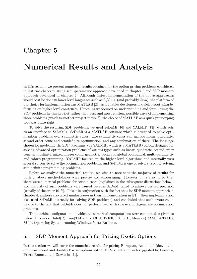
Chapter 5
Numerical Results and Analysis
In this section, we present numerical results obtained for the option pricing problems consideredin last two chapters: using semi-parametric approach developed in chapter 3 and SDP momentapproach developed in chapter 4. Although fastest implementation of the above approacheswould best be done in lower level languages such as C/C++ (and probably Java), the platform ofour choice for implementation was MATLAB [23] as it enables developers in quick prototyping byfocusing on higher level constructs. Hence, as we focused on understanding and formulating theSDP problems in this project rather than best and most efficient possible ways of implementingthose problems (which is another project in itself), the choice of MATLAB as a quick prototypingtool was quite right.
To solve the resulting SDP problems, we used SeDuMi [16] and YALMIP [13] (which actsas an interface to SeDuMi). SeDuMi is a MATLAB software which is designed to solve opti-mization problems over symmetric cones. The symmetric cones can include linear, quadratic,second order conic and semidefinite optimization, and any combination of these. The languagechosen for modelling the SDP programs was YALMIP, which is a MATLAB toolbox designed forsolving advanced optimization problems of various types such as linear, quadratic, second ordercone, semidefinite, mixed integer conic, geometric, local and global polynomial, multi-parametricand robust programming. YALMIP focuses on the higher level algorithms and internally usesseveral solvers to solve the optimization problems, and SeDuMi is one of solvers used for solvingsemidefinite programming problems.
Before we analyse the numerical results, we wish to note that the majority of results forboth of above methodologies were precise and encouraging. However, it is also noted thatthere were numerical problems for certain cases (explained in the subsequent discussions below),and majority of such problems were caused because SeDuMi failed to achieve desired precision(usually of the order 10−6). This is in conjunction with the fact that for SDP moment approach inchapter 4, authors also faced similar issues in their implementation in [21], (their implementationalso used SeDuMi internally for solving SDP problems) and concluded that such errors couldbe due to the fact that SeDuMi does not perform well with sparse and degenerate optimizationproblems.
The machine configuration on which all numerical computations were conducted is given asbelow: Processor: Intel(R) Core(TM)2 Duo CPU, T7100, 1.80 GHz, Memory(RAM): 2038 MB,32-bit Operating System running Windows Vista Business.
5.1 SDP Moment Approach for Pricing Exotic Options
In this section we will cover the numerical results for pricing European, Asian and (down-and-out, up-and-out and double) Barrier options with SDP Moment approach suggested by Lasserre,Prieto-Rumeau and Zervos in [21].
55
5.1 SDP Moment Approach for Pricing Exotic Options
5.1.1 European Options
Geometric Brownian MotionTable A.2 in Appendix A shows the discounted values of European call options (with under-
lying process following a geometric Brownian motion), obtained by solving SDP problem (4.5.4),for different values of volatility σ. We also compare the call option values thus obtained withthe Black Scholes value because we have an explicit formula available. The data set used for theproblem is also mentioned in the table. We note the following points regarding the results:
• The accuracy of results increase with increase in number or relaxations , when otherparameters are kept constant. This is expected behaviour because we are adding moreinformation about higher order moments to the SDP problems.
• In general, the accuracy of results is very high with very few relaxations. For example,with σ = 0.05 and R=4 to 8 relaxations, the relative error as defined by
Error = 2Upper Bound− Lower BoundUpper Bound + Lower Bound
(5.1.1)
is only of order ∼ 10−6%.
• The degree of improvement in bounds is not uniform and depends on values of volatilityσ, maturity time T and strike price K. For example, as we increase the volatility σ from0.05 to 0.25 and keep number of relaxations R constant, we note that distance betweenupper and lower bounds increases. Although not shown in the data, this increase wouldalso be evident if we keep all other parameter values constant and increase the maturitytime T .
• Black Scholes value always remains between the upper and lower bound, but the distancebetween Black Scholes value and the bounds decreases in general as we increase the numberof relaxations R (with constant volatility σ).
• For σ = 0.15 to 0.25, we observe that the value of upper and lower bounds are diverging,when we increase relaxations R from 7 to 8. This can attributed to following two facts:
– Lognormal distribution is not moment determinate, and
– SeDuMi failed in solving the SDP problems with desired accuracy. The results wereaccurate with precision of 10−3, but SeDuMi failed to achieve the desired precisionof 10−6.
• It is worth noting the fact that with R=8, the SDP problem has two semidefinite (moment)matrices of size 9 × 9 and two semidefinite (localizing) matrices of size 8 × 8 amongst itsconstraints, which roughly translates to 290 variables.
• The failure of SeDuMi to solve SDP problems with semidefinite matrices of higher order(of size 8× 8 in our case), is in conjunction with the results obtained by Lasserre, Prieto-Rumeau and Zervos in [21]. We also note that in the semi-parametric approach, authorsused a Cutting Plane algorithm developed in their article [8]. This algorithm also failedwhen the order of semidefinite matrix was over 9 or 10.
We now present the same data with different interpretation as below. The graphs in figure5.2 show the difference between bounds of higher order moments and Black-Scholes price. Thereare two graphs, in order to depict the effect of
• adding higher order moments while keeping volatility σ constant, and
56
5 Numerical Results and Analysis
(a) Volatility=0.05
(b) Volatility=0.25
Figure 5.1: European Call Option: Geometric Brownian Motion
• increasing the volatility σ with the same amount of moment information (i.e. keeping Rconstant).
We observe the following from figure 5.2(a):
• As we increase the number of relaxations, difference between upper/lower bound and BlackScholes value decreases.
• Difference between upper bound and Black-Scholes value is lesser than difference between
57
5.1 SDP Moment Approach for Pricing Exotic Options
lower bound and Black-Scholes value.
• Discrepancy in upper and lower bound increases as strike price K approaches the initialstock price S0, whereas same discrepancy is much less when strike price K is far frominitial stock price S0.
Observations from figure 5.2(b):
• Upper bound is relatively less sensitive to change in volatility σ as compared to lowerbound, which shows more discrepancy.
• As we increase the volatility σ, difference between upper/lower bound and Black Scholesvalue decreases.
• Discrepancy in upper and lower bound is highest when value of strike price K approachesthe initial stock price S0, whereas same discrepancy is much less when strike price K isfar from initial stock price S0.
58
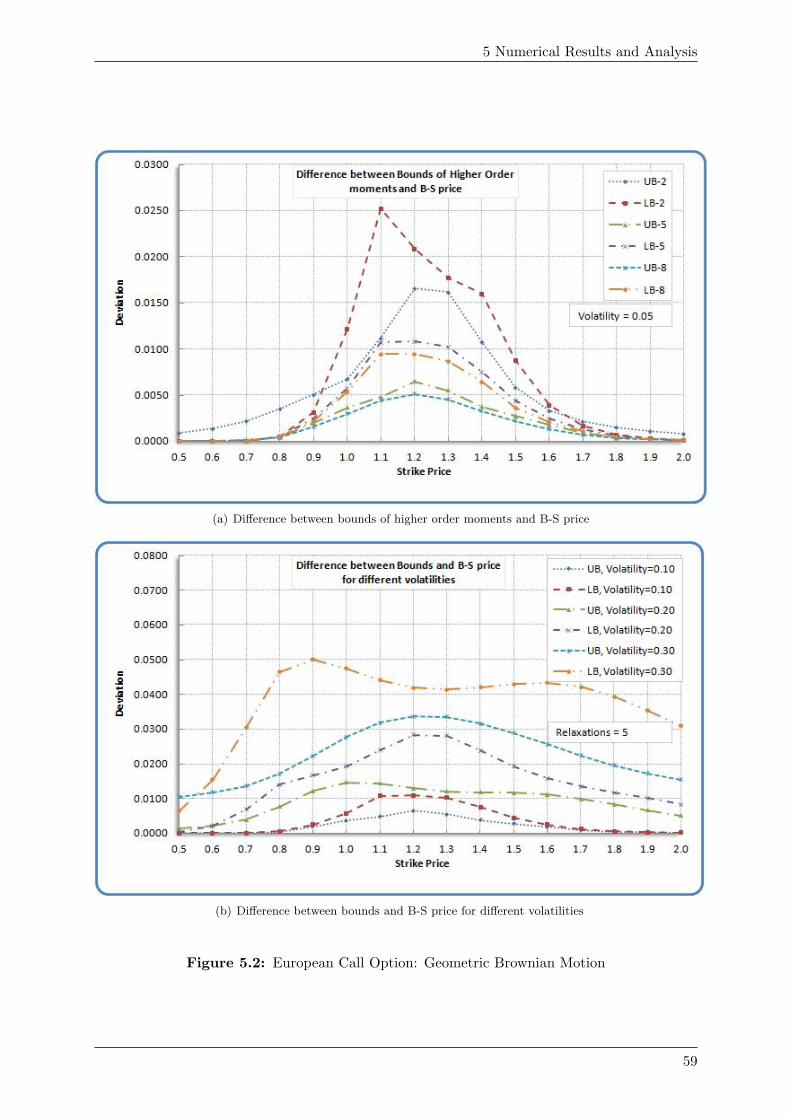
5 Numerical Results and Analysis
(a) Difference between bounds of higher order moments and B-S price
(b) Difference between bounds and B-S price for different volatilities
Figure 5.2: European Call Option: Geometric Brownian Motion
59
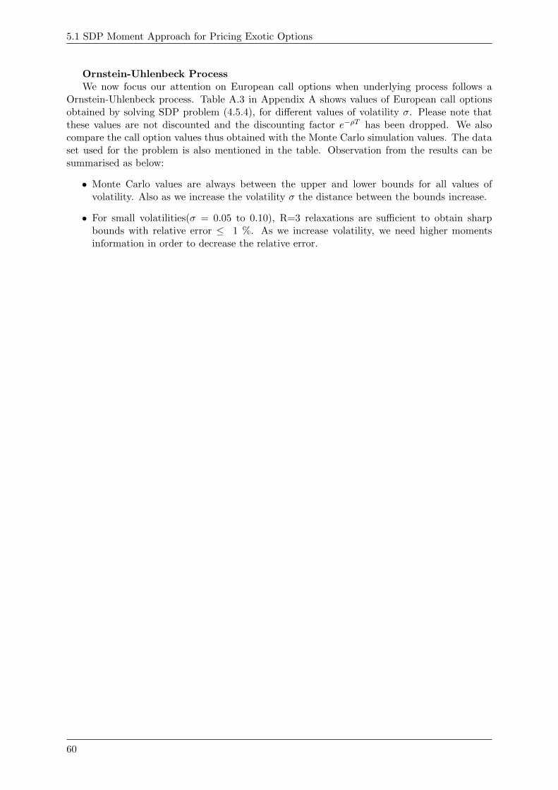
5.1 SDP Moment Approach for Pricing Exotic Options
Ornstein-Uhlenbeck ProcessWe now focus our attention on European call options when underlying process follows a
Ornstein-Uhlenbeck process. Table A.3 in Appendix A shows values of European call optionsobtained by solving SDP problem (4.5.4), for different values of volatility σ. Please note thatthese values are not discounted and the discounting factor e−ρT has been dropped. We alsocompare the call option values thus obtained with the Monte Carlo simulation values. The dataset used for the problem is also mentioned in the table. Observation from the results can besummarised as below:
• Monte Carlo values are always between the upper and lower bounds for all values ofvolatility. Also as we increase the volatility σ the distance between the bounds increase.
• For small volatilities(σ = 0.05 to 0.10), R=3 relaxations are sufficient to obtain sharpbounds with relative error ≤ 1 %. As we increase volatility, we need higher momentsinformation in order to decrease the relative error.
60
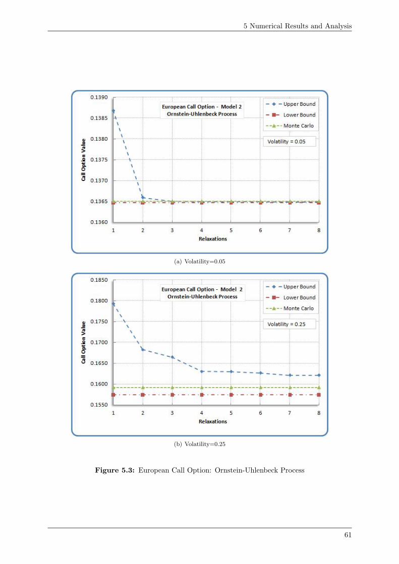
5 Numerical Results and Analysis
(a) Volatility=0.05
(b) Volatility=0.25
Figure 5.3: European Call Option: Ornstein-Uhlenbeck Process
61
5.1 SDP Moment Approach for Pricing Exotic Options
Cox-Ingersoll-Ross ProcessFinally we will observe the case for European call options when underlying process follows
a Cox-Ingersoll-Ross process. The numerical results are summarized in Table A.4 in AppendixA, which shows values of European call options obtained by solving SDP problem (4.5.4). Thevalues are not discounted as discounting factor e−ρT has been dropped. Interesting observationsare summarised below:
• Very accurate results are achieved when volatility σ is small, when R=3. For examplewith σ = 0.05 or 0.10, the relative error is less than 1 %.
• Monte Carlo values are bounded by the upper and lower bounds in all cases, but thedistance between upper lower bound and between bounds and Monte Carlo values increasewith increase in volatility.
Finally, it can be noted from the table A.2,A.3 and A.4 that in terms of performance, theSDP algorithm for pricing European options is very fast and excellent bounds were obtained forall relaxations well within 1 or 2 seconds.
62
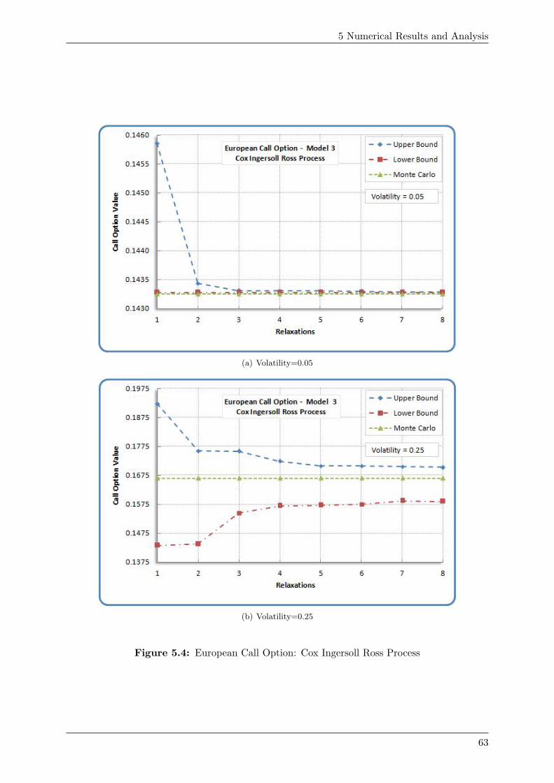
5 Numerical Results and Analysis
(a) Volatility=0.05
(b) Volatility=0.25
Figure 5.4: European Call Option: Cox Ingersoll Ross Process
63
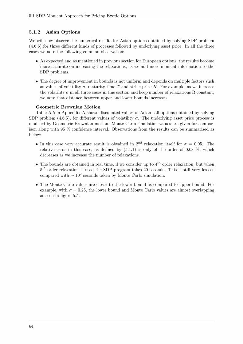
5.1 SDP Moment Approach for Pricing Exotic Options
5.1.2 Asian Options
We will now observe the numerical results for Asian options obtained by solving SDP problem(4.6.5) for three different kinds of processes followed by underlying asset price. In all the threecases we note the following common observation:
• As expected and as mentioned in previous section for European options, the results becomemore accurate on increasing the relaxations, as we add more moment information to theSDP problems.
• The degree of improvement in bounds is not uniform and depends on multiple factors suchas values of volatility σ, maturity time T and strike price K. For example, as we increasethe volatility σ in all three cases in this section and keep number of relaxations R constant,we note that distance between upper and lower bounds increases.
Geometric Brownian MotionTable A.5 in Appendix A shows discounted values of Asian call options obtained by solving
SDP problem (4.6.5), for different values of volatility σ. The underlying asset price process ismodeled by Geometric Brownian motion. Monte Carlo simulation values are given for compar-ison along with 95 % confidence interval. Observations from the results can be summarised asbelow:
• In this case very accurate result is obtained in 2nd relaxation itself for σ = 0.05. Therelative error in this case, as defined by (5.1.1) is only of the order of 0.08 %, whichdecreases as we increase the number of relaxations.
• The bounds are obtained in real time, if we consider up to 4th order relaxation, but when5th order relaxation is used the SDP program takes 20 seconds. This is still very less ascompared with ∼ 102 seconds taken by Monte Carlo simulation.
• The Monte Carlo values are closer to the lower bound as compared to upper bound. Forexample, with σ = 0.25, the lower bound and Monte Carlo values are almost overlappingas seen in figure 5.5.
64
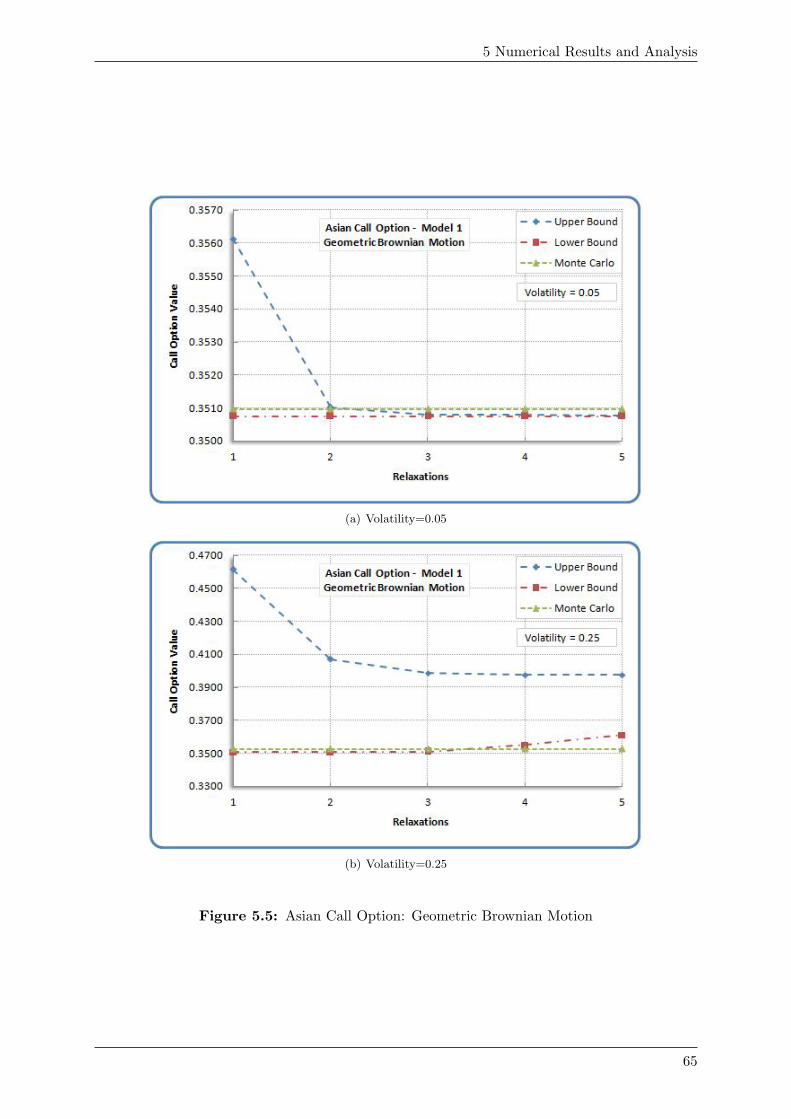
5 Numerical Results and Analysis
(a) Volatility=0.05
(b) Volatility=0.25
Figure 5.5: Asian Call Option: Geometric Brownian Motion
65
5.1 SDP Moment Approach for Pricing Exotic Options
Ornstein-Uhlenbeck ProcessThe numerical data for this case is available in Table A.6. We provide 2 graphs for reference
in figure 5.6. The call option values are not discounted and discounting factor e−ρT is ignoredin the calculation. We conclude the following from available numerical results:
• Monte Carlo values are in between the upper and lower bounds or are very near to lowerbound in all the cases.
• As compared with geometric Brownian motion case, the bounds in this case are obtainedin real time, and maximum time taken for any solving any SDP problem never exceeds 2seconds.
• In this case, very accurate results are obtained with 3rd order relaxation itself. This isevident from relative error which is 10−7 % when σ = 0.05 and R=3 relaxations.
66
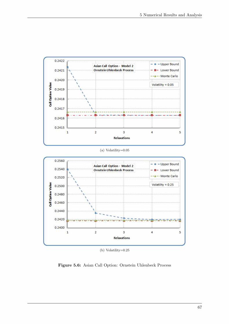
5 Numerical Results and Analysis
(a) Volatility=0.05
(b) Volatility=0.25
Figure 5.6: Asian Call Option: Ornstein Uhlenbeck Process
67
5.1 SDP Moment Approach for Pricing Exotic Options
Cox-Ingersoll-Ross ProcessWe summarize the numerical results for Asian call options with underlying process following
Cox-Ingersoll-Ross process in Table A.7 in Appendix A. Discounting factor has again beendropped and the observations from the numerical results are summarised as below:
• Monte Carlo value is below the lower bound when σ = 0.05. However the relative error inthis case for SDP approach is 0.01 % and variance of the call option price in Monte Carlosimulation is 0.001023, hence the SDP results are more accurate than Monte Carlo value.
• As we increase the volatility σ from 0.05 to 0.25, Monte Carlo values move more closer tothe lower bound, and for σ = 0.25, Monte Carlo values and lower bounds coincide witheach other with very little difference.
• The maximum time take for any SDP program for this case never exceeded 2 seconds, ascompared with that taken for Monte Carlo method, which was of order 102 seconds.
68
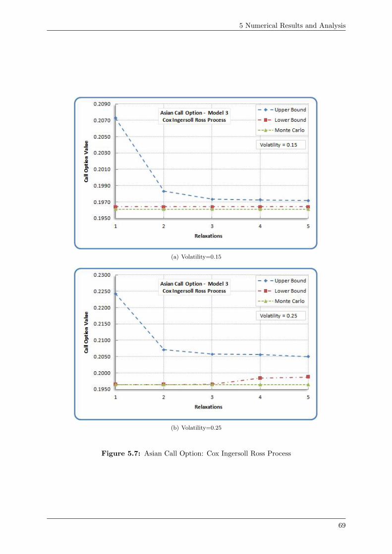
5 Numerical Results and Analysis
(a) Volatility=0.15
(b) Volatility=0.25
Figure 5.7: Asian Call Option: Cox Ingersoll Ross Process
69
5.1 SDP Moment Approach for Pricing Exotic Options
5.1.3 Down-and-out Barrier Options
This section covers numerical results for down-and-out Barrier options, obtained by solving SDPproblem (4.7.5) for two different kinds of processes followed by underlying asset price.
Ornstein-Uhlenbeck ProcessTable A.8 in Appendix A shows discounted values of down-and-out Barrier call options for
different values of volatility σ. The underlying asset price process is modeled by Ornstein-Uhlenbeck process. Monte Carlo simulation values are given for comparison. Graphs in figure5.8 are given as representative examples from the numerical data in table A.8.
Observations from the numerical results can be summarised as below:
• Monte Carlo values are in between the upper and lower bounds for almost all cases.
• When relaxations are low (between 1 and 3) the relative error is very high (nearly∼ 200 %).We get accurate results with 6th relaxation onwards. For example, for σ = 0.70, 6th
relaxation gives 1.8 % relative error.
• The bounds are obtained in real time, if we use up to 4th order relaxations, but for 5th and6th order relaxations, the SDP program takes 5 and 20 seconds respectively. Even thoughhigh, this value is still very less as compared with ∼ 102 seconds taken by Monte Carlosimulation.
70
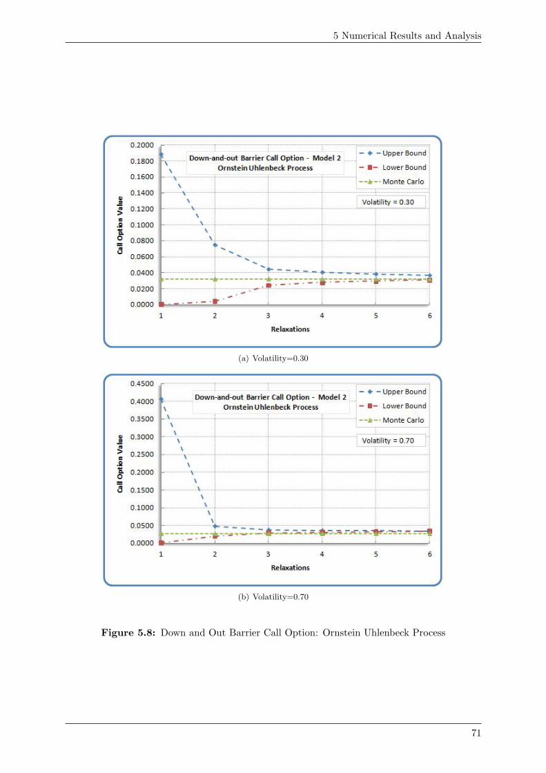
5 Numerical Results and Analysis
(a) Volatility=0.30
(b) Volatility=0.70
Figure 5.8: Down and Out Barrier Call Option: Ornstein Uhlenbeck Process
71
5.1 SDP Moment Approach for Pricing Exotic Options
Cox-Ingersoll-Ross ProcessNumerical data for this case is exhibited in Table A.8 in Appendix A. The values are not
discounted and underlying asset price process is modeled by Cox-Ingersoll-Ross process. Ref-erence graphs are given in 5.9. Observations from the numerical results can be summarised asbelow:
• As in the case with Ornstein-Uhlenbeck process, Monte Carlo values are either in betweenthe upper and lower bounds for almost all cases, or they are very near to the convergedvalue.
• Relative error is again very high for lower order relaxations (nearly ∼ 200 % for R=1)and we get accurate results with 6th relaxation onwards.
• For σ = 0.30, 6th relaxation gives 0.02 % relative error, where as variance for Monte Carlosimulation is 0.024312 which suggests that SDP approach is more accurate than MonteCarlo simulation.
• As in the previous case, SDP problems take very less time for lower order relaxations(specifically, less than 2 seconds with 4th relaxations). For 5th and 6th order relaxations,the SDP program roughly takes 6 and 18 seconds, respectively.
• We observe a peculiarity when σ = 0.70 and R=6, where upper bound is smaller thanlower bound. This observation can be attributed to the difference in level of precisionachieved by SeDuMi for these two cases and not as an error in model itself. It is to benoted that the bounds are still converging and relative error is −0.06 %.
72
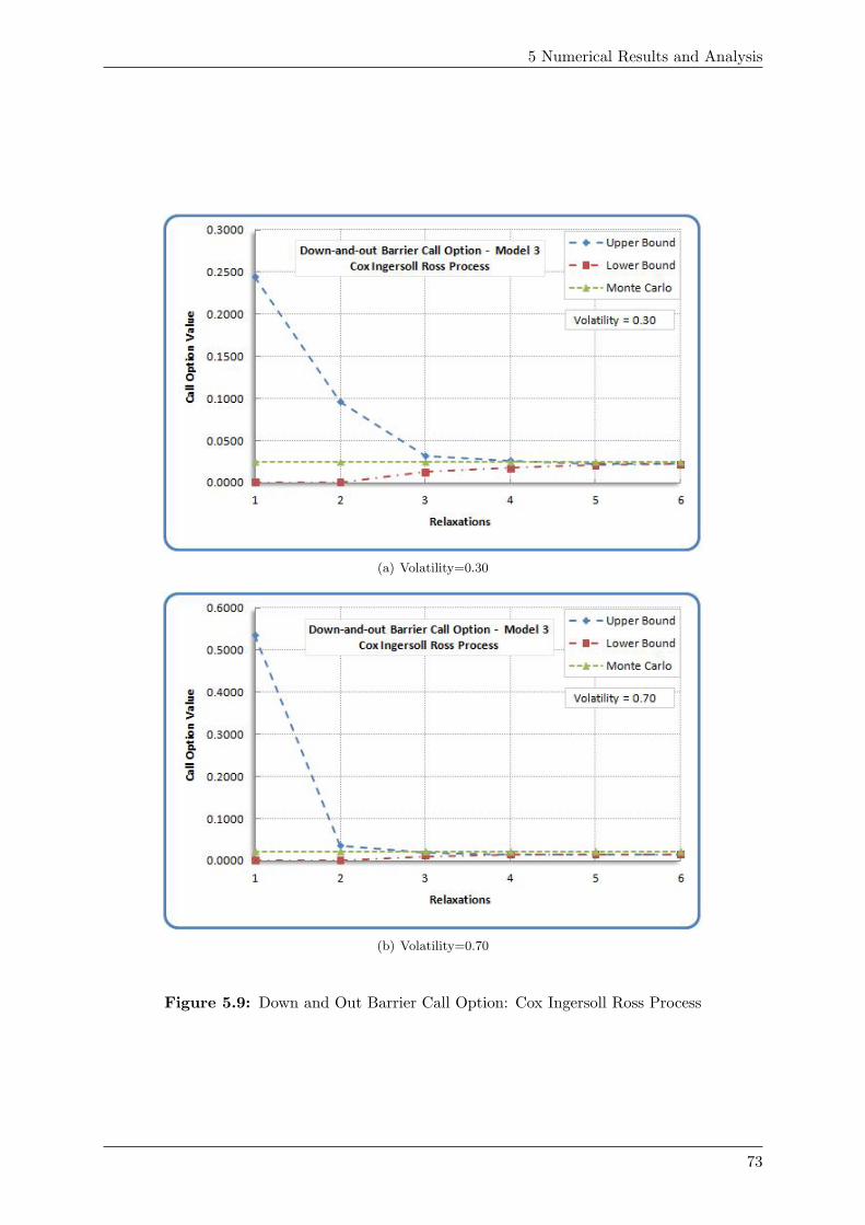
5 Numerical Results and Analysis
(a) Volatility=0.30
(b) Volatility=0.70
Figure 5.9: Down and Out Barrier Call Option: Cox Ingersoll Ross Process
73
5.1 SDP Moment Approach for Pricing Exotic Options
5.1.4 Up-and-out Barrier Options
In this section we cover the observations for numerical results for up-and-out Barrier options.We refer to SDP problem (4.7.11) for two cases: when underlying asset price follows Ornstein-Uhlenbeck and Cox-Ingersoll-Ross processes. Before going into detail, we note the followinginteresting facts in common for both the cases:
• Similar to down-and-out Barrier call options, Monte Carlo values are either in betweenthe upper and lower bounds for both cases, or they are very near to the converged value.
• Relative error rapidly improves with increase in number of relaxations. For R=5 in bothcases, relative error is well under 1 %. Lower relaxations give disproportionate error values(R=1 gives nearly 200 % error).
• The relative error increases with increase in volatility σ, when number of relaxation(R) iskept constant.
Ornstein-Uhlenbeck ProcessTable A.10 in Appendix A shows values of up-and-out Barrier call options for different values
of volatility σ. The underlying asset price process is modeled by Ornstein-Uhlenbeck process.We refer to figure 5.10 for two sample scenarios from amongst the numerical results obtained intable A.10.
Interesting observations for this particular case from the numerical results can be summarisedas below:
• Time taken for solving SDP problems with higher order relaxations increases linearly withincrease in number of relaxations. SDP problems with 4th and 6th order relaxation takesunder 2 and 7 seconds respectively.
• Again very good accuracy is obtained with higher order relaxations. For example withσ = 0.35, 5th relaxation gives 0.04 % relative error, where as variance for Monte Carlosimulation is 0.080599, proving the SDP approach more accurate than Monte Carlo simu-lation.
74
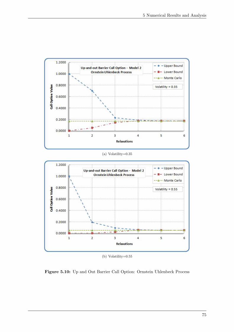
5 Numerical Results and Analysis
(a) Volatility=0.35
(b) Volatility=0.55
Figure 5.10: Up and Out Barrier Call Option: Ornstein Uhlenbeck Process
75
5.1 SDP Moment Approach for Pricing Exotic Options
Cox-Ingersoll-Ross ProcessNumerical results for this case are presented in Table A.11 in Appendix A. The underlying
asset price process follows Cox-Ingersoll-Ross process and two example cases are given in figure5.11. We note the following peculiar observations from the numerical data:
• For σ = 0.45 and 0.50, the upper bound is lower than lower bound. But as the sequence ofbounds is converging, we attribute this error to the difference in level of precision achievedby SeDuMi for these two cases and not as an error in model itself. It is worth to be notedthat the relative errors in both of above cases is −0.25 % and −0.26 % respectively.
76
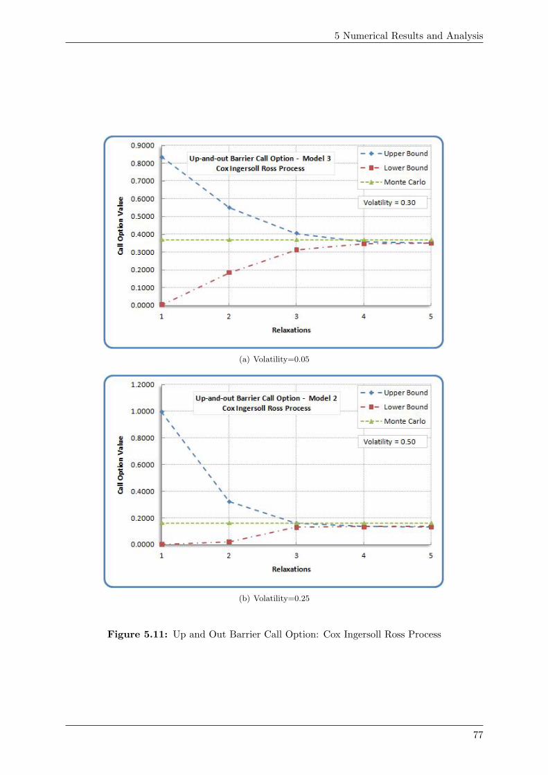
5 Numerical Results and Analysis
(a) Volatility=0.05
(b) Volatility=0.25
Figure 5.11: Up and Out Barrier Call Option: Cox Ingersoll Ross Process
77
5.1 SDP Moment Approach for Pricing Exotic Options
5.1.5 Double Barrier Options
We faced most of the numerical difficulties in SDP problems designed for pricing double Barrieroptions with higher order relaxations. Specifically we solved the SDP problem in (4.7.17) in orderto obtain the call option values of double Barrier options. In the following sections we coverthe cases when underlying process is modeled by Ornstein-Uhlenbeck and Cox-Ingersoll-Rossdiffusions.
Ornstein-Uhlenbeck ProcessFor this case we provide the numerical results in Table A.12 in Appendix A. The underlying
asset price process follows Ornstein-Uhlenbeck process. Please refer figure 5.12 for two examplesrepresenting the numerical results. We note the following observations from the numerical data:
• For σ = 0.10 and 0.15, and relaxations R = 5, 6, 7 and 8, SeDuMi failed with numericalproblems, citing failure to achieve desired precision in results as the reason. The valuesgiven in the table are the latest bounds available when SeDuMi failed, and hence theydon’t represent the accurate values. Hence we see that the upper and lower bounds arenot converging to a definite value.
• It is worth noting that the SDP problems with higher relaxations become huge and henceSeDuMi fails to successfully solve them. As an example for R=5, the SDP problem involves,amongst other constraints, 4 (moment) matrices of size 5 × 5, 1 (moment) matrix of size21 × 21 , 4 (localizing) matrices of size 5 × 5 and 2 (localizing matrices) of size 15 × 15,which involves total 1091 variables in semidefinite matrices.
• We however note that even though SeDuMi failed for higher order relaxations, we obtainencouraging accuracy from 6th order relaxation and even though the bounds don’t representthe correct values, they are very close to the Monte Carlo values.
• Finally we also note that in Lasserre, Prieto-Rumeau and Zervos in [21], authors also facednumerical difficulties with SeDuMi for SDP problems for Barrier options when relaxationsR=8. This fact is in conjunction with the errors faced by us for SDP problems withsemidefinite matrices of higher order.
78
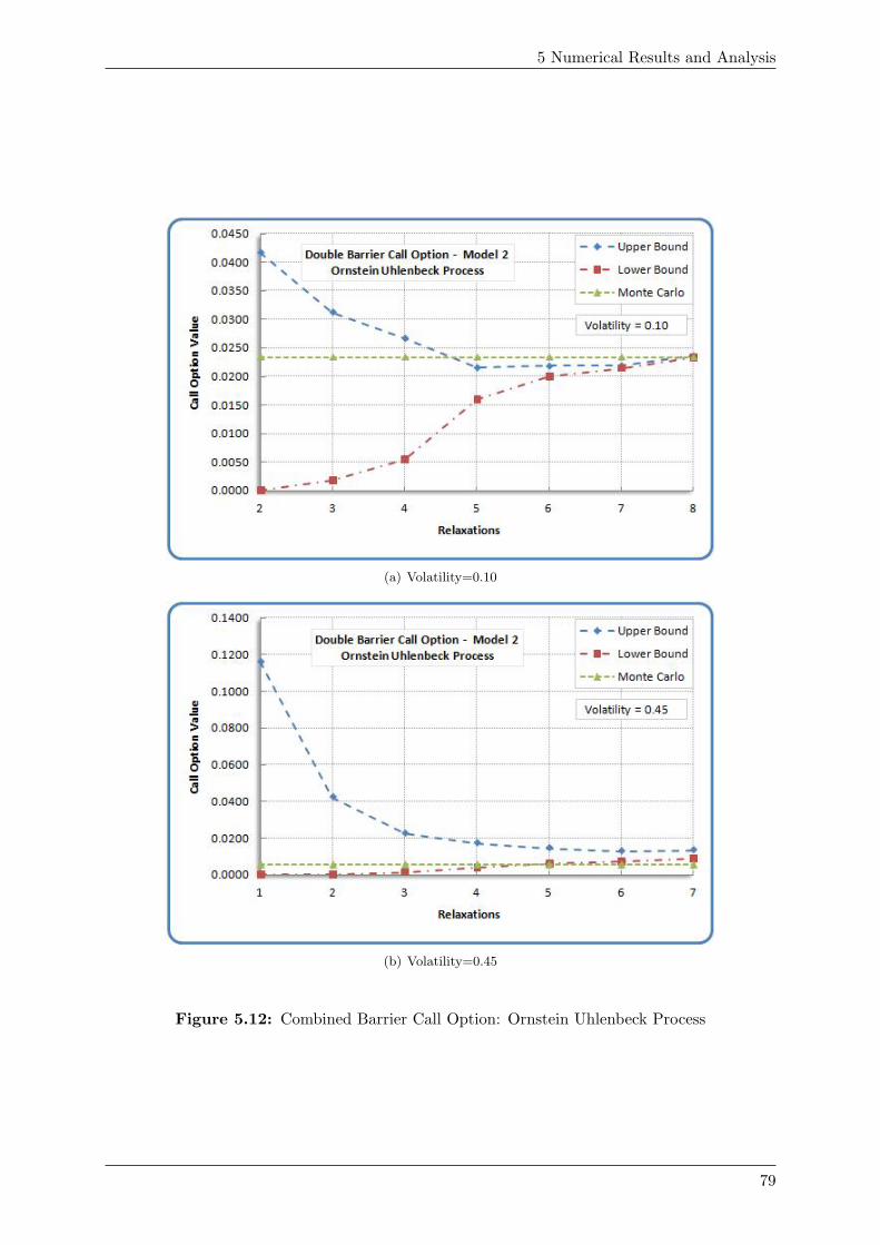
5 Numerical Results and Analysis
(a) Volatility=0.10
(b) Volatility=0.45
Figure 5.12: Combined Barrier Call Option: Ornstein Uhlenbeck Process
79
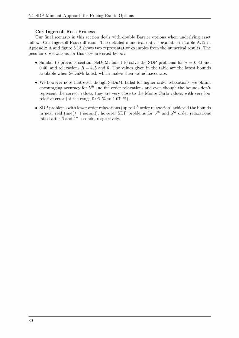
5.1 SDP Moment Approach for Pricing Exotic Options
Cox-Ingersoll-Ross ProcessOur final scenario in this section deals with double Barrier options when underlying asset
follows Cox-Ingersoll-Ross diffusion. The detailed numerical data is available in Table A.12 inAppendix A and figure 5.13 shows two representative examples from the numerical results. Thepeculiar observations for this case are cited below:
• Similar to previous section, SeDuMi failed to solve the SDP problems for σ = 0.30 and0.40, and relaxations R = 4, 5 and 6. The values given in the table are the latest boundsavailable when SeDuMi failed, which makes their value inaccurate.
• We however note that even though SeDuMi failed for higher order relaxations, we obtainencouraging accuracy for 5th and 6th order relaxations and even though the bounds don’trepresent the correct values, they are very close to the Monte Carlo values, with very lowrelative error (of the range 0.06 % to 1.07 %).
• SDP problems with lower order relaxations (up to 4th order relaxation) achieved the boundsin near real time(≤ 1 second), however SDP problems for 5th and 6th order relaxationsfailed after 6 and 17 seconds, respectively.
80
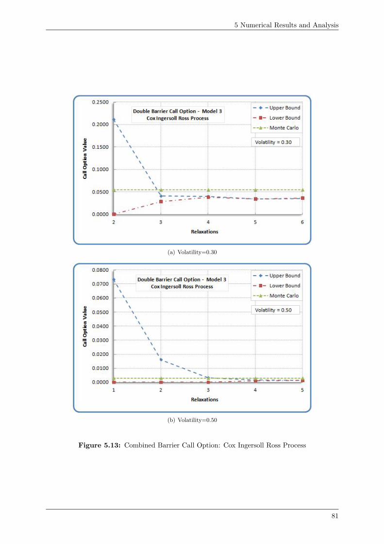
5 Numerical Results and Analysis
(a) Volatility=0.30
(b) Volatility=0.50
Figure 5.13: Combined Barrier Call Option: Cox Ingersoll Ross Process
81
5.2 Semi-parametric Approach for Pricing European Options
5.2 Semi-parametric Approach for Pricing European Options
Finally, before going on to next section, we will analyse the numerical results obtained forEuropean call options by following semi-parametric approach developed in chapter 3. Table A.1in Appendix A shows the discounted values of European call options (with underlying processfollowing a geometric Brownian motion), obtained by solving SDP problems (3.2.1), for differentvalues of volatility σ. For comparison, we have presented the Black Scholes value. Two examplesfrom the numerical data are shown in figure 5.14.
We note the following points regarding the numerical results:
• As we increase relaxations R, the accuracy of results increase and bounds become moretighter.
• The degree of improvement in bounds is not uniform and depends on values of volatilityσ, maturity time T and strike price K. For example, as we increase the volatility σ from0.20 to 0.80 and keep number of relaxations R constant, we note that distance betweenupper and lower bounds increases.
• When strike price is lower than initial stock price, the lower bound is higher than BlackScholes value. For example when strike price is less that 35, the lower bound is aboveBlack Scholes value and is thus not accurate.
• When strike price is higher (for example above 36 in given numerical example), the BlackScholes value is contained within upper and lower bounds.
82
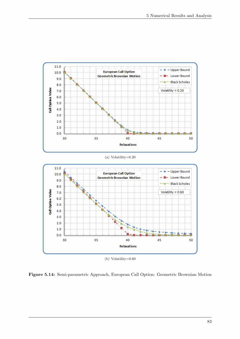
5 Numerical Results and Analysis
(a) Volatility=0.20
(b) Volatility=0.60
Figure 5.14: Semi-parametric Approach, European Call Option: Geometric Brownian Motion
83
5.2 Semi-parametric Approach for Pricing European Options
In order to interpret the data better, we now present the two different perspectives from thesame data. The two graphs present in figure 5.15 show the difference between bounds of higherorder moments and Black-Scholes price when we
• add higher order moments while keeping volatility σ constant, and
• increase the volatility σ with the same amount of moment information (i.e. keeping Rconstant).
We observe the following from figure 5.15(a):
• Lower bound solution (obtained from all SDP programs with higher order relaxations) isworse than Black Scholes price when strike price is comparatively lower than initial stockprice. This can be seen from the negative difference between Black-Scholes value and lowerbound.
• Increase in number of relaxations decreases the difference between upper/lower bound andBlack Scholes value.
• Difference between upper bound and Black-Scholes value is lesser than difference betweenlower bound and Black-Scholes value.
• Discrepancy in upper and lower bound increases as strike price K approaches the initialstock price S0, whereas same discrepancy is much less when strike price K is far frominitial stock price S0.
We also observe the following from figure 5.15(b):
• Lower bound is more sensitive to change in volatility σ as compared to upper bound.
• Increase in volatility σ decreases the difference between upper/lower bound and BlackScholes value.
• Discrepancy in upper and lower bound is highest when value of strike price K approachesthe initial stock price S0, whereas same discrepancy is much less when strike price K isfar from initial stock price S0.
84
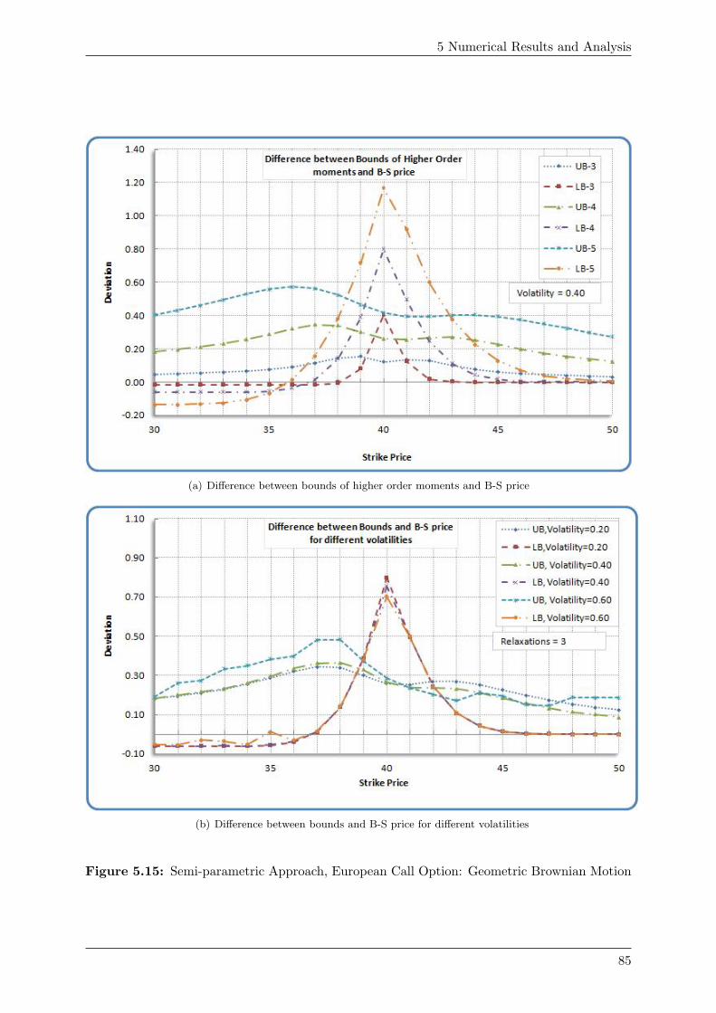
5 Numerical Results and Analysis
(a) Difference between bounds of higher order moments and B-S price
(b) Difference between bounds and B-S price for different volatilities
Figure 5.15: Semi-parametric Approach, European Call Option: Geometric Brownian Motion
85
Chapter 6
Conclusion
It is a well known fact that Black-Scholes formula was derived under several assumptions whichare not always true in the real capital market. For example, if the underlying asset pricedeviates from the geometric Brownian motion, then significant amount of mispricing can occur.Subsequently, several authors have suggested alternative models and methodologies for pricingoptions which attempt to overcome the shortcomings in Black-Scholes model. In this project,we investigated two such recently proposed methodologies for pricing various types of plain andexotic options.
In the semi-parametric approach proposed originally by Lo in [22] and extended by Bertsi-mas and Popescu in [1] and Gotoh and Konno in [9], we approximate the value of Europeancall options by solving two semidefinite programming(SDP) problems. For this approach, weneed to know the first few moments of the risk neutral probability, and not the probabilitydistribution itself. Very accurate bounds are available in real time as we saw in the numericalresults. According to authors, this approach assumes importance in scenarios where closed-formanalytical solution is not available for complex derivatives, but first few moments are available.Thus this semi-parametric approach could be applied to more general class of moment problems.
In the SDP moment approach suggested by Lasserre, Prieto-Rumeau and Zervos in [21],several exotic options could be priced, where underlying asset price process is not restricted tobe geometric Brownian motion as in Black-Scholes model. This approach also solves two SDPproblems for bounding the option price from above and below. Both approaches are similarin the sense that underlying problems to be solved are SDP problems, however the approachto develop those SDP problems are different. The main difference is that in the SDP momentapproach, we do not need to know the moments of underlying asset price process, as is thecase with semi-parametric approach. However one main restriction of SDP moment approachis that infinitesimal generator of the underlying asset price process must map polynomials intopolynomials of equal or lesser degree. Another major assumption for convergence of bounds inSDP moments approach requires that underlying asset price’s probability distribution shouldbe moment determinate. However, even though probability distribution of geometric Brownianmotion is not moment determinate, we could observe from the numerical results that impressivebounds were achieved in the cases when asset price was modeled to follow geometric Brownianmotion.
6.1 Numerical Remarks
In this project, we implemented semi-parametric approach for European options and SDP mo-ment approach for several class of exotic options. For the semi-parametric approach we obtainedvery accurate results in real time with first few moments. However the lower bounds were notaccurate when strike price was very small as compared to initial stock price.
For the SDP moment approach, we were successfully able to formulate the SDP problems for
86
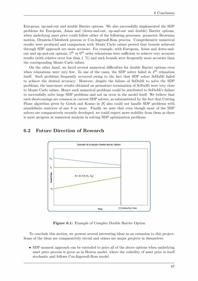
6 Conclusion
European, up-and-out and double Barrier options. We also successfully implemented the SDPproblems for European, Asian and (down-and-out, up-and-out and double) Barrier options,when underlying asset price could follow either of the following processes: geometric Brownianmotion, Ornstein-Uhlenbeck process or Cox-Ingersoll-Ross process. Comprehensive numericalresults were produced and comparison with Monte Carlo values proved that bounds achievedthrough SDP approach are more accurate. For example, with European, Asian and down-and-out and up-and-out options, 5th or 6th order relaxations were sufficient to achieve very accurateresults (with relative error less than 1 %) and such bounds were frequently more accurate thanthe corresponding Monte Carlo values.
On the other hand, we faced several numerical difficulties for double Barrier options evenwhen relaxations were very few. In one of the cases, the SDP solver failed in 4th relaxationitself. Such problems frequently occurred owing to the fact that SDP solver SeDuMi failedto achieve the desired accuracy. However, despite the failure of SeDuMi to solve the SDPproblems, the inaccurate results obtained on premature termination of SeDuMi were very closeto Monte Carlo values. Hence such numerical problems could be attributed to SeDuMi’s failureto successfully solve large SDP problems and not an error in the model itself. We believe thatsuch shortcomings are common in current SDP solvers, as substantiated by the fact that CuttingPlane algorithm given by Gotoh and Konno in [8] also could not handle SDP problems withsemidefinite matrices of size 9 or more. Finally we note that even though most of the SDPsolvers are comparatively recently developed, we could expect more stability from them as thereis more progress in numerical analysis in solving SDP optimization problems.
6.2 Future Direction of Research
Figure 6.1: Example of Complex Double Barrier Option
To conclude this section, we present several interesting ideas as an extension to this project.Some of the ideas are comparatively trivial and others are major projects in themselves.
• SDP moment approach can be extended to price all of the above options when underlyingasset price process is given as in Heston model, where the volatility of asset price is itselfstochastic and follows Cox-Ingersoll-Ross model.
87

6.2 Future Direction of Research
• SDP moment approach can be extended for average strike Asian options. (This projectcovers the average price Asian options).
• SDP moment approach can also be applied to the following generalizations of the barrieroptions:
– Partial barrier options, where barrier applies for a limited time interval.
– Parisian options where barriers must remain crossed from some pre-specified amountof time.
– More general time dependent barriers. For example as shown in figure 6.1, the lowerand upper Barriers change linearly with time.
88
Appendix A
Tables and Figures for NumericalResults
A.1 Semi-parametric Approach for Pricing European Options
In the table A.1, we present the numerical values for European call options obtained by followingsemi-parametric approach presented in chapter 3. In the table, upper and lower bounds aredenoted by abbreviations UB and LB respectively and Black-Scholes value is denoted by BS.The values of other parameters are listed on the top of table for reference where the symbolshave the usual meaning: R = relaxations, S0= initial stock price, K = strike price, T = time, r= risk-free interest rate and σ = volatility.
A.2 SDP Moment Approach for Pricing Exotic Options
Finally, we present the numerical values for different types of call options obtained by followingSDP moment approach presented in chapter 4. In the tables A.2 to A.13, upper bound, lowerbounds and Black-Scholes value are denoted by abbreviations UB, LB and BS respectively. Thevalues of other parameters are listed on the top of table for reference where the symbols have theusual meaning: R = relaxations, S0= initial stock price, K = strike price, T = time, r = risk-freeinterest rate, γ and θ = parameters for Ornstein-Uhlenbeck and Cox-Ingersoll-Ross diffusions,σ = volatility, HL and HU = lower and upper barriers, respectively, for Barrier options.
89
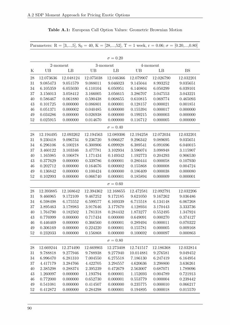
A.2 SDP Moment Approach for Pricing Exotic Options
Table A.1: European Call Option Values: Geometric Brownian Motion
Parameters: R = [3,...,5], S0 = 40, K = [28,...,52], T = 1 week, r = 0.06; σ = [0.20,...,0.80]
σ = 0.20
2-moment 3-moment 4-momentK UB LB UB LB UB LB BS
28 12.073636 12.048124 12.075038 12.046366 12.079907 12.026790 12.03220131 9.085473 9.051579 9.088011 9.046023 9.145044 8.993252 9.03565134 6.105359 6.055030 6.110104 6.050951 6.140804 6.050299 6.03910137 3.156013 3.058412 3.166005 3.056615 3.286707 3.047553 3.04322140 0.586467 0.061880 0.590438 0.068655 0.610815 0.069774 0.46509343 0.101725 0.000000 0.086801 0.000001 0.128157 0.000021 0.00185146 0.051371 0.000002 0.040485 0.000000 0.155394 0.000017 0.00000049 0.034286 0.000000 0.026938 0.000000 0.199215 0.000003 0.00000052 0.025915 0.000000 0.014670 0.000000 0.116712 0.000005 0.000000
σ = 0.40
28 12.194495 12.093262 12.194563 12.089306 12.194258 12.072034 12.03220131 9.230418 9.096734 9.236720 9.096627 9.296342 9.089695 9.03565134 6.296106 6.100218 6.300906 6.099928 6.389541 6.091696 6.04001537 3.460122 3.103346 3.477781 3.102934 3.596074 3.098948 3.11590740 1.165985 0.106878 1.171434 0.149342 1.192773 0.204293 0.90653043 0.377629 0.000000 0.339786 0.000001 0.280444 0.000058 0.10793046 0.202712 0.000000 0.164676 0.000002 0.155868 0.000008 0.00472449 0.136842 0.000000 0.100424 0.000000 0.186409 0.000038 0.00008052 0.102993 0.000000 0.066740 0.000001 0.185894 0.000009 0.000001
σ = 0.60
28 12.393885 12.168642 12.394362 12.168655 12.472581 12.092791 12.03220631 9.466965 9.172109 9.467252 9.172185 9.621050 9.167262 9.03648634 6.598498 6.175552 6.599577 6.169339 6.715518 6.134148 6.06726837 3.895463 3.178983 3.917646 3.177670 4.128934 3.170443 3.33373640 1.764790 0.182502 1.781318 0.284432 1.873277 0.552495 1.34792443 0.776999 0.000000 0.717434 0.000000 0.649091 0.000270 0.37412746 0.446469 0.000000 0.366560 0.000001 0.289494 0.000011 0.07032249 0.306169 0.000000 0.224220 0.000001 0.155781 0.000005 0.00916852 0.232033 0.000000 0.156868 0.000000 0.100692 0.000097 0.000863
σ = 0.80
28 12.669244 12.274490 12.669903 12.273408 12.741517 12.186368 12.03281431 9.788818 9.277946 9.788938 9.277940 10.014881 9.276581 9.04945234 6.996470 6.281310 7.004550 6.275518 7.186130 6.247419 6.16495437 4.417179 3.284766 4.422705 3.294557 4.620636 3.298800 3.63626140 2.385298 0.288374 2.395239 0.472679 2.563007 0.687071 1.78909643 1.260097 0.000000 1.193794 0.000001 1.152693 0.004789 0.72191346 0.772000 0.000000 0.652730 0.000001 0.553779 0.000004 0.23944249 0.541081 0.000000 0.414507 0.000000 0.235775 0.000010 0.06621752 0.412872 0.000000 0.284298 0.000001 0.194895 0.000018 0.015570
90
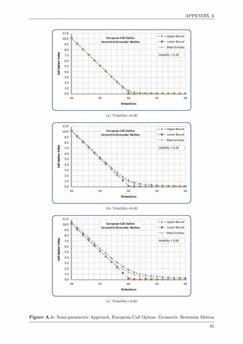
APPENDIX A
(a) Volatility=0.20
(b) Volatility=0.40
(c) Volatility=0.60
Figure A.1: Semi-parametric Approach, European Call Option: Geometric Brownian Motion
91
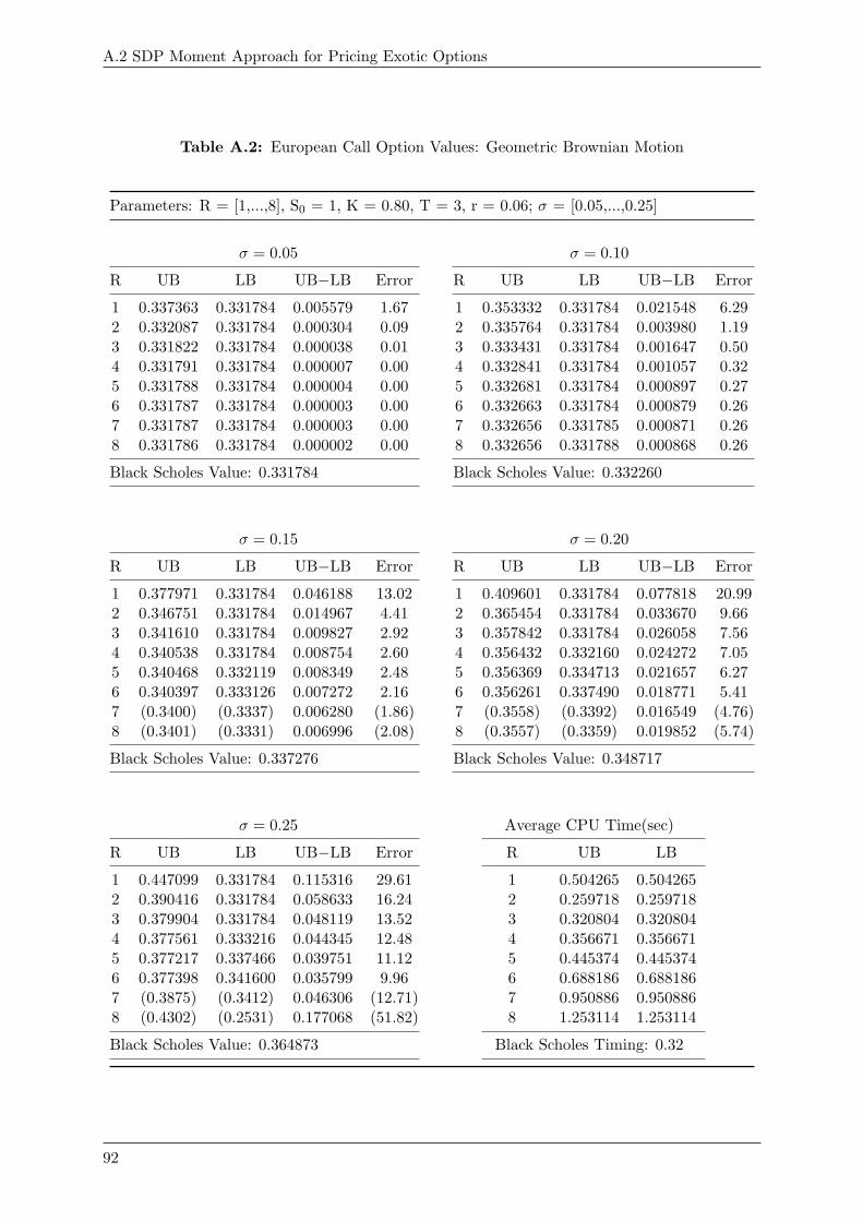
A.2 SDP Moment Approach for Pricing Exotic Options
Table A.2: European Call Option Values: Geometric Brownian Motion
Parameters: R = [1,...,8], S0 = 1, K = 0.80, T = 3, r = 0.06; σ = [0.05,...,0.25]
σ = 0.05 σ = 0.10
R UB LB UB−LB Error R UB LB UB−LB Error
1 0.337363 0.331784 0.005579 1.67 1 0.353332 0.331784 0.021548 6.292 0.332087 0.331784 0.000304 0.09 2 0.335764 0.331784 0.003980 1.193 0.331822 0.331784 0.000038 0.01 3 0.333431 0.331784 0.001647 0.504 0.331791 0.331784 0.000007 0.00 4 0.332841 0.331784 0.001057 0.325 0.331788 0.331784 0.000004 0.00 5 0.332681 0.331784 0.000897 0.276 0.331787 0.331784 0.000003 0.00 6 0.332663 0.331784 0.000879 0.267 0.331787 0.331784 0.000003 0.00 7 0.332656 0.331785 0.000871 0.268 0.331786 0.331784 0.000002 0.00 8 0.332656 0.331788 0.000868 0.26
Black Scholes Value: 0.331784 Black Scholes Value: 0.332260
σ = 0.15 σ = 0.20
R UB LB UB−LB Error R UB LB UB−LB Error
1 0.377971 0.331784 0.046188 13.02 1 0.409601 0.331784 0.077818 20.992 0.346751 0.331784 0.014967 4.41 2 0.365454 0.331784 0.033670 9.663 0.341610 0.331784 0.009827 2.92 3 0.357842 0.331784 0.026058 7.564 0.340538 0.331784 0.008754 2.60 4 0.356432 0.332160 0.024272 7.055 0.340468 0.332119 0.008349 2.48 5 0.356369 0.334713 0.021657 6.276 0.340397 0.333126 0.007272 2.16 6 0.356261 0.337490 0.018771 5.417 (0.3400) (0.3337) 0.006280 (1.86) 7 (0.3558) (0.3392) 0.016549 (4.76)8 (0.3401) (0.3331) 0.006996 (2.08) 8 (0.3557) (0.3359) 0.019852 (5.74)
Black Scholes Value: 0.337276 Black Scholes Value: 0.348717
σ = 0.25 Average CPU Time(sec)
R UB LB UB−LB Error R UB LB
1 0.447099 0.331784 0.115316 29.61 1 0.504265 0.5042652 0.390416 0.331784 0.058633 16.24 2 0.259718 0.2597183 0.379904 0.331784 0.048119 13.52 3 0.320804 0.3208044 0.377561 0.333216 0.044345 12.48 4 0.356671 0.3566715 0.377217 0.337466 0.039751 11.12 5 0.445374 0.4453746 0.377398 0.341600 0.035799 9.96 6 0.688186 0.6881867 (0.3875) (0.3412) 0.046306 (12.71) 7 0.950886 0.9508868 (0.4302) (0.2531) 0.177068 (51.82) 8 1.253114 1.253114
Black Scholes Value: 0.364873 Black Scholes Timing: 0.32
92
APPENDIX A
(a) Volatility=0.05
(b) Volatility=0.15
(c) Volatility=0.25
Figure A.2: European Call Option: Geometric Brownian Motion
93
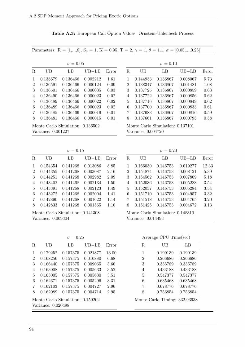
A.2 SDP Moment Approach for Pricing Exotic Options
Table A.3: European Call Option Values: Ornstein-Uhlenbeck Process
Parameters: R = [1,...,8], S0 = 1, K = 0.95, T = 2, γ = 1, θ = 1.1, σ = [0.05,...,0.25]
σ = 0.05 σ = 0.10
R UB LB UB−LB Error R UB LB UB−LB Error
1 0.138679 0.136466 0.002212 1.61 1 0.144933 0.136867 0.008067 5.732 0.136591 0.136466 0.000124 0.09 2 0.138347 0.136867 0.001481 1.083 0.136501 0.136466 0.000035 0.03 3 0.137725 0.136867 0.000859 0.634 0.136490 0.136466 0.000023 0.02 4 0.137722 0.136867 0.000856 0.625 0.136489 0.136466 0.000022 0.02 5 0.137716 0.136867 0.000849 0.626 0.136489 0.136466 0.000023 0.02 6 0.137700 0.136867 0.000833 0.617 0.136485 0.136466 0.000019 0.01 7 0.137683 0.136867 0.000816 0.598 0.136481 0.136466 0.000015 0.01 8 0.137661 0.136867 0.000795 0.58
Monte Carlo Simulation: 0.136502 Monte Carlo Simulation: 0.137101Variance: 0.001227 Variance: 0.004720
σ = 0.15 σ = 0.20
R UB LB UB−LB Error R UB LB UB−LB Error
1 0.154354 0.141268 0.013086 8.85 1 0.166030 0.146753 0.019277 12.332 0.144355 0.141268 0.003087 2.16 2 0.154874 0.146753 0.008121 5.393 0.144251 0.141268 0.002982 2.09 3 0.154562 0.146753 0.007809 5.184 0.143402 0.141268 0.002134 1.50 4 0.152036 0.146753 0.005283 3.545 0.143391 0.141268 0.002123 1.49 5 0.152037 0.146753 0.005284 3.546 0.143272 0.141268 0.002004 1.41 6 0.151710 0.146753 0.004957 3.327 0.142890 0.141268 0.001622 1.14 7 0.151518 0.146753 0.004765 3.208 0.142833 0.141268 0.001565 1.10 8 0.151425 0.146753 0.004672 3.13
Monte Carlo Simulation: 0.141308 Monte Carlo Simulation: 0.148310Variance: 0.009304 Variance: 0.014493
σ = 0.25 Average CPU Time(sec)
R UB LB UB−LB Error R UB LB
1 0.179252 0.157375 0.021877 13.00 1 0.199139 0.1991392 0.168256 0.157375 0.010880 6.68 2 0.266686 0.2666863 0.166440 0.157375 0.009065 5.60 3 0.335789 0.3357894 0.163008 0.157375 0.005633 3.52 4 0.433188 0.4331885 0.163005 0.157375 0.005630 3.51 5 0.547377 0.5473776 0.162671 0.157375 0.005296 3.31 6 0.635468 0.6354687 0.162103 0.157375 0.004727 2.96 7 0.678776 0.6787768 0.162089 0.157375 0.004714 2.95 8 0.756854 0.756854
Monte Carlo Simulation: 0.159202 Monte Carlo Timing: 332.93938Variance: 0.020498
94
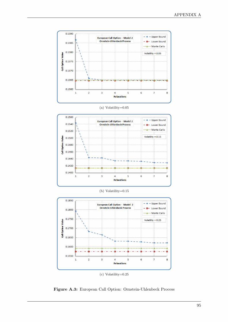
APPENDIX A
(a) Volatility=0.05
(b) Volatility=0.15
(c) Volatility=0.25
Figure A.3: European Call Option: Ornstein-Uhlenbeck Process
95

A.2 SDP Moment Approach for Pricing Exotic Options
Table A.4: European Call Option: Cox Ingersoll Ross Process
Parameters: R = [1,...,8], S0 = 1, K = 0.95, T = 3, γ = 0.9, θ = 1.1, σ = [0.05,...,0.25]
σ = 0.05 σ = 0.10
R UB LB UB−LB Error R UB LB UB−LB Error
1 0.145856 0.143279 0.002577 1.78 1 0.153100 0.143279 0.009820 6.632 0.143437 0.143279 0.000157 0.11 2 0.145494 0.143279 0.002214 1.533 0.143307 0.143279 0.000028 0.02 3 0.144654 0.143279 0.001375 0.954 0.143306 0.143279 0.000027 0.02 4 0.144628 0.143281 0.001347 0.945 0.143304 0.143279 0.000025 0.02 5 0.144604 0.143284 0.001321 0.926 0.143298 0.143279 0.000018 0.01 6 0.144582 0.143283 0.001299 0.907 0.143289 0.143279 0.000010 0.01 7 0.144564 0.143292 0.001272 0.888 0.143288 0.143279 0.000009 0.01 8 0.144567 0.143327 0.001240 0.86
Monte Carlo Simulation: 0.143251 Monte Carlo Simulation: 0.144219Variance: 0.001487 Variance: 0.005951
σ = 0.15 σ = 0.20
R UB LB UB−LB Error R UB LB UB−LB Error
1 0.163917 0.143279 0.020637 13.44 1 0.177215 0.143279 0.033935 21.182 0.151933 0.143279 0.008653 5.86 2 0.162624 0.143279 0.019344 12.653 0.151432 0.143702 0.007731 5.24 3 0.162599 0.147813 0.014786 9.534 0.150935 0.145123 0.005812 3.93 4 0.160606 0.150291 0.010315 6.645 0.150799 0.145297 0.005501 3.72 5 0.159601 0.150280 0.009321 6.026 0.150271 0.145434 0.004837 3.27 6 0.159330 0.150405 0.008926 5.767 0.150224 0.145693 0.004531 3.06 7 0.159279 0.150768 0.008510 5.498 0.150223 0.145736 0.004487 3.03 8 0.159015 0.150883 0.008132 5.25
Monte Carlo Simulation: 0.148184 Monte Carlo Simulation: 0.155946Variance: 0.011580 Variance: 0.018468
σ = 0.25 Average CPU Time(sec)
R UB LB UB−LB Error R UB LB
1 0.192176 0.143279 0.048896 29.15 1 0.5417 0.5416962 0.175931 0.143764 0.032167 20.12 2 0.28531 0.285313 0.175822 0.154467 0.021355 12.93 3 0.30444 0.3044444 0.172344 0.156922 0.015422 9.37 4 0.41626 0.4162635 0.170701 0.157171 0.013530 8.25 5 0.51578 0.5157796 0.170705 0.157466 0.013239 8.07 6 0.58219 0.5821897 0.170536 0.158631 0.011905 7.23 7 0.67982 0.6798228 0.170252 0.158495 0.011757 7.15 8 0.7827 0.782698
Monte Carlo Simulation: 0.166492 Monte Carlo Timing: 498.86Variance: 0.026874
96
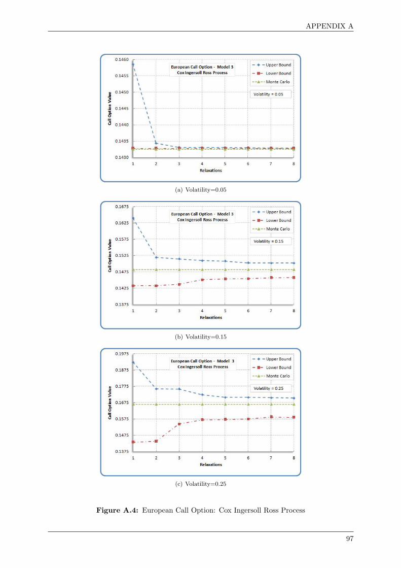
APPENDIX A
(a) Volatility=0.05
(b) Volatility=0.15
(c) Volatility=0.25
Figure A.4: European Call Option: Cox Ingersoll Ross Process
97
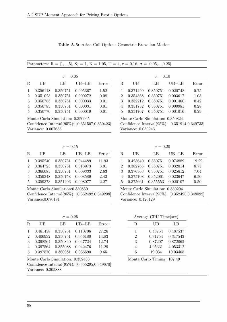
A.2 SDP Moment Approach for Pricing Exotic Options
Table A.5: Asian Call Option: Geometric Brownian Motion
Parameters: R = [1,...,5], S0 = 1, K = 1.05, T = 4, r = 0.16, σ = [0.05,...,0.25]
σ = 0.05 σ = 0.10
R UB LB UB−LB Error R UB LB UB−LB Error
1 0.356118 0.350751 0.005367 1.52 1 0.371499 0.350751 0.020748 5.752 0.351023 0.350751 0.000272 0.08 2 0.354368 0.350751 0.003617 1.033 0.350785 0.350751 0.000033 0.01 3 0.352212 0.350751 0.001460 0.424 0.350783 0.350751 0.000031 0.01 4 0.351732 0.350751 0.000981 0.285 0.350770 0.350751 0.000019 0.01 5 0.351767 0.350751 0.001016 0.29
Monte Carlo Simulation: 0.350965 Monte Carlo Simulation: 0.350824Confidence Interval(95%): [0.351507,0.350423] Confidence Interval(95%): [0.351914,0.349733]Variance: 0.007638 Variance: 0.030943
σ = 0.15 σ = 0.20
R UB LB UB−LB Error R UB LB UB−LB Error
1 0.395240 0.350751 0.044489 11.93 1 0.425640 0.350751 0.074889 19.292 0.364725 0.350751 0.013973 3.91 2 0.382765 0.350751 0.032014 8.733 0.360085 0.350751 0.009333 2.63 3 0.376363 0.350751 0.025612 7.044 0.359348 0.350758 0.008589 2.42 4 0.375708 0.352061 0.023647 6.505 0.359373 0.351296 0.008077 2.27 5 0.375661 0.355553 0.020107 5.50
Monte Carlo Simulation:0.350850 Monte Carlo Simulation: 0.350294Confidence Interval(95%): [0.352492,0.349208] Confidence Interval(95%): [0.352495,0.348092]Variance:0.070191 Variance: 0.126129
σ = 0.25 Average CPU Time(sec)
R UB LB UB−LB Error R UB LB
1 0.461458 0.350751 0.110706 27.26 1 0.48754 0.4875372 0.406932 0.350751 0.056180 14.83 2 0.31754 0.3175433 0.398564 0.350840 0.047724 12.74 3 0.87207 0.8720654 0.397564 0.355088 0.042476 11.29 4 4.05331 4.0533125 0.397570 0.360981 0.036590 9.65 5 19.034 19.03405
Monte Carlo Simulation: 0.352483 Monte Carlo Timing: 107.49Confidence Interval(95%): [0.355295,0.349670]Variance: 0.205888
98
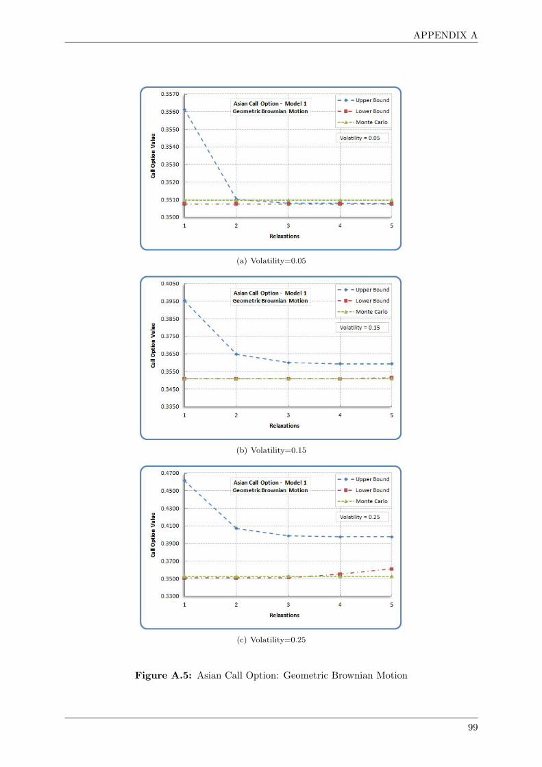
APPENDIX A
(a) Volatility=0.05
(b) Volatility=0.15
(c) Volatility=0.25
Figure A.5: Asian Call Option: Geometric Brownian Motion
99
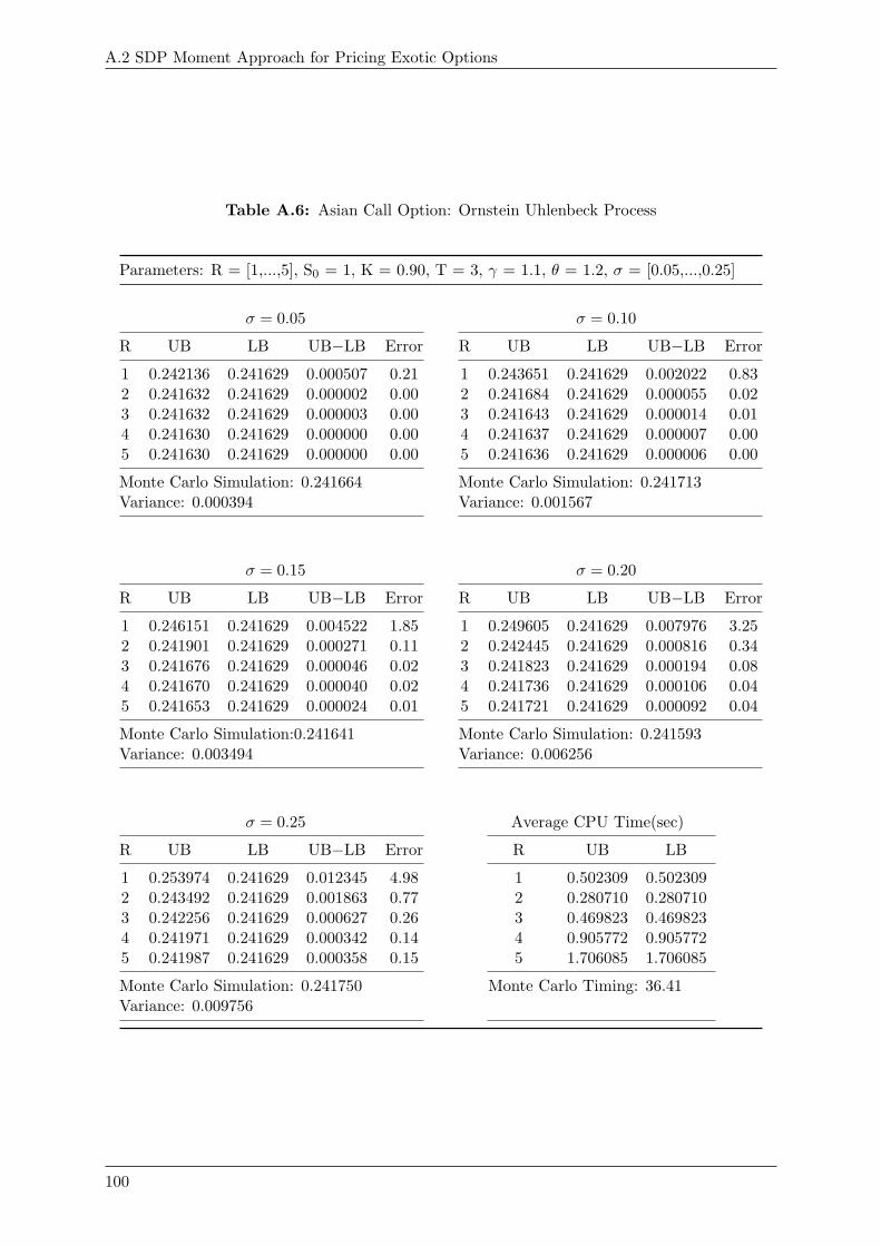
A.2 SDP Moment Approach for Pricing Exotic Options
Table A.6: Asian Call Option: Ornstein Uhlenbeck Process
Parameters: R = [1,...,5], S0 = 1, K = 0.90, T = 3, γ = 1.1, θ = 1.2, σ = [0.05,...,0.25]
σ = 0.05 σ = 0.10
R UB LB UB−LB Error R UB LB UB−LB Error
1 0.242136 0.241629 0.000507 0.21 1 0.243651 0.241629 0.002022 0.832 0.241632 0.241629 0.000002 0.00 2 0.241684 0.241629 0.000055 0.023 0.241632 0.241629 0.000003 0.00 3 0.241643 0.241629 0.000014 0.014 0.241630 0.241629 0.000000 0.00 4 0.241637 0.241629 0.000007 0.005 0.241630 0.241629 0.000000 0.00 5 0.241636 0.241629 0.000006 0.00
Monte Carlo Simulation: 0.241664 Monte Carlo Simulation: 0.241713Variance: 0.000394 Variance: 0.001567
σ = 0.15 σ = 0.20
R UB LB UB−LB Error R UB LB UB−LB Error
1 0.246151 0.241629 0.004522 1.85 1 0.249605 0.241629 0.007976 3.252 0.241901 0.241629 0.000271 0.11 2 0.242445 0.241629 0.000816 0.343 0.241676 0.241629 0.000046 0.02 3 0.241823 0.241629 0.000194 0.084 0.241670 0.241629 0.000040 0.02 4 0.241736 0.241629 0.000106 0.045 0.241653 0.241629 0.000024 0.01 5 0.241721 0.241629 0.000092 0.04
Monte Carlo Simulation:0.241641 Monte Carlo Simulation: 0.241593Variance: 0.003494 Variance: 0.006256
σ = 0.25 Average CPU Time(sec)
R UB LB UB−LB Error R UB LB
1 0.253974 0.241629 0.012345 4.98 1 0.502309 0.5023092 0.243492 0.241629 0.001863 0.77 2 0.280710 0.2807103 0.242256 0.241629 0.000627 0.26 3 0.469823 0.4698234 0.241971 0.241629 0.000342 0.14 4 0.905772 0.9057725 0.241987 0.241629 0.000358 0.15 5 1.706085 1.706085
Monte Carlo Simulation: 0.241750 Monte Carlo Timing: 36.41Variance: 0.009756
100
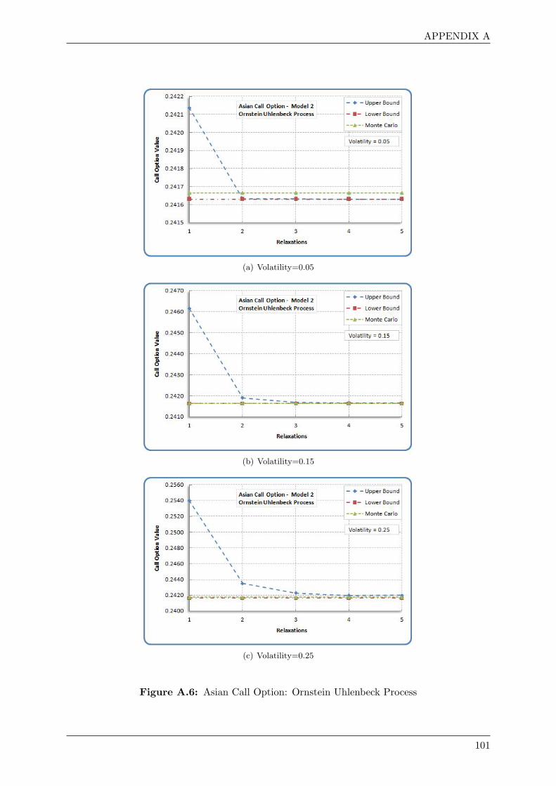
APPENDIX A
(a) Volatility=0.05
(b) Volatility=0.15
(c) Volatility=0.25
Figure A.6: Asian Call Option: Ornstein Uhlenbeck Process
101
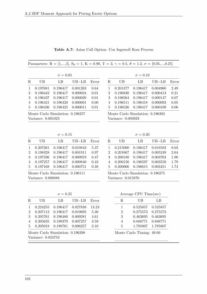
A.2 SDP Moment Approach for Pricing Exotic Options
Table A.7: Asian Call Option: Cox Ingersoll Ross Process
Parameters: R = [1,...,5], S0 = 1, K = 0.90, T = 3, γ = 0.5, θ = 1.2, σ = [0.05,...,0.25]
σ = 0.05 σ = 0.10
R UB LB UB−LB Error R UB LB UB−LB Error
1 0.197681 0.196417 0.001263 0.64 1 0.201377 0.196417 0.004960 2.492 0.196442 0.196417 0.000024 0.01 2 0.196830 0.196417 0.000413 0.213 0.196437 0.196417 0.000020 0.01 3 0.196564 0.196417 0.000147 0.074 0.196421 0.196420 0.000001 0.00 4 0.196511 0.196418 0.000093 0.055 0.196436 0.196425 0.000011 0.01 5 0.196526 0.196417 0.000109 0.06
Monte Carlo Simulation: 0.196257 Monte Carlo Simulation: 0.196382Variance: 0.001023 Variance: 0.003933
σ = 0.15 σ = 0.20
R UB LB UB−LB Error R UB LB UB−LB Error
1 0.207261 0.196417 0.010843 5.37 1 0.215000 0.196417 0.018583 9.032 0.198328 0.196417 0.001911 0.97 2 0.201667 0.196417 0.005249 2.643 0.197336 0.196417 0.000919 0.47 3 0.200180 0.196417 0.003763 1.904 0.197257 0.196417 0.000840 0.43 4 0.200156 0.196597 0.003559 1.795 0.197168 0.196417 0.000751 0.38 5 0.200066 0.196615 0.003451 1.74
Monte Carlo Simulation: 0.196111 Monte Carlo Simulation: 0.196275Variance: 0.008888 Variance: 0.015876
σ = 0.25 Average CPU Time(sec)
R UB LB UB−LB Error R UB LB
1 0.224255 0.196417 0.027838 13.23 1 0.525857 0.5258572 0.207112 0.196417 0.010695 5.30 2 0.275573 0.2755733 0.205761 0.196480 0.009281 4.61 3 0.463695 0.4636954 0.205635 0.198379 0.007257 3.59 4 0.888771 0.8887715 0.205018 0.198761 0.006257 3.10 5 1.785807 1.785807
Monte Carlo Simulation: 0.196398 Monte Carlo Timing: 49.00Variance: 0.024753
102
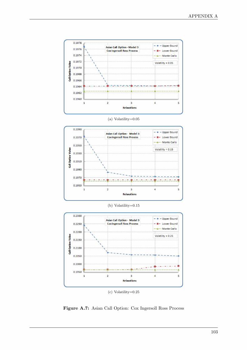
APPENDIX A
(a) Volatility=0.05
(b) Volatility=0.15
(c) Volatility=0.25
Figure A.7: Asian Call Option: Cox Ingersoll Ross Process
103
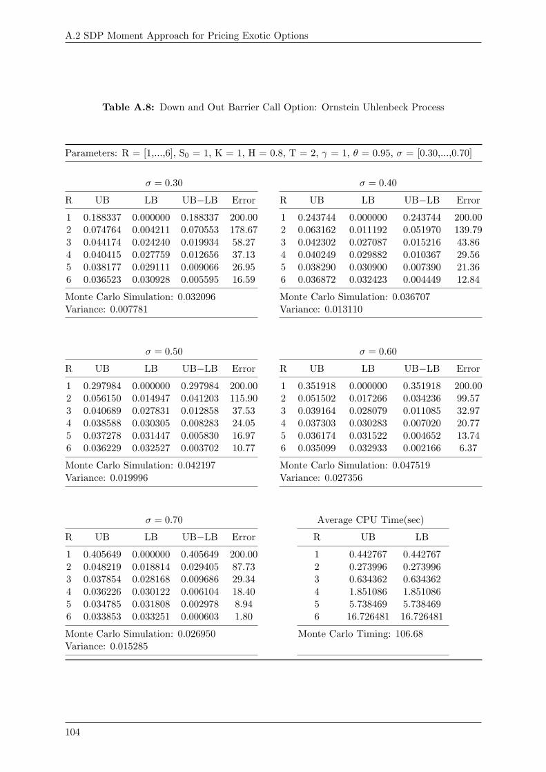
A.2 SDP Moment Approach for Pricing Exotic Options
Table A.8: Down and Out Barrier Call Option: Ornstein Uhlenbeck Process
Parameters: R = [1,...,6], S0 = 1, K = 1, H = 0.8, T = 2, γ = 1, θ = 0.95, σ = [0.30,...,0.70]
σ = 0.30 σ = 0.40
R UB LB UB−LB Error R UB LB UB−LB Error
1 0.188337 0.000000 0.188337 200.00 1 0.243744 0.000000 0.243744 200.002 0.074764 0.004211 0.070553 178.67 2 0.063162 0.011192 0.051970 139.793 0.044174 0.024240 0.019934 58.27 3 0.042302 0.027087 0.015216 43.864 0.040415 0.027759 0.012656 37.13 4 0.040249 0.029882 0.010367 29.565 0.038177 0.029111 0.009066 26.95 5 0.038290 0.030900 0.007390 21.366 0.036523 0.030928 0.005595 16.59 6 0.036872 0.032423 0.004449 12.84
Monte Carlo Simulation: 0.032096 Monte Carlo Simulation: 0.036707Variance: 0.007781 Variance: 0.013110
σ = 0.50 σ = 0.60
R UB LB UB−LB Error R UB LB UB−LB Error
1 0.297984 0.000000 0.297984 200.00 1 0.351918 0.000000 0.351918 200.002 0.056150 0.014947 0.041203 115.90 2 0.051502 0.017266 0.034236 99.573 0.040689 0.027831 0.012858 37.53 3 0.039164 0.028079 0.011085 32.974 0.038588 0.030305 0.008283 24.05 4 0.037303 0.030283 0.007020 20.775 0.037278 0.031447 0.005830 16.97 5 0.036174 0.031522 0.004652 13.746 0.036229 0.032527 0.003702 10.77 6 0.035099 0.032933 0.002166 6.37
Monte Carlo Simulation: 0.042197 Monte Carlo Simulation: 0.047519Variance: 0.019996 Variance: 0.027356
σ = 0.70 Average CPU Time(sec)
R UB LB UB−LB Error R UB LB
1 0.405649 0.000000 0.405649 200.00 1 0.442767 0.4427672 0.048219 0.018814 0.029405 87.73 2 0.273996 0.2739963 0.037854 0.028168 0.009686 29.34 3 0.634362 0.6343624 0.036226 0.030122 0.006104 18.40 4 1.851086 1.8510865 0.034785 0.031808 0.002978 8.94 5 5.738469 5.7384696 0.033853 0.033251 0.000603 1.80 6 16.726481 16.726481
Monte Carlo Simulation: 0.026950 Monte Carlo Timing: 106.68Variance: 0.015285
104
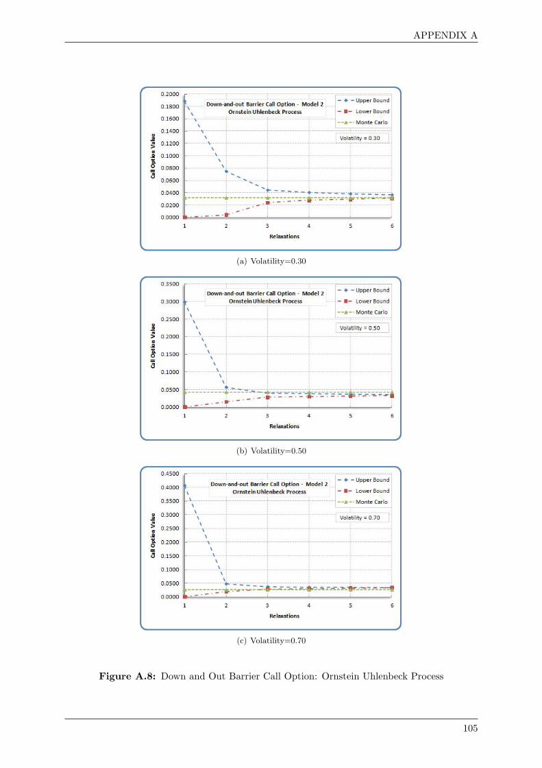
APPENDIX A
(a) Volatility=0.30
(b) Volatility=0.50
(c) Volatility=0.70
Figure A.8: Down and Out Barrier Call Option: Ornstein Uhlenbeck Process
105

A.2 SDP Moment Approach for Pricing Exotic Options
Table A.9: Down and Out Barrier Call Option: Cox Ingersoll Ross Process
Parameters: R = [1,...,6], S0 = 1, K = 1, T = 3, H=0.8, γ = 1, θ = 0.95, σ = [0.30,...,0.70]
σ = 0.30 σ = 0.40
R UB LB UB−LB Error R UB LB UB−LB Error
1 0.244159 0.000000 0.244159 200.00 1 0.320683 0.000000 0.320683 200.002 0.095773 0.000001 0.095772 200.00 2 0.063664 0.000000 0.063663 200.003 0.031514 0.012284 0.019230 87.81 3 0.026498 0.012305 0.014193 73.154 0.026075 0.017175 0.008899 41.15 4 0.022377 0.017092 0.005286 26.785 0.022336 0.020791 0.001546 7.17 5 0.020054 0.019285 0.000768 3.916 0.021982 0.021978 0.000004 0.02 6 0.019748 0.019714 0.000034 0.17
Monte Carlo Simulation: 0.024312 Monte Carlo Simulation: 0.023539Variance: 0.006167 Variance: 0.009553
σ = 0.50 σ = 0.60
R UB LB UB−LB Error R UB LB UB−LB Error
1 0.395038 0.000000 0.395038 200.00 1 0.467493 0.000000 0.467493 200.002 0.049769 0.000000 0.049769 200.00 2 0.041999 0.000000 0.041999 200.003 0.023115 0.011962 0.011153 63.59 3 0.020794 0.011569 0.009226 57.014 0.019490 0.015466 0.004025 23.03 4 0.018019 0.014480 0.003539 21.785 0.018220 0.017163 0.001056 5.97 5 0.016542 0.016160 0.000382 2.336 0.017904 0.017851 0.000053 0.30 6 0.016525 0.016464 0.000061 0.37
Monte Carlo Simulation: 0.026120 Monte Carlo Simulation: 0.024593Variance: 0.014680 Variance: 0.017088
σ = 0.70 Average CPU Time(sec)
R UB LB UB−LB Error R UB LB
1 0.534786 0.000000 0.534786 200.00 1 0.469574 0.4695742 0.037075 0.000000 0.037074 200.00 2 0.303902 0.3039023 0.019145 0.011312 0.007833 51.43 3 0.646331 0.6463314 0.016062 0.014459 0.001604 10.51 4 1.870097 1.8700975 0.015409 0.015212 0.000197 1.29 5 5.820117 5.8201176 0.015404 0.015413 -0.000009 -0.06 6 17.514597 17.514597
Monte Carlo Simulation: 0.020986 Monte Carlo Timing: 82.94Variance: 0.020768
106
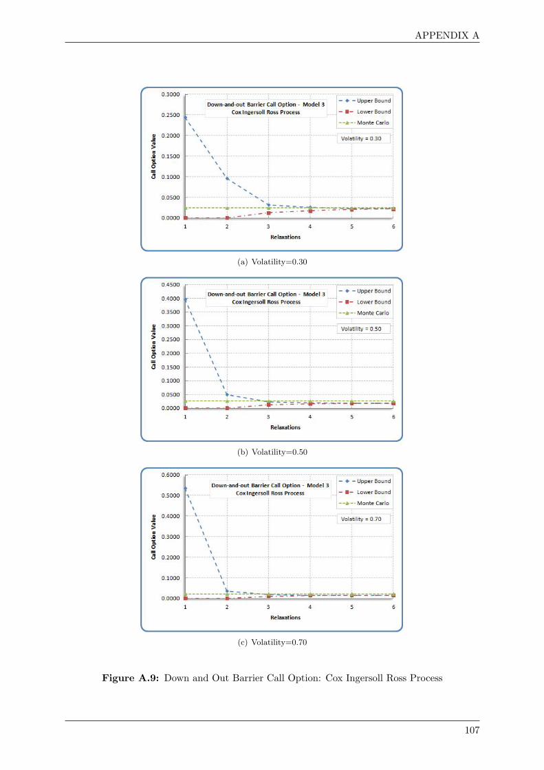
APPENDIX A
(a) Volatility=0.30
(b) Volatility=0.50
(c) Volatility=0.70
Figure A.9: Down and Out Barrier Call Option: Cox Ingersoll Ross Process
107
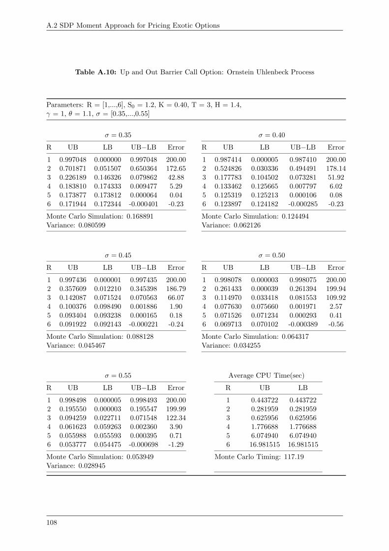
A.2 SDP Moment Approach for Pricing Exotic Options
Table A.10: Up and Out Barrier Call Option: Ornstein Uhlenbeck Process
Parameters: R = [1,...,6], S0 = 1.2, K = 0.40, T = 3, H = 1.4,γ = 1, θ = 1.1, σ = [0.35,...,0.55]
σ = 0.35 σ = 0.40
R UB LB UB−LB Error R UB LB UB−LB Error
1 0.997048 0.000000 0.997048 200.00 1 0.987414 0.000005 0.987410 200.002 0.701871 0.051507 0.650364 172.65 2 0.524826 0.030336 0.494491 178.143 0.226189 0.146326 0.079862 42.88 3 0.177783 0.104502 0.073281 51.924 0.183810 0.174333 0.009477 5.29 4 0.133462 0.125665 0.007797 6.025 0.173877 0.173812 0.000064 0.04 5 0.125319 0.125213 0.000106 0.086 0.171944 0.172344 -0.000401 -0.23 6 0.123897 0.124182 -0.000285 -0.23
Monte Carlo Simulation: 0.168891 Monte Carlo Simulation: 0.124494Variance: 0.080599 Variance: 0.062126
σ = 0.45 σ = 0.50
R UB LB UB−LB Error R UB LB UB−LB Error
1 0.997436 0.000001 0.997435 200.00 1 0.998078 0.000003 0.998075 200.002 0.357609 0.012210 0.345398 186.79 2 0.261433 0.000039 0.261394 199.943 0.142087 0.071524 0.070563 66.07 3 0.114970 0.033418 0.081553 109.924 0.100376 0.098490 0.001886 1.90 4 0.077630 0.075660 0.001971 2.575 0.093404 0.093238 0.000165 0.18 5 0.071526 0.071234 0.000293 0.416 0.091922 0.092143 -0.000221 -0.24 6 0.069713 0.070102 -0.000389 -0.56
Monte Carlo Simulation: 0.088128 Monte Carlo Simulation: 0.064317Variance: 0.045467 Variance: 0.034255
σ = 0.55 Average CPU Time(sec)
R UB LB UB−LB Error R UB LB
1 0.998498 0.000005 0.998493 200.00 1 0.443722 0.4437222 0.195550 0.000003 0.195547 199.99 2 0.281959 0.2819593 0.094259 0.022711 0.071548 122.34 3 0.625956 0.6259564 0.061623 0.059263 0.002360 3.90 4 1.776688 1.7766885 0.055988 0.055593 0.000395 0.71 5 6.074940 6.0749406 0.053777 0.054475 -0.000698 -1.29 6 16.981515 16.981515
Monte Carlo Simulation: 0.053949 Monte Carlo Timing: 117.19Variance: 0.028945
108
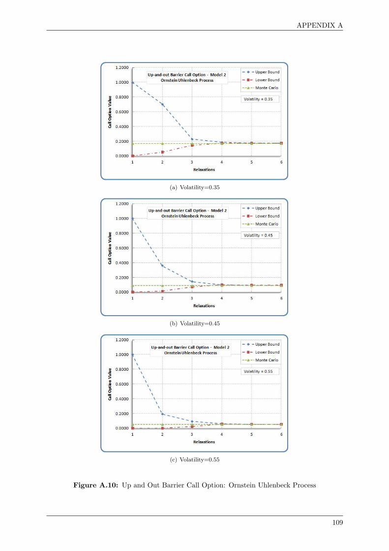
APPENDIX A
(a) Volatility=0.35
(b) Volatility=0.45
(c) Volatility=0.55
Figure A.10: Up and Out Barrier Call Option: Ornstein Uhlenbeck Process
109
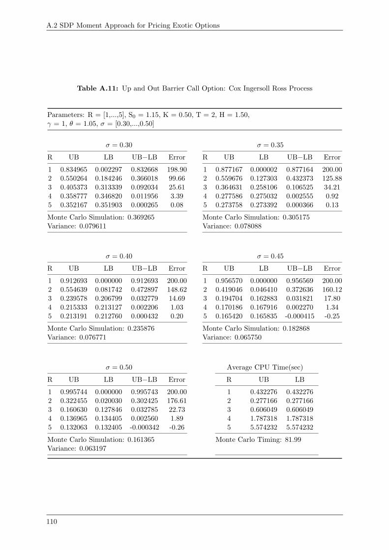
A.2 SDP Moment Approach for Pricing Exotic Options
Table A.11: Up and Out Barrier Call Option: Cox Ingersoll Ross Process
Parameters: R = [1,...,5], S0 = 1.15, K = 0.50, T = 2, H = 1.50,γ = 1, θ = 1.05, σ = [0.30,...,0.50]
σ = 0.30 σ = 0.35
R UB LB UB−LB Error R UB LB UB−LB Error
1 0.834965 0.002297 0.832668 198.90 1 0.877167 0.000002 0.877164 200.002 0.550264 0.184246 0.366018 99.66 2 0.559676 0.127303 0.432373 125.883 0.405373 0.313339 0.092034 25.61 3 0.364631 0.258106 0.106525 34.214 0.358777 0.346820 0.011956 3.39 4 0.277586 0.275032 0.002555 0.925 0.352167 0.351903 0.000265 0.08 5 0.273758 0.273392 0.000366 0.13
Monte Carlo Simulation: 0.369265 Monte Carlo Simulation: 0.305175Variance: 0.079611 Variance: 0.078088
σ = 0.40 σ = 0.45
R UB LB UB−LB Error R UB LB UB−LB Error
1 0.912693 0.000000 0.912693 200.00 1 0.956570 0.000000 0.956569 200.002 0.554639 0.081742 0.472897 148.62 2 0.419046 0.046410 0.372636 160.123 0.239578 0.206799 0.032779 14.69 3 0.194704 0.162883 0.031821 17.804 0.215333 0.213127 0.002206 1.03 4 0.170186 0.167916 0.002270 1.345 0.213191 0.212760 0.000432 0.20 5 0.165420 0.165835 -0.000415 -0.25
Monte Carlo Simulation: 0.235876 Monte Carlo Simulation: 0.182868Variance: 0.076771 Variance: 0.065750
σ = 0.50 Average CPU Time(sec)
R UB LB UB−LB Error R UB LB
1 0.995744 0.000000 0.995743 200.00 1 0.432276 0.4322762 0.322455 0.020030 0.302425 176.61 2 0.277166 0.2771663 0.160630 0.127846 0.032785 22.73 3 0.606049 0.6060494 0.136965 0.134405 0.002560 1.89 4 1.787318 1.7873185 0.132063 0.132405 -0.000342 -0.26 5 5.574232 5.574232
Monte Carlo Simulation: 0.161365 Monte Carlo Timing: 81.99Variance: 0.063197
110
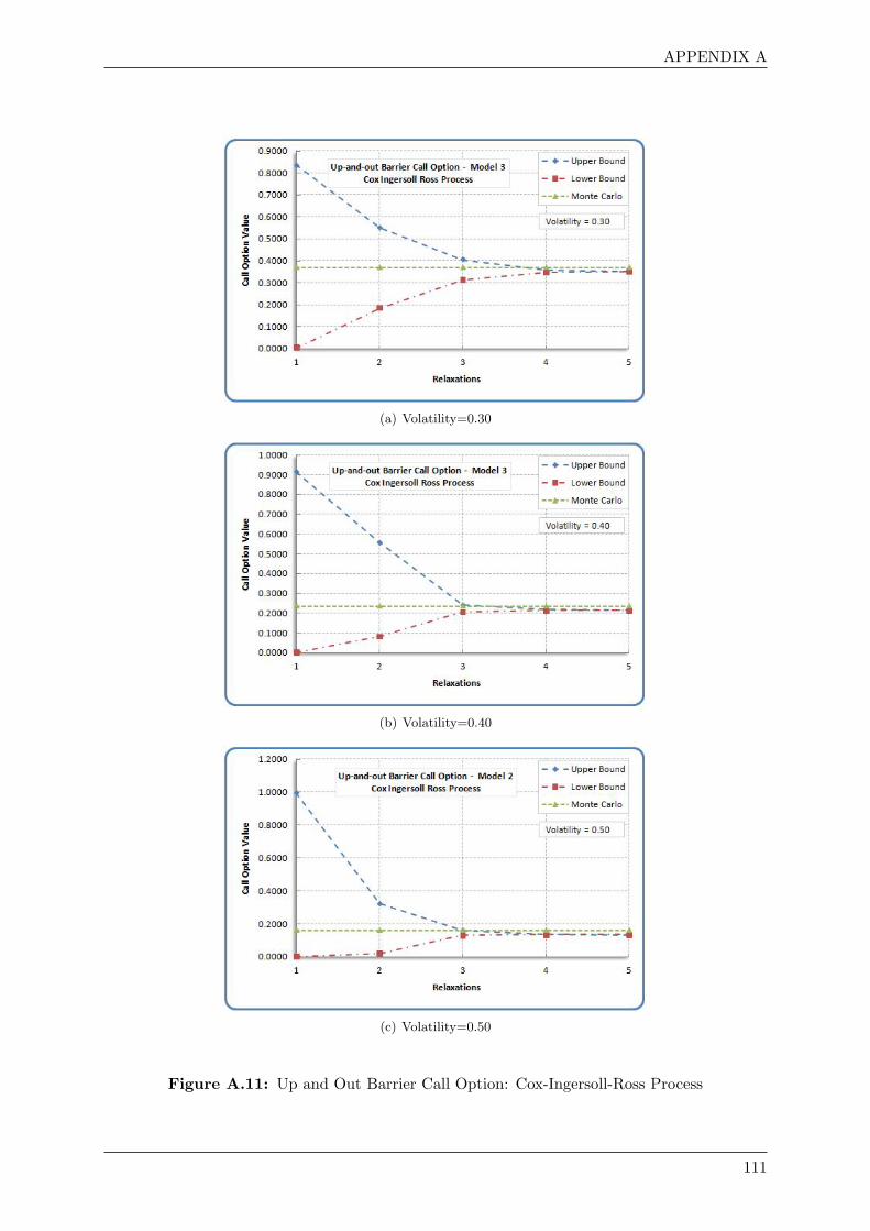
APPENDIX A
(a) Volatility=0.30
(b) Volatility=0.40
(c) Volatility=0.50
Figure A.11: Up and Out Barrier Call Option: Cox-Ingersoll-Ross Process
111
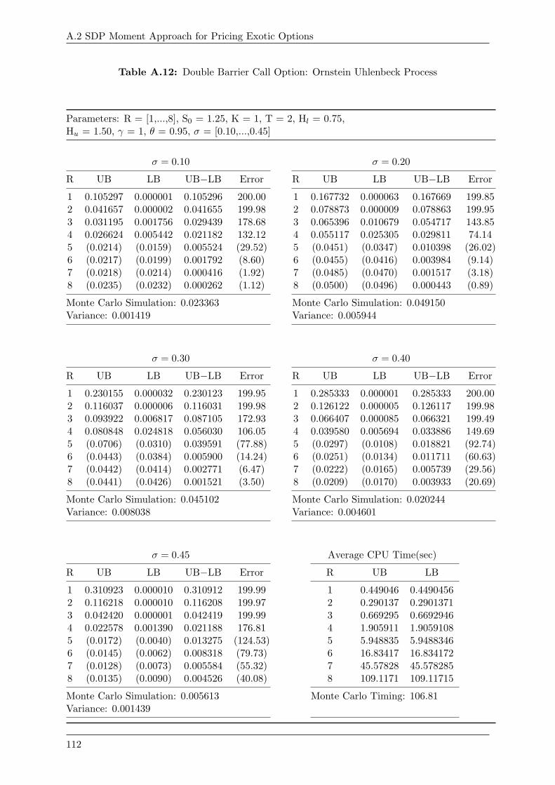
A.2 SDP Moment Approach for Pricing Exotic Options
Table A.12: Double Barrier Call Option: Ornstein Uhlenbeck Process
Parameters: R = [1,...,8], S0 = 1.25, K = 1, T = 2, Hl = 0.75,Hu = 1.50, γ = 1, θ = 0.95, σ = [0.10,...,0.45]
σ = 0.10 σ = 0.20
R UB LB UB−LB Error R UB LB UB−LB Error
1 0.105297 0.000001 0.105296 200.00 1 0.167732 0.000063 0.167669 199.852 0.041657 0.000002 0.041655 199.98 2 0.078873 0.000009 0.078863 199.953 0.031195 0.001756 0.029439 178.68 3 0.065396 0.010679 0.054717 143.854 0.026624 0.005442 0.021182 132.12 4 0.055117 0.025305 0.029811 74.145 (0.0214) (0.0159) 0.005524 (29.52) 5 (0.0451) (0.0347) 0.010398 (26.02)6 (0.0217) (0.0199) 0.001792 (8.60) 6 (0.0455) (0.0416) 0.003984 (9.14)7 (0.0218) (0.0214) 0.000416 (1.92) 7 (0.0485) (0.0470) 0.001517 (3.18)8 (0.0235) (0.0232) 0.000262 (1.12) 8 (0.0500) (0.0496) 0.000443 (0.89)
Monte Carlo Simulation: 0.023363 Monte Carlo Simulation: 0.049150Variance: 0.001419 Variance: 0.005944
σ = 0.30 σ = 0.40
R UB LB UB−LB Error R UB LB UB−LB Error
1 0.230155 0.000032 0.230123 199.95 1 0.285333 0.000001 0.285333 200.002 0.116037 0.000006 0.116031 199.98 2 0.126122 0.000005 0.126117 199.983 0.093922 0.006817 0.087105 172.93 3 0.066407 0.000085 0.066321 199.494 0.080848 0.024818 0.056030 106.05 4 0.039580 0.005694 0.033886 149.695 (0.0706) (0.0310) 0.039591 (77.88) 5 (0.0297) (0.0108) 0.018821 (92.74)6 (0.0443) (0.0384) 0.005900 (14.24) 6 (0.0251) (0.0134) 0.011711 (60.63)7 (0.0442) (0.0414) 0.002771 (6.47) 7 (0.0222) (0.0165) 0.005739 (29.56)8 (0.0441) (0.0426) 0.001521 (3.50) 8 (0.0209) (0.0170) 0.003933 (20.69)
Monte Carlo Simulation: 0.045102 Monte Carlo Simulation: 0.020244Variance: 0.008038 Variance: 0.004601
σ = 0.45 Average CPU Time(sec)
R UB LB UB−LB Error R UB LB
1 0.310923 0.000010 0.310912 199.99 1 0.449046 0.44904562 0.116218 0.000010 0.116208 199.97 2 0.290137 0.29013713 0.042420 0.000001 0.042419 199.99 3 0.669295 0.66929464 0.022578 0.001390 0.021188 176.81 4 1.905911 1.90591085 (0.0172) (0.0040) 0.013275 (124.53) 5 5.948835 5.94883466 (0.0145) (0.0062) 0.008318 (79.73) 6 16.83417 16.8341727 (0.0128) (0.0073) 0.005584 (55.32) 7 45.57828 45.5782858 (0.0135) (0.0090) 0.004526 (40.08) 8 109.1171 109.11715
Monte Carlo Simulation: 0.005613 Monte Carlo Timing: 106.81Variance: 0.001439
112
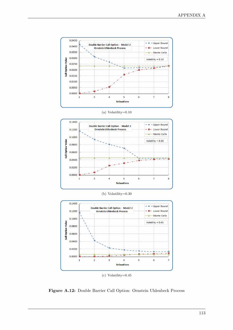
APPENDIX A
(a) Volatility=0.10
(b) Volatility=0.30
(c) Volatility=0.45
Figure A.12: Double Barrier Call Option: Ornstein Uhlenbeck Process
113
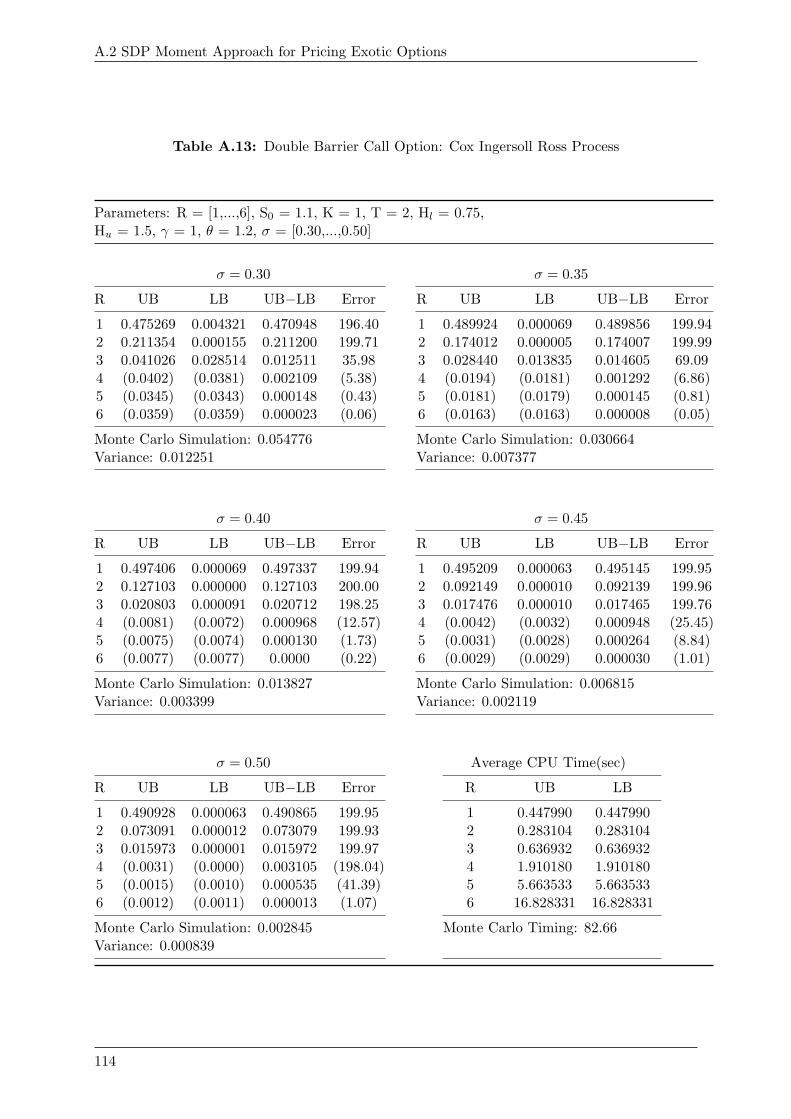
A.2 SDP Moment Approach for Pricing Exotic Options
Table A.13: Double Barrier Call Option: Cox Ingersoll Ross Process
Parameters: R = [1,...,6], S0 = 1.1, K = 1, T = 2, Hl = 0.75,Hu = 1.5, γ = 1, θ = 1.2, σ = [0.30,...,0.50]
σ = 0.30 σ = 0.35
R UB LB UB−LB Error R UB LB UB−LB Error
1 0.475269 0.004321 0.470948 196.40 1 0.489924 0.000069 0.489856 199.942 0.211354 0.000155 0.211200 199.71 2 0.174012 0.000005 0.174007 199.993 0.041026 0.028514 0.012511 35.98 3 0.028440 0.013835 0.014605 69.094 (0.0402) (0.0381) 0.002109 (5.38) 4 (0.0194) (0.0181) 0.001292 (6.86)5 (0.0345) (0.0343) 0.000148 (0.43) 5 (0.0181) (0.0179) 0.000145 (0.81)6 (0.0359) (0.0359) 0.000023 (0.06) 6 (0.0163) (0.0163) 0.000008 (0.05)
Monte Carlo Simulation: 0.054776 Monte Carlo Simulation: 0.030664Variance: 0.012251 Variance: 0.007377
σ = 0.40 σ = 0.45
R UB LB UB−LB Error R UB LB UB−LB Error
1 0.497406 0.000069 0.497337 199.94 1 0.495209 0.000063 0.495145 199.952 0.127103 0.000000 0.127103 200.00 2 0.092149 0.000010 0.092139 199.963 0.020803 0.000091 0.020712 198.25 3 0.017476 0.000010 0.017465 199.764 (0.0081) (0.0072) 0.000968 (12.57) 4 (0.0042) (0.0032) 0.000948 (25.45)5 (0.0075) (0.0074) 0.000130 (1.73) 5 (0.0031) (0.0028) 0.000264 (8.84)6 (0.0077) (0.0077) 0.0000 (0.22) 6 (0.0029) (0.0029) 0.000030 (1.01)
Monte Carlo Simulation: 0.013827 Monte Carlo Simulation: 0.006815Variance: 0.003399 Variance: 0.002119
σ = 0.50 Average CPU Time(sec)
R UB LB UB−LB Error R UB LB
1 0.490928 0.000063 0.490865 199.95 1 0.447990 0.4479902 0.073091 0.000012 0.073079 199.93 2 0.283104 0.2831043 0.015973 0.000001 0.015972 199.97 3 0.636932 0.6369324 (0.0031) (0.0000) 0.003105 (198.04) 4 1.910180 1.9101805 (0.0015) (0.0010) 0.000535 (41.39) 5 5.663533 5.6635336 (0.0012) (0.0011) 0.000013 (1.07) 6 16.828331 16.828331
Monte Carlo Simulation: 0.002845 Monte Carlo Timing: 82.66Variance: 0.000839
114
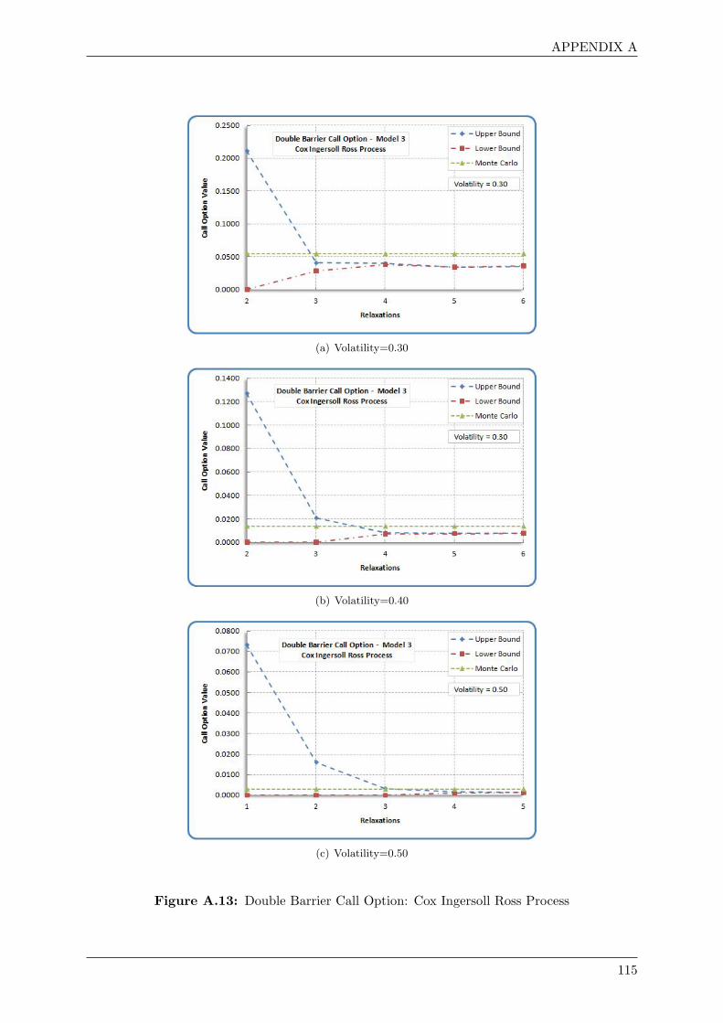
APPENDIX A
(a) Volatility=0.30
(b) Volatility=0.40
(c) Volatility=0.50
Figure A.13: Double Barrier Call Option: Cox Ingersoll Ross Process
115
Bibliography
[1] Bertsimas, D., and Popescu, I, Moment problems via semidefinite programming: Applicationsin probability and finance. Technical Report, 2000/27/TM, INSEAD, Fontainebleau, France,2000. This was a Nicholson paper competition finalist.
[2] Bertsimas, D., and Popescu, I, On the relation between option and stock prices: A convexoptimization approach. Operations Research 50, 2(2002), pp. 358-374.
[3] Black, F., and Scholes, M, The pricing of options and corporate liabilities. Journal of PoliticalEconomy 81 (1973), pp. 637-654.
[4] Boyle, P., and Lin, X., Bounds on multiple contingent claims based on several assets, Journalof Financial Economics 46 (December 2003), pp. 383-400.
[5] D.G. Luenberger, Investment Science, Oxford University Press, New York, 1998.
[6] D.J. Higham, An Introduction to financial option valuation, University Press, Cambridge,2005.
[7] Dawson D.A., Qualitative Behavior of Geostochastic Systems, Stoch. Proc. Appl. 10(1), pp.1-31, 1980.
[8] Gotoh. J., and Konno., H,, A cutting plane algorithm for semi-definite programming problemswith applications to failure discrimination and cancer diagnosis. CRAFT Working paper 00-05, Center for Research in Advanced Financial Technology, Tokyo Institute of Technology,Tokyo, Japan, 2000.
[9] Gotoh. J., and Konno., H,, Bounding option prices by semidefinite programming: a cuttingplane algorithm. Management Science 48, 5 (May 2002), 665-678.
[10] Han, D., Li, X., Sun, D., and Sun, J, Bounding option prices of multi-assets: a semidefiniteprogramming approach. Pacific Journal of Optimization 1, 1 (January 2005), 59-79. Specialissue in honor of the 70th birthday of R Tyrrell Rockafellar.
[11] Helmberg, C., F. Oustry. Bundle methods to minimize the maximum eigenvalue function.Handbook of Semidefinite Programming-Theory, Algorithms, and Applications, Kluwer Aca-demic Publishers, Dordrecht, The Netherlands, 2000.
[12] Helmes K., S.Rohl, R.H. Stockbridge, Computing Moments of the Exit Time Distributionfor Markov Processes by Linear Programming, Operations Research 49(4), pp. 516-530, 2001.
[13] J. Lofberg, YALMIP : A Toolbox for Modeling and Optimization inMATLAB, Proceedings of the CACSD Conference, Taipei, Taiwan, 2004,http://control.ee.ethz.ch/ joloef/yalmip.php.
[14] J.C. Hull, Options, Futures and Other Derivatives, Prentice Hall, New Jersey, 2006.
116
BIBLIOGRAPHY 117
[15] J.C.Cox, J.E. Ingersoll, and S.A. Ross, A Theory of Term Structures of Interest Rates,Econometrica-53, 1985, pp. 385-407.
[16] Jos F. Sturm, Using SeDuMi 1.02, a Matlab toolbox for optimization over symmetric cones.Optimization Methods and Software (1999) no. 11-12, pp. 625-653.
[17] Kevin Rubash, A Study of Option Pricing Models,http://bradley.bradley.edu/ arr/bsm/pg04.html.
[18] Lasserre J.B., Global Optimization with Polynomials and the Problem of Moments,, SIAMJ. Optim. 11(3), pp. 796-817, 2001.
[19] Lasserre J.B.,Henrion D., Gloptipoly: Global Optimization Over Polynomials with Matlaband SeDuMi, ACM Trans. Math. Soft. 29(2), pp. 165-198, 2003.
[20] Lasserre J.B.,Prieto-Rumeau T., SDP vs. LP Relaxations for the Moment Approach inSome Performance Evaluation Problems, Stoch. Models 20(4), pp. 439-456, 2004.
[21] Lasserre J.B.,Prieto-Rumeau T.,Zervos M., Pricing a Class of Exotic Options Via MomentsSDP Relaxations, Mathematical Finance, Vol. 16, No. 3, pp. 469-494, 2006.
[22] Lo, A. W., Semi-parametric upper bounds for options prices and expected payoffs. Journalof Financial Economics 19 (1987), 373-387.
[23] MATLAB by MathWorks, http://www.mathworks.com/.
[24] O.A. Vasicek, An Equilibrium Characterization of the Term Structures, Journal of FinancialEconomics 5, 1977, pp. 177-88.
[25] Paul Glasserman, Monte Carlo Methods in Financial Engineering, Springer Finance Series,2004.
[26] S.E. Shreve, Stochastic Calculus for Finance 1:Binomial Asset Pricing model, SpringerFinance Series, 2000.
[27] S.E. Shreve, Stochastic Calculus for Finance 2: Continuous Time models, Springer FinanceSeries, 2000.
[28] Wolkowicz, H., R. Saigal, L. Vandenberghe, Handbook of Semidefinite Programming-Theory,Algorithms, and Applications. Kluwer Academic Publishers, Dordrecht, The Netherlands,2000.
117