Transit Speed and Delay Study - Florida Department of ... Report Transit Speed and Delay Study Jacksonville, Florida Prepared for: Florida Department of Transportation, Public Transit

Final Report

Transit Speed and Delay Study

Jacksonville, Florida

April 2006

Final Report

Transit Speed and Delay Study

Jacksonville, Florida

Prepared for:

Florida Department of Transportation, Public Transit Office

Tara Bartee, FDOT Project Manager

605 Suwannee St., M.S. #26

Tallahassee, FL 32399-0450

Prepared by:

Kittelson & Associates, Inc.

610 SW Alder, Suite 700

Portland, OR 97205

(503) 228-5230

In association with:

URS, Inc.

Quality Counts, Inc.

April 2006

Paul Ryus, Project Manager

John Zegeer, Project Principal

Andrew Cibor

Michael Hendrix

Table of Contents

EXECUTIVE SUMMARY........................................................................................................................... 1 INTRODUCTION ........................................................................................................................................ 3

Project Background................................................................................................................................... 3 Project Purpose ......................................................................................................................................... 4

STUDY DESIGN.......................................................................................................................................... 5

Study Area Selection and Project Scope................................................................................................... 5 Route Selection ......................................................................................................................................... 6 Route Segmentation .................................................................................................................................. 8 Data Collection ......................................................................................................................................... 9 Data Reduction........................................................................................................................................ 12

ANALYSIS AND FINDINGS.................................................................................................................... 14

Overview................................................................................................................................................. 14 Bus Travel Times as Functions of Auto Travel Times—Segments........................................................ 14

Comparisons Within Facility Types ................................................................................................... 19 Comparisons to Previous Studies........................................................................................................ 20

Bus Travel Times as Functions of Planning-Level Variables—Segments ............................................. 20 Bus Travel Times as Functions of Auto Travel Times—Trips............................................................... 23 Bus Travel Times as Functions of Planning-Level Variables—Trips .................................................... 24 Transit-Auto Travel Time LOS............................................................................................................... 27

CONCLUSIONS......................................................................................................................................... 28

Recommended Models............................................................................................................................ 28 Conclusions............................................................................................................................................. 28 Future Steps ............................................................................................................................................ 29

APPENDIX A: SEGMENT TRAVEL TIME PLOTS (BUS VS. AUTO)................................................. 30 APPENDIX B: SEGMENT TRAVEL TIME PLOTS (BUS VS. SEGMENT LENGTH) ........................ 33

Transit Speed and Delay Study Project #: 7012 April 2006 Page 1

Executive Summary

Simultaneous speed and delay studies for the auto and transit modes were conducted in Jacksonville, Florida between Labor Day and Veterans Day 2005. Four sets of models for estimating transit speeds have been developed as a result of this work:

1. Bus speeds as functions of auto speeds and the number of stops to serve passengers, for roadway segments with consistent facility and area types;

2. Bus speeds for roadway segments as functions of other data available at a planning level (e.g., AADT, number of traffic signals, etc.);

3. Bus speeds as functions of auto speeds and passenger stops for entire trips (i.e., one end of the route to the other); and

4. Bus speeds for trips as functions of other data available at a planning level (e.g., route length, number of stops made to serve passengers, number of left turns made, etc.).

Model set #1 (bus vs. auto speeds for roadway segments) provides two types of models. For use with FSUTMS, four equations—one for each facility type— that directly relate bus travel time to auto travel time. For use with other applications, four similar equations are provided that relate bus travel time to both auto travel time and the number of stops made to serve passengers. All of these models have good fits to the data.

In most cases, good fits to the data could not be obtained for model set #2 (bus speeds for roadway segments using planning-level data). Any given roadway segment has more variation in bus travel time observations than can be explained simply from passenger boarding and alighting activity and comparisons of peak vs. off-peak time-of-day or direction-of-travel. It appears that more detailed operations-level data, such as peak 15-minute traffic volumes and number of stops for traffic signals, would be needed to explain these variations. Although this report presents the best-fitting models for each facility and area type combination, the recommended procedure is to estimate the auto segment speed by other means and then use the model set #1 equations to convert the auto speed to a bus speed.

The FDOT requires MPOs to perform transit quality of service analyses when updating their long-range transportation plans, including an evaluation of transit-auto travel time LOS. The equations developed for model set #3 (bus vs. auto speeds for trips) can be used for this purpose. A very strong linear relationship was found between auto trip times and bus trip times. Equations are provided relating bus trip time directly to auto trip time, and relating bus trip time to a combination of auto trip time and the number of stops made to serve passengers.

Model set #4 allows bus trip times to be estimated without requiring access to a regional planning model. Good fits to the data were obtained. One recommended model estimates bus trip times as a function of route length, number of stops to serve passengers, number of left turns made along the route, and route length during peak periods in the peak direction. The second recommended model replaces the single route length variable with five variables for route lengths along different facility types.

Kittelson & Associates, Inc. Portland, Oregon


The results of this study confirm several findings of a similar 2003 study conducted in the Tampa Bay area that used a much smaller dataset:

1. The relationship between bus and auto travel times (and speeds) is linear across the range of sampled auto travel times, unlike the current FSUTMS model structure, which uses three different linear functions for various ranges of auto speeds.

2. Maximum observed bus speeds in the field are higher than the speeds estimated by FSUTMS. In 14 of 16 cases, the bus speeds for a given facility type/area type combination from Jacksonville were not statistically different from the bus speeds from Tampa, which had higher maximum speeds than the FSUTMS estimates. In the other two cases, the observed Tampa speeds were higher than the observed Jacksonville speeds by about 4 mph.

3. The relationship between bus and auto travel times does not change during peak periods or in the peak direction. In other words, although bus travel times may be different in peak periods, compared to off-peak periods, bus travel times are a consistent proportion of auto travel times during the two periods.

Because the timing of this project coincided with that of several other projects, the data collected for this work are also helping to support other projects. These include calibrating the Northeast Regional Planning Model, providing “before” travel time runs in Jacksonville corridors planned for transit signal priority, supplying travel time data to support modeling work in Miami-Dade County, and providing insights to the NCHRP 3-79 project (Measuring and Predicting the Performance of Automobile Traffic on Urban Streets).



Introduction

PROJECT BACKGROUND The FDOT currently sponsors speed and delay studies for the automobile mode for the purpose of calibrating regional transportation planning models. The collected data are used to validate these models, so that the modeled link speeds more closely reflect existing conditions. In contrast, transit vehicle speeds typically have not been directly modeled.

The Public Transit Office now requires MPOs to calculate certain transit level-of-service (LOS) measures, based on procedures given in the Transit Capacity and Quality of Service Manual (TCQSM), each time they update their long-range transportation plan. One of these measures is transit-auto travel time, which compares the time required to make a trip by transit to the time required to make the same trip by automobile. To minimize the cost to MPOs to calculate this measure, the FDOT allows the auto travel time to be determined from the regional model, while the transit travel time may be determined from timetables.

An evaluation of the first-year MPO transit LOS reports1 found a concern among MPOs that the transit-auto travel time measure was not an apples-to-apples comparison: theoretical model-based auto travel times were being compared to scheduled transit travel times (which themselves may or may not reflect actual transit travel times). One suggested improvement was to conduct auto travel time runs for the same trips, which would allow an apples-to-apples comparison to be made with transit travel times. Although this suggested technique would allow a better calculation of transit-auto travel time LOS for existing conditions, the problem remains when calculating LOS for future conditions, as no transit timetables are available for comparison, and obviously no travel time runs can be conducted.

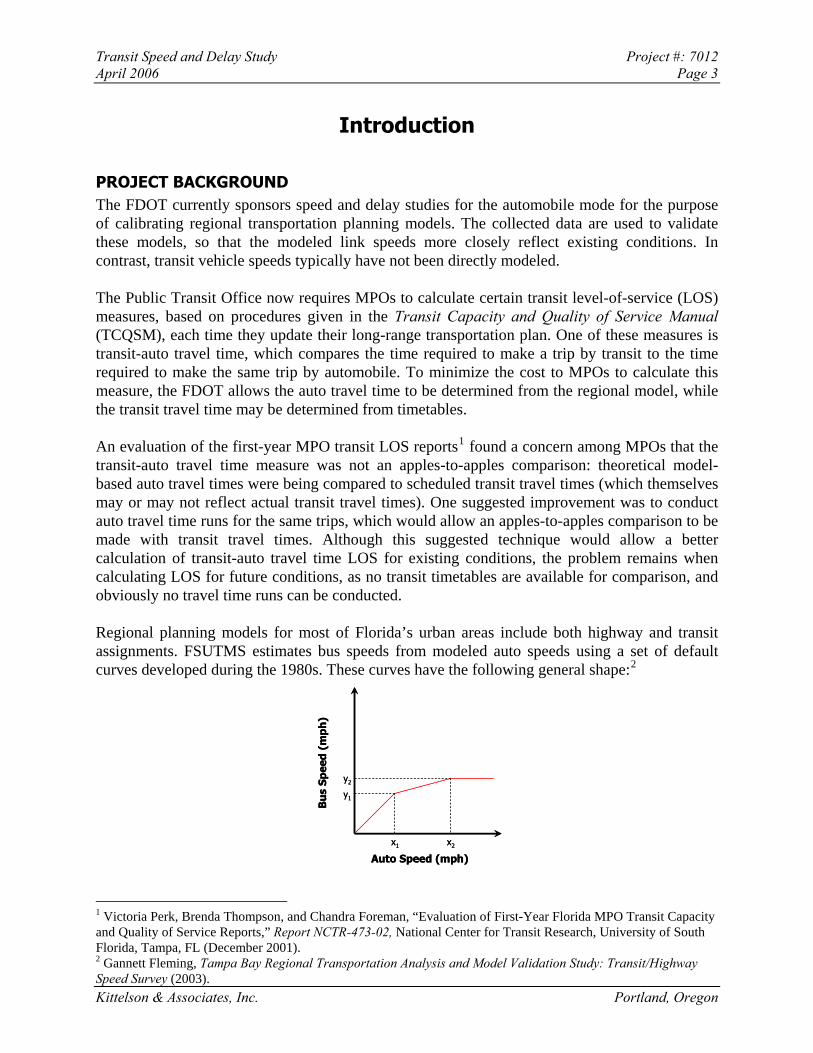
Regional planning models for most of Florida’s urban areas include both highway and transit assignments. FSUTMS estimates bus speeds from modeled auto speeds using a set of default curves developed during the 1980s. These curves have the following general shape:2

Auto Speed (mph)

Bu

s Sp

eed

(mp

h)

x1 x2

y1

y2

Auto Speed (mph)

Bu

s Sp

eed

(mp

h)

x1 x2

y1

y2

1 Victoria Perk, Brenda Thompson, and Chandra Foreman, “Evaluation of First-Year Florida MPO Transit Capacity and Quality of Service Reports,” Report NCTR-473-02, National Center for Transit Research, University of South Florida, Tampa, FL (December 2001).


2 Gannett Fleming, Tampa Bay Regional Transportation Analysis and Model Validation Study: Transit/Highway Speed Survey (2003).


Between 0 and an auto speed x1, bus speeds are lower than auto speeds by a fixed proportion. Between auto speeds x1 and x2, bus speeds continue to be a fixed proportion of auto speeds, but increase at a slower rate than before. Above auto speed x2, FSUMTS assumes a constant speed for buses, y2. Different sets of curves, with different values for x1, x2, y1, and y2, are used for different combinations of roadway facility types and area types. However, a 2003 study in the Tampa Bay area, using a relatively small number of data points, found that the relationship between bus speeds and auto speeds could be modeled as a single linear function for a given facility type/area type combination, rather than the three functions currently used.

Particularly at higher auto speeds, the Tampa finding means that transit speeds continue to increase in proportion to auto speeds, rather than being capped at some maximum value. If true, this finding would mean that FSUTMS is currently underestimating transit speeds. To address this issue, the Jacksonville project seeks to better establish the relationships between bus and auto speeds, thus helping to improve long-range modeling in Florida. This knowledge would result in better decision-making when evaluating and comparing auto and transit improvement projects.

PROJECT PURPOSE This project conducted simultaneous speed and delay studies for the auto and transit modes in selected corridors in Jacksonville, with the primary purpose of developing four models for estimating transit speeds:

1. At a segment level (i.e., a roadway section with a consistent area and facility type), with bus speeds estimated as functions of auto speeds and other factors;

2. At a segment level, with bus speeds estimated as functions of planning-level factors (e.g., daily traffic volumes, facility type, area type, etc.);

3. At a trip level (i.e., one end of a route to another), with bus speeds estimated as functions of auto speeds and other factors; and

4. At a trip level, with bus speeds estimated as a function of planning-level factors.

Additionally, because the timing of this study coincided with other ongoing projects, raw data and/or results from this work have helped support the following additional projects:

• First Coast MPO: Additional urban travel time runs for the automobile mode for use in calibrating the Northeast Regional Planning Model (NERPM);

• Jacksonville Transportation Authority (JTA): “Before” bus travel time runs in corridors where transit signal priority is planned to be installed;

• FDOT Systems Planning Office: Auto and bus travel time results to help support modeling work in Miami-Dade County; and

• NCHRP 3-79 (Measuring and Predicting the Performance of Automobile Traffic on Urban Streets): Exploring the potential use of this project’s results to allow buses equipped with automatic vehicle location (AVL) technology to be used as “probes” on arterial streets, allowing known real-time bus speeds to be converted to estimated real-time auto speeds.



Study Design

STUDY AREA SELECTION AND PROJECT SCOPE The project was originally planned to be jointly funded in 2004 by the Public Transit Office and Systems Planning Office. The funding available at the time permitted either six bus routes to be surveyed for a full day each, or twelve routes for a half-day each, over the course of a single week (Tuesday through Thursday). This would have resulted in 96 directional bus trips paired with 96 directional auto trips during the data collection period, and approximately 775 paired segment travel time observations. The data collection effort would have been approximately 50% greater than an earlier survey conducted in 2003 in the Tampa Bay area.3

The FSUTMS model classifies roadways by both area type (reflecting the surrounding land use) and facility type (reflecting the functional classification and geometric characteristics of the roadway). The area types fall into five major categories: AT 10 (central business districts or CBDs), AT 20 (CBD fringe areas), AT 30 (residential areas), AT 40 (outlying business districts), and AT 50 (rural areas).4 The first four, urban, area types are the ones where public transit service is most likely to be found. Similarly, the facility types fall into nine major categories. Of these, FT 20 (divided arterials), FT 30 (undivided arterials), FT 40 (collectors), and FT 60 (one-way streets) are the facility types where buses are likely to make stops to serve passengers and, therefore, would have travel speeds significantly different than other vehicles on the roadway. The four area types and four facility types of interest result in sixteen combinations of area type and facility type that this project uses to explore speed relationships between autos and buses.

FDOT desired that the region selected for data collection for this project be large enough to supply sufficient examples of the sixteen possible FT/AT combinations to draw statistically valid conclusions. At the same time, FDOT desired that the region be small enough that travel time runs could be conducted across a geographically representative portion of the region. Based on these criteria, the Daytona Beach region was deemed to be too small, while the Orlando region was deemed to be too large. The Jacksonville region, which is the smallest of the Florida metropolitan areas with populations over 1 million, was determined to be the right size.

After the project was initially scoped, FDOT delayed implementation until 2005, with the Public Transit Office taking over the entire funding role. The peak traffic season in Jacksonville occurs during the period between Labor Day and Veterans Day, unlike much of central and southern Florida, where winter is the peak season. By the time data collection commenced in September 2005, two other projects were underway in the Jacksonville area that also required travel time data. One of these projects was the NERPM update; the other was the JTA transit signal priority project. At a coordination meeting held in Jacksonville in early September, representatives of the First Coast MPO and JTA requested that the Public Transit Office fund additional travel time

3 Gannett Fleming, Tampa Bay Regional Transportation Analysis and Model Validation Study: Transit/Highway Speed Survey (2003).


4 FSUTMS models further subdivide the area type and facility type categories—for example, the NERPM model defines five residential area types (AT 31 to AT 35). However, speed and capacity characteristics are generally kept constant within a given category. (Source: URS, Inc., Northeast Regional Planning Model—Model Validation Report.)


data collection to support the needs of those projects. The Public Transit Office agreed to do so, which resulted in the data collection effort being greatly expanded at the last minute.

The final project scope called for data collection to occur on a minimum of 21 routes and a maximum of 27 routes, including a reserve of three days of make-up data collection in the event of tropical storms, hurricanes, severe weather, or major traffic incidents during the data collection period. In the end, data were collected on 26 routes, with one day of data collection being lost due to travel disruptions caused by Hurricane Wilma in South Florida. A total of 508 paired directional trips were made, a five-fold increase from the original plan.

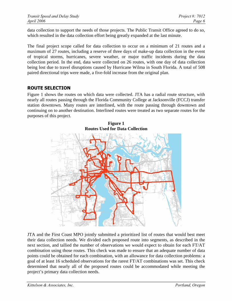
ROUTE SELECTION Figure 1 shows the routes on which data were collected. JTA has a radial route structure, with nearly all routes passing through the Florida Community College at Jacksonville (FCCJ) transfer station downtown. Many routes are interlined, with the route passing through downtown and continuing on to another destination. Interlined routes were treated as two separate routes for the purposes of this project.

Figure 1 Routes Used for Data Collection

JTA and the First Coast MPO jointly submitted a prioritized list of routes that would best meet their data collection needs. We divided each proposed route into segments, as described in the next section, and tallied the number of observations we would expect to obtain for each FT/AT combination using those routes. This check was made to ensure that an adequate number of data points could be obtained for each combination, with an allowance for data collection problems: a goal of at least 16 scheduled observations for the rarest FT/AT combinations was set. This check determined that nearly all of the proposed routes could be accommodated while meeting the project’s primary data collection needs.



Table 1 lists the routes included in the data collection program, and the weeks when data were collected for each route. Many of the routes have some sections where the routes operate non-stop either by design (i.e., S1 and X4) or because the routing includes sections on freeways or expressways (particularly on the approaches to downtown). Only the sections of routes where buses provide local service (i.e., make regular stops) were used in developing segment-based models. However, the entire route, including both local and non-stop sections, was used in developing trip-based models.

Table 1 Data Collection Schedule

Tuesday Wednesday Thursday September 13-15, 2005

R1 (Beaches) L8 (Lem Turner) P2 (Edgewood)/X4 (Orange Park) R1 (FCCJ-Kent) L8 (Ramona) P2 (Townsend)/X4 (Orange Park) S1 (Avenues)* B9 (Beaver/Lane)*

October 11-13 L7 (Soutel) P7 (Normandy) J1 (Mandarin) L7 (Avenues) P7 (FCCJ-North) J1 (University Park)

October 18-20 E2 (Phoenix) P4 (Myrtle Ave) K2 (Beach Blvd) E2 (Orange Park) P4 (Roosevelt) K2 (Amtrak)

October 25-27 Hurricane Wilma R5 (Murray Hill-UNF) R5 (Murray Hill-UNF)

November 1-3 I6 (St. Augustine-Main) I6 (St. Augustine-Main) S1 (Avenues)

November 8-10 B9 (Beaver/Lane) L9 (Lake Forest-Phillips) M5 (Moncrief B)

Make-up data collection as needed *Two data collection teams per route, except those marked with an asterisk.

Table 2 shows the centerline miles of roadway for each FT/AT combination within the JTA service area. To provide an apples-to-apples comparison across combinations, mileage calculated in GIS for FT 20 (divided arterials) and FT 60 (one-way streets) was divided by two. Divided arterial mileage was adjusted to avoid double-counting divided roadway segments (which are indicated by two parallel lines in GIS, rather than a single line). One-way street mileage was adjusted because each line represents only a single direction of travel, rather than two, and thus will generate only half as many observations as the other roadway types.

Table 2 Total Centerline Mileage of FT/AT Combinations in the JTA Service Area

Area Type Facility Type 10 20 30 40

20 0.46 3.81 98.31 28.93 30 5.10 25.81 86.16 6.21 40 4.86 42.22 426.05 31.30 60 6.74 3.40 0.86 1.01



As can be seen from Table 2, certain FT/AT combinations are rare in the Jacksonville area, particularly FT 20/AT 10, FT 60/AT 30, and FT 60/AT 40. The only example of FT 20/AT 10 in Jacksonville is the Acostia Bridge over the St. Johns River, which buses do not stop on. The only example of FT 60/AT 30 with bus service is the College Street/Post Street couplet west of downtown, while the only examples of FT 60/AT 40 with bus service are the one-way service roads along Arlington Expressway.

ROUTE SEGMENTATION Following the basic process used in the earlier Tampa Bay study, each route was divided into a series of segments. The key attribute used to define a segment was having a section of roadway with a consistent area type and facility type. Segments were generally broken at the following locations:

• Where a route turned onto a new street;

• Where the area type or facility type changed; and

• At timepoints (as a bus might need to hold at this location if it was running early).

To provide additional data points, segments that would otherwise be more than 2.5 miles long using the above criteria were split into two segments at a major intersection. For the purposes of developing segment-based models, only segments 0.50 miles in length or longer (0.30 miles for area type 10—CBD) were included in the modeling dataset, as we felt that shorter segments would not provide a sufficiently wide range of opportunities for buses to stop or otherwise be delayed. However, the GPS-based data collection methodology that was used provided bus and auto location observations at 1-3 second intervals, allowing future projects to resegment the data as needed for those projects’ needs. (For example, the Highway Capacity Manual defines roadway segments based on traffic signal locations, rather than area type and facility type.)

In a few situations, multiple streets were combined into a single segment. These situations included:

• Where the facility type is undefined (e.g., roadways internal to a shopping mall);

• Where a route follows several streets through a neighborhood, which would otherwise result in multiple short segments that would not meet the 0.5-mile threshold (e.g., Route M5 along Rhode Island, West Virginia, and Hema); or

• Where a route turns onto a new street, but not at an intersection (e.g., Route B9, where Mother Hubbard Drive makes a 90-degree turn to become Lane Avenue).

In the first case, no model was to be developed for undefined facility types, so there was no need to record times for what would otherwise be shorter segments. Similarly, in the second case, the individual streets would not be used for segment-based modeling, so they were aggregated to a series of streets sharing a common area type and facility type, for use in developing trip-based models. In the third case, where the street name changed, but the traffic flow was not interrupted, combining segments sometimes allowed the 0.5-mile threshold to be reached, resulting in additional observations for the database.



DATA COLLECTION Auto and bus data collectors were paired into teams. Under the original data collection plan, four teams would have collected the data over the course of one week (Tuesday through Thursday). After the data collection scope was increased just prior to the start of data collection efforts, the data collection period was spread over six weeks, with two to six teams active per week, depending on staff availability in a given week.

Two data collection teams were assigned to each route, with the result that four teams were used to cover interlined routes. On any given route, one team started in the morning at the downtown FCCJ Station, while the other team started at the outer end of the route. Both teams made at least one round trip during the morning peak (6:00-9:00 a.m.), one round trip during the late morning (9:00-11:30 a.m.), one round trip during the early afternoon (1:30-4:00 p.m.), and one round trip during the evening peak (4:00-6:30 p.m.). This schedule provided a minimum of eight directional trips per day per team. Additional trips were scheduled when possible, resulting in up to eleven trips per day on some routes. Under this data collection plan, any given segment of a route would have had at least sixteen observations, four for each combination of peak period, off-peak period, peak direction, and off-peak direction.

The bus trips used were selected in advance. The data collection schedule was provided to JTA in advance, so that bus drivers could be made aware that the data collection activities would be occurring. We are uncertain about how well this information was communicated to the bus drivers, but in any event, there were only one or two cases where bus drivers took issue with data collectors being on the bus. All data collectors were provided with customized route maps for their route. The auto drivers transported the bus riders to and from the ends of the routes, as needed. The bus data collectors purchased weekly bus passes to pay for their rides.

Data collectors were equipped with GPS units capable of recording position data at 1-3 second intervals. The bus data collectors were also equipped with Palm Pilots that were connected to the GPS units. The software installed on the Palm Pilots allowed additional data on boardings and alightings by stop, door closings, and locations of “off-line” (i.e., out of the flow of traffic) bus stops to be entered and associated with a particular bus location. Finally, the bus data collectors kept manual records of segment start and end times, boardings and alightings, and unusual delays (e.g., railroad crossing delays, unscheduled driver breaks, etc.), both as a backup in case their GPS unit lost its signal, and to flag potentially unusable observations.

Two approaches were considered for ensuring that the auto and bus members of a team encountered similar traffic conditions. The earlier Tampa Bay study used a “leapfrog” approach, where the auto departed a location at the same time as the bus, drove to the end of the segment, and turned back to wait for the bus to catch up before departing on the next segment. For this work, though, one project aim was to collect trip times in addition to segment times. The leapfrog approach provides similar traffic conditions for segment observations, but does not necessarily reflect the overall trip time that a non-leapfrogging driver would experience. In addition, requiring auto drivers to turn back and wait for buses to catch up could result in the autos artificially falling out of the progression band along arterials, which could also influence the automobile travel time results.



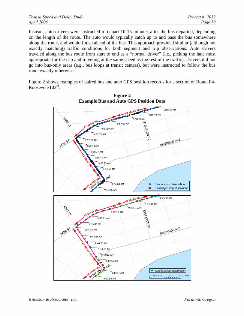
Instead, auto drivers were instructed to depart 10-15 minutes after the bus departed, depending on the length of the route. The auto would typically catch up to and pass the bus somewhere along the route, and would finish ahead of the bus. This approach provided similar (although not exactly matching) traffic conditions for both segment and trip observations. Auto drivers traveled along the bus route from start to end as a “normal driver” (i.e., picking the lane most appropriate for the trip and traveling at the same speed as the rest of the traffic). Drivers did not go into bus-only areas (e.g., bus loops at transit centers), but were instructed to follow the bus route exactly otherwise.

Figure 2 shows examples of paired bus and auto GPS position records for a section of Route P4-Roosevelt/103rd.

Figure 2 Example Bus and Auto GPS Position Data

PARK ST

KING ST

RIVERSIDE AVE

STOCKTO

N ST

SAINT JOHNS AVE

9:58:56 AM

9:58:46 AM

9:58:02 AM

9:57:50 AM

9:57:39 AM

9:57:32 AM

9:57:22 AM

9:56:44 AM

9:56:37 AM

9:56:31 AM

9:56:23 AM

9:54:53 AM

9:54:09 AM

9:53:56 AM

Bus location observationPassenger stop observation

FT 30/AT 30

FT 30/AT 30

FT 30/AT 20

FT 40/AT 30

!

!

!!!

!

!

!

!

!!

!

!

!

!

!

!

!

!

!

!

!

!

!

!

!!

!!

!!

!!

!!

!

PARK ST

KING ST

RIVERSIDE AVE

STOCKTO

N ST

SAINT JOHNS AVE

9:45:50 AM

9:45:41 AM

9:45:31 AM

9:45:21 AM

9:45:11 AM

9:45:04 AM

9:44:37 AM

9:44:26 AM

9:44:20 AM

9:44:16 AM

9:44:12 AM

9:44:06 AM

9:43:11 AM

9:42:54 AM

FT 30/AT 30

FT 30/AT 30

FT 30/AT 20

FT 40/AT 30

0 0.05 0.1 0.150.025 Miles

! Auto location observation



In the upper portion of Figure 2, each small dot represents the bus’ position at 1-second intervals, while in the lower portion, each small dot represents the auto’s position at approximately 3-second intervals while moving. The two larger dots in the upper portion show locations where the bus stopped to pick up or drop off passengers. It can be seen that it took the bus about two minutes longer than the auto to travel this section of the route, a result of stopping twice to serve passengers. The bus also experienced delay crossing Riverside Avenue that the auto did not experience.

It can also be seen from Figure 2 that segments were often fairly short—there are five different segments (St. Johns Avenue, King Street from St. Johns to Riverside, King Street from Riverside to Park, Park from King to one block west of Stockton, and the remainder of Park) within this 0.75-mile section of the route.

The following data were collected for each observation at the segment level:

• Auto travel time;5

• Bus travel time;

• Direction (peak vs. off-peak);

• Time of day (peak vs. off-peak);

• Facility type;

• Area type;

• Segment length;

• Passenger boardings and alightings;

• Number of stops to serve passengers; and

• Average annual daily traffic (AADT).

The number of traffic signals along the route was not included in the scoped data collection list. However, during the modeling phase of the project, we tried to obtain this information to include as another independent variable. Information on traffic signal locations was available for FDOT facilities; however, we were unsuccessful in obtaining such information for non-FDOT facilities. As a result, number of traffic signals was included as additional information for some segments, but not for trips. We also created a variable for whether the bus route turned left at the end of the segment (as opposed to continuing straight on the street, or turning right).

The following data were collected for each observation at the trip level:

• Auto travel time;

• Bus travel time;

• Direction (peak vs. off-peak);


5 Auto and bus travel times were computed from the middle of the intersection starting a segment to the middle of the intersection ending a segment. As a result, any traffic signal delay at the end of the segment is included in the segment travel time. Any signal delay at the intersection beginning the segment is assigned to the previous segment.


• Time of day (peak vs. off-peak);

• Number of turns (left and right);

• Number of bus stops (near-side, far-side, mid-block);

• Length (overall, by FT, and by AT);

• Passenger boardings and alightings; and

• Number of stops to serve passengers.

Problems that caused scheduled data collection runs to be missed were noted as they occurred, and make-up data collection was scheduled during the last week to address missing runs.

DATA REDUCTION The final step prior to analyzing the data was to reduce all of the collected data into a form usable for statistical modeling. A master spreadsheet was set up in Excel to hold all of the data. Separate worksheets within the spreadsheet were used to store general segment characteristics (e.g., length), general route characteristics (e.g., number of bus stops), individual segment observations, and individual trip observations.

GPS data from each auto trip were individually checked (1) to verify that GPS data existed for enough of the trip to be able to determine whether or not the driver followed the route correctly, and (2) to verify that the auto driver did indeed follow the route correctly. Trip observations were flagged as “lost driver” and not used for trip-based modeling in cases where the route was not followed correctly, except when the driver was able to recover immediately and not lose more than 30 seconds of time. Segment observations were flagged and discarded in cases where the driver turned too soon. Trip observations were flagged as “GPS problem” and not used for trip-based modeling when the GPS signal was lost through a section where the route made a turn.

GPS data and comments written on the backup sheets for each bus trip were individually checked for similar potential data problems. Issues that could cause either a bus trip or segment observation to be discarded included: the bus driver going off-route (e.g., due to a construction detour), unscheduled stops at convenience stores, railroad crossing delays, or a combination of both the GPS signal being lost and segment start/end times not being recorded to the second on the backup sheets.

Checks were also run on the calculated auto and bus segment speeds as an additional data verification step. Cases where the auto or bus speeds were unusually high or low, or where the auto and bus speeds varied by more than a factor of three were reviewed and, if a problem was identified, corrected. In some cases—typically situations where the bus GPS signal had been lost and the data collector apparently incorrectly identified the end of a segment—the calculated bus speeds were obviously incorrect (e.g., 70 mph on an arterial street), but could not be corrected. In these cases, the observations were flagged and discarded.



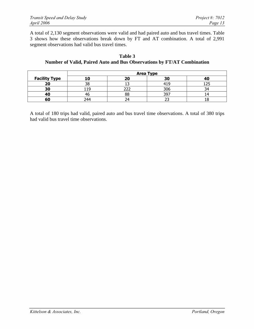
A total of 2,130 segment observations were valid and had paired auto and bus travel times. Table 3 shows how these observations break down by FT and AT combination. A total of 2,991 segment observations had valid bus travel times.

Table 3 Number of Valid, Paired Auto and Bus Observations by FT/AT Combination


20 38 13 419 125 30 119 222 306 34 40 46 88 397 14 60 244 24 23 18

A total of 180 trips had valid, paired auto and bus travel time observations. A total of 380 trips had valid bus travel time observations.



Analysis and Findings

OVERVIEW Data from the master Excel spreadsheet were imported into SPSS version 14 for statistical modeling. As noted previously, four model types were investigated:

1. At a segment (i.e., a roadway section with a consistent area and facility type) level, with bus speeds estimated as functions of auto speeds and other factors);

2. At a segment level, with bus speeds estimated as functions of planning-level factors (e.g., daily traffic volumes, facility type, area type, etc.);

3. At a trip (i.e., one end of a route to another) level, with bus speeds estimated as functions of auto speeds and other factors; and

4. At a trip level, with bus speeds estimated as functions of planning-level factors.

The following sections describe the development of, and results from, each of these model types.

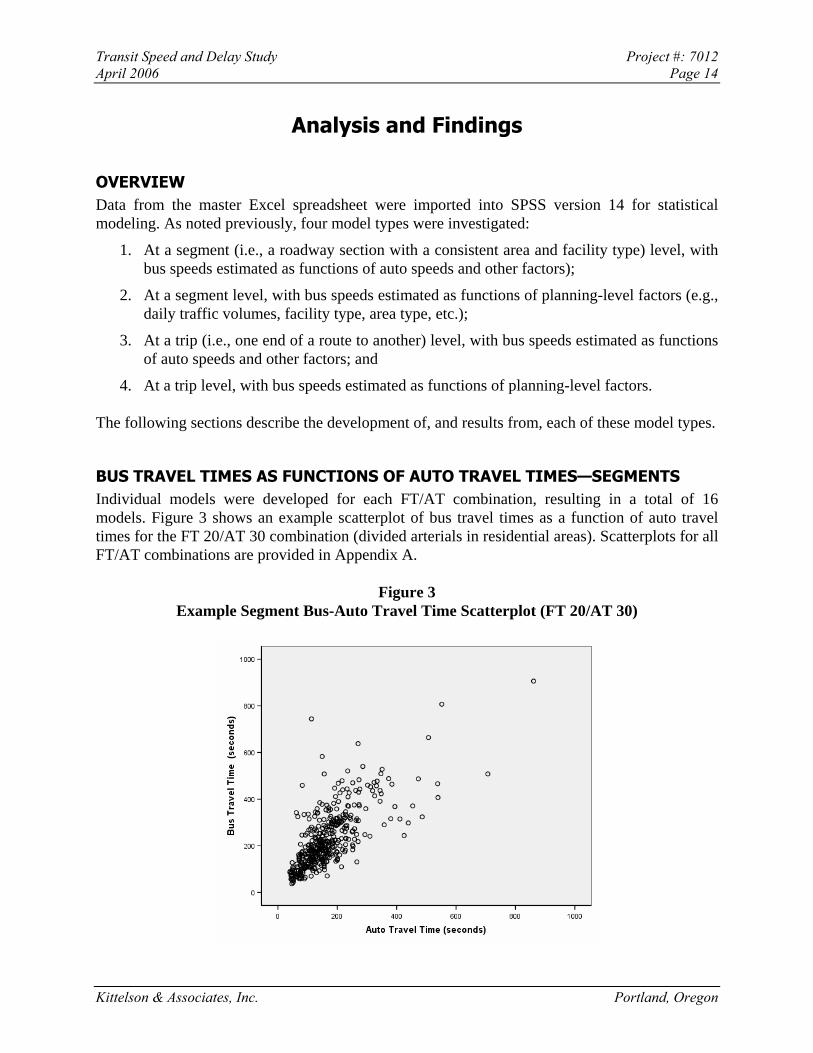
BUS TRAVEL TIMES AS FUNCTIONS OF AUTO TRAVEL TIMES—SEGMENTS Individual models were developed for each FT/AT combination, resulting in a total of 16 models. Figure 3 shows an example scatterplot of bus travel times as a function of auto travel times for the FT 20/AT 30 combination (divided arterials in residential areas). Scatterplots for all FT/AT combinations are provided in Appendix A.

Figure 3 Example Segment Bus-Auto Travel Time Scatterplot (FT 20/AT 30)



Although this particular FT/AT combination has more observations than any other, it is representative of the general patterns observed within all of the various combinations. In particular, there are two patterns of note: (1) there is visually a linear relationship between bus and auto travel times (later confirmed through statistical analysis), and (2) the spread of the observations increases as the auto travel time increases. Because we were able to obtain good fits to the data with linear models, we did not attempt to fit curve-based models.

The funnel-shaped pattern of the data, reflecting increasing spread in the data with increasing values of auto travel time, suggested that a basic linear regression model would not be sufficient, as one of the assumptions of linear regression is that the data have an equal spread. One approach to address this issue is to transform the data, which is often a good approach when the relationship appears curved and the spread increases. We tried a log transformation of both the dependent and independent variables, which was able to maintain the linear relationship of the data and which equalized the spread. The problem with transforming the data is that the resulting model is more difficult to interpret and understand: instead of a model where bus travel time is a simple factor of the auto travel time (e.g., Bus_Time = β1 * Auto_Time), the resulting model would be in the form of ln(Bus_Time) = β0 + β1 * ln(Auto_Time), plus any other variables that might be added to the model. In addition, because the untransformed data already had a linear relationship, introducing a transformation may result in an inappropriate relationship between the data in the new model.

Another approach in this situation is to use a weighted least squares regression. In this kind of regression, each data point is weighted by another variable when determining its influence on the final model. This weighting gives the data points with lower variance greater weight in fitting the model, with the goal of equalizing the spread between the model’s fitted values and the actual observations. A number of different weighting variables were tried, with the inverse of auto travel time providing the best results. The weighted model provides the same basic model form as a standard regression model (e.g., Bus_Time = β1 * Auto_Time); however, the fitted coefficient values are different and the standard deviations of the model coefficients are lower.

No regression constants (i.e., the β0 term in Bus_Time = β0 + β1 * Auto_Time) were used in fitting these models. That is, the models force the bus travel time (or speed) to be zero when the auto travel time is zero, which makes intuitive sense. It should be noted that the adjusted r2 values for models fitted without constants cannot be directly compared to the values for models fitted with constants, and will generally be quite a bit higher than the corresponding adjusted r2

values obtained from models with constants.

The full range of available variables were tested. Model forms that had significant relationships between the dependent and independent variables, in at least some cases, were the following:

1. Bus_Time = β1 * Auto_Time;

2. Bus_Time = β1 * Auto_Time + β2 * Bus_On + β3 * Bus_Off;

3. Bus_Time = β1 * Auto_Time + β2 * Bus_Stops; and

4. Bus_Speed = β1 * Auto_Speed



where Bus_On is the number of passengers boarding within a segment, Bus_Off is the number of passengers alighting within a segment, and Bus_Stop is the number of times the bus stopped within the segment to serve passengers.

Model #1, where bus travel time is a function of auto travel time, may be the most appropriate for incorporation into FSUTMS, as it does not require prior knowledge or estimation of transit boardings within a segment, and all of the model combinations have good fits. Travel times would need to be converted to speeds for use in regional modeling, based on known lengths of links within a FSUTMS model. Model #4 is similar to model #1, but is based directly on speed relationships, and thus would require fewer computations to implement in FSUTMS. Model #4’s fit was about as good as model #1’s—sometimes better, sometimes worse. However, model #4 does not lend itself to adding additional variables reflecting passenger activity and the number of stops made, because a fixed amount of delay associated with a stop will have a variable impact on speed, depending on the length of the segment. We believe it is more intuitive and ultimately more accurate to calculate travel time first and then convert the result to a speed.

In only 7 of 16 cases, the passenger boarding and alighting variables (model #2) were significant. This model form would be harder to apply in FSUTMS, as it requires knowledge of passenger activity and the relationships between the variables are not straightforward. Every bus stop entails a relatively fixed amount of delay associated with acceleration and deceleration, a variable amount of delay associated with passenger boarding and alighting activity, possible delay associated with waiting for a traffic signal to turn green after serving passengers, and possible delay merging back into traffic. Three of these four sources of delay are unrelated, or only minimally related, to passenger activity. Further, delay will be different depending on whether the passenger activity occurs at a single stop or multiple stops, and whether alighting passengers use the rear door while boarding passengers use the front door.

Model #3, which added a variable for the number of times the bus stopped to serve passengers within a segment, generally had the best fit. It was significant in 10 of 16 models; the models where it was not significant had 46 or fewer observations to work with. The value of the coefficient for the Bus_Stops variable ranged from 18.4 to 47.5 across the various FT/AT combinations. The Bus_Stops coefficient value reflects the average bus delay per stop, which is a combination of average dwell time, acceleration/deceleration delays, and traffic and signal delays exiting the stop. This model form is quite intuitive, as it allows bus travel time to be a fixed multiple of auto travel time, with a fixed amount of additional average delay for each stop made within a segment.

No significant difference in relative bus and auto segment travel times was found during peak periods or in peak vs. off-peak directions. That is, while overall travel times might be longer during peak periods, bus travel times appear to be the same proportion of auto times during peak periods as in off-peak periods. This finding is the same as the Tampa Bay study’s.

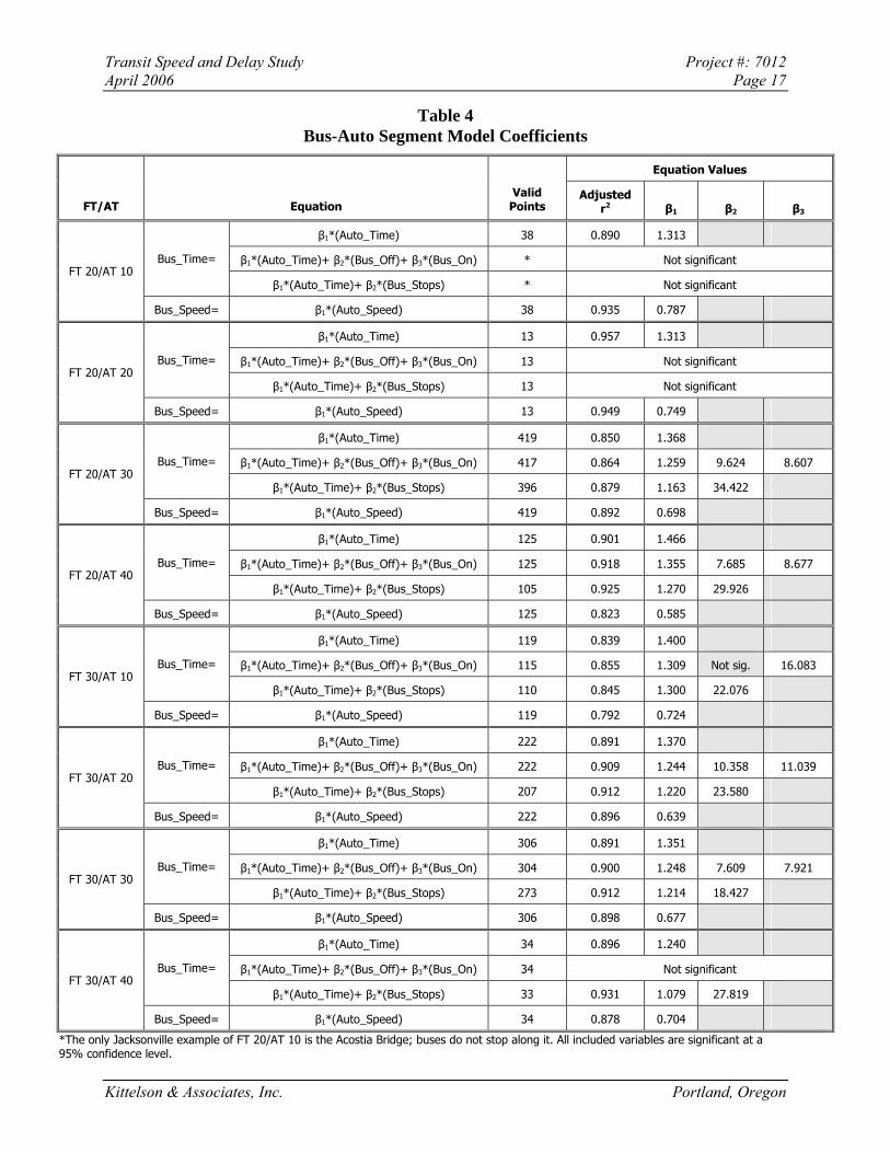
Table 4 provides the coefficients and adjusted r2 values for each of the four models for each of the 16 FT/AT combinations.



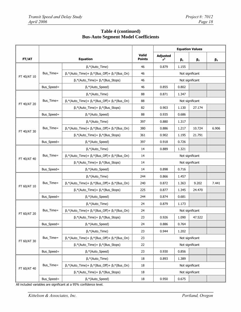
Table 4 Bus-Auto Segment Model Coefficients

Equation Values

FT/AT Equation Valid

Points Adjusted

r2 β1 β2 β3

β1*(Auto_Time) 38 0.890 1.313

β1*(Auto_Time)+ β2*(Bus_Off)+ β3*(Bus_On) * Not significant Bus_Time=

β1*(Auto_Time)+ β2*(Bus_Stops) * Not significant FT 20/AT 10

Bus_Speed= β1*(Auto_Speed) 38 0.935 0.787

β1*(Auto_Time) 13 0.957 1.313

β1*(Auto_Time)+ β2*(Bus_Off)+ β3*(Bus_On) 13 Not significant Bus_Time=

β1*(Auto_Time)+ β2*(Bus_Stops) 13 Not significant FT 20/AT 20


β1*(Auto_Time) 419 0.850 1.368

β1*(Auto_Time)+ β2*(Bus_Off)+ β3*(Bus_On) 417 0.864 1.259 9.624 8.607 Bus_Time=

β1*(Auto_Time)+ β2*(Bus_Stops) 396 0.879 1.163 34.422 FT 20/AT 30


β1*(Auto_Time) 125 0.901 1.466




β1*(Auto_Time) 119 0.839 1.400

β1*(Auto_Time)+ β2*(Bus_Off)+ β3*(Bus_On) 115 0.855 1.309 Not sig. 16.083 Bus_Time=



β1*(Auto_Time) 222 0.891 1.370




β1*(Auto_Time) 306 0.891 1.351




β1*(Auto_Time) 34 0.896 1.240




*The only Jacksonville example of FT 20/AT 10 is the Acostia Bridge; buses do not stop along it. All included variables are significant at a 95% confidence level.



Table 4 (continued) Bus-Auto Segment Model Coefficients

Equation Values

FT/AT Equation Valid

Points Adjusted

r2 β1 β2 β3

β1*(Auto_Time) 46 0.879 1.155




β1*(Auto_Time) 88 0.871 1.347




β1*(Auto_Time) 397 0.880 1.317




β1*(Auto_Time) 14 0.889 1.321




β1*(Auto_Time) 244 0.866 1.457




β1*(Auto_Time) 24 0.879 1.173




β1*(Auto_Time) 23 0.944 1.202




β1*(Auto_Time) 18 0.893 1.389




All included variables are significant at a 95% confidence level.



Comparisons Within Facility Types The Jacksonville data were examined to see whether significant differences existed between area types within individual facility types. Dummy variables (i.e., variables with a value of either 1 or 0) were set up for each area type, and multiple regression models were tested with forms similar to this: Bus_Time = β1 * Auto_Time + β2 * AT10_ATT + β3 * AT20_ATT + β4 * AT30_ATT, where ATxx_ATT is the ATxx dummy variable multiplied by the auto travel time. In this example, AT 40 would be represented by the base model Bus_Time = β1 * Auto_Time. If there was a significant auto travel time difference between (say) AT 10 and AT 40, the AT10_ATT variable would show up as significant and its coefficient β2 would represent the additional increment (positive or negative) of bus vs. auto travel time rate associated with AT 10. If none of the ATxx_ATT variables are significant at the 95% level when added to the regression model, it can be concluded that area type does not improve the model fit and that a single model based on data from all area types can be developed to cover a given facility type.

When only auto travel time was included in the regression, there was no significant difference among area types for a given facility type, although AT 30 was marginally not significantly different than the other area types for FT 20 (p = 0.051). Similarly, when both auto travel time and number of bus stops made within the segment were included in the regression model, there was no significant difference among area types for any of the facility types. Table 5 presents the combined models resulting from this analysis.

Table 5 Bus-Auto Segment Combined Model Coefficients

Equation Values

FT AT Bus Travel Time Equation Valid

Points Adj. r2 β1 β2

all β1*(Auto_Time) 595 0.867 1.393 20

all β1*(Auto_Time) + β2*(Bus_Stops) 551 0.893 1.196 32.533

all β1*(Auto_Time) 681 0.884 1.359 30


all β1*(Auto_Time) 545 0.878 1.310 40


all β1*(Auto_Time) 309 0.870 1.409 60




Comparisons to Previous Studies Table 6 compares the Jacksonville bus speed coefficients to the Tampa Bay models’.

Table 6 Bus Speed Coefficient Comparison: Jacksonville vs. Tampa Bay


20 0.787 (0.872) 0.749 (0.978) 0.698 (0.809) 0.585 (0.771) 30 0.724 (0.504) 0.639 (0.764) 0.677 (0.808) 0.704 (0.670) 40 0.802 (0.713) 0.686 (0.804) 0.726 (0.917) 0.716 (0.670) 60 0.682 (0.740) 0.764 (0.697) 0.856 (0.827) 0.675 (0.758)

##: Jacksonville coefficient value, (##): Tampa Bay coefficient value

Gannett Fleming generously provided a copy of the Tampa Bay dataset, which allowed us to statistically compare the Jacksonville speed results to the Tampa results. There was no significant difference in the model coefficients between the two datasets for 14 of the 16 FT/AT combinations, although FT 60/AT 40 was marginally not significant (p = 0.059). The two exceptions were:

• FT 20/AT 40: Tampa bus speeds averaged 3.9 mph higher (125 data points in the Jacksonville dataset and 59 in the Tampa dataset); and

• FT 40/AT 30: Tampa bus speeds averaged 4.3 mph higher (397 data points in the Jacksonville dataset and 19 in the Tampa dataset).

For the large majority of FT/AT combinations, the Jacksonville and Tampa results are statistically the same. For FT 20/AT 40 and FT 40/AT 30, enough different roadways were represented in the two datasets that one cannot simply attribute the differences to having a small sample of roadways to work with. Because the Tampa study did not collect bus passenger activity data, it is not possible to check whether passenger activity contributed to the difference in speeds for these two combinations. Nevertheless, it can be concluded that the Tampa bus speeds were statistically similar to, or higher than, the Jacksonville bus speeds in every case. It can also be concluded from the Tampa and Jacksonville data that a single linear function can be used to estimate bus speeds from auto speeds for a given FT/AT combination, and that maximum observed bus speeds in the field are higher than FSUTMS’s estimates. The similarities between the Tampa and Jacksonville results also suggest that the Jacksonville results may be applicable to other regions in Florida.

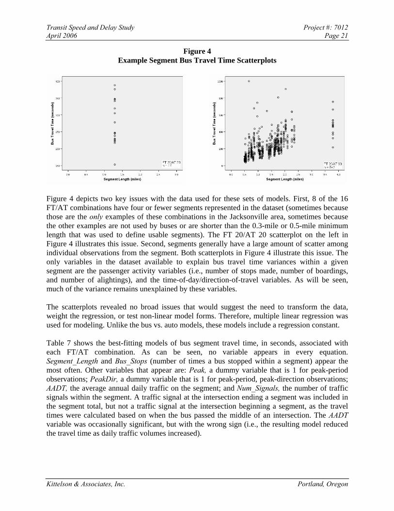
BUS TRAVEL TIMES AS FUNCTIONS OF PLANNING-LEVEL VARIABLES—SEGMENTS This set of models attempts to forecast bus travel time as a function of data that would be readily available at a planning level. Individual models were developed for each FT/AT combination, resulting in a total of 16 models. Figure 4 shows an example scatterplot of bus travel times as a function of segment length for the FT 20/AT 20 combination (divided arterials in the CBD fringe) and the FT 20/AT 30 combination (divided arterials in residential areas). Scatterplots for all FT/AT combinations are provided in Appendix B.



Figure 4 Example Segment Bus Travel Time Scatterplots

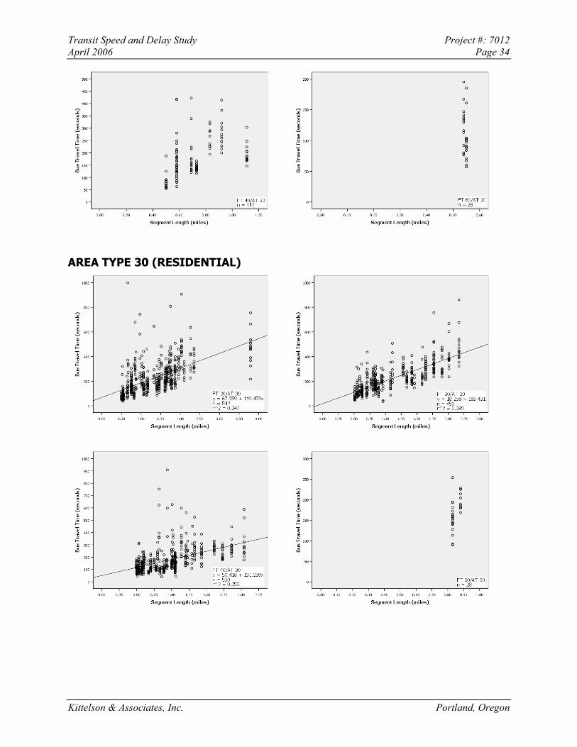
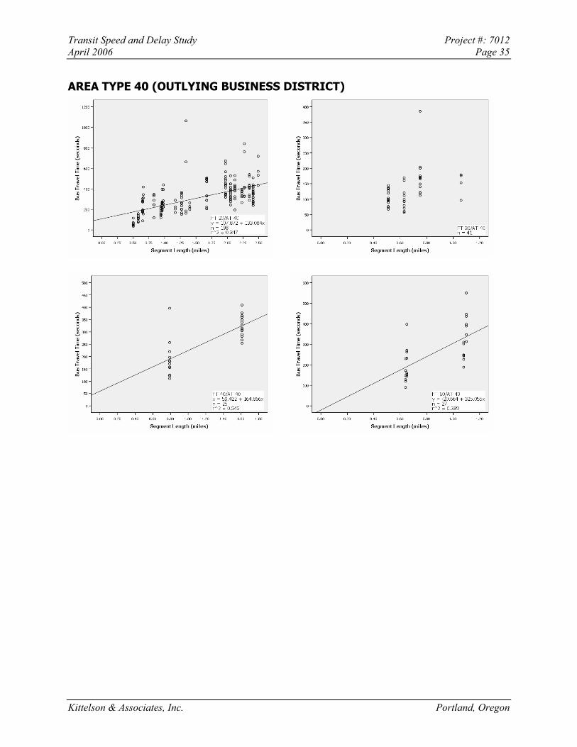
Figure 4 depicts two key issues with the data used for these sets of models. First, 8 of the 16 FT/AT combinations have four or fewer segments represented in the dataset (sometimes because those are the only examples of these combinations in the Jacksonville area, sometimes because the other examples are not used by buses or are shorter than the 0.3-mile or 0.5-mile minimum length that was used to define usable segments). The FT 20/AT 20 scatterplot on the left in Figure 4 illustrates this issue. Second, segments generally have a large amount of scatter among individual observations from the segment. Both scatterplots in Figure 4 illustrate this issue. The only variables in the dataset available to explain bus travel time variances within a given segment are the passenger activity variables (i.e., number of stops made, number of boardings, and number of alightings), and the time-of-day/direction-of-travel variables. As will be seen, much of the variance remains unexplained by these variables.

The scatterplots revealed no broad issues that would suggest the need to transform the data, weight the regression, or test non-linear model forms. Therefore, multiple linear regression was used for modeling. Unlike the bus vs. auto models, these models include a regression constant.

Table 7 shows the best-fitting models of bus segment travel time, in seconds, associated with each FT/AT combination. As can be seen, no variable appears in every equation. Segment_Length and Bus_Stops (number of times a bus stopped within a segment) appear the most often. Other variables that appear are: Peak, a dummy variable that is 1 for peak-period observations; PeakDir, a dummy variable that is 1 for peak-period, peak-direction observations; AADT, the average annual daily traffic on the segment; and Num_Signals, the number of traffic signals within the segment. A traffic signal at the intersection ending a segment was included in the segment total, but not a traffic signal at the intersection beginning a segment, as the travel times were calculated based on when the bus passed the middle of an intersection. The AADT variable was occasionally significant, but with the wrong sign (i.e., the resulting model reduced the travel time as daily traffic volumes increased).



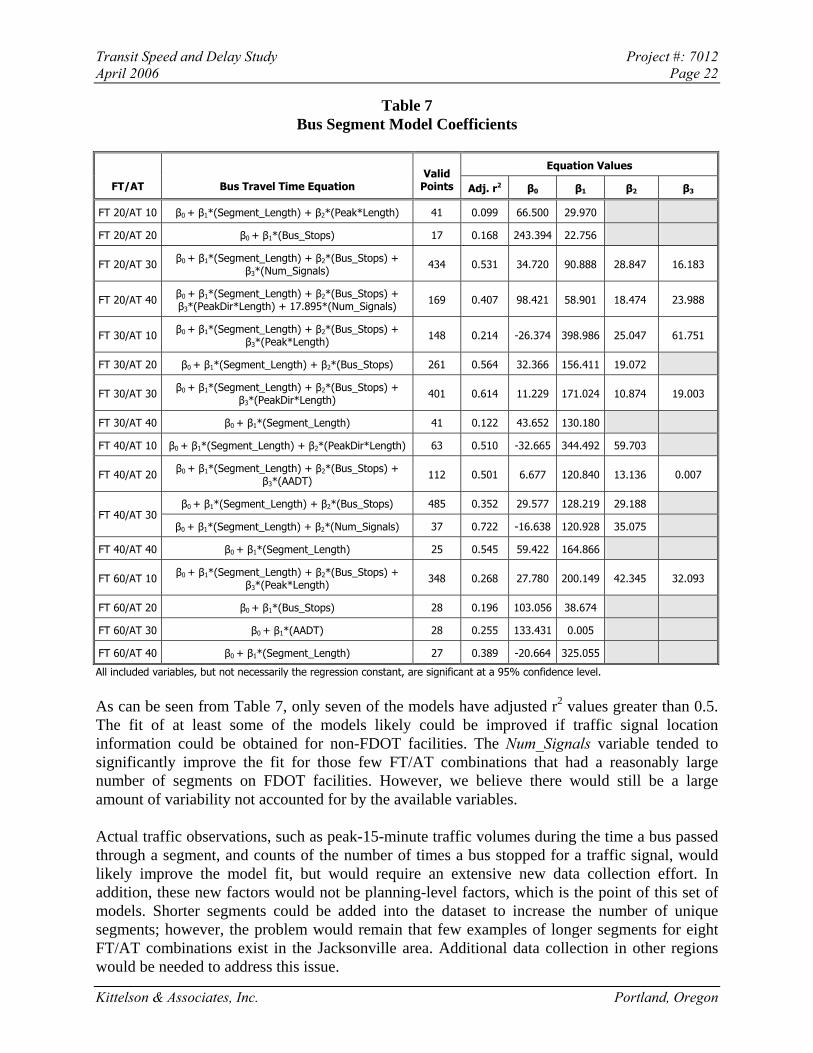
Table 7 Bus Segment Model Coefficients

Equation Values

FT/AT Bus Travel Time Equation Valid

Points Adj. r2 β0 β1 β2 β3

FT 20/AT 10 β0 + β1*(Segment_Length) + β2*(Peak*Length) 41 0.099 66.500 29.970

FT 20/AT 20 β0 + β1*(Bus_Stops) 17 0.168 243.394 22.756

FT 20/AT 30 β0 + β1*(Segment_Length) + β2*(Bus_Stops) + β3*(Num_Signals) 434 0.531 34.720 90.888 28.847 16.183

FT 20/AT 40 β0 + β1*(Segment_Length) + β2*(Bus_Stops) + β3*(PeakDir*Length) + 17.895*(Num_Signals) 169 0.407 98.421 58.901 18.474 23.988

FT 30/AT 10 β0 + β1*(Segment_Length) + β2*(Bus_Stops) + β3*(Peak*Length) 148 0.214 -26.374 398.986 25.047 61.751

FT 30/AT 20 β0 + β1*(Segment_Length) + β2*(Bus_Stops) 261 0.564 32.366 156.411 19.072

FT 30/AT 30 β0 + β1*(Segment_Length) + β2*(Bus_Stops) + β3*(PeakDir*Length) 401 0.614 11.229 171.024 10.874 19.003

FT 30/AT 40 β0 + β1*(Segment_Length) 41 0.122 43.652 130.180

FT 40/AT 10 β0 + β1*(Segment_Length) + β2*(PeakDir*Length) 63 0.510 -32.665 344.492 59.703

FT 40/AT 20 β0 + β1*(Segment_Length) + β2*(Bus_Stops) + β3*(AADT) 112 0.501 6.677 120.840 13.136 0.007

β0 + β1*(Segment_Length) + β2*(Bus_Stops) 485 0.352 29.577 128.219 29.188 FT 40/AT 30

β0 + β1*(Segment_Length) + β2*(Num_Signals) 37 0.722 -16.638 120.928 35.075

FT 40/AT 40 β0 + β1*(Segment_Length) 25 0.545 59.422 164.866

FT 60/AT 10 β0 + β1*(Segment_Length) + β2*(Bus_Stops) + β3*(Peak*Length) 348 0.268 27.780 200.149 42.345 32.093

FT 60/AT 20 β0 + β1*(Bus_Stops) 28 0.196 103.056 38.674

FT 60/AT 30 β0 + β1*(AADT) 28 0.255 133.431 0.005

FT 60/AT 40 β0 + β1*(Segment_Length) 27 0.389 -20.664 325.055

All included variables, but not necessarily the regression constant, are significant at a 95% confidence level.

As can be seen from Table 7, only seven of the models have adjusted r2 values greater than 0.5. The fit of at least some of the models likely could be improved if traffic signal location information could be obtained for non-FDOT facilities. The Num_Signals variable tended to significantly improve the fit for those few FT/AT combinations that had a reasonably large number of segments on FDOT facilities. However, we believe there would still be a large amount of variability not accounted for by the available variables.

Actual traffic observations, such as peak-15-minute traffic volumes during the time a bus passed through a segment, and counts of the number of times a bus stopped for a traffic signal, would likely improve the model fit, but would require an extensive new data collection effort. In addition, these new factors would not be planning-level factors, which is the point of this set of models. Shorter segments could be added into the dataset to increase the number of unique segments; however, the problem would remain that few examples of longer segments for eight FT/AT combinations exist in the Jacksonville area. Additional data collection in other regions would be needed to address this issue.



If more reliable speed or travel time estimation techniques exist at the segment level for the auto mode, an easier solution would be to first estimate the auto speed, and then convert it to a bus speed or travel time using one of the models developed in the previous section. One of the tasks of the ongoing NCHRP 3-79 project is to develop improved auto speed prediction methods at the segment (signalized intersection to signalized intersection) level.

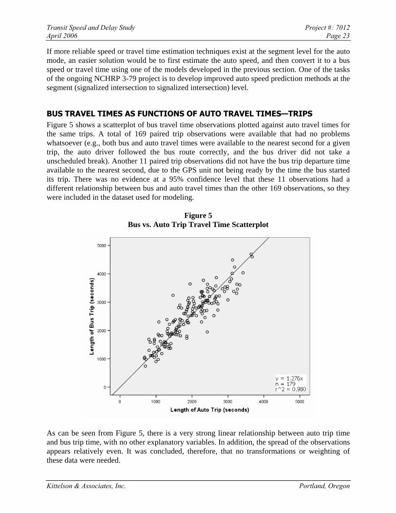
BUS TRAVEL TIMES AS FUNCTIONS OF AUTO TRAVEL TIMES—TRIPS Figure 5 shows a scatterplot of bus travel time observations plotted against auto travel times for the same trips. A total of 169 paired trip observations were available that had no problems whatsoever (e.g., both bus and auto travel times were available to the nearest second for a given trip, the auto driver followed the bus route correctly, and the bus driver did not take a unscheduled break). Another 11 paired trip observations did not have the bus trip departure time available to the nearest second, due to the GPS unit not being ready by the time the bus started its trip. There was no evidence at a 95% confidence level that these 11 observations had a different relationship between bus and auto travel times than the other 169 observations, so they were included in the dataset used for modeling.

Figure 5 Bus vs. Auto Trip Travel Time Scatterplot

As can be seen from Figure 5, there is a very strong linear relationship between auto trip time and bus trip time, with no other explanatory variables. In addition, the spread of the observations appears relatively even. It was concluded, therefore, that no transformations or weighting of these data were needed.



The model forms that were tested for these data were similar to those tested for bus vs. auto times at the segment level. However, individual segments have consistent facility and area types, while each trip passed through a variety of facility and area types. Therefore, dummy variables for the different area and facility types were tested as part of the model development; however, these were not found to be significant. As was done for the bus vs. auto segment models, no constant was used in the tested models, which forces the modeled bus travel time to be zero when the auto travel time is zero.

Table 8 provides the coefficients and adjusted r2 values for the model forms where the independent variables were significant at a 95% confidence level.

Table 8 Bus-Auto Trip Model Coefficients

Equation Values

Equation Valid

Points Adjusted r2 β1 β2 β3

β1*(Auto_Time) 180 0.980 1.276


β1*(Auto_Time)+ β2*(Bus_Stops) 84 0.987 1.086 20.807


All included variables are significant at a 95% confidence level.

All of the model forms in Table 8 have the expected signs for their coefficients, and all have good fits to the data. The same advantages and disadvantages discussed for the bus vs. auto segment models also apply to these models. As with the bus vs. auto segment models, peak time and peak direction did not add significance to the model fit.

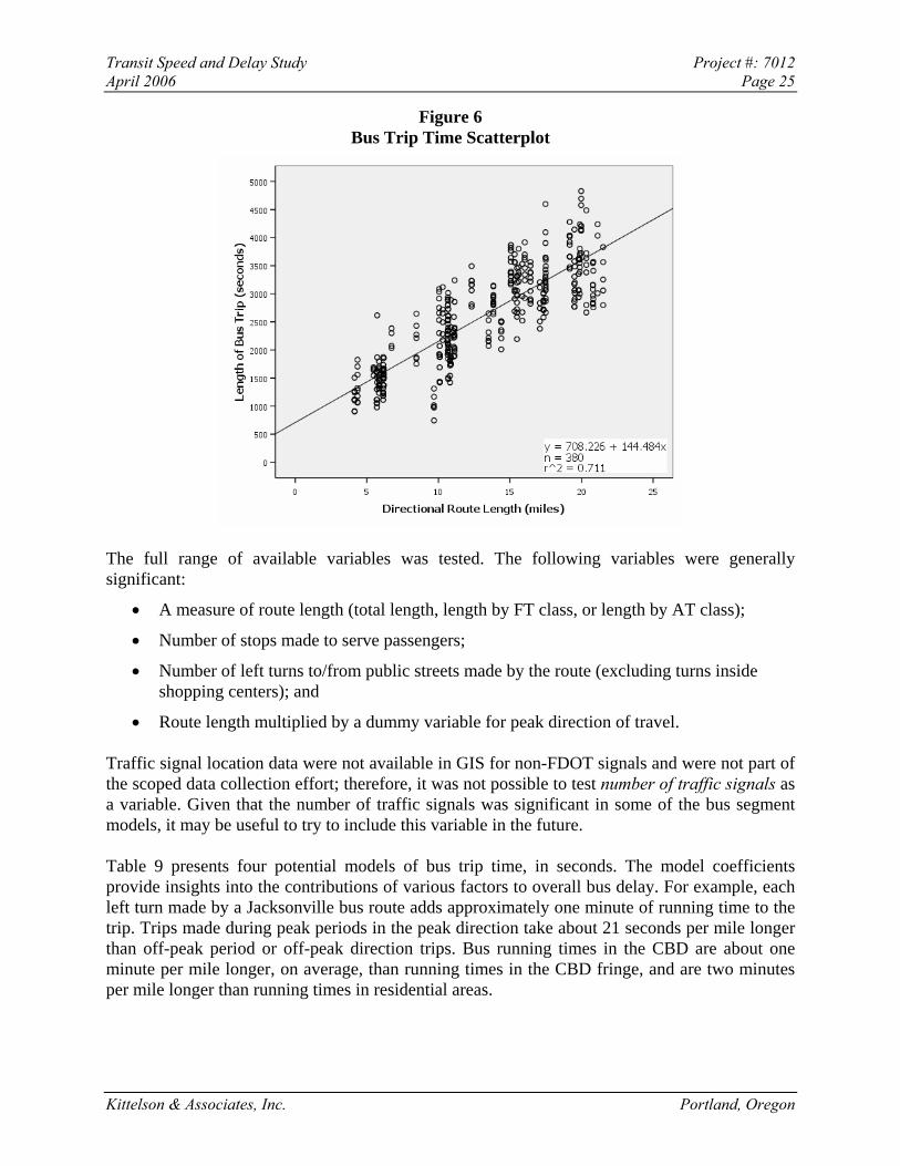
BUS TRAVEL TIMES AS FUNCTIONS OF PLANNING-LEVEL VARIABLES—TRIPS Figure 6 shows a scatterplot of bus travel time observations for trips plotted against trip length. A total of 352 trip observations were available that had no problems whatsoever. Another 28 observations did not have the bus trip departure time available to the nearest second, due to the GPS unit not being ready by the time the bus started its trip. There was no evidence at a 95% confidence level that these 28 observations had different bus trip time relationships than the other 352 observations, and so they were included in the dataset used for modeling.



Figure 6 Bus Trip Time Scatterplot

The full range of available variables was tested. The following variables were generally significant:

• A measure of route length (total length, length by FT class, or length by AT class);

• Number of stops made to serve passengers;

• Number of left turns to/from public streets made by the route (excluding turns inside shopping centers); and

• Route length multiplied by a dummy variable for peak direction of travel.

Traffic signal location data were not available in GIS for non-FDOT signals and were not part of the scoped data collection effort; therefore, it was not possible to test number of traffic signals as a variable. Given that the number of traffic signals was significant in some of the bus segment models, it may be useful to try to include this variable in the future.

Table 9 presents four potential models of bus trip time, in seconds. The model coefficients provide insights into the contributions of various factors to overall bus delay. For example, each left turn made by a Jacksonville bus route adds approximately one minute of running time to the trip. Trips made during peak periods in the peak direction take about 21 seconds per mile longer than off-peak period or off-peak direction trips. Bus running times in the CBD are about one minute per mile longer, on average, than running times in the CBD fringe, and are two minutes per mile longer than running times in residential areas.



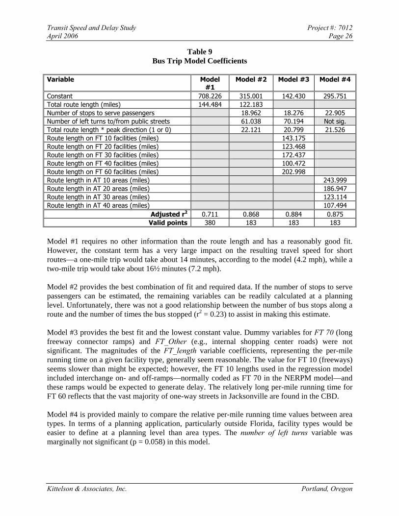
Table 9 Bus Trip Model Coefficients

Variable Model #1

Model #2 Model #3 Model #4

Constant 708.226 315.001 142.430 295.751 Total route length (miles) 144.484 122.183 Number of stops to serve passengers 18.962 18.276 22.905 Number of left turns to/from public streets 61.038 70.194 Not sig. Total route length * peak direction (1 or 0) 22.121 20.799 21.526 Route length on FT 10 facilities (miles) 143.175 Route length on FT 20 facilities (miles) 123.468 Route length on FT 30 facilities (miles) 172.437 Route length on FT 40 facilities (miles) 100.472 Route length on FT 60 facilities (miles) 202.998 Route length in AT 10 areas (miles) 243.999 Route length in AT 20 areas (miles) 186.947 Route length in AT 30 areas (miles) 123.114 Route length in AT 40 areas (miles) 107.494

Adjusted r2 0.711 0.868 0.884 0.875 Valid points 380 183 183 183

Model #1 requires no other information than the route length and has a reasonably good fit. However, the constant term has a very large impact on the resulting travel speed for short routes—a one-mile trip would take about 14 minutes, according to the model (4.2 mph), while a two-mile trip would take about 16½ minutes (7.2 mph).

Model #2 provides the best combination of fit and required data. If the number of stops to serve passengers can be estimated, the remaining variables can be readily calculated at a planning level. Unfortunately, there was not a good relationship between the number of bus stops along a route and the number of times the bus stopped (r2 = 0.23) to assist in making this estimate.

Model #3 provides the best fit and the lowest constant value. Dummy variables for FT 70 (long freeway connector ramps) and FT_Other (e.g., internal shopping center roads) were not significant. The magnitudes of the FT_length variable coefficients, representing the per-mile running time on a given facility type, generally seem reasonable. The value for FT 10 (freeways) seems slower than might be expected; however, the FT 10 lengths used in the regression model included interchange on- and off-ramps—normally coded as FT 70 in the NERPM model—and these ramps would be expected to generate delay. The relatively long per-mile running time for FT 60 reflects that the vast majority of one-way streets in Jacksonville are found in the CBD.

Model #4 is provided mainly to compare the relative per-mile running time values between area types. In terms of a planning application, particularly outside Florida, facility types would be easier to define at a planning level than area types. The number of left turns variable was marginally not significant (p = 0.058) in this model.



TRANSIT-AUTO TRAVEL TIME LOS As mentioned in the Project Background section of this report, the evaluation of Florida MPOs’ first-year transit quality of service reports identified a concern that the transit-auto travel time LOS methodology was not an apples-to-apples comparison. Auto travel times from FSUTMS were being compared to scheduled bus travel times, and it was also difficult to estimate future-year bus travel times. The work described in this report now provides a solution to these issues.

Both the bus vs. auto trip models and the planning-level bus trip models can be used to develop an estimate of the time required for the in-vehicle portion of a bus trip. The former requires estimates of auto travel times for the route from FSUTMS, while the latter requires knowledge of the facility types along a bus route and an estimate of passenger activity. Because transit-auto travel time LOS requires estimates of both bus and auto times to calculate the measure, the bus vs. auto trip models appear to be the easiest to apply. Speeds can be estimated for both existing and future conditions. Because transit-auto travel time LOS is a door-to-door measure, users will need to combine their in-vehicle travel time estimates from the models with their estimates of out-of-vehicle time, including walking, waiting, and transfer times.



Conclusions

RECOMMENDED MODELS The following are the recommended models from the four sets tested:

1. Bus vs. auto (segment): For FSUTMS use, pick the appropriate β1*(Auto_Time) model for a given FT/AT combination from Table 5. For other applications, pick the appropriate β1*(Auto_Time) + β2*(Bus_Stops) model for a given facility type from Table 5.

2. Bus segment times (planning level): Estimate the segment auto travel time (using FSUTMS or another methodology) and convert to a bus time using an appropriate model from model set #1.

3. Bus vs. auto (trip): Use either the β1*(Auto_Time) or β1*(Auto_Time) + β2*(Bus_Stops) model from Table 8.

4. Bus trip times (planning level): Use either Model #2 or Model #3 from Table 9.

To calculate transit-auto travel time LOS, use Model #3 to estimate the bus time and compare it to the known estimate of auto time. Make appropriate adjustments for the out-of-vehicle travel time (i.e., walking, waiting, and transfer time) involved with a door-to-door trip.

CONCLUSIONS The results of this study confirm several findings of the 2003 Tampa Bay study:

• The relationship between bus and auto travel times (and speeds) is linear across the range of sampled auto travel times, unlike the current FSUTMS model structure, which uses three different linear functions for various ranges of auto speeds.

• Maximum observed bus speeds in the field are higher than the speeds estimated by FSUTMS. In 14 of 16 cases, the bus speeds for a given facility type/area type combination from Jacksonville were not statistically different from the bus speeds from Tampa, which had higher maximum speeds than the FSUTMS estimates. In the other two cases, the observed Tampa speeds were higher than the observed Jacksonville speeds by about 4 mph.

• The relationship between bus and auto travel times does not change during peak periods or in the peak direction. In other words, although auto travel times may be different in peak periods, compared to off-peak periods, bus travel times are a consistent proportion of auto travel times during the two periods.



In addition, this study found the following:

• For a given facility type, there do not appear to be any statistically significant differences in bus vs. auto segment travel time estimates between different area types.

• Including the number of passenger stops as an explanatory variable improves the fit of the travel time estimates. Passenger stops added more significance to bus vs. auto segment travel time estimates than did separate estimates of passenger boardings and alightings.

• The general similarity of the Jacksonville and Tampa Bay speed estimates suggests (but does not conclusively prove) that the Jacksonville models can be applied to other large metropolitan areas in Florida.

FUTURE STEPS It would be expected that as the number of traffic signals along a bus route increases, travel time would be negatively impacted. To the extent that traffic signal spacing is consistent for given facility types, traffic signal impacts are taken into account somewhat by the per-mile running times in the bus trip travel time model #3 (Table 9). Number of traffic signals was a significant variable in some of the bus segment travel time models, but in many cases, there were very few segments for given FT/AT combinations for which we had traffic signal location information. Obtaining this information for non-FDOT facilities would allow this variable to be more fully tested.

The Jacksonville routes, with the exception of the X4, were all local routes that had frequent bus stop spacing. Some other routes had non-stop sections for part of the route, but otherwise provided local service. Although the recommended model forms include a variable for number of stops to serve passengers, it is not known whether limited-stop routes would have different speed and delay characteristics than the local routes used in this study. A follow-up study comparing local and MAX routes in Miami-Dade County, for example, could help shed light on whether any speed and delay differences exist between limited-stop and local routes.

Similarly, none of the routes surveyed had any BRT-like characteristics, such as traffic signal priority. After JTA implements traffic signal priority, a useful follow-up activity would be to pair auto travel time runs with the “after” bus travel time runs to determine whether or how signal priority changes the speed and delay relationships.



Appendix A: Segment Travel Time Plots (Bus Vs. Auto)

AREA TYPE 10 (CBD)6

AREA TYPE 20 (CBD FRINGE)


6 All r2 values shown in these plots are adjusted r2 values.


AREA TYPE 30 (RESIDENTIAL)



AREA TYPE 40 (OUTLYING BUSINESS DISTRICT)



Appendix B: Segment Travel Time Plots

AREA TYPE 10 (CBD)7

AREA TYPE 20 (CBD FRINGE)


7 All r2 values shown in these plots are adjusted r2 values.


AREA TYPE 30 (RESIDENTIAL)



AREA TYPE 40 (OUTLYING BUSINESS DISTRICT)


Documents

Transit Speed and Delay Study - Florida Department of ... Report Transit Speed and Delay Study Jacksonville, Florida Prepared for: Florida Department of Transportation, Public Transit