Embed Size (px)
Citation preview
ISSN 0280-5316 ISRN LUTFD2/TFRT--5810--SE
Trajectory Tracking Control of an Autonomous Ground Vehicle
Kristian Soltesz
Department of Automatic Control Lund University February 2008

Document name MASTER THESIS Date of issue February 2008
Lund University Department of Automatic Control Box 118 SE-221 00 Lund Sweden Document Number
ISRN LUTFD2/TFRT--5810--SE Supervisor Richard M. Murray at Caltech, USA Tore Hägglund at Automatic Contron. Lund (Examiner)
Author(s) Kristian Soltesz
Sponsoring organization
Title and subtitle Trajectory Tracking Control of an Autonomous Ground Vehicle (Banföljning vid körning med autonoma markfordon)
Abstract This thesis proposes a solution to the problem of making an autonomous nonholonomic ground vehicle track a special trajectory while following a reference velocity profile. The proposed strategies have been analyzed, simulated and eventually implemented and verified in Alice, Team Caltech's contribution to the 2007 DARPA Urban Challenge competition for autonomous vehicles. The system architecture of Alice is reviewed. A kinematic vehicle model is derived. Lateral and longitudinal controllers are proposed and analyzed, with emphasis on the nonlinear state feedback lateral controller. Relevant implementation aspects and contingency management is discussed. Finally, results from simulation and field tests are presented and discussed.
Keywords
Classification system and/or index terms (if any)
Supplementary bibliographical information ISSN and key title 0280-5316
ISBN
Language English
Number of pages 57
Security classification
Recipient’s notes
http://www.control.lth.se/publications/

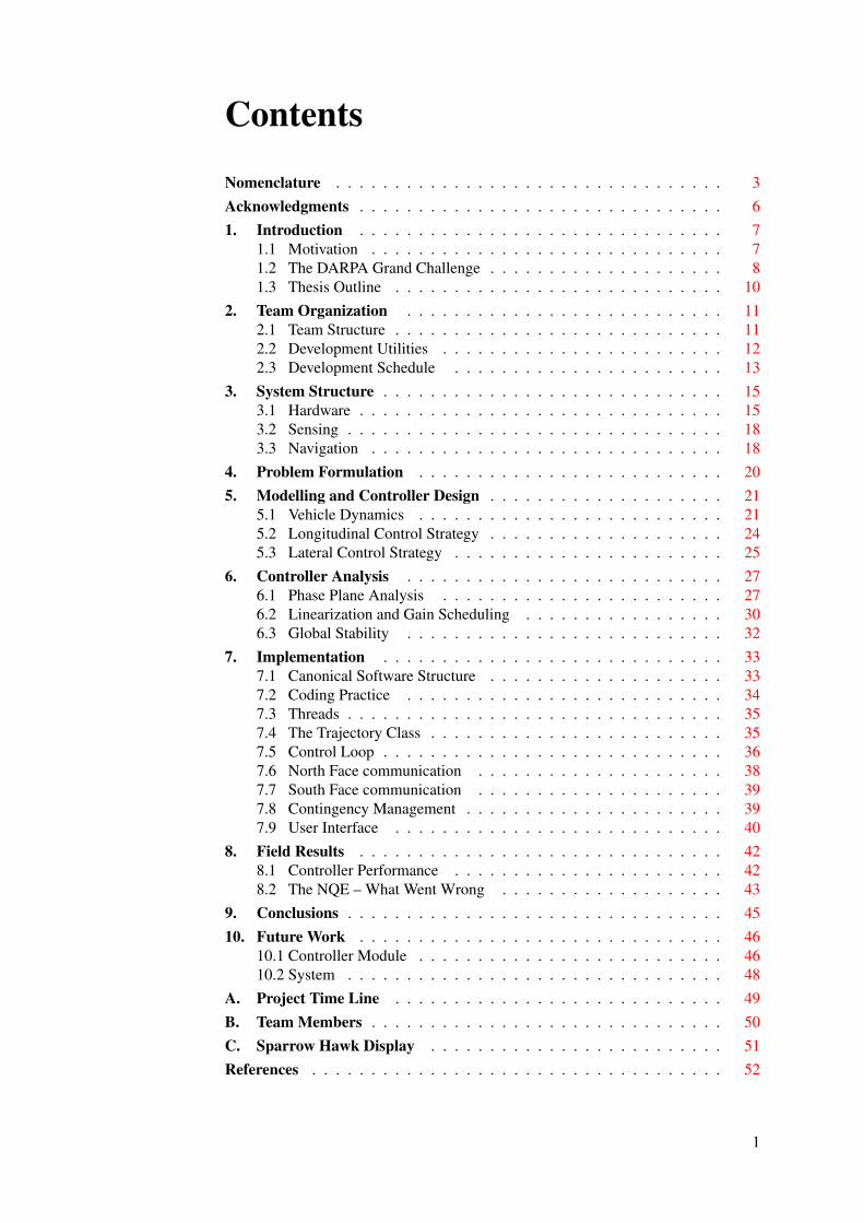
Contents
Nomenclature . . . . . . . . . . . . . . . . . . . . . . . . . . . . . . . . . 3Acknowledgments . . . . . . . . . . . . . . . . . . . . . . . . . . . . . . . 61. Introduction . . . . . . . . . . . . . . . . . . . . . . . . . . . . . . . 7
1.1 Motivation . . . . . . . . . . . . . . . . . . . . . . . . . . . . . . 71.2 The DARPA Grand Challenge . . . . . . . . . . . . . . . . . . . . 81.3 Thesis Outline . . . . . . . . . . . . . . . . . . . . . . . . . . . . 10
2. Team Organization . . . . . . . . . . . . . . . . . . . . . . . . . . . 112.1 Team Structure . . . . . . . . . . . . . . . . . . . . . . . . . . . . 112.2 Development Utilities . . . . . . . . . . . . . . . . . . . . . . . . 122.3 Development Schedule . . . . . . . . . . . . . . . . . . . . . . . 13
3. System Structure . . . . . . . . . . . . . . . . . . . . . . . . . . . . . 153.1 Hardware . . . . . . . . . . . . . . . . . . . . . . . . . . . . . . . 153.2 Sensing . . . . . . . . . . . . . . . . . . . . . . . . . . . . . . . . 183.3 Navigation . . . . . . . . . . . . . . . . . . . . . . . . . . . . . . 18
4. Problem Formulation . . . . . . . . . . . . . . . . . . . . . . . . . . 205. Modelling and Controller Design . . . . . . . . . . . . . . . . . . . . 21
5.1 Vehicle Dynamics . . . . . . . . . . . . . . . . . . . . . . . . . . 215.2 Longitudinal Control Strategy . . . . . . . . . . . . . . . . . . . . 245.3 Lateral Control Strategy . . . . . . . . . . . . . . . . . . . . . . . 25
6. Controller Analysis . . . . . . . . . . . . . . . . . . . . . . . . . . . 276.1 Phase Plane Analysis . . . . . . . . . . . . . . . . . . . . . . . . 276.2 Linearization and Gain Scheduling . . . . . . . . . . . . . . . . . 306.3 Global Stability . . . . . . . . . . . . . . . . . . . . . . . . . . . 32
7. Implementation . . . . . . . . . . . . . . . . . . . . . . . . . . . . . 337.1 Canonical Software Structure . . . . . . . . . . . . . . . . . . . . 337.2 Coding Practice . . . . . . . . . . . . . . . . . . . . . . . . . . . 347.3 Threads . . . . . . . . . . . . . . . . . . . . . . . . . . . . . . . . 357.4 The Trajectory Class . . . . . . . . . . . . . . . . . . . . . . . . . 357.5 Control Loop . . . . . . . . . . . . . . . . . . . . . . . . . . . . . 367.6 North Face communication . . . . . . . . . . . . . . . . . . . . . 387.7 South Face communication . . . . . . . . . . . . . . . . . . . . . 397.8 Contingency Management . . . . . . . . . . . . . . . . . . . . . . 397.9 User Interface . . . . . . . . . . . . . . . . . . . . . . . . . . . . 40
8. Field Results . . . . . . . . . . . . . . . . . . . . . . . . . . . . . . . 428.1 Controller Performance . . . . . . . . . . . . . . . . . . . . . . . 428.2 The NQE – What Went Wrong . . . . . . . . . . . . . . . . . . . 43
9. Conclusions . . . . . . . . . . . . . . . . . . . . . . . . . . . . . . . . 4510. Future Work . . . . . . . . . . . . . . . . . . . . . . . . . . . . . . . 46
10.1 Controller Module . . . . . . . . . . . . . . . . . . . . . . . . . . 4610.2 System . . . . . . . . . . . . . . . . . . . . . . . . . . . . . . . . 48
A. Project Time Line . . . . . . . . . . . . . . . . . . . . . . . . . . . . 49B. Team Members . . . . . . . . . . . . . . . . . . . . . . . . . . . . . . 50C. Sparrow Hawk Display . . . . . . . . . . . . . . . . . . . . . . . . . 51References . . . . . . . . . . . . . . . . . . . . . . . . . . . . . . . . . . . 52
1
List of Figures1.1 Photograph showing Team Caltech’s DUC vehicle Alice. . . . . . . 71.2 Time line of the 2007 DUC. . . . . . . . . . . . . . . . . . . . . . 81.3 Photograph showing Team Caltech’s 2004 DGC vehicle Bob. Cour-
tesy of DARPA. . . . . . . . . . . . . . . . . . . . . . . . . . . . . 93.1 Block diagram illustrating the Applanix POS LV 420 vehicle state
estimation system. . . . . . . . . . . . . . . . . . . . . . . . . . . 153.2 Photograph of Alice, indicating the location of its sensors. . . . . . 163.3 Photograph showing the computer rack of Alice. From top down:
core duo machines, quad core machine and cPCI box. (The lower-most box is a battery pack.) . . . . . . . . . . . . . . . . . . . . . 17
3.4 Photograph showing the actuators of Alice. . . . . . . . . . . . . . 173.5 Block diagram illustrating the data flow from sensors to map. . . . 183.6 Block diagram illustrating the navigation stack of Alice. . . . . . . 185.1 3D representation of the parametrized lookup table mapping (v,au)→
ua. . . . . . . . . . . . . . . . . . . . . . . . . . . . . . . . . . . . 225.2 Figure used in the deduction of (5.1, 5.2). . . . . . . . . . . . . . . 235.3 Graphical illustration of the lateral control strategy. . . . . . . . . . 255.4 Illustration showing the extension of the lateral control strategy to
the case of reverse driving. . . . . . . . . . . . . . . . . . . . . . . 266.1 Phase portraits showing the state evolution of error states ey,eθ for
different values of the trajectory radius rc and controller parameters l2. 286.2 Phase portraits illustrating tracking of a circular trajectory with ra-
dius rc = 5 m, which was smaller than the minimum turning radiusof Alice (7.4 m). The controller parameter was set to l2 = 5 m. . . . 29
6.3 Phase portrait illustrating the global behavior of the controlled sys-tem while tracking a circular trajectory with radius rc = 20 m. Thecontroller parameter was set to l2 = 5 m. . . . . . . . . . . . . . . 29
6.4 Cutoff ’frequency’ ωc [rad m−1] as function of l2. . . . . . . . . . . 316.5 Phase margin φm as function of l2. . . . . . . . . . . . . . . . . . . 316.6 Delay distance margin τm [m] as function of l2. . . . . . . . . . . . 317.1 Block diagram illustrating the structure of a CSS software module. . 337.2 Timing diagram showing one control loop cycle. . . . . . . . . . . 368.1 Cross track- and yaw error during 60 s of autonomous operation of
the vehicle. . . . . . . . . . . . . . . . . . . . . . . . . . . . . . . 428.2 Control signal and integral from the data set used to plot
Figures 8.1(a),8.1(b). . . . . . . . . . . . . . . . . . . . . . . . . . 438.3 Histograms showing the distribution of cross track- and yaw error
from 10 minutes of nominal operation. . . . . . . . . . . . . . . . . 43
2
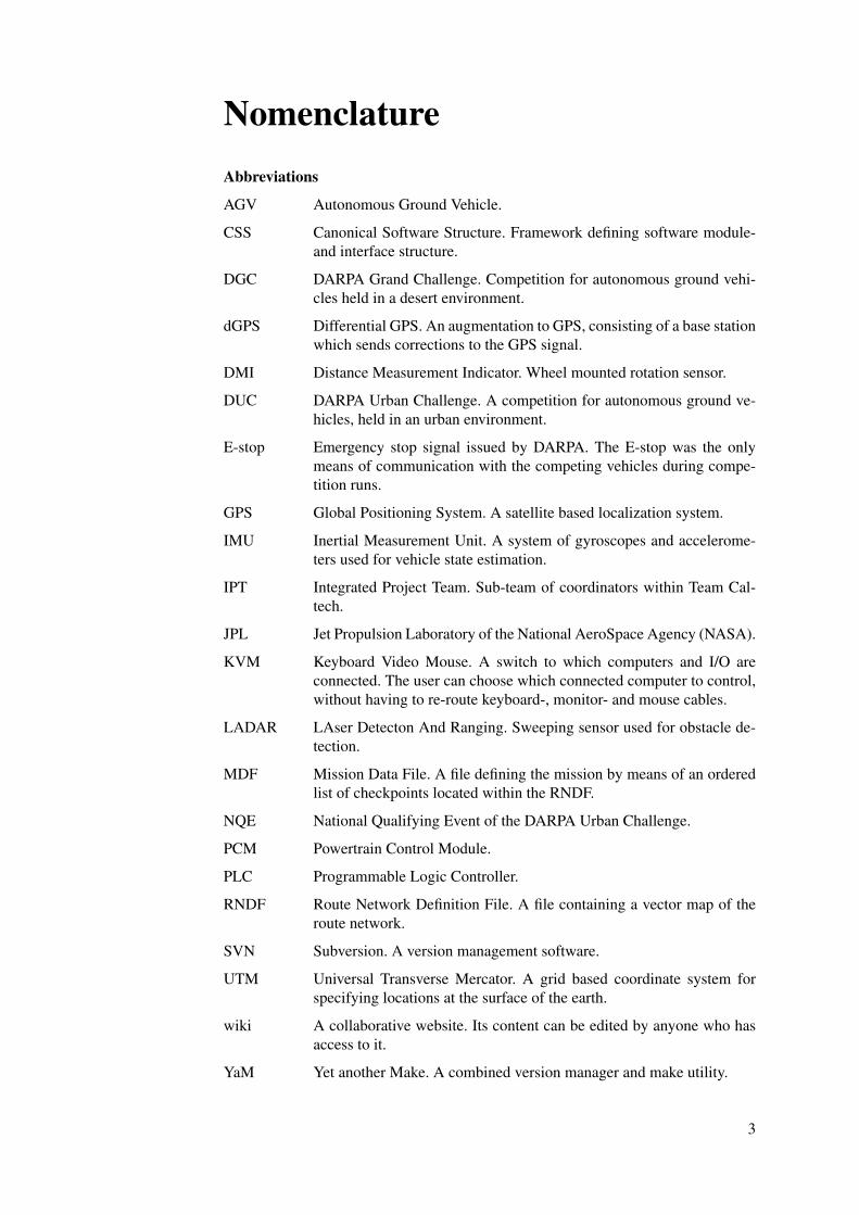
NomenclatureAbbreviations
AGV Autonomous Ground Vehicle.
CSS Canonical Software Structure. Framework defining software module-and interface structure.
DGC DARPA Grand Challenge. Competition for autonomous ground vehi-cles held in a desert environment.
dGPS Differential GPS. An augmentation to GPS, consisting of a base stationwhich sends corrections to the GPS signal.
DMI Distance Measurement Indicator. Wheel mounted rotation sensor.
DUC DARPA Urban Challenge. A competition for autonomous ground ve-hicles, held in an urban environment.
E-stop Emergency stop signal issued by DARPA. The E-stop was the onlymeans of communication with the competing vehicles during compe-tition runs.
GPS Global Positioning System. A satellite based localization system.
IMU Inertial Measurement Unit. A system of gyroscopes and accelerome-ters used for vehicle state estimation.
IPT Integrated Project Team. Sub-team of coordinators within Team Cal-tech.
JPL Jet Propulsion Laboratory of the National AeroSpace Agency (NASA).
KVM Keyboard Video Mouse. A switch to which computers and I/O areconnected. The user can choose which connected computer to control,without having to re-route keyboard-, monitor- and mouse cables.
LADAR LAser Detecton And Ranging. Sweeping sensor used for obstacle de-tection.
MDF Mission Data File. A file defining the mission by means of an orderedlist of checkpoints located within the RNDF.
NQE National Qualifying Event of the DARPA Urban Challenge.
PCM Powertrain Control Module.
PLC Programmable Logic Controller.
RNDF Route Network Definition File. A file containing a vector map of theroute network.
SVN Subversion. A version management software.
UTM Universal Transverse Mercator. A grid based coordinate system forspecifying locations at the surface of the earth.
wiki A collaborative website. Its content can be edited by anyone who hasaccess to it.
YaM Yet another Make. A combined version manager and make utility.
3
Nomenclature
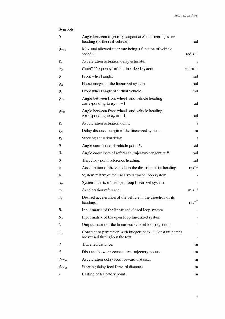
Symbols
δ Angle between trajectory tangent at R and steering wheelheading (of the real vehicle). rad
φmax Maximal allowed steer rate being a function of vehiclespeed v. rad s−1
τa Acceleration actuation delay estimate. s
ωc Cutoff ’frequency’ of the linearized system. rad m−1
φ Front wheel angle. rad
φm Phase margin of the linearized system. rad
φv Front wheel angle of virtual vehicle. rad
φmax Angle between front wheel- and vehicle headingcorresponding to uφ =−1. rad
φmin Angle between front wheel- and vehicle headingcorresponding to uφ =−1. rad
τa Acceleration actuation delay. s
τm Delay distance margin of the linearized system. m
τφ Steering actuation delay. s
θ Angle coordinate of vehicle point P. rad
θr Angle coordinate of reference trajectory tangent at R. rad
θr Trajectory point reference heading. rad
a Acceleration of the vehicle in the direction of its heading ms−2
Ac System matrix of the linearized closed loop system. -
Ao System matrix of the open loop linearized system. -
ar Acceleration reference. m s−2
au Desired acceleration of the vehicle in the direction of itsheading. ms−2
Bc Input matrix of the linearized closed loop system. -
Bo Input matrix of the open loop linearized system. -
C Output matrix of the linearized (closed loop) system. -
Cn Constant or parameter, with integer index n. Constant namesare reused throughout the text. -
d Travelled distance. m
di Distance between consecutive trajectory points. m
dFF,a Acceleration delay feed forward distance. m
dFF,a Steering delay feed forward distance. m
e Easting of trajectory point. m
4
Nomenclature
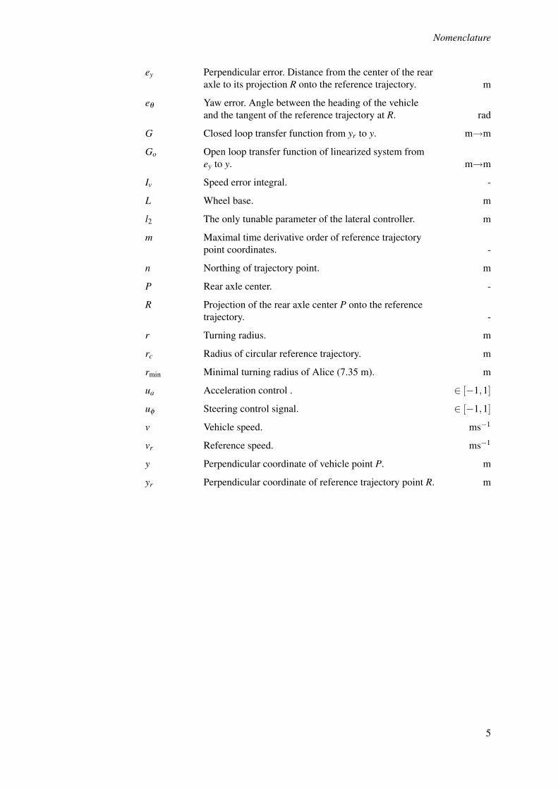
ey Perpendicular error. Distance from the center of the rearaxle to its projection R onto the reference trajectory. m
eθ Yaw error. Angle between the heading of the vehicleand the tangent of the reference trajectory at R. rad
G Closed loop transfer function from yr to y. m→m
Go Open loop transfer function of linearized system fromey to y. m→m
Iv Speed error integral. -
L Wheel base. m
l2 The only tunable parameter of the lateral controller. m
m Maximal time derivative order of reference trajectorypoint coordinates. -
n Northing of trajectory point. m
P Rear axle center. -
R Projection of the rear axle center P onto the referencetrajectory. -
r Turning radius. m
rc Radius of circular reference trajectory. m
rmin Minimal turning radius of Alice (7.35 m). m
ua Acceleration control . ∈ [−1,1]
uφ Steering control signal. ∈ [−1,1]
v Vehicle speed. ms−1
vr Reference speed. ms−1
y Perpendicular coordinate of vehicle point P. m
yr Perpendicular coordinate of reference trajectory point R. m
5
AcknowledgmentsThe work resulting in this thesis was carried out at the Department of Control andDynamical Systems, California Institute of Technology, Pasadena, USA with addi-tional supervision from the Department of Automatic Control, Lund Institute of Tech-nology, Lund, Sweden. It was part of Team Caltech’s autonomous vehicle program,aimed at the 2007 DARPA Urban Challenge.
I would like to thank my supervisor and the coordinator of Team Caltech, Profes-sor Richard Murray, California Institute of Technology. Additionally, I would wantto thank my co-supervisor Professor Tore Hägglund and Professor Anders Rantzer atLund Institute of Technology, Lund, Sweden together with the Caltech Summer Un-dergraduate Research Fellowship (SURF) program for making my stay in Californiaboth possible and pleasant.
Last, but not least, I owe great thanks to all members of Team Caltech – fortheir help, support and suggestions throughout the project – as well as all externalsupporters and sponsors of the project.
6
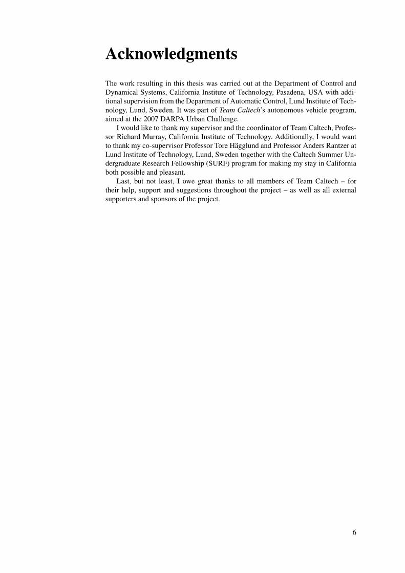
1. IntroductionThe concepts, ideas and results presented here are the outcome of Team Caltech’sdevelopment for the 2007 DARPA Urban Challenge (DUC) [15]. The aim of theproject was to develop an autonomous ground vehicle (AGV) for safe operation inan urban environment – in the presence of other vehicles. The final evaluation of thiseffort took place at the National Qualifying Event (NQE) of the DUC, see Section 8.2.A photograph of Team Caltech’s vehicle, Alice, is shown in Figure 1.1.
Figure 1.1 Photograph showing Team Caltech’s DUC vehicle Alice.
The focus of this paper lies on the trajectory tracking controllers which were de-veloped, implemented, and tested by me and Magnus Linderoth from Lund Instituteof Technology. However, it is important to emphasize that the development processwas a team effort. Consequently, a summary of previous work conducted at Caltech,as well as a review of current team- and system structure, are given before focus isshifted to the trajectory tracking controller module.
A motivation for the DUC is given in Section 1.1, followed by a brief historyof previous races in Section 1.2. The organization of this paper is then presented inSection 1.3.
1.1 Motivation
The aim of the DUC was to push the development of AGV systems, capable of per-forming safely in an urban environment – in the presence of other vehicles.
The main motivation for Team Caltech, the Stanford Race Team and others wasto develop fully autonomous vehicles, which are safer than their human maneuveredcounterparts, hence increasing traffic safety. A large amount of research and devel-opment has been made during the past few years, but there will still be some timebefore the technologies are ready for the consumer market. A more realistic shortterm application are systems, which prevent a human driver from making ’illegal’maneuvers, by e.g. clearing (suddenly appearing) obstacles, stopping at stop lines,etc. Such and similar applications are discussed in [19, 22].
Another category of teams, e.g. the Oshkosh Truck Company, aim to use theirfindings in military applications. Their main objective has been to produce reliableAGV transportation systems, which could be used in hazardous areas.
7
1.2 The DARPA Grand Challenge
Independent of application, autonomous driving is a complex applied roboticsproblem, stretching over diverse fields of engineering, including controls, signal pro-cessing, computer vision, computer science and mechanical engineering – to mentionsome of the major ones. To further complicate matters, the urban environment is richin both detail and unexpected situations, calling for highly robust systems.
Apart from the technical aspects, participating in Team Caltech was a great op-portunity for students to work in an environment otherwise rear in academia. Thework was project oriented, highly applied and involved hard deadlines.
1.2 The DARPA Grand Challenge
The 2007 DUC was the third in a series of autonomous road vehicle competitionsorganized by DARPA. The previous two went under the name DARPA Grand Chal-lenge (DGC) and took place in 2004 [14] and 2005 [16]. Team Caltech was formedin March 2003 in order to compete in the 2004 DGC and has also contributed withan entry for the 2005 competition.
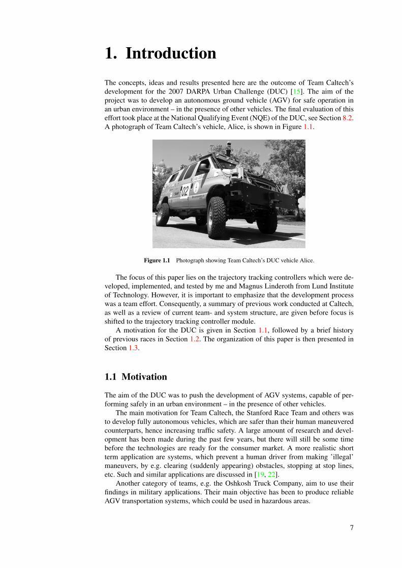
The 2007 DUC consisted of a series of qualifying steps, leading to a final event.These steps are shown in Figure 1.2. (Although details have changed, most of thefollowing applied also to the 2004 and 2005 races.)
1. Program AnnouncementMay 1, 2006
2. ParticipantsConferenceMay 20, 2006
3. Site VisitJune 11 - July 20, 2007
5. National Qualifying EventOctober 26-31, 2007
6. Final EventNovember 3, 2007
4. Semi-FinalistAnnouncementAugust 9, 2007
Figure 1.2 Time line of the 2007 DUC.
Here follows a short description of each step of the time line in Figure 1.2.
1. Program Announcement May 1, 2006. DARPA announced the schedule for the2007 DUC. New for the 2007 DUC was that 11 teams, including Team Caltech,were to receive funding of $ 1 M each, for developing their vehicles.
2. Participants Conference May 20, 2006. The Participants Conference served asa briefing session, informing the teams what to expect during the remainder ofthe DUC.
3. Site Visits June 11 - July 20, 2007. The test sites of the competing teams werevisited by DARPA officials. During these visits the teams had to demonstratesafe operation and basic functionality of their vehicles.
4. Semi-Finalists announcement August 9, 2007. Based mainly on the outcome ofthe site visits, 34 teams were recognized as semi finalists. Team Caltech wasone of the semi-finalist teams.
5. National Qualifying Event October 26 - 31, 2007. The NQE served as a seriesof ’unit tests’, where the vehicles needed to demonstrate successful handlingof advanced traffic scenarios (involving several vehicles).
6. Final Event November 3, 2007. Each team that qualified to the final event wasprovided with a USB stick holding two files from DARPA. These were theRoute Network Definition File (RNDF) and the Mission Data File (MDF) [17].
8
1.2 The DARPA Grand Challenge
The RNDF was a ’map’, where lane geometry, stop lines, intersections, way-points etc. were given in a frame fixed to absolute GPS coordinates. The MDFwas an ordered list of GPS waypoints located within the area of the RNDF. Italso defined speed limits for all road segments of the RNDF. The objective ofthe competition was to traverse the checkpoints of the MDF in correct orderand minimal time, while adhering to traffic rules [18], provided by DARPA.All finalist ran on the same RNDF – simultaneously.
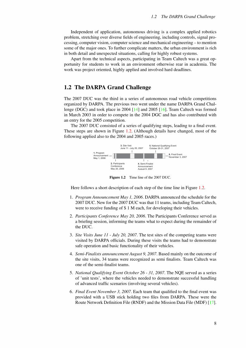
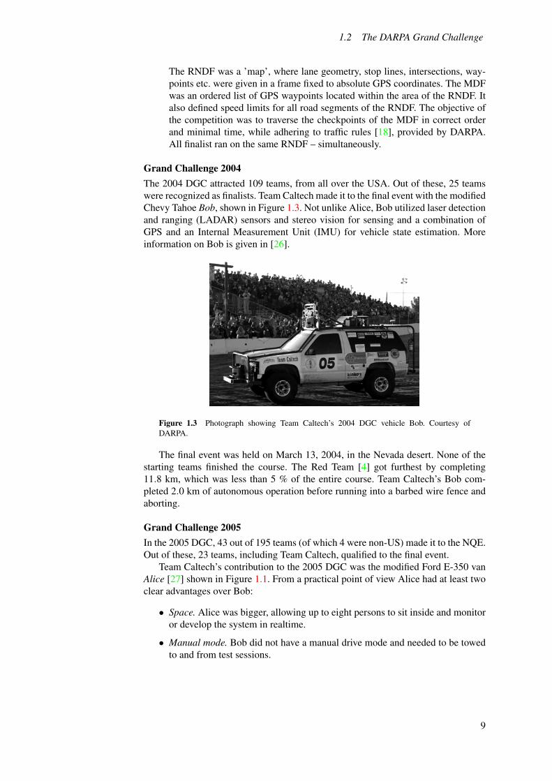
Grand Challenge 2004The 2004 DGC attracted 109 teams, from all over the USA. Out of these, 25 teamswere recognized as finalists. Team Caltech made it to the final event with the modifiedChevy Tahoe Bob, shown in Figure 1.3. Not unlike Alice, Bob utilized laser detectionand ranging (LADAR) sensors and stereo vision for sensing and a combination ofGPS and an Internal Measurement Unit (IMU) for vehicle state estimation. Moreinformation on Bob is given in [26].
Figure 1.3 Photograph showing Team Caltech’s 2004 DGC vehicle Bob. Courtesy ofDARPA.
The final event was held on March 13, 2004, in the Nevada desert. None of thestarting teams finished the course. The Red Team [4] got furthest by completing11.8 km, which was less than 5 % of the entire course. Team Caltech’s Bob com-pleted 2.0 km of autonomous operation before running into a barbed wire fence andaborting.
Grand Challenge 2005In the 2005 DGC, 43 out of 195 teams (of which 4 were non-US) made it to the NQE.Out of these, 23 teams, including Team Caltech, qualified to the final event.
Team Caltech’s contribution to the 2005 DGC was the modified Ford E-350 vanAlice [27] shown in Figure 1.1. From a practical point of view Alice had at least twoclear advantages over Bob:
• Space. Alice was bigger, allowing up to eight persons to sit inside and monitoror develop the system in realtime.
• Manual mode. Bob did not have a manual drive mode and needed to be towedto and from test sessions.
9
1.3 Thesis Outline
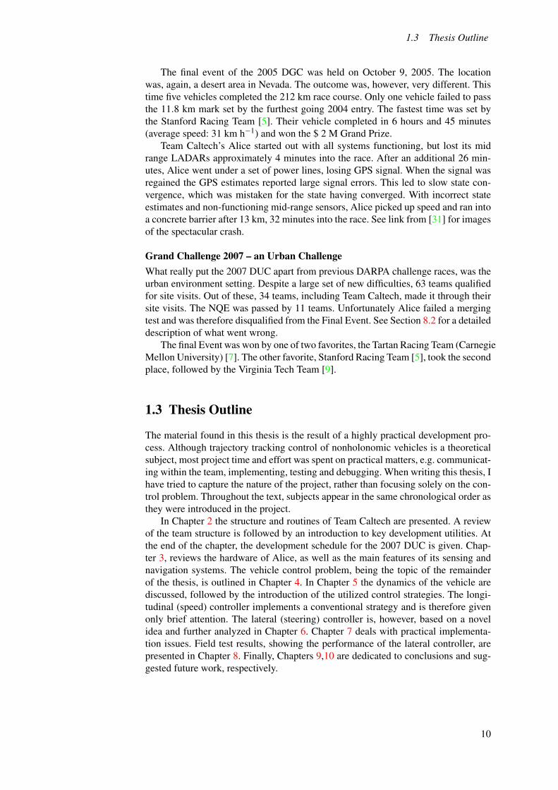
The final event of the 2005 DGC was held on October 9, 2005. The locationwas, again, a desert area in Nevada. The outcome was, however, very different. Thistime five vehicles completed the 212 km race course. Only one vehicle failed to passthe 11.8 km mark set by the furthest going 2004 entry. The fastest time was set bythe Stanford Racing Team [5]. Their vehicle completed in 6 hours and 45 minutes(average speed: 31 km h−1) and won the $ 2 M Grand Prize.
Team Caltech’s Alice started out with all systems functioning, but lost its midrange LADARs approximately 4 minutes into the race. After an additional 26 min-utes, Alice went under a set of power lines, losing GPS signal. When the signal wasregained the GPS estimates reported large signal errors. This led to slow state con-vergence, which was mistaken for the state having converged. With incorrect stateestimates and non-functioning mid-range sensors, Alice picked up speed and ran intoa concrete barrier after 13 km, 32 minutes into the race. See link from [31] for imagesof the spectacular crash.
Grand Challenge 2007 – an Urban ChallengeWhat really put the 2007 DUC apart from previous DARPA challenge races, was theurban environment setting. Despite a large set of new difficulties, 63 teams qualifiedfor site visits. Out of these, 34 teams, including Team Caltech, made it through theirsite visits. The NQE was passed by 11 teams. Unfortunately Alice failed a mergingtest and was therefore disqualified from the Final Event. See Section 8.2 for a detaileddescription of what went wrong.
The final Event was won by one of two favorites, the Tartan Racing Team (CarnegieMellon University) [7]. The other favorite, Stanford Racing Team [5], took the secondplace, followed by the Virginia Tech Team [9].
1.3 Thesis Outline
The material found in this thesis is the result of a highly practical development pro-cess. Although trajectory tracking control of nonholonomic vehicles is a theoreticalsubject, most project time and effort was spent on practical matters, e.g. communicat-ing within the team, implementing, testing and debugging. When writing this thesis, Ihave tried to capture the nature of the project, rather than focusing solely on the con-trol problem. Throughout the text, subjects appear in the same chronological order asthey were introduced in the project.
In Chapter 2 the structure and routines of Team Caltech are presented. A reviewof the team structure is followed by an introduction to key development utilities. Atthe end of the chapter, the development schedule for the 2007 DUC is given. Chap-ter 3, reviews the hardware of Alice, as well as the main features of its sensing andnavigation systems. The vehicle control problem, being the topic of the remainderof the thesis, is outlined in Chapter 4. In Chapter 5 the dynamics of the vehicle arediscussed, followed by the introduction of the utilized control strategies. The longi-tudinal (speed) controller implements a conventional strategy and is therefore givenonly brief attention. The lateral (steering) controller is, however, based on a novelidea and further analyzed in Chapter 6. Chapter 7 deals with practical implementa-tion issues. Field test results, showing the performance of the lateral controller, arepresented in Chapter 8. Finally, Chapters 9,10 are dedicated to conclusions and sug-gested future work, respectively.
10
2. Team OrganizationOne of the main challenges in the project was that of team coordination. Having indi-vidual developers wait for each other due to dependency issues, was avoided as far aspossible due to the given tight time frame. In the same fashion, good inter-team com-munication was necessary to maintain coherence in the system development. Thisrequired all developers to both comment code rigorously and stay up to date withcode changes. It was all facilitated by a clear team structure with well-establishedcommunication channels.
An overview of the team structure is given in Section 2.1. Section 2.2 reviews thekey utilities for team coordination are reviewed. All parts of the project were more orless influenced by its tight development schedule, reviewed in Section 2.3.
2.1 Team Structure
Team Caltech consisted mainly of students from Caltech and visiting students fromother universities. Team members also included Caltech faculty as well as NASA JetPropulsion Laboratory (JPL) and Northrop Grumman Corp. staff. Over the years a lotof people have joined, worked in and left Team Caltech. Consequently, a significantpart of the challenge was to maintain knowledge and experience within the team,although team members were frequently being exchanged.
The team actively working on preparing Alice for the 2007 DUC consisted of 77persons, listed in Appendix B. The team was divided into several sub-teams, eachwith a well-defined purpose. These sub-teams are the subject of the next few para-graphs. The two biggest – in terms of persons, code as well as functionality – aregiven extra attention.
Sensing Sub-TeamAlice made extensive use of sensors [13] including LADAR, radar and stereo cam-eras, in order to build a map of its environment. See Section 3.1 for further details.The task of the sensing team was to develop and maintain software which took in-formation from the sensors, and fused it into the map. A big part of this work layin segmenting data points into objects and classifying these objects as cars, staticobstacles, lane lines, etc.
Navigation Sub-TeamThe navigation sub-team developed the planning software of Alice. The purpose ofplanning was to frequently quarry information from the RNDF, MDF and the map,as well as vehicle state information supplied by a state estimator in order to gen-erate feasible trajectories. The trajectories were then sent to the trajectory trackingcontroller module, being the main subject of this thesis.
Other Sub-TeamsApart from sensing and navigation, there were four sub-teams:
• Integrated Project Team (IPT). This sub-team consisted of all the sub-teamcoordinators, as well as other ’key’ persons. Its responsibility was to managethe project at an overview level.
11
2.2 Development Utilities
• Systems Sub-team. All the sub-teams wrote their own programs, executed inseparate processes. The systems sub-team maintained the interfaces used to en-able inter-process communications. More information is given in Section 7.1.
• Vehicle Sub-team. The vehicle sub-team was responsible for all mechanicalwork and wiring on the vehicle.
• Sysadmin Sub-team. The sysadmin sub-team managed the networked worksta-tions, as well as the ’race’ computers in Alice.
2.2 Development Utilities
The following paragraphs describe six tools which were extensively used throughoutthe development process. They are mentioned here, because of their contributions interms of defining standards and significantly increasing development efficiency.
Team WikiThroughout the project the team wiki [8] hosted descriptions of all software modules,meeting notes, test schedules, etc. The wiki structure – version managed and editableby all project members – proved to be successful, mainly because of the rapid devel-opment process.
DoxygenDoxygen [2] is a documentation system for a number of languages, including C,C++ and Java. It can generate both an online documentation browser (in HTML) andoffline documentation (in LATEX). The documentation is extracted directly from thesource code on which doxygen is run. (Specific tokens are used to trigger the doxygenparser.)
The project utilized the HTML documentation, which was maintained for allsoftware modules. Apart from comments, the auto-generated documentation showedcode structure, relation between objects and inter-file dependencies in an intuitiveand graphically appealing format.
BugzillaBugzilla [1] is a data base with a HTML front end, used to keep track of bugs. Asidentified bugs were inserted into the Bugzilla database, they could be assigned to asub-team, or a specific developer. Managed bugs were associated with a severity, aswell as possible dependency relations with other bugs.
SubversionSubversion (SVN) [6] is a widely used version management software. File trees (orparts thereof) could be added to an SVN repository, kept on a backed up server. Eachdeveloper worked on a local copy of the code, a sandbox, and could at any given timecommit files to the repository. SVN kept track of commits and gave the developer theoption to revert files to any previously committed version. There was also a web frontend, which enabled developers to examine the version history of files without havingto check them out from the repository.
12
2.3 Development Schedule
YaMWhenever a developer came to a point where an owned module was stable, release ofthe module was made, making it officially available to other developers on the team.Releases were handled by YaM [21, 10]; a combined version manager and makeutility developed at JPL. It’s functionality was similar to that of SVN. However, itoperated on a module level, as opposed to a file level. It also implemented a custommake utility, used to build and link YaM-managed modules.
When a release of a software module was made, YaM checked that no changeshad been made to the particular module after it’s files were latest committed to theSVN repository. It also automatically generated a message with change-log entriesand posted it on the ’implement’ mailing list, informing all developers that a newmodule release had been made. The actual release consisted of a source part and alink part. The source part was simply the module source code, whereas the link partconsisted of binaries, libraries, headers and configuration files. Its purpose was tospare developers the time it took to check out and compile a module each time therewas a new release of it.
Mailing ListsThe implement mailing list served as the main communication channel between de-velopers. Whenever a YaM release was made, the release notes were automaticallyposted on this list. Notifications of meetings, schedule changes etc. were also postedhere. In addition to the implement mailing list, each sub-team had its own list, formatters not affecting the entire team.
2.3 Development Schedule
Based on experience from the previous DGC races, Team Caltech began implement-ing new software modules for the 2007 DUC in June 2007. A mostly stable hardwaresetup was already in place. (It was, however, augmented with new computer bladesand sensors. In addition to this, various electro-mechanic parts were replaced.) Thevast majority of development time was therefore spent implementing and testing newfunctionality. This section gives an overview of the project time line and developmentmethodology, utilized by the team in order to maximize development efficiency.
Project Time LineThe nominal project time line for the 2007 DUC preparations was divided into fivespirals. The goals for the individual spirals are reviewed in Appendix A.
Keeping up with the nominal time line turned out to be hard. There were a lot ofminor issues, which together ended up taking longer time than expected to resolve. Anominal version of almost all modules, including the controller described herein, wasin place by the end of spiral 1. However, Spiral 2 took longer time than planned for,making spirals 3 and 4 more stressful than originally intended. Nevertheless, by theend of spiral 4, Alice was capable of handling all the situations postulated by DARPA– but some of the functionality had not been thoroughly tuned and tested in the fieldprior to the NQE.
13
2.3 Development Schedule
Weekly MeetingsEach week the entire project group met. These meetings were coordinated by theteam leader, Prof. Richard Murray, and their structure were as follows:
• Review of what had happened since the last project meeting.
• Overview of the current project status with respect to the nominal time line.
• Determination of a plan for the coming week.
• Outline of a plan for the next few weeks.
In connection to the weekly project meeting, there was a weekly sub-team meet-ing. The structure was similar to the project meeting, but the scope was narrower,with focus on practical implementation and testing issues.
Code DevelopmentAlthough some code development was made in the vehicle, most development anddebugging took place in a lab reserved for the project. A utility, which was extensivelyused, was the system simulator. It enabled real time testing of all software (with minorexceptions), without the need to take Alice out of the workshop.
Code ReviewsOne software module was reviewed by its owner(s) each week. These reviews werevery helpful in giving developers insight into modules which they had a dependencyrelation to, but were not personally developing.
Field TestsOnce new code had been verified in simulation, it was field tested in Alice. Althoughthe simulator revealed many bugs, it was not perfect and a lot of bugs were firstobserved in the field. Consequently, a big effort was made to maximize test time.Team Caltech had access to three test sites:
• St. Luke Hospital Parking Area. This site had streets with painted lane- and stoplines. There were also some buildings, bushes and trees, putting the sensingsub-system to a test. Unfortunately, the site was rather small.
• Santa Anita Race Track parking Area. Being the parking lot of a big race track,the site was a huge paved area, with nothing on it except for some paintedlane lines. It was used mainly to test new code at higher speeds or to unit testspecific parts of the sensing sub-system.
• El Toro Former Military Base. The El Toro base was the site most extensivelyused towards the end of the project. It was a large area with real roads, parkinglots and several structures.
As indicated, the choice of test site depended on the particular feature(s) to betested. While the parking lots were suitable for controller tuning, basic traffic scenar-ios etc., the El Toro site provided a preview of what was expected for the NQE.
14
3. System StructureThis chapter gives an overview of the system architecture of Alice. The hardware isreviewed in Section 3.1. The structure and functionality of the sensing and navigationsub-systems are then explained in Sections 3.2,3.3, respectively.
3.1 Hardware
A complete set of sensing-, computation- and actuation hardware was inherited fromthe 2005 DGC. However, some of it needed to be replaced since it would not meetthe new and higher demands of the urban environment. There was also a need ofaugmenting the sensor array, in order to obtain both better coverage and higher reso-lution. The following description is aimed at the final 2007 DUC configuration.
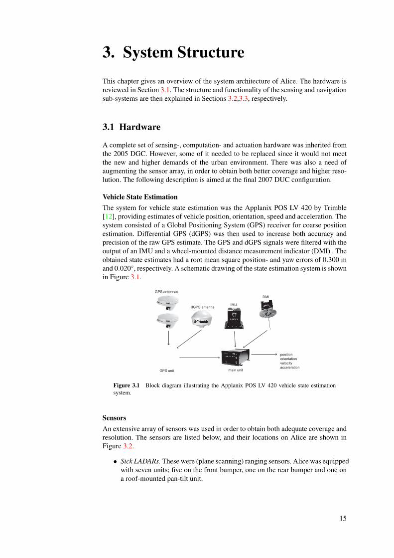
Vehicle State EstimationThe system for vehicle state estimation was the Applanix POS LV 420 by Trimble[12], providing estimates of vehicle position, orientation, speed and acceleration. Thesystem consisted of a Global Positioning System (GPS) receiver for coarse positionestimation. Differential GPS (dGPS) was then used to increase both accuracy andprecision of the raw GPS estimate. The GPS and dGPS signals were filtered with theoutput of an IMU and a wheel-mounted distance measurement indicator (DMI) . Theobtained state estimates had a root mean square position- and yaw errors of 0.300 mand 0.020◦, respectively. A schematic drawing of the state estimation system is shownin Figure 3.1.
IMU
GPS antennas
dGPS antenna
DMI
GPS unit main unit
positionorientationvelocityacceleration
Figure 3.1 Block diagram illustrating the Applanix POS LV 420 vehicle state estimationsystem.
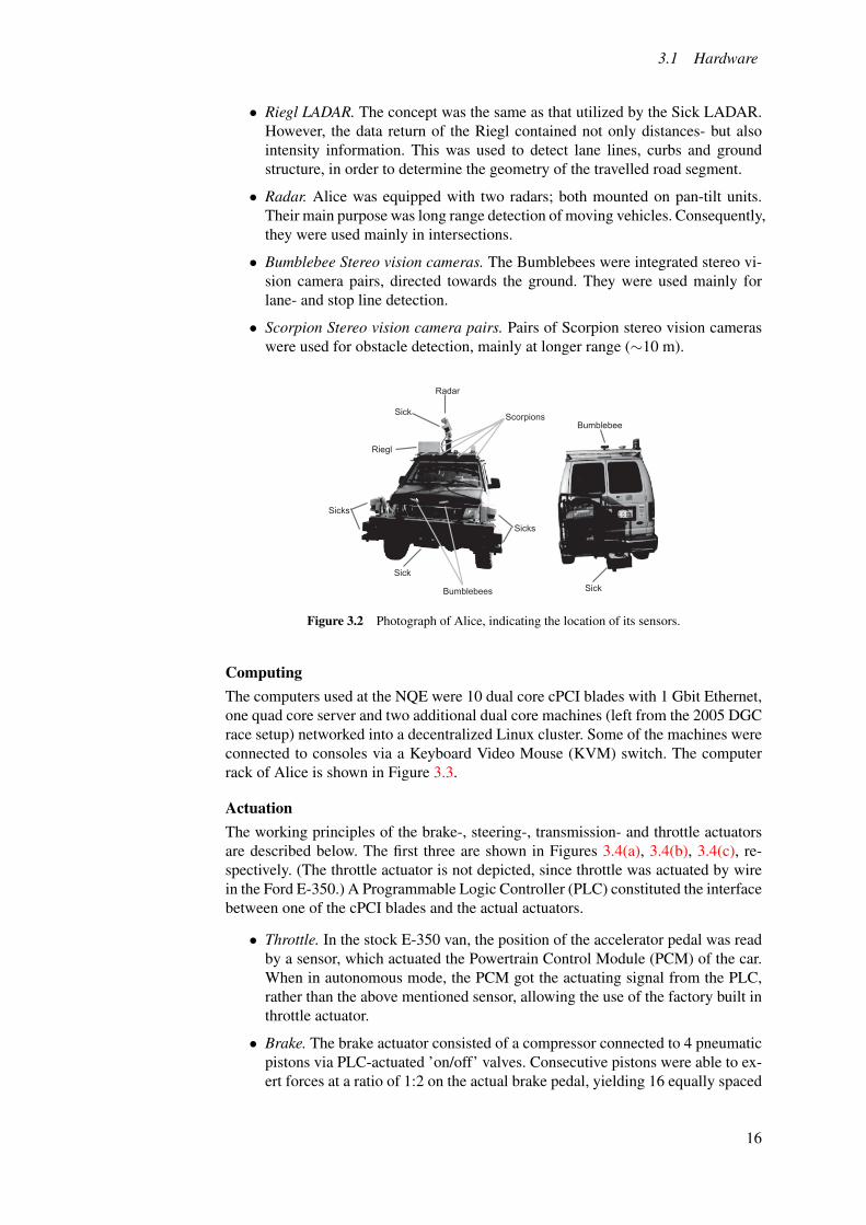
SensorsAn extensive array of sensors was used in order to obtain both adequate coverage andresolution. The sensors are listed below, and their locations on Alice are shown inFigure 3.2.
• Sick LADARs. These were (plane scanning) ranging sensors. Alice was equippedwith seven units; five on the front bumper, one on the rear bumper and one ona roof-mounted pan-tilt unit.
15
3.1 Hardware
• Riegl LADAR. The concept was the same as that utilized by the Sick LADAR.However, the data return of the Riegl contained not only distances- but alsointensity information. This was used to detect lane lines, curbs and groundstructure, in order to determine the geometry of the travelled road segment.
• Radar. Alice was equipped with two radars; both mounted on pan-tilt units.Their main purpose was long range detection of moving vehicles. Consequently,they were used mainly in intersections.
• Bumblebee Stereo vision cameras. The Bumblebees were integrated stereo vi-sion camera pairs, directed towards the ground. They were used mainly forlane- and stop line detection.
• Scorpion Stereo vision camera pairs. Pairs of Scorpion stereo vision cameraswere used for obstacle detection, mainly at longer range (∼10 m).
Riegl
Radar
Sick Scorpions
Sicks
Sicks
Sick
Bumblebees Sick
Bumblebee
Figure 3.2 Photograph of Alice, indicating the location of its sensors.
ComputingThe computers used at the NQE were 10 dual core cPCI blades with 1 Gbit Ethernet,one quad core server and two additional dual core machines (left from the 2005 DGCrace setup) networked into a decentralized Linux cluster. Some of the machines wereconnected to consoles via a Keyboard Video Mouse (KVM) switch. The computerrack of Alice is shown in Figure 3.3.
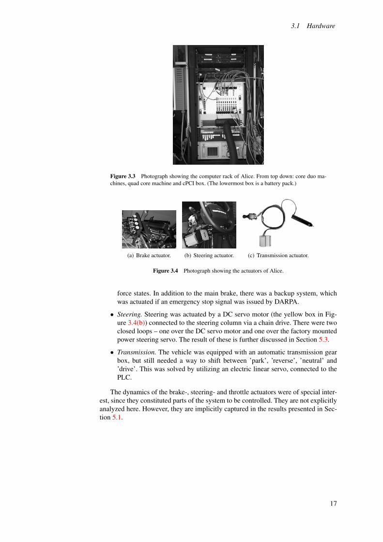
ActuationThe working principles of the brake-, steering-, transmission- and throttle actuatorsare described below. The first three are shown in Figures 3.4(a), 3.4(b), 3.4(c), re-spectively. (The throttle actuator is not depicted, since throttle was actuated by wirein the Ford E-350.) A Programmable Logic Controller (PLC) constituted the interfacebetween one of the cPCI blades and the actual actuators.
• Throttle. In the stock E-350 van, the position of the accelerator pedal was readby a sensor, which actuated the Powertrain Control Module (PCM) of the car.When in autonomous mode, the PCM got the actuating signal from the PLC,rather than the above mentioned sensor, allowing the use of the factory built inthrottle actuator.
• Brake. The brake actuator consisted of a compressor connected to 4 pneumaticpistons via PLC-actuated ’on/off’ valves. Consecutive pistons were able to ex-ert forces at a ratio of 1:2 on the actual brake pedal, yielding 16 equally spaced
16
3.1 Hardware
Figure 3.3 Photograph showing the computer rack of Alice. From top down: core duo ma-chines, quad core machine and cPCI box. (The lowermost box is a battery pack.)
(a) Brake actuator. (b) Steering actuator. (c) Transmission actuator.
Figure 3.4 Photograph showing the actuators of Alice.
force states. In addition to the main brake, there was a backup system, whichwas actuated if an emergency stop signal was issued by DARPA.
• Steering. Steering was actuated by a DC servo motor (the yellow box in Fig-ure 3.4(b)) connected to the steering column via a chain drive. There were twoclosed loops – one over the DC servo motor and one over the factory mountedpower steering servo. The result of these is further discussed in Section 5.3.
• Transmission. The vehicle was equipped with an automatic transmission gearbox, but still needed a way to shift between ’park’, ’reverse’, ’neutral’ and’drive’. This was solved by utilizing an electric linear servo, connected to thePLC.
The dynamics of the brake-, steering- and throttle actuators were of special inter-est, since they constituted parts of the system to be controlled. They are not explicitlyanalyzed here. However, they are implicitly captured in the results presented in Sec-tion 5.1.
17
3.2 Sensing
3.2 Sensing
As shown in Figure 3.2, Alice was equipped with a large number of sensors. Theywere set up in a modular fashion, enabling easy reconfiguration or addition of sensors.
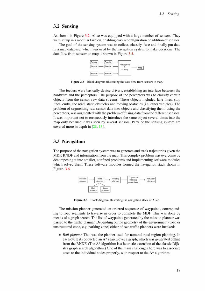
The goal of the sensing system was to collect, classify, fuse and finally put datain a map database, which was used by the navigation system to make decisions. Thedata flow from sensors to map is shown in Figure 3.5.
Feeder
Feeder
Feeder
...
Perception&
FusingMap
Sensor
Sensor
Sensor
...
Figure 3.5 Block diagram illustrating the data flow from sensors to map.
The feeders were basically device drivers, establishing an interface between thehardware and the perceptors. The purpose of the perceptors was to classify certainobjects from the sensor raw data streams. These objects included lane lines, stoplines, curbs, the road, static obstacles and moving obstacles (i.e. other vehicles). Theproblem of segmenting raw sensor data into objects and classifying them, using theperceptors, was augmented with the problem of fusing data from the different sensors.It was important not to erroneously introduce the same object several times into themap only because it was seen by several sensors. Parts of the sensing system arecovered more in depth in [28, 13].
3.3 Navigation
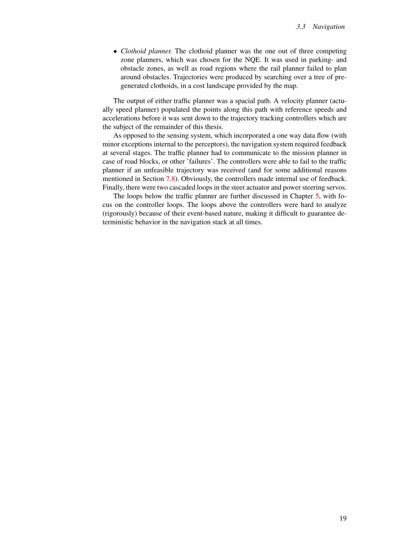
The purpose of the navigation system was to generate and track trajectories given theMDF, RNDF and information from the map. This complex problem was overcome bydecomposing it into smaller, confined problems and implementing software moduleswhich solved them. These software modules formed the navigation stack shown inFigure. 3.6.
Missionplanner
Trafficplanner
Railplanner
Zoneplanners
Velocityplanner
Trajectorytracking
controllers
Actuatorinterface
Figure 3.6 Block diagram illustrating the navigation stack of Alice.
The mission planner generated an ordered sequence of waypoints, correspond-ing to road segments to traverse in order to complete the MDF. This was done bymeans of a graph search. The list of waypoints generated by the mission planner waspassed to the traffic planner. Depending on the geometry of the environment (road orunstructured zone, e.g. parking zone) either of two traffic planners were invoked:
• Rail planner. This was the planner used for nominal road region planning. Ineach cycle it conducted an A* search over a graph, which was generated offlinefrom the RNDF. (The A* algorithm is a heuristic extension of the classic Dijk-stra graph search algorithm.) One of the main challenges here was to associatecosts to the individual nodes properly, with respect to the A* algorithm.
18
3.3 Navigation
• Clothoid planner. The clothoid planner was the one out of three competingzone planners, which was chosen for the NQE. It was used in parking- andobstacle zones, as well as road regions where the rail planner failed to planaround obstacles. Trajectories were produced by searching over a tree of pre-generated clothoids, in a cost landscape provided by the map.
The output of either traffic planner was a spacial path. A velocity planner (actu-ally speed planner) populated the points along this path with reference speeds andaccelerations before it was sent down to the trajectory tracking controllers which arethe subject of the remainder of this thesis.
As opposed to the sensing system, which incorporated a one way data flow (withminor exceptions internal to the perceptors), the navigation system required feedbackat several stages. The traffic planner had to communicate to the mission planner incase of road blocks, or other ’failures’. The controllers were able to fail to the trafficplanner if an unfeasible trajectory was received (and for some additional reasonsmentioned in Section 7.8). Obviously, the controllers made internal use of feedback.Finally, there were two cascaded loops in the steer actuator and power steering servos.
The loops below the traffic planner are further discussed in Chapter 5, with fo-cus on the controller loops. The loops above the controllers were hard to analyze(rigorously) because of their event-based nature, making it difficult to guarantee de-terministic behavior in the navigation stack at all times.
19
4. Problem FormulationThis chapter outlines the vehicle control problem, which needed to be approached andsolved during the project. First, it was decomposed into the confined sub-problems,listed below.
System IdentificationThe first part of the work was to deduce a parametrized model for the longitudinal-and lateral dynamics of a road vehicle. The parameters needed to be matched to thoseof the actual vehicle, by means of system identification experiments. The outcome ofthese experiments would prove if the suggested parametrization was well suited, orif the model needed to be altered.
Controller DesignA lateral- (steering-) and a longitudinal (speed) controller needed to be designedand implemented. These controllers should take a trajectory defined by a sequenceof points in the ground plane and an associated speed profile, and generate controlsignals issued to the steering-, gas-, brake- and transmission actuators. Simple algo-rithms were desired, since they would facilitate the entire development chain, fromanalysis and implementation to debugging and tuning.
There were no absolute performance requirements. Instead, the goal was to ob-tain a balance between responsiveness and robustness, which was to be extensivelyevaluated on the real process, prior to the NQE. Generally, well-damped behaviorwas prioritized over good performance for high frequencies in the references. Thiswas especially true for the lateral controller.
Contingency ManagementApart from performing well during nominal conditions, the controller module re-quired the ability to handle certain special situations, including actuator failures andtraffic planner errors, such as extensive delays between trajectories.
Implementation and TestingWhen the control algorithms and the contingency management scheme were at hand,they needed to be implemented and integrated into the fairly complex system. Thecontrollers needed to receive trajectories from a traffic planner and issue control sig-nals to a software module responsible for hardware actuation. Once implemented, themodule needed to be tuned and tested extensively together with the system, to findand correct unexpected behavior.
Time frameThe perhaps hardest problem during the project was its tight time frame. It was es-pecially true for the low level controllers since they needed to function adequatelyin order to test higher level parts of the project, such as traffic planning. This fur-ther stressed the need of implementation- and tuning-wise uncomplicated controlschemes.
20
5. Modelling and ControllerDesign
The longitudinal and lateral dynamics of the vehicle are introduced in Section 5.1.This is followed by a description of the longitudinal and lateral controllers in Sec-tions 5.2,5.3. The focus lies on the lateral control problem, which is further investi-gated in Chapter 6.
5.1 Vehicle Dynamics
In order to successfully design and analyse the trajectory tracking controllers, modelsof the vehicle dynamics were needed. These models are the subject of this section.
Longitudinal DynamicsThe brake and throttle actuators both acted on the acceleration of the vehicle. In Alicean acceleration control signal ua ∈ [−1,1] was utilized. Signals in [−1,0[ actuatedthe brake, whereas ua ∈]0,1] corresponded to the throttle. Because of dynamics inthe power train, ground friction and air resistance, the acceleration of the vehicle wasnot a strictly linear function of ua. Series of open loop experiments were conductedin order to analyze the non-linearity. During all these experiments the vehicle wasdriving forward along a straight line on a flat asphalt surface while time stampedspeed measurements were written to file. The experimental procedure was as follows:
1. A logger which recorded vehicle speed v , acceleration a and applied longitu-dinal control signal ua was started.
2. Subsequently, a constant control signal ua was issued until the vehicle reacheda steady state speed. (Note that the nature of the automatic transmission re-quired slight brake pressure to be applied in order to keep the vehicle station-ary.)
3. A step of parametrized height and duration was introduced in ua.
4. When the vehicle speed converged after the step, the experiment was termi-nated by stopping the logger and the vehicle.
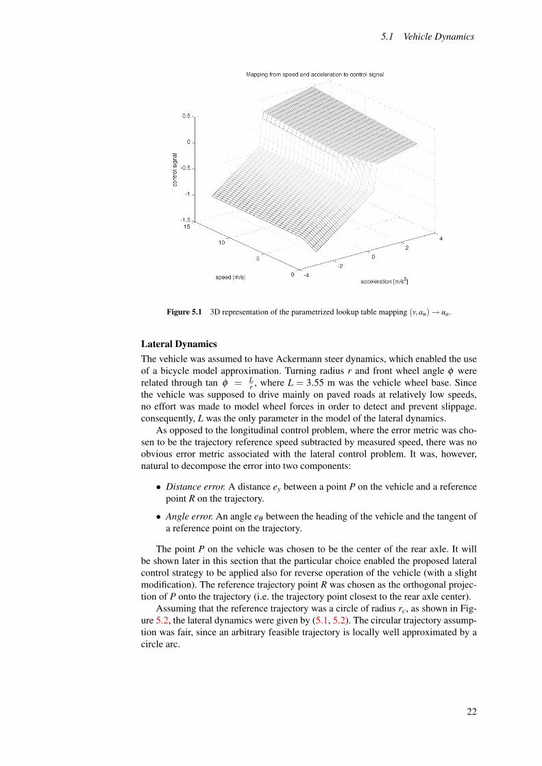
A large number (∼100) of open loop experiments were conducted with differentstep heights and durations. The results were compiled into a parametrized lookuptable, mapping vehicle speed v and desired acceleration au to required control signalua. A 3D representation of the resulting lookup table is shown in Figure 5.1.
To confirm the tacit time-invariance assumption, which was necessary for thevalidity of the non-linearity model, a subset of the open loop experiment was repeatedafter a few days.
No explicit attention was given to the non-linearity while the vehicle was revers-ing. Since the above deduced model constituted a good approximation – at least whenreversing at low speeds. This was adequate, since there were no plans to reverse au-tonomously at high speeds.
21
5.1 Vehicle Dynamics
Figure 5.1 3D representation of the parametrized lookup table mapping (v,au)→ ua.
Lateral DynamicsThe vehicle was assumed to have Ackermann steer dynamics, which enabled the useof a bicycle model approximation. Turning radius r and front wheel angle φ wererelated through tan φ = L
r , where L = 3.55 m was the vehicle wheel base. Sincethe vehicle was supposed to drive mainly on paved roads at relatively low speeds,no effort was made to model wheel forces in order to detect and prevent slippage.consequently, L was the only parameter in the model of the lateral dynamics.
As opposed to the longitudinal control problem, where the error metric was cho-sen to be the trajectory reference speed subtracted by measured speed, there was noobvious error metric associated with the lateral control problem. It was, however,natural to decompose the error into two components:
• Distance error. A distance ey between a point P on the vehicle and a referencepoint R on the trajectory.
• Angle error. An angle eθ between the heading of the vehicle and the tangent ofa reference point on the trajectory.
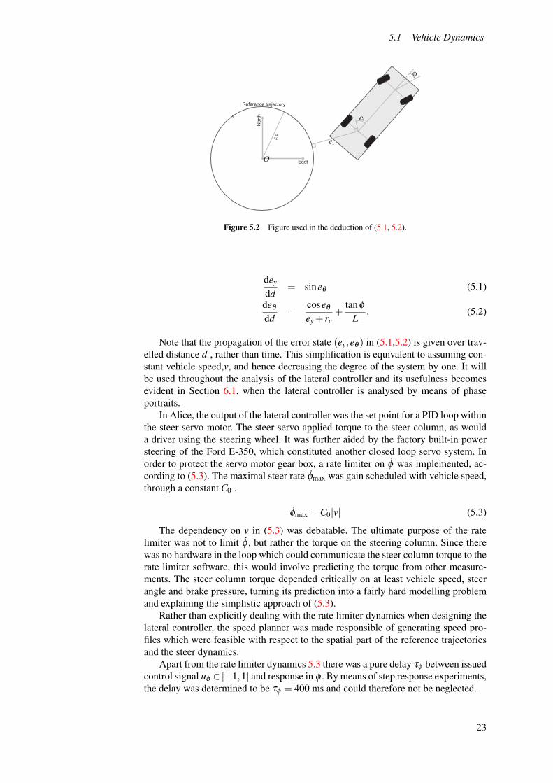
The point P on the vehicle was chosen to be the center of the rear axle. It willbe shown later in this section that the particular choice enabled the proposed lateralcontrol strategy to be applied also for reverse operation of the vehicle (with a slightmodification). The reference trajectory point R was chosen as the orthogonal projec-tion of P onto the trajectory (i.e. the trajectory point closest to the rear axle center).
Assuming that the reference trajectory was a circle of radius rc, as shown in Fig-ure 5.2, the lateral dynamics were given by (5.1, 5.2). The circular trajectory assump-tion was fair, since an arbitrary feasible trajectory is locally well approximated by acircle arc.
22
5.1 Vehicle Dynamics
re⊥
eθ
O East
Nor
th
Reference trajectory
φ
c
Figure 5.2 Figure used in the deduction of (5.1, 5.2).
dey
dd= sineθ (5.1)
deθ
dd=
coseθ
ey + rc+
tanφ
L. (5.2)
Note that the propagation of the error state (ey,eθ ) in (5.1,5.2) is given over trav-elled distance d , rather than time. This simplification is equivalent to assuming con-stant vehicle speed,v, and hence decreasing the degree of the system by one. It willbe used throughout the analysis of the lateral controller and its usefulness becomesevident in Section 6.1, when the lateral controller is analysed by means of phaseportraits.
In Alice, the output of the lateral controller was the set point for a PID loop withinthe steer servo motor. The steer servo applied torque to the steer column, as woulda driver using the steering wheel. It was further aided by the factory built-in powersteering of the Ford E-350, which constituted another closed loop servo system. Inorder to protect the servo motor gear box, a rate limiter on φ was implemented, ac-cording to (5.3). The maximal steer rate φmax was gain scheduled with vehicle speed,through a constant C0 .
φmax = C0|v| (5.3)
The dependency on v in (5.3) was debatable. The ultimate purpose of the ratelimiter was not to limit φ , but rather the torque on the steering column. Since therewas no hardware in the loop which could communicate the steer column torque to therate limiter software, this would involve predicting the torque from other measure-ments. The steer column torque depended critically on at least vehicle speed, steerangle and brake pressure, turning its prediction into a fairly hard modelling problemand explaining the simplistic approach of (5.3).
Rather than explicitly dealing with the rate limiter dynamics when designing thelateral controller, the speed planner was made responsible of generating speed pro-files which were feasible with respect to the spatial part of the reference trajectoriesand the steer dynamics.
Apart from the rate limiter dynamics 5.3 there was a pure delay τφ between issuedcontrol signal uφ ∈ [−1,1] and response in φ . By means of step response experiments,the delay was determined to be τφ = 400 ms and could therefore not be neglected.
23
5.2 Longitudinal Control Strategy
5.2 Longitudinal Control Strategy
After the introduction of the linearizing lookup table in Figure 5.1, it was straightforward to design a speed profile tracking controller, using any standard linear designmethod.
A PI controller was chosen, as opposed to the PID controller used for the 2005DGC. In fact, the D-part would have added functionality, since speed was controlledby actuating acceleration directly.
The PID controller used for the 2005 DGC did not utilize a linearizing lookuptable. This resulted in either a bunny-hopping or overshooting behavior when thevehicle stopped at stop lines etc. The mechanism behind the bunny-hopping was:
1. The vehicle braked too hard and stopped some distance before the stop line.
2. The integral built up and eventually put the vehicle back in motion.
3. The above was repeated until the stop line was reached (or passed by at mostone ’hop length’).
Using the lookup table, the bunny-hopping was suppressed, but not entirely elim-inated. There was a discussion whether to implement a position (as opposed to speed)controller and switch to it when the vehicle was to stop at a certain point. However,this would have required the implementation of a bumpless transfer mechanism andan augmentation of the trajectory structure. In order to generate a position error, thetrajectory points would need to be associated with a reference passing time. It wouldhence be necessary to calculate and update these times from the speed profile ofthe trajectory during run time. Eventually it was decided that the potentially gainedfunctionality (smoother stops) did not justify the increased complexity – and the de-velopment time it would take to obtain it.
Apart from the longitudinal dynamics captured by the lookup table in Figure 5.1there was a constant delay τa in actuation of the throttle and brake. It corresponded toa travelled distance dFF,a through (5.4), where τa was an estimate of the accelerationactuation delay.
dFF,a = vτa (5.4)
The speed planner populated the trajectory points with both reference speeds vrand corresponding reference accelerations ar . A prediction term consisting of a con-stant times the reference acceleration aFF corresponding the point a distance dFF,ain front of R along the trajectory was augmented to the PI control law in order tosuppress the effects of the actuation delay. The augmented control law, with speederror integral Iv and parameters C1,C2,C3 was given by (5.5).
au = C0(vr− v)+C1aFF +C2Iv (5.5)
Integral anti-windup was implemented on C2Iv. The idea was to limit the integral,so that it would not result in control signals ua outside [−1,1]. An analytic solutionto this problem was prevented by the form of the linearizing function shown in Fig-ure 5.1. Instead, the nominally updated integral was stepwise increased/decreaseduntil (5.5) yielded ua ∈ [−1,1]. Later on the feed forward term C1a f f was removedfrom (5.5) when checking for ua ∈ [−1,1], preventing the integral from changingrapidly when there was a large change in feed forward acceleration. This was a jus-tified change, since the role of the integral (capturing unmodelled low frequency dy-namics) was not affected.
24
5.3 Lateral Control Strategy
PI control of a first order process is perhaps one of the most explored areas ofautomatic control. Consequently, no further analysis of the longitudinal controllerwill be given, in favor of the lateral control strategy to be presented in Section 5.3.
5.3 Lateral Control Strategy
The lateral control problem was more difficult than the longitudinal one, treated inSection 5.2. The main reason being the error dynamics (5.1,5.2). Rather than im-plementing a linear controller, geometric reasoning was used to obtain an intuitivelyappealing strategy, described below.
The Existing SolutionIn the 2005 DGC, the lateral control of Alice was governed by a PID controller. Thecontrol error was a linear combination of the cross track- and yaw errors. As shownin (5.1,5.2), the system with control signal φ and output ey was nonlinear. Experiencefrom the 2005 DGC showed that the PID controller had difficulties in handling theparticular nonlinearity. Consequently, a new lateral control approach was sought.
Before continuing it is, however, worthwhile mentioning that the lateral controlproblem in nonholonomic road vehicles has been subject to numerous approaches,including [29, 24, 30, 11, 23, 20, 32]. Studying these and conclusions from theirimplementers constituted a useful background and helped in avoiding some pitfalls.
The New Lateral ControllerThe design to be presented below was based on geometric reasoning and yielded aninherently stable nonlinear state feedback controller with l2 as its only tunable param-eter. Further, its geometric nature facilitated realtime visualization and debugging, asmentioned in Section 7.9.
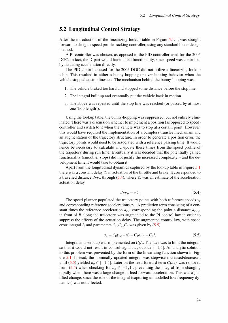
The control strategy is easily explained, using Figure 5.3. The rear axle centerof the real vehicle was projected onto the reference trajectory, as described in Sec-tion 5.1. The heading of the arising virtual vehicle was aligned with the tangent ofthe trajectory at R. Subsequently, the front wheels of the virtual vehicle were turnedso that its turning radius coincided with the curvature of the reference trajectory at R.The real vehicle was given a front wheel angle φ , steering it towards the end of animaginary handle of length l2, pulling the virtual vehicle along its path.
θ
S
O East
Nor
th F
Reference trajectoryVirtual
Referen
ce
Vehicle
Orthog
onal
projec
tion
Real V
ehicl
e
R
e⊥L
P
Q
l2
−φ
Figure 5.3 Graphical illustration of the lateral control strategy.
25
5.3 Lateral Control Strategy
Since the system was subject to an actuation delay τφ , as discussed in Section 5.1,the steering angle of the virtual reference vehicle was not computed from the curva-ture of the reference trajectory at R, but rather its curvature a distance dFF,φ ahead ofR.
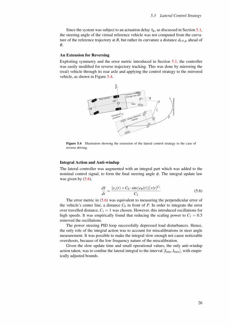
An Extension for ReversingExploiting symmetry and the error metric introduced in Section 5.1, the controllerwas easily modified for reverse trajectory tracking. This was done by mirroring the(real) vehicle through its rear axle and applying the control strategy to the mirroredvehicle, as shown in Figure 5.4.
F
East
Nor
th
Virtual reference
VehicleOrthogonal
projection
SReal Vehicle Reference trajectory
Vehicle mirrored
through rear axle
φ
O−θ
−φ
Q
e⊥
2l
R
P’
Figure 5.4 Illustration showing the extension of the lateral control strategy to the case ofreverse driving.
Integral Action and Anti-windupThe lateral controller was augmented with an integral part which was added to thenominal control signal, to form the final steering angle φ . The integral update lawwas given by (5.6).
dIdt
=[ey(t)+C0 · sin(eθ (t))]v(t)C1
C2(5.6)
The error metric in (5.6) was equivalent to measuring the perpendicular error ofthe vehicle’s center line, a distance C0 in front of P. In order to integrate the errorover travelled distance, C1 = 1 was chosen. However, this introduced oscillations forhigh speeds. It was empirically found that reducing the scaling power to C1 = 0.5removed the oscillations.
The power steering PID loop successfully depressed load disturbances. Hence,the only role of the integral action was to account for miscalibrations in steer anglemeasurement. It was possible to make the integral slow enough not cause noticeableovershoots, because of the low frequency nature of the miscalibration.
Given the slow update time and small operational values, the only anti-windupaction taken, was to confine the lateral integral to the interval [Imin, Imax], with empir-ically adjusted bounds.
26
6. Controller AnalysisThe nonlinear state feedback lateral controller is analyzed in this chapter. In Sec-tion 6.1 the global behavior of the controlled system is investigated by means of phaseportraits. Section 6.2 introduces a linearization of the controlled system around thezero error equilibrium, which is the region of nominal operation. The model is used toinvestigate stability margins and suggest a gain schedule of the controller parameterl2. Finally, global stability is discussed in Section 6.3.
6.1 Phase Plane Analysis
In order to analyze the performance of the lateral controller, the evolution of its er-ror state (ey,eθ ) was investigated by means of phase portraits. As suggested in Sec-tion 5.1, velocity dependence was dropped by plotting the error state evolution overtravelled distance d, rather than time.
Ultimately, it was desired to investigate the evolution of the error states with thereference trajectory taken to be an arbitrary parametrized curve in the ground plane.However, this was not possible, since (dey
dd , deθ
dd ) at a point (ey,eθ ,0) would not beuniquely defined, but depend on the location along the reference trajectory. The prob-lem was resolved by using circular trajectories and corresponding error dynamics(5.1,5.2) derived from Figure 5.2 in Section 5.1. Circular reference trajectories werechosen, since they were the most general curves, not leading to uniqueness problemsin (dey
dd , deθ
dd ). They were also good local approximations to any feasible trajectory.Further, model- and measurement errors were neglected and integral action was
omitted. The front wheel angle φ was confined to [φmin,φmax] = [−0.45 rad,0.45 rad],with numerical values obtained from measurements on Alice. Since curvature was
constant along the circular trajectory, the effect of the steering actuation delay τφ ,introduced in Section 5.1 could be neglected.
Under the above circumstances, the control law was given by (6.1,6.2,6.3) whereφv was the front wheel angle of the virtual vehicle and rc was the radius of the circularreference trajectory. Here, δ was the angle between the trajectory tangent at R (seeFigure 5.2) and steering wheel heading of the real vehicle. (The function atan2(x,y)in (6.2) is equivalent to arctan( x
y) with domain R\(0,0) and extended range [−π,π].)
φv = −arctanLrc
(6.1)
δ = atan2(l2 sinφv−Lsineθ − ey,L+ l2 cosφv−Lcoseθ ) (6.2)φ = satφmin,φmax (δ − eθ ) (6.3)
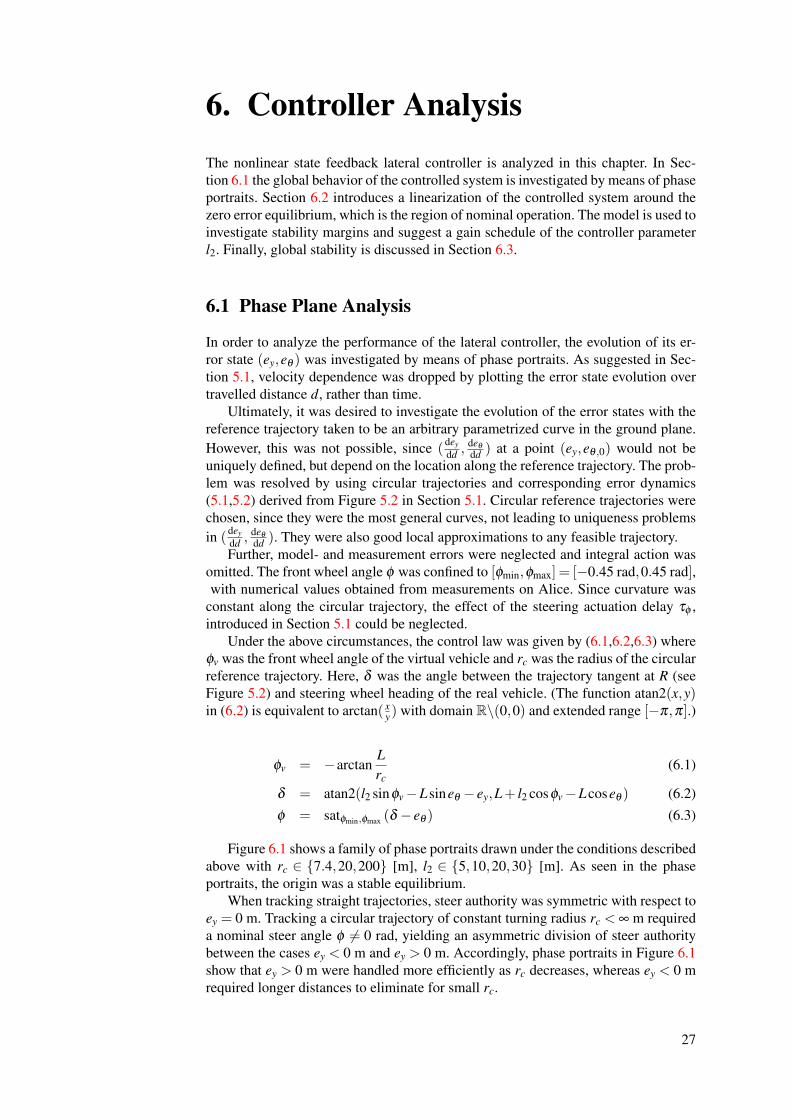
Figure 6.1 shows a family of phase portraits drawn under the conditions describedabove with rc ∈ {7.4,20,200} [m], l2 ∈ {5,10,20,30} [m]. As seen in the phaseportraits, the origin was a stable equilibrium.
When tracking straight trajectories, steer authority was symmetric with respect toey = 0 m. Tracking a circular trajectory of constant turning radius rc < ∞ m requireda nominal steer angle φ 6= 0 rad, yielding an asymmetric division of steer authoritybetween the cases ey < 0 m and ey > 0 m. Accordingly, phase portraits in Figure 6.1show that ey > 0 m were handled more efficiently as rc decreases, whereas ey < 0 mrequired longer distances to eliminate for small rc.
27
6.1 Phase Plane Analysis
-1.5 -1 -0.5 0 0.5 1 1.5
-5
0
5
10
eθ
e ⊥
rc = 7.4 m, l2 = 5 m
(a) rc = 7.4 m, l2 = 5 m
-1.5 -1 -0.5 0 0.5 1 1.5
-5
0
5
10
eθ
e ⊥
rc = 20, l2 = 5
(b) rc = 20 m, l2 = 5 m
-1.5 -1 -0.5 0 0.5 1 1.5
-5
0
5
10
eθ
e ⊥
rc = 200 m, l2 = 5 m
(c) rc = 200 m, l2 = 5 m
-1.5 -1 -0.5 0 0.5 1 1.5
-5
0
5
10
eθ
e ⊥
rc = 7.4 m, l2 = 10 m
(d) rc = 7.4 m, l2 = 10 m
-1.5 -1 -0.5 0 0.5 1 1.5
-5
0
5
10
eθ
e ⊥
rc = 20 m, l2 = 10 m
(e) rc = 20 m, l2 = 10 m
-1.5 -1 -0.5 0 0.5 1 1.5
-5
0
5
10
eθ
e ⊥
rc = 200 m, l2 = 10 m
(f) rc = 200 m, l2 = 10 m
-1.5 -1 -0.5 0 0.5 1 1.5
-5
0
5
10
eθ
e ⊥
rc = 7.4 m, l2 = 20 m
(g) rc = 7.4 m, l2 = 20 m
-1.5 -1 -0.5 0 0.5 1 1.5
-5
0
5
10
eθ
e ⊥
rc = 20 m, l2 = 20 m
(h) rc = 20 m, l2 = 20 m
-1.5 -1 -0.5 0 0.5 1 1.5
-5
0
5
10
eθ
e ⊥
rc = 200 m, l2 = 20 m
(i) rc = 200 m, l2 = 20 m
-1.5 -1 -0.5 0 0.5 1 1.5
-5
0
5
10
eθ
e ⊥
rc = 7.4 m, l2 = 30 m
(j) rc = 7.4 m, l2 = 30 m
-1.5 -1 -0.5 0 0.5 1 1.5
-5
0
5
10
eθ
e ⊥
rc = 20 m, l2 = 30 m
(k) rc = 20 m, l2 = 30 m
-1.5 -1 -0.5 0 0.5 1 1.5
-5
0
5
10
eθ
e ⊥
rc = 200 m, l2 = 30 m
(l) rc = 200 m, l2 = 30 m
Figure 6.1 Phase portraits showing the state evolution of error states ey,eθ for differentvalues of the trajectory radius rc and controller parameters l2.
Another observation was that controllers with larger l2 were more efficient inaligning the vehicle with the reference trajectory, but less efficient in eliminating thecross track error. This was obvious from the waggon-pulling analogy presented inSection 5.3.
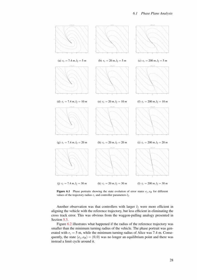
Figure 6.2 illustrates what happened if the radius of the reference trajectory wassmaller than the minimum turning radius of the vehicle. The phase portrait was gen-erated with rc = 5 m, while the minimum turning radius of Alice was 7.4 m. Conse-quently, the state (ey,eθ ) = (0,0) was no longer an equilibrium point and there wasinstead a limit cycle around it.
28
6.1 Phase Plane Analysis
-1.5 -1 -0.5 0 0.5 1 1.5
-5
0
5
10
eθ
e ⊥
rc = 5 m, l2 = 5 m
Figure 6.2 Phase portraits illustrating tracking of a circular trajectory with radius rc = 5 m,which was smaller than the minimum turning radius of Alice (7.4 m). The controller parameterwas set to l2 = 5 m.
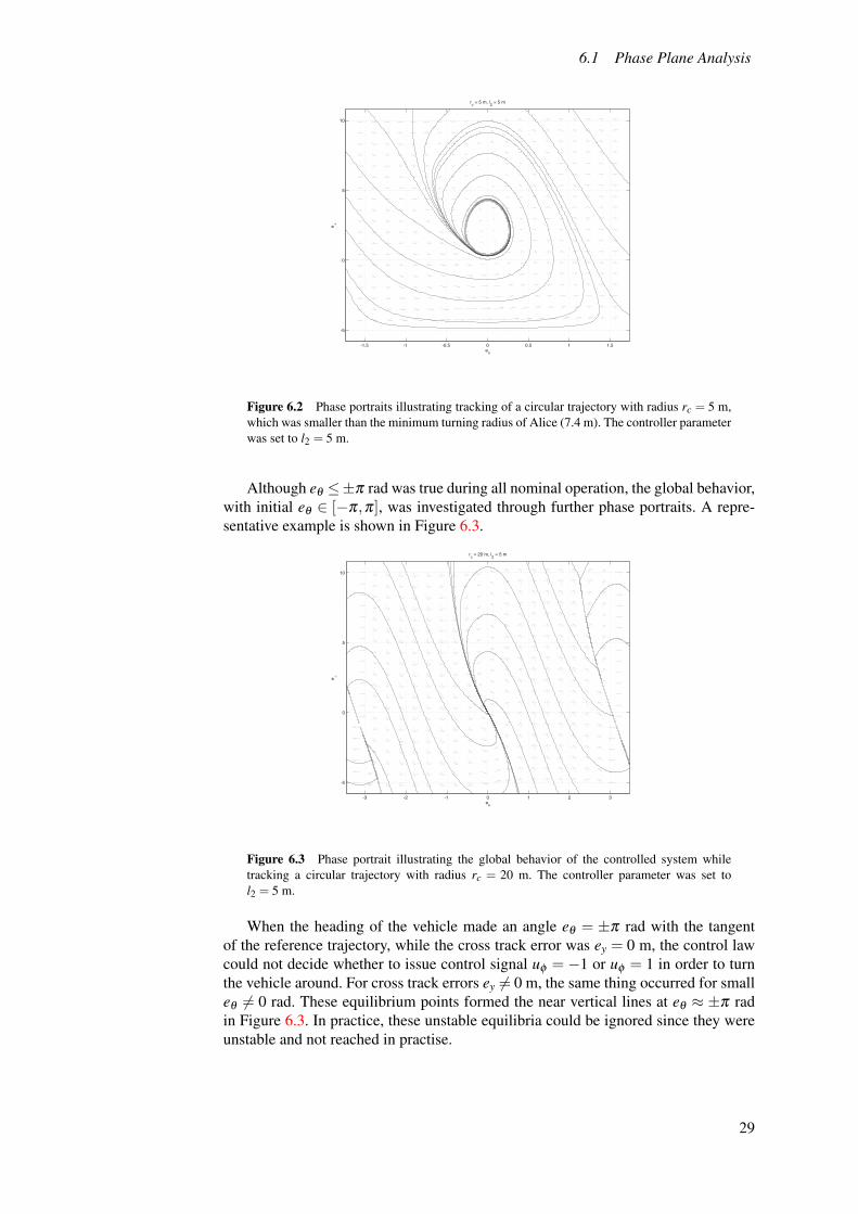
Although eθ ≤±π rad was true during all nominal operation, the global behavior,with initial eθ ∈ [−π,π], was investigated through further phase portraits. A repre-sentative example is shown in Figure 6.3.
-3 -2 -1 0 1 2 3
-5
0
5
10
eθ
e ⊥
rc = 20 m, l2 = 5 m
Figure 6.3 Phase portrait illustrating the global behavior of the controlled system whiletracking a circular trajectory with radius rc = 20 m. The controller parameter was set tol2 = 5 m.
When the heading of the vehicle made an angle eθ = ±π rad with the tangentof the reference trajectory, while the cross track error was ey = 0 m, the control lawcould not decide whether to issue control signal uφ = −1 or uφ = 1 in order to turnthe vehicle around. For cross track errors ey 6= 0 m, the same thing occurred for smalleθ 6= 0 rad. These equilibrium points formed the near vertical lines at eθ ≈ ±π radin Figure 6.3. In practice, these unstable equilibria could be ignored since they wereunstable and not reached in practise.
29
6.2 Linearization and Gain Scheduling
6.2 Linearization and Gain Scheduling
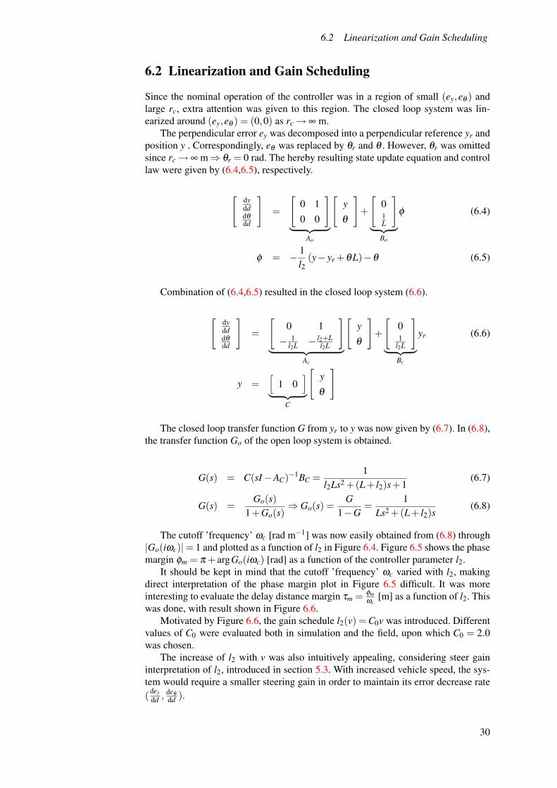
Since the nominal operation of the controller was in a region of small (ey,eθ ) andlarge rc, extra attention was given to this region. The closed loop system was lin-earized around (ey,eθ ) = (0,0) as rc→ ∞ m.
The perpendicular error ey was decomposed into a perpendicular reference yr andposition y . Correspondingly, eθ was replaced by θr and θ . However, θr was omittedsince rc→∞ m⇒ θr = 0 rad. The hereby resulting state update equation and controllaw were given by (6.4,6.5), respectively.
[dydddθ
dd
]=
[0 10 0
]︸ ︷︷ ︸
Ao
[y
θ
]+
[01L
]︸ ︷︷ ︸
Bo
φ (6.4)
φ = − 1l2
(y− yr +θL)−θ (6.5)
Combination of (6.4,6.5) resulted in the closed loop system (6.6).
[dydddθ
dd
]=
[0 1− 1
l2L − l2+Ll2L
]︸ ︷︷ ︸
Ac
[y
θ
]+
[01
l2L
]︸ ︷︷ ︸
Bc
yr (6.6)
y =[
1 0]
︸ ︷︷ ︸C
[y
θ
]
The closed loop transfer function G from yr to y was now given by (6.7). In (6.8),the transfer function Go of the open loop system is obtained.
G(s) = C(sI−AC)−1BC =1
l2Ls2 +(L+ l2)s+1(6.7)
G(s) =Go(s)
1+Go(s)⇒ Go(s) =
G1−G
=1
Ls2 +(L+ l2)s(6.8)
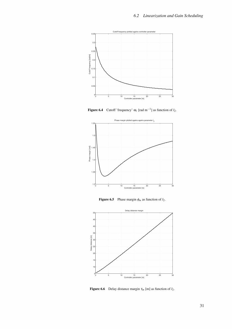
The cutoff ’frequency’ ωc [rad m−1] was now easily obtained from (6.8) through|Go(iωc)|= 1 and plotted as a function of l2 in Figure 6.4. Figure 6.5 shows the phasemargin φm = π + argGo(iωc) [rad] as a function of the controller parameter l2.
It should be kept in mind that the cutoff ’frequency’ ωc varied with l2, makingdirect interpretation of the phase margin plot in Figure 6.5 difficult. It was moreinteresting to evaluate the delay distance margin τm = φm
ωc[m] as a function of l2. This
was done, with result shown in Figure 6.6.Motivated by Figure 6.6, the gain schedule l2(v) = C0v was introduced. Different
values of C0 were evaluated both in simulation and the field, upon which C0 = 2.0was chosen.
The increase of l2 with v was also intuitively appealing, considering steer gaininterpretation of l2, introduced in section 5.3. With increased vehicle speed, the sys-tem would require a smaller steering gain in order to maintain its error decrease rate(dey
dd , deθ
dd ).
30
6.2 Linearization and Gain Scheduling
0 5 10 15 20 25 300
0.05
0.1
0.15
0.2
0.25
0.3
0.35Cutoff frequency plotted agains controller parameter
Controller parameter [m]
Cut
off f
requ
ency
[rad
/m]
Figure 6.4 Cutoff ’frequency’ ωc [rad m−1] as function of l2.
0 5 10 15 20 25 301.3
1.35
1.4
1.45
1.5
1.55Phase margin plotted agains agains parameter l2
Controller parameter [m]
Phas
e m
argi
n [ra
d]
Figure 6.5 Phase margin φm as function of l2.
0 5 10 15 20 25 305
10
15
20
25
30
35
40
45
50Delay distance margin
Controller parameter [m]
Del
ay d
ista
nce
[m]
Figure 6.6 Delay distance margin τm [m] as function of l2.
31

6.3 Global Stability
6.3 Global Stability
The analysis in Section 6.2 indicated stability with adequate margins around the zeroerror equilibrium. Further, geometric reasoning in Section 5.3 and the phase portraitsin Section 6.1 suggested global asymptotic stability (with the exception for the un-stable equilibrium points mentioned in Section 6.1). This was also validated, bothin simulation and the real process. However, devising a proof of asymptotic stabilitywas not an obvious problem to solve. A few Lyapunov-like approaches were made,but unfortunately this research was prevented by the tight time frame of the projectbefore a proof was obtained.
32
7. ImplementationThis chapter deals with the implementation of the trajectory tracking controller mod-ule. In Section 7.1 the structure, inherited by all software modules in the navigationstack, is explained. Section 7.2 reviews additional coding practise. This is followedby a discussion about the usage of threads in Section 7.3. The trajectory class is ex-plained in Section 7.4. The actual implementation of the closed loop controllers isthen handled in Section 7.5, with special attention to inter-module communicationsgiven in Sections 7.6 and 7.7. Finally, contingency management and the user interfaceare discussed in Sections 7.8 and 7.9, respectively.
7.1 Canonical Software Structure
All software modules in the navigation stack (including the trajectory tracking con-troller) adhered to the Canonical Software Structure (CSS) framework. The originalpurpose of this framework was threefold:
• Modularity. Providing flexibility and ease of re-use.
• Consistent structure. Making code more readable.
• Standardization. Providing predictability and increasing robustness.
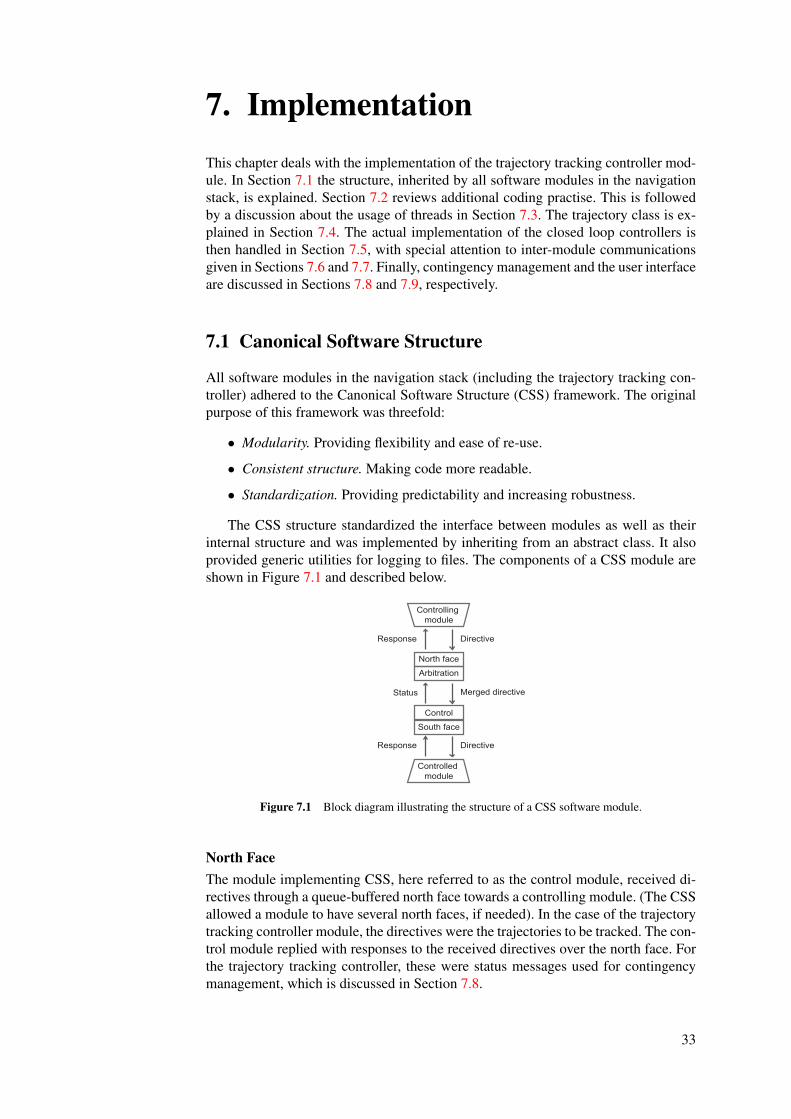
The CSS structure standardized the interface between modules as well as theirinternal structure and was implemented by inheriting from an abstract class. It alsoprovided generic utilities for logging to files. The components of a CSS module areshown in Figure 7.1 and described below.
Controlling module
Controlled module
Directive
Status Merged directive
Response
DirectiveResponse
Arbitration
North face
Control
South face
Figure 7.1 Block diagram illustrating the structure of a CSS software module.
North FaceThe module implementing CSS, here referred to as the control module, received di-rectives through a queue-buffered north face towards a controlling module. (The CSSallowed a module to have several north faces, if needed). In the case of the trajectorytracking controller module, the directives were the trajectories to be tracked. The con-trol module replied with responses to the received directives over the north face. Forthe trajectory tracking controller, these were status messages used for contingencymanagement, which is discussed in Section 7.8.
33
7.2 Coding Practice
ArbitrationReceiving directives and sending responses was handled by the arbitration block. It’smain purpose was to accept or reject incoming directives and send proper responses,depending on the state of the control module.
ControlThe arbitration block communicated with the control block by sending merged di-rectives and receiving status messages. (The term merged was explained by the casewhen the control module had more than one north face.) The control block was wherethe actual functionality of the control module lived. (In the CSS context control hadnothing to do with controller.) Apart from merged directives, the control block couldalso have ports towards estimators and device drivers and a south face towards thecontrolled module (or several south faces towards controlled modules). The controlblock made use of data arriving from arbitration and hardware ports, and generateddirectives which were sent to the controlled module over the south face(s).
South FaceThe south face was the interface between the control module and the controlled mod-ule. Structurally, the north and south faces were very similar.
7.2 Coding Practice
The CSS constituted a framework, defining code structure on a module level. In thissection additional implementation objectives, held in mind while implementing thetrajectory tracking controller module, will be reviewed.
Dynamic Memory AllocationDynamic memory allocation ’in the loop’ is slow and also dangerous, since it easilyleads to segmentation faults caused by memory leaks or dangling pointers. Wheneverpossible, memory was allocated at program initialization, and deallocated when theprogram terminated.
InheritanceInheritance, especially multiple inheritance, easily leads to pitfalls caused by incom-patibilities. Because of this, ’has-a’ relations were preferred to ’is-a’ ditto.
ThreadsMulti-threaded programs are generally harder to debug than single threaded ones.Also, code that is not thread safe easily leads to data corruption, when used in threadedenvironments. It was therefore desirable to minimize the number of simultaneouslyrunning threads. A short discussion is given in Section 7.3.
Magic NumbersThe occurrence of unexplained numerical values in the code was minimized. Wheresuitable, constants were defined in parameter files, which could be loaded duringruntime. For non-tunable constants, the #define and enum constructs were used.
Variable ScopeLimiting the scope of variables and functions was stressed. This increased the modu-larity of the code, and facilitated debugging.
34
7.3 Threads
7.3 Threads
As mentioned in Section 7.2 the number of threads was kept at a minimum. However,it was not practical to completely eliminate multi-threading. This was partly becausetrajectories were sent asynchronously and partly because the Sparrow Hawk userinterface (see Section 7.9) started a separate thread. Hence, the threads started by thetrajectory tracking controller module were:
• Trajectory receiving thread. This thread listened for trajectories on the northface. A mutex was implemented in order not to change reference trajectoryduring an ongoing control cycle. See Section 7.6 for details.
• Main program thread. This thread ran the actual controllers.
• User interface thread. The Sparrow Hawk user interface described in Sec-tion 7.9 was implemented using a separate thread.
• Canonical Software Structure. The inherited CSS structure ran several threads.It was, however, designed to be transparent to modules which inherited it.
7.4 The Trajectory Class
This section describes the class which implemented the trajectories to be tracked bythe trajectory tracking controller module. After reviewing the original implementa-tion, some augmentations and structural changes are suggested.
Original ImplementationA class, defining trajectories, was already in place at the beginning of the project.The trajectory object was defined by a trajectory header:
struct STrajHeader {
int m_numPoints; // number of points in this trajectory
int m_order; // max derivs of each point+1 (x,xdot -> 2)
int m_dir; // direction of the trajectory (-1 = rev)
} __attribute__((packed)) m_trajHeader;
The header defined the number of points in the trajectory, m_numPoints. Eachtrajectory point was assigned Cartesian coordinates (n,e), , defining northing andeasting, as well as time derivatives {(n, e),(n, e)...(n(m),e(m))} of these. The maximalorder m was defined through m_order. Further, the trajectory object was associatedwith a direction m_dir being either forward or reverse. It determined the drivingdirection of the tracking vehicle.
The actual trajectory was stored in two fixed sized arrays, allocated at construc-tion:
double *m_pN;
double *m_pE;
The size of these arrays was given by #define TRAJ_MAX_LEN 5000 and con-stituted an upper bound on m_numPoints in the trajectory header. The firstTRAJ_MAX_LEN elements of the northing array *m_pN were northing coordinates, n.The next TRAJ_MAX_LEN elements, were first order derivatives, n, and so on. (Thesame applied for the easting array *m_pE.) The derivative of order p associated withpoint i was hence easily accessible using#define INDEX(i,p) ((i) + (p)*TRAJ_MAX_LEN).
35
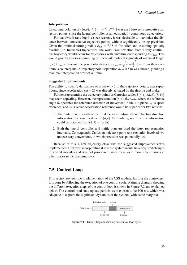
7.5 Control Loop
InterpolationLinear interpolation of {(n, e),(n, e)...(n(m),e(m))}was used between consecutive tra-jectory points, since the lateral controller assumed spatially continuous trajectories.
For bandwidth (and log file size) reasons, it was desirable to maximize the dis-tance between consecutive trajectory points, without significantly losing precision.Given the minimal turning radius rmin = 7.35 m for Alice and assuming spatiallyfeasible (i.e. trackable) trajectories, the worst case deviation from a truly continu-ous trajectory would occur for trajectories with curvature corresponding to rmin. Thiswould give trajectories consisting of linear interpolated segments of maximal length
di < 2rmin a maximal perpendicular deviation rmin−√
r2− di2
2[m] from their con-
tinuous counterparts. A trajectory point separation di = 0.5 m was chosen, yielding amaximal interpolation error of 4.3 mm.
Suggested ImprovementsThe ability to specify derivatives of order m > 2 in the trajectory points, was super-fluous, since acceleration (m = 2) was directly actuated by the throttle and brake.
Further, representing the trajectory points as Cartesian tuples {(n,e),(n, e),(n, e)}may seem appealing. However, the representation (n,e),θr,vr,ar, where the referenceangle θr specifies the reference direction of movement in the n,e-plane, vr is speedreference, and ar is scalar acceleration reference would be superior for two reasons:
1. The finite (fixed) length of the double was limiting when extracting directioninformation for small values of (n, e). Particularly, no direction informationcould be obtained for {(n, e) = (0,0)}.
2. Both the lateral controller and traffic planners used the latter representationinternally. Consequently, Cartesian trajectory point representation involved twounnecessary conversions, in which precision was potentially lost.
Because of this, a new trajectory class with the suggested improvements wasimplemented. However, incorporating it into the system would have required changesin several modules and was not prioritized, since there were more urgent issues atother places in the planning stack.
7.5 Control Loop
This section reviews the implementation of the CSS module, hosting the controllers.It is done by following the execution of one control cycle. A timing diagram showingthe different execution steps of the control loop is shown in Figure 7.2 and explainedbelow. The control- and state update periods were chosen to be 100 ms, which wasadequate to capture the significant dynamics of the system (with some margins).
Not to scale
2. Update state
3. Control
1. Arbitrate
4. Log
5. Sleep
Figure 7.2 Timing diagram showing one control loop cycle.
36
7.5 Control Loop
ArbitrationThe arbitrate function was invoked at the beginning of each control cycle. Its pur-pose was to populate and send response messages to the traffic planner through thenorth face. These responses were populated from a control status object, hosting twocategories of information. One was the actuator status information, which was pop-ulated in the arbitrate function by reading actuator status responses queued at thesouth face. The other part was populated during the previous control cycle and usedfor contingency management. See Section 7.8 for a description of the control statusobject.
State UpdatesAfter return of the arbitration function, the state variables used by the controllerswere updated. They were:
• Vehicle State. The vehicle state was read from a separate module, which com-municated with the Applanix state estimator described in Section 3.1. It es-timated the position (northing, easting, altitude) and orientation (roll, pitch,yaw) of the vehicle as well as the first time derivative of the listed entities. Forconvenience, the state was given in both (global) Universal Transverse Mer-cator (UTM) and (local) vehicle frame coordinates. The vehicle state struct
also held a time stamp used for detecting delays and when logging to file.
• Actuator State. The actuator state held information from the steer, throttle,brake and transmission actuators. A status (on/off), commanded position, mea-sured position and time stamp were populated by each mentioned actuator. Theactuator state also told whether the vehicle was stopped (used system wide) aswell as the E-stop state, explained below. (It also had some deprecated mem-bers, not mentioned here.)
• E-stop State. Implementation-wise, the E-stop state was part of the actuatorstate, despite the separate attention given here. It was defined by the followingenumeration:
enum EstopStatus {
EstopDisable = 0,
EstopPause = 1,
EstopRun = 2
};
During nominal autonomous operation the E-stop state was EstopRun. TheEstopPause state was used when the vehicle needed to be momentarily stopped(either by a safety driver or remotely). Transition from EstopPause to EstopRun
was straight forward, whereas transition from EstopDisable to EstopRun requiredmanual re-initialization of the system. EstopDisable was used when the vehiclewas manually driven (on e.g. public streets) or at other occasions when spurioustransitions into EstopRun were unwanted, or even dangerous.
ControlOnce all states were updated, The controllers were invoked in the following order:
• Longitudinal Controller.
• Lateral Controller.
37
7.6 North Face communication
• Transmission Controller.
The controllers were passed pointers to the current trajectory, vehicle state, con-trol status object and actuator directives to be populated. Once all three controllershad returned, the corresponding actuator directives were passed down through thesouth face to the hardware actuating software module.
LoggingDuring each cycle, the trajectory tracking controller module logged its current stateto file. The log files could be considered an augmentation to the user interface andare therefore briefly treated in Section 7.9.
SleepIn order to maintain a constant control period, the process in which the controllerswere running was issued to sleep for a variable amount of time at the end of eachcontrol cycle. As shown in Figure 7.2 the majority of the execution time (97 %) wasspent sleeping.
7.6 North Face communication
The trajectory tracking controller CSS module had a north face towards the trafficplanner. It was used to receive trajectories and send status responses. The latter wastightly associates with contingency management and is treated in Section 7.8. Thecode of the trajectory receiving thread is shown below.
void Follower::CommThread ()
{ int trajSocket;
trajSocket = m_skynet.listen(SNtraj, SNplanner);
CTraj* newTraj = new CTraj(3);
CTraj* tmpTraj;
while (!ExitHandler::quit) {
bool trajReceived = RecvTraj (trajSocket, newTraj);
while (m_skynet.is_msg(trajSocket)) {
trajReceived = RecvTraj(trajSocket, newTraj);
}
if (trajReceived) {
m_trajectoryCounter++;
DGClockMutex(&m_recvdTrajMutex);
tmpTraj = newTraj;
newTraj = m_recvdTraj;
m_recvdTraj = tmpTraj;
DGCunlockMutex(&m_recvdTrajMutex);
}
}
delete newTraj;
}
The purpose of the thread was to copy incoming trajectories to a memory locationpointed at by m_recvdTraj (which was accessible from the controllers), while lock-ing the m_recvdTrajMutex and hence rendering the copy operation atomic, from thecontrollers’ point of view.
38
7.7 South Face communication
At the beginning of the thread two trajectory pointers were declared of whichnewTraj pointed at an actual trajectory object. The thread then ran whileExitHandler::quit was false. (The role of the ExitHandler was to ensure thatthreads terminated in correct order when the module was shut down.) In order toavoid dynamic memory allocation in the loop, a scheme with three statically allo-cated trajectory pointers was used. Incoming trajectories were written to the memorylocation pointed at by newTraj. At this point a trajectory counter (used for debuggingpurposes) was incremented, followed by the locking of the m_trajRecvdMutex. Thenext three lines were ’pointer juggling’, making m_recvdTraj point at the newly re-ceived trajectory and newTraj at the previously received trajectory object (which wasa safe location to overwrite, once a new trajectory arrived from the traffic planner).
7.7 South Face communication
The individual controllers wrote their output directly into actuator directives. Thesewere given ID numbers before being queued at the south face and sent to the hard-ware actuating software module. The ID numbers were later used to match responsesfrom the hardware actuating software module to their corresponding directives. (Thedirective-response pair was handled upon which the directive was dequeued.) To betime-wise robust against lost or late responses, the queue was implemented as a linkedlist (rather than vector).
7.8 Contingency Management
To be successful, the trajectory tracking controller module needed to handle variousspecial situations and errors. A control status object was passed by reference to thedifferent controllers and maintained a centralized notion of execution state. It waspopulated by members of the following enumeration:
enum followerStates {
Running = 0,
TrajectoryTimeout = 1 << 0,
TrajectoryError = 1 << 1,
EstopPause = 1 << 2,
EstopDisable = 1 << 3,
TransmissionPending = 1 << 4,
TransmissionRejected = 1 << 5,
SteeringRejected = 1 << 6,
ThrottleRejected = 1 << 7,
BrakeRejected = 1 << 8,
TrajectoryEnd = 1 << 9,
LateralMaxError = 1 << 10,
LongitudinalMaxError = 1 << 11,
SteeringFailure = 1 << 12,
ThrottleFailure = 1 << 13,
BrakeFailure = 1 << 14,
TransmissionFailure = 1 << 15,
ReactiveObstacleAvoidance = 1 << 16
};
39
7.9 User Interface
These were all defined as powers of two, facilitating straight forward hosting ofthe control status in a single integer. Each member was represented by the bit ofcorresponding value and bit-wise masking was used to set and clear bits. This alsoexplains why the nominal Running state was represented by 0.
The LateralMaxError and LongitudinalMaxError bits were deprecated. (Theywere originally used to request a spatial re-plan from the traffic planner, if either thelateral or speed error exceeded thresholds given in a parameter file.) TheReactiveObstacleAvoidance bit is not treated here, since it falls outside the con-text. Remaining enumeration members can be divided into trajectory- and actuatorerrors, given separate attention below.
Trajectory ErrorsThe TrajectoryTimeout bit was set when a trajectory was not received for someparametrized time (nominally 2 s). The controller responded to these timeouts bybringing the vehicle to a stop. Once a new trajectory was received, the timeout bitwas cleared.
The TrajectoryError bit was set if a received trajectory did not adhere to thespecified format. When set, a request for a new trajectory was sent to the traffic plan-ner.
Actuator ErrorsActuator failures were detected by the software module receiving directives fromthe trajectory tracking controller. This module sent responses to all directives re-ceived from the controllers. There were two possible error responses – rejected orfailed, each associated with a specific actuator. A directive was failed if the corre-sponding actuator suffered from a hardware failure, whereas the rejection mecha-nism was part of a low level contingency management scheme. For instance, throt-tle directives were rejected while the vehicle was changing gears (indicated by theTransmissionPending bit) or if there was a steering failure.
Apart from the above mentioned errors, the actuating software module was alsoresponsible for updating the E-stop state, which was quarried and handled by thetrajectory tracking controller module.
7.9 User Interface
To facilitate debugging, both during simulation and field tests, the trajectory trackingcontroller module was equipped with a partly interactive user interface consisting ofseveral parts, handled below.
Sparrow HawkSparrow Hawk [25] is a collection of programs and a library of C functions intendedto aid in the implementation of real time controllers on PC-based data acquisitionand control systems. The part of it used in Alice was a framework for implement-ing interactive text-based console displays. They were interactive, since keys couldbe bound to trigger call-back functions. It was also possible to alter the values ofprogram variables directly from the console display.
A ’screen shot’ of the Sparrow Hawk display of the trajectory tracking controllermodule is shown and explained in Appendix C.
40
7.9 User Interface
Map Viewer VisualizationThe geometric nature of the lateral control algorithm, was very convenient when itcame to debugging. The ’handle’ described in Section 5.3 was drawn in the mapviewer software, providing visual information which was easier to interpret (duringrun time) than the corresponding numbers in the Sparrow Hawk display.
Parameter Files and Command Line ArgumentsGengetopt [3] is a tool for writing command line option parsing code for C programs.It was used for command line parsing at module startup as well as parsing of thecontroller parameter file, which could be updated from the sparrow hawk displayduring run time. This was very convenient, since it allowed new parameter sets to beloaded without having to restart the entire navigation stack.
Log FilesThe perhaps most important part of the user interface was the logger mentioned inSection 7.5. The following information was logged once per control cycle:
• Timing information.
• Vehicle state.
• Actuator state.
• Reference trajectory information.
• Control errors.
• Timing information.
• Vehicle state.
• Actuator state.
• Reference trajectory information.
• Control errors.
• Controller state.
Since file access was slow, with undeterministic duration, all log file writing washandled after the invocation of the actual controllers.
Log files were used extensively to debug and tune the controllers. They were alsothe basis for all material presented in Chapter 8.
41
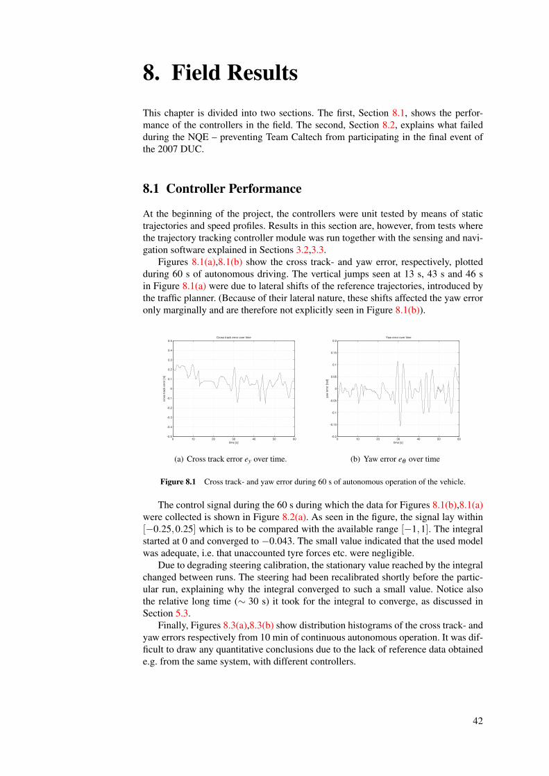
8. Field ResultsThis chapter is divided into two sections. The first, Section 8.1, shows the perfor-mance of the controllers in the field. The second, Section 8.2, explains what failedduring the NQE – preventing Team Caltech from participating in the final event ofthe 2007 DUC.
8.1 Controller Performance
At the beginning of the project, the controllers were unit tested by means of statictrajectories and speed profiles. Results in this section are, however, from tests wherethe trajectory tracking controller module was run together with the sensing and navi-gation software explained in Sections 3.2,3.3.
Figures 8.1(a),8.1(b) show the cross track- and yaw error, respectively, plottedduring 60 s of autonomous driving. The vertical jumps seen at 13 s, 43 s and 46 sin Figure 8.1(a) were due to lateral shifts of the reference trajectories, introduced bythe traffic planner. (Because of their lateral nature, these shifts affected the yaw erroronly marginally and are therefore not explicitly seen in Figure 8.1(b)).
0 10 20 30 40 50 60-0.5
-0.4
-0.3
-0.2
-0.1
0
0.1
0.2
0.3
0.4
0.5Cross track error over time
time [s]
cros
s tra
ck e
rror [
m]
(a) Cross track error ey over time.
0 10 20 30 40 50 60-0.2
-0.15
-0.1
-0.05
0
0.05
0.1
0.15
0.2Yaw error over time
time [s]
yaw
erro
r [ra
d]
(b) Yaw error eθ over time
Figure 8.1 Cross track- and yaw error during 60 s of autonomous operation of the vehicle.
The control signal during the 60 s during which the data for Figures 8.1(b),8.1(a)were collected is shown in Figure 8.2(a). As seen in the figure, the signal lay within[−0.25,0.25] which is to be compared with the available range [−1,1]. The integralstarted at 0 and converged to −0.043. The small value indicated that the used modelwas adequate, i.e. that unaccounted tyre forces etc. were negligible.
Due to degrading steering calibration, the stationary value reached by the integralchanged between runs. The steering had been recalibrated shortly before the partic-ular run, explaining why the integral converged to such a small value. Notice alsothe relative long time (∼ 30 s) it took for the integral to converge, as discussed inSection 5.3.
Finally, Figures 8.3(a),8.3(b) show distribution histograms of the cross track- andyaw errors respectively from 10 min of continuous autonomous operation. It was dif-ficult to draw any quantitative conclusions due to the lack of reference data obtainede.g. from the same system, with different controllers.
42
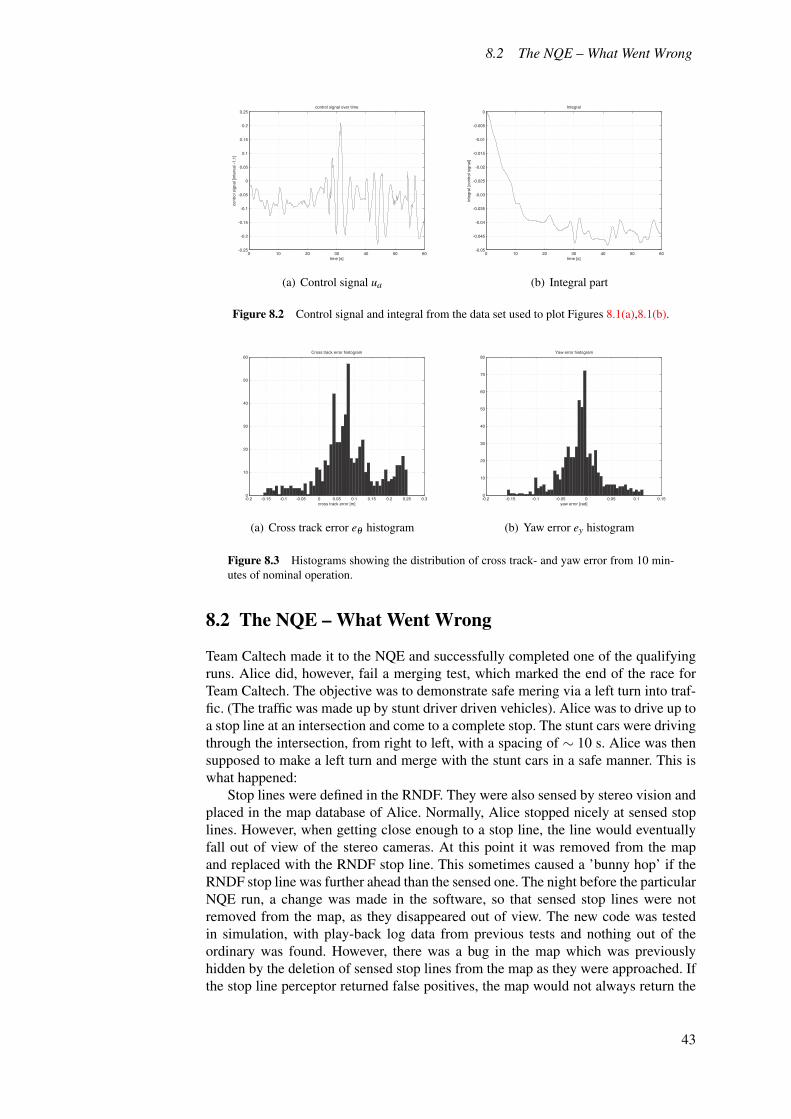
8.2 The NQE – What Went Wrong
0 10 20 30 40 50 60-0.25
-0.2
-0.15
-0.1
-0.05
0
0.05
0.1
0.15
0.2
0.25control signal over time
time [s]
cont
rol s
igna
l [in
terv
al -1
,1]
(a) Control signal ua
0 10 20 30 40 50 60-0.05
-0.045
-0.04
-0.035
-0.03
-0.025
-0.02
-0.015
-0.01
-0.005
0Integral
time [s]
inte
gral
[con
trol s
igna
l]
(b) Integral part
Figure 8.2 Control signal and integral from the data set used to plot Figures 8.1(a),8.1(b).
-0.2 -0.15 -0.1 -0.05 0 0.05 0.1 0.15 0.2 0.25 0.30
10
20
30
40
50
60Cross track error histogram
cross track error [m]
(a) Cross track error eθ histogram
-0.2 -0.15 -0.1 -0.05 0 0.05 0.1 0.150
10
20
30
40
50
60
70
80Yaw error histogram
yaw error [rad]
(b) Yaw error ey histogram
Figure 8.3 Histograms showing the distribution of cross track- and yaw error from 10 min-utes of nominal operation.
8.2 The NQE – What Went Wrong
Team Caltech made it to the NQE and successfully completed one of the qualifyingruns. Alice did, however, fail a merging test, which marked the end of the race forTeam Caltech. The objective was to demonstrate safe mering via a left turn into traf-fic. (The traffic was made up by stunt driver driven vehicles). Alice was to drive up toa stop line at an intersection and come to a complete stop. The stunt cars were drivingthrough the intersection, from right to left, with a spacing of ∼ 10 s. Alice was thensupposed to make a left turn and merge with the stunt cars in a safe manner. This iswhat happened:
Stop lines were defined in the RNDF. They were also sensed by stereo vision andplaced in the map database of Alice. Normally, Alice stopped nicely at sensed stoplines. However, when getting close enough to a stop line, the line would eventuallyfall out of view of the stereo cameras. At this point it was removed from the mapand replaced with the RNDF stop line. This sometimes caused a ’bunny hop’ if theRNDF stop line was further ahead than the sensed one. The night before the particularNQE run, a change was made in the software, so that sensed stop lines were notremoved from the map, as they disappeared out of view. The new code was testedin simulation, with play-back log data from previous tests and nothing out of theordinary was found. However, there was a bug in the map which was previouslyhidden by the deletion of sensed stop lines from the map as they were approached. Ifthe stop line perceptor returned false positives, the map would not always return the
43
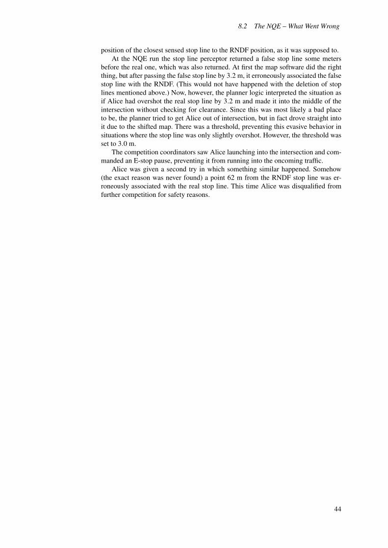
8.2 The NQE – What Went Wrong
position of the closest sensed stop line to the RNDF position, as it was supposed to.At the NQE run the stop line perceptor returned a false stop line some meters
before the real one, which was also returned. At first the map software did the rightthing, but after passing the false stop line by 3.2 m, it erroneously associated the falsestop line with the RNDF. (This would not have happened with the deletion of stoplines mentioned above.) Now, however, the planner logic interpreted the situation asif Alice had overshot the real stop line by 3.2 m and made it into the middle of theintersection without checking for clearance. Since this was most likely a bad placeto be, the planner tried to get Alice out of intersection, but in fact drove straight intoit due to the shifted map. There was a threshold, preventing this evasive behavior insituations where the stop line was only slightly overshot. However, the threshold wasset to 3.0 m.
The competition coordinators saw Alice launching into the intersection and com-manded an E-stop pause, preventing it from running into the oncoming traffic.
Alice was given a second try in which something similar happened. Somehow(the exact reason was never found) a point 62 m from the RNDF stop line was er-roneously associated with the real stop line. This time Alice was disqualified fromfurther competition for safety reasons.
44
9. ConclusionsA trajectory tracking software module was designed, analyzed, implemented andtested. A lot of time and effort was spent integrating it with the other modules ofthe system. In parallel with this, the other modules of the system were developed,integrated and tested. By the NQE all desired functionality was in place. However,there was not enough time for proper bug fixing and tuning. This became apparent atthe NQE, as indicated in Section 8.2. Here follows a list of conclusions, which wererealized throughout the project. Some conclusions are also found in Chapter 10.
• Test time. About one month prior to the NQE, there was a major code restruc-turing in which the main traffic planner was basically re-written. At this pointa lot of time was spent testing, and it got quite hectic as new bugs were foundand fixed, just to discover that they hid others. The lesson learned here, was thatit took more time than one would initially imagine, to properly test and tunea complex system like Alice and that late code changes should be avoided, ifpossible.
• Special cases. The design of Alice was complicated by the handling of variousspecial cases, which were introduced since it was hard to know what to expectat the finals. It is my belief that a more simplistic approach to the problem mightwell have taken Team Caltech to the finals. But once again, it was impossibleto know what situations were to be encountered. For example a lot of time wasspent developing code which would take Alice past road block, just to discoverthat there were none at neither the NQE nor the final event.
• Team work. Working in a big group was a challenge. Good communicationswere paramount to avoid misunderstandings, leading to bugs. Using the utili-ties, mentioned in Section 2.2, truly facilitated this work. It was also facilitatedby the friendliness and motivation found in all team members.
• CSS. The CSS, introduced in Section 7.1, was based on a good idea. However,the implementation was rather complicated. As a result it was fully inherited byonly one or two software modules. Hence, its role as a standardizing interfacewas somewhat lost.
• Personal reflections. Prior to the project, it was difficult to know what to expect.Initially, the mere amount of project code was chocking. I had never worked ona software project involving more than two persons and never written anythingin C++. Fortunately, it did not take more than one or two weeks to get started.Then the entire project was one long learning experience – partly because ofmy limited background in software engineering. It was very stressful at times,but at the same time I cannot think of a better way to learn practical problemsolving through programming. Last but not least, participating in Team Caltechhas given me new friends, from around the world.
45
10. Future WorkAlthough the controllers did their job in tracking reference trajectories, there re-mained things which could potentially improve the trajectory tracking controllermodule and the understanding of its behavior. The areas of these possible improve-ments are the subjects of Section 10.1, whereas Section 10.2 deals with possibleimprovements of the entire system. Generally, this chapter reviews known problems,rather than suggesting their solutions.
10.1 Controller Module
This section is divided into three sub-sections, addressing the longitudinal control,lateral control and control related hardware, respectively.
Longitudinal Control• Position controller. At low speeds, the non-linearity in the longitudinal actua-
tion was not perfectly captured by the lookup table introduced in Section 5.1.(E.g. stick-slip friction, which occurred when accelerating from zero speed,was not modelled at all.) To increase smoothness of operation, especially inparking situations, a position- (rather than speed-) tracking controller, as sug-gested in Section 5.2 would be valuable.
• Adaptive identification. No explicit attention was made to changes in road com-position (asphalt, dirt, etc.), winds, vehicle load or other factors affecting thevalidity of the lookup table shown in Figure 5.1. In general, the controlled sys-tem was robust to such changes. However, utilizing e.g. an adaptive updateof the lookup table would probably have increased performance, given slowenough update times not to jeopardize corruption of the lookup table due tohigh frequency phenomena.
Lateral Control• Error convergence. Apart from the numerical analysis of the lateral controller
given in Chapter 6, it would be interesting to obtain a lower bound of its errorconvergence rate.
• Stability margins. The delay margin was obtained for the linearization of thesystem around its zero error equilibrium in Section 6.2 and verified throughfield experiments (not presented here). In addition to this it would be of interestto obtain measures or sensitivity to disturbances introduced at different pointsof the loop. (The non-static components of such disturbances were shown to benegligible in Alice, through field tests.) In addition to this, further analysis ofthe nonlinear region of operation would provide deeper understanding of thecontroller.
• Gain schedule. It could be worthwhile to experiment with the gain schedule ofl2, which was introduced in Section 6.2. A possible candidate would be e.g. aschedule resulting in a speed independent upper limit of centripetal accelera-tion vehicle acceleration.
46
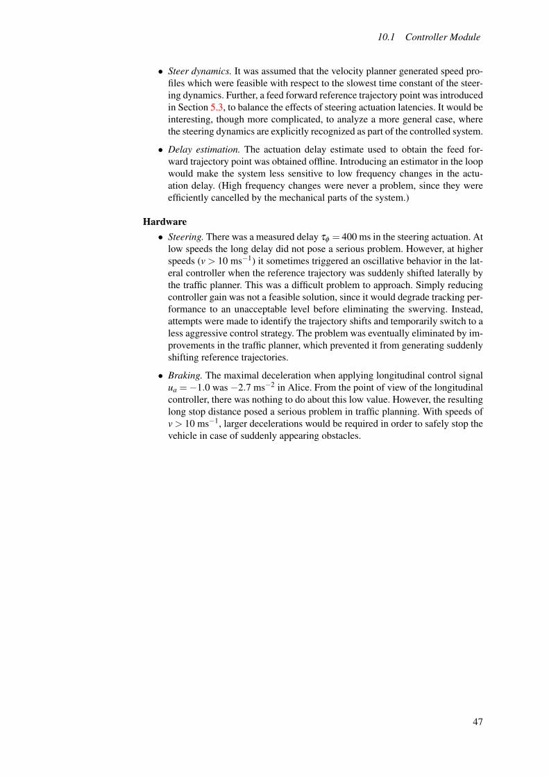
10.1 Controller Module
• Steer dynamics. It was assumed that the velocity planner generated speed pro-files which were feasible with respect to the slowest time constant of the steer-ing dynamics. Further, a feed forward reference trajectory point was introducedin Section 5.3, to balance the effects of steering actuation latencies. It would beinteresting, though more complicated, to analyze a more general case, wherethe steering dynamics are explicitly recognized as part of the controlled system.
• Delay estimation. The actuation delay estimate used to obtain the feed for-ward trajectory point was obtained offline. Introducing an estimator in the loopwould make the system less sensitive to low frequency changes in the actu-ation delay. (High frequency changes were never a problem, since they wereefficiently cancelled by the mechanical parts of the system.)
Hardware• Steering. There was a measured delay τφ = 400 ms in the steering actuation. At
low speeds the long delay did not pose a serious problem. However, at higherspeeds (v > 10 ms−1) it sometimes triggered an oscillative behavior in the lat-eral controller when the reference trajectory was suddenly shifted laterally bythe traffic planner. This was a difficult problem to approach. Simply reducingcontroller gain was not a feasible solution, since it would degrade tracking per-formance to an unacceptable level before eliminating the swerving. Instead,attempts were made to identify the trajectory shifts and temporarily switch to aless aggressive control strategy. The problem was eventually eliminated by im-provements in the traffic planner, which prevented it from generating suddenlyshifting reference trajectories.
• Braking. The maximal deceleration when applying longitudinal control signalua =−1.0 was −2.7 ms−2 in Alice. From the point of view of the longitudinalcontroller, there was nothing to do about this low value. However, the resultinglong stop distance posed a serious problem in traffic planning. With speeds ofv > 10 ms−1, larger decelerations would be required in order to safely stop thevehicle in case of suddenly appearing obstacles.
47
10.2 System
10.2 System
The trajectory tracking controller module was only a small part of a complex system.
• Vehicle state estimation. Throughout the development process, problems wereexperienced with the Applanix vehicle state estimator described in Section 3.1.Occasionally it introduced large (> 1 m) state drifts as the vehicle resumeddriving after long (> 30 s) stops. Unfortunately, the problem was never re-solved, since the team did not have access to the software of the Applanix –it was merely a black box, providing state data. Instead a workaround solutionutilizing drifting coordinate frames was introduced.
• Unit testing. A large amount of system test time was inefficiently spent, sinceit was difficult to unit test some of the individual modules before integratingthem into the system. A proper framework for unit testing would therefore havefacilitated the development process significantly.
• Sensor coverage. Although Alice was equipped with a seemingly large numberof sensors, sensor coverage proved to be inadequate in e.g. intersections. Thiswas worsened by the fact that the perception software sometimes confusedstatic- and moving obstacles.
48
A. Project Time LineThe nominal time line of Team Caltech’s development process for the 2007 DUC wasdivided into 5 spirals, each defined by a list of goals. The spirals and correspondinggoals are given below. A brief discussion of the time line was given in Section 2.3.
Spiral 0 – Planning and Preparation (13 Jun - 8 Jul)
1. Finalize plan for the summer (goals, time line, sub-teams).
2. Update architecture (navigation system, coding standards).
3. Update software infrastructure (unit test structure, common startup scripts,YaM improvements).
4. Update hardware infrastructure (remount sensors, cabin reorganization, final-ize power design, install new computers).
Spiral 1 – Navigation and Traffic (9 Jul - 5 Aug)
1. Safe and robust driving in all navigation- and basic traffic scenarios .
2. Working versions of all modules.
3. Hardware system finalized.
Spiral 2 – Advances Traffic (6 Aug - 2 Sep)
1. Safe, robust and persistent driving in all navigation- and traffic scenarios.
2. System functionality finalized.
Spiral 3 – Optimization (4 Sep - 30 Sep)
1. Race-ready operations and capability of autonomously driving 60 miles in lessthan 6 hours.
2. Code finalized.
Spiral 4 – NQE and Race Preparations (1 Oct - 21 Oct)
1. Mistake-free NQE and race procedures.
49
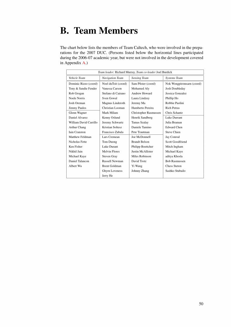
B. Team MembersThe chart below lists the members of Team Caltech, who were involved in the prepa-rations for the 2007 DUC. (Persons listed below the horizontal lines participatedduring the 2006-07 academic year, but were not involved in the development coveredin Appendix A.)
Team leader: Richard Murray, Team co-leader Joel Burdick
Vehicle Team Navigation Team Sensing Team Systems Team
Dominic Rizzo (coord) Noel duToit (coord) Sam Pfister (coord) Nok Wongpiromsarn (coord)
Tony & Sandie Fender Vanessa Carson Mohamed Aly Josh Doubleday
Rob Grogan Stefano di Cairano Andrew Howard Jessica Gonzalez
Noele Norris Sven Gowal Laura Lindzey Phillip Ho
Josh Oreman Magnus Linderoth Jeremy Ma Robbie Paolini
Jimmy Paulos Christian Looman Humberto Pereira Rich Petras
Glenn Wagner Mark Milam Christopher Rasmussen Chris Schantz
Daniel Alvarez Kenny Oslund Henrik Sandberg Luke Durrant
William David Carrillo Jeremy Schwartz Tamas Szalay Julia Braman
Arthur Chang Kristian Soltesz Daniele Tamino Edward Chen
Iain Cranston Francisco Zabala Pete Trautman Steve Chien
Matthew Feldman Lars Cremean Joe McDonnell Jay Conrod
Nicholas Fette Tom Duong Brandt Belson Scott Goodfriend
Ken Fisher Luke Durant Philipp Boettcher Mitch Ingham
Nikhil Jain Melvin Flores Justin McAllister Michael Kaye
Michael Kaye Steven Gray Miles Robinson aditya Khosla
Daniel Talancon Russell Newman David Trotz Bob Rasmussen
Albert Wu Brent Goldman Yi Wang Chess Steton
Ghyrn Loveness Johnny Zhang Sashko Stubailo
Jerry He
50
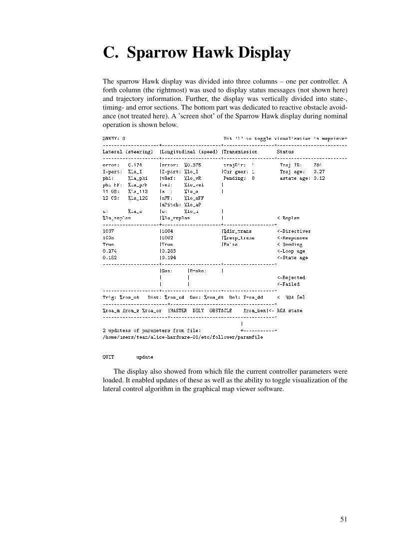
C. Sparrow Hawk DisplayThe sparrow Hawk display was divided into three columns – one per controller. Aforth column (the rightmost) was used to display status messages (not shown here)and trajectory information. Further, the display was vertically divided into state-,timing- and error sections. The bottom part was dedicated to reactive obstacle avoid-ance (not treated here). A ’screen shot’ of the Sparrow Hawk display during nominaloperation is shown below.
SNKEY: 0 Hit 'l' to toggle visualization in mapviewer
--------------------+---------------------+------------------+-------------------------
Lateral (steering) |Longitudinal (speed) |Transmission |Status
--------------------+---------------------+------------------+-------------------------
error: 0.174 |error: %0.375 |trajDir: 1 | Traj ID: 784
I-part: %la_I |I-part: %lo_I |Cur gear: 1 | Traj age: 0.27
phi: %la_phi |vRef: %lo_vR |Pending: 0 | astate age: 0.12
phi FF: %la_pFF |vel: %lo_vel | |
l1 GS: %la_l1G |a : %lo_a | |
l2 GS: %la_l2G |aFF: %lo_aFF | |
|aPitch: %lo_aP | |
u: %la_u |u: %lo_u | |
%la_replan |%lo_replan | |<-Replan
--------------------+---------------------+------------------+
1007 |1004 |%dir_trans |<-Directives
1005 |1002 |%resp_trans |<-Responses
True |True |False |<-Sending
0.274 |0.283 | |<-Loop age
0.182 |0.194 | |<-State age
--------------------+---------------------+------------------+
|Gas: |Brake: | |
| | | |<-Rejected
| | | |<-Failed
--------------------+---------------------+------------------+
Trig: %roa_ot Dist: %roa_cd Dec: %roa_dt Del: %roa_dd |<- ROA [m]
-----------------------+-------------------------------------+
%roa_m %roa_z %roa_or |MASTER DELY OBSTACLE %roa_ben|<- ROA state
-----------------------+-------------------------------------+
| |
2 updatess of parameters from file: +-----------+
/home/users/team/alice-hardware-01/etc/follower/paramfile
QUIT update
The display also showed from which file the current controller parameters wereloaded. It enabled updates of these as well as the ability to toggle visualization of thelateral control algorithm in the graphical map viewer software.
51
References
[1] The Bugzilla web page. Visited October 2007.http://www.bugzilla.org. 2.2
[2] The Doxygen web page. Visited November 2007.http://www.stack.nl/~dimitri/doxygen. 2.2
[3] The Gengetopt web page. Visited November 2007.http://www.gnu.org/software/gengetopt/gengetopt.html. 7.9
[4] The Red Racing Team web page. Visited October 2007.http://www.redteamracing.org. 1.2
[5] The Stanford Racing Team web page. Visited October 2007.http://cs.stanford.edu/group/roadrunner. 1.2
[6] The Subversion web page. Vistied October 2007.http://www.subversion.tigris.org. 2.2
[7] The Tartan Racing Team web page. Visited November 2007.http://www.tartanracing.org. 1.2
[8] The Team Caltech Wiki web page. Visited October 2007.http://gc.caltech.edu/wiki07. 2.2
[9] The Virginia Tech Team web page. Visited November 2007.http://www.me.vt.edu/urbanchallenge. 1.2
[10] The YaM Wiki web page. Visited October 2007.http://dartslab.jpl.nasa.gov/yam.The site requires user name and password authentication. 2.2
[11] R. H. Byrne, C. T. Abdallah, and P. Dorato. Experimental Results in RobustLateral Control of Highway Vehicles. IEEE Control Systems Magazine, pages70–76, April 1998. 5.3
[12] A. corp. POS LV V4 Installation and Operation Guide, 2006. 3.1
[13] L. B. Cremean, T. B. Foote, J. H. G. illula, G. H. Hines, D. Kogan, K. L.Kriechbaum, J. C. Lamb, J. Leibs, L. Lindzey, C. E. Rasmussen, A. D. Stewart,J. W. Burdick, and R. M. Murray. Alice: An Information-Rich AutonomousVehicle for High-Speed Desert Navigation. Journal of Field Robotics, Issue 9,Part 2, September 2006. 2.1, 3.2
[14] DARPA. 2004 Grand Challenge web page. Visited October 2007.http://www.darpa.mil/grandchallenge04. 1.2
[15] DARPA. 2007 Urban Challenge web page. Visited August 2007.http://www.darpa.mil/grandchallenge/index.asp. 1
[16] DARPA. DARPA 2005 Urban Challenge web page. Visited October 2007.http://www.darpa.mil/grandchallenge05. 1.2
[17] DARPA. Urban Challenge Route Network Definition File (RNDF) and MissionData File (MDF) Formats, March 2007.Available at: http://www.darpa.mil/grandchallenge. 6
52
References
[18] DARPA. Urban Challenge Rules, July 2007.Available at: http://www.darpa.mil/grandchallenge. 6
[19] H. Fritz. Longitudinal and lateral control of heavy duty trucks for automatedvehicle following in mixed traffic: experimental results from the CHAUFFEURproject. In Proceedings of the 1999 IEEE International Conference on ControlApplications, pages 1348 – 1352. IEEE, August 1999. 1.1
[20] G. Indiveri. Kinematic Time-invariant Control of a 2D Nonholonomic Vehicle.In Proceedigs of the 1999 IEEE Conference on Decision and Control, pages2112–2117. IEEE, December 1999. 5.3
[21] A. Jain and J. Biesiadecki. YAM- A Framework for Rapid Software Develop-ment. In Proceedings of the second IEEE International Conference on SpaceMission Challenges for Information Technology. IEEE, July 2006. 2.2
[22] A. Kampfer and E. Pucher. Principles of systems that enable autonomousdriving of vehicles. In Proceedings of the 2005 IEEE Conference on IntelligentTransportation Systems, pages 930–935. IEEE, September 2005. 1.1
[23] Y. Kanayama, Y. Kimura, F. Miyazaki, and T. Noguchi. A Stable TrackingControl Method for an Autonomous Mobile Robot. In Proceedings of the 1990IEEE International Conference on Robotics and Automation, pages 384–389.IEEE, May 1990. 5.3
[24] A. Kelly. A Feedforward Control Approach to the Local Navigation Problemfor Autonomous Vehicles. Technical report, The Robotics Institute, CarnegieMellon University, Pittsburgh, USA, May 1994. 5.3
[25] R. M. Murray. Sparrow Primer, July 1995. 7.9
[26] R. M. Murray et al. Team Caltech Technical Paper – DARPA Grand Challenge.Technical report, Department of Control and Dynamic Systems, CaliforniaInstitute of Technology, Pasadena, USA, February 2004. 1.2
[27] R. M. Murray et al. DARPA Technical Paper: Team Caltech. Technical report,Department of Control and Dynamic Systems, California Institute of Technol-ogy, Pasadena, USA, August 2005. 1.2
[28] R. M. Murray et al. Sensing, Navigation and Reasoning Technologies forthe DARPA Urban Challenge. Technical report, Department of Control andDynamic Systems, California Institute of Technology, Pasadena, USA, April2007. 3.2
[29] M. Netto, J.-M. Blosseville, B. Lusetti, and S. Mammar. A new robust con-trol system with optimized use of the lane detection data for vehicle full lateralcontrol under strong curvatures. In Proceedings of the IEEE Intelligent Trans-portation Systems Conference, pages 1382–1387. IEEE, September 2006. 5.3
[30] S. L. Tan and J. Gu. Investigation of Trajectory Tracking Control Algorithmsfor Autonomous Mobile Platforms: Theory and Simulation. In Proceedings ofthe IEEE International Conference on Mechatronics & Automation, pages 934–939. IEEE, July 2005. 5.3
[31] Team Caltech. Team Caltech web page. Visited August 2007.http://gc.caltech.edu/public/Main_Page. 1.2
[32] W. Weiguo and W. Yuejuan. A Novel Global Tracking Control Method forMobile Robots. In Proceedings of the 1999 IEEE/RSJ International Conferenceon Intelligent Robots and Systems, pages 623–628. IEEE, October 1999. 5.3
53