Nonlinear Trajectory Generation for Autonomous Vehicles ...groups.csail.mit.edu/graphics/pubs/dever-2006-ntg.pdf · Nonlinear Trajectory Generation for Autonomous Vehicles ... and

P1: GGY/ILT/KUQ P2: ILT

AIAA [jgcd] 13:23 1 February 2006 March–April’2006 #07-G7582(T)/Dever

JOURNAL OF GUIDANCE, CONTROL, AND DYNAMICS

Vol. 29, No. 2, March–April 2006

Nonlinear Trajectory Generation for Autonomous Vehiclesvia Parameterized Maneuver Classes

Chris Dever,∗ Bernard Mettler,† Eric Feron,‡ and Jovan Popovic§

Massachusetts Institute of Technology, Cambridge, Massachusetts 02139and

Marc McConley¶

Charles Stark Draper Laboratory, Inc., Cambridge, Massachusetts 02139

A technique is presented for creating continuously parameterized classes of feasible system trajectories. Theseclasses, which are useful for higher-level vehicle motion planners, follow directly from a small collection of user-provided example motions. A dynamically feasible trajectory interpolation algorithm generates a continuous familyof vehicle maneuvers across a range of boundary conditions while enforcing nonlinear system equations of motion aswell as nonlinear equality and inequality constraints. The scheme is particularly useful for describing motions thatdeviate widely from the range of linearized dynamics and where satisfactory example motions may be found fromoff-line nonlinear programming solutions or motion capture of human-piloted flight. The interpolation algorithmis computationally efficient, making it a viable method for real-time maneuver synthesis, particularly when usedin concert with a vehicle motion planner. Experimental application to a three-degree-of-freedom rotorcraft testbed demonstrates the essential features of system and trajectory modeling, maneuver example selection, maneuverclass synthesis, and integration into a hybrid system path planner.

Nomenclatureai = vehicle model coefficientsBi,k = i th B-spline basis function of order kb = binary variablebi = vehicle model coefficientsbarv = goal-attainment binary variablebman = maneuver class binary variableCc, j = time duration constant for maneuver class jCs, j = time duration matrix for maneuver class jci = vehicle model coefficientsci,v = i th spline coefficient for signal vcm = maneuver class duration stateDx = differentiation operator with respect to variable xdi = vehicle model coefficientse = data matching error metricF = nonlinear equation setf = nonlinear program objective functionf = continuous-time dynamic consistency functiong = inequality constraint vectorH = planning decision horizon

Presented as Paper 2004-5143 at the AIAA Guidance, Navigation, andControl Conference, Providence, RI, 16–19 August 2004; received 13September 2004; revision received 21 December 2004; accepted for pub-lication 19 January 2005. Copyright c© 2005 by the American Institute ofAeronautics and Astronautics, Inc. All rights reserved. Copies of this papermay be made for personal or internal use, on condition that the copier paythe $10.00 per-copy fee to the Copyright Clearance Center, Inc., 222 Rose-wood Drive, Danvers, MA 01923; include the code 0731-5090/06 $10.00 incorrespondence with the CCC.

∗Ph.D. Candidate, Department of Mechanical Engineering; currentlySenior Member, Technical Staff, Charles Stark Draper Laboratory, Inc.,Cambridge, MA 02139; [email protected]. Student Member AIAA.

†Research Scientist, Laboratory for Information and Decision Systems,Room 32-D784; [email protected]. Associate Member AIAA.

‡Associate Professor of Aeronautics and Astronautics, Laboratory of In-formation and Decision Systems, Room 32-D724; [email protected]. AssociateFellow AIAA.

§Assistant Professor of Electrical Engineering and Computer Science,Computer Science and Artificial Intelligence Laboratory, Room 32-D534;[email protected].

¶Principal Member, Technical Staff, 555 Technology Square;[email protected].

h = equality constraint vectorhbc = boundary condition equality constraint vectorh0

bc = boundary condition equality constraints invariantwith α

hem = dynamic consistency equality constraint vectorhem = continuous-time dynamic consistency functioni = summation indexJ = planning objective functionJi = active constraint set ij = summation indexk = spline order; planning decision stepki = affine maneuver design constants for planningl = summation index� = linear constraintMc, j = state transition vector for maneuver class jMs, j = state transition matrix for maneuver class jM = vector of large numbersm j = binary variable for maneuver class jN = number of data samplesN f = number of final condition maneuver parametersNi = number of initial condition maneuver parametersnv = number of spline coefficients for signal vp = finite-dimensional trajectory parametrizationSe = sampling of unit interval for equality constraintsSg = sampling of unit interval for inequality constraintss = arc length in v-spacesi = i th sampling pointT = maneuver durationTs = linear-time invariant (LTI)-mode discretization intervalt = timeu = direct difference vectoru = projected feasible difference vectorVcoll = collective voltageVcyc = cyclic voltagev = combined trajectory and maneuver parameter vector;

helicopter velocityWk = weighting matrix at kth sample instancex = planning state vectorx0 = initiation state for fixed maneuversx0, x0 = initiation upper, lower bounds for parameterized

maneuver classesxF = planning goal state

289



290 DEVER ET AL.

x = helicopter positiony1, y2 = affine boundary condition design vectorsZ = null space of current constraint derivative matrixz = user-selected system behavior functionz = helicopter elevationα = maneuver class/boundary condition parametersγ = dimensionality-reducing mapζ, ωn = damping ratio and natural frequency for closed-loop

LTI-mode modelθ = helicopter pitch angleθa = trim pitch angle at hoverσ = reduced maneuver parameterization (scalar)τ = normalized timeφ, ψ = boundary condition constraint terms

Subscripts

bc = trajectory boundary condition constraintsdata = related to flight datae = dynamic feasibility constraintsf = final conditiongoal = boundary condition of desired maneuver instancehov = hover statei = initial condition; summation index; sampling index;

i th coefficientJ(.) = current active constraint setj = summation index; j th maneuver classk = index set; data sample index; spline orderl = summation indexmax = upper boundmin = lower boundn = number of sampling pointst f = maneuver duration0 = initial guess; initial condition; initial maneuver

boundary condition set1 = first trajectory example2 = second trajectory example

Superscripts

T = vector transposey = equilibrium, or trim, value for quantity y+ = matrix pseudoinverse′ = differentiation with respect to normalized time0 = equality constraint not involving boundary conditions

I. Introduction

A CENTRAL challenge in the guidance and control of au-tonomous vehicles is the difficulty of generating, in a compu-

tationally efficient manner, system reference trajectories that exploitinteresting domains of vehicle nonlinear behavior. A desirable im-provement over existing methods is the ability to select and executefamilies of agile vehicle maneuvers with the same ease as a humanpilot flying a manned rotorcraft or fixed-wing airplane. In addition,for motion-planning purposes, it is beneficial to have a concise rep-resentation of agile, dynamically feasible maneuver classes withcontinuously variable boundary conditions. Such classes help re-duce the dimensionality of the planning space while increasing therichness of available guidance solutions, allowing greater situationalflexibility, and resulting in improved planning performance.

For the first problem of vehicle maneuver design, traditionaltrajectory generation methods for nonlinear systems formulate acontinuous-time optimal control problem, with necessary conditionsfor optimality following from the calculus of variations.1 For com-putational tractability, it is frequently necessary to reduce the math-ematics to a finite-dimensional space, often by formulating an ap-proximating nonlinear program (NLP).2 Typically, the NLP problemstatement employs equality constraint functions to dictate bound-ary conditions and enforce nonlinear model feasibility, whereas in-equality constraints impose bounds on states and controls and de-scribe obstacles lying in the vehicle navigation space. The literature

presents many useful methods for converting infinite-dimensionalvariational trajectory design problems to finite-dimensional nonlin-ear programs.3−5

Many modern approaches for generating vehicle motions em-ploy differentially flat, approximately flat, or other output-space andinverse dynamics trajectory parameterizations.6−13 These formula-tions provide algorithms with a direct handle on the output signalsthat best describe vehicle motion while helping to avoid costly for-ward integrations and sensitivity calculations.

However, these methods, and even those that exploit highly sim-plified models of vehicle motion,14 typically resort to an on-line NLPsolution procedure. While perhaps reasonable in some specializedcases, NLPs have several key liabilities when considered for real-time implementation: extreme sensitivity to initial solution guesses,no guarantees of convergence to optimal (or even feasible) results,and trajectory overparameterization. This last condition of havingtoo many variables to optimize drives up algorithm dimensionalitywhile allowing superfluous solution options, especially when whatis often required is simply a specific instance of a common trajectorytype. Thus, a desirable objective is that of bundling sets of usefulmaneuvers into continuous classes, organizing the flight envelopeinto something akin to a human pilot’s mental model, and simulta-neously providing a more direct method to synthesize motions.

Many research fields outside of aerospace confront similar chal-lenges when designing trajectories for complicated nonlinear sys-tems. Several areas employ data capture of real-world motion as ameans of seeding the trajectory generation process or even definingconcise motion basis sets. For example, in the realm of robotics, itis possible to adapt observed human walking motions for the con-trol of manmade legged robots15; other works illustrate a methodfor machine learning that is “primed” by example nonlinear sys-tem demonstrations16; and yet further research provides nonlinearsystem basis functions for capturing, reproducing, and modifyinghumanoid appendage motions.17 The practice of motion capture isalso common in synthesizing computer animations18−21 from phys-ical examples, as well as in biological motion research,22−26 wherethe goal is to understand the fundamental bases of motor control.

The concept of using example motions as an aid in trajectorygeneration and control of complicated nonlinear systems is alsoemerging in the aerospace community. In some cases, it is possibleto use mathematical homotopy methods to transform trajectories forsimple models into similar dynamically feasible motions for morecomplicated nonlinear systems.27 In another line of pursuit, severalvery practically oriented works directly study flight data from humanexpert-piloted aerobatic maneuvers performed on agile small-scalehelicopters.28−30

This paper combines the notion of working from known motionexamples with the rigor of nonlinear programming to create con-tinuously variable maneuver classes for autonomous vehicles. Thetwo essential features behind the scheme are the definition of a pa-rameterized trajectory space and a numerical procedure for feasiblyinterpolating between elements in that space. The specific charac-teristics of the maneuver classes follow from user-provided motionexamples, which may come from off-line nonlinear programmingsolutions or real-world motion capture. The feasible space descrip-tion and the interpolation process center around a low-dimensionalset of variable parameters describing a connected set of trajectoryboundary conditions. Following user-specified variations in theseboundary condition descriptors, the interpolation algorithm employsa continuation method31,32 adapted from nonlinear parametric pro-gramming (NLPP) to trace the corresponding variations in the ve-hicle feasible reference trajectory (which includes full system stateand input information). The result is a straightforward method forcombining the rigors of off-line trajectory design with an efficienton-line procedure to generate desired feasible motions.

The parameterized maneuver class scheme provides several keypractical benefits. First, it achieves a drastic dimensionality reduc-tion of the nonlinear trajectory generation problem, similar to lo-cally linear embedding methods,33,34 in effect describing maneuversin terms of intuitive engineering variations and not only as sets ofpolynomial coefficients.35 In addition, the interpolation process does



DEVER ET AL. 291

not include an explicit objective function, and thus allows access toall feasible and useful maneuvers, including trajectories known tobe particularly useful for typical vehicle missions yet hard to derivethrough mathematical optimization. The relaxation of strict opti-mality eliminates the need for Lagrange multipliers from the con-tinuation procedure, cutting the problem dimensionality essentiallyin half compared to NLPP. A further benefit of the method is itsnatural ability to represent vehicle motions as hierarchical elementsin existing motion-planning schemes, in particular, those inspiredby general hybrid model analysis and control frameworks.36−38

The paper first discusses maneuver classes as continuous pathsthrough a parameterized feasible space model of the vehicle flightenvelope. This feasible space arises from familiar nonlinear equalityand inequality constraint functions that define the characteristics ofuseful maneuvering trajectories. Introduction of a feasible trajec-tory interpolation algorithm then allows the user to create contin-uous maneuver classes easily from a pair of vehicle motion exam-ples. Next, experimental application to a three-degree-of-freedom(DOF) Quanser helicopter illustrates the method in practice, usingnonlinear equations of motion, nonlinear constraint functions, andthe creation of a specific maneuver class example. Finally, a briefintroduction to the mixed integer–linear programming hybrid sys-tem framework demonstrates a method of incorporating and plan-ning with parameterized maneuver sets. Application to an intuitiveguidance scenario and closed-loop tracking of planner reference so-lutions shows the complete framework in practice. Conclusions andan appendix giving identified nonlinear helicopter model numericalcoefficients then follow.

II. Parameterized ManeuversIn this paper, a maneuver class is defined as a family of related

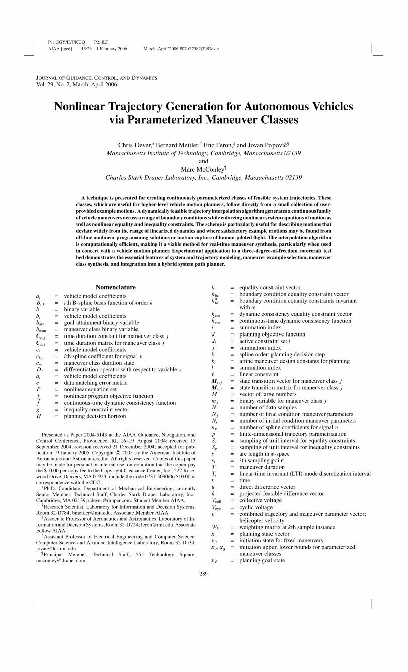
feasible vehicle trajectories and an associated (small) collection ofparameters α describing variable boundary conditions within thatfamily. As seen in Fig. 1, these “maneuver parameters” vary within auseful user-chosen set A, whereas a higher-dimensional dependentcollection of conventional “trajectory parameters” p(α) are usedto capture the corresponding reference vehicle state and controlhistories. The parameter vector p is typically a set of spline or basiscoefficients used to cast continuous-time-system “behavior” z(t)into a finite-dimensional form. The behavior function z(t) itself is auser-selected set of system state, output, and/or control signals thatcompletely specify the vehicle reference trajectory.

Practically speaking, the parameters α and the set A span usefulranges of vehicle maneuvering capabilities and provide free plan-ning variables for higher-level guidance algorithms. In general, thevector α may include Ni initial condition descriptors {αk

i }, N f fi-

nal condition descriptors {αkf }, and even a trajectory time length

descriptor αt f :

α = [α1

i · · · αNii α1

f · · · αN ff αt f

]T(1)

A. Trajectory InterpolationThe methods of nonlinear parametric programming (NLPP)39−41

determine p(α) families when every member of the maneuver classoptimizes a common objective function. In contrast, the trajectoryinterpolation method of this paper relaxes the strict optimality con-dition of NLPP and instead uses a feasible continuation procedurebetween pairs of user-provided example trajectories to generate a

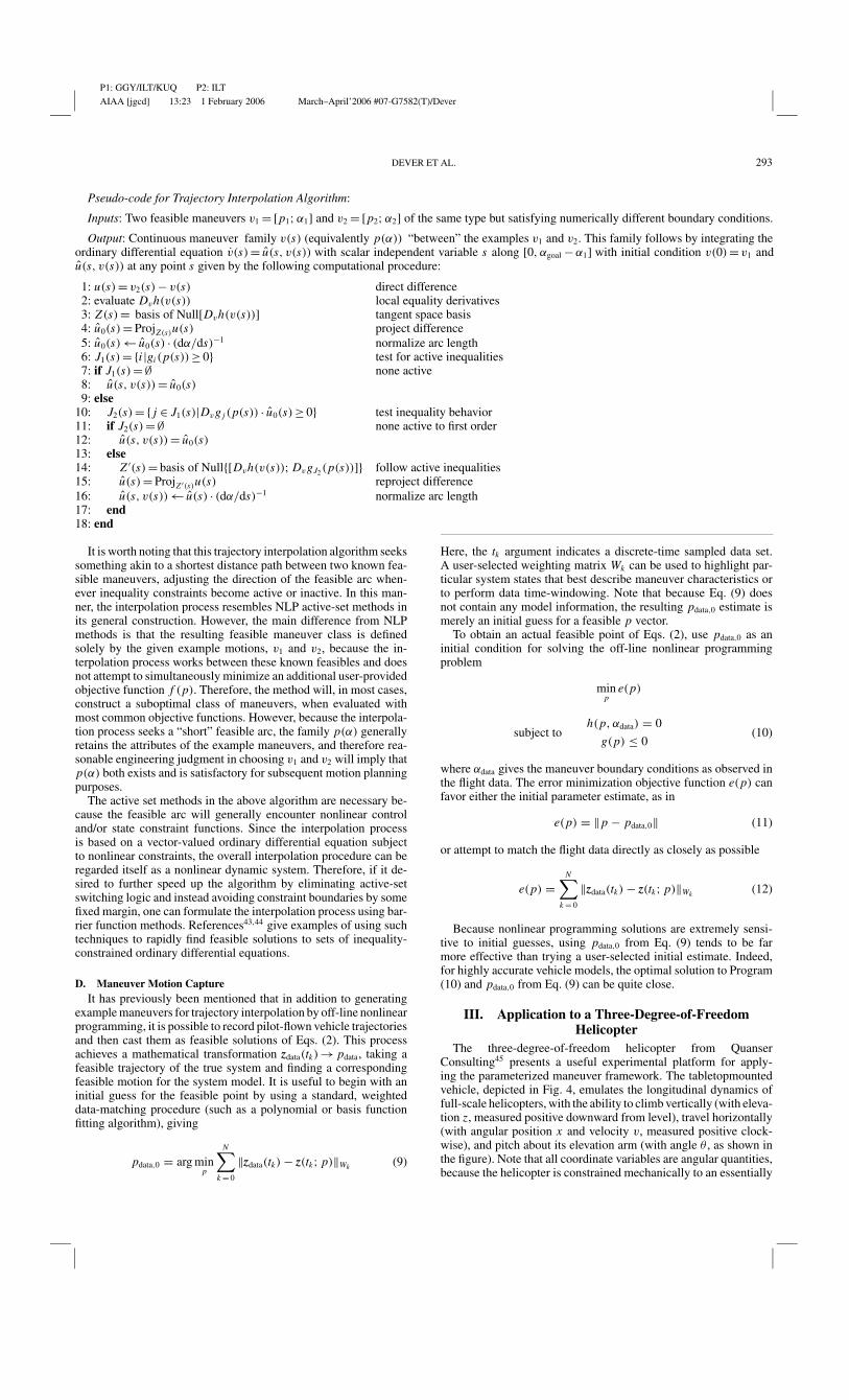
Fig. 1 Autonomous vehicle witha parameterized maneuver family.The low-dimensional vectorα speci-fies the particular maneuver bound-ary conditions, whereas the depen-dent function p(α) gives the cor-responding feasible trajectory stateand control histories.

range of new feasible motions p(α). This process is computation-ally less expensive than the full NLPP procedure, and thus makespossible fast, on-line feasible trajectory generators for nonlinearsystems. Moreover, the framework is extremely general in that theexample trajectories may come from any source, including rigor-ous off-line trajectory optimization or motion capture of humanpilot-inspired aerobatic and agile maneuvers. These latter trajecto-ries are extremely useful for autonomous vehicle operation, yet aretypically difficult to codify through an objective function. Giventhe trajectory interpolation mechanism, an engineer can constructa maneuver class by defining a useful set of control parameters αand then finding off-line a finite set of feasible trajectories fromwhich an entire family p(α) can be efficiently computed. Note thattrajectory interpolation attempts to retain the qualitative behaviorof the user-provided examples by taking the most “direct” availablefeasible path between them. For instance, time-optimal example tra-jectories from off-line NLP can serve as prototypes for constructionof a class of fast, agile (though likely suboptimal) maneuvers.

B. Constraint FunctionsIn most cases of interest, the maneuver parameters α dictate ini-

tial and/or final boundary conditions and therefore occur only in theequality constraint vector. This assumption, along with the discard-ing of an explicit objective function, leads to the following param-eterized trajectory feasible space:

h(p, α) = 0, g(p) ≤ 0 (2)

It is useful to think of a feasible trajectory as a concatenated vector

v =[

p

α

](3)

whose components satisfy Eqs. (2). (Here and in the sequel, asemicolon separator ; denotes vertical vector concatenation, so thatv = [p; α] = [pT αT ]T .)

For most autonomous vehicle models, the equality constraintfunction h(p) breaks down into two general partitions accordingto

h(p, α) =[

hem(p)

hbc(p, α)

](4)

Here, hem(p)denotes those constraints not specifying boundary con-ditions, but instead used to ensure basic dynamic feasibility. Thesefeasibility constraints typically arise in working with nonholonomicpath constraints, collocation formulations, quasi-differentially flatvehicle models, and/or mesh-sampled equations of motion. Thehbc(p, α) partition dictates the trajectory initial and final boundaryconditions, and thus depends explicitly on α:

hbc(p, α) =

⎡⎣ h0bc(p)

hi (p, αi )

h f (p, α f )

⎤⎦ (5)

(assuming here that Ni = N f = 1 for illustration purposes; moregeneral cases follow similarly). The subpartition h0

bc(p) denotesboundary constraints not directly depending on α, and hi (p, αi )and h f (p, α f ) are vectors containing control parameters for initialconditions αi and final conditions α f , respectively. Typically, hi hasa general form hi (p, αi ) = ψi (p) − φi (αi ), as a difference of somenonlinear vector functions ψi (p) and φi (αi ). The helicopter exampleof the following section will illustrate the role of these functions ψand φ. A similar breakdown applies for h f (p, α f ).

The inequality constraints in Eqs. (2) assume the general formg(p) ≤ 0 and capture state and control bounds imposed on vehicletrajectories during maneuvering. Because α typically determinesthe motion boundary conditions, which are captured in the equalityconstraint expression, the vector function g depends only the finite-dimensional trajectory parameterization p.



292 DEVER ET AL.

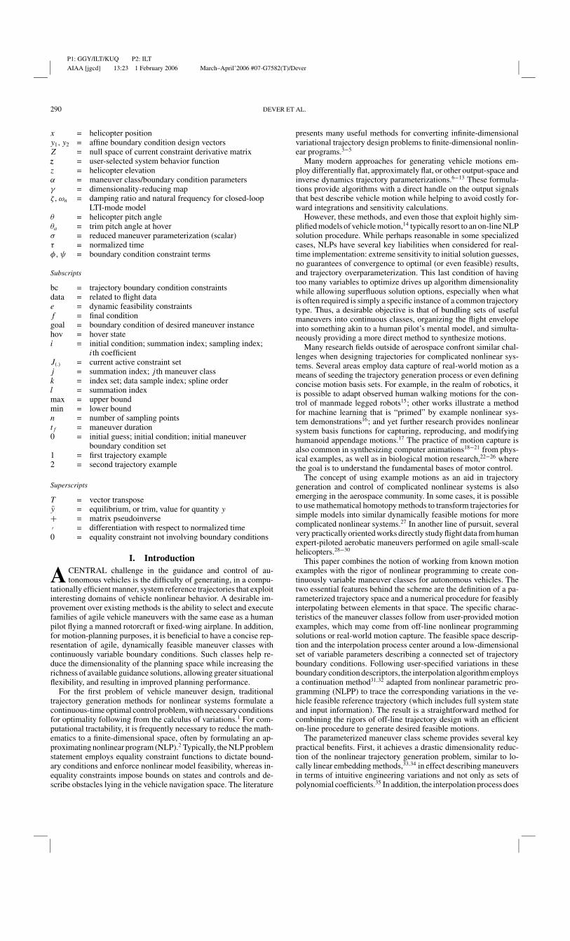
Fig. 2 General feasible maneuver space. Example maneuvers (p1 and p2) can come from any source, including off-line nonlinear programming andreal-flight motion capture. The parameterized family of feasible maneuvers based on these examples is then given by the feasible space arc p(α).

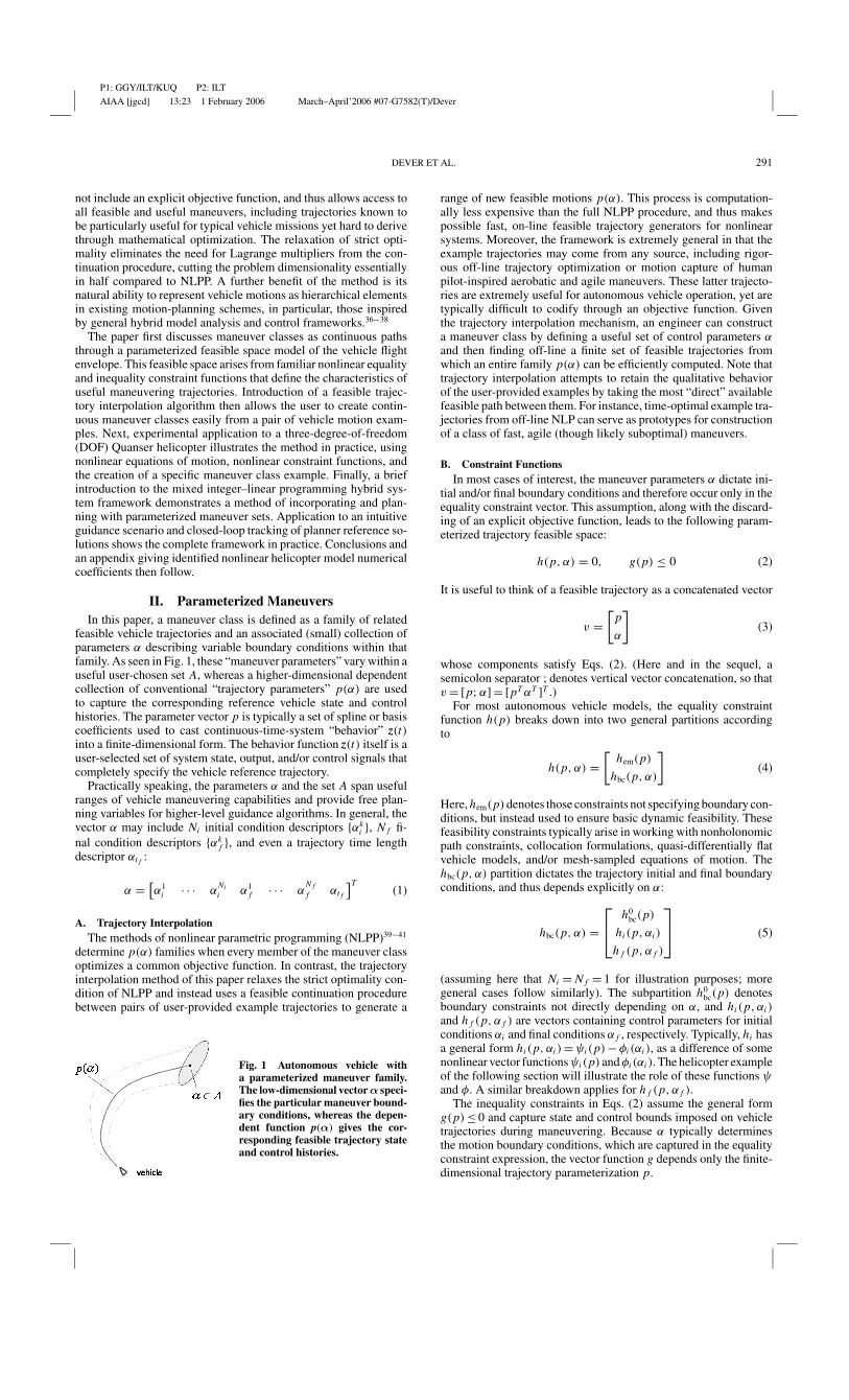
Fig. 3 Projection method for choosing a unique feasible direction. Thedifference vector u(s) is projected onto the local tangent hyperplane toobtain u(s), a tangent vector for the feasible path v(s) = [p (s); α (s)]. Thepath must take into account any inequality constraints occurring on thefeasible arc between v1 and v2.

C. AlgorithmNow, given the parameterized feasible space of Eqs. (2), the in-

terpolation algorithm takes as its inputs two user-provided feasiblemotions v1 and v2 describing different instances of the same generalmaneuver type (but with different boundary condition values) andcomputes as its output a continuous arc v(s) of feasible vehicle tra-jectories that lie “between” v1 and v2. The algorithm computes theparameterized family p(α) seen in Fig. 2, working through a vehiclefeasible p space from p1, with boundary condition α1, to p2, withboundary condition α2. Note that in the figure, and in the followingdiscussion, it is sufficient to treatα as a scalar without loss of general-ity, since it is typically possible to choose a (further) dimensionality-reducing function α = γ (σ ) mapping a vector-valued α down to asingle scalar parameter σ with some σ1 and σ2 such that α1 = γ (σ1)and α2 = γ (σ2).

Leaving specific details to the algorithm pseudo-code presentedbelow, the interpolation uses feasible projections of the numericaldifference between vectors v1 and v2 to define a unique, continuousarc that is traceable with standard numerical integration methods.Consider Fig. 3, which shows a general trajectory v(s) on the fea-sible solution path (at arc length s) and shows the projection of

the (generally infeasible) difference vector u(s) = v2 − v(s) ontothe tangent plane of equality constraints h and locally active in-equality constraints gJ0(s). Here, J0(s) denotes the active inequalityconstraint index set at a current feasible point v(s). A first-orderfeasible projection vector u(s) is easily obtained using the standard2-norm least-squares formula42

u(s) = ProjZ(s)u(s) ≡ Z(s)+u(s)

= Z(s)[Z(s)T Z(s)]−1 Z(s)[v2 − v(s)] (6)

where Z(s) is a matrix whose columns form a basis for the nullspaceNull(Dv[h(p, α); gJ0(s)(p)]). Note that u(s)defines a first-order fea-sible direction from v(s) toward v2. Because active inequalities gJ0(s)

function as equality constraints, Null(Dv[h(p, α); gJ0(s)(p)]) de-fines the tangent space at v(s), in which any direction vector movestowards feasible vehicle motion. The projection operation of Eq. (6)simply chooses the direction pointing to the known feasible v2.

Recalling that α is treated as scalar, it is possible to normalize theprojection vector u(s) according to u(s) ← u(s) · (dα/ds)−1 so thats ≡ α − α1 at every point along the arc. (This scaling allows one totreat v(s) and p(α) as equivalent functions.)

Given this arc-length normalization, and assuming a mechanismfor updating the active constraint set along the solution arc (as seenin Fig. 3), the numerically integrated feasible path gives a solutionfamily p(α) (equivalently v(s)) satisfying

FJ0(s)(p, α) = 0, g(p) ≤ 0 ∀ α1 ≤ α ≤ α2 (7)

where the definition

FJ0(s)(p, α) ≡[

h(p, α)

gJ0(s)(p)

](8)

indicates that the interpolation algorithm regards equality con-straints h and locally active inequality constraints gJ0(s) as a pa-rameterized set of nonlinear equations.

The complete trajectory interpolation algorithm in pseudo-codeis formulated as starting from the known feasible v1 = [p1; α1] andending at a maneuver with boundary condition parameter αgoal satis-fying α1 ≤ αgoal ≤ α2. The entire maneuver class results from choos-ing αgoal ≡ α2. Note that the algorithm begins at each integration stepby first assuming that no inequality constraints are active, testing forany active components of g, and then adding them to, or deletingthem from J0(s), depending on the direction of u(s) relative to thefirst-order behavior of gJ0

(s). For compactness of notation, h(v(s))denotes h(p, α) in the pseudo-code.



DEVER ET AL. 293

Pseudo-code for Trajectory Interpolation Algorithm:

Inputs: Two feasible maneuvers v1 = [p1; α1] and v2 = [p2; α2] of the same type but satisfying numerically different boundary conditions.

Output: Continuous maneuver family v(s) (equivalently p(α)) “between” the examples v1 and v2. This family follows by integrating theordinary differential equation v(s) = u(s, v(s)) with scalar independent variable s along [0, αgoal − α1] with initial condition v(0) = v1 andu(s, v(s)) at any point s given by the following computational procedure:

1: u(s) = v2(s) − v(s) direct difference2: evaluate Dvh(v(s)) local equality derivatives3: Z(s) = basis of Null[Dvh(v(s))] tangent space basis4: u0(s) = ProjZ(s)u(s) project difference5: u0(s) ← u0(s) · (dα/ds)−1 normalize arc length6: J1(s) = {i |gi (p(s)) ≥ 0} test for active inequalities7: if J1(s) = ∅ none active8: u(s, v(s)) = u0(s)9: else

10: J2(s) = { j ∈ J1(s)|Dvg j (p(s)) · u0(s) ≥ 0} test inequality behavior11: if J2(s) = ∅ none active to first order12: u(s, v(s)) = u0(s)13: else14: Z ′(s) = basis of Null{[Dvh(v(s)); DvgJ2

(p(s))]} follow active inequalities15: u(s) = ProjZ ′(s)u(s) reproject difference16: u(s, v(s)) ← u(s) · (dα/ds)−1 normalize arc length17: end18: end

It is worth noting that this trajectory interpolation algorithm seekssomething akin to a shortest distance path between two known fea-sible maneuvers, adjusting the direction of the feasible arc when-ever inequality constraints become active or inactive. In this man-ner, the interpolation process resembles NLP active-set methods inits general construction. However, the main difference from NLPmethods is that the resulting feasible maneuver class is definedsolely by the given example motions, v1 and v2, because the in-terpolation process works between these known feasibles and doesnot attempt to simultaneously minimize an additional user-providedobjective function f (p). Therefore, the method will, in most cases,construct a suboptimal class of maneuvers, when evaluated withmost common objective functions. However, because the interpola-tion process seeks a “short” feasible arc, the family p(α) generallyretains the attributes of the example maneuvers, and therefore rea-sonable engineering judgment in choosing v1 and v2 will imply thatp(α) both exists and is satisfactory for subsequent motion planningpurposes.

The active set methods in the above algorithm are necessary be-cause the feasible arc will generally encounter nonlinear controland/or state constraint functions. Since the interpolation processis based on a vector-valued ordinary differential equation subjectto nonlinear constraints, the overall interpolation procedure can beregarded itself as a nonlinear dynamic system. Therefore, if it de-sired to further speed up the algorithm by eliminating active-setswitching logic and instead avoiding constraint boundaries by somefixed margin, one can formulate the interpolation process using bar-rier function methods. References43,44 give examples of using suchtechniques to rapidly find feasible solutions to sets of inequality-constrained ordinary differential equations.

D. Maneuver Motion CaptureIt has previously been mentioned that in addition to generating

example maneuvers for trajectory interpolation by off-line nonlinearprogramming, it is possible to record pilot-flown vehicle trajectoriesand then cast them as feasible solutions of Eqs. (2). This processachieves a mathematical transformation zdata(tk) → pdata, taking afeasible trajectory of the true system and finding a correspondingfeasible motion for the system model. It is useful to begin with aninitial guess for the feasible point by using a standard, weighteddata-matching procedure (such as a polynomial or basis functionfitting algorithm), giving

pdata,0 = arg minp

N∑k = 0

‖zdata(tk) − z(tk; p)‖Wk (9)

Here, the tk argument indicates a discrete-time sampled data set.A user-selected weighting matrix Wk can be used to highlight par-ticular system states that best describe maneuver characteristics orto perform data time-windowing. Note that because Eq. (9) doesnot contain any model information, the resulting pdata,0 estimate ismerely an initial guess for a feasible p vector.

To obtain an actual feasible point of Eqs. (2), use pdata,0 as aninitial condition for solving the off-line nonlinear programmingproblem

minp

e(p)

subject toh(p, αdata) = 0

g(p) ≤ 0(10)

where αdata gives the maneuver boundary conditions as observed inthe flight data. The error minimization objective function e(p) canfavor either the initial parameter estimate, as in

e(p) = ‖p − pdata,0‖ (11)

or attempt to match the flight data directly as closely as possible

e(p) =N∑

k = 0

‖zdata(tk) − z(tk; p)‖Wk (12)

Because nonlinear programming solutions are extremely sensi-tive to initial guesses, using pdata,0 from Eq. (9) tends to be farmore effective than trying a user-selected initial estimate. Indeed,for highly accurate vehicle models, the optimal solution to Program(10) and pdata,0 from Eq. (9) can be quite close.

III. Application to a Three-Degree-of-FreedomHelicopter

The three-degree-of-freedom helicopter from QuanserConsulting45 presents a useful experimental platform for apply-ing the parameterized maneuver framework. The tabletopmountedvehicle, depicted in Fig. 4, emulates the longitudinal dynamics offull-scale helicopters, with the ability to climb vertically (with eleva-tion z, measured positive downward from level), travel horizontally(with angular position x and velocity v, measured positive clock-wise), and pitch about its elevation arm (with angle θ , as shown inthe figure). Note that all coordinate variables are angular quantities,because the helicopter is constrained mechanically to an essentially



294 DEVER ET AL.

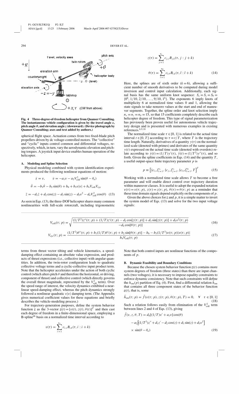
Fig. 4 Three-degree-of-freedom helicopter from Quanser Consulting.The instantaneous vehicle configuration is given by the travel angle x,pitch angle θ, and elevation angle z (downward). (Device photograph byQuanser Consulting; axes and text added by authors.)

spherical flight space. Actuation comes from two fixed-blade pitchpropellers driven by dc voltage-controlled motors. The “collective”and “cyclic” inputs control common and differential voltages, re-spectively, which, in turn, vary the aerodynamic elevation and pitch-ing torques. A joystick input device enables human operation of thehelicopter.

A. Modeling and Spline SelectionPhysical modeling combined with system identification experi-

ments produced the following nonlinear equations of motion:

x = v, v = −a1v − a2V 2coll sin(θ − θa)

θ = −b1θ − b2 sin(θ) + b0 + b3v|v| + b4VcollVcyc

z = −d1 z + d2 cos(z) − d3 sin(z) − d5v2 − d4V 2

coll cos(θ) (13)

As seen in Eqs. (13), the three-DOF helicopter shares many commonnonlinearities with full-scale rotorcraft, including trigonometric

Vcoll(τ ; p) =√

(1/T 2)z′′(τ ; p) + (1/T )z′(τ ; p) − d2 cos[z(τ ; p)] + d3 sin[z(τ ; p)] + d5v2(τ ; p)

−d4 cos[θ(τ ; p)](16)

Vcyc(τ ; p) = (1/T 2)θ ′′(τ ; p) + b1(1/T )θ ′(τ ; p) + b2 sin[θ(τ ; p)] − b0 − b3(1/T 2)v(τ ; p)|v(τ ; p)|b4Vcoll(τ ; p)

(17)

terms from thrust vector tilting and vehicle kinematics, a speed-damping effect containing an absolute value expression, and prod-ucts of thrust expressions (i.e., collective input) with angular quan-tities. In addition, the twin-rotor configuration leads to quadraticcollective voltage terms and a cyclic-collective input product term.Note that the helicopter accelerates under the action of both cycliccontrol (which alters pitch θ and therefore the horizontal, or driving,component of thrust) and collective control (which directly governsthe overall thrust magnitude, represented by the V 2

coll term). Overthe speed range of interest, the velocity dynamics exhibited a near-linear speed-damping effect, whereas the pitch dynamics stronglyfollowed a nonlinear quadratic v|v| damping term. (The Appendixgives numerical coefficient values for these equations and brieflydescribes the vehicle-modeling process.)

For trajectory-generation purposes, define the system behaviorfunction z as the 3-vector z(t) = [v(t), z(t), θ(t)]T and then casteach degree of freedom in a finite-dimensional space, employing aB-spline46 basis on a normalized time interval according to

v(τ) =nv∑

i = 1

ci,v Bi,k(τ, i : i + k)

z(τ ) =nz∑

j = 1

c j,z B j,k(τ, j : j + k)

θ(τ ) =nθ∑

l = 1

cl,θ Bl,k(τ, l : l + k) (14)

Here, the splines are of sixth order (k = 6), allowing a suffi-cient number of smooth derivatives to be computed during modelinversion and control input calculation. Additionally, each sig-nal basis has the same uniform knot sequence: Sv = Sz = Sθ ={06, 1/10, 2/10, . . . , 9/10, 16}. The exponents 6 imply knots ofmultiplicity 6 at normalized time values 0 and 1, allowing thestate signals to take nonzero values at the start and end of maneu-ver segments. Together, the spline order and knot selection implynv = nz = nθ = 15, so that 15 coefficients completely describe eachhelicopter degree of freedom. This type of signal parameterizationhas previously been proven useful for autonomous vehicle trajec-tory design and is presented with numerous examples in existingreferences.6,9,10

The normalized time scale τ ∈ [0, 1] is related to the actual timeinterval t ∈ [0, T ] according to τ = t/T , where T is the trajectorytime length. Naturally, derivatives of a quantity y(τ ) on the normal-ized scale (denoted with primes) and derivates of the same quantityy(t) expressed on the actual time scale (denoted with overdots) re-late according to y(t) = (1/T )y′(τ ), y(t) = (1/T 2)y′′(τ ), and soforth. Given the spline coefficients in Eqs. (14) and the quantity T ,a useful output-space finite trajectory parameter p is

p ≡ [{ci,v}nv

i = 1, {c j,z}nzj = 1, {cl,θ }nθ

l = 1, T]T

(15)

Working with a normalized time scale allows T to become a freeparameter and will enable direct control over trajectory durationwithin maneuver classes. It is useful to adopt the expanded notationv(τ) = v(τ ; p), z(τ ) = z(τ ; p), θ(τ ) = θ(τ ; p) as a reminder thatthese time domain signals depend explicitly on the components of p.

Given the above choices for z and p, it is a simple matter to invertthe system model of Eqs. (13) and solve for the two input voltagesignals:

Note that both control inputs are nonlinear functions of the compo-nents of p.

B. Dynamic Feasibility and Boundary ConditionsBecause the chosen system behavior function z(t) contains more

system degrees of freedom (three states) than there are input chan-nels (two voltages), it is necessary to impose equality constraints toenforce dynamic consistency. Note that such constraints will definethe hem(p) partition of Eq. (4). First, find a differential relation hem

that contains all three component states of the behavior functionz(t), that is, some

hem(τ ; p) = f (v(τ ; p), z(τ ; p), θ(τ ; p), T ) = 0, ∀ τ ∈ [0, 1](18)

Such a relation follows easily from elimination of the V 2coll term

between lines 2 and 4 of Eqs. (13), giving

f (v, z, θ, T ) = d4[(1/T )v′ + a1v] cos(θ)

− a2

[(1/T 2)z′′ + d1z′ − d2 cos(z) + d3 sin(z) + d5v

2]

× sin(θ − θa) (19)



DEVER ET AL. 295

To obtain an approximating finite-dimensional vector hem(p), sam-ple the continuous time constraint of Eqs. (18) and (19) along a finitepoint set to obtain

hem(p) ≡

⎡⎢⎣hem(τ1; p)...

hem(τn; p)

⎤⎥⎦ (20)

where the individual points τi are elements of a finite sampling Se

of the unit interval: Se = {τ1, . . . , τn} ⊂ [0, 1]. For the three-DOFhelicopter, a useful sampling is

Se = {0, 1/30, 1/15, 2/15, . . . , 14/15, 29/30, 59/60} (21)

The other partition of the general equality constraint vector h(p)is the boundary condition constraint hbc(p, α). As the presence ofthe α quantity shows, this vector is the main driver behind the cre-ation of continuous maneuver classes. Without selecting a specific αyet, consider first the set of quantities necessary to define an equilib-rium, or trim state at the beginning and end of a maneuver segment.Analysis of Eqs. (13) indicates that a steady velocity–elevation pair(v, z) is sufficient to determine trim values of pitch, collective volt-age, and cyclic voltage. For instance, setting all time derivatives tozero in Eqs. (13) gives the steady pitch relation

a2 sin(θ − θa)[d2 cos(z) − d3 sin(z) − d5v

2] + a1d4v cos(θ) = 0

(22)and steady input relations

Vcoll =√

d2 cos(z) − d3 sin(z) − d5v2

d4 cos(θ)

Vcyc = b2 sin(θ) − b0 − b3v|v|b4Vcoll

(23)

Solution for exact trim values in Eqs. (22) and (23) requires a nu-merical search procedure, similar to thrust-inflow iterations seen infull-scale helicopter models.47 However, a fortunate consequence ofthe trajectory interpolation algorithm is that only first-order equalityconstraint derivative information is required, requiring only implicitdifferentiation of the above relations.

The overall trim boundary condition constraint function requiresthe attainment of initial and final equilibrium values for velocity,elevation, pitch, collective, and cyclic. In addition, it is requiredthat elevation and pitch signals have first-order time derivativesequal to zero at the trajectory endpoints. (A corresponding zero-derivative condition on velocity proved redundant, given the trimstate boundary value constraints on the two inputs.) Concatenationof normalized time expressions for all these conditions gives the de-sired boundary condition equality constraint vector (denoted heretemporarily by hbc until the α argument is introduced):

hbc(p) ≡

⎡⎢⎢⎢⎢⎢⎢⎢⎢⎢⎢⎢⎢⎢⎢⎢⎢⎢⎢⎢⎢⎢⎢⎢⎢⎣

v(0; p) − vi

v(1; p) − v f

z(0; p) − zi

z(1; p) − z f

θ(0; p) − θi

θ(1; p) − θ f

Vcoll(0; p) − Vcoll,i

Vcoll(1; p) − Vcoll, f

Vcyc(0; p) − Vcyc,i

Vcyc(1; p) − Vcyc, f

(1/T )z′(0; p) − 0

(1/T )z′(1; p) − 0

(1/T )θ ′(0; p) − 0

(1/T )θ ′(1; p) − 0

⎤⎥⎥⎥⎥⎥⎥⎥⎥⎥⎥⎥⎥⎥⎥⎥⎥⎥⎥⎥⎥⎥⎥⎥⎥⎦

= 0 (24)

C. State and Control BoundsLast, inequality constraint functions are needed to keep helicopter

trajectories within a reasonable flight envelope and control signalswithin physical limits. For the three-DOF helicopter, it is useful tobound elevation to prevent collisions with the supporting surfaceand the upper mechanical restraint limits; the pitch angle must stayaway from extreme θ = ±90◦ values which induce a singularity inEqs. (16) and (23). Additionally, it is important to prevent the controlinputs from exceeding reasonable ranges, especially when workingwith agile maneuvers that require large control efforts.

These state and input constraints appear in continuous time as

zmin ≤ z(τ ; p) ≤ zmax ∀ τ ∈ [0, 1]

θmin ≤ θ(τ ; p) ≤ θmax ∀ τ ∈ [0, 1]

Vcoll,min ≤ Vcoll(τ ; p) ≤ Vcoll,max ∀ τ ∈ [0, 1]

Vcyc,min ≤ Vcyc(τ ; p) ≤ Vcyc,max ∀ τ ∈ [0, 1] (25)

Similarly to the continuous-time equality constraint of Eq. (18), itis necessary to sample Inequalities (25) along some sampling of theunit interval [0, 1] to obtain a finite-dimensional constraint vector.Therefore, employ the following sampled version of the precedinginequalities:

g(p) ≡

⎡⎢⎢⎢⎢⎢⎢⎢⎢⎢⎢⎢⎢⎣

zmin − zSg (p)

zSg (p) − zmax

θmin − θ Sg (p)

θ Sg (p) − θmax

Vcoll,min − VSg

coll(p)

VSg

coll(p) − Vcoll,max

Vcyc,min − VSg

cyc(p)

VSg

cyc(p) − Vcyc,max

⎤⎥⎥⎥⎥⎥⎥⎥⎥⎥⎥⎥⎥⎦≤ 0 (26)

where, for a generic parameterized unit time domain signal y(τ ; p),the symbol ySg (p) has the definition ySg (p) ≡ [y(s1; p), . . . ,y(sm; p)]T , where the si are the sampling points Sg = {s1, . . . , sm} ={0, 1/20, . . . , 1} ⊂ [0, 1].

D. Example: Bounded-Control Quick-Stop Maneuver ClassGiven the helicopter boundary constraint expression of Eq. (24),

it is a simple matter to create a parameterized class of quick-stopmaneuvers. Here, all trajectories end at a steady hover state withvi = zi = 0. However, let the initial trim velocity vi be variable; thatis, assign α ≡ vi . For simplicity, assume that zi = 0 is fixed over themaneuver class.

Given this specific choice of α, introduce it into all boundarycondition rows of Eq. (24) that depend on the initial helicoptervelocity. Recalling from Eqs. (22) and (23) that the initial trim pitchangle and input voltages vary with vi , insert the boundary parameterα into the corresponding rows of Eq. (24) to obtain

hbc(p, α) =

⎡⎢⎢⎢⎢⎢⎢⎢⎢⎢⎢⎢⎢⎢⎢⎢⎢⎢⎢⎢⎢⎢⎢⎢⎢⎣

v(0; p) − α

v(1; p) − 0

z(0; p) − 0

z(1; p) − 0

θ(0; p) − θi (α)

θ(1; p) − θhov

Vcoll(0; p) − Vcoll,i (α)

Vcoll(1; p) − Vcoll,hov

Vcyc(0; p) − Vcyc,i (α)

Vcyc(1; p) − Vcyc,hov

(1/T )z′(0; p) − 0

(1/T )z′(1; p) − 0

(1/T )θ ′(0; p) − 0

(1/T )θ ′(1; p) − 0

⎤⎥⎥⎥⎥⎥⎥⎥⎥⎥⎥⎥⎥⎥⎥⎥⎥⎥⎥⎥⎥⎥⎥⎥⎥⎦

= 0 (27)



296 DEVER ET AL.

Note that all boundary trim constraints depend on the spline param-eterization p (which includes T ) whereas only four rows dependon α. While carrying out the interpolation algorithm, it is necessaryto compute the derivative matrix Dvh(p, α), where h(p, α) has thedecomposition given in Eq. (4). Therefore this derivative matrix hasthe following block structure:

Dvh(p, α) =[

Dphem(p) 0

Dphbc(p, α) Dαhbc(p, α)

](28)

where comparison with Eq. (27) reveals that the Dαhbc(p, α) is acolumn vector with only four nonzero elements; these elements arethe mathematical drivers for interpolation of this maneuver class.

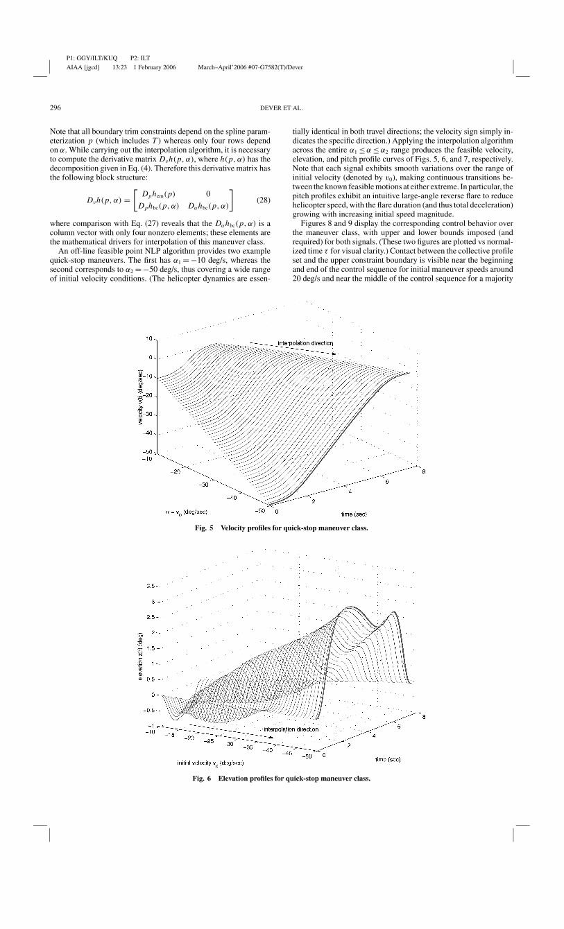
An off-line feasible point NLP algorithm provides two examplequick-stop maneuvers. The first has α1 = −10 deg/s, whereas thesecond corresponds to α2 = −50 deg/s, thus covering a wide rangeof initial velocity conditions. (The helicopter dynamics are essen-

Fig. 5 Velocity profiles for quick-stop maneuver class.

Fig. 6 Elevation profiles for quick-stop maneuver class.

tially identical in both travel directions; the velocity sign simply in-dicates the specific direction.) Applying the interpolation algorithmacross the entire α1 ≤ α ≤ α2 range produces the feasible velocity,elevation, and pitch profile curves of Figs. 5, 6, and 7, respectively.Note that each signal exhibits smooth variations over the range ofinitial velocity (denoted by v0), making continuous transitions be-tween the known feasible motions at either extreme. In particular, thepitch profiles exhibit an intuitive large-angle reverse flare to reducehelicopter speed, with the flare duration (and thus total deceleration)growing with increasing initial speed magnitude.

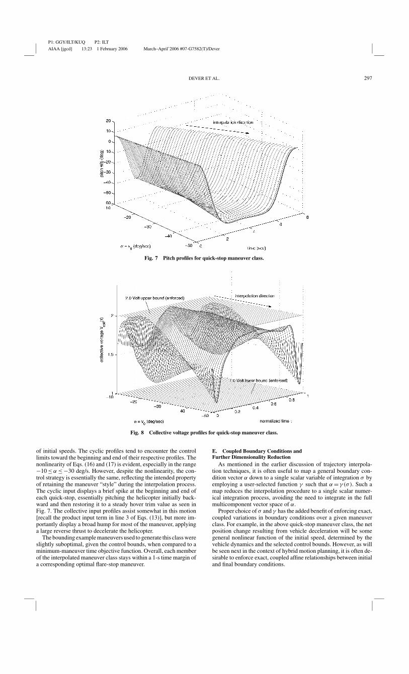
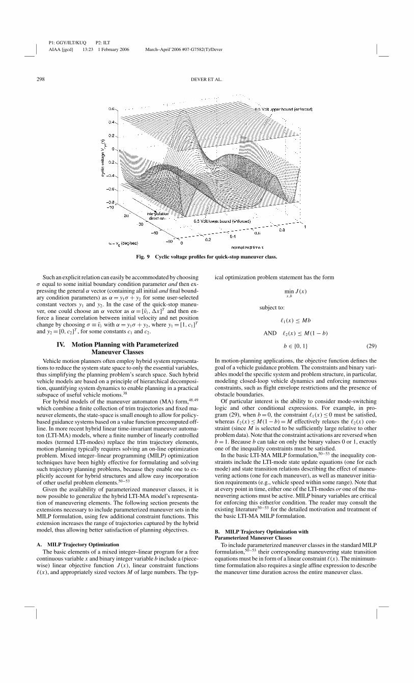
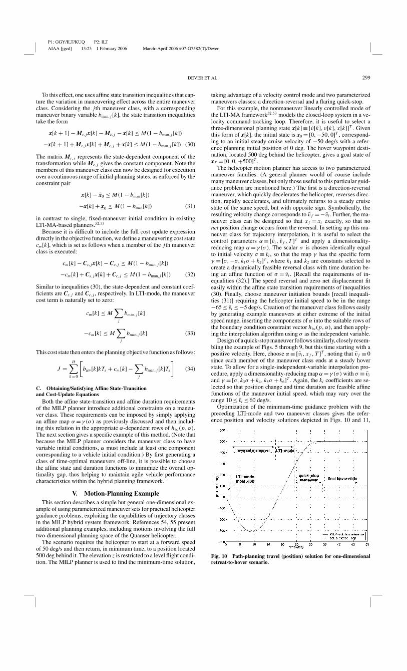
Figures 8 and 9 display the corresponding control behavior overthe maneuver class, with upper and lower bounds imposed (andrequired) for both signals. (These two figures are plotted vs normal-ized time τ for visual clarity.) Contact between the collective profileset and the upper constraint boundary is visible near the beginningand end of the control sequence for initial maneuver speeds around20 deg/s and near the middle of the control sequence for a majority



DEVER ET AL. 297

Fig. 7 Pitch profiles for quick-stop maneuver class.

Fig. 8 Collective voltage profiles for quick-stop maneuver class.

of initial speeds. The cyclic profiles tend to encounter the controllimits toward the beginning and end of their respective profiles. Thenonlinearity of Eqs. (16) and (17) is evident, especially in the range−10 ≤ α ≤ −30 deg/s. However, despite the nonlinearity, the con-trol strategy is essentially the same, reflecting the intended propertyof retaining the maneuver “style” during the interpolation process.The cyclic input displays a brief spike at the beginning and end ofeach quick-stop, essentially pitching the helicopter initially back-ward and then restoring it to a steady hover trim value as seen inFig. 7. The collective input profiles assist somewhat in this motion[recall the product input term in line 3 of Eqs. (13)], but more im-portantly display a broad hump for most of the maneuver, applyinga large reverse thrust to decelerate the helicopter.

The bounding example maneuvers used to generate this class wereslightly suboptimal, given the control bounds, when compared to aminimum-maneuver time objective function. Overall, each memberof the interpolated maneuver class stays within a 1-s time margin ofa corresponding optimal flare-stop maneuver.

E. Coupled Boundary Conditions andFurther Dimensionality Reduction

As mentioned in the earlier discussion of trajectory interpola-tion techniques, it is often useful to map a general boundary con-dition vector α down to a single scalar variable of integration σ byemploying a user-selected function γ such that α = γ (σ ). Such amap reduces the interpolation procedure to a single scalar numer-ical integration process, avoiding the need to integrate in the fullmulticomponent vector space of α.

Proper choice of σ and γ has the added benefit of enforcing exact,coupled variations in boundary conditions over a given maneuverclass. For example, in the above quick-stop maneuver class, the netposition change resulting from vehicle deceleration will be somegeneral nonlinear function of the initial speed, determined by thevehicle dynamics and the selected control bounds. However, as willbe seen next in the context of hybrid motion planning, it is often de-sirable to enforce exact, coupled affine relationships between initialand final boundary conditions.



298 DEVER ET AL.

Fig. 9 Cyclic voltage profiles for quick-stop maneuver class.

Such an explicit relation can easily be accommodated by choosingσ equal to some initial boundary condition parameter and then ex-pressing the general α vector (containing all initial and final bound-ary condition parameters) as α = y1σ + y2 for some user-selectedconstant vectors y1 and y2. In the case of the quick-stop maneu-ver, one could choose an α vector as α = [vi , �x]T and then en-force a linear correlation between initial velocity and net positionchange by choosing σ ≡ vi with α = y1σ + y2, where y1 = [1, c1]T

and y2 = [0, c2]T , for some constants c1 and c2.

IV. Motion Planning with ParameterizedManeuver Classes

Vehicle motion planners often employ hybrid system representa-tions to reduce the system state space to only the essential variables,thus simplifying the planning problem’s search space. Such hybridvehicle models are based on a principle of hierarchical decomposi-tion, quantifying system dynamics to enable planning in a practicalsubspace of useful vehicle motions.38

For hybrid models of the maneuver automaton (MA) form,48,49

which combine a finite collection of trim trajectories and fixed ma-neuver elements, the state-space is small enough to allow for policy-based guidance systems based on a value function precomputed off-line. In more recent hybrid linear time-invariant maneuver automa-ton (LTI-MA) models, where a finite number of linearly controlledmodes (termed LTI-modes) replace the trim trajectory elements,motion planning typically requires solving an on-line optimizationproblem. Mixed integer–linear programming (MILP) optimizationtechniques have been highly effective for formulating and solvingsuch trajectory planning problems, because they enable one to ex-plicitly account for hybrid structures and allow easy incorporationof other useful problem elements.50−53

Given the availability of parameterized maneuver classes, it isnow possible to generalize the hybrid LTI-MA model’s representa-tion of maneuvering elements. The following section presents theextensions necessary to include parameterized maneuver sets in theMILP formulation, using few additional constraint functions. Thisextension increases the range of trajectories captured by the hybridmodel, thus allowing better satisfaction of planning objectives.

A. MILP Trajectory OptimizationThe basic elements of a mixed integer–linear program for a free

continuous variable x and binary integer variable b include a (piece-wise) linear objective function J (x), linear constraint functions�(x), and appropriately sized vectors M of large numbers. The typ-

ical optimization problem statement has the form

minx,b

J (x)

subject to:

�1(x) ≤ Mb

AND �2(x) ≤ M(1 − b)

b ∈ {0, 1} (29)

In motion-planning applications, the objective function defines thegoal of a vehicle guidance problem. The constraints and binary vari-ables model the specific system and problem structure, in particular,modeling closed-loop vehicle dynamics and enforcing numerousconstraints, such as flight envelope restrictions and the presence ofobstacle boundaries.

Of particular interest is the ability to consider mode-switchinglogic and other conditional expressions. For example, in pro-gram (29), when b = 0, the constraint �1(x) ≤ 0 must be satisfied,whereas �2(x) ≤ M(1 − b) = M effectively relaxes the �2(x) con-straint (since M is selected to be sufficiently large relative to otherproblem data). Note that the constraint activations are reversed whenb = 1. Because b can take on only the binary values 0 or 1, exactlyone of the inequality constraints must be satisfied.

In the basic LTI-MA MILP formulation,50−53 the inequality con-straints include the LTI-mode state update equations (one for eachmode) and state transition relations describing the effect of maneu-vering actions (one for each maneuver), as well as maneuver initia-tion requirements (e.g., vehicle speed within some range). Note thatat every point in time, either one of the LTI-modes or one of the ma-neuvering actions must be active. MILP binary variables are criticalfor enforcing this either/or condition. The reader may consult theexisting literature50−53 for the detailed motivation and treatment ofthe basic LTI-MA MILP formulation.

B. MILP Trajectory Optimization withParameterized Maneuver Classes

To include parameterized maneuver classes in the standard MILPformulation,50−53 their corresponding maneuvering state transitionequations must be in form of a linear constraint �(x). The minimum-time formulation also requires a single affine expression to describethe maneuver time duration across the entire maneuver class.



DEVER ET AL. 299

To this effect, one uses affine state transition inequalities that cap-ture the variation in maneuvering effect across the entire maneuverclass. Considering the j th maneuver class, with a correspondingmaneuver binary variable bman, j [k], the state transition inequalitiestake the form

x[k + 1] − Ms, j x[k] − Mc, j − x[k] ≤ M(1 − bman, j [k])

−x[k + 1] + Ms, j x[k] + Mc, j + x[k] ≤ M(1 − bman, j [k]) (30)

The matrix Ms, j represents the state-dependent component of thetransformation while Mc, j gives the constant component. Note themembers of this maneuver class can now be designed for executionover a continuous range of initial planning states, as enforced by theconstraint pair

x[k] − x0 ≤ M(1 − bman[k])

−x[k] + x0 ≤ M(1 − bman[k]) (31)

in contrast to single, fixed-maneuver initial condition in existingLTI-MA-based planners.52,53

Because it is difficult to include the full cost update expressiondirectly in the objective function, we define a maneuvering cost statecm[k], which is set as follows when a member of the j th maneuverclass is executed:

cm[k] − Cs, j x[k] − Cc, j ≤ M(1 − bman, j [k])

−cm[k] + Cs, j x[k] + Cc, j ≤ M(1 − bman, j [k]) (32)

Similar to inequalities (30), the state-dependent and constant coef-ficients are Cs, j and Cc, j , respectively. In LTI-mode, the maneuvercost term is naturally set to zero:

cm[k] ≤ M∑

j

bman, j [k]

−cm[k] ≤ M∑

j

bman, j [k] (33)

This cost state then enters the planning objective function as follows:

J =H∑

k = 0

[barv[k]kTs + cm[k] −

∑j

bman, j [k]Ts

](34)

C. Obtaining/Satisfying Affine State-Transitionand Cost-Update Equations

Both the affine state-transition and affine duration requirementsof the MILP planner introduce additional constraints on a maneu-ver class. These requirements can be imposed by simply applyingan affine map α = γ (σ ) as previously discussed and then includ-ing this relation in the appropriate α-dependent rows of hbc(p, α).The next section gives a specific example of this method. (Note thatbecause the MILP planner considers the maneuver class to havevariable initial conditions, α must include at least one componentcorresponding to a vehicle initial condition.) By first generating aclass of time-optimal maneuvers off-line, it is possible to choosethe affine state and duration functions to minimize the overall op-timality gap, thus helping to maintain agile vehicle performancecharacteristics within the hybrid planning framework.

V. Motion-Planning ExampleThis section describes a simple but general one-dimensional ex-

ample of using parameterized maneuver sets for practical helicopterguidance problems, exploiting the capabilities of trajectory classesin the MILP hybrid system framework. References 54, 55 presentadditional planning examples, including motions involving the fulltwo-dimensional planning space of the Quanser helicopter.

The scenario requires the helicopter to start at a forward speedof 50 deg/s and then return, in minimum time, to a position located500 deg behind it. The elevation z is restricted to a level flight condi-tion. The MILP planner is used to find the minimum-time solution,

taking advantage of a velocity control mode and two parameterizedmaneuvers classes: a direction-reversal and a flaring quick-stop.

For this example, the nonmaneuver linearly controlled mode ofthe LTI-MA framework52,53 models the closed-loop system in a ve-locity command-tracking loop. Therefore, it is useful to select athree-dimensional planning state x[k] ≡ [v[k], v[k], x[k]]T . Giventhis form of x[k], the initial state is x0 = [0, −50, 0]T , correspond-ing to an initial steady cruise velocity of −50 deg/s with a refer-ence planning initial position of 0 deg. The hover waypoint desti-nation, located 500 deg behind the helicopter, gives a goal state ofxF = [0, 0, +500]T .

The helicopter motion planner has access to two parameterizedmaneuver families. (A general planner would of course includemany maneuver classes, but only those useful to this particular guid-ance problem are mentioned here.) The first is a direction-reversalmaneuver, which quickly decelerates the helicopter, reverses direc-tion, rapidly accelerates, and ultimately returns to a steady cruisestate of the same speed, but with opposite sign. Symbolically, theresulting velocity change corresponds to v f = −vi . Further, the ma-neuver class can be designed so that x f = xi exactly, so that nonet position change occurs from the reversal. In setting up this ma-neuver class for trajectory interpolation, it is useful to select thecontrol parameters α ≡ [vi , v f , T ]T and apply a dimensionality-reducing map α = γ (σ ). The scalar σ is chosen identically equalto initial velocity σ ≡ vi , so that the map γ has the specific formγ = [σ, −σ, k1σ + k2]T , where k1 and k2 are constants selected tocreate a dynamically feasible reversal class with time duration be-ing an affine function of σ = vi . [Recall the requirements of in-equalities (32).] The speed reversal and zero net displacement fiteasily within the affine state transition requirements of inequalities(30). Finally, choose maneuver initiation bounds [recall inequali-ties (31)] requiring the helicopter initial speed to be in the range−65 ≤ vi ≤ −5 deg/s. Creation of the maneuver class follows easilyby generating example maneuvers at either extreme of the initialspeed range, inserting the components of α into the suitable rows ofthe boundary condition constraint vector hbc(p, α), and then apply-ing the interpolation algorithm using σ as the independent variable.

Design of a quick-stop maneuver follows similarly, closely resem-bling the example of Figs. 5 through 9, but this time starting with apositive velocity. Here, choose α ≡ [vi , x f , T ]T , noting that v f ≡ 0since each member of the maneuver class ends at a steady hoverstate. To allow for a single-independent-variable interpolation pro-cedure, apply a dimensionality-reducing map α = γ (σ ) with σ ≡ vi

and γ = [σ, k3σ + k4, k5σ + k6]T . Again, the ki coefficients are se-lected so that position change and time duration are feasible affinefunctions of the maneuver initial speed, which may vary over therange 10 ≤ vi ≤ 60 deg/s.

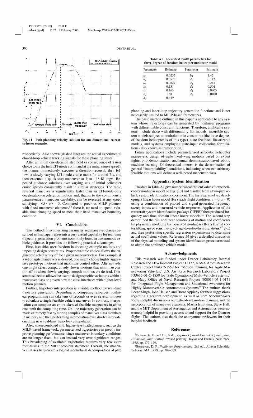
Optimization of the minimum-time guidance problem with thepreceding LTI-mode and two maneuver classes gives the refer-ence position and velocity solutions depicted in Figs. 10 and 11,

Fig. 10 Path-planning travel (position) solution for one-dimensionalretreat-to-hover scenario.



300 DEVER ET AL.

Fig. 11 Path-planning velocity solution for one-dimensional retreat-to-hover scenario.

respectively. Also shown (dashed line) are the actual experimentalclosed-loop vehicle tracking signals for these planning states.

After an initial one-decision step hold (a consequence of a userchoice to fix the first LTI-mode command at the initial cruise speed),the planner immediately executes a direction-reversal, then fol-lows a slowly varying LTI-mode cruise mode for around 7 s, andthen executes a quick-stop maneuver at vi = +48.48 deg/s. Re-peated guidance solutions over varying sets of initial helicoptercruise speeds consistently result in similar strategies. The rapidreversal maneuver is significantly faster than an LTI-mode-onlydeceleration–acceleration motion and, thanks to the continuouslyparameterized maneuver capability, can be executed at any speedsatisfying −65 ≤ v ≤ −5. Compared to previous MILP plannerswith fixed maneuver elements,52 there is no need to spend valu-able time changing speed to meet their fixed maneuver boundarycondition.

VI. ConclusionsThe method for synthesizing parameterized maneuver classes de-

scribed in this paper represents a very useful capability for real-timetrajectory generation problems commonly found in autonomous ve-hicle guidance. It provides the following practical advantages:

First, it enables user freedom in choosing example motions andimposing design constraints. Proper example choice allows the en-gineer to select a “style” for a given maneuver class. For example, ifa set of agile maneuvers is desired, one might choose highly aggres-sive prototype motions that maximize control effort. Alternatively,one might select comparatively slower motions that minimize con-trol effort when slowly varying, smooth motions are desired. Con-straint selection allows the user to design specific variations within amaneuver class or govern how the class interfaces with higher-levelmotion planners.

Further, trajectory interpolation is a viable method for real-timetrajectory generation. Depending on computing resources, nonlin-ear programming can take tens of seconds or even several minutesto calculate a single feasible vehicle maneuver. In contrast, interpo-lation can compute an entire class of feasible maneuvers in aboutone tenth the computing time. On-line trajectory generation can bemade extremely fast by storing samples of maneuver class membersin memory and then performing interpolation over shorter intervals,enabling near real-time trajectory computation.

Also, when combined with higher-level path planners, such as theMILP-based framework, parameterized trajectories can greatly im-prove planning performance, since maneuver boundary conditionsare no longer fixed, but can instead vary over significant ranges.This broadening of available trajectories requires very few extraformalisms in the MILP problem statement. Overall, the maneu-ver classes help create a logical hierarchical decomposition of path

Table A1 Identified model parameters forthree-degree-of-freedom helicopter nonlinear model

Parameter Estimate Parameter Estimate

a1 0.0252 b4 1.42a2 0.0525 d1 0.112θa 0.0827 d2 0.243b0 0.131 d3 0.504b1 0.163 d4 0.0905b2 1.58 d5 0.0400b3 0.449

planning and inner-loop trajectory generation functions and is notnecessarily limited to MILP-based frameworks.

The basic method outlined in this paper is applicable to any sys-tem whose trajectories can be generated by nonlinear programswith differentiable constraint functions. Therefore, applicable sys-tems include those with differentially flat models, invertible sys-tem models subject to nonholonomic constraints (the three-degree-of-freedom helicopter is of this type), state feedback linearizablemodels, and systems employing state-input collocation formula-tions (also known as transcription).

Future applications include parameterized aerobatic helicoptermaneuvers, design of agile fixed-wing motions based on expertfighter pilot demonstration, and human demonstrationbased roboticmachine learning. Of theoretical interest is the determination ofgeneral “interpolability” conditions, indicating when two arbitraryfeasible motions will define a well-posed maneuver class.

Appendix: System IdentificationThe data in Table A1 give numerical coefficient values for the heli-

copter nonlinear model of Eqs. (13) and resulted from a two-part ve-hicle system identification experiment. The first step involved devel-oping a linear hover model (for steady flight condition: v = 0, z = 0)using a combination of piloted and signal-generated frequencysweep inputs and measured vehicle responses. Application of therotorcraft system identification package CIFER® then produced fre-quency and time domain linear hover models.56 The second stepdetermined the full nonlinear equations of motion and coefficientsby physically modeling the observed nonlinear effects (thrust vec-tor tilting, speed sensitivity, voltage-to-rotor-thrust relations,47 etc.)and then performing specific regression experiments to determineactual coefficient values. Reference 54 gives a detailed discussionof the physical modeling and system identification procedures usedto obtain the nonlinear vehicle model.

AcknowledgmentsThis research was funded under Draper Laboratory Internal

Research and Development Project 13177, NASA Ames ResearchCenter Project NAG 2-1552 for “Motion Planning for Agile Ma-neuvering Vehicles,” U.S. Air Force Research Laboratory ProjectF33615-01-C-1850 for “Safe Operation of Multi-Vehicle Systems,”and Navy–Office of Naval Research Project N00014-03-1-0171for “Integrated Flight Management and Situational Awareness forHighly Maneuverable Autonomous Systems.” The authors thankLeena Singh, John Hauser, and Brent Appleby for their suggestionsregarding algorithm development, as well as Tom Schouwenaarsfor his helpful discussions on higher-level motion planning and theincorporation of maneuver elements. Masha Ishutkina, Steve Hall,and the MIT Department of Aeronautics and Astronautics were ex-tremely helpful in providing access to and support for the Quanserflights. The authors also thank the anonymous reviewers for theirhelpful feedback.

References1Bryson, A. E., and Ho, Y.-C., Applied Optimal Control: Optimization,

Estimation, and Control, revised printing, Taylor and Francis, New York,1975, pp. 177–179.

2Bertsekas, D. P., Nonlinear Programming, 2nd ed., Athena Scientific,Belmont, MA, 1999, pp. 307–309.



DEVER ET AL. 301

3Betts, J. T., “Survey of Numerical Methods for Trajectory Optimiza-tion,” Journal of Guidance, Control, and Dynamics, Vol. 21, No. 2, 1998,pp. 193–207.

4Betts, J. T., Practical Methods for Optimal Control Using Nonlinear Pro-gramming, Society for Industrial and Applied Mathematics, Philadelphia,2001, pp. 61–79.

5Hull, D. G., “Conversion of Optimal Control Problems into Parame-ter Optimization Problems,” Journal of Guidance, Control, and Dynamics,Vol. 20, No. 1, 1997, pp. 57–60.

6Chauvin, J., Sinegre, L., and Murray, R. M., “Nonlinear Trajectory Gen-eration for the Caltech Multi-vehicle Wireless Testbed,” European ControlConf., 2003.

7Faiz, N., Agrawal, S. K., and Murray, R. M., “Trajectory Plan-ning of Differentially Flat Systems with Dynamics and Inequalities,”Journal of Guidance, Control, and Dynamics, Vol. 24, No. 2, 2001,pp. 219–227.

8Kim, S. K., and Tilbury, D., “Trajectory Generation for a Class of Nonlin-ear Systems with Input and State Constraints,” Proceedings of the AmericanControl Conference, American Automatic Control Council, Evanston, IL,2001, pp. 4908–4913.

9Milam, M. B., Franz, R., and Murray, R. M., “Real-Time ConstrainedTrajectory Generation Applied to a Flight Control Experiment,” IFAC WorldConference, Barcelona, July 2002.

10Milam, M., Mushambi, K., and Murray, R. M., “A New Compu-tational Approach to Real-Time Trajectory Generation for ConstrainedMechanical Systems,” Proceedings of the 39th IEEE Conference on De-cision and Control, Vol. 1, IEEE Publications, Piscataway, NJ, 2000,pp. 845–851.

11Petit, N., Milam, M., and Murray, R., “Inversion Based Constrained Tra-jectory Optimization,” 5th IFAC Symposium on Nonlinear Control SystemDesign, 2001.

12van Nieuwstadt, M., Rathinam, M., and Murray, R. M., “Differ-ential Flatness and Absolute Equivalence of Nonlinear Control Sys-tems,” SIAM Journal on Control and Optimization, Vol. 36, No. 4, 1998,pp. 1225–1239.

13Verma, A. J., and Junkins, J. L., “Trajectory Generation for Transitionfrom VTOL to Wing-Bourne Flight Using Inverse Dynamics,” AIAA Paper2000-971, Jan. 2000.

14Seywald, H., “Trajectory Optimization Based on Differential Inclu-sion,” Journal of Guidance, Control, and Dynamics, Vol. 17, No. 3, 1994,pp. 480–487.

15Dasgupta, A., and Nakamura, Y., “Making Feasible Walking Motionof Humanoid Robots from Human Motion Capture Data,” Proceedings ofthe 1999 IEEE International Conference on Robotics and Automation, IEEEPublications, Piscataway, NJ, 1999, pp. 1044–1049.

16Schaal, S., “Learning from Demonstration,” Advances in Neural In-formation Processing Systems, edited by M. C. Mozer, M. I. Jordan, andT. Petsche, Vol. 9, MIT Press, Cambridge, MA, 1997, pp. 1040–1046.

17Ijspeert, A. J., Nakanishi, J., and Schaal, S., “Trajectory Formation forImitation with Nonlinear Dynamical Systems,” Proceedings of the IEEE/RSJInternational Conference on Intelligent Robots and Systems (IROS2001),IEEE Publications, Piscataway, NJ, 2001, pp. 752–757.

18Arikan, O., and Forsyth, D. A., “Interactive Motion Generationfrom Examples,” Proceedings of the 29th Annual Conference on Com-puter Graphics and Interactive Techniques (SIGGRAPH 2002), ACMSIGGRAPH, Association for Computing Machinery, New York, 2002,pp. 483–490.

19Kovar, L., Gleicher, M., and Pighin, F., “Motion Graphs,” Proceedingsof the 29th Annual Conference on Computer Graphics and Interactive Tech-niques (SIGGRAPH 2002), ACM SIGGRAPH, Association for ComputingMachinery, New York, 2002, pp. 473–482.

20Popovic, J., Seitz, S. M., and Erdmann, M., “Motion Sketching for Con-trol of Rigid Body Simulations,” ACM Transactions on Graphics, Vol. 22,No. 4, 2003, pp. 1034–1054.

21Witken, A., and Popovic, Z., “Motion Warping,” Proceedings of 23rdAnnual Conference on Computer Graphics and Interactive Techniques(SIGGRAPH 1995), edited by R. Cooke, ACM SIGGRAPH, Associationfor Computing Machinery, New York, 1995, pp. 105–108.

22Amit, R., and Mataric, M. J., “Parametric Primitives for Motor Rep-resentation and Control,” Proceedings of the International Conference onRobotics and Automation (ICRA-2002), IEEE Publications, Piscataway, NJ,2002, pp. 863–868.

23Amit, R., and Mataric, M. J., “Learning Movement Sequences fromDemonstration,” Proceedings of the International Conference Developmentand Learning (ICDL-2002), Inst. of Electrical and Electronics EngineersComputer Society, Los Alamitos, CA, 2002, pp. 302–306.

24Del Vecchio, D., Murray, R. M., and Perona, P., “Primitives for HumanMotion: A Dynamical Approach,” International Federation of AutomaticControl, World Congress, CDS TR 01-009, 2002.

25Fod, A., Mataric, M. J., and Jenkins, O. C., “Automated Derivationof Primitives for Movement Classification,” Autonomous Robots, Vol. 12,No. 1, 2002, pp. 39–54.

26Jenkins, O. C., and Mataric, M. J., “Deriving Action and BehaviorPrimitives from Human Motion Data,” Proceedings of the 2002 IEEE/RSJInternational Conference on Intelligent Robots and Systems (IROS-2002),IEEE Publications, Piscataway, NJ, 2002, pp. 2551–2556.

27Hauser, J., and Meyer, D., “Trajectory Morphing for Nonlinear Sys-tems,” Proceedings of the American Control Conference, American Auto-matic Control Council, Evanston, IL, 1998, pp. 2065–2070.

28Gavrilets, V., Frazzoli, E., Mettler, B., Piedmonte, M., and Feron, E.,“Aggressive Maneuvering of Small Autonomous Helicopters: A Human-Centered Approach,” International Journal of Robotics Research, Vol. 20,No. 10, 2001, pp. 795–807.

29Gavrilets, V., Mettler, B., and Feron, E., “Human-Inspired Control Logicfor Automated Maneuvering of Miniature Helicopter,” Journal of Guidance,Control, and Dynamics, Vol. 27, No. 5, 2004, pp. 752–759.

30Piedmonte, M., and Feron, E., “Aggressive Maneuvering of Aerial Ve-hicles: A Human-Centered Approach,” Robotics Research: The Ninth Inter-national Symposium, edited by J. M. Hollerbach and D. E. Koditschek, NewYork, Springer, 2000, pp. 413–420.

31Allgower, E. L., and Georg, K., Numerical Continuation Methods, AnIntroduction, Springer-Verlag, Berlin, 1990, pp. 37–74.

32Rheinboldt, W. C., Numerical Analysis of Parametrized NonlinearEquations, University of Arkansas Lecture Notes in the Mathematical Sci-ences, Vol. 7, Wiley, New York, 1986, pp. 113–139.

33Roweis, S., and Saul, L., “Nonlinear Dimensionality Reductionby Locally Linear Embedding,” Science, Vol. 290, No. 5500, 2000,pp. 2323–2326.

34Tenenbaum, J. B., de Silva, V., and Langford, J. C., “A Global GeometricFramework for Nonlinear Dimensionality Reduction,” Science, Vol. 290,No. 5500, 2000, pp. 2319–2323.

35Thomson, D. G., and Bradley, R., “The Mathematical Definition ofHelicopter Maneuvers,” Journal of the American Helicopter Society, Vol. 42,No. 4, 1997, pp. 307–309.

36Bemporad, A., and Morari, M., “Control of Systems IntegratingLogic, Dynamics, and Constraints,” Automatica, Vol. 35, No. 3, 1999,pp. 407–427.

37Borrelli, F., Constrained Optimal Control of Linear and Hybrid Systems,Springer-Verlag, Berlin, 2003, pp. 25–62.

38Brockett, R. W., “Hybrid Models for Motion Control Systems,” Essayson Control: Perspectives in the Theory and its Applications, edited by H. L.Trentelman and J. C. Willems, Birkhauser, Boston, 1993, pp. 29–53.

39Jongen, H. Th., and Weber, G.-W., “On Parametric Nonlinear Pro-gramming,” Annals of Operations Research, Vol. 27, No. 1–4, 1990,pp. 253–284.

40Lundberg, B. N., and Poore, A. B., “Numerical Continuation and Sin-gularity Detection Methods for Parametric Nonlinear Programming,” SIAMJournal on Optimization, Vol. 3, No. 1, 1993, pp. 134–154.

41Rakowska, J., Haftka, R. T., and Watson, L. T., “An Active Set Algorithmfor Tracing Parametrized Optima,” Structural Optimization, Vol. 3, 1991,pp. 29–44.

42Golub, G. H., and Van Loan, C. F., Matrix Computations, 3rd ed., JohnHopkins Univ. Press, Baltimore, MD, 1996, pp. 256–264.

43Spiteri, R. J., Pai, D. K., and Ascher, U. M., “Programming and Controlof Robots by Means of Differential Algebraic Inequalities,” IEEE Transac-tions on Robotics and Animation, Vol. 16, No. 2, 2000, pp. 135–145.

44Spiteri, R. J., Ascher, U. M., and Pai, D. K., “Numerical Solution ofDifferential Systems with Algebraic Inequalities Arising in Robot Program-ming,” Proceedings of the 1995 International Conference on Robotics andAutomation, Vol. 3, Robotics and Automation Society, Danvers, MA, 1995,pp. 2373–2380.

45“3D Helicopter System (with Active Disturbance),” User’s Manual,Quanser Consulting, Markham, ON, Canada, 2003.

46de Boor, C., A Practical Guide to Splines, revised edition, AppliedMathematical Sciences, Vol. 27, edited by J. E. Marsden and L. Sirovich,Springer-Verlag, New York, 2001, pp. 109–144.

47Leishman, J. G., Principles of Helicopter Aerodynamics, CambridgeUniv. Press, Cambridge, England, U.K., 2000, pp. 43, 44, 66–68.

48Frazzoli, E., Dahleh, M. A., and Feron, E., “Real-Time Motion Plan-ning for Agile Autonomous Vehicles,” Journal of Guidance, Control, andDynamics, Vol. 25, No. 1, 2002, pp. 116–129.

49Mettler, B., Valenti, M., Schouwenaars, T., Frazzoli, E., and Feron,E., “Rotorcraft Motion Planning for Agile Maneuvering,” Proceedingsof the 58th Forum of the American Helicopter Society, Alexandria, VA,2002.

50Bellingham, J., Richards, A., and How, J. P., “Receding Horizon Con-trol of Autonomous Aerial Vehicles,” Proceedings of the American Con-trol Conference, American Automatic Control Council, Evanston, IL, 2002,pp. 3741–3746.



302 DEVER ET AL.

51Richards, A., and How, J. P., “Aircraft Trajectory Planning with Colli-sion Avoidance Using Mixed Integer Linear Programming,” Proceedings ofthe American Control Conference, American Automatic Control Council,Evanston, IL, 2002.

52Schouwenaars, T., Mettler, B., Feron, E., and How, J., “Hybrid Ar-chitecture for Full-Envelope Autonomous Rotorcraft Guidance,” AmericanHelicopter Society 59th Annual Forum, Alexandria, VA, 2003.

53Schouwenaars, T., Mettler, B., Feron, E., and How, J., “Hybrid Modelfor Receding Horizon Guidance of Agile Autonomous Rotorcraft,” 16thIFAC Symposium on Automatic Control in Aerospace, 2004.

54Dever, C. W., “Parametrized Maneuvers for Autonomous Vehicles,”Ph.D. Dissertation, Massachusetts Inst. of Technology, Cambridge, MA,Sept. 2004.

55Dever, C., Mettler, B., Feron, E., Popovic, J., and McConley, M., “Tra-jectory Interpolation for Parametrized Maneuvering and Flexible MotionPlanning of Autonomous Vehicles,” AIAA Paper 2004-5143, Aug. 2004.

56Tischler, M. B., and Cauffman, M. G., “Comprehensive Identifica-tion from Frequency Responses: Flight Applications to BO-105 CoupledRotor/Fuselage Dynamics,” Journal of the American Helicopter Society,Vol. 37, No. 3, 1992, pp. 3–17.

Documents

Nonlinear Trajectory Generation for Autonomous Vehicles ...groups.csail.mit.edu/graphics/pubs/dever-2006-ntg.pdf · Nonlinear Trajectory Generation for Autonomous Vehicles ... and