TRAJECTORY TRACKING CONTROL OF NONHOLONOMIC WHEELED …

TRAJECTORY TRACKING CONTROL OF NONHOLONOMIC WHEELED MOBILE

ROBOTS WITH SLIPPING ON CURVILINEAR COORDINATES: A SINGULAR

PERTURBATION APPROACH

C. A. Pena Fernandez.∗ Jes J. F. Cerqueira∗ Antonio M. N. Lima†

∗Robotics Laboratory - Department of Electrical Engineering, Polytechnic School,Federal University of Bahia

Rua Aristides Novis, 02, Federacao, 40210-630, Salvador, Bahia, BrasilTelefone:+55-71-3203-9760.

†Department of Electrical Engineering at Center of Electrical and Computer Engineering,Federal University of Campina Grande

Rua Aprigio Veloso, 882, Universitario, 58429-970, Campina Grande, Paraıba, BrasilTelefone:+55-83-2101-1000.

Email: [email protected],[email protected],[email protected]

Abstract— This paper considers the trajectory tracking control of a wheeled mobile robot (WMR) withslipping in the wheels, i.e., when the kinematic constraints are not satisfied. The proposed controller guaranteesthat the tracking error converges to small ball of the origin such that the radius of this ball can be adjusted byselecting appropriate parameters. To this end, the controller is designed in two parts: the kinematic controllerbased in curvilinear coordinates and the dynamic controller based in a nonlinear state feedback. The dynamicmodel of the WMR considered in this paper is the given in formalism with the aid of the singular perturbationstheory. The singular perturbations theory allows to manipulate the flexibility through of a small factor inthe dynamic model (normally, known as ε) at the same time that scales the dissatisfaction of the kinematicsconstraints. Thus, we will observe the behavior of the tracking resultant when the controller is applied to suchmodel.

Keywords— Nonholonomic wheeled mobile robot, slipping, curvilinear coordinates, trajectory tracking con-trol, singular perturbations.

Resumo— Este artigo aborda o problema de controle de seguimento de trajetoria de um robo movel (RMR)com deslizamento nas rodas, ou seja, com insatisfacao das restricoes cinematicas. O controlador proposto garantecom que o erro de seguimento convirja a uma vizinhanca da origem representada por uma bola cujo raio podeser ajustado pela escolha de parametros apropriados. Para tal fim, o controlador e projetado em duas partes:o controlador cinematico baseado em coordenadas curvilıneas e o controlador dinamico baseado em uma reali-mentacao nao-linear de estados. O modelo dinamico do RMR considerado neste artigo e formalizado pelo uso dateoria de perturbacoes singulares. A teoria de perturbacoes singulares nao so permite manipular a flexibilidadedentro do modelo dinamico atraves de um pequeno fator (usualmente conhecido como ε), mas tambem pondera ainsatisfacao das restricoes cinematicas. Dessa forma, neste artigo sera observado o comportamento do controladorde seguimento de trajetoria proposto quando este seja aplicado no modelo dinamico.

Palavras-chave— Robo movel nao-holonomico, deslizamento, coordenadas curvilıneas, controle de seguimentode trajetoria, perturbacoes singulares.

1 Introduction

In recent years, there has been a growing inte-rest in the design of feedback-control laws formechanical systems subjected to nonholonomicconstraints. This is the case of the stabilizationand tracking problems of wheeled mobile robots(WMRs). The stabilization has been an extensiveresearch area in past decades due to its challen-ging theoretical nature, i.e., an intrinsic nonlinearcontrol problem, and its practical importance . Itis well-known that there does not exist a smo-oth pure state feedback control law1 such thatthe state of a wheeled mobile robot converges tothe origin (Dong and Kuhnert, 2005; Fernandezet al., 2013). In order to mitigate this difficulty,several types of controllers have been proposed,such as time-varying control laws, discontinuous

1Consequence of the Theorem 1, pp. 186 in Brockett(1983).

control laws, and hybrid control laws (For moredetails, see (Bloch et al., 2000; Kolmanovsky andMcClamroch, 1995)).

The tracking problem of WMRs has also beenstudied. The techniques for trajectory controlhas been based in linearization techniques for lo-cal controlling (Walsh et al., 1994); in techni-ques of nonlinear state feedback with singularparameters (D’Andrea-Novel et al., 1995; Lero-quais and D’Andrea-Novel, 1996; Motte and Cam-pion, 2000); or also in techniques based in backs-tepping (Jiang, 2000; Jiang and Nijmeijer, 1999).

In this paper, we consider the tracking con-trol problem of WMRs which are subjected toslipping effects, i.e., when the nonholonomic ki-nematic constraint of pure rolling is transgres-sed during the motion. In principle, this is dueto various effects such as deformability or flexibi-lity of the wheels (Leroquais and D’Andrea-Novel,1996; Fernandez et al., 2012; Fernandez and Cer-

Anais do XX Congresso Brasileiro de Automática Belo Horizonte, MG, 20 a 24 de Setembro de 2014

2089

queira, 2009b; Fernandez and Cerqueira, 2009a).By considering these effects, we will study the tra-jectory tracking control of the WMRs with slip-ping in the dynamic and aim at designing a robustcontroller based in a nonlinear state feedback. Tothis end, the kinematics of the WMR is derived byconsidering the slipping and small deformations ofthe wheels. Such consideration allows to use thesingular perturbations theory due to its powerfulutility to insert small parameters which can beused to represent the flexibility (or wheel’s defor-mation) (D’Andrea-Novel et al., 1995). Thus, thedynamic of the WMR is given in formalism withthe aid of Lagrange approach, like in (Fernandezet al., 2013). Complementary, the singular per-turbations theory is used to add a small scale fac-tor that represents the flexibility (or deformation).However, some assumptions are made about thekinematic constraints and the scale factor so thatthe kinematic controller and the dynamic control-ler can be designed.

This paper is organized as follow: In Section2 is showed the mathematical model and the pre-liminaries foundations associated with the singu-lar perturbation theory. In Section 3 is presentedthe project of the controller divided in two parts,the kinematic controller based in curvilinear co-ordinates and the dynamic controller based in anonlinear state feedback. In order to verify effec-tiveness of the proposed controller, in Section 4 asimulation is done. Finally, conclusions and finalremarks are made in Section 5.

2 Dynamic model and theoretical

preliminaries

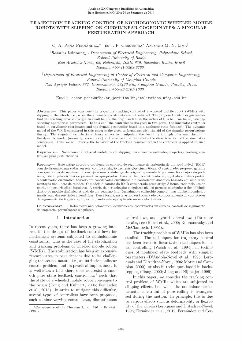
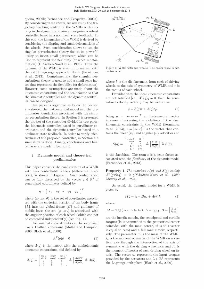
This paper consider the configuration of a WMRwith two controllable wheels (differential trac-tion), as shown in Figure 1. Such configurationcan be fully described by the vector q ∈ R

5 ofgeneralized coordinates defined by

q =[

x1 x2 θ ϕ1 ϕ2

]T

where {x1, x2, θ} is the set of coordinates associa-ted with the cartesian position of the body frame{L} into the global frame {G} and guidance ofmobile base, the set {ϕ1, ϕ2} is associated withthe angular position of each wheel (which can notbe controlled independently) (see Fig. 1).

The kinematic constraints can be expressedlike a Pfaffian constraint (Motte and Campion,2000; Bloch et al., 2000):

AT (q)q = 0 (1)

where A(q) is the matrix with the nonholonomickinematic constraints, and defined by

A(q) =

[

cos θ − sin θ sin θsin θ cos θ − cos θ0 b b0 r 00 0 r

]

,

[

A1(θ)

A2(θ)

]

, A(θ),

Roda Castor

Não - Controlável

L

x1

x2

m, Ic

θ

ϕ1, Iw

ϕ2, Iw

p

{G}

{L}

Figure 1: WMR with two wheels. The castor wheel is notcontrollable.

where b is the displacement from each of drivingwheels to the axis of symmetry of WMR and r isthe radius of each wheel.

Provided that the ideal kinematic constraintsare not satisfied [i.e., AT (q)q 6= 0] then the gene-ralized velocity vector q may be written as

q = S(q)v +A(q)εµ (2)

being µ = [ µ1 µ2 µ3 ]T

an instrumental vectorin sense of accessing the violations of the idealkinematic constraints in the WMR (Fernandez

et al., 2013), v = [ vn ω ]T is the vector that con-tains the linear (vn) and angular (ω) velocities and

S(q) =

− sin θ 0cos θ 00 1

−1/r −b/r

1/r −b/r

,

[

S1(θ)

S2(θ)

]

, S(θ),

is the Jacobian. The term ε is a scale factor as-sociated with the flexibility of the dynamic model(Fernandez et al., 2013).

Property 1 The matrices A(q) and S(q) satisfyA

T (q)S(q) = 0 (D’Andrea-Novel et al., 1995;Murray et al., 1994).

As usual, the dynamic model for a WMR isgiven by

Mq = Λ+Buε +A(θ)λ (3)

where

M = diag (m m Ic Iw Iw ) , Λ = 05×1, B =[

03×2

I2×2

]

are the inertia matrix, the centripetal and coriolistorques (It is assumed that the geometrical centercoincides with the mass center, thus this vectoris equal to zero) and a full rank matrix, respecti-vely. The parameter m is the mass of the WMR,Ic is the moment of inertia of the WMR on a ver-tical axis through the intersection of the axis ofsymmetry with the driving wheel axis and Iw isthe moment of inertia of each driving wheel on itsaxis. The vector uε represents the input torquesprovided by the actuators and λ ∈ R

3 representsthe Lagrange multipliers (Bloch et al., 2000).


2090

2.1 Singularly perturbed model

In practice, the constraint (1) does not hold. Mul-tiplying both sides of (2) by A

T (q), and by usingthe Property 1 is obtained that

AT (q)q = A

T (q)A(q)εµ. (4)

Assumption 1 Assume that the norm ofA

T (q)A(q)εµ is limited, i.e., ‖AT (q)A(q)εµ‖ ≤ ξ,where ξ is a non-negative known function whichdepends on the lateral acceleration of the robotand the deformation of the wheels.

If ε = 0 then (4) becomes the ideal constraint(1). In other words, the parameter ε governs thedissatisfaction of the kinematic constraints and itmust be included into the dynamic model. Tothis end, we propose a singularly perturbed dy-namic model for the WMR, like in (Fernandezet al., 2013), defined by the following state-space:

x = B0(q)v + [εB1(q) +B2(q)]µ+B3(q)uε

εµ = C0(q)v + [εC1(q) + C2(q)]µ+ C3(q)uε

y = P0(q)

(5)

(6)

(7)

where x = [ qT vT ]T

can be used to denote the“slow” variables and µ beyond its instrumentalmeaning can be used to denote the “fast” vari-ables; uε = [ uε,1 uε,2 ]

Thas the manipulated in-

puts associated with the torques at the motorsand y = [ y1 y2 ]

Thas the cartesian coordinates of

a point p located at a distance L of the symmetryaxle of the WMR, i.e., we define:

y = [ y1

y2] = P0(q) ,

[

x1−L sin θx2+L cos θ

]

. (8)

The matrices Bi(q), Ci(q), for i = 0, 1, 2, 3,are successively:

B0(q) =[

S(θ)∆0

]

, B1(q) =[

A(θ)∆1

]

,

B2(q) =[

05×3

∆2

]

, B3(q) =[

05×2

∆3

]

,

C0(q) =

[

−θ cos2θ 0

1/3 θ sin2θ 0

−1/3 θ sin2θ 0

]

, C1(q) =

[

0 θ −θ

1/3 θ 0 0

1/3 θ 0 0

]

,

C2(q) =

[

a3Do 0 00 a4Go a4Go

0 a4Go a4Go

]

, C3(q) =[

0 0a1 00 a1

]

,

being

∆0 =[

1/3 θ sin2θ 00 0

]

, ∆1 =[

−1/3 θ 0 00 0 0

]

∆2 =[

0 0 00 a2Go a2Go

]

, ∆3 =[

−a1 a1

−a1 −a1

]

with

a1 =r2

3 Iw, a2 = −

2 Iw b2 − 2 Ic r2

Ic Iw (δ + V )

a3 = −4

m (δ + V ), a4 = −

2 b2

Ic (δ + V )−

r2

Iw (δ + V )

where the parameter V is the velocity of the wheelcenter and δ is a “small”positive constant to avoidthe numerical problem for small values of V (i.e.,for small values of V , it is replaced by V + δ).The parameters Do and Go are normalized valuesdefined by

Do = εD and Go = εG, (9)

where D and G are the stiffness coefficients for thetransversal and longitudinal movements of eachwheel, respectively.

Assumption 2 The longitudinal and transversalstiffness coefficients (G and D, respectively) arethe same for the three wheels and

ε = inf{1/G, 1/D}.

Assumption 3 The velocities of both drivingwheels at their center are taken to be identical,and more precisely, equal to their average:

V =(

x21 + x

22 + θ

2)1/2

. (10)

Remark 1 When ε = 0 the model defined by(5)-(7) is called rigid model. When ε 6= 0 themodel is called flexible model (D’Andrea-Novelet al., 1995).

2.2 Problem of Trajectory tracking control incurvilinear coordinates

Given a differentiable simple curve C defined byone of its point, the unitary tangent vector at thepoint, and its curvature curv(s) where s is thecurvilinear coordinate along the curve, the fol-lowing assumptions will be considered in order tomake the controller design easy (Dong and Kuh-nert, 2005).

Assumption 4 Let |curv(s)| < 1/R, ∀ s whereR > 0 is a constant.

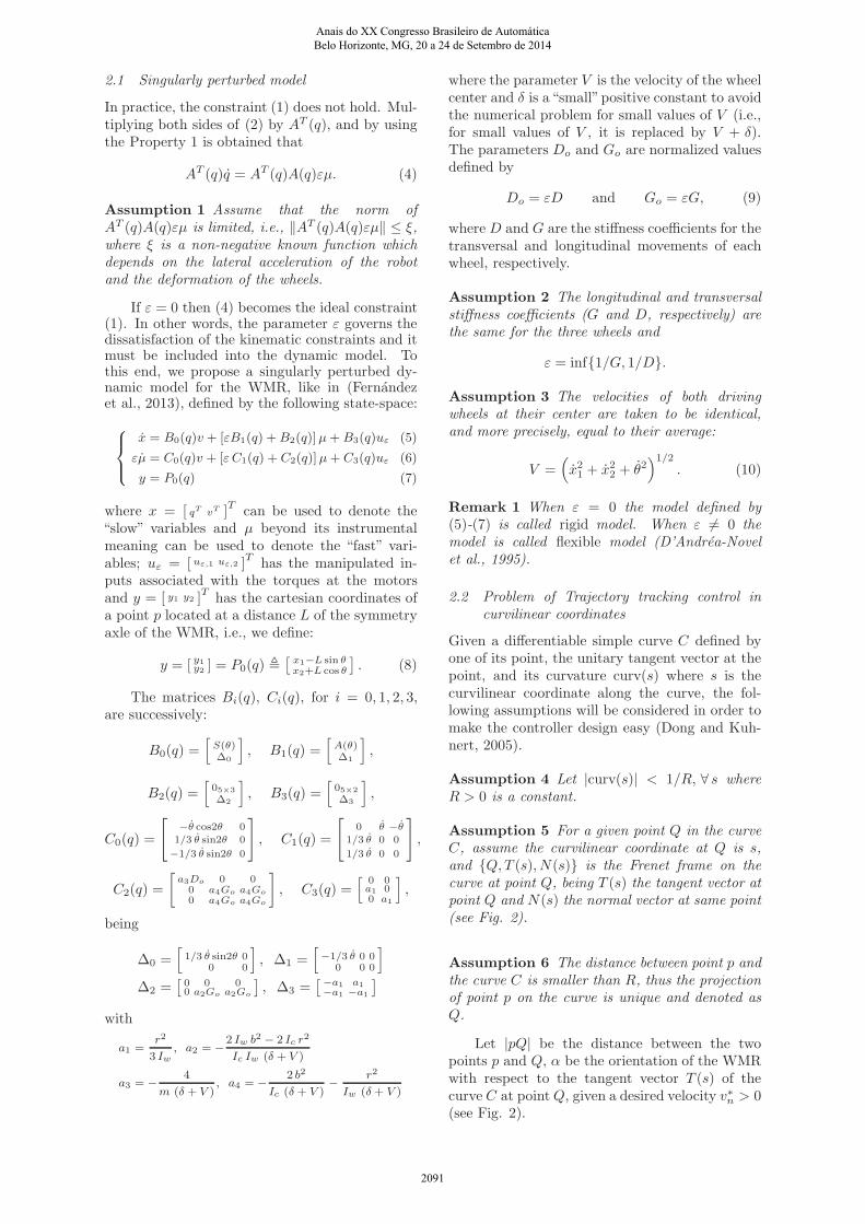
Assumption 5 For a given point Q in the curveC, assume the curvilinear coordinate at Q is s,and {Q, T (s), N(s)} is the Frenet frame on thecurve at point Q, being T (s) the tangent vector atpoint Q and N(s) the normal vector at same point(see Fig. 2).

Assumption 6 The distance between point p andthe curve C is smaller than R, thus the projectionof point p on the curve is unique and denoted asQ.

Let |pQ| be the distance between the twopoints p and Q, α be the orientation of the WMRwith respect to the tangent vector T (s) of thecurve C at pointQ, given a desired velocity v

∗n > 0

(see Fig. 2).


2091

d

T (s)

N(s)

θ

Q

γ

curve C

p

α

{G}

Figure 2: Configuration of the WMR on the curve C.

The control problem considered in this paperis finding a controller uε for system (5)-(7) suchthat |pQ|, |α| and |vn−v

∗n| are as small as possible

when time approaches to the infinity.

The position of point p is parameterized by(s, d), where d is the coordinate of point p alongN(s). Noting2 α = θ − γ, the WMR’s configura-tion is parameterized by

q∗ = [q1, q2, q3]

T = [s, d, α]T . (11)

By classic mechanics and also proposed in (Dongand Kuhnert, 2005):

q1 =vn cos q3 + ε sin q31− curv(q1)q2

(12)

q2 = vn sin q3 − ε cos q3 (13)

q3 = ω −

vn curv(q1) cos q31− curv(q1)q2

−

εcurv(q1) sin q31− curv(q1)q2

(14)

Noting the Assumption 4, the equations (12)and (14) are well-defined if |q2| < R. In the con-troller design, this condition will be guaranteed.

3 Controller design

The controller is designed in two parts. The firstpart, a kinematic controller for subsystem definedby (12)-(14) is designed with the aid of an ap-propriate transformation. In the second part, arobust nonlinear state feedback based controlleris proposed with the aid of the inverse dynamicsand the controller obtained in the first part.

3.1 Kinematic controller

Let e = [e1, e2, e3]T be the error of the tracking

trajectory associated with q∗, formally defined by

the following transformation

e = [e1, e2, e3]T = Π1(q) (15)

w = [w1, w2]T = Π−1

2 (q)v (16)

2γ is the angle between T (s) and the horizontal axis ofthe global frame {G}.

as

e1 = q1

e2 =2R

π

tanπq2

2Re3 = Lg1e2 + k2e2 +

π1

v∗n

w1 =vn cos q3

1− curv(q1)q2

w2 = w1

(

L2g1e2 +

Lg1φ1 − k2φ1

v∗n

+ k2e3∥

∥

∥− k

22e2

)

+ ωLg2Lg1e2,

where g2 = [0, 0, 1]T , φ1 = ξ∂e2∂q2

tanh

(

e2ξ

δ1

∂e2

∂q2

)

,

g1 = [1, (1 − curv(q1)q2) tan q3,−curv(q1)]T , g3 =

[

sin q31−curv(q1)q2

,− cos q3,−curv(q1) sin q31−curv(q1)q2

]T

, constants

k2 > 0 and δ1 > 0 are design parameters, L is theabbreviation of Lie Derivative, i.e.,

Lgie2 ,∂e2

∂q

gi, L2gie2 , Lgi (Lgie2)

LgiLgj e2 , Lgj (Lgie2) , (1 ≤ i, j ≤ 3),

then

e1 = w1 +ε sin q3

1− curv(q1)q2,

e2 = w1(e3 − k2e2)−w1φ1

v∗n

+ εLg3e2,

e3 = w2 −v∗oφ1

(v∗n)2+ εφ2,

(17)

(18)

(19)

where φ2 = Lg3Lg1e2 + k2Lg3e2 +Lg3φ1

v∗n

.

Assuming that w1 and w2 are control inputs,one has the following lemma.

Lemma 1 ((Dong, 2010)) Assume v∗n > δv >

0, ifw = η, (20)

then e2 and e3 converge exponentially to a smallball containing the origin. The radius of the ballcan be adjusted by δ1 > 0, where η = [η1, η2]

T and

η1 = v∗n,

η2 = −ξφ2 tanh

(

e3ξφ2

δ1

)

− k3e3v∗n − e2v

∗n +

v∗oφ1

(v∗n)2.

Proof : Let the Lyapunov function

V =1

2

(

e22 + e

23

)

differentiating it along the close-loop representedby (17)-(19), one obtains

V = −k2v∗ne

22 − k3v

∗ne

23 − e2φ1 + εe2Lg3e2

− e3ξ tanh

(

e3ξφ2

δ1

)

+ e3εφ2.


2092

In the above expression the following inequa-lities are satisfied:

|ξe2Lg3e2| ≤ ρδ1

−e3ξφ2 tanh

(

e3ξφ2

δ1

)

+ |e3ξφ2| ≤ ρδ1,

where ρ is a constant which satisfies ρ = e−(ρ+1)

(i.e., ρ = 0.2785). Thus,

V ≤ −k2v∗ne

22 − k3v

∗ne

23 + 2ρδ1

≤ −2min{k2δv, k3δv}V + 2ρδ1.

Noting v∗n ≥ δv > 0 it can be noted that

V exponentially converges to a small ball contai-ning the origin. The convergence rate is at leastmin{2k2δv, 2k3δv}. The radius of the ball can beadjusted by the parameter δ1. Therefore, e2 ande3 converge exponentially to the small ball contai-ning the origin, and the radius of the ball can alsobe adjusted by the control parameter δ1.

From (16) and (20) is obtained that

v = Π2(q)w = Π2(q)η. (21)

The equation (21) is so-called the kinematic con-troller for the WMR.

3.2 Dynamic controller

Like in (D’Andrea-Novel et al., 1995), assumingthat the control input uε is a smooth function oftime uε , uε(q, v) then, for ε = 0, the equation(6) can be rewritten as follows:

C0(q)v + C2(q)µ+ C3(q)uε(q, v) = 0, (22)

Definition 1 ((D’Andrea-Novel et al., 1995))

The model defined by (5)-(7) is in standard formif only if (22) has k ≥ 1 distinct isolated roots.

Indeed, the root of (22), here denoted by µ,is

µ = −C−12 (q) [C3(q)uε(q, v) + C0(q)v] , (23)

thus the reduced system associated is obtained bysubstituting (23) in (5):

˙x =B0(q)v − [εB1(q) +B2(q)]C−12 (q) [C3(q)×

uε(q, v) + C0(q)v] +B3(q)uε;

x(0) = x0, (24)

and the boundary layer system is

dµ

dτ

=C0(q)v0 + [εC1(q0) + C2(q0)] (µ+ µ)

+ C3(q0)uε;

µ(0) = µ0 − µ0, (25)

where τ = t/ε, v0, q0 are interpreted as fixed pa-rameters and µ = µ − µ being µ0 equal to (23)evaluated in v0, q0.

Now, we introduce two conditions:

Condition 1 There exist T, λ1, λ2, ε0 and theballs Z1 = (0;λ1), Z2 = (0;λ2) such that

• The matrices Bi(q) and Ci(q) in the model(5)-(7) (for i = 0, . . . , 3) and their partial de-rivatives with respect to x, µ and ε are conti-nuous in Z1 × Z2 × [0, ε0]× [0, T ],

• The function (23) and εC1(q) + C2(q) havecontinuous first partial derivatives,

• The reduced system (24) has an unique solu-tion x defined on [0, T ] which belongs to Z1.

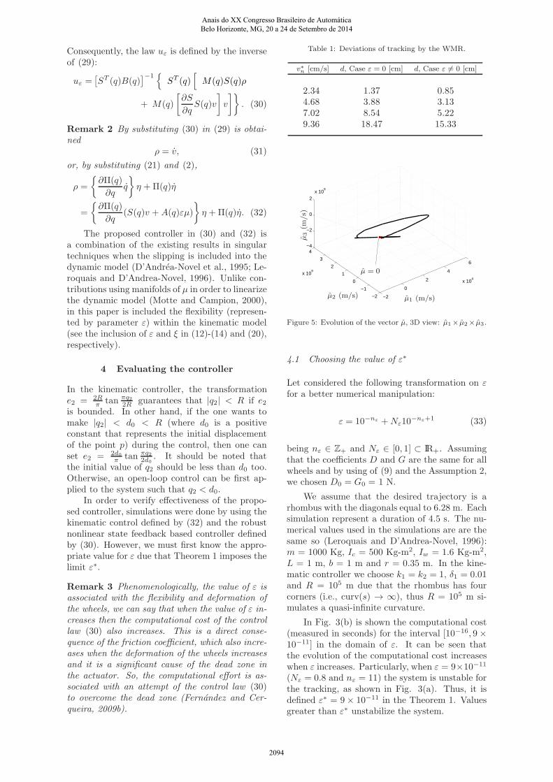
Condition 2 µ = 0 is an exponentially stableequilibrium point of the boundary layer system(25) uniformly in the parameter x0. Furthermore,µ0− µ(0) belongs to its domain of attraction. Thiscondition implies that µ(τ) exists for τ ≥ 0 andthat lim

τ→+∞µ(τ) = 0.

The Tikhonov’s theorem states the relationbetween x and x on one hand and µ, µ and µ onthe other hand.

Theorem 1 (Tikhonov’s theorem) For a sys-tem in a standard form, if the Conditions 1 and 2are satisfied, then there exist positive constants ν1,ν2 and ε

∗ such that if ‖x0‖ < ν1, ‖µ0 − µ0‖ < ν2

and ε < ε∗ then the following approximations are

valid for t ∈ [0, T ]:

x(t) =x(t) +O(ε) (26)

µ(t) = µ(t) + µ(τ) +O(ε) (27)

where O(ε) represents a quantity of the order ofε.

The Theorem 1 implies that there exists t1 >

0 such that the approximation

µ(t) = µ(t) +O(ε)

is valid for t ∈ [t1, T ]. Leaving only choose anappropriate value for ε, such that the Theorem 1is satisfied.

3.3 Computing the control law uε

The global feedback control uε = uε(q, v) is pro-jected by using the inverse dynamics of (3) andthe second derivative of (2). Thus,

q =

[

∂S

∂q

S(q)v

]

v + S(q)v. (28)

Eliminating Lagrange multipliers in (3) andusing the relation (28) give

v =[

ST (q)MS(q)

]−1ST (q)

[∥

∥

∥Buε−

M

[

∂S

∂q

S(q)v

]

v

]

. (29)


2093

Consequently, the law uε is defined by the inverseof (29):

uε =[

ST (q)B(q)

]−1{∥

∥

∥ST (q)

[∥

∥

∥M(q)S(q)ρ

+ M(q)

[

∂S

∂q

S(q)v

]

v

]}

. (30)

Remark 2 By substituting (30) in (29) is obtai-ned

ρ = v, (31)

or, by substituting (21) and (2),

ρ =

{

∂Π(q)

∂q

q

}

η +Π(q)η

=

{

∂Π(q)

∂q

(S(q)v + A(q)εµ)

}

η +Π(q)η. (32)

The proposed controller in (30) and (32) isa combination of the existing results in singulartechniques when the slipping is included into thedynamic model (D’Andrea-Novel et al., 1995; Le-roquais and D’Andrea-Novel, 1996). Unlike con-tributions using manifolds of µ in order to linearizethe dynamic model (Motte and Campion, 2000),in this paper is included the flexibility (represen-ted by parameter ε) within the kinematic model(see the inclusion of ε and ξ in (12)-(14) and (20),respectively).

4 Evaluating the controller

In the kinematic controller, the transformatione2 = 2R

πtan πq2

2R guarantees that |q2| < R if e2

is bounded. In other hand, if the one wants tomake |q2| < d0 < R (where d0 is a positiveconstant that represents the initial displacementof the point p) during the control, then one canset e2 = 2d0

πtan πq2

2d0. It should be noted that

the initial value of q2 should be less than d0 too.Otherwise, an open-loop control can be first ap-plied to the system such that q2 < d0.

In order to verify effectiveness of the propo-sed controller, simulations were done by using thekinematic control defined by (32) and the robustnonlinear state feedback based controller definedby (30). However, we must first know the appro-priate value for ε due that Theorem 1 imposes thelimit ε∗.

Remark 3 Phenomenologically, the value of ε isassociated with the flexibility and deformation ofthe wheels, we can say that when the value of ε in-creases then the computational cost of the controllaw (30) also increases. This is a direct conse-quence of the friction coefficient, which also incre-ases when the deformation of the wheels increasesand it is a significant cause of the dead zone inthe actuator. So, the computational effort is as-sociated with an attempt of the control law (30)to overcome the dead zone (Fernandez and Cer-queira, 2009b).

Table 1: Deviations of tracking by the WMR.

v∗n [cm/s] d, Case ε = 0 [cm] d, Case ε 6= 0 [cm]

2.34 1.37 0.854.68 3.88 3.137.02 8.54 5.229.36 18.47 15.33

−2

0

2

4

6

x 104

−2

−1

0

1

2

3

4

x 109

−4

−2

0

2x 10

9

µ1 (m/s)µ2 (m/s)µ3(m

/s)

µ = 0

Figure 5: Evolution of the vector µ, 3D view: µ1× µ2× µ3.

4.1 Choosing the value of ε∗

Let considered the following transformation on ε

for a better numerical manipulation:

ε = 10−nε +Nε10−nε+1 (33)

being nε ∈ Z+ and Nε ∈ [0, 1] ⊂ IR+. Assumingthat the coefficients D and G are the same for allwheels and by using of (9) and the Assumption 2,we chosen D0 = G0 = 1 N.

We assume that the desired trajectory is arhombus with the diagonals equal to 6.28 m. Eachsimulation represent a duration of 4.5 s. The nu-merical values used in the simulations are are thesame so (Leroquais and D’Andrea-Novel, 1996):m = 1000 Kg, Ic = 500 Kg-m2, Iw = 1.6 Kg-m2,L = 1 m, b = 1 m and r = 0.35 m. In the kine-matic controller we choose k1 = k2 = 1, δ1 = 0.01and R = 105 m due that the rhombus has fourcorners (i.e., curv(s) → ∞), thus R = 105 m si-mulates a quasi-infinite curvature.

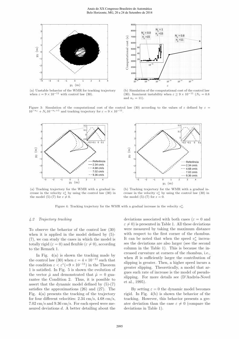
In Fig. 3(b) is shown the computational cost(measured in seconds) for the interval [10−16

, 9×10−11] in the domain of ε. It can be seen thatthe evolution of the computational cost increaseswhen ε increases. Particularly, when ε = 9×10−11

(Nε = 0.8 and nε = 11) the system is unstable forthe tracking, as shown in Fig. 3(a). Thus, it isdefined ε

∗ = 9× 10−11 in the Theorem 1. Valuesgreater than ε

∗ unstabilize the system.


2094

−4 −3 −2 −1 0 1 2 3 4−4

−3

−2

−1

0

1

2

3

4

y1 (m)

y2

(m)

(a) Unstable behavior of the WMR for tracking trajectorywhen ε = 9× 10−11 with control law (30).

10−16

10−15

10−14

10−13

10−12

10−11

0

1000

2000

3000

4000

5000

6000

7000

8000

9000

10−15

20

40

60

Nε = 0.8

nε =11

Nε = 0.0

nε =15

Nε = 1

nε =15

Computationalcost

(s)

ε

(b) Simulation of the computational cost of the control law(30). Imminent instability when ε ≥ 9× 10−11 (Nε = 0.8and nε = 11).

Figure 3: Simulation of the computational cost of the control law (30) according to the values of ε defined by ε =10−nε +Nε10−nε+1 and tracking trajectory for ε = 9× 10−11.

−3 −2 −1 0 1 2 3 4

−3

−2

−1

0

1

2

3

4

Referência2.34 cm/s4.68 cm/s7.02 cm/s9.36 cm/s

−0.2−0.1 0 0.1

2.9

3

3.1

3.2

y2

(m)

y1 (m)

(a) Tracking trajectory for the WMR with a gradual in-crease in the velocity v∗n by using the control law (30) inthe model (5)-(7) for ε 6= 0.

−3 −2 −1 0 1 2 3 4

−3

−2

−1

0

1

2

3

4

Referência2.34 cm/s4.68 cm/s7.02 cm/s9.36 cm/s

−0.2 −0.1 0 0.1

3

3.1

3.2

y2

(m)

y1 (m)

(b) Tracking trajectory for the WMR with a gradual in-crease in the velocity v∗n by using the control law (30) inthe model (5)-(7) for ε = 0.

Figure 4: Tracking trajectory for the WMR with a gradual increase in the velocity v∗n.

4.2 Trajectory tracking

To observe the behavior of the control law (30)when it is applied in the model defined by (5)-(7), we can study the cases in which the model istotally rigid (ε = 0) and flexible (ε 6= 0), accordingto the Remark 1.

In Fig. 4(a) is shown the tracking made bythe control law (30) when ε = 4× 10−11 such thatthe condition ε < ε

∗(=9× 10−11) in the Theorem1 is satisfied. In Fig. 5 is shown the evolution ofthe vector µ and demonstrated that µ = 0 gua-rantee the Condition 2. Thus, it is possible toassert that the dynamic model defined by (5)-(7)satisfies the approximations (26) and (27). TheFig. 4(a) presents the tracking of the trajectoryfor four different velocities: 2.34 cm/s, 4.68 cm/s,7.02 cm/s and 9.36 cm/s. For each speed were me-asured deviations d. A better detailing about the

deviations associated with both cases (ε = 0 andε 6= 0) is presented in Table 1. All these deviationswere measured by taking the maximum distancewith respect to the first corner of the rhombus.It can be noted that when the speed v

∗n increa-

ses the deviations are also larger (see the secondcolumn in the Table 1). This is because the in-creased curvature at corners of the rhombus, i.e.,when R is sufficiently larger the contribution ofslipping is greater. Then, a higher speed incurs agreater slipping. Theoretically, a model that ar-gues such rate of increase is the model of pseudo-slipping. For more details see (D’Andrea-Novelet al., 1995).

By setting ε = 0 the dynamic model becomesrigid. In Fig. 4(b) is shown the behavior of thetracking. However, this behavior presents a gre-ater deviation than the case ε 6= 0 (compare thedeviations in Table 1).


2095

5 Final remarks

In this paper, the path tracking control problem ofa WMR with slipping has been considered. A ro-bust controller based in a nonlinear state feedbackfor the dynamic model of the WMR also has beenproposed. The dynamic model was considered byusing the singular perturbations theory (see equa-tions (5)-(7)). The controller was designed in twoparts: on the one hand, the kinematic controllerwas projected by using the curvilinear coordinatesand the other hand the dynamic controller essen-tially based in inverse dynamic (compare (29) and(30)). The control law (30) was used in the dyna-mic model for the cases when ε = 0 (totally rigid)and when ε 6= 0 (flexible). The results observedin the Subsection 4.2 indicates that the considera-tion of the flexible system is better than the rigidsystem. However, the deviations observed in theTable 1 can be improved by choosing a minor va-lue of δ1 or by choosing larger values of k2 andk3.

Acknowledgment

The authors would like to thank to the CAPES

(Coordenacao de Aperfeicoamento de Pessoal deNıvel Superior), to the CNPq (Conselho Nacio-nal de Desenvolvimento Cientıfico e Tecnologico)and to the FAPESB (Fundacao de Amparo a Pes-quisa do Estado da Bahia) for the support givento this research.

References

Bloch, A. M., Baillieul, J., Crouch, P. and Mars-den, J. (2000). Nonholonomic Mechanics andControl, Springer, New York, MY, USA.

Brockett, R. W. (1983). Asymptotic Stability andFeedback Stabilization, in R. S. M. R. W.Brockett and H. J. Sussmann (eds), Differen-tial Geometric Control Theory, Birkhauser,Boston, pp. 181–191.

D’Andrea-Novel, B., Campion, G. and Bastin, G.(1995). Control of wheeled mobile robotsnot satisfying ideal velocity constraints: Asingular perturbation approach, Internatio-nal Journal of Robust and Nonlinear Control5(4): 243–267.

Dong, W. (2010). Control of uncertain wheeledmobile robots with slipping, 49th IEEE Con-ference on Decision and Control, pp. 7190–7195.

Dong, W. and Kuhnert, K.-D. (2005). Robustadaptive control of nonholonomic mobile ro-bot with parameter and nonparameter un-certainties, IEEE Transactions on Robotics21(2): 261–266.

Fernandez, C. A. P. and Cerqueira, J. J. F.(2009a). Control de velocidad con compen-sacion de deslizamiento en las ruedas de unabase holonomica usando un neurocontroladorbasado en el modelo narma-l2, IX CongressoBrasileiro de Redes Neurais, Ouro Preto -Brasil.

Fernandez, C. A. P. and Cerqueira, J. J. F.(2009b). Identificacao de uma base holono-mica para robos moveis com escorregamentonas rodas usando um modelo narmax polino-mial, IX Simposio Brasileiro de Automatica,Brasilia D.F - Brasil.

Fernandez, C. A. P., Cerqueira, J. J. F. and Lima,A. M. N. (2012). Dinamica nao-linear do es-corregamento de um robo movel omnidireci-onal com restricao de rolamento, XIX Con-gresso Brasileiro de Automatica - CBA 2012,Campina Grande - Brasil.

Fernandez, C. A. P., Cerqueira, J. J. F. and Lima,A. M. N. (2013). Suitable control laws to pathtracking in omnidirectional wheeled mobilerobots supported by the measuring of the rol-ling performance, XI Simposio Brasileiro deAutomacao Inteligente - SBAI 2013, Forta-leza - Brasil.

Jiang, Z.-P. (2000). Lyapunov design of glo-bal state and output feedback trackers fornon-holonomic control systems, InternationalJournal of Control 73(9): 744–761.

Jiang, Z.-P. and Nijmeijer, H. (1999). A recursivetechnique for tracking control of nonholono-mic systems in chained form, IEEE Transac-tions on Automatic Control 44(2): 265–279.

Kolmanovsky, I. and McClamroch, N. (1995).Developments in nonholonomic control pro-blems, IEEE Control Systems 15(6): 20–36.

Leroquais, W. and D’Andrea-Novel, B. (1996).Modeling and control of wheeled mobile ro-bots not satisfying ideal velocity constraints:the unicycle case, Conf. Rec. IEEE/CDC,Vol. 2, pp. 1437–1442.

Motte, I. and Campion, G. (2000). A slow ma-nifold approach for the control of mobile ro-bots not satisfying the kinematic constraints,IEEE Transactions on Robotics and Automa-tion 16(6): 875–880.

Murray, R. M., Li, Z. and Sastry, S. S. (1994). AMathematical Introduction to Robotic Mani-pulation, First edn, CRC Press LLC.

Walsh, G., Tilbury, D., Sastry, S., Murray, R.and Laumond, J.-P. (1994). Stabilization oftrajectories for systems with nonholonomicconstraints, IEEE Transactions on Automa-tic Control 39(1): 216–222.


2096

Documents

TRAJECTORY TRACKING CONTROL OF NONHOLONOMIC WHEELED …