TRAJECTORY TRACKING CONTROL OF A TRACKED MOBILE ROBOT · Abstract This paper presents a strategy for trajectory tracking control of a ... of a robot tra-jectory tracking control

TRAJECTORY TRACKING CONTROL OF A TRACKED MOBILE ROBOT

KAIO D. T. ROCHA1, THIAGO A. LIMA1, MARCUS D. N. FORTE1, MICHAEL COMBERIATE2, FABRÍCIO G. NOGUEIRA1,

BISMARK C. TORRICO1, WILKLEY B. CORREIA1

1. Department of Electrical Engineering, Federal University of Ceará, Fortaleza, CE

E-mails: [email protected], [email protected], [email protected], [email protected], [email protected]

2. NASA Goddard Space Flight Center / Capitol Technology University, USA

E-mail: [email protected]

Abstract This paper presents a strategy for trajectory tracking control of a tracked differential drive mobile robot. The utilized

controller is non-linear and has feedforward and feedback actions, with the latter using data from a SLAM (simultaneous localiza-

tion and mapping) algorithm. This strategy allows for the rejection of disturbances such as skidding and slipping during tracking

of a reference trajectory. The dynamic model that describes the tracks is identified by means of a system identification method and

a speed controller is designed in order to satisfy a desired dynamic behavior of the tracks. The performance of the proposed con-

trollers is tested and validated through experiments with a real mobile robot.

Keywords Mobile Robot Control, Robot Platform, Trajectory Tracking, System Identification.

ResumoEste artigo apresenta uma estratégia para controle de seguimento de trajetórias de um robô móvel com acionamento

diferencial com esteiras. O controlador utilizado é não-linear e apresenta ações feedforward e feedback, sendo na segunda utilizada

informação de realimentação proveniente de um algoritmo de SLAM (do inglês, simultaneous localization and mapping). Essa

estratégia possibilita a rejeição de perturbações externas, tal como deslizamento e derrapagem, durante o seguimento de uma

trajetória de referência. O modelo dinâmico que descreve as esteiras é identificado por meio de uma técnica de identificação de

sistemas e um controlador de velocidade é projetado para satisfazer o comportamento dinâmico desejado para as esteiras. O

desempenho dos controladores propostos é avaliado através de testes experimentais em um robô móvel real.

Palavras-chaveControle de Robôs Móveis, Plataformas Robóticas, Seguimento de Trajetória, Identificação de Sistemas.

1 Introduction

Control of mobile robots on a reference trajectory has

been the object of study in some previous works

(Klančar, Matko and Blažič, 2005). In order to over-

come the challenge of localizing the robot in real time,

some different sensorial techniques have been used,

such as encoder odometry, computer vision, and sen-

sor fusion.

In Chung, Hou and Chen (2015), magnetometer

and gyroscope data are fused using a Kalman filter

with fuzzy compensation to estimate a mobile robot

localization. Wang, Sun and Zhao (2015) used camera

images to identify an outdoor road in order for the ro-

bot to execute a reference tracking algorithm. More

specifically, on the tracked mobile robot case, Low

(2014) used GPS information to locate the robot in an

outdoor environment and fed the robot pose back to

the trajectory tracking control loop. However, note

that the GPS-based strategy is not suitable for indoor

environments and has limited precision. An alterna-

tive is to use modern LIDAR (light detection and rang-

ing) sensors, which allows for the operation in both

outdoor and indoor environments with precision in the

centimeters range and high scan rates. This type of

sensor is commonly used in SLAM (simultaneous lo-

calization and mapping) algorithms, mostly to gener-

ate maps of an environment.

Taking advantage of the high resolution and ac-

curacy of this kind of sensor, in this work, it is evalu-

ated the application of a LIDAR as part of a robot tra-

jectory tracking control system. More specifically, the

robot pose is estimated by means of a LIDAR-based

SLAM algorithm and used as feedback to the control-

ler. This strategy allows for the rejection of skidding

and slipping disturbances, which are naturally present

in real mobile robots. Lima et al. (2016) applied this

strategy in a wheeled mobile robot and, in this work,

it is assessed in a tracked mobile robot.

The implemented nonlinear controller is based on

Klančar, Matko and Blažič (2005), which is composed

of feedforward and feedback actions. Often, this con-

trol system uses odometry (estimated from encoders

and kinematic model) information as feedback to the

nonlinear controller.

The trajectory tracking controller generates the

speed reference for the tracks speed controller that

runs at a higher rate in an inner loop. Two digital RST

controllers were used to control the speed of the two

motor-wheel-track systems. The controller tuning was

made through a pole placement method. For this, the

LS (least squares) method was used to identify a par-

ametric dynamical model from data sets acquired ex-

perimentally with the robot.

Tests were performed in the real robot named Na-

nook. The robot was developed at NASA–GSFC in

2007 with the purposes of acquiring point cloud im-

ages and testing communication protocols that would

be later used in out of earth exploration rovers. The

robot was modernized with new control hardware, de-

XIII Simposio Brasileiro de Automacao Inteligente

Porto Alegre – RS, 1o – 4 de Outubro de 2017

ISSN 2175 8905 1930

veloped at DEE-UFC. Also, it runs the Robot Operat-

ing System (ROS), which allows for easier implemen-

tation of common robotics tasks, such as autonomous

navigation.

This work is organized as follows. In Section 2,

the kinematics mathematical model and hardware

components of the mobile robot are described. In Sec-

tion 3, the speed controller is designed after the system

identification. In Section 4, the trajectory tracking

controller is designed and the experimental results are

shown. Finally, Section 5 brings concluding remarks

about this paper.

2 Mobile robot description

2.1 Hardware description

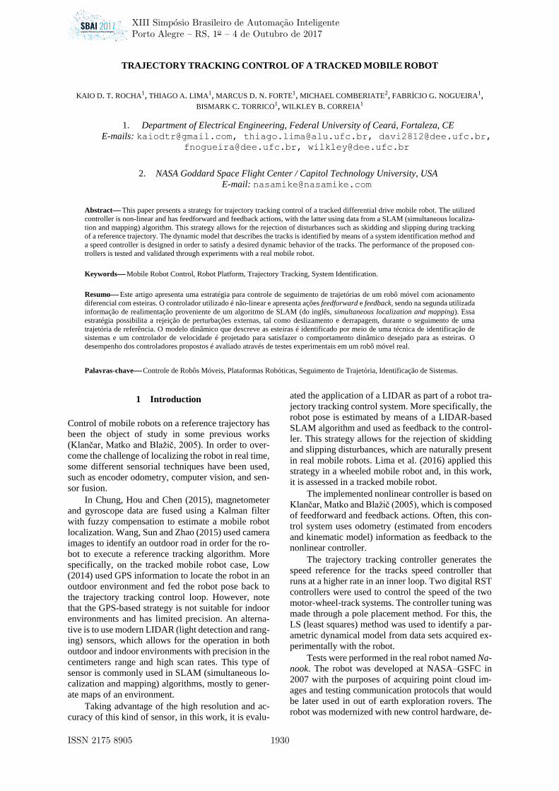
Nanook, shown in Figure 1, is the tracked differential

drive mobile robot used to carry out the experiments.

Its dimensions are 50 cm in width, 70 cm in length,

and 40 cm in height. Each track is driven by three

wheels, two of which are actuated and the middle one

is for better support. The wheels have 17 cm in diam-

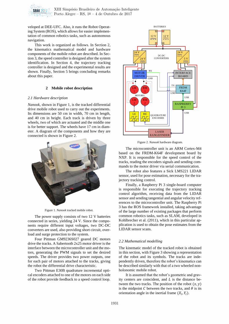
eter. A diagram of the components and how they are

connected is shown in Figure 2.

Figure 1. Nanook tracked mobile robot.

The power supply consists of two 12 V batteries

connected in series, yielding 24 V. Since the compo-

nents require different input voltages, two DC-DC

converters are used, also providing short circuit, over-

load and surge protection to the system.

Four Pittman GM9236S027 geared DC motors

drive the tracks. A Sabertooth 2x25 motor driver is the

interface between the microcontroller unit and the mo-

tors, generating the PWM signals to set the desired

speeds. The driver provides two power outputs, one

for each pair of motors attached to the tracks, giving

the robot the differential drive characteristic.

Two Pittman E30B quadrature incremental opti-

cal encoders attached to one of the motors on each side

of the robot provide feedback to a speed control loop.

Figure 2. Nanook hardware diagram.

The microcontroller unit is an ARM Cortex-M4

based on the FRDM-K64F development board by

NXP. It is responsible for the speed control of the

tracks, reading the encoders signals and sending com-

mands to the motor driver via serial communication.

The robot also features a Sick LMS221 LIDAR

sensor, used for pose estimation, necessary for the tra-

jectory tracking control.

Finally, a Raspberry Pi 3 single-board computer

is responsible for executing the trajectory tracking

control algorithm, receiving data from the LIDAR

sensor and sending tangential and angular velocity ref-

erences to the microcontroller unit. The Raspberry Pi

3 has the ROS framework installed, taking advantage

of the large number of existing packages that perform

common robotics tasks, such as SLAM, developed in

Kohlbrecher et al. (2011), which in this particular ap-

plication is used to obtain the pose estimates from the

LIDAR sensor scans.

2.2 Mathematical modelling

The kinematic model of the tracked robot is obtained

in this section, with Figure 3 showing a representation

of the robot and its symbols. The tracks are inde-

pendently driven, therefore the robot’s kinematics can

be described similarly with that of a two wheeled non-

holonomic mobile robot.

It is assumed that the robot’s geometric and grav-

ity centers are coincident, and 𝐿 is the distance be-

tween the two tracks. The position of the robot (𝑥, 𝑦)

is the midpoint 𝐶 between the two tracks, and 𝜃 is its

orientation angle in the inertial frame (𝑋𝐼, 𝑌𝐼).

MOTORS

RX

GND

TX

GND

USB

USBQUADRATURE

ENCODERS

24 V

5 V

24 V

24 V

12 V12 V

MOTOR

DRIVER

INTERFACE

BOARD

FRDM

K64FLM

1

RM

1

LM

2

RM

2 RASPBERRY

PI 3

LE RE

LASER

RANGEFINDER

DC-DC

CONVERTERS

BATTERIES



1931

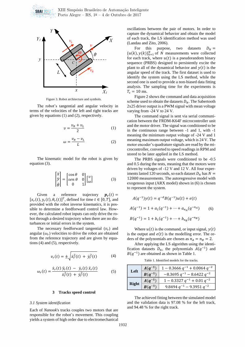
Figure 3. Robot architecture and symbols.

The robot’s tangential and angular velocity in

terms of the velocities of the left and right tracks are

given by equations (1) and (2), respectively.

𝜐 =𝜐𝑅 + 𝜐𝐿

2 (1)

𝜔 =𝜐𝑅 − 𝜐𝐿

𝐿 (2)

The kinematic model for the robot is given by

equation (3).

[

��

��

] = [cos 𝜃 0𝑠𝑒𝑛 𝜃 0

0 1] [

𝜐𝜔

] (3)

Given a reference trajectory 𝒑𝒓(𝑡) =[𝑥𝑟(𝑡), 𝑦𝑟(𝑡), 𝜃𝑟(𝑡)]𝑇, defined for time 𝑡 ∈ [0, 𝑇], and

provided with the robot inverse kinematics, it is pos-

sible to determine a feedforward control law. How-

ever, the calculated robot inputs can only drive the ro-

bot through a desired trajectory when there are no dis-

turbances or initial errors in the system.

The necessary feedforward tangential (𝑣𝑟) and

angular (𝜔𝑟) velocities to drive the robot are obtained

from the reference trajectory and are given by equa-

tions (4) and (5), respectively.

𝑣𝑟(𝑡) = ±√��𝑟2(𝑡) + ��𝑟

2(𝑡) (4)

𝜔𝑟(𝑡) =��𝑟(𝑡) ��𝑟(𝑡) − ��𝑟(𝑡) ��𝑟(𝑡)

��𝑟2(𝑡) + ��𝑟

2(𝑡) (5)

3 Tracks speed control

3.1 System identification

Each of Nanook's tracks couples two motors that are

responsible for the robot’s movement. This coupling

yields a system of high order due to electromechanical

oscillations between the pair of motors. In order to

capture the dynamical behavior and obtain the model

of each track, the LS identification method was used

(Landau and Zito, 2006).

For this purpose, two datasets 𝐷𝑁 ={𝑢(𝑘), 𝑦(𝑘)}𝑘=1

𝑁 of 𝑁 measurements were collected

for each track, where 𝑢(𝑡) is a pseudorandom binary

sequence (PRBS) designed to persistently excite the

plant to all of the dynamical behavior and 𝑦(𝑡) is the

angular speed of the track. The first dataset is used to

identify the system using the LS method, while the

second one is used to provide a non-biased data fitting

analysis. The sampling time for the experiments is

𝑇𝑠 = 10 ms.

Figure 2 shows the command and data acquisition

scheme used to obtain the datasets 𝐷𝑁. The Sabertooth

2x25 driver output is a PWM signal with mean voltage

varying from -24 V to 24 V.

The command signal is sent via serial communi-

cation between the FRDM-K64F microcontroller unit

and the motor driver. The signal was conditioned to be

in the continuous range between -1 and 1, with -1

meaning the minimum output voltage of -24 V and 1

meaning maximum output voltage, which is 24 V. The

motor encoder’s quadrature signals are read by the mi-

crocontroller, converted to speed readings in RPM and

stored to be later applied in the LS method.

The PRBS signals were conditioned to be -0.5

and 0.5 during the tests, meaning that the motors were

driven by voltages of -12 V and 12 V. All four exper-

iments lasted 120 seconds, so each dataset 𝐷𝑁 has 𝑁 =12000 measurements. The autoregressive model with

exogenous input (ARX model) shown in (6) is chosen

to represent the system.

𝐴(𝑞−1)𝑦(𝑡) = 𝑞−𝑑𝐵(𝑞−1)𝑢(𝑡) + 𝑒(𝑡)

𝐴(𝑞−1) = 1 + 𝑎1(𝑞−1) + ⋯ + 𝑎𝑛𝐴(𝑞−𝑛𝐴)

𝐵(𝑞−1) = 1 + 𝑏1(𝑞−1) + ⋯ + 𝑏𝑛𝐵

(𝑞−𝑛𝐵)

(6)

Where 𝑢(𝑡) is the command, or input signal, 𝑦(𝑡)

is the output and 𝑒(𝑡) is the modelling error. The or-

ders of the polynomials are chosen as 𝑛𝐴 = 𝑛𝐵 = 2.

After applying the LS algorithm using the identi-

fication datasets 𝐷𝑁, the polynomials 𝐴(𝑞−1) and

𝐵(𝑞−1) are obtained as shown in Table 1.

Table 1. Identified models for the tracks.

Left 𝑨(𝒒−𝟏) 1 − 0.3666 𝑞−1 + 0.0064 𝑞−2

𝑩(𝒒−𝟏) −8.3695 𝑞−1 − 8.6422 𝑞−2

Right 𝑨(𝒒−𝟏) 1 − 0.3327 𝑞−1 + 0.01 𝑞−2

𝑩(𝒒−𝟏) 9.8494 𝑞−1 − 9.3951 𝑞−2

The achieved fitting between the simulated model

and the validation data is 97.08 % for the left track,

and 94.48 % for the right track.

vLv

x

X

Y

Y I

LvR

Cy

XI



1932

3.2 Pole placement method

After the models for the tracks were identified, RST

digital speed controllers were designed for each of the

tracks using pole placement method. This method

yields some advantages when designing controllers,

such as the ability to work with both stable and unsta-

ble systems and without restriction upon the degrees

of 𝐴(𝑞−1) and 𝐵(𝑞−1). The control scheme shown in

Figure 4 is used to obtain the equations for the con-

troller design.

Figure 4. RST speed controller block diagram.

The closed loop transfer function in the backward

shift operator 𝑞−1 is given by equation (7), where de-

pendency on 𝑞−1 is omitted for simplicity. The desired

dynamical behavior of the system is defined in time

domain specifications, specifically the rise time and

the maximum overshoot of a second order system.

Then, the continuous time transfer function that pre-

sents the desired behavior for the plant is obtained and

discretized in order to gather the polynomial 𝑃(𝑞−1)

in equation (8), which defines the desired closed loop

poles. 𝑃(𝑞−1) may include additional non-dominant

poles in order to find a unique solution for polynomi-

als 𝑆(𝑞−1) and 𝑅(𝑞−1), where 𝑆(𝑞−1) includes an in-

tegrator in order to achieve zero steady-state error for

reference tracking and 𝑇(𝑞−1) is equal to the sum of

the coefficients of 𝑅(𝑞−1) so that no additional zeros

are introduced in the closed loop transfer function.

𝐻𝐶(𝑞−1) =𝑞−𝑑𝑇𝐵

𝐴𝑆 + 𝑞−𝑑𝐵𝑅 (7)

𝑃 = 𝐴𝑆 + 𝑞−𝑑𝐵 = 1 + ∑ 𝑝𝑖(𝑞−𝑖)

𝑛

𝑖=1

(8)

After specifying a rising time of 100 ms and 0 %

overshoot for both tracks, the controller parameters

were found, as shown in Table 2.

Table 2. Controller parameters for each track.

Left

𝑹(𝒒−𝟏) 0.0013 − 0.0056𝑞−1 + 0.0001𝑞−2

𝑺(𝒒−𝟏) 1.0000 − 1.1088𝑞−1 + 0.1088𝑞−2

𝑻(𝒒−𝟏) −0.0042

Right

𝑹(𝒒−𝟏) −0.0022 − 0.0061𝑞−1 + 0.0001𝑞−2

𝑺(𝒒−𝟏) 1.0000 − 1.1328𝑞−1 + 0.1328𝑞−2

𝑻(𝒒−𝟏) 0.0038

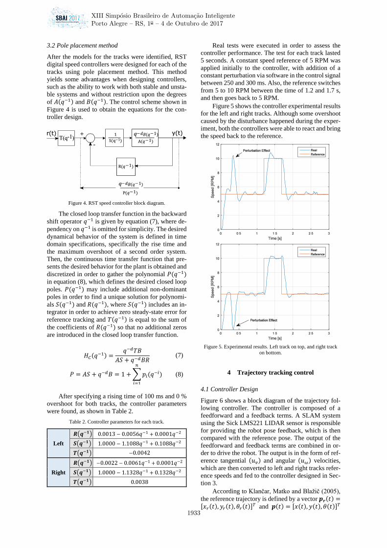
Real tests were executed in order to assess the

controller performance. The test for each track lasted

5 seconds. A constant speed reference of 5 RPM was

applied initially to the controller, with addition of a

constant perturbation via software in the control signal

between 250 and 300 ms. Also, the reference switches

from 5 to 10 RPM between the time of 1.2 and 1.7 s,

and then goes back to 5 RPM.

Figure 5 shows the controller experimental results

for the left and right tracks. Although some overshoot

caused by the disturbance happened during the exper-

iment, both the controllers were able to react and bring

the speed back to the reference.

Figure 5. Experimental results. Left track on top, and right track

on bottom.

4 Trajectory tracking control

4.1 Controller Design

Figure 6 shows a block diagram of the trajectory fol-

lowing controller. The controller is composed of a

feedforward and a feedback terms. A SLAM system

using the Sick LMS221 LIDAR sensor is responsible

for providing the robot pose feedback, which is then

compared with the reference pose. The output of the

feedforward and feedback terms are combined in or-

der to drive the robot. The output is in the form of ref-

erence tangential (𝑢𝑣) and angular (𝑢𝜔) velocities,

which are then converted to left and right tracks refer-

ence speeds and fed to the controller designed in Sec-

tion 3.

According to Klančar, Matko and Blažič (2005),

the reference trajectory is defined by a vector 𝒑𝒓(𝑡) =[𝑥𝑟(𝑡), 𝑦𝑟(𝑡), 𝜃𝑟(𝑡)]𝑇 and 𝒑(𝑡) = [𝑥(𝑡), 𝑦(𝑡), 𝜃(𝑡)]𝑇



1933

is the current robot pose. Omitting the time 𝑡 depend-

ency, one can write the pose error in the robot refer-

ence frame as in (9).

Figure 6. Trajectory tracking control scheme.

[

𝑒1

𝑒2

𝑒3

] = [cos 𝜃 sin 𝜃 0

− sin 𝜃 cos 𝜃 00 0 1

] [

𝑥𝑟 − 𝑥𝑦𝑟 − 𝑦𝜃𝑟 − 𝜃

] (9)

Differentiating equation (9) with respect to time

and using equations (3), (4) and (5), a dynamic model

for the tracking error is obtained, as shown in (10).

[

��1

��2

��3

] = [cos 𝑒3 0sin 𝑒3 0

0 1

] [𝑣𝑟

𝜔𝑟]

+ [−1 𝑒2

0 −𝑒1

0 −1] [

𝑢𝑣

𝑢𝜔]

(10)

Where 𝑣𝑟 and 𝜔𝑟 are the feedforward reference

tangential and angular velocities given by equations

(4) and (5). Then, the controller outputs, which are ap-

plied to the robot, are given by (11).

𝑢𝑣 = 𝑣𝑟 cos 𝑒3 − 𝑣1

𝑢𝜔 = 𝜔𝑟 − 𝑣2 (11)

Where 𝑣1 and 𝑣2 are the closed loop outputs. The

error model in equation (10) is then linearized and the

following control law is obtained:

[𝑣1

𝑣2] = [

−𝑘1 0 0

0 −𝑠𝑖𝑔𝑛(𝑣𝑟) 𝑘2 −𝑘3] [

𝑒1

𝑒2

𝑒3

] (12)

The controller tuning is based on the desired

damping ratio ζ and natural frequency 𝜔𝑛. The closed

loop response is related to these specifications. The

controller gains are calculated in real time using the

equations in (13). Proof and stability analysis are pre-

sented in Klančar, Matko and Blažič (2005).

𝑘1 = 𝑘3 = 2 ζ 𝜔𝑛(𝑡)

𝑘2 = 𝑔 |𝑣𝑟(𝑡)|

𝜔𝑛(𝑡) = √𝜔𝑟2(𝑡) + 𝑔 𝑣𝑟

2(𝑡)

(13)

4.2 Experimental Tests and Results

Successful application of this strategy in wheeled dif-

ferential drive mobile robots has been reported in Zer-

mas (2011) and Lima et al. (2016). In this section, the

performance of the controller is analyzed when ap-

plied to the tracked differential drive robot described

in Section 2.

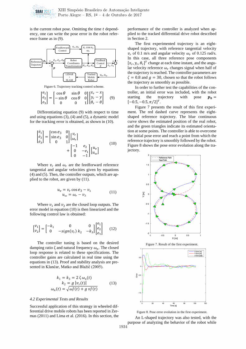
The first experimented trajectory is an eight-

shaped trajectory, with reference tangential velocity

𝑣𝑟 of 0.1 m/s and angular velocity 𝜔𝑟 of 0.125 rad/s.

In this case, all three reference pose components [𝑥𝑟 , 𝑦𝑟 , 𝜃𝑟]𝑇 change at each time instant, and the angu-

lar velocity reference 𝜔𝑟 changes signal when half of

the trajectory is reached. The controller parameters are

𝜁 = 0.8 and 𝑔 = 30, chosen so that the robot follows

the trajectory as smoothly as possible.

In order to further test the capabilities of the con-

troller, an initial error was included, with the robot

starting the trajectory with pose 𝒑𝟎 =[−0.5, −0.5, 𝜋 2⁄ ]𝑇.

Figure 7 presents the result of this first experi-

ment. The red dashed curve represents the eight-

shaped reference trajectory. The blue continuous

curve shows the estimated position of the real robot,

and the green triangles indicate its estimated orienta-

tion at some points. The controller is able to overcome

the initial pose error and reach a point from which the

reference trajectory is smoothly followed by the robot.

Figure 8 shows the pose error evolution along the tra-

jectory.

Figure 7. Result of the first experiment.

Figure 8. Pose error evolution in the first experiment.

An L-shaped trajectory was also tested, with the

purpose of analyzing the behavior of the robot while



1934

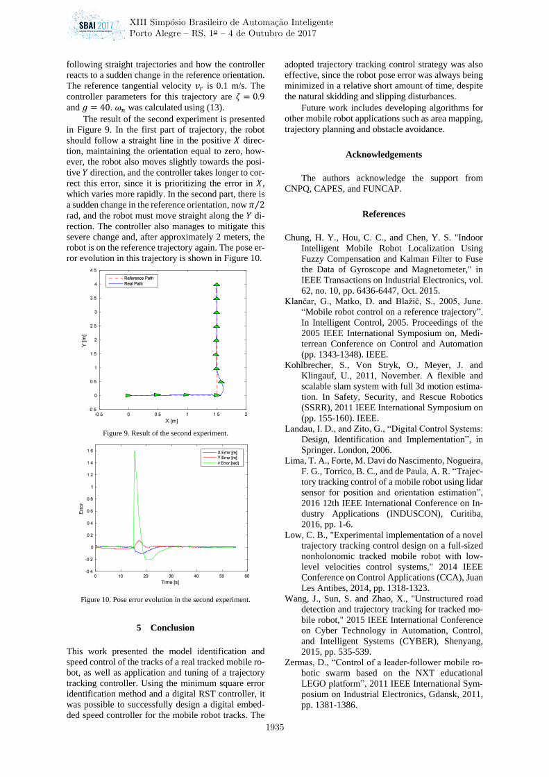
following straight trajectories and how the controller

reacts to a sudden change in the reference orientation.

The reference tangential velocity 𝑣𝑟 is 0.1 m/s. The

controller parameters for this trajectory are 𝜁 = 0.9

and 𝑔 = 40. 𝜔𝑛 was calculated using (13).

The result of the second experiment is presented

in Figure 9. In the first part of trajectory, the robot

should follow a straight line in the positive 𝑋 direc-

tion, maintaining the orientation equal to zero, how-

ever, the robot also moves slightly towards the posi-

tive 𝑌 direction, and the controller takes longer to cor-

rect this error, since it is prioritizing the error in 𝑋,

which varies more rapidly. In the second part, there is

a sudden change in the reference orientation, now 𝜋 2⁄

rad, and the robot must move straight along the 𝑌 di-

rection. The controller also manages to mitigate this

severe change and, after approximately 2 meters, the

robot is on the reference trajectory again. The pose er-

ror evolution in this trajectory is shown in Figure 10.

Figure 9. Result of the second experiment.

Figure 10. Pose error evolution in the second experiment.

5 Conclusion

This work presented the model identification and

speed control of the tracks of a real tracked mobile ro-

bot, as well as application and tuning of a trajectory

tracking controller. Using the minimum square error

identification method and a digital RST controller, it

was possible to successfully design a digital embed-

ded speed controller for the mobile robot tracks. The

adopted trajectory tracking control strategy was also

effective, since the robot pose error was always being

minimized in a relative short amount of time, despite

the natural skidding and slipping disturbances.

Future work includes developing algorithms for

other mobile robot applications such as area mapping,

trajectory planning and obstacle avoidance.

Acknowledgements

The authors acknowledge the support from

CNPQ, CAPES, and FUNCAP.

References

Chung, H. Y., Hou, C. C., and Chen, Y. S. "Indoor

Intelligent Mobile Robot Localization Using

Fuzzy Compensation and Kalman Filter to Fuse

the Data of Gyroscope and Magnetometer," in

IEEE Transactions on Industrial Electronics, vol.

62, no. 10, pp. 6436-6447, Oct. 2015.

Klančar, G., Matko, D. and Blažič, S., 2005, June.

“Mobile robot control on a reference trajectory”.

In Intelligent Control, 2005. Proceedings of the

2005 IEEE International Symposium on, Medi-

terrean Conference on Control and Automation

(pp. 1343-1348). IEEE.

Kohlbrecher, S., Von Stryk, O., Meyer, J. and

Klingauf, U., 2011, November. A flexible and

scalable slam system with full 3d motion estima-

tion. In Safety, Security, and Rescue Robotics

(SSRR), 2011 IEEE International Symposium on

(pp. 155-160). IEEE.

Landau, I. D., and Zito, G., “Digital Control Systems:

Design, Identification and Implementation”, in

Springer. London, 2006.

Lima, T. A., Forte, M. Davi do Nascimento, Nogueira,

F. G., Torrico, B. C., and de Paula, A. R. “Trajec-

tory tracking control of a mobile robot using lidar

sensor for position and orientation estimation”,

2016 12th IEEE International Conference on In-

dustry Applications (INDUSCON), Curitiba,

2016, pp. 1-6.

Low, C. B., "Experimental implementation of a novel

trajectory tracking control design on a full-sized

nonholonomic tracked mobile robot with low-

level velocities control systems," 2014 IEEE

Conference on Control Applications (CCA), Juan

Les Antibes, 2014, pp. 1318-1323.

Wang, J., Sun, S. and Zhao, X., "Unstructured road

detection and trajectory tracking for tracked mo-

bile robot," 2015 IEEE International Conference

on Cyber Technology in Automation, Control,

and Intelligent Systems (CYBER), Shenyang,

2015, pp. 535-539.

Zermas, D., “Control of a leader-follower mobile ro-

botic swarm based on the NXT educational

LEGO platform”, 2011 IEEE International Sym-

posium on Industrial Electronics, Gdansk, 2011,

pp. 1381-1386.



1935

Documents

TRAJECTORY TRACKING CONTROL OF A TRACKED MOBILE ROBOT · Abstract This paper presents a strategy for trajectory tracking control of a ... of a robot tra-jectory tracking control