TOWARD A GLOBAL BUNDLE ADJUSTMENT OF … A GLOBAL BUNDLE ADJUSTMENT OF SPOT 5 – HRS IMAGES S. Massera , P. Favé, R. Gachet, A. Orsoni IGN Espace, 6 avenue de …Authors: Stephane

TOWARD A GLOBAL BUNDLE ADJUSTMENT OF SPOT 5 – HRS IMAGES

S. Massera , P. Favé, R. Gachet, A. Orsoni

IGN Espace, 6 avenue de l’Europe, 31520 Ramonville-Saint-Agne, France – (stephane.massera, pascal.fave, roland.gachet, alain.orsoni)@ign.fr

Commission I/4

KEY WORDS: Space, Global, Bundle, Adjustment, SPOT, Matching, Processing, Production ABSTRACT: The HRS (High Resolution Stereoscopic) instrument carried on SPOT 5 enables quasi-simultaneous acquisition of stereoscopic images on wide segments --120 km wide-- with two forward and backward-looking telescopes observing the Earth with an angle of 20° ahead and behind the vertical. For 8 years IGN (Institut Géographique National) has been developing techniques to achieve spatiotriangulation of these images. During this time the capacities of bundle adjustment of SPOT 5 - HRS spatial images have largely improved. Today a global single block composed of about 20,000 images can be computed in reasonable calculation time. The progression was achieved step by step: first computed blocks were only composed of 40 images, then bigger blocks were computed. Finally only one global block is now computed. In the same time calculation tools have improved: for example the adjustment of 2,000 images of North Africa takes about 2 minutes whereas 8 hours were needed two years ago. To reach such a result a new independent software was developed to compute fast and efficient bundle adjustments. In the same time equipment --GCPs (Ground Control Points) and tie points-- and techniques have also evolved over the last 10 years. Studies were made to get recommendations about the equipment in order to make an accurate single block. Tie points can now be quickly and automatically computed with SURF (Speeded Up Robust Features) techniques. Today the updated equipment is composed of about 500 GCPs and studies show that the ideal configuration is around 100 tie points by square degree. With such an equipment, the location of the global HRS block becomes a few meters accurate whereas non adjusted images are only 15m accurate. This paper will describe the methods used in IGN Espace to compute a global single block composed of almost 20,000 HRS images, 500 GCPs and several million of tie points in reasonable calculation time. Many advantages can be found to use such a block. Because the global block is unique it becomes easier to manage the historic and the different evolutions of the computations (new images, new GCPs or tie points). The location is now unique and consequently coherent all around the world, avoiding steps and artifacts on the borders of DSMs (Digital Surface Models) and OrthoImages historically calculated from different blocks. No extrapolation far from GCPs in the limits of images is done anymore. Using the global block as a reference will allow new images from other sources to be easily located on this reference.

1. INTRODUCTION AND HISTORY OF SPATIOTRIANGULATION FOR GEOBASE®

PRODUCTS

1.1 Introduction

IGN is responsible for the production of Reference 3D®, a product composed of orthoimages and/or DEMs generated from Spot 5 images for the French Department of Defense (Bernard and al., 2005). More than 60Mkm2 have been produced since 2002, and other 80Mkm2 are to be achieved in 2015. All the products are made with SPOT 5 images that have been acquired from 2002 all over the world. The areas of the USA (excepted Alaska and GreenLand), the Antarctic continent, many isolated islands such as Açores or Antilles are not included in the contract of production. The specifications of the product are more and more severe, so that location, resolution and metadata are now more accurate. In this context, IGN has to achieve a spatiotriangulation to provide as accurate as possible models of images. This paper describes how this global spatiotriangulation has been made and how we can today compute a single block including all available SPOT 5 images. The end of the paper will explain the advantages of such a computation, and which accuracy can be reached.

1.2 History of spatiotriangulation: from small blocks to continental blocks

Continental or global blocks couldn’t have been made two years ago. Growth of block size has a 10-year history. First blocks were computed in 2002 to reach an accuracy of 15m. They were handmade and were composed of less than 100 images, tie points were generated manually and there weren’t any GCPs (Rudowski, 2003). Indeed, the average location of the HRS images was better than 15m and a relative orientation between images was enough.

From March 2007 to September 2009, IGN had to produce 70Mkm2 of Ortho Images, so that spatiotriangulation techniques had to be improved. Worksites were divided in 1,000-image blocks and were computed in several hours. Tie points were computed automatically (correlation between images) and GCPs were progressively added to improve the accuracy of the location. This work was achieved in the context of Reference3D Alpha® and had an objective of location close to the pixel size (Breton and al., 2008).

International Archives of the Photogrammetry, Remote Sensing and Spatial Information Sciences, Volume XXXIX-B1, 2012XXII ISPRS Congress, 25 August – 01 September 2012, Melbourne, Australia

251

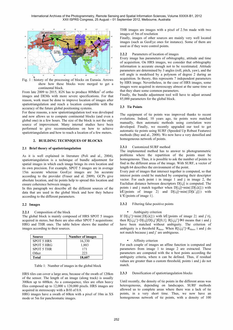
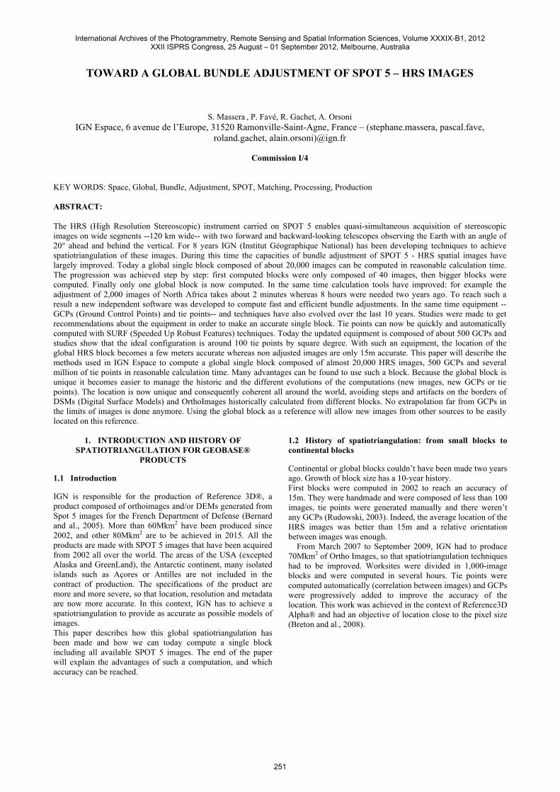
Fig. 1 : history of the processing of blocks on Eurasia. Arrows

show how these blocks were merged to get a continental block.

From late 2009 to 2015, IGN has to produce 80Mkm2 of ortho images and DEMs with more severe specifications. For that reason, work must be done to improve location of images after spatiotriangulation and reach a location compatible with the accuracy of the future global positioning systems. For these reasons, a new spatiotriangulation tool was developed and now allows us to compute continental blocks (and even a global one) in a few hours. The size of the block is not the only source of improvement. Many internal studies have been performed to give recommendations on how to achieve spatiotriangulation and how to reach a location of a few meters.

2. BUILDING TECHNIQUES OF BLOCKS

2.1 Brief theory of spatiotriangulation

As it is well explained in literature (Poli and al., 2004), spatiotriangulation is a technique of bundle adjustment for spatial images in which each image brings its own location and its own precision. For example, SPOT 5 images are in average 15m accurate whereas GeoEye images are 3m accurate according to the provider (Fraser and al. 2009). GCPs give absolute location, and tie points help to spread this location and ensure coherence between images. In this paragraph we describe all the different sources of the data that are used in the global block and how they behave according to the different parameters. 2.2 Images

2.2.1 Composition of the block The global block is mainly composed of HRS SPOT 5 images acquired in stereo, but there are also other SPOT 5 acquisitions: HRG and THR ones. The table below shows the number of images according to their sources.

Source Number of images SPOT 5 HRS 16,330 SPOT 5 HRG 1,883 SPOT 5 THR 171 Other 223 Total 18,607

Table 1: Number of images in the global block

HRS tiles can cover a large area, because of the swath of 120km of the sensor. The length of an image (along track) is usually 300km up to 600km. As a consequence, tiles are often heavy files composed up to 12,000 x 120,000 pixels. HRS images are acquired in stereoscopy with a B/H of 0.8. HRG images have a swath of 60km with a pixel of 10m in XS mode or 5m for panchromatic images.

THR images are images with a pixel of 2.5m made with two images of 5m of resolution Finally, images of other sources are mainly very well located images (such as GeoEye ones for instance). Some of them are used as if they were control points. 2.2.2 Parameters of location of images Every image has parameters of orbitography, attitude and time of acquisition. On HRS images, we consider that orbitography information is accurate enough not to be reestimated. Attitude parameters are determined by 3 angles (roll, pitch, yaw), and the roll angle is modelised by a polynom of degree 2 during an acquisition. In theory, this represents 7 independent parameters by HRS image. Nevertheless, in the case of HRS images, some images were acquired in stereoscopy almost at the same time so that they share some common parameters. Finally, the bundle adjustment tool will have to adjust around 85,000 parameters for the global block. 2.3 Tie Points

The equipment of tie points was improved thanks to recent evolutions. Indeed, 10 years ago, tie points were matched manually, then automatic methods using correlation were developed. Finally, we recently upgraded our tool to get automatic tie points using SURF (Speeded Up Robust Features) methods (Bay and al., 2008). We now have a very densified and homogeneous network of points. 2.3.1 Customized SURF method The implemented method has to answer to photogrammetric problems where the repartition of the points must be homogeneous. Thus, it is possible to ask the number of points to find in the different areas of the image. With SURF, a vector of length 64 describes the environment of the point. Every pair of images that intersect together is computed, so that interest points could be matched by comparing their descriptor vector. For each point i in image 1 and j in image 2, the Euclidian distance between descriptors D[i,j] is computed. The points i and j match together when D[i,j]=min({D[i,k]}) with k∈{points of image 2} and D[i,j]=min({D[k’,j]}) with k’∈{points of image 1}. 2.3.2 Filtering false positive points

• Ambiguity criterion If D[i,j’]=min({D[i,k]}) with k∈{points of image 2} and j’≠j, then R[i,j,j’]=D[i,j]/D[i,j’]∈[0,1]. R[i,j,j’]0 means that i and j have been matched without ambiguity. The criterion of ambiguity is a threshold Rthres. When R[i,j,j’]>Rthres, i and j do not match because j and j’ are ambiguous.

• Affinity criterion For each couple of images an affine function is computed and parameters from image 1 to image 2 are extracted. These parameters are computed with the n best points according the ambiguity criteria, where n can be defined. Thus, if residual values are greater than a custom threshold, points i and j do not match. 2.3.3 Densification of spatiotriangulation blocks Until recently, the density of tie points in the different areas was heterogeneous, depending on landscapes. SURF methods allowed us to complete areas where there was a lack of tie points, in a very short time. Thus, we now have an homogeneous network of tie points, with a density of 100


252

points/deg2. Our tests showed that with the weight affected to every measure, the propagation of the location of the GCPs is optimal. The figure below shows the evolution of the density of tie points on the Arabic Peninsula block.

Fig. 2: Density of tie points before (left) and after (right) the

introduction of SURF points Tests made with different networks of tie points showed that a homogeneous network consequently helps to spread the location of GCPs. 2.4 Ground Control Points

2.4.1 Description Ground Control Points used in the computation seem to be numerous (3,264). Nevertheless, most of those ones are grouped in sites of 5 or more points. Finally, there are around 500 sites of GCPs located all over the world. Using groups of GCPs increases the accuracy because of the redundancy of the measures. It is also an easy way to detect a bad located point. Each GCP is affected by a beforehand and an afterward accuracy. The beforehand accuracy is related to how we trust the data. The afterward accuracy is given by the difference of coordinates between the measured point and the calculated one. 2.4.2 Propagation of the location of a GCP The GCPs aim at applying their own location to the images. Thus, they often have a strong weight in the computation compared to images, in order to increase their influence. In nominal conditions, internal studies showed that GCPs can influence the location of the images up to 2,500km. The figure below shows the comparison between a spatiotriangulation computed with and without GCPs (black points). Between the two computations, the location has moved more than 1.50m in an area of 2,500 km wide around the GCPs.

Fig. 3: Difference of planimetric location between two

spatiotriangulations. According to these results, we recommend to use 1 GCP every 1,000 km in an ideal context, so that the influence of each one is correctly propagated.

2.4.3 Weight in the system Most GCPs were acquired by GPS measurements. As a consequence, their accuracy are often better than 1m. Nevertheless, it is sometimes hard to measure them in HRS images because of the poor definition of the image (5m x 10m). According to the sources of the GCPs and the way they are measured in images, the affected weight is around 1m for the point and 0.1-0.4 pixel for its image measurement. 2.5 Using images as GCPs

2.5.1 Description Getting precise GCPs all over the world is a very hard and expensive task, so that there are holes left in the coverage of GCPs. As a consequence, we decided to use precise satellite imagery to extract information of location in areas where there is a lack of GCPs, as it is shown in the figure below.

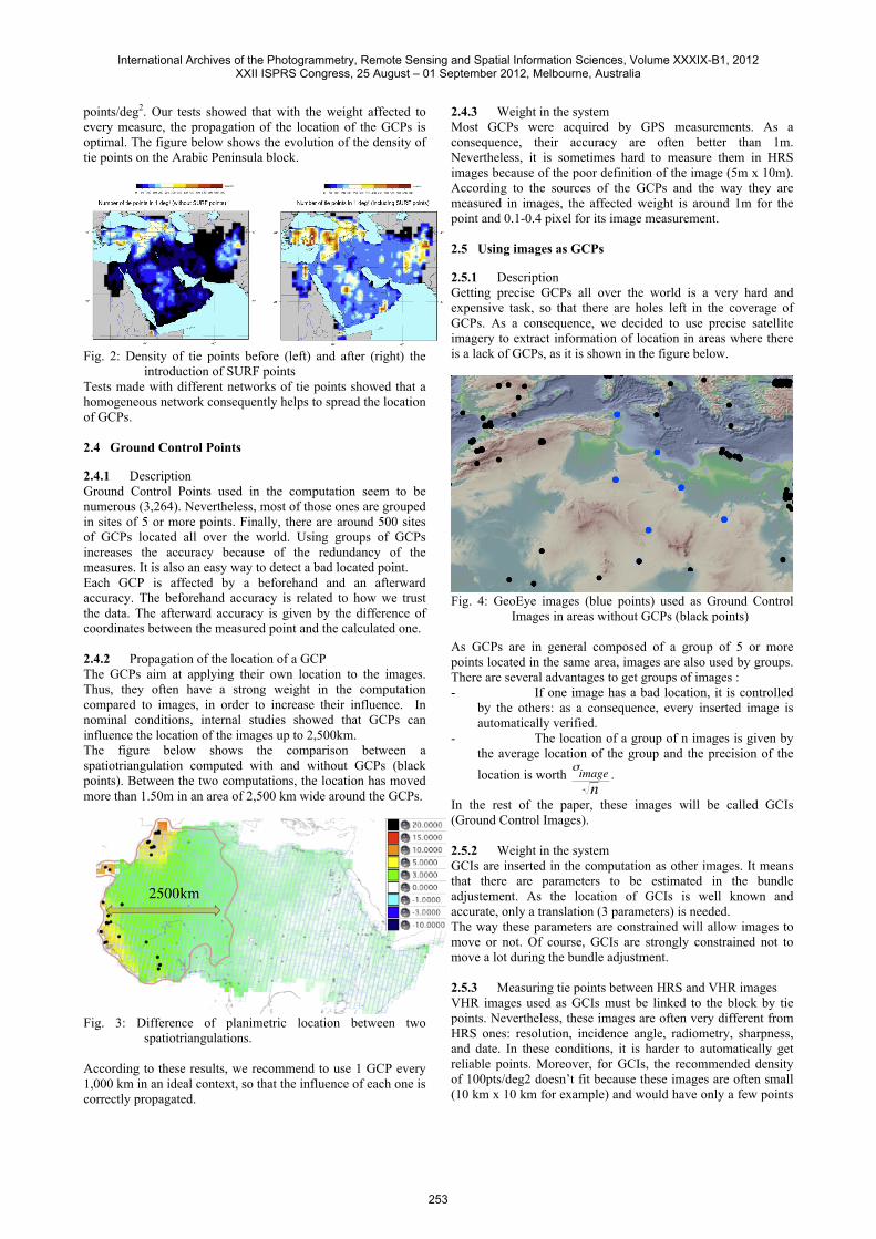
Fig. 4: GeoEye images (blue points) used as Ground Control

Images in areas without GCPs (black points) As GCPs are in general composed of a group of 5 or more points located in the same area, images are also used by groups. There are several advantages to get groups of images : - If one image has a bad location, it is controlled

by the others: as a consequence, every inserted image is automatically verified.

- The location of a group of n images is given by the average location of the group and the precision of the location is worth

€

σimagen

.

In the rest of the paper, these images will be called GCIs (Ground Control Images). 2.5.2 Weight in the system GCIs are inserted in the computation as other images. It means that there are parameters to be estimated in the bundle adjustement. As the location of GCIs is well known and accurate, only a translation (3 parameters) is needed. The way these parameters are constrained will allow images to move or not. Of course, GCIs are strongly constrained not to move a lot during the bundle adjustment. 2.5.3 Measuring tie points between HRS and VHR images VHR images used as GCIs must be linked to the block by tie points. Nevertheless, these images are often very different from HRS ones: resolution, incidence angle, radiometry, sharpness, and date. In these conditions, it is harder to automatically get reliable points. Moreover, for GCIs, the recommended density of 100pts/deg2 doesn’t fit because these images are often small (10 km x 10 km for example) and would have only a few points


253

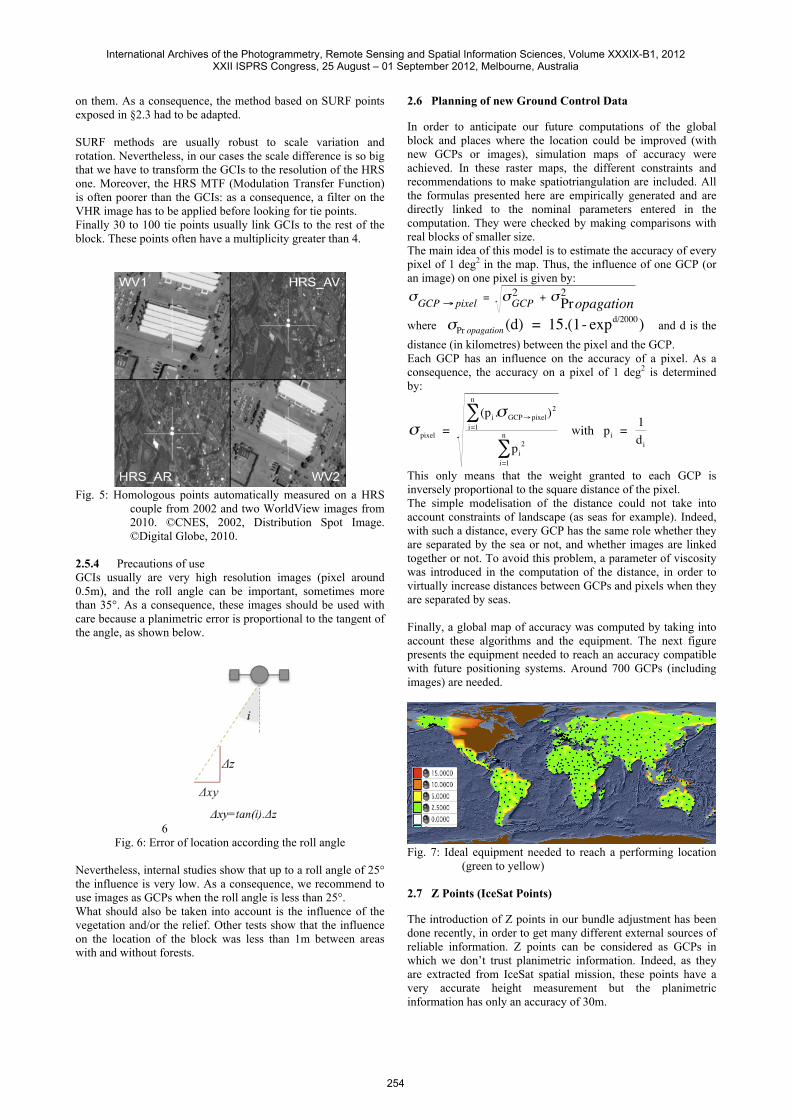
on them. As a consequence, the method based on SURF points exposed in §2.3 had to be adapted. SURF methods are usually robust to scale variation and rotation. Nevertheless, in our cases the scale difference is so big that we have to transform the GCIs to the resolution of the HRS one. Moreover, the HRS MTF (Modulation Transfer Function) is often poorer than the GCIs: as a consequence, a filter on the VHR image has to be applied before looking for tie points. Finally 30 to 100 tie points usually link GCIs to the rest of the block. These points often have a multiplicity greater than 4.

Fig. 5: Homologous points automatically measured on a HRS

couple from 2002 and two WorldView images from 2010. ©CNES, 2002, Distribution Spot Image. ©Digital Globe, 2010.

2.5.4 Precautions of use GCIs usually are very high resolution images (pixel around 0.5m), and the roll angle can be important, sometimes more than 35°. As a consequence, these images should be used with care because a planimetric error is proportional to the tangent of the angle, as shown below.

6 Fig. 6: Error of location according the roll angle

Nevertheless, internal studies show that up to a roll angle of 25° the influence is very low. As a consequence, we recommend to use images as GCPs when the roll angle is less than 25°. What should also be taken into account is the influence of the vegetation and/or the relief. Other tests show that the influence on the location of the block was less than 1m between areas with and without forests.

2.6 Planning of new Ground Control Data

In order to anticipate our future computations of the global block and places where the location could be improved (with new GCPs or images), simulation maps of accuracy were achieved. In these raster maps, the different constraints and recommendations to make spatiotriangulation are included. All the formulas presented here are empirically generated and are directly linked to the nominal parameters entered in the computation. They were checked by making comparisons with real blocks of smaller size. The main idea of this model is to estimate the accuracy of every pixel of 1 deg2 in the map. Thus, the influence of one GCP (or an image) on one pixel is given by:

€

σGCP → pixel = σGCP2 + σPropagation

2

where

€

σPr opagation (d) = 15.(1- expd/2000) and d is the distance (in kilometres) between the pixel and the GCP. Each GCP has an influence on the accuracy of a pixel. As a consequence, the accuracy on a pixel of 1 deg2 is determined by:

€

σ pixel = (pi.σ GCP→ pixel)

2

i=1

n

∑

pi2

i=1

n

∑ with pi = 1

di

This only means that the weight granted to each GCP is inversely proportional to the square distance of the pixel. The simple modelisation of the distance could not take into account constraints of landscape (as seas for example). Indeed, with such a distance, every GCP has the same role whether they are separated by the sea or not, and whether images are linked together or not. To avoid this problem, a parameter of viscosity was introduced in the computation of the distance, in order to virtually increase distances between GCPs and pixels when they are separated by seas. Finally, a global map of accuracy was computed by taking into account these algorithms and the equipment. The next figure presents the equipment needed to reach an accuracy compatible with future positioning systems. Around 700 GCPs (including images) are needed.

Fig. 7: Ideal equipment needed to reach a performing location

(green to yellow) 2.7 Z Points (IceSat Points)

The introduction of Z points in our bundle adjustment has been done recently, in order to get many different external sources of reliable information. Z points can be considered as GCPs in which we don’t trust planimetric information. Indeed, as they are extracted from IceSat spatial mission, these points have a very accurate height measurement but the planimetric information has only an accuracy of 30m.


254

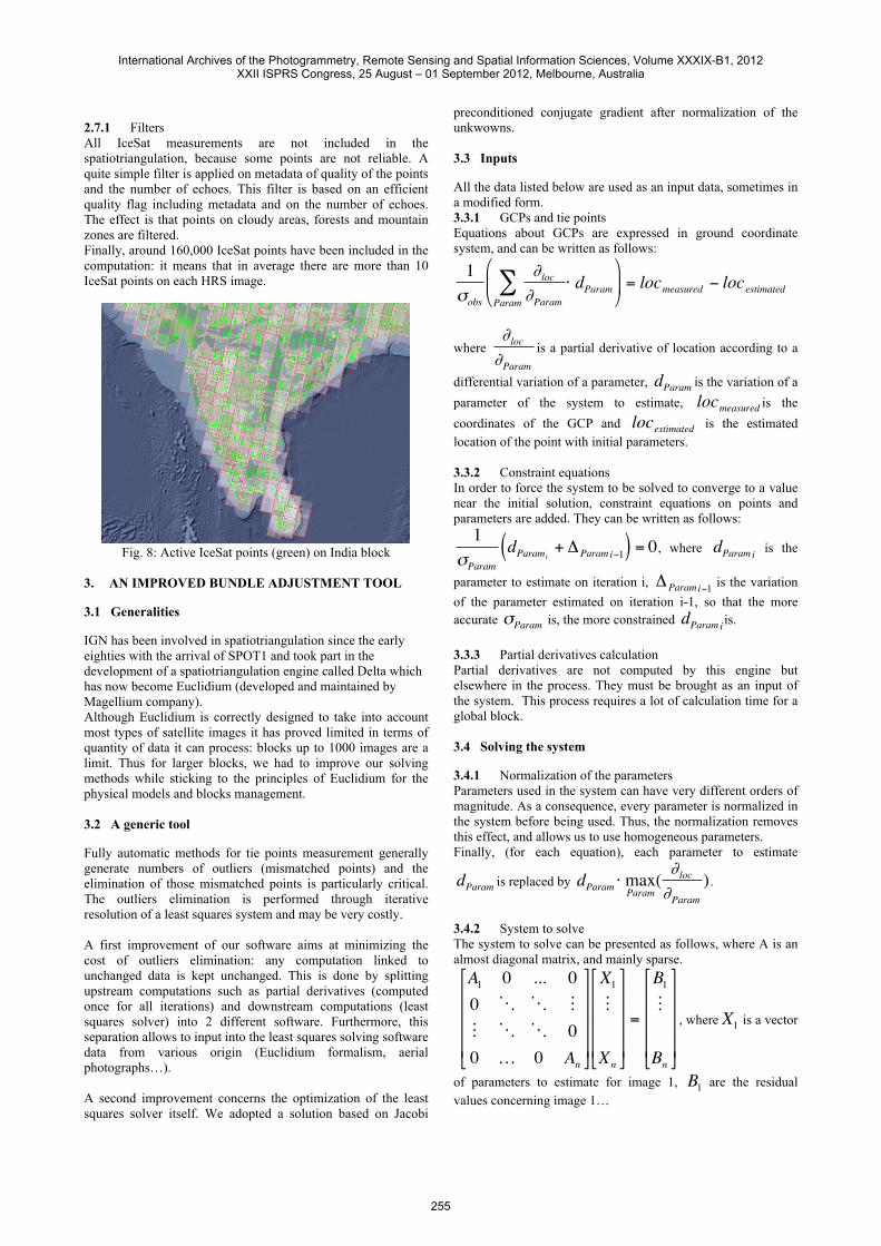
2.7.1 Filters All IceSat measurements are not included in the spatiotriangulation, because some points are not reliable. A quite simple filter is applied on metadata of quality of the points and the number of echoes. This filter is based on an efficient quality flag including metadata and on the number of echoes. The effect is that points on cloudy areas, forests and mountain zones are filtered. Finally, around 160,000 IceSat points have been included in the computation: it means that in average there are more than 10 IceSat points on each HRS image.

Fig. 8: Active IceSat points (green) on India block

3. AN IMPROVED BUNDLE ADJUSTMENT TOOL

3.1 Generalities

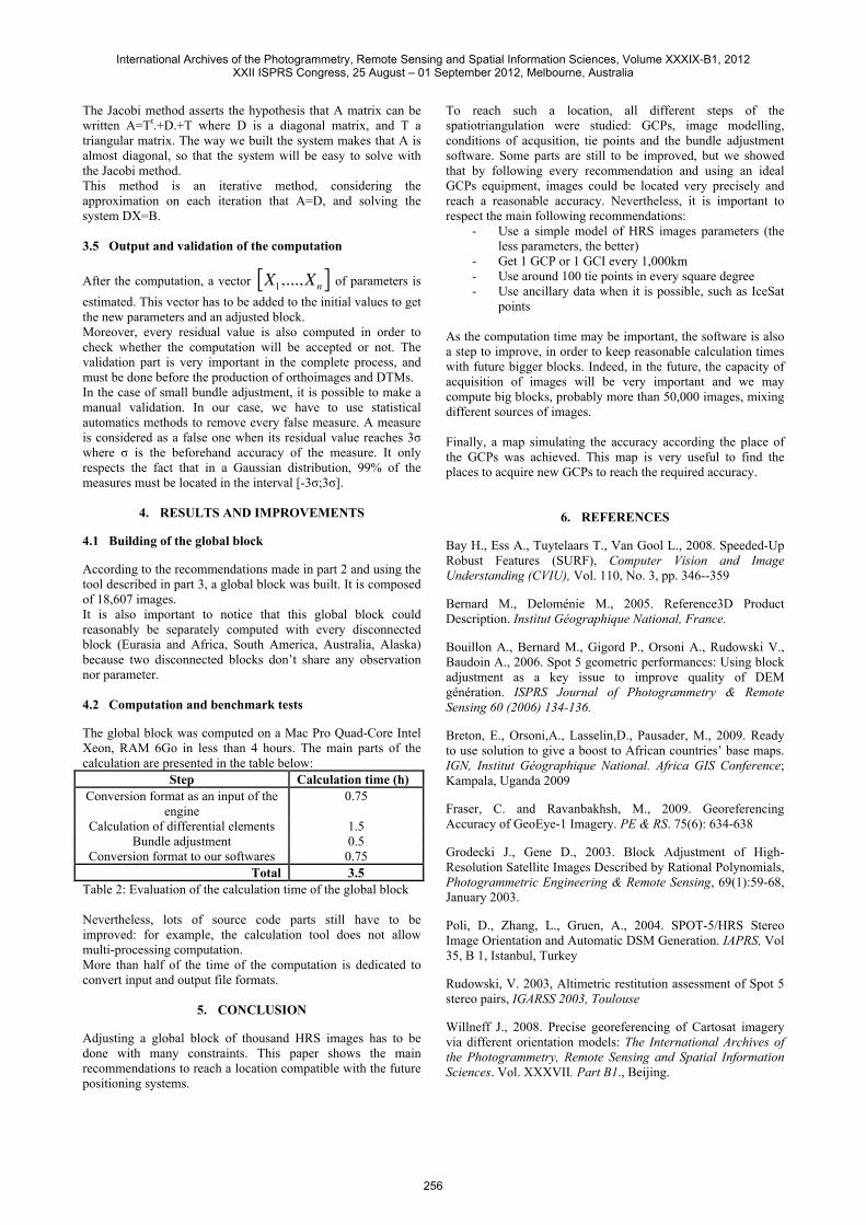
IGN has been involved in spatiotriangulation since the early eighties with the arrival of SPOT1 and took part in the development of a spatiotriangulation engine called Delta which has now become Euclidium (developed and maintained by Magellium company). Although Euclidium is correctly designed to take into account most types of satellite images it has proved limited in terms of quantity of data it can process: blocks up to 1000 images are a limit. Thus for larger blocks, we had to improve our solving methods while sticking to the principles of Euclidium for the physical models and blocks management. 3.2 A generic tool

Fully automatic methods for tie points measurement generally generate numbers of outliers (mismatched points) and the elimination of those mismatched points is particularly critical. The outliers elimination is performed through iterative resolution of a least squares system and may be very costly. A first improvement of our software aims at minimizing the cost of outliers elimination: any computation linked to unchanged data is kept unchanged. This is done by splitting upstream computations such as partial derivatives (computed once for all iterations) and downstream computations (least squares solver) into 2 different software. Furthermore, this separation allows to input into the least squares solving software data from various origin (Euclidium formalism, aerial photographs…). A second improvement concerns the optimization of the least squares solver itself. We adopted a solution based on Jacobi

preconditioned conjugate gradient after normalization of the unkwowns. 3.3 Inputs

All the data listed below are used as an input data, sometimes in a modified form. 3.3.1 GCPs and tie points Equations about GCPs are expressed in ground coordinate system, and can be written as follows:

€

1σobs

∂loc∂Param

⋅ dParamParam∑

⎛

⎝ ⎜

⎞

⎠ ⎟ = locmeasured − locestimated

where

€

∂loc∂Param

is a partial derivative of location according to a

differential variation of a parameter,

€

dParam is the variation of a parameter of the system to estimate,

€

locmeasured is the coordinates of the GCP and

€

locestimated is the estimated location of the point with initial parameters. 3.3.2 Constraint equations In order to force the system to be solved to converge to a value near the initial solution, constraint equations on points and parameters are added. They can be written as follows:

€

1σParam

dParami+ ΔParam i−1( ) = 0, where

€

dParam i is the

parameter to estimate on iteration i,

€

ΔParami−1 is the variation of the parameter estimated on iteration i-1, so that the more accurate

€

σParam is, the more constrained

€

dParam i is. 3.3.3 Partial derivatives calculation Partial derivatives are not computed by this engine but elsewhere in the process. They must be brought as an input of the system. This process requires a lot of calculation time for a global block. 3.4 Solving the system

3.4.1 Normalization of the parameters Parameters used in the system can have very different orders of magnitude. As a consequence, every parameter is normalized in the system before being used. Thus, the normalization removes this effect, and allows us to use homogeneous parameters. Finally, (for each equation), each parameter to estimate

€

dParam is replaced by

€

dParam ⋅ maxParam( ∂loc∂Param

).

3.4.2 System to solve The system to solve can be presented as follows, where A is an almost diagonal matrix, and mainly sparse.

€

A1 0 ... 00 00 … 0 An

⎡

⎣

⎢ ⎢ ⎢ ⎢

⎤

⎦

⎥ ⎥ ⎥ ⎥

X1

Xn

⎡

⎣

⎢ ⎢ ⎢ ⎢

⎤

⎦

⎥ ⎥ ⎥ ⎥

=

B1

Bn

⎡

⎣

⎢ ⎢ ⎢ ⎢

⎤

⎦

⎥ ⎥ ⎥ ⎥

, where

€

X1 is a vector

of parameters to estimate for image 1,

€

B1 are the residual values concerning image 1…


255

The Jacobi method asserts the hypothesis that A matrix can be written A=Tt.+D.+T where D is a diagonal matrix, and T a triangular matrix. The way we built the system makes that A is almost diagonal, so that the system will be easy to solve with the Jacobi method. This method is an iterative method, considering the approximation on each iteration that A=D, and solving the system DX=B. 3.5 Output and validation of the computation

After the computation, a vector

€

X1,...,Xn[ ] of parameters is estimated. This vector has to be added to the initial values to get the new parameters and an adjusted block. Moreover, every residual value is also computed in order to check whether the computation will be accepted or not. The validation part is very important in the complete process, and must be done before the production of orthoimages and DTMs. In the case of small bundle adjustment, it is possible to make a manual validation. In our case, we have to use statistical automatics methods to remove every false measure. A measure is considered as a false one when its residual value reaches 3σ where σ is the beforehand accuracy of the measure. It only respects the fact that in a Gaussian distribution, 99% of the measures must be located in the interval [-3σ;3σ].

4. RESULTS AND IMPROVEMENTS

4.1 Building of the global block

According to the recommendations made in part 2 and using the tool described in part 3, a global block was built. It is composed of 18,607 images. It is also important to notice that this global block could reasonably be separately computed with every disconnected block (Eurasia and Africa, South America, Australia, Alaska) because two disconnected blocks don’t share any observation nor parameter. 4.2 Computation and benchmark tests

The global block was computed on a Mac Pro Quad-Core Intel Xeon, RAM 6Go in less than 4 hours. The main parts of the calculation are presented in the table below:

Step Calculation time (h) Conversion format as an input of the

engine 0.75

Calculation of differential elements 1.5 Bundle adjustment 0.5

Conversion format to our softwares 0.75 Total 3.5

Table 2: Evaluation of the calculation time of the global block Nevertheless, lots of source code parts still have to be improved: for example, the calculation tool does not allow multi-processing computation. More than half of the time of the computation is dedicated to convert input and output file formats.

5. CONCLUSION

Adjusting a global block of thousand HRS images has to be done with many constraints. This paper shows the main recommendations to reach a location compatible with the future positioning systems.

To reach such a location, all different steps of the spatiotriangulation were studied: GCPs, image modelling, conditions of acqusition, tie points and the bundle adjustment software. Some parts are still to be improved, but we showed that by following every recommendation and using an ideal GCPs equipment, images could be located very precisely and reach a reasonable accuracy. Nevertheless, it is important to respect the main following recommendations:

- Use a simple model of HRS images parameters (the less parameters, the better)

- Get 1 GCP or 1 GCI every 1,000km - Use around 100 tie points in every square degree - Use ancillary data when it is possible, such as IceSat

points As the computation time may be important, the software is also a step to improve, in order to keep reasonable calculation times with future bigger blocks. Indeed, in the future, the capacity of acquisition of images will be very important and we may compute big blocks, probably more than 50,000 images, mixing different sources of images. Finally, a map simulating the accuracy according the place of the GCPs was achieved. This map is very useful to find the places to acquire new GCPs to reach the required accuracy.

6. REFERENCES

Bay H., Ess A., Tuytelaars T., Van Gool L., 2008. Speeded-Up Robust Features (SURF), Computer Vision and Image Understanding (CVIU), Vol. 110, No. 3, pp. 346--359

Bernard M., Deloménie M., 2005. Reference3D Product Description. Institut Géographique National, France.

Bouillon A., Bernard M., Gigord P., Orsoni A., Rudowski V., Baudoin A., 2006. Spot 5 geometric performances: Using block adjustment as a key issue to improve quality of DEM génération. ISPRS Journal of Photogrammetry & Remote Sensing 60 (2006) 134-136.

Breton, E., Orsoni,A., Lasselin,D., Pausader, M., 2009. Ready to use solution to give a boost to African countries’ base maps. IGN, Institut Géographique National. Africa GIS Conference; Kampala, Uganda 2009

Fraser, C. and Ravanbakhsh, M., 2009. Georeferencing Accuracy of GeoEye-1 Imagery. PE & RS. 75(6): 634-638

Grodecki J., Gene D., 2003. Block Adjustment of High-Resolution Satellite Images Described by Rational Polynomials, Photogrammetric Engineering & Remote Sensing, 69(1):59-68, January 2003.

Poli, D., Zhang, L., Gruen, A., 2004. SPOT-5/HRS Stereo Image Orientation and Automatic DSM Generation. IAPRS, Vol 35, B 1, Istanbul, Turkey

Rudowski, V. 2003, Altimetric restitution assessment of Spot 5 stereo pairs, IGARSS 2003, Toulouse

Willneff J., 2008. Precise georeferencing of Cartosat imagery via different orientation models: The International Archives of the Photogrammetry, Remote Sensing and Spatial Information Sciences. Vol. XXXVII. Part B1., Beijing.


256

Documents

TOWARD A GLOBAL BUNDLE ADJUSTMENT OF … A GLOBAL BUNDLE ADJUSTMENT OF SPOT 5 – HRS IMAGES S. Massera , P. Favé, R. Gachet, A. Orsoni IGN Espace, 6 avenue de …Authors: Stephane