Out-of-Core Bundle Adjustment for Large-Scale 3D Reconstruction

Kai Ni∗, Drew Steedly†, and Frank Dellaert∗∗College of Computing, Georgia Institute of Technology, Atlanta, GA 30332

†Microsoft Live Labs, Redmond, WA 98052{nikai,dellaert}@cc.gatech.edu, steedly@microsoft.com

Abstract

Large-scale 3D reconstruction has recently receivedmuch attention from the computer vision community. Bun-dle adjustment is a key component of 3D reconstructionproblems. However, traditional bundle adjustment algo-rithms require a considerable amount of memory and com-putational resources. In this paper, we present an ex-tremely efficient, inherently out-of-core bundle adjustmentalgorithm. We decouple the original problem into severalsubmaps that have their own local coordinate systems andcan be optimized in parallel. A key contribution to ouralgorithm is making as much progress towards optimizingthe global non-linear cost function as possible using thefragments of the reconstruction that are currently in corememory. This allows us to converge with very few globalsweeps (often only two) through the entire reconstruction.We present experimental results on large-scale 3D recon-struction datasets, both synthetic and real.

1. IntroductionIn this paper, we present an approach for generating

large-scale three-dimensional reconstructions from images.Our algorithm is inherently out-of-core and parallel andtherefore capable of tackling large optimization problemswith fewer computational resources. In addition, high qual-ity reconstructions of submaps can be computed early on inthe optimization, making the approach well suited for on-line mapping situations.

1.1. Motivation

Large-scale 3D reconstruction, especially image-basedurban reconstruction, has received considerable attentionrecently from the computer vision community [8, 16, 15].High-quality 3D models are useful in various successfulcartographic and architectural applications, such as GoogleEarth or Microsoft Live Local.

Traditional approaches usually build 3D city models

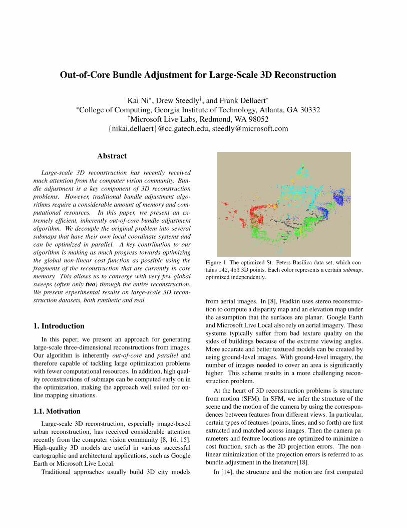
Figure 1. The optimized St. Peters Basilica data set, which con-tains 142, 453 3D points. Each color represents a certain submap,optimized independently.

from aerial images. In [8], Fradkin uses stereo reconstruc-tion to compute a disparity map and an elevation map underthe assumption that the surfaces are planar. Google Earthand Microsoft Live Local also rely on aerial imagery. Thesesystems typically suffer from bad texture quality on thesides of buildings because of the extreme viewing angles.More accurate and better textured models can be created byusing ground-level images. With ground-level imagery, thenumber of images needed to cover an area is significantlyhigher. This scheme results in a more challenging recon-struction problem.

At the heart of 3D reconstruction problems is structurefrom motion (SFM). In SFM, we infer the structure of thescene and the motion of the camera by using the correspon-dences between features from different views. In particular,certain types of features (points, lines, and so forth) are firstextracted and matched across images. Then the camera pa-rameters and feature locations are optimized to minimize acost function, such as the 2D projection errors. The non-linear minimization of the projection errors is referred to asbundle adjustment in the literature[18].

In [14], the structure and the motion are first computed

from the multi-view relations and then refined using bundleadjustment as the last step. Brown [4] employed an incre-mental bundle adjustment algorithm to do 3D object recon-struction. In particular, the approach incrementally insertsnew frames into the optimization problem, which computeswell conditioned initial reconstructions. These experimentsmainly focused on relatively small-scale objects and scenes.Snavely [15] employed an approach similar to that in [4] tobuild a photo tourism system enabling users to travel in alarge virtual 3D world. However, their incremental bun-dle adjustment approach does not scale well, and the algo-rithm inevitably becomes slow when the number of regis-tered cameras increases.

We create large-scale reconstructions in a hierarchicalmanner, which scales better than incremental approaches.We partition the scene into several smaller scenes, orsubmaps, that are independently optimized. The variablesin the submaps not directly used to merge submaps are fac-tored out and their linearizations are cached.

A key insight in this paper is that linearization ofsubmaps stay accurate during the global alignment whencameras and points are parameterized relative to a basenode local to their corresponding submap. This allows usto globally merge submaps without requiring that the en-tire reconstruction be in core memory at once. As we willshow, this leads to an inherently parallel, out-of-core imple-mentation. Our approach requires far fewer passes throughthe entire reconstruction, which corresponds to substantialsavings in disk I/O.

Finally, since the first step of our algorithm is to optimizeeach submap, our algorithm is particularly useful in onlineor distributed settings. In batch algorithms, all the imagesmust be available before a reconstruction is started. Usingour approach, usable reconstructions of each submap aregenerated as soon as they are captured.

1.2. Related Work

Many techniques have been used in large-scale urban re-construction to avoid having to do a full global bundle ad-just. One approach is to augment the image capture systemwith additional sensors, such as GPS receivers, so that accu-rate reconstructions can be generated with only local bundleadjustment. Chou [5] used a multi-image triangulation pro-cess to build up the feature correspondences and extract theinformation of lines and surfaces from the urban environ-ment. Akbarzadeh et al. [1] introduced a video-based ur-ban 3D reconstruction system in which the scene structurewas computed using the five-point algorithm as described in[13]. However, both approach [1] and [5] heavily rely on ac-curate camera pose information which is often unavailablein more general systems.

Teller developed an urban reconstruction system [16] inwhich rotations and translations of cameras are decoupled

and estimated separately. This approach assumes that ex-trinsic poses are approximately known, and bundle adjust-ment is employed to align the rotations of all cameras. Inaddition, the system requires that images in the same setshare the same optical center and that the scene containsenough line features.

In many situations, it is not practical (or possible) toaugment the capture setup in order to avoid global bun-dle adjustment. Therefore, there has been much work di-rected at making global bundle adjustment more efficient.In bundle adjustment, it is important to take advantage ofthe block sparsity structure of the system of equations. In[6], the block-diagonal structure of the Hessian matrix wasexploited and the Schur complement was used to first factorout the structure parameters, compute the camera poses, andthen back substitute for the structure parameters. For smallnumbers of cameras, [6] showed that a dense representa-tion for the reduced camera matrix was sufficient. As thenumber of images increases, the size of the reduced cameramatrix increases, and its factorization becomes a bottleneck.At that point, it is necessary to take full advantage of all thesparsity in the system of equations.

There are two main ways to solve a sparse systems ofequations, iterative approaches such as conjugate gradient,and direct sparse solvers [18]. One advantage of conju-gate gradient is that the full Hessian does not need to bestored, substantially lowering the amount of memory usedat the expense of computing the error and derivatives manymore times. Conjugate gradient methods tend to be com-petitive with direct linear solvers such as Cholesky decom-position only when sophisticated preconditioners are used.Our approach maintains the computational efficiency of di-rect solvers while not requiring that the entire Hessian bestored in physical memory at the same time.

For large-scale urban environments, the factored sparsematrices in traditional bundle adjustment are often still toobig to fit into core memory. Therefore, more sophisticatedtechniques must be used. One option is to take a hierarchi-cal, divide-and-conquer approach. For example, in both [7]and [12] the scene is partitioned into several smaller scenesthat are easier to solve.

Nested dissection is an approach that is closely related toours. It is a divide-and-conquer approach applied directly tosolving a sparse system of equations. The recursive par-titioning approach of [3]is an example of using a nesteddissection in an aerial photogrammetry setting. In nesteddissection, the parameter network is partitioned into sev-eral submaps. The submap parameters are grouped togetherand ordered first in the Hessian. Parameters associated withmeasurements that span submaps are called separator vari-ables, and are ordered last. By ordering the variables inthis manner, a standard sparse Cholesky factorization willcompute the factorization of each submap first, followed

by the factorization of the separator. Because submap vari-ables do not have connections to variables in other submaps,the Cholesky factorization can be modified to compute thesubmap factorizations in parallel.

Since bundle adjustment is a non-linear optimization,Levenberg-Marquardt is used to iteratively solve for theminimum of the cost function. Sparse Cholesky factor-izations are in the inner loop of the Levenberg-Marquardtiterations. Therefore, while nested dissection can be im-plemented in a parallel and out-of-core manner, it requiressweeping through the entire reconstruction as well as com-munication between processes during every iteration. Incontrast, we iterate each submap to convergence beforemerging them, requiring only a very small number of globaliterations. This means our approach needs very little com-munication between processes and a much smaller number(often only one or two) of sweeps through the entire recon-struction.

2. Notation and Bundle Adjustment ReviewIn photogrammetric bundle adjustment, we jointly esti-

mate the optimal 3D structure as well as the camera parame-ters by minimizing a least-squares cost function. Typically,the measurement function hk(.) is non-linear, and one as-sumes a normally distributed measurement noise with asso-ciated covariance matrix Σk, leading to

K∑k=1

‖hk(xik , ljk)− zk‖2Σk(1)

Above, xi(i ∈ 0...M) represents the intrinsic and extrinsiccamera calibrations, li(j ∈ 1...N) represents the 3D struc-ture, and zk(k ∈ 1 . . .K) represents the 2D measurementof the point ljk in camera xik . The notation ‖.‖2Σ stands forthe squared Mahalanobis distance with covariance matrixΣ.

Overall, we seek the maximum a posteriori (MAP) es-timate for the camera poses and the 3D structure given thefeature measurements. Under the assumption of indepen-dent, zero-mean, normally distributed noise, the MAP es-timate is the minimum of the non-linear least-squares costfunction given in (1). Equation 1 can be linearized as

hk(xik , ljk)−zk ≈{hk(x0

ik, l0jk) +Hik

k δxik + Jjkk δljk

}−zk

(2)where Hik

k , Jjkk are the Jacobians of hk(.) evaluated at

(x0ik, l0jk).

Inserting Equation 2 into Equation 1, we obtain

δ∗ = argminδ

{K∑k=1

∥∥∥Hikk δxik + Jjkk δljk − ek

∥∥∥2

Λi

}

where we define ek∆= zk − hk(x0

ik, l0jk).

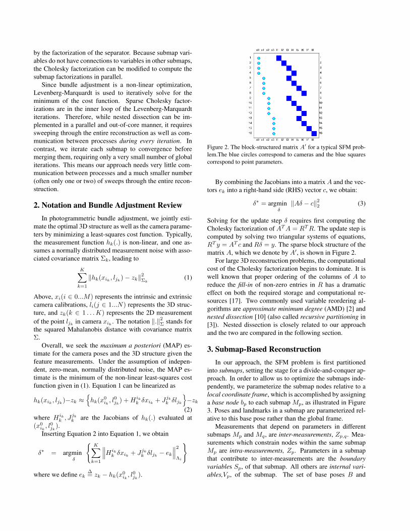
Figure 2. The block-structured matrix A′ for a typical SFM prob-lem.The blue circles correspond to cameras and the blue squarescorrespond to point parameters.

By combining the Jacobians into a matrixA and the vec-tors ek into a right-hand side (RHS) vector c, we obtain:

δ∗ = argminδ‖Aδ − c‖22 (3)

Solving for the update step δ requires first computing theCholesky factorization of ATA = RTR. The update step iscomputed by solving two triangular systems of equations,RT y = AT c and Rδ = y. The sparse block structure of thematrix A, which we denote by A′, is shown in Figure 2.

For large 3D reconstruction problems, the computationalcost of the Cholesky factorization begins to dominate. It iswell known that proper ordering of the columns of A toreduce the fill-in of non-zero entries in R has a dramaticeffect on both the required storage and computational re-sources [17]. Two commonly used variable reordering al-gorithms are approximate minimum degree (AMD) [2] andnested dissection [10] (also called recursive partitioning in[3]). Nested dissection is closely related to our approachand the two are compared in the following section.

3. Submap-Based ReconstructionIn our approach, the SFM problem is first partitioned

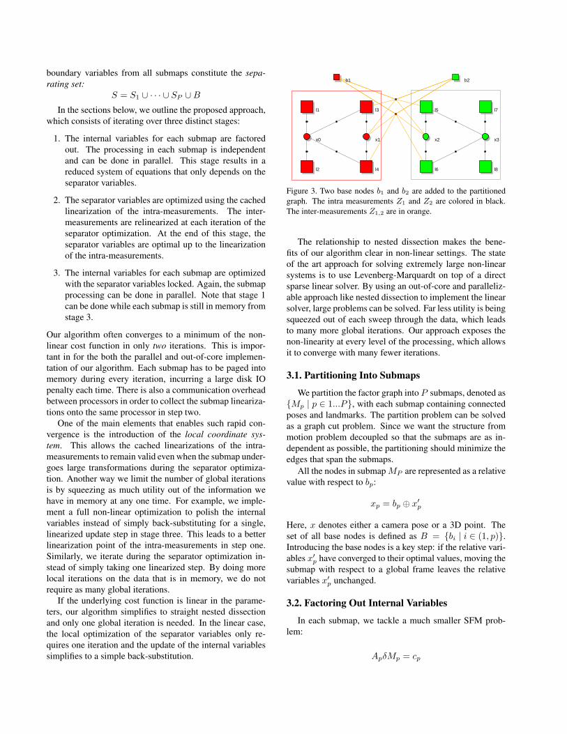
into submaps, setting the stage for a divide-and-conquer ap-proach. In order to allow us to optimize the submaps inde-pendently, we parameterize the submap nodes relative to alocal coordinate frame, which is accomplished by assigninga base node bp to each submap Mp, as illustrated in Figure3. Poses and landmarks in a submap are parameterized rel-ative to this base pose rather than the global frame.

Measurements that depend on parameters in differentsubmaps Mp and Mq , are inter-measurements, Zp,q . Mea-surements which constrain nodes within the same submapMp are intra-measurements, Zp. Parameters in a submapthat contribute to inter-measurements are the boundaryvariables Sp, of that submap. All others are internal vari-ables,Vp, of the submap. The set of base poses B and

boundary variables from all submaps constitute the sepa-rating set:

S = S1 ∪ · · · ∪ SP ∪BIn the sections below, we outline the proposed approach,

which consists of iterating over three distinct stages:

1. The internal variables for each submap are factoredout. The processing in each submap is independentand can be done in parallel. This stage results in areduced system of equations that only depends on theseparator variables.

2. The separator variables are optimized using the cachedlinearization of the intra-measurements. The inter-measurements are relinearized at each iteration of theseparator optimization. At the end of this stage, theseparator variables are optimal up to the linearizationof the intra-measurements.

3. The internal variables for each submap are optimizedwith the separator variables locked. Again, the submapprocessing can be done in parallel. Note that stage 1can be done while each submap is still in memory fromstage 3.

Our algorithm often converges to a minimum of the non-linear cost function in only two iterations. This is impor-tant in for the both the parallel and out-of-core implemen-tation of our algorithm. Each submap has to be paged intomemory during every iteration, incurring a large disk IOpenalty each time. There is also a communication overheadbetween processors in order to collect the submap lineariza-tions onto the same processor in step two.

One of the main elements that enables such rapid con-vergence is the introduction of the local coordinate sys-tem. This allows the cached linearizations of the intra-measurements to remain valid even when the submap under-goes large transformations during the separator optimiza-tion. Another way we limit the number of global iterationsis by squeezing as much utility out of the information wehave in memory at any one time. For example, we imple-ment a full non-linear optimization to polish the internalvariables instead of simply back-substituting for a single,linearized update step in stage three. This leads to a betterlinearization point of the intra-measurements in step one.Similarly, we iterate during the separator optimization in-stead of simply taking one linearized step. By doing morelocal iterations on the data that is in memory, we do notrequire as many global iterations.

If the underlying cost function is linear in the parame-ters, our algorithm simplifies to straight nested dissectionand only one global iteration is needed. In the linear case,the local optimization of the separator variables only re-quires one iteration and the update of the internal variablessimplifies to a simple back-substitution.

b1 b2

l1

l2

l3

l4

l5

l6

l7

l8

x0 x1 x2 x3

Figure 3. Two base nodes b1 and b2 are added to the partitionedgraph. The intra measurements Z1 and Z2 are colored in black.The inter-measurements Z1,2 are in orange.

The relationship to nested dissection makes the bene-fits of our algorithm clear in non-linear settings. The stateof the art approach for solving extremely large non-linearsystems is to use Levenberg-Marquardt on top of a directsparse linear solver. By using an out-of-core and paralleliz-able approach like nested dissection to implement the linearsolver, large problems can be solved. Far less utility is beingsqueezed out of each sweep through the data, which leadsto many more global iterations. Our approach exposes thenon-linearity at every level of the processing, which allowsit to converge with many fewer iterations.

3.1. Partitioning Into Submaps

We partition the factor graph into P submaps, denoted as{Mp | p ∈ 1...P}, with each submap containing connectedposes and landmarks. The partition problem can be solvedas a graph cut problem. Since we want the structure frommotion problem decoupled so that the submaps are as in-dependent as possible, the partitioning should minimize theedges that span the submaps.

All the nodes in submapMP are represented as a relativevalue with respect to bp:

xp = bp ⊕ x′p

Here, x denotes either a camera pose or a 3D point. Theset of all base nodes is defined as B = {bi | i ∈ (1, p)}.Introducing the base nodes is a key step: if the relative vari-ables x′p have converged to their optimal values, moving thesubmap with respect to a global frame leaves the relativevariables x′p unchanged.

3.2. Factoring Out Internal Variables

In each submap, we tackle a much smaller SFM prob-lem:

ApδMp = cp

where Ap and cp are the parts of A and c in Equation 3corresponding to submap p and contain only the columnscorresponding to Zp.

In order to re-use the linearization point of the intra-measurements, the columns ofAp corresponding to the sep-arator variables are put last, as follows:

[AVp

ASp

] [ δVpδSp

]= cp (4)

We then compute the Cholesky factor of the Hessian ma-trix

H =[AVp ASp

]T [AVp ASp

]=

[Rp Tp0 Up

]T [Rp Tp0 Up

]and reformat the system equations to[

Rp Tp0 Up

]T [βpβUp

]=[AVp

ASp

]Tcp

[Rp Tp0 Up

] [δVpδSp

]=[

βpβUp

]Since the separator variables correspond to the lower

right block of the Cholesky factor, the system of equationsinvolving only variables in the separating set can be ex-tracted trivially for later use in the separator optimization:

UpδSp = βUp

We could also have used the Schur complement to factorout the block of internal variables. Instead of ending up withan upper triangular system of equations, this would have re-sulted in a square symmetric system of equations. Whilethis might have saved some computation in the submap, itwould double the storage requirements for the cached lin-earizations and increase the computational cost of optimiz-ing the separator, so we opt to use the Cholesky factoriza-tion approach.

3.3. Globally Aligning the Submaps

Once all the submaps are aligned internally, they are as-sembled and optimized:

ASδS = cS

where S = S1∪· · ·∪SP ∪B. This procedure is no longer asimple bundle adjustment because of the following reasons:

Caching

Their linearizations of the intra measurements are not up-dated. Instead, we use the linearizations cached from the

previous step UpδSp = βUp(p = 1, . . . , P ) and stack them

into the full separator system:U1

...UPAS

δS =

βU1

...βUP

cS

Note that the inter-measurements are still linearized duringeach local iteration in response to the changing values forthe base nodes. Given a good graph cut, we find that thestacked part is usually much larger than the local part, whichmeans most of the computation time is saved by caching thelinearization.

Note that we can save time when computing the Hessianmatrix in each iteration by precomputing the inner productof the cached linearization terms:

H =[UAS

]T [UAS

]= ATSAS + UT U

where UT U is only calculated once. The gradients can alsobe partially precomputed in a similar manner.

Restriction to Separator

We modify only the values of the base nodes during eachlocal iteration. Once the base node optimization has con-verged, we do a final back-substitution to update the bound-ary variables. This allows us to avoid having to keeptrack of both the original linearization point of the bound-ary variables used to cache the linearization of the intra-measurements, and the changing linearization point of theinter-measurements.

In practice, we have found that the boundary variables donot change nearly as much as the base nodes, so this simpli-fication to the implementation is reasonable. For data setswhere the boundary variables are poorly conditioned, theupdate of the full separator should be performed iteratively.

3.4. Updating the Internal Variables

The final step is to update the internal variables in eachsubmap. This is done by non-linearly optimizing the in-ternal variables while locking the separator. In this op-timization, we do not need to consider any of the inter-measurements or of the intra-measurements that connectonly boundary variables. Just as they can be initially op-timized independently, the final update of each submap canbe done independently.

4. ImplementationWe want to choose partitions so that the number of inter-

measurements and therefore the number of separator vari-ables are small. We use the Metis graph partitioner from [9]

Failures of BA Failures with 10 partitions Total runs14 8 100

Table 1. The failure rate of bundle adjustment (BA) and our algo-rithm after 100 runs.

to find a k-way graph cut that minimizes the number of mea-surements that span the submaps. Note that the algorithmhas no special restriction on the graph cut itself, except thateach submap should remain full-rank.

For clarity in the paper, we describe the local optimiza-tions using a simple Gaussian-Newton solver. In our im-plementation, we use Levenberg-Marquardt for all the localoptimizations and add the damping factor λI to the Hessianmatrix.

Our system is implemented out-of-core. After thesubmap partitioning, the boundary variables {Vp}, separa-tor variables {Sp}, and the measurements are saved in sep-arate files. We only need to load Vp and Sp and their corre-sponding measurements when we optimize submap Mp.

We assume the nodes inside the local submaps are wellconstrained. While it is typically the case that 3D featuresare observed enough times inside a local map, a few nodesin the local submaps are sometimes rank-deficient. Hence,before each submap is optimized, filtering out these rankdeficient nodes and moving their intra-measurements to theseparator is necessary. Afterwards, the nodes are optimizedwith the base nodes together in the separator, using the inter-measurements and newly added intra-measurements.

5. Experimental ResultsAfter the implementation of the algorithm, we assess its

performance on both synthetic and real data. All the resultswere computed on a 1.83GHz CPU, 1GB memory laptop.

5.1. Synthetic Data: Downtown Area

We use the synthetic data of downtown area to demon-strate some important aspects of our algorithm. As shownin Figure 4, the 11, 965 synthetic 3D points are distributedalong roads obtained from real city street data. As the 3Dfeatures of a certain street are mainly observed in the im-ages taken from the same street, except at the intersections,the Metis partitioner automatically splits the map into tensubmaps consisting of different streets (Figure 4a). Al-though the internal structures are recovered well, as shownin Figure 4b, the streets are still offset with respect to oneanother because the submap positions have not been opti-mized. The optimization of the separator successfully re-covers the relationship between these submaps. Note thatnearly all previously offset boundaries are now well alignedin Figure 4c.

To evaluate the accuracy of the algorithm, we compareour algorithm to traditional bundle adjustment using the

1 1.5 2 2.5 3 3.5 4 4.5 50.4

0.402

0.404

0.406

0.408

0.41

0.412

0.414

0.416

0.418

Iterations

Res

idua

ls

BA1% above BA2 partitions4 partitions6 partitions8 partitions10 partitions12 partitions

Figure 5. The comparison of the residuals left by different numbersof partitions using our approach and bundle adjustment optimiza-tion. The green solid line indicates the minimum computed by thetraditional bundle adjustment (BA) that was run with a very tightstopping criteria to simulate the true minimum cost. The greendashed line indicates 1% above the true minima. The other sixlines shows the residual after 1− 5 global iterations using 2 to 12partitions. The plot data is based on the average of 100 runs.

residuals of the converged system. Our approach simpli-fies to traditional bundle adjustment if all the parametersare put in one submap. All the variables then become in-ternal variables, and the first two steps are not required anymore. The non-linear optimization of the internal variablesin step three converges to the minimum in the first iteration.We therefore show the results for bundle adjustment at thedata point corresponding to one partition in the figures.

We tested how many global iterations were needed forour algorithm to converge using the downtown data per-turbed by Gaussian noise. The average of 100 runs isshown in Figure 5. The residual of bundle adjustment actsas the base line under the true converge state. After thefirst iteration, the residual is about 2.12% − 3.69% abovethe minimum. After two iterations, the residuals drop to0.25%−1.87% above the minimum. A typical stopping cri-teria for bundle adjustment is when the rms error decreasesby less than 1%. For this data set, one to eight partitionscan be regarded as converged after only two global itera-tions and the rest after three. In practice, we found that therecovered geometry after one iteration was quite good.

Another important evaluation of the algorithm is the ro-bustness. We measured how many times the algorithm con-verged to a local minimum. As noted in [7], partitioned-based approaches are generally more robust than global op-timizations. We measured how many times traditional bun-dle adjustment failed to converge versus our partitioned al-gorithm with ten partitions (8 times). As shown in Table 1,the partitioned approach failed to converge 8 compared to14 times for traditional bundle adjustment.

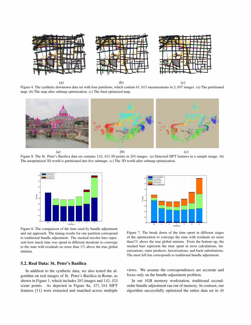
(a) (b) (c)Figure 4. The synthetic downtown data set with four partitions, which contain 81, 015 measurements in 2, 897 images. (a) The partitionedmap. (b) The map after submap optimization. (c) The final optimized map.

(a) (b) (c)Figure 8. The St. Peter’s Basilica data set contains 142, 453 3D points in 285 images. (a) Detected SIFT features in a sample image. (b)The unoptimized 3D world is partitioned into five submaps. (c) The 3D world after submap optimization.

BA 2 4 6 8 10 120

0.2

0.4

0.6

0.8

1

1.2

1.4

1.6

Partitions

Tim

ing

1st iteration2nd iteration3rd iteration

Figure 6. The comparison of the time used by bundle adjustmentand our approach. The timing results for one partition correspondto traditional bundle adjustment. The stacked tricolor bars repre-sent how much time was spend in different iterations to convergeto the state with residuals no more than 1% above the true globalminima.

5.2. Real Data: St. Peter’s Basilica

In addition to the synthetic data, we also tested the al-gorithm on real images of St. Peter’s Basilica in Rome, asshown in Figure 1, which includes 285 images and 142, 453scene points. As depicted in Figure 8a, 471, 584 SIFTfeatures [11] were extracted and matched across multiple

BA 2 4 6 8 10 120

0.2

0.4

0.6

0.8

1

1.2

1.4

1.6

Partitions

Tim

ing

Error calculationLinearizationOuter productFactorizationBack−substitution

Figure 7. The break down of the time spent in different stagesof the optimization to converge the state with residuals no morethan1% above the true global minima. From the bottom up, thestacked bars represent the time spent in error calculations, lin-earizations, outer products, factorizations, and back-substitutions.The most left bar corresponds to traditional bundle adjustment.

views. We assume the correspondences are accurate andfocus only on the bundle adjustment problem.

In our 1GB memory workstation, traditional second-order bundle adjustment ran out of memory. In contrast, ouralgorithm successfully optimized the entire data set in 48

minutes. First, we applied the Metis partitioner to split theproblem into five partitions, as shown in Figure 8b. Then weoptimized each submap, as described in Section 3.4 (Figure8c). Note that the building roofs in two submaps slightlyshift with respect to each other. After the separator is opti-mized, we have a well-constructed 3D world in Figures 1.One obvious change is that the roof is correctly aligned.

6. Conclusions and Future Work

Our contributions can be summarized as follows:

• We take a divide-and-conquer approach to the fullSFM problem. As a result, we may cache the deriva-tives of the locally optimized measurements and usethem in the separator optimization. By doing so, notonly do we save CPU cycles by not recomputing thelinearization, but we also save time when computingthe Hessian matrix.

• Our algorithm can run out-of-core and is straightfor-ward to parallelize. With this approach, reconstruc-tions that do not fit into physical memory can still bereconstructed efficiently.

• By exposing the non-linearity of the cost function tothe algorithm, our implementation requires far fewersweeps through the entire reconstruction. This resultsmuch less paging to disk for out-of-core implemen-tations and inter-processor communication in parallelimplementations.

Although our algorithm allows us to reconstruct a verylarge-scale system in a computationally efficient manner,we have not directly addressed the initialization problem.Generating a good initialization is an independent, butequally important problem. For future work, we plan toinvestigate both incremental and hierarchical initializationapproaches for the submaps.

References[1] A. Akbarzadeh, J. M. Frahm, P. Mordohai, B. Clipp, C. En-

gels, D. Gallup, P. Merrell, M. Phelps, S. Sinha, B. Tal-ton, L. Wang, Q. Yang, H. Stewenius, R. Yang, G. Welch,H. Towles, D. Nister, and M. Pollefeys. Towards urban 3dreconstruction from video. In Proc. of the International Sym-posium on 3D Data Processing, Visualization and Transmis-sion, 2006.

[2] P.R. Amestoy, T. Davis, and I.S. Duff. An approximate min-imum degree ordering algorithm. SIAM Journal on MatrixAnalysis and Applications, 17(4):886–905, 1996.

[3] Duane C. Brown. The bundle adjustment - progress andprospects. Int. Archives Photogrammetry, 21(3), 1976.

[4] M. Brown and D. G. Lowe. Unsupervised 3d object recogni-tion and reconstruction in unordered datasets. In Intl. Conf.on 3D Digital Imaging and Modeling, pages 56–63, 2005.

[5] G. Tao-Shun Chou. Large-Scale 3D Reconstruction: ATriangulation-Based Approach. PhD thesis, EECS, Mas-sachusetts Institute of Technology, 2000.

[6] C. Engels, H. Stewénius, and D. Nistér. Bundle adjustmentrules. In Symposium on Photogrammetric Computer Vision,Sep 2006.

[7] A. W. Fitzgibbon and A. Zisserman. Automatic camera re-covery for closed or open image sequences. In Eur. Conf. onComputer Vision (ECCV), pages 311–326, 1998.

[8] M. Fradkin, M. Roux, H. Maitre, and U. M. Leloglu. Sur-face reconstruction from multiple aerial images in dense ur-ban areas. In IEEE Conf. on Computer Vision and PatternRecognition (CVPR), 1999.

[9] G. Karypis and V. Kumar. Multilevel algorithms for multi-constraint graph partitioning. In Supercomputing ’98: Pro-ceedings of the 1998 ACM/IEEE conference on Supercom-puting (CDROM), pages 1–13, Washington, DC, USA, 1998.IEEE Computer Society.

[10] R.J. Lipton and R.E. Tarjan. Generalized nested dissec-tion. SIAM Journal on Applied Mathematics, 16(2):346–358,1979.

[11] D.G. Lowe. Distinctive image features from scale-invariantkeypoints. Intl. J. of Computer Vision, 60(2):91–110, 2004.

[12] D. Nistér. Reconstruction from uncalibrated sequences witha hierarchy of trifocal tensors. In ECCV, 2000.

[13] D. Nistér. An efficient solution to the five-point relative poseproblem. In CVPR, 2003.

[14] M. Pollefeys, L. V. Gool, M. Vergauwen, F. Verbiest, K. Cor-nelis, and J. Tops. Visual modeling with a hand-held camera.Intl. J. of Computer Vision, 59(3):207–232, 2004.

[15] N. Snavely, S.M. Seitz, and R. Szeliski. Photo tourism: Ex-ploring photo collections in 3D. In SIGGRAPH, pages 835–846, 2006.

[16] S. Teller, M. Antone, Z. Bodnar, M. Bosse, S. Coorg,M. Jethwa, and N. Master. Calibrated, registered imagesof an extended urban area. Intl. J. of Computer Vision,53(1):93–107, 2003.

[17] B. Triggs. Factorization methods for projective structure andmotion. In IEEE Conf. on Computer Vision and PatternRecognition (CVPR), pages 845–851, 1996.

[18] B. Triggs, P. McLauchlan, R. Hartley, and A. Fitzgibbon.Bundle adjustment – a modern synthesis. In W. Triggs,A. Zisserman, and R. Szeliski, editors, Vision Algorithms:Theory and Practice, LNCS, pages 298–375. Springer Ver-lag, 2000.