Embed Size (px)
Citation preview

Relative Bundle Adjustment
Gabe Sibley{[email protected]}
Technical Report No. 2307/09
Computing Laboratory
GAME-BASED PROBABILISTIC PREDICATE ABSTRACTIONIN PRISM
M. Kattenbelt M. Kwiatkowska G. Norman D. Parker
CL-RR-08-01
Oxford University Computing Laboratory
Wolfson Building, Parks Road, Oxford OX1 3QD
January 27, 2009
Robotics Research GroupDepartment of Engineering
University of OxfordParks Road, OX13PJ
Abstract
This report derives a relative objective function for bundleadjustment – driven by the desire for a truly large scale si-multaneous localization and mapping algorithm that can oper-ate incrementally in constant time. It is precisely the choiceof a single privileged coordinate frame that makes bundle ad-justment expensive to solve. This is especially true during loopclosures, when the single frame approach necessitates adjustingall parameters in the loop. We give a relative formulation that isdesigned specifically to avoid the cost of optimizing all parame-ters at loop closure. Instead of optimizing in a single Euclideanspace, relative bundle adjustment works in a metric-space de-fined by a connected Riemannian manifold. We find evidencethat in this space, the global maximum likelihood solution can befound incrementally in constant time – even at loop closure.
1 Introduction
Bundle adjustment is the optimal solution to the so-called “full” simultaneouslocalization and mapping problem, in that it solves for the maximum likelihoodsolution given all measurements over all time. The goal in bundle adjustment isto minimize error between observed and predicted image-measurements of n 3Dlandmarks sensed from m 6D sensor poses (or frames) [31]. Measurements andparameter estimates are usually considered to be normally distributed, and theproblem is typically tackled with non-linear least-squares optimization routineslike Levenberg–Marquardt or the Gauss-Newton method. The linearized systemmatrix that appears in this process matches the form of the Fisher Informationmatrix, which in turn defines the Cramer Rao Lower Bound that is used to assessestimator consistency and optimality. It is not surprising therefore that bundleadjustment is the optimal non-linear least-squares simultaneous localization andmapping algorithm.
The cost of optimizing the bundle adjustment objective-function is cubicin complexity (in either m or n). For large and growing problems, this canquickly become prohibitive. This is especially true during loop-closure, whenoften all parameters in the loop must be adjusted. In a single coordinate frame,the farther the robot travels from the origin, the larger position uncertaintybecomes. Errors at loop closure can therefore become arbitrarily large, whichin turn makes it impossible to compute the full maximum likelihood solution inconstant time (here the “full” solution is the one that finds the optimal estimatesfor all parameters).
It is not clear that it is necessary to estimate everything in a single coordinateframe – for instance most problems of autonomous navigation, such as pathplanning, obstacle avoidance or object manipulation, can be addressed withinthe confines of a metric manifold. Taking this route, we structure the problemas a graph of relative poses with landmarks specified in relation to these poses.In 3D this graph defines a connected Riemannian manifold of dimension six
2
with a distance metric based on shortest paths. Note that this is not a sub-mapping approach – there are no distinct overlapping estimates, and there isonly one objective function with a minimal parameter vector; similarly, this isnot a pose-graph relaxation approach.
Together with an adaptive optimization scheme that only ever solves for asmall sub-portion of the state vector, we find evidence that the full maximumlikelihood solution in the manifold can be found using an incrementally constanttime algorithm. Crucially, this appears true even at loop closure.
We stress at the outset that the relative solution is not equivalent to thenormal Euclidean-space solution and it does not produce an estimate that canbe easily embedded in a single Euclidean frame. Projecting from the relativemanifold into a single Euclidean space is a difficult problem that we argue is besthandled by external resources that do not have constant run-time requirements- e.g. by operator computers, not on the robot.
2 Related Work
There has been much interest in Gaussian non-linear least-squares solutions toSLAM based on “full-SLAM” or bundle adjustment [29][31][8][12][19], though theproblem is an old one [3][22]. The full SLAM problem tries to optimize the jointvehicle trajectory and map structure simultaneously given all measurementsever made. There are approximate incremental solutions that only optimize asmall local subset of the map [7], and there are methods that approximate thefull solution with various forms of marginalization [19][27], or by ignoring smalldependency information [30][21]. Recently some have successfully employedtechniques from the linear algebra and numerical optimization communities togreatly reduce the cost of finding the full solution [17]. Many use key-framesto reduce complexity, though at the expense of accuracy [10][23][18]. All thesetechniques suffer from computational complexity issues during loop closures.
In the context of long term autonomy, roboticists recognize the need foronline, real-time, navigation and mapping algorithms. This means that local-ization and mapping algorithms must operate incrementally within a constant-time budget. Driven by this need, many authors have recognized the benefitof relative representations [2][9][19][1][15][4][13][20]. The most common solutionis probably sub-mapping [2][25][6][9], which breaks the estimation into manysmaller mapping regions, computes individual solutions for each region, andthen estimates the relationships between these sub-maps. Many difficult issuesarise in sub-mapping, including map overlap, data duplication, map fusion andbreaking, map alignment, optimal sub-map size, and consistent global estima-tion in a single Euclidean frame. The relative bundle adjustment we propose canbe seen as a continuous sub-mapping approach that avoids these complications.
To solve large SLAM problems with many loops, the most successful meth-ods currently are the pose-graph optimization algorithms. Instead of solving thefull SLAM problem, these methods optimize a set of relative pose constraints[24][14]. This is attractive because using forward substitution it is possible to
3
transform full SLAM into a generally sparse set of pose constraints [11][29],and even to make the resulting system of equations relative [19]. Note that,given the assumed Gaussian problem structure, this kind of forward substitu-tion to a pose-graph is algebraically equivalent to marginalization; methods thatmarginalize landmark parameters onto pose parameters so as to define a pose-graph are executing the forward substitution phase of sparse bundle adjustment.In this light, pose-graph relaxation, which solves for the optimal path estimate,can be seen as one-half of one iteration of full SLAM, because full SLAM alsoback-substitutes for the map parameters, and iterates the procedure to conver-gence. Like other methods, pose-graph solvers have worst-case complexity atloop closure that scales with the length of the loop.
The work most similar to relative bundle adjustment is the relative formu-lations given by Eade [9] and Konolige [19]. The former is akin to sub-mappingmethods with constraints to enforce global Euclidean consistency at loop closure;the latter formulates the cost function relative to a single Euclidean frame andthen makes a series of approximations to produce a sparse relative pose-graph.Neither method derives the purely relative objective function (incrementally,both rely on some form of single-reference frame), neither formulates the objec-tive function completely without privileged frames, and both methods carry theburden of finding a globally consistent estimate in a single Euclidean frame. Ourapproach is substantially different because of the completely relative underlyingobjective function that we derive.
Finally, a number of adaptive region approaches have been explored usingglobal methods [28][26]. These techniques, together with all of the methodspresented in this section, are at least linear in complexity in the length of theirlargest loop – none is constant time at loop closure, and all but one [2] solve fora solution in a single Euclidean space.
3 Problem Formulation
The goal in bundle adjustment is to minimize error between the observed andpredicted image-measurements of n 3D landmarks sensed from m 6D sensorposes. Likewise, the method presented here will minimize the difference betweenpredicted and measured values.
• Let p={pj , j=0, ....,m-1} be a set of m 6D relative vehicle poses. Each pj
∈ SE3 is a 6× 1 vector that defines a 4× 4 homogeneous transformationmatrix, Tαj — this is “pose j in frame α”.
• Let l={l̄jk, k=1, ..., n, j∈ [0, ...,m-1]} be a set of n 3D landmarks each
parameterized relative to some base-frame j. Each ljk =�
l̄jk
1
�is a 4×1
homogeneous point; the bar notation selects the 3D component.
• Let t={tj , j=1, ....,M} be a set of M 6D transform estimates. Eachtj ∈ SE3 is a 6 × 1 error-state parameter. The set contains m-1 edge
4
l1,2 l3,3
l1,1
. . .
T12
T98,99T97,98
T1,97
T01
T96,97
p0
p1
p94
p95
p96
p97
p98p99
p3
z99,3,3z97,1,2
z1,1,2
z96,1,1
z1,1,1
z99,1,2
T23
z94,1,1z3,3,3
p2
T94,95
T95,96
Current frame
First frame
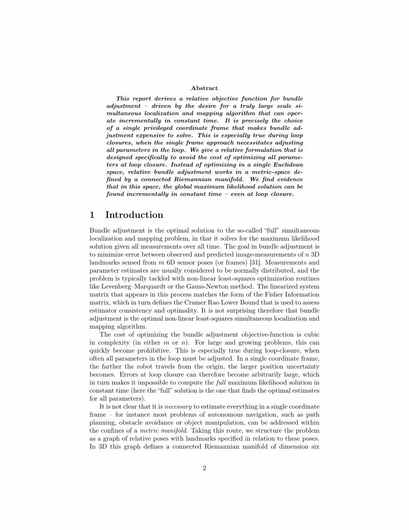
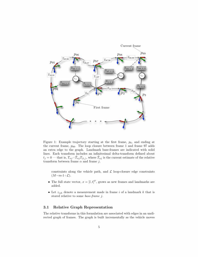
Figure 1: Example trajectory starting at the first frame, p0, and ending atthe current frame, p99. The loop closure between frame 1 and frame 97 addsan extra edge to the graph. Landmark base-frames are indicated with solidlines. Each transform includes an infinitesimal delta-transform defined abouttj = 0 — that is, Tαj=T̂αjT(tj), where T̂αj is the current estimate of the relativetransform between frame α and frame j.
constraints along the vehicle path, and L loop-closure edge constraints(M=m-1+L).
• The full state vector, x = [l, t]T , grows as new frames and landmarks areadded.
• Let zijk denote a measurement made in frame i of a landmark k that isstored relative to some base-frame j.
3.1 Relative Graph RepresentationThe relative transforms in this formulation are associated with edges in an undi-rected graph of frames. The graph is built incrementally as the vehicle moves
5
through the environment, and extra edges are added during loop closure. Thegraph defines a connected Riemannian manifold that is by definition everywherelocally Euclidean, though globally it is not embedded in a single Euclidean space.The relationship between parent-frame α and child-frame j is defined by a 4×4homogeneous transform matrix, Tαj=T̂αjT(tj), where T̂αj is the current esti-mate. An example trajectory and graph with this notation is shown in Figure1.
In order to predict a measurement of landmark ljk in frame i, the landmarkestimate must be transformed along the kinematic chain from j to i. This isdefined by a composition of 4× 4 homogeneous transforms
Tji = T̂j,j+1T(tj+1)T̂j+1,j+2T(tj+2), ..., T̂i−1,iT(ti).
Traversal of kinematic chains like this is what distinguishes relative bundleadjustment from the traditional approach.
3.2 Sensor ModelThe sensor model for a single measurement that describes how landmark k,stored relative to base-frame j, is transformed into frame i and projected intothe sensor, is
hijk(x) = Proj�T−1
ji ljk
�
= Proj (gijk(x))= K (M(gijk(x)) .
The projection function Proj is expanded in terms of the functions K andM to facilitate multi-camera rigs where the cameras are not coincident withthe body of interest (but are instead related to it by a known vehicle-to-sensortransform, Tis). Further,
• gijk : Rdim(x) → R4, x �→ T−1ji ljk transforms ljk from base-frame j to the
observation frame i.
• M : R4 → R3, p �→ [M, 0]T−1is p transforms a point p from vehicle frame i
to sensor frame s (useful for modeling multiple cameras and cameras notcoincident with the vehicle frame, such as stereo systems). Tis is the sensorin the vehicle frame. The 3×3 matrix M is just a signed-permutation ma-trix that converts from the problem specific coordinate-frame (fixed-frame
xyz-Euler angles in most robotics applications, which has +x forward, +yright and +z down) to the computer-vision coordinate-frame (which has+x right, +y down and +z forward). This function also projects fromhomogeneous to Euclidean coordinates.
• K : R3 → R2, is standard perspective projection via a 3 × 3 cameracalibration matrix, K.
6
Assuming measurements zijk are normally distributed, zijk ∼ N(hijk(x), Rijk),then the non-linear least-squares objective function for relative bundle adjust-ment is
J =n�
k=1
mk�
i∈1
(zijk − hijk(x))T R−1ijk (zijk − hijk(x)) (1)
= �z − h(x)�R−1 ,
which depends on the landmark estimate, ljk, and all the estimates tj+1, ..., tion the kinematic chain from the base-frame j to the measurement frame i. Thisproblem is solved using iterative non-linear least-squares Gauss-Newton mini-mization for the values of x that minimize re-projection error — this yields themaximum likelihood estimate (subject to local minima). Projecting via kine-matic chains like this is novel, but as we will see it changes the sparsity patternsin the system Jacobian. Compared to normal bundle adjustment, this new pat-tern increases the cost of solving the sparse normal equations for updates δxto the state vector x — though the ultimate computational complexity is thesame.
In general, there are multiple paths from frame j to frame i, which meansthat there might be multiple ways to project a landmark ljk into frame i, and wetherefore have to select which path to use. A simple solution is to always selectthe shortest path possible. If each edge has its weight set to the determinant ofthe edge transform uncertainty, then Dijkstra’s algorithm will define the shortestchains with minimal transformation uncertainty.
3.3 Sparse SolutionThe normal equations associated with the iterative non-linear least-squaresGauss-Newton solution to equation (1) are
HT R−1Hδx = HT R−1(z − h(x)). (2)
where H = ∂h∂x is the Jacobian of the sensor model, R is the block diagonal
covariance matrix describing the uncertainty of the collective observation z (thestacked vector of all measurements). Referring to the example problem in Figure3 we see that HT =
�HT
l HTt
�and δx = [δl, δt]T , which exposes the well known
2× 2 block structure of equation (2),�
V WWT U
� �δlδt
�=
�rl
rt
�.
Here δl and δt are state-updates for the map and edge-transforms, and
rl = HTl R−1(z − h(x)),
rt = HTt R−1(z − h(x)),
7
l0,1 l1,2 l1,3 l2,4 l1,5
p0 p1 p2 p3 p4
t1 t2 t3 t4
z1,5
z2,4z2,3
z2,2
z1,2
z0,2
z1,1
z0,1 z4,1z1,3
z4,5
z3,5
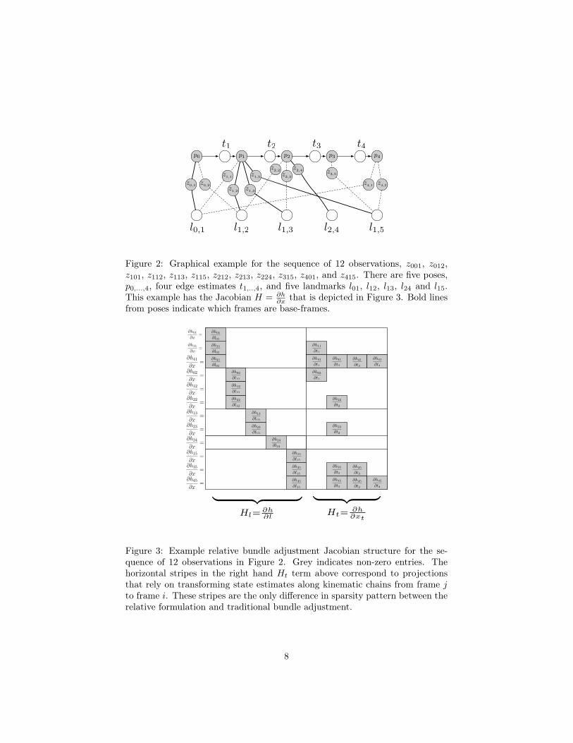
Figure 2: Graphical example for the sequence of 12 observations, z001, z012,z101, z112, z113, z115, z212, z213, z224, z315, z401, and z415. There are five poses,p0,...,4, four edge estimates t1,..,4, and five landmarks l01, l12, l13, l24 and l15.This example has the Jacobian H = ∂h
∂x that is depicted in Figure 3. Bold linesfrom poses indicate which frames are base-frames.
∂h01
∂x=
∂h11
∂x=
∂h41
∂x=
∂h02
∂x=
∂h12
∂x=
∂h22
∂x=
∂h13
∂x=
∂h23
∂x=
∂h24
∂x=
∂h15
∂x=
∂h35
∂x=
∂h45
∂x=
∂h11
∂l01
∂h02
∂l12
∂h41
∂l01
∂h22
∂l12
∂h12
∂l12
∂h23
∂l13
∂h13
∂l13
∂h24
∂l24
∂h15
∂l15
∂h35
∂l15
∂h11
∂t1
∂h01
∂l01
∂h45
∂l15
∂h41
∂t1
∂h41
∂t2
∂h41
∂t3
∂h41
∂t4
∂h02
∂t1
∂h22
∂t2
∂h23
∂t2
∂h35
∂t2
∂h45
∂t2
∂h35
∂t3
∂h45
∂t3
∂h45
∂t4
� �� �Hl=
∂h∂l
� �� �Ht= ∂h
∂xt
Figure 3: Example relative bundle adjustment Jacobian structure for the se-quence of 12 observations in Figure 2. Grey indicates non-zero entries. Thehorizontal stripes in the right hand Ht term above correspond to projectionsthat rely on transforming state estimates along kinematic chains from frame jto frame i. These stripes are the only difference in sparsity pattern between therelative formulation and traditional bundle adjustment.
8
V = HTl R−1Hl,
W = HTl R−1Ht,
and
U = HTt R−1Ht.
Building these linearized equations is the dominant cost in solving each Gauss-Newton iteration, which makes it important to compute the sparse Jacobian ofh efficiently.
3.4 Relative JacobiansThis section lists in detail how to compute the relative bundle adjustment Jaco-bians efficiently. Due to the functional dependence of the projection model onthe kinematic chain of relative poses, the Jacobian in the relative formulation isvery different from its Euclidean counterpart. With reference to Figure 4, focusfor a moment on a single infinitesimal transform T(tc) that is somewhere alongthe kinematic chain from frame i to j (note the direction). The individual termsshown in Figure 3 are
∂hijk
∂ l̄jk=
∂K∂M
∂M∂gijk
∂gijk
∂ l̄jk,
and
∂hijk
∂tc=
∂K∂M
∂M∂gijk
∂gijk
∂tc.
Computing these requires ∂K∂M , ∂M
∂gijk, ∂gijk
∂ l̄jk, and ∂gijk
∂tc, which we derive next.
3.4.1 Perspective Projection Jacobian
The perspective projection function using the camera calibration matrix, K, is
KM =
uvw
=
fx sx cx
0 fy cy
0 0 1
M1
M2
M3
,
which is scaled by w to get the final 2D pixel location
K(M) =�
uv
�/w = a(M)/b(M) =
�(fxM1 + sxM2 + cxM3)
(fyM2 + cyM3)
�/M3.
The Jacobian of K(M) is thus
∂K∂M =
b(M)a�(M)− a(M)b�(M)b(M)2
9
i
j
. ..
ljk
cTjc
Tci
. . . . . .
...
���
�
���
�
gik(x) = (TjcT(tc)Tci)−1ljk
T(tc)
ab
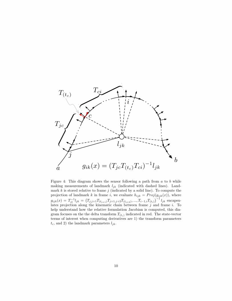
Figure 4: This diagram shows the sensor following a path from a to b whilemaking measurements of landmark ljk (indicated with dashed lines). Land-mark k is stored relative to frame j (indicated by a solid line). To compute theprojection of landmark k in frame i, we evaluate hijk = Proj(gijk(x)), wheregijk(x) = T−1
ji ljk =�Tj,j+1T(tj+1)Tj+1,j+2T(tj+2), ..., Ti−1,iT(ti)
�−1ljk encapsu-
lates projection along the kinematic chain between frame j and frame i. Tohelp understand how the relative formulation Jacobian is computed, this dia-gram focuses on the the delta transform T(tc) indicated in red. The state-vectorterms of interest when computing derivatives are 1) the transform parameterstc, and 2) the landmark parameters ljk.
10
where
a�(M) =∂a
∂M =�
fx sx cx
0 fy cy
�and b�(M) =
∂b
∂M =�
0 0 1�
leading to
∂K∂M =
�M3
�fx sx cx
0 fy cy
�−
�(fxM1 + sxM2 + cxM3)
(fyM2 + cyM3)
� �0 0 1
��/M2
3
=��
fx sx cx
0 fy cy
�−
�0 0 u0 0 v
��/M3
=�
fx sx cx − u0 fy cy − v
�/M3. (3)
3.4.2 Convention-Configuration Jacobian
The Jacobian of M is trivial; we list it for completeness:
∂M∂gijk
= [M, 0]T−1is . (4)
3.4.3 3D Point Jacobian
The 4× 3 Jacobian of gijk with respect to a 3D point l̄jk is
∂gijk
∂ l̄jk= T−1
ij [1, 1, 1, 0]T
=�
RTji
0
�. (5)
where Rij is the rotation matrix in Tij .
3.4.4 Transform Jacobian
The 4 × 6 Jacobian ∂gijk
∂tchas three cases that depend on the direction of the
transform T(tc) on the path from frame frame i to j (note the direction)
∂gijk
∂tc=
Tic∂T(tc)
∂tcTcj ljk if T(tc) points towards j
Tic∂T(−tc)
∂tcTcj ljk if T(tc) points towards i
0 if i = j
and ∂T(tc)∂tc
are the canonical generators of SE3 (a 4× 4× 6 tensor, see AppendixA). This expands to
11
∂gijk
∂tc=
Tic
�I
�l̄ck
�×
0 0
�if T(tc) points towards j
−Tic
�I
�l̄ck
�×
0 0
�if T(tc) points towards i
0 if i = j
(6)
Where l̄ck is just the point l̄jk transferred to frame c, and the operator [v]×maps a 3-vector v = [v1, v2, v3]T to a 3× 3 skew symmetric matrix,
[v] =
0 −v3 v2
v3 0 −v1
−v2 v1 0
.
3.4.5 Computing the Jacobians Efficiently
Putting equations (3), (4), (5) and (6) together,
∂hijk
∂tc=
∂K∂M
∂M∂gijk
∂gijk
∂tc
= ±�
fx sx cx − u0 fy cy − v
�/M3[M, 0]T−1
is Tic
�I
�l̄ck
�×
0 0
�
= ±�
fx sx cx − u0 fy cy − v
�/M3MRT
isRic
�I
�l̄ck
�×
�(7)
∂hijk
∂ l̄jk=
∂K∂M
∂K∂gijk
∂gijk
∂ l̄jk
=�
fx sx cx − u0 fy cy − v
�/M3[M, 0]T−1
is
�RT
ji
0
�
=�
fx sx cx − u0 fy cy − v
�/M3MRT
isRTji. (8)
This leads to the following efficient solution for both ∂hijk
∂ l̄jkand ∂hijk
∂tc
1. Compute the 2× 3 matrix A =�
fx sx cx − u0 fy cy − v
�/M3MRT
is
2. Compute the 2× 3 matrix ∂hijk
∂ l̄jk= ART
ji
3. Compute the 2× 6 matrix ∂hijk
∂tc= ±ARic
�I,
�l̄cj
�×
�
where the sign in step 3 depends on the direction of T(tc). As an aside, notethat this approach simplifies dealing with multi-camera systems, because theonly thing that changes is Tis, the vehicle-to-sensor transform.
12
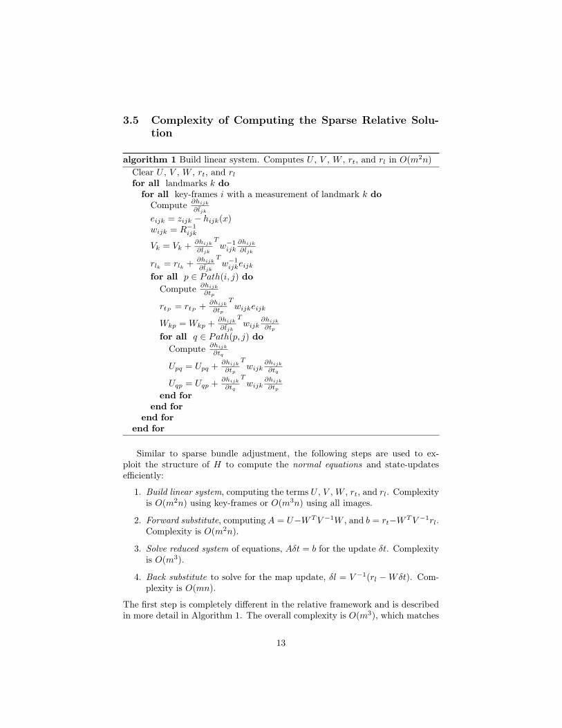
3.5 Complexity of Computing the Sparse Relative Solu-tion
algorithm 1 Build linear system. Computes U , V , W , rt, and rl in O(m2n)Clear U , V , W , rt, and rl
for all landmarks k dofor all key-frames i with a measurement of landmark k do
Compute ∂hijk
∂ l̄jk
eijk = zijk − hijk(x)wijk = R−1
ijk
Vk = Vk + ∂hijk
∂ l̄jk
Tw−1
ijk∂hijk
∂ l̄jk
rlk = rlk + ∂hijk
∂ l̄jk
Tw−1
ijkeijk
for all p ∈ Path(i, j) doCompute ∂hijk
∂tp
rtP = rtP + ∂hijk
∂tp
Twijkeijk
Wkp = Wkp + ∂hijk
∂ l̄jk
Twijk
∂hijk
∂tp
for all q ∈ Path(p, j) doCompute ∂hijk
∂tq
Upq = Upq + ∂hijk
∂tp
Twijk
∂hijk
∂tq
Uqp = Uqp + ∂hijk
∂tq
Twijk
∂hijk
∂tp
end forend for
end forend for
Similar to sparse bundle adjustment, the following steps are used to ex-ploit the structure of H to compute the normal equations and state-updatesefficiently:
1. Build linear system, computing the terms U , V , W , rt, and rl. Complexityis O(m2n) using key-frames or O(m3n) using all images.
2. Forward substitute, computing A = U−WT V −1W , and b = rt−WT V −1rl.Complexity is O(m2n).
3. Solve reduced system of equations, Aδt = b for the update δt. Complexityis O(m3).
4. Back substitute to solve for the map update, δl = V −1(rl −W δt). Com-plexity is O(mn).
The first step is completely different in the relative framework and is describedin more detail in Algorithm 1. The overall complexity is O(m3), which matches
13
traditional sparse bundle adjustment. Note that it is easy to convert Algorithm1 into a robust m-estimator by replacing the weights, wijk, with robust weightkernels, wijk = R−1
ijkW(eijk) — for example we use the Huber kernel [16].Focusing on a single transform c in the chain from j to i, note that equation
(7) can be split into a left part, Lc, and right part, Rc, as
∂hijk
∂tc= ±
�fx sx cx − u0 fy cy − v
�/m3MRT
isRic
�I [lck]×
�
= ±Lc∂T(tc)
∂tcRc.
This is useful because the terms Lc and Rc can be computed incrementally aswe traverse from node i to node j in Algorithm 1. Finally, notice that if featuretracks are contiguous over numerous frames (which they typically are), thenthe sparsity pattern in W will be the same in the relative-formulation as it isin traditional one – hence the relative-formulation cost of forward-substitution,solving the reduced system, and back-substitution (steps 2-4) should be approx-imately equivalent.
4 Adaptive Optimization
To reduce computation, it is important to optimize only those parameters thatmight change in light of new information [26][28]. Below we outline one approachto limit the parameters that are actively optimized.
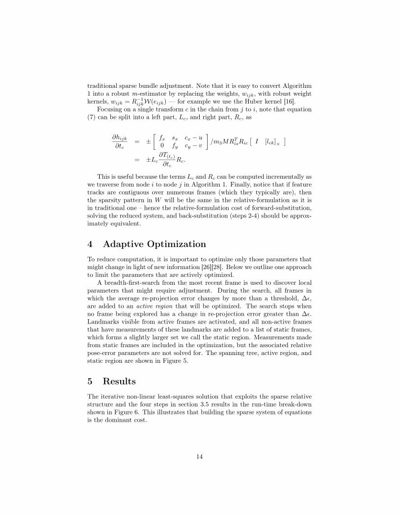
A breadth-first-search from the most recent frame is used to discover localparameters that might require adjustment. During the search, all frames inwhich the average re-projection error changes by more than a threshold, ∆�,are added to an active region that will be optimized. The search stops whenno frame being explored has a change in re-projection error greater than ∆�.Landmarks visible from active frames are activated, and all non-active framesthat have measurements of these landmarks are added to a list of static frames,which forms a slightly larger set we call the static region. Measurements madefrom static frames are included in the optimization, but the associated relativepose-error parameters are not solved for. The spanning tree, active region, andstatic region are shown in Figure 5.
5 Results
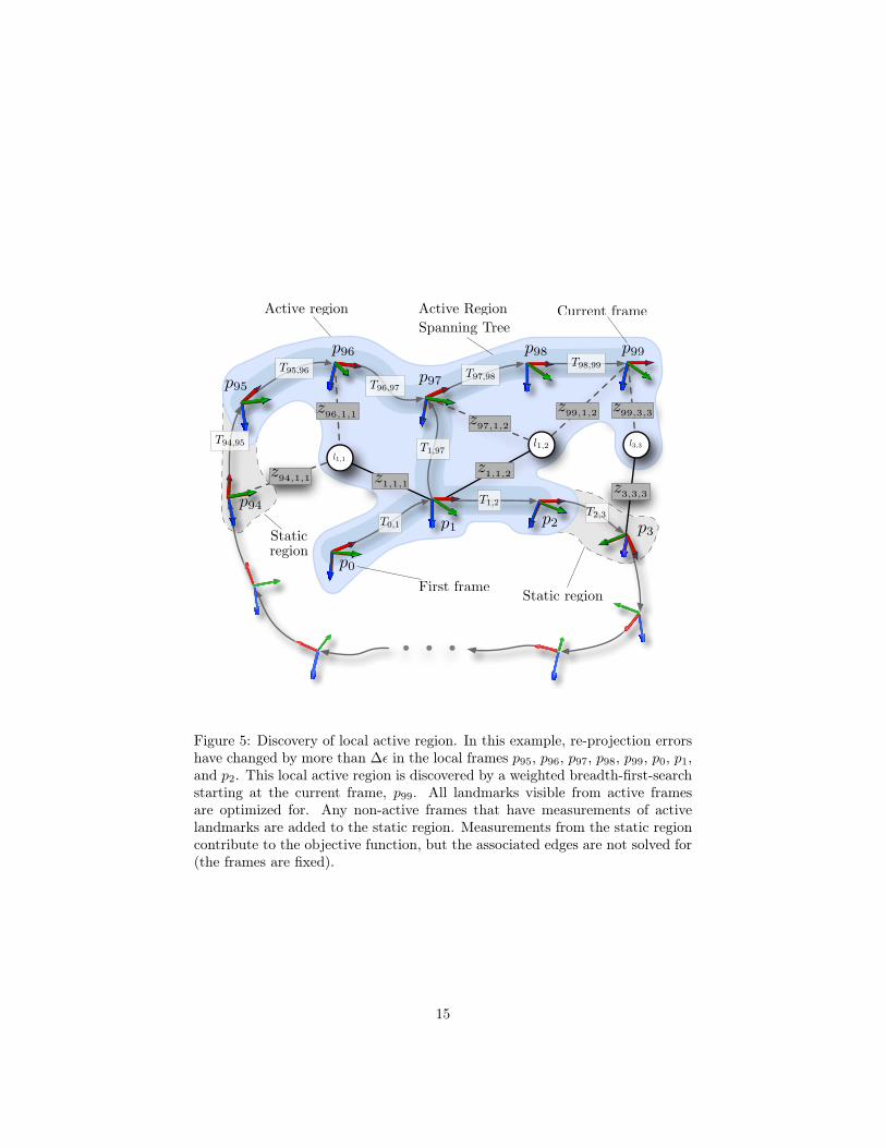
The iterative non-linear least-squares solution that exploits the sparse relativestructure and the four steps in section 3.5 results in the run-time break-downshown in Figure 6. This illustrates that building the sparse system of equationsis the dominant cost.
14
l1,2 l3,3
l1,1
. . .
T1,2
T98,99T97,98
T1,97
T0,1
T96,97
p0
p1
p94
p95
p96
p97
p98 p99
p3
z99,3,3z97,1,2
z1,1,2
z96,1,1
z1,1,1
z99,1,2
T2,3
z94,1,1z3,3,3
p2
T94,95
T95,96
Current frame
First frame
Active region
Static region
Staticregion
Active RegionSpanning Tree
Figure 5: Discovery of local active region. In this example, re-projection errorshave changed by more than ∆� in the local frames p95, p96, p97, p98, p99, p0, p1,and p2. This local active region is discovered by a weighted breadth-first-searchstarting at the current frame, p99. All landmarks visible from active framesare optimized for. Any non-active frames that have measurements of activelandmarks are added to the static region. Measurements from the static regioncontribute to the objective function, but the associated edges are not solved for(the frames are fixed).
15
Forward Substitute15%
2.75 ms
Solve Reduced System
3%0.56 ms
Back Substitute1%
0.27 ms
Build Ax=b80%
14.66 ms
Figure 6: Average run-times for the main steps of relative bundle adjustment.The average adaptive region from the Monte Carlo simulation was 4.6 frames.Note that it is the cost of building the linear system of equations that dominatesthe cubic complexity of solving for the adaptive region of poses.
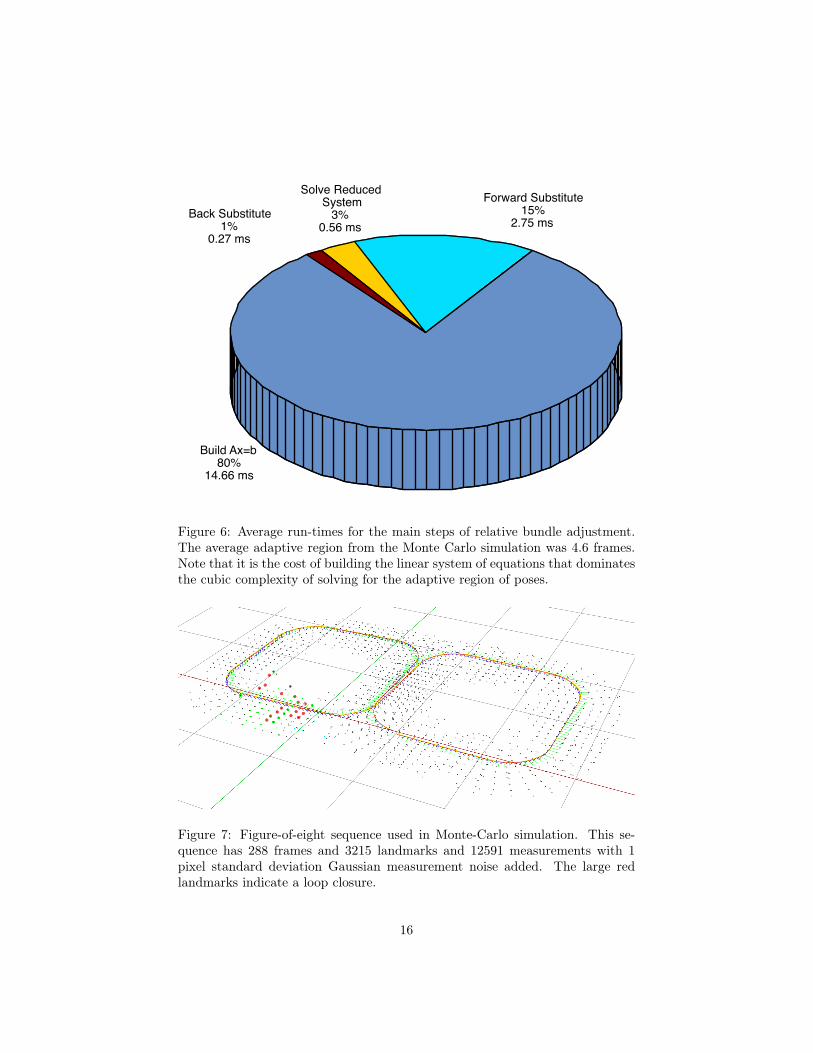
Figure 7: Figure-of-eight sequence used in Monte-Carlo simulation. This se-quence has 288 frames and 3215 landmarks and 12591 measurements with 1pixel standard deviation Gaussian measurement noise added. The large redlandmarks indicate a loop closure.
16
2 3 4 5 6 7 8 9 10
0.7
0.8
0.9
1
1.1
1.2
1.3
1.4
Number of Frames in Active Region
Aver
age
Reg
istra
ion
Erro
r (m
)
Average Registration Errorvs
Active Region Size
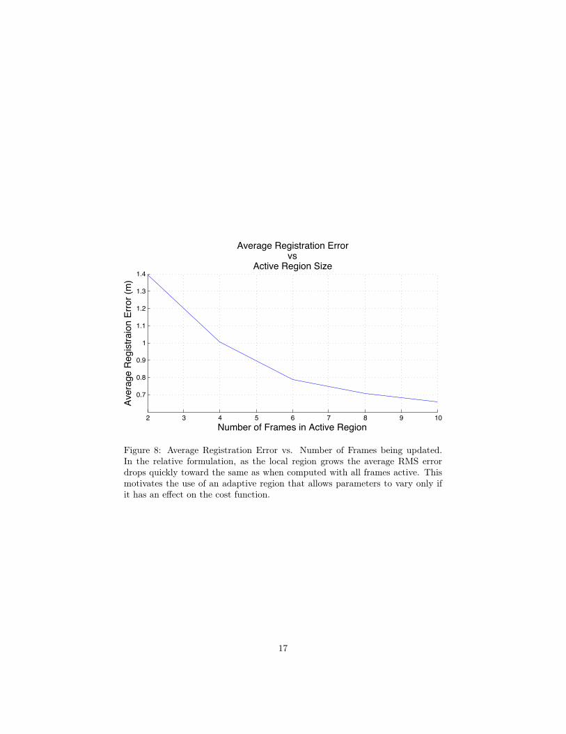
Figure 8: Average Registration Error vs. Number of Frames being updated.In the relative formulation, as the local region grows the average RMS errordrops quickly toward the same as when computed with all frames active. Thismotivates the use of an adaptive region that allows parameters to vary only ifit has an effect on the cost function.
17
0 50 100 150 200 250 300 3502
4
6
8
10
12
14
16
18
20
Frame Number
Adap
tive
Reg
ion
Size
(num
ber o
f fra
mes
) Adptive Region Size vs Frame Number
Loop Closure
(a) 50m loop with closure at frame 250.
0 50 100 150 200 250 300 350 400 450 500 5502
4
6
8
10
12
14
16
18
Frame Number
Adaptiv
e R
egio
n S
ize (
num
ber
for
fram
es)
Adaptive Region Size vs Frame Number
Loop Closure
(b) 100m loop with closure at frame 500.
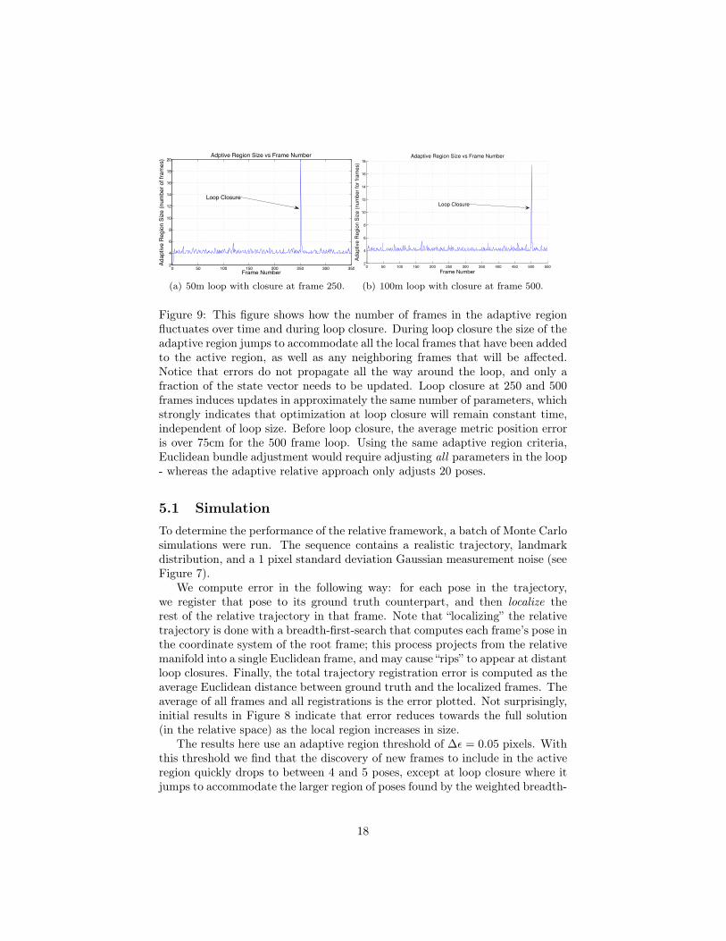
Figure 9: This figure shows how the number of frames in the adaptive regionfluctuates over time and during loop closure. During loop closure the size of theadaptive region jumps to accommodate all the local frames that have been addedto the active region, as well as any neighboring frames that will be affected.Notice that errors do not propagate all the way around the loop, and only afraction of the state vector needs to be updated. Loop closure at 250 and 500frames induces updates in approximately the same number of parameters, whichstrongly indicates that optimization at loop closure will remain constant time,independent of loop size. Before loop closure, the average metric position erroris over 75cm for the 500 frame loop. Using the same adaptive region criteria,Euclidean bundle adjustment would require adjusting all parameters in the loop- whereas the adaptive relative approach only adjusts 20 poses.
5.1 SimulationTo determine the performance of the relative framework, a batch of Monte Carlosimulations were run. The sequence contains a realistic trajectory, landmarkdistribution, and a 1 pixel standard deviation Gaussian measurement noise (seeFigure 7).
We compute error in the following way: for each pose in the trajectory,we register that pose to its ground truth counterpart, and then localize therest of the relative trajectory in that frame. Note that “localizing” the relativetrajectory is done with a breadth-first-search that computes each frame’s pose inthe coordinate system of the root frame; this process projects from the relativemanifold into a single Euclidean frame, and may cause “rips” to appear at distantloop closures. Finally, the total trajectory registration error is computed as theaverage Euclidean distance between ground truth and the localized frames. Theaverage of all frames and all registrations is the error plotted. Not surprisingly,initial results in Figure 8 indicate that error reduces towards the full solution(in the relative space) as the local region increases in size.
The results here use an adaptive region threshold of ∆� = 0.05 pixels. Withthis threshold we find that the discovery of new frames to include in the activeregion quickly drops to between 4 and 5 poses, except at loop closure where itjumps to accommodate the larger region of poses found by the weighted breadth-
18
first-search. Figure 9 shows the adaptive region size discovered for two differentloop closures, one 50m long and another 100m long. The point to note is thatthe discovered adaptive region is independent of loop size, and errors do notpropagate around the loop even though loop closure error is ~75cm on averagefor the 500 frame sequence. Using the same adaptive region criteria, Euclideanbundle adjustment would require adjusting all parameters in the loop - whereasthe adaptive relative approach adjusts just 20 poses.
Our adaptive strategy for discovering the active region is designed to havea rippling effect: when parameter estimates change, it affects the re-projectionerror in nearby frames, which, if greater than ∆�, will add those parametersto the active region, potentially causing them to change...etc. A key result ofthe relative formulation is that these errors stop propagating and balance outwith distance from the new information - that is, the network of parameters iscritically damped.
6 Discussion
The privileged-frame approach and the relative formulations are very different;their objective functions are different and they solve for different quantities.The former embeds the trajectory in a single Euclidean space; the latter ina connected Riemannian manifold. At first reading it may appear that thelack of a simple Euclidean distance metric between two points, and the factthat we cannot render the solution very easily, is a disadvantage of the relativeformulation. Note however that the manifold is a metric space, and distancebetween two points can be computed from shortest paths in the graph. Withthis in mind, the relative representation should still be amenable to planningalgorithms which are commonly defined over graphs in the first place. Fur-thermore, because the manifold is (by definition) locally Euclidean, algorithmsthat require precise local metric estimates, such as obstacle avoidance or objectmanipulation, can operate without impediment.
We posit that a topometric relative formulation is sufficient for many mobilerobot navigation tasks, and that a single global Euclidean representation israrely necessary. Certainly the benefits afforded by incrementally constant timeperformance are tremendous, and in the light of that, some inconvenience maybe acceptable. If a unified global Euclidean picture is deemed essential bya particular external application or technique, our choice would be to pushresponsibility for generating the single Euclidean embedding into that process- for example undertaking fast approximate pose-graph relaxation in order torender consistent results in a user interface [24, 14].
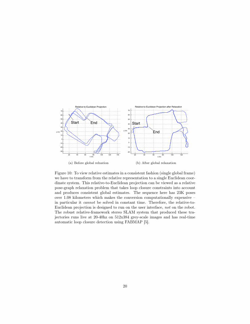
As an example, Figure 10 shows the result of transforming a large relativestate estimate into a single Euclidean frame using pose-graph relaxation. Notethat even this state-of-the art global Euclidean estimate fails to discover thetrue rectilinear structure. Arguably the best way to improve the map wouldbe to schedule new measurements across the diagonal of the map, thereby con-siderably constraining the solution. While this interventionist approach is used
19
20 40 60 80 100 120 140
-30
-20
-10
0
10
20
30
40
50
60
70
x (m)
y (m)
Relative-to-Euclidean Projection
Start End
(a) Before global relxation
-20
-10
0
10
20
30
40
50
60
70
y (m)
20 40 60 80 100 120
Relative-to-Euclidean Projection after Relaxation
x (m)
Start
End
(b) After global relaxation
Figure 10: To view relative estimates in a consistent fashion (single global frame)we have to transform from the relative representation to a single Euclidean coor-dinate system. This relative-to-Euclidean projection can be viewed as a relativepose-graph relaxation problem that takes loop closure constraints into accountand produces consistent global estimates. The sequence here has 23K posesover 1.08 kilometers which makes the conversion computationally expensive –in particular it cannot be solved in constant time. Therefore, the relative-to-Euclidean projection is designed to run on the user interface, not on the robot.The robust relative-framework stereo SLAM system that produced these tra-jectories runs live at 20-40hz on 512x384 grey-scale images and has real-timeautomatic loop closure detection using FABMAP [5].
20
extensively in surveying, we are not comfortable with placing such a require-ment on a mobile platform — ideally navigation and mapping should be a quietbackground task producing estimates for consumption by any interested clientprocess. With this example in mind, perhaps accurate global Euclidean stateestimates are the wrong goal to aim for — what matters is relative metric accu-racy and topological consistency — all of which can be attained with a relativemanifold approach.
7 Conclusion
The fact that the variables in bundle adjustment are defined relative to a singlecoordinate frame has a large impact on the algorithm’s iterative convergencerate. This is especially true at loop closure, when large errors must propagatearound the entire loop to correct for global errors that have accumulated alongthe path. As an alternative, we have presented an adaptive relative formulationthat can be viewed as a continuous sub-mapping approach – in many waysour relative treatment is an intuitive simplification of previous sub-mappingmethods. Furthermore by solving all parameters within an adaptive region,the proposed method attempts to match the full maximum likelihood solutionwithin the metric space defined by the manifold. In stark contrast to traditionalbundle adjustment, our evaluations and results indicate that state updates inthe relative approach are constant time, and crucially, remain so even duringloop closure events.
21
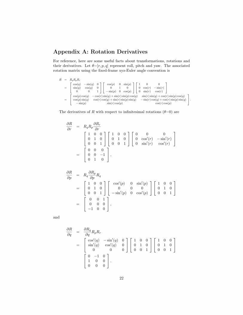
Appendix A: Rotation Derivatives
For reference, here are some useful facts about transformations, rotations andtheir derivatives. Let θ=[r, p, q] represent roll, pitch and yaw. The associatedrotation matrix using the fixed-frame xyz-Euler angle convention is
R = RqRpRr
=
cos(q) − sin(q) 0sin(q) cos(q) 0
0 0 1
cos(p) 0 sin(p)
0 1 0− sin(p) 0 cos(p)
1 0 00 cos(r) − sin(r)0 sin(r) cos(r)
=
cos(p) cos(q) − cos(r) sin(q) + sin(r) sin(p) cos(q) sin(r) sin(q) + cos(r) sin(p) cos(q)cos(p) sin(q) cos(r) cos(q) + sin(r) sin(p) sin(q) − sin(r) cos(q) + cos(r) sin(p) sin(q)− sin(p) sin(r) cos(p) cos(r) cos(p)
.
The derivatives of R with respect to infinitesimal rotations (θ=0) are
∂R
∂r= RqRp
∂Rr
∂r
1 0 00 1 00 0 1
1 0 00 1 00 0 1
0 0 00 cos�(r) − sin�(r)0 sin�(r) cos�(r)
=
0 0 00 0 −10 1 0
,
∂R
∂p= Rq
∂Rp
∂pRq
=
1 0 00 1 00 0 1
cos�(p) 0 sin�(p)
0 0 0− sin�(p) 0 cos�(p)
1 0 00 1 00 0 1
=
0 0 10 0 0−1 0 0
,
and
∂R
∂q=
∂Rq
∂qRpRr
=
cos�(q) − sin�(q) 0sin�(q) cos�(q) 0
0 0 0
1 0 00 1 00 0 1
1 0 00 1 00 0 1
0 −1 01 0 00 0 0
.
22
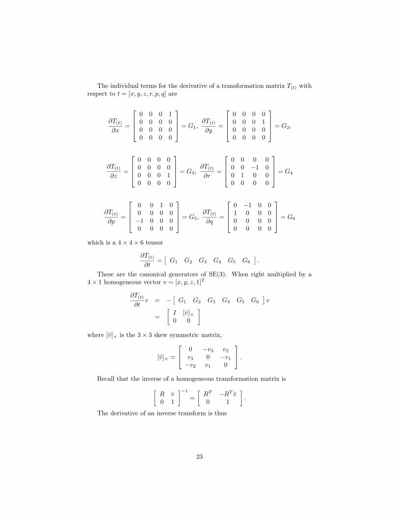
The individual terms for the derivative of a transformation matrix T(t) withrespect to t = [x, y, z, r, p, q] are
∂T(t)
∂x=
0 0 0 10 0 0 00 0 0 00 0 0 0
= G1,∂T(t)
∂y=
0 0 0 00 0 0 10 0 0 00 0 0 0
= G2,
∂T(t)
∂z=
0 0 0 00 0 0 00 0 0 10 0 0 0
= G3,∂T(t)
∂r=
0 0 0 00 0 −1 00 1 0 00 0 0 0
= G4
∂T(t)
∂p=
0 0 1 00 0 0 0−1 0 0 00 0 0 0
= G5,∂T(t)
∂q=
0 −1 0 01 0 0 00 0 0 00 0 0 0
= G6
which is a 4× 4× 6 tensor
∂T(t)
∂t=
�G1 G2 G3 G4 G5 G6
�.
These are the canonical generators of SE(3). When right multiplied by a4× 1 homogeneous vector v = [x, y, z, 1]T
∂T(t)
∂tv = −
�G1 G2 G3 G4 G5 G6
�v
=�
I [v̄]×0 0
�
where [v̄]× is the 3× 3 skew symmetric matrix,
[v̄]× =
0 −v3 v2
v3 0 −v1
−v2 v1 0
.
Recall that the inverse of a homogeneous transformation matrix is�
R v̄0 1
�−1
=�
RT −RT v̄0 1
�.
The derivative of an inverse transform is thus
23
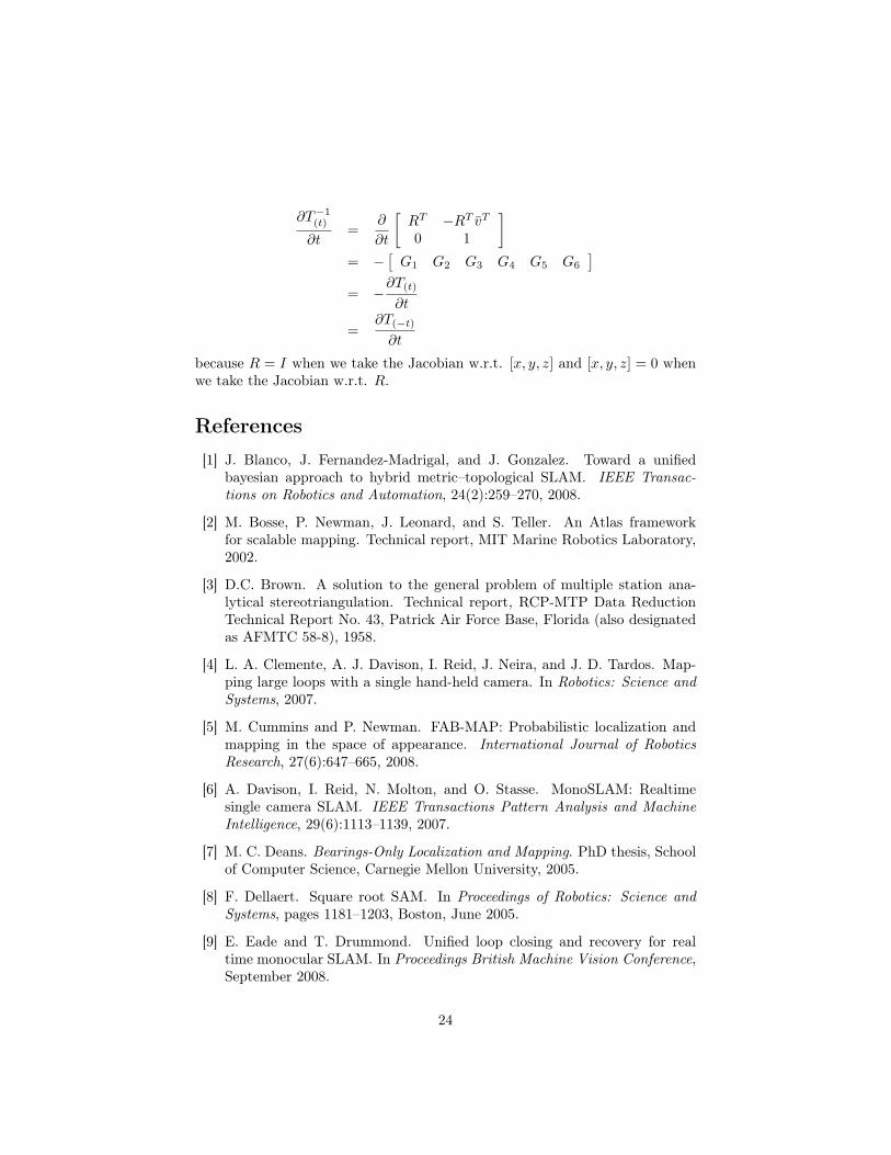
∂T−1(t)
∂t=
∂
∂t
�RT −RT v̄T
0 1
�
= −�
G1 G2 G3 G4 G5 G6
�
= −∂T(t)
∂t
=∂T(−t)
∂t
because R = I when we take the Jacobian w.r.t. [x, y, z] and [x, y, z] = 0 whenwe take the Jacobian w.r.t. R.
References
[1] J. Blanco, J. Fernandez-Madrigal, and J. Gonzalez. Toward a unifiedbayesian approach to hybrid metric–topological SLAM. IEEE Transac-
tions on Robotics and Automation, 24(2):259–270, 2008.
[2] M. Bosse, P. Newman, J. Leonard, and S. Teller. An Atlas frameworkfor scalable mapping. Technical report, MIT Marine Robotics Laboratory,2002.
[3] D.C. Brown. A solution to the general problem of multiple station ana-lytical stereotriangulation. Technical report, RCP-MTP Data ReductionTechnical Report No. 43, Patrick Air Force Base, Florida (also designatedas AFMTC 58-8), 1958.
[4] L. A. Clemente, A. J. Davison, I. Reid, J. Neira, and J. D. Tardos. Map-ping large loops with a single hand-held camera. In Robotics: Science and
Systems, 2007.
[5] M. Cummins and P. Newman. FAB-MAP: Probabilistic localization andmapping in the space of appearance. International Journal of Robotics
Research, 27(6):647–665, 2008.
[6] A. Davison, I. Reid, N. Molton, and O. Stasse. MonoSLAM: Realtimesingle camera SLAM. IEEE Transactions Pattern Analysis and Machine
Intelligence, 29(6):1113–1139, 2007.
[7] M. C. Deans. Bearings-Only Localization and Mapping. PhD thesis, Schoolof Computer Science, Carnegie Mellon University, 2005.
[8] F. Dellaert. Square root SAM. In Proceedings of Robotics: Science and
Systems, pages 1181–1203, Boston, June 2005.
[9] E. Eade and T. Drummond. Unified loop closing and recovery for realtime monocular SLAM. In Proceedings British Machine Vision Conference,September 2008.
24
[10] C. Engels, H. Stewenius, and D. Nister. Bundle adjustment rules. InPhotogrammetric Computer Vision, 2006.
[11] R. Eustice, H. Singh, J. Leonard, M. Walter, and R. Ballard. Visuallynavigating the RMS Titanic with SLAM information filters. In Robotics:
Science and Systems, pages 57–64, 2005.
[12] A. W. Fitzgibbon and A. Zisserman. Automatic Camera Recovery for
Closed or Open Image Sequences. Springer, Freiburg, Germany, June 2004.
[13] U. Frese and T. Duckett. A multigrid approach for accelerating relaxation-based SLAM. In Proceedings IJCAI Workshop on Reasoning with Uncer-
tainty in Robotics (RUR 2003), pages 39–46, Acapulco, Mexico, August2003.
[14] G. Grisetti, C. Stachniss, S. Grzonka, and W. Burgard. A tree parameter-ization for efficiently computing maximum likelihood maps using gradientdescent. In Proceedings Robotics: Science and Systems, Atlanta, June 2007.
[15] J.E. Guivant and E.M. Nebot. Optimization of the simultaneous local-ization and map-building algorithm for real-time implementation. IEEE
Transactions on Robotics and Automation, 17(3):242–257, June 2001.
[16] P. J. Huber. Robust estimation of a location parameter. The Annals of
Mathematical Statistics, 35(2):73–101, 1964.
[17] M. Kaess. Incremental Smoothing and Mapping. PhD thesis, Georgia In-stitute of Technology, 2008.
[18] G. Klein and D. Murray. Improving the agility of keyframe-based SLAM.In European Conference on Computer Vision, Marseille, October 2008.
[19] K. Konolige and M. Agrawal. FrameSLAM: from bundle adjustment torealtime visual mapping. IEEE Transactions on Robotics and Automation,24(5):1066–1077, 2008.
[20] A. Martinelli, V. Nguyen, N. Tomatis, and R. Siegwart. A relative mapapproach to SLAM based on shift and rotation invariants. Robotics and
Autonomous Systems, 55(1):50–61, 2007.
[21] P. F. McLauchlan. The variable state dimension filter applied to surface-based structure from motion. Technical report, University of Surrey, 1999.
[22] E. M. Mikhail. Observations and Least Squares. University Press of Amer-ica, Washington, D.C, 1983.
[23] E. Mouragnon, M. Lhuillier, M. Dhome, F. Dekeyse, and P. Sayd. Real timelocalization and 3d reconstruction. In Proceedings of Computer Vision and
Pattern Recognition, New York, New York, June 2006.
25
[24] E. Olson, J. Leonard, and S. Teller. Fast iterative alignment of pose graphswith poor initial estimates. In Proceedings of the IEEE International Con-
ference on Robotics and Automation, pages 2262–2269, Orlando, May 2006.
[25] P. Pinies and J. D. Tardos. Scalable slam building conditionally indepen-dent local maps. In IEEE conference on Intelligent Robots and Systems,2007.
[26] A. Ranganathan, M. Kaess, and F. Dellaert. Loopy SAM. In International
Joint Conferences on Artificial Intelligence, pages 2191–2196, 2007.
[27] G. Sibley, L. Matthies, and G. Sukhatme. A sliding window filter for incre-mental SLAM. In Ville Kyrki and Danica Kragic, editors, From features to
actions - Unifying perspectives in computational and robot vision, volume 8,chapter 7, pages 103–112. Springer Lecture Notes in Electrical Engineering,2007.
[28] D. Steedly and I. Essa. Propagation of innovative information in non-linearleast-squares structure from motion. In ICCV01, pages 223–229, 2001.
[29] S. Thrun, W. Burgard, and D. Fox. Probabilistic Robotics. MIT Press,Cambridge, MA, 2005.
[30] S. Thrun, D. Koller, Z. Ghahmarani, and H. Durrant-Whyte. SLAM up-dates require constant time. In Workshop on the Algorithmic Foundations
of Robotics, Nice, France, December 2002.
[31] B. Triggs, P. F. McLauchlan, R. I. Hartley, and A. W. Fitzgibbon. Bundleadjustment - a modern synthesis. In ICCV ’99: Proceedings of the Inter-
national Workshop on Vision Algorithms, pages 298–372. Springer-Verlag,London, UK, 2000.
26