Embed Size (px)
Citation preview
Bundle Adjustment — A Modern Synthesis
Bill Triggs1, Philip F. McLauchlan2, Richard I. Hartley3, and Andrew W. Fitzgibbon4
1 INRIA Rhone-Alpes, 655 avenue de l’Europe, 38330 Montbonnot, [email protected]
http://www.inrialpes.fr/movi/people/Triggs2 School of Electrical Engineering, Information Technology & Mathematics
University of Surrey, Guildford, GU2 5XH, [email protected]
3 General Electric CRD, Schenectady, NY, [email protected]
4 Dept of Engineering Science, University of Oxford, 19 Parks Road, OX1 3PJ, [email protected]
Abstract. This paper is a survey of the theory and methods of photogrammetricbundle adjustment, aimed at potential implementors in the computer vision commu-nity. Bundle adjustment is the problem of refining a visual reconstruction to producejointly optimal structure and viewing parameter estimates. Topics covered include:the choice of cost function and robustness; numerical optimization including sparseNewtonmethods, linearly convergent approximations, updating and recursive meth-ods; gauge (datum) invariance; and quality control. The theory is developed forgeneral robust cost functions rather than restricting attention to traditional nonlinearleast squares.
Keywords:BundleAdjustment, SceneReconstruction,GaugeFreedom,SparseMa-trices, Optimization.
1 Introduction
Thispaper isasurveyof the theoryandmethodsofbundleadjustmentaimedat thecomputervision community, andmore especially at potential implementorswho already knowa littleabout bundle methods. Most of the results appeared long ago in the photogrammetry andgeodesy literatures, but many seem to be little known in vision, where they are graduallybeing reinvented. By providing an accessible modern synthesis, we hope to forestall someof this duplication of effort, correct some common misconceptions, and speed progress invisual reconstruction by promoting interaction between the vision and photogrammetrycommunities.
Bundle adjustmentis the problemof refininga visual reconstruction to producejointlyoptimal3D structure and viewing parameter (camera pose and/or calibration) estimates.Optimalmeans that the parameter estimates are found by minimizing some cost functionthat quantifies themodel fitting error, andjointly that the solution is simultaneously optimalwith respect to both structure and camera variations. The name refers to the ‘bundles’
This work was supported in part by the European Commission Esprit LTR projectCu-muli (B. Triggs), the UK EPSRC project GR/L34099 (P. McLauchlan), and the Royal Society(A. Fitzgibbon). We would like to thank A. Zisserman, A. Grun and W. Forstner for valuablecomments and references.
B. Triggs, A. Zisserman, R. Szeliski (Eds.): Vision Algorithms’99, LNCS 1883, pp. 298–372, 2000.c© Springer-Verlag Berlin Heidelberg 2000
Bundle Adjustment — A Modern Synthesis 299
of light rays leaving each 3D feature and converging on each camera centre, which are‘adjusted’ optimally with respect to both feature and camera positions. Equivalently —unlike independent model methods, which merge partial reconstructions without updatingtheir internal structure — all of the structure and camera parameters are adjusted together‘in one bundle’.Bundle adjustment is really just a large sparsegeometric parameter estimationproblem,
the parameters being the combined 3D feature coordinates, camera poses and calibrations.Almost everything that we will say can be applied to many similar estimation problems invision, photogrammetry, industrial metrology, surveying and geodesy. Adjustment com-putations are a major common theme throughout the measurement sciences, and once thebasic theory and methods are understood, they are easy to adapt to a wide variety of prob-lems. Adaptation is largely a matter of choosing a numerical optimization scheme thatexploits the problem structure and sparsity. We will consider several such schemes belowfor bundle adjustment.Classically, bundle adjustment and similar adjustment computations are formulated
as nonlinear least squares problems [19, 46, 100, 21, 22, 69, 5, 73, 109]. The cost functionis assumed to be quadratic in the feature reprojection errors, and robustness is providedby explicit outlier screening. Although it is already very flexible, this model is not reallygeneral enough. Modern systems often use non-quadratic M-estimator-like distributionalmodels to handle outliers more integrally, and many include additional penalties related tooverfitting, model selection and system performance (priors, MDL). For this reason, wewill not assume a least squares / quadratic cost model. Instead, the cost will be modelledas a sum of opaque contributions from the independent information sources (individualobservations, prior distributions, overfitting penalties. . . ). The functional forms of thesecontributions and their dependence on fixed quantities such as observations will usually beleft implicit. This allowsmanydifferent typesof robust andnon-robust cost contributions tobe incorporated, without unduly cluttering the notation or hiding essential model structure.It fits well with modern sparse optimization methods (cost contributions are usually sparsefunctions of the parameters) and object-centred software organization, and it avoids manytedious displays of chain-rule results. Implementors are assumed to be capable of choosingappropriate functions and calculating derivatives themselves.
One aim of this paper is to correct a number ofmisconceptions that seem to be commonin the vision literature:
• “Optimization / bundle adjustment is slow”: Such statements often appear in papersintroducing yet another heuristic Structure from Motion (SFM) iteration. The claimedslowness is almost always due to the unthinking use of a general-purpose optimiza-tion routine that completely ignores the problem structure and sparseness. Real bundleroutines aremuchmore efficient than this, and usually considerably more efficient andflexible than the newly suggested method (§6, 7). That is why bundle adjustment re-mains the dominant structure refinement technique for real applications, after 40 yearsof research.
• “Only linear algebra is required”: This is a recent variant of the above, presumablymeant to imply that the new technique is especially simple. Virtually all iterative refine-ment techniques use only linear algebra, and bundle adjustment is simpler than manyin that it only solves linear systems: it makes no use of eigen-decomposition or SVD,which are themselves complex iterative methods.
300 B. Triggs et al.
• “Any sequence can be used”:Many visionworkers seem to be very resistant to the ideathat reconstruction problems should be planned in advance (§11), and results checkedafterwards to verify their reliability (§10). Systembuilders should at least be aware of thebasic techniques for this, even if application constraints make it difficult to use them.The extraordinary extent to which weak geometry and lack of redundancy can maskgross errors is too seldom appreciated,c.f . [34, 50, 30, 33].• “Point P is reconstructed accurately”: In reconstruction, just as there are no absolutereferences for position, there are none for uncertainty. The 3D coordinate frame isitself uncertain, as it can only be located relative to uncertain reconstructed features orcameras. All other feature and camera uncertainties are expressed relative to the frameand inherit its uncertainty, so statements about them are meaningless until the frameand its uncertainty are specified. Covariances can look completely different in differentframes, particularly in object-centred versus camera-centred ones. See§9.
There is a tendency in vision to develop a profusion ofad hocadjustment iterations. Whyshould you use bundle adjustment rather than one of these methods? :• Flexibility: Bundle adjustment gracefully handles a very wide variety of different 3Dfeature and camera types (points, lines, curves, surfaces, exotic cameras), scene types(including dynamic and articulatedmodels, scene constraints), information sources (2Dfeatures, intensities, 3D information, priors) and error models (including robust ones).It has no problems with missing data.• Accuracy:Bundle adjustment gives precise andeasily interpreted results because it usesaccurate statistical error models and supports a sound, well-developed quality controlmethodology.• Efficiency: Mature bundle algorithms are comparatively efficient even on very largeproblems. They use economical and rapidly convergent numerical methods and makenear-optimal use of problem sparseness.
In general, as computer vision reconstruction technology matures, we expect that bundleadjustment will predominate over alternative adjustmentmethods inmuch the sameway asit has in photogrammetry.Wesee this as an inevitable consequenceof a greater appreciationof optimization (notably, more effective use of problem structure and sparseness), and ofsystems issues such as quality control and network design.
Coverage:We will touch on a good many aspects of bundle methods. We start by consid-ering the camera projection model and the parametrization of the bundle problem§2, andthe choice of error metric or cost function§3. §4 gives a rapid sketch of the optimizationtheory we will use.§5 discusses the network structure (parameter interactions and char-acteristic sparseness) of the bundle problem. The following three sections consider threetypes of implementation strategies for adjustment computations:§6 covers second orderNewton-likemethods, which are still themost often used adjustment algorithms;§7 coversmethods with only first order convergence (most of thead hocmethods are in this class);and§8 discusses solution updating strategies and recursive filtering bundle methods.§9returns to the theoretical issue of gauge freedom (datum deficiency), including the theoryof inner constraints.§10 goes into some detail on quality control methods for monitoringthe accuracy and reliability of the parameter estimates.§11 gives some brief hints on net-work design,i.e. how to place your shots to ensure accurate, reliable reconstruction.§12completes the body of the paper by summarizing the main conclusions and giving someprovisional recommendations for methods. There are also several appendices.§A gives abrief historical overview of the development of bundle methods, with literature references.
Bundle Adjustment — A Modern Synthesis 301
§B gives some technical details of matrix factorization, updating and covariance calcula-tion methods.§C gives some hints on designing bundle software, and pointers to usefulresources on the Internet. The paper ends with a glossary and references.
General references:Cultural differences sometimes make it difficult for vision workersto read the photogrammetry literature. The collection edited by Atkinson [5] and themanual by Karara [69] are both relatively accessible introductions to close-range (ratherthan aerial) photogrammetry. Other accessible tutorial papers include [46, 21, 22]. Kraus[73] is probably the most widely used photogrammetry textbook. Brown’s early surveyof bundle methods [19] is well worth reading. The often-cited manual edited by Slama[100] is now quite dated, although its presentation of bundle adjustment is still relevant.Wolf & Ghiliani [109] is a text devoted to adjustment computations, with an emphasison surveying. Hartley & Zisserman [62] is an excellent recent textbook covering visiongeometry from a computer vision viewpoint. For nonlinear optimization, Fletcher [29]and Gillet al [42] are the traditional texts, and Nocedal & Wright [93] is a good modernintroduction. For linear least squares, Bjorck [11] is superlative, and Lawson & Hanson isa good older text. For more general numerical linear algebra, Golub & Van Loan [44] isthe standard. Duffet al [26] and George & Liu [40] are the standard texts on sparse matrixtechniques. We will not discuss initialization methods for bundle adjustment in detail, butappropriate reconstructionmethods are plentiful and well-known in the vision community.See,e.g., [62] for references.
Notation: The structure, cameras,etc., being estimated will be parametrized by a singlelargestate vectorx. In general the state belongs to a nonlinear manifold, but we linearizethis locally and work with small linear state displacements denotedδx. Observations (e.g.measured image features) are denotedz. The corresponding predicted values at parametervaluex aredenotedz = z(x), with residual prediction error �z(x) ≡ z−z(x). However,observations and prediction errors usually only appear implicitly, through their influenceon thecost function f(x) = f(predz(x)). The cost function’sgradient is g ≡ df
dx , and
its Hessianis H ≡ d2fdx2 . Theobservation-state Jacobianis J ≡ dz
dx . The dimensions ofδx, δz arenx, nz.
2 Projection Model and Problem Parametrization
2.1 The Projection Model
Webegin the development of bundle adjustment by considering the basic image projectionmodel and the issueof problemparametrization.Visual reconstructionattempts to recover amodel of a 3D scene frommultiple images. As part of this, it usually also recovers the poses(positionsandorientations) of the cameras that took the images, and informationabout theirinternal parameters. A simple scene model might be a collection of isolated 3D features,e.g., points, lines, planes, curves, or surface patches. However, far more complicated scenemodels are possible, involving,e.g., complex objects linked by constraints or articulations,photometry as well as geometry, dynamics,etc. One of the great strengths of adjustmentcomputations— and one reason for thinking that they have a considerable future in vision— is their ability to take such complex and heterogeneous models in their stride. Almostanypredictive parametricmodel can be handled,i.e. any model thatpredictsthe valuesof some known measurements or descriptors on the basis of some continuousparametricrepresentation of the world, which is to be estimated from the measurements.
302 B. Triggs et al.
Similarly, many possible camera models exist. Perspective projection is the standard,but the affine and orthographic projections are sometimes useful for distant cameras, andmore exotic models such as push-broom and rational polynomial cameras are needed forcertain applications [56, 63]. In addition to pose (position and orientation), and simpleinternal parameters such as focal length and principal point, real cameras also require vari-ous types ofadditional parameters to model internal aberrations such as radial distortion[17–19, 100, 69, 5].For simplicity, suppose that the scene is modelled by individual static 3D featuresXp,
p = 1 . . . n, imaged inm shots with camera pose and internal calibration parametersPi,i = 1 . . .m. There may also be further calibration parametersCc, c = 1 . . . k, constantacross several images (e.g., depending on which of several cameras was used). We aregiven uncertain measurementsxip of some subset of the possible image featuresxip (thetrue image of featureXp in imagei). For each observationxip, we assume that we havea predictive model xip = x(Cc,Pi,Xp) based on the parameters, that can be used toderive afeature prediction error :
�xip(Cc,Pi,Xp) ≡ xip − x(Cc,Pi,Xp) (1)
In the case of image observations the predictive model is image projection, but otherobservation types such as 3D measurements can also be included.To estimate the unknown 3D feature and camera parameters from the observations,
and hence reconstruct the scene, weminimize somemeasure (discussed in§3) of their totalprediction error. Bundle adjustment is themodel refinement part of this, starting fromgiveninitial parameter estimates (e.g., from some approximate reconstruction method). Hence,it is essentially a matter of optimizing a complicated nonlinear cost function (the totalprediction error) over a large nonlinear parameter space (the sceneand camera parameters).We will not go into the analytical forms of the various possible feature and image
projection models, as these do not affect the general structure of the adjustment network,and only tend to obscure its central simplicity. We simply stress that the bundle frameworkis flexible enough to handle almost any desired model. Indeed, there are so many differentcombinations of features, image projections and measurements, that it is best to regardthem as black boxes, capable of giving measurement predictions based on their currentparameters. (For optimization, first, and possibly second, derivatives with respect to theparameters are also needed).Formuch of the paperwewill take quite an abstract viewof this situation, collecting the
scene and camera parameters to be estimated into a largestate vectorx, and representingthe cost (total fitting error) as an abstract functionf(x). The cost is really a function ofthe feature prediction errors�xip = xip− x(Cc,Pi,Xp). But as the observationsxip areconstants during an adjustment calculation, we leave the cost’s dependence on them andon the projection modelx(·) implicit, and display only its dependence on the parametersx actually being adjusted.
2.2 Bundle Parametrization
Thebundleadjustment parameter space isgenerally ahigh-dimensional nonlinearmanifold— a large Cartesian product of projective 3D feature, 3D rotation, and camera calibrationmanifolds, perhaps with nonlinear constraints,etc. The statex is not strictly speaking avector, but rather a point in this space. Depending on how the entities that it contains are
Bundle Adjustment — A Modern Synthesis 303
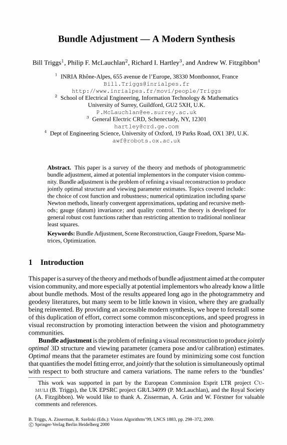
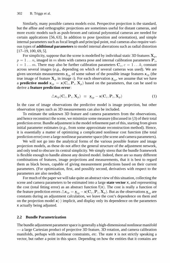
Fig. 1.Vision geometry and its errormodel are essentiallyprojective. Affine parametrization introduces an artificialsingularity at projective infinity, whichmay cause numer-ical problems for distant features.
represented,x can be subject to various types of complications including singularities,internal constraints, and unwanted internal degrees of freedom. These arise because geo-metric entities like rotations, 3D lines and even projective points and planes, do not havesimple global parametrizations. Their local parametrizations are nonlinear, with singular-ities that prevent them from covering the whole parameter space uniformly (e.g. the manyvariants on Euler angles for rotations, the singularity of affine point coordinates at infinity).And their global parametrizations either have constraints (e.g. quaternionswith‖q‖2 = 1),or unwanted internal degrees of freedom (e.g. homogeneous projective quantities have ascale factor freedom, two points defining a line can slide along the line). For more compli-cated compound entities such asmatching tensors and assemblies of 3D features linked bycoincidence, parallelism or orthogonality constraints, parametrization becomes evenmoredelicate.Although they are in principle equivalent, different parametrizations often have pro-
foundly different numerical behaviours which greatly affect the speed and reliability of theadjustment iteration. The most suitable parametrizations for optimization are as uniform,finite and well-behaved as possiblenear the current state estimate. Ideally, they shouldbe locally close to linear in terms of their effect on the chosen error model, so that thecost function is locally nearly quadratic. Nonlinearity hinders convergence by reducingthe accuracy of the second order cost model used to predict state updates (§6). Excessivecorrelations and parametrization singularities cause ill-conditioning and erratic numericalbehaviour. Large or infinite parameter values can only be reached after excessively manyfinite adjustment steps.Any given parametrization will usually only be well-behaved in this sense over a rela-
tively small section of state space. So to guarantee uniformly good performance, howeverthe state itself may be represented,state updates should be evaluated using a stablelocalparametrization based on increments from the current estimate. As examples we consider3D points and rotations.
3D points: Even for calibrated cameras, vision geometry and visual reconstructions areintrinsically projective. If a 3D(X Y Z)�parametrization (or equivalently a homogeneousaffine (X Y Z 1)� one) is used for very distant 3D points, largeX,Y, Z displacementsare needed to change the image significantly.I.e., in (X Y Z) space the cost functionbecomes very flat and steps needed for cost adjustment become very large for distantpoints. In comparison, with a homogeneous projective parametrization(X Y Z W )�, thebehaviour near infinity is natural, finite and well-conditioned so long as the normalizationkeeps the homogeneous 4-vector finite at infinity (by sendingW → 0 there). In fact,there is no immediate visual distinction between the images of real points near infinityand virtual ones ‘beyond’ it (all camera geometries admit such virtual points asbona fideprojective constructs). The optimal reconstruction of a real 3D point may even be virtualin this sense, if image noise happens to push it ‘across infinity’. Also, there is nothing tostop a reconstructed point wandering beyond infinity and back during the optimization.This sounds bizarre at first, but it is an inescapable consequence of the fact that the nat-ural geometry and error model for visual reconstruction is projective rather than affine.
304 B. Triggs et al.
Projectively,infinity is just like any other place. Affine parametrization(X Y Z 1)� isacceptable for points near the origin with close-range convergent camera geometries, butit is disastrous for distant ones because it artificially cuts away half of the natural parameterspace, and hides the fact by sending the resulting edge to infinite parameter values. Instead,you should use a homogeneous parametrization(X Y Z W )� for distant points,e.g. withspherical normalization
∑X2
i = 1.Rotations: Similarly, experience suggests that quasi-global 3 parameter rotation para-metrizations such as Euler angles cause numerical problems unless one can be certain toavoid their singularities and regions of uneven coverage. Rotations should be parametrizedusing either quaternions subject to‖q‖2 = 1, or local perturbationsRδR or δR R ofan existing rotationR, whereδR can be any well-behaved 3 parameter small rotationapproximation,e.g. δR = (I + [ δr ]×), the Rodriguez formula, local Euler angles,etc.
State updates:Just as state vectorsx represent points in some nonlinear space, stateupdatesx → x + δx represent displacements in this nonlinear space that often can notbe represented exactly by vector addition. Nevertheless, we assume that we can locallylinearize the state manifold, locally resolving any internal constraints and freedoms thatit may be subject to, to produce an unconstrained vectorδx parametrizing the possiblelocal state displacements. We can then,e.g., use Taylor expansion inδx to form a local
cost modelf(x + δx) ≈ f(x) + dfdx δx + 1
2δx� d2fdx2 δx, from which we can estimate the
state updateδx that optimizes this model (§4). The displacementδx need not have thesame structure or representation asx— indeed, if a well-behaved local parametrization isused to representδx, it generally will not have — but we must at least be able to updatethe state with the displacement to produce a new state estimate. We write this operationasx → x + δx, even though it may involve considerably more than vector addition. Forexample, apart from the change of representation, an updated quaternionq→ q+ dqwillneed to have its normalization‖q‖2 = 1 corrected, and a small rotation update of the formR→ R(1 + [ r ]×) will not in general give an exact rotation matrix.
3 Error Modelling
We now turn to the choice of the cost functionf(x), which quantifies the total prediction(image reprojection) error of the model parametrized by the combined scene and cameraparametersx. Our main conclusion will be that robust statistically-based error metricsbased on total (inlier + outlier) log likelihoods should be used, to correctly allow for thepresence of outliers. We will argue this at some length as it seems to be poorly understood.The traditional treatments of adjustment methods consider only least squares (albeit withdata trimming for robustness), andmost discussions of robust statistics give the impressionthat the choice of robustifier or M-estimator is wholly a matter of personal whim ratherthan data statistics.Bundle adjustment is essentially a parameter estimation problem. Any parameter es-
timation paradigm could be used, but we will consider onlyoptimal point estimators,whose output is by definition the single parameter vector that minimizes a predefinedcostfunction designed to measure how well the model fits the observations and backgroundknowledge. This framework covers many practical estimators including maximum likeli-hood (ML) and maximum a posteriori (MAP), but not explicit Bayesian model averaging.Robustification, regularization and model selection terms are easily incorporated in thecost.
Bundle Adjustment — A Modern Synthesis 305
A typical ML cost function would be the summed negative log likelihoods of theprediction errors of all the observed image features. For Gaussian error distributions,this reduces to the sum of squared covariance-weighted prediction errors (§3.2). A MAPestimator would typically add cost terms giving certain structure or camera calibrationparameters a bias towards their expected values.The cost function is also a tool for statistical interpretation. To the extent that lower
costs are uniformly ‘better’, it provides a natural model preference ordering, so that costiso-surfaces above the minimum define natural confidence regions. Locally, these regionsare nested ellipsoids centred on the cost minimum, with size and shape characterized by
thedispersionmatrix (the inverse of the cost function HessianH = d2fdx2 at theminimum).
Also, the residual cost at the minimum can be used as a test statistic for model validity(§10). E.g., for a negative log likelihood cost model with Gaussian error distributions,twice the residual is aχ2 variable.
3.1 Desiderata for the Cost Function
In adjustment computationswego to considerable lengths tooptimizea largenonlinear costmodel, so it seems reasonable to require that the refinement should actually improve theestimates in some objective (albeit statistical) sense. Heuristicallymotivated cost functionscan not usually guarantee this. They almost always lead to biased parameter estimates, andoften severely biased ones. A large body of statistical theory points tomaximum likelihood(ML) and its Bayesian cousin maximum a posteriori (MAP) as the estimators of choice.ML simply selects themodel for which the total probability of the observed data is highest,or saying the same thing in different words, for which thetotal posterior probabilityof themodel given the observations is highest. MAP adds a prior term representing backgroundinformation.ML could just as easily have included the prior as an additional ‘observation’:so far as estimation is concerned, the distinction betweenML /MAPandprior / observationis purely terminological.Information usually comes from many independent sources. In bundle adjustment
these include: covariance-weighted reprojection errors of individual image features; othermeasurements such as 3D positions of control points, GPS or inertial sensor readings;predictions from uncertain dynamical models (for ‘Kalman filtering’ of dynamic camerasor scenes); prior knowledge expressed as soft constraints (e.g. on camera calibration orpose values); and supplementary sources such as overfitting, regularization or descriptionlength penalties. Note the variety. One of the great strengths of adjustment computations istheir ability to combine information from disparate sources. Assuming that the sources arestatistically independent of one another given themodel, the total probability for themodelgiven the combined data is the product of the probabilities from the individual sources. Toget an additive cost function we take logs, so the total log likelihood for the model giventhe combined data is the sum of the individual source log likelihoods.
Properties of ML estimators: Apart from their obvious simplicity and intuitive appeal,ML and MAP estimators have strong statistical properties. Many of the most notable onesareasymptotic, i.e. they apply in the limit of a large number of independentmeasurements,or more precisely in thecentral limit where the posterior distribution becomes effectivelyGaussian1. In particular:1 Cost is additive, so as measurements of the same type are added the entire cost surface grows indirect proportion to the amount of datanz. This means that therelativesizes of the cost and all of
306 B. Triggs et al.
• Under mild regularity conditions on the observation distributions, the posterior distri-bution of the ML estimate converges asymptotically in probability to a Gaussian withcovariance equal to the dispersion matrix.• TheML estimate asymptotically has zero bias and the lowest variance that any unbiasedestimator can have. So in this sense, ML estimation is at least as good as any othermethod2.Non-asymptotically, the dispersion is not necessarily a good approximation for the
covariance of the ML estimator. The asymptotic limit is usually assumed to be a validfor well-designed highly-redundant photogrammetric measurement networks, but recentsampling-based empirical studies of posterior likelihood surfaces [35, 80, 68] suggest thatthe case ismuch less clear for small vision geometry problems andweaker networks. Morework is needed on this.
Theeffect of incorrect errormodels:It is clear that incorrectmodellingof theobservationdistributions is likely to disturb the ML estimate. Such mismodelling is to some extentinevitable because error distributions stand for influences that we can not fully predict orcontrol. To understand the distortions that unrealistic error models can cause, first realizethat geometric fitting is really a special case of parametric probability density estimation.For each set of parameter values, the geometric image projection model and the assumedobservation error models combine to predict a probability density for the observations.Maximizing the likelihood corresponds to fitting thispredicted observation densityto theobserved data. The geometry and camera model only enter indirectly, via their influenceon the predicted distributions.Accurate noise modelling is just as critical to successful estimation as accurate ge-
ometric modelling. The most important mismodelling is failure to take account of thepossibility of outliers (aberrant data values, causede.g., by blunders such as incorrectfeature correspondences). We stress that so long as the assumed error distributions modelthe behaviour ofall of the data used in the fit (includingboth inliers and outliers), theabove properties of ML estimation including asymptotic minimum variance remain validin the presence of outliers. In other words,ML estimation is naturally robust: there is no
its derivatives — and hence the sizer of the region around the minimum over which the secondorder Taylor terms dominate all higher order ones — remain roughly constant asnz increases.Within this region, the total cost is roughly quadratic, so if the cost function was taken to be theposterior log likelihood, the posterior distribution is roughly Gaussian. However the curvature ofthequadratic (i.e. the inversedispersionmatrix) increasesasdata is added, so theposterior standarddeviation shrinks asO(
σ/√nz − nx
), whereO(σ) characterizes the average standard deviation
from a single observation. Fornz − nx � (σ/r)2, essentially the entire posterior probabilitymass lies inside the quadratic region, so the posterior distribution converges asymptotically inprobability to a Gaussian. This happens atanyproper isolated cost minimum at which secondorder Taylor expansion is locally valid. The approximation gets better with more data (strongercurvature) and smaller higher order Taylor terms.
2 This result follows from theCramer-Rao bound(e.g. [23]), which says that the covariance of anyunbiasedestimator is boundedbelowby theFisher information ormeancurvature of theposterior
log likelihood surface〈(x−x)(x−x)�〉 � −〈d2 log pdx2 〉wherep is the posterior probability,x the
parameters being estimated,x the estimate given by any unbiased estimator,x the true underlyingx value, andA � B denotes positive semidefiniteness ofA − B. Asymptotically, the posteriordistribution becomesGaussian and the Fisher information converges to the inverse dispersion (thecurvature of the posterior log likelihood surface at the cost minimum), so the ML estimate attainsthe Cramer-Rao bound.
Bundle Adjustment — A Modern Synthesis 307
0
0.05
0.1
0.15
0.2
0.25
0.3
0.35
0.4
-10 -5 0 5 10
Gaussian PDFCauchy PDF
0
1
2
3
4
5
6
7
8
-10 -5 0 5 10
Gaussian -log likelihoodCauchy -log likelihood
0
20
40
60
80
100
0 100 200 300 400 500 600 700 800 900 1000
1000 Samples from a Cauchy and a Gaussian Distribution
CauchyGaussian
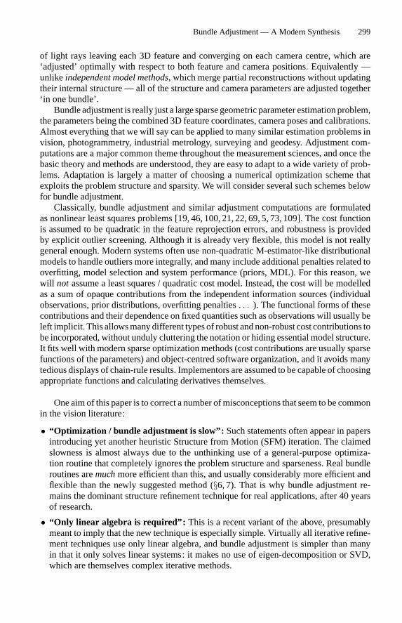
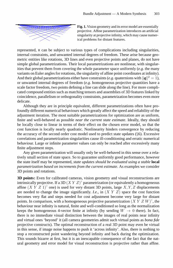
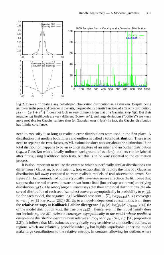
Fig. 2. Beware of treating any bell-shaped observation distribution as a Gaussian. Despite beingnarrower in the peak andbroader in the tails, the probability density function of aCauchy distribution,p(x) =
(π(1 + x2)
)−1, does not look so very different from that of a Gaussian (top left). But their
negative log likelihoods are very different (bottom left), and large deviations (“outliers”) aremuchmore probable for Cauchy variates than for Gaussian ones (right). In fact, the Cauchy distributionhas infinite covariance.
need to robustify it so long as realistic error distributions were used in the first place. Adistribution that models both inliers and outliers is called atotal distribution . There is noneed to separate the two classes, asML estimation does not care about the distinction. If thetotal distribution happens to be an explicit mixture of an inlier and an outlier distribution(e.g., a Gaussian with a locally uniform background of outliers), outliers can be labeledafter fitting using likelihood ratio tests, but this is in no way essential to the estimationprocess.It is also important to realize the extent to which superficially similar distributions can
differ from a Gaussian, or equivalently, how extraordinarily rapidly the tails of a Gaussiandistribution fall away compared to more realistic models of real observation errors. Seefigure 2. In fact, unmodelled outliers typically have very severe effects on the fit. To see this,suppose that the real observationsaredrawn fromafixed (but perhapsunknown)underlyingdistributionp0(z). Thelaw of large numberssays that their empirical distributions (the ob-served distribution of each set of samples) converge asymptotically in probability top0(z).So for each model, the negative log likelihood cost sum−∑i log pmodel(zi|x) convergesto−nz
∫p0(z) log(pmodel(z|x)) dz. Up to a model-independent constant, this isnz times
therelative entropy orKullback-Leibler divergence∫p0(z) log(p0(z)/pmodel(z|x))dz
of the model distribution w.r.t. the true onep0(z). Hence, even if the model family doesnot includep0, the ML estimate converges asymptotically to the model whose predictedobservation distribution hasminimum relative entropyw.r.t.p0. (See,e.g. [96, proposition2.2]). It follows that ML estimates are typically very sensitive to unmodelled outliers, asregions which are relatively probable underp0 but highly improbable under the modelmake large contributions to the relative entropy. In contrast, allowing for outliers where
308 B. Triggs et al.
none actually occur causes relatively little distortion, as no region which is probable underp0 will have large− log pmodel.In summary, if there is a possibility of outliers, non-robust distribution models such
as Gaussians should be replaced with more realistic long-tailed ones such as: mixtures ofa narrow ‘inlier’ and a wide ‘outlier’ density, Cauchy orα-densities, or densities definedpiecewise with a central peaked ‘inlier’ region surrounded by a constant ‘outlier’ region3.We emphasize again that poor robustness is due entirely to unrealistic distributional as-sumptions: the maximum likelihood framework itself is naturally robust provided that thetotal observation distribution including both inliers and outliers is modelled. In fact, realobservations can seldom be cleanly divided into inliers and outliers. There is a hard coreof outliers such as feature correspondence errors, but there is also a grey area of featuresthat for some reason (a specularity, a shadow, poor focus, motion blur. . . ) were not asaccurately located as other features, without clearly being outliers.
3.2 Nonlinear Least Squares
One of the most basic parameter estimation methods isnonlinear least squares. Supposethat we have vectors of observationszi predicted by a modelzi = zi(x), wherex is avector of model parameters. Then nonlinear least squares takes as estimates the parametervalues that minimize theweighted Sum of Squared Error (SSE)cost function:
f(x) ≡ 12
∑i
�zi(x)� Wi�zi(x) , �zi(x) ≡ zi − zi(x) (2)
Here,�zi(x) is the feature prediction error andWi is an arbitrary symmetric positivedefinite (SPD)weightmatrix .Modulo normalization terms independent ofx, theweightedSSE cost function coincides with the negative log likelihood for observationszi perturbedby Gaussian noise of mean zero and covarianceW−1
i . So for least squares to have a usefulstatistical interpretation, theWi should be chosen to approximate the inversemeasurementcovariance ofzi. Even for non-Gaussian noise with this mean and covariance, theGauss-Markov theorem [37, 11] states that if the modelszi(x) are linear, least squares gives theBest Linear Unbiased Estimator (BLUE), where ‘best’ means minimum variance4.Any weighted least squares model can be converted to an unweighted one (Wi = 1)
by pre-multiplyingzi, zi,�zi by anyL�i satisfyingWi = Li L�
i . Such anLi can be cal-culated efficiently fromWi orW−1
i using Cholesky decomposition (§B.1).�zi = L�i �zi
is called astandardized residual, and the resulting unweighted least squares problemminx
12
∑i ‖�zi(x)‖2 is said to be instandard form. One advantage of this is that opti-
mization methods based on linear least squares solvers can be used in place of ones basedon linear (normal) equation solvers, which allows ill-conditioned problems to be handledmore stably (§B.2).Another peculiarity of the SSE cost function is its indifference to the natural bound-
aries between the observations. If observationszi from any sources are assembled into a
3 The latter casecorresponds toahard inlier / outlier decision rule: for anyobservation in the ‘outlier’region, the density is constant so the observation has no influence at all on the fit. Similarly, themixture case corresponds to a softer inlier / outlier decision rule.
4 It may be possible (and even useful) to do better with either biased (towards the correct solution),or nonlinear estimators.
Bundle Adjustment — A Modern Synthesis 309
compound observation vectorz ≡ (z�1, . . . , z
�k)�, and their weight matricesWi are assem-
bled into compound block diagonal weight matrixW ≡ diag(W1, . . . ,Wk), the weightedsquared errorf(x) ≡ 1
2 �z(x)� W�z(x) is the same as the original SSE cost function,12
∑i �zi(x)� Wi�zi(x). The general quadratic form of the SSE cost is preserved under
such compounding, and also under arbitrary linear transformations ofz that mix compo-nents from different observations. The only place that the underlying structure is visibleis in the block structure ofW. Such invariances do not hold for essentially any other costfunction, but they simplify the formulation of least squares considerably.
3.3 Robustified Least Squares
Themain problemwith least squares is its high sensitivity to outliers. This happens becausethe Gaussian has extremely small tails compared to most real measurement error distribu-tions. For robust estimates, we must choose a more realistic likelihood model (§3.1). Theexact functional form is less important than the general way in which the expected typesof outliers enter. A single blunder such as a correspondence error may affect one or a fewof the observations, but it will usually leave all of the others unchanged. This locality isthe whole basis of robustification. If we can decide which observations were affected, wecan down-weight or eliminate them and use the remaining observations for the parameterestimates as usual. If all of the observations had been affected about equally (e.g. as byan incorrect projection model), we might still know that something was wrong, but not beable to fix it by simple data cleaning.We will adopt a ‘single layer’ robustness model, in which the observations are par-
titioned into independent groupszi, each group being irreducible in the sense that it isaccepted, down-weighted or rejected as a whole, independently of all the other groups.The partitions should reflect the types of blunders that occur. For example, if feature cor-respondence errors are the most common blunders, the two coordinates of a single imagepoint would naturally form a group as both would usually be invalidated by such a blunder,while no other image point would be affected. Even if one of the coordinates appeared tobe correct, if the other were incorrect we would usually want to discard both for safety.On the other hand, in stereo problems, the four coordinates of each pair of correspondingimage points might be a more natural grouping, as a point in one image is useless withoutits correspondent in the other one.Henceforth, when we sayobservationwe meanirreducible group of observations
treated as a unit by the robustifying model. I.e., our observations need not be scalars, butthey must be units, probabilistically independent of one another irrespective of whetherthey are inliers or outliers.As usual, each independent observationzi contributes an independent termfi(x | zi) to
the total cost function. This could have more or less any form, depending on the expectedtotal distribution of inliers and outliers for the observation. One very natural family are theradial distributions , which have negative log likelihoods of the form:
fi(x) ≡ 12 ρi(�zi(x)� Wi�zi(x) ) (3)
Here,ρi(s) can be any increasing function withρi(0) = 0 and ddsρi(0) = 1. (These
guarantee that at�zi = 0, f vanishes andd2fi
dz2i
= Wi). Weighted SSE hasρi(s) = s, while
more robust variants have sublinearρi, often tending to a constant at∞ so that distant
310 B. Triggs et al.
outliers are entirely ignored. The dispersionmatrixW−1i determines the spatial spread ofzi,
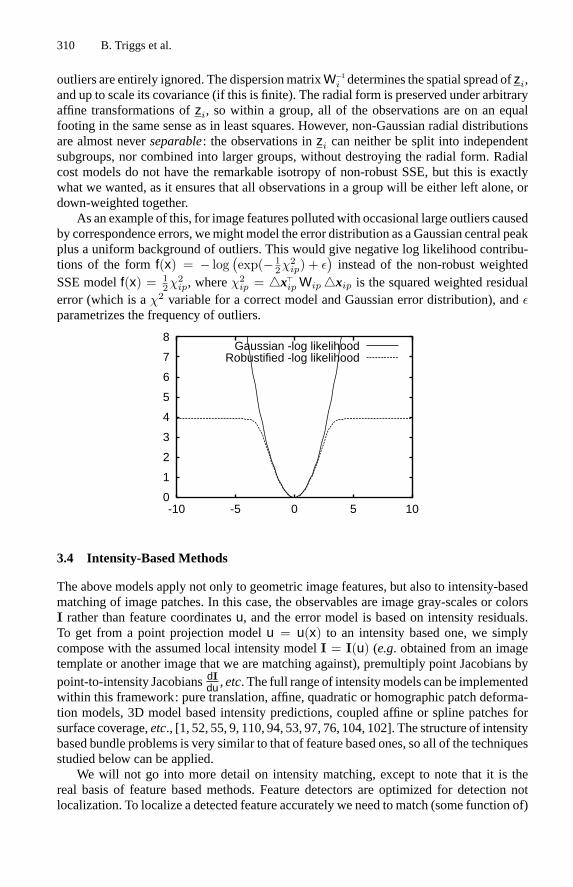
and up to scale its covariance (if this is finite). The radial form is preserved under arbitraryaffine transformations ofzi, so within a group, all of the observations are on an equalfooting in the same sense as in least squares. However, non-Gaussian radial distributionsare almost neverseparable: the observations inzi can neither be split into independentsubgroups, nor combined into larger groups, without destroying the radial form. Radialcost models do not have the remarkable isotropy of non-robust SSE, but this is exactlywhat we wanted, as it ensures that all observations in a group will be either left alone, ordown-weighted together.As an example of this, for image features pollutedwith occasional large outliers caused
by correspondence errors, wemightmodel the error distribution as aGaussian central peakplus a uniform background of outliers. This would give negative log likelihood contribu-tions of the formf(x) = − log
(exp(− 1
2χ2ip) + ε
)instead of the non-robust weighted
SSE modelf(x) = 12χ
2ip, whereχ
2ip = �x�
ip Wip�xip is the squared weighted residualerror (which is aχ2 variable for a correct model and Gaussian error distribution), andεparametrizes the frequency of outliers.
0
1
2
3
4
5
6
7
8
-10 -5 0 5 10
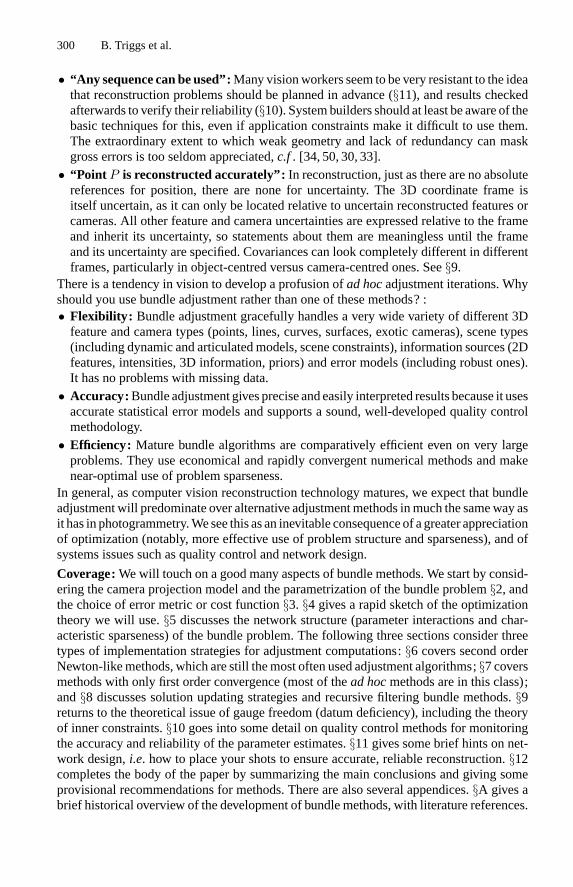
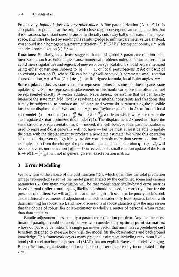
Gaussian -log likelihoodRobustified -log likelihood
3.4 Intensity-Based Methods
The above models apply not only to geometric image features, but also to intensity-basedmatching of image patches. In this case, the observables are image gray-scales or colorsI rather than feature coordinatesu, and the error model is based on intensity residuals.To get from a point projection modelu = u(x) to an intensity based one, we simplycompose with the assumed local intensity modelI = I(u) (e.g. obtained from an imagetemplate or another image that we are matching against), premultiply point Jacobians bypoint-to-intensity JacobiansdIdu ,etc. The full range of intensitymodels can be implementedwithin this framework: pure translation, affine, quadratic or homographic patch deforma-tion models, 3D model based intensity predictions, coupled affine or spline patches forsurface coverage,etc., [1, 52, 55, 9, 110, 94, 53, 97, 76, 104, 102]. The structure of intensitybased bundle problems is very similar to that of feature based ones, so all of the techniquesstudied below can be applied.We will not go into more detail on intensity matching, except to note that it is the
real basis of feature based methods. Feature detectors are optimized for detection notlocalization. To localize a detected feature accurately we need to match (some function of)
Bundle Adjustment — A Modern Synthesis 311
the image intensities in its region against either an idealized template or another image ofthe feature, using an appropriate geometric deformation model,etc. For example, supposethat the intensity matching model isf(u) = 1
2
∫∫ρ(‖δI(u)‖2) where the integration is
over some image patch,δI is the current intensity prediction error,u parametrizes the localgeometry (patch translation & warping), andρ(·) is some intensity error robustifier. Thenthe cost gradient in terms ofu is g�
u = dfdu =
∫∫ρ′ δI� dI
du . Similarly, the cost Hessian in
u in a Gauss-Newton approximation isHu = d2fdu2 ≈
∫∫ρ′′ ( dI
du )� dIdu . In a feature based
model, we expressu = u(x) as a function of the bundle parameters, so ifJu = dudx we have
a corresponding cost gradient and Hessian contributiong�x = g�
u Ju andHx = J�u Hu Ju.
In other words, the intensity matching model is locally equivalent to a quadratic featurematching one on the ‘features’u(x), with effective weight (inverse covariance) matrixWu = Hu. All image feature error models in vision are ultimately based on such anunderlying intensity matching model. As feature covariances are a function of intensitygradients
∫∫ρ′′ ( dI
du )� dIdu , they can be both highly variable between features (depending
on howmuch local gradient there is), and highly anisotropic (depending on howdirectionalthe gradients are).E.g., for points along a 1D intensity edge, the uncertainty is large in thealong edge direction and small in the across edge one.
3.5 Implicit Models
Sometimes observations are most naturally expressed in terms of an implicit observation-constraining modelh(x, z) = 0, rather than an explicit observation-predicting onez =z(x). (The associated image error still has the formf(z − z)). For example, if the modelis a 3D curve and we observe points on it (the noisy images of 3D points that may lieanywhere along the 3D curve), we can predict the whole image curve, but not the exactposition of each observation along it. We only have the constraint that the noiseless imageof the observed point would lie on the noiseless image of the curve, if we knew these. Thereare basically two ways to handle implicit models: nuisance parameters and reduction.Nuisance parameters:In this approach, the model is made explicit by adding additional‘nuisance’ parameters representing something equivalent to model-consistent estimatesof the unknown noise free observations,i.e. to z with h(x, z) = 0. The most direct wayto do this is to include the entire parameter vectorz as nuisance parameters, so that wehave to solve a constrained optimization problem on the extended parameter space(x, z),minimizing f(z − z) over (x, z) subject toh(x, z) = 0. This is a sparse constrainedproblem, which can be solved efficiently using sparse matrix techniques (§6.3). In fact,for image observations, the subproblems inz (optimizing f(z − z) over z for fixed zandx) are small and for typicalf rather simple. So in spite of the extra parametersz,optimizing this model is not significantly more expensive than optimizing an explicit onez = z(x) [14, 13, 105, 106]. For example, when estimating matching constraints betweenimage pairs or triplets [60, 62], instead of using an explicit 3D representation, pairs ortriplets of corresponding image points can be used as featureszi, subject to the epipolaror trifocal geometry contained inx [105, 106].However, if a smaller nuisance parameter vector thanz can be found, it is wise to use
it. In the case of a curve, it suffices to include just one nuisance parameter per observation,saying where along the curve the corresponding noise free observation is predicted tolie. This model exactly satisfies the constraints, so it converts the implicit model to anunconstrained explicit onez = z(x,λ), whereλ are the along-curve nuisance parameters.
312 B. Triggs et al.
The advantage of the nuisance parameter approach is that it gives the exact optimalparameter estimate forx, and jointly, optimalx-consistent estimates for the noise freeobservationsz.
Reduction: Alternatively, we can regardh(x, z) rather thanz as the observation vector,and hence fit the parameters to the explicit log likelihood model forh(x, z). To do this,we must transfer the underlying error model / distributionf(�z) on z to one f(h) onh(x, z). In principle, this should be done by marginalization: the density forh is givenby integrating that for�z over all�z giving the sameh. Within the point estimationframework, it can beapproximated by replacing the integrationwithmaximization.Neithercalculation is easy in general, but in the asymptotic limit where first order Taylor expansionh(x, z) = h(x, z +�z) ≈ 0 + dh
dz �z is valid, the distribution ofh is a marginalization ormaximization of that of�z over affine subspaces. This can be evaluated in closed form forsome robust distributions. Also, standard covariance propagation gives (more precisely,this applies to theh and�z dispersions):
〈h(x, z)〉 ≈ 0 , 〈h(x, z) h(x, z)�〉 ≈ dhdz 〈�z�z�〉 dh
dz
�= dh
dz W−1 dhdz
�(4)
whereW−1 is the covariance of�z. So at least for an outlier-free Gaussian model, thereduced distribution remains Gaussian (albeit withx-dependent covariance).
4 Basic Numerical Optimization
Having chosen a suitable model quality metric, we must optimize it. This section gives avery rapid sketch of the basic local optimization methods for differentiable functions. See[29, 93, 42] for more details. We need to minimize a cost functionf(x) over parametersx,starting from some given initial estimatex of the minimum, presumably supplied by someapproximate visual reconstructionmethodor prior knowledgeof theapproximate situation.As in §2.2, the parameter space may be nonlinear, but we assume that local displacementscan be parametrized by a local coordinate system / vector of free parametersδx. We tryto find a displacementx → x + δx that locally minimizes or at least reduces the costfunction. Real cost functions are too complicated to minimize in closed form, so insteadweminimize an approximatelocal modelfor the function,e.g. based on Taylor expansionor some other approximation at the current pointx. Although this does not usually give theexact minimum, with luck it will improve on the initial parameter estimate and allow us toiterate to convergence. The art of reliable optimization is largely in the details that makethis happen even without luck: which local model, how to minimize it, how to ensure thatthe estimate is improved, and how to decide when convergence has occurred. If you notare interested in such subjects, use a professionally designed package (§C.2): detailsareimportant here.
4.1 Second Order Methods
The reference for all local models is the quadratic Taylor series one:
f(x + δx) ≈ f(x) + g� δx + 12δx� H δx g ≡ df
dx (x) H ≡ d2fdx2 (x)
quadratic local model gradient vector Hessian matrix(5)
Bundle Adjustment — A Modern Synthesis 313
For now, assume that the HessianH is positive definite (but see below and§9). The localmodel is then a simple quadratic with a unique global minimum, which can be foundexplicitly using linear algebra. Settingdf
dx (x + δx) ≈ H δx + g to zero for the stationarypoint gives theNewton step:
δx = −H−1g (6)
The estimated new function value isf(x + δx) ≈ f(x) − 12δx� H δx = f(x) − 1
2g� H−1g.Iterating the Newton step givesNewton’s method. This is the canonical optimizationmethod for smooth cost functions, owing to its exceptionally rapid theoretical and practicalconvergence near the minimum. For quadratic functions it converges in one iteration, andfor more general analytic ones itsasymptotic convergenceis quadratic : as soon as theestimate gets close enough to the solution for the second order Taylor expansion to bereasonably accurate, the residual state error is approximatelysquaredat each iteration.This means that the number of significant digits in the estimate approximately doubles ateach iteration, so starting from any reasonable estimate, at most aboutlog2(16)+1 ≈ 5–6iterations are needed for full double precision (16 digit) accuracy. Methods that potentiallyachieve such rapid asymptotic convergence are calledsecond order methods. This is ahighaccolade for a local optimizationmethod, but it canonly beachieved if theNewtonstepis asymptotically well approximated. Despite their conceptual simplicity and asymptoticperformance, Newton-like methods have some disadvantages:• To guarantee convergence, a suitable step control policy must be added (§4.2).• Solving then× n Newton step equations takes timeO(n3
)for a dense system (§B.1),
which can be prohibitive for largen. Although the cost can often be reduced (verysubstantially for bundle adjustment) by exploiting sparseness inH, it remains true thatNewton-like methods tend to have a high cost per iteration, which increases relative tothat of other methods as the problem size increases. For this reason, it is sometimesworthwhile to consider more approximatefirst order methods (§7), which are occa-sionally more efficient, and generally simpler to implement, than sparse Newton-likemethods.• Calculating second derivativesH is by no means trivial for a complicated cost func-tion, both computationally, and in terms of implementation effort. TheGauss-Newtonmethod (§4.3) offers a simple analytic approximation toH for nonlinear least squaresproblems. Some other methods build up approximations toH from the way the gradientg changes during the iteration are in use (see§7.1, Krylov methods).• The asymptotic convergence of Newton-like methods is sometimes felt to be an expen-sive luxury when far from theminimum, especially when damping (see below) is active.However, it must be said that Newton-like methods generally do require significantlyfewer iterations than first order ones, even far from the minimum.
4.2 Step Control
Unfortunately, Newton’s method can fail in several ways. It may converge to a saddlepoint rather than a minimum, and for large steps the second order cost prediction may beinaccurate, so there is no guarantee that the true cost will actually decrease. To guaranteeconvergence to a minimum, the step must follow a localdescent direction(a directionwith a non-negligible component down the local cost gradient, or if the gradient is zero
314 B. Triggs et al.
near a saddle point, down a negative curvature direction of the Hessian), and it must makereasonable progress in this direction (neither so little that the optimization runs slowlyor stalls, nor so much that it greatly overshoots the cost minimum along this direction).It is also necessary to decide when the iteration has converged, and perhaps to limit anyover-large steps that are requested. Together, these topics form the delicate subject ofstepcontrol.To choose a descent direction, one can take the Newton step direction if this descends
(it may not near a saddle point), or more generally some combination of the Newton andgradient directions.DampedNewtonmethodssolve a regularized system to find the step:
(H + λW) δx = −g (7)
Here,λ is some weighting factor andW is some positive definite weight matrix (oftenthe identity, soλ → ∞ becomes gradient descentδx ∝ −g). λ can be chosen to limitthe step to a dynamically chosen maximum size (trust region methods), or manipulatedmore heuristically, to shorten the step if the prediction is poor (Levenberg-Marquardtmethods).Given a descent direction, progress along it is usually assured by aline searchmethod,
of which there are many based on quadratic and cubic 1D cost models. If the suggested(e.g. Newton) step isδx, line search finds theα that actually minimizesf along the linex + α δx, rather than simply taking the estimateα = 1.There is no space for further details on step control here (again, see [29, 93, 42]). How-
ever note that poor step control can make a huge difference in reliability and convergencerates, especially for ill-conditioned problems. Unless you are familiar with these issues, itis advisable to use professionally designed methods.
4.3 Gauss-Newton and Least Squares
Consider the nonlinear weighted SSE cost modelf(x) ≡ 12 �z(x)� W�z(x) (§3.2) with
prediction error�z(x) = z−z(x) andweightmatrixW. Differentiation gives the gradientand Hessian in terms of theJacobianor design matrix of the predictive model,J ≡ dz
dx :
g ≡ dfdx = �z� W J H ≡ d2f
dx2 = J� W J +∑
i(�z� W)id2zi
dx2 (8)
These formulae could be used directly in a dampedNewtonmethod, but thed2zi
dx2 term inHis likely to be small in comparison to the corresponding components ofJ� W J if either: (i)
the prediction error�z(x) is small; or (ii ) the model is nearly linear,d2zi
dx2 ≈ 0. Droppingthe second term gives theGauss-Newton approximationto the least squares Hessian,H ≈ J� W J. With this approximation, the Newton step prediction equations become theGauss-Newtonor normal equations:
(J� W J) δx = −J� W�z (9)
The Gauss-Newton approximation is extremely common in nonlinear least squares, andpractically all current bundle implementations use it. Its main advantage is simplicity: thesecondderivativesof theprojectionmodelz(x)arecomplexand troublesome to implement.
Bundle Adjustment — A Modern Synthesis 315
In fact, the normal equations are just one of many methods of solving the weightedlinear least squares problem5 min δx
12 (J δx − �z)� W (J δx − �z). Another notable
method is that based on QR decomposition (§B.2, [11, 44]), which is up to a factor of twoslower than the normal equations, but much less sensitive to ill-conditioning inJ 6.Whichever solution method is used, the main disadvantage of the Gauss-Newton ap-
proximation is that when the discarded terms are not negligible, the convergence rate isgreatly reduced (§7.2). In our experience, such reductions are indeed common in highlynonlinear problems with (at the current step) large residuals. For example, near a saddlepoint the Gauss-Newton approximation isneveraccurate, as its predicted Hessian is al-ways at least positive semidefinite. However, for well-parametrized (i.e. locally near linear,§2.2) bundle problemsunder an outlier-free least squares costmodel evaluated near the costminimum, the Gauss-Newton approximation is usually very accurate. Feature extractionerrors and hence�z andW−1have characteristic scales of at most a few pixels. In contrast,the nonlinearities ofz(x) are caused by nonlinear 3D feature-camera geometry (perspec-tive effects) and nonlinear image projection (lens distortion). For typical geometries andlenses, neither effect varies significantly on a scale of a few pixels. So the nonlinear correc-tions are usually small compared to the leading order linear terms, and bundle adjustmentbehaves as a near-linear small residual problem.However note that this doesnot extend to robust cost models. Robustification works
by introducing strong nonlinearity into the cost function at the scale of typical featurereprojectionerrors. For accurate stepprediction, theoptimization routinemust takeaccountof this. For radial cost functions (§3.3), a reasonable compromise is to take account ofthe exact second order derivatives of the robustifiersρi(·), while retaining only the firstorder Gauss-Newton approximation for the predicted observationszi(x). If ρ′
i andρ′′ are
respectively the first and second derivatives ofρi at the current evaluation point, we havea robustified Gauss-Newton approximation:
gi = ρ′i J�
i Wi�zi Hi ≈ J�i (ρ′
i Wi + 2 ρ′′i (Wi�zi) (Wi�zi)
�) Ji (10)
So robustification has two effects: (i) it down-weights the entire observation (bothgi andHi) by ρ′
i ; and (ii ) it makes a rank-one reduction7 of the curvatureHi in the radial (�zi)
direction, to account for the way in which the weight changes with the residual. Thereare reweighting-based optimization methods that include only the first effect. They stillfind the true cost minimumg = 0 as thegi are evaluated exactly8, but convergence may
5 Here, the dependence ofJ onx is ignored, which amounts to the same thing as ignoring thed2zi
dx2term inH.
6 The QR method gives the solution to a relative error of aboutO(Cε), as compared toO(C2ε
)for the normal equations, whereC is the condition number (the ratio of the largest to the smallestsingular value) ofJ, andε is the machine precision (10−16 for double precision floating point).
7 The useful robustifiersρi are sublinear, withρ′i < 1 andρ′′
i < 0 in the outlier region.8 Reweighting is also sometimes used in vision to handle projective homogeneous scale factorsrather than error weighting.E.g., suppose that image points(u/w, v/w)� are generated by ahomogeneous projection equation(u, v, w)� = P (X,Y, Z, 1)�, whereP is the3 × 4 homoge-neous image projection matrix. A scale factor reweighting scheme might take derivatives w.r.t.u, v while treating the inverse weightw as a constant within each iteration. Minimizing the re-sulting globally bilinear linear least squares error model overP and(X,Y, Z)� doesnot givethe true cost minimum: it zeros the gradient-ignoring-w-variations, not the true cost gradient.Such schemes should not be used for precise work as the bias can be substantial, especially forwide-angle lenses and close geometries.
316 B. Triggs et al.
be slowed owing to inaccuracy ofH, especially for the mainly radial deviations producedby non-robust initializers containing outliers.Hi has a direction of negative curvature ifρ′′
i �z�i Wi�zi < − 1
2ρ′i, but if not we can even reduce the robustified Gauss-Newton
model to a local unweighted SSE one for which linear least squares methods can be used.For simplicity suppose thatWi has already reduced to1 by premultiplyingzi andJi byL�
i
whereLi L�i = Wi. Then minimizing theeffective squared error 1
2‖δzi − Ji δx‖2 givesthe correct second order robust state update, whereα ≡ RootOf( 1
2α2−α−ρ′′
i /ρ′i ‖�zi‖2)
and:
δzi ≡√ρ′
i
1− α�zi(x) Ji ≡
√ρ′
i
(1− α
�zi�z�i
‖�zi‖2)
Ji (11)
In practice, ifρ′′i ‖�zi‖2 � − 1
2ρ′i, we can use the same formulae but limitα ≤ 1− ε for
some smallε. However, the full curvature correction is not applied in this case.
4.4 Constrained Problems
More generally, we may want to minimize a functionf(x) subject to a set of constraintsc(x) = 0 on x. These might be scene constraints, internal consistency constraints on theparametrization (§2.2), or constraints arising from an implicit observation model (§3.5).Given an initial estimatex of the solution, we try to improve this by optimizing thequadratic local model forf subject to a linear local model of the constraintsc. This linearlyconstrained quadratic problem has an exact solution in linear algebra. Letg,H be thegradient and Hessian off as before, and let the first order expansion of the constraints bec(x+δx) ≈ c(x)+C δxwhereC ≡ dc
dx . Introduceavector of Lagrangemultipliersλ for c.
We seek thex+δx that optimizesf+c� λ subject toc = 0, i.e.0 = ddx (f+c� λ)(x+δx) ≈
g+H δx+C� λ and0 = c(x+δx) ≈ c(x)+C δx. Combining these gives theSequentialQuadratic Programming (SQP)step:(
H C�
C 0
)(δxλ
)= −
(gc
), f(x + δx) ≈ f(x)− 1
2
(g� c�)(H C�
C 0
)−1(gc
)(12)
(H C�
C 0
)−1
=(
H−1− H−1C� D−1C H−1 H−1C� D−1
D−1C H−1 −D−1
), D ≡ C H−1C� (13)
At the optimumδx andc vanish, butC� λ = −g, which is generally non-zero.An alternative constrained approach uses the linearized constraints to eliminate some
of the variables, then optimizes over the rest. Suppose that we can order the variablesto give partitionsx = (x1 x2)� andC = (C1 C2), whereC1 is square and invertible.Then usingC1 x1 + C2 x2 = C x = −c, we can solve forx1 in terms ofx2 and c:x1 = −C−1
1 (C2x2 + c). Substituting this into the quadratic cost model has the effect ofeliminatingx1, leaving a smaller unconstrainedreduced problemH22 x2 = −g2, where:
H22 ≡ H22 − H21 C−11 C2 − C�
2 C−�1 H12 + C�
2 C−�1 H11 C−1
1 C2 (14)
g2 ≡ g2 − C�2 C−�
1 g1 − (H21 − C�2 C−�
1 H11) C−11 c (15)
(These matrices can be evaluated efficiently using simple matrix factorization schemes[11]). This method is stable provided that the chosenC1 is well-conditioned. It works well
Bundle Adjustment — A Modern Synthesis 317
for dense problems, but is not always suitable for sparse ones because ifC is dense, thereduced HessianH22 becomes dense too.For least squares cost models, constraints can also be handled within the linear least
squares framework,e.g. see [11].
4.5 General Implementation Issues
Before going into details, we mention a few points of good numerical practice for large-scale optimization problems such as bundle adjustment:
Exploit the problemstructure: Large-scale problemsare almost always highly structuredand bundle adjustment is no exception. In professional cartography and photogrammetricsite-modelling, bundle problems with thousands of images and many tens of thousandsof features are regularly solved. Such problems would simply be infeasible without athorough exploitation of the natural structure and sparsity of the bundle problem. We willhave much to say about sparsity below.
Use factorization effectively:Many of above formulae contain matrix inverses. This isa convenient short-hand for theoretical calculations, butnumerically, matrix inversion isalmost never used. Instead, the matrix is decomposed into its Cholesky, LU, QR,etc.,factors and these are used directly,e.g. linear systems are solved using forwards andbackwards substitution. This is much faster and numerically more accurate than explicituse of the inverse, particularly for sparse matrices such as the bundle Hessian, whosefactors are still quite sparse, but whose inverse is always dense. Explicit inversion isrequired only occasionally,e.g. for covariance estimates, and even then only a few ofthe entries may be needed (e.g. diagonal blocks of the covariance). Factorization is theheart of the optimization iteration, where most of the time is spent and where most can bedone to improve efficiency (by exploiting sparsity, symmetry and other problem structure)and numerical stability (by pivoting and scaling). Similarly, certain matrices (subspaceprojectors, Householder matrices) have (diagonal)+(low rank) forms which should not beexplicitly evaluated as they can be applied more efficiently in pieces.
Use stable local parametrizations:As discussed in§2.2, the parametrization used forstep prediction need not coincide with the global one used to store the state estimate. It ismore important that it should be finite, uniform and locally as nearly linear as possible.If the global parametrization is in some way complex, highly nonlinear, or potentiallyill-conditioned, it is usually preferable to use a stable local parametrization based onperturbations of the current state for step prediction.
Scaling and preconditioning:Another parametrization issue that has a profound and too-rarely recognized influence on numerical performance isvariable scaling (the choice of‘units’ or reference scale to use for each parameter), and more generallypreconditioning(the choice of which linear combinations of parameters to use). These represent the linearpart of the general parametrization problem. The performance of gradient descent andmostother linearly convergent optimizationmethods is critically dependent on preconditioning,to the extent that for large problems, they are seldom practically useful without it.One of the great advantages of the Newton-like methods is their theoretical indepen-
dence of such scaling issues9. But even for these, scaling makes itself felt indirectly in
9 Under a linear change of coordinatesx → Tx we haveg → T−� g and H → T−� H T−1, so theNewton stepδx = −H−1g varies correctly asδx → T δx, whereas the gradient oneδx ∼ g
318 B. Triggs et al.
Networkgraph
graphconnectionParameter
3
D
EC CB
D1
2
A
E4
3 K2
K1
A
2
1 4B
J =
AB C DE 1 2 3 4 K1K2
A1
A2
B1
B2
B4
C1
C3
D2
D3
D4
E3
E4
H =
AB C DE 1 2 3 4 K1K2
A
B
C
D
E
1
2
3
4
K1K2
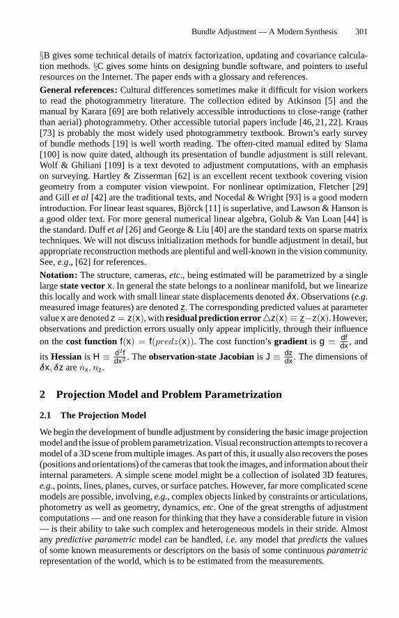
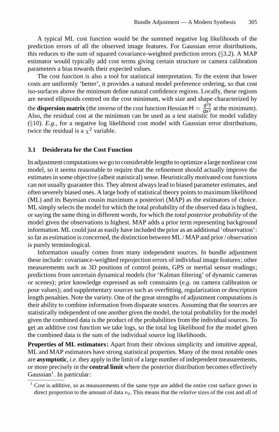
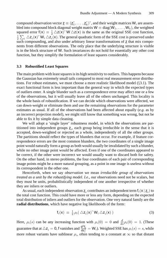
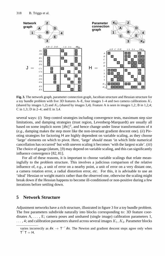
Fig. 3.The network graph, parameter connection graph, Jacobian structure and Hessian structure fora toy bundle problem with five 3D features A–E, four images 1–4 and two camera calibrationsK1
(shared by images 1,2) andK2 (shared by images 3,4). Feature A is seen in images 1,2; B in 1,2,4;C in 1,3; D in 2–4; and E in 3,4.
several ways: (i) Step control strategies including convergence tests, maximum step sizelimitations, and damping strategies (trust region, Levenberg-Marquardt) are usually allbased on some implicit norm‖δx‖2, and hence change under linear transformations ofx(e.g., damping makes the step more like the non-invariant gradient descent one). (ii ) Piv-oting strategies for factoringH are highly dependent on variable scaling, as they choose‘large’ elements on which to pivot. Here, ‘large’shouldmean ‘in which little numericalcancellation has occurred’ but with uneven scaling it becomes ‘with the largest scale’. (iii )The choice of gauge (datum,§9) may depend on variable scaling, and this can significantlyinfluence convergence [82, 81].For all of these reasons, it is important to choose variable scalings that relate mean-
ingfully to the problem structure. This involves a judicious comparison of the relativeinfluence of,e.g., a unit of error on a nearby point, a unit of error on a very distant one,a camera rotation error, a radial distortion error,etc. For this, it is advisable to use an‘ideal’ Hessian or weight matrix rather than the observed one, otherwise the scaling mightbreak down if the Hessian happens to become ill-conditioned or non-positive during a fewiterations before settling down.
5 Network Structure
Adjustment networks have a rich structure, illustrated in figure 3 for a toy bundle problem.The free parameters subdivide naturally into blocks corresponding to: 3D feature coor-dinates A,. . . , E; camera poses and unshared (single image) calibration parameters 1,. . . , 4; and calibration parameters shared across several imagesK1,K2. Parameter blocks
varies incorrectly asδx → T−� δx. The Newton and gradient descent steps agree only whenT� T = H.
Bundle Adjustment — A Modern Synthesis 319
interact only via their joint influence on image features and other observations,i.e. via theirjoint appearance in cost function contributions. The abstract structure of the measurementnetwork can be characterized graphically by thenetwork graph (top left), which showswhich features are seen in which images, and theparameter connection graph(top right)which details the sparse structure by showing which parameter blocks have direct interac-tions. Blocks are linked if and only if they jointly influence at least one observation. Thecost function Jacobian (bottom left) andHessian (bottom right) reflect this sparse structure.The shaded boxes correspond to non-zero blocks of matrix entries. Each block of rows inthe Jacobian corresponds to an observed image feature and contains contributions fromeach of the parameter blocks that influenced this observation. The Hessian contains anoff-diagonal block for each edge of the parameter connection graph,i.e. for each pair ofparameters that couple to at least one common feature / appear in at least one commoncost contribution10.Two layers of structure are visible in the Hessian. Theprimary structure consists of
the subdivision into structure (A–E) and camera (1–4,K1–K2) submatrices. Note that thestructure submatrix is block diagonal: 3D features couple only to cameras, not to otherfeatures. (This would no longer hold if inter-feature measurements such as distances orangles between points were present). The camera submatrix is often also block diagonal,but in this example the sharing of unknown calibration parameters produces off-diagonalblocks. Thesecondary structure is the internal sparsity pattern of the structure-cameraHessian submatrix. This is dense for small problems where all features are seen in allimages, but in larger problems it often becomes quite sparse because each image only seesa fraction of the features.All worthwhile bundle methods exploit at least the primary structure of the Hessian,
and advanced methods exploit the secondary structure as well. The secondary structure isparticularly sparse and regular in surface coverage problems such grids of photographs inaerial cartography. Such problems can be handled using a fixed ‘nested dissection’ variablereordering (§6.3). But for themore irregular connectivities of close rangeproblems, generalsparse factorization methods may be required to handle secondary structure.Bundle problems are by no means limited to the above structures. For example, for
more complex scene models with moving or articulated objects, there will be additionalconnections to object pose or joint angle nodes, with linkages reflecting the kinematicchain structure of the scene. It is often also necessary to add constraints to the adjustment,e.g. coplanarity of certain points. One of the greatest advantages of the bundle technique isits ability to adapt to almost arbitrarily complex scene, observation and constraint models.
10 The Jacobian structure canbedescribedmoredirectly by abipartite graphwhosenodes correspondon one side to the observations, and on the other to the parameter blocks that influence them. Theparameter connection graph is then obtained by deleting each observation node and linking eachpair of parameter nodes that it connects to. This is an example of elimination graph processing(see below).
320 B. Triggs et al.
6 Implementation Strategy 1: Second Order Adjustment Methods
The next three sections cover implementation strategies for optimizing the bundle adjust-ment cost functionf(x) over the complete set of unknown structure and camera parametersx. This section is devoted to second-order Newton-style approaches, which are the basisof the great majority of current implementations. Their most notable characteristics arerapid (second order) asymptotic convergence but relatively high cost per iteration, with
an emphasis on exploiting the network structure (the sparsity of the HessianH = d2fdx2 )
for efficiency. In fact, the optimization aspects are more or less standard (§4, [29, 93, 42]),so we will concentrate entirely on efficient methods for solving the linearized Newtonstep prediction equationsδx = −H−1g, (6). For now, we will assume that the HessianH is non-singular. This will be amended in§9 on gauge freedom, without changing theconclusions reached here.
6.1 The Schur Complement and the Reduced Bundle System
Schur complement:Consider the following block triangular matrix factorization:
M =(
A BC D
)=(
1 0C A−1 1
)(A 00 D
)(1 A−1B0 1
), D ≡ D− C A−1B (16)
( A BC D )−1
=(
1 −A−1B0 1
)(A−1 00 D
−1
)(1 0
−C A−1 1
)=(
A−1+A−1B D−1
C A−1 −A−1B D−1
−D−1
C A−1 D−1
)(17)
HereA must be square and invertible, and for (17), the whole matrix must also be squareand invertible.D is called theSchur complementofA inM. If bothA andD are invertible,complementing onD rather thanA gives
( A BC D )−1
=(
A−1 −A
−1B D−1
−D C A−1
D−1+D−1C A−1
B D−1
), A = A − B D−1C
Equating upper left blocks gives theWoodbury formula :
(A ± B D−1C)−1 = A−1∓ A−1B (D± C A−1B)−1 C A−1 (18)
This is the usual method of updating the inverse of a nonsingular matrixA after an update(especially a low rank one)A→ A ± B D−1C . (See§8.1).Reduction: Now consider the linear system( A B
C D )( x1x2 ) =
(b1b2
). Pre-multiplying by(
1 0−C A−1 1
)gives
(A B0 D
)( x1
x2 ) =(
b1
b2
)whereb2 ≡ b2 − C A−1b1. Hence we can use
Schur complement and forward substitution to find areduced systemD x2 = b2, solvethis forx2, then back-substitute and solve to findx1 :
D ≡ D− C A−1Bb2 ≡ b2 − C A−1b1
Schur complement +forward substitution
D x2 = b2 A x1 = b1 − B x2
reduced system back-substitution(19)
Bundle Adjustment — A Modern Synthesis 321
Note that the reducedsystementirely subsumes the contributionof thex1 rowsandcolumnsto the network. Once we have reduced, we can pretend that the problem does not involvex1 at all — it can be found later by back-substitution if needed, or ignored if not. This isthe basis of all recursive filtering methods. In bundle adjustment, if we use the primarysubdivision into feature and camera variables and subsume the structure ones, we get thereduced camera systemHCC xC = gC , where:
HCC ≡ HCC − HCS H−1SS HSC = HCC −
∑pHCp H−1
pp HpC
gC ≡ gC − HCS H−1SS gS = gC −
∑pHCp H−1
pp gp
(20)
Here, ‘S’ selects the structure block and ‘C ’ the camera one.HSS is block diagonal,so the reduction can be calculated rapidly by a sum of contributions from the individual3D features ‘p’ in S. Brown’s original 1958 method for bundle adjustment [16, 19, 100]was based on finding the reduced camera system as above, and solving it using Gaussianelimination. Profile Cholesky decomposition (§B.3) offers a more streamlined method ofachieving this.Occasionally, long image sequences havemore camera parameters than structure ones.
In this case it ismoreefficient to reduce thecameraparameters, leavingareducedstructuresystem.
6.2 Triangular Decompositions
If D in (16) is further subdivided into blocks, the factorization process can be contin-ued recursively. In fact, there is a family of block (lower triangular)*(diagonal)*(uppertriangular) factorizationsA = L D U:
(A11 A12 ··· A1nA21 A22 ··· A2n...
.........
Am1 Am2 ··· Amn
)=
L11L21 L22...
......
......
...Lm1 Lm2 ··· Lmr
(
D1D2 ...
Dr
)(U11 U12 ··· ··· U1n
U22 ··· ··· U2n......
··· Urn
)
(21)
See§B.1 for computational details. The main advantage of triangular factorizations is thatthey make linear algebra computations with the matrix much easier. In particular, if theinput matrixA is square and nonsingular, linear equationsA x = b can be solved by asequenceof three recursions that implicitly implementmultiplicationbyA−1 = U−1D−1L−1:
L c = b ci ← L−1ii
(bi −
∑j<i Lij cj
)forward substitution (22)
D d = c di ← D−1i ci diagonal solution (23)
U x = d xi ← U−1ii
(di −
∑j>i Uij xj
)back-substitution (24)
Forward substitution corrects for the influence of earlier variables on later ones, diagonalsolution solves the transformed system, and back-substitution propagates corrections dueto later variables back to earlier ones. In practice, this is usual method of solving linearequations such as the Newton step prediction equations. It is stabler and much faster thanexplicitly invertingA and multiplying byA−1.
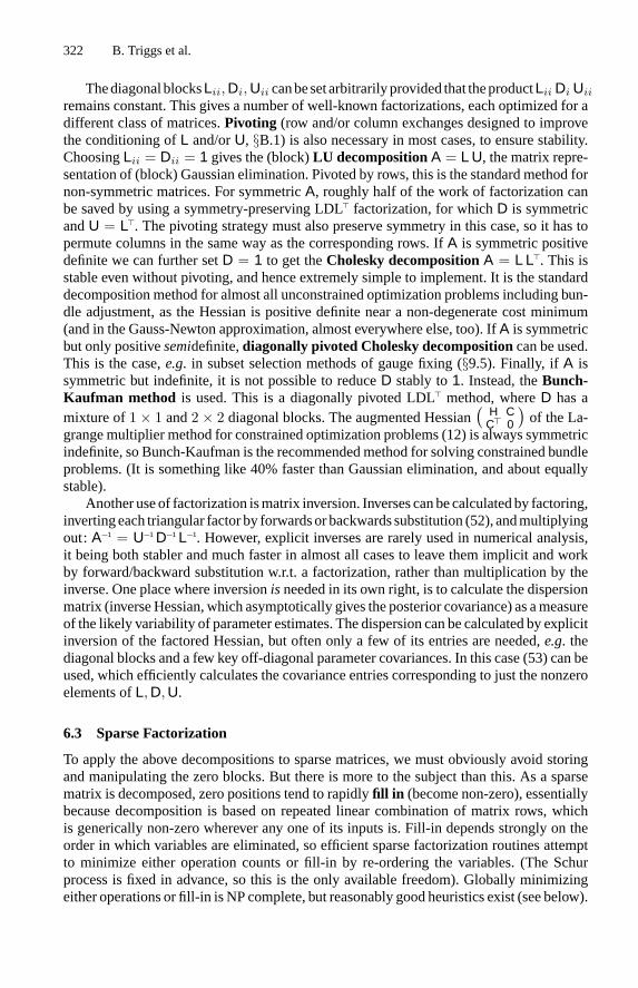
322 B. Triggs et al.
ThediagonalblocksLii,Di,Uii canbesetarbitrarilyprovided that theproductLii Di Uii
remains constant. This gives a number of well-known factorizations, each optimized for adifferent class of matrices.Pivoting (row and/or column exchanges designed to improvethe conditioning ofL and/orU, §B.1) is also necessary in most cases, to ensure stability.ChoosingLii = Dii = 1 gives the (block)LU decompositionA = L U, the matrix repre-sentation of (block) Gaussian elimination. Pivoted by rows, this is the standard method fornon-symmetric matrices. For symmetricA, roughly half of the work of factorization canbe saved by using a symmetry-preserving LDL� factorization, for whichD is symmetricandU = L�. The pivoting strategy must also preserve symmetry in this case, so it has topermute columns in the same way as the corresponding rows. IfA is symmetric positivedefinite we can further setD = 1 to get theCholesky decompositionA = L L�. This isstable even without pivoting, and hence extremely simple to implement. It is the standarddecomposition method for almost all unconstrained optimization problems including bun-dle adjustment, as the Hessian is positive definite near a non-degenerate cost minimum(and in the Gauss-Newton approximation, almost everywhere else, too). IfA is symmetricbut only positivesemidefinite,diagonally pivoted Cholesky decompositioncan be used.This is the case,e.g. in subset selection methods of gauge fixing (§9.5). Finally, ifA issymmetric but indefinite, it is not possible to reduceD stably to1. Instead, theBunch-Kaufman method is used. This is a diagonally pivoted LDL� method, whereD has amixture of1× 1 and2× 2 diagonal blocks. The augmented Hessian
(H C
C� 0
)of the La-
grangemultiplier method for constrained optimization problems (12) is always symmetricindefinite, so Bunch-Kaufman is the recommendedmethod for solving constrained bundleproblems. (It is something like 40% faster than Gaussian elimination, and about equallystable).Another useof factorization ismatrix inversion. Inverses canbecalculatedby factoring,
invertingeach triangular factor by forwardsorbackwardssubstitution (52), andmultiplyingout:A−1 = U−1D−1L−1. However, explicit inverses are rarely used in numerical analysis,it being both stabler and much faster in almost all cases to leave them implicit and workby forward/backward substitution w.r.t. a factorization, rather than multiplication by theinverse. One place where inversionisneeded in its own right, is to calculate the dispersionmatrix (inverseHessian, which asymptotically gives the posterior covariance) as ameasureof the likely variability of parameter estimates. The dispersion can be calculated by explicitinversion of the factored Hessian, but often only a few of its entries are needed,e.g. thediagonal blocks and a few key off-diagonal parameter covariances. In this case (53) can beused, which efficiently calculates the covariance entries corresponding to just the nonzeroelements ofL,D,U.
6.3 Sparse Factorization
To apply the above decompositions to sparse matrices, we must obviously avoid storingand manipulating the zero blocks. But there is more to the subject than this. As a sparsematrix is decomposed, zero positions tend to rapidlyfill in (become non-zero), essentiallybecause decomposition is based on repeated linear combination of matrix rows, whichis generically non-zero wherever any one of its inputs is. Fill-in depends strongly on theorder in which variables are eliminated, so efficient sparse factorization routines attemptto minimize either operation counts or fill-in by re-ordering the variables. (The Schurprocess is fixed in advance, so this is the only available freedom). Globally minimizingeither operations or fill-in is NP complete, but reasonably good heuristics exist (see below).

Bundle Adjustment — A Modern Synthesis 323
Variable order affects stability (pivoting) as well as speed, and these two goals conflict tosome extent. Finding heuristics that work well on both counts is still a research problem.Algorithmically, fill-in is characterized by anelimination graph derived from the pa-
rameter coupling / Hessian graph [40, 26, 11]. To create this, nodes (blocks of parameters)are visited in the given elimination ordering, at each step linking together all unvisitednodes that are currently linked to the current node. The coupling of blocki to blockj viavisited blockk corresponds to a non-zero Schur contributionLik D−1
k Ukj , and at each stagethe subgraph on the currently unvisited nodes is the coupling graph of the current reducedHessian. The amount of fill-in is the number of new graph edges created in this process.
Pattern Matrices We seek variable orderings that approximately minimize the totaloperation count or fill-in over the whole elimination chain. For many problems a suitableordering can be fixed in advance, typically giving one of a few standard pattern matricessuch as band or arrowhead matrices, perhaps with such structure at several levels.
bundle Hessian arrowhead matrix block tridiagonal matrix
(25)
The most prominent pattern structure in bundle adjustment is the primary subdivision ofthe Hessian into structure and camera blocks. To get the reduced camera system (19),we treat the Hessian as an arrowhead matrix with a broad final column containing all ofthe camera parameters. Arrowhead matrices are trivial to factor or reduce by block2× 2Schur complementation,c.f . (16, 19). For bundle problemswithmany independent imagesand only a few features, one can also complement on the image parameter block to get areducedstructuresystem.Another very commonpattern structure is theblock tridiagonal onewhich characterizes
all singly coupled chains (sequencesof imageswith only pairwiseoverlap,Kalmanfilteringand other time recursions, simple kinematic chains). Tridiagonal matrices are factored orreduced by recursive block2 × 2 Schur complementation starting from one end. TheLandU factors are also block tridiagonal, but the inverse is generally dense.Pattern orderings are often very natural but it is unwise to think of them as immutable:
structure often occurs at several levels anddeeper structure or simply changes in the relativesizes of the various parameter classesmaymake alternative orderings preferable. For moredifficult problems there are two basic classes of on-line ordering strategies.Bottom-upmethods try to minimize fill-in locally and greedily at each step, at the risk of global short-sightedness.Top-downmethods take a divide-and-conquer approach, recursively splittingthe problem into smaller sub-problems which are solved quasi-independently and latermerged.
Top-DownOrderingMethods Themost common top-downmethod is callednested dis-sectionor recursive partitioning [64, 57, 19, 38, 40, 11]. The basic idea is to recursivelysplit the factorization problem into smaller sub-problems, solve these independently, and
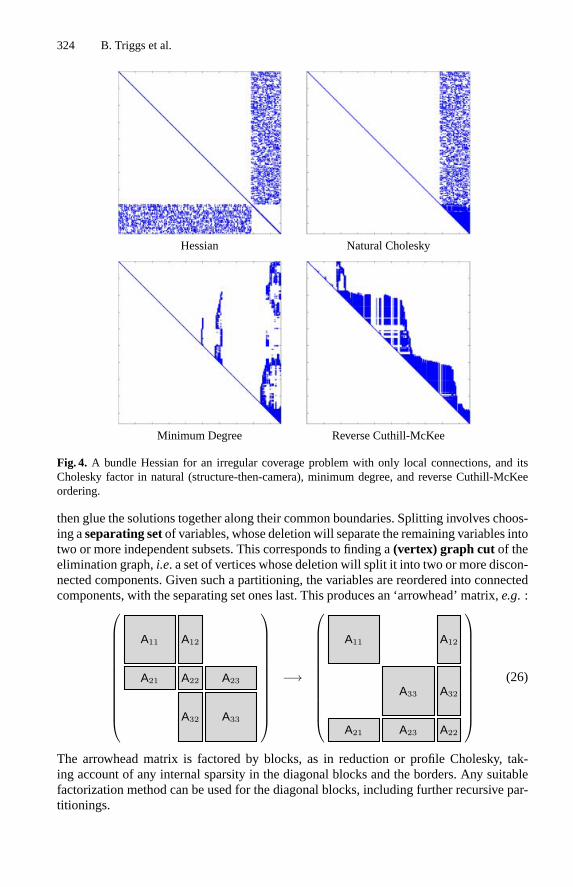
324 B. Triggs et al.
Hessian Natural Cholesky
Minimum Degree Reverse Cuthill-McKee
Fig. 4. A bundle Hessian for an irregular coverage problem with only local connections, and itsCholesky factor in natural (structure-then-camera), minimum degree, and reverse Cuthill-McKeeordering.
then glue the solutions together along their common boundaries. Splitting involves choos-ing aseparating setof variables, whose deletion will separate the remaining variables intotwo or more independent subsets. This corresponds to finding a(vertex) graph cut of theelimination graph,i.e. a set of vertices whose deletion will split it into two or more discon-nected components. Given such a partitioning, the variables are reordered into connectedcomponents, with the separating set ones last. This produces an ‘arrowhead’ matrix,e.g. :
A11 A12
A21 A22 A23
A32 A33
−→
A11 A12
A33 A32
A21 A23 A22
(26)
The arrowhead matrix is factored by blocks, as in reduction or profile Cholesky, tak-ing account of any internal sparsity in the diagonal blocks and the borders. Any suitablefactorization method can be used for the diagonal blocks, including further recursive par-titionings.
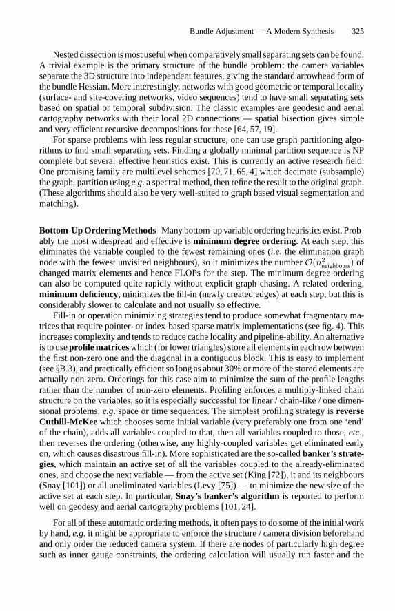
Bundle Adjustment — A Modern Synthesis 325
Nesteddissection ismostusefulwhencomparatively small separatingsetscanbe found.A trivial example is the primary structure of the bundle problem: the camera variablesseparate the 3D structure into independent features, giving the standard arrowhead form ofthe bundle Hessian. More interestingly, networks with good geometric or temporal locality(surface- and site-covering networks, video sequences) tend to have small separating setsbased on spatial or temporal subdivision. The classic examples are geodesic and aerialcartography networks with their local 2D connections — spatial bisection gives simpleand very efficient recursive decompositions for these [64, 57, 19].For sparse problems with less regular structure, one can use graph partitioning algo-
rithms to find small separating sets. Finding a globally minimal partition sequence is NPcomplete but several effective heuristics exist. This is currently an active research field.One promising family are multilevel schemes [70, 71, 65, 4] which decimate (subsample)the graph, partition usinge.g. a spectral method, then refine the result to the original graph.(These algorithms should also be very well-suited to graph based visual segmentation andmatching).
Bottom-UpOrderingMethods Manybottom-up variable orderingheuristics exist. Prob-ably the most widespread and effective isminimum degree ordering. At each step, thiseliminates the variable coupled to the fewest remaining ones (i.e. the elimination graphnode with the fewest unvisited neighbours), so it minimizes the numberO(n2
neighbours) ofchanged matrix elements and hence FLOPs for the step. The minimum degree orderingcan also be computed quite rapidly without explicit graph chasing. A related ordering,minimum deficiency, minimizes the fill-in (newly created edges) at each step, but this isconsiderably slower to calculate and not usually so effective.Fill-in or operation minimizing strategies tend to produce somewhat fragmentary ma-
trices that require pointer- or index-based sparse matrix implementations (see fig. 4). Thisincreases complexity and tends to reduce cache locality and pipeline-ability. An alternativeis to useprofilematriceswhich (for lower triangles) store all elements in each rowbetweenthe first non-zero one and the diagonal in a contiguous block. This is easy to implement(see§B.3), and practically efficient so long as about 30%ormore of the stored elements areactually non-zero. Orderings for this case aim to minimize the sum of the profile lengthsrather than the number of non-zero elements. Profiling enforces a multiply-linked chainstructure on the variables, so it is especially successful for linear / chain-like / one dimen-sional problems,e.g. space or time sequences. The simplest profiling strategy isreverseCuthill-McKee which chooses some initial variable (very preferably one from one ‘end’of the chain), adds all variables coupled to that, then all variables coupled to those,etc.,then reverses the ordering (otherwise, any highly-coupled variables get eliminated earlyon, which causes disastrous fill-in). More sophisticated are the so-calledbanker’s strate-gies, which maintain an active set of all the variables coupled to the already-eliminatedones, and choose the next variable — from the active set (King [72]), it and its neighbours(Snay [101]) or all uneliminated variables (Levy [75]) — to minimize the new size of theactive set at each step. In particular,Snay’s banker’s algorithm is reported to performwell on geodesy and aerial cartography problems [101, 24].
For all of these automatic orderingmethods, it often pays to do some of the initial workby hand,e.g. it might be appropriate to enforce the structure / camera division beforehandand only order the reduced camera system. If there are nodes of particularly high degreesuch as inner gauge constraints, the ordering calculation will usually run faster and the
326 B. Triggs et al.
quality may also be improved by removing these from the graph and placing them last byhand.The above ordering methods apply to both Cholesky / LDL� decomposition of the
Hessian and QR decomposition of the least squares Jacobian. Sparse QR methods can beimplemented either with Givens rotations or (more efficiently) with sparse Householdertransformations. Row ordering is important for the Givens methods [39]. For Householderones (and some Givens ones too) themultifrontal organization is now usual [41, 11], asit captures the natural parallelism of the problem.
7 Implementation Strategy 2: First Order Adjustment Methods
We have seen that for large problems, factoring the HessianH to compute the Newtonstep can be both expensive and (if done efficiently) rather complex. In this section weconsider alternative methods that avoid the cost of exact factorization. As the Newton stepcan not be calculated, such methods generally only achieve first order (linear) asymptoticconvergence: when close to the final state estimate, the error is asymptotically reduced by aconstant (and inpracticeoftendepressinglysmall) factorateachstep,whereasquadraticallyconvergent Newton methods roughly double the number of significant digits at each step.So first order methods require more iterations than second order ones, but each iterationis usually much cheaper. The relative efficiency depends on the relative sizes of thesetwo effects, both of which can be substantial. For large problems, the reduction in workper iteration is usually at leastO(n), wheren is the problem size. But whereas Newtonmethods converge fromO(1) toO(10−16
)in about1 + log2 16 = 5 iterations, linearly
convergent ones take respectivelylog 10−16/ log(1 − γ) = 16, 350, 3700 iterations forreductionγ = 0.9, 0.1, 0.01 per iteration. Unfortunately, reductions of only1% or less areby no means unusual in practice (§7.2), and the reduction tends to decrease asn increases.
7.1 First Order Iterations
Wefirst consider a number of common first ordermethods, before returning to the questionof why they are often slow.
Gradient descent:The simplest first order method isgradient descent, which “slidesdown the gradient” by takingδx ∼ g orHa = 1. Line search is needed, to find an appro-priate scale for the step. For most problems, gradient descent is spectacularly inefficientunless theHessian actually happens to be very close to amultiple of1. This can be arrangedby preconditioning with a linear transformL, x → L x, g → L−� g andH → L−� H L−1,whereL L� ∼ H is an approximate Cholesky factor (or other left square root) ofH, so thatH → L−� H L−1 ∼ 1. In this very special case, preconditioned gradient descent approxi-mates the Newton method. Strictly speaking, gradient descent is a cheat: the gradient is acovector (linear form on vectors) not a vector, so it does not actually define a direction inthe search space. Gradient descent’s sensitivity to the coordinate system is one symptomof this.
Alternation: Another simple approach isalternation : partition the variables into groupsand cycle through the groups optimizing over each in turn, with the other groups heldfixed. This is most appropriate when the subproblems are significantly easier to optimizethan the full one. A natural and often-rediscovered alternation for the bundle problem is
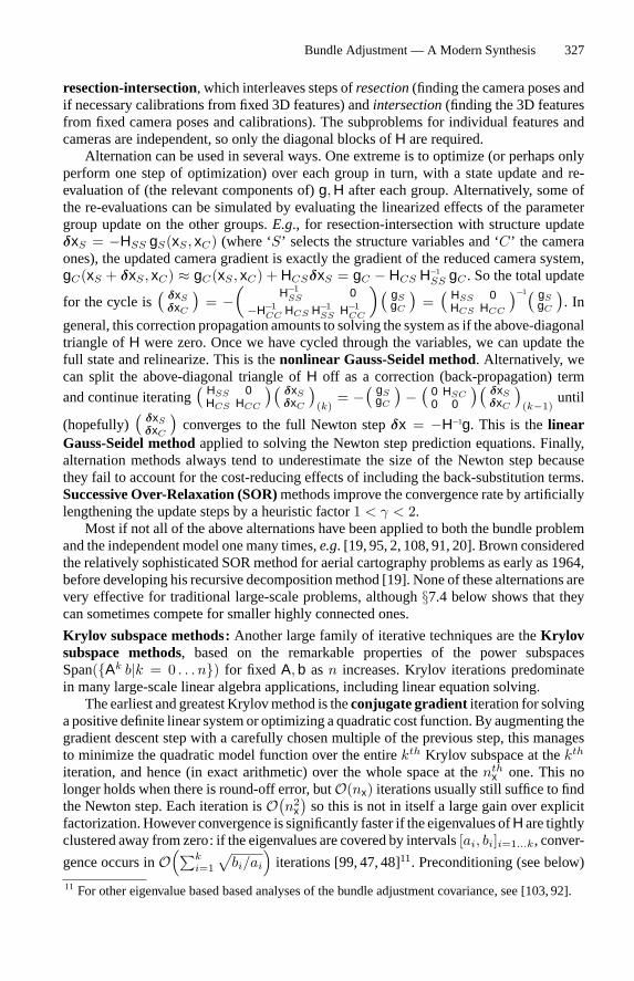
Bundle Adjustment — A Modern Synthesis 327
resection-intersection, which interleaves steps ofresection(finding the camera poses andif necessary calibrations from fixed 3D features) andintersection(finding the 3D featuresfrom fixed camera poses and calibrations). The subproblems for individual features andcameras are independent, so only the diagonal blocks ofH are required.Alternation can be used in several ways. One extreme is to optimize (or perhaps only
perform one step of optimization) over each group in turn, with a state update and re-evaluation of (the relevant components of)g,H after each group. Alternatively, some ofthe re-evaluations can be simulated by evaluating the linearized effects of the parametergroup update on the other groups.E.g., for resection-intersection with structure updateδxS = −HSS gS(xS , xC) (where ‘S’ selects the structure variables and ‘C ’ the cameraones), the updated camera gradient is exactly the gradient of the reduced camera system,gC(xS + δxS , xC) ≈ gC(xS , xC) + HCSδxS = gC − HCS H−1
SS gC . So the total update
for the cycle is(
δxSδxC
)= −
(H−1
SS 0
−H−1CC HCS H−1
SS H−1CC
)( gSgC
)=( HSS 0
HCS HCC
)−1( gSgC
). In
general, this correction propagation amounts to solving the system as if the above-diagonaltriangle ofH were zero. Once we have cycled through the variables, we can update thefull state and relinearize. This is thenonlinear Gauss-Seidel method. Alternatively, wecan split the above-diagonal triangle ofH off as a correction (back-propagation) termand continue iterating
( HSS 0HCS HCC
)(δxSδxC
)(k)
= −( gS
gC
)−(
0 HSC0 0
)(δxSδxC
)(k−1)
until
(hopefully)(
δxSδxC
)converges to the full Newton stepδx = −H−1g. This is thelinear
Gauss-Seidel methodapplied to solving the Newton step prediction equations. Finally,alternation methods always tend to underestimate the size of the Newton step becausethey fail to account for the cost-reducing effects of including the back-substitution terms.Successive Over-Relaxation (SOR)methods improve the convergence rate by artificiallylengthening the update steps by a heuristic factor1 < γ < 2.Most if not all of the above alternations have been applied to both the bundle problem
and the independent model onemany times,e.g. [19, 95, 2, 108, 91, 20]. Brown consideredthe relatively sophisticated SORmethod for aerial cartography problems as early as 1964,before developing his recursive decompositionmethod [19]. None of these alternations arevery effective for traditional large-scale problems, although§7.4 below shows that theycan sometimes compete for smaller highly connected ones.
Krylov subspace methods:Another large family of iterative techniques are theKrylovsubspace methods, based on the remarkable properties of the power subspacesSpan({Ak b|k = 0 . . . n}) for fixed A,b asn increases. Krylov iterations predominatein many large-scale linear algebra applications, including linear equation solving.The earliest and greatest Krylovmethod is theconjugate gradientiteration for solving
a positive definite linear systemor optimizing a quadratic cost function. By augmenting thegradient descent step with a carefully chosen multiple of the previous step, this managesto minimize the quadratic model function over the entirekth Krylov subspace at thekth
iteration, and hence (in exact arithmetic) over the whole space at thenthx one. This no
longer holds when there is round-off error, butO(nx) iterations usually still suffice to findthe Newton step. Each iteration isO(n2
x
)so this is not in itself a large gain over explicit
factorization.However convergence is significantly faster if the eigenvalues ofHare tightlyclustered away from zero: if the eigenvalues are covered by intervals[ai, bi]i=1...k, conver-
gence occurs inO(∑k
i=1
√bi/ai
)iterations [99, 47, 48]11. Preconditioning (see below)
11 For other eigenvalue based based analyses of the bundle adjustment covariance, see [103, 92].
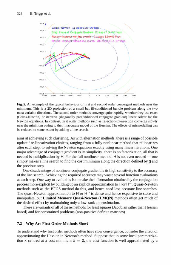
328 B. Triggs et al.
−0.05 −0.04 −0.03 −0.02 −0.01 0 0.01 0.02 0.03 0.04 0.05−0.05
−0.04
−0.03
−0.02
−0.01
0
0.01
0.02
0.03
0.04
0.05
Resect−intersect without line search 200 steps 1.1e+07 flops
Resect−Intersect with line search 71 steps 3.3e+06 flops
Diag. Precond. Conjugate Gradient 12 steps 7.5e+06 flops
Gauss−Newton 11 steps 1.2e+06 flops
−0.05 −0.04 −0.03 −0.02 −0.01 0 0.01 0.02 0.03 0.04 0.05−0.05
−0.04
−0.03
−0.02
−0.01
0
0.01
0.02
0.03
0.04
0.05
Resect−Intersect without line search 200 steps 1.1e+07 flops
Resect−Intersect with line search 71 steps 3.3e+06 flops
Diag. Precond. Conjugate Gradient 12 steps 7.5e+06 flops
Gauss−Newton 11 steps 1.2e+06 flops
Fig. 5.An example of the typical behaviour of first and second order convergent methods near theminimum. This is a 2D projection of a small but ill-conditioned bundle problem along the twomost variable directions. The second order methods converge quite rapidly, whether they use exact(Gauss-Newton) or iterative (diagonally preconditioned conjugate gradient) linear solver for theNewton equations. In contrast, first order methods such as resection-intersection converge slowlynear the minimum owing to their inaccurate model of the Hessian. The effects of mismodelling canbe reduced to some extent by adding a line search.
aims at achieving such clustering. As with alternation methods, there is a range of possibleupdate / re-linearization choices, ranging from a fully nonlinear method that relinearizesafter each step, to solving the Newton equations exactly using many linear iterations. Onemajor advantage of conjugate gradient is its simplicity: there is no factorization, all that isneeded is multiplication byH. For the full nonlinear method,H is not even needed— onesimply makes a line search to find the cost minimum along the direction defined byg andthe previous step.One disadvantage of nonlinear conjugate gradient is its high sensitivity to the accuracy
of the line search. Achieving the required accuracymay waste several function evaluationsat each step. One way to avoid this is to make the information obtained by the conjugationprocessmore explicit by building up an explicit approximation toH orH−1.Quasi-Newtonmethods such as the BFGS method do this, and hence need less accurate line searches.The quasi-Newton approximation toH or H−1 is dense and hence expensive to store andmanipulate, butLimited Memory Quasi-Newton (LMQN) methods often get much ofthe desired effect by maintaining only a low-rank approximation.There are variants of all of thesemethods for least squares (Jacobian rather thanHessian
based) and for constrained problems (non-positive definite matrices).
7.2 Why Are First Order Methods Slow?
To understand why first order methods often have slow convergence, consider the effect ofapproximating the Hessian in Newton’s method. Suppose that in some local parametriza-tion x centred at a cost minimumx = 0, the cost function is well approximated by a
Bundle Adjustment — A Modern Synthesis 329
quadratic near0: f(x) ≈ 12x� H x and henceg(x) ≡ H x, whereH is the true Hessian.
For most first order methods, the predicted step is linear in the gradientg. If we adopt aNewton-like state updateδx = −H−1
a g(x) based on some approximationHa toH, we getan iteration:
xk+1 = xk − H−1a g(xk) ≈ (1− H−1
a H) xk ≈ (1− H−1a H)k+1 x0 (27)
Thenumerical behaviour isdeterminedbyprojectingx0 along theeigenvectorsof1−H−1a H.
The components corresponding to large-modulus eigenvalues decay slowly and henceasymptotically dominate the residual error. For genericx0, themethod converges ‘linearly’(i.e. exponentially) at rate‖1−H−1
a H‖2, or diverges if this is greater than one. (Of course,the exact Newton stepδx = −H−1g converges in a single iteration, asHa = H). Alongeigen-directions corresponding to positive eigenvalues (for whichHa overestimatesH),the iteration is over-damped and convergence is slow but monotonic. Conversely, alongdirections corresponding to negative eigenvalues (for whichHa underestimatesH), theiteration is under-damped and zigzags towards the solution. IfH is underestimated by afactor greater than two along any direction, there is divergence. Figure 5 shows an exampleof the typical asymptotic behaviour of first and second order methods in a small bundleproblem.
Ignoring the camera-feature coupling:As an example, many approximate bundle meth-ods ignore or approximate the off-diagonal feature-camera blocks of the Hessian. Thisamounts to ignoring the fact that the cost of a feature displacement can be partially offsetby a compensatory camera displacement and vice versa. It therefore significantly over-estimates the total ‘stiffness’ of the network, particularly for large, loosely connectednetworks. The fact that off-diagonal blocks arenot negligible compared to the diagonalones can be seen in several ways:• Looking forward to§9, before the gauge is fixed, the full Hessian is singular owing togauge freedom. The diagonal blocks by themselves are well-conditioned, but includingthe off-diagonal ones entirely cancels this along the gauge orbit directions. Althoughgauge fixing removes the resulting singularity, it can not change the fact that the off-diagonal blocks have enough weight to counteract the diagonal ones.• In bundle adjustment, certain well-known ambiguities (poorly-controlled parametercombinations) often dominate the uncertainty. Camera distance and focal length es-timates, and structure depth and camera baseline ones (bas-relief), are both stronglycorrelated whenever the perspective is weak and become strict ambiguities in the affinelimit. The well-conditioned diagonal blocks of the Hessian give no hint of these ambi-guities: when both features and cameras are free, the overall network ismuchless rigidthan it appears to be when each treats the other as fixed.• During bundle adjustment, local structure refinements cause ‘ripples’ that must be prop-agated throughout the network. The camera-feature coupling information carried in theoff-diagonal blocks is essential to this. In the diagonal-only model, ripples can propa-gate at most one feature-camera-feature step per iteration, so it takes many iterationsfor them to cross and re-cross a sparsely coupled network.
These arguments suggest that any approximationHa to the bundle HessianH that sup-presses or significantly alters the off-diagonal terms is likely to have large‖1 − H−1
a H‖and hence slow convergence. This is exactly what we have observed in practice for allsuch methods that we have tested: near the minimum, convergence is linear and for largeproblems often extremely slow, with‖1 − H−1
a H‖2 very close to 1. The iteration may
330 B. Triggs et al.
either zigzag or converge slowly and monotonically, depending on the exact method andparameter values.
Line search:The above behaviour can often be improved significantly by adding a linesearch to the method. In principle, the resulting method converges foranypositive definiteHa. However, accurate modelling ofH is still highly desirable. Even with no roundingerrors, an exactly quadratic (but otherwise unknown) cost function and exact line searches(i.e. the minimum along the line is found exactly), the most efficient generic line searchbasedmethods suchas conjugate gradient or quasi-Newton require at leastO(nx) iterationsto converge. For large bundle problems with thousands of parameters, this can already beprohibitive. However, if knowledge aboutH is incorporated via a suitablepreconditioner,the number of iterations can often be reduced substantially.
7.3 Preconditioning
Gradient descent and Krylov methods are sensitive to the coordinate system and theirpractical success depends critically on good preconditioning. The aim is to find a lineartransformationx → T x and henceg → T−� g andH → T−� H T for which the trans-formedH is near1, or at least has only a few clusters of eigenvalues well separated fromthe origin. Ideally,T should be an accurate, low-cost approximation to the left Choleskyfactor ofH. (Exactly evaluating this would give the expensive Newton method again). Inthe experiments below, we tried conjugate gradient with preconditioners based on the di-agonal blocks ofH, and onpartial Cholesky decomposition, dropping either all filled-inelements, or all that are smaller than a preset size when performing Cholesky decomposi-tion. These methods were not competitive with the exact Gauss-Newton ones in the ‘strip’experiments below, but for large enough problems it is likely that a preconditioned Krylovmethod would predominate, especially if more effective preconditioners could be found.An exact Cholesky factor ofH from a previous iteration is often a quite effective
preconditioner. This gives hybrid methods in whichH is only evaluated and factored everyfew iterations, with the Newton step at these iterations and well-preconditioned gradientdescent or conjugate gradient at the others.
7.4 Experiments
Figure 6 shows the relative performance of several methods on two synthetic projectivebundle adjustment problems. In both cases, the number of 3Dpoints increases in proportionto the number of images, so the dense factorization time isO(n3
)wheren is the number
of points or images. The following methods are shown: ‘Sparse Gauss-Newton’ — sparseCholesky decomposition with variables ordered naturally (features then cameras); ‘DenseGauss-Newton’— the same, but (inefficiently) ignoring all sparsity of the Hessian; ‘Diag.Conj. Gradient’ — the Newton step is found by an iterative conjugate gradient linearsystem solver, preconditioned using the Cholesky factors of the diagonal blocks of theHessian; ‘Resect-Intersect’ — the state is optimized by alternate steps of resection andintersection, with relinearization after each. In the ‘spherical cloud’ problem, the pointsare uniformly distributed within a spherical cloud, all points are visible in all images,and the camera geometry is strongly convergent. These are ideal conditions, giving a lowdiameter network graph and a well-conditioned, nearly diagonal-dominant Hessian. Allof the methods converge quite rapidly. Resection-intersection is a competitive method for
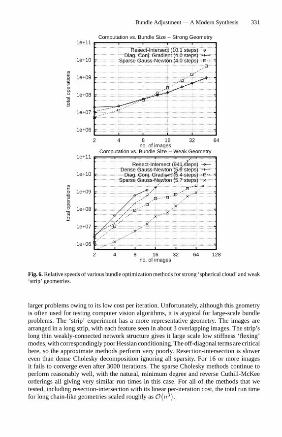
Bundle Adjustment — A Modern Synthesis 331
1e+06
1e+07
1e+08
1e+09
1e+10
1e+11
2 4 8 16 32 64
tota
l ope
ratio
ns
no. of images
Computation vs. Bundle Size -- Strong Geometry
Resect-Intersect (10.1 steps)Diag. Conj. Gradient (4.0 steps)
Sparse Gauss-Newton (4.0 steps)
1e+06
1e+07
1e+08
1e+09
1e+10
1e+11
2 4 8 16 32 64 128
tota
l ope
ratio
ns
no. of images
Computation vs. Bundle Size -- Weak Geometry
Resect-Intersect (941 steps)Dense Gauss-Newton (5.9 steps)
Diag. Conj. Gradient (5.4 steps)Sparse Gauss-Newton (5.7 steps)
Fig. 6.Relative speeds of various bundle optimizationmethods for strong ‘spherical cloud’ andweak‘strip’ geometries.
larger problems owing to its low cost per iteration. Unfortunately, although this geometryis often used for testing computer vision algorithms, it is atypical for large-scale bundleproblems. The ‘strip’ experiment has a more representative geometry. The images arearranged in a long strip, with each feature seen in about 3 overlapping images. The strip’slong thin weakly-connected network structure gives it large scale low stiffness ‘flexing’modes,with correspondinglypoorHessianconditioning.Theoff-diagonal termsarecriticalhere, so the approximate methods perform very poorly. Resection-intersection is slowereven than dense Cholesky decomposition ignoring all sparsity. For 16 or more imagesit fails to converge even after 3000 iterations. The sparse Cholesky methods continue toperform reasonably well, with the natural, minimum degree and reverse Cuthill-McKeeorderings all giving very similar run times in this case. For all of the methods that wetested, including resection-intersection with its linear per-iteration cost, the total run timefor long chain-like geometries scaled roughly asO(n3
).
332 B. Triggs et al.
8 Implementation Strategy 3: Updating and Recursion
8.1 Updating Rules
It is often convenient to be able toupdate a state estimate to reflect various types ofchanges,e.g. to incorporate new observations or to delete erroneous ones (‘downdating’).Parameters may have to be added or deleted too. Updating rules are often used recursively,to incorporate a series of observations one-by-one rather than solving a single batch system.This is useful in on-line applications where a rapid response is needed, and also to providepreliminary predictions,e.g. for correspondence searches. Much of the early developmentof updating methods was aimed at on-line data editing in aerial cartography workstations.The main challenge in adding or deleting observations is efficiently updating either a
factorization of the HessianH, or the covarianceH−1. Given either of these, the state updateδx is easily found by solving the Newton step equationsH δx = −g, where (assumingthat we started at an un-updated optimumg = 0) the gradientg depends only on the newlyadded terms. The Hessian updateH → H ± B W B� needs to have relatively low rank,otherwise nothing is saved over recomputing the batch solution. In least squares the rank isthe number of independent observations added or deleted, but even without this the rank isoften low in bundle problems because relatively few parameters are affected by any givenobservation.One limitation of updating is that it is seldom as accurate as a batch solution owing to
build-up of round-off error. Updating (adding observations) itself is numerically stable, butdowndating (deleting observations) is potentially ill-conditioned as it reduces the positivityof the Hessian, and may cause previously good pivot choices to become arbitrarily bad.This is particularly a problem if all observations relating to a parameter are deleted, orif there are repeated insertion-deletion cycles as in time window filtering. Factorizationupdating methods are stabler than Woodbury formula / covariance updating ones.Consider first the case where no parameters need be added nor deleted,e.g. adding or
deletinganobservationof anexistingpoint in anexisting image.Severalmethodshavebeensuggested [54, 66]. Mikhail & Helmering [88] use the Woodbury formula (18) to updatethe covarianceH−1. This simple approach becomes inefficient for problems with manyfeatures because the sparse structure is not exploited: the full covariance matrix is denseandwewould normally avoid calculating it in its entirety.Grun [51, 54] avoids this problemby maintaining a running copy of the reduced camera system (20), using an incrementalSchur complement / forward substitution (16) to fold each new observation into this, andthen re-factorizing and solving as usual after each update. This is effective when there aremany features in a few images, but for larger numbers of images it becomes inefficientowing to the re-factorization step. Factorization updating methods such as (55, 56) arecurrently the recommended update methods for most applications: they allow the existingfactorization to be exploited, they handle any number of images and features and arbitraryproblem structure efficiently, and they are numerically more accurate than Woodburyformula methods. The Givens rotation method [12, 54], which is equivalent to the rank1 Cholesky update (56), is probably the most common such method. The other updatingmethods are confusingly named in the literature. Mikhail & Helmering’s method [88]is sometimes called ‘Kalman filtering’, even though no dynamics and hence no actualfiltering is involved. Grun’s reduced camera systemmethod [51] is called ‘triangular factorupdate (TFU)’, even though it actually updates the (square) reduced Hessian rather thanits triangular factors.
Bundle Adjustment — A Modern Synthesis 333
For updates involving a previously unseen 3D feature or image, new variables mustalso be added to the system. This is easy. We simply choose where to put the variables inthe elimination sequence, and extendH and its L,D,U factors with the corresponding rowsand columns, setting all of the newly created positions to zero (except for the unit diagonalsof LDL�’s and LU’sL factor). The factorization can then be updated as usual, presumablyadding enough cost terms to make the extended Hessian nonsingular and couple the newparameters into the old network. If a direct covariance update is needed, the Woodburyformula (18) can be used on the old part of the matrix, then (17) to fill in the new blocks(equivalently, invert (54), withD1 ← A representing the old blocks andD2 ← 0 the newones).Conversely, it may be necessary to delete parameters,e.g. if an image or 3D feature
has lost most or all of its support. The corresponding rows and columns of the HessianH (and rows ofg, columns ofJ) must be deleted, and all cost contributions involving thedeleted parameters must also be removed using the usual factorization downdates (55, 56).To delete the rows and columns of blockb in a matrixA, we first delete theb rows andcolumns ofL,D,U. This maintains triangularity and gives the correct trimmedA, exceptthat the blocks in the lower right cornerAij =
∑k≤min(i,j) Lik Dk Ukj , i, j > b are
missing a termLib Db Ubj from the deleted columnb of L / row b ofU. This is added usingan update+L∗b Db Ub∗, ∗ > b. To updateA−1 when rows and columns ofA are deleted,permute the deleted rows and columns to the end and use (17) backwards:(A11)−1 =(A−1)11 − (A−1)12 (A−1)−1
22 (A−1)21.It is also possible to freeze some live parameters at fixed (current or default) values,
or to add extra parameters / unfreeze some previously frozen ones,c.f . (48, 49) below. Inthis case, rows and columns corresponding to the frozen parameters must be deleted oradded, but no other change to the cost function is required. Deletion is as above. To insertrows and columnsAb∗,A∗b at blockb of matrixA, we open space in row and columnb ofL,D,U and fill these positions with the usual recursively defined values (51). Fori, j > b,the sum (51) will now have a contributionLib Db Ubj that it should not have, so to correctthis we downdate the lower right submatrix∗ > b with a cost cancelling contribution−L∗b Db Ub∗.
8.2 Recursive Methods and Reduction
Each update computation is roughly quadratic in the size of the state vector, so if newfeatures and images are continually added the situation will eventually become unman-ageable. We must limit what we compute. In principle parameter refinement never stops:each observation update affects all components of the state estimate and its covariance.However, the refinements are in a sense trivial for parameters that are not directly coupledto the observation. If these parameters are eliminated using reduction (19), the observa-tion update can be applied directly to the reduced Hessian and gradient12. The eliminatedparameters can then be updated by simple back-substitution (19) and their covariances by(17). In particular, if we cease to receive new information relating to a block of parameters(an image that has been fully treated, a 3D feature that has become invisible), they andall the observations relating to them can be subsumed once-and-for-all in a reduced Hes-sian and gradient on the remaining parameters. If required, we can later re-estimate the12 In (19), onlyD andb2 are affected by the observation as it is independent of the subsumedcomponentsA,B,C, b1. So applying the update toD, b2 has the same effect as applying it toD, b2.
334 B. Triggs et al.
eliminated parameters by back-substitution. Otherwise, we do not need to consider themfurther.This elimination process has some limitations. Only ‘dead’ parameters can be elim-
inated: to merge a new observation into the problem, we need the current Hessian orfactorization entries for all parameter blocks relating to it. Reduction also commits us toa linearized / quadratic cost approximation for the eliminated variables at their currentestimates, although to the extent that this model is correct, the remaining variables can stillbe treated nonlinearly. It is perhaps best to view reduction as the first half-iteration of a fullnonlinear optimization: by (19), theNewtonmethod for the full model can be implementedby repeated cycles of reduction, solving the reduced system, and back-substitution, withrelinearization after each cycle, whereas for eliminated variables we stop after solving thefirst reduced system. Equivalently, reduction evaluates just the reduced components of thefull Newton step and the full covariance, leaving us the option of computing the remainingeliminated ones later if we wish.Reduction can be used to refine estimates of relative camera poses (or fundamental
matrices,etc.) for a fixed set of images, by reducing a sequence of feature correspondencesto their camera coordinates. Or conversely, to refine 3D structure estimates for a fixed setof features in many images, by reducing onto the feature coordinates.Reduction is also the basis of recursive (Kalman) filtering. In this case, one has a (e.g.
time) series of system state vectors linked by someprobabilistic transition rule (‘dynamicalmodel’), for which we also have some observations (‘observation model’). The parameterspace consists of the combined state vectors for all times,i.e. it represents a path throughthe states. Both the dynamical and the observation models provide “observations” in thesense of probabilistic constraints on the full state parameters, andwe seek amaximum like-lihood (or similar) parameter estimate / path through the states. The full Hessian is blocktridiagonal: the observations couple only to the current state and give the diagonal blocks,and dynamics couples only to the previous and next ones and gives the off-diagonal blocks(differential observations can also be included in the dynamics likelihood). So the modelis large (if there are many time steps) but very sparse. As always with a tridiagonal matrix,the Hessian can be decomposed by recursive steps of reduction, at each step Schur comple-menting to get the current reduced blockHt from the previous oneHt−1, the off-diagonal(dynamical) couplingHt t−1 and the current unreduced block (observation Hessian)Ht :Ht = Ht − Ht t−1 H
−1
t−1 H�t t−1. Similarly, for the gradientgt = gt − Ht t−1 H
−1
t−1 gt−1,
and as usual the reduced state update isδxt = −H−1
t gt.This forwards reduction process is calledfiltering . At each time step it finds the optimal
(linearized) current state estimate given all of the previous observations and dynamics. Thecorresponding unwinding of the recursion by back-substitution,smoothing, finds the opti-mal state estimate at each time given both past and future observations and dynamics. Theusual equations of Kalman filtering and smoothing are easily derived from this recursion,but we will not do this here. We emphasize that filtering is merely the first half-iteration ofa nonlinear optimization procedure: even for nonlinear dynamics and observation models,we can find the exact maximum likelihood state path by cyclic passes of filtering andsmoothing, with relinearization after each.For long or unbounded sequences it may not be feasible to run the full iteration, but
it can still be very helpful to run short sections of it,e.g. smoothing back over the last3–4 state estimates then filtering forwards again, to verify previous correspondences andanneal the effects of nonlinearities. (The traditionalextended Kalman filter optimizes
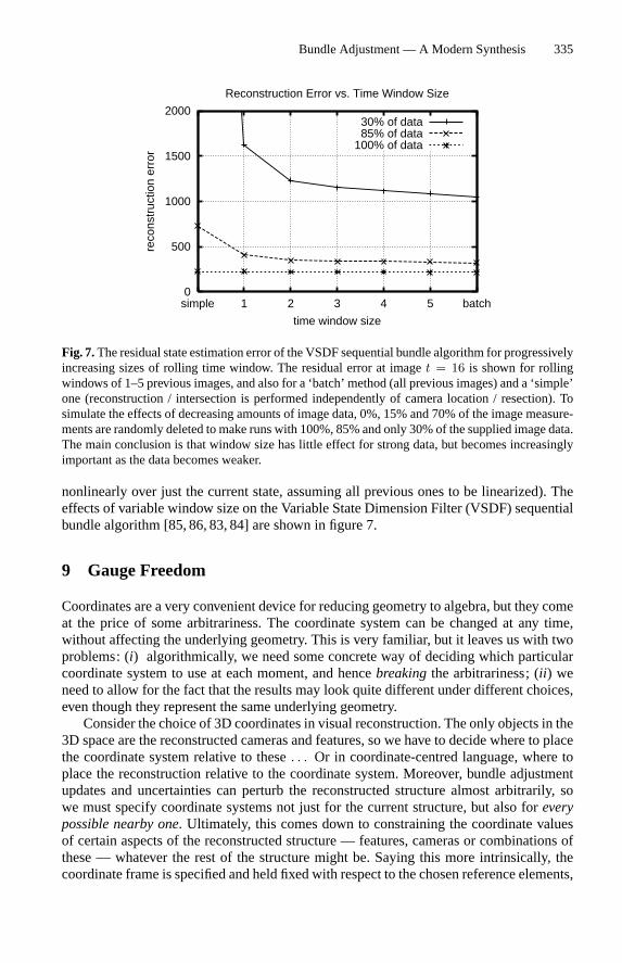
Bundle Adjustment — A Modern Synthesis 335
0
500
1000
1500
2000
simple 1 2 3 4 5 batch
reco
nstr
uctio
n er
ror
time window size
Reconstruction Error vs. Time Window Size
30% of data85% of data
100% of data
Fig. 7.The residual state estimation error of the VSDF sequential bundle algorithm for progressivelyincreasing sizes of rolling time window. The residual error at imaget = 16 is shown for rollingwindows of 1–5 previous images, and also for a ‘batch’ method (all previous images) and a ‘simple’one (reconstruction / intersection is performed independently of camera location / resection). Tosimulate the effects of decreasing amounts of image data, 0%, 15% and 70% of the image measure-ments are randomly deleted to make runs with 100%, 85% and only 30% of the supplied image data.The main conclusion is that window size has little effect for strong data, but becomes increasinglyimportant as the data becomes weaker.
nonlinearly over just the current state, assuming all previous ones to be linearized). Theeffects of variable window size on the Variable State Dimension Filter (VSDF) sequentialbundle algorithm [85, 86, 83, 84] are shown in figure 7.
9 Gauge Freedom
Coordinates are a very convenient device for reducing geometry to algebra, but they comeat the price of some arbitrariness. The coordinate system can be changed at any time,without affecting the underlying geometry. This is very familiar, but it leaves us with twoproblems: (i) algorithmically, we need some concrete way of deciding which particularcoordinate system to use at each moment, and hencebreakingthe arbitrariness; (ii ) weneed to allow for the fact that the results may look quite different under different choices,even though they represent the same underlying geometry.Consider the choice of 3D coordinates in visual reconstruction. The only objects in the
3D space are the reconstructed cameras and features, so we have to decide where to placethe coordinate system relative to these. . . Or in coordinate-centred language, where toplace the reconstruction relative to the coordinate system. Moreover, bundle adjustmentupdates and uncertainties can perturb the reconstructed structure almost arbitrarily, sowe must specify coordinate systems not just for the current structure, but also foreverypossible nearby one. Ultimately, this comes down to constraining the coordinate valuesof certain aspects of the reconstructed structure — features, cameras or combinations ofthese — whatever the rest of the structure might be. Saying this more intrinsically, thecoordinate frame is specified and held fixed with respect to the chosen reference elements,
336 B. Triggs et al.
and the rest of the geometry is then expressed in this frame as usual. In measurementscience such a set of coordinate system specifying rules is called adatum, but we willfollow the wider mathematics and physics usage and call it agauge13. The freedom in thechoice of coordinate fixing rules is calledgauge freedom.As a gauge anchors the coordinate system rigidly to its chosen reference elements, per-
turbing the reference elements has no effect on their own coordinates. Instead, it changesthe coordinate system itself and hence systematically changes the coordinates of all theother features, while leaving the reference coordinates fixed. Similarly, uncertainties inthe reference elements do not affect their own coordinates, but appear as highly correlateduncertainties in all of theother reconstructed features. The moral is thatstructural pertur-bations and uncertainties are highly relative. Their form depends profoundly on the gauge,and especially on how this changes as the state varies (i.e. which elements it holds fixed).The effects of disturbances arenot restricted to the coordinates of the features actuallydisturbed, but may appear almost anywhere depending on the gauge.In visual reconstruction, the differences between object-centred and camera-centred
gauges are often particularly marked. In object-centred gauges, object points appear to berelatively certain while cameras appear to have large and highly correlated uncertainties.In camera-centred gauges, it is the camera that appears to be precise and the object pointsthat appear to have large correlated uncertainties. One often sees statements like “thereconstructed depths are very uncertain”. This may be true in the camera frame, yet theobject may be very well reconstructed in its own frame — it all depends on what fractionof the total depth fluctuations are simply due to global uncertainty in the camera location,and hence identical for all object points.Besides 3D coordinates, many other types of geometric parametrization in vision in-
volve arbitrary choices, and hence are subject to gauge freedoms [106]. These include thechoice of: homogeneous scale factors in homogeneous-projective representations; sup-porting points in supporting-point based representations of lines and planes; referenceplane in plane + parallax representations; and homographies in homography-epipole rep-resentations of matching tensors. In each case the symptoms and the remedies are thesame.
9.1 General Formulation
The general set up is as follows:We take as our state vectorx the set of all of the 3D featurecoordinates, camera poses and calibrations,etc., that enter the problem. This state spacehas internal symmetries related to the arbitrary choices of 3D coordinates, homogeneousscale factors,etc., that are embedded inx. Any two state vectors that differ only by suchchoices represent thesameunderlying3Dgeometry, andhencehaveexactly thesame imageprojections and other intrinsic properties. So under change-of-coordinates equivalence, thestate space is partitioned into classes of intrinsically equivalent state vectors, each classrepresenting exactly one underlying 3D geometry. These classes are calledgauge orbits.Formally, they are the group orbits of the state space action of the relevantgauge group(coordinate transformation group), but we will not need the group structure below. A statespace function represents an intrinsic function of the underlying geometry if and only ifit is constant along each gauge orbit (i.e. coordinate system independent). Such quantities
13 Here,gaugejust means reference frame. The sense is that of a reference against which somethingis judged(O.Fr. jauger, gauger). Pronouncegeidj.
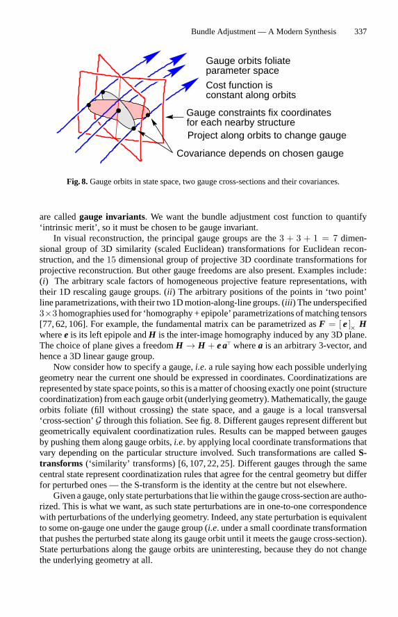
Bundle Adjustment — A Modern Synthesis 337
Gauge constraints fix coordinates
parameter space
Cost function isconstant along orbits
Gauge orbits foliate
for each nearby structure
Covariance depends on chosen gauge
Project along orbits to change gauge
Fig. 8.Gauge orbits in state space, two gauge cross-sections and their covariances.
are calledgauge invariants. We want the bundle adjustment cost function to quantify‘intrinsic merit’, so it must be chosen to be gauge invariant.In visual reconstruction, the principal gauge groups are the3 + 3 + 1 = 7 dimen-
sional group of 3D similarity (scaled Euclidean) transformations for Euclidean recon-struction, and the15 dimensional group of projective 3D coordinate transformations forprojective reconstruction. But other gauge freedoms are also present. Examples include:(i) The arbitrary scale factors of homogeneous projective feature representations, withtheir 1D rescaling gauge groups. (ii ) The arbitrary positions of the points in ‘two point’line parametrizations, with their two 1Dmotion-along-line groups. (iii ) The underspecified3×3 homographies used for ‘homography + epipole’ parametrizations ofmatching tensors[77, 62, 106]. For example, the fundamental matrix can be parametrized asF = [ e]× Hwheree is its left epipole andH is the inter-image homography induced by any 3D plane.The choice of plane gives a freedomH → H + e a�wherea is an arbitrary 3-vector, andhence a 3D linear gauge group.Now consider how to specify a gauge,i.e. a rule saying how each possible underlying
geometry near the current one should be expressed in coordinates. Coordinatizations arerepresented by state space points, so this is amatter of choosing exactly one point (structurecoordinatization) fromeach gauge orbit (underlying geometry). Mathematically, the gaugeorbits foliate (fill without crossing) the state space, and a gauge is a local transversal‘cross-section’G through this foliation. See fig. 8. Different gauges represent different butgeometrically equivalent coordinatization rules. Results can be mapped between gaugesby pushing them along gauge orbits,i.e. by applying local coordinate transformations thatvary depending on the particular structure involved. Such transformations are calledS-transforms (‘similarity’ transforms) [6, 107, 22, 25]. Different gauges through the samecentral state represent coordinatization rules that agree for the central geometry but differfor perturbed ones — the S-transform is the identity at the centre but not elsewhere.Givenagauge, only state perturbations that liewithin thegaugecross-sectionareautho-
rized. This is what we want, as such state perturbations are in one-to-one correspondencewith perturbations of the underlying geometry. Indeed, any state perturbation is equivalentto some on-gauge one under the gauge group (i.e. under a small coordinate transformationthat pushes the perturbed state along its gauge orbit until it meets the gauge cross-section).State perturbations along the gauge orbits are uninteresting, because they do not changethe underlying geometry at all.
338 B. Triggs et al.
Covariances are averages of squared perturbations andmust also be based on on-gaugeperturbations (they would be infinite if we permitted perturbations along the gauge orbits,as there is no limit to these — they do not change the cost at all). So covariance matricesare gauge-dependent and in fact represent ellipsoids tangent to the gauge cross-section atthe cost minimum. They can look very different for different gauges. But, as with states, S-transforms map them between gauges by projecting along gauge orbits / state equivalenceclasses.Note that there is no intrinsic notion of orthogonality on state space, so it ismeaningless
to ask which state-space directions are ‘orthogonal’ to the gauge orbits. This would in-volve deciding when two different structures have been “expressed in the same coordinatesystem”, so every gauge believes its own cross section to be orthogonal and all others tobe skewed.
9.2 Gauge Constraints
We will work near some pointx of state space, perhaps a cost minimum or a running stateestimate. Letnx be the dimension ofx andng the dimension of the gauge orbits. Letf,g,Hbe the cost function and its gradient and Hessian, andG be anynx × ng matrix whosecolumns span the local gauge orbit directions atx 14. By the exact gauge invariance off,its gradient and Hessian vanish along orbit directions:g� G = 0 andH G = 0. Note thatthe gauged HessianH is singular with (at least) rank deficiencyng and null spaceG. Thisis calledgauge deficiency. Many numerical optimization routines assume nonsingularH,andmust bemodified to work in gauge invariant problems. The singularity is an expressionof indifference: when we come to calculate state updates, any two updates ending on thesame gauge orbit are equivalent, both in terms of cost and in terms of the change in theunderlying geometry. All that we need is a method of telling the routine which particularupdate to choose.Gauge constraints are the most direct means of doing this. A gauge cross-sectionG
can be specified in two ways: (i) constrained form:specifyng local constraintsd(x)with d(x) = 0 for points onG ; (ii ) parametric form:specify a functionx(y) of nx − ng
independent local parametersy, with x = x(y) being the points ofG. For example, atrivial gauge is one that simply freezes the values ofng of the parameters inx (usuallyfeature or camera coordinates). In this case we can taked(x) to be the parameter freezingconstraints andy to be the remaining unfrozen parameters. Note that once the gauge isfixed the problem is no longer gauge invariant — the whole purpose ofd(x), x(y) is tobreakthe underlying gauge invariance.Examples of trivial gauges include: (i) using several visible 3D points as a ‘projective
basis’ for reconstruction (i.e. fixing their projective 3D coordinates to simple values, asin [27]); and (ii ) fixing the components of one projective3 × 4 camera matrix as(I 0),as in [61] (this only partially fixes the 3D projective gauge — 3 projective 3D degrees offreedom remain unfixed).
14 A suitableG is easily calculated from the infinitesimal action of the gauge group onx. Forexample, for spatial similarities the columns ofGwould be theng = 3+3+1 = 7 state velocityvectors describing the effects of infinitesimal translations, rotations and changes of spatial scaleonx.
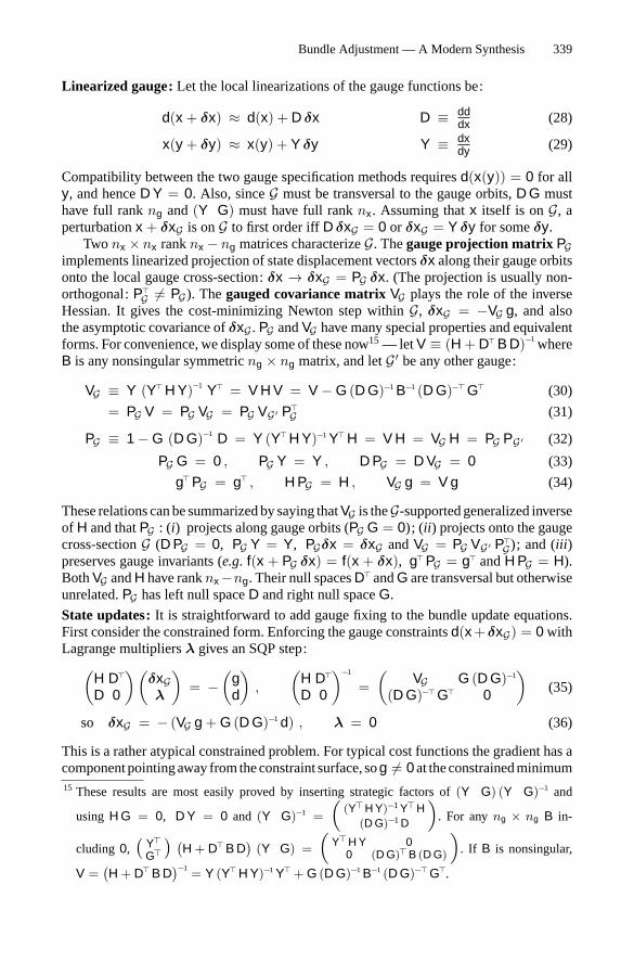
Bundle Adjustment — A Modern Synthesis 339
Linearized gauge:Let the local linearizations of the gauge functions be:
d(x + δx) ≈ d(x) + D δx D ≡ dddx (28)
x(y + δy) ≈ x(y) + Y δy Y ≡ dxdy (29)
Compatibility between the two gauge specification methods requiresd(x(y)) = 0 for ally, and henceD Y = 0. Also, sinceG must be transversal to the gauge orbits,D G musthave full rankng and(Y G) must have full ranknx. Assuming thatx itself is onG, aperturbationx + δxG is onG to first order iffD δxG = 0 or δxG = Y δy for someδy.Twonx × nx ranknx − ng matrices characterizeG. Thegauge projection matrixPG
implements linearized projection of state displacement vectorsδx along their gauge orbitsonto the local gauge cross-section:δx → δxG = PG δx. (The projection is usually non-orthogonal:P�
G �= PG). Thegauged covariance matrixVG plays the role of the inverseHessian. It gives the cost-minimizing Newton step withinG, δxG = −VG g, and alsothe asymptotic covariance ofδxG .PG andVG have many special properties and equivalentforms. For convenience, we display some of these now15— letV ≡ (H + D� B D)−1whereB is any nonsingular symmetricng × ng matrix, and letG′ be any other gauge:
VG ≡ Y (Y� H Y)−1 Y� = V H V = V−G (D G)−1B−1 (D G)−� G� (30)
= PG V = PG VG = PG VG′ P�G (31)
PG ≡ 1−G (D G)−1 D = Y (Y� H Y)−1Y� H = V H = VG H = PG PG′ (32)
PG G = 0 , PG Y = Y , D PG = D VG = 0 (33)
g� PG = g� , H PG = H , VG g = V g (34)
These relations canbesummarizedby saying thatVG is theG-supportedgeneralized inverseof H and thatPG : (i) projects along gauge orbits (PG G = 0); (ii ) projects onto the gaugecross-sectionG (D PG = 0, PG Y = Y, PGδx = δxG andVG = PG VG′ P�
G); and (iii )preserves gauge invariants (e.g. f(x + PG δx) = f(x + δx), g� PG = g� andH PG = H).BothVG andH have ranknx−ng. Their null spacesD�andG are transversal but otherwiseunrelated.PG has left null spaceD and right null spaceG.State updates:It is straightforward to add gauge fixing to the bundle update equations.First consider the constrained form. Enforcing the gauge constraintsd(x +δxG) = 0withLagrange multipliersλ gives an SQP step:(
H D�
D 0
)(δxGλ
)= −
(gd
),
(H D�
D 0
)−1
=(
VG G (D G)−1
(D G)−� G� 0
)(35)
so δxG = − (VG g + G (D G)−1d) , λ = 0 (36)
This is a rather atypical constrained problem. For typical cost functions the gradient has acomponentpointingaway from theconstraint surface, sog �= 0at theconstrainedminimum15 These results are most easily proved by inserting strategic factors of(Y G) (Y G)−1 and
usingH G = 0, D Y = 0 and (Y G)−1 =(
(Y� H Y)−1Y� H(D G)−1D
). For anyng × ng B in-
cluding 0,(
Y�G�) (
H + D� B D)
(Y G) =(
Y� H Y 00 (D G)� B (D G)
). If B is nonsingular,
V =(H + D� B D
)−1 = Y (Y� H Y)−1Y� + G (D G)−1B−1 (D G)−� G�.
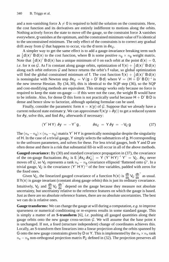
340 B. Triggs et al.
and a non-vanishing forceλ �= 0 is required to hold the solution on the constraints. Here,the cost function and its derivatives are entirely indifferent to motions along the orbits.Nothing actively forces the state to move off the gauge, so the constraint forceλ vanisheseverywhere,g vanishes at the optimum, and the constrainedminimumvalue off is identicalto the unconstrained minimum. The only effect of the constraints is to correct any gradualdrift away fromG that happens to occur, via thed term inδxG .A simpler way to get the same effect is to add a gauge-invariance breaking term such
as 12d(x)� B d(x) to the cost function, whereB is some positiveng × ng weight matrix.
Note that12d(x)� B d(x) has a unique minimum of0 on each orbit at the pointd(x) = 0,i.e. for x onG. As f is constant along gauge orbits, optimization off(x) + 1
2d(x)� B d(x)along each orbit enforcesG and hence returns the orbit’sf value, so global optimizationwill find the global constrained minimum off. The cost functionf(x) + 1
2d(x)� B d(x)is nonsingular with Newton stepδxG = V (g + D� B d) whereV = (H + D� B D)−1 isthe new inverse Hessian. By (34, 30), this is identical to the SQP step (36), so the SQPand cost-modifying methods are equivalent. This strategy works only because no force isrequired to keep the state on-gauge — if this were not the case, the weightB would haveto be infinite. Also, for denseD this form is not practically useful becauseH + D� B D isdense and hence slow to factorize, although updating formulae can be used.Finally, consider the parametric formx = x(y) of G. Suppose that we already have a
current reduced state estimatey. We can approximatef(x(y+δy)) to get a reduced systemfor δy, solve this, and findδxG afterwards if necessary:
(Y� H Y) δy = −Y� g , δxG = Y δy = −VG g (37)
The(nx−ng)×(nx−ng)matrixY� H Y is generically nonsingular despite the singularityofH. In the case of a trivial gauge,Y simply selects the submatrices ofg,H correspondingto the unfrozen parameters, and solves for these. For less trivial gauges, bothY andD areoften dense and there is a risk that substantial fill-in will occur in all of the above methods.
Gauged covariance:By (30) and standard covariance propagation in (37), the covarianceof the on-gauge fluctuationsδxG is E
[δxG δx�
G]
= Y (Y� H Y)−1 Y� = VG . δxG nevermoves offG, soVG represents a ranknx − ng covariance ellipsoid ‘flattened ontoG’. In atrivial gauge,VG is the covariance(Y� H Y)−1 of the free variables, padded with zeros forthe fixed ones.GivenVG , the linearized gauged covariance of a functionh(x) is dh
dx VGdhdx
�as usual.
If h(x) is gauge invariant (constant along gauge orbits) this is just its ordinary covariance.Intuitively, VG and
dhdx VG
dhdx
�depend on the gauge because they measure not absolute
uncertainty, but uncertainty relative to the reference features on which the gauge is based.Just as there are no absolute reference frames, there are no absolute uncertainties. The bestwe can do is relative ones.
Gauge transforms:Wecan change the gauge at will during a computation,e.g. to improvesparseness or numerical conditioning or re-express results in some standard gauge. Thisis simply a matter of anS-transform [6], i.e. pushing all gauged quantities along theirgauge orbits onto the new gauge cross-sectionG. We will assume that the base pointxis unchanged. If not, a fixed (structure independent) change of coordinates achieves this.Locally, an S-transform then linearizes into a linear projection along the orbits spanned byG onto the new gauge constraints given byD orY. This is implemented by thenx×nx ranknx−ng non-orthogonal projection matrixPG defined in (32). The projection preserves all
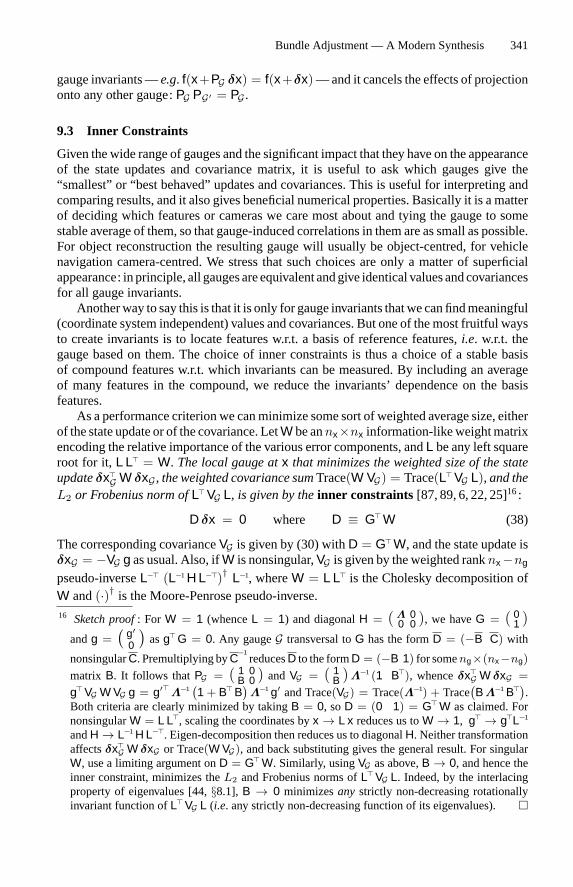
Bundle Adjustment — A Modern Synthesis 341
gauge invariants—e.g. f(x+PG δx) = f(x+δx)—and it cancels the effects of projectiononto any other gauge:PG PG′ = PG .
9.3 Inner Constraints
Given the wide range of gauges and the significant impact that they have on the appearanceof the state updates and covariance matrix, it is useful to ask which gauges give the“smallest” or “best behaved” updates and covariances. This is useful for interpreting andcomparing results, and it also gives beneficial numerical properties. Basically it is a matterof deciding which features or cameras we care most about and tying the gauge to somestable average of them, so that gauge-induced correlations in them are as small as possible.For object reconstruction the resulting gauge will usually be object-centred, for vehiclenavigation camera-centred. We stress that such choices are only a matter of superficialappearance: in principle, all gaugesareequivalent andgive identical valuesandcovariancesfor all gauge invariants.Anotherway to say this is that it is only for gauge invariants thatwe can findmeaningful
(coordinate system independent) values and covariances. But one of themost fruitful waysto create invariants is to locate features w.r.t. a basis of reference features,i.e. w.r.t. thegauge based on them. The choice of inner constraints is thus a choice of a stable basisof compound features w.r.t. which invariants can be measured. By including an averageof many features in the compound, we reduce the invariants’ dependence on the basisfeatures.As a performance criterion we canminimize some sort of weighted average size, either
of the state update or of the covariance. LetW be annx×nx information-likeweightmatrixencoding the relative importance of the various error components, andL be any left squareroot for it, L L� = W. The local gauge atx that minimizes the weighted size of the stateupdateδx�
G W δxG , the weighted covariance sumTrace(W VG) = Trace(L� VG L), and theL2 or Frobenius norm ofL� VG L, is given by theinner constraints [87, 89, 6, 22, 25]16:
D δx = 0 where D ≡ G� W (38)
The corresponding covarianceVG is given by (30) withD = G� W, and the state update isδxG = −VG g as usual. Also, ifW is nonsingular,VG is given by the weighted ranknx−ng
pseudo-inverseL−� (L−1H L−�)† L−1, whereW = L L� is the Cholesky decomposition ofW and(·)† is the Moore-Penrose pseudo-inverse.16 Sketch proof: ForW = 1 (whenceL = 1) and diagonalH = ( Λ 0
0 0 ), we haveG = ( 01 )
andg =(
g′0
)asg� G = 0. Any gaugeG transversal toG has the formD = (−B C) with
nonsingularC. Premultiplying byC−1reducesD to the formD = (−B 1) for someng×(nx −ng)
matrix B. It follows thatPG = ( 1 0B 0 ) andVG = ( 1
B )Λ−1 (1 B�), whenceδx�G W δxG =
g� VG W VG g = g′� Λ−1(1 + B� B
)Λ−1g′ and Trace(VG) = Trace(Λ−1) + Trace
(B Λ−1B�)
.Both criteria are clearly minimized by takingB = 0, soD = (0 1) = G� W as claimed. FornonsingularW = L L�, scaling the coordinates byx → L x reduces us toW → 1, g� → g�L−1
andH → L−1H L−�. Eigen-decomposition then reduces us to diagonalH. Neither transformationaffectsδx�
G W δxG or Trace(W VG), and back substituting gives the general result. For singularW, use a limiting argument onD = G� W. Similarly, usingVG as above,B → 0, and hence theinner constraint, minimizes theL2 and Frobenius norms ofL� VG L. Indeed, by the interlacingproperty of eigenvalues [44,§8.1], B → 0 minimizesany strictly non-decreasing rotationallyinvariant function ofL� VG L (i.e. any strictly non-decreasing function of its eigenvalues).�
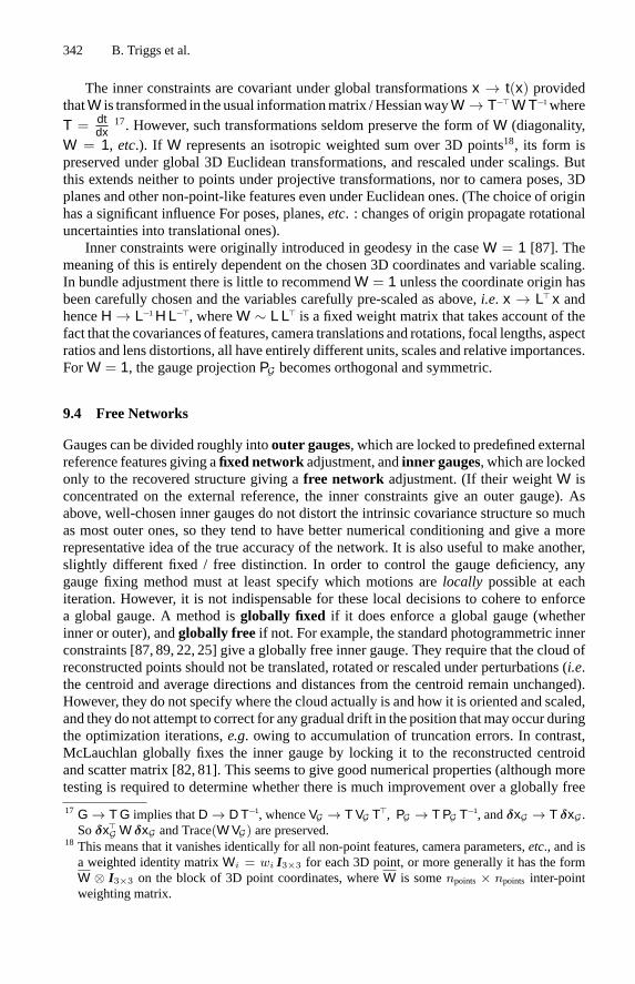
342 B. Triggs et al.
The inner constraints are covariant under global transformationsx → t(x) providedthatW is transformed in theusual informationmatrix /HessianwayW→ T−� W T−1whereT = dt
dx17. However, such transformations seldom preserve the form ofW (diagonality,
W = 1, etc.). If W represents an isotropic weighted sum over 3D points18, its form ispreserved under global 3D Euclidean transformations, and rescaled under scalings. Butthis extends neither to points under projective transformations, nor to camera poses, 3Dplanes and other non-point-like features even under Euclidean ones. (The choice of originhas a significant influence For poses, planes,etc. : changes of origin propagate rotationaluncertainties into translational ones).Inner constraints were originally introduced in geodesy in the caseW = 1 [87]. The
meaning of this is entirely dependent on the chosen 3D coordinates and variable scaling.In bundle adjustment there is little to recommendW = 1 unless the coordinate origin hasbeen carefully chosen and the variables carefully pre-scaled as above,i.e. x → L� x andhenceH→ L−1H L−�, whereW ∼ L L� is a fixed weight matrix that takes account of thefact that the covariances of features, camera translations and rotations, focal lengths, aspectratios and lens distortions, all have entirely different units, scales and relative importances.ForW = 1, the gauge projectionPG becomes orthogonal and symmetric.
9.4 Free Networks
Gauges can be divided roughly intoouter gauges, which are locked to predefined externalreference features giving afixed network adjustment, andinner gauges, which are lockedonly to the recovered structure giving afree network adjustment. (If their weightW isconcentrated on the external reference, the inner constraints give an outer gauge). Asabove, well-chosen inner gauges do not distort the intrinsic covariance structure so muchas most outer ones, so they tend to have better numerical conditioning and give a morerepresentative idea of the true accuracy of the network. It is also useful to make another,slightly different fixed / free distinction. In order to control the gauge deficiency, anygauge fixing method must at least specify which motions arelocally possible at eachiteration. However, it is not indispensable for these local decisions to cohere to enforcea global gauge. A method isglobally fixed if it does enforce a global gauge (whetherinner or outer), andglobally free if not. For example, the standard photogrammetric innerconstraints [87, 89, 22, 25] give a globally free inner gauge. They require that the cloud ofreconstructed points should not be translated, rotated or rescaled under perturbations (i.e.the centroid and average directions and distances from the centroid remain unchanged).However, they do not specify where the cloud actually is and how it is oriented and scaled,and they do not attempt to correct for any gradual drift in the position thatmay occur duringthe optimization iterations,e.g. owing to accumulation of truncation errors. In contrast,McLauchlan globally fixes the inner gauge by locking it to the reconstructed centroidand scatter matrix [82, 81]. This seems to give good numerical properties (although moretesting is required to determine whether there is much improvement over a globally free
17 G → T G implies thatD → D T−1, whenceVG → T VG T�, PG → T PG T−1, andδxG → T δxG .Soδx�
G W δxG and Trace(W VG) are preserved.18 This means that it vanishes identically for all non-point features, camera parameters,etc., and isa weighted identity matrixWi = wi I3×3 for each 3D point, or more generally it has the formW ⊗ I3×3 on the block of 3D point coordinates, whereW is somenpoints× npoints inter-pointweighting matrix.
Bundle Adjustment — A Modern Synthesis 343
inner gauge), and it has the advantage of actually fixing the coordinate system so thatdirect comparisons of solutions, covariances,etc., are possible. Numerically, a globallyfixed gauge can be implemented either by including the ‘d’ term in (36), or simply byapplying a rectifying gauge transformation to the estimate, at each step or when it driftstoo far from the chosen gauge.
9.5 Implementation of Gauge Constraints
Given that all gauges are in principle equivalent, it does not seem worthwhile to pay ahigh computational cost for gauge fixing during step prediction, so methods requiringlarge dense factorizations or (pseudo-)inverses should not be used directly. Instead, themain computation can be done in any convenient, low cost gauge, and the results latertransformed into the desired gauge using the gauge projector19 PG = 1 − G (D G)−1D.It is probably easiest to use a trivial gauge for the computation. This is simply a matterof deleting the rows and columns ofg,H corresponding tong preselected parameters,which should be chosen to give a reasonably well-conditioned gauge. The choice can bemade automatically by asubset selectionmethod (c.f ., e.g. [11]). H is left intact andfactored as usual, except that the final dense (owing to fill-in) submatrix is factored using astable pivotedmethod, and the factorization is stoppedng columns before completion. Theremainingng×ng block (and the corresponding block of the forward-substituted gradientg) should be zero owing to gauge deficiency. The corresponding rows of the state updateare set to zero (or anything else that is wanted) and back-substitution gives the remainingupdate components as usual. This method effectively finds theng parameters that are leastwell constrained by the data, and chooses the gauge constraints that freeze these by settingthe correspondingδxG components to zero.
10 Quality Control
This section discusses quality control methods for bundle adjustment, giving diagnostictests that can be used to detect outliers and characterize the overall accuracy and reliabilityof the parameter estimates. These techniques are not well known in vision so we will gointo some detail. Skip the technical details if you are not interested in them.Quality control is a serious issue in measurement science, and it is perhaps here that
the philosophical differences between photogrammetrists and vision workers are greatest:the photogrammetrist insists on good equipment, careful project planning, exploitationof prior knowledge and thorough error analyses, while the vision researcher advocates amore casual, flexible ‘point-and-shoot’ approach with minimal prior assumptions. Manyapplications demand a judicious compromise between these virtues.A basic maxim is “quality = accuracy + reliability”20. The absoluteaccuracyof the
system depends on the imaging geometry, number of measurements,etc. But theoretical19 The projectorPG itself is never calculated. Instead, it is applied in pieces, multiplying byD, etc.The gauged Newton stepδxG is easily found like this, and selected blocks of the covarianceVG = PG VG′ P�
G can also be found in this way, expandingPG and using (53) for the leading term,and for the remaining ones findingL−1D�, etc., by forwards substitution.
20 ‘Accuracy’ is sometimes called ‘precision’ in photogrammetry, but we have preferred to retainthe familiar meanings from numerical analysis: ‘precision’ means numerical error / number ofworking digits and ‘accuracy’ means statistical error / number of significant digits.
344 B. Triggs et al.
precision by itself is not enough: the system must also bereliable in the face of out-liers, small modelling errors, and so forth. The key to reliability is the intelligent use ofredundancy: the results should represent an internally self-consistent consensus amongmany independent observations, no aspect of them should rely excessively on just a fewobservations.Thephotogrammetric literatureonquality control deserves tobebetter known in vision,
especially among researchers working on statistical issues. Forstner [33, 34] and Grun[49, 50] give introductions with some sobering examples of the effects of poor design.See also [7, 8, 21, 22]. All of these papers use least squares cost functions and scalarmeasurements. Our treatment generalizes this to allow robust cost functions and vectormeasurements, and is also slightly more self-consistent than the traditional approach. Thetechniques considered are useful for data analysis and reporting, and also to check whetherdesign requirements are realistically attainable during project planning. Several propertiesshould be verified.Internal reliability is the ability to detect and remove large aberrantobservations using internal self-consistency checks. This is provided by traditional outlierdetection and/or robust estimation procedures.External reliability is the extent to whichany remainingundetected outliers can affect the estimates.Sensitivity analysisgivesuseful criteria for the quality of a design. Finally,model selection testsattempt to decidewhich of several possible models is most appropriate and whether certain parameters canbe eliminated.
10.1 Cost Perturbations
We start by analyzing the approximate effects of adding or deleting an observation, whichchanges thecost functionandhence thesolution.Wewill usesecondorderTaylorexpansionto characterize the effects of this. Letf−(x) and f+(x) ≡ f−(x) + δf(x) be respectivelythe total cost functions without and with the observation included, whereδf(x) is the costcontribution of the observation itself. Letg±, δg be the gradients andH±, δH the Hessiansof f±, δf. Letx0 be the unknown true underlying state andx± be the minima off±(x) (i.e.the optimal state estimates with and without the observation included). Residuals atx0are the most meaningful quantities for outlier decisions, butx0 is unknown so we will beforced to use residuals atx± instead. Unfortunately, as we will see below, these are biased.The bias is small for strong geometries but it can become large for weaker ones, so toproduce uniformly reliable statistical tests we will have to correct for it. The fundamentalresult is:For any sufficiently well behaved cost function, thedifference in fitted residualsf+(x+)− f−(x−) is asymptotically an unbiased and accurate estimate ofδf(x0) 21:
δf(x0) ≈ f+(x+)− f−(x−) + ν, ν ∼ O(‖δg‖/√nz − nx), 〈ν〉 ∼ 0 (39)
21 Sketch proof: From the Newton stepsδx± ≡ x± − x0 ≈ −H−1± g±(x0) at x0, we find
that f±(x±) − f±(x0) ≈ − 12δx�
± H± δx± and henceν ≡ f+(x+) − f−(x−) − δf(x0) ≈12
(δx�
− H− δx− − δx�+ H+ δx+
). ν is unbiased to relatively high order: by the central limit
property of ML estimators, the asymptotic distributions ofδx± are GaussianN (0,H−1±), so the
expectation of bothδx�± H± δx± is asymptotically the number of free model parametersnx.
Expandingδx± and usingg+ = g− + δg, the leading term isν ≈ −δg(x0)� x−, whichasymptotically has normal distributionν ∼ N (0, δg(x0)� H−1
− δg(x0)) with standard deviationof orderO(‖δg‖/√nz − nx
), asx− ∼ N (0,H−1
−) and‖H−‖ ∼ O(nz − nx). �
Bundle Adjustment — A Modern Synthesis 345
Note that by combining values at two known evaluation pointsx±, we simulate a value ata third unknown onex0. The estimate is not perfect, but it is the best that we can do in thecircumstances.There are usually many observations to test, so to avoid having to refit the model many
times we approximate the effects of adding or removing observations. Working atx± andusing the fact thatg±(x±) = 0, the Newton stepδx ≡ x+ − x− ≈ −H−1
∓ δg(x±) impliesa change in fitted residual of:
f+(x+)− f−(x−) ≈ δf(x±)± 12δx� H∓ δx
= δf(x±)± 12δg(x±)� H−1
∓ δg(x±)(40)
So δf(x+) systematically underestimatesf+(x+) − f−(x−) and henceδf(x0) by about12δx� H− δx, andδf(x−) overestimates it by about12δx� H+ δx. These biases are of orderO(1/(nz − nx)) and hence negligible when there is plenty of data, but they become largeat low redundancies. Intuitively, includingδf improves the estimate on average, bringingabout a ‘good’ reduction ofδf, but it also overfitsδf slightly, bringing about a further ‘bad’reduction. Alternatively, the reduction inδf on moving fromx− to x+ is bought at the costof a slight increase inf− (sincex− was already the minimum off−), which should morallyalso be ‘charged’ toδf.When deleting observations, we will usually have already evaluatedH−1
+ (or a corre-sponding factorization ofH+) to find the Newton step nearx+, whereas (40) requiresH−1
−.And vice versa for addition. Provided thatδH � H, it is usually sufficient to useH−1
± inplace ofH−1
∓ in the simple tests below. However if the observation couples to relatively fewstate variables, it is possible to calculate the relevant components ofH−1
∓ fairly economi-cally. If ‘∗’ means ‘select thek variables onwhichδH, δgare non-zero’, thenδg� H−1δg =
(δg∗)�(H−1)∗δg∗ and22 (H−1∓)∗ =
(((H−1
±)∗)−1∓ δH∗)−1
≈ (H−1±)∗ ± (H−1
±)∗ δH∗ (H−1±)∗.
Even without the approximation, this involves at most ak × k factorization or inverse.Indeed, for least squaresδH is usually of even lower rank (= the number of independentobservations inδf), so theWoodbury formula (18) can be used to calculate the inverse evenmore efficiently.
10.2 Inner Reliability and Outlier Detection
In robust cost models nothing special needs to be done with outliers — they are justnormal measurements that happen be downweighted owing to their large deviations. Butin non-robust models such as least squares, explicit outlier detection and removal areessential for inner reliability. An effective diagnostic is to estimateδf(x0) using (39, 40),and significance-test it against its distribution under the null hypothesis that the observationis an inlier. For the least squares cost model, the null distribution of2 δf(x0) is χ2
k wherek is the number of independent observations contributing toδf. So if α is a suitableχ2
k
significance threshold, the typical one-sided significance test is:
α?≤ 2 (f(x+)− f(x−)) ≈ 2 δf(x±) ± δg(x±)� H−1
∓ δg(x±) (41)
≈ �zi(x±)� (Wi ±Wi J�i H−1
∓ Ji Wi
) �zi(x±) (42)
22 C.f . the lower right corner of (17), where the ‘∗’ components correspond to block 2, so that((H−1
±)∗)−1is ‘D2’, the Schur complement of the remaining variables inH±. AddingδH∗ changes
the ‘D’ term but not the Schur complement correction.
346 B. Triggs et al.
As usual we approximateH−1∓ ≈ H−1
± and usex− results for additions andx+ ones fordeletions. These tests require the fitted covariance matrixH−1
± (or, if relatively few testswill be run, an equivalent factorization ofH±), but given this they are usually fairlyeconomical owing to the sparseness of the observation gradientsδg(x±). Equation (42)is for the nonlinear least squares model with residual error�zi(x) ≡ zi − zi(x), cost12�zi(x)� Wi�zi(x) and JacobianJi = dzi
dx . Note that even thoughzi induces a change inall components of the observation residual�z via its influenceonδx, only the immediatelyinvolved components�zi are required in (42). The bias-correction-induced change ofweight matrixWi → Wi ±Wi J�
i H−1∓ Ji Wi accounts for the others. For non-quadratic
cost functions, the above framework still applies but the cost function’s native distributionof negative log likelihood values must be used instead of the Gaussian’s1
2 χ2.
In principle, theaboveanalysis is only validwhenatmost oneoutlier causesa relativelysmall perturbationδx. In practice, the observations are repeatedly scanned for outliers, ateach stage removing any discovered outliers (and perhaps reinstating previously discardedobservations that have become inliers) and refitting. The net result is a form ofM-estimatorroutine with an abruptly vanishing weight function:outlier deletion is just a roundaboutway of simulating a robust cost function. (Hard inlier/outlier rules correspond to totallikelihood functions that become strictly constant in the outlier region).The tests (41, 42) givewhat is needed for outlier decisionsbasedonfittedstateestimates
x±, but for planning purposes it is also useful to knowhow large agross errormust typicallybe w.r.t. thetrue statex0 before it is detected. Outlier detection is based on the uncertainfitted state estimates, so we can only give an average case result. No adjustment forx± isneeded in this case, so the averageminimum detectable gross erroris simply:
α?≤ 2 δf(x0) ≈ �z(x0)� W�z(x0) (43)
10.3 Outer Reliability
Ideally, the state estimate should be as insensitive as possible to any remaining errors inthe observations. To estimate how much a particular observation influences the final stateestimate, we can directly monitor the displacementδx ≡ x+ − x− ≈ H−1
∓ δg±(x±).For example, we might define an importance weighting on the state parameters with acriterion matrixU and monitor absolute displacements‖U δx‖ ≈ ‖U H−1
∓ δg(x±)‖, orcompare the displacementδx to the covarianceH−1
± of x± by monitoringδx� H∓ δx ≈δg±(x±)� H−1
∓ δg±(x±). A bound onδg(x±) of the form23 δg δg� � V for some positivesemidefiniteV implies a boundδx δx� � H−1
∓ V H−1∓ onδx and hence a bound‖U δx‖2 ≤
N (U H−1∓ V H−1
∓ U�) whereN (·) can beL2 norm, trace or Frobenius norm. For a robust
23 This is a convenient intermediate form for deriving bounds. For positive semidefinite matri-cesA,B, we say thatB dominatesA, B � A, if B − A is positive semidefinite. It followsthatN (U A U�) ≤ N (U B U�) for any matrixU and any matrix functionN (·) that is non-decreasing under positive additions. Rotationally invariant non-decreasing functionsN (·) includeall non-decreasing functions of the eigenvalues,e.g.L2 normmaxλi, trace
∑λi, Frobenius norm√∑
λ2i . For a vectora and positiveB, a
�B a ≤ k if and only if a a� � k B−1. (Proof: Conju-gate byB1/2 and then by a(B1/2 a)-reducing Householder rotation to reduce the question to theequivalence of0 � Diag
(k − u2, k, . . . , k
)andu2 ≤ k, whereu2 = ‖B1/2 a‖2). Bounds of
the form‖U a‖2 ≤ kN (U B−1U�) follow for anyU and anyN (·) for whichN (v v�) = ‖v‖2,e.g. L2 norm, trace, Frobenius norm.
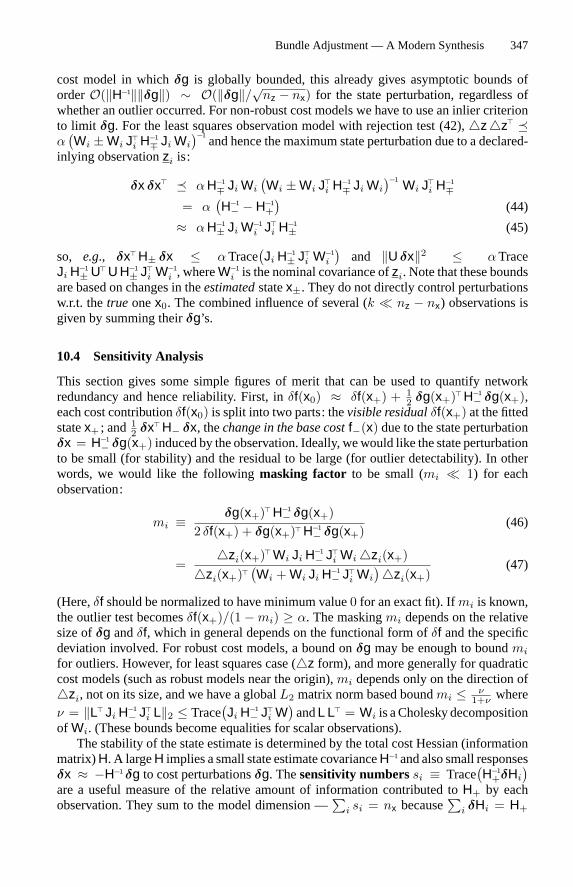
Bundle Adjustment — A Modern Synthesis 347
cost model in whichδg is globally bounded, this already gives asymptotic bounds oforderO(‖H−1‖‖δg‖) ∼ O(‖δg‖/√nz − nx) for the state perturbation, regardless ofwhether an outlier occurred. For non-robust cost models we have to use an inlier criterionto limit δg. For the least squares observation model with rejection test (42),�z�z� �α(Wi ±Wi J�
i H−1∓ Ji Wi
)−1and hence the maximum state perturbation due to a declared-
inlying observationzi is:
δx δx� � αH−1∓ Ji Wi
(Wi ±Wi J�
i H−1∓ Ji Wi
)−1Wi J�
i H−1∓
= α(H−1
− − H−1+)
(44)
≈ αH−1± Ji W−1
i J�i H−1
± (45)
so, e.g., δx� H± δx ≤ αTrace(Ji H−1
± J�i W−1
i
)and ‖U δx‖2 ≤ αTrace
Ji H−1± U� U H−1
± J�i W−1
i , whereW−1i is the nominal covariance ofzi. Note that these bounds
are based on changes in theestimatedstatex±. They do not directly control perturbationsw.r.t. thetrue onex0. The combined influence of several (k � nz − nx) observations isgiven by summing theirδg’s.
10.4 Sensitivity Analysis
This section gives some simple figures of merit that can be used to quantify networkredundancy and hence reliability. First, inδf(x0) ≈ δf(x+) + 1
2 δg(x+)� H−1− δg(x+),
each cost contributionδf(x0) is split into two parts: thevisible residualδf(x+) at the fittedstatex+ ; and 1
2 δx� H− δx, thechange in the base costf−(x) due to the state perturbationδx = H−1
− δg(x+) induced by the observation. Ideally, wewould like the state perturbationto be small (for stability) and the residual to be large (for outlier detectability). In otherwords, we would like the followingmasking factor to be small (mi � 1) for eachobservation:
mi ≡δg(x+)� H−1
− δg(x+)2 δf(x+) + δg(x+)� H−1
− δg(x+)(46)
=�zi(x+)� Wi Ji H−1
− J�i Wi�zi(x+)
�zi(x+)�(Wi + Wi Ji H−1
− J�i Wi
)�zi(x+)(47)
(Here,δf should be normalized to have minimum value0 for an exact fit). Ifmi is known,the outlier test becomesδf(x+)/(1 −mi) ≥ α. The maskingmi depends on the relativesize ofδg andδf, which in general depends on the functional form ofδf and the specificdeviation involved. For robust cost models, a bound onδg may be enough to boundmi
for outliers. However, for least squares case (�z form), and more generally for quadraticcost models (such as robust models near the origin),mi depends only on the direction of�zi, not on its size, and we have a globalL2 matrix norm based boundmi ≤ ν
1+ν whereν = ‖L� Ji H−1
− J�i L‖2 ≤ Trace
(Ji H−1
− J�i W)andL L� = Wi is aCholesky decomposition
ofWi. (These bounds become equalities for scalar observations).The stability of the state estimate is determined by the total cost Hessian (information
matrix)H. A largeH implies a small state estimate covarianceH−1and also small responsesδx ≈ −H−1δg to cost perturbationsδg. Thesensitivity numberssi ≡ Trace
(H−1
+δHi
)are a useful measure of the relative amount of information contributed toH+ by eachobservation. They sum to the model dimension —
∑i si = nx because
∑i δHi = H+
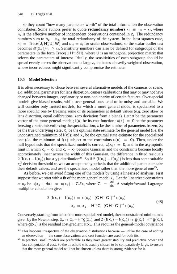
348 B. Triggs et al.
— so they count “how many parameters worth” of the total information the observationcontributes. Some authors prefer to quoteredundancy numbersri ≡ ni − si, whereni is the effective number of independent observations contained inzi. The redundancynumbers sum tonz − nx, the total redundancy of the system. In the least squares case,si = Trace
(Ji H−1
+ J�i W
)andmi = si for scalar observations, so the scalar outlier test
becomesδf(x+)/ri ≥ α. Sensitivity numbers can also be defined for subgroups of theparameters in the form Trace(U H−1δH), whereU is an orthogonal projection matrix thatselects the parameters of interest. Ideally, the sensitivities of each subgroup should bespread evenly across the observations: a largesi indicates a heavily weighted observation,whose incorrectness might significantly compromise the estimate.
10.5 Model Selection
It is often necessary to chose between several alternative models of the cameras or scene,e.g. additional parameters for lens distortion, camera calibrations that may ormay not havechanged between images, coplanarity or non-coplanarity of certain features. Over-specialmodels give biased results, while over-general ones tend to be noisy and unstable. Wewill consider onlynested models, for which a more general model is specialized to amore specific one by freezing some of its parameters at default values (e.g. zero skew orlens distortion, equal calibrations, zero deviation from a plane). Let:x be the parametervector of the more general model;f(x) be its cost function;c(x) = 0 be the parameterfreezing constraints enforcing the specialization;k be the number of parameters frozen;x0be the true underlying state;xg be the optimal state estimate for the general model (i.e. theunconstrained minimum off(x)); andxs be the optimal state estimate for the specializedone (i.e. the minimum off(x) subject to the constraintsc(x) = 0). Then, under thenull hypothesis that the specialized model is correct,c(x0) = 0, and in the asymptoticlimit in which xg − x0 andxs − x0 become Gaussian and the constraints become locallyapproximately linear across the width of this Gaussian, the difference in fitted residuals2 (f(xs)− f(xg)) has aχ2
k distribution24. So if2 (f(xs)− f(xg)) is less than some suitable
χ2k decision thresholdα, we can accept the hypothesis that the additional parameters taketheir default values, and use the specialized model rather than the more general one25.As before, we can avoid fitting one of the models by using a linearized analysis. First
suppose that we start with a fit of the more general modelxg. Let the linearized constraints
at xg be c(xg + δx) ≈ c(xg) + C δx, whereC ≡ dcdx . A straightforward Lagrange
multiplier calculation gives:
2 (f(xs)− f(xg)) ≈ c(xg)� (C H−1C�)−1 c(xg)
xs ≈ xg − H−1C� (C H−1C�)−1 c(xg)(48)
Conversely, starting fromafit of themorespecializedmodel, theunconstrainedminimum isgiven by theNewton step:xg ≈ xs−H−1g(xs), and2 (f(xs)− f(xg)) ≈ g(xs)� H−1g(xs),whereg(xs) is the residual cost gradient atxs. This requires the general-model covariance24 This happens irrespective of the observation distributions because — unlike the case of addingan observation — the same observations and cost function are used for both fits.
25 In practice, small models are preferable as they have greater stability and predictive power andless computational cost. So the thresholdα is usually chosen to be comparatively large, to ensurethat the more general model will not be chosen unless there is strong evidence for it.
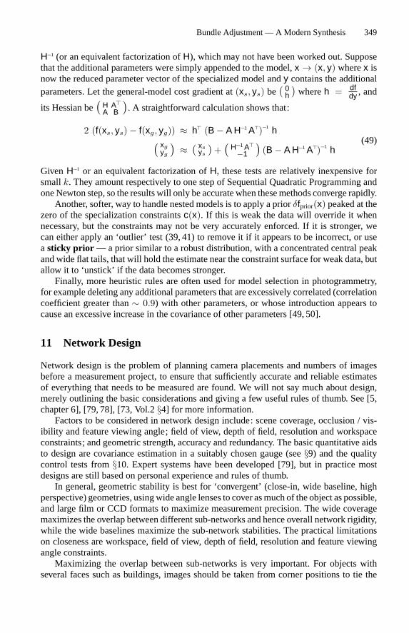
Bundle Adjustment — A Modern Synthesis 349
H−1 (or an equivalent factorization ofH), which may not have been worked out. Supposethat the additional parameters were simply appended to the model,x→ (x, y) wherex isnow the reduced parameter vector of the specialized model andy contains the additionalparameters. Let the general-model cost gradient at(xs, ys) be( 0
h ) whereh = dfdy , and
its Hessian be(
H A�A B
). A straightforward calculation shows that:
2 (f(xs, ys)− f(xg, yg)) ≈ h� (B− A H−1A�)−1 h( xgyg
)≈ ( xs
ys ) +(
H−1A�−1
)(B− A H−1A�)−1 h
(49)
GivenH−1 or an equivalent factorization ofH, these tests are relatively inexpensive forsmallk. They amount respectively to one step of Sequential Quadratic Programming andoneNewton step, so the results will only be accurate when thesemethods converge rapidly.Another, softer, way to handle nested models is to apply a priorδfprior(x) peaked at the
zero of the specialization constraintsc(x). If this is weak the data will override it whennecessary, but the constraints may not be very accurately enforced. If it is stronger, wecan either apply an ‘outlier’ test (39, 41) to remove it if it appears to be incorrect, or useasticky prior — a prior similar to a robust distribution, with a concentrated central peakand wide flat tails, that will hold the estimate near the constraint surface for weak data, butallow it to ‘unstick’ if the data becomes stronger.Finally, more heuristic rules are often used for model selection in photogrammetry,
for example deleting any additional parameters that are excessively correlated (correlationcoefficient greater than∼ 0.9) with other parameters, or whose introduction appears tocause an excessive increase in the covariance of other parameters [49, 50].
11 Network Design
Network design is the problem of planning camera placements and numbers of imagesbefore a measurement project, to ensure that sufficiently accurate and reliable estimatesof everything that needs to be measured are found. We will not say much about design,merely outlining the basic considerations and giving a few useful rules of thumb. See [5,chapter 6], [79, 78], [73, Vol.2§4] for more information.Factors to be considered in network design include: scene coverage, occlusion / vis-
ibility and feature viewing angle; field of view, depth of field, resolution and workspaceconstraints; and geometric strength, accuracy and redundancy. The basic quantitative aidsto design are covariance estimation in a suitably chosen gauge (see§9) and the qualitycontrol tests from§10. Expert systems have been developed [79], but in practice mostdesigns are still based on personal experience and rules of thumb.In general, geometric stability is best for ‘convergent’ (close-in, wide baseline, high
perspective) geometries, usingwide angle lenses to cover asmuch of the object as possible,and large film or CCD formats to maximize measurement precision. The wide coveragemaximizes the overlap between different sub-networks and hence overall network rigidity,while the wide baselines maximize the sub-network stabilities. The practical limitationson closeness are workspace, field of view, depth of field, resolution and feature viewingangle constraints.Maximizing the overlap between sub-networks is very important. For objects with
several faces such as buildings, images should be taken from corner positions to tie the
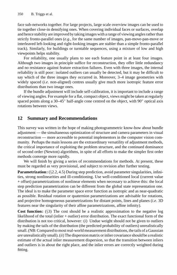
350 B. Triggs et al.
face sub-networks together. For large projects, large scale overview images can be used totie together close-in densifying ones. When covering individual faces or surfaces, overlapandhencestability are improvedby taking imageswitha rangeof viewingangles rather thanstrictly fronto-parallel ones (e.g., for the same number of images, pan-move-pan-move orinterleaved left-looking and right-looking images are stabler than a simple fronto-paralleltrack). Similarly, for buildings or turntable sequences, using a mixture of low and highviewpoints helps stability.For reliability, one usually plans to see each feature point in at least four images.
Although two images in principle suffice for reconstruction, they offer little redundancyand no resistance against feature extraction failures. Even with three images, the internalreliability is still poor: isolated outliers can usually be detected, but it may be difficult tosay which of the three images they occurred in. Moreover, 3–4 image geometries withwidely spaced (i.e. non-aligned) centres usually give much more isotropic feature errordistributions than two image ones.If the bundle adjustment will include self-calibration, it is important to include a range
of viewing angles. For example for a flat, compact object, viewsmight be taken at regularlyspaced points along a 30–45◦ half-angle cone centred on the object, with 90◦ optical axisrotations between views.
12 Summary and Recommendations
This survey was written in the hope of making photogrammetric know-how about bundleadjustment — the simultaneous optimization of structure and camera parameters in visualreconstruction — more accessible to potential implementors in the computer vision com-munity. Perhaps the main lessons are the extraordinary versatility of adjustment methods,the critical importance of exploiting the problem structure, and the continued dominanceof second order (Newton) algorithms, in spite of all efforts to make the simpler first ordermethods converge more rapidly.We will finish by giving a series of recommendations for methods. At present, these
must be regarded as very provisional, and subject to revision after further testing.
Parametrization: (§2.2, 4.5) During step prediction, avoid parameter singularities, infini-ties, strong nonlinearities and ill-conditioning. Use well-conditioned local (current value+ offset) parametrizations of nonlinear elements when necessary to achieve this: the localstep prediction parametrization can be different from the global state representation one.The ideal is to make the parameter space error function as isotropic and as near-quadraticas possible. Residual rotation or quaternion parametrizations are advisable for rotations,and projective homogeneous parametrizations for distant points, lines and planes (i.e. 3Dfeatures near the singularity of their affine parametrizations, affine infinity).
Cost function: (§3) The cost should be a realistic approximation to the negative loglikelihood of the total (inlier + outlier) error distribution. The exact functional form of thedistribution is not too critical, however: (i) Undue weight should not be given to outliersby making the tails of the distribution (the predicted probability of outliers) unrealisticallysmall. (NB:Compared tomost real-worldmeasurementdistributions, the tails of aGaussianareunrealistically small). (ii ) Thedispersionmatrix or inlier covarianceshouldbea realisticestimate of the actual inlier measurement dispersion, so that the transition between inliersand outliers is in about the right place, and the inlier errors are correctly weighted duringfitting.
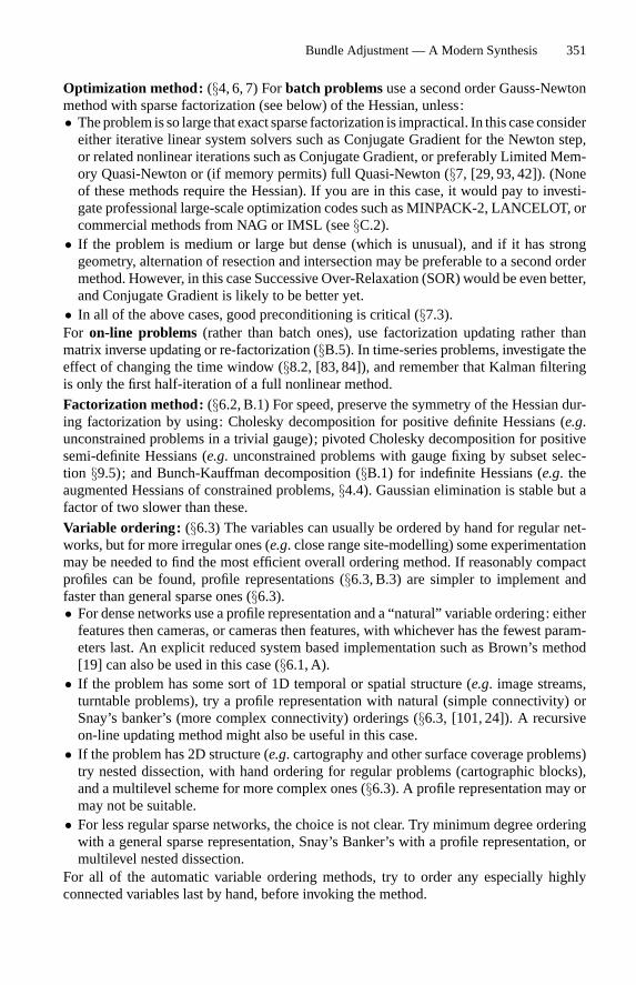
Bundle Adjustment — A Modern Synthesis 351
Optimization method: (§4, 6, 7) Forbatch problemsuse a second order Gauss-Newtonmethod with sparse factorization (see below) of the Hessian, unless:• Theproblem is so large that exact sparse factorization is impractical. In this case considereither iterative linear system solvers such as Conjugate Gradient for the Newton step,or related nonlinear iterations such as Conjugate Gradient, or preferably Limited Mem-ory Quasi-Newton or (if memory permits) full Quasi-Newton (§7, [29, 93, 42]). (Noneof these methods require the Hessian). If you are in this case, it would pay to investi-gate professional large-scale optimization codes such as MINPACK-2, LANCELOT, orcommercial methods from NAG or IMSL (see§C.2).• If the problem is medium or large but dense (which is unusual), and if it has stronggeometry, alternation of resection and intersection may be preferable to a second ordermethod. However, in this case Successive Over-Relaxation (SOR) would be even better,and Conjugate Gradient is likely to be better yet.• In all of the above cases, good preconditioning is critical (§7.3).For on-line problems (rather than batch ones), use factorization updating rather thanmatrix inverse updating or re-factorization (§B.5). In time-series problems, investigate theeffect of changing the time window (§8.2, [83, 84]), and remember that Kalman filteringis only the first half-iteration of a full nonlinear method.Factorization method: (§6.2, B.1) For speed, preserve the symmetry of the Hessian dur-ing factorization by using: Cholesky decomposition for positive definite Hessians (e.g.unconstrained problems in a trivial gauge); pivoted Cholesky decomposition for positivesemi-definite Hessians (e.g. unconstrained problems with gauge fixing by subset selec-tion §9.5); and Bunch-Kauffman decomposition (§B.1) for indefinite Hessians (e.g. theaugmented Hessians of constrained problems,§4.4). Gaussian elimination is stable but afactor of two slower than these.Variable ordering: (§6.3) The variables can usually be ordered by hand for regular net-works, but for more irregular ones (e.g. close range site-modelling) some experimentationmay be needed to find the most efficient overall ordering method. If reasonably compactprofiles can be found, profile representations (§6.3, B.3) are simpler to implement andfaster than general sparse ones (§6.3).• For dense networks use a profile representation and a “natural” variable ordering: eitherfeatures then cameras, or cameras then features, with whichever has the fewest param-eters last. An explicit reduced system based implementation such as Brown’s method[19] can also be used in this case (§6.1, A).• If the problem has some sort of 1D temporal or spatial structure (e.g. image streams,turntable problems), try a profile representation with natural (simple connectivity) orSnay’s banker’s (more complex connectivity) orderings (§6.3, [101, 24]). A recursiveon-line updating method might also be useful in this case.• If the problem has 2D structure (e.g. cartography and other surface coverage problems)try nested dissection, with hand ordering for regular problems (cartographic blocks),and a multilevel scheme for more complex ones (§6.3). A profile representation may ormay not be suitable.• For less regular sparse networks, the choice is not clear. Try minimum degree orderingwith a general sparse representation, Snay’s Banker’s with a profile representation, ormultilevel nested dissection.
For all of the automatic variable ordering methods, try to order any especially highlyconnected variables last by hand, before invoking the method.
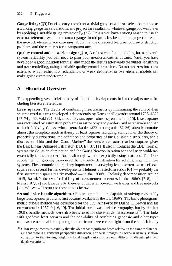
352 B. Triggs et al.
Gauge fixing:(§9) For efficiency, use either a trivial gauge or a subset selectionmethod asaworking gauge for calculations, and project the results intowhatever gauge youwant laterby applying a suitable gauge projectorPG (32). Unless you have a strong reason to use anexternal reference system, the output gauge should probably be an inner gauge centred onthe network elements you care most about,i.e. the observed features for a reconstructionproblem, and the cameras for a navigation one.
Quality control and network design: (§10) A robust cost function helps, but for overallsystem reliability you still need to plan your measurements in advance (until you havedeveloped a good intuition for this), and check the results afterwards for outlier sensitivityand over-modelling, using a suitable quality control procedure. Do not underestimate theextent to which either low redundancy, or weak geometry, or over-general models canmake gross errors undetectable.
A Historical Overview
This appendix gives a brief history of the main developments in bundle adjustment, in-cluding literature references.
Least squares:The theory of combining measurements by minimizing the sum of theirsquared residualswas developed independently byGauss and Legendre around 1795–1820[37, 74], [36, Vol.IV, 1–93], about 40 yearsafter robustL1 estimation [15]. Least squareswas motivated by estimation problems in astronomy and geodesy and extensively appliedto both fields by Gauss, whose remarkable 1823 monograph [37, 36] already containsalmost the complete modern theory of least squares including elements of the theory ofprobability distributions, the definition and properties of the Gaussian distribution, and adiscussion of bias and the “Gauss-Markov” theorem, which states that least squares givesthe Best Linear Unbiased Estimator (BLUE) [37, 11]. It also introduces theLDL� form ofsymmetric Gaussian elimination and the Gauss-Newton iteration for nonlinear problems,essentially in their modern forms although without explicitly using matrices. The 1828supplement on geodesy introduced the Gauss-Seidel iteration for solving large nonlinearsystems. The economic andmilitary importance of surveying lead to extensive use of leastsquares and several further developments: Helmert’s nested dissection [64]—probably thefirst systematic sparse matrix method — in the 1880’s, Cholesky decomposition around1915, Baarda’s theory of reliability of measurement networks in the 1960’s [7, 8], andMeissl [87, 89] and Baarda’s [6] theories of uncertain coordinate frames and free networks[22, 25]. We will return to these topics below.
Second order bundle algorithms:Electronic computers capable of solving reasonablylarge least squares problems first becameavailable in the late 1950’s. The basic photogram-metric bundle method was developed for the U.S. Air Force by Duane C. Brown and hisco-workers in 1957–9 [16, 19]. The initial focus was aerial cartography, but by the late1960’s bundle methods were also being used for close-range measurements26. The linkswith geodesic least squares and the possibility of combining geodesic and other typesof measurements with the photogrammetric ones were clear right from the start. Initially
26 Close rangemeans essentially that the object has significant depth relative to the camera distance,i.e. that there is significant perspective distortion. For aerial images the scene is usually shallowcompared to the viewing height, so focal length variations are very difficult to disentangle fromdepth variations.
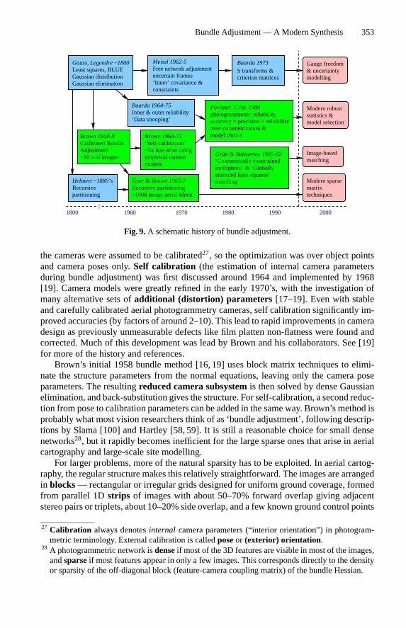
Bundle Adjustment — A Modern Synthesis 353
matching
Grün & Baltsavias 1985-92
Modern sparsematrixtechniques
Image-based
enforced least-squares’
& uncertaintycriterion matrices
Baarda 1973S transforms &
Recursive partitioning
matching
Gauge freedom
~5x less error using‘Self-calibration’
partitioning
Inner & outer reliabilityBaarda 1964-75
‘Data snooping’
constraints
Recursive
‘Inner’ covariance & uncertain frames
Helmert ~1880’s
multiphoto’ & ‘Globally
Gyer & Brown 1965-7
Free network adjustmentMeissl 1962-5
~1000 image aerial block
‘Geometrically constrained
Brown 1964-72
Gauss, Legendre ~1800
Gaussian eliminationGaussian distribution
modelsempirical camera
modellingLeast squares, BLUE
Förstner, Grün 1980
1960 2000
Modern robust statistics &model selection
photogrammetric reliabilityaccuracy = precision + reliabilityover-parametrization &model choice
1990
Brown 1958-9Calibrated BundleAdjustment~10’s of images
1800 1970 1980
Fig. 9.A schematic history of bundle adjustment.
the cameras were assumed to be calibrated27, so the optimization was over object pointsand camera poses only.Self calibration (the estimation of internal camera parametersduring bundle adjustment) was first discussed around 1964 and implemented by 1968[19]. Camera models were greatly refined in the early 1970’s, with the investigation ofmany alternative sets ofadditional (distortion) parameters [17–19]. Even with stableand carefully calibrated aerial photogrammetry cameras, self calibration significantly im-proved accuracies (by factors of around 2–10). This lead to rapid improvements in cameradesign as previously unmeasurable defects like film platten non-flatness were found andcorrected. Much of this development was lead by Brown and his collaborators. See [19]for more of the history and references.Brown’s initial 1958 bundle method [16, 19] uses block matrix techniques to elimi-
nate the structure parameters from the normal equations, leaving only the camera poseparameters. The resultingreduced camera subsystemis then solved by dense Gaussianelimination, and back-substitution gives the structure. For self-calibration, a second reduc-tion from pose to calibration parameters can be added in the same way. Brown’s method isprobably what most vision researchers think of as ‘bundle adjustment’, following descrip-tions by Slama [100] and Hartley [58, 59]. It is still a reasonable choice for small densenetworks28, but it rapidly becomes inefficient for the large sparse ones that arise in aerialcartography and large-scale site modelling.For larger problems, more of the natural sparsity has to be exploited. In aerial cartog-
raphy, the regular structure makes this relatively straightforward. The images are arrangedin blocks— rectangular or irregular grids designed for uniform ground coverage, formedfrom parallel 1Dstrips of images with about 50–70% forward overlap giving adjacentstereo pairs or triplets, about 10–20% side overlap, and a few known ground control points
27 Calibration always denotesinternal camera parameters (“interior orientation”) in photogram-metric terminology. External calibration is calledposeor (exterior) orientation .
28 A photogrammetric network isdenseif most of the 3D features are visible in most of the images,andsparseif most features appear in only a few images. This corresponds directly to the densityor sparsity of the off-diagonal block (feature-camera coupling matrix) of the bundle Hessian.
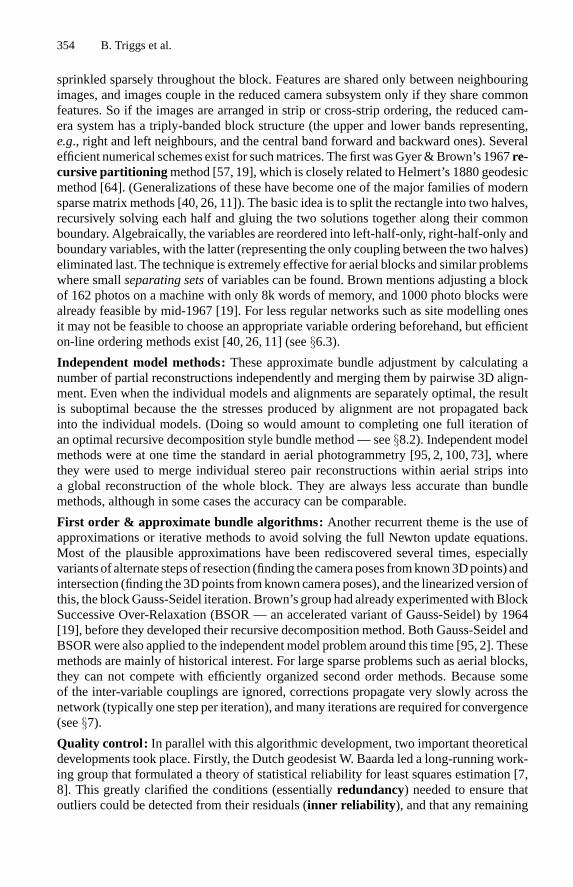
354 B. Triggs et al.
sprinkled sparsely throughout the block. Features are shared only between neighbouringimages, and images couple in the reduced camera subsystem only if they share commonfeatures. So if the images are arranged in strip or cross-strip ordering, the reduced cam-era system has a triply-banded block structure (the upper and lower bands representing,e.g., right and left neighbours, and the central band forward and backward ones). Severalefficient numerical schemes exist for suchmatrices. The first wasGyer &Brown’s 1967re-cursive partitioning method [57, 19], which is closely related to Helmert’s 1880 geodesicmethod [64]. (Generalizations of these have become one of the major families of modernsparsematrix methods [40, 26, 11]). The basic idea is to split the rectangle into two halves,recursively solving each half and gluing the two solutions together along their commonboundary. Algebraically, the variables are reordered into left-half-only, right-half-only andboundary variables, with the latter (representing the only coupling between the two halves)eliminated last. The technique is extremely effective for aerial blocks and similar problemswhere smallseparating setsof variables can be found. Brown mentions adjusting a blockof 162 photos on a machine with only 8k words of memory, and 1000 photo blocks werealready feasible by mid-1967 [19]. For less regular networks such as site modelling onesit may not be feasible to choose an appropriate variable ordering beforehand, but efficienton-line ordering methods exist [40, 26, 11] (see§6.3).Independent model methods:These approximate bundle adjustment by calculating anumber of partial reconstructions independently and merging them by pairwise 3D align-ment. Even when the individual models and alignments are separately optimal, the resultis suboptimal because the the stresses produced by alignment are not propagated backinto the individual models. (Doing so would amount to completing one full iteration ofan optimal recursive decomposition style bundle method— see§8.2). Independent modelmethods were at one time the standard in aerial photogrammetry [95, 2, 100, 73], wherethey were used to merge individual stereo pair reconstructions within aerial strips intoa global reconstruction of the whole block. They are always less accurate than bundlemethods, although in some cases the accuracy can be comparable.
First order & approximate bundle algorithms: Another recurrent theme is the use ofapproximations or iterative methods to avoid solving the full Newton update equations.Most of the plausible approximations have been rediscovered several times, especiallyvariants of alternate stepsof resection (finding thecameraposes fromknown3Dpoints) andintersection (finding the 3Dpoints fromknowncamera poses), and the linearized version ofthis, the blockGauss-Seidel iteration. Brown’s group had already experimentedwith BlockSuccessive Over-Relaxation (BSOR — an accelerated variant of Gauss-Seidel) by 1964[19], before they developed their recursive decomposition method. Both Gauss-Seidel andBSORwere also applied to the independent model problem around this time [95, 2]. Thesemethods are mainly of historical interest. For large sparse problems such as aerial blocks,they can not compete with efficiently organized second order methods. Because someof the inter-variable couplings are ignored, corrections propagate very slowly across thenetwork (typically one step per iteration), andmany iterations are required for convergence(see§7).Quality control: In parallel with this algorithmic development, two important theoreticaldevelopments took place. Firstly, the Dutch geodesist W. Baarda led a long-running work-ing group that formulated a theory of statistical reliability for least squares estimation [7,8]. This greatly clarified the conditions (essentiallyredundancy) needed to ensure thatoutliers could be detected from their residuals (inner reliability ), and that any remaining
Bundle Adjustment — A Modern Synthesis 355
undetected outliers had only a limited effect on the final results (outer reliability ). A. Grun[49, 50] and W. Forstner [30, 33, 34] adapted this theory to photogrammetry around 1980,and also gave some early correlation and covariance based model selection heuristics de-signed to control over-fitting problems caused by over-elaborate camera models in selfcalibration.
Datum / gauge freedom:Secondly, as problem size and sophistication increased, itbecame increasingly difficult to establish sufficiently accurate control points for largegeodesic and photogrammetric networks. Traditionally, the network had been viewed asa means of ‘densifying’ a fixed control coordinate system — propagating control-systemcoordinates from a few known control points to many unknown ones. But this viewpointis suboptimal when the network is intrinsically more accurate than the control, becausemost of the apparent uncertainty is simply due to the uncertain definition of the controlcoordinate system itself. In the early 1960’s,Meissl studied this problemand developed thefirst free network approach, in which the reference coordinate system floated freely ratherthan being locked to any given control points [87, 89]. More precisely, the coordinatesare pinned to a sort of average structure defined by so-calledinner constraints. Owingto the removal of control-related uncertainties, the nominal structure covariances becomesmaller and easier to interpret, and the numerical bundle iteration also converges morerapidly. Later, Baarda introduced another approach to this theory based onS-transforms— coordinate transforms between uncertain frames [6, 21, 22, 25].
Least squares matching:All of the above developments originally used manually ex-tracted image points. Automated image processing was clearly desirable, but it only grad-ually became feasible owing to the sheer size and detail of photogrammetric images. Bothfeature based,e.g. [31, 32], and direct (region based) [1, 52, 55, 110]methodswere studied,the latter especially for matching low-contrast natural terrain in cartographic applications.Both rely on some form ofleast squares matching(as image correlation is called in pho-togrammetry). Correlation based matching techniques remain the most accurate methodsof extracting precise translations from images, both for high contrast photogrammetrictargets and for low contrast natural terrain. Starting from around 1985, Grun and his co-workers combined region based least squaresmatchingwith various geometric constraints.Multi-photo geometrically constrainedmatchingoptimizes thematch overmultiple im-ages simultaneously, subject to the inter-image matching geometry [52, 55, 9]. For eachsurface patch there is a single search over patch depth and possibly slant, whichsimulta-neouslymoves it along epipolar lines in the other images. Initial versions assumed knowncamera matrices, but a full patch-based bundle method was later investigated [9]. Relatedmethods in computer vision include [94, 98, 67].Globally enforced least squaresmatch-ing [53, 97, 76] further stabilizes the solution in low-signal regions by enforcing continuityconstraints between adjacent patches. Patches are arranged in a grid and matched usinglocal affine or projective deformations, with additional terms to penalize mismatching atpatch boundaries. Related work in vision includes [104, 102]. The inter-patch constraintsgive a sparsely-coupled structure to the least squares matching equations, which can againbe handled efficiently by recursive decomposition.
356 B. Triggs et al.
B Matrix Factorization
This appendix covers some standard material on matrix factorization, including the tech-nical details of factorization, factorization updating, and covariance calculation methods.See [44, 11] for more details.
Terminology: Depending on the factorization, ‘L’ stands for lower triangular, ‘U’ or ‘R’for upper triangular, ‘D’ or ‘S’ for diagonal, ‘Q’ or ‘U’,‘V’ for orthogonal factors.
B.1 Triangular Decompositions
Any matrixA has a family of block (lower triangular)*(diagonal)*(upper triangular) fac-torizationsA = L D U:
A = L D U(A11 A12 ··· A1nA21 A22 ··· A2n...
.........
Am1 Am2 ··· Amn
)=
L11L21 L22...
......
......
...Lm1 Lm2 ··· Lmr
(
D1D2 ...
Dr
)(U11 U12 ··· ··· U1n
U22 ··· ··· U2n......
··· Urn
)
(50)
Lii Di Uii = Aii , i = j
Lij ≡ Aij U−1jj D−1
j , i > j
Uij ≡ D−1i L−1
ii Aij , i < j
Aij ≡ Aij −∑
k<min(i,j) Lik Dk Ukj
= Aij −∑
k<min(i,j) Aik A−1
kk Akj
(51)
Here, the diagonal blocksD1 . . .Dr−1 must be chosen to be square and invertible, andris determined by the rank ofA. The recursion (51) follows immediately from the productAij = (L D U)ij =
∑k≤min(i,j) Lik Dk Ukj . Given such a factorization, linear equations
can be solved by forwards and backwards substitution as in (22–24).The diagonal blocks ofL,D,U can be chosen freely subject toLii Dii Uii = Aii,
but once this is done the factorization is uniquely defined. ChoosingLii = Dii = 1 sothatUii = Aii gives the (block)LU decompositionA = L U, the matrix representationof (block) Gaussian elimination. ChoosingLii = Uii = 1 so thatDi = Aii gives theLDU decomposition. If A is symmetric, the LDU decomposition preserves the symmetryand becomes theLDL� decompositionA = L D L� whereU = L� andD = D�. If Ais symmetric positive definite we can setD = 1 to get theCholesky decompositionA = L L�, whereLii L�
ii = Aii (recursively) defines the Cholesky factorLii of the positivedefinite matrixAii. (For a scalar, Chol(a) =
√a). If all of the blocks are chosen to be
1×1, we get the conventional scalar forms of these decompositions. These decompositionsare obviously equivalent, but for speed and simplicity it is usual to use the most specificone that applies: LU for general matrices, LDL� for symmetric ones, and Cholesky forsymmetric positive definite ones. For symmetric matrices such as the bundle Hessian,LDL� / Cholesky are 1.5–2 times faster than LDU / LU. We will use the general form (50)below as it is trivial to specialize to any of the others.
Loop ordering: From (51), theij block of the decomposition depends only on the theupper left(m− 1)× (m− 1) submatrix and the firstm elements of rowi and columnj ofA, wherem = min(i, j). This allows considerable freedom in the ordering of operations
Bundle Adjustment — A Modern Synthesis 357
during decomposition,which canbeexploited to enhanceparallelismand improvememorycache locality.
Fill in: If A is sparse, itsL andU factors tend to become ever denser as the decompositionprogresses. Recursively expandingAik andAkj in (51) gives contributions of the form±Aik A
−1
kk Akl · · ·Apq A−1
qq Aqj for k, l . . . p, q < min(i, j). So even ifAij is zero, if thereis any path of the formi → k → l → . . . → p → q → j via non-zeroAkl withk, l . . . p, q < min(i, j), theij block of the decomposition will genericallyfill-in (becomenon-zero). The amount of fill-in is strongly dependent on the ordering of the variables(i.e. of the rows and columns ofA). Sparse factorization methods (§6.3) manipulate thisordering to minimize either fill-in or total operation counts.
Pivoting: For positive definite matrices, the above factorizations are very stable becausethepivots Aii must themselves remain positive definite. More generally, the pivots maybecome ill-conditioned causing the decomposition to break down. To deal with this, it isusual to search the undecomposed part of the matrix for a large pivot at each step, andpermute this into the leadingpositionbeforeproceeding. Thestablest policy isfull pivotingwhich searches the whole submatrix, but usually a less costlypartial pivoting searchover just the current column (column pivoting) or row (row pivoting ) suffices. Pivotingensures thatL and/orU are relatively well-conditioned and postpones ill-conditioning inD for as long as possible, but it can not ultimately makeD any better conditioned thanA is.Column pivoting is usual for the LU decomposition, but if applied to a symmetric matrixit destroys the symmetry and hence doubles the workload.Diagonal pivoting preservessymmetry by searching for the largest remaining diagonal element and permuting bothits row and its column to the front. This suffices for positive semidefinite matrices (e.g.gauge deficient Hessians). For general symmetric indefinite matrices (e.g. the augmentedHessians
(H C
C� 0
)of constrained problems (12)), off-diagonal pivots can not be avoided29,
but there are fast, stable, symmetry-preserving pivoted LDL� decompositions with blockdiagonalD having 1 × 1 and 2 × 2 blocks. Full pivoting is possible (Bunch-Parlettdecomposition), butBunch-Kaufman decompositionwhich searches the diagonal andonly one or at most two columns usually suffices. This method is nearly as fast as pivotedCholesky decomposition (to which it reduces for positive matrices), and as stable LUdecomposition with partial pivoting.Asen’s methodhas similar speed and stability butproduces a tridiagonalD. The constrained Hessian
(H C
C� 0
)has further special properties
owing to its zero block, but we will not consider these here — see [44,§4.4.6 EquilibriumSystems].
B.2 Orthogonal Decompositions
For least squares problems, there is an alternative family of decompositions based onorthogonal reduction of the JacobianJ = dz
dx . Given any rectangular matrixA, it can bedecomposed asA = Q RwhereR is upper triangular andQ is orthogonal (i.e., its columnsare orthonormal unit vectors). This is called theQR decompositionof A. R is identicalto the right Cholesky factor ofA� A = (R� Q�)(Q R) = R� R. The solution of the linear29 The archetypical failure is the unstable LDL� decomposition of the well-conditioned symmetric
indefinite matrix( ε 11 0 ) =
( 1 01/ε 1
)(ε 00 −1/ε
)(1 1/ε0 1
), for ε → 0. Fortunately, for small
diagonal elements, permuting the dominant off-diagonal element next to the diagonal and leavingthe resulting2 × 2 block undecomposed inD suffices for stability.
358 B. Triggs et al.
least squares problemminx ‖A x−b‖2 is x = R−1Q� b, andR−1Q� is the Moore-Penrosepseduo-inverse ofA. The QR decomposition is calculated by finding a series of simplerotations that successively zero below diagonal elements ofA to formR, and accumulatingthe rotations inQ, Q� A = R. Various types of rotations can be used.Givens rotationsare the fine-grained extreme: one-parameter2× 2 rotations that zero a single element ofA and affect only two of its rows.Householder reflectionsare coarser-grained reflectionsin hyperplanes1 − 2 v v�
‖v‖2 , designed to zero an entire below-diagonal column ofA andaffecting all elements ofA in or below the diagonal row of that column. Intermediatesizes of Householder reflections can also be used, the2 × 2 case being computationallyequivalent, and equal up to a sign, to the corresponding Givens rotation. This is useful forsparseQRdecompositions,e.g. multifrontalmethods (see§6.3 and [11]). TheHouseholdermethod is the most common one for general use, owing to its speed and simplicity. BoththeGivens andHouseholdermethods calculateR explicitly, butQ is not calculated directlyunless it is explicitly needed. Instead, it is stored in factorized form (as a series of2 × 2rotations or Householder vectors), and applied piecewise when needed. In particular,Q� bis needed to solve the least squares system, but it can be calculated progressively as part ofthe decomposition process. As for Cholesky decomposition, QR decomposition is stablewithout pivoting so long asA has full column rank and is not too ill-conditioned. FordegenerateA, Householder QR decomposition with column exchange pivoting can beused. See [11] for more information about QR decomposition.Both QR decomposition ofA and Cholesky decomposition of the normal matrixA� A
can be used to calculate the Cholesky / QR factorR and to solve least squares problemswith designmatrix / JacobianA. TheQRmethod runs about as fast as the normal / Choleskyone for squareA, but becomes twice as slow for long thinA (i.e. many observations inrelatively few parameters). However, the QR is numerically much stabler than the normal /Cholesky one in the following sense: ifA has condition number (ratio of largest to smallestsingular value)c and the machine precision isε, the QR solution has relative errorO(cε),whereas the normal matrixA� A has condition numberc2 and its solution has relative errorO(c2ε). This matters only ifc2ε approaches the relative accuracy to which the solutionis required. For example, even in accurate bundle adjustments, we do not need relativeaccuracies greater than about1 : 106. As ε ∼ 10−16 for double precision floating point,we can safely use the normal equation method forc(J) � 105, whereas the QR method issafe up toc(J) � 1010, whereJ is the bundle Jacobian. In practice, the Gauss-Newton /normal equation approach is used in most bundle implementations.Individual Householder reflections are also useful for projecting parametrizations of
geometric entities orthogonal to some constraint vector. For example, for quaternionsor homogeneous projective vectorsX, we often want to enforce spherical normalization‖X‖2 = 1. To first order, only displacementsδXorthogonal toXareallowed,X� δX = 0.To parametrize the directions we can move in, we need a basis for the vectors orthogonaltoX. A Householder reflectionQ based onX convertsX to (1 0 . . . 0)� and hence theorthogonal directions to vectors of the form(0 ∗ . . . ∗)�. So ifU contains rows 2–n of Q,we can reduce JacobiansddX to then − 1 independent parametersδu of the orthogonalsubspace by post-multiplying byU�, and once we have solved forδu, we can recoverthe orthogonalδX ≈ U δu by premultiplying byU. Multiple constraints can be enforcedby successiveHouseholder reductionsof this form. This corresponds exactly to theLQmethod for solving constrained least squares problems [11].
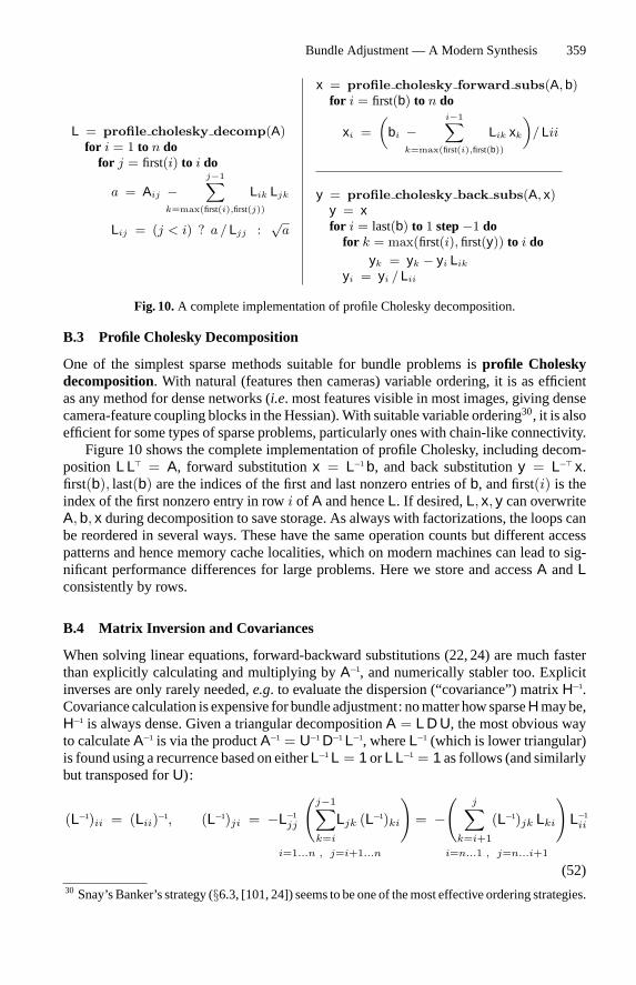
Bundle Adjustment — A Modern Synthesis 359
L = profile cholesky decomp(A)for i = 1 to n dofor j = first(i) to i do
a = Aij −j−1∑
k=max(first(i),first(j))
Lik Ljk
Lij = (j < i) ? a / Ljj :√a
x = profile cholesky forward subs(A, b)for i = first(b) to n do
xi =(
bi −i−1∑
k=max(first(i),first(b))
Lik xk
)/ Lii
y = profile cholesky back subs(A, x)y = xfor i = last(b) to 1 step−1 do
for k = max(first(i), first(y)) to i doyk = yk − yi Lik
yi = yi / Lii
Fig. 10.A complete implementation of profile Cholesky decomposition.
B.3 Profile Cholesky Decomposition
One of the simplest sparse methods suitable for bundle problems isprofile Choleskydecomposition. With natural (features then cameras) variable ordering, it is as efficientas any method for dense networks (i.e. most features visible in most images, giving densecamera-feature coupling blocks in the Hessian).With suitable variable ordering30, it is alsoefficient for some types of sparse problems, particularly ones with chain-like connectivity.Figure 10 shows the complete implementation of profile Cholesky, including decom-
positionL L� = A, forward substitutionx = L−1b, and back substitutiony = L−� x.first(b), last(b) are the indices of the first and last nonzero entries ofb, and first(i) is theindex of the first nonzero entry in rowi of A and henceL. If desired,L, x, y can overwriteA,b, x during decomposition to save storage. As always with factorizations, the loops canbe reordered in several ways. These have the same operation counts but different accesspatterns and hence memory cache localities, which on modern machines can lead to sig-nificant performance differences for large problems. Here we store and accessA andLconsistently by rows.
B.4 Matrix Inversion and Covariances
When solving linear equations, forward-backward substitutions (22, 24) are much fasterthan explicitly calculating and multiplying byA−1, and numerically stabler too. Explicitinverses are only rarely needed,e.g. to evaluate the dispersion (“covariance”) matrixH−1.Covariance calculation is expensive for bundle adjustment: nomatter howsparseHmaybe,H−1 is always dense. Given a triangular decompositionA = L D U, the most obvious wayto calculateA−1 is via the productA−1 = U−1D−1L−1, whereL−1 (which is lower triangular)is found using a recurrence based on eitherL−1L = 1 orL L−1 = 1 as follows (and similarlybut transposed forU):
(L−1)ii = (Lii)−1, (L−1)ji = −L−1jj
(j−1∑k=i
Ljk (L−1)ki
)= −
(j∑
k=i+1
(L−1)jk Lki
)L−1
ii
i=1...n , j=i+1...n i=n...1 , j=n...i+1
(52)30 Snay’s Banker’s strategy (§6.3, [101, 24]) seems to be one of themost effective ordering strategies.
360 B. Triggs et al.
Alternatively [45, 11], the diagonal and the (zero) upper triangle of the linear systemU A−1 = D−1L−1 can be combined with the (zero) lower triangle ofA−1L = U−1D−1 to givethe direct recursion (i = n . . . 1 andj = n . . . i + 1):
(A−1)ji = −(
n∑k=i+1
(A−1)jk Lki
)L−1
ii , (A−1)ij = −U−1ii
(n∑
k=i+1
Uik (A−1)kj
)
(A−1)ii = U−1ii
(D−1
i L−1ii −
n∑k=i+1
Uik (A−1)ki
)=
(U−1
ii D−1i −
n∑k=i+1
(A−1)ik Lki
)L−1
ii
(53)
In the symmetric case(A−1)ji = (A−1)ij so we can avoid roughly half of the work. If only afew blocks ofA−1 are required (e.g. the diagonal ones), this recursion has the property thatthe blocks ofA−1 associated with the filled positions ofL andU can be calculated withoutcalculating any blocks associated with unfilled positions. More precisely, to calculate(A−1)ij for which Lji (j > i) or Uji (j < i) is non-zero, we do not need any block(A−1)kl for which Llk = 0 (l > k) or Ulk = 0 (l < k) 31. This is a significant saving ifL,U are sparse, as in bundle problems. In particular, given the covariance of the reducedcamera system, the 3D feature variances and feature-camera covariances can be calculatedefficiently using (53) (or equivalently (17), whereA ← Hss is the block diagonal featureHessian andD2 is the reduced camera one).
B.5 Factorization Updating
For on-line applications (§8.2), it is useful to be able toupdate the decompositionA =L D U to account for a (usually low-rank) changeA → A ≡ A ± B W C. Let B ≡ L−1BandC ≡ C U−1 so thatL−1A U−1 = D ± B W C. This low-rank update ofD can be LDUdecomposed efficiently. Separating the first block ofD from the others we have:
(D1
D2
)±(
B1
B2
)W ( C1 C2 ) =
(1
±B2 W C1 D−11 1
)(D1
D2
)(1 ±D
−11 B1 W C2
1
)D1 ≡ D1 ± B1 W C1 D2 ≡ D2 ± B2
(W ∓W C1 D
−1
1 B1 W)
C2
(54)
D2 is a low-rank update ofD2 with the sameC2 andB2 but a differentW. Evaluatingthis recursively and merging the resulting L and U factors intoL andU gives the updated
31 This holds because of the way fill-in occurs in the LDU decomposition. Suppose that we want tofind (A−1)ij , wherej > i andLji �= 0. For this we need(A−1)kj for all non-zeroUik, k > i. Butfor theseAjk = Lji Di Uik + . . .+ Ajk �= 0, so(A−1)kj is associated with a filled position andwill already have been evaluated.
Bundle Adjustment — A Modern Synthesis 361
decomposition32 A = L D U :
W(1) ← ±W ; B(1) ← B ; C(1) ← C ;for i = 1 to n do
Bi ← B(i)i ; Ci ← C(i)
i ; Di ← Di + Bi W(i) Ci ;
W(i+1) ← W(i) −W(i) Ci D−1
i Bi W(i) =((W(i))−1 + Ci D−1
i Bi
)−1
;
for j = i + 1 to n do
B(i+1)j ← B(i)
j − Lji Bi ; Lji ← Lji + B(i+1)j W(i+1) Ci D−1
i ;C(i+1)
j ← C(i)j − Ci Uij ; Uij ← Uij + D−1
i Bi W(i+1) C(i+1)j ;
(55)
TheW−1 form of theW update is numerically stabler for additions (‘+’ sign inA±B W Cwith positiveW), but is not usable unlessW(i) is invertible. In either case, the updatetakes timeO((k2 + b2)N2
)whereA isN×N ,W is k×k and theDi areb×b. So other
things being equal,k should be kept as small as possible (e.g. by splitting the update intoindependent rows using an initial factorization ofW, and updating for each row in turn).The scalar Cholesky form of this method for a rank one updateA→ A + w b b� is:
w(1) ← w ; b(1) ← b ;for i = 1 to n do
bi ← b(i)i /Lii ; di ← 1 + w(i) b
2i ; Lii ← Lii
√di ;
w(i+1) ← w(i)/di ;for j = i + 1 to n do
b(i+1)j ← b(i)
j − Lji bi ; Lji ←(
Lji + b(i+1)j w(i+1) bi
)√di ;
(56)
This takesO(n2)operations. The same recursion rule (and several equivalent forms) can
be derived by reducing(L b)� to an upper triangular matrix using Givens rotations orHouseholder transformations [43, 11].
C Software
C.1 Software Organization
For a general purpose bundle adjustment code, an extensible object-based organization isnatural. The measurement network can be modelled as a network of objects, representingmeasurements and their error modelsand the different types of3D featuresandcameramodelsthat they depend on. It is obviously useful to allow the measurement, feature andcamera types to be open-ended. Measurements may be 2D or 3D, implicit or explicit, andmany different robust error models are possible. Features may range from points throughcurves and homographies to entire 3D object models. Many types of camera and lens
32 Here, B(i)j = Bj − ∑i−1
k=1 Ljk Bk =∑j
k=i Ljk Bk and C(i)j = Cj − ∑i−1
k=1 Ck Lkj =∑jk=i Ck Ukj accumulateL−1BandC U−1. For theL,UupdatesonecanalsouseW(i+1) Ci D−1
i =W(i) Ci D
−1i andD
−1i Bi W(i+1) = D
−1i Bi W(i).
362 B. Triggs et al.
distortionmodels exist. If the scene is dynamic or articulated, additional nodes representing3D transformations (kinematic chains or relative motions) may also be needed.Themain purposeof the network structure is to predict observations and their Jacobians
w.r.t. the free parameters, and then to integrate the resulting first order parameter updatesback into the internal 3D feature and camera state representations. Prediction is essentiallya matter of systematically propagating values through the network, with heavy use of thechain rule for derivative propagation. The network representation must interface with anumerical linear algebra one that supports appropriatemethods for forming and solving thesparse, damped Gauss-Newton (or other) step prediction equations. A fixed-order sparsefactorizationmay suffice for simple networks, while automatic variable ordering is neededfor more complicated networks and iterative solution methods for large ones.Several extensible bundle codes exist, but as far as we are aware, none of them are
currently available as freeware. Our own implementations include:• Carmen [59] is a program for camera modelling and scene reconstruction using itera-tive nonlinear least squares. It has a modular design that allows many different feature,measurement and camera types to be incorporated (including some quite exotic ones[56, 63]). It uses sparse matrix techniques similar to Brown’s reduced camera systemmethod [19] to make the bundle adjustment iteration efficient.
• Horatio (http://www.ee.surrey.ac.uk/Personal/P.McLauchlan/horatio/html, [85], [86],[83], [84]) is a C library supporting the development of efficient computer vision ap-plications. It contains support for image processing, linear algebra and visualization,and will soon be made publicly available. The bundle adjustment methods in Horatio,which are based on the Variable State Dimension Filter (VSDF) [83, 84], are beingcommercialized. These algorithms support sparse block matrix operations, arbitrarygauge constraints, global and local parametrizations, multiple feature types and cameramodels, as well as batch and sequential operation.
• vxl: This modular C++ vision environment is a new, lightweight version of the Tar-getJr/IUE environment, which is being developed mainly by the Universities of Oxfordand Leuven, and General Electric CRD. The initial public release onhttp://www.robots.ox.ac.uk/∼vxl will include an OpenGL user interface and classesfor multiple view geometry and numerics (the latter being mainly C++ wrappers to wellestablished routines from Netlib — see below). A bundle adjustment code exists for itbut is not currently planned for release [28, 62].
C.2 Software Resources
A great deal of useful numerical linear algebra and optimization software is available onthe Internet, although more commonly inFortran than in C/C++. The main reposi-tory isNetlib at http://www.netlib.org/. Other useful sites include: the ‘Guide to Avail-ableMathematical Software’ GAMSat http://gams.nist.gov; theNEOSguide http://www-fp.mcs.anl.gov/otc/Guide/, which is based in part onMore &Wright’s guidebook [90]; andthe Object Oriented Numerics page http://oonumerics.org. For large-scale dense linear al-gebra, LAPACK (http://www.netlib.org/lapack, [3]) is the best package available. Howeverit is optimized for relatively largeproblems (matricesof size100ormore), so if youaresolv-ingmany small ones (size less than 20 or so) it may be faster to use the older LINPACKandEISPACK routines. These libraries all use the BLAS (Basic Linear Algebra Subroutines)interface for low levelmatrixmanipulations,optimizedversionsofwhichareavailable from
Bundle Adjustment — A Modern Synthesis 363
most processor vendors. They are allFortran based, but C/C++ versions and interfacesexist (CLAPACK,http://www.netlib.org/clapack; LAPACK++, http://math.nist.gov/lapack++). For sparsematrices there is a bewildering array of packages. One good one is Boeing’s SPOOLES(http://www.netlib.org/linalg/spooles/spooles.2.2.html) which implements sparse Bunch-Kaufman decomposition in C with several ordering methods. For iterative linear systemsolvers implementation is seldom difficult, but there are again many methods and imple-mentations. The ‘Templates’ book [10] contains potted code. For nonlinear optimizationthere are various older codes such as MINPACK, and more recent codes designed mainlyfor very large problems such as MINPACK-2 (ftp://info.mcs.anl.gov/pub/MINPACK-2)and LANCELOT (http://www.cse.clrc.ac.uk/Activity/LANCELOT). (Both of these lattercodes have good reputations for other large scale problems, but as far as we are aware theyhave not yet been tested on bundle adjustment). All of the above packages are freely avail-able.Commercial vendors suchasNAG (ttp://www.nag.co.uk) and IMSL (www.imsl.com)have their own optimization codes.
Glossary
This glossary includes a few common terms from vision, photogrammetry, numerical optimizationand statistics, with their translations.
Additional parameters: Parameters added to the basic perspective model to represent lens distor-tion and similar small image deformations.
α-distribution: A family of wide tailed probability distributions, including theCauchy distribu-tion (α = 1) and the Gaussian (α = 2).
Alternation: A family of simplistic and largely outdated strategies for nonlinear optimization (andalso iterative solution of linear equations). Cycles through variables or groups of variables, opti-mizing over each in turn while holding all the others fixed. Nonlinear alternation methods usuallyrelinearize the equations after each group, whileGauss-Seidelmethods propagate first order cor-rections forwards and relinearize only at the end of the cycle (the results are the same to firstorder).Successive over-relaxationadds momentum terms to speed convergence. Seesepara-ble problem. Alternation ofresectionandintersection is a naıve and often-rediscovered bundlemethod.
Asymptotic limit: In statistics, the limit as the number of independent measurements is increasedto infinity, or as the second order moments dominate all higher order ones so that the posteriordistribution becomes approximately Gaussian.
Asymptotic convergence: In optimization, the limit of small deviations from the solution,i.e. asthe solution is reached.Second orderor quadratically convergentmethods such asNewton’smethod squarethe norm of the residual at each step, whilefirst order or linearly convergentmethods such asgradient descentandalternation only reduce the error by a constant factor ateach step.
Banker’s strategy: Seefill in , §6.3.Block: A (possibly irregular) grid of overlapping photos in aerial cartography.Bunch-Kauffman: A numerically efficient factorizationmethod for symmetric indefinitematrices,
A = L D L� whereL is lower triangular andD is block diagonal with1 × 1 and2 × 2 blocks(§6.2, B.1).
Bundle adjustment: Any refinementmethod for visual reconstructions that aims to produce jointlyoptimal structure and camera estimates.
364 B. Triggs et al.
Calibration: In photogrammetry, this always meansinternalcalibration of the cameras. Seeinnerorientation.
Central limit theorem: States thatmaximum likelihoodandsimilar estimators asymptotically haveGaussian distributions. The basis of most of our perturbation expansions.
Cholesky decomposition:Anumerically efficient factorizationmethod for symmetric positive def-inite matrices,A = L L�whereL is lower triangular.
Close Range:Any photogrammetric problem where the scene is relatively close to the camera,so that it has significant depth compared to the camera distance. Terrestrial photogrammetry asopposed toaerial cartography.
Conjugate gradient: A cleverly accelerated first order iteration for solving positive definite linearsystems or minimizing a nonlinear cost function. SeeKrylov subspace.
Cost function: The function quantifying the total residual error that is minimized in an adjustmentcomputation.
Cramer-Rao bound: SeeFisher information .Criterion matrix: In network design, an ideal or desired form for a covariance matrix.Damped Newton method: Newton’s methodwith a stabilizing step control policy added. See
Levenberg-Marquardt .Data snooping: Elimination of outliers based on examination of their residual errors.Datum: A reference coordinate system, against which other coordinates and uncertainties are mea-sured. Our principle example of agauge.
Dense: A matrix or system of equations with so few known-zero elements that it may as well betreated as having none. The opposite ofsparse. For photogrammetric networks,densemeans thatthe off-diagonal structure-camera block of the Hessian is dense,i.e. most features are seen in mostimages.
Descent direction: In optimization, anysearchdirectionwithadownhill component,i.e. that locallyreduces the cost.
Design: The process of defining ameasurement network (placement of cameras, number of images,etc.) to satisfy given accuracy and quality criteria.
Design matrix: The observation-state JacobianJ = dzdx .
Direct method: Dense correspondence or reconstruction methods based directly on cross-correlat-ing photometric intensities or related descriptor images, without extracting geometric features.Seeleast squares matching, feature based method.
Dispersion matrix: The inverse of the cost functionHessian, a measure of distribution spread. Intheasymptotic limit , the covariance is given by the dispersion.
Downdating: On-the-fly removal of observations, without recalculating everything from scratch.The inverse ofupdating.
Elimination graph: A graph derived from thenetwork graph, describing the progress offill induring sparse matrix factorization.
Empirical distribution: A set of samples from some probability distribution, viewed as an sum-of-delta-function approximation to the distribution itself. Thelaw of large numbersasserts thatthe approximation asymptotically converges to the true distribution in probability.
Fill-in: The tendency of zero positions to become nonzero as sparsematrix factorization progresses.Variable ordering strategiesseek to minimize fill-in by permuting the variables before factor-ization. Methods includeminimum degree, reverse Cuthill-McKee, Banker’s strategies, andnested dissection. See§6.3.
Fisher information: In parameter estimation, the mean curvature of the posterior log likelihoodfunction, regarded as ameasure of the certainty of an estimate. TheCramer-Rao boundsays thatany unbiased estimator has covariance≥ the inverse of the Fisher information.
Bundle Adjustment — A Modern Synthesis 365
Free gauge / free network: A gaugeor datum that is defined internally to the measurement net-work, rather than being based on predefined reference features like afixed gauge.
Feature based: Sparse correspondence / reconstructionmethodsbasedongeometric image features(points, lines, homographies. . . ) rather than direct photometry. Seedirect method.
Filtering: In sequential problems such as time series, the estimation of a current value using allof the previous measurements.Smoothing can correct this afterwards, by integrating also theinformation from future measurements.
First order method / convergence: Seeasymptotic convergence.Gauge: An internal or external referencecoordinate systemdefined for the current state and (at least)small variations of it, against which other quantitiesand their uncertaintiescan be measured. The3D coordinate gauge is also called thedatum. A gauge constraint is any constraint fixing aspecific gauge,e.g. for the current state and arbitrary (small) displacements of it. The fact thatthe gauge can be chosen arbitrarily without changing the underlying structure is calledgaugefreedomorgauge invariance. The rank-deficiency that this transformation-invariance of the costfunction induces on the Hessian is calledgauge deficiency. Displacements that violate the gaugeconstraints can be corrected by applying anS-transform, whose linear form is agauge projectionmatrix PG .
Gauss-Markov theorem: This says that for a linear system, least squares weighted by the truemeasurement covariancesgives theBest (minimumvariance)LinearUnbiasedEstimatororBLUE.
Gauss-Newton method:ANewton-like method for nonlinear least squares problems, in which theHessian is approximated by the Gauss-Newton oneH ≈ J� W J whereJ is thedesign matrixandW is a weight matrix. Thenormal equationsare the resulting Gauss-Newton step predictionequations(J� W J) δx = −(J W �z).
Gauss-Seidel method:Seealternation.Givens rotation: A 2 × 2 rotation used to as part of orthogonal reduction of a matrix,e.g. QR,SVD. SeeHouseholder reflection.
Gradient: The derivative of the cost function w.r.t. the parametersg = dfdx .
Gradient descent: Naıve optimization method which consists of steepest descent (in some givencoordinate system) down the gradient of the cost function.
Hessian: Thesecondderivativematrix of the cost functionH = d2fdx2 . Symmetric andpositive (semi-
)definite at a cost minimum. Measures how ‘stiff’ the state estimate is against perturbations. Itsinverse is thedispersion matrix.
Householder reflection: A matrix representing reflection in a hyperplane, used as a tool for or-thogonal reduction of a matrix,e.g. QR, SVD. SeeGivens rotation.
Independent model method: A suboptimal approximation to bundle adjustment developed foraerial cartography. Small local 3D models are reconstructed, each from a few images, and thenglued together viatie featuresat their common boundaries, without a subsequent adjustment torelax the internal stresses so caused.
Inner: Internal or intrinsic.Inner constraints: Gauge constraintslinking the gauge to some weighted average of the recon-structed features and cameras (rather than to an externally supplied reference system).
Inner orientation: Internal camera calibration, including lens distortion,etc.
Inner reliability: Theability to either resist outliers, or detect and reject thembasedon their residualerrors.
Intersection: (of optical rays). Solving for 3D feature positions given the corresponding imagefeatures and known 3D camera poses and calibrations. Seeresection, alternation.
Jacobian: Seedesign matrix.
366 B. Triggs et al.
Krylov subspace: The linear subspace spanned by the iterated products{Ak b|k = 0 . . . n} ofsomesquarematrixAwith somevectorb, used as a tool for generating linear algebra and nonlinearoptimization iterations.Conjugate gradient is the most famous Krylov method.
Kullback-Leibler divergence: Seerelative entropy.Least squares matching: Image matching based on photometric intensities. Seedirect method.Levenberg-Marquardt: A common damping (step control) method for nonlinear least squaresproblems, consisting of adding a multipleλD of some positive definite weight matrixD to theGauss-Newton Hessian before solving for the step. Levenberg-Marquardt uses a simple rescalingbased heuristic for settingλ, while trust region methods use a more sophisticated step-lengthbased one. Such methods are calleddamped Newtonmethods in general optimization.
Local model: In optimization, a local approximation to the function being optimized, which is easyenough to optimize that an iterative optimizer for the original function can be based on it. Thesecond order Taylor series model givesNewton’s method.
Local parametrization: Aparametrization of a nonlinear space based on offsets from some currentpoint. Used during an optimization step to give better local numerical conditioning than a moreglobal parametrization would.
LU decomposition: The usual matrix factorization form of Gaussian elimination.Minimum degree ordering: One of themost widely used automatic variable orderingmethods forsparse matrix factorization.
Minimum detectable gross error: Thesmallest outlier that canbedetectedonaveragebyanoutlierdetection method.
Nested dissection:A top-down divide-and-conquervariable ordering method for sparse matrixfactorization.Recursively splits the problem into disconnected halves, dealingwith theseparatingsetof connecting variables last. Particularly suitable for surface coverage problems. Also calledrecursive partitioning .
Nested models:Pairs of models, of which one is a specialization of the other obtained by freezingcertain parameters(s) at prespecified values.
Network: The interconnection structure of the 3D features, the cameras, and themeasurements thatare made of them (image points,etc.). Usually encoded as a graph structure.
Newton method: The basic iterative second order optimization method. TheNewton stepstateupdateδx = −H−1g minimizes a local quadratic Taylor approximation to the cost function ateach iteration.
Normal equations: SeeGauss-Newton method.Nuisance parameter: Any parameter that had to be estimated as part of a nonlinear parameterestimation problem, but whose value was not really wanted.
Outer: External. Seeinner.Outer orientation: Camera pose (position and angular orientation).Outer reliability: The influence of unremoved outliers on the final parameter estimates,i.e. theextent to which they are reliable even though some (presumably small or lowly-weighted) outliersmay remain undetected.
Outlier: An observation that deviates significantly from its predicted position. More generally,any observation that does not fit some preconceived notion of how the observations should bedistributed, and which must therefore be removed to avoid disturbing the parameter estimates.Seetotal distribution .
Pivoting: Row and/or column exchanges designed to promote stability during matrix factorization.Point estimator: Any estimator that returns a single “best” parameter estimate,e.g. maximumlikelihood, maximum a posteriori.
Pose: 3D position and orientation (angle),e.g. of a camera.
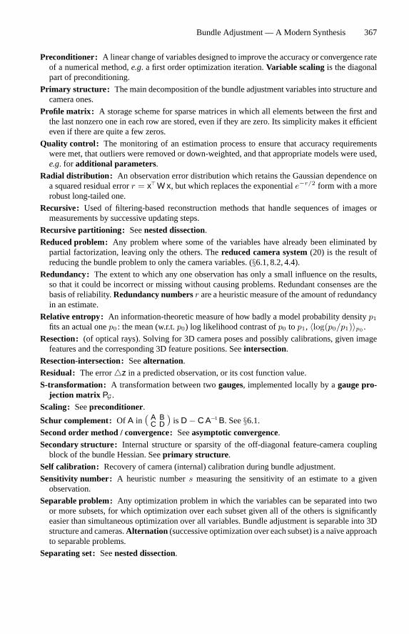
Bundle Adjustment — A Modern Synthesis 367
Preconditioner: A linear change of variables designed to improve the accuracy or convergence rateof a numerical method,e.g. a first order optimization iteration.Variable scaling is the diagonalpart of preconditioning.
Primary structure: The main decomposition of the bundle adjustment variables into structure andcamera ones.
Profile matrix: A storage scheme for sparse matrices in which all elements between the first andthe last nonzero one in each row are stored, even if they are zero. Its simplicity makes it efficienteven if there are quite a few zeros.
Quality control: The monitoring of an estimation process to ensure that accuracy requirementswere met, that outliers were removed or down-weighted, and that appropriate models were used,e.g. for additional parameters.
Radial distribution: An observation error distribution which retains the Gaussian dependence ona squared residual errorr = x� W x, but which replaces the exponentiale−r/2 form with a morerobust long-tailed one.
Recursive: Used of filtering-based reconstruction methods that handle sequences of images ormeasurements by successive updating steps.
Recursive partitioning: Seenested dissection.Reduced problem: Any problem where some of the variables have already been eliminated bypartial factorization, leaving only the others. Thereduced camera system(20) is the result ofreducing the bundle problem to only the camera variables. (§6.1, 8.2, 4.4).
Redundancy: The extent to which any one observation has only a small influence on the results,so that it could be incorrect or missing without causing problems. Redundant consenses are thebasis of reliability.Redundancy numbersr are a heuristic measure of the amount of redundancyin an estimate.
Relative entropy: An information-theoretic measure of how badly a model probability densityp1fits an actual onep0 : the mean (w.r.t.p0) log likelihood contrast ofp0 to p1, 〈log(p0/p1)〉p0 .
Resection: (of optical rays). Solving for 3D camera poses and possibly calibrations, given imagefeatures and the corresponding 3D feature positions. Seeintersection.
Resection-intersection:Seealternation.Residual: The error�z in a predicted observation, or its cost function value.S-transformation: A transformation between twogauges, implemented locally by agauge pro-
jection matrix PG .Scaling: Seepreconditioner.
Schur complement: Of A in ( A BC D ) isD − C A−1B. See§6.1.
Second order method / convergence:Seeasymptotic convergence.Secondary structure: Internal structure or sparsity of the off-diagonal feature-camera couplingblock of the bundle Hessian. Seeprimary structure .
Self calibration: Recovery of camera (internal) calibration during bundle adjustment.Sensitivity number: A heuristic numbers measuring the sensitivity of an estimate to a givenobservation.
Separable problem: Any optimization problem in which the variables can be separated into twoor more subsets, for which optimization over each subset given all of the others is significantlyeasier than simultaneous optimization over all variables. Bundle adjustment is separable into 3Dstructure and cameras.Alternation (successive optimization over each subset) is a naıve approachto separable problems.
Separating set: Seenested dissection.
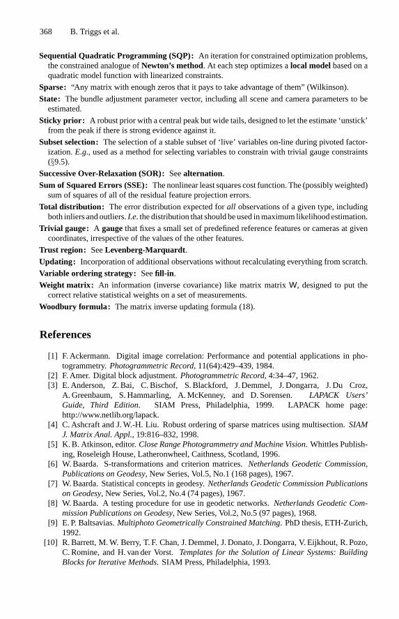
368 B. Triggs et al.
Sequential Quadratic Programming (SQP): An iteration for constrained optimization problems,the constrained analogue ofNewton’s method. At each step optimizes alocal modelbased on aquadratic model function with linearized constraints.
Sparse: “Any matrix with enough zeros that it pays to take advantage of them” (Wilkinson).State: The bundle adjustment parameter vector, including all scene and camera parameters to beestimated.
Sticky prior: A robust prior with a central peak but wide tails, designed to let the estimate ‘unstick’from the peak if there is strong evidence against it.
Subset selection:The selection of a stable subset of ‘live’ variables on-line during pivoted factor-ization.E.g., used as a method for selecting variables to constrain with trivial gauge constraints(§9.5).
Successive Over-Relaxation (SOR):Seealternation.Sum of Squared Errors (SSE): Thenonlinear least squares cost function. The (possiblyweighted)sum of squares of all of the residual feature projection errors.
Total distribution: The error distribution expected forall observations of a given type, includingboth inliers andoutliers.I.e. the distribution that should beused inmaximum likelihoodestimation.
Trivial gauge: A gaugethat fixes a small set of predefined reference features or cameras at givencoordinates, irrespective of the values of the other features.
Trust region: SeeLevenberg-Marquardt .Updating: Incorporation of additional observations without recalculating everything from scratch.Variable ordering strategy: Seefill-in .Weight matrix: An information (inverse covariance) like matrix matrixW, designed to put thecorrect relative statistical weights on a set of measurements.
Woodbury formula: The matrix inverse updating formula (18).
References
[1] F. Ackermann. Digital image correlation: Performance and potential applications in pho-togrammetry.Photogrammetric Record, 11(64):429–439, 1984.
[2] F. Amer. Digital block adjustment.Photogrammetric Record, 4:34–47, 1962.[3] E. Anderson, Z. Bai, C. Bischof, S. Blackford, J. Demmel, J. Dongarra, J. Du Croz,A.Greenbaum, S.Hammarling, A.McKenney, and D.Sorensen.LAPACK Users’Guide, Third Edition. SIAM Press, Philadelphia, 1999. LAPACK home page:http://www.netlib.org/lapack.
[4] C. Ashcraft and J.W.-H. Liu. Robust ordering of sparse matrices using multisection.SIAMJ. Matrix Anal. Appl., 19:816–832, 1998.
[5] K. B. Atkinson, editor.Close Range Photogrammetry and Machine Vision. Whittles Publish-ing, Roseleigh House, Latheronwheel, Caithness, Scotland, 1996.
[6] W.Baarda. S-transformations and criterion matrices.Netherlands Geodetic Commission,Publications on Geodesy, New Series, Vol.5, No.1 (168 pages), 1967.
[7] W.Baarda. Statistical concepts in geodesy.Netherlands Geodetic Commission Publicationson Geodesy, New Series, Vol.2, No.4 (74 pages), 1967.
[8] W.Baarda. A testing procedure for use in geodetic networks.Netherlands Geodetic Com-mission Publications on Geodesy, New Series, Vol.2, No.5 (97 pages), 1968.
[9] E. P. Baltsavias.Multiphoto Geometrically Constrained Matching. PhD thesis, ETH-Zurich,1992.
[10] R. Barrett, M.W. Berry, T. F. Chan, J. Demmel, J. Donato, J. Dongarra, V. Eijkhout, R. Pozo,C.Romine, and H. van der Vorst.Templates for the Solution of Linear Systems: BuildingBlocks for Iterative Methods. SIAM Press, Philadelphia, 1993.
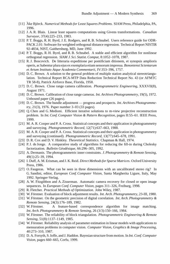
Bundle Adjustment — A Modern Synthesis 369
[11] Ake Bjorck.Numerical Methods for Least Squares Problems. SIAM Press, Philadelphia, PA,1996.
[12] J. A.R. Blais. Linear least squares computations using Givens transformations.CanadianSurveyor, 37(4):225–233, 1983.
[13] P. T. Boggs, R.H. Byrd, J. E. Rodgers, and R.B. Schnabel. Users reference guide for ODR-PACK 2.01: Software for weighted orthogonal distance regression. Technical Report NISTIR92-4834, NIST, Gaithersburg, MD, June 1992.
[14] P. T. Boggs, R.H. Byrd, and R.B. Schnabel. A stable and efficient algorithm for nonlinearorthogonal regression.SIAM J. Sci. Statist. Comput, 8:1052–1078, 1987.
[15] R. J. Boscovich. De litteraria expeditione per pontificiam ditionem, et synopsis ampliorisoperis, ac habentur plura ejus exexemplaria etiamsensorum impressa.Bononiensi Scientarumet Artum Instituto Atque Academia Commentarii, IV:353–396, 1757.
[16] D.C. Brown. A solution to the general problem of multiple station analytical stereotriangu-lation. Technical Report RCA-MTP Data Reduction Technical Report No. 43 (or AFMTCTR 58-8), Patrick Airforce Base, Florida, 1958.
[17] D.C. Brown. Close range camera calibration.Photogrammetric Engineering, XXXVII(8),August 1971.
[18] D.C. Brown. Calibration of close range cameras.Int. Archives Photogrammetry, 19(5), 1972.Unbound paper (26 pages).
[19] D.C. Brown. The bundle adjustment — progress and prospects.Int. Archives Photogramme-try, 21(3), 1976. Paper number 3–03 (33 pages).
[20] Q.Chen and G.Medioni. Efficient iterative solutions to m-view projective reconstructionproblem. InInt. Conf. Computer Vision & Pattern Recognition, pages II:55–61. IEEE Press,1999.
[21] M.A.R. Cooper and P. A. Cross. Statistical concepts and their application in photogrammetryand surveying.Photogrammetric Record, 12(71):637–663, 1988.
[22] M.A.R. Cooper and P. A. Cross. Statistical concepts and their application in photogrammetryand surveying (continued).Photogrammetric Record, 13(77):645–678, 1991.
[23] D.R. Cox and D.V. Hinkley.Theoretical Statistics. Chapman & Hall, 1974.[24] P. J. de Jonge. A comparative study of algorithms for reducing the fill-in during Cholesky
factorization.Bulletin Geodesique, 66:296–305, 1992.[25] A.Dermanis. The photogrammetric inner constraints.J. Photogrammetry & Remote Sensing,
49(1):25–39, 1994.[26] I. Duff, A.M.Erisman, and J. K.Reid.DirectMethods forSparseMatrices. OxfordUniversity
Press, 1986.[27] O. Faugeras. What can be seen in three dimensions with an uncalibrated stereo rig? In
G.Sandini, editor,European Conf. Computer Vision, Santa Margherita Ligure, Italy, May1992. Springer-Verlag.
[28] A.W. Fitzgibbon and A. Zisserman. Automatic camera recovery for closed or open imagesequences. InEuropean Conf. Computer Vision, pages 311–326, Freiburg, 1998.
[29] R. Fletcher.Practical Methods of Optimization. John Wiley, 1987.[30] W. Forstner. Evaluation of block adjustment results.Int. Arch. Photogrammetry, 23-III, 1980.[31] W. Forstner. On the geometric precision of digital correlation.Int. Arch. Photogrammetry &
Remote Sensing, 24(3):176–189, 1982.[32] W. Forstner. A feature-based correspondence algorithm for image matching.
Int. Arch. Photogrammetry & Remote Sensing, 26 (3/3):150–166, 1984.[33] W. Forstner. The reliability of block triangulation.Photogrammetric Engineering & Remote
Sensing, 51(8):1137–1149, 1985.[34] W. Forstner. Reliability analysis of parameter estimation in linear models with applications to
mensuration problems in computer vision.Computer Vision, Graphics & Image Processing,40:273–310, 1987.
[35] D. A. Forsyth, S. Ioffe, and J.Haddon. Bayesian structure frommotion. InInt. Conf. ComputerVision, pages 660–665, Corfu, 1999.
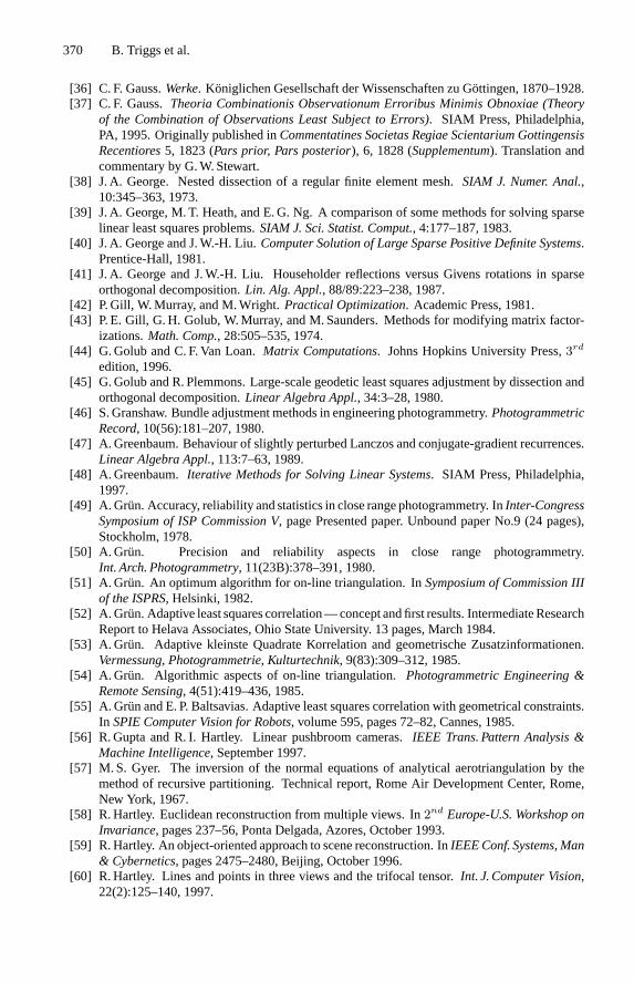
370 B. Triggs et al.
[36] C. F. Gauss.Werke. Koniglichen Gesellschaft der Wissenschaften zu Gottingen, 1870–1928.[37] C. F. Gauss.Theoria Combinationis Observationum Erroribus Minimis Obnoxiae (Theory
of the Combination of Observations Least Subject to Errors). SIAM Press, Philadelphia,PA, 1995. Originally published inCommentatines Societas Regiae Scientarium GottingensisRecentiores5, 1823 (Pars prior, Pars posterior), 6, 1828 (Supplementum). Translation andcommentary by G.W.Stewart.
[38] J. A. George. Nested dissection of a regular finite element mesh.SIAM J. Numer. Anal.,10:345–363, 1973.
[39] J. A. George, M. T. Heath, and E.G. Ng. A comparison of some methods for solving sparselinear least squares problems.SIAM J. Sci. Statist. Comput., 4:177–187, 1983.
[40] J. A. George and J.W.-H. Liu.Computer Solution of Large Sparse Positive Definite Systems.Prentice-Hall, 1981.
[41] J. A. George and J.W.-H. Liu. Householder reflections versus Givens rotations in sparseorthogonal decomposition.Lin. Alg. Appl., 88/89:223–238, 1987.
[42] P.Gill, W.Murray, and M.Wright.Practical Optimization. Academic Press, 1981.[43] P. E. Gill, G.H. Golub, W.Murray, and M.Saunders. Methods for modifying matrix factor-
izations.Math. Comp., 28:505–535, 1974.[44] G.Golub and C. F. Van Loan.Matrix Computations. Johns Hopkins University Press,3rd
edition, 1996.[45] G.Golub and R.Plemmons. Large-scale geodetic least squares adjustment by dissection and
orthogonal decomposition.Linear Algebra Appl., 34:3–28, 1980.[46] S.Granshaw. Bundle adjustment methods in engineering photogrammetry.Photogrammetric
Record, 10(56):181–207, 1980.[47] A.Greenbaum. Behaviour of slightly perturbed Lanczos and conjugate-gradient recurrences.
Linear Algebra Appl., 113:7–63, 1989.[48] A.Greenbaum.Iterative Methods for Solving Linear Systems. SIAM Press, Philadelphia,
1997.[49] A.Grun. Accuracy, reliability and statistics in close range photogrammetry. InInter-Congress
Symposium of ISP Commission V, page Presented paper. Unbound paper No.9 (24 pages),Stockholm, 1978.
[50] A.Grun. Precision and reliability aspects in close range photogrammetry.Int. Arch. Photogrammetry, 11(23B):378–391, 1980.
[51] A.Grun. An optimum algorithm for on-line triangulation. InSymposium of Commission IIIof the ISPRS, Helsinki, 1982.
[52] A.Grun. Adaptive least squares correlation—concept and first results. IntermediateResearchReport to Helava Associates, Ohio State University. 13 pages, March 1984.
[53] A.Grun. Adaptive kleinste Quadrate Korrelation and geometrische Zusatzinformationen.Vermessung, Photogrammetrie, Kulturtechnik, 9(83):309–312, 1985.
[54] A.Grun. Algorithmic aspects of on-line triangulation.Photogrammetric Engineering &Remote Sensing, 4(51):419–436, 1985.
[55] A.Grun and E. P. Baltsavias. Adaptive least squares correlation with geometrical constraints.In SPIE Computer Vision for Robots, volume 595, pages 72–82, Cannes, 1985.
[56] R.Gupta and R. I. Hartley. Linear pushbroom cameras.IEEE Trans. Pattern Analysis &Machine Intelligence, September 1997.
[57] M.S. Gyer. The inversion of the normal equations of analytical aerotriangulation by themethod of recursive partitioning. Technical report, Rome Air Development Center, Rome,New York, 1967.
[58] R.Hartley. Euclidean reconstruction from multiple views. In2nd Europe-U.S. Workshop onInvariance, pages 237–56, Ponta Delgada, Azores, October 1993.
[59] R.Hartley. An object-oriented approach to scene reconstruction. InIEEEConf. Systems, Man& Cybernetics, pages 2475–2480, Beijing, October 1996.
[60] R.Hartley. Lines and points in three views and the trifocal tensor.Int. J. Computer Vision,22(2):125–140, 1997.
Bundle Adjustment — A Modern Synthesis 371
[61] R.Hartley, R.Gupta, and T.Chang. Stereo from uncalibrated cameras. InInt. Conf. ComputerVision & Pattern Recognition, pages 761–4, Urbana-Champaign, Illinois, 1992.
[62] R.Hartley and A. Zisserman.Multiple View Geometry in Computer Vision. CambridgeUniversity Press, 2000.
[63] R. I. Hartley and T. Saxena. The cubic rational polynomial camera model. InImage Under-standing Workshop, pages 649–653, 1997.
[64] F.Helmert.DieMathematischen undPhysikalischen Theorien der hoherenGeodasie, volume1 Teil. Teubner, Leipzig, 1880.
[65] B.Hendrickson and E.Rothberg. Improving the run time and quality of nested dissectionordering.SIAM J. Sci. Comput., 20:468–489, 1998.
[66] K.R. Holm. Test of algorithms for sequential adjustment in on-line triangulation.Photogram-metria, 43:143–156, 1989.
[67] M. Irani, P. Anadan, and M.Cohen. Direct recovery of planar-parallax from multiple frames.In Vision Algorithms: Theory and Practice. Springer-Verlag, 2000.
[68] K. Kanatani and N.Ohta. Optimal robot self-localization and reliability evaluation. InEuro-pean Conf. Computer Vision, pages 796–808, Freiburg, 1998.
[69] H.M. Karara. Non-Topographic Photogrammetry. Americal Society for Photogrammetryand Remote Sensing, 1989.
[70] G. Karypis and V. Kumar. Multilevelk-way partitioning scheme for irregular graphs.J.Parallel & Distributed Computing, 48:96–129, 1998.
[71] G. Karypis andV. Kumar. A fast andhighly qualitymultilevel scheme for partitioning irregulargraphs.SIAMJ.ScientificComputing, 20(1):359–392, 1999. ForMetis codeseehttp://www-users.cs.umn.edu/ karypis/.
[72] I. P. King. An automatic reordering scheme for simultaneous equations derived from networksystems.Int. J. Numer. Meth. Eng., 2:479–509, 1970.
[73] K. Kraus. Photogrammetry. Dummler, Bonn, 1997. Vol.1: Fundamentals and StandardProcesses. Vol.2: Advanced Methods and Applications. Available in German, English &several other languages.
[74] A.M. Legendre.Nouvelles methodespour la determination des orbites des cometes. Courcier,Paris, 1805. Appendix on least squares.
[75] R. Levy. Restructuring the structural stiffnessmatrix to improve computational efficiency.JetPropulsion Lab. Technical Review, 1:61–70, 1971.
[76] M.X. Li. Hierarchical Multi-point Matching with Simultaneous Detection and Location ofBreaklines. PhD thesis, KTH Stockholm, 1989.
[77] Q.-T. Luong, R.Deriche, O. Faugeras, and T. Papadopoulo. On determining the fundamentalmatrix: Analysis of different methods and experimental results. Technical Report RR-1894,INRIA, Sophia Antipolis, France, 1993.
[78] S.Mason. Expert system based design of close-range photogrammetric networks.J. Photogrammetry & Remote Sensing, 50(5):13–24, 1995.
[79] S.O. Mason.Expert System Based Design of Photogrammetric Networks. Ph.D. Thesis,Institut fur Geodasie und Photogrammetrie, ETH Zurich, May 1994.
[80] B.Matei and P.Meer. Bootstrapping a heteroscedastic regression model with application to3D rigid motion evaluation. InVision Algorithms: Theory and Practice. Springer-Verlag,2000.
[81] P. F. McLauchlan. Gauge independence in optimization algorithms for 3D vision. InVisionAlgorithms: Theory and Practice, Lecture Notes in Computer Science, Corfu, September1999. Springer-Verlag.
[82] P. F. McLauchlan. Gauge invariance in projective 3D reconstruction. InMulti-ViewModelingand Analysis of Visual Scenes, Fort Collins, CO, June 1999. IEEE Press.
[83] P. F.McLauchlan. The variable state dimension filter. TechnicalReport VSSP5/99,Universityof Surrey, Dept of Electrical Engineering, December 1999.
[84] P. F. McLauchlan. A batch/recursive algorithm for 3D scene reconstruction. InInt. Conf. Computer Vision & Pattern Recognition, Hilton Head, South Carolina, 2000.
372 B. Triggs et al.
[85] P. F. McLauchlan and D.W.Murray. A unifying framework for structure andmotion recoveryfrom image sequences. In E.Grimson, editor,Int. Conf. Computer Vision, pages 314–20,Cambridge, MA, June 1995.
[86] P. F. McLauchlan andD.W.Murray. Active camera calibration for a Head-Eye platform usingthe Variable State-Dimension filter.IEEE Trans. Pattern Analysis & Machine Intelligence,18(1):15–22, 1996.
[87] P.Meissl. Die innere Genauigkeit eines Punkthaufens.Osterreichische Zeitschrift fur Ver-messungswesen, 50(5): 159–165 and 50(6): 186–194, 1962.
[88] E.Mikhail and R.Helmering. Recursive methods in photogrammetric data reduction.Pho-togrammetric Engineering, 39(9):983–989, 1973.
[89] E.Mittermayer. Zur Ausgleichung freier Netze.Zeitschrift fur Vermessungswesen,97(11):481–489, 1962.
[90] J. J. More and S. J. Wright.Optimization Software Guide. SIAM Press, Philadelphia, 1993.[91] D.D. Morris and T. Kanade. A unified factorization algorithm for points, line segments and
planes with uncertainty. InInt. Conf. Computer Vision, pages 696–702, Bombay, 1998.[92] D.D. Morris, K. Kanatani, and T. Kanade. Uncertainty modelling for optimal structure and
motion. InVision Algorithms: Theory and Practice. Springer-Verlag, 2000.[93] J. Nocedal and S. J. Wright.Numerical Optimization. Springer-Verlag, 1999.[94] M.Okutomi and T. Kanade. A multiple-baseline stereo.IEEE Trans. Pattern Analysis &
Machine Intelligence, 15(4):353–363, 1993.[95] D.W. Proctor. The adjustment of aerial triangulation by electronic digital computers.Pho-
togrammetric Record, 4:24–33, 1962.[96] B.D. Ripley.Pattern Recongition and Neural Networks. Cambridge University Press, 1996.[97] D.Rosenholm. Accuracy improvement of digital matching for elevation of digital terrain
models.Int. Arch. Photogrammetry & Remote Sensing, 26(3/2):573–587, 1986.[98] S.Roy and I. Cox. A maximum-flow formulation of the n-camera stereo correspondence
problem. InInt. Conf. Computer Vision, Bombay, 1998.[99] Y. Saad. On the rates of convergence of Lanczos and block-Lanczosmethods.SIAM J. Numer.
Anal., 17:687–706, 1980.[100] C.C. Slama, editor.Manual of Photogrammetry. American Society of Photogrammetry and
Remote Sensing, Falls Church, Virginia, USA, 1980.[101] R. A. Snay. Reducing the profile of sparse symmetric matrices.Bulletin Geodesique, 50:341–
352, 1976. Also NOAA Technical Memorandum NOS NGS-4, National Geodetic Survey,Rockville, MD.
[102] R. Szeliski, S. B. Kang, and H.Y. Shum. A parallel feature tracker for extended image se-quences. Technical Report CRL 95/2, DEC Cambridge Research Labs, May 1995.
[103] R. Szeliski and S.B. Kang. Shape ambiguities in structure from motion. InEuropeanConf. Computer Vision, pages 709–721, Cambridge, 1996.
[104] R. Szeliski and H.Y. Shum. Motion estimation with quadtree splines. InInt. Conf. ComputerVision, pages 757–763, Boston, 1995.
[105] B. Triggs. A new approach to geometric fitting. Available fromhttp://www.inrialpes.fr/movi/people/Triggs, 1997.
[106] B. Triggs. Optimal estimation of matching constraints. In R. Koch and L. Van Gool, editors,3D Structure from Multiple Images of Large-scale Environments SMILE’98, Lecture Notesin Computer Science. Springer-Verlag, 1998.
[107] G. L. Strang van Hees. Variance-covariance transformations of geodetic networks.Manuscripta Geodaetica, 7:1–20, 1982.
[108] X.Wang and T. A. Clarke. Separate adjustment of close range photogrammetric measure-ments.Int. Symp. Photogrammetry & Remote Sensing, XXXII, part 5:177–184, 1998.
[109] P.R. Wolf and C.D. Ghilani.Adjustment Computations: Statistics and Least Squares inSurveying and GIS. John Wiley & Sons, 1997.
[110] B. P. Wrobel. Facets stereo vision (FAST vision) — a new approach to computer stereovision and to digital photogrammetry. InISPRS Intercommission Conf. Fast Processing ofPhotogrammetric Data, pages 231–258, Interlaken, Switzerland, June 1987.