University of Wollongong University of Wollongong

Research Online Research Online

University of Wollongong Thesis Collection 1954-2016 University of Wollongong Thesis Collections

1997

Time to ponding in one & two dimensional infiltration systems Time to ponding in one & two dimensional infiltration systems

Janine M. Stewart University of Wollongong

Follow this and additional works at: https://ro.uow.edu.au/theses

University of Wollongong University of Wollongong

Copyright Warning Copyright Warning

You may print or download ONE copy of this document for the purpose of your own research or study. The University

does not authorise you to copy, communicate or otherwise make available electronically to any other person any

copyright material contained on this site.

You are reminded of the following: This work is copyright. Apart from any use permitted under the Copyright Act

1968, no part of this work may be reproduced by any process, nor may any other exclusive right be exercised,

without the permission of the author. Copyright owners are entitled to take legal action against persons who infringe

their copyright. A reproduction of material that is protected by copyright may be a copyright infringement. A court

may impose penalties and award damages in relation to offences and infringements relating to copyright material.

Higher penalties may apply, and higher damages may be awarded, for offences and infringements involving the

conversion of material into digital or electronic form.

Unless otherwise indicated, the views expressed in this thesis are those of the author and do not necessarily Unless otherwise indicated, the views expressed in this thesis are those of the author and do not necessarily

represent the views of the University of Wollongong. represent the views of the University of Wollongong.

Recommended Citation Recommended Citation Stewart, Janine M., Time to ponding in one & two dimensional infiltration systems, Master of Science (Hons.) thesis, Department of Mathematics, University of Wollongong, 1997. https://ro.uow.edu.au/theses/2849

Research Online is the open access institutional repository for the University of Wollongong. For further information contact the UOW Library: research-pubs@uow.edu.au

TIME TO PONDING IN

ONE & TWO DIMENSIONAL

INFILTRATION SYSTEMS

* A thesis submitted in fulfilment of the

requirements for the award of the degree

MASTER OF SCIENCE (HONOURS)

from

UNIVERSITY OF WOLLONGONG

by

JANINE M. STEWART, BMath(Hons), GradDipEd

DEPARTMENT OF MATHEMATICS

1997

u n iv e r s it y c .WOLLONGONG

LIBRARY

Dedicated to the memory o f Uncle Maurice BE(Civil), NSW

Contents

A. Abstract 1

1. Introduction 3

2. Infiltration In One Dimension

(2.1) Constant Supply Rate Boundary Conditions

(2.2) Time Dependent Boundary Conditions

a/ Linearly Increasing Time Dependent

11

3. Infiltration In Two Dimensions

(3.1) Constant Supply Rate Boundary Conditions

a/ Infiltration Boundary Conditions

b/ Infiltration & Evaporation Boundary Conditions

c/ Fractal Boundary Conditions

(3.2) Time Dependent Boundary Conditions

a/ Linearly Increasing Time Dependent

b/ Periodic Boundary Conditions

28

4. Steady Infiltration In Sloping Porous Domains 60

5. Conclusions 70

6. Appendix 74

7. References 87

(i)

A. Abstract

Infiltration is the process whereby water enters soil through the surface. This can be

a naturally occurring process, such as in rainfall, or can be artificially induced in

engineering or agricultural applications.

In most cases, fluid is infiltrated into soil that is unsaturated. As water infiltrates

drier unsaturated soil, the water molecules fill the smallest soil pores where they are bound

tightly by capillary forces. In the transition to saturated soil, the capillary forces become

less dominant and free water appears. Surface ponding is characterised by the appearance

of this free water pooling on the surface of the soil and can occur even if the soil is dry at

depth. Surface ponding is an important hydrological phenomenon with applications

relevant to many fields from agriculture to civil engineering. With excessive irrigation

techniques, once arable soils become water logged, the rising water table brings with it

geological salts which kill vegetation rendering fertile soils effectively useless. However,

ponding is a desirable phenomenon in areas of water catchment.

Before the emergence of highly versatile nonlinear analytic solution techniques for

groundwater flow, reasonably accurate estimations for ponding times were available only

with the use of numerical methods. Prior to this the linear and quasi linear models were

applied to the problem of groundwater flow with mixed results.

An estimation for the time to surface ponding for a variety of one and two

dimensional infiltration patterns is found using a number of analytic and numerical

solution methods. It is found and is observable in the field that as the wetted proportion

of the soil surface and the rate of surface infiltration increase the time to surface ponding

decreases. It is found that this effect dominates over the spatial pattern of irrigation.

In this application horizontal and sloping fields are considered. In the case of a

horizontal surface, it is found that surface ponding is unavoidable if the rate of surface

1

infiltration even locally exceeds the hydraulic conductivity at saturation. However, for an

inclined surface, for a given basal inclination there exists a maximal surface infiltration rate

for which basement saturation can be averted.

2

1. Introduction

The Darcy-Buckingham macroscopic theory of soil-water flow has endured the test

of time as a successful scientific theory. In this theory, one neglects small-scale

phenomena on the scale of single pores and grains. Just as for any fluid flow,

groundwater flow through soil obeys the Equation of Continuity, expressed in this case as

(1.1.1) — + V .v = 0a t - - ,

where 0(x,z,t) represents the local volumetric concentration of the fluid in the soil with

dimensions [length]3 [length] 3 and v is the Darcian volumetric flux density, measured in

units of [length\time]~l .

In order to derive an equation to model the flow of fluid through a uniform

nonswelling soil, the continuity equation (1.1.1) is combined with Darcy's Law

(1.1.2) v = -K(0)VO.

The hydraulic conductivity, K(0) is a measure of how well the soil transports fluid

and has the dimensions [length][time]~l . In the field, the hydraulic conductivity is a

highly nonlinear function, varying over several orders of magnitude.

The potential energy per unit weight of water, O, is a function of the capillary

potential and gravity. The capillary potential, 'P , is a measure of the energy state of

water, and like the total potential or hydraulic head O , is measured in units of [length] .

In terms of gravity and the capillary potential, the total potential can be written,

(1.1.3) <& = 'F (0 ) - z

3

where z is the vertical depth beneath the surface of the soil.

Combining equations (1.1.1) - (1.1.3), the resultant equation,

(1.1.4) ^ = Y .(A r(0)V 4'(0))-^ ^ l

known as Richards' Equation, models groundwater flow through a uniform nonswelling

soil. Assuming no hysteresis, there exists a one-to-one correspondence between the

capillary potential , and the soil water concentration 0. This equation can be written in

terms of a single dependent variable by noting that D(0) = K(6)cW ldd , where D(0) is

the diffusivity, with the dimensions [length]2[time]~l . Like the hydraulic conductivity,

field occurring diffusivities are highly nonlinear. The diffusivity D(0) is related to

capillary action rather than molecular diffusion. As fluid enters an initially dry soil, it is

absorbed by the smallest pores first and is bound tightly by capillary forces. As a larger

volume of fluid infiltrates into the soil, the new fluid is held by weaker capillary forces in

larger pores as the soil becomes progressively saturated.

In terms of the water content 0 (x ,z,t), Richards' Equation is written,

(1.1.5) |^ = V.(D (0)Ve)--^p)

Following the notation of Broadbridge and White (1988) Richards' Equation is

rescaled in terms of dimensionless variables

(1.1.6) ~ = V « .(D « (0 )V ,0 )-?-K*(e )at* v 0Z*

where

4

(1.1.7a) 0 _ ® ® 9s - e n A0

(1.1.7b)K (e ) -K n K (e ) -K n

K ( 0 ) - K , - K „ - AK

(1.1.7c) D . ( 0 ) = D ( 0 ) \As

(1.1.7d)t ,

u = —ts

d . l . 7 e )X z

x* — — z* —

(1.1.7f), _ D A 6A/„ —

5 AK

(1-1-7 g)j r fts = D ----

U k )

(1.1.7h) D = — \lsD{G)de. A Gie-

Here, D is the mean diffusivity, 0n is the initial concentration of fluid in the soil,

0S is the water content at saturation and Kn , Ks are the associated hydraulic

conductivities given these soil water contents.

The capillary length scale Xs is equal to a typical capillary rise and ts is the

associated gravity time scale, representing the time taken for a gravity-dominated travelling

wave solution to propagate over a typical capillary length.

5

The physical system under consideration is that of fluid infiltrating into an initially

dry soil, until surface ponding occurs. Surface ponding is characterised by the appearance

of free water pooling at the surface of the soil which is an indication that the soil is locally

saturated. In the case where the infiltration rate exceeds the value of the hydraulic

conductivity at saturation, Ks, however, it is entirely possible for surface ponding to

occur whilst the soil is dry at depth. The appearance of a free layer of fluid having depth h

ponding at the surface of the soil implies that the capillary potential 'F attains a non­

negative value. Given that is a monotonic decreasing function of the soil water content

Gand 4 '(0i ) = O , assuming no hysteresis, there exists a saturated zone at the surface of

the soil even if the soil is dry at depth. Conversely, if the rate of surface infiltration is less

than the hydraulic conductivity at saturation, unsaturated groundwater flow occurs in the

absence of ponding. This is true because from equations (1.1.1)-(1.1.3), even in the

absence of sorptive capillary action, water could be transported at the imposed rate R < K S

by the flux K(0) = R (for some 6 < 6S) which is due to gravity alone.

In agricultural applications and in civil construction work, the ponding phenomenon

is generally best avoided as it may result in water run-off, a rise in the water table,

increased soil salinity and soil erosion. During natural rainfall, some run-off is desirable

for the purposes of water catchment. The quantity of water run-off must be estimated in

the design of drainage systems. Because of the importance of the ponding phenomenon in

agricultural and engineering applications, the prediction of ponding time is an important

task in hydrological modelling and has come under the close scrutiny of many authors in a

wide context of applications.

Rubin (1966) investigated the three kinds of infiltration due to rainfall: non-ponding,

pre-ponding and post-ponding. A qualitative prediction of the changing characteristics of

the soil moisture profile in terms of the depth, time and moisture content was established.

Later authors however, investigated the ponding phenomenon exclusively.

6

Mein and Larson (1973) and later Swartzendruber (1974) modified the Green-Ampt

equation to determine the time to ponding for steady rainfall periods. The Green-Ampt

model is an over-simplified model that has a step function water concentration-depth

profile at all times. As shown by Philip (1969), this profile arises from a delta function

diffusivity that depends continuously on concentration. Chu (1978) extended the

modified Green-Ampt equation to describe infiltration during periods of unsteady rain. In

this case, two time parameters were utilised, ponding time and pseudotime which simply

entails a shift in the time scale.

Knight (1983) also investigated pre-ponding and post-ponding infiltration. In this

study, exact and approximate solutions of Richards' equation were utilised to express the

time to ponding as a function of easily measurable soil water parameters. These include

the soil water diffusivity, hydraulic conductivity at saturation and surface supply rate.

Knight showed that the infiltration rate for post-ponding, unlike the Green-Ampt model

used by Swartzendruber (1974), is not simply a translation of the curve for initial

ponding. Knight further developed evidence that the cumulative infiltration can be used as

an appropriate time-like variable in the case of variable surface flux.

Many problems involving variable surface flux can be difficult to solve analytically

to obtain meaningful physical results. This problem has been considered however from

an experimental perspective. Using an approximate analytical method, Parlange and

Smith (1976) calculated the time to ponding under variable surface infiltration rates and

expressed it in terms of soil water parameters easily measured in the field, namely the

infiltration rate, sorptivity and saturated hydraulic conductivity. Kutilek (1980) also used

heuristic techniques to calculate the time to ponding under conditions of constant

infiltration. Here, ponding time was expressed also in terms of the infiltration rate and

sorptivity. Unlike the Parlange and Smith model however, the time to ponding was also

expressed in terms of the coefficient of t in Philip's (1969) power series expansion of the

cumulative infiltration.

7

Chong (1983) applied the approximate solutions of both Parlange and Smith (1976)

and Kutilek (1980) solution to estimate the sorptivity and then used this estimate to predict

infiltration.

Previously, Hachum and Alfaro (1977) presented a physically based model to

describe infiltration under any surface infiltration supply rate to implicitly predict

infiltration after ponding. Experimental results were also used by Clothier et al (1981b)

to show that observable field infiltration phenomena agree with theoretical predictions

resulting from the theory of constant flux. Clothier et al further demonstrated that the

time to surface saturation can be predicted but post-ponding fluid run-off is substantially

more difficult to model as it is due to the influence of the particular soil matrix rather than

external environmental factors. Perroux et al (1981) further compared laboratory

experiments with theoretical predictions for constant flux infiltration. These experiments

were sufficiently accurate to become bench tests for later theorectical predictions of the

moisture profile and the time to surface ponding.

Ponding formulae were also derived in the case of variable infiltration for high

rainfall rates by Morel-Seytoux (1976, 1978, 1982). A power law relationship between

the relative permeability of water as a function of the normalised water content was

assumed. From these formulae, the depth of the cumulative infiltration and the ponding

infiltration rate were calculated.

Using an exactly solvable model, Broadbridge and White (1987) introduced an exact

expression for the time to ponding which encompasses soils with widely varying

properties. After rescaling length and time variables, field and repacked soils can be

expressed in terms of a single nonlinearity parameter which covers the spectrum from

highly nonlinear soils, such as fine textured clays, to weakly nonlinear soils, like coarsely

grained sands. A comparison for the time to ponding is made between the linear, Green-

Ampt, Burgers and versatile nonlinear model. The time to ponding for each of these

8

models is parameterised in terms of readily measured field properties such as the

sorptivity, infiltration rate and saturated hydraulic conductivity.

Under investigation in this thesis, is the occurrence of ponding in time and space

subject to a variety of soil surface supply patterns and surface infiltration rates to

determine which soil water parameter has the most influence over the transition from

unsaturated to saturated flow. Throughout this thesis, it will be assumed that there exists

no hysteresis. That is, a one-to-one relationship between the capillary potential and the

moisture content 0 exists. Incipient ponding will then occur when 'T rises to the same

value as that for free water, taken to be when 'P = 0. This corresponds to 0 reaching its

saturated value 0S. We begin by considering one dimensional infiltration subject to a

constant supply rate imposed at the surface of the soil. Analytic expressions are presented

for the time to ponding by obtaining solutions to the linear, Burgers and nonlinear models

respectively. These models swathe the range of soil types which occur naturally in the

field and in the laboratory after repacking. A solution for one dimensional infiltration is

also presented for the time to ponding under conditions of surface infiltration which has a

significant time dependence. Previous work in this area has used only approximate

solutions. Our aim in this application is to find an exact analytic solution to this problem

and to utilise this solution to obtain an accurate prediction of surface ponding time

involving a time dependent surface supply rate.

In agricultural applications of infiltration, such as irrigation through a series of

parallel irrigation furrows, one dimensional models are inapplicable. In this instance a

two dimensional model which incorporates a series of parallel strips is considered. Batu

(1978) considered a similar physical system to model steady and variable infiltration. In

this application we present analytic solutions for constant and variable surface supply rates

for the linear model. A numerical solution is also presented for this physical system using

the versatile nonlinear model attributed to Broadbridge and White (1988). No previous

study of ponding involving fractionally wetted surfaces has been earned out.

9

Finally, we consider the problem of infiltration through a sloping porous domain

where the effect of évapotranspiration is also evident. The aim is to determine whether the

slope of the porous domain, the magnitude of the wetted fraction or the critical infiltration

rate is the determining factor in the onset of saturation.

It is found that whilst the surface supply pattern has a significant influence on the

time to ponding, it is the infiltration rate that exerts the most influence. We are led to

surmise that in terms of modelling real-life hydrological events, there is little to be gained

by considering complex surface geometries. Generally, in the case of realistic flux rates it

is more computationally efficient to use the one dimensional model without significant

losses in the accuracy of the results.

10

2. Infiltration In One Dimension

(2.1) Constant Rate Rainfall Boundary Conditions

Fluid flow through an initially dry soil, subject to a constant infiltration rate

prescribed at the surface is modelled by Richards' Equation

where D(0) = K(6)cWldd is the nonlinear soil water diffusivity and K(0) is the

hydraulic conductivity.

In the field, both the diffusivity and the hydraulic conductivity may be highly

nonlinear functions. Over the range of water contents occurring in the field, these

functions often vary by several orders of magnitude.

Broadbridge and White (1988) deduced an exact analytical solution to the nonlinear

one dimensional Richards' Equation when the soil water diffusivity and hydraulic

conductivity functions had the form

(2.1.1)

(2.1.2)

and

(2.1.3) K(e) = ß + y ( b - e ) +2 (b -0 )2

11

with constants a, b, p, y, X respectively. Similar models were devised by Sander et al

(1988) with important differences explained by Broadbridge and White (1988). These

models not only enable an exact analytic solution by transform methods, but also emulate

data in the field to a high degree of accuracy.

To determine surface ponding time, the nonlinear flow equation (2.1.1) is solved

subject to a uniform initial condition and a constant rate surface flux condition.

It is important to note that an exact nonlinear analytic solution is available for the

constant rate surface flux condition only. Any other boundary condition normally

precludes the successful application of the requisite transforms. Recently however,

Broadbridge et al (1996) used an alternative transform method to solve equations (2.1.1)

- (2.1.3) with variable flux boundary conditions. However the parameters of the variable

flux boundary conditions can not be systematically varied in that case.

Broadbridge and White (1988) solved equation (2.1.1) subject to the following

surface supply rate boundary condition and uniform initial condition

(2.1.4) K(0) - D(6)— = R, z = 0dz

(2.1.5) e = en, = 4'„, t = o.

The solution found by Broadbridge and White (1988) at the surface of the soil is written in

terms of dimensionless variables,

(2.1.6) 0 (0 ,t) = c(

2p +1 - u-1 du y 1

)

with

12

(2.1.7) P = 4c(c -1 )

(2.1.8) u = 2exp^p2x)erf|px2 j + exp(p(p + l)x)

(2.1.9)du

3C2exp(p2x) - 2(1 + p)2 exp(p(p + l)x)erf|p(p + 1)2 x

+p 2exp(p2xjerf|px2

In the equations above,

(2.1.10a) t = 4c(c - l)r*

and

(2.1.10b) Ç = j ^ 4 c ( c - l )Z,.

Here R* is the dimensionless infiltration rate, p is the rescaled surface flux, x is the

rescaled dimensionless time, Ç is the rescaled depth variable and Z* is the depth variable

owing to the Storm transformation (Storm 1951).

Ponding occurs when free water first appears at the surface of the soil, and the time

to ponding, xpis found from 0^0, xp) = 1. Under this condition, the analytic solution

reduces to

13

3 0009 03201145 9

(2 .1.11) 2c 1 — = 1 -ex piv*

+

^R*xpc(c -1 )^

V

ferfc

\- R * J —V 4h

i j , 4 c ( c - l ) ) T /erfc

v R* J V

(R* + 4c(c - 1))R*Tj

4h

The parameter c is an indication of the nonlinearity of the model. In the field this

parameter generally ranges between 1.02 and 1.5. Highly nonlinear models are

characterised by c —> 1, whilst for large values of c, the model is weakly nonlinear. In the

field values where c>2 are considered large.

The function h(c) can be found from

(2-1.12) “ = exp|[4h(c)]_1je r fc |[4 h (c )p j

but is approximated to (within 1% accuracy) by Broadbridge and White (1988)

(2.1.13) h(c) = c(c -1 )[rc(c-l) + 1.46147] [4 (c - l) + 2.92294]*

For highly nonlinear models the solution (2.1.10) reduces to

(2.1.14) R*Xp = — Inf

V

R*R* -1

A

J

which is in agreement with Parlange and Smith (1976) while for weakly nonlinear models

the solution (2.1.10) reduces to a Burgers' Equation solution.

14

Burgers' Equation is characterised by a constant diffusivity and quadratic

dependence of K(0) on 0 and has previously been shown by Clothier et al (1981a) and

by White et al (1979) to give a good prediction for ponding time.

If we consider c large, then the soil water parameters are weakly nonlinear. For

large c the fluid flow equation (2.1.1) reduces to a Burgers' model.

(2.1.15) <90 D <920 ¿10—— = ------- J -----at* Ds dz* dz*

This is solved subject to constant rainfall rate surface flux condition

(2.1.16) Q2 _ D _ d Q A dz*

= R*, z* = 0

and uniform initial condition

(2.1.17) 0 = 0, t* = 0

Here the constant diffusivity is D = nS^/ 4(A0 )2, with scaling factor,

(2.1.18) Ds =h(c) f S n ^2

c(c -1 ) vA0 J

noting that as c —> co, for the Linear and Burgers' Equation models,

h(c) / c(c -1 ) —> k / 4 and thus the dimensionless D* = 1.

The sorptivity Sn is directly measurable from the cumulative absorption, i(t), of

water into soil at early times (Philip, 1957b).

15

(2.1.19) m = % ( e - e H)dz

= sntUo(t)

The cumulative absorption i(t) represents the total amount of fluid which has

infiltrated into the soil at time t. In addition, equation (2.1.19) also represents a definition

for the sorptivity of the soil, where the sorptivity is a representation of capillary influences

which follow a change in the surface concentration of fluid, neglecting gravitational

effects.

The Burgers' model (2.1.15) - (2.1.17) can be reduced to a linear diffusion model

by applying the Hopf-Cole transformation (Hopf, 1950)

(2.1.20) © = - — (lnu)Oz*

The resulting linear diffusion problem

(2.1.21) Ou _ 02u Ot* Ozi

(2.1.22) u = exp(R*t*), z* = 0

(2.1.23) u = 1, t* = 0

has solution

(2.1.24) u = -iexp(R*t*){F_ + F+} -e rfc( \ z*

j+ 1

16

with

(2.1.25)____ A

± ^R*U . )

The dimensionless water content 0 is found by inverting equation (2.1.24) using

the Hopf-Cole transformation (2.1.20). Thus,

(2.1.26) © = - u _1 —c)z*

At the soil surface, the ponding time is found from

(2.1.27) © (0 ,tp) = VR^erfÙR^Tp) = 1

which is solved for xp and the relevant soil water parameters are rescaled so the time scale

ts is consistent with the nonlinear model, the result of which is in agreement with

Broadbridge and White (1987: Equation 13),

(2.1.28)K

K*Tn —p 4

ff 1 11inveri

V 1V*** J,

The linear model for soil water flow uses the same constant soil water diffusivity as

the Burgers model, but a linear dependence of K(0) on 0 is assumed (Braester, 1973).

Recall however that the hydraulic conductivity is a highly nonlinear function. When the

soil water content is low, as in the case of early infiltration times, so too is the hydraulic

conductivity. The linear model, by assuming this linear dependence effectively over

17

estimates the hydraulic conductivity. Since in the absence of capillary action, the water

flux due to gravity is identical with conductivity, this is equivalent to an over-statement of

the importance of gravity. In this instance, the linear model predicts that a greater quantity

of water is removed from the surface than is actually the case - hence the over estimation

in the actual time to surface ponding. By determining a relationship between the linear and

nonlinear solutions a quantitative assessment of this overestimation is deduced. This

assessment can then be extended to physical systems where complex surface geometries

preclude an exact analytic nonlinear solution. The level of compensation necessary to

account for this modelling error in one dimension, will give us some indication of the

required correction in two dimensions.

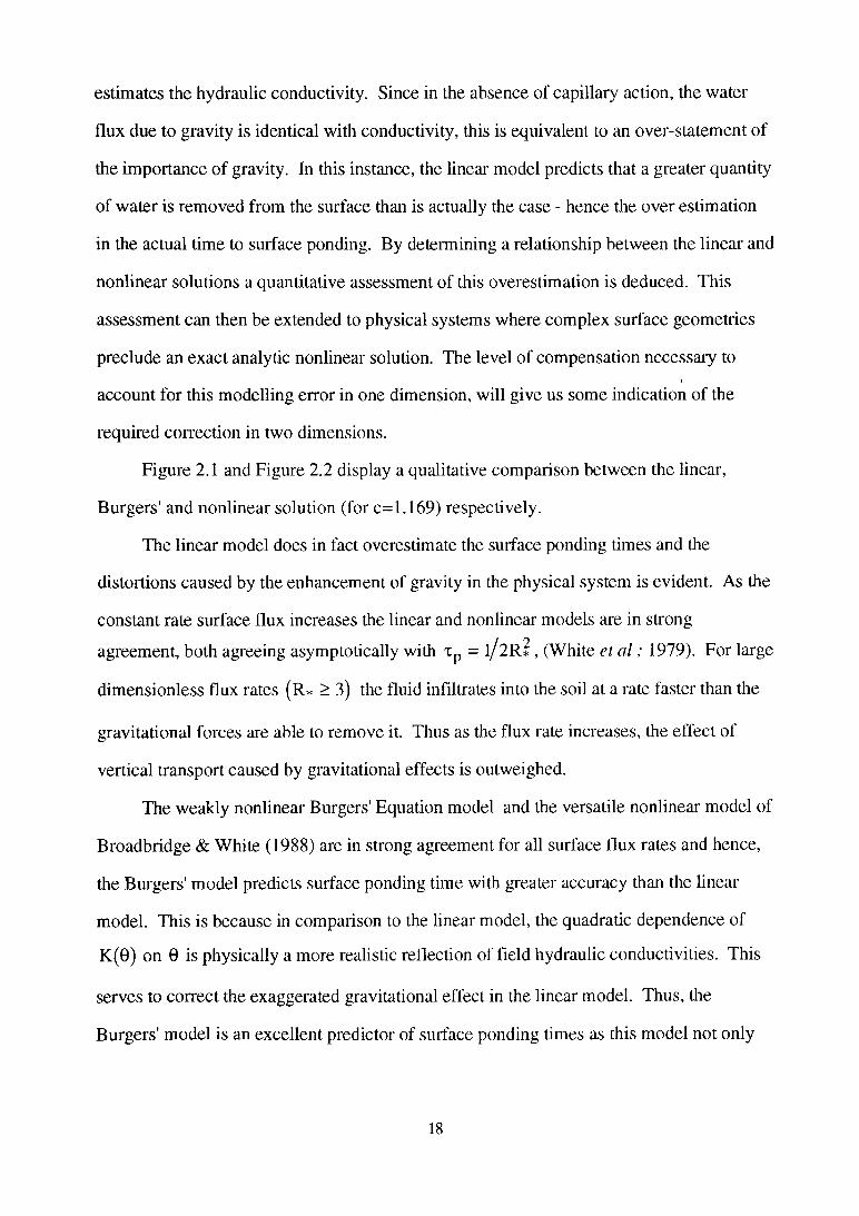
Figure 2.1 and Figure 2.2 display a qualitative comparison between the linear,

Burgers' and nonlinear solution (for c=1.169) respectively.

The linear model does in fact overestimate the surface ponding times and the

distortions caused by the enhancement of gravity in the physical system is evident. As the

constant rate surface flux increases the linear and nonlinear models are in strong

agreement, both agreeing asymptotically with Tp = l/2 R * , (White et a l ; 1979). For large

dimensionless flux rates (R* > 3) the fluid infiltrates into the soil at a rate faster than the

gravitational forces are able to remove it. Thus as the flux rate increases, the effect of

vertical transport caused by gravitational effects is outweighed.

The weakly nonlinear Burgers' Equation model and the versatile nonlinear model of

Broadbridge & White (1988) are in strong agreement for all surface flux rates and hence,

the Burgers' model predicts surface ponding time with greater accuracy than the linear

model. This is because in comparison to the linear model, the quadratic dependence of

K(0) on 0 is physically a more realistic reflection of field hydraulic conductivities. This

serves to correct the exaggerated gravitational effect in the linear model. Thus, the

Burgers' model is an excellent predictor of surface ponding times as this model not only

18

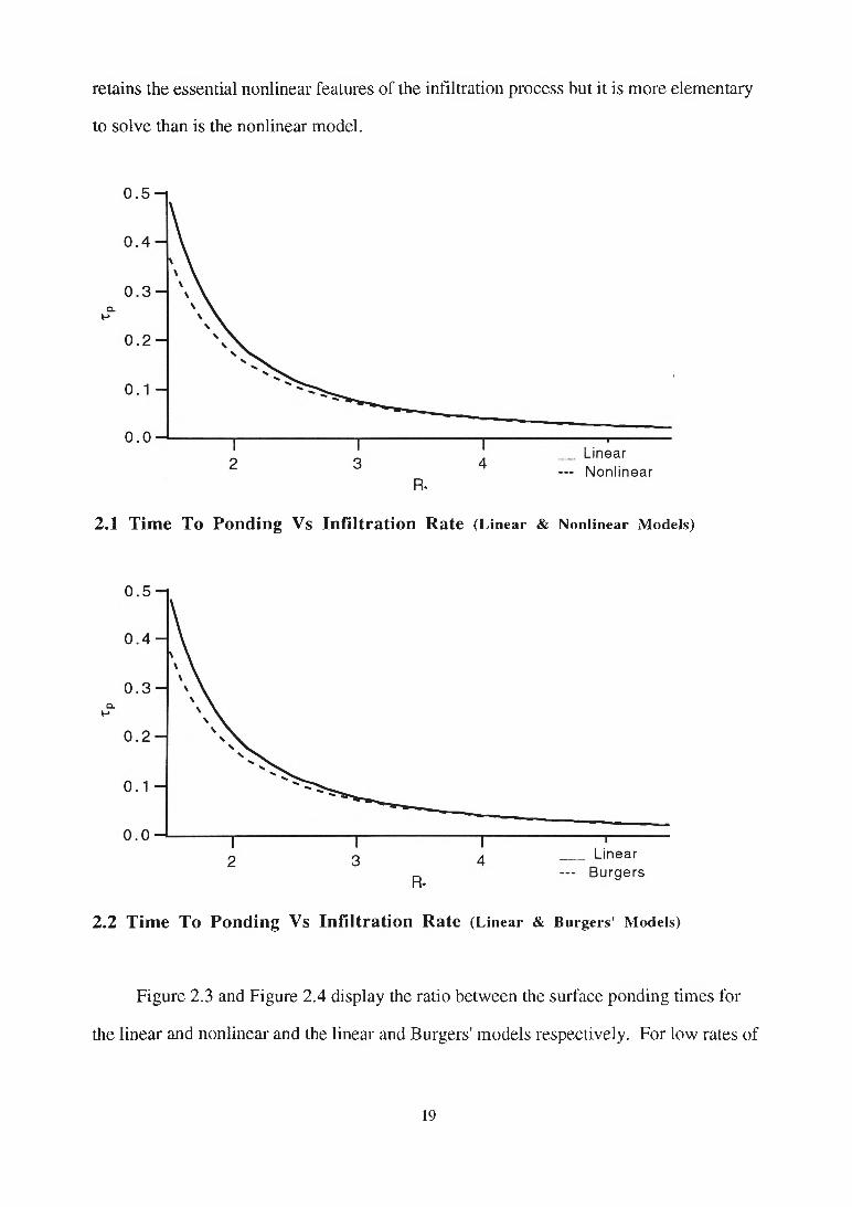
retains the essential nonlinear features of the infiltration process but it is more elementary

to solve than is the nonlinear model.

2.1 Time To Ponding Vs Infiltration Rate (Linear & Nonlinear Models)

2.2 Time To Ponding Vs Infiltration Rate (Linear & Burgers' Models)

Figure 2.3 and Figure 2.4 display the ratio between the surface ponding times for

the linear and nonlinear and the linear and Burgers' models respectively. For low rates of

19

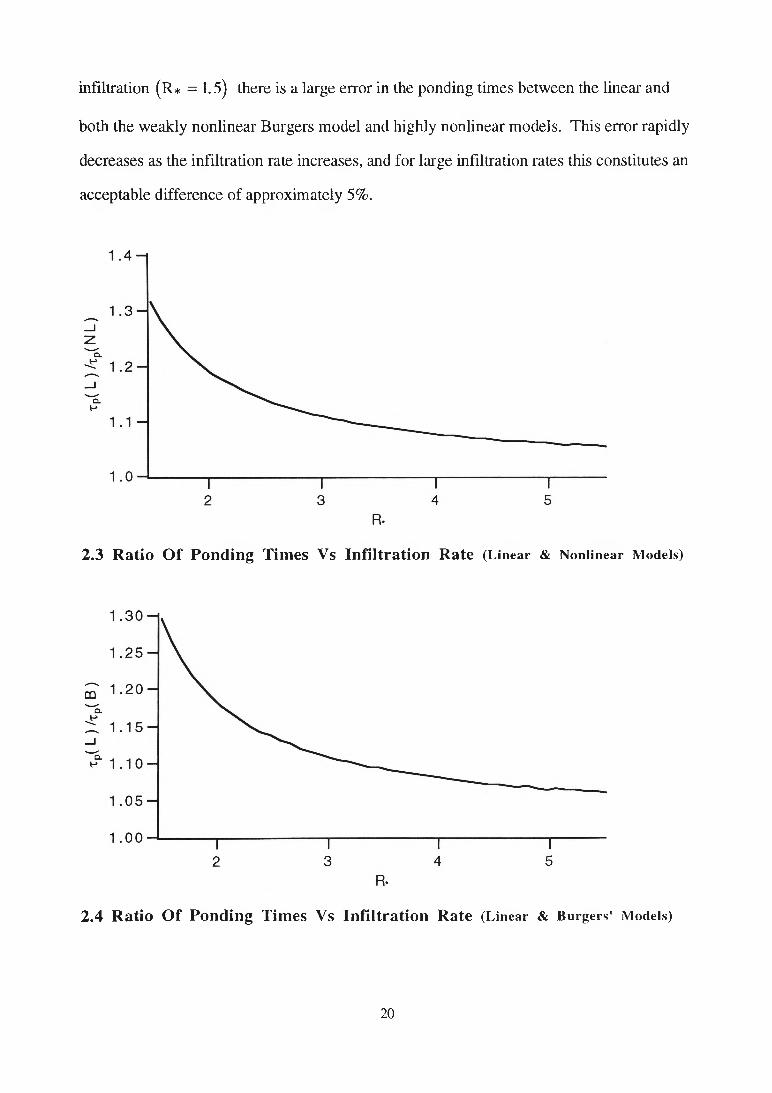
infiltration (R* = 1.5) there is a large error in the ponding times between the linear and

both the weakly nonlinear Burgers model and highly nonlinear models. This error rapidly

decreases as the infiltration rate increases, and for large infiltration rates this constitutes an

acceptable difference of approximately 5%.

2.3 Ratio O f Ponding Times Vs Infiltration Rate (Linear & Nonlinear Models)

2.4 Ratio O f Ponding Times Vs Infiltration Rate (Linear & Burgers' Models)

20

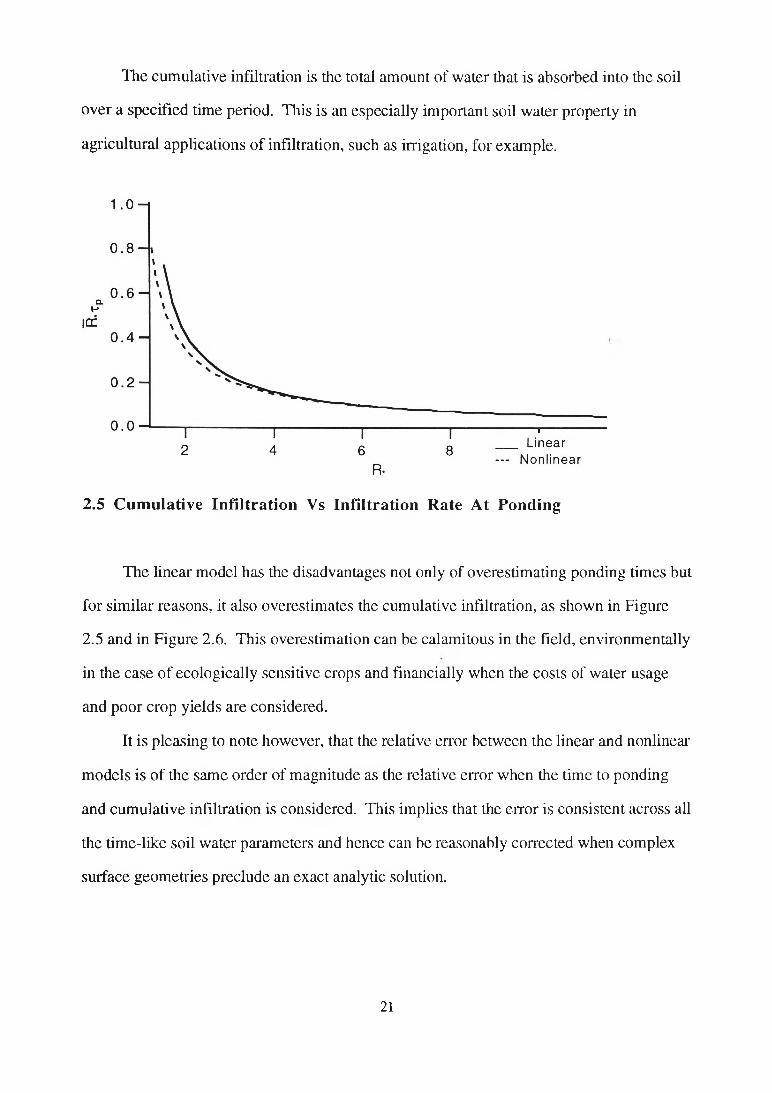
The cumulative infiltration is the total amount of water that is absorbed into the soil

over a specified time period. This is an especially important soil water property in

agricultural applications of infiltration, such as irrigation, for example.

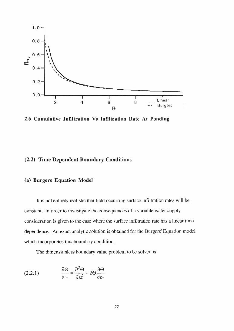
2.5 C um ulative In filtration Vs Infiltration Rate At Ponding

The linear model has the disadvantages not only of overestimating ponding times but

for similar reasons, it also overestimates the cumulative infiltration, as shown in Figure

2.5 and in Figure 2.6. This overestimation can be calamitous in the field, environmentally

in the case of ecologically sensitive crops and financially when the costs of water usage

and poor crop yields are considered.

It is pleasing to note however, that the relative error between the linear and nonlinear

models is of the same order of magnitude as the relative error when the time to ponding

and cumulative infiltration is considered. This implies that the error is consistent across all

the time-like soil water parameters and hence can be reasonably corrected when complex

surface geometries preclude an exact analytic solution.

21

1 . 0-1

0.8 —l

2.6 Cum ulative In filtration Vs Infiltration Rate At Ponding

(2.2) Time Dependent Boundary Conditions

(a) B urgers E quation Model

It is not entirely realistic that field occurring surface infiltration rates will be

constant. In order to investigate the consequences of a variable water supply

consideration is given to the case where the surface infiltration rate has a linear time

dependence. An exact analytic solution is obtained for the Burgers' Equation model

which incorporates this boundary condition.

The dimensionless boundary value problem to be solved is

(2.2 .1) 3 03t*

a 2©dzì

- 2 03 03z*

22

(2.2.2) 0 2 - — = Q(t*), z* = 03z*

(2.2.3) 0 = 0, t * = 0

where Q(t*) = R*t*.

As in the previous constant rate surface flux condition case, the Hopf-Cole

transformation (2.1.20) is applied to the boundary value problem, reducing the Burgers'

equation model to a linear diffusion problem. Thus, ’

(2.2.4) du _ 02u 3t* dz*

(2.2.5)f

u = expV

R*t*2 J

z* = 0

(2.2.6) u = 1, t* = 0

The linear diffusion boundary value problem (2.2.4) - (2.2.6) is solved by taking

Laplace Transforms with respect to the time variable t*, the result of which is

(2.2.7) u(z*,s) =1 i n }

va Jexp le r fc f

V4a J U V as >| 1

J Sexp(-z*Vs) +

Noting the large x asymptotic expansion, from Abramowitz and Stegun (1964:

Equation 7.1.23)

23

(2.2.8) V ix 2 exp^x2jerfc(x) ~ 1+ ( - l ) mm=l

1.3...(2m - 1 )

equation (2.2.7) is inverted for u(z*,t*). Therefore,

(2.2.9) u(z*,t*) = 1+ ^ ( - l ) mam25m[l.3...(2mm=l

(- l)]t2mi4merfc

V

Az^

y

where

(2.2.10) inerfc(x) = J in_1erfc(x)dx

is the repeated integral of the complementary error function.

At the soil surface equation (2.2.9) reduces to

(2.2.11) u(0,t*) = l+ ^ ( - l ) mam[l.3...(2m - l)]t*mi4merfc(0)m=l

and again we make use of Abramowitz and Stegun (1964: Equation 7.2.7), to wit

(2.2.12) inerfc(0) =1

2nTn- + 1

The dimensionless water content 0(0, t*) is easily obtained by inverting equation

(2.2.11) by making use of the Hopf-Cole transformation. Hence the ponding times are

deduced from

24

(2.2.13) 0(0,u) = exp(ü*). y ( - i)mam25m[l.3 ...(2m -l)]tlm^ ^A/711* m=l (4m)!

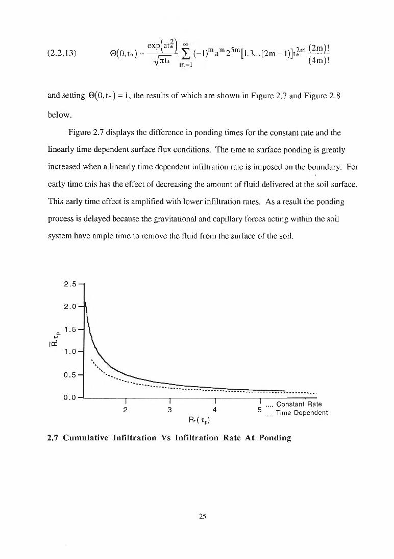
and setting 0 (0 , t*) = 1, the results of which are shown in Figure 2.7 and Figure 2.8

below.

Figure 2.7 displays the difference in ponding times for the constant rate and the

linearly time dependent surface flux conditions. The time to surface ponding is greatly

increased when a linearly time dependent infiltration rate is imposed on the boundary. For

early time this has the effect of decreasing the amount of fluid delivered at the soil surface.

This early time effect is amplified with lower infiltration rates. As a result the ponding

process is delayed because the gravitational and capillary forces acting within the soil

system have ample time to remove the fluid from the surface of the soil.

25

2 . 5-1

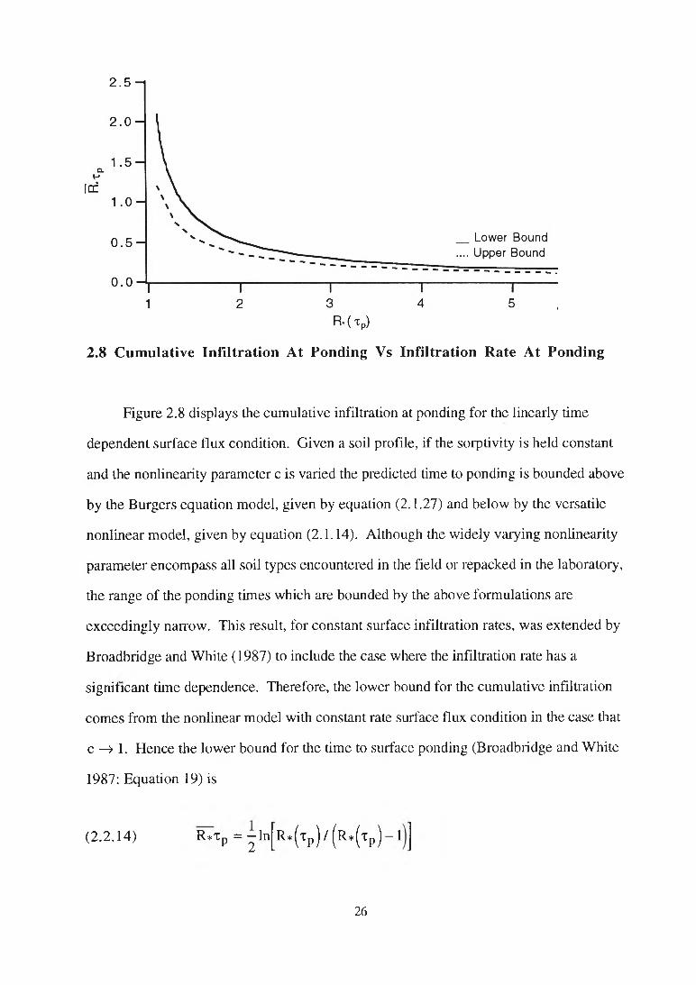
2.8 C um ulative In filtration At Ponding Vs Infiltration Rate At Ponding

Figure 2.8 displays the cumulative infiltration at ponding for the linearly time

dependent surface flux condition. Given a soil profile, if the sorptivity is held constant

and the nonlinearity parameter c is varied the predicted time to ponding is bounded above

by the Burgers equation model, given by equation (2.1.27) and below by the versatile

nonlinear model, given by equation (2.1.14). Although the widely varying nonlinearity

parameter encompass all soil types encountered in the field or repacked in the laboratory,

the range of the ponding times which are bounded by the above formulations are

exceedingly narrow. This result, for constant surface infiltration rates, was extended by

Broadbridge and W hite (1987) to include the case where the infiltration rate has a

significant time dependence. Therefore, the lower bound for the cumulative infiltration

comes from the nonlinear model with constant rate surface flux condition in the case that

c —> 1. Hence the lower bound for the time to surface ponding (Broadbridge and W hite

1987: Equation 19) is

(2 .2 .14) R*xn = — In P 2 R*(tp ) / ( r *(tp) - 1

26

which is in agreement with Pariange and Smith (1976). This lower bound provides a

reasonable estimate of the cumulative infiltration for the time dependent case. However,

as shown in Figure 2.7, it is reasonable to say that the errors are considerable which

contradicts the "time-condensation” postulate (Eagleson 1978) which predicts the

condensation of ponding curves when the cumulative infiltration is used as the time-like

variable. As expected the cumulative infiltration for the linearly time dependent surface

flux condition is greater than the corresponding constant rate boundary condition.

27

3 Infiltration In Two Dimensions

(3.1) Constant Supply Rate Surface Boundary Conditions

(a) Infiltration Boundary Conditions

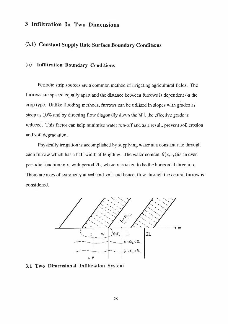
Periodic strip sources are a common method of irrigating agricultural fields. The

furrows are spaced equally apart and the distance between furrows is dependent on the

crop type. Unlike flooding methods, furrows can be utilised in slopes with grades as

steep as 10% and by directing flow diagonally down the hill, the effective grade is

reduced. This factor can help minimise water run-off and as a result, prevent soil erosion

and soil degradation.

Physically irrigation is accomplished by supplying water at a constant rate through

each furrow which has a half width of length w. The water content Q(x,z,t)is an even

periodic function in x, with period 2L, where x is taken to be the horizontal direction.

There are axes of symmetry at x=0 and x=L and hence, flow through the central furrow is

considered.

3.1 Two Dim ensional In filtra tion System

28

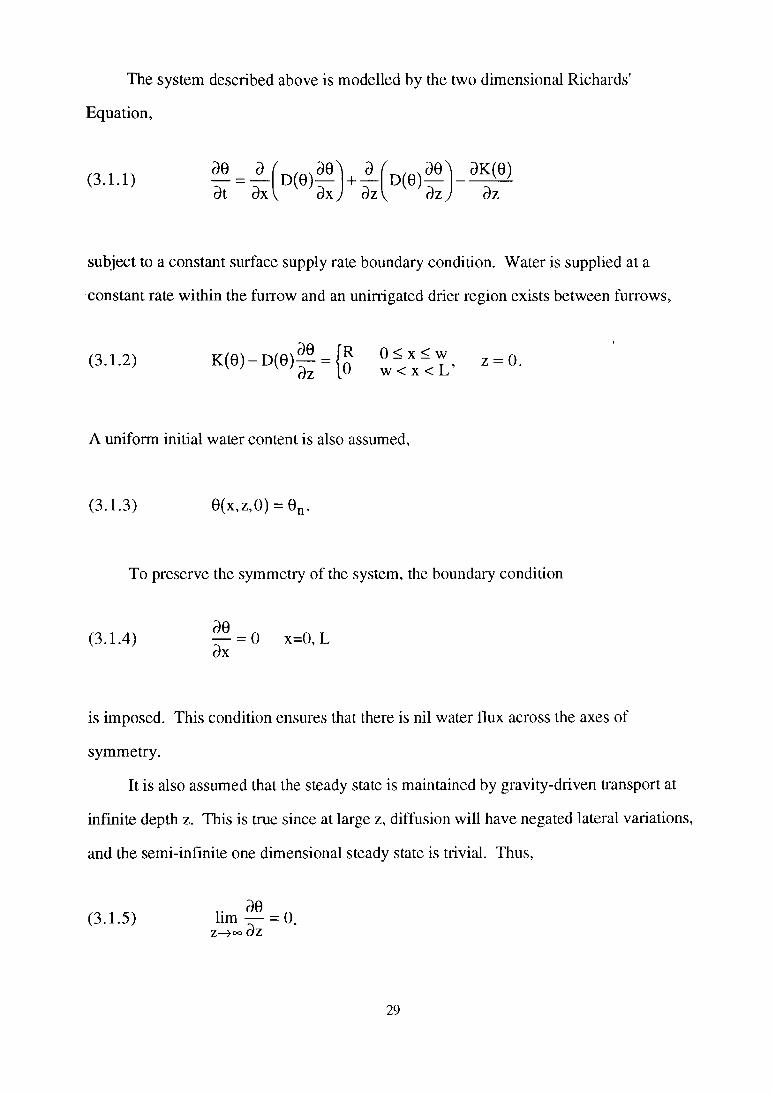
The system described above is modelled by the two dimensional Richards'

Equation,

(3.1.1)30at

_a_3x

D(e)do)dx

+d_dz m f )dz J

3K(0)dz

subject to a constant surface supply rate boundary condition. Water is supplied at a

constant rate within the furrow and an unirrigated drier region exists between furrows,

(3.1.2) K(e)-D(e)|dz

R 0 < x < w 0 w < x < L ’ z = 0.

A uniform initial water content is also assumed,

(3.1.3) 0(x,z,O) = 9n .

To preserve the symmetry of the system, the boundary condition

30(3.1.4) — = 0 x=0, L

dx

is imposed. This condition ensures that there is nil water flux across the axes of

symmetry.

It is also assumed that the steady state is maintained by gravity-driven transport at

infinite depth z. This is true since at large z, diffusion will have negated lateral variations,

and the semi-infinite one dimensional steady state is trivial. Thus,

30(3.1.5) lim — = 0.

z—>oo dz

29

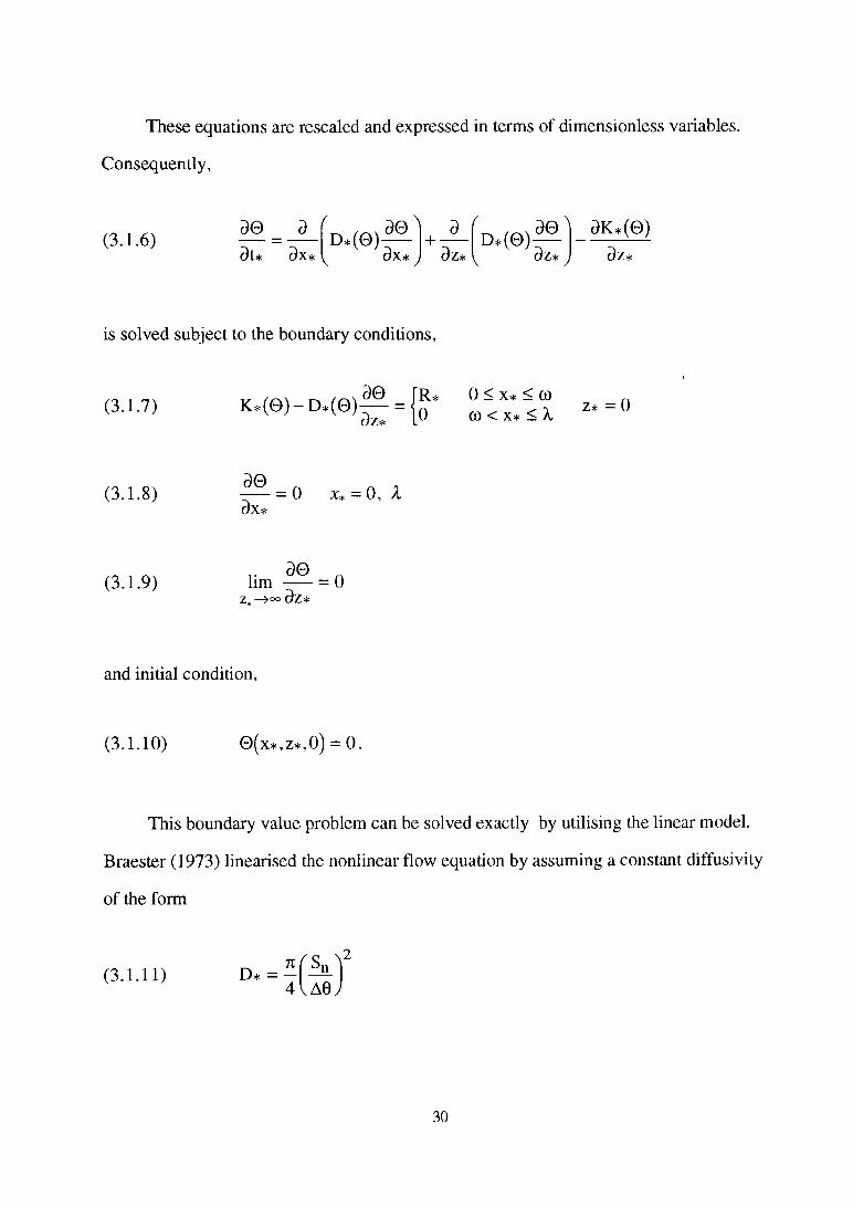
These equations are rescaled and expressed in terms of dimensionless variables.

Consequently,

(3 .1 .6)9 0 9 9 f _ , _ , a © Nl 9K *(0)---- = ------ D * (0 )----- + ----- D * (0 )----- ----------- —Ot* Ox* Ox* j Oz* Oz* j Oz*

is solved subject to the boundary conditions,

(3.1.7) v i e w T ic\\àfo JR* ()<X*<C0 K*(®) D*(0 ) dzt " j o c o < x * < \ z* 0

(3.1.8) dO n n 7-----= 0 x+ = 0, AOx*

(3.1.9) lim d& = 0z„—>°° Oz*

and initial condition,

(3.1.10) 0 (x* , z*, 0) = 0.

This boundary value problem can be solved exactly by utilising the linear model.

Braester (1973) linearised the nonlinear flow equation by assuming a constant diffusivity

of the form

(3.1.11) D* =4 { A d J

30

and a linear dependence of the hydraulic conductivity K*(0) on the water content 0 .

This constant diffusivity is selected as it ensures that the linearised and exact models of the

flow equation predict identical cumulative infiltration at early times during a constant

pressure experiment. This diffusivity will result in an exact solution in which the

sorptivity is equivalent to the measured value of the sorptivity Sn .

The linear flow equation,

(3.1.12)a© <)2e a2© d &

8t* 8x* 8z? 8z*

is solved subject to (3.1.8)-(3.1.10) and revised surface flux condition

(3.1.13) dO _ [R*Oz* IP

0 < x* < G) n- z* — U CO < X* < A

by taking Laplace transforms and using separation of variables. Batu (1978) deduced a

solution for a single and for periodic strip sources using similar techniques.

The series solution is of the form,

/ \ A n ' ( nTTX* ^(3.1.14) 0(x*,z*,t*) = ^ An cos! ——I

n=l v

with A0 = A0(z*,t*) and An = An(z*,t*). Batu (1978) used this solution to study the

two dimensional flow pattern and Philip (1984) used a related flow pattern irom a spatially

periodic source to study leaching patterns. So far this solution has not been used to

estimate ponding times.

Surface ponding first occurs at the centre of the wet strip x* = 0 . Thus to deduce

the time to surface ponding, we consider the expression 0 (0 ,0,t*), where

31

(3.1.15) 0(O,O,t*) = p ^ )( u \

1 + — exp —) 1 4 J

1 + -y je rfc

^ 2 R * .+ z — sin

n=l n7T V

n7TC0 \~ r j

(F_ + F+) + G

A

J

with

ferfc

(3.1.16) F+ =

+

V 1f „ 2 2 t An n 1

— + — t*

' 2 2 in n 12Vd 7

m- + —

V

and

(3.1.17) G =x2

2n27t2exp

V

n27t2t*“l 2“

Aerfc

y

A

)

respectively.

The time to surface ponding xp, is subsequently evaluated by solving

©(o ,0 ,xp) = 1, the results of which are shown in Figure 3.2 and Figure 3.3.

It is evident that although the linear model is expected to overestimate xp for all

values of co, the time to surface ponding through equally spaced irrigation furrows is

substantially higher than the time required for ponding in the corresponding one

dimensional infiltration system. In the two dimensional case, water is not only

transported from the soil surface by gravity and vertical diffusion, but also laterally by

horizontal diffusion. This additional degree of freedom results in longer ponding times.

32

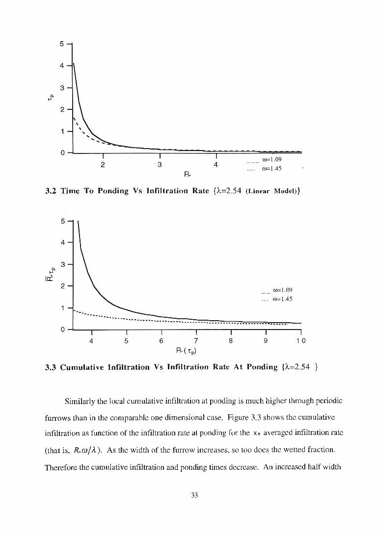
3.2 Time To Ponding Vs Infiltration Rate {X=2.54 (Linear M odel)}

3.3 Cum ulative In filtration Vs Infiltration Rate At Ponding {>.=2.54 }

Similarly the local cumulative infiltration at ponding is much higher through periodic

furrows than in the comparable one dimensional case. Figure 3.3 shows the cumulative

infiltration as function of the infiltration rate at ponding for the x* averaged infiltration rate

(that is, R*co/h). As the width o f the furrow increases, so too does the wetted fraction.

Therefore the cumulative infiltration and ponding times decrease. An increased half width

33

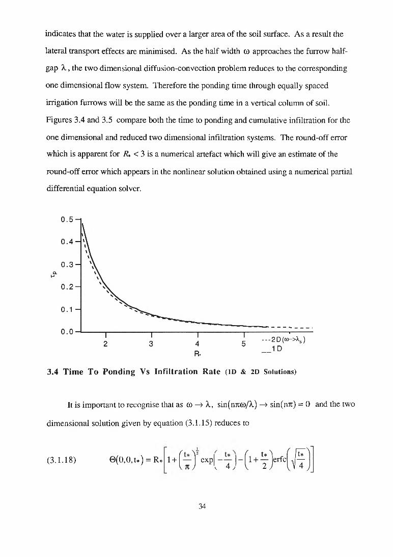
indicates that the water is supplied over a larger area of the soil surface. As a result the

lateral transport effects are minimised. As the half width co approaches the furrow half­

gap X , the two dimensional diffusion-convection problem reduces to the corresponding

one dimensional flow system. Therefore the ponding time through equally spaced

irrigation furrows will be the same as the ponding time in a vertical column of soil.

Figures 3.4 and 3.5 compare both the time to ponding and cumulative infiltration for the

one dimensional and reduced two dimensional infiltration systems. The round-off error

which is apparent for R* < 3 is a numerical artefact which will give an estimate of the

round-off error which appears in the nonlinear solution obtained using a numerical partial

differential equation solver.

3.4 Tim e To Ponding Vs Infiltration Rate (ID & 2D Solutions)

It is important to recognise that as co —> X, sin(n7tco/X) —» sin(n7t) = 0 and the two

dimensional solution given by equation (3.1.15) reduces to

(3.1.18) 0(0,0, t*) = R* 1 + ( ~ yV7ty

expk 4 J

34

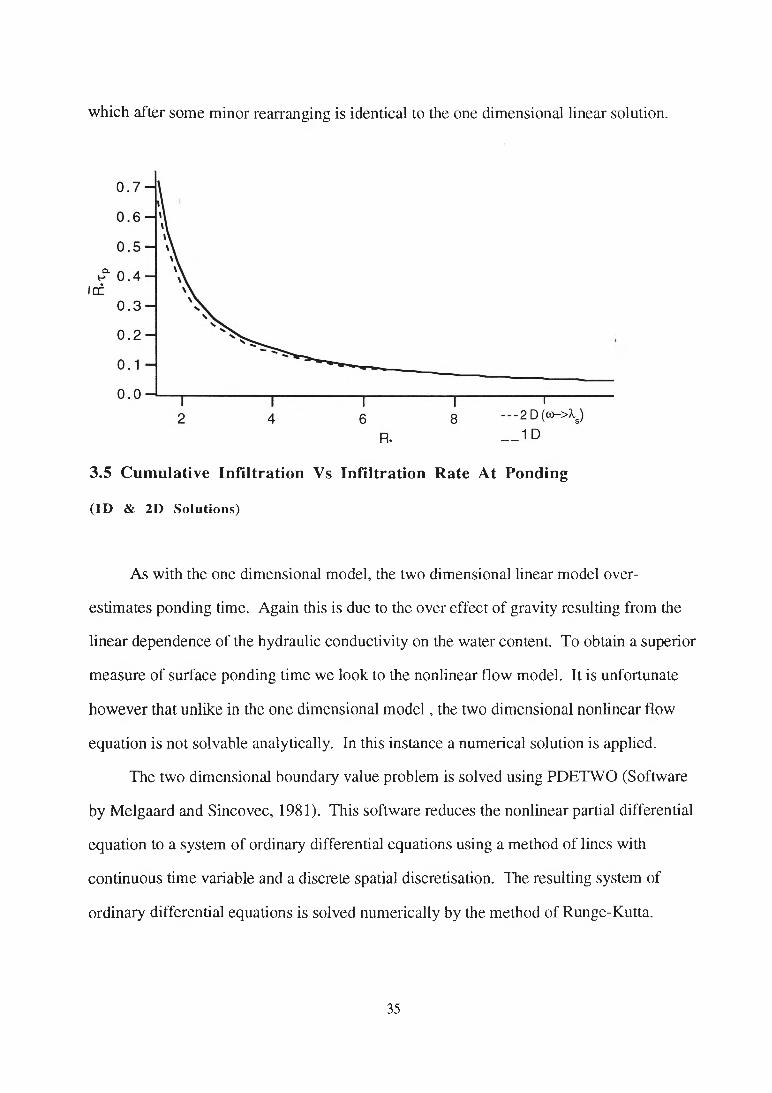
which after some minor rearranging is identical to the one dimensional linear solution.

3.5 C um ulative In filtra tion Vs Infiltration Rate At Ponding

(ID & 2D Solutions)

As with the one dimensional model, the two dimensional linear model over­

estimates ponding time. Again this is due to the over effect of gravity resulting from the

linear dependence of the hydraulic conductivity on the water content. To obtain a superior

measure of surface ponding time we look to the nonlinear flow model. It is unfortunate

however that unlike in the one dimensional m o d e l, the two dimensional nonlinear flow

equation is not solvable analytically. In this instance a numerical solution is applied.

The two dimensional boundary value problem is solved using PDETW O (Software

by M elgaard and Sincovec, 1981). This software reduces the nonlinear partial differential

equation to a system of ordinary differential equations using a method of lines with

continuous time variable and a discrete spatial discretisation. The resulting system of

ordinary differential equations is solved numerically by the method of Runge-Kutta.

35

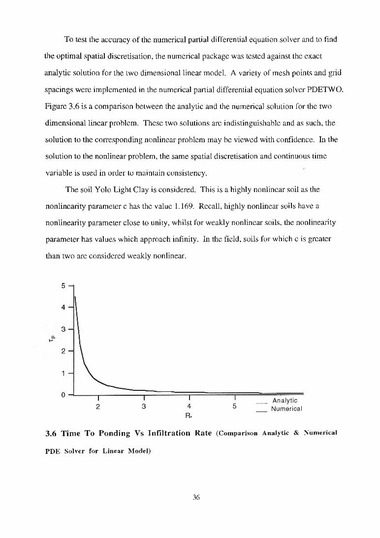
To test the accuracy of the numerical partial differential equation solver and to find

the optimal spatial discretisation, the numerical package was tested against the exact

analytic solution for the two dimensional linear model. A variety of mesh points and grid

spacings were implemented in the numerical partial differential equation solver PDETWO.

Figure 3.6 is a comparison between the analytic and the numerical solution for the two

dimensional linear problem. These two solutions are indistinguishable and as such, the

solution to the corresponding nonlinear problem may be viewed with confidence. In the

solution to the nonlinear problem, the same spatial discretisation and continuous time

variable is used in order to maintain consistency.

The soil Yolo Light Clay is considered. This is a highly nonlinear soil as the

nonlinearity parameter c has the value 1.169. Recall, highly nonlinear soils have a

nonlinearity parameter close to unity, whilst for weakly nonlinear soils, the nonlinearity

parameter has values which approach infinity. In the field, soils for which c is greater

than two are considered weakly nonlinear.

3.6 Time To Ponding Vs Infiltra tion Rate (Comparison Analytic & Numerical

PDE Solver for Linear Model)

36

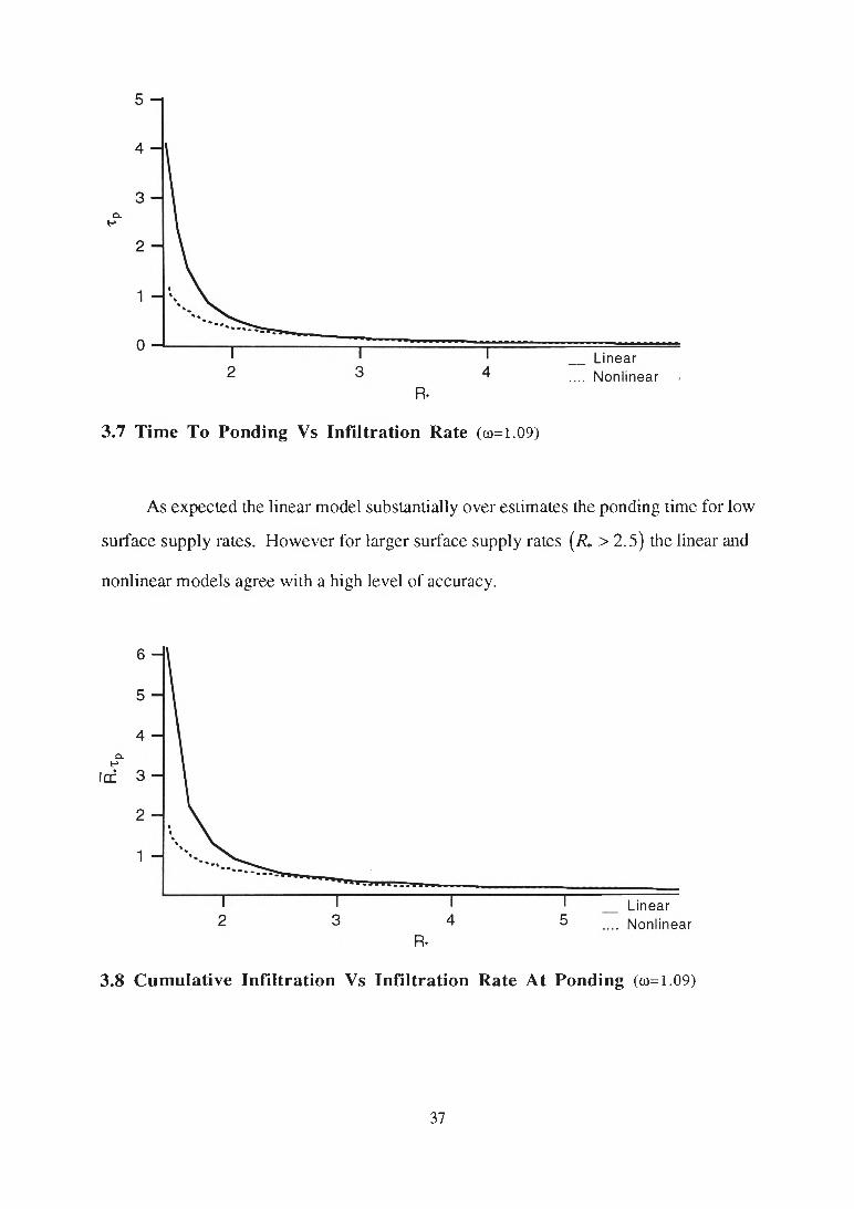
3.7 Time To Ponding Vs Infiltration Rate (co=1.09)

As expected the linear model substantially over estimates the ponding time for low

surface supply rates. However for larger surface supply rates (R* > 2.5) the linear and

nonlinear models agree with a high level of accuracy.

3.8 Cum ulative Infiltration Vs Infiltration Rate At Ponding (co=1.09)

37

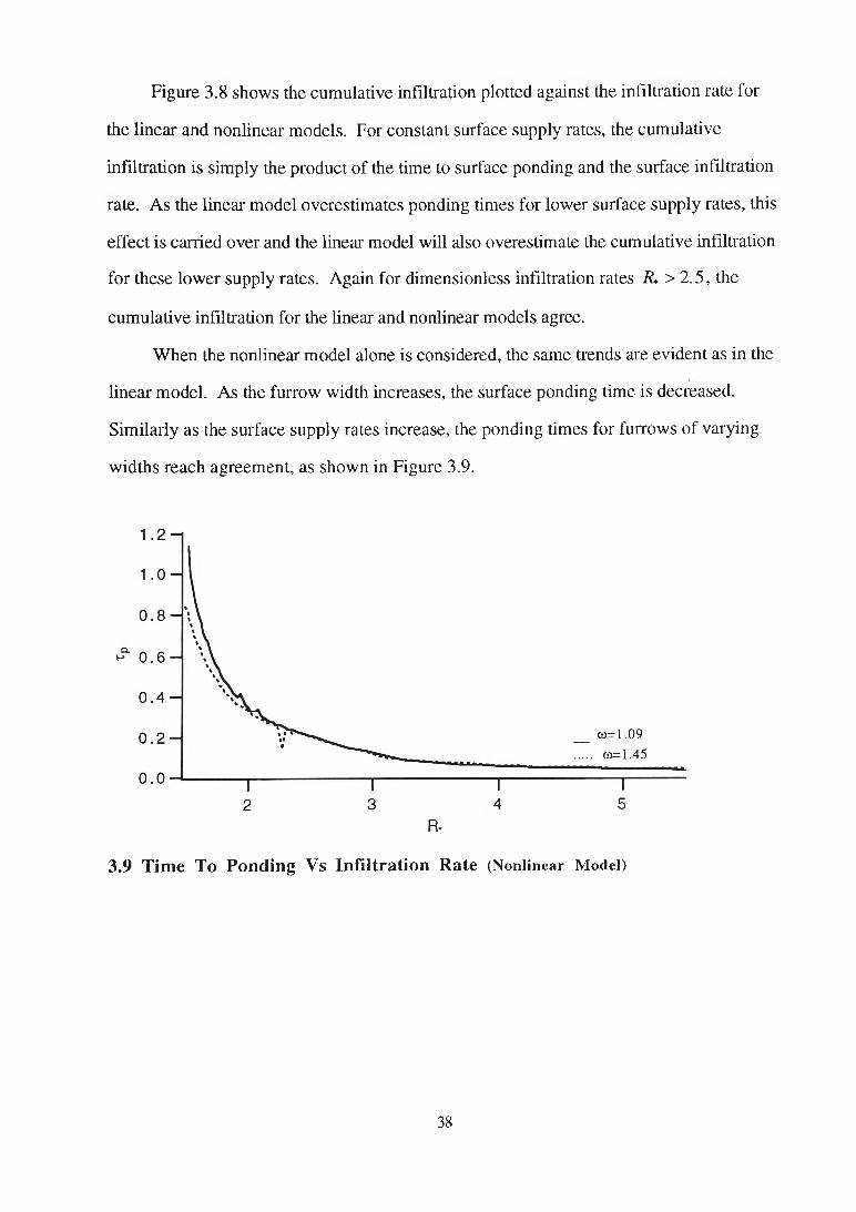
Figure 3.8 shows the cumulative infiltration plotted against the infiltration rate for

the linear and nonlinear models. For constant surface supply rates, the cumulative

infiltration is simply the product of the time to surface ponding and the surface infiltration

rate. As the linear model overestimates ponding times for lower surface supply rates, this

effect is carried over and the linear model will also overestimate the cumulative infiltration

for these lower supply rates. Again for dimensionless infiltration rates R* > 2 .5 , the

cumulative infiltration for the linear and nonlinear models agree.

W hen the nonlinear model alone is considered, the same trends are evident as in the

linear model. As the furrow width increases, the surface ponding time is decreased.

Similarly as the surface supply rates increase, the ponding times for furrows of varying

widths reach agreement, as shown in Figure 3.9.

3.9 Time To Ponding Vs Infiltration Rate (Nonlinear Model)

38

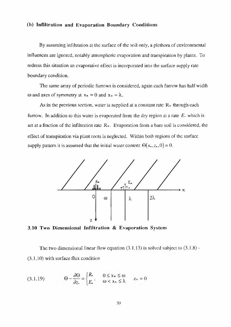
By assuming infiltration at the surface of the soil only, a plethora of environmental

influences are ignored, notably atmospheric evaporation and transpiration by plants. To

redress this situation an evaporative effect is incorporated into the surface supply rate

boundary condition.

The same array of periodic furrows is considered, again each furrow has half width

co and axes of symmetry at x* = 0 and x* = X.

As in the previous section, water is supplied at a constant rate R* through each

furrow. In addition to this water is evaporated from the dry region at a rate E* which is

set at a fraction of the infiltration rate R *. Evaporation from a bare soil is considered, the

effect of transpiration via plant roots is neglected. W ithin both regions of the surface

supply pattern it is assumed that the initial water content 0 ( x*,z*,0) = 0.

(b) In filtra tion and E vaporation B oundary Conditions

3.10 Two Dim ensional In filtration & E vaporation System

The two dimensional linear flow equation (3.1.13) is solved subject to (3.1.8) -

(3.1.10) with surface flux condition

(3 .1 .19)dG [R * 0 < x * < G)

~ ~ d Z ~ \ E , ' co< x* < X

39

This surface flux condition is perhaps physically more realistic than the surface flux

condition incorporating infiltration only as it encompasses vapour loss from the soil as a

result of evaporative effects. Beneath the evaporation surface, the dimensionless soil

water 0 attains a minimum value 0 ^ that may be negative. However, our solution

allows the initial volumetric water content Qn to be any specified non-negative value. If

6n is chosen to be large enough, then the negative value 0 ^ still corresponds to a non­

negative volumetric water content 0 ^ = 0 (0 5 - 0n) + 6n.

Laplace transforms are taken and separation of variables achieves the solution with

ease. In this case the dimensionless surface water content,

(3.1.20) 0(0,0, u ) =(R* -E*)co

V A1 + 1 — | exp - 1

4 J1 + y |erfc

/*

+2«=1

2(R* - £*)^. f nnco\nn V A JL2

1(F_ + F+) + G

where F+ and G are as defined by equations (3.1.16) and (3.1.17) respectively. Again,

the time to ponding is deduced from the solution to 0(0,0, t*) = 1.

Figures 3.11 and 3.12 display the results obtained with a fixed exfiltration rate and

varying furrow half widths. As in the previous infiltration only case, the time to surface

ponding and cumulative infiltration is decreased as the half width of the furrow increases.

Similarly, as the width of the half width approaches the length of the furrow X, the two

dimensional system reduces to a one dimensional system. In addition for an exfiltration

rate greater than 5% of the infiltration rate, ponding is delayed compared to the infiltration

only system. This effect is noticeably so as the half width of the furrow decreases. The

longer ponding times for low surface supply rates are attributed to the large effect that

evaporation from the dry region has on the system. As the surface supply rates increase

40

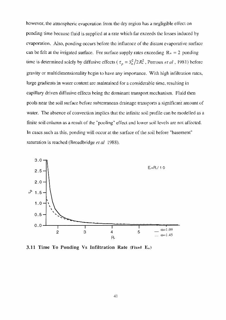
however, the atmospheric evaporation from the dry region has a negligible effect on

ponding time because fluid is supplied at a rate which far exceeds the losses induced by

evaporation. Also, ponding occurs before the influence of the distant evaporative surface

can be felt at the irrigated surface. For surface supply rates exceeding R* = 2 ponding

time is determined solely by diffusive effects ( Tp = S fJ lR '} , Perroux et a t , 1981) before

gravity or multidimensionality begin to have any importance. With high infiltration rates,

large gradients in water content are maintained for a considerable time, resulting in

capillary driven diffusive effects being the dominant transport mechanism. Fluid then

pools near the soil surface before subterranean drainage transports a significant amount of

water. The absence of convection implies that the infinite soil profile can be modelled as a

finite soil column as a result of the "pooling" effect and lower soil levels are not affected.

In cases such as this, ponding will occur at the surface of the soil before "basement"

saturation is reached (Broadbridge et al 1988).

3.11 Time To Ponding Vs Infiltration Rate (Fixed E*)

41

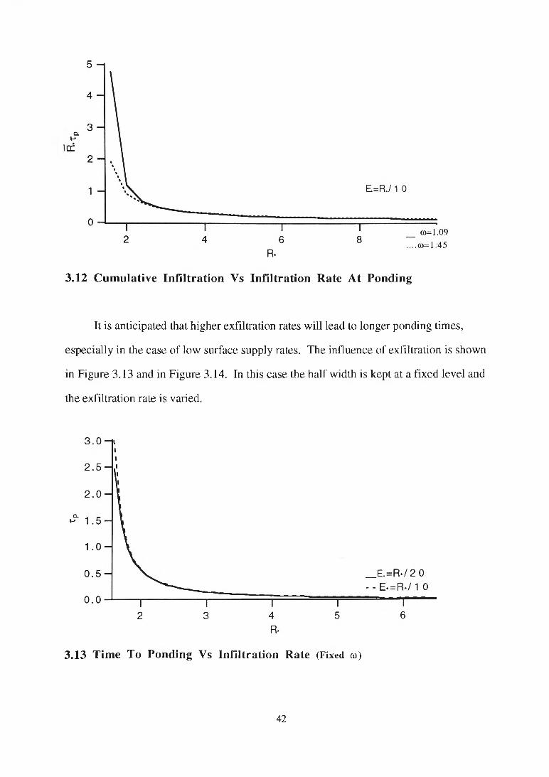
3.12 Cum ulative In filtra tion Vs Infiltration Rate At Ponding

It is anticipated that higher exfiltration rates will lead to longer ponding times,

especially in the case of low surface supply rates. The influence of exfiltration is shown

in Figure 3.13 and in Figure 3.14. In this case the half width is kept at a fixed level and

the exfiltration rate is varied.

3.13 Time To Ponding Vs Infiltration Rate (Fixed co)

42

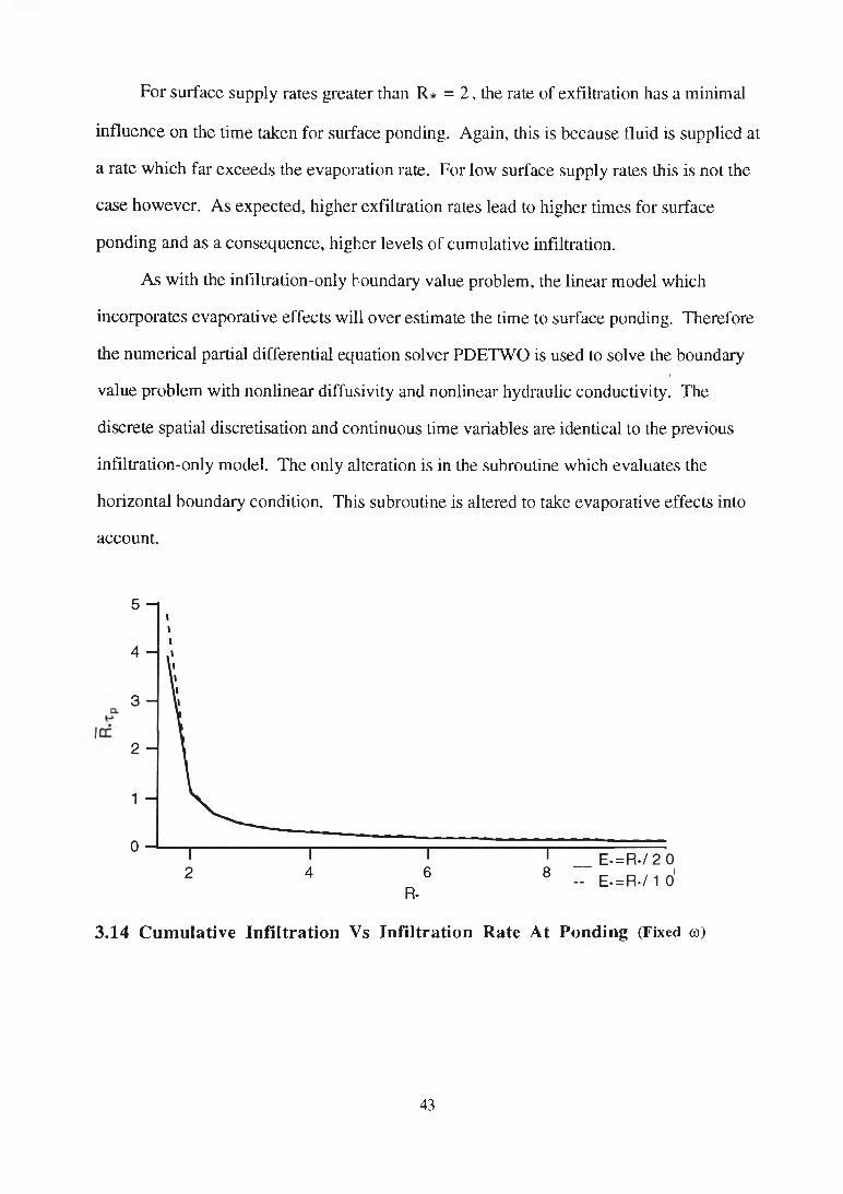
For surface supply rates greater than R* = 2 , the rate of exfiltration has a minimal

influence on the time taken for surface ponding. Again, this is because fluid is supplied at

a rate which far exceeds the evaporation rate. For low surface supply rates this is not the

case however. As expected, higher exfiltration rates lead to higher times for surface

ponding and as a consequence, higher levels of cumulative infiltration.

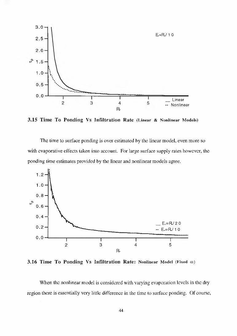
As with the infiltration-only boundary value problem, the linear model which

incorporates evaporative effects will over estimate the time to surface ponding. Therefore

the numerical partial differential equation solver PDETW O is used to solve the boundary

value problem with nonlinear diffusivity and nonlinear hydraulic conductivity. The

discrete spatial discretisation and continuous time variables are identical to the previous

infiltration-only model. The only alteration is in the subroutine which evaluates the

horizontal boundary condition. This subroutine is altered to take evaporative effects into

account.

3.14 C um ulative In filtra tion Vs In filtration Rate At Ponding (Fixed co)

43

3 . 0 - 1

2 .5

2 . 0 -

e- 1 . 5 H

1 . 0 ­

0 . 5 -

0.0 ~T4

R.

E=R./ 1 0

__ Linear-- Nonlinear

3.15 Time To Ponding Vs Infiltration Rate (Linear & Nonlinear Models)

The time to surface ponding is over estimated by the linear model, even more so

with evaporative effects taken into account. For large surface supply rates however, the

ponding time estimates provided by the linear and nonlinear models agree.

3.16 Time To Ponding Vs Infiltration Rate: Nonlinear Model (Fixed c o )

W hen the nonlinear model is considered with varying evaporation levels in the dry

region there is essentially very little difference in the time to surface ponding. Of course,

44

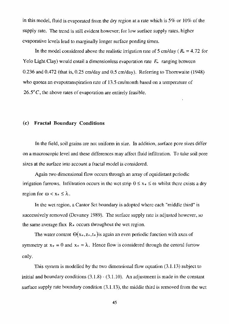
in this model, fluid is evaporated from the dry region at a rate which is 5% or 10% of the

supply rate. The trend is still evident however; for low surface supply rates, higher

evaporative levels lead to marginally longer surface ponding times.

In the model considered above the realistic irrigation rate of 5 cm/day ( R* = 4.12 for

Yolo Light Clay) would entail a dimensionless evaporation rate E* ranging between

0.236 and 0.472 (that is, 0.25 cm/day and 0.5 cm/day). Referring to Thomwaite (1948)

who quotes an évapotranspiration rate of 13.5 cm/month based on a temperature of

26.5°C, the above rates of evaporation are entirely feasible.

(c) Fractal Boundary Conditions

In the field, soil grains are not uniform in size. In addition, surface pore sizes differ

on a macroscopic level and these differences may affect fluid infiltration. To take soil pore

sizes at the surface into account a fractal model is considered.

Again two dimensional flow occurs through an array of equidistant periodic

irrigation furrows. Infiltration occurs in the wet strip 0 < x* < co whilst there exists a dry

region for co < x* < X .

In the wet region, a Cantor Set boundary is adopted where each "middle third" is

successively removed (Devaney 1989). The surface supply rate is adjusted however, so

the same average flux R* occurs throughout the wet region.

The water content 0(x*,z*,t*)is again an even periodic function with axes of

symmetry at x* = 0 and x* = X. Hence flow is considered through the central furrow

only.

This system is modelled by the two dimensional flow equation (3.1.13) subject to

initial and boundary conditions (3.1.8) - (3.1.10). An adjustment is made in the constant

surface supply rate boundary condition (3.1.13), the middle third is removed from the wet

45

strip and the infiltration rate is adjusted in order that the same average flux is absorbed

into the soil. Thus,

(3.1.21)3z*

| r *o§R*0

V

0 < x* < ^(04-co < X* < -i-CO3 3 z* — 0-jG) < X* < CO

co < x* < X

At the soil surface in the centre of the wet strip, the soil water content is given by

(3.1.22) 0 (0 ,0 ,u ) = R*co~ k ~

1 +V 71 )

expk 4> 1 2 )

erfc

^ 3R* f . ( nrccoA . f 2n7tcoA . ( n7tco

n=l l 3X J 3 \j ( F _ + F+ ) + G

with F+ and G defined by equations (3.1.16) and (3.1.17) respectively.

A second and third iteration of the Cantor Set surface boundary condition is taken.

The middle thirds of the remaining wet strips are removed and the readjustment in the

surface supply rate is made. These revised infiltration systems are solved, the results of

which are shown in Figure 3.17.

A comparison is made between the time to surface ponding for the uniform wet

region and the adjusted Cantor Set wet region. The same volumetric water content is

delivered at the soil surface, the only difference is in the distribution of the fluid flow

within the wet strip.

46

5 -1

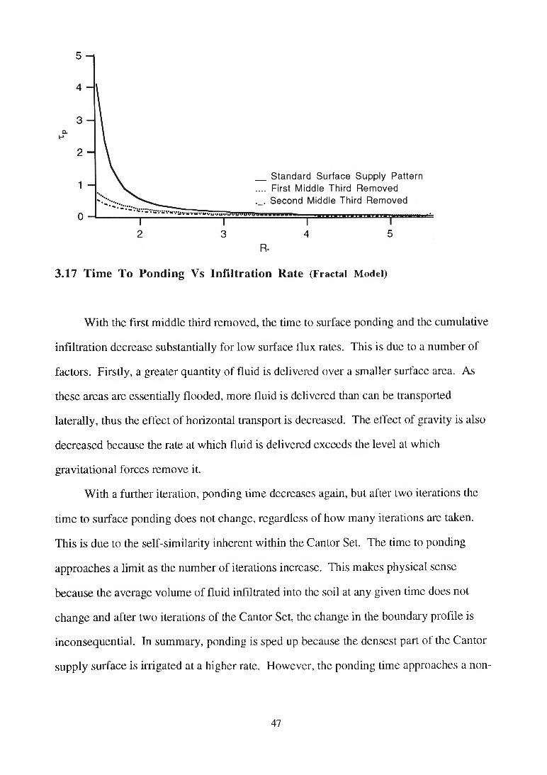
3.17 Time To Ponding Vs Infiltration Rate (Fractal M odel)

W ith the first middle third removed, the time to surface ponding and the cumulative

infiltration decrease substantially for low surface flux rates. This is due to a num ber of

factors. Firstly, a greater quantity of fluid is delivered over a sm aller surface area. As

these areas are essentially flooded, more fluid is delivered than can be transported

laterally, thus the effect of horizontal transport is decreased. The effect of gravity is also

decreased because the rate at which fluid is delivered exceeds the level at which

gravitational forces remove it.

W ith a further iteration, ponding time decreases again, but after two iterations the

tim e to surface ponding does not change, regardless of how m any iterations are taken.

This is due to the self-similarity inherent within the Cantor Set. The time to ponding

approaches a limit as the num ber of iterations increase. This makes physical sense

because the average volume of fluid infiltrated into the soil at any given time does not

change and after two iterations of the Cantor Set, the change in the boundary profile is

inconsequential. In summary, ponding is sped up because the densest part of the Cantor

supply surface is irrigated at a higher rate. However, the ponding tim e approaches a non­

47

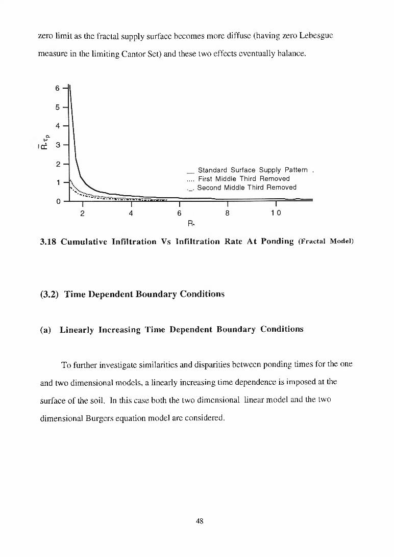
zero lim it as the fractal supply surface becom es more diffuse (having zero Lebesgue

m easure in the lim iting Cantor Set) and these two effects eventually balance.

3.18 Cumulative Infiltration Vs Infiltration Rate At Ponding (Fractal Model)

(3.2) Time Dependent Boundary Conditions

(a) Linearly Increasing Time Dependent Boundary Conditions

To further investigate similarities and disparities between ponding times for the one

and two dim ensional models, a linearly increasing time dependence is imposed at the

surface of the soil. In this case both the two dimensional linear model and the two

dim ensional Burgers equation model are considered.

48

(i) Linear Model

The linear two dimensional fluid flow equation (3.1.12) is solved subject to initial

condition (3.1.10) and boundary conditions (3.1.8) - (3.1.9) with the surface supply

condition,

(3.2.1) 3© ÎQ (u ) 0 < x * < c o d z * ~ 10 co < x* < X

z * = 0

once again by taking Laplace transforms and using separation of variables. Here, the

supply rate Q(t*) = R*t*.

The solution at the soil surface z* = 0 at the centre of the wet strip x* = 0 is given

by

(3.2.2)

r\(r\ r\ \ R*C0 ( t* ^0(O,O,t*) = -- - ■ exp|^——/ 1 A

TCt* j+ ^ Gi j i - 2 V 2 Gi —Ì

v 2 yexp^-yj(2V2 - 2)

00

+ Z -n=l

•sin -nn V X )

exp^-a2j<

c

-16 J i i exp(at*)

16a2 -1k \^ 7It* j

V

2 ° U JJ

a (4 a - 1)

^ 2 R * .+2rf— sm

n=l nTC h r J exp(“ a1 Y

y 7tt*- + 2 Vöc exp(at* )2

where,

(3.2.3) Cj(x ) = exp(x)erfc(Vx)

49

and after appropriate scaling,

(3 .2 .4 ) or2 2 n 7i

K

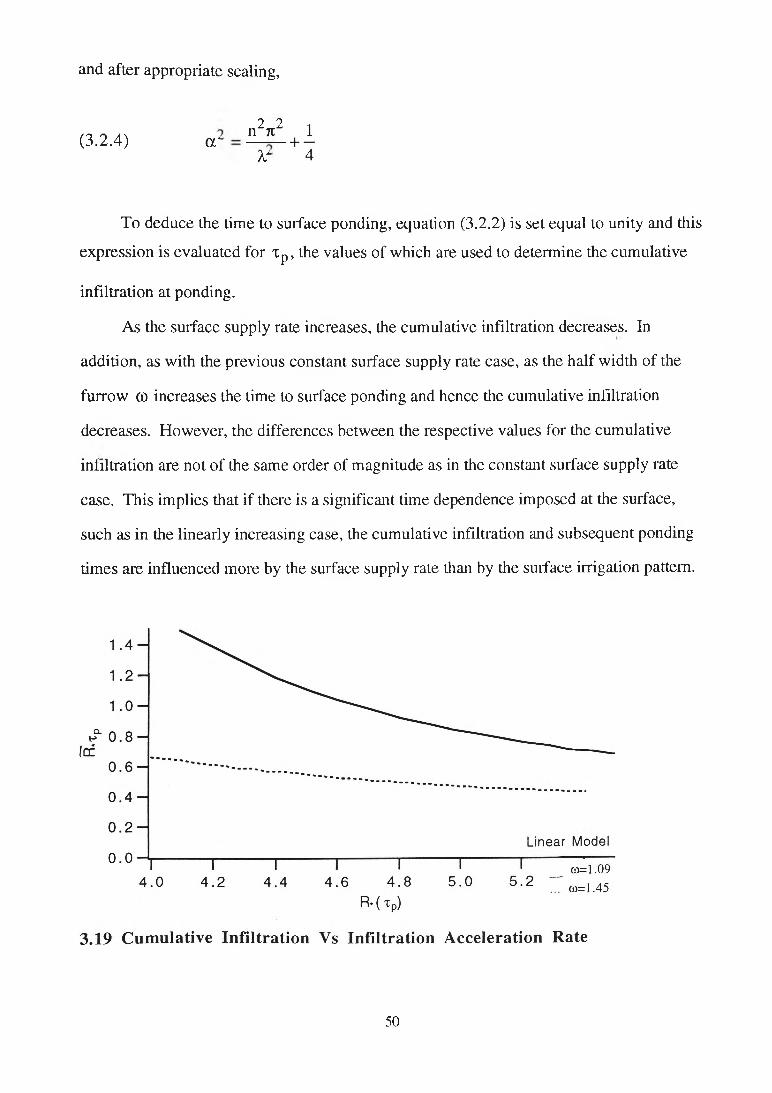
To deduce the tim e to surface ponding, equation (3.2.2) is set equal to unity and this

expression is evaluated for Tp, the values of which are used to determine the cumulative

infiltration at ponding.

As the surface supply rate increases, the cum ulative infiltration decreases. In

addition, as w ith the previous constant surface supply rate case, as the half w idth of the

furrow co increases the time to surface ponding and hence the cumulative infiltration

decreases. However, the differences between the respective values for the cumulative

infiltration are not o f the sam e order of magnitude as in the constant surface supply rate

case. This im plies that if there is a significant time dependence imposed at the surface,

such as in the linearly increasing case, the cumulative infiltration and subsequent ponding

tim es are influenced more by the surface supply rate than by the surface irrigation pattern.

50

(ii) Burgers Equation Model

The two dimensional Burgers equation,

(3.2.5) 3 03t*

d2Q a 2e3x* dzì

- 2 03 03z*

is solved subject to initial and boundary conditions (3.1.8) - (3.1.10) and surface flux

condition

(3.2.6) 0 '3 03z*

Q(t*) 0 < x* < CO0 co < x* < X z* = 0

numerically by the partial differential equation solver PDETWO. Again, Q(t*) = R*t*.

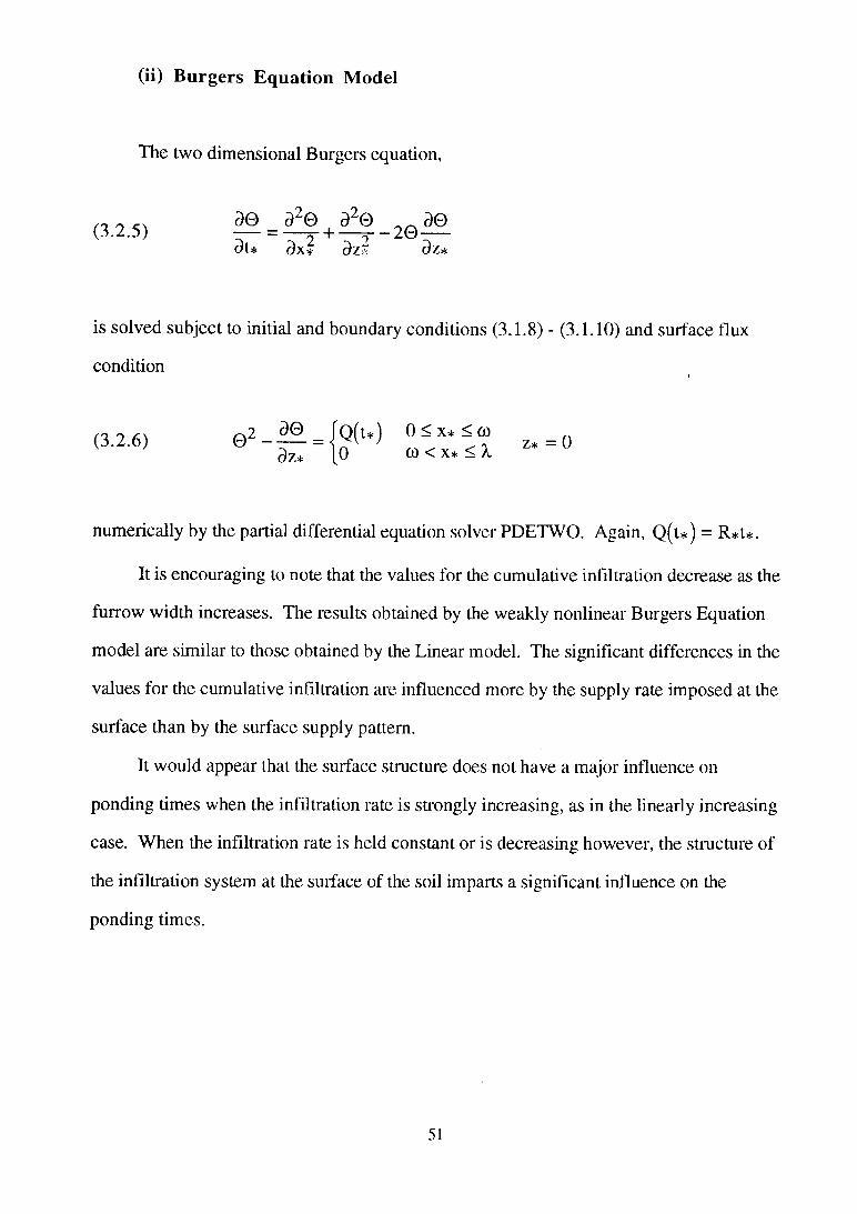
It is encouraging to note that the values for the cumulative infiltration decrease as the

furrow width increases. The results obtained by the weakly nonlinear Burgers Equation

model are similar to those obtained by the Linear model. The significant differences in the

values for the cumulative infiltration are influenced more by the supply rate imposed at the

surface than by the surface supply pattern.

It would appear that the surface structure does not have a major influence on

ponding times when the infiltration rate is strongly increasing, as in the linearly increasing

case. When the infiltration rate is held constant or is decreasing however, the structure of

the infiltration system at the surface of the soil imparts a significant influence on the

ponding times.

51

1 .2-1

1 . 0 -

0 . 8 -Q.

0 . 6 -

0 . 4 -

0 . 2 -

0.0Burgers Model

i -------- ï--------T--------1-------- T r ~3 . 6 3 . 8 4 . 0 4 . 2 4 . 4 4 . 6

R*(xp)

(o=1.09 co=l .45 5 .0

3.20 Cumulative Infiltration Vs Infiltration Acceleration Rate

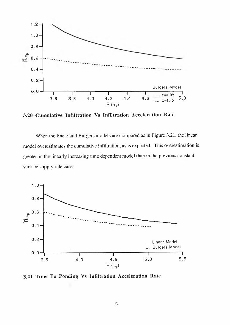
W hen the linear and Burgers m odels are com pared as in Figure 3.21, the linear

m odel overestim ates the cum ulative infiltration, as is expected. This overestimation is

greater in the linearly increasing time dependent model than in the previous constant

surface supply rate case.

52

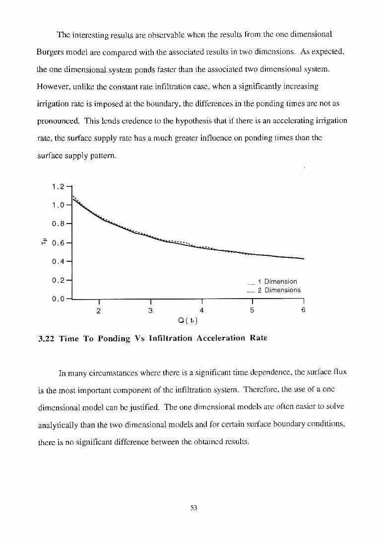
The interesting results are observable when the results from the one dim ensional

Burgers m odel are com pared with the associated results in two dimensions. As expected,

the one dim ensional system ponds faster than the associated two dim ensional system.

H ow ever, unlike the constant rate infiltration case, when a significantly increasing

irrigation rate is im posed at the boundary, the differences in the ponding tim es are not as

pronounced. This lends credence to the hypothesis that if there is an accelerating irrigation

rate, the surface supply rate has a much greater influence on ponding times than the

surface supply pattern.

Q(t*)

3 .22 Time To Ponding V s Infiltration Acceleration Rate

In m any circum stances where there is a significant time dependence, the surface flux

is the m ost im portant com ponent of the infiltration system. Therefore, the use of a one

dim ensional m odel can be justified. The one dimensional models are often easier to solve

analytically than the two dim ensional models and for certain surface boundary conditions,

there is no significant difference between the obtained results.

53

(b) Periodic Boundary Conditions

Field applications of infiltration rarely encompass a constant surface supply rate for

all times t* > 0. Likewise, it is impractical financially and environmentally to design an

irrigation system with a surface supply rate that has a strongly increasing linear time

dependence. Physically, field infiltration is highly varied, sprinkler systems are activated

and deactivated as demand dictates and periods of naturally occurring rainfall can be

highly mercurial. A number of periodic time dependent surface infiltration conditions are

considered, to model two dimensional infiltration where the surface supply rate is highly

variable.

Within the irrigated strip x* e [0,co], fluid is delivered at an oscillatory time

dependent rate. This models the physical system in which an irrigation system is switched

on or off at periodic time intervals. Two such cases are considered.

Firstly, we consider a surface supply rate which consists of both a constant

component and a steady oscillation. In this situation the two dimensional linear fluid flow

equation (3.1.12) is solved subject to initial and boundary conditions (3.1.8) - (3.1.10)

with surface supply rate boundary condition

S'! n r\ _ J R* “ OCCOs(jLtu) 0 < X* < CD(3 ' 2 '7) 0 _ 3 ^ _ lO w < x * < X

Z* = 0

by taking Laplace transforms and utilising the method of separation of variables. As there

exists an extra time dependent term in the oscillatory component of the surface supply rate

boundary condition, this leads to an extra time dependent term in the solution, found by

employing the Laplacian Convolution Theorem.

The time to surface ponding Tp at the centre of the wet strip, x* = 0 is found by

solving ©(0,0,Tp) = 1, where

54

(3.2.8) 0 (0 ,0,t*)coR

X i + i - 1 expV 4 y

f , t*1 + —

2 )Verfc

r

V

coR* ft.J *acos(n(t* - t))X J0

^ 2R * . n?tco3+ X — sin I ­* nn \ X Jn=l v y

V i ^1

2 r x^ 1 r ' fx Vexp — erfc

^ V T t X y V 4 y 2

^ ( F _ + F +) + G2R* . ( nTico i ------sin

M l v x )

xr*acos(}i(t* - x ) ) i f 1 !

17 f ( 2 2n r o

>1

exp — . 9 + — Xl^V TCxJ V l * 4 J )

dx

J )

dx

with F+ and G defined by equations (3.1.16) and (3.1.17) respectively and

(3.2.9) r 1Gj = - e x pf

V

n27t2t*

)

The two quantities which may affect the time to surface ponding in two dimensions

are the periodic strip half width and the magnitude of the surface infiltration rate.

The half widths considered are co approximately equal to the intrinsic length scale

X,s in the first case and this wetted fraction is increased so that co is greater than Xs in the

second case. Both of these cases have an identical surface infiltration rate imposed so that

the effect of the alteration in the wetted soil surface structure can be scrutinised.

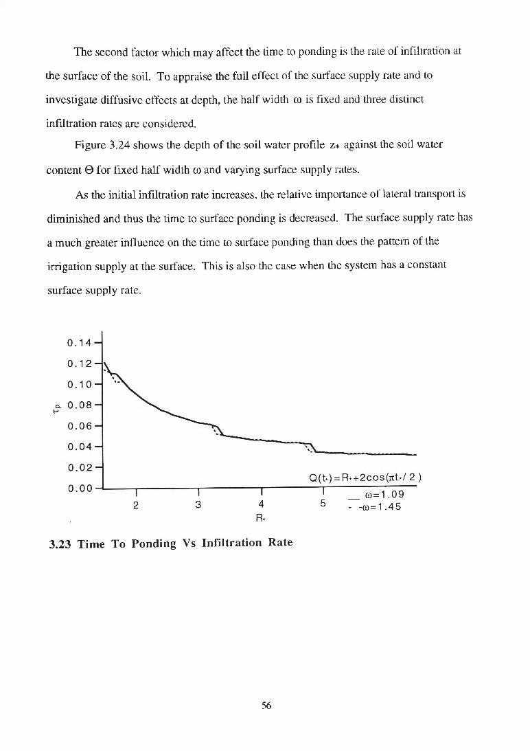
Figure 3.23 indicates that the time to surface ponding is generally independent of the

surface wetting pattern when the infiltration rate has a significant time dependence

imposed. The time to surface ponding xp, for each case is small when compared to the

period of the oscillation Infix which would explain the lack of oscillatory effects. When

the period of oscillation is decreased however, the time to surface ponding is not

significantly altered.

55

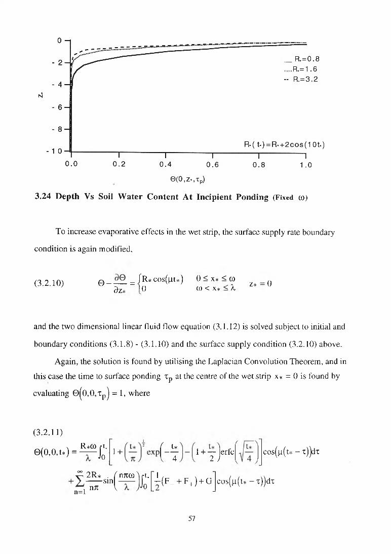
The second factor which may affect the time to ponding is the rate of infiltration at

the surface of the soil. To appraise the full effect of the surface supply rate and to

investigate diffusive effects at depth, the half width co is fixed and three distinct

infiltration rates are considered.

Figure 3.24 shows the depth o f the soil water profile z* against the soil water

content 0 for fixed half w idth co and varying surface supply rates.

As the initial infiltration rate increases, the relative importance of lateral transport is

dim inished and thus the time to surface ponding is decreased. The surface supply rate has

a m uch greater influence on the time to surface ponding than does the pattern of the

irrigation supply at the surface. This is also the case when the system has a constant

surface supply rate.

56

3.24 Depth Vs Soil Water Content At Incipient Ponding (Fixed co)

To increase evaporative effects in the

condition is again modified,

(3 .2 .10 ) © - — = j R * c°s(M.t*)Oz* 10

wet strip, the surface supply rate boundary

0 < x* < co\ z* — 0 CO < X* < A,

and the two dim ensional linear fluid flow equation (3.1.12) is solved subject to initial and

boundary conditions (3.1.8) - (3.1.10) and the surface supply condition (3.2.10) above.

Again, the solution is found by utilising the Laplacian Convolution Theorem, and in

this case the time to surface ponding xp at the centre of the wet strip x* = 0 is found by

evaluating 0^O,O,xp ) = 1, w here

(3 .2 .11 )

R*co ft.0 ( 0 ,0 .t* ) = — Jo 1 + f t*

T1 + —

2 )erfc

^ 2 R * . — sin

( nTtco Vt

n=l Ml V

cos(p(t* - x))dx

] f [ i ( F - + F + ) + G jc o s ( n ( u - T ) ) d x

57

with F+ and G defined by equations (3.1.16) and (3.1.17) respectively.

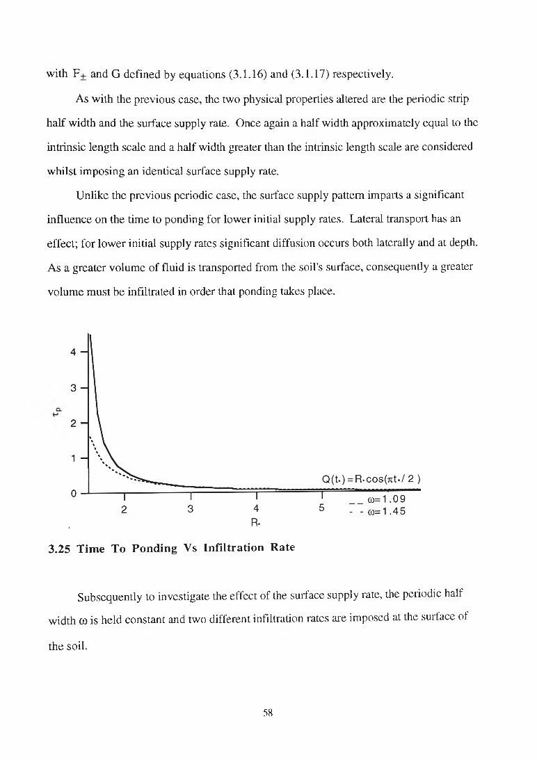
As with the previous case, the two physical properties altered are the periodic strip

half width and the surface supply rate. Once again a half width approximately equal to the

intrinsic length scale and a half width greater than the intrinsic length scale are considered

whilst imposing an identical surface supply rate.

Unlike the previous periodic case, the surface supply pattern imparts a significant

influence on the time to ponding for lower initial supply rates. Lateral transport has an

effect; for lower initial supply rates significant diffusion occurs both laterally and at depth.

As a greater volume of fluid is transported from the soil’s surface, consequently a greater

volume must be infiltrated in order that ponding takes place.

3.25 Tim e To Ponding Vs In filtra tion Rate

Subsequently to investigate the effect of the surface supply rate, the periodic half

w idth O) is held constant and two different infiltration rates are imposed at the surface of

the soil.

58

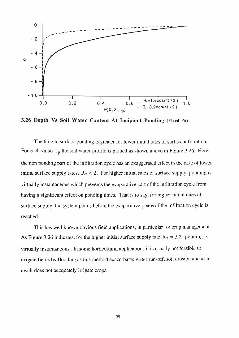
The time to surface ponding is greater for lower initial rates of surface infiltration.

For each value xp the soil water profile is plotted as shown above in Figure 3.26. Here

the non ponding part of the infiltration cycle has an exaggerated effect in the case of lower

initial surface supply rates, R* < 2. For higher initial rates of surface supply, ponding is

virtually instantaneous which prevents the evaporative part of the infiltration cycle from

having a significant effect on ponding times. That is to say, for higher initial rates of

surface supply, the system ponds before the evaporative phase of the infiltration cycle is

reached.

This has well known obvious field applications, in particular for crop management.

As Figure 3.26 indicates, for the higher initial surface supply rate R* =3.2, ponding is

virtually instantaneous. In some horticultural applications it is usually not feasible to

irrigate fields by flooding as this method exacerbates water run-off, soil erosion and as a

result does not adequately irrigate crops.

59

4. Steady Infiltration In Sloping Porous Domains

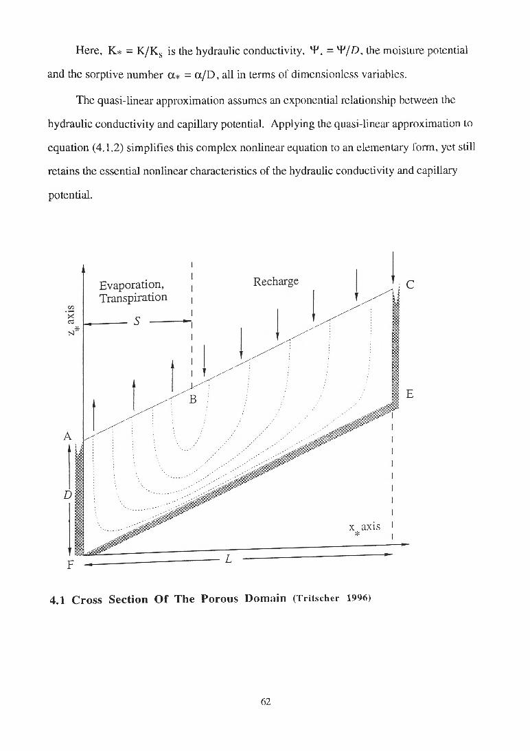
Under consideration is groundwater flow through a sloping porous domain. The

cross section of the region is assumed to be a long thin parallelogram, the vertical sides

and base of which are impermeable, as shown in Figure 4.1.

At the surface of the soil there exists a wetted fraction through which fluid is

recharged and through the remaining proportion of the soil surface evaporation and

transpiration (évapotranspiration) takes place. The rate of recharge is held equal to the rate

of évapotranspiration so that the system is in equilibrium and the total soil water content

remains constant.

Recently Read & Broadbridge (1996) solved the steady quasi linear unsaturated

flow problem through porous domains with an arbitrary shape modelled by a stream

function. Using the stream function method, the matrix flux potential and hydraulic head

are available as series expansions. The matrix flux potential,

(4.1.1) /i = fo D(6)d6 = £

sometimes referred to as the matric flux potential, is the horizontal flux potential and is due

to the characteristics of the soil matrix rather than gravitational effects. It is significant that

the matrix flux potential is not uniquely determined by the stream function as each stream

function can correspond to many moisture distributions. Read & Broadbridge (1996)

demonstrated however that in a finite porous domain there exists only one moisture

distribution that has an emergent saturated zone. In common with the time to ponding

studies of the previous section this phenomenon involves the prediction of a nascent

60

saturated zone. However, in this case of two dimensional flow, we are concerned with

the location of this nascent saturated zone in space rather than in time.

The flow solution for flow through a finite porous domain is dependent on many

soil water parameters including the size of the wetted fraction, the aspect ratio (that is, the

ratio between the length and depth of the vadose zone), the rate of recharge, the

dimensionless sorptive number and the basal inclination or slope. If the basal inclination

is positive, we assume recharge at the summit and évapotranspiration at the foot of the

porous region. A negative slope however, implies that évapotranspiration occurs at the

summit and recharge at the foot of the porous region.

The analytic series solution has the flexibility of allowing arbitrary boundary

conditions for the recharge representation. In addition it is computationally efficient and

effectively models seepage geometries for which the aspect ratios are significantly larger

than current numerical schemes allow.

For the system under consideration, the basement inclination is w. Given this

slope, the impermeable base is at z=wx and the soil surface is z=wx+D, where D is the

depth of the vadose zone. The system is recharged between x=S and x=L by a uniform

rate R and évapotranspiration occurs between x=0 and x=S.

The dimensionless fluid flow equation modelling flow through the unsaturated zone

(4.1.2) V .(/f.V 4/.) + - ^ = 0dz*

is simplified by making use of the Quasi linear approximation

(4.1.3) K, = exp(a,4/ .)

61

H ere, K* = K /K s is the hydraulic conductivity, 'P , = '¥/D, the moisture potential

and the sorptive num ber a* = a / D , all in term s of dim ensionless variables.

The quasi-linear approximation assumes an exponential relationship between the

hydraulic conductivity and capillary potential. Applying the quasi-linear approximation to

equation (4.1.2) sim plifies this com plex nonlinear equation to an elem entary form, yet still

retains the essential nonlinear characteristics of the hydraulic conductivity and capillary

potential.

4.1 Cross Section Of The Porous Domain (Tritscher 1996)

62

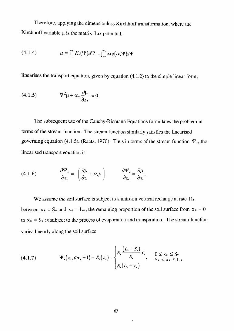
Therefore, applying the dimensionless Kirchhoff transformation, where the

Kirchhoff variable [i is the matrix flux potential,

(4.1.4) = fJtf.O F jd 'F = fjex p (a .'F > N '

linearises the transport equation, given by equation (4.1.2) to the simple linear form,

(4.1.5) V2n + a * -^ L = 0.3z*

The subsequent use of the Cauchy-Riemann Equations formulates the problem in

terms of the stream function. The stream function similarly satisfies the linearised

governing equation (4.1.5), (Raats, 1970). Thus in terms of the stream function 'P ,, the

linearised transport equation is

(4.1.6)d V .dxx

( dfl Kdz,

+ CC.I1 ,J

d ^ x = dfl dz* dxx

We assume the soil surface is subject to a uniform vertical recharge at rate R*

between x* = S* and x* = L*, the remaining proportion of the soil surface from x* = 0

to x* = S* is subject to the process of evaporation and transpiration. The stream function

varies linearly along the soil surface

(4.1.7) + 1) = H(X')

( L - S . )1— -X,

R . ( L - x . )

0 < x* < S* S* ^ x* — L*

63

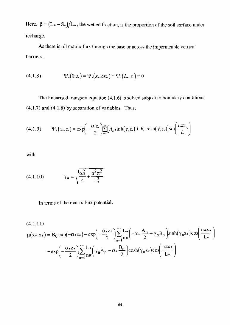
Here, p = (L* - S*)/L*, the wetted fraction, is the proportion of the soil surface under

recharge.

As there is nil matrix flux through the base or across the impermeable vertical

barriers,

(4.1.8) ^ . ( ( U ) = ¥ .(* .,<2» .) = ¥ . ( ! , . z.) = 0

The linearised transport equation (4.1.6) is solved subject to boundary conditions

(4.1.7) and (4.1.8) by separation of variables. Thus,

(4.1.9) ) = exp ^ i)¿ [A „ s in h (y „ z ,) + B„2 J n=\

\

)

with

(4.1.10) Yn = i2 2 2oc* n r

4 h i

In terms of the matrix flux potential,

(4.1.11)

|i(x*,z*) = B0 ex p (-a* z* )-ex p — _ a * ^ L + YnB n jsinh(Ynz* )cos yn=l

nrcx* ^

-ex pi

V

oc*z* 2 .

L* (I - YnAn - a*n=l n n \ 2 J

cos h(Yn z*)cosf MIX* ^

V y

64

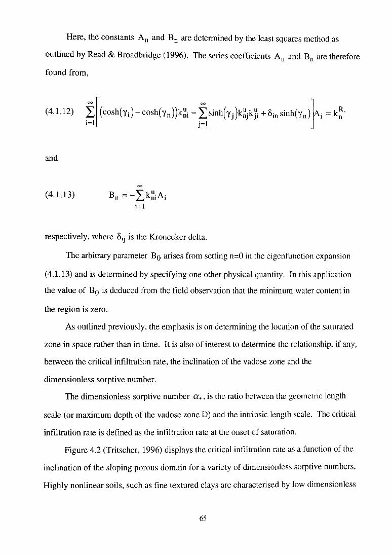
Here, the constants An and Bn are determined by the least squares method as

outlined by Read & Broadbridge (1996). The series coefficients An and Bn are therefore

found from,

(4.1.12) Ii—1

(cosh(Yi ) -c o s h (y n))k“i ^ s in h (y j )k“jkjli + 8 in sinh(yn ) j=l

R.n

and

oo

(4.1.13) Bn = - X k S i A ii—1

respectively, where Sjj is the Kronecker delta.

The arbitrary parameter Bq arises from setting n=() in the eigenfunction expansion

(4.1.13) and is determined by specifying one other physical quantity. In this application

the value of Bq is deduced from the field observation that the minimum water content in

the region is zero.

As outlined previously, the emphasis is on determining the location of the saturated

zone in space rather than in time. It is also of interest to determine the relationship, if any,

between the critical infiltration rate, the inclination of the vadose zone and the

dimensionless sorptive number.

The dimensionless sorptive number a * , is the ratio between the geometric length

scale (or maximum depth of the vadose zone D) and the intrinsic length scale. The critical

infiltration rate is defined as the infiltration rate at the onset of saturation.

Figure 4.2 (Tritscher, 1996) displays the critical infiltration rate as a function of the

inclination of the sloping porous domain for a variety of dimensionless soiptive numbers.

Highly nonlinear soils, such as fine textured clays are characterised by low dimensionless

65

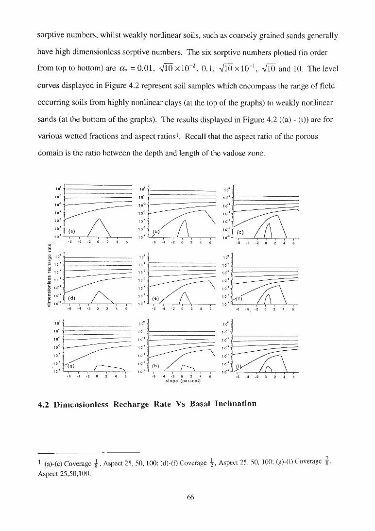
sorptive numbers, whilst weakly nonlinear soils, such as coarsely grained sands generally

have high dimensionless sorptive numbers. The six sorptive numbers plotted (in order

from top to bottom) are a* = 0.01, VIO x 1(T2, 0.1, Vl0 x 10"1, VlO and 10. The level

curves displayed in Figure 4.2 represent soil samples which encompass the range of field

occurring soils from highly nonlinear clays (at the top of the graphs) to weakly nonlinear

sands (at the bottom of the graphs). The results displayed in Figure 4.2 ((a) - (i)) are for

various wetted fractions and aspect ratios1. Recall that the aspect ratio of the porous

domain is the ratio between the depth and length of the vadose zone.

slope (percent)

4.2 D im ensionless R echarge Rate Vs Basal Inclination

1 (a)-(c) Coverage j , Aspect 25, 50, 100; (d)-(0 Coverage j , Aspect 25, 50, 100; (g)-(i) Coverage Aspect 25,50,100.

66

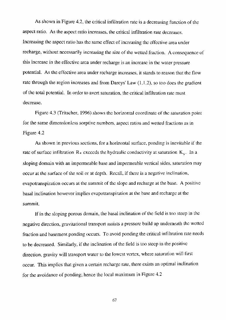
As shown in Figure 4.2, the critical infiltration rate is a decreasing function of the

aspect ratio. As the aspect ratio increases, the critical infiltration rate decreases.

Increasing the aspect ratio has the same effect of increasing the effective area under

recharge, without necessarily increasing the size of the wetted fraction. A consequence of

this increase in the effective area under recharge is an increase in the water pressure

potential. As the effective area under recharge increases, it stands to reason that the flow

rate through the region increases and from Darcys' Law (1.1.2), so too does the gradient

of the total potential. In order to avert saturation, the critical infiltration rate must

decrease.

Figure 4.3 (Tritscher, 1996) shows the horizontal coordinate of the saturation point

for the same dimensionless sorptive numbers, aspect ratios and wetted fractions as in

Figure 4.2

As shown in previous sections, for a horizontal surface, ponding is inevitable if the

rate of surface infiltration R* exceeds the hydraulic conductivity at saturation Ks . In a

sloping domain with an impermeable base and impermeable vertical sides, saturation may

occur at the surface of the soil or at depth. Recall, if there is a negative inclination,

evapotranspiration occurs at the summit of the slope and recharge at the base. A positive

basal inclination however implies evapotranspiration at the base and recharge at the

summit.

If in the sloping porous domain, the basal inclination of the field is too steep in the

negative direction, gravitational transport assists a pressure build up underneath the wetted

fraction and basement ponding occurs. To avoid ponding the critical infiltration rate needs

to be decreased. Similarly, if the inclination of the field is too steep in the positive

direction, gravity will transport water to the lowest vertex, where saturation will first

occur. This implies that given a certain recharge rate, there exists an optimal inclination

for the avoidance of ponding; hence the local maximum in Figure 4.2

67

2 0 1 5 1 0~\ 5

0 - (a)

5 0 ­

4 0 ­

3 0

2 0 1 0 0 (b)

6 - 4 - 2 0 2 4' 6 - 4 - 2 0 2 4

6 - 4 - 2 0 2 4 6 “l--r0 2 4 6 • 6 - 4 - 2 0 2 4 6

2 5

-

4.3 H orizon tal C oord inate of the S atu ration Point Vs Basal Inclination

For highly nonlinear soils such as fine textured clays, the basal inclination has

negligible effect on the maximum infiltration rate before the onset of saturation. If the soil

is weakly nonlinear however, such as in coarsely grained sands, the inclination of the

domain has a significant influence on the critical infiltration rate at the onset of saturation.

The dimensionless sorptive number, which characterises all soil types, is an indication of

the relative dominance of capillary and gravitational forces. In a coarse soil, capillary

action is relatively ineffective in transporting water laterally to the évapotranspiration zone

and then upwards to the evaporation surface. Gravity forces dominate, accounting for the

pressure build-up and basement saturation. A surprising result is that a saturated zone will

always emerge in a sand sample regardless of the rate of infiltration or the inclination of

the slope. The dominant gravitational forces transport fluid away from the surface until it

68

reaches the impermeable basement barrier. As capillary action is ineffective in soils with

high dimensionless sorptive numbers, there is very little lateral transport and extremely

large pressure gradients are required to transport the fluid upwards through the

évapotranspiration region to the evaporative surface.

For all soil types, as the coverage increases the critical infiltration rate decreases.

This is due to the fact that as the surface area under recharge increases, so to does the fluid

flow within the region. This increased fluid flow increases the water pressure potential

and the likelihood of saturation. To offset this, the critical infiltration rate before the onset

of saturation must decrease.

A common relationship for all soil types appears to be the rate of surface infiltration

and the proportion of soil through which fluid is delivered. As the rate of infiltration and

the proportion of soil under recharge increases, overall the time taken for the onset of

saturation decreases. For weakly nonlinear soils, the effect of increasing the surface

coverage through which fluid is delivered, although reduces the critical infiltration rate,

this is not as pronounced as altering the aspect ratio.

69

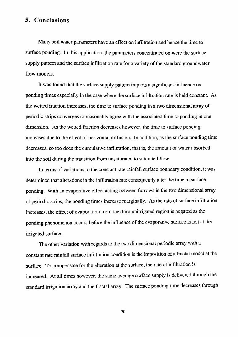
5. Conclusions

Many soil water parameters have an effect on infiltration and hence the time to

surface ponding. In this application, the parameters concentrated on were the surface

supply pattern and the surface infiltration rate for a variety of the standard groundwater

flow models.

It was found that the surface supply pattern imparts a significant influence on

ponding times especially in the case where the surface infiltration rate is held constant. As

the wetted fraction increases, the time to surface ponding in a two dimensional array of

periodic strips converges to reasonably agree with the associated time to ponding in one

dimension. As the wetted fraction decreases however, the time to surface ponding

increases due to the effect of horizontal diffusion. In addition, as the surface ponding time

decreases, so too does the cumulative infiltration, that is, the amount of water absorbed

into the soil during the transition from unsaturated to saturated flow.

In terms of variations to the constant rate rainfall surface boundary condition, it was

determined that alterations in the infiltration rate consequently alter the time to surface

ponding. With an evaporative effect acting between furrows in the two dimensional array

of periodic strips, the ponding times increase marginally. As the rate of surface infiltration

increases, the effect of evaporation from the drier unirrigated region is negated as the

ponding phenomenon occurs before the influence of the evaporative surface is felt at the

irrigated surface.

The other variation with regards to the two dimensional periodic array with a

constant rate rainfall surface infiltration condition is the imposition of a fractal model at the

surface. To compensate for the alteration at the surface, the rate of infiltration is

increased. At all times however, the same average surface supply is delivered through the

standard irrigation array and the fractal array. The surface ponding time decreases through

70

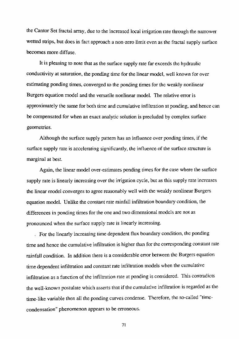
the Cantor Set fractal array, due to the increased local irrigation rate through the narrower

wetted strips, but does in fact approach a non-zero limit even as the fractal supply surface

becomes more diffuse.

It is pleasing to note that as the surface supply rate far exceeds the hydraulic

conductivity at saturation, the ponding time for the linear model, well known for over

estimating ponding times, converged to the ponding times for the weakly nonlinear

Burgers equation model and the versatile nonlinear model. The relative error is

approximately the same for both time and cumulative infiltration at ponding, and hence can

be compensated for when an exact analytic solution is precluded by complex surface

geometries.

Although the surface supply pattern has an influence over ponding times, if the

surface supply rate is accelerating significantly, the influence of the surface structure is

marginal at best.

Again, the linear model over-estimates ponding times for the case where the surface

supply rate is linearly increasing over the irrigation cycle, but as this supply rate increases

the Unear model converges to agree reasonably well with the weakly nonlinear Burgers

equation model. Unlike the constant rate rainfall infiltration boundary condition, the

differences in ponding times for the one and two dimensional models are not as

pronounced when the surface supply rate is linearly increasing.

, For the Unearly increasing time dependent flux boundary condition, the ponding

time and hence the cumulative infiltration is higher than for the corresponding constant rate

rainfaU condition. In addition there is a considerable error between the Burgers equation

time dependent infiltration and constant rate infiltration models when the cumulative

infiltration as a function of the infiltration rate at ponding is considered. This contradicts

the well-known postulate which asserts that if the cumulative infiltration is regarded as the

time-like variable then all the ponding curves condense. Therefore, the so-called "time-

condensation" phenomenon appears to be erroneous.

71

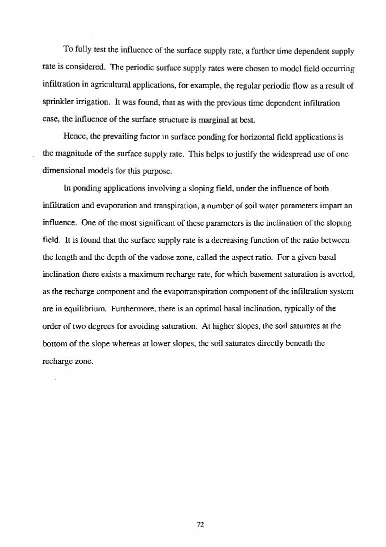
To fully test the influence of the surface supply rate, a further time dependent supply

rate is considered. The periodic surface supply rates were chosen to model field occurring

infiltration in agricultural applications, for example, the regular periodic flow as a result of

sprinkler irrigation. It was found, that as with the previous time dependent infiltration

case, the influence of the surface structure is marginal at best.

Hence, the prevailing factor in surface ponding for horizontal field applications is

the magnitude of the surface supply rate. This helps to justify the widespread use of one

dimensional models for this purpose.

In ponding applications involving a sloping field, under the influence of both

infiltration and evaporation and transpiration, a number of soil water parameters impart an

influence. One of the most significant of these parameters is the inclination of the sloping

field. It is found that the surface supply rate is a decreasing function of the ratio between

the length and the depth of the vadose zone, called the aspect ratio. For a given basal

inclination there exists a maximum recharge rate, for which basement saturation is averted,

as the recharge component and the évapotranspiration component of the infiltration system

are in equilibrium. Furthermore, there is an optimal basal inclination, typically of the

order of two degrees for avoiding saturation. At higher slopes, the soil saturates at the

bottom of the slope whereas at lower slopes, the soil saturates directly beneath the

recharge zone.

72

A cknow ledgm ent

From time to time there emerges an awe inspiring individual who stands head and

shoulders above the rest, who sets the standards others try to emulate; William

Shakespeare, John Donne, Vincent Van Gogh and my supervisor Professor Philip

Broadbridge.

I have had the rare privilege of working with a supervisor worth more than his

weight in gold and I can not adequately express my gratitude. Thanks Phil for your

fantastic support and encouragement, invaluable advice and inexhaustible patience.

73

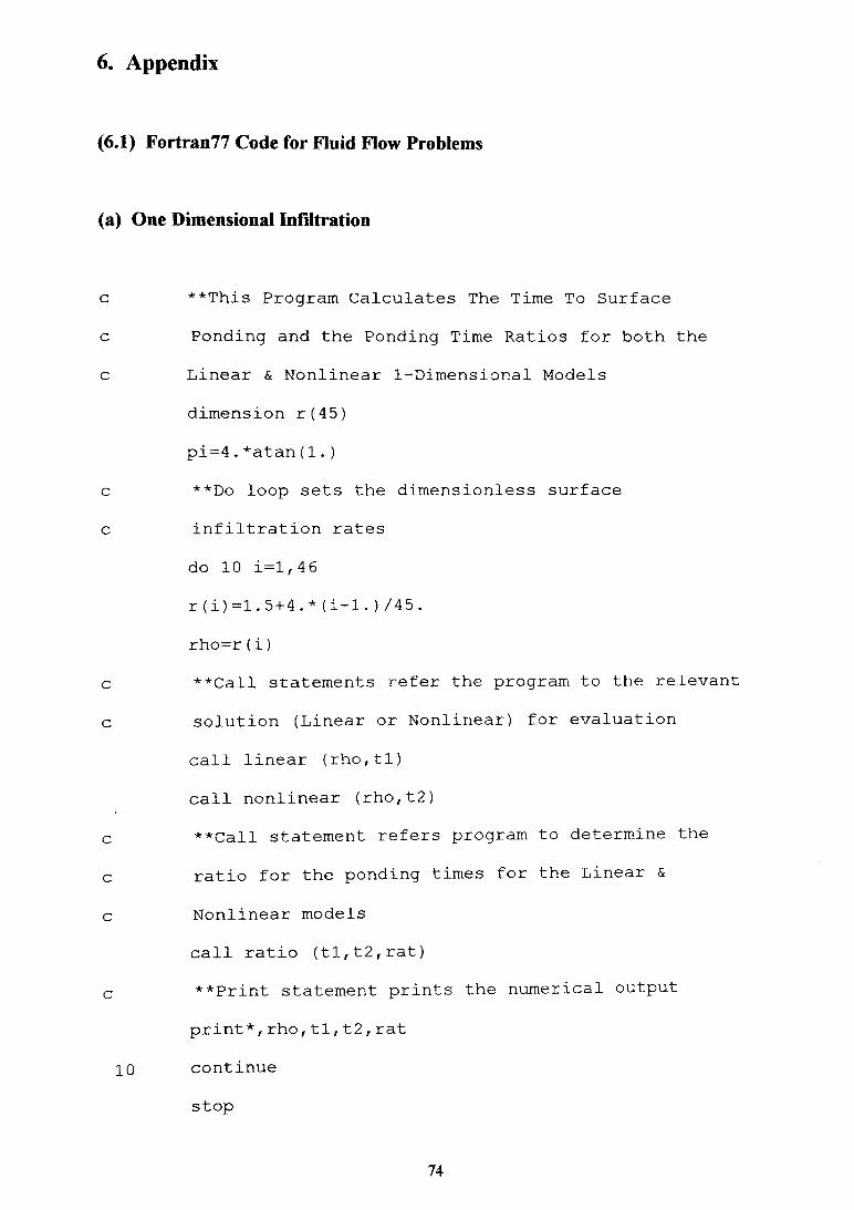
6. Appendix

(6.1) Fortran77 Code for Fluid Flow Problems

(a) One Dimensional Infiltration

c * * This P r o g r a m C a l c u l a t e s The T ime To S u r face

c P o n d i n g a n d the P o n d i n g T i m e Rati o s for b o t h the

c L i n e a r & N o n l i n e a r 1 - D i m e n s i o n a l M o d e l s

d i m e n s i o n r(45)

p i = 4 .* a t a n (1.)

c **Do loo p sets the d i m e n s i o n l e s s s u r face

c i n f i l t r a t i o n rates

do 10 i = l ,4 6

r ( i ) = l . 5 + 4 . M i - 1 - ) / 4 5 .

rho=r(i)

c * * C a l l s t a t e m e n t s r e f e r the p r o g r a m to the r e l e v a n t

c s o l u t i o n (Linear or Nonlinear) for e v a l u a t i o n

call l i n e a r (rho,tl)

c a l l n o n l i n e a r (rho,t2)

c * * C a l l s t a t e m e n t r e fers p r o g r a m to d e t e r m i n e the

c r a t i o for the p o n d i n g times for the L i n e a r &

c N o n l i n e a r m o d e l s

c all r a t i o (tl,t2,rat)

c * * P r i n t s t a t e m e n t p r i n t s the n u m e r i c a l output

p r i n t * , r h o , t l , t 2 , r a t

10 c o n t i n u e

s t o p

74

en d

c

c

c

c

c

25

c

c

c

c

c

c

s u b r o u t i n e l i n e a r ( r h o , t l )

d a t a d k , d t h , s / 1 . 0 5 9 , . 2 5 7 4 , 3 . 6 8 6 /

p i = 4 .* a t a n (1.)

* * t l o w & tu sets the lower & u p p e r b o u n d s for the

s u r f a c e p o n d i n g times

t l o w = . 5 / r h o * * 2

t u = l o g ( r h o / ( r h o - 1 .))/rho

**tl t a kes the a v e r a g e of the u p p e r & lower time

b o u n d s - > b i s e c t i o n m e t h o d

t l = . 5 * (tlow+tu)

**fl & f2 i n c o r p o r a t e the a n a l y t i c s o l u t i o n for the

l i n e a r m o d e l

f 1 = ( r h o - 1 .)/rho

f 2 = ( l . + 2 . * t l / p i ) * f ( s q r t ( t l / p i ) )

- ( 2 . / p i ) * s q r t ( t l ) * e x p (-1.*tl/pi)

**gl finds the a b s o l u t e v a l u e of the d i f f e r e n c e

b e t w e e n the two p a r t s of the s o l u t i o n - > t h e time

i n t e r v a l is s u c c e s s i v e l y n a r r o w e d d own b y u s i n g the

b i s e c t i o n m e t h o d

g l = a b s (f 2 - f 1)

i f ( g l . l e . . 0 0 0 1 ) t h e n

go to 20

els e i f (f 2 . I t .f 1 ) t hen

tu=tl

e l s e i f ( f 2 . g t .f 1 ) t h e n

t l o w = t l

75

en d i f

go to 25

20 c o n t i n u e

r e t u r n

end

c

s u b r o u t i n e n o n l i n e a r ( r h o ,t 2 )

c **t2 is the e x p l i c i t time to s u r f a c e p o n d i n g for the

c one d i m e n s i o n a l n o n l i n e a r m o d e l

t 2 = . 5 * ( l o g ( r h o / ( r h o - 1 .)) ) /rho

r e t u r n

end

c

s u b r o u t i n e r a t i o (t l ,t 2 ,r a t )

c **The r a t i o b e t w e e n the l i n e a r & n o n l i n e a r p o n d i n g

c time is d e t e r m i n e d

r a t = t l / t 2

r e t u r n

end

c

f u n c t i o n erfc(x)

c * * This s u b r o u t i n e d e t e r m i n e s an a p p r o x i m a t i o n to

c the C o m p l e m e n t a r y E r r o r F u n c t i o n (Abramowitz &

c S t e g u n 1964): E q u a t i o n 7.1.27

rea l x

d a t a a l , a 2 , a 3 , a 4 / . 278393, .230389, .000972, .078108/

e r f c = l ./(1.+ a l * x + a 2 * x * x + a 3 * x * x * x + a 4 * x * x * x * x ) * * 4

r e t u r n

76

en d

(b) Two Dimensional Infiltration: Analytic Solution

c * * This P r o g r a m C a l c u l a t e s The Time To Surface

c P o n d i n g In Two D i m e n s i o n s for the L i n e a r M o d e l

c (Analytic Solution)

rea l l , l s , l s t a r

d i m e n s i o n r(50)

c * * D a t a sets the v a l u e s of the v a r i o u s soil w a t e r

c p a r a m e t e r s

d a t a d k , d t h , s , w , 1 , I s / l . 0 5 9 , . 2 5 7 4 , 3 . 6 8 6 , 3 0 . , 7 0 . , 2 7 . 6 /

p i = 4 .* a t a n (1.)

c * * o m = d i m e n s i o n l e s s f u r r o w h a l f w i d t h

c * * l s t a r = d i m e n s i o n l e s s d i s t a n c e b e t w e e n furrows

c * * l s = c a p i l l a e y l e n g t h scale

o m = w / l s

l s t a r = l / l s

c **Do loop sets the d i m e n s i o n l e s s s u r face

c i n f i l t r a t i o n rates

do 50 i = l , 51

r ( i ) = 1 . 5 + 4 . * ( i - l ) / 5 0 .

r h o = r (i )

c **t is the d i m e n s i o n l e s s time of i n f i l t r a t i o n

t = 0 .

10 t = t + .0001

s u m = 0 .

t e r m = 0 .

77

0**Do l o o p e v a l u a t e s the series c o m p o n e n t of n

do 20 n = l , 20

a l = . 2 5 + ( n * p i / l s t a r )**2

a 2 = . 5

u l = 2 .* s q r t ( a l ) - 2 . * s q r t ( a l ) * f ( s q r t ( a l * t ) )

u l l = . 5 * u l / ( n * p i / l s t a r )**2

u 2 = e x p ( t * ( n * p i / l s t a r ) * * 2 ) * f ( s q r t (. 2 5 * t ) )

u 2 2 = u 2 / ( 2 . * (n*pi/lstar)**2)

t e r m = 2 .* r h o * s i n ( n * p i * o m / l s t a r ) * ( u l l + u 2 2 ) / (n*pi)

s u m = s u m + t e r m

c o n t i n u e

g l = l .+ s q r t ( t / p i ) * e x p (-.25 * t )

g 2 = ( l . + . 5 * t ) * f ( s q r t (. 2 5 * t ) )0

**th0 e v a l u a t e s 0

t h 0 = r h o * o m * ( g l - g 2 ) / l s t a r

t h = t h 0 + s u m

* * L o g i c a l o p e r a t o r s c o n t i n u e p r o g r a m l oop u n til s u r f a c e s aturation, d e f i n e d b y is r e a c h e d

i f (t h .I t .1)t h e n

go to 10

e l s e i f (t h . g e .1)then

go to 30

e n d if

c o n t i n u e

* * p r i n t s t a t e m e n t p r i n t s the n u m e r i c a l o u tput

p r i n t * , r h o , t

c o n t i n u e

s t o p

c

c * * T h i s s u b r o u t i n e d e t e r m i n e s an a p p r o x i m a t i o n to

c t he C o m p l e m e n t a r y E r r o r f u n c t i o n (Abramowitz &

c S t e g u n 1964): E q u a t i o n 7.1.27

f u n c t i o n f(x)

r e a l x

d a t a 3 1 , 3 2 , 3 3 , 3 4 7 . 2 7 8 3 9 3 , . 2 3 0 3 8 9 , . 0 0 0 9 7 2 , . 0 7 8 1 0 8 /

f = l . / ( 1 , + a l * x + a 2 * x * x + a 3 * x * x * x + a 4 * x * x * x * x ) * * 4

r e t u r n

e nd

(c) Two Dimensional Infiltration :Numerical Solution

c * * This P r o g r a m C a l c u l a t e s The T i m e To Su r f a c e

c P o n d i n g In Tw o D i m e n s i o n s

c (Numerical Solution)

real l , l s , l s t a r

c * * D i m e n s i o n s t a t e m e n t s set the size of the a r r a y

c for the r e l e v a n t p a r a m e t e r s :

c u = s o i l w a t e r c o n t e n t ,r e s u r f a c e i n f i l t r a t i o n rate

c x = h o r i z o n t a l m e s h p o i n t s ,y = v e r t i c a l m e s h p o i n t s

d i m e n s i o n u ( l , 2 1 , 1 0 1 ) ,x (21), y ( 1 0 1 ) ,r (100)

d i m e n s i o n w o r k ( 1 5 7 1 1 7 ) , i w o r k (2121)

c o m m o n o m , l s t a r ,r h o , d i f f

q * * D a t a sets the v a l u e s of the v a r i o u s soil w a t e r

c p a r a m e t e r s

d a t a d k , d t h , s , w , l , l s / 1 . 0 5 9 , . 2 5 7 4 , 3 . 6 8 6 , 7 0 . , 7 0 . , 2 7 . 6 /

79

* * o m = d i m e n s i o n l e s s f u r r o w h alf w i d t h

* * l s t a r = d i m e n s i o n l e s s d i s t a n c e b e t w e e n furrows

* * l s = c a p i l l a r y l e n g t h scale

o m = w / l s

l s t a r = l / l s

* * D i f f sets the d i m e n s i o n l e s s d i f f u s i v i t y

L i n e a r & B u r g e r s m o d e l s - > d i f f = l .

N o n l i n e a r m o d e l - > d i f f = c ( c - 1 ) / ( c - u (1))**2

d i f f = l .

**Do l oop sets the v a l u e s of the d i m e n s i o n l e s s

s u r f a c e i n f i l t r a t i o n rates

do 250 k = l ,101

r ( k ) = 1 . 5 + 2 0 . * (k-1)/100.

r h o - r (k)

* * n p d e = n u m b e r of c o u p l e d pde s to be s o l v e d b y P D ETWO

n p de=l

m o r d e r = 5

* * n x = n u m b e r h o r i z o n t a l d i s c r e t i s a t i o n p o i n t s

* * n y = n u m b e r v e r t i c a l d i s c r e t i s a t i o n p o i n t s

n x = 2 1

n y = 1 0 1

n o d e = n x * n y * n p d e

* * y ( n y )= d i m e n s i o n l e s s v e r t i c a l d e p t h

y ( n y ) =40.

d y = y ( n y ) / f l o a t ( n y - 1 )

**do loops j = l , n y set the v e r t i c a l s p acial

p i = 4 . * a t a n ( 1 . )

d i s c r e t i s a t i o n

y ( j ) = . l * ( j - l ) * d y

10 c o n t i n u e

do 11 j —1 f 12

y (j ) = . 2 * ( j - 1 ) * d y

11 c o n t i n u e

d y = ( y ( n y ) - y ( 1 2 ) ) / (ny-12)

do 13 j = 1 3 , ny

y ( j ) = y ( j - i ) + d y

13 c o n t i n u e

c * * x ( n x ) = d i m e n s i o n l e s s h o r i z o n t a l w i d t h

x ( n x ) = l s t a r

d x = x ( n x ) / f l o a t ( n x - 1 )

c **do loops i = l , n x set the h o r i z o n t a l sp a c i a l

c d i s c r e t i s a t i o n

do 15 i = l , n x

x (i ) = (i - 1 )*dx

15 c o n t i n u e

c set the i n i t i a l c o n d i t i o n

t i n = 0 .

do 20 i = l , n x

do 20 j = l , n y

u (1, i f j )= t i n

20 c o n t i n u e

h = . 001

e p s = .01

mf=22 i n d e x = l

do 10 j = l , 6

81

n o u t = l

c

c

25

c

c

c

c

c

c

c

i w o r k (1)= n p d e

i w o r k (2)=nx

i w o r k (3)= n y

i w o r k (4)= m o r d e r

i w o r k (5)=157117

i w o r k (6)=2121

**t0 & tou t are the input & outp u t times

r e s p e c t i v e l y

to=o

t o u t = . 2 5 / r h o * * 2

c o n t i n u e

* * d r i v e p is the s u b r o u t i n e w h i c h calls the

i n t e g r a t o r in P D ETWO

cal l d r i v e p ( n o d e , t O , h , u , t o u t , e p s , m f ,

i n d e x , w o r k , i w o r k , x , y )

**set the soil w a t e r c o n t e n t as the s u b ject of theA = yi 1 1 1 )n u m e r i c a l s o l u t i o n ie \ ? ? )

t h = u (1,1,1)

* * r e s e t the time v a r i a b l e

t O = t o u t

t o u t = t o u t + .01

* * L o g i c a l o p e r a t o r s c o n t i n u e p r o g r a m loop until

s u r f a c e s a t u r a t i o n is reached, ie u(l , l , l ) = l

i f (t h .g e .1)t h e n

go to 30

else i f ( t h . I t .1)t h e n

go to 25

82

en d i f

30 c o n t i n u e

c * * P r i n t s t a t e m e n t p r i n t s the n u m e r i c a l o u tput

p r i n t * ,r h o ,tout

250 c o n t i n u e

s top

e nd

c

c * * this s u b r o u t i n e sets the H o r i z o n t a l

c B o u n d a r y C o n d i t i o n s (surface & at depth)

s u b r o u t i n e b n d r y h (t ,x , y , u , a h , b h , c h , n p d e )

c * * set b o u n d a r y c o n d i t i o n c o e f f i c i e n t s

ah(i)ul + bh(i) — L = ch(i)dy

d i m e n s i o n u ( n p d e ) ,a h ( n p d e ) ,b h ( n p d e ) ,ch(npde)

c o m m o n o m , l s t a r ,r h o , d i f f

real lstar

c * * y = o - > s u r f a c e b o u n d a r y c o n d i t i o n

if (y.eq.0) go to 35

a h (1)=1

' b h (1)=0

c h (1)=0

go to 40

c **set s u r f a c e i n f i l t r a t i o n p a t t e r n

3 5 i f ( x .g t .0 ..a n d .x .l e .o m ) t h e n

f l u x = r h o

els e i f ( x .g t .o m . a n d .x .I t .l s t a r )then

f l u x = 0 .

e nd if

83

c * * c o n d = K ( t h ) :h y d r a u l i c c o n d u c t i v i t y

c L i n e a r K=l, B u r g e r s K=u(l)**2,

c N o n l i n e a r K = c A2 ( c - 1 ) / ( c - u ( l ) )- 2 c ( c - l ) + ( c - l ) ( c - u ( l ) )

a h (1)=0.

b h (1)= - d i f f

c h (1)= f l u x - c o n d

40 c o n t i n u e

r e t u r n

end

c

c **this s u b r o u t i n e sets the V e r t i c a l

c B o u n d a r y C o n d i t i o n s

s u b r o u t i n e b n d r y v ( t , x , y , u , a v , b v , c v , n p d e )

d i m e n s i o n u ( n p d e ) ,a v ( n p d e ) , b v ( n p d e ) ,cv(npde)

c o m m o n o m , l s t a r ,r h o , d i f f

real l s tar

c **set b o u n d a r y c o n d i t i o n c o e f f i c i e n t s

a v ( i)u . + b v ( i) — L = c v ( i) cx,

a v ( l ) =0.

■ b v (1)=1.

c v (1)=0.

r e t u r n

e nd

c

c *^this s u b r o u t i n e sets the h o r i z o n t a l

c d i f f u s i o n

s u b r o u t i n e d i f f h (t ,x,y ,u,dh,npde)

d i m e n s i o n u ( n p d e ),dh(npd e , n p d e )

84

c o m m o n om , l s t a r , r h o , diff

r eal l s tar

c * * d i f f = d i f f u s i o n

c L i n e a r , B u r g e r s - > diff=l

c N o n l i n e a r - > d i f f = c ( c - 1 ) / ( c - u (1))**2

d h (1,1)= d i f f

r e t u r n

e nd

c

c **th i s s u b r o u t i n e sets the v e r t i c a l

c d i f f u s i o n

s u b r o u t i n e d i f f v ( t , x , y , u , d v , n p d e )

d i m e n s i o n u ( n p d e ) ,dv(npde,npde)

c o m m o n o m , l s t a r ,r h o , d i f f

real l s tar

c * * d i f f u s i o n is u n i f o r m h o r i z o n t a l l y & vertically,

c t h e r e f o r e r e c a l l d i f f h & r e n a m e for d i f f v

call d i f f h ( t , x , y , u , d v , n p d e )

r e t u r n

end

c

c **th i s s u b r o u t i n e de f i n e s the g o v e r n i n g e q u a t i o n

s u b r o u t i n e f ( t , x , y , u , u x , u y , d u x x , d u y y , d u d t , n p d e )

d i m e n s i o n u x ( n p d e ) ,u y ( n p d e ) ,duxx(npde,npde)

d i m e n s i o n d u y y ( n p d e , n p d e ) ,d u d t ( n p d e ) ,u(npde)

c o m m o n o m , l s t a r ,r h o , d i f f

real l s t a r

c * * set c o e f f i c i e n t s for the g o v e r n i n g e q u a t i o n

85

C d c o n d = D K (th)

c L i n e a r - > dcond=l, B u r g e r s - > d c o n d = 2 .* u (1)

c N o n l i n e a r - > d c o n d = c A2 ( c - 1 ) / ( c - u (1))**2-(c-1)

d c o n d = 2 .* u (1)

d u d t (1)= d u x x (1,1)+ d u y y (1,1)- d c o n d * u y (1)

r e t u r n

e nd

86

7. References

1. Abramowitz A. and I. Stegun (Eds), Handbook of Mathematical Functions,

National Bureau of Standards, Washington D.C., 1964.

2. Batu V., Steady Infiltration from Single and Periodic Strip Sources, Soil Sci. Soc.

Am. I , 42:544-549, 1978.

3. Braester C., Moisture Variation at the Soil Surface and Advance of the Wetting

Front During Constant infiltration at Constant Flux, Water Resour. Res., 9:687-694,

1973.

4. Broadbridge P., Unpublished Lecture Notes, Integrability and Chaos in Nonlinear

Partial Differential Equations.

5. Broadbridge P., Edwards M.P., and J.E. Kearton, Closed Form Solutions for

Unsaturated Flow Under Variable Flux Boundary Conditions, Adv. Water Res.,

19:207-213, 1996.

6. Broadbridge P. and J.M. Stewart, Time to Ponding During Non-Constant

Infiltration, 2nd Biennial Aus. Eng. Math Confi, 469-476, 1996.

7. Broadbridge P., Knight J.H. and C. Rogers, Constant Rate Rainfall in a Bounded

Profile: Solutions o f a Nonlinear Model, Soil Sci. Am. J., 52:1526-1533, 1988.

8. Broadbridge P. and I. White, Time to Ponding: Comparison of Analytic,

Quasi-Analytic and Approximate Predictions, Water Resour. Res., 23:2302-2310,

1987.

87

9. Broadbridge P. and I. White, Constant Rate Rainfall Infiltration: A Versatile

Nonlinear Model 1. Analytic Solution, Water Resour. Res., 24:145-154, 1988a.

10. Broadbridge P. and I. White, Reply, Water Resour. Res., 24:2109-2110, 1988.

11. Carslaw H.S. and J.C. Jaeger, Conduction of Heat in Solids, 2nd Ed., Clarendon

Press, Oxford, 1959.

12. Chong S.-K., Calculation of Sorptivity from Constant Rate Rainfall Infiltration

Measurement, Soil Sci. Soc. Am. J., 47:627-630, 1983.

13. Chu S.H., Infiltration During an Unsteady Rain, Water Resour. Res., 14: 461-466,

1978.

14. Clothier B E. and I. White, Measurement of Sorptivity and Soil Water Diffusivity

in the Field, Soil Sci. Am. J., 45:241-245, 1981.

15. Clothier B.E, Knight J.H. and I. White, Burgers’ Equation: Application to Field

Constant-Flux Infiltration, Soil Sci., 132:252-261, 1981a.

16. Clothier BE. , I. White and G.J. Hamilton, Constant Rate Rainfall Infiltration:

Field Experiments, Soil Sci. Am. J., 45:245-249, 1981b.

17. Devaney R.L., An Introduction to Chaotic Dynamical Systems, 2nd Ed.,

Addison-Wesley, 1989.

18. Eagleson P. S., Climate, Soil and Vegetation, 5, A Derived Distribution of Storm

Surface Runoff, Water Resour. Res., 14:741-748, 1978.

88

19. Hachum A.Y. and Alfaro J.F., Water Infiltration and Run-Off Under Rain

Applications, Soil Sci. Soc. Am. I , 41:960-966,1977.

20. Hopf E., The Partial Differential Equation Ut + UUx ~ , Commun. Pure Appl.

Math, 3:201-230, 1950.

21. Gardiner W.R., Some Steady State Solutions of the Unsaturated Moisture Flow

Equation with Application to evaporation from a Water Table, Soil Sci., 85:228-232,

1958.

22. Knight J.H., Infiltration Functions from Exact and Approximate Solutions of

Richards’ Equation, (in) Advances in Infiltration: Proceedings of National Conference

on Advances in Infilration, pp 24-33, American Society of Agricultural Engineers, St.

Joseph, Mich., 1983.

23. Kutilek M., Constant-Rainfall Infiltration, J. Hydrol, 67:115-127, 1984.

24. Mein R.G. and Larson C.L., Modelling Infiltration During a Steady Rain, Water

Resour. Res., 9:384-397, 1973.

25. Melgaard D.K. and R.F. Sincovec, General Software for Two Dimensional

Nonlinear Partial Differental Equations, ACM Trans, on Math. Software, 7:106-125,

1981.

26. Morel-Seytoux H. J., Derivations of Equations for Rainfall Infiltration, J.

Hydrol., 59:203-219 1976.

89

27. Morel-Seytoux H. J., Derivations of Equations for Variable Rainfall Infiltration,

Water Resour. Res., 14:561-568, 1978.

28. Morel-Seytoux H. J., Analytical Results for Prediction of Variable Rainfall

Infiltration, J. Hydrol., 59:209-230, 1982.

29. Parlange J. Y. and R.E. Smith, Ponding Time for Varaible Rainfall Rates, Can. J.

Soil Sci., 56:121-123, 1976.

30. Perroux K.M., Smiles D.E. and I. White, Water Movement in Uniform Soils

During Constant Flux Infiltration, Soil Sci. Soc. Am. J., 45:237-240, 1981.

31. Philip J.R., The Theory of Infiltration 3, Moisture Profiles and Relation to

Experiment, Soil Sci., 84:163-178, 1957b.

32. Philip J.R., Mathematical-Physical Approach to Water Movement in Unsaturated

Soils, Paper Presented at Int. Soil Water Symp. Czech. Nat. Comm. Irrigation and

Drainage, Prague, 1967.

33. Philip J.R., The Theory of Infiltration , Adv. Hydrosci., 5:215-296, 1969.

34. Philip J.R., General Theorem on Steady Infiltration from Surface Sources with

Application to Point and Line Sources, Soil Sci. Am. Proc., 35:867-871, 1971.

35. Philip J.R., Nonuniform Leaching from Nonuniform Steady Infiltration, Soil Sci.

Am. J., 40:740-749, 1984.

90

36. Pullan A.J., The Quasi-Linear Approximation for Unsaturated Porous Media

Flow, Water Resourc. Res., 26:1219-1234, 1990.

37. Raats P.A.C., Steady Infiltration from Line Sources and Furrows, Soil Sci. Am.

Proc., 34:709-714, 1970.

38. Read W.W. and P. Broadbridge, Series Solutions for Steady Unsaturated Flow in

Irregular Porous Domains, Trans. In Porous Media, 22:195-214, 1996.

39. Rubin J., Theory o f Rainfall Uptake by Soils Initially Drier than their Field

Capacity and its Applications, Water Resour. Res., 14:739-749, 1966.

40. Sander G.C., Parlange J.Y., Kuhnel V., Hogarth W.L., Lockington D. and J.P.J.

O ’Kane, Exact Nonlinear Solution for Constant Flux Infiltration, J. Hydrol.,

97:341-346, 1988.

41. Storm M.L., Heat Conduction in Simple Metals, J. Appl. Phys., 22:240-251,

1951.

42. Swartzendruber D., Infiltration of Constant-Flux Rainfall Into Soils as Analysed

by the Approach of Green and Ampt, Soil Sci., 117:272-281, 1974.

43. Thomwaite C.W., An Approach Toward a Rational Classification of Climate,

Am. Geogr. Rev., 38:55-94, 1948.

44. Tritscher P., Read W.W., Broadbridge P. and J.M. Stewart, Steady Infiltration in

Sloping Porous Domains: The Onset of Saturation, Submitted to Trans, in Porous

Media, 1996.

91

45. White I., Smiles D.E. and K.M. Perroux, Absorption of Water by Soil: The

Constant Flux Boundary Condition, Soil Sci. Am. J., 43:659-664, 1979.

46. White I. and M.J. Sully, Macroscopic and Microscopic Capillary Length and

Time Scales from Field Infiltration, Water Resour. Res., 23:1514-1522, 1987.

92

a.B. AlTDHWWf M O R M l U i n

1 2 2 W «D A H e Ho.PHIMBEE 2802

PH (042) 742229