ApJ, in press, January 5, 2007

Three Year Wilkinson Microwave Anisotropy Probe (WMAP)

Observations:

Polarization Analysis

L. Page1, G. Hinshaw2, E. Komatsu 12, M. R. Nolta 9, D. N. Spergel 5, C. L. Bennett10, C.

Barnes1, R. Bean5,8, O. Dore5,9, J. Dunkley1,5, M. Halpern 3, R. S. Hill2, N. Jarosik 1, A.

Kogut 2, M. Limon 2, S. S. Meyer 4, N. Odegard 2, H. V. Peiris 4,14, G. S. Tucker 6, L.

Verde 13, J. L. Weiland2, E. Wollack 2, E. L. Wright 7

page@princeton.edu

ABSTRACT

The Wilkinson Microwave Anisotropy Probe (WMAP) has mapped the entire

sky in five frequency bands between 23 and 94 GHz with polarization sensitive

radiometers. We present three-year full-sky maps of the polarization and analyze

1Dept. of Physics, Jadwin Hall, Princeton University, Princeton, NJ 08544-0708

2Code 665, NASA/Goddard Space Flight Center, Greenbelt, MD 20771

3Dept. of Physics and Astronomy, University of British Columbia, Vancouver, BC Canada V6T 1Z1

4Depts. of Astrophysics and Physics, KICP and EFI, University of Chicago, Chicago, IL 60637

5Dept. of Astrophysical Sciences, Peyton Hall, Princeton University, Princeton, NJ 08544-1001

6Dept. of Physics, Brown University, 182 Hope St., Providence, RI 02912-1843

7UCLA Astronomy, PO Box 951562, Los Angeles, CA 90095-1562

8612 Space Sciences Building, Cornell University, Ithaca, NY 14853

9Canadian Institute for Theoretical Astrophysics, 60 St. George St, University of Toronto, Toronto, ON

Canada M5S 3H8

10Dept. of Physics & Astronomy, The Johns Hopkins University, 3400 N. Charles St., Baltimore, MD

21218-2686

12Univ. of Texas, Austin, Dept. of Astronomy, 2511 Speedway, RLM 15.306, Austin, TX 78712

13Univ. of Pennsylvania, Dept. of Physics and Astronomy, Philadelphia, PA 19104

14Hubble Fellow

– 2 –

them for foreground emission and cosmological implications. These observations

open up a new window for understanding how the universe began and help set a

foundation for future observations.

WMAP observes significant levels of polarized foreground emission due to

both Galactic synchrotron radiation and thermal dust emission. Synchrotron

radiation is the dominant signal at ℓ < 50 and ν . 40 GHz, while thermal dust

emission is evident at 94 GHz. The least contaminated channel is at 61 GHz. We

present a model of polarized foreground emission that captures the large angular

scale characteristics of the microwave sky.

After applying a Galactic mask that cuts 25.7% of the sky, we show that the

high Galactic latitude rms polarized foreground emission, averaged over ℓ = 4−6,

ranges from ≈ 5 µK at 22 GHz to . 0.6 µK at 61 GHz. By comparison, the

levels of intrinsic CMB polarization for a ΛCDM model with an optical depth of

τ = 0.09 and assumed tensor to scalar ratio r = 0.3 are ≈ 0.3 µK for E-mode

polarization and ≈ 0.1 µK for B-mode polarization. To analyze the maps for

CMB polarization at ℓ < 16, we subtract a model of the foreground emission

that is based primarily on a scaling WMAP’s 23 GHz map.

In the foreground corrected maps, we detect ℓ(ℓ+ 1)CEEℓ=<2−6>/2π = 0.086 ±

0.029 (µK)2. This is interpreted as the result of rescattering of the CMB by

free electrons released during reionization at zr = 11.0+2.6−2.5 for a model with

instantaneous reionization. By computing the likelihood of just the EE data as

a function of τ we find τ = 0.10± 0.03. When the same EE data are used in the

full six parameter fit to all WMAP data (TT, TE, EE), we find τ = 0.09± 0.03.

Marginalization over the foreground subtraction affects this value by δτ < 0.01.

We see no evidence for B-modes, limiting them to ℓ(ℓ + 1)CBBℓ=<2−6>/2π =

−0.04± 0.03 (µK)2. We perform a template fit to the E-mode and B-mode data

with an approximate model for the tensor scalar ratio. We find that the limit

from the polarization signals alone is r < 2.2 (95% CL) where r is evaluated

at k = 0.002 Mpc−1. This corresponds to a limit on the cosmic density of

gravitational waves of ΩGWh2 < 5 × 10−12. From the full WMAP analysis, we

find r < 0.55 (95% CL) corresponding to a limit of ΩGWh2 < 1 × 10−12 (95%

CL). The limit on r is approaching the upper bound of predictions for some of

the simplest models of inflation, r ∼ 0.3.

Subject headings: cosmic microwave background, polarization, cosmology: obser-

vations

– 3 –

1. Introduction

The temperature anisotropy in the cosmic microwave background is well established as

a powerful constraint on theories of the early universe. A related observable, the polarization

anisotropy of the CMB, gives us a new window into the physical conditions of that era. At

large angular scales the polarization has the potential to be a direct probe of the universe at

an age of 10−35 s as well as to inform us about the ionization history of the universe. This

paper reports on the direct detection of CMB polarization at large angular scales and helps

set a foundation for future observations. It is one of four related papers on the three-year

WMAP analysis: Jarosik et al. (2006) report on systematic errors and mapmaking, Hinshaw

et al. (2006) on the temperature anisotropy and basic results, and Spergel et al. (2006) on

the parameter estimation and cosmological significance.

The polarization of the CMB was predicted soon after the discovery of the CMB (Rees

1968). Since then, considerable advances have been made on both theoretical and observa-

tional fronts. The theoretical development (Basko & Polnarev 1980; Kaiser 1983; Bond &

Efstathiou 1984; Polnarev 1985; Bond & Efstathiou 1987; Crittenden et al. 1993; Harari &

Zaldarriaga 1993; Frewin et al. 1994; Coulson et al. 1994; Crittenden et al. 1995; Ng & Ng

1995; Zaldarriaga & Harari 1995; Kosowsky 1996; Seljak 1997; Zaldarriaga & Seljak 1997;

Kamionkowski et al. 1997) has evolved to where there are precise predictions and a common

language to describe the polarization signal. Hu & White (1997) give a pedagogical overview.

The first limits on the polarization were placed by Penzias & Wilson (1965), followed

by Caderni et al. (1978); Nanos (1979); Lubin & Smoot (1979, 1981); Lubin et al. (1983);

Wollack et al. (1993); Netterfield et al. (1997); Sironi et al. (1997); Torbet et al. (1999);

Keating et al. (2001) and Hedman et al. (2002). In 2002, the DASI team announced a

detection of CMB polarization at sub-degree angular scales based on 9 months of data from a

13 element 30 GHz interferometer (Kovac et al. 2002; Leitch et al. 2002). The signal level was

consistent with that expected from measurements of the temperature spectrum. The DASI

results were confirmed and extended (Leitch et al. 2005) almost contemporaneously with the

release of the CBI (Readhead et al. 2004) and CAPMAP (Barkats et al. 2005) results. More

recently, the Boomerang team has released its measurement of CMB polarization (Montroy

et al. 2005). All of these measurements were made at small angular scales (ℓ > 100). Of

the experiments that measure the polarization, the DASI, CBI, and Boomerang (Piacentini

et al. 2005) teams also report detections of the temperature-polarization cross correlation.

The CMB polarization probes the evolution of the decoupling and reionization epochs.

The polarization signal is generated by Thompson scattering of a local quadrupolar radiation

pattern by free electrons. The scattering of the same quadrupolar pattern in a direction

perpendicular to the line of sight to the observer has the effect of isotropizing the quadrupolar

– 4 –

radiation field. The net polarization results from a competition between these two effects. We

estimate the magnitude of the signal following Basko and Polnarev (1980). By integrating the

Boltzmann equation for the photon distribution they show that the ratio of the polarization

anisotropy (Erms) to the temperature (Trms) signal in a flat cosmology is given by

Erms

Trms

=

∫∞

0[e−0.3τ(z′) − e−τ(z′)]

√1 + z′dz′

∫∞

0[6e−τ(z′) + e−0.3τ(z′)]

√1 + z′dz′

, (1)

where τ(z) = cσT

∫ z

0ne(z

′)dz′(dt/dz′) is the optical depth. Here, σT is the Thompson cross

section, c is the speed of light, and ne is the free electron density. The difference in brackets

in the numerator sets the range in z over which polarization is generated. For example, if

the decoupling epoch entailed an instantaneous transition from an extremely high optical

depth (τ >> 1) to transparency (τ = 0), there would be no polarization signal.

To estimate the polarization fraction we compute the optical depth using ordinary

atomic physics and the thermal history of the universe (Peebles 1968; Zeldovich et al. 1969).

The result is shown in Figure 1. From inserting τ(z) in Equation 1, we find that the expected

level of polarization anisotropy is ≈ 5% (in Erms/Trms) of the anisotropy.

The polarization producing quadrupole is generated by different mechanisms at differ-

ent epochs. Near decoupling at zd = 1088 (Page et al. 2003b; Spergel et al. 2003), velocity

gradients in the flow of the primordial plasma give rise to the quadrupole. More specifically,

in the rest frame of an electron in such a flow, the radiation background has a quadrupolar

pattern proportional to the velocity gradient, ∇~v, and the mean free path between scatter-

ings, λ. Just before decoupling, z > zd, the photons are tightly coupled to the electrons

and λ is small. Thus, the polarization is small. As decoupling proceeds λ increases and the

quadrupole magnitude increases. The process is cut off at lower redshift because the optical

depth drops so rapidly. In the context of inflationary cosmology, Harari & Zaldarriaga (1993)

show that in Fourier space the polarization signal is ∝ kv∆ where k is the wavevector and

∆ ≈ λ is the width of the last scattering surface.

After decoupling there are no free electrons to scatter the CMB until the first generation

of stars ignite and reionize the universe at zr. The free electrons then scatter the intrinsic

CMB quadrupole, C2(zr), and produce a polarized signal ∝ C2(zr)1/2τ(zr). As this process

occurs well after decoupling, the effects of the scattering are manifest at comparatively lower

values of ℓ. We expect the maximum value of the signal to be at ℓmax ≈ π/θH(zr) where

θH(zr) is the current angular size of the horizon at reionization. For 6 < z < 30 a simple fit

gives θH(z) = 4.8/z0.7, so that for zr = 12, ℓmax ≈ 4. Thus, the signature of reionization in

polarization is cleanly separable from the signature of decoupling. In the first data release the

WMAP team published a measurement of the temperature-polarization (TE) cross spectrum

for 2 < ℓ < 450 (Bennett et al. 2003b; Kogut et al. 2003) with distinctive anti-peak and

– 5 –

peak structure (Page et al. 2003b). The ℓ > 16 part of the spectrum was consistent with the

prediction from the temperature power spectrum, while the ℓ < 16 part showed an excess

that was interpreted as reionization at 11 < zr < 30 (95% CL).

This paper builds on and extends these results. Not only are there three times as much

data, but the analysis has improved significantly: 1) The polarization mapmaking pipeline

now self-consistently includes almost all known effects and correlations due to instrumental

systematics, gain and offset drifts, unequal weighting, and masking (Jarosik et al. 2006).

For example, the noise matrix is no longer taken to be diagonal in pixel space, leading

to new estimates of the uncertainties. 2) The polarization power spectrum estimate now

consistently includes the temperature, E and B modes (defined below), and the coupling

between them (see also Hinshaw et al. 2006). 3) The polarized foreground emission is now

modeled and subtracted in pixel space (§4.3). Potential residual contamination is examined

ℓ by ℓ as a function of frequency. In addition to enabling the production of full sky maps

of the polarization and their power spectra, the combination of these three improvements

has led to a new measure of the ℓ < 16 TE and EE spectra, and therefore a new evaluation

of the optical depth based primarily on EE. The rest of the paper is organized as follows:

we discuss the measurement in §2 and consider systematic errors and maps in §3. In §4 we

discuss foreground emission. We then consider, in §5 and §6, the polarization power spectra

and their cosmological implications. We conclude in §7.

2. The Measurement

WMAP measures the difference in intensity between two beams separated by ≈ 140

in five frequency bands centered on 23, 33, 41, 61, and 94 GHz (Bennett et al. 2003b; Page

et al. 2003b; Jarosik et al. 2003a). These are called K, Ka, Q, V, and W bands respectively.

Corrugated feeds (Barnes et al. 2002) couple radiation from back-to-back telescopes to the

differential radiometers. Each feed supports two orthogonal polarizations aligned so that

the unit vectors along the direction of maximum electric field for an A-side feed follow

(xs, ys, zs) ≈ (±1,− sin 20,− cos 20)/√

2 in spacecraft coordinates (Page et al. 2003b). For

a B-side feed, the directions are (xs, ys, zs) ≈ (±1, sin 20,− cos 20)/√

2. The zs axis points

toward the Sun along the spacecraft spin axis; the ys − zs plane bisects the telescopes and

is perpendicular to the radiator panels (Bennett et al. 2003b, Figure 2) (Page et al. 2003b,

Figure 1). The angle between the spacecraft spin axis and the optical axes is ≈ 70. Thus

the two polarization axes on one side are oriented roughly ±45 with respect to the spin

axis.

The polarization maps are derived from the difference of two differential measurements

– 6 –

(Jarosik et al. 2006; Kogut et al. 2003; Hinshaw et al. 2003b). One half of one differencing

assembly (DA) (Jarosik et al. 2003a) measures the difference between two similarly oriented

polarizations, ∆T1, from one feed on the A side and one feed on the B side (e.g., W41:

polarization 1 of the 4th W-band DA corresponding to xs = +1 in both expressions above).

The other half of the DA measures the difference between the other polarizations in the same

pair of feeds, ∆T2 (e.g., W42: polarization 2 of the 4th W-band DA corresponding to xs = −1

in both the expression above). The polarization signal is proportional to ∆T1 − ∆T2. In

other words, WMAP measures a double difference in polarized intensity, not the intensity of

the difference of electric fields as with interferometers and correlation receivers (e.g., Leitch

et al. 2002; Keating et al. 2001; Hedman et al. 2002).

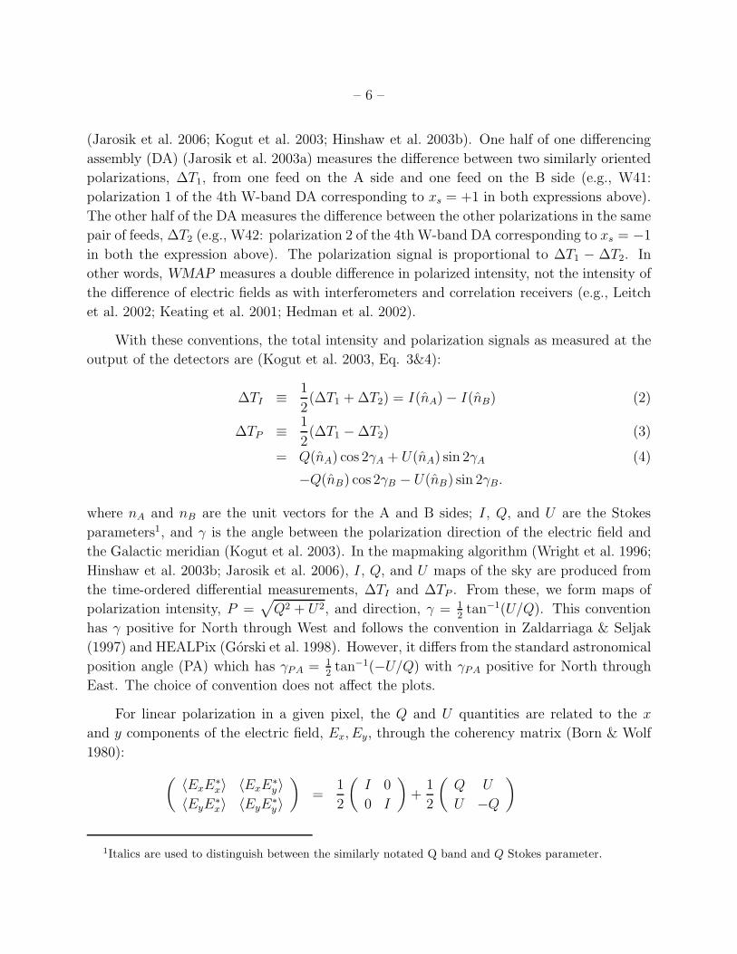
With these conventions, the total intensity and polarization signals as measured at the

output of the detectors are (Kogut et al. 2003, Eq. 3&4):

∆TI ≡ 1

2(∆T1 + ∆T2) = I(nA) − I(nB) (2)

∆TP ≡ 1

2(∆T1 − ∆T2) (3)

= Q(nA) cos 2γA + U(nA) sin 2γA (4)

−Q(nB) cos 2γB − U(nB) sin 2γB.

where nA and nB are the unit vectors for the A and B sides; I, Q, and U are the Stokes

parameters1, and γ is the angle between the polarization direction of the electric field and

the Galactic meridian (Kogut et al. 2003). In the mapmaking algorithm (Wright et al. 1996;

Hinshaw et al. 2003b; Jarosik et al. 2006), I, Q, and U maps of the sky are produced from

the time-ordered differential measurements, ∆TI and ∆TP . From these, we form maps of

polarization intensity, P =√

Q2 + U2, and direction, γ = 12tan−1(U/Q). This convention

has γ positive for North through West and follows the convention in Zaldarriaga & Seljak

(1997) and HEALPix (Gorski et al. 1998). However, it differs from the standard astronomical

position angle (PA) which has γPA = 12tan−1(−U/Q) with γPA positive for North through

East. The choice of convention does not affect the plots.

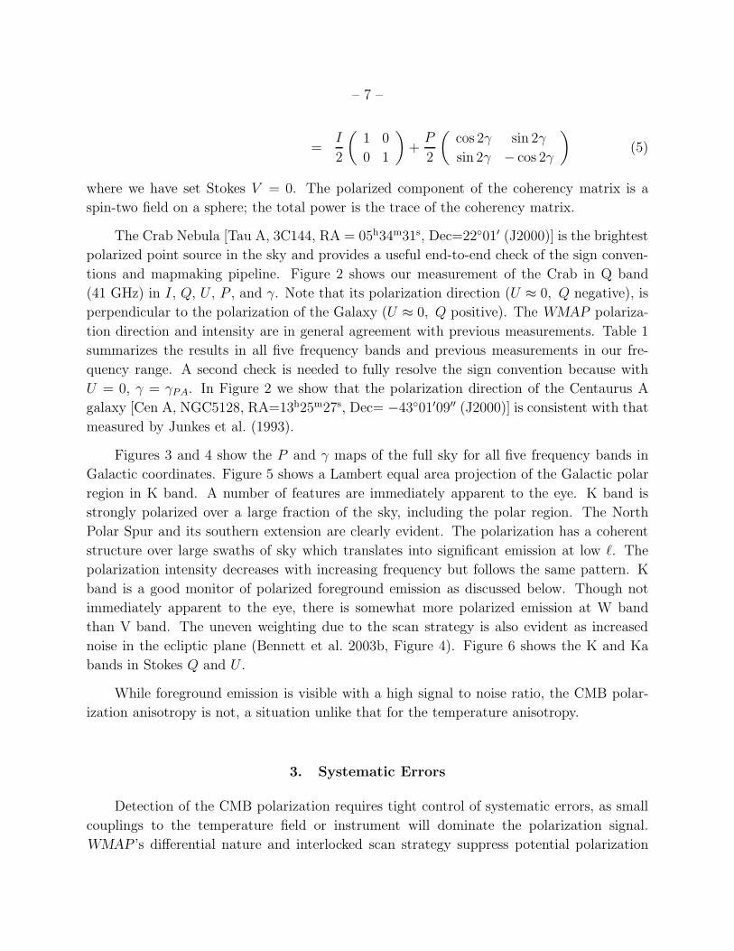
For linear polarization in a given pixel, the Q and U quantities are related to the x

and y components of the electric field, Ex, Ey, through the coherency matrix (Born & Wolf

1980):

(

〈ExE∗x〉 〈ExE

∗y〉

〈EyE∗x〉 〈EyE

∗y〉

)

=1

2

(

I 0

0 I

)

+1

2

(

Q U

U −Q

)

1Italics are used to distinguish between the similarly notated Q band and Q Stokes parameter.

– 7 –

=I

2

(

1 0

0 1

)

+P

2

(

cos 2γ sin 2γ

sin 2γ − cos 2γ

)

(5)

where we have set Stokes V = 0. The polarized component of the coherency matrix is a

spin-two field on a sphere; the total power is the trace of the coherency matrix.

The Crab Nebula [Tau A, 3C144, RA = 05h34m31s, Dec=2201′ (J2000)] is the brightest

polarized point source in the sky and provides a useful end-to-end check of the sign conven-

tions and mapmaking pipeline. Figure 2 shows our measurement of the Crab in Q band

(41 GHz) in I, Q, U , P , and γ. Note that its polarization direction (U ≈ 0, Q negative), is

perpendicular to the polarization of the Galaxy (U ≈ 0, Q positive). The WMAP polariza-

tion direction and intensity are in general agreement with previous measurements. Table 1

summarizes the results in all five frequency bands and previous measurements in our fre-

quency range. A second check is needed to fully resolve the sign convention because with

U = 0, γ = γPA. In Figure 2 we show that the polarization direction of the Centaurus A

galaxy [Cen A, NGC5128, RA=13h25m27s, Dec= −4301′09′′ (J2000)] is consistent with that

measured by Junkes et al. (1993).

Figures 3 and 4 show the P and γ maps of the full sky for all five frequency bands in

Galactic coordinates. Figure 5 shows a Lambert equal area projection of the Galactic polar

region in K band. A number of features are immediately apparent to the eye. K band is

strongly polarized over a large fraction of the sky, including the polar region. The North

Polar Spur and its southern extension are clearly evident. The polarization has a coherent

structure over large swaths of sky which translates into significant emission at low ℓ. The

polarization intensity decreases with increasing frequency but follows the same pattern. K

band is a good monitor of polarized foreground emission as discussed below. Though not

immediately apparent to the eye, there is somewhat more polarized emission at W band

than V band. The uneven weighting due to the scan strategy is also evident as increased

noise in the ecliptic plane (Bennett et al. 2003b, Figure 4). Figure 6 shows the K and Ka

bands in Stokes Q and U .

While foreground emission is visible with a high signal to noise ratio, the CMB polar-

ization anisotropy is not, a situation unlike that for the temperature anisotropy.

3. Systematic Errors

Detection of the CMB polarization requires tight control of systematic errors, as small

couplings to the temperature field or instrument will dominate the polarization signal.

WMAP’s differential nature and interlocked scan strategy suppress potential polarization

– 8 –

systematics in ways similar to the suppression for temperature systematics. The details are

different however, and more complex because of the tensorial nature of the polarization field

and the double difference required to measure the polarization. Throughout our analyses,

the overall level of systematic contamination is assessed with null tests as described here and

in Jarosik et al. (2006) & Hinshaw et al. (2006).

The mapmaking procedure is described in Jarosik et al. (2006). End-to-end simulations

of the instrument and scan strategy, incorporating realistic models of the frequency response,

foreground emission, and detector noise characteristics, are used to assess the possible lev-

els of contamination. Interactions between the slow < 1 % drifts in the gain, non-uniform

weighting across the sky, the 0.2% correlation due to the oppositely directed beams, the

time series masking of the planets, and the 1/f noise are accounted for in the map solu-

tion. In the following we discuss how the instrumental offset, gain/calibration uncertainty,

passband mismatch, main beam mismatch, polarization isolation and cross polarization, loss

imbalance, and sidelobes affect the polarization maps.

Offset and baseline drift—- The instrumental offset is the output of the detector in

the absence of celestial signal. The average polarization offset in the Q, V, and W bands

is 250 mK. Changes in this offset on time scales of minutes to hours arise from spacecraft

temperature changes and from 1/f drifts in the amplifier gain acting on the 250 mK. To

measure polarization at the level of 0.1 µK, we require that changes in the baseline be

suppressed by roughly a factor of 106. The first step in achieving this is maintaining a stable

instrument and environment. The physical temperature of the DAs averaged over a spin

period changes by less than 5 parts in 106 (Jarosik et al. 2006), suppressing changes in the

baseline by a similar factor. The second step in achieving this is through the baseline removal

in the mapmaking algorithm (Hinshaw et al. 2003b; Jarosik et al. 2006).

If the precession of the satellite were stopped, the temperature data for ℓ > 1 would

repeat in the time stream at the spin period (2.16 m). The offset, though, would change sign

relative to the celestial signal at half the spin period enabling the differentiation of celestial

and instrumental signals. (Alternatively, one may imagine observing a planet in which case

the temperature data would change sign at half the spin period and an offset would be con-

stant.) By contrast, with our choice of polarization orientations, the polarization data ∆TP ,

would repeat at half the spin period for some orientations of the satellite. Consequently, an

instrumental offset would not change sign relative to a celestial signal upon a 180 space-

craft rotation. Thus the polarization data are more sensitive to instrumental offsets than are

the temperature data. In general, the polarization data enters the time stream in a more

complex manner than does the temperature data.

Calibration— An incorrect calibration between channels leads to a leakage of the tem-

– 9 –

perature signal into ∆TP , contaminating the polarization map. Calibration drifts cause a

leakage that varies across the sky. Jarosik et al. (2003a) show that calibration drifts on ≈ 1

day time scales are the result of sub-Kelvin changes in the amplifier’s physical temperature.

The calibration can be faithfully modeled by fitting to the physical temperature of each DA

with a three parameter model. Here again WMAP’s stability plays a key role. The residual

calibration errors are at the ≈ 0.2% level. These errors do not limit the polarization maps be-

cause the bright Galactic plane is masked in the time ordered data when producing the high

Galactic latitude maps (Jarosik et al. 2006). The overall absolute calibration uncertainty is

still the first-year value, 0.5% (Jarosik et al. 2006).

Passband mismatch— The effective central frequencies (Jarosik et al. 2003b; Page et al.

2003b) for ∆T1 and ∆T2 are not the same. This affects both the beam patterns, treated

below, and the detected flux from a celestial source, treated in the following. The passbands

for the A and B sides of one polarization channel in a DA may be treated as the same

because the dominant contributions to the passband definition, the amplifiers and band

defining filters, are common to both sides.

Since WMAP is calibrated on the CMB dipole, the presence of a passband mismatch

means that the response to radiation with a non-thermal spectrum is different from the

response to radiation with a CMB spectrum (Kogut et al. 2003; Hinshaw et al. 2003b). This

would be true even if the sky were unpolarized, the polarization offset zero, and the beams

identical. The effect produces a response in the polarization data of the form:

∆TP = ∆I1 − ∆I2 + (6)

Q(nA) cos 2γA + U(nA) sin 2γA

−Q(nB) cos 2γB − U(nB) sin 2γB.

where ∆I1 is the unpolarized temperature difference observed in radiometer one, and sim-

ilarly for ∆I2. If these differ due to passband differences, the polarization data will have

an output component that is independent of parallactic angle. Given sufficient paralactic

coverage, such a term can be separated from Stokes Q and U in the mapmaking process.

We model the polarized signal as Q cos 2γ+U sin 2γ+S where the constant, S, absorbs the

signal due to passband mismatch. We solve for the mismatch term simultaneously with Q

and U as outlined in Jarosik et al. (2006). Note that we do not need to know the magnitude

of the passband mismatch, it is fit for in the mapmaking process. The S map resembles

a temperature map of the Galaxy but at a reduced amplitude of 3.5% in K band, 2.5% in

the V1 band, and on average ≈ 1% for the other bands. The maps of S agree with the

expectations based on the measured passband mismatch.

Beamwidth mismatch— The beamwidths of each polarization on each of the A and B

– 10 –

sides are different. The difference between the A and B side beam shapes is due to the

difference in shapes of the primary mirrors and is self consistently treated in the window

function (Page et al. 2003b). The difference in beam shapes between ∆T1 and ∆T2 is due to

the mismatch in central frequencies.2

This effect is most easily seen in the K-band observations of Jupiter. We denote the

brightness temperature and solid angle of Jupiter with TJ and ΩJ , and the measured quanti-

ties as TJ and ΩJ . Although the product TJΩJ = TJΩJ is the same for the two polarizations

(because Jupiter is almost a thermal source in K band), the beam solid angles differ by

8.1% on the A-side and 6.5% on the B-side (Page et al. 2003a). The primary effect of the

beamwidth mismatch is to complicate the determination of the intrinsic polarization of point

sources.

The difference in beams also leads to a small difference in window functions between ∆T1

and ∆T2. The signature would be leakage of power from the temperature anisotropy into the

polarization signal at high ℓ. We have analyzed the data for evidence of this effect and found

it to be negligible. Additionally, as most of the CMB and foreground polarization signal

comes from angular scales much larger than the beam, the difference in window functions

can safely be ignored in this data set.

Polarization isolation and cross polarization— Polarization isolation, Xcp, and cross

polarization are measures of the leakage of electric field from one polarization into the mea-

surement of the orthogonal polarization. For example, if a source were fully polarized in the

vertical direction with intensity Iv and was measured to have intensity Ih = 0.01Iv with a

horizontally polarized detector, one would say that the cross polar response (or isolation)

is |Xcp|2 = 1% or −20 dB. The term “polarization isolation” is usually applied to devices

whereas “cross polarization” is applied to the optical response of the telescope. We treat

these together as a cross-polar response. For WMAP, the off-axis design and imperfections

in the orthomode transducers (OMT) lead to a small cross-polar response. The ratio of the

maximum of the modeled crosspolar beam to the maximum of the modeled copolar beam is

−25, −27, −30, −30, & −35 dB in K through W bands respectively. The determination of

the feed and OMT polarization isolation is limited by component measurement. The maxi-

mum values we find are: |Xcp|2 = −40, −30, −30, −27, & −25 dB for K through W bands

respectively (Page et al. 2003b). We consider the combination of beams plus components

below.

Because WMAP measures only the difference in power from two polarizations, it mea-

2If the passbands were the same, the beam solid angles for ∆T1 and ∆T2 would be the same to < 0.5%

accuracy.

– 11 –

sures only Stokes Q in a reference frame fixed to the radiometers, QRad. The sensitivity to

celestial Stokes Q and U comes through multiple observations of a single pixel with different

orientations of the satellite. The formalism that describes how cross polarization interacts

with the observations is given in Appendix A. To leading order, the effect of a simple

cross polarization of the form Xcp = XeiY is to rotate some of the radiometer U into a Q

component. The measured quantity becomes:

∆TP = QARad +QB

Rad + 2X cos(Y )(UARad + UB

Rad) (7)

where QARad and QB

Rad are the Stokes Q components for the A and B sides in the radiometer

frame, similarly with UARad and UB

Rad. Note that in the frame of the radiometers QBRad (Stokes

Q in the B-side coordinate system) is −QARad. This leads to the difference in sign conventions

between the above and Equation 5. System measurements limit the magnitude of |Xcp|2but do not directly give the phase, Y . Laboratory measurements of selected OMTs show

Y = 90 ± 5, indicating the effective cross polar contamination is negligible.

We limit the net effect of the reflectors and OMT with measurements in the GEMAC

antenna range (Page et al. 2003b). We find that for a linearly polarized input, the ratios of

the maximum to minimum responses of the OMTs are 1) −25, −27, −25, −25, −22 dB for K

through W band respectively; 2) 90±2 apart; and 3) within ±1.5 of the design orientation.

Thus, we can limit any rotation of one component into another to < 2. The comparison

of γ derived from Tau A to the measurement by Flett & Henderson (1979) in Table 1 gives

further evidence that any possible rotation of the Stokes components is minimal. Based

on these multiple checks, we treat the effects of optical cross polarization and incomplete

polarization isolation as negligible.

Loss imbalance— A certain amount of celestial radiation is lost to absorption by the

optics and waveguide components. If the losses were equal for each of the four radiometer

inputs their effect would be indistinguishable from a change in the gain calibration. However,

small differences exist that produce a residual common-mode signal that is separable from the

gain drifts (Jarosik et al. 2003a). The mean loss difference (xim) between the A- and B-sides

is accounted for in the mapmaking algorithm (Hinshaw et al. 2003a; Jarosik et al. 2003a). In

addition, the imbalance between the two polarizations on a single side, the “loss imbalance

imbalance,” is also included (Jarosik et al. 2006). It contributes a term 2(LATA + LBTB)

to ∆TP . Here TA,B is the sky temperature observed by the A,B side, and LA,B is the loss

imbalance between the two polarizations on the A,B side (see Appendix A). The magnitude

of LA,B is . 1% (Jarosik et al. 2003b).

A change in the loss across the bandpass due to, for example, the feed horns is a poten-

tial systematic error that we do not quantify with the radiometer passband measurements

(Jarosik et al. 2003b). The magnitude of the effect is second order to the loss imbalance

– 12 –

which is 1%. We do not have a measurement of the effect. Nevertheless, as the effect mimics

a passband mismatch, it is accounted for in the map solution.

Sidelobes— When the sidelobes corresponding to ∆TP are measured, there are two terms

(Barnes et al. 2003). The largest term is due to the passband mismatch and is consistently

treated in the mapmaking process. The second smaller term is due to the intrinsic polariza-

tion. We assess the contribution of both terms by simulating the effects of scan pattern of the

sidelobes on the Q and U polarization maps. The results are reported in Barnes et al. (2003)

for the first-year polarization maps. In K band, the net rms contamination is 1µK outside

of the Kp0 mask region (Bennett et al. 2003b). The intrinsic polarized sidelobe pickup is

< 1µK and is not accounted for in this three-year data release. The contamination is more

than an order of magnitude smaller in the other bands.

4. The Foreground Emission Model

The microwave sky is polarized at all frequencies measured by WMAP. In K band

the polarized flux exceeds the level of CMB polarization over the full sky. By contrast,

unpolarized foreground emission dominates over the CMB only over ≈ 20% of the sky. Near

60 GHz and ℓ ≈ 5, the foreground emission temperature is roughly a factor of two larger than

the CMB polarization signal. Thus, the foreground emission must be subtracted before a

cosmological analysis is done. While it is possible to make significant progress working with

angular power spectra, we find that due to the correlations between foreground components,

a pixel space subtraction is required. Table 2 gives the foreground emission levels in a region

around the Galactic center.

The two dominant components of diffuse polarized foreground emission in the 23 −94 GHz range are synchrotron emission and thermal dust emission (Weiss 1984; Bennett

et al. 2003b). Free-free emission is unpolarized3 and spinning dust grains are expected to

have polarization fractions of 1-2% (Lazarian & Draine 2000). The signal from polarized

radio sources is negligible (Table 9, Hinshaw et al. 2006). The detected polarized sources

are all well known, and among the brightest objects in the temperature source catalog.

They include 3C273, 3C274 (M87, Vir A), 3C279, Fornax A, Pictor A, [HB93]2255-282,

and [HB93] 0637-752 and are masked as discussed below. The potential impact of polarized

foreground emission on the detection of the CMB polarization has been discussed by many

authors including Verde et al. (2006); Ponthieu et al. (2005); de Oliveira-Costa et al. (2003);

Giardino et al. (2002); Tucci et al. (2002); Baccigalupi et al. (2001); Tegmark et al. (2000).

3There may be polarized emission at the edges of HII clouds as noted in Keating et al. (1998).

– 13 –

Synchrotron emission is produced by cosmic-ray electrons orbiting in the ≈ 6 µG total

Galactic magnetic field. The unpolarized synchrotron component has been well measured

by WMAP in the 23 to 94 GHz range (Bennett et al. 2003a). The brightness temperature

of the radiation is characterized by T (ν) ∝ νβs where the index −3.1 < βs < −2.5 varies

considerably across the sky (Reich & Reich 1988; Lawson et al. 1987). In the microwave

range, the spectrum reddens (βs tends to more negative values) as the frequency increases

(Banday & Wolfendale 1991).

Synchrotron radiation can be strongly polarized in the direction perpendicular to the

Galactic magnetic field (Rybicki & Lightman 1979). The polarization has been measured

at a number of frequencies [from Leiden between 408 MHz to 1.4 GHz (Brouw & Spoelstra

1976; Wolleben et al. 2005), from Parkes at 2.4 GHz (Duncan et al. 1995, 1999), and by

the Medium Galactic Latitude Survey at 1.4 GHz (Uyanıker et al. 1999)]. At these low

frequencies, Faraday rotation alters the polarization. Electrons in the Galactic magnetic field

rotate the plane of polarization because the constituent left and right circular polarizations

propagate with different velocities in the medium. In the interstellar medium, the rotation

is a function of electron density, ne, and the component of the Galactic magnetic field along

the line of sight, B||,

∆θ = 420(1 GHz

ν

)2∫ L/1 kpc

0

dr( ne

0.1 cm−3

)( B||

1 µG

)

(8)

where the integral is over the line of sight. With ne ∼ 0.1 cm−3, L ∼ 1 kpc, and B|| ∼ 1µG,

the net rotation is ∆θ ∼ 420/ν2, with ν in GHz. At WMAP frequencies the rotation is

negligible, though the extrapolation of low frequency polarization measurements to WMAP

frequencies can be problematic. In addition there may be both observational and astro-

physical depolarization effects that are different at lower frequencies (Burn 1966; Cioffi &

Jones 1980; Cortiglioni & Spoelstra 1995). Thus, our method for subtracting the foreground

emission is based, to the extent possible, on the polarization directions measured by WMAP

.

The other dominant component of polarized foreground emission comes from thermal

dust. Nonspherical dust grains align their long axes perpendicularly to the Galactic magnetic

field through the Davis-Greenstein mechanism (Davis & Greenstein 1951). The aligned

grains preferentially absorb the component of starlight polarized along their longest axis.

Thus, when we observe starlight we see it polarized in the same direction as the magnetic

field. These same grains emit thermal radiation preferentially polarized along their longest

axis, perpendicular to the Galactic magnetic field. Thus we expect to observe thermal dust

emission and synchrotron emission polarized in the same direction, while starlight is polarized

perpendicularly to both.

– 14 –

In Section §4.1, we describe a physical model of the polarized microwave emission from

our Galaxy that explains the general features of the WMAP polarization maps. However

this model is not directly used to define the polarization mask or to clean the polarization

maps. We go on to define the polarization masks in §4.2 and in §4.3 we describe how we

subtract the polarized foreground emission.

4.1. The Galaxy Magnetic Field and a Model of Foreground Emission.

In the following, we present a general model of polarized foreground emission based on

WMAP observations. We view this as a starting point aimed at understanding the gross

features of the WMAP data. A more detailed model that includes the wide variety of external

data sets that relate to polarization is beyond the scope of this paper.

For both synchrotron and dust emission, the Galactic magnetic field breaks the spatial

isotropy thereby leading to polarization. Thus, to physically model the polarized foreground

emission we need a model of the Galactic magnetic field. As a first step, we note that the

K-band polarization maps suggest a large coherence scale for the Galactic magnetic field, as

shown in Figure 3.

We can fit the large-scale field structure seen in the K-band maps with a gas of cosmic

ray electrons interacting with a magnetic field that follows the spiral arms. The Galactic

magnetic field can be quite complicated (Beck 2006; Han et al. 2006; Reich 2006; Wielebinski

2005): there are field direction reversals in the Galactic plane; the field strength depends on

length scale, appearing turbulent on scales < 80 kpc (e.g., Mitner & Spangler 1996); and

the field strength of the large-scale field depends on the Galactocentric radius (e.g., Beck

2001). Nevertheless, most external spiral galaxies have magnetic fields that follow the spiral

arm pattern (e.g., Wielebinski 2005; Beck et al. 1996; Sofue et al. 1986). Inspired by this,

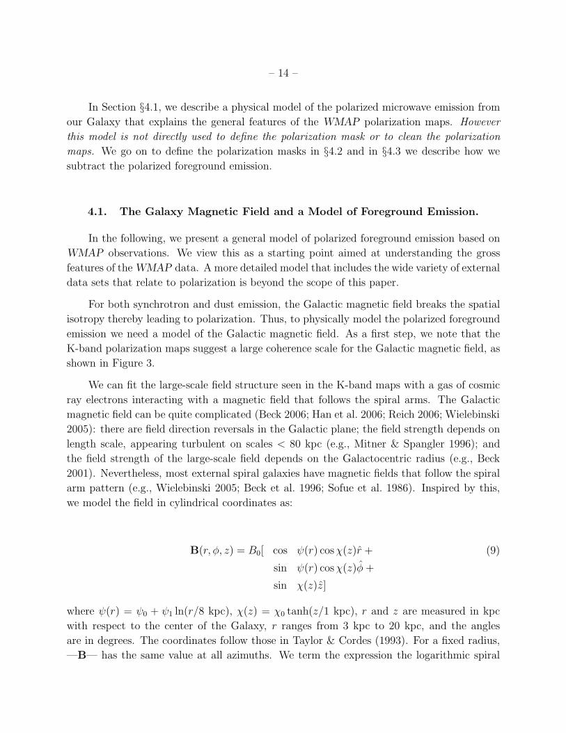
we model the field in cylindrical coordinates as:

B(r, φ, z) = B0[ cos ψ(r) cosχ(z)r + (9)

sin ψ(r) cosχ(z)φ +

sin χ(z)z]

where ψ(r) = ψ0 + ψ1 ln(r/8 kpc), χ(z) = χ0 tanh(z/1 kpc), r and z are measured in kpc

with respect to the center of the Galaxy, r ranges from 3 kpc to 20 kpc, and the angles

are in degrees. The coordinates follow those in Taylor & Cordes (1993). For a fixed radius,

—B— has the same value at all azimuths. We term the expression the logarithmic spiral

– 15 –

arm (LSA) model to distinguish it from previous forms. We take 8 kpc as the distance to

the center of the Galaxy (Eisenhauer et al. 2003; Reid & Brunthaler 2005). The values are

determined by fitting to the K-band field directions. While the tilt, χ(z) with χ0 = 25, and

the radial dependence, ψ(r) with ψ1 = 0.9, optimize the fit, the key parameter is ψ0, the

opening angle of the spiral arms. We find that the magnetic field is a loosely wound spiral

with ψ0 ≃ 35.

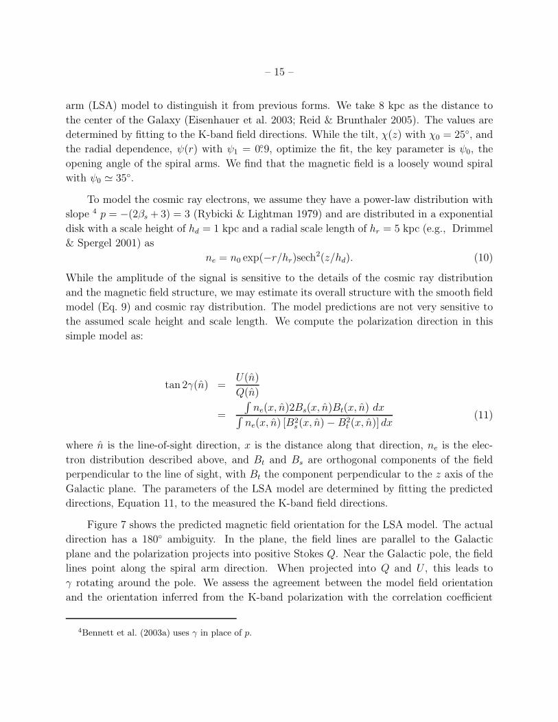
To model the cosmic ray electrons, we assume they have a power-law distribution with

slope 4 p = −(2βs + 3) = 3 (Rybicki & Lightman 1979) and are distributed in a exponential

disk with a scale height of hd = 1 kpc and a radial scale length of hr = 5 kpc (e.g., Drimmel

& Spergel 2001) as

ne = n0 exp(−r/hr)sech2(z/hd). (10)

While the amplitude of the signal is sensitive to the details of the cosmic ray distribution

and the magnetic field structure, we may estimate its overall structure with the smooth field

model (Eq. 9) and cosmic ray distribution. The model predictions are not very sensitive to

the assumed scale height and scale length. We compute the polarization direction in this

simple model as:

tan 2γ(n) =U(n)

Q(n)

=

∫

ne(x, n)2Bs(x, n)Bt(x, n) dx∫

ne(x, n) [B2s (x, n) − B2

t (x, n)] dx(11)

where n is the line-of-sight direction, x is the distance along that direction, ne is the elec-

tron distribution described above, and Bt and Bs are orthogonal components of the field

perpendicular to the line of sight, with Bt the component perpendicular to the z axis of the

Galactic plane. The parameters of the LSA model are determined by fitting the predicted

directions, Equation 11, to the measured the K-band field directions.

Figure 7 shows the predicted magnetic field orientation for the LSA model. The actual

direction has a 180 ambiguity. In the plane, the field lines are parallel to the Galactic

plane and the polarization projects into positive Stokes Q. Near the Galactic pole, the field

lines point along the spiral arm direction. When projected into Q and U , this leads to

γ rotating around the pole. We assess the agreement between the model field orientation

and the orientation inferred from the K-band polarization with the correlation coefficient

4Bennett et al. (2003a) uses γ in place of p.

– 16 –

r = cos(2(γmodel − γdata)), and take the rms average over 74.3% of the sky (outside the P06

mask described below). For our simple model the agreement is clear: r = 0.76 for K band.

Using using rotation measures derived from pulsar observations in the Galactic plane,

one finds instead a spiral arm opening angle of ψ0 ≃ 8 as reviewed in Beck (2001); Han

(2006). Our method is more sensitive to the fields above and below the plane; and, unlike

the case with pulsars, we have no depth information. It has been suggested by R. Beck

and others that the north polar spur may drive our best fit value to ψ0 ≃ 35. Though

the agreement between our simple model and the K-band polarization directions indicate

that we understand the basic mechanism, more modeling is needed to connect the WMAP

observations to other measures of the magnetic field.

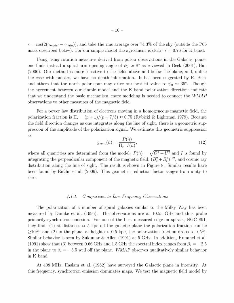
For a power law distribution of electrons moving in a homogeneous magnetic field, the

polarization fraction is Πs = (p+ 1)/(p+ 7/3) ≈ 0.75 (Rybicki & Lightman 1979). Because

the field direction changes as one integrates along the line of sight, there is a geometric sup-

pression of the amplitude of the polarization signal. We estimate this geometric suppression

as

gsync(n) =P (n)

Πs I(n), (12)

where all quantities are determined from the model: P (n) =√

Q2 + U2 and I is found by

integrating the perpendicular component of the magnetic field, (B2s +B2

t )1/2, and cosmic ray

distribution along the line of sight. The result is shown in Figure 8. Similar results have

been found by Enßlin et al. (2006). This geometric reduction factor ranges from unity to

zero.

4.1.1. Comparison to Low Frequency Observations

The polarization of a number of spiral galaxies similar to the Milky Way has been

measured by Dumke et al. (1995). The observations are at 10.55 GHz and thus probe

primarily synchrotron emission. For one of the best measured edge-on spirals, NGC 891,

they find: (1) at distances ≈ 5 kpc off the galactic plane the polarization fraction can be

≥10%; and (2) in the plane, at heights < 0.5 kpc, the polarization fraction drops to <5%.

Similar behavior is seen by Sukumar & Allen (1991) at 5 GHz. In addition, Hummel et al.

(1991) show that (3) between 0.66 GHz and 1.5 GHz the spectral index ranges from βs = −2.5

in the plane to βs = −3.5 well off the plane. WMAP observes qualitatively similar behavior

in K band.

At 408 MHz, Haslam et al. (1982) have surveyed the Galactic plane in intensity. At

this frequency, synchrotron emission dominates maps. We test the magnetic field model by

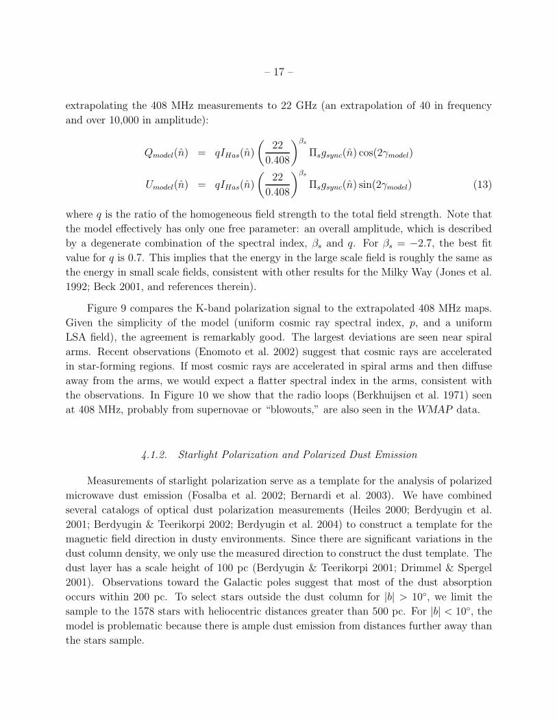
– 17 –

extrapolating the 408 MHz measurements to 22 GHz (an extrapolation of 40 in frequency

and over 10,000 in amplitude):

Qmodel(n) = qIHas(n)

(

22

0.408

)βs

Πsgsync(n) cos(2γmodel)

Umodel(n) = qIHas(n)

(

22

0.408

)βs

Πsgsync(n) sin(2γmodel) (13)

where q is the ratio of the homogeneous field strength to the total field strength. Note that

the model effectively has only one free parameter: an overall amplitude, which is described

by a degenerate combination of the spectral index, βs and q. For βs = −2.7, the best fit

value for q is 0.7. This implies that the energy in the large scale field is roughly the same as

the energy in small scale fields, consistent with other results for the Milky Way (Jones et al.

1992; Beck 2001, and references therein).

Figure 9 compares the K-band polarization signal to the extrapolated 408 MHz maps.

Given the simplicity of the model (uniform cosmic ray spectral index, p, and a uniform

LSA field), the agreement is remarkably good. The largest deviations are seen near spiral

arms. Recent observations (Enomoto et al. 2002) suggest that cosmic rays are accelerated

in star-forming regions. If most cosmic rays are accelerated in spiral arms and then diffuse

away from the arms, we would expect a flatter spectral index in the arms, consistent with

the observations. In Figure 10 we show that the radio loops (Berkhuijsen et al. 1971) seen

at 408 MHz, probably from supernovae or “blowouts,” are also seen in the WMAP data.

4.1.2. Starlight Polarization and Polarized Dust Emission

Measurements of starlight polarization serve as a template for the analysis of polarized

microwave dust emission (Fosalba et al. 2002; Bernardi et al. 2003). We have combined

several catalogs of optical dust polarization measurements (Heiles 2000; Berdyugin et al.

2001; Berdyugin & Teerikorpi 2002; Berdyugin et al. 2004) to construct a template for the

magnetic field direction in dusty environments. Since there are significant variations in the

dust column density, we only use the measured direction to construct the dust template. The

dust layer has a scale height of 100 pc (Berdyugin & Teerikorpi 2001; Drimmel & Spergel

2001). Observations toward the Galactic poles suggest that most of the dust absorption

occurs within 200 pc. To select stars outside the dust column for |b| > 10, we limit the

sample to the 1578 stars with heliocentric distances greater than 500 pc. For |b| < 10, the

model is problematic because there is ample dust emission from distances further away than

the stars sample.

– 18 –

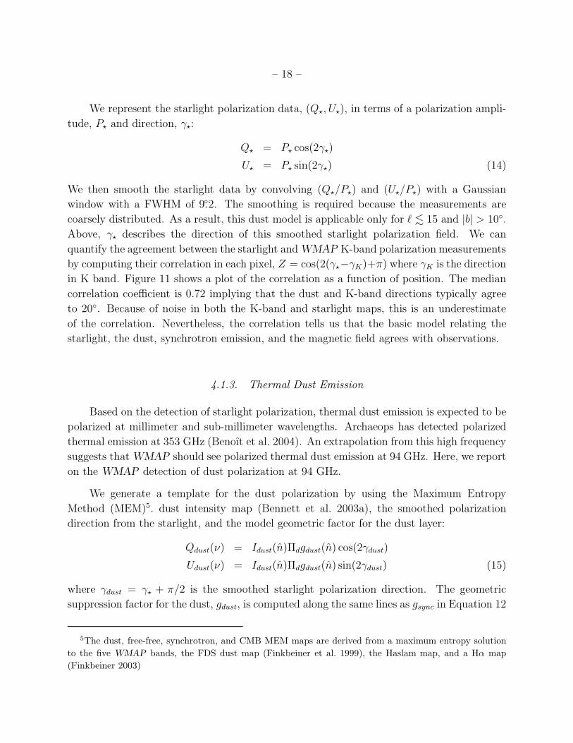
We represent the starlight polarization data, (Q⋆, U⋆), in terms of a polarization ampli-

tude, P⋆ and direction, γ⋆:

Q⋆ = P⋆ cos(2γ⋆)

U⋆ = P⋆ sin(2γ⋆) (14)

We then smooth the starlight data by convolving (Q⋆/P⋆) and (U⋆/P⋆) with a Gaussian

window with a FWHM of 9.2. The smoothing is required because the measurements are

coarsely distributed. As a result, this dust model is applicable only for ℓ . 15 and |b| > 10.

Above, γ⋆ describes the direction of this smoothed starlight polarization field. We can

quantify the agreement between the starlight and WMAP K-band polarization measurements

by computing their correlation in each pixel, Z = cos(2(γ⋆−γK)+π) where γK is the direction

in K band. Figure 11 shows a plot of the correlation as a function of position. The median

correlation coefficient is 0.72 implying that the dust and K-band directions typically agree

to 20. Because of noise in both the K-band and starlight maps, this is an underestimate

of the correlation. Nevertheless, the correlation tells us that the basic model relating the

starlight, the dust, synchrotron emission, and the magnetic field agrees with observations.

4.1.3. Thermal Dust Emission

Based on the detection of starlight polarization, thermal dust emission is expected to be

polarized at millimeter and sub-millimeter wavelengths. Archaeops has detected polarized

thermal emission at 353 GHz (Benoıt et al. 2004). An extrapolation from this high frequency

suggests that WMAP should see polarized thermal dust emission at 94 GHz. Here, we report

on the WMAP detection of dust polarization at 94 GHz.

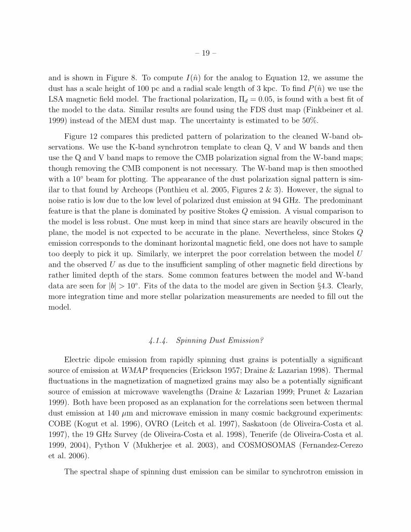
We generate a template for the dust polarization by using the Maximum Entropy

Method (MEM)5. dust intensity map (Bennett et al. 2003a), the smoothed polarization

direction from the starlight, and the model geometric factor for the dust layer:

Qdust(ν) = Idust(n)Πdgdust(n) cos(2γdust)

Udust(ν) = Idust(n)Πdgdust(n) sin(2γdust) (15)

where γdust = γ⋆ + π/2 is the smoothed starlight polarization direction. The geometric

suppression factor for the dust, gdust, is computed along the same lines as gsync in Equation 12

5The dust, free-free, synchrotron, and CMB MEM maps are derived from a maximum entropy solution

to the five WMAP bands, the FDS dust map (Finkbeiner et al. 1999), the Haslam map, and a Hα map

(Finkbeiner 2003)

– 19 –

and is shown in Figure 8. To compute I(n) for the analog to Equation 12, we assume the

dust has a scale height of 100 pc and a radial scale length of 3 kpc. To find P (n) we use the

LSA magnetic field model. The fractional polarization, Πd = 0.05, is found with a best fit of

the model to the data. Similar results are found using the FDS dust map (Finkbeiner et al.

1999) instead of the MEM dust map. The uncertainty is estimated to be 50%.

Figure 12 compares this predicted pattern of polarization to the cleaned W-band ob-

servations. We use the K-band synchrotron template to clean Q, V and W bands and then

use the Q and V band maps to remove the CMB polarization signal from the W-band maps;

though removing the CMB component is not necessary. The W-band map is then smoothed

with a 10 beam for plotting. The appearance of the dust polarization signal pattern is sim-

ilar to that found by Archeops (Ponthieu et al. 2005, Figures 2 & 3). However, the signal to

noise ratio is low due to the low level of polarized dust emission at 94 GHz. The predominant

feature is that the plane is dominated by positive Stokes Q emission. A visual comparison to

the model is less robust. One must keep in mind that since stars are heavily obscured in the

plane, the model is not expected to be accurate in the plane. Nevertheless, since Stokes Q

emission corresponds to the dominant horizontal magnetic field, one does not have to sample

too deeply to pick it up. Similarly, we interpret the poor correlation between the model U

and the observed U as due to the insufficient sampling of other magnetic field directions by

rather limited depth of the stars. Some common features between the model and W-band

data are seen for |b| > 10. Fits of the data to the model are given in Section §4.3. Clearly,

more integration time and more stellar polarization measurements are needed to fill out the

model.

4.1.4. Spinning Dust Emission?

Electric dipole emission from rapidly spinning dust grains is potentially a significant

source of emission at WMAP frequencies (Erickson 1957; Draine & Lazarian 1998). Thermal

fluctuations in the magnetization of magnetized grains may also be a potentially significant

source of emission at microwave wavelengths (Draine & Lazarian 1999; Prunet & Lazarian

1999). Both have been proposed as an explanation for the correlations seen between thermal

dust emission at 140 µm and microwave emission in many cosmic background experiments:

COBE (Kogut et al. 1996), OVRO (Leitch et al. 1997), Saskatoon (de Oliveira-Costa et al.

1997), the 19 GHz Survey (de Oliveira-Costa et al. 1998), Tenerife (de Oliveira-Costa et al.

1999, 2004), Python V (Mukherjee et al. 2003), and COSMOSOMAS (Fernandez-Cerezo

et al. 2006).

The spectral shape of spinning dust emission can be similar to synchrotron emission in

– 20 –

the 20-40 GHz range. Thus models with either variable synchrotron spectral index (Bennett

et al. 2003b) or with a spinning dust spectrum with a suitably fit cutoff frequency (Lagache

2003; Finkbeiner 2004) can give reasonable fits to the data. However, at ν < 20 GHz there is

a considerable body of evidence, reviewed in Bennett et al. (2003b) and Hinshaw et al. (2006),

that shows (1) that the synchrotron index varies across the sky steepening with increasing

galactic latitude (as is also seen in WMAP ) and (2) that in other galaxies and our galaxy

there is a strong correlation between 5 GHz synchrotron emission and 100 µm (3000 GHz)

dust emission. The combination of these two observations imply that the ν < 40 GHz

WMAP foreground emission is dominated by synchrotron emission as discussed in Hinshaw

et al. (2006). Nevertheless, we must consider spinning dust as a possible emission source.

While on a Galactic scale it appears to be sub-dominant, it may be dominant or a significant

fraction of the emission in some regions or clouds.

Spinning dust models predict an unambiguous signature in intensity maps: at 5-15 GHz,

the dust emission should be significantly less than the synchrotron emission. Finkbeiner

(2004) and de Oliveira-Costa et al. (2004) argue that the Tenerife and Green Bank data

show evidence for a rising spectrum between 10 and 15 GHz, suggesting the presence of

spinning dust. Observations of individual compact clouds also show evidence for spinning

dust emission (Finkbeiner et al. 2002, 2004; Watson et al. 2005) though the signature is not

ubiquitous. The status of the observations is discussed further in Hinshaw et al. (2006).

The WMAP polarization measurements potentially give us a new way to distinguish

between synchrotron and dust emission at microwave frequencies. While synchrotron emis-

sion is expected to be highly polarized, emission from spinning dust grains is thought to

be weakly polarized. While promising, the signature is not unique as a tangle of magnetic

field lines can also lead to a low polarization component (Sukumar & Allen 1991) as seen

at 5 GHz where spinning dust emission is expected to be negligible. Using a model for the

polarization fraction of the synchrotron emission based on the LSA structure, we separate

the microwave intensity emission into a high and low polarization component:

Iνhigh(n) = P ν(n)/qΠsgsync(n)

Iνlow(n) = Iν(n) − Iν

high(n) − IILCCMB − IMEM,ν

FF (16)

where Iν and P ν are the intensity and polarization maps at frequency ν. For notational

convenience, we use ν = K,Ka,Q,V,W. IILCCMB is the foreground-free CMB map made with

a linear combination of WMAP bands, and IMEM,νFF is the MEM free-free map for band

ν (Bennett et al. 2003b). In effect, we use the WMAP polarization maps to extract the

intensity map of the low-polarization component in the data.

Figure 13 compares the morphology of the low polarization K-band map to the W-band

MEM dust map (Bennett et al. 2003a). Even in this simple model based on a number of

– 21 –

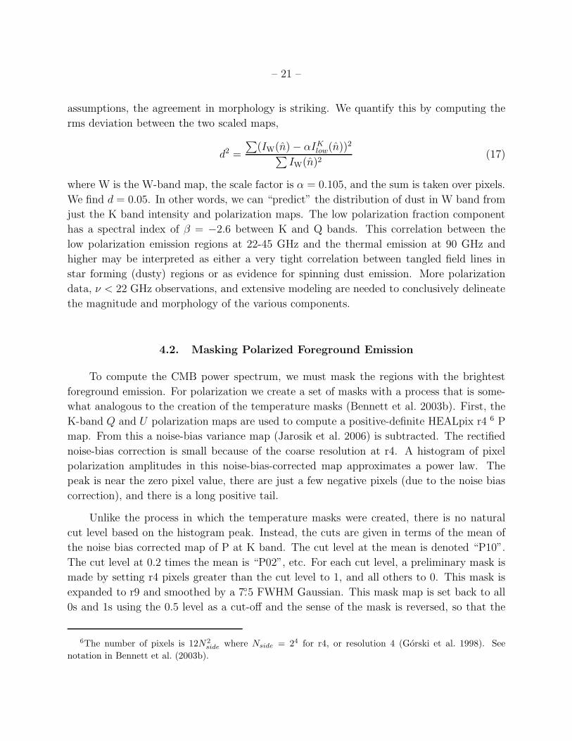
assumptions, the agreement in morphology is striking. We quantify this by computing the

rms deviation between the two scaled maps,

d2 =

∑

(IW(n) − αIKlow(n))2

∑

IW(n)2(17)

where W is the W-band map, the scale factor is α = 0.105, and the sum is taken over pixels.

We find d = 0.05. In other words, we can “predict” the distribution of dust in W band from

just the K band intensity and polarization maps. The low polarization fraction component

has a spectral index of β = −2.6 between K and Q bands. This correlation between the

low polarization emission regions at 22-45 GHz and the thermal emission at 90 GHz and

higher may be interpreted as either a very tight correlation between tangled field lines in

star forming (dusty) regions or as evidence for spinning dust emission. More polarization

data, ν < 22 GHz observations, and extensive modeling are needed to conclusively delineate

the magnitude and morphology of the various components.

4.2. Masking Polarized Foreground Emission

To compute the CMB power spectrum, we must mask the regions with the brightest

foreground emission. For polarization we create a set of masks with a process that is some-

what analogous to the creation of the temperature masks (Bennett et al. 2003b). First, the

K-band Q and U polarization maps are used to compute a positive-definite HEALpix r4 6 P

map. From this a noise-bias variance map (Jarosik et al. 2006) is subtracted. The rectified

noise-bias correction is small because of the coarse resolution at r4. A histogram of pixel

polarization amplitudes in this noise-bias-corrected map approximates a power law. The

peak is near the zero pixel value, there are just a few negative pixels (due to the noise bias

correction), and there is a long positive tail.

Unlike the process in which the temperature masks were created, there is no natural

cut level based on the histogram peak. Instead, the cuts are given in terms of the mean of

the noise bias corrected map of P at K band. The cut level at the mean is denoted “P10”.

The cut level at 0.2 times the mean is “P02”, etc. For each cut level, a preliminary mask is

made by setting r4 pixels greater than the cut level to 1, and all others to 0. This mask is

expanded to r9 and smoothed by a 7.5 FWHM Gaussian. This mask map is set back to all

0s and 1s using the 0.5 level as a cut-off and the sense of the mask is reversed, so that the

6The number of pixels is 12N2side

where Nside = 24 for r4, or resolution 4 (Gorski et al. 1998). See

notation in Bennett et al. (2003b).

– 22 –

masked-out parts of the sky have zeros (the WMAP convention). The above process results

in a synchrotron polarization mask.

In the case of temperature masks, we found that additional masking based on the higher

frequency bands was redundant. This is not the case with polarization. Thus we make a

dust polarization mask in a similar manner. We begin with the first-year MEM dust model

box-averaged to r7. Half the maximum value found in a subset of pixels in the polar caps

(|b| > 60) is adopted as the cut-off level. A preliminary mask is made by setting r7 pixels

greater than the cut-off level to unity, and all others to zero. This mask is then resolution

expanded to a r9 map, smoothed by a 4.0 Gaussian, and set back to digital levels with a

0.5 cut-off. The sense of the mask is then reversed to fit the WMAP convention. Each

synchrotron polarization mask is ANDed with the (constant) dust polarization mask and a

constant polarized source mask.

We find, in general, that the extragalactic point sources are minimally polarized in the

WMAP bands, as discussed in Hinshaw et al. (2006). We construct a source mask based

on the exceptions. The most significant exception (not already covered by the synchrotron

or dust polarization masks) is Centaurus A, an extended and polarized source. We found

excellent agreement between WMAP and previously published maps of Cen A (Figure 2).

Based on this information, we custom-masked the full extent of Cen A. Six other bright

polarized sources that we masked are Fornax A, Pictor A, 3C273, 3C274, 3C279, PKS 1209-

52. (Some bright polarized sources already covered by the synchrotron and dust mask regions

include: 3C58, Orion A, Taurus A, IC443, 1209-52, W51, W63, HB21, CTB104A). We have

determined that, for most applications, the mask that we call “P06” is the best compromise

between maximizing usable sky area while minimizing foreground contamination. With the

above considerations, the P06 mask masks 25.7% of the sky, mostly near the Galactic plane.

We use the terminology “outside the P06 mask” to refer to data in the 74.3% of the sky left

for cosmological analysis. Various masks are shown in Figure 14.

4.3. Removing the Polarized Foreground Emission from the Maps

Based on our analysis of the Galactic foreground emission, we have generated syn-

chrotron and dust template maps for the purposes of foreground removal. The template

maps are fit and subtracted from the Ka through W band data to generate cleaned maps

that are used for CMB analysis. We assess the efficacy of the subtraction with χ2 and by

examining the residuals as a function of frequency and multipole ℓ, as described in §5.2.

We use the K-band data to trace the synchrotron emission, taking care to account

– 23 –

for the (relatively weak) CMB signal in the K-band map when fitting and subtracting the

template. For dust emission, we construct a template following Equation (15) that is based

on the starlight-derived polarization directions and the FDS dust model eight (Finkbeiner

et al. 1999) evaluated at 94 GHz to trace the dust intensity, Idust. We call this combination

of foreground templates “KD3Pol”.

The synchrotron and dust templates are fit simultaneously in Stokes Q and U to three-

years maps in Ka through W bands. The three-year maps are constructed by optimally

combining the single-year maps for each DA in a frequency band. Specifically

[Qν , Uν ] = (∑

i

N−1i )−1

∑

i

N−1i [Qi, Ui] (18)

where i is a combined year and DA index, [Qi, Ui] is a polarization map degraded to r4

(Jarosik et al. 2006), and N−1i is the inverse noise matrix for polarization map i. The fit

coefficients, αs and αd are obtained by minimizing χ2, defined as

χ2 =∑

p

([Qν , Uν ] − αs,ν[Qs, Us] − αd,ν [Qd, Ud])2

[σ2Q, σ

2U ]

, (19)

where [Qs, Us] is the K-band polarization map (the synchrotron template), [Qd, Ud] is the

dust template, and [σ2Q, σ

2U ] is the noise per pixel per Stokes parameter in the three-year

combined maps. We have tried using optimal (N−1) weighting for the fits as well, and

found similar results for the coefficients. The results reported here are based on the simpler

diagonal weighting. The fit is evaluated for all pixels outside the processing mask (Jarosik

et al. 2006).

The fit coefficients are given in the top half of Table 3. For each emission component

we also report the effective spectral index derived from the fit: βs(νK , ν) for synchrotron

emission, and βd(ν, νW ) for dust. These results indicate that the spectrum of the component

traced by K-band is systematically flattening with increasing frequency, which is unexpected

for synchrotron emission. This behavior is statistically significant, and is robust to variations

in the dust model and the data weighting. We do not have a definitive explanation for this

behavior.

To guard against the possibility of subtracting CMB signal, we modified the template

model as follows. We take the four synchrotron coefficients in Table 3 and fit them to a

spectrum model of the form

αs(ν) = αs,0 · g(ν)(ν/νK)βs + αc, (20)

where αs,0, βs, and αc are model parameters that are fit to the αs(ν), and g(ν) is the

conversion from antenna temperature to thermodynamic temperature at frequency ν. This

– 24 –

results in a modified set of synchrotron coefficients that are forced to follow a power-law that

is largely determined by the Ka and Q-band results. Specifically, the modified coefficients

are given in Table 3. The implied synchrotron spectrum is βs = −3.33. This results in a

12% reduction in the synchrotron coefficients at Q-band, and a 33% reduction at V-band.

However, because the K-band template is dominated by an ℓ = 2 E-mode signal (see §5.1),

this change has a negligible effect on our cosmological conclusions, which are dominated by

E-mode signal at ℓ > 2. A comparison of selected “before and after” cleaning maps is shown

in Figure 15.

We also account for the cleaning in the map error bars. Since the K-band data are a

combination of synchrotron and CMB emission, subtracting a scaled version of K band from

a higher frequency channel also subtracts some CMB signal. If the fit coefficient to the higher

frequency channel is a0, then the cleaned map is M ′(ν) = (M(ν) − a0M(ν = K))/(1 − a0),

where M is the map and ν denotes the frequency band. The maps we use for cosmological

analysis were cleaned using the coefficients in the bottom half of Table 3. The factor of

1/(1 − a0) dilates the noise in the cleaned map. To account for this in the error budget

we scale the covariance matrix of the cleaned map by a factor of 1/(1 − a0)2. Additionally,

we modify the form of the inverse covariance matrix by projecting from it any mode that

has the K-band polarization pattern: N−1 → N′−1, where N′−1[QK , UK ] = 0. This ensures

that any residual signal traced by K-band (due, for example, to errors in the form of the

spectrum) will not contribute to cosmological parameter constraints.

One measure of the efficacy of the foreground removal is the change in χ2, relative to

a null signal, between pre-cleaned and cleaned maps. Table 4 gives the values for the full

sky and the P06 cut. In both cases the full pixel covariance matrix was used to compute χ2

for Stokes Q and U simultaneously. For the full sky the number of degrees of freedom, ν, is

6144 (twice the number of pixels in an r4 map) and outside the P06 mask ν = 4534. Note

the large ∆χ2 achieved with just a two parameter fit. By comparing the full sky to the P06

χ2, we find that the starlight-based dust template is insufficient in the plane as discussed

in §4.1.3. We also see that outside the P06 mask, that Q and V bands are the cleanest

maps and that they are cleaned to similar levels. Since χ2/ν for Q and V bands is so close

to unity for the cleaned maps, it is no longer an effective measure of cleaning. Instead, we

examine the power spectra ℓ by ℓ to assess the cleaning, and then test the sensitivity of the

cosmological conclusions to cleaning by including Ka and W band data.

We have tried a number of variants on the KD3Pol cleaning. We find, for example,

that setting gdust = 1 across the sky has negligible effect on the fits or the derived optical

depth. Alternatively, when one uses the K-band polarization direction to trace the dust

direction, γdust = γK in Equation 15, the cleaning is not as effective. Outside the P06 mask,

– 25 –

the reduced χ2 in the Q and V band maps is 1.022 and 1.016 as compared to 1.014 and

1.018 for the starlight-based directions. Thus the latter are used. Regardless of template, we

find that our cosmological conclusions are relatively insensitive to the details as indicated in

Figure 26.

5. Power Spectra

The Q & U maps are well suited to analyzing foreground emission, are useful for com-

paring to other polarization maps, and have straightforward noise properties. However, they

are not well suited to quantifying the CMB polarization anisotropy because their definition

is coordinate dependent. The Q and U maps may be transformed into scalar and pseudo-

scalar quantities called E and B modes (Seljak 1997; Kamionkowski et al. 1997; Zaldarriaga

& Seljak 1997). E and B are so named because they comprise a curl-free and divergence-

free decomposition of the spin-2 polarization field, analogous to static electric and magnetic

fields. The problem of separating E and B modes with an unevenly sampled and cut sky has

been considered by a number of authors (e.g., Tegmark et al. 2000; Lewis et al. 2002; Bunn

et al. 2003). In our analysis, we work directly with Q and U maps to produce the E and B

angular power spectra. The conventions follow Appendix A of Kogut et al. (2003).7

Fundamental symmetries in the production and growth of the polarized signal select

the possible configurations for the CMB polarization. Scalar (density) perturbations to the

matter power spectrum give rise to T and E modes. Tensor perturbations (gravitational

waves) give rise to T, E, and B modes primarily at ℓ . 2008. Both scalar and tensor

perturbations can produce polarization patterns in both the decoupling and reionization

epochs. Vector perturbations 9 (both inside and outside the horizon) are redshifted away

with the expansion of the universe, unless there are active sources creating the vector modes,

such as topological defects. We do not consider these modes here.

At the noise levels achievable with WMAP , the standard cosmological model predicts

that only the E mode of the CMB polarization and its correlation with T will be detected.

The B-mode polarization signal is expected to be too weak for WMAP to detect, while the

7In this paper we do not use the rotationally invariant Q′ and U ′ of Kogut et al. (2003).

8For r < 0.03 and ℓ & 70, primordial B modes are dominated by the gravitational lensing of E modes.

9Vector modes are produced by purely rotational fluid flow. Based on the fit of the adiabatic ΛCDM

model to WMAP TT data, the contribution of such modes is not large (Spergel et al. 2003). However, a

formal search for them has not been done.

– 26 –

correlations of T and E with B is zero by parity. Thus the TB and EB signals serve as a

useful null check for systematic effects. The polarization of foreground emission is produced

by different mechanisms. Foreground emission can have any mixture of E and B modes, it

can be circularly polarized (unlike the CMB), and E and B can be correlated with T.

We quantify the CMB polarization anisotropy with the CTEℓ , CEE

ℓ , and CBBℓ angular

power spectra, where

CXYℓ = 〈aX

ℓmaY ∗ℓm〉. (21)

Here the “〈〉” denote an ensemble average, aTℓm are the multipoles of the temperature map,

and aEℓm, a

Bℓm are related to the spin-2 decomposition of the polarization maps

[Q± iU ](x) =∑

ℓ>0

ℓ∑

m=−ℓ

∓2aℓm∓2Yℓm(x) (22)

via

±2aℓm = aEℓm ± iaB

ℓm (23)

(Zaldarriaga & Seljak 1997). The remaining polarization spectrum combinations (TB, EB)

have no expected cosmological signal because of the statistical isotropy of the universe.

We compute the angular power spectrum after applying the P06 polarization mask using

two methods depending on the ℓ range. All power spectra are initially based on the single-

year r9 Q and U maps (Jarosik et al. 2006). For ℓ > 23 10, we compute the power spectrum

following the method outlined in Hivon et al. (2002), and Kogut et al. (2003, Appendix A)

as updated in Hinshaw et al. (2006) and Appendix B.2. The statistical weight per pixel is

Nobs/σ20 where σ0 is the noise per observation (Jarosik et al. 2006; Hinshaw et al. 2006). Here

Nobs is a 2x2 weight matrix that multiplies the vector [Q,U ] in each pixel

Nobs =

(

NQ NQU

NQU NU

)

, (24)

where NQ, NU , and NQU are the elements of the weight arrays provided with the sky map

data. Note that the correlation between Q and U within each pixel is accounted for. We

refer to this as “Nobs weighting.” From these maps, only cross power spectra between DAs

and years are used. The cross spectra have the advantage that only signals common to two

10ℓ = 23 = 3Nside − 1 is the Nyquist limit on ℓ. For some analysis methods (§D) we use HEALPix r3 for

which nside = 23 = 8

– 27 –

independent maps contribute and there are no noise biases to subtract as there are for the

auto power spectra. The covariance matrices for the various Cℓ are given in Appendix C.3.

For ℓ < 23 we mask and degrade the r9 maps to r4 (see the last paragraph of Appendix D

and Jarosik et al. 2006) so that we may use the full r4 inverse pixel noise matrix, N−1, to

optimally weight the maps prior to evaluating the pseudo-Cℓ. This is necessary because the

maps have correlated noise that is significant compared to the faint CMB signal. By “N−1

weighting” the maps, we efficiently suppress modes in the sky that are poorly measured

given the WMAP beam separation and scan strategy (mostly modes with structure in the

ecliptic plane). We propagate the full noise errors through to the Fisher matrix of the

power spectrum. For the spectrum plots in this section, the errors are based on the diagonal

elements of the covariance matrix which is evaluated in Appendix B.

Figure 16 shows the effect that correlated noise has on the low ℓ errors in the EE and BB

spectra. The curves show the diagonal elements of the inverse Fisher matrix (the Cℓ errors)

computed in two ways: (1) assuming the noise is uncorrelated in pixel space and described

by Nobs (red) and (2) assuming it is correlated and correctly described by N−1 (black).The

smooth rise in both curves toward low ℓ is due to the effects of 1/f noise and is most

pronounced in the W4 DA, which has the highest 1/f noise. The structure in the black

trace is primarily due to the scan strategy. Note in particular, that we expect relatively

larger error bars on ℓ = 2, 5, 7 in EE and on ℓ = 3 in BB. We caution those analyzing

maps that to obtain accurate results, the N−1 weighting must be used when working with

the ℓ < 23 power spectra. For the Monte Carlo Markov Chains (MCMC) and cosmological

parameter evaluation, we do not use the power spectrum but find the exact likelihood of

the temperature and polarization maps given the cosmological parameters (Appendix D &

Hinshaw et al. 2006).

For both r4 and r9 maps there are 15 MASTER cross power spectra (see Table 5).

For the full three-year result, we form∑3

i,j=1 ui × vj/6 omitting the u1 × u1, u2 × u2, and

u3 × u3 auto power spectra. In this expression, u and v denote the frequency band (K-

W) and i and j denote the year. The noise per ℓ in the limit of no celestial signal, Nℓ, is

determined from analytical models that are informed by full simulations for r9 (including

1/f noise), and from the full map solution for r4.

5.1. Power Spectrum of Foreground Emission Outside the P06 Mask.

Figure 17 shows the EE and BB power spectra for the region outside the P06 mask,

74.3% of the sky, before any cleaning. The 15 cross spectra have been frequency averaged

– 28 –

into four groups (Table 5) by weighting with the diagonal elements of the covariance matrix.

Data are similarly binned over the indicated ranges of ℓ. It is clear that even on the cut sky

the foreground emission is non negligible. In K band, we find ℓ(ℓ+1)CEEℓ=<2−6>/2π = 66 (µK)2

and ℓ(ℓ+1)CBBℓ=<2−6>/2π = 48 (µK)2, where ℓ =< 2−6 > denotes the weighted average over

multipoles two through six. The emission drops by roughly a factor of 200 in Cℓ by 61 GHz

resulting in . 0.3 (µK)2 for both EE and BB. There is a “window” between ℓ = 4 and

ℓ = 8 in the EE where the emission is comparable to, though larger than, the detector noise.

Unfortunately, BB foreground emission dominates a fiducial r = 0.3, τ = 0.09 model by

roughly an order of magnitude at ℓ < 30. In general, the power spectrum of the foreground

emission scales approximately as ℓ−1/2 in ℓ(ℓ+ 1)Cℓ.

Figure 18 shows the power spectra as a function of frequency for a few ℓ bands. The

spectrum of the emission follows that of synchrotron with T ∝ νβs with βs = −2.9 for

both EE and BB11. There is some evidence for another component at ν > 60 as seen in

the flattening of the EE ℓ = 2 term. We interpret this as due to dust emission. In the

foreground model, we explicitly fit to a dust template and detect polarized dust emission.

However, there is not yet a sufficiently high signal to noise ratio to strongly constrain the

dust index or amplitude outside the P06 mask.

A simple parameterization of the foreground emission outside the P06 mask region is

given by

ℓ(ℓ+ 1)Cforeℓ /2π = (Bs(ν/65)2βs + Bd(ν/65)2βd)ℓm. (25)

We have introduced the notation BXX ≡ ℓ(ℓ + 1)CXXℓ /2π to simplify the expression. The

“d” and “s” subscripts stand for “dust” and “synchrotron.” From an unweighted fit to all

the raw ℓ < 100 data with the dust index fixed at βd = 1.5, we find for EE Bs = 0.36 (µK)2,

βs = −3.0, Bd = 1.0 (µK)2 and m = −0.6; and for BB Bs = 0.30 (µK)2, βs = −2.8,

Bd = 0.50 (µK)2 and m = −0.6. This model is given as an approximate guide. Its ℓ

dependence is shown in Figure 17 for ν = 65 GHz and its frequency dependence is shown

in Figure 18 for BB ℓ = 2. One can see that this scaling model picks up the general trends

but not the details of the foreground emission. For example, it ignores correlations between

dust and synchrotron emission. It predicts an average foreground emission of ≈ 1 (µK)2 at

30 GHz and ℓ = 300. Leitch et al. (2005) give an upper bound of ≈ 1 (µK)2 for synchrotron

emission in this range. As DASI observes a relatively synchrotron-free region and at ℓs

beyond where this simple parametrization can be tested, there is not a conflict with their

results. The same is true for the CBI experiment (Readhead et al. 2004) which also observed

11The fits to the power law index were done with the power spectra in CMB temperature units. The ratio

of these and the indicies corresponding to antenna are approximately 1.03 and 0.99 at 90 GHz (where the

difference is largest) for dust and synchrotron respectively. The difference is negligible.

– 29 –

at 30 GHz but at a predominantly higher ℓ and in a predetermined clean region of sky. The

dust amplitude in the model is especially uncertain. Depending on the region of sky within

the P06 cut, and the ℓ of interest, it may be an order of magnitude off.

For a more complete model of the power spectra of foreground emission, one must take

into account the correlations or anticorrelations between various foreground components and

between the foreground components and the CMB. For example, a reasonable fit to the ℓ = 2

EE spectrum, which is dominated by foreground emission, is given by

BEE(ν) = as(ν1ν2)βs + ρsdasad(ν

βs

1 νβd

2 + νβd

1 νβs

2 ) + ad(ν1ν2)βd (26)

where ρsd is the dust synchrotron correlation coefficient, ν1 and ν2 are the frequencies of the

two spectra that are correlated, the βd and βs are the dust and synchrotron spectral indices,

and ν =√ν1ν2. This fit is shown in Figure 18. After normalizing the frequency to 65 GHz,

the following coefficients were found to reasonably represent the data: as = 0.64, βs = −2.9,

ad = 0.65, βd = 1.5, and ρsd = 0.46. In order to produce the KV, KW, and KaW features,

there must be significant correlations between dust and synchrotron emission. For the ℓ = 4

EE spectrum a similar expression fits the data if ρsd is negative.

Some care is needed in interpreting the statistical significance of power spectra that

include foreground emission and a cut sky. The lack of statistical isotropy of the foreground

emission means that it must be treated separately from the CMB when assessing the net

noise. In the presence of foregrounds, the random uncertainty becomes

∆C2ℓ =

2

(2ℓ+ 1)f 2sky

[N2ℓ + 2NℓFℓ] (27)

where Fℓ is the foreground emission at each ℓ. We plot only the first term in Figures 17

& 18 to indicate the size of the statistical error. Additionally, with the sky cut there is a

noise-foreground coupling between NE,Bℓ and FE,B

ℓ±2 , and between NE,Bℓ and FB,E

ℓ±1 . This is

analogous to the noise coupling shown in Appendix C.

5.2. Power Spectrum of Foreground-Cleaned Maps Outside the P06 Mask

We next discuss the power spectrum after removing the foreground emission from the

maps. Cleaning foregrounds not only changes the mean of Cℓ, but it reduces ∆Cℓ because

of the couplings. The choice of model makes little difference to the conclusions. For all the

following we have subtracted the best fit KD3Pol Q and U templates from the Ka through

W maps (both r4 and r9 versions) as described in Section 4. Table 5 shows the EE ℓ = 2

and BB ℓ = 5, the multipoles with the largest foreground contributions, for both before and

– 30 –

after the subtraction. Where the foreground signal is dominant, the subtraction can reduce

its level by a factor of 6-10 in temperature.

When we fit and subtract the foreground templates, we use essentially all of the available

data on polarized foreground emission. The error bar on the power spectrum of the cleaned

maps is dilated in the cleaning process as discussed above. We do not include an additional

error for systematic uncertainty in the model. Rather, by comparing spectra of pre-cleaned

to cleaned maps, we estimate that the model removes at least 85% of the synchrotron.

This is demonstrated, for example, in the KKa and KaKa combinations for ℓ = 2 EE in

Table 5, in the subtraction shown in Figure 15, and to a lesser degree by the null EB and

BB power spectra. We also note that to a good approximation foreground emission adds

only in quadrature to CMB emission.

Figure 19 shows the power spectra of the foreground cleaned maps as a function of

frequency for ℓ = 2−9. It also shows what we estimate to be the maximum levels of residual

foreground contamination in the power spectrum. In the figure, we plot the synchrotron

spectrum scaled to 0.15 of the pre-cleaned Ka band value (in temperature). This shows that

there is negligible residual synchrotron from 40 to 60 GHz with the possible exception of

ℓ = 2 at 40 GHz. Given the size of the ℓ = 2 error bar, this potential contribution to the

determination of the optical depth is negligible as discussed in Section §6.1. Constraining

the residual dust contamination is more difficult. In Figure 19, we also show the MEM

temperature dust model scaled by 5%, a typical dust polarization value. A similarly scaled

FDS model is almost identical. This shows that even if we did not model and subtract dust,

the contamination from it would not be large in Q and V bands. A more detailed model

might have to take into account the possibility that the electrons and dust grains are in

regions at different line of sight distances with different magnetic fields or that variations in

the magnetic field could alias power from low multipoles to higher ones.

The cross power spectra of the cleaned maps are combined by frequency band for testing

cosmological models. The 10 cross spectra (since K-band is used in the model, there is no K-

band cleaned spectrum) are assessed ℓ by ℓ with a least squares fit to a flat line in Figure 19.

The results are shown for the QQ+QV+VV (denoted “QV combination”) and QV+KaV

combinations in EE, we find 0.1 < PTE < 1 for all ℓ < 16, where PTE is for “Probability

to Exceed” and is the probability that a random variable drawn from the same distribution

exceeds the measured value of χ2. When W band is added to the mix, we find PTE < 0.03

for ℓ = 5, 7, 9, though all other values of ℓ give reasonable values. For BB, all frequency

combinations yield reasonable PTEs for all ℓ. Thus, there is a residual signal in our power

spectra that we do not yet understand. It is evident in W band in EE at ℓ = 7 and to a

lesser degree at ℓ = 5 and ℓ = 9. We see no clear evidence of it anywhere else.

– 31 –

5.3. Null Tests and Systematic Checks Outside the P06 Mask

Null tests are critical for assessing the quality of the data. We have examined the data

in a wide variety of ways based on differencing assembly, frequency band, ℓ range, and year.

We present selected, though typical, results in the following. A particularly important test

is the null measurement of the BB, TB, and EB signals as shown in Table 6 and Figure 20.

These data combinations are derived from the same processing as the EE, TE, and TT

combinations, where a signal is detected. Thus, the null result highlights the stability of the

WMAP data, the mapmaking, the foreground cleaning, and the power spectrum estimation.

The power spectrum of the difference of the individual yearly maps is another significant

test. Table 7 shows the results for all the yearly differences for ℓ = 2−16, the critical region of

ℓ-space for the cosmological analysis. We have also used the (u1 × v1 + u2 × v2 − u1 × v2 − u2 × v1)/4

cross spectra to similar effect. Here again the u and v denote different frequency bands. This

combination is equivalent to forming the power spectrum of the difference between year one

and year two maps. In principle it does not contain any signal. The cross-spectrum method

treats the noise in a slightly different way from the straight map method, where one must

use the error bars from one of the maps. It has been checked with simulations. Similar

combinations are used for the other years.

Using a variant of cross-spectrum method, we have also tested combinations of DAs for

multiple ranges in ℓ within each frequency band. For all null tests, we find the expected

null measurements, apart from the previously mentioned residuals at ℓ = 5&7 in W band.

Table 6 gives the reduced χ2 for all combinations of T, E, and B data for a number of data

combinations.

From Figure 19, it is clear that the large signal in W band is not residual dust contam-

ination because the dust would not fit measurements in VW. Additionally, if one assumes

that the polarized emission at a particular ℓ is a fraction times the intensity at the same ℓ, it

would require > 40% dust polarization, which is unreasonable. Though this simple picture

does not take into account the aliasing of intensity from a lower ℓ, we do not observe a similar

effect with the synchrotron emission, which in the simplest case is polarized by the same

magnetic fields. The W-band EE ℓ = 7 value is essentially unchanged by cleaning, removing

a 10 radius around the Galactic caps, or by additionally masking ±10 in the ecliptic plane.

A number of tests have been done to identify this artifact of the data. We are not yet

certain if it is due to an ersatz signal or an incorrect noise term. The error bars on the

individual year differences are too large to clearly see if the effect is the same from year

to year. Simulations show that 1/f alone cannot explain the signal. The scan pattern in

combination with the change in polarization is directly related to the large error bars at

– 32 –

ℓ = 5, 7, 9 and is well understood. We have not identified a mechanism that leads to a

further increase in these uncertainties. We know that different treatments of the noise, for

example using Nobs weighting, decreases the magnitude of the discrepancy, though we are

confident that the N−1 treatment of the pixel noise is the correct approach. The discrepancy

can be made smaller by eliminating the W1 data simply because the error bars increase. The

W1 radiometer has the lowest noise but also the largest number of “glitches” (13, 4, 1 in

years 1, 2, & 3 respectively, Limon et al. 2003; Hinshaw et al. 2003b). However, since we

could not identify any correlation between the glitch rate (assuming that unmasked glitches

are responsible) and the magnitude of the signal, we do not have a basis for eliminating this

channel.

We believe there is an as yet unknown coupling in the W-band data that is driving the

signal but more simulations and more sensitivity are needed to understand it. We cannot

rule out similar lower-level problems in other bands, but we see no evidence of systematic

effects in BB, EB, or other values of ℓ and other frequencies in EE. To avoid biasing the result

by this residual artifact which also possibly masks some unmodeled dust and synchrotron

contamination, we limit the cosmological analysis to the QV combination. We also show

that including W band EE does not alter our conclusions.

5.4. Analysis of Foreground-Cleaned Power Spectra Outside the P06 Mask.

A comparison of the raw spectra and foreground cleaned spectra is shown in Figure 21.

We start with the weighted sum of the 8 cross spectra with ν > 40 GHz (without KW).

This is the upper-level line (green) in the figure. The individual maps are then cleaned and

the power spectra remade and coadded. This is shown in violet. Similar comparisons are

repeated for the QVW and QV combinations. A simple visual inspection shows that even

at the ℓs with the highest foreground contamination, the cleaning is effective.

From the bottom left panel in Figure 21 one sees that there is a clear signal above

the noise in EE at ℓ < 7. For the QV combination, BEEℓ=<2−6> = 0.086 ± 0.029 (µK)2.

The signal has persisted through a number of different analyses. We cannot rule out that

this signal might find explanation in an unmodeled foreground component; however, we

find this explanation unlikely since the emission would have to be strikingly different from

the measured spatial and frequency characteristics of the polarized foreground emission.

Additionally, when different bands are coadded, the signal level is consistent: for QVW

BEEℓ=<2−6> = 0.098 ± 0.022 (µK)2 and for all channels with ν > 40 GHz except KW,

BEEℓ=<2−6> = 0.095±0.019 (µK)2. We have searched for systematic effects in the EE ℓ = 2−8

range and have not been able to identify any, other than the one discussed above. We can-

– 33 –

not find a more plausible explanation than that the signal is in the sky. We are thus led to

interpret it cosmologically. This is done in the next section.

We show the EE signal for ℓ > 20 in Table 8 and in Figure 22 along with a comparison

to other recent measurements (Leitch et al. 2005; Sievers et al. 2005; Barkats et al. 2005;

Montroy et al. 2005). Based on the best fit to the TT spectra, we produce a template for

the predicted EE spectrum CEE,Tℓ and form:

χ2(AEE) =

800∑

ℓ=50

δCℓQEEℓℓ δCℓ (28)

where δCℓ = CEEℓ − AEECEE,T

ℓ , AEE is the fit amplitude, and QEEℓℓ is the diagonal Fisher

matrix in Appendix C.3. Off diagonal elements in QEEℓℓ′ have a negligible effect on the results.

The results of the fit are plotted in Figure 23 for various frequency combinations. We

plot ∆χ2 from the minimum value and find that AEE = 0.95 ± 0.35 for the pre-cleaned

QVW combination, where the uncertainty is determined from the bounds at ∆χ2 = 1. The

reduced χ2 at the minima are 1.34, 1.34, 1.24, and 1.30 for QV, VW, QVW, and KaQVW

combinations respectively, most likely indicating residual foreground contamination. At a

relative amplitude of zero, ∆χ2 = 1.0, 3.3, 6.2, & 16 respectively for the same frequency

combinations. It is clear that the noise is not yet low enough to use just QV as was done

at low multipoles. In addition, cleaning the maps with the KD3Pol is problematic because

the K-band window function is reduced to 0.1 by ℓ = 250. When the same code is used to

analyze EB and BB data, the fitted amplitude is always consistent with zero. To summarize,

the WMAP EE data are consistent with a model of adiabatic fluctuations based on the

temperature maps at greater than the 2σ level for the QVW and KaQVW combinations.

Figure 24 (left panel) shows the TE spectrum for ℓ < 16. We use V band for tem-

perature and the QV combination for polarization. Several aspects of the new processing

led to increased errors and a reduced low-ℓ signal estimate relative to the first-year result

(Figure 8, Kogut et al. 2003). These include: improvements in mapmaking and power spec-

trum estimation (especially accounting for correlated noise and applying N−1 weighting);

limiting the bands to just Q and V instead of Ka-W; increasing the cut from KP0 to P06;

and improvements in foreground modeling, including a new estimate of dust polarization.

Recall also that the first-year result was based on the combinations of Ka, Q, V, and W

bands and did not include a dust polarization template in contrast to the new prescription.

Furthermore, if the year-two data are processed in the same way as the first-year data, we

obtain a spectrum similar to that in Kogut et al. (2003) indicating that the major differ-

ence between first-year and three-year results rests on new knowledge of how to make and

clean polarization maps. The new spectrum is fully consistent with the first-year results and

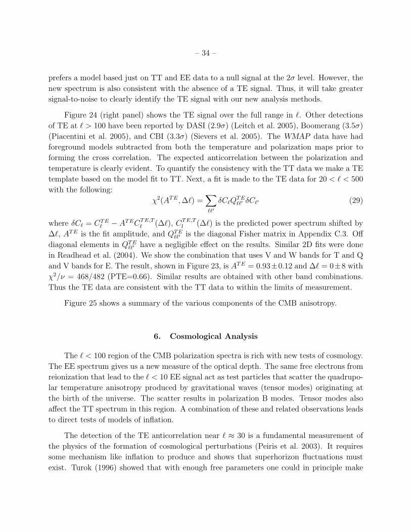
– 34 –

prefers a model based just on TT and EE data to a null signal at the 2σ level. However, the

new spectrum is also consistent with the absence of a TE signal. Thus, it will take greater

signal-to-noise to clearly identify the TE signal with our new analysis methods.

Figure 24 (right panel) shows the TE signal over the full range in ℓ. Other detections

of TE at ℓ > 100 have been reported by DASI (2.9σ) (Leitch et al. 2005), Boomerang (3.5σ)

(Piacentini et al. 2005), and CBI (3.3σ) (Sievers et al. 2005). The WMAP data have had

foreground models subtracted from both the temperature and polarization maps prior to

forming the cross correlation. The expected anticorrelation between the polarization and

temperature is clearly evident. To quantify the consistency with the TT data we make a TE

template based on the model fit to TT. Next, a fit is made to the TE data for 20 < ℓ < 500

with the following:

χ2(ATE,∆ℓ) =∑

ℓℓ′

δCℓQTEℓℓ′ δCℓ′ (29)

where δCℓ = CTEℓ − ATECTE,T

ℓ (∆ℓ), CTE,Tl (∆ℓ) is the predicted power spectrum shifted by

∆ℓ, ATE is the fit amplitude, and QTEℓℓ′ is the diagonal Fisher matrix in Appendix C.3. Off

diagonal elements in QTEℓℓ′ have a negligible effect on the results. Similar 2D fits were done

in Readhead et al. (2004). We show the combination that uses V and W bands for T and Q

and V bands for E. The result, shown in Figure 23, is ATE = 0.93±0.12 and ∆ℓ = 0±8 with

χ2/ν = 468/482 (PTE=0.66). Similar results are obtained with other band combinations.

Thus the TE data are consistent with the TT data to within the limits of measurement.

Figure 25 shows a summary of the various components of the CMB anisotropy.

6. Cosmological Analysis

The ℓ < 100 region of the CMB polarization spectra is rich with new tests of cosmology.

The EE spectrum gives us a new measure of the optical depth. The same free electrons from

reionization that lead to the ℓ < 10 EE signal act as test particles that scatter the quadrupo-

lar temperature anisotropy produced by gravitational waves (tensor modes) originating at

the birth of the universe. The scatter results in polarization B modes. Tensor modes also

affect the TT spectrum in this region. A combination of these and related observations leads

to direct tests of models of inflation.

The detection of the TE anticorrelation near ℓ ≈ 30 is a fundamental measurement of

the physics of the formation of cosmological perturbations (Peiris et al. 2003). It requires

some mechanism like inflation to produce and shows that superhorizon fluctuations must

exist. Turok (1996) showed that with enough free parameters one could in principle make

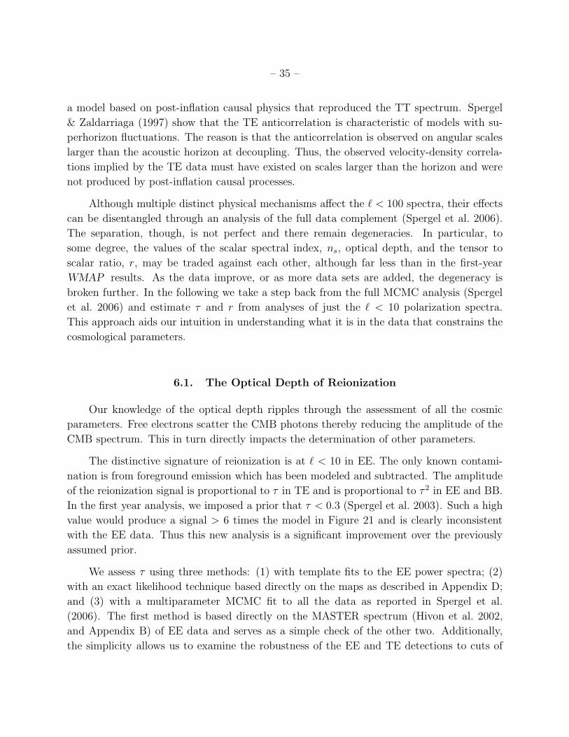
– 35 –

a model based on post-inflation causal physics that reproduced the TT spectrum. Spergel

& Zaldarriaga (1997) show that the TE anticorrelation is characteristic of models with su-

perhorizon fluctuations. The reason is that the anticorrelation is observed on angular scales

larger than the acoustic horizon at decoupling. Thus, the observed velocity-density correla-

tions implied by the TE data must have existed on scales larger than the horizon and were

not produced by post-inflation causal processes.

Although multiple distinct physical mechanisms affect the ℓ < 100 spectra, their effects

can be disentangled through an analysis of the full data complement (Spergel et al. 2006).

The separation, though, is not perfect and there remain degeneracies. In particular, to

some degree, the values of the scalar spectral index, ns, optical depth, and the tensor to

scalar ratio, r, may be traded against each other, although far less than in the first-year

WMAP results. As the data improve, or as more data sets are added, the degeneracy is

broken further. In the following we take a step back from the full MCMC analysis (Spergel

et al. 2006) and estimate τ and r from analyses of just the ℓ < 10 polarization spectra.

This approach aids our intuition in understanding what it is in the data that constrains the

cosmological parameters.

6.1. The Optical Depth of Reionization

Our knowledge of the optical depth ripples through the assessment of all the cosmic

parameters. Free electrons scatter the CMB photons thereby reducing the amplitude of the

CMB spectrum. This in turn directly impacts the determination of other parameters.

The distinctive signature of reionization is at ℓ < 10 in EE. The only known contami-

nation is from foreground emission which has been modeled and subtracted. The amplitude

of the reionization signal is proportional to τ in TE and is proportional to τ 2 in EE and BB.

In the first year analysis, we imposed a prior that τ < 0.3 (Spergel et al. 2003). Such a high

value would produce a signal > 6 times the model in Figure 21 and is clearly inconsistent

with the EE data. Thus this new analysis is a significant improvement over the previously

assumed prior.

We assess τ using three methods: (1) with template fits to the EE power spectra; (2)

with an exact likelihood technique based directly on the maps as described in Appendix D;

and (3) with a multiparameter MCMC fit to all the data as reported in Spergel et al.

(2006). The first method is based directly on the MASTER spectrum (Hivon et al. 2002,

and Appendix B) of EE data and serves as a simple check of the other two. Additionally,

the simplicity allows us to examine the robustness of the EE and TE detections to cuts of

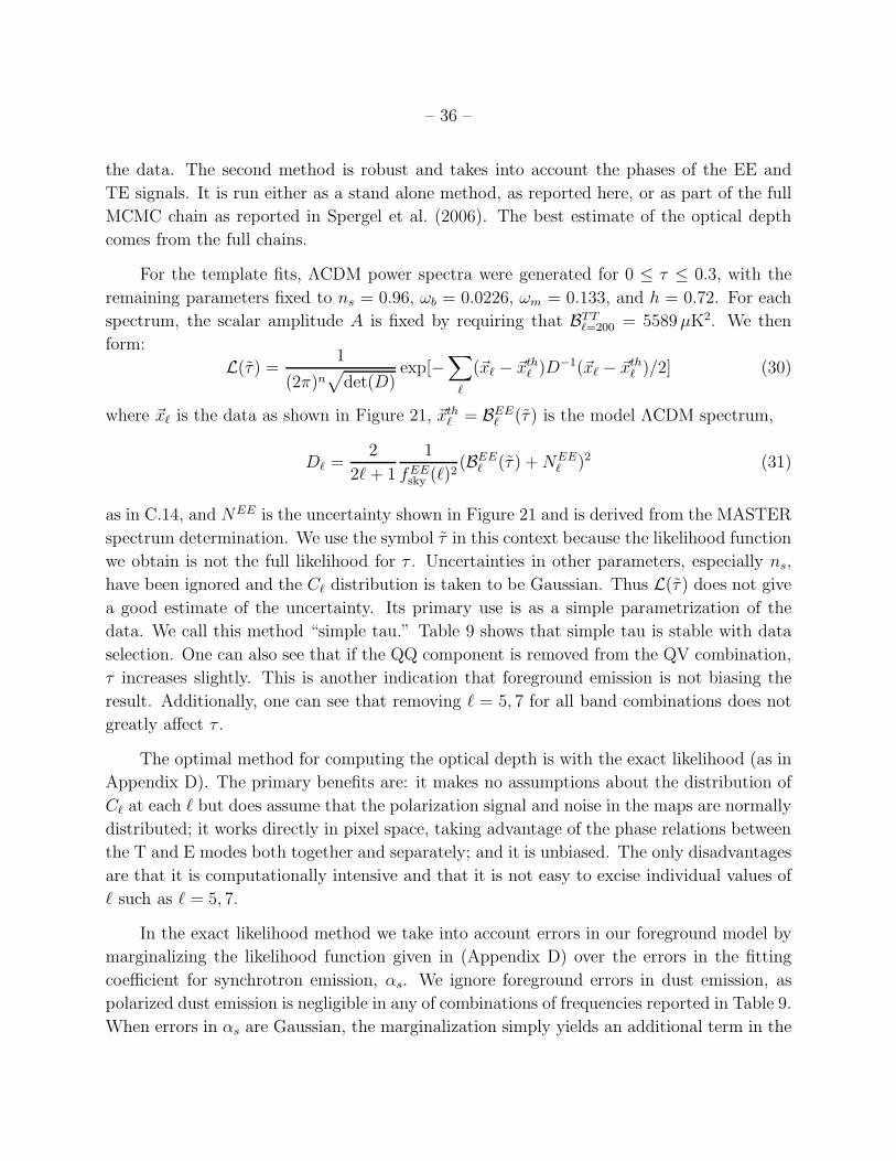
– 36 –

the data. The second method is robust and takes into account the phases of the EE and

TE signals. It is run either as a stand alone method, as reported here, or as part of the full

MCMC chain as reported in Spergel et al. (2006). The best estimate of the optical depth

comes from the full chains.

For the template fits, ΛCDM power spectra were generated for 0 ≤ τ ≤ 0.3, with the

remaining parameters fixed to ns = 0.96, ωb = 0.0226, ωm = 0.133, and h = 0.72. For each

spectrum, the scalar amplitude A is fixed by requiring that BTTℓ=200 = 5589µK2. We then

form:

L(τ) =1

(2π)n√

det(D)exp[−

∑

ℓ

(~xℓ − ~xthℓ )D−1(~xℓ − ~xth

ℓ )/2] (30)

where ~xℓ is the data as shown in Figure 21, ~xthℓ = BEE

ℓ (τ) is the model ΛCDM spectrum,

Dℓ =2

2ℓ+ 1

1

fEEsky (ℓ)2

(BEEℓ (τ ) +NEE

ℓ )2 (31)

as in C.14, and NEE is the uncertainty shown in Figure 21 and is derived from the MASTER

spectrum determination. We use the symbol τ in this context because the likelihood function

we obtain is not the full likelihood for τ . Uncertainties in other parameters, especially ns,

have been ignored and the Cℓ distribution is taken to be Gaussian. Thus L(τ ) does not give

a good estimate of the uncertainty. Its primary use is as a simple parametrization of the

data. We call this method “simple tau.” Table 9 shows that simple tau is stable with data

selection. One can also see that if the QQ component is removed from the QV combination,

τ increases slightly. This is another indication that foreground emission is not biasing the

result. Additionally, one can see that removing ℓ = 5, 7 for all band combinations does not

greatly affect τ .

The optimal method for computing the optical depth is with the exact likelihood (as in

Appendix D). The primary benefits are: it makes no assumptions about the distribution of

Cℓ at each ℓ but does assume that the polarization signal and noise in the maps are normally

distributed; it works directly in pixel space, taking advantage of the phase relations between

the T and E modes both together and separately; and it is unbiased. The only disadvantages

are that it is computationally intensive and that it is not easy to excise individual values of

ℓ such as ℓ = 5, 7.

In the exact likelihood method we take into account errors in our foreground model by

marginalizing the likelihood function given in (Appendix D) over the errors in the fitting

coefficient for synchrotron emission, αs. We ignore foreground errors in dust emission, as

polarized dust emission is negligible in any of combinations of frequencies reported in Table 9.

When errors in αs are Gaussian, the marginalization simply yields an additional term in the

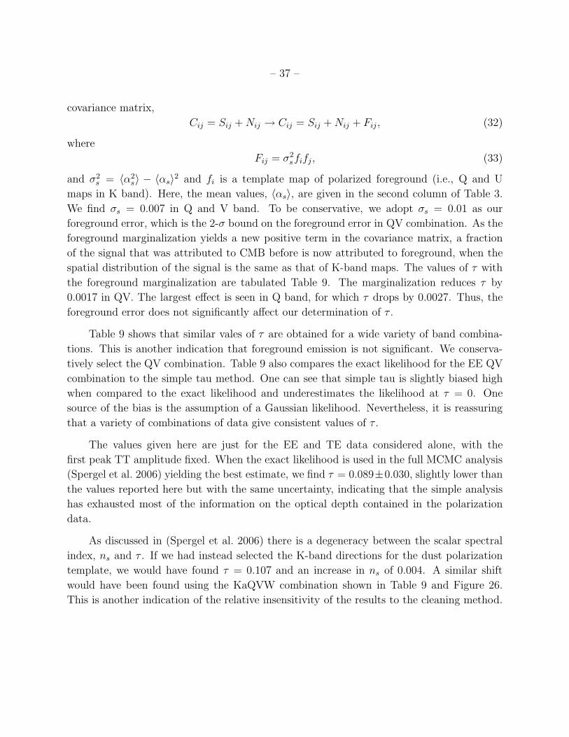
– 37 –

covariance matrix,

Cij = Sij +Nij → Cij = Sij +Nij + Fij , (32)

where

Fij = σ2sfifj , (33)

and σ2s = 〈α2

s〉 − 〈αs〉2 and fi is a template map of polarized foreground (i.e., Q and U

maps in K band). Here, the mean values, 〈αs〉, are given in the second column of Table 3.

We find σs = 0.007 in Q and V band. To be conservative, we adopt σs = 0.01 as our

foreground error, which is the 2-σ bound on the foreground error in QV combination. As the

foreground marginalization yields a new positive term in the covariance matrix, a fraction

of the signal that was attributed to CMB before is now attributed to foreground, when the

spatial distribution of the signal is the same as that of K-band maps. The values of τ with

the foreground marginalization are tabulated Table 9. The marginalization reduces τ by

0.0017 in QV. The largest effect is seen in Q band, for which τ drops by 0.0027. Thus, the

foreground error does not significantly affect our determination of τ .

Table 9 shows that similar vales of τ are obtained for a wide variety of band combina-

tions. This is another indication that foreground emission is not significant. We conserva-

tively select the QV combination. Table 9 also compares the exact likelihood for the EE QV

combination to the simple tau method. One can see that simple tau is slightly biased high

when compared to the exact likelihood and underestimates the likelihood at τ = 0. One

source of the bias is the assumption of a Gaussian likelihood. Nevertheless, it is reassuring

that a variety of combinations of data give consistent values of τ .

The values given here are just for the EE and TE data considered alone, with the

first peak TT amplitude fixed. When the exact likelihood is used in the full MCMC analysis

(Spergel et al. 2006) yielding the best estimate, we find τ = 0.089±0.030, slightly lower than

the values reported here but with the same uncertainty, indicating that the simple analysis

has exhausted most of the information on the optical depth contained in the polarization

data.

As discussed in (Spergel et al. 2006) there is a degeneracy between the scalar spectral

index, ns and τ . If we had instead selected the K-band directions for the dust polarization

template, we would have found τ = 0.107 and an increase in ns of 0.004. A similar shift

would have been found using the KaQVW combination shown in Table 9 and Figure 26.

This is another indication of the relative insensitivity of the results to the cleaning method.

– 38 –

6.2. Gravitational Waves

The CBBℓ spectrum directly probes the primordial gravitational wave background pro-

duced by tensor fluctuations in the early universe. The existence of these gravitational waves

was proposed by Starobinsky (1979). Modern treatments may be found in, for example, Lid-

dle & Lyth (2000); Dodelson (2003); Mukhanov (2005). While scalar and tensor fluctuations

both contribute to the TT and EE spectra, only tensors produce B modes. Inflation models

generally predict similar scalar spectra, but differ in their prediction of the tensor compo-

nent. For example, ekpyrotic/cyclic models (Khoury et al. 2002; Steinhardt & Turok 2002)

predict no observable tensor modes.

The tensor contribution is quantified with the tensor to scalar ratio r. We follow the

convention in the CAMB code (Lewis et al. 2000, Version, June 2004), in CMBFAST v4.5.1

(Seljak & Zaldarriaga 1996) and in Peiris et al. (2003); Verde et al. (2003):

r ≡ ∆2h(k0)

∆2R(k0)

. (34)

Here, ∆2R and ∆2

h are the variance due to scalar and tensor modes respectively. They are

defined through

〈R2〉 =

∫

dk

k∆2

R(k) (35)

and 〈hprimij hprim,ij〉 =

∫

dk

k∆2

h(k), (36)

where hprimij is the primordial tensor metric perturbation in real space that was generated

during inflation and stretched to outside the horizon12. Peiris et al. (2003) shows the k-

dependence of these expressions.

The expression for r is evaluated at k0 = 0.002 Mpc−1 corresponding to l ≈ η0k = 30

with the distance to the decoupling surface η0 ≈ 14, 400 Mpc. Following Verde et al. (2003),

we use ∆2R(k0) = 2 × 104π2A(k0)/9T

20 ≈ 2.95 × 10−9A(k0) with T0 in microkelvins. Some of

the simple models of inflation in a ΛCDM cosmology predict r ≃ 0.3 (e.g., Liddle & Lyth

2000; Boyle et al. 2005). For example, near this range inflationary models with a massive

scalar field, V (φ) = m2φ2/2, predict r = 8/Ne = 4(1 − ns) = 0.13 − 0.16 (Linde 1983) and

models with a self coupling, V (φ) = λφ4/4, predict r = 16/Ne = 16(1− ns)/3 = 0.27 − 0.32

for Ne = 60− 50. Here, Ne is the number of e-foldings before the end of inflation. However,

12Note that our convention yields r = 16ǫ for slow-roll inflationary models with a single scalar field. Here,

ǫ is the slow roll parameter related to the square of the slope of the inflaton potential.

– 39 –

some variants produce r > 0.32 (e.g. Mukhanov & Vikman 2005) while many other have

r ≪ 0.1.

For the best fit WMAP-only ΛCDM plus tensor model, the optical depth is τ = 0.091.

If we add to this model a tensor component with r = 0.3, then BBBℓ=<2−6> = 0.001µK2.

A simple average of the CBBℓ data gives BBB

ℓ=<2−6> = −0.044 ± 0.030µK2, BBBℓ=<2−6> =

−0.018 ± 0.023µK2, BBBℓ=<2−6> = 0.003 ± 0.020µK2, for QV, QVW, and ν > 40 GHz (no

KW) combinations respectively. To detect a signal at the upper range of the predictions

would require maps with ≈ 5 times smaller error bars.

We constrain r by directly fitting a template of CBBl to the BB data. With the above

definition, r directly scales the CBBl power spectrum. Additionally, the amplitude of CBB

l

for ℓ < 16 scales as τ 2. We set the template to be the standard ΛCDM model (Spergel

et al. 2006) and use the single field inflation consistency relation, nt = −r/8, to fix the

tensor spectral index. We assume the spectral index does not run and set ns = 0.96. We

distinguish the r in the template fit by the r notation. The sum is over 2 ≤ ℓ ≤ 11.

The results of the fit are plotted in Figure 27. When we consider just the limit on r

from the polarization spectra, ignoring the tensor contribution to TT, we find r < 2.2 (95%

CL) after marginalizing over τ . It is clear that the BB spectrum is not driving the limit on

r. After including the TT data, the limit drops to r < 0.27 (95% CL). This shows that the

TT data in combination with the limits on τ from EE and TE are leading to the limit on r.

The full MCMC analysis gives r < 0.55 (95% CL) with just the WMAP data. The increase

in the error over the simple method given above is the result of the marginalization over the

other parameters, particularly ns. Additionally, when ns is allowed to depend on k, the error

in r increases dramatically, allowing r < 1.3 (95% CL).

We can relate r to the current energy density in primordial gravitational radiation

(Krauss & White 1992; Peiris 2003),

ΩGW =1

12H20

∫

dk

k∆2

h(k)T2(k, η), (37)

where η is conformal time and the transfer function, T (k, η), is given in Equation E18.

The approximation given in Equation E31 evaluated for A = 0.838 and r < 2.2 yields

ΩGW < 9.6 × 10−12 (95% CL) and for r < 0.55, ΩGW < 2.0 × 10−12 (95% CL).

7. Discussion and Conclusions

WMAP detects significant levels of polarized foreground emission over much of the

sky. The minimum in contamination is near 60 GHz outside the P06 mask. To detect the

– 40 –

polarization in the CMB at ℓ < 10 a model of the foreground emission must be subtracted

from the data. This situation differs from that of the analysis of the temperature anisotropy

for which the foreground emission may be simply masked as a first approximation.13

WMAP has detected the primary temperature anisotropy, the temperature polarization

cross correlation, and the E-mode polarization of the CMB. We detect the optical depth with

τ = 0.089 ± 0.030 in a full fit to all WMAP data. This result is supported by stand-alone

analyses of the polarization data. Using primarily the TT spectrum, along with the optical

depth established with the TE and EE spectra, the tensor to scalar ratio is limited to

r0.002 < 0.55 (95% CL). When the large scale structure power spectrum is added to the

mix (Spergel et al. 2006), the limit tightens to r0.002 < 0.28 (95% CL). These values are

approaching the predictions of the simplest inflation models.

A clear detection of the B modes at ℓ < 100 would give a direct handle on the physics

of the early universe at energy scales of 1015 − 1016 GeV. This paper shows that care will

be required to unambiguously separate the intrinsic signal from the foreground emission.

However, the BB spectrum is particularly clean in WMAP and, at least for ℓ = 2, 3, the

foreground contamination is relatively low. In the noise dominated regime, the error bar on

CBBℓ decreases in proportion to time. Continued WMAP operations combined with other

experimental efforts are nearing a range of great interest.

These new results involve a complete reevaluation of all the components of our previous

analyses, from the beams and gain models through to the mapmaking and foreground mod-

eling. The data and most of the derived data products are available through the LAMBDA

website, http://lambda.gsfc.nasa.gov/. WMAP continues to operate nominally. In the fu-

ture we will address a number of the open issues raised above. In particular, we can anticipate

a better understanding of systematic errors and foreground emission, and therefore improved

constraints on τ and r. It is remarkable that our understanding of the cosmos has reached

the point where we have begun to quantitatively distinguish between different models of the

birth of the universe.

8. Acknowledgments

We wish to thank Uros Seljak, Suzanne Staggs, and Paul Steinhardt for enlightening

conversations on polarization and inflation, and Jim Peebles for his explanation of reioniza-

13Of course our full analysis (Hinshaw et al. 2003b) involved extensive modeling of the foregrounds (Bennett

et al. 2003b).

– 41 –

tion. We thank Bruce Draine for helpful discussions on dust polarization and Rainer Beck

for many suggestions on modeling the Galactic magnetic field. We thank Andre Waelkens

and Torsten Enßlin for pointing out a mistake in the original calculation of gsync. (The fix

affected Figures 8 and 9 but not the conclusions.) We thank Bruce Winstein for a detailed

set of comments on the submitted draft. EK acknowledges support from an Alfred P. Sloan

Research Fellowship. HVP wishes to acknowledge useful discussions with R. Easther, S.

Larson, D. Mortlock, and A. Lewis. The WMAP mission is made possible by the support

of the Office of Space Sciences at NASA Headquarters and by the hard and capable work

of scores of scientists, engineers, technicians, machinists, data analysts, budget analysts,

managers, administrative staff, and reviewers. HVP is supported by NASA through Hubble

Fellowship grant #HF-01177.01-A awarded by the Space Telescope Science Institute which

is operated by the Association of Universities for Research in Astronomy, Inc., for NASA

under contract NAS 5-26555. This research has made use of NASA’s Astrophysics Data

System Bibliographic Services, the HEALPix software, CAMB software, and the CMBFAST

software. This research was additionally supported by NASA LTSA03-000-0090, NASA

ATPNNG04GK55G, and NASA ADP03-0000-092 awards.

A. Radiometer Model

In this section we develop a simple model for the WMAP instrument using Jones matri-

ces (Jones 1941; Montgomery et al. 1948; Blum 1959; Faris 1967; Sault et al. 1996; Tinbergen

1996; Hu et al. 2003). In the following we assume that all circuit elements are matched and

ignore additive noise terms.

The Jones matrix J models the instrumental response to polarization,

Eout = JEin (A1)

linearly relating the output electric field to the input. WMAP is a differential instrument,

so the input radiation vector Ein has four elements, (EAx , E

Ay , E

Bx , E

By ), corresponding to the

electric field seen by the A- and B-side feed pair. The outputs Eout are the inputs to the

detectors.

The first link in the chain is to model the optics, feeds, and orthomode transducers

(OMTs). We consider them as a single unit, because ascribing effects to the individual

components is difficult and not well defined in terms of observations. We include two effects,

loss imbalance and polarization leakage:

JA,BOFO = JA,B

loss JA,Bcrosspol (A2)

– 42 –

JA,Bloss =

(

LA,Bx 0

0 LA,By

)

(A3)

JA,Bcrosspol =

(

1 XA,B1 eiY A,B

1

−XA,B2 e−iY A,B

2 1

)

(A4)

Here LA,Bx,y is the loss for the particular polarization and XA,B

1,2 quantifies the level of cross-

polarization (or polarization isolation) leakage, which we model as a small rotation error.

The matrix JA,Bcrosspol is the first term in the expansion of a general unitary matrix but is not

unitary itself. The subscripts “1” and “2” refer to the two orthogonally polarized radiometers

which are differenced to form ∆P . The matrix JA,Bcrosspol is the first term in the expansion

of a general unitary matrix, though it is not unitary itself. The cross-polarization terms

are allowed to have arbitrary phases Y A,B1,2 . It is possible for cross polarization to produce

circular polarization but WMAPcannot detect it in ∆I or ∆P . While in general there are

four loss terms, two of them are calibrated out. The two that remain are the radiometer loss

imbalances, xim,1 and xim,2. Jarosik et al. (2003b, Table 3) measured the loss imbalances by

fitting the response to the common mode CMB dipole signal, and found them to be . 1%.

The mean imbalance, xim = (xim,1 + xim,2)/2, is corrected for by the map-making algorithm,

while the “imbalance in the imbalance”, δxim = (xim,1 − xim,2)/2, is not (Hinshaw et al.

2003a, §C.3). To connect the different notations, LAx = L1(1 + xim,1), L

Ay = L2(1 + xim,2),

LBx = L2(1 − xim,2), and LB

y = L1(1 − xim,1). The L1 and L2 are calibrated out.

The next step is to model the radiometers. They are described in detail in Jarosik et al.

(2003a), so we simply present the Jones representation of the radiometer and refer the reader

to the paper for more details.

Jradiometer = JwarmTJswitchJampJcoldT (A5)

JcoldT =1√2

(

1 1

1 −1

)

(A6)

Jamp =

(

gs 0

0 gd

)

(A7)

Jswitch =

(

1 0

0 eiφ

)

(A8)

JwarmT =1√2

(

1 1

1 −1

)

(A9)

Here, gs, gd are the amplifier gains in the two legs of the radiometer, and φ is the instantaneous

phase of the (unjammed) phase switch. We have lumped the warm and cold amplifiers

together.

– 43 –

JDA = JbandpassJradiometerMconnectJOFO (A10)

Mconnect =

1 0 0 0

0 0 0 1

0 1 0 0

0 0 1 0

(A11)

Jradiometer =

(

J(1)radiometer 0

0 J(2)radiometer

)

(A12)

Jbandpass =

f13(ω) 0 0 0

0 f14(ω) 0 0

0 0 f23(ω) 0

0 0 0 f24(ω)

(A13)

The detector outputs in counts (c13, c14, c23, c24) are the diagonal elements of Pout =

〈EoutE†out〉, multiplied by the responsivities (s13, s14, s23, s24). JOFO is a 4x4 matrix with

JAOFO (Equation A2) filling the upper left 2x2 entries and JB

OFO filling the lower right 2x2

entries.

Pout = JDAPinJ†DA (A14)

Pin =

(

PAin 0

0 PBin

)

(A15)

PXin =

(

TX +QX UX − iV X

UX + iV X TX −QX

)

. (A16)

In this expression, Stokes Q, U , and V refer to the quantities measured in the radiometer

reference frame; we drop the “Rad” notation used in §3 for notational convenience. Before

the outputs are recorded they are demodulated in phase with the phase switch. We model

this process as

cij →1

2[cij(φi) − cij(φi + π − δi)] (A17)

where φi is the phase difference between the two radiometer legs, and δi is the error between

the two switch states.

Since the input radiation is incoherent,

Pout =

∫

dω∂Pout

∂ω. (A18)

– 44 –

Since Jbandpass is the only frequency dependent component in the model, we make the sub-

stitution f 2ij(ω) → f 2

ij , where

f 2ij =

∫

dω f 2ij(ω). (A19)

The calibrated detector outputs are dij = cij/Gij , where Gij is a gain for the temperature

difference,

Gij =1

2Ligisgidf

2ijsij cos(δi/2) cos(φi − δi/2)(1 − ǫij). (A20)

Here ǫij is the calibration uncertainty.

The radiometer signal channels are ∆Ti = (di3 − di4)/2, from which are formed the

temperature and polarization signal channels ∆TI ,∆TP . Then to first order in the systematic

uncertainties,

∆TI = 2 δximQ− + ǫ−Q+ +

(

1 + ǫ+)

T− + 2 xim T+ + ZA

− UA − ZB

− UB (A21)

∆TP = 2 ximQ− +

(

1 + ǫ+)

Q+ + ǫ− T− + 2 δxim T+ + ZA

+ UA + ZB

+ UB (A22)

Here T± ≡ TA ± TB, Q±, U±, L±, are similarly defined, ZA,B± = XA,B

1 cos(Y A,B1 ) ±

XA,B2 cos(Y A,B

2 ) encodes the influence of the crosspol effects, and ǫ± ≡ ((ǫ13 + ǫ14) ± (ǫ23 +

ǫ24))/4. The dominant ∆TP component is Q+, not Q−, because QA → −QB, QB → −QA

when the spacecraft rotates 180. In the limit of no loss imbalance or calibration error, and

similar cross polarization for all components, ∆TP = Q+ + 2X cos(Y )U+.

B. Estimation of the Polarization Power Spectra

The WMAP polarization power spectra at l < 32 incorporate an extension of the MAS-

TER quadratic estimator (Hivon et al. 2002), which is used to account for mode coupling.

The original method assumes that observations of every point on the sky give statistically

independent noise. However, WMAP has a significant component of the noise that is cor-

related between pointings due to its scan pattern and the 1/f noise, and thus the method

needs to be modified as described here to accommodate a full covariance matrix. The most

conspicuous mathematical feature of the original method is Wigner 3-j symbols, whereas in

the extended method, these objects are not used. For more details of the original method,

as well as the application to polarization, see Appendix A of Kogut et al. (2003), together

with the references therein.

– 45 –

B.1. Extended MASTER Algorithm for Temperature Power Spectrum

The original method is derived by modeling the sky brightness as a continuous function

of pointing. For example, the observed cut-sky spherical harmonic coefficients for Stokes I,

denoted as Tlm, are defined as follows:

Tlm =

∫

dn w(n) T (n)Y ∗lm(n). (B1)

Here, n is the unit vector of the pointing, w(n) is the weighting function, T (n) is the sky

brightness, and Ylm(n) is a spherical harmonic basis function. Expanding T (n) and w(n) in

spherical harmonics gives a series. Each term of the series includes an integral of a product

of three spherical harmonic basis functions:

Tlm =∑

l′m′

∑

l′′m′′

wl′′m′′Tl′m′

∫

dn Yl′m′(n)Yl′′m′′(n)Y ∗lm(n).

These distinctive integrals are what give rise to the 3-j symbols. The orthogonality relations

of 3-j symbols eliminate many terms in the expression for the observed power spectrum.

When there is noise covariance, the weight is a function of two pointings rather than

just one, and the 3-j symbols are not used. This case is most easily treated by modeling

the sky as a set of discrete pixels. The goal of the derivation is to form a mode-coupling

matrix MXY,X′Y ′

ll′ , where XY and X ′Y ′ are each chosen from the nine correlations TT , TE,

TB, ET , EE, EB, BT , BE, and BB. In order to introduce the formalism, we first discuss

the TT correlation, which is the simplest. Because there is no coupling between TT and

the other eight correlations, only MTT,TTll′ needs to be considered. We note here that we do

not actually use this formalism for TT but only for the others, as the temperature power

spectrum at low-l is dominated by the signal and the noise correlation is not important. We

use TT here to illustrate the main point of the method. The extension to the polarization

power spectra that follows TT (§ B.2) is what we use for the actual analysis.

The weighting is computed initially as the inverse of the covariance matrix of the pixels.

The sky cut is expressed by setting the appropriate rows and columns to a very large number

in the noise covariance matrix before inverting it [Eq. (D7)]. We call the resulting weight

matrix W . Further, let Ylm,p be a matrix containing (appropriately normalized) values of a

spherical harmonic basis function evaluated at each pixel, p. index lm. The number of rows

of Ylm,p is np, which is the number of pixels in each sky map. The observed Stokes I sky

map is Tp.

In this notation, the observed spherical harmonic coefficients are expressed as

Tlm =∑

pp′

Y ∗lm,pWpp′Tp′ .

– 46 –

If the matrix W is diagonal, this expression is simply the discrete version of Eq. B1 above.

Expanding Tp′ in spherical harmonics gives

Tlm =∑

l′m′

[

∑

pp′

Y ∗lm,pWpp′Yl′m′,p′

]

Tl′m′.

This expression suggests the utility of defining

Zlm,l′m′ ≡∑

pp′

Y ∗lm,pWpp′Yl′m′,p′ (B2)

so that

Tlm =∑

l′m′

Zlm,l′m′Tl′m′ .

The value of the observed power spectrum at l is expressed as follows:

(2l + 1)Cl =∑

m

T ∗lmTlm

=∑

m

∑

l′′m′′

∑

l′m′

(Zlm,l′′m′′Tl′′m′′)∗Zlm,l′m′Tl′m′ . (B3)

In order to get the true, underlying CMB power spectrum into the equation, the next step

is to take the expectation of Eq. B3:

(2l + 1)〈Cl〉 =∑

l′′m′′

∑

l′m′

∑

m

Z∗lm,l′′m′′Zlm,l′m′〈T ∗

l′′m′′Tl′m′〉

=∑

l′′m′′

∑

l′m′

∑

m

Z∗lm,l′′m′′Zlm,l′m′〈Cl′〉δl′l′′δm′m′′

=∑

l′

(

∑

mm′

Z∗lm,l′m′Zlm,l′m′

)

〈Cl′〉. (B4)

Therefore, we obtain the unbiased estimator of the underlying power spectrum as

Cl =∑

l′

(

M−1)

ll′Cl′, (B5)

where

Mll′ ≡1

2l + 1

∑

mm′

|Zlm,l′m′ |2 . (B6)

In order to apply this method to cross-correlations between DAs, one of the Z matrices in

Eq. B6 is computed from the noise matrix of the first DA, and the other from that of the

second DA.

– 47 –

B.2. Extended MASTER Algorithm for Polarization Power Spectra

The same formalism accommodates polarization. In what follows, uppercase X or Y

indicates one of the three harmonic transforms T , E, or B, and lowercase a or b denotes

the Stokes parameter label I, Q, or U . The following substitutions are made in the above

derivation:

Wpp′ → W(ap)(a′p′) (B7)

Ylm,p → Υ(Xlm)(ap) (B8)

where the non-zero elements of Υ are

Υ(T lm)(Ip) = Ylm,p (B9)

Υ(Elm)(Qp) = −1

2(+2Ylm,p + −2Ylm,p) (B10)

Υ(Blm)(Qp) = − i

2(+2Ylm,p − −2Ylm,p) (B11)

Υ(Elm)(Up) = −Υ(Blm)(Qp) (B12)

Υ(Blm)(Up) = Υ(Elm)(Qp) (B13)

±2Ylm,p are spin-2 spherical harmonics in the same matrix form as Ylm,p.

For each pair of DAs, a Z matrix is computed by analogy with Eq. B2. The derivation

follows the general steps above. The analog of Eq. B5 is

CXYl =

∑

X′Y ′l′

(

M−1)XY,X′Y ′

ll′cX

′Y ′

l′ , (B14)

where

MXY,X′Y ′

ll′ =1

2l + 1

∑

mm′

ZXX′∗lm,l′m′ZY Y ′

lm,l′m′ ,

where

ZXX′

lm,l′m′ ≡∑

ap,a′p′

Υ∗(Xlm)(ap)W(ap)(a′p′)Υ(X′l′m′)(a′p′) (B15)

For each DA pair, the 81 coupling submatrices MXY,X′Y ′

ll′ are combined in a grand

coupling matrix that takes into account all the coupling among the nine correlation types.

– 48 –

B.3. Analytical Approximation

The expressions for the coupling matrices greatly simplify when Wpp′ is diagonal in pixel

space, Wpp′ = δpp′Nobs,p. This limit is a good approximation to the WMAP data at high l,

where noise is approximately uncorrelated (diagonal in pixel space). In this limit, one can

evaluate the coupling matrices analytically.

It is convenient to write the Nobs matrix as

(

NQQobs,p NQU

obs,p

NUQobs,p NUU

obs,p

)

=

(

N+obs,p +N−

obs,p NQUobs,p

NUQobs,p N+

obs,p −N−obs,p

)

, (B16)

where

N+obs,p ≡

NQQobs,p +NUU

obs,p

2, (B17)

N−obs,p ≡

NQQobs,p −NUU

obs,p

2. (B18)

One can show that under a rotation of basis by an angle θ, these quantities transform as

N+obs,p → N+

obs,p, (B19)

N−obs,p ± iNQU

obs,p → e∓4iθ(N−obs,p ± iNQU

obs,p). (B20)

Therefore, we expand them into spin harmonics as follows:

N+obs,p =

∑

lm

n+lmYlm,p, (B21)

N−obs,p ± iNQU

obs,p =∑

lm

∓4nlm∓4Ylm,p. (B22)

We obtain

ZEElm,l′m′ =

1

2

∑

LM

ILMlm,l′m′

n+LM

[

1 + (−)L+l+l′]

(

L l l′

0 2 −2

)

+[

+4nLM + (−)L+l+l′−4nLM

]

(

L l l′

−4 2 2

)

, (B23)

ZBBlm,l′m′ =

1

2

∑

LM

ILMlm,l′m′

n+LM

[

1 + (−)L+l+l′]

(

L l l′

0 2 −2

)

−[

+4nLM + (−)L+l+l′−4nLM

]

(

L l l′

−4 2 2

)

, (B24)

– 49 –

ZEBlm,l′m′ =

i

2

∑

LM

ILMlm,l′m′

n+LM

[

1 − (−)L+l+l′]

(

L l l′

0 2 −2

)

−[

+4nLM − (−)L+l+l′−4nLM

]

(

L l l′

−4 2 2

)

, (B25)

where

ILMlm,l′m′ ≡ (−)m

√

(2L+ 1)(2l + 1)(2l′ + 1)

4π

(

L l l′

M −m m′

)

. (B26)

Using the identity∑

mm′

ILMlm,l′m′IL′M ′

lm,l′m′ =(2l + 1)(2l′ + 1)

4πδLL′δMM ′, (B27)

it is straightforward to evaluate all the relevant coupling matrices analytically:

MEE,EEll′ =

1

2l + 1

∑

mm′

|ZEElm,l′m′ |2

=2l′ + 1

16π

∑

LM

∣

∣

∣

∣

n+LM

[

1 + (−)L+l+l′]

(

L l l′

0 2 −2

)

+[

4nLM + (−)L+l+l′−4nLM

]

(

L l l′

−4 2 2

)∣

∣

∣

∣

2

, (B28)

MBB,BBll′ =

1

2l + 1

∑

mm′

|ZBBlm,l′m′ |2

=2l′ + 1

16π

∑

LM

∣

∣

∣

∣

n+LM

[

1 + (−)L+l+l′]

(

L l l′

0 2 −2

)

−[

4nLM + (−)L+l+l′−4nLM

]

(

L l l′

−4 2 2

)∣

∣

∣

∣

2

, (B29)

MEE,BBll′ =

1

2l + 1

∑

mm′

|ZEBlm,l′m′ |2

=2l′ + 1

16π

∑

LM

∣

∣

∣

∣

n+LM

[

1 − (−)L+l+l′]

(

L l l′

0 2 −2

)

−[

4nLM − (−)L+l+l′−4nLM

]

(

L l l′

−4 2 2

)∣

∣

∣

∣

2

, (B30)

MEB,EBll′ =

1

2l + 1

∑

mm′

ZEE∗lm,l′m′ZBB

lm,l′m′

=2l′ + 1

16π

∑

LM

∣

∣

∣

∣

n+LM

[

1 + (−)L+l+l′]

(

L l l′

0 2 −2

)∣

∣

∣

∣

2

– 50 –

−∣

∣

∣

∣

[

4nLM + (−)L+l+l′−4nLM

]

(

L l l′

−4 2 2

)∣

∣

∣

∣

2

. (B31)

C. Polarization Fisher and Covariance Matrix

In this Appendix, we derive expressions for the Fisher and covariance matrices of the

temperature and polarization power spectra. Our derivation extends the derivation of the TT

matrices given in Hinshaw et al. (2003b) to all combinations of polarization power spectra.

Note that we do not use these results for evaluating the likelihood that is used in the

cosmological analysis. At low multipoles, l ≤ 23, we evaluate the likelihood of polarization

data directly from the maps using the exact method described in Appendix D. Why do we

not use the Fisher or covariance matrix for the cosmological analysis, except for TT and TE

spectra at ℓ > 23? The reason is because the form of the likelihood function for the power

spectra is not a Gaussian at low multipoles, and therefore the Fisher or covariance matrix,

which only characterize the second-order moment of the power spectrum, is not sufficient

to fully specify the likelihood function. This was pointed out after the first year release by

Efstathiou (2004) and Slosar et al. (2004) and is discussed in Hinshaw et al. (2006). As we do

not know the precise form of the likelihood for the power spectra, we evaluate the likelihood

of the temperature and polarization maps directly, which is a Gaussian, at low multipoles,

l ≤ 23. For high multipoles, l > 23, the likelihood function may be approximated as a

Gaussian and therefore we use a Gaussian likelihood with the Fisher or covariance matrices.

While we do not use the EE or BB power spectra at l > 23, as they contain very little signal

compared to noise, we do use the covariance matrix of the TE power spectrum at l > 23 in

the likelihood code, for which we adopt the analytical ansatz given in Equation C12, which

was also used in the first-year analysis of the TE power spectrum (Kogut et al. 2003). For

the evaluation of the TT likelihood, see Hinshaw et al. (2006).

C.1. Fisher Matrix: Exact formula

The Fisher matrix, Fll′, is given by

FXY,X′Y ′

ll′ =1

2

∑

q

[

∑

qi

(C−1)qq1

∂Cq1q2

∂SXYl

(C−1)q2q3

∂Cq3q

∂SX′Y ′

l′

]

, (C1)

– 51 –

where the covariance matrix Cqq′ consists of the covariance matrices of all the bilinear com-

binations of T , Q, and U :

Cqq′ =

CTTpp′ CTQ

pp′ CTUpp′

CQTpp′ CQQ

pp′ CQUpp′

CUTpp′ CUQ

pp′ CUUpp′

, (C2)

and the covariance includes the signal and noise, Cqq′ = Sqq′ +Nqq′. Here SXYl is the angular

(cross) power spectrum of the signal where X and Y denote T , E, or B. The inverse

covariance matrix in harmonic space is then given by the harmonic transform of (C−1)qq′:

(C−1)XYlm,l′m′ =

∑

ap,a′p′

Υ(Xlm)(ap)(C−1)ap,a′p′Υ(Y ∗l′m′)(a′p′), (C3)

where Υ is given by the equations following (B8).

Using these quantities, each term of the Fisher matrix (Eq. [C1]) evaluates to

FXX,XXll′ =

1

2

∑

mm′

[

(C−1)XXlm,l′m′

]2, (C4)

FXX,XYll′ =

∑

mm′

[

(C−1)XXlm,l′m′(C−1)XY

lm,l′m′

]

, (C5)

FXX,Y Yll′ =

1

2

∑

mm′

[

(C−1)XYlm,l′m′

]2, (C6)

FXY,XYll′ =

∑

mm′

[

(C−1)XYlm,l′m′

]2+∑

mm′

[

(C−1)XXlm,l′m′(C−1)Y Y

lm,l′m′

]

, (C7)

where X 6= Y . In general cases where Sqq′ or Nqq′ (or both) are non-diagonal, one must

calculate (C−1)qq′ by directly inverting the covariance matrix given by equation (C2). In

reality, however, the matrix inversion requires n3p operations and thus it become computa-

tionally too expensive to evaluate for the full WMAP resolution. On the other hand, if one

considers only large scale anisotropies at low l, then the matrix inversion can be done in a

reasonable computational time. We use Eq. (C4)–(C7) for computing the Fisher matrices

for CTTl , CTE

l , CTBl , CEE

l , CEBl , and CBB

l , at low multipoles, l ≤ 32.

C.2. Fisher Matrix: Analytical Approximation

The expressions for the Fisher matrices can be evaluated analytically when Cqq′ is diag-

onal in pixel space. This limit is a good approximation to the WMAP data at high l, where

– 52 –

Cqq′ is dominated by noise and noise is approximately uncorrelated (diagonal in pixel space).

In this limit, one obtains the following analytical formulae:

FEE,EEll′ =

1

2

∑

mm′

|(N−1)EElm,l′m′ |2

=(2l + 1)(2l′ + 1)

32π

∑

LM

∣

∣

∣

∣

n+LM

[

1 + (−)L+l+l′]

(

L l l′

0 2 −2

)

+[

4nLM + (−)L+l+l′−4nLM

]

(

L l l′

−4 2 2

)∣

∣

∣

∣

2

, (C8)

FBB,BBll′ =

1

2

∑

mm′

|(N−1)BBlm,l′m′ |2

=(2l + 1)(2l′ + 1)

32π

∑

LM

∣

∣

∣

∣

n+LM

[

1 + (−)L+l+l′]

(

L l l′

0 2 −2

)

−[

4nLM + (−)L+l+l′−4nLM

]

(

L l l′

−4 2 2

)∣

∣

∣

∣

2

, (C9)

FEE,BBll′ =

1

2

∑

mm′

|(N−1)EBlm,l′m′ |2

=(2l + 1)(2l′ + 1)

32π

∑

LM

∣

∣

∣

∣

n+LM

[

1 − (−)L+l+l′]

(

L l l′

0 2 −2

)

−[

4nLM − (−)L+l+l′−4nLM

]

(

L l l′

−4 2 2

)∣

∣

∣

∣

2

, (C10)

MEB,EBll′ =

∑

mm′

|(N−1)EBlm,l′m′ |2 +

∑

mm′

(N−1)EE∗lm,l′m′(N−1)BB

lm,l′m′

=(2l + 1)(2l′ + 1)

32π

∑

LM

∣

∣

∣

∣

n+LM

[

1 − (−)L+l+l′]

(

L l l′

0 2 −2

)

−[

4nLM − (−)L+l+l′−4nLM

]

(

L l l′

−4 2 2

)∣

∣

∣

∣

2

+

∣

∣

∣

∣

n+LM

[

1 + (−)L+l+l′]

(

L l l′

0 2 −2

)∣

∣

∣

∣

2

−∣

∣

∣

∣

[

4nLM + (−)L+l+l′−4nLM

]

(

L l l′

−4 2 2

)∣

∣

∣

∣

2

. (C11)

– 53 –

C.3. Covariance Matrix: Ansatz

The inverse of the Fisher matrix gives the covariance matrix, Σ. While we use the

map-based exact likelihood described in Appendix D for the cosmological analysis, it is still

useful to have an approximate method to evaluate the likelihood of the data given theory

and noise model from the power spectra. For this purpose, we use the following ansatz:

ΣTE TEℓ =

(

STTℓ + nTT

eff ℓ

) (

SEEℓ + nEE

eff ℓ

)

+(

STEℓ

)2

(2ℓ+ 1)[

fTEsky eff (ℓ)

]2 (C12)

ΣTB TBℓ =

(

STTℓ + nTT

eff ℓ

) (

SBBℓ + nBB

eff ℓ

)

(2ℓ+ 1)[

fTBsky eff (ℓ)

]2 (C13)

ΣEE EEℓ =

2(

SEEℓ + nEE

eff ℓ

)2

(2ℓ+ 1)[

fEEsky eff(ℓ)

]2 (C14)

ΣBB BBℓ =

2(

SBBℓ + nBB

eff ℓ

)2

(2ℓ+ 1)[

fBBsky eff(ℓ)

]2 (C15)

ΣEB EBℓ =

(

SEEℓ + nEE

eff ℓ

) (

SBBℓ + nBB

eff ℓ

)

(2ℓ+ 1)[

fEBsky eff(ℓ)

]2 (C16)

In these expressions neff ℓ denotes the effective noise as a function of ℓ and fsky eff denotes

the effective fraction of the sky observed. These are obtained from comparing the ansatz

to the inverse of the Fisher matrices derived in the previous sections. We have found that

fXYsky ≃

√

fXXsky f

Y Ysky to a very good approximation. See also Kogut et al. (2003) for the

evaluation of ΣTE TEℓ and Hinshaw et al. (2006) for the evaluation of ΣTT TT

ℓ .

D. Exact Likelihood Evaluation at Low Multipoles

At low multipoles, l ≤ 23, we evaluate the likelihood of the data for a given theoretical

model exactly from the temperature and polarization maps. The standard likelihood is given

by

L(~m|S)d~m =exp

[

−12~mt(S +N)−1 ~m

]

|S +N |1/2

d~m

(2π)3np/2, (D1)

– 54 –

where ~m is the data vector containing the temperature map, ~T , as well as the polarization

maps, ~Q, and ~U , np is the number of pixels of each map, and S and N are the signal and

noise covariance matrix (3np × 3np), respectively. As the temperature data are completely

dominated by the signal at such low multipoles, noise in temperature may be ignored. This

simplifies the form of likelihood as

L(~m|S)d~m =exp

[

−12~m

t(SP +NP )−1 ~m

]

|SP +NP |1/2

d ~m

(2π)np

exp(

−12~T tS−1

T~T)

|ST |1/2

d~T

(2π)np/2, (D2)

where ST is the temperature signal matrix (np × np), the new polarization data vector,~m = (Qp, Up), is given by

Qp ≡ Qp −1

2

23∑

l=2

STEl

STTl

l∑

m=−l

Tlm(+2Ylm,p + −2Y∗lm,p), (D3)

Up ≡ Up −i

2

23∑

l=2

STEl

STTl

l∑

m=−l

Tlm(+2Ylm,p − −2Y∗lm,p), (D4)

and SP is the signal matrix for the new polarization vector with the size of 2np × 2np. As

Tlm is totally signal dominated, the noise matrix for (~Q, ~U) equals that for ( ~Q, ~U), np.

To estimate Tlm, we used the full-sky internal linear combination (ILC) temperature map

(Hinshaw et al. 2006).

One can show that equation (D1) and (D2) are mathematically equivalent when the

temperature noise is ignored. The new form, equation (D2), allows us to factorize the

likelihood of temperature and polarization, with the information in their cross-correlation,

STEl , fully retained. We further rewrite the polarization part of the likelihood as

L( ~m|S) =exp

[

−12(N−1

P~m)t(N−1

P SPN−1P +N−1

P )−1(N−1P~m)]

|N−1P SPN

−1P +N−1

P |1/2

|N−1P |d ~m

(2π)np. (D5)

This form is operationally more useful, as it contains only N−1P . Hinshaw et al. (2006)

describes the method to evaluate the temperature part of the likelihood.

The effect of P06 mask is included in N−1P . Suppose that the structure of N−1

P is given

by

N−1P =

(

A B

B D

)

, (D6)

where A is the noise matrix for unmasked pixels, D is for masked pixels, and B is for their

correlations. We assign infinite noise to the masked pixels such that NP → NP + λ(I −

– 55 –

M), where M is the diagonal matrix whose elements are zero for masked pixels and unity

otherwise. In the limit of λ→ ∞, the inverse of NP is given by

N−1P →

(

A− BtDB 0

0 0

)

. (D7)

We have checked that this form of N−1P yields the unbiased estimates of the signal matrix

from simulated realizations of the WMAP data. When the masked pixels were simply ignored

(i.e., BtDB = 0), on the other hand, the estimated signal matrix was found to be biased

high. As the likelihood form is sensitive to the precise form of N−1P , it is important to treat

the mask in this way so that the estimated signal matrix from the data is unbiased.

We mask the polarization maps as follows. We first mask the maps at the full resolution,

nside = 512, and then degrade the masked maps using the weight that is diagonal in pixel

space, N−1P,pp, to a lower resolution, nside = 16. (Note that while the weight is diagonal in

pixel space, it contains noise covariance between Qp and Up. The spurious polarization term,

S, is ignored in this process.) The degraded mask is redefined such that it takes on 1 when

the lower resolution pixel contains more than half of the original full resolution pixels, and 0

otherwise. We degrade these maps further to the resolution of nside = 8 using the full noise

matrix, and also degrade the mask and the noise matrix. (The noise matrix has been masked

using Eq [D7].) We use the resulting maps and noise matrix in the likelihood function given

in equation (D5).

E. An estimate of ΩGW

Tensor perturbations generated by inflation are stochastic in nature, so the gravity wave

perturbation can be expanded in plane waves

hij(η,x) =

∫

d3k

(2π)3

[

h+(η,k)ǫ+ije−ik.x + h×(η,k)ǫ×ije

−ik.x]

, (E1)

where ǫaij is the polarization tensor, and a = +,× are the two polarizations in the transverse

traceless (tt) gauge (in which hij,j = hii = 0; we also set h00 = h0j = 0). The stress-energy

tensor for gravity waves is defined as

Tµν =1

32πG〈hαβ,µh

αβ,ν〉, (E2)

and in the tt gauge, we have

T00 =1

32πG〈hijh

ij〉. (E3)

– 56 –

Thus,

〈hijhij〉 =

∫

d3k

(2π)3

∫

d3k′

(2π)3ei(k−k

′).x

[

〈h+(η,k)h+(η,k′)〉ǫ+ijǫ+ij + 〈h×(η,k)h×(η,k′)〉ǫ×ijǫ×ij]

(E4)

The variance of the perturbations in the h fields can be written as

〈ha(η,k)ha(η,k′)〉 = 〈|ha(η,k)|2〉(2π)3δ3(k − k′), (E5)

and since ǫaijǫaij = 2, we obtain

〈hijhij〉 =

∫

d3k

(2π)32[

〈|h+(η,k)|2〉 + 〈|h×(η,k)|2〉]

. (E6)

Writing

ha(η,k) = ha(0,k)T (η, k), (E7)

where T is the transfer function, we have

〈hijhij〉 =

∫

4πk2dk

(2π)32[

〈|h+(0,k)|2〉 + 〈|h×(0,k)|2〉]

T 2(η, k)

=

∫

dk

k

2k3

2π2

[

〈|h+(0,k)|2〉 + 〈|h×(0,k)|2〉]

T 2(η, k). (E8)

From the definition of the primordial tensor power spectrum,

∆2h(k) =

2k3

2π2

[

〈|h+(0,k)|2〉 + 〈|h×(0,k)|2〉]

, (E9)

we obtain

〈hijhij〉 =

∫

d ln k∆2h(k)T

2(η, k). (E10)

Now

T00 = ρGW ≡∫

d ln kdρGW

d ln k, (E11)

thus we havedρGW

d ln k=

∆2h(k)T

2(η, k)

32πG. (E12)

Remembering that Ω = ρ× (8πG/3H20), we obtain

dΩGW

d ln k=

∆2h(k)T

2(η, k)

12H20

. (E13)

– 57 –

Therefore,

ΩGW =

∫

d ln k∆2

h(k)T2(η, k)

12H20

. (E14)

The transfer function T and its time derivative T can be calculated easily by numerically

integrating the evolution equation for the polarization states, which, neglecting the neutrino

anisotropic stress, is given by

h′′a + 2

(

a′

a

)

h′a + k2ha = 0, (E15)

where prime denotes derivatives with respect to conformal time η, related to the time deriva-

tive by dη = dt/a(η). This expression may be numerically integrated. In the following,

however, we derive an analytic estimate relating a given limit on the tensor-to-scalar ratio,

r, and the measured amplitude of the primordial scalar power spectrum, A, to a limit on the

current energy density in primordial gravitational radiation.

There are several approaches taken in the literature to derive analytic expressions for

the tensor transfer function, though these results are obtained in almost all cases for a

universe containing only matter and radiation. These include using (1) an instantaneous

transition from radiation to matter domination (Abbott & Harari 1986; Ng & Speliotopoulos

1995; Grishchuk 2001; Pritchard & Kamionkowski 2005, e.g., ) (2) a “transfer function” to

account for the smooth transition from radiation domination to matter domination (Turner

et al. 1993; Wang 1996; Turner 1997, e.g., ), and (3) WKB methods (Ng & Speliotopoulos

1995; Pritchard & Kamionkowski 2005, e.g., ). In the following derivation, we will apply the

sudden transition approximation to a ΛCDM universe (Zhang et al. 2005, see also), which is

a good approximation for gravitational waves with wavelengths much longer than the time

taken for the transition to happen.

In a universe which undergoes a set of piecewise instantaneous transitions in the scale-

factor, given by a(η) ∝ η−ν , the solution to eq. E15 is given by

h (η, k) = (kη)ν+1 [C jν(kη) +D yν(kη)] , (E16)

where jν and yν are spherical Bessel functions of order ν of the first and second kinds,

respectively. Here, ν = −1 for radiation-domination (RD, η < ηeq1), ν = −2 for matter-

domination (MD, ηeq1 < η < ηeq2), and ν = +1 for Λ-domination (LD, η > ηeq2). ηeq1

is the conformal time at radiation-matter equality, with a scale-factor corresponding to

aeq1 = (Ωr/Ωm), and ηeq2 is the conformal time at matter-Λ equality, with a scale-factor

corresponding to aeq2 = (Ωm/ΩΛ)1/3. For a concordance cosmology with Ωr,Ωm,ΩΛ, h =

4.18 × 10−5/h2, 0.3, 0.7, 0.72, ηeq1 = 103 Mpc−1 and ηeq2 = 12270 Mpc−1 (115 and 12030

Mpc−1 respectively in the instantaneous approximation).

– 58 –

To obtain the coefficients C and D, we require h and h′ to be continuous at each of the

transitions, ηeq1 and ηeq2. Thus, denoting x ≡ kη0 and making use of special properties of

spherical Bessel functions, we obtain the transfer function and its derivative at present:

T (x) = x2 [C j1(x) +D y1(x)] , (E17)

T (k, x) = kx2 [C j0(x) +D y0(x)] . (E18)

The coefficients are given by

C =1

2x62

[

2Ax32 + 3B(1 + x2

2) + 3 cos(2x2)(

B + 2Ax2 − Bx22

)

+ 3 sin(2x2)(

2Bx2 + A(x22 − 1)

)]

(E19)

D =1

2x62

[

2Bx32 − 3A(1 + x2

2) + 3 cos(2x2)(

A− 2Bx2 − Ax22

)

+ 3 sin(2x2)(

B + 2Ax2 − Bx22

)]

(E20)

A =3x1 − x1 cos(2x1) + 2 sin(2x1)

2x1(E21)

B =2 − 2x2

1 − 2 cos(2x1) − x1 sin(2x1)

2x1

, (E22)

where x1 ≡ kηeq1 and x2 ≡ kηeq2.

Further, we have the following definitions:

∆2h(k) = ∆2

h(k0)

(

k

k0

)nt(k0)

(E23)

r ≡ ∆2h(k0)

∆2R(k0)

, (E24)

where

∆2R(k0) ≃ 2.95 × 10−9A(k0). (E25)

To eliminate nt, we use the inflationary single-field consistency relation, nt = −r/8.

Combining these equations, and evaluating them at the present conformal time η0 (with

a = 1) for modes within our current horizon, we are left with

ΩGW =1

12H20

∫ ∞

2π/η0

dk

kr∆2

R(k0)

(

k

k0

)−r/8

k2(kη0)4 [C(k, ηeq1, ηeq2)j0(kη0) +D(k, ηeq1, ηeq2)y0(kη0)]

2 ,

(E26)

where k and η0 are to be evaluated in units of 1/Mpc and k0 = 0.002 Mpc−1. We can now

change to the dimensionless variable x ≡ kη0 and obtain

ΩGW ≃ 2.95 × 10−9 rA(k0) xr/80

12H20η

20

∫ ∞

2π

dx x5−r/8 [Cj0(x) +Dy0(x)]2 , (E27)

– 59 –

where x0 = k0η0. We also have the result

dΩGW

d ln k(k, η0) = 2.21 × 10−3(rA)

(

k

k0

)−r/8[

T (k, η0)]2

(E28)

≃ 2.21 × 10−3(rA)

(

k

k0

)−r/8

kx2 [C j0(x) +D y0(x)]2. (E29)

Now

H0η0 =

∫ 1

0

1√Ωr + Ωma + ΩΛa4

, (E30)

and H0η0 = 3.25 for the concordance ΛCDM model. Taking the concordance model and

k0 = 0.002 Mpc−1, for given upper limits on r and A, the upper limit on ΩGW is given by

(Peiris 2003),

ΩGW ≤ 2.33×10−11 (r A) (27.05)r/8[

0.1278 − 0.0835 (log r) − 0.0671 (log r)2 − 0.0248 (log r)3]

,

(E31)

where the logarithm is taken in base ten.

REFERENCES

Abbott, L. F. & Harari, D. D. 1986, Nucl. Phys., B264, 487

Baccigalupi, C., Burigana, C., Perrotta, F., De Zotti, G., La Porta, L., Maino, D., Maris,

M., & Paladini, R. 2001, A&A, 372, 8

Banday, A. J. & Wolfendale, S. 1991, MNRAS, 248, 705

Barkats, D. et al. 2005, ApJ, 619, L127

Barnes, C., et al. 2002, ApJS, 143, 567

—. 2003, ApJS, 148, 51

Basko, M. M. & Polnarev, A. G. 1980, MNRAS, 191, 207

Beck, R. 2001, Space Science Reviews, 99, 243, kluwer Academic Publishers

Beck, R. 2006, in Polarisation 2005, ed. F. B. . M. Miville-Deschenes (EAS Publication

Series)

Beck, R., Brandenburg, A., Moss, D., Shukurov, A., & Sokoloff, D. 1996, Annu. Rev. Asron.

Astrophys., 34, 155

– 60 –

Bennett, C. L., et al. 2003a, ApJS, 148, 97

—. 2003b, ApJ, 583, 1

Benoıt, A., et al. 2004, A&A, 424, 571

Berdyugin, A., Piirola, V., & Teerikorpi, P. 2004, A&A, 424, 873

Berdyugin, A. & Teerikorpi, P. 2001, a, 368, 635

—. 2002, A&A, 384, 1050

Berdyugin, A., Teerikorpi, P., Haikala, L., Hanski, M., Knude, J., & Markkanen, T. 2001,

A&A, 372, 276

Berkhuijsen, E. M., Haslam, C. G. T., & Salter, C. J. 1971, A&A, 14, 252

Bernardi, G., Carretti, E., Fabbri, R., Sbarra, C., Poppi, S., & Cortiglioni, S. 2003, MNRAS,

344, 347

Blum, E. J. 1959, Annales D’ Astrophysique, 22, 140

Bond, J. R. & Efstathiou, G. 1984, ApJ, 285, L45

Bond, J. R. & Efstathiou, G. 1987, MNRAS, 226, 655

Born, M. & Wolf, E. 1980, Principles of Optics, sixth edn. (Pergamon Press)

Boyle, L., Steinhardt, P., & Turok, N. 2005, Phys. Rev. Lett., Phys. Rev. Lett., submitted,

(astro-ph/0507455)

Brouw, W. N. & Spoelstra, T. A. T. 1976, Astron. Astrophys. Suppl. Ser., 26, 129

Bunn, E. F., Zaldarriaga, M., Tegmark, M., & de Oliveira-Costa, A. 2003, Phys. Rev. D, 67,

23501

Burn, B. J. 1966, MNRAS, 133, 67

Caderni, N., Fabbri, R., Melchiorri, B., Melchiorri, F., & Natale, V. 1978, Phys. Rev. D, 17,

1908

Cioffi, D. F. & Jones, T. W. 1980, AJ, 85, 368

Cortiglioni, S. & Spoelstra, T. A. T. 1995, A&A, 302, 1

Coulson, D., Crittenden, R. G., & Turok, N. G. 1994, Phys. Rev. Lett., 73, 2390

– 61 –

Crittenden, R., Davis, R. L., & Steinhardt, P. J. 1993, ApJ, 417, L13

Crittenden, R. G., Coulson, D., & Turok, N. G. 1995, Phys. Rev. D, 52, 5402

Davis, L. J. & Greenstein, J. L. 1951, ApJ, 114, 206

de Oliveira-Costa, A., Kogut, A., Devlin, M. J., Netterfield, C. B., Page, L. A., & Wollack,

E. J. 1997, ApJ, 482, L17+

de Oliveira-Costa, A., Tegmark, M., Page, L., & Boughn, S. 1998, ApJ, 509, L9

de Oliveira-Costa, A. et al. 1999, ApJ, 527, L9

—. 2003, Phys. Rev. D, 68

—. 2004, Astrophys. J., 606, L89

Dodelson, S. 2003, Modern Cosmology (Academic Press)

Draine, B. T. & Lazarian, A. 1998, ApJ, 494, L19

—. 1999, ApJ, 512, 740

Drimmel, R. & Spergel, D. N. 2001, ApJ, 556, 181

Dumke, M., Krause, M., Wielebinski, R., & Klein, U. 1995, Astro. & Astro., 302, 691

Duncan, A., Reich, P., Reich, W., & Furst, E. 1999, A&A, 350, 447

Duncan, A. R., Haynes, R. F., Jones, K. L., & Stewart, R. T. 1995, MNRAS, 277, 36

Efstathiou, G. 2004, MNRAS, 348, 885

Eisenhauer, F., Schoedel, R., Genzel, R., Ott, T., Tecza, M., Abuter, R., Eckart, A., &

Alexander, T. 2003, ApJ, 597, 121

Enomoto, R., et al. 2002, Nature, 416, 823

Enßlin, T. A., Waelkens, A., Vogt, C., & Schekochihin, A. A. 2006, Astronomische

Nachrichten, 327, 626

Erickson, W. C. 1957, ApJ, 126, 480

Faris, J. 1967, J. Res. Nat. Bur. Stand., Engr. & Instr., 71C, 153

Fernandez-Cerezo, S., et al. 2006, ArXiv Astrophysics e-prints

– 62 –

Finkbeiner, D. P. 2003, ApJS, 146, 407, accepted (astro-ph/0301558)

—. 2004, ApJ, 614, 186

Finkbeiner, D. P., Davis, M., & Schlegel, D. J. 1999, ApJ, 524, 867

Finkbeiner, D. P., Langston, G. I., & Minter, A. H. 2004, ApJ, 617, 350

Finkbeiner, D. P., Schlegel, D. J., Frank, C., & Heiles, C. 2002, ApJ, 566, 898

Flett, A. M. & Henderson, C. 1979, MNRAS, 189, 867

Flett, A. M. & Murray, A. G. 1991, MNRAS, 249, 4P

Fosalba, P., Lazarian, A., Prunet, S., & Tauber, J. A. 2002, ApJ, 564, 762

Frewin, R. A., Polnarev, A. G., & Coles, P. 1994, MNRAS, 266, L21+

Giardino, G., Banday, A. J., Gorski, K. M., Bennett, K., Jonas, J. L., & Tauber, J. 2002,

A&A, 387, 82

Gorski, K. M., Hivon, E., & Wandelt, B. D. 1998, in Evolution of Large-Scale Structure:

From Recombination to Garching

Greaves, J. S., et al. 2003, MNRAS, 340, 353

Grishchuk, L. P. 2001, Lect. Notes Phys., 562, 167

Han, J.-L. 2006, Chinese Journal of Astronony and Astrophysics, submitted (astro-

ph/0603512)

Han, J.-L., Manchester, R. N., Lyne, A. G., Qiao, G. J., & van Straten, W. 2006, ApJ,

accepted (astro-ph/0601357)

Harari, D. D. & Zaldarriaga, M. 1993, Physics Letters B, 319, 96

Haslam, C. G. T., Stoffel, H., Salter, C. J., & Wilson, W. E. 1982, A&AS, 47, 1

Hedman, M. M., Barkats, D., Gundersen, J. O., McMahon, J. J., Staggs, S. T., & Winstein,

B. 2002, ApJ, 573, L73

Heiles, C. 2000, AJ, 119, 923

Hinshaw, G., et al. 2003a, ApJS, 148, 63

—. 2003b, ApJS, 148, 135

– 63 –

Hinshaw, G. et al. 2006, ApJ, submitted

Hivon, E., Gorski, K. M., Netterfield, C. B., Crill, B. P., Prunet, S., & Hansen, F. 2002,

ApJ, 567, 2

Hobbs, R. W., Maran, S. P., & Brown, L. W. 1978, ApJ, 223, 373

Holder, G. P., Haiman, Z., Kaplinghat, M., & Knox, L. 2003, ApJ, 595, 13

Hu, W., Hedman, M. M., & Zaldarriaga, M. 2003, Phys. Rev. D, 67, 43004

Hu, W. & White, M. 1997, Phys. Rev. D, 56, 596

Hummel, E., Dahlem, M., van der Hulst, J. M., & Sukumar, S. 1991, A&A, 246, 10

Jarosik, N., et al. 2003a, ApJS, 145, 413

—. 2003b, ApJS, 148, 29

Jarosik, N. et al. 2006, ApJ, submitted

Johnston, K. J. & Hobbs, R. W. 1969, ApJ, 158, 145

Jones, R. C. 1941, J. Opt. Soc. Am., 31, 488

Jones, T. J., Klebe, D., & Dickey, J. M. 1992, ApJ, 389, 602

Junkes, N., Haynes, R. F., Harnett, J. I., & Jauncey, D. L. 1993, A&A, 269, 29

Kaiser, N. 1983, MNRAS, 202, 1169

Kamionkowski, M., Kosowsky, A., & Stebbins, A. 1997, Phys. Rev. D, 55, 7368

Keating, B. G., O’Dell, C. W., de Oliveira-Costa, A., Klawikowski, S., Stebor, N., Piccirillo,

L., Tegmark, M., & Timbie, P. T. 2001, ApJ, 560, L1

Keating, B. G., Timbie, P. T., Polnarev, A., & Steinberger, J. 1998, ApJ, 495, 580

Khoury, J., Ovrut, B. A., Seiberg, N., Steinhardt, P. J., & Turok, N. 2002, Phys. Rev., D65,

086007

Kogut, A., Banday, A. J., Bennett, C. L., Gorski, K. M., Hinshaw, G., & Reach, W. T.

1996, ApJ, 460, 1

Kogut, A., et al. 2003, ApJS, 148, 161

– 64 –

Kosowsky, A. 1996, Ann. Phys., 246, 49

Kovac, J. M., Leitch, E. M., Pryke, C., Carlstrom, J. E., Halverson, N. W., & Holzapfel,

W. L. 2002, Nature, 420, 772

Krauss, L. M. & White, M. 1992, Physical Review Letters, 69, 869

Lagache, G. 2003, A&A, 405, 813

Lawson, K. D., Mayer, C. J., Osborne, J. L., & Parkinson, M. L. 1987, MNRAS, 225, 307

Lazarian, A. & Draine, B. T. 2000, ApJ, 536, L15

Leitch, E. M., Kovac, J. M., Halverson, N. W., Carlstrom, J. E., Pryke, C., & Smith,

M. W. E. 2005, ApJ, 624, 10

Leitch, E. M., Readhead, A. C. S., Pearson, T. J., & Myers, S. T. 1997, ApJ, 486, L23

Leitch, E. M., et al. 2002, Nature, 420, 763

Lewis, A., Challinor, A., & Lasenby, A. 2000, ApJ, 538, 473

Lewis, A., Challinor, A., & Turok, N. 2002, Phys. Rev. D, 65, 023505

Liddle, A. R. & Lyth, D. H. 2000, Cosmological inflation and large-scale structure (Cam-

bridge University Press)

Limon, M., et al. 2003, Wilkinson Microwave Anisotropy Probe (WMAP): Explanatory

Supplement, http://lambda.gsfc.nasa.gov/data/map/doc/MAP supplement.pdf

Linde, A. D. 1983, Phys. Lett., B129, 177

Lubin, P., Melese, P., & Smoot, G. 1983, ApJ, 273, L51

Lubin, P. M. & Smoot, G. F. 1979, Physical Review Letters, 42, 129

—. 1981, ApJ, 245, 1

Matveenko, L. I. & Conklin, E. K. 1973, Soviet Astronomy, 16, 726

Mayer, C. H. & Hollinger, J. P. 1968, ApJ, 151, 53

Mitner, A. H. & Spangler, S. R. 1996, ApJ, 458, 194

Montgomery, C. G., Dicke, R. H., & Purcell, E. M. 1948, MIT Radiation Laboratory Series,

Vol. 8, Principles of Microwave Circuits (New York: McGraw-Hill)

– 65 –

Montgomery, J. W., Epstein, E. E., Oliver, J. P., Dworetsky, M. M., & Fogarty, W. G. 1971,

ApJ, 167, 77

Montroy, T. E., et al. 2005, ApJ

Mukhanov, V. 2005, Physical Foundations of Cosmology (Cambridge University Press)

Mukhanov, V. & Vikman, A. 2005, LMU-ASC 78/05

Mukherjee, P., Coble, K., Dragovan, M., Ganga, K., Kovac, J., Ratra, B., & Souradeep, T.

2003, ApJ, 592, 692

Nanos, G. P. 1979, ApJ, 232, 341

Netterfield, C. B., Devlin, M. J., Jarosik, N., Page, L., & Wollack, E. J. 1997, ApJ, 474, 47

Ng, K. L. & Ng, K.-W. 1995, Phys. Rev., D51, 364

Ng, K.-W. & Speliotopoulos, A. D. 1995, Phys. Rev., D52, 2112

Page, L., et al. 2003a, ApJS, 148, 39

—. 2003b, ApJ, 585, 566

Peebles, P. J. E. 1968, ApJ, 153, 1

—. 1993, Principles of Physical Cosmology (Princeton, NJ: Princeton University Press)

Peiris, H. 2003, Ph.D. thesis, Princeton University

Peiris, H. V., et al. 2003, ApJS, 148, 213

Penzias, A. A. & Wilson, R. W. 1965, ApJ, 142, 419

Piacentini, F., et al. 2005, ArXiv Astrophysics e-prints

Polnarev, A. G. 1985, AZh, 62, 1041

Ponthieu, N. et al. 2005, Astron. & Astro,, 607, 655

Pritchard, J. R. & Kamionkowski, M. 2005, Annals Phys., 318, 2

Prunet, S. & Lazarian, A. 1999, in Microwave Foregrounds. Sloan Summit, Institute for

Advanced Study, Princeton, New Jersey 14-15 November 1998. Eds: A. Rde Oliveira-

Costa and M. Tegmark., Vol. 181 (Astronomical Society of the Pacific), 113

– 66 –

Readhead, A. C. S., et al. 2004, ApJ, 609, 498

Readhead, A. C. S., et al. 2004, Science, 306, 761

Rees, M. J. 1968, ApJ, 153, L1

Reich, P. & Reich, W. 1988, A&AS, 74, 7

Reich, W. 2006, in Cosmic Polarization, Ed: Roberto Fabbri (Research Signpost)

Reid, M. & Brunthaler, A. 2005, in Future Directions in High Resolution Astronomy: The

10th Anniversary of the VLBA, ASP Conference Proceedings, Eds: J. Romney and

M. Reid., Vol. 340 (Astronomical Society of the Pacific), 253

Rybicki, G. B. & Lightman, A. 1979, Radiative Processes in Astrophysics (Wiley & Sons:

New York)

Sault, R. J., Hamaker, J. P., & Bregman, J. D. 1996, A&AS, 117, 149

Seljak, U. 1997, ApJ, 482, 6

Seljak, U. & Zaldarriaga, M. 1996, ApJ, 469, 437

Sievers, J. L., et al. 2005, ArXiv Astrophysics e-prints

Sironi, G., Boella, G., Bonelli, G., Brunetti, L., Cavaliere, F., Gervasi, M., Giardino, G., &

Passerini, A. 1997, New Astronomy, 3, 1

Slosar, A., Seljak, U., & Makarov, A. 2004, Phys. Rev., D69, 123003

Sofue, Y., Fujimoto, M., & Wielebinski, R. 1986, ARA&A, 24, 459

Spergel, D. N. & Zaldarriaga, M. 1997, Phys. Rev. Lett., 79, 2180

Spergel, D. N., et al. 2003, ApJS, 148, 175

Spergel, D. N. et al. 2006, ApJ, submitted

Starobinsky, A. A. 1979, ZhETF Pis ma Redaktsiiu, 30, 719

Steinhardt, P. J. & Turok, N. 2002, Science, 296, 1436

Sukumar, S. & Allen, R. 1991, ApJ, 382, 100

Taylor, J. H. & Cordes, J. M. 1993, ApJ, 411, 674

– 67 –

Tegmark, M., Eisenstein, D. J., Hu, W., & de Oliveira-Costa, A. 2000, ApJ, 530, 133,

astro-ps/9905257

Tinbergen, J. 1996, Astronomical polarimetry (Cambridge University Press)

Torbet, E. et al. 1999, ApJ, 521, L79

Tucci, M., Carretti, E., Cecchini, S., Nicastro, L., Fabbri, R., Gaensler, B. M., Dickey, J. M.,

& McClure-Griffiths, N. M. 2002, ApJ, 579, 607

Turner, M. S. 1997, Phys. Rev. D, 55, 435

Turner, M. S., White, M. J., & Lidsey, J. E. 1993, Phys. Rev., D48, 4613

Turok, N. 1996, ApJ, 473, L5

Uyanıker, B., Fuerst, E., Reich, W., Reich, P., & Wielebinski, R. 1999, Astron. Astrophys.

Suppl. Ser., 138, 31

Verde, L., Peiris, H., & Jimenez, R. 2006, JCAP, 019

Verde, L., et al. 2003, ApJS, 148, 195

Wang, Y. 1996, Phys. Rev., D53, 639

Watson, R. A., Rebolo, R., Rubino-Martın, J. A., Hildebrandt, S., Gutierrez, C. M.,

Fernandez-Cerezo, S., Hoyland, R. J., & Battistelli, E. S. 2005, ApJ, 624, L89

Weiss, R. 1984, ARA&A, 12, 90

Wielebinski, R. 2005, in Cosmic Magnetic Fields, ed. R. W. . R. Reck, Vol. 664 (LSP, Berlin:

Springer), 89

Wollack, E. B., Jarosik, N., Netterfield, C. B., Page, L., & Wilkinson, D. 1993, ApJ, 419,

L49

Wolleben, M., Landecker, T. L., Reich, W., & Wielebinski, R. 2005, ArXiv Astrophysics

e-prints

Wright, E. L., Hinshaw, G., & Bennett, C. L. 1996, ApJ, 458, L53

Wright, M. C. H. & Forster, J. R. 1980, ApJ, 239, 873

Zaldarriaga, M. & Harari, D. D. 1995, Phys. Rev., D52, 3276

– 68 –

Zaldarriaga, M. & Seljak, U. 1997, Phys. Rev. D, 55, 1830

Zeldovich, Y. B., Kurt, V. G., & Syunyaev, R. A. 1969, Journal of Experimental and Theo-

retical Physics, 28, 146

Zhang, Y., Yuan, Y., Zhao, W., & Chen, Y.-T. 2005, Class. Quant. Grav., 22, 1383

This preprint was prepared with the AAS LATEX macros v5.2.

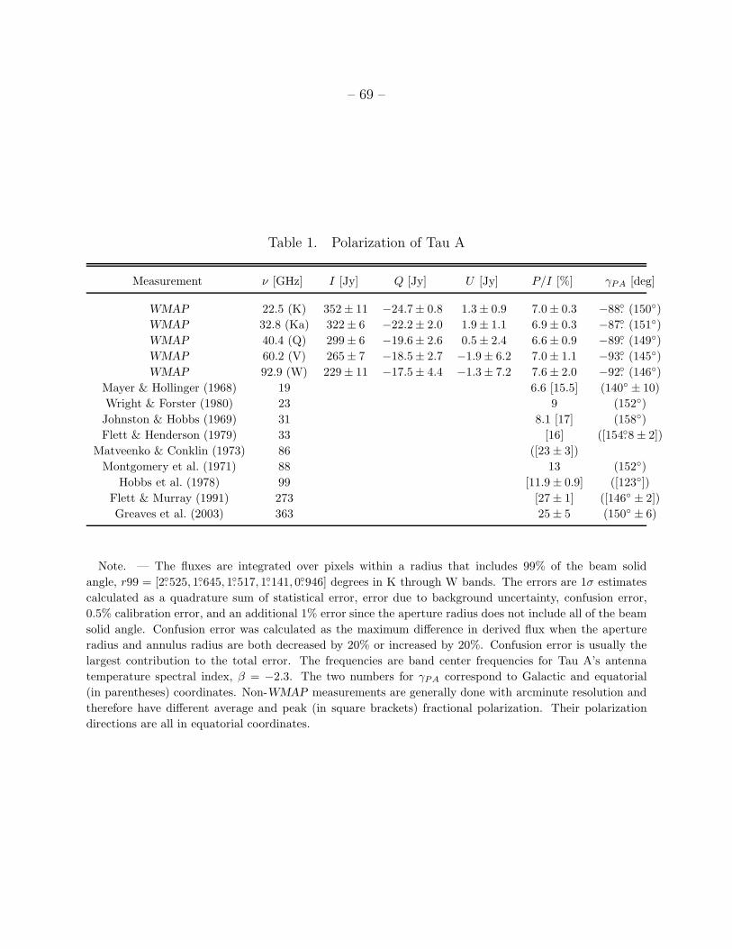
– 69 –

Table 1. Polarization of Tau A

Measurement ν [GHz] I [Jy] Q [Jy] U [Jy] P/I [%] γPA [deg]

WMAP 22.5 (K) 352 ± 11 −24.7± 0.8 1.3 ± 0.9 7.0 ± 0.3 −88. (150)

WMAP 32.8 (Ka) 322 ± 6 −22.2± 2.0 1.9 ± 1.1 6.9 ± 0.3 −87. (151)

WMAP 40.4 (Q) 299 ± 6 −19.6± 2.6 0.5 ± 2.4 6.6 ± 0.9 −89. (149)

WMAP 60.2 (V) 265 ± 7 −18.5± 2.7 −1.9 ± 6.2 7.0 ± 1.1 −93. (145)

WMAP 92.9 (W) 229 ± 11 −17.5± 4.4 −1.3 ± 7.2 7.6 ± 2.0 −92. (146)

Mayer & Hollinger (1968) 19 6.6 [15.5] (140 ± 10)

Wright & Forster (1980) 23 9 (152)

Johnston & Hobbs (1969) 31 8.1 [17] (158)

Flett & Henderson (1979) 33 [16] ([154.8 ± 2])

Matveenko & Conklin (1973) 86 ([23 ± 3])

Montgomery et al. (1971) 88 13 (152)

Hobbs et al. (1978) 99 [11.9 ± 0.9] ([123])

Flett & Murray (1991) 273 [27 ± 1] ([146 ± 2])

Greaves et al. (2003) 363 25 ± 5 (150 ± 6)

Note. — The fluxes are integrated over pixels within a radius that includes 99% of the beam solid

angle, r99 = [2.525, 1.645, 1.517, 1.141, 0.946] degrees in K through W bands. The errors are 1σ estimates

calculated as a quadrature sum of statistical error, error due to background uncertainty, confusion error,

0.5% calibration error, and an additional 1% error since the aperture radius does not include all of the beam

solid angle. Confusion error was calculated as the maximum difference in derived flux when the aperture

radius and annulus radius are both decreased by 20% or increased by 20%. Confusion error is usually the

largest contribution to the total error. The frequencies are band center frequencies for Tau A’s antenna

temperature spectral index, β = −2.3. The two numbers for γPA correspond to Galactic and equatorial

(in parentheses) coordinates. Non-WMAP measurements are generally done with arcminute resolution and

therefore have different average and peak (in square brackets) fractional polarization. Their polarization

directions are all in equatorial coordinates.

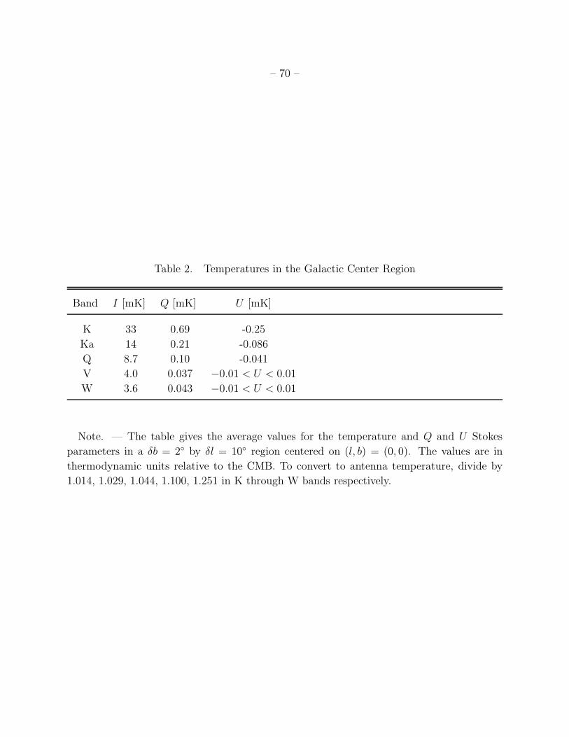
– 70 –

Table 2. Temperatures in the Galactic Center Region

Band I [mK] Q [mK] U [mK]

K 33 0.69 -0.25

Ka 14 0.21 -0.086

Q 8.7 0.10 -0.041

V 4.0 0.037 −0.01 < U < 0.01

W 3.6 0.043 −0.01 < U < 0.01

Note. — The table gives the average values for the temperature and Q and U Stokes

parameters in a δb = 2 by δl = 10 region centered on (l, b) = (0, 0). The values are in

thermodynamic units relative to the CMB. To convert to antenna temperature, divide by

1.014, 1.029, 1.044, 1.100, 1.251 in K through W bands respectively.

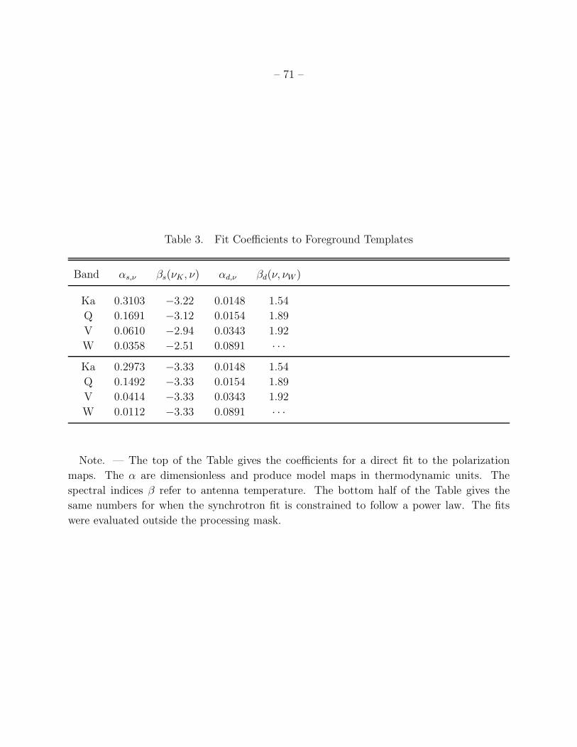
– 71 –

Table 3. Fit Coefficients to Foreground Templates

Band αs,ν βs(νK , ν) αd,ν βd(ν, νW )

Ka 0.3103 −3.22 0.0148 1.54

Q 0.1691 −3.12 0.0154 1.89

V 0.0610 −2.94 0.0343 1.92

W 0.0358 −2.51 0.0891 · · ·Ka 0.2973 −3.33 0.0148 1.54

Q 0.1492 −3.33 0.0154 1.89

V 0.0414 −3.33 0.0343 1.92

W 0.0112 −3.33 0.0891 · · ·

Note. — The top of the Table gives the coefficients for a direct fit to the polarization

maps. The α are dimensionless and produce model maps in thermodynamic units. The

spectral indices β refer to antenna temperature. The bottom half of the Table gives the

same numbers for when the synchrotron fit is constrained to follow a power law. The fits

were evaluated outside the processing mask.

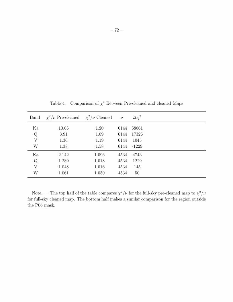
– 72 –

Table 4. Comparison of χ2 Between Pre-cleaned and cleaned Maps

Band χ2/ν Pre-cleaned χ2/ν Cleaned ν ∆χ2

Ka 10.65 1.20 6144 58061

Q 3.91 1.09 6144 17326

V 1.36 1.19 6144 1045

W 1.38 1.58 6144 -1229

Ka 2.142 1.096 4534 4743

Q 1.289 1.018 4534 1229

V 1.048 1.016 4534 145

W 1.061 1.050 4534 50

Note. — The top half of the table compares χ2/ν for the full-sky pre-cleaned map to χ2/ν

for full-sky cleaned map. The bottom half makes a similar comparison for the region outside

the P06 mask.

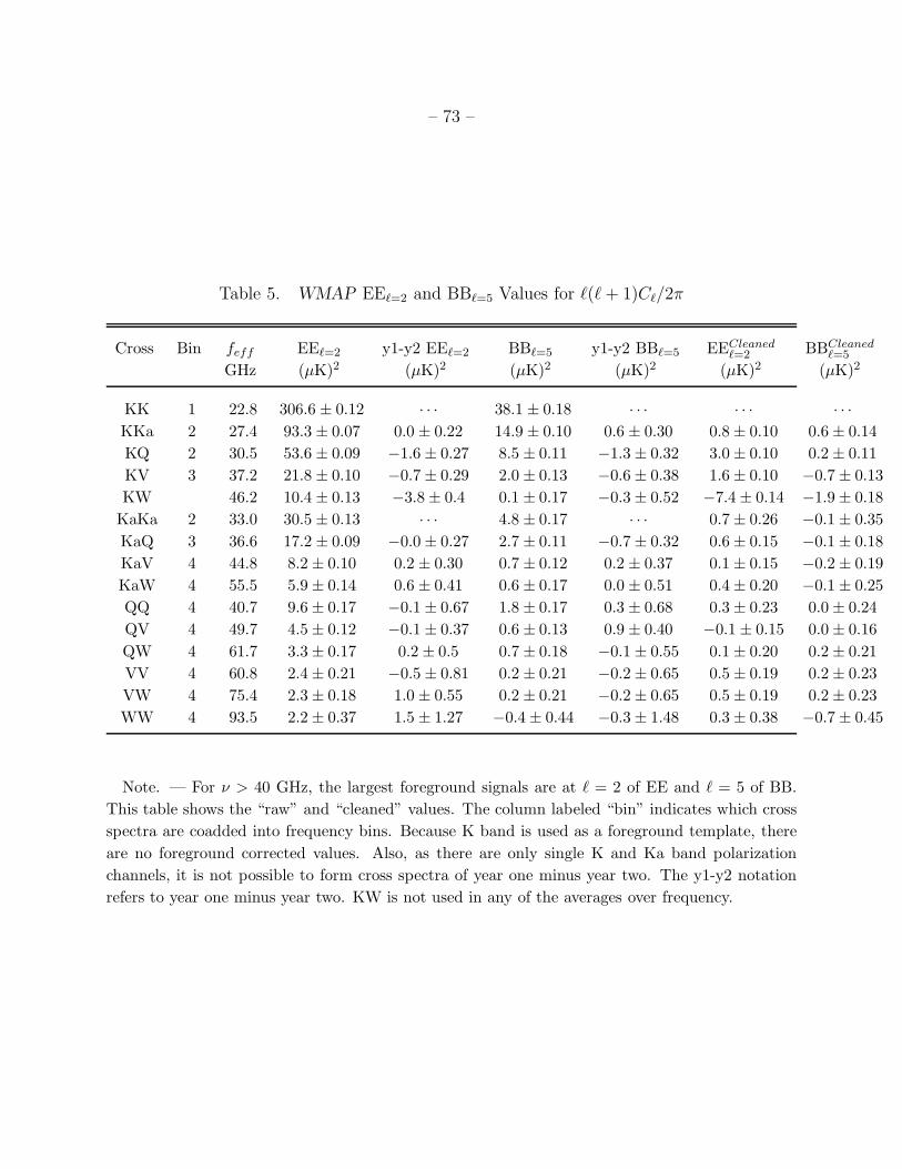
– 73 –

Table 5. WMAP EEℓ=2 and BBℓ=5 Values for ℓ(ℓ+ 1)Cℓ/2π

Cross Bin feff EEℓ=2 y1-y2 EEℓ=2 BBℓ=5 y1-y2 BBℓ=5 EECleanedℓ=2 BBCleaned

ℓ=5

GHz (µK)2 (µK)2 (µK)2 (µK)2 (µK)2 (µK)2

KK 1 22.8 306.6 ± 0.12 · · · 38.1 ± 0.18 · · · · · · · · ·KKa 2 27.4 93.3 ± 0.07 0.0 ± 0.22 14.9 ± 0.10 0.6 ± 0.30 0.8 ± 0.10 0.6 ± 0.14

KQ 2 30.5 53.6 ± 0.09 −1.6 ± 0.27 8.5 ± 0.11 −1.3 ± 0.32 3.0 ± 0.10 0.2 ± 0.11

KV 3 37.2 21.8 ± 0.10 −0.7 ± 0.29 2.0 ± 0.13 −0.6 ± 0.38 1.6 ± 0.10 −0.7 ± 0.13

KW 46.2 10.4 ± 0.13 −3.8 ± 0.4 0.1 ± 0.17 −0.3 ± 0.52 −7.4 ± 0.14 −1.9 ± 0.18

KaKa 2 33.0 30.5 ± 0.13 · · · 4.8 ± 0.17 · · · 0.7 ± 0.26 −0.1 ± 0.35

KaQ 3 36.6 17.2 ± 0.09 −0.0 ± 0.27 2.7 ± 0.11 −0.7 ± 0.32 0.6 ± 0.15 −0.1 ± 0.18

KaV 4 44.8 8.2 ± 0.10 0.2 ± 0.30 0.7 ± 0.12 0.2 ± 0.37 0.1 ± 0.15 −0.2 ± 0.19

KaW 4 55.5 5.9 ± 0.14 0.6 ± 0.41 0.6 ± 0.17 0.0 ± 0.51 0.4 ± 0.20 −0.1 ± 0.25

QQ 4 40.7 9.6 ± 0.17 −0.1 ± 0.67 1.8 ± 0.17 0.3 ± 0.68 0.3 ± 0.23 0.0 ± 0.24

QV 4 49.7 4.5 ± 0.12 −0.1 ± 0.37 0.6 ± 0.13 0.9 ± 0.40 −0.1 ± 0.15 0.0 ± 0.16

QW 4 61.7 3.3 ± 0.17 0.2 ± 0.5 0.7 ± 0.18 −0.1 ± 0.55 0.1 ± 0.20 0.2 ± 0.21

VV 4 60.8 2.4 ± 0.21 −0.5 ± 0.81 0.2 ± 0.21 −0.2 ± 0.65 0.5 ± 0.19 0.2 ± 0.23

VW 4 75.4 2.3 ± 0.18 1.0 ± 0.55 0.2 ± 0.21 −0.2 ± 0.65 0.5 ± 0.19 0.2 ± 0.23

WW 4 93.5 2.2 ± 0.37 1.5 ± 1.27 −0.4 ± 0.44 −0.3 ± 1.48 0.3 ± 0.38 −0.7 ± 0.45

Note. — For ν > 40 GHz, the largest foreground signals are at ℓ = 2 of EE and ℓ = 5 of BB.

This table shows the “raw” and “cleaned” values. The column labeled “bin” indicates which cross

spectra are coadded into frequency bins. Because K band is used as a foreground template, there

are no foreground corrected values. Also, as there are only single K and Ka band polarization

channels, it is not possible to form cross spectra of year one minus year two. The y1-y2 notation

refers to year one minus year two. KW is not used in any of the averages over frequency.

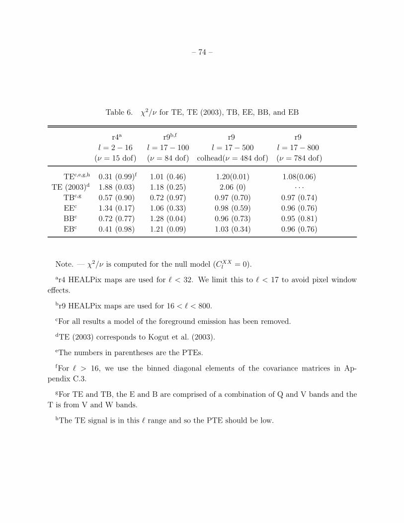
– 74 –

Table 6. χ2/ν for TE, TE (2003), TB, EE, BB, and EB

r4a r9b,f r9 r9

l = 2 − 16 l = 17 − 100 l = 17 − 500 l = 17 − 800

(ν = 15 dof) (ν = 84 dof) colhead(ν = 484 dof) (ν = 784 dof)

TEc,e,g,h 0.31 (0.99)f 1.01 (0.46) 1.20(0.01) 1.08(0.06)

TE (2003)d 1.88 (0.03) 1.18 (0.25) 2.06 (0) · · ·TBc,g 0.57 (0.90) 0.72 (0.97) 0.97 (0.70) 0.97 (0.74)

EEc 1.34 (0.17) 1.06 (0.33) 0.98 (0.59) 0.96 (0.76)

BBc 0.72 (0.77) 1.28 (0.04) 0.96 (0.73) 0.95 (0.81)

EBc 0.41 (0.98) 1.21 (0.09) 1.03 (0.34) 0.96 (0.76)

Note. — χ2/ν is computed for the null model (CXXl = 0).

ar4 HEALPix maps are used for ℓ < 32. We limit this to ℓ < 17 to avoid pixel window

effects.

br9 HEALPix maps are used for 16 < ℓ < 800.

cFor all results a model of the foreground emission has been removed.

dTE (2003) corresponds to Kogut et al. (2003).

eThe numbers in parentheses are the PTEs.

fFor ℓ > 16, we use the binned diagonal elements of the covariance matrices in Ap-

pendix C.3.

gFor TE and TB, the E and B are comprised of a combination of Q and V bands and the

T is from V and W bands.

hThe TE signal is in this ℓ range and so the PTE should be low.

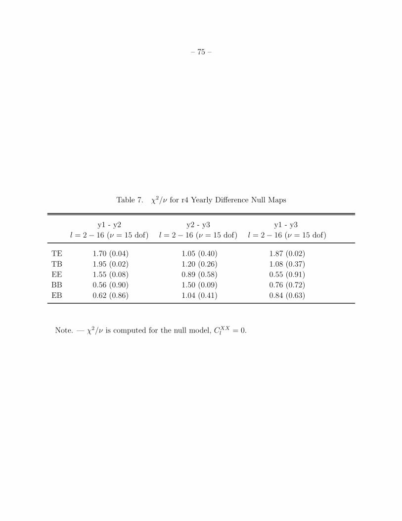
– 75 –

Table 7. χ2/ν for r4 Yearly Difference Null Maps

y1 - y2 y2 - y3 y1 - y3

l = 2 − 16 (ν = 15 dof) l = 2 − 16 (ν = 15 dof) l = 2 − 16 (ν = 15 dof)

TE 1.70 (0.04) 1.05 (0.40) 1.87 (0.02)

TB 1.95 (0.02) 1.20 (0.26) 1.08 (0.37)

EE 1.55 (0.08) 0.89 (0.58) 0.55 (0.91)

BB 0.56 (0.90) 1.50 (0.09) 0.76 (0.72)

EB 0.62 (0.86) 1.04 (0.41) 0.84 (0.63)

Note. — χ2/ν is computed for the null model, CXXl = 0.

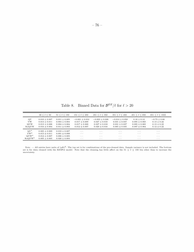
– 76 –

Table 8. Binned Data for BEE/ℓ for ℓ > 20

30 ≤ ℓ ≤ 50 51 ≤ ℓ ≤ 150 151 ≤ ℓ ≤ 250 251 ≤ ℓ ≤ 350 351 ≤ ℓ ≤ 450 451 ≤ ℓ ≤ 650 651 ≤ ℓ ≤ 1023

QV 0.010 ± 0.007 0.011 ± 0.005 −0.001 ± 0.012 −0.003 ± 0.026 −0.014 ± 0.058 0.16 ± 0.12 −0.73 ± 0.66

VW 0.013 ± 0.011 0.004 ± 0.004 0.017 ± 0.009 0.027 ± 0.018 0.031 ± 0.037 0.095 ± 0.065 0.13 ± 0.22

QVW 0.013 ± 0.006 0.004 ± 0.004 0.017 ± 0.009 0.027 ± 0.018 0.031 ± 0.037 0.095 ± 0.065 0.13 ± 0.22

KaQVW 0.016 ± 0.004 0.011 ± 0.003 0.012 ± 0.007 0.020 ± 0.016 0.065 ± 0.035 0.097 ± 0.064 0.12 ± 0.22

QVa 0.005 ± 0.009 0.018 ± 0.007 · · · · · · · · · · · · · · ·

VWa 0.013 ± 0.011 0.001 ± 0.008 · · · · · · · · · · · · · · ·

QVWa 0.012 ± 0.007 0.006 ± 0.005 · · · · · · · · · · · · · · ·

KaQVWa 0.005 ± 0.005 0.020 ± 0.004 · · · · · · · · · · · · · · ·

Note. — All entries have units of (µK)2. The top set is for combinations of the pre-cleaned data. Sample variance is not included. The bottom

set is for data cleaned with the KD3Pol model. Note that the cleaning has little affect on the 51 ≤ ℓ ≤ 150 bin other than to increase the

uncertainty.

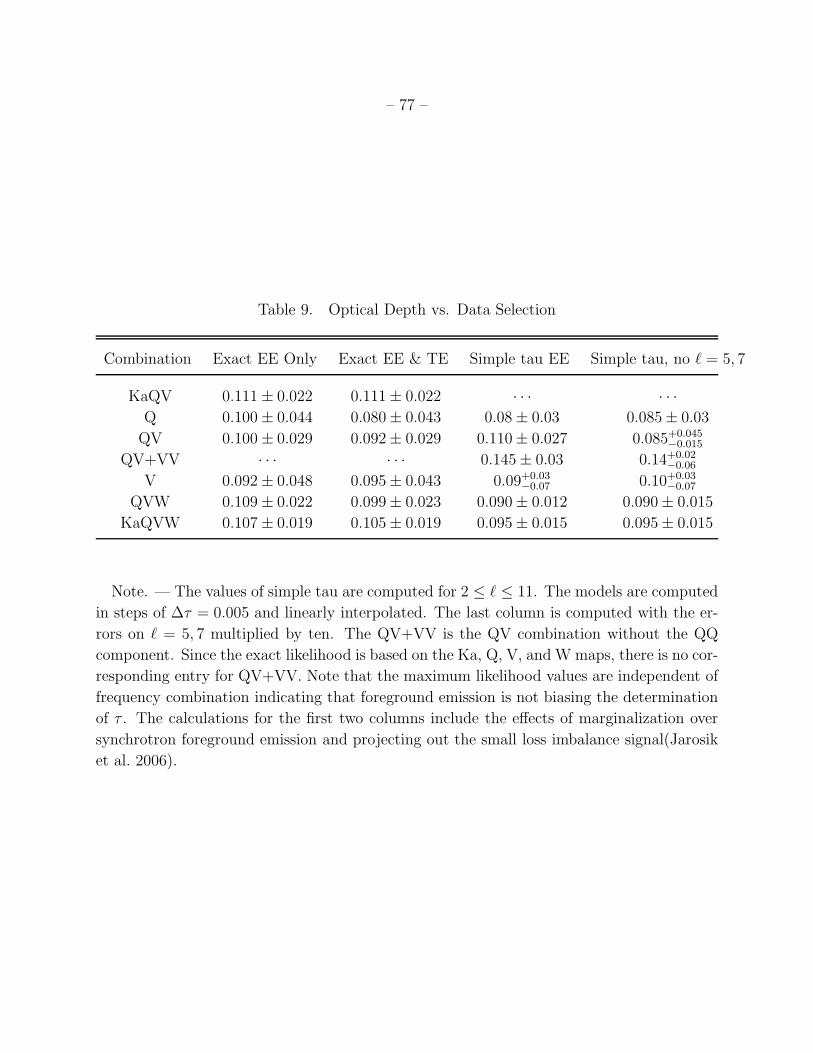
– 77 –

Table 9. Optical Depth vs. Data Selection

Combination Exact EE Only Exact EE & TE Simple tau EE Simple tau, no ℓ = 5, 7

KaQV 0.111 ± 0.022 0.111 ± 0.022 · · · · · ·Q 0.100 ± 0.044 0.080 ± 0.043 0.08 ± 0.03 0.085 ± 0.03

QV 0.100 ± 0.029 0.092 ± 0.029 0.110 ± 0.027 0.085+0.045−0.015

QV+VV · · · · · · 0.145 ± 0.03 0.14+0.02−0.06

V 0.092 ± 0.048 0.095 ± 0.043 0.09+0.03−0.07 0.10+0.03

−0.07

QVW 0.109 ± 0.022 0.099 ± 0.023 0.090 ± 0.012 0.090 ± 0.015

KaQVW 0.107 ± 0.019 0.105 ± 0.019 0.095 ± 0.015 0.095 ± 0.015

Note. — The values of simple tau are computed for 2 ≤ ℓ ≤ 11. The models are computed

in steps of ∆τ = 0.005 and linearly interpolated. The last column is computed with the er-

rors on ℓ = 5, 7 multiplied by ten. The QV+VV is the QV combination without the QQ

component. Since the exact likelihood is based on the Ka, Q, V, and W maps, there is no cor-

responding entry for QV+VV. Note that the maximum likelihood values are independent of

frequency combination indicating that foreground emission is not biasing the determination

of τ . The calculations for the first two columns include the effects of marginalization over

synchrotron foreground emission and projecting out the small loss imbalance signal(Jarosik

et al. 2006).

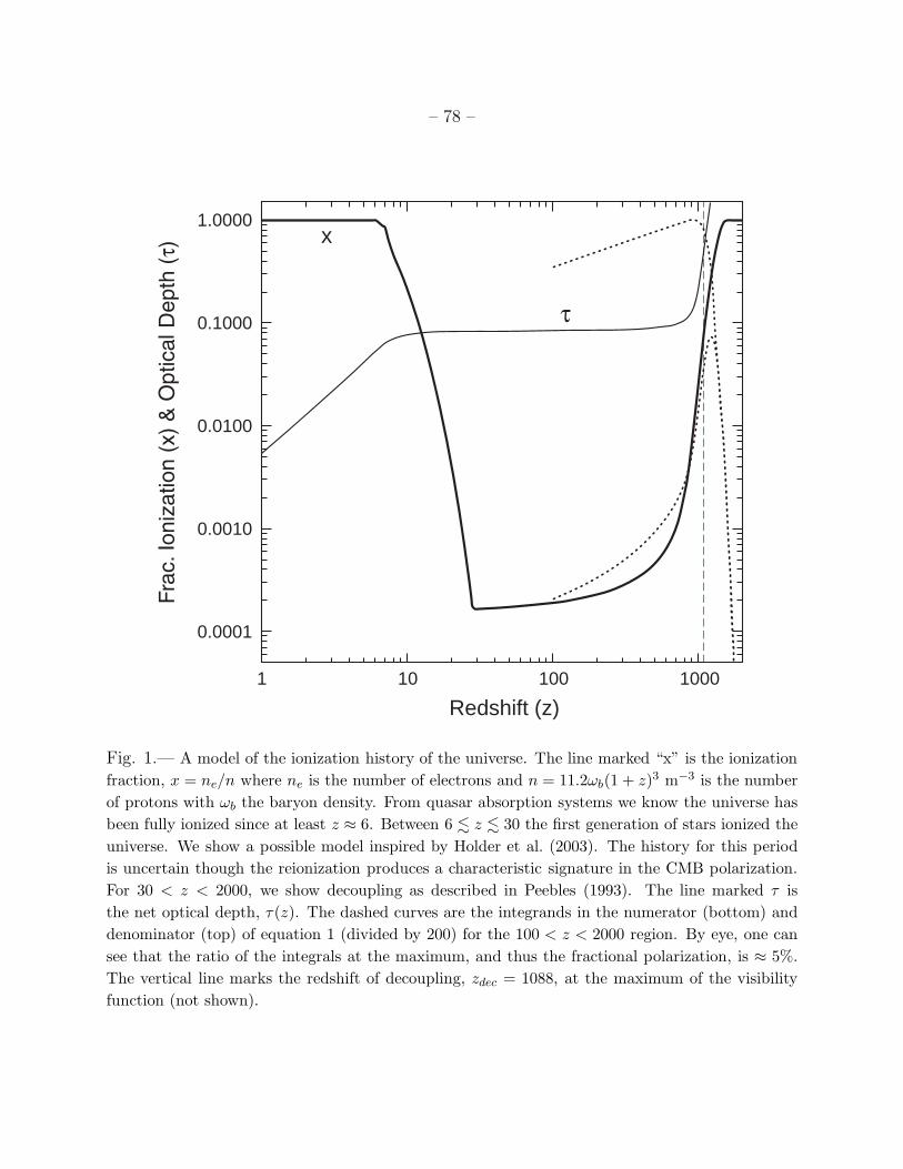
– 78 –

1

0.0001

0.0010

0.0100

0.1000

1.0000

10 100 1000

Redshift (z)

x

Fig. 1.— A model of the ionization history of the universe. The line marked “x” is the ionization

fraction, x = ne/n where ne is the number of electrons and n = 11.2ωb(1 + z)3 m−3 is the number

of protons with ωb the baryon density. From quasar absorption systems we know the universe has

been fully ionized since at least z ≈ 6. Between 6 . z . 30 the first generation of stars ionized the

universe. We show a possible model inspired by Holder et al. (2003). The history for this period

is uncertain though the reionization produces a characteristic signature in the CMB polarization.

For 30 < z < 2000, we show decoupling as described in Peebles (1993). The line marked τ is

the net optical depth, τ(z). The dashed curves are the integrands in the numerator (bottom) and

denominator (top) of equation 1 (divided by 200) for the 100 < z < 2000 region. By eye, one can

see that the ratio of the integrals at the maximum, and thus the fractional polarization, is ≈ 5%.

The vertical line marks the redshift of decoupling, zdec = 1088, at the maximum of the visibility

function (not shown).

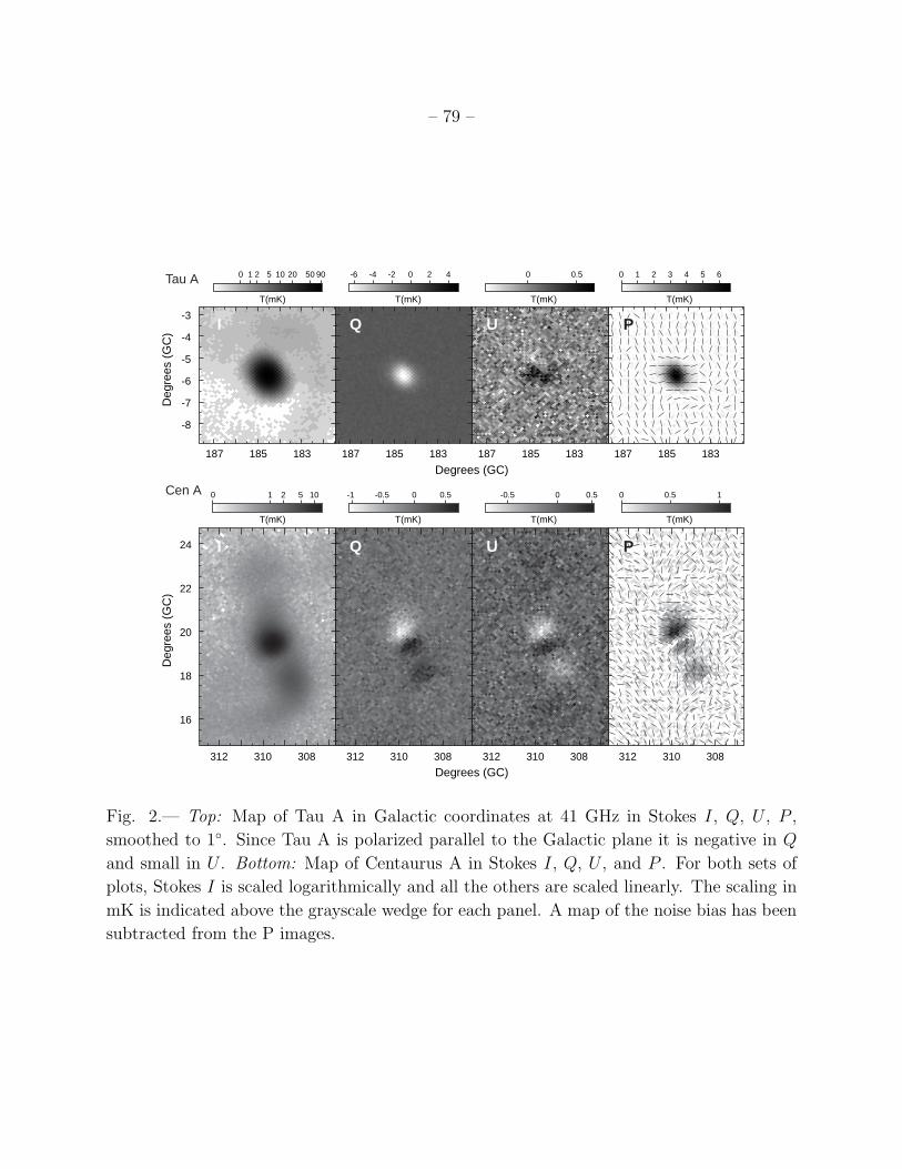
– 79 –

I Q U PP

I Q U PP

0 1 2 5 10 -1 -0.5 0 0.5 -0.5 0 0.5 0 0.5 1

0 1 2 5 10 20 50 90

T(mK) T(mK) T(mK) T(mK)

T(mK) T(mK) T(mK) T(mK)

-6 -4 -2 0 2 4 0 0.5 0 1 2 3 4 5 6

312 310 308

16

18

20

22

24

312 310 308 312 310 308 312 310 308

187 185 183

-8

-7

-6

-5

-4

-3

187 185 183 187 185 183 187 185 183

Degrees (GC)

Degrees (GC)

Deg

rees

(G

C)

Deg

rees

(G

C)

Tau A

Cen A

Fig. 2.— Top: Map of Tau A in Galactic coordinates at 41 GHz in Stokes I, Q, U , P ,

smoothed to 1. Since Tau A is polarized parallel to the Galactic plane it is negative in Q

and small in U . Bottom: Map of Centaurus A in Stokes I, Q, U , and P . For both sets of

plots, Stokes I is scaled logarithmically and all the others are scaled linearly. The scaling in

mK is indicated above the grayscale wedge for each panel. A map of the noise bias has been

subtracted from the P images.

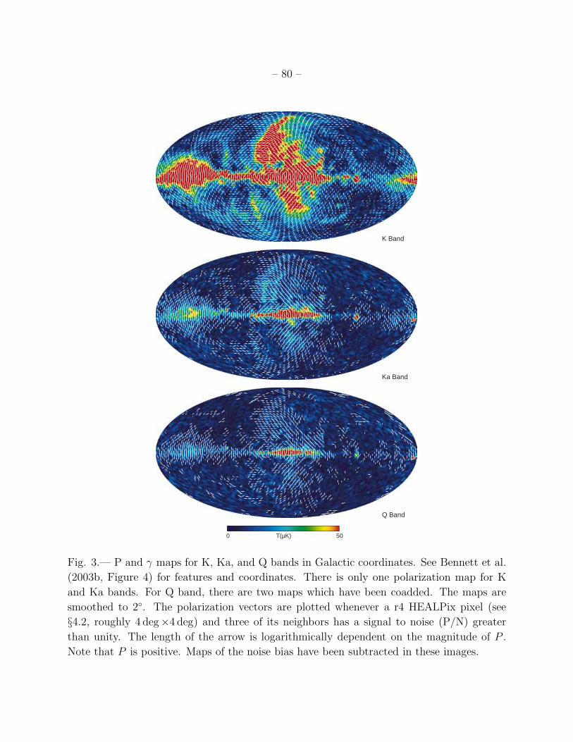
– 80 –

500 T(µK)

Q Band

Ka Band

K Band

Fig. 3.— P and γ maps for K, Ka, and Q bands in Galactic coordinates. See Bennett et al.

(2003b, Figure 4) for features and coordinates. There is only one polarization map for K

and Ka bands. For Q band, there are two maps which have been coadded. The maps are

smoothed to 2. The polarization vectors are plotted whenever a r4 HEALPix pixel (see

§4.2, roughly 4 deg×4 deg) and three of its neighbors has a signal to noise (P/N) greater

than unity. The length of the arrow is logarithmically dependent on the magnitude of P .

Note that P is positive. Maps of the noise bias have been subtracted in these images.

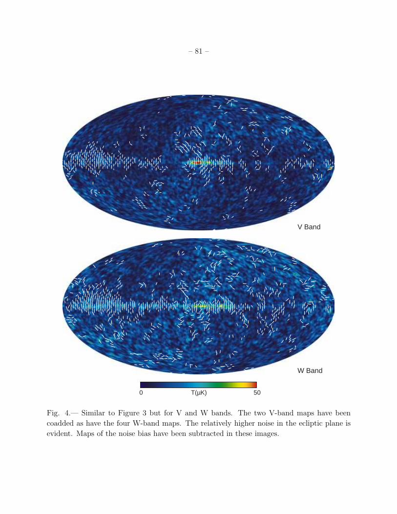
– 81 –

500 T(µK)

W Band

V Band

Fig. 4.— Similar to Figure 3 but for V and W bands. The two V-band maps have been

coadded as have the four W-band maps. The relatively higher noise in the ecliptic plane is

evident. Maps of the noise bias have been subtracted in these images.

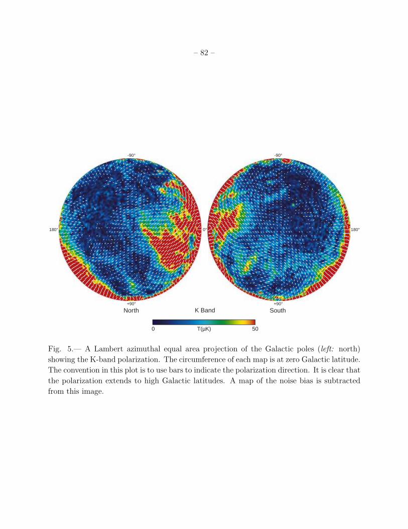
– 82 –

K Band

0°180° 180°

+90°

-90°

+90°

-90°

North South

500 T(µK)

Fig. 5.— A Lambert azimuthal equal area projection of the Galactic poles (left: north)

showing the K-band polarization. The circumference of each map is at zero Galactic latitude.

The convention in this plot is to use bars to indicate the polarization direction. It is clear that

the polarization extends to high Galactic latitudes. A map of the noise bias is subtracted

from this image.

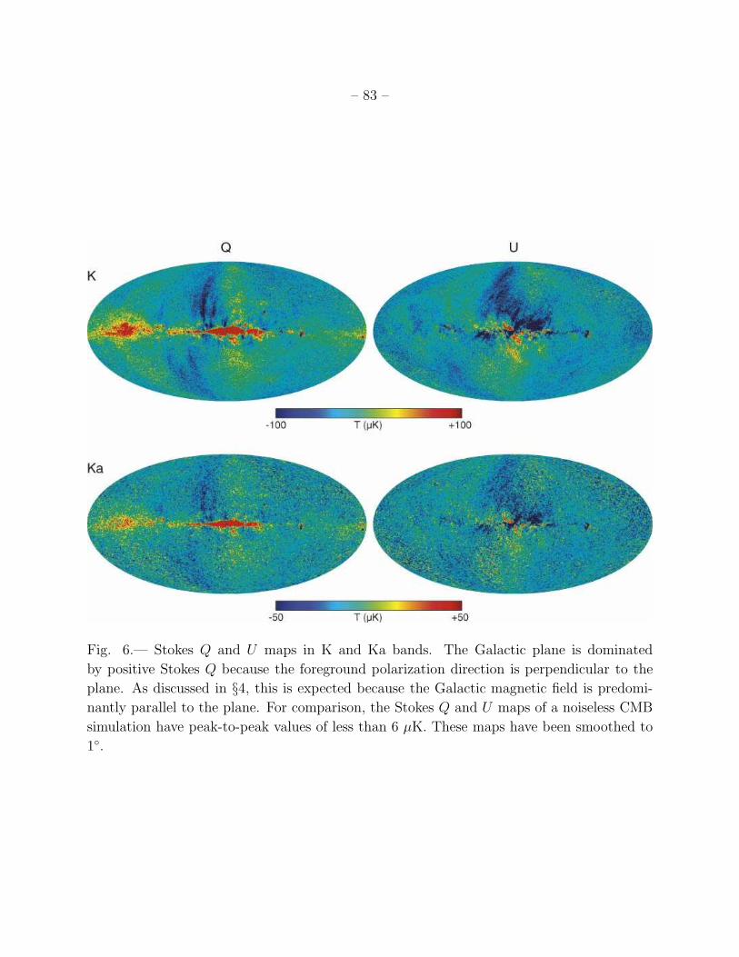
– 83 –

Fig. 6.— Stokes Q and U maps in K and Ka bands. The Galactic plane is dominated

by positive Stokes Q because the foreground polarization direction is perpendicular to the

plane. As discussed in §4, this is expected because the Galactic magnetic field is predomi-

nantly parallel to the plane. For comparison, the Stokes Q and U maps of a noiseless CMB

simulation have peak-to-peak values of less than 6 µK. These maps have been smoothed to

1.

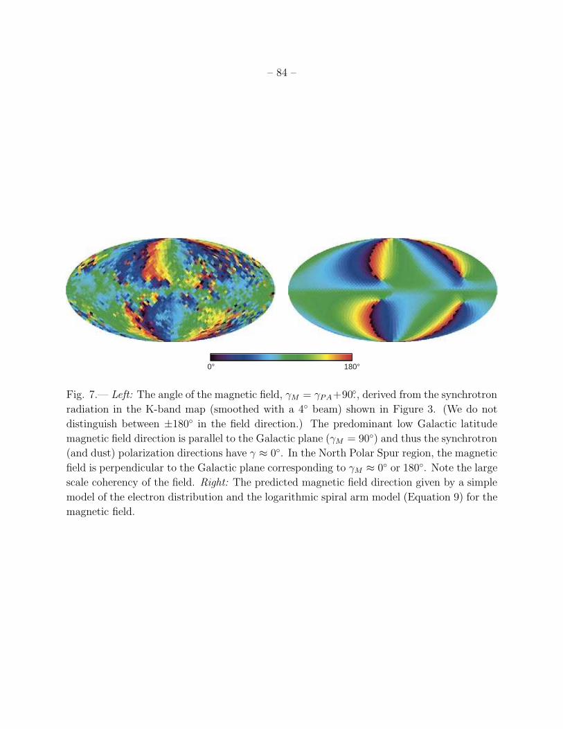
– 84 –

180°0°

Fig. 7.— Left: The angle of the magnetic field, γM = γPA+90., derived from the synchrotron

radiation in the K-band map (smoothed with a 4 beam) shown in Figure 3. (We do not

distinguish between ±180 in the field direction.) The predominant low Galactic latitude

magnetic field direction is parallel to the Galactic plane (γM = 90) and thus the synchrotron

(and dust) polarization directions have γ ≈ 0. In the North Polar Spur region, the magnetic

field is perpendicular to the Galactic plane corresponding to γM ≈ 0 or 180. Note the large

scale coherency of the field. Right: The predicted magnetic field direction given by a simple

model of the electron distribution and the logarithmic spiral arm model (Equation 9) for the

magnetic field.

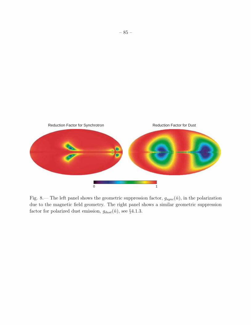
– 85 –

Reduction Factor for Synchrotron Reduction Factor for Dust

10

Fig. 8.— The left panel shows the geometric suppression factor, gsync(n), in the polarization

due to the magnetic field geometry. The right panel shows a similar geometric suppression

factor for polarized dust emission, gdust(n), see §4.1.3.

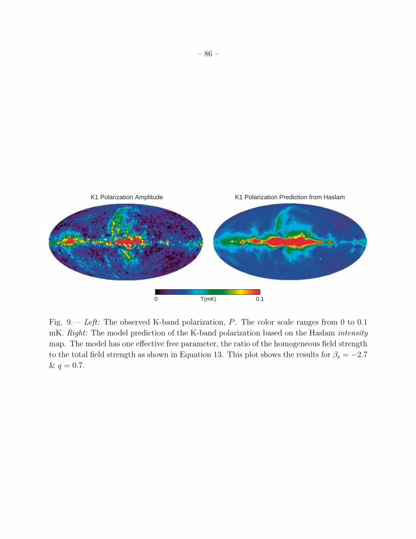
– 86 –

K1 Polarization Amplitude K1 Polarization Prediction from Haslam

0.1T(mK)0

Fig. 9.— Left: The observed K-band polarization, P . The color scale ranges from 0 to 0.1

mK. Right: The model prediction of the K-band polarization based on the Haslam intensity

map. The model has one effective free parameter, the ratio of the homogeneous field strength

to the total field strength as shown in Equation 13. This plot shows the results for βs = −2.7

& q = 0.7.

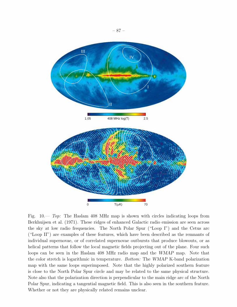
– 87 –

0 70

1.05 2.5

III

I

II

IV

Fig. 10.— Top: The Haslam 408 MHz map is shown with circles indicating loops from

Berkhuijsen et al. (1971). These ridges of enhanced Galactic radio emission are seen across

the sky at low radio frequencies. The North Polar Spur (“Loop I”) and the Cetus arc

(“Loop II”) are examples of these features, which have been described as the remnants of

individual supernovae, or of correlated supernovae outbursts that produce blowouts, or as

helical patterns that follow the local magnetic fields projecting out of the plane. Four such

loops can be seen in the Haslam 408 MHz radio map and the WMAP map. Note that

the color stretch is logarithmic in temperature. Bottom: The WMAP K-band polarization

map with the same loops superimposed. Note that the highly polarized southern feature

is close to the North Polar Spur circle and may be related to the same physical structure.

Note also that the polarization direction is perpendicular to the main ridge arc of the North

Polar Spur, indicating a tangential magnetic field. This is also seen in the southern feature.

Whether or not they are physically related remains unclear.

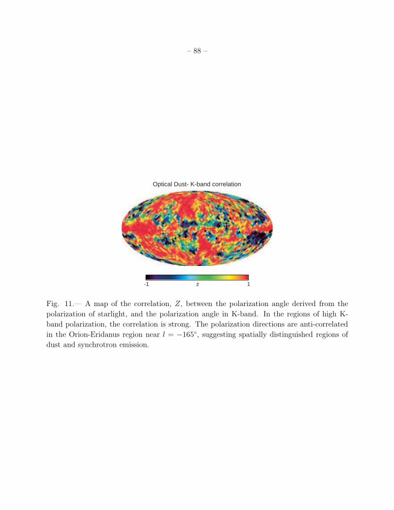
– 88 –

Optical Dust- K-band correlation

1z-1

Fig. 11.— A map of the correlation, Z, between the polarization angle derived from the

polarization of starlight, and the polarization angle in K-band. In the regions of high K-

band polarization, the correlation is strong. The polarization directions are anti-correlated

in the Orion-Eridanus region near l = −165, suggesting spatially distinguished regions of

dust and synchrotron emission.

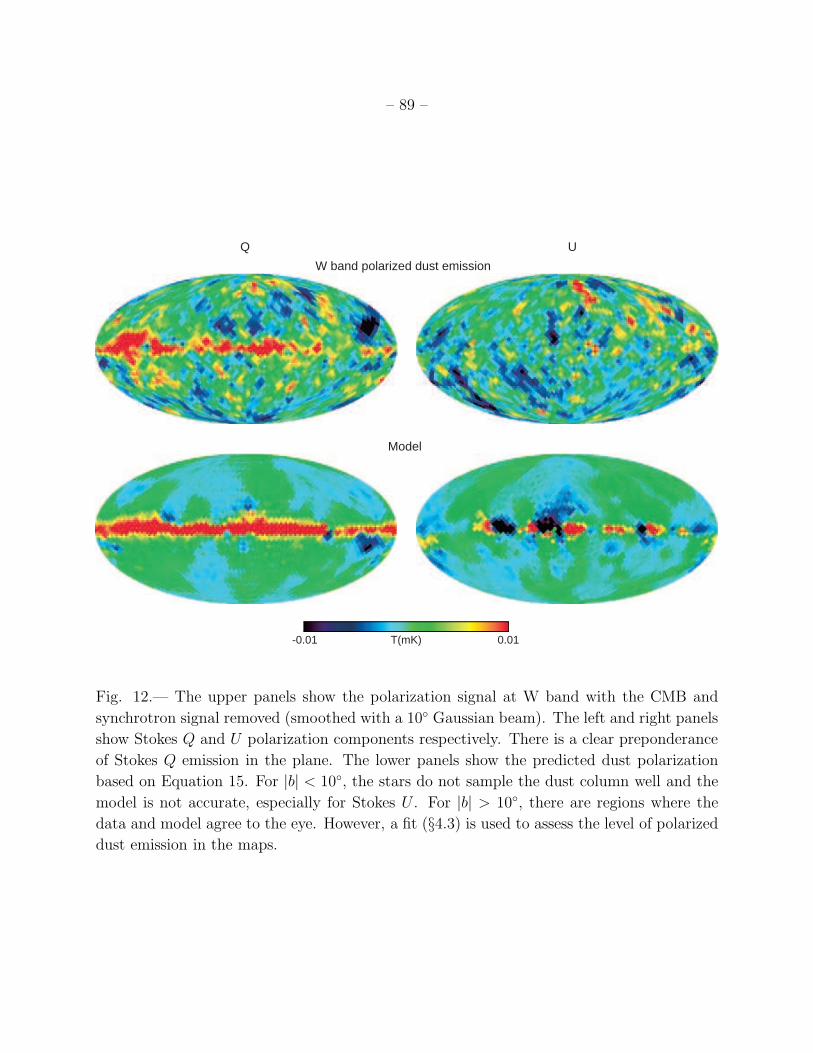
– 89 –

UQ

Model

0.01T(mK)-0.01

W band polarized dust emission

Fig. 12.— The upper panels show the polarization signal at W band with the CMB and

synchrotron signal removed (smoothed with a 10 Gaussian beam). The left and right panels

show Stokes Q and U polarization components respectively. There is a clear preponderance

of Stokes Q emission in the plane. The lower panels show the predicted dust polarization

based on Equation 15. For |b| < 10, the stars do not sample the dust column well and the

model is not accurate, especially for Stokes U . For |b| > 10, there are regions where the

data and model agree to the eye. However, a fit (§4.3) is used to assess the level of polarized

dust emission in the maps.

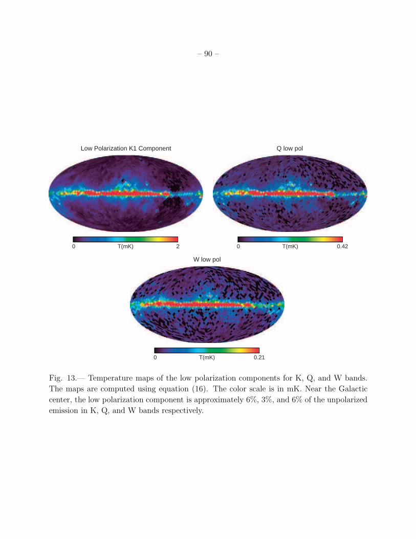
– 90 –

20 0.420

Low Polarization K1 Component Q low pol

0.21

T(mK) T(mK)

T(mK)0

W low pol

Fig. 13.— Temperature maps of the low polarization components for K, Q, and W bands.

The maps are computed using equation (16). The color scale is in mK. Near the Galactic

center, the low polarization component is approximately 6%, 3%, and 6% of the unpolarized

emission in K, Q, and W bands respectively.

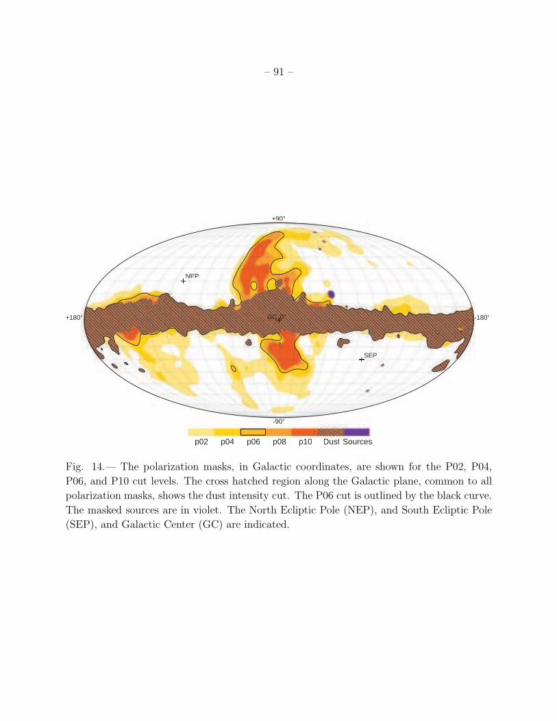
– 91 –

p02 p06p04 p08 p10 SourcesDust

0°

-90°

+90°

-180°+180°

NEP

SEP

GC

Fig. 14.— The polarization masks, in Galactic coordinates, are shown for the P02, P04,

P06, and P10 cut levels. The cross hatched region along the Galactic plane, common to all

polarization masks, shows the dust intensity cut. The P06 cut is outlined by the black curve.

The masked sources are in violet. The North Ecliptic Pole (NEP), and South Ecliptic Pole

(SEP), and Galactic Center (GC) are indicated.

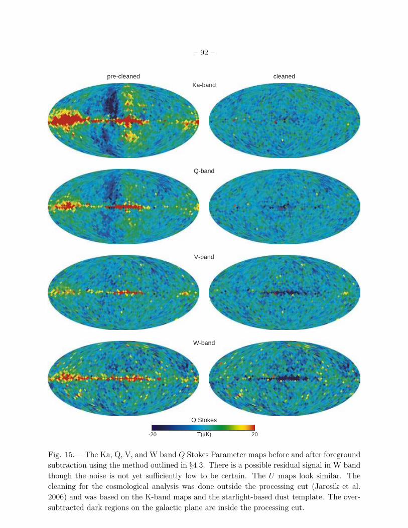
– 92 –

pre-cleaned cleaned

Q Stokes

W-band

V-band

Q-band

Ka-band

20-20

Fig. 15.— The Ka, Q, V, and W band Q Stokes Parameter maps before and after foreground

subtraction using the method outlined in §4.3. There is a possible residual signal in W band

though the noise is not yet sufficiently low to be certain. The U maps look similar. The

cleaning for the cosmological analysis was done outside the processing cut (Jarosik et al.

2006) and was based on the K-band maps and the starlight-based dust template. The over-

subtracted dark regions on the galactic plane are inside the processing cut.

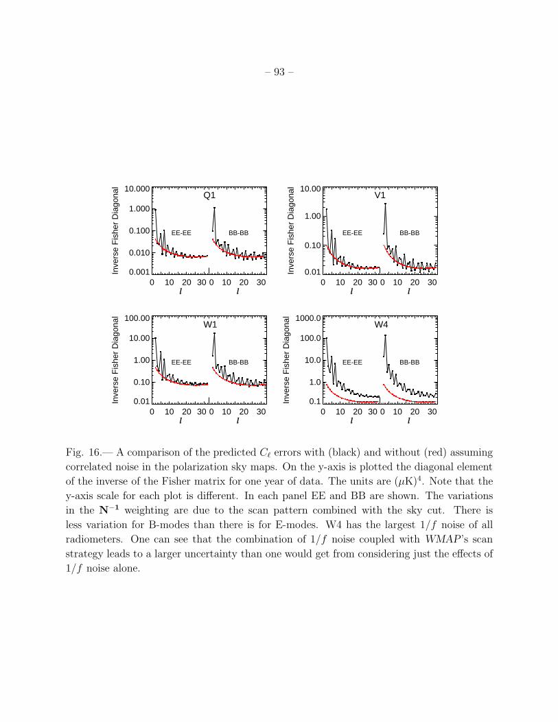
– 93 –

0.001

0.010

0.100

1.000

10.000

Inve

rse

Fis

her

Dia

gona

l

Q1

EE-EE BB-BB

0 10 20 30 l

0 10 20 30l

0.01

0.10

1.00

10.00

Inve

rse

Fis

her

Dia

gona

l

V1

EE-EE BB-BB

0 10 20 30 l

0 10 20 30l

0.01

0.10

1.00

10.00

100.00

Inve

rse

Fis

her

Dia

gona

l

W1

EE-EE BB-BB

0 10 20 30 l

0 10 20 30l

0.1

1.0

10.0

100.0

1000.0

Inve

rse

Fis

her

Dia

gona

l

W4

EE-EE BB-BB

0 10 20 30 l

0 10 20 30l

Fig. 16.— A comparison of the predicted Cℓ errors with (black) and without (red) assuming

correlated noise in the polarization sky maps. On the y-axis is plotted the diagonal element

of the inverse of the Fisher matrix for one year of data. The units are (µK)4. Note that the

y-axis scale for each plot is different. In each panel EE and BB are shown. The variations

in the N−1 weighting are due to the scan pattern combined with the sky cut. There is

less variation for B-modes than there is for E-modes. W4 has the largest 1/f noise of all

radiometers. One can see that the combination of 1/f noise coupled with WMAP’s scan

strategy leads to a larger uncertainty than one would get from considering just the effects of

1/f noise alone.

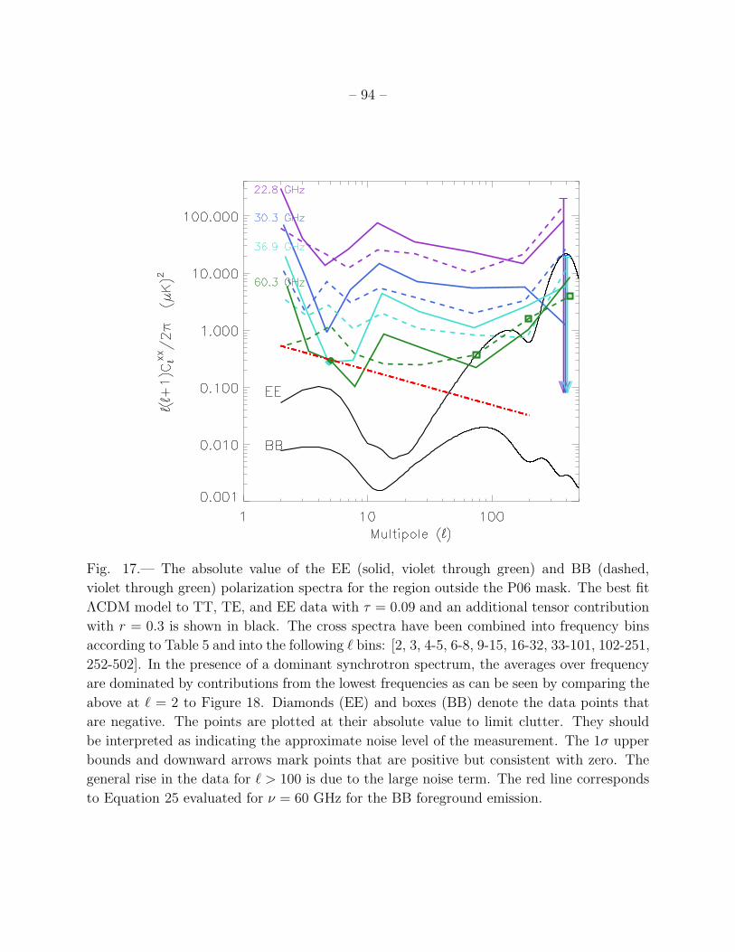
– 94 –

Fig. 17.— The absolute value of the EE (solid, violet through green) and BB (dashed,

violet through green) polarization spectra for the region outside the P06 mask. The best fit

ΛCDM model to TT, TE, and EE data with τ = 0.09 and an additional tensor contribution

with r = 0.3 is shown in black. The cross spectra have been combined into frequency bins

according to Table 5 and into the following ℓ bins: [2, 3, 4-5, 6-8, 9-15, 16-32, 33-101, 102-251,

252-502]. In the presence of a dominant synchrotron spectrum, the averages over frequency

are dominated by contributions from the lowest frequencies as can be seen by comparing the

above at ℓ = 2 to Figure 18. Diamonds (EE) and boxes (BB) denote the data points that

are negative. The points are plotted at their absolute value to limit clutter. They should

be interpreted as indicating the approximate noise level of the measurement. The 1σ upper

bounds and downward arrows mark points that are positive but consistent with zero. The

general rise in the data for ℓ > 100 is due to the large noise term. The red line corresponds

to Equation 25 evaluated for ν = 60 GHz for the BB foreground emission.

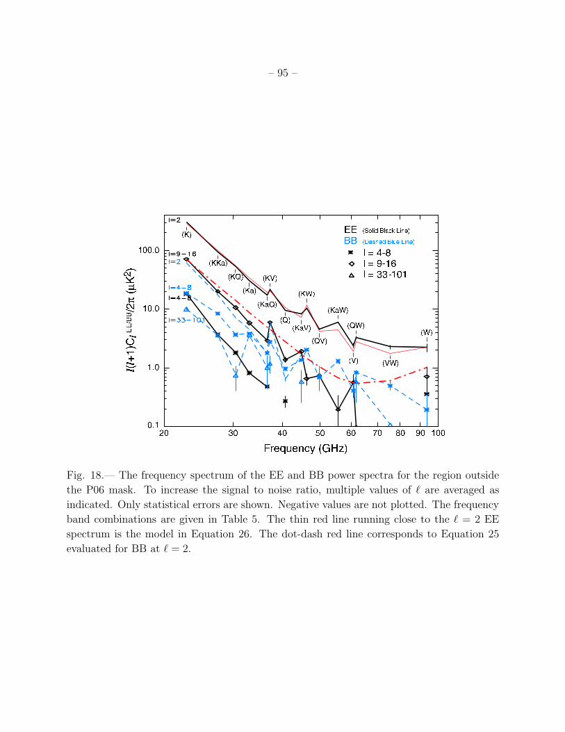
– 95 –

Fig. 18.— The frequency spectrum of the EE and BB power spectra for the region outside

the P06 mask. To increase the signal to noise ratio, multiple values of ℓ are averaged as

indicated. Only statistical errors are shown. Negative values are not plotted. The frequency

band combinations are given in Table 5. The thin red line running close to the ℓ = 2 EE

spectrum is the model in Equation 26. The dot-dash red line corresponds to Equation 25

evaluated for BB at ℓ = 2.

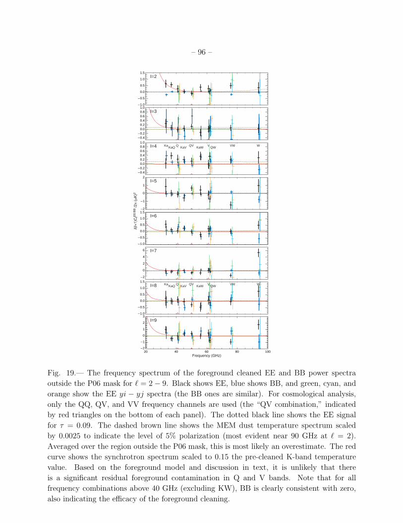
– 96 –

1.5

1.0

0.5

0.0

–0.5

–1.0

2

1

0

–1

–2

1.0

0.4

0.80.6

0.20.0

–0.2–0.4

1.0

0.60.8

0.40.20.0

–0.2–0.4

1.5

1.0

0.5

0.0

–0.5

–1.0

6

4

2

0

–21.5

1.0

0.5

0.0

–0.5

–1.03

2

1

0

–1

–220 40 60 80 100

KaKaQ KaV QV KaW V QW VW WQ

KaKaQ KaV QV KaW V QW VW WQ

I=6

I=7

I=8

I=9

I=2

I=3

I=4

I=5

Fig. 19.— The frequency spectrum of the foreground cleaned EE and BB power spectra

outside the P06 mask for ℓ = 2 − 9. Black shows EE, blue shows BB, and green, cyan, and

orange show the EE yi − yj spectra (the BB ones are similar). For cosmological analysis,

only the QQ, QV, and VV frequency channels are used (the “QV combination,” indicated

by red triangles on the bottom of each panel). The dotted black line shows the EE signal

for τ = 0.09. The dashed brown line shows the MEM dust temperature spectrum scaled

by 0.0025 to indicate the level of 5% polarization (most evident near 90 GHz at ℓ = 2).

Averaged over the region outside the P06 mask, this is most likely an overestimate. The red

curve shows the synchrotron spectrum scaled to 0.15 the pre-cleaned K-band temperature

value. Based on the foreground model and discussion in text, it is unlikely that there

is a significant residual foreground contamination in Q and V bands. Note that for all

frequency combinations above 40 GHz (excluding KW), BB is clearly consistent with zero,

also indicating the efficacy of the foreground cleaning.

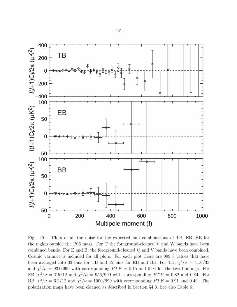
– 97 –

Multipole moment (l)0 200 400 600 800 1000

–50

0

50

100–50

0

50

100–400

0

–200

200

400

TB

EB

BB

Fig. 20.— Plots of all the noise for the expected null combinations of TB, EB, BB for

the region outside the P06 mask. For T the foreground-cleaned V and W bands have been

combined bands. For E and B, the foreground-cleaned Q and V bands have been combined.

Cosmic variance is included for all plots. For each plot there are 999 ℓ values that have

been averaged into 33 bins for TB and 12 bins for EB and BB. For TB, χ2/ν = 41.6/33

and χ2/ν = 931/999 with corresponding PTE = 0.15 and 0.94 for the two binnings. For

EB, χ2/ν = 7.5/12 and χ2/ν = 956/999 with corresponding PTE = 0.82 and 0.84. For

BB, χ2/ν = 6.2/12 and χ2/ν = 1000/999 with corresponding PTE = 0.91 and 0.49. The

polarization maps have been cleaned as described in Section §4.3. See also Table 6.

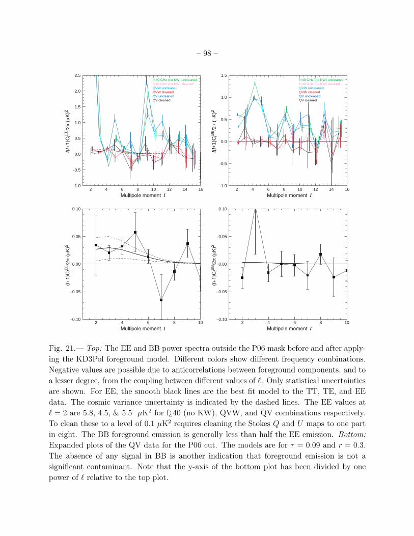
– 98 –

-1.0

-0.5

0.0

0.5

1.0

1.5

4 6 8 10 12 14 16

f>40 GHz (no KW) uncleanedf>40 GHz (no KW) cleanedQVW uncleanedQVW cleanedQV uncleanedQV cleaned

-1.0

-0.5

0.0

0.5

1.0

1.5

2.0

2.5

4 22 6 8 10 12 14 16

42 6 8 10 42 6 8 10

l(l+

1)C

lBB/2

/ (

+K

)2

–0.10

–0.05

0.00

0.05

0.10

–0.10

–0.05

0.00

0.05

0.10

f>40 GHz (no KW) uncleanedf>40 GHz (no KW) cleanedQVW uncleanedQVW cleanedQV uncleanedQV cleaned

Fig. 21.— Top: The EE and BB power spectra outside the P06 mask before and after apply-

ing the KD3Pol foreground model. Different colors show different frequency combinations.

Negative values are possible due to anticorrelations between foreground components, and to

a lesser degree, from the coupling between different values of ℓ. Only statistical uncertainties

are shown. For EE, the smooth black lines are the best fit model to the TT, TE, and EE

data. The cosmic variance uncertainty is indicated by the dashed lines. The EE values at

ℓ = 2 are 5.8, 4.5, & 5.5 µK2 for f¿40 (no KW), QVW, and QV combinations respectively.

To clean these to a level of 0.1 µK2 requires cleaning the Stokes Q and U maps to one part

in eight. The BB foreground emission is generally less than half the EE emission. Bottom:

Expanded plots of the QV data for the P06 cut. The models are for τ = 0.09 and r = 0.3.

The absence of any signal in BB is another indication that foreground emission is not a

significant contaminant. Note that the y-axis of the bottom plot has been divided by one

power of ℓ relative to the top plot.

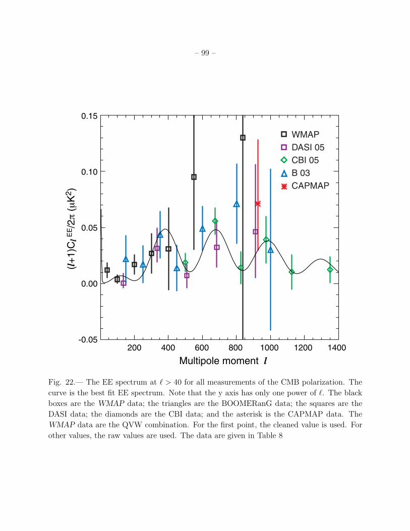
– 99 –

Multipole moment l

200-0.05

0.00

0.05

0.10

0.15

400 600 800 1000 1200 1400

(l+

1)C

lE

E/2

(K

2)

WMAP

DASI 05

CBI 05

B 03

CAPMAP

Fig. 22.— The EE spectrum at ℓ > 40 for all measurements of the CMB polarization. The

curve is the best fit EE spectrum. Note that the y axis has only one power of ℓ. The black

boxes are the WMAP data; the triangles are the BOOMERanG data; the squares are the

DASI data; the diamonds are the CBI data; and the asterisk is the CAPMAP data. The

WMAP data are the QVW combination. For the first point, the cleaned value is used. For

other values, the raw values are used. The data are given in Table 8

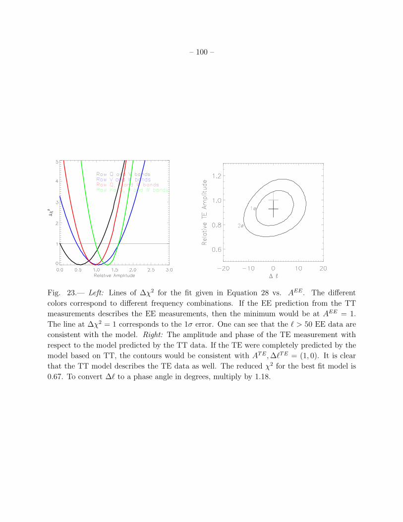
– 100 –

Fig. 23.— Left: Lines of ∆χ2 for the fit given in Equation 28 vs. AEE. The different

colors correspond to different frequency combinations. If the EE prediction from the TT

measurements describes the EE measurements, then the minimum would be at AEE = 1.

The line at ∆χ2 = 1 corresponds to the 1σ error. One can see that the ℓ > 50 EE data are

consistent with the model. Right: The amplitude and phase of the TE measurement with

respect to the model predicted by the TT data. If the TE were completely predicted by the

model based on TT, the contours would be consistent with ATE ,∆ℓTE = (1, 0). It is clear

that the TT model describes the TE data as well. The reduced χ2 for the best fit model is

0.67. To convert ∆ℓ to a phase angle in degrees, multiply by 1.18.

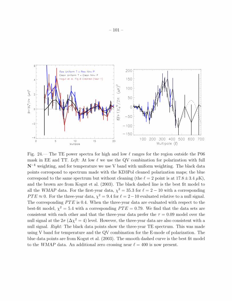
– 101 –

Fig. 24.— The TE power spectra for high and low ℓ ranges for the region outside the P06

mask in EE and TT. Left: At low ℓ we use the QV combination for polarization with full

N−1 weighting, and for temperature we use V band with uniform weighting. The black data

points correspond to spectrum made with the KD3Pol cleaned polarization maps; the blue

correspond to the same spectrum but without cleaning (the ℓ = 2 point is at 17.8± 3.4 µK),

and the brown are from Kogut et al. (2003). The black dashed line is the best fit model to

all the WMAP data. For the first-year data, χ2 = 35.3 for ℓ = 2 − 10 with a corresponding

PTE ≈ 0. For the three-year data, χ2 = 9.4 for ℓ = 2−10 evaluated relative to a null signal.

The corresponding PTE is 0.4. When the three-year data are evaluated with respect to the

best-fit model, χ2 = 5.4 with a corresponding PTE = 0.79. We find that the data sets are

consistent with each other and that the three-year data prefer the τ = 0.09 model over the

null signal at the 2σ (∆χ2 = 4) level. However, the three-year data are also consistent with a

null signal. Right: The black data points show the three-year TE spectrum. This was made

using V band for temperature and the QV combination for the E-mode of polarization. The

blue data points are from Kogut et al. (2003). The smooth dashed curve is the best fit model

to the WMAP data. An additional zero crossing near ℓ = 400 is now present.

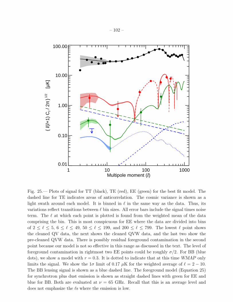
– 102 –

1 10 100 1000Multipole moment (l)

0.01

0.10

1.00

10.00

100.00

l(l+

1) C

l / 2

π 1

/2

[µK

]

Fig. 25.— Plots of signal for TT (black), TE (red), EE (green) for the best fit model. The

dashed line for TE indicates areas of anticorrelation. The cosmic variance is shown as a

light swath around each model. It is binned in ℓ in the same way as the data. Thus, its

variations reflect transitions between ℓ bin sizes. All error bars include the signal times noise

term. The ℓ at which each point is plotted is found from the weighted mean of the data

comprising the bin. This is most conspicuous for EE where the data are divided into bins

of 2 ≤ ℓ ≤ 5, 6 ≤ ℓ ≤ 49, 50 ≤ ℓ ≤ 199, and 200 ≤ ℓ ≤ 799. The lowest ℓ point shows

the cleaned QV data, the next shows the cleaned QVW data, and the last two show the

pre-cleaned QVW data. There is possibly residual foreground contamination in the second

point because our model is not so effective in this range as discussed in the text. The level of

foreground contamination in rightmost two EE points could be roughly σ/2. For BB (blue

dots), we show a model with r = 0.3. It is dotted to indicate that at this time WMAP only

limits the signal. We show the 1σ limit of 0.17 µK for the weighted average of ℓ = 2 − 10.

The BB lensing signal is shown as a blue dashed line. The foreground model (Equation 25)

for synchrotron plus dust emission is shown as straight dashed lines with green for EE and

blue for BB. Both are evaluated at ν = 65 GHz. Recall that this is an average level and

does not emphasize the ℓs where the emission is low.

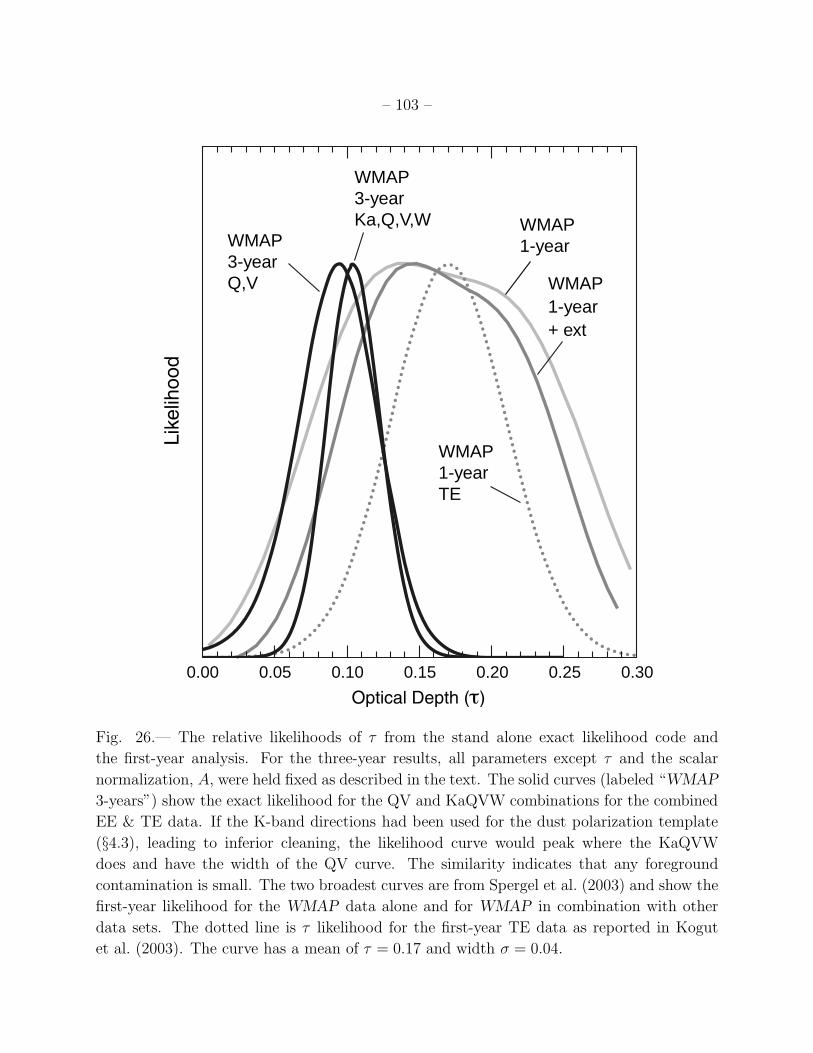
– 103 –

WMAP1-year

0.00 0.100.05 0.200.15 0.25 0.30

WMAP3-yearQ,V

WMAP3-yearKa,Q,V,W

WMAP1-yearTE

WMAP1-year+ ext

Fig. 26.— The relative likelihoods of τ from the stand alone exact likelihood code and

the first-year analysis. For the three-year results, all parameters except τ and the scalar

normalization, A, were held fixed as described in the text. The solid curves (labeled “WMAP

3-years”) show the exact likelihood for the QV and KaQVW combinations for the combined

EE & TE data. If the K-band directions had been used for the dust polarization template

(§4.3), leading to inferior cleaning, the likelihood curve would peak where the KaQVW

does and have the width of the QV curve. The similarity indicates that any foreground

contamination is small. The two broadest curves are from Spergel et al. (2003) and show the

first-year likelihood for the WMAP data alone and for WMAP in combination with other

data sets. The dotted line is τ likelihood for the first-year TE data as reported in Kogut

et al. (2003). The curve has a mean of τ = 0.17 and width σ = 0.04.

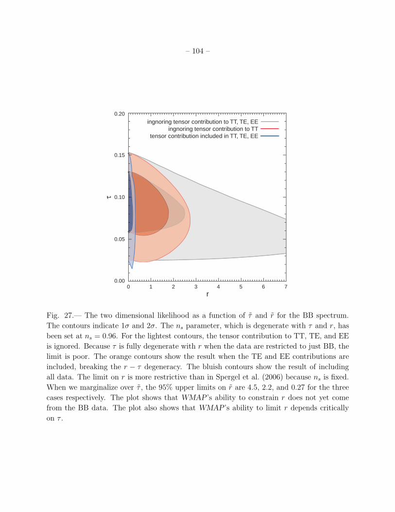
– 104 –

ingnoring tensor contribution to TT, TE, EEingnoring tensor contribution to TT

tensor contribution included in TT, TE, EE

0.20

0.15

0.10

0.05

0.000 1 2 3 4

r5 6 7

Fig. 27.— The two dimensional likelihood as a function of τ and r for the BB spectrum.

The contours indicate 1σ and 2σ. The ns parameter, which is degenerate with τ and r, has

been set at ns = 0.96. For the lightest contours, the tensor contribution to TT, TE, and EE

is ignored. Because τ is fully degenerate with r when the data are restricted to just BB, the

limit is poor. The orange contours show the result when the TE and EE contributions are

included, breaking the r − τ degeneracy. The bluish contours show the result of including

all data. The limit on r is more restrictive than in Spergel et al. (2006) because ns is fixed.

When we marginalize over τ , the 95% upper limits on r are 4.5, 2.2, and 0.27 for the three

cases respectively. The plot shows that WMAP’s ability to constrain r does not yet come

from the BB data. The plot also shows that WMAP’s ability to limit r depends critically

on τ .

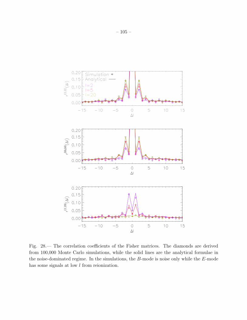
– 105 –

Fig. 28.— The correlation coefficients of the Fisher matrices. The diamonds are derived

from 100,000 Monte Carlo simulations, while the solid lines are the analytical formulae in

the noise-dominated regime. In the simulations, the B-mode is noise only while the E-mode

has some signals at low l from reionization.