Embed Size (px)
Citation preview

The Astrophysical Journal Supplement Series, 180:330–376, 2009 February doi:10.1088/0067-0049/180/2/330c© 2009. The American Astronomical Society. All rights reserved. Printed in the U.S.A.
FIVE-YEAR WILKINSON MICROWAVE ANISOTROPY PROBE∗ OBSERVATIONS: COSMOLOGICALINTERPRETATION
E. Komatsu1, J. Dunkley
2,3,4, M. R. Nolta
5, C. L. Bennett
6, B. Gold
6, G. Hinshaw
7, N. Jarosik
2, D. Larson
6, M. Limon
8,
L. Page2, D. N. Spergel
3,9, M. Halpern
10, R. S. Hill
11, A. Kogut
7, S. S. Meyer
12, G. S. Tucker
13, J. L. Weiland
11,
E. Wollack7, and E. L. Wright
141 Department of Astronomy, University of Texas, Austin, 2511 Speedway, RLM 15.306, Austin, TX 78712, USA; [email protected]
2 Department of Physics, Jadwin Hall, Princeton University, Princeton, NJ 08544-0708, USA3 Department of Astrophysical Sciences, Peyton Hall, Princeton University, Princeton, NJ 08544-1001, USA
4 Astrophysics, University of Oxford, Keble Road, Oxford, OX1 3RH, UK5 Canadian Institute for Theoretical Astrophysics, 60 St. George St, University of Toronto, Toronto, ON M5S 3H8, Canada
6 Department of Physics and Astronomy, The Johns Hopkins University, 3400 N. Charles St., Baltimore, MD 21218-2686, USA7 Code 665, NASA/Goddard Space Flight Center, Greenbelt, MD 20771, USA
8 Columbia Astrophysics Laboratory, 550 W. 120th St., Mail Code 5247, New York, NY 10027-6902, USA9 Princeton Center for Theoretical Sciences, Princeton University, Princeton, NJ 08544, USA
10 Department of Physics and Astronomy, University of British Columbia, Vancouver, BC V6T 1Z1, Canada11 Adnet Systems, Inc., 7515 Mission Dr., Suite A100, Lanham, MD 20706, USA
12 Departments of Astrophysics and Physics, KICP and EFI, University of Chicago, Chicago, IL 60637, USA13 Department of Physics, Brown University, 182 Hope St., Providence, RI 02912-1843, USA
14 UCLA Physics and Astronomy, P.O. Box 951547, Los Angeles, CA 90095-1547, USAReceived 2008 March 4; accepted 2008 June 25; published 2009 February 11
ABSTRACT
The Wilkinson Microwave Anisotropy Probe (WMAP) 5-year data provide stringent limits on deviations from theminimal, six-parameter Λ cold dark matter model. We report these limits and use them to constrain the physics ofcosmic inflation via Gaussianity, adiabaticity, the power spectrum of primordial fluctuations, gravitational waves,and spatial curvature. We also constrain models of dark energy via its equation of state, parity-violating interaction,and neutrino properties, such as mass and the number of species. We detect no convincing deviations from theminimal model. The six parameters and the corresponding 68% uncertainties, derived from the WMAP datacombined with the distance measurements from the Type Ia supernovae (SN) and the Baryon Acoustic Oscillations(BAO) in the distribution of galaxies, are: Ωbh
2 = 0.02267+0.00058−0.00059, Ωch
2 = 0.1131±0.0034, ΩΛ = 0.726±0.015,ns = 0.960 ± 0.013, τ = 0.084 ± 0.016, and Δ2
R = (2.445 ± 0.096) × 10−9 at k = 0.002 Mpc−1. From these,we derive σ8 = 0.812 ± 0.026, H0 = 70.5 ± 1.3 km s−1 Mpc−1, Ωb = 0.0456 ± 0.0015, Ωc = 0.228 ± 0.013,Ωmh2 = 0.1358+0.0037
−0.0036, zreion = 10.9 ± 1.4, and t0 = 13.72 ± 0.12 Gyr. With the WMAP data combined withBAO and SN, we find the limit on the tensor-to-scalar ratio of r < 0.22 (95% CL), and that ns > 1 is disfavoredeven when gravitational waves are included, which constrains the models of inflation that can produce significantgravitational waves, such as chaotic or power-law inflation models, or a blue spectrum, such as hybrid inflationmodels. We obtain tight, simultaneous limits on the (constant) equation of state of dark energy and the spatialcurvature of the universe: −0.14 < 1 + w < 0.12 (95% CL) and −0.0179 < Ωk < 0.0081 (95% CL). We providea set of “WMAP distance priors,” to test a variety of dark energy models with spatial curvature. We test a time-dependent w with a present value constrained as −0.33 < 1 + w0 < 0.21 (95% CL). Temperature and dark matterfluctuations are found to obey the adiabatic relation to within 8.9% and 2.1% for the axion-type and curvaton-typedark matter, respectively. The power spectra of TB and EB correlations constrain a parity-violating interaction,which rotates the polarization angle and converts E to B. The polarization angle could not be rotated more than−5.◦9 < Δα < 2.◦4 (95% CL) between the decoupling and the present epoch. We find the limit on the total massof massive neutrinos of
∑mν < 0.67 eV (95% CL), which is free from the uncertainty in the normalization
of the large-scale structure data. The number of relativistic degrees of freedom (dof), expressed in units of theeffective number of neutrino species, is constrained as Neff = 4.4 ± 1.5 (68%), consistent with the standardvalue of 3.04. Finally, quantitative limits on physically-motivated primordial non-Gaussianity parameters are−9 < f local
NL < 111 (95% CL) and −151 < fequilNL < 253 (95% CL) for the local and equilateral models, respectively.
Key words: cosmic microwave background – cosmology: observations – dark matter – early universe –instrumentation: detectors – space vehicles: instruments – telescopes
1. INTRODUCTION
Measurements of microwave background fluctuations bythe Cosmic Background Explorer (COBE; Smoot et al. 1992;Bennett et al. 1994, 1996), the Wilkinson Microwave Anisotropy
∗ WMAP is the result of a partnership between Princeton University andNASA’s Goddard Space Flight Center. Scientific guidance is provided by theWMAP Science Team.
Probe (WMAP; Bennett et al. 2003a, 2003b), and groundand balloon-borne experiments (Miller et al. 1999, 2002; deBernardis et al. 2000; Hanany et al. 2000; Netterfield et al. 2002;Ruhl et al. 2003; Mason et al. 2003; Sievers et al. 2003, 2007;Pearson et al. 2003; Readhead et al. 2004; Dickinson et al. 2004;Kuo et al. 2004, 2007; Reichardt et al. 2008; Jones et al. 2006;Montroy et al. 2006; Piacentini et al. 2006) have addressed manyof the questions that were the focus of cosmology for the past 50
330

No. 2, 2009 WMAP FIVE-YEAR OBSERVATIONS: COSMOLOGICAL INTERPRETATION 331
years: How old is the universe? How fast is it expanding? Whatis the size and shape of the universe? What is the compositionof the universe? What seeded the formation of galaxies andlarge-scale structure?
By accurately measuring the statistical properties of the mi-crowave background fluctuations, WMAP has helped establisha standard cosmology: a flat Λ cold dark matter (CDM) modelcomposed of atoms, dark matter, and dark energy, with nearlyscale-invariant adiabatic Gaussian fluctuations. With our mostrecent measurements, WMAP has measured the basic parame-ters of this cosmology to high precision: with the WMAP 5-yeardata alone, we find the density of dark matter (21.4%), the den-sity of atoms (4.4%), the expansion rate of the universe, theamplitude of density fluctuations, and their scale dependence,as well as the optical depth due to reionization (Dunkley et al.2009; also see Table 1 for summary).
Cosmologists are now focused on a new set of questions:What is the nature of the dark energy? What is the darkmatter? Did inflation seed the primordial fluctuations? If so,what is the class of the inflationary model? How did the firststars form? Microwave background observations from WMAP,Planck, and from the upcoming generation of cosmic microwavebackground (CMB) ground and balloon-borne experiments willplay an important role in addressing these questions.
This paper will discuss how the WMAP results, particularlywhen combined with other astronomical observations (mainlythe distance measurements), are now providing new insights intothese questions through constraints on gravitational waves andnonadiabatic (entropic) fluctuations, measurements of primor-dial non-Gaussianity, accurate determination of the primordialspectral index and the geometry of the universe, and limits onparity-violating interactions (see Table 2 for summary).
This paper is one of seven papers on the analysis of theWMAP 5-year data: Hinshaw et al. (2009) reported on the dataprocessing, map-making, and systematic error limits; Hill et al.(2009) on the physical optics modeling of beams and the 5-year window functions (beam transfer functions); Gold et al.(2009) on the modeling, understanding, and subtraction of thetemperature and polarized foreground emission; Wright et al.(2009) on the catalogue of point sources detected in the 5-yeartemperature data; Nolta et al. (2009) on the measurements ofthe temperature and polarization power spectra; and Dunkleyet al. (2009) on the parameter estimation methodology, thecosmological parameters inferred from the WMAP data alone,and comparison between different cosmological data sets.
This paper is organized as follows. In Section 2, we brieflysummarize new aspects of our analysis of the WMAP 5-year temperature and polarization data. In Section 3, weconstrain the spatial curvature of the observable universe,Gaussianity/adiabaticity/scale-invariance of the primordial fluc-tuations, and the amplitude of primordial gravitational waves.We discuss their implications for the physics of the early, pri-mordial universe. In Section 4, we demonstrate that the powerspectra of TB and EB correlations,15 which are usually ig-nored in the cosmological analysis, can be used to constraina certain parity-violating interaction that couples to photons. InSection 5, we explore the nature of dark energy, and in Section 6,we study the properties of neutrinos in cosmology. We concludein Section 7.
15 Here, “TB” refers to the power spectrum of a cross-correlation between thetemperature and B-mode polarization, while “EB” refers to a correlationbetween the E-mode and B-mode polarization.
2. SUMMARY OF 5-YEAR ANALYSIS
2.1. WMAP 5-year Data: Temperature and Polarization
With 5 years of observations of Jupiter and an extensivephysical optics modeling of beams (Hill et al. 2009), ourunderstanding of the beam transfer function, bl, has improvedsignificantly: the fractional beam errors, Δbl/bl , have beennearly halved in most differencing assemblies (DAs). In somecases, for example W4, the errors have been reduced by as muchas a factor of 4.
Many of the small-scale CMB experiments have been cali-brated to the WMAP 3-year data at high multipoles. Since thenew beam model raises the 5-year power spectrum almost uni-formly by ∼ 2.5% relative to the 3-year power spectrum overl � 200 (Hill et al. 2009), these small-scale CMB experimentshave been undercalibrated by the same amount, that is, ∼ 2.5%in power and 1.2% in temperature. For example, the latestArcminute Cosmology Bolometer Array Receiver (ACBAR)data (Reichardt et al. 2008) report on the calibration error of2.23% in temperature (4.5% in power), which is twice as largeas the magnitude of miscalibration; thus, we expect the effect ofmiscalibration to be subdominant in the error budget. Note thatthe change in the beam is fully consistent with the 1σ error of theprevious WMAP beam reported in Page et al. (2003). Since theACBAR calibration error includes the previous WMAP beamerror, the change in the beam should have a minimal impact onthe current ACBAR calibration.
While we use only V and W bands for the cosmologicalanalysis of the temperature data, the treatment of bl in Q bandaffects our determination of the point-source contaminationto the angular power spectrum, Aps.16 The 5-year estimateof the point-source correction, Aps = 0.011 ± 0.001 μK2 sr(Nolta et al. 2009), is slightly lower than the 3-year estimate,Aps = 0.014 ± 0.003 μK2 sr (Hinshaw et al. 2007), partlybecause more sources have been detected and masked by the5-year source mask (390 sources have been detected in the 5-year temperature data, whereas 323 sources were detected in the3-year data (Wright et al. 2009)).
Note that the uncertainty in Aps has been reduced by a factorof 3. The uncertainty in the previous estimate was inflated toinclude the lower value found by Huffenberger et al. (2006)(0.011) and higher value from our original estimate (0.017).Much of the discrepancy between these estimates is due to themultipole range over which Aps is fit. With the improved beammodel from the 5-year analysis, the dependence on the multipolerange has disappeared, and thus we no longer need to inflate ouruncertainty. See Nolta et al. (2009) for more details.
The method for cleaning foreground emission in both tem-perature and polarization data is the same as we used for the 3-year data, that is, the template-based cleaning method describedin Section 5.3 of Hinshaw et al. (2007) for temperature andSection 4.3 of Page et al. (2007) for polarization. Gold et al.(2009) described the results from the template cleaning of the5-year data with the new coefficients. In addition, Gold et al.(2009) and Dunkley et al. (2009) explored alternative modelingsof the foreground emission. All of these methods gave consistentresults. Gold et al. (2009) also described definitions of the newmasks, KQ75 and KQ85, that replace the previous masks, Kp0and Kp2, that are recommended for the analysis of Gaussianitytests and the power spectrum, respectively.
16 This quantity, Aps, is the value of the power spectrum, Cl, from unresolvedpoint sources in the Q band, in units of the antenna temperature. To convertthis value to the thermodynamic units, use Cps = 1.089Aps (Nolta et al. 2009).

332 KOMATSU ET AL. Vol. 180
The method for measuring the TT and TE spectra at highermultipoles, that is, l � 33 for TT and l � 24 for TE, is also thesame as we used for the 3-year data (Hinshaw et al. 2007). Asfor the estimation of the cosmological parameters from thesespectra, we now include the weak gravitational lensing effectof CMB due to the intervening matter fluctuations (see Lewis& Challinor 2006, for a review), which was not included inthe 3-year analysis. We continue to marginalize over a potentialcontribution from the Sunyaev–Zel’dovich effect (SZE), usingexactly the same template SZE power spectrum that we used forthe 3-year analysis: CSZE
l from Komatsu & Seljak (2002) withΩm = 0.26, Ωb = 0.044, h = 0.72, ns = 0.97, and σ8 = 0.80(see also Section 2.1 of Spergel et al. 2007). We continue to usethe V- and W -band data for estimating the high-l temperaturepower spectrum, and the Q- and V-band data for the high-lpolarization power spectra.
We have improved our treatment of the temperature andpolarization power spectra at lower multipoles, as describedbelow.
Low-l temperature. We use the Gibbs sampling techniqueand the Blackwell–Rao (BR) estimator to evaluate the likelihoodof the temperature power spectrum at l � 32 (Jewell et al.2004; Wandelt 2003; Wandelt et al. 2004; O’Dwyer et al. 2004;Eriksen et al. 2004a, 2007c, 2007b; Chu et al. 2005; Larson et al.2007). For the 3-year analysis, we used the resolution 4 InternalLinear Combination (ILC) temperature map (Nside = 16) with aGaussian smoothing of 9.◦183 (FWHM). Since the ILC maphas an intrinsic Gaussian smoothing of 1◦, we have addedan extra smoothing of 9.◦1285. We then directly evaluated thelikelihood in the pixel space for a given Cl. For the 5-yearanalysis, we use a higher-resolution map, the resolution 5 ILCmap (Nside = 32) with a smaller Gaussian smoothing of 5◦(FWHM). The potential foreground leakage due to smoothingis, therefore, reduced. The BR estimator has an advantage ofbeing much faster to compute, which is why we have adoptedthe Gibbs sampling and the BR estimator for the 5-year datarelease. We have confirmed that both the resolution 4 pixel-based likelihood and the resolution 5 Gibbs-based likelihoodyield consistent results (see Dunkley et al. 2009 for details). Bothoptions are made publicly available in the released likelihoodcode.
Low-l polarization. While we continue to use the directevaluation of the likelihood of polarization power spectra inpixel space from coadded resolution 3 (Nside = 8) polarizationmaps (Stokes Q and U maps), we now add the Ka band datato the coadded maps; we used only Q- and V-band data for the3-year analysis. We believe that we understand the polarizedforeground emission (dominated by synchrotron, traced well bythe K-band data) in the Ka band data well enough to justify theinclusion of the Ka band (Gold et al. 2009). This, with 2 years ofmore integration, has led to a significant reduction of the noisepower spectra (averaged over l = 2 − 7) in the polarization EEand BB power spectra by a factor of as much as 2.3 compared tothe 3-year analysis. As a result, the EE power spectrum averagedover l = 2 − 7 exceeds the noise by a factor of 10, that is, ourmeasurement of the EE power spectrum averaged over l = 2−7is now limited by cosmic variance and the possibility of residualforeground emission and/or systematic errors,17 rather than bynoise. In addition, we have added a capability of computing thelikelihood of TB and EB power spectra to the released likelihoodcode. This allows us to test models in which nonzero TB and
17 For our limits on the residual polarized foreground contamination, seeDunkley et al. (2008).
EB correlations can be generated. We discuss this further inSection 4.
We continue to use the Markov Chain Monte Carlo (MCMC)technique to explore the posterior distribution of cosmologi-cal parameters given the measured temperature and polarizationpower spectra. For details on the implementation and conver-gence criteria, see Dunkley et al. (2009).
2.2. Comments on Systematic Errors in the CosmologicalParameters Derived from the WMAP 5-year Data
Hinshaw et al. (2009) gave extensive descriptions of ourlimits on the systematic errors in the WMAP 5-year temperatureand polarization data. With the improved treatment of beamsand gain calibrations, we are confident that the instrumentalsystematic errors in the cosmological results derived from thetemperature data are negligible compared to the statistical errors.As for the polarization data, we find that the W-band polarizationdata still contain the systematic errors that we do not fullyunderstand, and thus we do not use the W-band polarization forthe cosmological analysis. We do not find any evidence for theunaccounted instrumental systematic errors in the other bandsthat we use for cosmology.
The most dominant systematic errors in the cosmologicalanalysis are the foreground emission. Since CMB dominatesover the foreground emission in the temperature data in V andW bands outside the galaxy mask, and we also reduce the sub-dominant foreground contamination at high Galactic latitudesfurther by using the K- and Ka-band data (for synchrotron emis-sion), the external Hα map (for free–free emission), and theexternal dust map, the systematic errors from the foregroundemission are unimportant for the temperature data, even at thelowest multipoles where the foreground is most important (Goldet al. 2009).
We, however, find that the uncertainty in our modeling of thepolarized foreground is not negligible compared to the statisticalerrors. For the 5-year polarization analysis, we have used twoindependent foreground-cleaning algorithms: one based uponthe template fitting (as developed for the 3-year analysis; seePage et al. 2007) and the other based upon the Gibbs sampling(Dunkley et al. 2008). The optical depth, τ , is the parameter thatis most affected by the uncertainty in the polarized foregroundmodel. The template fitting method gives τ = 0.087 ± 0.017.The Gibbs sampling method gives a range of values fromτ = 0.085 ± 0.025 to τ = 0.103 ± 0.018, depending uponvarious assumptions made about the properties of the polarizedsynchrotron and dust emission. Therefore, the systematic errorin τ is comparable to the statistical error.
This has an implication for the determination of the primordialtilt, ns, as there is a weak correlation between ns and τ (seeFigure 1): for τ = 0.087, we find ns = 0.963, while forτ = 0.105, we find ns = 0.98. Since the statistical error of ns is0.015, the systematic error in ns (from the polarized foreground)is comparable to the statistical one. The other parameters thatare correlated with ns, that is, the baryon density (Figure 1),the tensor-to-scalar ratio (Figure 2), and the amplitude ofnonadiabatic fluctuations (Sections 3.6.3 and 3.6.4), would besimilarly affected. For the parameters that are not correlatedwith ns or τ , the systematic errors are insignificant.
2.3. External Data Sets: Hubble Constant, Luminosity, andAngular Diameter Distances
Aside from the CMB data (including the small-scale CMBmeasurements), the main external astrophysical results that we

No. 2, 2009 WMAP FIVE-YEAR OBSERVATIONS: COSMOLOGICAL INTERPRETATION 333
Figure 1. Constraint on the primordial tilt, ns (Section 3.1.2). No running index or gravitational waves are included in the analysis. (Left) One-dimensional marginalizedconstraint on ns from the WMAP-only analysis. (Middle) Two-dimensional joint marginalized constraint (68% and 95% CL), showing a strong correlation between nsand Ωbh
2. (Right) A mild correlation with τ . None of these correlations are reduced significantly by including BAO or SN data, as these datasets are not sensitive toΩbh
2 or τ ; however, the situation changes when the gravitational wave contribution is included (see Figure 2).
shall use in this paper for the joint cosmological analysis are thefollowing distance-scale indicators.
1. A Gaussian prior on the present-day Hubble’s constantfrom the Hubble Key Project final results, H0 = 72 ±8 km s−1 Mpc−1 (Freedman et al. 2001). While the uncer-tainty is larger than the WMAP’s determination of H0 forthe minimal ΛCDM model (see Table 1), this informationimproves upon limits on the other models, such as modelswith nonzero spatial curvature.
2. The luminosity distances out to Type Ia supernovae (SNe)with their absolute magnitudes marginalized over uniformpriors. We use the “union” SN samples compiled byKowalski et al. (2008). The union compilation contains57 nearby (0.015 < z � 0.15) Type Ia SNe and 250high-z Type Ia SNe, after selection cuts. The high-z samplescontain the Type Ia SNe from the Hubble Space Telescope(HST; Knop et al. 2003; Riess et al. 2004, 2007), theSuperNova Legacy Survey (SNLS; Astier et al. 2006), theEquation of State: SupErNovae trace Cosmic Expansion(ESSENCE) survey (Wood-Vasey et al. 2007), as well asthose used in the original papers of the discovery of theacceleration of the universe (Riess et al. 1998; Perlmutteret al. 1999), and the samples from Barris et al. (2004) andTonry et al. (2003). The nearby Type Ia SNe are takenfrom Hamuy et al. (1996), Riess et al. (1999), Jha et al.(2006), Krisciunas et al. (2001, 2004a, 2004b). Kowalskiet al. (2008) have processed all of these samples using thesame light curve fitter called SALT (Guy et al. 2005), whichallowed them to combine all the data in a self-consistentfashion. The union compilation is the largest to date. Theprevious compilation by Davis et al. (2007) used a smallernumber of Type Ia SNe, and did not use the same light curvefitter for all the samples. We examine the difference in thederived ΛCDM cosmological parameters between the unioncompilation and Davis et al.’s compilation in Appendix D.While we ignore the systematic errors when we fit the TypeIa SN data, we examine the effects of systematic errors onthe ΛCDM parameters and the dark energy parameters inAppendix D.
3. Gaussian priors on the distance ratios, rs/DV (z), at z = 0.2and 0.35 measured from the Baryon Acoustic Oscillations(BAO) in the distribution of galaxies (Percival et al. 2007).The CMB observations measure the acoustic oscillations
in the photon-baryon plasma, which can be used to mea-sure the angular diameter distance to the photon decouplingepoch. The same oscillations are imprinted on the distribu-tion of matter, traced by the distribution of galaxies, whichcan be used to measure the angular distances to the galaxiesthat one observes from galaxy surveys. While both CMBand galaxies measure the same oscillations, in this paper,we shall use the term, BAO, to refer only to the oscillationsin the distribution of matter, for definiteness.
Here, we describe how we use the BAO data in more detail.The BAO can be used to measure not only the angular diameterdistance, DA(z), through the clustering perpendicular to theline of sight, but also the expansion rate of the universe, H (z),through the clustering along the line of sight. This is a powerfulprobe of dark energy; however, the accuracy of the current datadoes not allow us to extract DA(z) and H (z) separately, as onecan barely measure BAO in the spherically-averaged correlationfunction (Okumura et al. 2008).
The spherical average gives us the following effective distancemeasure (Eisenstein et al. 2005):
DV (z) ≡[
(1 + z)2D2A(z)
cz
H (z)
]1/3
, (1)
where DA(z) is the proper (not comoving) angular diameterdistance:
DA(z) = c
H0
fk
[H0
√|Ωk|∫ z
0dz′
H (z′)
](1 + z)
√|Ωk|, (2)
where fk[x] = sin x, x, and sinh x for Ωk < 0 (k = 1), Ωk = 0(k = 0), and Ωk > 0 (k = −1), respectively.
There is an additional subtlety. The peak positions of the(spherically averaged) BAO depend actually on the ratio ofDV (z) to the sound horizon size at the so-called drag epoch, zd ,at which baryons were released from photons. Note that thereis no reason why the decoupling epoch of photons, z∗, needs tobe the same as the drag epoch, zd . They would be equal onlywhen the energy density of photons and that of baryons wereequal at the decoupling epoch—more precisely, they would beequal only when R(z) ≡ 3ρb/(4ργ ) = (3Ωb/4Ωγ )/(1 + z) 0.67(Ωbh
2/0.023)[1090/(1 + z)] was unity at z = z∗. Since wehappen to live in the universe in which Ωbh
2 0.023, this ratio

334 KOMATSU ET AL. Vol. 180
Table 1Summary of the Cosmological Parameters of ΛCDM Model and the Corresponding 68% Intervals
Class Parameter WMAP 5 Year MLa WMAP+BAO+SN ML WMAP 5 Year Meanb WMAP+BAO+SN Mean
Primary 100Ωbh2 2.268 2.262 2.273 ± 0.062 2.267+0.058
−0.059Ωch
2 0.1081 0.1138 0.1099 ± 0.0062 0.1131 ± 0.0034ΩΛ 0.751 0.723 0.742 ± 0.030 0.726 ± 0.015ns 0.961 0.962 0.963+0.014
−0.015 0.960 ± 0.013τ 0.089 0.088 0.087 ± 0.017 0.084 ± 0.016
Δ2R(kc
0) 2.41 × 10⁻⁹ 2.46 × 10⁻⁹ (2.41 ± 0.11) × 10−9 (2.445 ± 0.096) × 10−9
Derived σ8 0.787 0.817 0.796 ± 0.036 0.812 ± 0.026H0 72.4 km s−1 Mpc−1 70.2 km s−1 Mpc−1 71.9+2.6
−2.7 km s−1 Mpc−1 70.5 ± 1.3 km s− Mpc−Ωb 0.0432 0.0459 0.0441 ± 0.0030 0.0456 ± 0.0015Ωc 0.206 0.231 0.214 ± 0.027 0.228 ± 0.013
Ωmh2 0.1308 0.1364 0.1326 ± 0.0063 0.1358+0.0037−0.0036
zdreion 11.2 11.3 11.0 ± 1.4 10.9 ± 1.4te0 13.69 Gyr 13.72 Gyr 13.69 ± 0.13 Gyr 13.72 ± 0.12 Gyr
Notes.a Dunkley et al. (2009). “ML” refers to the Maximum Likelihood parameters.b Dunkley et al. (2009). “Mean” refers to the mean of the posterior distribution of each parameter.c k0 = 0.002 Mpc−1. Δ2
R(k) = k3PR(k)/(2π2) (Equation (15)).d “Redshift of reionization,” if the universe was reionized instantaneously from the neutral state to the fully ionized state at zreion.e The present-day age of the universe.
Table 2Summary of the 95% Confidence Limits on Deviations from the Simple (Flat, Gaussian, Adiabatic, Power-Law) ΛCDM Model
Section Name Type WMAP 5 Year WMAP+BAO+SN
Section 3.2 Gravitational wavea No running index r < 0.43b r < 0.22Section 3.1.3 Running index No grav. wave −0.090 < dns/d ln k < 0.019c −0.068 < dns/d ln k < 0.012Section 3.4 Curvatured −0.063 < Ωk < 0.017e −0.0179 < Ωk < 0.0081f
Curvature radiusg Positive curv. Rcurv > 12 h−1 Gpc Rcurv > 22 h−1 GpcNegative curv. Rcurv > 23 h−1 Gpc Rcurv > 33 h−1 Gpc
Section 3.5 Gaussianity Local −9 < f localNL < 111h N/A
Equilateral −151 < fequilNL < 253i N/A
Section 3.6 Adiabaticity Axion α0 < 0.16j α0 < 0.072k
Curvaton α−1 < 0.011l α−1 < 0.0041m
Section 4 Parity violation Chern–Simonsn −5.◦9 < Δα < 2.◦4 N/ASection 5 Dark energy Constant wo −1.37 < 1 + w < 0.32p −0.14 < 1 + w < 0.12
Evolving w(z)q N/A −0.33 < 1 + w0 < 0.21r
Section 6.1 Neutrino masss ∑mν < 1.3 eVt ∑
mν < 0.67 eVu
Section 6.2 Neutrino species Neff > 2.3v Neff = 4.4 ± 1.5w (68%)
Notes.a In the form of the tensor-to-scalar ratio, r, at k = 0.002 Mpc−1.b Dunkley et al. (2009).c Dunkley et al. (2009).d (Constant) dark energy equation of state allowed to vary (w = −1).e With the HST prior, H0 = 72 ± 8 km s−1 Mpc−1. For w = −1, −0.052 < Ωk < 0.013 (95% CL).f For w = −1, −0.0178 < Ωk < 0.0066 (95% CL).g Rcurv = (c/H0)/
√|Ωk | = 3/√|Ωk | h−1 Gpc.
h Cleaned V + W map with lmax = 500 and the KQ75 mask, after the point-source correction.i Cleaned V + W map with lmax = 700 and the KQ75 mask, after the point-source correction.j Dunkley et al. (2009).k In terms of the adiabaticity deviation parameter, δ(c,γ )
adi = √α/3 (Equation (39)), the axion-like dark matter and photons are found to obey the adiabatic
relation (Equation (36)) to 8.9%.l Dunkley et al. (2009).m In terms of the adiabaticity deviation parameter, δ
(c,γ )adi = √
α/3 (Equation (39)), the curvaton-like dark matter and photons are found to obey theadiabatic relation (Equation (36)) to 2.1%.n For an interaction of the form given by [φ(t)/M]FαβF αβ , the polarization rotation angle is Δα = M−1
∫dta
φ.o For spatially curved universes (Ωk = 0).p With the HST prior, H0 = 72 ± 8 km s−1 Mpc−1.q For a flat universe (Ωk = 0).r w0 ≡ w(z = 0).s ∑
mν = 94(Ωνh2) eV.
t Dunkley et al. (2009).u For w = −1. For w = −1,
∑mν < 0.80 eV (95% CL).
v Dunkley et al. (2009).w With the HST prior, H0 = 72 ± 8 km s−1 Mpc−1. The 95% limit is 1.8 < Neff < 7.6.

No. 2, 2009 WMAP FIVE-YEAR OBSERVATIONS: COSMOLOGICAL INTERPRETATION 335
Table 3Sound Horizon Scales Determined by the WMAP 5-year Data
Quantity Equation 5 Year WMAP
CMB z∗ (66) 1090.51 ± 0.95CMB rs (z∗) (6) 146.8 ± 1.8 MpcMatter zd (3) 1020.5 ± 1.6Matter rs (zd ) (6) 153.3 ± 2.0 Mpc
Notes. CMB: the sound horizon scale at the photon decoupling epoch, z∗,imprinted on the CMB power spectrum; matter: the sound horizon scale at thebaryon drag epoch, zd , imprinted on the matter (galaxy) power spectrum.
is less than unity, and thus the drag epoch is slightly later thanthe photon decoupling epoch, zd < z∗. As a result, the soundhorizon size at the drag epoch happens to be slightly largerthan that at the photon decoupling epoch. In Table 3, we givethe CMB decoupling epoch, BAO drag epoch, as well as thecorresponding sound horizon radii that are determined from theWMAP 5-year data.
We use a fitting formula for zd proposed by Eisenstein & Hu(1998):
zd = 1291(Ωmh2)0.251
1 + 0.659(Ωmh2)0.828
[1 + b1(Ωbh
2)b2] , (3)
where
b1 = 0.313(Ωmh2)−0.419 [1 + 0.607(Ωmh2)0.674] , (4)
b2 = 0.238(Ωmh2)0.223. (5)
In this paper, we frequently combine the WMAP data withrs(zd )/DV (z) extracted from the Sloan Digital Sky Survey(SDSS) and the Two Degree Field Galaxy Redshift Survey(2dFGRS; Percival et al. 2007), where rs(z) is the comovingsound horizon size given by
rs(z) = c√3
∫ 1/(1+z)
0
da
a2H (a)√
1 + (3Ωb/4Ωγ )a, (6)
where Ωγ = 2.469 × 10⁻⁵h−2 for Tcmb = 2.725 K, and
H (a) = H0
[Ωm
a3+
Ωr
a4+
Ωk
a2+
ΩΛ
a3(1+weff (a))
]1/2
. (7)
The radiation density parameter, Ωr , is the sum of photons andrelativistic neutrinos,
Ωr = Ωγ (1 + 0.2271Neff) , (8)
where Neff is the effective number of neutrino species (thestandard value is 3.04). For more details on Neff , see Section 6.2.When neutrinos are nonrelativistic at a, one needs to reduce thevalue of Neff accordingly. Also, the matter density must containthe neutrino contribution when they are nonrelativistic,
Ωm = Ωc + Ωb + Ων, (9)
where Ων is related to the sum of neutrino masses as
Ων =∑
mν
94h2 eV. (10)
For more details on the neutrino mass, see Section 6.1.
All the density parameters refer to the values at the presentepoch, and add up to unity:
Ωm + Ωr + Ωk + ΩΛ = 1. (11)
Throughout this paper, we shall use ΩΛ to denote the dark energydensity parameter at present:
ΩΛ ≡ Ωde(z = 0). (12)
Here, weff(a) is the effective equation of state of dark energygiven by
weff(a) ≡ 1
ln a
∫ ln a
0d ln a′w(a′), (13)
and w(a) is the usual dark energy equation of state, that is, thedark energy pressure divided by the dark energy density:
w(a) ≡ Pde(a)
ρde(a). (14)
For vacuum energy (cosmological constant), w does not dependon time, and w = −1.
Percival et al. (2007) have determined rs(zd )/DV (z) out totwo redshifts, z = 0.2 and 0.35, as rs(zd )/DV (z = 0.2) =0.1980 ± 0.0058 and rs(zd )/DV (z = 0.35) = 0.1094 ± 0.0033,with a correlation coefficient of 0.39. We follow the descriptiongiven in Appendix A of Percival et al. (2007) to implementthese constraints in the likelihood code. We have checked thatour calculation of rs(zd ) using the above formulae (includingzd ) matches the value that they quote,18111.426 h−1 Mpc, towithin 0.2 h−1 Mpc, for their quoted cosmological parameters,Ωm = 0.25, Ωbh
2 = 0.0223, and h = 0.72.We have decided to use these results, as they measure only
the distances, and are not sensitive to the growth of structure.This property enables us to identify the information added bythe external astrophysical results more clearly. In addition tothese, we shall also use the BAO measurement by Eisensteinet al. (2005)19 and the flux power spectrum of Lyα forest fromSeljak et al. (2006) in the appropriate context.
For the 3-year data analysis in Spergel et al. (2007), we alsoused the shape of the galaxy power spectra measured from theSDSS main sample and the Luminous Red Galaxies (Tegmarket al. 2004b, 2006), and 2dFGRS (Cole et al. 2005). We havefound some tension between these data sets, which couldbe indicative of the degree by which our understanding ofnonlinearities, such as the nonlinear matter clustering, nonlinearbias, and nonlinear redshift space distortion, is still limited atlow redshifts, that is, z � 1. See Dunkley et al. (2009) for moredetailed study on this issue. Also see Sanchez & Cole (2008) onthe related subject. The galaxy power spectra should provide uswith important information on the growth of structure (whichhelps constrain the dark energy and neutrino masses) as ourunderstanding of nonlinearities improves in the future. In thispaper, we do not combine these datasets because of the limitedunderstanding of the consequences of nonlinearities.
18 In Percival et al. (2007), the authors used a different notation for the dragredshift, z∗, instead of zd . We have confirmed that they have used equation (6)of Eisenstein & Hu (1998) for rs, which makes an explicit use of the dragredshift (W. Percival 2008, private communication).19 We use a Gaussian prior on A = DV (z = 0.35)
√ΩmH 2
0 /(0.35c) =0.469(ns/0.98)−0.35 ± 0.017.
336 KOMATSU ET AL. Vol. 180
3. FLAT, GAUSSIAN, ADIABATIC, POWER-LAW ΛCDMMODEL, AND ITS ALTERNATIVES
The theory of inflation, the idea that the universe underwent abrief period of rapid accelerated expansion (Starobinsky 1979,1982; Kazanas 1980; Guth 1981; Sato 1981; Linde 1982;Albrecht & Steinhardt 1982), has become an indispensablebuilding block of the standard model of our universe.
Models of the early universe must explain the followingobservations: the universe is nearly flat and the fluctuationsobserved by WMAP appear to be nearly Gaussian (Komatsu et al.2003), scale-invariant, super-horizon, and adiabatic (Spergel& Zaldarriaga 1997; Spergel et al. 2003; Peiris et al. 2003).Inflation models have been able to explain these propertiessuccessfully (Mukhanov & Chibisov 1981; Hawking 1982;Starobinsky 1982; Guth & Pi 1982; Bardeen et al. 1983).
Although many models have been ruled out observationally(see Kinney et al. 2006; Alabidi & Lyth 2006a; Martin &Ringeval 2006, for recent surveys), there are more than 100candidate inflation models available (see Liddle & Lyth 2000;Bassett et al. 2006; Linde 2008, for reviews). Therefore, wenow focus on the question, “which model is the correct inflationmodel?” This must be answered by the observational data.
However, an inflationary expansion may not be the only wayto solve cosmological puzzles and create primordial fluctua-tions. Contraction of the primordial universe followed by abounce to expansion can, in principle, make a set of predictionsthat are qualitatively similar to those of inflation models (Khouryet al. 2001, 2002a, 2002b, 2003; Buchbinder et al. 2007, 2008;Koyama & Wands 2007; Koyama et al. 2007; Creminelli &Senatore 2007), although building concrete models and makingrobust predictions have been challenging (Kallosh et al. 2001a,2001b, 2008; Linde 2002).
There is also a fascinating possibility that one can learnsomething about the fundamental physics from cosmologicalobservations. For example, recent progress in implementing deSitter vacua and inflation in the context of string theory (seeMcAllister & Silverstein 2008, for a review) makes it possible toconnect the cosmological observations to the ingredients of thefundamental physics via their predicted properties of inflationsuch as the shape of the power spectrum, spatial curvature ofthe universe, and non-Gaussianity of primordial fluctuations.
3.1. Power Spectrum of Primordial Fluctuations
3.1.1. Motivation and Analysis
The shape of the power spectrum of primordial curvatureperturbations, PR(k), is one of the most powerful and practicaltool for distinguishing among inflation models. Inflation modelswith featureless scalar-field potentials usually predict that PR(k)is nearly a power law (Kosowsky & Turner 1995)
Δ2R(k) ≡ k3PR(k)
2π2= Δ2
R(k0)
(k
k0
)ns (k0)−1+ 12 dns/d ln k
. (15)
Here, Δ2R(k) is a useful quantity, which gives an approximate
contribution of R at a given scale per logarithmic interval in k tothe total variance of R, as 〈R2(x)〉 = ∫
d ln kΔ2R(k). It is clear
that the special case with ns = 1 and dns/d ln k = 0 results inthe “scale-invariant spectrum,” in which the contributions of Rat any scales per logarithmic interval in k to the total varianceare equal (hence, the term “scale invariance”). Following theusual terminology, we shall call ns and dns/d ln k the tilt of the
spectrum and the running index, respectively. We shall take k0to be 0.002 Mpc−1.
The significance of ns and dns/d ln k is that different inflationmodels motivated by different physics make specific, testablepredictions for the values of ns and dns/d ln k. For a givenshape of the scalar field potential, V (φ), of a single-fieldmodel, for instance, one finds that ns is given by a combinationof the first derivative and second derivative of the potential,1−ns = 3M2
pl(V′/V )2−2M2
pl(V′′/V ) (where M2
pl = 1/(8πG)is the reduced Planck mass), and dns/d ln k is given by acombination of V ′/V , V ′′/V , and V ′′′/V (see Liddle & Lyth2000, for a review).
This means that one can reconstruct the shape of V (φ) upto the first three derivatives in this way. As the expansion ratesquared is proportional to V (φ) via the Friedmann equation,H 2 = V/(3M2
pl), one can reconstruct the expansion historyduring inflation by measuring the shape of the primordial powerspectrum.
How generic are ns and dns/d ln k? They are physicallymotivated by the fact that most inflation models satisfy theslow-roll conditions, and thus deviations from a pure power-law, scale-invariant spectrum, ns = 1 and dns/d ln k = 0, areexpected to be small, and the higher-order derivative terms suchas V ′′′′ and higher are negligible. However, there is always adanger of missing some important effects, such as sharp features,when one relies too much on a simple parametrization like this.Therefore, a number of people have investigated various, moregeneral ways of reconstructing the shape of PR(k) (Matsumiyaet al. 2002, 2003; Mukherjee & Wang 2003b, 2003a, 2003c;Bridle et al. 2003; Kogo et al. 2004, 2005; Hu & Okamoto 2004;Hannestad 2004; Shafieloo & Souradeep 2004, 2008; Sealfonet al. 2005; Tocchini-Valentini et al. 2005, 2006; Spergel et al.2007; Verde & Peiris 2008) and V (φ) (Lidsey et al. 1997; Grivell& Liddle 2000; Kadota et al. 2005; Covi et al. 2006; Lesgourgues& Valkenburg 2007; Powell & Kinney 2007).
These studies have indicated that the parametrized form(Equation (15)) is basically a good fit, and no significant featureswere detected. Therefore, we do not repeat this type of analysisin this paper, but focus on constraining the parametrized formgiven by Equation (15).
Finally, let us comment on the choice of priors. We imposeuniform priors on ns and dns/d ln k, but there are other possibil-ities for the choice of priors. For example, one may impose uni-form priors on the slow-roll parameters, ε = (M2
pl/2)(V ′/V )2,η = M2
pl(V′′/V ) and ξ = M4
pl(V′V ′′′/V 2), and on the number
of e-foldings, N, rather than on ns and dns/d ln k (Peiris & Eas-ther 2006a, 2006b; Easther & Peiris 2006). It has been foundthat, as long as one imposes a reasonable lower bound on N,N > 30, both approaches yield similar results.
To constrain ns and dns/d ln k, we shall use the WMAP5-year temperature and polarization data, the small-scale CMBdata, and/or BAO and SN distance measurements. In Table 4,we summarize our results presented in Sections 3.1.2, 3.1.3,and 3.2.4.
3.1.2. Results: Tilt
First, we test the inflation models with dns/d ln k = 0 andnegligible gravitational waves. The WMAP 5-year temperatureand polarization data yield ns = 0.963+0.014
−0.015, which is slightlyabove the 3-year value with a smaller uncertainty, ns(3yr) =0.958±0.016 (Spergel et al. 2007). We shall provide the reasonfor this small upward shift in Section 3.1.3.

No. 2, 2009 WMAP FIVE-YEAR OBSERVATIONS: COSMOLOGICAL INTERPRETATION 337
Table 4Primordial Tilt ns, Running Index dns/d ln k, and Tensor-to-Scalar Ratio r
Section Model Parametera 5 Year WMAPb 5 Year WMAP = +CMBc 5 Year WMAP+ACBAR08d 5 Year WMAP+BAO+SN
Section 3.1.2 Power law ns 0.963+0.014−0.015 0.960 ± 0.014 0.964 ± 0.014 0.960 ± 0.013
Section 3.1.3 Running ns 1.031+0.054−0.055
e 1.059+0.051−0.049 1.031 ± 0.049 1.017+0.042
−0.043f
dns/d ln k −0.037 ± 0.028 −0.053 ± 0.025 −0.035+0.024−0.025 −0.028 ± 0.020g
Section 3.2.4 Tensor ns 0.986 ± 0.022 0.979 ± 0.020 0.985+0.019−0.020 0.970 ± 0.015
r <0.43 (95% CL) <0.36 (95% CL) <0.40 (95% CL) <0.22 (95% CL)
Section 3.2.4 Running ns 1.087+0.072−0.073 1.127+0.075
−0.071 1.083+0.063−0.062 1.089+0.070
−0.068+Tensor r <0.58 (95% CL) <0.64 (95% CL) <0.54 (95% CL) <0.55 (95% CL)h
dns/d ln k −0.050 ± 0.034 −0.072+0.031−0.030 −0.048 ± 0.027 −0.053 ± 0.028i
Notes.a Defined at k0 = 0.002 Mpc−1.b Dunkley et al. (2009).c “CMB” includes the small-scale CMB measurements from CBI (Mason et al. 2003; Sievers et al. 2003, 2007; Pearson et al. 2003; Readhead et al. 2004), VSA(Dickinson et al. 2004), ACBAR (Kuo et al. 2004, 2007), and BOOMERanG (Ruhl et al. 2003; Montroy et al. 2006; Piacentini et al. 2006).d “ACBAR08” is the complete ACBAR data set presented in Reichardt et al. (2008). We used the ACBAR data in the multipole range of 900 < l < 2000.e At the pivot point for WMAP only, kpivot = 0.080 Mpc−1, where ns and dns/d ln k are uncorrelated, ns (kpivot) = 0.963 ± 0.014.f At the pivot point for WMAP+BAO+SN, kpivot = 0.106 Mpc−1, where ns and dns/d ln k are uncorrelated, ns (kpivot) = 0.961 ± 0.014.g With the Lyα forest data (Seljak et al. 2006), dns/d ln k = −0.012 ± 0.012.h With the Lyα forest data (Seljak et al. 2006), r < 0.28 (95% CL).i With the Lyα forest data (Seljak et al. 2006), dns/d ln k = −0.017+0.014
−0.013.
The scale-invariant, Harrison–Zel’dovich–Peebles spectrum,ns = 1, is at 2.5 standard deviations away from the mean ofthe likelihood for the WMAP-only analysis. The significanceincreases to 3.1 standard deviations for WMAP+BAO+SN.Looking at the two-dimensional constraints that include ns, wefind that the most dominant correlation that is still left is thecorrelation between ns and Ωbh
2 (see Figure 1). The larger theΩbh
2 is, the smaller the second peak becomes, and the largerthe ns is required to compensate it. Also, the larger the Ωbh
2
is, the larger the Silk damping (diffusion damping) becomes,and the larger the ns is required to compensate it.
This argument suggests that the constraint on ns shouldimprove as we add more information from the small-scale CMBmeasurements that probe the Silk damping scales; however,the current data do not improve the constraint very much yet:ns = 0.960±0.014 from WMAP+CMB, where “CMB” includesthe small-scale CMB measurements from CBI (Mason et al.2003; Sievers et al. 2003, 2007; Pearson et al. 2003; Readheadet al. 2004), VSA (Dickinson et al. 2004), ACBAR (Kuo et al.2004, 2007), and BOOMERanG (Ruhl et al. 2003; Montroyet al. 2006; Piacentini et al. 2006), all of which go well beyondthe WMAP angular resolution, so that their small-scale data arestatistically independent of the WMAP data.
We find that the small-scale CMB data do not improve thedetermination of ns because of their relatively large statisticalerrors. We also find that the calibration and beam errors areimportant. Let us examine this using the latest ACBAR data(Reichardt et al. 2008). The WMAP+ACBAR yields 0.964 ±0.014. When the beam error of ACBAR is ignored, we findns = 0.964 ± 0.013. When the calibration error is ignored,we find ns = 0.962 ± 0.013. Therefore, both the beam andcalibration error are important in the error budget of the ACBARdata.
The Big Bang nucleosynthesis (BBN), combined with mea-surements of the deuterium-to-hydrogen ratio, D/H, fromquasar absorption systems, has been extensively used for de-termining Ωbh
2, independent of any other cosmological param-eters (see Steigman 2007, for a recent summary). The precisionof the latest determination of Ωbh
2 from BBN (Pettini et al.
2008) is comparable to that of the WMAP data-only analysis.More precise measurements of D/H will help reduce the cor-relation between ns and Ωbh
2, yielding a better determinationof ns.
There is still a bit of correlation left between ns and theelectron-scattering optical depth, τ (see Figure 1). While a bettermeasurement of τ from future WMAP observations as well asthe Planck satellite should help reduce the uncertainty in ns viaa better measurement of τ , the effect of Ωbh
2 is much larger.We find that the other datasets, such as BAO, SN, and the
shape of galaxy power spectrum from SDSS or 2dFGRS, do notimprove our constraints on ns, as these datasets are not sensitiveto Ωbh
2 or τ ; however, this will change when we include therunning index, dns/d ln k (Section 3.1.3) and/or the tensor-to-scalar ratio, r (Section 3.2.4).
3.1.3. Results: Running Index
Next, we explore more general models in which a sizablerunning index may be generated (we still do not includegravitational waves; see Section 3.2 for the analysis that includesgravitational waves). We find no evidence for dns/d ln k fromWMAP only, −0.090 < dns/d ln k < 0.019 (95% CL), orWMAP+BAO+SN −0.068 < dns/d ln k < 0.012 (95% CL).The improvement from WMAP-only to WMAP+BAO+SN isonly modest.
We find a slight upward shift from the 3-year result,dns/d ln k = −0.055+0.030
−0.031 (68% CL; Spergel et al. 2003), to the5-year result, dns/d ln k = −0.037 ± 0.028 (68% CL; WMAPonly). This is caused by a combination of three effects:
1. The 3-year number for dns/d ln k was derived from anolder analysis pipeline for the temperature data, namely theresolution 3 (instead of 4) pixel-based low-l temperaturelikelihood and a higher point-source amplitude, Aps =0.017 μK2sr.
2. With 2 years of more integration, we have a better signal-to-noise near the third acoustic peak, whose amplitude isslightly higher than the 3-year determination (Nolta et al.2009).

338 KOMATSU ET AL. Vol. 180
3. With the improved beam model (Hill et al. 2009), thetemperature power spectrum at l � 200 has been raisednearly uniformly by ∼ 2.5% (Hill et al. 2009; Nolta et al.2009).
All of these effects go in the same direction, that is, to increasethe power at high multipoles and reduce a negative runningindex. We find that these factors contribute to the upward shiftin dns/d ln k at comparable levels.
Note that an upward shift in ns for a power-law model, 0.958to 0.963 (Section 3.1.2), is not subject to (1) because the 3-yearnumber for ns was derived from an updated analysis pipelineusing the resolution 4 low-l code and Aps = 0.014 μK2 sr. Wefind that (2) and (3) contribute to the shift in ns at comparablelevels. An upward shift in σ8 from the 3-year value, 0.761, tothe 5-year value, 0.796, can be similarly explained.
We do not find any significant evidence for the runningindex when the WMAP data and small-scale CMB data (CBI,VSA, ACBAR07, BOOMERanG) are combined, −0.1002 <dns/d ln k < −0.0037 (95% CL), or the WMAP data and thelatest results from the analysis of the complete ACBAR data(Reichardt et al. 2008) are combined, −0.082 < dns/d ln k <0.015 (95% CL).
Our best 68% CL constraint from WMAP+BAO+SN shows noevidence for the running index, dns/d ln k = −0.028 ± 0.020.In order to improve upon the limit on dns/d ln k, one needs todetermine ns at small scales, as dns/d ln k is simply given bythe difference between ns’s measured at two different scales,divided by the logarithmic separation between two scales. TheLyα forest provides such information (see Section 7; alsoTable 4).
3.2. Primordial Gravitational Waves
3.2.1. Motivation
The presence of primordial gravitational waves is a robustprediction of inflation models, as the same mechanism thatgenerated primordial density fluctuations should also generateprimordial gravitational waves (Grishchuk 1975; Starobinsky1979). The amplitude of gravitational waves relative to that ofdensity fluctuations is model-dependent.
The primordial gravitational waves leave their signaturesimprinted on the CMB temperature anisotropy (Rubakov et al.1982; Fabbri & Pollock 1983; Abbott & Wise 1984; Starobinsky1985; Crittenden et al. 1993), as well as on polarization (Basko& Polnarev 1980; Bond & Efstathiou 1984; Polnarev 1985;Crittenden et al. 1993, 1995; Coulson et al. 1994).20 Thespin-2 nature of gravitational waves leads to two types of apolarization pattern on the sky (Zaldarriaga & Seljak 1997;Kamionkowski et al. 1997a): (1) the curl-free mode (E mode),in which the polarization directions are either purely radial orpurely tangential to hot/cold spots in temperature, and (2) thedivergence-free mode (B mode), in which the pattern formed bypolarization directions around hot/cold spots possess nonzerovorticity.
In the usual gravitational instability picture, in the linearregime (before shell crossing of fluid elements), velocity per-turbations can be written in terms of solely a gradient of ascalar velocity potential u, v = ∇u. This means that no vortic-ity would arise, and, therefore, no B mode polarization can begenerated from density or velocity perturbations in the linear
20 See, for example, Watanabe & Komatsu (2006) for the spectrum of theprimordial gravitational waves itself.
regime. However, primordial gravitational waves can generateboth E and B mode polarization; thus, the B mode polarizationoffers a smoking-gun signature for the presence of primordialgravitational waves (Seljak & Zaldarriaga 1997; Kamionkowskiet al. 1997a). This gives us a strong motivation to look for sig-natures of the primordial gravitational waves in CMB.
In Table 4, we summarize our constraints on the amplitude ofgravitational waves, expressed in terms of the tensor-to-scalarratio, r, defined by Equation (20).
3.2.2. Analysis
We quantify the amplitude and spectrum of primordial grav-itational waves in the following form:
Δ2h(k) ≡ k3Ph(k)
2π2= Δ2
h(k0)
(k
k0
)nt
, (16)
where we have ignored a possible scale dependence of nt (k), asthe current data cannot constrain it. Here, by Ph(k), we mean
〈hij (k)hij (k′)〉 = (2π )3Ph(k)δ3(k − k′), (17)
where hij (k) is the Fourier transform of the tensor metric per-turbations, gij = a2(δij +hij ), which can be further decomposedinto the two polarization states (+ and ×) with the appropriatepolarization tensor, e
(+,×)ij , as
hij (k) = h+(k)e+ij (k) + h×(k)e×
ij (k), (18)
with the normalization that e+ij e
+,ij = e×ij e
×,ij = 2 ande+ij e
×,ij = 0. Unless there was a parity-violating interaction term
such as f (φ)Rμνρσ Rμνρσ , where f (φ) is an arbitrary function ofa scalar field, Rμνρσ is the Riemann tensor, and Rμνρσ is a dualtensor (Lue et al. 1999), both polarization states are statisticallyindependent with the same amplitude, meaning
〈|h+|2〉 = 〈|h×|2〉 ≡ 〈|h2|〉, 〈h×h∗+〉 = 0. (19)
This implies that parity-violating correlations, such as the TBand EB correlations, must vanish. We shall explore such parity-violating correlations in Section 4 in a slightly different context.For limits on the difference between 〈|h+|2〉 and 〈|h×|2〉 from,respectively, the TB and EB spectra of the WMAP 3-year data,see Saito et al. (2007).
In any case, this definition suggests that Ph(k) is given byPh(k) = 4〈|h|2〉. Notice a factor of 4. This is the definition ofPh(k) that we have been consistently using since the first yearrelease (Peiris et al. 2003; Spergel et al. 2003, 2007; Page et al.2007). We continue to use this definition.
With this definition of Δ2h(k) (Equation (16)), we define the
tensor-to-scalar ratio, r, at k = k0, as
r ≡ Δ2h(k0)
Δ2R(k0)
, (20)
where ΔR(k) is the curvature perturbation spectrum given byEquation (15). We shall take k0 to be 0.002 Mpc−1. In thispaper, we sometimes loosely call this quantity the “amplitudeof gravitational waves.”
What about the tensor spectral tilt, nt? In single-field inflationmodels, there exists the so-called consistency relation betweenr and nt (see Liddle & Lyth 2000, for a review)
nt = − r
8. (21)

No. 2, 2009 WMAP FIVE-YEAR OBSERVATIONS: COSMOLOGICAL INTERPRETATION 339
Figure 2. Constraint on the tensor-to-scalar ratio, r, at k = 0.002 Mpc−1 (Section 3.2.4). No running index is assumed. See Figure 4 for r with the running index. In allpanels, we show the WMAP-only results in blue and WMAP+BAO+SN in red. (Left) One-dimensional marginalized distribution of r, showing the WMAP-only limit,r < 0.43 (95% CL), and WMAP+BAO+SN, r < 0.22 (95% CL). (Middle) Joint two-dimensional marginalized distribution (68% and 95% CL), showing a strongcorrelation between ns and r. (Right) Correlation between ns and Ωmh2. The BAO and SN data help to break this correlation which, in turn, reduces the correlationbetween r and ns, resulting in a factor of 2.2 better limit on r.
In order to reduce the number of parameters, we continue toimpose this relation at k = k0 = 0.002 Mpc−1. For a discussionon how to impose this constraint in a more self-consistent way,see Peiris & Easther (2006a).
To constrain r, we shall use the WMAP 5-year temperatureand polarization data, the small-scale CMB data, and/or BAOand SN distance measurements.
3.2.3. How WMAP Constrains the Amplitude of Gravitational Waves
Let us show how the gravitational wave contribution is con-strained by the WMAP data (see Figure 3). In this pedagogicalanalysis, we vary only r and τ , while adjusting the overall am-plitude of fluctuations such that the height of the first peak of thetemperature power spectrum is always held fixed. All the othercosmological parameters are fixed at Ωk = 0, Ωbh
2 = 0.02265,Ωch
2 = 0.1143, H0 = 70.1 km s−1 Mpc−1, and ns = 0.960.Note that the limit on r from this analysis should not be taken asour best limit, as this analysis ignores the correlation between rand the other cosmological parameters, especially ns. The limiton r from the full analysis will be given in Section 3.2.4.
1. (The gray contours in the left panel and the upper rightof the right panel of Figure 3.) The low-l polarization data(TE/EE/BB) at l � 10 are unable to place meaningful limitson r. A large r can be compensated by a small τ , producingnearly the same EE power spectrum at l � 10. (Recall thatthe gravitational waves also contribute to EE.) As a result,r that is as large as 10 is still allowed within 68% CL.21
2. (The red contours in the left panel and the lower leftof the right panel of Figure 3.) Such a high value of r,however, produces too negative a TE correlation between30 � l � 150. Therefore, we can improve the limit on rsignificantly—by nearly an order of magnitude—by simply
21 We have performed a similar, but different, analysis in Section 6.2 of Pageet al. (2007). In this paper, we include both the scalar and tensor contributionsto EE, whereas in Page et al. (2007), we have ignored the tensor contribution toEE and found a somewhat tighter limit, r < 4.5 (95% CL), from the low-lpolarization data. This is because, when the tensor contribution was ignored,the EE polarization could still be used to fix τ , whereas in our case, r and τ arefully degenerate when r � 1 (see Figure 3), as the EE is also dominated by thetensor contribution for such a high value of r.
using the high-l TE data. The 95% upper bound at this pointis still as large as r ∼ 2.22
3. (The blue contours in the left panel and the upper left ofthe right panel of Figure 3.) Finally, the low-l temperaturedata at l � 30 severely limit the excess low-l power dueto gravitational waves, bringing the upper bound down tor ∼ 0.2. Note that this bound is about a half of what weactually obtain from the full MCMC of the WMAP-onlyanalysis, r < 0.43 (95% CL). This is because we havefixed ns, and thus ignored the correlation between r and nsshown by Figure 2.
3.2.4. Results
Having understood which parts of the temperature and polar-ization spectra constrain r, we obtain the upper limit on r fromthe full exploration of the likelihood space using the MCMC.Figure 2 shows the one-dimensional constraint on r and thetwo-dimensional constraint on r and ns, assuming a negligi-ble running index. With the WMAP 5-year data alone, we findr < 0.43 (95% CL). Since the B-mode contributes little here,and most of the information essentially comes from TT and TE,our limit on r is highly degenerate with ns, and thus we canobtain a better limit on r only when we have a better limit on ns.
When we add BAO and SN data, the limit improves signif-icantly to r < 0.22 (95% CL). This is because the distanceinformation from BAO and SN reduces the uncertainty in thematter density, and thus it helps to determine ns better becausens is also degenerate with the matter density. This “chain of cor-relations” helped us improve our limit on r significantly fromthe previous results. This limit, r < 0.22 (95% CL), is the bestlimit on r to date.23 With the new data, we are able to get morestringent limits than our earlier analyses (Spergel et al. 2007)that combined the WMAP data with measurements of the galaxypower spectrum and found r < 0.30 (95% CL).
A dramatic reduction in the uncertainty in r has an importantimplication for ns as well. Previously, ns > 1 was within the 95%
22 See Polnarev et al. (2008); Miller et al. (2007) for a way to constrain r fromthe TE power spectrum alone.23 This is the one-dimensional marginalized 95% limit. From the jointtwo-dimensional marginalized distribution of ns and r, we find r < 0.27 (95%CL) at ns = 0.99. See Figure 2.

340 KOMATSU ET AL. Vol. 180
Figure 3. How the WMAP temperature and polarization data constrain the tensor-to-scalar ratio, r. (Left) The contours show 68% and 95% CL. The gray regionis derived from the low-l polarization data (TE/EE/BB at l � 23) only, the red region from the low-l polarization plus the high-l TE data at l � 450, and theblue region from the low-l polarization, the high-l TE, and the low-l temperature data at l � 32. (Right) The gray curves show (r, τ ) = (10, 0.050), the red curves(r, τ ) = (1.2, 0.075), and the blue curves (r, τ ) = (0.20, 0.080), which are combinations of r and τ that give the upper edge of the 68% CL contours shown on the leftpanel. The vertical lines indicate the maximum multipoles below which the data are used for each color. The data points with 68% CL errors are the WMAP 5-yearmeasurements (Nolta et al. 2009). Note that the BB power spectrum at l ∼ 130 is consistent with zero within 95% CL.
CL when the gravitational wave contribution was allowed, ow-ing to the correlation between ns and r. Now, we are beginning todisfavor ns > 1 even when r is nonzero: with WMAP+BAO+SN,we find −0.0022 < 1 − ns < 0.0589 (95% CL).24
However, these stringent limits on r and ns weaken to−0.246 < 1 − ns < 0.034 (95% CL) and r < 0.55 (95% CL)when a sizable running index is allowed. The BAO and SN datahelped reduce the uncertainty in dns/d ln k (Figure 4), but notenough to improve on the other parameters compared to theWMAP-only constraints. The Lyα forest data can improve thelimit on dns/d ln k even when r is present (see Section 7; alsoTable 4).
3.3. Implications for Inflation Models
How do the WMAP 5-year limits on ns and r constraininflationary models?25 In the context of single-field models, onecan write down ns and r in terms of the derivatives of potential,V (φ), as (Liddle & Lyth 2000)
1 − ns = 3M2pl
(V ′
V
)2
− 2M2pl
V ′′
V, (22)
r = 8M2pl
(V ′
V
)2
, (23)
where Mpl = 1/√
8πG is the reduced Planck mass, and thederivatives are evaluated at the mean value of the scalar field atthe time that a given scale leaves the horizon. These equationsmay be combined to give a relation between ns and r:
r = 8
3(1 − ns) +
16M2pl
3
V ′′
V. (24)
This equation indicates that it is the curvature of the potentialthat divides models on the ns-r plane; thus, it makes sense to
24 This is the one-dimensional marginalized 95% limit. From the jointtwo-dimensional marginalized distribution of ns and r, we find ns < 1.007(95% CL) at r = 0.2. See Figure 2.25 For recent surveys of inflation models in light of the WMAP 3-year data, seeAlabidi & Lyth (2006a), Kinney et al. (2006) and Martin & Ringeval (2006).
classify inflation models on the basis of the sign and magnitudeof the curvature of the potential (Peiris et al. 2003).26
What is the implication of our bound on r for inflationmodels? Equation (24) suggests that a large r can be generatedwhen the curvature of the potential is positive, that is, V ′′ > 0,at the field value that corresponds to the scales probed by theWMAP data. Therefore, it is a set of positive curvature modelsthat we can constrain from the limit on r. However, negativecurvature models are more difficult to constrain from r, as theytend to predict small r (Peiris et al. 2003). We shall not discussnegative curvature models in this paper: many of these models,including those based upon the Coleman–Weinberg potential,fit the WMAP data (see, e.g., Dvali et al. 1994; Shafi & Senoguz2006).
Here we shall pick three simple, but representative, forms ofV (φ) that can produce V ′′ > 0:27
1. Monomial (chaotic-type) potential, V (φ) ∝ φα . This formof the potential was proposed by, and is best known for,Linde’s chaotic inflation models (Linde 1983). This modelalso approximates a pseudo Nambu–Goldstone boson po-tential (natural inflation; Freese et al. 1990; Adams et al.1993) with the negative sign, V (φ) ∝ 1 − cos(φ/f ), whenφ/f � 1, or with the positive sign, V (φ) ∝ 1 + cos(φ/f ),when φ/f ∼ 1.28 This model can also approximate theLandau–Ginzburg type of spontaneous symmetry breakingpotential, V (φ) ∝ (φ2 − v2)2, in the appropriate limits.
26 This classification scheme is similar to, but different from, the most widelyused one, which is based upon the field value (small-field, large-field, hybrid)(Dodelson et al. 1997; Kinney 1998).27 These choices are used to sample the space of positive curvature models.Realistic potentials may be much more complicated: see, for example, Destriet al. (2008) for the WMAP 3-year limits on trinomial potentials. Also, theclassification scheme based upon derivatives of potentials sheds little light onthe models with noncanonical kinetic terms such as k-inflation(Armendariz-Picon et al. 1999; Garriga & Mukhanov 1999), ghost inflation(Arkani-Hamed et al. 2004), Dirac–Born–Infeld (DBI) inflation (Silverstein &Tong 2004; Alishahiha et al. 2004), or infrared-DBI (IR-DBI) inflation (Chen2005b, 2005a), as the tilt, ns, also depends on the derivative of the effectivespeed of sound of a scalar field (for recent constraints on this class of modelsfrom the WMAP 3-year data, see Bean et al. 2007a, 2008; Lorenz et al. 2008).28 The positive sign case, V (φ) ∝ 1 + cos(φ/f ), belongs to a negativecurvature model when φ/f � 1. See Savage et al. (2006) for constraints onthis class of models from the WMAP 3-year data.

No. 2, 2009 WMAP FIVE-YEAR OBSERVATIONS: COSMOLOGICAL INTERPRETATION 341
Figure 4. Constraint on the tensor-to-scalar ratio, r, the tilt, ns, and the running index, dns/d ln k, when all of them are allowed to vary (Section 3.2.4). In all panels,we show the WMAP-only results in blue and WMAP+BAO+SN in red. (Left) Joint two-dimensional marginalized distribution of ns and r at k = 0.002 Mpc−1 (68%and 95% CL). (Middle) ns and dns/d ln k. (Right) dns/d ln k and r. We find no evidence for the running index. While the inclusion of the running index weakensour constraint on ns and r, the data do not support any need for treating the running index as a free parameter: changes in χ2 between the power-law model and therunning model are χ2(running) − χ2(power − law) −1.8 with and without the tensor modes for WMAP5+BAO+SN, and 1.2 for WMAP5.
2. Exponential potential, V (φ) ∝ exp[−(φ/Mpl)√
2/p]. Aunique feature of this potential is that the dynamics ofinflation is exactly solvable, and the solution is a power-lawexpansion, a(t) ∝ tp, rather than an exponential one. Forthis reason, this type of model is called power-law inflation(Abbott & Wise 1984; Lucchin & Matarrese 1985). Theyoften appear in models of scalar-tensor theories of gravity(Accetta et al. 1985; La & Steinhardt 1989; Futamase &Maeda 1989; Steinhardt & Accetta 1990; Kalara et al.1990).
3. φ2 plus vacuum energy, V (φ) = V0 + m2φ2/2. Thesemodels are known as Linde’s hybrid inflation (Linde 1994).This model is a “hybrid” because the potential combines thechaotic-type (with α = 2) with a Higgs-like potential for thesecond field (which is not shown here). This model behavesas if it were a single-field model until the second fieldterminates inflation when φ reaches some critical value.When φ � (2V0)1/2/m, this model is the same as model1 with α = 2, although one of Linde’s motivation was toavoid having such a large field value that exceeds Mpl.
These potentials29 make the following predictions for r andns as a function of their parameters:
1. r = 8(1 − ns) αα+2
2. r = 8(1 − ns)3. r = 8(1 − ns)
φ2
2φ2−1.
Here, for 3, we have defined a dimensionless variable,φ ≡ mφ/(2V0)1/2. This model approaches model 1 with α = 2for φ � 1 and yields the scale-invariant spectrum, ns = 1,when φ = 1/
√2.
We summarize our findings below, and in Figure 5.
1. Assuming that the monomial potentials are valid to the endof inflation including the reheating of the universe, onecan relate ns and r to the number of e-folds of inflation,N ≡ ln(aend/aWMAP), between the expansion factors at theend of inflation, aend, and the epoch when the wavelengthof fluctuations that we probe with WMAP leave the horizon
29 In the language of Section 3.4 of Peiris et al. (2003), the models 1 and 2belong to “small positive curvature models,” and model 3 to “large positivecurvature models” for φ � 1, “small positive curvature models” for φ � 1,and “intermediate positive curvature models” for φ ∼ 1.
during inflation, aWMAP. The relations are (Liddle & Lyth2000)
r = 4α
N, 1 − ns = α + 2
2N. (25)
We take N = 50 and 60 as a reasonable range (Liddle &Leach 2003). For α = 4, that is, inflation by a masslessself-interacting scalar field V (φ) = (λ/4)φ4, we find thatboth N = 50 and 60 are far away from the 95% regionand they are excluded convincingly at more than 99% CL.For α = 2, that is, inflation by a massive free scalar fieldV (φ) = (1/2)m2φ2, the model with N = 50 lies outsideof the 68% region, whereas the model with N = 60 isat the boundary of the 68% region. Therefore, both ofthese models are consistent with the data within the 95%CL. While this limit applies to a single massive free field,Easther & McAllister (2006) showed that a model withmany massive axion fields (N-flation model; Dimopouloset al. 2005) can shift the predicted ns further away fromunity,
1 − nN.f.s = (
1 − ns.f.s
) (1 +
β
2
), (26)
where “N.f” refers to “N fields” and “s.f.” to “single field,”and β is a free parameter of the model. Easther & McAllister(2006) argued that β ∼ 1/2 is favored, for which 1 − ns islarger than the single-field prediction by as much as 25%.The prediction for the tensor-to-scalar ratio, r, is the same asthe single-field case (Alabidi & Lyth 2006b). Therefore, thismodel lies outside of the 95% region for N = 50. As usual,however, these monomial potentials can be made a better fitto the data by invoking a nonminimal coupling between theinflaton and gravity, as the nonminimal coupling can reducer to negligible levels (Komatsu & Futamase 1999; Hwang& Noh 1998; Tsujikawa & Gumjudpai 2004). Piao (2006)has shown that N-flation models with monomial potentials,V (φ) ∝ φα , generically predict ns that is smaller than thecorresponding single-field predictions.
2. For an exponential potential, r and ns are uniquely deter-mined by a single parameter, p, that determines a power-lawindex of the expansion factor, a(t) ∝ tp, as
r = 16
p, 1 − ns = 2
p. (27)

342 KOMATSU ET AL. Vol. 180
Figure 5. Constraint on three representative inflation models whose potentialis positively curved, V ′′ > 0 (Section 3.3). The contours show the 68% and95% CL derived from WMAP+BAO+SN. (Top) The monomial, chaotic-typepotential, V (φ) ∝ φα (Linde 1983), with α = 4 (solid) and α = 2 (dashed)for single-field models, and α = 2 for multiaxion field models with β = 1/2(Easther & McAllister 2006; dotted). The symbols show the predictions fromeach of these models with the number of e-folds of inflation equal to 50 and 60.The λφ4 potential is excluded convincingly, the m2φ2 single-field model liesoutside of (at the boundary of) the 68% region for N = 50 (60), and the m2φ2
multiaxion model with N = 50 lies outside of the 95% region. (Middle) Theexponential potential, V (φ) ∝ exp[−(φ/Mpl)
√2/p], which leads to a power-
law inflation, a(t) ∝ tp (Abbott & Wise 1984; Lucchin & Matarrese 1985). Allmodels but p ∼ 120 are outside of the 68% region. The models with p < 60are excluded at more than 99% CL, and those with p < 70 are outside of the95% region. For multifield models these limits can be translated into the numberof fields as p → npi , where pi is the p-parameter of each field (Liddle et al.1998). The data favor n ∼ 120/pi fields. (Bottom) The hybrid-type potential,V (φ) = V0 + (1/2)m2φ2 = V0(1 + φ2), where φ ≡ mφ/(2V0)1/2 (Linde 1994).The models with φ < 2/3 drive inflation by the vacuum energy term, V0, andare disfavored at more than 95% CL, while those with φ > 1 drive inflationby the quadratic term, and are similar to the chaotic type (the left panel withα = 2). The transition regime, 2/3 < φ < 1 are outside of the 68% region, butstill within the 95% region.
We find that p < 60 is excluded at more than 99% CL,60 < p < 70 is within the 99% region but outside ofthe 95% region, and p > 70 is within the 95% region. Themodels with p ∼ 120 lie on the boundary of the 68% region,but other parameters are not within the 68% CL. This modelcan be thought of as a single-field inflation with p � 1,or multifield inflation with n fields, each having pi ∼ 1or even pi < 1 (assisted inflation; Liddle et al. 1998). Inthis context, therefore, one can translate the above limitson p into the limits on the number of fields. The data favorn ∼ 120/pi fields.
3. For this model, we can divide the parameter space into threeregions, depending upon the value of φ that corresponds tothe field value when the wavelength of fluctuations thatwe probe with WMAP leaves the horizon. When φ � 1,the potential is dominated by a constant term, which wecall “Flat Potential Regime.” When φ � 1, the potentialis indistinguishable from the chaotic-type (model 1) withα = 2. We call this region “Chaotic Inflation-like Regime.”When φ ∼ 1, the model shows a transitional behavior, andthus we call it “Transition Regime.” We find that the flatpotential regime with φ � 2/3 lies outside of the 95%region. The transition regime with 2/3 � φ � 1 is withinthe 95% region, but outside of the 68% region. Finally, thechaotic-like regime contains the 68% region. Since inflationin this model ends by the second field whose dynamicsdepends on other parameters, there is no constraint fromthe number of e-folds.
These examples show that the WMAP 5-year data, combinedwith the distance information from BAO and SN, begin todisfavor a number of popular inflation models.
3.4. Curvature of the Observable Universe
3.4.1. Motivation
The flatness of the observable universe is one of the predic-tions of conventional inflation models. How much curvature canwe expect from inflation? The common view is that inflation nat-urally produces the spatial curvature parameter, Ωk , on the orderof the magnitude of quantum fluctuations, that is, Ωk ∼ 10−5.However, the current limit on Ωk is of order 10−2; thus, thecurrent data are not capable of reaching the level of Ωk that ispredicted by the common view.
Would a detection of Ωk rule out inflation? It is possible thatthe value of Ωk is just below our current detection limit, evenwithin the context of inflation: inflation may not have lastedfor so long, and the curvature radius of our universe may justbe large enough for us not to see the evidence for curvaturewithin our measurement accuracy, yet. While this sounds likefine-tuning, it is a possibility.
This is something we can test by constraining Ωk better. Thereis also a revived (and growing) interest in measurements of Ωk ,as Ωk is degenerate with the equation of state of dark energy,w. Therefore, a better determination of Ωk has an importantimplication for our ability to constrain the nature of dark energy.
3.4.2. Analysis
Measurements of the CMB power spectrum alone do notstrongly constrain Ωk . More precisely, any experiments thatmeasure the angular diameter or luminosity distance to a singleredshift are not able to constrain Ωk uniquely, as the distancedepends not only on Ωk , but also on the expansion history

No. 2, 2009 WMAP FIVE-YEAR OBSERVATIONS: COSMOLOGICAL INTERPRETATION 343
of the universe. For a universe containing matter and vacuumenergy, it is essential to combine at least two absolute distanceindicators, or the expansion rates, out to different redshifts, inorder to constrain the spatial curvature well. Note that CMB isalso sensitive to ΩΛ, via the late-time integrated Sachs–Wolfe(ISW) effect, and to Ωm, via the signatures of gravitationallensing in the CMB power spectrum. These properties can beused to reduce the correlation between Ωk and Ωm (Stompor& Efstathiou 1999) or ΩΛ (Ho et al. 2008; Giannantonio et al.2008).
It has been pointed out by a number of people (e.g., Eisensteinet al. 2005) that a combination of distance measurements fromBAO and CMB is a powerful way to constrain Ωk . One needsmore distances, if dark energy is not a constant but dynamical.
In this section, we shall make one important assumptionthat the dark energy component is vacuum energy, that is, acosmological constant. In Section 5, we shall study the case inwhich the equation of state, w, and Ωk are varied simultaneously.
3.4.3. Results
Figure 6 shows the limits on ΩΛ and Ωk . While the WMAPdata alone cannot constrain Ωk (see the left panel), the WMAPdata combined with the HST’s constraint on H0 tighten theconstraint significantly, to −0.052 < Ωk < 0.013 (95% CL).The WMAP data combined with SN yield ∼ 50% betterlimits, −0.0316 < Ωk < 0.0078 (95% CL), compared toWMAP+HST. Finally, the WMAP+BAO yields the smalleststatistical uncertainty, −0.0170 < Ωk < 0.0068 (95% CL),which is a factor of 2.6 and 1.7 better than WMAP+HSTand WMAP+SN, respectively. This shows how powerful theBAO is in terms of constraining the spatial curvature of theuniverse; however, this statement needs to be re-evaluated whendynamical dark energy is considered, for example, w = −1. Weshall come back to this point in Section 5.
Finally, when WMAP, BAO, and SN are combined, we find−0.0178 < Ωk < 0.0066 (95% CL). As one can see from theright panel of Figure 6, the constraint on Ωk is totally dominatedby that from WMAP+BAO; thus, the size of the uncertainty doesnot change very much from WMAP+BAO to WMAP+BAO+SN.Note that the above result indicates that we have reached 1.3%accuracy (95% CL) in determining Ωk , which is rather good.The future BAO surveys at z ∼ 3 are expected to yield an orderof magnitude better determination, that is, 0.1% level, of Ωk
(Knox 2006).It is instructive to convert our limit on Ωk to the limits
on the curvature radius of the universe. As Ωk is definedas Ωk = −kc2
/(H 2
0 R2curv
), where Rcurv is the present-day
curvature radius, one can convert the upper bounds on Ωk
into the lower bounds on Rcurv, as Rcurv = (c/H0)/√|Ωk| =
3/√|Ωk| h−1 Gpc. For negatively curved universes, we find
Rcurv > 37 h−1 Gpc, whereas for positively curved universes,Rcurv > 22 h−1 Gpc. Incidentally these values are greater thanthe particle horizon at present, 9.7 h−1 Gpc (computed for thesame model).
The 68% limits from the 3-year data (Spergel et al. 2007)were Ωk = −0.012 ± 0.010 from WMAP-3 yr+BAO (whereBAO is from the SDSS LRG of Eisenstein et al. (2005)), andΩk = −0.011 ± 0.011 from WMAP-3 yr+SN (where SN isfrom the SNLS data of Astier et al. 2006). The 68% limit fromWMAP-5 yr+BAO+SN (where both BAO and SN have moredata than for the 3-year analysis) is Ωk = −0.0050+0.0061
−0.0060. Asignificant improvement in the constraint is due to a combinationof the better WMAP, BAO, and SN data.
We conclude that, if dark energy is vacuum energy (cosmo-logical constant) with w = −1, we do not find any deviationfrom a spatially flat universe.
3.4.4. Implications for the Duration of Inflation
What does this imply for inflation? Since we do not detect anyfinite curvature radius, inflation had to last for a long enoughperiod in order to make the observable universe sufficientlyflat within the observational limits. This argument allows usto find a lower bound on the total number of e-foldings of theexpansion factor during inflation, from the beginning to the end,Ntot ≡ ln(aend/abegin) (see also Section 4.1 of Weinberg 2008).
When the curvature parameter, Ωk , is much smaller thanunity, it evolves with the expansion factor, a, as Ωk ∝ a−2, a2,and a during inflation, radiation, and matter era, respectively.Therefore, the observed Ωk is related to Ωk at the beginning ofinflation as30
Ωobsk
Ωbegink
=(
atoday
aeq
) (aeq
aend
)2 (abegin
aend
)2
(28)
= (1 + zeq)
(Tendg
1/3∗,end
Teqg1/3∗,eq
)2
e−2Ntot , (29)
where g∗ is the effective number of relativistic dof contributingto entropy, zeq is the matter–radiation equality redshift, and Tendand Teq are the reheating temperature of the universe at theend of inflation31 and the temperature at the equality epoch,respectively. To within 10% accuracy, we take 1 + zeq = 3200,Teq = 0.75 eV, and g∗,eq = 3.9. We find
Ntot = 47 − 1
2ln
Ωobsk /0.01
Ωbegink
+ lnTend
108GeV+
1
3ln
g∗,end
200. (30)
Here, it is plausible that g∗,end ∼ 100 in the standard modelof elementary particles, and ∼ 200 when the supersymmetricpartners are included. The difference between these two casesgives the error of only ΔNtot = −0.2, and thus can be ignored.
The curvature parameter at the beginning of inflation mustbe below of order unity, as inflation would not begin otherwise.However, it is plausible that Ωbegin
k was not too much smallerthan 1; otherwise, we have to explain why it was so small beforeinflation, and probably we would have to explain it by inflationbefore inflation. In that case, Ntot would refer to the sum of thenumber of e-foldings from two periods of inflation. From thisargument, we shall take Ωbegin
k ∼ 1.The reheating temperature can be anywhere between 1 MeV
and 1016 GeV. It is more likely that it is between 1 TeV and108 GeV for various reasons, but the allowed region is still large.If we scale the result to a reasonably conservative lower limiton the reheating temperature, Tend ∼ 1 TeV, then we find, fromour limit on the curvature of the universe,
Ntot > 36 + lnTend
1TeV. (31)
A factor of 10 improvement in the upper limit on |Ωbegink | will
raise this limit by ΔNtot = 1.2.
30 To simplify our discussion, we ignore the dark energy contribution, andassume that the universe is dominated matter at the present epoch. This leadsto a small error in the estimated lower bound on Ntot.31 For simplicity, we assume that reheating occurred as soon as inflation ended.

344 KOMATSU ET AL. Vol. 180
Again, Ntot here refers to the total number of e-foldings ofinflation. In Section 3.3, we use N ≡ ln(aend/aWMAP), whichis the number of e-foldings between the end of inflation andthe epoch when the wavelength of fluctuations that we probewith WMAP leaves the horizon during inflation. Therefore, bydefinition, N is less than Ntot.
3.5. Primordial Non-Gaussianity
3.5.1. Motivation and Background
In the simplest model of inflation, the distribution of primor-dial fluctuations is close to a Gaussian with random phases.The level of deviation from a Gaussian distribution and randomphases, called non-Gaussianity, predicted by the simplest modelof inflation is well below the current limit of measurement. Thus,any detection of non-Gaussianity would be a significant chal-lenge to the currently favored models of the early universe.
The assumption of Gaussianity is motivated by the follow-ing view: the probability distribution of quantum fluctuations,P (ϕ), of free scalar fields in the ground state of the Bunch–Davies vacuum, ϕ, is a Gaussian distribution; thus, the proba-bility distribution of primordial curvature perturbations (in thecomoving gauge), R, generated from ϕ (in the flat gauge) asR = −[H (φ)/φ0]ϕ (Mukhanov & Chibisov 1981; Hawking1982; Starobinsky 1982; Guth & Pi 1982; Bardeen et al. 1983),would also be a Gaussian distribution. Here, H (φ) is the ex-pansion rate during inflation and φ0 is the mean field, that is,φ = φ0 + ϕ.
This argument suggests that non-Gaussianity can be gener-ated when (a) scalar fields are not free, but have some interac-tions, (b) there are nonlinear corrections to the relation betweenR and ϕ, and (c) the initial state is not in the Bunch–Daviesvacuum.
For (a), one can think of expanding a general scalar fieldpotential V (φ) to the cubic order or higher, V (φ) = V +V ′ϕ+(1/2)V ′′ϕ2 +(1/6)V ′′′ϕ3 + · · ·. The cubic (or higher-order)interaction terms can yield non-Gaussianity in ϕ (Falk et al.1993). When perturbations in gravitational fields are included,there are many more interaction terms that arise from expandingthe Ricci scalar to the cubic order, with coefficients containingderivatives of V and φ0, such as φ0V
′′, φ03/H , etc. (Maldacena
2003).For (b), one can think of this relation, R = −[H (φ)/φ0]ϕ,
as the leading-order term of a Taylor series expansion of theunderlying nonlinear (gauge) transformation law between Rand ϕ. Salopek & Bond (1990) showed that, in the single-fieldmodels, R = 4πG
∫ φ0+ϕ
φ0dφ (∂ ln H/∂φ)−1. Therefore, even if
ϕ is precisely Gaussian,R can be non-Gaussian due to nonlinearterms such as ϕ2 in a Taylor series expansion of this relation.One can write this relation in the following form, up to secondorder in R,
R = RL − 1
8πG
(∂2 ln H
∂φ2
)R2
L, (32)
where RL is a linear part of the curvature perturbation. We thusfind that the second term makes R non-Gaussian, even whenRL is precisely Gaussian. This formula has also been foundindependently by other researchers, extended to multifield cases,and often referred to as the “δN formalism” (Sasaki & Stewart1996; Lyth et al. 2005; Lyth & Rodriguez 2005).
The observers like us, however, do not measure the primordialcurvature perturbations, R, directly. A more observationally-relevant quantity is the curvature perturbation during the matter
era, Φ. At the linear order, these quantities are related byΦ = (3/5)RL (e.g., Kodama & Sasaki 1984), but the actualrelation is more complicated at the nonlinear order (see Bartoloet al. 2004, for a review). In any case, this argument hasmotivated our defining the “local nonlinear coupling parameter,”f local
NL , as (Komatsu & Spergel 2001)32
Φ = ΦL + f localNL Φ2
L. (33)
If we take equation (32), for example, we find f localNL =
−(5/24πG)(∂2 ln H/∂φ2) (Komatsu 2001). Here, we havefollowed the terminology proposed by Babich et al. (2004) andcalled f local
NL the “local” parameter, as both sides of Equation (33)are evaluated at the same location in space. (Hence, the term“local.”)
Let us comment on the magnitude of the second term inEquation (33). Since Φ ∼ 10−5, the second term is smallerthan the first term by 10−5f local
NL ; thus, the second term is only0.1% of the first term for f local
NL ∼ 102. As we shall see below,the existing limits on f local
NL have already reached this level ofGaussianity, and thus it is clear that we are already talking abouta tiny deviation from Gaussian fluctuations. This limit is actuallybetter than the current limit on the spatial curvature, which isonly on the order of 1%. Therefore, Gaussianity tests offer astringent test of early universe models.
In the context of single-field inflation in which the scalarfield slowly rolls down the potential, the quantities, H, V, and φ,change slowly. Therefore, one generically expects that f local
NL issmall, on the order of the so-called slow-roll parameters ε andη, which are typically of order 10−2 or smaller. In this sense, thesingle-field, slow-roll inflation models are expected to result ina tiny amount of non-Gaussianity (Salopek & Bond 1990; Falket al. 1993; Gangui et al. 1994; Maldacena 2003; Acquavivaet al. 2003). These contributions from the epoch of inflationare much smaller than those from the ubiquitous, second-ordercosmological perturbations, that is, the nonlinear corrections tothe relation between Φ and R, which result in f local
NL of orderunity (Liguori et al. 2006; Smith & Zaldarriaga 2006). Also seeBartolo et al. (2004) for a review on this subject.
One can use the cosmological observations, such as the CMBdata, to constrain f local
NL (Verde et al. 2000; Komatsu & Spergel2001). While the temperature anisotropy, ΔT/T , is related toΦ via the Sachs–Wolfe formula as ΔT/T = −Φ/3 at thelinear order on very large angular scales (Sachs & Wolfe 1967),there are nonlinear corrections (nonlinear Sachs–Wolfe effect,nonlinear Integrated Sachs–Wolfe effect, gravitational lensing,etc.) to this relation, which add terms of order unity to f local
NL bythe time we observe it in CMB (Pyne & Carroll 1996; Mollerach& Matarrese 1997). On smaller angular scales, one must includethe effects of acoustic oscillations of photon-baryon plasma bysolving the Boltzmann equations. The second-order correctionsto the Boltzmann equations can also yield f local
NL of order unity(Bartolo et al. 2006, 2007).
Any detection of f localNL at the level that is currently accessible
would have a profound implication for the physics of inflation.How can a large f local
NL be generated? We essentially need tobreak either (a) single field or (b) slow-roll. For example, amultifield model, known as the curvaton scenario, can result inmuch larger values of f local
NL (Linde & Mukhanov 1997; Lyth
32 Note that f localNL can be related to the quantities discussed in earlier,
pioneering work: −Φ3/2 (Gangui et al. 1994), −Ainfl/2 (Wang &Kamionkowski 2000), and −α (Verde et al. 2000).

No. 2, 2009 WMAP FIVE-YEAR OBSERVATIONS: COSMOLOGICAL INTERPRETATION 345
et al. 2003), and so can the models with field-dependent (vari-able) decay widths for reheating of the universe after inflation(Dvali et al. 2004b, 2004a). A more violent, nonlinear reheat-ing process called “preheating” can give rise to a large f local
NL(Enqvist et al. 2005; Jokinen & Mazumdar 2006; Chambers &Rajantie 2008).
Although breaking of slow-roll usually results in a prematuretermination of inflation, it is possible to break it temporarily fora brief period, without terminating inflation, by some features(steps, dips, etc.) in the shape of the potential. In such a scenario,a large non-Gaussianity may be generated at a certain limitedscale at which the feature exists (Kofman et al. 1991; Wang& Kamionkowski 2000; Komatsu et al. 2003). The structureof non-Gaussianity from features is much more complex andmodel-dependent than f local
NL (Chen et al. 2007a, 2008).There is also a possibility that non-Gaussianity can be used to
test alternatives to inflation. In a collapsing universe followed bya bounce (e.g., new Ekpyrotic scenario), f local
NL is given by theinverse (as well as inverse-squared) of slow-roll parameters;thus, f local
NL as large as of order 10–102 is a fairly genericprediction of this class of models (Creminelli & Senatore2007; Koyama et al. 2007; Buchbinder et al. 2008; Lehners& Steinhardt 2008a, 2008b).
Using the angular bispectrum,33 the harmonic transform ofthe angular three-point correlation function, Komatsu et al.(2002) have obtained the first observational limit on f local
NLfrom the COBE 4-year data (Bennett et al. 1996), finding−3500 < f local
NL < 2000 (95% CL). The uncertainty was largedue to a relatively large beam size of COBE, which allowedus to go only to the maximum multipole of lmax = 20. Sincethe signal-to-noise ratio of f local
NL is proportional to lmax, it wasexpected that the WMAP data would yield a factor of ∼ 50improvement over the COBE data (Komatsu & Spergel 2001).
The full bispectrum analysis was not feasible with the WMAPdata, as the computational cost scales as N
5/2pix , where Npix is the
number of pixels, which is on the order of millions for theWMAP data. The “KSW” estimator (Komatsu et al. 2005) hassolved this problem by inventing a cubic statistic that combinesthe triangle configurations of the bispectrum optimally so that itis maximally sensitive to f local
NL .34 The computational cost of theKSW estimator scales as N
3/2pix . We give a detailed description
of the method that we use in this paper in Appendix A.We have applied this technique to the WMAP 1-year and 3-
year data, and found −58 < f localNL < 134 (l = 265; Komatsu
et al. 2003) and −54 < f localNL < 114 (lmax = 350; Spergel
et al. 2007), respectively, at 95% CL. Creminelli et al. performedan independent analysis of the WMAP data and found similarlimits: −27 < f local
NL < 121 (lmax = 335; Creminelli et al. 2006)and −36 < f local
NL < 100 (l = 370; Creminelli et al. 2007)for the 1-year and 3-year data, respectively. These constraintsare slightly better than the WMAP team’s, as their estimator forf local
NL was improved from the original KSW estimator.While these constraints are obtained from the KSW-like
fast bispectrum statistics, many groups have used the WMAPdata to measure f local
NL using various other statistics, such
33 For a pedagogical introduction to the bispectrum (three-point function) andtrispectrum (four-point function) and various topics on non-Gaussianity, seeKomatsu (2001) and Bartolo et al. (2004).34 Since the angular bispectrum is the harmonic transform of the angularthree-point function, it forms a triangle in the harmonic space. While there aremany possible triangles, the “squeezed triangles,” in which the two wavevectors are long and one is short, are most sensitive to f local
NL (Babich et al.2004).
as the Minkowski functionals (Komatsu et al. 2003; Spergelet al. 2007; Gott et al. 2007; Hikage et al. 2008), real-space three-point function (Gaztanaga & Wagg 2003; Chen &Szapudi 2005), integrated bispectrum (Cabella et al. 2006), 2-1cumulant correlator power spectrum (Chen & Szapudi 2006),local curvature (Cabella et al. 2004), and spherical Mexicanhat wavelet (Mukherjee & Wang 2004). The suborbital CMBexperiments have also yielded constraints on f local
NL : MAXIMA(Santos et al. 2003), VSA (Smith et al. 2004), Archeops (Curtoet al. 2007), and BOOMERanG (De Troia et al. 2007).
We stress that it is important to use different statistical toolsto measure f local
NL if any signal is found, as different tools aresensitive to different systematics. The analytical predictions forthe Minkowski functionals (Hikage et al. 2006) and the angulartrispectrum (the harmonic transform of the angular 4-pointcorrelation function; Okamoto & Hu 2002; Kogo & Komatsu2006) as a function of f local
NL are now available. Studies on theforms of the trispectrum from inflation models have just begun,and some important insights have been obtained (Boubekeur &Lyth 2006; Huang & Shiu 2006; Byrnes et al. 2006; Seery &Lidsey 2007; Seery et al. 2007; Arroja & Koyama 2008). It isnow understood that the trispectrum is at least as important asthe bispectrum in discriminating inflation models: some modelsdo not produce any bispectra but produce significant trispectra,and other models produce similar amplitudes of the bispectrabut produce very different trispectra (Huang & Shiu 2006;Buchbinder et al. 2008).
In this paper, we shall use the estimator that further improvesupon Creminelli et al. (2006) by correcting an inadvertentnumerical error of a factor of 2 in their derivation (Yadavet al. 2008). Yadav & Wandelt (2008) used this estimator tomeasure f local
NL from the WMAP 3-year data. We shall also usethe Minkowski functionals to find a limit on f local
NL .In addition to f local
NL , we shall also estimate the “equilateral
nonlinear coupling parameter,” fequilNL , which characterizes the
amplitude of the three-point function (i.e., the bispectrum) ofthe equilateral configurations, in which the lengths of all thethree wave vectors forming a triangle in Fourier space areequal. This parameter is useful and highly complementary tothe local one: while f local
NL mainly characterizes the amplitudeof the bispectrum of the squeezed configurations, in whichtwo wave vectors are large and nearly equal and the otherwave vector is small, and thus it is fairly insensitive to theequilateral configurations, f
equilNL is mainly sensitive to the
equilateral configurations with little sensitivity to the squeezedconfigurations. In other words, it is possible that one may detectf local
NL without any detection of fequilNL and vice versa.
These two parameters cover a fairly large class of models. Forexample, f equil
NL can be generated from inflation models in whichthe scalar field takes on the nonstandard (noncanonical) kineticform, such as L = P (X,φ), where X = (∂φ)2. In this class ofmodels, the effective sound speed of φ can be smaller than thespeed of light, c2
s = [1 + 2X(∂2P/∂X2)/(∂P/∂X)]−1 < 1.While the sign of f
equilNL is negative for the DBI inflation,
fequilNL ∼ −1/c2
s < 0 in the limit of cs � 1, it can be positive ornegative for more general models (Seery & Lidsey 2005; Chenet al. 2007b; Cheung et al. 2008; Li et al. 2008). Such models canbe realized in the context of String Theory via the noncanonicalkinetic action called the DBI form (Alishahiha et al. 2004), andin the context of an IR modification of gravity called the ghostcondensation (Arkani-Hamed et al. 2004).

346 KOMATSU ET AL. Vol. 180
The observational limits on fequilNL have been obtained from
the WMAP 1-year and 3-year data as −366 < fequilNL < 238
(l = 405; Creminelli et al. 2006) and −256 < fequilNL < 332
(lmax = 475; Creminelli et al. 2007), respectively.There are other forms, too. Warm inflation might produce a
different form of fNL(Moss & Xiong 2007; Moss & Graham2007). Also, the presence of particles at the beginning of infla-tion, that is, a departure of the initial state of quantum fluctua-tions from the Bunch–Davies vacuum, can result in an enhancednon-Gaussianity in the “flattened” triangle configurations (Chenet al. 2007b; Holman & Tolley 2008). We do not consider theseforms of non-Gaussianity in this paper.
In this paper, we do not discuss the non-Gaussian signaturesthat cannot be characterized by f local
NL , fequilNL , or bsrc (the point-
source bispectrum amplitude). There have been many studieson non-Gaussian signatures in the WMAP data in various forms(Chiang et al. 2003, 2007; Naselsky et al. 2007; Park 2004;de Oliveira-Costa et al. 2004; Tegmark et al. 2003; Larson &Wandelt 2004; Eriksen et al. 2004a, 2004b, 2004c, 2007a; Copiet al. 2004, 2006, 2007; Schwarz et al. 2004; Gordon et al.2005; Bielewicz et al. 2005; Jaffe et al. 2005, 2006; Vielva et al.2004; Cruz et al. 2005, 2006, 2007b, 2007a; Cayon et al. 2005;Bridges et al. 2008; Wiaux et al. 2008; Rath et al. 2007; Land& Magueijo 2005b, 2005a, 2007; Rakic & Schwarz 2007; Parket al. 2007; Bernui et al. 2007; Hajian & Souradeep 2003, 2006;Hajian et al. 2005; Prunet et al. 2005; Hansen et al. 2004a,2004b), many of which are related to the large-scale features atl � 20. We expect these features to be present in the WMAP5-year temperature map, as the structure of CMB anisotropy inthe WMAP data on such large angular scales has not changedvery much since the 3-year data.
3.5.2. Analysis
The largest concern in measuring primordial non-Gaussianityfrom the CMB data is the potential contamination from theGalactic diffuse foreground emission. To test how much theresults would be affected by this, we measure fNL parametersfrom the raw temperature maps and from the foreground-reduced maps.
We shall mainly use the KQ75 mask, the new mask that isrecommended for tests of Gaussianity (Gold et al. 2009). Theimportant difference between the new mask and the previousKp0 mask (Bennett et al. 2003c) is that the new mask is definedby the difference between the K-band map and the ILC map, andthat between the Q band and ILC. Therefore, the CMB signalwas absent when the mask was defined, which removes anyconcerns regarding a potential bias in the distribution of CMBon the masked sky.35
To carry out tests of Gaussianity, one should use the KQ75mask, which is slightly more conservative than Kp0, as the KQ75mask cuts slightly more sky: we retain 71.8% of the sky withKQ75, while 76.5% with Kp0. To see how sensitive we are tothe details of the mask, we also tried Kp0 as well as the new
35 Previously, the Kp0 mask was defined by the K-band map, which containsCMB as well as the foreground emission. By cutting bright pixels in theK-band map, it could be possible to cut also the bright CMB pixels,introducing the negative skewness in the distribution of CMB. Since we didnot include isolated “islands” on the high Galactic latitudes, some of whichcould be bright CMB spots, in the final mask when we defined the Kp0 mask,the skewness bias mentioned above should not be as large as one would expect,if any. Nevertheless, with the new definition of mask, the masked maps are freefrom this type of bias. For more details on the definition of the mask, see Goldet al. (2009).
Table 5Clean-Map Estimates and the Corresponding 68% Intervals of the Local form
of Primordial Non-Gaussianity, f localNL , the Point-Source Bispectrum
Amplitude, bsrc (in units of 10−5 μK3 sr2), and Monte-Carlo Estimates of BiasDue to Point Sources, Δf local
NL
Band Mask lmax f localNL Δf local
NL bsrc
V+W KQ85 400 50 ± 29 1 ± 2 0.26 ± 1.5V+W KQ85 500 61 ± 26 2.5 ± 1.5 0.05 ± 0.50V+W KQ85 600 68 ± 31 3 ± 2 0.53 ± 0.28V+W KQ85 700 67 ± 31 3.5 ± 2 0.34 ± 0.20V+W Kp0 500 61 ± 26 2.5 ± 1.5V+W KQ75p1a 500 53 ± 28 4 ± 2V+W KQ75 400 47 ± 32 3 ± 2 −0.50 ± 1.7V+W KQ75 500 55 ± 30 4 ± 2 0.15 ± 0.51V+W KQ75 600 61 ± 36 4 ± 2 0.53 ± 0.30V+W KQ75 700 58 ± 36 5 ± 2 0.38 ± 0.21
Note. a This mask replaces the point-source mask in KQ75 with the one thatdoes not mask the sources identified in the WMAP K-band data.
mask that is recommended for the power spectrum analysis,KQ85, which retains 81.7% of the sky. The previous mask thatcorresponds to KQ85 is the Kp2 mask, which retains 84.6% ofthe sky.
In addition, we use the KQ75p1 mask, which replaces thepoint-source mask of KQ75 with the one that does not mask thesources identified in the WMAP K-band data. Our point-sourceselection at K band removes more sources and sky in regionswith higher CMB flux. We estimate the amplitude of this bias byusing the KQ75p1 mask, which does not use any WMAP datafor the point-source identification. The small change in f local
NLshows that this is a small bias.
The unresolved extra-galactic point sources also contribute tothe bispectrum (Refregier et al. 2000; Komatsu & Spergel 2001;Argueso et al. 2003; Serra & Cooray 2008), and they can biasour estimates of primordial non-Gaussianity parameters suchas f local
NL and fequilNL . We estimate the bias by measuring f local
NL
and fequilNL from Monte Carlo simulations of point sources, and
list them as Δf localNL and Δf
equilNL in Tables 5 and 7, respectively.
As the errors in these estimates of the bias are limited by thenumber of Monte Carlo realizations (which is 300), one mayobtain a better estimate of the bias using more realizations.
We give a detailed description of our estimators for f localNL ,
fequilNL , and bsrc, the amplitude of the point-source bispectrum, as
well as of Monte Carlo simulations in Appendix A.
3.5.3. Results: Bispectrum
In Table 5, we show our measurement of f localNL from the
template-cleaned V+W map (Gold et al. 2009) with four differ-ent masks, KQ85, Kp0, KQ75p1, and KQ75, in the increasingorder of the size of the mask. For KQ85 and KQ75, we show theresults from different maximum multipoles used in the analysis,lmax = 400, 500, 600, and 700. The WMAP 5-year temperaturedata are limited by cosmic variance to l ∼ 500.
We find that both KQ85 and Kp0 for lmax = 500 showevidence for f local
NL > 0 at more than 95% CL, 9 < f localNL <
113 (95% CL), before the point-source bias correction, and6.5 < f local
NL < 110.5 (95% CL) after the correction. For ahigher lmax, lmax = 700, we still find evidence for f local
NL > 0,1.5 < f local
NL < 125.5 (95% CL), after the correction.36
36 The uncertainty for lmax > 500 is slightly larger than that for lmax = 500due to a small suboptimality of the estimator of f local
NL (Yadav et al. 2008).

No. 2, 2009 WMAP FIVE-YEAR OBSERVATIONS: COSMOLOGICAL INTERPRETATION 347
Table 6Null Tests, Frequency Dependence, and Raw-Map Estimates of the Local form
of Primordial Non-Gaussianity, f localNL , for lmax = 500
Band Foreground Mask f localNL
Q−W Raw KQ75 −0.53 ± 0.22V−W Raw KQ75 −0.31 ± 0.23Q−W Clean KQ75 0.10 ± 0.22V−W Clean KQ75 0.06 ± 0.23
Q Raw KQ75p1a −42 ± 45V Raw KQ75p1 38 ± 34W Raw KQ75p1 43 ± 33Q Raw KQ75 −42 ± 48V Raw KQ75 41 ± 35W Raw KQ75 46 ± 35Q Clean KQ75p1 9 ± 45V Clean KQ75p1 47 ± 34W Clean KQ75p1 60 ± 33Q Clean KQ75 10 ± 48V Clean KQ75 50 ± 35W Clean KQ75 62 ± 35
V+W Raw KQ85 9 ± 26V+W Raw Kp0 48 ± 26V+W Raw KQ75p1 41 ± 28V+W Raw KQ75 43 ± 30
Note. a This mask replaces the point-source mask in KQ75 with the one thatdoes not mask the sources identified in the WMAP K-band data.
Table 7Clean-Map Estimates and the Corresponding 68% Intervals of the EquilateralForm of Primordial Non-Gaussianity, f
equilNL , and Monte-Carlo Estimates of
Bias Due to Point Sources, ΔfequilNL
Band Mask lmax fequilNL Δf
equilNL
V+W KQ75 400 77 ± 146 9 ± 7V+W KQ75 500 78 ± 125 14 ± 6V+W KQ75 600 71 ± 108 27 ± 5V+W KQ75 700 73 ± 101 22 ± 4
This evidence is, however, reduced when we use larger masks,KQ75p1 and KQ75. For the latter, we find −5 < f local
NL < 115(95% CL) before the source bias correction, and −9 < f local
NL <111 (95% CL) after the correction, which we take as our bestestimate. This estimate improves upon our previous estimatefrom the 3-year data, −54 < f local
NL < 114 (95% CL; Spergelet al. 2007, for l = 350), by cutting much of the allowed regionfor f local
NL < 0. To test whether the evidence for f localNL > 0 can
also be seen with the KQ75 mask, we need more years of WMAPobservations.
Let us study the effect of mask further. We find that thecentral value of f local
NL (without the source correction) changesfrom 61 for KQ85 to 55 for KQ75 at lmax = 500. Is thischange expected? To study this, we have computed f local
NL fromeach of the Monte Carlo realizations using KQ85 and KQ75.We find the root mean square (rms) scatter of 〈(f local
NLKQ85 −
f localNL
KQ75)2〉1/2MC = 13, 12, 15, and 15, for lmax = 400, 500, 600,
and 700, respectively. Therefore, the change in f localNL measured
from the WMAP data is consistent with a statistical fluctuation.For the other masks at lmax = 500, we find 〈(f local
NLKp0 −
f localNL
KQ75)2〉1/2MC = 9.7 and 〈(f local
NLKQ75p1 − f local
NLKQ75)2〉1/2
MC =4.0.
In Table 6, we summarize the results from various tests. As anull test, we have measured f local
NL from the difference maps such
Table 8Point-Source Bispectrum Amplitude, bsrc, for lmax = 900
Band Foreground Mask bsrc (10−5μK3 sr2)
Q Raw KQ75p1a 11.1 ± 1.3V Raw KQ75p1 0.83 ± 0.31W Raw KQ75p1 0.16 ± 0.24V+W Raw KQ75p1 0.28 ± 0.16Q Raw KQ75 6.0 ± 1.3V Raw KQ75 0.43 ± 0.31W Raw KQ75 0.12 ± 0.24V+W Raw KQ75 0.14 ± 0.16V+W Raw KQ85 0.20 ± 0.15
Q Clean KQ75p1 8.7 ± 1.3V Clean KQ75p1 0.75 ± 0.31W Clean KQ75p1 0.16 ± 0.24V+W Clean KQ75p1 0.28 ± 0.16Q Clean KQ75 4.3 ± 1.3V Clean KQ75 0.36 ± 0.31W Clean KQ75 0.13 ± 0.24V+W Clean KQ75 0.14 ± 0.16V+W Clean KQ85 0.13 ± 0.15
Note.a This mask replaces the point-source mask in KQ75 with the one that does notmask the sources identified in the WMAP K-band data.
as Q−W and V−W, which are sensitive to non-Gaussianity innoise and the residual foreground emission, respectively. Sincethe difference maps do not contain the CMB signal, which isa source of a large cosmic variance in the estimation of f local
NL ,the errors in the estimated f local
NL are much smaller. Before theforeground cleaning (“Raw” in the second column), we seenegative values of f local
NL , which is consistent with the foregroundemission having positively skewed temperature distribution andf local
NL > 0 mainly generating negative skewness. We do notfind any significant signal of f local
NL at more than 99% CL forraw maps, or at more than 68% CL for cleaned maps, whichindicates that the temperature maps are quite clean outside ofthe KQ75 mask.
From the results presented in Table 6, we find that the raw-mapresults yield more scatter in f local
NL estimated from various datacombinations than the clean-map results. From these studies,we conclude that the clean-map results are robust against thedata combinations, as long as we use only the V- and W-banddata.
In Table 7, we show the equilateral bispectrum, fequilNL , from
the template-cleaned V+W map with the KQ75 mask. Wefind that the point-source bias is much more significant forf
equilNL : we detect the bias in f
equilNL at more than the 5σ level
for lmax = 600 and 700. After correcting for the bias, wefind −151 < f
equilNL < 253 (95% CL; lmax = 700) as our
best estimate. Our estimate improves upon the previous one,−256 < f
equilNL < 332 (95% CL; Creminelli et al. 2006, for
l = 475), by reducing the allowed region from both above andbelow by a similar amount.
Finally, the bispectrum from very high multipoles, for exam-ple, lmax = 900, can be used to estimate the amplitude of resid-ual point-source contamination. One can use this informationto check for a consistency between the estimate of the residualpoint sources from the power spectrum and that from the bis-pectrum. In Table 8, we list our estimates of bsrc. The raw mapsand cleaned maps yield somewhat different values, indicating apossible leakage from the diffuse foreground to an estimate of

348 KOMATSU ET AL. Vol. 180
Figure 6. Joint two-dimensional marginalized constraint on the vacuum energy density, ΩΛ, and the spatial curvature parameter, Ωk (Section 3.4.3). The contoursshow the 68% and 95% CL. (Left) The WMAP-only constraint (light blue) compared with WMAP+BAO+SN (purple). Note that we have a prior on ΩΛ, ΩΛ > 0. Thisfigure shows how powerful the extra distance information is for constraining Ωk . (Middle) A blow-up of the region within the dashed lines in the left panel, showingWMAP-only (light blue), WMAP+HST (gray), WMAP+SN (dark blue), and WMAP+BAO (red). The BAO provides the most stringent constraint on Ωk . (Right)One-dimensional marginalized constraint on Ωk from WMAP+HST, WMAP+SN, and WMAP+BAO. We find the best limit, −0.0178 < Ωk < 0.0066 (95% CL), fromWMAP+BAO+SN, which is essentially the same as WMAP+BAO. See Figure 12 for the constraints on Ωk when dark energy is dynamical, that is, w = −1, withtime-independent w. Note that neither BAO nor SN alone is able to constrain Ωk : they need the WMAP data for lifting the degeneracy. Also note that BAO+SN isunable to lift the degeneracy either, as BAO needs the sound horizon size measured by the WMAP data.
Table 9χ2 Analysis of the Minkowski Functionals for the Template-Cleaned V+W
map
Nside χ2WMAP/dof F (> χ2
WMAP)
256 51.5/45 0.241128 40.0/45 0.66064 54.2/45 0.16732 46.8/45 0.36116 44.7/45 0.3968 61.3/45 0.104
Note. The results from the area, contour length, and Euler charac-teristics are combined.
bsrc. Our best estimate in the Q band is bsrc = 4.3 ± 1.3 μK3 sr2
(68% CL). See Nolta et al. (2009) for the comparison betweenbsrc, Cps, and the point-source counts.
Incidentally, we also list bsrc from the KQ75p1 mask, whosesource mask is exactly the same as we used for the first-yearanalysis. We find bsrc = 8.7 ± 1.3 μK3 sr2 in the Q band,which is in an excellent agreement with the first-year result,bsrc = 9.5 ± 4.4 μK3 sr2 (Komatsu et al. 2003).
3.5.4. Results: Minkowski Functionals
For the analysis of the Minkowski functionals, we followthe method described in Komatsu et al. (2003) and Spergelet al. (2007). In Figure 7, we show all of the three Minkowskifunctionals (Gott et al. 1990; Mecke et al. 1994; Schmalzing& Buchert 1997; Schmalzing & Gorski 1998; Winitzki &Kosowsky 1998) that one can define on a two-dimensionalsphere: the cumulative surface area (bottom), the contour length(middle), and the Euler characteristics (which is also known asthe genus; top), as a function the “threshold,” ν, which is thenumber of σ of hot and cold spots, defined by
ν ≡ ΔT
σ0, (34)
where σ0 is the standard deviation of the temperature data (whichincludes both signal and noise) at a given resolution of the mapthat one works with. We compare the Minkowski functionals
measured from the WMAP data with the mean and dispersionof Gaussian realizations that include CMB signal and noise. Weuse the KQ75 mask and the V+W-band map.
While Figure 7 shows the results at resolution 7 (Nside = 128),we have carried out Gaussianity tests using the Minkowskifunctionals at six different resolutions from resolution 3 (Nside =8) to resolution 8 (Nside = 256). We find no evidence fordepartures from Gaussianity at any resolutions, as summarizedin Table 9; in this table, we list the values of χ2 of the Minkowskifunctionals relative to the Gaussian predictions:
χ2WMAP =
∑ij
∑ν1ν2
[F i
WMAP − 〈F isim〉]
ν1
× (Σ−1)ijν1ν2
[F
jWMAP − 〈F j
sim〉]ν2
, (35)
where F iWMAP and F i
sim are the ith Minkowski functionalsmeasured from the WMAP data and Gaussian simulations,respectively, the angular bracket denotes the average overrealizations, and Σij
ν1ν2 is the covariance matrix estimated fromthe simulations. We use 15 different thresholds from ν = −3.5to ν = +3.5, as indicated by the symbols in Figure 7, and thusthe number of dof in the fit is 15 × 3 = 45. We show thevalues of χ2
WMAP and the dof in the second column, and theprobability of having χ2 that is larger than the measured value,F
(> χ2
WMAP
), in the third column. The smallest probability is
0.1 (at Nside = 8), and thus we conclude that the Minkowskifunctionals measured from the WMAP 5-year data are fullyconsistent with Gaussianity.
What do these results imply for f localNL ? We find that the
absence of non-Gaussianity at Nside = 128 and 64 gives the 68%limits on f local
NL as f localNL = −57±60 and −68±69, respectively.
The 95% limit from Nside = 128 is −178 < f localNL < 64. The
errors are larger than those from the bispectrum analysis givenin Section 3.5.3 by a factor of 2, which is partly because wehave not used the Minkowski functional at all six resolutions toconstrain f local
NL . For a combined analysis of the WMAP 3-yeardata, see Hikage et al. (2008).
It is intriguing that the Minkowski functionals prefer anegative value of f local
NL , f localNL ∼ −60, whereas the bispectrum
prefers a positive value, f localNL ∼ 60. In the limit that non-

No. 2, 2009 WMAP FIVE-YEAR OBSERVATIONS: COSMOLOGICAL INTERPRETATION 349
Figure 7. Minkowski functionals from the WMAP 5-year data, measured fromthe template-cleaned V+W map at Nside = 128 (28′ pixels) outside of the KQ75mask. From the top to bottom panels, we show the Euler characteristics (alsoknown as the genus), the contour length, and the cumulative surface area, as afunction of the threshold (the number of σ ’s of hot and cold spots), ν ≡ ΔT/σ0.(Left) The data (symbols) are fully consistent with the mean and dispersionof Gaussian realizations that include CMB and noise. The gray bands showthe 68% intervals of Gaussian realizations. (Right) The residuals between theWMAP data and the mean of the Gaussian realizations. Note that the residualsare highly correlated from bin to bin. From this result, we find f local
NL = −57±60(68% CL). From Nside = 64, we find f local
NL = −68 ± 69 (68% CL).
Gaussianity is weak, the Minkowski functionals are sensitive tothree “skewness parameters”: (1) 〈(ΔT )3〉, (2) 〈(ΔT )2[∂2(ΔT )]〉,and (3) 〈[∂(ΔT )]2[∂2(ΔT )]〉, all of which can be written in termsof the weighted sum of the bispectrum; thus, the Minkowskifunctionals are sensitive to some selected configurations of thebispectrum (Hikage et al. 2006). It would be important to studywhere an apparent “tension” between the Minkowski functionalsand the KSW estimator comes from. This example shows howimportant it is to use different statistical tools to identify theorigin of non-Gaussian signals on the sky.
3.6. Adiabaticity of Primordial Fluctuations
3.6.1. Motivation
“Adiabaticity” of primordial fluctuations offers importanttests of inflation as well as clues to the origin of matter inthe universe. The negative correlation between the temperatureand E-mode polarization (TE) at l ∼ 100 is a generic signatureof adiabatic superhorizon fluctuations (Spergel & Zaldarriaga1997; Peiris et al. 2003). The improved measurement of theTE power spectrum and the temperature power spectrum from
the WMAP 5-year data, combined with the distance informationfrom BAO and SN, now provide tight limits on deviations ofprimordial fluctuations from adiabaticity.
Adiabaticity may be loosely defined as the following relationbetween fluctuations in radiation density and those in matterdensity:
3δρr
4ρr
= δρm
ρm
. (36)
This version37 of the condition guarantees that the entropydensity (dominated by radiation, sr ∝ ρ
3/4r ) per matter particle
is unperturbed, that is, δ(sr/nm) = 0.There are two situations in which the adiabatic condition may
be satisfied: (1) there is only one degree of freedom in the system,foe example, both radiation and matter were created from decayproducts of a single scalar field that was solely responsible forgenerating fluctuations, and (2) matter and radiation were inthermal equilibrium before any nonzero conserving quantumnumber (such as baryon number minus lepton number, B−L)was created (e.g., Weinberg 2004).
Therefore, detection of any nonadiabatic fluctuations, thatis, any deviation from the adiabatic condition (Equation (36)),would imply that there were multiple scalar fields duringinflation, and either matter (baryon or dark matter) was neverin thermal equilibrium with radiation, or a nonzero conservingquantum number associated with matter was created well beforethe era of thermal equilibrium. In any case, the detection ofnonadiabatic fluctuations between matter and radiation has aprofound implication for the physics of inflation and, perhapsmore importantly, the origin of matter.
For example, axions, a good candidate for dark matter, gener-ate nonadiabatic fluctuations between dark matter and photons,as axion density fluctuations could be produced during inflationindependent of curvature perturbations (which were generatedfrom inflaton fields, and responsible for CMB anisotropies thatwe observe today), and were not in thermal equilibrium withradiation in the early universe (see Kolb & Turner 1990; Sikivie2008, for reviews). We can, therefore, place stringent limits onthe properties of axions by looking at a signature of deviationfrom the adiabatic relation in the CMB temperature and polar-ization anisotropies.
In this paper, we focus on the nonadiabatic perturbationsbetween CDM and CMB photons. Nonadiabatic perturbationsbetween baryons and photons are exactly the same as thosebetween CDM and photons, up to an overall constant; thus, weshall not consider them separately in this paper. For neutrinosand photons, we consider only adiabatic perturbations. In otherwords, we consider only three standard neutrino species (i.e., nosterile neutrinos) and assume that the neutrinos were in thermalequilibrium before the lepton number was generated.
The basic idea behind this study is not new, and adiabaticityhas been extensively constrained using the WMAP data since thefirst-year release, including general (phenomenological) studieswithout references to specific models (Peiris et al. 2003; Crottyet al. 2003a; Bucher et al. 2004; Moodley et al. 2004; Lazarideset al. 2004; Kurki-Suonio et al. 2005; Beltran et al. 2005a;Dunkley et al. 2005; Bean et al. 2006; Trotta 2007; Keskitaloet al. 2007), as well as constraints on specific models such as
37 A more general relation is δρx/ρx = δρy/ρy , where x and y refer to someenergy components. Using the energy conservation equation,ρx = −3H (1 + wx )ρx (where wx is the equation of state for the component x),one can recover Equation (36), as wr = 1/3 and wm = 0. For a recentdiscussion on this topic, see, for example, Weinberg (2003).

350 KOMATSU ET AL. Vol. 180
double inflation (Silk & Turner 1987; Polarski & Starobinsky1992, 1994), axion (Weinberg 1978; Wilczek 1978; Seckel& Turner 1985; Linde 1985, 1991; Turner & Wilczek 1991),and curvaton (Lyth & Wands 2003; Moroi & Takahashi 2001,2002; Bartolo & Liddle 2002), all of which can be constrainedfrom the limits on nonadiabatic fluctuations (Gordon & Lewis2003; Gordon & Malik 2004; Beltran et al. 2004, 2005b, 2007;Lazarides 2005; Parkinson et al. 2005; Kawasaki & Sekiguchi2008).
We shall use the WMAP 5-year data, combined with thedistance information from BAO and SN, to place more stringentlimits on two types of nonadiabatic CDM fluctuations: (1) axion-type and (2) curvaton-type. Our study given below is similar tothat by Kawasaki & Sekiguchi (2008) for the WMAP 3-yeardata.
3.6.2. Analysis
We define the nonadiabatic, or entropic, perturbation betweenthe CDM and photons, Sc,γ , as
Sc,γ ≡ δρc
ρc
− 3δργ
4ργ
, (37)
and report on the limits on the ratio of the power spectrum ofSc,γ , PS (k), to the curvature perturbation, PR(k), at a given pivotwavenumber, k0, given by (e.g., Bean et al. 2006)
α(k0)
1 − α(k0)≡ PS (k0)
PR(k0). (38)
We shall take k0 to be 0.002 Mpc−1.While α parametrizes the ratio of the entropy power spectrum
to the curvature power spectrum, it may be more informative toquantify “how much the adiabatic relation (Equation (36)) canbe violated.” To quantify this, we introduce the adiabaticitydeviation parameter, δadi, given by
δ(c,γ )adi ≡ δρc/ρc − 3δργ /(4ργ )
12 [δρc/ρc + 3δργ /(4ργ )]
, (39)
which can be used to say, “the deviation from the adiabaticrelation between dark matter and photons must be less than100δ
(c,γ )adi %.” The numerator is just the definition of the entropy
perturbation, Sc,γ , whereas the denominator is given by
1
2
(δρc
ρc
+3δργ
4ργ
)= 3R + O(S). (40)
Therefore, we find, up to the first order in S/R,
δ(c,γ )adi ≈ S
3R≈
√α
3, (41)
for α � 1.There could be a significant correlation between Sc,γ and R
(Langlois 1999; Langlois & Riazuelo 2000; Gordon et al. 2001).We take this into account by introducing the cross-correlationcoefficient, as
− β(k0) ≡ PS,R(k0)√PS (k0)PR(k0)
, (42)
where PS,R(k) is the cross-correlation power spectrum.
Here, we have a negative sign on the left-hand side becauseof the following reason. In our notation that we used forGaussianity analysis, the sign convention of the curvatureperturbation is such that it gives temperature anisotropy on largescales (the Sachs–Wolfe limit) as ΔT/T = −(1/5)R. However,those who investigate correlations between S and R usually usean opposite sign convention for the curvature perturbation, suchthat the temperature anisotropy is given by
ΔT
T= 1
5R − 2
5S (43)
on large angular scales (Langlois 1999), where R ≡ −R, anddefine the correlation coefficient by
β(k0) = PS,R(k0)√PS (k0)PR(k0)
. (44)
Therefore, in order to use the same sign convention for β asmost of the previous work, we shall use Equation (42), and callβ = +1 “totally correlated” and β = −1 “totally anticorrelated,”entropy perturbations.
It is also useful to understand how the correlation or anticor-relation affects the CMB power spectrum at low multipoles. Bysquaring Equation (43) and taking the average, we obtain
〈(ΔT )2〉T 2
= 1
25
(PR + 4PS − 4β
√PRPS (k)
). (45)
Therefore, the “correlation,” β > 0, reduces the temperaturepower spectrum on low multipoles, whereas the “anticorre-lation,” β < 0, increases the power. This point will becomeimportant when we interpret our results: namely, models withβ < 0 will result in a positive correlation between α and ns(Gordon & Lewis 2003). Note that this property is similar tothat of the tensor mode: as the tensor mode adds a significantpower only to l � 50, the tensor-to-scalar ratio, r, is degeneratewith ns (see Figure 2).
Finally, we specify the power spectrum of S as a pure powerlaw,
PS (k) ∝ km−4, PS,R(k) ∝ k(m+ns )/2−4, (46)
in analogy to the curvature power spectrum, PR(k) ∝ kns−4.Note that β does not depend on k for this choice of PS,R(k).With this parametrization, it is straightforward to compute theangular power spectra of the temperature and polarization ofCMB.
In this paper, we shall pay attention to two limiting casesthat are physically motivated: totally uncorrelated (β = 0)entropy perturbations, axion-type (Seckel & Turner 1985; Linde1985, 1991; Turner & Wilczek 1991), and totally anticorrelated(β = −1) entropy perturbations, curvaton-type (Linde &Mukhanov 1997; Lyth & Wands 2003; Moroi & Takahashi 2001,2002; Bartolo & Liddle 2002). Then, we shall use α0 to denoteα for β = 0 and α−1 for β = −1.
3.6.3. Results: Implications for Axion
First, let us consider the axion case in which S and R aretotally uncorrelated, that is, β = 0. This case represents theentropy perturbation between photons and axions, with axionsaccounting for some fraction of dark matter in the universe.For simplicity, we take the axion perturbations to be scaleinvariant, that is, m = 1. In Appendix B, we show that thischoice corresponds to taking one of the slow-roll parameters,

No. 2, 2009 WMAP FIVE-YEAR OBSERVATIONS: COSMOLOGICAL INTERPRETATION 351
Figure 8. Constraint on the axion entropy perturbation fraction, α0 (Section 3.6.3). In all panels, we show the WMAP-only results in blue and WMAP+BAO+SN in red.(Left) One-dimensional marginalized constraint on α0, showing WMAP-only and WMAP+BAO+SN. (Middle) Joint two-dimensional marginalized constraint (68%and 95% CL), showing the correlation between α0 and ns for WMAP-only and WMAP+BAO+SN. (Right) Correlation between ns and Ωmh2. The BAO and SN datahelp to reduce this correlation which, in turn, reduces correlation between α0 and ns, resulting in a factor of 2.2 better limit on α0.
ε, to be less than 10−2 or adding a tiny amount of gravitationalwaves, r � 0.1, which justifies our ignoring gravitational wavesin the analysis.
The left panel of Figure 8 shows that we do not findany evidence for the axion entropy perturbations. The limitsare α0 < 0.16 (95% CL) and α0 < 0.072 (95% CL) forthe WMAP-only analysis and WMAP+BAO+SN, respectively.The latter limit is the most stringent to date, from whichwe find the adiabaticity deviation parameter of δ
c,γ
adi < 0.089(Equation (39)); thus, we conclude that the axion dark matterand photons should obey the adiabatic relation (Equation (36))to 8.9%, at the 95% CL.
We find that ns and α0 are strongly degenerate (see the mid-dle panel of Figure 8). It is easy to understand the direction ofcorrelation. As the entropy perturbation with a scale-invariantspectrum adds power to the temperature anisotropy on large an-gular scales only, the curvature perturbation tries to compensateit by reducing power on large scales with a larger tilt, ns. How-ever, since a larger ns produces too much power on small angularscales, the fitting tries to increase Ωbh
2 to suppress the secondpeak and reduce Ωch
2 to suppress the third peak. Overall, Ωmh2
needs to be reduced to compensate an increase in ns, as shownin the right panel of Figure 8.
Adding the distance information from the BAO and SN helpsto break the correlation between Ωmh2 and ns by constrainingΩmh2, independent of ns. Therefore, with WMAP+BAO+SN wefind an impressive, factor of 2.2 improvement in the constrainton α0.
What does this imply for the axions? It has been shown thatthe limit on the axion entropy perturbation can be used to placea constraint on the energy scale of inflation which, in turn, leadsto a stringent constraint on the tensor-to-scalar ratio, r (Kain2006; Beltran et al. 2007; Sikivie 2008; Kawasaki & Sekiguchi2008).
In Appendix B, we study a particular axion cosmology calledthe “misalignment angle scenario,” in which the Pecci–Quinnsymmetry breaking occurred during inflation and was neverrestored after inflation. In other words, we assume that thePecci–Quinn symmetry breaking scale set by the axion decayconstant, fa, which has been constrained to be greater than1010 GeV from the SN 1987 A (Yao et al. 2006), is at leastgreater than the reheating temperature of the universe afterinflation. This is a rather reasonable assumption, as the reheatingtemperature is usually taken to be as low as 108 GeV in order to
avoid overproduction of unwanted relics (Pagels & Primack1982; Coughlan et al. 1983; Ellis et al. 1986). Such a lowreheating temperature is natural also because a coupling betweeninflaton and matter had to be weak; otherwise, it would terminateinflation prematurely.
There is another constraint. The Hubble parameter duringinflation needs to be smaller than fa, that is, Hinf � fa;otherwise, the Pecci–Quinn symmetry would be restored byquantum fluctuations (Lyth & Stewart 1992).
In this scenario, axions acquired quantum fluctuations duringinflation, in the same way that inflaton fields would acquire fluc-tuations. These fluctuations were then converted to mass densityfluctuations when axions acquired mass at the QCD phase tran-sition at ∼ 200 MeV. We observe a signature of the axion massdensity fluctuations via CDM-photon entropy perturbations im-printed in the CMB temperature and polarization anisotropies.
We find that the tensor-to-scalar ratio, r, the axion density,Ωa , the CDM density, Ωc, the phase of the Pecci–Quinn fieldwithin our observable universe, θa , and α0 are related as (foran alternative expression that has fa left instead of θa , seeEquation (B7))
r = 4.7 × 10⁻¹²
θ10/7a
(Ωch
2
γ
)12/7 (Ωc
Ωa
)2/7α0
1 − α0, (47)
<(0.99 × 10⁻¹³)α0
θ10/7a γ 12/7
(Ωc
Ωa
)2/7
(48)
where γ � 1 is a “dilution factor” representing the amountby which the axion density parameter, Ωah
2, would have beendiluted due to a potential late-time entropy production by, forexample, decay of some (unspecified) heavy particles, between200 MeV and the epoch of nucleosynthesis, 1 MeV. Here, wehave used the limit on the CDM density parameter, Ωch
2, fromthe axion entropy perturbation model that we consider here,Ωch
2 = 0.1052+0.0068−0.0070, as well as the observational fact that
α0 � 1.With our limit, α0 < 0.072 (95% CL), we find a limit on r
within this scenario as
r <6.6 × 10⁻¹⁵
θ10/7a γ 12/7
(Ωc
Ωa
)2/7
. (49)
Therefore, in order for the axion dark matter scenario that wehave considered here to be compatible with Ωc ∼ Ωa and the

352 KOMATSU ET AL. Vol. 180
Figure 9. Constraint on the curvaton entropy perturbation fraction, α−1 (Section 3.6.4). In all panels, we show the WMAP-only results in blue and WMAP+BAO+SNin red. (Left) One-dimensional marginalized constraint on α−1, showing WMAP-only and WMAP+BAO+SN. (Middle) Joint two-dimensional marginalized constraint(68% and 95% CL), showing the correlation between α−1 and ns for WMAP-only and WMAP+BAO+SN. (Right) Correlation between ns and Ωmh2. The BAO andSN data help to reduce this correlation which, in turn, reduces correlation between α−1 and ns, resulting in a factor of 2.7 better limit on α−1. These properties aresimilar to those of the axion dark matter presented in Figure 8.
limits on the nonadiabaticity and Ωch2, the energy scale of
inflation should be low, and hence the gravitational waves arepredicted to be negligible, unless the axion density was dilutedseverely by a late-time entropy production, γ ∼ 0.8×10⁻⁷ (forθa ∼ 1), the axion phase (or the misalignment angle) withinour observable universe was close to zero, θa ∼ 3 × 10⁻⁹ (forγ ∼ 1), or both γ and θa were close to zero with lesser degree.All of these possibilities would give r ∼ 0.01, a value thatcould be barely detectable in the foreseeable future. One canalso reverse Equation (49) to obtain
Ωa
Ωc
<3.0 × 10−39
θ5a γ 6
(0.01
r
)7/2
. (50)
Therefore, the axion density would be negligible for the de-tectable r, unless θa , or γ , or both are tuned to be small.
Whether such an extreme production of entropy is highlyunlikely, or such a tiny angle is an undesirable fine-tuning,can be debated. In any case, it is clear that the cosmologicalobservations, such as the CDM density, entropy perturbations,and gravitational waves, can be used to place a rather stringentlimit on the axion cosmology based upon the misalignmentscenario, one of the most popular scenarios for axions to becomea dominant dark matter component in the universe.
3.6.4. Results: Implications for Curvaton
Next, let us consider one of the curvaton models in whichS and R are totally anticorrelated, that is, β = −1 (Lyth &Wands 2003; Moroi & Takahashi 2001, 2002; Bartolo & Liddle2002). One can also write S as S = BR = −BR where B > 0;thus, B2 = α−1/(1 − α−1).38 We take the spectral index of thecurvaton entropy perturbation, m, to be the same as that of theadiabatic perturbation, ns, that is, ns = m.
The left panel of Figure 9 shows that we do not find any evi-dence for the curvaton entropy perturbations, either. The limits,α−1 < 0.011 (95% CL) and α−1 < 0.0041 (95% CL) for theWMAP-only analysis and WMAP+BAO+SN, respectively, aremore than a factor of 10 better than those for the axion perturba-tions. The WMAP-only limit is better than the previous limit by afactor of 4 (Bean et al. 2006). From the WMAP+BAO+SN limit,
38 This variable, B, is the same as B used in Gordon & Lewis (2003),including the sign convention.
we find the adiabaticity deviation parameter of δ(c,γ )adi < 0.021
(Equation (39)); thus, we conclude that the curvaton dark matterand photons should obey the adiabatic relation (Equation (36))to 2.1% at the 95% CL.
Once again, adding the distance information from the BAOand SN helps to reduce the correlation between ns and Ωmh2
(see the right panel of Figure 9) and reduces the correlationbetween ns and α−1. The directions in which these parame-ters are degenerate are similar to those for the axion case (seeFigure 8), as the entropy perturbation with β = −1 also in-creases the CMB temperature power spectrum on large angularscales, as we described in Section 3.6.2.
What is the implication for this type of curvaton scenario,in which β = −1? This scenario would arise when CDM wascreated from the decay products of the curvaton field. One thenfinds a prediction (Lyth et al. 2003)
α−1
1 − α−1≈ 9
(1 − ρcurvaton/ρtotal
ρcurvaton/ρtotal
)2
, (51)
where ρcurvaton and ρtotal are the curvaton density and total densityat the curvaton decay, respectively. Note that there would be noentropy perturbation if curvaton dominated the energy densityof the universe completely at the decay. The reason is simple:in such a case, all of the curvaton perturbation would becomethe adiabatic perturbation, so would the CDM perturbation. Ourlimit, α−1 < 0.0041 (95% CL), indicates that ρcurvaton/ρtotal isclose to unity, which simplifies the relation (Equation (51)) togive
ρcurvaton
ρtotal≈ 1 −
√α−1
3= 1 − δ
(c,γ )adi . (52)
Note that it is the adiabaticity deviation parameter given byEquation (39) that gives the deviation of ρcurvaton/ρtotal fromunity. From this result, we find
1 � ρcurvaton
ρtotal� 0.98 (95% CL). (53)
As we mentioned in Section 3.5.1, the curvaton scenario iscapable of producting the local form of non-Gaussianity, andf local
NL is given by (Lyth & Rodriguez 2005, and references

No. 2, 2009 WMAP FIVE-YEAR OBSERVATIONS: COSMOLOGICAL INTERPRETATION 353
therein39)
f localNL = 5ρtotal
4ρcurvaton− 5
3− 5ρcurvaton
6ρtotal, (54)
which gives −1.25 � f localNL (curvaton) � −1.21, for α−1 <
0.0041 (95% CL). While we need to add additional contribu-tions from postinflationary, nonlinear gravitational perturbationsof order unity to this value in order to compare with what wemeasure from CMB, the limit from the curvaton entropy pertur-bation is consistent with the limit from the measured f local
NL (seeSection 3.5.3).
However, should the future data reveal f localNL � 1, then either
this scenario would be ruled out (Beltran 2008; Li et al. 2008b) orthe curvaton dark matter must have been in thermal equilibriumwith photons.
For the other possibilities, including possible baryon entropyperturbations, see Gordon & Lewis (2003).
4. PROBING PARITY VIOLATION OF THE UNIVERSE:TB AND EB CORRELATION
4.1. Motivation
Since the temperature and E-mode polarization are parity-even and the B-mode polarization is parity-odd, the TB and EBcorrelations should vanish in a universe that conserves parity(Kamionkowski et al. 1997a, 1997b; Seljak & Zaldarriaga 1997;Zaldarriaga & Seljak 1997). For this reason, the TB and EBcorrelations are usually used to check for systematics, and notwidely used as a cosmological probe.
However, parity is violated in the weak interactions (Lee &Yang 1956; Wu et al. 1957). Why cannot parity be violated atcosmological scales?
Polarization of photons offers a powerful way of probingthe cosmological parity violation or the “cosmological bire-fringence” (Lue et al. 1999; Carroll 1998). Let us consider aparity-violating interaction term in the Lagrangian such as theChern–Simons term, LCS = −(1/2)pαAβF αβ , where Fαβ andAβ are the usual electromagnetic tensor and vector potential, re-spectively, F αβ = (1/2)εαβ μνFμν is a dual tensor, and pα is anarbitrary timelike four-vector.40 Carroll et al. (1990) have shownthat the Chern–Simons term makes two polarization states ofphotons propagate with different group velocities, causing thepolarization plane to rotate by an angle Δα.
What would pα be? We may take this to be a derivativeof a light scalar field, pα = 2(∂αφ)/M , where M is someunspecified energy scale. In this case, the rotation angle isgiven by Δα = ∫
dtaφ/M = (Δφ)/M (Carroll et al. 1990;
Carroll 1998; Liu et al. 2006; Xia et al. 2008). Such a fieldmight have something to do with dark energy, for example. Weare, therefore, looking at a potential parity-violating interactionbetween the visible section (i.e., photons) and dark sector (i.e.,dark energy).
Such an unusual rotation of polarization vectors has beenconstrained by observations of radio galaxies and quasars(Carroll 1998); one of the best datasets available today at asingle redshift is 3C9 at z = 2.012, which gives a limit onthe rotation angle, Δα = 2◦ ± 3◦ (68% CL). There are about
39 Note that the sign convention of f localNL inLyth & Rodriguez (2005) is such
that f localNL ,WMAP = −f local
NL ,theirs.40 See Lepora (1998); Klinkhamer (2000); Adam & Klinkhamer (2001) forstudies on a spacelike pα , including its signatures in CMB.
ten measurements between z = 0.425 and z = 2.012, whoseaverage is Δα = −0.◦6 ± 1.◦5 (68% CL).
The rotation of the polarization plane converts the E-modepolarization to the B-mode. As a result, B modes can beproduced from E modes even if inflation did not produce much Bmodes. This is similar to the gravitational lensing effect, whichalso produces B modes from E modes (Zaldarriaga & Seljak1998), but there is an important difference: the lensing does notviolate parity, but this interaction does. As a result, the lensingdoes not yield nonzero TB or EB, but this interaction yields bothTB and EB.
We shall constrain Δα between the reionization epoch, z ∼10, and the present epoch, as well as Δα between the decouplingepoch, z 1090, and the present epoch, using the TB and EBspectra that we measure from the WMAP 5-year data.
4.2. Analysis
Before we proceed, we should remember that the magnitudeof polarization rotation angle, Δα, depends on the path lengthover which photons experienced a parity-violating interaction.As pointed out by Liu et al. (2006), this leads to the polarizationangle that depends on l. We can divide this l-dependence in tworegimes:
1. l � 20: the polarization signal was generated duringreionization (Zaldarriaga 1997). We are sensitive only tothe polarization rotation between the reionization epochand present epoch.
2. l � 20: the polarization signal was generated at thedecoupling epoch. We are sensitive to the polarizationrotation between the decoupling epoch and present epoch;thus, we have the largest path length in this case.
Below, we shall explore two cases separately. Note that we shalluse only the polarization spectra: TE, TB, EE, BB, and EB,and do not use the temperature spectrum, as the temperaturespectrum is not affected by the parity-violating interaction.
Moreover, for the analysis at l � 23, we only vary thepolarization angle, Δα, and the optical depth, τ , and fix theother parameters at Ωk = 0, Ωbh
2 = 0.02265, Ωch2 = 0.1143,
H0 = 70.1 km s−1 Mpc−1, and ns = 0.960. At each value ofτ , we readjust the overall normalization of power spectra suchthat the first peak of the temperature spectrum is held fixed. Forthe analysis at l � 24, we fix τ at 0.085 and vary only Δα, asthere is no correlation between Δα and τ at high multipoles. Weignore EE, BB, and EB at l � 24, as they are much noisier thanTE and TB and thus do not add much information.
When the polarization plane is rotated by Δα, the intrinsic(primordial) TE, EE, and BB spectra are converted into TE, TB,EE, BB, and EB spectra as (Lue et al. 1999; Feng et al. 2005)
CTE,obsl = CTE
l cos(2Δα), (55)
CTB,obsl = CTE
l sin(2Δα), (56)
CEE,obsl = CEE
l cos2(2Δα) + CBBl sin2(2Δα), (57)
CBB,obsl = CEE
l sin2(2Δα) + CBBl cos2(2Δα), (58)
CEB,obsl = 1
2
(CEE
l − CBBl
)sin(4Δα), (59)
where Cl’s are the primordial power spectra in the absence ofparity violation, while Cobs
l ’s are what we would observe inthe presence of parity violation. To simplify the problem and

354 KOMATSU ET AL. Vol. 180
Figure 10. Constraint on the polarization rotation angle, Δα, due to a parity-violating interaction that rotates the polarization angle of CMB (Section 4.3). We haveused the polarization spectra (TE/TB/EE/BB/EB at l � 23 and TE/TB at l � 24) and did not use the TT power spectrum. (Left) One-dimensional marginalizedconstraint on Δα in units of degrees. The dark blue, light blue, and red curves show the limits from the low-l (2 � l � 23), high-l (24 � l � 450), and combined(2 � l � 450) analysis of the polarization data, respectively. (Right) Joint two-dimensional marginalized constraint on τ and Δα (68% and 95% CL). The biggercontours are from the low-l analysis, while the smaller ones are from the combined analysis. The vertical dotted line shows the best-fitting optical depth in the absenceof parity violation (τ = 0.086), whereas the horizontal dotted line shows Δα = 0 to guide eyes.
maximize our sensitivity to a potential signal of Δα, we ignorethe primordial BB and use only a reduced set:
CTE,obsl = CTE
l cos(2Δα), (60)
CTB,obsl = CTE
l sin(2Δα), (61)
CEE,obsl = CEE
l cos2(2Δα), (62)
CBB,obsl = CEE
l sin2(2Δα), (63)
CEB,obsl = 1
2CEEl sin(4Δα). (64)
Therefore, TB and EB will be produced via the “leakage” fromTE and EE, respectively. Note that E and B are totally correlatedin this case:
(C
EB,obsl
)2 = CEE,obsl C
BB,obsl .
Several groups have constrained Δα from the WMAP 3-yeardata and from the BOOMERanG data (Feng et al. 2006; Liuet al. 2006; Kostelecky & Mewes 2007; Cabella et al. 2007; Xiaet al. 2008). All but Liu et al. (2006) assumed that Δα is constantat all multipoles, which is acceptable when they consider the TBand EB data at l � 20, that is, the BOOMERanG data and high-lWMAP data. However, this requires care when one considers thelow-l WMAP data. Moreover, all of the authors used a Gaussianform of the likelihood function for Cl, which is again acceptableat high multipoles, but it is inaccurate at low multipoles.
For the 5-year data release, we have added capabilitiesof computing the likelihood of TB and EB spectra at lowmultipoles, 2 � l � 23, exactly, and that of the TB spectrum athigh multipoles, 24 � l � 450, using the MASTER (pseudo-Cl)algorithm. We shall use this code to obtain the limit on Δα fromthe 5-year WMAP polarization data. For the low-l polarization,we use the Ka-, Q-, and V-band data, whereas for the high-lpolarization, we use the Q- and V-band data.
4.3. Results
Figure 10 shows our limit on Δα between (1) the reionizationepoch and present epoch from the low-l polarization data(dark blue), (2) between the decoupling epoch and presentepoch from the high-l polarization data (light blue), and (3)combined constraints from the low-l and high-l data assuminga constant Δα across the entire multipole range (red). We findno evidence for parity-violating interactions: the 95% CL (68%
CL) limits are −22.◦2 < Δα < 7.◦2 (Δα = −7.◦5 ± 7.◦3) for(1), −5.◦5 < Δα < 3.◦1 (Δα = −1.◦2 ± 2.◦2) for (2), and−5.◦9 < Δα < 2.◦4 (Δα = −1.◦7 ± 2.◦1) for (3).
The previous 95% CL (68% CL) limits on Δα are largelybased upon the high-l TB and EB data from the WMAP 3-year data and/or BOOMERanG: −13.◦7 < Δα < 1.◦9 (Δα =−6.◦0 ± 4.◦0; Feng et al. 2006), −25◦ < Δα < 2◦ (Δα =−12◦ ± 7◦; Kostelecky & Mewes 2007) −8.◦5 < Δα < 3.◦5(Δα = −2.◦5±3.◦0; Cabella et al. 2007), and −13.◦8 < Δα < 1.◦4(Δα = −6.◦2±3.◦8; Xia et al. 2008). Our limits from the WMAP5-year data are tighter than the previous ones by a factor of 1.5–2, and already comparable to those from the polarization dataof radio galaxies and quasars (see Section 4.1). Note that theradio galaxies and quasars measure the rotation of polarizationbetween up to z = 2 and the present epoch, whereas our limitsmeasure the rotation between the decoupling epoch, z 1090,and the present epoch.
These results show that the TB and EB polarization data canprovide interesting limits on parity-violating interaction terms.The future data will be able to place more stringent limits (Xiaet al. 2008). In particular, adding the Ka and W -band data tothe high-l polarization should improve our limit significantly.
5. DARK ENERGY
5.1. Motivation
Dark energy is one of the most mysterious observations inphysics today. The issue is the following: when the luminositydistances out to Type Ia SNe (Riess et al. 1998; Perlmutteret al. 1999) and the angular diameter distances measured fromthe BAO (Eisenstein et al. 2005) as well as CMB (Bennettet al. 2003b) are put together in the context of homogeneous andisotropic cosmological models, one cannot fit these distanceswithout having an accelerated expansion of the universe today.A straightforward interpretation of this result is that we needan additional energy component in the universe that has a largenegative pressure, which causes the expansion to accelerate.
However, we do not know much about dark energy. A study ofreview articles written over the past 20 years reveals a growingcircle of ignorance (Weinberg 1989; Carroll et al. 1992; Sahni& Starobinsky 2000; Padmanabhan 2003, 2005; Peebles &Ratra 2003; Copeland et al. 2006); physicists first struggled
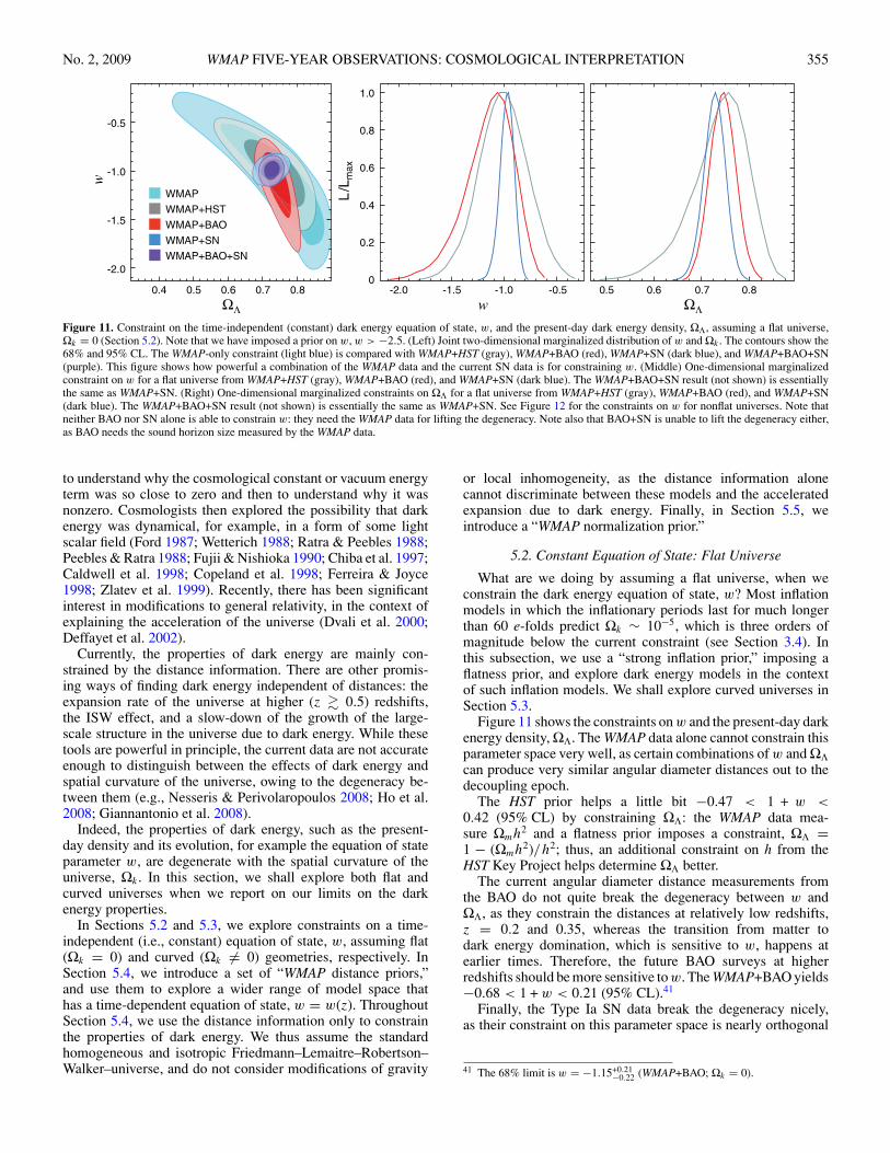
No. 2, 2009 WMAP FIVE-YEAR OBSERVATIONS: COSMOLOGICAL INTERPRETATION 355
Figure 11. Constraint on the time-independent (constant) dark energy equation of state, w, and the present-day dark energy density, ΩΛ, assuming a flat universe,Ωk = 0 (Section 5.2). Note that we have imposed a prior on w, w > −2.5. (Left) Joint two-dimensional marginalized distribution of w and Ωk . The contours show the68% and 95% CL. The WMAP-only constraint (light blue) is compared with WMAP+HST (gray), WMAP+BAO (red), WMAP+SN (dark blue), and WMAP+BAO+SN(purple). This figure shows how powerful a combination of the WMAP data and the current SN data is for constraining w. (Middle) One-dimensional marginalizedconstraint on w for a flat universe from WMAP+HST (gray), WMAP+BAO (red), and WMAP+SN (dark blue). The WMAP+BAO+SN result (not shown) is essentiallythe same as WMAP+SN. (Right) One-dimensional marginalized constraints on ΩΛ for a flat universe from WMAP+HST (gray), WMAP+BAO (red), and WMAP+SN(dark blue). The WMAP+BAO+SN result (not shown) is essentially the same as WMAP+SN. See Figure 12 for the constraints on w for nonflat universes. Note thatneither BAO nor SN alone is able to constrain w: they need the WMAP data for lifting the degeneracy. Note also that BAO+SN is unable to lift the degeneracy either,as BAO needs the sound horizon size measured by the WMAP data.
to understand why the cosmological constant or vacuum energyterm was so close to zero and then to understand why it wasnonzero. Cosmologists then explored the possibility that darkenergy was dynamical, for example, in a form of some lightscalar field (Ford 1987; Wetterich 1988; Ratra & Peebles 1988;Peebles & Ratra 1988; Fujii & Nishioka 1990; Chiba et al. 1997;Caldwell et al. 1998; Copeland et al. 1998; Ferreira & Joyce1998; Zlatev et al. 1999). Recently, there has been significantinterest in modifications to general relativity, in the context ofexplaining the acceleration of the universe (Dvali et al. 2000;Deffayet et al. 2002).
Currently, the properties of dark energy are mainly con-strained by the distance information. There are other promis-ing ways of finding dark energy independent of distances: theexpansion rate of the universe at higher (z � 0.5) redshifts,the ISW effect, and a slow-down of the growth of the large-scale structure in the universe due to dark energy. While thesetools are powerful in principle, the current data are not accurateenough to distinguish between the effects of dark energy andspatial curvature of the universe, owing to the degeneracy be-tween them (e.g., Nesseris & Perivolaropoulos 2008; Ho et al.2008; Giannantonio et al. 2008).
Indeed, the properties of dark energy, such as the present-day density and its evolution, for example the equation of stateparameter w, are degenerate with the spatial curvature of theuniverse, Ωk . In this section, we shall explore both flat andcurved universes when we report on our limits on the darkenergy properties.
In Sections 5.2 and 5.3, we explore constraints on a time-independent (i.e., constant) equation of state, w, assuming flat(Ωk = 0) and curved (Ωk = 0) geometries, respectively. InSection 5.4, we introduce a set of “WMAP distance priors,”and use them to explore a wider range of model space thathas a time-dependent equation of state, w = w(z). ThroughoutSection 5.4, we use the distance information only to constrainthe properties of dark energy. We thus assume the standardhomogeneous and isotropic Friedmann–Lemaitre–Robertson–Walker–universe, and do not consider modifications of gravity
or local inhomogeneity, as the distance information alonecannot discriminate between these models and the acceleratedexpansion due to dark energy. Finally, in Section 5.5, weintroduce a “WMAP normalization prior.”
5.2. Constant Equation of State: Flat Universe
What are we doing by assuming a flat universe, when weconstrain the dark energy equation of state, w? Most inflationmodels in which the inflationary periods last for much longerthan 60 e-folds predict Ωk ∼ 10−5, which is three orders ofmagnitude below the current constraint (see Section 3.4). Inthis subsection, we use a “strong inflation prior,” imposing aflatness prior, and explore dark energy models in the contextof such inflation models. We shall explore curved universes inSection 5.3.
Figure 11 shows the constraints on w and the present-day darkenergy density, ΩΛ. The WMAP data alone cannot constrain thisparameter space very well, as certain combinations of w and ΩΛcan produce very similar angular diameter distances out to thedecoupling epoch.
The HST prior helps a little bit −0.47 < 1 + w <0.42 (95% CL) by constraining ΩΛ: the WMAP data mea-sure Ωmh2 and a flatness prior imposes a constraint, ΩΛ =1 − (Ωmh2)/h2; thus, an additional constraint on h from theHST Key Project helps determine ΩΛ better.
The current angular diameter distance measurements fromthe BAO do not quite break the degeneracy between w andΩΛ, as they constrain the distances at relatively low redshifts,z = 0.2 and 0.35, whereas the transition from matter todark energy domination, which is sensitive to w, happens atearlier times. Therefore, the future BAO surveys at higherredshifts should be more sensitive to w. The WMAP+BAO yields−0.68 < 1 + w < 0.21 (95% CL).41
Finally, the Type Ia SN data break the degeneracy nicely,as their constraint on this parameter space is nearly orthogonal
41 The 68% limit is w = −1.15+0.21−0.22 (WMAP+BAO; Ωk = 0).

356 KOMATSU ET AL. Vol. 180
Figure 12. Joint two-dimensional marginalized constraint on the time-independent (constant) dark energy equation of state, w, and the curvature parameter, Ωk
(Section 5.3). Note that we have imposed a prior on w, w > −2.5. The contours show the 68% and 95% CL. (Left) The WMAP-only constraint (light blue; 95% CL)compared with WMAP+BAO+SN (purple; 68% and 95% CL). This figure shows how powerful the extra distance information from BAO and SN is for constrainingΩk and w simultaneously. (Middle) A blow-up of the left panel, showing WMAP+HST (gray), WMAP+BAO (red), WMAP+SN (dark blue), and WMAP+BAO+SN(purple). This figure shows that we need both BAO and SN to constrain Ωk and w simultaneously: WMAP+BAO fixes Ωk and WMAP+SN fixes w. (Right) The sameas the middle panel, but with the BAO prior re-weighted by a weaker BAO prior from the SDSS LRG sample (Eisenstein et al. 2005). The BAO data used in theother panels combine the SDSS main and LRG, as well as the 2dFGRS data (Percival et al. 2007). The constraints from these are similar, and thus our results are notsensitive to the exact form of the BAO data sets. Note that neither BAO nor SN alone is able to constrain w or Ωk : they need the WMAP data for lifting the degeneracy.Also note that BAO+SN is unable to lift the degeneracy either, as BAO needs the sound horizon size measured by the WMAP data.
to what is determined by the CMB data: WMAP+SN yields−0.12 < 1 + w < 0.14 (95% CL).42
With a flatness prior, the constraint on w from SN is sopowerful that WMAP+SN is similar to WMAP+BAO+SN. Weconclude that, when the equation of state does not depend onredshifts, dark energy is consistent with vacuum energy, with−0.12 < 1 + w < 0.13 (95% CL)43 (from WMAP+BAO+SN),in the context of a flat universe at the level of curvature that ispredicted by long-lasting inflation models.
5.3. Constant Equation of State: Curved Universe
In this subsection, we do not assume a flat universe, butdo assume a constant equation of state (for a time-dependentequation of state, see Section 5.4.2). As we discussed inSection 3.4, the WMAP data alone are unable to place meaning-ful constraints on the spatial curvature of the universe; however,two or more distance or expansion rate measurements breakthe degeneracy between Ωk and Ωm. As Figure 6 shows, thecombination of the WMAP measurement of the distance to thedecoupling epoch at z 1090, and the distance measurementsout to z = 0.2 and 0.35 from BAO, strongly constrains thecurvature, at the level of 1%–2%.
However, when dark energy is dynamical, we need threedistance indicators that cover a wide range of redshift. As thecurrent SN data cover a wider range in redshifts, 0.02 � z � 1.7,than the BAO data, the SN data help to constrain the evolutionof dark energy, that is, w.
Figure 12 shows the constraints on w and Ωk from the WMAP5-year data alone, WMAP+HST, WMAP+BAO, WMAP+SN, aswell as WMAP+BAO+SN. The middle panel is particularlyilluminating. The WMAP+BAO combination fixes Ωk , nearlyindependent of w.44 The WMAP+SN combination yields adegeneracy line that is tilted with respect to the WMAP+BAOline. The WMAP+BAO and WMAP+SN lines intersect at Ωk ∼ 0
42 The 68% limit is w = −0.977+0.065−0.064 (WMAP+SN; Ωk = 0).
43 The 68% limit is w = −0.992+0.061−0.062 (WMAP+BAO+SN; Ωk = 0).
44 For the WMAP+BAO limit, there is a long degenerate valley with asignificant volume at w < −1. Models anywhere in this valley are good fits toboth datasets. It is dangerous to marginalize over these degenerate parametersas conclusions are very sensitive to the choice and the form of priors.
and w ∼ −1, and the combined constraints are −0.0179 <Ωk < 0.0081 (95% CL) and −0.14 < 1 + w < 0.12 (95% CL),respectively.45 It is remarkable that the limit on Ωk is asgood as that for a vacuum energy model, −0.0178 < Ωk <0.0066 (95% CL). This is because the BAO and SN yieldconstraints on Ωk and w that are complementary to each other,breaking the degeneracy effectively.
These limits give the lower bounds to the curvature radii ofthe observable universe as Rcurv > 33 h−1 Gpc and Rcurv >22 h−1 Gpc for negatively and positively curved universes,respectively.
Is the apparent “tension” between the WMAP+BAO limitand the WMAP+SN limit in Figure 12 the signature of newphysics? We have checked this by the BAO distance scale out toz = 0.35 from the SDSS LRG sample, obtained by Eisensteinet al. (2005), instead of the z = 0.2 and z = 0.35 constraintsbased on the combination of SDSS LRGs with the SDSS mainsample and 2dFGRS (Percival et al. 2007). While it is not anindependent check, it does provide some measurement of thesensitivity of the constraints to the details of the BAO dataset.
The right panel of Figure 12 shows that the results are notsensitive to the exact form of the BAO datasets.46 The Eisensteinet al. (2005) BAO prior is a bit weaker than Percival et al.’s, andthus the WMAP+BAO contours extend more to w � −1. Theimportant point is that the direction of degeneracy does notchange. Therefore, the combined limits from WMAP, SN, andthe Eisenstein et al. BAO, −0.15 < 1 + w < 0.13 (95% CL),and −0.0241 < Ωk < 0.0094 (95% CL) are similar to thosewith Percival et al.’s BAO, −0.14 < 1 + w < 0.12 (95% CL),and −0.0179 < Ωk < 0.0081 (95% CL). As expected, a weakerBAO prior resulted in a weaker limit on Ωk .
While the above argument suggests that there is no serioustension between WMAP+BAO and WMAP+SN constraints,
45 The 68% limits are Ωk = −0.0049+0.0066−0.0064 and w = −1.006+0.067
−0.068(WMAP+BAO+SN).46 To obtain the WMAP+BAO contours in the right panel of Figure 12, wehave re-weighted the WMAP+BAO data in the middle panel of Figure 12 by thelikelihood ratio of L(Eisenstein’s BAO)/L(Percival’s BAO). As a result, thecontours do not extend to w ∼ 0; however, the contours would extend more tow ∼ 0 if we ran a MCMC from the beginning with the Eisenstein et al. BAO.

No. 2, 2009 WMAP FIVE-YEAR OBSERVATIONS: COSMOLOGICAL INTERPRETATION 357
would it be possible that the tension, if any, could be causedby the WMAP data? As the BAO data use the sound horizonsize measured by the WMAP data, rs(zd ), some systematicerrors causing the miscalculation of rs(zd ) could lead to amisinterpretation of the BAO data. The current measurementerrors in rs(zd )/DV (z) from the BAO data are 2.9% at z = 0.2and 3.0% at z = 0.35. However, WMAP measures rs(zd )with 1.3% accuracy (see Table 3). We are confident that thesystematic error in rs(zd ), if any, is smaller than the statisticalerror; thus, it is unlikely that WMAP causes a misinterpretationof the BAO data.
From these studies, we are able to place rather stringent,simultaneous limits on Ωk (to a 1%–2% level, depending uponthe sign) and w (to a 14% level). The spatial curvature isconsistent with zero and the dark energy is consistent withvacuum energy. How does this conclusion change when weallow w to vary?
5.4. WMAP Distance Priors for Testing Dark Energy Models
5.4.1. Motivation
Dark energy influences the distance scales as well as thegrowth of structure. The CMB power spectra are sensitive toboth, although sensitivity to the growth of structure is fairlylimited, as it influences the CMB power spectrum via the ISWeffect at low multipoles (l � 10), whose precise measurementis hampered by a large cosmic variance.
However, CMB is sensitive to the distance to the decouplingepoch via the locations of peaks and troughs of the acousticoscillations, which can be measured precisely. More specifically,CMB measures two distance ratios: (1) the angular diameterdistance to the decoupling epoch divided by the sound horizonsize at the decoupling epoch, DA(z∗)/rs(z∗), and (2) the angulardiameter distance to the decoupling epoch divided by the Hubblehorizon size at the decoupling epoch, DA(z∗)H (z∗)/c. Thisconsideration motivates our using these two distance ratios toconstrain various dark energy models, in the presence of thespatial curvature, on the basis of distance information (Wang &Mukherjee 2007; Wright 2007).
We shall quantify the first distance ratio, DA(z∗)/rs(z∗), bythe “acoustic scale,” lA, defined by
lA ≡ (1 + z∗)πDA(z∗)
rs(z∗), (65)
where a factor of (1 + z∗) arises because DA(z∗) is the proper(physical) angular diameter distance (Equation (2)), whereasrs(z∗) is the comoving sound horizon at z∗ (Equation (6)).Here, we shall use the fitting function of z∗ proposed by Hu& Sugiyama (1996):
z∗ = 1048[1 + 0.00124(Ωbh2)−0.738][1 + g1(Ωmh2)g2 ], (66)
where
g1 = 0.0783(Ωbh2)−0.238
1 + 39.5(Ωbh2)0.763, (67)
g2 = 0.560
1 + 21.1(Ωbh2)1.81. (68)
Note that one could also use the peak of the probability of lastscattering of photons, that is, the peak of the visibility function,to define the decoupling epoch, which we denote as zdec. Bothquantities yield similar values. We shall adopt z∗ here because it
is easier to compute, and, therefore, it allows one to implementthe WMAP distance priors in a straightforward manner.
The second distance ratio, DA(z∗)H (z∗)/c, is often called the“shift parameter,” R, given by (Bond et al. 1997)
R(z∗) ≡√
ΩmH 20
c(1 + z∗)DA(z∗). (69)
This quantity is different from DA(z∗)H (z∗)/c by a factor of√1 + z∗, and also ignores the contributions from radiation,
curvature, or dark energy to H (z∗). Nevertheless, we shall useR to follow the convention in the literature.
We give the 5-year WMAP constraints on lA, R, and z∗ thatwe recommend as the WMAP distance priors for constrainingdark energy models. However, we note an important caveat. Aspointed out by Elgarøy & Multamaki (2007) and Corasaniti& Melchiorri (2008), the derivation of the WMAP distancepriors requires us to assume the underlying cosmology first,as all of these quantities are derived parameters from fittingthe CMB power spectra. Therefore, one must be careful aboutwhich model one is testing. Here, we give the WMAP distancepriors, assuming the following model.
1. The standard Friedmann–Lemaitre–Robertson–Walker uni-verse with matter, radiation, dark energy, and spatial curva-ture.
2. Neutrinos with the effective number of neutrinos equal to3.04, and the minimal mass (mν ∼ 0.05 eV).
3. Nearly power-law primordial power spectrum of curvatureperturbations, |dns/d ln k| � 0.01.
4. Negligible primordial gravitational waves relative to thecurvature perturbations, r � 0.1.
5. Negligible entropy fluctuations relative to the curvatureperturbations, α � 0.1.
In Figure 13, we show the constraints on w and Ωk fromthe WMAP distance priors (combined with BAO and SN). Wefind a good agreement with the full MCMC results (comparethe middle and right panels of Figure 12 with the left and rightpanels of Figure 13, respectively). The constraints from theWMAP distance priors are slightly weaker than the full MCMC,as the distance priors use only a part of the information containedin the WMAP data.
Of course, the agreement between Figures 12 and 13 does notguarantee that these priors yield good results for the other, morecomplex dark energy models with a time-dependent w; however,the previous studies indicate that, under the assumptions givenabove, these priors can be used to constrain a wide varietyof dark energy models (Wang & Mukherjee 2007; Elgarøy &Multamaki 2007; Corasaniti & Melchiorri 2008). Also see Liet al. (2008a) for the latest comparison between the WMAPdistance priors and the full analysis.
Here is the prescription for using the WMAP distance priors.
1. For a given Ωbh2 and Ωmh2, compute z∗ from
Equation (66).2. For a given H0, Ωmh2, Ωrh
2 (which includes Neff = 3.04),ΩΛ, and w(z), compute the expansion rate, H (z), fromEquation (7), as well as the comoving sound horizon sizeat z∗, rs(z∗), from Equation (6).
3. For a given Ωk and H (z) from the previous step, com-pute the proper angular diameter distance, DA(z), fromEquation (2).
4. Use Equations (65) and (69) to compute lA(z∗) and R(z∗),respectively.

358 KOMATSU ET AL. Vol. 180
Figure 13. Joint two-dimensional marginalized constraint on the time-independent (constant) dark energy equation of state, w, and the curvature parameter, Ωk ,derived solely from the WMAP distance priors (lA, R, z∗) (see Section 5.4.1), combined with either BAO (red), SN (dark blue), or both (purple). The contours showthe Δχ2
total = 2.30 (68.3% CL) and Δχ2total = 6.17 (95.4% CL). The left (BAO data from Percival et al. 2007) and right (BAO data from Eisenstein et al. 2005) panels
should be compared with the middle and right panels of Figure 12, respectively, which have been derived from the full WMAP data combined with the same BAO andSN data. While the WMAP distance priors capture most of the information in this parameter space, the constraint is somewhat weaker than that from the full analysis.
5. Form a vector containing xi = (lA, R, z∗) in this order.6. Use Table 10 for the data vector, di = (
lWMAPA ,RWMAP,
zWMAP∗
). We recommend the maximum likelihood (ML)
values.7. Use Table 11 for the inverse covariance matrix, (C−1)ij .8. Compute the likelihood, L, as χ2
WMAP ≡ −2 ln L = (xi −di)(C−1)ij (xj − dj ).
9. Add this to the favorite combination of the cosmologicaldatasets. In this paper we add χ2
WMAP to the BAO and SNdata, that is, χ2
total = χ2WMAP + χ2
BAO + χ2SN .
10. Marginalize the posterior distribution over Ωbh2, Ωmh2,
and H0 with uniform priors. Since the WMAP distancepriors combined with the BAO and SN data provide tightconstraints on these parameters, the posterior distributionof these parameters is close to a Gaussian distribution.Therefore, the marginalization is equivalent to minimizingχ2
total with respect to Ωbh2, Ωmh2, and H0 (also see Cash
1976; Wright 2007). We use a downhill simplex methodfor minimization (amoeba routine in Numerical Recipes;Press et al. 1992). The marginalization over Ωbh
2, Ωmh2,and H0 leaves us with the the marginalized posteriordistribution of the dark energy function, w(a), and thecurvature parameter, Ωk .
Note that this prescription eliminates the need for running theMCMC entirely, and thus the computational cost for evaluatingthe posterior distribution of w(a) and Ωk is not demanding.In Section 5.4.2, we shall apply the WMAP distance priors toconstrain the dark energy equation of state that depends onredshifts, w = w(z).
For those who wish to include an additional prior on Ωbh2,
we give the inverse covariance matrix for the “extended”WMAP distance priors: (lA(z∗), R(z∗), z∗, 100Ωbh
2), as wellas the maximum likelihood value of 100Ωbh
2, in Table 12.We note, however, that it is sufficient to use the reduced set,(lA(z∗), R(z∗), z∗), as the extended WMAP distance priors givevery similar constraints on dark energy (see Wang 2008).
5.4.2. Application of the WMAP Distance Priors: Variable Equationof State
In this subsection, we explore a time-dependent equation ofstate of dark energy, w(z). We use the following parametrized
Table 10WMAP Distance Priors Obtained from the WMAP 5-year Fit to Models with
Spatial Curvature and Dark Energy
5 Year MLa 5 Year Meanb Error, σ
lA(z∗) 302.10 302.45 0.86R(z∗) 1.710 1.721 0.019zc∗ 1090.04 1091.13 0.93
Notes.
The correlation coefficients are: rlA,R = 0.1109, rlA,z∗ = 0.4215,and rR,z∗ = 0.6928.a Maximum likelihood values (recommended).b Mean of the likelihood.c Equation (66).
Table 11Inverse Covariance Matrix for the WMAP Distance Priors
lA(z∗) R(z∗) z∗lA(z∗) 1.800 27.968 −1.103R(z∗) 5667.577 −92.263z∗ 2.923
Table 12Inverse Covariance Matrix for the Extended WMAP Distance Priors
lA(z∗) R(z∗) z∗ 100Ωbh2
lA(z∗) 31.001 −5015.642 183.903 2337.977R(z∗) 876807.166 −32046.750 −403818.837z∗ 1175.054 14812.579100Ωbh
2 187191.186
Note. The maximum likelihood value of Ωbh2 is 100Ωbh
2 = 2.2765.
form:
w(a) = aw(a)
a + atrans− atrans
a + atrans, (70)
where w(a) = w0 +(1−a)wa . We give a motivation, derivation,and detailed discussion on this form of w(a) in Appendix C. Thisform has a number of desirable properties, as follows.
1. w(a) approaches −1 at early times, a < atrans, whereatrans = 1/(1 + ztrans) is the “transition epoch” and ztransis the transition redshift. Therefore, the dark energy densitytends to a constant value at a < atrans.

No. 2, 2009 WMAP FIVE-YEAR OBSERVATIONS: COSMOLOGICAL INTERPRETATION 359
Figure 14. Constraint on models of time-dependent dark energy equation of state, w(z) (Equation (70)), derived from the WMAP distance priors (lA, R, and z∗)combined with the BAO and SN distance data (Section 5.4.2). There are three parameters: w0 is the value of w at the present epoch, w0 ≡ w(z = 0), w′ is the firstderivative of w with respect to z at z = 0, w′ ≡ dw/dz|z=0, and ztrans is the transition redshift above which w(z) approaches −1. Here, we assume flatness of theuniverse, Ωk = 0. (Left) Joint two-dimensional marginalized distribution of w0 and w′ for ztrans = 10. The constraints are similar for the other values of ztrans. Thecontours show the Δχ2
total = 2.30 (68.3% CL) and Δχ2total = 6.17 (95.4% CL). (Middle) One-dimensional marginalized distribution of w0 for ztrans = 0.5 (dotted), 2
(dashed), and 10 (solid). (Right) One-dimensional marginalized distribution of w′ for ztrans = 0.5 (dotted), 2 (dashed), and 10 (solid). The constraints are similar forall ztrans. We do not find evidence for the evolution of dark energy. Note that neither BAO nor SN alone is able to constrain w0 or w′: they need the WMAP data forlifting the degeneracy. Also note that BAO+SN is unable to lift the degeneracy either, as BAO needs the sound horizon size measured by the WMAP data.
2. The dark energy density remains totally subdominant rela-tive to the matter density at the decoupling epoch.
3. We recover the widely-used linear form, w(a) = w0 + (1 −a)wa (Chevallier & Polarski 2001; Linder 2003), at latetimes, a > atrans.
4. The early-time behavior is consistent with some of scalarfield models classified as the “thawing models” (Caldwell& Linder 2005) in which a scalar field was moving veryslowly at early times and then began to move faster at recenttimes.
5. Since the late-time form of w(a) allows w(a) to go below−1, our form is more general than models based upon asingle scalar field.
6. The form is simple enough to give a closed, analyti-cal form of the effective equation of state, weff(a) =(ln a)−1
∫ ln a
0 d ln a′w(a′) (Equation C6), which determinesthe evolution of the dark energy density, ρde(a) =ρde(0)a−3[1+weff (a)]; thus, it allows one to easily compute theevolution of the expansion rate and cosmological distances.
While this form contains three free parameters, w0, wa , andztrans, we shall give constraints on the present-day value ofw, w0 ≡ w(a = 1), and the first derivative of w at present,w′ ≡ dw/dz|z=0, instead of w0 and wa , as they can be comparedto the previous results in the literature more directly. We findthat the results are not sensitive to the exact values of ztrans.
In Figure 14, we present the constraint on w0 and w′ thatwe have derived from the WMAP distance priors (lA, R, z∗),combined with the BAO and SN data. Note that we have assumeda flat universe in this analysis, although it is straightforward toinclude the spatial curvature. Wang & Mukherjee (2007) andWright (2007) showed that the two-dimensional distributionextends more towards southeast, that is, w > −1 and w′ < 0,when the spatial curvature is allowed.
The 95% limit on w0 for ztrans = 10 is −0.33 < 1 + w0 <0.21.47 Our results are consistent with the previous work usingthe WMAP 3-year data (see Zhao et al. 2007; Wang & Mukherjee2007; Wright 2007; Lazkoz et al. 2008, for recent work and
47 The 68% intervals are w0 = −1.06 ± 0.14 and w′ = 0.36 ± 0.62(WMAP+BAO+SN; Ωk = 0).
references therein). The WMAP 5-year data help tighten theupper limit on w′ and the lower limit on w0, whereas the lowerlimit on w′ and the upper limit on w0 come mainly from theType Ia SN data. As a result, the lower limit on w′ and the upperlimit on w0 are sensitive to whether we include the systematicerrors in the SN data. For this investigation, see Appendix D.
Alternatively, one may take the linear form, w(a) = w0 +(1−a)wa , literally and extend it to an arbitrarily high redshift. Thiscan result in an undesirable situation in which the dark energyis as important as the radiation density at the epoch of the BBN;however, one can severely constrain such a scenario by usingthe limit on the expansion rate from BBN (Steigman 2007). Wefollow Wright (2007) to adopt a Gaussian prior on√
1 +ΩΛ(1 + zBBN)3[1+weff (zBBN)]
Ωm(1 + zBBN)3 + Ωr (1 + zBBN)4 + Ωk(1 + zBBN)2
= 0.942 ± 0.030, (71)
where we have kept Ωm and Ωk for definiteness, but they areentirely negligible compared to the radiation density at theredshift of BBN, zBBN = 109. Figure 15 shows the constrainton w0 and w′ for the linear evolution model derived from theWMAP distance priors, the BAO and SN data, and the BBNprior. The 95% limit on w0 is −0.29 < 1 + w0 < 0.21,48 whichis similar to what we have obtained above.
5.5. WMAP Normalization Prior
So far, we have been mainly using the distance information toconstrain the properties of dark energy; however, this is not theonly information that one can use to constrain the properties ofdark energy. The amplitude of fluctuations is a powerful tool fordistinguishing between dark energy and modifications to gravity(Ishak et al. 2006; Koyama & Maartens 2006; Amarzguioui et al.2006; Dore et al. 2007; Linder & Cahn 2007; Upadhye 2007;Zhang et al. 2007; Yamamoto et al. 2007; Chiba & Takahashi2007; Bean et al. 2007b; Hu & Sawicki 2007; Song et al. 2007;Daniel et al. 2008; Jain & Zhang 2008; Bertschinger & Zukin
48 The 68% intervals are w0 = −1.04 ± 0.13 and w′ = 0.24 ± 0.55(WMAP+BAO+SN+BBN; Ωk = 0).

360 KOMATSU ET AL. Vol. 180
Figure 15. Constraint on the linear evolution model of dark energy equation of state, w(z) = w0 + w′z/(1 + z), derived from the WMAP distance priors (lA, R, and z∗)combined with the BAO and SN distance data as well as the BBN prior (Equation (71)). Here, we assume flatness of the universe, Ωk = 0. (Left) Joint two-dimensionalmarginalized distribution of w0 and w′. The contours show the Δχ2
total = 2.30 (68.3% CL) and Δχ2total = 6.17 (95.4% CL). (Middle) One-dimensional marginalized
distribution of w0. (Right) One-dimensional marginalized distribution of w′. We do not find evidence for the evolution of dark energy. Note that Linder (2003) definesw′ as the derivative of w at z = 1, whereas we define it as the derivative at z = 0. They are related by w′
linder = 0.5w′WMAP.
2008; Amin et al. 2008; Hu 2008), as well as for determiningthe mass of neutrinos (Hu et al. 1998; Lesgourgues & Pastor2006).
The microwave background observations measure the am-plitude of fluctuations at the decoupling epoch. By combiningthis measurement with the amplitude measured from variouslow redshift tracers, one can learn more about the dark energyproperties and the mass of neutrinos.
The overall amplitude of CMB anisotropy is set by the ampli-tude of primordial curvature perturbations, R. For example, onvery large angular scales where the Sachs–Wolfe limit can beused, the temperature anisotropy is given by ΔT/T = −R/5 or,in terms of the curvature perturbation during the matter era, Φ,it is given by ΔT/T = −Φ/3. On small angular scales wherethe acoustic physics must be taken into account, we have theacoustic oscillation whose amplitude is also given by R.
This motivates our reporting the “WMAP normalization,”a measurement of the overall normalization of the curvatureperturbations expressed in terms of Δ2
R(kWMAP), where Δ2R(k) ≡
k3PR(k)/(2π2) is a contribution to the total variance of R,〈R2〉, per logarithmic interval of k (also see Equation (15) anddescriptions below it).
Here, kWMAP is different from k0 = 0.002 Mpc−1 that weused to define ns, dns/d ln k, r, and Δ2
R(k0) reported in Tables 1and 4. The goal in this subsection is to give the normalizationthat is as model independent as possible.
At k0 = 0.002 Mpc−1, for example, we find 109Δ2R(k0) =
2.48, 2.41, and 2.46 for a flat ΛCDM model, a curved ΛCDMmodel, and a flat ΛCDM model with massive neutrinos. Thescatter between these values comes solely from the fact that k0 =0.002 Mpc−1 is not a right place to define the normalization. Inother words, this is not the pivot scale of the WMAP data.
We find that kWMAP = 0.02 Mpc−1, that is, a factor of 10 largerthan k0, gives similar values of Δ2
R(kWMAP) for a wide range ofmodels, as summarized in Table 13. From these results, we givethe WMAP normalization prior:
Δ2R(kWMAP) = (2.21 ± 0.09) × 10−9, (72)
which is valid for models with Ωk = 0, w = −1, ormν > 0. However, we find that these normalizations cannotbe used for the models that have the tensor modes, r > 0,or the running index, dns/d ln k = 0. We failed to find auniversal normalization for these models. Nevertheless, our
Table 13Amplitude of Curvature Perturbations, R, Measured by WMAP at
kWMAP = 0.02 Mpc−1
Model 109 × Δ2R(kWMAP)
Ωk = 0 and w = −1 2.211 ± 0.083Ωk = 0 and w = −1 2.212 ± 0.084Ωk = 0 and w = −1 2.208 ± 0.087Ωk = 0 and w = −1 2.210 ± 0.084Ωk = 0, w = −1 and mν > 0 2.212 ± 0.083Ωk = 0, w = −1 and mν > 0 2.218 ± 0.085
WMAP Normalization Prior 2.21 ± 0.09
WMAP normalization, given by Equation (72), is still valid fora wide range of cosmological models.
How can one use the WMAP normalization? In order to predictthe linear matter density power spectrum, Plin(k), one needs torelate the primordial curvature perturbations, Rk, to the linearmatter density fluctuations at arbitrary redshifts, δm,k(z). FromEinstein’s equations, we find (see, e.g., Appendix C of Takadaet al. 2006)
δm,k(z) = 2k3
5H 20 Ωm
RkT (k)D(k, z), (73)
where D(k,z) and T (k) are the linear growth rate and the mattertransfer function normalized such that T (k) → 1 as k → 0and (1 + z)D(k, z) → 1 as k → 0 during the matter era (e.g.,z = 30, where the radiation density is less than 1% of the matterdensity), respectively. Note that D(k, z) does not depend onk when neutrinos are massless; however, it depends on k whenthey are massive (e.g., Hu & Eisenstein 1998). The linear matterdensity power spectrum is given by
k3Plin(k, z)
2π2= (2.21 ± 0.09) × 10−9
(2k2
5H 20 Ωm
)2
× D2(k, z)T 2(k)
(k
kWMAP
)ns−1
. (74)
One application of the WMAP normalization is the compu-tation of the present-day normalization of matter fluctuations,

No. 2, 2009 WMAP FIVE-YEAR OBSERVATIONS: COSMOLOGICAL INTERPRETATION 361
Figure 16. Predictions for the present-day amplitude of matter fluctuations, σ8, as a function of the (constant) dark energy equation of state parameter, w, derivedfrom the full WMAP data (blue) and from WMAP+BAO+SN (red). The contours show the 68% and 95% CL. (Left) Flat universe, Ωk = 0. (Right) Curved universe,Ωk = 0.
Figure 17. Constraint on the total mass of neutrinos,∑
mν (Section 6.1.3). In all panels, we show the WMAP-only results in blue and WMAP+BAO+SN in red. (Left)Joint two-dimensional marginalized distribution of H0 and
∑mν (68% and 95% CL). The additional distance information from BAO helps reduce the correlation
between H0 and∑
mν . (Middle) The WMAP data, combined with the distances from BAO and SN, predict the present-day amplitude of matter fluctuations, σ8, as afunction of
∑mν . An independent determination of σ8 will help determine
∑mν tremendously. (Right) Joint two-dimensional marginalized distribution of w and∑
mν . No significant correlation is observed. Note that we have a prior on w, w > −2.5, and thus the WMAP-only lower limit on w in this panel cannot be trusted.
which is commonly expressed in terms of σ8, given by
σ 28 = (2.21 ± 0.09) × 10−9
(2
5Ωm
)2
×∫
dk
kD2(k, z = 0)T 2(k)
k4
H 40
(k
kWMAP
)ns−1
×[
3 sin(kR)
(kR)3− 3 cos(kR)
(kR)2
]2
, (75)
where R = 8 h−1 Mpc. Both the dark energy properties (ormodified gravity) and the mass of neutrinos change the value ofD(k, z = 0). The transfer function, T (k), is much less affected,as long as neutrinos are still relativistic at the decoupling epoch,and the dark energy or modified gravity effect is unimportant atthe decoupling epoch.
Ignoring the mass of neutrinos and modifications to gravity,one can obtain the growth rate by solving the followingdifferential equation (Wang & Steinhardt 1998; Linder &Jenkins 2003):
d2g
d ln a2+
[5
2+
1
2(Ωk(a) − 3weff(a)Ωde(a))
]dg
d ln a
+
[2Ωk(a) +
3
2(1 − weff(a))Ωde(a)
]g(a) = 0, (76)
where
g(a) ≡ D(a)
a= (1 + z)D(z), (77)
Ωk(a) ≡ ΩkH20
a2H 2(a), (78)
Ωde(a) ≡ ΩΛH 20
a3[1+weff (a)]H 2(a), (79)
weff(a) ≡ 1
ln a
∫ ln a
0d ln a′w(a′). (80)
During the matter era, g(a) does not depend on a; thus, thenatural choice for the initial conditions are g(ainitial) = 1 anddg/d ln a|a=ainitial
= 0, where ainitial must be taken during thematter era, for example, ainitial = 1/31 (i.e., z = 30).
In Figure 16, we show the predicted values of σ8 as a functionof w in a flat universe (left panel) and curved universes (rightpanel; see the middle panel of Figure 17 for σ8 as a function ofthe mass of neutrinos). Here, we have used the full information inthe WMAP data. The normalization information alone is unable

362 KOMATSU ET AL. Vol. 180
to give meaningful predictions for σ8, which depends not onlyon Δ2
R(kWMAP), but also on the other cosmological parametersvia T (k) and D(k, z = 0), especially w and Ωmh2. While thepredictions from the WMAP data alone are still weak, addingthe extra distance information from the BAO and SN data helpsimprove the predictions. We find σ8 = 0.807+0.045
−0.044 for a flatuniverse and σ8 = 0.795 ± 0.046 for curved universes.
By combining these results with σ8 measured from variouslow redshift tracers, one can reduce the remaining correlation be-tween w and σ8 to obtain a better limit on w. The precision of thecurrent data from weak lensing surveys is comparable to thesepredictions, for example, σ8(Ωm/0.25)0.64 = 0.785 ± 0.043(Canada-France-Hawaii Telescope Legacy Survey (CFHTLS);Fu et al. 2008). The weak lensing surveys will soon becomepowerful enough to yield smaller uncertainties in σ8 than pre-dicted from WMAP+BAO+SN.
6. NEUTRINOS
In this section, we shall use the WMAP data, combinedwith the distance information from BAO and SN observations,to place limits on the total mass of massive neutrino species(Section 6.1), as well as on the effective number of neutrino-like species that were still relativistic at the decoupling epoch(Section 6.2)
6.1. Neutrino Mass
6.1.1. Motivation
The existence of nonzero neutrino masses has been firmlyestablished by the experiments detecting atmospheric neutrinos(Hirata et al. 1992; Fukuda et al. 1994, 1998; Allison et al.1999; Ambrosio et al. 2001), solar neutrinos (Davis et al. 1968;Cleveland et al. 1998; Hampel et al. 1999; Abdurashitov et al.1999; Fukuda et al. 2001b, 2001a; Ahmad et al. 2002; Ahmedet al. 2004), reactor neutrinos (Eguchi et al. 2003; Araki et al.2005), and accelerator beam neutrinos (Ahn et al. 2003; Michaelet al. 2006). These experiments have placed stringent limitson the squared mass differences between the neutrino masseigenstates, Δm2
21 8 × 10⁻⁵ eV2, from the solar and reactorexperiments, and Δm2
32 3 × 10⁻³ eV2, from the atmosphericand accelerator beam experiments.
One needs different experiments to measure the absolutemasses. The next-generation tritium β-decay experiment, KA-TRIN,49 is expected to reach the electron neutrino mass of assmall as ∼ 0.2 eV. Cosmology has also been providing usefullimits on the mass of neutrinos (see Dolgov 2002; Elgarøy & La-hav 2005; Tegmark 2005; Lesgourgues & Pastor 2006; Fukugita2006; Hannestad 2006b, for reviews). Since the determinationof the neutrino mass is of fundamental importance in physics,there is enough motivation to pursue cosmological constraintson the neutrino mass.
How well can CMB constrain the mass of neutrinos? We donot expect massive neutrinos to affect the CMB power spectravery much (except through the gravitational lensing effect), ifthey were still relativistic at the decoupling epoch, z 1090.This means that, for massive neutrinos to affect the CMB powerspectra, at least one of the neutrino masses must be greater thanthe mean energy of relativistic neutrinos per particle at z 1090when the photon temperature of the universe is Tγ 3000 K 0.26 eV. Since the mean energy of relativistic neutrinos is given
49 http://www-ik.fzk.de/∼katrin.
by 〈E〉 = (7π4Tν)/(180ζ (3)) 3.15Tν = 3.15(4/11)1/3Tγ ,we need at least one neutrino species whose mass satisfiesmν > 3.15(4/11)1/3Tγ 0.58 eV; thus, it would not be possibleto constrain the neutrino mass using the CMB data alone, if themass of the heaviest neutrino species is below this value.
If the neutrino mass eigenstates are degenerate with theeffective number of species equal to 3.04, this argument suggeststhat
∑mν ∼ 1.8 eV would be the limit to which the CMB data
are sensitive. Ichikawa et al. (2005) argued that∑
mν ∼ 1.5 eVwould be the limit for the CMB data alone, which is fairly closeto the value given above.
In order to go beyond ∼ 1.5 eV, therefore, one needs tocombine the CMB data with the other cosmological probes.We shall combine the WMAP data with the distance informationfrom BAO and SN to place a limit on the neutrino mass. We shallnot use the galaxy power spectrum in this paper, and, therefore,our limit on the neutrino mass is free from the uncertainty in thegalaxy bias. We discuss this in more detail in Section 6.1.2.
6.1.2. Analysis
We assume that, for definiteness, the neutrino mass eigen-states are degenerate, which means that all of the three neutrinospecies have equal masses.50 We measure the neutrino massdensity parameter, Ωνh
2, and convert it to the total mass,∑
mν ,via ∑
mν ≡ Nνmν = 94 eV(Ωνh2), (81)
where Nν is the number of massive neutrino species. We take itto be 3.04. Note that in this case, the mass density parameter isthe sum of baryons, CDM, and neutrinos: Ωm = Ωb + Ωc + Ων .
Since the release of the 1 year (Spergel et al. 2003) and 3 year(Spergel et al. 2007) results on the cosmological analysis of theWMAP data, there have been a number of studies with regard tothe limits on the mass of neutrinos (Hannestad 2003; Elgarøy &Lahav 2003; Allen et al. 2003; Tegmark et al. 2004a; Barger et al.2004; Hannestad & Raffelt 2004; Crotty et al. 2004; Seljak et al.2005a, 2005b; Ichikawa et al. 2005; Hannestad 2005; Lattanziet al. 2005; Hannestad & Raffelt 2006; Goobar et al. 2006; Fenget al. 2006; Lesgourgues et al. 2007). These analyses reacheddifferent limits depending upon (1) the choice of datasets and(2) the parameters in the cosmological model.
The strongest limits quoted on neutrino masses come fromcombining CMB measurements with measurements of the am-plitude of density fluctuations in the recent universe. Clusteringof galaxies and Lyα forest observations have been used to obtainsome of the strongest limits on neutrino masses (Seljak et al.2005b, 2006; Viel et al. 2006). As the neutrino mass increases,the amplitude of mass fluctuations on small scales decreases(Bond et al. 1980; Bond & Szalay 1983; Ma 1996; also seethe middle panel of Figure 17), which can be used to weighneutrinos in the universe (Hu et al. 1998; Lesgourgues & Pastor2006).
These analyses are sensitive to correctly calculating therelationship between the level of observed fluctuations ingalaxies (or gas) and the mass fluctuation with the strongestlimits coming from the smallest scales in the analyses. Withthe new WMAP data, these limits are potentially even stronger.There are, however, several potential concerns with this limit:
50 While the current cosmological data are not yet sensitive to the mass ofindividual neutrino species, that is, the mass hierarchy, this situation maychange in the future, with high-z galaxy redshift surveys or weak lensingsurveys (Takada et al. 2006; Slosar 2006; Hannestad & Wong 2007; Kitchinget al. 2008; Abdalla & Rawlings 2007).

No. 2, 2009 WMAP FIVE-YEAR OBSERVATIONS: COSMOLOGICAL INTERPRETATION 363
Figure 18. Constraint on the effective number of neutrino species, Neff (Section 6.2.3). Note that we have imposed a prior on Neff , 0 < Neff < 10. In all panels, we showthe WMAP-only results in blue and WMAP+BAO+SN in red. (Left) Joint two-dimensional marginalized distribution (68% and 95% CL), showing a strong degeneracybetween Ωmh2 and Neff . This degeneracy line is given by the equality redshift, 1 + zeq = Ωm/Ωr = (4.050 × 10⁴)Ωmh2/(1 + 0.2271Neff ). The thick solid lines showthe 68% and 95% limits calculated from the WMAP-only limit on zeq: zeq = 3141+154
−157 (68% CL). The 95% CL contours do not follow the lines below Neff ∼ 1.5 butclose there, which shows a strong evidence for the cosmic neutrino background from its effects on the CMB power spectrum via the neutrino anisotropic stress. TheBAO and SN provide an independent constraint on Ωmh2, which helps reduce the degeneracy between Neff and Ωmh2. (Middle) When we transform the horizontalaxis of the left panel to zeq, we observe no degeneracy. The vertical solid lines show the one-dimensional marginalized 68% and 95% distributions calculated from theWMAP-only limit on zeq: zeq = 3141+154
−157 (68% CL). Therefore, the left panel is simply a rotation of this panel using a relation among zeq, Ωmh2, and Neff . (Right)One-dimensional marginalized distribution of Neff from WMAP-only and WMAP+BAO+SN+HST. Note that a gradual decline of the likelihood toward Neff � 6 forthe WMAP-only constraint should not be trusted, as it is affected by the hard prior, Neff < 10. The WMAP+BAO+SN+HST constraint is robust. This figure shows thatthe lower limit on Neff comes solely from the WMAP data. The 68% interval from WMAP+BAO+SN+HST, Neff = 4.4 ± 1.5, is consistent with the standard value,3.04, which is shown by the vertical line.
there is already “tension” between the high level of fluctuationsseen in the Lyman alpha forest and the amplitude of massfluctuations inferred from WMAP (Lesgourgues et al. 2007),the relationship between gas temperature and density appearsto be more complicated than assumed in the previous Lyαforest analysis (Kim et al. 2007; Bolton et al. 2008), andadditional astrophysics could potentially be the source of someof the small-scale fluctuations seen in the Lyα forest data.Given the power of the Lyα forest data, it is important toaddress these issues; however, they are beyond the scope of thispaper.
In this paper, we take the more conservative approach and useonly the WMAP data and the distance measures to place limitson the neutrino masses. Our approach is more conservative thanGoobar et al. (2006), who have found a limit of 0.62 eV onthe sum of the neutrino mass from the WMAP 3-year data,the SDSS–LRG BAO measurement, the SNLS SN data, andthe shape of the galaxy power spectra from the SDSS mainsample and 2dFGRS. While we use the WMAP 5-year data, theSDSS+2dFGRS BAO measurements, and the union SN data,we do not use the shape of the galaxy power spectra. SeeSection 2.3 in this paper or Dunkley et al. (2009) for moredetail on this choice.
In summary, we do not use the amplitude or shape of thematter power spectrum, but exclusively rely on the CMB dataand the distance measurements. As a result, our limits are weakerthan the strongest limits in the literature.
Next, let us discuss (2), the choice of parameters. A fewcorrelations between the neutrino mass and other cosmologicalparameters have been identified. Hannestad (2005) has foundthat the limit on the neutrino mass degrades significantly whenthe dark energy equation of state, w, is allowed to vary (alsosee Figure 18 of Spergel et al. 2007). This correlation wouldarise only when the amplitude of the galaxy or Lyα forestpower spectrum was included, as the dark energy equation ofstate influences the growth rate of the structure formation. Sincewe do not include them, our limit on the neutrino mass is not
degenerate with w. We shall come back to this point later in theSection 6.1.3. Incidentally, our limit is not degenerate with therunning index, dns/d ln k, or the tensor-to-scalar ratio, r.
6.1.3. Results
Figure 17 summarizes our limits on the sum of neutrinomasses,
∑mν .
With the WMAP data alone we find∑
mν < 1.3 eV (95% CL)for the ΛCDM model in which w = −1, and
∑mν <
1.5 eV (95% CL) for w = −1. We assume a flat universe inboth cases. These constraints are very similar, which means thatw and
∑mν are not degenerate. We show this more explicitly
on the right panel of Figure 17.When the BAO and SN data are added, our limits improve
significantly, by a factor 2, to∑
mν < 0.67 eV (95% CL)for w = −1, and
∑mν < 0.80 eV (95% CL) for w = −1.
Again, we do not observe much correlation between w and∑mν . While the distances out to either BAO or SN cannot
reduce correlation between Ωm (or H0) and w, a combinationof the two can reduce this correlation effectively, leaving littlecorrelation left on the right panel of Figure 17.
What information do BAO and SN add to improve the limiton
∑mν? It’s the Hubble constant, H0, as shown in the left
panel of Figure 17. This effect has been explained by Ichikawaet al. (2005) as follows.
The massive neutrinos modify the CMB power spectrum bytheir changing the matter-to-radiation ratio at the decouplingepoch. If the sum of degenerate neutrino masses is below 1.8 eV,the neutrinos were still relativistic at the decoupling epoch.However, they are definitely nonrelativistic at the present epoch,as the neutrino oscillation experiments have shown that at leastone neutrino species is heavier than 0.05 eV. This means thatthe Ωm that we measure must be the sum of Ωb, Ωc, andΩν ; however, at the decoupling epoch, neutrinos were stillrelativistic, and thus the matter density at the decoupling epochwas actually smaller than a naive extrapolation from the presentvalue.

364 KOMATSU ET AL. Vol. 180
As the matter-to-radiation ratio was smaller than one wouldnaively expect, it would accelerate the decay of gravitationalpotential around the decoupling epoch. This leads to an en-hancement in the so-called early integrated Sachs–Wolfe (ISW)effect. The larger
∑mν is, the larger early ISW becomes, as
long as the neutrinos were still relativistic at the decouplingepoch, that is,
∑mν � 1.8 eV.
The large ISW causes the first peak position to shift to lowermultipoles by adding power at l ∼ 200; however, this shift canbe absorbed by a reduction in the value of H0.51 This is why∑
mν and H0 are anticorrelated (see Ichikawa et al. 2005, for afurther discussion on this subject).
It is the BAO distance that provides a better limit on H0,as BAO is an absolute distance indicator. The SN is totallyinsensitive to H0, as their absolute magnitudes have beenmarginalized over (SN is a relative distance indicator); however,the SN data do help reduce the correlation between w and H0when w is allowed to vary. As a result, we have equally tightlimits on
∑mν regardless of w.
Our limit,∑
mν < 0.67 eV (95% CL) (for w = −1), isweaker than the best limit quoted in the literature, as we have notused the information on the amplitude of fluctuations traced bythe large-scale structure. The middle panel of Figure 17 showshow the WMAP data combined with BAO and SN predict thepresent-day amplitude of matter fluctuations, σ8, as a functionof
∑mν . From this, it is clear that an accurate, independent
measurement of σ8 will reduce the correlation between σ8 and∑mν , and provide a significant improvement in the limit on∑mν .Improving upon our understanding of nonlinear astrophysical
effects, such as those raised by Bolton et al. (2008) for theLyα forest data and Sanchez & Cole (2008) for the SDSS and2dFGRS data, is a promising way to improve upon the numericalvalue of the limit, as well as the robustness of the limit, on themass of neutrinos.
6.2. Effective Number of Neutrino Species
6.2.1. Motivation
While the absolute mass of neutrinos is unknown, the numberof neutrino species is well known: it is 3. The high precisionmeasurement of the decay width of Z into neutrinos (the totaldecay width minus the decay width to quarks and chargedleptons), carried out by LEP using the production of Z in e+e−collisions, has yielded Nν = 2.984 ± 0.008 (Yao et al. 2006).However, are there any other particles that we do not know yet,and that are relativistic at the photon decoupling epoch?
Such extra relativistic particle species can change the expan-sion rate of the universe during the radiation era. As a result,they change the predictions from the BBN for the abundance oflight elements such as helium and deuterium (Steigman et al.1977). One can use this property to place a tight bound on therelativistic dof, expressed in terms of the “effective number ofneutrino species,” Neff (see Equation (84) for the precise defini-tion). As the BBN occurred at the energy of ∼ 0.1 MeV, whichis later than the neutrino decoupling epoch immediately fol-lowed by e+e− annihilation, the value of Neff for three neutrino
51 This is similar to what happens to the curvature constraint from the CMBdata alone. A positive curvature model, Ωk < 0, shifts the acoustic peaks tolower multipoles; however, this shift can be absorbed by a reduction in thevalue of H0. As a result, a closed universe with Ωk ∼ −0.3 and ΩΛ ∼ 0 is stilla good fit, if Hubble’s constant is as low as H0 ∼ 30 km s−1 Mpc−1 (Spergelet al. 2007).
species is slightly larger than 3. With other subtle correctionsincluded, the current standard value is N standard
eff = 3.04 (Dicuset al. 1982; Gnedin & Gnedin 1998; Dolgov et al. 1999;Mangano et al. 2002). The 2σ interval for Neff from the observedhelium abundance, YP = 0.240 ± 0.006, is 1.61 < Neff < 3.30(see Steigman 2007, for a recent summary).
Many people have been trying to find evidence for the extrarelativistic dof in the universe, using the cosmological probessuch as CMB and the large-scale structure (Pierpaoli 2003;Hannestad 2003; Crotty et al. 2003b, 2004; Barger et al. 2003;Trotta & Melchiorri 2005; Lattanzi et al. 2005; Cirelli & Strumia2006; Hannestad 2006a; Ichikawa et al. 2007; Mangano et al.2007; Hamann et al. 2007; de Bernardis et al. 2008). Thereis a strong motivation to seek the answer for the followingquestion, “can we detect the cosmic neutrino background, andconfirm that the signal is consistent with the expected number ofneutrino species that we know?” Although we cannot detect thecosmic neutrino background directly yet, there is a possibilitythat we can detect it indirectly by looking for the signatures ofneutrinos in the CMB power spectrum.
In this section, we shall revisit this classical problem by usingthe WMAP 5-year data as well as the distance information fromBAO and SN, and Hubble’s constant measured by HST.
6.2.2. Analysis
It is common to write the energy density of neutrinos(including antineutrinos), when they were still relativistic, interms of the effective number of neutrino species, Neff , as
ρν = Neff7π2
120T 4
ν , (82)
where Tν is the temperature of neutrinos. How do we measureNeff from CMB?
The way that we use CMB to determine Neff is relativelysimple. The relativistic particles that stream freely influenceCMB in two ways: (1) their energy density changing the matter-radiation equality epoch and (2) their anisotropic stress acting asan additional source for the gravitational potential via Einstein’sequations. Incidentally, the relativistic particles that do notstream freely, but interact with matter frequently, do not have asignificant anisotropic stress because they isotropize themselvesvia interactions with matter; thus, anisotropic stress of photonsbefore the decoupling epoch was very small. Neutrinos, on theother hand, decoupled from matter much earlier (∼ 2 MeV), andthus their anisotropic stress was significant at the decouplingepoch.
The amount of the early ISW effect changes as the equalityredshift changes. The earlier the equality epoch is, the more theISW effect CMB photons receive. This effect can be measuredvia the height of the third acoustic peak relative to the first peak.Therefore, the equality redshift, zeq, is one of the fundamentalobservables that one can extract from the CMB power spectrum.
One usually uses zeq to determine Ωmh2 from the CMBpower spectrum, without noticing that it is actually zeq thatthey are measuring. However, the conversion from zeq to Ωmh2
is automatic only when one knows the radiation content of theuniverse exactly—in other words, when one knows Neff exactly:
1 + zeq = Ωm
Ωr
= Ωmh2
Ωγ h2
1
1 + 0.2271Neff, (83)
where Ωγ h2 = 2.469 × 10⁻⁵ is the present-day photon energydensity parameter for Tcmb = 2.725 K. Here, we have used the

No. 2, 2009 WMAP FIVE-YEAR OBSERVATIONS: COSMOLOGICAL INTERPRETATION 365
standard relation between the photon temperature and neutrinotemperature, Tν = (4/11)1/3Tγ , derived from the entropyconservation across the electron–positron annihilation (see, e.g.,Weinberg 1972; Kolb & Turner 1990).
However, if we do not know Neff precisely, it is not possible touse zeq to measure Ωmh2. In fact, we lose our ability to measureΩmh2 from CMB almost completely if we do not know Neff .Likewise, if we do not know Ωmh2 precisely, it is not possibleto use zeq to measure Neff . As a result, Neff and Ωmh2 are linearlycorrelated (degenerate), with the width of the degeneracy linegiven by the uncertainty in our determination of zeq.
The distance information from BAO and SN provides us withan independent constraint on Ωmh2, which helps to reduce thedegeneracy between zeq and Ωmh2.
The anisotropic stress of neutrinos also leaves distinct signa-tures in the CMB power spectrum, which is not degenerate withΩmh2 (Hu et al. 1995; Bashinsky & Seljak 2004). Trotta & Mel-chiorri (2005; also see Melchiorri & Serra 2006) have reportedon evidence for the neutrino anisotropic stress at slightly morethan 95% CL. They have parametrized the anisotropic stress bythe viscosity parameter, c2
vis (Hu 1998), and found c2vis > 0.12
(95% CL). However, they had to combine the WMAP 1-yeardata with the SDSS data to see the evidence for nonzero c2
vis.In Dunkley et al. (2009), we reported on the lower limit to
Neff solely from the WMAP 5-year data. In this paper, we shallcombine the WMAP data with the distance information fromBAO and SN as well as Hubble’s constant from HST to find thebest-fitting value of Neff .
6.2.3. Results
Figure 18 shows our constraint on Neff . The contours in theleft panel lie on the expected linear correlation between Ωmh2
and Neff given by
Neff = 3.04 + 7.44
(Ωmh2
0.1308
3139
1 + zeq− 1
), (84)
which follows from Equation (83). Here, Ωmh2 = 0.1308and zeq = 3138 are the maximum likelihood values from thesimplest ΛCDM model. The width of the degeneracy line isgiven by the accuracy of our determination of zeq, which isgiven by zeq = 3141+154
−157 (WMAP-only) for this model. Notethat the mean value of zeq for the simplest ΛCDM model withNeff = 3.04 is zeq = 3176+151
−150, which is close. This confirmsthat zeq is one of the fundamental observables, and Neff ismerely a secondary parameter that can be derived from zeq. Themiddle panel of Figure 18 shows this clearly: zeq is determinedindependently of Neff . For each value of Neff along a constantzeq line, there is a corresponding Ωmh2 that gives the same valueof zeq along the line.
However, the contours do not extend all the way down toNeff = 0, although Equation (84) predicts that Neff should goto zero when Ωmh2 is sufficiently small. This indicates thatwe see the effect of the neutrino anisotropic stress at a highsignificance. While we need to repeat the analysis of Trotta &Melchiorri (2005) in order to prove that our finding of Neff > 0comes from the neutrino anisotropic stress, we believe that thereis a strong evidence that we see nonzero Neff via the effect ofneutrino anisotropic stress, rather than via zeq.
While the WMAP data alone can give a lower limit on Neff(Dunkley et al. 2009), they cannot give an upper limit owingto the strong degeneracy with Ωmh2. Therefore, we use theBAO, SN, and HST data to break the degeneracy. We find
Neff = 4.4 ± 1.5 (68%) from WMAP+BAO+SN+HST, whichis fully consistent with the standard value, 3.04 (see the rightpanel of Figure 18).
7. CONCLUSION
With 5-years of integration, the WMAP temperature andpolarization data have improved significantly. An improveddetermination of the third acoustic peak has enabled us toreduce the uncertainty in the amplitude of matter fluctuation,parametrized by σ8, by a factor of 1.4 from the WMAP 3-yearresult. The E-mode polarization is now detected at five standarddeviations (see 3.0 standard deviations for the 3-year data; Pageet al. 2007), which rules out an instantaneous reionization atzreion = 6 at the 3.5σ level. Overall, the WMAP 5-year datacontinue to support the simplest, six-parameter ΛCDM model(Dunkley et al. 2009).
In this paper, we have explored our ability to limit deviationsfrom the simplest picture, namely non-Gaussianity, nonadia-batic fluctuations, nonzero gravitational waves, nonpower-lawspectrum, nonzero curvature, dynamical dark energy, parity-violating interactions, nonzero neutrino mass, and nonstandardnumber of neutrino species. Detection of any of these items willimmediately lead us to the new era in cosmology and a betterunderstanding of the physics of our universe.
From these studies, we conclude that we have not detected anyconvincing deviations from the simplest six-parameter ΛCDMmodel at the level greater than 99% CL. By combining WMAPdata with the distance information from BAO and SN, we haveimproved the accuracy of the derived cosmological parameters.As the distance information provides strong constraints on thematter density (both BAO and SN) and Hubble’s constant(BAO), the uncertainties in Ωmh2 and H0 have been reducedby factors of 1.7 and 2, respectively, from the WMAP-onlylimits. The better determination of H0 reduces the uncertaintyin ΩΛ (as well as Ωb and Ωc) by a factor of 2, and the betterdetermination of Ωmh2 reduces the uncertainty in σ8 by a factorof 1.4. These results are presented visually in Figure 19. Alsosee Table 1 for the summary of the cosmological parametersof the ΛCDM model. The addition of BAO and SN does notimprove the determinations of Ωbh
2 or τ as expected. Since nsis mainly degenerate with Ωbh
2 and τ , with the former beingmore degenerate, the addition of BAO and SN does not improveour determination of ns, when we consider the simplest six-parameter ΛCDM model.
To find the limits on various deviations from the simplestmodel, we have explored the parameter space by combiningthe WMAP 5-year data with the distance measurements fromthe BAO and Type Ia SN observations. Here, we summarizesignificant findings from our analysis (also see Table 2).
1. Gravitational waves and primordial power spectrum.Improved simultaneous constraint on the amplitude of pri-mordial gravitational waves and the shape of the primordialpower spectrum (from WMAP+BAO+SN). In terms of thetensor-to-scalar ratio, r, we have found r < 0.22 (95% CL),which is the tightest bound to date. A blue primordial spec-trum index, ns > 1, now begins to be disfavored even inthe presence of gravitational waves. We find no evidencefor the running index, dns/d ln k. The parameter space al-lowed for inflation models has shrunk significantly since the3-year data release (Section 3.3), most notably for modelsthat produce significant gravitational waves, such as chaoticor power-law inflation models, and models that producens > 1, such as hybrid inflation models.
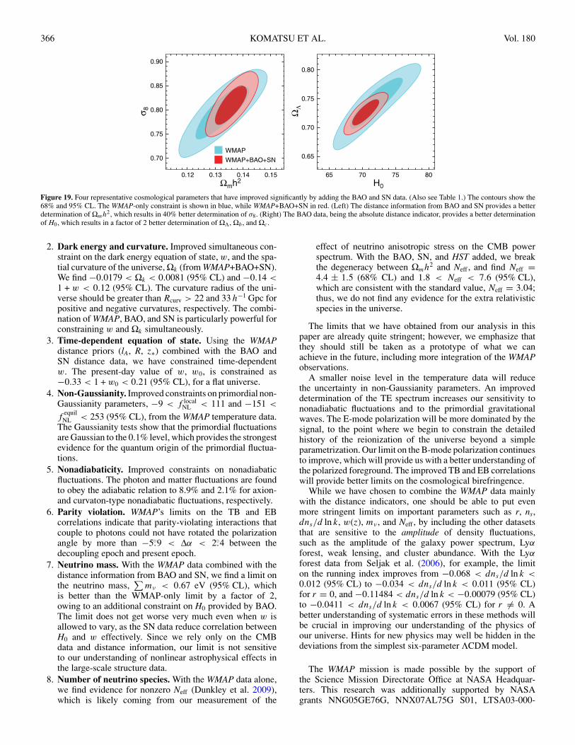
366 KOMATSU ET AL. Vol. 180
Figure 19. Four representative cosmological parameters that have improved significantly by adding the BAO and SN data. (Also see Table 1.) The contours show the68% and 95% CL. The WMAP-only constraint is shown in blue, while WMAP+BAO+SN in red. (Left) The distance information from BAO and SN provides a betterdetermination of Ωmh2, which results in 40% better determination of σ8. (Right) The BAO data, being the absolute distance indicator, provides a better determinationof H0, which results in a factor of 2 better determination of ΩΛ, Ωb , and Ωc .
2. Dark energy and curvature. Improved simultaneous con-straint on the dark energy equation of state, w, and the spa-tial curvature of the universe, Ωk (from WMAP+BAO+SN).We find −0.0179 < Ωk < 0.0081 (95% CL) and −0.14 <1 + w < 0.12 (95% CL). The curvature radius of the uni-verse should be greater than Rcurv > 22 and 33 h−1 Gpc forpositive and negative curvatures, respectively. The combi-nation of WMAP, BAO, and SN is particularly powerful forconstraining w and Ωk simultaneously.
3. Time-dependent equation of state. Using the WMAPdistance priors (lA, R, z∗) combined with the BAO andSN distance data, we have constrained time-dependentw. The present-day value of w, w0, is constrained as−0.33 < 1 + w0 < 0.21 (95% CL), for a flat universe.
4. Non-Gaussianity. Improved constraints on primordial non-Gaussianity parameters, −9 < f local
NL < 111 and −151 <
fequilNL < 253 (95% CL), from the WMAP temperature data.
The Gaussianity tests show that the primordial fluctuationsare Gaussian to the 0.1% level, which provides the strongestevidence for the quantum origin of the primordial fluctua-tions.
5. Nonadiabaticity. Improved constraints on nonadiabaticfluctuations. The photon and matter fluctuations are foundto obey the adiabatic relation to 8.9% and 2.1% for axion-and curvaton-type nonadiabatic fluctuations, respectively.
6. Parity violation. WMAP’s limits on the TB and EBcorrelations indicate that parity-violating interactions thatcouple to photons could not have rotated the polarizationangle by more than −5.◦9 < Δα < 2.◦4 between thedecoupling epoch and present epoch.
7. Neutrino mass. With the WMAP data combined with thedistance information from BAO and SN, we find a limit onthe neutrino mass,
∑mν < 0.67 eV (95% CL), which
is better than the WMAP-only limit by a factor of 2,owing to an additional constraint on H0 provided by BAO.The limit does not get worse very much even when w isallowed to vary, as the SN data reduce correlation betweenH0 and w effectively. Since we rely only on the CMBdata and distance information, our limit is not sensitiveto our understanding of nonlinear astrophysical effects inthe large-scale structure data.
8. Number of neutrino species. With the WMAP data alone,we find evidence for nonzero Neff (Dunkley et al. 2009),which is likely coming from our measurement of the
effect of neutrino anisotropic stress on the CMB powerspectrum. With the BAO, SN, and HST added, we breakthe degeneracy between Ωmh2 and Neff , and find Neff =4.4 ± 1.5 (68% CL) and 1.8 < Neff < 7.6 (95% CL),which are consistent with the standard value, Neff = 3.04;thus, we do not find any evidence for the extra relativisticspecies in the universe.
The limits that we have obtained from our analysis in thispaper are already quite stringent; however, we emphasize thatthey should still be taken as a prototype of what we canachieve in the future, including more integration of the WMAPobservations.
A smaller noise level in the temperature data will reducethe uncertainty in non-Gaussianity parameters. An improveddetermination of the TE spectrum increases our sensitivity tononadiabatic fluctuations and to the primordial gravitationalwaves. The E-mode polarization will be more dominated by thesignal, to the point where we begin to constrain the detailedhistory of the reionization of the universe beyond a simpleparametrization. Our limit on the B-mode polarization continuesto improve, which will provide us with a better understanding ofthe polarized foreground. The improved TB and EB correlationswill provide better limits on the cosmological birefringence.
While we have chosen to combine the WMAP data mainlywith the distance indicators, one should be able to put evenmore stringent limits on important parameters such as r, ns,dns/d ln k, w(z), mν , and Neff , by including the other datasetsthat are sensitive to the amplitude of density fluctuations,such as the amplitude of the galaxy power spectrum, Lyαforest, weak lensing, and cluster abundance. With the Lyαforest data from Seljak et al. (2006), for example, the limiton the running index improves from −0.068 < dns/d ln k <0.012 (95% CL) to −0.034 < dns/d ln k < 0.011 (95% CL)for r = 0, and −0.11484 < dns/d ln k < −0.00079 (95% CL)to −0.0411 < dns/d ln k < 0.0067 (95% CL) for r = 0. Abetter understanding of systematic errors in these methods willbe crucial in improving our understanding of the physics ofour universe. Hints for new physics may well be hidden in thedeviations from the simplest six-parameter ΛCDM model.
The WMAP mission is made possible by the support ofthe Science Mission Directorate Office at NASA Headquar-ters. This research was additionally supported by NASAgrants NNG05GE76G, NNX07AL75G S01, LTSA03-000-

No. 2, 2009 WMAP FIVE-YEAR OBSERVATIONS: COSMOLOGICAL INTERPRETATION 367
0090, ATPNNG04GK55G, and ADP03-0000-092. E.K. ac-knowledges support from an Alfred P. Sloan Research Fellow-ship. We thank M. Greason and N. Odegard for their help onthe analysis of the WMAP data, and B. Griswold for the art-work. We thank U. Seljak, A. Slosar, and P. McDonald forproviding the Lyα forest likelihood code, W. Percival for usefulinformation on the implementation of the BAO data, E. Hivonfor providing a new HEALPix routine to remove the monopoleand dipole from the weighted temperature maps, and K. Smithfor his help on implementing the bispectrum optimization al-gorithm. We thank A. Conley for valuable comments on ouroriginal treatment of the Type Ia SN data, and M. Kowalski,J. Guy, and A. Slosar for making the union SN data avail-able to us. Computations for the analysis of non-Gaussianity inSection 3.5 were carried out by the Terascale Infrastruc-ture for Groundbreaking Research in Engineering and Science(TIGRESS) at the Princeton Institute for Computational Sci-ence and Engineering (PICSciE). This research has made use ofNASA’s Astrophysics Data System Bibliographic Services. Weacknowledge use of the HEALPix (Gorski et al. 2005), CAMB(Lewis et al. 2000), and CMBFAST (Seljak & Zaldarriaga 1996)packages.
APPENDIX A
FAST CUBIC ESTIMATORS
We use the following estimators for f localNL , f equil
NL , and bsrc (theamplitude of the point-source bispectrum):
f localNL = (F−1)11S1 + (F−1)12S2 + (F−1)13S3, (A1)
fequilNL = (F−1)21S1 + (F−1)22S2 + (F−1)23S3, (A2)
bsrc = (F−1)31S1 + (F−1)32S2 + (F−1)33S3, (A3)
where Fij is the Fisher matrix given by
Fij ≡∑
2�l1�l2�l3
B(i)l1l2l3
B(j )l1l2l3
Cl1Cl2Cl3
. (A4)
Here, B(i)l1l2l3
are theoretically calculated angular bispectra (given
below), where i = 1 is used for f localNL , i = 2 for f
equilNL , and
i = 3 for bsrc. The denominator of Fij contains the total powerspectrum including the CMB signal (CCMB
l ) and noise (Nl),Cl ≡ CCMB
l b2l + Nl , and bl is the beam transfer function given
in Hill et al. (2009).While this formula allows one to estimate f local
NL , fequilNL , and
bsrc simultaneously, we find that a simultaneous estimation doesnot change the results significantly. Therefore, we use
f localNL = S1/F11, f
equilNL = S2/F22, bsrc = S3/F33,
(A5)to simplify the analysis, as well as to make the comparison withthe previous work easier. However, we do take into account apotential leakage of the point sources into f local
NL and fequilNL by
using the Monte Carlo simulation of point sources, as describedlater. These Monte Carlo estimates of the bias in f local
NL andf
equilNL due to the source contamination roughly agree with
contributions from the off-diagonal terms in Equations (A1)and (A2).
Assuming white noise, which is a good approximation athigh multipoles in which noise becomes important, one cananalytically compute the noise power spectrum as
Nl = Ωpix
∫d2n
4πfsky
σ 20 M(n)
Nobs(n), (A6)
where Ωpix ≡ 4π/Npix is the solid angle per pixel, M(n) is theKQ75 mask, fsky = 0.718 is the fraction of sky retained by theKQ75 mask, σ0 is the rms noise per observation, and Nobs(n) isthe number of observations per pixel.
The angular bispectra are given by
B(1)l1l2l3
= 2Il1l2l3
∫ ∞
0r2dr[αl1 (r)βl2 (r)βl3 (r) + (cyc.)], (A7)
B(2)l1l2l3
= − 3B(1)l1l2l3
+ 6Il1l2l3
∫ ∞
0r2dr{[βl1 (r)γl2 (r)δl3 (r) + (cyc.)]
− 2δl1 (r)δl2 (r)δl3 (r)}, (A8)
B(3)l1l2l3
= Il1l2l3 , (A9)
where
Il1l2l3 ≡√
(2l1 + 1)(2l2 + 1)(2l3 + 1)
4π
(l1 l1 l30 0 0
). (A10)
Various functions in B(i)l1l2l3
are given by
αl(r) ≡ 2
π
∫k2dkgT l(k)jl(kr), (A11)
βl(r) ≡ 2
π
∫k2dkPΦ(k)gT l(k)jl(kr), (A12)
γl(r) ≡ 2
π
∫k2dkP
1/3Φ (k)gT l(k)jl(kr), (A13)
δl(r) ≡ 2
π
∫k2dkP
2/3Φ (k)gT l(k)jl(kr). (A14)
Here, PΦ(k) ∝ kns−4 is the primordial power spectrum ofBardeen’s curvature perturbations, and gT l(k) is the radiationtransfer function that gives the angular power spectrum asCl = (2/π )
∫k2dkPΦ(k)g2
T l(k).The skewness parameters, Si, are given by (Komatsu et al.
2005; Babich 2005; Creminelli et al. 2006; Yadav et al. 2008)
S1 ≡ 4π
∫r2dr
∫d2n
w3
[A(n, r)B2(n, r)
− 2B(n, r)〈Asim(n, r)Bsim(n, r)〉MC − A(n, r)
× ⟨B2
sim(n, r)⟩MC
], (A15)
S2 ≡ − 3S1 + 24π
∫r2dr
∫d2n
w3
{[B(n, r)C(n, r)D(n, r)
− B(n, r)〈Csim(n, r)Dsim(n)〉MC − C(n, r)〈Bsim(n, r)
×Dsim(n)〉MC − D(n, r)〈Bsim(n, r)Csim(n, r)〉MC]
− 1
3[D3(n, r) − 3D(n, r)〈D2
sim(n, r)〉MC]
}(A16)

368 KOMATSU ET AL. Vol. 180
Figure 20. Evolution of dark energy for w0 = −1.1 and w′ = 1, and various transition redshifts, ztrans = 0.5, 2, and 10, above which w(z) approaches −1. (Top left)Evolution of the dark energy to matter density ratio as a function of z. Note that the vertical axis has been multiplied by 106. (Top right) Evolution of the dark energydensity relative to the dark energy density at present. The dark energy density was nearly constant at high redshifts above ztrans; thus, these models can describe the“thawing models” (Caldwell & Linder 2005), in which dark energy was nearly constant at early times, and had become dynamical at lower redshifts. (Bottom left)Evolution of the equation of state, w(z) = Pde(z)/ρde(z). By construction of the model, w(z) approaches −1 beyond ztrans. (Bottom right) Evolution of the effectiveequation of state, weff (z), which determines the evolution of dark energy density as ρde(z) = ρde(0)(1 + z)3[1+weff (z)].
S3 ≡ 2π
3
∫d2n
w3
[E3(n) − 3E(n)
⟨E2
sim(n)⟩MC
], (A17)
where w3 is the sum of the weighting function cubed:
w3 ≡∫
d2nW 3(n). (A18)
For a uniform weighting, the weighting function is simplygiven by the KQ75 mask, that is, W (n) = M(n), which givesw3 = 4πfsky. For our measurements of f local
NL , fequilNL , and bsrc,
we shall use a “combination signal-plus-noise weight,” given by
W (n) = M(n)
σ 2cmb + σ 2
0
/Nobs(n)
, (A19)
where σ 2cmb ≡ (1/4π )
∑l(2l + 1)Ccmb
l b2l is the CMB signal
variance, σ0 is the rms noise per observation, and Nobs(n) is thenumber of observations per pixel. This combination weightingyields a nearly optimal performance for bsrc and f
equilNL , whereas
it results in a minor improvement in f localNL over the uniform
weighting. The bracket, 〈〉MC, denotes the average over MonteCarlo realizations and “sim” denotes that these are the filteredmaps of the Monte Carlo realizations.
The filtered temperature maps, A, B, C, D, and E, are givenby
A(n, r) ≡lmax∑l=2
l∑m=−l
αl(r)bl
Cl
almYlm(n), (A20)
B(n, r) ≡lmax∑l=2
l∑m=−l
βl(r)bl
Cl
almYlm(n), (A21)
C(n, r) ≡lmax∑l=2
l∑m=−l
γl(r)bl
Cl
almYlm(n), (A22)
D(n, r) ≡lmax∑l=2
l∑m=−l
δl(r)bl
Cl
almYlm(n), (A23)
E(n) ≡lmax∑l=2
l∑m=−l
bl
Cl
almYlm(n), (A24)
respectively. Here, lmax is the maximum multipole that we usein the analysis. We vary lmax to see how much the results dependon lmax.
Equations (A15) and (A16) involve the integrals over theconformal distances, r. We evaluate these integrals as∫
r2dr[. . .](r) =∑
i
(wi)optr2i Δri[. . .](ri). (A25)
We use the bispectrum optimization algorithm described inSmith & Zaldarriaga (2006) to compute the optimal weights,(wi)opt, and decide on which quadrature points, ri, to keep. Wechoose the number of quadrature points such that the bispectrumcomputed in this way agrees with that from more dense sampling
No. 2, 2009 WMAP FIVE-YEAR OBSERVATIONS: COSMOLOGICAL INTERPRETATION 369
in r to 10−5, which typically gives ∼ 5 quadrature points forf local
NL and ∼ 15 points for fequilNL .52
The measurement of these estimators proceeds as follows.
1. Generate the simulated realizations of CMB signal maps,TS, from the input signal power spectrum, Ccmb
l , andthe beam transfer function, bl. We have generated 300realizations for the analysis given in this paper.
2. Add random noise, TN , using the rms noise per pixel givenby σ0/
√Nobs(n).
3. Add point sources. We use a simplified treatment for thesource simulation,
Tsrc(n)
2.725 K=
[sinh2(x/2)
x4
Fsrc/Ωpix
67.55MJy
]ε, (A26)
where Ωpix is the solid angle of pixel, x = hν/(kBTcmb) =56.80 GHz (for Tcmb = 2.725 K), ε is a Poisson randomvariable with the mean of 〈ε〉 = nsrcΩpix, and nsrc is theaverage number of sources per steradians. This simplifiedmodel assumes that there is only one population of sourceswith a fixed flux, Fsrc, and each source’s flux is independentof frequency. We choose nsrc = 0.85 sr−1 and Fsrc = 0.5 Jy,which yields the source power spectrum in the Q band ofCps = 8.7 × 10⁻³ μK2 sr and the source bispectrum inthe Q band of bsrc = 8.7 × 10⁻⁵ μK3 sr2, which roughlyreproduce the measured values. However, this model doesnot reproduce the source counts very well. (The sourcedensity of nsrc = 0.85 sr−1 at 0.5 Jy is too low.) The mainpurpose of this phenomenological model is to reproducethe power spectrum and bispectrum—we include pointsources in the simulations, in order to take into account thepotential effects of the unresolved sources on primordialnon-Gaussianity, f local
NL and fequilNL .
4. Coadd them to create the simulated temperature maps,T (n) = TS(n) + TN (n) + Tsrc(n).
5. Mask and weight the temperature maps, T (n) → T (n) =W (n)T (n), where W (n) is given by Equation (A19).
6. Remove the monopole and dipole from T (n).7. Compute the harmonic coefficients as
alm =∫
d2nT (n)Y ∗lm(n). (A27)
8. Generate the filtered maps, Asim, Bsim, Csim, Dsim, and Esim,and compute the appropriate Monte Carlo averages such as〈AsimBsim〉MC. This is the most time-consuming part.
9. Compute the filtered maps from the WMAP data. Whenwe coadd the V- and W -band data, we weight them asTV +W = (TV + 0.9TW )/1.9. The beam transfer function ofthe coadded map is given by bV +W
l = (bV
l + 0.9bWl
)/1.9,
and σ0/Nobs of the coadded map is given by
(σV +W
0
)2
NV +Wobs (n)
= 1
1.92
[ (σV
0
)2
NVobs(n)
+
(0.9σW
0
)2
NWobs(n)
]. (A28)
10. Compute the skewness parameters, Si, from the filteredWMAP data, and obtain f local
NL , f equilNL , and bsrc, either jointly
or separately.
52 Note that Smith & Zaldarriaga (2006) used 10−6 as a criterion, which givesmore quadrature points to evaluate. We find that 10−5 is sufficient for the sizeof statistical and systematic errors in the current measurements.
11. Compute these parameters from the simulated realizationsas well, and obtain the uncertainties.
For the computations of gT l(k) and generation of Monte Carlorealizations, we have used the maximum-likelihood values ofthe WMAP 3-year data (the power-law ΛCDM model fit bythe WMAP data alone with the Sunyaev–Zel’dovich effectmarginalized): Ωb = 0.0414, ΩCDM = 0.1946, ΩΛ = 0.7640,H0 = 73.2 km s−1 Mpc−1, τ = 0.091, and ns = 0.954 (Spergelet al. 2007). These parameters yield the conformal distance tot = 0 as cτ0 = 14.61 Gpc.
APPENDIX B
AXION
In this Appendix, we derive relations among the tensor-to-scalar ratio r, the axion mass density Ωah
2, the entropy-to-curvature perturbation ratio α, the phase of the Pecci–Quinnfield θa , and the axion decay constant fa.
Let us write the expectation value of the complex Pecci–Quinn field, ψPQ, as
〈ψPQ〉 = fa√2eiθa , (B1)
where fa is the axion decay constant and θa is the phase. Quantumfluctuations during inflation generate fluctuations in the phase,δθa , as
δθa = H
2πfa
. (B2)
As the number density of axions scales as the phase squared,na ∝ θ2
a , the mass density fluctuation is given by
δρa
ρa
= 2δθa
θa
= H
πθafa
. (B3)
As the energy density of axions was negligible during inflation,the axion density perturbation, δρa/ρa , would produce theisocurvature perturbation. While radiation (including photons)is generated by decay of inflaton fields, (some of) dark matteris in the form of axions whose generation is independent ofphotons; thus, the entropy perturbation between photons andaxions would be generated. We assume that axions were not inthermal equilibrium with photons in the subsequent evolutionof the universe.
The entropy perturbations and curvature perturbations aregiven, respectively, by
k3PS (k)
2π2= Ω2
a
Ω2c
H 2k
π2θ2a f 2
a
,k3PR(k)
2π2= H 4
k
4π2φ2k
≈ H 2k
8π2M2plε
,
(B4)
where Ωa � Ωc is the axion mass density, Hk is the expansionrate during inflation at which the wavenumber k went outsideof the horizon, φk is the value of inflaton at the same time,ε ≡ −H /H ≈ (
M2pl/2
)(V ′/V )2 is the usual slow-roll param-
eter, V (φ) is the inflaton potential, and Mpl = 1/√
8πG is thereduced Planck mass. We have used the slow-roll approxima-tion, φ ≈ −V ′/(3H ) and H 2 ≈ V
/(3M2
pl
).
Here, let us comment on our choice of m = 1, which makesk3PS ∝ km−1 independent of k. Since k3PS ∝ H 2
k ∝ k−2ε ,where ε = −H /H 2, this choice corresponds to having a very

370 KOMATSU ET AL. Vol. 180
Figure 21. The same as Figure 15, but the systematic errors in the Type Ia SN data are included.
small slow-roll parameter, ε � 1. This is consistent with ourlimit on the curvature power spectrum, ns = 1 + 6ε − 4η 1 − 4η < 1, where η is another slow-roll parameter. As thecurrent limit is 1 −ns ≈ 4η 0.04, our approximation, m = 1,is valid for ε < 0.01. It should be straightforward to extend ouranalysis to the case in which m = 1.
By dividing PS (k) by PR(k), we find the entropy-to-curvatureperturbation ratio for axions, α0(k), as
α0(k)
1 − α0(k)≡ PS (k)
PR(k)= Ω2
a
Ω2c
8ε
θ2a (fa/Mpl)2
. (B5)
At this point, it is clear that one cannot solve this constraintuniquely for any of ε, fa, or θa .
In order to break the degeneracy, we use the axion massdensity (Kawasaki & Sekiguchi 2008, and references therein)
Ωah2 = 1.0 × 10⁻³γ θ2
a
(fa
1010 GeV
)7/6
, (B6)
where γ is a dilution factor, representing the amount by whichthe axion density could have been diluted by a late-time entropyproduction between the QCD phase transition at ∼ 200 MeVand the epoch of nucleosynthesis at ∼ 1 Mpc.
Combining equation (B5) and (B6) to eliminate the phase, θa ,and using the relation between the tensor-to-scalar ratio r andthe slow-roll parameter ε, r = 16ε, we find
r = (1.6 × 10⁻¹²)
(Ωch
2
γ
) (Ωc
Ωa
) (fa
1012 GeV
)5/6α0
1 − α0.
(B7)Alternatively, we can eliminate the axion decay constant, fa, toobtain
r = 4.7 × 10⁻¹²
θ10/7a
(Ωch
2
γ
)12/7 (Ωc
Ωa
)2/7α0
1 − α0. (B8)
This is Equation (48).
APPENDIX C
EQUATION OF STATE OF DARK ENERGY: A NEWPARAMETRIZED FORM
In this Appendix, we describe the models of dark energy thatwe explore in Section 5.4. Our goal is to obtain a sensible form oftime-dependent dark energy equation of state, w(a). One of the
most commonly used form of w(a) is a linear form (Chevallier& Polarski 2001; Linder 2003)
w(a) = w0 + (1 − a)wa, (C1)
where w0 and wa parametrize the present-day value of w andthe first derivative. However, this form cannot be adopted as it iswhen one uses the CMB data to constrain w(a). Since this formis basically the leading-order term of a Taylor series expansion,the value of w(a) can become unreasonably too large or toosmall when extrapolated to the decoupling epoch at z∗ 1090(or a∗ 9.17 × 10⁻⁴), and thus one cannot extract meaningfulconstraints on the quantities, such as w0 and wa, that are definedat the present epoch.
To avoid this problem, yet to keep a close contact with theprevious work in the literature, we shall consider an alternativeparametrized form. Our idea is the following: we wish tokeep the form given by Equation (C1) at low redshifts, lowerthan some transition redshift, ztrans. However, we demand thatw(a) approach −1 at higher redshifts, z > ztrans. This formof w(a), therefore, has the following property: at early times,before the transition redshift, ztrans, dark energy was just like acosmological constant, and thus the dark energy density wasnearly constant, that is, ρde(z > ztrans) ≈ constant. Then,dark energy began to become dynamical at z ∼ ztrans, withthe equation of state given by the conventional linear form,Equation (C1).
Some of the properties of our form of w(a) are similarto those of “thawing models,” (Caldwell & Linder 2005) inwhich a scalar field was moving very slowly initially, givingw(a) ≈ −1 at early times, and then began to move faster towardlow redshifts, causing w(a) to deviate more and more from−1 at low redshifts. Our parametrization can describe a moregeneral class of models than single scalar field models, as itallows for w to go below −1. However, models that are basedupon a single scalar field cannot have w < −1 (e.g., Hu 2005).The “Forever regular” parametrization, explored in Wang &Tegmark (2004), also approaches a constant density at earlytimes, if the late-time equation of state is w < −1. The “Kinkmodel” explored in Bassett et al. (2002, 2004) and Corasanitiet al. (2004) also extrapolates a constant equation of state atearly times to a different constant equation of state at late times.Our parametrization is more general than theirs, as their formonly allows for a constant equation of state at late times.
We wish to find a smooth interpolation between wearly = −1and wlate = w0 + (1 − a)wa . We begin by writing
w(a) = w(a)f (a/atrans) + (−1) [1 − f (a/atrans)] , (C2)

No. 2, 2009 WMAP FIVE-YEAR OBSERVATIONS: COSMOLOGICAL INTERPRETATION 371
Table 14Comparison of ΛCDM Parameters from WMAP+BAO+SN with Various SN Compilations
Class Parameter Uniona Union+Sys. Err.b Davisc Alternatived
Primary 100Ωbh2 2.267+0.058
−0.059 2.267 ± 0.059 2.270 ± 0.060 2.265 ± 0.059Ωch
2 0.1131 ± 0.0034 0.1134+0.0036−0.0037 0.1121 ± 0.0035 0.1143 ± 0.0034
ΩΛ 0.726 ± 0.015 0.725 ± 0.016 0.732+0.014−0.015 0.721 ± 0.015
ns 0.960 ± 0.013 0.960 ± 0.013 0.962 ± 0.013 0.960+0.014−0.013
τ 0.084 ± 0.016 0.085 ± 0.016 0.085 ± 0.016 0.084 ± 0.016Δ2R(ke
0) (2.445 ± 0.096) × 10−9 (2.447+0.096−0.095) × 10−9 (2.429+0.096
−0.095) × 10−9 (2.457+0.092−0.093) × 10−9
Derived σ8 0.812 ± 0.026 0.813+0.026−0.027 0.807 ± 0.027 0.817 ± 0.026
H0 70.5 ± 1.3 km s−1 Mpc−1 70.4 ± 1.4 km s−1 Mpc−1 70.9 ± 1.3 km s−1 Mpc−1 70.1 ± 1.3 km s−1 Mpc−1
Ωb 0.0456 ± 0.0015 0.0458 ± 0.0016 0.0451+0.0016−0.0015 0.0462 ± 0.0015
Ωc 0.228 ± 0.013 0.229+0.014−0.015 0.223 ± 0.013 0.233 ± 0.013
Ωmh2 0.1358+0.0037−0.0036 0.1361+0.0038
−0.0039 0.1348 ± 0.0038 0.1369 ± 0.0037zf
reion 10.9 ± 1.4 10.9 ± 1.4 10.9 ± 1.4 10.8 ± 1.4tg0 13.72 ± 0.12 Gyr 13.72 ± 0.12 Gyr 13.71 ± 0.12 Gyr 13.73 ± 0.12 Gyr
Notes.a Compilation by Kowalski et al. (2008) without the systematic errors included.b Compilation by Kowalski et al. (2008) with the systematic errors included.c Compilation by Davis et al. (2007).d Compilation used in the original version of this paper (version 1 of arXiv:0803.0547).e k0 = 0.002 Mpc−1. Δ2
R(k) = k3PR(k)/(2π2) (Equation (15)).f “Redshift of reionization,” if the universe was reionized instantaneously from the neutral state to the fully ionized state at zreion.g The present-day age of the universe.
where atrans = 1/(1 + ztrans), and the function f (x) goes to zerofor x � 1 and to unity for x � 1. Here, w(a) is the form of wat low redshifts. Any function that has this property is adequatefor f (x). We choose
f (x) = 12 [tanh(ln x) + 1] = x
x + 1, (C3)
which gives the desired form of the equation of state of darkenergy,
w(a) = aw(a)
a + atrans− atrans
a + atrans, (C4)
wherew(a) = w0 + (1 − a)wa. (C5)
One nice property of this form is that it allows one to obtaina closed, analytical form of the effective equation of state,weff(a), which gives the evolution of dark energy density,ρde(a) = ρ(0)a−3[1+weff (a)]:
weff(a) = 1
ln a
∫ ln a
0d ln a′w(a′)
= −1 +(1 − a)wa
ln a+
1 + w0 + (1 + atrans)wa
ln a
× lna + atrans
1 + atrans. (C6)
This property allows one to compute the expansion rate, H (a)(Equation (7)), and hence the distance (Equation (2)), easily.
Finally, we use the present-day value of w, w0 ≡ w(z = 0),and the first derivative, w′ ≡ dw/dz|z=0, as free parameters.They are related to w0 and wa as
1 + w0 = 1 + w0
1 + atrans, (C7)
w′ = wa
1 + atrans− atrans(1 + w0)
(1 + atrans)2. (C8)
The inverse relations are
1 + w0 = (1 + atrans)(1 + w0), (C9)
wa = (1 + atrans)w′ + atrans(1 + w0). (C10)
In the limit of very early transition, atrans � 1, one findsw0 ≈ w0 and w′ ≈ wa , as expected. This completes thedescription of our form of w(a).
Figure 20 shows the evolution of dark energy density,ρde(z) = ρ(0)(1 + z)3[1+weff (a)], the equation of state, w(z),and the effective equation of state, weff(z), computed fromEquation (C4) and (C6). We choose w0 = −1.1 and w′ = 1,which are close to the best-fitting values that we found inSection 5.4 (see Figure 14). We show three curves for the transi-tion redshifts of ztrans = 0.5, 2, and 10. We find that the form ofw(z) that we have derived achieves our goal: w(z) approaches−1 and the dark energy density tends to a constant value athigh redshifts, giving sensible results at the decoupling epoch.The dark energy density is totally subdominant compared to thematter density at high redshifts, which is also desirable.
The constraints that we have obtained for w0 and w′ are notsensitive to the exact values of ztrans (see the right panel ofFigure 14). This is because all of the curves shown in Figure 20are very similar at z � 1, where the BAO and SN data arecurrently available.
APPENDIX D
COMPARISON OF SN COMPILATIONS AND EFFECTSOF SYSTEMATIC ERRORS
In Table 14, we show the ΛCDM parameters derived fromWMAP+BAO+SN, where we use various SN compilations:“Union” for the latest union compilation (Kowalski et al.2008), “Union+Sys.Err.” for the union compilation with sys-tematic errors included, “Davis” for the previous compilationby Davis et al. (2007), and “Alternative” for the compilationthat we used in the original version of this paper (version 1 ofarXiv:0803.0547).

372 KOMATSU ET AL. Vol. 180
For the “Alternative” compilation, we have combined mea-surements from the Hubble Space Telescope (HST; Riess et al.2004, 2007), the SNLS (Astier et al. 2006), and the Equation ofState: ESSENCE survey (Wood-Vasey et al. 2007), as well assome nearby Type Ia SNe. In the “Davis” and “Alternative” com-pilations, different light curve fitters were used for the SN datataken by different groups, and thus these compilations were notas optimal as the union compilation, for which the same SALTfitter was used for all the SNe samples. Moreover, the unioncompilation is the largest of all. For this reason, we have de-cided to update all the cosmological parameters using the unioncompilation.
Nevertheless, we find that all of these compilations yieldsimilar results: the mean values shift no more than ∼ 0.5σ .
The effects of the systematic errors in the Type Ia SNdata on the ΛCDM parameters are also very small forWMAP+BAO+SN; however, the effects on the dark energy pa-rameters, w0 and w′, turn out to be significant. In Figure 21, weshow the two-dimensional joint constraint on w0 and w′ fromWMAP+BAO+SN+BBN (also see Section 5.4.2) with the sys-tematic errors included. Comparing this with Figure 15, wherethe systematic errors are ignored, we find that the constraints onw0 and w′ weaken significantly: we find w0 = −1.00±0.19 andw′ = 0.11 ± 0.70 with the systematic errors included, whereasw0 = −1.04±0.13 and w′ = 0.24±0.55 without the systematicerrors.
REFERENCES
Abbott, L. F., & Wise, M. B. 1984, Nucl. Phys. B, 244, 541Abdalla, F. B., & Rawlings, S. 2007, MNRAS, 381, 1313Abdurashitov, J. N., et al. 1999, Phys. Rev., C60, 055801Accetta, F. S., Zoller, D. J., & Turner, M. S. 1985, Phys. Rev. D, 31, 3046Acquaviva, V., Bartolo, N., Matarrese, S., & Riotto, A. 2003, Nucl. Phys. B,
667, 119Adam, C., & Klinkhamer, F. R. 2001, Nucl. Phys. B, 607, 247Adams, F. C., Bond, J. R., Freese, K., Frieman, J. A., & Olinto, A. V. 1993, Phys.
Rev. D, 47, 426Ahmad, Q. R., et al. 2002, Phys. Rev. Lett., 89, 011301Ahmed, S. N., et al. 2004, Phys. Rev. Lett., 92, 181301Ahn, M. H., et al. 2003, Phys. Rev. Lett., 90, 041801Alabidi, L., & Lyth, D. H. 2006a, J. Cosmol. Astropart. Phys., JCAP08(2006)013Alabidi, L., & Lyth, D. H. 2006b, J. Cosmol. Astropart. Phys.,
JCAP05(2006)016Albrecht, A., & Steinhardt, P. J. 1982, Phys. Rev. Lett., 48, 1220Alishahiha, M., Silverstein, E., & Tong, D. 2004, Phys. Rev. D, 70, 123505Allen, S. W., Schmidt, R. W., & Bridle, S. L. 2003, MNRAS, 346, 593Allison, W. W. M., et al. 1999, Phys. Lett. B, 449, 137Amarzguioui, M., Elgarøy, Ø., Mota, D. F., & Multamaki, T. 2006, A&A, 454,
707Ambrosio, M., et al. 2001, Phys. Lett. B, 517, 59Amin, M. A., Wagoner, R. V., & Blandford, R. D. 2008, MNRAS, 390, 131Araki, T., et al. 2005, Phys. Rev. Lett., 94, 081801Argueso, F., Gonzalez-Nuevo, J., & Toffolatti, L. 2003, ApJ, 598, 86Arkani-Hamed, N., Creminelli, P., Mukohyama, S., & Zaldarriaga, M. 2004, J.
Cosmol. Astropart. Phys., JCAP04(2004)001Armendariz-Picon, C., Damour, T., & Mukhanov, V. F. 1999, Phys. Lett. B, 458,
209Arroja, F., & Koyama, K. 2008, Phys. Rev. D, 77, 083517Astier, P., et al. 2006, A&A, 447, 31Babich, D. 2005, Phys. Rev. D, 72, 043003Babich, D., Creminelli, P., & Zaldarriaga, M. 2004, J. Cosmol. Astropart. Phys.,
JCAP08(2004)009Bardeen, J. M., Steinhardt, P. J., & Turner, M. S. 1983, Phys. Rev. D, 28, 679Barger, V., Kneller, J. P., Lee, H.-S., Marfatia, D., & Steigman, G. 2003, Phys.
Lett. B, 566, 8Barger, V., Marfatia, D., & Tregre, A. 2004, Phys. Lett. B, 595, 55Barris, B. J., et al. 2004, ApJ, 602, 571Bartolo, N., Komatsu, E., Matarrese, S., & Riotto, A. 2004, Phys. Rep., 402,
103
Bartolo, N., & Liddle, A. R. 2002, Phys. Rev. D, 65, 121301Bartolo, N., Matarrese, S., & Riotto, A. 2006, J. Cosmol. Astropart. Phys.,
JCAP06(2006)024Bartolo, N., Matarrese, S., & Riotto, A. 2007, J. Cosmol. Astropart. Phys.,
JCAP01(2007)019Bashinsky, S., & Seljak, U. 2004, Phys. Rev. D, 69, 083002Basko, M. M., & Polnarev, A. G. 1980, MNRAS, 191, 207Bassett, B. A., Corasaniti, P. S., & Kunz, M. 2004, ApJ, 617, L1Bassett, B. A., Kunz, M., Silk, J., & Ungarelli, C. 2002, MNRAS, 336, 1217Bassett, B. A., Tsujikawa, S., & Wands, D. 2006, Rev. Mod. Phys., 78, 537Bean, R., Bernat, D., Pogosian, L., Silvestri, A., & Trodden, M.
2007b, Phys. Rev. D, 75, 064020Bean, R., Chen, X., Peiris, H. V., & Xu, J. 2008, Phys. Rev. D, 77, 023527Bean, R., Dunkley, J., & Pierpaoli, E. 2006, Phys. Rev. D, 74, 063503Bean, R., Shandera, S. E., Henry Tye, S. H., & Xu, J. 2007a, J. Cosmol. Astropart.
Phys., JCAP07(2005)004Beltran, M. 2008, Phys. Rev. D, 78, 023530Beltran, M., Garcia-Bellido, J., & Lesgourgues, J. 2007, Phys. Rev. D, 75,
103507Beltran, M., Garcıa-Bellido, J., Lesgourgues, J., Liddle, A. R., & Slosar, A.
2005a, Phys. Rev. D, 71, 063532Beltran, M., Garcia-Bellido, J., Lesgourgues, J., & Riazuelo, A. 2004, Phys.
Rev. D, 70, 103530Beltran, M., Garcia-Bellido, J., Lesgourgues, J., & Viel, M. 2005b, Phys. Rev.
D, 72, 103515Bennett, C. L., et al. 1994, ApJ, 436, 423Bennett, C. L., et al. 1996, ApJ, 464, L1Bennett, C. L., et al. 2003a, ApJ, 583, 1Bennett, C. L., et al. 2003b, ApJS, 148, 1Bennett, C. L., et al. 2003c, ApJS, 148, 97Bernui, A., Mota, B., Reboucas, M. J., & Tavakol, R. 2007, A&A, 464, 479Bertschinger, E., & Zukin, P. 2008, Phys. Rev. D, 78, 024015Bielewicz, P., Eriksen, H. K., Banday, A. J., Gorski, K. M., & Lilje, P. B.
2005, ApJ, 635, 750Bolton, J. S., Viel, M., Kim, T.-S., Haehnelt, M. G., & Carswell, R. F.
2008, MNRAS, 386, 1131Bond, J. R., & Efstathiou, G. 1984, ApJ, 285, L45Bond, J. R., Efstathiou, G., & Silk, J. 1980, Phys. Rev. Lett., 45, 1980Bond, J. R., Efstathiou, G., & Tegmark, M. 1997, MNRAS, 291, L33Bond, J. R., & Szalay, A. S. 1983, ApJ, 274, 443Boubekeur, L., & Lyth, D. H. 2006, Phys. Rev. D, 73, 021301Bridges, M., McEwen, J. D., Cruz, M., Hobson, M. P., Lasenby, A. N., Vielva,
P., & Martinez-Gonzalez, E. 2008, MNRAS, 390, 1372Bridle, S. L., Lewis, A. M., Weller, J., & Efstathiou, G. 2003, MNRAS, 342,
L72Buchbinder, E. I., Khoury, J., & Ovrut, B. A. 2007, Phys. Rev. D, 76, 123503Buchbinder, E. I., Khoury, J., & Ovrut, B. A. 2008, Phys. Rev. Lett., 100, 171302Bucher, M., Dunkley, J., Ferreira, P. G., Moodley, K., & Skordis, C. 2004, Phys.
Rev. Lett., 93, 081301Byrnes, C. T., Sasaki, M., & Wands, D. 2006, Phys. Rev. D, 74, 123519Cabella, P., Hansen, F., Marinucci, D., Pagano, D., & Vittorio, N.
2004, Phys. Rev. D, 69, 063007Cabella, P., Hansen, F. K., Liguori, M., Marinucci, D., Matarrese, S., Moscardini,
L., & Vittorio, N. 2006, MNRAS, 369, 819Cabella, P., Natoli, P., & Silk, J. 2007, Phys. Rev. D, 76, 123014Caldwell, R. R., Dave, R., & Steinhardt, P. J. 1998, Phys. Rev. Lett., 80, 1582Caldwell, R. R., & Linder, E. V. 2005, Phys. Rev. Lett., 95, 141301Carroll, S. M. 1998, Phys. Rev. Lett., 81, 3067Carroll, S. M., Field, G. B., & Jackiw, R. 1990, Phys. Rev. D, 41, 1231Carroll, S. M., Press, W. H., & Turner, E. L. 1992, ARA&A, 30, 499Cash, W. 1976, A&A, 52, 307Cayon, L., Jin, J., & Treaster, A. 2005, MNRAS, 362, 826Chambers, A., & Rajantie, A. 2008, Phys. Rev. Lett., 100, 041302Chen, G., & Szapudi, I. 2005, ApJ, 635, 743Chen, G., & Szapudi, I. 2006, ApJ, 647, L87Chen, X. 2005a, J. High Energy Phys., JHEP08(2005)045Chen, X. 2005b, Phys. Rev. D, 71, 063506Chen, X., Easther, R., & Lim, E. A. 2007a, J. Cosmol. Astropart. Phys.,
JCAP06(2007)023Chen, X., Easther, R., & Lim, E. A. 2008, J. Cosmol. Astropart. Phys.,
JCAP04(2008)010Chen, X., Huang, M.-X., Kachru, S., & Shiu, G. 2007b, J. Cosmol. Astropart.
Phys., JCAP01(2007)002Cheung, C., Creminelli, P., Fitzpatrick, A. L., Kaplan, J., & Senatore, L. 2008, J.
High Energy Phys., JHEP03(2008)014Chevallier, M., & Polarski, D. 2001, Int. J. Mod. Phys. D, 10, 213

No. 2, 2009 WMAP FIVE-YEAR OBSERVATIONS: COSMOLOGICAL INTERPRETATION 373
Chiang, L., Naselsky, P. D., Verkhodanov, O. V., & Way, M. J. 2003, ApJ, 590,L65
Chiang, L.-Y., Naselsky, P. D., & Coles, P. 2007, ApJ, 664, 8Chiba, T., Sugiyama, N., & Nakamura, T. 1997, MNRAS, 289, L5Chiba, T., & Takahashi, R. 2007, Phys. Rev. D, 75, 101301Chu, M., Eriksen, H. K., Knox, L., Gorski, K. M., Jewell, J. B., Larson, D. L.,
O’Dwyer, I. J., & Wandelt, B. D. 2005, Phys. Rev. D, 71, 103002Cirelli, M., & Strumia, A. 2006, J. Cosmol. Astropart. Phys., JCAP12(2006)013Cleveland, B. T., et al. 1998, ApJ, 496, 505Cole, S., et al. 2005, MNRAS, 362, 505Copeland, E. J., Liddle, A. R., & Wands, D. 1998, Phys. Rev. D, 57, 4686Copeland, E. J., Sami, M., & Tsujikawa, S. 2006, Int. J. Mod. Phys.D, 15, 1753Copi, C. J., Huterer, D., Schwarz, D. J., & Starkman, G. D. 2006, MNRAS, 367,
79Copi, C. J., Huterer, D., Schwarz, D. J., & Starkman, G. D. 2007, Phys. Rev. D,
75, 023507Copi, C. J., Huterer, D., & Starkman, G. D. 2004, Phys. Rev. D, 70, 043515Corasaniti, P. S., Kunz, M., Parkinson, D., Copeland, E. J., & Bassett, B. A.
2004, Phys. Rev. D, 70, 083006Corasaniti, P. S., & Melchiorri, A. 2008, Phys. Rev. D, 77, 103507Coughlan, G. D., Fischler, W., Kolb, E. W., Raby, S., & Ross, G. G. 1983, Phys.
Lett. B, 131, 59Coulson, D., Crittenden, R. G., & Turok, N. G. 1994, Phys. Rev. Lett., 73, 2390Covi, L., Hamann, J., Melchiorri, A., Slosar, A., & Sorbera, I.
2006, Phys. Rev. D, 74, 083509Creminelli, P., Nicolis, A., Senatore, L., Tegmark, M., & Zaldarriaga, M. 2006, J.
Cosmol. Astropart. Phys., JCAP05(2006)004Creminelli, P., & Senatore, L. 2007, J. Cosmol. Astropart. Phys.,
JCAP11(2007)010Creminelli, P., Senatore, L., Zaldarriaga, M., & Tegmark, M. 2007, J. Cosmol.
Astropart. Phys., JCAP03(2007)005Crittenden, R., Bond, J. R., Davis, R. L., Efstathiou, G., & Steinhardt, P. J.
1993, Phys. Rev. Lett., 71, 324Crittenden, R., Davis, R. L., & Steinhardt, P. J. 1993, ApJ, 417, L13Crittenden, R. G., Coulson, D., & Turok, N. G. 1995, Phys. Rev. D, 52, 5402Crotty, P., Garcia-Bellido, J., Lesgourgues, J., & Riazuelo, A. 2003a, Phys. Rev.
Lett., 91, 171301Crotty, P., Lesgourgues, J., & Pastor, S. 2003b, Phys. Rev. D, 67, 123005Crotty, P., Lesgourgues, J., & Pastor, S. 2004, Phys. Rev. D, 69, 123007Cruz, M., Cayon, L., Martınez-Gonzalez, E., Vielva, P., & Jin, J. 2007a, ApJ,
655, 11Cruz, M., Martınez-Gonzalez, E., Vielva, P., & Cayon, L. 2005, MNRAS, 356,
29Cruz, M., Tucci, M., Martınez-Gonzalez, E., & Vielva, P. 2006, MNRAS, 369,
57Cruz, M., Turok, N., Vielva, P., Martınez-Gonzalez, E., & Hobson, M.
2007b, Science, 318, 1612Curto, A., Aumont, J., Macıas-Perez, J. F., Martınez-Gonzalez, E., Barreiro, R.
B., Santos, D., Desert, F. X., & Tristram, M. 2007, A&A, 474, 23Daniel, S. F., Caldwell, R. R., Cooray, A., & Melchiorri, A. 2008, Phys. Rev. D,
77, 103513Davis, J., Raymond, , Harmer, D. S., & Hoffman, K. C. 1968, Phys. Rev. Lett.,
20, 1205Davis, T. M., et al. 2007, ApJ, 666, 716de Bernardis, F., Melchiorri, A., Verde, L., & Jimenez, R. 2008, J. Cosmol.
Astropart. Phys., JCAP03(2008)020de Bernardis, P., et al. 2000, Nature, 404, 955de Oliveira-Costa, A., Tegmark, M., Zaldarriaga, M., & Hamilton, A.
2004, Phys. Rev. D, 69, 063516De Troia, G., et al. 2007, ApJ, 670, L73Deffayet, C., Dvali, G., & Gabadadze, G. 2002, Phys. Rev. D, 65, 44023Destri, C., de Vega, H. J., & Sanchez, N. G. 2008, Phys. Rev. D, 77, 043509Dickinson, C., et al. 2004, MNRAS, 353, 732Dicus, D. A., et al. 1982, Phys. Rev. D, 26, 2694Dimopoulos, S., Kachru, S., McGreevy, J., & Wacker, J. 2005,
arXiv:hep-th/0507205Dodelson, S., Kinney, W. H., & Kolb, E. W. 1997, Phys. Rev. D, 56, 3207Dolgov, A. D. 2002, Phys. Rep., 370, 333Dolgov, A. D., Hansen, S. H., & Semikoz, D. V. 1999, Nucl. Phys. B, 543, 269Dore, O., et al. 2007, arXiv:0712.1599Dunkley, J., Bucher, M., Ferreira, P. G., Moodley, K., & Skordis, C. 2005, Phys.
Rev. Lett., 95, 261303Dunkley, J., et al. 2008, arXiv:0811.4280Dunkley, J., et al. 2009, ApJS, 180, 306Dvali, G., Gruzinov, A., & Zaldarriaga, M. 2004a, Phys. Rev. D, 69, 083505Dvali, G., Gruzinov, A., & Zaldarriaga, M. 2004b, Phys. Rev. D, 69, 023505Dvali, G. R., Gabadadze, G., & Porrati, M. 2000, Phys. Lett. B, 485, 208
Dvali, G. R., Shafi, Q., & Schaefer, R. 1994, Phys. Rev. Lett., 73, 1886Easther, R., & McAllister, L. 2006, J. Cosmol. Astropart. Phys.,
JCAP05(2006)018Easther, R., & Peiris, H. 2006, J. Cosmol. Astropart. Phys., JCAP09(2006)010Eguchi, K., et al. 2003, Phys. Rev. Lett., 90, 021802Eisenstein, D. J., & Hu, W. 1998, ApJ, 496, 605Eisenstein, D. J., et al. 2005, ApJ, 633, 560Elgarøy, Ø., & Lahav, O. 2003, J. Cosmol. Astropart. Phys., JCAP04(2003)004Elgarøy, Ø., & Lahav, O. 2005, New J. Phys., 7, 61Elgarøy, Ø., & Multamaki, T. 2007, A&A, 471, 65Ellis, J. R., Nanopoulos, D. V., & Quiros, M. 1986, Phys. Lett., B174, 176Enqvist, K., Jokinen, A., Mazumdar, A., Multamaki, T., & Vaihkonen, A.
2005, Phys. Rev. Lett., 94, 161301Eriksen, H. K., Banday, A. J., Gorski, K. M., Hansen, F. K., & Lilje, P. B.
2007a, ApJ, 660, L81Eriksen, H. K., Hansen, F. K., Banday, A. J., Gorski, K. M., & Lilje, P. B.
2004b, ApJ, 605, 14Eriksen, H. K., Huey, G., Banday, A. J., Gorski, K. M., Jewell, J. B., O’Dwyer,
I. J., & Wandelt, B. D. 2007b, ApJ, 665, L1Eriksen, H. K., Novikov, D. I., Lilje, P. B., Banday, A. J., & Gorski, K. M.
2004c, ApJ, 612, 64Eriksen, H. K., et al. 2004a, ApJS, 155, 227Eriksen, H. K., et al. 2007c, ApJ, 656, 641Fabbri, R., & Pollock, M. D. 1983, Phys. Lett. B, 125, 445Falk, T., Rangarajan, R., & Srednicki, M. 1993, ApJ, 403, L1Feng, B., Li, H., Li, M.-Z., & Zhang, X.-M. 2005, Phys. Lett. B, 620, 27Feng, B., Li, M., Xia, J.-Q., Chen, X., & Zhang, X. 2006, Phys. Rev. Lett., 96,
221302Ferreira, P. G., & Joyce, M. 1998, Phys. Rev. D, 58, 023503Ford, L. H. 1987, Phys. Rev. D, 35, 2339Freedman, W. L., et al. 2001, ApJ, 553, 47Freese, K., Frieman, J. A., & Olinto, A. V. 1990, Phys. Rev. Lett., 65, 3233Fu, L., et al. 2008, A&A, 479, 9Fujii, Y., & Nishioka, T. 1990, Phys. Rev. D, 42, 361Fukuda, S., et al. 2001a, Phys. Rev. Lett., 86, 5656Fukuda, S., et al. 2001b, Phys. Rev. Lett., 86, 5651Fukuda, Y., et al. 1994, Phys. Lett. B, 335, 237Fukuda, Y., et al. 1998, Phys. Rev. Lett., 81, 1562Fukugita, M. 2006, Nucl. Phys. Proc. Suppl., 155, 10Futamase, T., & Maeda, K. I. 1989, Phys. Rev. D, 39, 399Gangui, A., Lucchin, F., Matarrese, S., & Mollerach, S. 1994, ApJ, 430, 447Garriga, J., & Mukhanov, V. F. 1999, Phys. Lett. B, 458, 219Gaztanaga, E., & Wagg, J. 2003, Phys. Rev. D, 68, 021302Giannantonio, T., Scranton, R., Crittenden, R. G., Nichol, R. C., Boughn, S. P.,
Myers, A. D., & Richards, G. T. 2008, Phys. Rev. D, 77, 123520Gnedin, N. Y., & Gnedin, O. Y. 1998, ApJ, 509, 11Gold, B., et al. 2009, ApJS, 180, 265Goobar, A., Hannestad, S., Mortsell, E., & Tu, H. 2006, J. Cosmol. Astropart.
Phys., JCAP06(2006)019Gordon, C., Hu, W., Huterer, D., & Crawford, T. 2005, Phys. Rev. D, 72, 103002Gordon, C., & Lewis, A. 2003, Phys. Rev. D, 67, 123513Gordon, C., & Malik, K. A. 2004, Phys. Rev. D, 69, 063508Gordon, C., Wands, D., Bassett, B. A., & Maartens, R. 2001, Phys. Rev. D, 63,
023506Gorski, K. M., Hivon, E., Banday, A. J., Wandelt, B. D., Hansen, F. K., Reinecke,
M., & Bartlemann, M. 2005, ApJ, 622, 759Gott, J. R., Colley, W. N., Park, C.-G., Park, C., & Mugnolo, C. 2007, MNRAS,
377, 1668Gott, J. R. I., Park, C., Juszkiewicz, R., Bies, W. E., Bennett, D. P., Bouchet, F.
R., & Stebbins, A. 1990, ApJ, 352, 1Grishchuk, L. P. 1975, Sov. Phys.—JETP, 40, 409Grivell, I. J., & Liddle, A. R. 2000, Phys. Rev. D, 61, 081301Guth, A. H. 1981, Phys. Rev. D, 23, 347Guth, A. H., & Pi, S. Y. 1982, Phys. Rev. Lett., 49, 1110Guy, J., Astier, P., Nobili, S., Regnault, N., & Pain, R. 2005, A&A, 443, 781Hajian, A., & Souradeep, T. 2003, ApJ, 597, L5Hajian, A., & Souradeep, T. 2006, Phys. Rev. D, 74, 123521Hajian, A., Souradeep, T., & Cornish, N. 2005, ApJ, 618, L63Hamann, J., Hannestad, S., Raffelt, G. G., & Wong, Y. Y. Y. 2007, J. Cosmol.
Astropart. Phys., JCAP08(2007)021Hampel, W., et al. 1999, Phys. Lett. B, 447, 127Hamuy, M., Phillips, M. M., Suntzeff, N. B., Schommer, R. A., Maza, J., &
Aviles, R. 1996, AJ, 112, 2391Hanany, S., et al. 2000, ApJ, 545, L5Hannestad, S. 2003, J. Cosmol. Astropart. Phys., JCAP05(2003)004Hannestad, S. 2004, J. Cosmol. Astropart. Phys., JCAP04(2004)002Hannestad, S. 2005, Phys. Rev. Lett., 95, 221301

374 KOMATSU ET AL. Vol. 180
Hannestad, S. 2006a, J. Cosmol. Astropart. Phys., JCAP01(2006)001Hannestad, S. 2006b, Ann. Rev. Nucl. Part. Sci., 56, 137Hannestad, S., & Raffelt, G. 2004, J. Cosmol. Astropart. Phys.,
JCAP04(2004)008Hannestad, S., & Raffelt, G. G. 2006, J. Cosmol. Astropart. Phys.,
JCAP11(2006)016Hannestad, S., & Wong, Y. Y. Y. 2007, J. Cosmol. Astropart. Phys.,
JCAP07(2007)004Hansen, F. K., Banday, A. J., & Gorski, K. M. 2004a, MNRAS, 354, 641Hansen, F. K., Cabella, P., Marinucci, D., & Vittorio, N. 2004b, ApJ, 607, L67Hawking, S. W. 1982, Phys. Lett., B115, 295Hikage, C., Komatsu, E., & Matsubara, T. 2006, ApJ, 653, 11Hikage, C., Matsubara, T., Coles, P., Liguori, M., Hansen, F. K., & Matarrese,
S. 2008, MNRAS, 389, 1439Hill, R., et al. 2009, ApJS, 180, 246Hinshaw, G., et al. 2007, ApJS, 170, 288Hinshaw, G., et al. 2009, ApJS, 180, 225Hirata, K. S., et al. 1992, Phys. Lett. B, 280, 146Ho, S., Hirata, C. M., Padmanabhan, N., Seljak, U., & Bahcall, N. 2008, Phys.
Rev. D, 78, 043519Holman, R., & Tolley, A. J. 2008, J. Cosmol. Astropart. Phys.,
JCAP05(2008)001Hu, W. 1998, ApJ, 506, 485Hu, W. 2005, Phys. Rev. D, 71, 047301Hu, W. 2008, Phys. Rev. D, 77, 103524Hu, W., & Eisenstein, D. J. 1998, ApJ, 498, 497Hu, W., Eisenstein, D. J., & Tegmark, M. 1998, Phys. Rev. Lett., 80, 5255Hu, W., & Okamoto, T. 2004, Phys. Rev. D, 69, 043004Hu, W., & Sawicki, I. 2007, Phys. Rev. D, 76, 104043Hu, W., Scott, D., Sugiyama, N., & White, M. 1995, Phys. Rev. D, 52, 5498Hu, W., & Sugiyama, N. 1996, ApJ, 471, 542Huang, M.-X., & Shiu, G. 2006, Phys. Rev. D, 74, 121301Huffenberger, K. M., Eriksen, H. K., & Hansen, F. K. 2006, ApJ, 651, L81Hwang, J., & Noh, H. 1998, Phys. Rev. Lett., 81, 5274Ichikawa, K., Fukugita, M., & Kawasaki, M. 2005, Phys. Rev. D, 71, 043001Ichikawa, K., Kawasaki, M., & Takahashi, F. 2007, J. Cosmol. Astropart. Phys.,
JCAP05(2007)007Ishak, M., Upadhye, A., & Spergel, D. N. 2006, Phys. Rev. D, 74, 043513Jaffe, T. R., Banday, A. J., Eriksen, H. K., Gorski, K. M., & Hansen, F. K.
2005, ApJ, 629, L1Jaffe, T. R., Banday, A. J., Eriksen, H. K., Gorski, K. M., & Hansen, F. K.
2006, A&A, 460, 393Jain, B., & Zhang, P. 2008, Phys. Rev. D, 78, 063503Jewell, J., Levin, S., & Anderson, C. H. 2004, ApJ, 609, 1Jha, S., et al. 2006, AJ, 131, 527Jokinen, A., & Mazumdar, A. 2006, J. Cosmol. Astropart. Phys.,
JCAP04(2006)003Jones, W. C., et al. 2006, ApJ, 647, 823Kadota, K., Dodelson, S., Hu, W., & Stewart, E. D. 2005, Phys. Rev. D, 72,
023510Kain, B. 2006, Phys. Rev., D73, 123521Kalara, S., Kaloper, N., & Olive, K. A. 1990, Nucl. Phys. B, 341, 252Kallosh, R., Kang, J. U., Linde, A., & Mukhanov, V. 2008, J. Cosmol. Astropart.
Phys., JCAP04(2008)018Kallosh, R., Kofman, L., & Linde, A. D. 2001a, Phys. Rev. D, 64, 123523Kallosh, R., Kofman, L., Linde, A. D., & Tseytlin, A. A. 2001b, Phys. Rev. D,
64, 123524Kamionkowski, M., Kosowsky, A., & Stebbins, A. 1997b, Phys. Rev. Lett., 78,
2058Kamionkowski, M., Kosowsky, A., & Stebbins, A. 1997a, Phys. Rev. D, 55,
7368Kawasaki, M., & Sekiguchi, T. 2008, Prog. Theor. Phys., 120, 995Kazanas, D. 1980, ApJ, 241, L59Keskitalo, R., Kurki-Suonio, H., Muhonen, V., & Valiviita, J. 2007, J. Cosmol.
Astropart. Phys., JCAP09(2007)008Khoury, J., Ovrut, B. A., Seiberg, N., Steinhardt, P. J., & Turok, N. 2002a, Phys.
Rev. D, 65, 086007Khoury, J., Ovrut, B. A., Steinhardt, P. J., & Turok, N. 2001, Phys. Rev. D, 64,
123522Khoury, J., Ovrut, B. A., Steinhardt, P. J., & Turok, N. 2002b, Phys. Rev. D, 66,
046005Khoury, J., Steinhardt, P. J., & Turok, N. 2003, Phys. Rev. Lett., 91, 161301Kim, T.-S., Bolton, J. S., Viel, M., Haehnelt, M. G., & Carswell, R. F. 2007,
MNRAS, 382, 1657Kinney, W. H. 1998, Phys. Rev. D, 58, 123506Kinney, W. H., Kolb, E. W., Melchiorri, A., & Riotto, A. 2006, Phys. Rev., D74,
023502
Kitching, T. D., Heavens, A. F., Verde, L., Serra, P., & Melchiorri, A.2008, Phys. Rev. D, 77, 103008
Klinkhamer, F. R. 2000, Nucl. Phys. B, 578, 277Knop, R. A., et al. 2003, ApJ, 598, 102Knox, L. 2006, Phys. Rev. D, 73, 023503Kodama, H., & Sasaki, M. 1984, Prog. Theor. Phys. Suppl., 78, 1Kofman, L., Blumenthal, G. R., Hodges, H., & Primack, J. R. 1991, in ASP
Conf. Ser. 15, Large-Scale Structures and Peculiar Motions in the Universe(San Francisco, CA: ASP), 339
Kogo, N., & Komatsu, E. 2006, Phys. Rev. D, 73, 083007Kogo, N., Matsumiya, M., Sasaki, M., & Yokoyama, J. 2004, ApJ, 607, 32Kogo, N., Sasaki, M., & Yokoyama, J. 2005, Prog. Theor. Phys., 114, 555Kolb, E. W., & Turner, M. S. 1990, The Early Universe (New York: Addison-
Wesley)Komatsu, E. 2001, PhD thesis, Tohoku Univ. (arXiv:astro-ph/0206039)Komatsu, E., & Futamase, T. 1999, Phys. Rev. D, 59, 064029Komatsu, E., & Seljak, U. 2002, MNRAS, 336, 1256Komatsu, E., & Spergel, D. N. 2001, Phys. Rev. D, 63, 63002Komatsu, E., Spergel, D. N., & Wandelt, B. D. 2005, ApJ, 634, 14Komatsu, E., Wandelt, B. D., Spergel, D. N., Banday, A. J., & Gorski, K. M.
2002, ApJ, 566, 19Komatsu, E., et al. 2003, ApJS, 148, 119Kosowsky, A., & Turner, M. S. 1995, Phys. Rev. D, 52, 1739Kostelecky, A., & Mewes, M. 2007, Phys. Rev. Lett., 99, 011601Kowalski, M., et al. 2008, ApJ, 686, 749Koyama, K., & Maartens, R. 2006, J. Cosmol. Astropart. Phys.,
JCAP01(2006)016Koyama, K., Mizuno, S., Vernizzi, F., & Wands, D. 2007, J. Cosmol. Astropart.
Phys., JCAP11(2007)024Koyama, K., & Wands, D. 2007, J. Cosmol. Astropart. Phys., JCAP04(2007)008Krisciunas, K., et al. 2001, AJ, 122, 1616Krisciunas, K., et al. 2004a, AJ, 127, 1664Krisciunas, K., et al. 2004b, AJ, 128, 3034Kuo, C. L., et al. 2004, ApJ, 600, 32Kuo, C. L., et al. 2007, ApJ, 664, 687Kurki-Suonio, H., Muhonen, V., & Valiviita, J. 2005, Phys. Rev. D, 71, 063005La, D., & Steinhardt, P. J. 1989, Phys. Rev. Lett., 62, 376Land, K., & Magueijo, J. 2005a, MNRAS, 357, 994Land, K., & Magueijo, J. 2005b, Phys. Rev. Lett., 95, 071301Land, K., & Magueijo, J. 2007, MNRAS, 378, 153Langlois, D. 1999, Phys. Rev. D, 59, 123512Langlois, D., & Riazuelo, A. 2000, Phys. Rev. D, 62, 043504Larson, D. L., Eriksen, H. K., Wandelt, B. D., Gorski, K. M., Huey, G., Jewell,
J. B., & O’Dwyer, I. J. 2007, ApJ, 656, 653Larson, D. L., & Wandelt, B. D. 2004, ApJ, 613, L85Lattanzi, M., Ruffini, R., & Vereshchagin, G. V. 2005, Phys. Rev. D, 72, 063003Lazarides, G. 2005, Nucl. Phys. Proc. Suppl., 148, 84Lazarides, G., de Austri, R. R., & Trotta, R. 2004, Phys. Rev. D, 70, 123527Lazkoz, R., Nesseris, S., & Perivolaropoulos, L. 2008, J. Cosmol. Astropart.
Phys., JCAP07(2008)012Lee, T. D., & Yang, C.-N. 1956, Phys. Rev., 104, 254Lehners, J.-L., & Steinhardt, P. J. 2008a, Phys. Rev. D, 78, 023506Lehners, J.-L., & Steinhardt, P. J. 2008b, Phys. Rev. D, 77, 063533Lepora, N. F. 1998, arXiv:gr-gc 9812077Lesgourgues, J., & Pastor, S. 2006, Phys. Rep., 429, 307Lesgourgues, J., & Valkenburg, W. 2007, Phys. Rev. D, 75, 123519Lesgourgues, J., Viel, M., Haehnelt, M. G., & Massey, R. 2007, J. Cosmol.
Astropart. Phys., JCAP11(2007)008Lewis, A., & Challinor, A. 2006, Phys. Rep., 429, 1Lewis, A., Challinor, A., & Lasenby, A. 2000, ApJ, 538, 473Li, H., Xia, J.-Q., Zhao, G.-B., Fan, Z.-H., & Zhang, X. 2008a, ApJ, 683, L1Li, M., Lin, C., Wang, T., & Wang, Y. 2008b, arXiv:0805.1299Li, M., Wang, T., & Wang, Y. 2008, J. Cosmol. Astropart. Phys.,
JCAP03(2008)028Liddle, A. R., & Leach, S. M. 2003, Phys. Rev. D, 68, 103503Liddle, A. R., & Lyth, D. H. 2000, Cosmological Inflation and Large-Scale
Structure (Cambridge: Cambridge Univ. Press)Liddle, A. R., Mazumdar, A., & Schunck, F. E. 1998, Phys. Rev. D, 58, 061301Lidsey, J. E., Liddle, A. R., Kolb, E. W., Copeland, E. J., Barreiro, T., & Abney,
M. 1997, Rev. Mod. Phys., 69, 373Liguori, M., Hansen, F. K., Komatsu, E., Matarrese, S., & Riotto, A.
2006, Phys. Rev. D, 73, 043505Linde, A. 2002, arXiv:hep-th/0211048Linde, A. 2008, Lect. Notes Phys., 738, 1Linde, A., & Mukhanov, V. 1997, Phys. Rev. D, 56, 535Linde, A. D. 1982, Phys. Lett. B, 108, 389Linde, A. D. 1983, Phys. Lett. B, 129, 177
No. 2, 2009 WMAP FIVE-YEAR OBSERVATIONS: COSMOLOGICAL INTERPRETATION 375
Linde, A. D. 1985, Phys. Lett. B, 158, 375Linde, A. D. 1991, Phys. Lett. B, 259, 38Linde, A. D. 1994, Phys. Rev. D, 49, 748Linder, E. V. 2003, Phys. Rev. Lett., 90, 091301Linder, E. V., & Cahn, R. N. 2007, Astropart. Phys., 28, 481Linder, E. V., & Jenkins, A. 2003, MNRAS, 346, 573Liu, G.-C., Lee, S., & Ng, K.-W. 2006, Phys. Rev. Lett., 97, 161303Lorenz, L., Martin, J., & Ringeval, C. 2008, J. Cosmol. Astropart. Phys.,
JCAP04(2008)001Lucchin, F., & Matarrese, S. 1985, Phys. Rev. D, 32, 1316Lue, A., Wang, L., & Kamionkowski, M. 1999, Phys. Rev. Lett., 83, 1506Lyth, D. H., Malik, K. A., & Sasaki, M. 2005, J. Cosmol. Astropart. Phys.,
JCAP05(2005)004Lyth, D. H., & Rodriguez, Y. 2005, Phys. Rev. Lett., 95, 121302Lyth, D. H., & Stewart, E. D. 1992, Phys. Rev. D, 46, 532Lyth, D. H., Ungarelli, C., & Wands, D. 2003, Phys. Rev. D, 67, 23503Lyth, D. H., & Wands, D. 2003, Phys. Rev. D, 68, 103516Ma, C.-P. 1996, ApJ, 471, 13Maldacena, J. M. 2003, J. High Energy Phys., JHEP05(2003)013Mangano, G., Melchiorri, A., Mena, O., Miele, G., & Slosar, A. 2007, J. Cosmol.
Astropart. Phys., JCAP03(2007)006Mangano, G., Miele, G., Pastor, S., & Peloso, M. 2002, Phys. Lett. B, 534, 8Martin, J., & Ringeval, C. 2006, J. Cosmol. Astropart. Phys., JCAP08(2006)009Mason, B. S., et al. 2003, ApJ, 591, 540Matsumiya, M., Sasaki, M., & Yokoyama, J. 2002, Phys. Rev. D, 65, 083007Matsumiya, M., Sasaki, M., & Yokoyama, J. 2003, J. Cosmol. Astropart. Phys.,
JCAP02(2003)003McAllister, L., & Silverstein, E. 2008, Gen. Rel. Grav., 40, 565Mecke, K. R., Buchert, T., & Wagner, H. 1994, A&A, 288, 697Melchiorri, A., & Serra, P. 2006, Phys. Rev. D, 74, 127301Michael, D. G., et al. 2006, Phys. Rev. Lett., 97, 191801Miller, A. D., et al. 1999, ApJ, 524, L1Miller, A. D., et al. 2002, ApJS, 140, 115Miller, N. J., Keating, B. G., & Polnarev, A. G. 2007, arXiv:0710.3651Mollerach, S., & Matarrese, S. 1997, Phys. Rev. D, 56, 4494Montroy, T. E., et al. 2006, ApJ, 647, 813Moodley, K., Bucher, M., Dunkley, J., Ferreira, P. G., & Skordis, C. 2004, Phys.
Rev. D, 70, 103520Moroi, T., & Takahashi, T. 2001, Phys. Lett. B, 522, 215Moroi, T., & Takahashi, T. 2002, Phys. Rev. D, 66, 063501Moss, I. G., & Graham, C. M. 2007, J. Cosmol. Astropart. Phys.,
JCAP11(2007)004Moss, I. G., & Xiong, C. 2007, J. Cosmol. Astropart. Phys., JCAP04(2007)007Mukhanov, V. F., & Chibisov, G. V. 1981, JETP Lett., 33, 532Mukherjee, P., & Wang, Y. 2003a, ApJ, 598, 779Mukherjee, P., & Wang, Y. 2003b, ApJ, 599, 1Mukherjee, P., & Wang, Y. 2003c, ApJ, 593, 38Mukherjee, P., & Wang, Y. 2004, ApJ, 613, 51Naselsky, P. D., Christensen, P. R., Coles, P., Verkhodanov, O., Novikov, D., &
Kim, J. 2007, arXiv:0712.1118Nesseris, S., & Perivolaropoulos, L. 2008, Phys. Rev. D, 77, 023504Netterfield, C. B., et al. 2002, ApJ, 571, 604Nolta, M. R., et al. 2009, ApJS, 180, 296O’Dwyer, I. J., et al. 2004, ApJ, 617, L99Okamoto, T., & Hu, W. 2002, Phys. Rev. D, 66, 063008Okumura, T., Matsubara, T., Eisenstein, D. J., Kayo, I., Hikage, C., Szalay, A.
S., & Schneider, D. P. 2008, ApJ, 676, 889Padmanabhan, T. 2003, Phys. Rep., 380, 235Padmanabhan, T. 2005, Curr. Sci., 88, 1057Page, L., et al. 2003, ApJS, 148, 39Page, L., et al. 2007, ApJS, 170, 335Pagels, H., & Primack, J. R. 1982, Phys. Rev. Lett., 48, 223Park, C. 2004, MNRAS, 349, 313Park, C.-G., Park, C., & Gott, J. R. I. 2007, ApJ, 660, 959Parkinson, D., Tsujikawa, S., Bassett, B. A., & Amendola, L. 2005, Phys. Rev.
D, 71, 063524Pearson, T. J., et al. 2003, ApJ, 591, 556Peebles, P. J., & Ratra, B. 2003, Rev. Mod. Phys., 75, 559Peebles, P. J. E., & Ratra, B. 1988, ApJ, 325, L17Peiris, H., & Easther, R. 2006a, J. Cosmol. Astropart. Phys., JCAP07(2006)002Peiris, H., & Easther, R. 2006b, J. Cosmol. Astropart. Phys., JCAP10(2006)017Peiris, H. V., et al. 2003, ApJS, 148, 213Percival, W. J., Cole, S., Eisenstein, D. J., Nichol, R. C., Peacock, J. A., Pope,
A. C., & Szalay, A. S. 2007, MNRAS, 381, 1053Perlmutter, S., et al. 1999, ApJ, 517, 565Pettini, M., Zych, B. J., Murphy, M. T., Lewis, A., & Steidel, C. C. 2008,
MNRAS, 391, 1499
Piacentini, F., et al. 2006, ApJ, 647, 833Piao, Y.-S. 2006, Phys. Rev. D, 74, 047302Pierpaoli, E. 2003, MNRAS, 342, L63Polarski, D., & Starobinsky, A. A. 1992, Nucl. Phys. B, 385, 623Polarski, D., & Starobinsky, A. A. 1994, Phys. Rev. D, 50, 6123Polnarev, A. G. 1985, AZh, 62, 1041Polnarev, A. G., Miller, N. J., & Keating, B. G. 2008, MNRAS, 386, 1053Powell, B. A., & Kinney, W. H. 2007, J. Cosmol. Astropart. Phys.,
JCAP08(2007)006Press, W. H., Teukolsky, S. A., Vetterling, W. T., & Flannery, B. P. 1992,
Numerical Recipes in C (2nd ed.; Cambridge: Cambridge Univ. Press)Prunet, S., Uzan, J.-P., Bernardeau, F., & Brunier, T. 2005, Phys. Rev. D, 71,
083508Pyne, T., & Carroll, S. M. 1996, Phys. Rev. D, 53, 2920Rakic, A., & Schwarz, D. J. 2007, Phys. Rev. D, 75, 103002Rath, C., Schuecker, P., & Banday, A. J. 2007, MNRAS, 380, 466Ratra, B., & Peebles, P. J. E. 1988, Phys. Rev. D, 37, 3406Readhead, A. C. S., et al. 2004, ApJ, 609, 498Refregier, A., Spergel, D. N., & Herbig, T. 2000, ApJ, 531, 31Reichardt, C. L., et al. 2008, arXiv:0801.1491Riess, A. G., et al. 1998, AJ, 116, 1009Riess, A. G., et al. 1999, AJ, 117, 707Riess, A. G., et al. 2004, ApJ, 607, 665Riess, A. G., et al. 2007, ApJ, 659, 98Rubakov, V. A., Sazhin, M. V., & Veryaskin, A. V. 1982, Phys. Lett. B, 115, 189Ruhl, J. E., et al. 2003, ApJ, 599, 786Sachs, R. K., & Wolfe, A. M. 1967, ApJ, 147, 73Sahni, V., & Starobinsky, A. A. 2000, Int. J. Mod. Phys.D, 9, 373Saito, S., Ichiki, K., & Taruya, A. 2007, J. Cosmol. Astropart. Phys.,
JCAP09(2007)002Salopek, D. S., & Bond, J. R. 1990, Phys. Rev. D, 42, 3936Sanchez, A. G., & Cole, S. 2008, MNRAS, 385, 830Santos, M. G., et al. 2003, MNRAS, 341, 623Sasaki, M., & Stewart, E. D. 1996, Prog. Theor. Phys., 95, 71Sato, K. 1981, MNRAS, 195, 467Savage, C., Freese, K., & Kinney, W. H. 2006, Phys. Rev. D, 74, 123511Schmalzing, J., & Buchert, T. 1997, ApJ, 482, L1Schmalzing, J., & Gorski, K. M. 1998, MNRAS, 297, 355Schwarz, D. J., Starkman, G. D., Huterer, D., & Copi, C. J. 2004, Phys. Rev.
Lett., 93, 221301Sealfon, C., Verde, L., & Jimenez, R. 2005, Phys. Rev. D, 72, 103520Seckel, D., & Turner, M. S. 1985, Phys. Rev. D, 32, 3178Seery, D., & Lidsey, J. E. 2005, J. Cosmol. Astropart. Phys., JCAP06(2005)003Seery, D., & Lidsey, J. E. 2007, J. Cosmol. Astropart. Phys., JCAP01(2007)008Seery, D., Lidsey, J. E., & Sloth, M. S. 2007, J. Cosmol. Astropart. Phys.,
JCAP01(2007)027Seljak, U., Slosar, A., & McDonald, P. 2006, J. Cosmol. Astropart. Phys.,
JCAP10(2006)014Seljak, U., & Zaldarriaga, M. 1996, ApJ, 469, 437Seljak, U., & Zaldarriaga, M. 1997, Phys. Rev. Lett., 78, 2054Seljak, U., et al. 2005a, Phys. Rev. D, 71, 043511Seljak, U., et al. 2005b, Phys. Rev. D, 71, 103515Serra, P., & Cooray, A. 2008, Phys. Rev. D, 77, 107305Shafi, Q., & Senoguz, V. N. 2006, Phys. Rev. D, 73, 127301Shafieloo, A., & Souradeep, T. 2004, Phys. Rev. D, 70, 043523Shafieloo, A., & Souradeep, T. 2008, Phys. Rev. D, 78, 023511Sievers, J. L., et al. 2003, ApJ, 591, 599Sievers, J. L., et al. 2007, ApJ, 660, 976Sikivie, P. 2008, Lect. Notes Phys., 741, 19Silk, J., & Turner, M. S. 1987, Phys. Rev. D, 35, 419Silverstein, E., & Tong, D. 2004, Phys. Rev. D, 70, 103505Slosar, A. 2006, Phys. Rev. D, 73, 123501Smith, K. M., & Zaldarriaga, M. 2006, arXiv:astro-ph/0612571Smith, S., et al. 2004, MNRAS, 352, 887Smoot, G. F., et al. 1992, ApJ, 396, L1Song, Y.-S., Hu, W., & Sawicki, I. 2007, Phys. Rev. D, 75, 044004Spergel, D. N., & Zaldarriaga, M. 1997, Phys. Rev. Lett., 79, 2180Spergel, D. N., et al. 2003, ApJS, 148, 175Spergel, D. N., et al. 2007, ApJS, 170, 377Starobinsky, A. A. 1979, Pis’ma Zh. Eksp. Teor. Fiz., 30, 719Starobinsky, A. A. 1982, Phys. Lett. B, 117, 175Starobinsky, A. A. 1985, Sov. Astron. Lett., 11, 133Steigman, G. 2007, Annu. Rev. Nucl. Part. Sci., 57, 463Steigman, G., Schramm, D. N., & Gunn, J. E. 1977, Phys. Lett. B, 66, 202Steinhardt, P. J., & Accetta, F. S. 1990, Phys. Rev. Lett., 64, 2740Stompor, R., & Efstathiou, G. 1999, MNRAS, 302, 735Takada, M., Komatsu, E., & Futamase, T. 2006, Phys. Rev. D, 73, 083520

376 KOMATSU ET AL. Vol. 180
Tegmark, M. 2005, Phys. Scr., T121, 153Tegmark, M., de Oliveira-Costa, A., & Hamilton, A. J. 2003, Phys. Rev. D, 68,
123523Tegmark, M., et al. 2004a, ApJ, 606, 702Tegmark, M., et al. 2004b, Phys. Rev. D, 69, 103501Tegmark, M., et al. 2006, Phys. Rev. D, 74, 123507Tocchini-Valentini, D., Douspis, M., & Silk, J. 2005, MNRAS, 359, 31Tocchini-Valentini, D., Hoffman, Y., & Silk, J. 2006, MNRAS, 367, 1095Tonry, J. L., et al. 2003, ApJ, 594, 1Trotta, R. 2007, MNRAS Lett., 375, L26Trotta, R., & Melchiorri, A. 2005, Phys. Rev. Lett., 95, 011305Tsujikawa, S., & Gumjudpai, B. 2004, Phys. Rev. D, 69, 123523Turner, M. S., & Wilczek, F. 1991, Phys. Rev. Lett., 66, 5Upadhye, A. 2007, Nucl. Phys. Proc. Suppl., 173, 11Verde, L., & Peiris, H. V. 2008, J. Cosmol. Astropart. Phys., JCAP07(2008)009Verde, L., Wang, L., Heavens, A. F., & Kamionkowski, M. 2000, MNRAS, 313,
141Viel, M., Haehnelt, M. G., & Lewis, A. 2006, MNRAS, 370, L51Vielva, P., Martınez-Gonzalez, E., Barreiro, R. B., Sanz, J. L., & Cayon, L.
2004, ApJ, 609, 22Wandelt, B. D. 2003, ECONF, C030908, WELT001Wandelt, B. D., Larson, D. L., & Lakshminarayanan, A. 2004, Phys. Rev. D,
70, 083511Wang, L., & Kamionkowski, M. 2000, Phys. Rev. D, 61, 63504Wang, L., & Steinhardt, P. J. 1998, ApJ, 508, 483Wang, Y. 2008, Phys. Rev. D, 77, 123525Wang, Y., & Mukherjee, P. 2007, Phys. Rev. D, 76, 103533Wang, Y., & Tegmark, M. 2004, Phys. Rev. Lett., 92, 241302Watanabe, Y., & Komatsu, E. 2006, Phys. Rev. D, 73, 123515Weinberg, S. 1972, Gravitation and Cosmology (New York: Wiley)
Weinberg, S. 1978, Phys. Rev. Lett., 40, 223Weinberg, S. 1989, Rev. Mod. Phys., 61, 1Weinberg, S. 2003, Phys. Rev. D, 67, 123504Weinberg, S. 2004, Phys. Rev. D, 70, 083522Weinberg, S. 2008, Cosmology (Oxford: Oxford Univ. Press)Wetterich, C. 1988, Nucl. Phys. B, 302, 668Wiaux, Y., Vielva, P., Barreiro, R. B., Martınez-Gonzalez, E., & Vandergheynst,
P. 2008, MNRAS, 385, 939Wilczek, F. 1978, Phys. Rev. Lett., 40, 279Winitzki, S., & Kosowsky, A. 1998, New Astron., 3, 75Wood-Vasey, W. M., et al. 2007, ApJ, 666, 694Wright, E. L. 2007, ApJ, 664, 633Wright, E. L., et al. 2009, ApJS, 180, 283Wu, C. S., Ambler, E., Hayward, R. W., Hoppes, D. D., & Hudson, R. P.
1957, Phys. Rev., 105, 1413Xia, J.-Q., Li, H., Wang, X., & Zhang, X. 2008, A&A, 483, 715Yadav, A. P. S., Komatsu, E., Wandelt, B. D., Liguori, M., Hansen, F. K., &
Matarrese, S. 2008, ApJ, 678, 578Yadav, A. P. S., & Wandelt, B. D. 2008, Phys. Rev. Lett., 100, 181301Yamamoto, K., Parkinson, D., Hamana, T., Nichol, R. C., & Suto, Y.
2007, Phys. Rev. D, 76, 023504Yao, W. M., et al. 2006, J. Phys. G: Nucl. Part. Phys., 33, 1Zaldarriaga, M. 1997, Phys. Rev. D, 55, 1822Zaldarriaga, M., & Seljak, U. 1997, Phys. Rev. D, 55, 1830Zaldarriaga, M., & Seljak, U. 1998, Phys. Rev. D, 58, 023003Zhang, P., Liguori, M., Bean, R., & Dodelson, S. 2007, Phys. Rev. Lett., 99,
141302Zhao, G.-B., Xia, J.-Q., Feng, B., & Zhang, X. 2007, Int. J. Mod. Phys.D, 16,
1229Zlatev, I., Wang, L., & Steinhardt, P. J. 1999, Phys. Rev. Lett., 82, 896