Submitted to the Astrophysical Journal

First Year Wilkinson Microwave Anisotropy Probe (WMAP' ) Observations: The Angular Power Spectrum

G. Hinshaw2, D. N. Spergel', L. Verde3, R. S. Hill4, S. S. Meye?, C. Barnes6, C. L. Bennett2, M. Halpern7, N. Jarosik6, A. Kogut2, E. Komatsu', M. Limon2,8, L. Page6, G. S. T u ~ k e r ~ 7 ~ 3 ~ , J. L. Weiland4, E. Wollack2, E. L.

Wright"

Gary.F.Hinshaw@nasa.gov

ABSTRACT

We present the angular power spectrum derived from the first-year Wlkinson Microwave Anisotropy Probe (WMAP) sky maps. We study a variety of power spectrum estimation methods and data combina- tions and demonstrate that the results are robust. The data are modestly contaminated by diffuse Galactic foreground emission, but we show that a simple Galactic template model is sufficient to remove the signal. Point sources produce a modest contamination in the low frequency data. After masking -700 known bright sources from the maps, we estimate residual sources contribute -3500 pK2 at 41 GHz, and -130 pK2 at 94 GHz, to the power spectrum [l(l+ 1)C1/2~] at l = 1000. Systematic errors are negligible com- pared to the (modest) level offoreground emission. Our best estimate of the power spectrum is derived from 28 cross-power spectra of statistically independent channels. The final spectrum is essentially inde- pendent of the noise properties of an individual radiometer. The resulting spectrum provides a definitive measurement of the CMB power spectrum, with uncertainties limited by cosmic variance, up to 1 - 350. The spectrum clearly exhibits a first acoustic peak at l = 220 and a second acoustic peak at l - 540 (Page et al. 2003b), and it provides strong support for adiabatic initial conditions (Spergel et al. 2003). Kogut et al. (2003) analyze the CT" power spectrum, and present evidence for a relatively high optical depth, and an early period of cosmic reionization. Among other things, this implies that the temperature power spectrum has been suppressed by -30% on degree angular scales, due to secondary scattering.

Subject headings: cosmic microwave background, cosmology: observations, early universe, space vehi- cles: instruments

' WMAPis the result of a partnership between Princeton University and NASA's Goddard Space Flight Center. Scientifi c guidance is provided

'Code 685, Goddard Space Flight Center, Greenbelt, MD 20771

'Dept of Astrophysical Sciences, Princeton University, Princeton, NJ 08544

4Science Systems and Applications, Inc. (SSAI), 10210 Greenbelt Road, Suite 600 Lanham, Maryland 20706

'Depts. of Astrophysics and Physics, EFI and CfCP, University of Chicago, Chicago, IL 60637

'Dept. of Physics, Jadwin Hall, Princeton, NJ 08544

'Dept. of Physics and Astronomy, University of British Columbia, Vancouver, BC Canada V6T I21

'National Research Council (NRC) Fellow

'Dept. of Physics, Brown University, Providence, RI 02912

"UCLA Astronomy, PO Box 951562, Los Angeles, CA 90095-1562

by the WMAPScience Team.

https://ntrs.nasa.gov/search.jsp?R=20030053431 2018-06-09T22:02:40+00:00Z

- 2 -

1. INTRODUCTION

The Wilkinson Microwave Anisotropy Probe (WMAP) mission was designed to measure the CMB anisotropy with unprecedented precision and accuracy on angular scales from the full sky to several arc minutes by producing maps at five frequencies from 23 to 94 GHz. The WMAP satellite mission (Bennett et al. 2003a) employs a matched' pair of 1.4m telescopes (Page et al. 2003c) observing two areas on the sky separated by -141 '. A differential ra- diometer (Jarosik et al. 2003a) with a total of 10 feeds for each of the two sets of optics (Barnes et al. 2003; Page et al. 2003c) measures the difference in sky brightness between the two sky pixels. The satellite is deployed at the Earth-Sun Lagrange point, L2, and observes the sky with a compound spin and precession that covers the full sky every six months. The differential data are processed on the ground to produce full sky maps of the CMB anisotropy (Hinshaw et al. 2003b).

Full sky maps provide the smallest record of the CMB anisotropy without loss of information. They permit a wide variety of statistics to be computed from the data - one of the most fundamental is the angular power spectrum of the CMB. Indeed, if the temperature fluctuations are Gaussian, with random phase, then the angular power spectrum provides a complete description of the statistical properties of the CMB. Komatsu et al. (2003) have analyzed the first- year WMAP sky maps to search for evidence of non-Gaussianity and find none, aside from a modest level of point source contamination which we account for in this paper. Thus, the measured power spectrum may be compared to predictions of cosmological models to develop constraints on model parameters.

This paper presents the angular power spectrum obtained from the first-year WMAP sky maps. Companion papers present the maps and an overview of the basic results (Bennett et al. 2003b), and describe the foreground removal process that precedes the power spectrum analysis (Bennett et al. 2003~). Spergel et al. (2003), Verde et al. (2003), Peins et al. (2003), Kogut et al. (2003), and Page et al. (2003b) discuss the implications of the WMAP power spectrum for cosmological parameters and carry out a joint analysis of the WMAP spectrum together with other CMB data and data from large-scale structure probes. Hinshaw et al. (2003b), Jarosik et al. (2003b), Page et al. (2003a), Barnes et al. (2003), and Limon et al. (2003) discuss the data processing, the radiometer performance, the instrument beam characteristics and the spacecraft in-orbit performance, respectively.

A sky map AT(n) defined over the full sky can be decomposed in spherical harmonics

1>0 m=-1

with

arm = d% AT(n)Y,t,(n), (2) J where n is a unit direction vector, and Km(n) are the spherical harmonic functions evaluated in the direction n.

Lfthe CMB temperature fluctuation AT is Gaussian distributed, then each aim is an independent Gaussian deviate with

(arm) = 0, (3)

where Cl is the ensemble average power spectrum predicted by models, and 6 is the Kronecker symbol. The actual power spectrum realized in our sky is

-3-

In the absence of noise, and with full sky coverage, the right hand side of equation (5) provides an unbiased estimate of the underlying theoretical power spectrum, which is limited only by cosmic variance. However, realistic CMB anisotropy measurements contain noise and other sources of error that cause the quadratic estimator in equation (5) to be biased. In addition, while W A P measures the anisotropy over the full sky, the data near the Galactic plane are sufficiently contaminated by foreground emission that only a portion of the sky (-85%) can be used for CMB power spectrum estimation. Thus, the integral in equation (2) cannot be evaluated as such, and other methods must be found to estimate Cl.

In Appendix A, we review two methods that have appeared in the literature for estimating the angular power spectrum in the presence of instrument noise and sky cuts. The first (Hivon et al. 2002) is a quadratic estimator that evaluates equation (2) on the cut sky yielding a “pseudo power spectrum” el. The ensemble average of this quantity is related to the true power spectrum, Cl by means of a mode coupling matrix G p (Hauser & Peebles 1973). The second method (Oh et al. 1999) uses a maximum likelihood approach optimized for fast evaluation with WAP-l ike data. In Appendix A we demonstrate that the two methods produce consistent results.

and a “cross-power” spectrum, proportional to E, ai,a::, where the aim coefficients are estimated from two indepen- dent CMB maps, i and j . This latter form has the advantage that, if the noise in the two maps is uncorrelated, the quadratic estimator is not biased by the noise. For all cosmological analyses, we use only the cross-power spectra be- tween statistically independent channels. As a result, the angular spectra are, for all intents and purposes, independent of the noise properties of an individual radiometer. This is analogous to interferometric data which exhibits a high degree of immunity to systematic errors. The precise form of the estimator we use is given in Appendix A.

A quadratic estimator offers the possibility of computing both an “auto-power” spectrum, proportional to E, l a 1 ~ ~ 1 ~ ,

The plan of this paper is as follows. In $2 we review the properties of the WMAP instrument and how they affect the derived power spectrum. In $3 we present results for the angular power spectra obtained from individual pairs of radiometers, the cross-power spectra, and examine numerous consistency tests. In $4, in preparation for generating a final combined power spectrum, we present the full covariance matrix of the cross-power spectra. In $5 we present the methodology used to produce the final combined power spectrum and its covariance matrix. In $6 we compare the WMAP first-year power spectrum to a compilation of previous CMB measurements and to a prediction based on a combination of previous CMB data and the 2dFGRS data. We summarize our results in $7 and outline the power spectrum data products being made available through the Legacy Archive for Microwave Background Data Analysis (LAMBDA). Appendix A reviews two methods used to estimate the angular power spectrum from CMB maps. Appendix B describes how we account for point source contamination. Appendix C presents our approach to combining multi-channel data. Appendix D describes how the foreground mask correlates multipole moments in the Fisher matrix, and Appendix E collects some useful properties of the spherical harmonics.

2. INSTRUMENTAL PROPERTIES

The WMAP instrument is composed of 10 “differencing assemblies” @As) spanning 5 frequencies from 23 to 94 GHz (Bennett et al. 2003a). The 2 lowest frequency bands (K and Ka) are primarily Galactic foreground monitors, while the 3 highest (Q, V, and W) are primarily cosmological bands. There are 8 high frequ’ency differencing assemblies: QI, Q2, VI, V2, and W1 through W4. Each DA is formed from two differential radiometers which are sensitive to orthogonal linear polarization modes; the radiometers are designated 1 or 2 (e.g., VI 1 or W12) depending on which polarization mode is being sensed.

The temperature measured on the sky is modified by the properties of the instrument. The most important prop- erties that affect the angular power spectrum are finite resolution and instrument noise. Let Cy denote the auto or

- 4 -

cross-power spectrum evaluated from two sky maps, i and i‘, where i is a DA index. Further, define the shorthand i G (i, i‘) to denote a pair of indices, e.g., (Ql,V2). This spectrum will have the form

where w: E bf br p: is the window function that describes the combined smoothing effects of the beam and the finite sky map pixel size. Here bf is the beam transfer function for DA i, given by Page et al. (2003a) [note that they reserve the term “beam window function” for (bf)2], and P I is the pixel transfer function supplied with the HEALPix package (Gbrski et al. 1998). Nj is the noise spectrum realized in this particular measurement. On average, the observed spectrum estimates the underlying power spectrum, Cl,

(C;) = w’; Ci + (N:) , (7)

where (Ni) is the average noise power spectrum for differencing assembly i, and the Kronecker symbol indicates that the noise is uncorrelated between differencing assemblies. To estimate the underlying power spectrum on the sky, C,, the effects of the noise bias and beam convolution must be removed. The determination of transfer functions and noise properties are thus critical components of any CMB experiment.

In 92.1 we summarize the results of Page et al. (2003a) on the WMAP window functions and their uncertainties. We propagate these uncertainties through to the final Fisher matrix for the angular power spectrum. In 92.2 we present a model of the WMAP noise properties appropriate to power spectrum evaluation. For cross power spectra (i # i‘ above), the noise bias term drops out of equation (7) if the noise between the two DAs is uncorrelated. These cross- power spectra provide a nearly optimal estimate of the true power spectrum, essentially independent of errors in the noise model, thus we use them exclusively in our final power spectrum estimate. The noise model is primarily used to propagate noise errors through the analysis, and to test a variety of different power spectrum estimates for consistency with the combined cross-power spectrum.

2.1. Window Functions

As discussed in Page et al. (2003a), the instrument beam response was mapped in flight using observations of the planet Jupiter. The signal to noise ratio is such that the response, relative to the peak of the beam, is measured to approximately -35 dB in W band, the band with the highest angular resolution. The beam widths, measured in flight, range from OP82 at K band down to OP20 in some of the W band channels (FWHM). Maps of the full two-dimensional beam response are presented in Page et al. (2003a), and are available with the WMAP first-year data release. The radial beam profiles obtained from these maps have been fit to a model consisting of a sum of Hermite polynomials that accurately characterize the main Gaussian lobe and small deviations from it. The model profiles are then Legendre transformed to obtain the beam transfer functions bf for each DA i. Full details of this procedure are presented in Page et al. (2003a), and the resulting transfer functions are also provided in the first-year data release. We have chosen to normalize the transfer function to 1 at 1 = 1 because WMAP calibrates its intensity response using the modulation of the CMB dipole (1 = 1). This effectively partitions calibration uncertainty from window function uncertainties.

The bearr! processing described above provides a straightforward means of propagating the noise u n c e m t y directly from the time-ordered data through to the final transfer functions. The result is the covariance matrix E&/, for the normalized transfer function. Plots of the diagonal elements of E&,, are presented in Page et al. (2003a). The fractional error in the transfer functions bf are typically 1-2% in amplitude. In the end, these window function uncertainties dominate the small off-diagonal elements of the final covariance matrix for the combined power spectrum (see $4). Additional observations of Jupiter will reduce these uncertainties.

- 5 -

An additional source of error in our treatment of the beam response arises from non-circularity of the main beam. The effects of this non-circularity are mitigated by WAP's scan strategy which results in most sky pixels being observed over a wide range of azimuth angles. The effective beam response on the sky is thus largely symmetrized. We estimate that the effects of imperfect symmetrization produce window function errors of < 1 % relative to a perfectly symmetrized beam window function (Page et al. 2003a; Hinshaw et al. 2003b). This error is well within the formal uncertainty given in EL,[[,. In 95 we infer the optimal power spectrum by combining the 28 cross-power spectra measured by the 8 high frequency DAs Q1 through W4. As part of this process we marginalize over the window function uncertainty, which automatically propagates these errors into the final covariance matrix for the combined power spectrum. Both the combined power spectrum and the corresponding Fisher matrix are part of the first-year data release.

2.2. Instrument Noise Properties

The noise bias term in equation (7) is the noise per arm mode on the sky. If auto-power spectra are used in the final power spectrum estimate, the noise bias term must be known very accurately because it exponentially. dominates the convolved power spectrum at high 1. If only cross correlations are used, the noise bias is only required for propagating errors. Our final best spectrum is based only on cross correlations, and is independent of this term. However, as an independent check of our results, we evaluate the maximum likelihood spectrum based on a combined Q+V+W sky map. The noise bias must be estimated accurately for this application.

In the limit that the time-ordered instrument noise is white, the noise bias is a constant, independent of 1. If the time-ordered noise has a 1 / f component, the bias term will rise at low 1. In this subsection we estimate the noise bias properties for each of the high frequency WMAP radiometers based on the time-ordered noise properties presented in Jarosik et al. (2003b). While the MAP radiometer noise is nearly white by design (Jarosik et al. 2003a) with 1 / f knee frequencies of less than 10 mHz for 9 out of 10 differencing assemblies, one of the radiometers (W41) has a 1 /f knee frequency of -45 mHz. The latter is large enough that the deviations of (N;) from a constant must be accounted for.

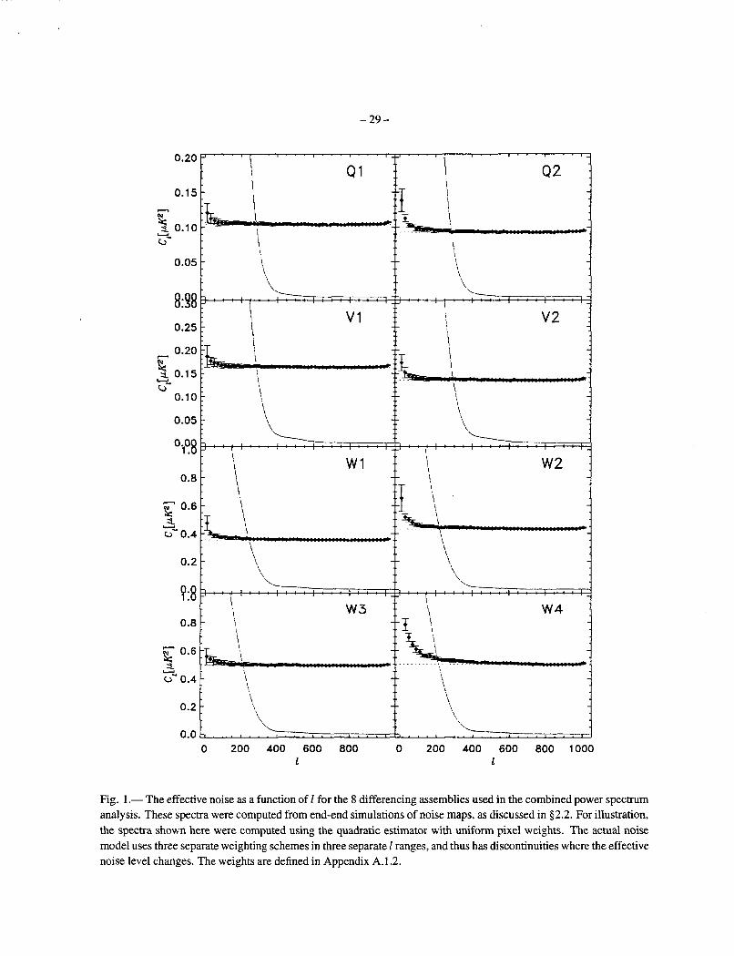
The most reliable way to estimate the effects of l/f noise on the measured power spectra is by Monte Carlo simulation. Using the pipeline simulator discussed in Hinshaw et al. (2003b) we have generated a library of noise maps with flight-like properties. Specifically we have included flight-like 1 /f noise in the simulated time-ordered data, and have run each full-year realization through the map-making pipeline, including the baseline pre-whitening discussed in Hinshaw et al. (2003b). We evaluate the power spectra of these maps using the quadratic estimator described in Appendix A with 3 different pixel weighting schemes. (See Appendix A.1.2 for definitions of the weights, and the 1 range in which each is used.) We define the effective noise as a function of 1 based on fits to these Monte Carlo noise spectra. For the analyses in this paper, we fit the spectra to a model of the form

where the cb are fit coefficients given in Table 1, with nmax = 3 foi I < 200, and nW = 1 for 1 > 200.

Figure 1 shows the noise spectrum derived from the simulations for each of the 8 high frequency DAs, using uniform weighting over the entire I range. For comparison, we also plot an estimate of the CMB power spectrum from 35 in grey. Note that the W4 spectrum is the only one of this set to exhibit deviations from white noise in an 1 range where the signal-to-noise is relatively low, and we believe this simulation slightly over-estimates the 1 / f noise in the flight W4 differencing assembly (Hinshaw et al. 2003a).

- 6 -

2.3. Systematic Errors

Hinshaw et al. (2003a) present limits on systematic errors in the first-year sky maps. They consider the effects of absolute and relative calibration errors, artifacts induced by environmental disturbances (thermal and electrical), errors from the map-making process, pointing errors, and other miscellaneous effects. The combined errors due to relative calibration errors, environmental effects, and map-making errors are limited to < 15 pK2 (2a) in the quadrupole moment C2 in any of the 8 high-frequency DAs. Tighter limits are placed on higher-order moments. We conservatively estimate the absolute calibration uncertainty in the first-year WMAPdata to be 0.5%.

Random pointing errors are accounted for in the beam mapping procedure; the beam transfer functions presented by Page et ai. (2003a) incorporate random pointing errors automatically. A systematic pointing error of -10" at the spin period is suspected in the quaternion solution that defines the spacecraft pointing. This is much smaller than the smallest beam width (-12' at W band), and we estimate that it would produce <I% error in the angular power spectrum at 1 = 1000, thus we do not attempt to correct for this effect. Barnes et al. (2003) place limits on spurious contributions due to stray light pickup through the far sidelobes of the instrument. They place limits of < 10 pK2 on spurious contributions to Cf, at Q through W band, due to far sidelobe pickup.

A detailed model of Galactic foreground emission based on the first-year W A P data is presented by Bennett et al. (2003~) and is summarized in $3.1. We show that diffuse foreground emission is a modest source of contamina- tion at large angular scales ( 2 2'). Systematic errors on these angular scales are negligible compared to the (modest) level of foreground emission. On smaller angular scale ( : 2'), the 1-3% uncertainty in the individual beam transfer functions is the largest source of uncertainty, while for multipole moments greater than -600, random white noise from the instrument is the largest source of uncertainty.

3. THEDATA

Figure 2 shows the cross-power spectra obtained from all 28 combinations of the 8 differencing assemblies Q1 through W4 using the quadratic estimator described in Appendix A.l . These spectra have been evaluated with the Kp2 sky cut described in Bennett et al. (2003~). The spectra are color coded by effective frequency, m, where v i is the frequency of differencing assembly i. The low frequency (4 1 GHz) data are shown in red, the high frequency (94 GHz) data in blue, with intermediate frequencies following the colors of the rainbow. The top panel shows 1(1+ 1)C1/27r in pK2, while the bottom panel plots the ratio of each channel to our final combined spectrum presented in $5. The top panel shows a very robust measurement of the first acoustic peak with a maximum near 1 - 220 and a shape that is consistent with the predictions of adiabatic fluctuation models. There is also a clear indication of the rise to a second peak at 1 - 540. See Page et al. (2003b) for an analysis and discussion of the peaks and troughs in the first-year WMAP power spectrum.

The red data in the top panel show very clearly that the low frequency data are contaminated by diffuse Galactic emission at low 1 and by point sources at higher 1. The higher frequency data show less apparent contamination, consistent with the foreground emission being dominated by radio emission, rather than thermal dust emission, as expected in this frequency range.

3.1. Galactic and Extragalactic Foregrounds

Bennett et al. (2003~) present a detailed model of the Galactic foreground emission based on a Maximum Entropy

,

- 7 -

analysis of all 5 WMAP frequency bands, in combination with external tracer templates. They demonstrate that the emission is well modeled by three distinct emission components. I ) Synchrotron emission from cosmic ray electrons, with a steeply falling spectrum in the WMAP frequency range: TA(v) 0: VB with p < -3, steepening with increasing frequency. 2) Free-free emission from the ionized interstellar medium that is well traced by H a emission in regions where the dust extinction is low. 3) Thermal emission from interstellar dust grains with an emissivity index - 2.2. The model has a Galactic signal minimum between V and W band.

In principal we could subtract the above model from each W A P channel and recompute the power spectrum. However, since the model is based on WMAP data that have been smoothed to an angular resolution of 1 PO, the resulting maps would have complicated noise properties. For the purposes of power spectrum analysis, we adopt a more straightforward approach based on fitting foreground tracer templates to the Q, V, and W band data. The details of this procedure, the resulting fit coefficients, and a comparison of the fits to the Maximum Entropy model are given in Bennett et al. (2003~). They estimate that the template model removes -85% of the foreground emission in Q, V, and W bands and that the remaining emission constitutes less than -2% of the CMB variance (up to I = 200) in Q band, and 2 1 % of the CMl3 variance in V and W bands.

The contribution from extragalactic radio sources has been analyzed in three separate ways. Bennett et al. (2003~) directly fit for sources in the sky maps. The result of this analysis is that we have identified 208 sources in the WMAP data with sufficient signal to noise ratio to pass the detection criterion (we estimate that -5 of these are likely to be spurious). The derived source count law is consistent with the following model for the power spectrum of the unresolved sources

with A = 0.015 pK2 sr (measured in thermodynamic temperature), /3 = -2.0, and vo 45 GHz. Komatsu et al. (2003) evaluate the bispectrum of the WMAP data and are able to fit a non-Gaussian source component based on a particular configuration of the bispectrum. They find the same source model, equation (9), fits the bispectrum data. For the remainder of this section, we adopt this model for correcting the cross-power spectra. At Q band (41 GHz) the correction to &I+ 1)C1/2x is 868 and 3468 pK2 at 1=500 and 1000, respectively. At W band (94 GHz), the correction is only 31 and 126 pK2 at the same 1 values. For comparison, the CMB power in this 1 range is N 2000 pK2 . Later, when we derive a final combined spectrum from the multi-frequency data, we adopt equation (9) as a model with A as a free parameter. We simultaneously fit for a combined CMB spectrum and source amplitude and marginalize over the residual uncertainty in A. The best-fit source amplitude from this process is consistent with the other two methods.

Figure 3 shows the cross-power spectra obtained from the same 28 combinations as in Figure 2, this time with the Galactic template model and source model subtracted. The bottom panel of the Figure shows the ratio of the 28 channels to the combined spectrum obtained in $5. The 28 cross-power spectra are consistent with each other at the 5 to 20% level over the 1 range 2 - 500. Similar scatter is seen in Monte Carlo simulations of an ensemble of 28 cross-power spectra with WMAPs beam and noise properties. The only significant deviation lies in the Q band data at low 1 which is - 10% below the higher frequency bands at 1 < 20. This is consistent with the accuracy estimated above for the Galactic template model, see also Figure 11 of Bennett et al. (2003~) for images of the maps after Galactic template subtraction. Since the WMAP data are not noise limited at low I , we use only V and W band data in the final combined spectrum for 1 < 100.

The subtraction of the source model, equation (9), brings the Q band spectrum into good agreement with the other cross-power spectra up to 1 - 500. At higher I , the Q band data contributes very little to the final combined spectrum because the (normalized) Q band window function has dropped to less than 5% (Page et al. 2003a). As discussed in $5, we marginalize over the source amplitude uncertainty, 6A, when obtaining the final power spectrum estimate and associated covariance matrix. Thus the uncertainty is also accounted for in subsequent cosmological parameter fits

- 8 -

(Verde et al. 2003; Spergel et al. 2003; Peiris et al. 2003).

Figure 4 shows a close-up of the 28 cross-power spectra in Figure 3 up to 1 = 100. The top panel shows the raw (unbinned) data which has correlations of ~ 2 % between neighboring points is this 1 range (see 94). These data are strikingly consistent with each other and support the conclusion that systematic errors at low 1 are insignificant. To assess the level of scatter that does exist between the spectra, we have generated a Monte Carlo simulation in which we compute the rms scatter among the 28 spectra at each I , relative to the measured power. The bottom panel of Figure 4 shows the results of this simulation, averaged over 1000 realizations, compared to the relative rms scatter in the data. The agreement is excellent, indicating that the uncertainty in the measured power spectrum in this 1 range is a few percent and is consistent with a combination of instrument noise and mode coupling due to the 15% sky cut.

Another striking feature is the low amplitude of the observed quadrupole, and the sharp rise in power, almost linear in I , to 1 = 5. Bennett et al. (2003b) quote a value for the rms quadrupole amplitude, Qrms = ,/- = 8 i 2 pK, where the uncertainty is largely due to Galactic model uncertainty. This is consistent with the amplitude measured by the COBE-DMR experiment, Qmlr = 10: pK (Bennett et al. 1996). The fast, nearly linear rise to I = 5 produces an angular correlation function with essentially no power on angular scales 2 60°, again in excellent agreement with the COBE-DMR correlation function (Bennett et al. 2003b; Hinshaw et ai. 1996). In the context of a standard ACDM model, the probability of observing this little power on scales greater than 60' is - 2 x (Bennett et al. 2003b).

4. THE FULL COVARIANCE MATRIX

In 95 we derive our best estimate of the angular power spectrum by optimally combining the 28 cross-power spectra discussed above. The procedure for combining spectra requires the full covariance matrix of the individual cross-power spectra - in this section we outline the salient features of this matrix. There are six principal sources of variance for the measured spectra, Cl: cosmic variance, instrument noise, mode coupling due to the foreground mask, point source subtraction errors, uncertainty in the beam window functions, and an overall calibration uncertainty. We ignore uncertainties in the diffuse foreground correction since they are everywhere sub-dominant to the cosmic variance uncertainty (see 93.1).

We may write the covariance matrix as

where the angle brackets represent an ensemble average, Cl is the true underlying power spectrum, wi is the window function of spectrum i, and AS' is the point source contribution to spectrum i. Here we have defined a point source spectral function, Si, as

where vi, vo, and ,6 are as defined after equation (9). Note that (Cfull);, is symmetric in both (U') and (ij)

In the process of forming the combined spectrum we will estimate a best-fit point source amplitude, A, and subtact the corresponding soiice contiibution from each spectrum i. We thus rewrite Cf~l l as

where will marginalize over as a nuisance parameter.

= -A94 is the source-subtracted spectrum, and 6A s A -A is the residual source amplitude, which we

,

- 9 -

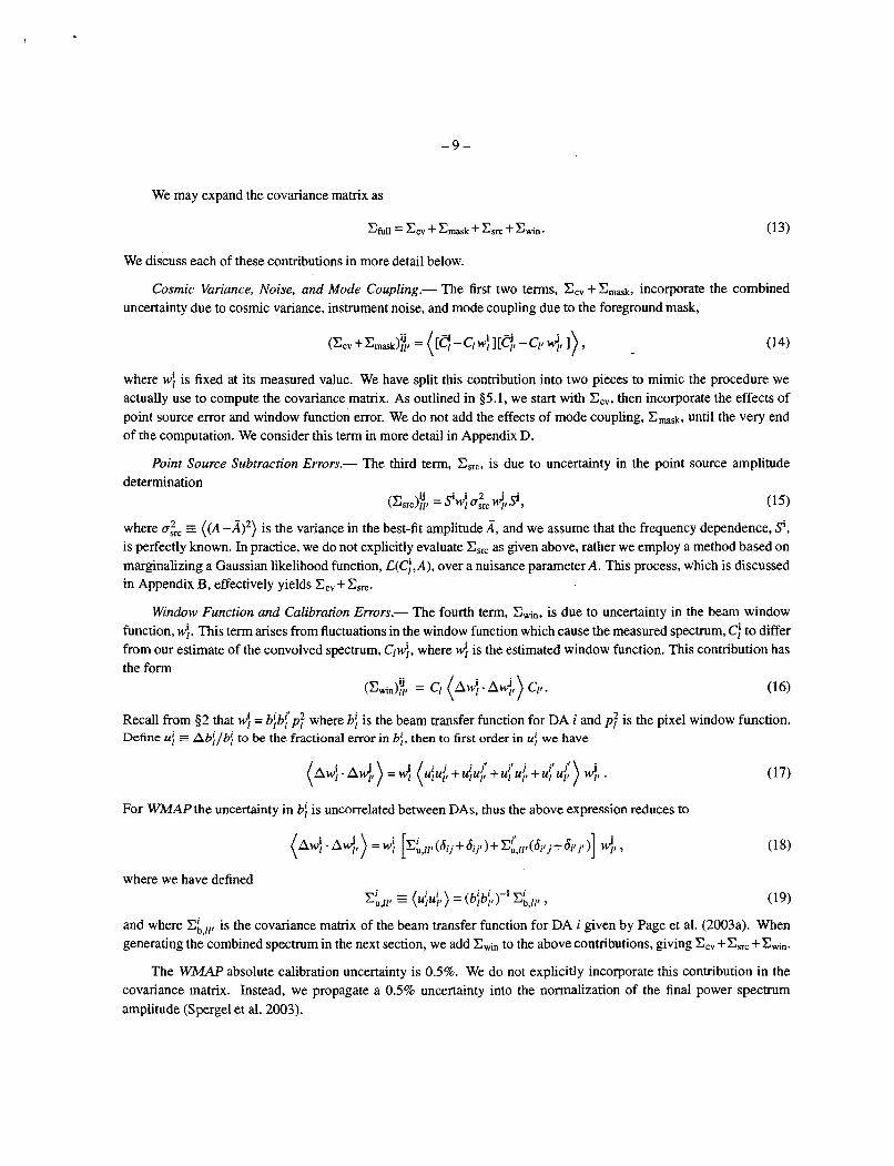
We may expand the covariance matrix as

We discuss each of these contributions in more detail below.

Cosmic Variance, Noise, and Mode Coupling.- The first two terms, E,, + Em&, incorporate the combined uncertainty due to cosmic variance, instrument noise, and mode coupling due to the foreground mask,

(Ccv+Emask);, = ( [ ~ : - C l W j l [ C ~ , -Cp 4, I ) , (14)

where w! is fixed at its measured value. We have split this contribution into two pieces to mimic the procedure we actually use to compute the covariance matrix. As outlined in $5.1, we start with Ccv, then incorporate the effects of point source error and window function error. We do not add the effects of mode coupling, Cmsk. until the very end of the computation. We consider this term in more detail in Appendix D.

Point Source Subtraction Errors.- The third term, Csrc, is due to uncertainty in the point source amplitude determination

(E STc )ij 11’ - - s i w i G 2 1 src J,sj, 1 (15)

where u$?rc = ( ( A -A)’) is the variance in the best-fit amplitude A, and we assume that the frequency dependence, Si , is perfectly known. In practice, we do not explicitly evaluate E,, as given above, rather we employ a method based on marginalizing a Gaussian likelihood function, C(C;,A), over a nuisance parameter A. This process, which is discussed in Appendix B, effectively yields Ccv + Csrc.

Window Function and Calibration Errors.- The fourth term, Cwin, is due to uncertainty in the beam window function, 4. This term arises from fluctuations in the window function which cause the measured spectrum, C; to differ from our estimate of the convolved spectrum, Clw;, where w: is the estimated window function. This contribution has the form

(16)

Recall from $2 that w! = bfbf p: where bf is the beam transfer function for DA i and p: is the pixel window function. Define uf E Abf/bf to be the fractional error in bf, then to first order in uf we have

(Cwin)i, = Cl ( 4 ~ : . A d , ) Cp .

For W A P the uncertainty in bf is uncorrelated between DAs, thus the above expression reduces to

where we have defined E (ufu;,) =(bfbf,)-’ ,

and where ELcl, is the covariance matrix of the beam transfer function for DA i given by Page et al. (2003a). When generating the combined spectrum in the next section, we add Cxpin to the above contributions, giving Ccv + Csrc + Cwin.

The WMAP absolute calibration uncertainty is 0.5%. We do not explicitly incorporate this contribution in the covariance matrix. Instead, we propagate a 0.5% uncertainty into the normalization of the final power spectrum amplitude (Spergel et al. 2003).

- 10-

5. THE COMBINED POWER SPECTRUM

In $3 we demonstrated that the three high frequency bands of WMAF’ data produced consistent estimates of the angular power spectrum, after a modest correction for diffuse Galactic emission and extragalactic point sources. It is therefore justifiable to combine these data into a single “optimal” estimate of the angular power spectrum of the CMB. In this section, we provide an overview of two methods we use to generate a single combined spectrum. The first is a multi-step process that simultaneously fits the 28 cross-power spectra presented above to a single CMB power spectrum and a point source model, equation (9), while correctly propagating beam and residual point source uncertainties through to a final Fisher matrix. This spectrum constitutes our best estimate of the CMB power spectrum from the first-year WMAP data. The second spectrum, which serves as a cross check of the first, is based on forming a single co-added sky map from the Q l through W4 maps, and using the quadratic estimator with noise bias subtraction. We compare the two spectra in 95.3.

5.1. Method I - Optimal Combination of Cross-Power Spectra

Since this method is relatively complicated, we outline the basic procedure here and relegate the details to Ap- pendices, as indicated. We present the result in 35.3. The steps are as follows.

1. Subtract best-fit Galactic foreground templates from each of the maps Q1 through W4, using the coefficients given in Table 3 of Bennett et al. (2003~).

2. Evaluate the 28 cross-power spectra from the maps Q1 through W4, where each spectrum has been evaluated using the quadratic estimator of Appendix A. 1 with the weighting scheme defined in Appendix A. 1.2.

3. Collect the noise bias estimate, (w), for each DA from $2.2. These estimates are used in the calculation of the covariance matrix for the combined spectrum, and in setting the relative weight of each cross-power spectrum in the final combined spectrum.

4. Apply the procedure presented in Appendix B. 1 to obtain an estimate for the point source amplitude. The value obtained is A = 0.0155 f 0.0017, roughly independent of l,, in equation (B6). This value is in good agreement with an estimate based on the bispectrum (Komatsu et al. 2003), and on an extrapolation of point source counts (Bennett et al. 2003b). Subtract the point source contribution from the cross-power spectra: = --AS%;.

5. Compute an approximate form of the full covariance matrix discussed in $4, &11. The procedure we use pro- duces a covariance matrix which includes cosmic variance, instrument noise, source subtraction uncertainties, and window function uncertainties. At this stage of the process, it does not yet include the effects of mode coupling. More details are given in $4 and Appendix B.

6. Invert the approximate covariance matrix for use in computing the optimal spectrum. This is the most computa- tionally intensive step in the process.

7. Compute the final combined spectrum from the 28 Cj as per the procedure given in Appendix C. In particular, assume a fiducial cosmological model (as specified in the Appendix), and use equation (C6), with E!ull 11, =

gi,l Note: for I < 100 we use a surrogate procedure for computing the combined spectrum. In order to minimize Galactic foreground contamination, we use only V and W band data. Moreover, because the statistics of the Cl are mildly non-Gaussian, and because point source contamination and window function uncertainties are small,

This produces a final spectrum which is very nearly optimal.

- 1 1 -

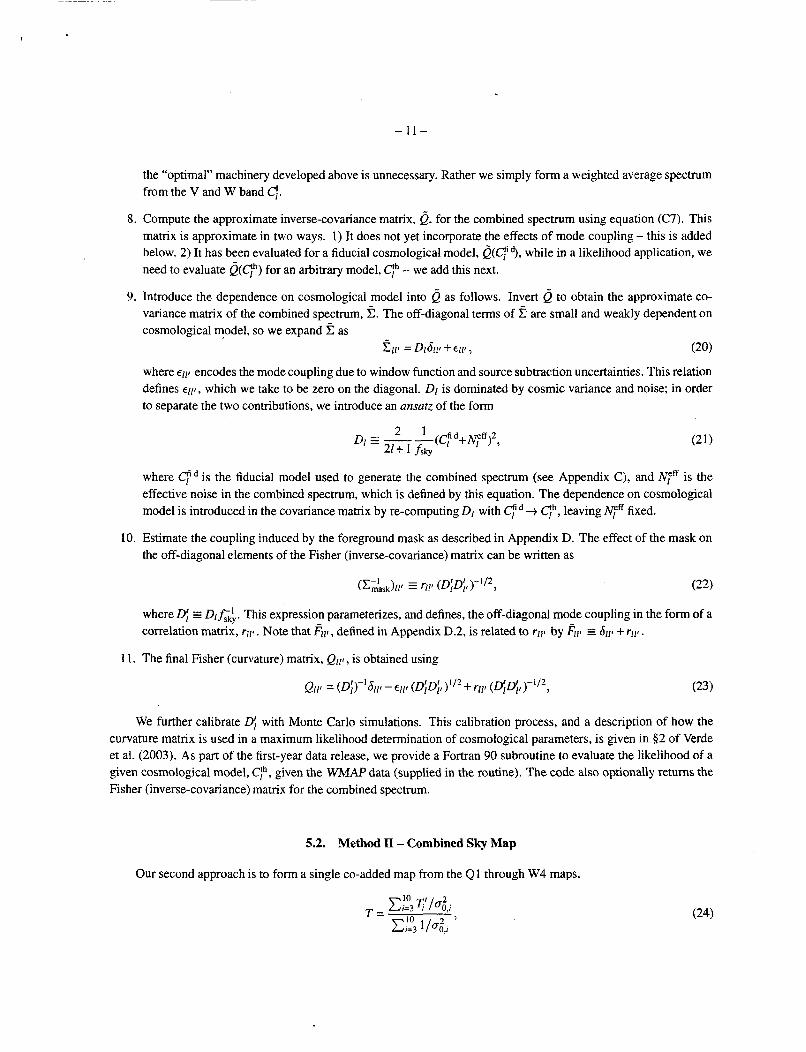
the “optimal” machinery developed above is unnecessary. Rather we simply form a weighted average spectrum from the V and W band <.

8. Compute the approximate inverse-covariance matrix, Q, for the combined spectrum using equation (C7). This matrix is approximate in two ways. 1) It does not yet incorporate the effects of mode coupling - this is added below. 2) It has been evaluated for a fiducial cosmological model, Q(q 9. while in a likelihood application, we need to evaluate Q(qh) for an arbitrary model, qh - we add this next.

9. Introduce the dependence on cosmological model into Q as follows. Invert Q to obtain the approximate CO- variance matrix of the combined spectrum, 9. The off-diagonal terms of 5 are small and weakly dependent on cosmological model, so we expand 9 as -

C1p = D ~ d ~ p +el/! , (20)

where encodes the mode coupling due to window function and source subtraction uncertainties. This relation defines elp, which we take to be zero on the diagonal. Dl is dominated by cosmic variance and noise; in order to separate the two contributions, we introduce an ansatz of the form

where cd is the fiducial model used to generate the combined spectrum (see Appendix C), and Neff is the effective noise in the combined spectrum, which is defined by this equation. The dependence on cosmological model is introduced in the covariance matrix by re-computing D1 with -+ qh, leaving y’ fixed.

10. Estimate the coupling induced by the foreground mask as described in Appendix D. The effect of the mask on the off-diagonal elements of the Fisher (inverse-covariance) matrix can be written as

(22)

where DI E D&&. This expression parameterizes, and defines, the off-diagonal mode coupling in the form of a correlation matrix, rip. Note that

I I -112 ( C A s k ) l 1 ’ = rll’ (DlDl!) 7

defined in Appendix D.2, is related to q 1 8 by 4 1 8 s du, + riff.

11. The final Fisher (curvature) matrix, Qlp , is obtained using

We further calibrate D; with Monte Carlo simulations. This calibration process, and a description of how the curvature matrix is used in a maximum likelihood determination of cosmological parameters, is given in §2 of Verde et al. (2003). As part of the first-year data release, we provide a Fortran 90 subroutine to evaluate the likelihood of a given cosmological model, qh, given the WMAP data (supplied in the routine). The code also optionally returns the Fisher (inverse-covariance) matrix for the combined spectrum.

5.2. Method II - Combined Sky Map

Our second approach is to form a single co-added map from the Q 1 through W4 maps,

- 12-

where 7;.’ is the sky map for DA i with the best-fit Galactic template model subtracted, and a& is the noise per observation for DA i, given by Bennett et al. (2003b). We evaluate the power spectrum of this map on the Kp2 cut sky using the quadratic estimator in Appendix A. 1. An effective noise model is obtained by using the same approach as described in $2.2: we generate co-added noise maps from the library of end-to-end simulations, evaluate their average spectra, then fit a noise model. The noise bias model is then subtracted from the power spectrum of the combined temperature map. We have performed this analysis with 3 distinct pixel weighting schemes (see Appendix A. 1.2) and 3 corresponding noise models. The results are shown in Figure 5 where it is seen that the three cases are virtually indistinguishable.

In effect, this analysis uses both the auto- and cross-power spectra. We view this as a useful check of the more sophisticated procedure described in $5.1, but we do not rely on it for a final result. Uncertainties in the noise model only effect the fourth moment of the cross-power spectra, but they effect the second moment of the auto-power spectra and potentially bias the final result. The -6% sensitivity advantage gained by including auto-power spectra was not deemed worth the effort required to guarantee that the final result was not biased.

5.3. Comparison of Results

Figure 6 compares the power spectra obtained from methods I and II above. The combined cross-power spectrum from 55.1 is shown in black, the auto-power spectrum obtained in 95.2 from the co-added map is shown in grey. The two methods agree extremely well with the only notable deviation being at the highest I range probed by the first-year data. This is the regime where the auto-power spectrum will be most sensitive to the noise bias subtraction. As can be seen in the error estimates shown in Figure 8, the deviation is less than lo.

A separate test of robustness is to compute the angular power spectrum in separate regions of the sky to see if the spectrum changes. We have computed the power spectrum in two subsets of the sky - the ecliptic poles, and the ecliptic plane, using the quadratic estimator with the combined sky map. The results are shown in Figure 7 where the pole data is shown in grey and the plane data in black. The two spectra are very consistent overall, but some of the features that appear in the combined spectrum, such as the “peak” at I - 40 and the “bite” at 1 - 210, are not robust to this test, thus we consider these features to be of marginal significance. There is also no evidence that beam ellipticity, which would be more manifest in the plane than in the poles, systematically biases the spectrum. This is consistent with estimates of the effect given by Page et al. (2003a).

6. DISCUSSION

Our best estimate of the angular power spectrum of the CMB is shown in Figure 8. Also shown is the best-fit ACDM model from Spergel et al. (2003) which is based on a fit to the this spectrum plus a compilation of additional CMB and large-scale structure data. The W A P d a t a points are plotted with measurement errors based on the diagonal elements of the Fisher matrix presented in Appendix D. The cosmic variance errors, which include the effects of the sky cut, are plotted as a lo band around the best-fit model. As discussed in Spergel et al. (2003), the model is an excellent fit to the data. The combined specbum provides a definitive measurement of the CMB power spectrum with uncertainties limited by cosmic variance up to I - 350. The spectrum clearly exhibits a first acoustic peak at E = 220.1 =k 0.8 and a second acoustic peak at 1 = 546 f 10. Page et al. (2003b) present an analysis and interpretation of the peaks and troughs in the first-year WMAP power spectrum.

Figure 9 compares the first-year Wi” spectrum to a compilation of recent balloon and ground-based measure-

- 13-

ments. In order to make this Figure meaningful, we plot the best-fit model spectrum to represent the W A P results. The data points are plotted with errors that include both measurement uncertainty and cosmic variance, so no error band is included with the model curve. (Since individual groups report band power measurement with different band- widths, it is not possible to represent a single cosmic variance band that applies to all data sets.) The model spectrum fit to WAF’ agrees very well with the ensemble of previous observations.

Wang et al. (2002a) have recently distilled a CMB power spectrum from an optimal combination of the extent pre-WMAP data. In Figure 10 we plot their derived band power points alongside the WMAP data. To make this comparison meaningful, we plot the WAF’ data with cosmic variance plus measurement errors and omit the error band from the model spectrum. The distilled spectrum is notably lower than the W A P data in the vicinity of the first acoustic peak. In a previous version of this work (Wang et al. 2002b) the authors noted that the first peak of their combined spectrum was lower than a significant fraction of their input data. They attribute this to their formalism allowing for a renormalization of individual experiments within their respective calibration uncertainties. Figure 1 in Bennett et al. (2003a) presents a similarly distilled spectrum from the data extent in late 2001 and found a first peak amplitude that was more intuitively consistent with the bulk of the input data, and which is now seen to be consistent with the W A P power spectrum.

Figure 1 1 shows the WMAP combined power spectrum compared to the locus of predicted spectra, in red, based on a joint analysis of pre-WAF’ CMB data and 2dFGRS large-scale structure data (Percival et al. 2002). As in Figure 8, the WMAP data are plotted with measurement uncertainties, and the best-fit ACDM model (Spergel et al. 2003) is plotted with a la cosmic variance error band. Percival et al. (2002) predict the location of the first peak should occur at I = 221.8 f 2 . 4 , which is quite consistent with the value reported by Page et al. (2003b) of 1 = 220.1 f0 .8 . The height of the first peak was predicted to be in the range 4920 f 170 pK2, while Page et al. (2003b) report a measured height of 5580 f 75 pK2, about 13% higher. Unlike the position, the amplitude of the first peak has a complicated dependence on cosmological parameters. Percival et al. (2002) report best-fit parameters for a ACDM model that are mostly consistent with those reported by Spergel et al. (2003) for the same class of models. The only mildly disparate comparison lies in the combination of normalization, 08 , and optical depth, T. Percival et al. (2002) report the product b g d 7 = 0.72 f 0.03 f 0.02, where the first error is a “theory” error and the second is measurement error. While Spergel et al. (2003) does not report a maximum likelihood range for this explicit parameter combination, the product of their maximum likelihood values for 08 and T yields o8.P = 0.74, which is consistent with Percival et al. (2002), but would make the first peak a few percent higher. Small differences in nbh2, fi,h2, and n,, may also contribute to the difference.

7. CONCLUSIONS

We present measurements of the angular power spectrum of the cosmic microwave background from the first- year W A F ’ data. The eight high-frequency sky maps from DAs Q1 through W4 were used to estimate 28 cross- power spectra, which are largely independent of the noise properties of the experiment. These data were tested for consistency in $3, then used in $5 as input to a final combined spectrum, discussed in 56. The procedure for estimating the uncertainties in the final combined spectrum were discussed in $4 and in numerous Appendices.

The combined spectrum provides a definitive measurement of the CMB power spectrum, with uncertainties lim- ited by cosmic variance up to E N 350, and a signal to noise per mode > 1 up to 1 - 650. The spectrum clearly exhibits a first acoustic peak at 1 = 220.1 f 0.8 and a second acoustic peak at 1 = 546 f 10. Page et al. (2003b) present an analysis and interpretation of the peaks and troughs in the first-year WAF’ power spectrum. Spergel et al. (2003), Verde et al. (2003), and Peins et al. (2003) analyze the combined spectrum in the context of cosmological models.

- 14-

They conclude that the data provide strong support adiabatic initial conditions, and they give precise measurements of a number of cosmological parameters. Kogut et a]. (2003) analyze the correlation between W s temperature and polarization signals, the CT" spectrum, and present evidence for a relatively high optical depth, and an early period of cosmic reionization. Among other things, this result implies that the temperature power spectrum is suppressed by -30% on degree angular scales, due to secondary scattering.

A variety of first-year WMAP data products are being made available by NASA's new Legacy Archive for Mi- crowave Background Data Analysis (LAMBDA). In addition to the sky maps and calibrated time-ordered data, we are providing the 28 cross power spectra used in this paper (with diffuse foregrounds subtracted), the combined spec- trum from $5.1, and a Fortran 90 subroutine to compute the likelihood of a given cosmological model, (the code will also optionally return the Fisher (inverse-covariance) mamx for the combined spectrum.) The LAMBDA URL is http://lambda.gsfc.nasa.gov/.

The WAP mission is made possible by the support of the Office of Space Sciences at NASA Headquarters and by the hard and capable work of scores of scientists, engineers, technicians, machinists, data analysts, budget analysts, managers, administrative staff, and reviewers. We thank Mike Nolta for helpful comments on an earlier draft of this manuscript. LV is supported by NASA through Chandra Fellowship PF2-30022 issued by the Chandra X-ray Observatory center, which is operated by the Smithsonian Astrophysical Observatory for an on behalf of NASA under contract NAS8-39073. We acknowledge use of the HEALPix package.

REFERENCES

Barnes, C. et al. 2003, ApJ, submitted

Bennett, C. L., Banday, A. J., Gbrski, K. M., Hinshaw, G., Jackson, P., Keegstra, P., Kogut, A., Smoot, G. F., Wilkin- son, D. T., & Wright, E. L. 1996, ApJ, 464, L1

Bennett, C. L., Bay, M., Halpern, M., Hinshaw, G., Jackson, C., Jarosik, N., Kogut, A., Limon, M., Meyer, S. S., Page, L., Spergel, D. N., Tucker, G. S., Wilkinson, D. T., Wollack, E., &Wright, E. L. 2003a, ApJ, 583, 1

Bennett, C. L., Halpern, M., Hinshaw, G., Jarosik, N., Kogut, A., Limon, M., Meyer, S. S., Page, L., Spergel, D. N., Tucker, G. S., Wollack, E., Wright, E. L., Barnes, C., Greason, M., Hill, R., Komatsu, E., Nolta, M., Odegard, N., Peiris, H., Verde, L., & Weiland, J. 2003b, ApJ, submitted

Bennett, C. L. et al. 2003c, ApJ, submitted

Gbrski, K. M., Hivon, E., & Wandelt, B. D. 1998, in Evolution of Large-Scale Structure: From Recombination to Garching

Gupta, S. & Heavens, A. E 2002, MNRAS, 334,167

Hauser, M. G. & Peebies, P. J. E. 1973, ApJ, 185,757

Hinshaw, G., Branday, A. J., Bennett, C. L., Gbrski, K. M., Kogut, A., Lineweaver, C. H., Smoot, G. E, & Wright, E. L. 1996, ApJ, 464, L25

Hinshaw, G. E et al. 2003a, ApJ, submitted

-. 2003b, ApJ, submitted

- 15-

Hivon, E., Gbrski, K. M., Netterfield, C. B., Crill, B. P., Prunet, S., & Hansen, E 2002, ApJ, 567,2

Jarosik, N. et al. 2003a, ApJS, 145

-. 2003b, ApJ, submitted

Kogut, A. et al. 2003, ApJ, submitted

Komatsu, E. et al. 2003, ApJ, submitted

Limon, M., Wollack, E., Bennett, C . L., Halpem, M., Hinshaw, G., Jarosik, N., Kogut, A., Meyer, S. S., Page, L., Spergel, D. N., Tucker, G. S., Wright, E. L., Barnes, C., Greason, M., Hill, R., Komatsu, E., Nolta, M., Ode- gard, N., Peins, H., Verde, L., & Weiland, J. 2003, Wilkinson Microwave Anisotropy Probe (WMAP): Explana- torySupplement,http://lambda.gsfc.nasa.gov/data/map/doc/MAP_supplement.pdf

Muciaccia, P. F., Natoli, P., & Vittorio, N. 1997, ApJ, 488, L63+

Oh, S. P., Spergel, D. N., & Hinshaw, G. 1999, ApJ, 510,551

Page, L. et al. 2003a, ApJ, submitted

-. 2003b, ApJ, submitted

-. 2003c, ApJ, 585, in press

Peins, H. et al. 2003, ApJ, submitted

Percival, W. J., Sutherland, W., Peacock, J. A., Baugh, C. M., Bland-Hawthorn, J., Bridges, T., Cannon, R., Cole, S., Colless, M., Collins, C., Couch, W., Dalton, G., De Propris, R., Driver, S. P., Efstathiou, G., Ellis, R. S., Frenk, C. S., Glazebrook, K., Jackson, C., Lahav, O., Lewis, I., Lumsden, S., Maddox, S., Moody, S., Norberg, P., Peterson, B. A., & Taylor, K. 2002, MNRAS, 337, 1068

Spergel, D. N. et al. 2003, ApJ, submitted

Tegmark, M., Taylor, A. N., & Heavens, A. E 1997, ApJ, 480,22

Verde, L. et al. 2003, ApJ, submitted

Wang, X., Tegmark, M., Jain, B., & Zaldamaga, M. 2002a. Phys. Rev. D, submitted (astro-ph/0212417)

Wang, X., Tegmark, M., & Zaldarriaga, M. 2002b, Phys. Rev. D, 65,123001

A. POWER SPECTRUM ESTIMATION METHODS

For the analysis of WMAPs first-year data, we have chosen two distinct methods for infemng the power spec- trum. The first is a fast and accurate quadratic method for estimating the power spectrum of a partial sky map (Hivon et al. 2002). We summarize the basic approach here, highlighting the aspects of the method that are especially perti- nent to M A P , and refer the reader to Hivon et al. (2002) for details. The second is a maximum likelihood method that provides an independent estimate of the spectrum measured by WMAP (Oh et al. 1999).

This preprint was prepared with the AAS LWEX macros v5.0.

- 16-

We have applied both of these methods to the WMAP data. The results are shown in Figure 12, which shows spectra estimated from the V band map, up to 1 = 200, for the two methods. The maximum likelihood estimate has slightly lower uncertainties at low 1, because the method optimally weights the data with a pixel-pixel covariance C = S+N M S where S is the covariance of the CMB signal and N is the covariance of the noise (see Appendix A.2). Our quadratic estimator uses uniform pixel weights at low 1 (see Appendix A.1.2) though it is clear from the Figure that the difference is not significant. At high I , where the WMAP data are noise dominated, the two estimators give essentially identical results because they effectively weight the data in the same way.

To obtain our “best” estimate of the “MAP power spectrum, we adopt the quadratic estimator because it can be readily applied to pairs of W A P radiometers in a way that is nearly independent of the properties of the instrument noise. In 5.5 we discuss our methodology for combining spectra from pairs of radiometers and present the final combined spectrum.

A.l. Quadratic Estimation

Hivon et al. (2002) start with the full-sky estimator in equation (2), add a position dependent weight, W(n), and set W to zero in the regions where the sky is contaminated. In other regions, W is chosen to optimize the sensitivity of the estimator. A temperature map AT(n) on which a weight W(n) is applied can be decomposed in spherical harmonic coefficients as

where the integral over the sky is approximated by a discrete sum over map pixels, each of which subtends solid angle 0,. Hivon et al. (2002) then define the “pseudo power spectrum” as

1

IGlml2. - 1 Cr = -

21+1 m=-1

The pseudo power spectrum c, given by the weighted spherical harmonic transform of a map, is clearly different from the full sky angular spectrum, Csb, but the ensemble averages of the two spectra can be related by

1’

where G1p describes the mode coupling resulting from the weight function W(n) (Hauser & Peebles 1973). Hivon et al. (2002) give the following expression for the coupling matrix, which depends only on the geometry of the weight function W(n)

where the final term in parentheses is the Wipe r 3 - j symbol, and Wl is the angular power spectrum of the weight function

1 2 WI = - IwlmI 21+1 ”,

- 17-

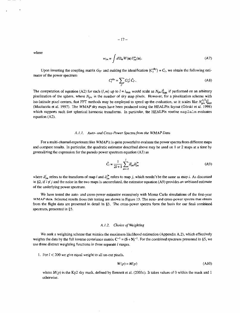
Upon inverting the coupling matrix G I ~ and making the identification (Csky) = CI, we obtain the following esti- mator of the power spectrum

Cpbs = G,f Cp . I'

The computation of equation (A2) for each (1,m) up to 1 = l,,, would scale as Npixl;,, if performed on an arbitrary pixelization of the sphere, where Npix is the number of sky map pixels. However, for a pixelization scheme with iso-latitude pixel centers, fast FFT methods may be employed to speed up the evaluation, so it scales like NifZAa (Muciaccia et al. 1997). The W A P sky maps have been produced using the HEALF'ix layout (G6rski et al. 1998) which supports such fast spherical harmonic transforms. In particular, the HEALPix routine map2alm evaluates equation (A2).

A. I . 1. Auto- and Cross-Power Spectra from the WMAP Data

For a multi-channel experiment like -Pit is quite powerful to evaluate the power spectra from different maps and compare results. In particular, the quadratic estimator described above may be used on 1 or 2 maps at a time by generalizing the expression for the pseudo power spectrum equation (A3) as

where Ef,, refers to the transform of map i and c7{2 refers to map j, which needn't be the same as map i . As discussed in 32, if i # j and the noise in the two maps is uncorrelated, the estimator equation (A9) provides an unbiased estimate of the underlying power spectrum.

We have tested the auto- and cross-power estimator extensively with Monte Carlo simulations of the first-year WlMAPdata. Selected results from this testing are shown in Figure 13. The auto- and cross-power spectra that obtain from the flight data are presented in detail in $3. The cross-power spectra form the basis for our final combined spectrum, presented in $5.

A.1.2. Choice of Weighting

We seek a weighting scheme that mimics the maximum likelihood estimation (Appendix A.2), which effectively weights the data by the full inverse covariance matrix C-' = (S+N)-'. For the combined spectrum presented in 35, we use three distinct weighting functions in three separate I ranges.

1. For 1 < 200 we give equal weight to all un-cut pixels,

where M ( p ) is the Kp2 sky mask, defined by Bennett et al. (2003~). It takes values of 0 within the mask and 1 otherwise.

- 18-

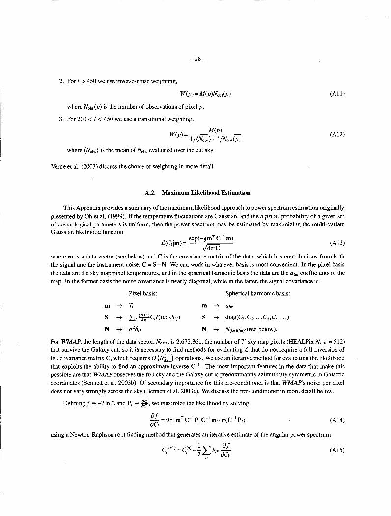
2. For 1 > 450 we use inverse-noise weighting,

w@> = M(p)Nobs(p)

where N , b ( p ) is the number of observations of pixel p .

3. For 200 < 1 < 450 we use a transitional weighting,

M ( p ) w(p)= I/(Nobs)+ 1/Nobs(p)

where (Nabs) is the mean of Nabs evaluated over the cut sky.

Verde et al. (2003) discuss the choice of weighting in more detail.

A.2. Maximum Likelihood Estimation

This Appendix provides a summary of the maximum likelihood approach to power spectrum estimation originally presented by Oh et al. (1999). If the temperature fluctuations are Gaussian, and the a priori probability of a given set of cosmological parameters is uniform, then the power spectrum may be estimated by maximizing the multi-variate Gaussian likelihood function

exp(-imT C-' m) m W l lm) =

where m is a data vector (see below) and C is the covariance matrix of the data, which has contributions from both the signal and the instrument noise, C = S+N. We can work in whatever basis is most convenient. In the pixel basis the data are the sky map pixel temperatures, and in the spherical harmonic basis the data are the aim coefficients of the map. In the former basis the noise covariance is nearly diagonal, while in the latter, the signal covariance is.

Pixel basis: Spherical harmonic basis:

m - + ' l ; . m -+ aim

s + cl ~ c l p l ( c o s e i j ) S + diag(C2,Cz ,... C3,C3 ,...)

N -+ ~ ? 6 i j N -+ N(rrn)(lm), (see below).

For WMAP, the length of the data vector, Ndata, is 2,672,361, the number of 7' sky map pixels (HEALPix Nside = 5 12) that survive the Galaxy cut, so it is necessary to find methods for evaluating L that do not require a full inversion of the covariance matrix C, which requires 0 operations. We use an iterative method for evaluating the likelihood that exploits the ability to find an approximate inverse e-'. The most important features in the data that make this possible are that WMAPobserves the full sky and the Galaxy cut is predominantly azimuthally symmetric in Galactic coordinates (Bennett et al. 2003b). Of secondary importance for this pre-conditioner is that WMAPs noise per pixel does not vary strongly across the sky (Bennett et al. 2003a). We discuss the pre-conditioner in more detail below.

Defining f = -2 In C and PI E, we maximize the likelihood by solving

(A 14) a.f - = o = mT C-' P[ C-' m+tr(C-' PI) ac1

using a Newton-Raphson root finding method that generates an iterative estimate of the angular power spectrum

- 19-

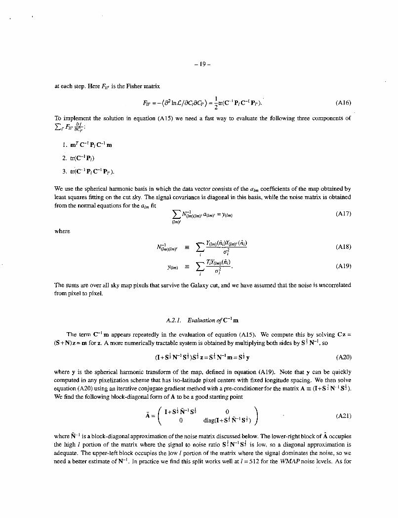
at each step. Here is the Fisher matrix

1 2 41, = - (8' In L / O C I ~ C ~ ) = -tr(c-' PI C-' PI, ).

To implement the solution in equation (A15) we need a fast way to evaluate the following three components of cp 411 & I. mT C-' PIC-' m

2. tr(c-' 9)

3. tr(c-' P/ c-' PI!).

We use the spherical harmonic basis in which the data vector consists of the arm coefficients of the map obtained by least squares fitting on the cut sky. The signal covariance is diagonal in this basis, while the noise matrix is obtained from the normal equations for the a!, fit

where

The sums are over all sky map pixels that survive the Galaxy cut, and we have assumed that the noise is uncorrelated from pixel to pixel.

A.2.1. Evaluation of C-' m

The term C-'m appears repeatedly in the evaluation of equation (A15). We compute this by solving Cz = (S +N) z = m for z. A more numerically tractable system is obtained by multiplying both sides by S f N-' , SO

(-420) 1 1 (I+sf N-' SI)SI z = sf N-'m = Sf y

where y is the spherical harmonic transform of the map, defined in equation (A19). Note that y can be quickly computed in any pixelization scheme that has iso-latitude pixel centers with fixed longitude spacing. We then solve equation (A20) using an iterative conjugate gradient method with a pre-conditioner for the matrix A G (I+S f N-' Sf) . We find the following block-diagonal form of A to be a good starting point

(A21)

where N-' is a block-diagonal approximation of the noise matrix discussed below. The lower-right block of occupies the high 1 portion of the matrix where the signal to noise ratio S 1 N-'Si is low, so a diagonal approximation is adequate. The upper-left block occupies the low 1 portion of the matrix where the signal dominates the noise, so we need a better estimate of N-' . In practice we find this split works well at 1 = 512 for the WMAP noise levels. As for

-20-

the approximate form of N-', defined in equation (A19), note that the dominant off-diagonal contributions arise from the azimuthally symmetric Galaxy cut, which couples different 1 modes, but not m modes. Thus N-' is approximately block diagonal, with perturbations induced by the non-uniform sky coverage of WMAP. We therefore use a block diagonal form of N-' as the pre-conditioner,

Using the pre-conditioner equation (A21) we find that the conjugate gradient solution of equation (A20) converges in approximately six iterations and requires only cpu-minutes of processing on an SGI Origin 2000.

B. POINT SOURCE SUBTRACTION

In this Appendix we describe the procedure we use to estimate and subtract the point source contribution directly from the multi-frequency cross-power spectra. We then show how we incorporate the source model uncertainty into the covariance matrix of the source-subtracted spectra by marginalizing a Gaussian likelihood function over the source model amplitude parameter.

This marks the starting point of the multi-frequency analysis which will lead to the combined power spectrum, discussed in 55.1. In order to generate the combined spectrum, we need the full covariance matrix of the cross-power spectra (see 94). Our approach to generating the full covariance is to start with the ideal, full-sky form, which only includes cosmic variance and instrument noise, then we incorporate additional effects step by step, as outlined in $5.1 and in these Appendices. For an ideal experiment with full sky coverage, no point source contamination, and no beam uncertainty the covariance matrix is

where 6 i j denotes the Kronecker symbol, wy 5 bf bjp: is the window function, and nini'&, = N'

B.l. Estimating the Point Source Amplitude

We start by assuming a Gaussian likelihood for the sky model, given the WMAP data

-2lnL(A, C11 c) = [ c -(C[ +AS')w:] (E-')? [ Ci - (C, +ASj)d 3, ij 1

where is cross-power spectrum i, w: is the window function for spectrum i, C, is the true CMB power spectrum, and AS' is the source model defined in equations (9) and (1 1). Here we assume the diagonal form of the covariance matrix in equation (B 1).

To determine the best-fit source amplitude, A, we marginalize this likelihood over the CMB spectrum, Cl. First we expand equation (B2) as

1 ij

I ij

-21 -

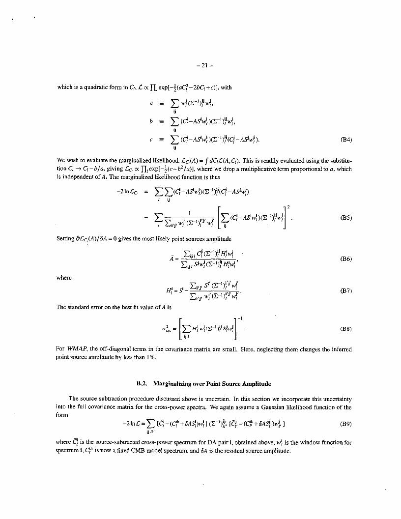
which is a quadratic form in Cl, C 0: n, exp[-f(aC:-2bCl+c)], with

034)

We wish to evaluate the marginalized likelihood, &,(A) = JdCrC(A,Cl). This is readily evaluated using the substitu- tion Cl -+ Cl-b/a, giving CC, cc nlexp[-i(c-b2/a)], where we drop a multiplicative term proportional to a, which is independent of A. The marginalized likelihood function is thus

Setting dCc,(A)/dA = 0 gives the most likely point sources amplitude

where

The standard error on the best fit value of A is

2

For WMAP, the off-diagonal terms in the covariance matrix are small. Here, neglecting them changes the inferred point source amplitude by less than 1%.

B.2. Marginalizing over Point Source Amplitude

The source subtraction procedure discussed above is uncertain. In this section we incorporate this uncertainty into the full covariance matrix for the cross-power spectra. We again assume a Gaussian likelihood function of the form

039)

is the source-subtracted cross-power spectrum for DA pair i, obtained above, M J ~ is the window function for

-2 In c = [Cj - (e GAS])^^ 3 (E-~);, [Cj, - (Q + b~$,)uj,, I ij 11'

where spectrum i, qh is now a fixed CMB model spectrum, and 6A is the residual source amplitude.

-22-

We can marginalize the likelihood function over the residual point source amplitude as follows. Expand equa- tion (B9) as

- 2 1 n ~ = ( C ~ - C ~ ~ ~ ~ ) ( E - ' ) E , ( ~ ~ , - C ~ ~ , ) ij 11'

- 2 ( 6 A ) c (Cj-_C[h~])(C-')E,Sj~,

ij 11'

ij /I'

which is a quadratic form in SA, C 0; e ~ p [ - ~ ( a ( S A ) ~ - 2 b ( b A ) + c ) ] , with

ij 11'

c (~-crw;)(E-');,(ci, -C;!d,) . ij 11'

We wish to evaluate the marginalized likelihood, LA = JLd(GA). This is readily evaluated using the substitution SA + SA-b/a, givini LA c( exp[-f(c-b*/a)], where we drop a multiplicative term proportional to a, which is independent of c. The marginalized likelihood function is thus

This expression may be recast in the form

The superscript "src" indicates that the Fisher matrix so obtained includes point source subtraction uncertainty, in addition to whatever effects have been included in (E-')!, already, in this case only cosmic variance and noise. Note that equation (B15) neglects a term proportional to Indet a which has a weak dependence on cosmological parame- ters. In the actual calculation, as in the previous section, we assume the diagonal form of the covariance matrix in equation (B 1).

C. OPTIMAL WEIGHTING OF MULTI-CHANNEL SPECTRA

We use the 8 high-frequency differencing assemblies Q1 through W4 to generate the final combined spectrum. In this Appendix we show how we combine these spectra into a single estimate of the angular power spectrum.

-23-

The ultimate goal of the WMAPanalysis is to produce a likelihood function for a set of cosmological parameters, {a}, given the data, c. Specifically

where P(dlc> is the probability of {d} given the data, ,C(CiICfh(C)) is the likelihood of the data given the model, e ( d ) , and P ( 3 is the prior probability of the parameter set (Verde et al. 2003). To this end, we seek a combined spectrum, ?I, that estimates the power spectrum in our sky, Cfb, with the property that P(dl?l) = P(c?lc), and hence

P(dlc;) = L(qCp(d))P(cq, (C1)

aGIc)h(C)) = aqq(cq3). To estimate the combined spectrum, we approximate the likelihood function for the cross-power spectra as Gaus-

(C2) sian

- ~ I ~ L ( < I c ~ ~ ) = C(<-c?w:) (C~~J: , (C!, -+vj,), ij 11’

where < is the spectrum with the best-fit source model subtracted, defined after equation (12), wJ is the window function of spectrum i, defined after equation (6), and Cf~ll is the covariance matrix of the 28 cross-power spectra. Note that the treatment in the remainder of this section does not depend on any specific property of the covariance, so we use generic notation for readability. However, when we generate the WMAPfirst-year combined spectrum, the actual form of the covariance used at this step is (%full)!,, where % indicates the approximate covariance, obtained in $4, that has not yet had the effects of the foreground mask accounted for.

We seek a spectrum e1 such that

A

where Qlp is the inverse-covariance matrix of the combined spectrum which comes with the estimate of Cl. Suppose, for simplicity, that Cf,ll is diagonal, (Cf~ll):, = (ChIl)y61l,, then it is straightforward to show that the deconvolved, weighted-average spectrum

with

is the desired spectrum. Substituting equations (C4) and (CS) into equation (C3) produces equation (C2) up to a term which has a weak dependence on comological model, which we ignore. This combined spectrum is equivalent to the result we would obtain using the “optimal data compression” of Tegmark et al. (1997).

If the inverse covariance matrix is not diagonal in I, it can be shown that the optimal combined spectrum is given bv

with

and where is a fiducial cosmological model which we take to be a flat ACDM model with nbh2 = 0.021, R,h2 = 0.129, R,,, = 1, h = 0.68, n, = 1.2, and ‘T = 0.2. While this model has parameters values that are substantially different than the best-fit WMAPmodel obtained (afterwards) by Spergel et al. (2003), the parameter degeneracies are such that c d i s close to the best-fit model for 1 > 100 where this estimator is actually used (see 05.1). The combined spectrum

-24-

is optimal if the fiducial model chosen is the correct one; otherwise it is still unbiased but slightly sub-optimal (Gupta & Heavens 2002).

D. CUT-SKY FISHER MATRIX

The WMAP sky maps have nearly diagonal pixel-pixel noise covariance (Hinshaw et al. 2003a) which greatly simplifies the properties of the power spectrum Fisher matrix. In this Appendix we present an analytic derivation of the effect of a sky cut and non-uniform pixel weighting. In D.l, we assume that we have an optimal estimator of the power spectrum. In the noise dominated limit, we can obtain an exact expression, while in the signal dominated limit, we need to approximate the signal correlation matrix to obtain an analytic expression. In D.2, we interpolate the Fisher matrix between the signal and noise-dominated regimes and show that it agrees with numerical estimates. In D.3, we estimate the power spectrum covariance matrix from Monte Carlo simulations of the sky and calibrate the interpolation formula.

D.1. Cut-Sky Fisher Matrix: Analytic Evaluation

We equate the Fisher matrix of the power spectrum to the curvature of the likelihood function, equation (A16), then develop an approximate form for the covariance matrix, C = S +N, where S is the signal matrix and N is the noise matrix. We split the noise matrix into two pieces: a weight term and a mask term. In the limit that the pixel noise is diagonal, the weight term has the form

(D1) (N-'). = -6.. ni =

ii oi 11 - wiaij

where i and j are pixel indices, ni is the number of observations of pixel i, 00 is the rms noise of a single observation, and, by definition, wi is the weight of pixeI i. The mask, Mi, is defined so that Mi equals 0 in pixels that are not used due to foreground contamination, and equals 1 otherwise. The noise matrix can then be written as the product of the two terms

N-' = N - ~ M = m-'= 26.. - +,.a. .

where lii = n; and Gi = w; in the unmasked pixels, and are set to 0 otherwise. We thus define the covariance matrix over the full sky, which allows us to exploit the orthogonality properties of the spherical harmonics. Note that M2 = M.

ii. @2) 4 ' I - ' I

W

The inverse of the full covariance matrix can now be written as

c-'= (S + ~ 1 - 1 = N-' (SN-' +I)-'

= M-'(SM-'+N,)-'

The covariance matrix has two limits. In the noise dominated limit, SN-' << I,

C-' + N-'.

In the signal dominated limit, SM-' << N,, only the mask alters the covariance matrix, so

c-' + MS-IM,

where we have set the inverse of the mask to zero where there is no data, i.e. M-' E M.

@3) 034)

- 25 -

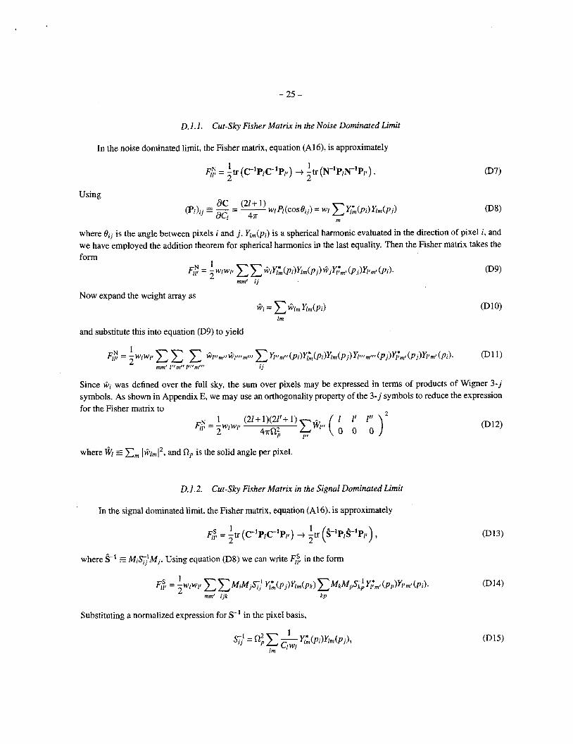
D. I . 1 . Cut-Sky Fisher Matrix in the Noise Dominated Limit

In the noise dominated limit, the Fisher matrix, equation (A16), is approximately

@7) 1 1 2 2

4; = -tr (C-'P/C-'P/,) + -tr (N-'P,N-'Pp).

Using

where Bij is the angle between pixels i and j , Yim(pi) is a spherical harmonic evaluated in the direction of pixel i, and we have employed the addition theorem for spherical harmonics in the last equality. Then the Fisher matrix takes the form

Now expand the weight array as Gi = Glni Km(pi)

and substitute this into equation (D9) to yield

Since Gi was defined over the full sky, the sum over pixels may be expressed in terms of products of Wigner 3 - j symbols. As shown in Appendix E, we may use an orthogonality property of the 3- j symbols to reduce the expression for the Fisher matrix to

4; = ~ W ' W ' 1 (21+ 1)(21'+ 1) p,, ( 0 0 I' 0 1

47ri-l;;

where W! E Ern l6lrnl2, and ill, is the solid angle per pixel.

0.1.2. Cut-SQ Fisher Matrix in the Signal Dominated Limit

In the signal dominated limit, the Fisher matrix, equation (A16), is approximately

Substituting a normalized expression for S-' in the pixel basis,

-26-

into equation (D14), one obtains a term

Since our mask cuts only - 15% of the sky, the coupling sum, ~ i M i Y , ~ m ~ (p i )v ,m, , (p i ) , peaks very sharply at Il'-l''I << 1'. Therefore, one may approximate equation (D16) with

where, in the last equality, we have used the completeness relation for the spherical harmonics

lm

With this approximation equation (D 14) reduces to

Following the same steps outlined above for the derivation of equation (D12) yields

F M p ( " ' I ' ) 1 1 (21+1)(21'+1) 2 crcp 47r 0 0 0

47, = - -

where Ml E Em (m1m(2, and ml, is the spherical harmonic transform of the mask. Note that Mo = 47rf&, where fsb is the fraction of the sky that survives the mask.

D.2. Interpolating the Cut-Sky Fisher Matrix

We can combine the two limiting cases of the Fisher matrix, obtained in the previous section, into a single expression

where N[ previous section, f i l l can be expressed in the low 1 (signal-dominated) and high 1 (noise-dominated) limits as

f i p f f i / ( f i & s w [ ) is the deconvolved noise power spectrum. Using equations (D12) and (D20) derived in the

F M l l , ( 0 0 0 " I" ) 2 ' (21 + 1)(21'+ 1)

47r"f&

and

By construction, these matrices are normalized to 1 on the diagonal, 6: = 6: = 1, since MO = 47rf& and @O = 47rf&fi:bs/u;'

We have computed F;Yk directly, for selected 1 values, by evaluating l$mC-'K~m~ using the pre-conditioner code described by Oh et al. (1999). We find that deviations between the numerical and analytical results are consistent with numerical noise in the Fisher matrix estimate. Figure 14 shows the estimated Fisher matrix for the Kp2 cut in the noise and the signal dominated limits.

We interpolate between the two regimes with the following expression:

Note that the form of the Fisher matrix primarily depends on Al, but is weakly dependent on I -there is more coupling in the noise dominated limit.

D.3. Power Spectrum Covariance: Monte Carlo Evaluation

As discussed in Appendix A. 1.2 we compute the C, using three different pixel weightings. The uniform weighting and the inverse-noise inverse weighting are optimal in the signal-dominated regime and the noise-dominated regime, respectively. In between these limits the transitional weighting performs better. In order to determine which ranges in 1 correspond to which regimes, and to calibrate our ansarz for the covariance matrix, equation (D21), we proceed as fol- lows. Using 100,000 Monte Carlo simulations of signal plus noise (with WMAPnoise levels and symmetrized beams), we compute the diagonal elements of the covariance matrix for the three different weighting schemes, evaluated with the Kp2 sky cut. Denote these estimates Dr"'

We find that the uniform weighting produces the smallest DFm below 1 = 200. Inverse-noise weighting is the best above 1 = 450, and the transitional weighting produces the lowest variance in between. In each of these regimes we use the resulting Dsim to calibrate our ansurz for the diagonal elements of the covariance matrix

as illustrated in Verde et al. (2003). These calibrations produce a smooth correction to equation (D24) of at most 6%. No correction at all is required in the signal dominated regime.

E. SOME USEFUL PROPERTIES OF SPHERICAL HARMONICS

The derivation of the form of the Fisher matrix in the signal and noise dominated limjts led to expressions which

K ~ ~ m ~ ~ ( P i ) q z l ( P i ) K m ( p j ) Y l ~ ~ ~ r n ~ ~ ~ ( p j ) q y m t ( P j I K f m ) ( P i ) , (El 1

where the sum is effectively a double integral over the full sky. This can be evaluated in terms of the Wigner 3 - j symbols, defined as

included a term

mm' i j

Substituting this into equation (El) gives

nim'

-28-

We simplify this using the Wigner 3- j orthogonality condition

where S(Z, l', 1") =' 1 for Il-Z'I 5 1'' 5 I+ I' and is 0 otherwise. This reduces equation (El) to

(21+1)(21'+1) 1 11 1" 4TR; ( 0 0 O ) * >

where the factor of 0; accounts for the fact that equation (El) is a double sum over pixels, instead of a double integral.

-29-

Fig. 1 .- The effective noise as a function of I for the 8 differencing assemblies used in the combined power spectrum analysis. These spectra were computed from end-end simulations of noise maps, as discussed in $2.2. For illustration, the spectra shown here were computed using the quadratic estimator with uniform pixel weights. The actual noise model uses three separate weighting schemes in three separate 1 ranges, and thus has discontinuities where the effective noise level changes. The weights are defined in Appendix A. 1.2.

-30-

7000 F 6000

3 5000 & 4000 \ u- 3000

2000 T

+ s 1000 0

c 9 *- 1.2 E

1.0 0 +

.-O 0.8

0.6

+ U aL

0 100 200 300 400 500 1

Fig. 2.- The full set of individual cross-power spectra for I < 500, computed from the 8 high frequency differencing assemblies Q1 through W4,28 spectra in all. The spectra were evaluated from the uncorrected sky maps (no Galaxy model subtracted) using the Kp2 sky cut with uniform weighting. The data are plotted in color by effective frequency

with red corresponding to 41 GHz and blue to 94 GHz. The top panel shows a very robust measurement of the first acoustic peak with a maximum near 1 - 220. There is also a clear indication of the rise to a second peak at I N 540 as discussed in $6. The bottom panel shows the ratio of each channel to the combined spectrum presented in $5. This clearly shows the residual foreground emission due to diffuse Galactic radio emission at low I and to point sources at higher I. The level of contamination, which is strongest at Q band. is consistent with the expected level of foreground emission. See Figure 3 for the spectra after foreground subtraction.

-31 -

7000 F7 6000

4000 \

- 2000 + T

s - " " " ~ 1000

U a c .n .-

0

1.4

1.2 r E 00 1.0 0 +

2 0.8

0.6

P E

0 100 200 300 400 500 1

Fig. 3.- The same set of cross-power spectra as shown in Figure 2. Here, the foreground model discussed in $3.1 has been subtracted from each channel. The bottom panel shows the ratio of each of the 28 cross-power spectra to the combined spectrum presented in $5. Aside from a -10% discrepancy in the Q band data at I < 20, the data are consistent with each other to the sensitivity limits of the individual spectra. Because the WMAP data are not sensitivity limited at low I, we use only V and W band data in the final combined spectrum for 1 < 100 (see $5) to minimize residual Galactic contamination.

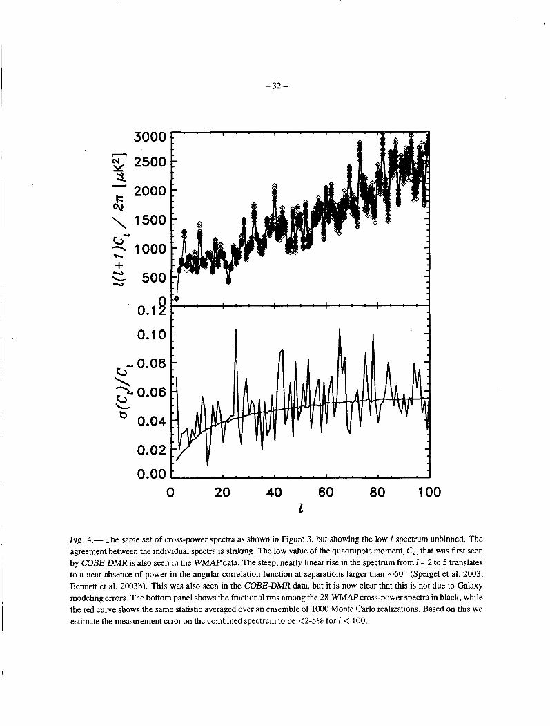
-32-

\ u- T h + s

3000

2500

2000

1500

1000

500

0.1s s 0.1 0

u- 0.08 \ 2- 0.06 L

0.04

0.02

b

Fig. 4.- The same set of cross-power spectra as shown in Figure 3, but showing the low I spectrum unbinned. The agreement between the individual spectra is striking. The low value of the quadrupole moment, Cz, that was first seen by COBE-DMR is also seen in the M A P data. The steep, nearly linear rise in the spectrum from I = 2 to 5 translates to a near absence of power in the angular correlation function at separations larger than -60° (Spergel et al. 2003; Bennett et al. 2003b). This was also seen in the COBE-DMR data, but it is now clear that this is not due to Galaxy modeling errors. The bottom panel shows the fractional rms among the 28 W A P cross-power spectra in black, while the red curve shows the same statistic averaged over an ensemble of 1000 Monte Carlo realizations. Based on this we estimate the measurement error on the combined spectrum to be <2-5% for I < 100.

- 3 3 -

n (Y Y a

Angular scule (deg) .

90 2 0.5 0.2

6000 k 5000

3000

2000

1000

0 10 40 100 200 400 800

Multipole moment 1

Fig. 5.- The auto-power spectrum of the combined Q+V+W map evaluated with the three weighting schemes defined in Appendix A. 1.2. In each case, the spectrum was computed over the entire 1 range, and black shows uniform weights, red shows inverse-noise weights, and green shows transitional weights. The agreement is excellent.

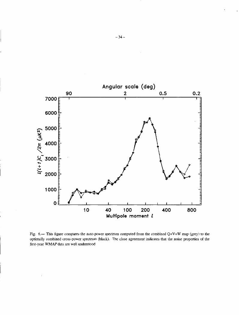
-34-

90 Angular scale (deg)

2 0.5 0.2

6ooo/

t

I n 5000 Y 3.

N

W

4000

b- 3000 2 Y

1 + 2000

looo[

0 10 800 40 100 200 400

Multipole moment 1

Fig. 6.- This figure compares the auto-power spectrum computed from the combined Q+V+W map (grey) to the optimally combined cross-power spectrum (black). The close agreement indicates that the noise properties of the first-year WMAP data are well understood

- 35 -

Angular scale (deg) 90 2 0.5 0.2

7000 t I I I I

6ooo t n 5000

i OJ Y U

4000

T u- 3000 Y )r t +

2000

1000

/ I I I I I I I

10 40 100 200 400 800 Multipole moment 1

Fig. 7.- A comparison of the power spectrum computed with data from the ecliptic plane (black) vs. data from the ecliptic poles (grey). Note that some of the “bite” features that appear in the combined spectrum are not robust to data excision. There is also no evidence that beam ellipticity, which would be more manifest in the plane than in the poles, systematically biases the spectrum. This is consistent with estimates of the effect given by Page et al. (2003a).

- 3 6 -

7000 1 I I I I - - 6ooo 1

5- 5000 1 -- Y W

Y 40001 Y u- 3000 1 h

- 1 + 2000

loo0 1 I I I I I I I I I l l

10 40 100 200 400 800 1400 Multipole moment 1

Fig. 8.- The final angular power spectrum, Z(Z+ 1)C1/27r, obtained from the 28 cross-power spectra, as described in $5. The data are plotted with la measurement errors only which reflect the combined uncertainty due to noise, beam, calibration, and source subtraction uncertainties. The solid line shows the best-fit ACDM model from Spergel et al. (2003). The grey band around the model is the la uncertainty due to cosmic variance on the cut sky. For this plot, both the model and the error band have been binned with the same boundaries as the data, but they have been plotted as a splined curve to guide the eye. On the scale of this plot the unbinned model curve would be virtually indistinguishable from the binned curve except in the vicinity of the third peak.

-37-

n el Y 3.

W

Angular scale (deg) 7000 7 90

5000 6oool Y 40001 x- 3000 + h

2000

COB€ ARCHEOPS TOCO BOOMERanG

1 I I I I I

0.5 0.2

10 40 100 200 400 800 1400 Multipole moment 1

Fig. 9.- A compilation of recent CMB power spectrum measurements compared to the best-fit ACDM model from the first-year WMAPdata. The data points include noise and cosmic variance uncertainty (but not calibration uncertainty) thus we omit the cosmic variance band from the model curve in the Figure. On average, the pre- WMAP data agree well with the WMAP power spectrum.

-38-

Angular scale (deg) 90 2 0.5 0.2

7000 I I I I

6oool n 5000 Y 3.

N

W

4000

+ 2000

1 I I I I I I I I l l

10 40 100 200 400 800 1400 Multipole moment 1

Fig. 10.- The WAF ' combined power spectrum, in black, compared to a compilation of all CMB data published prior to WMAPfrom Wang et al. (2002a), in red. The =data are plotted with cosmic variance plus measurement uncertainties here in order to facilitate a comparison with the compiled data which is reported in this way. The data agree well on COBE scales, I < 20, (but note that the W A P cosmic variance errors are computed from the best-fit model rather than the data, thus they appear larger than the COBE errors at the quadrupole). However, the overall normalization of the W A P spectrum is - 10% higher on smaller scales.

-39-

7000

6000

1 I I I I - - - - - - 5

t n 5000 ml Y 3. v

t O F * I I I I I I I I I l l

10 40 100 200 400 800 1400 Multipole moment 1

Fig. 1 1 .- The WMAP combined power spectrum compared to the locus of predicted spectra, in red, based on a joint analysis of pre-WMAPCMB data and 2dFGRS large-scale structure data (Percival et al. 2002). As in Figure 8, the WMAF' data are plotted with measurement uncertainties, and the best-fit hCDM model (Spergel et al. 2003) is plotted with a la cosmic variance error band. The locus of predicted spectra lie systematically below the WMAP data at intermediate 1.

-40-

n N

3

h + s

Fig. 12.- A comparison of two power spectra computed from a single V band map. The black points result from the maximum likelihood method, the red points from the quadratic estimator computed with uniform pixel weighting. In both cases a noise model has been assumed to treat the noise bias. At higher I, the two spectra would be nearly identical since both impose inverse noise weighting on the data.

-41-

6000

5000

N e 4000

Cj n 3000

2000

\

7 +

1000

6000

5000

e 4000

n 3000

2 2000

cu \

7 +

1000

ww ww

-I

0 0 200 400 600 800 1000

1

Fig. 13.- The quadratic estimator discussed in SA.1 has been extensively tested with Monte Carlo simulations of first-year WMAP data. The top panel shows a model spectrum in red, and the mean of 600 realizations of the cross- power spectrum, computed from the V and W band-averaged maps, in black. The red emor bars show the uncertainty in the mean in bins with AZ = 20. The cross-power spectrum estimator is unbiased. The bottom panel is similar, but with auto-power spectra computed from the W band-averaged map. Here the noise bias term was estimated directly from the high I tail of the computed spectrum. This simple auto-power spectrum estimator is unbiased if the noise is white, and is suitable for V band data, but see Figure 1 for examples of W band noise spectra.

-42-

0.06

0.04

n Y

v 0.02 L

0.00

-0.02 -40 -20 0 20 40

A1

Fig. 14.- Slices of the Fisher (or curvature) matrix normalized as F p / d m , plotted vs. A1 = 1 -l', from the Fisher matrix for the combined spectrum. Black is 1 = 30, red is 1 = 300, green is 1 = 600.

-43-

Table 1. WMAPPower Spectrum Noise Modela

Parameter Q1 4 2 VI v2 w1 w2 w 3 w 4

Co(X102) -6.604 -6.971 -6.823 -6.674 -7.174 -7.439 -7.044 -7.989 ~i(x10’) 1.934 4.244 2.497 1.395 3.060 3.721 1.459 4.820 C ~ ( X IO4) -3.798 -8.521 -5.203 -1.483 -6.021 -6.901 -2.677 -5.870 c3(xiO5) 2.549 5.921 3.715 0.242 4.147 4.540 1.750 2.167

200 < I < 450

co(x102) -6.143 -6.268 -6.320 -6.192 -6.618 -6.833 -6.768 -6.849 c1(xIO4) -1.334 1.341 -0.800 -1.351 0.769 2.582 0.885 2.443

I > 450

co(X10’) -6.202 -6.167 -6.338 -6.264 -6.564 -6.704 -6.688 -6.772 ~ i ( ~ 1 0 ’ ) 3.288 4.085 3.327 5.979 7.342 12.970 8.851 24.430

aBest-fi t coeffi cients for the noise model in equation (8). The units of the output noise are md, thermodynamic temperature.