Embed Size (px)
Citation preview

THREE ESSAYS ON HEALTH CARE
UTILIZATION, GOVERNANCE AND PROVIDER
REIMBURSEMENT IN URBAN CHINA
by
Wei Wang
M.A. in International Economics, Shanghai Academy of Social
Sciences, 2000
B.S. in International Finance, Shanghai Jiaotong University, 1997
Submitted to the Graduate Faculty of
the Arts and Sciences in partial fulfillment
of the requirements for the degree of
Doctor of Philosophy
University of Pittsburgh
2009

UNIVERSITY OF PITTSBURGH
DEPARTMENT OF ECONOMICS
This dissertation was presented
by
Wei Wang
It was defended on
August 18, 2009
and approved by
Thomas Rawski, Professor, Department of Economics, University of Pittsburgh
Siddharth Chandra, Professor, Graduate School of Public and International Affairs,
University of Pittsburgh
Alexis Leon, Assistant Professor, Department of Economics, University of Pittsburgh
Soiliou Namoro, Assistant Professor, Department of Economics, University of Pittsburgh
Shanti Gamper-Rabindran, Assistant Professor, Graduate School of Public and
International Affairs, University of Pittsburgh
Dissertation Director: Thomas Rawski, Professor, Department of Economics, University of
Pittsburgh
ii

THREE ESSAYS ON HEALTH CARE UTILIZATION, GOVERNANCE AND
PROVIDER REIMBURSEMENT IN URBAN CHINA
Wei Wang, PhD
University of Pittsburgh, 2009
The first essay uses a model of profit-maximizing hospitals to examine hospital responses to
global budgeting in the forms of dumping and cost shifting. The main findings include: (1)
Hospitals dump insured patients when the covered services are priced under costs. Whether
the budget target is binding depends on its size relative to the mandated fees and production
costs of insured services. (2) Only when hospitals operate at full capacity and the uninsured
patients have inelastic demand do providers shift costs to the uninsured. (3) When revenue
shocks dominate, cost shifting lowers the income from the insured while increasing that from
the uninsured patients. When cost shocks dominate, incomes from the two groups may be
positively correlated.
In the second essay, I use insurance claim data in a difference-in-differences model to
empirically investigate the effects of global budgeting on providers’ selection and skimping
against high-cost patients in China. It finds that non-last resort (LR) hospitals respond to
global budgeting by avoiding unprofitable patients as well as selectively reducing the intensity
of their treatment. Interestingly, I did not find evidence of skimping for LR providers. This
indicates that non-LR hospitals achieve at least part of the adverse selection by making
services inadequate for high-cost patients.
In the third essay,1 we use survey data in an endogenous switching regression model to
1This is essay is co-authored with Gordon Liu at Guanghua School of Management, Peking University,China
iii

analyze the price gap between state and private hospitals in China. Our analysis finds strong
evidence that outpatient care is not only much more expensive at the public sector, but more
expensive to a greater extent for certain disadvantaged social groups than for the general
population. We explain this finding by noting that the private sector can price discriminate
with greater flexibility than the tightly regulated public sector. We also find that the bigger
the share of physicians working in the private sector, the lower the public-private price gap
as well as the overall average price. These results indicate that increasing competition in
the market for physicians may significantly lower the price of health care by enabling private
providers to enhance their reputation through attracting well-trained physicians.
iv

TABLE OF CONTENTS
PREFACE . . . . . . . . . . . . . . . . . . . . . . . . . . . . . . . . . . . . . . . . . x
1.0 INTRODUCTION . . . . . . . . . . . . . . . . . . . . . . . . . . . . . . . . . 1
1.1 China’s Health Care System . . . . . . . . . . . . . . . . . . . . . . . . . . . 1
1.2 Recent Health System Reforms . . . . . . . . . . . . . . . . . . . . . . . . . 3
1.3 Objectives of the Dissertation . . . . . . . . . . . . . . . . . . . . . . . . . . 4
1.4 Contents of the Dissertation . . . . . . . . . . . . . . . . . . . . . . . . . . . 6
1.5 Contributions of the Dissertation . . . . . . . . . . . . . . . . . . . . . . . . 8
2.0 HOSPITAL RESPONSES TO THE GLOBAL BUDGET POLICY: THE
CASES OF PATIENT DUMPING AND COST SHIFTING . . . . . . . 10
2.1 Introduction . . . . . . . . . . . . . . . . . . . . . . . . . . . . . . . . . . . 10
2.2 Background: Delivering and Financing Health Care in Urban China . . . . . 12
2.2.1 Delivery: A Changing Paradigm . . . . . . . . . . . . . . . . . . . . . 12
2.2.2 Financing: Incomplete Coverage . . . . . . . . . . . . . . . . . . . . . 14
2.3 Literature Review . . . . . . . . . . . . . . . . . . . . . . . . . . . . . . . . 15
2.3.1 Cost Shifting . . . . . . . . . . . . . . . . . . . . . . . . . . . . . . . . 15
2.3.2 Payment Reforms in China . . . . . . . . . . . . . . . . . . . . . . . . 17
2.3.3 Contributions of the Paper . . . . . . . . . . . . . . . . . . . . . . . . 18
2.4 The Model . . . . . . . . . . . . . . . . . . . . . . . . . . . . . . . . . . . . 20
2.4.1 Patient Dumping . . . . . . . . . . . . . . . . . . . . . . . . . . . . . 24
2.4.2 Comparative Statics . . . . . . . . . . . . . . . . . . . . . . . . . . . . 27
v

2.4.3 Cost Shifting and Hospital Income . . . . . . . . . . . . . . . . . . . . 30
2.4.4 Elasticities . . . . . . . . . . . . . . . . . . . . . . . . . . . . . . . . . 31
2.5 Conclusions . . . . . . . . . . . . . . . . . . . . . . . . . . . . . . . . . . . . 34
3.0 HOW DO HIGH-COST PATIENTS FARE UNDER THE GLOBAL
BUDGET POLICY? — EVIDENCE FROM CHINA . . . . . . . . . . . 38
3.1 Introduction . . . . . . . . . . . . . . . . . . . . . . . . . . . . . . . . . . . 38
3.2 Literature Review . . . . . . . . . . . . . . . . . . . . . . . . . . . . . . . . 41
3.2.1 Patient Selection and Skimping on Services . . . . . . . . . . . . . . . 41
3.2.2 Global Budgeting . . . . . . . . . . . . . . . . . . . . . . . . . . . . . 42
3.2.3 Provider Payment Reforms in China . . . . . . . . . . . . . . . . . . . 43
3.3 Zhenjiang’s Provider Payment Reforms . . . . . . . . . . . . . . . . . . . . . 44
3.3.1 Reform Chronology . . . . . . . . . . . . . . . . . . . . . . . . . . . . 44
3.3.2 Economics of Patient Selection and Skimping . . . . . . . . . . . . . . 46
3.4 Data . . . . . . . . . . . . . . . . . . . . . . . . . . . . . . . . . . . . . . . . 47
3.5 Estimation Strategies . . . . . . . . . . . . . . . . . . . . . . . . . . . . . . 49
3.5.1 Definitions of Key Concepts . . . . . . . . . . . . . . . . . . . . . . . 50
3.5.1.1 Selection . . . . . . . . . . . . . . . . . . . . . . . . . . . . . . 50
3.5.1.2 Skimping . . . . . . . . . . . . . . . . . . . . . . . . . . . . . 50
3.5.1.3 Costliness of Patients . . . . . . . . . . . . . . . . . . . . . . . 50
3.5.2 Model Specification . . . . . . . . . . . . . . . . . . . . . . . . . . . . 51
3.5.3 Estimation . . . . . . . . . . . . . . . . . . . . . . . . . . . . . . . . . 54
3.6 Results . . . . . . . . . . . . . . . . . . . . . . . . . . . . . . . . . . . . . . 56
3.7 Discussion . . . . . . . . . . . . . . . . . . . . . . . . . . . . . . . . . . . . . 59
4.0 THE ROLE OF PRIVATE PROVIDERS IN LOWERING THE COST
OF HEALTH CARE: EVIDENCE FROM URBAN CHINA . . . . . . 67
4.1 Introduction . . . . . . . . . . . . . . . . . . . . . . . . . . . . . . . . . . . 67
4.2 China’s Health Care System . . . . . . . . . . . . . . . . . . . . . . . . . . . 70
4.3 Literature Review . . . . . . . . . . . . . . . . . . . . . . . . . . . . . . . . 74
vi

4.3.1 Provider Ownership . . . . . . . . . . . . . . . . . . . . . . . . . . . . 74
4.3.2 Market Competition . . . . . . . . . . . . . . . . . . . . . . . . . . . . 75
4.4 Public-Private Price Gap . . . . . . . . . . . . . . . . . . . . . . . . . . . . 76
4.4.1 Econometric Model . . . . . . . . . . . . . . . . . . . . . . . . . . . . 76
4.4.2 Semiparametric Estimation . . . . . . . . . . . . . . . . . . . . . . . . 79
4.4.2.1 Reduced-Form Selection Equation . . . . . . . . . . . . . . . . 79
4.4.2.2 Correction for Self-Selection Bias . . . . . . . . . . . . . . . . 79
4.4.2.3 Estimation of the Public-Private Price Gap . . . . . . . . . . . 81
4.4.2.4 Structural Selection Equation . . . . . . . . . . . . . . . . . . 82
4.5 Market Share Analysis . . . . . . . . . . . . . . . . . . . . . . . . . . . . . . 83
4.5.1 Econometric Model . . . . . . . . . . . . . . . . . . . . . . . . . . . . 83
4.5.1.1 Indicators of Market Liberalization . . . . . . . . . . . . . . . 84
4.5.1.2 Controls for Inter-City Heterogeneities . . . . . . . . . . . . . 85
4.5.2 Cluster Sample Analysis . . . . . . . . . . . . . . . . . . . . . . . . . 87
4.6 Data and Variables . . . . . . . . . . . . . . . . . . . . . . . . . . . . . . . . 87
4.6.1 Dependent Variable . . . . . . . . . . . . . . . . . . . . . . . . . . . . 88
4.6.2 Variable of Provider Ownership . . . . . . . . . . . . . . . . . . . . . 88
4.6.3 Identifying Variables . . . . . . . . . . . . . . . . . . . . . . . . . . . . 89
4.6.4 Other Variables . . . . . . . . . . . . . . . . . . . . . . . . . . . . . . 89
4.7 Empirical Results . . . . . . . . . . . . . . . . . . . . . . . . . . . . . . . . . 91
4.7.1 Semiparametric Regression . . . . . . . . . . . . . . . . . . . . . . . . 91
4.7.2 Public-Private Price Gap . . . . . . . . . . . . . . . . . . . . . . . . . 94
4.7.3 Price Gap for Various Socioeconomic Groups . . . . . . . . . . . . . . 97
4.7.4 Structural Selection Equation . . . . . . . . . . . . . . . . . . . . . . . 98
4.7.5 Market Share Analysis . . . . . . . . . . . . . . . . . . . . . . . . . . 99
4.8 Discussion . . . . . . . . . . . . . . . . . . . . . . . . . . . . . . . . . . . . . 102
5.0 CONCLUDING REMARKS . . . . . . . . . . . . . . . . . . . . . . . . . . 122
BIBLIOGRAPHY . . . . . . . . . . . . . . . . . . . . . . . . . . . . . . . . . . . . 125
vii

LIST OF TABLES
2.1 Structure of Per Capita Expenditure at Urban General Hospitals (%) . . . . . 37
2.2 Bed Occupancy Rates at Urban General Hospitals (%) . . . . . . . . . . . . . 37
3.1 Number of Visits to Last-Resort Hospitals by Age Group . . . . . . . . . . . 62
3.2 Descriptive Statistics of Covariates in the DD Estimation . . . . . . . . . . . 62
3.3 Parametric Estimation of the Patient Selection Model . . . . . . . . . . . . . 63
3.4 The Policy Effect on Selection against Costly Patients . . . . . . . . . . . . . 64
3.5 The Policy Effect on Skimping . . . . . . . . . . . . . . . . . . . . . . . . . . 65
3.6 Validation of the Difference-in-Differences Strategy . . . . . . . . . . . . . . . 66
4.1 Definitions & Descriptives of Variables in the Switching Regression . . . . . . 105
4.2 Variables in the Market Share Analysis . . . . . . . . . . . . . . . . . . . . . 107
4.3 Probit Estimation of the Selection Equation . . . . . . . . . . . . . . . . . . . 108
4.4 Differences in Estimated Coefficients . . . . . . . . . . . . . . . . . . . . . . . 111
4.5 Semiparametric Estimation for Key Socioeconomic Indicators . . . . . . . . . 114
4.6 Andews-Schafgans Intercept Estimates . . . . . . . . . . . . . . . . . . . . . . 115
4.7 Estimated Public-Private Price Gap . . . . . . . . . . . . . . . . . . . . . . . 116
4.8 Public-Private Price Gap for Various Socioeconomic Groups . . . . . . . . . . 117
4.9 Median Market Share Coefficients . . . . . . . . . . . . . . . . . . . . . . . . 118
viii

LIST OF FIGURES
4.1 Market Liberalization & Price of Care . . . . . . . . . . . . . . . . . . . . . . 119
4.2 Market Liberalization & Price Gap . . . . . . . . . . . . . . . . . . . . . . . . 120
4.3 Physician Work Load . . . . . . . . . . . . . . . . . . . . . . . . . . . . . . . 121
ix

PREFACE
I wish to express a deepest feeling of gratitude to my principal academic advisor, Professor
Thomas Rawski. Throughout the course of my doctoral study, he has offered me his guidance
and encouragement in the most generous manner. His breadth of knowledge and level of
scholastic achievement has given me constant inspiration, while, when my research is at its
ebbs, his understanding and tireless help has enabled me to obtain key breakthroughs. I
consider myself truly fortunate to have been his student, and wish only to do justice to his
trust by living up to his expectations.
My Committee Members, Professors Siddharth Chandra, Alexis Leon, Soiliou Namoro
and Shanti Gamper-Rabindran patiently examined my work and provided me with the most
insightful advice. Their comments and challenges are invaluable in increasing the quality of
my research and in helping me explore new directions.
I am grateful to my coauthor, Professor Gordon Liu at Peking University, for his patience,
motivation and contributions. The nineteen months I spent at the research center under
his direction was profoundly important for my academic development. I have benefited
substantially from his mentoring and his help with my career.
I wish to thank the staff members of the Economics Department, in particular Ms. Amy
Linn, Lauree Graham and Debbie Ziolkowski, who have on more than one occasion gone out
of their way to help me through my administrative duties.
I dedicate this dissertation and my Ph.D. degree to my parents. My late father will
be forever in my memories. His tender affection, which constantly betrayed itself despite
his stern appearance, has touched my life in the most profound way. My mother, with her
x

boundless love, patience and perseverance, is among the principal forces that have made the
completion of my Ph.D. studies possible.
xi

1.0 INTRODUCTION
1.1 CHINA’S HEALTH CARE SYSTEM
China’s market-oriented reforms have brought fascinating changes to its health care sector
in the past three decades. As in many other parts of the economy, decentralization and
incentivization have significantly altered the delivery and financing systems of health care.
The publicly owned hospital sector has obtained a substantial amount of financial autonomy
from the government. Moreover, reforms of the state economic sector have left the financing
of health care a largely personal responsibility. It has been argued that, within the span
of 20 years, China’s health system has transformed into the world’s most market-oriented
system [Wagstaff et al. (2009b)[119]].
In many other ways, the government still holds considerable control over the health sector.
It regulates the pricing of medical services, sets entry rules for the hospital care market, many
of which may restrict the development of the private health sector, and influences market
outcomes through regulating the massive state delivery system. Therefore, the Chinese
health care system is characterized by a mixture of market and regulatory incentives.
This mixture of incentives has created or even aggravated a number of problems in China.
Before 2003, economic liberalization reduced the coverage and generosity of health insurance
as the foundation of the publicly financed insurance system decayed.1 Not surprisingly, the
1According to the third national health services survey, the share of insured population in urban areasdropped from over 70% in the early 1990s to below 60% in 2003. The problem was much more severe inrural areas, where 80% of the residents did not have any kind of insurance.
1

share of out-of-pocket (OOP) financing in health spending rose substantially,2 resulting in
high rates of catastrophic expenses or even impoverishment.3
While financial protection from the health system weakened, the cost of health care
grew rapidly, fueled in part by perverse provider incentives. For public hospitals, financial
autonomy made the pursuit of economic returns a top priority on both the institutional
and the individual levels. As a result, providers responded readily to monetary incentives,
in particular the incentive embedded in the regulated fee schedule, where preventive and
basic services were priced below cost while drugs and diagnostic tests were priced at positive
margins. This created substantial bias toward prescribing costly services at the expense of
basic cost-effective care.4
The pattern of government health spending probably made matters worse. While it grew
in real terms from 1995 to 2003, government health spending in China was definitely pro-
rich by international standards [van Doorslaer et al. (2007)[114]]. In particular, it allocated
over 40% of its resources as demand-side subsidies to the urban health insurance system that
covered disproportionately the socially advantaged. Its supply-side subsidies were also biased
toward the better-off by favoring urban hospitals [Ministry of Health (2004)[89]]. Finally,
there were wide regional disparities in public health spending as local governments at the
provincial or county level assumed increased roles in health care financing [Wagstaff et al.
(2009a)[118]].
As a result of the above problems, China’s health care system before 2003 was charac-
terized by high incidence of catastrophic OOP expenses, escalating cost,5 reduced access to
2The OOP share almost tripled from 21.5% in 1980 to 60% by 2001. Since then, there has been a trendof steady decline, thanks largely to the creation of two social insurance systems in the urban and rural areas.
3Van Doorslaer et al. (2006)[115] found that, in 2000, OOP expenditure raised the dollar-a-day povertyhead count in China by 19%. In a later study, van Doorslaer et al. (2007)[114] found that the share ofthe population experiencing “catastrophic” health expenses, defined as more than 25% or 40% of householdnon-food consumption, was higher in China than elsewhere in Asia in 2000.
4China has one of the world’s highest shares of drug costs in total health spending, standing at 54.7%and 44.7% of outpatient and inpatient expenditure in 2003, respectively. By contrast, the average in theOECD countries is about 15% [Ministry of Health (2004)][89]]. In addition, the World Bank estimated that16% of China’s CT scanners were unnecessary. As a another example, the rate of caesarian sections inbirth deliveries increased from 20% in the 1980s to about 50% in two decades, far exceeding the WHO’srecommended level of 15% [Development Research Center, State Council (2005)[19]].
5Inflation-adjusted per-episode outpatient cost grew by 13.29% per annum between 1996 and 2003. The
2

health care,6 socioeconomic and geographic inequalities, and declines in improvements of the
population health level.7
1.2 RECENT HEALTH SYSTEM REFORMS
In answer to the challenges to its health care system, China has started a series of ambitious
reform measures since the beginning of the new millennium. The priority of the recent
reforms is to expand the spread of health insurance among the population.
In 1998, a national campaign was initiated to merge the existing publicly financed insur-
ance programs into a city-level system that provided coverage for urban residents with stable
employment.8 Called the urban basic medical insurance (BMI) system, the program has the
following characteristics: mandatory enrolment, employer and employee premium contribu-
tions proportional to individual incomes, and mixed use of individual savings accounts and
risk-pooling funds. While a typical benefit package includes a number of demand-side cost-
sharing measures, such as deductibles and drug/service formularies, reforms of the provider
payment method remain in the discretion of local health authorities [Liu (2002)[79]].9
Almost a decade after its launch, enrollment in the BMI program expanded to 30% of
the urban population as of 2007. Then in July of the same year, the central government
announced its plan to introduce a similar program for the 420 million urban residents not
ineligible for BMI. The target groups include children, the elderly, the unemployed and
same growth pattern was observed for inpatient expenditure. In contrast, the annual growth rate of realincome during the same period was 8.9% and 2.5% in urban and rural areas, respectively, while the consumerprice index increased by 1.25% per annum [Ministry of Health (2004)[89]].
6The third national health services survey reported that, in 2003, 48.9% of the respondents failed toreceive care against their medical needs, up from 38.5% in 1998.
7Several key health indicators, including life expectancy, infant mortality and under-five mortality rates,have experienced a “regression to the mean.” While well above the level expected of a country with low percapita income before the reform era, these health measures have regressed to the world average by 2000,despite rapid economic growth [Wang (2003)[121], Eggleston et al. (2008b)[36]].
8The national campaign was started following pilot experiments in two medium-sized cities, Zhenjiang ofJiangsu Province and Jiujiang of Jiangxi Province.
9By custom, providers are paid on the fee-for-service basis.
3
individuals without stable employment. Unlike the employee BMI, the new program enrols
households on a voluntary basis. In 2007, pilot experiments were started in 79 localities.
According to the official schedule, coverage would expand to 100% of the target population
by 2010. Preliminary evidence suggests that 40.68 million individuals had joined the program
as of July 2008 [Cheng (2008)[15]].
Substantial efforts have also been made to fill the vacuum of health insurance coverage
in rural areas. In 2003, roll-out of a program called the new cooperative medical system
(NCMS) began in selected rural counties. Its purpose was to provide farmers with risk
pooling of health care expenses at the county level. In most areas, participation is voluntary.
Despite generous demand-side subsidies from the central and local governments, the level of
financing for the program is low, especially in poor areas. A member household usually faces
high deductibles and copayment rates as well as low reimbursement ceilings. According to
statistics released by the Ministry of Health, NCMS coverage had spread to 91.5% of China’s
rural population by April 2009. Existing studies of its impact find that, although NCMS has
improved access to health care among the participants, it does not have significant effects
on household OOP expenses or health status [e.g., Lei & Lin (2009)[68], You & Kobayashi
(2009)[138]].
1.3 OBJECTIVES OF THE DISSERTATION
One element that has taken a less prominent position in the recent wave of reforms in China is
orchestrated effort to improve provider incentives through payment or competitive measures.
Experimentation with different provider payment methods has remained local initiatives. As
for the role of the market in health service delivery, a recent government report pledges full
financial support for low-level, basic-care facilities, in particular community health centers,
in the case of which the scope of the market is expected to be considerably curtailed.10
10The State Council report, published in January 2009, some three years after the project started, wassynthesized from the studies by a group of academics, international organizations and management consul-
4

Nevertheless, the report offers no prescription for higher-level providers.
In contrast to the lack of policy decision is the substantial attention these issues have
received in studies of health system reforms. In particular, the role of payment methods
in influencing provider behavior is much examined in the literature. While confirming the
general conclusions, recent research on China’s scattered payment reforms has deepened our
knowledge of payment incentives.11 However, since evidence of China’s payment reforms
has emerged only in recent years, the small number of studies available has left many an
important question unanswered.
The literature on the impacts of provider ownership and market competition, on the other
hand, is far from conclusive. Theoretical analyses originating from different assumptions or
empirical studies using different data sets have reached diametrically opposite conclusions
[e.g., Sloan (2000)[108], Kessler & McClellan (2000)[66]]. The limited evidence from China
does not shed much light on the puzzle either.12
Against this backdrop, my dissertation undertakes a rigorous examination of the issues of
payment incentives, provider ownership and market liberalization in the context of China’s
urban health care sector. It also relates the Chinese experience to our knowledge of interna-
tional health systems. In particular, I ask the following questions: Does the global budget
policy, a payment method that sees increasing use in China’s BMI system, induce providers
to avoid high-cost patients or to skimp on their treatment? What are the circumstances
under which hospitals respond to global budgeting by shifting costs to uninsured patients?
How does the dominant state health sector perform relative to the rapidly growing private
sector? Can market liberalization succeed in lowering the overall price of medical services in
urban China? Throughout the dissertation, I aspire to answer these questions in a manner
that will be useful for both academic health economists and China’s policy makers.
tants. According to the government of China, this report marks the beginning of the most comprehensivehealth system reform to date. Apart from subsidizing low-level providers, the other measure for ensuringaccess to affordable basic care is the expansion of health insurance coverage.
11For instance, Liu and Mills (2003)[78] found that individual bonus systems increased hospital revenuesand the volume of profitable services. Studying the use of global budgeting in Hainan Province, Egglestonand Yip (2001[33], 2004[34]) concluded that prepayment policies had exactly the opposite effects.
12In this light, the lack of action in the recent policy document is perhaps not surprising.
5

1.4 CONTENTS OF THE DISSERTATION
The dissertation consists of three chapters. The first chapter, “Hospital Responses to the
Global Budget Policy: The Cases of Patient Dumping and Cost Shifting,” uses a model
of profit-maximizing hospitals to examine the circumstances under which global budgeting
induces providers to avoid insured patients or to raise charges to uninsured patients. It
incorporates the fee regulation in China’s health care system by defining cost shifting as an
increase in the total provider charges for a given episode in response to rising cost-saving
pressure from the global budget policy. With a resource constraint, my model removes the
inconsistency between profit maximization and cost shifting usually found in the theoretical
literature. The main findings include: (1) Hospitals dump insured patients when most of
the covered services are priced under their costs. Whether the budget target is binding for
a hospital depends on its size relative to the mandated fees and production costs of the
services. (2) Only when hospitals operate at full capacity and the uninsured patients have
inelastic demand do providers shift costs to the uninsured. The degree of cost shifting varies
with the correlation between official fees and actual costs, the share of insured patients in
the hospital’s total volume, and the competition level of the market of hospital services. (3)
If the conditions of full capacity and inelastic demand are not satisfied, hospitals respond to
global budgeting by lowering charges to increase the volume of uninsured patients. (4) When
revenue shocks dominate, cost shifting lowers the income from the insured while increasing
that from the uninsured patients. When cost shocks dominate, incomes from the two groups
may be positively correlated.
In the second chapter, titled “How do High-Cost Patients Fare under the Global Budget
Policy? — Evidence from China,” I use insurance claim data from the BMI program of
Zhenjiang to investigate the discriminatory effects of the global budget policy. The study
uses as a natural experiment an amendment of the global budget system that relaxed the
cost-saving pressure on hospitals. In particular, it exploits the varying impact of the policy
change on different patient groups in a difference-in-differences model. It finds that, fol-
6
lowing the amendment, high-cost patients were less likely to be pushed to a “provider of
last resort” than before. This suggests that, before the policy change, non-last resort (LR)
providers responded to global budgeting by avoiding unprofitable patients. In addition,
non-LR hospitals selectively increased the intensity of services delivered to costly patients
after the amendment. Interestingly, I did not find evidence of skimping for LR providers.
This finding indicates that non-LR hospitals achieved at least part of the adverse selection
by making services inadequate for high-cost patients. The results are robust to sensitivity
analyses on a different control group.
In the third chapter, “The Role of Private Providers in Lowering the Cost of Health Care:
Evidence from Urban China” (co-authored with Gordon Liu13), we use World Bank survey
data in an endogenous switching regression model to analyze the price gap between state and
private hospitals. We also investigate the impact of expanding the private sector upon the
price of health care. As in the first chapter, we account for fee regulation by defining “price”
as the total provider charge for a hospital visit. Our analysis finds strong evidence that
outpatient care is not only much more expensive at the public sector, but more expensive
to a greater extent for certain disadvantaged social groups than for the general population.
We explain this finding by noting that the private sector can price discriminate with greater
flexibility than the tightly regulated public sector. We also find that the bigger the share of
physicians working in the private sector, the lower the public-private price gap as well as the
overall average price. These results indicate that the combination of state market control
and insufficient information on health care quality has hindered price competition in China’s
hospital sector. As a viable remedy, increasing competition in the market for physicians may
significantly lower the price of health care by enabling private providers to enhance their
reputation through attracting well-trained physicians.
13Guanghua School of Management, Peking University, China
7
1.5 CONTRIBUTIONS OF THE DISSERTATION
As China moves toward the goal of universal coverage, orchestrated changes to the provider
payment method and the structure of the health care market will appear high on the re-
form agenda. Therefore, fuller knowledge of the effects of supply-side measures will become
necessary. With its rigorous examination of these issues, my dissertation contributes to the
knowledge base that will inform the next stage of health system reforms in China.
Moreover, the problems China faces clearly have an international echo. Some of them
relate directly to health care issues typical of transitional economies, while others address
general health policy concerns. Studying these problems in China is not only interesting in
itself, for their impact on the largest population in the world, but will also generate useful
policy insights that are of relevance for many other countries.
For transitional economies, an important issue is defining the boundary between the
state and the market in health care delivery. The health systems of most of these countries
are characterized by dominance of state ownership of health delivery organizations. As has
China, many have reformed their delivery systems with liberalization and incentivization
measures. My study of the pricing behavior of public vs. private providers in China will help
determine the role of the market in such environments where both financial and regulatory
incentives are at play. In terms of general policy concerns, the issue of provider payment
methods has received considerable attention in the literature. My papers on the global
budget policy will help suggest ways to improve this method so as to induce proper provider
incentives with respect to two vulnerable patient groups: the high-cost and the uninsured.
Specifically, my dissertation makes the following contributions:
The first chapter studies the dumping and cost-shifting behavior of a profit-maximizing
hospital. It departs from the literature by defining cost shifting as an increase in the total
provider charge to the uninsured for a given medical contact (e.g., charges per outpatient
visit or hospital admission) following an exogenous change in the payment rules. As such,
cost shifting is not so much simple pricing behavior as a decision of resource allocation
8

among different patient groups. With a resource constraint, this specification removes the
analytical inconsistency between profit maximization and cost shifting that is usually seen
in the literature.
The second chapter of my dissertation is the first study on the discriminatory effects of
the global budget policy. Although patient discrimination is well analyzed in the context of
the prospective payment systems in the U.S., similar evidence for the global budget policy is
extremely rare. In addition, much of the literature on global budgeting is either theoretical
or descriptive in nature. It has yet to produce empirical evidence of a comparable quality and
influence to those on other payment methods. My study aims to fill these gaps by providing
rigorous evidence of the discriminatory effects global budgeting may create for the group of
high-cost patients. Moreover, it examines a particular type of global budget that creates
very different provider incentives from the one most frequently used in OECD countries.
Comparing the outcomes of these variants will produce insights that are of interest to the
policy-makers in both systems.
Finally, the third chapter takes an important step toward assessing the benefits of market
liberalization for China’s health delivery system. Although a vast literature has developed
to identify the effects of provider ownership and market competition, it focuses heavily on
developed countries, especially the US. Evidence from developing and transitional economies
is in short supply. This study aims to alleviate this shortage by investigating these two issues
in the context of China. Apart from their contributions to the literature, our results will
inform the health care reforms in other developing and transitional economies, with whom
the Chinese health system shares many salient features.
9

2.0 HOSPITAL RESPONSES TO THE GLOBAL BUDGET POLICY: THE
CASES OF PATIENT DUMPING AND COST SHIFTING
2.1 INTRODUCTION
This paper examines hospital responses to the recent provider payment reform in urban China
and their impact on access to care for patients insured by the public insurance program as
well as the uninsured. It investigates two questions: (1) As the reform changes the payment
method from fee-for-service (FFS) to global budgeting, do hospitals reduce expenditure by
refusing treatment to insured patients whose care becomes less profitable than before the
reform (i.e., patient dumping)? Second, do they attempt to recover the lost income by raising
charges to uninsured patients (i.e., cost shifting)?
The study is set against the backdrop of the public health insurance system of urban
China. To curb cost escalation, health insurance administrators throughout the country have
adopted measures aimed at altering the system incentives. Along with a set of managed care
instruments, such as provider contracting and drug formularies, payment reforms have been
implemented in many areas, moving away from FFS to some form of negotiated prepayment.
The prepayment method most frequently used is fixed budget because of its ease of
implementation. Compared to FFS, global budgeting lowers the return to providing services
beyond the expenditure cap. The heightened financial pressure may create adverse changes
in provider behavior. In particular, a provider may refuse treatment to insured patients or
reduce the quality of their care. It may also cross-subsidize the lost revenue by shifting costs
to services or patients not covered by prepayment. If global budgeting induces hospitals to
10

dump patients of certain characteristics or to make medical care more expensive for others,
the goal of cost containment is achieved only at the expense of reduced access.
This paper studies hospital responses to the payment reform. It departs from the liter-
ature in its definition of cost-shifting. To address the institutional characteristic of China’s
health care system where the fees of individual services are subject to government regula-
tion, the paper defines cost-shifting as the increase in per episode charges, rather than in
fees for single services, to one patient group as a provider attempts to recover the income
lost on another. Dumping is defined as a decrease in the load of insured patients below an
exogenous “normal” level. Based on these definitions, the paper develops a model of profit
maximizing hospitals that predicts both patient dumping and cost shifting. Unlike many
studies in the literature [e.g., Hay (1983)[53], Foster (1985)[43]], it shows that, when global
budgeting is used as a payment method, cost shifting is consistent with the paradigm of
profit maximization under certain conditions.
The main findings of the paper are as follows: (1) Hospitals dump insured patients when
most of the covered services are priced under their costs. Whether the budget target is
binding for a hospital depends on its size relative to the mandated fees and production costs
of the services. (2) Only when hospitals operate at full capacity and the uninsured patients
have inelastic demand do providers shift costs to the uninsured. The degree of cost shifting
varies with the correlation between official fees and actual costs, the share of insured patients
in the hospital’s total volume, and the competition level of the market of hospital services. (3)
If the conditions of full capacity and inelastic demand are not satisfied, hospitals respond to
global budgeting by lowering charges to increase the volume of uninsured patients. (4) When
revenue shocks dominate, cost shifting lowers the income from the insured while increasing
that from the uninsured patients. When cost shocks dominate, incomes from the two groups
may be positively correlated.
These findings have both theoretical and policy implications. The paper is the first study
that relates global budgeting with patient dumping and cost shifting. Its predictions will
help develop empirical strategies to identify the existence of cost shifting, which remains a
11

controversial issue in the literature.
In addition, the results can be used to evaluate the welfare consequences of global bud-
geting in China. As in many public insurance systems, interest has been rising in China in
effective supply-side cost control measures. However, there have been few studies on provider
responses to the payment changes. This paper indicates that these responses will determine
the real outcomes of the reforms. If hospitals dump insured patients, access among this
group will decline, especially for those with severe conditions. Furthermore, cost shifting
will compromise the goal of cost containment as prepayment will have little effect on total
expenditure if the hospitals are able to increase the charges to uninsured patients. More
importantly, subsidizing care for the insured with revenues from the uninsured will deepen
the inequity in the distribution of medical resources in China. Access to affordable care will
continue to be a major difficulty for a large number of urban citizens.
The rest of the chapter is organized as follows. Section 2.2 describes the institutional
characteristics of China’s health care system and the recent reforms. Section 2.3 reviews
the literature on cost shifting. Section 2.4 develops the model and its predictions. Finally,
Section 2.5 concludes.
2.2 BACKGROUND: DELIVERING AND FINANCING HEALTH CARE
IN URBAN CHINA
2.2.1 Delivery: A Changing Paradigm
State-owned hospitals are the predominant health care providers in urban China.1 They are
organized along a three-tiered system, consisting of street health stations (the first level),
district health centers (the second level) and municipal hospitals (the third level), with
increasing degrees of capacity and technological sophistication [Hsiao (1995)[59]]. In this
1In 2003, they employed 62.5% of the nation’s licensed physicians and 72.2% of the hospital beds [Ministryof Health (2004)[89]]. In 2002, over 2/3 of China’s health expenditure was spent on hospital services [ChinaHealth Yearbook Editorial Board (2004)[16]].
12
system, the pattern of health care provision has considerably changed since the early 1980s.
The locus of care has shifted from lower-level facilities to large and tertiary hospitals2 and
from preventive or basic care to invasive curative services. Furthermore, there has been a
proliferation of advanced medical technologies.3 As a result of these changes, health care in
China has become costlier than it was a decade ago.4
The transition to a more expensive style of health care in China has been attributed
to various factors, including growing income and higher expectations of the quality of life
[Bloom (2002)[10]], aging and increasing prevalence of chronic diseases5, and provider incen-
tives [Development Research Center, State Council (2005)[19], Liu et al. (2003)[75]]. Studies
using data from before the 1990s found that natural factors, such as aging of the covered pop-
ulation, accounted for 80% of the increase in health spending [e.g., Liu & Hsiao (1995)[76]].
Although there have been few similar studies using more recent data, the literature generally
agrees that the role of provider behavior in cost inflation has become much more important
in the past two decades.
The most important influence on provider behavior is an increasing degree of financial
autonomy. In the mid-1980s, reforms aimed at decentralizing management at health care
facilities limited state subsidy for public hospitals to only 10% of their revenue, covering
basic wages and capital investment. Hospitals rely on user charges for the bulk of their
income. Furthermore, they have full discretion over the distribution of revenue surplus
[Dong (2001)[22]].
Studies of China’s health care system contend that the combination of financial autonomy
2According to the second national health service survey, 67% of the patients in the sampled areas soughtcare from municipal or higher-level hospitals in 1997 [Statistics and Information Center, Ministry of Health(2004)[88]].
3Consumption of drugs, especially expensive brand-names, comprises the largest component in the coun-try’s total health expenditure. The share of drug spending in total health expenditure was 50% in 1990and decreased slightly to 46% by 2000 [Development Research Center, State Council (2005)[19]]. Moreover,half of the municipal and higher level hospitals owned a CT scanner in the late 1990s [Ministry of Health(2000)[89]].
4From 1989 to 2001, growths in the costs per outpatient visit and per hospital day were almost twice theincrease in per capita income in urban areas [Wang (2003)[121]].
5Life expectancy at birth rose from 67.9 to 71.4 between the 3th (1981) and the 5th (2000) nationalcensus [China Health Yearbook Editorial Board (2004)[16]]. Meanwhile, the ratio of pensioners to workersincreased from 1:12.8 to 1:4.8 from 1981 to 1995 [West (1999)[124]].
13
and decreased public funding has given the hospitals a strong incentive to pursue profit [Liu
& Hsiao (1995)[76], Liu et al. (2000)[77], Liu (2005)[?]]. A striking illustration of the profit
objective is the powerful impact of pricing structure on prescription behavior. In China, ser-
vice fees within the public sector are subject to government regulation.6 To provide implicit
insurance for the indigent, the government of China prices basic, non-invasive services at
below their cost, while allowing hospitals to cross-subsidize their income by charging mark-
ups on other services, such as imported drugs and high-tech diagnostic tests. As a result,
prescription is strongly biased toward these profitable services. Table 2.1 shows the structure
of the average expenditure per outpatient visit and per hospital admission, respectively, in
selected years between 1990 and 2003. Drug spending alone constituted over 50% of the
average spending on outpatient services and 40% of inpatient expenses. Although it has
been decreasing in the last decade, the share of drug expenditure in total health spending
in China is still much higher than in the developed countries [World Bank (2005)[132]].
Another illustration of the financial incentive is the responsibility system introduced in
the compensation for physicians in the 1980s. Under this system, bonuses are rewarded to
physicians whose service volume reaches or exceeds the quota set by the hospital adminis-
tration. This form of fee-splitting remains a tool widely used by urban hospitals to stimulate
their medical staff to generate revenue.
2.2.2 Financing: Incomplete Coverage
The backbones of the health insurance system in urban China are city-wide Basic Medical
Insurance (BMI) programs that cover urban workers with stable employment. Although
the system has been expanding since its inception in 1998, it has yet to achieve universal
coverage. In particular, enrolment rate is low amid three low-income groups: employees
of money-losing enterprises, the self-employed and temporary migrants from rural areas.7
6The fees of private for-profit providers are not under regulation, while private non-profit facilities cancharge within a wide region around the official fee schedule.
7According to the third national health service survey, 12.2% of urban residents in the lowest incomestratum were covered by social insurance in 2003, compared to 70.3% in the richest group.
14

Furthermore, some employers with young and healthy work forces have resisted joining.8 The
varied participation rate among population groups creates scope for cost shifting, though the
segment of the uninsured is heterogenous in terms of income and social status.
Various BMI programs have introduced payment reforms to contain providers’ prescrip-
tion behavior, moving away from FFS to prepayment [Cai et al. (2000)[12], Eggleston &
Yip (2001)[33]]. So far, the prepayment method most frequently used is global budgeting.
In Shanghai and Zhenjiang, for instance, hospitals are given an annual expenditure quota
for all the covered services. They absorb part of the expenses in excess of the quota. If
the quota is not reached, the actual expenditure is reimbursed [Shanghai Health Insurance
Bureau (2002)[107], Zhenjiang Social Security Bureau (2000)[141]].
Another key characteristic of the BMI system is free patient choice of providers. It
has profoundly influenced the structure of the health care market in China. In particular,
patients, who may not have sufficient information to judge the quality of care, usually favor
large tertiary-level hospitals for their reputed quality and market status [Eggleston et al.
(2008a)[35]]. The faith in large hospitals has created considerable pressure on their capacity,
contributing to the overuse of these facilities. Lower-level providers, on the other hand, have
seen significant reductions in their patient load since the launch of the BMI system.
2.3 LITERATURE REVIEW
2.3.1 Cost Shifting
Research on cost shifting in the US was driven by the claim of private insurers that Medicare
and Medicaid payment cuts had forced hospitals to raise charges to privately insured patients.
Based on this allegation, private insurers argued that all-payer rate setting would lead to
more equitable payment rates among all payers [HIAA (1982)[57], Zuckerman (1987)[144]].
8In Shanghai, for instance, foreign-invested companies and enterprises affiliated with the central govern-ment or the Ministries of Mining and Railways refused to participate in the local BMI program.
15

The literature regards cost shifting as the consequence of “underpayment” by public
insurance programs. Two definitions of underpayment are frequently seen. Hay (1983)[53]
holds that cost shifting occurs only when government programs pay less than the average
cost, while private payers pay more. Alternatively, Sloan and Becker (1984)[109] define cost
shifting as an increase in the price applied to one payer group because it is lowered for
another. Both definitions are appealing in some ways. Hay centers on the impact of lowered
payments on the financial viability of a hospital, emphasizing the need to cost shift. The
definition by Sloan and Becker, on the other hand, stresses the dynamics of provider behavior
and the welfare implications of cost shifting.9
The literature has produced considerable controversy over the existence of cost shifting.
Feldstein (1993)[42] argued that profit-maximizing hospitals do not shift costs in the Sloan-
Becker sense since, under profit maximization, prices would already be optimal. Foster
(1985)[43] studied a model where the profit-maximizing hospital faces a (de)marketing cost
as it tries to attract or dump government patients. He showed that cost shifting could
not take place if the production technology created economies of scale. In this case, private
patients would actually benefit from government fee reductions since the hospital would lower
private prices. Cost shifting is thus inconsistent with the assumption of profit maximization.
Empirical studies have yet to create unambiguous results to settle the debate.10 Hadley
and Feder (1985)[50] analyzed non-maximizing hospitals that may increase the price to
private paying patients as a survival strategy when their revenues are squeezed. Financial
pressure may arise from not only government payment cuts, but also other activities such as
provision of charity care. Using data from a national sample of private hospitals in 1980 and
9Cost shifting in the dynamic sense is different from price discrimination. To shift costs, the hospitalmust raise prices to one set of patients in response to lower prices from another [Morrisey (1996)[91]]. Twoconditions must be satisfied. First, the hospital must have market power, being able to increase prices withoutdriving patients away. Second, it must not have been fully exercising the market power by maximizing profit,since a profit maximizing hospital would already have chosen the optimal prices [Feldstein (1993)[42]].
10This paper cites only studies using the dynamic approach. This approach seeks to examine the changein some measure of private prices in response to a change in government payments or the “need to shiftcosts.” The exclusion of static, cross-sectional studies is justified by noting that while comparison is madeacross hospitals, it is very difficult to control for market or hospital-specific differences. Any result regardingcost shifting may thus be biased. In contrast, this problem disappears in a dynamic setting as the hospitalsare used as their own control [Morrisey (1996)[91]].
16

1982, they found that markups to private patients did not vary systematically with financial
pressure. Instead, hospitals cut back on personnel and reduced charity care. Following the
same strategy, Zuckerman (1987)[144] examined hospital survey data from 1980 to 1982,
and found that, while limited amounts of cost shifting occurred, hospitals were not able to
recover all the lost revenue. Moreover, Medicare rate controls led hospitals to contain costs,
substitute outpatient for inpatient services and accept lower margins. Thus the burden of
government rate cuts fell mainly on the hospitals, not on privately insured patients.
In a study using more recent data, Dranove and White (1998)[28] provided evidence
against cost shifting. Examining California hospitals, they compared changes in the net
prices and volumes of services for Medicaid, Medicare and privately insured patients between
1983 and 1992. The authors found that reductions in Medicare and Medicaid payments did
not lead to increasing private prices. If anything, they were actually lowered. Instead of cost
shifting, service levels fell for Medicaid and Medicare patients.
Addressing the inconsistency between profit maximization and cost shifting, Dranove
(1987)[24] studied the pricing behavior of non-profit hospitals. He argued that cost shifting
may take place for a hospital whose objective function includes both output and profit.
Moreover, single- and cross-sector shocks to the profit must be differentiated. If an external
shock occurs to only one patient group (e.g., payment cuts for government insured patients),
cost shifting leads to negatively correlated profit changes between the groups. If a common
shock occurs (e.g., production costs go up for both groups), profit changes are positively
related. Cost shifting is thus most readily detected where single-sector shocks dominate in
magnitude. Using data from the American Hospital Association’s annual surveys in 1981 and
1983, Dranove found that substantial reductions in Medicaid payments in Illinois induced
hospitals to shift costs to privately insured patients.
2.3.2 Payment Reforms in China
The city of Zhenjiang switched its payment method from FFS to global budgeting in 1997.
Immediately following the change, the growth rate of total program spending dropped sharply
17
from 40% to 20%. Moreover, compared with a similar city without payment reforms, the
expenditure growth in Zhenjiang was much smaller. Based on this observation, a research
group from Zhenjiang Health Insurance Bureau concluded that global budgeting was fun-
damental in controlling health care costs [Zhenjiang Health Insurance Bureau (2000)[140]].
However, their study failed to control for demand changes and inter-city heterogeneities that
might have confounded the policy effect.
Rehnberg et al. (2004)[103] examined the impact of insurance reforms in Nantong, a
medium-sized city in Jiangsu Province, in 1997 on hospital charges. Using patient-level data
on per episode charges two years before and after the policy change, the researchers found
that the reform reduced spending growth for insured patients and that the cost savings came
mainly from decreased drug use. They did not find evidence of cost shifting to uninsured
patients. A key limitation of their study is that they were not able to differentiate between
the effects of demand and supply-side measures that were adopted simultaneously.
Eggleston and Yip (2001)[33] examined the payment reform in Haikou (Hainan Province),
where a global budget plus a cost-sharing plan was applied to a subset of hospitals. The
study used the difference-in-differences model with the providers still paid on the FFS basis
as the control group and analyzed the impact of the payment policies on various utilization
measures. Their results showed substantial cost savings associated with the global budget
policy. However, without data on uninsured patients, the study could not prove that the
reduction in spending on insured services was not accompanied by cost shifting.
2.3.3 Contributions of the Paper
This study contributes to the literature on cost shifting in two ways. The first concerns
the modeling of the objective function of a Chinese public hospital. We argue that profit
maximization is an accurate description of provider behavior in China. As was discussed
in Section 2.2.1, economic incentives have become a prominent factor for decision-making
in the health care sector. The large share of drug spending, the focus on curative over
18

preventive care and the internal revenue responsibility system all attest to their importance.11
With this objective function, the paper removes the analytical inconsistency between profit
maximization and cost shifting by introducing a resource constraint. As the relative marginal
returns from two sectors (insured vs. uninsured patients) vary, the resource constraint will
force hospitals to transfer resources from the less profitable to the more profitable sector,
creating the substitution effect necessary for cost shifting.
The second contribution of the study is that it defines cost shifting as changes in the total
provider charge to the uninsured for a given medical contact (e.g., charges per outpatient visit
or hospital admission) following an exogenous change in the payment rules. This definition
is different from what is used in studies on the US health system, where pricing is a market
behavior and hospitals shift costs by increasing the fee charged to one patient group for
the same services. Because of fee regulations, however, providers in China cannot simply
increase their fees. In order to increase the charges, they must persuade the patient to
consume services of a larger price tag. In other words, they must change the content of the
care provided.
Whether this change implies provision of more advanced services depends on the official
fee structure. If there is a high correlation between official fees and the actual cost, hospital
charges reflect true production cost. Studies on the fee schedule in China confirm that this is
indeed the case. Although many services are underpriced, their fees generally increase with
the level of technical sophistication [Liu et al. (2000)[77]].
The correlation between the official fee and the production cost is an important feature
of the model in this paper. In particular, it assumes that the average cost of treatment
rises with the technical level of the care provided. Under these circumstances, cost shifting
involves real resource cost for the hospital. Raising charges to one patient group is not so
much simple pricing behavior as a decision of resource allocation.
11The pursuit of financial goals was a frequently raised theme during my discussions with medical prac-titioners in China. While the impact of changes in the institutional environment is widely acknowledged,the fundamental cause of the pursuit for profit is not clear. Some ascribe it to the shift of the collectivementality from public welfare to individual interests created by economic liberalization. Others characterizeit as a survival response to intensified competition among hospitals.
19

2.4 THE MODEL
This paper studies cost shifting in a model of a profit-maximizing hospital serving two patient
groups: the uninsured and those covered by the global budget policy. The hospital has a
fixed amount of resources available for the production of care for the two groups and all
related activities, as defined in the following.
All services are charged at prices on the official fee schedule and applied to both patient
groups. Nonetheless, the hospital can influence the content of care given to a patient. There
are few medical conditions for which standard textbook treatment exists. When there are
multiple alternatives, the provider has considerable discretion over what type of care the
patient will receive. In the case of China, choices can be made among services with different
administered prices. Thus the hospital has control over the charges per episode, through
changing the content of medical care. In recognition of this, the model specifies the charge
to uninsured patients as a control variable in the hospital’s profit maximization problem.
Given the definition of price as service charges, quantity is more accurately interpreted as
the number of episodes (i.e., out-patient visits or admissions).
Of course, the provider can use the same strategy for an insured patient, providing
uncovered services for which the patient pays out of pocket. It thus faces a problem of
allocating resources between services on the formulary and those that are not, which is very
similar to the allocation problem involving the two patient groups. Therefore, the model
can also be applied to the analysis of cost shifting among different services. In this paper,
we abstract away from this possibility so as to focus our attention on cost-shifting among
patient groups. In the specification of the model, we assume that, within the global budget
system, the hospital takes the unit price for each insured case as exogenous. It has control
over the quantity, rather than the price, of services delivered to insured patients.
The hospital’s goal is to select the profit-maximizing quantity and service charges specific
to the two patient groups. Formally, it aims to
20

maxq1,p2
{αmin(B, p1q1) + [1− α]p1q1 + p2q2(p2)− c1q1 − c2(p2)q2(p2)− CM(q1 − q0)}
s.t. c1q1 + c2(p2)q2(p2) + CM(q1 − q0) ≤ G,
where
q1 = volume of care to insured patients,
q0 = volume of care to insured patients that would arrive without marketing,
p1 = administered price of services covered by the insurance program,
p2 = charges to uninsured patients,
q2 = volume of care given to uninsured patients, assumed to be a function of p2,
B = fixed budget target set by the insurer,
α = cost-absorption rate of the hospital for actual expenditure in excess of B,
c1 = average production cost of care to insured patients, assumed constant,
c2 = average production cost of care to uninsured patients, assumed a function of p2,
CM(q1 − q0) = (de)marketing cost of delivering q1 to insured patients,
G = available resources.
The insurance program sets an expenditure target B for all services delivered to all the
members treated at the hospital. The amount is determined by the reported last-period
expenses, adjusted by two factors: (1) anticipated exogenous changes in the service volume;
(2) differences between the hospital’s service volume or unit expenses (i.e., expenditure per
visit or per hospital day) and the market averages.12
If actual expenditure exceeds B, the hospital bears a proportion of the extra expenses.
Its cost-absorption rate is α. If, on the other hand, actual expenditure is less than B, the
hospital will be reimbursed for the realized expenses. In the above notation, when B < p1q1,
total revenue from serving insured patients becomes
αB + [1− α]p1q1,
12The purpose of the second adjustment is to remove the incentive to secure larger future reimbursementby exaggerating current expenses.
21

while when B > p1q1, total revenue is
αp1q1 + [1− α]p1q1 = p1q1.
Variations in α lead to different forms of payment. When α = 0, hospitals are paid fee
for service. α = 1 implies pure fixed budget, while partial cost absorption corresponds to
0 < α < 1. A direct test of cost shifting is thus the effect of a change in α on p2, the charges
to uninsured patients.
For covered services, the hospital takes p1 as exogenously given. As prices also influence
the profitability of providing insured care, the effect of a change in p1 on p2 constitutes
another test of cost shifting.
For uninsured patients, the hospital’s discretion over the type of care determines their
expenditure on treatment. Thus p2 should be interpreted as the cost of medical care for
the patient. It is determined by the type (i.e., low or high technical level) of care pro-
vided. Since the market for hospital services is characterized by imperfect competition, the
quantity demanded is a monotonically decreasing function of price. Formally, q2 = q2(p2)
and q′2 = ∂q2
∂p2< 0.13 We make further assumptions about the hospital’s marginal revenue
from uninsured services. Note the first assumption below implies that demand of uninsured
patients is inelastic.
q2 + q′2p2 > 0;
2q′2 + q′′2p2 < 0.
For simplicity, the unit cost of insured care c1 is assumed to be constant. Hence, c1 also
measures the marginal cost of services delivered to insured patients. On the other hand, c2
13The assumption about a downward sloping demand function implies the hospital does not engage indemand inducement. To increase the volume of service, the demand curve is not shifted outward so thatquantity rises under the same price. Instead, price has to be lowered. If demand inducement occurs, to theextent that it is successful, the hospital does not sacrifice quantity when it tries to sell expensive services topatients. The extent of cost shifting derived below from the model containing a downward sloping demandis thus more limited than under demand inducement.
22

is modeled as an increasing function of p2 to reflect the fact that the unit cost of production
must rise as the content of care becomes increasingly sophisticated.
To simplify the analysis below, we make further assumptions about the impact of selecting
more advanced treatment on total production cost
c′2q2 + c2q′2 > 0;
c′′2q2 + c2q′′2 + 2c′2q
′2 > 0.
The inclusion of marketing cost, CM(q1 − q0), is intended to capture the concern that
the hospital may dump unprofitable patients. This idea is identical to the marketing cost in
Foster (1985)[43], who posited that it is costly to attract or refuse Medicare patients. We
assume that the hospital can sell q0 to insured patients at any time because of its reputation
or market power. To move the volume away from q0, it must pay a marketing cost depen-
dent on the distance between q0 and q1. The case of increased volume is straightforward. To
reduce quantity below q0, on the other hand, the hospital will have to turn insured patients
away by referring them to other providers, using long waiting lists or shortening their lengths
of stay. The explicit avoidance of patients risks being detected and punished by the insurer.
Therefore, dumping insured patients is costly.
Assumptions about the marketing cost include:
CM =
≥ 0, ∀ q0, q1
0, for q1 = q0 (the marketing cost is non-negative)
CM ′
= 0, for q1 = q0
> 0, for q1 > q0
< 0, for q1 < q0 (the marginal marketing cost of deviating from q0 is positive)
23

CM ′′ > 0, ∀ q0 q1 (the marginal cost of deviating from q0 increases with the
distance between q0 and q1)
Finally, the resource constraint specifies that the quantity and the quality of care a
hospital can provide is limited by the size of G. As will be shown in the comparative static
analysis, cost shifting can occur only when the resource constraint is binding. This implies
that hospitals with excess capacity do not cost shift.
2.4.1 Patient Dumping
We derive the results of patient dumping by solving the optimization problem.
I. The case of B < p1q1
When B < p1q1, the hospital finds it optimal to exceed the volume of insured care the
insurance program would reimburse in full. Given the payment policy specified above, the
Lagrangian can be written as:
L = αB + [1− α]p1q1 + p2q2(p2)− c1q1 − c2(p2)q2(p2)
CM(q1 − q0) + λ[G− c1q1 − c2q2 − CM(q1 − q0)],
where λ ≥ 0.
Taking derivatives yields the following conditions:
[1− α]p1 = [1 + λ][c1 + CM ′] (2.1)
and
q2 + q′2p2 = [1 + λ][c′2q2 + c2q′2] (2.2)
24

When λ > 0, the solution is the set (q∗1, p∗2, λ
∗) that solves equations (2.1), (2.2) and the
resource constraint. The other case is λ = 0, where the resource constraint is not binding
and the hospital picks (q∗1, p∗2) that solves conditions (1) and (2) under λ = 0.
To determine whether dumping takes place (q∗1 < q0) in equilibrium, consider p1, the
mandated price of covered services. Suppose coverage of the insurance program is restricted
to low-priced items, whose price is less than the marginal cost of production, [1 − α]p1 <
p1 < c1 ≤ (1 + λ)c1. Then CM ′ must be negative for equation (2.1) to hold.14 Recall
that CM ′ < 0 when q1 < q0. This implies that the hospital would turn insured patients
away if covered services were priced below their marginal cost. Since the objective function
was specified for the case where B < p1q1, this implies B < p1q0. Then when the quota is
exceeded, it must be that the insurer’s reimbursement is less than what the hospital would
earn normally from treating insured patients. Intuitively, the hospital refuses care to insured
patients when the service incurs losses. Yet it is prevented from cutting insured care all the
way to B by the cost of dumping.
On the other hand, when p1 > [1+λ∗]c11−α
, CM ′ can be positive for equation (2.1) to hold.
Thus q1 > q0 in equilibrium. Therefore, when the mandated price of insured services is
sufficiently high, the hospital invests in marketing efforts to attract insured patients.
Finally, we examine the conditions under which B < p1q∗1 holds. Equation (2.1) implies
that, in equilibrium,
CM ′(q∗1) =1− α
1 + λ∗p1 − c1 ≥ −c1
The inequality follows from α ∈ [0, 1] and λ∗ ≥ 0. Next, note that CM ′ monotonically
increases in q1. If we let h(q1) = CM ′(q1), h−1 exists. It follows that
q∗1 ≥ h−1(−c1).
14Note that for equation (1) to hold, c1 + CM ′ must be positive. In other words, the magnitude of CM ′
must not be too big. Even if the hospital dumps insured patients, the volume of insured care cannot bemuch lower than the normal level in equilibrium.
25

Then, if B < h−1(−c1)p1, B < p1q∗1 holds. Therefore, when the size of the expendi-
ture target is small relative to the regulated fee and production cost of insured services (in
particular, when h−1(−c1)p1), the hospital finds it optimal to exceed the quota.
II. The case of B > p1q1
When the hospital does not meet the program’s production quota, the Lagrangian of its
optimization problem becomes:
L = p1q1 +p2(q2)q2(p2)−c1q1−c2(p2)q2(p2)−CM(q1−q0)+µ[G−c1q1−c2q2−CM(q1−q0)],
where µ ≥ 0.
The first-order conditions are:
p1 = [1 + µ][c1 + CM ′] (2.3)
and
q2 + q′2p2 = [1 + µ][c′2q2 + c2q′2] (2.4)
The analysis proceeds in much the same way as in the previous case. Specifically, when
p1 < c1, q1 < q0 in equilibrium. Thus when the regulated fees of insured services are
below cost, the hospital’s volume shrinks below the normal load. On the other hand, when
p1 > [1 + µ∗]c1, the hospital invests in marketing efforts to attract insured patients.
To see whether B > p1q∗1 holds, we rearrange equation (2.3) to obtain:
CM ′(q∗1) =p1
1 + µ∗− c1 ≤ p1 − c1
The inequality follows from µ∗ ≥ 0. Then, if B > h−1(p1 − c1)p1, B > p1q∗1.
26
We summarize the results of patient dumping in the following proposition.
Proposition 1:
• If the insured services are priced below the marginal cost of production, the hospital dumps
insured patients by bringing the patient load below the normal level (q0). If the price of
covered services is sufficiently above the marginal cost of production, the hospital markets
its services to attract insured patients.
• Whether the expenditure budget is binding depends on its size relative to the mandated
fee and marginal cost of insured services. In particular:
1. If B < h−1(−c1)p1, the volume of insured patients exceeds the quota.
2. If B > h−1(p1 − c1)p1, the hospital finds it optimal not to reach the quota.
The case where B < p1q∗1 < p1q0 is applicable to the tertiary hospitals in an urban area
to which patients flock for their reputed quality of service. When the mandate price of care
is low, the hospital dumps insured patients to reduce the losses from providing insured care.
But their ability to do so is constrained by the cost of dumping.
The case with secondary-level hospitals is very different. Since the start of the BMI pro-
gram, there have been substantial reductions in the patient load of secondary-level providers.
This can be interpreted as a decrease in q0. To increase revenue,15 the hospital invests in
marketing to attract patients, but it stops short of meeting the quota because of the cost of
marketing. As a result, p1q0 < p1q∗1 < B. These hospitals are “starved” of business.
2.4.2 Comparative Statics
I. The case of B < p1q1
15This is true as long as p1 > c1.
27

Recall that λ ≥ 0. When λ equals 0, the resource constraint is not binding. Any change
in the profitability of insured services has no effect on the provision of uninsured care, or
vice versa. The reason is that when there exist excess resources, changes in income from
either of the patient groups can be absorbed by changes in the amount of resource used. The
substitution effect is thus lost.
This result implies that only hospitals running at full capacity engage in cost shifting
while those with excess capacity do not. Given the fact that there is excess capacity at
Chinese hospitals at lower levels (See Table 2.2.), cost shifting is expected to be most visible
at large high-level hospitals.
To obtain the effect of cost shifting, we will focus on the case of λ > 0. We are interested
in how q1 changes with respect to α, p1, c1 and q0. To test cost shifting, the effects of these
parameters on p2 will also be examined. Derivation of the relevant comparative statics, a
familiar but tedious exercise, will be supplied upon request. The results are shown here:
• ∂q1/∂α < 0
The effect of cost-sharing rate on q1 is negative. The volume of insured care is lower
when the hospital has to absorb a larger share of the excess expenditure.
• ∂q1/∂p1 > 0
The effect of a change in the price of covered services on q1 is positive. The lower the
return to treating insured patients, the smaller the volume of insured care.
• ∂q1/∂c1 < 0
The effect of the marginal cost of providing insured care on q1 is negative. The more
costly it is to treat insured patients, the less insured care delivered. This result, to-
gether with the previous one regarding ∂q1/∂p1 determines how the volume of insured
services changes with the degree of underpricing. In particular, the more the services are
underpriced, the smaller the volume of insured care.
28

• ∂q1/∂q0 depends on the sign of CM ′
When q1 > q0, an increase in q0 causes q1 to rise. Intuitively, as the normal load of
insured services increases, it becomes less costly to attract a large number of insured
patients. Moreover, it is profitable to increase q1 if p1 > c1. Therefore, changes in the
revenue and the cost of providing insured care subsequent to a change in q0 have the
same effect on q1.
When q1 < q0, an increase in q0 may give rise to a decrease in q1. This result is somewhat
surprising because bringing the volume further below the normal level increases the cost
of dumping. Unfortunately, the mathematical expression is too complicated to afford an
intuitive explanation.
• ∂p2/∂α > 0
As treating insured patients becomes less profitable, the hospital makes up for the lost
income by increasing charges to uninsured patients. As charges are positively related
with the level of sophistication of services, resources are substituted away from the less
profitable to the more profitable services.
• ∂p2/∂p1 < 0
The hospital shifts costs if the price of covered services decreases.
• ∂p2/∂c1 < 0 if the total marginal cost with respect to q1 changes fast.
A change in c1 has a negative effect on p2 if c1 + CM ′ − q1CM ′′ < 0. Recognizing that
CM ′′ = d(c1 + CM ′)/dq1 and rearranging terms, we change the inequality into
ε(MCq1) =d(c1 + CM ′)/(c1 + CM ′)
dq1/q1
> 1
where ε(MCq1) is the elasticity of the total marginal cost with respect to q1.
29

Intuitively, the quantity of insured care decreases as the marginal cost of production
rises. The more elastic the total marginal cost, the faster the total cost of insured care
decreases. Then q2 must rise to balance the resource constraint. For q2 to increase, the
charge to uninsured patients, p2, must be lowered.
II. The case of B > p1q1
The analysis is almost identical to that in the pervious section, save that ∂q1/∂α and
∂p2/∂α do not appear in the results.
2.4.3 Cost Shifting and Hospital Income
As was shown earlier, ∂p2/∂α > 0 (when α is relevant) and ∂p2/∂p1 < 0. The charges to
uninsured patients always increase when services to insured patients become less profitable.
However, dumping takes place only when the marginal return to insured care is less than
the marginal cost of production. Thus the hospital’s decision of cost shifting is independent
of its dumping behavior.16
As the hospital shifts costs, income from insured patients decreases while that from
the uninsured rises. The latter occurs because the marginal revenue of raising uninsured
charges is positive under inelastic demand. Revenue increases can also be achieved by raising
quantities when demand is elastic. It can be easily shown that, with elastic demand, the
hospital recovers lost income on the insured by lowering charges and expanding the load of
uninsured patients. Thus cost shifting is a response to heightened financial pressure only
when the demand of uninsured patients is inelastic.
The analysis so far has centered on changes in p2 in response to α or p1. It would seem
to suggest that profits are always negatively correlated across the two sectors. This in fact
16Note that q1 and p2 are correlated in equilibrium. The “independence” should be understood in thesense that patient dumping is a static concept, while cost shifting is defined in the dynamic sense of theexpression.
30

is not the case. Profits from insured and uninsured care can respond in the same manner to
an external shock. This is shown by the partial derivatives of p2 and q1 with respect to c1.
When the elasticity of the total marginal cost of q1 is large, a reduction in c1 causes both p2
and q1 to rise. This leads to an increase in profits in both sectors.
Therefore, profits from insured and uninsured care can be positively or negatively related,
dependent on the nature of the external profit shock. Revenue changes (i.e., changes in α or
p1) create negative correlations, while cost changes (i.e., changes in c1) may have identical
effects on the two sectors. It is thus critical to identify the type of shock received by the
hospitals. If cost influences dominate, empirical tests based on the changes in charges to
insured and uninsured patients may bias against the detection of cost shifting. To test for
cost shifting, changes in the production cost of insured care must be controlled for.
Our result is similar to that in Dranove (1987)[24]. In that paper, the unit cost of
care is assumed to be identical across the two sectors. Any change in the unit cost is
thus a common profit shock. The author showed that, under certain conditions, a common
shock has the same effect on profits from insured and uninsured care. We have obtained
the same result with a different model specification. However, Dranove’s interpretation
remains valid for our case. Although of different technical levels, the services provided to
insured and uninsured patients share some common production factors, such as physician
and nursing personnel, hospital beds and essential equipment and materials. Changes in
the cost of any of these factors are therefore common across the sectors. A decrease in c1
may well be accompanied by a lower marginal cost of uninsured care as it may become less
costly to provide resource-intensive services to the uninsured. Since the marginal revenue of
uninsured care is unchanged, p2 must rise to re-establish the optimality condition. Although
not rigorously shown in the analytical model, this interpretation remains fit to the result.
2.4.4 Elasticities
It is informative to express the effects of α on q1 and p2 in elasticity terms. In particular,
31

εαq1
= − α
1− α× 1
y[θz − γxyz + ϕx]
and
εαp2
=α
1− α× 1
θ + x[ϕ/z − γy]
= −εαq1
yz
As defined above, α is the rate of cost sharing. γ is the elasticity of marginal revenue with
respect to increasing technical levels of health services. It measures how fast the marginal
revenue declines as charges to the uninsured are raised. θ is the elasticity of marginal cost
with respect to rising technical levels. It indicates how fast the marginal cost increases
as charges to the uninsured are raised. ϕ is the elasticity of marginal cost with respect
to q1. It measures how fast the marginal cost decreases as the volume of insured care is
reduced. x = MR(p2)/p1 = MR(p2)/MR(q1) is the relative marginal revenues of p2 and q1.
y = c1/MC(p2) = MC(q1)/MC(p2) denotes the relative marginal costs of q1 and p2. Finally,
z is the ratio q1/p2.
Examining the expression for εαp2
, one observes that uninsured charges become more
elastic to the rate of cost sharing when:
• α increases.
If the hospital is paid fee-for-service (i.e., α = 0), the elasticity becomes 0. The hospital
sees no need to shift costs. On the other hand, the degree of cost shifting tends to infinity
as the payment method moves closer to a fixed budget (i.e., α → 1).
• θ declines.
The more slowly cost grows as the technical level of uninsured services rises, the larger
the degree of cost shifting.
32

• |γ| declines.
The more slowly the marginal revenue of raising technical level decreases, the larger the
degree of cost shifting.
• ϕ declines.
Recall that q1 decreases in response to a rise in α. Whether or not the hospital was
dumping patients before the change, the cost of insured care declines.17 Resources are
thus substituted away from q1 to providing uninsured care. The more slowly the marginal
cost of q1 declines, the more rapidly q1 decreases to allow sufficient resources to be released
for the more profitable business. Since the elasticities of q1 and p2 rise simultaneously in
magnitude, the degree of cost shifting becomes larger.
• x declines.
As the hospital shifts costs, it loses MR(q1) from insured care and gains MR(p2) from
uninsured services at the margin. The smaller the ratio between incremental gains and
incremental losses, the higher the degree of cost shifting to make up for the lost income.
• y declines.
As the hospital shifts costs, it saves MC(q1) in the cost of insured care and pays MC(p2)
in providing uninsured services at the margin. The higher the ratio between incremental
savings and incremental payment, the looser the resource constraint. This implies larger
room for the cost of uninsured care to rise. Thus the degree of cost shifting becomes
bigger.
• z increases.
z can rise under an increase in either q1 or q2.18 Thus an increase in the total scale of
production, from either insured or uninsured business, causes the degree of cost shifting
to rise. One plausible explanation is that higher service volumes can be translated into
17Note that c1 + CM ′ > 0 in equilibrium.18Recall that the demand function q2 = q2(p2) is downward sloping.
33

a larger market share. As the hospital gains more market power, its ability to shift costs
without fearing losing patients also increases.
We summarize the results regarding cost shifting in Proposition 2.
Proposition 2
1. Only hospitals running at full capacity engage in cost shifting.
2. The decision of cost shifting is independent of that of patient dumping. The latter occurs
only when the price of covered services is lower than the marginal cost of production.
3. When the demand of uninsured patients is inelastic, the hospital deals with decreased
revenue from insured services by shifting costs to uninsured patients. If demand is elastic,
on the other hand, the financial pressure is removed by lowering charges so as to increase
the load of uninsured patients.
4. When revenue shocks dominate, cost shifting lowers the income from insured patients
while increasing that from the uninsured. On the other hand, when cost shocks dominate,
incomes from the two sectors may be positively correlated.
5. The degree of cost shifting increases with parameters α and z. It decreases with θ, |γ|,ϕ, x and y. The parameters are defined as above.
2.5 CONCLUSIONS
Using a model of profit-maximizing hospitals, this paper obtains the following predictions
about hospital responses to a shift in the provider payment method from FFS to global bud-
geting. Hospitals dump insured patients when most of the covered services are priced under
their costs. Whether the budget target is binding for a hospital depends on its size relative
34

to the mandated fee and marginal cost of insured services. Moreover, only when hospitals
operate at full capacity and the uninsured patients have inelastic demand do providers shift
costs to the uninsured. The degree of cost shifting varies with the correlation between official
fees and actual costs, the share of insured patients in the hospital’s total volume, and the
competition level of the market of hospital services. If the conditions of full capacity and
inelastic demand are not satisfied, hospital respond to global budgeting by lowering charges
to increase the volume of uninsured patients. Finally, when revenue shocks dominate, cost
shifting lowers the income from the insured while increasing that from the uninsured patients.
When cost shocks dominate, incomes from the two groups may be positively correlated.
Our findings have important implications for the design of China’s urban health insurance
system. If there is evidence of cost shifting, the goal of cost control would be compromised
since prepayment had little effect on overall hospital expenditure. Moreover, it would have
significantly adverse welfare implications. In the US health care market, hospitals may shift
costs to commercially insured patients because of losses from uncompensated care to the
uninsured. Ironically, the case of cost shifting would be exactly the opposite in China’s public
insurance program. The providers, especially large tertiary-level state hospitals, may respond
by over-charging uninsured patients, thus exacerbating their access problem. Therefore, cost
shifting should be of great concern to policy-makers. Given the results of the model, a
simple remedy may be to correct the official fee schedule to reflect the real cost of health
care production. This measure will not only improve access to care for a vulnerable group
of patients, but also ensure the hospitals’ financial health.
If, on the other hand, cost shifting does not occur following the switch to global budgeting,
it may indicate that some other aspects of the health care reform (e.g., policies encouraging
provider competition) have restricted the hospitals’ ability to shift costs. In the short run,
this suggests that further payment reforms can continue without impairing access to health
care for the uninsured.
The theoretical predictions of our model suggest strategies for empirically testing the
existence of cost shifting. In particular, the conditions necessary for cost shifting indicate
35
that facilities operating at full capacity and/or services for which the demand is inelastic are
good candidates as objects of analysis. For instance, because of their reputation and market
status, urban tertiary hospitals in China run at near full capacity. Therefore, one could test
for cost shifting by examining changes in the average charge to an uninsured patient at such
facilities following exogenous changes in the regulated service fee or payment rules. Moreover,
the result regarding the profits from the insured and the uninsured sectors suggests that,
to obtain accurate estimates of cost shifting, concurrent changes in the production cost of
insured care must be controlled for.
Our research can be extended in several ways. First, recall from Section 2.2.1 that the
insured group is heterogeneous in terms of socioeconomic status. Within this group, the
scope for hospitals to shift costs to low-income patients is obviously limited. An interesting
extension will be to formally analyze divide the uninsured into two sub-groups by income
and relate income with Second, we studied a static model of profit maximization where the
“normal” patient load of a hospital is exogenously determined. An interesting extension
is to endogenize this variable by solving a sequential maximization problem in which the
future normal load depends on current dumping and cost-shifting behavior. Third, we could
introduce strategic interactions in a model of Cournot competition involving a social planner
and two duopolistic hospitals. This model will allow us to solve for the optimal pair (B, p1)
given the hospital responses to the global budget policy. The setting of Cournot competition
will also provide a formal framework with which to investigate the effects of production scale
and degrees of competition.
36
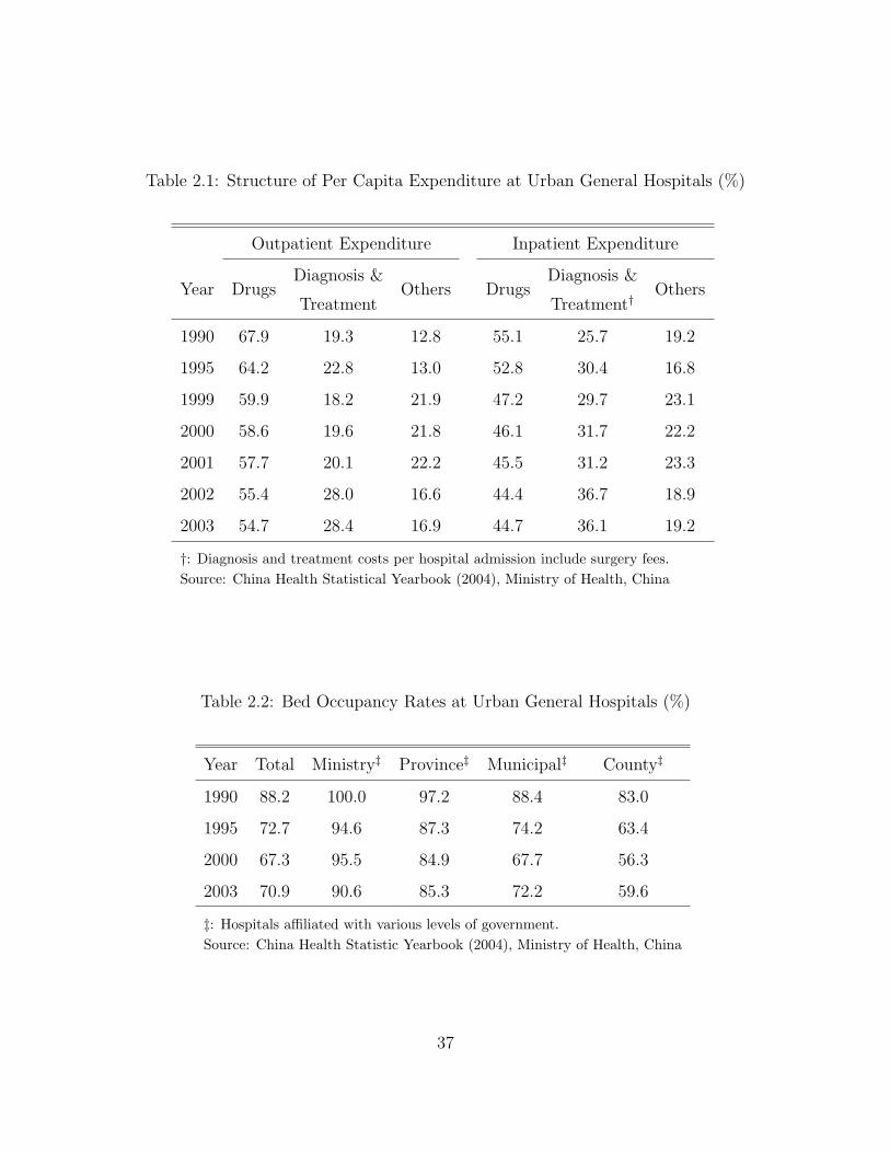
Table 2.1: Structure of Per Capita Expenditure at Urban General Hospitals (%)
Outpatient Expenditure Inpatient Expenditure
Diagnosis & Diagnosis &Year Drugs
TreatmentOthers Drugs
Treatment†Others
1990 67.9 19.3 12.8 55.1 25.7 19.2
1995 64.2 22.8 13.0 52.8 30.4 16.8
1999 59.9 18.2 21.9 47.2 29.7 23.1
2000 58.6 19.6 21.8 46.1 31.7 22.2
2001 57.7 20.1 22.2 45.5 31.2 23.3
2002 55.4 28.0 16.6 44.4 36.7 18.9
2003 54.7 28.4 16.9 44.7 36.1 19.2
†: Diagnosis and treatment costs per hospital admission include surgery fees.Source: China Health Statistical Yearbook (2004), Ministry of Health, China
Table 2.2: Bed Occupancy Rates at Urban General Hospitals (%)
Year Total Ministry‡ Province‡ Municipal‡ County‡
1990 88.2 100.0 97.2 88.4 83.0
1995 72.7 94.6 87.3 74.2 63.4
2000 67.3 95.5 84.9 67.7 56.3
2003 70.9 90.6 85.3 72.2 59.6
‡: Hospitals affiliated with various levels of government.Source: China Health Statistic Yearbook (2004), Ministry of Health, China
37

3.0 HOW DO HIGH-COST PATIENTS FARE UNDER THE GLOBAL
BUDGET POLICY? — EVIDENCE FROM CHINA
3.1 INTRODUCTION
As health care spending has grown rapidly in many parts of the world since the 1970s,
country after country has turned to prospective payment methods as the solutions to cost
inflation. Unlike the cost-based system, prospective payment reimburses providers with a
pre-determined amount for a certain quantity of services. Different definitions of “quantity”
produce various types of prospective payment methods: per diem, where the unit quantity
is an outpatient visit or inpatient day;1 disease-related groups (DRG), where the unit is a
hospital stay with a specific diagnosis;2 capitation, where the unit is an individual patient;3
and global budgeting, where the unit is a geographical region or a health system.
Given the non-contractibility or non-observability of certain aspects of health care quality,
each of the above methods must strike a balance between cost-containment and the quality
of services [Newhouse (1996)[95]]. Indeed, while studies of per diem, DRG and capitation
demonstrate their effectiveness in lowering health care spending, the literature also reveals
their potential to induce providers to shun costly patients or to skimp on their services. If
these risk-selection incentives prevail, cost containment is achieved at the expense of reduced
access to as well as quality of care.
1Examples include Medicare payments to nursing homes and rehabilitation centers.2Medicare adopted the DRG system in 1983 as a payment policy for hospital care. The method has since
spread to the private insurance sector.3For example, some primary-care physicians employed by health maintenance organizations as “gate-
keepers” are paid a fixed amount for each assigned member.
38

In this paper, we analyze these issues in the context of the global budget (GB) system, a
payment method that sees increasing use in China’s urban Basic Medical Insurance (BMI)
programs. Since the late 1990s, many of these regional programs have switched from the
cost-based fee-for-service (FFS) to the global budget policy.
Before its adoption by China, global budgeting has seen many years of popularity in
Taiwan and various OECD countries.4 It attempts to contain the growth of health care
spending by imposing caps on the total expenditure of a certain region.5 Since global bud-
geting directly restricts the overall spending level, most of the current evidence shows that
it is effective in lowering total expenditure [U.S. General Accounting Office (1991)[113]], the
growth rate of health spending [Eggleston & Yip (2001)[33]], health care utilization [Leonard
et al. (2003)[69]] or the use of expensive services [Eggleston & Yip (2004)[34]].
However, much of the literature is either theoretical or descriptive in nature. Rigorous
empirical studies are relatively rare. Therefore, this literature has yet to produce empirical
evidence of a comparable quality and influence to those on other payment methods. In
addition, most of the studies focus on the impact on overall spending, without considering
the consequences for health care quality or variations in the effect on different patient groups.
Our study aims to fill these gaps in the literature by providing rigorous evidence of
the discriminatory effects global budgeting may create for the group of high-cost patients.
Moreover, it examines a particular type of GB method that creates very different provider
incentives from the one most frequently used in OECD countries. Comparing the outcomes of
these variants will produce insights that are of interest to the policy-makers in both systems.
A third contribution of our paper is that it uses data from the city of Zhenjiang,6 whose
BMI administration has been particulary active in reforming the local health care system.7
4Examples of European GB measures include the 1986 and 1993 Health Care Reform Acts in Germanyand the “global envelope” policy introduced in France in 1996. Taiwan started its GB system in July 1998under the National Health Insurance Act.
5For more descriptions of global budget systems, see Wolfe and Moran (1993)[125] and the Journal ofHealth Politics, Policy and Law ’s special issue on European health policies [Journal of Health Politics, Policyand Law, Vol. 30, February-April, 2005].
6Zhenjiang is located in the southwest of Jiangsu Province in southern China, with a population of 660,000as of the end of 2005.
7Zhenjiang was one of the two pilot regions where China started its reform of the urban health insurance
39

Knowledge of its experience thus has substantial value to the other regions of China.
The Zhenjiang Health Insurance Bureau supplied access to its claims database span-
ning the period between 1995 and October 2006. The data set contains observations of the
enrollees’ socio-demographic characteristics, employer identifier, facility identifier and reim-
bursable provider charges for each hospital visit. We define high-cost patients as those whose
annual health expenditure lies above pre-defined percentiles of the cumulative spending dis-
tribution. To identify the discriminatory effects of global budgeting, we take advantage of a
change in the GB policy in 2005 as a natural experiment in a difference-in-differences (DD)
model. To examine patient selection, we use the number of visits a high-cost patient pays to
a provider of last resort (LR) as the outcome variable. Skimping is measured by the changes
in the intensity of treatment before and after the policy shift.
Our results suggest that Zhenjiang’s global budget policy induces non-LR providers to
select against costly patients by pushing them to LR hospitals. To relieve the cost-saving
pressure, they also skimp on the intensity of services delivered to these patients. However,
LR providers do not appear to engage in similar behavior. Therefore, the non-LR providers
achieve at least part of the risk selection through making the level of their services inadequate
for high-cost patients.
The rest of the chapter is organized as follows. Section 3.2 reviews three strands of
literature: patient selection and skimping, global budgeting, and the payment reforms in
China. Section 3.3 analyzes the discriminatory incentive the global budget policy creates
after introducing the history of provider payment reforms in Zhenjiang. Section 3.4 describes
the data used in the study. Sections 3.5 and 3.6 present the estimation strategies and the
results of the DD model, respectively. Finally, Section 3.7 suggests areas for future research.
system in 1995. Since then, it has taken a series of initiatives on both demand and supply-side measures.For instance, see Liu et al. (2003)[75] and Lin et al. (2004)[73].
40

3.2 LITERATURE REVIEW
3.2.1 Patient Selection and Skimping on Services
Most studies on selection and skimping are built on the theoretical insights of Newhouse
(1996)[95] and Ellis (1998)[38]. In his paper, Newhouse argued that the tradeoff between
selection and production efficiency is inherent in any provider payment method. Ellis’s paper
developed an integrated model that predicted all three discriminatory behaviors: creaming,
the over-provision of services to low severity patients; skimping, the under-provision of ser-
vices to high severity patients; and selection, the explicit avoidance of high-severity patients.
It showed that, in equilibrium, prospectively paid providers cream low severity patients and
skimp on high severity ones. In addition, if there is dumping, there will also be skimping.
Both Newhouse and Ellis proved that competition may exacerbate the discriminatory effects
of prospective payment.
Most of the empirical literature on selection8 concerns health maintenance organizations
and other managed care plans [Hill & Brown (1990)[58], Morgan et al. (1997)[90], Hamil-
ton (2002)[51] and Polsky & Nicholson (2004)[101]]. Selection at the hospital level is less
well studied. An early paper is Newhouse (1989)[94] where the author demonstrated that
Medicare’s prospective payment system (PPS) increased the likelihood for patients in un-
profitable DRGs to end up at “hospitals of last resort.” A more recent study by Paddock
et al. (2007)[97], however, found no evidence of patient selection. Examining the impact of
case-based payments9 on the severity level and resource use at Medicare inpatient rehabil-
itation facilities, they found no significant change in the patient mix before and after the
PPS implementation.
Among the empirical studies on skimping, Ellis and McGuire (1996)[40] showed that
8There is another strand of research that aims to develop “risk adjustments” in insurance premiums inorder to minimize selection. For a sample of this literature, both theoretical and empirical, see Ash et al.(1989)[6], Newhouse et al. (1993)[96], Brown et al. (1993)[11], Eggleston (2000)[32] & Barros (2003)[7].
9The payment method Paddock and colleagues examined is called Case Mix Groups (CMG). Similar toDRGs, CMGs classify hospital stays into groups according to the patients’ age, impairment, functional statusand comorbidities.
41

the Medicaid DRG policy for mental health services in New Hampshire resulted in skimp-
ing on services for the sickest patients. Using discharge and financial data from California,
Meltzer et al. (2002)[82] also found that the combined force of competition and DRG pay-
ments selectively reduced spending on the most expensive patients. These findings confirmed
the theoretical predictions of Ellis (1998)[38]; i.e., supply-side cost-saving measures induce
skimping on services to costly patients.
3.2.2 Global Budgeting
Most of the literature on global budget is based on the European experience. Poterba
(1994)[102] expressed skeptical views on the ability of the global budget system to slow the
growth of health spending, while van de Ven (1995)[117] questioned its efficiency as a tool of
price regulation. Nonetheless, there are many studies that show the effectiveness of global
budgeting in cost control. For instance, Ulrich and Wille (1996)[112] found that the global
budget system Germany introduced in 1993 had a strong and long-lasting cost-containment
effect. Leonard et al. (2003)[69] showed that, relative to the case-based payment system,
global budgeting was associated with a lower spending level and shorter lengths of stay.
A study by Fan et al. (1998)[41] was the first to distinguish between two types of com-
pensation methods within the global budget system: the “expenditure target” and the “ex-
penditure cap.” Under an expenditure target, a fixed spending quota is allocated to each
provider. Expenditures below the quota are reimbursed in full. If the quota is exceeded, the
unit amount of reimbursement for each service will be lowered. In the most rigid form, the
unit price is reduced to 0. For smaller fee reductions, there is a partial degree of risk sharing
between the insurer and the provider.
The expenditure cap method attaches points to each type of service. At the end of the
settlement period, the regional budget is divided by the total number of points summed over
all providers so as to determine the unit price of each service. A hospital’s revenue is the
product of its service points and the unit price of the region.
The target and the cap policies produce very different provider incentives. While the
42

revenue under expenditure targets depends only on a provider’s own volume of services,
the expenditure cap relates income to the decisions of the other providers. In their lab
experiments, Fan et al. (1998)[41] found that, for the same level of spending, the cap policy
leads to a larger quantity of services than the expenditure target.
Mougeot and Naegelen (2005)[92] examined the impact of the expenditure cap policy
on the quality of care. Using a model of Cournot competition, they showed that, when the
number of providers is large, the optimal cap policy may implement the second-best outcome,
but cannot implement the first-best outcome. For the same level of expenses, the cap policy
always involves a lower level of quality. It increases hospital utility, while decreasing patient
utility. The level of social welfare is therefore lower than under the first-best outcome.
In a separate study, Hsueh et al. (2004)[61] examined the effects of a switch from FFS
to expenditure caps in Taiwan’s dental care system.10 They found that the switch reduced
dental care utilization. In addition, global budgeting did not improve the geographical
distribution of dental supply in Taiwan.
Since the definition of the “expenditure target” best fits the characteristics of the pay-
ment method used in Zhenjiang, we will borrow this concept from Fan et al. and use it
interchangeably with the term “global budget” in the rest of the paper.
3.2.3 Provider Payment Reforms in China
There are a small number of studies on the payment reforms in China. Using data from
Hainan Province, Eggleston and Yip (2001[33], 2004[34]) found that a shift from FFS to a
monthly global budget reduced the average expenditure per admission. It also slowed the
growth of spending on expensive diagnostic services. Meng et al. (2004)[86] reported on a
comparison between two cities, one with a set of health system reforms, including changes
in the provider payment method, and the other without. They found a smaller cost increase
in the reform city, without any measurable impact on quality. However, it was impossible to
10Their paper used the term “global budgeting” and did not distinguish between expenditure caps andtargets.
43
separate the effects of the payment reform from those of the other policy changes that took
place simultaneously.
3.3 ZHENJIANG’S PROVIDER PAYMENT REFORMS
3.3.1 Reform Chronology
As an experiment of national health insurance reforms, the Zhenjiang BMI program was
formed in 1995 by merging two existing insurance systems that covered employees of govern-
ment institutions and state-owned enterprises. Since the inception, its coverage has gradually
expanded to the population of all city residents with stable employment.11 As a result, the
number of beneficiaries almost doubled from 260 thousand in 1996 to 492 thousand in Oc-
tober 2006, the latest month for which data is available. As the program expands, there has
been a distinctive trend of aging. The share of individuals under 35 years old declined from
34.9% in 1997 to 24.4% in 2006, while that of those above 65 increased from just under 8%
to 14.6%. Aging is therefore an important policy concern for local health authorities.
Financed by employee and employer premium contributions, the program provides manda-
tory coverage under a single, citywide system. It combines individual medical savings ac-
counts (MSA) with a social pooling fund (SPF). MSAs serve as the first tier of payment.
When funds in the patient’s MSA are depleted, reimbursements from the SPF become avail-
able. The benefits package is identical across economic sectors or employers, to the exception
of two groups of enrollees: civil servants and individuals who have received official valedic-
tion as “model workers.” Coverage for the latter two groups is more generous than for the
general population.
Since 1995, the program has undergone a series of major changes. For the purposes of
this paper, we discuss only those in the provider payment method.
11As is typical with most employee BMI programs in China, migrants without official residential permitare not covered.
44

1. 1995 - 1996
This was the pre-global budgeting period. As part of the reform initiative, the insurance
administration switched its provider payment method from FFS to per diem reimbursement.
Under this system, the insurer paid each provider a fixed amount per outpatient visit or
inpatient day. The total annual payment to the provider was thus the product of the number
of visits/days and the unit amount. Although an improvement over FFS, the per diem
method still leaves considerable room for providers to increase the supply of services. Soon
after the policy took effect, hospitals in Zhenjiang learned to “beat the system” by inflating
the number of visits/admissions. As a counter-measure, the administration changed the
payment method to a rigid expenditure target in 1997.
2. 1997 - 1998
As discussed above, the expenditure target is a type of GB measure that divides the
city-wide budget into fixed expenditure targets for each contracted provider. The regional
budget is determined at the beginning of the period and is set to be equal to the expected
premium contributions of the same year. For any provider, the target applies to all the
services it delivers to BMI enrollees within a year.12 This implies that the global budget
policy covers the entire spectrum of medical conditions treated at any facility.
The 1997/98 method adopted the most rigid form of expenditure target by providing no
risk-sharing for any spending overruns by the provider. In the two years of its existence, this
measure put a sharp brake in the growth of health care expenditure in the region [Lin et al.
(2004)[73]].
3. 1999 - 2000
In 1999, as a result of mounting complaints from the local providers of heavy cost-saving
pressure, the insurance bureau narrowed the scope of the expenditure target to the expenses
12By contrast, the GB systems of Taiwan, Canada, Germany and France are specific to different sectorsof the health care delivery system. The “global” application of the GB method is partially attributable tothe comprehensive nature of providers in urban China, where general hospitals offer a wide range of services,including those usually associated with specialty hospitals, such as dental, ophthalmological and Ob/Gynservices.
45

reimbursed by the SPF account. The restriction on payments made from the MSAs was
hence removed.
4. 2001 - 2004
In 2001, the insurance bureau introduced two policy changes: abolishing the payment
separation of the 1999/2000 system and incorporating cost-sharing measures into the expen-
diture target policy. While the 1997/98 system allowed for no spending overruns, the new
method reimburses expenditures that exceed the spending target on a capitation basis. In
particular, if the number of patients treated by a provider is greater than the average patient
load of the previous three years at facilities of the same specialty and administrative level,
a fixed payment is made to the provider for each additional patient treated. The payment
differs by inpatient and outpatient services. For each service category, it is equal to the
average three-year per capita expenditure at comparable facilities.
5. 2005
In recognition of the health needs of an aging population, the insurance bureau amended
the payment policy in July 2005 with a clause that exempted patients with chronic diseases
from the expenditure target of each hospital. Expenses on the treatment of a defined group
of chronic conditions are fully reimbursed.
3.3.2 Economics of Patient Selection and Skimping
As discussed above, the expenditure cap policy results in higher levels of services than the
expenditure target. However, both methods create incentives to discriminate against high-
cost patients. To see this, note that, under an expenditure cap, the unit price depends only
on the quantity, rather than the intensity of resource use, of each service. Therefore, it is a
best response for a provider to lower the unit cost of care by either avoiding high-cost patients
or lowering the intensity of their treatment. The degree of discrimination is restricted by
the possibility of decreasing quantity if the high-cost patients turn to the other providers.
46

In the case of expenditure targets, the provider faces a non-linear price structure: p below
the spending quota; and (1−α)p above the quota, where p indicates the price and α ∈ [0, 1]
is the degree of provider cost-absorption. Therefore, whether the provider discriminates
against costly patients depends on the size of the target. If the target is large enough to
cover the normal patient load, the provider has little incentive to discriminate. In fact, a
generous target is not much different from the FFS payment method. It will encourage the
provider to increase the intensity of services for all patients. If, on the other hand, the target
is strictly binding, the reduced price will induce the provider to lower the unit cost of services.
A natural response will thus be to shun high-cost patients or to skimp on their treatment.
The degree of discrimination decreases with the level of risk sharing. It is strongest when
the provider bears the entire risk of budgetary overruns.
In Zhenjiang’s BMI program, whose global budget policy takes the form of expenditure
targets, the degree of discrimination evolves along with the payment reforms. In particu-
lar, we hypothesize that the 1999 policy change relaxed the discriminatory incentive of the
1997/98 expenditure target for patients with high MSA expenditures. Furthermore, by re-
moving the payment separation while introducing cost sharing measures, the 2001 reform
had offsetting impacts on provider behavior. The reimbursement for additional patient loads
mitigated the discriminatory effect created by the expansion of global budgeting to MSA ac-
counts. Finally, the 2005 amendment weakened the incentive to select against or skimp on
patients with chronic diseases.
3.4 DATA
We use claims data obtained from the Zhenjiang Health Insurance Bureau. The data set
spans the period between 1995 and October 2006. It covers all reimbursable transactions,
including outpatient visits, inpatient stays and pharmaceutical purchases, at every contracted
health care facility. There are four types of facilities in the data: general/specialty hospitals,
47

community health centers, clinics, and pharmacies. For each transaction, the data set records
the patient’s age, gender, employment, annual wage income, professional distinctions, type of
policy held, time of enrolment and reimbursable provider charges by service category. Using
the provider ID number in the claims data, we are also able to extract information about a
hospital’s location, administrative level and type of contract with the insurer.13
In the following analysis, we will use only data on outpatient services. Since the occur-
rences of hospitalizations are rare, the observations on inpatient care may not form a panel
data structure necessary for the difference-in-differences analysis. Second, we exclude cases
treated at community health centers since their reimbursement falls under the purview of
a parallel insurance program that uses capitation rather than global budgeting payment.
Drug purchases at pharmacies are also excluded, as the degree of risk selection is minimum
at these facilities. Finally, we screen out new enrollees that joined the BMI program in the
year of analysis, in order to remove the impact of acquiring insurance on the demand for
health services.
The main limitations of the Zhenjiang data are its lack of patient health/severity level
and diagnosis information. To the extent that unobserved health or severity level remains
fixed over time, the DD model is designed to remove its effect. The latter is a more serious
problem. For any outpatient visit or hospitalization, we do not know the condition that
was being treated. However, we argue that this limitation does not invalidate our analysis.
Unlike the DRG system, the global budget policy imposes cost-control incentives across the
entire spectrum of diseases, instead of at the level of specific conditions. Therefore, the
providers should respond to high-cost patients in much the same manner, regardless of the
particular condition. That being said, nonetheless, there remains a methodological concern
with respect to the potential impact of the disease on a patient’s elasticity of demand for
health care. We will discuss this issue in greater detail in the concluding section.
Apart from the claims data, we obtained statistics of occupancy rates and the share of
13Keeping this basic structure intact, the bureau upgraded its database twice, in 1999 and in 2004, increas-ing the amount of information reported. For instance, the latest database contains more detailed informationon the structure of individual copayments than the earlier versions.
48

the BMI reimbursement in the hospitals’ total revenue from Zhenjiang’s Health Bureau.
3.5 ESTIMATION STRATEGIES
The payment policy reforms described in Section 3.3.1 provide the potential objects of anal-
ysis for the DD model. However, it is difficult to study the pre-2001 reforms, since before
2001, Zhenjiang’s insurance system was characterized by rapid successions of policy changes.
Each new payment method was introduced concurrently with demand-side measures or pric-
ing policy changes. The year of 2001 marked the stabilization of the system. Since then, the
only major policy shifts are the changes to the global budget policy: the 2001 refinement of
the expenditure target and the 2005 amendment exempting chronic conditions.
A problem with the 2001 refinement is that it affected all hospitals and patients so that
we cannot identify cases to be used as controls in the DD analysis. Take patients as an
example. As the policy change expanded global budgeting from SPF to MSA accounts,
hospitals may have the incentive to attract less expensive outpatient cases, since doing so
would increase its reimbursement level by raising the head count. This positive selection
could occur independently of the dumping of high cost patients. Using the less expensive
patients as controls would confound the two types of selection behavior. Second, if we use
hospitals as the unit of analysis, our strategy of measuring selection with the number of
visits to last-resort providers would leave no hospital in the control group.
Compared with the 2001 policy, the 2005 amendment provides a cleaner source of iden-
tifying variation. Since it is a physiological fact that old people are more likely to suffer
from chronic diseases than the general population, it is conceivable that the policy change
affected the elderly population more substantially. Therefore, age can be used to define the
treatment and the control groups. The effects of the 2005 amendment are thus obtained by
comparing the before-after changes in the outcome variables across different age groups.
49

3.5.1 Definitions of Key Concepts
3.5.1.1 Selection To examine selection, we look at the number of visits a high-cost
patient pays to a “provider of last resort.” In interviews with Zhenjiang health authorities,
it became evident that low-level facilities often pushed costly patients “upward” to higher-
level providers, on the excuse that the latter were better equipped or skilled to treat their
illnesses. Therefore, we define tertiary hospitals, which are the highest-level providers in
urban China, as “providers of last resort.” In Zhenjiang, only 2 out 267 health care facilities
are tertiary hospitals.
3.5.1.2 Skimping We follow the literature in defining skimping as the under-provision
of services to high severity patients. We hypothesize that, apart from pushing costly patients
away, a hospital may also respond to cost-saving pressure by reducing how much a high-cost
patient spends on each visit. Therefore, the outcome variable in this analysis is the intensity
of service use, measured by the average expenditure on an outpatient visit to any non-last
resort hospitals.
3.5.1.3 Costliness of Patients We use a patient’s percentile in the cumulative distri-
bution of annual outpatient expenditure as a proxy for his costliness. It then follows that
high-cost patients are those that lie above certain levels of the spending distribution. In our
analysis, we use the 90th percentile as a threshold.
Due to data limitations, we cannot measure costliness within specific disease groups.
Although, as argued above, this is not a major issue in the context of global budget systems,
the lack of patient health information presents other methodological problems.
Since health affects health care spending, a patient’s costliness, which is defined on the
spending distribution, is also correlated with health. Any change in the patient’s health level
will affect both the degree of costliness and health care utilization. This will create a spurious
policy effect.14 Another concern is that, expansions of the program and the trend of aging
14Although this is a lesser problem if the costliness indicator is used only to determine whether an obser-
50

among enrollees may shift the cumulative distribution function of outpatient expenditure.
As a result, a patient’s cost percentile may change even without changes in his health level.
To address both problems, we use only the cost percentile of the pre-policy period. This
time-invariant, baseline measure is not affected by future changes in either the payment
policy or the patient health/severity level. Therefore, the costliness variable represents the
degree of cost-saving pressure specific to each patient before the 2005 amendment took effect.
3.5.2 Model Specification
Our objective is to estimate the average effects of the 2005 policy on (i) the number of
visits by high-cost patients to last-resort (LR) providers; and (ii) the per visit expenditure
at non-LR hospitals by the same patients. In a DD model, the parameter of interest is:
4 = E(y1t − y1t′|X,D = 1)− E(y0t − y0t′|X,D = 0), (3.1)
where E(·) is the expectation operator; y1t is the outcome for patients in the treatment group
at time t, while y0t is the outcome for the control group in the same period; t′ and t refer to
the pre- and post-policy period, respectively. D is a binary indicator that equals 1 for the
treatment group and 0 otherwise.
In our estimation, we define the values of D as follows. It indicates the treatment group
if a patient is above the age of 65 and his annual outpatient spending is greater than the
90th percentile of the cumulative spending distribution. It indicates the control group if a
patient is younger than 65, but also lies above the 90th percentile of the cost distribution.
In other words, we obtain our comparison groups from the population of high-cost patients.
The identification relies on the varying impact of the 2005 policy upon different age groups
within the same population.
One concern with this identification strategy is that individuals aged between 55 and 65
may be a contaminated control group. This could happen because this group of patients may
vation is included in the estimation. Technically, it reduces sample size of the DD estimation.
51
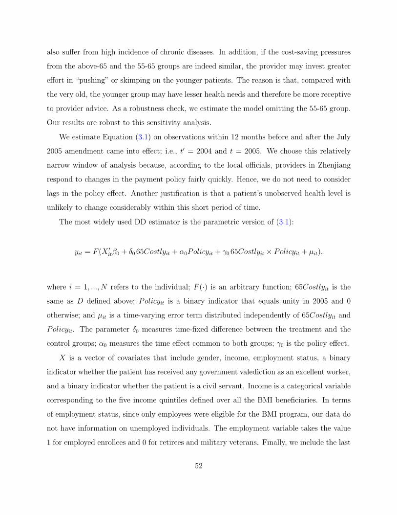
also suffer from high incidence of chronic diseases. In addition, if the cost-saving pressures
from the above-65 and the 55-65 groups are indeed similar, the provider may invest greater
effort in “pushing” or skimping on the younger patients. The reason is that, compared with
the very old, the younger group may have lesser health needs and therefore be more receptive
to provider advice. As a robustness check, we estimate the model omitting the 55-65 group.
Our results are robust to this sensitivity analysis.
We estimate Equation (3.1) on observations within 12 months before and after the July
2005 amendment came into effect; i.e., t′ = 2004 and t = 2005. We choose this relatively
narrow window of analysis because, according to the local officials, providers in Zhenjiang
respond to changes in the payment policy fairly quickly. Hence, we do not need to consider
lags in the policy effect. Another justification is that a patient’s unobserved health level is
unlikely to change considerably within this short period of time.
The most widely used DD estimator is the parametric version of (3.1):
yit = F (X ′itβ0 + δ0 65Costlyit + α0Policyit + γ0 65Costlyit × Policyit + µit),
where i = 1, ..., N refers to the individual; F (·) is an arbitrary function; 65Costlyit is the
same as D defined above; Policyit is a binary indicator that equals unity in 2005 and 0
otherwise; and µit is a time-varying error term distributed independently of 65Costlyit and
Policyit. The parameter δ0 measures time-fixed difference between the treatment and the
control groups; α0 measures the time effect common to both groups; γ0 is the policy effect.
X is a vector of covariates that include gender, income, employment status, a binary
indicator whether the patient has received any government valediction as an excellent worker,
and a binary indicator whether the patient is a civil servant. Income is a categorical variable
corresponding to the five income quintiles defined over all the BMI beneficiaries. In terms
of employment status, since only employees were eligible for the BMI program, our data do
not have information on unemployed individuals. The employment variable takes the value
1 for employed enrollees and 0 for retirees and military veterans. Finally, we include the last
52
two variables in recognition that official valediction or government employment may entail
health benefits in addition to the standard BMI package. These variables are thus used as
proxies for the level of insurance coverage.
Examination of the data shows that all of the covariates in X have constant values over
time. This suggests that the economy of Zhenjiang may still have much of the planned-era
legacy, where the degree of social mobility is low. In the estimation, we take the before-after
difference of the outcome and regress it on the set of control and policy variables. In the
case of patient selection, the model becomes:
4V isitsi = F (α1 + X ′iβ1 + γ165Costlyi + εi), (3.2)
where 4V isitsi is the before-after change in visits to LR hospitals for patient i.
The intercept, α1, identifies the common time trend in the number of visits to LR-
providers. The coefficient γ1 measures the effect of the policy change. Recall that the
2005 amendment softens the providers’ incentive to avoid patients with chronic conditions.
Hence, we expect γ1 to be negative. Because the covariates in X are time-invariant, the fixed
difference between the treatment and control groups is not identified. Finally, since there
are only two time periods, the problem that DD models underestimate the standard errors
if the outcome variable is serially correlated15 is not a concern for our estimation.
We model skimping in a similar framework. Since per-visit expenditure is a continuous
variable, we estimate a linear model:
4ln(Intensityi) = α2 + X ′iβ2 + γ265Costlyi + υi, (3.3)
where 4ln(Intensityi) is the before-after change in logged average spending per visit to
non-LR hospitals. The parameters α2 and γ2 measure the time trend and the policy effect
15See Bertrand et al. (2004)[8].
53
on service intensity, respectively. If the hospitals did engage in skimping, the softening of
this incentive following the amendment implies that γ2 is positive.
Finally, we validate the DD identification strategy by estimating Equations (3.2) and
(3.3) on a placebo law generated between 2002 and 2004. To do so, we first draw a random
number from the uniform distribution between 1 and 12. These numbers correspond to the
months of the year 2003.16 Then we use the selected number as the point of time when the
placebo policy took effect. The DD model is estimated on data within twelve months before
and after the fictitious policy. If we found a significant policy effect in this exercise, it would
imply that heterogeneous trends between the treatment and the control groups had existed
before the 2005 amendment. Any of the impact we obtained earlier would thus be spurious.
3.5.3 Estimation
Equation (3.2) is a count data model. The literature suggests several methods for its estima-
tion. First, under assumptions on the functional form of F (·), the model can be estimated
parametrically. The two most commonly used models are Poisson and negative binomial
(NB). Compared with Poisson, the NB model allows for greater dispersion in the data.
An alternative is nonparametric estimation with matching methods. For each (y1|X, D =
1), matching constructs its counterfactual, (y1|X, D = 0), from observations in the control
group. Then the policy effect can be estimated as the change in E[(y1|X, D = 1)−(y1|X, D =
0)] before and after the policy was adopted. This is the generalized DD matching estima-
tor developed by Heckment et al. (1998)[56]. In this paper, we use propensity score (PS)
matching estimator with kernel weighting.
In the first step, we estimate a probit model to obtain the propensity scores, the condi-
tional probabilities that a high-cost patient falls in the treatment group given the values of
X. Then we construct a common support of the predicted propensity scores for the treat-
ment and the control groups.17 Cases that fall into the common support constitute the set
16We limit the placebo policy change within 2003 to ensure that enough numbers of months exist bothbefore and after the policy for the validation analysis.
17In particular, we excluded cases in the control group whose propensity score is smaller than that at the
54

of matched observations.
On the common support, we compute the counterfactual (y1|X, D = 0) as follows. Let
ST = (1, 2, ..., NT ) and SC = (1, 2, ..., NC) be the set of treatment and control observations
over the common support, respectively. Then for any i ∈ ST , we have:
yi1|D = 0 =
NC∑j=1
ω(i, j)× (yi0|D = 0),
where
ω(i, j) =K[P (xi)− P (xj)]∑NC
j=1 K[P (xi)− P (xj)], j = 1, ..., NC
and P (x) is the estimated propensity score; K(·) is the kernel function given by the standard
normal density function.
For each i, the matching estimator is defined by:
4V isitsi = [(V isitsi1t|D = 1)−( V isitsi1t|D = 0)]− [(V isitsi1t′|D = 1)−( V isitsi1t′|D = 0)].
We estimate the average policy effect as the sample average of 4V isitsi over all patients
in the treatment group. The standard errors are estimated by bootstrap.
The matching estimator has several advantages over the parametric estimates. First, it
abstracts away from any arbitrary assumption about the data generating process. Second, it
eliminates the bias in a simple DD estimation of Equation (3.2) which arises if some cases in
the treatment and the control groups are incomparable to each other. PS matching removes
this bias by comparing cases that lie in the common support of their propensity score.
Third, matching also addresses the bias from different distributions of X between treatment
first percentile of the distribution of the treatment propensity scores. On the other end, we trim cases in thetreatment group whose propensity score is greater than that at the 99th percentile of the distribution of thecontrol propensity scores.
55
and control groups by weighting the control observations. Given these advantages, we will
estimate Equation (3.2) using all the three methods (i.e., Poisson, NB and PS matching with
kernel weighting) and compare their results.
In the analysis of skimping, notice that, since all the covariates in X are categorical
variables, Equation (3.3) is a fully saturated model. Thus we do not impose strong distribu-
tional assumptions by estimating it with OLS. To reduce the biases arising from potential
incomparability between the treatment and the control groups, we conduct the estimation
within the common support of the propensity scores.
3.6 RESULTS
Table 3.1 shows the unadjusted difference-in-differences estimate of the policy effect on pa-
tient selection. Compared with younger patients, old patients with chronic conditions re-
duced their visits to LR hospitals by 3.42 on average following the 2005 amendment. Table
3.2 presents the sample means and standard deviations of the covariates by treatment status.
It is clear that elderly and non-elderly high-cost patients differ quiet significantly in their
socio-demographic characteristics. In particular, the treatment group has more women, a
larger proportion of the wealthiest members of society, more recipients of official valediction
and more civil servants. This indicates that the treated group has a higher socio-economic
status on average than the control. It is likely that many of its members are retired gov-
ernment or party officials (the so-called “cadres”) who enjoy generous insurance benefits.
Their large expenditure is thus driven mostly by a high demand for health care services.
Overall, the between group differences in all the covariates, except for employment status,
are statistically significant at the 1% level.
We present the results of parametric estimation of Equation (3.2) in Table 3.3. Although
there are differences in the magnitudes of the coefficient estimates, the Poisson and the
negative binomial models reveal similar pictures. In particular, there is a striking trend of
56
decreasing utilization of tertiary-level hospitals. The time trend parameter is both large
and statistically significant. This may reflect the effects of the cost-containment measures
Zhenjiang’s BMI program had adopted by the year 2005. Another explanation is that the
local hospital market became more competitive over the years, with lower-level facilities
competing for patients increasingly aggressively.
The most important result is that the coefficient associated with the treatment indicator
is statistically significant. This indicates that elderly high-cost patients paid fewer visits to
last-resort providers relative to the younger patients following the 2005 amendment. We
infer that the policy change did soften the selection incentive created by the expenditure
target method. While they used to have to visit a tertiary hospital for basic treatment,
patients with chronic diseases were able to seek care from a nearby, lower-cost provider after
July 2005. This is a welfare-improving outcome. The patients could not only pay less, but,
since there is a considerably larger number of low-level facilities than tertiary hospitals, also
have easier access to constant sources of medical care.
In the other results, the policy change led women to reduce their visits to last resort
providers relative to men. Use of tertiary-level hospitals also declined for the employed
relative to the retired and army veterans. By contrast, the effects of income, valediction and
government employment do not change over time. A likelihood ratio test rejects the null of
Poisson distribution.
In Table 3.4, the magnitudes of the policy effect on adverse selection estimated from
various empirical models are shown side by side. The results of the Poisson and the negative
binomial models are not obtained directly from the coefficient estimates. Instead, they
are computed as relative changes in the predicted number of visits with and without the
policy change. All the standard errors are obtained with bootstrap. The mean differences
computed directly from the data is -3.42. The magnitude of the estimated policy effect falls
considerably to 2.98 in the Poisson model and further to 2.56 in negative binomial. Finally,
the generalized DD-matching estimate18 is 2.83 and significant at the 5% level. The policy
18Results of the probit propensity score regression are available from the author upon request.
57

change reduced the average number of visits to last-resort hospitals by 2.83 above and beyond
the time trend and the time-fixed between-group difference. The average number of visits
for the treatment group prior to the amendment was 22.76. Therefore, the policy change
produced a 12.43% fall in the number of visits to LR providers.
The results of the analysis of skimping behavior are presented in Table 3.5. We estimated
the model at both last-resort and non-last resort providers. The rationale is that, while it is
relatively difficult for tertiary hospitals to find excuses to turn patients away, they can relieve
the cost-saving pressure of global budgeting by reducing the intensity of services provided
to costly patients. As the spending cap was removed, hospitals would have the incentive to
increase the level of care to compete for patients with chronic conditions.
Interestingly, this does not seem to be the case. The coefficient associated with the
treatment variable is significant for the non-last resort estimation. This result implies that,
following the 2005 amendment, non-LR providers increased the average service intensity for
elderly high-cost patients by 10%.19 The coefficient for last resort providers, on the other
hand, is small and statistically insignificant. To put it differently, the exemption from global
budgeting restrictions led low-level facilities to provide more intensive care for elderly high-
cost patients. The behavior of tertiary hospitals, however, did not change significantly from
the pre-policy level. This suggests that last resort providers may have engaged in a minimum
level of service skimping prior to July 2005.
The differential policy effect on skimping has substantial implications for the selection
behavior discussed earlier. One can imagine that, as low-level facilities reduced the intensity
of their services without corresponding cutbacks in tertiary hospitals, patients, especially
those with greater health needs, would visit the latter more frequently. Therefore, at least
part of the selection was achieved by making medical services inadequate for patients with
great health needs. The literature has documented this indirect selection among health
maintenance organizations in the US. It appears that the same strategy was being used by
19The average per-visit expenditure of the treatment group prior to the policy change was RMB912. A10% increase would imply an additional spending of RMB91, equivalent to USD11 per the exchange ratebetween RMB and US dollars as of December 31, 2004.
58

hospitals in China.
Finally, Table 3.6 presents the results of the validation exercise for the DD model. They
indicate that the effects of the placebo policy on either patient selection or skimping are not
statistically different from 0. The lack of “effect” before the 2005 amendment validates the
difference-in-differences identification strategy.
3.7 DISCUSSION
This paper studies the incentive global budgeting policies create for providers to select against
costly patients and to skimp on their services. It finds strong evidence of adverse selection.
To relieve the cost-saving pressure, non last-resort hospitals also skimp on the intensity of
services to high-cost patients. However, last-resort providers do not appear to engage in
similar behavior. Therefore, at least part of the risk selection is achieved by making the
services inadequate to high-severity patients.
Our results confirm the insight of Newhouse (1996)[95] that all provider payment methods
must address the trade-off between the goals of cost control and maintaining an adequate
level of accessibility and quality of care. Our study showed that global budgeting made
it difficult for high-cost patients with chronic diseases to seek care from low-level facilities
and, among those who remained at these hospitals, their intensity of treatment decreased.
The problem was aggravated by the directionality of the patient transfer from lower-level to
tertiary hospitals. This not only reduced the patients’ access to a stable source of regular
care, but also increased their medical spending. In other words, they had to pay more
for an inappropriate style of treatment. Therefore, the type of global budgeting that is
indiscriminate with respect to the disease/condition is particularly unfavorable for patients
with special medical needs.
Recognition of these negative welfare consequences was clearly the motivation for the
59
2005 amendment. While it indicates a more nuanced approach to supplier cost-sharing
measures, this policy response begets a series of interesting questions. In the most general
terms, how does global budgeting affect high-cost patients suffering from other diseases.
Furthermore, if adverse selection and skimping is thought to be harmful in most cases, how
can the insurer design a global budget system that is more amenable to the particularities of
different medical conditions. Second, although the 2005 policy change may have improved
the quality and accessibility of care for the chronically ill, it may have compromised the
objective of cost control. Both low and high-level hospitals may have the incentive to increase
their spending on chronical conditions. It is therefore important to examine changes in the
total expenditure by high-cost chronic patients. Third, the Zhenjiang BMI program has
experimented with various types of global budget payment, each with a distinctive degree
of supplier cost-saving pressure. It will be of substantial policy value to investigate the
provider responses to these different policies so as to determine the optimal policy measure
for containing the selection and skimping behavior.
There are several caveats to our analysis. First, the lack of diagnostic information may
undermine our results. If patients with different medical conditions have distinct elasticity
of demand for health care, they may respond to hospitals’ selection or skimping behavior in
different ways. In particular, the above- and below-65 groups might have different trends
in health care utilization without the policy change because older and younger patients
suffered from different diseases. It is therefore important that data sets with richer diagnosis
information be obtained so as to estimate the policy effects for specific disease categories.
Second, we study a policy change that relaxed the cost-saving incentives for providers. The
validity of this approach is based on the assumption that providers responds to positive and
negative incentives in the same way. However, this may not hold. The literature on incentives
has shown that individuals do no consider positive and negative incentives as flip sides of
each other. Third, since the claims data only have information on reimbursable services, we
are not able to detect cost shifting to uncovered services. If cost shifting exists, the observed
reduction in the reimbursed expenditure does not necessarily imply a lower quality of care
60

for high-cost patients. This may lead to an overestimate of the true magnitude of skimping.
These discussions suggest several areas for future research. First, by running the estima-
tion on data with information on all the services provided and by examining total expenditure
as well as spending on various service categories, we can make an accurate assessment of the
full use of health resources by high-cost patients.20
Second, we can extend our study by directly comparing the different variants of global
budgeting the Zhenjiang BMI program has implemented. Although data for the pre-2004
period are available, the rapid policy shifts that characterized these years make it difficult to
have a clean analysis of any specific reform measures. A promising alternative is to extend
the analysis to other insurance programs, such as the system of Shanghai, that use only
the rigid spending target, and make inter-city comparisons. Doing so will not only afford
a full view of the welfare implications of different compensation schemes, but also produce
valuable evidence on how provider behavior changes in response to fine variations in the
payment policy.
20Another probable explanation for the pattern of differential spending could be that an exogenous changein medical technology or practice style selectively reduced spending on the high-cost patients. However, Iconcluded from my discussions with local health officials, administrators of the insurance fund and hospi-tal managers that the hospitals reacted most strongly to changes in the payment policy, not to externaltechnological trends.
61

Table 3.1: Number of Visits to Last-Resort Hospitals by Age Group
2004 2005
Patients younger than 65 18.89 16.78
Difference 2005 – 2004 (4V isits young05−04) -2.11
Patients aged 65 or above 22.76 17.23
Difference 2005 – 2004 (4V isits old05−04) -5.53
Difference-in-Differences (4V isits old05−04 −4V isits young
05−04) -3.42
Table 3.2: Descriptive Statistics of Covariates in the DD Estimation
Variable 65 or Above Below 65 t-statistic
Gender 0.58 (0.49) 0.49 (0.002) -4.62
Employed 0.68 (0.46) 0.68 (0.47) -1.74
Income
Highest 20% 0.26 (0.42) 0.15 (0.36) 21.66
2nd Highest 20% 0.13 (0.34) 0.21 (0.41) 18.75
Mid 20% 0.09 (0.30) 0.21 (0.41) 29.89
2nd Lowest 20% 0.09 (0.29) 0.17 (0.38) 21.32
Recipient of Valediction 0.62 (0.49) 0.004 (0.06) -1.9e+02
Civil Servant 0.09 (0.29) 0.08 (0.27) -2.98
N 8532 38748
62

Table 3.3: Parametric Estimation of the Patient Selection Model
Poisson Negative Binomial
Policy Variables
Time Trend -1.20 (0.09) -1.01 (0.19)
65Costly -0.30 (0.11) -0.47 (0.23)
Covariates
Gender -0.41 (0.02) -0.06 (0.02)
Employed -0.13 (0.03) -0.13 (0.02)
Income
Highest 20% 0.03 (0.03) 0.05 (0.03)
2nd Highest 20% 0.04 (0.03) 0.07 (0.03)
Mid 20% 0.02 (0.03) 0.04 (0.03)
2nd Lowest 20% 0.06 (0.03) 0.07 (0.03)
Recipient of Valediction -0.17 (0.11) -0.10 (0.13)
Civil Servant 0.04 (0.04) 0.04 (0.04)
Specification Test of Poisson Model 3.26
N 47,280
Note: The standard errors are robust to arbitrary heteroskedasticity.
63
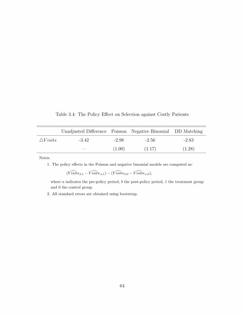
Table 3.4: The Policy Effect on Selection against Costly Patients
Unadjusted Difference Poisson Negative Binomial DD Matching
4V isits -3.42 -2.98 -2.56 -2.83
— (1.00) (1.17) (1.28)
Notes:
1. The policy effects in the Poisson and negative binomial models are computed as:
( V isits b,1 − V isits a,1)− ( V isits b,0 − V isits a,0),
where a indicates the pre-policy period, b the post-policy period, 1 the treatment groupand 0 the control group.
2. All standard errors are obtained using bootstrap.
64

Table 3.5: The Policy Effect on Skimping
Non-Last Resort Hospitals Last Resort Hospitals
Policy Variables
Time Trend -0.80 (0.25) -1.23 (0.20)
65Costly 0.10 (0.017) 0.02 (0.35)
Covariates
Gender 0.001 (0.01) 0.03 (0.01)
Employed -0.22 (0.01) -0.06 (0.01)
Income
Highest 20% 0.07 (0.01) 0.01 (0.02)
2nd Highest 20% 0.07 (0.01) 0.005 (0.023)
Mid 20% 0.03 (0.01) -0.02 (0.02)
2nd Lowest 20% 0.03 (0.02) -0.002 (0.02)
Recipient of Valediction -0.04 (0.07) 0.01(0.10)
Civil Servant -0.03 (0.01) -0.007 (0.03)
N 47,280 30,384
65

Table 3.6: Validation of the Difference-in-Differences Strategy
Panel A. Selection
Poisson Negative Binomial DD Matching
65Costly -0.019 -0.028 —
(0.070) (0.044) —
Policy Effect -0.45 -0.63 -0.43
(0.73) (0.88) (1.03)
Panel B. Skimping
Non-Last Resort Hospitals Last-Resort Hospitals
65Costly -0.02 0.02
(0.03) (0.04)
66

4.0 THE ROLE OF PRIVATE PROVIDERS IN LOWERING THE COST
OF HEALTH CARE: EVIDENCE FROM URBAN CHINA
4.1 INTRODUCTION
1Designing appropriate roles for the government and the private sector in health care delivery
is a complex task for transitional economies, where inefficiencies of the planned-era health
system may compound market failures. As one of the fastest growing transitional economies,
China presents an intriguing case. Although market liberalization has undoubtedly benefited
most of its economy, the role of private providers in China’s health care sector has remained
controversial.
This controversy has assumed the center stage in recent policy discussions as China
searches for ways to reform its embattled health system.2 Some contend that state-owned
providers abuse their predominant market status in pursuit of financial interests, thanks
largely to government policies that obstruct private entry.3 One solution is to break up state
dominance by encouraging competition from private providers. Another line of argument
holds that the profit-seeking behavior results from the economic incentive introduced by
the liberalizing measures in the past three decades.4 Increased competition with private
1This paper is co-authored with Gordon Liu of Guanghua School of Management at Peking University,China.
2Criticisms of the Chinese health system include reduced access to health care, increased risk of out-of-pocket expenditure, widening disparities across regions and socioeconomic classes, stagnation of populationhealth achievements and health care cost escalation. See Wang (2003)[121], Eggleston et al. (2008a)[35],Wagstaff et al. (2009a)[118].
3As shown in Section 4.2, state-owned institutions possess a predominant share of the market, thankslargely to legal barriers to entry and insufficient information on provider performance.
4Within the public health sector, there has been a movement toward financial decentralization since the
67

providers, many of which are profit oriented, will sanction and hence intensify the motive to
over-supply and over-charge for medical services. The solution prescribed by this school is
to remove the negative impact of economic incentives by nationalizing the health sector, at
least at the level of basic care.5,6
At the center of the debate are two issues essential to the efficiency of any health system:
provider ownership and market competition. A vast literature has developed to identify their
impacts in the hospital care market. Because of the peculiarities of health care, the literature,
whether theoretical or empirical, has yet to reach unambiguous conclusions. In addition, it
focuses heavily on developed countries, especially the US. Evidence from developing and
transitional economies is in short supply [Sloan (2000)[108], Eggleston et al. (2008a)[35]].
Differences in their socioeconomic priorities and institutional characteristics make it difficult
for results obtained from one type of countries to find direct applications in the other.
In this paper, we aim to alleviate this shortage in the literature by investigating two
questions in the context of China: (1) How do state and private providers compare with one
another in one important aspect: the price of care, as measured by the total hospital charge
for a given treatment episode? (2) What is the association between the price of care and the
degree of market liberalization?
Apart from their contributions to the literature, the answers we provide will suggest mea-
sures to improve the efficiency of health spending in China, at a critical moment when the
government prepares to substantially shore up its share of health care financing.7 Further-
more, they will inform the health care reforms in other developing and transitional economies,
with whom the Chinese health system shares many salient features.8
1980s. See Section 4.2 for details.5Another rationale for the “pro-government” argument is the public good property of health care.6For detailed discussions of the debate, please visit http://www.chinahealthreform.org, a website dedi-
cated to health reform issues by China Society of Economic Reform.7In its health sector reform report published in April 2009, the government of China promised to increase
its health spending by USD125 billion over the next three years [Wagstaff et al. (2009b)[119]].8The common features include dominance of state ownership of health delivery organizations, non-
universal insurance coverage and limited government administrative capacity. As is the case in China,most of these countries have reformed their health delivery systems with liberalization and incentivizationmeasures [Eggleston et al. (2008b)[36]].
68

In our analysis, we make an important distinction between the fee for health services and
the price of health care. The former refers to the charge for a single service. In China, health
service fees are subject to government regulation. In contrast, the price of care refers to the
total provider charge for a given encounter with the patient. It depends on not only the fees,
but also the type and quantity of services delivered. In this paper, we are interested in the
price of health care, since it represents the real cost of the consumption of medical services
for a household. For this reason, we will use the term “the cost of care” interchangeably
with “the price of care” in the following.
The data we use come from a household survey the World Bank conducted in five Chinese
metropolitan areas in December 2005. The survey provides information on spending on
the most recent hospital visit by any household member, ownership of the provider visited
and a set of patient/provider characteristics. We define the public-private price gap as the
difference in hospital charge between the state and the private sectors, and estimate it in a
non-parametric endogenous switching regression model to correct for the self-selection bias
in the patients’ choice of hospital. To answer the second question, we use a series of linear
regressions to explore the relationship between various measures of private provider market
shares and (1) the price of care; (2) the estimated public-private price gap.
The main findings of the paper are as follows. Our estimation shows that outpatient
care is significantly more expensive at public hospitals than at private providers. Moreover,
the price gap is larger for several underprivileged social groups, including the poor, the
uninsured and rural migrants, than for the general population. Second, the patients’ choice
of provider is insensitive to the public-private price gap. In the market share analysis, we
find strong negative correlations between the price of care and the private providers’ share
in the market for physicians, especially those with advanced medical degrees. The same is
true for the estimated public-private price gap. These findings indicate that, as an increasing
number of doctors work for non-government hospitals, the more expensive state providers
converge toward the cheaper private sector. More importantly, health services at both public
and private hospitals become less expensive.
69

Our results suggest that policies aiming to facilitate the growth of low-cost private insti-
tutions in China will considerably increase social welfare. In particular, they will benefit the
underprivileged social groups who experience significant public-private price gaps. Examina-
tion of China’s health care institutions further demonstrates that development of the private
health sector must overcome the barriers of state market control and insufficient information
on health care quality. The price gap we find may have arisen because the lack of quality
information, especially with regard to private providers, has hindered price competition in
China’s hospital sector. Our results from the market-share analysis suggest that an effective
market-based approach to eroding the information barrier is to liberalize the market for med-
ical personnel. By employing well-trained physicians, private providers can send a credible
signal about the quality of their services. This will help dispel the uncertainty around the
quality of private hospitals and, consequently, foster market competition on price.
The remainder of the chapter is organized as follows. Section 4.2 describes the institu-
tional characteristics of China’s urban health care system. Section 4.3 reviews the literature
on provider ownership and competition in the health care market. In Sections 4.4 and 4.5,
we discuss the econometric model and the estimation techniques used for analyzing the two
research questions: the public-private price gap and market liberalization. The data set
used in our analysis is described in Section 4.6. Sections 4.7 presents the estimation results.
Finally, section 4.8 concludes.
4.2 CHINA’S HEALTH CARE SYSTEM
China’s urban health delivery system is organized as a three tier structure, consisting from
bottom to top of street level primary care facilities, secondary level hospitals and tertiary
hospitals. The level of technical capability rises along the ladder. The system is character-
ized by the dominance of state ownership. Since the early 1990s, however, there has been
widespread opening to the entry of private hospitals [Wang & Zhang (2002)[120], Eggleston
70

et al. (2008a)[35]]. Although generally smaller,9 private institutions have grown more rapidly
than their public counterparts.10
Concurrent with the growth of private providers, the Chinese government has consider-
ably reduced its financial support for the state health sector.11 State-owned hospitals earn
the better part of their income from user charges and enjoy complete discretion over the use
of revenue surplus. It has been argued that this financial autonomy is part of a larger trend
of decentralization in the public health sector, under which government hospitals are increas-
ingly treated as a type of state-owned enterprise upon which incentive-oriented reforms are
introduced [Li & Song (2002)[70]].
In most localities, public hospitals are reimbursed on a fee-for-service (FFS) basis ac-
cording to a regulated fee schedule. The FFS method pays providers a pre-determined fee
for each medical service delivered. The literature shows that, since it rewards the quantity,
rather than quality, of care, this method is associated with high levels of use, especially of
profitable services [Eggleston & Yip (2004)[34]].
Such is indeed the case in China, where fee regulation has further distorted provider in-
centives. To give implicit insurance to the indigent, the government sets the regulated prices
of basic, non-invasive services at below their cost. Hospitals are allowed to cross-subsidize
their income by charging handsome mark-ups on more advanced care, such as pharmaceutical
products and high-tech diagnostic tests [Liu et al. (2000)[77]]. This “dual-track” fee schedule
has created strong incentives for providers to over-prescribe drugs and diagnostic tests.12 In
recent years, the government of China has tried to reduce the distortion by increasing the
fees of labor-intensive services and lowering those of high-tech care. However, studies show
9In 2003, for example, non-profit private hospitals employed 4% of the beds and 3% of the physiciansworking in urban hospitals [Ministry of Health (2004)[89]].
10Between 1996 and 2001, the number of outpatient visits paid to state-owned facilities grew by only 2.1%while it increased by 300% at the private sector [Ministry of Health (2003)[88]].
11Government subsidies now account for 10∼15% of public hospitals’ operating cost, covering basic wagesand the cost of equipment maintenance.
12For instance, a study of village clinics found that prescriptions are strongly associated with the need togenerate revenue, rather than patients’ clinical conditions [Zheng et al. (2003)[139]]. Consequently, Chinahas one of the world’s highest shares of drug costs in total health spending, standing at 54.7% and 44.7% ofoutpatient and inpatient expenditure in 2003, respectively. By contrast, the average in the OECD countriesis about 15% [Ministry of Health (2004)[89]].
71
that this policy change has produced limited effects on providers’ prescribing behavior [Bian
et al. (2002)[9], Meng et al. (2002)[84], Sun et al. (2005)[110]].
Another strategy for correcting provider incentives is to move away from FFS to prospec-
tive payment methods. Prospective payment restrains the incentive to over-supply by pay-
ing providers a pre-specified amount for a well-defined quantity of services. Various types
of prospective payment method have emerged in China’s urban insurance system, includ-
ing: global budgeting, capitation, fixed charges per inpatient day and disease-related groups.
In some cases, a mixture of various payment methods is used. Most studies of these pay-
ment reforms find that they are effective in reducing health care spending [Meng (2002)[83],
Eggleston & Yip (2004)[34], Lin (2004)[74], Wu et al. (2004)[133]]. However, evidence of their
impact on the quality of care is scant. Chapter 2 of my dissertation finds that the switch
from FFS to global budgeting induces hospitals to discriminate against costly patients.
As discussed above, private medical care is a young industry in urban China. Unlike
public providers, many private health institutions are excluded from the publicly-financed
health insurance systems. The bulk of their income comes from direct patient payments made
on the FFS basis. In addition, private hospitals are subject to less government regulation
in areas such as pricing, procurement and managerial decisions. Within the private sector,
the governing policies differ somewhat by the provider’s declared organizational objective.
Non-profit institutions can charge fees within a wide range of the official fee schedule. By
contrast, for-profit facilities enjoy full pricing flexibility. Furthermore, non-profit hospitals
are exempt from income taxes,13 while for-profit ones are not.
We now turn to the demand side of the health care equation. In urban areas, insurance
coverage has declined since the 1990s.14 Before the economic reforms, the urban health
insurance system had two main components, the government insurance scheme (GIS) and
the labor insurance scheme (LIS).15 As the economic reforms proceed, an increasing section
13State-owned hospitals are also exempt from income taxes.14The share of insured population dropped from over 70% in the early 1990s to below 60% in 2003 [Ministry
of Health (2005)[89]].15GIS covered government employees, soldiers, students and teachers, while LIS insured workers at state-
owned enterprises.
72
of the economy becomes independent of the state while the private sector grows rapidly.
As a result, many individuals have fallen out of the state-based medical safety net. In
an effort to expand insurance coverage in the urban areas,16 the government consolidated
GIS and LIS in the late 1990s into a single insurance program for all eligible employees,
called the urban workers’ basic medical insurance (BMI) system. The program is currently
undergoing another expansion to the entire urban population, bringing coverage to those
formerly uninsured, including children, retirees, the unemployed and the self-employed.17
However, this expanded program does not cover migrants from rural areas, most of whom do
not have official residential status in cities and are hence not entitled to the local benefits.
The urban BMI system uses various demand-side cost-sharing measures, such as copay-
ment and drug/service formularies, to control expenditure. Yet it does not restrain patients’
choice of provider with tools such as the gate-keeping system. When a patient, whether
insured or uninsured, makes a contact with the medical system, (s)he has full discretion
over the hospital and the doctor to seek care from. A standard assumption in the health
economics literature holds that patients lack the knowledge to make well-informed decisions
with regard to provider choices. Governments and insurers in China have taken few mea-
sures to fill this information gap. Without credible information, patients frequently turn
to the providers that have good reputation and market standing. In Chinese cities, these
are usually state-owned tertiary hospitals, resulting in the over-use of these facilities. Al-
though financial incentives are in place, such as lower prices and more generous insurance
reimbursement for serviced provided by lower-level facilities, to direct patients away from
tertiary hospitals, these measures have produced limited effects.18
16Another important motivation was to increase the level of risk pooling from individual “work units”under GIS and LIS to the city level.
17In July 2007, the State Council passed the decision to launch the urban resident BMI program. Duringthe same year, pilot experiments were started in 79 localities. According to the official schedule, coveragewould expand to 50% of the target population by 2008, to 80% by 2009 and finally to universal coverage by2010.
18The reason is that the price differentials are too modest to have any real effect, or, as one of the resultsof the paper demonstrates, price is not a key determinant on the patients’ choice of provider.
73

4.3 LITERATURE REVIEW
4.3.1 Provider Ownership
Studies of provider ownership in the health care sector originate mostly from the U.S., where
the differences between for-profit and non-profit hospitals have been extensively analyzed.
Theories of the behavior of non-profit hospitals fall broadly into four categories. The first,
the altruism class, posits that non-profit hospitals pursue altruistic objectives such as the
quality of care [Newhouse (1970)[93]] and charity care [Frank & Salkever (1991)[44]]. The
second category, represented by the paper of Pauly & Redisch (1973)[99], holds that physi-
cians take advantage of the hospital resources to maximize their joint income. In the third
group of studies, the existence of non-profit hospitals depends on the trade-off between tax
benefits available to non-profit organizations and the ability to pursue profit maximization
[Weisbrod (1988)[123], Lakdawalla & Philipson (1998)[67]]. Incomplete information charac-
terizes the fourth category, where it is argued that non-profit hospitals are a solution the
health service industry develops to the information asymmetry between the consumer and
the producer. The nondistribution constraint sends a trust signal with regard to the non-
contractible aspects of health care quality [Arrow (1963)[5], Hansmann (1980)[52], Glaeser
& Shleifer (2001)[47]].
Empirical studies of hospital ownership have produced mixed evidence. Some suggest
that ownership and profit status do not make any difference in the performance of hospi-
tals [e.g., Sloan (2000)[108]], while others find that for-profit providers have lower technical
quality and higher mortality rates [e.g., Devereaux et al. (2002)[20]].
A related body of literature examines the interaction between providers of different own-
ership forms. For example, studying the three types of hospitals in the U.S., Duggan
(2000)[30] concluded that for-profit and non-profit providers both skimmed for profitable
patients, leaving the care for indigent and uninsured individuals to government hospitals.
In a later paper, Duggan (2002)[31] found that non-profit hospitals tended to mimic the
behavior of for-profit hospitals as competition from the latter increased.
74
The limited evidence available from China is mixed. Some studies show that public and
private providers do not differ significantly in their behavior. They are just as likely to induce
unnecessary demand or, if properly paid, to deliver preventive care [Meng et al. (2000)[85],
Li & Song (2002)[70]]. A study by Eggelston et al. (2009)[37] finds that the mortality rates
at private providers do not differ statistically from those at similar government hospitals.
On the other hand, there is evidence that the state sector charges a higher price for
its services than the private sector. In a study directly related to ours, a research team in
Wenzhou (of Zhejiang Province) compares the charges by public and private hospitals for a
number of inpatient cases. They find that the state sector invariably has higher charges and
longer lengths of stay [Wenzhou Health Economics Association (2004)[122]]. However, this
study fails to control for hospital case-mix, thus subjecting its results to biases arising from
patient heterogeneities. Our analysis will use methods from the treatment effect literature
to address the self-selection bias.
4.3.2 Market Competition
The literature on competition in the health care market is also based mostly on the U.S.
experience. It documents that, prior to the advent of managed care, hospitals competed
on quality to attract patients covered by generous indemnity insurance. This led to rapid
spread of advanced technologies, a phenomenon referred to as “medical arms race” [Salkever
(1978)[105], Robinson & Luft (1985)[104], Dranove et al. (1993)[27]]. During this period,
competition led to higher prices and socially wasteful outcomes [Dranove & Statterthwaite
(2000)[28]].
In the mid-1980s, the rise of managed care and the change in the provider payment
method19 transformed the locus of competition from quality to price. Some studies of this
period show that hospital competition not only lowered the cost but also improved the
outcome of health care services [Kessler & McClellan (2000)[66]].
A question relevant for our analysis is: in China’s hospital care market, where the share
19In particular, the change from fee-for-service to prospective payment.
75

of out-of-pocket payment is high and the purchasing of medical services is scattered, does
competition reduce or increase the price of care? The answer is not immediately clear.
Competition for cost-conscious patients may not suffice to lower the price. The literature has
suggested numerous reasons, including imprecision of the information on price and quality
[Dranove & Satterthewaite (1992)[27]], search cost [Satterthewaite (1979)[106]], physician-
induced demand [Fuchs (1978)[45]] and brand loyalty [Grabowski & Vernon (1992)[48]].
4.4 PUBLIC-PRIVATE PRICE GAP
4.4.1 Econometric Model
Our empirical model adopts the framework of the treatment effect literature. Let Ys and Yp
denote logged expenditure on a visit to a state and a private provider, respectively. For each
patient i, the reduced-form cost functions can be written as:
Ysi = β0s + X ′iβs + εsi (4.1)
and
Ypi = β0p + X ′iβp + εpi (4.2)
where s indicates the state and p the private sector. X is a set of observable patient and
provider characteristics. β0s , β0p , βs and βp are parameters to be estimated. The error terms
εs and εp have zero means and are independent of X.
We compute the price differential as the mean difference in per-visit expenditure between
the state and the private sectors; i.e., the parameter of interest is 4(X) = E(Ys − Yp|X).
Since the survey reports information on the most recent visit, we observe only Ys or Yp for
76

each patient, but not both. Let Yi denote the observed expenditure and Si a dummy variable
indicating whether the patient selected a state-owned provider. Then we have,
Yi = YisSi + Yip(1− Si). (4.3)
To define how Si is determined, let s∗i be a latent variable measuring the net utility of
receiving treatment at a state hospital. Then we can write:
s∗i = α4(Xi) + R′iδ + ε0i (4.4)
Si = 1(s∗i > 0),
where R is a set of exogenous variables that may overlap with X and 1(·) is the indicator
function. Following the standard specification, the variance of ε0 is normalized to 1.
Equation (4.4) is a structural selection function. A patient visits a public provider if the
net utility of doing so is positive. Since higher health care cost reduces the patient’s utility,
we anticipate α, the parameter associated with the expected price gap, to be negative.
Equations (4.1)-(4.4) form a switching regression model in which the change from one
state to another is endogenous [Jones (2000)[65]]. The endogeneity arises from the possibility
that the unobserved (to the econometrician) factors influencing expenditure (εs and εp) are
correlated with those affecting the selection of provider (ε0). In our case, these factors include
preference for the state sector, observable aspects of service quality, and the complexity and
severity of illness. For example, if the average patient selecting a public hospital is sicker
than that going to the private sector, failing to address selection on severity of illness would
lead to biased estimates of the public-private price gap. In the following, we will use both
parametric and semiparametric methods to correct for the bias.
Identification of the model is achieved with exclusion restrictions. To identify the struc-
tural selection equation, we need a variable that appears only in X, but not in R. We
use a dummy variable that indicates whether the patient thinks (s)he received unnecessary
77

care during the visit. Unnecessary care is significantly correlated with expenditure. If used,
it substantially increases the cost of care. Conversely, high expenditure is likely to arouse
suspicion of the use of excessive services. To justify that the unnecessary variable does not
appear in R, we note that studies have shown the public and the private hospitals in China
have equally strong financial incentives to over-prescribe [Meng et al. (2000)[85]]. More im-
portantly, they are indistinguishable in popular perception in terms of the tendency to use
unnecessary care [Lim et al. (2004)[72]]. Therefore, the anticipation of unnecessary care does
not influence the choice of state or private providers.
The expenditure functions are identified with a variable that appears in R, but not X.
We use a binary indicator of the ownership of the patient’s employer. It takes the value 1
if the employer is a state-owned entity, and 0 otherwise. The rationale behind this strategy
is that the old GIS and LIS schemes, which covered employees of the state economic sector,
provided full reimbursement for expenditure at appointed public hospitals. Because of this
legacy, employees of the state sector have a stronger tendency than the general population
to use public providers, even in the new insurance system.
A potential drawback of this strategy is that employer ownership may directly influence
the spending on care for various reasons. For example, workers may self-select into state
employment on the basis of their health status. If an average state-sector employee is less
(or more) healthy than the private employee, the estimated “price gap” will confound the real
price difference with the effect of health needs on expenditure. To avoid this bias, we include
the patients’ self-evaluated health level as a covariate in the structural selection equation. A
similar problem may arise if the state sector offers more generous health benefits than the
other employers, so that state-sector employees can afford to spend more on medical care.
However, such is not the case in China, where the new BMI system provides equal benefits
across all economic sectors. Therefore, employer ownership (controlling for patient health
level) is a valid identifying variable for the expenditure functions.
78

4.4.2 Semiparametric Estimation
In the parametric approach to the estimation of Equations (4.1)-(4.4), the error terms
(ε0, εs, εp) are assumed to be trivariate normally distributed [Heckman (1979)[54], Vella
& Verbeek (1999)[116], Wooldridge (2001)[126]]. Using the diagnostic methods described in
Pagan and Vella (1989)[98], we reject the joint normality assumption for our data. Moreover,
we find evidence of substantial heteroskedasticity in both expenditure equations. Therefore,
we adopt a more general framework that allows the conditional expectations of εs and εp
given hospital ownership to enter the expenditure equations nonparametrically.
4.4.2.1 Reduced-Form Selection Equation In the first step, we substitute Equations
(4.1) and (4.2) into (4.4) to derive a reduced-form selection function, written as:
Si = 1(Z ′iγ + εi), (4.5)
where Z = (X,R).
Since our diagnostic tests did not reject the normality assumption for the choice function,
Equation (4.5) is estimated as a probit model, from which we obtain P , the estimated
probability of the patient selecting a public hospital.
4.4.2.2 Correction for Self-Selection Bias We correct for selection bias by estimating
the following equations:
Ysi = β0s + X ′iβs + Us(Zi, Si) + νsi (4.6)
and
Ypi = β0p + X ′iβp + Up(Zi, Si) + νpi, (4.7)
79

where Us(Zi, Si) = E(εsi | Zi, Si = 1) and Up(Zi, Si) = E(εpi | Zi, Si = 0).20 The error terms
νs and νp satisfy the usual assumptions.
Equations (4.6) and (4.7) are partial linear models, where the functional form of the non-
parametric parts, Us and Up , is unknown. Under the standard index sufficiency condition,21
it is easy to show that Us and Up depend on Z only through P , the probability of receiving
the treatment [Amemiya (1985)[3], Heckman (1980)[55], Heckman et al. (1998)[56]]:
Uk(Z, S) = Uk(Z′γ) = Uk(P (Z))
With this simplification, we estimate Equations (4.6) and (4.7) with the differencing-
based method developed by Yatchew (1997[136], 2003[137]). In his work, Yatchew shows
that this method is valid only if the number of arguments in the nonparametric functions is
no greater than 3.
To implement the differencing-based method, we sort the data, within each sub-sample,
by ascending values of P . Subsequently, an m-order differencing is taken of the sorted data.
For example, the first-order differencing produces:
Yki − Yk, i−1 = [X ′i −X ′
i−1]βk + [Uk(Pi)− Uk(Pi−1)] + [νki − νk, i−1] (4.8)
Yatchew shows that, if Uk is continuous and has bounded derivatives, Uk(Pi)−Uk(Pi−1)
vanishes in large samples. Then an OLS regression can be run on the differenced data to
obtain consistent and√
n-normal estimates of βk. That is,
βk = (X ′kXk)
−1(X ′kYk), (4.9)
where Xk and Yk are the differenced data.
Notice that taking differences as in Equation (4.8) removes the intercept terms in the
expenditure equations. However, intercepts are essential in the computation of the average
20These terms would be the inverse Mill’s ratios in the parametric model.21The condition requires that R and Z be exogenous and that the dependence between S and (εs, εp) arise
only through ε0.
80

price gap. Therefore, we use the method developed by Andrews and Schafgans (1998)[4] to
recover these terms. The Andrews-Schafgans estimator is
β0k =
∑Nk
i=1(Yi −X ′iβk)Si h(Z ′
iγ − λk)∑Nk
i=1 Si h(Z ′iγ − λk)
,
where k = s or p. βk is the estimated slope coefficient obtained from Equation (4.9). h(·)is a weighting function defined as in Andrews and Schafgans (1998)[4]. The parameter λk is
the bandwidth or the smoothing parameter. By varying its value, we control the proportion
of observations used in the estimation of the intercept.
Once we obtain β0k and βk (k = s or p), the parametric parts of Equations (4.6) and
(4.7) are moved to the left-hand side of the equations to create new dependent variables:
Yki = Yki − β0k −X ′iβk
= Qk(Pi) + νki.
In this paper, we use the local linear regression estimator to estimate Qk(P ) nonpara-
metrically. The smoothness bound is chosen by minimizing the cross-validation function.
According to Yatchew (2003)[137], this modular approach yields consistent and asymptot-
ically normal estimates of the nonparametric functions, since the convergence rate of the
parametric coefficients, βk, is much faster than that of Qk(P ).
4.4.2.3 Estimation of the Public-Private Price Gap With the above results, we
compute the estimated public-private price differential, 4(X), as:
4(X) = (Ys − Yp)|X
= (β0s − β0p) + X ′(βs − βp).
Notice that, since Ys and Yp were defined as logged expenditures, 4(X) is also on the log
scale. For our result to have any relevance for policy discussions, we must convert the logged
81

price gap to the original scale in order to obtain E(Ws|X)/E(Wp|X), where Wk = exp(Yk).
Various studies have shown that E(Wk|X) depends not only on E(Yk|X), but also on the
conditional distribution of the error term in the log transformed model [Manning (1998)[80],
Manning & Mullahy (2000)[81], Ai & Norton (2008)[2]]. In this paper, we use the semipara-
metric derivative estimator developed by Ai and Norton (2008)[2].22
Finally, let D(X) = E(Ws|X)/E(Wp|X). Then we can obtain the mean price gap by
averaging D(X) over X in some region J . That is,
D(J) =
∫
J
D(X)dF (X), (4.10)
where F (X) is the CDF of X and D(J) is the average public-private price gap over J .
We produce interesting results by varying the definition of J over which the average
gap is estimated. In particular, we define various sub-samples on the metrics of income,
employment, insurance and official residential status, and calculate D(J) for each sub-sample.
This allows us to examine the average price gap relevant for different socioeconomic groups.
4.4.2.4 Structural Selection Equation To estimate the structural selection equation,
we substitute the estimated logged price gap, 4(X), in Equation (4.4) and run a Probit
regression. This step produces consistent, but inefficient, estimates of the parameters of the
structural selection function. Since we do not adjust for the fact that the regressors contain
the estimate, rather than the real, value of a variable,23 the standard errors of the estimated
coefficients are underestimated. However, this turns out not to be a problem since, as will
be shown in Section 4.7.4, the unadjusted estimate of α, the parameter of real interest, is
statistically insignificant. Further adjustment will only reduce its significance level.
22There are other methods that account for the conditional distribution of the error term [Duan (1983)[29],Manning (1998)[80], Ai & Norton (2000)[1]]. However, these methods require either homoskedasticity of theerrors or knowledge of the parametric form of their distribution function. To our knowledge, Ai and Norton(2008)[2] provide the most general approach by allowing for heterskedasticity of any form.
23In particular, 4(X).
82
4.5 MARKET SHARE ANALYSIS
4.5.1 Econometric Model
In this part of the analysis, we examine the association between the share of private providers
in a city’s health care market and (1) the realized price of hospital care; (2) the estimated
price gap. This is equivalent to asking:“With the individual characteristics controlled for,
to what extent can regional variations in the cost of care and the public-private price gap be
attributed to differences in the market share of private providers?”
We operationalize this by adding regional variables, including the market share indicator,
to Equations (4.1) and (4.2) to estimate the impact of the private market share on Yi:
Ykig = β0k + X ′igβk + θ1Mg + C ′
gθ2 + εkig, (4.11)
where k = s or p ; i indicates individual patients; g = 1...G refers to the city. In our data,
G = 5. The variable Mg measures the market share of private providers and Cg is a vector of
other macro-level variables that affect a city’s health care spending. Since we are interested
in only the average effect of Mg on the price of care, θ1 is constrained to be equal for both
public and private providers.
We apply the same method to analyzing the association between the private market
share and the estimated price gap:
4(Xig) = τ1Mg + C ′gτ2 + µig, (4.12)
where 4(Xig) is the estimated price gap for patient i in city g, and µig are random errors.
If θ1 < 0, the average cost of health care in a city decreases with the market share of
private hospitals. If τ1 < 0, the pricing levels of state and private providers converge as the
private health sector expands.
83

4.5.1.1 Indicators of Market Liberalization Our analysis intends to infer the effect
of market liberalization from the association between price/price gap and private provider
market shares. The validity of our approach depends on two inter-related issues: (1) whether
private market share is an appropriate measure of the degree of liberalization; (2) whether
it can be considered exogenous.24
To address the first question, note that the government of China holds considerable
control over the entry of private providers through such means as accreditation, licensing
and quota. The share of private hospitals in the market is therefore a direct result of the
degree of openness of health sector regulation.
Nevertheless, there still are methodological concerns. The problem of reverse causality
may occur if governments of areas where the demand for health care services, and hence
their prices, are low face less resistance from the public sector to open up the market.
Furthermore, the private market share and the price or price gap may both be correlated
with other factors. The following section discusses the variables we use to control for the some
of the confounding factors. However, our data do not have information on three important
aspects: the production cost of health care services, the level of medical technology and the
depth of insurance coverage.
Low production cost, in terms such things as low wages, both reduces the price of care
and attracts private providers to set up facilities. Second, medical technology may create
the natural barrier to entry. If the prevailing technological level of an area is high, it may
be difficult for private hospitals to expand in the market due to insufficient investment
or expertise. In such cases, the association between high prices/large price gaps and low
private market shares is attributable to technology rather than an “illiberal” market. Finally,
since China’s urban health insurance programs tend to exclude private providers from their
networks, shallow insurance coverage, where a large number of services are uncovered, may
be correlated with both low prices and high private market shares. Not having information
24Although the market share variable varies by only five areas, this does not invalidate our examinationof the effect of market liberalization on individual outcomes. As Wooldridge (2003[127], 2006[128]) explains,the validity of cluster-sample analysis depends not so much on the sample size on the cluster level as on theexogeneity of the aggregate variables.
84

on these potentially confounding factors remains a limitation of our data.
4.5.1.2 Controls for Inter-City Heterogeneities Since the number of cities in our
data set is very small, only limited room is available to address inter-city heterogeneities
and other specification issues. To overcome this restriction, we run repeated estimations of
Equations (4.11) and (4.12), alternating the market share indicator and the other city-level
variables used. This can be thought of as a rough robustness test of our specification.
We use five candidate measures of the private provider market share: the percentage
of outpatient visits paid to private hospitals, the shares of high-tech medical equipment,25
hospital beds, physicians and physicians with MD degrees26 employed by the private sector.
The first indicator measures the private share in the service market, while the rest reflect
liberalization of the input markets.
Apart from the private market share, we control for inter-city heterogeneities in three
other aspects: income level, population health, and the availability and utilization of medical
resources. For each aspect, we have a group of candidate variables, each of which contributes
to the regional variations in health care expenditure in distinct ways.
In the case of income level, we use three candidates: per capita disposable income, savings
rate and the Gini coefficient. Per capita income indicates the level of economic development,
while savings rate reflects other factors that may also affect health care spending, such as
the price level and the propensity to consume. The Gini coefficient measures the inequality
of the income distribution. In a highly unequal society, the public-private price gap may
be driven mostly by income inequality, if poor patients favor a particular type of providers,
either public or private, for low-cost care.
Second, we select five indicators to control for population health: neonatal mortality rate,
maternal mortality rate, life expectancy, emergency-room (ER) death rate and intensive-
care-unit (ICU) death rate. Of these variables, life expectancy reflects the health needs
25Equipment such as MRI machines and CT scanners.26According to the regulations in China, physicians with at least the bachelor’s degree are allowed to
practice medicine upon passing a national certifying exam.
85

of an aging society. Infant and maternal mortality rates reveal the status of a region’s
health system [Jamison et al. (2006)[64]].27 In particular, reducing neonatal and maternal
mortality demands of a health delivery system the type of abilities, such as the effectiveness
of risk-screening, service delivery and response to clinical emergencies, that affect the general
quality of all medical services. Finally, the other two variables of this category, ER and ICU
death rates, indicate the severity of urgent and difficult medical cases, as well as the health
profession’s ability to manage them.
We control for regional differences in medical resources with the following variables:
number of hospital beds per 1,000 persons, number of physicians per 1,000 persons, general
occupancy rate and occupancy rate at state hospitals. The numbers of hospital beds and
physicians measure the supply of health care resources, while the occupancy rates reflect their
utilization. We incorporate the latter indices to address the balance between the demand and
the supply forces of medical services. In particular, a low demand for services provided by
state hospitals may lead to both a small public-private price gap and a high private market
share. We control for this by introducing the occupancy rate at the state sector.
Given their distinct effects on health spending, we alternate the use of the above variables,
rather than select any of them arbitrarily. Choosing one from each of the four groups
and running the estimation on Equations (4.11) and (4.12) separately leads to a total of
600 procedures. If, for Equation (4.11), a private market share indicator yields negative
and statistically significant coefficients in most of the procedures, this provides consistent
evidence that market liberalization lowers the price of hospital care. Likewise, we obtain
evidence that liberalization reduces the public-private price gap if a market-share indicator
has a significantly negative effect in most of the regressions on Equation (4.12).
27Infant and maternal mortality rates are also highly correlated with a region’s level of economic develop-ment, a factor we already control for.
86
4.5.2 Cluster Sample Analysis
Equations (4.11) and (4.12) examine the impact of aggregate-level variables on individual
outcomes. To obtain correct inference on θ1 and τ1, we adopt the minimum distance-type
estimator developed by Wooldridge (2003)[127].
4.6 DATA AND VARIABLES
Our data come from a household survey the World Bank administered in December 2005 in
five metropolitan areas: the Pudong region of Shanghai, Shenzhen (Guangdong Province),
Dalian (Liaoning Province), Xi’an (Shaanxi Province) and Chengdu (Sichuan Province).
The survey produced retrospective and current data from a random sample of households
selected with a multi-stage sampling method.28 To our knowledge, except for a World Bank
report on health care utilization patterns, our paper is the first study that uses this data set.
The data contain cross-sectional observations on the use of various types of health care
services, including hospitalizations and outpatient visits. This paper uses only outpatient
data. The reason is that the high cost of inpatient care in China places substantial financial
burdens on households, especially for the poor and the uninsured.29 This may induce a high
degree of simultaneity between inpatient spending and household income. Therefore, we
examine only outpatient expenditure in order to avoid the simultaneity problem. Since a
patient may have multiple outpatient visits during a year while we observe only the most
recent episode, we assume that there is no monthly or seasonal fixed effect on expenditure.
As employer characteristics are necessary for the identification of our model, individuals
under the legal working age of 18 are excluded from the estimation. We also screen out cases
treated at specialty facilities, such as hospitals for otolaryngology and communicable diseases.
28For details regarding the sampling methodology and a full of the survey instruments, please contact theauthors.
29According to World Bank calculations, the average cost of hospitalization in 2003, just under 4000 RMBfor an inpatient stay, was equivalent to 43% of per capita income. For a patient in the poorest quintile ofthe population, the ratio was nearly 200% [World Bank (2005)[132]].
87
The reason is that specialized care represents an area where a high degree of differentiation
exists between the public and the private sectors. Facilities for disease prevention are usually
government-owned, as the low profitability of these services is unlikely to attract private
providers. Moreover, it has been documented that specialization in services not covered by
the urban health insurance program (BMI) is a strategy used by many private providers
to circumvent the dominant public sector [Meng et al. (2000)[85], Lim et al. (2004)[72],
Eggleston et al. (2009)[37]]. Given this differentiation, we should exclude specialty hospitals
in order to increase the level of comparability between the two sectors.
Our screening process produces a sample of 1,955 cases, of which 85.6% were treated at
a state hospital. Table 4.1 lists the definitions and descriptive statistics of the variables used
in the estimation, separated by provider ownership. The last column shows the t-statistics
for tests of equal means between the two samples. The four groups of candidate variables
used in the market share analysis, shown in Table 4.2, are collected from regional statistics
and health yearbooks.
4.6.1 Dependent Variable
The dependent variable is logged total hospital charge for the most recent outpatient visit
in the past 12 months. It is the sum of the patient’s out-of-pocket payment and insurance
reimbursement (if the patient is insured). As shown in Table 4.1, a state provider charges
higher on average than a private hospital. The difference is significant at the 1% level.
4.6.2 Variable of Provider Ownership
We create the key conditioning variable from the survey question regarding the ownership
of the selected provider. The original question specified five types of providers: state-owned,
private domestic, private joint-venture, private foreign and others.30 We recode this variable
by merging the last four groups into one category and defining it as the “private sector.”
30The category of private domestic providers includes collectively owned facilities. The survey does notspecify what the term “others” refers to.
88
4.6.3 Identifying Variables
The values of the identifying variables are as expected. Table 4.1 shows that approximately
equal proportions of patients treated at a public or a private hospital reported receiving
unnecessary services. In addition, the (suspected) use of excessive care has a substantial
impact upon expenditure, with those reporting unnecessary services spending over 76% more
(significant at the 1% level) than those who did not.
As described in Section 4.4, we use the ownership of the patient’s employer to identify
the expenditure functions. In our data, this type of employers includes government agencies,
educational institutions and state-owned enterprises. It is clear from Table 4.1 that state
employees are more likely to select a public hospital than those working in the private sector
(significant at the 1% level). On the other hand, expenditure does not vary significantly by
the patient’s sector of employment.
4.6.4 Other Variables
The other regressors we use in the price gap model are standard. In particular, we control
for the patient’s age, gender, marital status, self-reported health level, family income, official
residential status, insurance status, employment status and education. We also include
indicators of provider characteristics.
The variable of health status is measured on a 5-level scale. Family income is the sum of
monthly incomes of all household members.31 It is recoded into quintiles, from the poorest
to the wealthiest 20%, within each city. The residential status of an individual is determined
by the area where (s)he is officially registered as a resident. It is an important socioeconomic
indicator in China, especially for the vast army of migrant workers who temporarily relocate
from rural areas to seek employment in cities. It determines access to local welfare benefits,
such as stable employment, housing and health insurance. In our data, we count a family
as migrant if more than two of its members have non-local residential status. The variable
31We also estimated the model using family per capita income. The results are very similar.
89

on health insurance includes three categories: job-based insurance, voluntarily purchased
insurance and no insurance. The first category refers to coverage under BMI and GIS
programs, both of which are closely tied with an individual’s employment. Most cases in the
second category are policies purchased from commercial insurance companies, while there is
also a small number of patients receiving government assistance for health care expenditure.
Although the latter is not obtained through voluntary purchasing, the government may well
dispense medical subsidies based on an individual’s health needs or income level. Therefore,
the degree of selection may be equally high for the two types of insurance. Furthermore,
compared with the BMI and GIS programs, their level of benefits is considerably lower. For
these reasons, we consider it appropriate to place them in the same category. In terms of
employment status, there are four possible states: unemployed, retired, not working and
employed. Among these, those “not working” are individuals who are of a legal working age
but decide to deter employment to obtain further education or training. In our data, these
are mostly college students. Since the vast majority of higher education institutions in China
are run by the government, we assign “state-owned” to the employer ownership variable for
these individuals. Finally, the patient’s education level and the provider characteristics are
as defined in Table 4.1.
The behavior of key socioeconomic indicators, including income, residential status, in-
surance and employment, is of central interest in our analysis. A methodological concern
is that their values are rarely randomly determined. Instead, they are influenced by factors
that may affect health care expenditure or the choice of providers. In our model, we control
for the most important confounding factor — the patient’s health level. We assume that,
conditional on health, the socioeconomic indicators are uncorrelated with the error terms.
Our data are limited on medical conditions and provider characteristics. They do not
report the type of illness for which hospital care was sought. Neither do they provide infor-
mation on the characteristics of the hospitals beyond their specialization and administrative
level. As will be discussed in Section 4.8, this may cast doubt on the comparability between
90

the state and the private sectors.32
As Table 4.1 shows, the patient groups at the state and the private health sectors differ
significantly from each other in various aspects. In particular, those selecting a public hos-
pital are older, better educated, and more likely to be local residents or retired. They also
have slightly lower self-evaluation of health, but higher income and better insurance cover-
age. Moreover, utilization at the state sector is concentrated in high-level general hospitals,
while the type of private providers most frequently used is low-level outpatient clinics.
4.7 EMPIRICAL RESULTS
4.7.1 Semiparametric Regression
Results from Probit regression of the reduced-form selection equation (4.5) are shown in the
first column of Table 4.3.33 The identifying variables are well-behaved. In particular, the
ownership of the patient’s employer is a strong predictor of the choice of provider. The point
estimate is 0.373, equivalent to a marginal effect of 0.04, and statistically significant at the
1% level. On the other hand, the use of excessive care does not differ significantly across the
hospital sectors. Diagnostic tests of normality and heteroskedasticity find no misspecification
of the model.
Before estimating the expenditure equations (4.6) and (4.7), it is necessary to define
a common support for P between the state and the private sub-samples. Heckman et al.
(1998)[56] show that estimating the average treatment effect outside the common support
introduces a bias that arises from comparing the incomparable. After data trimming, 79% of
the public (S = 1) and 89% of the private samples (S = 0), or a total of 1,572 observations,
32This problem is partially alleviated by excluding specialty hospitals from the sample. In theory, moreover,these unobserved heterogeneities, like the unobserved severity of illness, are corrected for in the switchingregression model. Essentially, the concern is that, if data were available on these variables, including themin the estimation would reduce the overlapping region of the probabilities of selecting the state sector. SeeHeckman et al. (1998)[56] for discussions.
33As with all tables in this section, the figures in the parentheses give the standard errors of the estimates.
91

remain in the overlapping region.
We report the estimation results of the expenditure equations in Tables 4.4, 4.5 and 4.6.
In each table, various corrections for self-selection bias are considered, including: (i) no cor-
rection; (ii) parametric estimation based on the normality assumption; and (iii) differencing-
based semiparametric correction.
To our knowledge, there is no empirical evidence regarding the optimal order of differenc-
ing,34 nor the bandwidth parameter in the estimation of intercepts. Therefore, we experiment
with various choices of parameter values, and examine the sensitivity of the results to these
choices. In particular, we select orders of 1, 5, 10, 25 and 50,35 as well as bandwidths that
allow for 2.5%, 5%, 10% and 20% of the observations to be used in the intercept estimation.
Since we are essentially interested in how the state and the private health sectors com-
pare with one another, Table 4.4 presents the differences in the estimated slope coefficients
between Equations (4.6) and (4.7). Comparing the first two columns of the table, we ob-
serve that estimates of the slope coefficients are very similar with no correction and with
the parametric correction for selection bias. In fact, neither of the correction terms (i.e., the
inverse Mill’s ratios) in the parametric model is statistically significant.
In the semiparametric estimation, the results are very sensitive to the choice of the
differencing order. The values of the coefficient estimates vary substantially. In a few cases,
even the signs are different. There does not seem to be a discernable trend in the variation.
We believe that the instability of the semiparametric estimation is attributable to the small
number of observations from private hospitals. Recall that 251 observations in the private
sample survived the trimming process a la Heckman et al. (1998)[56]. By taking an order of
50, for instance, we would lose 20% of the observations. This indicates that, although higher
orders of differencing increase the efficiency of estimation in large samples, they impose a
cost of lost precision for small samples.
We test the semiparametric models against the nulls of: (i) no correction; and (ii) the
parametric specification. The results are presented in the bottom panel of Table 4.4. They
34In general, as the order of differencing increases, the estimator approaches asymptotic efficiency.35Yatchew (2003)[137] gives the optimal differencing weights for each order.
92

show that, except for the cases of the private sub-sample with orders of 5 and 10, both nulls
are rejected at the conventional level. This indicates that not correcting for self-selection
would create considerable bias in estimation. Furthermore, normality is not an appropriate
assumption for our data. However, given the sensitivity of the semiparametric results to the
parameter choice, we will still consider the parametric estimate as a viable alternative.
Despite their instability, however, the differencing-based estimates do produce consistent
signs in front of the key socioeconomic indicators (with the exception of the “migrant”
variable). Hence, we are able to draw a general picture of how the treatment for patients
of various socioeconomic status differs across the hospital sectors. In particular, note that
most of the coefficients in front of the following variables are positive: Migrant, Poorest 1/5
Household, No Insurance and Unemployed. Furthermore, those associated with income and
employment status are statistically significant. This finding indicates that, ceteris paribus,
the charge for a migrant, poor, uninsured or unemployed patient relative to the reference
groups is higher at the state than at the private sector.
To demonstrate this pattern more clearly, we present in Table 4.5 the estimated coeffi-
cients associated with the socioeconomic indicators for the state and the private sub-samples
separately. As seen from the table, a poor patient spends significantly less than an affluent
patient at both hospital sectors. However, the expenditure gap is considerably narrower
in state hospitals. Furthermore, if visiting a private provider, unemployed patients spend
less than individuals with stable employment. Yet this difference disappears in the public
sector.36 As will be shown in Section 4.7.3, these results suggest that the public-private price
gap is larger for these disadvantaged groups than for the most well-to-do.
The last row of Table 4.5 shows that the use of unnecessary services has a strong impact on
expenditure. Combining this result with Table 4.4, where it was shown that this impact does
vary across the hospital sectors, we conclude that the identifying variable for the expenditure
equations is valid.
Table 4.6 presents the estimated intercepts obtained with the Andrews-Schafgans esti-
36A similar pattern is observed of residential and insurance status. However, the differences in spendingbetween migrants/uninsured patients and the reference groups are not statistically significant.
93

mator of various bandwidth parameters. It shows that, unlike those in the differencing-based
regression, the results of intercept estimation are fairly stable with respect to both the choice
of bandwidth and the order of differencing. One peculiar finding concerns the standard er-
rors of the estimates. For the private sector, the standard errors decrease, as expected, with
the proportion of the observations used in the estimation, with the exception of the level of
2.5%. This is another indication that methods that would increase the efficiency of estima-
tion in large samples, such as selecting a higher order of differencing or a smaller proportion
of observations, may create substantial instability in small samples.
4.7.2 Public-Private Price Gap
We report the estimated public-private price gap with various corrections for self-selection
bias in Table 4.7. Not surprisingly, the results of the semiparametric model are very sensitive
to the choice of parameters. To choose the optimal parameters, we compute the values of the
cross-validation (CV) function given each combination of differencing order and bandwidth
parameter. Our computations show that following combinations minimize the CV function:
(1) order of 1 & 5% of observations; (2) order of 10 & 5% of observations; (3) order of 10
& 10% of observations; and (4) order of 10 & 20% of observations. These parameters give a
set of optimal estimates for the price gap: (92%, 99%, 103%, 139%).37
Notice in Table 4.7 that this optimal set of semiparametric price gaps is only slightly
above the parametric estimate of 91.6%. However, since their standard errors are consider-
ably smaller, we prefer the results of the semiparametric estimation to those of the parametric
model.
An interesting finding in Table 4.7 is that substantial price gaps emerge only after we
correct for self-selection bias, either parametrically or semiparametrically. In fact, the price
differential estimated without correction is negligible. This suggests that the unobservable
factors upon which patients select a hospital tend to increase the expenditure at the private
37The figures are obtained by subtracting 1 from D defined in Equation (7) and multiplying with 100%.The standard errors are computed with the method described in Ai & Norton (2008)[2].
94
sector. For example, the cases treated at private hospitals may be more severe on average
than those at public providers. It may be that, while they favor the state sector as the first
choice, patients visit private hospitals mostly for cases that are too severe or complicated to
be treated at the state sector. In this sense, private hospitals may be regarded as “providers
of last resort.” Another explanation is that patients may be attracted to the private sector
by the observable characteristics of its quality, such as a clean and comfortable environment,
friendly staff and efficient services, and are willing to pay a premium for these qualities. In
both cases, failure to correct for selection would overestimate the “pure” impact of private
ownership on the price of care and, consequently, underestimate the public-private price gap.
Policy Implications
Taken together, our results provide strong evidence that hospital care is significantly
more expensive at the public sector. In this section, we discuss alternative explanations for
this substantial price gap.
The first possibility we consider is the structure of China’s health care market. Recall
from Section 4.2 that state providers own a predominant share of the market in urban areas
and that the development of the private sector is a recent phenomenon. The state dominance
could contribute to the public-private price gap in various ways. First, private providers may
benefit from what Eggleston et al. (2009)[37] call the “late entrant” effect. In particular,
private hospitals have far fewer retirees to provide for than public hospitals. Therefore,
their production cost could be much lower.38 Second, state providers may charge substantial
premiums for their services by taking advantage of their dominant market status.
Nevertheless, whether arising from production cost or pricing behavior, the price gap
could not have been sustained were there not factors that obstruct competition between
public and private hospitals. One important factor is the policy barrier to entry for private
providers. Although the central government recognized the legal status of the private health
sector in the early 1990s, there have been few policy measures that encourage its development.
38Our data do not have observations on hospitals’ wage costs. Therefore, we are not able to test thishypothesis.
95

On the contrary, studies of local-government policies reveal discrimination against private
providers in terms of accreditation, access to financing, participation in insurance networks
and professional associations, and personnel and procurement policies. Because of these
restrictions, public hospitals have been able to maintain their dominance of the health care
market [Guan (2003)[49], Tao et al. (2004)[111]].
Our data allow us to test the effect of one of the discriminatory policies: participation
in insurance networks. The BMI system, the biggest third-party payer in urban China,
excludes many private providers from its provider networks. Restricted to the state health
sector, patients with BMI coverage may visit private providers only for conditions or services
not covered by BMI. Therefore, the public-private price gap may simply be the result of the
difference in insurance coverage.39 To test this hypothesis, we estimate the price gap for the
sub-sample that (i) excludes employment-based insurance; or (ii) contains only uninsured pa-
tients. The rationale is that if the price gap is driven by the difference in insurance coverage,
the charges for patients without BMI coverage or any insurance at all should be equal across
the public and the private hospital sectors. Our estimation40 shows that substantial price
gaps remain for these patients. Hence, we reject the hypothesis of insurance coverage. In
the section on market share analysis, we will discuss another hypothesis: personnel policies.
The second explanation we consider is the quality of care. In particular, public hospitals
may charge higher prices simply because they offer better-quality services. Although our
data do not contain information on health care quality, evidence from the literature does
not lend strong support to this explanation. For instance, using data from a random sample
of village clinics in Shandong Province, Meng et al. (2000)[85] find virtually no difference
across public and private providers in observable measures of quality, such as training of
health personnel, medical equipment and working conditions. Li and Song (2002)[70] analyze
the transformation of state hospitals into share-holding organizations and find no evidence
that quality problems are associated with any particular ownership structure. Finally, a
39Note that using employment-based insurance as a regressor in this case does not remove the differencesince BMI coverage is practically useless at non-participating private hospitals.
40These results are available from the authors upon request.
96

recent study by Eggleston et al. (2009) [37] finds that mortality rates at private hospitals in
Guangdong Province do not differ statistically from those at state providers of a similar size
and case mix.41
However, there still is widespread concern among patients about the technical quality of
private hospitals. The World Bank survey used in our study reported that, while patients
were satisfied with the private sector on various observable aspects of quality, they ranked
private providers below state hospitals in terms of technical capability. The household sur-
vey studied by Lim et al. (2004)[72] also shows considerable distrust in the quality of private
providers. We believe that at least part of the discrepancy between findings from the litera-
ture and the popular perception is attributable to lack of information on health care quality.
There is no reliable source in China, whether a government agency, an insurer or an inde-
pendent organization, that collects and circulates quality information, especially evidence of
outcomes quality at private hospitals. Unable to judge the quality of care, patients naturally
turn to the public sector for its long-term market standing. As a result, uncertainty about
the quality of private hospitals may have hindered competition between the state and the
private sectors, which in turn sustains the substantial public-private price gap.
4.7.3 Price Gap for Various Socioeconomic Groups
Table 4.8 presents the estimated price gap specific to various socioeconomic groups. The
estimates corresponding to the optimal parameter values demonstrate that, to the exception
of employment status, the price gap is considerably larger for the socially disadvantaged
than for the privileged groups. The differences are particularly striking between the lowest
and the highest income groups. These results are consistent with our earlier discussion of
the estimated coefficients associated with the socioeconomic indicators. They indicate that
health care at the public sector is not only more expensive, but more expensive to a greater
extent for underprivileged patients.
41Most of the cited studies use descriptive analysis. More rigorous evidence regarding the outcomes qualityof care in China is needed.
97

Several key characteristics of China’s health delivery system point to a plausible explana-
tion for this regressive relative price structure. As discussed in Section 4.2, the fee schedule
at the public hospital sector is subject to government regulation. More importantly, the reg-
ulation distorts the behavior of state hospitals by creating strong incentives to over-prescribe
expensive drugs and services. Such incentives are much mitigated for private hospitals which
enjoy greater freedom in pricing their services. In addition, their dominant market status
has severely blunted the public providers’ responsiveness to patients’ circumstances. Studies
often find that patients are much more satisfied with private hospitals’ readiness in answer-
ing their needs than with the public providers [Lim et al. (2002)[71], Lim et al. (2004)[72]].
Therefore, private hospitals may have a stronger incentive to price discriminate according to
the patients’ ability to pay. Public providers, on the other hand, may not find it necessary to
lower the charges for underprivileged patients since the latter usually have weak bargaining
powers against the hospitals.42
4.7.4 Structural Selection Equation
Columns 2-6 of Table 4.3 report the estimation results of the structural selection equation.
The only set of variables that has a significant impact on the choice of provider is hospital
characteristics. In particular, patients are more likely to select a state provider if it is a
general hospital or a high-level facility.
The most important finding is that the expected price gap, while having a negative sign
as anticipated, does not have a significant effect on the choice of provider. This result is
somewhat surprising, since, given the large share of out-of-pocket payments in China’s health
care spending, one would expect the price differential to have a strong effect on the cost-
conscious consumers. Our finding suggests the importance of non-price factors, including
hospital location and perception of service quality, in China’s health care demand function.
42Another possible explanation for the variations in price gap by socioeconomic status is that the under-privileged patients frequent low-cost, low-skill private providers and go to a state hospital only for severeconditions. However, to the extent that differences in the severity of illness and observed service qualityare observed by patients and taken into account in their selection, our model sufficiently controls for theseheterogeneities.
98

In particular, recall our earlier discussion of the distrust in the quality of private hospitals.
The uncertainty about quality may be so strong as to make it difficult for patients to shop on
prices. Instead, they look to certain provider characteristics, such as administrative ranking,
as proxies for quality. This provides further evidence that imperfections of China’s health
care market have created and sustained a substantial price gap between the public and the
private hospitals sectors.
4.7.5 Market Share Analysis
In this section, we present only the results obtained using the differencing order of 10 and
10% of observations in the intercept estimation. The other results corresponding to the
optimal set of parameter choices, which are available from the authors upon request, are
very similar. Figures 4.1 and 4.2 show the proportions of regressions in Equations (4.11)
and (4.12) that return a negative coefficient for the various private market share indicators.
Table 4.9 reports the median estimate for each indicator. Combined, these results reveal a
striking picture.
The share of physicians working in the private sector, especially those with doctoral
medical degrees, is strongly associated with decreases in the price of care. About 80% of the
regressions in (4.11) and (4.12) using the share of doctoral physicians at private hospitals
produce a negative coefficient. Both median estimates are large and statistically significant.
The same is true for the share of physicians, though to a lesser degree.
If we examine the structure of the outcome market, measured by the share of outpatient
visits paid to the private sector, we also find that a stronger presence of private hospitals is
associated with both lower individual charges and smaller public-private price gap.
However, increasing the amount of hospital beds and medical equipment in private hos-
pitals does not appear to be effective in lowering the price of care. Only a small proportion
of the estimations using these as indicators yields negative coefficients. The median estimate
for the share of beds is positive and marginally significant, while that for medical equipment
is statistically insignificant.
99

Reductions in the price gap indicate a convergence of pricing levels between the public
and the private sectors. In addition, the negative correlation between the individual cost
of care and private market shares implies that the average prices at both sectors fall as
the private hospitals expand. Therefore, our findings provide preliminary evidence that
liberalization of the markets for hospital care and, more importantly, for physicians leads
the price at the expensive state sector to converge to that of the cheaper private sector. In
addition, the average prices at both sector decrease.
Policy Implications
These findings have important implications for China’s health system reform. As we
demonstrated earlier, patients are not responsive to price differences when selecting a hospi-
tal. As a result, simply allowing competition for individual patients may not be effective in
fostering price competition. Indeed, studies of other health care systems suggest that compe-
tition for insurance contracts and production inputs (e.g., physicians and hospital managers)
offers greater opportunities in reducing the cost of care [Docteur & Oxley (2003)[21], World
Bank (2005)[132]].
In light of the international literature, our results suggest that an effective mechanism
of market liberalization is to increase the private providers’ competitiveness in the market
for medical personnel. Recall our earlier discussion that patients’ concern about the quality
of care may have discouraged the competition between the public and the private sectors.
Liberalizing the market of physicians will give private hospitals greater access to the most
critical input for the production of health care. This will not only increase the quality of their
services, but, more importantly, send credible signals about their credentials and technical
skills. Patients will select the private sector more willingly, given the knowledge that they
will be treated by well-qualified health workers. Once the information barrier to the private
sector breaks down, the level of competition in the outcome market will increase. Since the
vast majority of patients in China do not have generous insurance coverage, competition is
likely to rise on the dimension of price rather than quality. Consequently, the cost of care
100

will fall.43
To liberalize the market for physicians, the government must first remove the policy
barriers to access for private providers. Apart from monetary compensation, non-financial
incentives, such as professional ranking and access to research grants, are important deter-
minants on physicians’ utility in urban China. Yet current regulations prevent most private
hospitals from offering these benefits. As a result, physicians are generally reluctant to join
the private sector out of concerns of poor career prospects. If hiring doctors from other
areas, private hospitals must also overcome the obstacle of obtaining legal residential status
for their employees [Tao et al. (2004)[111]]. In summary, private providers have substantial
difficulty attracting and retaining medical personnel. Based on our findings, we argue the
these barriers should be removed to create opportunities for price competition in China’s
health care market.
Finally, we discuss the impact of liberalization on the quality of care. One might be
concerned that if a large number of physicians move from state to private hospitals, the
quality of care may fall at the public sector. Figure 3 shows that this may be an unlikely
scenario. The figure plots the number of outpatient visits per physician between 1990 and
2006. We can see that, while the number of visits per doctor at high-level hospitals increased
during this period, the workload at low-level facilities fell in general, despite a mild increase
after 2000. The graph indicates that there may be an excess supply of physicians at low-level
hospitals. As the private health sector expands, one would expect doctors at these facilities
to make the first move to private hospitals. This re-allocation of human resources may
strengthen the private sector’s competitiveness without significantly affecting the quality of
services at state providers.
43If intense competition in the input markets drives up the production cost, liberalization may actuallyincrease the overall price of medical services. However, our results indicate the contrary; namely, largerprivate shares of physicians are associated with lower prices in both the state and the private sectors.
101

4.8 DISCUSSION
In this paper, we analyze the public-private price gap in China’s urban health care market.
After correcting for self-selection bias, we find that outpatient services are not only much
more expensive in the state sector, but more expensive to a larger degree for the disadvan-
taged social groups than for the well-off. Paradoxically, this substantial price gap does not
have a strong impact on the patients’ choice of provider. In the second part of the analysis,
we examine the effect of expanding the private health care sector. Our results show that a
stronger private sector is associated with both lower individuals charges and smaller public-
private price gaps. Moreover, the mechanism of market liberalization matters. In particular,
liberalizing the market for medical personnel has the greatest potential for fostering effective
price competition between the public and the private sectors.
How we interpret the above results has important policy implications. The first question
is whether the public-private price gap should be of concern to policy-makers. Obtained in
a model of rational individuals, the price differential appears to be a legitimate outcome of
utility-maximizing behavior. For several reasons, however, it is unlikely a socially optimal
outcome. More importantly, there is considerable room for government policies to increase
social welfare. As is typical for health care, the patients’ choice of provider is based on
incomplete information. In particular, lack of information on the quality of private hospitals
may have discouraged the selection of provider on price. The price gap may thus arise from
the public providers’ rent-seeking behavior as they exploit their superior market status. In
addition, since the gap is larger for disadvantaged social groups, the underprivileged patients
may face substantial barriers to access. The government may wish to narrow the gap for
these patients out of equity concerns. Policies that facilitate the growth of low-cost private
institutions or allow for pricing flexibility within the state sector may considerably increase
social welfare.
Our second finding of low price consciousness in the choice of provider may result from
the patients’ weak bargaining power and inability to judge the quality of services. The
102

international literature suggests that, under such circumstances, the capacity of the insurer
to improve system incentives, through such means as selective contracting and provider
payment methods, should be emphasized. Furthermore, local governments or insurance funds
can play an important role in the collection, organization and dissemination of quality-related
information.
Finally, our results regarding private provider market shares suggest that an effective
mechanism for lowering the price of health care is to liberalize China’s market for medical
personnel. By employing well-trained physicians, nurses or managers, private providers can
send a credible signal of the quality of their services. This will help dispel the uncertainty
around the quality of private hospitals and, consequently, foster market competition on price.
The main drawback of our study arises from data limitations. Our data set provides no
disease information. If differentiation of services is a principal survival strategy for private
providers, the patient groups at the two sectors may be very different in their medical
conditions and, consequently, health care spending. Furthermore, the data have limited
information on provider characteristics. Apart from specialization and administrative level,
there are many other characteristics that may affect our results, including size, location,
years of practice, technical/education level of medical staff, etc. Lack of such information
may undermine the comparability between our samples of state and private hospitals.
More importantly, our study calls for future efforts of data collection and research on the
effect of competition on China’s health care system. Our data offer no direct information on
market competition. We need better measures of the degree of market liberalization. More
importantly, we need to find exogenous variations that can identify the effect of liberalization
on price. Furthermore, the share of such things as beds, doctors and visits owned by private
hospitals does not reveal the real structure of the market. We do not know whether expanded
private entry leads to market differentiation or head-to-head competition with the state
establishment. Nor are we able to tell how private expansion influences the way in which
patients select hospitals. Better data, such as panel data, are needed to examine the causal
link between competition and price.
103

In addition, the price of care has been the sole subject of this study. Future research is
necessary to examine the impact of competition, or more precisely, private entry, on patient
health outcomes, such as rate of recovery and future medical spending. Another interesting
topic is the effect of increased competition on the hospitals’ pricing behavior. Stronger
empirical evidence is needed to explore whether competition leads to uniform pricing or
price discrimination, and the implications of the pricing behavior on provider profits and
social welfare.
104

Table 4.1: Definitions & Descriptives of Variables in the Switching Regression
State Provider Private Provider t-statistic
Ns = 1,673 Np = 282Variable
Mean (S.D.) Mean (S.D.)
Dependent Variable
Logged Hospital Charge 5.53(1.05) 4.92(1.22) -7.89
Individual Characteristics
Age 45.6(14.4) 41.6(12.9) -4.79
Gender 0.42(0.49) 0.41(0.49) -0.50
Married 0.86(0.33) 0.89(0.33) 1.07
Self-Reported Health
Poor 0.02(0.15) 0.02(0.15) 0.09
Fair 0.17(0.38) 0.09(0.29) -3.97
Good 0.37(0.48) 0.44(0.50) 2.17
Very Good 0.38(0.49) 0.40(0.49) 0.63
Excellent (reference) 0.05(0.21) 0.04(0.19) -0.88
Migrant 0.29(0.45) 0.53(0.50) 7.71
Family Monthly Income 3,332(3,117) 2,738(3,811) -2.48
Insurance
Uninsured 0.28(0.45) 0.57(0.50) 9.40
Voluntary 0.07(0.25) 0.05(0.23) -1.09
Job-based (reference) 0.65(0.49) 0.37(0.49) -8.99
Continues...
105

Table 4.1 Continued
State Provider Private Provider t-statistic
Ns = 1,673 Np = 282Variable
Mean (S.D.) Mean (S.D.)
Employment
Unemployed 0.10(0.31) 0.12(0.33) 0.93
Retired 0.27(0.44) 0.18(0.38) -3.70
Not Working 0.03(0.17) 0.01(0.12) -1.78
Employed (reference) 0.62(0.49) 0.67(0.47) 1.72
Education
Higher Education 0.16(0.37) 0.09(0.30) -3.55
High School 0.42(0.49) 0.36(0.49) -1.90
Junior High 0.29(0.45) 0.36(0.48) 2.15
Primary Schooling 0.10(0.31) 0.17(0.38) 2.85
No Education (reference) 0.02(0.15) 0.02(0.14) -0.64
Provider Characteristics
High-Level Hospital 0.67(0.48) 0.11(0.32) -25.23
Low-Level Hospital 0.17(0.38) 0.20(0.40) 1.24
High-Level Clinic 0.01(0.11) 0.01(0.08) -0.86
Low-Level Clinic (reference) 0.16(0.35) 0.68(0.48) 18.20
Identifying Variables
Selection Function
Use of Unnecessary Care 0.25(0.44) 0.23(0.42) -0.71
Expenditure Functions
Employer Ownership 0.47(0.49) 0.25(0.44) -7.71
106

Table 4.2: Variables in the Market Share Analysis
Market Share Income Population Health Health Care Resources
Outpatient Visits Per Capita Income Infant Mortality Hospital Beds/1,000
Hospital Beds Savings Rate Maternal Mortality Physicians/1,000
Medical Equipment Gini Coefficient Life Expectancy General Occupancy Rate
Physicians ER Death Rate State Occupancy Rate
Doctoral Physicians ICU Death Rate
107
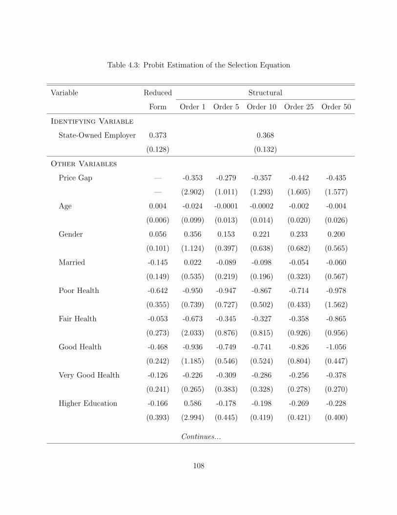
Table 4.3: Probit Estimation of the Selection Equation
Variable Reduced Structural
Form Order 1 Order 5 Order 10 Order 25 Order 50
Identifying Variable
State-Owned Employer 0.373 0.368
(0.128) (0.132)
Other Variables
Price Gap — -0.353 -0.279 -0.357 -0.442 -0.435
— (2.902) (1.011) (1.293) (1.605) (1.577)
Age 0.004 -0.024 -0.0001 -0.0002 -0.002 -0.004
(0.006) (0.099) (0.013) (0.014) (0.020) (0.026)
Gender 0.056 0.356 0.153 0.221 0.233 0.200
(0.101) (1.124) (0.397) (0.638) (0.682) (0.565)
Married -0.145 0.022 -0.089 -0.098 -0.054 -0.060
(0.149) (0.535) (0.219) (0.196) (0.323) (0.567)
Poor Health -0.642 -0.950 -0.947 -0.867 -0.714 -0.978
(0.355) (0.739) (0.727) (0.502) (0.433) (1.562)
Fair Health -0.053 -0.673 -0.345 -0.327 -0.358 -0.865
(0.273) (2.033) (0.876) (0.815) (0.926) (0.956)
Good Health -0.468 -0.936 -0.749 -0.741 -0.826 -1.056
(0.242) (1.185) (0.546) (0.524) (0.804) (0.447)
Very Good Health -0.126 -0.226 -0.309 -0.286 -0.256 -0.378
(0.241) (0.265) (0.383) (0.328) (0.278) (0.270)
Higher Education -0.166 0.586 -0.178 -0.198 -0.269 -0.228
(0.393) (2.994) (0.445) (0.419) (0.421) (0.400)
Continues...
108

Table 4.3 Continued
Variable Reduced Structural
Form Order 1 Order 5 Order 10 Order 25 Order 50
High-School Education 0.048 0.629 0.035 0.005 0.002 0.028
(0.361) (2.174) (0.368) (0.387) (0.389) (0.370)
Junior High School 0.060 0.661 0.064 0.056 0.063 0.087
(0.358) (2.182) (0.367) (0.370) (0.367) (0.373)
Primary School -0.187 0.310 -0.200 -0.206 -0.223 -0.132
(0.363) (2.183) (0.375) (0.380) (0.398) (0.414)
Migrant -0.200 0.147 -0.216 -0.132 -0.196 -0.175
(0.139) (1.154) (0.210) (0.195) (0.174) (0.144)
Poorest 1/5 0.427 1.344 0.540 0.576 0.639 0.568
(0.163) (3.656) (0.798) (0.854) (1.109) (0.854)
Next Poorest 1/5 0.472 0.583 0.489 0.477 0.581 0.528
(0.171) (0.798) (0.470) (0.432) (0.788) (0.603)
Middle Income 0.155 0.480 0.226 0.232 0.331 0.271
(0.151) (1.367) (0.464) (0.485) (0.831) (0.621)
Next Richest 1/5 0.158 1.088 0.282 0.264 0.448 0.369
(0.150) (3.700) (0.789) (0.726) (1.385) (1.097)
No Insurance -0.307 -0.139 -0.221 -0.227 -0.288 -0.278
(0.136) (0.574) (0.293) (0.275) (0.140) (0.149)
Voluntary Insurance 0.461 0.605 0.498 0.514 0.572 0.677
(0.209) (1.684) (0.312) (0.315) (0.527) (0.897)
Unemployed 0.042 0.757 0.114 0.136 0.163 0.201
(0.170) (2.557) (0.282) (0.347) (0.434) (0.561)
Retired -0.194 0.672 -0.202 -0.027 -0.049 -0.040
(0.181) (2.941) (0.467) (0.442) (0.374) (0.400)
Continues...
109

Table 4.3 Continued
Variable Reduced Structural
Form Order 1 Order 5 Order 10 Order 25 Order 50
Not Working 0.565 -0.248 0.400 0.378 0.404 0.239
(0.343) (2.923) (0.658) (0.724) (0.604) (1.192)
High-Level Hospital 2.094 2.122 2.054 2.105 2.163 2.292
(0.126) (0.234) (0.268) (0.141) (0.210) (0.643)
Low-Level Hospital 0.757 0.716 0.913 0.706 0.768 0.861
(0.127) (0.130) (0.155) (0.134) (0.234) (0.179)
High-Level Clinic 1.543 1.548 1.629 1.724 1.923 2.158
(0.419) (0.422) (0.505) (0.748) (1.408) (2.235)
Unnecessary Care -0.046 — — — — —
(0.116) — — — — —
N 1,955 1,572
110
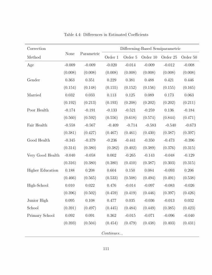
Table 4.4: Differences in Estimated Coefficients
Correction Differening-Based Semiparametric
MethodNone Parametric
Order 1 Order 5 Order 10 Order 25 Order 50
Age -0.009 -0.009 -0.020 -0.014 -0.009 -0.012 -0.008
(0.008) (0.008) (0.008) (0.008) (0.008) (0.008) (0.008)
Gender 0.363 0.351 0.229 0.381 0.488 0.421 0.446
(0.154) (0.148) (0.155) (0.152) (0.156) (0.155) (0.165)
Married 0.032 0.033 0.113 0.125 0.089 0.173 0.063
(0.192) (0.213) (0.193) (0.208) (0.202) (0.202) (0.211)
Poor Health -0.174 -0.191 -0.133 -0.521 -0.259 0.136 -0.184
(0.560) (0.592) (0.556) (0.618) (0.574) (0.844) (0.471)
Fair Health -0.558 -0.567 -0.409 -0.714 -0.583 -0.540 -0.673
(0.381) (0.427) (0.467) (0.461) (0.430) (0.387) (0.397)
Good Health -0.345 -0.379 -0.236 -0.441 -0.350 -0.473 -0.396
(0.314) (0.380) (0.382) (0.402) (0.389) (0.376) (0.315)
Very Good Health -0.040 -0.058 0.002 -0.265 -0.143 -0.048 -0.129
(0.316) (0.380) (0.380) (0.410) (0.387) (0.303) (0.315)
Higher Education 0.188 0.208 0.604 0.150 0.084 -0.093 0.206
(0.466) (0.565) (0.533) (0.508) (0.494) (0.491) (0.538)
High-School 0.010 0.022 0.476 -0.014 -0.097 -0.083 -0.026
(0.396) (0.502) (0.459) (0.419) (0.446) (0.397) (0.426)
Junior High 0.095 0.108 0.477 0.035 -0.036 -0.013 0.032
School (0.391) (0.497) (0.445) (0.484) (0.449) (0.385) (0.423)
Primary School 0.092 0.091 0.362 -0.015 -0.071 -0.096 -0.040
(0.393) (0.504) (0.454) (0.479) (0.438) (0.403) (0.431)
Continues...
111

Table 4.4 Continued
Correction Differencing-Based Semiparametric
MethodNone Parametric
Order 1 Order 5 Order 10 Order 25 Order 50
Migrant 0.061 0.044 0.233 0.122 0.097 -0.066 0.068
(0.181) (0.193) (0.178) (0.183) (0.197) (0.187) (0.192)
Poorest 1/5 0.629 0.667 0.744 0.625 0.650 0.681 0.770
(0.253) (0.254) (0.238) (0.268) (0.266) (0.283) (0.268)
Next Poorest 1/5 0.334 0.373 0.170 0.367 0.311 0.482 0.379
(0.252) (0.269) (0.247) (0.239) (0.262) (0.284) (0.288)
Middle Income 0.480 0.501 0.277 0.366 0.359 0.510 0.528
(0.237) (0.237) (0.248) (0.253) (0.244) (0.278) (0.270)
Next Richest 1/5 0.665 0.762 0.753 0.597 0.550 0.855 0.649
(0.234) (0.239) (0.222) (0.253) (0.255) (0.265) (0.262)
No Insurance 0.100 0.071 0.115 0.258 0.189 0.019 0.014
(0.189) (0.216) (0.225) (0.227) (0.210) (0.209) (0.213)
Voluntary Insurance 0.151 0.197 0.340 0.396 0.208 0.297 0.313
(0.351) (0.328) (0.369) (0.372) (0.339) (0.365) (0.324)
Unemployed 0.249 0.259 0.518 0.176 0.225 0.241 0.332
(0.254) (0.248) (0.238) (0.245) (0.253) (0.252) (0.229)
Retired 0.195 0.185 0.598 0.375 0.309 0.199 0.283
(0.243) (0.259) (0.270) (0.264) (0.277) (0.249) (0.267)
Not Working -0.416 -0.377 -0.592 -0.467 -0.496 -0.338 -0.255
(0.406) (0.547) (0.424) (0.392) (0.452) (0.475) (0.442)
High-Level Hospital 0.171 0.283 -0.943 -0.206 -0.046 0.092 0.153
(0.227) (0.402) (0.387) (0.355) (0.391) (0.539) (0.866)
Low-Level Hospital -0.147 -0.132 -0.212 -0.074 -0.028 0.119 -0.032
(0.208) (0.221) (0.261) (0.264) (0.313) (0.262) (0.281)
Continues...
112
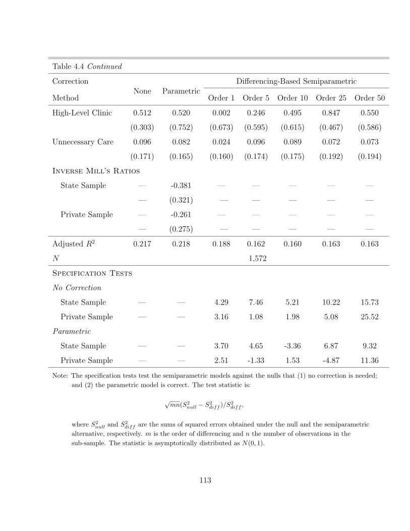
Table 4.4 Continued
Correction Differencing-Based Semiparametric
MethodNone Parametric
Order 1 Order 5 Order 10 Order 25 Order 50
High-Level Clinic 0.512 0.520 0.002 0.246 0.495 0.847 0.550
(0.303) (0.752) (0.673) (0.595) (0.615) (0.467) (0.586)
Unnecessary Care 0.096 0.082 0.024 0.096 0.089 0.072 0.073
(0.171) (0.165) (0.160) (0.174) (0.175) (0.192) (0.194)
Inverse Mill’s Ratios
State Sample — -0.381 — — — — —
— (0.321) — — — — —
Private Sample — -0.261 — — — — —
— (0.275) — — — — —
Adjusted R2 0.217 0.218 0.188 0.162 0.160 0.163 0.163
N 1,572
Specification Tests
No Correction
State Sample — — 4.29 7.46 5.21 10.22 15.73
Private Sample — — 3.16 1.08 1.98 5.08 25.52
Parametric
State Sample — — 3.70 4.65 -3.36 6.87 9.32
Private Sample — — 2.51 -1.33 1.53 -4.87 11.36
Note: The specification tests test the semiparametric models against the nulls that (1) no correction is needed;and (2) the parametric model is correct. The test statistic is:
√mn(S2
null − S2diff )/S2
diff ,
where S2null and S2
diff are the sums of squared errors obtained under the null and the semiparametricalternative, respectively. m is the order of differencing and n the number of observations in thesub-sample. The statistic is asymptotically distributed as N(0, 1).
113

Tab
le4.
5:Sem
ipar
amet
ric
Est
imat
ion
for
Key
Soci
oec
onom
icIn
dic
ator
s
Ord
er1
Ord
er5
Ord
er10
Ord
er25
Ord
er50
Sta
teP
riva
teSta
teP
riva
teSta
teP
riva
teSta
teP
riva
teSta
teP
riva
te
Mig
rant
0.10
3-0
.130
0.11
8-0
.007
0.13
00.
032
0.10
40.
045
0.09
60.
028
(0.0
91)
(0.1
67)
(0.0
90)
(0.1
90)
(0.0
90)
(0.1
77)
(0.0
90)
(0.1
76)
(0.0
90)
(0.1
77)
Income
Poor
est
1/5
-0.3
62-1
.111
-0.3
48-0
.972
-0.3
18-0
.968
-0.3
51-1
.104
-0.3
28-1
.098
(0.1
23)
(0.2
24)
(0.1
24)
(0.2
50)
(0.1
24)
(0.2
40)
(0.1
24)
(0.2
40)
(0.1
21)
(0.2
52)
Nex
tPoor
est
1/5
-0.3
73-0
.543
-0.2
91-0
.632
-0.2
51-0
.562
-0.2
74-0
.703
-0.2
60-0
.639
(0.1
29)
(0.2
38)
(0.1
29)
(0.2
38)
(0.1
25)
(0.2
35)
(0.1
25)
(0.2
35)
(0.1
22)
(0.2
44)
Mid
dle
Inco
me
-0.2
28-0
.511
-0.1
70-0
.549
-0.1
43-0
.502
-0.1
50-0
.610
-0.1
23-0
.651
(0.0
90)
(0.2
28)
(0.0
89)
(0.2
33)
(0.0
90)
(0.2
21)
(0.0
90)
(0.2
21)
(0.0
89)
(0.2
31)
Nex
tR
iches
t1/
5-0
.161
-0.9
23-0
.145
-0.7
42-0
.134
-0.5
83-0
.136
-0.7
59-0
.117
-0.7
66(0
.083
)(0
.207
)(0
.086
)(0
.240
)(0
.085
)(0
.236
)(0
.086
)(0
.236
)(0
.086
)(0
.238
)In
surance
No
Insu
rance
0.19
30.
078
0.11
7-0
.140
0.07
9-0
.110
0.12
90.
110
0.08
50.
070
(0.1
11)
(0.2
13)
(0.1
12)
(0.2
11)
(0.1
09)
(0.1
94)
(0.1
09)
(0.1
94)
(0.1
07)
(0.1
96)
Vol
unta
ryIn
sura
nce
-0.1
22-0
.432
-0.0
36-0
.432
-0.0
23-0
.418
-0.0
23-0
.325
0.01
4-0
.299
(0.1
24)
(0.3
54)
(0.1
32)
(0.3
46)
(0.1
15)
(0.3
34)
(0.1
15)
(0.3
34)
(0.1
05)
(0.3
45)
Employment
Unem
plo
yed
0.08
6-0
.430
0.02
9-0
.143
0.01
6-0
.209
0.01
3-0
.303
0.01
6-0
.320
(0.0
96)
(0.2
06)
(0.1
00)
(0.2
17)
(0.1
00)
(0.2
43)
(0.1
00)
(0.2
43)
(0.1
02)
(0.2
61)
Ret
ired
0.12
2-0
.470
-0.0
23-0
.397
-0.0
24-0
.334
-0.0
14-0
.326
-0.0
15-0
.303
(0.1
00)
(0.2
53)
(0.1
01)
(0.2
51)
(0.1
04)
(0.2
54)
(0.1
04)
(0.2
54)
(0.1
05)
(0.2
61)
Not
Wor
kin
g0.
129
0.72
60.
211
0.67
90.
252
0.74
90.
237
0.50
80.
249
0.50
3(0
.224
)(0
.372
)(0
.231
)(0
.459
)(0
.207
)(0
.366
)(0
.207
)(0
.366
)(0
.213
)(0
.350
)U
nnec
essa
ryC
are
0.39
40.
370
0.37
10.
257
0.34
70.
257
0.33
60.
235
0.32
90.
300
(0.0
66)
(0.1
45)
(0.0
64)
(0.1
59)
(0.0
66)
(0.1
62)
(0.0
67)
(0.1
66)
(0.0
69)
(0.1
95)
114
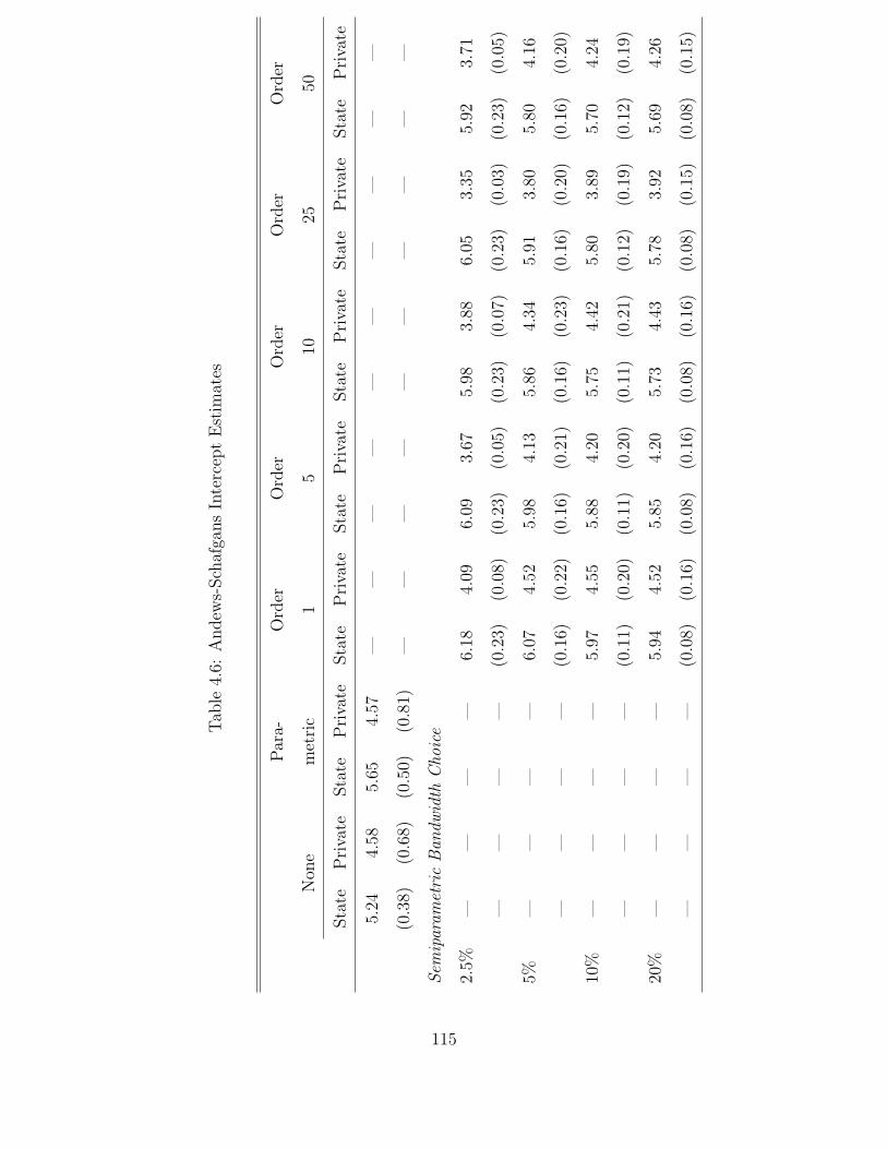
Tab
le4.
6:A
ndew
s-Sch
afga
ns
Inte
rcep
tE
stim
ates
Par
a-O
rder
Ord
erO
rder
Ord
erO
rder
Non
em
etri
c1
510
2550
Sta
teP
riva
teSta
teP
riva
teSta
teP
riva
teSta
teP
riva
teSta
teP
riva
teSta
teP
riva
teSta
teP
riva
te
5.24
4.58
5.65
4.57
——
——
——
——
——
(0.3
8)(0
.68)
(0.5
0)(0
.81)
——
——
——
——
——
Sem
ipar
amet
ric
Ban
dwid
thC
hoic
e
2.5%
——
——
6.18
4.09
6.09
3.67
5.98
3.88
6.05
3.35
5.92
3.71
——
——
(0.2
3)(0
.08)
(0.2
3)(0
.05)
(0.2
3)(0
.07)
(0.2
3)(0
.03)
(0.2
3)(0
.05)
5%—
——
—6.
074.
525.
984.
135.
864.
345.
913.
805.
804.
16
——
——
(0.1
6)(0
.22)
(0.1
6)(0
.21)
(0.1
6)(0
.23)
(0.1
6)(0
.20)
(0.1
6)(0
.20)
10%
——
——
5.97
4.55
5.88
4.20
5.75
4.42
5.80
3.89
5.70
4.24
——
——
(0.1
1)(0
.20)
(0.1
1)(0
.20)
(0.1
1)(0
.21)
(0.1
2)(0
.19)
(0.1
2)(0
.19)
20%
——
——
5.94
4.52
5.85
4.20
5.73
4.43
5.78
3.92
5.69
4.26
——
——
(0.0
8)(0
.16)
(0.0
8)(0
.16)
(0.0
8)(0
.16)
(0.0
8)(0
.15)
(0.0
8)(0
.15)
115

Table 4.7: Estimated Public-Private Price Gap
9.2%No Correction
(2.28)
91.6%Parametric Estimation
(4.07)
Semiparametric % of Sample Used in Intercept Estimation
Estimation 2.5% 5% 10% 20%
Order 1 246% 103% 77% 78%
(1.86) (1.70) (1.79) (1.79)
Order Order 5 322% 137% 100% 99%
(1.30) (1.26) (1.25) (1.25)
of Order 10 326% 139% 99% 92%
(1.28) (1.25) (1.24) (1.24)
Differencing Order 25 426% 246% 184% 168%
(1.52) (1.48) (1.48) (1.48)
Order 50 428% 200% 149% 139%
(1.29) (1.25) (1.23) (1.23)
116

Table 4.8: Public-Private Price Gap for Various Socioeconomic Groups
Socioeconomic Income Residence Employment Insurance
Indicator Poor Rich Migrant Local Jobless Employed No Yes
Order 1
5% of Sample 180% -16% 170% 65% 65% 121% 164% 59%
(2.42) (1.99) (2.42) (2.19) (2.35) (2.33) (2.09) (2.30)
10% of Sample 140% -17% 135% 43% 43% 92% 129% 38%
(2.46) (1.98) (2.23) (2.19) (2.26) (2.32) (2.08) (2.29)
20% of Sample 143% -16% 137% 45% 45% 94% 132% 40%
(2.46) (1.98) (2.23) (2.19) (2.27) (2.32) (2.08) (2.29)
Order 5
5% of Sample 211% 18% 203% 106% 98% 160% 206% 96%
(1.94) (1.64) (1.72) (1.82) (1.69) (1.86) (1.63) (1.89)
10% of Sample 163% -0.3% 156% 73% 67% 119% 158% 65%
(1.93) (1.63) (1.71) (1.82) (1.67) (1.86) (1.62) (1.88)
20% of Sample 160% -1% 154% 73% 66% 117% 156% 64%
(1.93) (1.63) (1.71) (1.82) (1.67) (1.86) (1.62) (1.88)
Order 10
5% of Sample 210% 23% 197% 111% 107% 158% 199% 102%
(1.86) (1.46) (1.60) (1.64) (1.57) (1.70) (1.54) (1.68)
10% of Sample 158% 3% 147% 75% 72% 115% 149% 68%
(1.93) (1.45) (1.59) (1.64) (1.55) (1.86) (1.53) (1.68)
20% of Sample 150% -1% 139% 70% 66% 108% 140% 62%
(1.84) (1.45) (1.59) (1.64) (1.54) (1.70) (1.53) (1.68)
Note: The comparison groups on the metric of income are individuals whose household income is in the lowestand the highest quintile, respectively, of each city’s income distribution.
117
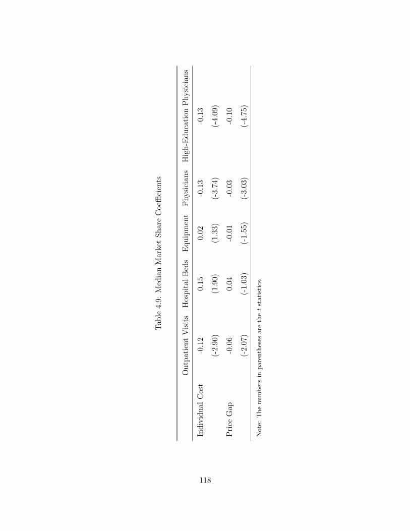
Tab
le4.
9:M
edia
nM
arke
tShar
eC
oeffi
cien
ts
Outp
atie
nt
Vis
its
Hos
pit
alB
eds
Equip
men
tP
hysi
cian
sH
igh-E
duca
tion
Physi
cian
s
Indiv
idual
Cos
t-0
.12
0.15
0.02
-0.1
3-0
.13
(-2.
90)
(1.9
0)(1
.33)
(-3.
74)
(-4.
09)
Pri
ceG
ap-0
.06
0.04
-0.0
1-0
.03
-0.1
0
(-2.
07)
(-1.
03)
(-1.
55)
(-3.
03)
(-4.
75)
Not
e:T
henu
mbe
rsin
pare
nthe
ses
are
the
tst
atis
tics
.
118

Figure 4.1: Market Liberalization & Price of Care
119
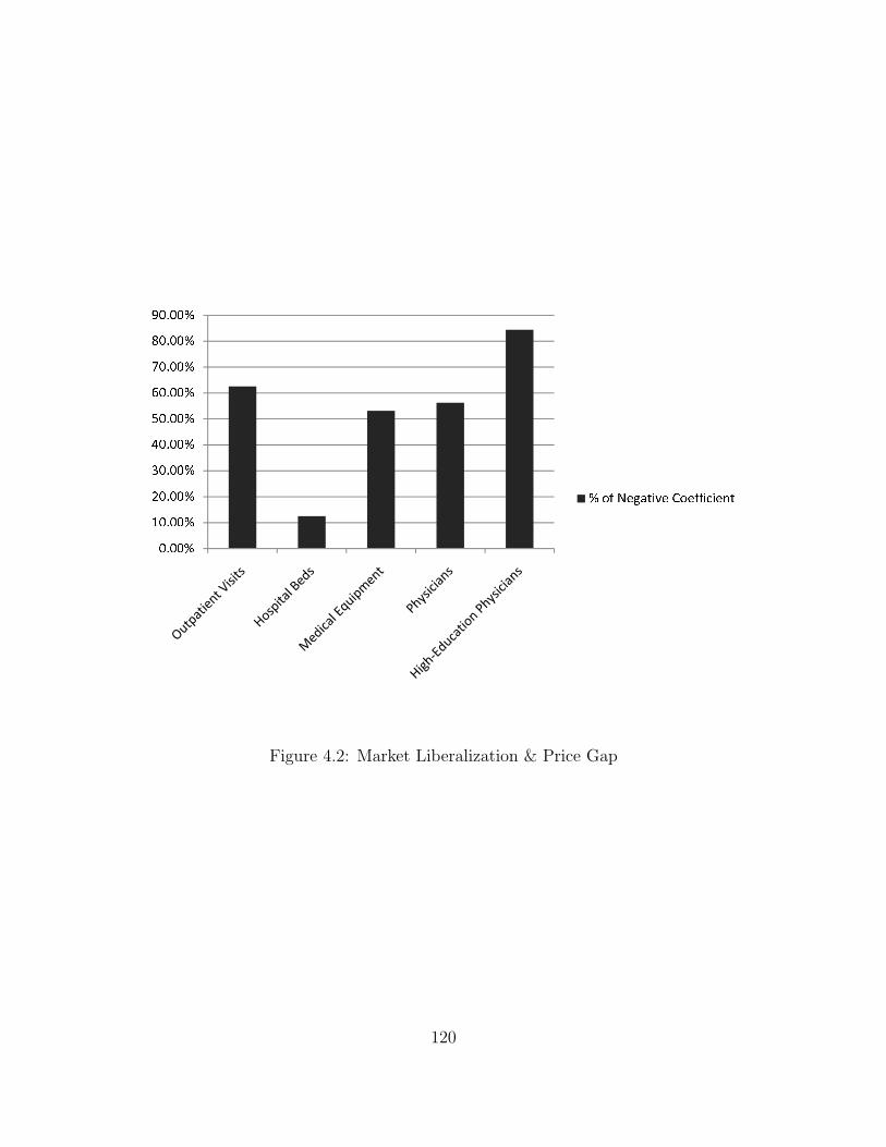
Figure 4.2: Market Liberalization & Price Gap
120

Figure 4.3: Physician Work Load
121

5.0 CONCLUDING REMARKS
My dissertation studies two supply-side issues in the context of China’s health care system:
(1) the impact of global budgeting on provider behavior; and (2) the role of the market in the
delivery of health care services. The two chapters on the global budget policy investigate its
adverse effects on special patient groups from both theoretical and empirical perspectives.
They find that the cost-saving pressure created by global budgeting could induce providers to
avoid insured or high-cost patients, shift costs to the uninsured or skimp on the intensity of
services for costly patients. The third chapter compares the price of care between the public
and the private health sectors in urban China. It finds that services are not only much
more expensive in the state sector, but more expensive to a larger degree for disadvantaged
social groups than for the well-off. In addition, liberalizing the market for medical personnel
appears to be an effective mechanism for narrowing the public-private price gap as well as
for lowering the average cost of care.
All the three studies address the key institutional characteristics of China’s health care
system. In particular, the policy of fee regulation has given rise to unique definitions or
model specifications that (1) in the case of Chapter 2, determine the study’s departures
from the literature; or (2) in the case of Chapter 4, play a crucial role in the interpretation
of the results.
The findings of the dissertation have important implications for China’s health system
reform. In the case of the global budget policy, provider responses to this policy will deter-
mine the real outcome of supply-side cost-saving measures. If hospitals dump patients or
skimp on their treatment, the goal of cost containment is achieved only at the expense of
122

reduced access and quality for certain patient groups, especially those with severe medical
conditions. In addition, cost shifting, whether among patient groups or services, will com-
promise the objective of cost containment as prepayment will have little effect on the total
expenditure. Knowledge of these behavioral changes is necessary for finding ways to counter
perverse provider responses to global budgeting.
The study of the urban hospital care market suggests that there is considerable room
for government policies to increase social welfare. The lack of information on the quality
of private hospitals may have discouraged patients from selecting providers on the basis of
price. The substantial public-private price gap may thus arise from the public providers’
rent-seeking behavior as they exploit their superior market status. In addition, since the gap
is larger for disadvantaged social groups, the government may wish to narrow the gap for
these patients out of equity concerns. Policies that facilitate the growth of low-cost private
institutions or allow for pricing flexibility within the state sector may considerably increase
social welfare. Our results regarding private provider market shares indicate that an effective
mechanism is to liberalize China’s market for medical personnel. By employing well-trained
physicians, nurses or managers, private providers can send a credible signal of the quality of
their services. This will help dispel the uncertainty around the quality of private hospitals
and, consequently, foster market competition on price.
More importantly, our study underscores the importance of research on the role of the
market in health care delivery. There has been a tendency in recent policy discussions to as-
cribe the problems of China’s health system to an “unfettered market approach”1 and to call
for public investment that will supposedly supplant financial motives. Our research suggests
that this denial of the market may be as misguided as the earlier embrace of incentivization
that took hold of China’s health system in the 1980s. As I discussed in the opening remarks,
the Chinese system is characterized by a mixture of strong market and regulatory incentives.
Some of them (e.g., financial incentives on the organizational and the individual level) may
have transpired with others (e.g., the regulated fee schedule that biases prescription toward
1For instance, see Hsiao (2008)[60].
123

expensive services and the policies that discourage the growth of the private health sector)
to create perverse outcomes. What seems to be an appropriate policy approach is to find the
balance between the market and the government that will help obtain efficiency in health
care delivery.
124

BIBLIOGRAPHY
[1] Ai, C. & E. Norton (2000), “Standard Errors for the Retransformation Problem withHeteroscedasticity,” Journal of Health Economics 19(5):697-718.
[2] ——– (2008), “A Semiparametric Derivative Estimator in Log Transformation Mod-els,” Econometrics Journal 11(3): 538-553.
[3] Amemiya, T. (1985), “Advanced Econometrics,” Cambridge: Harvard UniversityPress.
[4] Andrews, D. & M. Schafgans (1998), “Semiparametric Estimation of the Intercept ofa Sample Selection Model,” Review of Economic Studies 65(3): 497-517.
[5] Arrow, K. (1963), “Uncertainty and the Welfare Economics of Medical Care,” AmericanEconomic Review 53(5): 941-973.
[6] Ash, A., F. Porell, L. Gruenberg, E. Sawitz & A. Beiser (1989), “Adjusting MedicareCapitation Payments Using Prior Hospitalization Data,” Health Care Financing Review10(4): 17-29.
[7] Barros, P. (2003), “Cream-Skimming, Incentives for Efficiency and Payment System,”Journal of Health Economics 22(3): 419-443.
[8] Bertrand, M., E. Duflo & S. Mullainathan (2004), “How Much Should We TrustDifferences-in-Differences Estimates?,” Quarterly Journal of Economics 119(1): 249-275.
[9] * Bian, Y., N. Zhuang, Q. Meng & S. Yu (2002), “Cost and Efficiency of Use of PET,”Chinese Journal of Health Economics (Zhongguo Weisheng Jingji) 2002(8): 15-17.
[10] Bloom, G. (2004), “China in Transition: Challenges to Urban Health Services,” in G.Bloom & S. Tang, ed., Health Care Transition in Urban China (Ashgate), Chapter 1.
[11] Brown R., D. Clement, J. Hill, S. Retchin & J. Bergeron (1993), “Do Health Mainte-nance Organizations Work for Medicare?,” Health Care Financing Review 15(1): 7-23.
125

[12] * Cai, W., M. Ma & W. Zhu (2000), “Exploring the Cost Control Mechanisms Asso-ciated with the Integration of Global Budget and Individual Payment,” Health Eco-nomics Research (Weisheng Jingji Yanjiu) 19(4): 20-24.
[13] * Cao, J. & K. Yu (2004), “A Comparative Analysis of the Impact of the Basic HealthInsurance Policy on Hospitals of Different Level and Type,” Chinese Hospital Manage-ment (Zhongguo Yiyuan Guanli) 24(7): 28-30.
[14] * Center for Health Statistics and Information, Ministry of Health (2004), “An AnalysisReport of National Health Services Survey in 2003 (Zhongguo Weisheng Fuwu DiaochaYanjiu: Di San Ci Guojia Weisheng Fuwu Diaocha Fenxi Baogao),” Peking UnionMedical University Publishing House (Zhongguo Xiehe Yike Daxue Chubanshe).
[15] Cheng, T. (2008), “China’s Latest Health Reforms: A Conversation with ChineseHealth Minister Chen Zhu,” Health Affairs 27(4): 1103-1110.
[16] * China Health Yearbook Editorial Board (2004), ”China Health Yearbook (ZhongguoWeisheng Nianjian),” People’s Medical Publishing House (Renmin Weisheng Chuban-she).
[17] * China Statistical Yearbook Editorial Board (2001, 2004), “China Statistical Yearbook(Zhongguo Tongji Nianjian),” China Statistics Press (Zhongguo Tongji Chubanshe).
[18] * Department of Population & Employment Statistics, National Bureau of Statisticsof China, & Department of Financial Planning, Ministry of Human Resources & SocialSecurity of China (2001, 2004), “China Labor Statistical Yearbook (Zhongguo LaodongTongji Nianjian),” China Statistics Press (Zhongguo Tongji Chubanshe).
[19] * Development Research Center (2005), “Comments and Suggestions on the StructuralReform of the Health Care System in China (Dui Zhongguo Yiliao Weisheng TizhiGaige De Pingjia Yu Jianyi),” State Council Development Research Center PolicyReport (Guowuyuan Fazhan Yanjiu Zhongxin Zhengce Baogao).
[20] Devereaux, P., P. Choi, C. Lacchetti, B. Weaver, H. Schnemann, T. Haines, J. Lavis,B. Grant, D. Haslam, M. Bhandari, T. Sullivan, D. Cook, S. Walter, M. Meade, H.Khan, N. Bhatnagar & G. Guyatt (2002), “A Systematic Review and Meta-Analysisof Studies Comparing Mortality Rates of Private For-Profit and Private Not-For-ProfitHospitals,” Canadian Medical Association Journal 166(11): 1399-1406.
[21] Docteur, E. & H. Oxley (2003), “Health-Care System: Lessons from the Reform Ex-perience,” OECD Health Working Paper.
[22] Dong, W. (2001), “Health Care Reform in Urban China,” Working Paper, ComparativeProgram on Health and Society, Munk Center for Internationl Studies at the Universityof Toronto.
126

[23] Dran, J. & B. Campbell (1981), “Hospital Investment and Medicare Reimbursement,”Journal of Financial Research 4(2):147-160.
[24] Dranove, D. (1987), “Pricing by Non-Profit Institutions: The Case of Hospital Cost-Shifting,” Journal of Health Economics 7(1): 47-57.
[25] Dranove, D. & M. Satterthwaite (1998), “Monopolistic Competition When Price andQuality are not Perfectly Observed,,” RAND Journal of Economics 23(4): 518-534.
[26] ——– (2000), “The Industrial Organization of Health Care Markets,” in A. Culyer &J. Newhouse ed., Handbook of Health Economics (Elsevier North-Holland), Chapter20.
[27] Dranove, D., M. Shanley & W. White (1993), “Price and Concentration in HospitalMarkets: The Switch from Patient-Driven to Payer-Driven Competition,” Journal ofLaw & Economics 36(1): 179-204.
[28] Dranove, D. & W. White (1998), “Medicaid-Dependent Hospitals and Their Patients:How Have They Fared?,” Health Services Research 33(2): 163-186.
[29] Duan, N. (1983), “Smearing Estimate: A Nonparametric Retransformation Method,”Journal of the American Statistical Association 78(383): 605-610.
[30] Duggan, M. (2000), “Hospital Ownership and Public Medical Spending,” QuarterlyJournal of Economics 115(4): 1343-1373.
[31] ——– (2002), “Hospital Market Structure and the Behavior of Not-for-Profit Hospi-tals,” RAND Journal of Economics 33(3): 433-446.
[32] Eggleston, K. (2000), “Risk Selection and Optimal Health Insurance-Provider PaymentSystems,” Journal of Risk & Insurance 67(2): 173-196.
[33] Eggleston, K. & W. Yip (2001), “Provider Response to Prospective Hospital Paymentin Hainan Province in the People’s Republic of China,” Health Economics 10(4):325-339.
[34] ——– (2004), “Addressing Government and Market Failures with Payment Incentives:Hospital Reimbursement Reform in Hainan, China,” Social Science & Medicine 58(2):267-277.
[35] Eggleston, K., L. Li, Q. Meng, M. Lindelow & A. Wagstaff (2008a), “Health ServiceDelivery in China: A Literature Review,” Health Economics 17(2): 149-165.
[36] Eggleston, K., J. Wang & K. Rao (2008b), “From Plan to Market in the Health Sector?China’s Experience,” Journal of Asian Economics 19(5-6): 400-412.
127

[37] Eggleston, K., M. Liu, J. Wang, C. Li, Z. Yang & J. Zhang (2009), “ComparingPublic and Private Hospitals in China: Evidence from Guangdong Province,” StanfordUniversity ARPAC Asia Health Policy Program Working Paper No. 7.
[38] Ellis, R. (1998), “Creaming, Skimping and Dumping: Provider Competition on theIntensive and Extensive Margins,” Journal of Health Economics 17(5): 537-555.
[39] Ellis, R. & T. McGuire (1993), “Supply-Side and Demand-Side Cost Sharing in HealthCare,” Journal of Economic Perspectives 7(4): 135-151.
[40] ——– (1996), “Hospital Response to Prospective Payment: Moral Hazard, Selection,and Practice-Style Effects,” Journal of Health Economics 15(3): 257-277.
[41] Fan, C., K. Chen & K. Kan (1998), “The Design of Payment Systems for Physiciansunder Global Budget — An Experimental Study,” Journal of Economic Behavior &Organization 34(2): 295-311.
[42] Feldstein, P. (1993), Health Care Economics, Delmar Publishers.
[43] Foster, R. (1985), “Cost-Shifting under Cost Reimbursement and Prospective Pay-ment,” Journal of Health Economics 4(3): 261-271.
[44] Frank, R. & D. Salkever (1991), “The Supply of Charity Services by Nonprofit Hospi-tals: Motives and Market Structure,” RAND Journal of Economics 22(3): 430-445.
[45] Fuchs, V. (1978), “The Supply of Surgeons and the Demand for Operations,” Journalof Human Resources 13(Suppl): 35-56.
[46] Gao, J., S. Tang, R. Tolhurst & K. Rao (2001), “Changing Access to Health Servicesin Urban China: Implications for Equity?,” Health Policy & Planning 16(3): 302-312.
[47] Glaeser, E. & A. Shleifer (2001), “Not-for-Profit Entrepreneurs,” Journal of PublicEconomics 81(1): 99-115.
[48] Grabowski, H. & J. Vernon (1992), “Brand Loyalty, Entry and Price Competitionin Pharmaceuticals after the 1984 Drug Act,” Journal of Law & Economics 35(2):331-350.
[49] * Guan, W., “Some Thoughts and Suggestions for the Development of Private Hospi-tals,” Chinese Hospitals (Zhongguo Yiyuan) 5: 50-51.
[50] Hadley, J. & J. Feder (1985), “Hospital Cost Shifting and Care for the Uninsured,”Health Affairs 4(3): 67-80.
128
[51] Hamilton, B. (2002), “HMO Selection and Medicare Costs: Bayesian MCMC Estima-tion of a Robust Panel Data Tobit Model with Survival,” in A. Jones & O. O’Donnelled., Econometric Analysis of Health Data (John Wiley and Sons), Chapter 16.
[52] Hansmann, H. (1980), “The Role of Nonprofit Enterprise,” Yale Law Journal 89(5):835-901.
[53] Hay, J. (1983), “The Impact of Public Health Care Financing Policies on Private SectorHospital Costs,” Journal of Health Politics, Policy & Law 7(4): 945-952.
[54] Heckman, J. (1979), “Sample Selection as a Specification Error,” Econometrica 47(1):153-161.
[55] ——– (1980), “Addendum to Sample Selection Bias as a Specification Error,” in E.Stromsdorfer & G. Farkas, ed., Evaluation Studies Review Annual, Vol. 5 (Sage Press).
[56] Heckman, J., H. Ichimura, J. Smith & P. Todd (1998), “Characterizing Selection BiasUsing Experimental Data,” Econometrica 66(5): 1017-1098.
[57] Health Insurance Association of America (1982), “Hospital Cost Shifting: The HiddenTax,” HIAA, Wahsington, D.C.
[58] Hill, J. & R. Brown (1990), “Biased Selection in the TEFRA HMO/CMP Program,”Mathematica Policy Research Working Paper No. 7786-503, Princeton University.
[59] Hsiao, W. (1995), “The Chinese Health Care System: Lessons for Other Nations,”Social Science & Medicine 41(8): 1047-1055.
[60] ——– (2008), “When Incentives and Professionalism Collide,” Health Affairs 27(4):949-951
[61] Hsueh, Y., S. Lee & Y. Huang (2004), “Effects of Global Budgeting on the Distributionof Dentists and Use of Dental Care in Taiwan,” Health Services Research 39(6): 2135-2153.
[62] * Hu, A. (1999), “The Biggest Adjustment for Entering the New Century: China Entersa Period of High Unemployment (Jinru Xin Shiji De Zuida Tiaozheng: Zhongguo JinruGao Shiye Qi),” in Analytical Report on the State of Country for China (ZhongguoGuoqing Fenxi Yanjiu Baogao), Chinese Academy of Sciences and Tsinghua University(Zhongguo Kexueyuan Yu Qinghua Daxue).
[63] Hussain, A. (2003), “Urban Poverty in China: Measurement, Patterns and Policies,”InFocus Programme on Socio-Economic Security, International Labour Organization,Geneva.
129

[64] Jamison, D., J. Breman, A. Measham, G. Alleyne, M. Claeson, D. Evans, P. Jha,A. Mills & P. Musgrove (2006), “Cost-Effective Strategies for the Excess Burden ofDisease in Developing Countries,” Priorities in Health, New York: Oxford UniversityPress.
[65] Jones, A. (2000), “Health Econometrics,” in A. Cuyler & J. Newhouse ed., Handbookof Health Economics (Elsevier North-Holland), Chapter 6.
[66] Kessler, D. & M. McClellan (2000), “Is Hospital Competition Socially Wasteful?,”Quarterly Journal of Economics 115(2): 577-615.
[67] Lakdawalla, D. & T. Philipson (1998), “Nonprofit Production and Competition,”NBER Working Paper No. 6377.
[68] Lei, X. & W. Lin (2009), “The New Cooperative Medical Scheme in Rural China: DoesMore Coverage Mean More Service and Better Health?,” Health Economics 18(2): S25-S46.
[69] Leonard K., M. Rauner, M. Schaffhauser-Linzatti & R. Yap (2003), “The Effect ofFunding Policy on Day of Week Admissions and Discharges in Hospitals: The Casesof Austria and Canada,” Health Policy 63(3): 239-257.
[70] * Li, W. & W. Song (2002), “A Practical Analysis of the Hospital Property RightsSystem” Chinese Health Economics (Zhongguo Weisheng Jingji) 21(3): 1-5.
[71] Lim, M., H. Yang, T. Zhang, W. Feng, Z. Zhou & Y. Chen (2002), “The Role andScope of Private Medical Practice in China,” Word Bank Working Paper.
[72] Lim, M., H. Yang, T. Zhang, W. Feng & Z. Zhou (2004), “Public Perceptions of PrivateHealth Care in Socialist China,” Health Affairs 23(6): 222-234.
[73] * Lin, F., M. Qiu & S. Zhang (2004), “Exploring the Medical Insurance PaymentMethod in Zhenjiang,” Chinese Health Economics (Zhongguo Weisheng Jingji) 23(9):37.
[74] * Lin, Q. (2004), “Adjustment of Payment Methods for Urban Health InsuranceSchemes,” Chinese Advanced Hospital Management (Zhongguo Gaoji Yiyuan Guanli)7: 23-25.
[75] Liu, G., P. Yuen, T. Hu, L. Li & X. Liu (2003), “Urban Health Insurance Reform:What Can we Learn from the Pilot Experiments?” in A. Chen et al. ed., Urbanizationand Social Welfare in China (Ashgate Publishing).
[76] Liu, X. & W. Hsiao (1995), “The Cost Escalation of Social Health Insurance Plan inChina: Its Implication for Public Policy,” Social Science & Medicine 41(8): 1095-1101.
130

[77] Liu, X., Y. Liu & N. Chen (2000), “The Chinese Experience of Hospital Price Regula-tion,” Health Policy & Planning 15(2): 157-163.
[78] Liu, X. & A. Mills (2003), “The Influence of Bonus Payments to Doctors on HospitalRevenue: Results of a Quasi-experimental Study,” Applied Health Economics & HealthPolicy, 2(2): 91-98.
[79] Liu, Y. (2002), “Reforming China’s Urban Health Insurance System,” Health Policy60(2): 133-150.
[80] Manning, W. (1998), “The Logged Dependent Variable, Heteroskedasticity, and theRetransformation Problem,” Journal of Health Economics 17(3): 283-295.
[81] Manning, W. & J. Mullahy (2001), “Estimating Log Models: To Transform or Not ToTransform?” Journal of Health Economics 20(4): 461-494.
[82] Meltzer D., J. Chung & A. Basu (2002), “Does Competition under Medicare Prospec-tive Payment Selectively Reduce Expenditures on High-Cost Patients?,” RAND Jour-nal of Economics 33(3): 447-468.
[83] * Meng, Q. (2002), “The Impact of Provider Payment Reforms on Cost Containment,”Chinese Health Economics Research (Zhonghua Weisheng Jingji Yanjiu) 9: 18-20.
[84] * Meng, Q., Y. Bian & Q. Sun (2002), “Improving the Pricing System for HealthCare (I),” Chinese Journal of Health Economics (Zhongguo Weisheng Jingji) 2002(5):31-34.
[85] Meng, Q., X. Liu & J. Shi (2000), “Comparing the Services and Quality of Private andPublic Clinics in Rural China”, Health Policy & Planning 15(4): 349-356.
[86] Meng, Q., C. Rehnberg, N. Zhuang, Y. Bian, T. Goran & S. Tang (2004), “The Impactof Urban Health Insurance Reform on Hospital Charges: A Case Study from Two Citiesin China,” Health Policy 68(2): 197-209.
[87] Meng, Q. & S. Tang (2004), “Introduction to the Urban Health System and Reviewof Reform Initiatives,” in G. Bloom & S. Tang, ed., Health Care Transition in UrbanChina (Ashgate), Chapter 2.
[88] * Ministry of Health (2003), “Chinese Health Statistical Digest (Zhongguo WeishengTongji Tiyao),” China Statistics Press (Zhongguo Tongji Chubanshe).
[89] * ——– (2000, 2004, 2005, 2006, 2007, 2008), “China Health Statistics Yearbook(Zhongguo Weisheng Tongji Nianjian),” Peking Union Medical University PublishingHouse (Zhongguo Xiehe Yike Daxue Chubanshe).
131

[90] Morgan, R., B. Vernig, C. DeVito & N. Persily (1997), “The Medicare-HMO RevolvingDoor: The Healthy Go In and the Sick Go Out,” New England Journal of Medicine337(3): 169-175.
[91] Morrisey, M. (1996), “Hospital Cost Shifting: A Continuing Debate,” EBRI Issue BriefNo. 180.
[92] Mougeot, M. & F. Naegelen (2005), “Hospital Price Regulation and Expenditure CapPolicy,” Journal of Health Economics 24(1): 55-72.
[93] Newhouse, J. (1970), “Toward a Theory of Nonprofit Institutions: An Economic Modelof a Hospital,” American Economic Review 60(1): 60-74.
[94] ——– (1989), “Do Unprofitable Patients Face Access Problems?,” Health Care Financ-ing Review 11(2): 33-42.
[95] ——– (1996), “Reimbursing Health Plans and Health Providers: Efficiency in Produc-tion Versus Selection,” Journal of Economic Literature 34(3): 1236-1263.
[96] Newhouse, J., E. Sloss, W. Manning & E. Keeler (1993), “Risk Adjustment for AChildren’s Capitation Rate,” Health Care Financing Review 15(1): 39-54.
[97] Paddock, S., J. Escarce, H. Orla & B. Beeuwkes (2007), “Did the Medicare InpatientRehabilitation Facility Prospective Payment System Result in Changes in RelativePatient Severity and Relative Resource Use?,” Medical Care 45(2):123-130.
[98] Pagan, A. & F. Vella (1989), “Diagnostic Tests for Models Based on Individual Data:A Survey,” Journal of Applied Econometrics 4: S29-S59.
[99] Pauly, M. & M. Redisch (1973), “The Not-for-Profit Hospital as a Physicians’ Coop-erative,” American Economic Review 63(1): 87-99.
[100] * Peking University Research Team (2002), “The Function and Scope of Private Prac-tice in Health Sector in China,” Hospital Management (Yiyuan Guanli) 3: 4-6.
[101] Polsky, D. & S. Nicholson (2004), “Why Are Managed Care Plans Less Inexpensive:Risk Selection, Utilization, or Reimbursement?,” Journal of Risk & Insurance 71(1):21-40.
[102] Poterba, J. (1994), “A Skeptic’s View of Global Budget Caps,” Journal of EconomicPerspectives 8(3): 67-73.
[103] Rehnberg, C., Q. Meng, Y. Bian, N. Zhuang & S. Tang (2004), “The Impact of HealthInsurance Reform on Hospital Charges: A Comparison of Nantong and Zibo,” in G.Bloom & S. Tang, ed., Health Care Transition in Urban China (Ashgate), Chapter 10.
132

[104] Robinson, J. & H. Luft (1985), “The Impact of Hospital Market Structure on PatientVolume, Average Length of Stay, and the Cost of Care,” Journal of Health Economics4(4): 333-356.
[105] Salkever, D. (1978), “Competition among Hospitals,” in W. Greenberg ed., Competitionin the Health Care Sector: Past, Present the Future (Aspen Press).
[106] Satterthwaite, M. (1979), “Consumer Information, Equilibrium Industry Price and theNumber of Sellers,” Bell Journal of Economics 10(2): 483-502.
[107] * Shanghai Health Insurance Bureau (2002), “Collections of Official Doc-uments on Health Insurance Policies (Yiliao Baoxian Zhengce Huibian),”http://www.shyb.gov.cn.
[108] Sloan, F. (2000), “Not-for-Profit Ownership and Hosptial Behavior,” in A. Cuyler & J.Newhouse ed., Handbook of Health Economics (Elsevier North-Holland), Chapter 21.
[109] Sloan, F. & E. Becker (1984), “Cross-Subsidies and Payment for Hospital Care,” Jour-nal of Health Politics, Policy & Law 8(4): 660-685.
[110] * Sun, Q., R. Ge & Q. Meng (2005), “Cost and Efficiency of PET/CT,” ChineseJournal of Health Economics (Zhongguo Weisheng Jingji) 2005(2): 37-41.
[111] * Tao, Y. Q. Cai & B. Ren (2004), “Barriers to the Development of Private Hospitalsand Some Suggestions,”Chinese Journal of Current Hospital Administration (ZhongguoXiandai Yiyuan Guanli) 2(12): 35-37.
[112] Ulrich, V. & E. Wille (1996), “Healthcare Reform and Expenditure on Drugs: TheGerman Situation,” Pharmacoeconomics 10(Supp): 81-88.
[113] U.S. Genral Accounting Office (1991), “Health Care Spending Control: The Experienceof France, Germany and Japan,” Gaithersburg: U.S. General Accounting Office.
[114] Van Doorslaer, E., O. O’Donnell, R. Rannan-Eliya, A. Somanathan, S. Adhikari, C.Garg, D. Harbianto, A. Herrin, M. Huq, S. Ibragimova, A. Karan, T. Lee, G. Leung,R. Lu, C. Ng, B. Pande, R. Racelis, S. Tao, K. Tin, K. Tisayaticom, L. Trisnantoro, C.Vasavid & Y. Zhao (2007), “Catastrophic Payments for Health Care in Asia,” HealthEconomics 16(11): 1159-1184.
[115] Van Doorslaer, E., O. O’Donnell, R. Rannan-Eliya, A. Somanathan, S. Adhikari, C.Garg, D. Harbianto, A. Herrin, M. Huq, S. Ibragimova, A. Karan, C. Ng, B. Pande, R.Racelis, S. Tao, K. Tin, K. Tisayaticom, L. Trisnantoro, C. Vasavid & Y. Zhao (2006),“Effect of Payments for Health Care on Poverty Estimates in 11 Countries in Asia: AnAnalysis of Household Survey Data,” Lancet 384(9544): 1357-1364.
133

[116] Vella, F. & M. Verbeek (1999), “Estimating and Interpreting Models with EndogenousTreatment Effects,” Journal of Business & Economic Statistics 17(4): 473-478.
[117] Van de Ven, W. (1995), “Regulated Competition in Health Care: With or Without aGlobal Budget?,” European Economic Review 39(3/4): 786-794.
[118] Wagstaff, A., M. Lindelow, S. Wang & S. Zhang (2009a), “Reforming China’s RuralHealth System,” World Bank Human Development Report.
[119] Wagstaff, A., W. Yip, M. Lindelow & W. Hsiao (2009b), “China’s Health System andits Reform: A Review of Recent Studies,” Health Economics 18(2): S7-S23.
[120] * Wang, B. & Y. Zhang (2002), “An Investigative Analysis of Six Private Hospitals,”Chinese Health Economics (Zhongguo Weisheng Jingji) 21(1): 51-54.
[121] * Wang, S. (2003), “Crises and Opportunities for Public Health in China,” ComparativeStudies (Bijiao) 7.
[122] * Wenzhou Health Economics Association (Research Team) (2004), “A Study on theTax Policies for the Profit Hospital,” Health Economics Research (Weisheng JingjiYanjiu) 2004(7): 31-33.
[123] Weisbrod, B. (1988), “The Nonprofit Economy,” Harvard University Press.
[124] West, L. (1999), “Pension Reform in China: Preparing for the Future,” Journal ofDevelopment Studies, 35(3): 153-183.
[125] Wolfe, P. & R. Moran (1993), “Ramsey Pricing and Supply-Side Incentives in PhysicianMarkets,” Journal of Health Economics 12(4): 365-384.
[126] Wooldridge, J. (2001), “Econometric Analysis of Cross Section and Panel Data,” MITPress.
[127] ——– (2003), “Cluster-Sample Methods in Applied Econometrics,” American Eco-nomic Review 93(2): 133-138.
[128] ——– (2006), “Cluster-Sample Methods in Applied Econometrics: An Extended Anal-ysis,” Michigan State University Working Paper.
[129] World Health Organziation (2000), The World Health Report 2000: Health Systems:Improving Performance.
[130] World Bank (1992), “China: Long Term Issues and Options in the Health Care Tran-sition,” World Bank Country Report.
134

[131] ——– (1997), ”Financing Health Care: Issues and Options for China,” in “China 2020”series.
[132] ——– (2005), “Rural Health in China: Briefing Notes Series.”
[133] * Wu, A., Y. Li, Y. Zhang & X. Cheng (2004), “DRG-based Payment Reform for UrbanHealth Insurance Scheme,” Chinese Journal of Health Economics (Zhongguo WeishengJingji) 9:38-39.
[134] * Wu, R. (2001), “Establishing and Improving the Chinese Social Security System,”Chinese Health Care (Zhongguo Yiliao) 2001(2): 9-11.
[135] * Xu, Z. (2002), “Social Health Insurance: Institutional Choice and Management Model(Shehui Yiliao Baoxian: Zhidu Xuanze Yu Guanli Moshi),” Social Science ArchivePublishing House (Shehui Kexue Wenxian Chubanshe).
[136] Yatchew, A. (1997), “An Elementary Estimator of the Partial Linear Model,” Eco-nomics Letters 57(2): 35-43.
[137] ——— (2003), “Semiparametric Regression for the Applied Econometrician,” Cam-bridge University Press.
[138] You, X. & Y. Kobayashi (2009), “The New Cooperative Medical Scheme in China,”Health Policy 91(1): 1-9.
[139] * Zheng, Q., Z. Wang & H. Yan (2003), “Investigation and Analysis about VillageDoctors of 46 Poor Counties in Nine Provinces and Cities in Western China,” ChineseJournal of Public Health Management (Zhongguo Gonggong Weisheng Guanli) 19(2):175-176.
[140] * Zhenjiang Health Insurance Bureau (2000), “Lessons from Zhen Jiang’s Reimburse-ment Methods on Health Insurance Expenditures,” Soft Science of Health (WeishengRuan Kexue) 14(3): 103-104.
[141] * Zhenjiang Social Security Bureau (2000), “To Establish and Improve Control Mea-sures on Health Expenditures; To Deepen the Reform of Employees’ Basic HealthInsurance System of China,” Soft Science of Health (Weisheng Ruan Kexue) 14(3):107-112.
[142] * Zhong, G. (2000), “Analysis of Market Competition in Health Care,” Health Eco-nomics Research (Weisheng Jingji Yanjiu) 4: 13-15.
[143] * Zhu, W. (2005), “The Monopoly of Large Hospitals,” Sanlian Life Weekly (SanlianShenghuo Zhoukan) Iss 349 (08-22-2005).
135

[144] Zuckerman, S. (1987), “Commercial Insurers and All Payer Regulation: Evidence onHospitals’ Responses to Financial Need,” Journal of Health Economics 6(3): 165-187.
Note: * indicates Chinese-language publications or presentations.
136