Embed Size (px)
Citation preview


`Work is always a spiritual necessity even if, for some, work is not an economic
necessity.'

Protein Refinement & Engineering Methods
!!
Abstract
The future of chemical and pharmaceutical industry will strongly rely on custom-
made proteins. These small molecular machines are capable of amazing functions in nature.
To harness the power of these biological entities a deeper understanding of the governing
principles in their design is crucial. The physical description of proteins have been explored
in the past and yielded the powerful tool of molecular dynamics simulation. For specific
applications like the determination of small structural changes due to single point mutations,
the contemporary simulations methods are not adequate.
The main goal of this thesis is the development of improved simulation techniques
that will enable protein engineers to predict reliably the outcomes of certain design decision
on a protein. In the context of this thesis several aspects of the field of computational protein
engineering were explored. Based on a method developed by Andre Wildberg a detailed
analysis of the performance of a novel simulation protocol was analyzed on a benchmark set
of protein homology models. The motivating ideas behind this and the performance on the
benchmark set are reported in this thesis. This method was further refined and used in the
international protein structure prediction competition CASP11. The results of this
competition revealed the power of this method to consistently refine protein structures and are
reported here as well. Furthermore this thesis contains a semi-empirical derivation of the
fundamental ideas from statistical mechanics that govern the improved performances of this
novel simulation approach. The concluding chapter of this thesis introduces a novel
simulation pipeline that is able to improve the substrate selectivity of an enzyme. The
predictions made with this simulation protocol can aid directed evolution experiments. Single
and double point mutations were proposed and the experimental validations are presented in
this thesis as well.


Protein Refinement & Engineering Methods
!!
Zusammenfassung
Die Zukunft der Chemischen und Pharmazeutischen Industrie wird sich immer
mehr auf Proteine stützen, die maßgeschneidert hergestellt werden. Proteine sind
flexibel einsetzbare molekulare Maschinen die verschiedenste Aufgaben in der Natur
übernehmen. Um Proteine zu unserem Gunsten einsetzen zu können bedarf es eines
tieferen Verständnisses der zugrunde liegenden Prinzipien. Die physikalische
Beschreibung von Proteinen wurde in den letzten Jahren weiter voran getragen und
Simulationen haben sich als ein wirkungsvolles Werkzeug herausgestellt, um Proteine
noch besser zu verstehen. Für bestimme Anwendungen, wie die Berechnung
struktureller Veränderungen aufgrund von Mutationen, sind die Simulationen aber
noch nicht ausgereift genug.
Das Ziel dieser Arbeit ist es die bestehenden Methoden weiter zu verbessern
und Protein Ingenieuren die Möglichkeit zu geben am Computer die Auswirkungen
von Veränderungen an Proteinen vorherzusagen. Im Zusammenhang mit dieser
Arbeit wurden einige Aspekte des Protein Designs untersucht. Auf der Arbeit von
Andre Wildberg basierend wird ein Protokoll zum Verbessern von Protein Strukturen
untersucht. Die Ergebnisse anhand eines Benchmark Tests werden hier präsentiert.
Weiterhin wurde diese Methode in abgewandelter Form von mir in einem
Internationalen Wettbewerb zur Strukturvorhersage ( CASP11 ) angewandt. Dieser
Wettbewerb konnte die Verlässlichkeit der Methode unter Beweis stellen. Die
Ergebnisse dazu sind hier ebenfalls dargestellt. Im weiteren wird der Versuch
angestellt die statistischen Grundlagen hinter der Methode an vereinfachten
Beispielen darzustellen. Im Abschluss wird eine Methode eingeführt, die gezielten
Evolution-Experimenten dabei helfen kann effektiver Proteine mit verbesserten
Eigenschaften zu erzeugen.


Acknowledgements

Cont ent s
A cknowledgement s vi i
Cont ent s vi i i
1 I nt roduct ion . . . . . . . . . . . . . . . . . . . . . . . . . . . . . . . . . . . . . . . . . . . . . . . . . . . 1
2 Coupling an ensemble of homologs improves re�nement of prot einhomology models . . . . . . . . . . . . . . . . . . . . . . . . . . . . . . . . . . . . . . . . . . . . . . 17
3 Prot ein St ruct ure Re�nement wit h A dapt ively Rest rained H o-mologous Replicas . . . . . . . . . . . . . . . . . . . . . . . . . . . . . . . . . . . . . . . . . . . . . 33
4 I mproved Free Energy M inima Sampling t hrough D eformableElast ic N etworks. . . . . . . . . . . . . . . . . . . . . . . . . . . . . . . . . . . . . . . . . . . . . . . 62
5 Redesign of L ipase L ipA . . . . . . . . . . . . . . . . . . . . . . . . . . . . . . . . . . . . . . . 80
References. . . . . . . . . . . . . . . . . . . . . . . . . . . . . . . . . . . . . . . . . . . . . . . . . . . . . . . . 111


To Adrian

Chapter 1 Introduction Protein Refinement & Engineering Methods
��
Chapter 1 Introduction
1.1 General Introduction
The intersection of physics, computer science and biology covers some of the
most fundamental and interesting challenges that mankind has faced so far.[1, 2] One
of these challenges involves the smallest assemblies of molecules that compose living
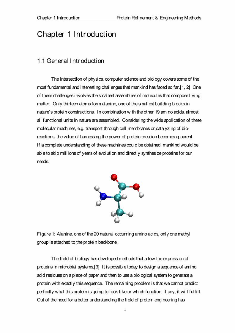
matter. Only thirteen atoms form alanine, one of the smallest building blocks in
nature’s protein constructions. In combination with the other 19 amino acids, almost
all functional units in nature are assembled. Considering the wide application of these
molecular machines, e.g. transport through cell membranes or catalyzing of bio-
reactions, the value of harnessing the power of protein creation becomes apparent.
If a complete understanding of these machines could be obtained, mankind would be
able to skip millions of years of evolution and directly synthesize proteins for our
needs.
Figure 1: Alanine, one of the 20 natural occurring amino acids, only one methyl
group is attached to the protein backbone.
The field of biology has developed methods that allow the expression of
proteins in microbial systems.[3] It is possible today to design a sequence of amino
acid residues on a piece of paper and then to use a biological system to generate a
protein with exactly this sequence. The remaining problem is that we cannot predict
perfectly what this protein is going to look like or which function, if any, it will fulfill.
Out of the need for a better understanding the field of protein engineering has

Chapter 1 Introduction Protein Refinement & Engineering Methods
��
evolved. The increased computational power, larger knowledge databases and deeper
physical understanding of recent years are driving this field forward.
The discipline of protein engineering deals with the design of new proteins
and aims at enhancing our understanding of fundamental processes on molecular
levels. For systems of atomistic sizes detailed real time observations are
experimentally not possible.[4] On the scale of atomic resolution where most of the
basic reactions in living organisms take place, only the combined efforts of these
disciplines can elucidate the unknown territory. Physicists have derived the
governing equations for systems at this scale during the last century. The
development of multi-core processors with billions of transistors and improved
numeric simulation libraries have made it feasible to apply the laws of physics to
system sizes of interest. Only recent advances in computational power, however,
allow the penetration of timescales with sufficient length for more complex
reactions.[5]
One of the most interesting and pressing questions deals with the prediction of
functional assemblies of atoms.[6] In nature these molecular machines are called
proteins. A goal of the field of protein engineering is to change and design proteins
so that they perform new and useful functions.[6] Unfortunately our understanding of
proteins is still limited; the way they form and find their native conformation, referred
to as protein folding, is a topic of current research.[7] Next to the design approach,
there is an ever-growing need to predict structure and functions of proteins.[8]
In this thesis the technique of molecular dynamics simulation (MD) will be
applied to some pressing open questions. The first question deals with the refinement
of protein structures in the context of the CASP11 competition. Protein refinement is
the act of further improving a three-dimensional representation of a protein that can
originate in low-resolution experiments or other computational predictions like
homology modeling. The CASP competition provided the environment to show how
MD simulations can be used to further improve protein structures obtained from
knowledge-based homology modeling. Furthermore, the fundamental principles that
allow this structure refinement will be analyzed on a benchmark set of homology

Chapter 1 Introduction Protein Refinement & Engineering Methods
��
models. The achievements in this area are due to a novel algorithm, based on
deformable elastic networks, which were introduced to the force fields used in the
MD technique. The statistical mechanics of this theory will also be explained. The
second important question aims at understanding the impact of protein mutations on
the function and substrate selectivity of a protein. The lipase LipA from Pseudomonas
aeruginosa will be the subject of a directed evolution study. If a directed evolution
study is performed only in the lab, amino acid sequence spaces of astronomical sizes
need to be expressed and screened in a random fashion. Computational methods can
provide a faster and cheaper alternative in order to search systematically through the
space of possible conformations. The last chapter introduces a computational pipeline
that will help predict mutational candidates in the protein, which lead to improved
activity for an industrial relevant substrate.
1.2 Computational Protein Engineer ing
Nature offers access to a vast array of proteins with different functions. For
many laboratory and industrial applications, enzymes are of greatest interest. These
specialized proteins can increase the reaction rates of chemical processes. The main
ability of an enzyme is its power to stabilize the transition state geometry of a
substrate and therefore to reduce the energy barrier that needs to be crossed along the
reaction coordinate. Unfortunately, the enzymes found so far in nature do not cover
all reactions important to mankind. Nevertheless, existing enzymes often support
reactions very similar to those of interest. This situation was the cradle for the idea of
protein engineering. In the early 1980s the field emerged with the goal of creating or
adapting proteins and enzymes to novel tasks or to enhance their natural
performances.[9] The first attempts to alter existing proteins went hand in hand with
arising high resolution protein structures obtained from x-ray crystallography. The
approach was coined rational design and involved manual investigation of the active
pocket of a protein. At this stage it was common to propose possible mutations to the
protein based on experience and instinctive feeling. Due to the lack of computational
power at this time, most success was achieved via experimental processes. It soon
became the predominant idea to create larger libraries of protein mutants and to
screen them for desired alterations. The process of iterative mutating and screening

Chapter 1 Introduction Protein Refinement & Engineering Methods
��
was called directed evolution, as it is an iterative procedure that selects always the
best performing mutations under certain artificial evolutionary pressures. This
method was successful in finding enantio-selective enzymes, enhancing stability and
catalytic rates, and even changing substrate selectivity.[10] But with the emergence
of ever faster super computers in the late 1990s, it became once more attractive to
approach the problem of protein design in-silico. The greatest successes are marked
by the creation of novel proteins and enzymes facilitating the Diels-Alder reaction and
the Kemp elimination following the “ inside out” approach proposed by Houk.[11]
But the main drawback of this is the reaction rates achieved by these designed
proteins. Even after further improvements through directed evolution rounds, they
remained over 8 magnitudes below the rates achieved by nature’s pendants.[12]
The computational approach to protein design has still a long way to go. So
far most successes have been strongly dependent on additional experiments in the
scope of directed evolution. Nevertheless, much can be learned from the lessons of
the past. The main point that can be taken from the vast amount of available data is
the requirement of a well-stabilized transition state geometry. Many more
sophisticated ideas involving protein dynamics and long-range interactions have been
proposed, but the consus at this point is that only a stabilized transition state yields
active mutants.[12, 13] It is not yet fully understood which method yields the best
quantification of the stability of the transition state. There are many computationally
expensive approaches involving quantum mechanical computations. There are also
very approximate methods in the field of docking simulations. The main problem one
has to keep in mind is that a successful method needs to include a tradeoff between
two factors: First, an accurate description of the transition state stability and second,
scalability that allows it to be applied to thousands of mutations. A review of the
most influential sources suggests that it is necessary to perform a high quality
parameterization of the transition state using quantum mechanical methods prior to
running more scalable simulations in Newtonian molecular dynamics simulations.[6,
11] The protocol described in the last chapter of this thesis will exploit these two
ideas to design a mutation evaluation scheme that can reasonably quickly search
through a large mutational space.

Chapter 1 Introduction Protein Refinement & Engineering Methods
��
1.3 Molecular Dynamics Simulations
It has always been a dream of mankind to look into the future.[14] The great
minds of the past have derived formulae and expressions that govern the classical
movement of rigid bodies.[15] But to predict the exact future of a system, an
analytical solution needs to be found for the equations of motion for each of its
constituents. Even in the simple case of having 3 balls in a box, no closed analytical
expression can be found to describe the motion for variable starting conditions. The
strong dependency of a system’s behavior on slight differences in the initial
conditions is commonly referred to as chaos.[16] If one imagines the world around us
as a gigantic box full of little balls that form all larger bodies, it becomes apparent
why one cannot predict the exact future. Even under the assumption of a fully
deterministic universe in which we know everything about the current state of each of
its particles, one could not calculate its future conformations. Despite this limitation
it might as well be a worthwhile goal to learn as much as one can through as little
approximations as possible.
Late Richard Feynman said, “…everything that is living can be understood in
terms of the jiggling and wiggling of atoms.” Understanding macroscopic objects
appears impossible because of the vast number of jiggling atoms. But this is not true
for the smallest conglomerates of atoms, the molecules. And the role of molecules is
of greatest importance to every aspect of life.[17, 18] Methods that can elucidate the
jiggling and wiggling of molecules are therefore paths that lead to a greater
understanding of life in all of its spheres. Of particular interest is the behavior of
proteins in the human body. Almost every biochemical reaction in the body involves
these macromolecules. Proteins are referred to as molecular machines because they
are often specialized workhorses that fulfill a certain task to perfection. They
regulate, for example, the trans membrane diffusion in living cells, perform important
roles in the immune system, or enable us to smell a rose. In order to understand the
function of a protein it is of greatest importance to know its structure and
dynamics.[18] At physiological temperatures the atoms inside a protein are never at
rest, but constantly moving about. The laws that govern this movement have been

Chapter 1 Introduction Protein Refinement & Engineering Methods
��
known for centuries. However, only in recent years feasible computer systems have
evolved that enable us to calculate the behavior of proteins.[5]
Because no analytical solution can be found to describe a system of many
hundreds of atoms, approximations have to be made. Molecular dynamics
simulations (MD) are one approach to gain structural and dynamical insights into
proteins. The main approximation made in an MD is the expression of all interatomic
forces in terms of a force field.[19-24] A detailed description of a force field is given
in a later section. With a force field, the Newtonian equations of motion can be
written out for each atom in a protein. These equations can then be solved by
numerical integration. There are many different algorithms that can be applied in
numerical integrations; some of the important ones are described in a following
section. A protein does not live in a vacuum. Solvent and other proteins surround it.
To understand the true behavior of a protein in its native environment, solvent and
boundary conditions have to be applied.[25, 26] The common choices for these
approximations are described in a later section as well. During a numerical
integration a lot of data is produced. The analysis of this data is an art in and of itself.
A later section describes common post processing tools to gain the most from a MD.
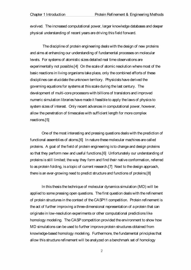
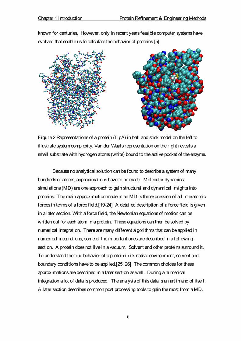
Figure 2 Representations of a protein (LipA) in ball and stick model on the left to
illustrate system complexity. Van der Waals representation on the right reveals a
small substrate with hydrogen atoms (white) bound to the active pocket of the enzyme.

Chapter 1 Introduction Protein Refinement & Engineering Methods
��
1.4 Equation of Motions and Numer ical Integrations
From the set of numerical integrators, perhaps the most elegant one is the
Verlet algorithm.[27] It is easy to implement and to derive as can be shown by the
following considerations. If a particle is at a position r at time t, then it can be
advanced to a time t + ∆t using Taylor expansion:
�푟푡+ ∆푡= 푟푡+
휕푟(푡)
휕푡∆푡+
1
2
휕!푟(푡)
휕푡!∆푡! +
1
6
휕!푟(푡)
휕푡!∆푡! + 푂(4) (1)�
For a time step into the past, Taylor expansion yields:
� 푟푡− ∆푡= 푟푡−
휕푟푡
휕푡∆푡+
1
2
휕!푟푡
휕푡!∆푡! −
1
6
휕!푟(푡)
휕푡!∆푡! + 푂(4) (2)�
� � �
The sum of these two equations can be rearranged to give the Verlet update:
� 휕!푟(푡)
휕푡!∆푡! = 2푟푡+
휕!푟(푡)
휕푡!∆푡! − 푟푡− ∆푡+ 푂(4) (3)�
From Newton’s second law[15] we can conclude that !!!(!)
!!!=
!(!)
!. The velocities can
be obtained by averaging ! " (!)
! "=
! !!∆! !! !!∆!
!∆!.
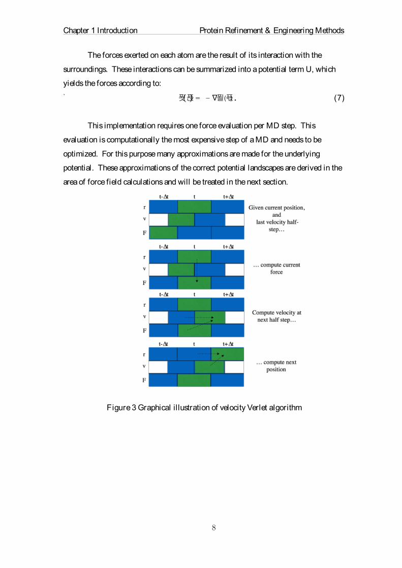
A more frequently implemented variation of this algorithm is the time
reversible and area preserving (symplectic) Velocity Verlet[28] formulation. Here the
position update occurs after a half step propagation of the velocity according to:
�휕푟푡+
12훥푡
휕푡=휕푟푡
휕푡+1
2
푓푡
푚훥푡
(4)�
�
푟푡+ ∆푡= 푟푡+휕푟(푡+
12훥푡)
휕푡∆푡
(5)�
and the final velocity update by:
�휕푟푡+ 훥푡
휕푡=휕푟푡+
12훥푡
휕푡+1
2
푓푡+ 훥푡
푚훥푡.
(6)�

Chapter 1 Introduction Protein Refinement & Engineering Methods
��
The forces exerted on each atom are the result of its interaction with the
surroundings. These interactions can be summarized into a potential term U, which
yields the forces according to:
`� 푓푡= −∇푈(푟).
(7)�
This implementation requires one force evaluation per MD step. This
evaluation is computationally the most expensive step of a MD and needs to be
optimized. For this purpose many approximations are made for the underlying
potential. These approximations of the correct potential landscapes are derived in the
area of force field calculations and will be treated in the next section.
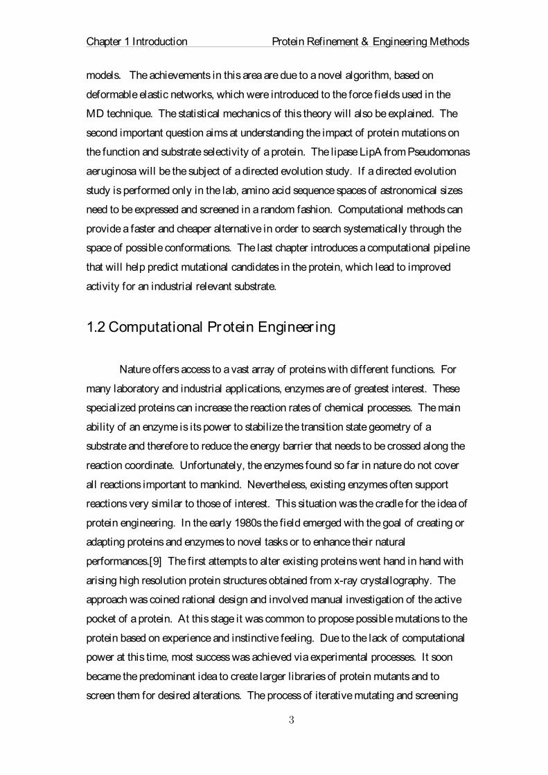
Figure 3 Graphical illustration of velocity Verlet algorithm

Chapter 1 Introduction Protein Refinement & Engineering Methods
��
1.5 Force Fields
For a perfect force calculation the time dependent Schrödinger equation would
have to be solved for all atoms and electrons in a model. Normal simulation times
require millions of iterations, which yield such a force evaluation infeasible. The
Born-Oppenheimer approximation simplifies the situation by assuming that electrons
instantaneously follow the nuclei and therefore only the position of the nuclei of the
atoms needs to be considered. In this thesis only classical force calculations will be
used for the MD. Instead of solving first principle equations, a set of parameters is
chosen to describe an atom and its interactions. Through rigorous derivations or
empirical fitting, these parameters have been identified and stored in the many
different force field databases that are available. All simulations in this work are
based on the parameters derived for the AMBER99SB-ILDN[30] force field.
The interactions that an atom can have may be sorted into two categories,
bonded and non-bonded.
� 푈푟 = 푈! " #$%$ 푟+ 푈! " ! ! ! " #$%$ 푟. (8)�
The bonded interactions consist of influences due to covalent bonds between
the atoms. Between two covalently bonded atoms one can imagine a spring with a
spring constant 퐾! and a minimum at a displacement 푏!. If three atoms are connected
in a chain an angle will form between the two bonds. These angles have preferred
values for the different atom types and bonds. The energy stored in an angle can
again be described by a harmonic potential term with a minimum at angle 휃! with a
spring constant of 퐾! . For four atoms in a chain the rotation between the planes
through the first and last two bonds is defined as the dihedral angle. The best fit for
this parameter is a trigonometric form. If three atoms are all connected to a fourth
atom they form an improper dihedral interaction. This is once again a quadratic term.
The sum of these contributions composes the bonded interactions and can be written
as such:

Chapter 1 Introduction Protein Refinement & Engineering Methods
��
�푈! " #$%$ 푟 =
1
2퐾! 푏− 푏!
!
! " #$%$
+ 1
2퐾! 휃− 휃!
! +1
2퐾! 휉− 휉!
!
!" #$%#&$ ! "!! " #$%! " #$%&
! " #$ ! " #$%&
+ 퐾휑 1 + cos 푚휑− 훿 .! " #! $"
! "!! " #$%&
(9)�
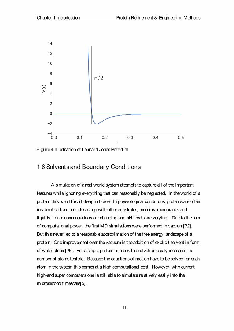
The non-bonded interactions are caused by the electric charge of the atoms,
the limitations imposed by the Pauli exclusion principle, and the ability to induce
dipoles. The first aspect is encompassed in the Coulomb term[31] dealing with
electrostatic interactions and the other aspects are approximated with the Lennard
Jones Potential[27]. This can be expressed as such,
�푈! " ! ! ! " #$%$ 푟 = (
퐶!"푟!"
−퐶!푟!
! "#$! " #$%
) + 푞!푞!
4 휋휖!휖!푟! "#$! " #$%
. (10)�
The non-bonded energy is mainly a function of the distance between two
atoms. The parameters 퐶!" and 퐶!define the Lennard-Jones interaction, qi and qj are
the charges of the atoms i and j, 휖! is the electric constant, and 휖! denotes the relative
dielectric permittivity.
In addition to the physics-based energy terms, a force field might need to be
extended for certain applications. For example in the protein structure refinement
process described in this thesis, it is necessary to introduce restraints on certain atoms.
Adding other energy terms can achieve this.

Chapter 1 Introduction Protein Refinement & Engineering Methods
��
1.6 Solvents and Boundary Conditions
A simulation of a real world system attempts to capture all of the important
features while ignoring everything that can reasonably be neglected. In the world of a
protein this is a difficult design choice. In physiological conditions, proteins are often
inside of cells or are interacting with other substrates, proteins, membranes and
liquids. Ionic concentrations are changing and pH levels are varying. Due to the lack
of computational power, the first MD simulations were performed in vacuum[32].
But this never led to a reasonable approximation of the free energy landscape of a
protein. One improvement over the vacuum is the addition of explicit solvent in form
of water atoms[26]. For a single protein in a box the solvation easily increases the
number of atoms tenfold. Because the equations of motion have to be solved for each
atom in the system this comes at a high computational cost. However, with current
high-end super computers one is still able to simulate relatively easily into the
microsecond timescale[5].
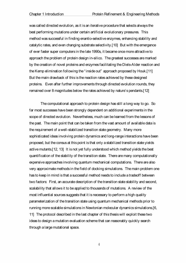
Figure 4 Illustration of Lennard Jones Potential

Chapter 1 Introduction Protein Refinement & Engineering Methods
��
It is difficult to exchange particles in a running simulation[33]. It is therefore
common practice to add salt ions to the solvent before starting a simulation. This
allows for physiological salt concentration and can compensate possible charges of
the protein. For a protein in a box it is always dangerous if it drifts towards the
borders of the box. Edge effects can occur that have nothing to do with the real
dynamics of the proteins[34]. To compensate for this it is common practice to include
periodic boundary conditions. These allow the protein to diffuse through one wall of
the system and to enter back in through the opposite one. One problem with this is
that the protein may be able to interact with itself, if the box is too small. Therefore it
is often required to enlarge the box, and therewith the number of solvent atoms, if
periodic boundary conditions are to be applied.
Oftentimes the simulations are desired to happen in the canonical ensemble
with a constant number of particles, and constant pressure and temperature. This can
be ensured through the addition of thermostats[35, 36] next to the periodic boundary
conditions. In some situations it is unavoidable to have to sacrifice the accuracy of
explicit simulations for a gain of speed through implicit solvation. An implicit
solvent is a continuous medium, which has interactions that are defined by a set of
derived constants.[25] For testing thousands of proteins in simulations it becomes
necessary to replace the explicit with the implicit solvent. One point in favor of this
approximation is the deterministic effect of the solvent. For short simulations the
potential energy terms of different systems become more easily comparable for
implicit solvent. This fact will be used in the last chapter of this thesis, which deals
with the redesign of a phospholipase.
1.6 Energy Minimization
A typical protein structure as obtained from the Protein Data Bank (PDB) is
described as a set of three-dimensional coordinates of all heavy atoms. The distances
and angles in such a structure are usually optimized to one set of force field
parameters. Because it might not necessarily be the same force field as chosen for
further processing, an initial energy minimization is required prior to other MD steps.
Such a procedure will resolve high-energy clashes that could otherwise yield non-

Chapter 1 Introduction Protein Refinement & Engineering Methods
��
physical solutions. All energy minimizations in this thesis are conducted via the
steepest descent algorithm as implemented in GROMACS.
The fundamental idea of steepest descent can be described as running down a
hill. Given a position along the hillside one looks for the direction that shows the
steepest slope downwards and takes a step in that direction. In the new position the
optimal new direction is again searched for. This is repeated until the next local
energy minimum is found, a position where no direction yields a slope downward
beyond a predefined cut-off. If the step size is too small, such a procedure has bad
convergence. If it is too large, then the risk of overshooting exists. Therefore it is
necessary to adapt the step size during the minimization.
The algorithm as implemented has the following form. First, the force vector
on all atoms is calculated according to
� 푓푘 = −∇푈(푟). (11)�
Here U(r) denotes the potential energy as evaluated in the force field and k the
integration step. Next the position of each atom is shifted along the direction of the
force by the magnitude of the step size s,
�푟푘+ 1 = 푟푘 +
푓푘
max(푎푏푠푓(푘) )∗푠. (12)�
The step size is then adapted according to the rule
� 푖푓 (푈푟!!! < 푈푟! , 푠!!! = 1.2 ∗푠!�
푖푓 (푈푟!!! ≥ 푈푟! , 푠!!! = 0.2 ∗푠!.�(13)�
This iteration is repeated until k reaches the predefined number of steps, a
local minimum is found, or the algorithm converges to machine precision.

Chapter 1 Introduction Protein Refinement & Engineering Methods
��
1.7 Analysis of MD Trajector ies
At the end of a simulation it is always necessary to analyze the produced data.
Because of the very high number of degrees of freedom inside a protein, a lot of noise
will cover the most essential signal from a simulation. If one is interested in the
function of a protein, then the main structural change becomes important. One
elegant way of filtering the signal from the noise is the method of principal
component analysis.[37] In this technique a new set basic vectors is found that will
only display the movement of a protein along the greatest variance. This is usually
achieved through diagonalization of the covariance matrix of all Cα atoms and
determination of the eigenvector associated with the largest eigenvalue. Another
method that is commonly used to determine the best structure from an ensemble of
MD frames is[38] averaging. Alignment is a simple procedure that aligns proteins to
each other and then computes the average position in Cartesian space for each atom.
This technique is frequently used in the determination of refined structures from MD
refinement methods.

Chapter 2 Protein Refinement Protein Refinement & Engineering Methods
!!
Chapter 2 Protein Refinement
2.1 General Introduction to Protein Refinement
Protein function is closely related to protein structure. Though physiological
temperatures generate an ensemble of protein conformations referred to as the
Boltzmann ensemble, it is common practice to associate a protein with a single crystal
structure. These structures can be obtained from experiments but are often difficult to
observe due to expression and crystallization challenges posed by the protein. An
interesting alternative to lab experiments and expensive synchrotron X-ray methods is
an in-silico prediction of an unknown protein structure. These predictions typically
rely on already existing structures from proteins that are similar in sequence.
Sequence related proteins are referred to as sequence homologs and have the
marvelous attribute of having almost the same conformation in space. Structure of
proteins is better conserved than sequence, meaning that sequence identities down to
50 % still end up in the same structural fold.
The best homology building tools are able to predict high quality structures,
but these structures are not perfect. The aim of protein refinement is to further
improve the best models achievable. The international blind test Critical Assessment
of Protein Structure Prediction (CASP) is a biannually competition in which groups
from across the world compare their refinement protocols. This chapter describes the
development of a protein refinement protocol that was used with some derivations in
the CASP11 competition. The report on CASP11 is given in the next chapter.
The work contained in this chapter has been submitted for peer review and
follows the guidelines of a short communication with supplement material. This work
is based mainly on the PhD thesis of Andre Wildberg and was compiled in close
collaboration with him.
!

Chapter 2 Protein Refinement Protein Refinement & Engineering Methods
!!
2.2 Abstract
Atomic models of proteins built by homology modeling or from low-
resolution experimental data may contain considerable local errors such as wrong
loop conformations, errors in side-chain packing, or shifts of secondary structure
elements. The refinement success of molecular dynamics simulations is usually
limited by both force field accuracies and by the substantial width of the
conformational distribution at physiological temperatures. We propose a method to
overcome these problems by coupling homologous replicas during a molecular
dynamics simulation, which narrows the conformational distribution, smoothens and
even improves the energy landscape by adding evolutionary information. The
coupling of replicas mainly changes slow dynamics but leaves fast dynamics mostly
unperturbed, which means that the important solvent interaction and therefore the
solvation free energy is not strongly affected by the replica coupling. We show that
our method yields consistent improvement of protein models.
2.3 Introduction
The interpretation of genomics data in terms of protein structure is an
important post genomic challenge. Building atomic models for individual amino acid
sequences becomes increasingly important to understand the molecular effects of
genetic variation. Homology modeling is a useful tool to build atomic models if the
structure of an homologous protein is known. However, due to the limitation of
current methodology such models of protein structures may contain considerable
errors. Similarly, atomic models built with low-resolution (e.g. from X-ray
diffraction or cryo-EM) or sparse experimental data might contain comparable errors.
Refinement approaches have the goal of correcting these errors in atomic
protein models. The types of errors we consider as being amenable to refinement
include disrupted hydrogen bond networks, small shifts of secondary structure
elements, incorrect side-chain packing and rotamers, and wrong loop conformations.
Correcting such errors is typically challenging since the energy differences between
alternative, slightly different conformations are rather small. The Critical Assessment

Chapter 2 Protein Refinement Protein Refinement & Engineering Methods
!!
of Structure Prediction (CASP) experiment has a refinement category to test the
performance of refinement methods [40, 41].
Regular molecular dynamics (MD) simulations are generally unable to refine
homology models and do not consistently yield a structure that is moved closer to the
"correct" structure (as usually determined by high-resolution X-ray crystallography)
[42]. Even though MD simulations can sample closer-to-native structures, reliably
selecting these structures is not possible [43].
The main causes for this limitation of MD simulations are 1) force field
inaccuracies [44], 2) high energy barriers that need to be crossed, and 3) the fact that
the Boltzmann distribution, which is approximated by the MD simulation, is broad at
physiological temperatures. Simulation at physiological temperatures is however
necessary to correctly describe the influence of the entropy; only then is the free
energy of conformational states correctly described.
Position restraints have been used successfully to prevent the simulation from
exploring the broad Boltzmann distribution; these restraints force the structure to
sample a region around the starting model, which also leads to sampling closer-to-
native structures with higher probability [44-46]. Position restraints however also set
an upper limit to the extent of the conformational change, which might hinder
sufficient sampling and refinement.
The goal of structure refinement is to determine the most probable
conformation, which corresponds to the free energy minimum, rather than the
conformational distribution. It has been shown that the most probable conformation
can be approximated by averaging the structures from an MD ensemble more robustly
than by selecting a single structure with a scoring function[45, 46]. However, for the
averaging to yield a good structure requires the simulation to predominantly sample
near native structures.

Chapter 2 Protein Refinement Protein Refinement & Engineering Methods
!!
2.4 Method
We here present in two steps a modified MD protocol that addresses all three
problems of regular MD simulations mentioned above (force field inaccuracies, high
energy barriers, broad Boltzmann distribution).
In the first modification step, we simulate simultaneously eight identical
replicas of the starting structure. These replicas are subjected to the same harmonic
position restraints (on Cα-atoms), which forces them to remain similar to each other.
The positions of the restraints are constantly updated during the simulation and slowly
follow the motion of the center of mass of all replicas. These adaptive restraints were
inspired by deformable elastic network restraints (DEN), which have been shown to
guide structure refinement against X-ray diffraction and cryo-EM data [47-49]. Since
the restraints are adaptive, the coupled replicas are allowed to undergo any
conformational motion as long as they stay close together.
The harmonic restraints restrict larger motions more than smaller motions,
which leads to a time-scale dependent diffusion coefficient (cf. Supplementary Fig.
1). For small time-scales the size of the diffusion coefficient is comparable to that of
free MD simulations, which enables individual replicas to cross local energy barriers.
In addition, entropic contributions of solvent and side-chains (which are not
restrained) are not strongly affected, which means that in particular the solvation free
energy is mostly unperturbed. For longer time-scales the diffusion coefficient
decreases significantly, which reduces large conformational fluctuations. Smaller
fluctuations mean that the system of coupled replicas is less likely to drift in random
directions and will sample low free energy states more frequently than a free MD
simulation. Furthermore, the coupling of replicas has an effect of smoothening the
energy landscape, similar to particle swarm optimization, which has been applied to
MD simulations before [50]. The motion of the center of mass is the result of an
effective force averaged over all replicas. Because the replicas are in different
positions on the energy landscape the center of mass moves on a locally averaged, i.e.
smoothened energy landscape.


Chapter 2 Protein Refinement Protein Refinement & Engineering Methods
!!
In the second modification step, the target sequence in seven of the replicas is
replaced with homologous sequences. This is motivated by the observation that
structure is much more conserved than sequence which causes homologous proteins
to fold into similar structures [51]. This fact can be exploited by coupling
homologous proteins (with pairwise sequence identity of at least 50%) instead of
identical replicas during a MD simulation. Keasar et al. [52-54] have proposed that
such a coupling of homologous proteins with slightly different energy landscapes
results in an energy landscape that is smoothened not only in structure space but also
in sequence space. The methodology was implemented in the GROMACS 4.5.3 [55]
software (see Online Methods).
2.5 Results
To benchmark our approach a representative test set of 5 homology models
was selected from the Badretdinov decoy set [56] (see Supplementary Table 1) and
simulated 5 times for 10 ns each. We compared three different simulation protocols:
1) a free MD simulation of the homology model, 2) coupled identical replicas, and 3)
coupled homologous replicas.

Chapter 2 Protein Refinement Protein Refinement & Engineering Methods
!!
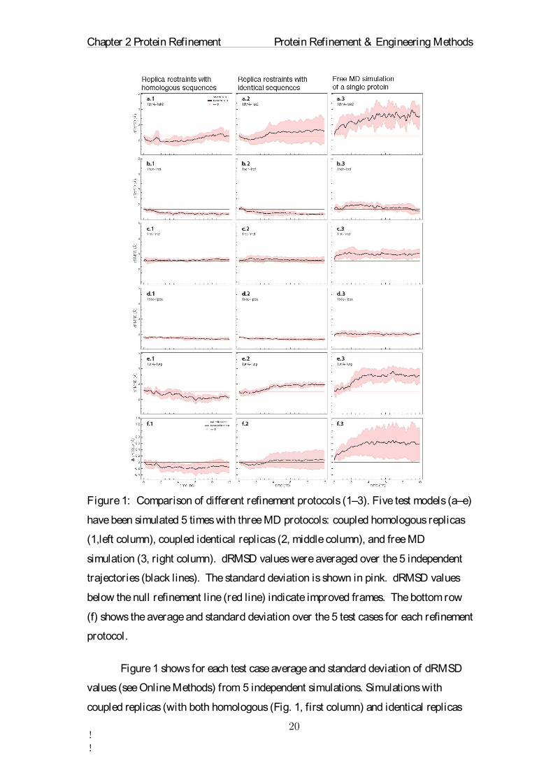
Figure 1: Comparison of different refinement protocols (1–3). Five test models (a–e)
have been simulated 5 times with three MD protocols: coupled homologous replicas
(1,left column), coupled identical replicas (2, middle column), and free MD
simulation (3, right column). dRMSD values were averaged over the 5 independent
trajectories (black lines). The standard deviation is shown in pink. dRMSD values
below the null refinement line (red line) indicate improved frames. The bottom row
(f) shows the average and standard deviation over the 5 test cases for each refinement
protocol.
Figure 1 shows for each test case average and standard deviation of dRMSD
values (see Online Methods) from 5 independent simulations. Simulations with
coupled replicas (with both homologous (Fig. 1, first column) and identical replicas

Chapter 2 Protein Refinement Protein Refinement & Engineering Methods
!!
(Fig. 1, second column)) show clear improvement over regular free MD simulations
(Fig. 1, third column). In free MD simulations the structure drifted away from the
correct structure in all cases except for 1hdn-1ptf, where a small number of frames
was improved. In simulations with identical replicas 51 % of the frames were
improved on average, but the improvements are small fluctuations around the null
refinement (horizontal red line). In contrast, simulations with homologous replicas
consistently improve the structure and sample conformations closer to the native
structure most of the time.
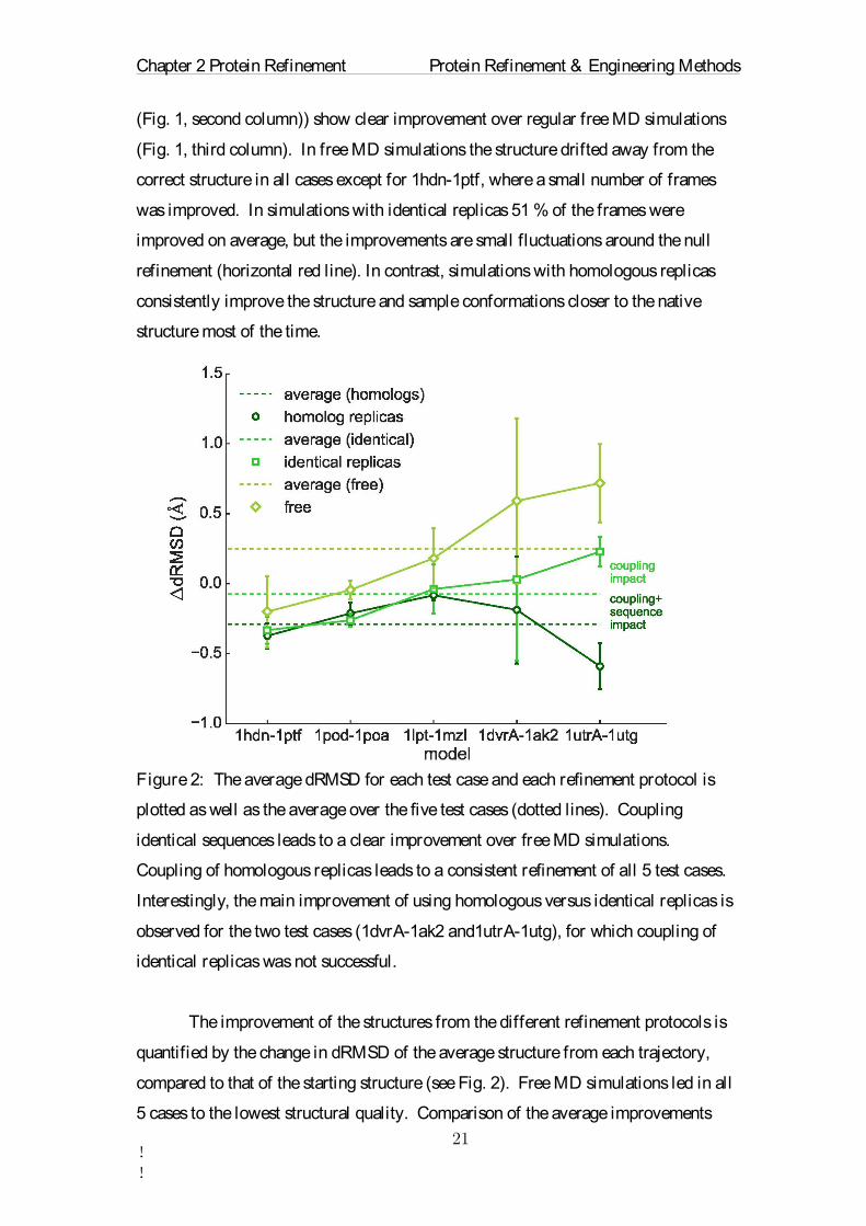
Figure 2: The average dRMSD for each test case and each refinement protocol is
plotted as well as the average over the five test cases (dotted lines). Coupling
identical sequences leads to a clear improvement over free MD simulations.
Coupling of homologous replicas leads to a consistent refinement of all 5 test cases.
Interestingly, the main improvement of using homologous versus identical replicas is
observed for the two test cases (1dvrA-1ak2 and1utrA-1utg), for which coupling of
identical replicas was not successful.
The improvement of the structures from the different refinement protocols is
quantified by the change in dRMSD of the average structure from each trajectory,
compared to that of the starting structure (see Fig. 2). Free MD simulations led in all
5 cases to the lowest structural quality. Comparison of the average improvements

Chapter 2 Protein Refinement Protein Refinement & Engineering Methods
!!
(Fig. 2, dashed lines) shows an offset between free MD simulation and coupling of
identical replicas, which can be attributed to the particle swarm optimization effect.
More importantly another offset can be seen between coupling with identical and with
homologous replicas, which represents the improvement that is due to the added
evolutionary information and which we interpret as an improvement of the force field.
Only for 1lpt-1mzl, which has the lowest starting quality of 3.8 Å RMSD, the average
dRMSD was not improved (see Fig. 1 c.1), however, the dRMSD of the average
structure was slightly improved (Fig. 2), clearly showing the benefit of structural
averaging[45].
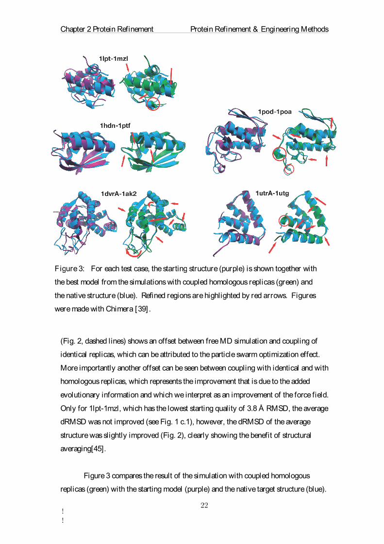
Figure 3 compares the result of the simulation with coupled homologous
replicas (green) with the starting model (purple) and the native target structure (blue).
Figure 3: For each test case, thestarting structure (purple) is shown together with
the best model from the simulations with coupled homologous replicas (green) and
the native structure (blue). Refined regions are highlighted by red arrows. Figures
were made with Chimera [39] .

Chapter 2 Protein Refinement Protein Refinement & Engineering Methods
!!
Several secondary structure elements and loop regions are shifted towards the correct
structure. In contrast to free MD simulations, the coupled-replica simulations yielded
very consistent results: the average structures from 5 independent simulations are very
similar, as visualized in Supplementary Fig. 2 by multi-dimensional scaling [57].
2.6 Conclusion
We found that refinement with coupled homologous replicas outperforms
regular MD simulations in all test cases. Recently, we applied our method in the
CASP11 experiment and could improve 65 % of the targets, with an average increase
in GDT-HA score by 6.6 for the improved models. The additional evolutionary
information and the reduction in global fluctuations through coupling of homologous
replicas leads to consistently sampling structures closer to their native state compared
with free MD simulations. This insight will help to develop even more powerful
refinement methods based on MD.
2.7 Online mater ial - Methods
Distance root mean square deviation (dRMSD).
The dRMSD is used to measure the deviation of two atomic models. It is
calculated as the root mean square deviation of corresponding pairs of Cα-atom
distances in two structures. All possible pairs of Cα-atoms were considered.
Implementation of replica coupling in GROMACS 4.5.3.
For the replica-coupled simulations, the simulation box was composed of 8
replicas, which are positioned at the edges of a cube. The distance between the
replicas needs to be large enough to avoid electrostatic interactions between the
replicas.
The replicas are coupled through adaptive position restraints on all Cα-atoms.
GROMACS does not by default support dynamic updates of position restraints during
a simulation. We implemented the necessary changes into the source code of Gromacs

Chapter 2 Protein Refinement Protein Refinement & Engineering Methods
!!
4.5.3 [55] to enable updates without reducing the speed of GROMACS. We
implemented the changes only for domain decomposition runs (in source code file
domdec.c).
For each Cα-atom i in each replica j a position restraint 풑!,!!is defined on its
initial position. The time dependent energy term for the position restraints is given by
퐸posre(푡)= 푤! 풙!,!(푡)− 풑!,!(푡)!!!!!!!!!!!!!!!!!!!!!!!!!!!!!!!!!!!!!!!!!!!(1)
!
!!!
!
!!!
with the coordinates!풙!,!!of Cα-atom i in replica j, the number of atoms N, and the
number of replicas M which we chose to be 8. The force constant w was set to 100
kJ/(mol nm2). After a period, n, of 500 steps the position restraints are updated
according to:
풑!,! 푡+ 푛∗Δ푡= 풑!,! 푡+ 휅!풙!,! 푡− 풑!,! 푡 !!!!!!!!!!!!!!!!!!!!!!!!!!!!!!!!!(2)
with the integration timestep ∆t of 2 fs. The relaxation rate κ at which the position
restraints follow the average coordinate displacement was set to 0.5. The same
displacement vector 풙!,! 푡− 풑!,! 푡 !!, which is an average over the corresponding
displacements in all replicas j, is added to all replicas, which leads to a coupling of
the replicas. These adaptive restraints were inspired by deformable elastic network
(DEN) restraints, which yield a similar effect for a γ-value of 1. The original DEN
method employs a network of (also long) distance restraints, which cannot efficiently
be parallelized with domain decomposition. We therefore decided to use adaptive
position restraints.
For identical replicas the assignement of corresponding atoms in different
replicas is trivial. However, in case of homologous replicas, a multisequence
alignment is performed to assign each Cα-atom from the starting sequence to the
corresponding Cα-atoms in the homologs. If there are no gaps or insertions the
assignment is again trivial. If the alignment shows a gap for k sequences at a certain
amino acid position, then position restraints are applied and averaged only for the

Chapter 2 Protein Refinement Protein Refinement & Engineering Methods
!!
remaining (8-k) residues that are present at this position, which means that the
displacement vector will be averaged over (8-k) replicas. Insertions will not generate
extra position restraints; those residues instead are kept unrestrained and are free to
move. The total number of position restraints is therefore always identical to the
number of Cα-atoms in the target sequence.
Method availability.
The modified GROMACS version with adaptive position restraints to couple
multiple replicas is available from the SimTK website: http://simtk.org/home/adpt-
gromacs.
MD Protocols.
All simulations used the AMBER99SB-ILDN force field with TIP3P explicit
water with an integration time step of 2 fs. Temperature was kept constant at 300 K
by the Nosè-Hoover algorithm. Electrostatic long-range interactions were calculated
with PME and bond-lengths were constrained by the P-LINCS approach. Na+/Cl- ions
were added at physiological concentration. Before and after adding the solvent
molecules, the structure was energy minimized to remove any sterical clashes that
may be the result of homology model building.
Each simulation was repeated 5 times with duration of 10 ns. For comparison
we performed three different simulation protocols: 1) free MD simulation of a single
protein structure, 2) replica-coupled simulation with identical sequences, and 3)
replica-coupled simulations with homologous sequences. The computational expense
for the replica-coupled simulations is much larger than for the single MD simulations,
since the simulation system is eight times larger. The total amount of simulation time
equals a single protein simulation in solvent for 4.25 μs.

Chapter 2 Protein Refinement Protein Refinement & Engineering Methods
!!
Sequence Selection Strategy.
To build the homologous replicas, seven homologous sequences were
searched via BLAST [58] on the RefSeq [59] database. Sequences were manually
selected that fulfilled two criteria: 1) their sequence identities with the target sequence
needs to be between 50 and 80 %, and 2) the sequence identities between all pairs of
the 8 sequences should ideally also be in the range 50–80 %. However, for some test
cases the second criterion could not be strictly fulfilled. The sequences chosen haven
an average sequence identity of 61.8 % to the target structure and are shown in
Supplementary Table 2. The homology models used as the replicas were generated
with MODELLERv9 [60].
Test case selection strategy.
Homology models from the Badretdinov decoy set[56] were chosen as test
cases. We aimed to cover a wide range of protein properties, such as size, secondary
structure composition and shape. The five homology models that were selected
represent starting qualities between 2-4 Å RMSD to the solved crystal structure. The
sequence lengths vary between 70 and 220 amino acids. The details of the selected
models are shown in Supplementary Table 1. The naming scheme of the models is
xxxxX-yyyy, where xxxx and yyyy are the PDB IDs of the the template and the
target, respectively, and X is the chain ID of the target.
ACKNOWLEDGMENTS
The authors gratefully acknowledge the computing time granted on the
supercomputer JUROPA at Jülich Supercomputing Centre (JSC).

Chapter 2 Protein Refinement Protein Refinement & Engineering Methods
!!
2.8 Supplemental Mater ial
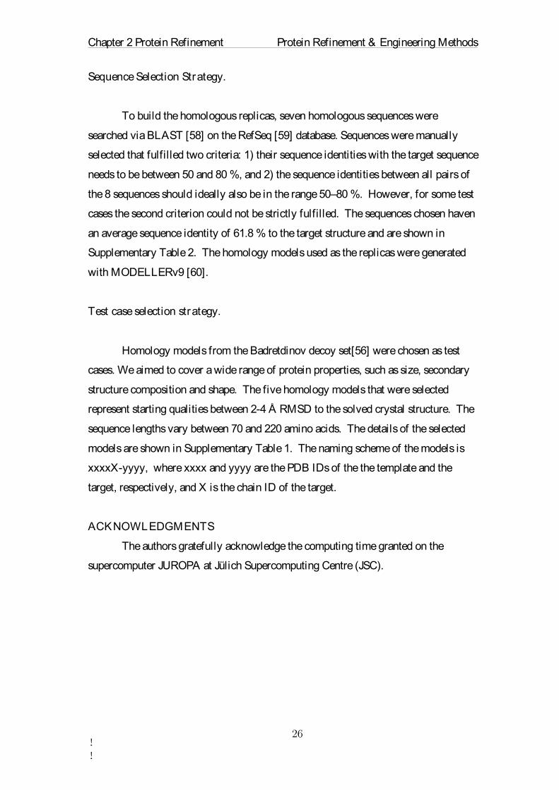
Supplementary Figure 1: Mean square displacement as a function of time is shown
as an example for the 1utrA-1utg test case for different simulation protocols. All
simulations were performed at a temperature of 300 K. The gradient is proportional
to the diffusion coefficient. The free MD simulation (black) has the largest diffusion
coefficient. For MD simulations with position restraints the diffusion coefficient is
decreasing with increasing strength of position restraints. For comparison a
simulation with 8 coupled identical replicas was performed where the coupling of the
replicas was achieved by adaptive position restraints with a strength of 100 kJ/mol.
Interestingly, the simulation with the coupled replicas shows a strongly timescale-
dependent diffusion coefficient. For small timescales the diffusion is similar to a free
MD simulation, but for larger timescales the diffusion coefficient is similar to the
position restrained simulation with a restraint strength of 1000 kJ/mol. This allows
small and fast motions such as those of side-chains and solvent molecules to be rather
unperturbed, while at the same time, large scale conformational fluctuations of the
protein structure are suppressed.
0 10 20 30 40 50Time (ps)
0
0.01
0.02
0.03
0.04
0.05
Me
an s
qua
re d
ispl
ace
men
t (nm
^2)
Free MD simulation
Restrained MD (10 kJ/mol)
Restrained MD (100 kJ/mol)
Restrained MD (1000 kJ/mol)
MD with 8 coupled replicas

Chapter 2 Protein Refinement Protein Refinement & Engineering Methods
!!
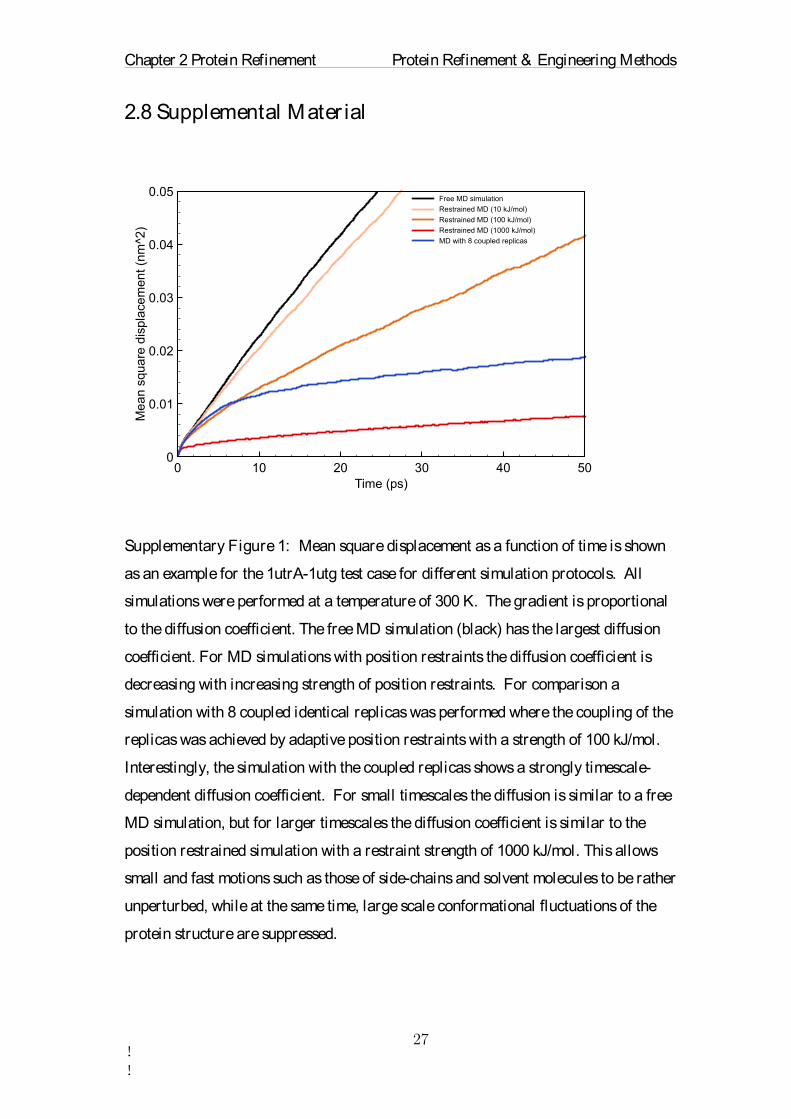
Supplementary Figure 2: Shown are multi-dimensional scaling plots based on the
dRMSD values between all pairs of structures. dRMSD distances between structures
are preserved as closely as possible in these two-dimensional representations. For
each test case and each refinement protocol, 5 independent simulations were
performed. The simulations with the coupled replicas (identical replicas in cyan,
homologous replicas in blue) yield consistent structures, i.e. the average structure
from each independent simulation is similar to each other, while the structures from
the free MD simulation are much farther apart from each other and also from the

Chapter 2 Protein Refinement Protein Refinement & Engineering Methods
!!
target structure (green). Free MD simulations drift away more randomly and less
directed towards the target than the coupled replicas. The multi-dimensional scaling
was performed with MDSJ (Algorithmics Group. MDSJ: Java Library for
Multidimensional Scaling (Version 0.2). Available at http://www.inf.uni-
konstanz.de/algo/software/mdsj/. University of Konstanz, 2009).
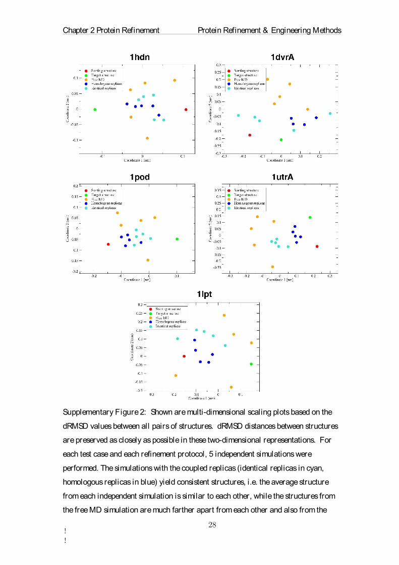
MODEL
(PDB-ID)
#atoms
Cα/all
RMSD
(Å)
dRMSD
(Å)
1dvrA-1ak2 220/3452 2.790 2.250
1hdn-1ptf 87/1297 2.150 1.712
1lpt-1mzl 93/1240 3.887 2.572
1pod-1poa 118/1730 2.347 1.860
1utrA-1utg 70/1116 3.002 2.509
Supplementary Table 1: The 5 test cases chosen from the Badretdinov decoy set
(http://salilab.org/decoys/) and their root mean square deviation (RMSD) and
distance root mean square deviation (dRMSD) from the corresponding native
structures.

Chapter 2 Protein Refinement Protein Refinement & Engineering Methods
!!
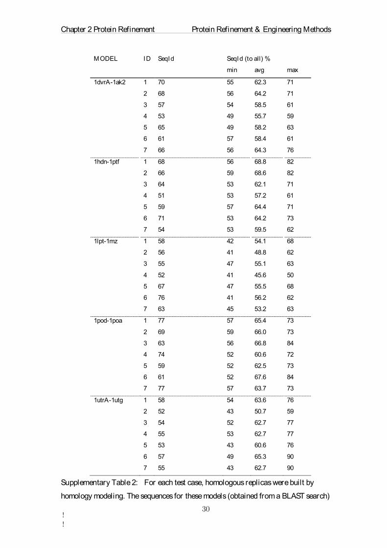
Supplementary Table 2: For each test case, homologous replicas were built by
homology modeling. The sequences for these models (obtained from a BLAST search)
MODEL ID SeqId SeqId (to all) %
min avg max
1dvrA-1ak2 1 70 55 62.3 71
2 68 56 64.2 71
3 57 54 58.5 61
4 53 49 55.7 59
5 65 49 58.2 63
6 61 57 58.4 61
7 66 56 64.3 76
1hdn-1ptf 1 68 56 68.8 82
2 66 59 68.6 82
3 64 53 62.1 71
4 51 53 57.2 61
5 59 57 64.4 71
6 71 53 64.2 73
7 54 53 59.5 62
1lpt-1mz 1 58 42 54.1 68
2 56 41 48.8 62
3 55 47 55.1 63
4 52 41 45.6 50
5 67 47 55.5 68
6 76 41 56.2 62
7 63 45 53.2 63
1pod-1poa 1 77 57 65.4 73
2 69 59 66.0 73
3 63 56 66.8 84
4 74 52 60.6 72
5 59 52 62.5 73
6 61 52 67.6 84
7 77 57 63.7 73
1utrA-1utg 1 58 54 63.6 76
2 52 43 50.7 59
3 54 52 62.7 77
4 55 53 62.7 77
5 53 43 60.6 76
6 57 49 65.3 90
7 55 43 62.7 90


Chapter 2 Protein Refinement Protein Refinement & Engineering Methods
!!
were selected to have a sequence identity to the target sequence (third column, SeqId)
of between 50 and 80%. Furthermore, the sequences were chosen to have low
pairwise sequence identities to each other, as indicated by the SeqId(to all) values.

Chapter 3 CASP11 - Refinement Protein Refinement & Engineering Methods
!!
Chapter 3 CASP 11 Protein Refinement
3.1 GENERAL INTRODUCTION TO CASP11
This chapter contains the application of the protocol introduced in Chapter 2.
The eleventh iteration of the CASP competition took place between April 2014 and
December 2014. Over the course of 3 months, multiple protein structures were
released from predictors for further refinement. Each target had a prescribed deadline
of about 3 weeks for the refinement process. Due to the computational expense of our
method, a grant for the super computer JUROPA was secured. In total, 37 targets
were released and refined by our method.
In conclusion of the challenge a final meeting was held in Mexico and the best
performing groups were announced. The assessor ranked our method as second best
for initial model submissions. In the context of this successful evaluation an
invitation was extended to publish the results in a special issue of PROTEINS.
The text of this chapter contains the final results as submitted to PROTEINS
and is based on the application of a modified protocol as previously discussed. The
author, under very helpful supervision of Professor Schröder, has performed the
experiments, analysis and formulation by himself. The format is of a full research
article as prescribed by PROTEINS.
3.2 ABSTRACT
A novel protein refinement protocol is presented which utilizes molecular
dynamics simulations of an ensemble of adaptively restrained homologous replicas.
This approach adds evolutionary information to the force field and reduces random
conformational fluctuations by coupling of several replicas. It is shown that this
protocol refines the majority of models from the CASP11 refinement category and
that larger conformational changes of the starting structure are possible than with
current state of the art methods. The performance of this protocol in the CASP11

Chapter 3 CASP11 - Refinement Protein Refinement & Engineering Methods
!!
experiment is discussed. We found that the quality of the refined model is correlated
with the structural variance of the coupled replicas, which therefore provides a good
estimator of model quality. Furthermore some remarkable refinement results are
discussed in detail.
3.3 INTRODUCTION
Understanding protein function, folding, and interactions requires detailed
knowledge of protein structures. The determination of protein structures, e.g. by X-
ray crystallography, is usually time-consuming, challenging and sometimes not even
possible with current methods.[61, 62] The correct prediction of protein structures
from amino acid sequences is therefore a very important problem[63]. Protein
structure prediction is most successful if the structure of a protein with a similar
sequence is already known, which can then be used as a template for modeling.[64-
67] The achieved template-based models have approximate root mean square
deviations (RMSD) of 2 – 6 Å to the corresponding experimentally determined
structures.[68, 69] This deviation is mainly caused by an insufficient number of
highly homologous structures in the Protein Data Bank and the structural differences
between those that are available The field of protein structure refinement has the
goal to bridge the gap between prediction and experimental accuracy. The Critical
Assessment of Protein Structure Prediction (CASP) experiment is a biennial
community-wide blind test, which introduced a refinement category in 2004.[70] In
this category of CASP, participants test their refinement protocols on protein models
that were predicted earlier in the same round of CASP and that were selected by the
organizers as refinement targets. Over the last years the interest in the refinement
problem has consistently grown. This is reflected in the increasing number of
refinement targets handed out to the predictors during the last CASP experiments as
well as in the steadily growing number of participating groups.[68, 71]
Over the last 50 years various approaches have been proposed to solve the
refinement problem. The earliest methods used vacuum energy minimization to find
the closest potential energy minimum [72], and were further improved with better

Chapter 3 CASP11 - Refinement Protein Refinement & Engineering Methods
!!
parameterizations [73, 74]. With increasing computational power the impact of
solvent became more apparent.[75] Different sampling methods have been used,
from Monte-Carlo Methods[76] over fragment guided simulations[77] and
knowledge-based refinements[78-80] to physics-based molecular dynamics (MD)
simulations[81-83]. The most recent advances in the refinement field by the Feig
group indicate that MD simulations have the potential to refine predicted protein
models consistently.[84, 85]
Our approach to refine protein structures employs MD simulations with
coupled homologous replicas, as is described in detail below. The performance of our
method during the CASP11 experiment is presented and the results for the 37 released
targets are analyzed in detail. We find that our method has a high chance of improving
a model if the quality of the starting structures lies in an intermediate range of initial
model quality. Finally, we demonstrate how the model quality can be estimated even
when the quality of the starting structure is not known.
3.4 METHOD
The main idea of our refinement protocol is the improvement of a physical
force field through the addition of an extra parameter that incorporates evolutionary
information. We present a modification of the classical MD approach that improves
the sampling of native protein conformations and yields, therefore, better refinement
results than standard MD simulations. Our approach has two components: 1)
simulation of an ensemble of restrained replicas and 2) coupling of homologous
sequences. In the following we motivate the choice of this approach. A single
protein will usually drift quickly away from its native structure during a standard
room temperature MD simulation, which is caused by thermal fluctuations, random
start conditions, as well as inaccuracies of the force field. Position restraints can
suppress this effect and force the protein to sample a region around the start
conformation. The disadvantage of such restraints is however that the protein cannot
progress far towards the native structure and therefore often does not yield optimal
refinement results.[84] Our approach is devised to reduce large fluctuations and at the

Chapter 3 CASP11 - Refinement Protein Refinement & Engineering Methods
!!
same time allow for large conformational changes. For this, we perform an MD
simulation of multiple replicas that are harmonically restrained to be similar to each
other but are otherwise free to move. The restraints are weak for small structural
differences such that local fluctuations are relatively unperturbed, which enables
individual replicas to cross local energy barriers almost as in a free MD simulation.
The coupling leads to a time-scale dependent diffusion coefficient. The diffusion
coefficient becomes smaller for longer time-scales (and larger conformational
changes). On longer time-scales the motion of each replica is highly correlated with
the motion of the center of mass. The effective force that moves the center of mass is
an average over all replicas, which visit slightly different points on the energy
landscape. The center of mass therefore moves on a locally averaged, i.e.,
smoothened energy landscape. For such a coupled system it is thus possible to cross
energy barriers more easily, which makes energy minima more accessible. As a
result, the coupled system is less likely to drift in random directions but will move
more directly towards low free energy states. We had some success in CASP9 with a
similar approach of coupling replicas during short simulated annealing MD
simulations.
The native conformations of proteins are assumed to be global minima of their
free energy landscapes.[86-88] Empirical observations have shown that homologous
proteins fold into similar structures as structure is much more conserved than
sequence.[89] This means that the position of their global free energy minima are
similar. We exploit this fact by coupling homologous proteins instead of identical
replicas in a MD simulation.
Since the energy landscapes of homologous proteins are slightly different, the
coupling of such homologs results in an energy landscape that is smoothened in
structure and sequence space. Keasar et al. have proposed a similar idea earlier.[90,
91] The averaged energy landscapes contain thus also evolutionary information,
which potentially increases the overall accuracy of the force field. This improvement
is not due to the fact that we changed the parameterization of the force field, but is
rather the result of the additional position restraints that are used in the force
evaluation.

Chapter 3 CASP11 - Refinement Protein Refinement & Engineering Methods
!!
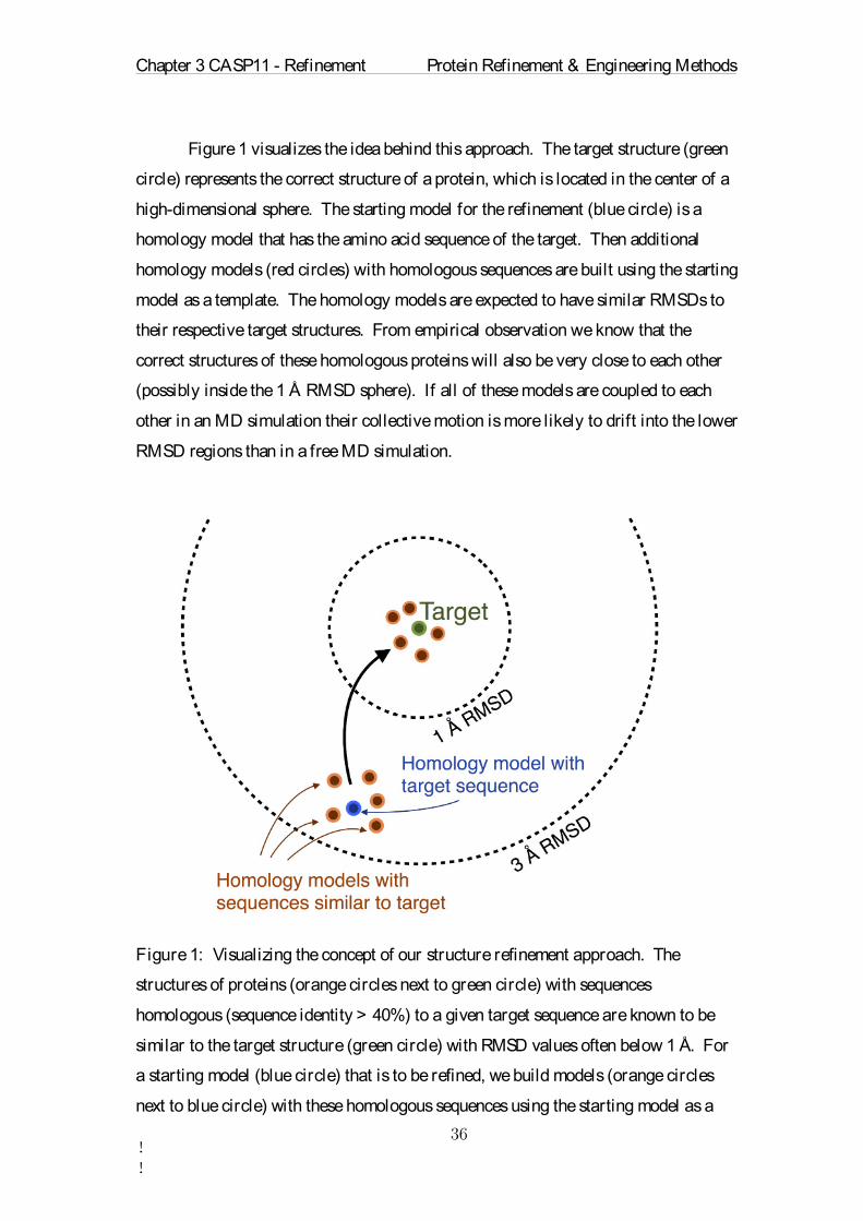
Figure 1 visualizes the idea behind this approach. The target structure (green
circle) represents the correct structure of a protein, which is located in the center of a
high-dimensional sphere. The starting model for the refinement (blue circle) is a
homology model that has the amino acid sequence of the target. Then additional
homology models (red circles) with homologous sequences are built using the starting
model as a template. The homology models are expected to have similar RMSDs to
their respective target structures. From empirical observation we know that the
correct structures of these homologous proteins will also be very close to each other
(possibly inside the 1 Å RMSD sphere). If all of these models are coupled to each
other in an MD simulation their collective motion is more likely to drift into the lower
RMSD regions than in a free MD simulation.
Figure 1: Visualizing the concept of our structure refinement approach. The
structures of proteins (orange circles next to green circle) with sequences
homologous (sequence identity > 40%) to a given target sequence are known to be
similar to the target structure (green circle) with RMSD values often below 1 Å. For
a starting model (blue circle) that is to be refined, we build models (orange circles
next to blue circle) with these homologous sequences using the starting model as a

Chapter 3 CASP11 - Refinement Protein Refinement & Engineering Methods
!!
template. All these models should then have the tendency to move close to the correct
target structure. By coupling all models to each other during an MD simulation, the
system of coupled models is moving on an energy landscape that is averaged in
sequence space. The coupling additionally reduces random conformational
fluctuations.
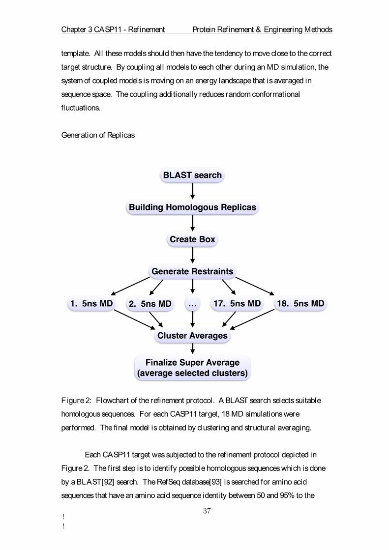
Generation of Replicas
Figure 2: Flowchart of the refinement protocol. A BLAST search selects suitable
homologous sequences. For each CASP11 target, 18 MD simulations were
performed. The final model is obtained by clustering and structural averaging.
Each CASP11 target was subjected to the refinement protocol depicted in
Figure 2. The first step is to identify possible homologous sequences which is done
by a BLAST[92] search. The RefSeq database[93] is searched for amino acid
sequences that have an amino acid sequence identity between 50 and 95% to the

Chapter 3 CASP11 - Refinement Protein Refinement & Engineering Methods
!!
target sequence. From this set of sequences a subset of seven sequences is selected.
Another selection criterion is that these seven sequences are not allowed to have more
than 95% sequence identity among each other. This extra criterion ensures that no
homology model will dominate the sampling process. In the case that an insufficient
number of sequences is found the target sequence is selected multiple times. The
number of found sequences and the average sequence identity they share with the
target sequence are summarized in Table 1. At the end of this step a list of seven
sequences is generated.
In the next step, an atomic model is created for each of these sequences. We
used MODELLER.v9[78] to map the sequences to the provided starting model, which
is used as a template for building the homology models. The results of this step are
eight homologous protein structures, one of which is the provided CASP starting
model and the others are seven homology models. The number of amino acids can be
different in these models, which mainly affects the length of the termini.
Homologous sequences with large insertions or deletions should be avoided.
Otherwise the sampling of this region will perturb the structure and will not take full
advantage of the evolutionary information. At the end of this step the eight models
are aligned.
Setup of Simulations
To prepare the MD simulation these eight aligned structures are linearly
translated into the corners of a cube. It is important to maintain enough space for
solvent between the models to avoid electrostatic interactions. To couple the models
time-dependent position restraints at positions pi,j(t) are defined for Cα atom i in
replica j of the system. We modified the GROMACS 4.5.3[94] code to update the
position restraints after a predefined number of steps n.

Chapter 3 CASP11 - Refinement Protein Refinement & Engineering Methods
!!
Target ∆GDT-HA
Number Seq.
Sequence Identity
Start GDT-HA
Avg RMSD
Std. of PAVG RMSD
Avg. Restraint Energy
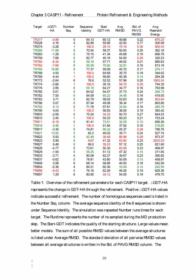
TR217 -4.88 5 84.13 65.12 49.88 0.22 875.23TR228 4.16 4 82.86 55.66 42.93 0.17 300.09 TR274 -3.28 1 100.0 29.10 75.16 0.36 950.43 TR280 11.99 8 70.54 59.37 50.83 0.25 362.18 TR283 -1.28 8 75.15 41.34 45.68 0.19 666.79 TR759 7.66 8 82.77 45.16 54.00 0.28 320.23 TR760 -6.34 8 56.18 57.71 49.02 0.21 885.63 TR762 -7.69 8 55.59 70.82 32.81 0.16 813.19 TR765 16.88 8 77.37 59.09 45.70 0.17 274.11 TR768 4.54 1 100.0 64.69 35.75 0.18 344.62 TR769 6.44 1 100.0 59.80 40.38 0.14 294.28 TR772 -2.64 6 76.6 52.52 57.99 0.20 1063.24 TR774 -2.66 1 100.0 39.16 59.70 0.29 744.35 TR776 2.85 8 55.19 64.27 34.77 0.16 793.99 TR780 5.01 8 84.52 54.47 37.73 0.24 294.73 TR782 7.50 8 64.09 65.23 34.48 0.16 419.05 TR783 3.71 8 82.79 58.02 52.63 0.26 903.64 TR786 5.07 8 87.94 49.08 39.34 0.17 663.80 TR792 8.13 8 71.78 57.81 33.04 0.16 265.78 TR795 4.04 1 100.0 59.93 38.05 0.19 383.42 TR803 -2.06 8 75.24 34.33 50.70 0.27 644.53 TR810 2.45 1 100.0 55.33 59.23 0.21 753.24 TR811 -6.18 8 81.41 73.51 32.09 0.15 656.26 TR816 8.46 1 100.0 51.84 37.92 0.16 218.80 TR817 -3.30 8 74.81 66.32 45.37 0.28 796.76 TR821 13.92 5 82.2 49.02 35.71 0.24 527.74 TR822 5.93 8 42.49 30.48 80.98 0.29 973.37 TR823 5.99 8 9.67 41.32 63.90 0.23 2033.03 TR827 6.48 8 69.0 35.23 57.12 0.25 821.60 TR828 -4.77 5 73.61 50.30 63.58 0.23 468.97 TR829 -1.50 8 55.25 51.12 47.32 0.15 311.65 TR833 -3.71 4 80.08 62.27 39.67 0.23 390.82 TR837 -0.62 8 78.81 43.80 50.09 0.15 458.97 TR848 5.98 6 68.14 58.88 40.93 0.18 542.59 TR854 -0.36 4 84.51 60.36 33.49 0.14 242.50 TR856 -9.43 8 76.16 62.26 49.26 0.19 629.36 TR857 1.29 6 80.85 34.12 54.05 0.19 478.75
Table 1: Overview of the refinement parameters for each CASP11 target. ∆GDT-HA
represents the change in GDT-HA through the refinement. Positive ∆GDT-HA values
indicate successful refinement. The number of homologous sequences used is listed in
the Number Seq. column. The average sequence identity of the 8 sequences is shown
under Sequence Identity. The simulation was repeated Number runs times for each
target. The Runtime represents the number of ns sampled during the MD production
step. The Start-GDT indicates the quality of the starting structure. Large values mean
better models. The sum of all possible RMSD values between the average structures
is listed under Average RMSD. The standard deviation of all pairwise RMSD values
between all average structures is written in the Std. of PAVG RMSD column. The

Chapter 3 CASP11 - Refinement Protein Refinement & Engineering Methods
!!
final column is the energy contained in the dynamic position restraints averaged over
all 18 runs.
The replicas are coupled to the target through the position restraints. For this
purpose a multiple sequence alignment is carried out to assign the Cα atoms of the
target structure to the corresponding Cα atoms in the replicas. The position restraints
of the assigned Cα atoms are updated by the same vector every n number of steps
during the simulation. The update vector is the displacement between each Cα atom
position xi,j(t) and the corresponding position restraint pi,j(t) averaged over all eight
models. This procedure forces each model to follow the average movement of the
ensemble. The great advantage of this method over classical position restraints[85] is
the ability of the system to undergo large conformational changes. The structure of
the target sequence is not restrained to the start model; it is only restrained to the
replicas. This removes a fundamental refinement limit and allows theoretically any
structural changes necessary to reach the correct target structure.
The position restraint energy is defined for homologs with the same sequence
length as a sum over all N Cα atoms and all eight replicas
퐸posre(푡)= 푤! 풙!,!(푡)− 풑!,!(푡)!!!!!!!!!!!!!!!!!!!!!!!!!!!!!!!!!!!!!!!!!!!(1)
!
!!!
!
!!!
The minima of the position restraints are updated every n integration time steps by
풑!,! 푡+ 푛∗Δ푡= 풑!,! 푡+ 휅!풙!,! 푡− 풑!,! 푡 !!!!!!!!!!!!!!!!!!!!!!!!!!!!!!!!!(2)
where ! denotes averaging over all j replicas. The main parameters that need to
be chosen are the number of simulation steps, n, before the position restraints are
updated, the force constant, w ,of the position restraints and the relaxation rate, 휅, at
which the restraints follow the average displacement. These parameters influence the
dynamics of the system; a low rate 휅 results in strong damping of motion. There is a
tradeoff between reducing fluctuations and improving sampling of the conformational
space per simulation length. We found an update every 500 steps, a force constant w
of 100 kJ/(mol nm2) and a relaxation rate 휅 of .5 as the best compromise.

Chapter 3 CASP11 - Refinement Protein Refinement & Engineering Methods
!!
Each production run contained three steps. As the first step, the system was
energy-minimized to remove potential atomic clashes due to the homology model
building. The minimization was performed with the steepest descent algorithm
implemented in GROMACS and ran for 5000 steps or until converged in the
AMBER99SB-ILDN[95] force field. Afterwards TIP3P water was added to the
system. Some of the water molecules were then replaced by sodium-chloride ions to
generate a physiological salt concentration and to neutralize the system. In the second
step an MD simulation was performed using an integration time step of 2 fs. . For
each simulation random initial atomic velocities were drawn. The simulations were
carried out with periodic boundary conditions in all directions. The particle mesh
Ewald algorithm was used for electrostatic interactions with a Fourier spacing of 0.12
nm and cutoff values of 0.9 nm. The Nosé-Hoover temperature coupling[96] was
used with a target temperature of 300 K. The model structure was written to an
output file every 5 ps. The total runtime of each simulation was 5 ns as listed in Table
1. This means that for each target we actually simulated eight proteins 18 times for 5
ns, which equates to 720 ns for a single protein simulation in explicit solvent. In the
last step an average structure for the target sequence was extracted from the
simulation trajectory. For this the trajectory of the model with target sequence was
retrieved from the total MD trajectory. The trajectories of the homologous replicas
were of no further interest and therefore discarded. The extracted trajectory only
contained heavy atoms belonging to the target sequence. This trajectory was finally
aligned and averaged in Cartesian coordinates.
Analysis of Simulations
Following the protocol shown in Figure 2 the 18 generated averages were
clustered. The clustering algorithm is based on the pairwise RMSD between all
possible pairs of averages: The nclust averages that were closest to each other in
pairwise RMSD were identified. For this, all 153 possible pairwise RMSD values
were calculated. In the case of nclust=4, all 1530 possible sets of 4 averages were
formed. Each of these had 6 possible pairs for which the corresponding RMSDs were

Chapter 3 CASP11 - Refinement Protein Refinement & Engineering Methods
!!
added together. The set of averages that yields the minimum total sum is the set with
the highest similarity.
This clustering aims to select those trajectories that sample a similar
conformational space. We assume that if several simulations sample similar regions
in conformational space they are likely driven by lowering the free energy instead of
by random fluctuations. This selection should therefore increase the probability of
selecting the best trajectories closest to the correct structure for further processing.
The final step is the computation of a super-average from the previously selected nclust
averages. After alignment the averages are again averaged in Cartesian space, which
leads to poor stereo-chemical properties such as wrong bond lengths and angles. To
fix the geometry we first used the SCWRL4.0[97] package for side chain
replacement. Since the super-averages still contained a good approximation of the
center of mass for each side chain we did not perform a full rotamer optimization
search but simply used the rotamer with a center of mass most similar to the averaged
side chain. To fix the atomic distances and angles, we performed one final energy
minimization with weak position restraints of 100 kJ/(mol nm2) on all heavy atoms
and additional strong position restraints of 50000 kJ/(mol nm2) on the Cα atoms. The
strong restraints prevented the structure from moving too far from the refined atomic
positions, but still allowed for sufficient flexibility to correct the local molecular
geometry.
Our submission models 1 to 5 were calculated using nclust from 4 to 5, 6, 8 or
10. In Table 1 the details for each CASP11 target are summarized. It is again
important to underline that this protocol differs fundamentally from fixed position
restraint MD simulation. There is no restriction to the possible conformational
changes due to the start conditions. We do not employ any further information about
the target starting quality or special regions of interest in a model as provided by the
Prediction Center. Every CASP target was treated in the same way, ignoring any
hints provided.

Chapter 3 CASP11 - Refinement Protein Refinement & Engineering Methods
!!
3.5 RESULTS
General CASP11 results
Our refinement method was applied to all 37 refinement targets released in the
refinement category by the Prediction Center during the CASP11 competition. For
each target 18 independent simulations with different random initial atomic velocities
were performed. Instead of a single long simulation, we performed multiple short
simulations which has been observed to better sample closer to native structures [85],
For each target five submission models were created (see METHOD).
However, a reliable prediction requires selecting the best possible model; ranking
models according to quality is therefore an important but typically challenging part of
the prediction process. This discussion, therefore, only focuses on our first
submission models, which represent our best guesses. However, it should be noted
that in all cases the five submission models were very similar with an average
standard deviation of GDT-HA values between the 5 models of 0.78 . A detailed
analysis comparing each submission model with its corresponding correct target
structure was made available by the assessors on the official CASP11 website, after
the end of the prediction period. The quantitative analysis of our submissions is based
in part on this information provided by the CASP11 assessors as well as on our own
analysis. The most common measures of refinement quality are the final values in the
high accuracy global distance test (GDT-HA)[98] score, the template modeling score
(TMscore) [99], and the root mean square deviation (RMSD) of the submission model
compared to the template. These three measures test mainly the correct placement of
Cα-atoms and use Cartesian distances after alignment to evaluate the similarity
between two structures. The Molprobity score (MolProb)[100] and the Sphere
Grinder Score (SphGr)[101] are used to assess the quality of stereochemistry and side
chain orientation.

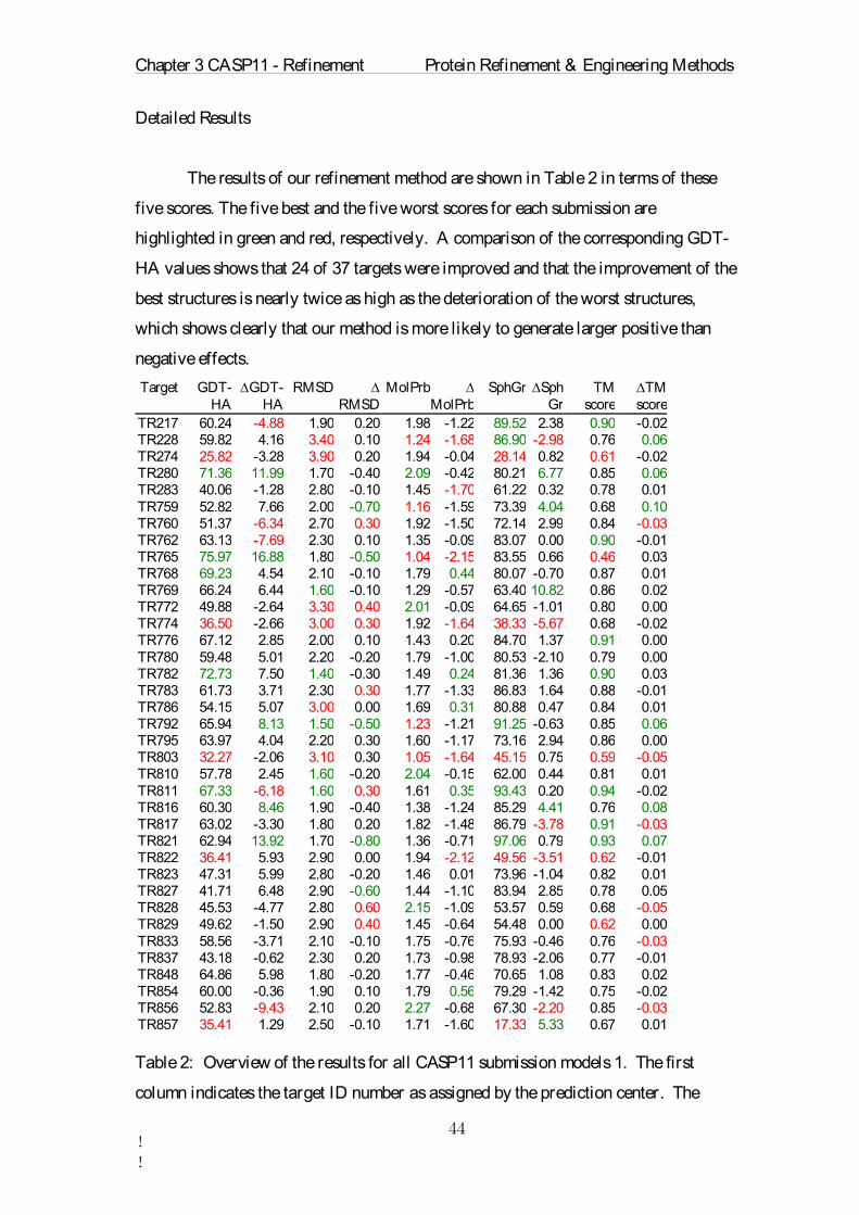
Chapter 3 CASP11 - Refinement Protein Refinement & Engineering Methods
!!
Detailed Results
The results of our refinement method are shown in Table 2 in terms of these
five scores. The five best and the five worst scores for each submission are
highlighted in green and red, respectively. A comparison of the corresponding GDT-
HA values shows that 24 of 37 targets were improved and that the improvement of the
best structures is nearly twice as high as the deterioration of the worst structures,
which shows clearly that our method is more likely to generate larger positive than
negative effects.
Target
GDT-HA
∆GDT-HA
RMSD ∆RMSD
MolPrb ∆MolPrb
SphGr ∆SphGr
TMscore
∆TMscore
TR217 60.24 -4.88 1.90 0.20 1.98 -1.22 89.52 2.38 0.90 -0.02TR228 59.82 4.16 3.40 0.10 1.24 -1.68 86.90 -2.98 0.76 0.06TR274 25.82 -3.28 3.90 0.20 1.94 -0.04 28.14 0.82 0.61 -0.02TR280 71.36 11.99 1.70 -0.40 2.09 -0.42 80.21 6.77 0.85 0.06TR283 40.06 -1.28 2.80 -0.10 1.45 -1.70 61.22 0.32 0.78 0.01TR759 52.82 7.66 2.00 -0.70 1.16 -1.59 73.39 4.04 0.68 0.10TR760 51.37 -6.34 2.70 0.30 1.92 -1.50 72.14 2.99 0.84 -0.03TR762 63.13 -7.69 2.30 0.10 1.35 -0.09 83.07 0.00 0.90 -0.01TR765 75.97 16.88 1.80 -0.50 1.04 -2.15 83.55 0.66 0.46 0.03TR768 69.23 4.54 2.10 -0.10 1.79 0.44 80.07 -0.70 0.87 0.01TR769 66.24 6.44 1.60 -0.10 1.29 -0.57 63.40 10.82 0.86 0.02TR772 49.88 -2.64 3.30 0.40 2.01 -0.09 64.65 -1.01 0.80 0.00TR774 36.50 -2.66 3.00 0.30 1.92 -1.64 38.33 -5.67 0.68 -0.02TR776 67.12 2.85 2.00 0.10 1.43 0.20 84.70 1.37 0.91 0.00TR780 59.48 5.01 2.20 -0.20 1.79 -1.00 80.53 -2.10 0.79 0.00TR782 72.73 7.50 1.40 -0.30 1.49 0.24 81.36 1.36 0.90 0.03TR783 61.73 3.71 2.30 0.30 1.77 -1.33 86.83 1.64 0.88 -0.01TR786 54.15 5.07 3.00 0.00 1.69 0.31 80.88 0.47 0.84 0.01TR792 65.94 8.13 1.50 -0.50 1.23 -1.21 91.25 -0.63 0.85 0.06TR795 63.97 4.04 2.20 0.30 1.60 -1.17 73.16 2.94 0.86 0.00TR803 32.27 -2.06 3.10 0.30 1.05 -1.64 45.15 0.75 0.59 -0.05TR810 57.78 2.45 1.60 -0.20 2.04 -0.15 62.00 0.44 0.81 0.01TR811 67.33 -6.18 1.60 0.30 1.61 0.35 93.43 0.20 0.94 -0.02TR816 60.30 8.46 1.90 -0.40 1.38 -1.24 85.29 4.41 0.76 0.08TR817 63.02 -3.30 1.80 0.20 1.82 -1.48 86.79 -3.78 0.91 -0.03TR821 62.94 13.92 1.70 -0.80 1.36 -0.71 97.06 0.79 0.93 0.07TR822 36.41 5.93 2.90 0.00 1.94 -2.12 49.56 -3.51 0.62 -0.01TR823 47.31 5.99 2.80 -0.20 1.46 0.01 73.96 -1.04 0.82 0.01TR827 41.71 6.48 2.90 -0.60 1.44 -1.10 83.94 2.85 0.78 0.05TR828 45.53 -4.77 2.80 0.60 2.15 -1.09 53.57 0.59 0.68 -0.05TR829 49.62 -1.50 2.90 0.40 1.45 -0.64 54.48 0.00 0.62 0.00TR833 58.56 -3.71 2.10 -0.10 1.75 -0.76 75.93 -0.46 0.76 -0.03TR837 43.18 -0.62 2.30 0.20 1.73 -0.98 78.93 -2.06 0.77 -0.01TR848 64.86 5.98 1.80 -0.20 1.77 -0.46 70.65 1.08 0.83 0.02TR854 60.00 -0.36 1.90 0.10 1.79 0.56 79.29 -1.42 0.75 -0.02TR856 52.83 -9.43 2.10 0.20 2.27 -0.68 67.30 -2.20 0.85 -0.03TR857 35.41 1.29 2.50 -0.10 1.71 -1.60 17.33 5.33 0.67 0.01 Table 2: Overview of the results for all CASP11 submission models 1. The first
column indicates the target ID number as assigned by the prediction center. The

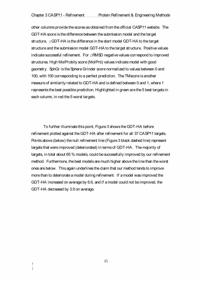
Chapter 3 CASP11 - Refinement Protein Refinement & Engineering Methods
!!
other columns provide the scores as obtained from the official CASP11 website. The
GDT-HA score is the difference between the submission model and the target
structure. ∆GDT-HA is the difference in the start model GDT-HA to the target
structure and the submission model GDT-HA to the target structure. Positive values
indicate successful refinement. For ∆RMSD negative values correspond to improved
structures. High MolProbity score (MolPrb) values indicate model with good
geometry. SphGr is the Sphere Grinder score normalized to values between 0 and
100, with 100 corresponding to a perfect prediction. The TMscore is another
measure of similarity related to GDT-HA and is defined between 0 and 1, where 1
represents the best possible prediction. Highlighted in green are the 5 best targets in
each column, in red the 5 worst targets.
To further illuminate this point, Figure 3 shows the GDT-HA before
refinement plotted against the GDT-HA after refinement for all 37 CASP11 targets.
Points above (below) the null refinement line (Figure 3 black dashed line) represent
targets that were improved (deteriorated) in terms of GDT-HA. The majority of
targets, in total about 65 % models, could be successfully improved by our refinement
method. Furthermore, the best models are much higher above the line than the worst
ones are below. This again underlines the claim that our method tends to improve
more than to deteriorate a model during refinement. If a model was improved the
GDT-HA increased on average by 6.6, and if a model could not be improved, the
GDT-HA decreased by 3.9 on average.

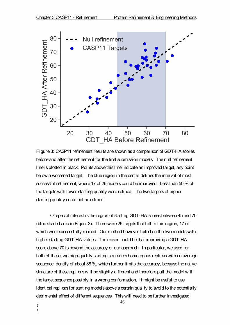
Chapter 3 CASP11 - Refinement Protein Refinement & Engineering Methods
!!
Figure 3: CASP11 refinement results are shown as a comparison of GDT-HA scores
before and after the refinement for the first submission models. The null refinement
line is plotted in black. Points above this line indicate an improved target, any point
below a worsened target. The blue region in the center defines the interval of most
successful refinement, where 17 of 26 models could be improved. Less than 50 % of
the targets with lower starting quality were refined. The two targets of higher
starting quality could not be refined.
Of special interest is the region of starting GDT-HA scores between 45 and 70
(blue shaded area in Figure 3). There were 26 targets that fell in this region, 17 of
which were successfully refined. Our method however failed on the two models with
higher starting GDT-HA values. The reason could be that improving a GDT-HA
score above 70 is beyond the accuracy of our approach. In particular, we used for
both of these two high-quality starting structures homologous replicas with an average
sequence identity of about 88 %, which further limits the accuracy, because the native
structure of these replicas will be slightly different and therefore pull the model with
the target sequence possibly in a wrong conformation. It might be useful to use
identical replicas for starting models above a certain quality to avoid to the potentially
detrimental effect of different sequences. This will need to be further investigated.

Chapter 3 CASP11 - Refinement Protein Refinement & Engineering Methods
!!
For starting GDT-HA scores below 45, less than 50% of the models were
refined. The large distance of the starting model from the native structure could mean
that the free energy landscape is not strongly funneled towards the global free energy
minimum. For structures this far away from the global minimum the initial
movement could therefore be driven more by random fluctuations rather than by
directed motions. Further the length of each individual simulation run limits the
refinement. To achieve successful refinement in this quality range it might be
required to run longer simulations, which would allow the coupled proteins to
undergo larger conformational motions.
The blue shaded region in Figure 3 defines the range in which our method is
most likely to produce successful model refinement. It can be assumed that protein
structures falling into this region benefit the most from the effect of coupled
homologs. The starting quality is sufficiently high to reduce random motions within
local energy minima. And it is not so high that the homologous structures end up in a
tug-of-war between their individually favored conformations and the desired target
structure. If the starting quality of a homology model is known this observation
allows an a priori estimation of the likelihood that this method will yield an improved
structure. Below we will demonstrate how this likelihood can also be estimated a
posteriori using a correlation between starting quality and the variability of the
different simulations.
A close up on interesting targets
In order to elucidate the effect of starting quality all 18 trajectories of 4
representative targets were plotted in Figure 4. A frame of the model with the target
sequence was written to file every 5 ps during the simulation. For each frame the
TMscore to the correct structure was calculated. The top curves show target TR811,
which had an initial TMscore of 0.96 and a GDT-HA score of 73.5. This target
belongs to the group of targets with a high starting GDT-HA. In all 18 trajectories the
quality of the model worsened immediately to an average TMscore of 0.926. After 1

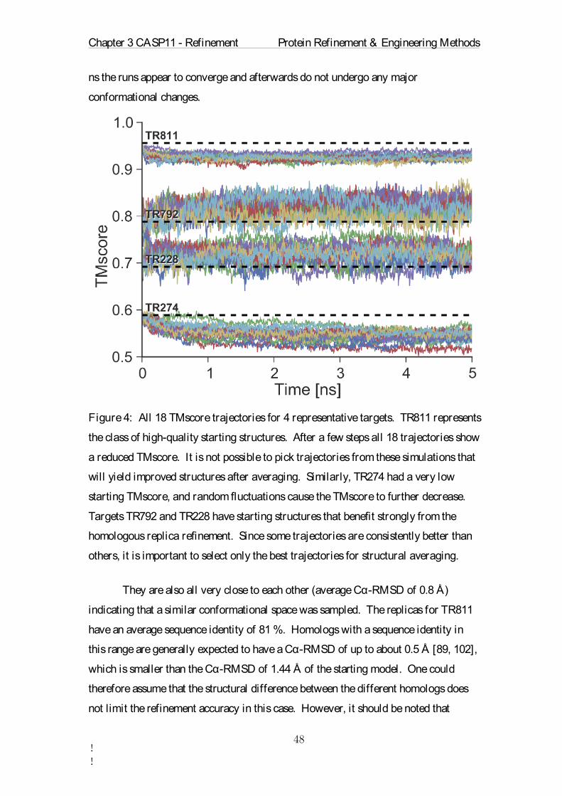
Chapter 3 CASP11 - Refinement Protein Refinement & Engineering Methods
!!
ns the runs appear to converge and afterwards do not undergo any major
conformational changes.
Figure 4: All 18 TMscore trajectories for 4 representative targets. TR811 represents
the class of high-quality starting structures. After a few steps all 18 trajectories show
a reduced TMscore. It is not possible to pick trajectories from these simulations that
will yield improved structures after averaging. Similarly, TR274 had a very low
starting TMscore, and random fluctuations cause the TMscore to further decrease.
Targets TR792 and TR228 have starting structures that benefit strongly from the
homologous replica refinement. Since some trajectories are consistently better than
others, it is important to select only the best trajectories for structural averaging.
They are also all very close to each other (average Cα-RMSD of 0.8 Å)
indicating that a similar conformational space was sampled. The replicas for TR811
have an average sequence identity of 81 %. Homologs with a sequence identity in
this range are generally expected to have a Cα-RMSD of up to about 0.5 Å [89, 102],
which is smaller than the Cα-RMSD of 1.44 Å of the starting model. One could
therefore assume that the structural difference between the different homologs does
not limit the refinement accuracy in this case. However, it should be noted that

Chapter 3 CASP11 - Refinement Protein Refinement & Engineering Methods
!!
crystal structures in different space groups already have significant deviations, e.g.
different crystal structures of myoglobin have Cα-RMSD values of 0.54–0.79 Å
[103]. The target structure is therefore not precisely defined, which might contribute
to the fact that our refinement protocol was not able to improve the high-quality
structures.
Target TR274, shown in the bottom of Figure 4, represents the class of low-
quality targets. In comparison to TR811 a wider spread of the TMscores can be
observed, which suggests that the free energy funnel becomes flat with increasing
distance from the target structure. Because of this lack in guidance the simulation
might explore more random conformations instead of driving the structure towards
the target conformation.
The trajectories for targets TR792 and TR228 are typical for starting structures
from the quality range that yields the best refinement results with our approach. It can
be observed that the individual trajectories have high fluctuations during the
simulation. Furthermore some trajectories are consistently improving the TMscore,
while others fluctuate around the null refinement line. It would be beneficial to select
only the trajectories that yield the largest and most consistent improvement in
TMscore for further processing. To illustrate whether our clustering approach (see
Analysis of Simulations) is able to perform this task, the percentage of frames with a
TMscore above the null refinement is calculated for all trajectories. The same
calculation is then repeated for the four trajectories selected based on the clustering of
average structures by our protocol.

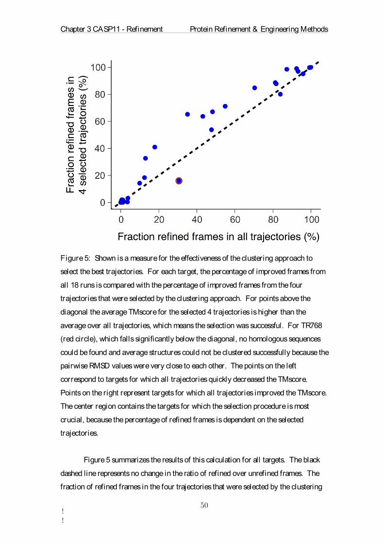
Chapter 3 CASP11 - Refinement Protein Refinement & Engineering Methods
!!
Figure 5: Shown is a measure for the effectiveness of the clustering approach to
select the best trajectories. For each target, the percentage of improved frames from
all 18 runs is compared with the percentage of improved frames from the four
trajectories that were selected by the clustering approach. For points above the
diagonal the average TMscore for the selected 4 trajectories is higher than the
average over all trajectories, which means the selection was successful. For TR768
(red circle), which falls significantly below the diagonal, no homologous sequences
could be found and average structures could not be clustered successfully because the
pairwise RMSD values were very close to each other. The points on the left
correspond to targets for which all trajectories quickly decreased the TMscore.
Points on the right represent targets for which all trajectories improved the TMscore.
The center region contains the targets for which the selection procedure is most
crucial, because the percentage of refined frames is dependent on the selected
trajectories.
Figure 5 summarizes the results of this calculation for all targets. The black
dashed line represents no change in the ratio of refined over unrefined frames. The
fraction of refined frames in the four trajectories that were selected by the clustering

Chapter 3 CASP11 - Refinement Protein Refinement & Engineering Methods
!!
method is consistently higher than the fraction of refined frames in all trajectories, as
shown by the concave curve (blue dots) with start and end points on the no change
line. This is easily understood if one considers that trajectories that had zero percent
of improved frames cannot yield a subset that has more than zero percent improved
frames. The same argument is valid for trajectories with more than 95%
improvement. Any subset of selected trajectories is likely to yield again the same
amount of improvement. Most interesting is the intermediate range from 10 to 90%.
The trajectories for a target in this range have a high discrepancy between each other.
An appropriate selection as done by our method therefore increases the fraction of
refined frames drastically. For all targets but TR768 the subset of selected trajectories
improved the fraction of refined frames. For TR768 no homologous sequences could
be found and the clustered averages are all very close to each other making it difficult
to select the four most similar ones. It is interesting to note that, however, the
refinement of TR768 did not suffer too much from this problem: With an increase of
the GDT-HA score by 4.54 it can still be considered a successfully refined target.
Overall Figure 5 emphasizes that trajectories that sample a similar conformational
space, are moving into the right direction. If a single trajectory explores a path very
different from the other trajectories, it is most likely driven by random forces and
should therefore be excluded from further processing.
We tested whether 18 simulations per target were necessary to achieve the
refinement quality. Hypothetical submission models were calculated and compared
for 9 randomly selected trajectories with the true submission model. The difference in
TMscore was less then 1 % on average from which we conclude that the required
simulation time could effectively be reduced by factor of 2.

Chapter 3 CASP11 - Refinement Protein Refinement & Engineering Methods
!!
3.6 DISCUSSION
Quantitative Analysis
From the observations mentioned above, it can be concluded that our method
reliably refines most structures in a certain starting quality range. In CASP11 a
measure of the starting quality is provided in terms of an initial GDT-HA value. In
applications where the correct structure is not known, however, it is not easily
possible to determine the initial quality of a homology model. It would therefore be
useful to estimate the quality of a starting structure retrospectively after a refinement
calculation. Such an a posteriori approximation is possible by using the data
generated during the clustering of average structures. In the refinement protocol 18
average structures were created. For each pair of averages the RMSD was calculated.
The standard deviation of the obtained 153 RMSD values is a measure of the total
variance in the trajectories. We observe that high-quality starting structures produce
very similar averages. Bad starting structures, on the other hand, yield quite disperse
average structures. In Figure 6 the standard deviation of the pairwise RMSD values
for all CASP11 targets is plotted against the corresponding starting quality as
measured by the TMscore. A Pearson correlation coefficient of -0.73 was found
between these two measures. This strong negative correlation means that the quality
of a homology model can be well estimated from the standard deviation of pairwise
RMSD values after the refinement protocol is finished.

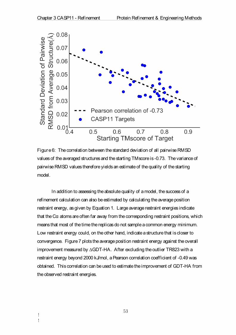
Chapter 3 CASP11 - Refinement Protein Refinement & Engineering Methods
!!
Figure 6: The correlation between the standard deviation of all pairwise RMSD
values of the averaged structures and the starting TMscore is -0.73. The variance of
pairwise RMSD values therefore yields an estimate of the quality of the starting
model.
In addition to assessing the absolute quality of a model, the success of a
refinement calculation can also be estimated by calculating the average position
restraint energy, as given by Equation 1. Large average restraint energies indicate
that the Cα atoms are often far away from the corresponding restraint positions, which
means that most of the time the replicas do not sample a common energy minimum.
Low restraint energy could, on the other hand, indicate a structure that is closer to
convergence. Figure 7 plots the average position restraint energy against the overall
improvement measured by ∆GDT-HA. After excluding the outlier TR823 with a
restraint energy beyond 2000 kJ/mol, a Pearson correlation coefficient of -0.49 was
obtained. This correlation can be used to estimate the improvement of GDT-HA from
the observed restraint energies.

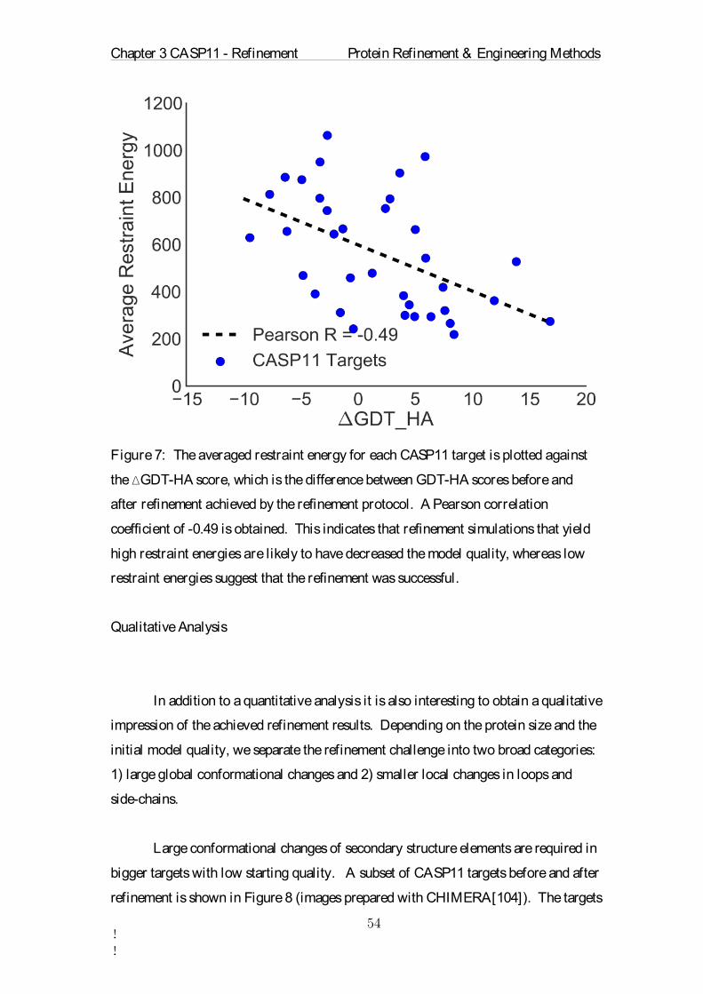
Chapter 3 CASP11 - Refinement Protein Refinement & Engineering Methods
!!
Figure 7: The averaged restraint energy for each CASP11 target is plotted against
the ∆GDT-HA score, which is the difference between GDT-HA scores before and
after refinement achieved by the refinement protocol. A Pearson correlation
coefficient of -0.49 is obtained. This indicates that refinement simulations that yield
high restraint energies are likely to have decreased the model quality, whereas low
restraint energies suggest that the refinement was successful.
Qualitative Analysis
In addition to a quantitative analysis it is also interesting to obtain a qualitative
impression of the achieved refinement results. Depending on the protein size and the
initial model quality, we separate the refinement challenge into two broad categories:
1) large global conformational changes and 2) smaller local changes in loops and
side-chains.
Large conformational changes of secondary structure elements are required in
bigger targets with low starting quality. A subset of CASP11 targets before and after
refinement is shown in Figure 8 (images prepared with CHIMERA[104]). The targets

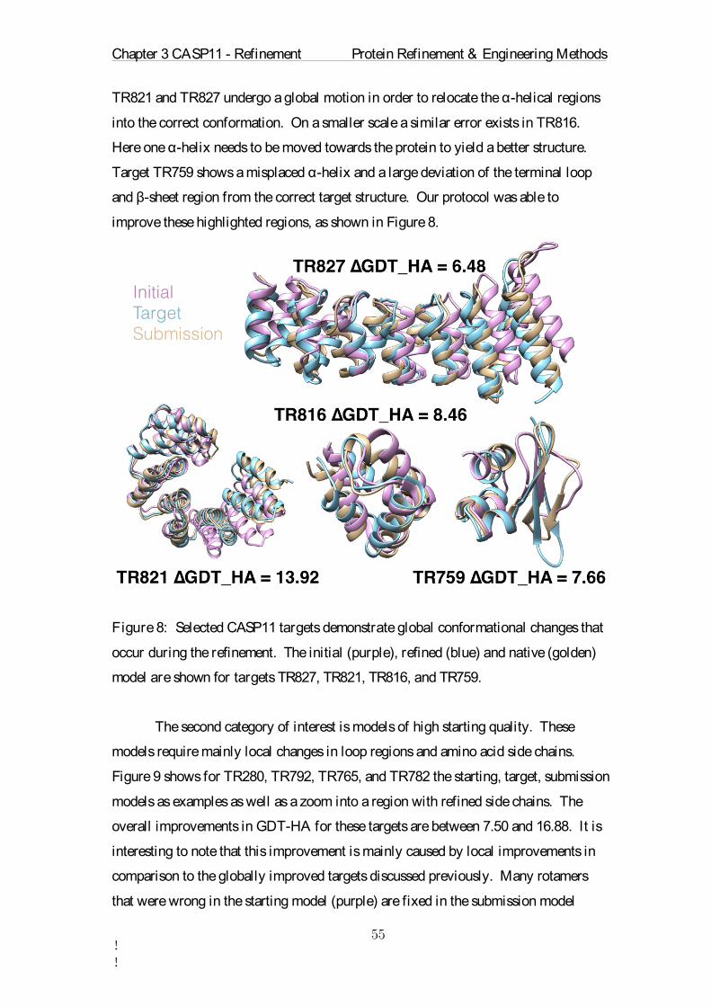
Chapter 3 CASP11 - Refinement Protein Refinement & Engineering Methods
!!
TR821 and TR827 undergo a global motion in order to relocate the α-helical regions
into the correct conformation. On a smaller scale a similar error exists in TR816.
Here one α-helix needs to be moved towards the protein to yield a better structure.
Target TR759 shows a misplaced α-helix and a large deviation of the terminal loop
and β-sheet region from the correct target structure. Our protocol was able to
improve these highlighted regions, as shown in Figure 8.
Figure 8: Selected CASP11 targets demonstrate global conformational changes that
occur during the refinement. The initial (purple), refined (blue) and native (golden)
model are shown for targets TR827, TR821, TR816, and TR759.
The second category of interest is models of high starting quality. These
models require mainly local changes in loop regions and amino acid side chains.
Figure 9 shows for TR280, TR792, TR765, and TR782 the starting, target, submission
models as examples as well as a zoom into a region with refined side chains. The
overall improvements in GDT-HA for these targets are between 7.50 and 16.88. It is
interesting to note that this improvement is mainly caused by local improvements in
comparison to the globally improved targets discussed previously. Many rotamers
that were wrong in the starting model (purple) are fixed in the submission model


Chapter 3 CASP11 - Refinement Protein Refinement & Engineering Methods
!!
(gold). The final step of our refinement protocol is the optimization of
stereochemistry after the structural averaging. This step has a lot of potential to be
improved upon for further side chain optimization. The low sphere grinder scores for
many of our models are mainly due to this weak spot in our protocol. Considering
that this error is avoidable, the refinement results on the local level are nevertheless
remarkable.

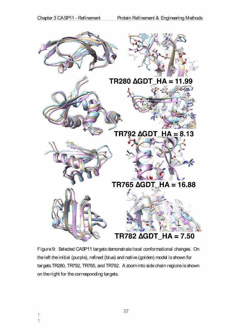
Chapter 3 CASP11 - Refinement Protein Refinement & Engineering Methods
!!
Figure 9: Selected CASP11 targets demonstrate local conformational changes. On
the left the initial (purple), refined (blue) and native (golden) model is shown for
targets TR280, TR792, TR765, and TR782. A zoom into side chain regions is shown
on the right for the corresponding targets.

Chapter 3 CASP11 - Refinement Protein Refinement & Engineering Methods
!!
3.7 CONCLUSION
The CASP11 experiment was an immensely important validation tool for our
refinement approach. We identified a starting model quality interval in which this
method can be used with confidence to refine homology models. We were also able
to identify a criterion to estimate the model quality and the probability for refinement
success. This will be of particular importance for applications where model quality is
not known. The refinement protocol can be further improved upon, as this study has
shown. It was found that similar results could have been obtained with a lower
demand in computer time. Furthermore, we found that local structure refinement
could be further improved by an adaption of the side chain optimization step.
Acknowledgments
The authors express their appreciation to the Prediction Center for the
CASP11 experiment and conference organization. The authors gratefully
acknowledge the computing time granted on the supercomputer JUROPA at Jülich
Supercomputing Centre (JSC).

Chapter 4 Refinement with Restraints Protein Refinement & Engineering Methods
Chapter 4 Refinement with Adaptable
Restraints
4.1 General Introduction
The last two chapters relied heavily on the technique of adaptable restraints.
This is not per se a novelty, but rather an adaptation of the existing deformable elastic
network method that has been used effectively in refinement of crystallographic
models. The underlying mathematical description of this method has not been
investigated so far. The aim of this chapter is to investigate the impact exercised by
additional dynamic restraints on a molecular dynamics simulation.
The case of a simple one dimensional energy landscape with a single particle
will be investigated. The forces acting on the particle will be modified through the
addition of a virtual mass that is connected with a spring to the particle. This virtual
mass does not experience the underlying potential and is therefore another
representation of dynamic restraints.
This one-dimensional case will be expanded into higher dimensions and
finally be applied to a small bio-molecule, trialanine. The author has performed the
implementation of the algorithms, the experimental setup, the derivations and final
analysis under supervision of Professor Schröder. This chapter will soon be
submitted to peer review and follows the guidelines of JCTC.

Chapter 4 Refinement with Restraints Protein Refinement & Engineering Methods
4.2 Abstract
High-dimensional search problems are of great importance. The method of
adaptable restraints in elastic networks has been very successful in guiding high
dimensional searches in the X-ray crystallographic settings and protein structure
refinement problems. Here we present the fundamental reasoning from statistical
mechanics that shows the impact of such elastic networks. We find that they rescale
and smooths the energy landscape and allow searches to explore free energy minima
more frequently.
4.3 Introduction
The refinement of a protein structure requires finding the most probable
conformation of the protein. The most probable conformation corresponds to the
lowest free energy state. Several methods such as replica exchange[105], Monte
Carlo sampling[106, 107] or importance sampling[108] have been developed to
improve sampling of the energy landscape[109]. It is the aim of these methods to
determine the Boltzmann distribution more efficiently. However, in the case of
protein structure refinement, we are mostly interested in the most probable structure,
which belongs to the free energy minimum[110]. Sampling the (broad) Boltzmann
distribution should therefore not be necessary. In a high-dimensional system there are
many local free energy minima. Even though the state with the lowest free energy is
most probable, the chance of visiting this state is low because of the large number of
accessible states. Global minimization (e.g. simulated annealing [111], potential
smoothing[112], global optimization[107]) methods are not suitable because we are
not searching for the global energy minimum, but the free energy minimum at a given
temperature. It is important to make sure that the order of states remains unchanged.
Here we investigate the effect of applying an adaptive restraint during the
sampling. The idea is to add an extra harmonic potential to the energy landscape and
to couple the minimum of this potential to the particle coordinates. This can also be
described as a coupling to a virtual heavy mass that is attached by a spring to the

Chapter 4 Refinement with Restraints Protein Refinement & Engineering Methods
particle, but that does not feel the energy landscape. The motion of the virtual mass is
instead over-damped such that the heavy mass slowly follows the motion of the
particle. Such adaptive restraints have been introduced recently to the field of
crystallographic and cryo-EM model refinement in the form of the Deformable Elastic
Network (DEN) restraints [113-116]. Refinement with DEN restraints has been
shown to lead to significantly improved structures especially with low-resolution data,
where such a hybrid energy landscape is less tilted towards a global minimum. The
method of adaptable restraints has also gained importance in the field of protein
structure prediction. Here large and heterogeneous proteins and complexes have been
successfully refined using a DEN like approach, as seen in the CASP competitions
(see Chapters 2 and 3).
Here we first develop an analytical description for adaptive restraints in one
dimension. We then explore the impact of adaptive restraints in higher dimensions.
Following this, the difference between lowering the temperature and the effect of
adaptive restraints is explained. Finally we apply this method to a high dimensional
search problem on a small bio-molecule [117]. We apply the adaptive restraints to
sample the conformational space of trialanine by molecular dynamics (MD)
simulation and demonstrate improved sampling over classical MD simulation.

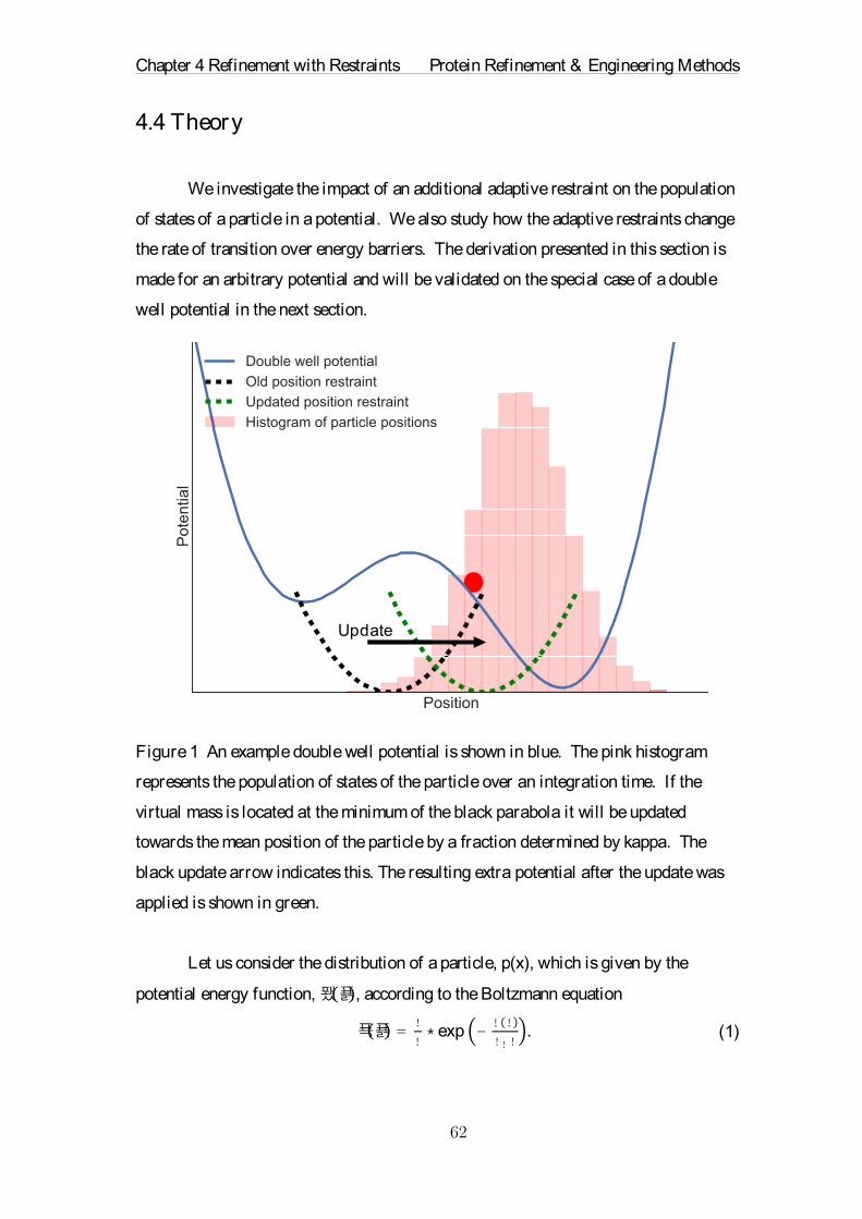
Chapter 4 Refinement with Restraints Protein Refinement & Engineering Methods
4.4 Theory
We investigate the impact of an additional adaptive restraint on the population
of states of a particle in a potential. We also study how the adaptive restraints change
the rate of transition over energy barriers. The derivation presented in this section is
made for an arbitrary potential and will be validated on the special case of a double
well potential in the next section.
Figure 1 An example double well potential is shown in blue. The pink histogram
represents the population of states of the particle over an integration time. If the
virtual mass is located at the minimum of the black parabola it will be updated
towards the mean position of the particle by a fraction determined by kappa. The
black update arrow indicates this. The resulting extra potential after the update was
applied is shown in green.
Let us consider the distribution of a particle, p(x), which is given by the
potential energy function, 퐸푥, according to the Boltzmann equation
푝푥 =
!
!∗exp −
! !
!! !. (1)
Update

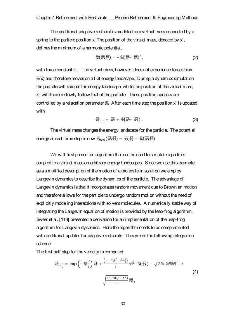
Chapter 4 Refinement with Restraints Protein Refinement & Engineering Methods
The additional adaptive restraint is modeled as a virtual mass connected by a
spring to the particle position x. The position of the virtual mass, denoted by x’ ,
defines the minimum of a harmonic potential,
퐻푥,푥! =!
!휔푥− 푥! !, (2)
with force constant ω . The virtual mass, however, does not experience forces from
E(x) and therefore moves on a flat energy landscape. During a dynamics simulation
the particle will sample the energy landscape, while the position of the virtual mass,
x', will therein slowly follow that of the particle. These position updates are
controlled by a relaxation parameter!휅. After each time step the position x’ is updated
with
푥!!!! = 푥!! + 휅푥− 푥!! . (3)
The virtual mass changes the energy landscape for the particle. The potential
energy at each time step is now 퐸total 푥,푥! = 퐸푥 + 퐻푥,푥! .
We will first present an algorithm that can be used to simulate a particle
coupled to a virtual mass on arbitrary energy landscapes. Since we use this example
as a simplified description of the motion of a molecule in solution we employ
Langevin dynamics to describe the dynamics of the particle. The advantage of
Langevin dynamics is that it incorporates random movement due to Brownian motion
and therefore allows for the particle to undergo random motion without the need of
explicitly modeling interactions with solvent molecules. A numerically stable way of
integrating the Langevin equation of motion is provided by the leap-frog algorithm.
Sweet et al. [118] presented a derivation for an implementation of the leap-frog
algorithm for Langevin dynamics. Here the algorithm needs to be complemented
with additional updates for adaptive restraints. This yields the following integration
scheme:
The first half step for the velocity is computed
푣!!
!!= exp −훾
! "
!푣! +
!! ! " # !!! "!
!푀!!푓푥! + 2푘!푇!훾푀
!!! ∗
!! ! " # !!!! "
!!푅! ,
(4)

Chapter 4 Refinement with Restraints Protein Refinement & Engineering Methods
with the friction coefficient,!훾, the time step,!훥푡, the mass of the particle,!푀, the
force,!푓(푥!) , acting on the particle at position 푥! , the Boltzmann constant 푘! , the
temperature 푇, and a normal random variable 푅! .
2. Propagation of the particle
푥!!! = !푥! + 훥푡!푣!!!!!!. (5)
3. Propagate the adaptive restraint
푥!!!! = 푥!! + (푥!!! − 푥!!)∗휅!.!!!!!! (6)
4. Calculate the force on the particle
푓푥!!! = !−
푑퐸푥!!!푑푥
−푑퐻푥!!! − 푥!!!
!
푑푥!!.!!!! (7)
5. The final half step for the velocity
푣!!! = exp −훾훥푡
2푣!!
!!+
1− exp −훾훥푡2
훾푀!!푓푥!!! +
2푘!푇!훾푀!!! ∗ !! ! " # !!!! "
!!푅!!!.
(8)
This algorithm has been implemented in Python.
In the following we aim to determine the distribution of particle positions for a
given energy landscape with adaptive restraints, 퐸total 푥,푥! = 퐸푥 + 퐻푥,푥! . This
expression is, however, not very useful for analytical investigation, because of the
time dependency of x and x’ and a strong correlation between x and x'. If we instead
look at the equilibrium situation, the effect of the virtual mass can be written as a
continuous offset in potential energy denoted as 퐸′푥, which leads to a modified
expression of the Boltzmann distribution of the particle
푝′(푥)=!
!!∗exp −
! ! !!! !
!! !!. (9)
The difference between Eq. 9 and Eq. 1 is the additional energy term 퐸′푥
and the new partition function 푧!. The distribution of particle positions, 푝′(푥), can
easily be calculated numerically using the Langevin-dynamics algorithm described
above. The term 퐸′푥!describes the average offset in energy caused by the virtual
mass in the limit of long simulation times. We are now interested in understanding

Chapter 4 Refinement with Restraints Protein Refinement & Engineering Methods
how!푝′(푥) depends on the strength, 휔, and the relaxation rate, 휅, of the adaptive
restraint. For this we will derive an analytical expression of!퐸′(푥).
The effect of the virtual mass on the energy landscape in equilibrium can be described
as the contribution of the harmonic potential at each position, x. This can be written
as
퐸!푥 = !!∫푝푥,푥! ∗!퐻푥,푥!푑푥!!. (10)
Here 푝(푥,푥′) represents the joint probability to find the particle at a position x
and the virtual mass at a position x’ . This expression can be substituted according to
the multiplication rule as
푝푥,푥! = 푝푥푥! !푝′푥! !.! (11)
The conditional probability 푝푥푥! describes the distribution of the particle
around a certain position of the virtual mass. We approximate this distribution with a
Gaussian distribution,
푝푥푥! =
!
!!!exp −
!!!!!
!!!. (12)
The standard deviation in this expression depends on the strength, 휔, and the
relaxation rate 휅 of the adaptive restraints. The rate 휅 determines how fast the virtual
mass follows the particle. An increase in temperature will generate larger fluctuations
of the particle around the virtual mass. In a linear approximation this fluctuation
increases with 1− 휅. With increasing force constant 휔 the restraints connecting
particle and virtual mass become stiffer, which reduces the fluctuation. Combining
these observations we express the variance of the particle fluctuations as
휎휔,푘!푇,휅 = !
!!!(!!!)
!!!. (13)
To solve Eq. 11 the distribution 푝!푥! !could be obtained from a simulation
and be used to solve Eq. 9 numerically. But a priori 푝!푥! !is unknown. We therefore
turn to an alternative representation of the joint probability in Eq. 10,
푝푥!,푥 = 푝푥!푥!푝!푥!. (14)
Here the distribution of the virtual mass around a given particle position is
needed. We assume again that this distribution can be modeled with a Gaussian of the
form

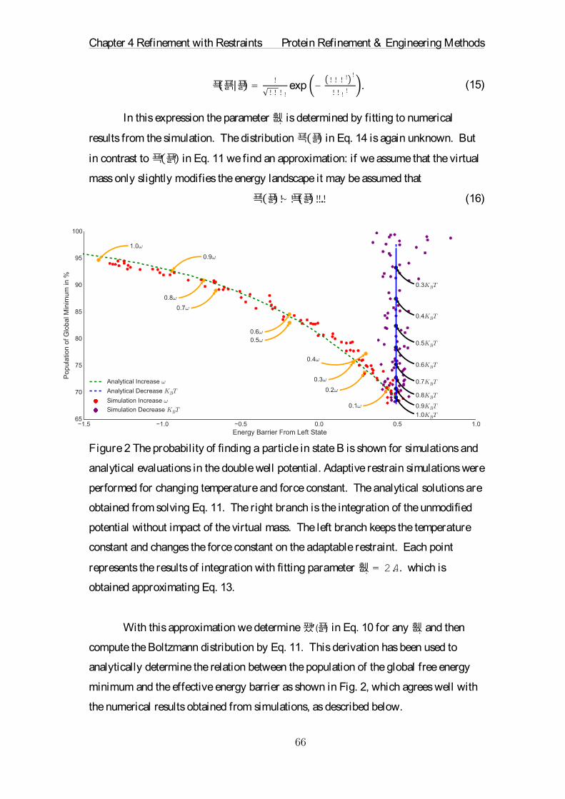
Chapter 4 Refinement with Restraints Protein Refinement & Engineering Methods
푝푥!푥 =
!
!!!!exp −
!!!!!
!!!!. (15)
In this expression the parameter 휎! is determined by fitting to numerical
results from the simulation. The distribution 푝!푥 in Eq. 14 is again unknown. But
in contrast to 푝′푥′ in Eq. 11 we find an approximation: if we assume that the virtual
mass only slightly modifies the energy landscape it may be assumed that
푝!푥!~!푝푥!!.! (16)
Figure 2 The probability of finding a particle in state B is shown for simulations and
analytical evaluations in the double well potential. Adaptive restrain simulations were
performed for changing temperature and force constant. The analytical solutions are
obtained from solving Eq. 11. The right branch is the integration of the unmodified
potential without impact of the virtual mass. The left branch keeps the temperature
constant and changes the force constant on the adaptable restraint. Each point
represents the results of integration with fitting parameter 휎! = 2.4. which is
obtained approximating Eq. 13.
With this approximation we determine 퐸′(푥) in Eq. 10 for any 휎! and then
compute the Boltzmann distribution by Eq. 11. This derivation has been used to
analytically determine the relation between the population of the global free energy
minimum and the effective energy barrier as shown in Fig. 2, which agrees well with
the numerical results obtained from simulations, as described below.

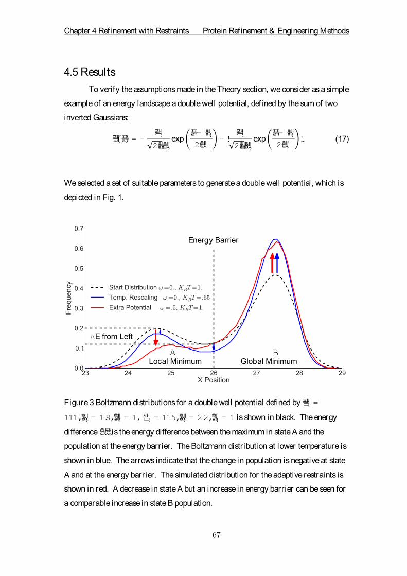
Chapter 4 Refinement with Restraints Protein Refinement & Engineering Methods
4.5 Results
To verify the assumptions made in the Theory section, we consider as a simple
example of an energy landscape a double well potential, defined by the sum of two
inverted Gaussians:
퐸푥 = −
퐴!
2휋휎!exp
푥− 휇!2휎!
! − !퐴!
2휋휎!exp
푥− 휇!2휎!
! !. (17)
We selected a set of suitable parameters to generate a double well potential, which is
depicted in Fig. 1.
Figure 3 Boltzmann distributions for a double well potential defined by 퐴! =
111,휎! = 1.8,휇! = 1,퐴! = 115,휎! = 2.2,휇! = 1!is shown in black. The energy
difference 훥퐸 is the energy difference between the maximum in state A and the
population at the energy barrier. The Boltzmann distribution at lower temperature is
shown in blue. The arrows indicate that the change in population is negative at state
A and at the energy barrier. The simulated distribution for the adaptive restraints is
shown in red. A decrease in state A but an increase in energy barrier can be seen for
a comparable increase in state B population.
Energy Barrier
Local Minimum Global Minimum
∆E from Left
A B


Chapter 4 Refinement with Restraints Protein Refinement & Engineering Methods
A Python implementation of the Langevin dynamics integration scheme was
used to simulate a particle in this double well potential. We chose to set the mass and
friction coefficient to 1. Only 푘!푇 was left variable to control the simulation
temperature. To ensure sufficient sampling each simulation was performed for 2
million integration steps. For a simulation without adaptive restraints the distribution
of particle positions in the potential follows as expected the Boltzmann distribution,
as shown for comparison for 푘!푇= 1 in Fig. 3 (black). The particle can be found in
two separate states according to the two energy minima in the double well potential.
The local minimum on the left corresponds to state A, and the global minimum on the
right corresponds to state B. The left-sided energy barrier 훥퐸 is defined as
훥퐸= 푘!푇!(− ln!(푝푥barrier )+ ln 푝푥minimum !), (18)
where p(x) denotes the probability to find the particle in a position x as obtained from
the normalized histogram of particle positions and xbarrier is fixed at the position of the
barrier in the original energy landscape. Figure 3 also shows the particle distribution
obtained from a simulation at!푘!푇=0.65 (blue curve). According to the Boltzmann
equation lower temperatures increase the population of states with lower potential
energy leading to an increase in the population of state B. Instead the populations of
state A and at the energy barrier are reduced.
Effect of adaptive restraints in 1D
If we now apply the adaptive position restraint in the simulation a very
different behavior is observed. Figure 3 shows the resulting particle distribution for 휔
set to 0.5 at 1푘!푇 (red curve). The population of the global minimum (state B) with
adaptive restraints is comparable to that obtained from the low temperature
simulation. But the population of state A has decreased even below the population of
the energy barrier. This causes a change in the sign of 훥퐸 for simulations with virtual
mass. Turning back to Eq. 10 it becomes apparent why this effect occurs. In the limit
of long simulations a particle in position x will see the virtual mass with a joint
probability 푝(푥!,푥) at a position x’ . To get the cumulative effect of the extra
potentials we need to integrate over all possible positions x’ . Because of the higher
probability to find the extra potential in state B the energy of state A is raised. Due to

Chapter 4 Refinement with Restraints Protein Refinement & Engineering Methods
the harmonic form of the extra potential the effect is even stronger for states farther
away from state B. This causes the energy of the local minimum to be raised above
the level of the energy barrier. From this we conclude that an extra potential raises
the probability to be in the global minimum and increases transitions from nearby
local minima into the global minimum. The overall diffusion is however slowed
down due to the relaxing additional harmonic potential. For dynamics driven
processes this is more advantageous than a reduction in temperature to find global
energy minima. In the further discussion we will also see that the extra potential
increases the probability to be in free energy minima, a feature foreign to temperature
downscaling.
Figure 2 further illuminates our observations. The purple points in the figure
represent simulations performed at decreasing values of 푘!푇. From each simulation
we obtain an estimate for the energy barrier from the left state 훥퐸 according to Eq.
18. Further we calculate the population of the global energy minimum. The blue
curve represents the analytical values obtained from the Boltzmann distribution at a
given 푘!푇. We note that the as the population of the global minimum increases the
energy barrier remains constant. The red points show simulation results with an extra
potential for increasing coupling strength 휔. We observe that the same improvements
in population of global minimum are achievable as by temperature reduction. Further
we point out that 훥퐸 decreases with increasing population. In green we can observe
that our approximated solution to Eq. 10 is capable of describing the effect of a virtual
mass over a range of coupling strengths. This solidifies our claim that dynamic
coupling improves the sampling of energy minima.
High-dimensional energy landscapes
An even more important task than sampling energy minima is the sampling of
free energy minima. In high dimensional problems entropic influences often times
favor high-energy states above lower ones. To discuss the impact of an extra
potential on the population of free energy minima we generalize our Langevin
dynamics simulation into higher dimensions. For this it is only required to update
each component of an n dimensional position and velocity vector with the previously

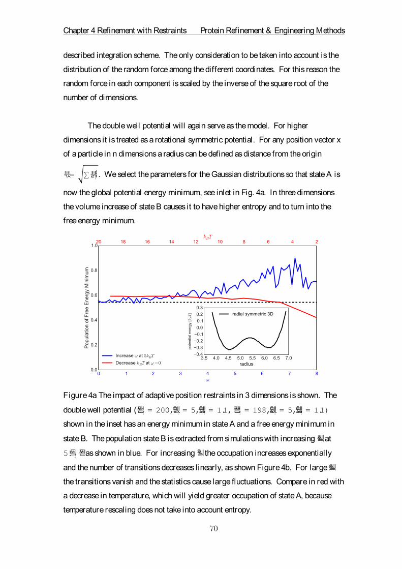
Chapter 4 Refinement with Restraints Protein Refinement & Engineering Methods
described integration scheme. The only consideration to be taken into account is the
distribution of the random force among the different coordinates. For this reason the
random force in each component is scaled by the inverse of the square root of the
number of dimensions.
The double well potential will again serve as the model. For higher
dimensions it is treated as a rotational symmetric potential. For any position vector x
of a particle in n dimensions a radius can be defined as distance from the origin
푟= ∑푥!!. We select the parameters for the Gaussian distributions so that state A is
now the global potential energy minimum, see inlet in Fig. 4a. In three dimensions
the volume increase of state B causes it to have higher entropy and to turn into the
free energy minimum.
Figure 4a The impact of adaptive position restraints in 3 dimensions is shown. The
double well potential (퐴! = 200,휎! = 5,휇! = 1.1,퐴! = 198,휎! = 5,휇! = 1.1)
shown in the inset has an energy minimum in state A and a free energy minimum in
state B. The population state B is extracted from simulations with increasing 휔 at
5!푘!푇 as shown in blue. For increasing 휔 the occupation increases exponentially
and the number of transitions decreases linearly, as shown Figure 4b. For large!휔
the transitions vanish and the statistics cause large fluctuations. Compare in red with
a decrease in temperature, which will yield greater occupation of state A, because
temperature rescaling does not take into account entropy.

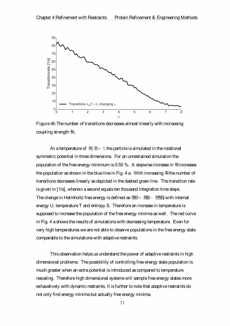
Chapter 4 Refinement with Restraints Protein Refinement & Engineering Methods
Figure 4b The number of transitions decreases almost linearly with increasing
coupling strength 휔.
At a temperature of !푘!푇= 5 the particle is simulated in the rotational
symmetric potential in three dimensions. For an unrestrained simulation the
population of the free energy minimum is 0.55 %. A stepwise increase in 휔 increases
the population as shown in the blue line in Fig. 4 a. With increasing 휔 the number of
transitions decreases linearly as depicted in the dashed green line. The transition rate
is given in [1/s], wherein a second equals ten thousand integration time steps.
The change in Helmholtz free energy is defined as 훥퐹= 훥푈− 푇훥푆, with internal
energy U, temperature T and entropy S. Therefore an increase in temperature is
supposed to increase the population of the free energy minima as well. The red curve
in Fig. 4 a shows the results of simulations with decreasing temperature. Even for
very high temperatures we are not able to observe populations in the free energy state
comparable to the simulations with adaptive restraints.
This observation helps us understand the power of adaptive restraints in high
dimensional problems. The possibility of controlling free energy state population is
much greater when an extra potential is introduced as compared to temperature
rescaling. Therefore high dimensional systems will sample free energy states more
exhaustively with dynamic restraints. It is further to note that adaptive restraints do
not only find energy minima but actually free energy minima.

Chapter 4 Refinement with Restraints Protein Refinement & Engineering Methods
MD simulations with adaptive position restraints
One application of the adaptive restraint network is molecular dynamic
simulations (MD). It is commonly believed that proteins fold into conformations that
minimize free energy. For this reason it can be advantageous to add adaptive
restraints to a MD. These restraints will guide the simulation to explore
conformations of proteins that are more native. This can for example be used to
refine protein structures obtained from homology modeling. Adaptive restraints were
added to the GROMACS[119] (see Chapter 3) MD software. They are implemented
as harmonic position restraints with a strength 휔 that follow the restrained particles
with a rate 휅.
As a simple model we choose to investigate the conformational changes of a
trialanine in explicit water when subject to dynamic restraints. Mu et al. [120] have
performed a detailed analysis of the states that trialanine can enter in a simulation.
They further compared the calculated probabilities to experimental data. They found
that different MD force fields yield different population rates for the conformation
that is found most frequently in lab experiments. The stable conformations at 300K
are the poly(Gly)II (P_II) structure, an extended 훽 conformation and the right handed
helix conformation 훼! .
These conformations are fully determined by the dihedral angles φ and ψ of
the central alanine as shown in Fig. 5. The center of each state have been proposed by
Mu et al. as follows for (φ ,ψ ):
P_II ≈ (-60°, +140°)
훼! ≈ (-80°, -50°)
훽 ≈ (-120°, +130°)

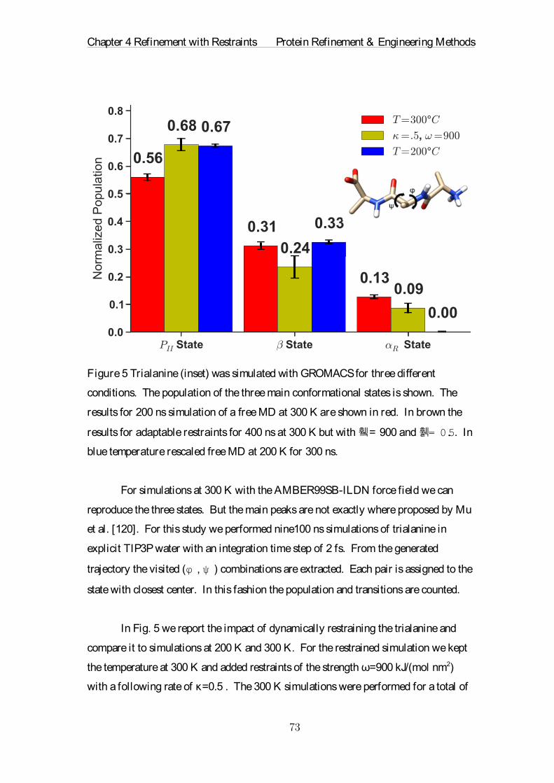
Chapter 4 Refinement with Restraints Protein Refinement & Engineering Methods
Figure 5 Trialanine (inset) was simulated with GROMACS for three different
conditions. The population of the three main conformational states is shown. The
results for 200 ns simulation of a free MD at 300 K are shown in red. In brown the
results for adaptable restraints for 400 ns at 300 K but with 휔 = 900 and 휅= 0.5. In
blue temperature rescaled free MD at 200 K for 300 ns.
For simulations at 300 K with the AMBER99SB-ILDN force field we can
reproduce the three states. But the main peaks are not exactly where proposed by Mu
et al. [120]. For this study we performed nine100 ns simulations of trialanine in
explicit TIP3P water with an integration time step of 2 fs. From the generated
trajectory the visited (φ , ψ ) combinations are extracted. Each pair is assigned to the
state with closest center. In this fashion the population and transitions are counted.
In Fig. 5 we report the impact of dynamically restraining the trialanine and
compare it to simulations at 200 K and 300 K. For the restrained simulation we kept
the temperature at 300 K and added restraints of the strength ω=900 kJ/(mol nm2)
with a following rate of κ=0.5 . The 300 K simulations were performed for a total of

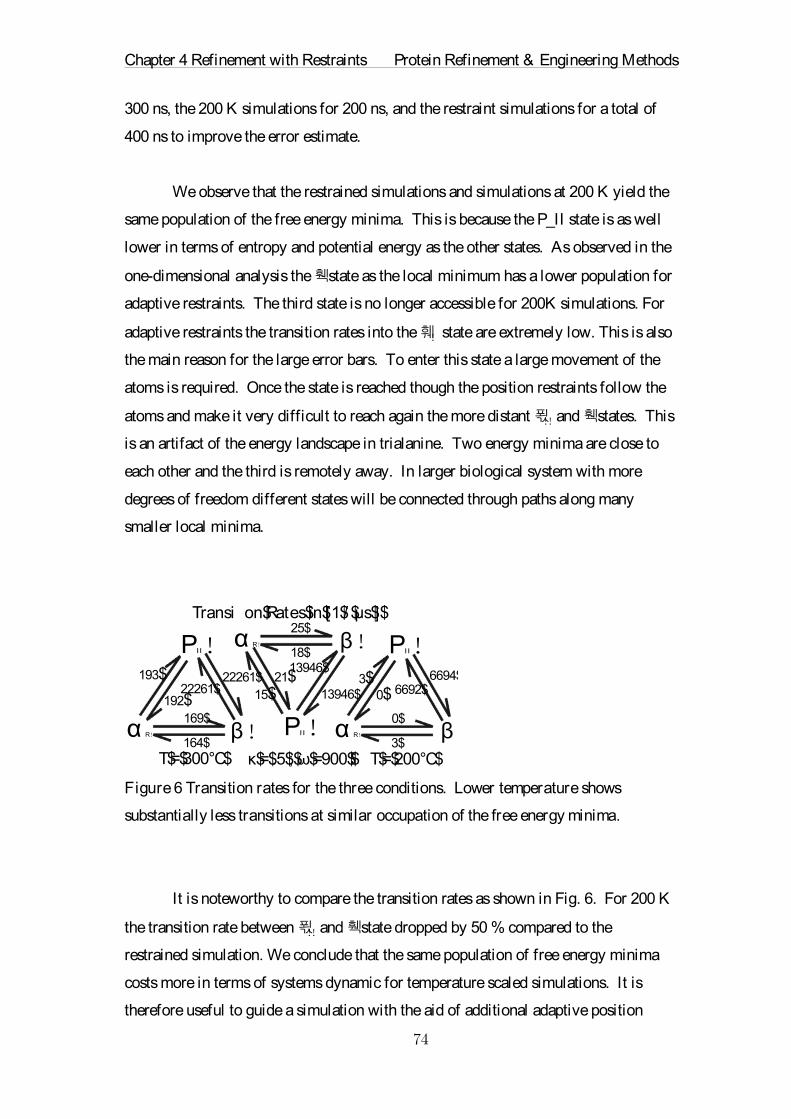
Chapter 4 Refinement with Restraints Protein Refinement & Engineering Methods
300 ns, the 200 K simulations for 200 ns, and the restraint simulations for a total of
400 ns to improve the error estimate.
We observe that the restrained simulations and simulations at 200 K yield the
same population of the free energy minima. This is because the P_II state is as well
lower in terms of entropy and potential energy as the other states. As observed in the
one-dimensional analysis the 훽 state as the local minimum has a lower population for
adaptive restraints. The third state is no longer accessible for 200K simulations. For
adaptive restraints the transition rates into the 훼! state are extremely low. This is also
the main reason for the large error bars. To enter this state a large movement of the
atoms is required. Once the state is reached though the position restraints follow the
atoms and make it very difficult to reach again the more distant 푃!! and 훽 states. This
is an artifact of the energy landscape in trialanine. Two energy minima are close to
each other and the third is remotely away. In larger biological system with more
degrees of freedom different states will be connected through paths along many
smaller local minima.
Figure 6 Transition rates for the three conditions. Lower temperature shows
substantially less transitions at similar occupation of the free energy minima.
It is noteworthy to compare the transition rates as shown in Fig. 6. For 200 K
the transition rate between 푃!! and 훽 state dropped by 50 % compared to the
restrained simulation. We conclude that the same population of free energy minima
costs more in terms of systems dynamic for temperature scaled simulations. It is
therefore useful to guide a simulation with the aid of additional adaptive position
β!α R!
Pıı!22261$
22261$
169$192$
193$
164$β!α R!
Pıı!6694$
6692$
0$
0$3$
3$
β!α R!
Pıı!
13946$
13946$
25$
21$15$
18$
T$=$300°C$ κ$=$.5$;$ω$=900$$ T$=$200°C$
Transi�on$Rates$in$[1$/ $μs$]$

Chapter 4 Refinement with Restraints Protein Refinement & Engineering Methods
restraints. This example has shown how adaptive restraints increase the sampling of
free energy minima in biological relevant settings. The same approach can also be
used in more abstract methods. We applied it for example successfully in high
dimensional search problems.
4.6 Conclusion
This study has revealed the effect of adaptive restraints in molecular dynamics
simulations. We have derived an expression for the one-dimensional case of a particle
in an energy landscape. This expression was verified for different coupling strengths
in Langevin dynamic simulations.
For high dimensional problems the adaptive restraints have been shown to
sample the free energy minima more frequently. This is an effect not always
achievable by temperature rescaling. A small trialanine peptide was used to
demonstrate the advantages of using adaptive restraints. Adding adaptive restraints is
powerful for a wide variety of search and sampling problems.

Chapter 5 Redesign of LipA Protein Refinement & Engineering Methods
��
Chapter 5 Redesign of L ipase LipA
5.1 General Introduction
This chapter deals with the application of protein engineering methods to a
real world example. The lipase LipA from Pseudomonas aeruginosa will be the test
subject of this study. The aim is to modify this enzyme to catalyze a substrate that it
does not catalyze in its wild-type form. There are several aspects that are of great
importance when designing a protein. First one needs to find a way of reducing the
search space of amino acid sequences. The number of options for amino acid
sequences is so large that it would not even be feasible to write them out. Even a
most simplistic ranking method, like alphabetical sorting, could not be achieved on
the data set. Second a tool is needed that can quickly and reliably compare and rank
amino acid sequences with respect to their activity.
In this chapter we will introduce the idea of sequential mutations to cope with
the astronomical search space. This will enable us to iteratively increase the activity
with each new mutation. A computational protocol is presented that can relatively
quickly assign binding energies to amino acid sequences. The combination of both
methods has the purpose to assist directed evolution experiments to find a mutation of
LipA with 900 % increased activity. This work has been supported strongly by Dr.
Filip Kovacic and Professor Karl-Erich Jäger. The experiments and the
corresponding analyses were performed in their lab. The design of the simulation
protocol and the search strategy is the work of the author under helpful supervision of
Professor Schröder. The calculations were performed with a computing grant on the
super computer JUROPA. The contents of this chapter will be submitted after final
results are obtained from the lab.

Chapter 5 Redesign of LipA Protein Refinement & Engineering Methods
��
5.2 Introduction:
The Roche Ester is a molecule of high industrial relevance. After hydrolysis a
valuable component is generated that can be used for the production of detergents.
Because no enzyme is known to facilitate this reaction, the aim of this study is to
design one. Protein engineering is the art of changing or altering, or even designing, a
protein to make it serve a specific purpose. [121] Nature appears able to adapt
proteins for all of its own purposes. The vast amount of sequence and structural data
available today provides an impressive glimpse into the potential that rests in
proteins.[122] Most proteins consist of an amino acid chain with in between twenty
and many thousand elements. Each element is a small molecule, picked from the pool
of 20 natural amino acids. The amino acids form the basic set of building blocks
from which the most complex molecular machines have emerged.[123] The power to
manipulate the coding sequence of genes has been harnessed for the last 30
years.[124] Provided the knowledge of a target amino acid sequence, advances in
biotechnology allow the expression of any desired amount of a mutant protein in a
suitable host system.[121] The key problem with protein engineering up until now
rests in the following question: how can we find the amino acid sequence that
encodes a desired protein?[125]
The most powerful tool in protein engineering to date is directed
evolution.[126] Random mutations are introduced to create a library of proteins.
They are exposed to artificial evolutionary pressures in an attempt to identify more
active mutations in the amino acid sequence. The success of directed evolution over
other protein design schemes is mainly due to of our current lack of understanding
about the principal functions and interactions of the molecular machines.[127] [125]
The alternative route to random experiments is rational design that utilizes existing
knowledge about a protein such as its structure or sequence.[126] The often disastrous
effects of 'rationally introduced' mutations on the stability and activity of proteins
prompted Charles Craik to muse that 'protein terrorism' was a more suitable descriptor
than protein engineering.[128] But despite the very high failure rate associated with
rational design, some proteins have been successfully engineered for industrial and
biomedical applications.[129] Oftentimes the engineered proteins are supposed to act

Chapter 5 Redesign of LipA Protein Refinement & Engineering Methods
��
as enzymes to accelerate desired reactions. But even the best performing engineered
enzymes are 5 to 10 magnitudes lower in activity than nature's counterparts.[125]
Nowadays the distinction between rational design and directed evolution is becoming
less clear as researchers commonly combine these techniques.[126] In this work. a
rational design approach is used to identify promising mutational candidates in the
lipase LipA from Pseudomonas aeruginosa. The predicted mutations have been
introduced via PCR and tested for activity. The described protocol can aid to reduce
the size of the screening libraries used in directed evolution experiments
5.3 METHOD
For a protein with 300 amino acids, which is about the size of an average
protein, there exist a total of 10114 possible amino acid sequences (the known universe
consists of approximately 1080 atoms). To search for the best sequence is a search in
an almost infinite space. Therefore we need to make the assumption that there are
many sequences that will yield the desired activity if we want to have any hope of
tackling this problem successfully. We start our search with the amino acids sequence
of LipA from PA (PDB 1EX9) that has been crystalized in its open conformation.[130]
It is the common belief that the transition state of an enzyme substrate complex has
the greatest effect on activity. If the transition state is more easily accessible and
better stabilized by the binding pocket for a mutated sequence, then an increase in
enzyme activity is expected.
Here the next problem unravels. How can one determine the transition state
geometry for the amino acid sequences? The correct geometry of the transition state
can only be determined in the structure space. The stable conformations of a protein
are the minima of its free energy surface.[131] The number of possible conformations
that a protein of 300 amino acids can take may be approximated by the number of
combinations of dihedral angles as has been done by Levinthal to be 10143[132],
another astronomical number. In a different paper Levinthal proposed a solution to
the paradox arising from the vast number of different conformations a protein can
explore and the efficiency of its folding. He argued that pathways or energy funnels

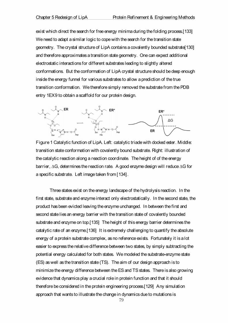
Chapter 5 Redesign of LipA Protein Refinement & Engineering Methods
��
exist which direct the search for free energy minima during the folding process.[133]
We need to adapt a similar logic to cope with the search for the transition state
geometry. The crystal structure of LipA contains a covalently bounded substrate[130]
and therefore approximates a transition state geometry. One can expect additional
electrostatic interactions for different substrates leading to slightly altered
conformations. But the conformation of LipA crystal structure should be deep enough
inside the energy funnel for various substrates to allow a prediction of the true
transition conformation. We therefore simply removed the substrate from the PDB
entry 1EX9 to obtain a scaffold for our protein design.
Figure 1 Catalytic function of LipA. Left: catalytic triade with docked ester. Middle:
transition state conformation with covalently bound substrate. Right: illustration of
the catalytic reaction along a reaction coordinate. The height of of the energy
barrier, ∆G, determines the reaction rate. A good enzyme design will reduce ∆G for
a specific substrate. Left image taken from [134] .
Three states exist on the energy landscape of the hydrolysis reaction. In the
first state, substrate and enzyme interact only electrostatically. In the second state, the
product has been evicted leaving the enzyme unchanged. In between the first and
second state lies an energy barrier with the transition state of covalently bounded
substrate and enzyme on top.[135] The height of this energy barrier determines the
catalytic rate of an enzyme.[136] It is extremely challenging to quantify the absolute
energy of a protein substrate complex, as no reference exists. Fortunately it is a lot
easier to express the relative difference between two states, by simply subtracting the
potential energy calculated for both states. We modeled the substrate-enzyme state
(ES) as well as the transition state (TS). The aim of our design approach is to
minimize the energy difference between the ES and TS states. There is also growing
evidence that dynamics play a crucial role in protein function and that it should
therefore be considered in the protein engineering process.[129] Any simulation
approach that wants to illustrate the change in dynamics due to mutations is

Chapter 5 Redesign of LipA Protein Refinement & Engineering Methods
��
computationally expensive. Because we do not want to ignore this important factor
we do not consider only one single conformation of the protein. Instead we generated
an ensemble of 96 structures with exactly the same transition state geometry but with
a spread of 2.5�Å�root�mean�square�deviation�(RMSD) in the remaining C-α protein
backbone. The RMSD value was calculated as the average of all C-α RMSD values
between the 95 conformations and the crystal structure. For each of these 96
conformations the energy barrier is calculated. The ensemble approach yields an idea
of the role that dynamics plays. If only a few conformations yield low energy
barriers, then we can conclude that most of the structural space is unfavorable for the
desired reaction.
The transition state is the ground state geometry of the system consisting of
the substrate, catalytic triad, and supporting amide groups in the protein
backbone.[130] For this set of molecules a density functional (DFT) transition state
search was performed with SPARTAN[137]. From this calculation the charges and
ground state geometry were obtained for the transition state geometry. In addition a
ground state search was performed just for the substrate to identify its geometry in the
non-covalently bounded state. The derived parameters and structures are listed in the
next subsection. With the ground and transition state geometries we are able to
compare the energy difference between the ES and TS states for the wild-type LipA.
At first 95 conformation of the crystal structure are created with CONCOORD[138],
with the constraint of fixed atomic positions for the atoms used in the DFT
calculation. The crystal structure is also included into this ensemble. For each
structure in the ensemble two structures are generated, one with the ground state
substrate inserted into the active site and one in the transition state conformation.
The natural next question is how to calculate the energy difference between
the substrate-bound and transition state. Calculating the energy difference between
the ES and TS states is the most crucial part of our design approach. The scoring
function needs to be precise enough to pick up small changes in the atomic
composition of the protein, as well as fast enough to be applied to thousands of
structures. A full molecular dynamics simulation (MD) of the ES and TS systems
would go beyond the constraints of time efficiency. An energy minimization (EM),

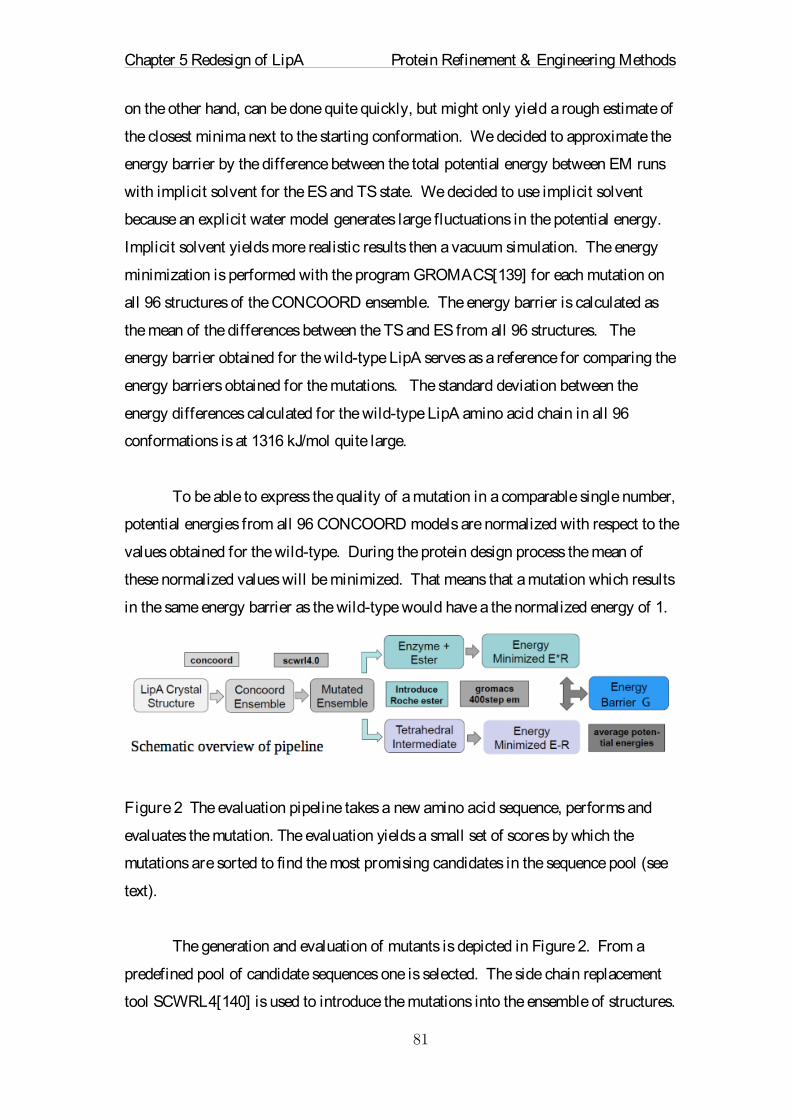
Chapter 5 Redesign of LipA Protein Refinement & Engineering Methods
��
on the other hand, can be done quite quickly, but might only yield a rough estimate of
the closest minima next to the starting conformation. We decided to approximate the
energy barrier by the difference between the total potential energy between EM runs
with implicit solvent for the ES and TS state. We decided to use implicit solvent
because an explicit water model generates large fluctuations in the potential energy.
Implicit solvent yields more realistic results then a vacuum simulation. The energy
minimization is performed with the program GROMACS[139] for each mutation on
all 96 structures of the CONCOORD ensemble. The energy barrier is calculated as
the mean of the differences between the TS and ES from all 96 structures. The
energy barrier obtained for the wild-type LipA serves as a reference for comparing the
energy barriers obtained for the mutations. The standard deviation between the
energy differences calculated for the wild-type LipA amino acid chain in all 96
conformations is at 1316 kJ/mol quite large.
To be able to express the quality of a mutation in a comparable single number,
potential energies from all 96 CONCOORD models are normalized with respect to the
values obtained for the wild-type. During the protein design process the mean of
these normalized values will be minimized. That means that a mutation which results
in the same energy barrier as the wild-type would have a the normalized energy of 1.
Figure 2 The evaluation pipeline takes a new amino acid sequence, performs and
evaluates the mutation. The evaluation yields a small set of scores by which the
mutations are sorted to find the most promising candidates in the sequence pool (see
text).
The generation and evaluation of mutants is depicted in Figure 2. From a
predefined pool of candidate sequences one is selected. The side chain replacement
tool SCWRL4[140] is used to introduce the mutations into the ensemble of structures.

Chapter 5 Redesign of LipA Protein Refinement & Engineering Methods
��
Only the mutated side chains will be optimized, the remainder of the protein is kept as
it was. The replacement is done in the presence of the substrate to avoid unnecessary
steric clashes. The result of this step is an ensemble of 96 mutated structures, for
which the procedure described for the wild-type ensemble is repeated. After
minimization the potential energies are rescaled and averaged. If the resulting value
is smaller than 1 a potential candidate for the experiment was found. One main
challenge of this protocol is the creation of a useful pool of sequences. When faced
with the realization that it cannot be possible for a protein to try out every possible
combination of dihedral angles, Levinthal proposed an energy funnel that guides the
folding of a protein. We are in a situation similar to Levinthal’s paradox. It is not
feasible to try out every possible combination of amino acids to find the best
performing protein. In nature proteins that have emerged from evolution gained their
function one mutation at a time. Therefore we propose a funnel in sequence space,
similar to the energy funnel proposed by Levinthal that leads to improved activity.
Instead of jumping right towards the optimal sequence, we propose an iterative
procedure. Starting from single-point mutations we select the best candidate and then
continue to double mutants and so forth. A first the pool of sequences, therefore,
consists of single point mutations. We repeat the whole procedure to obtain two-point
mutations for the successful candidates from this first iteration, treating the best one
point mutations like the wild-type. We can consider this strategy as a search tree. At
the root we have the wild-type sequence. The first layer contains all possible
(300*20-1) single-point mutations as children of the root. Each consecutive layer
adds the same number of children to each parent node. Our search algorithm is a
mixture of breadth and depth first searches. All possible states that can be reached
with a single-point mutation from the current node are first evaluated (breadth first).
Then we jump to the child with the lowest scoring function value (depth first) and
repeat for its children. This process can be repeated until convergence for some
higher point mutation.
5.3 In silico Results
In this subsection, different steps of the design protocol are presented. When
redesigning an enzyme it is first crucial to understand its functional mechanism. The

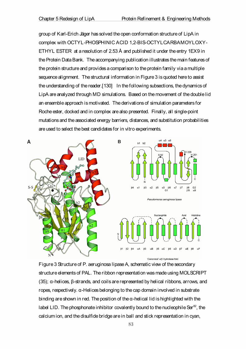
Chapter 5 Redesign of LipA Protein Refinement & Engineering Methods
��
group of Karl-Erich Jäger has solved the open conformation structure of LipA in
complex with OCTYL-PHOSPHINIC ACID 1,2-BIS-OCTYLCARBAMOYLOXY-
ETHYL ESTER at a resolution of 2.53 Å and published it under the entry 1EX9 in
the Protein Data Bank. The accompanying publication illustrates the main features of
the protein structure and provides a comparison to the protein family via a multiple
sequence alignment. The structural information in Figure 3 is quoted here to assist
the understanding of the reader.[130] In the following subsections, the dynamics of
LipA are analyzed through MD simulations. Based on the movement of the double lid
an ensemble approach is motivated. The derivations of simulation parameters for
Roche ester, docked and in complex are also presented. Finally, all single-point
mutations and the associated energy barriers, distances, and substitution probabilities
are used to select the best candidates for in vitro experiments.
Figure 3 Structure of P. aeruginosa lipase A, schematic view of the secondary
structure elements of PAL. The ribbon representation was made using MOLSCRIPT
(35); α-helices, β-strands, and coils are represented by helical ribbons, arrows, and
ropes, respectively. α-Helices belonging to the cap domain involved in substrate
binding are shown in red. The position of the α-helical lid is highlighted with the
label LID. The phosphonate inhibitor covalently bound to the nucleophile Ser82, the
calcium ion, and the disulfide bridge are in ball and stick representation in cyan,

Chapter 5 Redesign of LipA Protein Refinement & Engineering Methods
��
black, and yellow, respectively. B, secondary structure topology diagram of PAL. The
catalytic triad residues (Ser82, Asp229, and His251) and the position of the disulfide
bridge are indicated, and a comparison with the canonical α/β hydrolase fold is
given. α-Helices and β-strands are represented byrectangles and arrows,
respectively. G1 and G2 are 310 helices and are represented by squares. Locations
where insertions in the canonical fold may occur are indicated by dashed lines.
Figure taken from Nardini et al. [130]
5.3.1 MD Simulations of LipA
The main points to take from Figure 3 are the helical lid motif right above the
active pocket and the position of the catalytic triad. To better understand the function
of the lid and the overall dynamics of LipA, a MD simulation was performed starting
from the crystal structure. First, the ligand was removed from the PDB file.
Afterwards a 1000 step energy minimization was performed with GROMACS. The
minimized structure was then solvated and the system neutralized by adding ions.
Following this, short equilibrations were performed firstly in the canonical (NVT)
ensemble to stabilize the temperature and then secondly another short equilibration in
the isothermal-isobaric (NPT) ensemble to equilibrate the pressure. This allows the
water to relax and the following production run to occur at physiological conditions.
The system was then simulated at 300 K for 200 ns with an integration time step of 2
fs with temperature and pressure coupling. The simulations were performed with
periodic boundary conditions and long-range interactions were computed using the
particle mesh Ewald method.
The final trajectory was analyzed with the GROMACS tools and the results
are visualized with PYTHON scripts. The RMSD curve in Figure 5 shows certain
transitions at about 100 ns. A closer look into the structures reveals that the transition
correlates with the movement of the helical lid. To illustrate the movement further a
principle component analysis was performed on the trajectory. The aim of the
principle component analysis is to identify the main components contributing to the
dynamics of the protein. For this a covariance matrix of all C-α atoms is computed
and diagonalized. The eigenvalues and eigenvectors belonging to this matrix are the

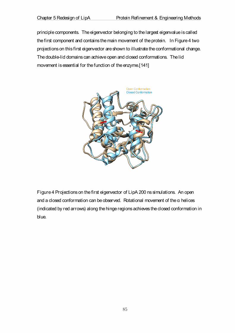
Chapter 5 Redesign of LipA Protein Refinement & Engineering Methods
��
principle components. The eigenvector belonging to the largest eigenvalue is called
the first component and contains the main movement of the protein. In Figure 4 two
projections on this first eigenvector are shown to illustrate the conformational change.
The double-lid domains can achieve open and closed conformations. The lid
movement is essential for the function of the enzyme.[141]
Figure 4 Projections on the first eigenvector of LipA 200 ns simulations. An open
and a closed conformation can be observed. Rotational movement of the α helices
(indicated by red arrows) along the hinge regions achieves the closed conformation in
blue.

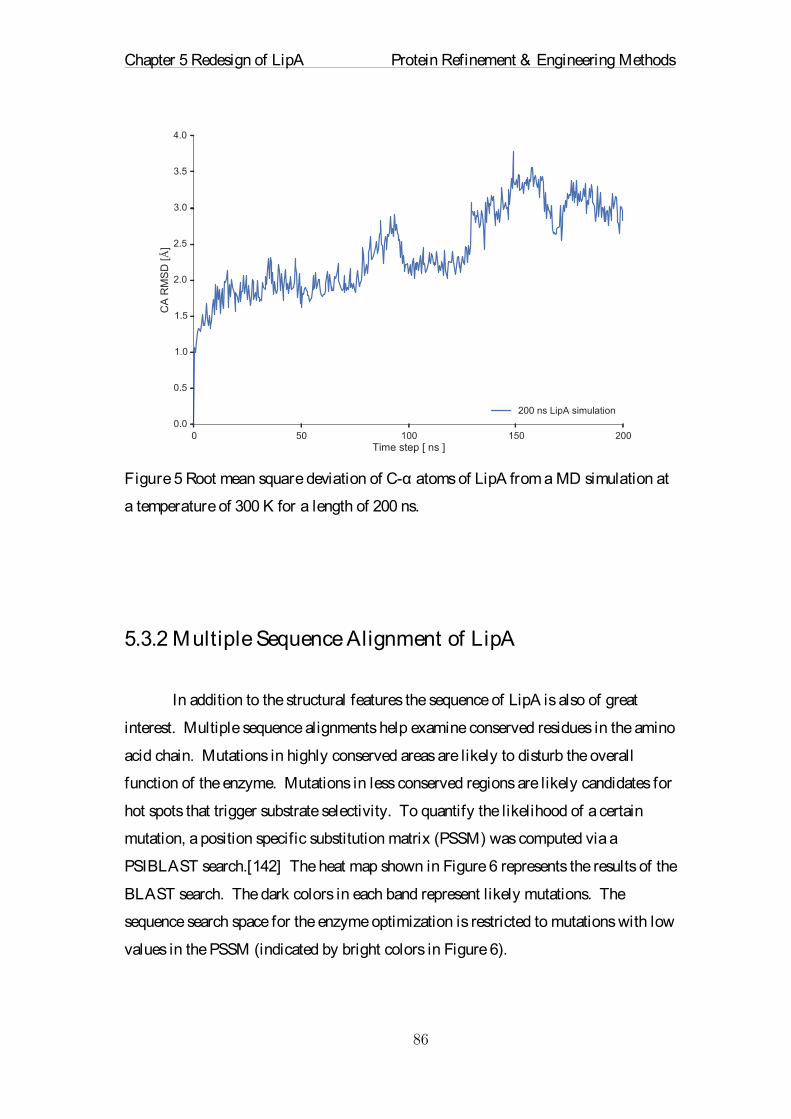
Chapter 5 Redesign of LipA Protein Refinement & Engineering Methods
��
Figure 5 Root mean square deviation of C-α atoms of LipA from a MD simulation at
a temperature of 300 K for a length of 200 ns.
5.3.2 Multiple Sequence Alignment of LipA
In addition to the structural features the sequence of LipA is also of great
interest. Multiple sequence alignments help examine conserved residues in the amino
acid chain. Mutations in highly conserved areas are likely to disturb the overall
function of the enzyme. Mutations in less conserved regions are likely candidates for
hot spots that trigger substrate selectivity. To quantify the likelihood of a certain
mutation, a position specific substitution matrix (PSSM) was computed via a
PSIBLAST search.[142] The heat map shown in Figure 6 represents the results of the
BLAST search. The dark colors in each band represent likely mutations. The
sequence search space for the enzyme optimization is restricted to mutations with low
values in the PSSM (indicated by bright colors in Figure 6).

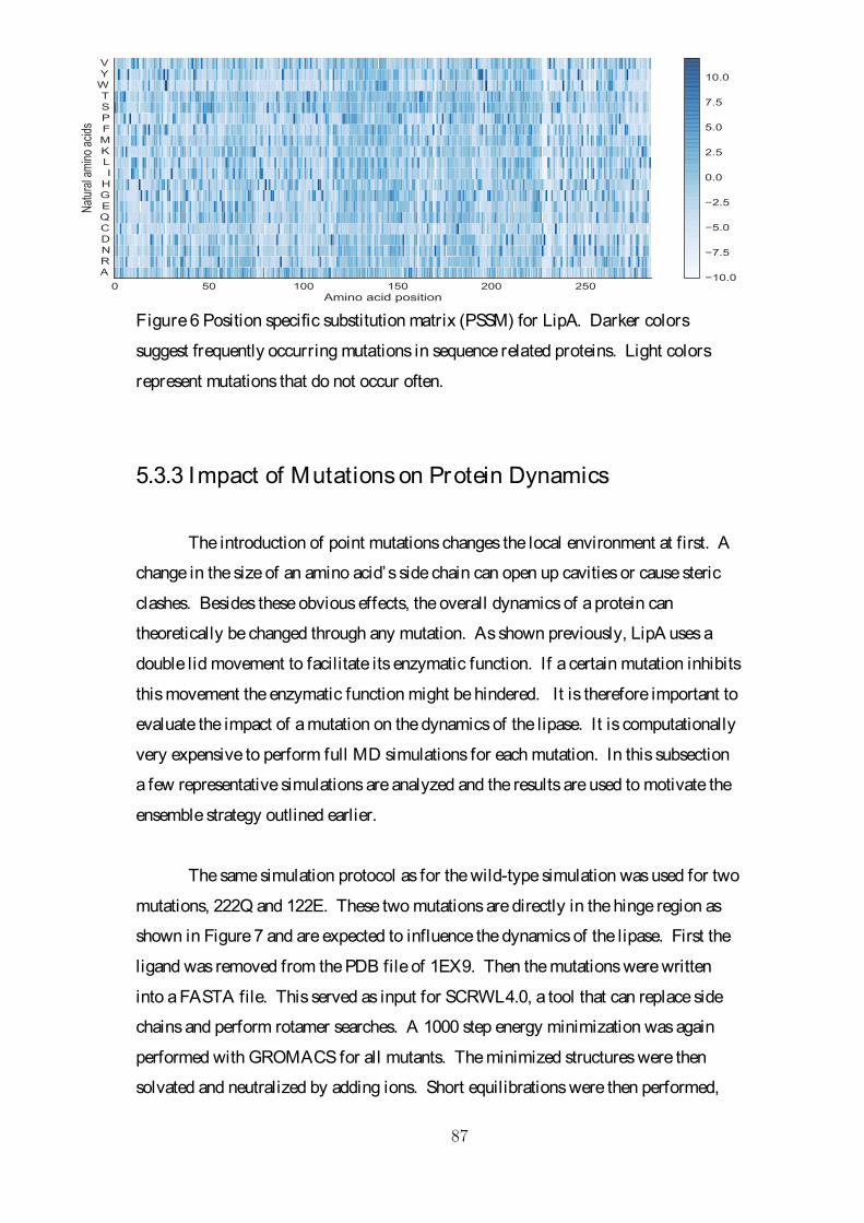
Chapter 5 Redesign of LipA Protein Refinement & Engineering Methods
��
Figure 6 Position specific substitution matrix (PSSM) for LipA. Darker colors
suggest frequently occurring mutations in sequence related proteins. Light colors
represent mutations that do not occur often.
5.3.3 Impact of Mutations on Protein Dynamics
The introduction of point mutations changes the local environment at first. A
change in the size of an amino acid’s side chain can open up cavities or cause steric
clashes. Besides these obvious effects, the overall dynamics of a protein can
theoretically be changed through any mutation. As shown previously, LipA uses a
double lid movement to facilitate its enzymatic function. If a certain mutation inhibits
this movement the enzymatic function might be hindered. It is therefore important to
evaluate the impact of a mutation on the dynamics of the lipase. It is computationally
very expensive to perform full MD simulations for each mutation. In this subsection
a few representative simulations are analyzed and the results are used to motivate the
ensemble strategy outlined earlier.
The same simulation protocol as for the wild-type simulation was used for two
mutations, 222Q and 122E. These two mutations are directly in the hinge region as
shown in Figure 7 and are expected to influence the dynamics of the lipase. First the
ligand was removed from the PDB file of 1EX9. Then the mutations were written
into a FASTA file. This served as input for SCRWL4.0, a tool that can replace side
chains and perform rotamer searches. A 1000 step energy minimization was again
performed with GROMACS for all mutants. The minimized structures were then
solvated and neutralized by adding ions. Short equilibrations were then performed,

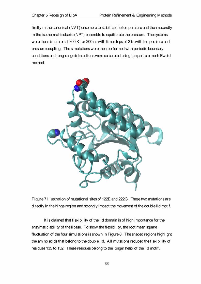
Chapter 5 Redesign of LipA Protein Refinement & Engineering Methods
��
firstly in the canonical (NVT) ensemble to stabilize the temperature and then secondly
in the isothermal-isobaric (NPT) ensemble to equilibrate the pressure. The systems
were then simulated at 300 K for 200 ns with time steps of 2 fs with temperature and
pressure coupling. The simulations were then performed with periodic boundary
conditions and long-range interactions were calculated using the particle mesh Ewald
method.
Figure 7 Illustration of mutational sites of 122E and 222G. These two mutations are
directly in the hinge region and strongly impact the movement of the double lid motif.
It is claimed that flexibility of the lid domain is of high importance for the
enzymatic ability of the lipase. To show the flexibility, the root mean square
fluctuation of the four simulations is shown in Figure 8. The shaded regions highlight
the amino acids that belong to the double lid. All mutations reduced the flexibility of
residues 135 to 152. These residues belong to the longer helix of the lid motif.

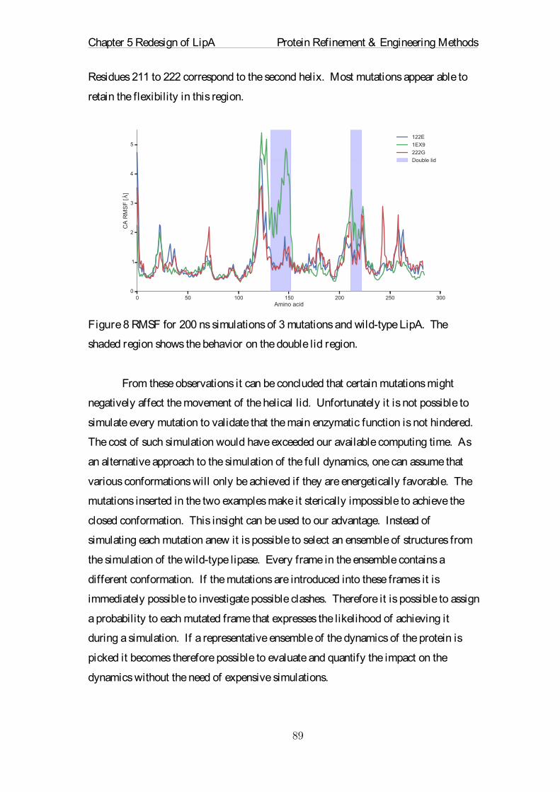
Chapter 5 Redesign of LipA Protein Refinement & Engineering Methods
��
Residues 211 to 222 correspond to the second helix. Most mutations appear able to
retain the flexibility in this region.
Figure 8 RMSF for 200 ns simulations of 3 mutations and wild-type LipA. The
shaded region shows the behavior on the double lid region.
From these observations it can be concluded that certain mutations might
negatively affect the movement of the helical lid. Unfortunately it is not possible to
simulate every mutation to validate that the main enzymatic function is not hindered.
The cost of such simulation would have exceeded our available computing time. As
an alternative approach to the simulation of the full dynamics, one can assume that
various conformations will only be achieved if they are energetically favorable. The
mutations inserted in the two examples make it sterically impossible to achieve the
closed conformation. This insight can be used to our advantage. Instead of
simulating each mutation anew it is possible to select an ensemble of structures from
the simulation of the wild-type lipase. Every frame in the ensemble contains a
different conformation. If the mutations are introduced into these frames it is
immediately possible to investigate possible clashes. Therefore it is possible to assign
a probability to each mutated frame that expresses the likelihood of achieving it
during a simulation. If a representative ensemble of the dynamics of the protein is
picked it becomes therefore possible to evaluate and quantify the impact on the
dynamics without the need of expensive simulations.

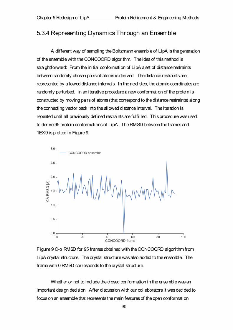
Chapter 5 Redesign of LipA Protein Refinement & Engineering Methods
��
5.3.4 Representing Dynamics Through an Ensemble
A different way of sampling the Boltzmann ensemble of LipA is the generation
of the ensemble with the CONCOORD algorithm. The idea of this method is
straightforward: From the initial conformation of LipA a set of distance restraints
between randomly chosen pairs of atoms is derived. The distance restraints are
represented by allowed distance intervals. In the next step, the atomic coordinates are
randomly perturbed. In an iterative procedure a new conformation of the protein is
constructed by moving pairs of atoms (that correspond to the distance restraints) along
the connecting vector back into the allowed distance interval. The iteration is
repeated until all previously defined restraints are fulfilled. This procedure was used
to derive 95 protein conformations of LipA. The RMSD between the frames and
1EX9 is plotted in Figure 9.
Figure 9 C-α RMSD for 95 frames obtained with the CONCOORD algorithm from
LipA crystal structure. The crystal structure was also added to the ensemble. The
frame with 0 RMSD corresponds to the crystal structure.
Whether or not to include the closed conformation in the ensemble was an
important design decision. After discussion with our collaborators it was decided to
focus on an ensemble that represents the main features of the open conformation

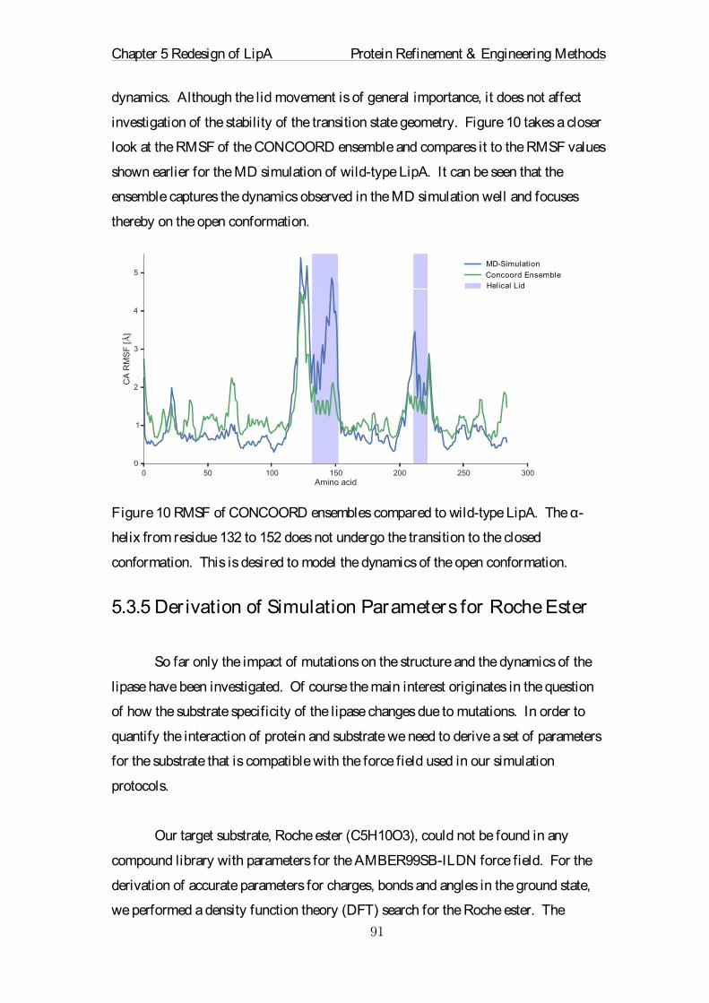
Chapter 5 Redesign of LipA Protein Refinement & Engineering Methods
��
dynamics. Although the lid movement is of general importance, it does not affect
investigation of the stability of the transition state geometry. Figure 10 takes a closer
look at the RMSF of the CONCOORD ensemble and compares it to the RMSF values
shown earlier for the MD simulation of wild-type LipA. It can be seen that the
ensemble captures the dynamics observed in the MD simulation well and focuses
thereby on the open conformation.
Figure 10 RMSF of CONCOORD ensembles compared to wild-type LipA. The α-
helix from residue 132 to 152 does not undergo the transition to the closed
conformation. This is desired to model the dynamics of the open conformation.
�
5.3.5 Der ivation of Simulation Parameters for Roche Ester
So far only the impact of mutations on the structure and the dynamics of the
lipase have been investigated. Of course the main interest originates in the question
of how the substrate specificity of the lipase changes due to mutations. In order to
quantify the interaction of protein and substrate we need to derive a set of parameters
for the substrate that is compatible with the force field used in our simulation
protocols.
Our target substrate, Roche ester (C5H10O3), could not be found in any
compound library with parameters for the AMBER99SB-ILDN force field. For the
derivation of accurate parameters for charges, bonds and angles in the ground state,
we performed a density function theory (DFT) search for the Roche ester. The
MD-Simulation
Concoord EnsembleHelical Lid

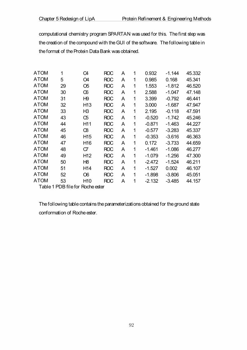
Chapter 5 Redesign of LipA Protein Refinement & Engineering Methods
��
computational chemistry program SPARTAN was used for this. The first step was
the creation of the compound with the GUI of the software. The following table in
the format of the Protein Data Bank was obtained.
Table 1 PDB file for Roche ester
The following table contains the parameterizations obtained for the ground state
conformation of Roche ester.
ATOM 1� C4� ROC� A� 1� 0.932� -1.144� 45.332�ATOM 5� O4� ROC� A� 1� 0.985� 0.168� 45.341�ATOM 29� O5� ROC� A� 1� 1.553� -1.812� 46.520�ATOM 30� C6� ROC� A� 1� 2.588� -1.047� 47.148�ATOM 31� H9� ROC� A� 1� 3.399� -0.792� 46.441�ATOM 32� H13� ROC� A� 1� 3.000� -1.687� 47.947�ATOM 33� H3� ROC� A� 1� 2.195� -0.118� 47.591�ATOM 43� C5� ROC� A� 1� -0.520� -1.742� 45.246�ATOM 44� H11� ROC� A� 1� -0.871� -1.463� 44.227�ATOM 45� C8� ROC� A� 1� -0.577� -3.283� 45.337�ATOM 46� H15� ROC� A� 1� -0.353� -3.616� 46.363�ATOM 47� H16� ROC� A� 1� 0.172� -3.733� 44.659�ATOM 48� C7� ROC� A� 1� -1.461� -1.086� 46.277�ATOM 49� H12� ROC� A� 1� -1.079� -1.256� 47.300�ATOM 50� H8� ROC� A� 1� -2.472� -1.524� 46.211�ATOM 51� H14� ROC� A� 1� -1.527� 0.002� 46.107�ATOM 52� O6� ROC� A� 1� -1.898� -3.806� 45.051�ATOM 53� H10� ROC� A� 1� -2.132� -3.485� 44.157�

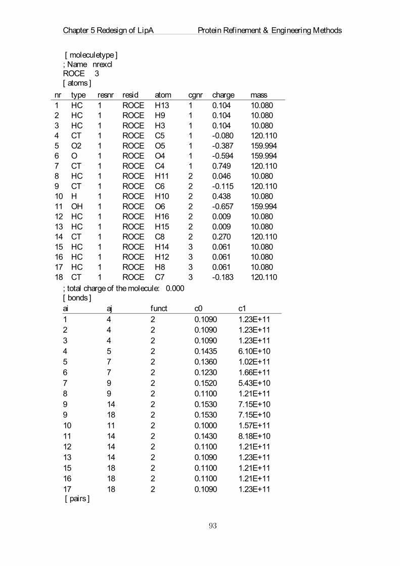
Chapter 5 Redesign of LipA Protein Refinement & Engineering Methods
��
[ moleculetype ] ; Name nrexcl ROCE 3 [ atoms ]
; total charge of the molecule: 0.000 [ bonds ]
[ pairs ]
nr type resnr resid atom cgnr charge mass 1 HC 1 ROCE H13 1 0.104 10.080 2 HC 1 ROCE H9 1 0.104 10.080 3 HC 1 ROCE H3 1 0.104 10.080 4 CT 1 ROCE C5 1 -0.080 120.110 5 O2 1 ROCE O5 1 -0.387 159.994 6 O 1 ROCE O4 1 -0.594 159.994 7 CT 1 ROCE C4 1 0.749 120.110 8 HC 1 ROCE H11 2 0.046 10.080 9 CT 1 ROCE C6 2 -0.115 120.110 10 H 1 ROCE H10 2 0.438 10.080 11 OH 1 ROCE O6 2 -0.657 159.994 12 HC 1 ROCE H16 2 0.009 10.080 13 HC 1 ROCE H15 2 0.009 10.080 14 CT 1 ROCE C8 2 0.270 120.110 15 HC 1 ROCE H14 3 0.061 10.080 16 HC 1 ROCE H12 3 0.061 10.080 17 HC 1 ROCE H8 3 0.061 10.080 18 CT 1 ROCE C7 3 -0.183 120.110
ai aj funct c0 c1 1 4 2 0.1090 1.23E+11 2 4 2 0.1090 1.23E+11 3 4 2 0.1090 1.23E+11 4 5 2 0.1435 6.10E+10 5 7 2 0.1360 1.02E+11 6 7 2 0.1230 1.66E+11 7 9 2 0.1520 5.43E+10 8 9 2 0.1100 1.21E+11 9 14 2 0.1530 7.15E+10 9 18 2 0.1530 7.15E+10 10 11 2 0.1000 1.57E+11 11 14 2 0.1430 8.18E+10 12 14 2 0.1100 1.21E+11 13 14 2 0.1090 1.23E+11 15 18 2 0.1100 1.21E+11 16 18 2 0.1100 1.21E+11 17 18 2 0.1090 1.23E+11

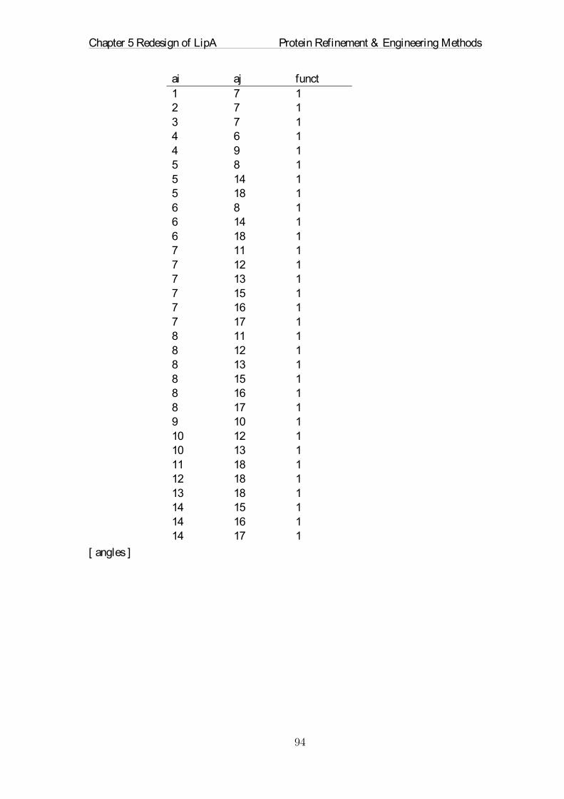
Chapter 5 Redesign of LipA Protein Refinement & Engineering Methods
��
[ angles ]
ai aj funct 1 7 1 2 7 1 3 7 1 4 6 1 4 9 1 5 8 1 5 14 1 5 18 1 6 8 1 6 14 1 6 18 1 7 11 1 7 12 1 7 13 1 7 15 1 7 16 1 7 17 1 8 11 1 8 12 1 8 13 1 8 15 1 8 16 1 8 17 1 9 10 1 10 12 1 10 13 1 11 18 1 12 18 1 13 18 1 14 15 1 14 16 1 14 17 1

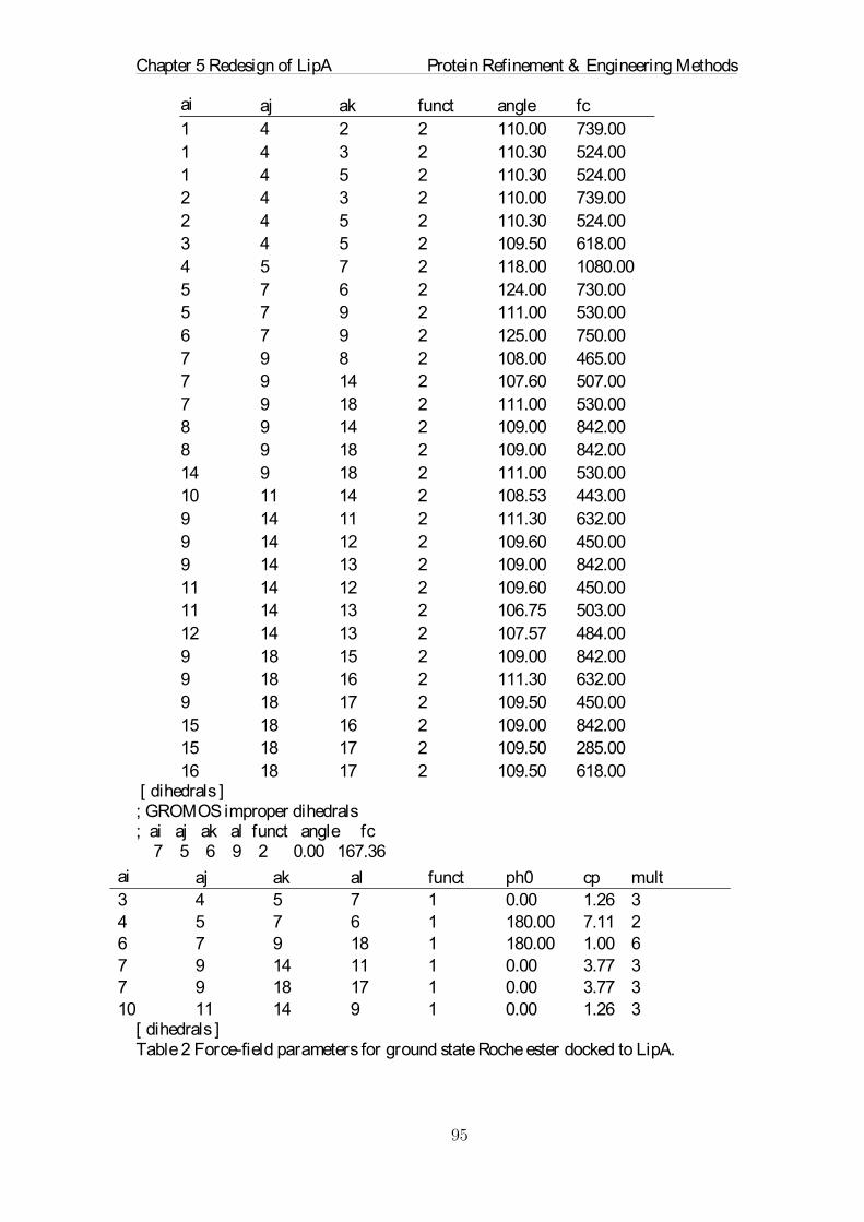
Chapter 5 Redesign of LipA Protein Refinement & Engineering Methods
��
[ dihedrals ] ; GROMOS improper dihedrals ; ai aj ak al funct angle fc 7 5 6 9 2 0.00 167.36
[ dihedrals ] Table 2 Force-field parameters for ground state Roche ester docked to LipA.
ai aj� ak� funct� angle� fc�1� 4� 2� 2� 110.00� 739.00�1� 4� 3� 2� 110.30� 524.00�1� 4� 5� 2� 110.30� 524.00�2� 4� 3� 2� 110.00� 739.00�2� 4� 5� 2� 110.30� 524.00�3� 4� 5� 2� 109.50� 618.00�4� 5� 7� 2� 118.00� 1080.00�5� 7� 6� 2� 124.00� 730.00�5� 7� 9� 2� 111.00� 530.00�6� 7� 9� 2� 125.00� 750.00�7� 9� 8� 2� 108.00� 465.00�7� 9� 14� 2� 107.60� 507.00�7� 9� 18� 2� 111.00� 530.00�8� 9� 14� 2� 109.00� 842.00�8� 9� 18� 2� 109.00� 842.00�14� 9� 18� 2� 111.00� 530.00�10� 11� 14� 2� 108.53� 443.00�9� 14� 11� 2� 111.30� 632.00�9� 14� 12� 2� 109.60� 450.00�9� 14� 13� 2� 109.00� 842.00�11� 14� 12� 2� 109.60� 450.00�11� 14� 13� 2� 106.75� 503.00�12� 14� 13� 2� 107.57� 484.00�9� 18� 15� 2� 109.00� 842.00�9� 18� 16� 2� 111.30� 632.00�9� 18� 17� 2� 109.50� 450.00�15� 18� 16� 2� 109.00� 842.00�15� 18� 17� 2� 109.50� 285.00�16� 18� 17� 2� 109.50� 618.00�
ai aj� ak� al� funct� ph0� cp� mult�3� 4� 5� 7� 1� 0.00� 1.26� 3�4� 5� 7� 6� 1� 180.00� 7.11� 2�6� 7� 9� 18� 1� 180.00� 1.00� 6�7� 9� 14� 11� 1� 0.00� 3.77� 3�7� 9� 18� 17� 1� 0.00� 3.77� 3�10� 11� 14� 9� 1� 0.00� 1.26� 3�

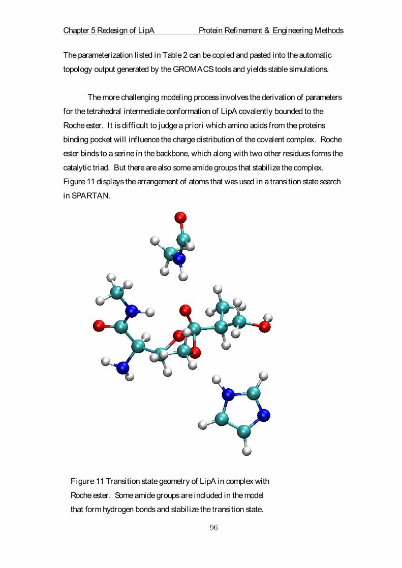
Chapter 5 Redesign of LipA Protein Refinement & Engineering Methods
��
The parameterization listed in Table 2 can be copied and pasted into the automatic
topology output generated by the GROMACS tools and yields stable simulations.
The more challenging modeling process involves the derivation of parameters
for the tetrahedral intermediate conformation of LipA covalently bounded to the
Roche ester. It is difficult to judge a priori which amino acids from the proteins
binding pocket will influence the charge distribution of the covalent complex. Roche
ester binds to a serine in the backbone, which along with two other residues forms the
catalytic triad. But there are also some amide groups that stabilize the complex.
Figure 11 displays the arrangement of atoms that was used in a transition state search
in SPARTAN.
Figure 11 Transition state geometry of LipA in complex with
Roche ester. Some amide groups are included in the model
that form hydrogen bonds and stabilize the transition state.
�

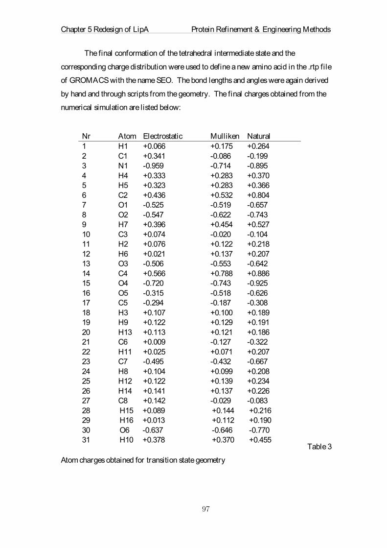
Chapter 5 Redesign of LipA Protein Refinement & Engineering Methods
��
The final conformation of the tetrahedral intermediate state and the
corresponding charge distribution were used to define a new amino acid in the .rtp file
of GROMACS with the name SEO. The bond lengths and angles were again derived
by hand and through scripts from the geometry. The final charges obtained from the
numerical simulation are listed below:
Table 3
Atom charges obtained for transition state geometry
Nr Atom Electrostatic Mulliken Natural 1 H1 +0.066 +0.175 +0.264 2 C1 +0.341 -0.086 -0.199 3 N1 -0.959 -0.714 -0.895 4 H4 +0.333 +0.283 +0.370 5 H5 +0.323 +0.283 +0.366 6 C2 +0.436 +0.532 +0.804 7 O1 -0.525 -0.519 -0.657 8 O2 -0.547 -0.622 -0.743 9 H7 +0.396 +0.454 +0.527 10 C3 +0.074 -0.020 -0.104 11 H2 +0.076 +0.122 +0.218 12 H6 +0.021 +0.137 +0.207 13 O3 -0.506 -0.553 -0.642 14 C4 +0.566 +0.788 +0.886 15 O4 -0.720 -0.743 -0.925 16 O5 -0.315 -0.518 -0.626 17 C5 -0.294 -0.187 -0.308 18 H3 +0.107 +0.100 +0.189 19 H9 +0.122 +0.129 +0.191 20 H13 +0.113 +0.121 +0.186 21 C6 +0.009 -0.127 -0.322 22 H11 +0.025 +0.071 +0.207 23 C7 -0.495 -0.432 -0.667 24 H8 +0.104 +0.099 +0.208 25 H12 +0.122 +0.139 +0.234 26 H14 +0.141 +0.137 +0.226 27 C8 +0.142 -0.029 -0.083 28 H15 +0.089 +0.144 +0.216 29 H16 +0.013 +0.112 +0.190 30 O6 -0.637 -0.646 -0.770 31 H10 +0.378 +0.370 +0.455

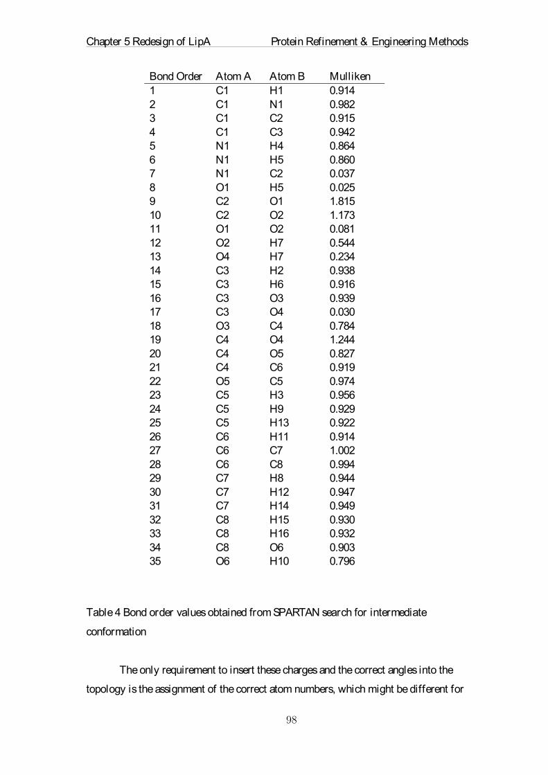
Chapter 5 Redesign of LipA Protein Refinement & Engineering Methods
��
Table 4 Bond order values obtained from SPARTAN search for intermediate
conformation
The only requirement to insert these charges and the correct angles into the
topology is the assignment of the correct atom numbers, which might be different for
Bond Order Atom A Atom B Mulliken 1 C1 H1 0.914 2 C1 N1 0.982 3 C1 C2 0.915 4 C1 C3 0.942 5 N1 H4 0.864 6 N1 H5 0.860 7 N1 C2 0.037 8 O1 H5 0.025 9 C2 O1 1.815 10 C2 O2 1.173 11 O1 O2 0.081 12 O2 H7 0.544 13 O4 H7 0.234 14 C3 H2 0.938 15 C3 H6 0.916 16 C3 O3 0.939 17 C3 O4 0.030 18 O3 C4 0.784 19 C4 O4 1.244 20 C4 O5 0.827 21 C4 C6 0.919 22 O5 C5 0.974 23 C5 H3 0.956 24 C5 H9 0.929 25 C5 H13 0.922 26 C6 H11 0.914 27 C6 C7 1.002 28 C6 C8 0.994 29 C7 H8 0.944 30 C7 H12 0.947 31 C7 H14 0.949 32 C8 H15 0.930 33 C8 H16 0.932 34 C8 O6 0.903 35 O6 H10 0.796

Chapter 5 Redesign of LipA Protein Refinement & Engineering Methods
��
each calculation due to the mutations. The correct mapping of the atoms is achieved
through a PYTHON script and enables very fast assembly of running parameter files
for the GROMACS simulations.
5.3.6 Estimation of the Energy Barr ier
All the tools are available to introduce the Roche ester to different
conformations and mutations of LipA both non-covalently bounded in the binding
pocket as well as covalently bounded in the transition state. Because of sterical
clashes, it is not possible to calculate a point energy for each conformation directly
after inserting the substrate. Even small deviations from the ideal parameters cause
gigantic contributions to the potential energies of the complex. It is therefore
essential to perform an energy minimization of each LipA + Roche ester complex.
This means that we need to construct 96 conformations of LipA with docked and
covalently bounded Roche ester and minimize each of these complexes. In total 192
energy minimizations have to be performed for each mutation. 192 energy
minimizations is feasible but still computationally demanding. One issue with a
physiological energy minimization is the impact of solvent molecules like water and
ions on the potential energy. Because of thermal noise, it would be impossible to get
accurate potential point energy from a short MD if explicit water would be used in the
simulations. Due to the thermal noise we decided to use the GBSA implicit water
model with a dielectric coefficient of 80 for the solvent in the minimization. Figure
12 illustrates the change of potential energy during the energy minimization. It is
apparent that the minimization is required to reduce the energy contributions due to
clashes and seemingly small deviations in ideal bond lengths and angles.

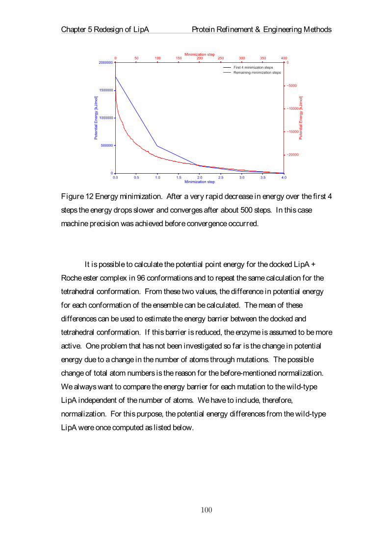
Chapter 5 Redesign of LipA Protein Refinement & Engineering Methods
��
Figure 12 Energy minimization. After a very rapid decrease in energy over the first 4
steps the energy drops slower and converges after about 500 steps. In this case
machine precision was achieved before convergence occurred.
It is possible to calculate the potential point energy for the docked LipA +
Roche ester complex in 96 conformations and to repeat the same calculation for the
tetrahedral conformation. From these two values, the difference in potential energy
for each conformation of the ensemble can be calculated. The mean of these
differences can be used to estimate the energy barrier between the docked and
tetrahedral conformation. If this barrier is reduced, the enzyme is assumed to be more
active. One problem that has not been investigated so far is the change in potential
energy due to a change in the number of atoms through mutations. The possible
change of total atom numbers is the reason for the before-mentioned normalization.
We always want to compare the energy barrier for each mutation to the wild-type
LipA independent of the number of atoms. We have to include, therefore,
normalization. For this purpose, the potential energy differences from the wild-type
LipA were once computed as listed below.

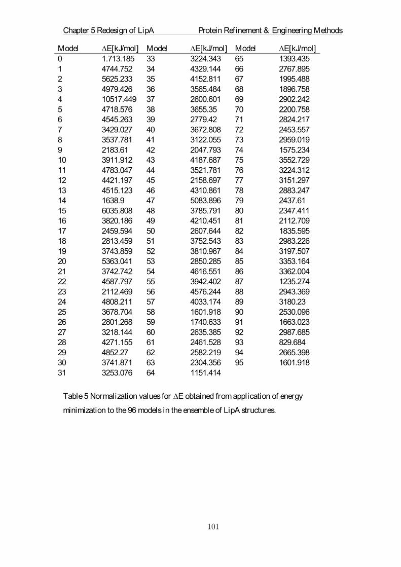
Chapter 5 Redesign of LipA Protein Refinement & Engineering Methods
��
Table 5 Normalization values for ∆E obtained from application of energy
minimization to the 96 models in the ensemble of LipA structures.
Model ∆E[kJ/mol] Model ∆E[kJ/mol] Model ∆E[kJ/mol] 0 1.713.185 33 3224.343 65 1393.435 1 4744.752 34 4329.144 66 2767.895 2 5625.233 35 4152.811 67 1995.488 3 4979.426 36 3565.484 68 1896.758 4 10517.449 37 2600.601 69 2902.242 5 4718.576 38 3655.35 70 2200.758 6 4545.263 39 2779.42 71 2824.217 7 3429.027 40 3672.808 72 2453.557 8 3537.781 41 3122.055 73 2959.019 9 2183.61 42 2047.793 74 1575.234 10 3911.912 43 4187.687 75 3552.729 11 4783.047 44 3521.781 76 3224.312 12 4421.197 45 2158.697 77 3151.297 13 4515.123 46 4310.861 78 2883.247 14 1638.9 47 5083.896 79 2437.61 15 6035.808 48 3785.791 80 2347.411 16 3820.186 49 4210.451 81 2112.709 17 2459.594 50 2607.644 82 1835.595 18 2813.459 51 3752.543 83 2983.226 19 3743.859 52 3810.967 84 3197.507 20 5363.041 53 2850.285 85 3353.164 21 3742.742 54 4616.551 86 3362.004 22 4587.797 55 3942.402 87 1235.274 23 2112.469 56 4576.244 88 2943.369 24 4808.211 57 4033.174 89 3180.23 25 3678.704 58 1601.918 90 2530.096 26 2801.268 59 1740.633 91 1663.023 27 3218.144 60 2635.385 92 2987.685 28 4271.155 61 2461.528 93 829.684 29 4852.27 62 2582.219 94 2665.398 30 3741.871 63 2304.356 95 1601.918 31 3253.076 64 1151.414

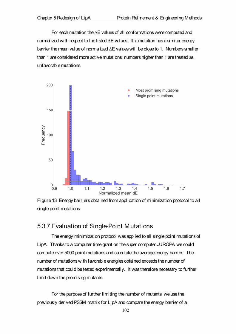
Chapter 5 Redesign of LipA Protein Refinement & Engineering Methods
��
For each mutation the ∆E values of all conformations were computed and
normalized with respect to the listed ∆E values. If a mutation has a similar energy
barrier the mean value of normalized ∆E values will be close to 1. Numbers smaller
than 1 are considered more active mutations; numbers higher than 1 are treated as
unfavorable mutations.
Figure 13 Energy barriers obtained from application of minimization protocol to all
single point mutations
5.3.7 Evaluation of Single-Point Mutations
The energy minimization protocol was applied to all single point mutations of
LipA. Thanks to a computer time grant on the super computer JUROPA we could
compute over 5000 point mutations and calculate the average energy barrier. The
number of mutations with favorable energies obtained exceeds the number of
mutations that could be tested experimentally. It was therefore necessary to further
limit down the promising mutants.
For the purpose of further limiting the number of mutants, we use the
previously derived PSSM matrix for LipA and compare the energy barrier of a

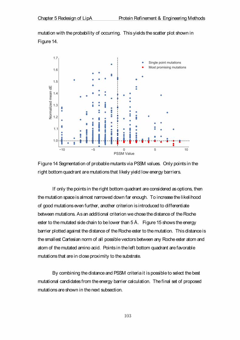
Chapter 5 Redesign of LipA Protein Refinement & Engineering Methods
��
mutation with the probability of occurring. This yields the scatter plot shown in
Figure 14.
Figure 14 Segmentation of probable mutants via PSSM values. Only points in the
right bottom quadrant are mutations that likely yield low energy barriers.
If only the points in the right bottom quadrant are considered as options, then
the mutation space is almost narrowed down far enough. To increase the likelihood
of good mutations even further, another criterion is introduced to differentiate
between mutations. As an additional criterion we chose the distance of the Roche
ester to the mutated side chain to be lower than 5 Å. Figure 15 shows the energy
barrier plotted against the distance of the Roche ester to the mutation. This distance is
the smallest Cartesian norm of all possible vectors between any Roche ester atom and
atom of the mutated amino acid. Points in the left bottom quadrant are favorable
mutations that are in close proximity to the substrate.
By combining the distance and PSSM criteria it is possible to select the best
mutational candidates from the energy barrier calculation. The final set of proposed
mutations are shown in the next subsection.

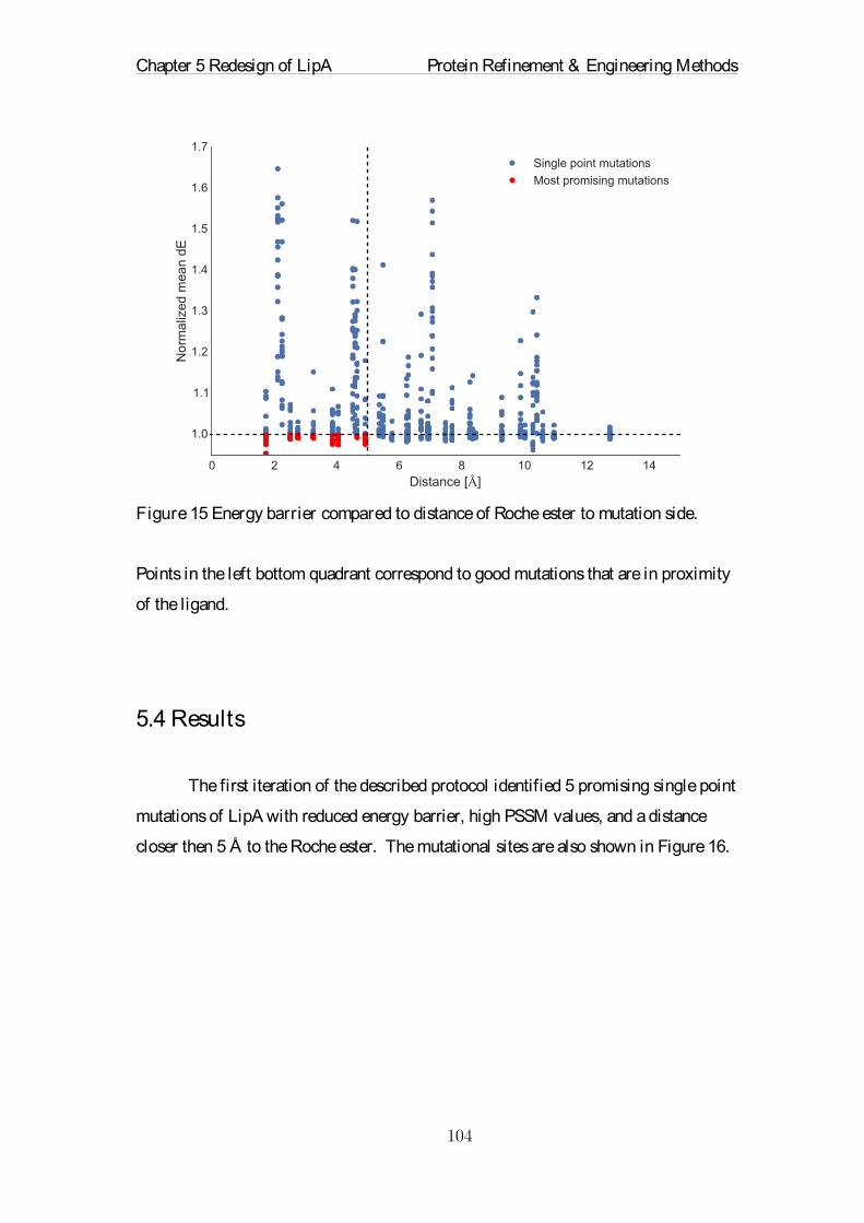
Chapter 5 Redesign of LipA Protein Refinement & Engineering Methods
��
Figure 15 Energy barrier compared to distance of Roche ester to mutation side.
Points in the left bottom quadrant correspond to good mutations that are in proximity
of the ligand.
5.4 Results
The first iteration of the described protocol identified 5 promising single point
mutations of LipA with reduced energy barrier, high PSSM values, and a distance
closer then 5 Å to the Roche ester. The mutational sites are also shown in Figure 16.

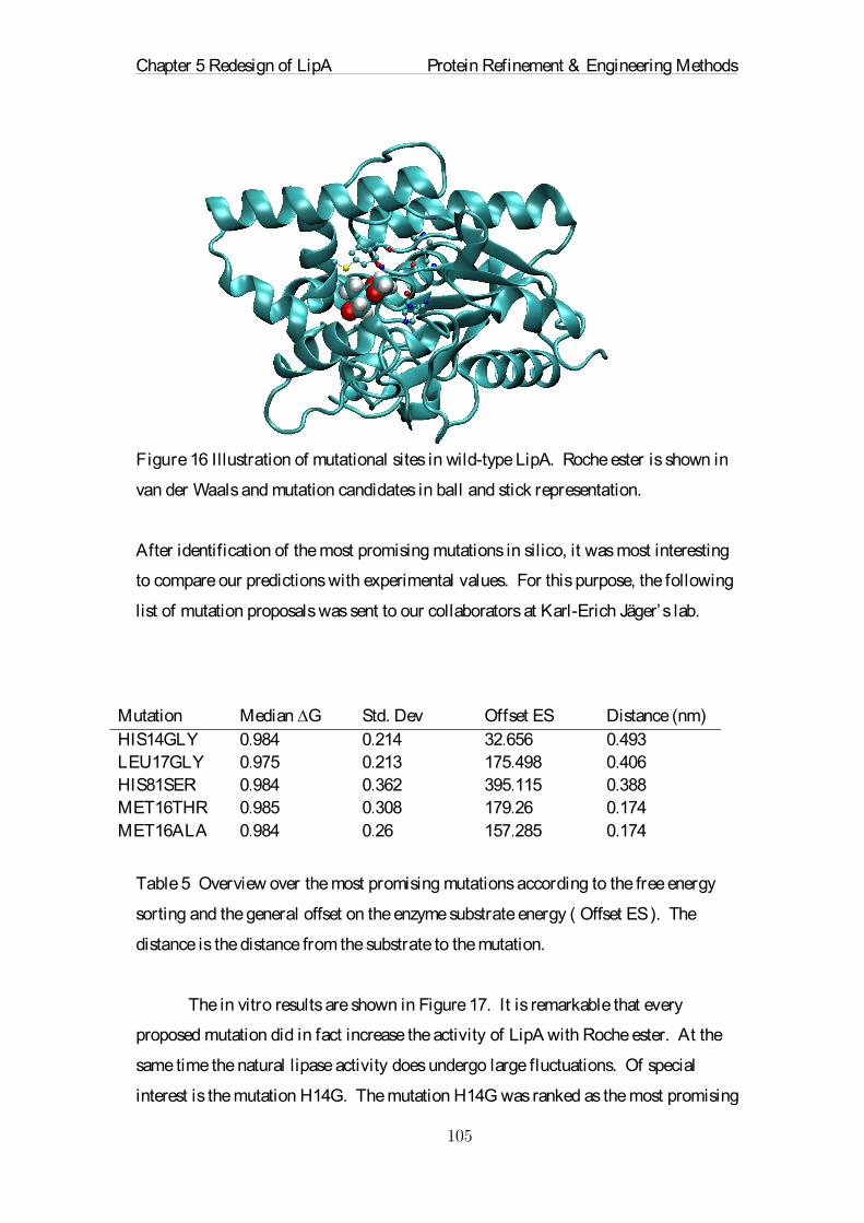
Chapter 5 Redesign of LipA Protein Refinement & Engineering Methods
��
Figure 16 Illustration of mutational sites in wild-type LipA. Roche ester is shown in
van der Waals and mutation candidates in ball and stick representation.
After identification of the most promising mutations in silico, it was most interesting
to compare our predictions with experimental values. For this purpose, the following
list of mutation proposals was sent to our collaborators at Karl-Erich Jäger’s lab.
Table 5 Overview over the most promising mutations according to the free energy
sorting and the general offset on the enzyme substrate energy ( Offset ES ). The
distance is the distance from the substrate to the mutation.
The in vitro results are shown in Figure 17. It is remarkable that every
proposed mutation did in fact increase the activity of LipA with Roche ester. At the
same time the natural lipase activity does undergo large fluctuations. Of special
interest is the mutation H14G. The mutation H14G was ranked as the most promising
Mutation Median ∆G Std. Dev Offset ES Distance (nm) HIS14GLY 0.984 0.214 32.656 0.493 LEU17GLY 0.975 0.213 175.498 0.406 HIS81SER 0.984 0.362 395.115 0.388 MET16THR 0.985 0.308 179.26 0.174 MET16ALA 0.984 0.26 157.285 0.174

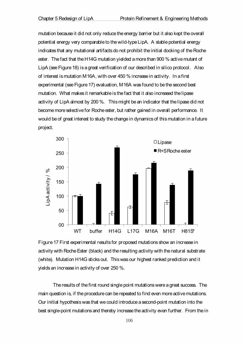
Chapter 5 Redesign of LipA Protein Refinement & Engineering Methods
��
mutation because it did not only reduce the energy barrier but it also kept the overall
potential energy very comparable to the wild-type LipA. A stable potential energy
indicates that any mutational artifacts do not prohibit the initial docking of the Roche
ester. The fact that the H14G mutation yielded a more than 900 % active mutant of
LipA (see Figure 18) is a great verification of our described in silico protocol. Also
of interest is mutation M16A, with over 450 % increase in activity. In a first
experimental (see Figure 17) evaluation, M16A was found to be the second best
mutation. What makes it remarkable is the fact that it also increased the lipase
activity of LipA almost by 200 %. This might be an indicator that the lipase did not
become more selective for Roche ester, but rather gained in overall performance. It
would be of great interest to study the change in dynamics of this mutation in a future
project.
Figure 17 First experimental results for proposed mutations show an increase in
activity with Roche Ester (black) and the resulting activity with the natural substrate
(white). Mutation H14G sticks out. This was our highest ranked prediction and it
yields an increase in activity of over 250 %.
The results of the first round single point mutations were a great success. The
main question is, if the procedure can be repeated to find even more active mutations.
Our initial hypothesis was that we could introduce a second-point mutation into the
best single-point mutations and thereby increase the activity even further. From the in
00�
50�
100�
150�
200�
250�
300�
WT� buffer� H14G� L17G� M16A� M16T�� H81S*�
Lip
A�a
ctiv
ity�
/�%
�
Lipase�
R+S�Roche�ester�

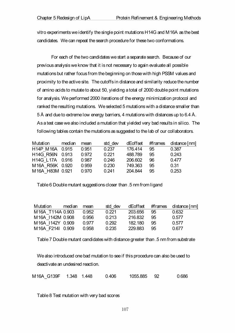
Chapter 5 Redesign of LipA Protein Refinement & Engineering Methods
��
vitro experiments we identify the single point mutations H14G and M16A as the best
candidates. We can repeat the search procedure for these two conformations.
For each of the two candidates we start a separate search. Because of our
previous analysis we know that it is not necessary to again evaluate all possible
mutations but rather focus from the beginning on those with high PSSM values and
proximity to the active site. The cutoffs in distance and similarity reduce the number
of amino acids to mutate to about 50, yielding a total of 2000 double point mutations
for analysis. We performed 2000 iterations of the energy minimization protocol and
ranked the resulting mutations. We selected 5 mutations with a distance smaller than
5 Å and due to extreme low energy barriers, 4 mutations with distances up to 6.4 Å.
As a test case we also included a mutation that yielded very bad results in silico. The
following tables contain the mutations as suggested to the lab of our collaborators.
Table 6 Double mutant suggestions closer than .5 nm from ligand
Table 7 Double mutant candidates with distance greater than .5 nm from substrate
We also introduced one bad mutation to see if this procedure can also be used to
deactivate an undesired reaction.
Table 8 Test mutation with very bad scores
Mutation median mean std_dev dEoffset #frames distance [nm]H14P_M16A 0.915 0.951 0.237 176.414 95 0.387 H14G_R56N 0.913 0.972 0.221 488.789 95 0.243 H14G_L17A 0.916 0.987 0.246 206.602 96 0.477 M16A_R56K 0.920 0.959 0.230 749.363 95 0.31 M16A_H83M 0.921 0.970 0.241 204.844 95 0.253
Mutation median mean std_dev dEoffset #frames distance [nm]M16A_T114A 0.903 0.952 0.221 203.656 95 0.632 M16A_I142M 0.908 0.956 0.213 216.832 95 0.577 M16A_I142Y 0.909 0.977 0.292 182.180 95 0.577 M16A_F214I 0.909 0.958 0.235 229.883 95 0.677
M16A_G139F 1.348
1.448 0.406 1055.885 92 0.686

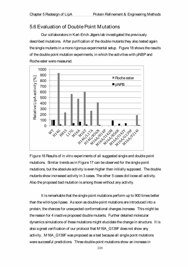
Chapter 5 Redesign of LipA Protein Refinement & Engineering Methods
��
5.6 Evaluation of Double Point Mutations
Our collaborators in Karl-Erich Jägers lab investigated the previously
described mutations. After purification of the double mutants they also tested again
the single mutants in a more rigorous experimental setup. Figure 18 shows the results
of the double point mutation experiments, in which the activities with pNBP and
Roche ester were measured.
Figure 18 Results of in vitro experiments of all suggested single and double point
mutations. Similar trends as in Figure 17 can be observed for the single point
mutations, but the absolute activity is even higher than initially supposed. The double
mutants show increased activity in 3 cases. The other 5 cases did loose all activity.
Also the proposed bad mutation is among those without any activity.
It is remarkable that the single point mutations perform up to 900 times better
than the wild-type lipase. As soon as double-point mutations are introduced into a
protein, the chances for unexpected conformational changes increase. This might be
the reason for 4 inactive proposed double mutants. Further detailed molecular
dynamics simulations of these mutations might elucidate the change in structure. It is
also a great verification of our protocol that M16A_G139F does not show any
activity. M16A_G139F was proposed as a test because all single point mutations
were successful predictions. Three double-point mutations show an increase in
0�
100�
200�
300�
400�
500�
600�
700�
800�
900�
1000�
Rel
ativ
e�Li
pA
�act
ivit
y�[%
]�
Roche�ester�
pNPB�

Chapter 5 Redesign of LipA Protein Refinement & Engineering Methods
��
activity compared to the wild-type lipase. H14G_R56N shows more then 400 %
increase and serves as a motivation to explore even higher mutational spaces in the
future.
5.7 Conclusion
We developed a protocol that is able to rank the influence of mutations on the
substrate selectivity of LipA with Roche ester in silico. This protocol provides
guidance to directed evolution experiments and was able to predict a single point
mutation with more then 900 % increased activity compared to wild-type LipA. It
was shown that the energy barrier of a protein between docked and covalently
bounded substrate could be approximated by the potential energy difference of an
ensemble of structures. The main double-lid movement of the lipase was verified in
MD simulations and considered as a possible criterion to rank mutations.
Unfortunately restraints on computational time did not make is feasible to study the
effect of all mutations on the lid dynamics.
The best performing single-point mutations were used as new starting points
for a second round of predictions. In this second iteration, 10 mutations were selected
and proposed to the experimental partners. The evaluation of the double-point
mutations generated three highly active derivatives of LipA. A mutation with very
bad scores was also tested and showed zero activity with Roche ester. Although the
activities did not add up as hoped for, the next steps would include the calculations of
even higher order mutations.

Publication L ist Paper I – See Chapter 2
Protein Structure Refinement with Adaptively Restrained Homologous Replicas
Dennis Della Corte, André Wildberg, and Gunnar F. Schröder (Proteins, Accepted)
Paper I I – See Chapter 3
Coupling an ensemble of homologs improves refinement of protein homology models
André Wildberg, Dennis Della Corte, and Gunnar F. Schröder (JCTC, in review)
Paper I I I – See Chapter 4
The origin of improved sampling of free energy minima through adaptive restraints
Dennis Della Corte and Gunnar F. Schröder (soon to be submitted)
Paper IV – Not included
Design and application of a custom-made L-histidine sensor for the ultra-high-
throughput screening of Corynebacterium glutamicum producer strains
Marcus Schallmey, Dennis Della Corte, Felix Tobola, Hugo van Beek, Alexander
Grünberger, Sascha Sokolowsky, Gunnar F. Schröder, Jan Marienhagen (soon to be
submitted)
Paper V – Not included
Dynamics of the Autophagy-related Protein GABARAP on the Pico- to Nanosecond
Time-scale by NMR and Fluorescence Spectroscopy in Concert with Molecular
Dynamics Simulations
Christina Möller, Jakub Kubiak, Oliver Schillinger, Ralf Kühnemuth, Dennis Della
Corte, Gunnar F. Schröder, Birgit Strodel, Claus A. M. Seidel, Dieter Willbold, and
Philipp Neudecker (soon to be submitted)
Paper VI – See Chapter 5
Simulation Guided Directed Evolution Experiments Increase Phospholipase Activity
by Over 900 %
Dennis Della Corte, Filip Kovacic, Karl-Erich Jäger, and Gunnar F. Schröder (in
preparation)

Chapter 1 Introduction Protein Refinement & Engineering Methods
!!
REFERENCES
1. Marcotte, E.M., et al., Detecting protein function and protein-protein interactions from genome sequences. Science, 1999. 285(5428): p. 751-753.
2. Gentleman, R.C., et al., Bioconductor: open software development for computational biology and bioinformatics. Genome Biology, 2004. 5(10): p. R80.
3. Zubay, G., In vitro synthesis of protein in microbial systems. Annual Review of Genetics, 1973. 7(1): p. 267-287.
4. Scherzer, O., The theoretical resolution limit of the electron microscope. Journal of Applied Physics, 1949. 20(1): p. 20-29.
5. Shaw, D.E., et al., Anton, a special-purpose machine for molecular dynamics simulation. Communications of the ACM, 2008. 51(7): p. 91-97.
6. Baker, D., An exciting but challenging road ahead for computational enzyme design. Protein Science, 2010. 19(10): p. 1817-1819.
7. Dill, K.A. and J.L. MacCallum, The protein-folding problem, 50 years on. Science, 2012. 338(6110): p. 1042-1046.
8. Moult, J., et al., Critical assessment of methods of protein structure prediction (CASP)—round x. Proteins: Structure, Function, and Bioinformatics, 2014. 82(S2): p. 1-6.
9. Carter, P.J., Introduction to current and future protein therapeutics: a protein engineering perspective. Experimental Cell Research, 2011. 317(9): p. 1261-1269.
10. Dalby, P.A., Strategy and success for the directed evolution of enzymes. Current Opinion in Structural Biology, 2011. 21(4): p. 473-480.
11. Kiss, G., et al., Computational enzyme design. Angewandte Chemie International Edition, 2013. 52(22): p. 5700-5725.
12. Frushicheva, M.P., et al., Computer aided enzyme design and catalytic concepts. Current Opinion in Chemical Biology, 2014. 21: p. 56-62.
13. Woodley, J.M., Protein engineering of enzymes for process applications. Current Opinion in Chemical Biology, 2013. 17(2): p. 310-316.

Chapter 1 Introduction Protein Refinement & Engineering Methods
!!
14. Starobinsky, A., Future and origin of our universe: Modern view. The Future of the Universe and the Future of our Civilization, 2000. 10: p. 9789812793324_0008.
15. Newton, I., et al., Philosophiae naturalis principia mathematica. Vol. 1. 1833: excudit G. Brookman; impensis TT et J. Tegg, Londini.
16. Alligood, K.T., T.D. Sauer, and J.A. Yorke, Chaos. 1997: Springer.
17. Dayhoff, M.O. and R.M. Schwartz. A model of evolutionary change in proteins. in In Atlas of Protein Sequence and Structure. 1978. Citeseer.
18. Roca, A.I. and M.M. Cox, RecA protein: structure, function, and role in recombinational DNA repair. Progress in Nucleic Acid Research and Molecular Biology, 1997(56): p. 129-223.
19. Cornell, W.D., et al., A second generation force field for the simulation of proteins, nucleic acids, and organic molecules. Journal of the American Chemical Society, 1995. 117(19): p. 5179-5197.
20. Jorgensen, W.L., D.S. Maxwell, and J. Tirado-Rives, Development and testing of the OPLS all-atom force field on conformational energetics and properties of organic liquids. Journal of the American Chemical Society, 1996. 118(45): p. 11225-11236.
21. Oostenbrink, C., et al., A biomolecular force field based on the free enthalpy of hydration and solvation: The GROMOS force- field parameter sets 53A5 and 53A6. Journal of Computational Chemistry, 2004. 25(13): p. 1656-1676.
22. Pearlman, D.A., et al., AMBER, a package of computer programs for applying molecular mechanics, normal mode analysis, molecular dynamics and free energy calculations to simulate the structural and energetic properties of molecules. Computer Physics Communications, 1995. 91(1): p. 1-41.
23. Weiner, P.K. and P.A. Kollman, AMBER: Assisted model building with energy refinement. A general program for modeling molecules and their interactions. Journal of Computational Chemistry, 1981. 2(3): p. 287-303.
24. Karplus, M., CHARMM: A program for macromolecular energy, minimization, and dynamics calculations. J Comput Chem, 1983. 4: p. 187217.
25. Chen, J., C.L. Brooks, and J. Khandogin, Recent advances in implicit solvent-based methods for biomolecular simulations. Current Opinion in Structural Biology, 2008. 18(2): p. 140-148.

Chapter 1 Introduction Protein Refinement & Engineering Methods
!!
26. Linge, J.P., et al., Refinement of protein structures in explicit solvent. Proteins: Structure, Function, and Bioinformatics, 2003. 50(3): p. 496-506.
27. Verlet, L., Computer" experiments" on classical fluids. I. Thermodynamical properties of Lennard-Jones molecules. Physical Review, 1967. 159(1): p. 98.
28. Tuckerman, M., B.J. Berne, and G.J. Martyna, Reversible multiple time scale molecular dynamics. The Journal of Chemical Physics, 1992. 97(3): p. 1990-2001.
29. Payne, M.C., et al., Iterative minimization techniques for ab initio total-energy calculations: molecular dynamics and conjugate gradients. Reviews of Modern Physics, 1992. 64(4): p. 1045.
30. Lindorff- Larsen, K., et al., Improved side- chain torsion potentials for the Amber ff99SB protein force field. Proteins: Structure, Function, and Bioinformatics, 2010. 78(8): p. 1950-1958.
31. de Coulomb, C.A., Collection de mémoires relatifs à la physique. Vol. 2. 1889: Gauthier-Villars.
32. Levitt, M. and R. Sharon, Accurate simulation of protein dynamics in solution. Proceedings of the National Academy of Sciences, 1988. 85(20): p. 7557-7561.
33. Rapaport, D.C., The art of molecular dynamics simulation. 2004: Cambridge university press.
34. Alder, B.J. and T. Wainwright, Studies in molecular dynamics. I. General method. The Journal of Chemical Physics, 1959. 31(2): p. 459-466.
35. Berendsen, H.J., et al., Molecular dynamics with coupling to an external bath. The Journal of Chemical Physics, 1984. 81(8): p. 3684-3690.
36. Evans, D.J. and B.L. Holian, The nose–hoover thermostat. The Journal of Chemical Physics, 1985. 83(8): p. 4069-4074.
37. Balsera, M.A., et al., Principal component analysis and long time protein dynamics. The Journal of Physical Chemistry, 1996. 100(7): p. 2567-2572.
38. Mirjalili, V., K. Noyes, and M. Feig, Physics- based protein structure refinement through multiple molecular dynamics trajectories and structure averaging. Proteins: Structure, Function, and Bioinformatics, 2014. 82(S2): p. 196-207.

Chapter 2 Protein Refinement Protein Refinement & Engineering Methods
!!
39. Pettersen, E.F., et al., UCSF Chimera—a visualization system for exploratory research and analysis. Journal of Computational Chemistry, 2004. 25(13): p. 1605-1612.
40. MacCallum, J.L., et al., Assessment of protein structure refinement in CASP9. Proteins: Structure, Function, and Bioinformatics, 2011. 79(S10): p. 74-90.
41. Nugent, T., D. Cozzetto, and D.T. Jones, Evaluation of predictions in the CASP10 model refinement category. Proteins: Structure, Function, and Bioinformatics, 2014. 82(S2): p. 98-111.
42. Fan, H. and A.E. Mark, Refinement of homology- based protein structures by molecular dynamics simulation techniques. Protein Science, 2004. 13(1): p. 211-220.
43. Zhu, J., et al., Refining homology models by combining replica- exchange molecular dynamics and statistical potentials. Proteins: Structure, Function, and Bioinformatics, 2008. 72(4): p. 1171-1188.
44. Raval, A., et al., Refinement of protein structure homology models via long, all-atom molecular dynamics simulations. Proteins, 2012. 80(8): p. 2071-2079.
45. Mirjalili, V. and M. Feig, Protein structure refinement through structure selection and averaging from molecular dynamics ensembles. Journal of Chemical Theory and Computation, 2013. 9(2): p. 1294-1303.
46. Mirjalili, V., K. Noyes, and M. Feig, Physics- based protein structure refinement through multiple molecular dynamics trajectories and structure averaging. Proteins: Structure, Function, and Bioinformatics, 2014. 82(S2): p. 196-207.
47. Schröder, G.F., A.T. Brunger, and M. Levitt, Combining efficient conformational sampling with a deformable elastic network model facilitates structure refinement at low resolution. Structure, 2007. 15(12): p. 1630-41.
48. Schröder, G.F., M. Levitt, and A.T. Brunger, Super-resolution biomolecular crystallography with low-resolution data. Nature, 2010. 464(7292): p. 1218-22.
49. Schröder, G.F., M. Levitt, and A.T. Brunger, Deformable elastic network refinement for low-resolution macromolecular crystallography. Acta Cryst. D, 2014. D70: p. 2241-2255.

Chapter 2 Protein Refinement Protein Refinement & Engineering Methods
!!
50. Huber, T. and W.F. van Gunsteren, SWARM-MD: Searching Conformational Space by Cooperative Molecular Dynamics. J. Phys. Chem. A, 1998. 102(29): p. 5937-5943.
51. Chothia, C. and A.M. Lesk, The relation between the divergence of sequence and structure in proteins. The EMBO journal, 1986. 5(4): p. 823.
52. Keasar, C., R. Elber, and J. Skolnick, Simultaneous and coupled energy optimization of homologous proteins: a new tool for structure prediction. Fold Des, 1997. 2(4): p. 247-59.
53. Keasar, C., et al., Coupling the folding of homologous proteins. Proc Natl Acad Sci U S A, 1998. 95(11): p. 5880-3.
54. Keasar, C. and R. Elber, Homology as a tool in optimization problems: structure determination of 2D heteropolymers. J. Phys. Chem., 1995. 99(29): p. 11550-11556.
55. Pronk, S., et al., GROMACS 4.5: a high-throughput and highly parallel open source molecular simulation toolkit. Bioinformatics, 2013: p. btt055.
56. Badretdinov, A. 1997; Available from: http://salilab.org/decoys/.
57. Algorithmics Group, MDSJ: Java Library for Multidimensional Scaling (Version 0.2). 2009, University of Konstanz.
58. Altschul, S.F., et al., Gapped BLAST and PSI-BLAST: a new generation of protein database search programs. Nucleic acids research, 1997. 25(17): p. 3389-3402.
59. Pruitt, K.D., T. Tatusova, and D.R. Maglott, NCBI reference sequences (RefSeq): a curated non-redundant sequence database of genomes, transcripts and proteins. Nucleic Acids Research, 2007. 35(suppl 1): p. D61-D65.
60. Fiser, A. and A. Šali, Modeller: generation and refinement of homology-based protein structure models. Methods in Enzymology, 2003. 374: p. 461-491.

Chapter 3 CASP11 - Refinement Protein Refinement & Engineering Methods
!!
61. Rosenbaum, D.M., S.G. Rasmussen, and B.K. Kobilka, The structure and function of G-protein-coupled receptors. Nature, 2009. 459(7245): p. 356-363.
62. Branden, C.I., Introduction to protein structure. 1999: Garland Science.
63. Baker, D. and A. Sali, Protein Structure Prediction and Structural Genomics. Science, 2001. 294(5540): p. 93-96.
64. Zhang, Y. and J. Skolnick, The protein structure prediction problem could be solved using the current PDB library. Proc. Natl. Acad. Sci. U.S.A., 2005. 102(4): p. 1029-1034.
65. Ko, J., H. Park, and C. Seok, GalaxyTBM: template-based modeling by building a reliable core and refining unreliable local regions. BMC Bioinformatics, 2012. 13(1): p. 198.
66. Qu, X., et al., A guide to template based structure prediction. Curr. Protein. Pept. Sci., 2009. 10(3): p. 270-85.
67. Koehl, P. and M. Levitt, A brighter future for protein structure prediction. Nat. Struct. Mol. Biol., 1999. 6: p. 108-111.
68. MacCallum, J.L., et al., Assessment of protein structure refinement in CASP9. Proteins, 2011. 79(S10): p. 74-90.
69. MacCallum, J.L., et al., Assessment of the protein-structure refinement category in CASP8. Proteins, 2009. 77(S9): p. 66-80.
70. Valencia, A., Protein refinement: a new challenge for CASP in its 10th anniversary. Bioinformatics, 2005. 21(3): p. 277-277.
71. Nugent, T., D. Cozzetto, and D.T. Jones, Evaluation of predictions in the CASP10 model refinement category. Proteins, 2014. 82(S2): p. 98-111.
72. Levitt, M. and S. Lifson, Refinement of protein conformations using a macromolecular energy minimization procedure. J. Mol. Biol., 1969. 46(2): p. 269-279.
73. Engh, R.A. and R. Huber, Accurate bond and angle parameters for X-ray protein structure refinement. Acta Cryst. A, 1991. 47(4): p. 392-400.

Chapter 3 CASP11 - Refinement Protein Refinement & Engineering Methods
!!
74. Levitt, M., Accurate modeling of protein conformation by automatic segment matching. J. Mol. Biol., 1992. 226(2): p. 507-533.
75. Chopra, G., C.M. Summa, and M. Levitt, Solvent dramatically affects protein structure refinement. Proc. Natl. Acad. Sci. U.S.A., 2008. 105(51): p. 20239-20244.
76. Rohl, C.A., et al., Protein structure prediction using Rosetta. Meth. Enzymol., 2004. 383: p. 66-93.
77. Zhang, J., Y. Liang, and Y. Zhang, Atomic-level protein structure refinement using fragment-guided molecular dynamics conformation sampling. Structure, 2011. 19(12): p. 1784-1795.
78. Fiser, A. and A. Šali, Modeller: generation and refinement of homology-based protein structure models. Meth. Enzymol., 2003. 374: p. 461-491.
79. Rodrigues, J.P., M. Levitt, and G. Chopra, KoBaMIN: a knowledge-based minimization web server for protein structure refinement. Nucleic Acids Res., 2012: p. gks376.
80. Lu, H. and J. Skolnick, Application of statistical potentials to protein structure refinement from low resolution ab initio models. Biopolymers, 2003. 70(4): p. 575-584.
81. Fan, H. and A.E. Mark, Refinement of homology- based protein structures by molecular dynamics simulation techniques. Protein Sci., 2004. 13(1): p. 211-220.
82. Flohil, J., G. Vriend, and H. Berendsen, Completion and refinement of 3- D homology models with restricted molecular dynamics: Application to targets 47, 58, and 111 in the CASP modeling competition and posterior analysis. Proteins, 2002. 48(4): p. 593-604.
83. Zhu, J., et al., Refining homology models by combining replica- exchange molecular dynamics and statistical potentials. Proteins, 2008. 72(4): p. 1171-1188.
84. Mirjalili, V. and M. Feig, Protein structure refinement through structure selection and averaging from molecular dynamics ensembles. J. Chem. Theory Comput., 2013. 9(2): p. 1294-1303.

Chapter 3 CASP11 - Refinement Protein Refinement & Engineering Methods
!!
85. Mirjalili, V., K. Noyes, and M. Feig, Physics- based protein structure refinement through multiple molecular dynamics trajectories and structure averaging. Proteins, 2014. 82(S2): p. 196-207.
86. Dinner, A.R., et al., Understanding protein folding via free-energy surfaces from theory and experiment. Trends Biochem. Sci., 2000. 25(7): p. 331-339.
87. Kuhlman, B. and D. Baker, Native protein sequences are close to optimal for their structures. Proc. Natl. Acad. Sci. U.S.A., 2000. 97(19): p. 10383-10388.
88. Anfinsen, C.B., Principles that Govern the Folding of Protein Chains. Science, 1973. 181(4096): p. 223–230.
89. Chothia, C. and A.M. Lesk, The relation between the divergence of sequence and structure in proteins. EMBO J., 1986. 5(4): p. 823.
90. Keasar, C., R. Elber, and J. Skolnick, Simultaneous and coupled energy optimization of homologous proteins: a new tool for structure prediction. Fold Des, 1997. 2(4): p. 247-59.
91. Keasar, C., et al., Coupling the folding of homologous proteins. Proc. Natl. Acad. Sci. U. S. A., 1998. 95(11): p. 5880-3.
92. Altschul, S.F., et al., Gapped BLAST and PSI-BLAST: a new generation of protein database search programs. Nucleic Acids Res., 1997. 25(17): p. 3389-3402.
93. Pruitt, K.D., T. Tatusova, and D.R. Maglott, NCBI reference sequences (RefSeq): a curated non-redundant sequence database of genomes, transcripts and proteins. Nucleic Acids Res., 2007. 35(suppl 1): p. D61-D65.
94. Pronk, S., et al., GROMACS 4.5: a high-throughput and highly parallel open source molecular simulation toolkit. Bioinformatics, 2013: p. btt055.
95. Best, R.B. and G. Hummer, Optimized molecular dynamics force fields applied to the helix− coil transition of polypeptides. J. Phys. Chem. B, 2009. 113(26): p. 9004-9015.
96. Evans, D.J. and B.L. Holian, The Nose–Hoover thermostat. J. Chem. Phys., 1985. 83(8): p. 4069-4074.

Chapter 3 CASP11 - Refinement Protein Refinement & Engineering Methods
!!
97. Krivov, G.G., M.V. Shapovalov, and R.L. Dunbrack, Improved prediction of protein side- chain conformations with SCWRL4. Proteins, 2009. 77(4): p. 778-795.
98. Read, R.J. and G. Chavali, Assessment of CASP7 predictions in the high accuracy template- based modeling category. Proteins, 2007. 69(S8): p. 27-37.
99. Zhang, Y. and J. Skolnick, Scoring function for automated assessment of protein structure template quality. Proteins, 2004. 57(4): p. 702-710.
100. Chen, V.B., et al., MolProbity: all-atom structure validation for macromolecular crystallography. Acta Cryst. D, 2009. 66(1): p. 12-21.
101. Piotr Lukasiak, M.A., Tomasz Ratajczak, Marta Szachniuk and Jacek Blazewicz. Quality assessment methodologies in analysis of structural models. in Proceedings of the 25th European Conference on Operational Research. 2012.
102. Wilson, C.A., J. Kreychman, and M. Gerstein, Assessing annotation transfer for genomics: quantifying the relations between protein sequence, structure and function through traditional and probabilistic scores. J. Mol. Biol., 2000. 297(1): p. 233-249.
103. Kondrashov, D.A., et al., Sampling of native conformational ensemble of myoglobin via structures in different crystalline environments. Proteins 2008. 70: p. 353–362.
104. Pettersen, E.F., et al., UCSF Chimera—a visualization system for exploratory research and analysis. J. Comput. Chem., 2004. 25(13): p. 1605-1612.

Chapter 4 Refinement with Restraints Protein Refinement & Engineering Methods
105. Sugita, Y., A. Kitao, and Y. Okamoto, Multidimensional replica-exchange method for free-energy calculations. The Journal of Chemical Physics, 2000. 113(15): p. 6042-6051.
106. Li, Z. and H.A. Scheraga, Monte Carlo-minimization approach to the multiple-minima problem in protein folding. Proceedings of the National Academy of Sciences, 1987. 84(19): p. 6611-6615.
107. Torrie, G.M. and J.P. Valleau, Nonphysical sampling distributions in Monte Carlo free-energy estimation: Umbrella sampling. Journal of Computational Physics, 1977. 23(2): p. 187-199.
108. Liu, J., Metropolized independent sampling with comparisons to rejection sampling and importance sampling. Statistics and Computing, 1996. 6(2): p. 113-119.
109. Gront, D., et al., Optimization of protein models. Wiley Interdisciplinary Reviews: Computational Molecular Science, 2012. 2(3): p. 479-493.
110. Piela, L., J. Kostrowicki, and H.A. Scheraga, On the multiple-minima problem in the conformational analysis of molecules: deformation of the potential energy hypersurface by the diffusion equation method. The Journal of Physical Chemistry, 1989. 93(8): p. 3339-3346.
111. Goffe, W.L., G.D. Ferrier, and J. Rogers, Global optimization of statistical functions with simulated annealing. Journal of Econometrics, 1994. 60(1): p. 65-99.
112. Hart, R.K., R.V. Pappu, and J.W. Ponder, Exploring the similarities between potential smoothing and simulated annealing. Journal of Computational Chemistry, 2000. 21(7): p. 531-552.
113. Brunger, A.T., et al., Application of DEN refinement and automated model building to a difficult case of molecular-replacement phasing: the structure of a putative succinyl-diaminopimelate desuccinylase from Corynebacterium glutamicum. Acta Crystallographica Section D, 2012. 68(4): p. 391-403.
114. Wang, Z. and G.F. Schröder, Real-space refinement with DireX: From global fitting to side-chain improvements. Biopolymers, 2012. 97(9): p. 687-697.
115. Schröder, G.F., A.T. Brunger, and M. Levitt, Combining Efficient Conformational Sampling with a Deformable Elastic Network Model Facilitates Structure Refinement at Low Resolution. Structure, 2007. 15(12): p. 1630-1641.

Chapter 4 Refinement with Restraints Protein Refinement & Engineering Methods
116. Schroder, G.F., M. Levitt, and A.T. Brunger, Super-resolution biomolecular crystallography with low-resolution data. Nature, 2010. 464(7292): p. 1218-1222.
117. Nakajima, N., H. Nakamura, and A. Kidera, Multicanonical Ensemble Generated by Molecular Dynamics Simulation for Enhanced Conformational Sampling of Peptides. The Journal of Physical Chemistry B, 1997. 101(5): p. 817-824.
118. Sweet, C.R., et al., Normal mode partitioning of Langevin dynamics for biomolecules. The Journal of Chemical Physics, 2008. 128(14): p. 145101.
119. Van Der Spoel, D., et al., GROMACS: fast, flexible, and free. Journal of Computational Chemistry, 2005. 26(16): p. 1701-1718.
120. Mu, D.S. Kosov, and G. Stock, Conformational Dynamics of Trialanine in Water. 2. Comparison of AMBER, CHARMM, GROMOS, and OPLS Force Fields to NMR and Infrared Experiments. The Journal of Physical Chemistry B, 2003. 107(21): p. 5064-5073.

Chapter 5 Redesign of LipA Protein Refinement & Engineering Methods
!!
121. van Gunsteren, W.F., The role of computer simulation techniques in protein engineering. Protein Engineering, 1988. 2(1): p. 5-13.
122. Eisenberg, D., et al., Protein function in the post-genomic era. Nature, 2000. 405(6788): p. 823-826.
123. Dolezal, P., et al., Evolution of the molecular machines for protein import into mitochondria. Science, 2006. 313(5785): p. 314-318.
124. Saiki, R.K., et al., Primer-directed enzymatic amplification of DNA with a thermostable DNA polymerase. Science, 1988. 239(4839): p. 487-491.
125. Baker, D., An exciting but challenging road ahead for computational enzyme design. Protein Science, 2010. 19(10): p. 1817-1819.
126. Eriksen, D.T., J. Lian, and H. Zhao, Protein design for pathway engineering. Journal of Structural Biology, 2014. 185(2): p. 234-242.
127. Baker, M., Protein engineering: navigating between chance and reason. nature methods, 2011. 8(8): p. 623.
128. Brannigan, J.A. and A.J. Wilkinson, Protein engineering 20 years on. Nature Reviews Molecular Cell Biology, 2002. 3(12): p. 964-970.
129. Chica, R.A., Protein engineering in the 21st century. Protein Science, 2015. 24(4): p. 431-433.
130. Nardini, M., et al., Crystal Structure of Pseudomonas aeruginosa Lipase in the Open Conformation; the prototype for family I. 1 of bacterial lipases. Journal of Biological Chemistry, 2000. 275(40): p. 31219-31225.
131. Dill, K.A., Theory for the folding and stability of globular proteins. Biochemistry, 1985. 24(6): p. 1501-1509.
132. Levinthal, C., How to fold graciously. Mossbauer Spectroscopy in Biological Systems, 1969: p. 22-24.
133. Levinthal, C., Are there pathways for protein folding. J. Chim. phys, 1968. 65(1): p. 44-45.
134. Bocola, M., et al., Learning from directed evolution: theoretical investigations into cooperative mutations in lipase enantioselectivity. ChemBioChem, 2004. 5(2): p. 214-223.

Chapter 5 Redesign of LipA Protein Refinement & Engineering Methods
!!
135. Eigen, M., Proton Transfer, Acid- Base Catalysis, and Enzymatic Hydrolysis. Part I: ELEMENTARY PROCESSES. Angewandte Chemie International Edition in English, 1964. 3(1): p. 1-19.
136. Hänggi, P., P. Talkner, and M. Borkovec, Reaction-rate theory: fifty years after Kramers. Reviews of Modern Physics, 1990. 62(2): p. 251.
137. Hehre, W.J. and L. Lou, A guide to density functional calculations in Spartan. 1997: Wavefunction.
138. Benedix, A., et al., Predicting free energy changes using structural ensembles. Nature Methods, 2009. 6(1): p. 3-4.
139. Van Der Spoel, D., et al., GROMACS: fast, flexible, and free. Journal of Computational Chemistry, 2005. 26(16): p. 1701-1718.
140. Krivov, G.G., M.V. Shapovalov, and R.L. Dunbrack, Improved prediction of protein side- chain conformations with SCWRL4. Proteins: Structure, Function, and Bioinformatics, 2009. 77(4): p. 778-795.
141. Liebeton, K., et al., Directed evolution of an enantioselective lipase. Chemistry & Biology, 2000. 7(9): p. 709-718.
142. Altschul, S.F., et al., Gapped BLAST and PSI-BLAST: a new generation of protein database search programs. Nucleic Acids Research, 1997. 25(17): p. 3389-3402.