NPS-OC-98-003

NAVAL POSTGRADUATE SCHOOL MONTEREY, CALIFORNIA

THESIS

A WIND-FORCED MODELING STUDY OF THE CANARY CURRENT SYSTEM FROM

30° N TO 42.5° N by

Daniel W. Bryan

June 1998

Thesis Advisor: Mary L. Batteen

Approved for public release; distribution is unlimited.

Prepared for: Office of Naval Research 800 N. Quincy Street Arlington, VA 22217

gflEÖ QUALITY INSPECTED'

NAVAL POSTGRADUATE SCHOOL MONTEREY, CALIFORNIA 93943

Rear Admiral Robert C. Chaplin Superintendent

This thesis was prepared in conjunction with research sponsored in part by the Office of Naval Research, 800 N. Quincy Street, Arlington, VA 22217.

Reproduction of all or part of this report is authorized.

Released by:

id W. Netzei>j\ssoci David W. NetzeX\\ssociate Provost and Dean of Research

REPORT DOCUMENTATION PAGE Form Approved OMB No. 0704-0188

Public reporting burden for this collection of information is estimated to average 1 hour per response, including the time for reviewing instruction, searching existing data sources, gathering and maintaining the data needed, and completing and reviewing the collection of information. Send comments regarding this burden estimate or any other aspect of this collection of information, including suggestions for reducing this burden, to Washington Headquarters Services, Directorate for Information Operations and Reports, 1215 Jefferson Davis Highway, Suite 1204, Arlington, VA 22202-4302, and to the Office of Management and Budget, Paperwork Reduction Project (0704-0188) Washington DC 20503.

1. AGENCY USE ONLY (Leave blank) 2. REPORT DATE June 1998

3. REPORT TYPE AND DATES COVERED Master's Thesis

4. TITLE AND SUBTITLE A WIND-FORCED MODELING STUDY OF THE CANARY CURRENT SYSTEM FROM 30° N TO 42.5° N

6. AUTHOR(S) Daniel W. Bryan in conjunction with Mary L. Batteen and Eric J. Buch

FUNDING NUMBERS

7. PERFORMING ORGANIZATION NAME(S) AND ADDRESS(ES) Naval Postgraduate School Monterey, CA 93943-5000

8. PERFORMING ORGANIZATION REPORT NUMBER NPS-OC-98-003

9. SPONSORING/MONITORING AGENCY NAME(S) AND ADDRESS(ES) Office of Naval Research 800 N. Quincy Street, Arlington, VA 22217

10.SPONSORING/MONITORING AGENCY REPORT NUMBER

11. SUPPLEMENTARY NOTES The views expressed in this thesis are those of the author and do not reflect the official policy or position of the Department of Defense or the U.S. Government.

12a. DISTRIBUTION/AVAILABILITY STATEMENT Approved for public release; distribution is unlimited.

12b. DISTRIBUTION CODE

13. ABSTRACT (maximum 200 words)

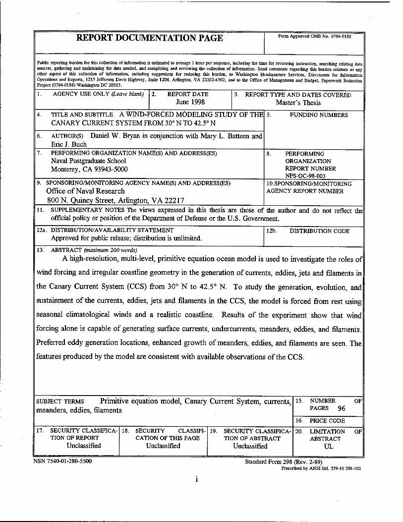
A high-resolution, multi-level, primitive equation ocean model is used to investigate the roles of

wind forcing and irregular coastline geometry in the generation of currents, eddies, jets and filaments in

the Canary Current System (CCS) from 30° N to 42.5° N. To study the generation, evolution, and

sustainment of the currents, eddies, jets and filaments in the CCS, the model is forced from rest using

seasonal climatological winds and a realistic coastline. Results of the experiment show that wind

forcing alone is capable of generating surface currents, undercurrents, meanders, eddies, and filaments.

Preferred eddy generation locations, enhanced growth of meanders, eddies, and filaments are seen. The

features produced by the model are consistent with available observations of the CCS.

SUBJECT TERMS Primitive equation model, Canary Current System, currents, meanders, eddies, filaments

15. NUMBER

PAGES 96 OF

16. PRICE CODE

17. SECURITY CLASSIFICA- TION OF REPORT

Unclassified

18. SECURITY CLASSIFI- CATION OF THIS PAGE

Unclassified

19. SECURITY CLASSIFICA- TION OF ABSTRACT

Unclassified

20. LIMITATION ABSTRACT

UL

OF

NSN 7540-01-280-5500 Standard Form 298 (Rev. 2-89) Prescribed by ANSI Std. 239-18 298-102

Approved for public release; distribution is unlimited.

A WIND-FORCED MODELING STUDY OF THE CANARY CURRENT SYSTEM FROM 30° N TO 42.5° N

Daniel W. Bryan Lieutenant, United States Navy

B.S., United States Naval Academy, 1990

Submitted in partial fulfillment of the requirements for the degree of

MASTER OF SCDZNCE IN PHYSICAL OCEANOGRAPHY

fromme

NAVAL POSTGRADUATE SCHOOL June 1998

Author:

Approved by:

Daniel W^Bryan

^lfY]£u^\ A« %3-gU^g^-y-i.

Mary L. Batteen, Thesis Advisor

&^C*-e*£<l^ Curtis A. Collins, Second Reader

Robert iL Bourke, Chairman Department of Oceanography

m

IV

ABSTRACT

A high-resolution, multi-level, primitive equation ocean model is used to

investigate the roles of wind forcing and irregular coastline geometry in the generation of

currents, eddies, jets and filaments in the Canary Current System (CCS) from 30° N to

42.5° N. To study the generation, evolution, and sustainment of the currents, eddies, jets

and filaments in the CCS, the model is forced from rest using seasonal climatological

winds and a realistic coastline. Results of the experiment show that wind forcing alone is

capable of generating surface currents, undercurrents, meanders, eddies, and filaments.

Preferred eddy generation locations, enhanced growth of meanders, eddies, and filaments

are seen. The features produced by the model are consistent with available observations

of the CCS.

VI

TABLE OF CONTENTS

I. INTRODUCTION 1

H. MODEL DESCRIPTION 5

A. MODEL EQUATIONS 5

B. TYPE OF WIND FORCING 7

C. EXPERIMENTAL DESIGN 8

IE. RESULTS FROM THE MODEL SIMULATION 11

A SPIN-UP PHASE 11

B. QUASI-EQUILBRIUM PHASE 12

C. COMPARISONS OF MODEL RESULTS WITH OBSERVATIONS .15

1. Comparison of Ocean Currents 16

2. Comparison of Eddies 17

3. Comparison of Upwelling 17

4. Comparison of Filaments 18

IV. SUMMARY 21

APPENDLX. METHOD OF SOLUTION 67

LIST OF REFERENCES 73

INITIAL DISTRIBUTION LIST 79

vu

Vlll

LIST OF FIGURES

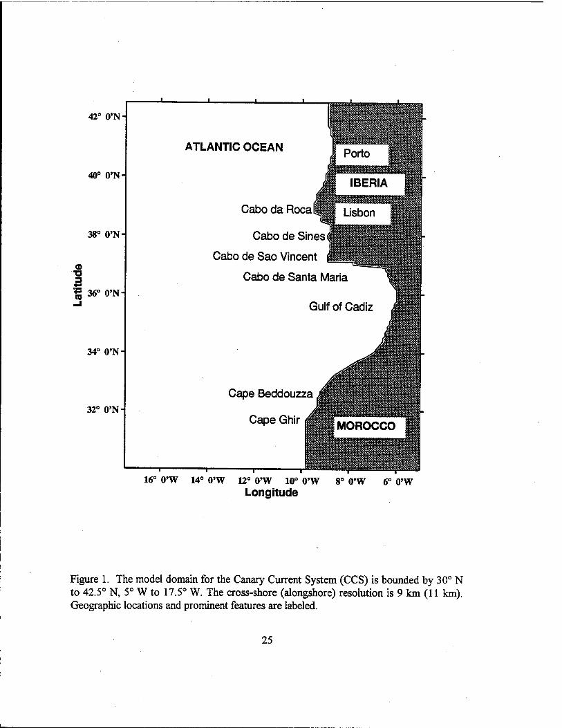
1. The model domain for the Canary Current System (CCS) is bounded by 30° N to 42.5° N, 5° W to 17.5° W. The cross-shore (alongshore) resolution is 9 km (11 km). Geographic locations and prominent features are labeled 25

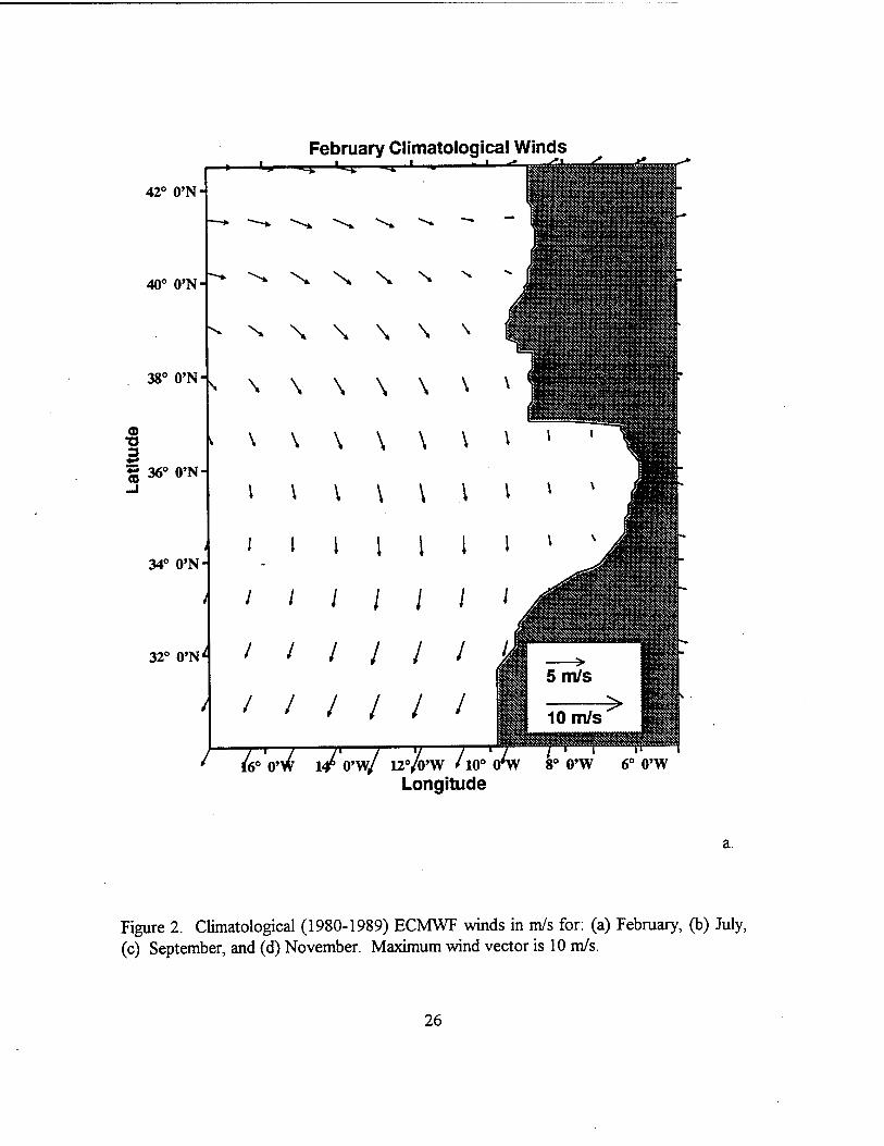
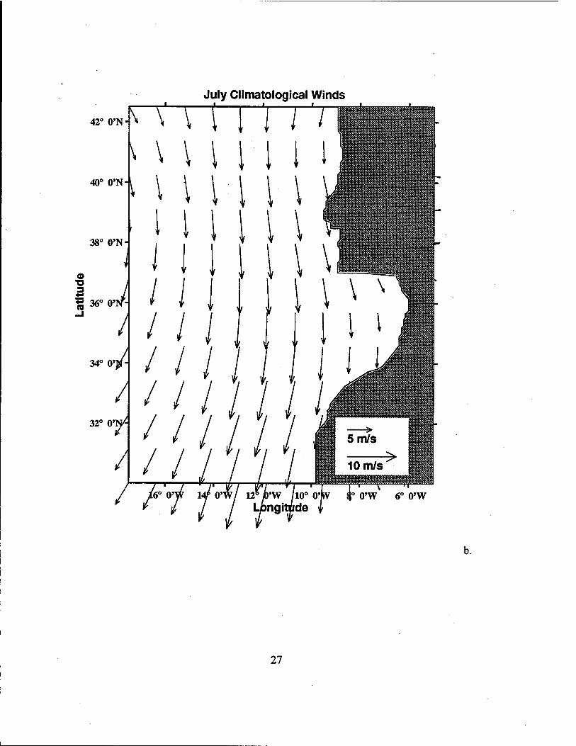
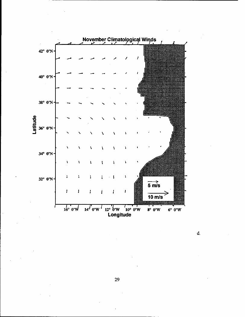
2. Climatological (1980-1989) ECMWF winds in m/s for: (a) February, (b) July, (c) September, and (d) November. Maximum wind vector is 10 m/s 26

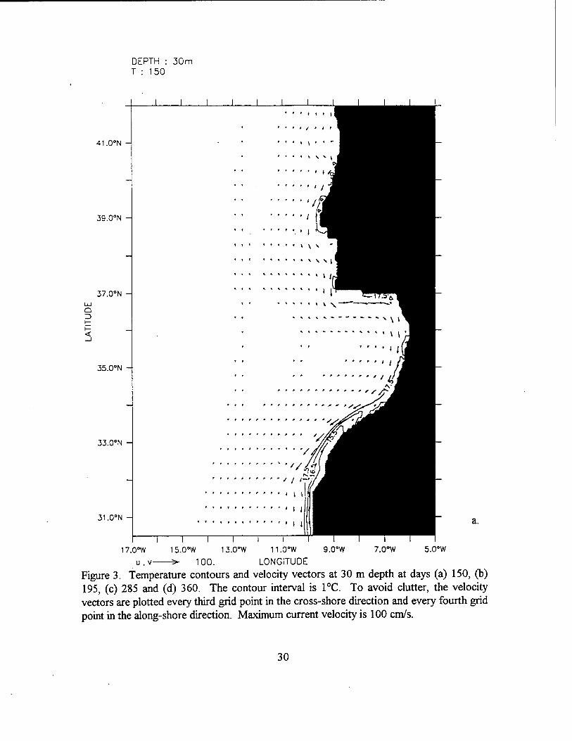
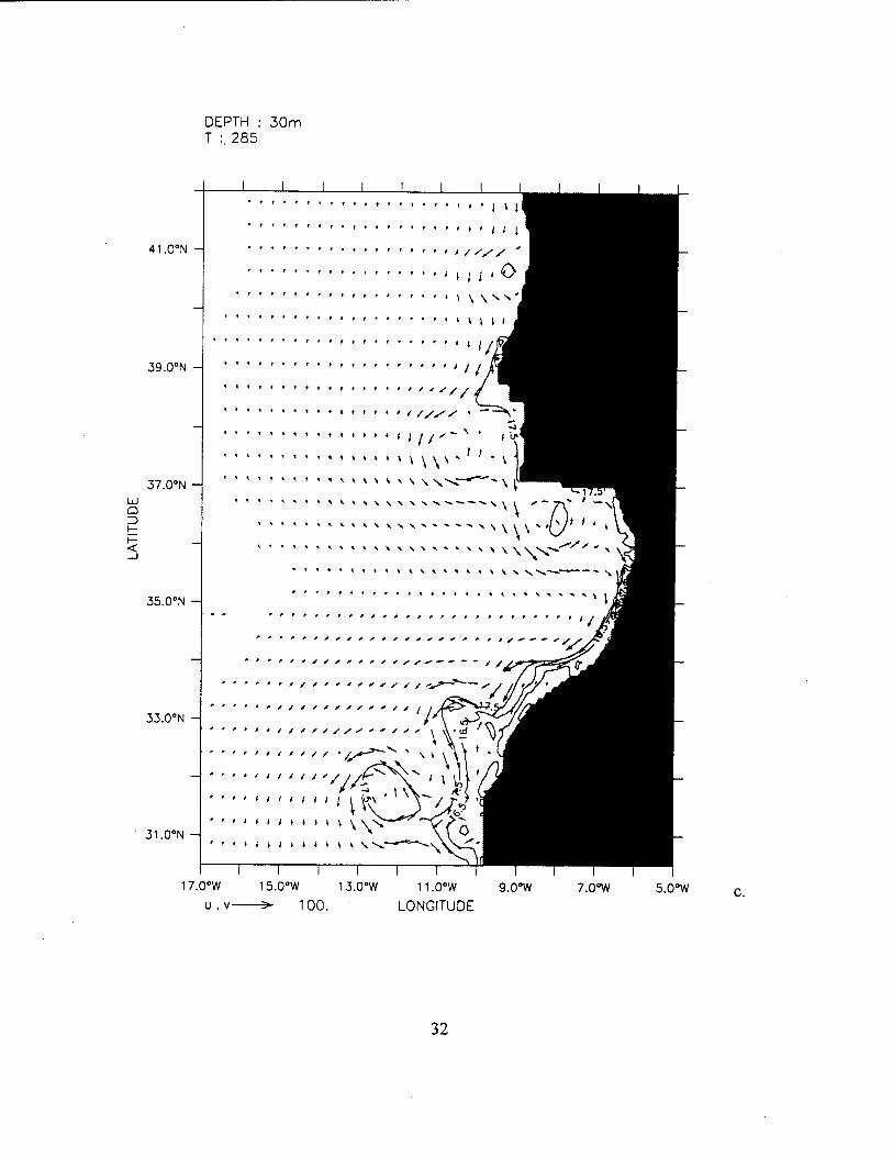
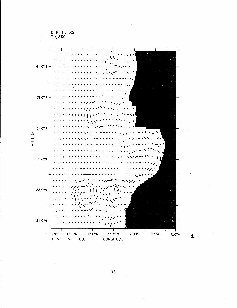
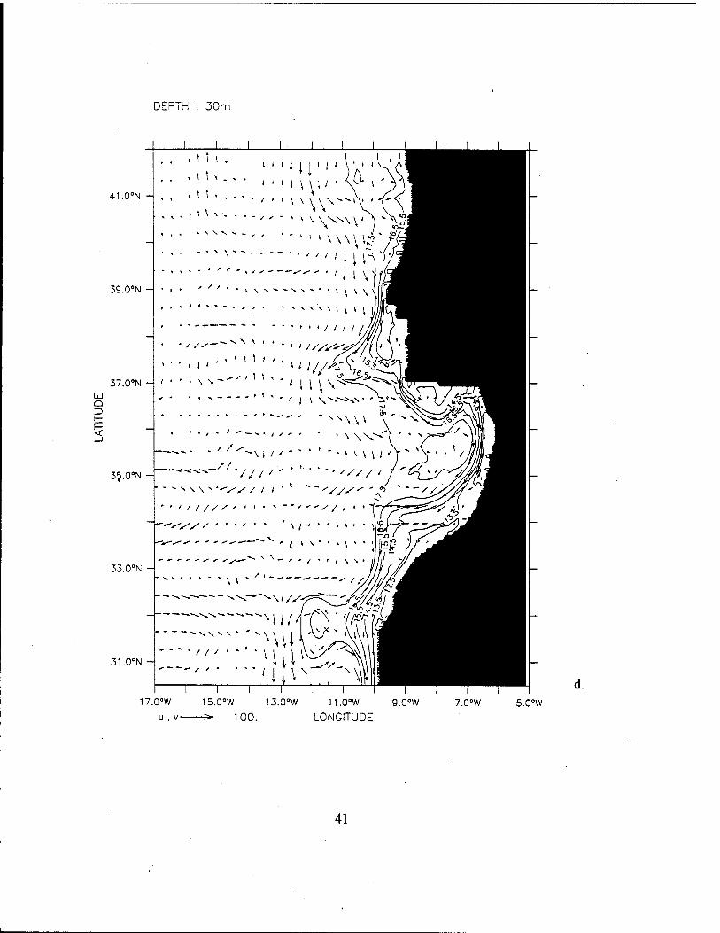
3. Figure 3. Temperature contours and velocity vectors at 30 m depth at days (a) 150, (b) 195, (c) 285 and (d) 360. The contour interval is 1°C. To avoid clutter, the velocity vectors are plotted every third grid point in the cross-shore direction and every fourth grid point in the along-shore direction. Maximum current velocity is 100 cm/s 30

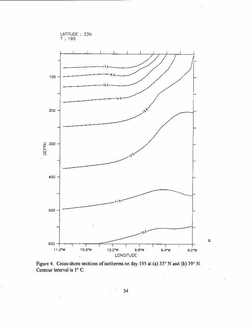
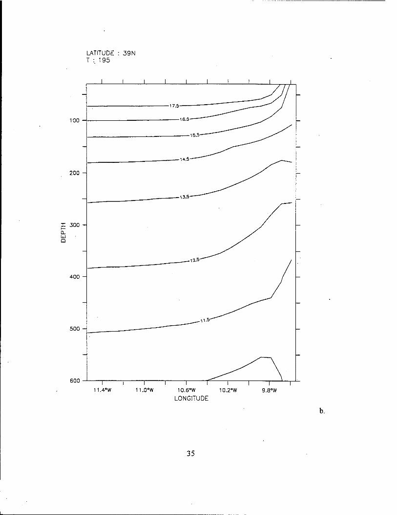
4. Cross-shore sections of isotherms on day 195 at (a) 33° N and (b) 39° N. Contour interval is 1° C 34

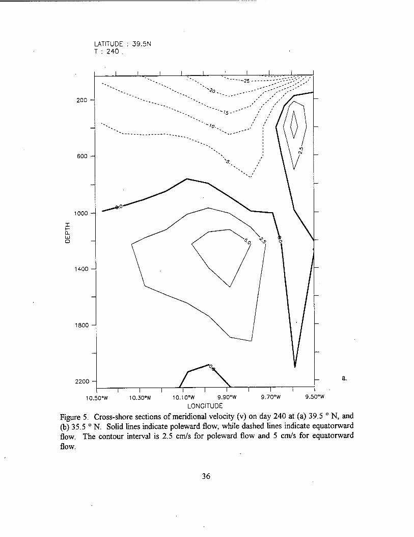
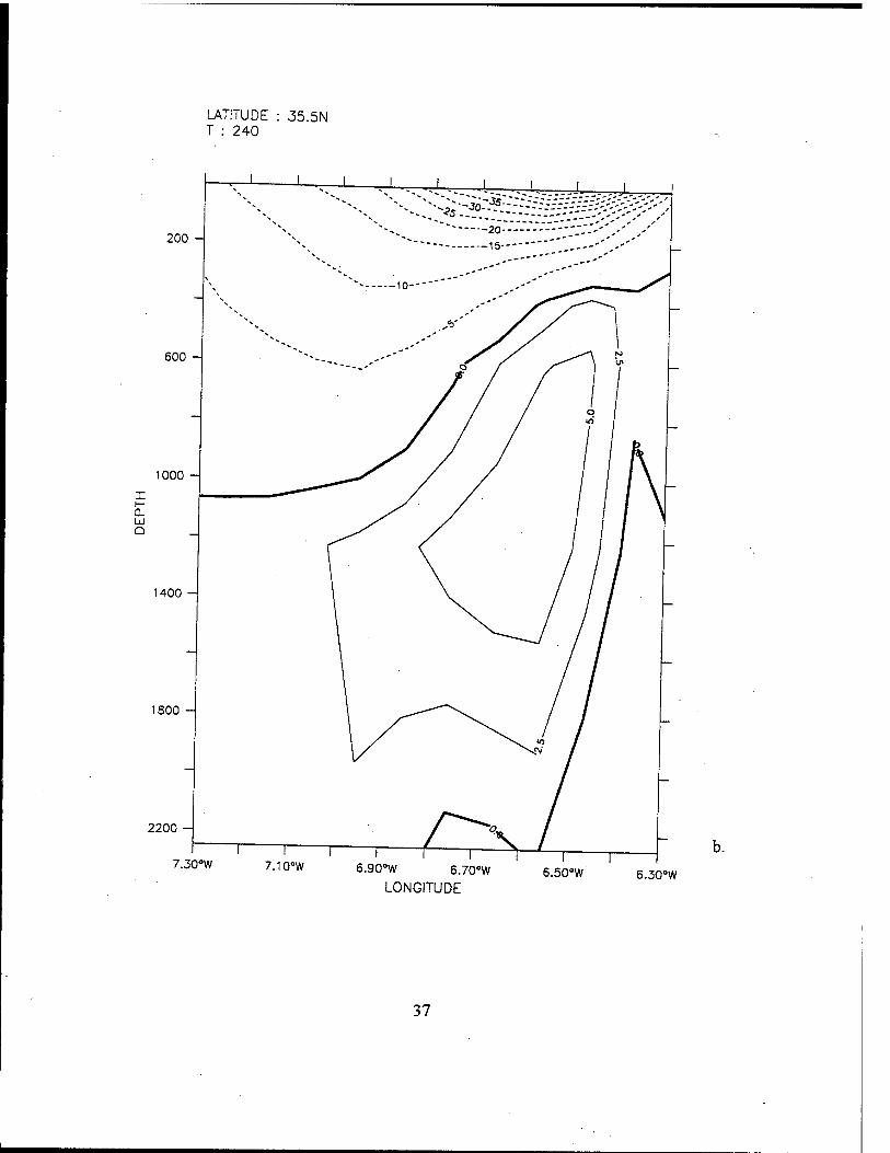
5. Cross-shore sections of meridional velocity (v) on day 240 at (a) 39.5 ° N, and (b) 35.5 ° N. Solid lines indicate poleward flow, while dashed lines indicate equatorward flow. The contour interval is 2.5 cm/s for poleward flow and 5 cm/s for equatorward flow 36

6. Figure 6. Temperature contours (b-e) and velocity vectors (a-e) at 30 m depth in the third year of the model simulation time-averaged over the months of (a) January, (b) June, (c) August, (d) September and (e) November. The contour interval is 1° C. Maximum current velocity is 100 cm/s 38

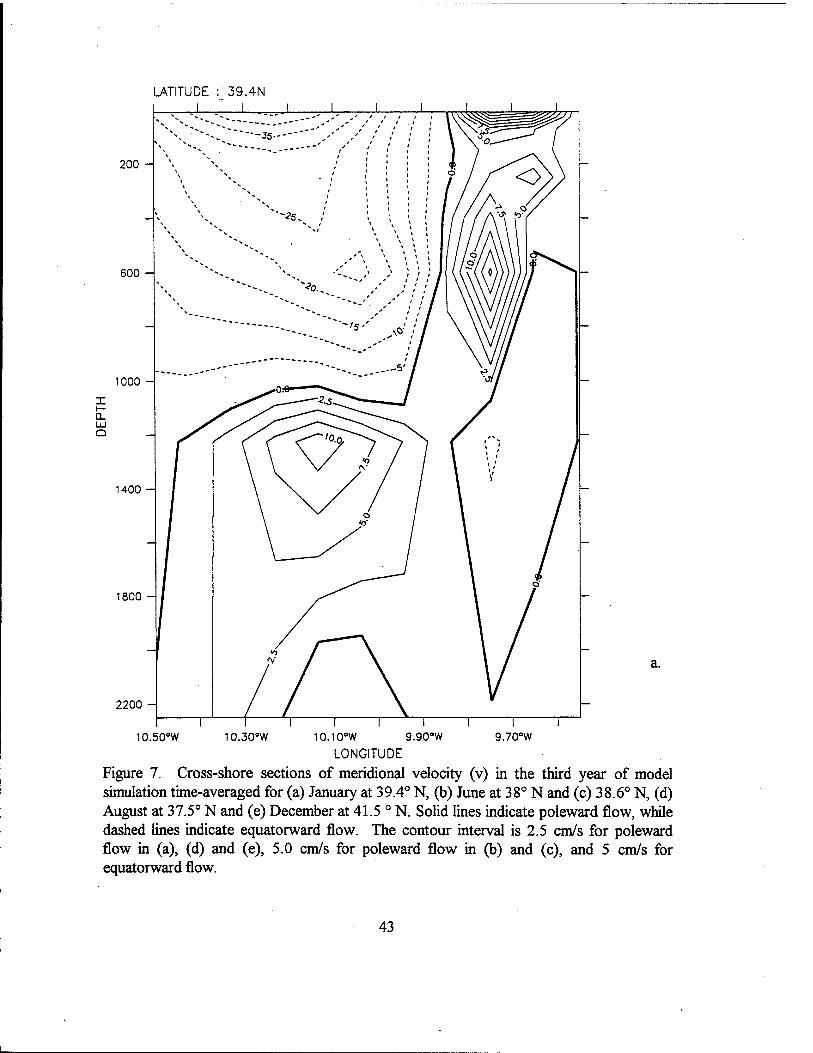
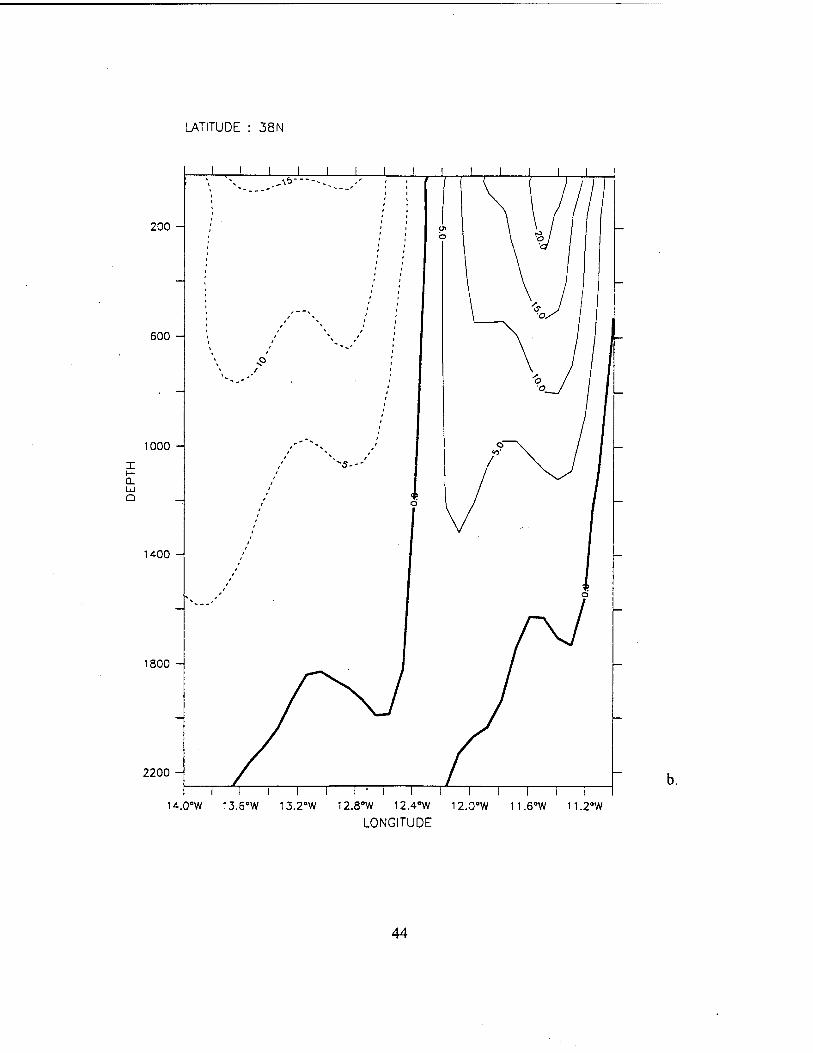
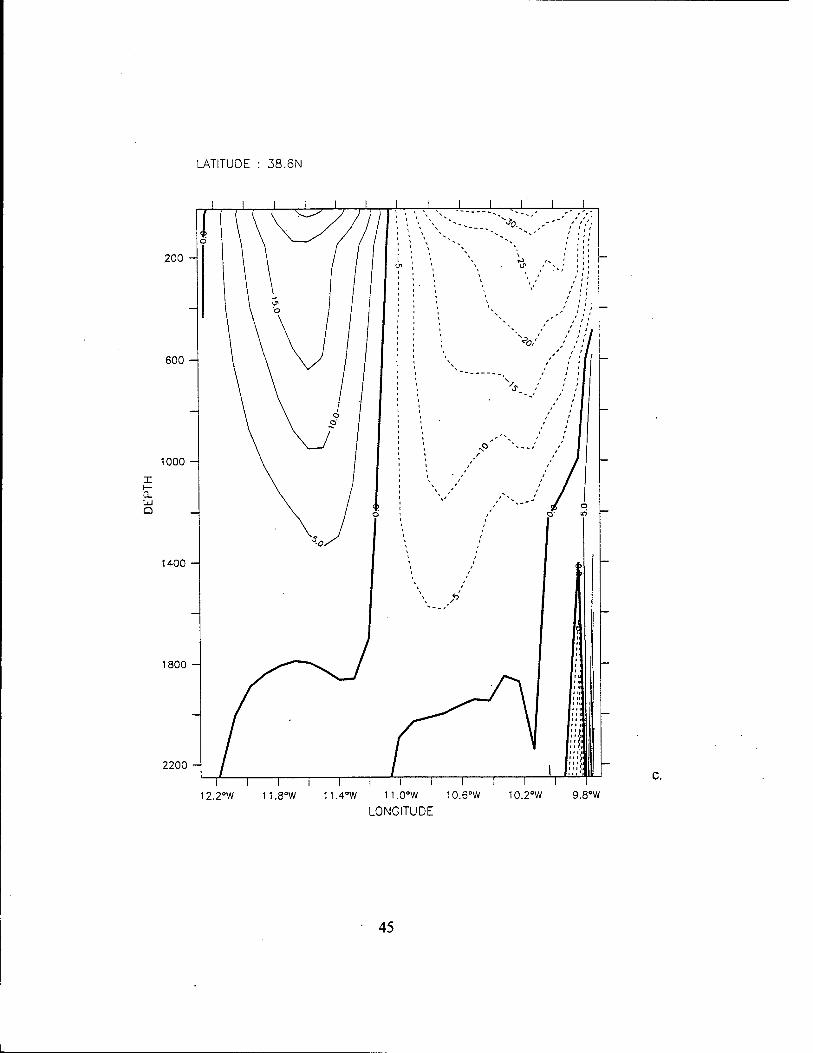
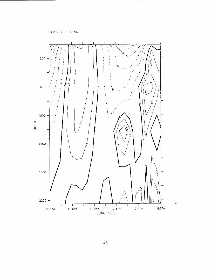
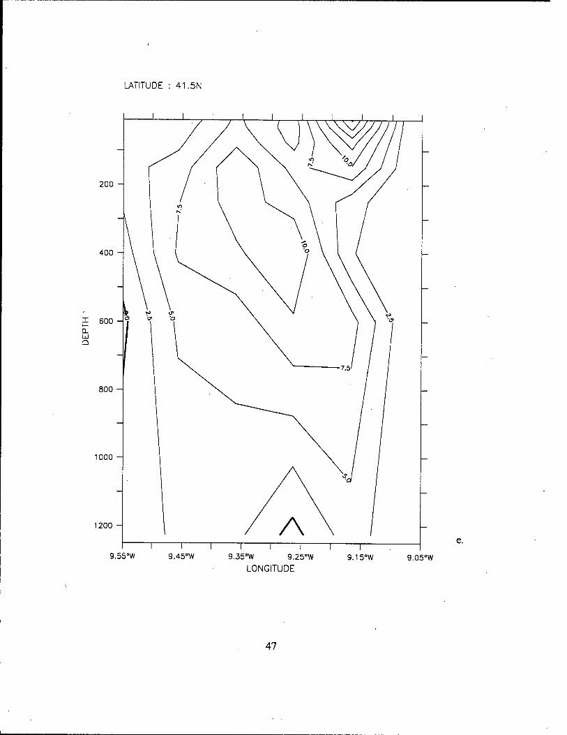
7. Cross-shore sections of meridional velocity (v) in the third year of model simulation time-averaged for (a) January at 39.4° N, (b) June at 38° N and (c) 38.6° N, (d) August at 37.5° N, and (e) December at 41.5° N. Solid lines indicate poleward flow, while dashed lines indicate equatorward flow. The contour interval is 2.5 cm/s for poleward flow in (a), (d) and (e), 5 cm/s for poleward flow in (b) and (c), and 5 cm/s for equatorward flow 43

IX

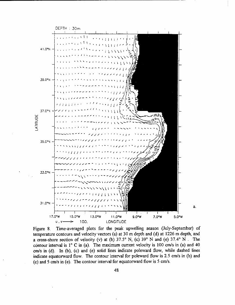
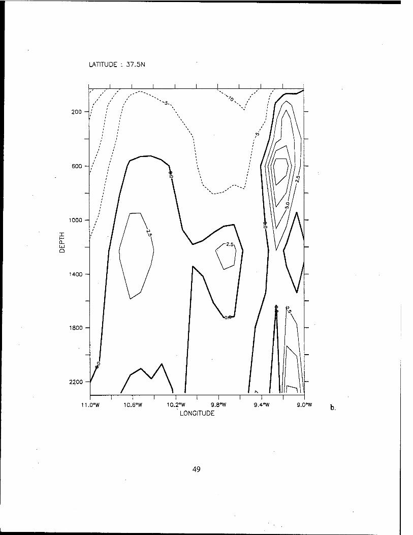
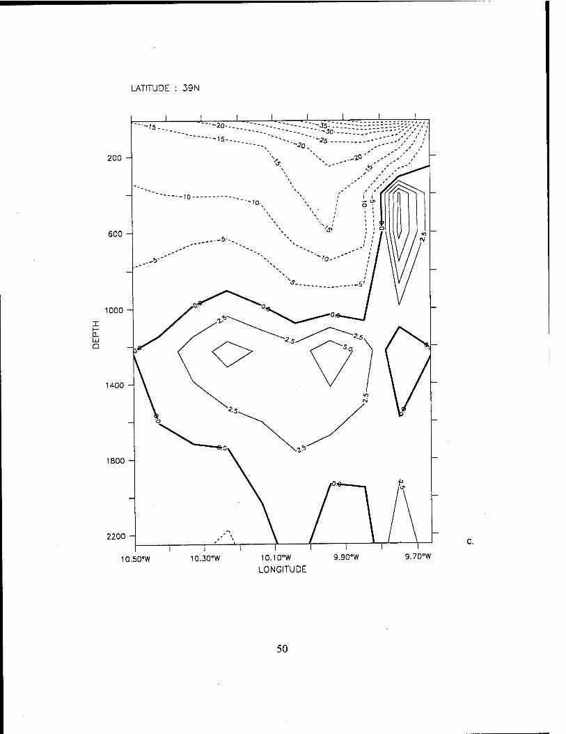
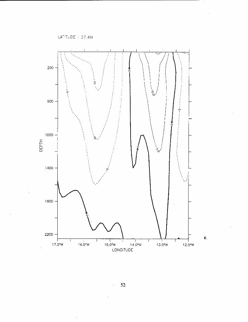
8. Time-averaged plots for the peak upwelling season (July-September) of temperature contours and velocity vectors (a) at 30 m depth and (d) at 1226 m depth, and a cross- shore section of velocity (v) at (b) 37.5° N, (c) 39° N and (e) 37.4° N. The contour interval is 1° C in (a). The maximum current velocity is 100 cm/s in (a) and 40 cm/s in (d). In (b), (c) and (d) solid lines indicate poleward flow, while dashed lines indicate equatorward flow. The contour interval for poleward flow is 2.5 cm/s in (b) and (c) and 5 cm/s in (e). The contour interval for equatorward flow is 5 cm/s 48

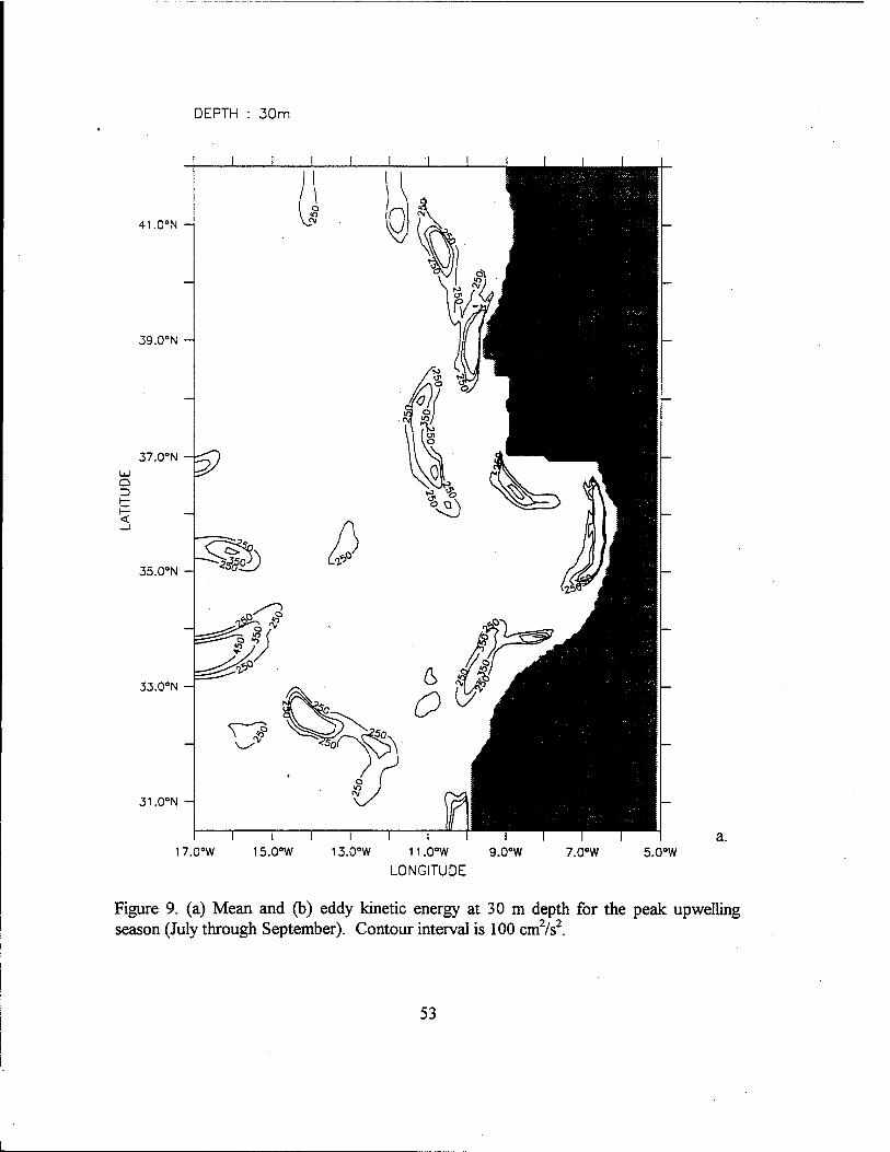
9. (a) Mean and (b) eddy kinetic energy at 30 m depth for the peak upwelling season (July through September). Contour interval is 100 cm2/s2 53

10. Computer representation of AVHRR NOAA7 Sea Surface Temperatures (SST) with observed eddy formations from 5 August 1982. "After Fiuza 1984." 55

11. Temperature contours and velocity vectors at 30 m showing upwelling in the third year at day (a) 137, (b) 152, (c) 173, (d) 209, (e) 263, (f) 290, and (g) 317. The contour interval is 1 ° C. The maximum current velocity is 100 cm/s 56

12. AVHRR sea surface temperatures (SST) from (a) 21 June 1995 showing increased cold SST southwest of Cabo de Sao Vincent caused by intensified upwelling and advection of upwelled water around the cape and (b) 27 July 1993 showing strong upwelling and numerous filaments off the west coast of the DP. In (c) SST show intense upwelling north of Cabo da Roca on 29 July 1977. Figures (a) and (b) are from the Remote Sensing Data Analysis Service (RSDAS), Plymouth Marine Laboratory, UK. Figure (c) is from Fiuza (1982) 63

LIST OF TABLES

1. Values of Constants Used in the Model 71

XI

Xll

ACKNOWLEDGEMENT

The professional guidance and considerable knowledge of Dr. Mary Batteen made

this study possible. Hugh thanks to Pete Braccio, Mike Cook and Phaedra Green for

FORTRAN, FERRET and MATLAB assistance. Thanks also to NERC Remote Sensing

Data Analysis Service, Plymouth Marine Laboratory, UK for the use of their high quality

AVHRR SST images (http://www.ac.uk/rsdas).

Finally, I would like to thank my wife for her patience and support during the last

twenty-one months.

xni

XIV

I. INTRODUCTION

The Canary Current System (CCS) is a classical eastern boundary current (EBC)

system located off the west coasts of Northwest Africa and the Iberian Peninsula (IP). It

extends from -10° N to 45° N, and forms the closing, eastern boundary of the North

Atlantic gyre. The climatological mean CCS consists of several large-scale currents of

which the Canary Current (CC) is predominant. Like other EBCs, the CC is a broad

(-1000 km), relatively slow (-10-30 cm/s), equatorward, yearlong surface flow extending

to depths of- 500 m (Wooster et al, 1976). The portion of the CC which lies off the

west coast of the IP is occasionally referred to as the Portugal Current (e.g., Tomczak and

Godfrey, 1994). Embedded in the CC are narrower, somewhat swifter flows occasionally

reaching speeds of 100 cm/s (DMAH/TC, 1988)).

Beneath the CC and near the coast, a narrower (-10-40 km) and weaker (-2-10

cm/s) poleward undercurrent is present. While the undercurrent is usually strongest

between 100 and 600 m depth (Haynes and Barton, 1990), the depth and strength of the

undercurrent can vary both seasonally and latitudinally. During the winter the

undercurrent shoals to the north, occasionally reaching the surface, to form a third flow

component referred to as the Iberian Current (IC) (Haynes and Barton, 1990). The IC is a

narrow (25-40 km), relatively weak (-20-30 cm/s) seasonal surface poleward current

found trapped near the coast against the shelf break (Fiuza, 1980; Frouin et al, 1990;

Haynes and Barton, 1990). Geographically, the IC is normally found north of Cabo da

Roca (see Figure 1 for geographical locations) but occasionally extends south nearly to

Cabo de Sao Vincent during the winter months. A second deeper undercurrent also flows

poleward off the west coast of the IP. Attributed to the Mediterranean Outflow (MO), this

flow has at least two main cores, a shallow core at depths of 600-900 m and a deeper core

at 1100-1200 m (Ambar, 1980). An additional third, and shallower, poleward core of

Mediterranean water has also been shown to exist near 400 m (Fiuza, 1979; Ambar,

1980).

The CCS is influenced predominantly by equatorward, upwelling favorable winds

produced by the Azores High. The Azores High is a semi-permanent subtropical high

pressure system similar in nature and behavior to its counterpart off the west coast of

North America, the North Pacific Subtropical High, as described in Nelson (1977). The

center of the Azores High migrates meridionally with the seasons, reaching -27° N, its

southernmost extent, in March and ridging north to -33° N by August. As a result of this

migration, maximum wind stress values vary temporally at given locations. The summer

mean east-west pressure contrast between Portugal and the center of the Azores High is

~8 mb. During the winter, the contrast lessens to ~1 mb. This pressure difference results

in correspondingly strong northerly to northwesterly winds during the summer and weaker

northwesterly to even slight southerly winds off of northern Portugal and northwest Spain

during the winter. The shift of maximum wind stress also causes the upwelling favorable

winds to shift from -27° N near the Canary Islands in January, to -43° N off the IP by

July. (Fiuza, 1982)

Recent observations have shown highly energetic, mesoscale features such as jet-

like surface currents, meanders, eddies, and filaments superimposed on the broad,

climatological mean flow of the CC and other EBCs. Specifically, satellite images of sea

surface temperatures have shown several filaments extending off the coast of Portugal and

northwest Spain (Fiuza et al., 1989) as well as off Cape Ghir in northwest Africa (Van

Camp et al, 1991; Hagen et al, 1996). Observations have also shown pairs of

anticyclonic and cyclonic mesoscale eddies on the order of 100 km off the coast of Iberia

(Fiuza, 1984). Observed during periods of predominantly equatorward, upwelling

favorable winds, these features seem to be located near prominent coastal features such as

capes. These observations provide evidence that wind forcing and coastal irregularities

could be important mechanisms in the formation and sustainment of many of the

mesoscale features found in EBC regions.

Over the past few decades numerous wind forcing models of EBCs, particularly of

the California Current System, have been conducted. Early work included steady wind

stress (Pedlosky, 1974) and transient wind forcing (Philander and Yoon, 1982). The

response of reduced gravity models to realistic coastal winds was investigated by Carton

(1984) and Carton and Philander (1984). McCreary et al. (1987) conducted a series of

experiments using a linear model with both transient and steady wind forcing in the

California Current System. In each of these previous models, relatively weak currents (5-

10 cm/s) were generated and no eddies or filaments developed.

Recent modeling studies have focused on the driving mechanisms of complex

features, such as filaments, observed in EBC regions. Ikeda et al. (1984a, b) and

Haidvogel etal. (1991) studied baroclinic and barotropic instability, coastal irregularities,

and bottom topography as possible mechanisms, while Batteen et al. (1989), McCreary et

al. (1991), Pares-Sierra et al. (1993), and Batteen (1997) studied wind forcing as a

possible generative mechanism. Recently, a multilevel primitive equation (PE) model of

the California Current System from 35° N to 47.5° N was used by Batteen (1997) to study

the effects of seasonal winds and coastal irregularities and by Batteen and Vance (1998) to

study the additional effects of thermohaline gradients. In a more recent study Batteen and

Monroe (1998) studied the contribution of seasonal wind forcing, thermohaline gradients

and irregular coastline geometry to the generation of eddies and filaments for the entire

California Current System, i.e., from 22.5° N to 47.5° N. The results showed that wind

forcing was the dominant process responsible for many of the observed features of the

California Current System.

In contrast, coastal modeling studies of the CCS have been scarce. McClain et al.

(1986) performed the first limited modeling study in the region, using ship-derived winds

to produce a large negative wind stress curl off the northwest coast of the IP, resulting in

opposing equatorward and poleward surface currents. Recently Batteen et al. (1992)

used an eddy resolving PE model with both uniform and variable wind stress, the latter

computed from synoptic surface pressure analyses, to produce realistic currents as well as

mesoscale eddies. This study, however, covered only a limited region of the CCS (the

northwest coast of the IP) and had a straight coast in its model domain.

The objective of this study is to investigate the roles of seasonal climatological

wind forcing and irregular coastline geometry in the generation of currents, eddies, jets

and filaments in the CCS. The high-resolution, multi-level, PE model of Batteen and

Monroe (1998) will be used. To allow larger scale eddies and elongated filaments to be

generated and the model to reach quasi-equilibrium, the model will be allowed to run for

~3 years.

This study is organized as follows: the PE model, type of wind forcing, initial and

specific experimental conditions, and the energy analysis technique are described in

chapter II. Results of the model simulations and comparisons with observations are

discussed in chapter III. A summary and discussion are presented in chapter IV.

H. MODEL DESCRIPTION

A. MODEL EQUATIONS

The PE numerical model used in this study was originally a coarse resolution

model used by Haney (1974) to study closed basins. It has since been adapted for eddy-

resolving, limited EBC regions with open northern, western, and southern boundaries by

Batteen (1997). The multi-level, non-adiabatic, model uses beta-plane, hydrostatic,

Boussinesq, and rigid lid approximations and has baroclinic and barotropic velocity

components. Equations governing the model are as follows:

* p0 dx M M dz + fi,-AMV*u + KM— (1)

dt p0 dy J M . M dz = —-!:.-fi<-Wv + KM— (2)

(3) du d\>

dx dy

dw

~dz~" 0

dp

dz = ~Pg

P = A,P- a(T- -T0) + ß(S- -st )]

dT

dt = -^ ,V4T + KH

d2T

dz2

(4)

(5)

(6)

^—A^S + K»^ (7) dt H H dz2 v '

In the above equations, / is time, T is temperature, S is salinity, p is density, and p is

pressure. A right-handed Cartesian coordinate system (x,y,z) is used where x points

toward shore, y alongshore, and z upward. The corresponding velocity components are

(u,v,w). Table 1 provides a list of symbols found in the model equations, as well as values

of constants used throughout the study.

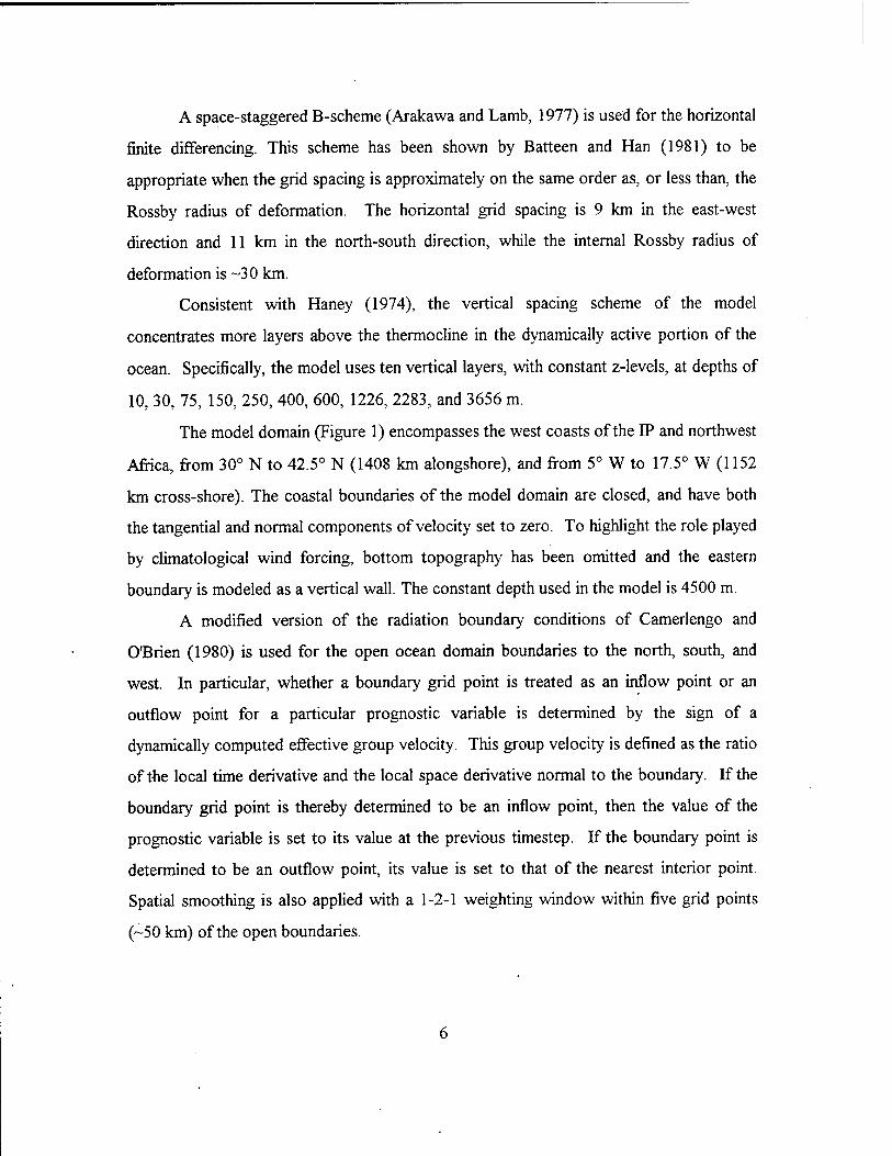
A space-staggered B-scheme (Arakawa and Lamb, 1977) is used for the horizontal

finite differencing. This scheme has been shown by Batteen and Han (1981) to be

appropriate when the grid spacing is approximately on the same order as, or less than, the

Rossby radius of deformation. The horizontal grid spacing is 9 km in the east-west

direction and 11 km in the north-south direction, while the internal Rossby radius of

deformation is -30 km.

Consistent with Haney (1974), the vertical spacing scheme of the model

concentrates more layers above the thermocline in the dynamically active portion of the

ocean. Specifically, the model uses ten vertical layers, with constant z-levels, at depths of

10, 30, 75, 150, 250, 400, 600, 1226, 2283, and 3656 m.

The model domain (Figure 1) encompasses the west coasts of the IP and northwest

Africa, from 30° N to 42.5° N (1408 km alongshore), and from 5° W to 17.5° W (1152

km cross-shore). The coastal boundaries of the model domain are closed, and have both

the tangential and normal components of velocity set to zero. To highlight the role played

by climatological wind forcing, bottom topography has been omitted and the eastern

boundary is modeled as a vertical wall. The constant depth used in the model is 4500 m.

A modified version of the radiation boundary conditions of Camerlengo and

O'Brien (1980) is used for the open ocean domain boundaries to the north, south, and

west. In particular, whether a boundary grid point is treated as an inflow point or an

outflow point for a particular prognostic variable is determined by the sign of a

dynamically computed effective group velocity. This group velocity is defined as the ratio

of the local time derivative and the local space derivative normal to the boundary. If the

boundary grid point is thereby determined to be an inflow point, then the value of the

prognostic variable is set to its value at the previous timestep. If the boundary point is

determined to be an outflow point, its value is set to that of the nearest interior point.

Spatial smoothing is also applied with a 1-2-1 weighting window within five grid points

(-50 km) of the open boundaries.

Biharmonic lateral heat and momentum diffusion is used in the model with the

17 4 same choice of coefficients (i.e., 2.0x10 cm/s) as in Batteen (1997). Holland (1978)

showed that highly selective biharmonic diffusion acts predominantly on submesoscales,

while Holland and Batteen (1986) found that baroclinic mesoscale processes can be

damped by Laplacian lateral heat diffusion. As a result, the use of biharmonic lateral

diffusion should allow mesoscale eddy generation via barotropic (horizontal shear) and/or

baroclinic (vertical shear) instability mechanisms. As in Batteen (1997), weak (0.5 cm Is)

vertical eddy viscosities and conductivities are used. Bottom stress is parameterized by a

simplified quadratic drag law (Weatherly, 1972), as in Batteen (1997).

The method of solution is straightforward with the rigid lid and flat bottom

assumptions because the vertically integrated horizontal velocity is subsequently

nondivergent. The vertical mean flow can be described by a streamfunction which can be

predicted from the vorticity equation, while the vertical shear currents can be predicted

after the vertical mean flow is subtracted from the original equations. The other variables,

i.e. temperature, salinity, vertical velocity, and pressure, can be explicitly obtained from

the thermodynamic energy equation (6), salinity equation (7), continuity equation (3), and

hydrostatic equation (4), respectively (For more complete details on the method of

solution, see the Appendix).

B. TYPE OF WIND FORCING

Previous experiments by Batteen et cd. (1992) investigated the role of steady

equatorward winds with anticyclonic wind stress curl in the generation of features off the

IP. In a more recent study Batteen and Monroe (1998) studied the contributions of

seasonal wind forcing and irregular coastline geometry in the generation of eddies and

filaments in the California Current system. Following Batteen and Monroe (1998), in this

study, seasonal wind forcing and irregular coastline geometry will be used to investigate

the generation of similar features in the CCS.

To explain the effects of seasonal wind, the model is forced from rest with

climotalogical wind fields from a 2.5° by 2.5° grid of the European Centre for Medium

Range Weather Forecasts (ECMWF) near-surface wind analyses (Trenberth et al., 1990).

The monthly mean stresses based on twice daily wind analyses from 1980-1989 have been

interpolated spatially to the 9 by 11 km model resolution and temporally to daily wind

values.

Sample wind fields used can be seen in Figure 2, which shows the annual migration

of the Azores Subtropical High from the south in the winter (e.g., Figure 2d), to its most

northern extent in the summer (e.g., Figure 2b). The atmospheric pressure pattern for

November (Figure 2d) depicts a low to the north and the Azores High to the south, which

results in a wind divergence at -40° N. This pattern of weakly poleward winds north of

40° N and equatorward winds to the south continues through December. During January

(not shown) and February (Figure 2a) the divergence in the wind field migrates poleward.

By March (not shown) an equatorward component in the wind field is observed along the

entire domain. The strongest equatorward winds are discernible from July (Figure 2b)

through August (not shown). By September (Figure 2c) the winds start to weaken

throughout the domain, and divergence in the wind field is observed in the north in

October (not shown). In November (Figure 2d) the wind divergence returns to -40° N.

C. EXPERIMENTAL DESIGN

The design of the model experiment is as follows. The model is forced from rest

with seasonal ECMWF winds. The initial mean stratification used are annual

climatological temperature fields based on Levitus and Boyer (1994) centered at -37.5° N

(corresponding to the center of the model domain). The temperatures (°C) used for the

ten levels from the surface to 4500 m are 17.5, 17.3, 16.5, 15.0, 13.7, 12.5, 11.0, 8.52,

3.59, and 2.09, respectively, while a salinity constant of 34.7 is used for all levels.

Like all major EBC systems, the CCS is a region of net annual gain. This heat gain

occurs because of relatively low cloud cover (compared with farther offshore), reduced

latent heat flux, and downward sensible heat flux due to the presence of cold upwelled

water during summer. To focus the experiment on wind forcing as a possible mechanism

for the generation of thermal variability in the CCS, the surface thermal forcing in the

model was highly simplified. The solar radiation at the sea surface So, was specified to be

the summer mean and CCS mean value. On the other hand, the sum of the net longwave

radiation, latent, and sensible heat fluxes, Qb, was computed during the model's

experiments from standard bulk formulas (Haney et al. 1978) using the summer and CCS-

mean value of the alongshore wind (above), cloud cover, relative humidity, air

temperature, and model-predicted sea surface temperature. The initial sea surface

temperature was chosen so that the total heat flux across the sea surface, So - Qb, was

zero at the initial time. Therefore, the only surface heat flux forcing in the experiments

was that which developed in Qb as a result of (wind forced) fluctuations in the sea surface

temperature. As discussed in Haney (1985), such a surface thermal forcing damps the sea

surface temperature fluctuations to the atmosphere on a time scale of the order of 100

days. Consequently, sea surface temperature fluctuations that develop due to wind forcing

should be observed long before they are damped by the computed surface heat flux.

10

HI. RESULTS FROM THE MODEL SIMULATION

A. SPIN-UP PHASE

On day one of the model (1 January), the Azores High is stationed near its

southernmost position. In response to predominantly equatorward winds, a coastal

equatorward surface current develops in the southern end of the domain and by day 60

extends along the entire coast (not shown).

In the spring as the Azores High migrates north, the wind intensifies and

transitions to equatorward flow over the entire domain. As a result, increased stress is

exerted on the ocean surface creating Ekman transport offshore and upwelling of cooler

water along the coast. Upwelling predominantly occurs in the south where stronger winds

exist (e.g., Figure 3a), but by mid-summer is evident along the entire coast (e.g., Figures

3b and 4). Upwelling is enhanced near capes (e.g., Figure 3b), where both the alongshore

component of the wind stress and the coastal current velocity are at local maxima

(Batteen, 1997).

Below the equatorward surface current, a poleward undercurrent develops first at

the equatorward side and then at the poleward side of the model domain. The coastal jet

extends from -200 m depth near the coast to -600-800 m depth offshore, and has a peak

core velocity of-30-45 cm/s (Figures 5a and 5b). Along the west coast of the IP (e.g.,

Figure 5a) and Morocco (not shown) the undercurrent develops separate cores at -400 m

depth and 1200 m depth. The -400 m depth core of the undercurrent has a peak velocity

of-5-10 cm/s and remains within -20-30 km of the coast. The -1200 m depth core of the

undercurrent has a peak velocity of-5-10 cm/s and generally remains within -40-50 km of

the coast.

11

In the Gulf of Cadiz there is no separation of the undercurrent cores. The core of

the undercurrent is found between -400 and 1200 m depth and has speeds of 5 cm/s

(Figure 5b).

As the coastal jet and the subsurface undercurrent become fully established (for

example, see Figures 5 a and 5b, which shows the structure of the currents prior to

meander formation), strong vertical and horizontal shears develop in the upper layers

between the opposing currents. This shear causes the flow to become both barotropically

and baroclinically unstable and leads to the formation of meanders and filaments.

Meanders occur first off Cape Ghir, Cabo da Roca and Cabo de Sao Vincent. These

meanders intensify and develop into predominantly cyclonic cold core eddies, which in

time coalesce with other eddies to form larger cyclonic eddies on the order of-150-250

km. By day 285 (Figure 3 c) meanders and eddies are visible throughout the coastal

region.

In the late fall as the Azores High migrates south, first the winds and then the

currents begin to weaken. In time, upwelling, as expected, also weakens. By the end of

the first year of model simulation (Figure 3d), the equatorward surface flow extends as far

as -350 km offshore and has taken the form of a meandering jet embedded with

predominantly cyclonic eddies.

B. QUASI-EQUILBRIUM PHASE

Continuous formation and sustainment of meanders, eddies and filaments indicate

that the model has reached a quasi-equilibrium state by year three. Time-averaging model

output fields for each month as well as the peak upwelling season (July through

September) in year three provides an opportunity to see the complex structure and

seasonal variability of the CCS.

The winter model results (e.g., Figure 6a) depict a predominantly equatorward

flow, which is embedded with eddies throughout the domain. Along the IP, a surface

12

coastal poleward flow with speeds as high as -22.5 cm/s is visible (Figures 6a and 7a).

Beneath the surface (Figure 7a), cores of poleward flow with speeds of-10-17.5 cm/s at

-600 and -1200 m depth are discernible. An additional third core of poleward flow at

-250 m depth with a speed of-10 cm/s is also formed along the IP in the vicinity of-39°

N (Figure 7a).

By early spring an equatorward coastal jet appears off the coast of Morocco south

of 32° N and upwelling resumes (not shown). By June (Figure 6b) upwelling appears all

along the IP and a strong equatorward current with speeds of -25-40 cm/s meanders

along the IP. Off Cabo da Roca the equatorward current weakens as it flows into the Gulf

of Cadiz. South of 35° N the equatorward current becomes a coastal jet with speeds of

-40 cm/s. Downstream of Cabo da Roca (Figure 6b) and Cape Beddouzza (not shown)

pairs of cyclonic (Figures 6b and 7b) and anticyclonic (Figures 6b and 7c) eddies of O(150

km) in size and extending to greater than 1400 m depth are discernible.

In the summer (Figure 6c) upwelling is visible along the western and southern

coast of the IP as well as along the coast of Morocco. As the equatorward jet flows along

the IP, it impinges upon Cabo da Roca and is deflected offshore adverting cold water with

it, resulting in the formation of filaments (e.g., Figure 6c) off Cabo da Roca and Cabo de

Sao Vincent. Filaments are also discernible off Cabo de Santa Maria and the southern

coast of Portugal (Figure 6d). The filaments typically extend from -75 to 150 m depth

(not shown). Beneath the surface (Figure 7d), cores of poleward flow with speeds of-5-

7.5 cm/s at -600 and -1200 m depth are evident. An additional weaker core of poleward

flow at -250 m depth with a speed of-5 cm/s is also formed off the west coast of the IP

in the vicinity of 37° N.

The results (Figure 8) of averaging the temperature and current fields for the

period when the most intense upwelling (i.e., July through September) occurs off both the

IP and Morocco shows that a meandering equatorward current offshore, an equatorward

coastal jet, subsurface poleward flow with cores at -600 m depth and -1200 m depth,

coastal upwelling, filaments and eddies are regular features of the CCS during the

13

upwelling season. Figure 8a shows the surface equatorward current offshore of the -

17.5° C isotherm until south of Cabo da Roca where the 16.5° C and 17.5° C isotherms

separate. South of Cabo de Sao Vincent the offshore equatorward current once again

splits into two distinct flows. The westernmost flow continues equatorward while the

easternmost flow meanders cyclonically and joins the coastal jet in the Gulf of Cadiz. Off

Cape Beddouzza the offshore flow and coastal current rejoin, and continue down the

coast of Morocco. The offshore current has speeds of -15-45 cm/s and extends to -1000

m depth (Figures 8b and 8c). The coastal jet has peak speeds of -45 cm/s and extends to

-250 m depth near the coast (Figure 8c). Upwelling is visible all along the IP coast as

well as along the coast of Morocco (Figure 8a). Cold, upwelled filaments are also

discernible downstream of prominent capes (Figure 8a). The filaments typically extend

-125 km offshore, have widths of -75 km and extend to -100 m depth (not shown).

Figure 8b shows the often fuzed -250 m depth and 600 m depth undercurrent cores found

between Cabo da Roca and Cabo de Sao Vincent as well as the -1200 m depth

undercurrent core. The -250 m and 600 m depth cores reach speeds of-10 cm/s while

the 1200m depth core reaches speeds of-2.5-5 cm/s. Figure 8d shows the -1200 m depth

undercurrent as it flows along the entire coast from Morocco into the Gulf of Cadiz and

along the IP during the peak upwelling season. Offshore of the undercurrent are both

cyclonic and anticyclonic eddies of O(150) km in size that extend to at least 1000 m depth

(Figures 8d and 8e).

Figures 9a and 9b show horizontal maps of upper layer mean kinetic energy

(MKE) and eddy kinetic energy (EKE) averaged during the peak upwelling season.

Holland et al. (1983) showed that maps of MKE and EKE can be used to locate sources

of mean and eddy energy. From Figure 9a it can be seen that high values of MKE follow

the equatorward jet and that the highest values of MKE appear near areas of tightened

temperature gradients off Cabo da Roca, in the Gulf of Cadiz and off Cape Beddouzza.

A comparison of Figures 8 a and 9b shows maximum values of EKE in the vicinity

of the large cyclonic meander that extends downstream from Cabo da Roca. High values

14

are also formed along the axes of the equatorward jet on the west coast of the Gulf of

Cadiz and offshore of Cape Ghir and Cape Beddouzza. The lowest coastal values of EKE

are along the southern coast of the IP, indicating that this region is not a primary source of

eddy energy.

A comparison of Figures 8a, 9a and 9b shows that overall, the regions of

maximum MKE and EKE are found along the axes of the equatorward jet. This is

consistent with the results of the model simulation, which showed that the eddies are

generated from instabilities of the mean equatorward current and subsurface undercurrent

via baroclinic and/or barotropic instability processes.

By Fall (e.g., Figure 6e) upwelling has weakened and the coastal jet is no longer

visible north of Cabo da Roca. Offshore, a meandering equatorward current embedded

with westward propagating, cyclonic eddies is discernible. Farther south, the coastal jet

leaves the coast at Cape Beddouzza and is entrained in a large cyclonic eddy 0(200 km)

prior to continuing south along the coast of Morocco. By winter, poleward surface flow

with speeds of-15-25 cm/s has developed north of 41° N. The flow is found within -60

km of the coast and extends to -200 m depth (Figure 7e).

C. COMPARISONS OF MODEL RESULTS WITH OBSERVATIONS

To ensure model results are consistent with realistic features of the CCS, the

model results are compared to available field and satellite observations. Since this is an

idealized process-oriented study and not a model hindcast, direct comparisons are not

valid; however, it can be shown that the model's phenomenological behavior is

qualitatively similar to observed data. The discussion in the ensuing paragraphs first

details general CCS features and then specific magnitudes and characteristics of features

generated along the western coasts of the IP and Northwest Africa. Overall, there exists

impressive similarities between the results of the model simulation and the major

characteristics of the CCS.

15

1. Comparison of Ocean Currents

The major characteristics of the modeled Canary Current off western Iberia and

northwestern Africa are consistent with the few field observations and studies available.

Satellite imagery also reveals a system of meanders, eddies, and along-shelf jets, on a

range of length scales that correspond closely with model output.

a. Equatorward Flow

Using climatological wind data and a realistic coastline, the model develops

an ocean current with features similar to those observed in the CCS. The broad,

equatorward flow found throughout the model domain matches the general description of

classical EBCs by Wooster and Reid (1963). The sustained magnitude of the model's

equatorward flow also compares favorably with available data. For example, DMAH/TC

(1988) shows a mean predominantly equatorward flow of -0.5 to 0.7 kts (-25-35 cm/s),

which is consistent with velocities found in the model simulation (e.g., Figures 8a and 8c).

b. Poleward Flow

The model establishes a poleward undercurrent with cores at -600 m depth

and -1200 m depth throughout the domain (Figures 5a, 7a, 8b, and 8c). In addition, a

third core of poleward flow at -250 m depth is seen near 37° N along the west coast of

the IP predominantly during June, July and August (e.g., Figure 7d) and near 39° N during

November and January (e.g., Figure 7a). The depths and magnitudes of the 600 m and

1200 m depth model's poleward flow cores are consistent with Ambar (1980), which

shows these cores located between 600-900 m and 1100-1200 m depth along the entire

western coast of the IP. The depth and speed of the 250 m model's poleward flow is

consistent with Haynes and Barton (1990), which shows this core located between 100

and 600 m depth off the IP.

16

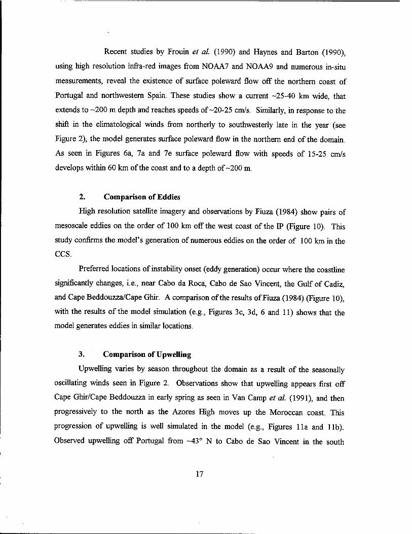
Recent studies by Frouin et al. (1990) and Haynes and Barton (1990),

using high resolution infra-red images from NOAA7 and NOAA9 and numerous in-situ

measurements, reveal the existence of surface poleward flow off the northern coast of

Portugal and northwestern Spain. These studies show a current -25-40 km wide, that

extends to -200 m depth and reaches speeds of-20-25 cm/s. Similarly, in response to the

shift in the climatological winds from northerly to southwesterly late in the year (see

Figure 2), the model generates surface poleward flow in the northern end of the domain.

As seen in Figures 6a, 7a and 7e surface poleward flow with speeds of 15-25 cm/s

develops within 60 km of the coast and to a depth of-200 m.

2. Comparison of Eddies

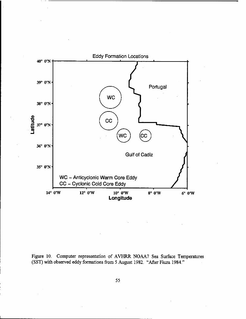
High resolution satellite imagery and observations by Fiuza (1984) show pairs of

mesoscale eddies on the order of 100 km off the west coast of the IP (Figure 10). This

study confirms the model's generation of numerous eddies on the order of 100 km in the

CCS.

Preferred locations of instability onset (eddy generation) occur where the coastline

significantly changes, i.e., near Cabo da Roca, Cabo de Sao Vincent, the Gulf of Cadiz,

and Cape Beddouzza/Cape Ghir. A comparison of the results of Fiuza (1984) (Figure 10),

with the results of the model simulation (e.g., Figures 3c, 3d, 6 and 11) shows that the

model generates eddies in similar locations.

3. Comparison of Upwelling

Upwelling varies by season throughout the domain as a result of the seasonally

oscillating winds seen in Figure 2. Observations show that upwelling appears first off

Cape Ghir/Cape Beddouzza in early spring as seen in Van Camp et al. (1991), and then

progressively to the north as the Azores High moves up the Moroccan coast. This

progression of upwelling is well simulated in the model (e.g., Figures 11a and lib).

Observed upwelling off Portugal from -43° N to Cabo de Sao Vincent in the south

17

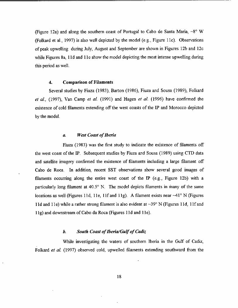
(Figure 12a) and along the southern coast of Portugal to Cabo de Santa Maria, -8° W

(Folkard et al., 1997) is also well depicted by the model (e.g., Figure 1 lc). Observations

of peak upwelling during July, August and September are shown in Figures 12b and 12c

while Figures 8a, lid and lie show the model depicting the most intense upwelling during

this period as well.

4. Comparison of Filaments

Several studies by Fiuza (1983), Barton (1986), Fiuza and Sousa (1989), Folkard

et al, (1997), Van Camp et al. (1991) and Hagen et al. (1996) have confirmed the

existence of cold filaments extending off the west coasts of the IP and Morocco depicted

by the model.

a. West Coast of Iberia

Fiuza (1983) was the first study to indicate the existence of filaments off

the west coast of the IP. Subsequent studies by Fiuza and Sousa (1989) using CTD data

and satellite imagery confirmed the existence of filaments including a large filament off

Cabo de Roca. In addition, recent SST observations show several good images of

filaments occurring along the entire west coast of the IP (e.g., Figure 12b) with a

particularly long filament at 40.5° N. The model depicts filaments in many of the same

locations as well (Figures lid, lie, 1 If and 1 lg). A filament exists near -41° N (Figures

lid and lie) while a rather strong filament is also evident at -39° N (Figures 1 Id, 1 If and

llg) and downstream of Cabo da Roca (Figures 1 Id and lie).

b. South Coast of Iberia/Gulf of Cadiz

While investigating the waters of southern Iberia in the Gulf of Cadiz,

Folkard et al (1997) observed cold, upwelled filaments extending southward from the

18

coast. The model results shown in Figures 6d, 6e, 1 If and llg depict these filaments as

well.

c. Cape Ghir/Northwest Africa

Satellite observations from Van Camp et al. (1991) and Hagen et al.

(1996) show a filament of cold, upwelled water extending off Cape Ghir near 31° N for

about 200 km. Consistent with these observations, the model depicts this filament as an

equatorward meandering coastal jet which transports cold, upwelled water offshore

(Figure 1 le). Observations show that the coastal jet and subsequent frontal zone caused

by the advected cold water results in the generation near -12° W of a cyclonic eddy-like

feature on the southern side of the jet, while an anticyclonic eddy forms on the northern

side. The model results (Figure lie) show that, consistent with the observations, on the

northern side of the jet is an anticyclonic eddy centered at -12° W, 33° N and on the

southern side of the jet a cyclonic eddy at -12° W, 31.5° N.

In summary, the variety of length scales and life time scales, in conjunction

with the differences in field observations themselves, emphasize the complex flow region

of the CCS. Despite this complexity, the numerical model results show striking similarities

to available field observations of surface and subsurface currents, upwelling, filaments,

meanders, and cyclonic and anticyclonic eddies.

19

20

IV. SUMMARY

The objective of this study was to investigate the role of seasonal climatological

wind forcing in the generation of currents, eddies, jets, and filaments in the CCS. Toward

this end, a high resolution, multi-level, PE model using a realistic coastline was forced

from rest using spatially and temporally varying winds. The cyclic migration of the Azores

High, and the subsequent role it has on the seasonal variability of alongshore winds, was

shown to play a significant role in the generation, evolution and sustainment of mesoscale

features in the CCS.

An equatorward surface current and a subsurface poleward current with cores at

-600 m and 1200 m depth developed and were maintained throughout the year. A third

core of poleward flow was also generated at -250 m depth at -37° N from June through

August and at -39° N during January and November. Along the northern IP, surface

poleward flow developed in the late fall and lasted until late spring. The opposing nature

of the equatorward and subsurface poleward currents resulted in both horizontal

(barotropic instability) and vertical (baroclinic instability) shear. This shear caused the

currents to become unstable, meander, and eventually lead to the formation of cyclonic

and anticyclonic eddies. As meanders intensified along the coast, cold, upwelled water

was advected offshore forming filaments.

Model results also depicted a seasonal upwelling cycle tied to the migrating Azores

High. Upwelling began in the spring along the southern coast of Morocco, progressed

northward, and by mid-summer was visible along the coast throughout the domain.

During the upwelling season a surface equatorward coastal jet overlying the poleward

undercurrent was generated. As the coastal jet reached its maximum velocity during the

peak upwelling season (July through September), eddy formation along the coast

increased. Seasonal filament generation also occurred during and just after the upwelling

season.

21

Coastline irregularities also appeared to play a significant role in the formation of

mesoscale features. Specifically, the capes acted as barriers that forced the coastal

equatorward flow offshore. This continuous offshore deflection caused some meanders

and eddies to appear as quasi-permanent rather than seasonal features. Capes were also

areas of enhanced upwelling and were significant in the location and formation of

filaments.

A comparison of the currents, eddies, jets, and filaments generated by the model

with available observations showed that the model successfully simulated the location,

size, and velocity of these features. Of the features generated, the poleward undercurrent

and its cores are of particular interest. Until now, it has generally been accepted, that

these cores were the result of Mediterranean Outflow influence (e.g., Ambar, 1980). This

study showed, however, that the cores could be generated by wind forcing alone.

Future modeling efforts to enhance the simulation and resolution of CCS features

should include the addition of thermohaline gradients, bottom topography and MO.

Observations have shown that, depending on prevailing wind direction, an inflow or

outflow through the Strait of Gibraltar can exist, which can affect the flow in the Gulf of

Cadiz (e.g., Folkard et al., 1997). Opening the Strait of Gibraltar into the Mediterranean

Sea would also allow the study of density-driven undercurrent components. With the

addition of bottom topography, the topographical steering of MO and anchoring of coastal

features could be studied.

Using ECMWF winds of relatively coarse spatial resolution, this study focused on

the role of seasonal winds in the CCS. It would be of interest to investigate this role using

winds of higher spatial and temporal resolution. The use of winds with spatial resolution

down to ~1 km and temporal resolution of ~1 day would allow the oceanic response to

wind events, relaxations, and reversals to be studied.

The lack of readily available data along the Moroccan and IP coasts was a concern

to this study. Although several studies discuss briefly the surface temperature, salinity,

and density patterns off the IP, and northwest Africa and for the Cape Ghir Filament, little

22

discussion is available about the basics. Few observations concerning the velocity and

structure of equatorward flow exist. Fewer still are observations of surface poleward flow

along the IP and subsurface observations of filaments, meanders and eddies. In short, this

area remains a prime candidate for a refreshing update of the generalization given the

Canary Current by Wooster and Reid (1963).

Nevertheless, the results from this experiment show surprising similarities to the

large-scale observational data available in the area studied. The results also support the

hypothesis that wind forcing and coastal irregularities play a key role in the generation,

evolution, and sustainment of the currents, meanders, eddies, and filaments of the CCS.

23

24

42° O'N-J

40° O'N-

38° O'N-

<D ■a 3

*± -«" ft'M-l CO 36° O'N

34° O'N-

32° O'N-

ATLANTIC OCEAN

Caboda Roca|w§ Lisbon

Cabo de Sines (

Cabo de Sao Vincent

Cabo de Santa Maria

Cape Beddouzza

CapeGhir ^MQROCCO

—i 1 , r

16° O'W 14° O'W 12° O'W 10° O'W 8° O'W 6° O'W Longitude

Figure 1. The model domain for the Canary Current System (CCS) is bounded by 30° N to 42.5° N, 5° W to 17.5° W. The cross-shore (alongshore) resolution is 9 km (11 km). Geographic locations and prominent features are labeled.

25

42° O'N-

40° O'N -s. X X x ^

^ N \ \ \ \ \

38° O'N- >• \ \ \ \ \ \ *

•a 3 f= 36° O'N

34° O'N-

February Climatological Winds > fay———^^——fa*^ —L^ ' ■ iiwpiiiiiww * I ^

32° O'N ,»iw^

* \ \ \ \ \ \ i ' '

i \ \ \ \ 1 l >

i i 1 1 1 1 1 >

i l I I I I I

l I I I I I

' I I I I I I

^6°Vw 14^0'w/ 12%'W '10° 0*W 8° O'W 6° O'W Longitude

Figure 2 Climatological (1980-1989) ECMWF winds in m/s for: (a) February, (b) July, (c) September, and (d) November. Maximum wind vector is 10 m/s.

26

42° 0

July Climatological Winds

40° 0'

\ M 1 1 "i Mil

• 111

I I

38° O'N-

I J l 1 1 £ 36° <W- f

A I

0>

(D

34c

32c

\ \

|1\ i^'Ul li y 7///////

/ / / 7 / 7 7 Ih» fl>° O'W 14/ O'W/ 12^0'W /10° OW $° O'W

* I l TngTde *

\

> ■■ 6° O'W

27

September Climatological Winds

42° O'N

40° O'N

38° O'N-

"O

% 36° O'N

/

/ 34° O'N-

/

32° O'N^

/

/

' ' I l 1 i J * ' ' * / / / / / / '

' ' l- l l 1 l l '' ''Ulli ' 11111 ''{III 16° O'W 14/ O'W/ 12° ß'W /l0° 0

* l L£ngitfide O'W 6° O'W

28

.^ -* -* November Climatological Winds

42° O'N-

40° O'N-

38° 0'N-~ — -^

3

*§ 36° O'N-

34° O'N-

32° O'N-

^ N

N \ \

^ \ \ \

t v \ \ \ v

i l i ii i

i i / i '

-71 J Ti 1 «T J r-! 16° O'W 14rf O'W ' 12° O'W 10° 0' W 8° O'W 6° O'W

Longitude

29

DEPTH : 30m T : 150

J I

41.0°N

39.0°N -

37.0°N - LJ Q 3

35.0°N

33.0°N

31.0°N -

I I I I 17.0°W 15.0"W 13.0°W

U.V 5» 100.

11.0°W

LONGITUDE

9.0°W 7.0°W 5.0°W

Figure 3. Temperature contours and velocity vectors at 30 m depth at days (a) 150, (b) 195, (c) 285 and (d) 360. The contour interval is 1°C. To avoid clutter, the velocity vectors are plotted every third grid point in the cross-shore direction and every fourth grid point in the along-shore direction. Maximum current velocity is 100 cm/s.

30

DEPTH : 30m T : 195

4-1.0'N

39.0°N -

37.0°N - UJ Q

35.0°N -

33.0°N -

31.0°N -

17.0-W 15.0°W 13.0°W 11.0°W

u.v => 100. LONGITUDE 9.0°W 7.0°W 5.0°W

31

DEPTH : 30m T :. 285

41.0"N -

39.0°N -

37.0°N - Ld Q D

35.0°N -

33.0°N -

31.0°N

17.0°W 15.0°W 13.0°W 11.0"W

u.v > 100. LONGITUDE 9.0°W 7.0°W 5.0°W

32

DEPTH : 30m T : 360

41.0'N

39.0°N -

37.0-N LÜ Q 3

35.0°N -

33.0'

31.0°N -

—r—r 17.0°W 15.0°W 13.0°W 11.0°W

u.v s* 100. LONGITUDE 9.0-W 7.0°W 5.0°W

33

L.

LATITUDE : 33N T : 195

100

200

I 300 - Q.

Q

400 -

500 -

600

11.0°W 10.6°W 10.2-W 9.8°W

LONGITUDE 9.4°W 9.0°W

Figure 4. Cross-shore sections of isotherms on day 195 at (a) 33° N and (b) 39° N. Contour interval is 1° C.

34

LATITUDE : 39N T : 195

100 -

200 -

I 300 - Q-

Q

400

500 -

600

11.4°W 11.0°W 10.6°W 10.2°W

LONGITUDE 9.8°W

35

LATITUDE : 39.5N T : 240 .

200

600 -

1000 -

Q. UJ Q

1400 -

1800 -

2200 - a.

10.50°W 10.30°W "I 1 T

10.10°W 9.90°W 9.70°W 9.50°W

LONGITUDE

Figure 5. Cross-shore sections of meridional velocity (v) on day 240 at (a) 39.5 ° N, and (b) 35.5 ° N. Solid lines indicate poleward flow, while dashed lines indicate equatorward flow. The contour interval is 2.5 cm/s for poleward flow and 5 cm/s for equatorward flow.

36

LATITUDE : 35.5N T : 240

7.10°W 6.90°W 6.70°W

LONGITUDE 6.50°W 6.30°W

37

DEPTH : 30m

41.0-N

39.0°N

37.0°N - UJ Q

35.0°N

33.0°N

31.0°N M \ \ \ "-^/ / / \ \ • ■

f T

r 17.0°W 15.0°W 13.0°W 11.0°W 9.0°W 7.0°W 5.0°W

U . v- 100. LONGITUDE

Figure 6. Temperature contours (b-e) and velocity vectors (a-e) at 30 m depth in the third year of the model simulation time-averaged over the months of (a) January, (b) June, (c) August, (d) September and (e) November. The contour interval is 1° C. Maximum current velocity is 100 cm/s.

38

DEPTH : 30m

3

I I I I I I I \ \ \

41.0°N -

0\\\ * ^1 //*"*-" ' //;■

39.0°N - * ' ^ \\ \ * * ' ' .' ' ■" ' ' - ^v\\ ',-fl 1

Vjx-' ■ H

///•*» | ■ ■ 37.0°N -

v-'vs^—v-/ M \ \ ^--^ l^^^^i 1

' —x^-~ -''///' - ' * \ \ \' — ^» \^B 1 '\N^-J-<»)^<> 11

35.0°N -

^ \ \ \ \ \ • i > ■ ■ i ' < i / ^|

"^IIIJI/Ml-M"' '/"-'• ^/^JB —''/////''■'' '•/' —-'■ • '/t^l^A 1'

^a 1

33.0°N -

' '\I'X»\JH|

31.0°N - ' W * " V " ' ^ ^ / ^ ^ ~~V / - ' i 11

///• ' ' "-'/// "\ 1 Ml, /Ulf

1 1 1 1 1 1 17.0°W 15.0°W 13.0°W 11.0°W 9.0°W 7.0°W

u.v > 100. LONGITUDE 5.0°W

39

DEPTH : 30m

41.0°N

39.0°N

37.0°N -

Q D

35.0-N

33.0°N -

31.0°N -

17.0°W 15.0°W 13.0°W 11.0°W

u.v > 100. LONGITUDE

9.0°W 7.0°W 5.0°W

40

DEPTH : 30m

41.0°N -

39.0°N -

37.0"N -

Q

3$.0°N -

33.0°N -i

31.0°N -

17. i i 1 1 r~.—r

0°W 15.0°W 13.0°W 11.0°W

u.v ^ 100. LONGITUDE 9.0°W 7.0°W 5.0°W

41

DEPTH : 30m

41.0°N

UJ Q Z>

33.0°N -

31.0°N -

e.

17.0°W 15.0°W 13.0°W 11.0°W

u.v => 100. LONGITUDE 9.0°W 7.0°W 5.0°W

42

LATITUDE : 39.4N

200 -

600 -

1000 -

I— Q_ ÜJ Q

1400

1800 -

2200 -

10.50°W 10.30°W 10.10°W 9.90°W 9.70°W

a.

LONGITUDE

Figure 7. Cross-shore sections of meridional velocity (v) in the third year of model simulation time-averaged for (a) January at 39.4° N, (b) June at 38° N and (c) 38.6° N, (d) August at 37.5° N and (e) December at 41.5 ° N. Solid lines indicate poleward flow, while dashed lines indicate equatorward flow. The contour interval is 2.5 cm/s for poleward flow in (a), (d) and (e), 5.0 cm/s for poleward flow in (b) and (c), and 5 cm/s for equatorward flow.

43

LATITUDE : 38N

200

600

1000 -

X I— Q. Ld Q

1400

1800

2200 -

i r 14.0°W 13.6°W 13.2°W 12.8°W 12.4°W 12.0°W 11.6°W 11.2°W

LONGITUDE

44

LATITUDE : 38.6N

200 -

600 -

1000

Q. Id Q

1400 -

1800 -

2200

I I 12.2°W 11.8°W

I I I I T 11.4°W 11.0°W 10.6°W

LONGITUDE

10.2°W 9.8°W

45

LATITUDE : 37.5N

200 - : 2?

600 -

1000 -

a. Q

1400 -

1800 -

2200

11.0°W 10.6°W 10.2°W 9.8°W

LONGITUDE 9.4°w 9.0°w

46

LATITUDE : 41.5N

200

400 -

? 600 - Q. Ld Q

800

1000

1200 -

9.55°W 9.45°W 9.35°W 9.25°W

LONGITUDE 9.15°W 9.05°W

47

DEPTH : 30m

41.0°N -.

39.0°N —

37.0°N -J Ld Q ID

35.0°N -

33.0°N

31.0°N a.

11 .o°w LONGITUDE

9.0°W 7.0°W 5.0°W

Figure 8. Time-averaged plots for the peak upwelling season (July-September) of temperature contours and velocity vectors (a) at 30 m depth and (d) at 1226 m depth, and a cross-shore section of velocity (v) at (b) 37.5° N, (c) 39° N and (e) 37.4° N . The contour interval is 1° C in (a). The maximum current velocity is 100 cm/s in (a) and 40 cm/s in (d). In (b), (c) and (e) solid lines indicate poleward flow, while dashed lines indicate equatorward flow. The contour interval for poleward flow is 2.5 cm/s in (b) and (c) and 5 cm/s in (e). The contour interval for equatorward flow is 5 cm/s.

48

LATITUDE : 37.5N

200

600

1000 -

Q. UJ Q

1400 -

1800

2200

11.0°W 10.6°W 10.2°W 9.8°W 9.4°W 9.0°W

LONGITUDE

49

LATITUDE : 39N

200 -

600 -

1000

D-

Q

uoo

1800 -

2200

10.50°W 10.30°W 10.10°W

LONGITUDE

9.90°W 9.70°W

C.

50

DEPTH : 1226m

41.0°N -.

39.0°N -

37.0°N - Ld Q

35.0°N -

33.0°N

31.0°N

17. I T

13.0°W 11.0°W

LONGITUDE

9.0°W 7.0°W 5.0°W

40.0

51

LATITUDE : 37.4M

200 -

600 -

1000

a. Ld Q

1400 -

1800 -

2200

I I 17.0°W 16.0°W 15.0°W 14.0°W

LONGITUDE

13.0°W 12.0°W

52

DEPTH : 30m

41.0°N -

39.0°N -

37.0-N

Q

35.0°N -

33.0°N -

31.0°N -

i 1 1 r 17.0°W 15.0°W 13.0°W 11.0°W 9.0°W 7.0°W 5.0°W

LONGITUDE

a.

Figure 9. (a) Mean and (b) eddy kinetic energy at 30 m depth for the peak upwelling season (July through September). Contour interval is 100 cm2/s2.

53

DEPTH : 30m

41.0-N -

39.0°N -

37.0°N -

Q

i—

35.0°N -

33.0°N -

31.0°N -

i r 17.0°W 1 5.0°W

i r 13.0°W 11.0°W 9.0°W

LONGITUDE 7.0°W 5.0°W

54

40° O'N

39° O'N

38° O'N

<D X3 3 37° O'N- +■» (0

36° O'N-

35° O'N-

Eddy Formation Locations i i . i

( WC j

0 Portugal

WC CC

Gulf of Cadiz

WC - Anticyclonic Warm Core Eddy CC - Cyclonic Cold Core Eddy

14° O'W 12° O'W 10° O'W Longitude

8° O'W 6° O'W

Figure 10. Computer representation of AVHRR NOAA7 Sea Surface Temperatures (SST) with observed eddy formations from 5 August 1982. "After Fiuza 1984."

55

DEPTH : 30m

41.0°N -

39.0°N

37.0°N -

Q

35.0°N -

33.0-N -

31.0°N -

11.0°W

LONGITUDE 7.0"W 5.0°W

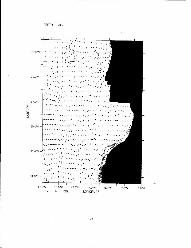
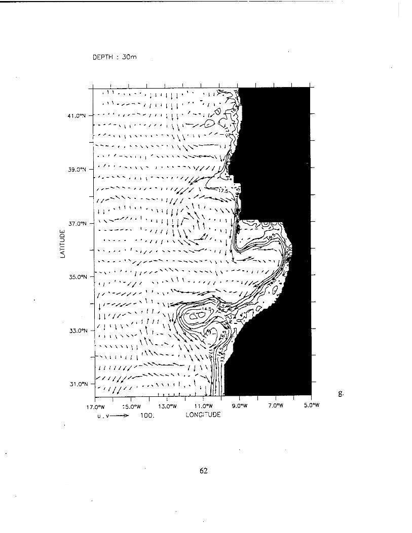
Figure 11. Temperature contours and velocity vectors at 30 m showing upwelling in the third year at day (a) 137, (b) 152, (c) 173, (d) 209, (e) 263, (f) 290, and (g) 317. The contour interval is 1° C. The maximum current velocity is 100 cm/s.

56

DEPTH : 30m

41.0°N -

39.0°N

37.0°N

Q 3

* t »

"'lit

* - » \ \

•\ ' '. i

TTT,

35.0°N -

33.0°N

31.0-N

.. . . , 1 \ \ \__,_^__ . N \\ \ -r- i --M /

•, /•""■•NX."- ^ ''

17.0°W 15.0°W 13.0°W 11.0°W 9.0°W 7.0°W

u.v > 100. LONGITUDE 5.0°W

57

DEPTH : 30m

41.0°N -

39.0°N

37.0°N - Ld Q Z> f—

35.0°N -

33.0°N

31.0°N -

17.0°W

U . v-

15.0°W 13.0°W

100.

11.0°W

LONGITUDE 9.0°W 7.0°W 5.0°W

58

DEPTH : 30m

41.0°N -• » »

Q

35.0°N

33.0°N -

31.0°N -

-—• s

t

17.0°W 15.0°W 13.0°W 11.0°W 9.0°W 7.0°W

u.v s» 100. LONGITUDE 5.0°W

59

DEPTH : 30m

41.0°N

39.0°N -

37.0°N -

3

35.0°N -

33.0-N

31.0°N -

17 —i i r

0°W 1 5.0°W 13.0°W 11.0°W

u.v > 100. LONGITUDE 9.0°W 7.0°W 5.0°W

60

DEPTH : 30m

41.0°N -

39.0°N -

37.0°N -

Q

35.0°N -

33.0°N -

31.0°N

15.0°W 13.0°W 11.0°W

H> 100. LONGITUDE 7.0°W 5.CTW

61

DEPTH : 30m

41.0°N

39.0°N

37.0°N - LÜ Q D

35.0°N -

33.0°N -

31.0°N

g-

.0°W 15.0°W 13.0°W

u.v 3»- 100.

11.0°W

LONGITUDE

9.0°W 7.0°W 5.0°W

62

a.

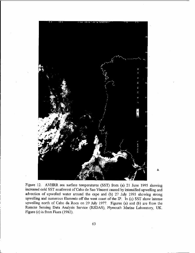
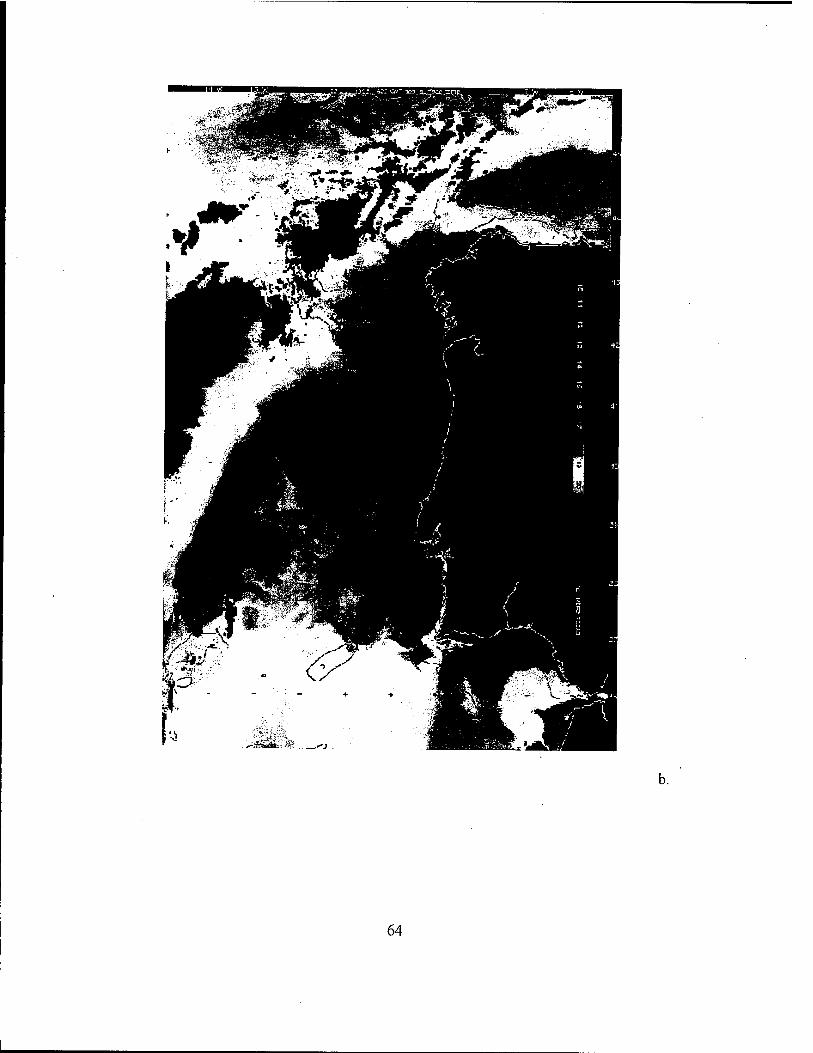
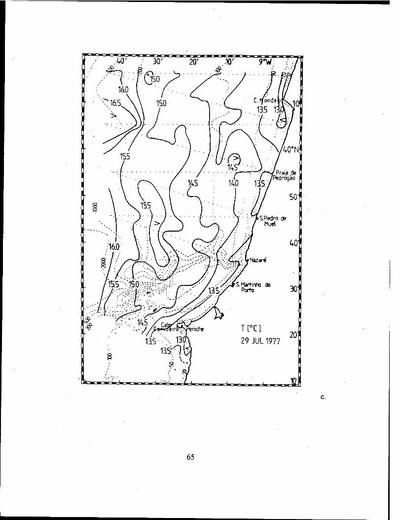
Figure 12. AVHRR sea surface temperatures (SST) from (a) 21 June 1995 showing increased cold SST southwest of Cabo de Sao Vincent caused by intensified upwelling and advection of upwelled water around the cape and (b) 27 July 1993 showing strong upwelling and numerous filaments off the west coast of the IP. In (c) SST show intense upwelling north of Cabo da Roca on 29 July 1977. Figures (a) and (b) are from the Remote Sensing Data Analysis Service (RSDAS), Plymouth Marine Laboratory, UK. Figure (c) is from Fiuza (1982).

63

64

65

66

APPENDIX. METHOD OF SOLUTION

Equations (1) through (7) comprise a closed system of seven scalar equations and

seven unknowns, u, v, w, p, p, T, and S. The variables, u, v, T, and S are prognostic

variables whose time rates of change are predicted from (1), (3), (6) and (7), respectively.

Although the diagnostic variables w, p, and p can be determined from (3), (4), and (5),

respectively, additional constraints are imposed on p and w by the choice of the rigid lid

boundary conditions. The vertically integrated pressure can no longer be obtained by

integrating the hydrostatic equation (4) for the free surface, and the vertically-integrated

horizontal velocity is subsequently constrained to be non-divergent, i.e.,

po (du du d^ + ds = 0 , (Al)

,<3c dyj

which is obtained by integrating (3) and applying the vertical boundary conditions where

s is a dummy variable representing the vertical coordinate.

For any quantity q, let its vertical average be denoted by q and its departure

(vertical shear) by q'. From (Al) the vertical mean flow can then be described by a

streamfunction i//, such that:

1 dw

-if <A3> The streamfunction y/ is predicted from the vorticity equation, which is derived by

applying the curl operator to the vertical average of (1) and (2), and then using (A2) and

(A3), the vorticity equation becomes

67

d£_d_ a ~ a H dx2 H

rd2y/\ dy/dH'1 dy/dH'' dy2 ) dx dx dy dy

dx H dy) dy\H dx

*(_*_f ff d£d2) g f o f ° dp - I -^-dsdz

(A4)

dx\Hp0}-»}: dy ) cy\Hp0

dxKH*-» ) dy\HJ~H J

where G and F represent the collected contributions of the nonlinear and viscous terms

from equations (1) and (2).

The vorticity equation (A4) is solved by obtaining an updated value of £ by

application of the leapfrog (or every 11 time steps, the Euler-backward) time-differencing

scheme. The associated value of y/ can then be obtained from:

C = '<?V

H fa' H ' d V

dy2 + dy/ ffl-x dyr dH' dx dx dy dy

(A5)

which is an elliptic equation. A solution to (A5) is fully prescribed by specifying the values

of y/ on the open and closed boundaries of the model domain. Currently, to solve (A5),

the model uses an elliptic solver when there are no variations in coastline geometry and/or

topography, and successive over-relaxation techniques when there are variations in

coastline geometry and/or topography.

The vertical shear current («', v') is predicted from (1) and (2) after subtracting

the vertical mean flow. The results are:

a Po dx dz p0H ; (A6)

Sv' -I dp' . d2v' - x" — if£--jS('-4VV + ^ —+ G-G — a p0 dy J" "M ' ' "M dz2 p0H (A7)

In (A6) and (A7), p', which represents the departure of the pressure from the vertical

average, is, using (4), expressed in terms of p as:

0 ,0/^0

p'=J/>gd£- — J \pgds z " -H\z

(A8) dz.

-H

68

The method of solution consists of predicting V2y/,y/,u',v',T, and S from (A4),

(A5), (A6), (A7), (6) and (7), respectively. The total current is then obtained by adding

the vertical shear part to the vertical average part, after the latter is obtained from y/

using (A2) and (A3). The diagnostics p, w, and p' are then obtained explicitly from the

equation of state (5), continuity equation (Al), and hydrostatic relation (A8), respectively.

69

70

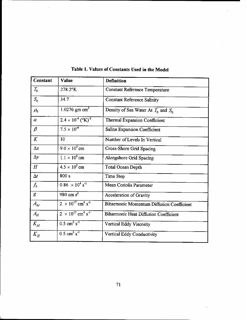
Table 1. Values of Constants Used in the Model

Constant Value

A>

a

ß K

Ax

Ay

H

At

/o

g

*M

A 1H

K, M

K H

278.2°K

34.7

1.0276 gm cm3

2.4 x 1(T (°K) ,-4 rov\-l

7.5 X 10"

Definition

Constant Reference Temperature

Constant Reference Salinity

Density of Sea Water At T0 and S0

Thermal Expansion Coefficient

10

9.0 x 10" cm

1.1 x 10° cm

4.5 x lO'cm

800 s

0.86 x 104 s ,4„-l

980 cm sz

2 x 1017 cm4 s_1

2 x 1017 cm4 s_1

0.5 cm2 s"1

0.5 cm2 s"1

Saline Expansion Coefficient

Number of Levels In Vertical

Cross-Shore Grid Spacing

Alongshore Grid Spacing

Total Ocean Depth

Time Step

Mean Coriolis Parameter

Acceleration of Gravity

Biharmonic Momentum Diffusion Coefficient

Biharmonic Heat Diffusion Coefficient

Vertical Eddy Viscosity

Vertical Eddy Conductivity

71

72

LIST OF REFERENCES

Ambar, I., Mediterranean influence off Portugal, in Present problems of oceanography in

Portugal, Junta Nacional de Investigacao Cientificae Tecnologica, Lisboa, 73-87, 1980.

Arakawa, A. and V. R. Lamb, Computational design of the basic dynamical processes of

the UCLA general circulation model, Methods Comput. Phys., 17, 173-265, 1977.

Barton, E. D., A filament programme in the Iberian upwelling region, Coastal Transition

Zone Newsletter, 1,2-5, 1986.

Batteen, M. L., Wind-forced modeling studies of currents, meanders, and eddies in the

California Current System, J. Geophys. Res., 102, 985-1009, 1997.

Batteen, M. L. and Y. -J. Han, On the computational noise of finite difference schemes

used in ocean models, Tellus, 33, 387-396, 1981.

Batteen, M. L., C. N. Lopes da Costa, and C. S. Nelson, A numerical study of wind stress

curl effects on eddies and filaments off the Northwest coast of the Iberian Peninsula, J.

Mar. Systems, 3, 249-266, 1992.

Batteen, M. L. and J. T. Monroe, A large-scale modeling study of the California Current

System Deep-SeaRes., submitted, 1998.

Batteen, M. L., and P. W. Vance, Modeling studies of the effects of wind forcing and

thermohaline gradients in the California Current System, Deep-SeaRes., in press, 1998.

73

Batteen, M. L., R. L. Haney, T. A. Tielking, and P. G. Renaud, A numerical study of wind

forcing of eddies and jets in the California Current System, J. Mar. Res., 47, 493-523,

1989.

Camerlengo, A. L. and J. J. O'Brien, Open boundary conditions in rotating fluids, J.

Comput. Phys., 89, 12-35, 1980.

Carton, J. A., Coastal circulation caused by an isolated storm, J. Phys Oceanogr., 14,

114-124, 1984.

Carton, J. A. and S. G. H. Philander, Coastal upwelling viewed as a stochastic

phenomena, J. Phys Oceanogr., 14, 1499-1509, 1984.

Defense Mapping Agency Hydrographie/Topographie Center (DMAH/TC), Sailing

Directions (Planning Guide) for the North Atlantic, DMA Pub. No. 140, Washington D.

C, 390 pp., 1988.

Fiuza, A. F. de G, Circulation of the water of the Portuguese continental margin during

the upwelling regime, Grupo de Oceanografia, Laboratorio de Fisica, Faculdade de

Ciencias da Universidade de Lisboa, 1979.

Fiuza, A. F. de G., The Portuguese coastal upwelling system, in Present problems of

oceanography in Portugal, Junta Nacional de Investigacao Cientifica e Tecnologica,

Lisboa, 45-71, 1980.

Fiuza, A. F. de G, M. E. de Macedo, M. R. Guerreiro, Climatological space and time

variation of the Portuguese coastal upwelling, Oceanologica Ada, Vol. 5, No. 1, 31-40,

1982.

74

Fiuza, A. F. de G., Upwelling patterns off Portugal, in E. Suess and J. Thiede (Editors),

Coastal Upwelling. Its Sediment Record. Plenum Press, New York, pp. 85-97, 1983.

Fiuza, A. F. de G., Hidrologia e dinamica das Aguas costeiras de Portugal. Dissertacao

apresentada a Universidade de Lisboa para obtencao do grau de Doutor em Fisica,

especializacao em Ciencias Geofisicas. Univ Lisboa, 294pp., 1984.

Fiuza, A. F. de G. and F. M. Sousa, Preliminary results of a CTD survey in the Coastal

Transition Zone off Portugal during 1-9 September 1988, Coastal Transition Zone

Newsletter, 4, 2-9, 1989.

Folkard, A. M., P. A. Davis, A. F. de G. Fiuza, and I. Ambar, Remotely sensed sea

surface thermal patterns in the Gulf of Cadiz and the Strait of Gibraltar: Variability,

correlations, and relationships with the surface wind field, J. Geophys. Res.,102, 5669-

5683, 1997.

Frouin, R, A. F. G. Fiuza, I. Ambar, and T. J. Boyd, Observations of a poleward surface

current off the coasts of Portugal and Spain during Winter, J. Geophys. Res., 95, 679-691,

1990.

Hagen, E., C. Zulicke, and R. Feistel, Near-surface structures in the Cape Ghir filament

off Morocco, Oceanol. Ada, 19, 6, 577-598, 1996.

Haidvogel, D. B., A. Beckmann, and K. S. Hedstrom, Dynamical simulation of filament

formation and evolution in the coastal transition zone, J. Geophys. Res.,96, 15,017-

15,040, 1991. '5v ' "3

75

Haney, R. L., A numerical study of the response of an idealized ocean to large-scale

surface heat and momentum flux, J. Phys. Oceanogr., 4, 145-167, 1974.

Haney, R. L., W. S. Shiver, and K. H. Hunt, A dynamical-numerical study of the

formation and evolution of large-scale anomalies, J. Phys. Oceanogr., 8, 952-969, 1978.

Haney, R. L., Midlatitude sea surface temperature anomalies: A numerical hindcast, J.

Phys. Oceanogr., 15, 787-799, 1985.

Haynes, R. and E. D. Barton, A poleward flow along the Atlantic coast of the Iberian

Peninsula, J. Geophys. Res., 95, 11425-11441, 1990.

Holland, W. R, The role of mesoscale eddies in the general circulation of the ocean-

Numerical experiments using a wind-driven quasi-geostrophic model, J. Phys. Oceanogr.,

8, 363-392, 1978.

Holland, W. R., D. E. Harrison and A. J. Semtner Jr., Eddy-resolving numerical models of

large-scale ocean circulation, II, in Eddies in Marine Science, edited by A. R. Robinson,

379-403, Springer-Verlag, New York, 1983.

Holland, W. R. and M. L. Batteen, The parameterization of subgrid scale heat diffusion in

eddy-resolved ocean circulation models, J. Phys. Oceanogr., 16, 200-206, 1986.

Ikeda, M., W. J. Emery, and L. A. Mysak, Seasonal variability in meanders of the

California Current system off Vancouver Island, J. Geophys. Res., 89, 3487-3505, 1984a.

Ikeda, M., L. A. Mysak, and W. J. Emery, Observations and modeling of satellite-sensed

meanders and eddies off Vancouver Island, J. Phys. Oceanogr., 14, 3-21, 1984b.

76

Levitus, S., and T. P. Boyer, World ocean atlas 1994, Vol. 4: Temperature, NOAA Atlas

NESDI4, 117 pp., U. S. Dept. of Commerce, Washington, D.C., 1994.

McClain, C. R., S. Chao, L. P. Atkinson, J. O. Blanton, and F. Castillejo, Wind-driven

upwelling in the vicinity of Cape Finisterre, Spain, J. Geophys. Res., 91, 8470-8486, 1986.

McCreary, J. P., Y. Fukamachi, and P. K. Kundu, A numerical investigation of jets and

eddies near an eastern ocean boundary, J. Geophys. Res., 92, 2515-2534, 1991.

McCreary, J. P., P. K. Kundu, and S. Y. Chao, On the dynamics of the California Current

system, J. Mar. Res., 45, 1-32, 1987.

Nelson, C. S., Wind stress and wind stress curl over the California Current, NOAA Tech

Rep. NMFS SSFR-714, U. S. Dept. Commerce, 87 pp., 1977.

Pares-Sierra, A, W. B. White, and C. -K. Tai, Wind-driven coastal generation of annual

mesoscale eddy activity in the California Current system: A numerical model, J. Phys

Oceanogr., 23, 1110-1121, 1993.

Pedlosky, J., Longshore currents, upwelling, and bottom topography, J. Phys Oceanogr.,

4, 214-226, 1974.

Philander, S. G. H. and J. H. Yoon, Eastern boundary currents and upwelling, J. Phys

Oceanogr., 12, 862-879, 1982.

Tomczak, M. and J. S. Godfrey, Regional Oceanography: An Introduction, Pergamon

Press, New York, 422 pp., 1994.

77

Trenberth, K. E., W. G. Large, J. G. Olsen, The mean annual cycle in global ocean wind

stress, J. Phys Oceanogr., 20, 1742-1760, 1990.

Van Camp, L., L. Nykjaer, E. Mittelstaedt, and P. Schlittenhardt, Upwelling and boundary

circulation off Northwest Africa as depicted by infrared and visible satellite observations,

Prog. Oceanog., 26, 357-402, 1991.

Weatherly, G. L., A study of the bottom boundary layer of the Florida Current, J. Phys

Oceanogr., 2, 54-72, 1972.

Wooster, W. S. and J. L. Reid, Jr., Eastern Boundary Currents in The Sea, Vol. 2, M. N.

Hill, Ed., Wiley International, New York, 253-280, 1963.

Wooster, W. S., A. Bakun, and D. R. McLain, The seasonal upwelling cycle along the

eastern boundary of the North Atlantic, J. Mar. Res., 34, 131-140, 1976.

78

INITIAL DISTRIBUTION LIST

No. Copies

1. Defense Technical Information Center 2 8725 John J. Kingman Rd, STE 0944 Ft. Belvoir, VA 22060-6218

2. Dudley Knox Library 2 Naval Postgraduate School 411 DyerRd Monterey, CA 93943-5101

3. Chairman (Code OC/Bf) 1 Department of Oceanography Naval Postgraduate School Monterey, CA 93943-5122

4. Chairman (Code MR/Wx) 1 Department of Meteorology Naval Postgraduate School Monterey, CA 93943-5114

5. Dr. Mary L. Batteen (Code OC/Bv) 4 Department of Oceanography Naval Postgraduate School Monterey, CA 93943-5122

6. Dr. Curtis A. Collins (Code OC/Co) 1 Department of Oceanography Naval Postgraduate School Monterey, CA 93943-5122

Dr. TomCurtin Office of Naval Research 800 N. Quincy Street Arlington, VA 22217

79

Dr. Tom Kinder Physical Oceanography Division Office of Naval Research 800 N. Quincy Street Arlington, VA 22217

LT Daniel W. Bryan. 1840 Cox Rd Cocoa, Fl 32926

80