Isentropic Analysis, Page 1

Synoptic Meteorology II: Isentropic Analysis

31 March – 2 April 2015

Readings: Chapter 3 of Midlatitude Synoptic Meteorology.

Introduction

Before we can appropriately introduce and describe the concept of isentropic potential vorticity, we must first introduce the principles of isentropic analysis.

What is meant by isentropic? On a basic level, it refers to constant entropy, such that an isentropic surface is a surface of constant entropy. Entropy, however, is equivalent to the natural logarithm of potential temperature plus a scaling factor. Thus, we say that entropy is directly proportional to potential temperature. As a consequence of this, the term isentropic is most commonly used to refer to constant potential temperature, such that an isentropic surface is a surface of constant potential temperature.

Why do we care about isentropic analysis? The air streams associated with mid-latitude, synoptic-scale weather systems are three-dimensional; air parcels can and do move from one isobaric surface to another. However, to first approximation, air parcels do conserve potential temperature as they move. This implies that the flow along the air streams associated with mid-latitude, synoptic-scale weather systems remains approximately confined to a single isentropic surface. As a result, we care about isentropic analysis because it gives a more accurate depiction of the three-dimensional synoptic-scale motions through mid-latitude weather systems.

Vertical Structure of Potential Temperature

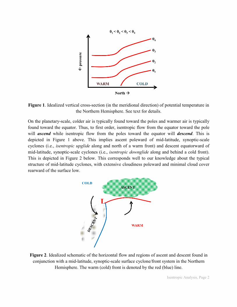
In the troposphere, potential temperature typically increases with increasing height. Since colder air temperatures on an isobaric surface correspond to colder potential temperature and warmer air temperatures on an isobaric surface correspond to warmer potential temperature, isentropic surfaces slope upward over a horizontal distance toward colder air.

Isentropic Analysis, Page 2

Figure 1. Idealized vertical cross-section (in the meridional direction) of potential temperature in the Northern Hemisphere. See text for details.

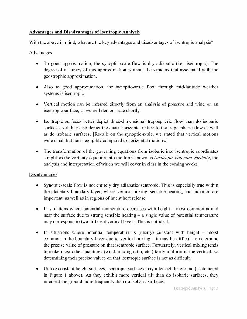
On the planetary-scale, colder air is typically found toward the poles and warmer air is typically found toward the equator. Thus, to first order, isentropic flow from the equator toward the pole will ascend while isentropic flow from the poles toward the equator will descend. This is depicted in Figure 1 above. This implies ascent poleward of mid-latitude, synoptic-scale cyclones (i.e., isentropic upglide along and north of a warm front) and descent equatorward of mid-latitude, synoptic-scale cyclones (i.e., isentropic downglide along and behind a cold front). This is depicted in Figure 2 below. This corresponds well to our knowledge about the typical structure of mid-latitude cyclones, with extensive cloudiness poleward and minimal cloud cover rearward of the surface low.

Figure 2. Idealized schematic of the horizontal flow and regions of ascent and descent found in conjunction with a mid-latitude, synoptic-scale surface cyclone/front system in the Northern

Hemisphere. The warm (cold) front is denoted by the red (blue) line.

Isentropic Analysis, Page 3

Advantages and Disadvantages of Isentropic Analysis

With the above in mind, what are the key advantages and disadvantages of isentropic analysis?

Advantages

• To good approximation, the synoptic-scale flow is dry adiabatic (i.e., isentropic). The degree of accuracy of this approximation is about the same as that associated with the geostrophic approximation.

• Also to good approximation, the synoptic-scale flow through mid-latitude weather systems is isentropic.

• Vertical motion can be inferred directly from an analysis of pressure and wind on an isentropic surface, as we will demonstrate shortly.

• Isentropic surfaces better depict three-dimensional tropospheric flow than do isobaric surfaces, yet they also depict the quasi-horizontal nature to the tropospheric flow as well as do isobaric surfaces. [Recall: on the synoptic-scale, we stated that vertical motions were small but non-negligible compared to horizontal motions.]

• The transformation of the governing equations from isobaric into isentropic coordinates simplifies the vorticity equation into the form known as isentropic potential vorticity, the analysis and interpretation of which we will cover in class in the coming weeks.

Disadvantages

• Synoptic-scale flow is not entirely dry adiabatic/isentropic. This is especially true within the planetary boundary layer, where vertical mixing, sensible heating, and radiation are important, as well as in regions of latent heat release.

• In situations where potential temperature decreases with height – most common at and near the surface due to strong sensible heating – a single value of potential temperature may correspond to two different vertical levels. This is not ideal.

• In situations where potential temperature is (nearly) constant with height – moist common in the boundary layer due to vertical mixing – it may be difficult to determine the precise value of pressure on that isentropic surface. Fortunately, vertical mixing tends to make most other quantities (wind, mixing ratio, etc.) fairly uniform in the vertical, so determining their precise values on that isentropic surface is not as difficult.

• Unlike constant height surfaces, isentropic surfaces may intersect the ground (as depicted in Figure 1 above). As they exhibit more vertical tilt than do isobaric surfaces, they intersect the ground more frequently than do isobaric surfaces.

Isentropic Analysis, Page 4

• We don’t often see or analyze isentropic charts, largely because it is not immediately straightforward to transform meteorological data, which is typically obtained on isobaric surfaces, to the isentropic vertical coordinate.

• The range of isentropic surfaces to look at varies by season and thus from event to event. In other words, unlike with isobaric charts where we typically look at well-defined isobaric surfaces (850 hPa, 500 hPa, etc.), there is no one isentropic chart to look at for all events. Typically, warmer isentropic surfaces (300+ K) are considered during the warm season while colder isentropic surfaces (290-295 K) are considered during the cool season.

Geostrophic Flow and Isentropic Analysis

On an isobaric surface, the geostrophic wind blows parallel to the geopotential height contours. It is natural to ask, then, if an analog to the geostrophic wind exists on isentropic surface. Indeed, there is such an analog. We first introduce the concept of dry static energy (s). Dry static energy is conserved for dry adiabatic motions, horizontal and/or vertical in nature, just as is potential temperature. This states that an air parcel does not change its value of dry static energy for dry adiabatic motions. On an isentropic surface, therefore, the wind should blow parallel to contours of constant dry static energy so long as the flow remains dry adiabatic.

As we stated earlier that the dry adiabatic assumption is equally valid to the geostrophic approximation, we will term the flow parallel to contours of constant dry static energy as the geostrophic flow on an isentropic surface.

The dry static energy can be expressed as:

Tcs p+Φ= (1) The dry static energy on an isentropic surface is equivalently known as the Montgomery streamfunction, or M. For a parcel to conserve s or M as it moves along an isentropic surface, its motion should be parallel to lines of constant s or M. This is the same basic concept as the geostrophic wind on an isobaric surface flowing parallel to lines of constant geopotential height.

With this in mind, we state the geostrophic wind on isentropic surfaces as follows:

xM

fvg ∂

∂=

0

1θ (2a)

yM

fug ∂

∂−=

0

1θ (2b)

Isentropic Analysis, Page 5

Note that this is directly analogous to the geostrophic wind on isobaric surfaces, except with M replacing Φ, with the calculation being carried out on an isentropic surface.

Fundamentals of Isentropic Analysis

Neglect of Diabatic Processes

Let us now explore the fundamental basis of the isentropic system. It can be shown that the thermodynamic equation can be written as:

dtd

dtdQ

ptDtD

pθθωθθθ

≈∝∂∂

+∇⋅+∂∂

= v (3)

In (3), the subscript of p on the horizontal potential advection term denotes that it, like the rest of the terms of (3), is computed on an isobaric surface.

As before, dQ/dt (alternatively expressed as dθ/dt) represents the diabatic heating rate. There are four primary causes of diabatic heating that we must be concerned with in the troposphere:

• Condensation and evaporation

• Sensible heating at the surface

• Absorption and emission of radiative energy (nominally, radiative processes)

• Turbulent vertical mixing, particularly in the boundary layer

Let us presume that condensation and evaporation are not ongoing; i.e., there is no precipitation, cloud cover, or convection in the synoptic-scale environment. Sensible heating and turbulent mixing may be and often are large within the planetary boundary layer (i.e., near the surface) but are typically negligible in the middle to upper troposphere. If we either constrain ourselves to looking above the top of the boundary layer, or otherwise neglect sensible heating and turbulent mixing, the only remaining diabatic forcing is radiative cooling.

Long-term satellite-based observations suggest that radiative cooling contributes to 1-2 K cooling per day throughout the troposphere in the mid-latitudes. The precise magnitude of this cooling varies with the seasonal cycle; it is greatest in winter and lowest in summer. How does this compare to the adiabatic forcing terms in (3), however? If we have a gradient of potential temperature of 1 K over 500 km, a wind speed of 10 m s-1 blowing along this gradient from cold to warm air will result in a local cooling of 1.728 K per day. Since this magnitude of the horizontal potential temperature gradient is weak compared to what is typically observed in the mid-latitudes, we can, to good approximation, safely neglect diabatic cooling.

Isentropic Analysis, Page 6

With this, (3) becomes:

0=∂∂

+∇⋅+∂∂

=ptDt

Dp

θωθθθ v (4)

Equation (4) states that potential temperature is conserved following the motion. Because we are dealing with purely isentropic, dry adiabatic flow, we also know that mixing ratio is conserved following the motion. To confirm this, think about ascent and descent in the context of a skew-T diagram: dry adiabatic ascent and descent follows dry adiabats and lines of constant mixing ratio for temperature and moisture, respectively. That mixing ratio is conserved for isentropic flow will prove useful when we look at moisture transport on isentropic surfaces.

If we solve (4) for ω, we obtain:

p

t p

∂∂

−

∇⋅+∂∂

= θ

θθ

ωv

(5)

In (5), the denominator is a measure of the static stability, or how tightly packed isentropes are in the vertical. The more tightly packed that isentropes are in the vertical, the greater the static stability.

Equation (5) states that ω is a function of the sum of potential temperature advection on an isobaric surface and the local change of potential temperature, all divided by the static stability. We term this form of ω the isentropic vertical motion, or alternatively, adiabatic omega. Departures in the total vertical motion from the adiabatic vertical motion occur when the flow is non-isentropic (e.g., in deep, moist convection).

Typically, we do not utilize (5) to obtain an estimate for ω on an isobaric surface. Instead, as is demonstrated in the next section, we transform the vertical coordinate of (5) from pressure p to potential temperature θ in order to obtain an equation for ω along an isentropic surface.

Vertical Motion on an Isentropic Surface

As noted above, we can transform (5) such that it is applicable on isentropic rather than isobaric surfaces. To do so, we need to transform the partial derivatives in (5) – those with respect to t, x, and y – that appear in the number of (5). We can do so by making use of the following relationships:

θ

θθ

∂∂

∂∂

−=

∂∂

tp

pt p

θ

θθ

∂∂

∂∂

−=

∂∂

xp

px p

θ

θθ

∂∂

∂∂

−=

∂∂

yp

py p

(6)

Isentropic Analysis, Page 7

Subscripts of p reflect evaluation on isobaric surfaces, while subscripts of θ reflect evaluation on isentropic surfaces. In (6), the static stability acts as the transform operator between isobaric (p) and isentropic (θ) coordinates.

Notably, (6) demonstrates that horizontal gradients of potential temperature on isobaric surfaces are proportional to horizontal gradients of pressure on isentropic surfaces! As applied to synoptic-scale analysis, what does this mean? Let us first consider a cold front as an illustrative example. A cold front separates relatively cool air behind it from relatively warm air ahead of it, with the front itself located along the leading edge of the relatively cool air. This implies the presence of a horizontal (potential) temperature gradient along and to the rear of the cold front on an isobaric surface.

Since a horizontal gradient of potential temperature on an isobaric surface is proportional to a horizontal gradient of pressure on an isentropic surface, from the above, there must be a horizontal pressure gradient along and to the rear of the cold front on an isentropic surface. Thus, when analyzed on an isentropic surface, a cold front separates relatively low pressure behind it from relatively high pressure ahead of it, with the front itself located along the leading edge of relatively low pressure. Similar arguments can be made for warm fronts.

Additionally, (6) demonstrates that, on an isentropic surface, an isobar is equivalent to an isotherm. This can be demonstrated using Poisson’s relationship; if both p and θ are constant, so is T. Because of this, isentropic vertical motion can be viewed as akin to a thermal forcing term. Where have we seen such a forcing term before? In the quasi-geostrophic omega equation, under the assumption that the synoptic-scale motion on isobaric surfaces is largely geostrophic!

If we substitute (6) into (5) and simplify, we obtain:

ptp

θθθ

ω ∇⋅+

∂∂

= v (7)

As before, subscripts of θ reflect evaluation on isentropic surfaces. Equation (7) shows that isentropic vertical motion can be determined from the distribution of pressure on an isentropic surface. There are two forcing terms: the local rate of change of pressure on the isentropic surface and the advection of pressure by the horizontal wind on the isentropic surface.

Equation (7) can be further simplified by making use of what is known as the “frozen wave” approximation. This approximation states that the local rate of change of some quantity (here, p) is due entirely to the motion of a synoptic-scale weather system. Thus, in a reference frame moving with the synoptic-scale weather system – not with the synoptic-scale flow – the first term on the right-hand side of (7) is zero. Furthermore, in this reference frame, it is necessary to replace the advective velocity θv in (7) with the system-relative (or storm-relative) advective

Isentropic Analysis, Page 8

velocity, cv −θ . Here, c represents the motion of the synoptic-scale weather system, which is

typically estimated from a 12-36 h series of appropriate meteorological charts.

With all of this in mind, (7) becomes:

( ) pθθω ∇⋅−= cv (8) Equation (8) states that, at a fixed location, the isentropic vertical motion is a function of the advection of pressure by the system-relative horizontal wind on the isentropic surface.

Based upon the definition of the advection operator, higher pressure advection is defined where ( ) 0>∇⋅−− pθθ cv . Because (8) lacks the leading negative sign, higher pressure advection

results in ω < 0, signifying ascent. Conversely, lower pressure advection is defined where ( ) 0<∇⋅−− pθθ cv . Again, because (8) lacks the leading negative sign, lower pressure advection

results in ω > 0, signifying descent.

Higher pressure advection refers to the situation where the wind is blowing from higher toward lower pressures. For an air parcel moving with this wind, it starts at a higher pressure and ends at a lower pressure, thus ascending as it moves. Conversely, lower pressure advection refers to the situation where the wind is blowing from lower toward higher pressures. For an air parcel moving with this wind, it starts at a lower pressure and ends at a higher pressure, thus descending as it moves.

From (8), the magnitude of the vertical motion is directly proportional to the magnitude of the pressure advection. Thus, stronger vertical motions result from larger magnitudes of horizontal pressure advection. This is accomplished by having a large horizontal change in pressure over a short distance (large p∇ ) and/or a strong system-relative wind (large cv

−θ ) blowing across the isobars. Thus, air parcels that change pressure rapidly over a short distance on an isentropic surface are associated with stronger vertical motions.

For synoptic-scale weather systems that move much slower than the synoptic-scale flow on an isentropic surface (e.g., those that are quasi-stationary), (8) can be approximated by:

pθθω ∇⋅= v (9) However, for faster-moving weather systems, making use of this approximation can substantially change the magnitude and/or sign of the vertical motion from that obtained via (8). We will examine this in more detail shortly.

Inclusion of Diabatic Processes

Impact of Diabatic Heating upon Vertical Motion on Isentropic Surfaces

Isentropic Analysis, Page 9

If diabatic heating is included as a forcing term upon ω in the derivation and formulation of (8), we obtain:

( )dtdpp θ

θω θθ ∂

∂+∇⋅−= cv (10)

In isolation, the impact of diabatic heating upon the vertical motion on an isentropic surface is given by:

dtdp θ

θω

∂∂

= (11)

Since potential temperature typically increases with increasing height, the ∂p/∂θ term is typically negative (∂p < 0, ∂θ > 0). Therefore, diabatic warming (dθ/dt > 0) results in ω < 0, or ascent, while diabatic cooling (dθ/dt < 0) results in ω > 0, or descent. This is unsurprising, as this is the same conclusion that we arrived at in the context of the quasi-geostrophic omega equation.

However, the physical meaning is slightly different, owing in large part to (11) being cast on isentropic rather than isobaric surfaces. Diabatic warming results in the increase of an air parcel’s potential temperature. The air parcel rises as it moves from one isentropic surface to another given that potential temperature typically increases upward away from the surface. Conversely, diabatic cooling results in the decrease of an air parcel’s potential temperature. The air parcel descends as it moves from one isentropic surface to another given that potential temperature typically decreases downward toward the surface.

Further Thoughts

Dry adiabatic (or isentropic) motion is not strictly valid in regions of clouds and precipitation, although the vertical distribution of moisture is such that the adiabatic approximation is not significantly in error in the middle to upper troposphere in the mid-latitudes. Nevertheless, most synoptic-scale weather systems are associated with condensation – and, therefore, latent heat release and the non-conservation of potential temperature. Therefore, it stands to follow that the principles of isentropic analysis may be fundamentally invalid in the vicinity of the very systems that we are most interested in.

While this is true in a quantitative sense, it is not a significant hindrance in a qualitative sense, as demonstrated within Section 3.3 of the Lackmann text. Let us demonstrate this concept utilizing a figure, Figure 3.12 from the Lackmann text (reproduced below as Figure 3).

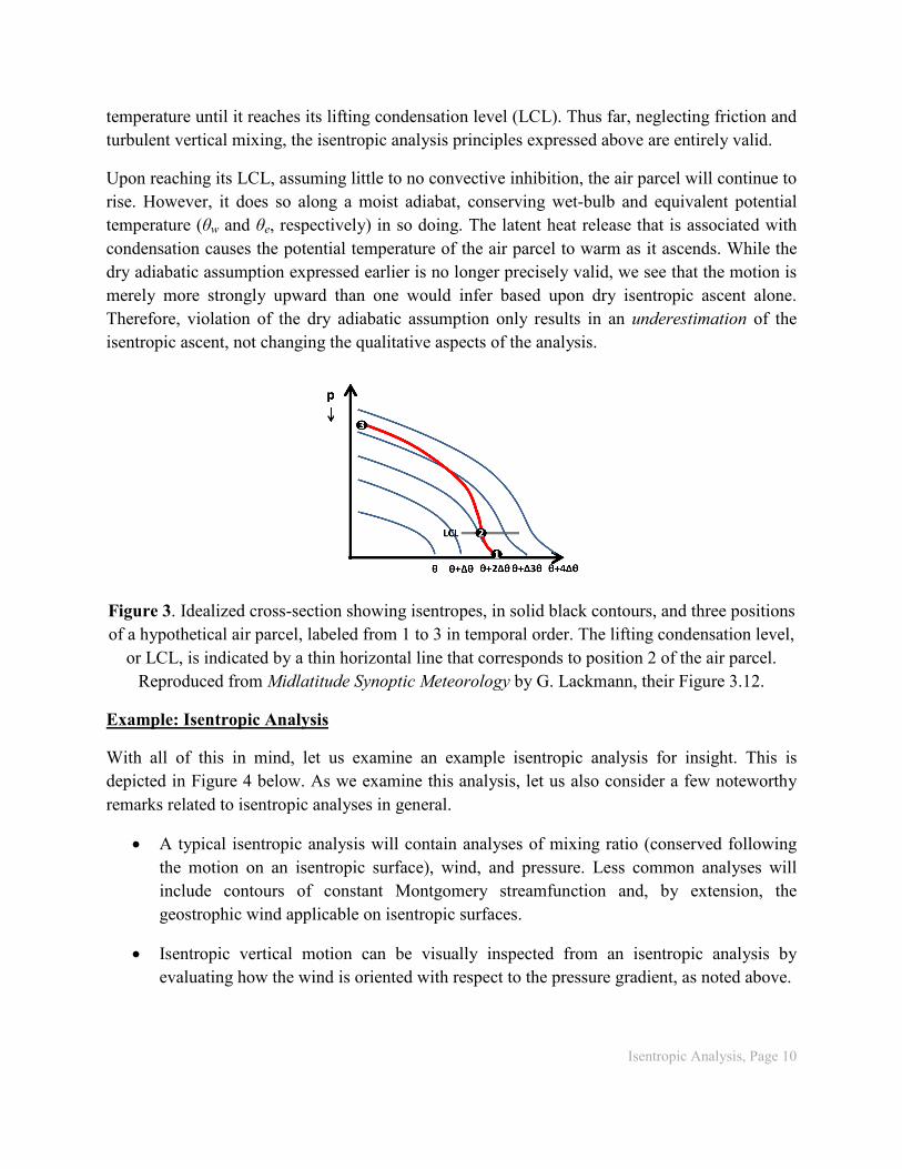
Consider an air parcel near the ground with an initial potential temperature of θ+2∆θ. Presuming that the wind on this isentropic surface is from right to left (e.g., east to west), this parcel will ascend along the isentropic surface. This ascent is along a dry adiabat, conserving potential

Isentropic Analysis, Page 10

temperature until it reaches its lifting condensation level (LCL). Thus far, neglecting friction and turbulent vertical mixing, the isentropic analysis principles expressed above are entirely valid.

Upon reaching its LCL, assuming little to no convective inhibition, the air parcel will continue to rise. However, it does so along a moist adiabat, conserving wet-bulb and equivalent potential temperature (θw and θe, respectively) in so doing. The latent heat release that is associated with condensation causes the potential temperature of the air parcel to warm as it ascends. While the dry adiabatic assumption expressed earlier is no longer precisely valid, we see that the motion is merely more strongly upward than one would infer based upon dry isentropic ascent alone. Therefore, violation of the dry adiabatic assumption only results in an underestimation of the isentropic ascent, not changing the qualitative aspects of the analysis.

Figure 3. Idealized cross-section showing isentropes, in solid black contours, and three positions of a hypothetical air parcel, labeled from 1 to 3 in temporal order. The lifting condensation level,

or LCL, is indicated by a thin horizontal line that corresponds to position 2 of the air parcel. Reproduced from Midlatitude Synoptic Meteorology by G. Lackmann, their Figure 3.12.

Example: Isentropic Analysis

With all of this in mind, let us examine an example isentropic analysis for insight. This is depicted in Figure 4 below. As we examine this analysis, let us also consider a few noteworthy remarks related to isentropic analyses in general.

• A typical isentropic analysis will contain analyses of mixing ratio (conserved following the motion on an isentropic surface), wind, and pressure. Less common analyses will include contours of constant Montgomery streamfunction and, by extension, the geostrophic wind applicable on isentropic surfaces.

• Isentropic vertical motion can be visually inspected from an isentropic analysis by evaluating how the wind is oriented with respect to the pressure gradient, as noted above.

Isentropic Analysis, Page 11

• Frontal boundaries are located along horizontal pressure gradients on isentropic surfaces, with cold fronts found on the leading edge of lower pressure and warm fronts found on back edge of higher pressure.

• For greatest accuracy, the wind on an isentropic surface should be that the system-relative wind rather than the full wind. However, it can be difficult to accurately estimate the motion of synoptic-scale weather systems – they often change their speed or direction of motion, and redevelopment can often be confused for motion. Likewise, it is entirely possible that two weather systems on a given chart may move in different directions and/or different rates of speed, making a single system motion estimate unreliable at best. Therefore, most isentropic analyses are construed using the full wind.

• As noted in our listing of the disadvantages of isentropic analysis, isentropic charts may have large areas of missing or meaningless data where the isentropic surface is below ground or corresponds to two different pressure levels. Data in such regions, if plotted, should be discarded.

• The actual construction of an isentropic analysis is typically handled by computer software. It is time consuming to for a human to conduct all of the necessary interpolation of meteorological data from an isobaric surface to an isentropic surface and, subsequently, to analyze the data.

• Isentropic surfaces closer to the ground are on constant surfaces of relatively low potential temperature. Conversely, isentropic surfaces higher above the ground are on constant surfaces of relatively high potential temperature.

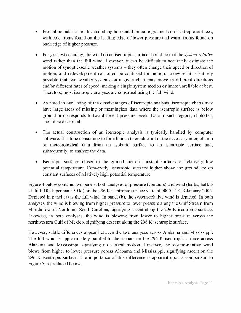
Figure 4 below contains two panels, both analyses of pressure (contours) and wind (barbs; half: 5 kt, full: 10 kt; pennant: 50 kt) on the 296 K isentropic surface valid at 0000 UTC 3 January 2002. Depicted in panel (a) is the full wind. In panel (b), the system-relative wind is depicted. In both analyses, the wind is blowing from higher pressure to lower pressure along the Gulf Stream from Florida toward North and South Carolina, signifying ascent along the 296 K isentropic surface. Likewise, in both analyses, the wind is blowing from lower to higher pressure across the northwestern Gulf of Mexico, signifying descent along the 296 K isentropic surface.

However, subtle differences appear between the two analyses across Alabama and Mississippi. The full wind is approximately parallel to the isobars on the 296 K isentropic surface across Alabama and Mississippi, signifying no vertical motion. However, the system-relative wind blows from higher to lower pressure across Alabama and Mississippi, signifying ascent on the 296 K isentropic surface. The importance of this difference is apparent upon a comparison to Figure 5, reproduced below.

Isentropic Analysis, Page 12

Figure 4. Pressure (hPa, contours) and wind (kt, barbs; full wind in panel a, system-relative wind in panel b) on the 296 K isentropic surface, valid at 0000 UTC 3 January 2002. Reproduced from

Midlatitude Synoptic Meteorology by G. Lackmann, their Figure 3.9.

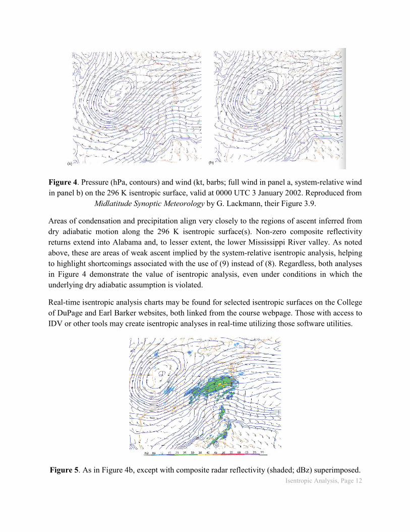
Areas of condensation and precipitation align very closely to the regions of ascent inferred from dry adiabatic motion along the 296 K isentropic surface(s). Non-zero composite reflectivity returns extend into Alabama and, to lesser extent, the lower Mississippi River valley. As noted above, these are areas of weak ascent implied by the system-relative isentropic analysis, helping to highlight shortcomings associated with the use of (9) instead of (8). Regardless, both analyses in Figure 4 demonstrate the value of isentropic analysis, even under conditions in which the underlying dry adiabatic assumption is violated.

Real-time isentropic analysis charts may be found for selected isentropic surfaces on the College of DuPage and Earl Barker websites, both linked from the course webpage. Those with access to IDV or other tools may create isentropic analyses in real-time utilizing those software utilities.

Figure 5. As in Figure 4b, except with composite radar reflectivity (shaded; dBz) superimposed.