Theory of turbo machinery / Turbomaskinernas teori Chapter 2 fileTurbomaskinernas teori Chapter 2. Lunds universitet / Kraftverksteknik / JK Basic Thermodynamics, Fluid Mechanics:

Theory of turbo machinery / Turbomaskinernas teori

Chapter 2

Lunds universitet / Kraftverksteknik / JK

Basic Thermodynamics, Fluid Mechanics:Definition of Efficiency

Take your choice of those that can best aid your action. (Shakespeare, Coriolanus)

The continuity of flow equation (mass conservation)First law of thermodynamics and the steady flow energy equation

The momentum equationThe second law of thermodynamics


Equation of continuity

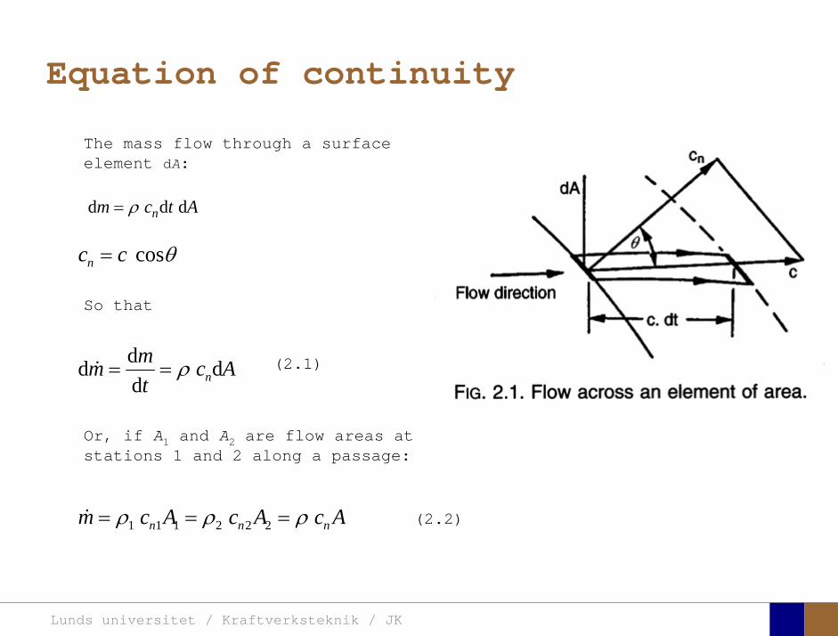
The mass flow through a surface element dA:

d d dnm c t Aρ=

θcosc cn =

So that

Or, if A1 and A2 are flow areas at stations 1 and 2 along a passage:

Actmm ndd

dd ρ== (2.1)

AcAcAcm nnn ρρρ === 222111 (2.2)


The first law

( ) 0dd =−∫ WQ

( )∫ −=−2

112 dd WQEE

WQE ddd −=

The first law of Thermodynamics: For a system that completes a cycle during which heat is supplied and work is done:

If a change is done from state 1 to state 2, energy differences must be represented by changes in property internal energy:

(2.3)

or

(2.4)

(2.4a)


The first law

xWEnergy is transferred from fluid to the blades of the machine, positive work is at the rate

Heat transfer, , is positive from surrounding to machineQ

Mass flow, , enters at 1 and exits at 2m


The first law

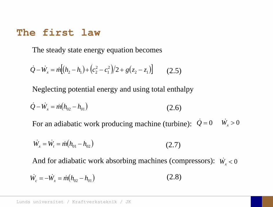
( ) ( ) ( )[ ]1221

2212 2 zzgcchhmWQ x −+−+−=−

( )0102 hhmWQ x −=−

(2.5)

Neglecting potential energy and using total enthalpy

0=Q 0>xWFor an adiabatic work producing machine (turbine):

(2.6)

The steady state energy equation becomes

( )0201 hhmWW tx −== (2.7)

And for adiabatic work absorbing machines (compressors): 0<xW

( )0102 hhmWW xc −=−= (2.8)


The momentum equationNewton's second law: The sum of all forces acting on a mass, m, equals the time rate of momentum change:

( )xx mct

Fdd

=Σ (2.9)

Here, only x-component of force and velocity is considered. For steady state the equation reduces to:

( )12 xxx ccmF −=Σ (2.9a)

If shear forces (viscosity) are neglected, the Euler’s equation for one-dimensional flow can be obtained:

0ddd1=++ zgccp

ρ(2.10)


The momentum equation

( ) 02

d112

21

22

2

1

=−+−

+∫ zzgccpρ

(2.10a)

Integrating Euler’s equation in the stream direction yields Bernoulli’s equation:

FIG. 2.3. Control volume in a streaming fluid.


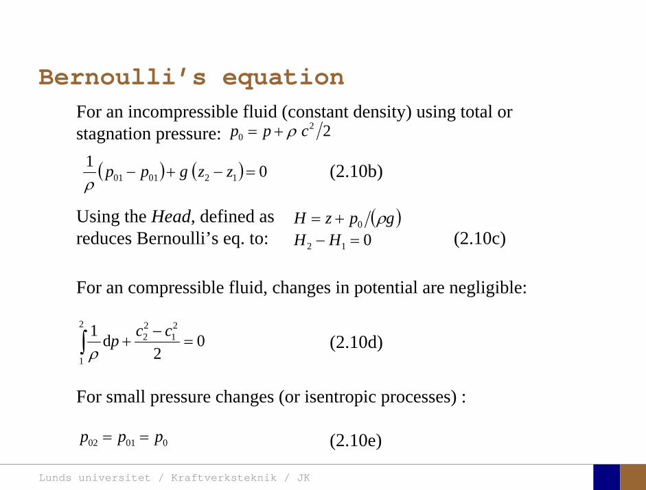
Bernoulli’s equationFor an incompressible fluid (constant density) using total or stagnation pressure:

(2.10b)( ) ( ) 01120101 =−+− zzgpp

ρ

220 cpp ρ+=

( )gpzH ρ0+=Using the Head, defined as reduces Bernoulli’s eq. to: 012 =− HH (2.10c)

For an compressible fluid, changes in potential are negligible:

02

d1 21

22

2

1

=−

+∫ccp

ρ(2.10d)

For small pressure changes (or isentropic processes) :

00102 ppp == (2.10e)


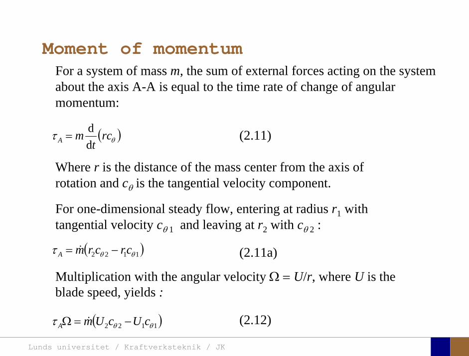
Moment of momentumFor a system of mass m, the sum of external forces acting on the system about the axis A-A is equal to the time rate of change of angular momentum:

( )θτ rct

mA dd

= (2.11)

Where r is the distance of the mass center from the axis of rotation and cθ is the tangential velocity component.

For one-dimensional steady flow, entering at radius r1 with tangential velocity cθ 1 and leaving at r2 with cθ 2 :

( )1122 θθτ crcrmA −= (2.11a)

Multiplication with the angular velocity Ω = U/r, where U is the blade speed, yields :

( )1122 θθτ cUcUmA −=Ω (2.12)


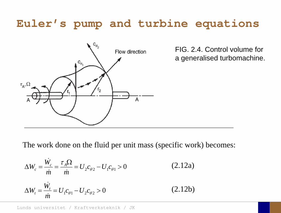
Euler’s pump and turbine equations

The work done on the fluid per unit mass (specific work) becomes:

01122 >−=Ω

==Δ θθτ cUcU

mmWW Ac

c(2.12a)

02211 >−==Δ θθ cUcUmWW t

t(2.12b)

FIG. 2.4. Control volume for a generalised turbomachine.


Exempel radialpumpExempel radialpump


Hastighetstrianglar vid inHastighetstrianglar vid in-- & utlopp& utlopp

[ ]02 01 2 2 1 1 1 2 20xW h h U c U c c U cθ θ θ θ= − = ⋅ − ⋅ = = = ⋅

Relativ hastighettangent till skoveln

Absoluthast. ändras i rotationsriktningen(pump)


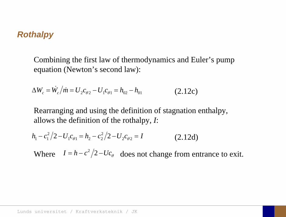
Rothalpy

Combining the first law of thermodynamics and Euler’s pump equation (Newton’s second law):

(2.12c)

(2.12d)

01021122 hhcUcUmWW cc −=−==Δ θθ

IcUchcUch =−−=−− 2222211

211 22 θθ

Rearranging and using the definition of stagnation enthalpy, allows the definition of the rothalpy, I:

θUcchI −−= 22Where does not change from entrance to exit.


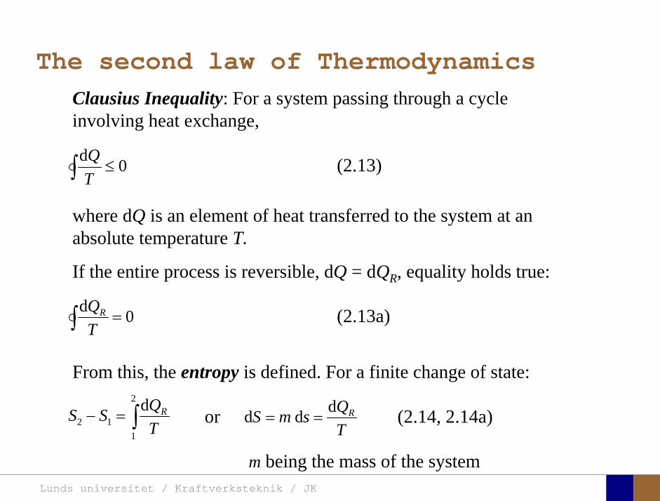
The second law of ThermodynamicsClausius Inequality: For a system passing through a cycle involving heat exchange,

(2.13)

where dQ is an element of heat transferred to the system at an absolute temperature T.

If the entire process is reversible, dQ = dQR, equality holds true:

(2.13a)

0d≤∫ T

Q

0d=∫ T

QR

From this, the entropy is defined. For a finite change of state:

∫=−2

112

dTQSS R or

TQsmS Rddd == (2.14, 2.14a)

m being the mass of the system


EntropyFor steady one-dimensional flow in which the fluid goes from state 1 to state 2:

(2.15)

For adiabatic processes, dQ = 0 and 2.15 becomes: 12 ss ≥

For a system undergoing a reversible process , dQ = dQR = m T dsand dW = dWR = m p dυ, the first law becomes:

dE = dQ - dW = m T ds - m p dυ or with u = E / m

T ds = du - p dυ (2.17)

Further, with h = u + pυ, dh = du + p dυ + υ dp:

T ds = dh - υ dp (2.18)

( )12

2

1

d ssmTQ

−≤∫


Definitions of efficiencyConsider a turbine: The overall efficiency can be defined as

Mechanical energy available at coupling of output shaft in unit time

Maximum energy difference possible for the fluid in unit time η0 =

If mechanical losses in bearings etc. are not the aim of the analyses, the isentropic or hydraulic efficiency is suitable:

Mechanical energy supplied to the rotor in unit time

Maximum energy difference possible for the fluid in unit time ηt =

The Mechanical efficiency now becomes η0 / ηt


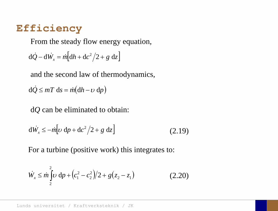
EfficiencyFrom the steady flow energy equation,

(2.19)

and the second law of thermodynamics,

dQ can be eliminated to obtain:

[ ]zgchmWQ x d2dddd 2 ++=−

( )phmsmTQ dddd υ−=≤

[ ]zgcpmWx d2ddd 2 ++−≤ υ

For a turbine (positive work) this integrates to:

( ) ( )1222

21

2

2

2d zzgccpmWx −+−+≤ ∫υ (2.20)


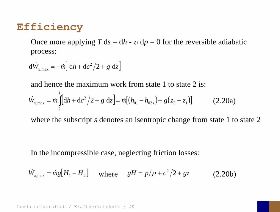
EfficiencyOnce more applying T ds = dh - υ dp = 0 for the reversible adiabatic process:

(2.20a)

and hence the maximum work from state 1 to state 2 is:

where the subscript s denotes an isentropic change from state 1 to state 2

gzcpgH ++= 22ρ

In the incompressible case, neglecting friction losses:

[ ]zgchmWx d2ddd 2max, ++−=

[ ] ( ) ( )[ ]120201

1

2

2max, d2dd zzghhmzgchmW sx −+−=++= ∫

[ ]21max, HHgmWx −= where (2.20b)


Efficiency

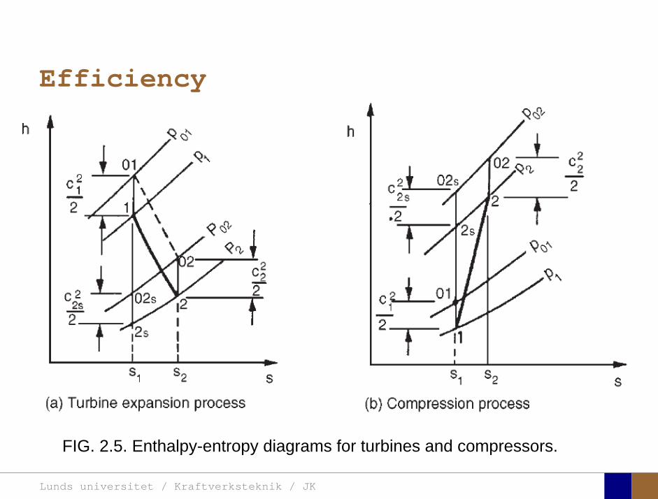
FIG. 2.5. Enthalpy-entropy diagrams for turbines and compressors.


Efficiency

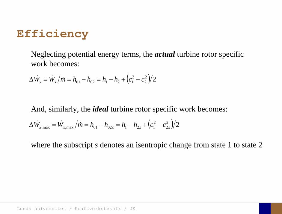
Neglecting potential energy terms, the actual turbine rotor specific work becomes:

And, similarly, the ideal turbine rotor specific work becomes:

where the subscript s denotes an isentropic change from state 1 to state 2

( ) 222

21210201 cchhhhmWW xx −+−=−==Δ

( ) 222

21210201max,max, sssxx cchhhhmWW −+−=−==Δ


EfficiencyIf the kinetic energy can be made useful, we define the total-to-total efficiency as

Which, if the difference between inlet and outlet kinetic energies is small, reduces to

( ) ( )sxxtt hhhhWW 02010201max, −−=ΔΔ=η

( ) ( )stt hhhh 2121 −−=η

(2.21)

(2.21a)

If the exhaust kinetic energy is wasted, it is useful to define the total-to-static efficiency as

( ) ( )sts hhhh 2010201 −−=η (2.22)

Since, here the ideal work is obtained between points 01 and 2s


Efficiency

Efficiencies of compressors are obtained from similar considerations:

( ) ( )01020102 hhhh sc −−=η (2.28)

(2.28a)

Minimum adiabatic work input per unit time

Actual adiabatic work input to rotor per unit timeηc =

Which, if the difference between inlet and outlet kinetic energies is small, reduces to

( ) ( )1212 hhhh sc −−=η


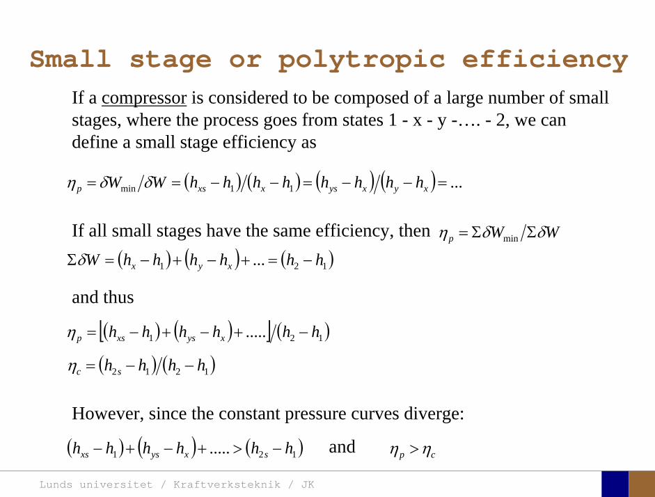
Small stage or polytropic efficiencyIf a compressor is considered to be composed of a large number of small stages, where the process goes from states 1 - x - y -…. - 2, we can define a small stage efficiency as

( ) ( ) ( ) ( ) ...11min =−−=−−== xyxysxxsp hhhhhhhhWW δδη

If all small stages have the same efficiency, then

However, since the constant pressure curves diverge:

WWp δδη ΣΣ= min

( ) ( ) ( )121 ... hhhhhhW xyx −=+−+−=Σδ

and thus

( ) ( )[ ] ( )121 ..... hhhhhh xysxsp −+−+−=η

( ) ( )1212 hhhh sc −−=η

( ) ( ) ( )121 ..... hhhhhh sxysxs −>+−+− and cp ηη >


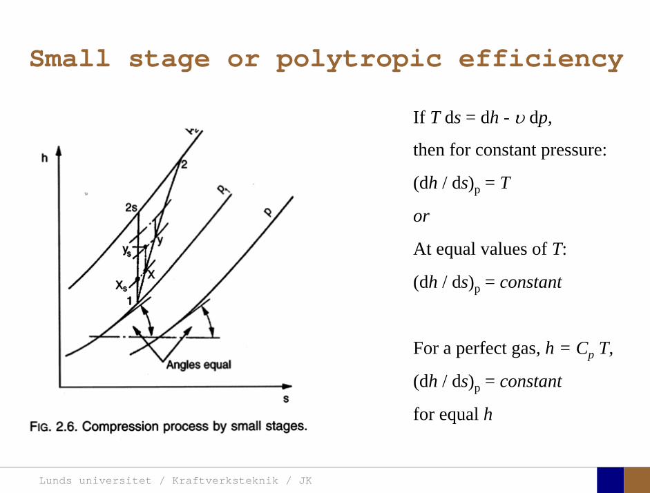
If T ds = dh - υ dp,

then for constant pressure:

(dh / ds)p = T

or

At equal values of T:

(dh / ds)p = constant

For a perfect gas, h = Cp T,

(dh / ds)p = constant

for equal h

Small stage or polytropic efficiency


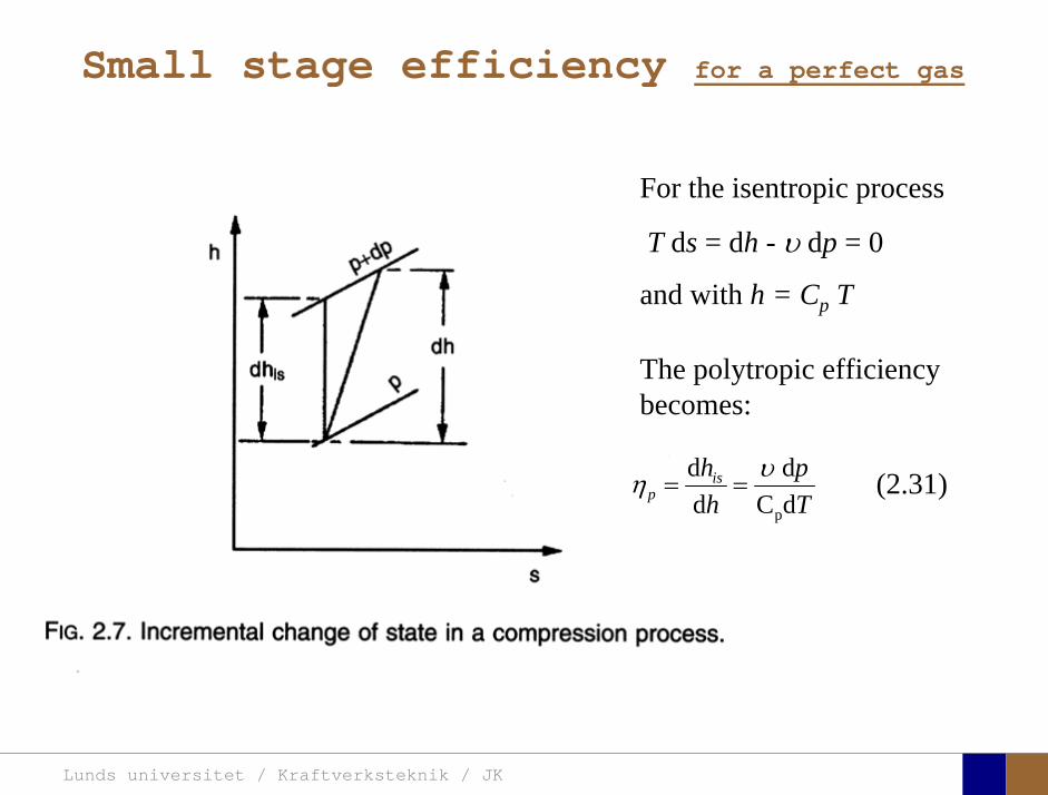
Small stage efficiency for a perfect gas

Tp

hhis

p dCd

dd

p

υη ==

For the isentropic process

T ds = dh - υ dp = 0

and with h = Cp T

The polytropic efficiency becomes:

(2.31)


Tp

pTR

p dd

Cp

=η

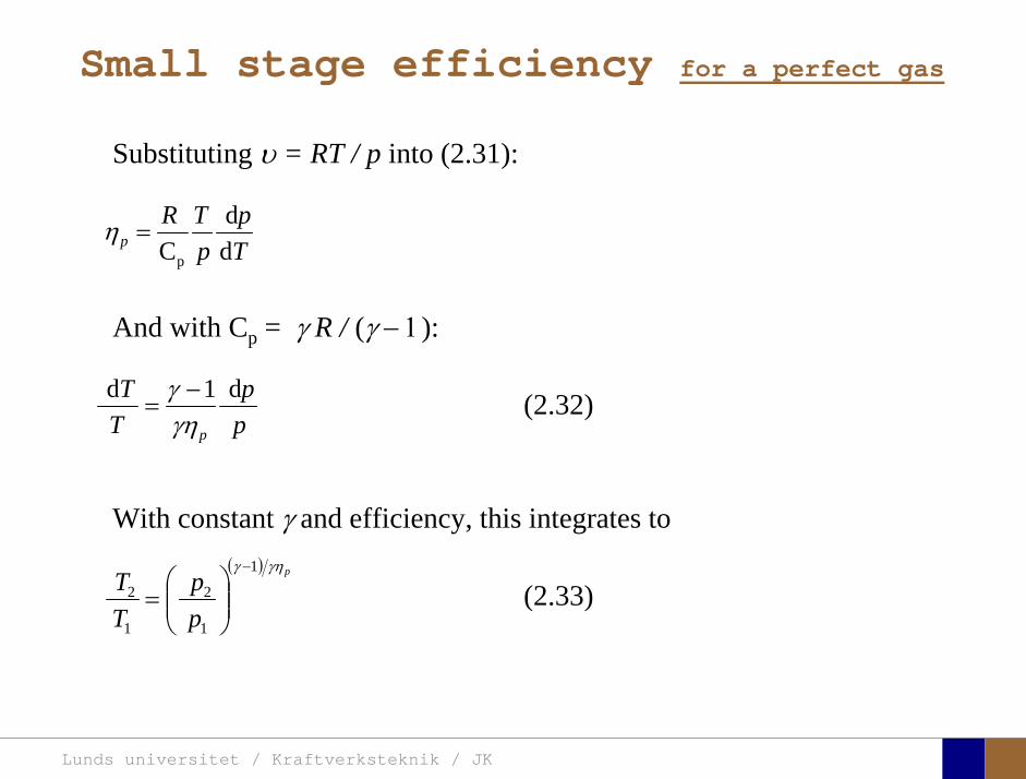
Substituting υ = RT / p into (2.31):

pp

TT

p

d1dγηγ −

= (2.32)

And with Cp = γ R / (γ − 1):

( ) p

pp

TT

γηγ 1

1

2

1

2

−

⎟⎟⎠

⎞⎜⎜⎝

⎛= (2.33)

With constant γ and efficiency, this integrates to




For the ideal compression, ηp = 1, and the temperature ratio becomes:

( ) ( )

⎥⎥⎦

⎤

⎢⎢⎣

⎡−⎟⎟

⎠

⎞⎜⎜⎝

⎛

⎥⎥⎦

⎤

⎢⎢⎣

⎡−⎟⎟

⎠

⎞⎜⎜⎝

⎛=

−−

111

1

2

1

1

2p

pp

pp

c

ηγγγγ

η (2.36)

Which is also obtainable from pγ = constant and pυ = RT. If this is substituted into the isentropic efficiency of compression for a perfect gas,

( ) γγ 1

1

2

1

2

−

⎟⎟⎠

⎞⎜⎜⎝

⎛=

pp

TT

(2.35)

a relation between the isentropic and polytropic efficiencies is obtained:

( ) ( )1212 TTTT sc −−=η (2.34)





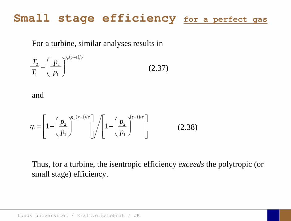
For a turbine, similar analyses results in

( ) ( )

⎥⎥⎦

⎤

⎢⎢⎣

⎡⎟⎟⎠

⎞⎜⎜⎝

⎛−

⎥⎥⎦

⎤

⎢⎢⎣

⎡⎟⎟⎠

⎞⎜⎜⎝

⎛−=

−− γγγγη

η1

1

2

1

1

2 11pp

pp p

t (2.38)

and

( ) γγη 1

1

2

1

2

−

⎟⎟⎠

⎞⎜⎜⎝

⎛=

p

pp

TT

(2.37)

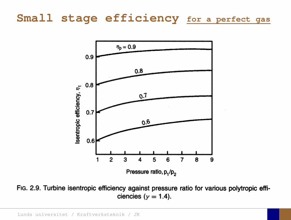
Thus, for a turbine, the isentropic efficiency exceeds the polytropic (or small stage) efficiency.




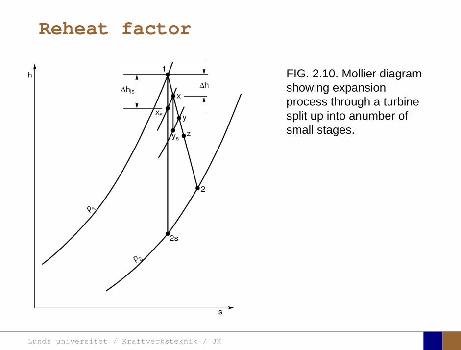
Reheat factor

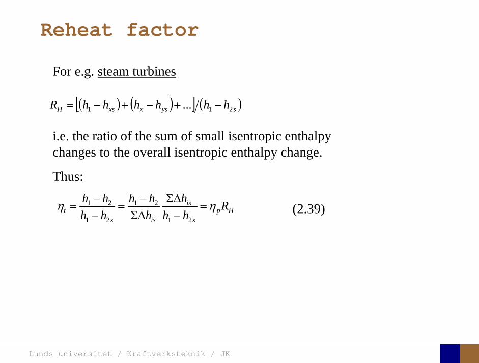
For e.g. steam turbines

Hps

is

isst R

hhh

hhh

hhhh ηη =

−ΣΔ

ΣΔ−

=−−

=21

21

21

21 (2.39)

i.e. the ratio of the sum of small isentropic enthalpy changes to the overall isentropic enthalpy change.

Thus:

( ) ( )[ ] ( )sysxxsH hhhhhhR 211 ... −+−+−=


Reheat factor

FIG. 2.10. Mollier diagram showing expansion process through a turbinesplit up into anumber of small stages.


Nozzles

Device in which the fluid is accelerated at the expense of pressure dropIn the adiabatic case, this means that stagnation enthalpy is conservedTypically this occurs in the compressor inlet and in the stationary blade rows in turbines (impulse machines)

At subsonic conditions, a nozzle represents a contraction (decrease in flow cross sectional area)


Nozzle efficiency

ssN hh

hhcc

201

20122

22

22

−−

==η

Enthalpy loss coeff.

Nozzle efficiency

222

22

chh s

N−

=ζ

Velocity coeff.

sN c

cK2

2=

Combining these:2

11

NN

N K=+

=ζ

ηFIG. 2.11. Relationship between reheat factor, pressure ratio and polytropic efficiency(n = 1.3).


Nozzle efficiency

FIG. 2.12. Mollier diagrams for the flow processes through a nozzle and a diffuser: (a) nozzle; (b) diffuser.


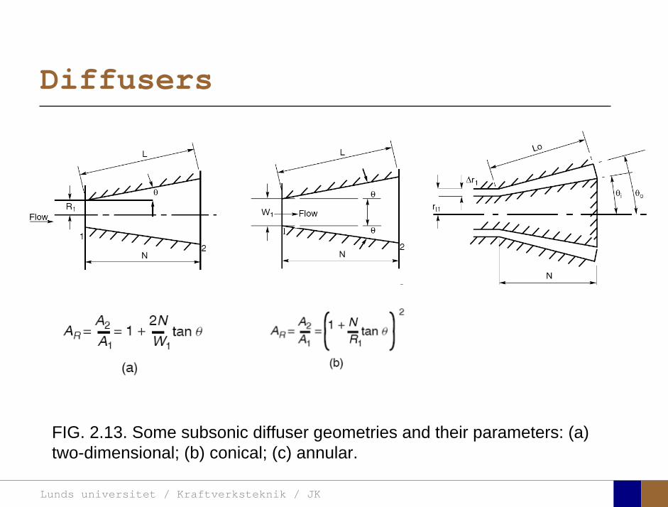
Diffusers

FIG. 2.13. Some subsonic diffuser geometries and their parameters: (a) two-dimensional; (b) conical; (c) annular.


Venturi tube flow meter


Diagram

FIG. 2.14. Variation of diffuser efficiency with staticpressure ratio for constantvalues of total pressurerecovery factor (γ = 1.4).


( )( )

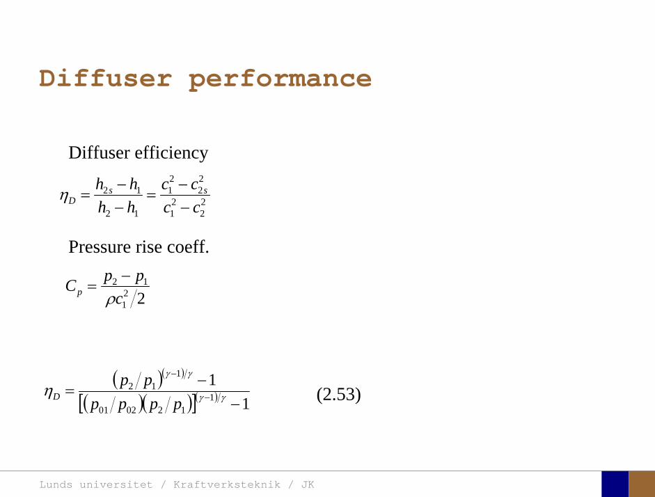
( )( )[ ]( ) 111

120201

112

−−

= −

−

γγ

γγ

ηpppp

ppD (2.53)

22

21

22

21

12

12

cccc

hhhh ss

D −−

=−−

=η

Diffuser efficiency

Pressure rise coeff.

221

12

cppCp ρ

−=

Diffuser performance


Diagram

FIG. 2.15. Flow regime chart for two-dimensional diffusers (adaptedfrom Sovran and Klomp 1967).


Diagram

FIG. 2.16. Typical diffuser performance curves for a two-dimensionaldiffuser, with L/W1 = 8 (adapted from Kline et al. 1959).


Diagram

1 0.02B

FIG. 2.17. Performance chart for conicaldiffusers with

(adapted from Sovran andKlomp 1967).

1 0.02B

Documents

Theory of turbo machinery / Turbomaskinernas teori Chapter 2 fileTurbomaskinernas teori Chapter 2. Lunds universitet / Kraftverksteknik / JK Basic Thermodynamics, Fluid Mechanics: