Embed Size (px)
Citation preview
Energy Sciences Jens Klingmann
Theory of turbo machinery Turbomaskinernas teori
Beyond Dixon
Computational Fluid Dynamics (CFD) and Experimental methods
Energy Sciences Jens Klingmann
Det blir aringttahundra grader Du kan lita paring mej Du kan lita paring mej
(Ebba Groumln)
Energy Sciences Jens Klingmann
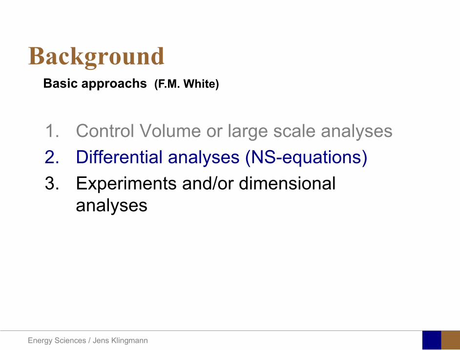
1 Control Volume or large scale analyses2 Differential analyses (NS-equations)3 Experiments andor dimensional
analyses
Basic approachs (FM White)
Background
Energy Sciences Jens Klingmann
CFD and experiments
bull No this is not a CFD course butbull Experiments
Energy Sciences Jens Klingmann
Conservation of mass Conservation of linear momentum Conservation of energy
Basic laws that can be used in Control Volume or Differential analyses
Background
Energy Sciences Jens Klingmann
Newtonrsquos second law applied to fluid element
x
y
z
dy
dz
dx
Forces
bull Body forces (per unit vol) eg gravity
bull Surface forces (per unit area)
amF sdot= or per unit volume
aVF sdot= ρ V
Fa =sdotρor
Energy Sciences Jens Klingmann
Newtonrsquos second law applied to fluid element (outline only)
x
y
z
dy
dz
dx
Stresses
bull Shear stresses
bull Normal stresses
Pressure
These are the constitutive assumption
+=
dzdu
dxdu xz
zx microτ
zyτzyτzzσ
pzz =σ
Energy Sciences Jens Klingmann
Stresses change continuously
Sum of forces in z-direction
Newtonrsquos second law applied to fluid element
zp
VF
dxdydzzpF
dxdydzVdydxA
dzzpAdp
zppApAF
z
z
z
partpart
minus=
partpart
minus=
==partpart
minus=
partpart
+sdotminussdot=
x
y
z
dy
dz
dx
p
dzzpp
partpart
+
Same principle in other directions
Same principle for shear stresses
Energy Sciences Jens Klingmann
Acceleration due to timederivatives
but also due to advection (movement into regions with varying velocities)
What about the acceleration
z
clzu
tuz
partpart
zuu z
z partpart
zuz
partpart
partpart
+partpart
+yuu
xuu z
yz
x
Energy Sciences Jens Klingmann
Summing up
zu
zyu
yxu
xzp
zuu
yuu
xuu
tu
zu
zyu
yxu
xyp
zu
uy
uu
xu
ut
u
zu
zyu
yxu
xxp
zuu
yuu
xuu
tu
zzzzz
zy
zx
z
yyyyz
yy
yx
y
xxxxz
xy
xx
x
partpart
partpart
+partpart
partpart
+partpart
partpart
+partpart
minus=
part
part+
partpart
+partpart
+part
part
part
part
partpart
+part
part
partpart
+part
part
partpart
+partpart
minus=
part
part+
part
part+
part
part+
part
part
partpart
partpart
+part
partpartpart
+part
partpartpart
+partpart
minus=
part
part+
partpart
+part
part+
partpart
micromicromicroρ
micromicromicroρ
micromicromicroρ
Navier-Stokes Equations Incompressible (isochoric)
Energy Sciences Jens Klingmann
Summing up
4 unknown (3 velocity components pressure)4 equations (3 NS eq and continuity)
Nonlinear second order set of PDEOnly very simple analytic solution available
0=part
part+
part
part+
partpart
zu
yu
xu zyx
zu
zyu
yxu
xzp
zuu
yuu
xuu
tu
zu
zyu
yxu
xyp
zu
uy
uu
xu
ut
u
zu
zyu
yxu
xxp
zuu
yuu
xuu
tu
zzzzz
zy
zx
z
yyyyz
yy
yx
y
xxxxz
xy
xx
x
partpart
partpart
+partpart
partpart
+partpart
partpart
+partpart
minus=
part
part+
partpart
+partpart
+part
part
part
part
partpart
+part
part
partpart
+part
part
partpart
+partpart
minus=
part
part+
part
part+
part
part+
part
part
partpart
partpart
+part
partpartpart
+part
partpartpart
+partpart
minus=
part
part+
partpart
+part
part+
partpart
micromicromicroρ
micromicromicroρ
micromicromicroρ
Navier-Stokes Equations Incompressible (isochoric)
and continuity eq
Worst slide ever
Energy Sciences Jens Klingmann
Solving the equations Equations solved in discrete point in a grid (mesh)
Derivatives approximated by eg finite differences
System transformed to large set of algebraic equations
xxjiji
ji ∆
minusasymp
partpart + 1
φφφ
Where φ is any dependent variable and ∆xis the distance between the meshpoints
∆x Example
Energy Sciences Jens Klingmann
Turbulence
Energy Sciences Jens Klingmann
Osborne Reynoldsrsquo Experiments
Energy Sciences Jens Klingmann
Characteristics of turbulence
bull Irregularity
bull Diffusivity the capability of turbulence to enhance transport of mass heat and momentum
bull Large Reynolds numbers Many flow fields are laminar at low Re but become unstable and turbulent at higher Re
bull Three-dimensional vorticity fluctuations
bull Dissipation Viscous shear stresses perform deformation work on the fluid which increases the internal energy at the expense of the kinetic energy
bull Continuum In most technical applications the distance between molecules is orders of magnitude shorter than the size of even the smallest scales of the flow
Energy Sciences Jens Klingmann
Turbulence is irregularity
025 03 035 04 045 05t0
001002003004005006007008009
01
u(x
t)
u(xt)
u(x)
bull Small (unresolvable) scalesbull Statistical approach required bull How can we define an average velocity
0
1( ) ( )T
u u t dtT
= intx x
Energy Sciences Jens Klingmann
Turbulence averaging
Havenrsquot we already done this once
Energy Sciences Jens Klingmann
y zx zz z z z z z
x y z
z z z
u uu uu u u u u uu u ut x x y y z z
u u upz x x y y z z
ρ
micro micro micro
partpartpart part part part part + + + + + + = part part part part part part part
part part partpart part part part= minus + + +
part part part part part part part
Turbulence averaging
uuu += ppp +=
Insert into NS (only z-direction shown) and average entire equation
and
Decompose velocity and pressure (Reynoldsrsquo decomposition)
Additional terms that look like stresses
Energy Sciences Jens Klingmann
Turbulence RANS modellingReynoldsrsquo stress tensor
Needs to be expressed as a function of variables we know or intend to solve for
TURBULENCE MODEL
x x x y x z
y x y y y z
z x z y z z
u u u u u u
u u u u u u
u u u u u u
ρ
=
R
6 new variables (symmetry )xyyx uuuu =
Energy Sciences Jens Klingmann
Turbulence RANS modellingReynolds stress tensor
ij i j
u u u v u w
R u u v u v v v w
w u w v w w
ρ ρ ρ
= minus otimes = = =
R u u
Turbulent Kinetic Energy
( ) ( )1 1 1 1 2 2 2 2ii i ik tr R u u u u v v w wρ ρ= = = = + +R
Represents the kinetic energy of the fluctuations (or vortices)
Energy Sciences Jens Klingmann
Turbulence closure problem
10 unknownvelocity components pressure and correlations of fluctuating velocity
4 equationsAveraged momentum equations and averaged continuity equation
i ju u
Energy Sciences Jens Klingmann
Turbulence RANS modelling
23
i jij T ij
j i
u uR kx x
micro ρ δ part part
= + minus part part
2 T kmicro ρ εpropldquoTurbulent viscosityrdquo
Transport of k Some terms may be derived other need modelling
( ) ( ) ( )advection diffusion productionk k k kt
εpart+ + = minus
part
Energy from mean flow to turbulence
Dissipation Energy converted to heat
Energy Sciences Jens Klingmann
Turbulence RANS modelling
23
i jij T ij
j i
u uR kx x
micro ρ δ part part
= + minus part part ερmicro micro 2kCT =
k Tklk
k l k k k
uk ku Rx x x x
microρ ε micro
σ part part part part
= minus + + part part part part 2
1 2k T
klkk l k k
uu C R C
x k x k x xε εε
microε ε ε ερ ρ micropart σ
part part part part= minus + + part part part
4411 =εC 9212 =εC 090=microC 1=kσ31=εσ
Closure coefficients
Energy Sciences Jens Klingmann
Energy Sciences Jens Klingmann
Computational Fluid Dynamics (CFD)
U Waringhleacuten ldquoThe Aerodynamic design and testing of a supersonic turbine for rocket engine propulsionrdquo Proc Of 3rd European conference on Turbomachinery Fluid dynamics and thermodynamics
Energy Sciences Jens Klingmann
Subsonic flow in an aerofoilplate junction computed with a second-moment closure (D Apsley 1998)
Computational Fluid Dynamics(CFD)
Energy Sciences Jens Klingmann
Hydraulic turbine research CFD digital simulation Distribution of speed on an axial turbine
Computational Fluid Dynamics(CFD)
Energy Sciences Jens Klingmann
Scales of turbulence
10-01
1000
1001
1002
1003
1004
1005
κ LI
10-08
10-07
10-06
10-05
10-04
10-03
10-02
10-01
1000
E(u
2 LI)
10-04
10-03
10-02
10-01
1000
κ LK
10-05
10-04
10-03
10-02
10-01
1000
1001
1002
D( ε L
K )10-01
1000
1001
1002
1003
1004
1005
E = 15 (κ LI)-53
10-04
10-03
10-02
10-01
1000
1001
D = 3 ( κ LΚ) 13
Normalized energy and dissipation spectra for
Adapted from Tennekeys and Lumley
ReLI= times2 105
1 2Re 500IL asymp
3 4Re 10000IL asymp
Energy Sciences Jens Klingmann
References Turbulence
bull Tennekeys and Lumley ldquoA first course in Turbulencerdquo MIT Press 1972
bull J O Hinze ldquoTurbulencerdquo McGraw-Hill 1959bull D C Wilcox ldquoTurbulence Modeling for CFDrdquo DCW Industries
2006
Energy Sciences Jens Klingmann
Boundary layers
Energy Sciences Jens Klingmann
Boundary Layer Theory (BLT) Sensitive to Pressure
gradients Appropriate scaling from
dimensional analyses
Energy Sciences Jens Klingmann
Boundary layers
Energy Sciences Jens Klingmann
Air foil theory
Energy Sciences Jens Klingmann
Visualisation of diffusor separation
Energy Sciences Jens Klingmann
BL equations
+minus=+
yu
yxp
xuv
xuu
partpartmicro
partpart
partpart
partρpart
partρpart and 0=+
yxu
partυpart
partpart
Applying the BL approximations the 2D stationary incompressible NS-eq and continuity equation become
yvu
yu
yxuu
xp
yu
xuu
partpartρ
partpartmicro
partpart
partρpart
partpart
partυρpart
partρpart
minus
+minusminus=+
and
0=+yx
upart
υpartpartpart
Reynolds averaged BL eqs are
Energy Sciences Jens Klingmann
Boundary layers
Energy Sciences Jens Klingmann
Turbulent BL at different Pressure gradients
Energy Sciences Jens Klingmann
Boundary Layers
ν
yuy =+
ρτWu =
0=
partpart
=y
w yuτ
uuu =+
Energy Sciences Jens Klingmann
Diffuser efficiency
Energy Sciences Jens Klingmann
Reynolds Number (Order of magnitude)
At eg a compressor inlet
ρ = O(1) kgm3
U = O(100) msx lt O(01) mmicro = O(10-5)
Re = ρ U x micro =O(106)
In subsequent stages large amounts of turbulence (from stator wakes) will be convected into the Boundary layer
Energy Sciences Jens Klingmann
References Boundary layers
bull Frank M White ldquoViscous Fluid Flowrdquobull Hermann Schlichting ldquoBoundary Layer Theoryrdquo
Energy Sciences Jens Klingmann
CFD and experiments
bull No this is not a CFD course butbull Experiments
Energy Sciences Jens Klingmann
What do we need to measureOverall performance
Flow rates (mass or volume) Pressure Temperature Shaft power
Performance increase
Separations (velocity) Secondary flows eg tip clearance losses (velocity) Shock waves (supersonic applications) Pressure (resolved in time and space) Temperature (resolved in time and space)
Energy Sciences Jens Klingmann
Cascade wind tunnels
FIG 31 Compressor cascade wind tunnels (a) Conventional low-speed continuousrunning cascade tunnel (adapted from Carter et al 1950)(b) Transonicsupersoniccascade tunnel (adapted from Sieverding 1985)
Energy Sciences Jens Klingmann
Closed circuit tunnels
Energy Sciences Jens Klingmann
components
Settling Chamber
The settling chamber is located between the fan or wide angle diffuser and the contraction and contains the honeycombs and screens used to moderate longitudinal variations in the flow Screens in the chamber should be spaced at 02 chamber diameters apart so that flow disturbed by the first screen can settle before it encounters the second
Honeycombs
Honeycombs are located in the settling chamber and are used to reduce nonuniformities in the flow For optimum benefit honeycombs should be 6-8 cell diameters thick and cell size should be on the order of about 150 cells per settling chamber diameter
Energy Sciences Jens Klingmann
components
Screens
Screens are typically located just downstream of the honeycomb and sometime at the inlet of the test section Screens create a static pressure drop and serve to reduce boundary layer size and increase flow uniformity
Contraction Section
Contractions sections are located between the settling chamber and the test sections and serve to both increase mean velocities at the test section inlet and moderate inconsistencies in the uniformity of the flow Large contraction ratios and short contraction lengths are generally more desirable as they reduce the power loss across the screens and the thickness of boundary layers Small tunnels typically have contraction ratios between 6 and 9
Energy Sciences Jens Klingmann
Flow meters with pressure measurement
Venturi-tube
A1 A2
P1 P2
1 1 2 2C A C A=In the incompressible case
2 21 1 2 2
2 2C P C P
ρ ρ+ = +Assuming horisontal mounting
Energy Sciences Jens Klingmann
Daniel Bernoulli 1700-1782
Daniel Bernoulli was the son of Johann Bernoulli He was born in Groningen while his father held the chair of mathematics there His older brother was Nicolaus(II) Bernoulli and his uncle was Jacob Bernoulli so he was born into a family of leading mathematicians but also into a family where there was unfortunate rivalry jealousy and bitterness
Undoubtedly the most important work which Daniel Bernoulli did was his work on hydrodynamics Even the term itself is based on the title of the work which he produced called Hydrodynamica and before he left St Petersburg Daniel left a draft copy of the book with a printer However the work was not published until 1738 and although he revised it considerably between 1734 and 1738 it is more the presentation that he changed rather then the substance
This work contains for the first time the correct analysis of water flowing from a hole in a container This was based on the principle of conservation of energy which he had studied with his father in 1720 Daniel also discussed pumps and other machines to raise water One remarkable discovery appears in Chapter 10 of Hydrodynamica where Daniel discussed the basis for the kinetic theory of gases He was able to give the basic laws for the theory of gases and gave although not in full detail the equation of state discovered by Van der Waals a century later
Energy Sciences Jens Klingmann
Venturi-tube (2)
22 2 12 2
2
2A PC CA ρ
∆minus =
A1 A2
P1 P2
Solve for eg C2
1 2P P P∆ = minus
( )
12
2 2 21 2
21
PCA Aρ
∆ = minus
and( )
12
2 2 2 2 21 2
21
Pm A C AA Aρρ
∆ = = minus
where
Flow meters with pressure measurement
Energy Sciences Jens Klingmann
Flow meters with pressure measurement
Orifice meters
A1
A2
P1 P2
Applicable for pipe flows Same principle as for Venturi Positioning of pressure taps important Vena contracta and losses require inclusion
of Discharge Coefficient CD
( )
12
2 2 21 2
21D
Pm C AA Aρ ∆ =
minus where ( )1 2ReDC f A A=
CD available from manufacturer (measurements) or Standards (eg ISO)
Energy Sciences Jens Klingmann
Coriolis flow meter
An actuator (not shown) induces a vibration of the tubes
When there is mass flow Coriolis forces induce twisting of the tubes
degree of phase-shift is a measure for the amount of mass that is flowing through the tubes
Energy Sciences Jens Klingmann
Thermal flow meter Heat is added electrically to the flow Temperature is measured before and after heat addition
pP mC T∆=
Energy Sciences Jens Klingmann
Ultrasonic flow meters
Ultrasound is emitted to small particles in the flow (dust or other) Reflections of the sound is frequency shifted by the Doppler effect The frequency change is proportional to the particles velocity (volume flow
meter)
Energy Sciences Jens Klingmann
Inductive flow metersA magnetic flowmeter is based upon Faradays Law
The voltage induced across any conductor as it moves at right angles through a magnetic field is proportional to the velocity of that conductor
E is proportional to V x B x D where
E = The voltage generated in a conductorV = The velocity of the conductorB = The magnetic field strengthD = The length of the conductor
NB electric conductivity is required
Energy Sciences Jens Klingmann
Temperature measurements
Thermocouples
The basis established by Thomas Johann Seebeck in 1821
A conductor generates a voltage when subjected to a temperature gradient
To measure this voltage one must use a second conductor material which generates a different voltage under the same temperature gradient
Energy Sciences Jens Klingmann
Pressure sensing
1 2p pgt 2p p2 may be the atmosphere a static pressure tap or a known reference pressure
The strain of the diaphragm (or itrsquos deflection) may be measured by a number of electric methods
Diaphragm
Energy Sciences Jens Klingmann
Pressure sensingPiezoresistive Strain Gage
Uses the piezoresistive effect of bonded or formed strain gauges to detect strain due to applied pressure
Capacitive
Uses a diaghragm and pressure cavity to create a variable capacitor to detect strain due to applied pressure
Magnetic
Measures the displacement of a diaphragm by means of changes in inductance (reluctance) LVDT Hall Effect or by eddy current principal
Piezoelectric
Uses the piezoelectric effect in certain materials such as quartz to measure the strain upon the sensing mechanism due to pressure
Potentiometric
Uses the motion of a wiper along a resistive mechanism to detect the strain caused by applied pressure
Energy Sciences Jens Klingmann
3D highly instationary (periodic) flow Potentially very high velocities (Supersonic) Large temperature differences Low accessibility (difficult to probe between rotors) Low turbulence levels in most of the domain Very high turbulence in BL and wakes
Properties of measuring object
Point measurements
Energy Sciences Jens Klingmann
Conventional or non-opticalndash Static Pressure Measurementsndash Total Pressure Measurements
bull Multy hole probes
ndash Total Temperature ndash Hot Wire Anemometry (HWA)
Optical techniques for Velocity Measurementsndash Laser Two Focous (L2F)ndash Laser Doppler Anemometry (LDA)ndash Particle Image velocimetry (PIV)
Point Measurements
Energy Sciences Jens Klingmann
Static and total pressure
2 2 21 2 1
2 1 2 2 2C C CP P ρ ρ ρ
minus = minus =
2 0C =Stagnation point
C1Static pressure tap
Prandtl or Pitot tube
Apply the Bernoulli equation from free stream to stagnation point
21
2 12CP Pρ
= +or
We can also define a stagnation or total pressure
( )2
101 1 022
CP P Pρ= + =
Total pressure = Static pressure + dynamic pressure
or
Energy Sciences Jens Klingmann
Static pressure
Energy Sciences Jens Klingmann
Total Pressure and Temperature
Shrouded Probes
Shrouded Probe
Pitot or Prandtl tube
Sensitive to direction
Energy Sciences Jens Klingmann
Ludwig Prandtl 1875-1953
Ludwig Prandtl born at Freising Bavaria on February 4 1875 was a German Physicist famous for his work in aeronautics He qualified at Munchen in 1900 with a thesis on elastic stability and held the position of Professor of Applied Mechanics at Gottingen for forty-nine years (from 1904 until his death there on August 15 1953) In 1925 Prandtl became the Director of the Kaiser Wilhelm Institute for Fluid Mechanics His discovery in 1904 of the Boundary Layer which adjoins the surface of a body moving in a fluid led to an understanding of skin friction drag and of the way in which streamlining reduces the drag of airplane wings and other moving bodies His work on wing theory published in 1918 - 1919 followed that of FW Lanchester (1902-1907) but was carried out independently and elucidated the flow over airplane wings of finite span Prandtls work and decisive advances in boundary layer and wing theories became the basic material of aeronautics He also made important contributions to the theories of supersonic flow and of turbulence and contributed much to the development of wind tunnels and other aerodynamic equipment In addition he devised the soap-film analogy for the torsion of non-circular sections and wrote on the theory of plasticity and of meteorology
Energy Sciences Jens Klingmann
Total Pressure multy hole
Cobra Probe Yaw Probe
5 Hole Probe
Energy Sciences Jens Klingmann
5 Hole Probes Calibration
Energy Sciences Jens Klingmann
The inherent unsteadiness of the flow within turbomachines
Energy Sciences Jens Klingmann
Hot Wire Anemometry (HWA) The heat transfer from a thin (one micron)
electrically heated wire can be used to determine velocity
The resistance of the wire is temperature dependent Within a small temperature range it can be assumed linear R = R0+α R0(Tm-T0) where R0 is the resistance at a reference temperature T0 and Tm is the mean wire temperature
The thermal power induced in the wire is balanced by heat transfer to the surrounding fluid I2R=hπDL(Tm-T0) where h is the heat transfer coefficient and D and L the diameter and length of the wire respectively
E = I R
Energy Sciences Jens Klingmann
Constant Temperature Anemometry (CTA) The wire is often placed in a Whetstone bridge If the output from the
bridge is amplified and fed back to the bridge the resistance of the probe and thus the temperature will be held constant
This prevents the temperature of the wire to become excessive at low velocities
R1
R2 R3
Probe
Bridge Voltage
Energy Sciences Jens Klingmann
Constant Temperature Anemometry (CTA)
Energy Sciences Jens Klingmann
Characteristics of LDA (according to Dantec)
Invented by Yeh and Cummins in 1964 Velocity measurements in Fluid Dynamics (gas liquid) Up to 3 velocity components Non-intrusive measurements (optical technique) Absolute measurement technique (no calibration required) Very high accuracy Very high spatial resolution due to small measurement volume Tracer particles are required
Energy Sciences Jens Klingmann
LDA - Fringe Model
Focused Laser beams intersect and form the measurement volume Plane wave fronts beam waist in the plane of intersection Interference in the plane of intersection Pattern of bright and dark stripesplanes Fringes
Energy Sciences Jens Klingmann
LDA-measuring volume
d
x
x
y
y
z
z
e-2 CONTOUR
FRINGES
κ
κ
κ
κ
De-2
De-2
dml m
a
b
cx
b
z
ya
cd
d
=
=
=
J
J
J
J
JP
JP
JP
JD
JD
JD
+
+
+
a
b
c
d
κπλ
=minus sinD
f4l2e
m
κπλ
=minus cosD
f4D2e
m
Energy Sciences Jens Klingmann
Laser Two Focus
Energy Sciences Jens Klingmann
Laser Two Focus
Energy Sciences Jens Klingmann
PIV measurements
PIV is a fairly new technique capable of simultaneous velocity measurements at many points in a plane This gives information on large scale structures vorticity etc which is very difficult or impossible to obtain from one-point measuring techniques
PIV involves the illumination of a plane of the flow under investigation with a thin pulsed sheet of light The flow is seeded with particles
The light scattered from the particles and from successive pulses are being recorded either on film or a CCD array forming a multiple exposure of each particle image If the time between the pulses is known velocity can be determined as the ratio of the particle displacement and the elapsed time
t∆∆= xu
Energy Sciences Jens Klingmann
PIV
Energy Sciences Jens Klingmann
PIV measurements illumination
YA
G
YA
G
Two frequency doubled YAG Lasers aligned to one double pulsed laser sheet
Two or more separate light pulses can be obtained by chopping a continuous laser or from pulsed lasers
The limited pulse energies obtained from continuous lasers limits their applicability to low velocity flows or flows where large seeding particles can be used (ie liquid flows)
The low repetition rate of most pulsed lasers makes the use of two lasers advantageous
Energy Sciences Jens Klingmann
PIV measurements recording
High seeding density in laminar flame
Film or CCD-cameras Cross- or Auto-correlation
ndash ie both particle images on the same frame or on separate frames
CCD-camera requirementndash A many pixels as possiblendash 2k by 2k available 4k by 4k coming
Energy Sciences Jens Klingmann
PIV measurements analyses
Low seeding density (Number of seeding particles per unit volume)
Each particle image pair can be identified This is called particle tracking
High seeding density (PIV)
Small sub-regions of the image containing many particle image pairs are processed to obtain one velocity vector
Energy Sciences Jens Klingmann
PIV measurements analyses
Energy Sciences Jens Klingmann
PIV measurements analyses
( ) ( ) ( ) xsxxs dIIR 2A
1
I
+= int
Cross correlation between ( )x1I and ( )x2I
s is a two dimensional displacement vector
IA is the interrogation area
Cross correlation between
(
)
x
1
I
and
(
)
x
2
I
s is a two dimensional displacement vector
I
A
is the interrogation area
Energy Sciences Jens Klingmann
Energy Sciences Jens Klingmann
PIV from IOWA state university
Energy Sciences Jens Klingmann
PIV sample of evaluation
Energy Sciences Jens Klingmann
LDA PIV HWA Velocity range 01 mms ndash 300
ms 02 ndash 150 ms
Measuring Volume
D = 005 L = 05 mm
2 by 2 by 05 mm
L = 05 mm
Freq response O(10 000) Hz O(10) Hz O(100 000) Hz Calibration Yes No No Sensitivity to other than velocity
Low (ref Index) Low (ref Index) Large (temperature concentrationshellip)
Continuous Signal
Sometimes Seldom Always
Noise High High Low Turbulence intensity
No limitation Some limitation lt 20
Price O(1 000 000) SEK
O(1 000 000) SEK
O(50 000) SEK
Required Knowledge
High medium Low
Comparison of techniques
Energy Sciences Jens Klingmann
References experiments
R J Goldstein ldquoFluid Mechanics Measurementsrdquo Hemisphere Publishing 1983 A V Johansson amp P H Alfredsson ldquoExperimentella metoder inom
stroumlmningsmekanikenrdquo Inst Foumlr Mekanik KTH F Durst A Melling and J H Whitelaw ldquoPrincipals and Practice of Laser Doppler
Anemometryrdquo 1984 R J Adrian ldquoParticle-imaging techniques for experimental fluid mechnicsrdquo Ann Rev
Fluid Mech 1991
Energy Sciences Jens Klingmann
Sample of LDA-measurements
Rotor blade
Glas window
Emitted beams
Scattered Light
Adjustable mirror
Energy Sciences Jens Klingmann
Axial velocity sorted into 10 bins
0 1 2 3 4 5 6tangential coordinate (degrees)
-20
0
20
40
60
80
100
120
140
160Ax
ial v
eloc
ity a
nd s
tand
ard
devi
atio
n (m
s)
radial position 7 mm from inner window surfaceaxial position 23 mm behind rotor blades
Energy Sciences Jens Klingmann
Axial velocities in the radial-tangential plane
Energy Sciences Jens Klingmann
Airfoils NACA 4-digit
The NACA four-digit wing sections define the profile by
One digit describing maximum camber as percentage of the chord
One digit describing the distance of maximum camber from the airfoil leading edge in tens of percents of the chord
Two digits describing maximum thickness of the airfoil as percent of the chord
Example the NACA 2412 airfoil has a maximum camber of 2 located 40 (04 chords) from the leading edge with a maximum thickness of 12 of the chord
Four-digit series airfoils by default have maximum thickness at 30 of the chord (03 chords) from the leading edge
Energy Sciences Jens Klingmann
Airfoils NACA 4-digit
bull c is the chord lengthbull x is the position along
the chord from 0 to cbull y is the half thickness at
a given value of x (centerline to surface)
bull t is the maximum thickness as a fraction of the chord
Energy Sciences Jens Klingmann
Death by PowerPoint
| LDA | PIV | HWA | |||||
| Velocity range | 01 mms ndash 300 ms | 02 ndash 150 ms | |||||
| Measuring Volume | D = 005 L = 05 mm | 2 by 2 by 05 mm | L = 05 mm | ||||
| Freq response | O(10 000) Hz | O(10) Hz | O(100 000) Hz | ||||
| Calibration | Yes | No | No | ||||
| Sensitivity to other than velocity | Low (ref Index) | Low (ref Index) | Large (temperature concentrationshellip) | ||||
| Continuous Signal | Sometimes | Seldom | Always | ||||
| Noise | High | High | Low | ||||
| Turbulence intensity | No limitation | Some limitation | lt 20 | ||||
| Price | O(1 000 000) SEK | O(1 000 000) SEK | O(50 000) SEK | ||||
| Required Knowledge | High | medium | Low |

Energy Sciences Jens Klingmann
Det blir aringttahundra grader Du kan lita paring mej Du kan lita paring mej
(Ebba Groumln)
Energy Sciences Jens Klingmann
1 Control Volume or large scale analyses2 Differential analyses (NS-equations)3 Experiments andor dimensional
analyses
Basic approachs (FM White)
Background
Energy Sciences Jens Klingmann
CFD and experiments
bull No this is not a CFD course butbull Experiments
Energy Sciences Jens Klingmann
Conservation of mass Conservation of linear momentum Conservation of energy
Basic laws that can be used in Control Volume or Differential analyses
Background
Energy Sciences Jens Klingmann
Newtonrsquos second law applied to fluid element
x
y
z
dy
dz
dx
Forces
bull Body forces (per unit vol) eg gravity
bull Surface forces (per unit area)
amF sdot= or per unit volume
aVF sdot= ρ V
Fa =sdotρor
Energy Sciences Jens Klingmann
Newtonrsquos second law applied to fluid element (outline only)
x
y
z
dy
dz
dx
Stresses
bull Shear stresses
bull Normal stresses
Pressure
These are the constitutive assumption
+=
dzdu
dxdu xz
zx microτ
zyτzyτzzσ
pzz =σ
Energy Sciences Jens Klingmann
Stresses change continuously
Sum of forces in z-direction
Newtonrsquos second law applied to fluid element
zp
VF
dxdydzzpF
dxdydzVdydxA
dzzpAdp
zppApAF
z
z
z
partpart
minus=
partpart
minus=
==partpart
minus=
partpart
+sdotminussdot=
x
y
z
dy
dz
dx
p
dzzpp
partpart
+
Same principle in other directions
Same principle for shear stresses
Energy Sciences Jens Klingmann
Acceleration due to timederivatives
but also due to advection (movement into regions with varying velocities)
What about the acceleration
z
clzu
tuz
partpart
zuu z
z partpart
zuz
partpart
partpart
+partpart
+yuu
xuu z
yz
x
Energy Sciences Jens Klingmann
Summing up
zu
zyu
yxu
xzp
zuu
yuu
xuu
tu
zu
zyu
yxu
xyp
zu
uy
uu
xu
ut
u
zu
zyu
yxu
xxp
zuu
yuu
xuu
tu
zzzzz
zy
zx
z
yyyyz
yy
yx
y
xxxxz
xy
xx
x
partpart
partpart
+partpart
partpart
+partpart
partpart
+partpart
minus=
part
part+
partpart
+partpart
+part
part
part
part
partpart
+part
part
partpart
+part
part
partpart
+partpart
minus=
part
part+
part
part+
part
part+
part
part
partpart
partpart
+part
partpartpart
+part
partpartpart
+partpart
minus=
part
part+
partpart
+part
part+
partpart
micromicromicroρ
micromicromicroρ
micromicromicroρ
Navier-Stokes Equations Incompressible (isochoric)
Energy Sciences Jens Klingmann
Summing up
4 unknown (3 velocity components pressure)4 equations (3 NS eq and continuity)
Nonlinear second order set of PDEOnly very simple analytic solution available
0=part
part+
part
part+
partpart
zu
yu
xu zyx
zu
zyu
yxu
xzp
zuu
yuu
xuu
tu
zu
zyu
yxu
xyp
zu
uy
uu
xu
ut
u
zu
zyu
yxu
xxp
zuu
yuu
xuu
tu
zzzzz
zy
zx
z
yyyyz
yy
yx
y
xxxxz
xy
xx
x
partpart
partpart
+partpart
partpart
+partpart
partpart
+partpart
minus=
part
part+
partpart
+partpart
+part
part
part
part
partpart
+part
part
partpart
+part
part
partpart
+partpart
minus=
part
part+
part
part+
part
part+
part
part
partpart
partpart
+part
partpartpart
+part
partpartpart
+partpart
minus=
part
part+
partpart
+part
part+
partpart
micromicromicroρ
micromicromicroρ
micromicromicroρ
Navier-Stokes Equations Incompressible (isochoric)
and continuity eq
Worst slide ever
Energy Sciences Jens Klingmann
Solving the equations Equations solved in discrete point in a grid (mesh)
Derivatives approximated by eg finite differences
System transformed to large set of algebraic equations
xxjiji
ji ∆
minusasymp
partpart + 1
φφφ
Where φ is any dependent variable and ∆xis the distance between the meshpoints
∆x Example
Energy Sciences Jens Klingmann
Turbulence
Energy Sciences Jens Klingmann
Osborne Reynoldsrsquo Experiments
Energy Sciences Jens Klingmann
Characteristics of turbulence
bull Irregularity
bull Diffusivity the capability of turbulence to enhance transport of mass heat and momentum
bull Large Reynolds numbers Many flow fields are laminar at low Re but become unstable and turbulent at higher Re
bull Three-dimensional vorticity fluctuations
bull Dissipation Viscous shear stresses perform deformation work on the fluid which increases the internal energy at the expense of the kinetic energy
bull Continuum In most technical applications the distance between molecules is orders of magnitude shorter than the size of even the smallest scales of the flow
Energy Sciences Jens Klingmann
Turbulence is irregularity
025 03 035 04 045 05t0
001002003004005006007008009
01
u(x
t)
u(xt)
u(x)
bull Small (unresolvable) scalesbull Statistical approach required bull How can we define an average velocity
0
1( ) ( )T
u u t dtT
= intx x
Energy Sciences Jens Klingmann
Turbulence averaging
Havenrsquot we already done this once
Energy Sciences Jens Klingmann
y zx zz z z z z z
x y z
z z z
u uu uu u u u u uu u ut x x y y z z
u u upz x x y y z z
ρ
micro micro micro
partpartpart part part part part + + + + + + = part part part part part part part
part part partpart part part part= minus + + +
part part part part part part part
Turbulence averaging
uuu += ppp +=
Insert into NS (only z-direction shown) and average entire equation
and
Decompose velocity and pressure (Reynoldsrsquo decomposition)
Additional terms that look like stresses
Energy Sciences Jens Klingmann
Turbulence RANS modellingReynoldsrsquo stress tensor
Needs to be expressed as a function of variables we know or intend to solve for
TURBULENCE MODEL
x x x y x z
y x y y y z
z x z y z z
u u u u u u
u u u u u u
u u u u u u
ρ
=
R
6 new variables (symmetry )xyyx uuuu =
Energy Sciences Jens Klingmann
Turbulence RANS modellingReynolds stress tensor
ij i j
u u u v u w
R u u v u v v v w
w u w v w w
ρ ρ ρ
= minus otimes = = =
R u u
Turbulent Kinetic Energy
( ) ( )1 1 1 1 2 2 2 2ii i ik tr R u u u u v v w wρ ρ= = = = + +R
Represents the kinetic energy of the fluctuations (or vortices)
Energy Sciences Jens Klingmann
Turbulence closure problem
10 unknownvelocity components pressure and correlations of fluctuating velocity
4 equationsAveraged momentum equations and averaged continuity equation
i ju u
Energy Sciences Jens Klingmann
Turbulence RANS modelling
23
i jij T ij
j i
u uR kx x
micro ρ δ part part
= + minus part part
2 T kmicro ρ εpropldquoTurbulent viscosityrdquo
Transport of k Some terms may be derived other need modelling
( ) ( ) ( )advection diffusion productionk k k kt
εpart+ + = minus
part
Energy from mean flow to turbulence
Dissipation Energy converted to heat
Energy Sciences Jens Klingmann
Turbulence RANS modelling
23
i jij T ij
j i
u uR kx x
micro ρ δ part part
= + minus part part ερmicro micro 2kCT =
k Tklk
k l k k k
uk ku Rx x x x
microρ ε micro
σ part part part part
= minus + + part part part part 2
1 2k T
klkk l k k
uu C R C
x k x k x xε εε
microε ε ε ερ ρ micropart σ
part part part part= minus + + part part part
4411 =εC 9212 =εC 090=microC 1=kσ31=εσ
Closure coefficients
Energy Sciences Jens Klingmann
Energy Sciences Jens Klingmann
Computational Fluid Dynamics (CFD)
U Waringhleacuten ldquoThe Aerodynamic design and testing of a supersonic turbine for rocket engine propulsionrdquo Proc Of 3rd European conference on Turbomachinery Fluid dynamics and thermodynamics
Energy Sciences Jens Klingmann
Subsonic flow in an aerofoilplate junction computed with a second-moment closure (D Apsley 1998)
Computational Fluid Dynamics(CFD)
Energy Sciences Jens Klingmann
Hydraulic turbine research CFD digital simulation Distribution of speed on an axial turbine
Computational Fluid Dynamics(CFD)
Energy Sciences Jens Klingmann
Scales of turbulence
10-01
1000
1001
1002
1003
1004
1005
κ LI
10-08
10-07
10-06
10-05
10-04
10-03
10-02
10-01
1000
E(u
2 LI)
10-04
10-03
10-02
10-01
1000
κ LK
10-05
10-04
10-03
10-02
10-01
1000
1001
1002
D( ε L
K )10-01
1000
1001
1002
1003
1004
1005
E = 15 (κ LI)-53
10-04
10-03
10-02
10-01
1000
1001
D = 3 ( κ LΚ) 13
Normalized energy and dissipation spectra for
Adapted from Tennekeys and Lumley
ReLI= times2 105
1 2Re 500IL asymp
3 4Re 10000IL asymp
Energy Sciences Jens Klingmann
References Turbulence
bull Tennekeys and Lumley ldquoA first course in Turbulencerdquo MIT Press 1972
bull J O Hinze ldquoTurbulencerdquo McGraw-Hill 1959bull D C Wilcox ldquoTurbulence Modeling for CFDrdquo DCW Industries
2006
Energy Sciences Jens Klingmann
Boundary layers
Energy Sciences Jens Klingmann
Boundary Layer Theory (BLT) Sensitive to Pressure
gradients Appropriate scaling from
dimensional analyses
Energy Sciences Jens Klingmann
Boundary layers
Energy Sciences Jens Klingmann
Air foil theory
Energy Sciences Jens Klingmann
Visualisation of diffusor separation
Energy Sciences Jens Klingmann
BL equations
+minus=+
yu
yxp
xuv
xuu
partpartmicro
partpart
partpart
partρpart
partρpart and 0=+
yxu
partυpart
partpart
Applying the BL approximations the 2D stationary incompressible NS-eq and continuity equation become
yvu
yu
yxuu
xp
yu
xuu
partpartρ
partpartmicro
partpart
partρpart
partpart
partυρpart
partρpart
minus
+minusminus=+
and
0=+yx
upart
υpartpartpart
Reynolds averaged BL eqs are
Energy Sciences Jens Klingmann
Boundary layers
Energy Sciences Jens Klingmann
Turbulent BL at different Pressure gradients
Energy Sciences Jens Klingmann
Boundary Layers
ν
yuy =+
ρτWu =
0=
partpart
=y
w yuτ
uuu =+
Energy Sciences Jens Klingmann
Diffuser efficiency
Energy Sciences Jens Klingmann
Reynolds Number (Order of magnitude)
At eg a compressor inlet
ρ = O(1) kgm3
U = O(100) msx lt O(01) mmicro = O(10-5)
Re = ρ U x micro =O(106)
In subsequent stages large amounts of turbulence (from stator wakes) will be convected into the Boundary layer
Energy Sciences Jens Klingmann
References Boundary layers
bull Frank M White ldquoViscous Fluid Flowrdquobull Hermann Schlichting ldquoBoundary Layer Theoryrdquo
Energy Sciences Jens Klingmann
CFD and experiments
bull No this is not a CFD course butbull Experiments
Energy Sciences Jens Klingmann
What do we need to measureOverall performance
Flow rates (mass or volume) Pressure Temperature Shaft power
Performance increase
Separations (velocity) Secondary flows eg tip clearance losses (velocity) Shock waves (supersonic applications) Pressure (resolved in time and space) Temperature (resolved in time and space)
Energy Sciences Jens Klingmann
Cascade wind tunnels
FIG 31 Compressor cascade wind tunnels (a) Conventional low-speed continuousrunning cascade tunnel (adapted from Carter et al 1950)(b) Transonicsupersoniccascade tunnel (adapted from Sieverding 1985)
Energy Sciences Jens Klingmann
Closed circuit tunnels
Energy Sciences Jens Klingmann
components
Settling Chamber
The settling chamber is located between the fan or wide angle diffuser and the contraction and contains the honeycombs and screens used to moderate longitudinal variations in the flow Screens in the chamber should be spaced at 02 chamber diameters apart so that flow disturbed by the first screen can settle before it encounters the second
Honeycombs
Honeycombs are located in the settling chamber and are used to reduce nonuniformities in the flow For optimum benefit honeycombs should be 6-8 cell diameters thick and cell size should be on the order of about 150 cells per settling chamber diameter
Energy Sciences Jens Klingmann
components
Screens
Screens are typically located just downstream of the honeycomb and sometime at the inlet of the test section Screens create a static pressure drop and serve to reduce boundary layer size and increase flow uniformity
Contraction Section
Contractions sections are located between the settling chamber and the test sections and serve to both increase mean velocities at the test section inlet and moderate inconsistencies in the uniformity of the flow Large contraction ratios and short contraction lengths are generally more desirable as they reduce the power loss across the screens and the thickness of boundary layers Small tunnels typically have contraction ratios between 6 and 9
Energy Sciences Jens Klingmann
Flow meters with pressure measurement
Venturi-tube
A1 A2
P1 P2
1 1 2 2C A C A=In the incompressible case
2 21 1 2 2
2 2C P C P
ρ ρ+ = +Assuming horisontal mounting
Energy Sciences Jens Klingmann
Daniel Bernoulli 1700-1782
Daniel Bernoulli was the son of Johann Bernoulli He was born in Groningen while his father held the chair of mathematics there His older brother was Nicolaus(II) Bernoulli and his uncle was Jacob Bernoulli so he was born into a family of leading mathematicians but also into a family where there was unfortunate rivalry jealousy and bitterness
Undoubtedly the most important work which Daniel Bernoulli did was his work on hydrodynamics Even the term itself is based on the title of the work which he produced called Hydrodynamica and before he left St Petersburg Daniel left a draft copy of the book with a printer However the work was not published until 1738 and although he revised it considerably between 1734 and 1738 it is more the presentation that he changed rather then the substance
This work contains for the first time the correct analysis of water flowing from a hole in a container This was based on the principle of conservation of energy which he had studied with his father in 1720 Daniel also discussed pumps and other machines to raise water One remarkable discovery appears in Chapter 10 of Hydrodynamica where Daniel discussed the basis for the kinetic theory of gases He was able to give the basic laws for the theory of gases and gave although not in full detail the equation of state discovered by Van der Waals a century later
Energy Sciences Jens Klingmann
Venturi-tube (2)
22 2 12 2
2
2A PC CA ρ
∆minus =
A1 A2
P1 P2
Solve for eg C2
1 2P P P∆ = minus
( )
12
2 2 21 2
21
PCA Aρ
∆ = minus
and( )
12
2 2 2 2 21 2
21
Pm A C AA Aρρ
∆ = = minus
where
Flow meters with pressure measurement
Energy Sciences Jens Klingmann
Flow meters with pressure measurement
Orifice meters
A1
A2
P1 P2
Applicable for pipe flows Same principle as for Venturi Positioning of pressure taps important Vena contracta and losses require inclusion
of Discharge Coefficient CD
( )
12
2 2 21 2
21D
Pm C AA Aρ ∆ =
minus where ( )1 2ReDC f A A=
CD available from manufacturer (measurements) or Standards (eg ISO)
Energy Sciences Jens Klingmann
Coriolis flow meter
An actuator (not shown) induces a vibration of the tubes
When there is mass flow Coriolis forces induce twisting of the tubes
degree of phase-shift is a measure for the amount of mass that is flowing through the tubes
Energy Sciences Jens Klingmann
Thermal flow meter Heat is added electrically to the flow Temperature is measured before and after heat addition
pP mC T∆=
Energy Sciences Jens Klingmann
Ultrasonic flow meters
Ultrasound is emitted to small particles in the flow (dust or other) Reflections of the sound is frequency shifted by the Doppler effect The frequency change is proportional to the particles velocity (volume flow
meter)
Energy Sciences Jens Klingmann
Inductive flow metersA magnetic flowmeter is based upon Faradays Law
The voltage induced across any conductor as it moves at right angles through a magnetic field is proportional to the velocity of that conductor
E is proportional to V x B x D where
E = The voltage generated in a conductorV = The velocity of the conductorB = The magnetic field strengthD = The length of the conductor
NB electric conductivity is required
Energy Sciences Jens Klingmann
Temperature measurements
Thermocouples
The basis established by Thomas Johann Seebeck in 1821
A conductor generates a voltage when subjected to a temperature gradient
To measure this voltage one must use a second conductor material which generates a different voltage under the same temperature gradient
Energy Sciences Jens Klingmann
Pressure sensing
1 2p pgt 2p p2 may be the atmosphere a static pressure tap or a known reference pressure
The strain of the diaphragm (or itrsquos deflection) may be measured by a number of electric methods
Diaphragm
Energy Sciences Jens Klingmann
Pressure sensingPiezoresistive Strain Gage
Uses the piezoresistive effect of bonded or formed strain gauges to detect strain due to applied pressure
Capacitive
Uses a diaghragm and pressure cavity to create a variable capacitor to detect strain due to applied pressure
Magnetic
Measures the displacement of a diaphragm by means of changes in inductance (reluctance) LVDT Hall Effect or by eddy current principal
Piezoelectric
Uses the piezoelectric effect in certain materials such as quartz to measure the strain upon the sensing mechanism due to pressure
Potentiometric
Uses the motion of a wiper along a resistive mechanism to detect the strain caused by applied pressure
Energy Sciences Jens Klingmann
3D highly instationary (periodic) flow Potentially very high velocities (Supersonic) Large temperature differences Low accessibility (difficult to probe between rotors) Low turbulence levels in most of the domain Very high turbulence in BL and wakes
Properties of measuring object
Point measurements
Energy Sciences Jens Klingmann
Conventional or non-opticalndash Static Pressure Measurementsndash Total Pressure Measurements
bull Multy hole probes
ndash Total Temperature ndash Hot Wire Anemometry (HWA)
Optical techniques for Velocity Measurementsndash Laser Two Focous (L2F)ndash Laser Doppler Anemometry (LDA)ndash Particle Image velocimetry (PIV)
Point Measurements
Energy Sciences Jens Klingmann
Static and total pressure
2 2 21 2 1
2 1 2 2 2C C CP P ρ ρ ρ
minus = minus =
2 0C =Stagnation point
C1Static pressure tap
Prandtl or Pitot tube
Apply the Bernoulli equation from free stream to stagnation point
21
2 12CP Pρ
= +or
We can also define a stagnation or total pressure
( )2
101 1 022
CP P Pρ= + =
Total pressure = Static pressure + dynamic pressure
or
Energy Sciences Jens Klingmann
Static pressure
Energy Sciences Jens Klingmann
Total Pressure and Temperature
Shrouded Probes
Shrouded Probe
Pitot or Prandtl tube
Sensitive to direction
Energy Sciences Jens Klingmann
Ludwig Prandtl 1875-1953
Ludwig Prandtl born at Freising Bavaria on February 4 1875 was a German Physicist famous for his work in aeronautics He qualified at Munchen in 1900 with a thesis on elastic stability and held the position of Professor of Applied Mechanics at Gottingen for forty-nine years (from 1904 until his death there on August 15 1953) In 1925 Prandtl became the Director of the Kaiser Wilhelm Institute for Fluid Mechanics His discovery in 1904 of the Boundary Layer which adjoins the surface of a body moving in a fluid led to an understanding of skin friction drag and of the way in which streamlining reduces the drag of airplane wings and other moving bodies His work on wing theory published in 1918 - 1919 followed that of FW Lanchester (1902-1907) but was carried out independently and elucidated the flow over airplane wings of finite span Prandtls work and decisive advances in boundary layer and wing theories became the basic material of aeronautics He also made important contributions to the theories of supersonic flow and of turbulence and contributed much to the development of wind tunnels and other aerodynamic equipment In addition he devised the soap-film analogy for the torsion of non-circular sections and wrote on the theory of plasticity and of meteorology
Energy Sciences Jens Klingmann
Total Pressure multy hole
Cobra Probe Yaw Probe
5 Hole Probe
Energy Sciences Jens Klingmann
5 Hole Probes Calibration
Energy Sciences Jens Klingmann
The inherent unsteadiness of the flow within turbomachines
Energy Sciences Jens Klingmann
Hot Wire Anemometry (HWA) The heat transfer from a thin (one micron)
electrically heated wire can be used to determine velocity
The resistance of the wire is temperature dependent Within a small temperature range it can be assumed linear R = R0+α R0(Tm-T0) where R0 is the resistance at a reference temperature T0 and Tm is the mean wire temperature
The thermal power induced in the wire is balanced by heat transfer to the surrounding fluid I2R=hπDL(Tm-T0) where h is the heat transfer coefficient and D and L the diameter and length of the wire respectively
E = I R
Energy Sciences Jens Klingmann
Constant Temperature Anemometry (CTA) The wire is often placed in a Whetstone bridge If the output from the
bridge is amplified and fed back to the bridge the resistance of the probe and thus the temperature will be held constant
This prevents the temperature of the wire to become excessive at low velocities
R1
R2 R3
Probe
Bridge Voltage
Energy Sciences Jens Klingmann
Constant Temperature Anemometry (CTA)
Energy Sciences Jens Klingmann
Characteristics of LDA (according to Dantec)
Invented by Yeh and Cummins in 1964 Velocity measurements in Fluid Dynamics (gas liquid) Up to 3 velocity components Non-intrusive measurements (optical technique) Absolute measurement technique (no calibration required) Very high accuracy Very high spatial resolution due to small measurement volume Tracer particles are required
Energy Sciences Jens Klingmann
LDA - Fringe Model
Focused Laser beams intersect and form the measurement volume Plane wave fronts beam waist in the plane of intersection Interference in the plane of intersection Pattern of bright and dark stripesplanes Fringes
Energy Sciences Jens Klingmann
LDA-measuring volume
d
x
x
y
y
z
z
e-2 CONTOUR
FRINGES
κ
κ
κ
κ
De-2
De-2
dml m
a
b
cx
b
z
ya
cd
d
=
=
=
J
J
J
J
JP
JP
JP
JD
JD
JD
+
+
+
a
b
c
d
κπλ
=minus sinD
f4l2e
m
κπλ
=minus cosD
f4D2e
m
Energy Sciences Jens Klingmann
Laser Two Focus
Energy Sciences Jens Klingmann
Laser Two Focus
Energy Sciences Jens Klingmann
PIV measurements
PIV is a fairly new technique capable of simultaneous velocity measurements at many points in a plane This gives information on large scale structures vorticity etc which is very difficult or impossible to obtain from one-point measuring techniques
PIV involves the illumination of a plane of the flow under investigation with a thin pulsed sheet of light The flow is seeded with particles
The light scattered from the particles and from successive pulses are being recorded either on film or a CCD array forming a multiple exposure of each particle image If the time between the pulses is known velocity can be determined as the ratio of the particle displacement and the elapsed time
t∆∆= xu
Energy Sciences Jens Klingmann
PIV
Energy Sciences Jens Klingmann
PIV measurements illumination
YA
G
YA
G
Two frequency doubled YAG Lasers aligned to one double pulsed laser sheet
Two or more separate light pulses can be obtained by chopping a continuous laser or from pulsed lasers
The limited pulse energies obtained from continuous lasers limits their applicability to low velocity flows or flows where large seeding particles can be used (ie liquid flows)
The low repetition rate of most pulsed lasers makes the use of two lasers advantageous
Energy Sciences Jens Klingmann
PIV measurements recording
High seeding density in laminar flame
Film or CCD-cameras Cross- or Auto-correlation
ndash ie both particle images on the same frame or on separate frames
CCD-camera requirementndash A many pixels as possiblendash 2k by 2k available 4k by 4k coming
Energy Sciences Jens Klingmann
PIV measurements analyses
Low seeding density (Number of seeding particles per unit volume)
Each particle image pair can be identified This is called particle tracking
High seeding density (PIV)
Small sub-regions of the image containing many particle image pairs are processed to obtain one velocity vector
Energy Sciences Jens Klingmann
PIV measurements analyses
Energy Sciences Jens Klingmann
PIV measurements analyses
( ) ( ) ( ) xsxxs dIIR 2A
1
I
+= int
Cross correlation between ( )x1I and ( )x2I
s is a two dimensional displacement vector
IA is the interrogation area
Cross correlation between
(
)
x
1
I
and
(
)
x
2
I
s is a two dimensional displacement vector
I
A
is the interrogation area
Energy Sciences Jens Klingmann
Energy Sciences Jens Klingmann
PIV from IOWA state university
Energy Sciences Jens Klingmann
PIV sample of evaluation
Energy Sciences Jens Klingmann
LDA PIV HWA Velocity range 01 mms ndash 300
ms 02 ndash 150 ms
Measuring Volume
D = 005 L = 05 mm
2 by 2 by 05 mm
L = 05 mm
Freq response O(10 000) Hz O(10) Hz O(100 000) Hz Calibration Yes No No Sensitivity to other than velocity
Low (ref Index) Low (ref Index) Large (temperature concentrationshellip)
Continuous Signal
Sometimes Seldom Always
Noise High High Low Turbulence intensity
No limitation Some limitation lt 20
Price O(1 000 000) SEK
O(1 000 000) SEK
O(50 000) SEK
Required Knowledge
High medium Low
Comparison of techniques
Energy Sciences Jens Klingmann
References experiments
R J Goldstein ldquoFluid Mechanics Measurementsrdquo Hemisphere Publishing 1983 A V Johansson amp P H Alfredsson ldquoExperimentella metoder inom
stroumlmningsmekanikenrdquo Inst Foumlr Mekanik KTH F Durst A Melling and J H Whitelaw ldquoPrincipals and Practice of Laser Doppler
Anemometryrdquo 1984 R J Adrian ldquoParticle-imaging techniques for experimental fluid mechnicsrdquo Ann Rev
Fluid Mech 1991
Energy Sciences Jens Klingmann
Sample of LDA-measurements
Rotor blade
Glas window
Emitted beams
Scattered Light
Adjustable mirror
Energy Sciences Jens Klingmann
Axial velocity sorted into 10 bins
0 1 2 3 4 5 6tangential coordinate (degrees)
-20
0
20
40
60
80
100
120
140
160Ax
ial v
eloc
ity a
nd s
tand
ard
devi
atio
n (m
s)
radial position 7 mm from inner window surfaceaxial position 23 mm behind rotor blades
Energy Sciences Jens Klingmann
Axial velocities in the radial-tangential plane
Energy Sciences Jens Klingmann
Airfoils NACA 4-digit
The NACA four-digit wing sections define the profile by
One digit describing maximum camber as percentage of the chord
One digit describing the distance of maximum camber from the airfoil leading edge in tens of percents of the chord
Two digits describing maximum thickness of the airfoil as percent of the chord
Example the NACA 2412 airfoil has a maximum camber of 2 located 40 (04 chords) from the leading edge with a maximum thickness of 12 of the chord
Four-digit series airfoils by default have maximum thickness at 30 of the chord (03 chords) from the leading edge
Energy Sciences Jens Klingmann
Airfoils NACA 4-digit
bull c is the chord lengthbull x is the position along
the chord from 0 to cbull y is the half thickness at
a given value of x (centerline to surface)
bull t is the maximum thickness as a fraction of the chord
Energy Sciences Jens Klingmann
Death by PowerPoint
| LDA | PIV | HWA | |||||
| Velocity range | 01 mms ndash 300 ms | 02 ndash 150 ms | |||||
| Measuring Volume | D = 005 L = 05 mm | 2 by 2 by 05 mm | L = 05 mm | ||||
| Freq response | O(10 000) Hz | O(10) Hz | O(100 000) Hz | ||||
| Calibration | Yes | No | No | ||||
| Sensitivity to other than velocity | Low (ref Index) | Low (ref Index) | Large (temperature concentrationshellip) | ||||
| Continuous Signal | Sometimes | Seldom | Always | ||||
| Noise | High | High | Low | ||||
| Turbulence intensity | No limitation | Some limitation | lt 20 | ||||
| Price | O(1 000 000) SEK | O(1 000 000) SEK | O(50 000) SEK | ||||
| Required Knowledge | High | medium | Low |
Energy Sciences Jens Klingmann
CFD and experiments
bull No this is not a CFD course butbull Experiments
Energy Sciences Jens Klingmann
Conservation of mass Conservation of linear momentum Conservation of energy
Basic laws that can be used in Control Volume or Differential analyses
Background
Energy Sciences Jens Klingmann
Newtonrsquos second law applied to fluid element
x
y
z
dy
dz
dx
Forces
bull Body forces (per unit vol) eg gravity
bull Surface forces (per unit area)
amF sdot= or per unit volume
aVF sdot= ρ V
Fa =sdotρor
Energy Sciences Jens Klingmann
Newtonrsquos second law applied to fluid element (outline only)
x
y
z
dy
dz
dx
Stresses
bull Shear stresses
bull Normal stresses
Pressure
These are the constitutive assumption
+=
dzdu
dxdu xz
zx microτ
zyτzyτzzσ
pzz =σ
Energy Sciences Jens Klingmann
Stresses change continuously
Sum of forces in z-direction
Newtonrsquos second law applied to fluid element
zp
VF
dxdydzzpF
dxdydzVdydxA
dzzpAdp
zppApAF
z
z
z
partpart
minus=
partpart
minus=
==partpart
minus=
partpart
+sdotminussdot=
x
y
z
dy
dz
dx
p
dzzpp
partpart
+
Same principle in other directions
Same principle for shear stresses
Energy Sciences Jens Klingmann
Acceleration due to timederivatives
but also due to advection (movement into regions with varying velocities)
What about the acceleration
z
clzu
tuz
partpart
zuu z
z partpart
zuz
partpart
partpart
+partpart
+yuu
xuu z
yz
x
Energy Sciences Jens Klingmann
Summing up
zu
zyu
yxu
xzp
zuu
yuu
xuu
tu
zu
zyu
yxu
xyp
zu
uy
uu
xu
ut
u
zu
zyu
yxu
xxp
zuu
yuu
xuu
tu
zzzzz
zy
zx
z
yyyyz
yy
yx
y
xxxxz
xy
xx
x
partpart
partpart
+partpart
partpart
+partpart
partpart
+partpart
minus=
part
part+
partpart
+partpart
+part
part
part
part
partpart
+part
part
partpart
+part
part
partpart
+partpart
minus=
part
part+
part
part+
part
part+
part
part
partpart
partpart
+part
partpartpart
+part
partpartpart
+partpart
minus=
part
part+
partpart
+part
part+
partpart
micromicromicroρ
micromicromicroρ
micromicromicroρ
Navier-Stokes Equations Incompressible (isochoric)
Energy Sciences Jens Klingmann
Summing up
4 unknown (3 velocity components pressure)4 equations (3 NS eq and continuity)
Nonlinear second order set of PDEOnly very simple analytic solution available
0=part
part+
part
part+
partpart
zu
yu
xu zyx
zu
zyu
yxu
xzp
zuu
yuu
xuu
tu
zu
zyu
yxu
xyp
zu
uy
uu
xu
ut
u
zu
zyu
yxu
xxp
zuu
yuu
xuu
tu
zzzzz
zy
zx
z
yyyyz
yy
yx
y
xxxxz
xy
xx
x
partpart
partpart
+partpart
partpart
+partpart
partpart
+partpart
minus=
part
part+
partpart
+partpart
+part
part
part
part
partpart
+part
part
partpart
+part
part
partpart
+partpart
minus=
part
part+
part
part+
part
part+
part
part
partpart
partpart
+part
partpartpart
+part
partpartpart
+partpart
minus=
part
part+
partpart
+part
part+
partpart
micromicromicroρ
micromicromicroρ
micromicromicroρ
Navier-Stokes Equations Incompressible (isochoric)
and continuity eq
Worst slide ever
Energy Sciences Jens Klingmann
Solving the equations Equations solved in discrete point in a grid (mesh)
Derivatives approximated by eg finite differences
System transformed to large set of algebraic equations
xxjiji
ji ∆
minusasymp
partpart + 1
φφφ
Where φ is any dependent variable and ∆xis the distance between the meshpoints
∆x Example
Energy Sciences Jens Klingmann
Turbulence
Energy Sciences Jens Klingmann
Osborne Reynoldsrsquo Experiments
Energy Sciences Jens Klingmann
Characteristics of turbulence
bull Irregularity
bull Diffusivity the capability of turbulence to enhance transport of mass heat and momentum
bull Large Reynolds numbers Many flow fields are laminar at low Re but become unstable and turbulent at higher Re
bull Three-dimensional vorticity fluctuations
bull Dissipation Viscous shear stresses perform deformation work on the fluid which increases the internal energy at the expense of the kinetic energy
bull Continuum In most technical applications the distance between molecules is orders of magnitude shorter than the size of even the smallest scales of the flow
Energy Sciences Jens Klingmann
Turbulence is irregularity
025 03 035 04 045 05t0
001002003004005006007008009
01
u(x
t)
u(xt)
u(x)
bull Small (unresolvable) scalesbull Statistical approach required bull How can we define an average velocity
0
1( ) ( )T
u u t dtT
= intx x
Energy Sciences Jens Klingmann
Turbulence averaging
Havenrsquot we already done this once
Energy Sciences Jens Klingmann
y zx zz z z z z z
x y z
z z z
u uu uu u u u u uu u ut x x y y z z
u u upz x x y y z z
ρ
micro micro micro
partpartpart part part part part + + + + + + = part part part part part part part
part part partpart part part part= minus + + +
part part part part part part part
Turbulence averaging
uuu += ppp +=
Insert into NS (only z-direction shown) and average entire equation
and
Decompose velocity and pressure (Reynoldsrsquo decomposition)
Additional terms that look like stresses
Energy Sciences Jens Klingmann
Turbulence RANS modellingReynoldsrsquo stress tensor
Needs to be expressed as a function of variables we know or intend to solve for
TURBULENCE MODEL
x x x y x z
y x y y y z
z x z y z z
u u u u u u
u u u u u u
u u u u u u
ρ
=
R
6 new variables (symmetry )xyyx uuuu =
Energy Sciences Jens Klingmann
Turbulence RANS modellingReynolds stress tensor
ij i j
u u u v u w
R u u v u v v v w
w u w v w w
ρ ρ ρ
= minus otimes = = =
R u u
Turbulent Kinetic Energy
( ) ( )1 1 1 1 2 2 2 2ii i ik tr R u u u u v v w wρ ρ= = = = + +R
Represents the kinetic energy of the fluctuations (or vortices)
Energy Sciences Jens Klingmann
Turbulence closure problem
10 unknownvelocity components pressure and correlations of fluctuating velocity
4 equationsAveraged momentum equations and averaged continuity equation
i ju u
Energy Sciences Jens Klingmann
Turbulence RANS modelling
23
i jij T ij
j i
u uR kx x
micro ρ δ part part
= + minus part part
2 T kmicro ρ εpropldquoTurbulent viscosityrdquo
Transport of k Some terms may be derived other need modelling
( ) ( ) ( )advection diffusion productionk k k kt
εpart+ + = minus
part
Energy from mean flow to turbulence
Dissipation Energy converted to heat
Energy Sciences Jens Klingmann
Turbulence RANS modelling
23
i jij T ij
j i
u uR kx x
micro ρ δ part part
= + minus part part ερmicro micro 2kCT =
k Tklk
k l k k k
uk ku Rx x x x
microρ ε micro
σ part part part part
= minus + + part part part part 2
1 2k T
klkk l k k
uu C R C
x k x k x xε εε
microε ε ε ερ ρ micropart σ
part part part part= minus + + part part part
4411 =εC 9212 =εC 090=microC 1=kσ31=εσ
Closure coefficients
Energy Sciences Jens Klingmann
Energy Sciences Jens Klingmann
Computational Fluid Dynamics (CFD)
U Waringhleacuten ldquoThe Aerodynamic design and testing of a supersonic turbine for rocket engine propulsionrdquo Proc Of 3rd European conference on Turbomachinery Fluid dynamics and thermodynamics
Energy Sciences Jens Klingmann
Subsonic flow in an aerofoilplate junction computed with a second-moment closure (D Apsley 1998)
Computational Fluid Dynamics(CFD)
Energy Sciences Jens Klingmann
Hydraulic turbine research CFD digital simulation Distribution of speed on an axial turbine
Computational Fluid Dynamics(CFD)
Energy Sciences Jens Klingmann
Scales of turbulence
10-01
1000
1001
1002
1003
1004
1005
κ LI
10-08
10-07
10-06
10-05
10-04
10-03
10-02
10-01
1000
E(u
2 LI)
10-04
10-03
10-02
10-01
1000
κ LK
10-05
10-04
10-03
10-02
10-01
1000
1001
1002
D( ε L
K )10-01
1000
1001
1002
1003
1004
1005
E = 15 (κ LI)-53
10-04
10-03
10-02
10-01
1000
1001
D = 3 ( κ LΚ) 13
Normalized energy and dissipation spectra for
Adapted from Tennekeys and Lumley
ReLI= times2 105
1 2Re 500IL asymp
3 4Re 10000IL asymp
Energy Sciences Jens Klingmann
References Turbulence
bull Tennekeys and Lumley ldquoA first course in Turbulencerdquo MIT Press 1972
bull J O Hinze ldquoTurbulencerdquo McGraw-Hill 1959bull D C Wilcox ldquoTurbulence Modeling for CFDrdquo DCW Industries
2006
Energy Sciences Jens Klingmann
Boundary layers
Energy Sciences Jens Klingmann
Boundary Layer Theory (BLT) Sensitive to Pressure
gradients Appropriate scaling from
dimensional analyses
Energy Sciences Jens Klingmann
Boundary layers
Energy Sciences Jens Klingmann
Air foil theory
Energy Sciences Jens Klingmann
Visualisation of diffusor separation
Energy Sciences Jens Klingmann
BL equations
+minus=+
yu
yxp
xuv
xuu
partpartmicro
partpart
partpart
partρpart
partρpart and 0=+
yxu
partυpart
partpart
Applying the BL approximations the 2D stationary incompressible NS-eq and continuity equation become
yvu
yu
yxuu
xp
yu
xuu
partpartρ
partpartmicro
partpart
partρpart
partpart
partυρpart
partρpart
minus
+minusminus=+
and
0=+yx
upart
υpartpartpart
Reynolds averaged BL eqs are
Energy Sciences Jens Klingmann
Boundary layers
Energy Sciences Jens Klingmann
Turbulent BL at different Pressure gradients
Energy Sciences Jens Klingmann
Boundary Layers
ν
yuy =+
ρτWu =
0=
partpart
=y
w yuτ
uuu =+
Energy Sciences Jens Klingmann
Diffuser efficiency
Energy Sciences Jens Klingmann
Reynolds Number (Order of magnitude)
At eg a compressor inlet
ρ = O(1) kgm3
U = O(100) msx lt O(01) mmicro = O(10-5)
Re = ρ U x micro =O(106)
In subsequent stages large amounts of turbulence (from stator wakes) will be convected into the Boundary layer
Energy Sciences Jens Klingmann
References Boundary layers
bull Frank M White ldquoViscous Fluid Flowrdquobull Hermann Schlichting ldquoBoundary Layer Theoryrdquo
Energy Sciences Jens Klingmann
CFD and experiments
bull No this is not a CFD course butbull Experiments
Energy Sciences Jens Klingmann
What do we need to measureOverall performance
Flow rates (mass or volume) Pressure Temperature Shaft power
Performance increase
Separations (velocity) Secondary flows eg tip clearance losses (velocity) Shock waves (supersonic applications) Pressure (resolved in time and space) Temperature (resolved in time and space)
Energy Sciences Jens Klingmann
Cascade wind tunnels
FIG 31 Compressor cascade wind tunnels (a) Conventional low-speed continuousrunning cascade tunnel (adapted from Carter et al 1950)(b) Transonicsupersoniccascade tunnel (adapted from Sieverding 1985)
Energy Sciences Jens Klingmann
Closed circuit tunnels
Energy Sciences Jens Klingmann
components
Settling Chamber
The settling chamber is located between the fan or wide angle diffuser and the contraction and contains the honeycombs and screens used to moderate longitudinal variations in the flow Screens in the chamber should be spaced at 02 chamber diameters apart so that flow disturbed by the first screen can settle before it encounters the second
Honeycombs
Honeycombs are located in the settling chamber and are used to reduce nonuniformities in the flow For optimum benefit honeycombs should be 6-8 cell diameters thick and cell size should be on the order of about 150 cells per settling chamber diameter
Energy Sciences Jens Klingmann
components
Screens
Screens are typically located just downstream of the honeycomb and sometime at the inlet of the test section Screens create a static pressure drop and serve to reduce boundary layer size and increase flow uniformity
Contraction Section
Contractions sections are located between the settling chamber and the test sections and serve to both increase mean velocities at the test section inlet and moderate inconsistencies in the uniformity of the flow Large contraction ratios and short contraction lengths are generally more desirable as they reduce the power loss across the screens and the thickness of boundary layers Small tunnels typically have contraction ratios between 6 and 9
Energy Sciences Jens Klingmann
Flow meters with pressure measurement
Venturi-tube
A1 A2
P1 P2
1 1 2 2C A C A=In the incompressible case
2 21 1 2 2
2 2C P C P
ρ ρ+ = +Assuming horisontal mounting
Energy Sciences Jens Klingmann
Daniel Bernoulli 1700-1782
Daniel Bernoulli was the son of Johann Bernoulli He was born in Groningen while his father held the chair of mathematics there His older brother was Nicolaus(II) Bernoulli and his uncle was Jacob Bernoulli so he was born into a family of leading mathematicians but also into a family where there was unfortunate rivalry jealousy and bitterness
Undoubtedly the most important work which Daniel Bernoulli did was his work on hydrodynamics Even the term itself is based on the title of the work which he produced called Hydrodynamica and before he left St Petersburg Daniel left a draft copy of the book with a printer However the work was not published until 1738 and although he revised it considerably between 1734 and 1738 it is more the presentation that he changed rather then the substance
This work contains for the first time the correct analysis of water flowing from a hole in a container This was based on the principle of conservation of energy which he had studied with his father in 1720 Daniel also discussed pumps and other machines to raise water One remarkable discovery appears in Chapter 10 of Hydrodynamica where Daniel discussed the basis for the kinetic theory of gases He was able to give the basic laws for the theory of gases and gave although not in full detail the equation of state discovered by Van der Waals a century later
Energy Sciences Jens Klingmann
Venturi-tube (2)
22 2 12 2
2
2A PC CA ρ
∆minus =
A1 A2
P1 P2
Solve for eg C2
1 2P P P∆ = minus
( )
12
2 2 21 2
21
PCA Aρ
∆ = minus
and( )
12
2 2 2 2 21 2
21
Pm A C AA Aρρ
∆ = = minus
where
Flow meters with pressure measurement
Energy Sciences Jens Klingmann
Flow meters with pressure measurement
Orifice meters
A1
A2
P1 P2
Applicable for pipe flows Same principle as for Venturi Positioning of pressure taps important Vena contracta and losses require inclusion
of Discharge Coefficient CD
( )
12
2 2 21 2
21D
Pm C AA Aρ ∆ =
minus where ( )1 2ReDC f A A=
CD available from manufacturer (measurements) or Standards (eg ISO)
Energy Sciences Jens Klingmann
Coriolis flow meter
An actuator (not shown) induces a vibration of the tubes
When there is mass flow Coriolis forces induce twisting of the tubes
degree of phase-shift is a measure for the amount of mass that is flowing through the tubes
Energy Sciences Jens Klingmann
Thermal flow meter Heat is added electrically to the flow Temperature is measured before and after heat addition
pP mC T∆=
Energy Sciences Jens Klingmann
Ultrasonic flow meters
Ultrasound is emitted to small particles in the flow (dust or other) Reflections of the sound is frequency shifted by the Doppler effect The frequency change is proportional to the particles velocity (volume flow
meter)
Energy Sciences Jens Klingmann
Inductive flow metersA magnetic flowmeter is based upon Faradays Law
The voltage induced across any conductor as it moves at right angles through a magnetic field is proportional to the velocity of that conductor
E is proportional to V x B x D where
E = The voltage generated in a conductorV = The velocity of the conductorB = The magnetic field strengthD = The length of the conductor
NB electric conductivity is required
Energy Sciences Jens Klingmann
Temperature measurements
Thermocouples
The basis established by Thomas Johann Seebeck in 1821
A conductor generates a voltage when subjected to a temperature gradient
To measure this voltage one must use a second conductor material which generates a different voltage under the same temperature gradient
Energy Sciences Jens Klingmann
Pressure sensing
1 2p pgt 2p p2 may be the atmosphere a static pressure tap or a known reference pressure
The strain of the diaphragm (or itrsquos deflection) may be measured by a number of electric methods
Diaphragm
Energy Sciences Jens Klingmann
Pressure sensingPiezoresistive Strain Gage
Uses the piezoresistive effect of bonded or formed strain gauges to detect strain due to applied pressure
Capacitive
Uses a diaghragm and pressure cavity to create a variable capacitor to detect strain due to applied pressure
Magnetic
Measures the displacement of a diaphragm by means of changes in inductance (reluctance) LVDT Hall Effect or by eddy current principal
Piezoelectric
Uses the piezoelectric effect in certain materials such as quartz to measure the strain upon the sensing mechanism due to pressure
Potentiometric
Uses the motion of a wiper along a resistive mechanism to detect the strain caused by applied pressure
Energy Sciences Jens Klingmann
3D highly instationary (periodic) flow Potentially very high velocities (Supersonic) Large temperature differences Low accessibility (difficult to probe between rotors) Low turbulence levels in most of the domain Very high turbulence in BL and wakes
Properties of measuring object
Point measurements
Energy Sciences Jens Klingmann
Conventional or non-opticalndash Static Pressure Measurementsndash Total Pressure Measurements
bull Multy hole probes
ndash Total Temperature ndash Hot Wire Anemometry (HWA)
Optical techniques for Velocity Measurementsndash Laser Two Focous (L2F)ndash Laser Doppler Anemometry (LDA)ndash Particle Image velocimetry (PIV)
Point Measurements
Energy Sciences Jens Klingmann
Static and total pressure
2 2 21 2 1
2 1 2 2 2C C CP P ρ ρ ρ
minus = minus =
2 0C =Stagnation point
C1Static pressure tap
Prandtl or Pitot tube
Apply the Bernoulli equation from free stream to stagnation point
21
2 12CP Pρ
= +or
We can also define a stagnation or total pressure
( )2
101 1 022
CP P Pρ= + =
Total pressure = Static pressure + dynamic pressure
or
Energy Sciences Jens Klingmann
Static pressure
Energy Sciences Jens Klingmann
Total Pressure and Temperature
Shrouded Probes
Shrouded Probe
Pitot or Prandtl tube
Sensitive to direction
Energy Sciences Jens Klingmann
Ludwig Prandtl 1875-1953
Ludwig Prandtl born at Freising Bavaria on February 4 1875 was a German Physicist famous for his work in aeronautics He qualified at Munchen in 1900 with a thesis on elastic stability and held the position of Professor of Applied Mechanics at Gottingen for forty-nine years (from 1904 until his death there on August 15 1953) In 1925 Prandtl became the Director of the Kaiser Wilhelm Institute for Fluid Mechanics His discovery in 1904 of the Boundary Layer which adjoins the surface of a body moving in a fluid led to an understanding of skin friction drag and of the way in which streamlining reduces the drag of airplane wings and other moving bodies His work on wing theory published in 1918 - 1919 followed that of FW Lanchester (1902-1907) but was carried out independently and elucidated the flow over airplane wings of finite span Prandtls work and decisive advances in boundary layer and wing theories became the basic material of aeronautics He also made important contributions to the theories of supersonic flow and of turbulence and contributed much to the development of wind tunnels and other aerodynamic equipment In addition he devised the soap-film analogy for the torsion of non-circular sections and wrote on the theory of plasticity and of meteorology
Energy Sciences Jens Klingmann
Total Pressure multy hole
Cobra Probe Yaw Probe
5 Hole Probe
Energy Sciences Jens Klingmann
5 Hole Probes Calibration
Energy Sciences Jens Klingmann
The inherent unsteadiness of the flow within turbomachines
Energy Sciences Jens Klingmann
Hot Wire Anemometry (HWA) The heat transfer from a thin (one micron)
electrically heated wire can be used to determine velocity
The resistance of the wire is temperature dependent Within a small temperature range it can be assumed linear R = R0+α R0(Tm-T0) where R0 is the resistance at a reference temperature T0 and Tm is the mean wire temperature
The thermal power induced in the wire is balanced by heat transfer to the surrounding fluid I2R=hπDL(Tm-T0) where h is the heat transfer coefficient and D and L the diameter and length of the wire respectively
E = I R
Energy Sciences Jens Klingmann
Constant Temperature Anemometry (CTA) The wire is often placed in a Whetstone bridge If the output from the
bridge is amplified and fed back to the bridge the resistance of the probe and thus the temperature will be held constant
This prevents the temperature of the wire to become excessive at low velocities
R1
R2 R3
Probe
Bridge Voltage
Energy Sciences Jens Klingmann
Constant Temperature Anemometry (CTA)
Energy Sciences Jens Klingmann
Characteristics of LDA (according to Dantec)
Invented by Yeh and Cummins in 1964 Velocity measurements in Fluid Dynamics (gas liquid) Up to 3 velocity components Non-intrusive measurements (optical technique) Absolute measurement technique (no calibration required) Very high accuracy Very high spatial resolution due to small measurement volume Tracer particles are required
Energy Sciences Jens Klingmann
LDA - Fringe Model
Focused Laser beams intersect and form the measurement volume Plane wave fronts beam waist in the plane of intersection Interference in the plane of intersection Pattern of bright and dark stripesplanes Fringes
Energy Sciences Jens Klingmann
LDA-measuring volume
d
x
x
y
y
z
z
e-2 CONTOUR
FRINGES
κ
κ
κ
κ
De-2
De-2
dml m
a
b
cx
b
z
ya
cd
d
=
=
=
J
J
J
J
JP
JP
JP
JD
JD
JD
+
+
+
a
b
c
d
κπλ
=minus sinD
f4l2e
m
κπλ
=minus cosD
f4D2e
m
Energy Sciences Jens Klingmann
Laser Two Focus
Energy Sciences Jens Klingmann
Laser Two Focus
Energy Sciences Jens Klingmann
PIV measurements
PIV is a fairly new technique capable of simultaneous velocity measurements at many points in a plane This gives information on large scale structures vorticity etc which is very difficult or impossible to obtain from one-point measuring techniques
PIV involves the illumination of a plane of the flow under investigation with a thin pulsed sheet of light The flow is seeded with particles
The light scattered from the particles and from successive pulses are being recorded either on film or a CCD array forming a multiple exposure of each particle image If the time between the pulses is known velocity can be determined as the ratio of the particle displacement and the elapsed time
t∆∆= xu
Energy Sciences Jens Klingmann
PIV
Energy Sciences Jens Klingmann
PIV measurements illumination
YA
G
YA
G
Two frequency doubled YAG Lasers aligned to one double pulsed laser sheet
Two or more separate light pulses can be obtained by chopping a continuous laser or from pulsed lasers
The limited pulse energies obtained from continuous lasers limits their applicability to low velocity flows or flows where large seeding particles can be used (ie liquid flows)
The low repetition rate of most pulsed lasers makes the use of two lasers advantageous
Energy Sciences Jens Klingmann
PIV measurements recording
High seeding density in laminar flame
Film or CCD-cameras Cross- or Auto-correlation
ndash ie both particle images on the same frame or on separate frames
CCD-camera requirementndash A many pixels as possiblendash 2k by 2k available 4k by 4k coming
Energy Sciences Jens Klingmann
PIV measurements analyses
Low seeding density (Number of seeding particles per unit volume)
Each particle image pair can be identified This is called particle tracking
High seeding density (PIV)
Small sub-regions of the image containing many particle image pairs are processed to obtain one velocity vector
Energy Sciences Jens Klingmann
PIV measurements analyses
Energy Sciences Jens Klingmann
PIV measurements analyses
( ) ( ) ( ) xsxxs dIIR 2A
1
I
+= int
Cross correlation between ( )x1I and ( )x2I
s is a two dimensional displacement vector
IA is the interrogation area
Cross correlation between
(
)
x
1
I
and
(
)
x
2
I
s is a two dimensional displacement vector
I
A
is the interrogation area
Energy Sciences Jens Klingmann
Energy Sciences Jens Klingmann
PIV from IOWA state university
Energy Sciences Jens Klingmann
PIV sample of evaluation
Energy Sciences Jens Klingmann
LDA PIV HWA Velocity range 01 mms ndash 300
ms 02 ndash 150 ms
Measuring Volume
D = 005 L = 05 mm
2 by 2 by 05 mm
L = 05 mm
Freq response O(10 000) Hz O(10) Hz O(100 000) Hz Calibration Yes No No Sensitivity to other than velocity
Low (ref Index) Low (ref Index) Large (temperature concentrationshellip)
Continuous Signal
Sometimes Seldom Always
Noise High High Low Turbulence intensity
No limitation Some limitation lt 20
Price O(1 000 000) SEK
O(1 000 000) SEK
O(50 000) SEK
Required Knowledge
High medium Low
Comparison of techniques
Energy Sciences Jens Klingmann
References experiments
R J Goldstein ldquoFluid Mechanics Measurementsrdquo Hemisphere Publishing 1983 A V Johansson amp P H Alfredsson ldquoExperimentella metoder inom
stroumlmningsmekanikenrdquo Inst Foumlr Mekanik KTH F Durst A Melling and J H Whitelaw ldquoPrincipals and Practice of Laser Doppler
Anemometryrdquo 1984 R J Adrian ldquoParticle-imaging techniques for experimental fluid mechnicsrdquo Ann Rev
Fluid Mech 1991
Energy Sciences Jens Klingmann
Sample of LDA-measurements
Rotor blade
Glas window
Emitted beams
Scattered Light
Adjustable mirror
Energy Sciences Jens Klingmann
Axial velocity sorted into 10 bins
0 1 2 3 4 5 6tangential coordinate (degrees)
-20
0
20
40
60
80
100
120
140
160Ax
ial v
eloc
ity a
nd s
tand
ard
devi
atio
n (m
s)
radial position 7 mm from inner window surfaceaxial position 23 mm behind rotor blades
Energy Sciences Jens Klingmann
Axial velocities in the radial-tangential plane
Energy Sciences Jens Klingmann
Airfoils NACA 4-digit
The NACA four-digit wing sections define the profile by
One digit describing maximum camber as percentage of the chord
One digit describing the distance of maximum camber from the airfoil leading edge in tens of percents of the chord
Two digits describing maximum thickness of the airfoil as percent of the chord
Example the NACA 2412 airfoil has a maximum camber of 2 located 40 (04 chords) from the leading edge with a maximum thickness of 12 of the chord
Four-digit series airfoils by default have maximum thickness at 30 of the chord (03 chords) from the leading edge
Energy Sciences Jens Klingmann
Airfoils NACA 4-digit
bull c is the chord lengthbull x is the position along
the chord from 0 to cbull y is the half thickness at
a given value of x (centerline to surface)
bull t is the maximum thickness as a fraction of the chord
Energy Sciences Jens Klingmann
Death by PowerPoint
| LDA | PIV | HWA | |||||
| Velocity range | 01 mms ndash 300 ms | 02 ndash 150 ms | |||||
| Measuring Volume | D = 005 L = 05 mm | 2 by 2 by 05 mm | L = 05 mm | ||||
| Freq response | O(10 000) Hz | O(10) Hz | O(100 000) Hz | ||||
| Calibration | Yes | No | No | ||||
| Sensitivity to other than velocity | Low (ref Index) | Low (ref Index) | Large (temperature concentrationshellip) | ||||
| Continuous Signal | Sometimes | Seldom | Always | ||||
| Noise | High | High | Low | ||||
| Turbulence intensity | No limitation | Some limitation | lt 20 | ||||
| Price | O(1 000 000) SEK | O(1 000 000) SEK | O(50 000) SEK | ||||
| Required Knowledge | High | medium | Low |
Energy Sciences Jens Klingmann
Conservation of mass Conservation of linear momentum Conservation of energy
Basic laws that can be used in Control Volume or Differential analyses
Background
Energy Sciences Jens Klingmann
Newtonrsquos second law applied to fluid element
x
y
z
dy
dz
dx
Forces
bull Body forces (per unit vol) eg gravity
bull Surface forces (per unit area)
amF sdot= or per unit volume
aVF sdot= ρ V
Fa =sdotρor
Energy Sciences Jens Klingmann
Newtonrsquos second law applied to fluid element (outline only)
x
y
z
dy
dz
dx
Stresses
bull Shear stresses
bull Normal stresses
Pressure
These are the constitutive assumption
+=
dzdu
dxdu xz
zx microτ
zyτzyτzzσ
pzz =σ
Energy Sciences Jens Klingmann
Stresses change continuously
Sum of forces in z-direction
Newtonrsquos second law applied to fluid element
zp
VF
dxdydzzpF
dxdydzVdydxA
dzzpAdp
zppApAF
z
z
z
partpart
minus=
partpart
minus=
==partpart
minus=
partpart
+sdotminussdot=
x
y
z
dy
dz
dx
p
dzzpp
partpart
+
Same principle in other directions
Same principle for shear stresses
Energy Sciences Jens Klingmann
Acceleration due to timederivatives
but also due to advection (movement into regions with varying velocities)
What about the acceleration
z
clzu
tuz
partpart
zuu z
z partpart
zuz
partpart
partpart
+partpart
+yuu
xuu z
yz
x
Energy Sciences Jens Klingmann
Summing up
zu
zyu
yxu
xzp
zuu
yuu
xuu
tu
zu
zyu
yxu
xyp
zu
uy
uu
xu
ut
u
zu
zyu
yxu
xxp
zuu
yuu
xuu
tu
zzzzz
zy
zx
z
yyyyz
yy
yx
y
xxxxz
xy
xx
x
partpart
partpart
+partpart
partpart
+partpart
partpart
+partpart
minus=
part
part+
partpart
+partpart
+part
part
part
part
partpart
+part
part
partpart
+part
part
partpart
+partpart
minus=
part
part+
part
part+
part
part+
part
part
partpart
partpart
+part
partpartpart
+part
partpartpart
+partpart
minus=
part
part+
partpart
+part
part+
partpart
micromicromicroρ
micromicromicroρ
micromicromicroρ
Navier-Stokes Equations Incompressible (isochoric)
Energy Sciences Jens Klingmann
Summing up
4 unknown (3 velocity components pressure)4 equations (3 NS eq and continuity)
Nonlinear second order set of PDEOnly very simple analytic solution available
0=part
part+
part
part+
partpart
zu
yu
xu zyx
zu
zyu
yxu
xzp
zuu
yuu
xuu
tu
zu
zyu
yxu
xyp
zu
uy
uu
xu
ut
u
zu
zyu
yxu
xxp
zuu
yuu
xuu
tu
zzzzz
zy
zx
z
yyyyz
yy
yx
y
xxxxz
xy
xx
x
partpart
partpart
+partpart
partpart
+partpart
partpart
+partpart
minus=
part
part+
partpart
+partpart
+part
part
part
part
partpart
+part
part
partpart
+part
part
partpart
+partpart
minus=
part
part+
part
part+
part
part+
part
part
partpart
partpart
+part
partpartpart
+part
partpartpart
+partpart
minus=
part
part+
partpart
+part
part+
partpart
micromicromicroρ
micromicromicroρ
micromicromicroρ
Navier-Stokes Equations Incompressible (isochoric)
and continuity eq
Worst slide ever
Energy Sciences Jens Klingmann
Solving the equations Equations solved in discrete point in a grid (mesh)
Derivatives approximated by eg finite differences
System transformed to large set of algebraic equations
xxjiji
ji ∆
minusasymp
partpart + 1
φφφ
Where φ is any dependent variable and ∆xis the distance between the meshpoints
∆x Example
Energy Sciences Jens Klingmann
Turbulence
Energy Sciences Jens Klingmann
Osborne Reynoldsrsquo Experiments
Energy Sciences Jens Klingmann
Characteristics of turbulence
bull Irregularity
bull Diffusivity the capability of turbulence to enhance transport of mass heat and momentum
bull Large Reynolds numbers Many flow fields are laminar at low Re but become unstable and turbulent at higher Re
bull Three-dimensional vorticity fluctuations
bull Dissipation Viscous shear stresses perform deformation work on the fluid which increases the internal energy at the expense of the kinetic energy
bull Continuum In most technical applications the distance between molecules is orders of magnitude shorter than the size of even the smallest scales of the flow
Energy Sciences Jens Klingmann
Turbulence is irregularity
025 03 035 04 045 05t0
001002003004005006007008009
01
u(x
t)
u(xt)
u(x)
bull Small (unresolvable) scalesbull Statistical approach required bull How can we define an average velocity
0
1( ) ( )T
u u t dtT
= intx x
Energy Sciences Jens Klingmann
Turbulence averaging
Havenrsquot we already done this once
Energy Sciences Jens Klingmann
y zx zz z z z z z
x y z
z z z
u uu uu u u u u uu u ut x x y y z z
u u upz x x y y z z
ρ
micro micro micro
partpartpart part part part part + + + + + + = part part part part part part part
part part partpart part part part= minus + + +
part part part part part part part
Turbulence averaging
uuu += ppp +=
Insert into NS (only z-direction shown) and average entire equation
and
Decompose velocity and pressure (Reynoldsrsquo decomposition)
Additional terms that look like stresses
Energy Sciences Jens Klingmann
Turbulence RANS modellingReynoldsrsquo stress tensor
Needs to be expressed as a function of variables we know or intend to solve for
TURBULENCE MODEL
x x x y x z
y x y y y z
z x z y z z
u u u u u u
u u u u u u
u u u u u u
ρ
=
R
6 new variables (symmetry )xyyx uuuu =
Energy Sciences Jens Klingmann
Turbulence RANS modellingReynolds stress tensor
ij i j
u u u v u w
R u u v u v v v w
w u w v w w
ρ ρ ρ
= minus otimes = = =
R u u
Turbulent Kinetic Energy
( ) ( )1 1 1 1 2 2 2 2ii i ik tr R u u u u v v w wρ ρ= = = = + +R
Represents the kinetic energy of the fluctuations (or vortices)
Energy Sciences Jens Klingmann
Turbulence closure problem
10 unknownvelocity components pressure and correlations of fluctuating velocity
4 equationsAveraged momentum equations and averaged continuity equation
i ju u
Energy Sciences Jens Klingmann
Turbulence RANS modelling
23
i jij T ij
j i
u uR kx x
micro ρ δ part part
= + minus part part
2 T kmicro ρ εpropldquoTurbulent viscosityrdquo
Transport of k Some terms may be derived other need modelling
( ) ( ) ( )advection diffusion productionk k k kt
εpart+ + = minus
part
Energy from mean flow to turbulence
Dissipation Energy converted to heat
Energy Sciences Jens Klingmann
Turbulence RANS modelling
23
i jij T ij
j i
u uR kx x
micro ρ δ part part
= + minus part part ερmicro micro 2kCT =
k Tklk
k l k k k
uk ku Rx x x x
microρ ε micro
σ part part part part
= minus + + part part part part 2
1 2k T
klkk l k k
uu C R C
x k x k x xε εε
microε ε ε ερ ρ micropart σ
part part part part= minus + + part part part
4411 =εC 9212 =εC 090=microC 1=kσ31=εσ
Closure coefficients
Energy Sciences Jens Klingmann
Energy Sciences Jens Klingmann
Computational Fluid Dynamics (CFD)
U Waringhleacuten ldquoThe Aerodynamic design and testing of a supersonic turbine for rocket engine propulsionrdquo Proc Of 3rd European conference on Turbomachinery Fluid dynamics and thermodynamics
Energy Sciences Jens Klingmann
Subsonic flow in an aerofoilplate junction computed with a second-moment closure (D Apsley 1998)
Computational Fluid Dynamics(CFD)
Energy Sciences Jens Klingmann
Hydraulic turbine research CFD digital simulation Distribution of speed on an axial turbine
Computational Fluid Dynamics(CFD)
Energy Sciences Jens Klingmann
Scales of turbulence
10-01
1000
1001
1002
1003
1004
1005
κ LI
10-08
10-07
10-06
10-05
10-04
10-03
10-02
10-01
1000
E(u
2 LI)
10-04
10-03
10-02
10-01
1000
κ LK
10-05
10-04
10-03
10-02
10-01
1000
1001
1002
D( ε L
K )10-01
1000
1001
1002
1003
1004
1005
E = 15 (κ LI)-53
10-04
10-03
10-02
10-01
1000
1001
D = 3 ( κ LΚ) 13
Normalized energy and dissipation spectra for
Adapted from Tennekeys and Lumley
ReLI= times2 105
1 2Re 500IL asymp
3 4Re 10000IL asymp
Energy Sciences Jens Klingmann
References Turbulence
bull Tennekeys and Lumley ldquoA first course in Turbulencerdquo MIT Press 1972
bull J O Hinze ldquoTurbulencerdquo McGraw-Hill 1959bull D C Wilcox ldquoTurbulence Modeling for CFDrdquo DCW Industries
2006
Energy Sciences Jens Klingmann
Boundary layers
Energy Sciences Jens Klingmann
Boundary Layer Theory (BLT) Sensitive to Pressure
gradients Appropriate scaling from
dimensional analyses
Energy Sciences Jens Klingmann
Boundary layers
Energy Sciences Jens Klingmann
Air foil theory
Energy Sciences Jens Klingmann
Visualisation of diffusor separation
Energy Sciences Jens Klingmann
BL equations
+minus=+
yu
yxp
xuv
xuu
partpartmicro
partpart
partpart
partρpart
partρpart and 0=+
yxu
partυpart
partpart
Applying the BL approximations the 2D stationary incompressible NS-eq and continuity equation become
yvu
yu
yxuu
xp
yu
xuu
partpartρ
partpartmicro
partpart
partρpart
partpart
partυρpart
partρpart
minus
+minusminus=+
and
0=+yx
upart
υpartpartpart
Reynolds averaged BL eqs are
Energy Sciences Jens Klingmann
Boundary layers
Energy Sciences Jens Klingmann
Turbulent BL at different Pressure gradients
Energy Sciences Jens Klingmann
Boundary Layers
ν
yuy =+
ρτWu =
0=
partpart
=y
w yuτ
uuu =+
Energy Sciences Jens Klingmann
Diffuser efficiency
Energy Sciences Jens Klingmann
Reynolds Number (Order of magnitude)
At eg a compressor inlet
ρ = O(1) kgm3
U = O(100) msx lt O(01) mmicro = O(10-5)
Re = ρ U x micro =O(106)
In subsequent stages large amounts of turbulence (from stator wakes) will be convected into the Boundary layer
Energy Sciences Jens Klingmann
References Boundary layers
bull Frank M White ldquoViscous Fluid Flowrdquobull Hermann Schlichting ldquoBoundary Layer Theoryrdquo
Energy Sciences Jens Klingmann
CFD and experiments
bull No this is not a CFD course butbull Experiments
Energy Sciences Jens Klingmann
What do we need to measureOverall performance
Flow rates (mass or volume) Pressure Temperature Shaft power
Performance increase
Separations (velocity) Secondary flows eg tip clearance losses (velocity) Shock waves (supersonic applications) Pressure (resolved in time and space) Temperature (resolved in time and space)
Energy Sciences Jens Klingmann
Cascade wind tunnels
FIG 31 Compressor cascade wind tunnels (a) Conventional low-speed continuousrunning cascade tunnel (adapted from Carter et al 1950)(b) Transonicsupersoniccascade tunnel (adapted from Sieverding 1985)
Energy Sciences Jens Klingmann
Closed circuit tunnels
Energy Sciences Jens Klingmann
components
Settling Chamber
The settling chamber is located between the fan or wide angle diffuser and the contraction and contains the honeycombs and screens used to moderate longitudinal variations in the flow Screens in the chamber should be spaced at 02 chamber diameters apart so that flow disturbed by the first screen can settle before it encounters the second
Honeycombs
Honeycombs are located in the settling chamber and are used to reduce nonuniformities in the flow For optimum benefit honeycombs should be 6-8 cell diameters thick and cell size should be on the order of about 150 cells per settling chamber diameter
Energy Sciences Jens Klingmann
components
Screens
Screens are typically located just downstream of the honeycomb and sometime at the inlet of the test section Screens create a static pressure drop and serve to reduce boundary layer size and increase flow uniformity
Contraction Section
Contractions sections are located between the settling chamber and the test sections and serve to both increase mean velocities at the test section inlet and moderate inconsistencies in the uniformity of the flow Large contraction ratios and short contraction lengths are generally more desirable as they reduce the power loss across the screens and the thickness of boundary layers Small tunnels typically have contraction ratios between 6 and 9
Energy Sciences Jens Klingmann
Flow meters with pressure measurement
Venturi-tube
A1 A2
P1 P2
1 1 2 2C A C A=In the incompressible case
2 21 1 2 2
2 2C P C P
ρ ρ+ = +Assuming horisontal mounting
Energy Sciences Jens Klingmann
Daniel Bernoulli 1700-1782
Daniel Bernoulli was the son of Johann Bernoulli He was born in Groningen while his father held the chair of mathematics there His older brother was Nicolaus(II) Bernoulli and his uncle was Jacob Bernoulli so he was born into a family of leading mathematicians but also into a family where there was unfortunate rivalry jealousy and bitterness
Undoubtedly the most important work which Daniel Bernoulli did was his work on hydrodynamics Even the term itself is based on the title of the work which he produced called Hydrodynamica and before he left St Petersburg Daniel left a draft copy of the book with a printer However the work was not published until 1738 and although he revised it considerably between 1734 and 1738 it is more the presentation that he changed rather then the substance
This work contains for the first time the correct analysis of water flowing from a hole in a container This was based on the principle of conservation of energy which he had studied with his father in 1720 Daniel also discussed pumps and other machines to raise water One remarkable discovery appears in Chapter 10 of Hydrodynamica where Daniel discussed the basis for the kinetic theory of gases He was able to give the basic laws for the theory of gases and gave although not in full detail the equation of state discovered by Van der Waals a century later
Energy Sciences Jens Klingmann
Venturi-tube (2)
22 2 12 2
2
2A PC CA ρ
∆minus =
A1 A2
P1 P2
Solve for eg C2
1 2P P P∆ = minus
( )
12
2 2 21 2
21
PCA Aρ
∆ = minus
and( )
12
2 2 2 2 21 2
21
Pm A C AA Aρρ
∆ = = minus
where
Flow meters with pressure measurement
Energy Sciences Jens Klingmann
Flow meters with pressure measurement
Orifice meters
A1
A2
P1 P2
Applicable for pipe flows Same principle as for Venturi Positioning of pressure taps important Vena contracta and losses require inclusion
of Discharge Coefficient CD
( )
12
2 2 21 2
21D
Pm C AA Aρ ∆ =
minus where ( )1 2ReDC f A A=
CD available from manufacturer (measurements) or Standards (eg ISO)
Energy Sciences Jens Klingmann
Coriolis flow meter
An actuator (not shown) induces a vibration of the tubes
When there is mass flow Coriolis forces induce twisting of the tubes
degree of phase-shift is a measure for the amount of mass that is flowing through the tubes
Energy Sciences Jens Klingmann
Thermal flow meter Heat is added electrically to the flow Temperature is measured before and after heat addition
pP mC T∆=
Energy Sciences Jens Klingmann
Ultrasonic flow meters
Ultrasound is emitted to small particles in the flow (dust or other) Reflections of the sound is frequency shifted by the Doppler effect The frequency change is proportional to the particles velocity (volume flow
meter)
Energy Sciences Jens Klingmann
Inductive flow metersA magnetic flowmeter is based upon Faradays Law
The voltage induced across any conductor as it moves at right angles through a magnetic field is proportional to the velocity of that conductor
E is proportional to V x B x D where
E = The voltage generated in a conductorV = The velocity of the conductorB = The magnetic field strengthD = The length of the conductor
NB electric conductivity is required
Energy Sciences Jens Klingmann
Temperature measurements
Thermocouples
The basis established by Thomas Johann Seebeck in 1821
A conductor generates a voltage when subjected to a temperature gradient
To measure this voltage one must use a second conductor material which generates a different voltage under the same temperature gradient
Energy Sciences Jens Klingmann
Pressure sensing
1 2p pgt 2p p2 may be the atmosphere a static pressure tap or a known reference pressure
The strain of the diaphragm (or itrsquos deflection) may be measured by a number of electric methods
Diaphragm
Energy Sciences Jens Klingmann
Pressure sensingPiezoresistive Strain Gage
Uses the piezoresistive effect of bonded or formed strain gauges to detect strain due to applied pressure
Capacitive
Uses a diaghragm and pressure cavity to create a variable capacitor to detect strain due to applied pressure
Magnetic
Measures the displacement of a diaphragm by means of changes in inductance (reluctance) LVDT Hall Effect or by eddy current principal
Piezoelectric
Uses the piezoelectric effect in certain materials such as quartz to measure the strain upon the sensing mechanism due to pressure
Potentiometric
Uses the motion of a wiper along a resistive mechanism to detect the strain caused by applied pressure
Energy Sciences Jens Klingmann
3D highly instationary (periodic) flow Potentially very high velocities (Supersonic) Large temperature differences Low accessibility (difficult to probe between rotors) Low turbulence levels in most of the domain Very high turbulence in BL and wakes
Properties of measuring object
Point measurements
Energy Sciences Jens Klingmann
Conventional or non-opticalndash Static Pressure Measurementsndash Total Pressure Measurements
bull Multy hole probes
ndash Total Temperature ndash Hot Wire Anemometry (HWA)
Optical techniques for Velocity Measurementsndash Laser Two Focous (L2F)ndash Laser Doppler Anemometry (LDA)ndash Particle Image velocimetry (PIV)
Point Measurements
Energy Sciences Jens Klingmann
Static and total pressure
2 2 21 2 1
2 1 2 2 2C C CP P ρ ρ ρ
minus = minus =
2 0C =Stagnation point
C1Static pressure tap
Prandtl or Pitot tube
Apply the Bernoulli equation from free stream to stagnation point
21
2 12CP Pρ
= +or
We can also define a stagnation or total pressure
( )2
101 1 022
CP P Pρ= + =
Total pressure = Static pressure + dynamic pressure
or
Energy Sciences Jens Klingmann
Static pressure
Energy Sciences Jens Klingmann
Total Pressure and Temperature
Shrouded Probes
Shrouded Probe
Pitot or Prandtl tube
Sensitive to direction
Energy Sciences Jens Klingmann
Ludwig Prandtl 1875-1953
Ludwig Prandtl born at Freising Bavaria on February 4 1875 was a German Physicist famous for his work in aeronautics He qualified at Munchen in 1900 with a thesis on elastic stability and held the position of Professor of Applied Mechanics at Gottingen for forty-nine years (from 1904 until his death there on August 15 1953) In 1925 Prandtl became the Director of the Kaiser Wilhelm Institute for Fluid Mechanics His discovery in 1904 of the Boundary Layer which adjoins the surface of a body moving in a fluid led to an understanding of skin friction drag and of the way in which streamlining reduces the drag of airplane wings and other moving bodies His work on wing theory published in 1918 - 1919 followed that of FW Lanchester (1902-1907) but was carried out independently and elucidated the flow over airplane wings of finite span Prandtls work and decisive advances in boundary layer and wing theories became the basic material of aeronautics He also made important contributions to the theories of supersonic flow and of turbulence and contributed much to the development of wind tunnels and other aerodynamic equipment In addition he devised the soap-film analogy for the torsion of non-circular sections and wrote on the theory of plasticity and of meteorology
Energy Sciences Jens Klingmann
Total Pressure multy hole
Cobra Probe Yaw Probe
5 Hole Probe
Energy Sciences Jens Klingmann
5 Hole Probes Calibration
Energy Sciences Jens Klingmann
The inherent unsteadiness of the flow within turbomachines
Energy Sciences Jens Klingmann
Hot Wire Anemometry (HWA) The heat transfer from a thin (one micron)
electrically heated wire can be used to determine velocity
The resistance of the wire is temperature dependent Within a small temperature range it can be assumed linear R = R0+α R0(Tm-T0) where R0 is the resistance at a reference temperature T0 and Tm is the mean wire temperature
The thermal power induced in the wire is balanced by heat transfer to the surrounding fluid I2R=hπDL(Tm-T0) where h is the heat transfer coefficient and D and L the diameter and length of the wire respectively
E = I R
Energy Sciences Jens Klingmann
Constant Temperature Anemometry (CTA) The wire is often placed in a Whetstone bridge If the output from the
bridge is amplified and fed back to the bridge the resistance of the probe and thus the temperature will be held constant
This prevents the temperature of the wire to become excessive at low velocities
R1
R2 R3
Probe
Bridge Voltage
Energy Sciences Jens Klingmann
Constant Temperature Anemometry (CTA)
Energy Sciences Jens Klingmann
Characteristics of LDA (according to Dantec)
Invented by Yeh and Cummins in 1964 Velocity measurements in Fluid Dynamics (gas liquid) Up to 3 velocity components Non-intrusive measurements (optical technique) Absolute measurement technique (no calibration required) Very high accuracy Very high spatial resolution due to small measurement volume Tracer particles are required
Energy Sciences Jens Klingmann
LDA - Fringe Model
Focused Laser beams intersect and form the measurement volume Plane wave fronts beam waist in the plane of intersection Interference in the plane of intersection Pattern of bright and dark stripesplanes Fringes
Energy Sciences Jens Klingmann
LDA-measuring volume
d
x
x
y
y
z
z
e-2 CONTOUR
FRINGES
κ
κ
κ
κ
De-2
De-2
dml m
a
b
cx
b
z
ya
cd
d
=
=
=
J
J
J
J
JP
JP
JP
JD
JD
JD
+
+
+
a
b
c
d
κπλ
=minus sinD
f4l2e
m
κπλ
=minus cosD
f4D2e
m
Energy Sciences Jens Klingmann
Laser Two Focus
Energy Sciences Jens Klingmann
Laser Two Focus
Energy Sciences Jens Klingmann
PIV measurements
PIV is a fairly new technique capable of simultaneous velocity measurements at many points in a plane This gives information on large scale structures vorticity etc which is very difficult or impossible to obtain from one-point measuring techniques
PIV involves the illumination of a plane of the flow under investigation with a thin pulsed sheet of light The flow is seeded with particles
The light scattered from the particles and from successive pulses are being recorded either on film or a CCD array forming a multiple exposure of each particle image If the time between the pulses is known velocity can be determined as the ratio of the particle displacement and the elapsed time
t∆∆= xu
Energy Sciences Jens Klingmann
PIV
Energy Sciences Jens Klingmann
PIV measurements illumination
YA
G
YA
G
Two frequency doubled YAG Lasers aligned to one double pulsed laser sheet
Two or more separate light pulses can be obtained by chopping a continuous laser or from pulsed lasers
The limited pulse energies obtained from continuous lasers limits their applicability to low velocity flows or flows where large seeding particles can be used (ie liquid flows)
The low repetition rate of most pulsed lasers makes the use of two lasers advantageous
Energy Sciences Jens Klingmann
PIV measurements recording
High seeding density in laminar flame
Film or CCD-cameras Cross- or Auto-correlation
ndash ie both particle images on the same frame or on separate frames
CCD-camera requirementndash A many pixels as possiblendash 2k by 2k available 4k by 4k coming
Energy Sciences Jens Klingmann
PIV measurements analyses
Low seeding density (Number of seeding particles per unit volume)
Each particle image pair can be identified This is called particle tracking
High seeding density (PIV)
Small sub-regions of the image containing many particle image pairs are processed to obtain one velocity vector
Energy Sciences Jens Klingmann
PIV measurements analyses
Energy Sciences Jens Klingmann
PIV measurements analyses
( ) ( ) ( ) xsxxs dIIR 2A
1
I
+= int
Cross correlation between ( )x1I and ( )x2I
s is a two dimensional displacement vector
IA is the interrogation area
Cross correlation between
(
)
x
1
I
and
(
)
x
2
I
s is a two dimensional displacement vector
I
A
is the interrogation area
Energy Sciences Jens Klingmann
Energy Sciences Jens Klingmann
PIV from IOWA state university
Energy Sciences Jens Klingmann
PIV sample of evaluation
Energy Sciences Jens Klingmann
LDA PIV HWA Velocity range 01 mms ndash 300
ms 02 ndash 150 ms
Measuring Volume
D = 005 L = 05 mm
2 by 2 by 05 mm
L = 05 mm
Freq response O(10 000) Hz O(10) Hz O(100 000) Hz Calibration Yes No No Sensitivity to other than velocity
Low (ref Index) Low (ref Index) Large (temperature concentrationshellip)
Continuous Signal
Sometimes Seldom Always
Noise High High Low Turbulence intensity
No limitation Some limitation lt 20
Price O(1 000 000) SEK
O(1 000 000) SEK
O(50 000) SEK
Required Knowledge
High medium Low
Comparison of techniques
Energy Sciences Jens Klingmann
References experiments
R J Goldstein ldquoFluid Mechanics Measurementsrdquo Hemisphere Publishing 1983 A V Johansson amp P H Alfredsson ldquoExperimentella metoder inom
stroumlmningsmekanikenrdquo Inst Foumlr Mekanik KTH F Durst A Melling and J H Whitelaw ldquoPrincipals and Practice of Laser Doppler
Anemometryrdquo 1984 R J Adrian ldquoParticle-imaging techniques for experimental fluid mechnicsrdquo Ann Rev
Fluid Mech 1991
Energy Sciences Jens Klingmann
Sample of LDA-measurements
Rotor blade
Glas window
Emitted beams
Scattered Light
Adjustable mirror
Energy Sciences Jens Klingmann
Axial velocity sorted into 10 bins
0 1 2 3 4 5 6tangential coordinate (degrees)
-20
0
20
40
60
80
100
120
140
160Ax
ial v
eloc
ity a
nd s
tand
ard
devi
atio
n (m
s)
radial position 7 mm from inner window surfaceaxial position 23 mm behind rotor blades
Energy Sciences Jens Klingmann
Axial velocities in the radial-tangential plane
Energy Sciences Jens Klingmann
Airfoils NACA 4-digit
The NACA four-digit wing sections define the profile by
One digit describing maximum camber as percentage of the chord
One digit describing the distance of maximum camber from the airfoil leading edge in tens of percents of the chord
Two digits describing maximum thickness of the airfoil as percent of the chord
Example the NACA 2412 airfoil has a maximum camber of 2 located 40 (04 chords) from the leading edge with a maximum thickness of 12 of the chord
Four-digit series airfoils by default have maximum thickness at 30 of the chord (03 chords) from the leading edge
Energy Sciences Jens Klingmann
Airfoils NACA 4-digit
bull c is the chord lengthbull x is the position along
the chord from 0 to cbull y is the half thickness at
a given value of x (centerline to surface)
bull t is the maximum thickness as a fraction of the chord
Energy Sciences Jens Klingmann
Death by PowerPoint
| LDA | PIV | HWA | |||||
| Velocity range | 01 mms ndash 300 ms | 02 ndash 150 ms | |||||
| Measuring Volume | D = 005 L = 05 mm | 2 by 2 by 05 mm | L = 05 mm | ||||
| Freq response | O(10 000) Hz | O(10) Hz | O(100 000) Hz | ||||
| Calibration | Yes | No | No | ||||
| Sensitivity to other than velocity | Low (ref Index) | Low (ref Index) | Large (temperature concentrationshellip) | ||||
| Continuous Signal | Sometimes | Seldom | Always | ||||
| Noise | High | High | Low | ||||
| Turbulence intensity | No limitation | Some limitation | lt 20 | ||||
| Price | O(1 000 000) SEK | O(1 000 000) SEK | O(50 000) SEK | ||||
| Required Knowledge | High | medium | Low |
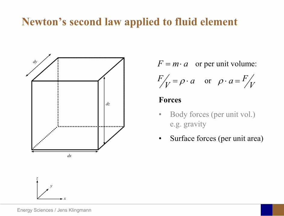
Energy Sciences Jens Klingmann
Newtonrsquos second law applied to fluid element
x
y
z
dy
dz
dx
Forces
bull Body forces (per unit vol) eg gravity
bull Surface forces (per unit area)
amF sdot= or per unit volume
aVF sdot= ρ V
Fa =sdotρor
Energy Sciences Jens Klingmann
Newtonrsquos second law applied to fluid element (outline only)
x
y
z
dy
dz
dx
Stresses
bull Shear stresses
bull Normal stresses
Pressure
These are the constitutive assumption
+=
dzdu
dxdu xz
zx microτ
zyτzyτzzσ
pzz =σ
Energy Sciences Jens Klingmann
Stresses change continuously
Sum of forces in z-direction
Newtonrsquos second law applied to fluid element
zp
VF
dxdydzzpF
dxdydzVdydxA
dzzpAdp
zppApAF
z
z
z
partpart
minus=
partpart
minus=
==partpart
minus=
partpart
+sdotminussdot=
x
y
z
dy
dz
dx
p
dzzpp
partpart
+
Same principle in other directions
Same principle for shear stresses
Energy Sciences Jens Klingmann
Acceleration due to timederivatives
but also due to advection (movement into regions with varying velocities)
What about the acceleration
z
clzu
tuz
partpart
zuu z
z partpart
zuz
partpart
partpart
+partpart
+yuu
xuu z
yz
x
Energy Sciences Jens Klingmann
Summing up
zu
zyu
yxu
xzp
zuu
yuu
xuu
tu
zu
zyu
yxu
xyp
zu
uy
uu
xu
ut
u
zu
zyu
yxu
xxp
zuu
yuu
xuu
tu
zzzzz
zy
zx
z
yyyyz
yy
yx
y
xxxxz
xy
xx
x
partpart
partpart
+partpart
partpart
+partpart
partpart
+partpart
minus=
part
part+
partpart
+partpart
+part
part
part
part
partpart
+part
part
partpart
+part
part
partpart
+partpart
minus=
part
part+
part
part+
part
part+
part
part
partpart
partpart
+part
partpartpart
+part
partpartpart
+partpart
minus=
part
part+
partpart
+part
part+
partpart
micromicromicroρ
micromicromicroρ
micromicromicroρ
Navier-Stokes Equations Incompressible (isochoric)
Energy Sciences Jens Klingmann
Summing up
4 unknown (3 velocity components pressure)4 equations (3 NS eq and continuity)
Nonlinear second order set of PDEOnly very simple analytic solution available
0=part
part+
part
part+
partpart
zu
yu
xu zyx
zu
zyu
yxu
xzp
zuu
yuu
xuu
tu
zu
zyu
yxu
xyp
zu
uy
uu
xu
ut
u
zu
zyu
yxu
xxp
zuu
yuu
xuu
tu
zzzzz
zy
zx
z
yyyyz
yy
yx
y
xxxxz
xy
xx
x
partpart
partpart
+partpart
partpart
+partpart
partpart
+partpart
minus=
part
part+
partpart
+partpart
+part
part
part
part
partpart
+part
part
partpart
+part
part
partpart
+partpart
minus=
part
part+
part
part+
part
part+
part
part
partpart
partpart
+part
partpartpart
+part
partpartpart
+partpart
minus=
part
part+
partpart
+part
part+
partpart
micromicromicroρ
micromicromicroρ
micromicromicroρ
Navier-Stokes Equations Incompressible (isochoric)
and continuity eq
Worst slide ever
Energy Sciences Jens Klingmann
Solving the equations Equations solved in discrete point in a grid (mesh)
Derivatives approximated by eg finite differences
System transformed to large set of algebraic equations
xxjiji
ji ∆
minusasymp
partpart + 1
φφφ
Where φ is any dependent variable and ∆xis the distance between the meshpoints
∆x Example
Energy Sciences Jens Klingmann
Turbulence
Energy Sciences Jens Klingmann
Osborne Reynoldsrsquo Experiments
Energy Sciences Jens Klingmann
Characteristics of turbulence
bull Irregularity
bull Diffusivity the capability of turbulence to enhance transport of mass heat and momentum
bull Large Reynolds numbers Many flow fields are laminar at low Re but become unstable and turbulent at higher Re
bull Three-dimensional vorticity fluctuations
bull Dissipation Viscous shear stresses perform deformation work on the fluid which increases the internal energy at the expense of the kinetic energy
bull Continuum In most technical applications the distance between molecules is orders of magnitude shorter than the size of even the smallest scales of the flow
Energy Sciences Jens Klingmann
Turbulence is irregularity
025 03 035 04 045 05t0
001002003004005006007008009
01
u(x
t)
u(xt)
u(x)
bull Small (unresolvable) scalesbull Statistical approach required bull How can we define an average velocity
0
1( ) ( )T
u u t dtT
= intx x
Energy Sciences Jens Klingmann
Turbulence averaging
Havenrsquot we already done this once
Energy Sciences Jens Klingmann
y zx zz z z z z z
x y z
z z z
u uu uu u u u u uu u ut x x y y z z
u u upz x x y y z z
ρ
micro micro micro
partpartpart part part part part + + + + + + = part part part part part part part
part part partpart part part part= minus + + +
part part part part part part part
Turbulence averaging
uuu += ppp +=
Insert into NS (only z-direction shown) and average entire equation
and
Decompose velocity and pressure (Reynoldsrsquo decomposition)
Additional terms that look like stresses
Energy Sciences Jens Klingmann
Turbulence RANS modellingReynoldsrsquo stress tensor
Needs to be expressed as a function of variables we know or intend to solve for
TURBULENCE MODEL
x x x y x z
y x y y y z
z x z y z z
u u u u u u
u u u u u u
u u u u u u
ρ
=
R
6 new variables (symmetry )xyyx uuuu =
Energy Sciences Jens Klingmann
Turbulence RANS modellingReynolds stress tensor
ij i j
u u u v u w
R u u v u v v v w
w u w v w w
ρ ρ ρ
= minus otimes = = =
R u u
Turbulent Kinetic Energy
( ) ( )1 1 1 1 2 2 2 2ii i ik tr R u u u u v v w wρ ρ= = = = + +R
Represents the kinetic energy of the fluctuations (or vortices)
Energy Sciences Jens Klingmann
Turbulence closure problem
10 unknownvelocity components pressure and correlations of fluctuating velocity
4 equationsAveraged momentum equations and averaged continuity equation
i ju u
Energy Sciences Jens Klingmann
Turbulence RANS modelling
23
i jij T ij
j i
u uR kx x
micro ρ δ part part
= + minus part part
2 T kmicro ρ εpropldquoTurbulent viscosityrdquo
Transport of k Some terms may be derived other need modelling
( ) ( ) ( )advection diffusion productionk k k kt
εpart+ + = minus
part
Energy from mean flow to turbulence
Dissipation Energy converted to heat
Energy Sciences Jens Klingmann
Turbulence RANS modelling
23
i jij T ij
j i
u uR kx x
micro ρ δ part part
= + minus part part ερmicro micro 2kCT =
k Tklk
k l k k k
uk ku Rx x x x
microρ ε micro
σ part part part part
= minus + + part part part part 2
1 2k T
klkk l k k
uu C R C
x k x k x xε εε
microε ε ε ερ ρ micropart σ
part part part part= minus + + part part part
4411 =εC 9212 =εC 090=microC 1=kσ31=εσ
Closure coefficients
Energy Sciences Jens Klingmann
Energy Sciences Jens Klingmann
Computational Fluid Dynamics (CFD)
U Waringhleacuten ldquoThe Aerodynamic design and testing of a supersonic turbine for rocket engine propulsionrdquo Proc Of 3rd European conference on Turbomachinery Fluid dynamics and thermodynamics
Energy Sciences Jens Klingmann
Subsonic flow in an aerofoilplate junction computed with a second-moment closure (D Apsley 1998)
Computational Fluid Dynamics(CFD)
Energy Sciences Jens Klingmann
Hydraulic turbine research CFD digital simulation Distribution of speed on an axial turbine
Computational Fluid Dynamics(CFD)
Energy Sciences Jens Klingmann
Scales of turbulence
10-01
1000
1001
1002
1003
1004
1005
κ LI
10-08
10-07
10-06
10-05
10-04
10-03
10-02
10-01
1000
E(u
2 LI)
10-04
10-03
10-02
10-01
1000
κ LK
10-05
10-04
10-03
10-02
10-01
1000
1001
1002
D( ε L
K )10-01
1000
1001
1002
1003
1004
1005
E = 15 (κ LI)-53
10-04
10-03
10-02
10-01
1000
1001
D = 3 ( κ LΚ) 13
Normalized energy and dissipation spectra for
Adapted from Tennekeys and Lumley
ReLI= times2 105
1 2Re 500IL asymp
3 4Re 10000IL asymp
Energy Sciences Jens Klingmann
References Turbulence
bull Tennekeys and Lumley ldquoA first course in Turbulencerdquo MIT Press 1972
bull J O Hinze ldquoTurbulencerdquo McGraw-Hill 1959bull D C Wilcox ldquoTurbulence Modeling for CFDrdquo DCW Industries
2006
Energy Sciences Jens Klingmann
Boundary layers
Energy Sciences Jens Klingmann
Boundary Layer Theory (BLT) Sensitive to Pressure
gradients Appropriate scaling from
dimensional analyses
Energy Sciences Jens Klingmann
Boundary layers
Energy Sciences Jens Klingmann
Air foil theory
Energy Sciences Jens Klingmann
Visualisation of diffusor separation
Energy Sciences Jens Klingmann
BL equations
+minus=+
yu
yxp
xuv
xuu
partpartmicro
partpart
partpart
partρpart
partρpart and 0=+
yxu
partυpart
partpart
Applying the BL approximations the 2D stationary incompressible NS-eq and continuity equation become
yvu
yu
yxuu
xp
yu
xuu
partpartρ
partpartmicro
partpart
partρpart
partpart
partυρpart
partρpart
minus
+minusminus=+
and
0=+yx
upart
υpartpartpart
Reynolds averaged BL eqs are
Energy Sciences Jens Klingmann
Boundary layers
Energy Sciences Jens Klingmann
Turbulent BL at different Pressure gradients
Energy Sciences Jens Klingmann
Boundary Layers
ν
yuy =+
ρτWu =
0=
partpart
=y
w yuτ
uuu =+
Energy Sciences Jens Klingmann
Diffuser efficiency
Energy Sciences Jens Klingmann
Reynolds Number (Order of magnitude)
At eg a compressor inlet
ρ = O(1) kgm3
U = O(100) msx lt O(01) mmicro = O(10-5)
Re = ρ U x micro =O(106)
In subsequent stages large amounts of turbulence (from stator wakes) will be convected into the Boundary layer
Energy Sciences Jens Klingmann
References Boundary layers
bull Frank M White ldquoViscous Fluid Flowrdquobull Hermann Schlichting ldquoBoundary Layer Theoryrdquo
Energy Sciences Jens Klingmann
CFD and experiments
bull No this is not a CFD course butbull Experiments
Energy Sciences Jens Klingmann
What do we need to measureOverall performance
Flow rates (mass or volume) Pressure Temperature Shaft power
Performance increase
Separations (velocity) Secondary flows eg tip clearance losses (velocity) Shock waves (supersonic applications) Pressure (resolved in time and space) Temperature (resolved in time and space)
Energy Sciences Jens Klingmann
Cascade wind tunnels
FIG 31 Compressor cascade wind tunnels (a) Conventional low-speed continuousrunning cascade tunnel (adapted from Carter et al 1950)(b) Transonicsupersoniccascade tunnel (adapted from Sieverding 1985)
Energy Sciences Jens Klingmann
Closed circuit tunnels
Energy Sciences Jens Klingmann
components
Settling Chamber
The settling chamber is located between the fan or wide angle diffuser and the contraction and contains the honeycombs and screens used to moderate longitudinal variations in the flow Screens in the chamber should be spaced at 02 chamber diameters apart so that flow disturbed by the first screen can settle before it encounters the second
Honeycombs
Honeycombs are located in the settling chamber and are used to reduce nonuniformities in the flow For optimum benefit honeycombs should be 6-8 cell diameters thick and cell size should be on the order of about 150 cells per settling chamber diameter
Energy Sciences Jens Klingmann
components
Screens
Screens are typically located just downstream of the honeycomb and sometime at the inlet of the test section Screens create a static pressure drop and serve to reduce boundary layer size and increase flow uniformity
Contraction Section
Contractions sections are located between the settling chamber and the test sections and serve to both increase mean velocities at the test section inlet and moderate inconsistencies in the uniformity of the flow Large contraction ratios and short contraction lengths are generally more desirable as they reduce the power loss across the screens and the thickness of boundary layers Small tunnels typically have contraction ratios between 6 and 9
Energy Sciences Jens Klingmann
Flow meters with pressure measurement
Venturi-tube
A1 A2
P1 P2
1 1 2 2C A C A=In the incompressible case
2 21 1 2 2
2 2C P C P
ρ ρ+ = +Assuming horisontal mounting
Energy Sciences Jens Klingmann
Daniel Bernoulli 1700-1782
Daniel Bernoulli was the son of Johann Bernoulli He was born in Groningen while his father held the chair of mathematics there His older brother was Nicolaus(II) Bernoulli and his uncle was Jacob Bernoulli so he was born into a family of leading mathematicians but also into a family where there was unfortunate rivalry jealousy and bitterness
Undoubtedly the most important work which Daniel Bernoulli did was his work on hydrodynamics Even the term itself is based on the title of the work which he produced called Hydrodynamica and before he left St Petersburg Daniel left a draft copy of the book with a printer However the work was not published until 1738 and although he revised it considerably between 1734 and 1738 it is more the presentation that he changed rather then the substance
This work contains for the first time the correct analysis of water flowing from a hole in a container This was based on the principle of conservation of energy which he had studied with his father in 1720 Daniel also discussed pumps and other machines to raise water One remarkable discovery appears in Chapter 10 of Hydrodynamica where Daniel discussed the basis for the kinetic theory of gases He was able to give the basic laws for the theory of gases and gave although not in full detail the equation of state discovered by Van der Waals a century later
Energy Sciences Jens Klingmann
Venturi-tube (2)
22 2 12 2
2
2A PC CA ρ
∆minus =
A1 A2
P1 P2
Solve for eg C2
1 2P P P∆ = minus
( )
12
2 2 21 2
21
PCA Aρ
∆ = minus
and( )
12
2 2 2 2 21 2
21
Pm A C AA Aρρ
∆ = = minus
where
Flow meters with pressure measurement
Energy Sciences Jens Klingmann
Flow meters with pressure measurement
Orifice meters
A1
A2
P1 P2
Applicable for pipe flows Same principle as for Venturi Positioning of pressure taps important Vena contracta and losses require inclusion
of Discharge Coefficient CD
( )
12
2 2 21 2
21D
Pm C AA Aρ ∆ =
minus where ( )1 2ReDC f A A=
CD available from manufacturer (measurements) or Standards (eg ISO)
Energy Sciences Jens Klingmann
Coriolis flow meter
An actuator (not shown) induces a vibration of the tubes
When there is mass flow Coriolis forces induce twisting of the tubes
degree of phase-shift is a measure for the amount of mass that is flowing through the tubes
Energy Sciences Jens Klingmann
Thermal flow meter Heat is added electrically to the flow Temperature is measured before and after heat addition
pP mC T∆=
Energy Sciences Jens Klingmann
Ultrasonic flow meters
Ultrasound is emitted to small particles in the flow (dust or other) Reflections of the sound is frequency shifted by the Doppler effect The frequency change is proportional to the particles velocity (volume flow
meter)
Energy Sciences Jens Klingmann
Inductive flow metersA magnetic flowmeter is based upon Faradays Law
The voltage induced across any conductor as it moves at right angles through a magnetic field is proportional to the velocity of that conductor
E is proportional to V x B x D where
E = The voltage generated in a conductorV = The velocity of the conductorB = The magnetic field strengthD = The length of the conductor
NB electric conductivity is required
Energy Sciences Jens Klingmann
Temperature measurements
Thermocouples
The basis established by Thomas Johann Seebeck in 1821
A conductor generates a voltage when subjected to a temperature gradient
To measure this voltage one must use a second conductor material which generates a different voltage under the same temperature gradient
Energy Sciences Jens Klingmann
Pressure sensing
1 2p pgt 2p p2 may be the atmosphere a static pressure tap or a known reference pressure
The strain of the diaphragm (or itrsquos deflection) may be measured by a number of electric methods
Diaphragm
Energy Sciences Jens Klingmann
Pressure sensingPiezoresistive Strain Gage
Uses the piezoresistive effect of bonded or formed strain gauges to detect strain due to applied pressure
Capacitive
Uses a diaghragm and pressure cavity to create a variable capacitor to detect strain due to applied pressure
Magnetic
Measures the displacement of a diaphragm by means of changes in inductance (reluctance) LVDT Hall Effect or by eddy current principal
Piezoelectric
Uses the piezoelectric effect in certain materials such as quartz to measure the strain upon the sensing mechanism due to pressure
Potentiometric
Uses the motion of a wiper along a resistive mechanism to detect the strain caused by applied pressure
Energy Sciences Jens Klingmann
3D highly instationary (periodic) flow Potentially very high velocities (Supersonic) Large temperature differences Low accessibility (difficult to probe between rotors) Low turbulence levels in most of the domain Very high turbulence in BL and wakes
Properties of measuring object
Point measurements
Energy Sciences Jens Klingmann
Conventional or non-opticalndash Static Pressure Measurementsndash Total Pressure Measurements
bull Multy hole probes
ndash Total Temperature ndash Hot Wire Anemometry (HWA)
Optical techniques for Velocity Measurementsndash Laser Two Focous (L2F)ndash Laser Doppler Anemometry (LDA)ndash Particle Image velocimetry (PIV)
Point Measurements
Energy Sciences Jens Klingmann
Static and total pressure
2 2 21 2 1
2 1 2 2 2C C CP P ρ ρ ρ
minus = minus =
2 0C =Stagnation point
C1Static pressure tap
Prandtl or Pitot tube
Apply the Bernoulli equation from free stream to stagnation point
21
2 12CP Pρ
= +or
We can also define a stagnation or total pressure
( )2
101 1 022
CP P Pρ= + =
Total pressure = Static pressure + dynamic pressure
or
Energy Sciences Jens Klingmann
Static pressure
Energy Sciences Jens Klingmann
Total Pressure and Temperature
Shrouded Probes
Shrouded Probe
Pitot or Prandtl tube
Sensitive to direction
Energy Sciences Jens Klingmann
Ludwig Prandtl 1875-1953
Ludwig Prandtl born at Freising Bavaria on February 4 1875 was a German Physicist famous for his work in aeronautics He qualified at Munchen in 1900 with a thesis on elastic stability and held the position of Professor of Applied Mechanics at Gottingen for forty-nine years (from 1904 until his death there on August 15 1953) In 1925 Prandtl became the Director of the Kaiser Wilhelm Institute for Fluid Mechanics His discovery in 1904 of the Boundary Layer which adjoins the surface of a body moving in a fluid led to an understanding of skin friction drag and of the way in which streamlining reduces the drag of airplane wings and other moving bodies His work on wing theory published in 1918 - 1919 followed that of FW Lanchester (1902-1907) but was carried out independently and elucidated the flow over airplane wings of finite span Prandtls work and decisive advances in boundary layer and wing theories became the basic material of aeronautics He also made important contributions to the theories of supersonic flow and of turbulence and contributed much to the development of wind tunnels and other aerodynamic equipment In addition he devised the soap-film analogy for the torsion of non-circular sections and wrote on the theory of plasticity and of meteorology
Energy Sciences Jens Klingmann
Total Pressure multy hole
Cobra Probe Yaw Probe
5 Hole Probe
Energy Sciences Jens Klingmann
5 Hole Probes Calibration
Energy Sciences Jens Klingmann
The inherent unsteadiness of the flow within turbomachines
Energy Sciences Jens Klingmann
Hot Wire Anemometry (HWA) The heat transfer from a thin (one micron)
electrically heated wire can be used to determine velocity
The resistance of the wire is temperature dependent Within a small temperature range it can be assumed linear R = R0+α R0(Tm-T0) where R0 is the resistance at a reference temperature T0 and Tm is the mean wire temperature
The thermal power induced in the wire is balanced by heat transfer to the surrounding fluid I2R=hπDL(Tm-T0) where h is the heat transfer coefficient and D and L the diameter and length of the wire respectively
E = I R
Energy Sciences Jens Klingmann
Constant Temperature Anemometry (CTA) The wire is often placed in a Whetstone bridge If the output from the
bridge is amplified and fed back to the bridge the resistance of the probe and thus the temperature will be held constant
This prevents the temperature of the wire to become excessive at low velocities
R1
R2 R3
Probe
Bridge Voltage
Energy Sciences Jens Klingmann
Constant Temperature Anemometry (CTA)
Energy Sciences Jens Klingmann
Characteristics of LDA (according to Dantec)
Invented by Yeh and Cummins in 1964 Velocity measurements in Fluid Dynamics (gas liquid) Up to 3 velocity components Non-intrusive measurements (optical technique) Absolute measurement technique (no calibration required) Very high accuracy Very high spatial resolution due to small measurement volume Tracer particles are required
Energy Sciences Jens Klingmann
LDA - Fringe Model
Focused Laser beams intersect and form the measurement volume Plane wave fronts beam waist in the plane of intersection Interference in the plane of intersection Pattern of bright and dark stripesplanes Fringes
Energy Sciences Jens Klingmann
LDA-measuring volume
d
x
x
y
y
z
z
e-2 CONTOUR
FRINGES
κ
κ
κ
κ
De-2
De-2
dml m
a
b
cx
b
z
ya
cd
d
=
=
=
J
J
J
J
JP
JP
JP
JD
JD
JD
+
+
+
a
b
c
d
κπλ
=minus sinD
f4l2e
m
κπλ
=minus cosD
f4D2e
m
Energy Sciences Jens Klingmann
Laser Two Focus
Energy Sciences Jens Klingmann
Laser Two Focus
Energy Sciences Jens Klingmann
PIV measurements
PIV is a fairly new technique capable of simultaneous velocity measurements at many points in a plane This gives information on large scale structures vorticity etc which is very difficult or impossible to obtain from one-point measuring techniques
PIV involves the illumination of a plane of the flow under investigation with a thin pulsed sheet of light The flow is seeded with particles
The light scattered from the particles and from successive pulses are being recorded either on film or a CCD array forming a multiple exposure of each particle image If the time between the pulses is known velocity can be determined as the ratio of the particle displacement and the elapsed time
t∆∆= xu
Energy Sciences Jens Klingmann
PIV
Energy Sciences Jens Klingmann
PIV measurements illumination
YA
G
YA
G
Two frequency doubled YAG Lasers aligned to one double pulsed laser sheet
Two or more separate light pulses can be obtained by chopping a continuous laser or from pulsed lasers
The limited pulse energies obtained from continuous lasers limits their applicability to low velocity flows or flows where large seeding particles can be used (ie liquid flows)
The low repetition rate of most pulsed lasers makes the use of two lasers advantageous
Energy Sciences Jens Klingmann
PIV measurements recording
High seeding density in laminar flame
Film or CCD-cameras Cross- or Auto-correlation
ndash ie both particle images on the same frame or on separate frames
CCD-camera requirementndash A many pixels as possiblendash 2k by 2k available 4k by 4k coming
Energy Sciences Jens Klingmann
PIV measurements analyses
Low seeding density (Number of seeding particles per unit volume)
Each particle image pair can be identified This is called particle tracking
High seeding density (PIV)
Small sub-regions of the image containing many particle image pairs are processed to obtain one velocity vector
Energy Sciences Jens Klingmann
PIV measurements analyses
Energy Sciences Jens Klingmann
PIV measurements analyses
( ) ( ) ( ) xsxxs dIIR 2A
1
I
+= int
Cross correlation between ( )x1I and ( )x2I
s is a two dimensional displacement vector
IA is the interrogation area
Cross correlation between
(
)
x
1
I
and
(
)
x
2
I
s is a two dimensional displacement vector
I
A
is the interrogation area
Energy Sciences Jens Klingmann
Energy Sciences Jens Klingmann
PIV from IOWA state university
Energy Sciences Jens Klingmann
PIV sample of evaluation
Energy Sciences Jens Klingmann
LDA PIV HWA Velocity range 01 mms ndash 300
ms 02 ndash 150 ms
Measuring Volume
D = 005 L = 05 mm
2 by 2 by 05 mm
L = 05 mm
Freq response O(10 000) Hz O(10) Hz O(100 000) Hz Calibration Yes No No Sensitivity to other than velocity
Low (ref Index) Low (ref Index) Large (temperature concentrationshellip)
Continuous Signal
Sometimes Seldom Always
Noise High High Low Turbulence intensity
No limitation Some limitation lt 20
Price O(1 000 000) SEK
O(1 000 000) SEK
O(50 000) SEK
Required Knowledge
High medium Low
Comparison of techniques
Energy Sciences Jens Klingmann
References experiments
R J Goldstein ldquoFluid Mechanics Measurementsrdquo Hemisphere Publishing 1983 A V Johansson amp P H Alfredsson ldquoExperimentella metoder inom
stroumlmningsmekanikenrdquo Inst Foumlr Mekanik KTH F Durst A Melling and J H Whitelaw ldquoPrincipals and Practice of Laser Doppler
Anemometryrdquo 1984 R J Adrian ldquoParticle-imaging techniques for experimental fluid mechnicsrdquo Ann Rev
Fluid Mech 1991
Energy Sciences Jens Klingmann
Sample of LDA-measurements
Rotor blade
Glas window
Emitted beams
Scattered Light
Adjustable mirror
Energy Sciences Jens Klingmann
Axial velocity sorted into 10 bins
0 1 2 3 4 5 6tangential coordinate (degrees)
-20
0
20
40
60
80
100
120
140
160Ax
ial v
eloc
ity a
nd s
tand
ard
devi
atio
n (m
s)
radial position 7 mm from inner window surfaceaxial position 23 mm behind rotor blades
Energy Sciences Jens Klingmann
Axial velocities in the radial-tangential plane
Energy Sciences Jens Klingmann
Airfoils NACA 4-digit
The NACA four-digit wing sections define the profile by
One digit describing maximum camber as percentage of the chord
One digit describing the distance of maximum camber from the airfoil leading edge in tens of percents of the chord
Two digits describing maximum thickness of the airfoil as percent of the chord
Example the NACA 2412 airfoil has a maximum camber of 2 located 40 (04 chords) from the leading edge with a maximum thickness of 12 of the chord
Four-digit series airfoils by default have maximum thickness at 30 of the chord (03 chords) from the leading edge
Energy Sciences Jens Klingmann
Airfoils NACA 4-digit
bull c is the chord lengthbull x is the position along
the chord from 0 to cbull y is the half thickness at
a given value of x (centerline to surface)
bull t is the maximum thickness as a fraction of the chord
Energy Sciences Jens Klingmann
Death by PowerPoint
| LDA | PIV | HWA | |||||
| Velocity range | 01 mms ndash 300 ms | 02 ndash 150 ms | |||||
| Measuring Volume | D = 005 L = 05 mm | 2 by 2 by 05 mm | L = 05 mm | ||||
| Freq response | O(10 000) Hz | O(10) Hz | O(100 000) Hz | ||||
| Calibration | Yes | No | No | ||||
| Sensitivity to other than velocity | Low (ref Index) | Low (ref Index) | Large (temperature concentrationshellip) | ||||
| Continuous Signal | Sometimes | Seldom | Always | ||||
| Noise | High | High | Low | ||||
| Turbulence intensity | No limitation | Some limitation | lt 20 | ||||
| Price | O(1 000 000) SEK | O(1 000 000) SEK | O(50 000) SEK | ||||
| Required Knowledge | High | medium | Low |
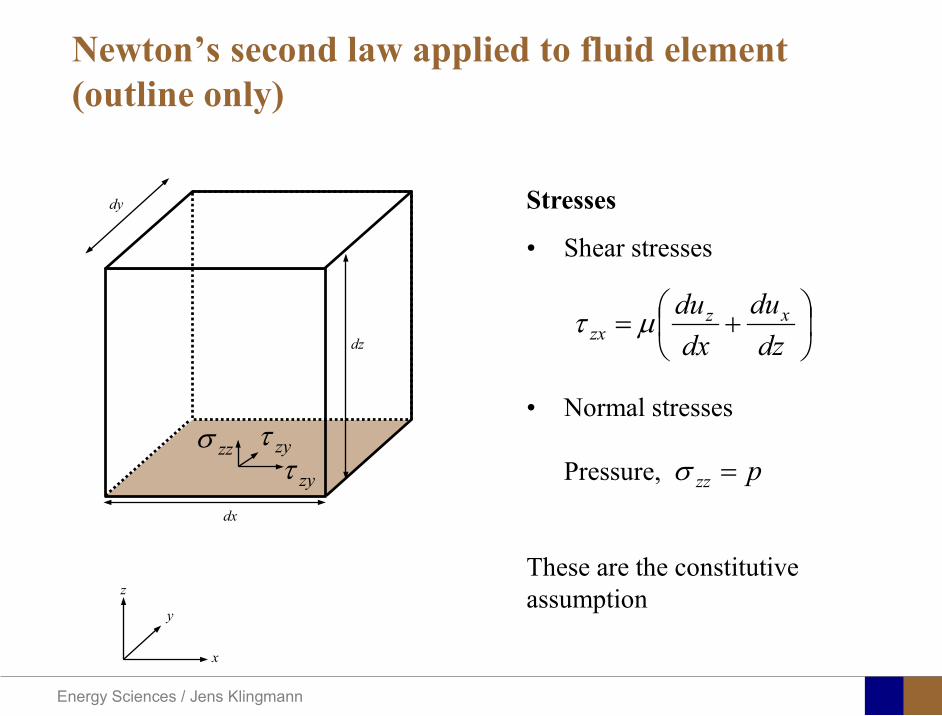
Energy Sciences Jens Klingmann
Newtonrsquos second law applied to fluid element (outline only)
x
y
z
dy
dz
dx
Stresses
bull Shear stresses
bull Normal stresses
Pressure
These are the constitutive assumption
+=
dzdu
dxdu xz
zx microτ
zyτzyτzzσ
pzz =σ
Energy Sciences Jens Klingmann
Stresses change continuously
Sum of forces in z-direction
Newtonrsquos second law applied to fluid element
zp
VF
dxdydzzpF
dxdydzVdydxA
dzzpAdp
zppApAF
z
z
z
partpart
minus=
partpart
minus=
==partpart
minus=
partpart
+sdotminussdot=
x
y
z
dy
dz
dx
p
dzzpp
partpart
+
Same principle in other directions
Same principle for shear stresses
Energy Sciences Jens Klingmann
Acceleration due to timederivatives
but also due to advection (movement into regions with varying velocities)
What about the acceleration
z
clzu
tuz
partpart
zuu z
z partpart
zuz
partpart
partpart
+partpart
+yuu
xuu z
yz
x
Energy Sciences Jens Klingmann
Summing up
zu
zyu
yxu
xzp
zuu
yuu
xuu
tu
zu
zyu
yxu
xyp
zu
uy
uu
xu
ut
u
zu
zyu
yxu
xxp
zuu
yuu
xuu
tu
zzzzz
zy
zx
z
yyyyz
yy
yx
y
xxxxz
xy
xx
x
partpart
partpart
+partpart
partpart
+partpart
partpart
+partpart
minus=
part
part+
partpart
+partpart
+part
part
part
part
partpart
+part
part
partpart
+part
part
partpart
+partpart
minus=
part
part+
part
part+
part
part+
part
part
partpart
partpart
+part
partpartpart
+part
partpartpart
+partpart
minus=
part
part+
partpart
+part
part+
partpart
micromicromicroρ
micromicromicroρ
micromicromicroρ
Navier-Stokes Equations Incompressible (isochoric)
Energy Sciences Jens Klingmann
Summing up
4 unknown (3 velocity components pressure)4 equations (3 NS eq and continuity)
Nonlinear second order set of PDEOnly very simple analytic solution available
0=part
part+
part
part+
partpart
zu
yu
xu zyx
zu
zyu
yxu
xzp
zuu
yuu
xuu
tu
zu
zyu
yxu
xyp
zu
uy
uu
xu
ut
u
zu
zyu
yxu
xxp
zuu
yuu
xuu
tu
zzzzz
zy
zx
z
yyyyz
yy
yx
y
xxxxz
xy
xx
x
partpart
partpart
+partpart
partpart
+partpart
partpart
+partpart
minus=
part
part+
partpart
+partpart
+part
part
part
part
partpart
+part
part
partpart
+part
part
partpart
+partpart
minus=
part
part+
part
part+
part
part+
part
part
partpart
partpart
+part
partpartpart
+part
partpartpart
+partpart
minus=
part
part+
partpart
+part
part+
partpart
micromicromicroρ
micromicromicroρ
micromicromicroρ
Navier-Stokes Equations Incompressible (isochoric)
and continuity eq
Worst slide ever
Energy Sciences Jens Klingmann
Solving the equations Equations solved in discrete point in a grid (mesh)
Derivatives approximated by eg finite differences
System transformed to large set of algebraic equations
xxjiji
ji ∆
minusasymp
partpart + 1
φφφ
Where φ is any dependent variable and ∆xis the distance between the meshpoints
∆x Example
Energy Sciences Jens Klingmann
Turbulence
Energy Sciences Jens Klingmann
Osborne Reynoldsrsquo Experiments
Energy Sciences Jens Klingmann
Characteristics of turbulence
bull Irregularity
bull Diffusivity the capability of turbulence to enhance transport of mass heat and momentum
bull Large Reynolds numbers Many flow fields are laminar at low Re but become unstable and turbulent at higher Re
bull Three-dimensional vorticity fluctuations
bull Dissipation Viscous shear stresses perform deformation work on the fluid which increases the internal energy at the expense of the kinetic energy
bull Continuum In most technical applications the distance between molecules is orders of magnitude shorter than the size of even the smallest scales of the flow
Energy Sciences Jens Klingmann
Turbulence is irregularity
025 03 035 04 045 05t0
001002003004005006007008009
01
u(x
t)
u(xt)
u(x)
bull Small (unresolvable) scalesbull Statistical approach required bull How can we define an average velocity
0
1( ) ( )T
u u t dtT
= intx x
Energy Sciences Jens Klingmann
Turbulence averaging
Havenrsquot we already done this once
Energy Sciences Jens Klingmann
y zx zz z z z z z
x y z
z z z
u uu uu u u u u uu u ut x x y y z z
u u upz x x y y z z
ρ
micro micro micro
partpartpart part part part part + + + + + + = part part part part part part part
part part partpart part part part= minus + + +
part part part part part part part
Turbulence averaging
uuu += ppp +=
Insert into NS (only z-direction shown) and average entire equation
and
Decompose velocity and pressure (Reynoldsrsquo decomposition)
Additional terms that look like stresses
Energy Sciences Jens Klingmann
Turbulence RANS modellingReynoldsrsquo stress tensor
Needs to be expressed as a function of variables we know or intend to solve for
TURBULENCE MODEL
x x x y x z
y x y y y z
z x z y z z
u u u u u u
u u u u u u
u u u u u u
ρ
=
R
6 new variables (symmetry )xyyx uuuu =
Energy Sciences Jens Klingmann
Turbulence RANS modellingReynolds stress tensor
ij i j
u u u v u w
R u u v u v v v w
w u w v w w
ρ ρ ρ
= minus otimes = = =
R u u
Turbulent Kinetic Energy
( ) ( )1 1 1 1 2 2 2 2ii i ik tr R u u u u v v w wρ ρ= = = = + +R
Represents the kinetic energy of the fluctuations (or vortices)
Energy Sciences Jens Klingmann
Turbulence closure problem
10 unknownvelocity components pressure and correlations of fluctuating velocity
4 equationsAveraged momentum equations and averaged continuity equation
i ju u
Energy Sciences Jens Klingmann
Turbulence RANS modelling
23
i jij T ij
j i
u uR kx x
micro ρ δ part part
= + minus part part
2 T kmicro ρ εpropldquoTurbulent viscosityrdquo
Transport of k Some terms may be derived other need modelling
( ) ( ) ( )advection diffusion productionk k k kt
εpart+ + = minus
part
Energy from mean flow to turbulence
Dissipation Energy converted to heat
Energy Sciences Jens Klingmann
Turbulence RANS modelling
23
i jij T ij
j i
u uR kx x
micro ρ δ part part
= + minus part part ερmicro micro 2kCT =
k Tklk
k l k k k
uk ku Rx x x x
microρ ε micro
σ part part part part
= minus + + part part part part 2
1 2k T
klkk l k k
uu C R C
x k x k x xε εε
microε ε ε ερ ρ micropart σ
part part part part= minus + + part part part
4411 =εC 9212 =εC 090=microC 1=kσ31=εσ
Closure coefficients
Energy Sciences Jens Klingmann
Energy Sciences Jens Klingmann
Computational Fluid Dynamics (CFD)
U Waringhleacuten ldquoThe Aerodynamic design and testing of a supersonic turbine for rocket engine propulsionrdquo Proc Of 3rd European conference on Turbomachinery Fluid dynamics and thermodynamics
Energy Sciences Jens Klingmann
Subsonic flow in an aerofoilplate junction computed with a second-moment closure (D Apsley 1998)
Computational Fluid Dynamics(CFD)
Energy Sciences Jens Klingmann
Hydraulic turbine research CFD digital simulation Distribution of speed on an axial turbine
Computational Fluid Dynamics(CFD)
Energy Sciences Jens Klingmann
Scales of turbulence
10-01
1000
1001
1002
1003
1004
1005
κ LI
10-08
10-07
10-06
10-05
10-04
10-03
10-02
10-01
1000
E(u
2 LI)
10-04
10-03
10-02
10-01
1000
κ LK
10-05
10-04
10-03
10-02
10-01
1000
1001
1002
D( ε L
K )10-01
1000
1001
1002
1003
1004
1005
E = 15 (κ LI)-53
10-04
10-03
10-02
10-01
1000
1001
D = 3 ( κ LΚ) 13
Normalized energy and dissipation spectra for
Adapted from Tennekeys and Lumley
ReLI= times2 105
1 2Re 500IL asymp
3 4Re 10000IL asymp
Energy Sciences Jens Klingmann
References Turbulence
bull Tennekeys and Lumley ldquoA first course in Turbulencerdquo MIT Press 1972
bull J O Hinze ldquoTurbulencerdquo McGraw-Hill 1959bull D C Wilcox ldquoTurbulence Modeling for CFDrdquo DCW Industries
2006
Energy Sciences Jens Klingmann
Boundary layers
Energy Sciences Jens Klingmann
Boundary Layer Theory (BLT) Sensitive to Pressure
gradients Appropriate scaling from
dimensional analyses
Energy Sciences Jens Klingmann
Boundary layers
Energy Sciences Jens Klingmann
Air foil theory
Energy Sciences Jens Klingmann
Visualisation of diffusor separation
Energy Sciences Jens Klingmann
BL equations
+minus=+
yu
yxp
xuv
xuu
partpartmicro
partpart
partpart
partρpart
partρpart and 0=+
yxu
partυpart
partpart
Applying the BL approximations the 2D stationary incompressible NS-eq and continuity equation become
yvu
yu
yxuu
xp
yu
xuu
partpartρ
partpartmicro
partpart
partρpart
partpart
partυρpart
partρpart
minus
+minusminus=+
and
0=+yx
upart
υpartpartpart
Reynolds averaged BL eqs are
Energy Sciences Jens Klingmann
Boundary layers
Energy Sciences Jens Klingmann
Turbulent BL at different Pressure gradients
Energy Sciences Jens Klingmann
Boundary Layers
ν
yuy =+
ρτWu =
0=
partpart
=y
w yuτ
uuu =+
Energy Sciences Jens Klingmann
Diffuser efficiency
Energy Sciences Jens Klingmann
Reynolds Number (Order of magnitude)
At eg a compressor inlet
ρ = O(1) kgm3
U = O(100) msx lt O(01) mmicro = O(10-5)
Re = ρ U x micro =O(106)
In subsequent stages large amounts of turbulence (from stator wakes) will be convected into the Boundary layer
Energy Sciences Jens Klingmann
References Boundary layers
bull Frank M White ldquoViscous Fluid Flowrdquobull Hermann Schlichting ldquoBoundary Layer Theoryrdquo
Energy Sciences Jens Klingmann
CFD and experiments
bull No this is not a CFD course butbull Experiments
Energy Sciences Jens Klingmann
What do we need to measureOverall performance
Flow rates (mass or volume) Pressure Temperature Shaft power
Performance increase
Separations (velocity) Secondary flows eg tip clearance losses (velocity) Shock waves (supersonic applications) Pressure (resolved in time and space) Temperature (resolved in time and space)
Energy Sciences Jens Klingmann
Cascade wind tunnels
FIG 31 Compressor cascade wind tunnels (a) Conventional low-speed continuousrunning cascade tunnel (adapted from Carter et al 1950)(b) Transonicsupersoniccascade tunnel (adapted from Sieverding 1985)
Energy Sciences Jens Klingmann
Closed circuit tunnels
Energy Sciences Jens Klingmann
components
Settling Chamber
The settling chamber is located between the fan or wide angle diffuser and the contraction and contains the honeycombs and screens used to moderate longitudinal variations in the flow Screens in the chamber should be spaced at 02 chamber diameters apart so that flow disturbed by the first screen can settle before it encounters the second
Honeycombs
Honeycombs are located in the settling chamber and are used to reduce nonuniformities in the flow For optimum benefit honeycombs should be 6-8 cell diameters thick and cell size should be on the order of about 150 cells per settling chamber diameter
Energy Sciences Jens Klingmann
components
Screens
Screens are typically located just downstream of the honeycomb and sometime at the inlet of the test section Screens create a static pressure drop and serve to reduce boundary layer size and increase flow uniformity
Contraction Section
Contractions sections are located between the settling chamber and the test sections and serve to both increase mean velocities at the test section inlet and moderate inconsistencies in the uniformity of the flow Large contraction ratios and short contraction lengths are generally more desirable as they reduce the power loss across the screens and the thickness of boundary layers Small tunnels typically have contraction ratios between 6 and 9
Energy Sciences Jens Klingmann
Flow meters with pressure measurement
Venturi-tube
A1 A2
P1 P2
1 1 2 2C A C A=In the incompressible case
2 21 1 2 2
2 2C P C P
ρ ρ+ = +Assuming horisontal mounting
Energy Sciences Jens Klingmann
Daniel Bernoulli 1700-1782
Daniel Bernoulli was the son of Johann Bernoulli He was born in Groningen while his father held the chair of mathematics there His older brother was Nicolaus(II) Bernoulli and his uncle was Jacob Bernoulli so he was born into a family of leading mathematicians but also into a family where there was unfortunate rivalry jealousy and bitterness
Undoubtedly the most important work which Daniel Bernoulli did was his work on hydrodynamics Even the term itself is based on the title of the work which he produced called Hydrodynamica and before he left St Petersburg Daniel left a draft copy of the book with a printer However the work was not published until 1738 and although he revised it considerably between 1734 and 1738 it is more the presentation that he changed rather then the substance
This work contains for the first time the correct analysis of water flowing from a hole in a container This was based on the principle of conservation of energy which he had studied with his father in 1720 Daniel also discussed pumps and other machines to raise water One remarkable discovery appears in Chapter 10 of Hydrodynamica where Daniel discussed the basis for the kinetic theory of gases He was able to give the basic laws for the theory of gases and gave although not in full detail the equation of state discovered by Van der Waals a century later
Energy Sciences Jens Klingmann
Venturi-tube (2)
22 2 12 2
2
2A PC CA ρ
∆minus =
A1 A2
P1 P2
Solve for eg C2
1 2P P P∆ = minus
( )
12
2 2 21 2
21
PCA Aρ
∆ = minus
and( )
12
2 2 2 2 21 2
21
Pm A C AA Aρρ
∆ = = minus
where
Flow meters with pressure measurement
Energy Sciences Jens Klingmann
Flow meters with pressure measurement
Orifice meters
A1
A2
P1 P2
Applicable for pipe flows Same principle as for Venturi Positioning of pressure taps important Vena contracta and losses require inclusion
of Discharge Coefficient CD
( )
12
2 2 21 2
21D
Pm C AA Aρ ∆ =
minus where ( )1 2ReDC f A A=
CD available from manufacturer (measurements) or Standards (eg ISO)
Energy Sciences Jens Klingmann
Coriolis flow meter
An actuator (not shown) induces a vibration of the tubes
When there is mass flow Coriolis forces induce twisting of the tubes
degree of phase-shift is a measure for the amount of mass that is flowing through the tubes
Energy Sciences Jens Klingmann
Thermal flow meter Heat is added electrically to the flow Temperature is measured before and after heat addition
pP mC T∆=
Energy Sciences Jens Klingmann
Ultrasonic flow meters
Ultrasound is emitted to small particles in the flow (dust or other) Reflections of the sound is frequency shifted by the Doppler effect The frequency change is proportional to the particles velocity (volume flow
meter)
Energy Sciences Jens Klingmann
Inductive flow metersA magnetic flowmeter is based upon Faradays Law
The voltage induced across any conductor as it moves at right angles through a magnetic field is proportional to the velocity of that conductor
E is proportional to V x B x D where
E = The voltage generated in a conductorV = The velocity of the conductorB = The magnetic field strengthD = The length of the conductor
NB electric conductivity is required
Energy Sciences Jens Klingmann
Temperature measurements
Thermocouples
The basis established by Thomas Johann Seebeck in 1821
A conductor generates a voltage when subjected to a temperature gradient
To measure this voltage one must use a second conductor material which generates a different voltage under the same temperature gradient
Energy Sciences Jens Klingmann
Pressure sensing
1 2p pgt 2p p2 may be the atmosphere a static pressure tap or a known reference pressure
The strain of the diaphragm (or itrsquos deflection) may be measured by a number of electric methods
Diaphragm
Energy Sciences Jens Klingmann
Pressure sensingPiezoresistive Strain Gage
Uses the piezoresistive effect of bonded or formed strain gauges to detect strain due to applied pressure
Capacitive
Uses a diaghragm and pressure cavity to create a variable capacitor to detect strain due to applied pressure
Magnetic
Measures the displacement of a diaphragm by means of changes in inductance (reluctance) LVDT Hall Effect or by eddy current principal
Piezoelectric
Uses the piezoelectric effect in certain materials such as quartz to measure the strain upon the sensing mechanism due to pressure
Potentiometric
Uses the motion of a wiper along a resistive mechanism to detect the strain caused by applied pressure
Energy Sciences Jens Klingmann
3D highly instationary (periodic) flow Potentially very high velocities (Supersonic) Large temperature differences Low accessibility (difficult to probe between rotors) Low turbulence levels in most of the domain Very high turbulence in BL and wakes
Properties of measuring object
Point measurements
Energy Sciences Jens Klingmann
Conventional or non-opticalndash Static Pressure Measurementsndash Total Pressure Measurements
bull Multy hole probes
ndash Total Temperature ndash Hot Wire Anemometry (HWA)
Optical techniques for Velocity Measurementsndash Laser Two Focous (L2F)ndash Laser Doppler Anemometry (LDA)ndash Particle Image velocimetry (PIV)
Point Measurements
Energy Sciences Jens Klingmann
Static and total pressure
2 2 21 2 1
2 1 2 2 2C C CP P ρ ρ ρ
minus = minus =
2 0C =Stagnation point
C1Static pressure tap
Prandtl or Pitot tube
Apply the Bernoulli equation from free stream to stagnation point
21
2 12CP Pρ
= +or
We can also define a stagnation or total pressure
( )2
101 1 022
CP P Pρ= + =
Total pressure = Static pressure + dynamic pressure
or
Energy Sciences Jens Klingmann
Static pressure
Energy Sciences Jens Klingmann
Total Pressure and Temperature
Shrouded Probes
Shrouded Probe
Pitot or Prandtl tube
Sensitive to direction
Energy Sciences Jens Klingmann
Ludwig Prandtl 1875-1953
Ludwig Prandtl born at Freising Bavaria on February 4 1875 was a German Physicist famous for his work in aeronautics He qualified at Munchen in 1900 with a thesis on elastic stability and held the position of Professor of Applied Mechanics at Gottingen for forty-nine years (from 1904 until his death there on August 15 1953) In 1925 Prandtl became the Director of the Kaiser Wilhelm Institute for Fluid Mechanics His discovery in 1904 of the Boundary Layer which adjoins the surface of a body moving in a fluid led to an understanding of skin friction drag and of the way in which streamlining reduces the drag of airplane wings and other moving bodies His work on wing theory published in 1918 - 1919 followed that of FW Lanchester (1902-1907) but was carried out independently and elucidated the flow over airplane wings of finite span Prandtls work and decisive advances in boundary layer and wing theories became the basic material of aeronautics He also made important contributions to the theories of supersonic flow and of turbulence and contributed much to the development of wind tunnels and other aerodynamic equipment In addition he devised the soap-film analogy for the torsion of non-circular sections and wrote on the theory of plasticity and of meteorology
Energy Sciences Jens Klingmann
Total Pressure multy hole
Cobra Probe Yaw Probe
5 Hole Probe
Energy Sciences Jens Klingmann
5 Hole Probes Calibration
Energy Sciences Jens Klingmann
The inherent unsteadiness of the flow within turbomachines
Energy Sciences Jens Klingmann
Hot Wire Anemometry (HWA) The heat transfer from a thin (one micron)
electrically heated wire can be used to determine velocity
The resistance of the wire is temperature dependent Within a small temperature range it can be assumed linear R = R0+α R0(Tm-T0) where R0 is the resistance at a reference temperature T0 and Tm is the mean wire temperature
The thermal power induced in the wire is balanced by heat transfer to the surrounding fluid I2R=hπDL(Tm-T0) where h is the heat transfer coefficient and D and L the diameter and length of the wire respectively
E = I R
Energy Sciences Jens Klingmann
Constant Temperature Anemometry (CTA) The wire is often placed in a Whetstone bridge If the output from the
bridge is amplified and fed back to the bridge the resistance of the probe and thus the temperature will be held constant
This prevents the temperature of the wire to become excessive at low velocities
R1
R2 R3
Probe
Bridge Voltage
Energy Sciences Jens Klingmann
Constant Temperature Anemometry (CTA)
Energy Sciences Jens Klingmann
Characteristics of LDA (according to Dantec)
Invented by Yeh and Cummins in 1964 Velocity measurements in Fluid Dynamics (gas liquid) Up to 3 velocity components Non-intrusive measurements (optical technique) Absolute measurement technique (no calibration required) Very high accuracy Very high spatial resolution due to small measurement volume Tracer particles are required
Energy Sciences Jens Klingmann
LDA - Fringe Model
Focused Laser beams intersect and form the measurement volume Plane wave fronts beam waist in the plane of intersection Interference in the plane of intersection Pattern of bright and dark stripesplanes Fringes
Energy Sciences Jens Klingmann
LDA-measuring volume
d
x
x
y
y
z
z
e-2 CONTOUR
FRINGES
κ
κ
κ
κ
De-2
De-2
dml m
a
b
cx
b
z
ya
cd
d
=
=
=
J
J
J
J
JP
JP
JP
JD
JD
JD
+
+
+
a
b
c
d
κπλ
=minus sinD
f4l2e
m
κπλ
=minus cosD
f4D2e
m
Energy Sciences Jens Klingmann
Laser Two Focus
Energy Sciences Jens Klingmann
Laser Two Focus
Energy Sciences Jens Klingmann
PIV measurements
PIV is a fairly new technique capable of simultaneous velocity measurements at many points in a plane This gives information on large scale structures vorticity etc which is very difficult or impossible to obtain from one-point measuring techniques
PIV involves the illumination of a plane of the flow under investigation with a thin pulsed sheet of light The flow is seeded with particles
The light scattered from the particles and from successive pulses are being recorded either on film or a CCD array forming a multiple exposure of each particle image If the time between the pulses is known velocity can be determined as the ratio of the particle displacement and the elapsed time
t∆∆= xu
Energy Sciences Jens Klingmann
PIV
Energy Sciences Jens Klingmann
PIV measurements illumination
YA
G
YA
G
Two frequency doubled YAG Lasers aligned to one double pulsed laser sheet
Two or more separate light pulses can be obtained by chopping a continuous laser or from pulsed lasers
The limited pulse energies obtained from continuous lasers limits their applicability to low velocity flows or flows where large seeding particles can be used (ie liquid flows)
The low repetition rate of most pulsed lasers makes the use of two lasers advantageous
Energy Sciences Jens Klingmann
PIV measurements recording
High seeding density in laminar flame
Film or CCD-cameras Cross- or Auto-correlation
ndash ie both particle images on the same frame or on separate frames
CCD-camera requirementndash A many pixels as possiblendash 2k by 2k available 4k by 4k coming
Energy Sciences Jens Klingmann
PIV measurements analyses
Low seeding density (Number of seeding particles per unit volume)
Each particle image pair can be identified This is called particle tracking
High seeding density (PIV)
Small sub-regions of the image containing many particle image pairs are processed to obtain one velocity vector
Energy Sciences Jens Klingmann
PIV measurements analyses
Energy Sciences Jens Klingmann
PIV measurements analyses
( ) ( ) ( ) xsxxs dIIR 2A
1
I
+= int
Cross correlation between ( )x1I and ( )x2I
s is a two dimensional displacement vector
IA is the interrogation area
Cross correlation between
(
)
x
1
I
and
(
)
x
2
I
s is a two dimensional displacement vector
I
A
is the interrogation area
Energy Sciences Jens Klingmann
Energy Sciences Jens Klingmann
PIV from IOWA state university
Energy Sciences Jens Klingmann
PIV sample of evaluation
Energy Sciences Jens Klingmann
LDA PIV HWA Velocity range 01 mms ndash 300
ms 02 ndash 150 ms
Measuring Volume
D = 005 L = 05 mm
2 by 2 by 05 mm
L = 05 mm
Freq response O(10 000) Hz O(10) Hz O(100 000) Hz Calibration Yes No No Sensitivity to other than velocity
Low (ref Index) Low (ref Index) Large (temperature concentrationshellip)
Continuous Signal
Sometimes Seldom Always
Noise High High Low Turbulence intensity
No limitation Some limitation lt 20
Price O(1 000 000) SEK
O(1 000 000) SEK
O(50 000) SEK
Required Knowledge
High medium Low
Comparison of techniques
Energy Sciences Jens Klingmann
References experiments
R J Goldstein ldquoFluid Mechanics Measurementsrdquo Hemisphere Publishing 1983 A V Johansson amp P H Alfredsson ldquoExperimentella metoder inom
stroumlmningsmekanikenrdquo Inst Foumlr Mekanik KTH F Durst A Melling and J H Whitelaw ldquoPrincipals and Practice of Laser Doppler
Anemometryrdquo 1984 R J Adrian ldquoParticle-imaging techniques for experimental fluid mechnicsrdquo Ann Rev
Fluid Mech 1991
Energy Sciences Jens Klingmann
Sample of LDA-measurements
Rotor blade
Glas window
Emitted beams
Scattered Light
Adjustable mirror
Energy Sciences Jens Klingmann
Axial velocity sorted into 10 bins
0 1 2 3 4 5 6tangential coordinate (degrees)
-20
0
20
40
60
80
100
120
140
160Ax
ial v
eloc
ity a
nd s
tand
ard
devi
atio
n (m
s)
radial position 7 mm from inner window surfaceaxial position 23 mm behind rotor blades
Energy Sciences Jens Klingmann
Axial velocities in the radial-tangential plane
Energy Sciences Jens Klingmann
Airfoils NACA 4-digit
The NACA four-digit wing sections define the profile by
One digit describing maximum camber as percentage of the chord
One digit describing the distance of maximum camber from the airfoil leading edge in tens of percents of the chord
Two digits describing maximum thickness of the airfoil as percent of the chord
Example the NACA 2412 airfoil has a maximum camber of 2 located 40 (04 chords) from the leading edge with a maximum thickness of 12 of the chord
Four-digit series airfoils by default have maximum thickness at 30 of the chord (03 chords) from the leading edge
Energy Sciences Jens Klingmann
Airfoils NACA 4-digit
bull c is the chord lengthbull x is the position along
the chord from 0 to cbull y is the half thickness at
a given value of x (centerline to surface)
bull t is the maximum thickness as a fraction of the chord
Energy Sciences Jens Klingmann
Death by PowerPoint
| LDA | PIV | HWA | |||||
| Velocity range | 01 mms ndash 300 ms | 02 ndash 150 ms | |||||
| Measuring Volume | D = 005 L = 05 mm | 2 by 2 by 05 mm | L = 05 mm | ||||
| Freq response | O(10 000) Hz | O(10) Hz | O(100 000) Hz | ||||
| Calibration | Yes | No | No | ||||
| Sensitivity to other than velocity | Low (ref Index) | Low (ref Index) | Large (temperature concentrationshellip) | ||||
| Continuous Signal | Sometimes | Seldom | Always | ||||
| Noise | High | High | Low | ||||
| Turbulence intensity | No limitation | Some limitation | lt 20 | ||||
| Price | O(1 000 000) SEK | O(1 000 000) SEK | O(50 000) SEK | ||||
| Required Knowledge | High | medium | Low |
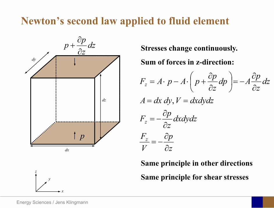
Energy Sciences Jens Klingmann
Stresses change continuously
Sum of forces in z-direction
Newtonrsquos second law applied to fluid element
zp
VF
dxdydzzpF
dxdydzVdydxA
dzzpAdp
zppApAF
z
z
z
partpart
minus=
partpart
minus=
==partpart
minus=
partpart
+sdotminussdot=
x
y
z
dy
dz
dx
p
dzzpp
partpart
+
Same principle in other directions
Same principle for shear stresses
Energy Sciences Jens Klingmann
Acceleration due to timederivatives
but also due to advection (movement into regions with varying velocities)
What about the acceleration
z
clzu
tuz
partpart
zuu z
z partpart
zuz
partpart
partpart
+partpart
+yuu
xuu z
yz
x
Energy Sciences Jens Klingmann
Summing up
zu
zyu
yxu
xzp
zuu
yuu
xuu
tu
zu
zyu
yxu
xyp
zu
uy
uu
xu
ut
u
zu
zyu
yxu
xxp
zuu
yuu
xuu
tu
zzzzz
zy
zx
z
yyyyz
yy
yx
y
xxxxz
xy
xx
x
partpart
partpart
+partpart
partpart
+partpart
partpart
+partpart
minus=
part
part+
partpart
+partpart
+part
part
part
part
partpart
+part
part
partpart
+part
part
partpart
+partpart
minus=
part
part+
part
part+
part
part+
part
part
partpart
partpart
+part
partpartpart
+part
partpartpart
+partpart
minus=
part
part+
partpart
+part
part+
partpart
micromicromicroρ
micromicromicroρ
micromicromicroρ
Navier-Stokes Equations Incompressible (isochoric)
Energy Sciences Jens Klingmann
Summing up
4 unknown (3 velocity components pressure)4 equations (3 NS eq and continuity)
Nonlinear second order set of PDEOnly very simple analytic solution available
0=part
part+
part
part+
partpart
zu
yu
xu zyx
zu
zyu
yxu
xzp
zuu
yuu
xuu
tu
zu
zyu
yxu
xyp
zu
uy
uu
xu
ut
u
zu
zyu
yxu
xxp
zuu
yuu
xuu
tu
zzzzz
zy
zx
z
yyyyz
yy
yx
y
xxxxz
xy
xx
x
partpart
partpart
+partpart
partpart
+partpart
partpart
+partpart
minus=
part
part+
partpart
+partpart
+part
part
part
part
partpart
+part
part
partpart
+part
part
partpart
+partpart
minus=
part
part+
part
part+
part
part+
part
part
partpart
partpart
+part
partpartpart
+part
partpartpart
+partpart
minus=
part
part+
partpart
+part
part+
partpart
micromicromicroρ
micromicromicroρ
micromicromicroρ
Navier-Stokes Equations Incompressible (isochoric)
and continuity eq
Worst slide ever
Energy Sciences Jens Klingmann
Solving the equations Equations solved in discrete point in a grid (mesh)
Derivatives approximated by eg finite differences
System transformed to large set of algebraic equations
xxjiji
ji ∆
minusasymp
partpart + 1
φφφ
Where φ is any dependent variable and ∆xis the distance between the meshpoints
∆x Example
Energy Sciences Jens Klingmann
Turbulence
Energy Sciences Jens Klingmann
Osborne Reynoldsrsquo Experiments
Energy Sciences Jens Klingmann
Characteristics of turbulence
bull Irregularity
bull Diffusivity the capability of turbulence to enhance transport of mass heat and momentum
bull Large Reynolds numbers Many flow fields are laminar at low Re but become unstable and turbulent at higher Re
bull Three-dimensional vorticity fluctuations
bull Dissipation Viscous shear stresses perform deformation work on the fluid which increases the internal energy at the expense of the kinetic energy
bull Continuum In most technical applications the distance between molecules is orders of magnitude shorter than the size of even the smallest scales of the flow
Energy Sciences Jens Klingmann
Turbulence is irregularity
025 03 035 04 045 05t0
001002003004005006007008009
01
u(x
t)
u(xt)
u(x)
bull Small (unresolvable) scalesbull Statistical approach required bull How can we define an average velocity
0
1( ) ( )T
u u t dtT
= intx x
Energy Sciences Jens Klingmann
Turbulence averaging
Havenrsquot we already done this once
Energy Sciences Jens Klingmann
y zx zz z z z z z
x y z
z z z
u uu uu u u u u uu u ut x x y y z z
u u upz x x y y z z
ρ
micro micro micro
partpartpart part part part part + + + + + + = part part part part part part part
part part partpart part part part= minus + + +
part part part part part part part
Turbulence averaging
uuu += ppp +=
Insert into NS (only z-direction shown) and average entire equation
and
Decompose velocity and pressure (Reynoldsrsquo decomposition)
Additional terms that look like stresses
Energy Sciences Jens Klingmann
Turbulence RANS modellingReynoldsrsquo stress tensor
Needs to be expressed as a function of variables we know or intend to solve for
TURBULENCE MODEL
x x x y x z
y x y y y z
z x z y z z
u u u u u u
u u u u u u
u u u u u u
ρ
=
R
6 new variables (symmetry )xyyx uuuu =
Energy Sciences Jens Klingmann
Turbulence RANS modellingReynolds stress tensor
ij i j
u u u v u w
R u u v u v v v w
w u w v w w
ρ ρ ρ
= minus otimes = = =
R u u
Turbulent Kinetic Energy
( ) ( )1 1 1 1 2 2 2 2ii i ik tr R u u u u v v w wρ ρ= = = = + +R
Represents the kinetic energy of the fluctuations (or vortices)
Energy Sciences Jens Klingmann
Turbulence closure problem
10 unknownvelocity components pressure and correlations of fluctuating velocity
4 equationsAveraged momentum equations and averaged continuity equation
i ju u
Energy Sciences Jens Klingmann
Turbulence RANS modelling
23
i jij T ij
j i
u uR kx x
micro ρ δ part part
= + minus part part
2 T kmicro ρ εpropldquoTurbulent viscosityrdquo
Transport of k Some terms may be derived other need modelling
( ) ( ) ( )advection diffusion productionk k k kt
εpart+ + = minus
part
Energy from mean flow to turbulence
Dissipation Energy converted to heat
Energy Sciences Jens Klingmann
Turbulence RANS modelling
23
i jij T ij
j i
u uR kx x
micro ρ δ part part
= + minus part part ερmicro micro 2kCT =
k Tklk
k l k k k
uk ku Rx x x x
microρ ε micro
σ part part part part
= minus + + part part part part 2
1 2k T
klkk l k k
uu C R C
x k x k x xε εε
microε ε ε ερ ρ micropart σ
part part part part= minus + + part part part
4411 =εC 9212 =εC 090=microC 1=kσ31=εσ
Closure coefficients
Energy Sciences Jens Klingmann
Energy Sciences Jens Klingmann
Computational Fluid Dynamics (CFD)
U Waringhleacuten ldquoThe Aerodynamic design and testing of a supersonic turbine for rocket engine propulsionrdquo Proc Of 3rd European conference on Turbomachinery Fluid dynamics and thermodynamics
Energy Sciences Jens Klingmann
Subsonic flow in an aerofoilplate junction computed with a second-moment closure (D Apsley 1998)
Computational Fluid Dynamics(CFD)
Energy Sciences Jens Klingmann
Hydraulic turbine research CFD digital simulation Distribution of speed on an axial turbine
Computational Fluid Dynamics(CFD)
Energy Sciences Jens Klingmann
Scales of turbulence
10-01
1000
1001
1002
1003
1004
1005
κ LI
10-08
10-07
10-06
10-05
10-04
10-03
10-02
10-01
1000
E(u
2 LI)
10-04
10-03
10-02
10-01
1000
κ LK
10-05
10-04
10-03
10-02
10-01
1000
1001
1002
D( ε L
K )10-01
1000
1001
1002
1003
1004
1005
E = 15 (κ LI)-53
10-04
10-03
10-02
10-01
1000
1001
D = 3 ( κ LΚ) 13
Normalized energy and dissipation spectra for
Adapted from Tennekeys and Lumley
ReLI= times2 105
1 2Re 500IL asymp
3 4Re 10000IL asymp
Energy Sciences Jens Klingmann
References Turbulence
bull Tennekeys and Lumley ldquoA first course in Turbulencerdquo MIT Press 1972
bull J O Hinze ldquoTurbulencerdquo McGraw-Hill 1959bull D C Wilcox ldquoTurbulence Modeling for CFDrdquo DCW Industries
2006
Energy Sciences Jens Klingmann
Boundary layers
Energy Sciences Jens Klingmann
Boundary Layer Theory (BLT) Sensitive to Pressure
gradients Appropriate scaling from
dimensional analyses
Energy Sciences Jens Klingmann
Boundary layers
Energy Sciences Jens Klingmann
Air foil theory
Energy Sciences Jens Klingmann
Visualisation of diffusor separation
Energy Sciences Jens Klingmann
BL equations
+minus=+
yu
yxp
xuv
xuu
partpartmicro
partpart
partpart
partρpart
partρpart and 0=+
yxu
partυpart
partpart
Applying the BL approximations the 2D stationary incompressible NS-eq and continuity equation become
yvu
yu
yxuu
xp
yu
xuu
partpartρ
partpartmicro
partpart
partρpart
partpart
partυρpart
partρpart
minus
+minusminus=+
and
0=+yx
upart
υpartpartpart
Reynolds averaged BL eqs are
Energy Sciences Jens Klingmann
Boundary layers
Energy Sciences Jens Klingmann
Turbulent BL at different Pressure gradients
Energy Sciences Jens Klingmann
Boundary Layers
ν
yuy =+
ρτWu =
0=
partpart
=y
w yuτ
uuu =+
Energy Sciences Jens Klingmann
Diffuser efficiency
Energy Sciences Jens Klingmann
Reynolds Number (Order of magnitude)
At eg a compressor inlet
ρ = O(1) kgm3
U = O(100) msx lt O(01) mmicro = O(10-5)
Re = ρ U x micro =O(106)
In subsequent stages large amounts of turbulence (from stator wakes) will be convected into the Boundary layer
Energy Sciences Jens Klingmann
References Boundary layers
bull Frank M White ldquoViscous Fluid Flowrdquobull Hermann Schlichting ldquoBoundary Layer Theoryrdquo
Energy Sciences Jens Klingmann
CFD and experiments
bull No this is not a CFD course butbull Experiments
Energy Sciences Jens Klingmann
What do we need to measureOverall performance
Flow rates (mass or volume) Pressure Temperature Shaft power
Performance increase
Separations (velocity) Secondary flows eg tip clearance losses (velocity) Shock waves (supersonic applications) Pressure (resolved in time and space) Temperature (resolved in time and space)
Energy Sciences Jens Klingmann
Cascade wind tunnels
FIG 31 Compressor cascade wind tunnels (a) Conventional low-speed continuousrunning cascade tunnel (adapted from Carter et al 1950)(b) Transonicsupersoniccascade tunnel (adapted from Sieverding 1985)
Energy Sciences Jens Klingmann
Closed circuit tunnels
Energy Sciences Jens Klingmann
components
Settling Chamber
The settling chamber is located between the fan or wide angle diffuser and the contraction and contains the honeycombs and screens used to moderate longitudinal variations in the flow Screens in the chamber should be spaced at 02 chamber diameters apart so that flow disturbed by the first screen can settle before it encounters the second
Honeycombs
Honeycombs are located in the settling chamber and are used to reduce nonuniformities in the flow For optimum benefit honeycombs should be 6-8 cell diameters thick and cell size should be on the order of about 150 cells per settling chamber diameter
Energy Sciences Jens Klingmann
components
Screens
Screens are typically located just downstream of the honeycomb and sometime at the inlet of the test section Screens create a static pressure drop and serve to reduce boundary layer size and increase flow uniformity
Contraction Section
Contractions sections are located between the settling chamber and the test sections and serve to both increase mean velocities at the test section inlet and moderate inconsistencies in the uniformity of the flow Large contraction ratios and short contraction lengths are generally more desirable as they reduce the power loss across the screens and the thickness of boundary layers Small tunnels typically have contraction ratios between 6 and 9
Energy Sciences Jens Klingmann
Flow meters with pressure measurement
Venturi-tube
A1 A2
P1 P2
1 1 2 2C A C A=In the incompressible case
2 21 1 2 2
2 2C P C P
ρ ρ+ = +Assuming horisontal mounting
Energy Sciences Jens Klingmann
Daniel Bernoulli 1700-1782
Daniel Bernoulli was the son of Johann Bernoulli He was born in Groningen while his father held the chair of mathematics there His older brother was Nicolaus(II) Bernoulli and his uncle was Jacob Bernoulli so he was born into a family of leading mathematicians but also into a family where there was unfortunate rivalry jealousy and bitterness
Undoubtedly the most important work which Daniel Bernoulli did was his work on hydrodynamics Even the term itself is based on the title of the work which he produced called Hydrodynamica and before he left St Petersburg Daniel left a draft copy of the book with a printer However the work was not published until 1738 and although he revised it considerably between 1734 and 1738 it is more the presentation that he changed rather then the substance
This work contains for the first time the correct analysis of water flowing from a hole in a container This was based on the principle of conservation of energy which he had studied with his father in 1720 Daniel also discussed pumps and other machines to raise water One remarkable discovery appears in Chapter 10 of Hydrodynamica where Daniel discussed the basis for the kinetic theory of gases He was able to give the basic laws for the theory of gases and gave although not in full detail the equation of state discovered by Van der Waals a century later
Energy Sciences Jens Klingmann
Venturi-tube (2)
22 2 12 2
2
2A PC CA ρ
∆minus =
A1 A2
P1 P2
Solve for eg C2
1 2P P P∆ = minus
( )
12
2 2 21 2
21
PCA Aρ
∆ = minus
and( )
12
2 2 2 2 21 2
21
Pm A C AA Aρρ
∆ = = minus
where
Flow meters with pressure measurement
Energy Sciences Jens Klingmann
Flow meters with pressure measurement
Orifice meters
A1
A2
P1 P2
Applicable for pipe flows Same principle as for Venturi Positioning of pressure taps important Vena contracta and losses require inclusion
of Discharge Coefficient CD
( )
12
2 2 21 2
21D
Pm C AA Aρ ∆ =
minus where ( )1 2ReDC f A A=
CD available from manufacturer (measurements) or Standards (eg ISO)
Energy Sciences Jens Klingmann
Coriolis flow meter
An actuator (not shown) induces a vibration of the tubes
When there is mass flow Coriolis forces induce twisting of the tubes
degree of phase-shift is a measure for the amount of mass that is flowing through the tubes
Energy Sciences Jens Klingmann
Thermal flow meter Heat is added electrically to the flow Temperature is measured before and after heat addition
pP mC T∆=
Energy Sciences Jens Klingmann
Ultrasonic flow meters
Ultrasound is emitted to small particles in the flow (dust or other) Reflections of the sound is frequency shifted by the Doppler effect The frequency change is proportional to the particles velocity (volume flow
meter)
Energy Sciences Jens Klingmann
Inductive flow metersA magnetic flowmeter is based upon Faradays Law
The voltage induced across any conductor as it moves at right angles through a magnetic field is proportional to the velocity of that conductor
E is proportional to V x B x D where
E = The voltage generated in a conductorV = The velocity of the conductorB = The magnetic field strengthD = The length of the conductor
NB electric conductivity is required
Energy Sciences Jens Klingmann
Temperature measurements
Thermocouples
The basis established by Thomas Johann Seebeck in 1821
A conductor generates a voltage when subjected to a temperature gradient
To measure this voltage one must use a second conductor material which generates a different voltage under the same temperature gradient
Energy Sciences Jens Klingmann
Pressure sensing
1 2p pgt 2p p2 may be the atmosphere a static pressure tap or a known reference pressure
The strain of the diaphragm (or itrsquos deflection) may be measured by a number of electric methods
Diaphragm
Energy Sciences Jens Klingmann
Pressure sensingPiezoresistive Strain Gage
Uses the piezoresistive effect of bonded or formed strain gauges to detect strain due to applied pressure
Capacitive
Uses a diaghragm and pressure cavity to create a variable capacitor to detect strain due to applied pressure
Magnetic
Measures the displacement of a diaphragm by means of changes in inductance (reluctance) LVDT Hall Effect or by eddy current principal
Piezoelectric
Uses the piezoelectric effect in certain materials such as quartz to measure the strain upon the sensing mechanism due to pressure
Potentiometric
Uses the motion of a wiper along a resistive mechanism to detect the strain caused by applied pressure
Energy Sciences Jens Klingmann
3D highly instationary (periodic) flow Potentially very high velocities (Supersonic) Large temperature differences Low accessibility (difficult to probe between rotors) Low turbulence levels in most of the domain Very high turbulence in BL and wakes
Properties of measuring object
Point measurements
Energy Sciences Jens Klingmann
Conventional or non-opticalndash Static Pressure Measurementsndash Total Pressure Measurements
bull Multy hole probes
ndash Total Temperature ndash Hot Wire Anemometry (HWA)
Optical techniques for Velocity Measurementsndash Laser Two Focous (L2F)ndash Laser Doppler Anemometry (LDA)ndash Particle Image velocimetry (PIV)
Point Measurements
Energy Sciences Jens Klingmann
Static and total pressure
2 2 21 2 1
2 1 2 2 2C C CP P ρ ρ ρ
minus = minus =
2 0C =Stagnation point
C1Static pressure tap
Prandtl or Pitot tube
Apply the Bernoulli equation from free stream to stagnation point
21
2 12CP Pρ
= +or
We can also define a stagnation or total pressure
( )2
101 1 022
CP P Pρ= + =
Total pressure = Static pressure + dynamic pressure
or
Energy Sciences Jens Klingmann
Static pressure
Energy Sciences Jens Klingmann
Total Pressure and Temperature
Shrouded Probes
Shrouded Probe
Pitot or Prandtl tube
Sensitive to direction
Energy Sciences Jens Klingmann
Ludwig Prandtl 1875-1953
Ludwig Prandtl born at Freising Bavaria on February 4 1875 was a German Physicist famous for his work in aeronautics He qualified at Munchen in 1900 with a thesis on elastic stability and held the position of Professor of Applied Mechanics at Gottingen for forty-nine years (from 1904 until his death there on August 15 1953) In 1925 Prandtl became the Director of the Kaiser Wilhelm Institute for Fluid Mechanics His discovery in 1904 of the Boundary Layer which adjoins the surface of a body moving in a fluid led to an understanding of skin friction drag and of the way in which streamlining reduces the drag of airplane wings and other moving bodies His work on wing theory published in 1918 - 1919 followed that of FW Lanchester (1902-1907) but was carried out independently and elucidated the flow over airplane wings of finite span Prandtls work and decisive advances in boundary layer and wing theories became the basic material of aeronautics He also made important contributions to the theories of supersonic flow and of turbulence and contributed much to the development of wind tunnels and other aerodynamic equipment In addition he devised the soap-film analogy for the torsion of non-circular sections and wrote on the theory of plasticity and of meteorology
Energy Sciences Jens Klingmann
Total Pressure multy hole
Cobra Probe Yaw Probe
5 Hole Probe
Energy Sciences Jens Klingmann
5 Hole Probes Calibration
Energy Sciences Jens Klingmann
The inherent unsteadiness of the flow within turbomachines
Energy Sciences Jens Klingmann
Hot Wire Anemometry (HWA) The heat transfer from a thin (one micron)
electrically heated wire can be used to determine velocity
The resistance of the wire is temperature dependent Within a small temperature range it can be assumed linear R = R0+α R0(Tm-T0) where R0 is the resistance at a reference temperature T0 and Tm is the mean wire temperature
The thermal power induced in the wire is balanced by heat transfer to the surrounding fluid I2R=hπDL(Tm-T0) where h is the heat transfer coefficient and D and L the diameter and length of the wire respectively
E = I R
Energy Sciences Jens Klingmann
Constant Temperature Anemometry (CTA) The wire is often placed in a Whetstone bridge If the output from the
bridge is amplified and fed back to the bridge the resistance of the probe and thus the temperature will be held constant
This prevents the temperature of the wire to become excessive at low velocities
R1
R2 R3
Probe
Bridge Voltage
Energy Sciences Jens Klingmann
Constant Temperature Anemometry (CTA)
Energy Sciences Jens Klingmann
Characteristics of LDA (according to Dantec)
Invented by Yeh and Cummins in 1964 Velocity measurements in Fluid Dynamics (gas liquid) Up to 3 velocity components Non-intrusive measurements (optical technique) Absolute measurement technique (no calibration required) Very high accuracy Very high spatial resolution due to small measurement volume Tracer particles are required
Energy Sciences Jens Klingmann
LDA - Fringe Model
Focused Laser beams intersect and form the measurement volume Plane wave fronts beam waist in the plane of intersection Interference in the plane of intersection Pattern of bright and dark stripesplanes Fringes
Energy Sciences Jens Klingmann
LDA-measuring volume
d
x
x
y
y
z
z
e-2 CONTOUR
FRINGES
κ
κ
κ
κ
De-2
De-2
dml m
a
b
cx
b
z
ya
cd
d
=
=
=
J
J
J
J
JP
JP
JP
JD
JD
JD
+
+
+
a
b
c
d
κπλ
=minus sinD
f4l2e
m
κπλ
=minus cosD
f4D2e
m
Energy Sciences Jens Klingmann
Laser Two Focus
Energy Sciences Jens Klingmann
Laser Two Focus
Energy Sciences Jens Klingmann
PIV measurements
PIV is a fairly new technique capable of simultaneous velocity measurements at many points in a plane This gives information on large scale structures vorticity etc which is very difficult or impossible to obtain from one-point measuring techniques
PIV involves the illumination of a plane of the flow under investigation with a thin pulsed sheet of light The flow is seeded with particles
The light scattered from the particles and from successive pulses are being recorded either on film or a CCD array forming a multiple exposure of each particle image If the time between the pulses is known velocity can be determined as the ratio of the particle displacement and the elapsed time
t∆∆= xu
Energy Sciences Jens Klingmann
PIV
Energy Sciences Jens Klingmann
PIV measurements illumination
YA
G
YA
G
Two frequency doubled YAG Lasers aligned to one double pulsed laser sheet
Two or more separate light pulses can be obtained by chopping a continuous laser or from pulsed lasers
The limited pulse energies obtained from continuous lasers limits their applicability to low velocity flows or flows where large seeding particles can be used (ie liquid flows)
The low repetition rate of most pulsed lasers makes the use of two lasers advantageous
Energy Sciences Jens Klingmann
PIV measurements recording
High seeding density in laminar flame
Film or CCD-cameras Cross- or Auto-correlation
ndash ie both particle images on the same frame or on separate frames
CCD-camera requirementndash A many pixels as possiblendash 2k by 2k available 4k by 4k coming
Energy Sciences Jens Klingmann
PIV measurements analyses
Low seeding density (Number of seeding particles per unit volume)
Each particle image pair can be identified This is called particle tracking
High seeding density (PIV)
Small sub-regions of the image containing many particle image pairs are processed to obtain one velocity vector
Energy Sciences Jens Klingmann
PIV measurements analyses
Energy Sciences Jens Klingmann
PIV measurements analyses
( ) ( ) ( ) xsxxs dIIR 2A
1
I
+= int
Cross correlation between ( )x1I and ( )x2I
s is a two dimensional displacement vector
IA is the interrogation area
Cross correlation between
(
)
x
1
I
and
(
)
x
2
I
s is a two dimensional displacement vector
I
A
is the interrogation area
Energy Sciences Jens Klingmann
Energy Sciences Jens Klingmann
PIV from IOWA state university
Energy Sciences Jens Klingmann
PIV sample of evaluation
Energy Sciences Jens Klingmann
LDA PIV HWA Velocity range 01 mms ndash 300
ms 02 ndash 150 ms
Measuring Volume
D = 005 L = 05 mm
2 by 2 by 05 mm
L = 05 mm
Freq response O(10 000) Hz O(10) Hz O(100 000) Hz Calibration Yes No No Sensitivity to other than velocity
Low (ref Index) Low (ref Index) Large (temperature concentrationshellip)
Continuous Signal
Sometimes Seldom Always
Noise High High Low Turbulence intensity
No limitation Some limitation lt 20
Price O(1 000 000) SEK
O(1 000 000) SEK
O(50 000) SEK
Required Knowledge
High medium Low
Comparison of techniques
Energy Sciences Jens Klingmann
References experiments
R J Goldstein ldquoFluid Mechanics Measurementsrdquo Hemisphere Publishing 1983 A V Johansson amp P H Alfredsson ldquoExperimentella metoder inom
stroumlmningsmekanikenrdquo Inst Foumlr Mekanik KTH F Durst A Melling and J H Whitelaw ldquoPrincipals and Practice of Laser Doppler
Anemometryrdquo 1984 R J Adrian ldquoParticle-imaging techniques for experimental fluid mechnicsrdquo Ann Rev
Fluid Mech 1991
Energy Sciences Jens Klingmann
Sample of LDA-measurements
Rotor blade
Glas window
Emitted beams
Scattered Light
Adjustable mirror
Energy Sciences Jens Klingmann
Axial velocity sorted into 10 bins
0 1 2 3 4 5 6tangential coordinate (degrees)
-20
0
20
40
60
80
100
120
140
160Ax
ial v
eloc
ity a
nd s
tand
ard
devi
atio
n (m
s)
radial position 7 mm from inner window surfaceaxial position 23 mm behind rotor blades
Energy Sciences Jens Klingmann
Axial velocities in the radial-tangential plane
Energy Sciences Jens Klingmann
Airfoils NACA 4-digit
The NACA four-digit wing sections define the profile by
One digit describing maximum camber as percentage of the chord
One digit describing the distance of maximum camber from the airfoil leading edge in tens of percents of the chord
Two digits describing maximum thickness of the airfoil as percent of the chord
Example the NACA 2412 airfoil has a maximum camber of 2 located 40 (04 chords) from the leading edge with a maximum thickness of 12 of the chord
Four-digit series airfoils by default have maximum thickness at 30 of the chord (03 chords) from the leading edge
Energy Sciences Jens Klingmann
Airfoils NACA 4-digit
bull c is the chord lengthbull x is the position along
the chord from 0 to cbull y is the half thickness at
a given value of x (centerline to surface)
bull t is the maximum thickness as a fraction of the chord
Energy Sciences Jens Klingmann
Death by PowerPoint
| LDA | PIV | HWA | |||||
| Velocity range | 01 mms ndash 300 ms | 02 ndash 150 ms | |||||
| Measuring Volume | D = 005 L = 05 mm | 2 by 2 by 05 mm | L = 05 mm | ||||
| Freq response | O(10 000) Hz | O(10) Hz | O(100 000) Hz | ||||
| Calibration | Yes | No | No | ||||
| Sensitivity to other than velocity | Low (ref Index) | Low (ref Index) | Large (temperature concentrationshellip) | ||||
| Continuous Signal | Sometimes | Seldom | Always | ||||
| Noise | High | High | Low | ||||
| Turbulence intensity | No limitation | Some limitation | lt 20 | ||||
| Price | O(1 000 000) SEK | O(1 000 000) SEK | O(50 000) SEK | ||||
| Required Knowledge | High | medium | Low |
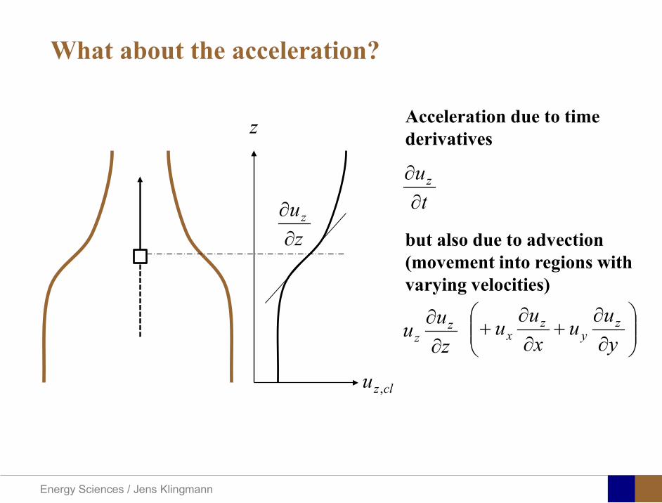
Energy Sciences Jens Klingmann
Acceleration due to timederivatives
but also due to advection (movement into regions with varying velocities)
What about the acceleration
z
clzu
tuz
partpart
zuu z
z partpart
zuz
partpart
partpart
+partpart
+yuu
xuu z
yz
x
Energy Sciences Jens Klingmann
Summing up
zu
zyu
yxu
xzp
zuu
yuu
xuu
tu
zu
zyu
yxu
xyp
zu
uy
uu
xu
ut
u
zu
zyu
yxu
xxp
zuu
yuu
xuu
tu
zzzzz
zy
zx
z
yyyyz
yy
yx
y
xxxxz
xy
xx
x
partpart
partpart
+partpart
partpart
+partpart
partpart
+partpart
minus=
part
part+
partpart
+partpart
+part
part
part
part
partpart
+part
part
partpart
+part
part
partpart
+partpart
minus=
part
part+
part
part+
part
part+
part
part
partpart
partpart
+part
partpartpart
+part
partpartpart
+partpart
minus=
part
part+
partpart
+part
part+
partpart
micromicromicroρ
micromicromicroρ
micromicromicroρ
Navier-Stokes Equations Incompressible (isochoric)
Energy Sciences Jens Klingmann
Summing up
4 unknown (3 velocity components pressure)4 equations (3 NS eq and continuity)
Nonlinear second order set of PDEOnly very simple analytic solution available
0=part
part+
part
part+
partpart
zu
yu
xu zyx
zu
zyu
yxu
xzp
zuu
yuu
xuu
tu
zu
zyu
yxu
xyp
zu
uy
uu
xu
ut
u
zu
zyu
yxu
xxp
zuu
yuu
xuu
tu
zzzzz
zy
zx
z
yyyyz
yy
yx
y
xxxxz
xy
xx
x
partpart
partpart
+partpart
partpart
+partpart
partpart
+partpart
minus=
part
part+
partpart
+partpart
+part
part
part
part
partpart
+part
part
partpart
+part
part
partpart
+partpart
minus=
part
part+
part
part+
part
part+
part
part
partpart
partpart
+part
partpartpart
+part
partpartpart
+partpart
minus=
part
part+
partpart
+part
part+
partpart
micromicromicroρ
micromicromicroρ
micromicromicroρ
Navier-Stokes Equations Incompressible (isochoric)
and continuity eq
Worst slide ever
Energy Sciences Jens Klingmann
Solving the equations Equations solved in discrete point in a grid (mesh)
Derivatives approximated by eg finite differences
System transformed to large set of algebraic equations
xxjiji
ji ∆
minusasymp
partpart + 1
φφφ
Where φ is any dependent variable and ∆xis the distance between the meshpoints
∆x Example
Energy Sciences Jens Klingmann
Turbulence
Energy Sciences Jens Klingmann
Osborne Reynoldsrsquo Experiments
Energy Sciences Jens Klingmann
Characteristics of turbulence
bull Irregularity
bull Diffusivity the capability of turbulence to enhance transport of mass heat and momentum
bull Large Reynolds numbers Many flow fields are laminar at low Re but become unstable and turbulent at higher Re
bull Three-dimensional vorticity fluctuations
bull Dissipation Viscous shear stresses perform deformation work on the fluid which increases the internal energy at the expense of the kinetic energy
bull Continuum In most technical applications the distance between molecules is orders of magnitude shorter than the size of even the smallest scales of the flow
Energy Sciences Jens Klingmann
Turbulence is irregularity
025 03 035 04 045 05t0
001002003004005006007008009
01
u(x
t)
u(xt)
u(x)
bull Small (unresolvable) scalesbull Statistical approach required bull How can we define an average velocity
0
1( ) ( )T
u u t dtT
= intx x
Energy Sciences Jens Klingmann
Turbulence averaging
Havenrsquot we already done this once
Energy Sciences Jens Klingmann
y zx zz z z z z z
x y z
z z z
u uu uu u u u u uu u ut x x y y z z
u u upz x x y y z z
ρ
micro micro micro
partpartpart part part part part + + + + + + = part part part part part part part
part part partpart part part part= minus + + +
part part part part part part part
Turbulence averaging
uuu += ppp +=
Insert into NS (only z-direction shown) and average entire equation
and
Decompose velocity and pressure (Reynoldsrsquo decomposition)
Additional terms that look like stresses
Energy Sciences Jens Klingmann
Turbulence RANS modellingReynoldsrsquo stress tensor
Needs to be expressed as a function of variables we know or intend to solve for
TURBULENCE MODEL
x x x y x z
y x y y y z
z x z y z z
u u u u u u
u u u u u u
u u u u u u
ρ
=
R
6 new variables (symmetry )xyyx uuuu =
Energy Sciences Jens Klingmann
Turbulence RANS modellingReynolds stress tensor
ij i j
u u u v u w
R u u v u v v v w
w u w v w w
ρ ρ ρ
= minus otimes = = =
R u u
Turbulent Kinetic Energy
( ) ( )1 1 1 1 2 2 2 2ii i ik tr R u u u u v v w wρ ρ= = = = + +R
Represents the kinetic energy of the fluctuations (or vortices)
Energy Sciences Jens Klingmann
Turbulence closure problem
10 unknownvelocity components pressure and correlations of fluctuating velocity
4 equationsAveraged momentum equations and averaged continuity equation
i ju u
Energy Sciences Jens Klingmann
Turbulence RANS modelling
23
i jij T ij
j i
u uR kx x
micro ρ δ part part
= + minus part part
2 T kmicro ρ εpropldquoTurbulent viscosityrdquo
Transport of k Some terms may be derived other need modelling
( ) ( ) ( )advection diffusion productionk k k kt
εpart+ + = minus
part
Energy from mean flow to turbulence
Dissipation Energy converted to heat
Energy Sciences Jens Klingmann
Turbulence RANS modelling
23
i jij T ij
j i
u uR kx x
micro ρ δ part part
= + minus part part ερmicro micro 2kCT =
k Tklk
k l k k k
uk ku Rx x x x
microρ ε micro
σ part part part part
= minus + + part part part part 2
1 2k T
klkk l k k
uu C R C
x k x k x xε εε
microε ε ε ερ ρ micropart σ
part part part part= minus + + part part part
4411 =εC 9212 =εC 090=microC 1=kσ31=εσ
Closure coefficients
Energy Sciences Jens Klingmann
Energy Sciences Jens Klingmann
Computational Fluid Dynamics (CFD)
U Waringhleacuten ldquoThe Aerodynamic design and testing of a supersonic turbine for rocket engine propulsionrdquo Proc Of 3rd European conference on Turbomachinery Fluid dynamics and thermodynamics
Energy Sciences Jens Klingmann
Subsonic flow in an aerofoilplate junction computed with a second-moment closure (D Apsley 1998)
Computational Fluid Dynamics(CFD)
Energy Sciences Jens Klingmann
Hydraulic turbine research CFD digital simulation Distribution of speed on an axial turbine
Computational Fluid Dynamics(CFD)
Energy Sciences Jens Klingmann
Scales of turbulence
10-01
1000
1001
1002
1003
1004
1005
κ LI
10-08
10-07
10-06
10-05
10-04
10-03
10-02
10-01
1000
E(u
2 LI)
10-04
10-03
10-02
10-01
1000
κ LK
10-05
10-04
10-03
10-02
10-01
1000
1001
1002
D( ε L
K )10-01
1000
1001
1002
1003
1004
1005
E = 15 (κ LI)-53
10-04
10-03
10-02
10-01
1000
1001
D = 3 ( κ LΚ) 13
Normalized energy and dissipation spectra for
Adapted from Tennekeys and Lumley
ReLI= times2 105
1 2Re 500IL asymp
3 4Re 10000IL asymp
Energy Sciences Jens Klingmann
References Turbulence
bull Tennekeys and Lumley ldquoA first course in Turbulencerdquo MIT Press 1972
bull J O Hinze ldquoTurbulencerdquo McGraw-Hill 1959bull D C Wilcox ldquoTurbulence Modeling for CFDrdquo DCW Industries
2006
Energy Sciences Jens Klingmann
Boundary layers
Energy Sciences Jens Klingmann
Boundary Layer Theory (BLT) Sensitive to Pressure
gradients Appropriate scaling from
dimensional analyses
Energy Sciences Jens Klingmann
Boundary layers
Energy Sciences Jens Klingmann
Air foil theory
Energy Sciences Jens Klingmann
Visualisation of diffusor separation
Energy Sciences Jens Klingmann
BL equations
+minus=+
yu
yxp
xuv
xuu
partpartmicro
partpart
partpart
partρpart
partρpart and 0=+
yxu
partυpart
partpart
Applying the BL approximations the 2D stationary incompressible NS-eq and continuity equation become
yvu
yu
yxuu
xp
yu
xuu
partpartρ
partpartmicro
partpart
partρpart
partpart
partυρpart
partρpart
minus
+minusminus=+
and
0=+yx
upart
υpartpartpart
Reynolds averaged BL eqs are
Energy Sciences Jens Klingmann
Boundary layers
Energy Sciences Jens Klingmann
Turbulent BL at different Pressure gradients
Energy Sciences Jens Klingmann
Boundary Layers
ν
yuy =+
ρτWu =
0=
partpart
=y
w yuτ
uuu =+
Energy Sciences Jens Klingmann
Diffuser efficiency
Energy Sciences Jens Klingmann
Reynolds Number (Order of magnitude)
At eg a compressor inlet
ρ = O(1) kgm3
U = O(100) msx lt O(01) mmicro = O(10-5)
Re = ρ U x micro =O(106)
In subsequent stages large amounts of turbulence (from stator wakes) will be convected into the Boundary layer
Energy Sciences Jens Klingmann
References Boundary layers
bull Frank M White ldquoViscous Fluid Flowrdquobull Hermann Schlichting ldquoBoundary Layer Theoryrdquo
Energy Sciences Jens Klingmann
CFD and experiments
bull No this is not a CFD course butbull Experiments
Energy Sciences Jens Klingmann
What do we need to measureOverall performance
Flow rates (mass or volume) Pressure Temperature Shaft power
Performance increase
Separations (velocity) Secondary flows eg tip clearance losses (velocity) Shock waves (supersonic applications) Pressure (resolved in time and space) Temperature (resolved in time and space)
Energy Sciences Jens Klingmann
Cascade wind tunnels
FIG 31 Compressor cascade wind tunnels (a) Conventional low-speed continuousrunning cascade tunnel (adapted from Carter et al 1950)(b) Transonicsupersoniccascade tunnel (adapted from Sieverding 1985)
Energy Sciences Jens Klingmann
Closed circuit tunnels
Energy Sciences Jens Klingmann
components
Settling Chamber
The settling chamber is located between the fan or wide angle diffuser and the contraction and contains the honeycombs and screens used to moderate longitudinal variations in the flow Screens in the chamber should be spaced at 02 chamber diameters apart so that flow disturbed by the first screen can settle before it encounters the second
Honeycombs
Honeycombs are located in the settling chamber and are used to reduce nonuniformities in the flow For optimum benefit honeycombs should be 6-8 cell diameters thick and cell size should be on the order of about 150 cells per settling chamber diameter
Energy Sciences Jens Klingmann
components
Screens
Screens are typically located just downstream of the honeycomb and sometime at the inlet of the test section Screens create a static pressure drop and serve to reduce boundary layer size and increase flow uniformity
Contraction Section
Contractions sections are located between the settling chamber and the test sections and serve to both increase mean velocities at the test section inlet and moderate inconsistencies in the uniformity of the flow Large contraction ratios and short contraction lengths are generally more desirable as they reduce the power loss across the screens and the thickness of boundary layers Small tunnels typically have contraction ratios between 6 and 9
Energy Sciences Jens Klingmann
Flow meters with pressure measurement
Venturi-tube
A1 A2
P1 P2
1 1 2 2C A C A=In the incompressible case
2 21 1 2 2
2 2C P C P
ρ ρ+ = +Assuming horisontal mounting
Energy Sciences Jens Klingmann
Daniel Bernoulli 1700-1782
Daniel Bernoulli was the son of Johann Bernoulli He was born in Groningen while his father held the chair of mathematics there His older brother was Nicolaus(II) Bernoulli and his uncle was Jacob Bernoulli so he was born into a family of leading mathematicians but also into a family where there was unfortunate rivalry jealousy and bitterness
Undoubtedly the most important work which Daniel Bernoulli did was his work on hydrodynamics Even the term itself is based on the title of the work which he produced called Hydrodynamica and before he left St Petersburg Daniel left a draft copy of the book with a printer However the work was not published until 1738 and although he revised it considerably between 1734 and 1738 it is more the presentation that he changed rather then the substance
This work contains for the first time the correct analysis of water flowing from a hole in a container This was based on the principle of conservation of energy which he had studied with his father in 1720 Daniel also discussed pumps and other machines to raise water One remarkable discovery appears in Chapter 10 of Hydrodynamica where Daniel discussed the basis for the kinetic theory of gases He was able to give the basic laws for the theory of gases and gave although not in full detail the equation of state discovered by Van der Waals a century later
Energy Sciences Jens Klingmann
Venturi-tube (2)
22 2 12 2
2
2A PC CA ρ
∆minus =
A1 A2
P1 P2
Solve for eg C2
1 2P P P∆ = minus
( )
12
2 2 21 2
21
PCA Aρ
∆ = minus
and( )
12
2 2 2 2 21 2
21
Pm A C AA Aρρ
∆ = = minus
where
Flow meters with pressure measurement
Energy Sciences Jens Klingmann
Flow meters with pressure measurement
Orifice meters
A1
A2
P1 P2
Applicable for pipe flows Same principle as for Venturi Positioning of pressure taps important Vena contracta and losses require inclusion
of Discharge Coefficient CD
( )
12
2 2 21 2
21D
Pm C AA Aρ ∆ =
minus where ( )1 2ReDC f A A=
CD available from manufacturer (measurements) or Standards (eg ISO)
Energy Sciences Jens Klingmann
Coriolis flow meter
An actuator (not shown) induces a vibration of the tubes
When there is mass flow Coriolis forces induce twisting of the tubes
degree of phase-shift is a measure for the amount of mass that is flowing through the tubes
Energy Sciences Jens Klingmann
Thermal flow meter Heat is added electrically to the flow Temperature is measured before and after heat addition
pP mC T∆=
Energy Sciences Jens Klingmann
Ultrasonic flow meters
Ultrasound is emitted to small particles in the flow (dust or other) Reflections of the sound is frequency shifted by the Doppler effect The frequency change is proportional to the particles velocity (volume flow
meter)
Energy Sciences Jens Klingmann
Inductive flow metersA magnetic flowmeter is based upon Faradays Law
The voltage induced across any conductor as it moves at right angles through a magnetic field is proportional to the velocity of that conductor
E is proportional to V x B x D where
E = The voltage generated in a conductorV = The velocity of the conductorB = The magnetic field strengthD = The length of the conductor
NB electric conductivity is required
Energy Sciences Jens Klingmann
Temperature measurements
Thermocouples
The basis established by Thomas Johann Seebeck in 1821
A conductor generates a voltage when subjected to a temperature gradient
To measure this voltage one must use a second conductor material which generates a different voltage under the same temperature gradient
Energy Sciences Jens Klingmann
Pressure sensing
1 2p pgt 2p p2 may be the atmosphere a static pressure tap or a known reference pressure
The strain of the diaphragm (or itrsquos deflection) may be measured by a number of electric methods
Diaphragm
Energy Sciences Jens Klingmann
Pressure sensingPiezoresistive Strain Gage
Uses the piezoresistive effect of bonded or formed strain gauges to detect strain due to applied pressure
Capacitive
Uses a diaghragm and pressure cavity to create a variable capacitor to detect strain due to applied pressure
Magnetic
Measures the displacement of a diaphragm by means of changes in inductance (reluctance) LVDT Hall Effect or by eddy current principal
Piezoelectric
Uses the piezoelectric effect in certain materials such as quartz to measure the strain upon the sensing mechanism due to pressure
Potentiometric
Uses the motion of a wiper along a resistive mechanism to detect the strain caused by applied pressure
Energy Sciences Jens Klingmann
3D highly instationary (periodic) flow Potentially very high velocities (Supersonic) Large temperature differences Low accessibility (difficult to probe between rotors) Low turbulence levels in most of the domain Very high turbulence in BL and wakes
Properties of measuring object
Point measurements
Energy Sciences Jens Klingmann
Conventional or non-opticalndash Static Pressure Measurementsndash Total Pressure Measurements
bull Multy hole probes
ndash Total Temperature ndash Hot Wire Anemometry (HWA)
Optical techniques for Velocity Measurementsndash Laser Two Focous (L2F)ndash Laser Doppler Anemometry (LDA)ndash Particle Image velocimetry (PIV)
Point Measurements
Energy Sciences Jens Klingmann
Static and total pressure
2 2 21 2 1
2 1 2 2 2C C CP P ρ ρ ρ
minus = minus =
2 0C =Stagnation point
C1Static pressure tap
Prandtl or Pitot tube
Apply the Bernoulli equation from free stream to stagnation point
21
2 12CP Pρ
= +or
We can also define a stagnation or total pressure
( )2
101 1 022
CP P Pρ= + =
Total pressure = Static pressure + dynamic pressure
or
Energy Sciences Jens Klingmann
Static pressure
Energy Sciences Jens Klingmann
Total Pressure and Temperature
Shrouded Probes
Shrouded Probe
Pitot or Prandtl tube
Sensitive to direction
Energy Sciences Jens Klingmann
Ludwig Prandtl 1875-1953
Ludwig Prandtl born at Freising Bavaria on February 4 1875 was a German Physicist famous for his work in aeronautics He qualified at Munchen in 1900 with a thesis on elastic stability and held the position of Professor of Applied Mechanics at Gottingen for forty-nine years (from 1904 until his death there on August 15 1953) In 1925 Prandtl became the Director of the Kaiser Wilhelm Institute for Fluid Mechanics His discovery in 1904 of the Boundary Layer which adjoins the surface of a body moving in a fluid led to an understanding of skin friction drag and of the way in which streamlining reduces the drag of airplane wings and other moving bodies His work on wing theory published in 1918 - 1919 followed that of FW Lanchester (1902-1907) but was carried out independently and elucidated the flow over airplane wings of finite span Prandtls work and decisive advances in boundary layer and wing theories became the basic material of aeronautics He also made important contributions to the theories of supersonic flow and of turbulence and contributed much to the development of wind tunnels and other aerodynamic equipment In addition he devised the soap-film analogy for the torsion of non-circular sections and wrote on the theory of plasticity and of meteorology
Energy Sciences Jens Klingmann
Total Pressure multy hole
Cobra Probe Yaw Probe
5 Hole Probe
Energy Sciences Jens Klingmann
5 Hole Probes Calibration
Energy Sciences Jens Klingmann
The inherent unsteadiness of the flow within turbomachines
Energy Sciences Jens Klingmann
Hot Wire Anemometry (HWA) The heat transfer from a thin (one micron)
electrically heated wire can be used to determine velocity
The resistance of the wire is temperature dependent Within a small temperature range it can be assumed linear R = R0+α R0(Tm-T0) where R0 is the resistance at a reference temperature T0 and Tm is the mean wire temperature
The thermal power induced in the wire is balanced by heat transfer to the surrounding fluid I2R=hπDL(Tm-T0) where h is the heat transfer coefficient and D and L the diameter and length of the wire respectively
E = I R
Energy Sciences Jens Klingmann
Constant Temperature Anemometry (CTA) The wire is often placed in a Whetstone bridge If the output from the
bridge is amplified and fed back to the bridge the resistance of the probe and thus the temperature will be held constant
This prevents the temperature of the wire to become excessive at low velocities
R1
R2 R3
Probe
Bridge Voltage
Energy Sciences Jens Klingmann
Constant Temperature Anemometry (CTA)
Energy Sciences Jens Klingmann
Characteristics of LDA (according to Dantec)
Invented by Yeh and Cummins in 1964 Velocity measurements in Fluid Dynamics (gas liquid) Up to 3 velocity components Non-intrusive measurements (optical technique) Absolute measurement technique (no calibration required) Very high accuracy Very high spatial resolution due to small measurement volume Tracer particles are required
Energy Sciences Jens Klingmann
LDA - Fringe Model
Focused Laser beams intersect and form the measurement volume Plane wave fronts beam waist in the plane of intersection Interference in the plane of intersection Pattern of bright and dark stripesplanes Fringes
Energy Sciences Jens Klingmann
LDA-measuring volume
d
x
x
y
y
z
z
e-2 CONTOUR
FRINGES
κ
κ
κ
κ
De-2
De-2
dml m
a
b
cx
b
z
ya
cd
d
=
=
=
J
J
J
J
JP
JP
JP
JD
JD
JD
+
+
+
a
b
c
d
κπλ
=minus sinD
f4l2e
m
κπλ
=minus cosD
f4D2e
m
Energy Sciences Jens Klingmann
Laser Two Focus
Energy Sciences Jens Klingmann
Laser Two Focus
Energy Sciences Jens Klingmann
PIV measurements
PIV is a fairly new technique capable of simultaneous velocity measurements at many points in a plane This gives information on large scale structures vorticity etc which is very difficult or impossible to obtain from one-point measuring techniques
PIV involves the illumination of a plane of the flow under investigation with a thin pulsed sheet of light The flow is seeded with particles
The light scattered from the particles and from successive pulses are being recorded either on film or a CCD array forming a multiple exposure of each particle image If the time between the pulses is known velocity can be determined as the ratio of the particle displacement and the elapsed time
t∆∆= xu
Energy Sciences Jens Klingmann
PIV
Energy Sciences Jens Klingmann
PIV measurements illumination
YA
G
YA
G
Two frequency doubled YAG Lasers aligned to one double pulsed laser sheet
Two or more separate light pulses can be obtained by chopping a continuous laser or from pulsed lasers
The limited pulse energies obtained from continuous lasers limits their applicability to low velocity flows or flows where large seeding particles can be used (ie liquid flows)
The low repetition rate of most pulsed lasers makes the use of two lasers advantageous
Energy Sciences Jens Klingmann
PIV measurements recording
High seeding density in laminar flame
Film or CCD-cameras Cross- or Auto-correlation
ndash ie both particle images on the same frame or on separate frames
CCD-camera requirementndash A many pixels as possiblendash 2k by 2k available 4k by 4k coming
Energy Sciences Jens Klingmann
PIV measurements analyses
Low seeding density (Number of seeding particles per unit volume)
Each particle image pair can be identified This is called particle tracking
High seeding density (PIV)
Small sub-regions of the image containing many particle image pairs are processed to obtain one velocity vector
Energy Sciences Jens Klingmann
PIV measurements analyses
Energy Sciences Jens Klingmann
PIV measurements analyses
( ) ( ) ( ) xsxxs dIIR 2A
1
I
+= int
Cross correlation between ( )x1I and ( )x2I
s is a two dimensional displacement vector
IA is the interrogation area
Cross correlation between
(
)
x
1
I
and
(
)
x
2
I
s is a two dimensional displacement vector
I
A
is the interrogation area
Energy Sciences Jens Klingmann
Energy Sciences Jens Klingmann
PIV from IOWA state university
Energy Sciences Jens Klingmann
PIV sample of evaluation
Energy Sciences Jens Klingmann
LDA PIV HWA Velocity range 01 mms ndash 300
ms 02 ndash 150 ms
Measuring Volume
D = 005 L = 05 mm
2 by 2 by 05 mm
L = 05 mm
Freq response O(10 000) Hz O(10) Hz O(100 000) Hz Calibration Yes No No Sensitivity to other than velocity
Low (ref Index) Low (ref Index) Large (temperature concentrationshellip)
Continuous Signal
Sometimes Seldom Always
Noise High High Low Turbulence intensity
No limitation Some limitation lt 20
Price O(1 000 000) SEK
O(1 000 000) SEK
O(50 000) SEK
Required Knowledge
High medium Low
Comparison of techniques
Energy Sciences Jens Klingmann
References experiments
R J Goldstein ldquoFluid Mechanics Measurementsrdquo Hemisphere Publishing 1983 A V Johansson amp P H Alfredsson ldquoExperimentella metoder inom
stroumlmningsmekanikenrdquo Inst Foumlr Mekanik KTH F Durst A Melling and J H Whitelaw ldquoPrincipals and Practice of Laser Doppler
Anemometryrdquo 1984 R J Adrian ldquoParticle-imaging techniques for experimental fluid mechnicsrdquo Ann Rev
Fluid Mech 1991
Energy Sciences Jens Klingmann
Sample of LDA-measurements
Rotor blade
Glas window
Emitted beams
Scattered Light
Adjustable mirror
Energy Sciences Jens Klingmann
Axial velocity sorted into 10 bins
0 1 2 3 4 5 6tangential coordinate (degrees)
-20
0
20
40
60
80
100
120
140
160Ax
ial v
eloc
ity a
nd s
tand
ard
devi
atio
n (m
s)
radial position 7 mm from inner window surfaceaxial position 23 mm behind rotor blades
Energy Sciences Jens Klingmann
Axial velocities in the radial-tangential plane
Energy Sciences Jens Klingmann
Airfoils NACA 4-digit
The NACA four-digit wing sections define the profile by
One digit describing maximum camber as percentage of the chord
One digit describing the distance of maximum camber from the airfoil leading edge in tens of percents of the chord
Two digits describing maximum thickness of the airfoil as percent of the chord
Example the NACA 2412 airfoil has a maximum camber of 2 located 40 (04 chords) from the leading edge with a maximum thickness of 12 of the chord
Four-digit series airfoils by default have maximum thickness at 30 of the chord (03 chords) from the leading edge
Energy Sciences Jens Klingmann
Airfoils NACA 4-digit
bull c is the chord lengthbull x is the position along
the chord from 0 to cbull y is the half thickness at
a given value of x (centerline to surface)
bull t is the maximum thickness as a fraction of the chord
Energy Sciences Jens Klingmann
Death by PowerPoint
| LDA | PIV | HWA | |||||
| Velocity range | 01 mms ndash 300 ms | 02 ndash 150 ms | |||||
| Measuring Volume | D = 005 L = 05 mm | 2 by 2 by 05 mm | L = 05 mm | ||||
| Freq response | O(10 000) Hz | O(10) Hz | O(100 000) Hz | ||||
| Calibration | Yes | No | No | ||||
| Sensitivity to other than velocity | Low (ref Index) | Low (ref Index) | Large (temperature concentrationshellip) | ||||
| Continuous Signal | Sometimes | Seldom | Always | ||||
| Noise | High | High | Low | ||||
| Turbulence intensity | No limitation | Some limitation | lt 20 | ||||
| Price | O(1 000 000) SEK | O(1 000 000) SEK | O(50 000) SEK | ||||
| Required Knowledge | High | medium | Low |
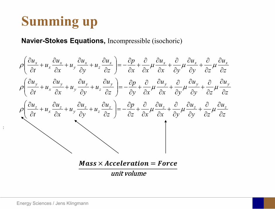
Energy Sciences Jens Klingmann
Summing up
zu
zyu
yxu
xzp
zuu
yuu
xuu
tu
zu
zyu
yxu
xyp
zu
uy
uu
xu
ut
u
zu
zyu
yxu
xxp
zuu
yuu
xuu
tu
zzzzz
zy
zx
z
yyyyz
yy
yx
y
xxxxz
xy
xx
x
partpart
partpart
+partpart
partpart
+partpart
partpart
+partpart
minus=
part
part+
partpart
+partpart
+part
part
part
part
partpart
+part
part
partpart
+part
part
partpart
+partpart
minus=
part
part+
part
part+
part
part+
part
part
partpart
partpart
+part
partpartpart
+part
partpartpart
+partpart
minus=
part
part+
partpart
+part
part+
partpart
micromicromicroρ
micromicromicroρ
micromicromicroρ
Navier-Stokes Equations Incompressible (isochoric)
Energy Sciences Jens Klingmann
Summing up
4 unknown (3 velocity components pressure)4 equations (3 NS eq and continuity)
Nonlinear second order set of PDEOnly very simple analytic solution available
0=part
part+
part
part+
partpart
zu
yu
xu zyx
zu
zyu
yxu
xzp
zuu
yuu
xuu
tu
zu
zyu
yxu
xyp
zu
uy
uu
xu
ut
u
zu
zyu
yxu
xxp
zuu
yuu
xuu
tu
zzzzz
zy
zx
z
yyyyz
yy
yx
y
xxxxz
xy
xx
x
partpart
partpart
+partpart
partpart
+partpart
partpart
+partpart
minus=
part
part+
partpart
+partpart
+part
part
part
part
partpart
+part
part
partpart
+part
part
partpart
+partpart
minus=
part
part+
part
part+
part
part+
part
part
partpart
partpart
+part
partpartpart
+part
partpartpart
+partpart
minus=
part
part+
partpart
+part
part+
partpart
micromicromicroρ
micromicromicroρ
micromicromicroρ
Navier-Stokes Equations Incompressible (isochoric)
and continuity eq
Worst slide ever
Energy Sciences Jens Klingmann
Solving the equations Equations solved in discrete point in a grid (mesh)
Derivatives approximated by eg finite differences
System transformed to large set of algebraic equations
xxjiji
ji ∆
minusasymp
partpart + 1
φφφ
Where φ is any dependent variable and ∆xis the distance between the meshpoints
∆x Example
Energy Sciences Jens Klingmann
Turbulence
Energy Sciences Jens Klingmann
Osborne Reynoldsrsquo Experiments
Energy Sciences Jens Klingmann
Characteristics of turbulence
bull Irregularity
bull Diffusivity the capability of turbulence to enhance transport of mass heat and momentum
bull Large Reynolds numbers Many flow fields are laminar at low Re but become unstable and turbulent at higher Re
bull Three-dimensional vorticity fluctuations
bull Dissipation Viscous shear stresses perform deformation work on the fluid which increases the internal energy at the expense of the kinetic energy
bull Continuum In most technical applications the distance between molecules is orders of magnitude shorter than the size of even the smallest scales of the flow
Energy Sciences Jens Klingmann
Turbulence is irregularity
025 03 035 04 045 05t0
001002003004005006007008009
01
u(x
t)
u(xt)
u(x)
bull Small (unresolvable) scalesbull Statistical approach required bull How can we define an average velocity
0
1( ) ( )T
u u t dtT
= intx x
Energy Sciences Jens Klingmann
Turbulence averaging
Havenrsquot we already done this once
Energy Sciences Jens Klingmann
y zx zz z z z z z
x y z
z z z
u uu uu u u u u uu u ut x x y y z z
u u upz x x y y z z
ρ
micro micro micro
partpartpart part part part part + + + + + + = part part part part part part part
part part partpart part part part= minus + + +
part part part part part part part
Turbulence averaging
uuu += ppp +=
Insert into NS (only z-direction shown) and average entire equation
and
Decompose velocity and pressure (Reynoldsrsquo decomposition)
Additional terms that look like stresses
Energy Sciences Jens Klingmann
Turbulence RANS modellingReynoldsrsquo stress tensor
Needs to be expressed as a function of variables we know or intend to solve for
TURBULENCE MODEL
x x x y x z
y x y y y z
z x z y z z
u u u u u u
u u u u u u
u u u u u u
ρ
=
R
6 new variables (symmetry )xyyx uuuu =
Energy Sciences Jens Klingmann
Turbulence RANS modellingReynolds stress tensor
ij i j
u u u v u w
R u u v u v v v w
w u w v w w
ρ ρ ρ
= minus otimes = = =
R u u
Turbulent Kinetic Energy
( ) ( )1 1 1 1 2 2 2 2ii i ik tr R u u u u v v w wρ ρ= = = = + +R
Represents the kinetic energy of the fluctuations (or vortices)
Energy Sciences Jens Klingmann
Turbulence closure problem
10 unknownvelocity components pressure and correlations of fluctuating velocity
4 equationsAveraged momentum equations and averaged continuity equation
i ju u
Energy Sciences Jens Klingmann
Turbulence RANS modelling
23
i jij T ij
j i
u uR kx x
micro ρ δ part part
= + minus part part
2 T kmicro ρ εpropldquoTurbulent viscosityrdquo
Transport of k Some terms may be derived other need modelling
( ) ( ) ( )advection diffusion productionk k k kt
εpart+ + = minus
part
Energy from mean flow to turbulence
Dissipation Energy converted to heat
Energy Sciences Jens Klingmann
Turbulence RANS modelling
23
i jij T ij
j i
u uR kx x
micro ρ δ part part
= + minus part part ερmicro micro 2kCT =
k Tklk
k l k k k
uk ku Rx x x x
microρ ε micro
σ part part part part
= minus + + part part part part 2
1 2k T
klkk l k k
uu C R C
x k x k x xε εε
microε ε ε ερ ρ micropart σ
part part part part= minus + + part part part
4411 =εC 9212 =εC 090=microC 1=kσ31=εσ
Closure coefficients
Energy Sciences Jens Klingmann
Energy Sciences Jens Klingmann
Computational Fluid Dynamics (CFD)
U Waringhleacuten ldquoThe Aerodynamic design and testing of a supersonic turbine for rocket engine propulsionrdquo Proc Of 3rd European conference on Turbomachinery Fluid dynamics and thermodynamics
Energy Sciences Jens Klingmann
Subsonic flow in an aerofoilplate junction computed with a second-moment closure (D Apsley 1998)
Computational Fluid Dynamics(CFD)
Energy Sciences Jens Klingmann
Hydraulic turbine research CFD digital simulation Distribution of speed on an axial turbine
Computational Fluid Dynamics(CFD)
Energy Sciences Jens Klingmann
Scales of turbulence
10-01
1000
1001
1002
1003
1004
1005
κ LI
10-08
10-07
10-06
10-05
10-04
10-03
10-02
10-01
1000
E(u
2 LI)
10-04
10-03
10-02
10-01
1000
κ LK
10-05
10-04
10-03
10-02
10-01
1000
1001
1002
D( ε L
K )10-01
1000
1001
1002
1003
1004
1005
E = 15 (κ LI)-53
10-04
10-03
10-02
10-01
1000
1001
D = 3 ( κ LΚ) 13
Normalized energy and dissipation spectra for
Adapted from Tennekeys and Lumley
ReLI= times2 105
1 2Re 500IL asymp
3 4Re 10000IL asymp
Energy Sciences Jens Klingmann
References Turbulence
bull Tennekeys and Lumley ldquoA first course in Turbulencerdquo MIT Press 1972
bull J O Hinze ldquoTurbulencerdquo McGraw-Hill 1959bull D C Wilcox ldquoTurbulence Modeling for CFDrdquo DCW Industries
2006
Energy Sciences Jens Klingmann
Boundary layers
Energy Sciences Jens Klingmann
Boundary Layer Theory (BLT) Sensitive to Pressure
gradients Appropriate scaling from
dimensional analyses
Energy Sciences Jens Klingmann
Boundary layers
Energy Sciences Jens Klingmann
Air foil theory
Energy Sciences Jens Klingmann
Visualisation of diffusor separation
Energy Sciences Jens Klingmann
BL equations
+minus=+
yu
yxp
xuv
xuu
partpartmicro
partpart
partpart
partρpart
partρpart and 0=+
yxu
partυpart
partpart
Applying the BL approximations the 2D stationary incompressible NS-eq and continuity equation become
yvu
yu
yxuu
xp
yu
xuu
partpartρ
partpartmicro
partpart
partρpart
partpart
partυρpart
partρpart
minus
+minusminus=+
and
0=+yx
upart
υpartpartpart
Reynolds averaged BL eqs are
Energy Sciences Jens Klingmann
Boundary layers
Energy Sciences Jens Klingmann
Turbulent BL at different Pressure gradients
Energy Sciences Jens Klingmann
Boundary Layers
ν
yuy =+
ρτWu =
0=
partpart
=y
w yuτ
uuu =+
Energy Sciences Jens Klingmann
Diffuser efficiency
Energy Sciences Jens Klingmann
Reynolds Number (Order of magnitude)
At eg a compressor inlet
ρ = O(1) kgm3
U = O(100) msx lt O(01) mmicro = O(10-5)
Re = ρ U x micro =O(106)
In subsequent stages large amounts of turbulence (from stator wakes) will be convected into the Boundary layer
Energy Sciences Jens Klingmann
References Boundary layers
bull Frank M White ldquoViscous Fluid Flowrdquobull Hermann Schlichting ldquoBoundary Layer Theoryrdquo
Energy Sciences Jens Klingmann
CFD and experiments
bull No this is not a CFD course butbull Experiments
Energy Sciences Jens Klingmann
What do we need to measureOverall performance
Flow rates (mass or volume) Pressure Temperature Shaft power
Performance increase
Separations (velocity) Secondary flows eg tip clearance losses (velocity) Shock waves (supersonic applications) Pressure (resolved in time and space) Temperature (resolved in time and space)
Energy Sciences Jens Klingmann
Cascade wind tunnels
FIG 31 Compressor cascade wind tunnels (a) Conventional low-speed continuousrunning cascade tunnel (adapted from Carter et al 1950)(b) Transonicsupersoniccascade tunnel (adapted from Sieverding 1985)
Energy Sciences Jens Klingmann
Closed circuit tunnels
Energy Sciences Jens Klingmann
components
Settling Chamber
The settling chamber is located between the fan or wide angle diffuser and the contraction and contains the honeycombs and screens used to moderate longitudinal variations in the flow Screens in the chamber should be spaced at 02 chamber diameters apart so that flow disturbed by the first screen can settle before it encounters the second
Honeycombs
Honeycombs are located in the settling chamber and are used to reduce nonuniformities in the flow For optimum benefit honeycombs should be 6-8 cell diameters thick and cell size should be on the order of about 150 cells per settling chamber diameter
Energy Sciences Jens Klingmann
components
Screens
Screens are typically located just downstream of the honeycomb and sometime at the inlet of the test section Screens create a static pressure drop and serve to reduce boundary layer size and increase flow uniformity
Contraction Section
Contractions sections are located between the settling chamber and the test sections and serve to both increase mean velocities at the test section inlet and moderate inconsistencies in the uniformity of the flow Large contraction ratios and short contraction lengths are generally more desirable as they reduce the power loss across the screens and the thickness of boundary layers Small tunnels typically have contraction ratios between 6 and 9
Energy Sciences Jens Klingmann
Flow meters with pressure measurement
Venturi-tube
A1 A2
P1 P2
1 1 2 2C A C A=In the incompressible case
2 21 1 2 2
2 2C P C P
ρ ρ+ = +Assuming horisontal mounting
Energy Sciences Jens Klingmann
Daniel Bernoulli 1700-1782
Daniel Bernoulli was the son of Johann Bernoulli He was born in Groningen while his father held the chair of mathematics there His older brother was Nicolaus(II) Bernoulli and his uncle was Jacob Bernoulli so he was born into a family of leading mathematicians but also into a family where there was unfortunate rivalry jealousy and bitterness
Undoubtedly the most important work which Daniel Bernoulli did was his work on hydrodynamics Even the term itself is based on the title of the work which he produced called Hydrodynamica and before he left St Petersburg Daniel left a draft copy of the book with a printer However the work was not published until 1738 and although he revised it considerably between 1734 and 1738 it is more the presentation that he changed rather then the substance
This work contains for the first time the correct analysis of water flowing from a hole in a container This was based on the principle of conservation of energy which he had studied with his father in 1720 Daniel also discussed pumps and other machines to raise water One remarkable discovery appears in Chapter 10 of Hydrodynamica where Daniel discussed the basis for the kinetic theory of gases He was able to give the basic laws for the theory of gases and gave although not in full detail the equation of state discovered by Van der Waals a century later
Energy Sciences Jens Klingmann
Venturi-tube (2)
22 2 12 2
2
2A PC CA ρ
∆minus =
A1 A2
P1 P2
Solve for eg C2
1 2P P P∆ = minus
( )
12
2 2 21 2
21
PCA Aρ
∆ = minus
and( )
12
2 2 2 2 21 2
21
Pm A C AA Aρρ
∆ = = minus
where
Flow meters with pressure measurement
Energy Sciences Jens Klingmann
Flow meters with pressure measurement
Orifice meters
A1
A2
P1 P2
Applicable for pipe flows Same principle as for Venturi Positioning of pressure taps important Vena contracta and losses require inclusion
of Discharge Coefficient CD
( )
12
2 2 21 2
21D
Pm C AA Aρ ∆ =
minus where ( )1 2ReDC f A A=
CD available from manufacturer (measurements) or Standards (eg ISO)
Energy Sciences Jens Klingmann
Coriolis flow meter
An actuator (not shown) induces a vibration of the tubes
When there is mass flow Coriolis forces induce twisting of the tubes
degree of phase-shift is a measure for the amount of mass that is flowing through the tubes
Energy Sciences Jens Klingmann
Thermal flow meter Heat is added electrically to the flow Temperature is measured before and after heat addition
pP mC T∆=
Energy Sciences Jens Klingmann
Ultrasonic flow meters
Ultrasound is emitted to small particles in the flow (dust or other) Reflections of the sound is frequency shifted by the Doppler effect The frequency change is proportional to the particles velocity (volume flow
meter)
Energy Sciences Jens Klingmann
Inductive flow metersA magnetic flowmeter is based upon Faradays Law
The voltage induced across any conductor as it moves at right angles through a magnetic field is proportional to the velocity of that conductor
E is proportional to V x B x D where
E = The voltage generated in a conductorV = The velocity of the conductorB = The magnetic field strengthD = The length of the conductor
NB electric conductivity is required
Energy Sciences Jens Klingmann
Temperature measurements
Thermocouples
The basis established by Thomas Johann Seebeck in 1821
A conductor generates a voltage when subjected to a temperature gradient
To measure this voltage one must use a second conductor material which generates a different voltage under the same temperature gradient
Energy Sciences Jens Klingmann
Pressure sensing
1 2p pgt 2p p2 may be the atmosphere a static pressure tap or a known reference pressure
The strain of the diaphragm (or itrsquos deflection) may be measured by a number of electric methods
Diaphragm
Energy Sciences Jens Klingmann
Pressure sensingPiezoresistive Strain Gage
Uses the piezoresistive effect of bonded or formed strain gauges to detect strain due to applied pressure
Capacitive
Uses a diaghragm and pressure cavity to create a variable capacitor to detect strain due to applied pressure
Magnetic
Measures the displacement of a diaphragm by means of changes in inductance (reluctance) LVDT Hall Effect or by eddy current principal
Piezoelectric
Uses the piezoelectric effect in certain materials such as quartz to measure the strain upon the sensing mechanism due to pressure
Potentiometric
Uses the motion of a wiper along a resistive mechanism to detect the strain caused by applied pressure
Energy Sciences Jens Klingmann
3D highly instationary (periodic) flow Potentially very high velocities (Supersonic) Large temperature differences Low accessibility (difficult to probe between rotors) Low turbulence levels in most of the domain Very high turbulence in BL and wakes
Properties of measuring object
Point measurements
Energy Sciences Jens Klingmann
Conventional or non-opticalndash Static Pressure Measurementsndash Total Pressure Measurements
bull Multy hole probes
ndash Total Temperature ndash Hot Wire Anemometry (HWA)
Optical techniques for Velocity Measurementsndash Laser Two Focous (L2F)ndash Laser Doppler Anemometry (LDA)ndash Particle Image velocimetry (PIV)
Point Measurements
Energy Sciences Jens Klingmann
Static and total pressure
2 2 21 2 1
2 1 2 2 2C C CP P ρ ρ ρ
minus = minus =
2 0C =Stagnation point
C1Static pressure tap
Prandtl or Pitot tube
Apply the Bernoulli equation from free stream to stagnation point
21
2 12CP Pρ
= +or
We can also define a stagnation or total pressure
( )2
101 1 022
CP P Pρ= + =
Total pressure = Static pressure + dynamic pressure
or
Energy Sciences Jens Klingmann
Static pressure
Energy Sciences Jens Klingmann
Total Pressure and Temperature
Shrouded Probes
Shrouded Probe
Pitot or Prandtl tube
Sensitive to direction
Energy Sciences Jens Klingmann
Ludwig Prandtl 1875-1953
Ludwig Prandtl born at Freising Bavaria on February 4 1875 was a German Physicist famous for his work in aeronautics He qualified at Munchen in 1900 with a thesis on elastic stability and held the position of Professor of Applied Mechanics at Gottingen for forty-nine years (from 1904 until his death there on August 15 1953) In 1925 Prandtl became the Director of the Kaiser Wilhelm Institute for Fluid Mechanics His discovery in 1904 of the Boundary Layer which adjoins the surface of a body moving in a fluid led to an understanding of skin friction drag and of the way in which streamlining reduces the drag of airplane wings and other moving bodies His work on wing theory published in 1918 - 1919 followed that of FW Lanchester (1902-1907) but was carried out independently and elucidated the flow over airplane wings of finite span Prandtls work and decisive advances in boundary layer and wing theories became the basic material of aeronautics He also made important contributions to the theories of supersonic flow and of turbulence and contributed much to the development of wind tunnels and other aerodynamic equipment In addition he devised the soap-film analogy for the torsion of non-circular sections and wrote on the theory of plasticity and of meteorology
Energy Sciences Jens Klingmann
Total Pressure multy hole
Cobra Probe Yaw Probe
5 Hole Probe
Energy Sciences Jens Klingmann
5 Hole Probes Calibration
Energy Sciences Jens Klingmann
The inherent unsteadiness of the flow within turbomachines
Energy Sciences Jens Klingmann
Hot Wire Anemometry (HWA) The heat transfer from a thin (one micron)
electrically heated wire can be used to determine velocity
The resistance of the wire is temperature dependent Within a small temperature range it can be assumed linear R = R0+α R0(Tm-T0) where R0 is the resistance at a reference temperature T0 and Tm is the mean wire temperature
The thermal power induced in the wire is balanced by heat transfer to the surrounding fluid I2R=hπDL(Tm-T0) where h is the heat transfer coefficient and D and L the diameter and length of the wire respectively
E = I R
Energy Sciences Jens Klingmann
Constant Temperature Anemometry (CTA) The wire is often placed in a Whetstone bridge If the output from the
bridge is amplified and fed back to the bridge the resistance of the probe and thus the temperature will be held constant
This prevents the temperature of the wire to become excessive at low velocities
R1
R2 R3
Probe
Bridge Voltage
Energy Sciences Jens Klingmann
Constant Temperature Anemometry (CTA)
Energy Sciences Jens Klingmann
Characteristics of LDA (according to Dantec)
Invented by Yeh and Cummins in 1964 Velocity measurements in Fluid Dynamics (gas liquid) Up to 3 velocity components Non-intrusive measurements (optical technique) Absolute measurement technique (no calibration required) Very high accuracy Very high spatial resolution due to small measurement volume Tracer particles are required
Energy Sciences Jens Klingmann
LDA - Fringe Model
Focused Laser beams intersect and form the measurement volume Plane wave fronts beam waist in the plane of intersection Interference in the plane of intersection Pattern of bright and dark stripesplanes Fringes
Energy Sciences Jens Klingmann
LDA-measuring volume
d
x
x
y
y
z
z
e-2 CONTOUR
FRINGES
κ
κ
κ
κ
De-2
De-2
dml m
a
b
cx
b
z
ya
cd
d
=
=
=
J
J
J
J
JP
JP
JP
JD
JD
JD
+
+
+
a
b
c
d
κπλ
=minus sinD
f4l2e
m
κπλ
=minus cosD
f4D2e
m
Energy Sciences Jens Klingmann
Laser Two Focus
Energy Sciences Jens Klingmann
Laser Two Focus
Energy Sciences Jens Klingmann
PIV measurements
PIV is a fairly new technique capable of simultaneous velocity measurements at many points in a plane This gives information on large scale structures vorticity etc which is very difficult or impossible to obtain from one-point measuring techniques
PIV involves the illumination of a plane of the flow under investigation with a thin pulsed sheet of light The flow is seeded with particles
The light scattered from the particles and from successive pulses are being recorded either on film or a CCD array forming a multiple exposure of each particle image If the time between the pulses is known velocity can be determined as the ratio of the particle displacement and the elapsed time
t∆∆= xu
Energy Sciences Jens Klingmann
PIV
Energy Sciences Jens Klingmann
PIV measurements illumination
YA
G
YA
G
Two frequency doubled YAG Lasers aligned to one double pulsed laser sheet
Two or more separate light pulses can be obtained by chopping a continuous laser or from pulsed lasers
The limited pulse energies obtained from continuous lasers limits their applicability to low velocity flows or flows where large seeding particles can be used (ie liquid flows)
The low repetition rate of most pulsed lasers makes the use of two lasers advantageous
Energy Sciences Jens Klingmann
PIV measurements recording
High seeding density in laminar flame
Film or CCD-cameras Cross- or Auto-correlation
ndash ie both particle images on the same frame or on separate frames
CCD-camera requirementndash A many pixels as possiblendash 2k by 2k available 4k by 4k coming
Energy Sciences Jens Klingmann
PIV measurements analyses
Low seeding density (Number of seeding particles per unit volume)
Each particle image pair can be identified This is called particle tracking
High seeding density (PIV)
Small sub-regions of the image containing many particle image pairs are processed to obtain one velocity vector
Energy Sciences Jens Klingmann
PIV measurements analyses
Energy Sciences Jens Klingmann
PIV measurements analyses
( ) ( ) ( ) xsxxs dIIR 2A
1
I
+= int
Cross correlation between ( )x1I and ( )x2I
s is a two dimensional displacement vector
IA is the interrogation area
Cross correlation between
(
)
x
1
I
and
(
)
x
2
I
s is a two dimensional displacement vector
I
A
is the interrogation area
Energy Sciences Jens Klingmann
Energy Sciences Jens Klingmann
PIV from IOWA state university
Energy Sciences Jens Klingmann
PIV sample of evaluation
Energy Sciences Jens Klingmann
LDA PIV HWA Velocity range 01 mms ndash 300
ms 02 ndash 150 ms
Measuring Volume
D = 005 L = 05 mm
2 by 2 by 05 mm
L = 05 mm
Freq response O(10 000) Hz O(10) Hz O(100 000) Hz Calibration Yes No No Sensitivity to other than velocity
Low (ref Index) Low (ref Index) Large (temperature concentrationshellip)
Continuous Signal
Sometimes Seldom Always
Noise High High Low Turbulence intensity
No limitation Some limitation lt 20
Price O(1 000 000) SEK
O(1 000 000) SEK
O(50 000) SEK
Required Knowledge
High medium Low
Comparison of techniques
Energy Sciences Jens Klingmann
References experiments
R J Goldstein ldquoFluid Mechanics Measurementsrdquo Hemisphere Publishing 1983 A V Johansson amp P H Alfredsson ldquoExperimentella metoder inom
stroumlmningsmekanikenrdquo Inst Foumlr Mekanik KTH F Durst A Melling and J H Whitelaw ldquoPrincipals and Practice of Laser Doppler
Anemometryrdquo 1984 R J Adrian ldquoParticle-imaging techniques for experimental fluid mechnicsrdquo Ann Rev
Fluid Mech 1991
Energy Sciences Jens Klingmann
Sample of LDA-measurements
Rotor blade
Glas window
Emitted beams
Scattered Light
Adjustable mirror
Energy Sciences Jens Klingmann
Axial velocity sorted into 10 bins
0 1 2 3 4 5 6tangential coordinate (degrees)
-20
0
20
40
60
80
100
120
140
160Ax
ial v
eloc
ity a
nd s
tand
ard
devi
atio
n (m
s)
radial position 7 mm from inner window surfaceaxial position 23 mm behind rotor blades
Energy Sciences Jens Klingmann
Axial velocities in the radial-tangential plane
Energy Sciences Jens Klingmann
Airfoils NACA 4-digit
The NACA four-digit wing sections define the profile by
One digit describing maximum camber as percentage of the chord
One digit describing the distance of maximum camber from the airfoil leading edge in tens of percents of the chord
Two digits describing maximum thickness of the airfoil as percent of the chord
Example the NACA 2412 airfoil has a maximum camber of 2 located 40 (04 chords) from the leading edge with a maximum thickness of 12 of the chord
Four-digit series airfoils by default have maximum thickness at 30 of the chord (03 chords) from the leading edge
Energy Sciences Jens Klingmann
Airfoils NACA 4-digit
bull c is the chord lengthbull x is the position along
the chord from 0 to cbull y is the half thickness at
a given value of x (centerline to surface)
bull t is the maximum thickness as a fraction of the chord
Energy Sciences Jens Klingmann
Death by PowerPoint
| LDA | PIV | HWA | |||||
| Velocity range | 01 mms ndash 300 ms | 02 ndash 150 ms | |||||
| Measuring Volume | D = 005 L = 05 mm | 2 by 2 by 05 mm | L = 05 mm | ||||
| Freq response | O(10 000) Hz | O(10) Hz | O(100 000) Hz | ||||
| Calibration | Yes | No | No | ||||
| Sensitivity to other than velocity | Low (ref Index) | Low (ref Index) | Large (temperature concentrationshellip) | ||||
| Continuous Signal | Sometimes | Seldom | Always | ||||
| Noise | High | High | Low | ||||
| Turbulence intensity | No limitation | Some limitation | lt 20 | ||||
| Price | O(1 000 000) SEK | O(1 000 000) SEK | O(50 000) SEK | ||||
| Required Knowledge | High | medium | Low |
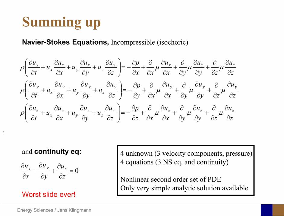
Energy Sciences Jens Klingmann
Summing up
4 unknown (3 velocity components pressure)4 equations (3 NS eq and continuity)
Nonlinear second order set of PDEOnly very simple analytic solution available
0=part
part+
part
part+
partpart
zu
yu
xu zyx
zu
zyu
yxu
xzp
zuu
yuu
xuu
tu
zu
zyu
yxu
xyp
zu
uy
uu
xu
ut
u
zu
zyu
yxu
xxp
zuu
yuu
xuu
tu
zzzzz
zy
zx
z
yyyyz
yy
yx
y
xxxxz
xy
xx
x
partpart
partpart
+partpart
partpart
+partpart
partpart
+partpart
minus=
part
part+
partpart
+partpart
+part
part
part
part
partpart
+part
part
partpart
+part
part
partpart
+partpart
minus=
part
part+
part
part+
part
part+
part
part
partpart
partpart
+part
partpartpart
+part
partpartpart
+partpart
minus=
part
part+
partpart
+part
part+
partpart
micromicromicroρ
micromicromicroρ
micromicromicroρ
Navier-Stokes Equations Incompressible (isochoric)
and continuity eq
Worst slide ever
Energy Sciences Jens Klingmann
Solving the equations Equations solved in discrete point in a grid (mesh)
Derivatives approximated by eg finite differences
System transformed to large set of algebraic equations
xxjiji
ji ∆
minusasymp
partpart + 1
φφφ
Where φ is any dependent variable and ∆xis the distance between the meshpoints
∆x Example
Energy Sciences Jens Klingmann
Turbulence
Energy Sciences Jens Klingmann
Osborne Reynoldsrsquo Experiments
Energy Sciences Jens Klingmann
Characteristics of turbulence
bull Irregularity
bull Diffusivity the capability of turbulence to enhance transport of mass heat and momentum
bull Large Reynolds numbers Many flow fields are laminar at low Re but become unstable and turbulent at higher Re
bull Three-dimensional vorticity fluctuations
bull Dissipation Viscous shear stresses perform deformation work on the fluid which increases the internal energy at the expense of the kinetic energy
bull Continuum In most technical applications the distance between molecules is orders of magnitude shorter than the size of even the smallest scales of the flow
Energy Sciences Jens Klingmann
Turbulence is irregularity
025 03 035 04 045 05t0
001002003004005006007008009
01
u(x
t)
u(xt)
u(x)
bull Small (unresolvable) scalesbull Statistical approach required bull How can we define an average velocity
0
1( ) ( )T
u u t dtT
= intx x
Energy Sciences Jens Klingmann
Turbulence averaging
Havenrsquot we already done this once
Energy Sciences Jens Klingmann
y zx zz z z z z z
x y z
z z z
u uu uu u u u u uu u ut x x y y z z
u u upz x x y y z z
ρ
micro micro micro
partpartpart part part part part + + + + + + = part part part part part part part
part part partpart part part part= minus + + +
part part part part part part part
Turbulence averaging
uuu += ppp +=
Insert into NS (only z-direction shown) and average entire equation
and
Decompose velocity and pressure (Reynoldsrsquo decomposition)
Additional terms that look like stresses
Energy Sciences Jens Klingmann
Turbulence RANS modellingReynoldsrsquo stress tensor
Needs to be expressed as a function of variables we know or intend to solve for
TURBULENCE MODEL
x x x y x z
y x y y y z
z x z y z z
u u u u u u
u u u u u u
u u u u u u
ρ
=
R
6 new variables (symmetry )xyyx uuuu =
Energy Sciences Jens Klingmann
Turbulence RANS modellingReynolds stress tensor
ij i j
u u u v u w
R u u v u v v v w
w u w v w w
ρ ρ ρ
= minus otimes = = =
R u u
Turbulent Kinetic Energy
( ) ( )1 1 1 1 2 2 2 2ii i ik tr R u u u u v v w wρ ρ= = = = + +R
Represents the kinetic energy of the fluctuations (or vortices)
Energy Sciences Jens Klingmann
Turbulence closure problem
10 unknownvelocity components pressure and correlations of fluctuating velocity
4 equationsAveraged momentum equations and averaged continuity equation
i ju u
Energy Sciences Jens Klingmann
Turbulence RANS modelling
23
i jij T ij
j i
u uR kx x
micro ρ δ part part
= + minus part part
2 T kmicro ρ εpropldquoTurbulent viscosityrdquo
Transport of k Some terms may be derived other need modelling
( ) ( ) ( )advection diffusion productionk k k kt
εpart+ + = minus
part
Energy from mean flow to turbulence
Dissipation Energy converted to heat
Energy Sciences Jens Klingmann
Turbulence RANS modelling
23
i jij T ij
j i
u uR kx x
micro ρ δ part part
= + minus part part ερmicro micro 2kCT =
k Tklk
k l k k k
uk ku Rx x x x
microρ ε micro
σ part part part part
= minus + + part part part part 2
1 2k T
klkk l k k
uu C R C
x k x k x xε εε
microε ε ε ερ ρ micropart σ
part part part part= minus + + part part part
4411 =εC 9212 =εC 090=microC 1=kσ31=εσ
Closure coefficients
Energy Sciences Jens Klingmann
Energy Sciences Jens Klingmann
Computational Fluid Dynamics (CFD)
U Waringhleacuten ldquoThe Aerodynamic design and testing of a supersonic turbine for rocket engine propulsionrdquo Proc Of 3rd European conference on Turbomachinery Fluid dynamics and thermodynamics
Energy Sciences Jens Klingmann
Subsonic flow in an aerofoilplate junction computed with a second-moment closure (D Apsley 1998)
Computational Fluid Dynamics(CFD)
Energy Sciences Jens Klingmann
Hydraulic turbine research CFD digital simulation Distribution of speed on an axial turbine
Computational Fluid Dynamics(CFD)
Energy Sciences Jens Klingmann
Scales of turbulence
10-01
1000
1001
1002
1003
1004
1005
κ LI
10-08
10-07
10-06
10-05
10-04
10-03
10-02
10-01
1000
E(u
2 LI)
10-04
10-03
10-02
10-01
1000
κ LK
10-05
10-04
10-03
10-02
10-01
1000
1001
1002
D( ε L
K )10-01
1000
1001
1002
1003
1004
1005
E = 15 (κ LI)-53
10-04
10-03
10-02
10-01
1000
1001
D = 3 ( κ LΚ) 13
Normalized energy and dissipation spectra for
Adapted from Tennekeys and Lumley
ReLI= times2 105
1 2Re 500IL asymp
3 4Re 10000IL asymp
Energy Sciences Jens Klingmann
References Turbulence
bull Tennekeys and Lumley ldquoA first course in Turbulencerdquo MIT Press 1972
bull J O Hinze ldquoTurbulencerdquo McGraw-Hill 1959bull D C Wilcox ldquoTurbulence Modeling for CFDrdquo DCW Industries
2006
Energy Sciences Jens Klingmann
Boundary layers
Energy Sciences Jens Klingmann
Boundary Layer Theory (BLT) Sensitive to Pressure
gradients Appropriate scaling from
dimensional analyses
Energy Sciences Jens Klingmann
Boundary layers
Energy Sciences Jens Klingmann
Air foil theory
Energy Sciences Jens Klingmann
Visualisation of diffusor separation
Energy Sciences Jens Klingmann
BL equations
+minus=+
yu
yxp
xuv
xuu
partpartmicro
partpart
partpart
partρpart
partρpart and 0=+
yxu
partυpart
partpart
Applying the BL approximations the 2D stationary incompressible NS-eq and continuity equation become
yvu
yu
yxuu
xp
yu
xuu
partpartρ
partpartmicro
partpart
partρpart
partpart
partυρpart
partρpart
minus
+minusminus=+
and
0=+yx
upart
υpartpartpart
Reynolds averaged BL eqs are
Energy Sciences Jens Klingmann
Boundary layers
Energy Sciences Jens Klingmann
Turbulent BL at different Pressure gradients
Energy Sciences Jens Klingmann
Boundary Layers
ν
yuy =+
ρτWu =
0=
partpart
=y
w yuτ
uuu =+
Energy Sciences Jens Klingmann
Diffuser efficiency
Energy Sciences Jens Klingmann
Reynolds Number (Order of magnitude)
At eg a compressor inlet
ρ = O(1) kgm3
U = O(100) msx lt O(01) mmicro = O(10-5)
Re = ρ U x micro =O(106)
In subsequent stages large amounts of turbulence (from stator wakes) will be convected into the Boundary layer
Energy Sciences Jens Klingmann
References Boundary layers
bull Frank M White ldquoViscous Fluid Flowrdquobull Hermann Schlichting ldquoBoundary Layer Theoryrdquo
Energy Sciences Jens Klingmann
CFD and experiments
bull No this is not a CFD course butbull Experiments
Energy Sciences Jens Klingmann
What do we need to measureOverall performance
Flow rates (mass or volume) Pressure Temperature Shaft power
Performance increase
Separations (velocity) Secondary flows eg tip clearance losses (velocity) Shock waves (supersonic applications) Pressure (resolved in time and space) Temperature (resolved in time and space)
Energy Sciences Jens Klingmann
Cascade wind tunnels
FIG 31 Compressor cascade wind tunnels (a) Conventional low-speed continuousrunning cascade tunnel (adapted from Carter et al 1950)(b) Transonicsupersoniccascade tunnel (adapted from Sieverding 1985)
Energy Sciences Jens Klingmann
Closed circuit tunnels
Energy Sciences Jens Klingmann
components
Settling Chamber
The settling chamber is located between the fan or wide angle diffuser and the contraction and contains the honeycombs and screens used to moderate longitudinal variations in the flow Screens in the chamber should be spaced at 02 chamber diameters apart so that flow disturbed by the first screen can settle before it encounters the second
Honeycombs
Honeycombs are located in the settling chamber and are used to reduce nonuniformities in the flow For optimum benefit honeycombs should be 6-8 cell diameters thick and cell size should be on the order of about 150 cells per settling chamber diameter
Energy Sciences Jens Klingmann
components
Screens
Screens are typically located just downstream of the honeycomb and sometime at the inlet of the test section Screens create a static pressure drop and serve to reduce boundary layer size and increase flow uniformity
Contraction Section
Contractions sections are located between the settling chamber and the test sections and serve to both increase mean velocities at the test section inlet and moderate inconsistencies in the uniformity of the flow Large contraction ratios and short contraction lengths are generally more desirable as they reduce the power loss across the screens and the thickness of boundary layers Small tunnels typically have contraction ratios between 6 and 9
Energy Sciences Jens Klingmann
Flow meters with pressure measurement
Venturi-tube
A1 A2
P1 P2
1 1 2 2C A C A=In the incompressible case
2 21 1 2 2
2 2C P C P
ρ ρ+ = +Assuming horisontal mounting
Energy Sciences Jens Klingmann
Daniel Bernoulli 1700-1782
Daniel Bernoulli was the son of Johann Bernoulli He was born in Groningen while his father held the chair of mathematics there His older brother was Nicolaus(II) Bernoulli and his uncle was Jacob Bernoulli so he was born into a family of leading mathematicians but also into a family where there was unfortunate rivalry jealousy and bitterness
Undoubtedly the most important work which Daniel Bernoulli did was his work on hydrodynamics Even the term itself is based on the title of the work which he produced called Hydrodynamica and before he left St Petersburg Daniel left a draft copy of the book with a printer However the work was not published until 1738 and although he revised it considerably between 1734 and 1738 it is more the presentation that he changed rather then the substance
This work contains for the first time the correct analysis of water flowing from a hole in a container This was based on the principle of conservation of energy which he had studied with his father in 1720 Daniel also discussed pumps and other machines to raise water One remarkable discovery appears in Chapter 10 of Hydrodynamica where Daniel discussed the basis for the kinetic theory of gases He was able to give the basic laws for the theory of gases and gave although not in full detail the equation of state discovered by Van der Waals a century later
Energy Sciences Jens Klingmann
Venturi-tube (2)
22 2 12 2
2
2A PC CA ρ
∆minus =
A1 A2
P1 P2
Solve for eg C2
1 2P P P∆ = minus
( )
12
2 2 21 2
21
PCA Aρ
∆ = minus
and( )
12
2 2 2 2 21 2
21
Pm A C AA Aρρ
∆ = = minus
where
Flow meters with pressure measurement
Energy Sciences Jens Klingmann
Flow meters with pressure measurement
Orifice meters
A1
A2
P1 P2
Applicable for pipe flows Same principle as for Venturi Positioning of pressure taps important Vena contracta and losses require inclusion
of Discharge Coefficient CD
( )
12
2 2 21 2
21D
Pm C AA Aρ ∆ =
minus where ( )1 2ReDC f A A=
CD available from manufacturer (measurements) or Standards (eg ISO)
Energy Sciences Jens Klingmann
Coriolis flow meter
An actuator (not shown) induces a vibration of the tubes
When there is mass flow Coriolis forces induce twisting of the tubes
degree of phase-shift is a measure for the amount of mass that is flowing through the tubes
Energy Sciences Jens Klingmann
Thermal flow meter Heat is added electrically to the flow Temperature is measured before and after heat addition
pP mC T∆=
Energy Sciences Jens Klingmann
Ultrasonic flow meters
Ultrasound is emitted to small particles in the flow (dust or other) Reflections of the sound is frequency shifted by the Doppler effect The frequency change is proportional to the particles velocity (volume flow
meter)
Energy Sciences Jens Klingmann
Inductive flow metersA magnetic flowmeter is based upon Faradays Law
The voltage induced across any conductor as it moves at right angles through a magnetic field is proportional to the velocity of that conductor
E is proportional to V x B x D where
E = The voltage generated in a conductorV = The velocity of the conductorB = The magnetic field strengthD = The length of the conductor
NB electric conductivity is required
Energy Sciences Jens Klingmann
Temperature measurements
Thermocouples
The basis established by Thomas Johann Seebeck in 1821
A conductor generates a voltage when subjected to a temperature gradient
To measure this voltage one must use a second conductor material which generates a different voltage under the same temperature gradient
Energy Sciences Jens Klingmann
Pressure sensing
1 2p pgt 2p p2 may be the atmosphere a static pressure tap or a known reference pressure
The strain of the diaphragm (or itrsquos deflection) may be measured by a number of electric methods
Diaphragm
Energy Sciences Jens Klingmann
Pressure sensingPiezoresistive Strain Gage
Uses the piezoresistive effect of bonded or formed strain gauges to detect strain due to applied pressure
Capacitive
Uses a diaghragm and pressure cavity to create a variable capacitor to detect strain due to applied pressure
Magnetic
Measures the displacement of a diaphragm by means of changes in inductance (reluctance) LVDT Hall Effect or by eddy current principal
Piezoelectric
Uses the piezoelectric effect in certain materials such as quartz to measure the strain upon the sensing mechanism due to pressure
Potentiometric
Uses the motion of a wiper along a resistive mechanism to detect the strain caused by applied pressure
Energy Sciences Jens Klingmann
3D highly instationary (periodic) flow Potentially very high velocities (Supersonic) Large temperature differences Low accessibility (difficult to probe between rotors) Low turbulence levels in most of the domain Very high turbulence in BL and wakes
Properties of measuring object
Point measurements
Energy Sciences Jens Klingmann
Conventional or non-opticalndash Static Pressure Measurementsndash Total Pressure Measurements
bull Multy hole probes
ndash Total Temperature ndash Hot Wire Anemometry (HWA)
Optical techniques for Velocity Measurementsndash Laser Two Focous (L2F)ndash Laser Doppler Anemometry (LDA)ndash Particle Image velocimetry (PIV)
Point Measurements
Energy Sciences Jens Klingmann
Static and total pressure
2 2 21 2 1
2 1 2 2 2C C CP P ρ ρ ρ
minus = minus =
2 0C =Stagnation point
C1Static pressure tap
Prandtl or Pitot tube
Apply the Bernoulli equation from free stream to stagnation point
21
2 12CP Pρ
= +or
We can also define a stagnation or total pressure
( )2
101 1 022
CP P Pρ= + =
Total pressure = Static pressure + dynamic pressure
or
Energy Sciences Jens Klingmann
Static pressure
Energy Sciences Jens Klingmann
Total Pressure and Temperature
Shrouded Probes
Shrouded Probe
Pitot or Prandtl tube
Sensitive to direction
Energy Sciences Jens Klingmann
Ludwig Prandtl 1875-1953
Ludwig Prandtl born at Freising Bavaria on February 4 1875 was a German Physicist famous for his work in aeronautics He qualified at Munchen in 1900 with a thesis on elastic stability and held the position of Professor of Applied Mechanics at Gottingen for forty-nine years (from 1904 until his death there on August 15 1953) In 1925 Prandtl became the Director of the Kaiser Wilhelm Institute for Fluid Mechanics His discovery in 1904 of the Boundary Layer which adjoins the surface of a body moving in a fluid led to an understanding of skin friction drag and of the way in which streamlining reduces the drag of airplane wings and other moving bodies His work on wing theory published in 1918 - 1919 followed that of FW Lanchester (1902-1907) but was carried out independently and elucidated the flow over airplane wings of finite span Prandtls work and decisive advances in boundary layer and wing theories became the basic material of aeronautics He also made important contributions to the theories of supersonic flow and of turbulence and contributed much to the development of wind tunnels and other aerodynamic equipment In addition he devised the soap-film analogy for the torsion of non-circular sections and wrote on the theory of plasticity and of meteorology
Energy Sciences Jens Klingmann
Total Pressure multy hole
Cobra Probe Yaw Probe
5 Hole Probe
Energy Sciences Jens Klingmann
5 Hole Probes Calibration
Energy Sciences Jens Klingmann
The inherent unsteadiness of the flow within turbomachines
Energy Sciences Jens Klingmann
Hot Wire Anemometry (HWA) The heat transfer from a thin (one micron)
electrically heated wire can be used to determine velocity
The resistance of the wire is temperature dependent Within a small temperature range it can be assumed linear R = R0+α R0(Tm-T0) where R0 is the resistance at a reference temperature T0 and Tm is the mean wire temperature
The thermal power induced in the wire is balanced by heat transfer to the surrounding fluid I2R=hπDL(Tm-T0) where h is the heat transfer coefficient and D and L the diameter and length of the wire respectively
E = I R
Energy Sciences Jens Klingmann
Constant Temperature Anemometry (CTA) The wire is often placed in a Whetstone bridge If the output from the
bridge is amplified and fed back to the bridge the resistance of the probe and thus the temperature will be held constant
This prevents the temperature of the wire to become excessive at low velocities
R1
R2 R3
Probe
Bridge Voltage
Energy Sciences Jens Klingmann
Constant Temperature Anemometry (CTA)
Energy Sciences Jens Klingmann
Characteristics of LDA (according to Dantec)
Invented by Yeh and Cummins in 1964 Velocity measurements in Fluid Dynamics (gas liquid) Up to 3 velocity components Non-intrusive measurements (optical technique) Absolute measurement technique (no calibration required) Very high accuracy Very high spatial resolution due to small measurement volume Tracer particles are required
Energy Sciences Jens Klingmann
LDA - Fringe Model
Focused Laser beams intersect and form the measurement volume Plane wave fronts beam waist in the plane of intersection Interference in the plane of intersection Pattern of bright and dark stripesplanes Fringes
Energy Sciences Jens Klingmann
LDA-measuring volume
d
x
x
y
y
z
z
e-2 CONTOUR
FRINGES
κ
κ
κ
κ
De-2
De-2
dml m
a
b
cx
b
z
ya
cd
d
=
=
=
J
J
J
J
JP
JP
JP
JD
JD
JD
+
+
+
a
b
c
d
κπλ
=minus sinD
f4l2e
m
κπλ
=minus cosD
f4D2e
m
Energy Sciences Jens Klingmann
Laser Two Focus
Energy Sciences Jens Klingmann
Laser Two Focus
Energy Sciences Jens Klingmann
PIV measurements
PIV is a fairly new technique capable of simultaneous velocity measurements at many points in a plane This gives information on large scale structures vorticity etc which is very difficult or impossible to obtain from one-point measuring techniques
PIV involves the illumination of a plane of the flow under investigation with a thin pulsed sheet of light The flow is seeded with particles
The light scattered from the particles and from successive pulses are being recorded either on film or a CCD array forming a multiple exposure of each particle image If the time between the pulses is known velocity can be determined as the ratio of the particle displacement and the elapsed time
t∆∆= xu
Energy Sciences Jens Klingmann
PIV
Energy Sciences Jens Klingmann
PIV measurements illumination
YA
G
YA
G
Two frequency doubled YAG Lasers aligned to one double pulsed laser sheet
Two or more separate light pulses can be obtained by chopping a continuous laser or from pulsed lasers
The limited pulse energies obtained from continuous lasers limits their applicability to low velocity flows or flows where large seeding particles can be used (ie liquid flows)
The low repetition rate of most pulsed lasers makes the use of two lasers advantageous
Energy Sciences Jens Klingmann
PIV measurements recording
High seeding density in laminar flame
Film or CCD-cameras Cross- or Auto-correlation
ndash ie both particle images on the same frame or on separate frames
CCD-camera requirementndash A many pixels as possiblendash 2k by 2k available 4k by 4k coming
Energy Sciences Jens Klingmann
PIV measurements analyses
Low seeding density (Number of seeding particles per unit volume)
Each particle image pair can be identified This is called particle tracking
High seeding density (PIV)
Small sub-regions of the image containing many particle image pairs are processed to obtain one velocity vector
Energy Sciences Jens Klingmann
PIV measurements analyses
Energy Sciences Jens Klingmann
PIV measurements analyses
( ) ( ) ( ) xsxxs dIIR 2A
1
I
+= int
Cross correlation between ( )x1I and ( )x2I
s is a two dimensional displacement vector
IA is the interrogation area
Cross correlation between
(
)
x
1
I
and
(
)
x
2
I
s is a two dimensional displacement vector
I
A
is the interrogation area
Energy Sciences Jens Klingmann
Energy Sciences Jens Klingmann
PIV from IOWA state university
Energy Sciences Jens Klingmann
PIV sample of evaluation
Energy Sciences Jens Klingmann
LDA PIV HWA Velocity range 01 mms ndash 300
ms 02 ndash 150 ms
Measuring Volume
D = 005 L = 05 mm
2 by 2 by 05 mm
L = 05 mm
Freq response O(10 000) Hz O(10) Hz O(100 000) Hz Calibration Yes No No Sensitivity to other than velocity
Low (ref Index) Low (ref Index) Large (temperature concentrationshellip)
Continuous Signal
Sometimes Seldom Always
Noise High High Low Turbulence intensity
No limitation Some limitation lt 20
Price O(1 000 000) SEK
O(1 000 000) SEK
O(50 000) SEK
Required Knowledge
High medium Low
Comparison of techniques
Energy Sciences Jens Klingmann
References experiments
R J Goldstein ldquoFluid Mechanics Measurementsrdquo Hemisphere Publishing 1983 A V Johansson amp P H Alfredsson ldquoExperimentella metoder inom
stroumlmningsmekanikenrdquo Inst Foumlr Mekanik KTH F Durst A Melling and J H Whitelaw ldquoPrincipals and Practice of Laser Doppler
Anemometryrdquo 1984 R J Adrian ldquoParticle-imaging techniques for experimental fluid mechnicsrdquo Ann Rev
Fluid Mech 1991
Energy Sciences Jens Klingmann
Sample of LDA-measurements
Rotor blade
Glas window
Emitted beams
Scattered Light
Adjustable mirror
Energy Sciences Jens Klingmann
Axial velocity sorted into 10 bins
0 1 2 3 4 5 6tangential coordinate (degrees)
-20
0
20
40
60
80
100
120
140
160Ax
ial v
eloc
ity a
nd s
tand
ard
devi
atio
n (m
s)
radial position 7 mm from inner window surfaceaxial position 23 mm behind rotor blades
Energy Sciences Jens Klingmann
Axial velocities in the radial-tangential plane
Energy Sciences Jens Klingmann
Airfoils NACA 4-digit
The NACA four-digit wing sections define the profile by
One digit describing maximum camber as percentage of the chord
One digit describing the distance of maximum camber from the airfoil leading edge in tens of percents of the chord
Two digits describing maximum thickness of the airfoil as percent of the chord
Example the NACA 2412 airfoil has a maximum camber of 2 located 40 (04 chords) from the leading edge with a maximum thickness of 12 of the chord
Four-digit series airfoils by default have maximum thickness at 30 of the chord (03 chords) from the leading edge
Energy Sciences Jens Klingmann
Airfoils NACA 4-digit
bull c is the chord lengthbull x is the position along
the chord from 0 to cbull y is the half thickness at
a given value of x (centerline to surface)
bull t is the maximum thickness as a fraction of the chord
Energy Sciences Jens Klingmann
Death by PowerPoint
| LDA | PIV | HWA | |||||
| Velocity range | 01 mms ndash 300 ms | 02 ndash 150 ms | |||||
| Measuring Volume | D = 005 L = 05 mm | 2 by 2 by 05 mm | L = 05 mm | ||||
| Freq response | O(10 000) Hz | O(10) Hz | O(100 000) Hz | ||||
| Calibration | Yes | No | No | ||||
| Sensitivity to other than velocity | Low (ref Index) | Low (ref Index) | Large (temperature concentrationshellip) | ||||
| Continuous Signal | Sometimes | Seldom | Always | ||||
| Noise | High | High | Low | ||||
| Turbulence intensity | No limitation | Some limitation | lt 20 | ||||
| Price | O(1 000 000) SEK | O(1 000 000) SEK | O(50 000) SEK | ||||
| Required Knowledge | High | medium | Low |
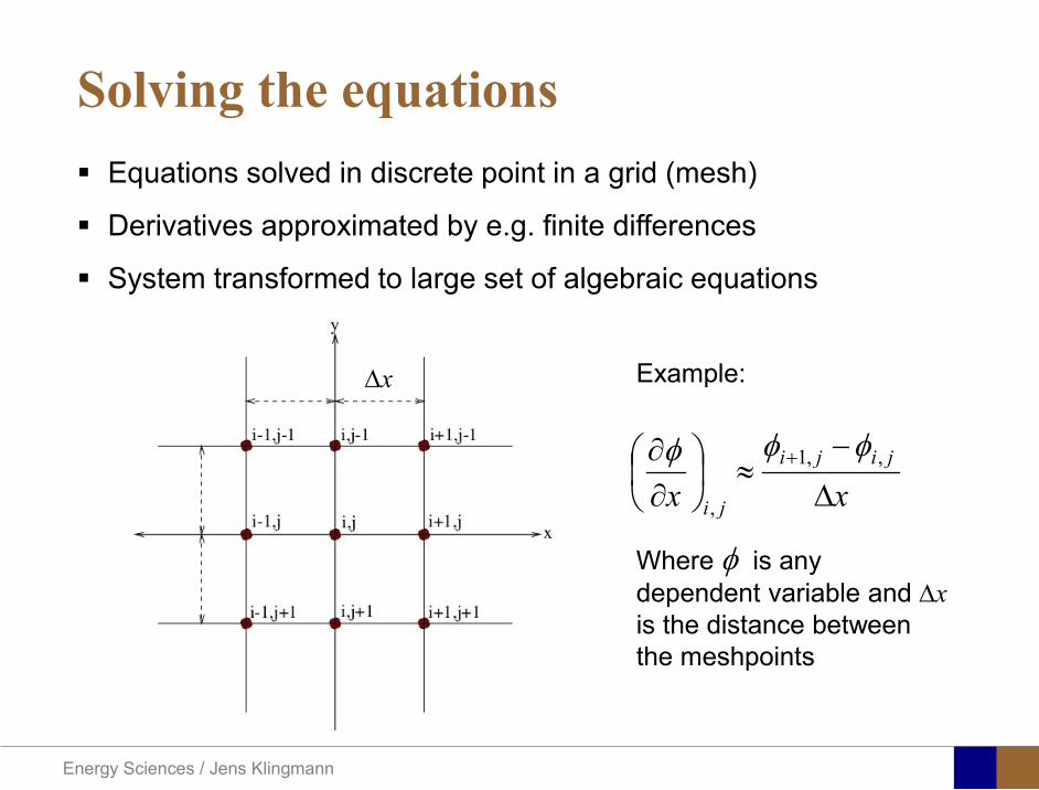
Energy Sciences Jens Klingmann
Solving the equations Equations solved in discrete point in a grid (mesh)
Derivatives approximated by eg finite differences
System transformed to large set of algebraic equations
xxjiji
ji ∆
minusasymp
partpart + 1
φφφ
Where φ is any dependent variable and ∆xis the distance between the meshpoints
∆x Example
Energy Sciences Jens Klingmann
Turbulence
Energy Sciences Jens Klingmann
Osborne Reynoldsrsquo Experiments
Energy Sciences Jens Klingmann
Characteristics of turbulence
bull Irregularity
bull Diffusivity the capability of turbulence to enhance transport of mass heat and momentum
bull Large Reynolds numbers Many flow fields are laminar at low Re but become unstable and turbulent at higher Re
bull Three-dimensional vorticity fluctuations
bull Dissipation Viscous shear stresses perform deformation work on the fluid which increases the internal energy at the expense of the kinetic energy
bull Continuum In most technical applications the distance between molecules is orders of magnitude shorter than the size of even the smallest scales of the flow
Energy Sciences Jens Klingmann
Turbulence is irregularity
025 03 035 04 045 05t0
001002003004005006007008009
01
u(x
t)
u(xt)
u(x)
bull Small (unresolvable) scalesbull Statistical approach required bull How can we define an average velocity
0
1( ) ( )T
u u t dtT
= intx x
Energy Sciences Jens Klingmann
Turbulence averaging
Havenrsquot we already done this once
Energy Sciences Jens Klingmann
y zx zz z z z z z
x y z
z z z
u uu uu u u u u uu u ut x x y y z z
u u upz x x y y z z
ρ
micro micro micro
partpartpart part part part part + + + + + + = part part part part part part part
part part partpart part part part= minus + + +
part part part part part part part
Turbulence averaging
uuu += ppp +=
Insert into NS (only z-direction shown) and average entire equation
and
Decompose velocity and pressure (Reynoldsrsquo decomposition)
Additional terms that look like stresses
Energy Sciences Jens Klingmann
Turbulence RANS modellingReynoldsrsquo stress tensor
Needs to be expressed as a function of variables we know or intend to solve for
TURBULENCE MODEL
x x x y x z
y x y y y z
z x z y z z
u u u u u u
u u u u u u
u u u u u u
ρ
=
R
6 new variables (symmetry )xyyx uuuu =
Energy Sciences Jens Klingmann
Turbulence RANS modellingReynolds stress tensor
ij i j
u u u v u w
R u u v u v v v w
w u w v w w
ρ ρ ρ
= minus otimes = = =
R u u
Turbulent Kinetic Energy
( ) ( )1 1 1 1 2 2 2 2ii i ik tr R u u u u v v w wρ ρ= = = = + +R
Represents the kinetic energy of the fluctuations (or vortices)
Energy Sciences Jens Klingmann
Turbulence closure problem
10 unknownvelocity components pressure and correlations of fluctuating velocity
4 equationsAveraged momentum equations and averaged continuity equation
i ju u
Energy Sciences Jens Klingmann
Turbulence RANS modelling
23
i jij T ij
j i
u uR kx x
micro ρ δ part part
= + minus part part
2 T kmicro ρ εpropldquoTurbulent viscosityrdquo
Transport of k Some terms may be derived other need modelling
( ) ( ) ( )advection diffusion productionk k k kt
εpart+ + = minus
part
Energy from mean flow to turbulence
Dissipation Energy converted to heat
Energy Sciences Jens Klingmann
Turbulence RANS modelling
23
i jij T ij
j i
u uR kx x
micro ρ δ part part
= + minus part part ερmicro micro 2kCT =
k Tklk
k l k k k
uk ku Rx x x x
microρ ε micro
σ part part part part
= minus + + part part part part 2
1 2k T
klkk l k k
uu C R C
x k x k x xε εε
microε ε ε ερ ρ micropart σ
part part part part= minus + + part part part
4411 =εC 9212 =εC 090=microC 1=kσ31=εσ
Closure coefficients
Energy Sciences Jens Klingmann
Energy Sciences Jens Klingmann
Computational Fluid Dynamics (CFD)
U Waringhleacuten ldquoThe Aerodynamic design and testing of a supersonic turbine for rocket engine propulsionrdquo Proc Of 3rd European conference on Turbomachinery Fluid dynamics and thermodynamics
Energy Sciences Jens Klingmann
Subsonic flow in an aerofoilplate junction computed with a second-moment closure (D Apsley 1998)
Computational Fluid Dynamics(CFD)
Energy Sciences Jens Klingmann
Hydraulic turbine research CFD digital simulation Distribution of speed on an axial turbine
Computational Fluid Dynamics(CFD)
Energy Sciences Jens Klingmann
Scales of turbulence
10-01
1000
1001
1002
1003
1004
1005
κ LI
10-08
10-07
10-06
10-05
10-04
10-03
10-02
10-01
1000
E(u
2 LI)
10-04
10-03
10-02
10-01
1000
κ LK
10-05
10-04
10-03
10-02
10-01
1000
1001
1002
D( ε L
K )10-01
1000
1001
1002
1003
1004
1005
E = 15 (κ LI)-53
10-04
10-03
10-02
10-01
1000
1001
D = 3 ( κ LΚ) 13
Normalized energy and dissipation spectra for
Adapted from Tennekeys and Lumley
ReLI= times2 105
1 2Re 500IL asymp
3 4Re 10000IL asymp
Energy Sciences Jens Klingmann
References Turbulence
bull Tennekeys and Lumley ldquoA first course in Turbulencerdquo MIT Press 1972
bull J O Hinze ldquoTurbulencerdquo McGraw-Hill 1959bull D C Wilcox ldquoTurbulence Modeling for CFDrdquo DCW Industries
2006
Energy Sciences Jens Klingmann
Boundary layers
Energy Sciences Jens Klingmann
Boundary Layer Theory (BLT) Sensitive to Pressure
gradients Appropriate scaling from
dimensional analyses
Energy Sciences Jens Klingmann
Boundary layers
Energy Sciences Jens Klingmann
Air foil theory
Energy Sciences Jens Klingmann
Visualisation of diffusor separation
Energy Sciences Jens Klingmann
BL equations
+minus=+
yu
yxp
xuv
xuu
partpartmicro
partpart
partpart
partρpart
partρpart and 0=+
yxu
partυpart
partpart
Applying the BL approximations the 2D stationary incompressible NS-eq and continuity equation become
yvu
yu
yxuu
xp
yu
xuu
partpartρ
partpartmicro
partpart
partρpart
partpart
partυρpart
partρpart
minus
+minusminus=+
and
0=+yx
upart
υpartpartpart
Reynolds averaged BL eqs are
Energy Sciences Jens Klingmann
Boundary layers
Energy Sciences Jens Klingmann
Turbulent BL at different Pressure gradients
Energy Sciences Jens Klingmann
Boundary Layers
ν
yuy =+
ρτWu =
0=
partpart
=y
w yuτ
uuu =+
Energy Sciences Jens Klingmann
Diffuser efficiency
Energy Sciences Jens Klingmann
Reynolds Number (Order of magnitude)
At eg a compressor inlet
ρ = O(1) kgm3
U = O(100) msx lt O(01) mmicro = O(10-5)
Re = ρ U x micro =O(106)
In subsequent stages large amounts of turbulence (from stator wakes) will be convected into the Boundary layer
Energy Sciences Jens Klingmann
References Boundary layers
bull Frank M White ldquoViscous Fluid Flowrdquobull Hermann Schlichting ldquoBoundary Layer Theoryrdquo
Energy Sciences Jens Klingmann
CFD and experiments
bull No this is not a CFD course butbull Experiments
Energy Sciences Jens Klingmann
What do we need to measureOverall performance
Flow rates (mass or volume) Pressure Temperature Shaft power
Performance increase
Separations (velocity) Secondary flows eg tip clearance losses (velocity) Shock waves (supersonic applications) Pressure (resolved in time and space) Temperature (resolved in time and space)
Energy Sciences Jens Klingmann
Cascade wind tunnels
FIG 31 Compressor cascade wind tunnels (a) Conventional low-speed continuousrunning cascade tunnel (adapted from Carter et al 1950)(b) Transonicsupersoniccascade tunnel (adapted from Sieverding 1985)
Energy Sciences Jens Klingmann
Closed circuit tunnels
Energy Sciences Jens Klingmann
components
Settling Chamber
The settling chamber is located between the fan or wide angle diffuser and the contraction and contains the honeycombs and screens used to moderate longitudinal variations in the flow Screens in the chamber should be spaced at 02 chamber diameters apart so that flow disturbed by the first screen can settle before it encounters the second
Honeycombs
Honeycombs are located in the settling chamber and are used to reduce nonuniformities in the flow For optimum benefit honeycombs should be 6-8 cell diameters thick and cell size should be on the order of about 150 cells per settling chamber diameter
Energy Sciences Jens Klingmann
components
Screens
Screens are typically located just downstream of the honeycomb and sometime at the inlet of the test section Screens create a static pressure drop and serve to reduce boundary layer size and increase flow uniformity
Contraction Section
Contractions sections are located between the settling chamber and the test sections and serve to both increase mean velocities at the test section inlet and moderate inconsistencies in the uniformity of the flow Large contraction ratios and short contraction lengths are generally more desirable as they reduce the power loss across the screens and the thickness of boundary layers Small tunnels typically have contraction ratios between 6 and 9
Energy Sciences Jens Klingmann
Flow meters with pressure measurement
Venturi-tube
A1 A2
P1 P2
1 1 2 2C A C A=In the incompressible case
2 21 1 2 2
2 2C P C P
ρ ρ+ = +Assuming horisontal mounting
Energy Sciences Jens Klingmann
Daniel Bernoulli 1700-1782
Daniel Bernoulli was the son of Johann Bernoulli He was born in Groningen while his father held the chair of mathematics there His older brother was Nicolaus(II) Bernoulli and his uncle was Jacob Bernoulli so he was born into a family of leading mathematicians but also into a family where there was unfortunate rivalry jealousy and bitterness
Undoubtedly the most important work which Daniel Bernoulli did was his work on hydrodynamics Even the term itself is based on the title of the work which he produced called Hydrodynamica and before he left St Petersburg Daniel left a draft copy of the book with a printer However the work was not published until 1738 and although he revised it considerably between 1734 and 1738 it is more the presentation that he changed rather then the substance
This work contains for the first time the correct analysis of water flowing from a hole in a container This was based on the principle of conservation of energy which he had studied with his father in 1720 Daniel also discussed pumps and other machines to raise water One remarkable discovery appears in Chapter 10 of Hydrodynamica where Daniel discussed the basis for the kinetic theory of gases He was able to give the basic laws for the theory of gases and gave although not in full detail the equation of state discovered by Van der Waals a century later
Energy Sciences Jens Klingmann
Venturi-tube (2)
22 2 12 2
2
2A PC CA ρ
∆minus =
A1 A2
P1 P2
Solve for eg C2
1 2P P P∆ = minus
( )
12
2 2 21 2
21
PCA Aρ
∆ = minus
and( )
12
2 2 2 2 21 2
21
Pm A C AA Aρρ
∆ = = minus
where
Flow meters with pressure measurement
Energy Sciences Jens Klingmann
Flow meters with pressure measurement
Orifice meters
A1
A2
P1 P2
Applicable for pipe flows Same principle as for Venturi Positioning of pressure taps important Vena contracta and losses require inclusion
of Discharge Coefficient CD
( )
12
2 2 21 2
21D
Pm C AA Aρ ∆ =
minus where ( )1 2ReDC f A A=
CD available from manufacturer (measurements) or Standards (eg ISO)
Energy Sciences Jens Klingmann
Coriolis flow meter
An actuator (not shown) induces a vibration of the tubes
When there is mass flow Coriolis forces induce twisting of the tubes
degree of phase-shift is a measure for the amount of mass that is flowing through the tubes
Energy Sciences Jens Klingmann
Thermal flow meter Heat is added electrically to the flow Temperature is measured before and after heat addition
pP mC T∆=
Energy Sciences Jens Klingmann
Ultrasonic flow meters
Ultrasound is emitted to small particles in the flow (dust or other) Reflections of the sound is frequency shifted by the Doppler effect The frequency change is proportional to the particles velocity (volume flow
meter)
Energy Sciences Jens Klingmann
Inductive flow metersA magnetic flowmeter is based upon Faradays Law
The voltage induced across any conductor as it moves at right angles through a magnetic field is proportional to the velocity of that conductor
E is proportional to V x B x D where
E = The voltage generated in a conductorV = The velocity of the conductorB = The magnetic field strengthD = The length of the conductor
NB electric conductivity is required
Energy Sciences Jens Klingmann
Temperature measurements
Thermocouples
The basis established by Thomas Johann Seebeck in 1821
A conductor generates a voltage when subjected to a temperature gradient
To measure this voltage one must use a second conductor material which generates a different voltage under the same temperature gradient
Energy Sciences Jens Klingmann
Pressure sensing
1 2p pgt 2p p2 may be the atmosphere a static pressure tap or a known reference pressure
The strain of the diaphragm (or itrsquos deflection) may be measured by a number of electric methods
Diaphragm
Energy Sciences Jens Klingmann
Pressure sensingPiezoresistive Strain Gage
Uses the piezoresistive effect of bonded or formed strain gauges to detect strain due to applied pressure
Capacitive
Uses a diaghragm and pressure cavity to create a variable capacitor to detect strain due to applied pressure
Magnetic
Measures the displacement of a diaphragm by means of changes in inductance (reluctance) LVDT Hall Effect or by eddy current principal
Piezoelectric
Uses the piezoelectric effect in certain materials such as quartz to measure the strain upon the sensing mechanism due to pressure
Potentiometric
Uses the motion of a wiper along a resistive mechanism to detect the strain caused by applied pressure
Energy Sciences Jens Klingmann
3D highly instationary (periodic) flow Potentially very high velocities (Supersonic) Large temperature differences Low accessibility (difficult to probe between rotors) Low turbulence levels in most of the domain Very high turbulence in BL and wakes
Properties of measuring object
Point measurements
Energy Sciences Jens Klingmann
Conventional or non-opticalndash Static Pressure Measurementsndash Total Pressure Measurements
bull Multy hole probes
ndash Total Temperature ndash Hot Wire Anemometry (HWA)
Optical techniques for Velocity Measurementsndash Laser Two Focous (L2F)ndash Laser Doppler Anemometry (LDA)ndash Particle Image velocimetry (PIV)
Point Measurements
Energy Sciences Jens Klingmann
Static and total pressure
2 2 21 2 1
2 1 2 2 2C C CP P ρ ρ ρ
minus = minus =
2 0C =Stagnation point
C1Static pressure tap
Prandtl or Pitot tube
Apply the Bernoulli equation from free stream to stagnation point
21
2 12CP Pρ
= +or
We can also define a stagnation or total pressure
( )2
101 1 022
CP P Pρ= + =
Total pressure = Static pressure + dynamic pressure
or
Energy Sciences Jens Klingmann
Static pressure
Energy Sciences Jens Klingmann
Total Pressure and Temperature
Shrouded Probes
Shrouded Probe
Pitot or Prandtl tube
Sensitive to direction
Energy Sciences Jens Klingmann
Ludwig Prandtl 1875-1953
Ludwig Prandtl born at Freising Bavaria on February 4 1875 was a German Physicist famous for his work in aeronautics He qualified at Munchen in 1900 with a thesis on elastic stability and held the position of Professor of Applied Mechanics at Gottingen for forty-nine years (from 1904 until his death there on August 15 1953) In 1925 Prandtl became the Director of the Kaiser Wilhelm Institute for Fluid Mechanics His discovery in 1904 of the Boundary Layer which adjoins the surface of a body moving in a fluid led to an understanding of skin friction drag and of the way in which streamlining reduces the drag of airplane wings and other moving bodies His work on wing theory published in 1918 - 1919 followed that of FW Lanchester (1902-1907) but was carried out independently and elucidated the flow over airplane wings of finite span Prandtls work and decisive advances in boundary layer and wing theories became the basic material of aeronautics He also made important contributions to the theories of supersonic flow and of turbulence and contributed much to the development of wind tunnels and other aerodynamic equipment In addition he devised the soap-film analogy for the torsion of non-circular sections and wrote on the theory of plasticity and of meteorology
Energy Sciences Jens Klingmann
Total Pressure multy hole
Cobra Probe Yaw Probe
5 Hole Probe
Energy Sciences Jens Klingmann
5 Hole Probes Calibration
Energy Sciences Jens Klingmann
The inherent unsteadiness of the flow within turbomachines
Energy Sciences Jens Klingmann
Hot Wire Anemometry (HWA) The heat transfer from a thin (one micron)
electrically heated wire can be used to determine velocity
The resistance of the wire is temperature dependent Within a small temperature range it can be assumed linear R = R0+α R0(Tm-T0) where R0 is the resistance at a reference temperature T0 and Tm is the mean wire temperature
The thermal power induced in the wire is balanced by heat transfer to the surrounding fluid I2R=hπDL(Tm-T0) where h is the heat transfer coefficient and D and L the diameter and length of the wire respectively
E = I R
Energy Sciences Jens Klingmann
Constant Temperature Anemometry (CTA) The wire is often placed in a Whetstone bridge If the output from the
bridge is amplified and fed back to the bridge the resistance of the probe and thus the temperature will be held constant
This prevents the temperature of the wire to become excessive at low velocities
R1
R2 R3
Probe
Bridge Voltage
Energy Sciences Jens Klingmann
Constant Temperature Anemometry (CTA)
Energy Sciences Jens Klingmann
Characteristics of LDA (according to Dantec)
Invented by Yeh and Cummins in 1964 Velocity measurements in Fluid Dynamics (gas liquid) Up to 3 velocity components Non-intrusive measurements (optical technique) Absolute measurement technique (no calibration required) Very high accuracy Very high spatial resolution due to small measurement volume Tracer particles are required
Energy Sciences Jens Klingmann
LDA - Fringe Model
Focused Laser beams intersect and form the measurement volume Plane wave fronts beam waist in the plane of intersection Interference in the plane of intersection Pattern of bright and dark stripesplanes Fringes
Energy Sciences Jens Klingmann
LDA-measuring volume
d
x
x
y
y
z
z
e-2 CONTOUR
FRINGES
κ
κ
κ
κ
De-2
De-2
dml m
a
b
cx
b
z
ya
cd
d
=
=
=
J
J
J
J
JP
JP
JP
JD
JD
JD
+
+
+
a
b
c
d
κπλ
=minus sinD
f4l2e
m
κπλ
=minus cosD
f4D2e
m
Energy Sciences Jens Klingmann
Laser Two Focus
Energy Sciences Jens Klingmann
Laser Two Focus
Energy Sciences Jens Klingmann
PIV measurements
PIV is a fairly new technique capable of simultaneous velocity measurements at many points in a plane This gives information on large scale structures vorticity etc which is very difficult or impossible to obtain from one-point measuring techniques
PIV involves the illumination of a plane of the flow under investigation with a thin pulsed sheet of light The flow is seeded with particles
The light scattered from the particles and from successive pulses are being recorded either on film or a CCD array forming a multiple exposure of each particle image If the time between the pulses is known velocity can be determined as the ratio of the particle displacement and the elapsed time
t∆∆= xu
Energy Sciences Jens Klingmann
PIV
Energy Sciences Jens Klingmann
PIV measurements illumination
YA
G
YA
G
Two frequency doubled YAG Lasers aligned to one double pulsed laser sheet
Two or more separate light pulses can be obtained by chopping a continuous laser or from pulsed lasers
The limited pulse energies obtained from continuous lasers limits their applicability to low velocity flows or flows where large seeding particles can be used (ie liquid flows)
The low repetition rate of most pulsed lasers makes the use of two lasers advantageous
Energy Sciences Jens Klingmann
PIV measurements recording
High seeding density in laminar flame
Film or CCD-cameras Cross- or Auto-correlation
ndash ie both particle images on the same frame or on separate frames
CCD-camera requirementndash A many pixels as possiblendash 2k by 2k available 4k by 4k coming
Energy Sciences Jens Klingmann
PIV measurements analyses
Low seeding density (Number of seeding particles per unit volume)
Each particle image pair can be identified This is called particle tracking
High seeding density (PIV)
Small sub-regions of the image containing many particle image pairs are processed to obtain one velocity vector
Energy Sciences Jens Klingmann
PIV measurements analyses
Energy Sciences Jens Klingmann
PIV measurements analyses
( ) ( ) ( ) xsxxs dIIR 2A
1
I
+= int
Cross correlation between ( )x1I and ( )x2I
s is a two dimensional displacement vector
IA is the interrogation area
Cross correlation between
(
)
x
1
I
and
(
)
x
2
I
s is a two dimensional displacement vector
I
A
is the interrogation area
Energy Sciences Jens Klingmann
Energy Sciences Jens Klingmann
PIV from IOWA state university
Energy Sciences Jens Klingmann
PIV sample of evaluation
Energy Sciences Jens Klingmann
LDA PIV HWA Velocity range 01 mms ndash 300
ms 02 ndash 150 ms
Measuring Volume
D = 005 L = 05 mm
2 by 2 by 05 mm
L = 05 mm
Freq response O(10 000) Hz O(10) Hz O(100 000) Hz Calibration Yes No No Sensitivity to other than velocity
Low (ref Index) Low (ref Index) Large (temperature concentrationshellip)
Continuous Signal
Sometimes Seldom Always
Noise High High Low Turbulence intensity
No limitation Some limitation lt 20
Price O(1 000 000) SEK
O(1 000 000) SEK
O(50 000) SEK
Required Knowledge
High medium Low
Comparison of techniques
Energy Sciences Jens Klingmann
References experiments
R J Goldstein ldquoFluid Mechanics Measurementsrdquo Hemisphere Publishing 1983 A V Johansson amp P H Alfredsson ldquoExperimentella metoder inom
stroumlmningsmekanikenrdquo Inst Foumlr Mekanik KTH F Durst A Melling and J H Whitelaw ldquoPrincipals and Practice of Laser Doppler
Anemometryrdquo 1984 R J Adrian ldquoParticle-imaging techniques for experimental fluid mechnicsrdquo Ann Rev
Fluid Mech 1991
Energy Sciences Jens Klingmann
Sample of LDA-measurements
Rotor blade
Glas window
Emitted beams
Scattered Light
Adjustable mirror
Energy Sciences Jens Klingmann
Axial velocity sorted into 10 bins
0 1 2 3 4 5 6tangential coordinate (degrees)
-20
0
20
40
60
80
100
120
140
160Ax
ial v
eloc
ity a
nd s
tand
ard
devi
atio
n (m
s)
radial position 7 mm from inner window surfaceaxial position 23 mm behind rotor blades
Energy Sciences Jens Klingmann
Axial velocities in the radial-tangential plane
Energy Sciences Jens Klingmann
Airfoils NACA 4-digit
The NACA four-digit wing sections define the profile by
One digit describing maximum camber as percentage of the chord
One digit describing the distance of maximum camber from the airfoil leading edge in tens of percents of the chord
Two digits describing maximum thickness of the airfoil as percent of the chord
Example the NACA 2412 airfoil has a maximum camber of 2 located 40 (04 chords) from the leading edge with a maximum thickness of 12 of the chord
Four-digit series airfoils by default have maximum thickness at 30 of the chord (03 chords) from the leading edge
Energy Sciences Jens Klingmann
Airfoils NACA 4-digit
bull c is the chord lengthbull x is the position along
the chord from 0 to cbull y is the half thickness at
a given value of x (centerline to surface)
bull t is the maximum thickness as a fraction of the chord
Energy Sciences Jens Klingmann
Death by PowerPoint
| LDA | PIV | HWA | |||||
| Velocity range | 01 mms ndash 300 ms | 02 ndash 150 ms | |||||
| Measuring Volume | D = 005 L = 05 mm | 2 by 2 by 05 mm | L = 05 mm | ||||
| Freq response | O(10 000) Hz | O(10) Hz | O(100 000) Hz | ||||
| Calibration | Yes | No | No | ||||
| Sensitivity to other than velocity | Low (ref Index) | Low (ref Index) | Large (temperature concentrationshellip) | ||||
| Continuous Signal | Sometimes | Seldom | Always | ||||
| Noise | High | High | Low | ||||
| Turbulence intensity | No limitation | Some limitation | lt 20 | ||||
| Price | O(1 000 000) SEK | O(1 000 000) SEK | O(50 000) SEK | ||||
| Required Knowledge | High | medium | Low |
Energy Sciences Jens Klingmann
Turbulence
Energy Sciences Jens Klingmann
Osborne Reynoldsrsquo Experiments
Energy Sciences Jens Klingmann
Characteristics of turbulence
bull Irregularity
bull Diffusivity the capability of turbulence to enhance transport of mass heat and momentum
bull Large Reynolds numbers Many flow fields are laminar at low Re but become unstable and turbulent at higher Re
bull Three-dimensional vorticity fluctuations
bull Dissipation Viscous shear stresses perform deformation work on the fluid which increases the internal energy at the expense of the kinetic energy
bull Continuum In most technical applications the distance between molecules is orders of magnitude shorter than the size of even the smallest scales of the flow
Energy Sciences Jens Klingmann
Turbulence is irregularity
025 03 035 04 045 05t0
001002003004005006007008009
01
u(x
t)
u(xt)
u(x)
bull Small (unresolvable) scalesbull Statistical approach required bull How can we define an average velocity
0
1( ) ( )T
u u t dtT
= intx x
Energy Sciences Jens Klingmann
Turbulence averaging
Havenrsquot we already done this once
Energy Sciences Jens Klingmann
y zx zz z z z z z
x y z
z z z
u uu uu u u u u uu u ut x x y y z z
u u upz x x y y z z
ρ
micro micro micro
partpartpart part part part part + + + + + + = part part part part part part part
part part partpart part part part= minus + + +
part part part part part part part
Turbulence averaging
uuu += ppp +=
Insert into NS (only z-direction shown) and average entire equation
and
Decompose velocity and pressure (Reynoldsrsquo decomposition)
Additional terms that look like stresses
Energy Sciences Jens Klingmann
Turbulence RANS modellingReynoldsrsquo stress tensor
Needs to be expressed as a function of variables we know or intend to solve for
TURBULENCE MODEL
x x x y x z
y x y y y z
z x z y z z
u u u u u u
u u u u u u
u u u u u u
ρ
=
R
6 new variables (symmetry )xyyx uuuu =
Energy Sciences Jens Klingmann
Turbulence RANS modellingReynolds stress tensor
ij i j
u u u v u w
R u u v u v v v w
w u w v w w
ρ ρ ρ
= minus otimes = = =
R u u
Turbulent Kinetic Energy
( ) ( )1 1 1 1 2 2 2 2ii i ik tr R u u u u v v w wρ ρ= = = = + +R
Represents the kinetic energy of the fluctuations (or vortices)
Energy Sciences Jens Klingmann
Turbulence closure problem
10 unknownvelocity components pressure and correlations of fluctuating velocity
4 equationsAveraged momentum equations and averaged continuity equation
i ju u
Energy Sciences Jens Klingmann
Turbulence RANS modelling
23
i jij T ij
j i
u uR kx x
micro ρ δ part part
= + minus part part
2 T kmicro ρ εpropldquoTurbulent viscosityrdquo
Transport of k Some terms may be derived other need modelling
( ) ( ) ( )advection diffusion productionk k k kt
εpart+ + = minus
part
Energy from mean flow to turbulence
Dissipation Energy converted to heat
Energy Sciences Jens Klingmann
Turbulence RANS modelling
23
i jij T ij
j i
u uR kx x
micro ρ δ part part
= + minus part part ερmicro micro 2kCT =
k Tklk
k l k k k
uk ku Rx x x x
microρ ε micro
σ part part part part
= minus + + part part part part 2
1 2k T
klkk l k k
uu C R C
x k x k x xε εε
microε ε ε ερ ρ micropart σ
part part part part= minus + + part part part
4411 =εC 9212 =εC 090=microC 1=kσ31=εσ
Closure coefficients
Energy Sciences Jens Klingmann
Energy Sciences Jens Klingmann
Computational Fluid Dynamics (CFD)
U Waringhleacuten ldquoThe Aerodynamic design and testing of a supersonic turbine for rocket engine propulsionrdquo Proc Of 3rd European conference on Turbomachinery Fluid dynamics and thermodynamics
Energy Sciences Jens Klingmann
Subsonic flow in an aerofoilplate junction computed with a second-moment closure (D Apsley 1998)
Computational Fluid Dynamics(CFD)
Energy Sciences Jens Klingmann
Hydraulic turbine research CFD digital simulation Distribution of speed on an axial turbine
Computational Fluid Dynamics(CFD)
Energy Sciences Jens Klingmann
Scales of turbulence
10-01
1000
1001
1002
1003
1004
1005
κ LI
10-08
10-07
10-06
10-05
10-04
10-03
10-02
10-01
1000
E(u
2 LI)
10-04
10-03
10-02
10-01
1000
κ LK
10-05
10-04
10-03
10-02
10-01
1000
1001
1002
D( ε L
K )10-01
1000
1001
1002
1003
1004
1005
E = 15 (κ LI)-53
10-04
10-03
10-02
10-01
1000
1001
D = 3 ( κ LΚ) 13
Normalized energy and dissipation spectra for
Adapted from Tennekeys and Lumley
ReLI= times2 105
1 2Re 500IL asymp
3 4Re 10000IL asymp
Energy Sciences Jens Klingmann
References Turbulence
bull Tennekeys and Lumley ldquoA first course in Turbulencerdquo MIT Press 1972
bull J O Hinze ldquoTurbulencerdquo McGraw-Hill 1959bull D C Wilcox ldquoTurbulence Modeling for CFDrdquo DCW Industries
2006
Energy Sciences Jens Klingmann
Boundary layers
Energy Sciences Jens Klingmann
Boundary Layer Theory (BLT) Sensitive to Pressure
gradients Appropriate scaling from
dimensional analyses
Energy Sciences Jens Klingmann
Boundary layers
Energy Sciences Jens Klingmann
Air foil theory
Energy Sciences Jens Klingmann
Visualisation of diffusor separation
Energy Sciences Jens Klingmann
BL equations
+minus=+
yu
yxp
xuv
xuu
partpartmicro
partpart
partpart
partρpart
partρpart and 0=+
yxu
partυpart
partpart
Applying the BL approximations the 2D stationary incompressible NS-eq and continuity equation become
yvu
yu
yxuu
xp
yu
xuu
partpartρ
partpartmicro
partpart
partρpart
partpart
partυρpart
partρpart
minus
+minusminus=+
and
0=+yx
upart
υpartpartpart
Reynolds averaged BL eqs are
Energy Sciences Jens Klingmann
Boundary layers
Energy Sciences Jens Klingmann
Turbulent BL at different Pressure gradients
Energy Sciences Jens Klingmann
Boundary Layers
ν
yuy =+
ρτWu =
0=
partpart
=y
w yuτ
uuu =+
Energy Sciences Jens Klingmann
Diffuser efficiency
Energy Sciences Jens Klingmann
Reynolds Number (Order of magnitude)
At eg a compressor inlet
ρ = O(1) kgm3
U = O(100) msx lt O(01) mmicro = O(10-5)
Re = ρ U x micro =O(106)
In subsequent stages large amounts of turbulence (from stator wakes) will be convected into the Boundary layer
Energy Sciences Jens Klingmann
References Boundary layers
bull Frank M White ldquoViscous Fluid Flowrdquobull Hermann Schlichting ldquoBoundary Layer Theoryrdquo
Energy Sciences Jens Klingmann
CFD and experiments
bull No this is not a CFD course butbull Experiments
Energy Sciences Jens Klingmann
What do we need to measureOverall performance
Flow rates (mass or volume) Pressure Temperature Shaft power
Performance increase
Separations (velocity) Secondary flows eg tip clearance losses (velocity) Shock waves (supersonic applications) Pressure (resolved in time and space) Temperature (resolved in time and space)
Energy Sciences Jens Klingmann
Cascade wind tunnels
FIG 31 Compressor cascade wind tunnels (a) Conventional low-speed continuousrunning cascade tunnel (adapted from Carter et al 1950)(b) Transonicsupersoniccascade tunnel (adapted from Sieverding 1985)
Energy Sciences Jens Klingmann
Closed circuit tunnels
Energy Sciences Jens Klingmann
components
Settling Chamber
The settling chamber is located between the fan or wide angle diffuser and the contraction and contains the honeycombs and screens used to moderate longitudinal variations in the flow Screens in the chamber should be spaced at 02 chamber diameters apart so that flow disturbed by the first screen can settle before it encounters the second
Honeycombs
Honeycombs are located in the settling chamber and are used to reduce nonuniformities in the flow For optimum benefit honeycombs should be 6-8 cell diameters thick and cell size should be on the order of about 150 cells per settling chamber diameter
Energy Sciences Jens Klingmann
components
Screens
Screens are typically located just downstream of the honeycomb and sometime at the inlet of the test section Screens create a static pressure drop and serve to reduce boundary layer size and increase flow uniformity
Contraction Section
Contractions sections are located between the settling chamber and the test sections and serve to both increase mean velocities at the test section inlet and moderate inconsistencies in the uniformity of the flow Large contraction ratios and short contraction lengths are generally more desirable as they reduce the power loss across the screens and the thickness of boundary layers Small tunnels typically have contraction ratios between 6 and 9
Energy Sciences Jens Klingmann
Flow meters with pressure measurement
Venturi-tube
A1 A2
P1 P2
1 1 2 2C A C A=In the incompressible case
2 21 1 2 2
2 2C P C P
ρ ρ+ = +Assuming horisontal mounting
Energy Sciences Jens Klingmann
Daniel Bernoulli 1700-1782
Daniel Bernoulli was the son of Johann Bernoulli He was born in Groningen while his father held the chair of mathematics there His older brother was Nicolaus(II) Bernoulli and his uncle was Jacob Bernoulli so he was born into a family of leading mathematicians but also into a family where there was unfortunate rivalry jealousy and bitterness
Undoubtedly the most important work which Daniel Bernoulli did was his work on hydrodynamics Even the term itself is based on the title of the work which he produced called Hydrodynamica and before he left St Petersburg Daniel left a draft copy of the book with a printer However the work was not published until 1738 and although he revised it considerably between 1734 and 1738 it is more the presentation that he changed rather then the substance
This work contains for the first time the correct analysis of water flowing from a hole in a container This was based on the principle of conservation of energy which he had studied with his father in 1720 Daniel also discussed pumps and other machines to raise water One remarkable discovery appears in Chapter 10 of Hydrodynamica where Daniel discussed the basis for the kinetic theory of gases He was able to give the basic laws for the theory of gases and gave although not in full detail the equation of state discovered by Van der Waals a century later
Energy Sciences Jens Klingmann
Venturi-tube (2)
22 2 12 2
2
2A PC CA ρ
∆minus =
A1 A2
P1 P2
Solve for eg C2
1 2P P P∆ = minus
( )
12
2 2 21 2
21
PCA Aρ
∆ = minus
and( )
12
2 2 2 2 21 2
21
Pm A C AA Aρρ
∆ = = minus
where
Flow meters with pressure measurement
Energy Sciences Jens Klingmann
Flow meters with pressure measurement
Orifice meters
A1
A2
P1 P2
Applicable for pipe flows Same principle as for Venturi Positioning of pressure taps important Vena contracta and losses require inclusion
of Discharge Coefficient CD
( )
12
2 2 21 2
21D
Pm C AA Aρ ∆ =
minus where ( )1 2ReDC f A A=
CD available from manufacturer (measurements) or Standards (eg ISO)
Energy Sciences Jens Klingmann
Coriolis flow meter
An actuator (not shown) induces a vibration of the tubes
When there is mass flow Coriolis forces induce twisting of the tubes
degree of phase-shift is a measure for the amount of mass that is flowing through the tubes
Energy Sciences Jens Klingmann
Thermal flow meter Heat is added electrically to the flow Temperature is measured before and after heat addition
pP mC T∆=
Energy Sciences Jens Klingmann
Ultrasonic flow meters
Ultrasound is emitted to small particles in the flow (dust or other) Reflections of the sound is frequency shifted by the Doppler effect The frequency change is proportional to the particles velocity (volume flow
meter)
Energy Sciences Jens Klingmann
Inductive flow metersA magnetic flowmeter is based upon Faradays Law
The voltage induced across any conductor as it moves at right angles through a magnetic field is proportional to the velocity of that conductor
E is proportional to V x B x D where
E = The voltage generated in a conductorV = The velocity of the conductorB = The magnetic field strengthD = The length of the conductor
NB electric conductivity is required
Energy Sciences Jens Klingmann
Temperature measurements
Thermocouples
The basis established by Thomas Johann Seebeck in 1821
A conductor generates a voltage when subjected to a temperature gradient
To measure this voltage one must use a second conductor material which generates a different voltage under the same temperature gradient
Energy Sciences Jens Klingmann
Pressure sensing
1 2p pgt 2p p2 may be the atmosphere a static pressure tap or a known reference pressure
The strain of the diaphragm (or itrsquos deflection) may be measured by a number of electric methods
Diaphragm
Energy Sciences Jens Klingmann
Pressure sensingPiezoresistive Strain Gage
Uses the piezoresistive effect of bonded or formed strain gauges to detect strain due to applied pressure
Capacitive
Uses a diaghragm and pressure cavity to create a variable capacitor to detect strain due to applied pressure
Magnetic
Measures the displacement of a diaphragm by means of changes in inductance (reluctance) LVDT Hall Effect or by eddy current principal
Piezoelectric
Uses the piezoelectric effect in certain materials such as quartz to measure the strain upon the sensing mechanism due to pressure
Potentiometric
Uses the motion of a wiper along a resistive mechanism to detect the strain caused by applied pressure
Energy Sciences Jens Klingmann
3D highly instationary (periodic) flow Potentially very high velocities (Supersonic) Large temperature differences Low accessibility (difficult to probe between rotors) Low turbulence levels in most of the domain Very high turbulence in BL and wakes
Properties of measuring object
Point measurements
Energy Sciences Jens Klingmann
Conventional or non-opticalndash Static Pressure Measurementsndash Total Pressure Measurements
bull Multy hole probes
ndash Total Temperature ndash Hot Wire Anemometry (HWA)
Optical techniques for Velocity Measurementsndash Laser Two Focous (L2F)ndash Laser Doppler Anemometry (LDA)ndash Particle Image velocimetry (PIV)
Point Measurements
Energy Sciences Jens Klingmann
Static and total pressure
2 2 21 2 1
2 1 2 2 2C C CP P ρ ρ ρ
minus = minus =
2 0C =Stagnation point
C1Static pressure tap
Prandtl or Pitot tube
Apply the Bernoulli equation from free stream to stagnation point
21
2 12CP Pρ
= +or
We can also define a stagnation or total pressure
( )2
101 1 022
CP P Pρ= + =
Total pressure = Static pressure + dynamic pressure
or
Energy Sciences Jens Klingmann
Static pressure
Energy Sciences Jens Klingmann
Total Pressure and Temperature
Shrouded Probes
Shrouded Probe
Pitot or Prandtl tube
Sensitive to direction
Energy Sciences Jens Klingmann
Ludwig Prandtl 1875-1953
Ludwig Prandtl born at Freising Bavaria on February 4 1875 was a German Physicist famous for his work in aeronautics He qualified at Munchen in 1900 with a thesis on elastic stability and held the position of Professor of Applied Mechanics at Gottingen for forty-nine years (from 1904 until his death there on August 15 1953) In 1925 Prandtl became the Director of the Kaiser Wilhelm Institute for Fluid Mechanics His discovery in 1904 of the Boundary Layer which adjoins the surface of a body moving in a fluid led to an understanding of skin friction drag and of the way in which streamlining reduces the drag of airplane wings and other moving bodies His work on wing theory published in 1918 - 1919 followed that of FW Lanchester (1902-1907) but was carried out independently and elucidated the flow over airplane wings of finite span Prandtls work and decisive advances in boundary layer and wing theories became the basic material of aeronautics He also made important contributions to the theories of supersonic flow and of turbulence and contributed much to the development of wind tunnels and other aerodynamic equipment In addition he devised the soap-film analogy for the torsion of non-circular sections and wrote on the theory of plasticity and of meteorology
Energy Sciences Jens Klingmann
Total Pressure multy hole
Cobra Probe Yaw Probe
5 Hole Probe
Energy Sciences Jens Klingmann
5 Hole Probes Calibration
Energy Sciences Jens Klingmann
The inherent unsteadiness of the flow within turbomachines
Energy Sciences Jens Klingmann
Hot Wire Anemometry (HWA) The heat transfer from a thin (one micron)
electrically heated wire can be used to determine velocity
The resistance of the wire is temperature dependent Within a small temperature range it can be assumed linear R = R0+α R0(Tm-T0) where R0 is the resistance at a reference temperature T0 and Tm is the mean wire temperature
The thermal power induced in the wire is balanced by heat transfer to the surrounding fluid I2R=hπDL(Tm-T0) where h is the heat transfer coefficient and D and L the diameter and length of the wire respectively
E = I R
Energy Sciences Jens Klingmann
Constant Temperature Anemometry (CTA) The wire is often placed in a Whetstone bridge If the output from the
bridge is amplified and fed back to the bridge the resistance of the probe and thus the temperature will be held constant
This prevents the temperature of the wire to become excessive at low velocities
R1
R2 R3
Probe
Bridge Voltage
Energy Sciences Jens Klingmann
Constant Temperature Anemometry (CTA)
Energy Sciences Jens Klingmann
Characteristics of LDA (according to Dantec)
Invented by Yeh and Cummins in 1964 Velocity measurements in Fluid Dynamics (gas liquid) Up to 3 velocity components Non-intrusive measurements (optical technique) Absolute measurement technique (no calibration required) Very high accuracy Very high spatial resolution due to small measurement volume Tracer particles are required
Energy Sciences Jens Klingmann
LDA - Fringe Model
Focused Laser beams intersect and form the measurement volume Plane wave fronts beam waist in the plane of intersection Interference in the plane of intersection Pattern of bright and dark stripesplanes Fringes
Energy Sciences Jens Klingmann
LDA-measuring volume
d
x
x
y
y
z
z
e-2 CONTOUR
FRINGES
κ
κ
κ
κ
De-2
De-2
dml m
a
b
cx
b
z
ya
cd
d
=
=
=
J
J
J
J
JP
JP
JP
JD
JD
JD
+
+
+
a
b
c
d
κπλ
=minus sinD
f4l2e
m
κπλ
=minus cosD
f4D2e
m
Energy Sciences Jens Klingmann
Laser Two Focus
Energy Sciences Jens Klingmann
Laser Two Focus
Energy Sciences Jens Klingmann
PIV measurements
PIV is a fairly new technique capable of simultaneous velocity measurements at many points in a plane This gives information on large scale structures vorticity etc which is very difficult or impossible to obtain from one-point measuring techniques
PIV involves the illumination of a plane of the flow under investigation with a thin pulsed sheet of light The flow is seeded with particles
The light scattered from the particles and from successive pulses are being recorded either on film or a CCD array forming a multiple exposure of each particle image If the time between the pulses is known velocity can be determined as the ratio of the particle displacement and the elapsed time
t∆∆= xu
Energy Sciences Jens Klingmann
PIV
Energy Sciences Jens Klingmann
PIV measurements illumination
YA
G
YA
G
Two frequency doubled YAG Lasers aligned to one double pulsed laser sheet
Two or more separate light pulses can be obtained by chopping a continuous laser or from pulsed lasers
The limited pulse energies obtained from continuous lasers limits their applicability to low velocity flows or flows where large seeding particles can be used (ie liquid flows)
The low repetition rate of most pulsed lasers makes the use of two lasers advantageous
Energy Sciences Jens Klingmann
PIV measurements recording
High seeding density in laminar flame
Film or CCD-cameras Cross- or Auto-correlation
ndash ie both particle images on the same frame or on separate frames
CCD-camera requirementndash A many pixels as possiblendash 2k by 2k available 4k by 4k coming
Energy Sciences Jens Klingmann
PIV measurements analyses
Low seeding density (Number of seeding particles per unit volume)
Each particle image pair can be identified This is called particle tracking
High seeding density (PIV)
Small sub-regions of the image containing many particle image pairs are processed to obtain one velocity vector
Energy Sciences Jens Klingmann
PIV measurements analyses
Energy Sciences Jens Klingmann
PIV measurements analyses
( ) ( ) ( ) xsxxs dIIR 2A
1
I
+= int
Cross correlation between ( )x1I and ( )x2I
s is a two dimensional displacement vector
IA is the interrogation area
Cross correlation between
(
)
x
1
I
and
(
)
x
2
I
s is a two dimensional displacement vector
I
A
is the interrogation area
Energy Sciences Jens Klingmann
Energy Sciences Jens Klingmann
PIV from IOWA state university
Energy Sciences Jens Klingmann
PIV sample of evaluation
Energy Sciences Jens Klingmann
LDA PIV HWA Velocity range 01 mms ndash 300
ms 02 ndash 150 ms
Measuring Volume
D = 005 L = 05 mm
2 by 2 by 05 mm
L = 05 mm
Freq response O(10 000) Hz O(10) Hz O(100 000) Hz Calibration Yes No No Sensitivity to other than velocity
Low (ref Index) Low (ref Index) Large (temperature concentrationshellip)
Continuous Signal
Sometimes Seldom Always
Noise High High Low Turbulence intensity
No limitation Some limitation lt 20
Price O(1 000 000) SEK
O(1 000 000) SEK
O(50 000) SEK
Required Knowledge
High medium Low
Comparison of techniques
Energy Sciences Jens Klingmann
References experiments
R J Goldstein ldquoFluid Mechanics Measurementsrdquo Hemisphere Publishing 1983 A V Johansson amp P H Alfredsson ldquoExperimentella metoder inom
stroumlmningsmekanikenrdquo Inst Foumlr Mekanik KTH F Durst A Melling and J H Whitelaw ldquoPrincipals and Practice of Laser Doppler
Anemometryrdquo 1984 R J Adrian ldquoParticle-imaging techniques for experimental fluid mechnicsrdquo Ann Rev
Fluid Mech 1991
Energy Sciences Jens Klingmann
Sample of LDA-measurements
Rotor blade
Glas window
Emitted beams
Scattered Light
Adjustable mirror
Energy Sciences Jens Klingmann
Axial velocity sorted into 10 bins
0 1 2 3 4 5 6tangential coordinate (degrees)
-20
0
20
40
60
80
100
120
140
160Ax
ial v
eloc
ity a
nd s
tand
ard
devi
atio
n (m
s)
radial position 7 mm from inner window surfaceaxial position 23 mm behind rotor blades
Energy Sciences Jens Klingmann
Axial velocities in the radial-tangential plane
Energy Sciences Jens Klingmann
Airfoils NACA 4-digit
The NACA four-digit wing sections define the profile by
One digit describing maximum camber as percentage of the chord
One digit describing the distance of maximum camber from the airfoil leading edge in tens of percents of the chord
Two digits describing maximum thickness of the airfoil as percent of the chord
Example the NACA 2412 airfoil has a maximum camber of 2 located 40 (04 chords) from the leading edge with a maximum thickness of 12 of the chord
Four-digit series airfoils by default have maximum thickness at 30 of the chord (03 chords) from the leading edge
Energy Sciences Jens Klingmann
Airfoils NACA 4-digit
bull c is the chord lengthbull x is the position along
the chord from 0 to cbull y is the half thickness at
a given value of x (centerline to surface)
bull t is the maximum thickness as a fraction of the chord
Energy Sciences Jens Klingmann
Death by PowerPoint
| LDA | PIV | HWA | |||||
| Velocity range | 01 mms ndash 300 ms | 02 ndash 150 ms | |||||
| Measuring Volume | D = 005 L = 05 mm | 2 by 2 by 05 mm | L = 05 mm | ||||
| Freq response | O(10 000) Hz | O(10) Hz | O(100 000) Hz | ||||
| Calibration | Yes | No | No | ||||
| Sensitivity to other than velocity | Low (ref Index) | Low (ref Index) | Large (temperature concentrationshellip) | ||||
| Continuous Signal | Sometimes | Seldom | Always | ||||
| Noise | High | High | Low | ||||
| Turbulence intensity | No limitation | Some limitation | lt 20 | ||||
| Price | O(1 000 000) SEK | O(1 000 000) SEK | O(50 000) SEK | ||||
| Required Knowledge | High | medium | Low |
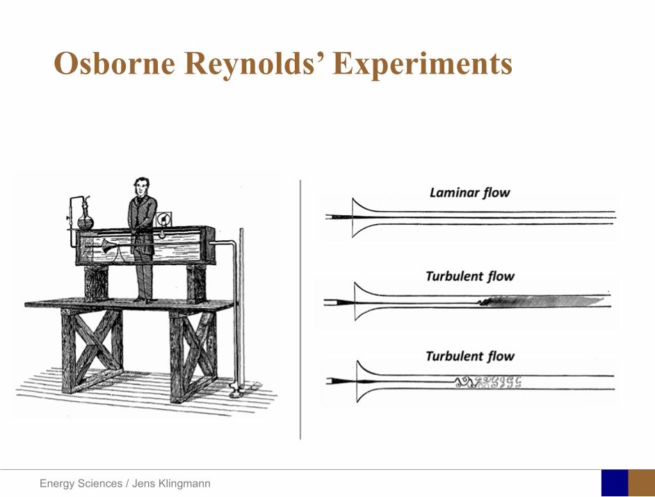
Energy Sciences Jens Klingmann
Osborne Reynoldsrsquo Experiments
Energy Sciences Jens Klingmann
Characteristics of turbulence
bull Irregularity
bull Diffusivity the capability of turbulence to enhance transport of mass heat and momentum
bull Large Reynolds numbers Many flow fields are laminar at low Re but become unstable and turbulent at higher Re
bull Three-dimensional vorticity fluctuations
bull Dissipation Viscous shear stresses perform deformation work on the fluid which increases the internal energy at the expense of the kinetic energy
bull Continuum In most technical applications the distance between molecules is orders of magnitude shorter than the size of even the smallest scales of the flow
Energy Sciences Jens Klingmann
Turbulence is irregularity
025 03 035 04 045 05t0
001002003004005006007008009
01
u(x
t)
u(xt)
u(x)
bull Small (unresolvable) scalesbull Statistical approach required bull How can we define an average velocity
0
1( ) ( )T
u u t dtT
= intx x
Energy Sciences Jens Klingmann
Turbulence averaging
Havenrsquot we already done this once
Energy Sciences Jens Klingmann
y zx zz z z z z z
x y z
z z z
u uu uu u u u u uu u ut x x y y z z
u u upz x x y y z z
ρ
micro micro micro
partpartpart part part part part + + + + + + = part part part part part part part
part part partpart part part part= minus + + +
part part part part part part part
Turbulence averaging
uuu += ppp +=
Insert into NS (only z-direction shown) and average entire equation
and
Decompose velocity and pressure (Reynoldsrsquo decomposition)
Additional terms that look like stresses
Energy Sciences Jens Klingmann
Turbulence RANS modellingReynoldsrsquo stress tensor
Needs to be expressed as a function of variables we know or intend to solve for
TURBULENCE MODEL
x x x y x z
y x y y y z
z x z y z z
u u u u u u
u u u u u u
u u u u u u
ρ
=
R
6 new variables (symmetry )xyyx uuuu =
Energy Sciences Jens Klingmann
Turbulence RANS modellingReynolds stress tensor
ij i j
u u u v u w
R u u v u v v v w
w u w v w w
ρ ρ ρ
= minus otimes = = =
R u u
Turbulent Kinetic Energy
( ) ( )1 1 1 1 2 2 2 2ii i ik tr R u u u u v v w wρ ρ= = = = + +R
Represents the kinetic energy of the fluctuations (or vortices)
Energy Sciences Jens Klingmann
Turbulence closure problem
10 unknownvelocity components pressure and correlations of fluctuating velocity
4 equationsAveraged momentum equations and averaged continuity equation
i ju u
Energy Sciences Jens Klingmann
Turbulence RANS modelling
23
i jij T ij
j i
u uR kx x
micro ρ δ part part
= + minus part part
2 T kmicro ρ εpropldquoTurbulent viscosityrdquo
Transport of k Some terms may be derived other need modelling
( ) ( ) ( )advection diffusion productionk k k kt
εpart+ + = minus
part
Energy from mean flow to turbulence
Dissipation Energy converted to heat
Energy Sciences Jens Klingmann
Turbulence RANS modelling
23
i jij T ij
j i
u uR kx x
micro ρ δ part part
= + minus part part ερmicro micro 2kCT =
k Tklk
k l k k k
uk ku Rx x x x
microρ ε micro
σ part part part part
= minus + + part part part part 2
1 2k T
klkk l k k
uu C R C
x k x k x xε εε
microε ε ε ερ ρ micropart σ
part part part part= minus + + part part part
4411 =εC 9212 =εC 090=microC 1=kσ31=εσ
Closure coefficients
Energy Sciences Jens Klingmann
Energy Sciences Jens Klingmann
Computational Fluid Dynamics (CFD)
U Waringhleacuten ldquoThe Aerodynamic design and testing of a supersonic turbine for rocket engine propulsionrdquo Proc Of 3rd European conference on Turbomachinery Fluid dynamics and thermodynamics
Energy Sciences Jens Klingmann
Subsonic flow in an aerofoilplate junction computed with a second-moment closure (D Apsley 1998)
Computational Fluid Dynamics(CFD)
Energy Sciences Jens Klingmann
Hydraulic turbine research CFD digital simulation Distribution of speed on an axial turbine
Computational Fluid Dynamics(CFD)
Energy Sciences Jens Klingmann
Scales of turbulence
10-01
1000
1001
1002
1003
1004
1005
κ LI
10-08
10-07
10-06
10-05
10-04
10-03
10-02
10-01
1000
E(u
2 LI)
10-04
10-03
10-02
10-01
1000
κ LK
10-05
10-04
10-03
10-02
10-01
1000
1001
1002
D( ε L
K )10-01
1000
1001
1002
1003
1004
1005
E = 15 (κ LI)-53
10-04
10-03
10-02
10-01
1000
1001
D = 3 ( κ LΚ) 13
Normalized energy and dissipation spectra for
Adapted from Tennekeys and Lumley
ReLI= times2 105
1 2Re 500IL asymp
3 4Re 10000IL asymp
Energy Sciences Jens Klingmann
References Turbulence
bull Tennekeys and Lumley ldquoA first course in Turbulencerdquo MIT Press 1972
bull J O Hinze ldquoTurbulencerdquo McGraw-Hill 1959bull D C Wilcox ldquoTurbulence Modeling for CFDrdquo DCW Industries
2006
Energy Sciences Jens Klingmann
Boundary layers
Energy Sciences Jens Klingmann
Boundary Layer Theory (BLT) Sensitive to Pressure
gradients Appropriate scaling from
dimensional analyses
Energy Sciences Jens Klingmann
Boundary layers
Energy Sciences Jens Klingmann
Air foil theory
Energy Sciences Jens Klingmann
Visualisation of diffusor separation
Energy Sciences Jens Klingmann
BL equations
+minus=+
yu
yxp
xuv
xuu
partpartmicro
partpart
partpart
partρpart
partρpart and 0=+
yxu
partυpart
partpart
Applying the BL approximations the 2D stationary incompressible NS-eq and continuity equation become
yvu
yu
yxuu
xp
yu
xuu
partpartρ
partpartmicro
partpart
partρpart
partpart
partυρpart
partρpart
minus
+minusminus=+
and
0=+yx
upart
υpartpartpart
Reynolds averaged BL eqs are
Energy Sciences Jens Klingmann
Boundary layers
Energy Sciences Jens Klingmann
Turbulent BL at different Pressure gradients
Energy Sciences Jens Klingmann
Boundary Layers
ν
yuy =+
ρτWu =
0=
partpart
=y
w yuτ
uuu =+
Energy Sciences Jens Klingmann
Diffuser efficiency
Energy Sciences Jens Klingmann
Reynolds Number (Order of magnitude)
At eg a compressor inlet
ρ = O(1) kgm3
U = O(100) msx lt O(01) mmicro = O(10-5)
Re = ρ U x micro =O(106)
In subsequent stages large amounts of turbulence (from stator wakes) will be convected into the Boundary layer
Energy Sciences Jens Klingmann
References Boundary layers
bull Frank M White ldquoViscous Fluid Flowrdquobull Hermann Schlichting ldquoBoundary Layer Theoryrdquo
Energy Sciences Jens Klingmann
CFD and experiments
bull No this is not a CFD course butbull Experiments
Energy Sciences Jens Klingmann
What do we need to measureOverall performance
Flow rates (mass or volume) Pressure Temperature Shaft power
Performance increase
Separations (velocity) Secondary flows eg tip clearance losses (velocity) Shock waves (supersonic applications) Pressure (resolved in time and space) Temperature (resolved in time and space)
Energy Sciences Jens Klingmann
Cascade wind tunnels
FIG 31 Compressor cascade wind tunnels (a) Conventional low-speed continuousrunning cascade tunnel (adapted from Carter et al 1950)(b) Transonicsupersoniccascade tunnel (adapted from Sieverding 1985)
Energy Sciences Jens Klingmann
Closed circuit tunnels
Energy Sciences Jens Klingmann
components
Settling Chamber
The settling chamber is located between the fan or wide angle diffuser and the contraction and contains the honeycombs and screens used to moderate longitudinal variations in the flow Screens in the chamber should be spaced at 02 chamber diameters apart so that flow disturbed by the first screen can settle before it encounters the second
Honeycombs
Honeycombs are located in the settling chamber and are used to reduce nonuniformities in the flow For optimum benefit honeycombs should be 6-8 cell diameters thick and cell size should be on the order of about 150 cells per settling chamber diameter
Energy Sciences Jens Klingmann
components
Screens
Screens are typically located just downstream of the honeycomb and sometime at the inlet of the test section Screens create a static pressure drop and serve to reduce boundary layer size and increase flow uniformity
Contraction Section
Contractions sections are located between the settling chamber and the test sections and serve to both increase mean velocities at the test section inlet and moderate inconsistencies in the uniformity of the flow Large contraction ratios and short contraction lengths are generally more desirable as they reduce the power loss across the screens and the thickness of boundary layers Small tunnels typically have contraction ratios between 6 and 9
Energy Sciences Jens Klingmann
Flow meters with pressure measurement
Venturi-tube
A1 A2
P1 P2
1 1 2 2C A C A=In the incompressible case
2 21 1 2 2
2 2C P C P
ρ ρ+ = +Assuming horisontal mounting
Energy Sciences Jens Klingmann
Daniel Bernoulli 1700-1782
Daniel Bernoulli was the son of Johann Bernoulli He was born in Groningen while his father held the chair of mathematics there His older brother was Nicolaus(II) Bernoulli and his uncle was Jacob Bernoulli so he was born into a family of leading mathematicians but also into a family where there was unfortunate rivalry jealousy and bitterness
Undoubtedly the most important work which Daniel Bernoulli did was his work on hydrodynamics Even the term itself is based on the title of the work which he produced called Hydrodynamica and before he left St Petersburg Daniel left a draft copy of the book with a printer However the work was not published until 1738 and although he revised it considerably between 1734 and 1738 it is more the presentation that he changed rather then the substance
This work contains for the first time the correct analysis of water flowing from a hole in a container This was based on the principle of conservation of energy which he had studied with his father in 1720 Daniel also discussed pumps and other machines to raise water One remarkable discovery appears in Chapter 10 of Hydrodynamica where Daniel discussed the basis for the kinetic theory of gases He was able to give the basic laws for the theory of gases and gave although not in full detail the equation of state discovered by Van der Waals a century later
Energy Sciences Jens Klingmann
Venturi-tube (2)
22 2 12 2
2
2A PC CA ρ
∆minus =
A1 A2
P1 P2
Solve for eg C2
1 2P P P∆ = minus
( )
12
2 2 21 2
21
PCA Aρ
∆ = minus
and( )
12
2 2 2 2 21 2
21
Pm A C AA Aρρ
∆ = = minus
where
Flow meters with pressure measurement
Energy Sciences Jens Klingmann
Flow meters with pressure measurement
Orifice meters
A1
A2
P1 P2
Applicable for pipe flows Same principle as for Venturi Positioning of pressure taps important Vena contracta and losses require inclusion
of Discharge Coefficient CD
( )
12
2 2 21 2
21D
Pm C AA Aρ ∆ =
minus where ( )1 2ReDC f A A=
CD available from manufacturer (measurements) or Standards (eg ISO)
Energy Sciences Jens Klingmann
Coriolis flow meter
An actuator (not shown) induces a vibration of the tubes
When there is mass flow Coriolis forces induce twisting of the tubes
degree of phase-shift is a measure for the amount of mass that is flowing through the tubes
Energy Sciences Jens Klingmann
Thermal flow meter Heat is added electrically to the flow Temperature is measured before and after heat addition
pP mC T∆=
Energy Sciences Jens Klingmann
Ultrasonic flow meters
Ultrasound is emitted to small particles in the flow (dust or other) Reflections of the sound is frequency shifted by the Doppler effect The frequency change is proportional to the particles velocity (volume flow
meter)
Energy Sciences Jens Klingmann
Inductive flow metersA magnetic flowmeter is based upon Faradays Law
The voltage induced across any conductor as it moves at right angles through a magnetic field is proportional to the velocity of that conductor
E is proportional to V x B x D where
E = The voltage generated in a conductorV = The velocity of the conductorB = The magnetic field strengthD = The length of the conductor
NB electric conductivity is required
Energy Sciences Jens Klingmann
Temperature measurements
Thermocouples
The basis established by Thomas Johann Seebeck in 1821
A conductor generates a voltage when subjected to a temperature gradient
To measure this voltage one must use a second conductor material which generates a different voltage under the same temperature gradient
Energy Sciences Jens Klingmann
Pressure sensing
1 2p pgt 2p p2 may be the atmosphere a static pressure tap or a known reference pressure
The strain of the diaphragm (or itrsquos deflection) may be measured by a number of electric methods
Diaphragm
Energy Sciences Jens Klingmann
Pressure sensingPiezoresistive Strain Gage
Uses the piezoresistive effect of bonded or formed strain gauges to detect strain due to applied pressure
Capacitive
Uses a diaghragm and pressure cavity to create a variable capacitor to detect strain due to applied pressure
Magnetic
Measures the displacement of a diaphragm by means of changes in inductance (reluctance) LVDT Hall Effect or by eddy current principal
Piezoelectric
Uses the piezoelectric effect in certain materials such as quartz to measure the strain upon the sensing mechanism due to pressure
Potentiometric
Uses the motion of a wiper along a resistive mechanism to detect the strain caused by applied pressure
Energy Sciences Jens Klingmann
3D highly instationary (periodic) flow Potentially very high velocities (Supersonic) Large temperature differences Low accessibility (difficult to probe between rotors) Low turbulence levels in most of the domain Very high turbulence in BL and wakes
Properties of measuring object
Point measurements
Energy Sciences Jens Klingmann
Conventional or non-opticalndash Static Pressure Measurementsndash Total Pressure Measurements
bull Multy hole probes
ndash Total Temperature ndash Hot Wire Anemometry (HWA)
Optical techniques for Velocity Measurementsndash Laser Two Focous (L2F)ndash Laser Doppler Anemometry (LDA)ndash Particle Image velocimetry (PIV)
Point Measurements
Energy Sciences Jens Klingmann
Static and total pressure
2 2 21 2 1
2 1 2 2 2C C CP P ρ ρ ρ
minus = minus =
2 0C =Stagnation point
C1Static pressure tap
Prandtl or Pitot tube
Apply the Bernoulli equation from free stream to stagnation point
21
2 12CP Pρ
= +or
We can also define a stagnation or total pressure
( )2
101 1 022
CP P Pρ= + =
Total pressure = Static pressure + dynamic pressure
or
Energy Sciences Jens Klingmann
Static pressure
Energy Sciences Jens Klingmann
Total Pressure and Temperature
Shrouded Probes
Shrouded Probe
Pitot or Prandtl tube
Sensitive to direction
Energy Sciences Jens Klingmann
Ludwig Prandtl 1875-1953
Ludwig Prandtl born at Freising Bavaria on February 4 1875 was a German Physicist famous for his work in aeronautics He qualified at Munchen in 1900 with a thesis on elastic stability and held the position of Professor of Applied Mechanics at Gottingen for forty-nine years (from 1904 until his death there on August 15 1953) In 1925 Prandtl became the Director of the Kaiser Wilhelm Institute for Fluid Mechanics His discovery in 1904 of the Boundary Layer which adjoins the surface of a body moving in a fluid led to an understanding of skin friction drag and of the way in which streamlining reduces the drag of airplane wings and other moving bodies His work on wing theory published in 1918 - 1919 followed that of FW Lanchester (1902-1907) but was carried out independently and elucidated the flow over airplane wings of finite span Prandtls work and decisive advances in boundary layer and wing theories became the basic material of aeronautics He also made important contributions to the theories of supersonic flow and of turbulence and contributed much to the development of wind tunnels and other aerodynamic equipment In addition he devised the soap-film analogy for the torsion of non-circular sections and wrote on the theory of plasticity and of meteorology
Energy Sciences Jens Klingmann
Total Pressure multy hole
Cobra Probe Yaw Probe
5 Hole Probe
Energy Sciences Jens Klingmann
5 Hole Probes Calibration
Energy Sciences Jens Klingmann
The inherent unsteadiness of the flow within turbomachines
Energy Sciences Jens Klingmann
Hot Wire Anemometry (HWA) The heat transfer from a thin (one micron)
electrically heated wire can be used to determine velocity
The resistance of the wire is temperature dependent Within a small temperature range it can be assumed linear R = R0+α R0(Tm-T0) where R0 is the resistance at a reference temperature T0 and Tm is the mean wire temperature
The thermal power induced in the wire is balanced by heat transfer to the surrounding fluid I2R=hπDL(Tm-T0) where h is the heat transfer coefficient and D and L the diameter and length of the wire respectively
E = I R
Energy Sciences Jens Klingmann
Constant Temperature Anemometry (CTA) The wire is often placed in a Whetstone bridge If the output from the
bridge is amplified and fed back to the bridge the resistance of the probe and thus the temperature will be held constant
This prevents the temperature of the wire to become excessive at low velocities
R1
R2 R3
Probe
Bridge Voltage
Energy Sciences Jens Klingmann
Constant Temperature Anemometry (CTA)
Energy Sciences Jens Klingmann
Characteristics of LDA (according to Dantec)
Invented by Yeh and Cummins in 1964 Velocity measurements in Fluid Dynamics (gas liquid) Up to 3 velocity components Non-intrusive measurements (optical technique) Absolute measurement technique (no calibration required) Very high accuracy Very high spatial resolution due to small measurement volume Tracer particles are required
Energy Sciences Jens Klingmann
LDA - Fringe Model
Focused Laser beams intersect and form the measurement volume Plane wave fronts beam waist in the plane of intersection Interference in the plane of intersection Pattern of bright and dark stripesplanes Fringes
Energy Sciences Jens Klingmann
LDA-measuring volume
d
x
x
y
y
z
z
e-2 CONTOUR
FRINGES
κ
κ
κ
κ
De-2
De-2
dml m
a
b
cx
b
z
ya
cd
d
=
=
=
J
J
J
J
JP
JP
JP
JD
JD
JD
+
+
+
a
b
c
d
κπλ
=minus sinD
f4l2e
m
κπλ
=minus cosD
f4D2e
m
Energy Sciences Jens Klingmann
Laser Two Focus
Energy Sciences Jens Klingmann
Laser Two Focus
Energy Sciences Jens Klingmann
PIV measurements
PIV is a fairly new technique capable of simultaneous velocity measurements at many points in a plane This gives information on large scale structures vorticity etc which is very difficult or impossible to obtain from one-point measuring techniques
PIV involves the illumination of a plane of the flow under investigation with a thin pulsed sheet of light The flow is seeded with particles
The light scattered from the particles and from successive pulses are being recorded either on film or a CCD array forming a multiple exposure of each particle image If the time between the pulses is known velocity can be determined as the ratio of the particle displacement and the elapsed time
t∆∆= xu
Energy Sciences Jens Klingmann
PIV
Energy Sciences Jens Klingmann
PIV measurements illumination
YA
G
YA
G
Two frequency doubled YAG Lasers aligned to one double pulsed laser sheet
Two or more separate light pulses can be obtained by chopping a continuous laser or from pulsed lasers
The limited pulse energies obtained from continuous lasers limits their applicability to low velocity flows or flows where large seeding particles can be used (ie liquid flows)
The low repetition rate of most pulsed lasers makes the use of two lasers advantageous
Energy Sciences Jens Klingmann
PIV measurements recording
High seeding density in laminar flame
Film or CCD-cameras Cross- or Auto-correlation
ndash ie both particle images on the same frame or on separate frames
CCD-camera requirementndash A many pixels as possiblendash 2k by 2k available 4k by 4k coming
Energy Sciences Jens Klingmann
PIV measurements analyses
Low seeding density (Number of seeding particles per unit volume)
Each particle image pair can be identified This is called particle tracking
High seeding density (PIV)
Small sub-regions of the image containing many particle image pairs are processed to obtain one velocity vector
Energy Sciences Jens Klingmann
PIV measurements analyses
Energy Sciences Jens Klingmann
PIV measurements analyses
( ) ( ) ( ) xsxxs dIIR 2A
1
I
+= int
Cross correlation between ( )x1I and ( )x2I
s is a two dimensional displacement vector
IA is the interrogation area
Cross correlation between
(
)
x
1
I
and
(
)
x
2
I
s is a two dimensional displacement vector
I
A
is the interrogation area
Energy Sciences Jens Klingmann
Energy Sciences Jens Klingmann
PIV from IOWA state university
Energy Sciences Jens Klingmann
PIV sample of evaluation
Energy Sciences Jens Klingmann
LDA PIV HWA Velocity range 01 mms ndash 300
ms 02 ndash 150 ms
Measuring Volume
D = 005 L = 05 mm
2 by 2 by 05 mm
L = 05 mm
Freq response O(10 000) Hz O(10) Hz O(100 000) Hz Calibration Yes No No Sensitivity to other than velocity
Low (ref Index) Low (ref Index) Large (temperature concentrationshellip)
Continuous Signal
Sometimes Seldom Always
Noise High High Low Turbulence intensity
No limitation Some limitation lt 20
Price O(1 000 000) SEK
O(1 000 000) SEK
O(50 000) SEK
Required Knowledge
High medium Low
Comparison of techniques
Energy Sciences Jens Klingmann
References experiments
R J Goldstein ldquoFluid Mechanics Measurementsrdquo Hemisphere Publishing 1983 A V Johansson amp P H Alfredsson ldquoExperimentella metoder inom
stroumlmningsmekanikenrdquo Inst Foumlr Mekanik KTH F Durst A Melling and J H Whitelaw ldquoPrincipals and Practice of Laser Doppler
Anemometryrdquo 1984 R J Adrian ldquoParticle-imaging techniques for experimental fluid mechnicsrdquo Ann Rev
Fluid Mech 1991
Energy Sciences Jens Klingmann
Sample of LDA-measurements
Rotor blade
Glas window
Emitted beams
Scattered Light
Adjustable mirror
Energy Sciences Jens Klingmann
Axial velocity sorted into 10 bins
0 1 2 3 4 5 6tangential coordinate (degrees)
-20
0
20
40
60
80
100
120
140
160Ax
ial v
eloc
ity a
nd s
tand
ard
devi
atio
n (m
s)
radial position 7 mm from inner window surfaceaxial position 23 mm behind rotor blades
Energy Sciences Jens Klingmann
Axial velocities in the radial-tangential plane
Energy Sciences Jens Klingmann
Airfoils NACA 4-digit
The NACA four-digit wing sections define the profile by
One digit describing maximum camber as percentage of the chord
One digit describing the distance of maximum camber from the airfoil leading edge in tens of percents of the chord
Two digits describing maximum thickness of the airfoil as percent of the chord
Example the NACA 2412 airfoil has a maximum camber of 2 located 40 (04 chords) from the leading edge with a maximum thickness of 12 of the chord
Four-digit series airfoils by default have maximum thickness at 30 of the chord (03 chords) from the leading edge
Energy Sciences Jens Klingmann
Airfoils NACA 4-digit
bull c is the chord lengthbull x is the position along
the chord from 0 to cbull y is the half thickness at
a given value of x (centerline to surface)
bull t is the maximum thickness as a fraction of the chord
Energy Sciences Jens Klingmann
Death by PowerPoint
| LDA | PIV | HWA | |||||
| Velocity range | 01 mms ndash 300 ms | 02 ndash 150 ms | |||||
| Measuring Volume | D = 005 L = 05 mm | 2 by 2 by 05 mm | L = 05 mm | ||||
| Freq response | O(10 000) Hz | O(10) Hz | O(100 000) Hz | ||||
| Calibration | Yes | No | No | ||||
| Sensitivity to other than velocity | Low (ref Index) | Low (ref Index) | Large (temperature concentrationshellip) | ||||
| Continuous Signal | Sometimes | Seldom | Always | ||||
| Noise | High | High | Low | ||||
| Turbulence intensity | No limitation | Some limitation | lt 20 | ||||
| Price | O(1 000 000) SEK | O(1 000 000) SEK | O(50 000) SEK | ||||
| Required Knowledge | High | medium | Low |
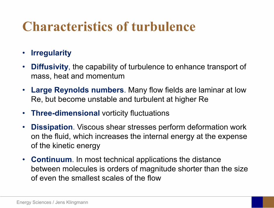
Energy Sciences Jens Klingmann
Characteristics of turbulence
bull Irregularity
bull Diffusivity the capability of turbulence to enhance transport of mass heat and momentum
bull Large Reynolds numbers Many flow fields are laminar at low Re but become unstable and turbulent at higher Re
bull Three-dimensional vorticity fluctuations
bull Dissipation Viscous shear stresses perform deformation work on the fluid which increases the internal energy at the expense of the kinetic energy
bull Continuum In most technical applications the distance between molecules is orders of magnitude shorter than the size of even the smallest scales of the flow
Energy Sciences Jens Klingmann
Turbulence is irregularity
025 03 035 04 045 05t0
001002003004005006007008009
01
u(x
t)
u(xt)
u(x)
bull Small (unresolvable) scalesbull Statistical approach required bull How can we define an average velocity
0
1( ) ( )T
u u t dtT
= intx x
Energy Sciences Jens Klingmann
Turbulence averaging
Havenrsquot we already done this once
Energy Sciences Jens Klingmann
y zx zz z z z z z
x y z
z z z
u uu uu u u u u uu u ut x x y y z z
u u upz x x y y z z
ρ
micro micro micro
partpartpart part part part part + + + + + + = part part part part part part part
part part partpart part part part= minus + + +
part part part part part part part
Turbulence averaging
uuu += ppp +=
Insert into NS (only z-direction shown) and average entire equation
and
Decompose velocity and pressure (Reynoldsrsquo decomposition)
Additional terms that look like stresses
Energy Sciences Jens Klingmann
Turbulence RANS modellingReynoldsrsquo stress tensor
Needs to be expressed as a function of variables we know or intend to solve for
TURBULENCE MODEL
x x x y x z
y x y y y z
z x z y z z
u u u u u u
u u u u u u
u u u u u u
ρ
=
R
6 new variables (symmetry )xyyx uuuu =
Energy Sciences Jens Klingmann
Turbulence RANS modellingReynolds stress tensor
ij i j
u u u v u w
R u u v u v v v w
w u w v w w
ρ ρ ρ
= minus otimes = = =
R u u
Turbulent Kinetic Energy
( ) ( )1 1 1 1 2 2 2 2ii i ik tr R u u u u v v w wρ ρ= = = = + +R
Represents the kinetic energy of the fluctuations (or vortices)
Energy Sciences Jens Klingmann
Turbulence closure problem
10 unknownvelocity components pressure and correlations of fluctuating velocity
4 equationsAveraged momentum equations and averaged continuity equation
i ju u
Energy Sciences Jens Klingmann
Turbulence RANS modelling
23
i jij T ij
j i
u uR kx x
micro ρ δ part part
= + minus part part
2 T kmicro ρ εpropldquoTurbulent viscosityrdquo
Transport of k Some terms may be derived other need modelling
( ) ( ) ( )advection diffusion productionk k k kt
εpart+ + = minus
part
Energy from mean flow to turbulence
Dissipation Energy converted to heat
Energy Sciences Jens Klingmann
Turbulence RANS modelling
23
i jij T ij
j i
u uR kx x
micro ρ δ part part
= + minus part part ερmicro micro 2kCT =
k Tklk
k l k k k
uk ku Rx x x x
microρ ε micro
σ part part part part
= minus + + part part part part 2
1 2k T
klkk l k k
uu C R C
x k x k x xε εε
microε ε ε ερ ρ micropart σ
part part part part= minus + + part part part
4411 =εC 9212 =εC 090=microC 1=kσ31=εσ
Closure coefficients
Energy Sciences Jens Klingmann
Energy Sciences Jens Klingmann
Computational Fluid Dynamics (CFD)
U Waringhleacuten ldquoThe Aerodynamic design and testing of a supersonic turbine for rocket engine propulsionrdquo Proc Of 3rd European conference on Turbomachinery Fluid dynamics and thermodynamics
Energy Sciences Jens Klingmann
Subsonic flow in an aerofoilplate junction computed with a second-moment closure (D Apsley 1998)
Computational Fluid Dynamics(CFD)
Energy Sciences Jens Klingmann
Hydraulic turbine research CFD digital simulation Distribution of speed on an axial turbine
Computational Fluid Dynamics(CFD)
Energy Sciences Jens Klingmann
Scales of turbulence
10-01
1000
1001
1002
1003
1004
1005
κ LI
10-08
10-07
10-06
10-05
10-04
10-03
10-02
10-01
1000
E(u
2 LI)
10-04
10-03
10-02
10-01
1000
κ LK
10-05
10-04
10-03
10-02
10-01
1000
1001
1002
D( ε L
K )10-01
1000
1001
1002
1003
1004
1005
E = 15 (κ LI)-53
10-04
10-03
10-02
10-01
1000
1001
D = 3 ( κ LΚ) 13
Normalized energy and dissipation spectra for
Adapted from Tennekeys and Lumley
ReLI= times2 105
1 2Re 500IL asymp
3 4Re 10000IL asymp
Energy Sciences Jens Klingmann
References Turbulence
bull Tennekeys and Lumley ldquoA first course in Turbulencerdquo MIT Press 1972
bull J O Hinze ldquoTurbulencerdquo McGraw-Hill 1959bull D C Wilcox ldquoTurbulence Modeling for CFDrdquo DCW Industries
2006
Energy Sciences Jens Klingmann
Boundary layers
Energy Sciences Jens Klingmann
Boundary Layer Theory (BLT) Sensitive to Pressure
gradients Appropriate scaling from
dimensional analyses
Energy Sciences Jens Klingmann
Boundary layers
Energy Sciences Jens Klingmann
Air foil theory
Energy Sciences Jens Klingmann
Visualisation of diffusor separation
Energy Sciences Jens Klingmann
BL equations
+minus=+
yu
yxp
xuv
xuu
partpartmicro
partpart
partpart
partρpart
partρpart and 0=+
yxu
partυpart
partpart
Applying the BL approximations the 2D stationary incompressible NS-eq and continuity equation become
yvu
yu
yxuu
xp
yu
xuu
partpartρ
partpartmicro
partpart
partρpart
partpart
partυρpart
partρpart
minus
+minusminus=+
and
0=+yx
upart
υpartpartpart
Reynolds averaged BL eqs are
Energy Sciences Jens Klingmann
Boundary layers
Energy Sciences Jens Klingmann
Turbulent BL at different Pressure gradients
Energy Sciences Jens Klingmann
Boundary Layers
ν
yuy =+
ρτWu =
0=
partpart
=y
w yuτ
uuu =+
Energy Sciences Jens Klingmann
Diffuser efficiency
Energy Sciences Jens Klingmann
Reynolds Number (Order of magnitude)
At eg a compressor inlet
ρ = O(1) kgm3
U = O(100) msx lt O(01) mmicro = O(10-5)
Re = ρ U x micro =O(106)
In subsequent stages large amounts of turbulence (from stator wakes) will be convected into the Boundary layer
Energy Sciences Jens Klingmann
References Boundary layers
bull Frank M White ldquoViscous Fluid Flowrdquobull Hermann Schlichting ldquoBoundary Layer Theoryrdquo
Energy Sciences Jens Klingmann
CFD and experiments
bull No this is not a CFD course butbull Experiments
Energy Sciences Jens Klingmann
What do we need to measureOverall performance
Flow rates (mass or volume) Pressure Temperature Shaft power
Performance increase
Separations (velocity) Secondary flows eg tip clearance losses (velocity) Shock waves (supersonic applications) Pressure (resolved in time and space) Temperature (resolved in time and space)
Energy Sciences Jens Klingmann
Cascade wind tunnels
FIG 31 Compressor cascade wind tunnels (a) Conventional low-speed continuousrunning cascade tunnel (adapted from Carter et al 1950)(b) Transonicsupersoniccascade tunnel (adapted from Sieverding 1985)
Energy Sciences Jens Klingmann
Closed circuit tunnels
Energy Sciences Jens Klingmann
components
Settling Chamber
The settling chamber is located between the fan or wide angle diffuser and the contraction and contains the honeycombs and screens used to moderate longitudinal variations in the flow Screens in the chamber should be spaced at 02 chamber diameters apart so that flow disturbed by the first screen can settle before it encounters the second
Honeycombs
Honeycombs are located in the settling chamber and are used to reduce nonuniformities in the flow For optimum benefit honeycombs should be 6-8 cell diameters thick and cell size should be on the order of about 150 cells per settling chamber diameter
Energy Sciences Jens Klingmann
components
Screens
Screens are typically located just downstream of the honeycomb and sometime at the inlet of the test section Screens create a static pressure drop and serve to reduce boundary layer size and increase flow uniformity
Contraction Section
Contractions sections are located between the settling chamber and the test sections and serve to both increase mean velocities at the test section inlet and moderate inconsistencies in the uniformity of the flow Large contraction ratios and short contraction lengths are generally more desirable as they reduce the power loss across the screens and the thickness of boundary layers Small tunnels typically have contraction ratios between 6 and 9
Energy Sciences Jens Klingmann
Flow meters with pressure measurement
Venturi-tube
A1 A2
P1 P2
1 1 2 2C A C A=In the incompressible case
2 21 1 2 2
2 2C P C P
ρ ρ+ = +Assuming horisontal mounting
Energy Sciences Jens Klingmann
Daniel Bernoulli 1700-1782
Daniel Bernoulli was the son of Johann Bernoulli He was born in Groningen while his father held the chair of mathematics there His older brother was Nicolaus(II) Bernoulli and his uncle was Jacob Bernoulli so he was born into a family of leading mathematicians but also into a family where there was unfortunate rivalry jealousy and bitterness
Undoubtedly the most important work which Daniel Bernoulli did was his work on hydrodynamics Even the term itself is based on the title of the work which he produced called Hydrodynamica and before he left St Petersburg Daniel left a draft copy of the book with a printer However the work was not published until 1738 and although he revised it considerably between 1734 and 1738 it is more the presentation that he changed rather then the substance
This work contains for the first time the correct analysis of water flowing from a hole in a container This was based on the principle of conservation of energy which he had studied with his father in 1720 Daniel also discussed pumps and other machines to raise water One remarkable discovery appears in Chapter 10 of Hydrodynamica where Daniel discussed the basis for the kinetic theory of gases He was able to give the basic laws for the theory of gases and gave although not in full detail the equation of state discovered by Van der Waals a century later
Energy Sciences Jens Klingmann
Venturi-tube (2)
22 2 12 2
2
2A PC CA ρ
∆minus =
A1 A2
P1 P2
Solve for eg C2
1 2P P P∆ = minus
( )
12
2 2 21 2
21
PCA Aρ
∆ = minus
and( )
12
2 2 2 2 21 2
21
Pm A C AA Aρρ
∆ = = minus
where
Flow meters with pressure measurement
Energy Sciences Jens Klingmann
Flow meters with pressure measurement
Orifice meters
A1
A2
P1 P2
Applicable for pipe flows Same principle as for Venturi Positioning of pressure taps important Vena contracta and losses require inclusion
of Discharge Coefficient CD
( )
12
2 2 21 2
21D
Pm C AA Aρ ∆ =
minus where ( )1 2ReDC f A A=
CD available from manufacturer (measurements) or Standards (eg ISO)
Energy Sciences Jens Klingmann
Coriolis flow meter
An actuator (not shown) induces a vibration of the tubes
When there is mass flow Coriolis forces induce twisting of the tubes
degree of phase-shift is a measure for the amount of mass that is flowing through the tubes
Energy Sciences Jens Klingmann
Thermal flow meter Heat is added electrically to the flow Temperature is measured before and after heat addition
pP mC T∆=
Energy Sciences Jens Klingmann
Ultrasonic flow meters
Ultrasound is emitted to small particles in the flow (dust or other) Reflections of the sound is frequency shifted by the Doppler effect The frequency change is proportional to the particles velocity (volume flow
meter)
Energy Sciences Jens Klingmann
Inductive flow metersA magnetic flowmeter is based upon Faradays Law
The voltage induced across any conductor as it moves at right angles through a magnetic field is proportional to the velocity of that conductor
E is proportional to V x B x D where
E = The voltage generated in a conductorV = The velocity of the conductorB = The magnetic field strengthD = The length of the conductor
NB electric conductivity is required
Energy Sciences Jens Klingmann
Temperature measurements
Thermocouples
The basis established by Thomas Johann Seebeck in 1821
A conductor generates a voltage when subjected to a temperature gradient
To measure this voltage one must use a second conductor material which generates a different voltage under the same temperature gradient
Energy Sciences Jens Klingmann
Pressure sensing
1 2p pgt 2p p2 may be the atmosphere a static pressure tap or a known reference pressure
The strain of the diaphragm (or itrsquos deflection) may be measured by a number of electric methods
Diaphragm
Energy Sciences Jens Klingmann
Pressure sensingPiezoresistive Strain Gage
Uses the piezoresistive effect of bonded or formed strain gauges to detect strain due to applied pressure
Capacitive
Uses a diaghragm and pressure cavity to create a variable capacitor to detect strain due to applied pressure
Magnetic
Measures the displacement of a diaphragm by means of changes in inductance (reluctance) LVDT Hall Effect or by eddy current principal
Piezoelectric
Uses the piezoelectric effect in certain materials such as quartz to measure the strain upon the sensing mechanism due to pressure
Potentiometric
Uses the motion of a wiper along a resistive mechanism to detect the strain caused by applied pressure
Energy Sciences Jens Klingmann
3D highly instationary (periodic) flow Potentially very high velocities (Supersonic) Large temperature differences Low accessibility (difficult to probe between rotors) Low turbulence levels in most of the domain Very high turbulence in BL and wakes
Properties of measuring object
Point measurements
Energy Sciences Jens Klingmann
Conventional or non-opticalndash Static Pressure Measurementsndash Total Pressure Measurements
bull Multy hole probes
ndash Total Temperature ndash Hot Wire Anemometry (HWA)
Optical techniques for Velocity Measurementsndash Laser Two Focous (L2F)ndash Laser Doppler Anemometry (LDA)ndash Particle Image velocimetry (PIV)
Point Measurements
Energy Sciences Jens Klingmann
Static and total pressure
2 2 21 2 1
2 1 2 2 2C C CP P ρ ρ ρ
minus = minus =
2 0C =Stagnation point
C1Static pressure tap
Prandtl or Pitot tube
Apply the Bernoulli equation from free stream to stagnation point
21
2 12CP Pρ
= +or
We can also define a stagnation or total pressure
( )2
101 1 022
CP P Pρ= + =
Total pressure = Static pressure + dynamic pressure
or
Energy Sciences Jens Klingmann
Static pressure
Energy Sciences Jens Klingmann
Total Pressure and Temperature
Shrouded Probes
Shrouded Probe
Pitot or Prandtl tube
Sensitive to direction
Energy Sciences Jens Klingmann
Ludwig Prandtl 1875-1953
Ludwig Prandtl born at Freising Bavaria on February 4 1875 was a German Physicist famous for his work in aeronautics He qualified at Munchen in 1900 with a thesis on elastic stability and held the position of Professor of Applied Mechanics at Gottingen for forty-nine years (from 1904 until his death there on August 15 1953) In 1925 Prandtl became the Director of the Kaiser Wilhelm Institute for Fluid Mechanics His discovery in 1904 of the Boundary Layer which adjoins the surface of a body moving in a fluid led to an understanding of skin friction drag and of the way in which streamlining reduces the drag of airplane wings and other moving bodies His work on wing theory published in 1918 - 1919 followed that of FW Lanchester (1902-1907) but was carried out independently and elucidated the flow over airplane wings of finite span Prandtls work and decisive advances in boundary layer and wing theories became the basic material of aeronautics He also made important contributions to the theories of supersonic flow and of turbulence and contributed much to the development of wind tunnels and other aerodynamic equipment In addition he devised the soap-film analogy for the torsion of non-circular sections and wrote on the theory of plasticity and of meteorology
Energy Sciences Jens Klingmann
Total Pressure multy hole
Cobra Probe Yaw Probe
5 Hole Probe
Energy Sciences Jens Klingmann
5 Hole Probes Calibration
Energy Sciences Jens Klingmann
The inherent unsteadiness of the flow within turbomachines
Energy Sciences Jens Klingmann
Hot Wire Anemometry (HWA) The heat transfer from a thin (one micron)
electrically heated wire can be used to determine velocity
The resistance of the wire is temperature dependent Within a small temperature range it can be assumed linear R = R0+α R0(Tm-T0) where R0 is the resistance at a reference temperature T0 and Tm is the mean wire temperature
The thermal power induced in the wire is balanced by heat transfer to the surrounding fluid I2R=hπDL(Tm-T0) where h is the heat transfer coefficient and D and L the diameter and length of the wire respectively
E = I R
Energy Sciences Jens Klingmann
Constant Temperature Anemometry (CTA) The wire is often placed in a Whetstone bridge If the output from the
bridge is amplified and fed back to the bridge the resistance of the probe and thus the temperature will be held constant
This prevents the temperature of the wire to become excessive at low velocities
R1
R2 R3
Probe
Bridge Voltage
Energy Sciences Jens Klingmann
Constant Temperature Anemometry (CTA)
Energy Sciences Jens Klingmann
Characteristics of LDA (according to Dantec)
Invented by Yeh and Cummins in 1964 Velocity measurements in Fluid Dynamics (gas liquid) Up to 3 velocity components Non-intrusive measurements (optical technique) Absolute measurement technique (no calibration required) Very high accuracy Very high spatial resolution due to small measurement volume Tracer particles are required
Energy Sciences Jens Klingmann
LDA - Fringe Model
Focused Laser beams intersect and form the measurement volume Plane wave fronts beam waist in the plane of intersection Interference in the plane of intersection Pattern of bright and dark stripesplanes Fringes
Energy Sciences Jens Klingmann
LDA-measuring volume
d
x
x
y
y
z
z
e-2 CONTOUR
FRINGES
κ
κ
κ
κ
De-2
De-2
dml m
a
b
cx
b
z
ya
cd
d
=
=
=
J
J
J
J
JP
JP
JP
JD
JD
JD
+
+
+
a
b
c
d
κπλ
=minus sinD
f4l2e
m
κπλ
=minus cosD
f4D2e
m
Energy Sciences Jens Klingmann
Laser Two Focus
Energy Sciences Jens Klingmann
Laser Two Focus
Energy Sciences Jens Klingmann
PIV measurements
PIV is a fairly new technique capable of simultaneous velocity measurements at many points in a plane This gives information on large scale structures vorticity etc which is very difficult or impossible to obtain from one-point measuring techniques
PIV involves the illumination of a plane of the flow under investigation with a thin pulsed sheet of light The flow is seeded with particles
The light scattered from the particles and from successive pulses are being recorded either on film or a CCD array forming a multiple exposure of each particle image If the time between the pulses is known velocity can be determined as the ratio of the particle displacement and the elapsed time
t∆∆= xu
Energy Sciences Jens Klingmann
PIV
Energy Sciences Jens Klingmann
PIV measurements illumination
YA
G
YA
G
Two frequency doubled YAG Lasers aligned to one double pulsed laser sheet
Two or more separate light pulses can be obtained by chopping a continuous laser or from pulsed lasers
The limited pulse energies obtained from continuous lasers limits their applicability to low velocity flows or flows where large seeding particles can be used (ie liquid flows)
The low repetition rate of most pulsed lasers makes the use of two lasers advantageous
Energy Sciences Jens Klingmann
PIV measurements recording
High seeding density in laminar flame
Film or CCD-cameras Cross- or Auto-correlation
ndash ie both particle images on the same frame or on separate frames
CCD-camera requirementndash A many pixels as possiblendash 2k by 2k available 4k by 4k coming
Energy Sciences Jens Klingmann
PIV measurements analyses
Low seeding density (Number of seeding particles per unit volume)
Each particle image pair can be identified This is called particle tracking
High seeding density (PIV)
Small sub-regions of the image containing many particle image pairs are processed to obtain one velocity vector
Energy Sciences Jens Klingmann
PIV measurements analyses
Energy Sciences Jens Klingmann
PIV measurements analyses
( ) ( ) ( ) xsxxs dIIR 2A
1
I
+= int
Cross correlation between ( )x1I and ( )x2I
s is a two dimensional displacement vector
IA is the interrogation area
Cross correlation between
(
)
x
1
I
and
(
)
x
2
I
s is a two dimensional displacement vector
I
A
is the interrogation area
Energy Sciences Jens Klingmann
Energy Sciences Jens Klingmann
PIV from IOWA state university
Energy Sciences Jens Klingmann
PIV sample of evaluation
Energy Sciences Jens Klingmann
LDA PIV HWA Velocity range 01 mms ndash 300
ms 02 ndash 150 ms
Measuring Volume
D = 005 L = 05 mm
2 by 2 by 05 mm
L = 05 mm
Freq response O(10 000) Hz O(10) Hz O(100 000) Hz Calibration Yes No No Sensitivity to other than velocity
Low (ref Index) Low (ref Index) Large (temperature concentrationshellip)
Continuous Signal
Sometimes Seldom Always
Noise High High Low Turbulence intensity
No limitation Some limitation lt 20
Price O(1 000 000) SEK
O(1 000 000) SEK
O(50 000) SEK
Required Knowledge
High medium Low
Comparison of techniques
Energy Sciences Jens Klingmann
References experiments
R J Goldstein ldquoFluid Mechanics Measurementsrdquo Hemisphere Publishing 1983 A V Johansson amp P H Alfredsson ldquoExperimentella metoder inom
stroumlmningsmekanikenrdquo Inst Foumlr Mekanik KTH F Durst A Melling and J H Whitelaw ldquoPrincipals and Practice of Laser Doppler
Anemometryrdquo 1984 R J Adrian ldquoParticle-imaging techniques for experimental fluid mechnicsrdquo Ann Rev
Fluid Mech 1991
Energy Sciences Jens Klingmann
Sample of LDA-measurements
Rotor blade
Glas window
Emitted beams
Scattered Light
Adjustable mirror
Energy Sciences Jens Klingmann
Axial velocity sorted into 10 bins
0 1 2 3 4 5 6tangential coordinate (degrees)
-20
0
20
40
60
80
100
120
140
160Ax
ial v
eloc
ity a
nd s
tand
ard
devi
atio
n (m
s)
radial position 7 mm from inner window surfaceaxial position 23 mm behind rotor blades
Energy Sciences Jens Klingmann
Axial velocities in the radial-tangential plane
Energy Sciences Jens Klingmann
Airfoils NACA 4-digit
The NACA four-digit wing sections define the profile by
One digit describing maximum camber as percentage of the chord
One digit describing the distance of maximum camber from the airfoil leading edge in tens of percents of the chord
Two digits describing maximum thickness of the airfoil as percent of the chord
Example the NACA 2412 airfoil has a maximum camber of 2 located 40 (04 chords) from the leading edge with a maximum thickness of 12 of the chord
Four-digit series airfoils by default have maximum thickness at 30 of the chord (03 chords) from the leading edge
Energy Sciences Jens Klingmann
Airfoils NACA 4-digit
bull c is the chord lengthbull x is the position along
the chord from 0 to cbull y is the half thickness at
a given value of x (centerline to surface)
bull t is the maximum thickness as a fraction of the chord
Energy Sciences Jens Klingmann
Death by PowerPoint
| LDA | PIV | HWA | |||||
| Velocity range | 01 mms ndash 300 ms | 02 ndash 150 ms | |||||
| Measuring Volume | D = 005 L = 05 mm | 2 by 2 by 05 mm | L = 05 mm | ||||
| Freq response | O(10 000) Hz | O(10) Hz | O(100 000) Hz | ||||
| Calibration | Yes | No | No | ||||
| Sensitivity to other than velocity | Low (ref Index) | Low (ref Index) | Large (temperature concentrationshellip) | ||||
| Continuous Signal | Sometimes | Seldom | Always | ||||
| Noise | High | High | Low | ||||
| Turbulence intensity | No limitation | Some limitation | lt 20 | ||||
| Price | O(1 000 000) SEK | O(1 000 000) SEK | O(50 000) SEK | ||||
| Required Knowledge | High | medium | Low |
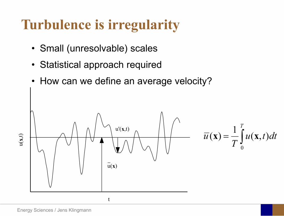
Energy Sciences Jens Klingmann
Turbulence is irregularity
025 03 035 04 045 05t0
001002003004005006007008009
01
u(x
t)
u(xt)
u(x)
bull Small (unresolvable) scalesbull Statistical approach required bull How can we define an average velocity
0
1( ) ( )T
u u t dtT
= intx x
Energy Sciences Jens Klingmann
Turbulence averaging
Havenrsquot we already done this once
Energy Sciences Jens Klingmann
y zx zz z z z z z
x y z
z z z
u uu uu u u u u uu u ut x x y y z z
u u upz x x y y z z
ρ
micro micro micro
partpartpart part part part part + + + + + + = part part part part part part part
part part partpart part part part= minus + + +
part part part part part part part
Turbulence averaging
uuu += ppp +=
Insert into NS (only z-direction shown) and average entire equation
and
Decompose velocity and pressure (Reynoldsrsquo decomposition)
Additional terms that look like stresses
Energy Sciences Jens Klingmann
Turbulence RANS modellingReynoldsrsquo stress tensor
Needs to be expressed as a function of variables we know or intend to solve for
TURBULENCE MODEL
x x x y x z
y x y y y z
z x z y z z
u u u u u u
u u u u u u
u u u u u u
ρ
=
R
6 new variables (symmetry )xyyx uuuu =
Energy Sciences Jens Klingmann
Turbulence RANS modellingReynolds stress tensor
ij i j
u u u v u w
R u u v u v v v w
w u w v w w
ρ ρ ρ
= minus otimes = = =
R u u
Turbulent Kinetic Energy
( ) ( )1 1 1 1 2 2 2 2ii i ik tr R u u u u v v w wρ ρ= = = = + +R
Represents the kinetic energy of the fluctuations (or vortices)
Energy Sciences Jens Klingmann
Turbulence closure problem
10 unknownvelocity components pressure and correlations of fluctuating velocity
4 equationsAveraged momentum equations and averaged continuity equation
i ju u
Energy Sciences Jens Klingmann
Turbulence RANS modelling
23
i jij T ij
j i
u uR kx x
micro ρ δ part part
= + minus part part
2 T kmicro ρ εpropldquoTurbulent viscosityrdquo
Transport of k Some terms may be derived other need modelling
( ) ( ) ( )advection diffusion productionk k k kt
εpart+ + = minus
part
Energy from mean flow to turbulence
Dissipation Energy converted to heat
Energy Sciences Jens Klingmann
Turbulence RANS modelling
23
i jij T ij
j i
u uR kx x
micro ρ δ part part
= + minus part part ερmicro micro 2kCT =
k Tklk
k l k k k
uk ku Rx x x x
microρ ε micro
σ part part part part
= minus + + part part part part 2
1 2k T
klkk l k k
uu C R C
x k x k x xε εε
microε ε ε ερ ρ micropart σ
part part part part= minus + + part part part
4411 =εC 9212 =εC 090=microC 1=kσ31=εσ
Closure coefficients
Energy Sciences Jens Klingmann
Energy Sciences Jens Klingmann
Computational Fluid Dynamics (CFD)
U Waringhleacuten ldquoThe Aerodynamic design and testing of a supersonic turbine for rocket engine propulsionrdquo Proc Of 3rd European conference on Turbomachinery Fluid dynamics and thermodynamics
Energy Sciences Jens Klingmann
Subsonic flow in an aerofoilplate junction computed with a second-moment closure (D Apsley 1998)
Computational Fluid Dynamics(CFD)
Energy Sciences Jens Klingmann
Hydraulic turbine research CFD digital simulation Distribution of speed on an axial turbine
Computational Fluid Dynamics(CFD)
Energy Sciences Jens Klingmann
Scales of turbulence
10-01
1000
1001
1002
1003
1004
1005
κ LI
10-08
10-07
10-06
10-05
10-04
10-03
10-02
10-01
1000
E(u
2 LI)
10-04
10-03
10-02
10-01
1000
κ LK
10-05
10-04
10-03
10-02
10-01
1000
1001
1002
D( ε L
K )10-01
1000
1001
1002
1003
1004
1005
E = 15 (κ LI)-53
10-04
10-03
10-02
10-01
1000
1001
D = 3 ( κ LΚ) 13
Normalized energy and dissipation spectra for
Adapted from Tennekeys and Lumley
ReLI= times2 105
1 2Re 500IL asymp
3 4Re 10000IL asymp
Energy Sciences Jens Klingmann
References Turbulence
bull Tennekeys and Lumley ldquoA first course in Turbulencerdquo MIT Press 1972
bull J O Hinze ldquoTurbulencerdquo McGraw-Hill 1959bull D C Wilcox ldquoTurbulence Modeling for CFDrdquo DCW Industries
2006
Energy Sciences Jens Klingmann
Boundary layers
Energy Sciences Jens Klingmann
Boundary Layer Theory (BLT) Sensitive to Pressure
gradients Appropriate scaling from
dimensional analyses
Energy Sciences Jens Klingmann
Boundary layers
Energy Sciences Jens Klingmann
Air foil theory
Energy Sciences Jens Klingmann
Visualisation of diffusor separation
Energy Sciences Jens Klingmann
BL equations
+minus=+
yu
yxp
xuv
xuu
partpartmicro
partpart
partpart
partρpart
partρpart and 0=+
yxu
partυpart
partpart
Applying the BL approximations the 2D stationary incompressible NS-eq and continuity equation become
yvu
yu
yxuu
xp
yu
xuu
partpartρ
partpartmicro
partpart
partρpart
partpart
partυρpart
partρpart
minus
+minusminus=+
and
0=+yx
upart
υpartpartpart
Reynolds averaged BL eqs are
Energy Sciences Jens Klingmann
Boundary layers
Energy Sciences Jens Klingmann
Turbulent BL at different Pressure gradients
Energy Sciences Jens Klingmann
Boundary Layers
ν
yuy =+
ρτWu =
0=
partpart
=y
w yuτ
uuu =+
Energy Sciences Jens Klingmann
Diffuser efficiency
Energy Sciences Jens Klingmann
Reynolds Number (Order of magnitude)
At eg a compressor inlet
ρ = O(1) kgm3
U = O(100) msx lt O(01) mmicro = O(10-5)
Re = ρ U x micro =O(106)
In subsequent stages large amounts of turbulence (from stator wakes) will be convected into the Boundary layer
Energy Sciences Jens Klingmann
References Boundary layers
bull Frank M White ldquoViscous Fluid Flowrdquobull Hermann Schlichting ldquoBoundary Layer Theoryrdquo
Energy Sciences Jens Klingmann
CFD and experiments
bull No this is not a CFD course butbull Experiments
Energy Sciences Jens Klingmann
What do we need to measureOverall performance
Flow rates (mass or volume) Pressure Temperature Shaft power
Performance increase
Separations (velocity) Secondary flows eg tip clearance losses (velocity) Shock waves (supersonic applications) Pressure (resolved in time and space) Temperature (resolved in time and space)
Energy Sciences Jens Klingmann
Cascade wind tunnels
FIG 31 Compressor cascade wind tunnels (a) Conventional low-speed continuousrunning cascade tunnel (adapted from Carter et al 1950)(b) Transonicsupersoniccascade tunnel (adapted from Sieverding 1985)
Energy Sciences Jens Klingmann
Closed circuit tunnels
Energy Sciences Jens Klingmann
components
Settling Chamber
The settling chamber is located between the fan or wide angle diffuser and the contraction and contains the honeycombs and screens used to moderate longitudinal variations in the flow Screens in the chamber should be spaced at 02 chamber diameters apart so that flow disturbed by the first screen can settle before it encounters the second
Honeycombs
Honeycombs are located in the settling chamber and are used to reduce nonuniformities in the flow For optimum benefit honeycombs should be 6-8 cell diameters thick and cell size should be on the order of about 150 cells per settling chamber diameter
Energy Sciences Jens Klingmann
components
Screens
Screens are typically located just downstream of the honeycomb and sometime at the inlet of the test section Screens create a static pressure drop and serve to reduce boundary layer size and increase flow uniformity
Contraction Section
Contractions sections are located between the settling chamber and the test sections and serve to both increase mean velocities at the test section inlet and moderate inconsistencies in the uniformity of the flow Large contraction ratios and short contraction lengths are generally more desirable as they reduce the power loss across the screens and the thickness of boundary layers Small tunnels typically have contraction ratios between 6 and 9
Energy Sciences Jens Klingmann
Flow meters with pressure measurement
Venturi-tube
A1 A2
P1 P2
1 1 2 2C A C A=In the incompressible case
2 21 1 2 2
2 2C P C P
ρ ρ+ = +Assuming horisontal mounting
Energy Sciences Jens Klingmann
Daniel Bernoulli 1700-1782
Daniel Bernoulli was the son of Johann Bernoulli He was born in Groningen while his father held the chair of mathematics there His older brother was Nicolaus(II) Bernoulli and his uncle was Jacob Bernoulli so he was born into a family of leading mathematicians but also into a family where there was unfortunate rivalry jealousy and bitterness
Undoubtedly the most important work which Daniel Bernoulli did was his work on hydrodynamics Even the term itself is based on the title of the work which he produced called Hydrodynamica and before he left St Petersburg Daniel left a draft copy of the book with a printer However the work was not published until 1738 and although he revised it considerably between 1734 and 1738 it is more the presentation that he changed rather then the substance
This work contains for the first time the correct analysis of water flowing from a hole in a container This was based on the principle of conservation of energy which he had studied with his father in 1720 Daniel also discussed pumps and other machines to raise water One remarkable discovery appears in Chapter 10 of Hydrodynamica where Daniel discussed the basis for the kinetic theory of gases He was able to give the basic laws for the theory of gases and gave although not in full detail the equation of state discovered by Van der Waals a century later
Energy Sciences Jens Klingmann
Venturi-tube (2)
22 2 12 2
2
2A PC CA ρ
∆minus =
A1 A2
P1 P2
Solve for eg C2
1 2P P P∆ = minus
( )
12
2 2 21 2
21
PCA Aρ
∆ = minus
and( )
12
2 2 2 2 21 2
21
Pm A C AA Aρρ
∆ = = minus
where
Flow meters with pressure measurement
Energy Sciences Jens Klingmann
Flow meters with pressure measurement
Orifice meters
A1
A2
P1 P2
Applicable for pipe flows Same principle as for Venturi Positioning of pressure taps important Vena contracta and losses require inclusion
of Discharge Coefficient CD
( )
12
2 2 21 2
21D
Pm C AA Aρ ∆ =
minus where ( )1 2ReDC f A A=
CD available from manufacturer (measurements) or Standards (eg ISO)
Energy Sciences Jens Klingmann
Coriolis flow meter
An actuator (not shown) induces a vibration of the tubes
When there is mass flow Coriolis forces induce twisting of the tubes
degree of phase-shift is a measure for the amount of mass that is flowing through the tubes
Energy Sciences Jens Klingmann
Thermal flow meter Heat is added electrically to the flow Temperature is measured before and after heat addition
pP mC T∆=
Energy Sciences Jens Klingmann
Ultrasonic flow meters
Ultrasound is emitted to small particles in the flow (dust or other) Reflections of the sound is frequency shifted by the Doppler effect The frequency change is proportional to the particles velocity (volume flow
meter)
Energy Sciences Jens Klingmann
Inductive flow metersA magnetic flowmeter is based upon Faradays Law
The voltage induced across any conductor as it moves at right angles through a magnetic field is proportional to the velocity of that conductor
E is proportional to V x B x D where
E = The voltage generated in a conductorV = The velocity of the conductorB = The magnetic field strengthD = The length of the conductor
NB electric conductivity is required
Energy Sciences Jens Klingmann
Temperature measurements
Thermocouples
The basis established by Thomas Johann Seebeck in 1821
A conductor generates a voltage when subjected to a temperature gradient
To measure this voltage one must use a second conductor material which generates a different voltage under the same temperature gradient
Energy Sciences Jens Klingmann
Pressure sensing
1 2p pgt 2p p2 may be the atmosphere a static pressure tap or a known reference pressure
The strain of the diaphragm (or itrsquos deflection) may be measured by a number of electric methods
Diaphragm
Energy Sciences Jens Klingmann
Pressure sensingPiezoresistive Strain Gage
Uses the piezoresistive effect of bonded or formed strain gauges to detect strain due to applied pressure
Capacitive
Uses a diaghragm and pressure cavity to create a variable capacitor to detect strain due to applied pressure
Magnetic
Measures the displacement of a diaphragm by means of changes in inductance (reluctance) LVDT Hall Effect or by eddy current principal
Piezoelectric
Uses the piezoelectric effect in certain materials such as quartz to measure the strain upon the sensing mechanism due to pressure
Potentiometric
Uses the motion of a wiper along a resistive mechanism to detect the strain caused by applied pressure
Energy Sciences Jens Klingmann
3D highly instationary (periodic) flow Potentially very high velocities (Supersonic) Large temperature differences Low accessibility (difficult to probe between rotors) Low turbulence levels in most of the domain Very high turbulence in BL and wakes
Properties of measuring object
Point measurements
Energy Sciences Jens Klingmann
Conventional or non-opticalndash Static Pressure Measurementsndash Total Pressure Measurements
bull Multy hole probes
ndash Total Temperature ndash Hot Wire Anemometry (HWA)
Optical techniques for Velocity Measurementsndash Laser Two Focous (L2F)ndash Laser Doppler Anemometry (LDA)ndash Particle Image velocimetry (PIV)
Point Measurements
Energy Sciences Jens Klingmann
Static and total pressure
2 2 21 2 1
2 1 2 2 2C C CP P ρ ρ ρ
minus = minus =
2 0C =Stagnation point
C1Static pressure tap
Prandtl or Pitot tube
Apply the Bernoulli equation from free stream to stagnation point
21
2 12CP Pρ
= +or
We can also define a stagnation or total pressure
( )2
101 1 022
CP P Pρ= + =
Total pressure = Static pressure + dynamic pressure
or
Energy Sciences Jens Klingmann
Static pressure
Energy Sciences Jens Klingmann
Total Pressure and Temperature
Shrouded Probes
Shrouded Probe
Pitot or Prandtl tube
Sensitive to direction
Energy Sciences Jens Klingmann
Ludwig Prandtl 1875-1953
Ludwig Prandtl born at Freising Bavaria on February 4 1875 was a German Physicist famous for his work in aeronautics He qualified at Munchen in 1900 with a thesis on elastic stability and held the position of Professor of Applied Mechanics at Gottingen for forty-nine years (from 1904 until his death there on August 15 1953) In 1925 Prandtl became the Director of the Kaiser Wilhelm Institute for Fluid Mechanics His discovery in 1904 of the Boundary Layer which adjoins the surface of a body moving in a fluid led to an understanding of skin friction drag and of the way in which streamlining reduces the drag of airplane wings and other moving bodies His work on wing theory published in 1918 - 1919 followed that of FW Lanchester (1902-1907) but was carried out independently and elucidated the flow over airplane wings of finite span Prandtls work and decisive advances in boundary layer and wing theories became the basic material of aeronautics He also made important contributions to the theories of supersonic flow and of turbulence and contributed much to the development of wind tunnels and other aerodynamic equipment In addition he devised the soap-film analogy for the torsion of non-circular sections and wrote on the theory of plasticity and of meteorology
Energy Sciences Jens Klingmann
Total Pressure multy hole
Cobra Probe Yaw Probe
5 Hole Probe
Energy Sciences Jens Klingmann
5 Hole Probes Calibration
Energy Sciences Jens Klingmann
The inherent unsteadiness of the flow within turbomachines
Energy Sciences Jens Klingmann
Hot Wire Anemometry (HWA) The heat transfer from a thin (one micron)
electrically heated wire can be used to determine velocity
The resistance of the wire is temperature dependent Within a small temperature range it can be assumed linear R = R0+α R0(Tm-T0) where R0 is the resistance at a reference temperature T0 and Tm is the mean wire temperature
The thermal power induced in the wire is balanced by heat transfer to the surrounding fluid I2R=hπDL(Tm-T0) where h is the heat transfer coefficient and D and L the diameter and length of the wire respectively
E = I R
Energy Sciences Jens Klingmann
Constant Temperature Anemometry (CTA) The wire is often placed in a Whetstone bridge If the output from the
bridge is amplified and fed back to the bridge the resistance of the probe and thus the temperature will be held constant
This prevents the temperature of the wire to become excessive at low velocities
R1
R2 R3
Probe
Bridge Voltage
Energy Sciences Jens Klingmann
Constant Temperature Anemometry (CTA)
Energy Sciences Jens Klingmann
Characteristics of LDA (according to Dantec)
Invented by Yeh and Cummins in 1964 Velocity measurements in Fluid Dynamics (gas liquid) Up to 3 velocity components Non-intrusive measurements (optical technique) Absolute measurement technique (no calibration required) Very high accuracy Very high spatial resolution due to small measurement volume Tracer particles are required
Energy Sciences Jens Klingmann
LDA - Fringe Model
Focused Laser beams intersect and form the measurement volume Plane wave fronts beam waist in the plane of intersection Interference in the plane of intersection Pattern of bright and dark stripesplanes Fringes
Energy Sciences Jens Klingmann
LDA-measuring volume
d
x
x
y
y
z
z
e-2 CONTOUR
FRINGES
κ
κ
κ
κ
De-2
De-2
dml m
a
b
cx
b
z
ya
cd
d
=
=
=
J
J
J
J
JP
JP
JP
JD
JD
JD
+
+
+
a
b
c
d
κπλ
=minus sinD
f4l2e
m
κπλ
=minus cosD
f4D2e
m
Energy Sciences Jens Klingmann
Laser Two Focus
Energy Sciences Jens Klingmann
Laser Two Focus
Energy Sciences Jens Klingmann
PIV measurements
PIV is a fairly new technique capable of simultaneous velocity measurements at many points in a plane This gives information on large scale structures vorticity etc which is very difficult or impossible to obtain from one-point measuring techniques
PIV involves the illumination of a plane of the flow under investigation with a thin pulsed sheet of light The flow is seeded with particles
The light scattered from the particles and from successive pulses are being recorded either on film or a CCD array forming a multiple exposure of each particle image If the time between the pulses is known velocity can be determined as the ratio of the particle displacement and the elapsed time
t∆∆= xu
Energy Sciences Jens Klingmann
PIV
Energy Sciences Jens Klingmann
PIV measurements illumination
YA
G
YA
G
Two frequency doubled YAG Lasers aligned to one double pulsed laser sheet
Two or more separate light pulses can be obtained by chopping a continuous laser or from pulsed lasers
The limited pulse energies obtained from continuous lasers limits their applicability to low velocity flows or flows where large seeding particles can be used (ie liquid flows)
The low repetition rate of most pulsed lasers makes the use of two lasers advantageous
Energy Sciences Jens Klingmann
PIV measurements recording
High seeding density in laminar flame
Film or CCD-cameras Cross- or Auto-correlation
ndash ie both particle images on the same frame or on separate frames
CCD-camera requirementndash A many pixels as possiblendash 2k by 2k available 4k by 4k coming
Energy Sciences Jens Klingmann
PIV measurements analyses
Low seeding density (Number of seeding particles per unit volume)
Each particle image pair can be identified This is called particle tracking
High seeding density (PIV)
Small sub-regions of the image containing many particle image pairs are processed to obtain one velocity vector
Energy Sciences Jens Klingmann
PIV measurements analyses
Energy Sciences Jens Klingmann
PIV measurements analyses
( ) ( ) ( ) xsxxs dIIR 2A
1
I
+= int
Cross correlation between ( )x1I and ( )x2I
s is a two dimensional displacement vector
IA is the interrogation area
Cross correlation between
(
)
x
1
I
and
(
)
x
2
I
s is a two dimensional displacement vector
I
A
is the interrogation area
Energy Sciences Jens Klingmann
Energy Sciences Jens Klingmann
PIV from IOWA state university
Energy Sciences Jens Klingmann
PIV sample of evaluation
Energy Sciences Jens Klingmann
LDA PIV HWA Velocity range 01 mms ndash 300
ms 02 ndash 150 ms
Measuring Volume
D = 005 L = 05 mm
2 by 2 by 05 mm
L = 05 mm
Freq response O(10 000) Hz O(10) Hz O(100 000) Hz Calibration Yes No No Sensitivity to other than velocity
Low (ref Index) Low (ref Index) Large (temperature concentrationshellip)
Continuous Signal
Sometimes Seldom Always
Noise High High Low Turbulence intensity
No limitation Some limitation lt 20
Price O(1 000 000) SEK
O(1 000 000) SEK
O(50 000) SEK
Required Knowledge
High medium Low
Comparison of techniques
Energy Sciences Jens Klingmann
References experiments
R J Goldstein ldquoFluid Mechanics Measurementsrdquo Hemisphere Publishing 1983 A V Johansson amp P H Alfredsson ldquoExperimentella metoder inom
stroumlmningsmekanikenrdquo Inst Foumlr Mekanik KTH F Durst A Melling and J H Whitelaw ldquoPrincipals and Practice of Laser Doppler
Anemometryrdquo 1984 R J Adrian ldquoParticle-imaging techniques for experimental fluid mechnicsrdquo Ann Rev
Fluid Mech 1991
Energy Sciences Jens Klingmann
Sample of LDA-measurements
Rotor blade
Glas window
Emitted beams
Scattered Light
Adjustable mirror
Energy Sciences Jens Klingmann
Axial velocity sorted into 10 bins
0 1 2 3 4 5 6tangential coordinate (degrees)
-20
0
20
40
60
80
100
120
140
160Ax
ial v
eloc
ity a
nd s
tand
ard
devi
atio
n (m
s)
radial position 7 mm from inner window surfaceaxial position 23 mm behind rotor blades
Energy Sciences Jens Klingmann
Axial velocities in the radial-tangential plane
Energy Sciences Jens Klingmann
Airfoils NACA 4-digit
The NACA four-digit wing sections define the profile by
One digit describing maximum camber as percentage of the chord
One digit describing the distance of maximum camber from the airfoil leading edge in tens of percents of the chord
Two digits describing maximum thickness of the airfoil as percent of the chord
Example the NACA 2412 airfoil has a maximum camber of 2 located 40 (04 chords) from the leading edge with a maximum thickness of 12 of the chord
Four-digit series airfoils by default have maximum thickness at 30 of the chord (03 chords) from the leading edge
Energy Sciences Jens Klingmann
Airfoils NACA 4-digit
bull c is the chord lengthbull x is the position along
the chord from 0 to cbull y is the half thickness at
a given value of x (centerline to surface)
bull t is the maximum thickness as a fraction of the chord
Energy Sciences Jens Klingmann
Death by PowerPoint
| LDA | PIV | HWA | |||||
| Velocity range | 01 mms ndash 300 ms | 02 ndash 150 ms | |||||
| Measuring Volume | D = 005 L = 05 mm | 2 by 2 by 05 mm | L = 05 mm | ||||
| Freq response | O(10 000) Hz | O(10) Hz | O(100 000) Hz | ||||
| Calibration | Yes | No | No | ||||
| Sensitivity to other than velocity | Low (ref Index) | Low (ref Index) | Large (temperature concentrationshellip) | ||||
| Continuous Signal | Sometimes | Seldom | Always | ||||
| Noise | High | High | Low | ||||
| Turbulence intensity | No limitation | Some limitation | lt 20 | ||||
| Price | O(1 000 000) SEK | O(1 000 000) SEK | O(50 000) SEK | ||||
| Required Knowledge | High | medium | Low |
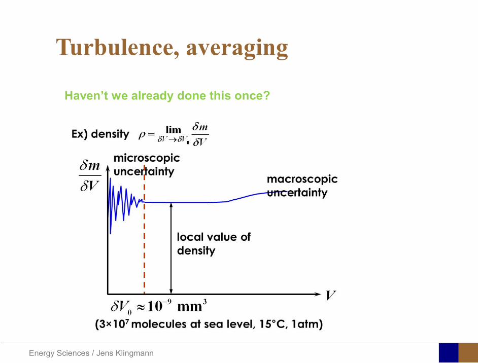
Energy Sciences Jens Klingmann
Turbulence averaging
Havenrsquot we already done this once
Energy Sciences Jens Klingmann
y zx zz z z z z z
x y z
z z z
u uu uu u u u u uu u ut x x y y z z
u u upz x x y y z z
ρ
micro micro micro
partpartpart part part part part + + + + + + = part part part part part part part
part part partpart part part part= minus + + +
part part part part part part part
Turbulence averaging
uuu += ppp +=
Insert into NS (only z-direction shown) and average entire equation
and
Decompose velocity and pressure (Reynoldsrsquo decomposition)
Additional terms that look like stresses
Energy Sciences Jens Klingmann
Turbulence RANS modellingReynoldsrsquo stress tensor
Needs to be expressed as a function of variables we know or intend to solve for
TURBULENCE MODEL
x x x y x z
y x y y y z
z x z y z z
u u u u u u
u u u u u u
u u u u u u
ρ
=
R
6 new variables (symmetry )xyyx uuuu =
Energy Sciences Jens Klingmann
Turbulence RANS modellingReynolds stress tensor
ij i j
u u u v u w
R u u v u v v v w
w u w v w w
ρ ρ ρ
= minus otimes = = =
R u u
Turbulent Kinetic Energy
( ) ( )1 1 1 1 2 2 2 2ii i ik tr R u u u u v v w wρ ρ= = = = + +R
Represents the kinetic energy of the fluctuations (or vortices)
Energy Sciences Jens Klingmann
Turbulence closure problem
10 unknownvelocity components pressure and correlations of fluctuating velocity
4 equationsAveraged momentum equations and averaged continuity equation
i ju u
Energy Sciences Jens Klingmann
Turbulence RANS modelling
23
i jij T ij
j i
u uR kx x
micro ρ δ part part
= + minus part part
2 T kmicro ρ εpropldquoTurbulent viscosityrdquo
Transport of k Some terms may be derived other need modelling
( ) ( ) ( )advection diffusion productionk k k kt
εpart+ + = minus
part
Energy from mean flow to turbulence
Dissipation Energy converted to heat
Energy Sciences Jens Klingmann
Turbulence RANS modelling
23
i jij T ij
j i
u uR kx x
micro ρ δ part part
= + minus part part ερmicro micro 2kCT =
k Tklk
k l k k k
uk ku Rx x x x
microρ ε micro
σ part part part part
= minus + + part part part part 2
1 2k T
klkk l k k
uu C R C
x k x k x xε εε
microε ε ε ερ ρ micropart σ
part part part part= minus + + part part part
4411 =εC 9212 =εC 090=microC 1=kσ31=εσ
Closure coefficients
Energy Sciences Jens Klingmann
Energy Sciences Jens Klingmann
Computational Fluid Dynamics (CFD)
U Waringhleacuten ldquoThe Aerodynamic design and testing of a supersonic turbine for rocket engine propulsionrdquo Proc Of 3rd European conference on Turbomachinery Fluid dynamics and thermodynamics
Energy Sciences Jens Klingmann
Subsonic flow in an aerofoilplate junction computed with a second-moment closure (D Apsley 1998)
Computational Fluid Dynamics(CFD)
Energy Sciences Jens Klingmann
Hydraulic turbine research CFD digital simulation Distribution of speed on an axial turbine
Computational Fluid Dynamics(CFD)
Energy Sciences Jens Klingmann
Scales of turbulence
10-01
1000
1001
1002
1003
1004
1005
κ LI
10-08
10-07
10-06
10-05
10-04
10-03
10-02
10-01
1000
E(u
2 LI)
10-04
10-03
10-02
10-01
1000
κ LK
10-05
10-04
10-03
10-02
10-01
1000
1001
1002
D( ε L
K )10-01
1000
1001
1002
1003
1004
1005
E = 15 (κ LI)-53
10-04
10-03
10-02
10-01
1000
1001
D = 3 ( κ LΚ) 13
Normalized energy and dissipation spectra for
Adapted from Tennekeys and Lumley
ReLI= times2 105
1 2Re 500IL asymp
3 4Re 10000IL asymp
Energy Sciences Jens Klingmann
References Turbulence
bull Tennekeys and Lumley ldquoA first course in Turbulencerdquo MIT Press 1972
bull J O Hinze ldquoTurbulencerdquo McGraw-Hill 1959bull D C Wilcox ldquoTurbulence Modeling for CFDrdquo DCW Industries
2006
Energy Sciences Jens Klingmann
Boundary layers
Energy Sciences Jens Klingmann
Boundary Layer Theory (BLT) Sensitive to Pressure
gradients Appropriate scaling from
dimensional analyses
Energy Sciences Jens Klingmann
Boundary layers
Energy Sciences Jens Klingmann
Air foil theory
Energy Sciences Jens Klingmann
Visualisation of diffusor separation
Energy Sciences Jens Klingmann
BL equations
+minus=+
yu
yxp
xuv
xuu
partpartmicro
partpart
partpart
partρpart
partρpart and 0=+
yxu
partυpart
partpart
Applying the BL approximations the 2D stationary incompressible NS-eq and continuity equation become
yvu
yu
yxuu
xp
yu
xuu
partpartρ
partpartmicro
partpart
partρpart
partpart
partυρpart
partρpart
minus
+minusminus=+
and
0=+yx
upart
υpartpartpart
Reynolds averaged BL eqs are
Energy Sciences Jens Klingmann
Boundary layers
Energy Sciences Jens Klingmann
Turbulent BL at different Pressure gradients
Energy Sciences Jens Klingmann
Boundary Layers
ν
yuy =+
ρτWu =
0=
partpart
=y
w yuτ
uuu =+
Energy Sciences Jens Klingmann
Diffuser efficiency
Energy Sciences Jens Klingmann
Reynolds Number (Order of magnitude)
At eg a compressor inlet
ρ = O(1) kgm3
U = O(100) msx lt O(01) mmicro = O(10-5)
Re = ρ U x micro =O(106)
In subsequent stages large amounts of turbulence (from stator wakes) will be convected into the Boundary layer
Energy Sciences Jens Klingmann
References Boundary layers
bull Frank M White ldquoViscous Fluid Flowrdquobull Hermann Schlichting ldquoBoundary Layer Theoryrdquo
Energy Sciences Jens Klingmann
CFD and experiments
bull No this is not a CFD course butbull Experiments
Energy Sciences Jens Klingmann
What do we need to measureOverall performance
Flow rates (mass or volume) Pressure Temperature Shaft power
Performance increase
Separations (velocity) Secondary flows eg tip clearance losses (velocity) Shock waves (supersonic applications) Pressure (resolved in time and space) Temperature (resolved in time and space)
Energy Sciences Jens Klingmann
Cascade wind tunnels
FIG 31 Compressor cascade wind tunnels (a) Conventional low-speed continuousrunning cascade tunnel (adapted from Carter et al 1950)(b) Transonicsupersoniccascade tunnel (adapted from Sieverding 1985)
Energy Sciences Jens Klingmann
Closed circuit tunnels
Energy Sciences Jens Klingmann
components
Settling Chamber
The settling chamber is located between the fan or wide angle diffuser and the contraction and contains the honeycombs and screens used to moderate longitudinal variations in the flow Screens in the chamber should be spaced at 02 chamber diameters apart so that flow disturbed by the first screen can settle before it encounters the second
Honeycombs
Honeycombs are located in the settling chamber and are used to reduce nonuniformities in the flow For optimum benefit honeycombs should be 6-8 cell diameters thick and cell size should be on the order of about 150 cells per settling chamber diameter
Energy Sciences Jens Klingmann
components
Screens
Screens are typically located just downstream of the honeycomb and sometime at the inlet of the test section Screens create a static pressure drop and serve to reduce boundary layer size and increase flow uniformity
Contraction Section
Contractions sections are located between the settling chamber and the test sections and serve to both increase mean velocities at the test section inlet and moderate inconsistencies in the uniformity of the flow Large contraction ratios and short contraction lengths are generally more desirable as they reduce the power loss across the screens and the thickness of boundary layers Small tunnels typically have contraction ratios between 6 and 9
Energy Sciences Jens Klingmann
Flow meters with pressure measurement
Venturi-tube
A1 A2
P1 P2
1 1 2 2C A C A=In the incompressible case
2 21 1 2 2
2 2C P C P
ρ ρ+ = +Assuming horisontal mounting
Energy Sciences Jens Klingmann
Daniel Bernoulli 1700-1782
Daniel Bernoulli was the son of Johann Bernoulli He was born in Groningen while his father held the chair of mathematics there His older brother was Nicolaus(II) Bernoulli and his uncle was Jacob Bernoulli so he was born into a family of leading mathematicians but also into a family where there was unfortunate rivalry jealousy and bitterness
Undoubtedly the most important work which Daniel Bernoulli did was his work on hydrodynamics Even the term itself is based on the title of the work which he produced called Hydrodynamica and before he left St Petersburg Daniel left a draft copy of the book with a printer However the work was not published until 1738 and although he revised it considerably between 1734 and 1738 it is more the presentation that he changed rather then the substance
This work contains for the first time the correct analysis of water flowing from a hole in a container This was based on the principle of conservation of energy which he had studied with his father in 1720 Daniel also discussed pumps and other machines to raise water One remarkable discovery appears in Chapter 10 of Hydrodynamica where Daniel discussed the basis for the kinetic theory of gases He was able to give the basic laws for the theory of gases and gave although not in full detail the equation of state discovered by Van der Waals a century later
Energy Sciences Jens Klingmann
Venturi-tube (2)
22 2 12 2
2
2A PC CA ρ
∆minus =
A1 A2
P1 P2
Solve for eg C2
1 2P P P∆ = minus
( )
12
2 2 21 2
21
PCA Aρ
∆ = minus
and( )
12
2 2 2 2 21 2
21
Pm A C AA Aρρ
∆ = = minus
where
Flow meters with pressure measurement
Energy Sciences Jens Klingmann
Flow meters with pressure measurement
Orifice meters
A1
A2
P1 P2
Applicable for pipe flows Same principle as for Venturi Positioning of pressure taps important Vena contracta and losses require inclusion
of Discharge Coefficient CD
( )
12
2 2 21 2
21D
Pm C AA Aρ ∆ =
minus where ( )1 2ReDC f A A=
CD available from manufacturer (measurements) or Standards (eg ISO)
Energy Sciences Jens Klingmann
Coriolis flow meter
An actuator (not shown) induces a vibration of the tubes
When there is mass flow Coriolis forces induce twisting of the tubes
degree of phase-shift is a measure for the amount of mass that is flowing through the tubes
Energy Sciences Jens Klingmann
Thermal flow meter Heat is added electrically to the flow Temperature is measured before and after heat addition
pP mC T∆=
Energy Sciences Jens Klingmann
Ultrasonic flow meters
Ultrasound is emitted to small particles in the flow (dust or other) Reflections of the sound is frequency shifted by the Doppler effect The frequency change is proportional to the particles velocity (volume flow
meter)
Energy Sciences Jens Klingmann
Inductive flow metersA magnetic flowmeter is based upon Faradays Law
The voltage induced across any conductor as it moves at right angles through a magnetic field is proportional to the velocity of that conductor
E is proportional to V x B x D where
E = The voltage generated in a conductorV = The velocity of the conductorB = The magnetic field strengthD = The length of the conductor
NB electric conductivity is required
Energy Sciences Jens Klingmann
Temperature measurements
Thermocouples
The basis established by Thomas Johann Seebeck in 1821
A conductor generates a voltage when subjected to a temperature gradient
To measure this voltage one must use a second conductor material which generates a different voltage under the same temperature gradient
Energy Sciences Jens Klingmann
Pressure sensing
1 2p pgt 2p p2 may be the atmosphere a static pressure tap or a known reference pressure
The strain of the diaphragm (or itrsquos deflection) may be measured by a number of electric methods
Diaphragm
Energy Sciences Jens Klingmann
Pressure sensingPiezoresistive Strain Gage
Uses the piezoresistive effect of bonded or formed strain gauges to detect strain due to applied pressure
Capacitive
Uses a diaghragm and pressure cavity to create a variable capacitor to detect strain due to applied pressure
Magnetic
Measures the displacement of a diaphragm by means of changes in inductance (reluctance) LVDT Hall Effect or by eddy current principal
Piezoelectric
Uses the piezoelectric effect in certain materials such as quartz to measure the strain upon the sensing mechanism due to pressure
Potentiometric
Uses the motion of a wiper along a resistive mechanism to detect the strain caused by applied pressure
Energy Sciences Jens Klingmann
3D highly instationary (periodic) flow Potentially very high velocities (Supersonic) Large temperature differences Low accessibility (difficult to probe between rotors) Low turbulence levels in most of the domain Very high turbulence in BL and wakes
Properties of measuring object
Point measurements
Energy Sciences Jens Klingmann
Conventional or non-opticalndash Static Pressure Measurementsndash Total Pressure Measurements
bull Multy hole probes
ndash Total Temperature ndash Hot Wire Anemometry (HWA)
Optical techniques for Velocity Measurementsndash Laser Two Focous (L2F)ndash Laser Doppler Anemometry (LDA)ndash Particle Image velocimetry (PIV)
Point Measurements
Energy Sciences Jens Klingmann
Static and total pressure
2 2 21 2 1
2 1 2 2 2C C CP P ρ ρ ρ
minus = minus =
2 0C =Stagnation point
C1Static pressure tap
Prandtl or Pitot tube
Apply the Bernoulli equation from free stream to stagnation point
21
2 12CP Pρ
= +or
We can also define a stagnation or total pressure
( )2
101 1 022
CP P Pρ= + =
Total pressure = Static pressure + dynamic pressure
or
Energy Sciences Jens Klingmann
Static pressure
Energy Sciences Jens Klingmann
Total Pressure and Temperature
Shrouded Probes
Shrouded Probe
Pitot or Prandtl tube
Sensitive to direction
Energy Sciences Jens Klingmann
Ludwig Prandtl 1875-1953
Ludwig Prandtl born at Freising Bavaria on February 4 1875 was a German Physicist famous for his work in aeronautics He qualified at Munchen in 1900 with a thesis on elastic stability and held the position of Professor of Applied Mechanics at Gottingen for forty-nine years (from 1904 until his death there on August 15 1953) In 1925 Prandtl became the Director of the Kaiser Wilhelm Institute for Fluid Mechanics His discovery in 1904 of the Boundary Layer which adjoins the surface of a body moving in a fluid led to an understanding of skin friction drag and of the way in which streamlining reduces the drag of airplane wings and other moving bodies His work on wing theory published in 1918 - 1919 followed that of FW Lanchester (1902-1907) but was carried out independently and elucidated the flow over airplane wings of finite span Prandtls work and decisive advances in boundary layer and wing theories became the basic material of aeronautics He also made important contributions to the theories of supersonic flow and of turbulence and contributed much to the development of wind tunnels and other aerodynamic equipment In addition he devised the soap-film analogy for the torsion of non-circular sections and wrote on the theory of plasticity and of meteorology
Energy Sciences Jens Klingmann
Total Pressure multy hole
Cobra Probe Yaw Probe
5 Hole Probe
Energy Sciences Jens Klingmann
5 Hole Probes Calibration
Energy Sciences Jens Klingmann
The inherent unsteadiness of the flow within turbomachines
Energy Sciences Jens Klingmann
Hot Wire Anemometry (HWA) The heat transfer from a thin (one micron)
electrically heated wire can be used to determine velocity
The resistance of the wire is temperature dependent Within a small temperature range it can be assumed linear R = R0+α R0(Tm-T0) where R0 is the resistance at a reference temperature T0 and Tm is the mean wire temperature
The thermal power induced in the wire is balanced by heat transfer to the surrounding fluid I2R=hπDL(Tm-T0) where h is the heat transfer coefficient and D and L the diameter and length of the wire respectively
E = I R
Energy Sciences Jens Klingmann
Constant Temperature Anemometry (CTA) The wire is often placed in a Whetstone bridge If the output from the
bridge is amplified and fed back to the bridge the resistance of the probe and thus the temperature will be held constant
This prevents the temperature of the wire to become excessive at low velocities
R1
R2 R3
Probe
Bridge Voltage
Energy Sciences Jens Klingmann
Constant Temperature Anemometry (CTA)
Energy Sciences Jens Klingmann
Characteristics of LDA (according to Dantec)
Invented by Yeh and Cummins in 1964 Velocity measurements in Fluid Dynamics (gas liquid) Up to 3 velocity components Non-intrusive measurements (optical technique) Absolute measurement technique (no calibration required) Very high accuracy Very high spatial resolution due to small measurement volume Tracer particles are required
Energy Sciences Jens Klingmann
LDA - Fringe Model
Focused Laser beams intersect and form the measurement volume Plane wave fronts beam waist in the plane of intersection Interference in the plane of intersection Pattern of bright and dark stripesplanes Fringes
Energy Sciences Jens Klingmann
LDA-measuring volume
d
x
x
y
y
z
z
e-2 CONTOUR
FRINGES
κ
κ
κ
κ
De-2
De-2
dml m
a
b
cx
b
z
ya
cd
d
=
=
=
J
J
J
J
JP
JP
JP
JD
JD
JD
+
+
+
a
b
c
d
κπλ
=minus sinD
f4l2e
m
κπλ
=minus cosD
f4D2e
m
Energy Sciences Jens Klingmann
Laser Two Focus
Energy Sciences Jens Klingmann
Laser Two Focus
Energy Sciences Jens Klingmann
PIV measurements
PIV is a fairly new technique capable of simultaneous velocity measurements at many points in a plane This gives information on large scale structures vorticity etc which is very difficult or impossible to obtain from one-point measuring techniques
PIV involves the illumination of a plane of the flow under investigation with a thin pulsed sheet of light The flow is seeded with particles
The light scattered from the particles and from successive pulses are being recorded either on film or a CCD array forming a multiple exposure of each particle image If the time between the pulses is known velocity can be determined as the ratio of the particle displacement and the elapsed time
t∆∆= xu
Energy Sciences Jens Klingmann
PIV
Energy Sciences Jens Klingmann
PIV measurements illumination
YA
G
YA
G
Two frequency doubled YAG Lasers aligned to one double pulsed laser sheet
Two or more separate light pulses can be obtained by chopping a continuous laser or from pulsed lasers
The limited pulse energies obtained from continuous lasers limits their applicability to low velocity flows or flows where large seeding particles can be used (ie liquid flows)
The low repetition rate of most pulsed lasers makes the use of two lasers advantageous
Energy Sciences Jens Klingmann
PIV measurements recording
High seeding density in laminar flame
Film or CCD-cameras Cross- or Auto-correlation
ndash ie both particle images on the same frame or on separate frames
CCD-camera requirementndash A many pixels as possiblendash 2k by 2k available 4k by 4k coming
Energy Sciences Jens Klingmann
PIV measurements analyses
Low seeding density (Number of seeding particles per unit volume)
Each particle image pair can be identified This is called particle tracking
High seeding density (PIV)
Small sub-regions of the image containing many particle image pairs are processed to obtain one velocity vector
Energy Sciences Jens Klingmann
PIV measurements analyses
Energy Sciences Jens Klingmann
PIV measurements analyses
( ) ( ) ( ) xsxxs dIIR 2A
1
I
+= int
Cross correlation between ( )x1I and ( )x2I
s is a two dimensional displacement vector
IA is the interrogation area
Cross correlation between
(
)
x
1
I
and
(
)
x
2
I
s is a two dimensional displacement vector
I
A
is the interrogation area
Energy Sciences Jens Klingmann
Energy Sciences Jens Klingmann
PIV from IOWA state university
Energy Sciences Jens Klingmann
PIV sample of evaluation
Energy Sciences Jens Klingmann
LDA PIV HWA Velocity range 01 mms ndash 300
ms 02 ndash 150 ms
Measuring Volume
D = 005 L = 05 mm
2 by 2 by 05 mm
L = 05 mm
Freq response O(10 000) Hz O(10) Hz O(100 000) Hz Calibration Yes No No Sensitivity to other than velocity
Low (ref Index) Low (ref Index) Large (temperature concentrationshellip)
Continuous Signal
Sometimes Seldom Always
Noise High High Low Turbulence intensity
No limitation Some limitation lt 20
Price O(1 000 000) SEK
O(1 000 000) SEK
O(50 000) SEK
Required Knowledge
High medium Low
Comparison of techniques
Energy Sciences Jens Klingmann
References experiments
R J Goldstein ldquoFluid Mechanics Measurementsrdquo Hemisphere Publishing 1983 A V Johansson amp P H Alfredsson ldquoExperimentella metoder inom
stroumlmningsmekanikenrdquo Inst Foumlr Mekanik KTH F Durst A Melling and J H Whitelaw ldquoPrincipals and Practice of Laser Doppler
Anemometryrdquo 1984 R J Adrian ldquoParticle-imaging techniques for experimental fluid mechnicsrdquo Ann Rev
Fluid Mech 1991
Energy Sciences Jens Klingmann
Sample of LDA-measurements
Rotor blade
Glas window
Emitted beams
Scattered Light
Adjustable mirror
Energy Sciences Jens Klingmann
Axial velocity sorted into 10 bins
0 1 2 3 4 5 6tangential coordinate (degrees)
-20
0
20
40
60
80
100
120
140
160Ax
ial v
eloc
ity a
nd s
tand
ard
devi
atio
n (m
s)
radial position 7 mm from inner window surfaceaxial position 23 mm behind rotor blades
Energy Sciences Jens Klingmann
Axial velocities in the radial-tangential plane
Energy Sciences Jens Klingmann
Airfoils NACA 4-digit
The NACA four-digit wing sections define the profile by
One digit describing maximum camber as percentage of the chord
One digit describing the distance of maximum camber from the airfoil leading edge in tens of percents of the chord
Two digits describing maximum thickness of the airfoil as percent of the chord
Example the NACA 2412 airfoil has a maximum camber of 2 located 40 (04 chords) from the leading edge with a maximum thickness of 12 of the chord
Four-digit series airfoils by default have maximum thickness at 30 of the chord (03 chords) from the leading edge
Energy Sciences Jens Klingmann
Airfoils NACA 4-digit
bull c is the chord lengthbull x is the position along
the chord from 0 to cbull y is the half thickness at
a given value of x (centerline to surface)
bull t is the maximum thickness as a fraction of the chord
Energy Sciences Jens Klingmann
Death by PowerPoint
| LDA | PIV | HWA | |||||
| Velocity range | 01 mms ndash 300 ms | 02 ndash 150 ms | |||||
| Measuring Volume | D = 005 L = 05 mm | 2 by 2 by 05 mm | L = 05 mm | ||||
| Freq response | O(10 000) Hz | O(10) Hz | O(100 000) Hz | ||||
| Calibration | Yes | No | No | ||||
| Sensitivity to other than velocity | Low (ref Index) | Low (ref Index) | Large (temperature concentrationshellip) | ||||
| Continuous Signal | Sometimes | Seldom | Always | ||||
| Noise | High | High | Low | ||||
| Turbulence intensity | No limitation | Some limitation | lt 20 | ||||
| Price | O(1 000 000) SEK | O(1 000 000) SEK | O(50 000) SEK | ||||
| Required Knowledge | High | medium | Low |
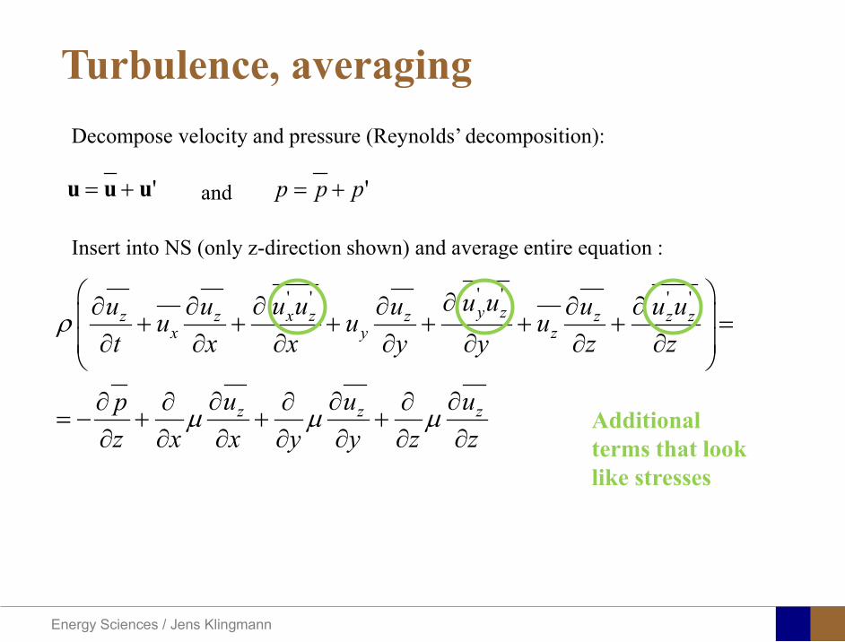
Energy Sciences Jens Klingmann
y zx zz z z z z z
x y z
z z z
u uu uu u u u u uu u ut x x y y z z
u u upz x x y y z z
ρ
micro micro micro
partpartpart part part part part + + + + + + = part part part part part part part
part part partpart part part part= minus + + +
part part part part part part part
Turbulence averaging
uuu += ppp +=
Insert into NS (only z-direction shown) and average entire equation
and
Decompose velocity and pressure (Reynoldsrsquo decomposition)
Additional terms that look like stresses
Energy Sciences Jens Klingmann
Turbulence RANS modellingReynoldsrsquo stress tensor
Needs to be expressed as a function of variables we know or intend to solve for
TURBULENCE MODEL
x x x y x z
y x y y y z
z x z y z z
u u u u u u
u u u u u u
u u u u u u
ρ
=
R
6 new variables (symmetry )xyyx uuuu =
Energy Sciences Jens Klingmann
Turbulence RANS modellingReynolds stress tensor
ij i j
u u u v u w
R u u v u v v v w
w u w v w w
ρ ρ ρ
= minus otimes = = =
R u u
Turbulent Kinetic Energy
( ) ( )1 1 1 1 2 2 2 2ii i ik tr R u u u u v v w wρ ρ= = = = + +R
Represents the kinetic energy of the fluctuations (or vortices)
Energy Sciences Jens Klingmann
Turbulence closure problem
10 unknownvelocity components pressure and correlations of fluctuating velocity
4 equationsAveraged momentum equations and averaged continuity equation
i ju u
Energy Sciences Jens Klingmann
Turbulence RANS modelling
23
i jij T ij
j i
u uR kx x
micro ρ δ part part
= + minus part part
2 T kmicro ρ εpropldquoTurbulent viscosityrdquo
Transport of k Some terms may be derived other need modelling
( ) ( ) ( )advection diffusion productionk k k kt
εpart+ + = minus
part
Energy from mean flow to turbulence
Dissipation Energy converted to heat
Energy Sciences Jens Klingmann
Turbulence RANS modelling
23
i jij T ij
j i
u uR kx x
micro ρ δ part part
= + minus part part ερmicro micro 2kCT =
k Tklk
k l k k k
uk ku Rx x x x
microρ ε micro
σ part part part part
= minus + + part part part part 2
1 2k T
klkk l k k
uu C R C
x k x k x xε εε
microε ε ε ερ ρ micropart σ
part part part part= minus + + part part part
4411 =εC 9212 =εC 090=microC 1=kσ31=εσ
Closure coefficients
Energy Sciences Jens Klingmann
Energy Sciences Jens Klingmann
Computational Fluid Dynamics (CFD)
U Waringhleacuten ldquoThe Aerodynamic design and testing of a supersonic turbine for rocket engine propulsionrdquo Proc Of 3rd European conference on Turbomachinery Fluid dynamics and thermodynamics
Energy Sciences Jens Klingmann
Subsonic flow in an aerofoilplate junction computed with a second-moment closure (D Apsley 1998)
Computational Fluid Dynamics(CFD)
Energy Sciences Jens Klingmann
Hydraulic turbine research CFD digital simulation Distribution of speed on an axial turbine
Computational Fluid Dynamics(CFD)
Energy Sciences Jens Klingmann
Scales of turbulence
10-01
1000
1001
1002
1003
1004
1005
κ LI
10-08
10-07
10-06
10-05
10-04
10-03
10-02
10-01
1000
E(u
2 LI)
10-04
10-03
10-02
10-01
1000
κ LK
10-05
10-04
10-03
10-02
10-01
1000
1001
1002
D( ε L
K )10-01
1000
1001
1002
1003
1004
1005
E = 15 (κ LI)-53
10-04
10-03
10-02
10-01
1000
1001
D = 3 ( κ LΚ) 13
Normalized energy and dissipation spectra for
Adapted from Tennekeys and Lumley
ReLI= times2 105
1 2Re 500IL asymp
3 4Re 10000IL asymp
Energy Sciences Jens Klingmann
References Turbulence
bull Tennekeys and Lumley ldquoA first course in Turbulencerdquo MIT Press 1972
bull J O Hinze ldquoTurbulencerdquo McGraw-Hill 1959bull D C Wilcox ldquoTurbulence Modeling for CFDrdquo DCW Industries
2006
Energy Sciences Jens Klingmann
Boundary layers
Energy Sciences Jens Klingmann
Boundary Layer Theory (BLT) Sensitive to Pressure
gradients Appropriate scaling from
dimensional analyses
Energy Sciences Jens Klingmann
Boundary layers
Energy Sciences Jens Klingmann
Air foil theory
Energy Sciences Jens Klingmann
Visualisation of diffusor separation
Energy Sciences Jens Klingmann
BL equations
+minus=+
yu
yxp
xuv
xuu
partpartmicro
partpart
partpart
partρpart
partρpart and 0=+
yxu
partυpart
partpart
Applying the BL approximations the 2D stationary incompressible NS-eq and continuity equation become
yvu
yu
yxuu
xp
yu
xuu
partpartρ
partpartmicro
partpart
partρpart
partpart
partυρpart
partρpart
minus
+minusminus=+
and
0=+yx
upart
υpartpartpart
Reynolds averaged BL eqs are
Energy Sciences Jens Klingmann
Boundary layers
Energy Sciences Jens Klingmann
Turbulent BL at different Pressure gradients
Energy Sciences Jens Klingmann
Boundary Layers
ν
yuy =+
ρτWu =
0=
partpart
=y
w yuτ
uuu =+
Energy Sciences Jens Klingmann
Diffuser efficiency
Energy Sciences Jens Klingmann
Reynolds Number (Order of magnitude)
At eg a compressor inlet
ρ = O(1) kgm3
U = O(100) msx lt O(01) mmicro = O(10-5)
Re = ρ U x micro =O(106)
In subsequent stages large amounts of turbulence (from stator wakes) will be convected into the Boundary layer
Energy Sciences Jens Klingmann
References Boundary layers
bull Frank M White ldquoViscous Fluid Flowrdquobull Hermann Schlichting ldquoBoundary Layer Theoryrdquo
Energy Sciences Jens Klingmann
CFD and experiments
bull No this is not a CFD course butbull Experiments
Energy Sciences Jens Klingmann
What do we need to measureOverall performance
Flow rates (mass or volume) Pressure Temperature Shaft power
Performance increase
Separations (velocity) Secondary flows eg tip clearance losses (velocity) Shock waves (supersonic applications) Pressure (resolved in time and space) Temperature (resolved in time and space)
Energy Sciences Jens Klingmann
Cascade wind tunnels
FIG 31 Compressor cascade wind tunnels (a) Conventional low-speed continuousrunning cascade tunnel (adapted from Carter et al 1950)(b) Transonicsupersoniccascade tunnel (adapted from Sieverding 1985)
Energy Sciences Jens Klingmann
Closed circuit tunnels
Energy Sciences Jens Klingmann
components
Settling Chamber
The settling chamber is located between the fan or wide angle diffuser and the contraction and contains the honeycombs and screens used to moderate longitudinal variations in the flow Screens in the chamber should be spaced at 02 chamber diameters apart so that flow disturbed by the first screen can settle before it encounters the second
Honeycombs
Honeycombs are located in the settling chamber and are used to reduce nonuniformities in the flow For optimum benefit honeycombs should be 6-8 cell diameters thick and cell size should be on the order of about 150 cells per settling chamber diameter
Energy Sciences Jens Klingmann
components
Screens
Screens are typically located just downstream of the honeycomb and sometime at the inlet of the test section Screens create a static pressure drop and serve to reduce boundary layer size and increase flow uniformity
Contraction Section
Contractions sections are located between the settling chamber and the test sections and serve to both increase mean velocities at the test section inlet and moderate inconsistencies in the uniformity of the flow Large contraction ratios and short contraction lengths are generally more desirable as they reduce the power loss across the screens and the thickness of boundary layers Small tunnels typically have contraction ratios between 6 and 9
Energy Sciences Jens Klingmann
Flow meters with pressure measurement
Venturi-tube
A1 A2
P1 P2
1 1 2 2C A C A=In the incompressible case
2 21 1 2 2
2 2C P C P
ρ ρ+ = +Assuming horisontal mounting
Energy Sciences Jens Klingmann
Daniel Bernoulli 1700-1782
Daniel Bernoulli was the son of Johann Bernoulli He was born in Groningen while his father held the chair of mathematics there His older brother was Nicolaus(II) Bernoulli and his uncle was Jacob Bernoulli so he was born into a family of leading mathematicians but also into a family where there was unfortunate rivalry jealousy and bitterness
Undoubtedly the most important work which Daniel Bernoulli did was his work on hydrodynamics Even the term itself is based on the title of the work which he produced called Hydrodynamica and before he left St Petersburg Daniel left a draft copy of the book with a printer However the work was not published until 1738 and although he revised it considerably between 1734 and 1738 it is more the presentation that he changed rather then the substance
This work contains for the first time the correct analysis of water flowing from a hole in a container This was based on the principle of conservation of energy which he had studied with his father in 1720 Daniel also discussed pumps and other machines to raise water One remarkable discovery appears in Chapter 10 of Hydrodynamica where Daniel discussed the basis for the kinetic theory of gases He was able to give the basic laws for the theory of gases and gave although not in full detail the equation of state discovered by Van der Waals a century later
Energy Sciences Jens Klingmann
Venturi-tube (2)
22 2 12 2
2
2A PC CA ρ
∆minus =
A1 A2
P1 P2
Solve for eg C2
1 2P P P∆ = minus
( )
12
2 2 21 2
21
PCA Aρ
∆ = minus
and( )
12
2 2 2 2 21 2
21
Pm A C AA Aρρ
∆ = = minus
where
Flow meters with pressure measurement
Energy Sciences Jens Klingmann
Flow meters with pressure measurement
Orifice meters
A1
A2
P1 P2
Applicable for pipe flows Same principle as for Venturi Positioning of pressure taps important Vena contracta and losses require inclusion
of Discharge Coefficient CD
( )
12
2 2 21 2
21D
Pm C AA Aρ ∆ =
minus where ( )1 2ReDC f A A=
CD available from manufacturer (measurements) or Standards (eg ISO)
Energy Sciences Jens Klingmann
Coriolis flow meter
An actuator (not shown) induces a vibration of the tubes
When there is mass flow Coriolis forces induce twisting of the tubes
degree of phase-shift is a measure for the amount of mass that is flowing through the tubes
Energy Sciences Jens Klingmann
Thermal flow meter Heat is added electrically to the flow Temperature is measured before and after heat addition
pP mC T∆=
Energy Sciences Jens Klingmann
Ultrasonic flow meters
Ultrasound is emitted to small particles in the flow (dust or other) Reflections of the sound is frequency shifted by the Doppler effect The frequency change is proportional to the particles velocity (volume flow
meter)
Energy Sciences Jens Klingmann
Inductive flow metersA magnetic flowmeter is based upon Faradays Law
The voltage induced across any conductor as it moves at right angles through a magnetic field is proportional to the velocity of that conductor
E is proportional to V x B x D where
E = The voltage generated in a conductorV = The velocity of the conductorB = The magnetic field strengthD = The length of the conductor
NB electric conductivity is required
Energy Sciences Jens Klingmann
Temperature measurements
Thermocouples
The basis established by Thomas Johann Seebeck in 1821
A conductor generates a voltage when subjected to a temperature gradient
To measure this voltage one must use a second conductor material which generates a different voltage under the same temperature gradient
Energy Sciences Jens Klingmann
Pressure sensing
1 2p pgt 2p p2 may be the atmosphere a static pressure tap or a known reference pressure
The strain of the diaphragm (or itrsquos deflection) may be measured by a number of electric methods
Diaphragm
Energy Sciences Jens Klingmann
Pressure sensingPiezoresistive Strain Gage
Uses the piezoresistive effect of bonded or formed strain gauges to detect strain due to applied pressure
Capacitive
Uses a diaghragm and pressure cavity to create a variable capacitor to detect strain due to applied pressure
Magnetic
Measures the displacement of a diaphragm by means of changes in inductance (reluctance) LVDT Hall Effect or by eddy current principal
Piezoelectric
Uses the piezoelectric effect in certain materials such as quartz to measure the strain upon the sensing mechanism due to pressure
Potentiometric
Uses the motion of a wiper along a resistive mechanism to detect the strain caused by applied pressure
Energy Sciences Jens Klingmann
3D highly instationary (periodic) flow Potentially very high velocities (Supersonic) Large temperature differences Low accessibility (difficult to probe between rotors) Low turbulence levels in most of the domain Very high turbulence in BL and wakes
Properties of measuring object
Point measurements
Energy Sciences Jens Klingmann
Conventional or non-opticalndash Static Pressure Measurementsndash Total Pressure Measurements
bull Multy hole probes
ndash Total Temperature ndash Hot Wire Anemometry (HWA)
Optical techniques for Velocity Measurementsndash Laser Two Focous (L2F)ndash Laser Doppler Anemometry (LDA)ndash Particle Image velocimetry (PIV)
Point Measurements
Energy Sciences Jens Klingmann
Static and total pressure
2 2 21 2 1
2 1 2 2 2C C CP P ρ ρ ρ
minus = minus =
2 0C =Stagnation point
C1Static pressure tap
Prandtl or Pitot tube
Apply the Bernoulli equation from free stream to stagnation point
21
2 12CP Pρ
= +or
We can also define a stagnation or total pressure
( )2
101 1 022
CP P Pρ= + =
Total pressure = Static pressure + dynamic pressure
or
Energy Sciences Jens Klingmann
Static pressure
Energy Sciences Jens Klingmann
Total Pressure and Temperature
Shrouded Probes
Shrouded Probe
Pitot or Prandtl tube
Sensitive to direction
Energy Sciences Jens Klingmann
Ludwig Prandtl 1875-1953
Ludwig Prandtl born at Freising Bavaria on February 4 1875 was a German Physicist famous for his work in aeronautics He qualified at Munchen in 1900 with a thesis on elastic stability and held the position of Professor of Applied Mechanics at Gottingen for forty-nine years (from 1904 until his death there on August 15 1953) In 1925 Prandtl became the Director of the Kaiser Wilhelm Institute for Fluid Mechanics His discovery in 1904 of the Boundary Layer which adjoins the surface of a body moving in a fluid led to an understanding of skin friction drag and of the way in which streamlining reduces the drag of airplane wings and other moving bodies His work on wing theory published in 1918 - 1919 followed that of FW Lanchester (1902-1907) but was carried out independently and elucidated the flow over airplane wings of finite span Prandtls work and decisive advances in boundary layer and wing theories became the basic material of aeronautics He also made important contributions to the theories of supersonic flow and of turbulence and contributed much to the development of wind tunnels and other aerodynamic equipment In addition he devised the soap-film analogy for the torsion of non-circular sections and wrote on the theory of plasticity and of meteorology
Energy Sciences Jens Klingmann
Total Pressure multy hole
Cobra Probe Yaw Probe
5 Hole Probe
Energy Sciences Jens Klingmann
5 Hole Probes Calibration
Energy Sciences Jens Klingmann
The inherent unsteadiness of the flow within turbomachines
Energy Sciences Jens Klingmann
Hot Wire Anemometry (HWA) The heat transfer from a thin (one micron)
electrically heated wire can be used to determine velocity
The resistance of the wire is temperature dependent Within a small temperature range it can be assumed linear R = R0+α R0(Tm-T0) where R0 is the resistance at a reference temperature T0 and Tm is the mean wire temperature
The thermal power induced in the wire is balanced by heat transfer to the surrounding fluid I2R=hπDL(Tm-T0) where h is the heat transfer coefficient and D and L the diameter and length of the wire respectively
E = I R
Energy Sciences Jens Klingmann
Constant Temperature Anemometry (CTA) The wire is often placed in a Whetstone bridge If the output from the
bridge is amplified and fed back to the bridge the resistance of the probe and thus the temperature will be held constant
This prevents the temperature of the wire to become excessive at low velocities
R1
R2 R3
Probe
Bridge Voltage
Energy Sciences Jens Klingmann
Constant Temperature Anemometry (CTA)
Energy Sciences Jens Klingmann
Characteristics of LDA (according to Dantec)
Invented by Yeh and Cummins in 1964 Velocity measurements in Fluid Dynamics (gas liquid) Up to 3 velocity components Non-intrusive measurements (optical technique) Absolute measurement technique (no calibration required) Very high accuracy Very high spatial resolution due to small measurement volume Tracer particles are required
Energy Sciences Jens Klingmann
LDA - Fringe Model
Focused Laser beams intersect and form the measurement volume Plane wave fronts beam waist in the plane of intersection Interference in the plane of intersection Pattern of bright and dark stripesplanes Fringes
Energy Sciences Jens Klingmann
LDA-measuring volume
d
x
x
y
y
z
z
e-2 CONTOUR
FRINGES
κ
κ
κ
κ
De-2
De-2
dml m
a
b
cx
b
z
ya
cd
d
=
=
=
J
J
J
J
JP
JP
JP
JD
JD
JD
+
+
+
a
b
c
d
κπλ
=minus sinD
f4l2e
m
κπλ
=minus cosD
f4D2e
m
Energy Sciences Jens Klingmann
Laser Two Focus
Energy Sciences Jens Klingmann
Laser Two Focus
Energy Sciences Jens Klingmann
PIV measurements
PIV is a fairly new technique capable of simultaneous velocity measurements at many points in a plane This gives information on large scale structures vorticity etc which is very difficult or impossible to obtain from one-point measuring techniques
PIV involves the illumination of a plane of the flow under investigation with a thin pulsed sheet of light The flow is seeded with particles
The light scattered from the particles and from successive pulses are being recorded either on film or a CCD array forming a multiple exposure of each particle image If the time between the pulses is known velocity can be determined as the ratio of the particle displacement and the elapsed time
t∆∆= xu
Energy Sciences Jens Klingmann
PIV
Energy Sciences Jens Klingmann
PIV measurements illumination
YA
G
YA
G
Two frequency doubled YAG Lasers aligned to one double pulsed laser sheet
Two or more separate light pulses can be obtained by chopping a continuous laser or from pulsed lasers
The limited pulse energies obtained from continuous lasers limits their applicability to low velocity flows or flows where large seeding particles can be used (ie liquid flows)
The low repetition rate of most pulsed lasers makes the use of two lasers advantageous
Energy Sciences Jens Klingmann
PIV measurements recording
High seeding density in laminar flame
Film or CCD-cameras Cross- or Auto-correlation
ndash ie both particle images on the same frame or on separate frames
CCD-camera requirementndash A many pixels as possiblendash 2k by 2k available 4k by 4k coming
Energy Sciences Jens Klingmann
PIV measurements analyses
Low seeding density (Number of seeding particles per unit volume)
Each particle image pair can be identified This is called particle tracking
High seeding density (PIV)
Small sub-regions of the image containing many particle image pairs are processed to obtain one velocity vector
Energy Sciences Jens Klingmann
PIV measurements analyses
Energy Sciences Jens Klingmann
PIV measurements analyses
( ) ( ) ( ) xsxxs dIIR 2A
1
I
+= int
Cross correlation between ( )x1I and ( )x2I
s is a two dimensional displacement vector
IA is the interrogation area
Cross correlation between
(
)
x
1
I
and
(
)
x
2
I
s is a two dimensional displacement vector
I
A
is the interrogation area
Energy Sciences Jens Klingmann
Energy Sciences Jens Klingmann
PIV from IOWA state university
Energy Sciences Jens Klingmann
PIV sample of evaluation
Energy Sciences Jens Klingmann
LDA PIV HWA Velocity range 01 mms ndash 300
ms 02 ndash 150 ms
Measuring Volume
D = 005 L = 05 mm
2 by 2 by 05 mm
L = 05 mm
Freq response O(10 000) Hz O(10) Hz O(100 000) Hz Calibration Yes No No Sensitivity to other than velocity
Low (ref Index) Low (ref Index) Large (temperature concentrationshellip)
Continuous Signal
Sometimes Seldom Always
Noise High High Low Turbulence intensity
No limitation Some limitation lt 20
Price O(1 000 000) SEK
O(1 000 000) SEK
O(50 000) SEK
Required Knowledge
High medium Low
Comparison of techniques
Energy Sciences Jens Klingmann
References experiments
R J Goldstein ldquoFluid Mechanics Measurementsrdquo Hemisphere Publishing 1983 A V Johansson amp P H Alfredsson ldquoExperimentella metoder inom
stroumlmningsmekanikenrdquo Inst Foumlr Mekanik KTH F Durst A Melling and J H Whitelaw ldquoPrincipals and Practice of Laser Doppler
Anemometryrdquo 1984 R J Adrian ldquoParticle-imaging techniques for experimental fluid mechnicsrdquo Ann Rev
Fluid Mech 1991
Energy Sciences Jens Klingmann
Sample of LDA-measurements
Rotor blade
Glas window
Emitted beams
Scattered Light
Adjustable mirror
Energy Sciences Jens Klingmann
Axial velocity sorted into 10 bins
0 1 2 3 4 5 6tangential coordinate (degrees)
-20
0
20
40
60
80
100
120
140
160Ax
ial v
eloc
ity a
nd s
tand
ard
devi
atio
n (m
s)
radial position 7 mm from inner window surfaceaxial position 23 mm behind rotor blades
Energy Sciences Jens Klingmann
Axial velocities in the radial-tangential plane
Energy Sciences Jens Klingmann
Airfoils NACA 4-digit
The NACA four-digit wing sections define the profile by
One digit describing maximum camber as percentage of the chord
One digit describing the distance of maximum camber from the airfoil leading edge in tens of percents of the chord
Two digits describing maximum thickness of the airfoil as percent of the chord
Example the NACA 2412 airfoil has a maximum camber of 2 located 40 (04 chords) from the leading edge with a maximum thickness of 12 of the chord
Four-digit series airfoils by default have maximum thickness at 30 of the chord (03 chords) from the leading edge
Energy Sciences Jens Klingmann
Airfoils NACA 4-digit
bull c is the chord lengthbull x is the position along
the chord from 0 to cbull y is the half thickness at
a given value of x (centerline to surface)
bull t is the maximum thickness as a fraction of the chord
Energy Sciences Jens Klingmann
Death by PowerPoint
| LDA | PIV | HWA | |||||
| Velocity range | 01 mms ndash 300 ms | 02 ndash 150 ms | |||||
| Measuring Volume | D = 005 L = 05 mm | 2 by 2 by 05 mm | L = 05 mm | ||||
| Freq response | O(10 000) Hz | O(10) Hz | O(100 000) Hz | ||||
| Calibration | Yes | No | No | ||||
| Sensitivity to other than velocity | Low (ref Index) | Low (ref Index) | Large (temperature concentrationshellip) | ||||
| Continuous Signal | Sometimes | Seldom | Always | ||||
| Noise | High | High | Low | ||||
| Turbulence intensity | No limitation | Some limitation | lt 20 | ||||
| Price | O(1 000 000) SEK | O(1 000 000) SEK | O(50 000) SEK | ||||
| Required Knowledge | High | medium | Low |
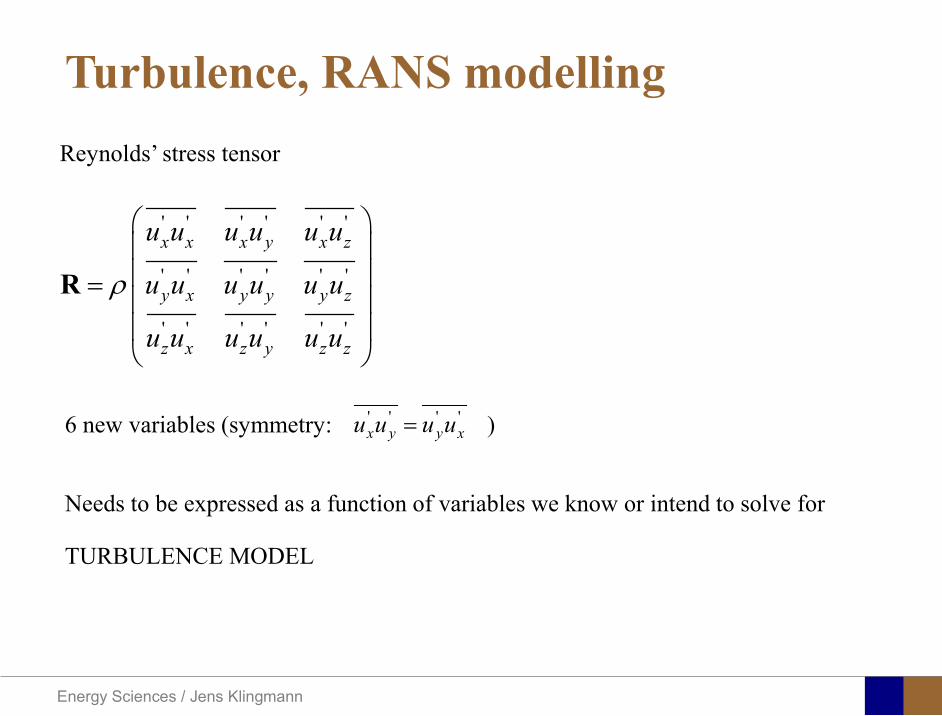
Energy Sciences Jens Klingmann
Turbulence RANS modellingReynoldsrsquo stress tensor
Needs to be expressed as a function of variables we know or intend to solve for
TURBULENCE MODEL
x x x y x z
y x y y y z
z x z y z z
u u u u u u
u u u u u u
u u u u u u
ρ
=
R
6 new variables (symmetry )xyyx uuuu =
Energy Sciences Jens Klingmann
Turbulence RANS modellingReynolds stress tensor
ij i j
u u u v u w
R u u v u v v v w
w u w v w w
ρ ρ ρ
= minus otimes = = =
R u u
Turbulent Kinetic Energy
( ) ( )1 1 1 1 2 2 2 2ii i ik tr R u u u u v v w wρ ρ= = = = + +R
Represents the kinetic energy of the fluctuations (or vortices)
Energy Sciences Jens Klingmann
Turbulence closure problem
10 unknownvelocity components pressure and correlations of fluctuating velocity
4 equationsAveraged momentum equations and averaged continuity equation
i ju u
Energy Sciences Jens Klingmann
Turbulence RANS modelling
23
i jij T ij
j i
u uR kx x
micro ρ δ part part
= + minus part part
2 T kmicro ρ εpropldquoTurbulent viscosityrdquo
Transport of k Some terms may be derived other need modelling
( ) ( ) ( )advection diffusion productionk k k kt
εpart+ + = minus
part
Energy from mean flow to turbulence
Dissipation Energy converted to heat
Energy Sciences Jens Klingmann
Turbulence RANS modelling
23
i jij T ij
j i
u uR kx x
micro ρ δ part part
= + minus part part ερmicro micro 2kCT =
k Tklk
k l k k k
uk ku Rx x x x
microρ ε micro
σ part part part part
= minus + + part part part part 2
1 2k T
klkk l k k
uu C R C
x k x k x xε εε
microε ε ε ερ ρ micropart σ
part part part part= minus + + part part part
4411 =εC 9212 =εC 090=microC 1=kσ31=εσ
Closure coefficients
Energy Sciences Jens Klingmann
Energy Sciences Jens Klingmann
Computational Fluid Dynamics (CFD)
U Waringhleacuten ldquoThe Aerodynamic design and testing of a supersonic turbine for rocket engine propulsionrdquo Proc Of 3rd European conference on Turbomachinery Fluid dynamics and thermodynamics
Energy Sciences Jens Klingmann
Subsonic flow in an aerofoilplate junction computed with a second-moment closure (D Apsley 1998)
Computational Fluid Dynamics(CFD)
Energy Sciences Jens Klingmann
Hydraulic turbine research CFD digital simulation Distribution of speed on an axial turbine
Computational Fluid Dynamics(CFD)
Energy Sciences Jens Klingmann
Scales of turbulence
10-01
1000
1001
1002
1003
1004
1005
κ LI
10-08
10-07
10-06
10-05
10-04
10-03
10-02
10-01
1000
E(u
2 LI)
10-04
10-03
10-02
10-01
1000
κ LK
10-05
10-04
10-03
10-02
10-01
1000
1001
1002
D( ε L
K )10-01
1000
1001
1002
1003
1004
1005
E = 15 (κ LI)-53
10-04
10-03
10-02
10-01
1000
1001
D = 3 ( κ LΚ) 13
Normalized energy and dissipation spectra for
Adapted from Tennekeys and Lumley
ReLI= times2 105
1 2Re 500IL asymp
3 4Re 10000IL asymp
Energy Sciences Jens Klingmann
References Turbulence
bull Tennekeys and Lumley ldquoA first course in Turbulencerdquo MIT Press 1972
bull J O Hinze ldquoTurbulencerdquo McGraw-Hill 1959bull D C Wilcox ldquoTurbulence Modeling for CFDrdquo DCW Industries
2006
Energy Sciences Jens Klingmann
Boundary layers
Energy Sciences Jens Klingmann
Boundary Layer Theory (BLT) Sensitive to Pressure
gradients Appropriate scaling from
dimensional analyses
Energy Sciences Jens Klingmann
Boundary layers
Energy Sciences Jens Klingmann
Air foil theory
Energy Sciences Jens Klingmann
Visualisation of diffusor separation
Energy Sciences Jens Klingmann
BL equations
+minus=+
yu
yxp
xuv
xuu
partpartmicro
partpart
partpart
partρpart
partρpart and 0=+
yxu
partυpart
partpart
Applying the BL approximations the 2D stationary incompressible NS-eq and continuity equation become
yvu
yu
yxuu
xp
yu
xuu
partpartρ
partpartmicro
partpart
partρpart
partpart
partυρpart
partρpart
minus
+minusminus=+
and
0=+yx
upart
υpartpartpart
Reynolds averaged BL eqs are
Energy Sciences Jens Klingmann
Boundary layers
Energy Sciences Jens Klingmann
Turbulent BL at different Pressure gradients
Energy Sciences Jens Klingmann
Boundary Layers
ν
yuy =+
ρτWu =
0=
partpart
=y
w yuτ
uuu =+
Energy Sciences Jens Klingmann
Diffuser efficiency
Energy Sciences Jens Klingmann
Reynolds Number (Order of magnitude)
At eg a compressor inlet
ρ = O(1) kgm3
U = O(100) msx lt O(01) mmicro = O(10-5)
Re = ρ U x micro =O(106)
In subsequent stages large amounts of turbulence (from stator wakes) will be convected into the Boundary layer
Energy Sciences Jens Klingmann
References Boundary layers
bull Frank M White ldquoViscous Fluid Flowrdquobull Hermann Schlichting ldquoBoundary Layer Theoryrdquo
Energy Sciences Jens Klingmann
CFD and experiments
bull No this is not a CFD course butbull Experiments
Energy Sciences Jens Klingmann
What do we need to measureOverall performance
Flow rates (mass or volume) Pressure Temperature Shaft power
Performance increase
Separations (velocity) Secondary flows eg tip clearance losses (velocity) Shock waves (supersonic applications) Pressure (resolved in time and space) Temperature (resolved in time and space)
Energy Sciences Jens Klingmann
Cascade wind tunnels
FIG 31 Compressor cascade wind tunnels (a) Conventional low-speed continuousrunning cascade tunnel (adapted from Carter et al 1950)(b) Transonicsupersoniccascade tunnel (adapted from Sieverding 1985)
Energy Sciences Jens Klingmann
Closed circuit tunnels
Energy Sciences Jens Klingmann
components
Settling Chamber
The settling chamber is located between the fan or wide angle diffuser and the contraction and contains the honeycombs and screens used to moderate longitudinal variations in the flow Screens in the chamber should be spaced at 02 chamber diameters apart so that flow disturbed by the first screen can settle before it encounters the second
Honeycombs
Honeycombs are located in the settling chamber and are used to reduce nonuniformities in the flow For optimum benefit honeycombs should be 6-8 cell diameters thick and cell size should be on the order of about 150 cells per settling chamber diameter
Energy Sciences Jens Klingmann
components
Screens
Screens are typically located just downstream of the honeycomb and sometime at the inlet of the test section Screens create a static pressure drop and serve to reduce boundary layer size and increase flow uniformity
Contraction Section
Contractions sections are located between the settling chamber and the test sections and serve to both increase mean velocities at the test section inlet and moderate inconsistencies in the uniformity of the flow Large contraction ratios and short contraction lengths are generally more desirable as they reduce the power loss across the screens and the thickness of boundary layers Small tunnels typically have contraction ratios between 6 and 9
Energy Sciences Jens Klingmann
Flow meters with pressure measurement
Venturi-tube
A1 A2
P1 P2
1 1 2 2C A C A=In the incompressible case
2 21 1 2 2
2 2C P C P
ρ ρ+ = +Assuming horisontal mounting
Energy Sciences Jens Klingmann
Daniel Bernoulli 1700-1782
Daniel Bernoulli was the son of Johann Bernoulli He was born in Groningen while his father held the chair of mathematics there His older brother was Nicolaus(II) Bernoulli and his uncle was Jacob Bernoulli so he was born into a family of leading mathematicians but also into a family where there was unfortunate rivalry jealousy and bitterness
Undoubtedly the most important work which Daniel Bernoulli did was his work on hydrodynamics Even the term itself is based on the title of the work which he produced called Hydrodynamica and before he left St Petersburg Daniel left a draft copy of the book with a printer However the work was not published until 1738 and although he revised it considerably between 1734 and 1738 it is more the presentation that he changed rather then the substance
This work contains for the first time the correct analysis of water flowing from a hole in a container This was based on the principle of conservation of energy which he had studied with his father in 1720 Daniel also discussed pumps and other machines to raise water One remarkable discovery appears in Chapter 10 of Hydrodynamica where Daniel discussed the basis for the kinetic theory of gases He was able to give the basic laws for the theory of gases and gave although not in full detail the equation of state discovered by Van der Waals a century later
Energy Sciences Jens Klingmann
Venturi-tube (2)
22 2 12 2
2
2A PC CA ρ
∆minus =
A1 A2
P1 P2
Solve for eg C2
1 2P P P∆ = minus
( )
12
2 2 21 2
21
PCA Aρ
∆ = minus
and( )
12
2 2 2 2 21 2
21
Pm A C AA Aρρ
∆ = = minus
where
Flow meters with pressure measurement
Energy Sciences Jens Klingmann
Flow meters with pressure measurement
Orifice meters
A1
A2
P1 P2
Applicable for pipe flows Same principle as for Venturi Positioning of pressure taps important Vena contracta and losses require inclusion
of Discharge Coefficient CD
( )
12
2 2 21 2
21D
Pm C AA Aρ ∆ =
minus where ( )1 2ReDC f A A=
CD available from manufacturer (measurements) or Standards (eg ISO)
Energy Sciences Jens Klingmann
Coriolis flow meter
An actuator (not shown) induces a vibration of the tubes
When there is mass flow Coriolis forces induce twisting of the tubes
degree of phase-shift is a measure for the amount of mass that is flowing through the tubes
Energy Sciences Jens Klingmann
Thermal flow meter Heat is added electrically to the flow Temperature is measured before and after heat addition
pP mC T∆=
Energy Sciences Jens Klingmann
Ultrasonic flow meters
Ultrasound is emitted to small particles in the flow (dust or other) Reflections of the sound is frequency shifted by the Doppler effect The frequency change is proportional to the particles velocity (volume flow
meter)
Energy Sciences Jens Klingmann
Inductive flow metersA magnetic flowmeter is based upon Faradays Law
The voltage induced across any conductor as it moves at right angles through a magnetic field is proportional to the velocity of that conductor
E is proportional to V x B x D where
E = The voltage generated in a conductorV = The velocity of the conductorB = The magnetic field strengthD = The length of the conductor
NB electric conductivity is required
Energy Sciences Jens Klingmann
Temperature measurements
Thermocouples
The basis established by Thomas Johann Seebeck in 1821
A conductor generates a voltage when subjected to a temperature gradient
To measure this voltage one must use a second conductor material which generates a different voltage under the same temperature gradient
Energy Sciences Jens Klingmann
Pressure sensing
1 2p pgt 2p p2 may be the atmosphere a static pressure tap or a known reference pressure
The strain of the diaphragm (or itrsquos deflection) may be measured by a number of electric methods
Diaphragm
Energy Sciences Jens Klingmann
Pressure sensingPiezoresistive Strain Gage
Uses the piezoresistive effect of bonded or formed strain gauges to detect strain due to applied pressure
Capacitive
Uses a diaghragm and pressure cavity to create a variable capacitor to detect strain due to applied pressure
Magnetic
Measures the displacement of a diaphragm by means of changes in inductance (reluctance) LVDT Hall Effect or by eddy current principal
Piezoelectric
Uses the piezoelectric effect in certain materials such as quartz to measure the strain upon the sensing mechanism due to pressure
Potentiometric
Uses the motion of a wiper along a resistive mechanism to detect the strain caused by applied pressure
Energy Sciences Jens Klingmann
3D highly instationary (periodic) flow Potentially very high velocities (Supersonic) Large temperature differences Low accessibility (difficult to probe between rotors) Low turbulence levels in most of the domain Very high turbulence in BL and wakes
Properties of measuring object
Point measurements
Energy Sciences Jens Klingmann
Conventional or non-opticalndash Static Pressure Measurementsndash Total Pressure Measurements
bull Multy hole probes
ndash Total Temperature ndash Hot Wire Anemometry (HWA)
Optical techniques for Velocity Measurementsndash Laser Two Focous (L2F)ndash Laser Doppler Anemometry (LDA)ndash Particle Image velocimetry (PIV)
Point Measurements
Energy Sciences Jens Klingmann
Static and total pressure
2 2 21 2 1
2 1 2 2 2C C CP P ρ ρ ρ
minus = minus =
2 0C =Stagnation point
C1Static pressure tap
Prandtl or Pitot tube
Apply the Bernoulli equation from free stream to stagnation point
21
2 12CP Pρ
= +or
We can also define a stagnation or total pressure
( )2
101 1 022
CP P Pρ= + =
Total pressure = Static pressure + dynamic pressure
or
Energy Sciences Jens Klingmann
Static pressure
Energy Sciences Jens Klingmann
Total Pressure and Temperature
Shrouded Probes
Shrouded Probe
Pitot or Prandtl tube
Sensitive to direction
Energy Sciences Jens Klingmann
Ludwig Prandtl 1875-1953
Ludwig Prandtl born at Freising Bavaria on February 4 1875 was a German Physicist famous for his work in aeronautics He qualified at Munchen in 1900 with a thesis on elastic stability and held the position of Professor of Applied Mechanics at Gottingen for forty-nine years (from 1904 until his death there on August 15 1953) In 1925 Prandtl became the Director of the Kaiser Wilhelm Institute for Fluid Mechanics His discovery in 1904 of the Boundary Layer which adjoins the surface of a body moving in a fluid led to an understanding of skin friction drag and of the way in which streamlining reduces the drag of airplane wings and other moving bodies His work on wing theory published in 1918 - 1919 followed that of FW Lanchester (1902-1907) but was carried out independently and elucidated the flow over airplane wings of finite span Prandtls work and decisive advances in boundary layer and wing theories became the basic material of aeronautics He also made important contributions to the theories of supersonic flow and of turbulence and contributed much to the development of wind tunnels and other aerodynamic equipment In addition he devised the soap-film analogy for the torsion of non-circular sections and wrote on the theory of plasticity and of meteorology
Energy Sciences Jens Klingmann
Total Pressure multy hole
Cobra Probe Yaw Probe
5 Hole Probe
Energy Sciences Jens Klingmann
5 Hole Probes Calibration
Energy Sciences Jens Klingmann
The inherent unsteadiness of the flow within turbomachines
Energy Sciences Jens Klingmann
Hot Wire Anemometry (HWA) The heat transfer from a thin (one micron)
electrically heated wire can be used to determine velocity
The resistance of the wire is temperature dependent Within a small temperature range it can be assumed linear R = R0+α R0(Tm-T0) where R0 is the resistance at a reference temperature T0 and Tm is the mean wire temperature
The thermal power induced in the wire is balanced by heat transfer to the surrounding fluid I2R=hπDL(Tm-T0) where h is the heat transfer coefficient and D and L the diameter and length of the wire respectively
E = I R
Energy Sciences Jens Klingmann
Constant Temperature Anemometry (CTA) The wire is often placed in a Whetstone bridge If the output from the
bridge is amplified and fed back to the bridge the resistance of the probe and thus the temperature will be held constant
This prevents the temperature of the wire to become excessive at low velocities
R1
R2 R3
Probe
Bridge Voltage
Energy Sciences Jens Klingmann
Constant Temperature Anemometry (CTA)
Energy Sciences Jens Klingmann
Characteristics of LDA (according to Dantec)
Invented by Yeh and Cummins in 1964 Velocity measurements in Fluid Dynamics (gas liquid) Up to 3 velocity components Non-intrusive measurements (optical technique) Absolute measurement technique (no calibration required) Very high accuracy Very high spatial resolution due to small measurement volume Tracer particles are required
Energy Sciences Jens Klingmann
LDA - Fringe Model
Focused Laser beams intersect and form the measurement volume Plane wave fronts beam waist in the plane of intersection Interference in the plane of intersection Pattern of bright and dark stripesplanes Fringes
Energy Sciences Jens Klingmann
LDA-measuring volume
d
x
x
y
y
z
z
e-2 CONTOUR
FRINGES
κ
κ
κ
κ
De-2
De-2
dml m
a
b
cx
b
z
ya
cd
d
=
=
=
J
J
J
J
JP
JP
JP
JD
JD
JD
+
+
+
a
b
c
d
κπλ
=minus sinD
f4l2e
m
κπλ
=minus cosD
f4D2e
m
Energy Sciences Jens Klingmann
Laser Two Focus
Energy Sciences Jens Klingmann
Laser Two Focus
Energy Sciences Jens Klingmann
PIV measurements
PIV is a fairly new technique capable of simultaneous velocity measurements at many points in a plane This gives information on large scale structures vorticity etc which is very difficult or impossible to obtain from one-point measuring techniques
PIV involves the illumination of a plane of the flow under investigation with a thin pulsed sheet of light The flow is seeded with particles
The light scattered from the particles and from successive pulses are being recorded either on film or a CCD array forming a multiple exposure of each particle image If the time between the pulses is known velocity can be determined as the ratio of the particle displacement and the elapsed time
t∆∆= xu
Energy Sciences Jens Klingmann
PIV
Energy Sciences Jens Klingmann
PIV measurements illumination
YA
G
YA
G
Two frequency doubled YAG Lasers aligned to one double pulsed laser sheet
Two or more separate light pulses can be obtained by chopping a continuous laser or from pulsed lasers
The limited pulse energies obtained from continuous lasers limits their applicability to low velocity flows or flows where large seeding particles can be used (ie liquid flows)
The low repetition rate of most pulsed lasers makes the use of two lasers advantageous
Energy Sciences Jens Klingmann
PIV measurements recording
High seeding density in laminar flame
Film or CCD-cameras Cross- or Auto-correlation
ndash ie both particle images on the same frame or on separate frames
CCD-camera requirementndash A many pixels as possiblendash 2k by 2k available 4k by 4k coming
Energy Sciences Jens Klingmann
PIV measurements analyses
Low seeding density (Number of seeding particles per unit volume)
Each particle image pair can be identified This is called particle tracking
High seeding density (PIV)
Small sub-regions of the image containing many particle image pairs are processed to obtain one velocity vector
Energy Sciences Jens Klingmann
PIV measurements analyses
Energy Sciences Jens Klingmann
PIV measurements analyses
( ) ( ) ( ) xsxxs dIIR 2A
1
I
+= int
Cross correlation between ( )x1I and ( )x2I
s is a two dimensional displacement vector
IA is the interrogation area
Cross correlation between
(
)
x
1
I
and
(
)
x
2
I
s is a two dimensional displacement vector
I
A
is the interrogation area
Energy Sciences Jens Klingmann
Energy Sciences Jens Klingmann
PIV from IOWA state university
Energy Sciences Jens Klingmann
PIV sample of evaluation
Energy Sciences Jens Klingmann
LDA PIV HWA Velocity range 01 mms ndash 300
ms 02 ndash 150 ms
Measuring Volume
D = 005 L = 05 mm
2 by 2 by 05 mm
L = 05 mm
Freq response O(10 000) Hz O(10) Hz O(100 000) Hz Calibration Yes No No Sensitivity to other than velocity
Low (ref Index) Low (ref Index) Large (temperature concentrationshellip)
Continuous Signal
Sometimes Seldom Always
Noise High High Low Turbulence intensity
No limitation Some limitation lt 20
Price O(1 000 000) SEK
O(1 000 000) SEK
O(50 000) SEK
Required Knowledge
High medium Low
Comparison of techniques
Energy Sciences Jens Klingmann
References experiments
R J Goldstein ldquoFluid Mechanics Measurementsrdquo Hemisphere Publishing 1983 A V Johansson amp P H Alfredsson ldquoExperimentella metoder inom
stroumlmningsmekanikenrdquo Inst Foumlr Mekanik KTH F Durst A Melling and J H Whitelaw ldquoPrincipals and Practice of Laser Doppler
Anemometryrdquo 1984 R J Adrian ldquoParticle-imaging techniques for experimental fluid mechnicsrdquo Ann Rev
Fluid Mech 1991
Energy Sciences Jens Klingmann
Sample of LDA-measurements
Rotor blade
Glas window
Emitted beams
Scattered Light
Adjustable mirror
Energy Sciences Jens Klingmann
Axial velocity sorted into 10 bins
0 1 2 3 4 5 6tangential coordinate (degrees)
-20
0
20
40
60
80
100
120
140
160Ax
ial v
eloc
ity a
nd s
tand
ard
devi
atio
n (m
s)
radial position 7 mm from inner window surfaceaxial position 23 mm behind rotor blades
Energy Sciences Jens Klingmann
Axial velocities in the radial-tangential plane
Energy Sciences Jens Klingmann
Airfoils NACA 4-digit
The NACA four-digit wing sections define the profile by
One digit describing maximum camber as percentage of the chord
One digit describing the distance of maximum camber from the airfoil leading edge in tens of percents of the chord
Two digits describing maximum thickness of the airfoil as percent of the chord
Example the NACA 2412 airfoil has a maximum camber of 2 located 40 (04 chords) from the leading edge with a maximum thickness of 12 of the chord
Four-digit series airfoils by default have maximum thickness at 30 of the chord (03 chords) from the leading edge
Energy Sciences Jens Klingmann
Airfoils NACA 4-digit
bull c is the chord lengthbull x is the position along
the chord from 0 to cbull y is the half thickness at
a given value of x (centerline to surface)
bull t is the maximum thickness as a fraction of the chord
Energy Sciences Jens Klingmann
Death by PowerPoint
| LDA | PIV | HWA | |||||
| Velocity range | 01 mms ndash 300 ms | 02 ndash 150 ms | |||||
| Measuring Volume | D = 005 L = 05 mm | 2 by 2 by 05 mm | L = 05 mm | ||||
| Freq response | O(10 000) Hz | O(10) Hz | O(100 000) Hz | ||||
| Calibration | Yes | No | No | ||||
| Sensitivity to other than velocity | Low (ref Index) | Low (ref Index) | Large (temperature concentrationshellip) | ||||
| Continuous Signal | Sometimes | Seldom | Always | ||||
| Noise | High | High | Low | ||||
| Turbulence intensity | No limitation | Some limitation | lt 20 | ||||
| Price | O(1 000 000) SEK | O(1 000 000) SEK | O(50 000) SEK | ||||
| Required Knowledge | High | medium | Low |
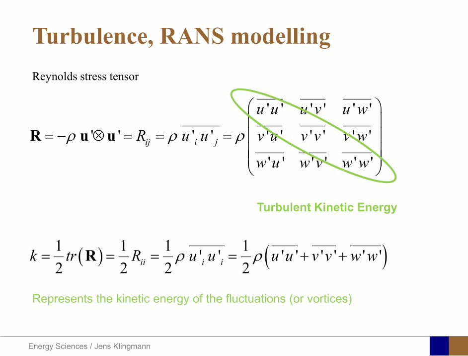
Energy Sciences Jens Klingmann
Turbulence RANS modellingReynolds stress tensor
ij i j
u u u v u w
R u u v u v v v w
w u w v w w
ρ ρ ρ
= minus otimes = = =
R u u
Turbulent Kinetic Energy
( ) ( )1 1 1 1 2 2 2 2ii i ik tr R u u u u v v w wρ ρ= = = = + +R
Represents the kinetic energy of the fluctuations (or vortices)
Energy Sciences Jens Klingmann
Turbulence closure problem
10 unknownvelocity components pressure and correlations of fluctuating velocity
4 equationsAveraged momentum equations and averaged continuity equation
i ju u
Energy Sciences Jens Klingmann
Turbulence RANS modelling
23
i jij T ij
j i
u uR kx x
micro ρ δ part part
= + minus part part
2 T kmicro ρ εpropldquoTurbulent viscosityrdquo
Transport of k Some terms may be derived other need modelling
( ) ( ) ( )advection diffusion productionk k k kt
εpart+ + = minus
part
Energy from mean flow to turbulence
Dissipation Energy converted to heat
Energy Sciences Jens Klingmann
Turbulence RANS modelling
23
i jij T ij
j i
u uR kx x
micro ρ δ part part
= + minus part part ερmicro micro 2kCT =
k Tklk
k l k k k
uk ku Rx x x x
microρ ε micro
σ part part part part
= minus + + part part part part 2
1 2k T
klkk l k k
uu C R C
x k x k x xε εε
microε ε ε ερ ρ micropart σ
part part part part= minus + + part part part
4411 =εC 9212 =εC 090=microC 1=kσ31=εσ
Closure coefficients
Energy Sciences Jens Klingmann
Energy Sciences Jens Klingmann
Computational Fluid Dynamics (CFD)
U Waringhleacuten ldquoThe Aerodynamic design and testing of a supersonic turbine for rocket engine propulsionrdquo Proc Of 3rd European conference on Turbomachinery Fluid dynamics and thermodynamics
Energy Sciences Jens Klingmann
Subsonic flow in an aerofoilplate junction computed with a second-moment closure (D Apsley 1998)
Computational Fluid Dynamics(CFD)
Energy Sciences Jens Klingmann
Hydraulic turbine research CFD digital simulation Distribution of speed on an axial turbine
Computational Fluid Dynamics(CFD)
Energy Sciences Jens Klingmann
Scales of turbulence
10-01
1000
1001
1002
1003
1004
1005
κ LI
10-08
10-07
10-06
10-05
10-04
10-03
10-02
10-01
1000
E(u
2 LI)
10-04
10-03
10-02
10-01
1000
κ LK
10-05
10-04
10-03
10-02
10-01
1000
1001
1002
D( ε L
K )10-01
1000
1001
1002
1003
1004
1005
E = 15 (κ LI)-53
10-04
10-03
10-02
10-01
1000
1001
D = 3 ( κ LΚ) 13
Normalized energy and dissipation spectra for
Adapted from Tennekeys and Lumley
ReLI= times2 105
1 2Re 500IL asymp
3 4Re 10000IL asymp
Energy Sciences Jens Klingmann
References Turbulence
bull Tennekeys and Lumley ldquoA first course in Turbulencerdquo MIT Press 1972
bull J O Hinze ldquoTurbulencerdquo McGraw-Hill 1959bull D C Wilcox ldquoTurbulence Modeling for CFDrdquo DCW Industries
2006
Energy Sciences Jens Klingmann
Boundary layers
Energy Sciences Jens Klingmann
Boundary Layer Theory (BLT) Sensitive to Pressure
gradients Appropriate scaling from
dimensional analyses
Energy Sciences Jens Klingmann
Boundary layers
Energy Sciences Jens Klingmann
Air foil theory
Energy Sciences Jens Klingmann
Visualisation of diffusor separation
Energy Sciences Jens Klingmann
BL equations
+minus=+
yu
yxp
xuv
xuu
partpartmicro
partpart
partpart
partρpart
partρpart and 0=+
yxu
partυpart
partpart
Applying the BL approximations the 2D stationary incompressible NS-eq and continuity equation become
yvu
yu
yxuu
xp
yu
xuu
partpartρ
partpartmicro
partpart
partρpart
partpart
partυρpart
partρpart
minus
+minusminus=+
and
0=+yx
upart
υpartpartpart
Reynolds averaged BL eqs are
Energy Sciences Jens Klingmann
Boundary layers
Energy Sciences Jens Klingmann
Turbulent BL at different Pressure gradients
Energy Sciences Jens Klingmann
Boundary Layers
ν
yuy =+
ρτWu =
0=
partpart
=y
w yuτ
uuu =+
Energy Sciences Jens Klingmann
Diffuser efficiency
Energy Sciences Jens Klingmann
Reynolds Number (Order of magnitude)
At eg a compressor inlet
ρ = O(1) kgm3
U = O(100) msx lt O(01) mmicro = O(10-5)
Re = ρ U x micro =O(106)
In subsequent stages large amounts of turbulence (from stator wakes) will be convected into the Boundary layer
Energy Sciences Jens Klingmann
References Boundary layers
bull Frank M White ldquoViscous Fluid Flowrdquobull Hermann Schlichting ldquoBoundary Layer Theoryrdquo
Energy Sciences Jens Klingmann
CFD and experiments
bull No this is not a CFD course butbull Experiments
Energy Sciences Jens Klingmann
What do we need to measureOverall performance
Flow rates (mass or volume) Pressure Temperature Shaft power
Performance increase
Separations (velocity) Secondary flows eg tip clearance losses (velocity) Shock waves (supersonic applications) Pressure (resolved in time and space) Temperature (resolved in time and space)
Energy Sciences Jens Klingmann
Cascade wind tunnels
FIG 31 Compressor cascade wind tunnels (a) Conventional low-speed continuousrunning cascade tunnel (adapted from Carter et al 1950)(b) Transonicsupersoniccascade tunnel (adapted from Sieverding 1985)
Energy Sciences Jens Klingmann
Closed circuit tunnels
Energy Sciences Jens Klingmann
components
Settling Chamber
The settling chamber is located between the fan or wide angle diffuser and the contraction and contains the honeycombs and screens used to moderate longitudinal variations in the flow Screens in the chamber should be spaced at 02 chamber diameters apart so that flow disturbed by the first screen can settle before it encounters the second
Honeycombs
Honeycombs are located in the settling chamber and are used to reduce nonuniformities in the flow For optimum benefit honeycombs should be 6-8 cell diameters thick and cell size should be on the order of about 150 cells per settling chamber diameter
Energy Sciences Jens Klingmann
components
Screens
Screens are typically located just downstream of the honeycomb and sometime at the inlet of the test section Screens create a static pressure drop and serve to reduce boundary layer size and increase flow uniformity
Contraction Section
Contractions sections are located between the settling chamber and the test sections and serve to both increase mean velocities at the test section inlet and moderate inconsistencies in the uniformity of the flow Large contraction ratios and short contraction lengths are generally more desirable as they reduce the power loss across the screens and the thickness of boundary layers Small tunnels typically have contraction ratios between 6 and 9
Energy Sciences Jens Klingmann
Flow meters with pressure measurement
Venturi-tube
A1 A2
P1 P2
1 1 2 2C A C A=In the incompressible case
2 21 1 2 2
2 2C P C P
ρ ρ+ = +Assuming horisontal mounting
Energy Sciences Jens Klingmann
Daniel Bernoulli 1700-1782
Daniel Bernoulli was the son of Johann Bernoulli He was born in Groningen while his father held the chair of mathematics there His older brother was Nicolaus(II) Bernoulli and his uncle was Jacob Bernoulli so he was born into a family of leading mathematicians but also into a family where there was unfortunate rivalry jealousy and bitterness
Undoubtedly the most important work which Daniel Bernoulli did was his work on hydrodynamics Even the term itself is based on the title of the work which he produced called Hydrodynamica and before he left St Petersburg Daniel left a draft copy of the book with a printer However the work was not published until 1738 and although he revised it considerably between 1734 and 1738 it is more the presentation that he changed rather then the substance
This work contains for the first time the correct analysis of water flowing from a hole in a container This was based on the principle of conservation of energy which he had studied with his father in 1720 Daniel also discussed pumps and other machines to raise water One remarkable discovery appears in Chapter 10 of Hydrodynamica where Daniel discussed the basis for the kinetic theory of gases He was able to give the basic laws for the theory of gases and gave although not in full detail the equation of state discovered by Van der Waals a century later
Energy Sciences Jens Klingmann
Venturi-tube (2)
22 2 12 2
2
2A PC CA ρ
∆minus =
A1 A2
P1 P2
Solve for eg C2
1 2P P P∆ = minus
( )
12
2 2 21 2
21
PCA Aρ
∆ = minus
and( )
12
2 2 2 2 21 2
21
Pm A C AA Aρρ
∆ = = minus
where
Flow meters with pressure measurement
Energy Sciences Jens Klingmann
Flow meters with pressure measurement
Orifice meters
A1
A2
P1 P2
Applicable for pipe flows Same principle as for Venturi Positioning of pressure taps important Vena contracta and losses require inclusion
of Discharge Coefficient CD
( )
12
2 2 21 2
21D
Pm C AA Aρ ∆ =
minus where ( )1 2ReDC f A A=
CD available from manufacturer (measurements) or Standards (eg ISO)
Energy Sciences Jens Klingmann
Coriolis flow meter
An actuator (not shown) induces a vibration of the tubes
When there is mass flow Coriolis forces induce twisting of the tubes
degree of phase-shift is a measure for the amount of mass that is flowing through the tubes
Energy Sciences Jens Klingmann
Thermal flow meter Heat is added electrically to the flow Temperature is measured before and after heat addition
pP mC T∆=
Energy Sciences Jens Klingmann
Ultrasonic flow meters
Ultrasound is emitted to small particles in the flow (dust or other) Reflections of the sound is frequency shifted by the Doppler effect The frequency change is proportional to the particles velocity (volume flow
meter)
Energy Sciences Jens Klingmann
Inductive flow metersA magnetic flowmeter is based upon Faradays Law
The voltage induced across any conductor as it moves at right angles through a magnetic field is proportional to the velocity of that conductor
E is proportional to V x B x D where
E = The voltage generated in a conductorV = The velocity of the conductorB = The magnetic field strengthD = The length of the conductor
NB electric conductivity is required
Energy Sciences Jens Klingmann
Temperature measurements
Thermocouples
The basis established by Thomas Johann Seebeck in 1821
A conductor generates a voltage when subjected to a temperature gradient
To measure this voltage one must use a second conductor material which generates a different voltage under the same temperature gradient
Energy Sciences Jens Klingmann
Pressure sensing
1 2p pgt 2p p2 may be the atmosphere a static pressure tap or a known reference pressure
The strain of the diaphragm (or itrsquos deflection) may be measured by a number of electric methods
Diaphragm
Energy Sciences Jens Klingmann
Pressure sensingPiezoresistive Strain Gage
Uses the piezoresistive effect of bonded or formed strain gauges to detect strain due to applied pressure
Capacitive
Uses a diaghragm and pressure cavity to create a variable capacitor to detect strain due to applied pressure
Magnetic
Measures the displacement of a diaphragm by means of changes in inductance (reluctance) LVDT Hall Effect or by eddy current principal
Piezoelectric
Uses the piezoelectric effect in certain materials such as quartz to measure the strain upon the sensing mechanism due to pressure
Potentiometric
Uses the motion of a wiper along a resistive mechanism to detect the strain caused by applied pressure
Energy Sciences Jens Klingmann
3D highly instationary (periodic) flow Potentially very high velocities (Supersonic) Large temperature differences Low accessibility (difficult to probe between rotors) Low turbulence levels in most of the domain Very high turbulence in BL and wakes
Properties of measuring object
Point measurements
Energy Sciences Jens Klingmann
Conventional or non-opticalndash Static Pressure Measurementsndash Total Pressure Measurements
bull Multy hole probes
ndash Total Temperature ndash Hot Wire Anemometry (HWA)
Optical techniques for Velocity Measurementsndash Laser Two Focous (L2F)ndash Laser Doppler Anemometry (LDA)ndash Particle Image velocimetry (PIV)
Point Measurements
Energy Sciences Jens Klingmann
Static and total pressure
2 2 21 2 1
2 1 2 2 2C C CP P ρ ρ ρ
minus = minus =
2 0C =Stagnation point
C1Static pressure tap
Prandtl or Pitot tube
Apply the Bernoulli equation from free stream to stagnation point
21
2 12CP Pρ
= +or
We can also define a stagnation or total pressure
( )2
101 1 022
CP P Pρ= + =
Total pressure = Static pressure + dynamic pressure
or
Energy Sciences Jens Klingmann
Static pressure
Energy Sciences Jens Klingmann
Total Pressure and Temperature
Shrouded Probes
Shrouded Probe
Pitot or Prandtl tube
Sensitive to direction
Energy Sciences Jens Klingmann
Ludwig Prandtl 1875-1953
Ludwig Prandtl born at Freising Bavaria on February 4 1875 was a German Physicist famous for his work in aeronautics He qualified at Munchen in 1900 with a thesis on elastic stability and held the position of Professor of Applied Mechanics at Gottingen for forty-nine years (from 1904 until his death there on August 15 1953) In 1925 Prandtl became the Director of the Kaiser Wilhelm Institute for Fluid Mechanics His discovery in 1904 of the Boundary Layer which adjoins the surface of a body moving in a fluid led to an understanding of skin friction drag and of the way in which streamlining reduces the drag of airplane wings and other moving bodies His work on wing theory published in 1918 - 1919 followed that of FW Lanchester (1902-1907) but was carried out independently and elucidated the flow over airplane wings of finite span Prandtls work and decisive advances in boundary layer and wing theories became the basic material of aeronautics He also made important contributions to the theories of supersonic flow and of turbulence and contributed much to the development of wind tunnels and other aerodynamic equipment In addition he devised the soap-film analogy for the torsion of non-circular sections and wrote on the theory of plasticity and of meteorology
Energy Sciences Jens Klingmann
Total Pressure multy hole
Cobra Probe Yaw Probe
5 Hole Probe
Energy Sciences Jens Klingmann
5 Hole Probes Calibration
Energy Sciences Jens Klingmann
The inherent unsteadiness of the flow within turbomachines
Energy Sciences Jens Klingmann
Hot Wire Anemometry (HWA) The heat transfer from a thin (one micron)
electrically heated wire can be used to determine velocity
The resistance of the wire is temperature dependent Within a small temperature range it can be assumed linear R = R0+α R0(Tm-T0) where R0 is the resistance at a reference temperature T0 and Tm is the mean wire temperature
The thermal power induced in the wire is balanced by heat transfer to the surrounding fluid I2R=hπDL(Tm-T0) where h is the heat transfer coefficient and D and L the diameter and length of the wire respectively
E = I R
Energy Sciences Jens Klingmann
Constant Temperature Anemometry (CTA) The wire is often placed in a Whetstone bridge If the output from the
bridge is amplified and fed back to the bridge the resistance of the probe and thus the temperature will be held constant
This prevents the temperature of the wire to become excessive at low velocities
R1
R2 R3
Probe
Bridge Voltage
Energy Sciences Jens Klingmann
Constant Temperature Anemometry (CTA)
Energy Sciences Jens Klingmann
Characteristics of LDA (according to Dantec)
Invented by Yeh and Cummins in 1964 Velocity measurements in Fluid Dynamics (gas liquid) Up to 3 velocity components Non-intrusive measurements (optical technique) Absolute measurement technique (no calibration required) Very high accuracy Very high spatial resolution due to small measurement volume Tracer particles are required
Energy Sciences Jens Klingmann
LDA - Fringe Model
Focused Laser beams intersect and form the measurement volume Plane wave fronts beam waist in the plane of intersection Interference in the plane of intersection Pattern of bright and dark stripesplanes Fringes
Energy Sciences Jens Klingmann
LDA-measuring volume
d
x
x
y
y
z
z
e-2 CONTOUR
FRINGES
κ
κ
κ
κ
De-2
De-2
dml m
a
b
cx
b
z
ya
cd
d
=
=
=
J
J
J
J
JP
JP
JP
JD
JD
JD
+
+
+
a
b
c
d
κπλ
=minus sinD
f4l2e
m
κπλ
=minus cosD
f4D2e
m
Energy Sciences Jens Klingmann
Laser Two Focus
Energy Sciences Jens Klingmann
Laser Two Focus
Energy Sciences Jens Klingmann
PIV measurements
PIV is a fairly new technique capable of simultaneous velocity measurements at many points in a plane This gives information on large scale structures vorticity etc which is very difficult or impossible to obtain from one-point measuring techniques
PIV involves the illumination of a plane of the flow under investigation with a thin pulsed sheet of light The flow is seeded with particles
The light scattered from the particles and from successive pulses are being recorded either on film or a CCD array forming a multiple exposure of each particle image If the time between the pulses is known velocity can be determined as the ratio of the particle displacement and the elapsed time
t∆∆= xu
Energy Sciences Jens Klingmann
PIV
Energy Sciences Jens Klingmann
PIV measurements illumination
YA
G
YA
G
Two frequency doubled YAG Lasers aligned to one double pulsed laser sheet
Two or more separate light pulses can be obtained by chopping a continuous laser or from pulsed lasers
The limited pulse energies obtained from continuous lasers limits their applicability to low velocity flows or flows where large seeding particles can be used (ie liquid flows)
The low repetition rate of most pulsed lasers makes the use of two lasers advantageous
Energy Sciences Jens Klingmann
PIV measurements recording
High seeding density in laminar flame
Film or CCD-cameras Cross- or Auto-correlation
ndash ie both particle images on the same frame or on separate frames
CCD-camera requirementndash A many pixels as possiblendash 2k by 2k available 4k by 4k coming
Energy Sciences Jens Klingmann
PIV measurements analyses
Low seeding density (Number of seeding particles per unit volume)
Each particle image pair can be identified This is called particle tracking
High seeding density (PIV)
Small sub-regions of the image containing many particle image pairs are processed to obtain one velocity vector
Energy Sciences Jens Klingmann
PIV measurements analyses
Energy Sciences Jens Klingmann
PIV measurements analyses
( ) ( ) ( ) xsxxs dIIR 2A
1
I
+= int
Cross correlation between ( )x1I and ( )x2I
s is a two dimensional displacement vector
IA is the interrogation area
Cross correlation between
(
)
x
1
I
and
(
)
x
2
I
s is a two dimensional displacement vector
I
A
is the interrogation area
Energy Sciences Jens Klingmann
Energy Sciences Jens Klingmann
PIV from IOWA state university
Energy Sciences Jens Klingmann
PIV sample of evaluation
Energy Sciences Jens Klingmann
LDA PIV HWA Velocity range 01 mms ndash 300
ms 02 ndash 150 ms
Measuring Volume
D = 005 L = 05 mm
2 by 2 by 05 mm
L = 05 mm
Freq response O(10 000) Hz O(10) Hz O(100 000) Hz Calibration Yes No No Sensitivity to other than velocity
Low (ref Index) Low (ref Index) Large (temperature concentrationshellip)
Continuous Signal
Sometimes Seldom Always
Noise High High Low Turbulence intensity
No limitation Some limitation lt 20
Price O(1 000 000) SEK
O(1 000 000) SEK
O(50 000) SEK
Required Knowledge
High medium Low
Comparison of techniques
Energy Sciences Jens Klingmann
References experiments
R J Goldstein ldquoFluid Mechanics Measurementsrdquo Hemisphere Publishing 1983 A V Johansson amp P H Alfredsson ldquoExperimentella metoder inom
stroumlmningsmekanikenrdquo Inst Foumlr Mekanik KTH F Durst A Melling and J H Whitelaw ldquoPrincipals and Practice of Laser Doppler
Anemometryrdquo 1984 R J Adrian ldquoParticle-imaging techniques for experimental fluid mechnicsrdquo Ann Rev
Fluid Mech 1991
Energy Sciences Jens Klingmann
Sample of LDA-measurements
Rotor blade
Glas window
Emitted beams
Scattered Light
Adjustable mirror
Energy Sciences Jens Klingmann
Axial velocity sorted into 10 bins
0 1 2 3 4 5 6tangential coordinate (degrees)
-20
0
20
40
60
80
100
120
140
160Ax
ial v
eloc
ity a
nd s
tand
ard
devi
atio
n (m
s)
radial position 7 mm from inner window surfaceaxial position 23 mm behind rotor blades
Energy Sciences Jens Klingmann
Axial velocities in the radial-tangential plane
Energy Sciences Jens Klingmann
Airfoils NACA 4-digit
The NACA four-digit wing sections define the profile by
One digit describing maximum camber as percentage of the chord
One digit describing the distance of maximum camber from the airfoil leading edge in tens of percents of the chord
Two digits describing maximum thickness of the airfoil as percent of the chord
Example the NACA 2412 airfoil has a maximum camber of 2 located 40 (04 chords) from the leading edge with a maximum thickness of 12 of the chord
Four-digit series airfoils by default have maximum thickness at 30 of the chord (03 chords) from the leading edge
Energy Sciences Jens Klingmann
Airfoils NACA 4-digit
bull c is the chord lengthbull x is the position along
the chord from 0 to cbull y is the half thickness at
a given value of x (centerline to surface)
bull t is the maximum thickness as a fraction of the chord
Energy Sciences Jens Klingmann
Death by PowerPoint
| LDA | PIV | HWA | |||||
| Velocity range | 01 mms ndash 300 ms | 02 ndash 150 ms | |||||
| Measuring Volume | D = 005 L = 05 mm | 2 by 2 by 05 mm | L = 05 mm | ||||
| Freq response | O(10 000) Hz | O(10) Hz | O(100 000) Hz | ||||
| Calibration | Yes | No | No | ||||
| Sensitivity to other than velocity | Low (ref Index) | Low (ref Index) | Large (temperature concentrationshellip) | ||||
| Continuous Signal | Sometimes | Seldom | Always | ||||
| Noise | High | High | Low | ||||
| Turbulence intensity | No limitation | Some limitation | lt 20 | ||||
| Price | O(1 000 000) SEK | O(1 000 000) SEK | O(50 000) SEK | ||||
| Required Knowledge | High | medium | Low |
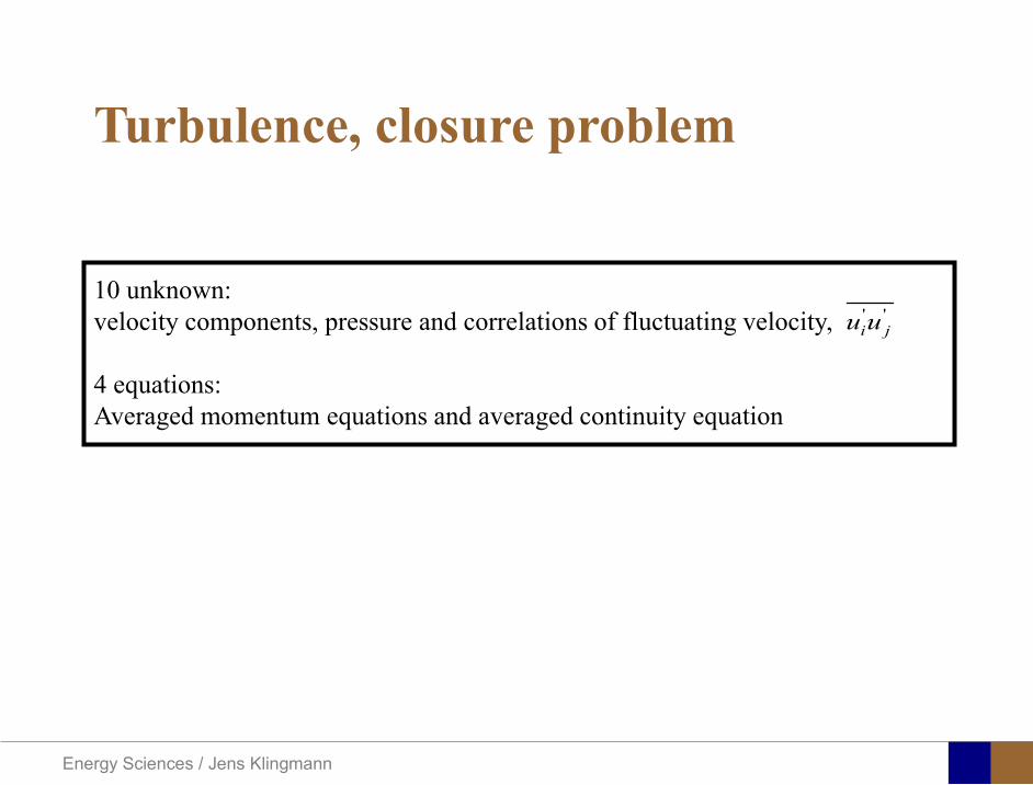
Energy Sciences Jens Klingmann
Turbulence closure problem
10 unknownvelocity components pressure and correlations of fluctuating velocity
4 equationsAveraged momentum equations and averaged continuity equation
i ju u
Energy Sciences Jens Klingmann
Turbulence RANS modelling
23
i jij T ij
j i
u uR kx x
micro ρ δ part part
= + minus part part
2 T kmicro ρ εpropldquoTurbulent viscosityrdquo
Transport of k Some terms may be derived other need modelling
( ) ( ) ( )advection diffusion productionk k k kt
εpart+ + = minus
part
Energy from mean flow to turbulence
Dissipation Energy converted to heat
Energy Sciences Jens Klingmann
Turbulence RANS modelling
23
i jij T ij
j i
u uR kx x
micro ρ δ part part
= + minus part part ερmicro micro 2kCT =
k Tklk
k l k k k
uk ku Rx x x x
microρ ε micro
σ part part part part
= minus + + part part part part 2
1 2k T
klkk l k k
uu C R C
x k x k x xε εε
microε ε ε ερ ρ micropart σ
part part part part= minus + + part part part
4411 =εC 9212 =εC 090=microC 1=kσ31=εσ
Closure coefficients
Energy Sciences Jens Klingmann
Energy Sciences Jens Klingmann
Computational Fluid Dynamics (CFD)
U Waringhleacuten ldquoThe Aerodynamic design and testing of a supersonic turbine for rocket engine propulsionrdquo Proc Of 3rd European conference on Turbomachinery Fluid dynamics and thermodynamics
Energy Sciences Jens Klingmann
Subsonic flow in an aerofoilplate junction computed with a second-moment closure (D Apsley 1998)
Computational Fluid Dynamics(CFD)
Energy Sciences Jens Klingmann
Hydraulic turbine research CFD digital simulation Distribution of speed on an axial turbine
Computational Fluid Dynamics(CFD)
Energy Sciences Jens Klingmann
Scales of turbulence
10-01
1000
1001
1002
1003
1004
1005
κ LI
10-08
10-07
10-06
10-05
10-04
10-03
10-02
10-01
1000
E(u
2 LI)
10-04
10-03
10-02
10-01
1000
κ LK
10-05
10-04
10-03
10-02
10-01
1000
1001
1002
D( ε L
K )10-01
1000
1001
1002
1003
1004
1005
E = 15 (κ LI)-53
10-04
10-03
10-02
10-01
1000
1001
D = 3 ( κ LΚ) 13
Normalized energy and dissipation spectra for
Adapted from Tennekeys and Lumley
ReLI= times2 105
1 2Re 500IL asymp
3 4Re 10000IL asymp
Energy Sciences Jens Klingmann
References Turbulence
bull Tennekeys and Lumley ldquoA first course in Turbulencerdquo MIT Press 1972
bull J O Hinze ldquoTurbulencerdquo McGraw-Hill 1959bull D C Wilcox ldquoTurbulence Modeling for CFDrdquo DCW Industries
2006
Energy Sciences Jens Klingmann
Boundary layers
Energy Sciences Jens Klingmann
Boundary Layer Theory (BLT) Sensitive to Pressure
gradients Appropriate scaling from
dimensional analyses
Energy Sciences Jens Klingmann
Boundary layers
Energy Sciences Jens Klingmann
Air foil theory
Energy Sciences Jens Klingmann
Visualisation of diffusor separation
Energy Sciences Jens Klingmann
BL equations
+minus=+
yu
yxp
xuv
xuu
partpartmicro
partpart
partpart
partρpart
partρpart and 0=+
yxu
partυpart
partpart
Applying the BL approximations the 2D stationary incompressible NS-eq and continuity equation become
yvu
yu
yxuu
xp
yu
xuu
partpartρ
partpartmicro
partpart
partρpart
partpart
partυρpart
partρpart
minus
+minusminus=+
and
0=+yx
upart
υpartpartpart
Reynolds averaged BL eqs are
Energy Sciences Jens Klingmann
Boundary layers
Energy Sciences Jens Klingmann
Turbulent BL at different Pressure gradients
Energy Sciences Jens Klingmann
Boundary Layers
ν
yuy =+
ρτWu =
0=
partpart
=y
w yuτ
uuu =+
Energy Sciences Jens Klingmann
Diffuser efficiency
Energy Sciences Jens Klingmann
Reynolds Number (Order of magnitude)
At eg a compressor inlet
ρ = O(1) kgm3
U = O(100) msx lt O(01) mmicro = O(10-5)
Re = ρ U x micro =O(106)
In subsequent stages large amounts of turbulence (from stator wakes) will be convected into the Boundary layer
Energy Sciences Jens Klingmann
References Boundary layers
bull Frank M White ldquoViscous Fluid Flowrdquobull Hermann Schlichting ldquoBoundary Layer Theoryrdquo
Energy Sciences Jens Klingmann
CFD and experiments
bull No this is not a CFD course butbull Experiments
Energy Sciences Jens Klingmann
What do we need to measureOverall performance
Flow rates (mass or volume) Pressure Temperature Shaft power
Performance increase
Separations (velocity) Secondary flows eg tip clearance losses (velocity) Shock waves (supersonic applications) Pressure (resolved in time and space) Temperature (resolved in time and space)
Energy Sciences Jens Klingmann
Cascade wind tunnels
FIG 31 Compressor cascade wind tunnels (a) Conventional low-speed continuousrunning cascade tunnel (adapted from Carter et al 1950)(b) Transonicsupersoniccascade tunnel (adapted from Sieverding 1985)
Energy Sciences Jens Klingmann
Closed circuit tunnels
Energy Sciences Jens Klingmann
components
Settling Chamber
The settling chamber is located between the fan or wide angle diffuser and the contraction and contains the honeycombs and screens used to moderate longitudinal variations in the flow Screens in the chamber should be spaced at 02 chamber diameters apart so that flow disturbed by the first screen can settle before it encounters the second
Honeycombs
Honeycombs are located in the settling chamber and are used to reduce nonuniformities in the flow For optimum benefit honeycombs should be 6-8 cell diameters thick and cell size should be on the order of about 150 cells per settling chamber diameter
Energy Sciences Jens Klingmann
components
Screens
Screens are typically located just downstream of the honeycomb and sometime at the inlet of the test section Screens create a static pressure drop and serve to reduce boundary layer size and increase flow uniformity
Contraction Section
Contractions sections are located between the settling chamber and the test sections and serve to both increase mean velocities at the test section inlet and moderate inconsistencies in the uniformity of the flow Large contraction ratios and short contraction lengths are generally more desirable as they reduce the power loss across the screens and the thickness of boundary layers Small tunnels typically have contraction ratios between 6 and 9
Energy Sciences Jens Klingmann
Flow meters with pressure measurement
Venturi-tube
A1 A2
P1 P2
1 1 2 2C A C A=In the incompressible case
2 21 1 2 2
2 2C P C P
ρ ρ+ = +Assuming horisontal mounting
Energy Sciences Jens Klingmann
Daniel Bernoulli 1700-1782
Daniel Bernoulli was the son of Johann Bernoulli He was born in Groningen while his father held the chair of mathematics there His older brother was Nicolaus(II) Bernoulli and his uncle was Jacob Bernoulli so he was born into a family of leading mathematicians but also into a family where there was unfortunate rivalry jealousy and bitterness
Undoubtedly the most important work which Daniel Bernoulli did was his work on hydrodynamics Even the term itself is based on the title of the work which he produced called Hydrodynamica and before he left St Petersburg Daniel left a draft copy of the book with a printer However the work was not published until 1738 and although he revised it considerably between 1734 and 1738 it is more the presentation that he changed rather then the substance
This work contains for the first time the correct analysis of water flowing from a hole in a container This was based on the principle of conservation of energy which he had studied with his father in 1720 Daniel also discussed pumps and other machines to raise water One remarkable discovery appears in Chapter 10 of Hydrodynamica where Daniel discussed the basis for the kinetic theory of gases He was able to give the basic laws for the theory of gases and gave although not in full detail the equation of state discovered by Van der Waals a century later
Energy Sciences Jens Klingmann
Venturi-tube (2)
22 2 12 2
2
2A PC CA ρ
∆minus =
A1 A2
P1 P2
Solve for eg C2
1 2P P P∆ = minus
( )
12
2 2 21 2
21
PCA Aρ
∆ = minus
and( )
12
2 2 2 2 21 2
21
Pm A C AA Aρρ
∆ = = minus
where
Flow meters with pressure measurement
Energy Sciences Jens Klingmann
Flow meters with pressure measurement
Orifice meters
A1
A2
P1 P2
Applicable for pipe flows Same principle as for Venturi Positioning of pressure taps important Vena contracta and losses require inclusion
of Discharge Coefficient CD
( )
12
2 2 21 2
21D
Pm C AA Aρ ∆ =
minus where ( )1 2ReDC f A A=
CD available from manufacturer (measurements) or Standards (eg ISO)
Energy Sciences Jens Klingmann
Coriolis flow meter
An actuator (not shown) induces a vibration of the tubes
When there is mass flow Coriolis forces induce twisting of the tubes
degree of phase-shift is a measure for the amount of mass that is flowing through the tubes
Energy Sciences Jens Klingmann
Thermal flow meter Heat is added electrically to the flow Temperature is measured before and after heat addition
pP mC T∆=
Energy Sciences Jens Klingmann
Ultrasonic flow meters
Ultrasound is emitted to small particles in the flow (dust or other) Reflections of the sound is frequency shifted by the Doppler effect The frequency change is proportional to the particles velocity (volume flow
meter)
Energy Sciences Jens Klingmann
Inductive flow metersA magnetic flowmeter is based upon Faradays Law
The voltage induced across any conductor as it moves at right angles through a magnetic field is proportional to the velocity of that conductor
E is proportional to V x B x D where
E = The voltage generated in a conductorV = The velocity of the conductorB = The magnetic field strengthD = The length of the conductor
NB electric conductivity is required
Energy Sciences Jens Klingmann
Temperature measurements
Thermocouples
The basis established by Thomas Johann Seebeck in 1821
A conductor generates a voltage when subjected to a temperature gradient
To measure this voltage one must use a second conductor material which generates a different voltage under the same temperature gradient
Energy Sciences Jens Klingmann
Pressure sensing
1 2p pgt 2p p2 may be the atmosphere a static pressure tap or a known reference pressure
The strain of the diaphragm (or itrsquos deflection) may be measured by a number of electric methods
Diaphragm
Energy Sciences Jens Klingmann
Pressure sensingPiezoresistive Strain Gage
Uses the piezoresistive effect of bonded or formed strain gauges to detect strain due to applied pressure
Capacitive
Uses a diaghragm and pressure cavity to create a variable capacitor to detect strain due to applied pressure
Magnetic
Measures the displacement of a diaphragm by means of changes in inductance (reluctance) LVDT Hall Effect or by eddy current principal
Piezoelectric
Uses the piezoelectric effect in certain materials such as quartz to measure the strain upon the sensing mechanism due to pressure
Potentiometric
Uses the motion of a wiper along a resistive mechanism to detect the strain caused by applied pressure
Energy Sciences Jens Klingmann
3D highly instationary (periodic) flow Potentially very high velocities (Supersonic) Large temperature differences Low accessibility (difficult to probe between rotors) Low turbulence levels in most of the domain Very high turbulence in BL and wakes
Properties of measuring object
Point measurements
Energy Sciences Jens Klingmann
Conventional or non-opticalndash Static Pressure Measurementsndash Total Pressure Measurements
bull Multy hole probes
ndash Total Temperature ndash Hot Wire Anemometry (HWA)
Optical techniques for Velocity Measurementsndash Laser Two Focous (L2F)ndash Laser Doppler Anemometry (LDA)ndash Particle Image velocimetry (PIV)
Point Measurements
Energy Sciences Jens Klingmann
Static and total pressure
2 2 21 2 1
2 1 2 2 2C C CP P ρ ρ ρ
minus = minus =
2 0C =Stagnation point
C1Static pressure tap
Prandtl or Pitot tube
Apply the Bernoulli equation from free stream to stagnation point
21
2 12CP Pρ
= +or
We can also define a stagnation or total pressure
( )2
101 1 022
CP P Pρ= + =
Total pressure = Static pressure + dynamic pressure
or
Energy Sciences Jens Klingmann
Static pressure
Energy Sciences Jens Klingmann
Total Pressure and Temperature
Shrouded Probes
Shrouded Probe
Pitot or Prandtl tube
Sensitive to direction
Energy Sciences Jens Klingmann
Ludwig Prandtl 1875-1953
Ludwig Prandtl born at Freising Bavaria on February 4 1875 was a German Physicist famous for his work in aeronautics He qualified at Munchen in 1900 with a thesis on elastic stability and held the position of Professor of Applied Mechanics at Gottingen for forty-nine years (from 1904 until his death there on August 15 1953) In 1925 Prandtl became the Director of the Kaiser Wilhelm Institute for Fluid Mechanics His discovery in 1904 of the Boundary Layer which adjoins the surface of a body moving in a fluid led to an understanding of skin friction drag and of the way in which streamlining reduces the drag of airplane wings and other moving bodies His work on wing theory published in 1918 - 1919 followed that of FW Lanchester (1902-1907) but was carried out independently and elucidated the flow over airplane wings of finite span Prandtls work and decisive advances in boundary layer and wing theories became the basic material of aeronautics He also made important contributions to the theories of supersonic flow and of turbulence and contributed much to the development of wind tunnels and other aerodynamic equipment In addition he devised the soap-film analogy for the torsion of non-circular sections and wrote on the theory of plasticity and of meteorology
Energy Sciences Jens Klingmann
Total Pressure multy hole
Cobra Probe Yaw Probe
5 Hole Probe
Energy Sciences Jens Klingmann
5 Hole Probes Calibration
Energy Sciences Jens Klingmann
The inherent unsteadiness of the flow within turbomachines
Energy Sciences Jens Klingmann
Hot Wire Anemometry (HWA) The heat transfer from a thin (one micron)
electrically heated wire can be used to determine velocity
The resistance of the wire is temperature dependent Within a small temperature range it can be assumed linear R = R0+α R0(Tm-T0) where R0 is the resistance at a reference temperature T0 and Tm is the mean wire temperature
The thermal power induced in the wire is balanced by heat transfer to the surrounding fluid I2R=hπDL(Tm-T0) where h is the heat transfer coefficient and D and L the diameter and length of the wire respectively
E = I R
Energy Sciences Jens Klingmann
Constant Temperature Anemometry (CTA) The wire is often placed in a Whetstone bridge If the output from the
bridge is amplified and fed back to the bridge the resistance of the probe and thus the temperature will be held constant
This prevents the temperature of the wire to become excessive at low velocities
R1
R2 R3
Probe
Bridge Voltage
Energy Sciences Jens Klingmann
Constant Temperature Anemometry (CTA)
Energy Sciences Jens Klingmann
Characteristics of LDA (according to Dantec)
Invented by Yeh and Cummins in 1964 Velocity measurements in Fluid Dynamics (gas liquid) Up to 3 velocity components Non-intrusive measurements (optical technique) Absolute measurement technique (no calibration required) Very high accuracy Very high spatial resolution due to small measurement volume Tracer particles are required
Energy Sciences Jens Klingmann
LDA - Fringe Model
Focused Laser beams intersect and form the measurement volume Plane wave fronts beam waist in the plane of intersection Interference in the plane of intersection Pattern of bright and dark stripesplanes Fringes
Energy Sciences Jens Klingmann
LDA-measuring volume
d
x
x
y
y
z
z
e-2 CONTOUR
FRINGES
κ
κ
κ
κ
De-2
De-2
dml m
a
b
cx
b
z
ya
cd
d
=
=
=
J
J
J
J
JP
JP
JP
JD
JD
JD
+
+
+
a
b
c
d
κπλ
=minus sinD
f4l2e
m
κπλ
=minus cosD
f4D2e
m
Energy Sciences Jens Klingmann
Laser Two Focus
Energy Sciences Jens Klingmann
Laser Two Focus
Energy Sciences Jens Klingmann
PIV measurements
PIV is a fairly new technique capable of simultaneous velocity measurements at many points in a plane This gives information on large scale structures vorticity etc which is very difficult or impossible to obtain from one-point measuring techniques
PIV involves the illumination of a plane of the flow under investigation with a thin pulsed sheet of light The flow is seeded with particles
The light scattered from the particles and from successive pulses are being recorded either on film or a CCD array forming a multiple exposure of each particle image If the time between the pulses is known velocity can be determined as the ratio of the particle displacement and the elapsed time
t∆∆= xu
Energy Sciences Jens Klingmann
PIV
Energy Sciences Jens Klingmann
PIV measurements illumination
YA
G
YA
G
Two frequency doubled YAG Lasers aligned to one double pulsed laser sheet
Two or more separate light pulses can be obtained by chopping a continuous laser or from pulsed lasers
The limited pulse energies obtained from continuous lasers limits their applicability to low velocity flows or flows where large seeding particles can be used (ie liquid flows)
The low repetition rate of most pulsed lasers makes the use of two lasers advantageous
Energy Sciences Jens Klingmann
PIV measurements recording
High seeding density in laminar flame
Film or CCD-cameras Cross- or Auto-correlation
ndash ie both particle images on the same frame or on separate frames
CCD-camera requirementndash A many pixels as possiblendash 2k by 2k available 4k by 4k coming
Energy Sciences Jens Klingmann
PIV measurements analyses
Low seeding density (Number of seeding particles per unit volume)
Each particle image pair can be identified This is called particle tracking
High seeding density (PIV)
Small sub-regions of the image containing many particle image pairs are processed to obtain one velocity vector
Energy Sciences Jens Klingmann
PIV measurements analyses
Energy Sciences Jens Klingmann
PIV measurements analyses
( ) ( ) ( ) xsxxs dIIR 2A
1
I
+= int
Cross correlation between ( )x1I and ( )x2I
s is a two dimensional displacement vector
IA is the interrogation area
Cross correlation between
(
)
x
1
I
and
(
)
x
2
I
s is a two dimensional displacement vector
I
A
is the interrogation area
Energy Sciences Jens Klingmann
Energy Sciences Jens Klingmann
PIV from IOWA state university
Energy Sciences Jens Klingmann
PIV sample of evaluation
Energy Sciences Jens Klingmann
LDA PIV HWA Velocity range 01 mms ndash 300
ms 02 ndash 150 ms
Measuring Volume
D = 005 L = 05 mm
2 by 2 by 05 mm
L = 05 mm
Freq response O(10 000) Hz O(10) Hz O(100 000) Hz Calibration Yes No No Sensitivity to other than velocity
Low (ref Index) Low (ref Index) Large (temperature concentrationshellip)
Continuous Signal
Sometimes Seldom Always
Noise High High Low Turbulence intensity
No limitation Some limitation lt 20
Price O(1 000 000) SEK
O(1 000 000) SEK
O(50 000) SEK
Required Knowledge
High medium Low
Comparison of techniques
Energy Sciences Jens Klingmann
References experiments
R J Goldstein ldquoFluid Mechanics Measurementsrdquo Hemisphere Publishing 1983 A V Johansson amp P H Alfredsson ldquoExperimentella metoder inom
stroumlmningsmekanikenrdquo Inst Foumlr Mekanik KTH F Durst A Melling and J H Whitelaw ldquoPrincipals and Practice of Laser Doppler
Anemometryrdquo 1984 R J Adrian ldquoParticle-imaging techniques for experimental fluid mechnicsrdquo Ann Rev
Fluid Mech 1991
Energy Sciences Jens Klingmann
Sample of LDA-measurements
Rotor blade
Glas window
Emitted beams
Scattered Light
Adjustable mirror
Energy Sciences Jens Klingmann
Axial velocity sorted into 10 bins
0 1 2 3 4 5 6tangential coordinate (degrees)
-20
0
20
40
60
80
100
120
140
160Ax
ial v
eloc
ity a
nd s
tand
ard
devi
atio
n (m
s)
radial position 7 mm from inner window surfaceaxial position 23 mm behind rotor blades
Energy Sciences Jens Klingmann
Axial velocities in the radial-tangential plane
Energy Sciences Jens Klingmann
Airfoils NACA 4-digit
The NACA four-digit wing sections define the profile by
One digit describing maximum camber as percentage of the chord
One digit describing the distance of maximum camber from the airfoil leading edge in tens of percents of the chord
Two digits describing maximum thickness of the airfoil as percent of the chord
Example the NACA 2412 airfoil has a maximum camber of 2 located 40 (04 chords) from the leading edge with a maximum thickness of 12 of the chord
Four-digit series airfoils by default have maximum thickness at 30 of the chord (03 chords) from the leading edge
Energy Sciences Jens Klingmann
Airfoils NACA 4-digit
bull c is the chord lengthbull x is the position along
the chord from 0 to cbull y is the half thickness at
a given value of x (centerline to surface)
bull t is the maximum thickness as a fraction of the chord
Energy Sciences Jens Klingmann
Death by PowerPoint
| LDA | PIV | HWA | |||||
| Velocity range | 01 mms ndash 300 ms | 02 ndash 150 ms | |||||
| Measuring Volume | D = 005 L = 05 mm | 2 by 2 by 05 mm | L = 05 mm | ||||
| Freq response | O(10 000) Hz | O(10) Hz | O(100 000) Hz | ||||
| Calibration | Yes | No | No | ||||
| Sensitivity to other than velocity | Low (ref Index) | Low (ref Index) | Large (temperature concentrationshellip) | ||||
| Continuous Signal | Sometimes | Seldom | Always | ||||
| Noise | High | High | Low | ||||
| Turbulence intensity | No limitation | Some limitation | lt 20 | ||||
| Price | O(1 000 000) SEK | O(1 000 000) SEK | O(50 000) SEK | ||||
| Required Knowledge | High | medium | Low |
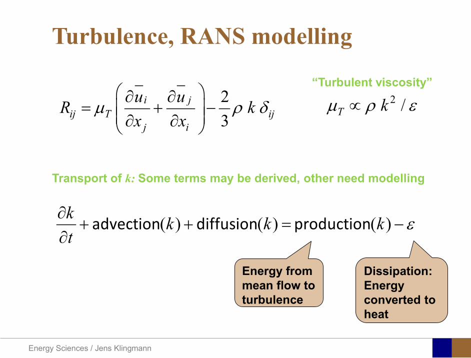
Energy Sciences Jens Klingmann
Turbulence RANS modelling
23
i jij T ij
j i
u uR kx x
micro ρ δ part part
= + minus part part
2 T kmicro ρ εpropldquoTurbulent viscosityrdquo
Transport of k Some terms may be derived other need modelling
( ) ( ) ( )advection diffusion productionk k k kt
εpart+ + = minus
part
Energy from mean flow to turbulence
Dissipation Energy converted to heat
Energy Sciences Jens Klingmann
Turbulence RANS modelling
23
i jij T ij
j i
u uR kx x
micro ρ δ part part
= + minus part part ερmicro micro 2kCT =
k Tklk
k l k k k
uk ku Rx x x x
microρ ε micro
σ part part part part
= minus + + part part part part 2
1 2k T
klkk l k k
uu C R C
x k x k x xε εε
microε ε ε ερ ρ micropart σ
part part part part= minus + + part part part
4411 =εC 9212 =εC 090=microC 1=kσ31=εσ
Closure coefficients
Energy Sciences Jens Klingmann
Energy Sciences Jens Klingmann
Computational Fluid Dynamics (CFD)
U Waringhleacuten ldquoThe Aerodynamic design and testing of a supersonic turbine for rocket engine propulsionrdquo Proc Of 3rd European conference on Turbomachinery Fluid dynamics and thermodynamics
Energy Sciences Jens Klingmann
Subsonic flow in an aerofoilplate junction computed with a second-moment closure (D Apsley 1998)
Computational Fluid Dynamics(CFD)
Energy Sciences Jens Klingmann
Hydraulic turbine research CFD digital simulation Distribution of speed on an axial turbine
Computational Fluid Dynamics(CFD)
Energy Sciences Jens Klingmann
Scales of turbulence
10-01
1000
1001
1002
1003
1004
1005
κ LI
10-08
10-07
10-06
10-05
10-04
10-03
10-02
10-01
1000
E(u
2 LI)
10-04
10-03
10-02
10-01
1000
κ LK
10-05
10-04
10-03
10-02
10-01
1000
1001
1002
D( ε L
K )10-01
1000
1001
1002
1003
1004
1005
E = 15 (κ LI)-53
10-04
10-03
10-02
10-01
1000
1001
D = 3 ( κ LΚ) 13
Normalized energy and dissipation spectra for
Adapted from Tennekeys and Lumley
ReLI= times2 105
1 2Re 500IL asymp
3 4Re 10000IL asymp
Energy Sciences Jens Klingmann
References Turbulence
bull Tennekeys and Lumley ldquoA first course in Turbulencerdquo MIT Press 1972
bull J O Hinze ldquoTurbulencerdquo McGraw-Hill 1959bull D C Wilcox ldquoTurbulence Modeling for CFDrdquo DCW Industries
2006
Energy Sciences Jens Klingmann
Boundary layers
Energy Sciences Jens Klingmann
Boundary Layer Theory (BLT) Sensitive to Pressure
gradients Appropriate scaling from
dimensional analyses
Energy Sciences Jens Klingmann
Boundary layers
Energy Sciences Jens Klingmann
Air foil theory
Energy Sciences Jens Klingmann
Visualisation of diffusor separation
Energy Sciences Jens Klingmann
BL equations
+minus=+
yu
yxp
xuv
xuu
partpartmicro
partpart
partpart
partρpart
partρpart and 0=+
yxu
partυpart
partpart
Applying the BL approximations the 2D stationary incompressible NS-eq and continuity equation become
yvu
yu
yxuu
xp
yu
xuu
partpartρ
partpartmicro
partpart
partρpart
partpart
partυρpart
partρpart
minus
+minusminus=+
and
0=+yx
upart
υpartpartpart
Reynolds averaged BL eqs are
Energy Sciences Jens Klingmann
Boundary layers
Energy Sciences Jens Klingmann
Turbulent BL at different Pressure gradients
Energy Sciences Jens Klingmann
Boundary Layers
ν
yuy =+
ρτWu =
0=
partpart
=y
w yuτ
uuu =+
Energy Sciences Jens Klingmann
Diffuser efficiency
Energy Sciences Jens Klingmann
Reynolds Number (Order of magnitude)
At eg a compressor inlet
ρ = O(1) kgm3
U = O(100) msx lt O(01) mmicro = O(10-5)
Re = ρ U x micro =O(106)
In subsequent stages large amounts of turbulence (from stator wakes) will be convected into the Boundary layer
Energy Sciences Jens Klingmann
References Boundary layers
bull Frank M White ldquoViscous Fluid Flowrdquobull Hermann Schlichting ldquoBoundary Layer Theoryrdquo
Energy Sciences Jens Klingmann
CFD and experiments
bull No this is not a CFD course butbull Experiments
Energy Sciences Jens Klingmann
What do we need to measureOverall performance
Flow rates (mass or volume) Pressure Temperature Shaft power
Performance increase
Separations (velocity) Secondary flows eg tip clearance losses (velocity) Shock waves (supersonic applications) Pressure (resolved in time and space) Temperature (resolved in time and space)
Energy Sciences Jens Klingmann
Cascade wind tunnels
FIG 31 Compressor cascade wind tunnels (a) Conventional low-speed continuousrunning cascade tunnel (adapted from Carter et al 1950)(b) Transonicsupersoniccascade tunnel (adapted from Sieverding 1985)
Energy Sciences Jens Klingmann
Closed circuit tunnels
Energy Sciences Jens Klingmann
components
Settling Chamber
The settling chamber is located between the fan or wide angle diffuser and the contraction and contains the honeycombs and screens used to moderate longitudinal variations in the flow Screens in the chamber should be spaced at 02 chamber diameters apart so that flow disturbed by the first screen can settle before it encounters the second
Honeycombs
Honeycombs are located in the settling chamber and are used to reduce nonuniformities in the flow For optimum benefit honeycombs should be 6-8 cell diameters thick and cell size should be on the order of about 150 cells per settling chamber diameter
Energy Sciences Jens Klingmann
components
Screens
Screens are typically located just downstream of the honeycomb and sometime at the inlet of the test section Screens create a static pressure drop and serve to reduce boundary layer size and increase flow uniformity
Contraction Section
Contractions sections are located between the settling chamber and the test sections and serve to both increase mean velocities at the test section inlet and moderate inconsistencies in the uniformity of the flow Large contraction ratios and short contraction lengths are generally more desirable as they reduce the power loss across the screens and the thickness of boundary layers Small tunnels typically have contraction ratios between 6 and 9
Energy Sciences Jens Klingmann
Flow meters with pressure measurement
Venturi-tube
A1 A2
P1 P2
1 1 2 2C A C A=In the incompressible case
2 21 1 2 2
2 2C P C P
ρ ρ+ = +Assuming horisontal mounting
Energy Sciences Jens Klingmann
Daniel Bernoulli 1700-1782
Daniel Bernoulli was the son of Johann Bernoulli He was born in Groningen while his father held the chair of mathematics there His older brother was Nicolaus(II) Bernoulli and his uncle was Jacob Bernoulli so he was born into a family of leading mathematicians but also into a family where there was unfortunate rivalry jealousy and bitterness
Undoubtedly the most important work which Daniel Bernoulli did was his work on hydrodynamics Even the term itself is based on the title of the work which he produced called Hydrodynamica and before he left St Petersburg Daniel left a draft copy of the book with a printer However the work was not published until 1738 and although he revised it considerably between 1734 and 1738 it is more the presentation that he changed rather then the substance
This work contains for the first time the correct analysis of water flowing from a hole in a container This was based on the principle of conservation of energy which he had studied with his father in 1720 Daniel also discussed pumps and other machines to raise water One remarkable discovery appears in Chapter 10 of Hydrodynamica where Daniel discussed the basis for the kinetic theory of gases He was able to give the basic laws for the theory of gases and gave although not in full detail the equation of state discovered by Van der Waals a century later
Energy Sciences Jens Klingmann
Venturi-tube (2)
22 2 12 2
2
2A PC CA ρ
∆minus =
A1 A2
P1 P2
Solve for eg C2
1 2P P P∆ = minus
( )
12
2 2 21 2
21
PCA Aρ
∆ = minus
and( )
12
2 2 2 2 21 2
21
Pm A C AA Aρρ
∆ = = minus
where
Flow meters with pressure measurement
Energy Sciences Jens Klingmann
Flow meters with pressure measurement
Orifice meters
A1
A2
P1 P2
Applicable for pipe flows Same principle as for Venturi Positioning of pressure taps important Vena contracta and losses require inclusion
of Discharge Coefficient CD
( )
12
2 2 21 2
21D
Pm C AA Aρ ∆ =
minus where ( )1 2ReDC f A A=
CD available from manufacturer (measurements) or Standards (eg ISO)
Energy Sciences Jens Klingmann
Coriolis flow meter
An actuator (not shown) induces a vibration of the tubes
When there is mass flow Coriolis forces induce twisting of the tubes
degree of phase-shift is a measure for the amount of mass that is flowing through the tubes
Energy Sciences Jens Klingmann
Thermal flow meter Heat is added electrically to the flow Temperature is measured before and after heat addition
pP mC T∆=
Energy Sciences Jens Klingmann
Ultrasonic flow meters
Ultrasound is emitted to small particles in the flow (dust or other) Reflections of the sound is frequency shifted by the Doppler effect The frequency change is proportional to the particles velocity (volume flow
meter)
Energy Sciences Jens Klingmann
Inductive flow metersA magnetic flowmeter is based upon Faradays Law
The voltage induced across any conductor as it moves at right angles through a magnetic field is proportional to the velocity of that conductor
E is proportional to V x B x D where
E = The voltage generated in a conductorV = The velocity of the conductorB = The magnetic field strengthD = The length of the conductor
NB electric conductivity is required
Energy Sciences Jens Klingmann
Temperature measurements
Thermocouples
The basis established by Thomas Johann Seebeck in 1821
A conductor generates a voltage when subjected to a temperature gradient
To measure this voltage one must use a second conductor material which generates a different voltage under the same temperature gradient
Energy Sciences Jens Klingmann
Pressure sensing
1 2p pgt 2p p2 may be the atmosphere a static pressure tap or a known reference pressure
The strain of the diaphragm (or itrsquos deflection) may be measured by a number of electric methods
Diaphragm
Energy Sciences Jens Klingmann
Pressure sensingPiezoresistive Strain Gage
Uses the piezoresistive effect of bonded or formed strain gauges to detect strain due to applied pressure
Capacitive
Uses a diaghragm and pressure cavity to create a variable capacitor to detect strain due to applied pressure
Magnetic
Measures the displacement of a diaphragm by means of changes in inductance (reluctance) LVDT Hall Effect or by eddy current principal
Piezoelectric
Uses the piezoelectric effect in certain materials such as quartz to measure the strain upon the sensing mechanism due to pressure
Potentiometric
Uses the motion of a wiper along a resistive mechanism to detect the strain caused by applied pressure
Energy Sciences Jens Klingmann
3D highly instationary (periodic) flow Potentially very high velocities (Supersonic) Large temperature differences Low accessibility (difficult to probe between rotors) Low turbulence levels in most of the domain Very high turbulence in BL and wakes
Properties of measuring object
Point measurements
Energy Sciences Jens Klingmann
Conventional or non-opticalndash Static Pressure Measurementsndash Total Pressure Measurements
bull Multy hole probes
ndash Total Temperature ndash Hot Wire Anemometry (HWA)
Optical techniques for Velocity Measurementsndash Laser Two Focous (L2F)ndash Laser Doppler Anemometry (LDA)ndash Particle Image velocimetry (PIV)
Point Measurements
Energy Sciences Jens Klingmann
Static and total pressure
2 2 21 2 1
2 1 2 2 2C C CP P ρ ρ ρ
minus = minus =
2 0C =Stagnation point
C1Static pressure tap
Prandtl or Pitot tube
Apply the Bernoulli equation from free stream to stagnation point
21
2 12CP Pρ
= +or
We can also define a stagnation or total pressure
( )2
101 1 022
CP P Pρ= + =
Total pressure = Static pressure + dynamic pressure
or
Energy Sciences Jens Klingmann
Static pressure
Energy Sciences Jens Klingmann
Total Pressure and Temperature
Shrouded Probes
Shrouded Probe
Pitot or Prandtl tube
Sensitive to direction
Energy Sciences Jens Klingmann
Ludwig Prandtl 1875-1953
Ludwig Prandtl born at Freising Bavaria on February 4 1875 was a German Physicist famous for his work in aeronautics He qualified at Munchen in 1900 with a thesis on elastic stability and held the position of Professor of Applied Mechanics at Gottingen for forty-nine years (from 1904 until his death there on August 15 1953) In 1925 Prandtl became the Director of the Kaiser Wilhelm Institute for Fluid Mechanics His discovery in 1904 of the Boundary Layer which adjoins the surface of a body moving in a fluid led to an understanding of skin friction drag and of the way in which streamlining reduces the drag of airplane wings and other moving bodies His work on wing theory published in 1918 - 1919 followed that of FW Lanchester (1902-1907) but was carried out independently and elucidated the flow over airplane wings of finite span Prandtls work and decisive advances in boundary layer and wing theories became the basic material of aeronautics He also made important contributions to the theories of supersonic flow and of turbulence and contributed much to the development of wind tunnels and other aerodynamic equipment In addition he devised the soap-film analogy for the torsion of non-circular sections and wrote on the theory of plasticity and of meteorology
Energy Sciences Jens Klingmann
Total Pressure multy hole
Cobra Probe Yaw Probe
5 Hole Probe
Energy Sciences Jens Klingmann
5 Hole Probes Calibration
Energy Sciences Jens Klingmann
The inherent unsteadiness of the flow within turbomachines
Energy Sciences Jens Klingmann
Hot Wire Anemometry (HWA) The heat transfer from a thin (one micron)
electrically heated wire can be used to determine velocity
The resistance of the wire is temperature dependent Within a small temperature range it can be assumed linear R = R0+α R0(Tm-T0) where R0 is the resistance at a reference temperature T0 and Tm is the mean wire temperature
The thermal power induced in the wire is balanced by heat transfer to the surrounding fluid I2R=hπDL(Tm-T0) where h is the heat transfer coefficient and D and L the diameter and length of the wire respectively
E = I R
Energy Sciences Jens Klingmann
Constant Temperature Anemometry (CTA) The wire is often placed in a Whetstone bridge If the output from the
bridge is amplified and fed back to the bridge the resistance of the probe and thus the temperature will be held constant
This prevents the temperature of the wire to become excessive at low velocities
R1
R2 R3
Probe
Bridge Voltage
Energy Sciences Jens Klingmann
Constant Temperature Anemometry (CTA)
Energy Sciences Jens Klingmann
Characteristics of LDA (according to Dantec)
Invented by Yeh and Cummins in 1964 Velocity measurements in Fluid Dynamics (gas liquid) Up to 3 velocity components Non-intrusive measurements (optical technique) Absolute measurement technique (no calibration required) Very high accuracy Very high spatial resolution due to small measurement volume Tracer particles are required
Energy Sciences Jens Klingmann
LDA - Fringe Model
Focused Laser beams intersect and form the measurement volume Plane wave fronts beam waist in the plane of intersection Interference in the plane of intersection Pattern of bright and dark stripesplanes Fringes
Energy Sciences Jens Klingmann
LDA-measuring volume
d
x
x
y
y
z
z
e-2 CONTOUR
FRINGES
κ
κ
κ
κ
De-2
De-2
dml m
a
b
cx
b
z
ya
cd
d
=
=
=
J
J
J
J
JP
JP
JP
JD
JD
JD
+
+
+
a
b
c
d
κπλ
=minus sinD
f4l2e
m
κπλ
=minus cosD
f4D2e
m
Energy Sciences Jens Klingmann
Laser Two Focus
Energy Sciences Jens Klingmann
Laser Two Focus
Energy Sciences Jens Klingmann
PIV measurements
PIV is a fairly new technique capable of simultaneous velocity measurements at many points in a plane This gives information on large scale structures vorticity etc which is very difficult or impossible to obtain from one-point measuring techniques
PIV involves the illumination of a plane of the flow under investigation with a thin pulsed sheet of light The flow is seeded with particles
The light scattered from the particles and from successive pulses are being recorded either on film or a CCD array forming a multiple exposure of each particle image If the time between the pulses is known velocity can be determined as the ratio of the particle displacement and the elapsed time
t∆∆= xu
Energy Sciences Jens Klingmann
PIV
Energy Sciences Jens Klingmann
PIV measurements illumination
YA
G
YA
G
Two frequency doubled YAG Lasers aligned to one double pulsed laser sheet
Two or more separate light pulses can be obtained by chopping a continuous laser or from pulsed lasers
The limited pulse energies obtained from continuous lasers limits their applicability to low velocity flows or flows where large seeding particles can be used (ie liquid flows)
The low repetition rate of most pulsed lasers makes the use of two lasers advantageous
Energy Sciences Jens Klingmann
PIV measurements recording
High seeding density in laminar flame
Film or CCD-cameras Cross- or Auto-correlation
ndash ie both particle images on the same frame or on separate frames
CCD-camera requirementndash A many pixels as possiblendash 2k by 2k available 4k by 4k coming
Energy Sciences Jens Klingmann
PIV measurements analyses
Low seeding density (Number of seeding particles per unit volume)
Each particle image pair can be identified This is called particle tracking
High seeding density (PIV)
Small sub-regions of the image containing many particle image pairs are processed to obtain one velocity vector
Energy Sciences Jens Klingmann
PIV measurements analyses
Energy Sciences Jens Klingmann
PIV measurements analyses
( ) ( ) ( ) xsxxs dIIR 2A
1
I
+= int
Cross correlation between ( )x1I and ( )x2I
s is a two dimensional displacement vector
IA is the interrogation area
Cross correlation between
(
)
x
1
I
and
(
)
x
2
I
s is a two dimensional displacement vector
I
A
is the interrogation area
Energy Sciences Jens Klingmann
Energy Sciences Jens Klingmann
PIV from IOWA state university
Energy Sciences Jens Klingmann
PIV sample of evaluation
Energy Sciences Jens Klingmann
LDA PIV HWA Velocity range 01 mms ndash 300
ms 02 ndash 150 ms
Measuring Volume
D = 005 L = 05 mm
2 by 2 by 05 mm
L = 05 mm
Freq response O(10 000) Hz O(10) Hz O(100 000) Hz Calibration Yes No No Sensitivity to other than velocity
Low (ref Index) Low (ref Index) Large (temperature concentrationshellip)
Continuous Signal
Sometimes Seldom Always
Noise High High Low Turbulence intensity
No limitation Some limitation lt 20
Price O(1 000 000) SEK
O(1 000 000) SEK
O(50 000) SEK
Required Knowledge
High medium Low
Comparison of techniques
Energy Sciences Jens Klingmann
References experiments
R J Goldstein ldquoFluid Mechanics Measurementsrdquo Hemisphere Publishing 1983 A V Johansson amp P H Alfredsson ldquoExperimentella metoder inom
stroumlmningsmekanikenrdquo Inst Foumlr Mekanik KTH F Durst A Melling and J H Whitelaw ldquoPrincipals and Practice of Laser Doppler
Anemometryrdquo 1984 R J Adrian ldquoParticle-imaging techniques for experimental fluid mechnicsrdquo Ann Rev
Fluid Mech 1991
Energy Sciences Jens Klingmann
Sample of LDA-measurements
Rotor blade
Glas window
Emitted beams
Scattered Light
Adjustable mirror
Energy Sciences Jens Klingmann
Axial velocity sorted into 10 bins
0 1 2 3 4 5 6tangential coordinate (degrees)
-20
0
20
40
60
80
100
120
140
160Ax
ial v
eloc
ity a
nd s
tand
ard
devi
atio
n (m
s)
radial position 7 mm from inner window surfaceaxial position 23 mm behind rotor blades
Energy Sciences Jens Klingmann
Axial velocities in the radial-tangential plane
Energy Sciences Jens Klingmann
Airfoils NACA 4-digit
The NACA four-digit wing sections define the profile by
One digit describing maximum camber as percentage of the chord
One digit describing the distance of maximum camber from the airfoil leading edge in tens of percents of the chord
Two digits describing maximum thickness of the airfoil as percent of the chord
Example the NACA 2412 airfoil has a maximum camber of 2 located 40 (04 chords) from the leading edge with a maximum thickness of 12 of the chord
Four-digit series airfoils by default have maximum thickness at 30 of the chord (03 chords) from the leading edge
Energy Sciences Jens Klingmann
Airfoils NACA 4-digit
bull c is the chord lengthbull x is the position along
the chord from 0 to cbull y is the half thickness at
a given value of x (centerline to surface)
bull t is the maximum thickness as a fraction of the chord
Energy Sciences Jens Klingmann
Death by PowerPoint
| LDA | PIV | HWA | |||||
| Velocity range | 01 mms ndash 300 ms | 02 ndash 150 ms | |||||
| Measuring Volume | D = 005 L = 05 mm | 2 by 2 by 05 mm | L = 05 mm | ||||
| Freq response | O(10 000) Hz | O(10) Hz | O(100 000) Hz | ||||
| Calibration | Yes | No | No | ||||
| Sensitivity to other than velocity | Low (ref Index) | Low (ref Index) | Large (temperature concentrationshellip) | ||||
| Continuous Signal | Sometimes | Seldom | Always | ||||
| Noise | High | High | Low | ||||
| Turbulence intensity | No limitation | Some limitation | lt 20 | ||||
| Price | O(1 000 000) SEK | O(1 000 000) SEK | O(50 000) SEK | ||||
| Required Knowledge | High | medium | Low |
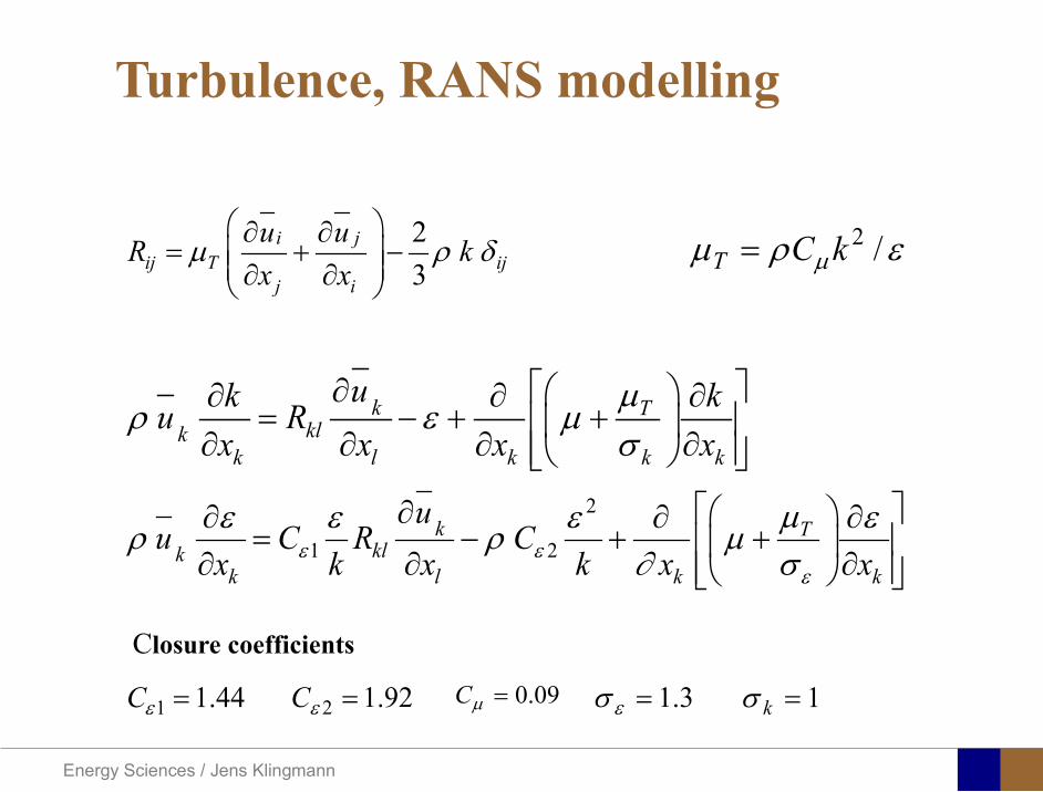
Energy Sciences Jens Klingmann
Turbulence RANS modelling
23
i jij T ij
j i
u uR kx x
micro ρ δ part part
= + minus part part ερmicro micro 2kCT =
k Tklk
k l k k k
uk ku Rx x x x
microρ ε micro
σ part part part part
= minus + + part part part part 2
1 2k T
klkk l k k
uu C R C
x k x k x xε εε
microε ε ε ερ ρ micropart σ
part part part part= minus + + part part part
4411 =εC 9212 =εC 090=microC 1=kσ31=εσ
Closure coefficients
Energy Sciences Jens Klingmann
Energy Sciences Jens Klingmann
Computational Fluid Dynamics (CFD)
U Waringhleacuten ldquoThe Aerodynamic design and testing of a supersonic turbine for rocket engine propulsionrdquo Proc Of 3rd European conference on Turbomachinery Fluid dynamics and thermodynamics
Energy Sciences Jens Klingmann
Subsonic flow in an aerofoilplate junction computed with a second-moment closure (D Apsley 1998)
Computational Fluid Dynamics(CFD)
Energy Sciences Jens Klingmann
Hydraulic turbine research CFD digital simulation Distribution of speed on an axial turbine
Computational Fluid Dynamics(CFD)
Energy Sciences Jens Klingmann
Scales of turbulence
10-01
1000
1001
1002
1003
1004
1005
κ LI
10-08
10-07
10-06
10-05
10-04
10-03
10-02
10-01
1000
E(u
2 LI)
10-04
10-03
10-02
10-01
1000
κ LK
10-05
10-04
10-03
10-02
10-01
1000
1001
1002
D( ε L
K )10-01
1000
1001
1002
1003
1004
1005
E = 15 (κ LI)-53
10-04
10-03
10-02
10-01
1000
1001
D = 3 ( κ LΚ) 13
Normalized energy and dissipation spectra for
Adapted from Tennekeys and Lumley
ReLI= times2 105
1 2Re 500IL asymp
3 4Re 10000IL asymp
Energy Sciences Jens Klingmann
References Turbulence
bull Tennekeys and Lumley ldquoA first course in Turbulencerdquo MIT Press 1972
bull J O Hinze ldquoTurbulencerdquo McGraw-Hill 1959bull D C Wilcox ldquoTurbulence Modeling for CFDrdquo DCW Industries
2006
Energy Sciences Jens Klingmann
Boundary layers
Energy Sciences Jens Klingmann
Boundary Layer Theory (BLT) Sensitive to Pressure
gradients Appropriate scaling from
dimensional analyses
Energy Sciences Jens Klingmann
Boundary layers
Energy Sciences Jens Klingmann
Air foil theory
Energy Sciences Jens Klingmann
Visualisation of diffusor separation
Energy Sciences Jens Klingmann
BL equations
+minus=+
yu
yxp
xuv
xuu
partpartmicro
partpart
partpart
partρpart
partρpart and 0=+
yxu
partυpart
partpart
Applying the BL approximations the 2D stationary incompressible NS-eq and continuity equation become
yvu
yu
yxuu
xp
yu
xuu
partpartρ
partpartmicro
partpart
partρpart
partpart
partυρpart
partρpart
minus
+minusminus=+
and
0=+yx
upart
υpartpartpart
Reynolds averaged BL eqs are
Energy Sciences Jens Klingmann
Boundary layers
Energy Sciences Jens Klingmann
Turbulent BL at different Pressure gradients
Energy Sciences Jens Klingmann
Boundary Layers
ν
yuy =+
ρτWu =
0=
partpart
=y
w yuτ
uuu =+
Energy Sciences Jens Klingmann
Diffuser efficiency
Energy Sciences Jens Klingmann
Reynolds Number (Order of magnitude)
At eg a compressor inlet
ρ = O(1) kgm3
U = O(100) msx lt O(01) mmicro = O(10-5)
Re = ρ U x micro =O(106)
In subsequent stages large amounts of turbulence (from stator wakes) will be convected into the Boundary layer
Energy Sciences Jens Klingmann
References Boundary layers
bull Frank M White ldquoViscous Fluid Flowrdquobull Hermann Schlichting ldquoBoundary Layer Theoryrdquo
Energy Sciences Jens Klingmann
CFD and experiments
bull No this is not a CFD course butbull Experiments
Energy Sciences Jens Klingmann
What do we need to measureOverall performance
Flow rates (mass or volume) Pressure Temperature Shaft power
Performance increase
Separations (velocity) Secondary flows eg tip clearance losses (velocity) Shock waves (supersonic applications) Pressure (resolved in time and space) Temperature (resolved in time and space)
Energy Sciences Jens Klingmann
Cascade wind tunnels
FIG 31 Compressor cascade wind tunnels (a) Conventional low-speed continuousrunning cascade tunnel (adapted from Carter et al 1950)(b) Transonicsupersoniccascade tunnel (adapted from Sieverding 1985)
Energy Sciences Jens Klingmann
Closed circuit tunnels
Energy Sciences Jens Klingmann
components
Settling Chamber
The settling chamber is located between the fan or wide angle diffuser and the contraction and contains the honeycombs and screens used to moderate longitudinal variations in the flow Screens in the chamber should be spaced at 02 chamber diameters apart so that flow disturbed by the first screen can settle before it encounters the second
Honeycombs
Honeycombs are located in the settling chamber and are used to reduce nonuniformities in the flow For optimum benefit honeycombs should be 6-8 cell diameters thick and cell size should be on the order of about 150 cells per settling chamber diameter
Energy Sciences Jens Klingmann
components
Screens
Screens are typically located just downstream of the honeycomb and sometime at the inlet of the test section Screens create a static pressure drop and serve to reduce boundary layer size and increase flow uniformity
Contraction Section
Contractions sections are located between the settling chamber and the test sections and serve to both increase mean velocities at the test section inlet and moderate inconsistencies in the uniformity of the flow Large contraction ratios and short contraction lengths are generally more desirable as they reduce the power loss across the screens and the thickness of boundary layers Small tunnels typically have contraction ratios between 6 and 9
Energy Sciences Jens Klingmann
Flow meters with pressure measurement
Venturi-tube
A1 A2
P1 P2
1 1 2 2C A C A=In the incompressible case
2 21 1 2 2
2 2C P C P
ρ ρ+ = +Assuming horisontal mounting
Energy Sciences Jens Klingmann
Daniel Bernoulli 1700-1782
Daniel Bernoulli was the son of Johann Bernoulli He was born in Groningen while his father held the chair of mathematics there His older brother was Nicolaus(II) Bernoulli and his uncle was Jacob Bernoulli so he was born into a family of leading mathematicians but also into a family where there was unfortunate rivalry jealousy and bitterness
Undoubtedly the most important work which Daniel Bernoulli did was his work on hydrodynamics Even the term itself is based on the title of the work which he produced called Hydrodynamica and before he left St Petersburg Daniel left a draft copy of the book with a printer However the work was not published until 1738 and although he revised it considerably between 1734 and 1738 it is more the presentation that he changed rather then the substance
This work contains for the first time the correct analysis of water flowing from a hole in a container This was based on the principle of conservation of energy which he had studied with his father in 1720 Daniel also discussed pumps and other machines to raise water One remarkable discovery appears in Chapter 10 of Hydrodynamica where Daniel discussed the basis for the kinetic theory of gases He was able to give the basic laws for the theory of gases and gave although not in full detail the equation of state discovered by Van der Waals a century later
Energy Sciences Jens Klingmann
Venturi-tube (2)
22 2 12 2
2
2A PC CA ρ
∆minus =
A1 A2
P1 P2
Solve for eg C2
1 2P P P∆ = minus
( )
12
2 2 21 2
21
PCA Aρ
∆ = minus
and( )
12
2 2 2 2 21 2
21
Pm A C AA Aρρ
∆ = = minus
where
Flow meters with pressure measurement
Energy Sciences Jens Klingmann
Flow meters with pressure measurement
Orifice meters
A1
A2
P1 P2
Applicable for pipe flows Same principle as for Venturi Positioning of pressure taps important Vena contracta and losses require inclusion
of Discharge Coefficient CD
( )
12
2 2 21 2
21D
Pm C AA Aρ ∆ =
minus where ( )1 2ReDC f A A=
CD available from manufacturer (measurements) or Standards (eg ISO)
Energy Sciences Jens Klingmann
Coriolis flow meter
An actuator (not shown) induces a vibration of the tubes
When there is mass flow Coriolis forces induce twisting of the tubes
degree of phase-shift is a measure for the amount of mass that is flowing through the tubes
Energy Sciences Jens Klingmann
Thermal flow meter Heat is added electrically to the flow Temperature is measured before and after heat addition
pP mC T∆=
Energy Sciences Jens Klingmann
Ultrasonic flow meters
Ultrasound is emitted to small particles in the flow (dust or other) Reflections of the sound is frequency shifted by the Doppler effect The frequency change is proportional to the particles velocity (volume flow
meter)
Energy Sciences Jens Klingmann
Inductive flow metersA magnetic flowmeter is based upon Faradays Law
The voltage induced across any conductor as it moves at right angles through a magnetic field is proportional to the velocity of that conductor
E is proportional to V x B x D where
E = The voltage generated in a conductorV = The velocity of the conductorB = The magnetic field strengthD = The length of the conductor
NB electric conductivity is required
Energy Sciences Jens Klingmann
Temperature measurements
Thermocouples
The basis established by Thomas Johann Seebeck in 1821
A conductor generates a voltage when subjected to a temperature gradient
To measure this voltage one must use a second conductor material which generates a different voltage under the same temperature gradient
Energy Sciences Jens Klingmann
Pressure sensing
1 2p pgt 2p p2 may be the atmosphere a static pressure tap or a known reference pressure
The strain of the diaphragm (or itrsquos deflection) may be measured by a number of electric methods
Diaphragm
Energy Sciences Jens Klingmann
Pressure sensingPiezoresistive Strain Gage
Uses the piezoresistive effect of bonded or formed strain gauges to detect strain due to applied pressure
Capacitive
Uses a diaghragm and pressure cavity to create a variable capacitor to detect strain due to applied pressure
Magnetic
Measures the displacement of a diaphragm by means of changes in inductance (reluctance) LVDT Hall Effect or by eddy current principal
Piezoelectric
Uses the piezoelectric effect in certain materials such as quartz to measure the strain upon the sensing mechanism due to pressure
Potentiometric
Uses the motion of a wiper along a resistive mechanism to detect the strain caused by applied pressure
Energy Sciences Jens Klingmann
3D highly instationary (periodic) flow Potentially very high velocities (Supersonic) Large temperature differences Low accessibility (difficult to probe between rotors) Low turbulence levels in most of the domain Very high turbulence in BL and wakes
Properties of measuring object
Point measurements
Energy Sciences Jens Klingmann
Conventional or non-opticalndash Static Pressure Measurementsndash Total Pressure Measurements
bull Multy hole probes
ndash Total Temperature ndash Hot Wire Anemometry (HWA)
Optical techniques for Velocity Measurementsndash Laser Two Focous (L2F)ndash Laser Doppler Anemometry (LDA)ndash Particle Image velocimetry (PIV)
Point Measurements
Energy Sciences Jens Klingmann
Static and total pressure
2 2 21 2 1
2 1 2 2 2C C CP P ρ ρ ρ
minus = minus =
2 0C =Stagnation point
C1Static pressure tap
Prandtl or Pitot tube
Apply the Bernoulli equation from free stream to stagnation point
21
2 12CP Pρ
= +or
We can also define a stagnation or total pressure
( )2
101 1 022
CP P Pρ= + =
Total pressure = Static pressure + dynamic pressure
or
Energy Sciences Jens Klingmann
Static pressure
Energy Sciences Jens Klingmann
Total Pressure and Temperature
Shrouded Probes
Shrouded Probe
Pitot or Prandtl tube
Sensitive to direction
Energy Sciences Jens Klingmann
Ludwig Prandtl 1875-1953
Ludwig Prandtl born at Freising Bavaria on February 4 1875 was a German Physicist famous for his work in aeronautics He qualified at Munchen in 1900 with a thesis on elastic stability and held the position of Professor of Applied Mechanics at Gottingen for forty-nine years (from 1904 until his death there on August 15 1953) In 1925 Prandtl became the Director of the Kaiser Wilhelm Institute for Fluid Mechanics His discovery in 1904 of the Boundary Layer which adjoins the surface of a body moving in a fluid led to an understanding of skin friction drag and of the way in which streamlining reduces the drag of airplane wings and other moving bodies His work on wing theory published in 1918 - 1919 followed that of FW Lanchester (1902-1907) but was carried out independently and elucidated the flow over airplane wings of finite span Prandtls work and decisive advances in boundary layer and wing theories became the basic material of aeronautics He also made important contributions to the theories of supersonic flow and of turbulence and contributed much to the development of wind tunnels and other aerodynamic equipment In addition he devised the soap-film analogy for the torsion of non-circular sections and wrote on the theory of plasticity and of meteorology
Energy Sciences Jens Klingmann
Total Pressure multy hole
Cobra Probe Yaw Probe
5 Hole Probe
Energy Sciences Jens Klingmann
5 Hole Probes Calibration
Energy Sciences Jens Klingmann
The inherent unsteadiness of the flow within turbomachines
Energy Sciences Jens Klingmann
Hot Wire Anemometry (HWA) The heat transfer from a thin (one micron)
electrically heated wire can be used to determine velocity
The resistance of the wire is temperature dependent Within a small temperature range it can be assumed linear R = R0+α R0(Tm-T0) where R0 is the resistance at a reference temperature T0 and Tm is the mean wire temperature
The thermal power induced in the wire is balanced by heat transfer to the surrounding fluid I2R=hπDL(Tm-T0) where h is the heat transfer coefficient and D and L the diameter and length of the wire respectively
E = I R
Energy Sciences Jens Klingmann
Constant Temperature Anemometry (CTA) The wire is often placed in a Whetstone bridge If the output from the
bridge is amplified and fed back to the bridge the resistance of the probe and thus the temperature will be held constant
This prevents the temperature of the wire to become excessive at low velocities
R1
R2 R3
Probe
Bridge Voltage
Energy Sciences Jens Klingmann
Constant Temperature Anemometry (CTA)
Energy Sciences Jens Klingmann
Characteristics of LDA (according to Dantec)
Invented by Yeh and Cummins in 1964 Velocity measurements in Fluid Dynamics (gas liquid) Up to 3 velocity components Non-intrusive measurements (optical technique) Absolute measurement technique (no calibration required) Very high accuracy Very high spatial resolution due to small measurement volume Tracer particles are required
Energy Sciences Jens Klingmann
LDA - Fringe Model
Focused Laser beams intersect and form the measurement volume Plane wave fronts beam waist in the plane of intersection Interference in the plane of intersection Pattern of bright and dark stripesplanes Fringes
Energy Sciences Jens Klingmann
LDA-measuring volume
d
x
x
y
y
z
z
e-2 CONTOUR
FRINGES
κ
κ
κ
κ
De-2
De-2
dml m
a
b
cx
b
z
ya
cd
d
=
=
=
J
J
J
J
JP
JP
JP
JD
JD
JD
+
+
+
a
b
c
d
κπλ
=minus sinD
f4l2e
m
κπλ
=minus cosD
f4D2e
m
Energy Sciences Jens Klingmann
Laser Two Focus
Energy Sciences Jens Klingmann
Laser Two Focus
Energy Sciences Jens Klingmann
PIV measurements
PIV is a fairly new technique capable of simultaneous velocity measurements at many points in a plane This gives information on large scale structures vorticity etc which is very difficult or impossible to obtain from one-point measuring techniques
PIV involves the illumination of a plane of the flow under investigation with a thin pulsed sheet of light The flow is seeded with particles
The light scattered from the particles and from successive pulses are being recorded either on film or a CCD array forming a multiple exposure of each particle image If the time between the pulses is known velocity can be determined as the ratio of the particle displacement and the elapsed time
t∆∆= xu
Energy Sciences Jens Klingmann
PIV
Energy Sciences Jens Klingmann
PIV measurements illumination
YA
G
YA
G
Two frequency doubled YAG Lasers aligned to one double pulsed laser sheet
Two or more separate light pulses can be obtained by chopping a continuous laser or from pulsed lasers
The limited pulse energies obtained from continuous lasers limits their applicability to low velocity flows or flows where large seeding particles can be used (ie liquid flows)
The low repetition rate of most pulsed lasers makes the use of two lasers advantageous
Energy Sciences Jens Klingmann
PIV measurements recording
High seeding density in laminar flame
Film or CCD-cameras Cross- or Auto-correlation
ndash ie both particle images on the same frame or on separate frames
CCD-camera requirementndash A many pixels as possiblendash 2k by 2k available 4k by 4k coming
Energy Sciences Jens Klingmann
PIV measurements analyses
Low seeding density (Number of seeding particles per unit volume)
Each particle image pair can be identified This is called particle tracking
High seeding density (PIV)
Small sub-regions of the image containing many particle image pairs are processed to obtain one velocity vector
Energy Sciences Jens Klingmann
PIV measurements analyses
Energy Sciences Jens Klingmann
PIV measurements analyses
( ) ( ) ( ) xsxxs dIIR 2A
1
I
+= int
Cross correlation between ( )x1I and ( )x2I
s is a two dimensional displacement vector
IA is the interrogation area
Cross correlation between
(
)
x
1
I
and
(
)
x
2
I
s is a two dimensional displacement vector
I
A
is the interrogation area
Energy Sciences Jens Klingmann
Energy Sciences Jens Klingmann
PIV from IOWA state university
Energy Sciences Jens Klingmann
PIV sample of evaluation
Energy Sciences Jens Klingmann
LDA PIV HWA Velocity range 01 mms ndash 300
ms 02 ndash 150 ms
Measuring Volume
D = 005 L = 05 mm
2 by 2 by 05 mm
L = 05 mm
Freq response O(10 000) Hz O(10) Hz O(100 000) Hz Calibration Yes No No Sensitivity to other than velocity
Low (ref Index) Low (ref Index) Large (temperature concentrationshellip)
Continuous Signal
Sometimes Seldom Always
Noise High High Low Turbulence intensity
No limitation Some limitation lt 20
Price O(1 000 000) SEK
O(1 000 000) SEK
O(50 000) SEK
Required Knowledge
High medium Low
Comparison of techniques
Energy Sciences Jens Klingmann
References experiments
R J Goldstein ldquoFluid Mechanics Measurementsrdquo Hemisphere Publishing 1983 A V Johansson amp P H Alfredsson ldquoExperimentella metoder inom
stroumlmningsmekanikenrdquo Inst Foumlr Mekanik KTH F Durst A Melling and J H Whitelaw ldquoPrincipals and Practice of Laser Doppler
Anemometryrdquo 1984 R J Adrian ldquoParticle-imaging techniques for experimental fluid mechnicsrdquo Ann Rev
Fluid Mech 1991
Energy Sciences Jens Klingmann
Sample of LDA-measurements
Rotor blade
Glas window
Emitted beams
Scattered Light
Adjustable mirror
Energy Sciences Jens Klingmann
Axial velocity sorted into 10 bins
0 1 2 3 4 5 6tangential coordinate (degrees)
-20
0
20
40
60
80
100
120
140
160Ax
ial v
eloc
ity a
nd s
tand
ard
devi
atio
n (m
s)
radial position 7 mm from inner window surfaceaxial position 23 mm behind rotor blades
Energy Sciences Jens Klingmann
Axial velocities in the radial-tangential plane
Energy Sciences Jens Klingmann
Airfoils NACA 4-digit
The NACA four-digit wing sections define the profile by
One digit describing maximum camber as percentage of the chord
One digit describing the distance of maximum camber from the airfoil leading edge in tens of percents of the chord
Two digits describing maximum thickness of the airfoil as percent of the chord
Example the NACA 2412 airfoil has a maximum camber of 2 located 40 (04 chords) from the leading edge with a maximum thickness of 12 of the chord
Four-digit series airfoils by default have maximum thickness at 30 of the chord (03 chords) from the leading edge
Energy Sciences Jens Klingmann
Airfoils NACA 4-digit
bull c is the chord lengthbull x is the position along
the chord from 0 to cbull y is the half thickness at
a given value of x (centerline to surface)
bull t is the maximum thickness as a fraction of the chord
Energy Sciences Jens Klingmann
Death by PowerPoint
| LDA | PIV | HWA | |||||
| Velocity range | 01 mms ndash 300 ms | 02 ndash 150 ms | |||||
| Measuring Volume | D = 005 L = 05 mm | 2 by 2 by 05 mm | L = 05 mm | ||||
| Freq response | O(10 000) Hz | O(10) Hz | O(100 000) Hz | ||||
| Calibration | Yes | No | No | ||||
| Sensitivity to other than velocity | Low (ref Index) | Low (ref Index) | Large (temperature concentrationshellip) | ||||
| Continuous Signal | Sometimes | Seldom | Always | ||||
| Noise | High | High | Low | ||||
| Turbulence intensity | No limitation | Some limitation | lt 20 | ||||
| Price | O(1 000 000) SEK | O(1 000 000) SEK | O(50 000) SEK | ||||
| Required Knowledge | High | medium | Low |
Energy Sciences Jens Klingmann
Energy Sciences Jens Klingmann
Computational Fluid Dynamics (CFD)
U Waringhleacuten ldquoThe Aerodynamic design and testing of a supersonic turbine for rocket engine propulsionrdquo Proc Of 3rd European conference on Turbomachinery Fluid dynamics and thermodynamics
Energy Sciences Jens Klingmann
Subsonic flow in an aerofoilplate junction computed with a second-moment closure (D Apsley 1998)
Computational Fluid Dynamics(CFD)
Energy Sciences Jens Klingmann
Hydraulic turbine research CFD digital simulation Distribution of speed on an axial turbine
Computational Fluid Dynamics(CFD)
Energy Sciences Jens Klingmann
Scales of turbulence
10-01
1000
1001
1002
1003
1004
1005
κ LI
10-08
10-07
10-06
10-05
10-04
10-03
10-02
10-01
1000
E(u
2 LI)
10-04
10-03
10-02
10-01
1000
κ LK
10-05
10-04
10-03
10-02
10-01
1000
1001
1002
D( ε L
K )10-01
1000
1001
1002
1003
1004
1005
E = 15 (κ LI)-53
10-04
10-03
10-02
10-01
1000
1001
D = 3 ( κ LΚ) 13
Normalized energy and dissipation spectra for
Adapted from Tennekeys and Lumley
ReLI= times2 105
1 2Re 500IL asymp
3 4Re 10000IL asymp
Energy Sciences Jens Klingmann
References Turbulence
bull Tennekeys and Lumley ldquoA first course in Turbulencerdquo MIT Press 1972
bull J O Hinze ldquoTurbulencerdquo McGraw-Hill 1959bull D C Wilcox ldquoTurbulence Modeling for CFDrdquo DCW Industries
2006
Energy Sciences Jens Klingmann
Boundary layers
Energy Sciences Jens Klingmann
Boundary Layer Theory (BLT) Sensitive to Pressure
gradients Appropriate scaling from
dimensional analyses
Energy Sciences Jens Klingmann
Boundary layers
Energy Sciences Jens Klingmann
Air foil theory
Energy Sciences Jens Klingmann
Visualisation of diffusor separation
Energy Sciences Jens Klingmann
BL equations
+minus=+
yu
yxp
xuv
xuu
partpartmicro
partpart
partpart
partρpart
partρpart and 0=+
yxu
partυpart
partpart
Applying the BL approximations the 2D stationary incompressible NS-eq and continuity equation become
yvu
yu
yxuu
xp
yu
xuu
partpartρ
partpartmicro
partpart
partρpart
partpart
partυρpart
partρpart
minus
+minusminus=+
and
0=+yx
upart
υpartpartpart
Reynolds averaged BL eqs are
Energy Sciences Jens Klingmann
Boundary layers
Energy Sciences Jens Klingmann
Turbulent BL at different Pressure gradients
Energy Sciences Jens Klingmann
Boundary Layers
ν
yuy =+
ρτWu =
0=
partpart
=y
w yuτ
uuu =+
Energy Sciences Jens Klingmann
Diffuser efficiency
Energy Sciences Jens Klingmann
Reynolds Number (Order of magnitude)
At eg a compressor inlet
ρ = O(1) kgm3
U = O(100) msx lt O(01) mmicro = O(10-5)
Re = ρ U x micro =O(106)
In subsequent stages large amounts of turbulence (from stator wakes) will be convected into the Boundary layer
Energy Sciences Jens Klingmann
References Boundary layers
bull Frank M White ldquoViscous Fluid Flowrdquobull Hermann Schlichting ldquoBoundary Layer Theoryrdquo
Energy Sciences Jens Klingmann
CFD and experiments
bull No this is not a CFD course butbull Experiments
Energy Sciences Jens Klingmann
What do we need to measureOverall performance
Flow rates (mass or volume) Pressure Temperature Shaft power
Performance increase
Separations (velocity) Secondary flows eg tip clearance losses (velocity) Shock waves (supersonic applications) Pressure (resolved in time and space) Temperature (resolved in time and space)
Energy Sciences Jens Klingmann
Cascade wind tunnels
FIG 31 Compressor cascade wind tunnels (a) Conventional low-speed continuousrunning cascade tunnel (adapted from Carter et al 1950)(b) Transonicsupersoniccascade tunnel (adapted from Sieverding 1985)
Energy Sciences Jens Klingmann
Closed circuit tunnels
Energy Sciences Jens Klingmann
components
Settling Chamber
The settling chamber is located between the fan or wide angle diffuser and the contraction and contains the honeycombs and screens used to moderate longitudinal variations in the flow Screens in the chamber should be spaced at 02 chamber diameters apart so that flow disturbed by the first screen can settle before it encounters the second
Honeycombs
Honeycombs are located in the settling chamber and are used to reduce nonuniformities in the flow For optimum benefit honeycombs should be 6-8 cell diameters thick and cell size should be on the order of about 150 cells per settling chamber diameter
Energy Sciences Jens Klingmann
components
Screens
Screens are typically located just downstream of the honeycomb and sometime at the inlet of the test section Screens create a static pressure drop and serve to reduce boundary layer size and increase flow uniformity
Contraction Section
Contractions sections are located between the settling chamber and the test sections and serve to both increase mean velocities at the test section inlet and moderate inconsistencies in the uniformity of the flow Large contraction ratios and short contraction lengths are generally more desirable as they reduce the power loss across the screens and the thickness of boundary layers Small tunnels typically have contraction ratios between 6 and 9
Energy Sciences Jens Klingmann
Flow meters with pressure measurement
Venturi-tube
A1 A2
P1 P2
1 1 2 2C A C A=In the incompressible case
2 21 1 2 2
2 2C P C P
ρ ρ+ = +Assuming horisontal mounting
Energy Sciences Jens Klingmann
Daniel Bernoulli 1700-1782
Daniel Bernoulli was the son of Johann Bernoulli He was born in Groningen while his father held the chair of mathematics there His older brother was Nicolaus(II) Bernoulli and his uncle was Jacob Bernoulli so he was born into a family of leading mathematicians but also into a family where there was unfortunate rivalry jealousy and bitterness
Undoubtedly the most important work which Daniel Bernoulli did was his work on hydrodynamics Even the term itself is based on the title of the work which he produced called Hydrodynamica and before he left St Petersburg Daniel left a draft copy of the book with a printer However the work was not published until 1738 and although he revised it considerably between 1734 and 1738 it is more the presentation that he changed rather then the substance
This work contains for the first time the correct analysis of water flowing from a hole in a container This was based on the principle of conservation of energy which he had studied with his father in 1720 Daniel also discussed pumps and other machines to raise water One remarkable discovery appears in Chapter 10 of Hydrodynamica where Daniel discussed the basis for the kinetic theory of gases He was able to give the basic laws for the theory of gases and gave although not in full detail the equation of state discovered by Van der Waals a century later
Energy Sciences Jens Klingmann
Venturi-tube (2)
22 2 12 2
2
2A PC CA ρ
∆minus =
A1 A2
P1 P2
Solve for eg C2
1 2P P P∆ = minus
( )
12
2 2 21 2
21
PCA Aρ
∆ = minus
and( )
12
2 2 2 2 21 2
21
Pm A C AA Aρρ
∆ = = minus
where
Flow meters with pressure measurement
Energy Sciences Jens Klingmann
Flow meters with pressure measurement
Orifice meters
A1
A2
P1 P2
Applicable for pipe flows Same principle as for Venturi Positioning of pressure taps important Vena contracta and losses require inclusion
of Discharge Coefficient CD
( )
12
2 2 21 2
21D
Pm C AA Aρ ∆ =
minus where ( )1 2ReDC f A A=
CD available from manufacturer (measurements) or Standards (eg ISO)
Energy Sciences Jens Klingmann
Coriolis flow meter
An actuator (not shown) induces a vibration of the tubes
When there is mass flow Coriolis forces induce twisting of the tubes
degree of phase-shift is a measure for the amount of mass that is flowing through the tubes
Energy Sciences Jens Klingmann
Thermal flow meter Heat is added electrically to the flow Temperature is measured before and after heat addition
pP mC T∆=
Energy Sciences Jens Klingmann
Ultrasonic flow meters
Ultrasound is emitted to small particles in the flow (dust or other) Reflections of the sound is frequency shifted by the Doppler effect The frequency change is proportional to the particles velocity (volume flow
meter)
Energy Sciences Jens Klingmann
Inductive flow metersA magnetic flowmeter is based upon Faradays Law
The voltage induced across any conductor as it moves at right angles through a magnetic field is proportional to the velocity of that conductor
E is proportional to V x B x D where
E = The voltage generated in a conductorV = The velocity of the conductorB = The magnetic field strengthD = The length of the conductor
NB electric conductivity is required
Energy Sciences Jens Klingmann
Temperature measurements
Thermocouples
The basis established by Thomas Johann Seebeck in 1821
A conductor generates a voltage when subjected to a temperature gradient
To measure this voltage one must use a second conductor material which generates a different voltage under the same temperature gradient
Energy Sciences Jens Klingmann
Pressure sensing
1 2p pgt 2p p2 may be the atmosphere a static pressure tap or a known reference pressure
The strain of the diaphragm (or itrsquos deflection) may be measured by a number of electric methods
Diaphragm
Energy Sciences Jens Klingmann
Pressure sensingPiezoresistive Strain Gage
Uses the piezoresistive effect of bonded or formed strain gauges to detect strain due to applied pressure
Capacitive
Uses a diaghragm and pressure cavity to create a variable capacitor to detect strain due to applied pressure
Magnetic
Measures the displacement of a diaphragm by means of changes in inductance (reluctance) LVDT Hall Effect or by eddy current principal
Piezoelectric
Uses the piezoelectric effect in certain materials such as quartz to measure the strain upon the sensing mechanism due to pressure
Potentiometric
Uses the motion of a wiper along a resistive mechanism to detect the strain caused by applied pressure
Energy Sciences Jens Klingmann
3D highly instationary (periodic) flow Potentially very high velocities (Supersonic) Large temperature differences Low accessibility (difficult to probe between rotors) Low turbulence levels in most of the domain Very high turbulence in BL and wakes
Properties of measuring object
Point measurements
Energy Sciences Jens Klingmann
Conventional or non-opticalndash Static Pressure Measurementsndash Total Pressure Measurements
bull Multy hole probes
ndash Total Temperature ndash Hot Wire Anemometry (HWA)
Optical techniques for Velocity Measurementsndash Laser Two Focous (L2F)ndash Laser Doppler Anemometry (LDA)ndash Particle Image velocimetry (PIV)
Point Measurements
Energy Sciences Jens Klingmann
Static and total pressure
2 2 21 2 1
2 1 2 2 2C C CP P ρ ρ ρ
minus = minus =
2 0C =Stagnation point
C1Static pressure tap
Prandtl or Pitot tube
Apply the Bernoulli equation from free stream to stagnation point
21
2 12CP Pρ
= +or
We can also define a stagnation or total pressure
( )2
101 1 022
CP P Pρ= + =
Total pressure = Static pressure + dynamic pressure
or
Energy Sciences Jens Klingmann
Static pressure
Energy Sciences Jens Klingmann
Total Pressure and Temperature
Shrouded Probes
Shrouded Probe
Pitot or Prandtl tube
Sensitive to direction
Energy Sciences Jens Klingmann
Ludwig Prandtl 1875-1953
Ludwig Prandtl born at Freising Bavaria on February 4 1875 was a German Physicist famous for his work in aeronautics He qualified at Munchen in 1900 with a thesis on elastic stability and held the position of Professor of Applied Mechanics at Gottingen for forty-nine years (from 1904 until his death there on August 15 1953) In 1925 Prandtl became the Director of the Kaiser Wilhelm Institute for Fluid Mechanics His discovery in 1904 of the Boundary Layer which adjoins the surface of a body moving in a fluid led to an understanding of skin friction drag and of the way in which streamlining reduces the drag of airplane wings and other moving bodies His work on wing theory published in 1918 - 1919 followed that of FW Lanchester (1902-1907) but was carried out independently and elucidated the flow over airplane wings of finite span Prandtls work and decisive advances in boundary layer and wing theories became the basic material of aeronautics He also made important contributions to the theories of supersonic flow and of turbulence and contributed much to the development of wind tunnels and other aerodynamic equipment In addition he devised the soap-film analogy for the torsion of non-circular sections and wrote on the theory of plasticity and of meteorology
Energy Sciences Jens Klingmann
Total Pressure multy hole
Cobra Probe Yaw Probe
5 Hole Probe
Energy Sciences Jens Klingmann
5 Hole Probes Calibration
Energy Sciences Jens Klingmann
The inherent unsteadiness of the flow within turbomachines
Energy Sciences Jens Klingmann
Hot Wire Anemometry (HWA) The heat transfer from a thin (one micron)
electrically heated wire can be used to determine velocity
The resistance of the wire is temperature dependent Within a small temperature range it can be assumed linear R = R0+α R0(Tm-T0) where R0 is the resistance at a reference temperature T0 and Tm is the mean wire temperature
The thermal power induced in the wire is balanced by heat transfer to the surrounding fluid I2R=hπDL(Tm-T0) where h is the heat transfer coefficient and D and L the diameter and length of the wire respectively
E = I R
Energy Sciences Jens Klingmann
Constant Temperature Anemometry (CTA) The wire is often placed in a Whetstone bridge If the output from the
bridge is amplified and fed back to the bridge the resistance of the probe and thus the temperature will be held constant
This prevents the temperature of the wire to become excessive at low velocities
R1
R2 R3
Probe
Bridge Voltage
Energy Sciences Jens Klingmann
Constant Temperature Anemometry (CTA)
Energy Sciences Jens Klingmann
Characteristics of LDA (according to Dantec)
Invented by Yeh and Cummins in 1964 Velocity measurements in Fluid Dynamics (gas liquid) Up to 3 velocity components Non-intrusive measurements (optical technique) Absolute measurement technique (no calibration required) Very high accuracy Very high spatial resolution due to small measurement volume Tracer particles are required
Energy Sciences Jens Klingmann
LDA - Fringe Model
Focused Laser beams intersect and form the measurement volume Plane wave fronts beam waist in the plane of intersection Interference in the plane of intersection Pattern of bright and dark stripesplanes Fringes
Energy Sciences Jens Klingmann
LDA-measuring volume
d
x
x
y
y
z
z
e-2 CONTOUR
FRINGES
κ
κ
κ
κ
De-2
De-2
dml m
a
b
cx
b
z
ya
cd
d
=
=
=
J
J
J
J
JP
JP
JP
JD
JD
JD
+
+
+
a
b
c
d
κπλ
=minus sinD
f4l2e
m
κπλ
=minus cosD
f4D2e
m
Energy Sciences Jens Klingmann
Laser Two Focus
Energy Sciences Jens Klingmann
Laser Two Focus
Energy Sciences Jens Klingmann
PIV measurements
PIV is a fairly new technique capable of simultaneous velocity measurements at many points in a plane This gives information on large scale structures vorticity etc which is very difficult or impossible to obtain from one-point measuring techniques
PIV involves the illumination of a plane of the flow under investigation with a thin pulsed sheet of light The flow is seeded with particles
The light scattered from the particles and from successive pulses are being recorded either on film or a CCD array forming a multiple exposure of each particle image If the time between the pulses is known velocity can be determined as the ratio of the particle displacement and the elapsed time
t∆∆= xu
Energy Sciences Jens Klingmann
PIV
Energy Sciences Jens Klingmann
PIV measurements illumination
YA
G
YA
G
Two frequency doubled YAG Lasers aligned to one double pulsed laser sheet
Two or more separate light pulses can be obtained by chopping a continuous laser or from pulsed lasers
The limited pulse energies obtained from continuous lasers limits their applicability to low velocity flows or flows where large seeding particles can be used (ie liquid flows)
The low repetition rate of most pulsed lasers makes the use of two lasers advantageous
Energy Sciences Jens Klingmann
PIV measurements recording
High seeding density in laminar flame
Film or CCD-cameras Cross- or Auto-correlation
ndash ie both particle images on the same frame or on separate frames
CCD-camera requirementndash A many pixels as possiblendash 2k by 2k available 4k by 4k coming
Energy Sciences Jens Klingmann
PIV measurements analyses
Low seeding density (Number of seeding particles per unit volume)
Each particle image pair can be identified This is called particle tracking
High seeding density (PIV)
Small sub-regions of the image containing many particle image pairs are processed to obtain one velocity vector
Energy Sciences Jens Klingmann
PIV measurements analyses
Energy Sciences Jens Klingmann
PIV measurements analyses
( ) ( ) ( ) xsxxs dIIR 2A
1
I
+= int
Cross correlation between ( )x1I and ( )x2I
s is a two dimensional displacement vector
IA is the interrogation area
Cross correlation between
(
)
x
1
I
and
(
)
x
2
I
s is a two dimensional displacement vector
I
A
is the interrogation area
Energy Sciences Jens Klingmann
Energy Sciences Jens Klingmann
PIV from IOWA state university
Energy Sciences Jens Klingmann
PIV sample of evaluation
Energy Sciences Jens Klingmann
LDA PIV HWA Velocity range 01 mms ndash 300
ms 02 ndash 150 ms
Measuring Volume
D = 005 L = 05 mm
2 by 2 by 05 mm
L = 05 mm
Freq response O(10 000) Hz O(10) Hz O(100 000) Hz Calibration Yes No No Sensitivity to other than velocity
Low (ref Index) Low (ref Index) Large (temperature concentrationshellip)
Continuous Signal
Sometimes Seldom Always
Noise High High Low Turbulence intensity
No limitation Some limitation lt 20
Price O(1 000 000) SEK
O(1 000 000) SEK
O(50 000) SEK
Required Knowledge
High medium Low
Comparison of techniques
Energy Sciences Jens Klingmann
References experiments
R J Goldstein ldquoFluid Mechanics Measurementsrdquo Hemisphere Publishing 1983 A V Johansson amp P H Alfredsson ldquoExperimentella metoder inom
stroumlmningsmekanikenrdquo Inst Foumlr Mekanik KTH F Durst A Melling and J H Whitelaw ldquoPrincipals and Practice of Laser Doppler
Anemometryrdquo 1984 R J Adrian ldquoParticle-imaging techniques for experimental fluid mechnicsrdquo Ann Rev
Fluid Mech 1991
Energy Sciences Jens Klingmann
Sample of LDA-measurements
Rotor blade
Glas window
Emitted beams
Scattered Light
Adjustable mirror
Energy Sciences Jens Klingmann
Axial velocity sorted into 10 bins
0 1 2 3 4 5 6tangential coordinate (degrees)
-20
0
20
40
60
80
100
120
140
160Ax
ial v
eloc
ity a
nd s
tand
ard
devi
atio
n (m
s)
radial position 7 mm from inner window surfaceaxial position 23 mm behind rotor blades
Energy Sciences Jens Klingmann
Axial velocities in the radial-tangential plane
Energy Sciences Jens Klingmann
Airfoils NACA 4-digit
The NACA four-digit wing sections define the profile by
One digit describing maximum camber as percentage of the chord
One digit describing the distance of maximum camber from the airfoil leading edge in tens of percents of the chord
Two digits describing maximum thickness of the airfoil as percent of the chord
Example the NACA 2412 airfoil has a maximum camber of 2 located 40 (04 chords) from the leading edge with a maximum thickness of 12 of the chord
Four-digit series airfoils by default have maximum thickness at 30 of the chord (03 chords) from the leading edge
Energy Sciences Jens Klingmann
Airfoils NACA 4-digit
bull c is the chord lengthbull x is the position along
the chord from 0 to cbull y is the half thickness at
a given value of x (centerline to surface)
bull t is the maximum thickness as a fraction of the chord
Energy Sciences Jens Klingmann
Death by PowerPoint
| LDA | PIV | HWA | |||||
| Velocity range | 01 mms ndash 300 ms | 02 ndash 150 ms | |||||
| Measuring Volume | D = 005 L = 05 mm | 2 by 2 by 05 mm | L = 05 mm | ||||
| Freq response | O(10 000) Hz | O(10) Hz | O(100 000) Hz | ||||
| Calibration | Yes | No | No | ||||
| Sensitivity to other than velocity | Low (ref Index) | Low (ref Index) | Large (temperature concentrationshellip) | ||||
| Continuous Signal | Sometimes | Seldom | Always | ||||
| Noise | High | High | Low | ||||
| Turbulence intensity | No limitation | Some limitation | lt 20 | ||||
| Price | O(1 000 000) SEK | O(1 000 000) SEK | O(50 000) SEK | ||||
| Required Knowledge | High | medium | Low |
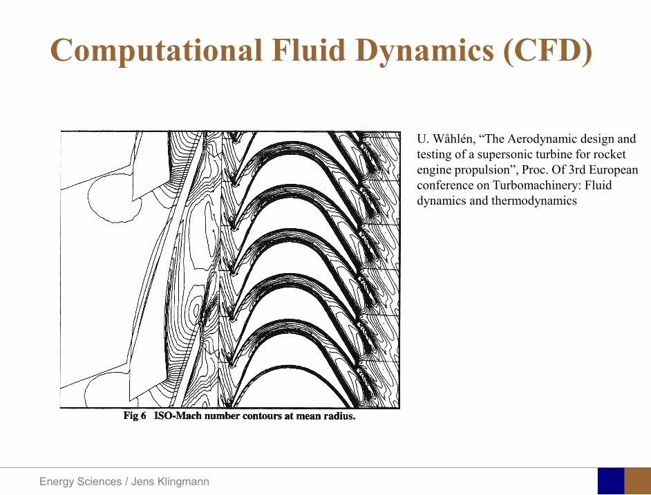
Energy Sciences Jens Klingmann
Computational Fluid Dynamics (CFD)
U Waringhleacuten ldquoThe Aerodynamic design and testing of a supersonic turbine for rocket engine propulsionrdquo Proc Of 3rd European conference on Turbomachinery Fluid dynamics and thermodynamics
Energy Sciences Jens Klingmann
Subsonic flow in an aerofoilplate junction computed with a second-moment closure (D Apsley 1998)
Computational Fluid Dynamics(CFD)
Energy Sciences Jens Klingmann
Hydraulic turbine research CFD digital simulation Distribution of speed on an axial turbine
Computational Fluid Dynamics(CFD)
Energy Sciences Jens Klingmann
Scales of turbulence
10-01
1000
1001
1002
1003
1004
1005
κ LI
10-08
10-07
10-06
10-05
10-04
10-03
10-02
10-01
1000
E(u
2 LI)
10-04
10-03
10-02
10-01
1000
κ LK
10-05
10-04
10-03
10-02
10-01
1000
1001
1002
D( ε L
K )10-01
1000
1001
1002
1003
1004
1005
E = 15 (κ LI)-53
10-04
10-03
10-02
10-01
1000
1001
D = 3 ( κ LΚ) 13
Normalized energy and dissipation spectra for
Adapted from Tennekeys and Lumley
ReLI= times2 105
1 2Re 500IL asymp
3 4Re 10000IL asymp
Energy Sciences Jens Klingmann
References Turbulence
bull Tennekeys and Lumley ldquoA first course in Turbulencerdquo MIT Press 1972
bull J O Hinze ldquoTurbulencerdquo McGraw-Hill 1959bull D C Wilcox ldquoTurbulence Modeling for CFDrdquo DCW Industries
2006
Energy Sciences Jens Klingmann
Boundary layers
Energy Sciences Jens Klingmann
Boundary Layer Theory (BLT) Sensitive to Pressure
gradients Appropriate scaling from
dimensional analyses
Energy Sciences Jens Klingmann
Boundary layers
Energy Sciences Jens Klingmann
Air foil theory
Energy Sciences Jens Klingmann
Visualisation of diffusor separation
Energy Sciences Jens Klingmann
BL equations
+minus=+
yu
yxp
xuv
xuu
partpartmicro
partpart
partpart
partρpart
partρpart and 0=+
yxu
partυpart
partpart
Applying the BL approximations the 2D stationary incompressible NS-eq and continuity equation become
yvu
yu
yxuu
xp
yu
xuu
partpartρ
partpartmicro
partpart
partρpart
partpart
partυρpart
partρpart
minus
+minusminus=+
and
0=+yx
upart
υpartpartpart
Reynolds averaged BL eqs are
Energy Sciences Jens Klingmann
Boundary layers
Energy Sciences Jens Klingmann
Turbulent BL at different Pressure gradients
Energy Sciences Jens Klingmann
Boundary Layers
ν
yuy =+
ρτWu =
0=
partpart
=y
w yuτ
uuu =+
Energy Sciences Jens Klingmann
Diffuser efficiency
Energy Sciences Jens Klingmann
Reynolds Number (Order of magnitude)
At eg a compressor inlet
ρ = O(1) kgm3
U = O(100) msx lt O(01) mmicro = O(10-5)
Re = ρ U x micro =O(106)
In subsequent stages large amounts of turbulence (from stator wakes) will be convected into the Boundary layer
Energy Sciences Jens Klingmann
References Boundary layers
bull Frank M White ldquoViscous Fluid Flowrdquobull Hermann Schlichting ldquoBoundary Layer Theoryrdquo
Energy Sciences Jens Klingmann
CFD and experiments
bull No this is not a CFD course butbull Experiments
Energy Sciences Jens Klingmann
What do we need to measureOverall performance
Flow rates (mass or volume) Pressure Temperature Shaft power
Performance increase
Separations (velocity) Secondary flows eg tip clearance losses (velocity) Shock waves (supersonic applications) Pressure (resolved in time and space) Temperature (resolved in time and space)
Energy Sciences Jens Klingmann
Cascade wind tunnels
FIG 31 Compressor cascade wind tunnels (a) Conventional low-speed continuousrunning cascade tunnel (adapted from Carter et al 1950)(b) Transonicsupersoniccascade tunnel (adapted from Sieverding 1985)
Energy Sciences Jens Klingmann
Closed circuit tunnels
Energy Sciences Jens Klingmann
components
Settling Chamber
The settling chamber is located between the fan or wide angle diffuser and the contraction and contains the honeycombs and screens used to moderate longitudinal variations in the flow Screens in the chamber should be spaced at 02 chamber diameters apart so that flow disturbed by the first screen can settle before it encounters the second
Honeycombs
Honeycombs are located in the settling chamber and are used to reduce nonuniformities in the flow For optimum benefit honeycombs should be 6-8 cell diameters thick and cell size should be on the order of about 150 cells per settling chamber diameter
Energy Sciences Jens Klingmann
components
Screens
Screens are typically located just downstream of the honeycomb and sometime at the inlet of the test section Screens create a static pressure drop and serve to reduce boundary layer size and increase flow uniformity
Contraction Section
Contractions sections are located between the settling chamber and the test sections and serve to both increase mean velocities at the test section inlet and moderate inconsistencies in the uniformity of the flow Large contraction ratios and short contraction lengths are generally more desirable as they reduce the power loss across the screens and the thickness of boundary layers Small tunnels typically have contraction ratios between 6 and 9
Energy Sciences Jens Klingmann
Flow meters with pressure measurement
Venturi-tube
A1 A2
P1 P2
1 1 2 2C A C A=In the incompressible case
2 21 1 2 2
2 2C P C P
ρ ρ+ = +Assuming horisontal mounting
Energy Sciences Jens Klingmann
Daniel Bernoulli 1700-1782
Daniel Bernoulli was the son of Johann Bernoulli He was born in Groningen while his father held the chair of mathematics there His older brother was Nicolaus(II) Bernoulli and his uncle was Jacob Bernoulli so he was born into a family of leading mathematicians but also into a family where there was unfortunate rivalry jealousy and bitterness
Undoubtedly the most important work which Daniel Bernoulli did was his work on hydrodynamics Even the term itself is based on the title of the work which he produced called Hydrodynamica and before he left St Petersburg Daniel left a draft copy of the book with a printer However the work was not published until 1738 and although he revised it considerably between 1734 and 1738 it is more the presentation that he changed rather then the substance
This work contains for the first time the correct analysis of water flowing from a hole in a container This was based on the principle of conservation of energy which he had studied with his father in 1720 Daniel also discussed pumps and other machines to raise water One remarkable discovery appears in Chapter 10 of Hydrodynamica where Daniel discussed the basis for the kinetic theory of gases He was able to give the basic laws for the theory of gases and gave although not in full detail the equation of state discovered by Van der Waals a century later
Energy Sciences Jens Klingmann
Venturi-tube (2)
22 2 12 2
2
2A PC CA ρ
∆minus =
A1 A2
P1 P2
Solve for eg C2
1 2P P P∆ = minus
( )
12
2 2 21 2
21
PCA Aρ
∆ = minus
and( )
12
2 2 2 2 21 2
21
Pm A C AA Aρρ
∆ = = minus
where
Flow meters with pressure measurement
Energy Sciences Jens Klingmann
Flow meters with pressure measurement
Orifice meters
A1
A2
P1 P2
Applicable for pipe flows Same principle as for Venturi Positioning of pressure taps important Vena contracta and losses require inclusion
of Discharge Coefficient CD
( )
12
2 2 21 2
21D
Pm C AA Aρ ∆ =
minus where ( )1 2ReDC f A A=
CD available from manufacturer (measurements) or Standards (eg ISO)
Energy Sciences Jens Klingmann
Coriolis flow meter
An actuator (not shown) induces a vibration of the tubes
When there is mass flow Coriolis forces induce twisting of the tubes
degree of phase-shift is a measure for the amount of mass that is flowing through the tubes
Energy Sciences Jens Klingmann
Thermal flow meter Heat is added electrically to the flow Temperature is measured before and after heat addition
pP mC T∆=
Energy Sciences Jens Klingmann
Ultrasonic flow meters
Ultrasound is emitted to small particles in the flow (dust or other) Reflections of the sound is frequency shifted by the Doppler effect The frequency change is proportional to the particles velocity (volume flow
meter)
Energy Sciences Jens Klingmann
Inductive flow metersA magnetic flowmeter is based upon Faradays Law
The voltage induced across any conductor as it moves at right angles through a magnetic field is proportional to the velocity of that conductor
E is proportional to V x B x D where
E = The voltage generated in a conductorV = The velocity of the conductorB = The magnetic field strengthD = The length of the conductor
NB electric conductivity is required
Energy Sciences Jens Klingmann
Temperature measurements
Thermocouples
The basis established by Thomas Johann Seebeck in 1821
A conductor generates a voltage when subjected to a temperature gradient
To measure this voltage one must use a second conductor material which generates a different voltage under the same temperature gradient
Energy Sciences Jens Klingmann
Pressure sensing
1 2p pgt 2p p2 may be the atmosphere a static pressure tap or a known reference pressure
The strain of the diaphragm (or itrsquos deflection) may be measured by a number of electric methods
Diaphragm
Energy Sciences Jens Klingmann
Pressure sensingPiezoresistive Strain Gage
Uses the piezoresistive effect of bonded or formed strain gauges to detect strain due to applied pressure
Capacitive
Uses a diaghragm and pressure cavity to create a variable capacitor to detect strain due to applied pressure
Magnetic
Measures the displacement of a diaphragm by means of changes in inductance (reluctance) LVDT Hall Effect or by eddy current principal
Piezoelectric
Uses the piezoelectric effect in certain materials such as quartz to measure the strain upon the sensing mechanism due to pressure
Potentiometric
Uses the motion of a wiper along a resistive mechanism to detect the strain caused by applied pressure
Energy Sciences Jens Klingmann
3D highly instationary (periodic) flow Potentially very high velocities (Supersonic) Large temperature differences Low accessibility (difficult to probe between rotors) Low turbulence levels in most of the domain Very high turbulence in BL and wakes
Properties of measuring object
Point measurements
Energy Sciences Jens Klingmann
Conventional or non-opticalndash Static Pressure Measurementsndash Total Pressure Measurements
bull Multy hole probes
ndash Total Temperature ndash Hot Wire Anemometry (HWA)
Optical techniques for Velocity Measurementsndash Laser Two Focous (L2F)ndash Laser Doppler Anemometry (LDA)ndash Particle Image velocimetry (PIV)
Point Measurements
Energy Sciences Jens Klingmann
Static and total pressure
2 2 21 2 1
2 1 2 2 2C C CP P ρ ρ ρ
minus = minus =
2 0C =Stagnation point
C1Static pressure tap
Prandtl or Pitot tube
Apply the Bernoulli equation from free stream to stagnation point
21
2 12CP Pρ
= +or
We can also define a stagnation or total pressure
( )2
101 1 022
CP P Pρ= + =
Total pressure = Static pressure + dynamic pressure
or
Energy Sciences Jens Klingmann
Static pressure
Energy Sciences Jens Klingmann
Total Pressure and Temperature
Shrouded Probes
Shrouded Probe
Pitot or Prandtl tube
Sensitive to direction
Energy Sciences Jens Klingmann
Ludwig Prandtl 1875-1953
Ludwig Prandtl born at Freising Bavaria on February 4 1875 was a German Physicist famous for his work in aeronautics He qualified at Munchen in 1900 with a thesis on elastic stability and held the position of Professor of Applied Mechanics at Gottingen for forty-nine years (from 1904 until his death there on August 15 1953) In 1925 Prandtl became the Director of the Kaiser Wilhelm Institute for Fluid Mechanics His discovery in 1904 of the Boundary Layer which adjoins the surface of a body moving in a fluid led to an understanding of skin friction drag and of the way in which streamlining reduces the drag of airplane wings and other moving bodies His work on wing theory published in 1918 - 1919 followed that of FW Lanchester (1902-1907) but was carried out independently and elucidated the flow over airplane wings of finite span Prandtls work and decisive advances in boundary layer and wing theories became the basic material of aeronautics He also made important contributions to the theories of supersonic flow and of turbulence and contributed much to the development of wind tunnels and other aerodynamic equipment In addition he devised the soap-film analogy for the torsion of non-circular sections and wrote on the theory of plasticity and of meteorology
Energy Sciences Jens Klingmann
Total Pressure multy hole
Cobra Probe Yaw Probe
5 Hole Probe
Energy Sciences Jens Klingmann
5 Hole Probes Calibration
Energy Sciences Jens Klingmann
The inherent unsteadiness of the flow within turbomachines
Energy Sciences Jens Klingmann
Hot Wire Anemometry (HWA) The heat transfer from a thin (one micron)
electrically heated wire can be used to determine velocity
The resistance of the wire is temperature dependent Within a small temperature range it can be assumed linear R = R0+α R0(Tm-T0) where R0 is the resistance at a reference temperature T0 and Tm is the mean wire temperature
The thermal power induced in the wire is balanced by heat transfer to the surrounding fluid I2R=hπDL(Tm-T0) where h is the heat transfer coefficient and D and L the diameter and length of the wire respectively
E = I R
Energy Sciences Jens Klingmann
Constant Temperature Anemometry (CTA) The wire is often placed in a Whetstone bridge If the output from the
bridge is amplified and fed back to the bridge the resistance of the probe and thus the temperature will be held constant
This prevents the temperature of the wire to become excessive at low velocities
R1
R2 R3
Probe
Bridge Voltage
Energy Sciences Jens Klingmann
Constant Temperature Anemometry (CTA)
Energy Sciences Jens Klingmann
Characteristics of LDA (according to Dantec)
Invented by Yeh and Cummins in 1964 Velocity measurements in Fluid Dynamics (gas liquid) Up to 3 velocity components Non-intrusive measurements (optical technique) Absolute measurement technique (no calibration required) Very high accuracy Very high spatial resolution due to small measurement volume Tracer particles are required
Energy Sciences Jens Klingmann
LDA - Fringe Model
Focused Laser beams intersect and form the measurement volume Plane wave fronts beam waist in the plane of intersection Interference in the plane of intersection Pattern of bright and dark stripesplanes Fringes
Energy Sciences Jens Klingmann
LDA-measuring volume
d
x
x
y
y
z
z
e-2 CONTOUR
FRINGES
κ
κ
κ
κ
De-2
De-2
dml m
a
b
cx
b
z
ya
cd
d
=
=
=
J
J
J
J
JP
JP
JP
JD
JD
JD
+
+
+
a
b
c
d
κπλ
=minus sinD
f4l2e
m
κπλ
=minus cosD
f4D2e
m
Energy Sciences Jens Klingmann
Laser Two Focus
Energy Sciences Jens Klingmann
Laser Two Focus
Energy Sciences Jens Klingmann
PIV measurements
PIV is a fairly new technique capable of simultaneous velocity measurements at many points in a plane This gives information on large scale structures vorticity etc which is very difficult or impossible to obtain from one-point measuring techniques
PIV involves the illumination of a plane of the flow under investigation with a thin pulsed sheet of light The flow is seeded with particles
The light scattered from the particles and from successive pulses are being recorded either on film or a CCD array forming a multiple exposure of each particle image If the time between the pulses is known velocity can be determined as the ratio of the particle displacement and the elapsed time
t∆∆= xu
Energy Sciences Jens Klingmann
PIV
Energy Sciences Jens Klingmann
PIV measurements illumination
YA
G
YA
G
Two frequency doubled YAG Lasers aligned to one double pulsed laser sheet
Two or more separate light pulses can be obtained by chopping a continuous laser or from pulsed lasers
The limited pulse energies obtained from continuous lasers limits their applicability to low velocity flows or flows where large seeding particles can be used (ie liquid flows)
The low repetition rate of most pulsed lasers makes the use of two lasers advantageous
Energy Sciences Jens Klingmann
PIV measurements recording
High seeding density in laminar flame
Film or CCD-cameras Cross- or Auto-correlation
ndash ie both particle images on the same frame or on separate frames
CCD-camera requirementndash A many pixels as possiblendash 2k by 2k available 4k by 4k coming
Energy Sciences Jens Klingmann
PIV measurements analyses
Low seeding density (Number of seeding particles per unit volume)
Each particle image pair can be identified This is called particle tracking
High seeding density (PIV)
Small sub-regions of the image containing many particle image pairs are processed to obtain one velocity vector
Energy Sciences Jens Klingmann
PIV measurements analyses
Energy Sciences Jens Klingmann
PIV measurements analyses
( ) ( ) ( ) xsxxs dIIR 2A
1
I
+= int
Cross correlation between ( )x1I and ( )x2I
s is a two dimensional displacement vector
IA is the interrogation area
Cross correlation between
(
)
x
1
I
and
(
)
x
2
I
s is a two dimensional displacement vector
I
A
is the interrogation area
Energy Sciences Jens Klingmann
Energy Sciences Jens Klingmann
PIV from IOWA state university
Energy Sciences Jens Klingmann
PIV sample of evaluation
Energy Sciences Jens Klingmann
LDA PIV HWA Velocity range 01 mms ndash 300
ms 02 ndash 150 ms
Measuring Volume
D = 005 L = 05 mm
2 by 2 by 05 mm
L = 05 mm
Freq response O(10 000) Hz O(10) Hz O(100 000) Hz Calibration Yes No No Sensitivity to other than velocity
Low (ref Index) Low (ref Index) Large (temperature concentrationshellip)
Continuous Signal
Sometimes Seldom Always
Noise High High Low Turbulence intensity
No limitation Some limitation lt 20
Price O(1 000 000) SEK
O(1 000 000) SEK
O(50 000) SEK
Required Knowledge
High medium Low
Comparison of techniques
Energy Sciences Jens Klingmann
References experiments
R J Goldstein ldquoFluid Mechanics Measurementsrdquo Hemisphere Publishing 1983 A V Johansson amp P H Alfredsson ldquoExperimentella metoder inom
stroumlmningsmekanikenrdquo Inst Foumlr Mekanik KTH F Durst A Melling and J H Whitelaw ldquoPrincipals and Practice of Laser Doppler
Anemometryrdquo 1984 R J Adrian ldquoParticle-imaging techniques for experimental fluid mechnicsrdquo Ann Rev
Fluid Mech 1991
Energy Sciences Jens Klingmann
Sample of LDA-measurements
Rotor blade
Glas window
Emitted beams
Scattered Light
Adjustable mirror
Energy Sciences Jens Klingmann
Axial velocity sorted into 10 bins
0 1 2 3 4 5 6tangential coordinate (degrees)
-20
0
20
40
60
80
100
120
140
160Ax
ial v
eloc
ity a
nd s
tand
ard
devi
atio
n (m
s)
radial position 7 mm from inner window surfaceaxial position 23 mm behind rotor blades
Energy Sciences Jens Klingmann
Axial velocities in the radial-tangential plane
Energy Sciences Jens Klingmann
Airfoils NACA 4-digit
The NACA four-digit wing sections define the profile by
One digit describing maximum camber as percentage of the chord
One digit describing the distance of maximum camber from the airfoil leading edge in tens of percents of the chord
Two digits describing maximum thickness of the airfoil as percent of the chord
Example the NACA 2412 airfoil has a maximum camber of 2 located 40 (04 chords) from the leading edge with a maximum thickness of 12 of the chord
Four-digit series airfoils by default have maximum thickness at 30 of the chord (03 chords) from the leading edge
Energy Sciences Jens Klingmann
Airfoils NACA 4-digit
bull c is the chord lengthbull x is the position along
the chord from 0 to cbull y is the half thickness at
a given value of x (centerline to surface)
bull t is the maximum thickness as a fraction of the chord
Energy Sciences Jens Klingmann
Death by PowerPoint
| LDA | PIV | HWA | |||||
| Velocity range | 01 mms ndash 300 ms | 02 ndash 150 ms | |||||
| Measuring Volume | D = 005 L = 05 mm | 2 by 2 by 05 mm | L = 05 mm | ||||
| Freq response | O(10 000) Hz | O(10) Hz | O(100 000) Hz | ||||
| Calibration | Yes | No | No | ||||
| Sensitivity to other than velocity | Low (ref Index) | Low (ref Index) | Large (temperature concentrationshellip) | ||||
| Continuous Signal | Sometimes | Seldom | Always | ||||
| Noise | High | High | Low | ||||
| Turbulence intensity | No limitation | Some limitation | lt 20 | ||||
| Price | O(1 000 000) SEK | O(1 000 000) SEK | O(50 000) SEK | ||||
| Required Knowledge | High | medium | Low |
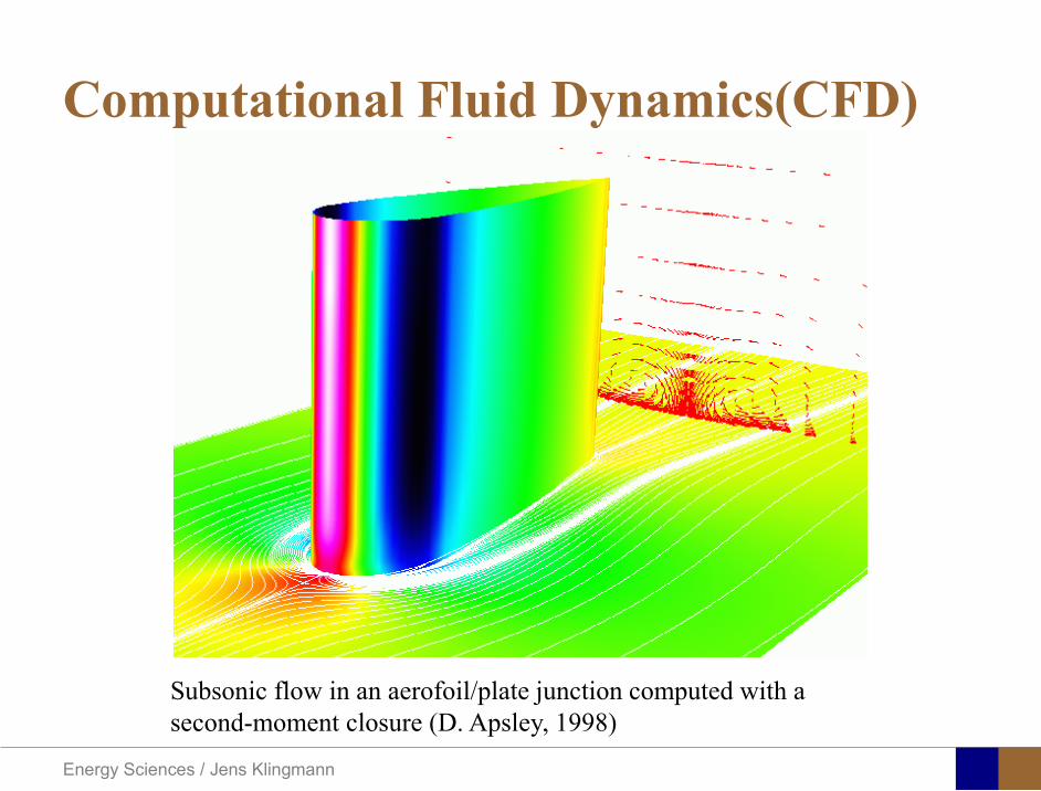
Energy Sciences Jens Klingmann
Subsonic flow in an aerofoilplate junction computed with a second-moment closure (D Apsley 1998)
Computational Fluid Dynamics(CFD)
Energy Sciences Jens Klingmann
Hydraulic turbine research CFD digital simulation Distribution of speed on an axial turbine
Computational Fluid Dynamics(CFD)
Energy Sciences Jens Klingmann
Scales of turbulence
10-01
1000
1001
1002
1003
1004
1005
κ LI
10-08
10-07
10-06
10-05
10-04
10-03
10-02
10-01
1000
E(u
2 LI)
10-04
10-03
10-02
10-01
1000
κ LK
10-05
10-04
10-03
10-02
10-01
1000
1001
1002
D( ε L
K )10-01
1000
1001
1002
1003
1004
1005
E = 15 (κ LI)-53
10-04
10-03
10-02
10-01
1000
1001
D = 3 ( κ LΚ) 13
Normalized energy and dissipation spectra for
Adapted from Tennekeys and Lumley
ReLI= times2 105
1 2Re 500IL asymp
3 4Re 10000IL asymp
Energy Sciences Jens Klingmann
References Turbulence
bull Tennekeys and Lumley ldquoA first course in Turbulencerdquo MIT Press 1972
bull J O Hinze ldquoTurbulencerdquo McGraw-Hill 1959bull D C Wilcox ldquoTurbulence Modeling for CFDrdquo DCW Industries
2006
Energy Sciences Jens Klingmann
Boundary layers
Energy Sciences Jens Klingmann
Boundary Layer Theory (BLT) Sensitive to Pressure
gradients Appropriate scaling from
dimensional analyses
Energy Sciences Jens Klingmann
Boundary layers
Energy Sciences Jens Klingmann
Air foil theory
Energy Sciences Jens Klingmann
Visualisation of diffusor separation
Energy Sciences Jens Klingmann
BL equations
+minus=+
yu
yxp
xuv
xuu
partpartmicro
partpart
partpart
partρpart
partρpart and 0=+
yxu
partυpart
partpart
Applying the BL approximations the 2D stationary incompressible NS-eq and continuity equation become
yvu
yu
yxuu
xp
yu
xuu
partpartρ
partpartmicro
partpart
partρpart
partpart
partυρpart
partρpart
minus
+minusminus=+
and
0=+yx
upart
υpartpartpart
Reynolds averaged BL eqs are
Energy Sciences Jens Klingmann
Boundary layers
Energy Sciences Jens Klingmann
Turbulent BL at different Pressure gradients
Energy Sciences Jens Klingmann
Boundary Layers
ν
yuy =+
ρτWu =
0=
partpart
=y
w yuτ
uuu =+
Energy Sciences Jens Klingmann
Diffuser efficiency
Energy Sciences Jens Klingmann
Reynolds Number (Order of magnitude)
At eg a compressor inlet
ρ = O(1) kgm3
U = O(100) msx lt O(01) mmicro = O(10-5)
Re = ρ U x micro =O(106)
In subsequent stages large amounts of turbulence (from stator wakes) will be convected into the Boundary layer
Energy Sciences Jens Klingmann
References Boundary layers
bull Frank M White ldquoViscous Fluid Flowrdquobull Hermann Schlichting ldquoBoundary Layer Theoryrdquo
Energy Sciences Jens Klingmann
CFD and experiments
bull No this is not a CFD course butbull Experiments
Energy Sciences Jens Klingmann
What do we need to measureOverall performance
Flow rates (mass or volume) Pressure Temperature Shaft power
Performance increase
Separations (velocity) Secondary flows eg tip clearance losses (velocity) Shock waves (supersonic applications) Pressure (resolved in time and space) Temperature (resolved in time and space)
Energy Sciences Jens Klingmann
Cascade wind tunnels
FIG 31 Compressor cascade wind tunnels (a) Conventional low-speed continuousrunning cascade tunnel (adapted from Carter et al 1950)(b) Transonicsupersoniccascade tunnel (adapted from Sieverding 1985)
Energy Sciences Jens Klingmann
Closed circuit tunnels
Energy Sciences Jens Klingmann
components
Settling Chamber
The settling chamber is located between the fan or wide angle diffuser and the contraction and contains the honeycombs and screens used to moderate longitudinal variations in the flow Screens in the chamber should be spaced at 02 chamber diameters apart so that flow disturbed by the first screen can settle before it encounters the second
Honeycombs
Honeycombs are located in the settling chamber and are used to reduce nonuniformities in the flow For optimum benefit honeycombs should be 6-8 cell diameters thick and cell size should be on the order of about 150 cells per settling chamber diameter
Energy Sciences Jens Klingmann
components
Screens
Screens are typically located just downstream of the honeycomb and sometime at the inlet of the test section Screens create a static pressure drop and serve to reduce boundary layer size and increase flow uniformity
Contraction Section
Contractions sections are located between the settling chamber and the test sections and serve to both increase mean velocities at the test section inlet and moderate inconsistencies in the uniformity of the flow Large contraction ratios and short contraction lengths are generally more desirable as they reduce the power loss across the screens and the thickness of boundary layers Small tunnels typically have contraction ratios between 6 and 9
Energy Sciences Jens Klingmann
Flow meters with pressure measurement
Venturi-tube
A1 A2
P1 P2
1 1 2 2C A C A=In the incompressible case
2 21 1 2 2
2 2C P C P
ρ ρ+ = +Assuming horisontal mounting
Energy Sciences Jens Klingmann
Daniel Bernoulli 1700-1782
Daniel Bernoulli was the son of Johann Bernoulli He was born in Groningen while his father held the chair of mathematics there His older brother was Nicolaus(II) Bernoulli and his uncle was Jacob Bernoulli so he was born into a family of leading mathematicians but also into a family where there was unfortunate rivalry jealousy and bitterness
Undoubtedly the most important work which Daniel Bernoulli did was his work on hydrodynamics Even the term itself is based on the title of the work which he produced called Hydrodynamica and before he left St Petersburg Daniel left a draft copy of the book with a printer However the work was not published until 1738 and although he revised it considerably between 1734 and 1738 it is more the presentation that he changed rather then the substance
This work contains for the first time the correct analysis of water flowing from a hole in a container This was based on the principle of conservation of energy which he had studied with his father in 1720 Daniel also discussed pumps and other machines to raise water One remarkable discovery appears in Chapter 10 of Hydrodynamica where Daniel discussed the basis for the kinetic theory of gases He was able to give the basic laws for the theory of gases and gave although not in full detail the equation of state discovered by Van der Waals a century later
Energy Sciences Jens Klingmann
Venturi-tube (2)
22 2 12 2
2
2A PC CA ρ
∆minus =
A1 A2
P1 P2
Solve for eg C2
1 2P P P∆ = minus
( )
12
2 2 21 2
21
PCA Aρ
∆ = minus
and( )
12
2 2 2 2 21 2
21
Pm A C AA Aρρ
∆ = = minus
where
Flow meters with pressure measurement
Energy Sciences Jens Klingmann
Flow meters with pressure measurement
Orifice meters
A1
A2
P1 P2
Applicable for pipe flows Same principle as for Venturi Positioning of pressure taps important Vena contracta and losses require inclusion
of Discharge Coefficient CD
( )
12
2 2 21 2
21D
Pm C AA Aρ ∆ =
minus where ( )1 2ReDC f A A=
CD available from manufacturer (measurements) or Standards (eg ISO)
Energy Sciences Jens Klingmann
Coriolis flow meter
An actuator (not shown) induces a vibration of the tubes
When there is mass flow Coriolis forces induce twisting of the tubes
degree of phase-shift is a measure for the amount of mass that is flowing through the tubes
Energy Sciences Jens Klingmann
Thermal flow meter Heat is added electrically to the flow Temperature is measured before and after heat addition
pP mC T∆=
Energy Sciences Jens Klingmann
Ultrasonic flow meters
Ultrasound is emitted to small particles in the flow (dust or other) Reflections of the sound is frequency shifted by the Doppler effect The frequency change is proportional to the particles velocity (volume flow
meter)
Energy Sciences Jens Klingmann
Inductive flow metersA magnetic flowmeter is based upon Faradays Law
The voltage induced across any conductor as it moves at right angles through a magnetic field is proportional to the velocity of that conductor
E is proportional to V x B x D where
E = The voltage generated in a conductorV = The velocity of the conductorB = The magnetic field strengthD = The length of the conductor
NB electric conductivity is required
Energy Sciences Jens Klingmann
Temperature measurements
Thermocouples
The basis established by Thomas Johann Seebeck in 1821
A conductor generates a voltage when subjected to a temperature gradient
To measure this voltage one must use a second conductor material which generates a different voltage under the same temperature gradient
Energy Sciences Jens Klingmann
Pressure sensing
1 2p pgt 2p p2 may be the atmosphere a static pressure tap or a known reference pressure
The strain of the diaphragm (or itrsquos deflection) may be measured by a number of electric methods
Diaphragm
Energy Sciences Jens Klingmann
Pressure sensingPiezoresistive Strain Gage
Uses the piezoresistive effect of bonded or formed strain gauges to detect strain due to applied pressure
Capacitive
Uses a diaghragm and pressure cavity to create a variable capacitor to detect strain due to applied pressure
Magnetic
Measures the displacement of a diaphragm by means of changes in inductance (reluctance) LVDT Hall Effect or by eddy current principal
Piezoelectric
Uses the piezoelectric effect in certain materials such as quartz to measure the strain upon the sensing mechanism due to pressure
Potentiometric
Uses the motion of a wiper along a resistive mechanism to detect the strain caused by applied pressure
Energy Sciences Jens Klingmann
3D highly instationary (periodic) flow Potentially very high velocities (Supersonic) Large temperature differences Low accessibility (difficult to probe between rotors) Low turbulence levels in most of the domain Very high turbulence in BL and wakes
Properties of measuring object
Point measurements
Energy Sciences Jens Klingmann
Conventional or non-opticalndash Static Pressure Measurementsndash Total Pressure Measurements
bull Multy hole probes
ndash Total Temperature ndash Hot Wire Anemometry (HWA)
Optical techniques for Velocity Measurementsndash Laser Two Focous (L2F)ndash Laser Doppler Anemometry (LDA)ndash Particle Image velocimetry (PIV)
Point Measurements
Energy Sciences Jens Klingmann
Static and total pressure
2 2 21 2 1
2 1 2 2 2C C CP P ρ ρ ρ
minus = minus =
2 0C =Stagnation point
C1Static pressure tap
Prandtl or Pitot tube
Apply the Bernoulli equation from free stream to stagnation point
21
2 12CP Pρ
= +or
We can also define a stagnation or total pressure
( )2
101 1 022
CP P Pρ= + =
Total pressure = Static pressure + dynamic pressure
or
Energy Sciences Jens Klingmann
Static pressure
Energy Sciences Jens Klingmann
Total Pressure and Temperature
Shrouded Probes
Shrouded Probe
Pitot or Prandtl tube
Sensitive to direction
Energy Sciences Jens Klingmann
Ludwig Prandtl 1875-1953
Ludwig Prandtl born at Freising Bavaria on February 4 1875 was a German Physicist famous for his work in aeronautics He qualified at Munchen in 1900 with a thesis on elastic stability and held the position of Professor of Applied Mechanics at Gottingen for forty-nine years (from 1904 until his death there on August 15 1953) In 1925 Prandtl became the Director of the Kaiser Wilhelm Institute for Fluid Mechanics His discovery in 1904 of the Boundary Layer which adjoins the surface of a body moving in a fluid led to an understanding of skin friction drag and of the way in which streamlining reduces the drag of airplane wings and other moving bodies His work on wing theory published in 1918 - 1919 followed that of FW Lanchester (1902-1907) but was carried out independently and elucidated the flow over airplane wings of finite span Prandtls work and decisive advances in boundary layer and wing theories became the basic material of aeronautics He also made important contributions to the theories of supersonic flow and of turbulence and contributed much to the development of wind tunnels and other aerodynamic equipment In addition he devised the soap-film analogy for the torsion of non-circular sections and wrote on the theory of plasticity and of meteorology
Energy Sciences Jens Klingmann
Total Pressure multy hole
Cobra Probe Yaw Probe
5 Hole Probe
Energy Sciences Jens Klingmann
5 Hole Probes Calibration
Energy Sciences Jens Klingmann
The inherent unsteadiness of the flow within turbomachines
Energy Sciences Jens Klingmann
Hot Wire Anemometry (HWA) The heat transfer from a thin (one micron)
electrically heated wire can be used to determine velocity
The resistance of the wire is temperature dependent Within a small temperature range it can be assumed linear R = R0+α R0(Tm-T0) where R0 is the resistance at a reference temperature T0 and Tm is the mean wire temperature
The thermal power induced in the wire is balanced by heat transfer to the surrounding fluid I2R=hπDL(Tm-T0) where h is the heat transfer coefficient and D and L the diameter and length of the wire respectively
E = I R
Energy Sciences Jens Klingmann
Constant Temperature Anemometry (CTA) The wire is often placed in a Whetstone bridge If the output from the
bridge is amplified and fed back to the bridge the resistance of the probe and thus the temperature will be held constant
This prevents the temperature of the wire to become excessive at low velocities
R1
R2 R3
Probe
Bridge Voltage
Energy Sciences Jens Klingmann
Constant Temperature Anemometry (CTA)
Energy Sciences Jens Klingmann
Characteristics of LDA (according to Dantec)
Invented by Yeh and Cummins in 1964 Velocity measurements in Fluid Dynamics (gas liquid) Up to 3 velocity components Non-intrusive measurements (optical technique) Absolute measurement technique (no calibration required) Very high accuracy Very high spatial resolution due to small measurement volume Tracer particles are required
Energy Sciences Jens Klingmann
LDA - Fringe Model
Focused Laser beams intersect and form the measurement volume Plane wave fronts beam waist in the plane of intersection Interference in the plane of intersection Pattern of bright and dark stripesplanes Fringes
Energy Sciences Jens Klingmann
LDA-measuring volume
d
x
x
y
y
z
z
e-2 CONTOUR
FRINGES
κ
κ
κ
κ
De-2
De-2
dml m
a
b
cx
b
z
ya
cd
d
=
=
=
J
J
J
J
JP
JP
JP
JD
JD
JD
+
+
+
a
b
c
d
κπλ
=minus sinD
f4l2e
m
κπλ
=minus cosD
f4D2e
m
Energy Sciences Jens Klingmann
Laser Two Focus
Energy Sciences Jens Klingmann
Laser Two Focus
Energy Sciences Jens Klingmann
PIV measurements
PIV is a fairly new technique capable of simultaneous velocity measurements at many points in a plane This gives information on large scale structures vorticity etc which is very difficult or impossible to obtain from one-point measuring techniques
PIV involves the illumination of a plane of the flow under investigation with a thin pulsed sheet of light The flow is seeded with particles
The light scattered from the particles and from successive pulses are being recorded either on film or a CCD array forming a multiple exposure of each particle image If the time between the pulses is known velocity can be determined as the ratio of the particle displacement and the elapsed time
t∆∆= xu
Energy Sciences Jens Klingmann
PIV
Energy Sciences Jens Klingmann
PIV measurements illumination
YA
G
YA
G
Two frequency doubled YAG Lasers aligned to one double pulsed laser sheet
Two or more separate light pulses can be obtained by chopping a continuous laser or from pulsed lasers
The limited pulse energies obtained from continuous lasers limits their applicability to low velocity flows or flows where large seeding particles can be used (ie liquid flows)
The low repetition rate of most pulsed lasers makes the use of two lasers advantageous
Energy Sciences Jens Klingmann
PIV measurements recording
High seeding density in laminar flame
Film or CCD-cameras Cross- or Auto-correlation
ndash ie both particle images on the same frame or on separate frames
CCD-camera requirementndash A many pixels as possiblendash 2k by 2k available 4k by 4k coming
Energy Sciences Jens Klingmann
PIV measurements analyses
Low seeding density (Number of seeding particles per unit volume)
Each particle image pair can be identified This is called particle tracking
High seeding density (PIV)
Small sub-regions of the image containing many particle image pairs are processed to obtain one velocity vector
Energy Sciences Jens Klingmann
PIV measurements analyses
Energy Sciences Jens Klingmann
PIV measurements analyses
( ) ( ) ( ) xsxxs dIIR 2A
1
I
+= int
Cross correlation between ( )x1I and ( )x2I
s is a two dimensional displacement vector
IA is the interrogation area
Cross correlation between
(
)
x
1
I
and
(
)
x
2
I
s is a two dimensional displacement vector
I
A
is the interrogation area
Energy Sciences Jens Klingmann
Energy Sciences Jens Klingmann
PIV from IOWA state university
Energy Sciences Jens Klingmann
PIV sample of evaluation
Energy Sciences Jens Klingmann
LDA PIV HWA Velocity range 01 mms ndash 300
ms 02 ndash 150 ms
Measuring Volume
D = 005 L = 05 mm
2 by 2 by 05 mm
L = 05 mm
Freq response O(10 000) Hz O(10) Hz O(100 000) Hz Calibration Yes No No Sensitivity to other than velocity
Low (ref Index) Low (ref Index) Large (temperature concentrationshellip)
Continuous Signal
Sometimes Seldom Always
Noise High High Low Turbulence intensity
No limitation Some limitation lt 20
Price O(1 000 000) SEK
O(1 000 000) SEK
O(50 000) SEK
Required Knowledge
High medium Low
Comparison of techniques
Energy Sciences Jens Klingmann
References experiments
R J Goldstein ldquoFluid Mechanics Measurementsrdquo Hemisphere Publishing 1983 A V Johansson amp P H Alfredsson ldquoExperimentella metoder inom
stroumlmningsmekanikenrdquo Inst Foumlr Mekanik KTH F Durst A Melling and J H Whitelaw ldquoPrincipals and Practice of Laser Doppler
Anemometryrdquo 1984 R J Adrian ldquoParticle-imaging techniques for experimental fluid mechnicsrdquo Ann Rev
Fluid Mech 1991
Energy Sciences Jens Klingmann
Sample of LDA-measurements
Rotor blade
Glas window
Emitted beams
Scattered Light
Adjustable mirror
Energy Sciences Jens Klingmann
Axial velocity sorted into 10 bins
0 1 2 3 4 5 6tangential coordinate (degrees)
-20
0
20
40
60
80
100
120
140
160Ax
ial v
eloc
ity a
nd s
tand
ard
devi
atio
n (m
s)
radial position 7 mm from inner window surfaceaxial position 23 mm behind rotor blades
Energy Sciences Jens Klingmann
Axial velocities in the radial-tangential plane
Energy Sciences Jens Klingmann
Airfoils NACA 4-digit
The NACA four-digit wing sections define the profile by
One digit describing maximum camber as percentage of the chord
One digit describing the distance of maximum camber from the airfoil leading edge in tens of percents of the chord
Two digits describing maximum thickness of the airfoil as percent of the chord
Example the NACA 2412 airfoil has a maximum camber of 2 located 40 (04 chords) from the leading edge with a maximum thickness of 12 of the chord
Four-digit series airfoils by default have maximum thickness at 30 of the chord (03 chords) from the leading edge
Energy Sciences Jens Klingmann
Airfoils NACA 4-digit
bull c is the chord lengthbull x is the position along
the chord from 0 to cbull y is the half thickness at
a given value of x (centerline to surface)
bull t is the maximum thickness as a fraction of the chord
Energy Sciences Jens Klingmann
Death by PowerPoint
| LDA | PIV | HWA | |||||
| Velocity range | 01 mms ndash 300 ms | 02 ndash 150 ms | |||||
| Measuring Volume | D = 005 L = 05 mm | 2 by 2 by 05 mm | L = 05 mm | ||||
| Freq response | O(10 000) Hz | O(10) Hz | O(100 000) Hz | ||||
| Calibration | Yes | No | No | ||||
| Sensitivity to other than velocity | Low (ref Index) | Low (ref Index) | Large (temperature concentrationshellip) | ||||
| Continuous Signal | Sometimes | Seldom | Always | ||||
| Noise | High | High | Low | ||||
| Turbulence intensity | No limitation | Some limitation | lt 20 | ||||
| Price | O(1 000 000) SEK | O(1 000 000) SEK | O(50 000) SEK | ||||
| Required Knowledge | High | medium | Low |
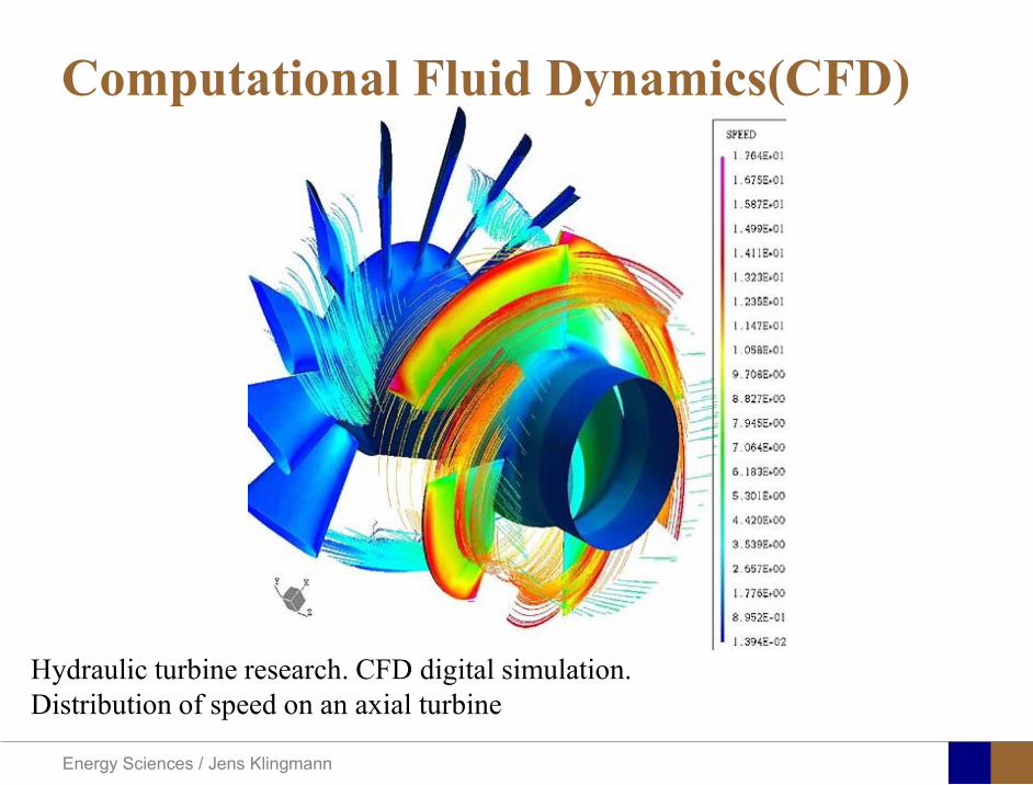
Energy Sciences Jens Klingmann
Hydraulic turbine research CFD digital simulation Distribution of speed on an axial turbine
Computational Fluid Dynamics(CFD)
Energy Sciences Jens Klingmann
Scales of turbulence
10-01
1000
1001
1002
1003
1004
1005
κ LI
10-08
10-07
10-06
10-05
10-04
10-03
10-02
10-01
1000
E(u
2 LI)
10-04
10-03
10-02
10-01
1000
κ LK
10-05
10-04
10-03
10-02
10-01
1000
1001
1002
D( ε L
K )10-01
1000
1001
1002
1003
1004
1005
E = 15 (κ LI)-53
10-04
10-03
10-02
10-01
1000
1001
D = 3 ( κ LΚ) 13
Normalized energy and dissipation spectra for
Adapted from Tennekeys and Lumley
ReLI= times2 105
1 2Re 500IL asymp
3 4Re 10000IL asymp
Energy Sciences Jens Klingmann
References Turbulence
bull Tennekeys and Lumley ldquoA first course in Turbulencerdquo MIT Press 1972
bull J O Hinze ldquoTurbulencerdquo McGraw-Hill 1959bull D C Wilcox ldquoTurbulence Modeling for CFDrdquo DCW Industries
2006
Energy Sciences Jens Klingmann
Boundary layers
Energy Sciences Jens Klingmann
Boundary Layer Theory (BLT) Sensitive to Pressure
gradients Appropriate scaling from
dimensional analyses
Energy Sciences Jens Klingmann
Boundary layers
Energy Sciences Jens Klingmann
Air foil theory
Energy Sciences Jens Klingmann
Visualisation of diffusor separation
Energy Sciences Jens Klingmann
BL equations
+minus=+
yu
yxp
xuv
xuu
partpartmicro
partpart
partpart
partρpart
partρpart and 0=+
yxu
partυpart
partpart
Applying the BL approximations the 2D stationary incompressible NS-eq and continuity equation become
yvu
yu
yxuu
xp
yu
xuu
partpartρ
partpartmicro
partpart
partρpart
partpart
partυρpart
partρpart
minus
+minusminus=+
and
0=+yx
upart
υpartpartpart
Reynolds averaged BL eqs are
Energy Sciences Jens Klingmann
Boundary layers
Energy Sciences Jens Klingmann
Turbulent BL at different Pressure gradients
Energy Sciences Jens Klingmann
Boundary Layers
ν
yuy =+
ρτWu =
0=
partpart
=y
w yuτ
uuu =+
Energy Sciences Jens Klingmann
Diffuser efficiency
Energy Sciences Jens Klingmann
Reynolds Number (Order of magnitude)
At eg a compressor inlet
ρ = O(1) kgm3
U = O(100) msx lt O(01) mmicro = O(10-5)
Re = ρ U x micro =O(106)
In subsequent stages large amounts of turbulence (from stator wakes) will be convected into the Boundary layer
Energy Sciences Jens Klingmann
References Boundary layers
bull Frank M White ldquoViscous Fluid Flowrdquobull Hermann Schlichting ldquoBoundary Layer Theoryrdquo
Energy Sciences Jens Klingmann
CFD and experiments
bull No this is not a CFD course butbull Experiments
Energy Sciences Jens Klingmann
What do we need to measureOverall performance
Flow rates (mass or volume) Pressure Temperature Shaft power
Performance increase
Separations (velocity) Secondary flows eg tip clearance losses (velocity) Shock waves (supersonic applications) Pressure (resolved in time and space) Temperature (resolved in time and space)
Energy Sciences Jens Klingmann
Cascade wind tunnels
FIG 31 Compressor cascade wind tunnels (a) Conventional low-speed continuousrunning cascade tunnel (adapted from Carter et al 1950)(b) Transonicsupersoniccascade tunnel (adapted from Sieverding 1985)
Energy Sciences Jens Klingmann
Closed circuit tunnels
Energy Sciences Jens Klingmann
components
Settling Chamber
The settling chamber is located between the fan or wide angle diffuser and the contraction and contains the honeycombs and screens used to moderate longitudinal variations in the flow Screens in the chamber should be spaced at 02 chamber diameters apart so that flow disturbed by the first screen can settle before it encounters the second
Honeycombs
Honeycombs are located in the settling chamber and are used to reduce nonuniformities in the flow For optimum benefit honeycombs should be 6-8 cell diameters thick and cell size should be on the order of about 150 cells per settling chamber diameter
Energy Sciences Jens Klingmann
components
Screens
Screens are typically located just downstream of the honeycomb and sometime at the inlet of the test section Screens create a static pressure drop and serve to reduce boundary layer size and increase flow uniformity
Contraction Section
Contractions sections are located between the settling chamber and the test sections and serve to both increase mean velocities at the test section inlet and moderate inconsistencies in the uniformity of the flow Large contraction ratios and short contraction lengths are generally more desirable as they reduce the power loss across the screens and the thickness of boundary layers Small tunnels typically have contraction ratios between 6 and 9
Energy Sciences Jens Klingmann
Flow meters with pressure measurement
Venturi-tube
A1 A2
P1 P2
1 1 2 2C A C A=In the incompressible case
2 21 1 2 2
2 2C P C P
ρ ρ+ = +Assuming horisontal mounting
Energy Sciences Jens Klingmann
Daniel Bernoulli 1700-1782
Daniel Bernoulli was the son of Johann Bernoulli He was born in Groningen while his father held the chair of mathematics there His older brother was Nicolaus(II) Bernoulli and his uncle was Jacob Bernoulli so he was born into a family of leading mathematicians but also into a family where there was unfortunate rivalry jealousy and bitterness
Undoubtedly the most important work which Daniel Bernoulli did was his work on hydrodynamics Even the term itself is based on the title of the work which he produced called Hydrodynamica and before he left St Petersburg Daniel left a draft copy of the book with a printer However the work was not published until 1738 and although he revised it considerably between 1734 and 1738 it is more the presentation that he changed rather then the substance
This work contains for the first time the correct analysis of water flowing from a hole in a container This was based on the principle of conservation of energy which he had studied with his father in 1720 Daniel also discussed pumps and other machines to raise water One remarkable discovery appears in Chapter 10 of Hydrodynamica where Daniel discussed the basis for the kinetic theory of gases He was able to give the basic laws for the theory of gases and gave although not in full detail the equation of state discovered by Van der Waals a century later
Energy Sciences Jens Klingmann
Venturi-tube (2)
22 2 12 2
2
2A PC CA ρ
∆minus =
A1 A2
P1 P2
Solve for eg C2
1 2P P P∆ = minus
( )
12
2 2 21 2
21
PCA Aρ
∆ = minus
and( )
12
2 2 2 2 21 2
21
Pm A C AA Aρρ
∆ = = minus
where
Flow meters with pressure measurement
Energy Sciences Jens Klingmann
Flow meters with pressure measurement
Orifice meters
A1
A2
P1 P2
Applicable for pipe flows Same principle as for Venturi Positioning of pressure taps important Vena contracta and losses require inclusion
of Discharge Coefficient CD
( )
12
2 2 21 2
21D
Pm C AA Aρ ∆ =
minus where ( )1 2ReDC f A A=
CD available from manufacturer (measurements) or Standards (eg ISO)
Energy Sciences Jens Klingmann
Coriolis flow meter
An actuator (not shown) induces a vibration of the tubes
When there is mass flow Coriolis forces induce twisting of the tubes
degree of phase-shift is a measure for the amount of mass that is flowing through the tubes
Energy Sciences Jens Klingmann
Thermal flow meter Heat is added electrically to the flow Temperature is measured before and after heat addition
pP mC T∆=
Energy Sciences Jens Klingmann
Ultrasonic flow meters
Ultrasound is emitted to small particles in the flow (dust or other) Reflections of the sound is frequency shifted by the Doppler effect The frequency change is proportional to the particles velocity (volume flow
meter)
Energy Sciences Jens Klingmann
Inductive flow metersA magnetic flowmeter is based upon Faradays Law
The voltage induced across any conductor as it moves at right angles through a magnetic field is proportional to the velocity of that conductor
E is proportional to V x B x D where
E = The voltage generated in a conductorV = The velocity of the conductorB = The magnetic field strengthD = The length of the conductor
NB electric conductivity is required
Energy Sciences Jens Klingmann
Temperature measurements
Thermocouples
The basis established by Thomas Johann Seebeck in 1821
A conductor generates a voltage when subjected to a temperature gradient
To measure this voltage one must use a second conductor material which generates a different voltage under the same temperature gradient
Energy Sciences Jens Klingmann
Pressure sensing
1 2p pgt 2p p2 may be the atmosphere a static pressure tap or a known reference pressure
The strain of the diaphragm (or itrsquos deflection) may be measured by a number of electric methods
Diaphragm
Energy Sciences Jens Klingmann
Pressure sensingPiezoresistive Strain Gage
Uses the piezoresistive effect of bonded or formed strain gauges to detect strain due to applied pressure
Capacitive
Uses a diaghragm and pressure cavity to create a variable capacitor to detect strain due to applied pressure
Magnetic
Measures the displacement of a diaphragm by means of changes in inductance (reluctance) LVDT Hall Effect or by eddy current principal
Piezoelectric
Uses the piezoelectric effect in certain materials such as quartz to measure the strain upon the sensing mechanism due to pressure
Potentiometric
Uses the motion of a wiper along a resistive mechanism to detect the strain caused by applied pressure
Energy Sciences Jens Klingmann
3D highly instationary (periodic) flow Potentially very high velocities (Supersonic) Large temperature differences Low accessibility (difficult to probe between rotors) Low turbulence levels in most of the domain Very high turbulence in BL and wakes
Properties of measuring object
Point measurements
Energy Sciences Jens Klingmann
Conventional or non-opticalndash Static Pressure Measurementsndash Total Pressure Measurements
bull Multy hole probes
ndash Total Temperature ndash Hot Wire Anemometry (HWA)
Optical techniques for Velocity Measurementsndash Laser Two Focous (L2F)ndash Laser Doppler Anemometry (LDA)ndash Particle Image velocimetry (PIV)
Point Measurements
Energy Sciences Jens Klingmann
Static and total pressure
2 2 21 2 1
2 1 2 2 2C C CP P ρ ρ ρ
minus = minus =
2 0C =Stagnation point
C1Static pressure tap
Prandtl or Pitot tube
Apply the Bernoulli equation from free stream to stagnation point
21
2 12CP Pρ
= +or
We can also define a stagnation or total pressure
( )2
101 1 022
CP P Pρ= + =
Total pressure = Static pressure + dynamic pressure
or
Energy Sciences Jens Klingmann
Static pressure
Energy Sciences Jens Klingmann
Total Pressure and Temperature
Shrouded Probes
Shrouded Probe
Pitot or Prandtl tube
Sensitive to direction
Energy Sciences Jens Klingmann
Ludwig Prandtl 1875-1953
Ludwig Prandtl born at Freising Bavaria on February 4 1875 was a German Physicist famous for his work in aeronautics He qualified at Munchen in 1900 with a thesis on elastic stability and held the position of Professor of Applied Mechanics at Gottingen for forty-nine years (from 1904 until his death there on August 15 1953) In 1925 Prandtl became the Director of the Kaiser Wilhelm Institute for Fluid Mechanics His discovery in 1904 of the Boundary Layer which adjoins the surface of a body moving in a fluid led to an understanding of skin friction drag and of the way in which streamlining reduces the drag of airplane wings and other moving bodies His work on wing theory published in 1918 - 1919 followed that of FW Lanchester (1902-1907) but was carried out independently and elucidated the flow over airplane wings of finite span Prandtls work and decisive advances in boundary layer and wing theories became the basic material of aeronautics He also made important contributions to the theories of supersonic flow and of turbulence and contributed much to the development of wind tunnels and other aerodynamic equipment In addition he devised the soap-film analogy for the torsion of non-circular sections and wrote on the theory of plasticity and of meteorology
Energy Sciences Jens Klingmann
Total Pressure multy hole
Cobra Probe Yaw Probe
5 Hole Probe
Energy Sciences Jens Klingmann
5 Hole Probes Calibration
Energy Sciences Jens Klingmann
The inherent unsteadiness of the flow within turbomachines
Energy Sciences Jens Klingmann
Hot Wire Anemometry (HWA) The heat transfer from a thin (one micron)
electrically heated wire can be used to determine velocity
The resistance of the wire is temperature dependent Within a small temperature range it can be assumed linear R = R0+α R0(Tm-T0) where R0 is the resistance at a reference temperature T0 and Tm is the mean wire temperature
The thermal power induced in the wire is balanced by heat transfer to the surrounding fluid I2R=hπDL(Tm-T0) where h is the heat transfer coefficient and D and L the diameter and length of the wire respectively
E = I R
Energy Sciences Jens Klingmann
Constant Temperature Anemometry (CTA) The wire is often placed in a Whetstone bridge If the output from the
bridge is amplified and fed back to the bridge the resistance of the probe and thus the temperature will be held constant
This prevents the temperature of the wire to become excessive at low velocities
R1
R2 R3
Probe
Bridge Voltage
Energy Sciences Jens Klingmann
Constant Temperature Anemometry (CTA)
Energy Sciences Jens Klingmann
Characteristics of LDA (according to Dantec)
Invented by Yeh and Cummins in 1964 Velocity measurements in Fluid Dynamics (gas liquid) Up to 3 velocity components Non-intrusive measurements (optical technique) Absolute measurement technique (no calibration required) Very high accuracy Very high spatial resolution due to small measurement volume Tracer particles are required
Energy Sciences Jens Klingmann
LDA - Fringe Model
Focused Laser beams intersect and form the measurement volume Plane wave fronts beam waist in the plane of intersection Interference in the plane of intersection Pattern of bright and dark stripesplanes Fringes
Energy Sciences Jens Klingmann
LDA-measuring volume
d
x
x
y
y
z
z
e-2 CONTOUR
FRINGES
κ
κ
κ
κ
De-2
De-2
dml m
a
b
cx
b
z
ya
cd
d
=
=
=
J
J
J
J
JP
JP
JP
JD
JD
JD
+
+
+
a
b
c
d
κπλ
=minus sinD
f4l2e
m
κπλ
=minus cosD
f4D2e
m
Energy Sciences Jens Klingmann
Laser Two Focus
Energy Sciences Jens Klingmann
Laser Two Focus
Energy Sciences Jens Klingmann
PIV measurements
PIV is a fairly new technique capable of simultaneous velocity measurements at many points in a plane This gives information on large scale structures vorticity etc which is very difficult or impossible to obtain from one-point measuring techniques
PIV involves the illumination of a plane of the flow under investigation with a thin pulsed sheet of light The flow is seeded with particles
The light scattered from the particles and from successive pulses are being recorded either on film or a CCD array forming a multiple exposure of each particle image If the time between the pulses is known velocity can be determined as the ratio of the particle displacement and the elapsed time
t∆∆= xu
Energy Sciences Jens Klingmann
PIV
Energy Sciences Jens Klingmann
PIV measurements illumination
YA
G
YA
G
Two frequency doubled YAG Lasers aligned to one double pulsed laser sheet
Two or more separate light pulses can be obtained by chopping a continuous laser or from pulsed lasers
The limited pulse energies obtained from continuous lasers limits their applicability to low velocity flows or flows where large seeding particles can be used (ie liquid flows)
The low repetition rate of most pulsed lasers makes the use of two lasers advantageous
Energy Sciences Jens Klingmann
PIV measurements recording
High seeding density in laminar flame
Film or CCD-cameras Cross- or Auto-correlation
ndash ie both particle images on the same frame or on separate frames
CCD-camera requirementndash A many pixels as possiblendash 2k by 2k available 4k by 4k coming
Energy Sciences Jens Klingmann
PIV measurements analyses
Low seeding density (Number of seeding particles per unit volume)
Each particle image pair can be identified This is called particle tracking
High seeding density (PIV)
Small sub-regions of the image containing many particle image pairs are processed to obtain one velocity vector
Energy Sciences Jens Klingmann
PIV measurements analyses
Energy Sciences Jens Klingmann
PIV measurements analyses
( ) ( ) ( ) xsxxs dIIR 2A
1
I
+= int
Cross correlation between ( )x1I and ( )x2I
s is a two dimensional displacement vector
IA is the interrogation area
Cross correlation between
(
)
x
1
I
and
(
)
x
2
I
s is a two dimensional displacement vector
I
A
is the interrogation area
Energy Sciences Jens Klingmann
Energy Sciences Jens Klingmann
PIV from IOWA state university
Energy Sciences Jens Klingmann
PIV sample of evaluation
Energy Sciences Jens Klingmann
LDA PIV HWA Velocity range 01 mms ndash 300
ms 02 ndash 150 ms
Measuring Volume
D = 005 L = 05 mm
2 by 2 by 05 mm
L = 05 mm
Freq response O(10 000) Hz O(10) Hz O(100 000) Hz Calibration Yes No No Sensitivity to other than velocity
Low (ref Index) Low (ref Index) Large (temperature concentrationshellip)
Continuous Signal
Sometimes Seldom Always
Noise High High Low Turbulence intensity
No limitation Some limitation lt 20
Price O(1 000 000) SEK
O(1 000 000) SEK
O(50 000) SEK
Required Knowledge
High medium Low
Comparison of techniques
Energy Sciences Jens Klingmann
References experiments
R J Goldstein ldquoFluid Mechanics Measurementsrdquo Hemisphere Publishing 1983 A V Johansson amp P H Alfredsson ldquoExperimentella metoder inom
stroumlmningsmekanikenrdquo Inst Foumlr Mekanik KTH F Durst A Melling and J H Whitelaw ldquoPrincipals and Practice of Laser Doppler
Anemometryrdquo 1984 R J Adrian ldquoParticle-imaging techniques for experimental fluid mechnicsrdquo Ann Rev
Fluid Mech 1991
Energy Sciences Jens Klingmann
Sample of LDA-measurements
Rotor blade
Glas window
Emitted beams
Scattered Light
Adjustable mirror
Energy Sciences Jens Klingmann
Axial velocity sorted into 10 bins
0 1 2 3 4 5 6tangential coordinate (degrees)
-20
0
20
40
60
80
100
120
140
160Ax
ial v
eloc
ity a
nd s
tand
ard
devi
atio
n (m
s)
radial position 7 mm from inner window surfaceaxial position 23 mm behind rotor blades
Energy Sciences Jens Klingmann
Axial velocities in the radial-tangential plane
Energy Sciences Jens Klingmann
Airfoils NACA 4-digit
The NACA four-digit wing sections define the profile by
One digit describing maximum camber as percentage of the chord
One digit describing the distance of maximum camber from the airfoil leading edge in tens of percents of the chord
Two digits describing maximum thickness of the airfoil as percent of the chord
Example the NACA 2412 airfoil has a maximum camber of 2 located 40 (04 chords) from the leading edge with a maximum thickness of 12 of the chord
Four-digit series airfoils by default have maximum thickness at 30 of the chord (03 chords) from the leading edge
Energy Sciences Jens Klingmann
Airfoils NACA 4-digit
bull c is the chord lengthbull x is the position along
the chord from 0 to cbull y is the half thickness at
a given value of x (centerline to surface)
bull t is the maximum thickness as a fraction of the chord
Energy Sciences Jens Klingmann
Death by PowerPoint
| LDA | PIV | HWA | |||||
| Velocity range | 01 mms ndash 300 ms | 02 ndash 150 ms | |||||
| Measuring Volume | D = 005 L = 05 mm | 2 by 2 by 05 mm | L = 05 mm | ||||
| Freq response | O(10 000) Hz | O(10) Hz | O(100 000) Hz | ||||
| Calibration | Yes | No | No | ||||
| Sensitivity to other than velocity | Low (ref Index) | Low (ref Index) | Large (temperature concentrationshellip) | ||||
| Continuous Signal | Sometimes | Seldom | Always | ||||
| Noise | High | High | Low | ||||
| Turbulence intensity | No limitation | Some limitation | lt 20 | ||||
| Price | O(1 000 000) SEK | O(1 000 000) SEK | O(50 000) SEK | ||||
| Required Knowledge | High | medium | Low |
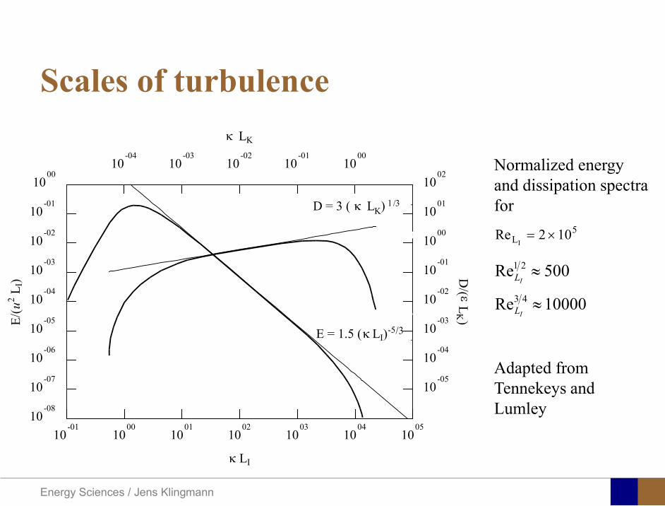
Energy Sciences Jens Klingmann
Scales of turbulence
10-01
1000
1001
1002
1003
1004
1005
κ LI
10-08
10-07
10-06
10-05
10-04
10-03
10-02
10-01
1000
E(u
2 LI)
10-04
10-03
10-02
10-01
1000
κ LK
10-05
10-04
10-03
10-02
10-01
1000
1001
1002
D( ε L
K )10-01
1000
1001
1002
1003
1004
1005
E = 15 (κ LI)-53
10-04
10-03
10-02
10-01
1000
1001
D = 3 ( κ LΚ) 13
Normalized energy and dissipation spectra for
Adapted from Tennekeys and Lumley
ReLI= times2 105
1 2Re 500IL asymp
3 4Re 10000IL asymp
Energy Sciences Jens Klingmann
References Turbulence
bull Tennekeys and Lumley ldquoA first course in Turbulencerdquo MIT Press 1972
bull J O Hinze ldquoTurbulencerdquo McGraw-Hill 1959bull D C Wilcox ldquoTurbulence Modeling for CFDrdquo DCW Industries
2006
Energy Sciences Jens Klingmann
Boundary layers
Energy Sciences Jens Klingmann
Boundary Layer Theory (BLT) Sensitive to Pressure
gradients Appropriate scaling from
dimensional analyses
Energy Sciences Jens Klingmann
Boundary layers
Energy Sciences Jens Klingmann
Air foil theory
Energy Sciences Jens Klingmann
Visualisation of diffusor separation
Energy Sciences Jens Klingmann
BL equations
+minus=+
yu
yxp
xuv
xuu
partpartmicro
partpart
partpart
partρpart
partρpart and 0=+
yxu
partυpart
partpart
Applying the BL approximations the 2D stationary incompressible NS-eq and continuity equation become
yvu
yu
yxuu
xp
yu
xuu
partpartρ
partpartmicro
partpart
partρpart
partpart
partυρpart
partρpart
minus
+minusminus=+
and
0=+yx
upart
υpartpartpart
Reynolds averaged BL eqs are
Energy Sciences Jens Klingmann
Boundary layers
Energy Sciences Jens Klingmann
Turbulent BL at different Pressure gradients
Energy Sciences Jens Klingmann
Boundary Layers
ν
yuy =+
ρτWu =
0=
partpart
=y
w yuτ
uuu =+
Energy Sciences Jens Klingmann
Diffuser efficiency
Energy Sciences Jens Klingmann
Reynolds Number (Order of magnitude)
At eg a compressor inlet
ρ = O(1) kgm3
U = O(100) msx lt O(01) mmicro = O(10-5)
Re = ρ U x micro =O(106)
In subsequent stages large amounts of turbulence (from stator wakes) will be convected into the Boundary layer
Energy Sciences Jens Klingmann
References Boundary layers
bull Frank M White ldquoViscous Fluid Flowrdquobull Hermann Schlichting ldquoBoundary Layer Theoryrdquo
Energy Sciences Jens Klingmann
CFD and experiments
bull No this is not a CFD course butbull Experiments
Energy Sciences Jens Klingmann
What do we need to measureOverall performance
Flow rates (mass or volume) Pressure Temperature Shaft power
Performance increase
Separations (velocity) Secondary flows eg tip clearance losses (velocity) Shock waves (supersonic applications) Pressure (resolved in time and space) Temperature (resolved in time and space)
Energy Sciences Jens Klingmann
Cascade wind tunnels
FIG 31 Compressor cascade wind tunnels (a) Conventional low-speed continuousrunning cascade tunnel (adapted from Carter et al 1950)(b) Transonicsupersoniccascade tunnel (adapted from Sieverding 1985)
Energy Sciences Jens Klingmann
Closed circuit tunnels
Energy Sciences Jens Klingmann
components
Settling Chamber
The settling chamber is located between the fan or wide angle diffuser and the contraction and contains the honeycombs and screens used to moderate longitudinal variations in the flow Screens in the chamber should be spaced at 02 chamber diameters apart so that flow disturbed by the first screen can settle before it encounters the second
Honeycombs
Honeycombs are located in the settling chamber and are used to reduce nonuniformities in the flow For optimum benefit honeycombs should be 6-8 cell diameters thick and cell size should be on the order of about 150 cells per settling chamber diameter
Energy Sciences Jens Klingmann
components
Screens
Screens are typically located just downstream of the honeycomb and sometime at the inlet of the test section Screens create a static pressure drop and serve to reduce boundary layer size and increase flow uniformity
Contraction Section
Contractions sections are located between the settling chamber and the test sections and serve to both increase mean velocities at the test section inlet and moderate inconsistencies in the uniformity of the flow Large contraction ratios and short contraction lengths are generally more desirable as they reduce the power loss across the screens and the thickness of boundary layers Small tunnels typically have contraction ratios between 6 and 9
Energy Sciences Jens Klingmann
Flow meters with pressure measurement
Venturi-tube
A1 A2
P1 P2
1 1 2 2C A C A=In the incompressible case
2 21 1 2 2
2 2C P C P
ρ ρ+ = +Assuming horisontal mounting
Energy Sciences Jens Klingmann
Daniel Bernoulli 1700-1782
Daniel Bernoulli was the son of Johann Bernoulli He was born in Groningen while his father held the chair of mathematics there His older brother was Nicolaus(II) Bernoulli and his uncle was Jacob Bernoulli so he was born into a family of leading mathematicians but also into a family where there was unfortunate rivalry jealousy and bitterness
Undoubtedly the most important work which Daniel Bernoulli did was his work on hydrodynamics Even the term itself is based on the title of the work which he produced called Hydrodynamica and before he left St Petersburg Daniel left a draft copy of the book with a printer However the work was not published until 1738 and although he revised it considerably between 1734 and 1738 it is more the presentation that he changed rather then the substance
This work contains for the first time the correct analysis of water flowing from a hole in a container This was based on the principle of conservation of energy which he had studied with his father in 1720 Daniel also discussed pumps and other machines to raise water One remarkable discovery appears in Chapter 10 of Hydrodynamica where Daniel discussed the basis for the kinetic theory of gases He was able to give the basic laws for the theory of gases and gave although not in full detail the equation of state discovered by Van der Waals a century later
Energy Sciences Jens Klingmann
Venturi-tube (2)
22 2 12 2
2
2A PC CA ρ
∆minus =
A1 A2
P1 P2
Solve for eg C2
1 2P P P∆ = minus
( )
12
2 2 21 2
21
PCA Aρ
∆ = minus
and( )
12
2 2 2 2 21 2
21
Pm A C AA Aρρ
∆ = = minus
where
Flow meters with pressure measurement
Energy Sciences Jens Klingmann
Flow meters with pressure measurement
Orifice meters
A1
A2
P1 P2
Applicable for pipe flows Same principle as for Venturi Positioning of pressure taps important Vena contracta and losses require inclusion
of Discharge Coefficient CD
( )
12
2 2 21 2
21D
Pm C AA Aρ ∆ =
minus where ( )1 2ReDC f A A=
CD available from manufacturer (measurements) or Standards (eg ISO)
Energy Sciences Jens Klingmann
Coriolis flow meter
An actuator (not shown) induces a vibration of the tubes
When there is mass flow Coriolis forces induce twisting of the tubes
degree of phase-shift is a measure for the amount of mass that is flowing through the tubes
Energy Sciences Jens Klingmann
Thermal flow meter Heat is added electrically to the flow Temperature is measured before and after heat addition
pP mC T∆=
Energy Sciences Jens Klingmann
Ultrasonic flow meters
Ultrasound is emitted to small particles in the flow (dust or other) Reflections of the sound is frequency shifted by the Doppler effect The frequency change is proportional to the particles velocity (volume flow
meter)
Energy Sciences Jens Klingmann
Inductive flow metersA magnetic flowmeter is based upon Faradays Law
The voltage induced across any conductor as it moves at right angles through a magnetic field is proportional to the velocity of that conductor
E is proportional to V x B x D where
E = The voltage generated in a conductorV = The velocity of the conductorB = The magnetic field strengthD = The length of the conductor
NB electric conductivity is required
Energy Sciences Jens Klingmann
Temperature measurements
Thermocouples
The basis established by Thomas Johann Seebeck in 1821
A conductor generates a voltage when subjected to a temperature gradient
To measure this voltage one must use a second conductor material which generates a different voltage under the same temperature gradient
Energy Sciences Jens Klingmann
Pressure sensing
1 2p pgt 2p p2 may be the atmosphere a static pressure tap or a known reference pressure
The strain of the diaphragm (or itrsquos deflection) may be measured by a number of electric methods
Diaphragm
Energy Sciences Jens Klingmann
Pressure sensingPiezoresistive Strain Gage
Uses the piezoresistive effect of bonded or formed strain gauges to detect strain due to applied pressure
Capacitive
Uses a diaghragm and pressure cavity to create a variable capacitor to detect strain due to applied pressure
Magnetic
Measures the displacement of a diaphragm by means of changes in inductance (reluctance) LVDT Hall Effect or by eddy current principal
Piezoelectric
Uses the piezoelectric effect in certain materials such as quartz to measure the strain upon the sensing mechanism due to pressure
Potentiometric
Uses the motion of a wiper along a resistive mechanism to detect the strain caused by applied pressure
Energy Sciences Jens Klingmann
3D highly instationary (periodic) flow Potentially very high velocities (Supersonic) Large temperature differences Low accessibility (difficult to probe between rotors) Low turbulence levels in most of the domain Very high turbulence in BL and wakes
Properties of measuring object
Point measurements
Energy Sciences Jens Klingmann
Conventional or non-opticalndash Static Pressure Measurementsndash Total Pressure Measurements
bull Multy hole probes
ndash Total Temperature ndash Hot Wire Anemometry (HWA)
Optical techniques for Velocity Measurementsndash Laser Two Focous (L2F)ndash Laser Doppler Anemometry (LDA)ndash Particle Image velocimetry (PIV)
Point Measurements
Energy Sciences Jens Klingmann
Static and total pressure
2 2 21 2 1
2 1 2 2 2C C CP P ρ ρ ρ
minus = minus =
2 0C =Stagnation point
C1Static pressure tap
Prandtl or Pitot tube
Apply the Bernoulli equation from free stream to stagnation point
21
2 12CP Pρ
= +or
We can also define a stagnation or total pressure
( )2
101 1 022
CP P Pρ= + =
Total pressure = Static pressure + dynamic pressure
or
Energy Sciences Jens Klingmann
Static pressure
Energy Sciences Jens Klingmann
Total Pressure and Temperature
Shrouded Probes
Shrouded Probe
Pitot or Prandtl tube
Sensitive to direction
Energy Sciences Jens Klingmann
Ludwig Prandtl 1875-1953
Ludwig Prandtl born at Freising Bavaria on February 4 1875 was a German Physicist famous for his work in aeronautics He qualified at Munchen in 1900 with a thesis on elastic stability and held the position of Professor of Applied Mechanics at Gottingen for forty-nine years (from 1904 until his death there on August 15 1953) In 1925 Prandtl became the Director of the Kaiser Wilhelm Institute for Fluid Mechanics His discovery in 1904 of the Boundary Layer which adjoins the surface of a body moving in a fluid led to an understanding of skin friction drag and of the way in which streamlining reduces the drag of airplane wings and other moving bodies His work on wing theory published in 1918 - 1919 followed that of FW Lanchester (1902-1907) but was carried out independently and elucidated the flow over airplane wings of finite span Prandtls work and decisive advances in boundary layer and wing theories became the basic material of aeronautics He also made important contributions to the theories of supersonic flow and of turbulence and contributed much to the development of wind tunnels and other aerodynamic equipment In addition he devised the soap-film analogy for the torsion of non-circular sections and wrote on the theory of plasticity and of meteorology
Energy Sciences Jens Klingmann
Total Pressure multy hole
Cobra Probe Yaw Probe
5 Hole Probe
Energy Sciences Jens Klingmann
5 Hole Probes Calibration
Energy Sciences Jens Klingmann
The inherent unsteadiness of the flow within turbomachines
Energy Sciences Jens Klingmann
Hot Wire Anemometry (HWA) The heat transfer from a thin (one micron)
electrically heated wire can be used to determine velocity
The resistance of the wire is temperature dependent Within a small temperature range it can be assumed linear R = R0+α R0(Tm-T0) where R0 is the resistance at a reference temperature T0 and Tm is the mean wire temperature
The thermal power induced in the wire is balanced by heat transfer to the surrounding fluid I2R=hπDL(Tm-T0) where h is the heat transfer coefficient and D and L the diameter and length of the wire respectively
E = I R
Energy Sciences Jens Klingmann
Constant Temperature Anemometry (CTA) The wire is often placed in a Whetstone bridge If the output from the
bridge is amplified and fed back to the bridge the resistance of the probe and thus the temperature will be held constant
This prevents the temperature of the wire to become excessive at low velocities
R1
R2 R3
Probe
Bridge Voltage
Energy Sciences Jens Klingmann
Constant Temperature Anemometry (CTA)
Energy Sciences Jens Klingmann
Characteristics of LDA (according to Dantec)
Invented by Yeh and Cummins in 1964 Velocity measurements in Fluid Dynamics (gas liquid) Up to 3 velocity components Non-intrusive measurements (optical technique) Absolute measurement technique (no calibration required) Very high accuracy Very high spatial resolution due to small measurement volume Tracer particles are required
Energy Sciences Jens Klingmann
LDA - Fringe Model
Focused Laser beams intersect and form the measurement volume Plane wave fronts beam waist in the plane of intersection Interference in the plane of intersection Pattern of bright and dark stripesplanes Fringes
Energy Sciences Jens Klingmann
LDA-measuring volume
d
x
x
y
y
z
z
e-2 CONTOUR
FRINGES
κ
κ
κ
κ
De-2
De-2
dml m
a
b
cx
b
z
ya
cd
d
=
=
=
J
J
J
J
JP
JP
JP
JD
JD
JD
+
+
+
a
b
c
d
κπλ
=minus sinD
f4l2e
m
κπλ
=minus cosD
f4D2e
m
Energy Sciences Jens Klingmann
Laser Two Focus
Energy Sciences Jens Klingmann
Laser Two Focus
Energy Sciences Jens Klingmann
PIV measurements
PIV is a fairly new technique capable of simultaneous velocity measurements at many points in a plane This gives information on large scale structures vorticity etc which is very difficult or impossible to obtain from one-point measuring techniques
PIV involves the illumination of a plane of the flow under investigation with a thin pulsed sheet of light The flow is seeded with particles
The light scattered from the particles and from successive pulses are being recorded either on film or a CCD array forming a multiple exposure of each particle image If the time between the pulses is known velocity can be determined as the ratio of the particle displacement and the elapsed time
t∆∆= xu
Energy Sciences Jens Klingmann
PIV
Energy Sciences Jens Klingmann
PIV measurements illumination
YA
G
YA
G
Two frequency doubled YAG Lasers aligned to one double pulsed laser sheet
Two or more separate light pulses can be obtained by chopping a continuous laser or from pulsed lasers
The limited pulse energies obtained from continuous lasers limits their applicability to low velocity flows or flows where large seeding particles can be used (ie liquid flows)
The low repetition rate of most pulsed lasers makes the use of two lasers advantageous
Energy Sciences Jens Klingmann
PIV measurements recording
High seeding density in laminar flame
Film or CCD-cameras Cross- or Auto-correlation
ndash ie both particle images on the same frame or on separate frames
CCD-camera requirementndash A many pixels as possiblendash 2k by 2k available 4k by 4k coming
Energy Sciences Jens Klingmann
PIV measurements analyses
Low seeding density (Number of seeding particles per unit volume)
Each particle image pair can be identified This is called particle tracking
High seeding density (PIV)
Small sub-regions of the image containing many particle image pairs are processed to obtain one velocity vector
Energy Sciences Jens Klingmann
PIV measurements analyses
Energy Sciences Jens Klingmann
PIV measurements analyses
( ) ( ) ( ) xsxxs dIIR 2A
1
I
+= int
Cross correlation between ( )x1I and ( )x2I
s is a two dimensional displacement vector
IA is the interrogation area
Cross correlation between
(
)
x
1
I
and
(
)
x
2
I
s is a two dimensional displacement vector
I
A
is the interrogation area
Energy Sciences Jens Klingmann
Energy Sciences Jens Klingmann
PIV from IOWA state university
Energy Sciences Jens Klingmann
PIV sample of evaluation
Energy Sciences Jens Klingmann
LDA PIV HWA Velocity range 01 mms ndash 300
ms 02 ndash 150 ms
Measuring Volume
D = 005 L = 05 mm
2 by 2 by 05 mm
L = 05 mm
Freq response O(10 000) Hz O(10) Hz O(100 000) Hz Calibration Yes No No Sensitivity to other than velocity
Low (ref Index) Low (ref Index) Large (temperature concentrationshellip)
Continuous Signal
Sometimes Seldom Always
Noise High High Low Turbulence intensity
No limitation Some limitation lt 20
Price O(1 000 000) SEK
O(1 000 000) SEK
O(50 000) SEK
Required Knowledge
High medium Low
Comparison of techniques
Energy Sciences Jens Klingmann
References experiments
R J Goldstein ldquoFluid Mechanics Measurementsrdquo Hemisphere Publishing 1983 A V Johansson amp P H Alfredsson ldquoExperimentella metoder inom
stroumlmningsmekanikenrdquo Inst Foumlr Mekanik KTH F Durst A Melling and J H Whitelaw ldquoPrincipals and Practice of Laser Doppler
Anemometryrdquo 1984 R J Adrian ldquoParticle-imaging techniques for experimental fluid mechnicsrdquo Ann Rev
Fluid Mech 1991
Energy Sciences Jens Klingmann
Sample of LDA-measurements
Rotor blade
Glas window
Emitted beams
Scattered Light
Adjustable mirror
Energy Sciences Jens Klingmann
Axial velocity sorted into 10 bins
0 1 2 3 4 5 6tangential coordinate (degrees)
-20
0
20
40
60
80
100
120
140
160Ax
ial v
eloc
ity a
nd s
tand
ard
devi
atio
n (m
s)
radial position 7 mm from inner window surfaceaxial position 23 mm behind rotor blades
Energy Sciences Jens Klingmann
Axial velocities in the radial-tangential plane
Energy Sciences Jens Klingmann
Airfoils NACA 4-digit
The NACA four-digit wing sections define the profile by
One digit describing maximum camber as percentage of the chord
One digit describing the distance of maximum camber from the airfoil leading edge in tens of percents of the chord
Two digits describing maximum thickness of the airfoil as percent of the chord
Example the NACA 2412 airfoil has a maximum camber of 2 located 40 (04 chords) from the leading edge with a maximum thickness of 12 of the chord
Four-digit series airfoils by default have maximum thickness at 30 of the chord (03 chords) from the leading edge
Energy Sciences Jens Klingmann
Airfoils NACA 4-digit
bull c is the chord lengthbull x is the position along
the chord from 0 to cbull y is the half thickness at
a given value of x (centerline to surface)
bull t is the maximum thickness as a fraction of the chord
Energy Sciences Jens Klingmann
Death by PowerPoint
| LDA | PIV | HWA | |||||
| Velocity range | 01 mms ndash 300 ms | 02 ndash 150 ms | |||||
| Measuring Volume | D = 005 L = 05 mm | 2 by 2 by 05 mm | L = 05 mm | ||||
| Freq response | O(10 000) Hz | O(10) Hz | O(100 000) Hz | ||||
| Calibration | Yes | No | No | ||||
| Sensitivity to other than velocity | Low (ref Index) | Low (ref Index) | Large (temperature concentrationshellip) | ||||
| Continuous Signal | Sometimes | Seldom | Always | ||||
| Noise | High | High | Low | ||||
| Turbulence intensity | No limitation | Some limitation | lt 20 | ||||
| Price | O(1 000 000) SEK | O(1 000 000) SEK | O(50 000) SEK | ||||
| Required Knowledge | High | medium | Low |
Energy Sciences Jens Klingmann
Boundary layers
Energy Sciences Jens Klingmann
Boundary Layer Theory (BLT) Sensitive to Pressure
gradients Appropriate scaling from
dimensional analyses
Energy Sciences Jens Klingmann
Boundary layers
Energy Sciences Jens Klingmann
Air foil theory
Energy Sciences Jens Klingmann
Visualisation of diffusor separation
Energy Sciences Jens Klingmann
BL equations
+minus=+
yu
yxp
xuv
xuu
partpartmicro
partpart
partpart
partρpart
partρpart and 0=+
yxu
partυpart
partpart
Applying the BL approximations the 2D stationary incompressible NS-eq and continuity equation become
yvu
yu
yxuu
xp
yu
xuu
partpartρ
partpartmicro
partpart
partρpart
partpart
partυρpart
partρpart
minus
+minusminus=+
and
0=+yx
upart
υpartpartpart
Reynolds averaged BL eqs are
Energy Sciences Jens Klingmann
Boundary layers
Energy Sciences Jens Klingmann
Turbulent BL at different Pressure gradients
Energy Sciences Jens Klingmann
Boundary Layers
ν
yuy =+
ρτWu =
0=
partpart
=y
w yuτ
uuu =+
Energy Sciences Jens Klingmann
Diffuser efficiency
Energy Sciences Jens Klingmann
Reynolds Number (Order of magnitude)
At eg a compressor inlet
ρ = O(1) kgm3
U = O(100) msx lt O(01) mmicro = O(10-5)
Re = ρ U x micro =O(106)
In subsequent stages large amounts of turbulence (from stator wakes) will be convected into the Boundary layer
Energy Sciences Jens Klingmann
References Boundary layers
bull Frank M White ldquoViscous Fluid Flowrdquobull Hermann Schlichting ldquoBoundary Layer Theoryrdquo
Energy Sciences Jens Klingmann
CFD and experiments
bull No this is not a CFD course butbull Experiments
Energy Sciences Jens Klingmann
What do we need to measureOverall performance
Flow rates (mass or volume) Pressure Temperature Shaft power
Performance increase
Separations (velocity) Secondary flows eg tip clearance losses (velocity) Shock waves (supersonic applications) Pressure (resolved in time and space) Temperature (resolved in time and space)
Energy Sciences Jens Klingmann
Cascade wind tunnels
FIG 31 Compressor cascade wind tunnels (a) Conventional low-speed continuousrunning cascade tunnel (adapted from Carter et al 1950)(b) Transonicsupersoniccascade tunnel (adapted from Sieverding 1985)
Energy Sciences Jens Klingmann
Closed circuit tunnels
Energy Sciences Jens Klingmann
components
Settling Chamber
The settling chamber is located between the fan or wide angle diffuser and the contraction and contains the honeycombs and screens used to moderate longitudinal variations in the flow Screens in the chamber should be spaced at 02 chamber diameters apart so that flow disturbed by the first screen can settle before it encounters the second
Honeycombs
Honeycombs are located in the settling chamber and are used to reduce nonuniformities in the flow For optimum benefit honeycombs should be 6-8 cell diameters thick and cell size should be on the order of about 150 cells per settling chamber diameter
Energy Sciences Jens Klingmann
components
Screens
Screens are typically located just downstream of the honeycomb and sometime at the inlet of the test section Screens create a static pressure drop and serve to reduce boundary layer size and increase flow uniformity
Contraction Section
Contractions sections are located between the settling chamber and the test sections and serve to both increase mean velocities at the test section inlet and moderate inconsistencies in the uniformity of the flow Large contraction ratios and short contraction lengths are generally more desirable as they reduce the power loss across the screens and the thickness of boundary layers Small tunnels typically have contraction ratios between 6 and 9
Energy Sciences Jens Klingmann
Flow meters with pressure measurement
Venturi-tube
A1 A2
P1 P2
1 1 2 2C A C A=In the incompressible case
2 21 1 2 2
2 2C P C P
ρ ρ+ = +Assuming horisontal mounting
Energy Sciences Jens Klingmann
Daniel Bernoulli 1700-1782
Daniel Bernoulli was the son of Johann Bernoulli He was born in Groningen while his father held the chair of mathematics there His older brother was Nicolaus(II) Bernoulli and his uncle was Jacob Bernoulli so he was born into a family of leading mathematicians but also into a family where there was unfortunate rivalry jealousy and bitterness
Undoubtedly the most important work which Daniel Bernoulli did was his work on hydrodynamics Even the term itself is based on the title of the work which he produced called Hydrodynamica and before he left St Petersburg Daniel left a draft copy of the book with a printer However the work was not published until 1738 and although he revised it considerably between 1734 and 1738 it is more the presentation that he changed rather then the substance
This work contains for the first time the correct analysis of water flowing from a hole in a container This was based on the principle of conservation of energy which he had studied with his father in 1720 Daniel also discussed pumps and other machines to raise water One remarkable discovery appears in Chapter 10 of Hydrodynamica where Daniel discussed the basis for the kinetic theory of gases He was able to give the basic laws for the theory of gases and gave although not in full detail the equation of state discovered by Van der Waals a century later
Energy Sciences Jens Klingmann
Venturi-tube (2)
22 2 12 2
2
2A PC CA ρ
∆minus =
A1 A2
P1 P2
Solve for eg C2
1 2P P P∆ = minus
( )
12
2 2 21 2
21
PCA Aρ
∆ = minus
and( )
12
2 2 2 2 21 2
21
Pm A C AA Aρρ
∆ = = minus
where
Flow meters with pressure measurement
Energy Sciences Jens Klingmann
Flow meters with pressure measurement
Orifice meters
A1
A2
P1 P2
Applicable for pipe flows Same principle as for Venturi Positioning of pressure taps important Vena contracta and losses require inclusion
of Discharge Coefficient CD
( )
12
2 2 21 2
21D
Pm C AA Aρ ∆ =
minus where ( )1 2ReDC f A A=
CD available from manufacturer (measurements) or Standards (eg ISO)
Energy Sciences Jens Klingmann
Coriolis flow meter
An actuator (not shown) induces a vibration of the tubes
When there is mass flow Coriolis forces induce twisting of the tubes
degree of phase-shift is a measure for the amount of mass that is flowing through the tubes
Energy Sciences Jens Klingmann
Thermal flow meter Heat is added electrically to the flow Temperature is measured before and after heat addition
pP mC T∆=
Energy Sciences Jens Klingmann
Ultrasonic flow meters
Ultrasound is emitted to small particles in the flow (dust or other) Reflections of the sound is frequency shifted by the Doppler effect The frequency change is proportional to the particles velocity (volume flow
meter)
Energy Sciences Jens Klingmann
Inductive flow metersA magnetic flowmeter is based upon Faradays Law
The voltage induced across any conductor as it moves at right angles through a magnetic field is proportional to the velocity of that conductor
E is proportional to V x B x D where
E = The voltage generated in a conductorV = The velocity of the conductorB = The magnetic field strengthD = The length of the conductor
NB electric conductivity is required
Energy Sciences Jens Klingmann
Temperature measurements
Thermocouples
The basis established by Thomas Johann Seebeck in 1821
A conductor generates a voltage when subjected to a temperature gradient
To measure this voltage one must use a second conductor material which generates a different voltage under the same temperature gradient
Energy Sciences Jens Klingmann
Pressure sensing
1 2p pgt 2p p2 may be the atmosphere a static pressure tap or a known reference pressure
The strain of the diaphragm (or itrsquos deflection) may be measured by a number of electric methods
Diaphragm
Energy Sciences Jens Klingmann
Pressure sensingPiezoresistive Strain Gage
Uses the piezoresistive effect of bonded or formed strain gauges to detect strain due to applied pressure
Capacitive
Uses a diaghragm and pressure cavity to create a variable capacitor to detect strain due to applied pressure
Magnetic
Measures the displacement of a diaphragm by means of changes in inductance (reluctance) LVDT Hall Effect or by eddy current principal
Piezoelectric
Uses the piezoelectric effect in certain materials such as quartz to measure the strain upon the sensing mechanism due to pressure
Potentiometric
Uses the motion of a wiper along a resistive mechanism to detect the strain caused by applied pressure
Energy Sciences Jens Klingmann
3D highly instationary (periodic) flow Potentially very high velocities (Supersonic) Large temperature differences Low accessibility (difficult to probe between rotors) Low turbulence levels in most of the domain Very high turbulence in BL and wakes
Properties of measuring object
Point measurements
Energy Sciences Jens Klingmann
Conventional or non-opticalndash Static Pressure Measurementsndash Total Pressure Measurements
bull Multy hole probes
ndash Total Temperature ndash Hot Wire Anemometry (HWA)
Optical techniques for Velocity Measurementsndash Laser Two Focous (L2F)ndash Laser Doppler Anemometry (LDA)ndash Particle Image velocimetry (PIV)
Point Measurements
Energy Sciences Jens Klingmann
Static and total pressure
2 2 21 2 1
2 1 2 2 2C C CP P ρ ρ ρ
minus = minus =
2 0C =Stagnation point
C1Static pressure tap
Prandtl or Pitot tube
Apply the Bernoulli equation from free stream to stagnation point
21
2 12CP Pρ
= +or
We can also define a stagnation or total pressure
( )2
101 1 022
CP P Pρ= + =
Total pressure = Static pressure + dynamic pressure
or
Energy Sciences Jens Klingmann
Static pressure
Energy Sciences Jens Klingmann
Total Pressure and Temperature
Shrouded Probes
Shrouded Probe
Pitot or Prandtl tube
Sensitive to direction
Energy Sciences Jens Klingmann
Ludwig Prandtl 1875-1953
Ludwig Prandtl born at Freising Bavaria on February 4 1875 was a German Physicist famous for his work in aeronautics He qualified at Munchen in 1900 with a thesis on elastic stability and held the position of Professor of Applied Mechanics at Gottingen for forty-nine years (from 1904 until his death there on August 15 1953) In 1925 Prandtl became the Director of the Kaiser Wilhelm Institute for Fluid Mechanics His discovery in 1904 of the Boundary Layer which adjoins the surface of a body moving in a fluid led to an understanding of skin friction drag and of the way in which streamlining reduces the drag of airplane wings and other moving bodies His work on wing theory published in 1918 - 1919 followed that of FW Lanchester (1902-1907) but was carried out independently and elucidated the flow over airplane wings of finite span Prandtls work and decisive advances in boundary layer and wing theories became the basic material of aeronautics He also made important contributions to the theories of supersonic flow and of turbulence and contributed much to the development of wind tunnels and other aerodynamic equipment In addition he devised the soap-film analogy for the torsion of non-circular sections and wrote on the theory of plasticity and of meteorology
Energy Sciences Jens Klingmann
Total Pressure multy hole
Cobra Probe Yaw Probe
5 Hole Probe
Energy Sciences Jens Klingmann
5 Hole Probes Calibration
Energy Sciences Jens Klingmann
The inherent unsteadiness of the flow within turbomachines
Energy Sciences Jens Klingmann
Hot Wire Anemometry (HWA) The heat transfer from a thin (one micron)
electrically heated wire can be used to determine velocity
The resistance of the wire is temperature dependent Within a small temperature range it can be assumed linear R = R0+α R0(Tm-T0) where R0 is the resistance at a reference temperature T0 and Tm is the mean wire temperature
The thermal power induced in the wire is balanced by heat transfer to the surrounding fluid I2R=hπDL(Tm-T0) where h is the heat transfer coefficient and D and L the diameter and length of the wire respectively
E = I R
Energy Sciences Jens Klingmann
Constant Temperature Anemometry (CTA) The wire is often placed in a Whetstone bridge If the output from the
bridge is amplified and fed back to the bridge the resistance of the probe and thus the temperature will be held constant
This prevents the temperature of the wire to become excessive at low velocities
R1
R2 R3
Probe
Bridge Voltage
Energy Sciences Jens Klingmann
Constant Temperature Anemometry (CTA)
Energy Sciences Jens Klingmann
Characteristics of LDA (according to Dantec)
Invented by Yeh and Cummins in 1964 Velocity measurements in Fluid Dynamics (gas liquid) Up to 3 velocity components Non-intrusive measurements (optical technique) Absolute measurement technique (no calibration required) Very high accuracy Very high spatial resolution due to small measurement volume Tracer particles are required
Energy Sciences Jens Klingmann
LDA - Fringe Model
Focused Laser beams intersect and form the measurement volume Plane wave fronts beam waist in the plane of intersection Interference in the plane of intersection Pattern of bright and dark stripesplanes Fringes
Energy Sciences Jens Klingmann
LDA-measuring volume
d
x
x
y
y
z
z
e-2 CONTOUR
FRINGES
κ
κ
κ
κ
De-2
De-2
dml m
a
b
cx
b
z
ya
cd
d
=
=
=
J
J
J
J
JP
JP
JP
JD
JD
JD
+
+
+
a
b
c
d
κπλ
=minus sinD
f4l2e
m
κπλ
=minus cosD
f4D2e
m
Energy Sciences Jens Klingmann
Laser Two Focus
Energy Sciences Jens Klingmann
Laser Two Focus
Energy Sciences Jens Klingmann
PIV measurements
PIV is a fairly new technique capable of simultaneous velocity measurements at many points in a plane This gives information on large scale structures vorticity etc which is very difficult or impossible to obtain from one-point measuring techniques
PIV involves the illumination of a plane of the flow under investigation with a thin pulsed sheet of light The flow is seeded with particles
The light scattered from the particles and from successive pulses are being recorded either on film or a CCD array forming a multiple exposure of each particle image If the time between the pulses is known velocity can be determined as the ratio of the particle displacement and the elapsed time
t∆∆= xu
Energy Sciences Jens Klingmann
PIV
Energy Sciences Jens Klingmann
PIV measurements illumination
YA
G
YA
G
Two frequency doubled YAG Lasers aligned to one double pulsed laser sheet
Two or more separate light pulses can be obtained by chopping a continuous laser or from pulsed lasers
The limited pulse energies obtained from continuous lasers limits their applicability to low velocity flows or flows where large seeding particles can be used (ie liquid flows)
The low repetition rate of most pulsed lasers makes the use of two lasers advantageous
Energy Sciences Jens Klingmann
PIV measurements recording
High seeding density in laminar flame
Film or CCD-cameras Cross- or Auto-correlation
ndash ie both particle images on the same frame or on separate frames
CCD-camera requirementndash A many pixels as possiblendash 2k by 2k available 4k by 4k coming
Energy Sciences Jens Klingmann
PIV measurements analyses
Low seeding density (Number of seeding particles per unit volume)
Each particle image pair can be identified This is called particle tracking
High seeding density (PIV)
Small sub-regions of the image containing many particle image pairs are processed to obtain one velocity vector
Energy Sciences Jens Klingmann
PIV measurements analyses
Energy Sciences Jens Klingmann
PIV measurements analyses
( ) ( ) ( ) xsxxs dIIR 2A
1
I
+= int
Cross correlation between ( )x1I and ( )x2I
s is a two dimensional displacement vector
IA is the interrogation area
Cross correlation between
(
)
x
1
I
and
(
)
x
2
I
s is a two dimensional displacement vector
I
A
is the interrogation area
Energy Sciences Jens Klingmann
Energy Sciences Jens Klingmann
PIV from IOWA state university
Energy Sciences Jens Klingmann
PIV sample of evaluation
Energy Sciences Jens Klingmann
LDA PIV HWA Velocity range 01 mms ndash 300
ms 02 ndash 150 ms
Measuring Volume
D = 005 L = 05 mm
2 by 2 by 05 mm
L = 05 mm
Freq response O(10 000) Hz O(10) Hz O(100 000) Hz Calibration Yes No No Sensitivity to other than velocity
Low (ref Index) Low (ref Index) Large (temperature concentrationshellip)
Continuous Signal
Sometimes Seldom Always
Noise High High Low Turbulence intensity
No limitation Some limitation lt 20
Price O(1 000 000) SEK
O(1 000 000) SEK
O(50 000) SEK
Required Knowledge
High medium Low
Comparison of techniques
Energy Sciences Jens Klingmann
References experiments
R J Goldstein ldquoFluid Mechanics Measurementsrdquo Hemisphere Publishing 1983 A V Johansson amp P H Alfredsson ldquoExperimentella metoder inom
stroumlmningsmekanikenrdquo Inst Foumlr Mekanik KTH F Durst A Melling and J H Whitelaw ldquoPrincipals and Practice of Laser Doppler
Anemometryrdquo 1984 R J Adrian ldquoParticle-imaging techniques for experimental fluid mechnicsrdquo Ann Rev
Fluid Mech 1991
Energy Sciences Jens Klingmann
Sample of LDA-measurements
Rotor blade
Glas window
Emitted beams
Scattered Light
Adjustable mirror
Energy Sciences Jens Klingmann
Axial velocity sorted into 10 bins
0 1 2 3 4 5 6tangential coordinate (degrees)
-20
0
20
40
60
80
100
120
140
160Ax
ial v
eloc
ity a
nd s
tand
ard
devi
atio
n (m
s)
radial position 7 mm from inner window surfaceaxial position 23 mm behind rotor blades
Energy Sciences Jens Klingmann
Axial velocities in the radial-tangential plane
Energy Sciences Jens Klingmann
Airfoils NACA 4-digit
The NACA four-digit wing sections define the profile by
One digit describing maximum camber as percentage of the chord
One digit describing the distance of maximum camber from the airfoil leading edge in tens of percents of the chord
Two digits describing maximum thickness of the airfoil as percent of the chord
Example the NACA 2412 airfoil has a maximum camber of 2 located 40 (04 chords) from the leading edge with a maximum thickness of 12 of the chord
Four-digit series airfoils by default have maximum thickness at 30 of the chord (03 chords) from the leading edge
Energy Sciences Jens Klingmann
Airfoils NACA 4-digit
bull c is the chord lengthbull x is the position along
the chord from 0 to cbull y is the half thickness at
a given value of x (centerline to surface)
bull t is the maximum thickness as a fraction of the chord
Energy Sciences Jens Klingmann
Death by PowerPoint
| LDA | PIV | HWA | |||||
| Velocity range | 01 mms ndash 300 ms | 02 ndash 150 ms | |||||
| Measuring Volume | D = 005 L = 05 mm | 2 by 2 by 05 mm | L = 05 mm | ||||
| Freq response | O(10 000) Hz | O(10) Hz | O(100 000) Hz | ||||
| Calibration | Yes | No | No | ||||
| Sensitivity to other than velocity | Low (ref Index) | Low (ref Index) | Large (temperature concentrationshellip) | ||||
| Continuous Signal | Sometimes | Seldom | Always | ||||
| Noise | High | High | Low | ||||
| Turbulence intensity | No limitation | Some limitation | lt 20 | ||||
| Price | O(1 000 000) SEK | O(1 000 000) SEK | O(50 000) SEK | ||||
| Required Knowledge | High | medium | Low |
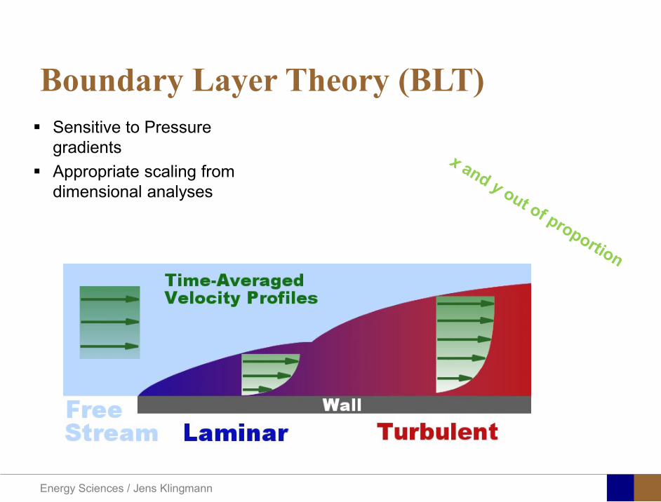
Energy Sciences Jens Klingmann
Boundary Layer Theory (BLT) Sensitive to Pressure
gradients Appropriate scaling from
dimensional analyses
Energy Sciences Jens Klingmann
Boundary layers
Energy Sciences Jens Klingmann
Air foil theory
Energy Sciences Jens Klingmann
Visualisation of diffusor separation
Energy Sciences Jens Klingmann
BL equations
+minus=+
yu
yxp
xuv
xuu
partpartmicro
partpart
partpart
partρpart
partρpart and 0=+
yxu
partυpart
partpart
Applying the BL approximations the 2D stationary incompressible NS-eq and continuity equation become
yvu
yu
yxuu
xp
yu
xuu
partpartρ
partpartmicro
partpart
partρpart
partpart
partυρpart
partρpart
minus
+minusminus=+
and
0=+yx
upart
υpartpartpart
Reynolds averaged BL eqs are
Energy Sciences Jens Klingmann
Boundary layers
Energy Sciences Jens Klingmann
Turbulent BL at different Pressure gradients
Energy Sciences Jens Klingmann
Boundary Layers
ν
yuy =+
ρτWu =
0=
partpart
=y
w yuτ
uuu =+
Energy Sciences Jens Klingmann
Diffuser efficiency
Energy Sciences Jens Klingmann
Reynolds Number (Order of magnitude)
At eg a compressor inlet
ρ = O(1) kgm3
U = O(100) msx lt O(01) mmicro = O(10-5)
Re = ρ U x micro =O(106)
In subsequent stages large amounts of turbulence (from stator wakes) will be convected into the Boundary layer
Energy Sciences Jens Klingmann
References Boundary layers
bull Frank M White ldquoViscous Fluid Flowrdquobull Hermann Schlichting ldquoBoundary Layer Theoryrdquo
Energy Sciences Jens Klingmann
CFD and experiments
bull No this is not a CFD course butbull Experiments
Energy Sciences Jens Klingmann
What do we need to measureOverall performance
Flow rates (mass or volume) Pressure Temperature Shaft power
Performance increase
Separations (velocity) Secondary flows eg tip clearance losses (velocity) Shock waves (supersonic applications) Pressure (resolved in time and space) Temperature (resolved in time and space)
Energy Sciences Jens Klingmann
Cascade wind tunnels
FIG 31 Compressor cascade wind tunnels (a) Conventional low-speed continuousrunning cascade tunnel (adapted from Carter et al 1950)(b) Transonicsupersoniccascade tunnel (adapted from Sieverding 1985)
Energy Sciences Jens Klingmann
Closed circuit tunnels
Energy Sciences Jens Klingmann
components
Settling Chamber
The settling chamber is located between the fan or wide angle diffuser and the contraction and contains the honeycombs and screens used to moderate longitudinal variations in the flow Screens in the chamber should be spaced at 02 chamber diameters apart so that flow disturbed by the first screen can settle before it encounters the second
Honeycombs
Honeycombs are located in the settling chamber and are used to reduce nonuniformities in the flow For optimum benefit honeycombs should be 6-8 cell diameters thick and cell size should be on the order of about 150 cells per settling chamber diameter
Energy Sciences Jens Klingmann
components
Screens
Screens are typically located just downstream of the honeycomb and sometime at the inlet of the test section Screens create a static pressure drop and serve to reduce boundary layer size and increase flow uniformity
Contraction Section
Contractions sections are located between the settling chamber and the test sections and serve to both increase mean velocities at the test section inlet and moderate inconsistencies in the uniformity of the flow Large contraction ratios and short contraction lengths are generally more desirable as they reduce the power loss across the screens and the thickness of boundary layers Small tunnels typically have contraction ratios between 6 and 9
Energy Sciences Jens Klingmann
Flow meters with pressure measurement
Venturi-tube
A1 A2
P1 P2
1 1 2 2C A C A=In the incompressible case
2 21 1 2 2
2 2C P C P
ρ ρ+ = +Assuming horisontal mounting
Energy Sciences Jens Klingmann
Daniel Bernoulli 1700-1782
Daniel Bernoulli was the son of Johann Bernoulli He was born in Groningen while his father held the chair of mathematics there His older brother was Nicolaus(II) Bernoulli and his uncle was Jacob Bernoulli so he was born into a family of leading mathematicians but also into a family where there was unfortunate rivalry jealousy and bitterness
Undoubtedly the most important work which Daniel Bernoulli did was his work on hydrodynamics Even the term itself is based on the title of the work which he produced called Hydrodynamica and before he left St Petersburg Daniel left a draft copy of the book with a printer However the work was not published until 1738 and although he revised it considerably between 1734 and 1738 it is more the presentation that he changed rather then the substance
This work contains for the first time the correct analysis of water flowing from a hole in a container This was based on the principle of conservation of energy which he had studied with his father in 1720 Daniel also discussed pumps and other machines to raise water One remarkable discovery appears in Chapter 10 of Hydrodynamica where Daniel discussed the basis for the kinetic theory of gases He was able to give the basic laws for the theory of gases and gave although not in full detail the equation of state discovered by Van der Waals a century later
Energy Sciences Jens Klingmann
Venturi-tube (2)
22 2 12 2
2
2A PC CA ρ
∆minus =
A1 A2
P1 P2
Solve for eg C2
1 2P P P∆ = minus
( )
12
2 2 21 2
21
PCA Aρ
∆ = minus
and( )
12
2 2 2 2 21 2
21
Pm A C AA Aρρ
∆ = = minus
where
Flow meters with pressure measurement
Energy Sciences Jens Klingmann
Flow meters with pressure measurement
Orifice meters
A1
A2
P1 P2
Applicable for pipe flows Same principle as for Venturi Positioning of pressure taps important Vena contracta and losses require inclusion
of Discharge Coefficient CD
( )
12
2 2 21 2
21D
Pm C AA Aρ ∆ =
minus where ( )1 2ReDC f A A=
CD available from manufacturer (measurements) or Standards (eg ISO)
Energy Sciences Jens Klingmann
Coriolis flow meter
An actuator (not shown) induces a vibration of the tubes
When there is mass flow Coriolis forces induce twisting of the tubes
degree of phase-shift is a measure for the amount of mass that is flowing through the tubes
Energy Sciences Jens Klingmann
Thermal flow meter Heat is added electrically to the flow Temperature is measured before and after heat addition
pP mC T∆=
Energy Sciences Jens Klingmann
Ultrasonic flow meters
Ultrasound is emitted to small particles in the flow (dust or other) Reflections of the sound is frequency shifted by the Doppler effect The frequency change is proportional to the particles velocity (volume flow
meter)
Energy Sciences Jens Klingmann
Inductive flow metersA magnetic flowmeter is based upon Faradays Law
The voltage induced across any conductor as it moves at right angles through a magnetic field is proportional to the velocity of that conductor
E is proportional to V x B x D where
E = The voltage generated in a conductorV = The velocity of the conductorB = The magnetic field strengthD = The length of the conductor
NB electric conductivity is required
Energy Sciences Jens Klingmann
Temperature measurements
Thermocouples
The basis established by Thomas Johann Seebeck in 1821
A conductor generates a voltage when subjected to a temperature gradient
To measure this voltage one must use a second conductor material which generates a different voltage under the same temperature gradient
Energy Sciences Jens Klingmann
Pressure sensing
1 2p pgt 2p p2 may be the atmosphere a static pressure tap or a known reference pressure
The strain of the diaphragm (or itrsquos deflection) may be measured by a number of electric methods
Diaphragm
Energy Sciences Jens Klingmann
Pressure sensingPiezoresistive Strain Gage
Uses the piezoresistive effect of bonded or formed strain gauges to detect strain due to applied pressure
Capacitive
Uses a diaghragm and pressure cavity to create a variable capacitor to detect strain due to applied pressure
Magnetic
Measures the displacement of a diaphragm by means of changes in inductance (reluctance) LVDT Hall Effect or by eddy current principal
Piezoelectric
Uses the piezoelectric effect in certain materials such as quartz to measure the strain upon the sensing mechanism due to pressure
Potentiometric
Uses the motion of a wiper along a resistive mechanism to detect the strain caused by applied pressure
Energy Sciences Jens Klingmann
3D highly instationary (periodic) flow Potentially very high velocities (Supersonic) Large temperature differences Low accessibility (difficult to probe between rotors) Low turbulence levels in most of the domain Very high turbulence in BL and wakes
Properties of measuring object
Point measurements
Energy Sciences Jens Klingmann
Conventional or non-opticalndash Static Pressure Measurementsndash Total Pressure Measurements
bull Multy hole probes
ndash Total Temperature ndash Hot Wire Anemometry (HWA)
Optical techniques for Velocity Measurementsndash Laser Two Focous (L2F)ndash Laser Doppler Anemometry (LDA)ndash Particle Image velocimetry (PIV)
Point Measurements
Energy Sciences Jens Klingmann
Static and total pressure
2 2 21 2 1
2 1 2 2 2C C CP P ρ ρ ρ
minus = minus =
2 0C =Stagnation point
C1Static pressure tap
Prandtl or Pitot tube
Apply the Bernoulli equation from free stream to stagnation point
21
2 12CP Pρ
= +or
We can also define a stagnation or total pressure
( )2
101 1 022
CP P Pρ= + =
Total pressure = Static pressure + dynamic pressure
or
Energy Sciences Jens Klingmann
Static pressure
Energy Sciences Jens Klingmann
Total Pressure and Temperature
Shrouded Probes
Shrouded Probe
Pitot or Prandtl tube
Sensitive to direction
Energy Sciences Jens Klingmann
Ludwig Prandtl 1875-1953
Ludwig Prandtl born at Freising Bavaria on February 4 1875 was a German Physicist famous for his work in aeronautics He qualified at Munchen in 1900 with a thesis on elastic stability and held the position of Professor of Applied Mechanics at Gottingen for forty-nine years (from 1904 until his death there on August 15 1953) In 1925 Prandtl became the Director of the Kaiser Wilhelm Institute for Fluid Mechanics His discovery in 1904 of the Boundary Layer which adjoins the surface of a body moving in a fluid led to an understanding of skin friction drag and of the way in which streamlining reduces the drag of airplane wings and other moving bodies His work on wing theory published in 1918 - 1919 followed that of FW Lanchester (1902-1907) but was carried out independently and elucidated the flow over airplane wings of finite span Prandtls work and decisive advances in boundary layer and wing theories became the basic material of aeronautics He also made important contributions to the theories of supersonic flow and of turbulence and contributed much to the development of wind tunnels and other aerodynamic equipment In addition he devised the soap-film analogy for the torsion of non-circular sections and wrote on the theory of plasticity and of meteorology
Energy Sciences Jens Klingmann
Total Pressure multy hole
Cobra Probe Yaw Probe
5 Hole Probe
Energy Sciences Jens Klingmann
5 Hole Probes Calibration
Energy Sciences Jens Klingmann
The inherent unsteadiness of the flow within turbomachines
Energy Sciences Jens Klingmann
Hot Wire Anemometry (HWA) The heat transfer from a thin (one micron)
electrically heated wire can be used to determine velocity
The resistance of the wire is temperature dependent Within a small temperature range it can be assumed linear R = R0+α R0(Tm-T0) where R0 is the resistance at a reference temperature T0 and Tm is the mean wire temperature
The thermal power induced in the wire is balanced by heat transfer to the surrounding fluid I2R=hπDL(Tm-T0) where h is the heat transfer coefficient and D and L the diameter and length of the wire respectively
E = I R
Energy Sciences Jens Klingmann
Constant Temperature Anemometry (CTA) The wire is often placed in a Whetstone bridge If the output from the
bridge is amplified and fed back to the bridge the resistance of the probe and thus the temperature will be held constant
This prevents the temperature of the wire to become excessive at low velocities
R1
R2 R3
Probe
Bridge Voltage
Energy Sciences Jens Klingmann
Constant Temperature Anemometry (CTA)
Energy Sciences Jens Klingmann
Characteristics of LDA (according to Dantec)
Invented by Yeh and Cummins in 1964 Velocity measurements in Fluid Dynamics (gas liquid) Up to 3 velocity components Non-intrusive measurements (optical technique) Absolute measurement technique (no calibration required) Very high accuracy Very high spatial resolution due to small measurement volume Tracer particles are required
Energy Sciences Jens Klingmann
LDA - Fringe Model
Focused Laser beams intersect and form the measurement volume Plane wave fronts beam waist in the plane of intersection Interference in the plane of intersection Pattern of bright and dark stripesplanes Fringes
Energy Sciences Jens Klingmann
LDA-measuring volume
d
x
x
y
y
z
z
e-2 CONTOUR
FRINGES
κ
κ
κ
κ
De-2
De-2
dml m
a
b
cx
b
z
ya
cd
d
=
=
=
J
J
J
J
JP
JP
JP
JD
JD
JD
+
+
+
a
b
c
d
κπλ
=minus sinD
f4l2e
m
κπλ
=minus cosD
f4D2e
m
Energy Sciences Jens Klingmann
Laser Two Focus
Energy Sciences Jens Klingmann
Laser Two Focus
Energy Sciences Jens Klingmann
PIV measurements
PIV is a fairly new technique capable of simultaneous velocity measurements at many points in a plane This gives information on large scale structures vorticity etc which is very difficult or impossible to obtain from one-point measuring techniques
PIV involves the illumination of a plane of the flow under investigation with a thin pulsed sheet of light The flow is seeded with particles
The light scattered from the particles and from successive pulses are being recorded either on film or a CCD array forming a multiple exposure of each particle image If the time between the pulses is known velocity can be determined as the ratio of the particle displacement and the elapsed time
t∆∆= xu
Energy Sciences Jens Klingmann
PIV
Energy Sciences Jens Klingmann
PIV measurements illumination
YA
G
YA
G
Two frequency doubled YAG Lasers aligned to one double pulsed laser sheet
Two or more separate light pulses can be obtained by chopping a continuous laser or from pulsed lasers
The limited pulse energies obtained from continuous lasers limits their applicability to low velocity flows or flows where large seeding particles can be used (ie liquid flows)
The low repetition rate of most pulsed lasers makes the use of two lasers advantageous
Energy Sciences Jens Klingmann
PIV measurements recording
High seeding density in laminar flame
Film or CCD-cameras Cross- or Auto-correlation
ndash ie both particle images on the same frame or on separate frames
CCD-camera requirementndash A many pixels as possiblendash 2k by 2k available 4k by 4k coming
Energy Sciences Jens Klingmann
PIV measurements analyses
Low seeding density (Number of seeding particles per unit volume)
Each particle image pair can be identified This is called particle tracking
High seeding density (PIV)
Small sub-regions of the image containing many particle image pairs are processed to obtain one velocity vector
Energy Sciences Jens Klingmann
PIV measurements analyses
Energy Sciences Jens Klingmann
PIV measurements analyses
( ) ( ) ( ) xsxxs dIIR 2A
1
I
+= int
Cross correlation between ( )x1I and ( )x2I
s is a two dimensional displacement vector
IA is the interrogation area
Cross correlation between
(
)
x
1
I
and
(
)
x
2
I
s is a two dimensional displacement vector
I
A
is the interrogation area
Energy Sciences Jens Klingmann
Energy Sciences Jens Klingmann
PIV from IOWA state university
Energy Sciences Jens Klingmann
PIV sample of evaluation
Energy Sciences Jens Klingmann
LDA PIV HWA Velocity range 01 mms ndash 300
ms 02 ndash 150 ms
Measuring Volume
D = 005 L = 05 mm
2 by 2 by 05 mm
L = 05 mm
Freq response O(10 000) Hz O(10) Hz O(100 000) Hz Calibration Yes No No Sensitivity to other than velocity
Low (ref Index) Low (ref Index) Large (temperature concentrationshellip)
Continuous Signal
Sometimes Seldom Always
Noise High High Low Turbulence intensity
No limitation Some limitation lt 20
Price O(1 000 000) SEK
O(1 000 000) SEK
O(50 000) SEK
Required Knowledge
High medium Low
Comparison of techniques
Energy Sciences Jens Klingmann
References experiments
R J Goldstein ldquoFluid Mechanics Measurementsrdquo Hemisphere Publishing 1983 A V Johansson amp P H Alfredsson ldquoExperimentella metoder inom
stroumlmningsmekanikenrdquo Inst Foumlr Mekanik KTH F Durst A Melling and J H Whitelaw ldquoPrincipals and Practice of Laser Doppler
Anemometryrdquo 1984 R J Adrian ldquoParticle-imaging techniques for experimental fluid mechnicsrdquo Ann Rev
Fluid Mech 1991
Energy Sciences Jens Klingmann
Sample of LDA-measurements
Rotor blade
Glas window
Emitted beams
Scattered Light
Adjustable mirror
Energy Sciences Jens Klingmann
Axial velocity sorted into 10 bins
0 1 2 3 4 5 6tangential coordinate (degrees)
-20
0
20
40
60
80
100
120
140
160Ax
ial v
eloc
ity a
nd s
tand
ard
devi
atio
n (m
s)
radial position 7 mm from inner window surfaceaxial position 23 mm behind rotor blades
Energy Sciences Jens Klingmann
Axial velocities in the radial-tangential plane
Energy Sciences Jens Klingmann
Airfoils NACA 4-digit
The NACA four-digit wing sections define the profile by
One digit describing maximum camber as percentage of the chord
One digit describing the distance of maximum camber from the airfoil leading edge in tens of percents of the chord
Two digits describing maximum thickness of the airfoil as percent of the chord
Example the NACA 2412 airfoil has a maximum camber of 2 located 40 (04 chords) from the leading edge with a maximum thickness of 12 of the chord
Four-digit series airfoils by default have maximum thickness at 30 of the chord (03 chords) from the leading edge
Energy Sciences Jens Klingmann
Airfoils NACA 4-digit
bull c is the chord lengthbull x is the position along
the chord from 0 to cbull y is the half thickness at
a given value of x (centerline to surface)
bull t is the maximum thickness as a fraction of the chord
Energy Sciences Jens Klingmann
Death by PowerPoint
| LDA | PIV | HWA | |||||
| Velocity range | 01 mms ndash 300 ms | 02 ndash 150 ms | |||||
| Measuring Volume | D = 005 L = 05 mm | 2 by 2 by 05 mm | L = 05 mm | ||||
| Freq response | O(10 000) Hz | O(10) Hz | O(100 000) Hz | ||||
| Calibration | Yes | No | No | ||||
| Sensitivity to other than velocity | Low (ref Index) | Low (ref Index) | Large (temperature concentrationshellip) | ||||
| Continuous Signal | Sometimes | Seldom | Always | ||||
| Noise | High | High | Low | ||||
| Turbulence intensity | No limitation | Some limitation | lt 20 | ||||
| Price | O(1 000 000) SEK | O(1 000 000) SEK | O(50 000) SEK | ||||
| Required Knowledge | High | medium | Low |
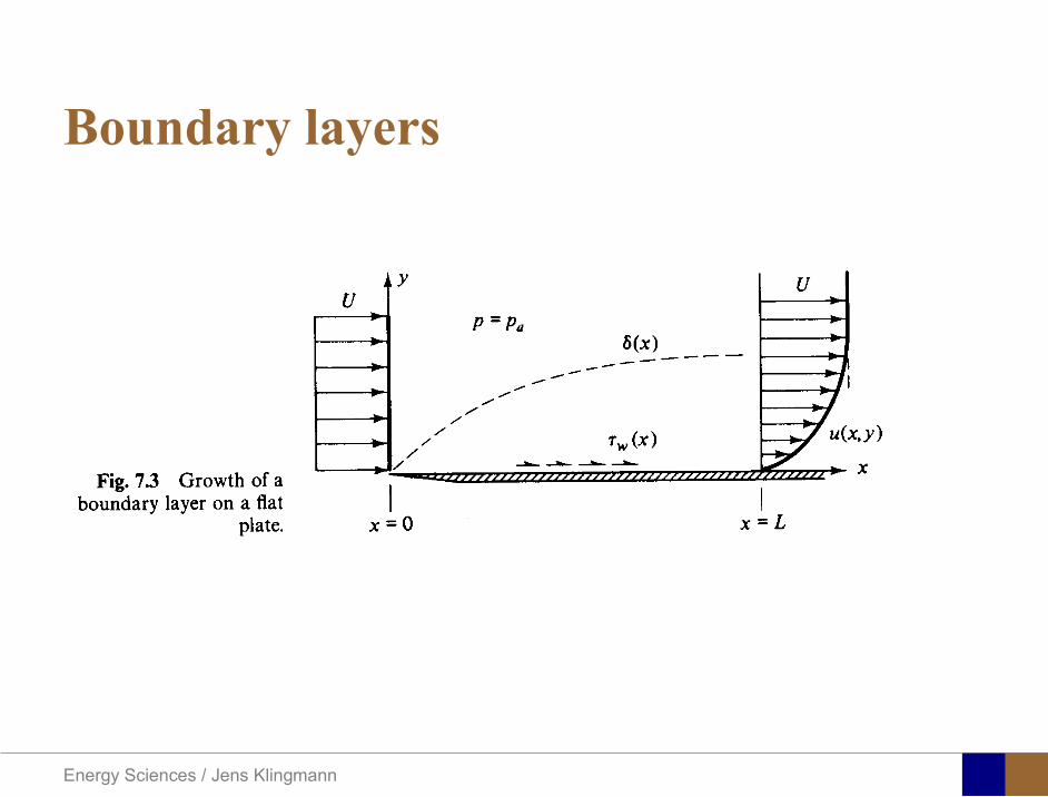
Energy Sciences Jens Klingmann
Boundary layers
Energy Sciences Jens Klingmann
Air foil theory
Energy Sciences Jens Klingmann
Visualisation of diffusor separation
Energy Sciences Jens Klingmann
BL equations
+minus=+
yu
yxp
xuv
xuu
partpartmicro
partpart
partpart
partρpart
partρpart and 0=+
yxu
partυpart
partpart
Applying the BL approximations the 2D stationary incompressible NS-eq and continuity equation become
yvu
yu
yxuu
xp
yu
xuu
partpartρ
partpartmicro
partpart
partρpart
partpart
partυρpart
partρpart
minus
+minusminus=+
and
0=+yx
upart
υpartpartpart
Reynolds averaged BL eqs are
Energy Sciences Jens Klingmann
Boundary layers
Energy Sciences Jens Klingmann
Turbulent BL at different Pressure gradients
Energy Sciences Jens Klingmann
Boundary Layers
ν
yuy =+
ρτWu =
0=
partpart
=y
w yuτ
uuu =+
Energy Sciences Jens Klingmann
Diffuser efficiency
Energy Sciences Jens Klingmann
Reynolds Number (Order of magnitude)
At eg a compressor inlet
ρ = O(1) kgm3
U = O(100) msx lt O(01) mmicro = O(10-5)
Re = ρ U x micro =O(106)
In subsequent stages large amounts of turbulence (from stator wakes) will be convected into the Boundary layer
Energy Sciences Jens Klingmann
References Boundary layers
bull Frank M White ldquoViscous Fluid Flowrdquobull Hermann Schlichting ldquoBoundary Layer Theoryrdquo
Energy Sciences Jens Klingmann
CFD and experiments
bull No this is not a CFD course butbull Experiments
Energy Sciences Jens Klingmann
What do we need to measureOverall performance
Flow rates (mass or volume) Pressure Temperature Shaft power
Performance increase
Separations (velocity) Secondary flows eg tip clearance losses (velocity) Shock waves (supersonic applications) Pressure (resolved in time and space) Temperature (resolved in time and space)
Energy Sciences Jens Klingmann
Cascade wind tunnels
FIG 31 Compressor cascade wind tunnels (a) Conventional low-speed continuousrunning cascade tunnel (adapted from Carter et al 1950)(b) Transonicsupersoniccascade tunnel (adapted from Sieverding 1985)
Energy Sciences Jens Klingmann
Closed circuit tunnels
Energy Sciences Jens Klingmann
components
Settling Chamber
The settling chamber is located between the fan or wide angle diffuser and the contraction and contains the honeycombs and screens used to moderate longitudinal variations in the flow Screens in the chamber should be spaced at 02 chamber diameters apart so that flow disturbed by the first screen can settle before it encounters the second
Honeycombs
Honeycombs are located in the settling chamber and are used to reduce nonuniformities in the flow For optimum benefit honeycombs should be 6-8 cell diameters thick and cell size should be on the order of about 150 cells per settling chamber diameter
Energy Sciences Jens Klingmann
components
Screens
Screens are typically located just downstream of the honeycomb and sometime at the inlet of the test section Screens create a static pressure drop and serve to reduce boundary layer size and increase flow uniformity
Contraction Section
Contractions sections are located between the settling chamber and the test sections and serve to both increase mean velocities at the test section inlet and moderate inconsistencies in the uniformity of the flow Large contraction ratios and short contraction lengths are generally more desirable as they reduce the power loss across the screens and the thickness of boundary layers Small tunnels typically have contraction ratios between 6 and 9
Energy Sciences Jens Klingmann
Flow meters with pressure measurement
Venturi-tube
A1 A2
P1 P2
1 1 2 2C A C A=In the incompressible case
2 21 1 2 2
2 2C P C P
ρ ρ+ = +Assuming horisontal mounting
Energy Sciences Jens Klingmann
Daniel Bernoulli 1700-1782
Daniel Bernoulli was the son of Johann Bernoulli He was born in Groningen while his father held the chair of mathematics there His older brother was Nicolaus(II) Bernoulli and his uncle was Jacob Bernoulli so he was born into a family of leading mathematicians but also into a family where there was unfortunate rivalry jealousy and bitterness
Undoubtedly the most important work which Daniel Bernoulli did was his work on hydrodynamics Even the term itself is based on the title of the work which he produced called Hydrodynamica and before he left St Petersburg Daniel left a draft copy of the book with a printer However the work was not published until 1738 and although he revised it considerably between 1734 and 1738 it is more the presentation that he changed rather then the substance
This work contains for the first time the correct analysis of water flowing from a hole in a container This was based on the principle of conservation of energy which he had studied with his father in 1720 Daniel also discussed pumps and other machines to raise water One remarkable discovery appears in Chapter 10 of Hydrodynamica where Daniel discussed the basis for the kinetic theory of gases He was able to give the basic laws for the theory of gases and gave although not in full detail the equation of state discovered by Van der Waals a century later
Energy Sciences Jens Klingmann
Venturi-tube (2)
22 2 12 2
2
2A PC CA ρ
∆minus =
A1 A2
P1 P2
Solve for eg C2
1 2P P P∆ = minus
( )
12
2 2 21 2
21
PCA Aρ
∆ = minus
and( )
12
2 2 2 2 21 2
21
Pm A C AA Aρρ
∆ = = minus
where
Flow meters with pressure measurement
Energy Sciences Jens Klingmann
Flow meters with pressure measurement
Orifice meters
A1
A2
P1 P2
Applicable for pipe flows Same principle as for Venturi Positioning of pressure taps important Vena contracta and losses require inclusion
of Discharge Coefficient CD
( )
12
2 2 21 2
21D
Pm C AA Aρ ∆ =
minus where ( )1 2ReDC f A A=
CD available from manufacturer (measurements) or Standards (eg ISO)
Energy Sciences Jens Klingmann
Coriolis flow meter
An actuator (not shown) induces a vibration of the tubes
When there is mass flow Coriolis forces induce twisting of the tubes
degree of phase-shift is a measure for the amount of mass that is flowing through the tubes
Energy Sciences Jens Klingmann
Thermal flow meter Heat is added electrically to the flow Temperature is measured before and after heat addition
pP mC T∆=
Energy Sciences Jens Klingmann
Ultrasonic flow meters
Ultrasound is emitted to small particles in the flow (dust or other) Reflections of the sound is frequency shifted by the Doppler effect The frequency change is proportional to the particles velocity (volume flow
meter)
Energy Sciences Jens Klingmann
Inductive flow metersA magnetic flowmeter is based upon Faradays Law
The voltage induced across any conductor as it moves at right angles through a magnetic field is proportional to the velocity of that conductor
E is proportional to V x B x D where
E = The voltage generated in a conductorV = The velocity of the conductorB = The magnetic field strengthD = The length of the conductor
NB electric conductivity is required
Energy Sciences Jens Klingmann
Temperature measurements
Thermocouples
The basis established by Thomas Johann Seebeck in 1821
A conductor generates a voltage when subjected to a temperature gradient
To measure this voltage one must use a second conductor material which generates a different voltage under the same temperature gradient
Energy Sciences Jens Klingmann
Pressure sensing
1 2p pgt 2p p2 may be the atmosphere a static pressure tap or a known reference pressure
The strain of the diaphragm (or itrsquos deflection) may be measured by a number of electric methods
Diaphragm
Energy Sciences Jens Klingmann
Pressure sensingPiezoresistive Strain Gage
Uses the piezoresistive effect of bonded or formed strain gauges to detect strain due to applied pressure
Capacitive
Uses a diaghragm and pressure cavity to create a variable capacitor to detect strain due to applied pressure
Magnetic
Measures the displacement of a diaphragm by means of changes in inductance (reluctance) LVDT Hall Effect or by eddy current principal
Piezoelectric
Uses the piezoelectric effect in certain materials such as quartz to measure the strain upon the sensing mechanism due to pressure
Potentiometric
Uses the motion of a wiper along a resistive mechanism to detect the strain caused by applied pressure
Energy Sciences Jens Klingmann
3D highly instationary (periodic) flow Potentially very high velocities (Supersonic) Large temperature differences Low accessibility (difficult to probe between rotors) Low turbulence levels in most of the domain Very high turbulence in BL and wakes
Properties of measuring object
Point measurements
Energy Sciences Jens Klingmann
Conventional or non-opticalndash Static Pressure Measurementsndash Total Pressure Measurements
bull Multy hole probes
ndash Total Temperature ndash Hot Wire Anemometry (HWA)
Optical techniques for Velocity Measurementsndash Laser Two Focous (L2F)ndash Laser Doppler Anemometry (LDA)ndash Particle Image velocimetry (PIV)
Point Measurements
Energy Sciences Jens Klingmann
Static and total pressure
2 2 21 2 1
2 1 2 2 2C C CP P ρ ρ ρ
minus = minus =
2 0C =Stagnation point
C1Static pressure tap
Prandtl or Pitot tube
Apply the Bernoulli equation from free stream to stagnation point
21
2 12CP Pρ
= +or
We can also define a stagnation or total pressure
( )2
101 1 022
CP P Pρ= + =
Total pressure = Static pressure + dynamic pressure
or
Energy Sciences Jens Klingmann
Static pressure
Energy Sciences Jens Klingmann
Total Pressure and Temperature
Shrouded Probes
Shrouded Probe
Pitot or Prandtl tube
Sensitive to direction
Energy Sciences Jens Klingmann
Ludwig Prandtl 1875-1953
Ludwig Prandtl born at Freising Bavaria on February 4 1875 was a German Physicist famous for his work in aeronautics He qualified at Munchen in 1900 with a thesis on elastic stability and held the position of Professor of Applied Mechanics at Gottingen for forty-nine years (from 1904 until his death there on August 15 1953) In 1925 Prandtl became the Director of the Kaiser Wilhelm Institute for Fluid Mechanics His discovery in 1904 of the Boundary Layer which adjoins the surface of a body moving in a fluid led to an understanding of skin friction drag and of the way in which streamlining reduces the drag of airplane wings and other moving bodies His work on wing theory published in 1918 - 1919 followed that of FW Lanchester (1902-1907) but was carried out independently and elucidated the flow over airplane wings of finite span Prandtls work and decisive advances in boundary layer and wing theories became the basic material of aeronautics He also made important contributions to the theories of supersonic flow and of turbulence and contributed much to the development of wind tunnels and other aerodynamic equipment In addition he devised the soap-film analogy for the torsion of non-circular sections and wrote on the theory of plasticity and of meteorology
Energy Sciences Jens Klingmann
Total Pressure multy hole
Cobra Probe Yaw Probe
5 Hole Probe
Energy Sciences Jens Klingmann
5 Hole Probes Calibration
Energy Sciences Jens Klingmann
The inherent unsteadiness of the flow within turbomachines
Energy Sciences Jens Klingmann
Hot Wire Anemometry (HWA) The heat transfer from a thin (one micron)
electrically heated wire can be used to determine velocity
The resistance of the wire is temperature dependent Within a small temperature range it can be assumed linear R = R0+α R0(Tm-T0) where R0 is the resistance at a reference temperature T0 and Tm is the mean wire temperature
The thermal power induced in the wire is balanced by heat transfer to the surrounding fluid I2R=hπDL(Tm-T0) where h is the heat transfer coefficient and D and L the diameter and length of the wire respectively
E = I R
Energy Sciences Jens Klingmann
Constant Temperature Anemometry (CTA) The wire is often placed in a Whetstone bridge If the output from the
bridge is amplified and fed back to the bridge the resistance of the probe and thus the temperature will be held constant
This prevents the temperature of the wire to become excessive at low velocities
R1
R2 R3
Probe
Bridge Voltage
Energy Sciences Jens Klingmann
Constant Temperature Anemometry (CTA)
Energy Sciences Jens Klingmann
Characteristics of LDA (according to Dantec)
Invented by Yeh and Cummins in 1964 Velocity measurements in Fluid Dynamics (gas liquid) Up to 3 velocity components Non-intrusive measurements (optical technique) Absolute measurement technique (no calibration required) Very high accuracy Very high spatial resolution due to small measurement volume Tracer particles are required
Energy Sciences Jens Klingmann
LDA - Fringe Model
Focused Laser beams intersect and form the measurement volume Plane wave fronts beam waist in the plane of intersection Interference in the plane of intersection Pattern of bright and dark stripesplanes Fringes
Energy Sciences Jens Klingmann
LDA-measuring volume
d
x
x
y
y
z
z
e-2 CONTOUR
FRINGES
κ
κ
κ
κ
De-2
De-2
dml m
a
b
cx
b
z
ya
cd
d
=
=
=
J
J
J
J
JP
JP
JP
JD
JD
JD
+
+
+
a
b
c
d
κπλ
=minus sinD
f4l2e
m
κπλ
=minus cosD
f4D2e
m
Energy Sciences Jens Klingmann
Laser Two Focus
Energy Sciences Jens Klingmann
Laser Two Focus
Energy Sciences Jens Klingmann
PIV measurements
PIV is a fairly new technique capable of simultaneous velocity measurements at many points in a plane This gives information on large scale structures vorticity etc which is very difficult or impossible to obtain from one-point measuring techniques
PIV involves the illumination of a plane of the flow under investigation with a thin pulsed sheet of light The flow is seeded with particles
The light scattered from the particles and from successive pulses are being recorded either on film or a CCD array forming a multiple exposure of each particle image If the time between the pulses is known velocity can be determined as the ratio of the particle displacement and the elapsed time
t∆∆= xu
Energy Sciences Jens Klingmann
PIV
Energy Sciences Jens Klingmann
PIV measurements illumination
YA
G
YA
G
Two frequency doubled YAG Lasers aligned to one double pulsed laser sheet
Two or more separate light pulses can be obtained by chopping a continuous laser or from pulsed lasers
The limited pulse energies obtained from continuous lasers limits their applicability to low velocity flows or flows where large seeding particles can be used (ie liquid flows)
The low repetition rate of most pulsed lasers makes the use of two lasers advantageous
Energy Sciences Jens Klingmann
PIV measurements recording
High seeding density in laminar flame
Film or CCD-cameras Cross- or Auto-correlation
ndash ie both particle images on the same frame or on separate frames
CCD-camera requirementndash A many pixels as possiblendash 2k by 2k available 4k by 4k coming
Energy Sciences Jens Klingmann
PIV measurements analyses
Low seeding density (Number of seeding particles per unit volume)
Each particle image pair can be identified This is called particle tracking
High seeding density (PIV)
Small sub-regions of the image containing many particle image pairs are processed to obtain one velocity vector
Energy Sciences Jens Klingmann
PIV measurements analyses
Energy Sciences Jens Klingmann
PIV measurements analyses
( ) ( ) ( ) xsxxs dIIR 2A
1
I
+= int
Cross correlation between ( )x1I and ( )x2I
s is a two dimensional displacement vector
IA is the interrogation area
Cross correlation between
(
)
x
1
I
and
(
)
x
2
I
s is a two dimensional displacement vector
I
A
is the interrogation area
Energy Sciences Jens Klingmann
Energy Sciences Jens Klingmann
PIV from IOWA state university
Energy Sciences Jens Klingmann
PIV sample of evaluation
Energy Sciences Jens Klingmann
LDA PIV HWA Velocity range 01 mms ndash 300
ms 02 ndash 150 ms
Measuring Volume
D = 005 L = 05 mm
2 by 2 by 05 mm
L = 05 mm
Freq response O(10 000) Hz O(10) Hz O(100 000) Hz Calibration Yes No No Sensitivity to other than velocity
Low (ref Index) Low (ref Index) Large (temperature concentrationshellip)
Continuous Signal
Sometimes Seldom Always
Noise High High Low Turbulence intensity
No limitation Some limitation lt 20
Price O(1 000 000) SEK
O(1 000 000) SEK
O(50 000) SEK
Required Knowledge
High medium Low
Comparison of techniques
Energy Sciences Jens Klingmann
References experiments
R J Goldstein ldquoFluid Mechanics Measurementsrdquo Hemisphere Publishing 1983 A V Johansson amp P H Alfredsson ldquoExperimentella metoder inom
stroumlmningsmekanikenrdquo Inst Foumlr Mekanik KTH F Durst A Melling and J H Whitelaw ldquoPrincipals and Practice of Laser Doppler
Anemometryrdquo 1984 R J Adrian ldquoParticle-imaging techniques for experimental fluid mechnicsrdquo Ann Rev
Fluid Mech 1991
Energy Sciences Jens Klingmann
Sample of LDA-measurements
Rotor blade
Glas window
Emitted beams
Scattered Light
Adjustable mirror
Energy Sciences Jens Klingmann
Axial velocity sorted into 10 bins
0 1 2 3 4 5 6tangential coordinate (degrees)
-20
0
20
40
60
80
100
120
140
160Ax
ial v
eloc
ity a
nd s
tand
ard
devi
atio
n (m
s)
radial position 7 mm from inner window surfaceaxial position 23 mm behind rotor blades
Energy Sciences Jens Klingmann
Axial velocities in the radial-tangential plane
Energy Sciences Jens Klingmann
Airfoils NACA 4-digit
The NACA four-digit wing sections define the profile by
One digit describing maximum camber as percentage of the chord
One digit describing the distance of maximum camber from the airfoil leading edge in tens of percents of the chord
Two digits describing maximum thickness of the airfoil as percent of the chord
Example the NACA 2412 airfoil has a maximum camber of 2 located 40 (04 chords) from the leading edge with a maximum thickness of 12 of the chord
Four-digit series airfoils by default have maximum thickness at 30 of the chord (03 chords) from the leading edge
Energy Sciences Jens Klingmann
Airfoils NACA 4-digit
bull c is the chord lengthbull x is the position along
the chord from 0 to cbull y is the half thickness at
a given value of x (centerline to surface)
bull t is the maximum thickness as a fraction of the chord
Energy Sciences Jens Klingmann
Death by PowerPoint
| LDA | PIV | HWA | |||||
| Velocity range | 01 mms ndash 300 ms | 02 ndash 150 ms | |||||
| Measuring Volume | D = 005 L = 05 mm | 2 by 2 by 05 mm | L = 05 mm | ||||
| Freq response | O(10 000) Hz | O(10) Hz | O(100 000) Hz | ||||
| Calibration | Yes | No | No | ||||
| Sensitivity to other than velocity | Low (ref Index) | Low (ref Index) | Large (temperature concentrationshellip) | ||||
| Continuous Signal | Sometimes | Seldom | Always | ||||
| Noise | High | High | Low | ||||
| Turbulence intensity | No limitation | Some limitation | lt 20 | ||||
| Price | O(1 000 000) SEK | O(1 000 000) SEK | O(50 000) SEK | ||||
| Required Knowledge | High | medium | Low |
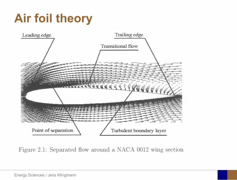
Energy Sciences Jens Klingmann
Air foil theory
Energy Sciences Jens Klingmann
Visualisation of diffusor separation
Energy Sciences Jens Klingmann
BL equations
+minus=+
yu
yxp
xuv
xuu
partpartmicro
partpart
partpart
partρpart
partρpart and 0=+
yxu
partυpart
partpart
Applying the BL approximations the 2D stationary incompressible NS-eq and continuity equation become
yvu
yu
yxuu
xp
yu
xuu
partpartρ
partpartmicro
partpart
partρpart
partpart
partυρpart
partρpart
minus
+minusminus=+
and
0=+yx
upart
υpartpartpart
Reynolds averaged BL eqs are
Energy Sciences Jens Klingmann
Boundary layers
Energy Sciences Jens Klingmann
Turbulent BL at different Pressure gradients
Energy Sciences Jens Klingmann
Boundary Layers
ν
yuy =+
ρτWu =
0=
partpart
=y
w yuτ
uuu =+
Energy Sciences Jens Klingmann
Diffuser efficiency
Energy Sciences Jens Klingmann
Reynolds Number (Order of magnitude)
At eg a compressor inlet
ρ = O(1) kgm3
U = O(100) msx lt O(01) mmicro = O(10-5)
Re = ρ U x micro =O(106)
In subsequent stages large amounts of turbulence (from stator wakes) will be convected into the Boundary layer
Energy Sciences Jens Klingmann
References Boundary layers
bull Frank M White ldquoViscous Fluid Flowrdquobull Hermann Schlichting ldquoBoundary Layer Theoryrdquo
Energy Sciences Jens Klingmann
CFD and experiments
bull No this is not a CFD course butbull Experiments
Energy Sciences Jens Klingmann
What do we need to measureOverall performance
Flow rates (mass or volume) Pressure Temperature Shaft power
Performance increase
Separations (velocity) Secondary flows eg tip clearance losses (velocity) Shock waves (supersonic applications) Pressure (resolved in time and space) Temperature (resolved in time and space)
Energy Sciences Jens Klingmann
Cascade wind tunnels
FIG 31 Compressor cascade wind tunnels (a) Conventional low-speed continuousrunning cascade tunnel (adapted from Carter et al 1950)(b) Transonicsupersoniccascade tunnel (adapted from Sieverding 1985)
Energy Sciences Jens Klingmann
Closed circuit tunnels
Energy Sciences Jens Klingmann
components
Settling Chamber
The settling chamber is located between the fan or wide angle diffuser and the contraction and contains the honeycombs and screens used to moderate longitudinal variations in the flow Screens in the chamber should be spaced at 02 chamber diameters apart so that flow disturbed by the first screen can settle before it encounters the second
Honeycombs
Honeycombs are located in the settling chamber and are used to reduce nonuniformities in the flow For optimum benefit honeycombs should be 6-8 cell diameters thick and cell size should be on the order of about 150 cells per settling chamber diameter
Energy Sciences Jens Klingmann
components
Screens
Screens are typically located just downstream of the honeycomb and sometime at the inlet of the test section Screens create a static pressure drop and serve to reduce boundary layer size and increase flow uniformity
Contraction Section
Contractions sections are located between the settling chamber and the test sections and serve to both increase mean velocities at the test section inlet and moderate inconsistencies in the uniformity of the flow Large contraction ratios and short contraction lengths are generally more desirable as they reduce the power loss across the screens and the thickness of boundary layers Small tunnels typically have contraction ratios between 6 and 9
Energy Sciences Jens Klingmann
Flow meters with pressure measurement
Venturi-tube
A1 A2
P1 P2
1 1 2 2C A C A=In the incompressible case
2 21 1 2 2
2 2C P C P
ρ ρ+ = +Assuming horisontal mounting
Energy Sciences Jens Klingmann
Daniel Bernoulli 1700-1782
Daniel Bernoulli was the son of Johann Bernoulli He was born in Groningen while his father held the chair of mathematics there His older brother was Nicolaus(II) Bernoulli and his uncle was Jacob Bernoulli so he was born into a family of leading mathematicians but also into a family where there was unfortunate rivalry jealousy and bitterness
Undoubtedly the most important work which Daniel Bernoulli did was his work on hydrodynamics Even the term itself is based on the title of the work which he produced called Hydrodynamica and before he left St Petersburg Daniel left a draft copy of the book with a printer However the work was not published until 1738 and although he revised it considerably between 1734 and 1738 it is more the presentation that he changed rather then the substance
This work contains for the first time the correct analysis of water flowing from a hole in a container This was based on the principle of conservation of energy which he had studied with his father in 1720 Daniel also discussed pumps and other machines to raise water One remarkable discovery appears in Chapter 10 of Hydrodynamica where Daniel discussed the basis for the kinetic theory of gases He was able to give the basic laws for the theory of gases and gave although not in full detail the equation of state discovered by Van der Waals a century later
Energy Sciences Jens Klingmann
Venturi-tube (2)
22 2 12 2
2
2A PC CA ρ
∆minus =
A1 A2
P1 P2
Solve for eg C2
1 2P P P∆ = minus
( )
12
2 2 21 2
21
PCA Aρ
∆ = minus
and( )
12
2 2 2 2 21 2
21
Pm A C AA Aρρ
∆ = = minus
where
Flow meters with pressure measurement
Energy Sciences Jens Klingmann
Flow meters with pressure measurement
Orifice meters
A1
A2
P1 P2
Applicable for pipe flows Same principle as for Venturi Positioning of pressure taps important Vena contracta and losses require inclusion
of Discharge Coefficient CD
( )
12
2 2 21 2
21D
Pm C AA Aρ ∆ =
minus where ( )1 2ReDC f A A=
CD available from manufacturer (measurements) or Standards (eg ISO)
Energy Sciences Jens Klingmann
Coriolis flow meter
An actuator (not shown) induces a vibration of the tubes
When there is mass flow Coriolis forces induce twisting of the tubes
degree of phase-shift is a measure for the amount of mass that is flowing through the tubes
Energy Sciences Jens Klingmann
Thermal flow meter Heat is added electrically to the flow Temperature is measured before and after heat addition
pP mC T∆=
Energy Sciences Jens Klingmann
Ultrasonic flow meters
Ultrasound is emitted to small particles in the flow (dust or other) Reflections of the sound is frequency shifted by the Doppler effect The frequency change is proportional to the particles velocity (volume flow
meter)
Energy Sciences Jens Klingmann
Inductive flow metersA magnetic flowmeter is based upon Faradays Law
The voltage induced across any conductor as it moves at right angles through a magnetic field is proportional to the velocity of that conductor
E is proportional to V x B x D where
E = The voltage generated in a conductorV = The velocity of the conductorB = The magnetic field strengthD = The length of the conductor
NB electric conductivity is required
Energy Sciences Jens Klingmann
Temperature measurements
Thermocouples
The basis established by Thomas Johann Seebeck in 1821
A conductor generates a voltage when subjected to a temperature gradient
To measure this voltage one must use a second conductor material which generates a different voltage under the same temperature gradient
Energy Sciences Jens Klingmann
Pressure sensing
1 2p pgt 2p p2 may be the atmosphere a static pressure tap or a known reference pressure
The strain of the diaphragm (or itrsquos deflection) may be measured by a number of electric methods
Diaphragm
Energy Sciences Jens Klingmann
Pressure sensingPiezoresistive Strain Gage
Uses the piezoresistive effect of bonded or formed strain gauges to detect strain due to applied pressure
Capacitive
Uses a diaghragm and pressure cavity to create a variable capacitor to detect strain due to applied pressure
Magnetic
Measures the displacement of a diaphragm by means of changes in inductance (reluctance) LVDT Hall Effect or by eddy current principal
Piezoelectric
Uses the piezoelectric effect in certain materials such as quartz to measure the strain upon the sensing mechanism due to pressure
Potentiometric
Uses the motion of a wiper along a resistive mechanism to detect the strain caused by applied pressure
Energy Sciences Jens Klingmann
3D highly instationary (periodic) flow Potentially very high velocities (Supersonic) Large temperature differences Low accessibility (difficult to probe between rotors) Low turbulence levels in most of the domain Very high turbulence in BL and wakes
Properties of measuring object
Point measurements
Energy Sciences Jens Klingmann
Conventional or non-opticalndash Static Pressure Measurementsndash Total Pressure Measurements
bull Multy hole probes
ndash Total Temperature ndash Hot Wire Anemometry (HWA)
Optical techniques for Velocity Measurementsndash Laser Two Focous (L2F)ndash Laser Doppler Anemometry (LDA)ndash Particle Image velocimetry (PIV)
Point Measurements
Energy Sciences Jens Klingmann
Static and total pressure
2 2 21 2 1
2 1 2 2 2C C CP P ρ ρ ρ
minus = minus =
2 0C =Stagnation point
C1Static pressure tap
Prandtl or Pitot tube
Apply the Bernoulli equation from free stream to stagnation point
21
2 12CP Pρ
= +or
We can also define a stagnation or total pressure
( )2
101 1 022
CP P Pρ= + =
Total pressure = Static pressure + dynamic pressure
or
Energy Sciences Jens Klingmann
Static pressure
Energy Sciences Jens Klingmann
Total Pressure and Temperature
Shrouded Probes
Shrouded Probe
Pitot or Prandtl tube
Sensitive to direction
Energy Sciences Jens Klingmann
Ludwig Prandtl 1875-1953
Ludwig Prandtl born at Freising Bavaria on February 4 1875 was a German Physicist famous for his work in aeronautics He qualified at Munchen in 1900 with a thesis on elastic stability and held the position of Professor of Applied Mechanics at Gottingen for forty-nine years (from 1904 until his death there on August 15 1953) In 1925 Prandtl became the Director of the Kaiser Wilhelm Institute for Fluid Mechanics His discovery in 1904 of the Boundary Layer which adjoins the surface of a body moving in a fluid led to an understanding of skin friction drag and of the way in which streamlining reduces the drag of airplane wings and other moving bodies His work on wing theory published in 1918 - 1919 followed that of FW Lanchester (1902-1907) but was carried out independently and elucidated the flow over airplane wings of finite span Prandtls work and decisive advances in boundary layer and wing theories became the basic material of aeronautics He also made important contributions to the theories of supersonic flow and of turbulence and contributed much to the development of wind tunnels and other aerodynamic equipment In addition he devised the soap-film analogy for the torsion of non-circular sections and wrote on the theory of plasticity and of meteorology
Energy Sciences Jens Klingmann
Total Pressure multy hole
Cobra Probe Yaw Probe
5 Hole Probe
Energy Sciences Jens Klingmann
5 Hole Probes Calibration
Energy Sciences Jens Klingmann
The inherent unsteadiness of the flow within turbomachines
Energy Sciences Jens Klingmann
Hot Wire Anemometry (HWA) The heat transfer from a thin (one micron)
electrically heated wire can be used to determine velocity
The resistance of the wire is temperature dependent Within a small temperature range it can be assumed linear R = R0+α R0(Tm-T0) where R0 is the resistance at a reference temperature T0 and Tm is the mean wire temperature
The thermal power induced in the wire is balanced by heat transfer to the surrounding fluid I2R=hπDL(Tm-T0) where h is the heat transfer coefficient and D and L the diameter and length of the wire respectively
E = I R
Energy Sciences Jens Klingmann
Constant Temperature Anemometry (CTA) The wire is often placed in a Whetstone bridge If the output from the
bridge is amplified and fed back to the bridge the resistance of the probe and thus the temperature will be held constant
This prevents the temperature of the wire to become excessive at low velocities
R1
R2 R3
Probe
Bridge Voltage
Energy Sciences Jens Klingmann
Constant Temperature Anemometry (CTA)
Energy Sciences Jens Klingmann
Characteristics of LDA (according to Dantec)
Invented by Yeh and Cummins in 1964 Velocity measurements in Fluid Dynamics (gas liquid) Up to 3 velocity components Non-intrusive measurements (optical technique) Absolute measurement technique (no calibration required) Very high accuracy Very high spatial resolution due to small measurement volume Tracer particles are required
Energy Sciences Jens Klingmann
LDA - Fringe Model
Focused Laser beams intersect and form the measurement volume Plane wave fronts beam waist in the plane of intersection Interference in the plane of intersection Pattern of bright and dark stripesplanes Fringes
Energy Sciences Jens Klingmann
LDA-measuring volume
d
x
x
y
y
z
z
e-2 CONTOUR
FRINGES
κ
κ
κ
κ
De-2
De-2
dml m
a
b
cx
b
z
ya
cd
d
=
=
=
J
J
J
J
JP
JP
JP
JD
JD
JD
+
+
+
a
b
c
d
κπλ
=minus sinD
f4l2e
m
κπλ
=minus cosD
f4D2e
m
Energy Sciences Jens Klingmann
Laser Two Focus
Energy Sciences Jens Klingmann
Laser Two Focus
Energy Sciences Jens Klingmann
PIV measurements
PIV is a fairly new technique capable of simultaneous velocity measurements at many points in a plane This gives information on large scale structures vorticity etc which is very difficult or impossible to obtain from one-point measuring techniques
PIV involves the illumination of a plane of the flow under investigation with a thin pulsed sheet of light The flow is seeded with particles
The light scattered from the particles and from successive pulses are being recorded either on film or a CCD array forming a multiple exposure of each particle image If the time between the pulses is known velocity can be determined as the ratio of the particle displacement and the elapsed time
t∆∆= xu
Energy Sciences Jens Klingmann
PIV
Energy Sciences Jens Klingmann
PIV measurements illumination
YA
G
YA
G
Two frequency doubled YAG Lasers aligned to one double pulsed laser sheet
Two or more separate light pulses can be obtained by chopping a continuous laser or from pulsed lasers
The limited pulse energies obtained from continuous lasers limits their applicability to low velocity flows or flows where large seeding particles can be used (ie liquid flows)
The low repetition rate of most pulsed lasers makes the use of two lasers advantageous
Energy Sciences Jens Klingmann
PIV measurements recording
High seeding density in laminar flame
Film or CCD-cameras Cross- or Auto-correlation
ndash ie both particle images on the same frame or on separate frames
CCD-camera requirementndash A many pixels as possiblendash 2k by 2k available 4k by 4k coming
Energy Sciences Jens Klingmann
PIV measurements analyses
Low seeding density (Number of seeding particles per unit volume)
Each particle image pair can be identified This is called particle tracking
High seeding density (PIV)
Small sub-regions of the image containing many particle image pairs are processed to obtain one velocity vector
Energy Sciences Jens Klingmann
PIV measurements analyses
Energy Sciences Jens Klingmann
PIV measurements analyses
( ) ( ) ( ) xsxxs dIIR 2A
1
I
+= int
Cross correlation between ( )x1I and ( )x2I
s is a two dimensional displacement vector
IA is the interrogation area
Cross correlation between
(
)
x
1
I
and
(
)
x
2
I
s is a two dimensional displacement vector
I
A
is the interrogation area
Energy Sciences Jens Klingmann
Energy Sciences Jens Klingmann
PIV from IOWA state university
Energy Sciences Jens Klingmann
PIV sample of evaluation
Energy Sciences Jens Klingmann
LDA PIV HWA Velocity range 01 mms ndash 300
ms 02 ndash 150 ms
Measuring Volume
D = 005 L = 05 mm
2 by 2 by 05 mm
L = 05 mm
Freq response O(10 000) Hz O(10) Hz O(100 000) Hz Calibration Yes No No Sensitivity to other than velocity
Low (ref Index) Low (ref Index) Large (temperature concentrationshellip)
Continuous Signal
Sometimes Seldom Always
Noise High High Low Turbulence intensity
No limitation Some limitation lt 20
Price O(1 000 000) SEK
O(1 000 000) SEK
O(50 000) SEK
Required Knowledge
High medium Low
Comparison of techniques
Energy Sciences Jens Klingmann
References experiments
R J Goldstein ldquoFluid Mechanics Measurementsrdquo Hemisphere Publishing 1983 A V Johansson amp P H Alfredsson ldquoExperimentella metoder inom
stroumlmningsmekanikenrdquo Inst Foumlr Mekanik KTH F Durst A Melling and J H Whitelaw ldquoPrincipals and Practice of Laser Doppler
Anemometryrdquo 1984 R J Adrian ldquoParticle-imaging techniques for experimental fluid mechnicsrdquo Ann Rev
Fluid Mech 1991
Energy Sciences Jens Klingmann
Sample of LDA-measurements
Rotor blade
Glas window
Emitted beams
Scattered Light
Adjustable mirror
Energy Sciences Jens Klingmann
Axial velocity sorted into 10 bins
0 1 2 3 4 5 6tangential coordinate (degrees)
-20
0
20
40
60
80
100
120
140
160Ax
ial v
eloc
ity a
nd s
tand
ard
devi
atio
n (m
s)
radial position 7 mm from inner window surfaceaxial position 23 mm behind rotor blades
Energy Sciences Jens Klingmann
Axial velocities in the radial-tangential plane
Energy Sciences Jens Klingmann
Airfoils NACA 4-digit
The NACA four-digit wing sections define the profile by
One digit describing maximum camber as percentage of the chord
One digit describing the distance of maximum camber from the airfoil leading edge in tens of percents of the chord
Two digits describing maximum thickness of the airfoil as percent of the chord
Example the NACA 2412 airfoil has a maximum camber of 2 located 40 (04 chords) from the leading edge with a maximum thickness of 12 of the chord
Four-digit series airfoils by default have maximum thickness at 30 of the chord (03 chords) from the leading edge
Energy Sciences Jens Klingmann
Airfoils NACA 4-digit
bull c is the chord lengthbull x is the position along
the chord from 0 to cbull y is the half thickness at
a given value of x (centerline to surface)
bull t is the maximum thickness as a fraction of the chord
Energy Sciences Jens Klingmann
Death by PowerPoint
| LDA | PIV | HWA | |||||
| Velocity range | 01 mms ndash 300 ms | 02 ndash 150 ms | |||||
| Measuring Volume | D = 005 L = 05 mm | 2 by 2 by 05 mm | L = 05 mm | ||||
| Freq response | O(10 000) Hz | O(10) Hz | O(100 000) Hz | ||||
| Calibration | Yes | No | No | ||||
| Sensitivity to other than velocity | Low (ref Index) | Low (ref Index) | Large (temperature concentrationshellip) | ||||
| Continuous Signal | Sometimes | Seldom | Always | ||||
| Noise | High | High | Low | ||||
| Turbulence intensity | No limitation | Some limitation | lt 20 | ||||
| Price | O(1 000 000) SEK | O(1 000 000) SEK | O(50 000) SEK | ||||
| Required Knowledge | High | medium | Low |
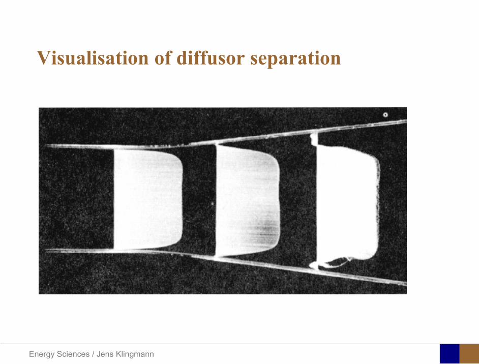
Energy Sciences Jens Klingmann
Visualisation of diffusor separation
Energy Sciences Jens Klingmann
BL equations
+minus=+
yu
yxp
xuv
xuu
partpartmicro
partpart
partpart
partρpart
partρpart and 0=+
yxu
partυpart
partpart
Applying the BL approximations the 2D stationary incompressible NS-eq and continuity equation become
yvu
yu
yxuu
xp
yu
xuu
partpartρ
partpartmicro
partpart
partρpart
partpart
partυρpart
partρpart
minus
+minusminus=+
and
0=+yx
upart
υpartpartpart
Reynolds averaged BL eqs are
Energy Sciences Jens Klingmann
Boundary layers
Energy Sciences Jens Klingmann
Turbulent BL at different Pressure gradients
Energy Sciences Jens Klingmann
Boundary Layers
ν
yuy =+
ρτWu =
0=
partpart
=y
w yuτ
uuu =+
Energy Sciences Jens Klingmann
Diffuser efficiency
Energy Sciences Jens Klingmann
Reynolds Number (Order of magnitude)
At eg a compressor inlet
ρ = O(1) kgm3
U = O(100) msx lt O(01) mmicro = O(10-5)
Re = ρ U x micro =O(106)
In subsequent stages large amounts of turbulence (from stator wakes) will be convected into the Boundary layer
Energy Sciences Jens Klingmann
References Boundary layers
bull Frank M White ldquoViscous Fluid Flowrdquobull Hermann Schlichting ldquoBoundary Layer Theoryrdquo
Energy Sciences Jens Klingmann
CFD and experiments
bull No this is not a CFD course butbull Experiments
Energy Sciences Jens Klingmann
What do we need to measureOverall performance
Flow rates (mass or volume) Pressure Temperature Shaft power
Performance increase
Separations (velocity) Secondary flows eg tip clearance losses (velocity) Shock waves (supersonic applications) Pressure (resolved in time and space) Temperature (resolved in time and space)
Energy Sciences Jens Klingmann
Cascade wind tunnels
FIG 31 Compressor cascade wind tunnels (a) Conventional low-speed continuousrunning cascade tunnel (adapted from Carter et al 1950)(b) Transonicsupersoniccascade tunnel (adapted from Sieverding 1985)
Energy Sciences Jens Klingmann
Closed circuit tunnels
Energy Sciences Jens Klingmann
components
Settling Chamber
The settling chamber is located between the fan or wide angle diffuser and the contraction and contains the honeycombs and screens used to moderate longitudinal variations in the flow Screens in the chamber should be spaced at 02 chamber diameters apart so that flow disturbed by the first screen can settle before it encounters the second
Honeycombs
Honeycombs are located in the settling chamber and are used to reduce nonuniformities in the flow For optimum benefit honeycombs should be 6-8 cell diameters thick and cell size should be on the order of about 150 cells per settling chamber diameter
Energy Sciences Jens Klingmann
components
Screens
Screens are typically located just downstream of the honeycomb and sometime at the inlet of the test section Screens create a static pressure drop and serve to reduce boundary layer size and increase flow uniformity
Contraction Section
Contractions sections are located between the settling chamber and the test sections and serve to both increase mean velocities at the test section inlet and moderate inconsistencies in the uniformity of the flow Large contraction ratios and short contraction lengths are generally more desirable as they reduce the power loss across the screens and the thickness of boundary layers Small tunnels typically have contraction ratios between 6 and 9
Energy Sciences Jens Klingmann
Flow meters with pressure measurement
Venturi-tube
A1 A2
P1 P2
1 1 2 2C A C A=In the incompressible case
2 21 1 2 2
2 2C P C P
ρ ρ+ = +Assuming horisontal mounting
Energy Sciences Jens Klingmann
Daniel Bernoulli 1700-1782
Daniel Bernoulli was the son of Johann Bernoulli He was born in Groningen while his father held the chair of mathematics there His older brother was Nicolaus(II) Bernoulli and his uncle was Jacob Bernoulli so he was born into a family of leading mathematicians but also into a family where there was unfortunate rivalry jealousy and bitterness
Undoubtedly the most important work which Daniel Bernoulli did was his work on hydrodynamics Even the term itself is based on the title of the work which he produced called Hydrodynamica and before he left St Petersburg Daniel left a draft copy of the book with a printer However the work was not published until 1738 and although he revised it considerably between 1734 and 1738 it is more the presentation that he changed rather then the substance
This work contains for the first time the correct analysis of water flowing from a hole in a container This was based on the principle of conservation of energy which he had studied with his father in 1720 Daniel also discussed pumps and other machines to raise water One remarkable discovery appears in Chapter 10 of Hydrodynamica where Daniel discussed the basis for the kinetic theory of gases He was able to give the basic laws for the theory of gases and gave although not in full detail the equation of state discovered by Van der Waals a century later
Energy Sciences Jens Klingmann
Venturi-tube (2)
22 2 12 2
2
2A PC CA ρ
∆minus =
A1 A2
P1 P2
Solve for eg C2
1 2P P P∆ = minus
( )
12
2 2 21 2
21
PCA Aρ
∆ = minus
and( )
12
2 2 2 2 21 2
21
Pm A C AA Aρρ
∆ = = minus
where
Flow meters with pressure measurement
Energy Sciences Jens Klingmann
Flow meters with pressure measurement
Orifice meters
A1
A2
P1 P2
Applicable for pipe flows Same principle as for Venturi Positioning of pressure taps important Vena contracta and losses require inclusion
of Discharge Coefficient CD
( )
12
2 2 21 2
21D
Pm C AA Aρ ∆ =
minus where ( )1 2ReDC f A A=
CD available from manufacturer (measurements) or Standards (eg ISO)
Energy Sciences Jens Klingmann
Coriolis flow meter
An actuator (not shown) induces a vibration of the tubes
When there is mass flow Coriolis forces induce twisting of the tubes
degree of phase-shift is a measure for the amount of mass that is flowing through the tubes
Energy Sciences Jens Klingmann
Thermal flow meter Heat is added electrically to the flow Temperature is measured before and after heat addition
pP mC T∆=
Energy Sciences Jens Klingmann
Ultrasonic flow meters
Ultrasound is emitted to small particles in the flow (dust or other) Reflections of the sound is frequency shifted by the Doppler effect The frequency change is proportional to the particles velocity (volume flow
meter)
Energy Sciences Jens Klingmann
Inductive flow metersA magnetic flowmeter is based upon Faradays Law
The voltage induced across any conductor as it moves at right angles through a magnetic field is proportional to the velocity of that conductor
E is proportional to V x B x D where
E = The voltage generated in a conductorV = The velocity of the conductorB = The magnetic field strengthD = The length of the conductor
NB electric conductivity is required
Energy Sciences Jens Klingmann
Temperature measurements
Thermocouples
The basis established by Thomas Johann Seebeck in 1821
A conductor generates a voltage when subjected to a temperature gradient
To measure this voltage one must use a second conductor material which generates a different voltage under the same temperature gradient
Energy Sciences Jens Klingmann
Pressure sensing
1 2p pgt 2p p2 may be the atmosphere a static pressure tap or a known reference pressure
The strain of the diaphragm (or itrsquos deflection) may be measured by a number of electric methods
Diaphragm
Energy Sciences Jens Klingmann
Pressure sensingPiezoresistive Strain Gage
Uses the piezoresistive effect of bonded or formed strain gauges to detect strain due to applied pressure
Capacitive
Uses a diaghragm and pressure cavity to create a variable capacitor to detect strain due to applied pressure
Magnetic
Measures the displacement of a diaphragm by means of changes in inductance (reluctance) LVDT Hall Effect or by eddy current principal
Piezoelectric
Uses the piezoelectric effect in certain materials such as quartz to measure the strain upon the sensing mechanism due to pressure
Potentiometric
Uses the motion of a wiper along a resistive mechanism to detect the strain caused by applied pressure
Energy Sciences Jens Klingmann
3D highly instationary (periodic) flow Potentially very high velocities (Supersonic) Large temperature differences Low accessibility (difficult to probe between rotors) Low turbulence levels in most of the domain Very high turbulence in BL and wakes
Properties of measuring object
Point measurements
Energy Sciences Jens Klingmann
Conventional or non-opticalndash Static Pressure Measurementsndash Total Pressure Measurements
bull Multy hole probes
ndash Total Temperature ndash Hot Wire Anemometry (HWA)
Optical techniques for Velocity Measurementsndash Laser Two Focous (L2F)ndash Laser Doppler Anemometry (LDA)ndash Particle Image velocimetry (PIV)
Point Measurements
Energy Sciences Jens Klingmann
Static and total pressure
2 2 21 2 1
2 1 2 2 2C C CP P ρ ρ ρ
minus = minus =
2 0C =Stagnation point
C1Static pressure tap
Prandtl or Pitot tube
Apply the Bernoulli equation from free stream to stagnation point
21
2 12CP Pρ
= +or
We can also define a stagnation or total pressure
( )2
101 1 022
CP P Pρ= + =
Total pressure = Static pressure + dynamic pressure
or
Energy Sciences Jens Klingmann
Static pressure
Energy Sciences Jens Klingmann
Total Pressure and Temperature
Shrouded Probes
Shrouded Probe
Pitot or Prandtl tube
Sensitive to direction
Energy Sciences Jens Klingmann
Ludwig Prandtl 1875-1953
Ludwig Prandtl born at Freising Bavaria on February 4 1875 was a German Physicist famous for his work in aeronautics He qualified at Munchen in 1900 with a thesis on elastic stability and held the position of Professor of Applied Mechanics at Gottingen for forty-nine years (from 1904 until his death there on August 15 1953) In 1925 Prandtl became the Director of the Kaiser Wilhelm Institute for Fluid Mechanics His discovery in 1904 of the Boundary Layer which adjoins the surface of a body moving in a fluid led to an understanding of skin friction drag and of the way in which streamlining reduces the drag of airplane wings and other moving bodies His work on wing theory published in 1918 - 1919 followed that of FW Lanchester (1902-1907) but was carried out independently and elucidated the flow over airplane wings of finite span Prandtls work and decisive advances in boundary layer and wing theories became the basic material of aeronautics He also made important contributions to the theories of supersonic flow and of turbulence and contributed much to the development of wind tunnels and other aerodynamic equipment In addition he devised the soap-film analogy for the torsion of non-circular sections and wrote on the theory of plasticity and of meteorology
Energy Sciences Jens Klingmann
Total Pressure multy hole
Cobra Probe Yaw Probe
5 Hole Probe
Energy Sciences Jens Klingmann
5 Hole Probes Calibration
Energy Sciences Jens Klingmann
The inherent unsteadiness of the flow within turbomachines
Energy Sciences Jens Klingmann
Hot Wire Anemometry (HWA) The heat transfer from a thin (one micron)
electrically heated wire can be used to determine velocity
The resistance of the wire is temperature dependent Within a small temperature range it can be assumed linear R = R0+α R0(Tm-T0) where R0 is the resistance at a reference temperature T0 and Tm is the mean wire temperature
The thermal power induced in the wire is balanced by heat transfer to the surrounding fluid I2R=hπDL(Tm-T0) where h is the heat transfer coefficient and D and L the diameter and length of the wire respectively
E = I R
Energy Sciences Jens Klingmann
Constant Temperature Anemometry (CTA) The wire is often placed in a Whetstone bridge If the output from the
bridge is amplified and fed back to the bridge the resistance of the probe and thus the temperature will be held constant
This prevents the temperature of the wire to become excessive at low velocities
R1
R2 R3
Probe
Bridge Voltage
Energy Sciences Jens Klingmann
Constant Temperature Anemometry (CTA)
Energy Sciences Jens Klingmann
Characteristics of LDA (according to Dantec)
Invented by Yeh and Cummins in 1964 Velocity measurements in Fluid Dynamics (gas liquid) Up to 3 velocity components Non-intrusive measurements (optical technique) Absolute measurement technique (no calibration required) Very high accuracy Very high spatial resolution due to small measurement volume Tracer particles are required
Energy Sciences Jens Klingmann
LDA - Fringe Model
Focused Laser beams intersect and form the measurement volume Plane wave fronts beam waist in the plane of intersection Interference in the plane of intersection Pattern of bright and dark stripesplanes Fringes
Energy Sciences Jens Klingmann
LDA-measuring volume
d
x
x
y
y
z
z
e-2 CONTOUR
FRINGES
κ
κ
κ
κ
De-2
De-2
dml m
a
b
cx
b
z
ya
cd
d
=
=
=
J
J
J
J
JP
JP
JP
JD
JD
JD
+
+
+
a
b
c
d
κπλ
=minus sinD
f4l2e
m
κπλ
=minus cosD
f4D2e
m
Energy Sciences Jens Klingmann
Laser Two Focus
Energy Sciences Jens Klingmann
Laser Two Focus
Energy Sciences Jens Klingmann
PIV measurements
PIV is a fairly new technique capable of simultaneous velocity measurements at many points in a plane This gives information on large scale structures vorticity etc which is very difficult or impossible to obtain from one-point measuring techniques
PIV involves the illumination of a plane of the flow under investigation with a thin pulsed sheet of light The flow is seeded with particles
The light scattered from the particles and from successive pulses are being recorded either on film or a CCD array forming a multiple exposure of each particle image If the time between the pulses is known velocity can be determined as the ratio of the particle displacement and the elapsed time
t∆∆= xu
Energy Sciences Jens Klingmann
PIV
Energy Sciences Jens Klingmann
PIV measurements illumination
YA
G
YA
G
Two frequency doubled YAG Lasers aligned to one double pulsed laser sheet
Two or more separate light pulses can be obtained by chopping a continuous laser or from pulsed lasers
The limited pulse energies obtained from continuous lasers limits their applicability to low velocity flows or flows where large seeding particles can be used (ie liquid flows)
The low repetition rate of most pulsed lasers makes the use of two lasers advantageous
Energy Sciences Jens Klingmann
PIV measurements recording
High seeding density in laminar flame
Film or CCD-cameras Cross- or Auto-correlation
ndash ie both particle images on the same frame or on separate frames
CCD-camera requirementndash A many pixels as possiblendash 2k by 2k available 4k by 4k coming
Energy Sciences Jens Klingmann
PIV measurements analyses
Low seeding density (Number of seeding particles per unit volume)
Each particle image pair can be identified This is called particle tracking
High seeding density (PIV)
Small sub-regions of the image containing many particle image pairs are processed to obtain one velocity vector
Energy Sciences Jens Klingmann
PIV measurements analyses
Energy Sciences Jens Klingmann
PIV measurements analyses
( ) ( ) ( ) xsxxs dIIR 2A
1
I
+= int
Cross correlation between ( )x1I and ( )x2I
s is a two dimensional displacement vector
IA is the interrogation area
Cross correlation between
(
)
x
1
I
and
(
)
x
2
I
s is a two dimensional displacement vector
I
A
is the interrogation area
Energy Sciences Jens Klingmann
Energy Sciences Jens Klingmann
PIV from IOWA state university
Energy Sciences Jens Klingmann
PIV sample of evaluation
Energy Sciences Jens Klingmann
LDA PIV HWA Velocity range 01 mms ndash 300
ms 02 ndash 150 ms
Measuring Volume
D = 005 L = 05 mm
2 by 2 by 05 mm
L = 05 mm
Freq response O(10 000) Hz O(10) Hz O(100 000) Hz Calibration Yes No No Sensitivity to other than velocity
Low (ref Index) Low (ref Index) Large (temperature concentrationshellip)
Continuous Signal
Sometimes Seldom Always
Noise High High Low Turbulence intensity
No limitation Some limitation lt 20
Price O(1 000 000) SEK
O(1 000 000) SEK
O(50 000) SEK
Required Knowledge
High medium Low
Comparison of techniques
Energy Sciences Jens Klingmann
References experiments
R J Goldstein ldquoFluid Mechanics Measurementsrdquo Hemisphere Publishing 1983 A V Johansson amp P H Alfredsson ldquoExperimentella metoder inom
stroumlmningsmekanikenrdquo Inst Foumlr Mekanik KTH F Durst A Melling and J H Whitelaw ldquoPrincipals and Practice of Laser Doppler
Anemometryrdquo 1984 R J Adrian ldquoParticle-imaging techniques for experimental fluid mechnicsrdquo Ann Rev
Fluid Mech 1991
Energy Sciences Jens Klingmann
Sample of LDA-measurements
Rotor blade
Glas window
Emitted beams
Scattered Light
Adjustable mirror
Energy Sciences Jens Klingmann
Axial velocity sorted into 10 bins
0 1 2 3 4 5 6tangential coordinate (degrees)
-20
0
20
40
60
80
100
120
140
160Ax
ial v
eloc
ity a
nd s
tand
ard
devi
atio
n (m
s)
radial position 7 mm from inner window surfaceaxial position 23 mm behind rotor blades
Energy Sciences Jens Klingmann
Axial velocities in the radial-tangential plane
Energy Sciences Jens Klingmann
Airfoils NACA 4-digit
The NACA four-digit wing sections define the profile by
One digit describing maximum camber as percentage of the chord
One digit describing the distance of maximum camber from the airfoil leading edge in tens of percents of the chord
Two digits describing maximum thickness of the airfoil as percent of the chord
Example the NACA 2412 airfoil has a maximum camber of 2 located 40 (04 chords) from the leading edge with a maximum thickness of 12 of the chord
Four-digit series airfoils by default have maximum thickness at 30 of the chord (03 chords) from the leading edge
Energy Sciences Jens Klingmann
Airfoils NACA 4-digit
bull c is the chord lengthbull x is the position along
the chord from 0 to cbull y is the half thickness at
a given value of x (centerline to surface)
bull t is the maximum thickness as a fraction of the chord
Energy Sciences Jens Klingmann
Death by PowerPoint
| LDA | PIV | HWA | |||||
| Velocity range | 01 mms ndash 300 ms | 02 ndash 150 ms | |||||
| Measuring Volume | D = 005 L = 05 mm | 2 by 2 by 05 mm | L = 05 mm | ||||
| Freq response | O(10 000) Hz | O(10) Hz | O(100 000) Hz | ||||
| Calibration | Yes | No | No | ||||
| Sensitivity to other than velocity | Low (ref Index) | Low (ref Index) | Large (temperature concentrationshellip) | ||||
| Continuous Signal | Sometimes | Seldom | Always | ||||
| Noise | High | High | Low | ||||
| Turbulence intensity | No limitation | Some limitation | lt 20 | ||||
| Price | O(1 000 000) SEK | O(1 000 000) SEK | O(50 000) SEK | ||||
| Required Knowledge | High | medium | Low |
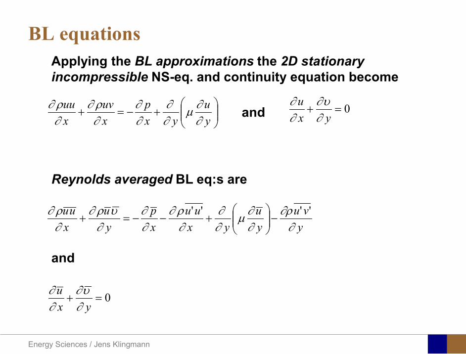
Energy Sciences Jens Klingmann
BL equations
+minus=+
yu
yxp
xuv
xuu
partpartmicro
partpart
partpart
partρpart
partρpart and 0=+
yxu
partυpart
partpart
Applying the BL approximations the 2D stationary incompressible NS-eq and continuity equation become
yvu
yu
yxuu
xp
yu
xuu
partpartρ
partpartmicro
partpart
partρpart
partpart
partυρpart
partρpart
minus
+minusminus=+
and
0=+yx
upart
υpartpartpart
Reynolds averaged BL eqs are
Energy Sciences Jens Klingmann
Boundary layers
Energy Sciences Jens Klingmann
Turbulent BL at different Pressure gradients
Energy Sciences Jens Klingmann
Boundary Layers
ν
yuy =+
ρτWu =
0=
partpart
=y
w yuτ
uuu =+
Energy Sciences Jens Klingmann
Diffuser efficiency
Energy Sciences Jens Klingmann
Reynolds Number (Order of magnitude)
At eg a compressor inlet
ρ = O(1) kgm3
U = O(100) msx lt O(01) mmicro = O(10-5)
Re = ρ U x micro =O(106)
In subsequent stages large amounts of turbulence (from stator wakes) will be convected into the Boundary layer
Energy Sciences Jens Klingmann
References Boundary layers
bull Frank M White ldquoViscous Fluid Flowrdquobull Hermann Schlichting ldquoBoundary Layer Theoryrdquo
Energy Sciences Jens Klingmann
CFD and experiments
bull No this is not a CFD course butbull Experiments
Energy Sciences Jens Klingmann
What do we need to measureOverall performance
Flow rates (mass or volume) Pressure Temperature Shaft power
Performance increase
Separations (velocity) Secondary flows eg tip clearance losses (velocity) Shock waves (supersonic applications) Pressure (resolved in time and space) Temperature (resolved in time and space)
Energy Sciences Jens Klingmann
Cascade wind tunnels
FIG 31 Compressor cascade wind tunnels (a) Conventional low-speed continuousrunning cascade tunnel (adapted from Carter et al 1950)(b) Transonicsupersoniccascade tunnel (adapted from Sieverding 1985)
Energy Sciences Jens Klingmann
Closed circuit tunnels
Energy Sciences Jens Klingmann
components
Settling Chamber
The settling chamber is located between the fan or wide angle diffuser and the contraction and contains the honeycombs and screens used to moderate longitudinal variations in the flow Screens in the chamber should be spaced at 02 chamber diameters apart so that flow disturbed by the first screen can settle before it encounters the second
Honeycombs
Honeycombs are located in the settling chamber and are used to reduce nonuniformities in the flow For optimum benefit honeycombs should be 6-8 cell diameters thick and cell size should be on the order of about 150 cells per settling chamber diameter
Energy Sciences Jens Klingmann
components
Screens
Screens are typically located just downstream of the honeycomb and sometime at the inlet of the test section Screens create a static pressure drop and serve to reduce boundary layer size and increase flow uniformity
Contraction Section
Contractions sections are located between the settling chamber and the test sections and serve to both increase mean velocities at the test section inlet and moderate inconsistencies in the uniformity of the flow Large contraction ratios and short contraction lengths are generally more desirable as they reduce the power loss across the screens and the thickness of boundary layers Small tunnels typically have contraction ratios between 6 and 9
Energy Sciences Jens Klingmann
Flow meters with pressure measurement
Venturi-tube
A1 A2
P1 P2
1 1 2 2C A C A=In the incompressible case
2 21 1 2 2
2 2C P C P
ρ ρ+ = +Assuming horisontal mounting
Energy Sciences Jens Klingmann
Daniel Bernoulli 1700-1782
Daniel Bernoulli was the son of Johann Bernoulli He was born in Groningen while his father held the chair of mathematics there His older brother was Nicolaus(II) Bernoulli and his uncle was Jacob Bernoulli so he was born into a family of leading mathematicians but also into a family where there was unfortunate rivalry jealousy and bitterness
Undoubtedly the most important work which Daniel Bernoulli did was his work on hydrodynamics Even the term itself is based on the title of the work which he produced called Hydrodynamica and before he left St Petersburg Daniel left a draft copy of the book with a printer However the work was not published until 1738 and although he revised it considerably between 1734 and 1738 it is more the presentation that he changed rather then the substance
This work contains for the first time the correct analysis of water flowing from a hole in a container This was based on the principle of conservation of energy which he had studied with his father in 1720 Daniel also discussed pumps and other machines to raise water One remarkable discovery appears in Chapter 10 of Hydrodynamica where Daniel discussed the basis for the kinetic theory of gases He was able to give the basic laws for the theory of gases and gave although not in full detail the equation of state discovered by Van der Waals a century later
Energy Sciences Jens Klingmann
Venturi-tube (2)
22 2 12 2
2
2A PC CA ρ
∆minus =
A1 A2
P1 P2
Solve for eg C2
1 2P P P∆ = minus
( )
12
2 2 21 2
21
PCA Aρ
∆ = minus
and( )
12
2 2 2 2 21 2
21
Pm A C AA Aρρ
∆ = = minus
where
Flow meters with pressure measurement
Energy Sciences Jens Klingmann
Flow meters with pressure measurement
Orifice meters
A1
A2
P1 P2
Applicable for pipe flows Same principle as for Venturi Positioning of pressure taps important Vena contracta and losses require inclusion
of Discharge Coefficient CD
( )
12
2 2 21 2
21D
Pm C AA Aρ ∆ =
minus where ( )1 2ReDC f A A=
CD available from manufacturer (measurements) or Standards (eg ISO)
Energy Sciences Jens Klingmann
Coriolis flow meter
An actuator (not shown) induces a vibration of the tubes
When there is mass flow Coriolis forces induce twisting of the tubes
degree of phase-shift is a measure for the amount of mass that is flowing through the tubes
Energy Sciences Jens Klingmann
Thermal flow meter Heat is added electrically to the flow Temperature is measured before and after heat addition
pP mC T∆=
Energy Sciences Jens Klingmann
Ultrasonic flow meters
Ultrasound is emitted to small particles in the flow (dust or other) Reflections of the sound is frequency shifted by the Doppler effect The frequency change is proportional to the particles velocity (volume flow
meter)
Energy Sciences Jens Klingmann
Inductive flow metersA magnetic flowmeter is based upon Faradays Law
The voltage induced across any conductor as it moves at right angles through a magnetic field is proportional to the velocity of that conductor
E is proportional to V x B x D where
E = The voltage generated in a conductorV = The velocity of the conductorB = The magnetic field strengthD = The length of the conductor
NB electric conductivity is required
Energy Sciences Jens Klingmann
Temperature measurements
Thermocouples
The basis established by Thomas Johann Seebeck in 1821
A conductor generates a voltage when subjected to a temperature gradient
To measure this voltage one must use a second conductor material which generates a different voltage under the same temperature gradient
Energy Sciences Jens Klingmann
Pressure sensing
1 2p pgt 2p p2 may be the atmosphere a static pressure tap or a known reference pressure
The strain of the diaphragm (or itrsquos deflection) may be measured by a number of electric methods
Diaphragm
Energy Sciences Jens Klingmann
Pressure sensingPiezoresistive Strain Gage
Uses the piezoresistive effect of bonded or formed strain gauges to detect strain due to applied pressure
Capacitive
Uses a diaghragm and pressure cavity to create a variable capacitor to detect strain due to applied pressure
Magnetic
Measures the displacement of a diaphragm by means of changes in inductance (reluctance) LVDT Hall Effect or by eddy current principal
Piezoelectric
Uses the piezoelectric effect in certain materials such as quartz to measure the strain upon the sensing mechanism due to pressure
Potentiometric
Uses the motion of a wiper along a resistive mechanism to detect the strain caused by applied pressure
Energy Sciences Jens Klingmann
3D highly instationary (periodic) flow Potentially very high velocities (Supersonic) Large temperature differences Low accessibility (difficult to probe between rotors) Low turbulence levels in most of the domain Very high turbulence in BL and wakes
Properties of measuring object
Point measurements
Energy Sciences Jens Klingmann
Conventional or non-opticalndash Static Pressure Measurementsndash Total Pressure Measurements
bull Multy hole probes
ndash Total Temperature ndash Hot Wire Anemometry (HWA)
Optical techniques for Velocity Measurementsndash Laser Two Focous (L2F)ndash Laser Doppler Anemometry (LDA)ndash Particle Image velocimetry (PIV)
Point Measurements
Energy Sciences Jens Klingmann
Static and total pressure
2 2 21 2 1
2 1 2 2 2C C CP P ρ ρ ρ
minus = minus =
2 0C =Stagnation point
C1Static pressure tap
Prandtl or Pitot tube
Apply the Bernoulli equation from free stream to stagnation point
21
2 12CP Pρ
= +or
We can also define a stagnation or total pressure
( )2
101 1 022
CP P Pρ= + =
Total pressure = Static pressure + dynamic pressure
or
Energy Sciences Jens Klingmann
Static pressure
Energy Sciences Jens Klingmann
Total Pressure and Temperature
Shrouded Probes
Shrouded Probe
Pitot or Prandtl tube
Sensitive to direction
Energy Sciences Jens Klingmann
Ludwig Prandtl 1875-1953
Ludwig Prandtl born at Freising Bavaria on February 4 1875 was a German Physicist famous for his work in aeronautics He qualified at Munchen in 1900 with a thesis on elastic stability and held the position of Professor of Applied Mechanics at Gottingen for forty-nine years (from 1904 until his death there on August 15 1953) In 1925 Prandtl became the Director of the Kaiser Wilhelm Institute for Fluid Mechanics His discovery in 1904 of the Boundary Layer which adjoins the surface of a body moving in a fluid led to an understanding of skin friction drag and of the way in which streamlining reduces the drag of airplane wings and other moving bodies His work on wing theory published in 1918 - 1919 followed that of FW Lanchester (1902-1907) but was carried out independently and elucidated the flow over airplane wings of finite span Prandtls work and decisive advances in boundary layer and wing theories became the basic material of aeronautics He also made important contributions to the theories of supersonic flow and of turbulence and contributed much to the development of wind tunnels and other aerodynamic equipment In addition he devised the soap-film analogy for the torsion of non-circular sections and wrote on the theory of plasticity and of meteorology
Energy Sciences Jens Klingmann
Total Pressure multy hole
Cobra Probe Yaw Probe
5 Hole Probe
Energy Sciences Jens Klingmann
5 Hole Probes Calibration
Energy Sciences Jens Klingmann
The inherent unsteadiness of the flow within turbomachines
Energy Sciences Jens Klingmann
Hot Wire Anemometry (HWA) The heat transfer from a thin (one micron)
electrically heated wire can be used to determine velocity
The resistance of the wire is temperature dependent Within a small temperature range it can be assumed linear R = R0+α R0(Tm-T0) where R0 is the resistance at a reference temperature T0 and Tm is the mean wire temperature
The thermal power induced in the wire is balanced by heat transfer to the surrounding fluid I2R=hπDL(Tm-T0) where h is the heat transfer coefficient and D and L the diameter and length of the wire respectively
E = I R
Energy Sciences Jens Klingmann
Constant Temperature Anemometry (CTA) The wire is often placed in a Whetstone bridge If the output from the
bridge is amplified and fed back to the bridge the resistance of the probe and thus the temperature will be held constant
This prevents the temperature of the wire to become excessive at low velocities
R1
R2 R3
Probe
Bridge Voltage
Energy Sciences Jens Klingmann
Constant Temperature Anemometry (CTA)
Energy Sciences Jens Klingmann
Characteristics of LDA (according to Dantec)
Invented by Yeh and Cummins in 1964 Velocity measurements in Fluid Dynamics (gas liquid) Up to 3 velocity components Non-intrusive measurements (optical technique) Absolute measurement technique (no calibration required) Very high accuracy Very high spatial resolution due to small measurement volume Tracer particles are required
Energy Sciences Jens Klingmann
LDA - Fringe Model
Focused Laser beams intersect and form the measurement volume Plane wave fronts beam waist in the plane of intersection Interference in the plane of intersection Pattern of bright and dark stripesplanes Fringes
Energy Sciences Jens Klingmann
LDA-measuring volume
d
x
x
y
y
z
z
e-2 CONTOUR
FRINGES
κ
κ
κ
κ
De-2
De-2
dml m
a
b
cx
b
z
ya
cd
d
=
=
=
J
J
J
J
JP
JP
JP
JD
JD
JD
+
+
+
a
b
c
d
κπλ
=minus sinD
f4l2e
m
κπλ
=minus cosD
f4D2e
m
Energy Sciences Jens Klingmann
Laser Two Focus
Energy Sciences Jens Klingmann
Laser Two Focus
Energy Sciences Jens Klingmann
PIV measurements
PIV is a fairly new technique capable of simultaneous velocity measurements at many points in a plane This gives information on large scale structures vorticity etc which is very difficult or impossible to obtain from one-point measuring techniques
PIV involves the illumination of a plane of the flow under investigation with a thin pulsed sheet of light The flow is seeded with particles
The light scattered from the particles and from successive pulses are being recorded either on film or a CCD array forming a multiple exposure of each particle image If the time between the pulses is known velocity can be determined as the ratio of the particle displacement and the elapsed time
t∆∆= xu
Energy Sciences Jens Klingmann
PIV
Energy Sciences Jens Klingmann
PIV measurements illumination
YA
G
YA
G
Two frequency doubled YAG Lasers aligned to one double pulsed laser sheet
Two or more separate light pulses can be obtained by chopping a continuous laser or from pulsed lasers
The limited pulse energies obtained from continuous lasers limits their applicability to low velocity flows or flows where large seeding particles can be used (ie liquid flows)
The low repetition rate of most pulsed lasers makes the use of two lasers advantageous
Energy Sciences Jens Klingmann
PIV measurements recording
High seeding density in laminar flame
Film or CCD-cameras Cross- or Auto-correlation
ndash ie both particle images on the same frame or on separate frames
CCD-camera requirementndash A many pixels as possiblendash 2k by 2k available 4k by 4k coming
Energy Sciences Jens Klingmann
PIV measurements analyses
Low seeding density (Number of seeding particles per unit volume)
Each particle image pair can be identified This is called particle tracking
High seeding density (PIV)
Small sub-regions of the image containing many particle image pairs are processed to obtain one velocity vector
Energy Sciences Jens Klingmann
PIV measurements analyses
Energy Sciences Jens Klingmann
PIV measurements analyses
( ) ( ) ( ) xsxxs dIIR 2A
1
I
+= int
Cross correlation between ( )x1I and ( )x2I
s is a two dimensional displacement vector
IA is the interrogation area
Cross correlation between
(
)
x
1
I
and
(
)
x
2
I
s is a two dimensional displacement vector
I
A
is the interrogation area
Energy Sciences Jens Klingmann
Energy Sciences Jens Klingmann
PIV from IOWA state university
Energy Sciences Jens Klingmann
PIV sample of evaluation
Energy Sciences Jens Klingmann
LDA PIV HWA Velocity range 01 mms ndash 300
ms 02 ndash 150 ms
Measuring Volume
D = 005 L = 05 mm
2 by 2 by 05 mm
L = 05 mm
Freq response O(10 000) Hz O(10) Hz O(100 000) Hz Calibration Yes No No Sensitivity to other than velocity
Low (ref Index) Low (ref Index) Large (temperature concentrationshellip)
Continuous Signal
Sometimes Seldom Always
Noise High High Low Turbulence intensity
No limitation Some limitation lt 20
Price O(1 000 000) SEK
O(1 000 000) SEK
O(50 000) SEK
Required Knowledge
High medium Low
Comparison of techniques
Energy Sciences Jens Klingmann
References experiments
R J Goldstein ldquoFluid Mechanics Measurementsrdquo Hemisphere Publishing 1983 A V Johansson amp P H Alfredsson ldquoExperimentella metoder inom
stroumlmningsmekanikenrdquo Inst Foumlr Mekanik KTH F Durst A Melling and J H Whitelaw ldquoPrincipals and Practice of Laser Doppler
Anemometryrdquo 1984 R J Adrian ldquoParticle-imaging techniques for experimental fluid mechnicsrdquo Ann Rev
Fluid Mech 1991
Energy Sciences Jens Klingmann
Sample of LDA-measurements
Rotor blade
Glas window
Emitted beams
Scattered Light
Adjustable mirror
Energy Sciences Jens Klingmann
Axial velocity sorted into 10 bins
0 1 2 3 4 5 6tangential coordinate (degrees)
-20
0
20
40
60
80
100
120
140
160Ax
ial v
eloc
ity a
nd s
tand
ard
devi
atio
n (m
s)
radial position 7 mm from inner window surfaceaxial position 23 mm behind rotor blades
Energy Sciences Jens Klingmann
Axial velocities in the radial-tangential plane
Energy Sciences Jens Klingmann
Airfoils NACA 4-digit
The NACA four-digit wing sections define the profile by
One digit describing maximum camber as percentage of the chord
One digit describing the distance of maximum camber from the airfoil leading edge in tens of percents of the chord
Two digits describing maximum thickness of the airfoil as percent of the chord
Example the NACA 2412 airfoil has a maximum camber of 2 located 40 (04 chords) from the leading edge with a maximum thickness of 12 of the chord
Four-digit series airfoils by default have maximum thickness at 30 of the chord (03 chords) from the leading edge
Energy Sciences Jens Klingmann
Airfoils NACA 4-digit
bull c is the chord lengthbull x is the position along
the chord from 0 to cbull y is the half thickness at
a given value of x (centerline to surface)
bull t is the maximum thickness as a fraction of the chord
Energy Sciences Jens Klingmann
Death by PowerPoint
| LDA | PIV | HWA | |||||
| Velocity range | 01 mms ndash 300 ms | 02 ndash 150 ms | |||||
| Measuring Volume | D = 005 L = 05 mm | 2 by 2 by 05 mm | L = 05 mm | ||||
| Freq response | O(10 000) Hz | O(10) Hz | O(100 000) Hz | ||||
| Calibration | Yes | No | No | ||||
| Sensitivity to other than velocity | Low (ref Index) | Low (ref Index) | Large (temperature concentrationshellip) | ||||
| Continuous Signal | Sometimes | Seldom | Always | ||||
| Noise | High | High | Low | ||||
| Turbulence intensity | No limitation | Some limitation | lt 20 | ||||
| Price | O(1 000 000) SEK | O(1 000 000) SEK | O(50 000) SEK | ||||
| Required Knowledge | High | medium | Low |
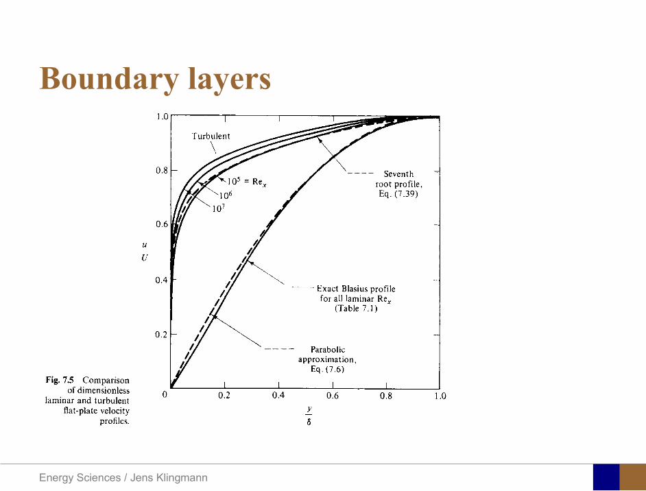
Energy Sciences Jens Klingmann
Boundary layers
Energy Sciences Jens Klingmann
Turbulent BL at different Pressure gradients
Energy Sciences Jens Klingmann
Boundary Layers
ν
yuy =+
ρτWu =
0=
partpart
=y
w yuτ
uuu =+
Energy Sciences Jens Klingmann
Diffuser efficiency
Energy Sciences Jens Klingmann
Reynolds Number (Order of magnitude)
At eg a compressor inlet
ρ = O(1) kgm3
U = O(100) msx lt O(01) mmicro = O(10-5)
Re = ρ U x micro =O(106)
In subsequent stages large amounts of turbulence (from stator wakes) will be convected into the Boundary layer
Energy Sciences Jens Klingmann
References Boundary layers
bull Frank M White ldquoViscous Fluid Flowrdquobull Hermann Schlichting ldquoBoundary Layer Theoryrdquo
Energy Sciences Jens Klingmann
CFD and experiments
bull No this is not a CFD course butbull Experiments
Energy Sciences Jens Klingmann
What do we need to measureOverall performance
Flow rates (mass or volume) Pressure Temperature Shaft power
Performance increase
Separations (velocity) Secondary flows eg tip clearance losses (velocity) Shock waves (supersonic applications) Pressure (resolved in time and space) Temperature (resolved in time and space)
Energy Sciences Jens Klingmann
Cascade wind tunnels
FIG 31 Compressor cascade wind tunnels (a) Conventional low-speed continuousrunning cascade tunnel (adapted from Carter et al 1950)(b) Transonicsupersoniccascade tunnel (adapted from Sieverding 1985)
Energy Sciences Jens Klingmann
Closed circuit tunnels
Energy Sciences Jens Klingmann
components
Settling Chamber
The settling chamber is located between the fan or wide angle diffuser and the contraction and contains the honeycombs and screens used to moderate longitudinal variations in the flow Screens in the chamber should be spaced at 02 chamber diameters apart so that flow disturbed by the first screen can settle before it encounters the second
Honeycombs
Honeycombs are located in the settling chamber and are used to reduce nonuniformities in the flow For optimum benefit honeycombs should be 6-8 cell diameters thick and cell size should be on the order of about 150 cells per settling chamber diameter
Energy Sciences Jens Klingmann
components
Screens
Screens are typically located just downstream of the honeycomb and sometime at the inlet of the test section Screens create a static pressure drop and serve to reduce boundary layer size and increase flow uniformity
Contraction Section
Contractions sections are located between the settling chamber and the test sections and serve to both increase mean velocities at the test section inlet and moderate inconsistencies in the uniformity of the flow Large contraction ratios and short contraction lengths are generally more desirable as they reduce the power loss across the screens and the thickness of boundary layers Small tunnels typically have contraction ratios between 6 and 9
Energy Sciences Jens Klingmann
Flow meters with pressure measurement
Venturi-tube
A1 A2
P1 P2
1 1 2 2C A C A=In the incompressible case
2 21 1 2 2
2 2C P C P
ρ ρ+ = +Assuming horisontal mounting
Energy Sciences Jens Klingmann
Daniel Bernoulli 1700-1782
Daniel Bernoulli was the son of Johann Bernoulli He was born in Groningen while his father held the chair of mathematics there His older brother was Nicolaus(II) Bernoulli and his uncle was Jacob Bernoulli so he was born into a family of leading mathematicians but also into a family where there was unfortunate rivalry jealousy and bitterness
Undoubtedly the most important work which Daniel Bernoulli did was his work on hydrodynamics Even the term itself is based on the title of the work which he produced called Hydrodynamica and before he left St Petersburg Daniel left a draft copy of the book with a printer However the work was not published until 1738 and although he revised it considerably between 1734 and 1738 it is more the presentation that he changed rather then the substance
This work contains for the first time the correct analysis of water flowing from a hole in a container This was based on the principle of conservation of energy which he had studied with his father in 1720 Daniel also discussed pumps and other machines to raise water One remarkable discovery appears in Chapter 10 of Hydrodynamica where Daniel discussed the basis for the kinetic theory of gases He was able to give the basic laws for the theory of gases and gave although not in full detail the equation of state discovered by Van der Waals a century later
Energy Sciences Jens Klingmann
Venturi-tube (2)
22 2 12 2
2
2A PC CA ρ
∆minus =
A1 A2
P1 P2
Solve for eg C2
1 2P P P∆ = minus
( )
12
2 2 21 2
21
PCA Aρ
∆ = minus
and( )
12
2 2 2 2 21 2
21
Pm A C AA Aρρ
∆ = = minus
where
Flow meters with pressure measurement
Energy Sciences Jens Klingmann
Flow meters with pressure measurement
Orifice meters
A1
A2
P1 P2
Applicable for pipe flows Same principle as for Venturi Positioning of pressure taps important Vena contracta and losses require inclusion
of Discharge Coefficient CD
( )
12
2 2 21 2
21D
Pm C AA Aρ ∆ =
minus where ( )1 2ReDC f A A=
CD available from manufacturer (measurements) or Standards (eg ISO)
Energy Sciences Jens Klingmann
Coriolis flow meter
An actuator (not shown) induces a vibration of the tubes
When there is mass flow Coriolis forces induce twisting of the tubes
degree of phase-shift is a measure for the amount of mass that is flowing through the tubes
Energy Sciences Jens Klingmann
Thermal flow meter Heat is added electrically to the flow Temperature is measured before and after heat addition
pP mC T∆=
Energy Sciences Jens Klingmann
Ultrasonic flow meters
Ultrasound is emitted to small particles in the flow (dust or other) Reflections of the sound is frequency shifted by the Doppler effect The frequency change is proportional to the particles velocity (volume flow
meter)
Energy Sciences Jens Klingmann
Inductive flow metersA magnetic flowmeter is based upon Faradays Law
The voltage induced across any conductor as it moves at right angles through a magnetic field is proportional to the velocity of that conductor
E is proportional to V x B x D where
E = The voltage generated in a conductorV = The velocity of the conductorB = The magnetic field strengthD = The length of the conductor
NB electric conductivity is required
Energy Sciences Jens Klingmann
Temperature measurements
Thermocouples
The basis established by Thomas Johann Seebeck in 1821
A conductor generates a voltage when subjected to a temperature gradient
To measure this voltage one must use a second conductor material which generates a different voltage under the same temperature gradient
Energy Sciences Jens Klingmann
Pressure sensing
1 2p pgt 2p p2 may be the atmosphere a static pressure tap or a known reference pressure
The strain of the diaphragm (or itrsquos deflection) may be measured by a number of electric methods
Diaphragm
Energy Sciences Jens Klingmann
Pressure sensingPiezoresistive Strain Gage
Uses the piezoresistive effect of bonded or formed strain gauges to detect strain due to applied pressure
Capacitive
Uses a diaghragm and pressure cavity to create a variable capacitor to detect strain due to applied pressure
Magnetic
Measures the displacement of a diaphragm by means of changes in inductance (reluctance) LVDT Hall Effect or by eddy current principal
Piezoelectric
Uses the piezoelectric effect in certain materials such as quartz to measure the strain upon the sensing mechanism due to pressure
Potentiometric
Uses the motion of a wiper along a resistive mechanism to detect the strain caused by applied pressure
Energy Sciences Jens Klingmann
3D highly instationary (periodic) flow Potentially very high velocities (Supersonic) Large temperature differences Low accessibility (difficult to probe between rotors) Low turbulence levels in most of the domain Very high turbulence in BL and wakes
Properties of measuring object
Point measurements
Energy Sciences Jens Klingmann
Conventional or non-opticalndash Static Pressure Measurementsndash Total Pressure Measurements
bull Multy hole probes
ndash Total Temperature ndash Hot Wire Anemometry (HWA)
Optical techniques for Velocity Measurementsndash Laser Two Focous (L2F)ndash Laser Doppler Anemometry (LDA)ndash Particle Image velocimetry (PIV)
Point Measurements
Energy Sciences Jens Klingmann
Static and total pressure
2 2 21 2 1
2 1 2 2 2C C CP P ρ ρ ρ
minus = minus =
2 0C =Stagnation point
C1Static pressure tap
Prandtl or Pitot tube
Apply the Bernoulli equation from free stream to stagnation point
21
2 12CP Pρ
= +or
We can also define a stagnation or total pressure
( )2
101 1 022
CP P Pρ= + =
Total pressure = Static pressure + dynamic pressure
or
Energy Sciences Jens Klingmann
Static pressure
Energy Sciences Jens Klingmann
Total Pressure and Temperature
Shrouded Probes
Shrouded Probe
Pitot or Prandtl tube
Sensitive to direction
Energy Sciences Jens Klingmann
Ludwig Prandtl 1875-1953
Ludwig Prandtl born at Freising Bavaria on February 4 1875 was a German Physicist famous for his work in aeronautics He qualified at Munchen in 1900 with a thesis on elastic stability and held the position of Professor of Applied Mechanics at Gottingen for forty-nine years (from 1904 until his death there on August 15 1953) In 1925 Prandtl became the Director of the Kaiser Wilhelm Institute for Fluid Mechanics His discovery in 1904 of the Boundary Layer which adjoins the surface of a body moving in a fluid led to an understanding of skin friction drag and of the way in which streamlining reduces the drag of airplane wings and other moving bodies His work on wing theory published in 1918 - 1919 followed that of FW Lanchester (1902-1907) but was carried out independently and elucidated the flow over airplane wings of finite span Prandtls work and decisive advances in boundary layer and wing theories became the basic material of aeronautics He also made important contributions to the theories of supersonic flow and of turbulence and contributed much to the development of wind tunnels and other aerodynamic equipment In addition he devised the soap-film analogy for the torsion of non-circular sections and wrote on the theory of plasticity and of meteorology
Energy Sciences Jens Klingmann
Total Pressure multy hole
Cobra Probe Yaw Probe
5 Hole Probe
Energy Sciences Jens Klingmann
5 Hole Probes Calibration
Energy Sciences Jens Klingmann
The inherent unsteadiness of the flow within turbomachines
Energy Sciences Jens Klingmann
Hot Wire Anemometry (HWA) The heat transfer from a thin (one micron)
electrically heated wire can be used to determine velocity
The resistance of the wire is temperature dependent Within a small temperature range it can be assumed linear R = R0+α R0(Tm-T0) where R0 is the resistance at a reference temperature T0 and Tm is the mean wire temperature
The thermal power induced in the wire is balanced by heat transfer to the surrounding fluid I2R=hπDL(Tm-T0) where h is the heat transfer coefficient and D and L the diameter and length of the wire respectively
E = I R
Energy Sciences Jens Klingmann
Constant Temperature Anemometry (CTA) The wire is often placed in a Whetstone bridge If the output from the
bridge is amplified and fed back to the bridge the resistance of the probe and thus the temperature will be held constant
This prevents the temperature of the wire to become excessive at low velocities
R1
R2 R3
Probe
Bridge Voltage
Energy Sciences Jens Klingmann
Constant Temperature Anemometry (CTA)
Energy Sciences Jens Klingmann
Characteristics of LDA (according to Dantec)
Invented by Yeh and Cummins in 1964 Velocity measurements in Fluid Dynamics (gas liquid) Up to 3 velocity components Non-intrusive measurements (optical technique) Absolute measurement technique (no calibration required) Very high accuracy Very high spatial resolution due to small measurement volume Tracer particles are required
Energy Sciences Jens Klingmann
LDA - Fringe Model
Focused Laser beams intersect and form the measurement volume Plane wave fronts beam waist in the plane of intersection Interference in the plane of intersection Pattern of bright and dark stripesplanes Fringes
Energy Sciences Jens Klingmann
LDA-measuring volume
d
x
x
y
y
z
z
e-2 CONTOUR
FRINGES
κ
κ
κ
κ
De-2
De-2
dml m
a
b
cx
b
z
ya
cd
d
=
=
=
J
J
J
J
JP
JP
JP
JD
JD
JD
+
+
+
a
b
c
d
κπλ
=minus sinD
f4l2e
m
κπλ
=minus cosD
f4D2e
m
Energy Sciences Jens Klingmann
Laser Two Focus
Energy Sciences Jens Klingmann
Laser Two Focus
Energy Sciences Jens Klingmann
PIV measurements
PIV is a fairly new technique capable of simultaneous velocity measurements at many points in a plane This gives information on large scale structures vorticity etc which is very difficult or impossible to obtain from one-point measuring techniques
PIV involves the illumination of a plane of the flow under investigation with a thin pulsed sheet of light The flow is seeded with particles
The light scattered from the particles and from successive pulses are being recorded either on film or a CCD array forming a multiple exposure of each particle image If the time between the pulses is known velocity can be determined as the ratio of the particle displacement and the elapsed time
t∆∆= xu
Energy Sciences Jens Klingmann
PIV
Energy Sciences Jens Klingmann
PIV measurements illumination
YA
G
YA
G
Two frequency doubled YAG Lasers aligned to one double pulsed laser sheet
Two or more separate light pulses can be obtained by chopping a continuous laser or from pulsed lasers
The limited pulse energies obtained from continuous lasers limits their applicability to low velocity flows or flows where large seeding particles can be used (ie liquid flows)
The low repetition rate of most pulsed lasers makes the use of two lasers advantageous
Energy Sciences Jens Klingmann
PIV measurements recording
High seeding density in laminar flame
Film or CCD-cameras Cross- or Auto-correlation
ndash ie both particle images on the same frame or on separate frames
CCD-camera requirementndash A many pixels as possiblendash 2k by 2k available 4k by 4k coming
Energy Sciences Jens Klingmann
PIV measurements analyses
Low seeding density (Number of seeding particles per unit volume)
Each particle image pair can be identified This is called particle tracking
High seeding density (PIV)
Small sub-regions of the image containing many particle image pairs are processed to obtain one velocity vector
Energy Sciences Jens Klingmann
PIV measurements analyses
Energy Sciences Jens Klingmann
PIV measurements analyses
( ) ( ) ( ) xsxxs dIIR 2A
1
I
+= int
Cross correlation between ( )x1I and ( )x2I
s is a two dimensional displacement vector
IA is the interrogation area
Cross correlation between
(
)
x
1
I
and
(
)
x
2
I
s is a two dimensional displacement vector
I
A
is the interrogation area
Energy Sciences Jens Klingmann
Energy Sciences Jens Klingmann
PIV from IOWA state university
Energy Sciences Jens Klingmann
PIV sample of evaluation
Energy Sciences Jens Klingmann
LDA PIV HWA Velocity range 01 mms ndash 300
ms 02 ndash 150 ms
Measuring Volume
D = 005 L = 05 mm
2 by 2 by 05 mm
L = 05 mm
Freq response O(10 000) Hz O(10) Hz O(100 000) Hz Calibration Yes No No Sensitivity to other than velocity
Low (ref Index) Low (ref Index) Large (temperature concentrationshellip)
Continuous Signal
Sometimes Seldom Always
Noise High High Low Turbulence intensity
No limitation Some limitation lt 20
Price O(1 000 000) SEK
O(1 000 000) SEK
O(50 000) SEK
Required Knowledge
High medium Low
Comparison of techniques
Energy Sciences Jens Klingmann
References experiments
R J Goldstein ldquoFluid Mechanics Measurementsrdquo Hemisphere Publishing 1983 A V Johansson amp P H Alfredsson ldquoExperimentella metoder inom
stroumlmningsmekanikenrdquo Inst Foumlr Mekanik KTH F Durst A Melling and J H Whitelaw ldquoPrincipals and Practice of Laser Doppler
Anemometryrdquo 1984 R J Adrian ldquoParticle-imaging techniques for experimental fluid mechnicsrdquo Ann Rev
Fluid Mech 1991
Energy Sciences Jens Klingmann
Sample of LDA-measurements
Rotor blade
Glas window
Emitted beams
Scattered Light
Adjustable mirror
Energy Sciences Jens Klingmann
Axial velocity sorted into 10 bins
0 1 2 3 4 5 6tangential coordinate (degrees)
-20
0
20
40
60
80
100
120
140
160Ax
ial v
eloc
ity a
nd s
tand
ard
devi
atio
n (m
s)
radial position 7 mm from inner window surfaceaxial position 23 mm behind rotor blades
Energy Sciences Jens Klingmann
Axial velocities in the radial-tangential plane
Energy Sciences Jens Klingmann
Airfoils NACA 4-digit
The NACA four-digit wing sections define the profile by
One digit describing maximum camber as percentage of the chord
One digit describing the distance of maximum camber from the airfoil leading edge in tens of percents of the chord
Two digits describing maximum thickness of the airfoil as percent of the chord
Example the NACA 2412 airfoil has a maximum camber of 2 located 40 (04 chords) from the leading edge with a maximum thickness of 12 of the chord
Four-digit series airfoils by default have maximum thickness at 30 of the chord (03 chords) from the leading edge
Energy Sciences Jens Klingmann
Airfoils NACA 4-digit
bull c is the chord lengthbull x is the position along
the chord from 0 to cbull y is the half thickness at
a given value of x (centerline to surface)
bull t is the maximum thickness as a fraction of the chord
Energy Sciences Jens Klingmann
Death by PowerPoint
| LDA | PIV | HWA | |||||
| Velocity range | 01 mms ndash 300 ms | 02 ndash 150 ms | |||||
| Measuring Volume | D = 005 L = 05 mm | 2 by 2 by 05 mm | L = 05 mm | ||||
| Freq response | O(10 000) Hz | O(10) Hz | O(100 000) Hz | ||||
| Calibration | Yes | No | No | ||||
| Sensitivity to other than velocity | Low (ref Index) | Low (ref Index) | Large (temperature concentrationshellip) | ||||
| Continuous Signal | Sometimes | Seldom | Always | ||||
| Noise | High | High | Low | ||||
| Turbulence intensity | No limitation | Some limitation | lt 20 | ||||
| Price | O(1 000 000) SEK | O(1 000 000) SEK | O(50 000) SEK | ||||
| Required Knowledge | High | medium | Low |
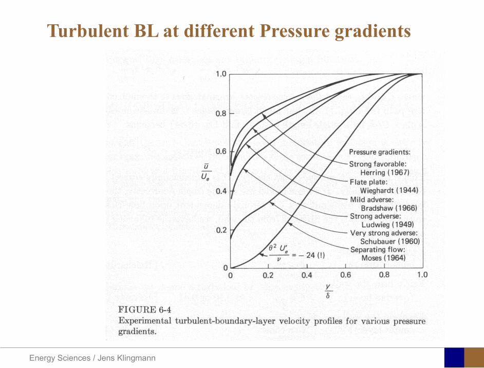
Energy Sciences Jens Klingmann
Turbulent BL at different Pressure gradients
Energy Sciences Jens Klingmann
Boundary Layers
ν
yuy =+
ρτWu =
0=
partpart
=y
w yuτ
uuu =+
Energy Sciences Jens Klingmann
Diffuser efficiency
Energy Sciences Jens Klingmann
Reynolds Number (Order of magnitude)
At eg a compressor inlet
ρ = O(1) kgm3
U = O(100) msx lt O(01) mmicro = O(10-5)
Re = ρ U x micro =O(106)
In subsequent stages large amounts of turbulence (from stator wakes) will be convected into the Boundary layer
Energy Sciences Jens Klingmann
References Boundary layers
bull Frank M White ldquoViscous Fluid Flowrdquobull Hermann Schlichting ldquoBoundary Layer Theoryrdquo
Energy Sciences Jens Klingmann
CFD and experiments
bull No this is not a CFD course butbull Experiments
Energy Sciences Jens Klingmann
What do we need to measureOverall performance
Flow rates (mass or volume) Pressure Temperature Shaft power
Performance increase
Separations (velocity) Secondary flows eg tip clearance losses (velocity) Shock waves (supersonic applications) Pressure (resolved in time and space) Temperature (resolved in time and space)
Energy Sciences Jens Klingmann
Cascade wind tunnels
FIG 31 Compressor cascade wind tunnels (a) Conventional low-speed continuousrunning cascade tunnel (adapted from Carter et al 1950)(b) Transonicsupersoniccascade tunnel (adapted from Sieverding 1985)
Energy Sciences Jens Klingmann
Closed circuit tunnels
Energy Sciences Jens Klingmann
components
Settling Chamber
The settling chamber is located between the fan or wide angle diffuser and the contraction and contains the honeycombs and screens used to moderate longitudinal variations in the flow Screens in the chamber should be spaced at 02 chamber diameters apart so that flow disturbed by the first screen can settle before it encounters the second
Honeycombs
Honeycombs are located in the settling chamber and are used to reduce nonuniformities in the flow For optimum benefit honeycombs should be 6-8 cell diameters thick and cell size should be on the order of about 150 cells per settling chamber diameter
Energy Sciences Jens Klingmann
components
Screens
Screens are typically located just downstream of the honeycomb and sometime at the inlet of the test section Screens create a static pressure drop and serve to reduce boundary layer size and increase flow uniformity
Contraction Section
Contractions sections are located between the settling chamber and the test sections and serve to both increase mean velocities at the test section inlet and moderate inconsistencies in the uniformity of the flow Large contraction ratios and short contraction lengths are generally more desirable as they reduce the power loss across the screens and the thickness of boundary layers Small tunnels typically have contraction ratios between 6 and 9
Energy Sciences Jens Klingmann
Flow meters with pressure measurement
Venturi-tube
A1 A2
P1 P2
1 1 2 2C A C A=In the incompressible case
2 21 1 2 2
2 2C P C P
ρ ρ+ = +Assuming horisontal mounting
Energy Sciences Jens Klingmann
Daniel Bernoulli 1700-1782
Daniel Bernoulli was the son of Johann Bernoulli He was born in Groningen while his father held the chair of mathematics there His older brother was Nicolaus(II) Bernoulli and his uncle was Jacob Bernoulli so he was born into a family of leading mathematicians but also into a family where there was unfortunate rivalry jealousy and bitterness
Undoubtedly the most important work which Daniel Bernoulli did was his work on hydrodynamics Even the term itself is based on the title of the work which he produced called Hydrodynamica and before he left St Petersburg Daniel left a draft copy of the book with a printer However the work was not published until 1738 and although he revised it considerably between 1734 and 1738 it is more the presentation that he changed rather then the substance
This work contains for the first time the correct analysis of water flowing from a hole in a container This was based on the principle of conservation of energy which he had studied with his father in 1720 Daniel also discussed pumps and other machines to raise water One remarkable discovery appears in Chapter 10 of Hydrodynamica where Daniel discussed the basis for the kinetic theory of gases He was able to give the basic laws for the theory of gases and gave although not in full detail the equation of state discovered by Van der Waals a century later
Energy Sciences Jens Klingmann
Venturi-tube (2)
22 2 12 2
2
2A PC CA ρ
∆minus =
A1 A2
P1 P2
Solve for eg C2
1 2P P P∆ = minus
( )
12
2 2 21 2
21
PCA Aρ
∆ = minus
and( )
12
2 2 2 2 21 2
21
Pm A C AA Aρρ
∆ = = minus
where
Flow meters with pressure measurement
Energy Sciences Jens Klingmann
Flow meters with pressure measurement
Orifice meters
A1
A2
P1 P2
Applicable for pipe flows Same principle as for Venturi Positioning of pressure taps important Vena contracta and losses require inclusion
of Discharge Coefficient CD
( )
12
2 2 21 2
21D
Pm C AA Aρ ∆ =
minus where ( )1 2ReDC f A A=
CD available from manufacturer (measurements) or Standards (eg ISO)
Energy Sciences Jens Klingmann
Coriolis flow meter
An actuator (not shown) induces a vibration of the tubes
When there is mass flow Coriolis forces induce twisting of the tubes
degree of phase-shift is a measure for the amount of mass that is flowing through the tubes
Energy Sciences Jens Klingmann
Thermal flow meter Heat is added electrically to the flow Temperature is measured before and after heat addition
pP mC T∆=
Energy Sciences Jens Klingmann
Ultrasonic flow meters
Ultrasound is emitted to small particles in the flow (dust or other) Reflections of the sound is frequency shifted by the Doppler effect The frequency change is proportional to the particles velocity (volume flow
meter)
Energy Sciences Jens Klingmann
Inductive flow metersA magnetic flowmeter is based upon Faradays Law
The voltage induced across any conductor as it moves at right angles through a magnetic field is proportional to the velocity of that conductor
E is proportional to V x B x D where
E = The voltage generated in a conductorV = The velocity of the conductorB = The magnetic field strengthD = The length of the conductor
NB electric conductivity is required
Energy Sciences Jens Klingmann
Temperature measurements
Thermocouples
The basis established by Thomas Johann Seebeck in 1821
A conductor generates a voltage when subjected to a temperature gradient
To measure this voltage one must use a second conductor material which generates a different voltage under the same temperature gradient
Energy Sciences Jens Klingmann
Pressure sensing
1 2p pgt 2p p2 may be the atmosphere a static pressure tap or a known reference pressure
The strain of the diaphragm (or itrsquos deflection) may be measured by a number of electric methods
Diaphragm
Energy Sciences Jens Klingmann
Pressure sensingPiezoresistive Strain Gage
Uses the piezoresistive effect of bonded or formed strain gauges to detect strain due to applied pressure
Capacitive
Uses a diaghragm and pressure cavity to create a variable capacitor to detect strain due to applied pressure
Magnetic
Measures the displacement of a diaphragm by means of changes in inductance (reluctance) LVDT Hall Effect or by eddy current principal
Piezoelectric
Uses the piezoelectric effect in certain materials such as quartz to measure the strain upon the sensing mechanism due to pressure
Potentiometric
Uses the motion of a wiper along a resistive mechanism to detect the strain caused by applied pressure
Energy Sciences Jens Klingmann
3D highly instationary (periodic) flow Potentially very high velocities (Supersonic) Large temperature differences Low accessibility (difficult to probe between rotors) Low turbulence levels in most of the domain Very high turbulence in BL and wakes
Properties of measuring object
Point measurements
Energy Sciences Jens Klingmann
Conventional or non-opticalndash Static Pressure Measurementsndash Total Pressure Measurements
bull Multy hole probes
ndash Total Temperature ndash Hot Wire Anemometry (HWA)
Optical techniques for Velocity Measurementsndash Laser Two Focous (L2F)ndash Laser Doppler Anemometry (LDA)ndash Particle Image velocimetry (PIV)
Point Measurements
Energy Sciences Jens Klingmann
Static and total pressure
2 2 21 2 1
2 1 2 2 2C C CP P ρ ρ ρ
minus = minus =
2 0C =Stagnation point
C1Static pressure tap
Prandtl or Pitot tube
Apply the Bernoulli equation from free stream to stagnation point
21
2 12CP Pρ
= +or
We can also define a stagnation or total pressure
( )2
101 1 022
CP P Pρ= + =
Total pressure = Static pressure + dynamic pressure
or
Energy Sciences Jens Klingmann
Static pressure
Energy Sciences Jens Klingmann
Total Pressure and Temperature
Shrouded Probes
Shrouded Probe
Pitot or Prandtl tube
Sensitive to direction
Energy Sciences Jens Klingmann
Ludwig Prandtl 1875-1953
Ludwig Prandtl born at Freising Bavaria on February 4 1875 was a German Physicist famous for his work in aeronautics He qualified at Munchen in 1900 with a thesis on elastic stability and held the position of Professor of Applied Mechanics at Gottingen for forty-nine years (from 1904 until his death there on August 15 1953) In 1925 Prandtl became the Director of the Kaiser Wilhelm Institute for Fluid Mechanics His discovery in 1904 of the Boundary Layer which adjoins the surface of a body moving in a fluid led to an understanding of skin friction drag and of the way in which streamlining reduces the drag of airplane wings and other moving bodies His work on wing theory published in 1918 - 1919 followed that of FW Lanchester (1902-1907) but was carried out independently and elucidated the flow over airplane wings of finite span Prandtls work and decisive advances in boundary layer and wing theories became the basic material of aeronautics He also made important contributions to the theories of supersonic flow and of turbulence and contributed much to the development of wind tunnels and other aerodynamic equipment In addition he devised the soap-film analogy for the torsion of non-circular sections and wrote on the theory of plasticity and of meteorology
Energy Sciences Jens Klingmann
Total Pressure multy hole
Cobra Probe Yaw Probe
5 Hole Probe
Energy Sciences Jens Klingmann
5 Hole Probes Calibration
Energy Sciences Jens Klingmann
The inherent unsteadiness of the flow within turbomachines
Energy Sciences Jens Klingmann
Hot Wire Anemometry (HWA) The heat transfer from a thin (one micron)
electrically heated wire can be used to determine velocity
The resistance of the wire is temperature dependent Within a small temperature range it can be assumed linear R = R0+α R0(Tm-T0) where R0 is the resistance at a reference temperature T0 and Tm is the mean wire temperature
The thermal power induced in the wire is balanced by heat transfer to the surrounding fluid I2R=hπDL(Tm-T0) where h is the heat transfer coefficient and D and L the diameter and length of the wire respectively
E = I R
Energy Sciences Jens Klingmann
Constant Temperature Anemometry (CTA) The wire is often placed in a Whetstone bridge If the output from the
bridge is amplified and fed back to the bridge the resistance of the probe and thus the temperature will be held constant
This prevents the temperature of the wire to become excessive at low velocities
R1
R2 R3
Probe
Bridge Voltage
Energy Sciences Jens Klingmann
Constant Temperature Anemometry (CTA)
Energy Sciences Jens Klingmann
Characteristics of LDA (according to Dantec)
Invented by Yeh and Cummins in 1964 Velocity measurements in Fluid Dynamics (gas liquid) Up to 3 velocity components Non-intrusive measurements (optical technique) Absolute measurement technique (no calibration required) Very high accuracy Very high spatial resolution due to small measurement volume Tracer particles are required
Energy Sciences Jens Klingmann
LDA - Fringe Model
Focused Laser beams intersect and form the measurement volume Plane wave fronts beam waist in the plane of intersection Interference in the plane of intersection Pattern of bright and dark stripesplanes Fringes
Energy Sciences Jens Klingmann
LDA-measuring volume
d
x
x
y
y
z
z
e-2 CONTOUR
FRINGES
κ
κ
κ
κ
De-2
De-2
dml m
a
b
cx
b
z
ya
cd
d
=
=
=
J
J
J
J
JP
JP
JP
JD
JD
JD
+
+
+
a
b
c
d
κπλ
=minus sinD
f4l2e
m
κπλ
=minus cosD
f4D2e
m
Energy Sciences Jens Klingmann
Laser Two Focus
Energy Sciences Jens Klingmann
Laser Two Focus
Energy Sciences Jens Klingmann
PIV measurements
PIV is a fairly new technique capable of simultaneous velocity measurements at many points in a plane This gives information on large scale structures vorticity etc which is very difficult or impossible to obtain from one-point measuring techniques
PIV involves the illumination of a plane of the flow under investigation with a thin pulsed sheet of light The flow is seeded with particles
The light scattered from the particles and from successive pulses are being recorded either on film or a CCD array forming a multiple exposure of each particle image If the time between the pulses is known velocity can be determined as the ratio of the particle displacement and the elapsed time
t∆∆= xu
Energy Sciences Jens Klingmann
PIV
Energy Sciences Jens Klingmann
PIV measurements illumination
YA
G
YA
G
Two frequency doubled YAG Lasers aligned to one double pulsed laser sheet
Two or more separate light pulses can be obtained by chopping a continuous laser or from pulsed lasers
The limited pulse energies obtained from continuous lasers limits their applicability to low velocity flows or flows where large seeding particles can be used (ie liquid flows)
The low repetition rate of most pulsed lasers makes the use of two lasers advantageous
Energy Sciences Jens Klingmann
PIV measurements recording
High seeding density in laminar flame
Film or CCD-cameras Cross- or Auto-correlation
ndash ie both particle images on the same frame or on separate frames
CCD-camera requirementndash A many pixels as possiblendash 2k by 2k available 4k by 4k coming
Energy Sciences Jens Klingmann
PIV measurements analyses
Low seeding density (Number of seeding particles per unit volume)
Each particle image pair can be identified This is called particle tracking
High seeding density (PIV)
Small sub-regions of the image containing many particle image pairs are processed to obtain one velocity vector
Energy Sciences Jens Klingmann
PIV measurements analyses
Energy Sciences Jens Klingmann
PIV measurements analyses
( ) ( ) ( ) xsxxs dIIR 2A
1
I
+= int
Cross correlation between ( )x1I and ( )x2I
s is a two dimensional displacement vector
IA is the interrogation area
Cross correlation between
(
)
x
1
I
and
(
)
x
2
I
s is a two dimensional displacement vector
I
A
is the interrogation area
Energy Sciences Jens Klingmann
Energy Sciences Jens Klingmann
PIV from IOWA state university
Energy Sciences Jens Klingmann
PIV sample of evaluation
Energy Sciences Jens Klingmann
LDA PIV HWA Velocity range 01 mms ndash 300
ms 02 ndash 150 ms
Measuring Volume
D = 005 L = 05 mm
2 by 2 by 05 mm
L = 05 mm
Freq response O(10 000) Hz O(10) Hz O(100 000) Hz Calibration Yes No No Sensitivity to other than velocity
Low (ref Index) Low (ref Index) Large (temperature concentrationshellip)
Continuous Signal
Sometimes Seldom Always
Noise High High Low Turbulence intensity
No limitation Some limitation lt 20
Price O(1 000 000) SEK
O(1 000 000) SEK
O(50 000) SEK
Required Knowledge
High medium Low
Comparison of techniques
Energy Sciences Jens Klingmann
References experiments
R J Goldstein ldquoFluid Mechanics Measurementsrdquo Hemisphere Publishing 1983 A V Johansson amp P H Alfredsson ldquoExperimentella metoder inom
stroumlmningsmekanikenrdquo Inst Foumlr Mekanik KTH F Durst A Melling and J H Whitelaw ldquoPrincipals and Practice of Laser Doppler
Anemometryrdquo 1984 R J Adrian ldquoParticle-imaging techniques for experimental fluid mechnicsrdquo Ann Rev
Fluid Mech 1991
Energy Sciences Jens Klingmann
Sample of LDA-measurements
Rotor blade
Glas window
Emitted beams
Scattered Light
Adjustable mirror
Energy Sciences Jens Klingmann
Axial velocity sorted into 10 bins
0 1 2 3 4 5 6tangential coordinate (degrees)
-20
0
20
40
60
80
100
120
140
160Ax
ial v
eloc
ity a
nd s
tand
ard
devi
atio
n (m
s)
radial position 7 mm from inner window surfaceaxial position 23 mm behind rotor blades
Energy Sciences Jens Klingmann
Axial velocities in the radial-tangential plane
Energy Sciences Jens Klingmann
Airfoils NACA 4-digit
The NACA four-digit wing sections define the profile by
One digit describing maximum camber as percentage of the chord
One digit describing the distance of maximum camber from the airfoil leading edge in tens of percents of the chord
Two digits describing maximum thickness of the airfoil as percent of the chord
Example the NACA 2412 airfoil has a maximum camber of 2 located 40 (04 chords) from the leading edge with a maximum thickness of 12 of the chord
Four-digit series airfoils by default have maximum thickness at 30 of the chord (03 chords) from the leading edge
Energy Sciences Jens Klingmann
Airfoils NACA 4-digit
bull c is the chord lengthbull x is the position along
the chord from 0 to cbull y is the half thickness at
a given value of x (centerline to surface)
bull t is the maximum thickness as a fraction of the chord
Energy Sciences Jens Klingmann
Death by PowerPoint
| LDA | PIV | HWA | |||||
| Velocity range | 01 mms ndash 300 ms | 02 ndash 150 ms | |||||
| Measuring Volume | D = 005 L = 05 mm | 2 by 2 by 05 mm | L = 05 mm | ||||
| Freq response | O(10 000) Hz | O(10) Hz | O(100 000) Hz | ||||
| Calibration | Yes | No | No | ||||
| Sensitivity to other than velocity | Low (ref Index) | Low (ref Index) | Large (temperature concentrationshellip) | ||||
| Continuous Signal | Sometimes | Seldom | Always | ||||
| Noise | High | High | Low | ||||
| Turbulence intensity | No limitation | Some limitation | lt 20 | ||||
| Price | O(1 000 000) SEK | O(1 000 000) SEK | O(50 000) SEK | ||||
| Required Knowledge | High | medium | Low |
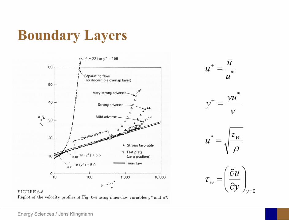
Energy Sciences Jens Klingmann
Boundary Layers
ν
yuy =+
ρτWu =
0=
partpart
=y
w yuτ
uuu =+
Energy Sciences Jens Klingmann
Diffuser efficiency
Energy Sciences Jens Klingmann
Reynolds Number (Order of magnitude)
At eg a compressor inlet
ρ = O(1) kgm3
U = O(100) msx lt O(01) mmicro = O(10-5)
Re = ρ U x micro =O(106)
In subsequent stages large amounts of turbulence (from stator wakes) will be convected into the Boundary layer
Energy Sciences Jens Klingmann
References Boundary layers
bull Frank M White ldquoViscous Fluid Flowrdquobull Hermann Schlichting ldquoBoundary Layer Theoryrdquo
Energy Sciences Jens Klingmann
CFD and experiments
bull No this is not a CFD course butbull Experiments
Energy Sciences Jens Klingmann
What do we need to measureOverall performance
Flow rates (mass or volume) Pressure Temperature Shaft power
Performance increase
Separations (velocity) Secondary flows eg tip clearance losses (velocity) Shock waves (supersonic applications) Pressure (resolved in time and space) Temperature (resolved in time and space)
Energy Sciences Jens Klingmann
Cascade wind tunnels
FIG 31 Compressor cascade wind tunnels (a) Conventional low-speed continuousrunning cascade tunnel (adapted from Carter et al 1950)(b) Transonicsupersoniccascade tunnel (adapted from Sieverding 1985)
Energy Sciences Jens Klingmann
Closed circuit tunnels
Energy Sciences Jens Klingmann
components
Settling Chamber
The settling chamber is located between the fan or wide angle diffuser and the contraction and contains the honeycombs and screens used to moderate longitudinal variations in the flow Screens in the chamber should be spaced at 02 chamber diameters apart so that flow disturbed by the first screen can settle before it encounters the second
Honeycombs
Honeycombs are located in the settling chamber and are used to reduce nonuniformities in the flow For optimum benefit honeycombs should be 6-8 cell diameters thick and cell size should be on the order of about 150 cells per settling chamber diameter
Energy Sciences Jens Klingmann
components
Screens
Screens are typically located just downstream of the honeycomb and sometime at the inlet of the test section Screens create a static pressure drop and serve to reduce boundary layer size and increase flow uniformity
Contraction Section
Contractions sections are located between the settling chamber and the test sections and serve to both increase mean velocities at the test section inlet and moderate inconsistencies in the uniformity of the flow Large contraction ratios and short contraction lengths are generally more desirable as they reduce the power loss across the screens and the thickness of boundary layers Small tunnels typically have contraction ratios between 6 and 9
Energy Sciences Jens Klingmann
Flow meters with pressure measurement
Venturi-tube
A1 A2
P1 P2
1 1 2 2C A C A=In the incompressible case
2 21 1 2 2
2 2C P C P
ρ ρ+ = +Assuming horisontal mounting
Energy Sciences Jens Klingmann
Daniel Bernoulli 1700-1782
Daniel Bernoulli was the son of Johann Bernoulli He was born in Groningen while his father held the chair of mathematics there His older brother was Nicolaus(II) Bernoulli and his uncle was Jacob Bernoulli so he was born into a family of leading mathematicians but also into a family where there was unfortunate rivalry jealousy and bitterness
Undoubtedly the most important work which Daniel Bernoulli did was his work on hydrodynamics Even the term itself is based on the title of the work which he produced called Hydrodynamica and before he left St Petersburg Daniel left a draft copy of the book with a printer However the work was not published until 1738 and although he revised it considerably between 1734 and 1738 it is more the presentation that he changed rather then the substance
This work contains for the first time the correct analysis of water flowing from a hole in a container This was based on the principle of conservation of energy which he had studied with his father in 1720 Daniel also discussed pumps and other machines to raise water One remarkable discovery appears in Chapter 10 of Hydrodynamica where Daniel discussed the basis for the kinetic theory of gases He was able to give the basic laws for the theory of gases and gave although not in full detail the equation of state discovered by Van der Waals a century later
Energy Sciences Jens Klingmann
Venturi-tube (2)
22 2 12 2
2
2A PC CA ρ
∆minus =
A1 A2
P1 P2
Solve for eg C2
1 2P P P∆ = minus
( )
12
2 2 21 2
21
PCA Aρ
∆ = minus
and( )
12
2 2 2 2 21 2
21
Pm A C AA Aρρ
∆ = = minus
where
Flow meters with pressure measurement
Energy Sciences Jens Klingmann
Flow meters with pressure measurement
Orifice meters
A1
A2
P1 P2
Applicable for pipe flows Same principle as for Venturi Positioning of pressure taps important Vena contracta and losses require inclusion
of Discharge Coefficient CD
( )
12
2 2 21 2
21D
Pm C AA Aρ ∆ =
minus where ( )1 2ReDC f A A=
CD available from manufacturer (measurements) or Standards (eg ISO)
Energy Sciences Jens Klingmann
Coriolis flow meter
An actuator (not shown) induces a vibration of the tubes
When there is mass flow Coriolis forces induce twisting of the tubes
degree of phase-shift is a measure for the amount of mass that is flowing through the tubes
Energy Sciences Jens Klingmann
Thermal flow meter Heat is added electrically to the flow Temperature is measured before and after heat addition
pP mC T∆=
Energy Sciences Jens Klingmann
Ultrasonic flow meters
Ultrasound is emitted to small particles in the flow (dust or other) Reflections of the sound is frequency shifted by the Doppler effect The frequency change is proportional to the particles velocity (volume flow
meter)
Energy Sciences Jens Klingmann
Inductive flow metersA magnetic flowmeter is based upon Faradays Law
The voltage induced across any conductor as it moves at right angles through a magnetic field is proportional to the velocity of that conductor
E is proportional to V x B x D where
E = The voltage generated in a conductorV = The velocity of the conductorB = The magnetic field strengthD = The length of the conductor
NB electric conductivity is required
Energy Sciences Jens Klingmann
Temperature measurements
Thermocouples
The basis established by Thomas Johann Seebeck in 1821
A conductor generates a voltage when subjected to a temperature gradient
To measure this voltage one must use a second conductor material which generates a different voltage under the same temperature gradient
Energy Sciences Jens Klingmann
Pressure sensing
1 2p pgt 2p p2 may be the atmosphere a static pressure tap or a known reference pressure
The strain of the diaphragm (or itrsquos deflection) may be measured by a number of electric methods
Diaphragm
Energy Sciences Jens Klingmann
Pressure sensingPiezoresistive Strain Gage
Uses the piezoresistive effect of bonded or formed strain gauges to detect strain due to applied pressure
Capacitive
Uses a diaghragm and pressure cavity to create a variable capacitor to detect strain due to applied pressure
Magnetic
Measures the displacement of a diaphragm by means of changes in inductance (reluctance) LVDT Hall Effect or by eddy current principal
Piezoelectric
Uses the piezoelectric effect in certain materials such as quartz to measure the strain upon the sensing mechanism due to pressure
Potentiometric
Uses the motion of a wiper along a resistive mechanism to detect the strain caused by applied pressure
Energy Sciences Jens Klingmann
3D highly instationary (periodic) flow Potentially very high velocities (Supersonic) Large temperature differences Low accessibility (difficult to probe between rotors) Low turbulence levels in most of the domain Very high turbulence in BL and wakes
Properties of measuring object
Point measurements
Energy Sciences Jens Klingmann
Conventional or non-opticalndash Static Pressure Measurementsndash Total Pressure Measurements
bull Multy hole probes
ndash Total Temperature ndash Hot Wire Anemometry (HWA)
Optical techniques for Velocity Measurementsndash Laser Two Focous (L2F)ndash Laser Doppler Anemometry (LDA)ndash Particle Image velocimetry (PIV)
Point Measurements
Energy Sciences Jens Klingmann
Static and total pressure
2 2 21 2 1
2 1 2 2 2C C CP P ρ ρ ρ
minus = minus =
2 0C =Stagnation point
C1Static pressure tap
Prandtl or Pitot tube
Apply the Bernoulli equation from free stream to stagnation point
21
2 12CP Pρ
= +or
We can also define a stagnation or total pressure
( )2
101 1 022
CP P Pρ= + =
Total pressure = Static pressure + dynamic pressure
or
Energy Sciences Jens Klingmann
Static pressure
Energy Sciences Jens Klingmann
Total Pressure and Temperature
Shrouded Probes
Shrouded Probe
Pitot or Prandtl tube
Sensitive to direction
Energy Sciences Jens Klingmann
Ludwig Prandtl 1875-1953
Ludwig Prandtl born at Freising Bavaria on February 4 1875 was a German Physicist famous for his work in aeronautics He qualified at Munchen in 1900 with a thesis on elastic stability and held the position of Professor of Applied Mechanics at Gottingen for forty-nine years (from 1904 until his death there on August 15 1953) In 1925 Prandtl became the Director of the Kaiser Wilhelm Institute for Fluid Mechanics His discovery in 1904 of the Boundary Layer which adjoins the surface of a body moving in a fluid led to an understanding of skin friction drag and of the way in which streamlining reduces the drag of airplane wings and other moving bodies His work on wing theory published in 1918 - 1919 followed that of FW Lanchester (1902-1907) but was carried out independently and elucidated the flow over airplane wings of finite span Prandtls work and decisive advances in boundary layer and wing theories became the basic material of aeronautics He also made important contributions to the theories of supersonic flow and of turbulence and contributed much to the development of wind tunnels and other aerodynamic equipment In addition he devised the soap-film analogy for the torsion of non-circular sections and wrote on the theory of plasticity and of meteorology
Energy Sciences Jens Klingmann
Total Pressure multy hole
Cobra Probe Yaw Probe
5 Hole Probe
Energy Sciences Jens Klingmann
5 Hole Probes Calibration
Energy Sciences Jens Klingmann
The inherent unsteadiness of the flow within turbomachines
Energy Sciences Jens Klingmann
Hot Wire Anemometry (HWA) The heat transfer from a thin (one micron)
electrically heated wire can be used to determine velocity
The resistance of the wire is temperature dependent Within a small temperature range it can be assumed linear R = R0+α R0(Tm-T0) where R0 is the resistance at a reference temperature T0 and Tm is the mean wire temperature
The thermal power induced in the wire is balanced by heat transfer to the surrounding fluid I2R=hπDL(Tm-T0) where h is the heat transfer coefficient and D and L the diameter and length of the wire respectively
E = I R
Energy Sciences Jens Klingmann
Constant Temperature Anemometry (CTA) The wire is often placed in a Whetstone bridge If the output from the
bridge is amplified and fed back to the bridge the resistance of the probe and thus the temperature will be held constant
This prevents the temperature of the wire to become excessive at low velocities
R1
R2 R3
Probe
Bridge Voltage
Energy Sciences Jens Klingmann
Constant Temperature Anemometry (CTA)
Energy Sciences Jens Klingmann
Characteristics of LDA (according to Dantec)
Invented by Yeh and Cummins in 1964 Velocity measurements in Fluid Dynamics (gas liquid) Up to 3 velocity components Non-intrusive measurements (optical technique) Absolute measurement technique (no calibration required) Very high accuracy Very high spatial resolution due to small measurement volume Tracer particles are required
Energy Sciences Jens Klingmann
LDA - Fringe Model
Focused Laser beams intersect and form the measurement volume Plane wave fronts beam waist in the plane of intersection Interference in the plane of intersection Pattern of bright and dark stripesplanes Fringes
Energy Sciences Jens Klingmann
LDA-measuring volume
d
x
x
y
y
z
z
e-2 CONTOUR
FRINGES
κ
κ
κ
κ
De-2
De-2
dml m
a
b
cx
b
z
ya
cd
d
=
=
=
J
J
J
J
JP
JP
JP
JD
JD
JD
+
+
+
a
b
c
d
κπλ
=minus sinD
f4l2e
m
κπλ
=minus cosD
f4D2e
m
Energy Sciences Jens Klingmann
Laser Two Focus
Energy Sciences Jens Klingmann
Laser Two Focus
Energy Sciences Jens Klingmann
PIV measurements
PIV is a fairly new technique capable of simultaneous velocity measurements at many points in a plane This gives information on large scale structures vorticity etc which is very difficult or impossible to obtain from one-point measuring techniques
PIV involves the illumination of a plane of the flow under investigation with a thin pulsed sheet of light The flow is seeded with particles
The light scattered from the particles and from successive pulses are being recorded either on film or a CCD array forming a multiple exposure of each particle image If the time between the pulses is known velocity can be determined as the ratio of the particle displacement and the elapsed time
t∆∆= xu
Energy Sciences Jens Klingmann
PIV
Energy Sciences Jens Klingmann
PIV measurements illumination
YA
G
YA
G
Two frequency doubled YAG Lasers aligned to one double pulsed laser sheet
Two or more separate light pulses can be obtained by chopping a continuous laser or from pulsed lasers
The limited pulse energies obtained from continuous lasers limits their applicability to low velocity flows or flows where large seeding particles can be used (ie liquid flows)
The low repetition rate of most pulsed lasers makes the use of two lasers advantageous
Energy Sciences Jens Klingmann
PIV measurements recording
High seeding density in laminar flame
Film or CCD-cameras Cross- or Auto-correlation
ndash ie both particle images on the same frame or on separate frames
CCD-camera requirementndash A many pixels as possiblendash 2k by 2k available 4k by 4k coming
Energy Sciences Jens Klingmann
PIV measurements analyses
Low seeding density (Number of seeding particles per unit volume)
Each particle image pair can be identified This is called particle tracking
High seeding density (PIV)
Small sub-regions of the image containing many particle image pairs are processed to obtain one velocity vector
Energy Sciences Jens Klingmann
PIV measurements analyses
Energy Sciences Jens Klingmann
PIV measurements analyses
( ) ( ) ( ) xsxxs dIIR 2A
1
I
+= int
Cross correlation between ( )x1I and ( )x2I
s is a two dimensional displacement vector
IA is the interrogation area
Cross correlation between
(
)
x
1
I
and
(
)
x
2
I
s is a two dimensional displacement vector
I
A
is the interrogation area
Energy Sciences Jens Klingmann
Energy Sciences Jens Klingmann
PIV from IOWA state university
Energy Sciences Jens Klingmann
PIV sample of evaluation
Energy Sciences Jens Klingmann
LDA PIV HWA Velocity range 01 mms ndash 300
ms 02 ndash 150 ms
Measuring Volume
D = 005 L = 05 mm
2 by 2 by 05 mm
L = 05 mm
Freq response O(10 000) Hz O(10) Hz O(100 000) Hz Calibration Yes No No Sensitivity to other than velocity
Low (ref Index) Low (ref Index) Large (temperature concentrationshellip)
Continuous Signal
Sometimes Seldom Always
Noise High High Low Turbulence intensity
No limitation Some limitation lt 20
Price O(1 000 000) SEK
O(1 000 000) SEK
O(50 000) SEK
Required Knowledge
High medium Low
Comparison of techniques
Energy Sciences Jens Klingmann
References experiments
R J Goldstein ldquoFluid Mechanics Measurementsrdquo Hemisphere Publishing 1983 A V Johansson amp P H Alfredsson ldquoExperimentella metoder inom
stroumlmningsmekanikenrdquo Inst Foumlr Mekanik KTH F Durst A Melling and J H Whitelaw ldquoPrincipals and Practice of Laser Doppler
Anemometryrdquo 1984 R J Adrian ldquoParticle-imaging techniques for experimental fluid mechnicsrdquo Ann Rev
Fluid Mech 1991
Energy Sciences Jens Klingmann
Sample of LDA-measurements
Rotor blade
Glas window
Emitted beams
Scattered Light
Adjustable mirror
Energy Sciences Jens Klingmann
Axial velocity sorted into 10 bins
0 1 2 3 4 5 6tangential coordinate (degrees)
-20
0
20
40
60
80
100
120
140
160Ax
ial v
eloc
ity a
nd s
tand
ard
devi
atio
n (m
s)
radial position 7 mm from inner window surfaceaxial position 23 mm behind rotor blades
Energy Sciences Jens Klingmann
Axial velocities in the radial-tangential plane
Energy Sciences Jens Klingmann
Airfoils NACA 4-digit
The NACA four-digit wing sections define the profile by
One digit describing maximum camber as percentage of the chord
One digit describing the distance of maximum camber from the airfoil leading edge in tens of percents of the chord
Two digits describing maximum thickness of the airfoil as percent of the chord
Example the NACA 2412 airfoil has a maximum camber of 2 located 40 (04 chords) from the leading edge with a maximum thickness of 12 of the chord
Four-digit series airfoils by default have maximum thickness at 30 of the chord (03 chords) from the leading edge
Energy Sciences Jens Klingmann
Airfoils NACA 4-digit
bull c is the chord lengthbull x is the position along
the chord from 0 to cbull y is the half thickness at
a given value of x (centerline to surface)
bull t is the maximum thickness as a fraction of the chord
Energy Sciences Jens Klingmann
Death by PowerPoint
| LDA | PIV | HWA | |||||
| Velocity range | 01 mms ndash 300 ms | 02 ndash 150 ms | |||||
| Measuring Volume | D = 005 L = 05 mm | 2 by 2 by 05 mm | L = 05 mm | ||||
| Freq response | O(10 000) Hz | O(10) Hz | O(100 000) Hz | ||||
| Calibration | Yes | No | No | ||||
| Sensitivity to other than velocity | Low (ref Index) | Low (ref Index) | Large (temperature concentrationshellip) | ||||
| Continuous Signal | Sometimes | Seldom | Always | ||||
| Noise | High | High | Low | ||||
| Turbulence intensity | No limitation | Some limitation | lt 20 | ||||
| Price | O(1 000 000) SEK | O(1 000 000) SEK | O(50 000) SEK | ||||
| Required Knowledge | High | medium | Low |
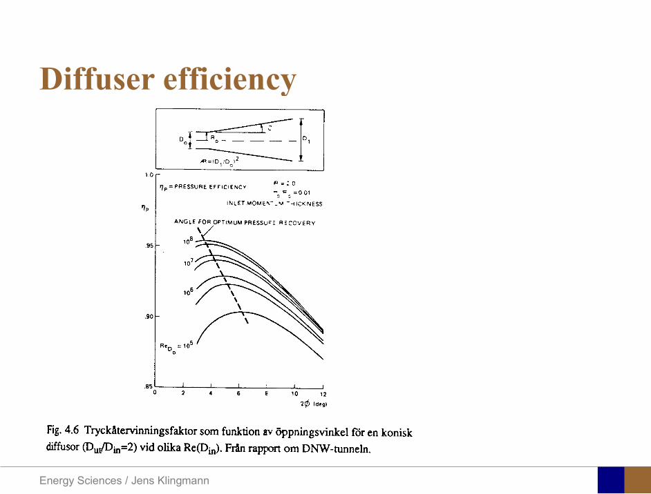
Energy Sciences Jens Klingmann
Diffuser efficiency
Energy Sciences Jens Klingmann
Reynolds Number (Order of magnitude)
At eg a compressor inlet
ρ = O(1) kgm3
U = O(100) msx lt O(01) mmicro = O(10-5)
Re = ρ U x micro =O(106)
In subsequent stages large amounts of turbulence (from stator wakes) will be convected into the Boundary layer
Energy Sciences Jens Klingmann
References Boundary layers
bull Frank M White ldquoViscous Fluid Flowrdquobull Hermann Schlichting ldquoBoundary Layer Theoryrdquo
Energy Sciences Jens Klingmann
CFD and experiments
bull No this is not a CFD course butbull Experiments
Energy Sciences Jens Klingmann
What do we need to measureOverall performance
Flow rates (mass or volume) Pressure Temperature Shaft power
Performance increase
Separations (velocity) Secondary flows eg tip clearance losses (velocity) Shock waves (supersonic applications) Pressure (resolved in time and space) Temperature (resolved in time and space)
Energy Sciences Jens Klingmann
Cascade wind tunnels
FIG 31 Compressor cascade wind tunnels (a) Conventional low-speed continuousrunning cascade tunnel (adapted from Carter et al 1950)(b) Transonicsupersoniccascade tunnel (adapted from Sieverding 1985)
Energy Sciences Jens Klingmann
Closed circuit tunnels
Energy Sciences Jens Klingmann
components
Settling Chamber
The settling chamber is located between the fan or wide angle diffuser and the contraction and contains the honeycombs and screens used to moderate longitudinal variations in the flow Screens in the chamber should be spaced at 02 chamber diameters apart so that flow disturbed by the first screen can settle before it encounters the second
Honeycombs
Honeycombs are located in the settling chamber and are used to reduce nonuniformities in the flow For optimum benefit honeycombs should be 6-8 cell diameters thick and cell size should be on the order of about 150 cells per settling chamber diameter
Energy Sciences Jens Klingmann
components
Screens
Screens are typically located just downstream of the honeycomb and sometime at the inlet of the test section Screens create a static pressure drop and serve to reduce boundary layer size and increase flow uniformity
Contraction Section
Contractions sections are located between the settling chamber and the test sections and serve to both increase mean velocities at the test section inlet and moderate inconsistencies in the uniformity of the flow Large contraction ratios and short contraction lengths are generally more desirable as they reduce the power loss across the screens and the thickness of boundary layers Small tunnels typically have contraction ratios between 6 and 9
Energy Sciences Jens Klingmann
Flow meters with pressure measurement
Venturi-tube
A1 A2
P1 P2
1 1 2 2C A C A=In the incompressible case
2 21 1 2 2
2 2C P C P
ρ ρ+ = +Assuming horisontal mounting
Energy Sciences Jens Klingmann
Daniel Bernoulli 1700-1782
Daniel Bernoulli was the son of Johann Bernoulli He was born in Groningen while his father held the chair of mathematics there His older brother was Nicolaus(II) Bernoulli and his uncle was Jacob Bernoulli so he was born into a family of leading mathematicians but also into a family where there was unfortunate rivalry jealousy and bitterness
Undoubtedly the most important work which Daniel Bernoulli did was his work on hydrodynamics Even the term itself is based on the title of the work which he produced called Hydrodynamica and before he left St Petersburg Daniel left a draft copy of the book with a printer However the work was not published until 1738 and although he revised it considerably between 1734 and 1738 it is more the presentation that he changed rather then the substance
This work contains for the first time the correct analysis of water flowing from a hole in a container This was based on the principle of conservation of energy which he had studied with his father in 1720 Daniel also discussed pumps and other machines to raise water One remarkable discovery appears in Chapter 10 of Hydrodynamica where Daniel discussed the basis for the kinetic theory of gases He was able to give the basic laws for the theory of gases and gave although not in full detail the equation of state discovered by Van der Waals a century later
Energy Sciences Jens Klingmann
Venturi-tube (2)
22 2 12 2
2
2A PC CA ρ
∆minus =
A1 A2
P1 P2
Solve for eg C2
1 2P P P∆ = minus
( )
12
2 2 21 2
21
PCA Aρ
∆ = minus
and( )
12
2 2 2 2 21 2
21
Pm A C AA Aρρ
∆ = = minus
where
Flow meters with pressure measurement
Energy Sciences Jens Klingmann
Flow meters with pressure measurement
Orifice meters
A1
A2
P1 P2
Applicable for pipe flows Same principle as for Venturi Positioning of pressure taps important Vena contracta and losses require inclusion
of Discharge Coefficient CD
( )
12
2 2 21 2
21D
Pm C AA Aρ ∆ =
minus where ( )1 2ReDC f A A=
CD available from manufacturer (measurements) or Standards (eg ISO)
Energy Sciences Jens Klingmann
Coriolis flow meter
An actuator (not shown) induces a vibration of the tubes
When there is mass flow Coriolis forces induce twisting of the tubes
degree of phase-shift is a measure for the amount of mass that is flowing through the tubes
Energy Sciences Jens Klingmann
Thermal flow meter Heat is added electrically to the flow Temperature is measured before and after heat addition
pP mC T∆=
Energy Sciences Jens Klingmann
Ultrasonic flow meters
Ultrasound is emitted to small particles in the flow (dust or other) Reflections of the sound is frequency shifted by the Doppler effect The frequency change is proportional to the particles velocity (volume flow
meter)
Energy Sciences Jens Klingmann
Inductive flow metersA magnetic flowmeter is based upon Faradays Law
The voltage induced across any conductor as it moves at right angles through a magnetic field is proportional to the velocity of that conductor
E is proportional to V x B x D where
E = The voltage generated in a conductorV = The velocity of the conductorB = The magnetic field strengthD = The length of the conductor
NB electric conductivity is required
Energy Sciences Jens Klingmann
Temperature measurements
Thermocouples
The basis established by Thomas Johann Seebeck in 1821
A conductor generates a voltage when subjected to a temperature gradient
To measure this voltage one must use a second conductor material which generates a different voltage under the same temperature gradient
Energy Sciences Jens Klingmann
Pressure sensing
1 2p pgt 2p p2 may be the atmosphere a static pressure tap or a known reference pressure
The strain of the diaphragm (or itrsquos deflection) may be measured by a number of electric methods
Diaphragm
Energy Sciences Jens Klingmann
Pressure sensingPiezoresistive Strain Gage
Uses the piezoresistive effect of bonded or formed strain gauges to detect strain due to applied pressure
Capacitive
Uses a diaghragm and pressure cavity to create a variable capacitor to detect strain due to applied pressure
Magnetic
Measures the displacement of a diaphragm by means of changes in inductance (reluctance) LVDT Hall Effect or by eddy current principal
Piezoelectric
Uses the piezoelectric effect in certain materials such as quartz to measure the strain upon the sensing mechanism due to pressure
Potentiometric
Uses the motion of a wiper along a resistive mechanism to detect the strain caused by applied pressure
Energy Sciences Jens Klingmann
3D highly instationary (periodic) flow Potentially very high velocities (Supersonic) Large temperature differences Low accessibility (difficult to probe between rotors) Low turbulence levels in most of the domain Very high turbulence in BL and wakes
Properties of measuring object
Point measurements
Energy Sciences Jens Klingmann
Conventional or non-opticalndash Static Pressure Measurementsndash Total Pressure Measurements
bull Multy hole probes
ndash Total Temperature ndash Hot Wire Anemometry (HWA)
Optical techniques for Velocity Measurementsndash Laser Two Focous (L2F)ndash Laser Doppler Anemometry (LDA)ndash Particle Image velocimetry (PIV)
Point Measurements
Energy Sciences Jens Klingmann
Static and total pressure
2 2 21 2 1
2 1 2 2 2C C CP P ρ ρ ρ
minus = minus =
2 0C =Stagnation point
C1Static pressure tap
Prandtl or Pitot tube
Apply the Bernoulli equation from free stream to stagnation point
21
2 12CP Pρ
= +or
We can also define a stagnation or total pressure
( )2
101 1 022
CP P Pρ= + =
Total pressure = Static pressure + dynamic pressure
or
Energy Sciences Jens Klingmann
Static pressure
Energy Sciences Jens Klingmann
Total Pressure and Temperature
Shrouded Probes
Shrouded Probe
Pitot or Prandtl tube
Sensitive to direction
Energy Sciences Jens Klingmann
Ludwig Prandtl 1875-1953
Ludwig Prandtl born at Freising Bavaria on February 4 1875 was a German Physicist famous for his work in aeronautics He qualified at Munchen in 1900 with a thesis on elastic stability and held the position of Professor of Applied Mechanics at Gottingen for forty-nine years (from 1904 until his death there on August 15 1953) In 1925 Prandtl became the Director of the Kaiser Wilhelm Institute for Fluid Mechanics His discovery in 1904 of the Boundary Layer which adjoins the surface of a body moving in a fluid led to an understanding of skin friction drag and of the way in which streamlining reduces the drag of airplane wings and other moving bodies His work on wing theory published in 1918 - 1919 followed that of FW Lanchester (1902-1907) but was carried out independently and elucidated the flow over airplane wings of finite span Prandtls work and decisive advances in boundary layer and wing theories became the basic material of aeronautics He also made important contributions to the theories of supersonic flow and of turbulence and contributed much to the development of wind tunnels and other aerodynamic equipment In addition he devised the soap-film analogy for the torsion of non-circular sections and wrote on the theory of plasticity and of meteorology
Energy Sciences Jens Klingmann
Total Pressure multy hole
Cobra Probe Yaw Probe
5 Hole Probe
Energy Sciences Jens Klingmann
5 Hole Probes Calibration
Energy Sciences Jens Klingmann
The inherent unsteadiness of the flow within turbomachines
Energy Sciences Jens Klingmann
Hot Wire Anemometry (HWA) The heat transfer from a thin (one micron)
electrically heated wire can be used to determine velocity
The resistance of the wire is temperature dependent Within a small temperature range it can be assumed linear R = R0+α R0(Tm-T0) where R0 is the resistance at a reference temperature T0 and Tm is the mean wire temperature
The thermal power induced in the wire is balanced by heat transfer to the surrounding fluid I2R=hπDL(Tm-T0) where h is the heat transfer coefficient and D and L the diameter and length of the wire respectively
E = I R
Energy Sciences Jens Klingmann
Constant Temperature Anemometry (CTA) The wire is often placed in a Whetstone bridge If the output from the
bridge is amplified and fed back to the bridge the resistance of the probe and thus the temperature will be held constant
This prevents the temperature of the wire to become excessive at low velocities
R1
R2 R3
Probe
Bridge Voltage
Energy Sciences Jens Klingmann
Constant Temperature Anemometry (CTA)
Energy Sciences Jens Klingmann
Characteristics of LDA (according to Dantec)
Invented by Yeh and Cummins in 1964 Velocity measurements in Fluid Dynamics (gas liquid) Up to 3 velocity components Non-intrusive measurements (optical technique) Absolute measurement technique (no calibration required) Very high accuracy Very high spatial resolution due to small measurement volume Tracer particles are required
Energy Sciences Jens Klingmann
LDA - Fringe Model
Focused Laser beams intersect and form the measurement volume Plane wave fronts beam waist in the plane of intersection Interference in the plane of intersection Pattern of bright and dark stripesplanes Fringes
Energy Sciences Jens Klingmann
LDA-measuring volume
d
x
x
y
y
z
z
e-2 CONTOUR
FRINGES
κ
κ
κ
κ
De-2
De-2
dml m
a
b
cx
b
z
ya
cd
d
=
=
=
J
J
J
J
JP
JP
JP
JD
JD
JD
+
+
+
a
b
c
d
κπλ
=minus sinD
f4l2e
m
κπλ
=minus cosD
f4D2e
m
Energy Sciences Jens Klingmann
Laser Two Focus
Energy Sciences Jens Klingmann
Laser Two Focus
Energy Sciences Jens Klingmann
PIV measurements
PIV is a fairly new technique capable of simultaneous velocity measurements at many points in a plane This gives information on large scale structures vorticity etc which is very difficult or impossible to obtain from one-point measuring techniques
PIV involves the illumination of a plane of the flow under investigation with a thin pulsed sheet of light The flow is seeded with particles
The light scattered from the particles and from successive pulses are being recorded either on film or a CCD array forming a multiple exposure of each particle image If the time between the pulses is known velocity can be determined as the ratio of the particle displacement and the elapsed time
t∆∆= xu
Energy Sciences Jens Klingmann
PIV
Energy Sciences Jens Klingmann
PIV measurements illumination
YA
G
YA
G
Two frequency doubled YAG Lasers aligned to one double pulsed laser sheet
Two or more separate light pulses can be obtained by chopping a continuous laser or from pulsed lasers
The limited pulse energies obtained from continuous lasers limits their applicability to low velocity flows or flows where large seeding particles can be used (ie liquid flows)
The low repetition rate of most pulsed lasers makes the use of two lasers advantageous
Energy Sciences Jens Klingmann
PIV measurements recording
High seeding density in laminar flame
Film or CCD-cameras Cross- or Auto-correlation
ndash ie both particle images on the same frame or on separate frames
CCD-camera requirementndash A many pixels as possiblendash 2k by 2k available 4k by 4k coming
Energy Sciences Jens Klingmann
PIV measurements analyses
Low seeding density (Number of seeding particles per unit volume)
Each particle image pair can be identified This is called particle tracking
High seeding density (PIV)
Small sub-regions of the image containing many particle image pairs are processed to obtain one velocity vector
Energy Sciences Jens Klingmann
PIV measurements analyses
Energy Sciences Jens Klingmann
PIV measurements analyses
( ) ( ) ( ) xsxxs dIIR 2A
1
I
+= int
Cross correlation between ( )x1I and ( )x2I
s is a two dimensional displacement vector
IA is the interrogation area
Cross correlation between
(
)
x
1
I
and
(
)
x
2
I
s is a two dimensional displacement vector
I
A
is the interrogation area
Energy Sciences Jens Klingmann
Energy Sciences Jens Klingmann
PIV from IOWA state university
Energy Sciences Jens Klingmann
PIV sample of evaluation
Energy Sciences Jens Klingmann
LDA PIV HWA Velocity range 01 mms ndash 300
ms 02 ndash 150 ms
Measuring Volume
D = 005 L = 05 mm
2 by 2 by 05 mm
L = 05 mm
Freq response O(10 000) Hz O(10) Hz O(100 000) Hz Calibration Yes No No Sensitivity to other than velocity
Low (ref Index) Low (ref Index) Large (temperature concentrationshellip)
Continuous Signal
Sometimes Seldom Always
Noise High High Low Turbulence intensity
No limitation Some limitation lt 20
Price O(1 000 000) SEK
O(1 000 000) SEK
O(50 000) SEK
Required Knowledge
High medium Low
Comparison of techniques
Energy Sciences Jens Klingmann
References experiments
R J Goldstein ldquoFluid Mechanics Measurementsrdquo Hemisphere Publishing 1983 A V Johansson amp P H Alfredsson ldquoExperimentella metoder inom
stroumlmningsmekanikenrdquo Inst Foumlr Mekanik KTH F Durst A Melling and J H Whitelaw ldquoPrincipals and Practice of Laser Doppler
Anemometryrdquo 1984 R J Adrian ldquoParticle-imaging techniques for experimental fluid mechnicsrdquo Ann Rev
Fluid Mech 1991
Energy Sciences Jens Klingmann
Sample of LDA-measurements
Rotor blade
Glas window
Emitted beams
Scattered Light
Adjustable mirror
Energy Sciences Jens Klingmann
Axial velocity sorted into 10 bins
0 1 2 3 4 5 6tangential coordinate (degrees)
-20
0
20
40
60
80
100
120
140
160Ax
ial v
eloc
ity a
nd s
tand
ard
devi
atio
n (m
s)
radial position 7 mm from inner window surfaceaxial position 23 mm behind rotor blades
Energy Sciences Jens Klingmann
Axial velocities in the radial-tangential plane
Energy Sciences Jens Klingmann
Airfoils NACA 4-digit
The NACA four-digit wing sections define the profile by
One digit describing maximum camber as percentage of the chord
One digit describing the distance of maximum camber from the airfoil leading edge in tens of percents of the chord
Two digits describing maximum thickness of the airfoil as percent of the chord
Example the NACA 2412 airfoil has a maximum camber of 2 located 40 (04 chords) from the leading edge with a maximum thickness of 12 of the chord
Four-digit series airfoils by default have maximum thickness at 30 of the chord (03 chords) from the leading edge
Energy Sciences Jens Klingmann
Airfoils NACA 4-digit
bull c is the chord lengthbull x is the position along
the chord from 0 to cbull y is the half thickness at
a given value of x (centerline to surface)
bull t is the maximum thickness as a fraction of the chord
Energy Sciences Jens Klingmann
Death by PowerPoint
| LDA | PIV | HWA | |||||
| Velocity range | 01 mms ndash 300 ms | 02 ndash 150 ms | |||||
| Measuring Volume | D = 005 L = 05 mm | 2 by 2 by 05 mm | L = 05 mm | ||||
| Freq response | O(10 000) Hz | O(10) Hz | O(100 000) Hz | ||||
| Calibration | Yes | No | No | ||||
| Sensitivity to other than velocity | Low (ref Index) | Low (ref Index) | Large (temperature concentrationshellip) | ||||
| Continuous Signal | Sometimes | Seldom | Always | ||||
| Noise | High | High | Low | ||||
| Turbulence intensity | No limitation | Some limitation | lt 20 | ||||
| Price | O(1 000 000) SEK | O(1 000 000) SEK | O(50 000) SEK | ||||
| Required Knowledge | High | medium | Low |
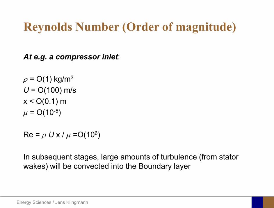
Energy Sciences Jens Klingmann
Reynolds Number (Order of magnitude)
At eg a compressor inlet
ρ = O(1) kgm3
U = O(100) msx lt O(01) mmicro = O(10-5)
Re = ρ U x micro =O(106)
In subsequent stages large amounts of turbulence (from stator wakes) will be convected into the Boundary layer
Energy Sciences Jens Klingmann
References Boundary layers
bull Frank M White ldquoViscous Fluid Flowrdquobull Hermann Schlichting ldquoBoundary Layer Theoryrdquo
Energy Sciences Jens Klingmann
CFD and experiments
bull No this is not a CFD course butbull Experiments
Energy Sciences Jens Klingmann
What do we need to measureOverall performance
Flow rates (mass or volume) Pressure Temperature Shaft power
Performance increase
Separations (velocity) Secondary flows eg tip clearance losses (velocity) Shock waves (supersonic applications) Pressure (resolved in time and space) Temperature (resolved in time and space)
Energy Sciences Jens Klingmann
Cascade wind tunnels
FIG 31 Compressor cascade wind tunnels (a) Conventional low-speed continuousrunning cascade tunnel (adapted from Carter et al 1950)(b) Transonicsupersoniccascade tunnel (adapted from Sieverding 1985)
Energy Sciences Jens Klingmann
Closed circuit tunnels
Energy Sciences Jens Klingmann
components
Settling Chamber
The settling chamber is located between the fan or wide angle diffuser and the contraction and contains the honeycombs and screens used to moderate longitudinal variations in the flow Screens in the chamber should be spaced at 02 chamber diameters apart so that flow disturbed by the first screen can settle before it encounters the second
Honeycombs
Honeycombs are located in the settling chamber and are used to reduce nonuniformities in the flow For optimum benefit honeycombs should be 6-8 cell diameters thick and cell size should be on the order of about 150 cells per settling chamber diameter
Energy Sciences Jens Klingmann
components
Screens
Screens are typically located just downstream of the honeycomb and sometime at the inlet of the test section Screens create a static pressure drop and serve to reduce boundary layer size and increase flow uniformity
Contraction Section
Contractions sections are located between the settling chamber and the test sections and serve to both increase mean velocities at the test section inlet and moderate inconsistencies in the uniformity of the flow Large contraction ratios and short contraction lengths are generally more desirable as they reduce the power loss across the screens and the thickness of boundary layers Small tunnels typically have contraction ratios between 6 and 9
Energy Sciences Jens Klingmann
Flow meters with pressure measurement
Venturi-tube
A1 A2
P1 P2
1 1 2 2C A C A=In the incompressible case
2 21 1 2 2
2 2C P C P
ρ ρ+ = +Assuming horisontal mounting
Energy Sciences Jens Klingmann
Daniel Bernoulli 1700-1782
Daniel Bernoulli was the son of Johann Bernoulli He was born in Groningen while his father held the chair of mathematics there His older brother was Nicolaus(II) Bernoulli and his uncle was Jacob Bernoulli so he was born into a family of leading mathematicians but also into a family where there was unfortunate rivalry jealousy and bitterness
Undoubtedly the most important work which Daniel Bernoulli did was his work on hydrodynamics Even the term itself is based on the title of the work which he produced called Hydrodynamica and before he left St Petersburg Daniel left a draft copy of the book with a printer However the work was not published until 1738 and although he revised it considerably between 1734 and 1738 it is more the presentation that he changed rather then the substance
This work contains for the first time the correct analysis of water flowing from a hole in a container This was based on the principle of conservation of energy which he had studied with his father in 1720 Daniel also discussed pumps and other machines to raise water One remarkable discovery appears in Chapter 10 of Hydrodynamica where Daniel discussed the basis for the kinetic theory of gases He was able to give the basic laws for the theory of gases and gave although not in full detail the equation of state discovered by Van der Waals a century later
Energy Sciences Jens Klingmann
Venturi-tube (2)
22 2 12 2
2
2A PC CA ρ
∆minus =
A1 A2
P1 P2
Solve for eg C2
1 2P P P∆ = minus
( )
12
2 2 21 2
21
PCA Aρ
∆ = minus
and( )
12
2 2 2 2 21 2
21
Pm A C AA Aρρ
∆ = = minus
where
Flow meters with pressure measurement
Energy Sciences Jens Klingmann
Flow meters with pressure measurement
Orifice meters
A1
A2
P1 P2
Applicable for pipe flows Same principle as for Venturi Positioning of pressure taps important Vena contracta and losses require inclusion
of Discharge Coefficient CD
( )
12
2 2 21 2
21D
Pm C AA Aρ ∆ =
minus where ( )1 2ReDC f A A=
CD available from manufacturer (measurements) or Standards (eg ISO)
Energy Sciences Jens Klingmann
Coriolis flow meter
An actuator (not shown) induces a vibration of the tubes
When there is mass flow Coriolis forces induce twisting of the tubes
degree of phase-shift is a measure for the amount of mass that is flowing through the tubes
Energy Sciences Jens Klingmann
Thermal flow meter Heat is added electrically to the flow Temperature is measured before and after heat addition
pP mC T∆=
Energy Sciences Jens Klingmann
Ultrasonic flow meters
Ultrasound is emitted to small particles in the flow (dust or other) Reflections of the sound is frequency shifted by the Doppler effect The frequency change is proportional to the particles velocity (volume flow
meter)
Energy Sciences Jens Klingmann
Inductive flow metersA magnetic flowmeter is based upon Faradays Law
The voltage induced across any conductor as it moves at right angles through a magnetic field is proportional to the velocity of that conductor
E is proportional to V x B x D where
E = The voltage generated in a conductorV = The velocity of the conductorB = The magnetic field strengthD = The length of the conductor
NB electric conductivity is required
Energy Sciences Jens Klingmann
Temperature measurements
Thermocouples
The basis established by Thomas Johann Seebeck in 1821
A conductor generates a voltage when subjected to a temperature gradient
To measure this voltage one must use a second conductor material which generates a different voltage under the same temperature gradient
Energy Sciences Jens Klingmann
Pressure sensing
1 2p pgt 2p p2 may be the atmosphere a static pressure tap or a known reference pressure
The strain of the diaphragm (or itrsquos deflection) may be measured by a number of electric methods
Diaphragm
Energy Sciences Jens Klingmann
Pressure sensingPiezoresistive Strain Gage
Uses the piezoresistive effect of bonded or formed strain gauges to detect strain due to applied pressure
Capacitive
Uses a diaghragm and pressure cavity to create a variable capacitor to detect strain due to applied pressure
Magnetic
Measures the displacement of a diaphragm by means of changes in inductance (reluctance) LVDT Hall Effect or by eddy current principal
Piezoelectric
Uses the piezoelectric effect in certain materials such as quartz to measure the strain upon the sensing mechanism due to pressure
Potentiometric
Uses the motion of a wiper along a resistive mechanism to detect the strain caused by applied pressure
Energy Sciences Jens Klingmann
3D highly instationary (periodic) flow Potentially very high velocities (Supersonic) Large temperature differences Low accessibility (difficult to probe between rotors) Low turbulence levels in most of the domain Very high turbulence in BL and wakes
Properties of measuring object
Point measurements
Energy Sciences Jens Klingmann
Conventional or non-opticalndash Static Pressure Measurementsndash Total Pressure Measurements
bull Multy hole probes
ndash Total Temperature ndash Hot Wire Anemometry (HWA)
Optical techniques for Velocity Measurementsndash Laser Two Focous (L2F)ndash Laser Doppler Anemometry (LDA)ndash Particle Image velocimetry (PIV)
Point Measurements
Energy Sciences Jens Klingmann
Static and total pressure
2 2 21 2 1
2 1 2 2 2C C CP P ρ ρ ρ
minus = minus =
2 0C =Stagnation point
C1Static pressure tap
Prandtl or Pitot tube
Apply the Bernoulli equation from free stream to stagnation point
21
2 12CP Pρ
= +or
We can also define a stagnation or total pressure
( )2
101 1 022
CP P Pρ= + =
Total pressure = Static pressure + dynamic pressure
or
Energy Sciences Jens Klingmann
Static pressure
Energy Sciences Jens Klingmann
Total Pressure and Temperature
Shrouded Probes
Shrouded Probe
Pitot or Prandtl tube
Sensitive to direction
Energy Sciences Jens Klingmann
Ludwig Prandtl 1875-1953
Ludwig Prandtl born at Freising Bavaria on February 4 1875 was a German Physicist famous for his work in aeronautics He qualified at Munchen in 1900 with a thesis on elastic stability and held the position of Professor of Applied Mechanics at Gottingen for forty-nine years (from 1904 until his death there on August 15 1953) In 1925 Prandtl became the Director of the Kaiser Wilhelm Institute for Fluid Mechanics His discovery in 1904 of the Boundary Layer which adjoins the surface of a body moving in a fluid led to an understanding of skin friction drag and of the way in which streamlining reduces the drag of airplane wings and other moving bodies His work on wing theory published in 1918 - 1919 followed that of FW Lanchester (1902-1907) but was carried out independently and elucidated the flow over airplane wings of finite span Prandtls work and decisive advances in boundary layer and wing theories became the basic material of aeronautics He also made important contributions to the theories of supersonic flow and of turbulence and contributed much to the development of wind tunnels and other aerodynamic equipment In addition he devised the soap-film analogy for the torsion of non-circular sections and wrote on the theory of plasticity and of meteorology
Energy Sciences Jens Klingmann
Total Pressure multy hole
Cobra Probe Yaw Probe
5 Hole Probe
Energy Sciences Jens Klingmann
5 Hole Probes Calibration
Energy Sciences Jens Klingmann
The inherent unsteadiness of the flow within turbomachines
Energy Sciences Jens Klingmann
Hot Wire Anemometry (HWA) The heat transfer from a thin (one micron)
electrically heated wire can be used to determine velocity
The resistance of the wire is temperature dependent Within a small temperature range it can be assumed linear R = R0+α R0(Tm-T0) where R0 is the resistance at a reference temperature T0 and Tm is the mean wire temperature
The thermal power induced in the wire is balanced by heat transfer to the surrounding fluid I2R=hπDL(Tm-T0) where h is the heat transfer coefficient and D and L the diameter and length of the wire respectively
E = I R
Energy Sciences Jens Klingmann
Constant Temperature Anemometry (CTA) The wire is often placed in a Whetstone bridge If the output from the
bridge is amplified and fed back to the bridge the resistance of the probe and thus the temperature will be held constant
This prevents the temperature of the wire to become excessive at low velocities
R1
R2 R3
Probe
Bridge Voltage
Energy Sciences Jens Klingmann
Constant Temperature Anemometry (CTA)
Energy Sciences Jens Klingmann
Characteristics of LDA (according to Dantec)
Invented by Yeh and Cummins in 1964 Velocity measurements in Fluid Dynamics (gas liquid) Up to 3 velocity components Non-intrusive measurements (optical technique) Absolute measurement technique (no calibration required) Very high accuracy Very high spatial resolution due to small measurement volume Tracer particles are required
Energy Sciences Jens Klingmann
LDA - Fringe Model
Focused Laser beams intersect and form the measurement volume Plane wave fronts beam waist in the plane of intersection Interference in the plane of intersection Pattern of bright and dark stripesplanes Fringes
Energy Sciences Jens Klingmann
LDA-measuring volume
d
x
x
y
y
z
z
e-2 CONTOUR
FRINGES
κ
κ
κ
κ
De-2
De-2
dml m
a
b
cx
b
z
ya
cd
d
=
=
=
J
J
J
J
JP
JP
JP
JD
JD
JD
+
+
+
a
b
c
d
κπλ
=minus sinD
f4l2e
m
κπλ
=minus cosD
f4D2e
m
Energy Sciences Jens Klingmann
Laser Two Focus
Energy Sciences Jens Klingmann
Laser Two Focus
Energy Sciences Jens Klingmann
PIV measurements
PIV is a fairly new technique capable of simultaneous velocity measurements at many points in a plane This gives information on large scale structures vorticity etc which is very difficult or impossible to obtain from one-point measuring techniques
PIV involves the illumination of a plane of the flow under investigation with a thin pulsed sheet of light The flow is seeded with particles
The light scattered from the particles and from successive pulses are being recorded either on film or a CCD array forming a multiple exposure of each particle image If the time between the pulses is known velocity can be determined as the ratio of the particle displacement and the elapsed time
t∆∆= xu
Energy Sciences Jens Klingmann
PIV
Energy Sciences Jens Klingmann
PIV measurements illumination
YA
G
YA
G
Two frequency doubled YAG Lasers aligned to one double pulsed laser sheet
Two or more separate light pulses can be obtained by chopping a continuous laser or from pulsed lasers
The limited pulse energies obtained from continuous lasers limits their applicability to low velocity flows or flows where large seeding particles can be used (ie liquid flows)
The low repetition rate of most pulsed lasers makes the use of two lasers advantageous
Energy Sciences Jens Klingmann
PIV measurements recording
High seeding density in laminar flame
Film or CCD-cameras Cross- or Auto-correlation
ndash ie both particle images on the same frame or on separate frames
CCD-camera requirementndash A many pixels as possiblendash 2k by 2k available 4k by 4k coming
Energy Sciences Jens Klingmann
PIV measurements analyses
Low seeding density (Number of seeding particles per unit volume)
Each particle image pair can be identified This is called particle tracking
High seeding density (PIV)
Small sub-regions of the image containing many particle image pairs are processed to obtain one velocity vector
Energy Sciences Jens Klingmann
PIV measurements analyses
Energy Sciences Jens Klingmann
PIV measurements analyses
( ) ( ) ( ) xsxxs dIIR 2A
1
I
+= int
Cross correlation between ( )x1I and ( )x2I
s is a two dimensional displacement vector
IA is the interrogation area
Cross correlation between
(
)
x
1
I
and
(
)
x
2
I
s is a two dimensional displacement vector
I
A
is the interrogation area
Energy Sciences Jens Klingmann
Energy Sciences Jens Klingmann
PIV from IOWA state university
Energy Sciences Jens Klingmann
PIV sample of evaluation
Energy Sciences Jens Klingmann
LDA PIV HWA Velocity range 01 mms ndash 300
ms 02 ndash 150 ms
Measuring Volume
D = 005 L = 05 mm
2 by 2 by 05 mm
L = 05 mm
Freq response O(10 000) Hz O(10) Hz O(100 000) Hz Calibration Yes No No Sensitivity to other than velocity
Low (ref Index) Low (ref Index) Large (temperature concentrationshellip)
Continuous Signal
Sometimes Seldom Always
Noise High High Low Turbulence intensity
No limitation Some limitation lt 20
Price O(1 000 000) SEK
O(1 000 000) SEK
O(50 000) SEK
Required Knowledge
High medium Low
Comparison of techniques
Energy Sciences Jens Klingmann
References experiments
R J Goldstein ldquoFluid Mechanics Measurementsrdquo Hemisphere Publishing 1983 A V Johansson amp P H Alfredsson ldquoExperimentella metoder inom
stroumlmningsmekanikenrdquo Inst Foumlr Mekanik KTH F Durst A Melling and J H Whitelaw ldquoPrincipals and Practice of Laser Doppler
Anemometryrdquo 1984 R J Adrian ldquoParticle-imaging techniques for experimental fluid mechnicsrdquo Ann Rev
Fluid Mech 1991
Energy Sciences Jens Klingmann
Sample of LDA-measurements
Rotor blade
Glas window
Emitted beams
Scattered Light
Adjustable mirror
Energy Sciences Jens Klingmann
Axial velocity sorted into 10 bins
0 1 2 3 4 5 6tangential coordinate (degrees)
-20
0
20
40
60
80
100
120
140
160Ax
ial v
eloc
ity a
nd s
tand
ard
devi
atio
n (m
s)
radial position 7 mm from inner window surfaceaxial position 23 mm behind rotor blades
Energy Sciences Jens Klingmann
Axial velocities in the radial-tangential plane
Energy Sciences Jens Klingmann
Airfoils NACA 4-digit
The NACA four-digit wing sections define the profile by
One digit describing maximum camber as percentage of the chord
One digit describing the distance of maximum camber from the airfoil leading edge in tens of percents of the chord
Two digits describing maximum thickness of the airfoil as percent of the chord
Example the NACA 2412 airfoil has a maximum camber of 2 located 40 (04 chords) from the leading edge with a maximum thickness of 12 of the chord
Four-digit series airfoils by default have maximum thickness at 30 of the chord (03 chords) from the leading edge
Energy Sciences Jens Klingmann
Airfoils NACA 4-digit
bull c is the chord lengthbull x is the position along
the chord from 0 to cbull y is the half thickness at
a given value of x (centerline to surface)
bull t is the maximum thickness as a fraction of the chord
Energy Sciences Jens Klingmann
Death by PowerPoint
| LDA | PIV | HWA | |||||
| Velocity range | 01 mms ndash 300 ms | 02 ndash 150 ms | |||||
| Measuring Volume | D = 005 L = 05 mm | 2 by 2 by 05 mm | L = 05 mm | ||||
| Freq response | O(10 000) Hz | O(10) Hz | O(100 000) Hz | ||||
| Calibration | Yes | No | No | ||||
| Sensitivity to other than velocity | Low (ref Index) | Low (ref Index) | Large (temperature concentrationshellip) | ||||
| Continuous Signal | Sometimes | Seldom | Always | ||||
| Noise | High | High | Low | ||||
| Turbulence intensity | No limitation | Some limitation | lt 20 | ||||
| Price | O(1 000 000) SEK | O(1 000 000) SEK | O(50 000) SEK | ||||
| Required Knowledge | High | medium | Low |
Energy Sciences Jens Klingmann
CFD and experiments
bull No this is not a CFD course butbull Experiments
Energy Sciences Jens Klingmann
What do we need to measureOverall performance
Flow rates (mass or volume) Pressure Temperature Shaft power
Performance increase
Separations (velocity) Secondary flows eg tip clearance losses (velocity) Shock waves (supersonic applications) Pressure (resolved in time and space) Temperature (resolved in time and space)
Energy Sciences Jens Klingmann
Cascade wind tunnels
FIG 31 Compressor cascade wind tunnels (a) Conventional low-speed continuousrunning cascade tunnel (adapted from Carter et al 1950)(b) Transonicsupersoniccascade tunnel (adapted from Sieverding 1985)
Energy Sciences Jens Klingmann
Closed circuit tunnels
Energy Sciences Jens Klingmann
components
Settling Chamber
The settling chamber is located between the fan or wide angle diffuser and the contraction and contains the honeycombs and screens used to moderate longitudinal variations in the flow Screens in the chamber should be spaced at 02 chamber diameters apart so that flow disturbed by the first screen can settle before it encounters the second
Honeycombs
Honeycombs are located in the settling chamber and are used to reduce nonuniformities in the flow For optimum benefit honeycombs should be 6-8 cell diameters thick and cell size should be on the order of about 150 cells per settling chamber diameter
Energy Sciences Jens Klingmann
components
Screens
Screens are typically located just downstream of the honeycomb and sometime at the inlet of the test section Screens create a static pressure drop and serve to reduce boundary layer size and increase flow uniformity
Contraction Section
Contractions sections are located between the settling chamber and the test sections and serve to both increase mean velocities at the test section inlet and moderate inconsistencies in the uniformity of the flow Large contraction ratios and short contraction lengths are generally more desirable as they reduce the power loss across the screens and the thickness of boundary layers Small tunnels typically have contraction ratios between 6 and 9
Energy Sciences Jens Klingmann
Flow meters with pressure measurement
Venturi-tube
A1 A2
P1 P2
1 1 2 2C A C A=In the incompressible case
2 21 1 2 2
2 2C P C P
ρ ρ+ = +Assuming horisontal mounting
Energy Sciences Jens Klingmann
Daniel Bernoulli 1700-1782
Daniel Bernoulli was the son of Johann Bernoulli He was born in Groningen while his father held the chair of mathematics there His older brother was Nicolaus(II) Bernoulli and his uncle was Jacob Bernoulli so he was born into a family of leading mathematicians but also into a family where there was unfortunate rivalry jealousy and bitterness
Undoubtedly the most important work which Daniel Bernoulli did was his work on hydrodynamics Even the term itself is based on the title of the work which he produced called Hydrodynamica and before he left St Petersburg Daniel left a draft copy of the book with a printer However the work was not published until 1738 and although he revised it considerably between 1734 and 1738 it is more the presentation that he changed rather then the substance
This work contains for the first time the correct analysis of water flowing from a hole in a container This was based on the principle of conservation of energy which he had studied with his father in 1720 Daniel also discussed pumps and other machines to raise water One remarkable discovery appears in Chapter 10 of Hydrodynamica where Daniel discussed the basis for the kinetic theory of gases He was able to give the basic laws for the theory of gases and gave although not in full detail the equation of state discovered by Van der Waals a century later
Energy Sciences Jens Klingmann
Venturi-tube (2)
22 2 12 2
2
2A PC CA ρ
∆minus =
A1 A2
P1 P2
Solve for eg C2
1 2P P P∆ = minus
( )
12
2 2 21 2
21
PCA Aρ
∆ = minus
and( )
12
2 2 2 2 21 2
21
Pm A C AA Aρρ
∆ = = minus
where
Flow meters with pressure measurement
Energy Sciences Jens Klingmann
Flow meters with pressure measurement
Orifice meters
A1
A2
P1 P2
Applicable for pipe flows Same principle as for Venturi Positioning of pressure taps important Vena contracta and losses require inclusion
of Discharge Coefficient CD
( )
12
2 2 21 2
21D
Pm C AA Aρ ∆ =
minus where ( )1 2ReDC f A A=
CD available from manufacturer (measurements) or Standards (eg ISO)
Energy Sciences Jens Klingmann
Coriolis flow meter
An actuator (not shown) induces a vibration of the tubes
When there is mass flow Coriolis forces induce twisting of the tubes
degree of phase-shift is a measure for the amount of mass that is flowing through the tubes
Energy Sciences Jens Klingmann
Thermal flow meter Heat is added electrically to the flow Temperature is measured before and after heat addition
pP mC T∆=
Energy Sciences Jens Klingmann
Ultrasonic flow meters
Ultrasound is emitted to small particles in the flow (dust or other) Reflections of the sound is frequency shifted by the Doppler effect The frequency change is proportional to the particles velocity (volume flow
meter)
Energy Sciences Jens Klingmann
Inductive flow metersA magnetic flowmeter is based upon Faradays Law
The voltage induced across any conductor as it moves at right angles through a magnetic field is proportional to the velocity of that conductor
E is proportional to V x B x D where
E = The voltage generated in a conductorV = The velocity of the conductorB = The magnetic field strengthD = The length of the conductor
NB electric conductivity is required
Energy Sciences Jens Klingmann
Temperature measurements
Thermocouples
The basis established by Thomas Johann Seebeck in 1821
A conductor generates a voltage when subjected to a temperature gradient
To measure this voltage one must use a second conductor material which generates a different voltage under the same temperature gradient
Energy Sciences Jens Klingmann
Pressure sensing
1 2p pgt 2p p2 may be the atmosphere a static pressure tap or a known reference pressure
The strain of the diaphragm (or itrsquos deflection) may be measured by a number of electric methods
Diaphragm
Energy Sciences Jens Klingmann
Pressure sensingPiezoresistive Strain Gage
Uses the piezoresistive effect of bonded or formed strain gauges to detect strain due to applied pressure
Capacitive
Uses a diaghragm and pressure cavity to create a variable capacitor to detect strain due to applied pressure
Magnetic
Measures the displacement of a diaphragm by means of changes in inductance (reluctance) LVDT Hall Effect or by eddy current principal
Piezoelectric
Uses the piezoelectric effect in certain materials such as quartz to measure the strain upon the sensing mechanism due to pressure
Potentiometric
Uses the motion of a wiper along a resistive mechanism to detect the strain caused by applied pressure
Energy Sciences Jens Klingmann
3D highly instationary (periodic) flow Potentially very high velocities (Supersonic) Large temperature differences Low accessibility (difficult to probe between rotors) Low turbulence levels in most of the domain Very high turbulence in BL and wakes
Properties of measuring object
Point measurements
Energy Sciences Jens Klingmann
Conventional or non-opticalndash Static Pressure Measurementsndash Total Pressure Measurements
bull Multy hole probes
ndash Total Temperature ndash Hot Wire Anemometry (HWA)
Optical techniques for Velocity Measurementsndash Laser Two Focous (L2F)ndash Laser Doppler Anemometry (LDA)ndash Particle Image velocimetry (PIV)
Point Measurements
Energy Sciences Jens Klingmann
Static and total pressure
2 2 21 2 1
2 1 2 2 2C C CP P ρ ρ ρ
minus = minus =
2 0C =Stagnation point
C1Static pressure tap
Prandtl or Pitot tube
Apply the Bernoulli equation from free stream to stagnation point
21
2 12CP Pρ
= +or
We can also define a stagnation or total pressure
( )2
101 1 022
CP P Pρ= + =
Total pressure = Static pressure + dynamic pressure
or
Energy Sciences Jens Klingmann
Static pressure
Energy Sciences Jens Klingmann
Total Pressure and Temperature
Shrouded Probes
Shrouded Probe
Pitot or Prandtl tube
Sensitive to direction
Energy Sciences Jens Klingmann
Ludwig Prandtl 1875-1953
Ludwig Prandtl born at Freising Bavaria on February 4 1875 was a German Physicist famous for his work in aeronautics He qualified at Munchen in 1900 with a thesis on elastic stability and held the position of Professor of Applied Mechanics at Gottingen for forty-nine years (from 1904 until his death there on August 15 1953) In 1925 Prandtl became the Director of the Kaiser Wilhelm Institute for Fluid Mechanics His discovery in 1904 of the Boundary Layer which adjoins the surface of a body moving in a fluid led to an understanding of skin friction drag and of the way in which streamlining reduces the drag of airplane wings and other moving bodies His work on wing theory published in 1918 - 1919 followed that of FW Lanchester (1902-1907) but was carried out independently and elucidated the flow over airplane wings of finite span Prandtls work and decisive advances in boundary layer and wing theories became the basic material of aeronautics He also made important contributions to the theories of supersonic flow and of turbulence and contributed much to the development of wind tunnels and other aerodynamic equipment In addition he devised the soap-film analogy for the torsion of non-circular sections and wrote on the theory of plasticity and of meteorology
Energy Sciences Jens Klingmann
Total Pressure multy hole
Cobra Probe Yaw Probe
5 Hole Probe
Energy Sciences Jens Klingmann
5 Hole Probes Calibration
Energy Sciences Jens Klingmann
The inherent unsteadiness of the flow within turbomachines
Energy Sciences Jens Klingmann
Hot Wire Anemometry (HWA) The heat transfer from a thin (one micron)
electrically heated wire can be used to determine velocity
The resistance of the wire is temperature dependent Within a small temperature range it can be assumed linear R = R0+α R0(Tm-T0) where R0 is the resistance at a reference temperature T0 and Tm is the mean wire temperature
The thermal power induced in the wire is balanced by heat transfer to the surrounding fluid I2R=hπDL(Tm-T0) where h is the heat transfer coefficient and D and L the diameter and length of the wire respectively
E = I R
Energy Sciences Jens Klingmann
Constant Temperature Anemometry (CTA) The wire is often placed in a Whetstone bridge If the output from the
bridge is amplified and fed back to the bridge the resistance of the probe and thus the temperature will be held constant
This prevents the temperature of the wire to become excessive at low velocities
R1
R2 R3
Probe
Bridge Voltage
Energy Sciences Jens Klingmann
Constant Temperature Anemometry (CTA)
Energy Sciences Jens Klingmann
Characteristics of LDA (according to Dantec)
Invented by Yeh and Cummins in 1964 Velocity measurements in Fluid Dynamics (gas liquid) Up to 3 velocity components Non-intrusive measurements (optical technique) Absolute measurement technique (no calibration required) Very high accuracy Very high spatial resolution due to small measurement volume Tracer particles are required
Energy Sciences Jens Klingmann
LDA - Fringe Model
Focused Laser beams intersect and form the measurement volume Plane wave fronts beam waist in the plane of intersection Interference in the plane of intersection Pattern of bright and dark stripesplanes Fringes
Energy Sciences Jens Klingmann
LDA-measuring volume
d
x
x
y
y
z
z
e-2 CONTOUR
FRINGES
κ
κ
κ
κ
De-2
De-2
dml m
a
b
cx
b
z
ya
cd
d
=
=
=
J
J
J
J
JP
JP
JP
JD
JD
JD
+
+
+
a
b
c
d
κπλ
=minus sinD
f4l2e
m
κπλ
=minus cosD
f4D2e
m
Energy Sciences Jens Klingmann
Laser Two Focus
Energy Sciences Jens Klingmann
Laser Two Focus
Energy Sciences Jens Klingmann
PIV measurements
PIV is a fairly new technique capable of simultaneous velocity measurements at many points in a plane This gives information on large scale structures vorticity etc which is very difficult or impossible to obtain from one-point measuring techniques
PIV involves the illumination of a plane of the flow under investigation with a thin pulsed sheet of light The flow is seeded with particles
The light scattered from the particles and from successive pulses are being recorded either on film or a CCD array forming a multiple exposure of each particle image If the time between the pulses is known velocity can be determined as the ratio of the particle displacement and the elapsed time
t∆∆= xu
Energy Sciences Jens Klingmann
PIV
Energy Sciences Jens Klingmann
PIV measurements illumination
YA
G
YA
G
Two frequency doubled YAG Lasers aligned to one double pulsed laser sheet
Two or more separate light pulses can be obtained by chopping a continuous laser or from pulsed lasers
The limited pulse energies obtained from continuous lasers limits their applicability to low velocity flows or flows where large seeding particles can be used (ie liquid flows)
The low repetition rate of most pulsed lasers makes the use of two lasers advantageous
Energy Sciences Jens Klingmann
PIV measurements recording
High seeding density in laminar flame
Film or CCD-cameras Cross- or Auto-correlation
ndash ie both particle images on the same frame or on separate frames
CCD-camera requirementndash A many pixels as possiblendash 2k by 2k available 4k by 4k coming
Energy Sciences Jens Klingmann
PIV measurements analyses
Low seeding density (Number of seeding particles per unit volume)
Each particle image pair can be identified This is called particle tracking
High seeding density (PIV)
Small sub-regions of the image containing many particle image pairs are processed to obtain one velocity vector
Energy Sciences Jens Klingmann
PIV measurements analyses
Energy Sciences Jens Klingmann
PIV measurements analyses
( ) ( ) ( ) xsxxs dIIR 2A
1
I
+= int
Cross correlation between ( )x1I and ( )x2I
s is a two dimensional displacement vector
IA is the interrogation area
Cross correlation between
(
)
x
1
I
and
(
)
x
2
I
s is a two dimensional displacement vector
I
A
is the interrogation area
Energy Sciences Jens Klingmann
Energy Sciences Jens Klingmann
PIV from IOWA state university
Energy Sciences Jens Klingmann
PIV sample of evaluation
Energy Sciences Jens Klingmann
LDA PIV HWA Velocity range 01 mms ndash 300
ms 02 ndash 150 ms
Measuring Volume
D = 005 L = 05 mm
2 by 2 by 05 mm
L = 05 mm
Freq response O(10 000) Hz O(10) Hz O(100 000) Hz Calibration Yes No No Sensitivity to other than velocity
Low (ref Index) Low (ref Index) Large (temperature concentrationshellip)
Continuous Signal
Sometimes Seldom Always
Noise High High Low Turbulence intensity
No limitation Some limitation lt 20
Price O(1 000 000) SEK
O(1 000 000) SEK
O(50 000) SEK
Required Knowledge
High medium Low
Comparison of techniques
Energy Sciences Jens Klingmann
References experiments
R J Goldstein ldquoFluid Mechanics Measurementsrdquo Hemisphere Publishing 1983 A V Johansson amp P H Alfredsson ldquoExperimentella metoder inom
stroumlmningsmekanikenrdquo Inst Foumlr Mekanik KTH F Durst A Melling and J H Whitelaw ldquoPrincipals and Practice of Laser Doppler
Anemometryrdquo 1984 R J Adrian ldquoParticle-imaging techniques for experimental fluid mechnicsrdquo Ann Rev
Fluid Mech 1991
Energy Sciences Jens Klingmann
Sample of LDA-measurements
Rotor blade
Glas window
Emitted beams
Scattered Light
Adjustable mirror
Energy Sciences Jens Klingmann
Axial velocity sorted into 10 bins
0 1 2 3 4 5 6tangential coordinate (degrees)
-20
0
20
40
60
80
100
120
140
160Ax
ial v
eloc
ity a
nd s
tand
ard
devi
atio
n (m
s)
radial position 7 mm from inner window surfaceaxial position 23 mm behind rotor blades
Energy Sciences Jens Klingmann
Axial velocities in the radial-tangential plane
Energy Sciences Jens Klingmann
Airfoils NACA 4-digit
The NACA four-digit wing sections define the profile by
One digit describing maximum camber as percentage of the chord
One digit describing the distance of maximum camber from the airfoil leading edge in tens of percents of the chord
Two digits describing maximum thickness of the airfoil as percent of the chord
Example the NACA 2412 airfoil has a maximum camber of 2 located 40 (04 chords) from the leading edge with a maximum thickness of 12 of the chord
Four-digit series airfoils by default have maximum thickness at 30 of the chord (03 chords) from the leading edge
Energy Sciences Jens Klingmann
Airfoils NACA 4-digit
bull c is the chord lengthbull x is the position along
the chord from 0 to cbull y is the half thickness at
a given value of x (centerline to surface)
bull t is the maximum thickness as a fraction of the chord
Energy Sciences Jens Klingmann
Death by PowerPoint
| LDA | PIV | HWA | |||||
| Velocity range | 01 mms ndash 300 ms | 02 ndash 150 ms | |||||
| Measuring Volume | D = 005 L = 05 mm | 2 by 2 by 05 mm | L = 05 mm | ||||
| Freq response | O(10 000) Hz | O(10) Hz | O(100 000) Hz | ||||
| Calibration | Yes | No | No | ||||
| Sensitivity to other than velocity | Low (ref Index) | Low (ref Index) | Large (temperature concentrationshellip) | ||||
| Continuous Signal | Sometimes | Seldom | Always | ||||
| Noise | High | High | Low | ||||
| Turbulence intensity | No limitation | Some limitation | lt 20 | ||||
| Price | O(1 000 000) SEK | O(1 000 000) SEK | O(50 000) SEK | ||||
| Required Knowledge | High | medium | Low |
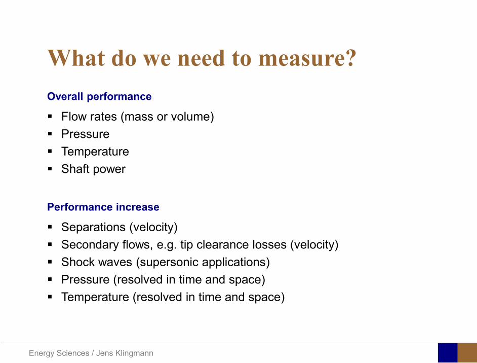
Energy Sciences Jens Klingmann
What do we need to measureOverall performance
Flow rates (mass or volume) Pressure Temperature Shaft power
Performance increase
Separations (velocity) Secondary flows eg tip clearance losses (velocity) Shock waves (supersonic applications) Pressure (resolved in time and space) Temperature (resolved in time and space)
Energy Sciences Jens Klingmann
Cascade wind tunnels
FIG 31 Compressor cascade wind tunnels (a) Conventional low-speed continuousrunning cascade tunnel (adapted from Carter et al 1950)(b) Transonicsupersoniccascade tunnel (adapted from Sieverding 1985)
Energy Sciences Jens Klingmann
Closed circuit tunnels
Energy Sciences Jens Klingmann
components
Settling Chamber
The settling chamber is located between the fan or wide angle diffuser and the contraction and contains the honeycombs and screens used to moderate longitudinal variations in the flow Screens in the chamber should be spaced at 02 chamber diameters apart so that flow disturbed by the first screen can settle before it encounters the second
Honeycombs
Honeycombs are located in the settling chamber and are used to reduce nonuniformities in the flow For optimum benefit honeycombs should be 6-8 cell diameters thick and cell size should be on the order of about 150 cells per settling chamber diameter
Energy Sciences Jens Klingmann
components
Screens
Screens are typically located just downstream of the honeycomb and sometime at the inlet of the test section Screens create a static pressure drop and serve to reduce boundary layer size and increase flow uniformity
Contraction Section
Contractions sections are located between the settling chamber and the test sections and serve to both increase mean velocities at the test section inlet and moderate inconsistencies in the uniformity of the flow Large contraction ratios and short contraction lengths are generally more desirable as they reduce the power loss across the screens and the thickness of boundary layers Small tunnels typically have contraction ratios between 6 and 9
Energy Sciences Jens Klingmann
Flow meters with pressure measurement
Venturi-tube
A1 A2
P1 P2
1 1 2 2C A C A=In the incompressible case
2 21 1 2 2
2 2C P C P
ρ ρ+ = +Assuming horisontal mounting
Energy Sciences Jens Klingmann
Daniel Bernoulli 1700-1782
Daniel Bernoulli was the son of Johann Bernoulli He was born in Groningen while his father held the chair of mathematics there His older brother was Nicolaus(II) Bernoulli and his uncle was Jacob Bernoulli so he was born into a family of leading mathematicians but also into a family where there was unfortunate rivalry jealousy and bitterness
Undoubtedly the most important work which Daniel Bernoulli did was his work on hydrodynamics Even the term itself is based on the title of the work which he produced called Hydrodynamica and before he left St Petersburg Daniel left a draft copy of the book with a printer However the work was not published until 1738 and although he revised it considerably between 1734 and 1738 it is more the presentation that he changed rather then the substance
This work contains for the first time the correct analysis of water flowing from a hole in a container This was based on the principle of conservation of energy which he had studied with his father in 1720 Daniel also discussed pumps and other machines to raise water One remarkable discovery appears in Chapter 10 of Hydrodynamica where Daniel discussed the basis for the kinetic theory of gases He was able to give the basic laws for the theory of gases and gave although not in full detail the equation of state discovered by Van der Waals a century later
Energy Sciences Jens Klingmann
Venturi-tube (2)
22 2 12 2
2
2A PC CA ρ
∆minus =
A1 A2
P1 P2
Solve for eg C2
1 2P P P∆ = minus
( )
12
2 2 21 2
21
PCA Aρ
∆ = minus
and( )
12
2 2 2 2 21 2
21
Pm A C AA Aρρ
∆ = = minus
where
Flow meters with pressure measurement
Energy Sciences Jens Klingmann
Flow meters with pressure measurement
Orifice meters
A1
A2
P1 P2
Applicable for pipe flows Same principle as for Venturi Positioning of pressure taps important Vena contracta and losses require inclusion
of Discharge Coefficient CD
( )
12
2 2 21 2
21D
Pm C AA Aρ ∆ =
minus where ( )1 2ReDC f A A=
CD available from manufacturer (measurements) or Standards (eg ISO)
Energy Sciences Jens Klingmann
Coriolis flow meter
An actuator (not shown) induces a vibration of the tubes
When there is mass flow Coriolis forces induce twisting of the tubes
degree of phase-shift is a measure for the amount of mass that is flowing through the tubes
Energy Sciences Jens Klingmann
Thermal flow meter Heat is added electrically to the flow Temperature is measured before and after heat addition
pP mC T∆=
Energy Sciences Jens Klingmann
Ultrasonic flow meters
Ultrasound is emitted to small particles in the flow (dust or other) Reflections of the sound is frequency shifted by the Doppler effect The frequency change is proportional to the particles velocity (volume flow
meter)
Energy Sciences Jens Klingmann
Inductive flow metersA magnetic flowmeter is based upon Faradays Law
The voltage induced across any conductor as it moves at right angles through a magnetic field is proportional to the velocity of that conductor
E is proportional to V x B x D where
E = The voltage generated in a conductorV = The velocity of the conductorB = The magnetic field strengthD = The length of the conductor
NB electric conductivity is required
Energy Sciences Jens Klingmann
Temperature measurements
Thermocouples
The basis established by Thomas Johann Seebeck in 1821
A conductor generates a voltage when subjected to a temperature gradient
To measure this voltage one must use a second conductor material which generates a different voltage under the same temperature gradient
Energy Sciences Jens Klingmann
Pressure sensing
1 2p pgt 2p p2 may be the atmosphere a static pressure tap or a known reference pressure
The strain of the diaphragm (or itrsquos deflection) may be measured by a number of electric methods
Diaphragm
Energy Sciences Jens Klingmann
Pressure sensingPiezoresistive Strain Gage
Uses the piezoresistive effect of bonded or formed strain gauges to detect strain due to applied pressure
Capacitive
Uses a diaghragm and pressure cavity to create a variable capacitor to detect strain due to applied pressure
Magnetic
Measures the displacement of a diaphragm by means of changes in inductance (reluctance) LVDT Hall Effect or by eddy current principal
Piezoelectric
Uses the piezoelectric effect in certain materials such as quartz to measure the strain upon the sensing mechanism due to pressure
Potentiometric
Uses the motion of a wiper along a resistive mechanism to detect the strain caused by applied pressure
Energy Sciences Jens Klingmann
3D highly instationary (periodic) flow Potentially very high velocities (Supersonic) Large temperature differences Low accessibility (difficult to probe between rotors) Low turbulence levels in most of the domain Very high turbulence in BL and wakes
Properties of measuring object
Point measurements
Energy Sciences Jens Klingmann
Conventional or non-opticalndash Static Pressure Measurementsndash Total Pressure Measurements
bull Multy hole probes
ndash Total Temperature ndash Hot Wire Anemometry (HWA)
Optical techniques for Velocity Measurementsndash Laser Two Focous (L2F)ndash Laser Doppler Anemometry (LDA)ndash Particle Image velocimetry (PIV)
Point Measurements
Energy Sciences Jens Klingmann
Static and total pressure
2 2 21 2 1
2 1 2 2 2C C CP P ρ ρ ρ
minus = minus =
2 0C =Stagnation point
C1Static pressure tap
Prandtl or Pitot tube
Apply the Bernoulli equation from free stream to stagnation point
21
2 12CP Pρ
= +or
We can also define a stagnation or total pressure
( )2
101 1 022
CP P Pρ= + =
Total pressure = Static pressure + dynamic pressure
or
Energy Sciences Jens Klingmann
Static pressure
Energy Sciences Jens Klingmann
Total Pressure and Temperature
Shrouded Probes
Shrouded Probe
Pitot or Prandtl tube
Sensitive to direction
Energy Sciences Jens Klingmann
Ludwig Prandtl 1875-1953
Ludwig Prandtl born at Freising Bavaria on February 4 1875 was a German Physicist famous for his work in aeronautics He qualified at Munchen in 1900 with a thesis on elastic stability and held the position of Professor of Applied Mechanics at Gottingen for forty-nine years (from 1904 until his death there on August 15 1953) In 1925 Prandtl became the Director of the Kaiser Wilhelm Institute for Fluid Mechanics His discovery in 1904 of the Boundary Layer which adjoins the surface of a body moving in a fluid led to an understanding of skin friction drag and of the way in which streamlining reduces the drag of airplane wings and other moving bodies His work on wing theory published in 1918 - 1919 followed that of FW Lanchester (1902-1907) but was carried out independently and elucidated the flow over airplane wings of finite span Prandtls work and decisive advances in boundary layer and wing theories became the basic material of aeronautics He also made important contributions to the theories of supersonic flow and of turbulence and contributed much to the development of wind tunnels and other aerodynamic equipment In addition he devised the soap-film analogy for the torsion of non-circular sections and wrote on the theory of plasticity and of meteorology
Energy Sciences Jens Klingmann
Total Pressure multy hole
Cobra Probe Yaw Probe
5 Hole Probe
Energy Sciences Jens Klingmann
5 Hole Probes Calibration
Energy Sciences Jens Klingmann
The inherent unsteadiness of the flow within turbomachines
Energy Sciences Jens Klingmann
Hot Wire Anemometry (HWA) The heat transfer from a thin (one micron)
electrically heated wire can be used to determine velocity
The resistance of the wire is temperature dependent Within a small temperature range it can be assumed linear R = R0+α R0(Tm-T0) where R0 is the resistance at a reference temperature T0 and Tm is the mean wire temperature
The thermal power induced in the wire is balanced by heat transfer to the surrounding fluid I2R=hπDL(Tm-T0) where h is the heat transfer coefficient and D and L the diameter and length of the wire respectively
E = I R
Energy Sciences Jens Klingmann
Constant Temperature Anemometry (CTA) The wire is often placed in a Whetstone bridge If the output from the
bridge is amplified and fed back to the bridge the resistance of the probe and thus the temperature will be held constant
This prevents the temperature of the wire to become excessive at low velocities
R1
R2 R3
Probe
Bridge Voltage
Energy Sciences Jens Klingmann
Constant Temperature Anemometry (CTA)
Energy Sciences Jens Klingmann
Characteristics of LDA (according to Dantec)
Invented by Yeh and Cummins in 1964 Velocity measurements in Fluid Dynamics (gas liquid) Up to 3 velocity components Non-intrusive measurements (optical technique) Absolute measurement technique (no calibration required) Very high accuracy Very high spatial resolution due to small measurement volume Tracer particles are required
Energy Sciences Jens Klingmann
LDA - Fringe Model
Focused Laser beams intersect and form the measurement volume Plane wave fronts beam waist in the plane of intersection Interference in the plane of intersection Pattern of bright and dark stripesplanes Fringes
Energy Sciences Jens Klingmann
LDA-measuring volume
d
x
x
y
y
z
z
e-2 CONTOUR
FRINGES
κ
κ
κ
κ
De-2
De-2
dml m
a
b
cx
b
z
ya
cd
d
=
=
=
J
J
J
J
JP
JP
JP
JD
JD
JD
+
+
+
a
b
c
d
κπλ
=minus sinD
f4l2e
m
κπλ
=minus cosD
f4D2e
m
Energy Sciences Jens Klingmann
Laser Two Focus
Energy Sciences Jens Klingmann
Laser Two Focus
Energy Sciences Jens Klingmann
PIV measurements
PIV is a fairly new technique capable of simultaneous velocity measurements at many points in a plane This gives information on large scale structures vorticity etc which is very difficult or impossible to obtain from one-point measuring techniques
PIV involves the illumination of a plane of the flow under investigation with a thin pulsed sheet of light The flow is seeded with particles
The light scattered from the particles and from successive pulses are being recorded either on film or a CCD array forming a multiple exposure of each particle image If the time between the pulses is known velocity can be determined as the ratio of the particle displacement and the elapsed time
t∆∆= xu
Energy Sciences Jens Klingmann
PIV
Energy Sciences Jens Klingmann
PIV measurements illumination
YA
G
YA
G
Two frequency doubled YAG Lasers aligned to one double pulsed laser sheet
Two or more separate light pulses can be obtained by chopping a continuous laser or from pulsed lasers
The limited pulse energies obtained from continuous lasers limits their applicability to low velocity flows or flows where large seeding particles can be used (ie liquid flows)
The low repetition rate of most pulsed lasers makes the use of two lasers advantageous
Energy Sciences Jens Klingmann
PIV measurements recording
High seeding density in laminar flame
Film or CCD-cameras Cross- or Auto-correlation
ndash ie both particle images on the same frame or on separate frames
CCD-camera requirementndash A many pixels as possiblendash 2k by 2k available 4k by 4k coming
Energy Sciences Jens Klingmann
PIV measurements analyses
Low seeding density (Number of seeding particles per unit volume)
Each particle image pair can be identified This is called particle tracking
High seeding density (PIV)
Small sub-regions of the image containing many particle image pairs are processed to obtain one velocity vector
Energy Sciences Jens Klingmann
PIV measurements analyses
Energy Sciences Jens Klingmann
PIV measurements analyses
( ) ( ) ( ) xsxxs dIIR 2A
1
I
+= int
Cross correlation between ( )x1I and ( )x2I
s is a two dimensional displacement vector
IA is the interrogation area
Cross correlation between
(
)
x
1
I
and
(
)
x
2
I
s is a two dimensional displacement vector
I
A
is the interrogation area
Energy Sciences Jens Klingmann
Energy Sciences Jens Klingmann
PIV from IOWA state university
Energy Sciences Jens Klingmann
PIV sample of evaluation
Energy Sciences Jens Klingmann
LDA PIV HWA Velocity range 01 mms ndash 300
ms 02 ndash 150 ms
Measuring Volume
D = 005 L = 05 mm
2 by 2 by 05 mm
L = 05 mm
Freq response O(10 000) Hz O(10) Hz O(100 000) Hz Calibration Yes No No Sensitivity to other than velocity
Low (ref Index) Low (ref Index) Large (temperature concentrationshellip)
Continuous Signal
Sometimes Seldom Always
Noise High High Low Turbulence intensity
No limitation Some limitation lt 20
Price O(1 000 000) SEK
O(1 000 000) SEK
O(50 000) SEK
Required Knowledge
High medium Low
Comparison of techniques
Energy Sciences Jens Klingmann
References experiments
R J Goldstein ldquoFluid Mechanics Measurementsrdquo Hemisphere Publishing 1983 A V Johansson amp P H Alfredsson ldquoExperimentella metoder inom
stroumlmningsmekanikenrdquo Inst Foumlr Mekanik KTH F Durst A Melling and J H Whitelaw ldquoPrincipals and Practice of Laser Doppler
Anemometryrdquo 1984 R J Adrian ldquoParticle-imaging techniques for experimental fluid mechnicsrdquo Ann Rev
Fluid Mech 1991
Energy Sciences Jens Klingmann
Sample of LDA-measurements
Rotor blade
Glas window
Emitted beams
Scattered Light
Adjustable mirror
Energy Sciences Jens Klingmann
Axial velocity sorted into 10 bins
0 1 2 3 4 5 6tangential coordinate (degrees)
-20
0
20
40
60
80
100
120
140
160Ax
ial v
eloc
ity a
nd s
tand
ard
devi
atio
n (m
s)
radial position 7 mm from inner window surfaceaxial position 23 mm behind rotor blades
Energy Sciences Jens Klingmann
Axial velocities in the radial-tangential plane
Energy Sciences Jens Klingmann
Airfoils NACA 4-digit
The NACA four-digit wing sections define the profile by
One digit describing maximum camber as percentage of the chord
One digit describing the distance of maximum camber from the airfoil leading edge in tens of percents of the chord
Two digits describing maximum thickness of the airfoil as percent of the chord
Example the NACA 2412 airfoil has a maximum camber of 2 located 40 (04 chords) from the leading edge with a maximum thickness of 12 of the chord
Four-digit series airfoils by default have maximum thickness at 30 of the chord (03 chords) from the leading edge
Energy Sciences Jens Klingmann
Airfoils NACA 4-digit
bull c is the chord lengthbull x is the position along
the chord from 0 to cbull y is the half thickness at
a given value of x (centerline to surface)
bull t is the maximum thickness as a fraction of the chord
Energy Sciences Jens Klingmann
Death by PowerPoint
| LDA | PIV | HWA | |||||
| Velocity range | 01 mms ndash 300 ms | 02 ndash 150 ms | |||||
| Measuring Volume | D = 005 L = 05 mm | 2 by 2 by 05 mm | L = 05 mm | ||||
| Freq response | O(10 000) Hz | O(10) Hz | O(100 000) Hz | ||||
| Calibration | Yes | No | No | ||||
| Sensitivity to other than velocity | Low (ref Index) | Low (ref Index) | Large (temperature concentrationshellip) | ||||
| Continuous Signal | Sometimes | Seldom | Always | ||||
| Noise | High | High | Low | ||||
| Turbulence intensity | No limitation | Some limitation | lt 20 | ||||
| Price | O(1 000 000) SEK | O(1 000 000) SEK | O(50 000) SEK | ||||
| Required Knowledge | High | medium | Low |
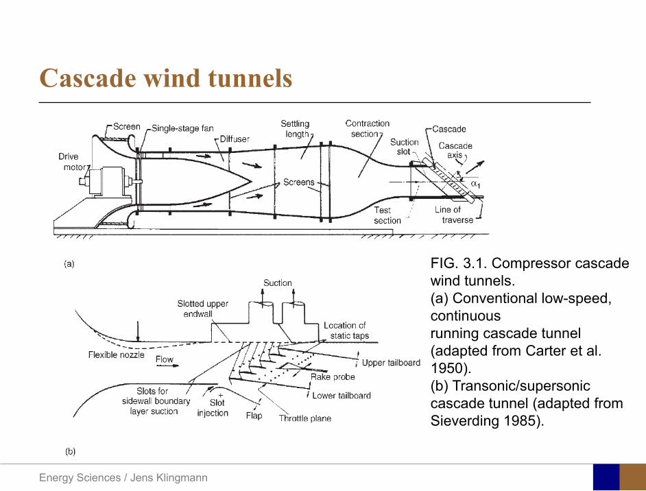
Energy Sciences Jens Klingmann
Cascade wind tunnels
FIG 31 Compressor cascade wind tunnels (a) Conventional low-speed continuousrunning cascade tunnel (adapted from Carter et al 1950)(b) Transonicsupersoniccascade tunnel (adapted from Sieverding 1985)
Energy Sciences Jens Klingmann
Closed circuit tunnels
Energy Sciences Jens Klingmann
components
Settling Chamber
The settling chamber is located between the fan or wide angle diffuser and the contraction and contains the honeycombs and screens used to moderate longitudinal variations in the flow Screens in the chamber should be spaced at 02 chamber diameters apart so that flow disturbed by the first screen can settle before it encounters the second
Honeycombs
Honeycombs are located in the settling chamber and are used to reduce nonuniformities in the flow For optimum benefit honeycombs should be 6-8 cell diameters thick and cell size should be on the order of about 150 cells per settling chamber diameter
Energy Sciences Jens Klingmann
components
Screens
Screens are typically located just downstream of the honeycomb and sometime at the inlet of the test section Screens create a static pressure drop and serve to reduce boundary layer size and increase flow uniformity
Contraction Section
Contractions sections are located between the settling chamber and the test sections and serve to both increase mean velocities at the test section inlet and moderate inconsistencies in the uniformity of the flow Large contraction ratios and short contraction lengths are generally more desirable as they reduce the power loss across the screens and the thickness of boundary layers Small tunnels typically have contraction ratios between 6 and 9
Energy Sciences Jens Klingmann
Flow meters with pressure measurement
Venturi-tube
A1 A2
P1 P2
1 1 2 2C A C A=In the incompressible case
2 21 1 2 2
2 2C P C P
ρ ρ+ = +Assuming horisontal mounting
Energy Sciences Jens Klingmann
Daniel Bernoulli 1700-1782
Daniel Bernoulli was the son of Johann Bernoulli He was born in Groningen while his father held the chair of mathematics there His older brother was Nicolaus(II) Bernoulli and his uncle was Jacob Bernoulli so he was born into a family of leading mathematicians but also into a family where there was unfortunate rivalry jealousy and bitterness
Undoubtedly the most important work which Daniel Bernoulli did was his work on hydrodynamics Even the term itself is based on the title of the work which he produced called Hydrodynamica and before he left St Petersburg Daniel left a draft copy of the book with a printer However the work was not published until 1738 and although he revised it considerably between 1734 and 1738 it is more the presentation that he changed rather then the substance
This work contains for the first time the correct analysis of water flowing from a hole in a container This was based on the principle of conservation of energy which he had studied with his father in 1720 Daniel also discussed pumps and other machines to raise water One remarkable discovery appears in Chapter 10 of Hydrodynamica where Daniel discussed the basis for the kinetic theory of gases He was able to give the basic laws for the theory of gases and gave although not in full detail the equation of state discovered by Van der Waals a century later
Energy Sciences Jens Klingmann
Venturi-tube (2)
22 2 12 2
2
2A PC CA ρ
∆minus =
A1 A2
P1 P2
Solve for eg C2
1 2P P P∆ = minus
( )
12
2 2 21 2
21
PCA Aρ
∆ = minus
and( )
12
2 2 2 2 21 2
21
Pm A C AA Aρρ
∆ = = minus
where
Flow meters with pressure measurement
Energy Sciences Jens Klingmann
Flow meters with pressure measurement
Orifice meters
A1
A2
P1 P2
Applicable for pipe flows Same principle as for Venturi Positioning of pressure taps important Vena contracta and losses require inclusion
of Discharge Coefficient CD
( )
12
2 2 21 2
21D
Pm C AA Aρ ∆ =
minus where ( )1 2ReDC f A A=
CD available from manufacturer (measurements) or Standards (eg ISO)
Energy Sciences Jens Klingmann
Coriolis flow meter
An actuator (not shown) induces a vibration of the tubes
When there is mass flow Coriolis forces induce twisting of the tubes
degree of phase-shift is a measure for the amount of mass that is flowing through the tubes
Energy Sciences Jens Klingmann
Thermal flow meter Heat is added electrically to the flow Temperature is measured before and after heat addition
pP mC T∆=
Energy Sciences Jens Klingmann
Ultrasonic flow meters
Ultrasound is emitted to small particles in the flow (dust or other) Reflections of the sound is frequency shifted by the Doppler effect The frequency change is proportional to the particles velocity (volume flow
meter)
Energy Sciences Jens Klingmann
Inductive flow metersA magnetic flowmeter is based upon Faradays Law
The voltage induced across any conductor as it moves at right angles through a magnetic field is proportional to the velocity of that conductor
E is proportional to V x B x D where
E = The voltage generated in a conductorV = The velocity of the conductorB = The magnetic field strengthD = The length of the conductor
NB electric conductivity is required
Energy Sciences Jens Klingmann
Temperature measurements
Thermocouples
The basis established by Thomas Johann Seebeck in 1821
A conductor generates a voltage when subjected to a temperature gradient
To measure this voltage one must use a second conductor material which generates a different voltage under the same temperature gradient
Energy Sciences Jens Klingmann
Pressure sensing
1 2p pgt 2p p2 may be the atmosphere a static pressure tap or a known reference pressure
The strain of the diaphragm (or itrsquos deflection) may be measured by a number of electric methods
Diaphragm
Energy Sciences Jens Klingmann
Pressure sensingPiezoresistive Strain Gage
Uses the piezoresistive effect of bonded or formed strain gauges to detect strain due to applied pressure
Capacitive
Uses a diaghragm and pressure cavity to create a variable capacitor to detect strain due to applied pressure
Magnetic
Measures the displacement of a diaphragm by means of changes in inductance (reluctance) LVDT Hall Effect or by eddy current principal
Piezoelectric
Uses the piezoelectric effect in certain materials such as quartz to measure the strain upon the sensing mechanism due to pressure
Potentiometric
Uses the motion of a wiper along a resistive mechanism to detect the strain caused by applied pressure
Energy Sciences Jens Klingmann
3D highly instationary (periodic) flow Potentially very high velocities (Supersonic) Large temperature differences Low accessibility (difficult to probe between rotors) Low turbulence levels in most of the domain Very high turbulence in BL and wakes
Properties of measuring object
Point measurements
Energy Sciences Jens Klingmann
Conventional or non-opticalndash Static Pressure Measurementsndash Total Pressure Measurements
bull Multy hole probes
ndash Total Temperature ndash Hot Wire Anemometry (HWA)
Optical techniques for Velocity Measurementsndash Laser Two Focous (L2F)ndash Laser Doppler Anemometry (LDA)ndash Particle Image velocimetry (PIV)
Point Measurements
Energy Sciences Jens Klingmann
Static and total pressure
2 2 21 2 1
2 1 2 2 2C C CP P ρ ρ ρ
minus = minus =
2 0C =Stagnation point
C1Static pressure tap
Prandtl or Pitot tube
Apply the Bernoulli equation from free stream to stagnation point
21
2 12CP Pρ
= +or
We can also define a stagnation or total pressure
( )2
101 1 022
CP P Pρ= + =
Total pressure = Static pressure + dynamic pressure
or
Energy Sciences Jens Klingmann
Static pressure
Energy Sciences Jens Klingmann
Total Pressure and Temperature
Shrouded Probes
Shrouded Probe
Pitot or Prandtl tube
Sensitive to direction
Energy Sciences Jens Klingmann
Ludwig Prandtl 1875-1953
Ludwig Prandtl born at Freising Bavaria on February 4 1875 was a German Physicist famous for his work in aeronautics He qualified at Munchen in 1900 with a thesis on elastic stability and held the position of Professor of Applied Mechanics at Gottingen for forty-nine years (from 1904 until his death there on August 15 1953) In 1925 Prandtl became the Director of the Kaiser Wilhelm Institute for Fluid Mechanics His discovery in 1904 of the Boundary Layer which adjoins the surface of a body moving in a fluid led to an understanding of skin friction drag and of the way in which streamlining reduces the drag of airplane wings and other moving bodies His work on wing theory published in 1918 - 1919 followed that of FW Lanchester (1902-1907) but was carried out independently and elucidated the flow over airplane wings of finite span Prandtls work and decisive advances in boundary layer and wing theories became the basic material of aeronautics He also made important contributions to the theories of supersonic flow and of turbulence and contributed much to the development of wind tunnels and other aerodynamic equipment In addition he devised the soap-film analogy for the torsion of non-circular sections and wrote on the theory of plasticity and of meteorology
Energy Sciences Jens Klingmann
Total Pressure multy hole
Cobra Probe Yaw Probe
5 Hole Probe
Energy Sciences Jens Klingmann
5 Hole Probes Calibration
Energy Sciences Jens Klingmann
The inherent unsteadiness of the flow within turbomachines
Energy Sciences Jens Klingmann
Hot Wire Anemometry (HWA) The heat transfer from a thin (one micron)
electrically heated wire can be used to determine velocity
The resistance of the wire is temperature dependent Within a small temperature range it can be assumed linear R = R0+α R0(Tm-T0) where R0 is the resistance at a reference temperature T0 and Tm is the mean wire temperature
The thermal power induced in the wire is balanced by heat transfer to the surrounding fluid I2R=hπDL(Tm-T0) where h is the heat transfer coefficient and D and L the diameter and length of the wire respectively
E = I R
Energy Sciences Jens Klingmann
Constant Temperature Anemometry (CTA) The wire is often placed in a Whetstone bridge If the output from the
bridge is amplified and fed back to the bridge the resistance of the probe and thus the temperature will be held constant
This prevents the temperature of the wire to become excessive at low velocities
R1
R2 R3
Probe
Bridge Voltage
Energy Sciences Jens Klingmann
Constant Temperature Anemometry (CTA)
Energy Sciences Jens Klingmann
Characteristics of LDA (according to Dantec)
Invented by Yeh and Cummins in 1964 Velocity measurements in Fluid Dynamics (gas liquid) Up to 3 velocity components Non-intrusive measurements (optical technique) Absolute measurement technique (no calibration required) Very high accuracy Very high spatial resolution due to small measurement volume Tracer particles are required
Energy Sciences Jens Klingmann
LDA - Fringe Model
Focused Laser beams intersect and form the measurement volume Plane wave fronts beam waist in the plane of intersection Interference in the plane of intersection Pattern of bright and dark stripesplanes Fringes
Energy Sciences Jens Klingmann
LDA-measuring volume
d
x
x
y
y
z
z
e-2 CONTOUR
FRINGES
κ
κ
κ
κ
De-2
De-2
dml m
a
b
cx
b
z
ya
cd
d
=
=
=
J
J
J
J
JP
JP
JP
JD
JD
JD
+
+
+
a
b
c
d
κπλ
=minus sinD
f4l2e
m
κπλ
=minus cosD
f4D2e
m
Energy Sciences Jens Klingmann
Laser Two Focus
Energy Sciences Jens Klingmann
Laser Two Focus
Energy Sciences Jens Klingmann
PIV measurements
PIV is a fairly new technique capable of simultaneous velocity measurements at many points in a plane This gives information on large scale structures vorticity etc which is very difficult or impossible to obtain from one-point measuring techniques
PIV involves the illumination of a plane of the flow under investigation with a thin pulsed sheet of light The flow is seeded with particles
The light scattered from the particles and from successive pulses are being recorded either on film or a CCD array forming a multiple exposure of each particle image If the time between the pulses is known velocity can be determined as the ratio of the particle displacement and the elapsed time
t∆∆= xu
Energy Sciences Jens Klingmann
PIV
Energy Sciences Jens Klingmann
PIV measurements illumination
YA
G
YA
G
Two frequency doubled YAG Lasers aligned to one double pulsed laser sheet
Two or more separate light pulses can be obtained by chopping a continuous laser or from pulsed lasers
The limited pulse energies obtained from continuous lasers limits their applicability to low velocity flows or flows where large seeding particles can be used (ie liquid flows)
The low repetition rate of most pulsed lasers makes the use of two lasers advantageous
Energy Sciences Jens Klingmann
PIV measurements recording
High seeding density in laminar flame
Film or CCD-cameras Cross- or Auto-correlation
ndash ie both particle images on the same frame or on separate frames
CCD-camera requirementndash A many pixels as possiblendash 2k by 2k available 4k by 4k coming
Energy Sciences Jens Klingmann
PIV measurements analyses
Low seeding density (Number of seeding particles per unit volume)
Each particle image pair can be identified This is called particle tracking
High seeding density (PIV)
Small sub-regions of the image containing many particle image pairs are processed to obtain one velocity vector
Energy Sciences Jens Klingmann
PIV measurements analyses
Energy Sciences Jens Klingmann
PIV measurements analyses
( ) ( ) ( ) xsxxs dIIR 2A
1
I
+= int
Cross correlation between ( )x1I and ( )x2I
s is a two dimensional displacement vector
IA is the interrogation area
Cross correlation between
(
)
x
1
I
and
(
)
x
2
I
s is a two dimensional displacement vector
I
A
is the interrogation area
Energy Sciences Jens Klingmann
Energy Sciences Jens Klingmann
PIV from IOWA state university
Energy Sciences Jens Klingmann
PIV sample of evaluation
Energy Sciences Jens Klingmann
LDA PIV HWA Velocity range 01 mms ndash 300
ms 02 ndash 150 ms
Measuring Volume
D = 005 L = 05 mm
2 by 2 by 05 mm
L = 05 mm
Freq response O(10 000) Hz O(10) Hz O(100 000) Hz Calibration Yes No No Sensitivity to other than velocity
Low (ref Index) Low (ref Index) Large (temperature concentrationshellip)
Continuous Signal
Sometimes Seldom Always
Noise High High Low Turbulence intensity
No limitation Some limitation lt 20
Price O(1 000 000) SEK
O(1 000 000) SEK
O(50 000) SEK
Required Knowledge
High medium Low
Comparison of techniques
Energy Sciences Jens Klingmann
References experiments
R J Goldstein ldquoFluid Mechanics Measurementsrdquo Hemisphere Publishing 1983 A V Johansson amp P H Alfredsson ldquoExperimentella metoder inom
stroumlmningsmekanikenrdquo Inst Foumlr Mekanik KTH F Durst A Melling and J H Whitelaw ldquoPrincipals and Practice of Laser Doppler
Anemometryrdquo 1984 R J Adrian ldquoParticle-imaging techniques for experimental fluid mechnicsrdquo Ann Rev
Fluid Mech 1991
Energy Sciences Jens Klingmann
Sample of LDA-measurements
Rotor blade
Glas window
Emitted beams
Scattered Light
Adjustable mirror
Energy Sciences Jens Klingmann
Axial velocity sorted into 10 bins
0 1 2 3 4 5 6tangential coordinate (degrees)
-20
0
20
40
60
80
100
120
140
160Ax
ial v
eloc
ity a
nd s
tand
ard
devi
atio
n (m
s)
radial position 7 mm from inner window surfaceaxial position 23 mm behind rotor blades
Energy Sciences Jens Klingmann
Axial velocities in the radial-tangential plane
Energy Sciences Jens Klingmann
Airfoils NACA 4-digit
The NACA four-digit wing sections define the profile by
One digit describing maximum camber as percentage of the chord
One digit describing the distance of maximum camber from the airfoil leading edge in tens of percents of the chord
Two digits describing maximum thickness of the airfoil as percent of the chord
Example the NACA 2412 airfoil has a maximum camber of 2 located 40 (04 chords) from the leading edge with a maximum thickness of 12 of the chord
Four-digit series airfoils by default have maximum thickness at 30 of the chord (03 chords) from the leading edge
Energy Sciences Jens Klingmann
Airfoils NACA 4-digit
bull c is the chord lengthbull x is the position along
the chord from 0 to cbull y is the half thickness at
a given value of x (centerline to surface)
bull t is the maximum thickness as a fraction of the chord
Energy Sciences Jens Klingmann
Death by PowerPoint
| LDA | PIV | HWA | |||||
| Velocity range | 01 mms ndash 300 ms | 02 ndash 150 ms | |||||
| Measuring Volume | D = 005 L = 05 mm | 2 by 2 by 05 mm | L = 05 mm | ||||
| Freq response | O(10 000) Hz | O(10) Hz | O(100 000) Hz | ||||
| Calibration | Yes | No | No | ||||
| Sensitivity to other than velocity | Low (ref Index) | Low (ref Index) | Large (temperature concentrationshellip) | ||||
| Continuous Signal | Sometimes | Seldom | Always | ||||
| Noise | High | High | Low | ||||
| Turbulence intensity | No limitation | Some limitation | lt 20 | ||||
| Price | O(1 000 000) SEK | O(1 000 000) SEK | O(50 000) SEK | ||||
| Required Knowledge | High | medium | Low |
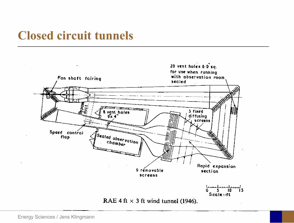
Energy Sciences Jens Klingmann
Closed circuit tunnels
Energy Sciences Jens Klingmann
components
Settling Chamber
The settling chamber is located between the fan or wide angle diffuser and the contraction and contains the honeycombs and screens used to moderate longitudinal variations in the flow Screens in the chamber should be spaced at 02 chamber diameters apart so that flow disturbed by the first screen can settle before it encounters the second
Honeycombs
Honeycombs are located in the settling chamber and are used to reduce nonuniformities in the flow For optimum benefit honeycombs should be 6-8 cell diameters thick and cell size should be on the order of about 150 cells per settling chamber diameter
Energy Sciences Jens Klingmann
components
Screens
Screens are typically located just downstream of the honeycomb and sometime at the inlet of the test section Screens create a static pressure drop and serve to reduce boundary layer size and increase flow uniformity
Contraction Section
Contractions sections are located between the settling chamber and the test sections and serve to both increase mean velocities at the test section inlet and moderate inconsistencies in the uniformity of the flow Large contraction ratios and short contraction lengths are generally more desirable as they reduce the power loss across the screens and the thickness of boundary layers Small tunnels typically have contraction ratios between 6 and 9
Energy Sciences Jens Klingmann
Flow meters with pressure measurement
Venturi-tube
A1 A2
P1 P2
1 1 2 2C A C A=In the incompressible case
2 21 1 2 2
2 2C P C P
ρ ρ+ = +Assuming horisontal mounting
Energy Sciences Jens Klingmann
Daniel Bernoulli 1700-1782
Daniel Bernoulli was the son of Johann Bernoulli He was born in Groningen while his father held the chair of mathematics there His older brother was Nicolaus(II) Bernoulli and his uncle was Jacob Bernoulli so he was born into a family of leading mathematicians but also into a family where there was unfortunate rivalry jealousy and bitterness
Undoubtedly the most important work which Daniel Bernoulli did was his work on hydrodynamics Even the term itself is based on the title of the work which he produced called Hydrodynamica and before he left St Petersburg Daniel left a draft copy of the book with a printer However the work was not published until 1738 and although he revised it considerably between 1734 and 1738 it is more the presentation that he changed rather then the substance
This work contains for the first time the correct analysis of water flowing from a hole in a container This was based on the principle of conservation of energy which he had studied with his father in 1720 Daniel also discussed pumps and other machines to raise water One remarkable discovery appears in Chapter 10 of Hydrodynamica where Daniel discussed the basis for the kinetic theory of gases He was able to give the basic laws for the theory of gases and gave although not in full detail the equation of state discovered by Van der Waals a century later
Energy Sciences Jens Klingmann
Venturi-tube (2)
22 2 12 2
2
2A PC CA ρ
∆minus =
A1 A2
P1 P2
Solve for eg C2
1 2P P P∆ = minus
( )
12
2 2 21 2
21
PCA Aρ
∆ = minus
and( )
12
2 2 2 2 21 2
21
Pm A C AA Aρρ
∆ = = minus
where
Flow meters with pressure measurement
Energy Sciences Jens Klingmann
Flow meters with pressure measurement
Orifice meters
A1
A2
P1 P2
Applicable for pipe flows Same principle as for Venturi Positioning of pressure taps important Vena contracta and losses require inclusion
of Discharge Coefficient CD
( )
12
2 2 21 2
21D
Pm C AA Aρ ∆ =
minus where ( )1 2ReDC f A A=
CD available from manufacturer (measurements) or Standards (eg ISO)
Energy Sciences Jens Klingmann
Coriolis flow meter
An actuator (not shown) induces a vibration of the tubes
When there is mass flow Coriolis forces induce twisting of the tubes
degree of phase-shift is a measure for the amount of mass that is flowing through the tubes
Energy Sciences Jens Klingmann
Thermal flow meter Heat is added electrically to the flow Temperature is measured before and after heat addition
pP mC T∆=
Energy Sciences Jens Klingmann
Ultrasonic flow meters
Ultrasound is emitted to small particles in the flow (dust or other) Reflections of the sound is frequency shifted by the Doppler effect The frequency change is proportional to the particles velocity (volume flow
meter)
Energy Sciences Jens Klingmann
Inductive flow metersA magnetic flowmeter is based upon Faradays Law
The voltage induced across any conductor as it moves at right angles through a magnetic field is proportional to the velocity of that conductor
E is proportional to V x B x D where
E = The voltage generated in a conductorV = The velocity of the conductorB = The magnetic field strengthD = The length of the conductor
NB electric conductivity is required
Energy Sciences Jens Klingmann
Temperature measurements
Thermocouples
The basis established by Thomas Johann Seebeck in 1821
A conductor generates a voltage when subjected to a temperature gradient
To measure this voltage one must use a second conductor material which generates a different voltage under the same temperature gradient
Energy Sciences Jens Klingmann
Pressure sensing
1 2p pgt 2p p2 may be the atmosphere a static pressure tap or a known reference pressure
The strain of the diaphragm (or itrsquos deflection) may be measured by a number of electric methods
Diaphragm
Energy Sciences Jens Klingmann
Pressure sensingPiezoresistive Strain Gage
Uses the piezoresistive effect of bonded or formed strain gauges to detect strain due to applied pressure
Capacitive
Uses a diaghragm and pressure cavity to create a variable capacitor to detect strain due to applied pressure
Magnetic
Measures the displacement of a diaphragm by means of changes in inductance (reluctance) LVDT Hall Effect or by eddy current principal
Piezoelectric
Uses the piezoelectric effect in certain materials such as quartz to measure the strain upon the sensing mechanism due to pressure
Potentiometric
Uses the motion of a wiper along a resistive mechanism to detect the strain caused by applied pressure
Energy Sciences Jens Klingmann
3D highly instationary (periodic) flow Potentially very high velocities (Supersonic) Large temperature differences Low accessibility (difficult to probe between rotors) Low turbulence levels in most of the domain Very high turbulence in BL and wakes
Properties of measuring object
Point measurements
Energy Sciences Jens Klingmann
Conventional or non-opticalndash Static Pressure Measurementsndash Total Pressure Measurements
bull Multy hole probes
ndash Total Temperature ndash Hot Wire Anemometry (HWA)
Optical techniques for Velocity Measurementsndash Laser Two Focous (L2F)ndash Laser Doppler Anemometry (LDA)ndash Particle Image velocimetry (PIV)
Point Measurements
Energy Sciences Jens Klingmann
Static and total pressure
2 2 21 2 1
2 1 2 2 2C C CP P ρ ρ ρ
minus = minus =
2 0C =Stagnation point
C1Static pressure tap
Prandtl or Pitot tube
Apply the Bernoulli equation from free stream to stagnation point
21
2 12CP Pρ
= +or
We can also define a stagnation or total pressure
( )2
101 1 022
CP P Pρ= + =
Total pressure = Static pressure + dynamic pressure
or
Energy Sciences Jens Klingmann
Static pressure
Energy Sciences Jens Klingmann
Total Pressure and Temperature
Shrouded Probes
Shrouded Probe
Pitot or Prandtl tube
Sensitive to direction
Energy Sciences Jens Klingmann
Ludwig Prandtl 1875-1953
Ludwig Prandtl born at Freising Bavaria on February 4 1875 was a German Physicist famous for his work in aeronautics He qualified at Munchen in 1900 with a thesis on elastic stability and held the position of Professor of Applied Mechanics at Gottingen for forty-nine years (from 1904 until his death there on August 15 1953) In 1925 Prandtl became the Director of the Kaiser Wilhelm Institute for Fluid Mechanics His discovery in 1904 of the Boundary Layer which adjoins the surface of a body moving in a fluid led to an understanding of skin friction drag and of the way in which streamlining reduces the drag of airplane wings and other moving bodies His work on wing theory published in 1918 - 1919 followed that of FW Lanchester (1902-1907) but was carried out independently and elucidated the flow over airplane wings of finite span Prandtls work and decisive advances in boundary layer and wing theories became the basic material of aeronautics He also made important contributions to the theories of supersonic flow and of turbulence and contributed much to the development of wind tunnels and other aerodynamic equipment In addition he devised the soap-film analogy for the torsion of non-circular sections and wrote on the theory of plasticity and of meteorology
Energy Sciences Jens Klingmann
Total Pressure multy hole
Cobra Probe Yaw Probe
5 Hole Probe
Energy Sciences Jens Klingmann
5 Hole Probes Calibration
Energy Sciences Jens Klingmann
The inherent unsteadiness of the flow within turbomachines
Energy Sciences Jens Klingmann
Hot Wire Anemometry (HWA) The heat transfer from a thin (one micron)
electrically heated wire can be used to determine velocity
The resistance of the wire is temperature dependent Within a small temperature range it can be assumed linear R = R0+α R0(Tm-T0) where R0 is the resistance at a reference temperature T0 and Tm is the mean wire temperature
The thermal power induced in the wire is balanced by heat transfer to the surrounding fluid I2R=hπDL(Tm-T0) where h is the heat transfer coefficient and D and L the diameter and length of the wire respectively
E = I R
Energy Sciences Jens Klingmann
Constant Temperature Anemometry (CTA) The wire is often placed in a Whetstone bridge If the output from the
bridge is amplified and fed back to the bridge the resistance of the probe and thus the temperature will be held constant
This prevents the temperature of the wire to become excessive at low velocities
R1
R2 R3
Probe
Bridge Voltage
Energy Sciences Jens Klingmann
Constant Temperature Anemometry (CTA)
Energy Sciences Jens Klingmann
Characteristics of LDA (according to Dantec)
Invented by Yeh and Cummins in 1964 Velocity measurements in Fluid Dynamics (gas liquid) Up to 3 velocity components Non-intrusive measurements (optical technique) Absolute measurement technique (no calibration required) Very high accuracy Very high spatial resolution due to small measurement volume Tracer particles are required
Energy Sciences Jens Klingmann
LDA - Fringe Model
Focused Laser beams intersect and form the measurement volume Plane wave fronts beam waist in the plane of intersection Interference in the plane of intersection Pattern of bright and dark stripesplanes Fringes
Energy Sciences Jens Klingmann
LDA-measuring volume
d
x
x
y
y
z
z
e-2 CONTOUR
FRINGES
κ
κ
κ
κ
De-2
De-2
dml m
a
b
cx
b
z
ya
cd
d
=
=
=
J
J
J
J
JP
JP
JP
JD
JD
JD
+
+
+
a
b
c
d
κπλ
=minus sinD
f4l2e
m
κπλ
=minus cosD
f4D2e
m
Energy Sciences Jens Klingmann
Laser Two Focus
Energy Sciences Jens Klingmann
Laser Two Focus
Energy Sciences Jens Klingmann
PIV measurements
PIV is a fairly new technique capable of simultaneous velocity measurements at many points in a plane This gives information on large scale structures vorticity etc which is very difficult or impossible to obtain from one-point measuring techniques
PIV involves the illumination of a plane of the flow under investigation with a thin pulsed sheet of light The flow is seeded with particles
The light scattered from the particles and from successive pulses are being recorded either on film or a CCD array forming a multiple exposure of each particle image If the time between the pulses is known velocity can be determined as the ratio of the particle displacement and the elapsed time
t∆∆= xu
Energy Sciences Jens Klingmann
PIV
Energy Sciences Jens Klingmann
PIV measurements illumination
YA
G
YA
G
Two frequency doubled YAG Lasers aligned to one double pulsed laser sheet
Two or more separate light pulses can be obtained by chopping a continuous laser or from pulsed lasers
The limited pulse energies obtained from continuous lasers limits their applicability to low velocity flows or flows where large seeding particles can be used (ie liquid flows)
The low repetition rate of most pulsed lasers makes the use of two lasers advantageous
Energy Sciences Jens Klingmann
PIV measurements recording
High seeding density in laminar flame
Film or CCD-cameras Cross- or Auto-correlation
ndash ie both particle images on the same frame or on separate frames
CCD-camera requirementndash A many pixels as possiblendash 2k by 2k available 4k by 4k coming
Energy Sciences Jens Klingmann
PIV measurements analyses
Low seeding density (Number of seeding particles per unit volume)
Each particle image pair can be identified This is called particle tracking
High seeding density (PIV)
Small sub-regions of the image containing many particle image pairs are processed to obtain one velocity vector
Energy Sciences Jens Klingmann
PIV measurements analyses
Energy Sciences Jens Klingmann
PIV measurements analyses
( ) ( ) ( ) xsxxs dIIR 2A
1
I
+= int
Cross correlation between ( )x1I and ( )x2I
s is a two dimensional displacement vector
IA is the interrogation area
Cross correlation between
(
)
x
1
I
and
(
)
x
2
I
s is a two dimensional displacement vector
I
A
is the interrogation area
Energy Sciences Jens Klingmann
Energy Sciences Jens Klingmann
PIV from IOWA state university
Energy Sciences Jens Klingmann
PIV sample of evaluation
Energy Sciences Jens Klingmann
LDA PIV HWA Velocity range 01 mms ndash 300
ms 02 ndash 150 ms
Measuring Volume
D = 005 L = 05 mm
2 by 2 by 05 mm
L = 05 mm
Freq response O(10 000) Hz O(10) Hz O(100 000) Hz Calibration Yes No No Sensitivity to other than velocity
Low (ref Index) Low (ref Index) Large (temperature concentrationshellip)
Continuous Signal
Sometimes Seldom Always
Noise High High Low Turbulence intensity
No limitation Some limitation lt 20
Price O(1 000 000) SEK
O(1 000 000) SEK
O(50 000) SEK
Required Knowledge
High medium Low
Comparison of techniques
Energy Sciences Jens Klingmann
References experiments
R J Goldstein ldquoFluid Mechanics Measurementsrdquo Hemisphere Publishing 1983 A V Johansson amp P H Alfredsson ldquoExperimentella metoder inom
stroumlmningsmekanikenrdquo Inst Foumlr Mekanik KTH F Durst A Melling and J H Whitelaw ldquoPrincipals and Practice of Laser Doppler
Anemometryrdquo 1984 R J Adrian ldquoParticle-imaging techniques for experimental fluid mechnicsrdquo Ann Rev
Fluid Mech 1991
Energy Sciences Jens Klingmann
Sample of LDA-measurements
Rotor blade
Glas window
Emitted beams
Scattered Light
Adjustable mirror
Energy Sciences Jens Klingmann
Axial velocity sorted into 10 bins
0 1 2 3 4 5 6tangential coordinate (degrees)
-20
0
20
40
60
80
100
120
140
160Ax
ial v
eloc
ity a
nd s
tand
ard
devi
atio
n (m
s)
radial position 7 mm from inner window surfaceaxial position 23 mm behind rotor blades
Energy Sciences Jens Klingmann
Axial velocities in the radial-tangential plane
Energy Sciences Jens Klingmann
Airfoils NACA 4-digit
The NACA four-digit wing sections define the profile by
One digit describing maximum camber as percentage of the chord
One digit describing the distance of maximum camber from the airfoil leading edge in tens of percents of the chord
Two digits describing maximum thickness of the airfoil as percent of the chord
Example the NACA 2412 airfoil has a maximum camber of 2 located 40 (04 chords) from the leading edge with a maximum thickness of 12 of the chord
Four-digit series airfoils by default have maximum thickness at 30 of the chord (03 chords) from the leading edge
Energy Sciences Jens Klingmann
Airfoils NACA 4-digit
bull c is the chord lengthbull x is the position along
the chord from 0 to cbull y is the half thickness at
a given value of x (centerline to surface)
bull t is the maximum thickness as a fraction of the chord
Energy Sciences Jens Klingmann
Death by PowerPoint
| LDA | PIV | HWA | |||||
| Velocity range | 01 mms ndash 300 ms | 02 ndash 150 ms | |||||
| Measuring Volume | D = 005 L = 05 mm | 2 by 2 by 05 mm | L = 05 mm | ||||
| Freq response | O(10 000) Hz | O(10) Hz | O(100 000) Hz | ||||
| Calibration | Yes | No | No | ||||
| Sensitivity to other than velocity | Low (ref Index) | Low (ref Index) | Large (temperature concentrationshellip) | ||||
| Continuous Signal | Sometimes | Seldom | Always | ||||
| Noise | High | High | Low | ||||
| Turbulence intensity | No limitation | Some limitation | lt 20 | ||||
| Price | O(1 000 000) SEK | O(1 000 000) SEK | O(50 000) SEK | ||||
| Required Knowledge | High | medium | Low |
Energy Sciences Jens Klingmann
components
Screens
Screens are typically located just downstream of the honeycomb and sometime at the inlet of the test section Screens create a static pressure drop and serve to reduce boundary layer size and increase flow uniformity
Contraction Section
Contractions sections are located between the settling chamber and the test sections and serve to both increase mean velocities at the test section inlet and moderate inconsistencies in the uniformity of the flow Large contraction ratios and short contraction lengths are generally more desirable as they reduce the power loss across the screens and the thickness of boundary layers Small tunnels typically have contraction ratios between 6 and 9
Energy Sciences Jens Klingmann
Flow meters with pressure measurement
Venturi-tube
A1 A2
P1 P2
1 1 2 2C A C A=In the incompressible case
2 21 1 2 2
2 2C P C P
ρ ρ+ = +Assuming horisontal mounting
Energy Sciences Jens Klingmann
Daniel Bernoulli 1700-1782
Daniel Bernoulli was the son of Johann Bernoulli He was born in Groningen while his father held the chair of mathematics there His older brother was Nicolaus(II) Bernoulli and his uncle was Jacob Bernoulli so he was born into a family of leading mathematicians but also into a family where there was unfortunate rivalry jealousy and bitterness
Undoubtedly the most important work which Daniel Bernoulli did was his work on hydrodynamics Even the term itself is based on the title of the work which he produced called Hydrodynamica and before he left St Petersburg Daniel left a draft copy of the book with a printer However the work was not published until 1738 and although he revised it considerably between 1734 and 1738 it is more the presentation that he changed rather then the substance
This work contains for the first time the correct analysis of water flowing from a hole in a container This was based on the principle of conservation of energy which he had studied with his father in 1720 Daniel also discussed pumps and other machines to raise water One remarkable discovery appears in Chapter 10 of Hydrodynamica where Daniel discussed the basis for the kinetic theory of gases He was able to give the basic laws for the theory of gases and gave although not in full detail the equation of state discovered by Van der Waals a century later
Energy Sciences Jens Klingmann
Venturi-tube (2)
22 2 12 2
2
2A PC CA ρ
∆minus =
A1 A2
P1 P2
Solve for eg C2
1 2P P P∆ = minus
( )
12
2 2 21 2
21
PCA Aρ
∆ = minus
and( )
12
2 2 2 2 21 2
21
Pm A C AA Aρρ
∆ = = minus
where
Flow meters with pressure measurement
Energy Sciences Jens Klingmann
Flow meters with pressure measurement
Orifice meters
A1
A2
P1 P2
Applicable for pipe flows Same principle as for Venturi Positioning of pressure taps important Vena contracta and losses require inclusion
of Discharge Coefficient CD
( )
12
2 2 21 2
21D
Pm C AA Aρ ∆ =
minus where ( )1 2ReDC f A A=
CD available from manufacturer (measurements) or Standards (eg ISO)
Energy Sciences Jens Klingmann
Coriolis flow meter
An actuator (not shown) induces a vibration of the tubes
When there is mass flow Coriolis forces induce twisting of the tubes
degree of phase-shift is a measure for the amount of mass that is flowing through the tubes
Energy Sciences Jens Klingmann
Thermal flow meter Heat is added electrically to the flow Temperature is measured before and after heat addition
pP mC T∆=
Energy Sciences Jens Klingmann
Ultrasonic flow meters
Ultrasound is emitted to small particles in the flow (dust or other) Reflections of the sound is frequency shifted by the Doppler effect The frequency change is proportional to the particles velocity (volume flow
meter)
Energy Sciences Jens Klingmann
Inductive flow metersA magnetic flowmeter is based upon Faradays Law
The voltage induced across any conductor as it moves at right angles through a magnetic field is proportional to the velocity of that conductor
E is proportional to V x B x D where
E = The voltage generated in a conductorV = The velocity of the conductorB = The magnetic field strengthD = The length of the conductor
NB electric conductivity is required
Energy Sciences Jens Klingmann
Temperature measurements
Thermocouples
The basis established by Thomas Johann Seebeck in 1821
A conductor generates a voltage when subjected to a temperature gradient
To measure this voltage one must use a second conductor material which generates a different voltage under the same temperature gradient
Energy Sciences Jens Klingmann
Pressure sensing
1 2p pgt 2p p2 may be the atmosphere a static pressure tap or a known reference pressure
The strain of the diaphragm (or itrsquos deflection) may be measured by a number of electric methods
Diaphragm
Energy Sciences Jens Klingmann
Pressure sensingPiezoresistive Strain Gage
Uses the piezoresistive effect of bonded or formed strain gauges to detect strain due to applied pressure
Capacitive
Uses a diaghragm and pressure cavity to create a variable capacitor to detect strain due to applied pressure
Magnetic
Measures the displacement of a diaphragm by means of changes in inductance (reluctance) LVDT Hall Effect or by eddy current principal
Piezoelectric
Uses the piezoelectric effect in certain materials such as quartz to measure the strain upon the sensing mechanism due to pressure
Potentiometric
Uses the motion of a wiper along a resistive mechanism to detect the strain caused by applied pressure
Energy Sciences Jens Klingmann
3D highly instationary (periodic) flow Potentially very high velocities (Supersonic) Large temperature differences Low accessibility (difficult to probe between rotors) Low turbulence levels in most of the domain Very high turbulence in BL and wakes
Properties of measuring object
Point measurements
Energy Sciences Jens Klingmann
Conventional or non-opticalndash Static Pressure Measurementsndash Total Pressure Measurements
bull Multy hole probes
ndash Total Temperature ndash Hot Wire Anemometry (HWA)
Optical techniques for Velocity Measurementsndash Laser Two Focous (L2F)ndash Laser Doppler Anemometry (LDA)ndash Particle Image velocimetry (PIV)
Point Measurements
Energy Sciences Jens Klingmann
Static and total pressure
2 2 21 2 1
2 1 2 2 2C C CP P ρ ρ ρ
minus = minus =
2 0C =Stagnation point
C1Static pressure tap
Prandtl or Pitot tube
Apply the Bernoulli equation from free stream to stagnation point
21
2 12CP Pρ
= +or
We can also define a stagnation or total pressure
( )2
101 1 022
CP P Pρ= + =
Total pressure = Static pressure + dynamic pressure
or
Energy Sciences Jens Klingmann
Static pressure
Energy Sciences Jens Klingmann
Total Pressure and Temperature
Shrouded Probes
Shrouded Probe
Pitot or Prandtl tube
Sensitive to direction
Energy Sciences Jens Klingmann
Ludwig Prandtl 1875-1953
Ludwig Prandtl born at Freising Bavaria on February 4 1875 was a German Physicist famous for his work in aeronautics He qualified at Munchen in 1900 with a thesis on elastic stability and held the position of Professor of Applied Mechanics at Gottingen for forty-nine years (from 1904 until his death there on August 15 1953) In 1925 Prandtl became the Director of the Kaiser Wilhelm Institute for Fluid Mechanics His discovery in 1904 of the Boundary Layer which adjoins the surface of a body moving in a fluid led to an understanding of skin friction drag and of the way in which streamlining reduces the drag of airplane wings and other moving bodies His work on wing theory published in 1918 - 1919 followed that of FW Lanchester (1902-1907) but was carried out independently and elucidated the flow over airplane wings of finite span Prandtls work and decisive advances in boundary layer and wing theories became the basic material of aeronautics He also made important contributions to the theories of supersonic flow and of turbulence and contributed much to the development of wind tunnels and other aerodynamic equipment In addition he devised the soap-film analogy for the torsion of non-circular sections and wrote on the theory of plasticity and of meteorology
Energy Sciences Jens Klingmann
Total Pressure multy hole
Cobra Probe Yaw Probe
5 Hole Probe
Energy Sciences Jens Klingmann
5 Hole Probes Calibration
Energy Sciences Jens Klingmann
The inherent unsteadiness of the flow within turbomachines
Energy Sciences Jens Klingmann
Hot Wire Anemometry (HWA) The heat transfer from a thin (one micron)
electrically heated wire can be used to determine velocity
The resistance of the wire is temperature dependent Within a small temperature range it can be assumed linear R = R0+α R0(Tm-T0) where R0 is the resistance at a reference temperature T0 and Tm is the mean wire temperature
The thermal power induced in the wire is balanced by heat transfer to the surrounding fluid I2R=hπDL(Tm-T0) where h is the heat transfer coefficient and D and L the diameter and length of the wire respectively
E = I R
Energy Sciences Jens Klingmann
Constant Temperature Anemometry (CTA) The wire is often placed in a Whetstone bridge If the output from the
bridge is amplified and fed back to the bridge the resistance of the probe and thus the temperature will be held constant
This prevents the temperature of the wire to become excessive at low velocities
R1
R2 R3
Probe
Bridge Voltage
Energy Sciences Jens Klingmann
Constant Temperature Anemometry (CTA)
Energy Sciences Jens Klingmann
Characteristics of LDA (according to Dantec)
Invented by Yeh and Cummins in 1964 Velocity measurements in Fluid Dynamics (gas liquid) Up to 3 velocity components Non-intrusive measurements (optical technique) Absolute measurement technique (no calibration required) Very high accuracy Very high spatial resolution due to small measurement volume Tracer particles are required
Energy Sciences Jens Klingmann
LDA - Fringe Model
Focused Laser beams intersect and form the measurement volume Plane wave fronts beam waist in the plane of intersection Interference in the plane of intersection Pattern of bright and dark stripesplanes Fringes
Energy Sciences Jens Klingmann
LDA-measuring volume
d
x
x
y
y
z
z
e-2 CONTOUR
FRINGES
κ
κ
κ
κ
De-2
De-2
dml m
a
b
cx
b
z
ya
cd
d
=
=
=
J
J
J
J
JP
JP
JP
JD
JD
JD
+
+
+
a
b
c
d
κπλ
=minus sinD
f4l2e
m
κπλ
=minus cosD
f4D2e
m
Energy Sciences Jens Klingmann
Laser Two Focus
Energy Sciences Jens Klingmann
Laser Two Focus
Energy Sciences Jens Klingmann
PIV measurements
PIV is a fairly new technique capable of simultaneous velocity measurements at many points in a plane This gives information on large scale structures vorticity etc which is very difficult or impossible to obtain from one-point measuring techniques
PIV involves the illumination of a plane of the flow under investigation with a thin pulsed sheet of light The flow is seeded with particles
The light scattered from the particles and from successive pulses are being recorded either on film or a CCD array forming a multiple exposure of each particle image If the time between the pulses is known velocity can be determined as the ratio of the particle displacement and the elapsed time
t∆∆= xu
Energy Sciences Jens Klingmann
PIV
Energy Sciences Jens Klingmann
PIV measurements illumination
YA
G
YA
G
Two frequency doubled YAG Lasers aligned to one double pulsed laser sheet
Two or more separate light pulses can be obtained by chopping a continuous laser or from pulsed lasers
The limited pulse energies obtained from continuous lasers limits their applicability to low velocity flows or flows where large seeding particles can be used (ie liquid flows)
The low repetition rate of most pulsed lasers makes the use of two lasers advantageous
Energy Sciences Jens Klingmann
PIV measurements recording
High seeding density in laminar flame
Film or CCD-cameras Cross- or Auto-correlation
ndash ie both particle images on the same frame or on separate frames
CCD-camera requirementndash A many pixels as possiblendash 2k by 2k available 4k by 4k coming
Energy Sciences Jens Klingmann
PIV measurements analyses
Low seeding density (Number of seeding particles per unit volume)
Each particle image pair can be identified This is called particle tracking
High seeding density (PIV)
Small sub-regions of the image containing many particle image pairs are processed to obtain one velocity vector
Energy Sciences Jens Klingmann
PIV measurements analyses
Energy Sciences Jens Klingmann
PIV measurements analyses
( ) ( ) ( ) xsxxs dIIR 2A
1
I
+= int
Cross correlation between ( )x1I and ( )x2I
s is a two dimensional displacement vector
IA is the interrogation area
Cross correlation between
(
)
x
1
I
and
(
)
x
2
I
s is a two dimensional displacement vector
I
A
is the interrogation area
Energy Sciences Jens Klingmann
Energy Sciences Jens Klingmann
PIV from IOWA state university
Energy Sciences Jens Klingmann
PIV sample of evaluation
Energy Sciences Jens Klingmann
LDA PIV HWA Velocity range 01 mms ndash 300
ms 02 ndash 150 ms
Measuring Volume
D = 005 L = 05 mm
2 by 2 by 05 mm
L = 05 mm
Freq response O(10 000) Hz O(10) Hz O(100 000) Hz Calibration Yes No No Sensitivity to other than velocity
Low (ref Index) Low (ref Index) Large (temperature concentrationshellip)
Continuous Signal
Sometimes Seldom Always
Noise High High Low Turbulence intensity
No limitation Some limitation lt 20
Price O(1 000 000) SEK
O(1 000 000) SEK
O(50 000) SEK
Required Knowledge
High medium Low
Comparison of techniques
Energy Sciences Jens Klingmann
References experiments
R J Goldstein ldquoFluid Mechanics Measurementsrdquo Hemisphere Publishing 1983 A V Johansson amp P H Alfredsson ldquoExperimentella metoder inom
stroumlmningsmekanikenrdquo Inst Foumlr Mekanik KTH F Durst A Melling and J H Whitelaw ldquoPrincipals and Practice of Laser Doppler
Anemometryrdquo 1984 R J Adrian ldquoParticle-imaging techniques for experimental fluid mechnicsrdquo Ann Rev
Fluid Mech 1991
Energy Sciences Jens Klingmann
Sample of LDA-measurements
Rotor blade
Glas window
Emitted beams
Scattered Light
Adjustable mirror
Energy Sciences Jens Klingmann
Axial velocity sorted into 10 bins
0 1 2 3 4 5 6tangential coordinate (degrees)
-20
0
20
40
60
80
100
120
140
160Ax
ial v
eloc
ity a
nd s
tand
ard
devi
atio
n (m
s)
radial position 7 mm from inner window surfaceaxial position 23 mm behind rotor blades
Energy Sciences Jens Klingmann
Axial velocities in the radial-tangential plane
Energy Sciences Jens Klingmann
Airfoils NACA 4-digit
The NACA four-digit wing sections define the profile by
One digit describing maximum camber as percentage of the chord
One digit describing the distance of maximum camber from the airfoil leading edge in tens of percents of the chord
Two digits describing maximum thickness of the airfoil as percent of the chord
Example the NACA 2412 airfoil has a maximum camber of 2 located 40 (04 chords) from the leading edge with a maximum thickness of 12 of the chord
Four-digit series airfoils by default have maximum thickness at 30 of the chord (03 chords) from the leading edge
Energy Sciences Jens Klingmann
Airfoils NACA 4-digit
bull c is the chord lengthbull x is the position along
the chord from 0 to cbull y is the half thickness at
a given value of x (centerline to surface)
bull t is the maximum thickness as a fraction of the chord
Energy Sciences Jens Klingmann
Death by PowerPoint
| LDA | PIV | HWA | |||||
| Velocity range | 01 mms ndash 300 ms | 02 ndash 150 ms | |||||
| Measuring Volume | D = 005 L = 05 mm | 2 by 2 by 05 mm | L = 05 mm | ||||
| Freq response | O(10 000) Hz | O(10) Hz | O(100 000) Hz | ||||
| Calibration | Yes | No | No | ||||
| Sensitivity to other than velocity | Low (ref Index) | Low (ref Index) | Large (temperature concentrationshellip) | ||||
| Continuous Signal | Sometimes | Seldom | Always | ||||
| Noise | High | High | Low | ||||
| Turbulence intensity | No limitation | Some limitation | lt 20 | ||||
| Price | O(1 000 000) SEK | O(1 000 000) SEK | O(50 000) SEK | ||||
| Required Knowledge | High | medium | Low |
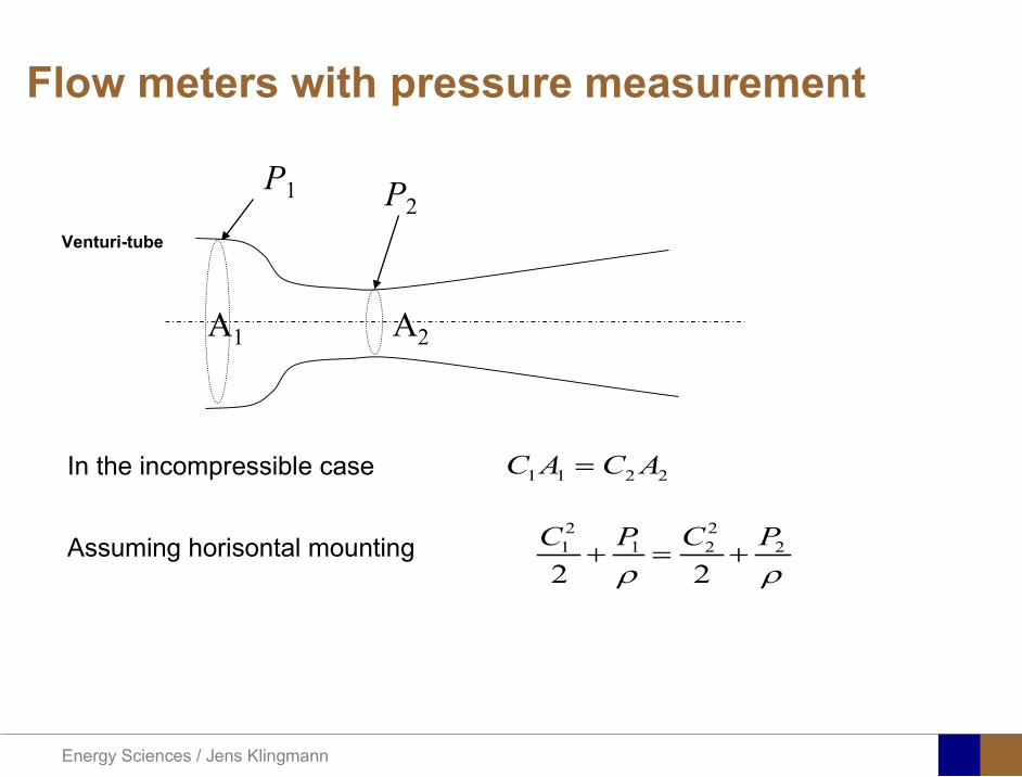
Energy Sciences Jens Klingmann
Flow meters with pressure measurement
Venturi-tube
A1 A2
P1 P2
1 1 2 2C A C A=In the incompressible case
2 21 1 2 2
2 2C P C P
ρ ρ+ = +Assuming horisontal mounting
Energy Sciences Jens Klingmann
Daniel Bernoulli 1700-1782
Daniel Bernoulli was the son of Johann Bernoulli He was born in Groningen while his father held the chair of mathematics there His older brother was Nicolaus(II) Bernoulli and his uncle was Jacob Bernoulli so he was born into a family of leading mathematicians but also into a family where there was unfortunate rivalry jealousy and bitterness
Undoubtedly the most important work which Daniel Bernoulli did was his work on hydrodynamics Even the term itself is based on the title of the work which he produced called Hydrodynamica and before he left St Petersburg Daniel left a draft copy of the book with a printer However the work was not published until 1738 and although he revised it considerably between 1734 and 1738 it is more the presentation that he changed rather then the substance
This work contains for the first time the correct analysis of water flowing from a hole in a container This was based on the principle of conservation of energy which he had studied with his father in 1720 Daniel also discussed pumps and other machines to raise water One remarkable discovery appears in Chapter 10 of Hydrodynamica where Daniel discussed the basis for the kinetic theory of gases He was able to give the basic laws for the theory of gases and gave although not in full detail the equation of state discovered by Van der Waals a century later
Energy Sciences Jens Klingmann
Venturi-tube (2)
22 2 12 2
2
2A PC CA ρ
∆minus =
A1 A2
P1 P2
Solve for eg C2
1 2P P P∆ = minus
( )
12
2 2 21 2
21
PCA Aρ
∆ = minus
and( )
12
2 2 2 2 21 2
21
Pm A C AA Aρρ
∆ = = minus
where
Flow meters with pressure measurement
Energy Sciences Jens Klingmann
Flow meters with pressure measurement
Orifice meters
A1
A2
P1 P2
Applicable for pipe flows Same principle as for Venturi Positioning of pressure taps important Vena contracta and losses require inclusion
of Discharge Coefficient CD
( )
12
2 2 21 2
21D
Pm C AA Aρ ∆ =
minus where ( )1 2ReDC f A A=
CD available from manufacturer (measurements) or Standards (eg ISO)
Energy Sciences Jens Klingmann
Coriolis flow meter
An actuator (not shown) induces a vibration of the tubes
When there is mass flow Coriolis forces induce twisting of the tubes
degree of phase-shift is a measure for the amount of mass that is flowing through the tubes
Energy Sciences Jens Klingmann
Thermal flow meter Heat is added electrically to the flow Temperature is measured before and after heat addition
pP mC T∆=
Energy Sciences Jens Klingmann
Ultrasonic flow meters
Ultrasound is emitted to small particles in the flow (dust or other) Reflections of the sound is frequency shifted by the Doppler effect The frequency change is proportional to the particles velocity (volume flow
meter)
Energy Sciences Jens Klingmann
Inductive flow metersA magnetic flowmeter is based upon Faradays Law
The voltage induced across any conductor as it moves at right angles through a magnetic field is proportional to the velocity of that conductor
E is proportional to V x B x D where
E = The voltage generated in a conductorV = The velocity of the conductorB = The magnetic field strengthD = The length of the conductor
NB electric conductivity is required
Energy Sciences Jens Klingmann
Temperature measurements
Thermocouples
The basis established by Thomas Johann Seebeck in 1821
A conductor generates a voltage when subjected to a temperature gradient
To measure this voltage one must use a second conductor material which generates a different voltage under the same temperature gradient
Energy Sciences Jens Klingmann
Pressure sensing
1 2p pgt 2p p2 may be the atmosphere a static pressure tap or a known reference pressure
The strain of the diaphragm (or itrsquos deflection) may be measured by a number of electric methods
Diaphragm
Energy Sciences Jens Klingmann
Pressure sensingPiezoresistive Strain Gage
Uses the piezoresistive effect of bonded or formed strain gauges to detect strain due to applied pressure
Capacitive
Uses a diaghragm and pressure cavity to create a variable capacitor to detect strain due to applied pressure
Magnetic
Measures the displacement of a diaphragm by means of changes in inductance (reluctance) LVDT Hall Effect or by eddy current principal
Piezoelectric
Uses the piezoelectric effect in certain materials such as quartz to measure the strain upon the sensing mechanism due to pressure
Potentiometric
Uses the motion of a wiper along a resistive mechanism to detect the strain caused by applied pressure
Energy Sciences Jens Klingmann
3D highly instationary (periodic) flow Potentially very high velocities (Supersonic) Large temperature differences Low accessibility (difficult to probe between rotors) Low turbulence levels in most of the domain Very high turbulence in BL and wakes
Properties of measuring object
Point measurements
Energy Sciences Jens Klingmann
Conventional or non-opticalndash Static Pressure Measurementsndash Total Pressure Measurements
bull Multy hole probes
ndash Total Temperature ndash Hot Wire Anemometry (HWA)
Optical techniques for Velocity Measurementsndash Laser Two Focous (L2F)ndash Laser Doppler Anemometry (LDA)ndash Particle Image velocimetry (PIV)
Point Measurements
Energy Sciences Jens Klingmann
Static and total pressure
2 2 21 2 1
2 1 2 2 2C C CP P ρ ρ ρ
minus = minus =
2 0C =Stagnation point
C1Static pressure tap
Prandtl or Pitot tube
Apply the Bernoulli equation from free stream to stagnation point
21
2 12CP Pρ
= +or
We can also define a stagnation or total pressure
( )2
101 1 022
CP P Pρ= + =
Total pressure = Static pressure + dynamic pressure
or
Energy Sciences Jens Klingmann
Static pressure
Energy Sciences Jens Klingmann
Total Pressure and Temperature
Shrouded Probes
Shrouded Probe
Pitot or Prandtl tube
Sensitive to direction
Energy Sciences Jens Klingmann
Ludwig Prandtl 1875-1953
Ludwig Prandtl born at Freising Bavaria on February 4 1875 was a German Physicist famous for his work in aeronautics He qualified at Munchen in 1900 with a thesis on elastic stability and held the position of Professor of Applied Mechanics at Gottingen for forty-nine years (from 1904 until his death there on August 15 1953) In 1925 Prandtl became the Director of the Kaiser Wilhelm Institute for Fluid Mechanics His discovery in 1904 of the Boundary Layer which adjoins the surface of a body moving in a fluid led to an understanding of skin friction drag and of the way in which streamlining reduces the drag of airplane wings and other moving bodies His work on wing theory published in 1918 - 1919 followed that of FW Lanchester (1902-1907) but was carried out independently and elucidated the flow over airplane wings of finite span Prandtls work and decisive advances in boundary layer and wing theories became the basic material of aeronautics He also made important contributions to the theories of supersonic flow and of turbulence and contributed much to the development of wind tunnels and other aerodynamic equipment In addition he devised the soap-film analogy for the torsion of non-circular sections and wrote on the theory of plasticity and of meteorology
Energy Sciences Jens Klingmann
Total Pressure multy hole
Cobra Probe Yaw Probe
5 Hole Probe
Energy Sciences Jens Klingmann
5 Hole Probes Calibration
Energy Sciences Jens Klingmann
The inherent unsteadiness of the flow within turbomachines
Energy Sciences Jens Klingmann
Hot Wire Anemometry (HWA) The heat transfer from a thin (one micron)
electrically heated wire can be used to determine velocity
The resistance of the wire is temperature dependent Within a small temperature range it can be assumed linear R = R0+α R0(Tm-T0) where R0 is the resistance at a reference temperature T0 and Tm is the mean wire temperature
The thermal power induced in the wire is balanced by heat transfer to the surrounding fluid I2R=hπDL(Tm-T0) where h is the heat transfer coefficient and D and L the diameter and length of the wire respectively
E = I R
Energy Sciences Jens Klingmann
Constant Temperature Anemometry (CTA) The wire is often placed in a Whetstone bridge If the output from the
bridge is amplified and fed back to the bridge the resistance of the probe and thus the temperature will be held constant
This prevents the temperature of the wire to become excessive at low velocities
R1
R2 R3
Probe
Bridge Voltage
Energy Sciences Jens Klingmann
Constant Temperature Anemometry (CTA)
Energy Sciences Jens Klingmann
Characteristics of LDA (according to Dantec)
Invented by Yeh and Cummins in 1964 Velocity measurements in Fluid Dynamics (gas liquid) Up to 3 velocity components Non-intrusive measurements (optical technique) Absolute measurement technique (no calibration required) Very high accuracy Very high spatial resolution due to small measurement volume Tracer particles are required
Energy Sciences Jens Klingmann
LDA - Fringe Model
Focused Laser beams intersect and form the measurement volume Plane wave fronts beam waist in the plane of intersection Interference in the plane of intersection Pattern of bright and dark stripesplanes Fringes
Energy Sciences Jens Klingmann
LDA-measuring volume
d
x
x
y
y
z
z
e-2 CONTOUR
FRINGES
κ
κ
κ
κ
De-2
De-2
dml m
a
b
cx
b
z
ya
cd
d
=
=
=
J
J
J
J
JP
JP
JP
JD
JD
JD
+
+
+
a
b
c
d
κπλ
=minus sinD
f4l2e
m
κπλ
=minus cosD
f4D2e
m
Energy Sciences Jens Klingmann
Laser Two Focus
Energy Sciences Jens Klingmann
Laser Two Focus
Energy Sciences Jens Klingmann
PIV measurements
PIV is a fairly new technique capable of simultaneous velocity measurements at many points in a plane This gives information on large scale structures vorticity etc which is very difficult or impossible to obtain from one-point measuring techniques
PIV involves the illumination of a plane of the flow under investigation with a thin pulsed sheet of light The flow is seeded with particles
The light scattered from the particles and from successive pulses are being recorded either on film or a CCD array forming a multiple exposure of each particle image If the time between the pulses is known velocity can be determined as the ratio of the particle displacement and the elapsed time
t∆∆= xu
Energy Sciences Jens Klingmann
PIV
Energy Sciences Jens Klingmann
PIV measurements illumination
YA
G
YA
G
Two frequency doubled YAG Lasers aligned to one double pulsed laser sheet
Two or more separate light pulses can be obtained by chopping a continuous laser or from pulsed lasers
The limited pulse energies obtained from continuous lasers limits their applicability to low velocity flows or flows where large seeding particles can be used (ie liquid flows)
The low repetition rate of most pulsed lasers makes the use of two lasers advantageous
Energy Sciences Jens Klingmann
PIV measurements recording
High seeding density in laminar flame
Film or CCD-cameras Cross- or Auto-correlation
ndash ie both particle images on the same frame or on separate frames
CCD-camera requirementndash A many pixels as possiblendash 2k by 2k available 4k by 4k coming
Energy Sciences Jens Klingmann
PIV measurements analyses
Low seeding density (Number of seeding particles per unit volume)
Each particle image pair can be identified This is called particle tracking
High seeding density (PIV)
Small sub-regions of the image containing many particle image pairs are processed to obtain one velocity vector
Energy Sciences Jens Klingmann
PIV measurements analyses
Energy Sciences Jens Klingmann
PIV measurements analyses
( ) ( ) ( ) xsxxs dIIR 2A
1
I
+= int
Cross correlation between ( )x1I and ( )x2I
s is a two dimensional displacement vector
IA is the interrogation area
Cross correlation between
(
)
x
1
I
and
(
)
x
2
I
s is a two dimensional displacement vector
I
A
is the interrogation area
Energy Sciences Jens Klingmann
Energy Sciences Jens Klingmann
PIV from IOWA state university
Energy Sciences Jens Klingmann
PIV sample of evaluation
Energy Sciences Jens Klingmann
LDA PIV HWA Velocity range 01 mms ndash 300
ms 02 ndash 150 ms
Measuring Volume
D = 005 L = 05 mm
2 by 2 by 05 mm
L = 05 mm
Freq response O(10 000) Hz O(10) Hz O(100 000) Hz Calibration Yes No No Sensitivity to other than velocity
Low (ref Index) Low (ref Index) Large (temperature concentrationshellip)
Continuous Signal
Sometimes Seldom Always
Noise High High Low Turbulence intensity
No limitation Some limitation lt 20
Price O(1 000 000) SEK
O(1 000 000) SEK
O(50 000) SEK
Required Knowledge
High medium Low
Comparison of techniques
Energy Sciences Jens Klingmann
References experiments
R J Goldstein ldquoFluid Mechanics Measurementsrdquo Hemisphere Publishing 1983 A V Johansson amp P H Alfredsson ldquoExperimentella metoder inom
stroumlmningsmekanikenrdquo Inst Foumlr Mekanik KTH F Durst A Melling and J H Whitelaw ldquoPrincipals and Practice of Laser Doppler
Anemometryrdquo 1984 R J Adrian ldquoParticle-imaging techniques for experimental fluid mechnicsrdquo Ann Rev
Fluid Mech 1991
Energy Sciences Jens Klingmann
Sample of LDA-measurements
Rotor blade
Glas window
Emitted beams
Scattered Light
Adjustable mirror
Energy Sciences Jens Klingmann
Axial velocity sorted into 10 bins
0 1 2 3 4 5 6tangential coordinate (degrees)
-20
0
20
40
60
80
100
120
140
160Ax
ial v
eloc
ity a
nd s
tand
ard
devi
atio
n (m
s)
radial position 7 mm from inner window surfaceaxial position 23 mm behind rotor blades
Energy Sciences Jens Klingmann
Axial velocities in the radial-tangential plane
Energy Sciences Jens Klingmann
Airfoils NACA 4-digit
The NACA four-digit wing sections define the profile by
One digit describing maximum camber as percentage of the chord
One digit describing the distance of maximum camber from the airfoil leading edge in tens of percents of the chord
Two digits describing maximum thickness of the airfoil as percent of the chord
Example the NACA 2412 airfoil has a maximum camber of 2 located 40 (04 chords) from the leading edge with a maximum thickness of 12 of the chord
Four-digit series airfoils by default have maximum thickness at 30 of the chord (03 chords) from the leading edge
Energy Sciences Jens Klingmann
Airfoils NACA 4-digit
bull c is the chord lengthbull x is the position along
the chord from 0 to cbull y is the half thickness at
a given value of x (centerline to surface)
bull t is the maximum thickness as a fraction of the chord
Energy Sciences Jens Klingmann
Death by PowerPoint
| LDA | PIV | HWA | |||||
| Velocity range | 01 mms ndash 300 ms | 02 ndash 150 ms | |||||
| Measuring Volume | D = 005 L = 05 mm | 2 by 2 by 05 mm | L = 05 mm | ||||
| Freq response | O(10 000) Hz | O(10) Hz | O(100 000) Hz | ||||
| Calibration | Yes | No | No | ||||
| Sensitivity to other than velocity | Low (ref Index) | Low (ref Index) | Large (temperature concentrationshellip) | ||||
| Continuous Signal | Sometimes | Seldom | Always | ||||
| Noise | High | High | Low | ||||
| Turbulence intensity | No limitation | Some limitation | lt 20 | ||||
| Price | O(1 000 000) SEK | O(1 000 000) SEK | O(50 000) SEK | ||||
| Required Knowledge | High | medium | Low |

Energy Sciences Jens Klingmann
Daniel Bernoulli 1700-1782
Daniel Bernoulli was the son of Johann Bernoulli He was born in Groningen while his father held the chair of mathematics there His older brother was Nicolaus(II) Bernoulli and his uncle was Jacob Bernoulli so he was born into a family of leading mathematicians but also into a family where there was unfortunate rivalry jealousy and bitterness
Undoubtedly the most important work which Daniel Bernoulli did was his work on hydrodynamics Even the term itself is based on the title of the work which he produced called Hydrodynamica and before he left St Petersburg Daniel left a draft copy of the book with a printer However the work was not published until 1738 and although he revised it considerably between 1734 and 1738 it is more the presentation that he changed rather then the substance
This work contains for the first time the correct analysis of water flowing from a hole in a container This was based on the principle of conservation of energy which he had studied with his father in 1720 Daniel also discussed pumps and other machines to raise water One remarkable discovery appears in Chapter 10 of Hydrodynamica where Daniel discussed the basis for the kinetic theory of gases He was able to give the basic laws for the theory of gases and gave although not in full detail the equation of state discovered by Van der Waals a century later
Energy Sciences Jens Klingmann
Venturi-tube (2)
22 2 12 2
2
2A PC CA ρ
∆minus =
A1 A2
P1 P2
Solve for eg C2
1 2P P P∆ = minus
( )
12
2 2 21 2
21
PCA Aρ
∆ = minus
and( )
12
2 2 2 2 21 2
21
Pm A C AA Aρρ
∆ = = minus
where
Flow meters with pressure measurement
Energy Sciences Jens Klingmann
Flow meters with pressure measurement
Orifice meters
A1
A2
P1 P2
Applicable for pipe flows Same principle as for Venturi Positioning of pressure taps important Vena contracta and losses require inclusion
of Discharge Coefficient CD
( )
12
2 2 21 2
21D
Pm C AA Aρ ∆ =
minus where ( )1 2ReDC f A A=
CD available from manufacturer (measurements) or Standards (eg ISO)
Energy Sciences Jens Klingmann
Coriolis flow meter
An actuator (not shown) induces a vibration of the tubes
When there is mass flow Coriolis forces induce twisting of the tubes
degree of phase-shift is a measure for the amount of mass that is flowing through the tubes
Energy Sciences Jens Klingmann
Thermal flow meter Heat is added electrically to the flow Temperature is measured before and after heat addition
pP mC T∆=
Energy Sciences Jens Klingmann
Ultrasonic flow meters
Ultrasound is emitted to small particles in the flow (dust or other) Reflections of the sound is frequency shifted by the Doppler effect The frequency change is proportional to the particles velocity (volume flow
meter)
Energy Sciences Jens Klingmann
Inductive flow metersA magnetic flowmeter is based upon Faradays Law
The voltage induced across any conductor as it moves at right angles through a magnetic field is proportional to the velocity of that conductor
E is proportional to V x B x D where
E = The voltage generated in a conductorV = The velocity of the conductorB = The magnetic field strengthD = The length of the conductor
NB electric conductivity is required
Energy Sciences Jens Klingmann
Temperature measurements
Thermocouples
The basis established by Thomas Johann Seebeck in 1821
A conductor generates a voltage when subjected to a temperature gradient
To measure this voltage one must use a second conductor material which generates a different voltage under the same temperature gradient
Energy Sciences Jens Klingmann
Pressure sensing
1 2p pgt 2p p2 may be the atmosphere a static pressure tap or a known reference pressure
The strain of the diaphragm (or itrsquos deflection) may be measured by a number of electric methods
Diaphragm
Energy Sciences Jens Klingmann
Pressure sensingPiezoresistive Strain Gage
Uses the piezoresistive effect of bonded or formed strain gauges to detect strain due to applied pressure
Capacitive
Uses a diaghragm and pressure cavity to create a variable capacitor to detect strain due to applied pressure
Magnetic
Measures the displacement of a diaphragm by means of changes in inductance (reluctance) LVDT Hall Effect or by eddy current principal
Piezoelectric
Uses the piezoelectric effect in certain materials such as quartz to measure the strain upon the sensing mechanism due to pressure
Potentiometric
Uses the motion of a wiper along a resistive mechanism to detect the strain caused by applied pressure
Energy Sciences Jens Klingmann
3D highly instationary (periodic) flow Potentially very high velocities (Supersonic) Large temperature differences Low accessibility (difficult to probe between rotors) Low turbulence levels in most of the domain Very high turbulence in BL and wakes
Properties of measuring object
Point measurements
Energy Sciences Jens Klingmann
Conventional or non-opticalndash Static Pressure Measurementsndash Total Pressure Measurements
bull Multy hole probes
ndash Total Temperature ndash Hot Wire Anemometry (HWA)
Optical techniques for Velocity Measurementsndash Laser Two Focous (L2F)ndash Laser Doppler Anemometry (LDA)ndash Particle Image velocimetry (PIV)
Point Measurements
Energy Sciences Jens Klingmann
Static and total pressure
2 2 21 2 1
2 1 2 2 2C C CP P ρ ρ ρ
minus = minus =
2 0C =Stagnation point
C1Static pressure tap
Prandtl or Pitot tube
Apply the Bernoulli equation from free stream to stagnation point
21
2 12CP Pρ
= +or
We can also define a stagnation or total pressure
( )2
101 1 022
CP P Pρ= + =
Total pressure = Static pressure + dynamic pressure
or
Energy Sciences Jens Klingmann
Static pressure
Energy Sciences Jens Klingmann
Total Pressure and Temperature
Shrouded Probes
Shrouded Probe
Pitot or Prandtl tube
Sensitive to direction
Energy Sciences Jens Klingmann
Ludwig Prandtl 1875-1953
Ludwig Prandtl born at Freising Bavaria on February 4 1875 was a German Physicist famous for his work in aeronautics He qualified at Munchen in 1900 with a thesis on elastic stability and held the position of Professor of Applied Mechanics at Gottingen for forty-nine years (from 1904 until his death there on August 15 1953) In 1925 Prandtl became the Director of the Kaiser Wilhelm Institute for Fluid Mechanics His discovery in 1904 of the Boundary Layer which adjoins the surface of a body moving in a fluid led to an understanding of skin friction drag and of the way in which streamlining reduces the drag of airplane wings and other moving bodies His work on wing theory published in 1918 - 1919 followed that of FW Lanchester (1902-1907) but was carried out independently and elucidated the flow over airplane wings of finite span Prandtls work and decisive advances in boundary layer and wing theories became the basic material of aeronautics He also made important contributions to the theories of supersonic flow and of turbulence and contributed much to the development of wind tunnels and other aerodynamic equipment In addition he devised the soap-film analogy for the torsion of non-circular sections and wrote on the theory of plasticity and of meteorology
Energy Sciences Jens Klingmann
Total Pressure multy hole
Cobra Probe Yaw Probe
5 Hole Probe
Energy Sciences Jens Klingmann
5 Hole Probes Calibration
Energy Sciences Jens Klingmann
The inherent unsteadiness of the flow within turbomachines
Energy Sciences Jens Klingmann
Hot Wire Anemometry (HWA) The heat transfer from a thin (one micron)
electrically heated wire can be used to determine velocity
The resistance of the wire is temperature dependent Within a small temperature range it can be assumed linear R = R0+α R0(Tm-T0) where R0 is the resistance at a reference temperature T0 and Tm is the mean wire temperature
The thermal power induced in the wire is balanced by heat transfer to the surrounding fluid I2R=hπDL(Tm-T0) where h is the heat transfer coefficient and D and L the diameter and length of the wire respectively
E = I R
Energy Sciences Jens Klingmann
Constant Temperature Anemometry (CTA) The wire is often placed in a Whetstone bridge If the output from the
bridge is amplified and fed back to the bridge the resistance of the probe and thus the temperature will be held constant
This prevents the temperature of the wire to become excessive at low velocities
R1
R2 R3
Probe
Bridge Voltage
Energy Sciences Jens Klingmann
Constant Temperature Anemometry (CTA)
Energy Sciences Jens Klingmann
Characteristics of LDA (according to Dantec)
Invented by Yeh and Cummins in 1964 Velocity measurements in Fluid Dynamics (gas liquid) Up to 3 velocity components Non-intrusive measurements (optical technique) Absolute measurement technique (no calibration required) Very high accuracy Very high spatial resolution due to small measurement volume Tracer particles are required
Energy Sciences Jens Klingmann
LDA - Fringe Model
Focused Laser beams intersect and form the measurement volume Plane wave fronts beam waist in the plane of intersection Interference in the plane of intersection Pattern of bright and dark stripesplanes Fringes
Energy Sciences Jens Klingmann
LDA-measuring volume
d
x
x
y
y
z
z
e-2 CONTOUR
FRINGES
κ
κ
κ
κ
De-2
De-2
dml m
a
b
cx
b
z
ya
cd
d
=
=
=
J
J
J
J
JP
JP
JP
JD
JD
JD
+
+
+
a
b
c
d
κπλ
=minus sinD
f4l2e
m
κπλ
=minus cosD
f4D2e
m
Energy Sciences Jens Klingmann
Laser Two Focus
Energy Sciences Jens Klingmann
Laser Two Focus
Energy Sciences Jens Klingmann
PIV measurements
PIV is a fairly new technique capable of simultaneous velocity measurements at many points in a plane This gives information on large scale structures vorticity etc which is very difficult or impossible to obtain from one-point measuring techniques
PIV involves the illumination of a plane of the flow under investigation with a thin pulsed sheet of light The flow is seeded with particles
The light scattered from the particles and from successive pulses are being recorded either on film or a CCD array forming a multiple exposure of each particle image If the time between the pulses is known velocity can be determined as the ratio of the particle displacement and the elapsed time
t∆∆= xu
Energy Sciences Jens Klingmann
PIV
Energy Sciences Jens Klingmann
PIV measurements illumination
YA
G
YA
G
Two frequency doubled YAG Lasers aligned to one double pulsed laser sheet
Two or more separate light pulses can be obtained by chopping a continuous laser or from pulsed lasers
The limited pulse energies obtained from continuous lasers limits their applicability to low velocity flows or flows where large seeding particles can be used (ie liquid flows)
The low repetition rate of most pulsed lasers makes the use of two lasers advantageous
Energy Sciences Jens Klingmann
PIV measurements recording
High seeding density in laminar flame
Film or CCD-cameras Cross- or Auto-correlation
ndash ie both particle images on the same frame or on separate frames
CCD-camera requirementndash A many pixels as possiblendash 2k by 2k available 4k by 4k coming
Energy Sciences Jens Klingmann
PIV measurements analyses
Low seeding density (Number of seeding particles per unit volume)
Each particle image pair can be identified This is called particle tracking
High seeding density (PIV)
Small sub-regions of the image containing many particle image pairs are processed to obtain one velocity vector
Energy Sciences Jens Klingmann
PIV measurements analyses
Energy Sciences Jens Klingmann
PIV measurements analyses
( ) ( ) ( ) xsxxs dIIR 2A
1
I
+= int
Cross correlation between ( )x1I and ( )x2I
s is a two dimensional displacement vector
IA is the interrogation area
Cross correlation between
(
)
x
1
I
and
(
)
x
2
I
s is a two dimensional displacement vector
I
A
is the interrogation area
Energy Sciences Jens Klingmann
Energy Sciences Jens Klingmann
PIV from IOWA state university
Energy Sciences Jens Klingmann
PIV sample of evaluation
Energy Sciences Jens Klingmann
LDA PIV HWA Velocity range 01 mms ndash 300
ms 02 ndash 150 ms
Measuring Volume
D = 005 L = 05 mm
2 by 2 by 05 mm
L = 05 mm
Freq response O(10 000) Hz O(10) Hz O(100 000) Hz Calibration Yes No No Sensitivity to other than velocity
Low (ref Index) Low (ref Index) Large (temperature concentrationshellip)
Continuous Signal
Sometimes Seldom Always
Noise High High Low Turbulence intensity
No limitation Some limitation lt 20
Price O(1 000 000) SEK
O(1 000 000) SEK
O(50 000) SEK
Required Knowledge
High medium Low
Comparison of techniques
Energy Sciences Jens Klingmann
References experiments
R J Goldstein ldquoFluid Mechanics Measurementsrdquo Hemisphere Publishing 1983 A V Johansson amp P H Alfredsson ldquoExperimentella metoder inom
stroumlmningsmekanikenrdquo Inst Foumlr Mekanik KTH F Durst A Melling and J H Whitelaw ldquoPrincipals and Practice of Laser Doppler
Anemometryrdquo 1984 R J Adrian ldquoParticle-imaging techniques for experimental fluid mechnicsrdquo Ann Rev
Fluid Mech 1991
Energy Sciences Jens Klingmann
Sample of LDA-measurements
Rotor blade
Glas window
Emitted beams
Scattered Light
Adjustable mirror
Energy Sciences Jens Klingmann
Axial velocity sorted into 10 bins
0 1 2 3 4 5 6tangential coordinate (degrees)
-20
0
20
40
60
80
100
120
140
160Ax
ial v
eloc
ity a
nd s
tand
ard
devi
atio
n (m
s)
radial position 7 mm from inner window surfaceaxial position 23 mm behind rotor blades
Energy Sciences Jens Klingmann
Axial velocities in the radial-tangential plane
Energy Sciences Jens Klingmann
Airfoils NACA 4-digit
The NACA four-digit wing sections define the profile by
One digit describing maximum camber as percentage of the chord
One digit describing the distance of maximum camber from the airfoil leading edge in tens of percents of the chord
Two digits describing maximum thickness of the airfoil as percent of the chord
Example the NACA 2412 airfoil has a maximum camber of 2 located 40 (04 chords) from the leading edge with a maximum thickness of 12 of the chord
Four-digit series airfoils by default have maximum thickness at 30 of the chord (03 chords) from the leading edge
Energy Sciences Jens Klingmann
Airfoils NACA 4-digit
bull c is the chord lengthbull x is the position along
the chord from 0 to cbull y is the half thickness at
a given value of x (centerline to surface)
bull t is the maximum thickness as a fraction of the chord
Energy Sciences Jens Klingmann
Death by PowerPoint
| LDA | PIV | HWA | |||||
| Velocity range | 01 mms ndash 300 ms | 02 ndash 150 ms | |||||
| Measuring Volume | D = 005 L = 05 mm | 2 by 2 by 05 mm | L = 05 mm | ||||
| Freq response | O(10 000) Hz | O(10) Hz | O(100 000) Hz | ||||
| Calibration | Yes | No | No | ||||
| Sensitivity to other than velocity | Low (ref Index) | Low (ref Index) | Large (temperature concentrationshellip) | ||||
| Continuous Signal | Sometimes | Seldom | Always | ||||
| Noise | High | High | Low | ||||
| Turbulence intensity | No limitation | Some limitation | lt 20 | ||||
| Price | O(1 000 000) SEK | O(1 000 000) SEK | O(50 000) SEK | ||||
| Required Knowledge | High | medium | Low |
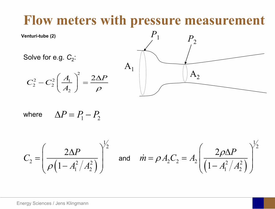
Energy Sciences Jens Klingmann
Venturi-tube (2)
22 2 12 2
2
2A PC CA ρ
∆minus =
A1 A2
P1 P2
Solve for eg C2
1 2P P P∆ = minus
( )
12
2 2 21 2
21
PCA Aρ
∆ = minus
and( )
12
2 2 2 2 21 2
21
Pm A C AA Aρρ
∆ = = minus
where
Flow meters with pressure measurement
Energy Sciences Jens Klingmann
Flow meters with pressure measurement
Orifice meters
A1
A2
P1 P2
Applicable for pipe flows Same principle as for Venturi Positioning of pressure taps important Vena contracta and losses require inclusion
of Discharge Coefficient CD
( )
12
2 2 21 2
21D
Pm C AA Aρ ∆ =
minus where ( )1 2ReDC f A A=
CD available from manufacturer (measurements) or Standards (eg ISO)
Energy Sciences Jens Klingmann
Coriolis flow meter
An actuator (not shown) induces a vibration of the tubes
When there is mass flow Coriolis forces induce twisting of the tubes
degree of phase-shift is a measure for the amount of mass that is flowing through the tubes
Energy Sciences Jens Klingmann
Thermal flow meter Heat is added electrically to the flow Temperature is measured before and after heat addition
pP mC T∆=
Energy Sciences Jens Klingmann
Ultrasonic flow meters
Ultrasound is emitted to small particles in the flow (dust or other) Reflections of the sound is frequency shifted by the Doppler effect The frequency change is proportional to the particles velocity (volume flow
meter)
Energy Sciences Jens Klingmann
Inductive flow metersA magnetic flowmeter is based upon Faradays Law
The voltage induced across any conductor as it moves at right angles through a magnetic field is proportional to the velocity of that conductor
E is proportional to V x B x D where
E = The voltage generated in a conductorV = The velocity of the conductorB = The magnetic field strengthD = The length of the conductor
NB electric conductivity is required
Energy Sciences Jens Klingmann
Temperature measurements
Thermocouples
The basis established by Thomas Johann Seebeck in 1821
A conductor generates a voltage when subjected to a temperature gradient
To measure this voltage one must use a second conductor material which generates a different voltage under the same temperature gradient
Energy Sciences Jens Klingmann
Pressure sensing
1 2p pgt 2p p2 may be the atmosphere a static pressure tap or a known reference pressure
The strain of the diaphragm (or itrsquos deflection) may be measured by a number of electric methods
Diaphragm
Energy Sciences Jens Klingmann
Pressure sensingPiezoresistive Strain Gage
Uses the piezoresistive effect of bonded or formed strain gauges to detect strain due to applied pressure
Capacitive
Uses a diaghragm and pressure cavity to create a variable capacitor to detect strain due to applied pressure
Magnetic
Measures the displacement of a diaphragm by means of changes in inductance (reluctance) LVDT Hall Effect or by eddy current principal
Piezoelectric
Uses the piezoelectric effect in certain materials such as quartz to measure the strain upon the sensing mechanism due to pressure
Potentiometric
Uses the motion of a wiper along a resistive mechanism to detect the strain caused by applied pressure
Energy Sciences Jens Klingmann
3D highly instationary (periodic) flow Potentially very high velocities (Supersonic) Large temperature differences Low accessibility (difficult to probe between rotors) Low turbulence levels in most of the domain Very high turbulence in BL and wakes
Properties of measuring object
Point measurements
Energy Sciences Jens Klingmann
Conventional or non-opticalndash Static Pressure Measurementsndash Total Pressure Measurements
bull Multy hole probes
ndash Total Temperature ndash Hot Wire Anemometry (HWA)
Optical techniques for Velocity Measurementsndash Laser Two Focous (L2F)ndash Laser Doppler Anemometry (LDA)ndash Particle Image velocimetry (PIV)
Point Measurements
Energy Sciences Jens Klingmann
Static and total pressure
2 2 21 2 1
2 1 2 2 2C C CP P ρ ρ ρ
minus = minus =
2 0C =Stagnation point
C1Static pressure tap
Prandtl or Pitot tube
Apply the Bernoulli equation from free stream to stagnation point
21
2 12CP Pρ
= +or
We can also define a stagnation or total pressure
( )2
101 1 022
CP P Pρ= + =
Total pressure = Static pressure + dynamic pressure
or
Energy Sciences Jens Klingmann
Static pressure
Energy Sciences Jens Klingmann
Total Pressure and Temperature
Shrouded Probes
Shrouded Probe
Pitot or Prandtl tube
Sensitive to direction
Energy Sciences Jens Klingmann
Ludwig Prandtl 1875-1953
Ludwig Prandtl born at Freising Bavaria on February 4 1875 was a German Physicist famous for his work in aeronautics He qualified at Munchen in 1900 with a thesis on elastic stability and held the position of Professor of Applied Mechanics at Gottingen for forty-nine years (from 1904 until his death there on August 15 1953) In 1925 Prandtl became the Director of the Kaiser Wilhelm Institute for Fluid Mechanics His discovery in 1904 of the Boundary Layer which adjoins the surface of a body moving in a fluid led to an understanding of skin friction drag and of the way in which streamlining reduces the drag of airplane wings and other moving bodies His work on wing theory published in 1918 - 1919 followed that of FW Lanchester (1902-1907) but was carried out independently and elucidated the flow over airplane wings of finite span Prandtls work and decisive advances in boundary layer and wing theories became the basic material of aeronautics He also made important contributions to the theories of supersonic flow and of turbulence and contributed much to the development of wind tunnels and other aerodynamic equipment In addition he devised the soap-film analogy for the torsion of non-circular sections and wrote on the theory of plasticity and of meteorology
Energy Sciences Jens Klingmann
Total Pressure multy hole
Cobra Probe Yaw Probe
5 Hole Probe
Energy Sciences Jens Klingmann
5 Hole Probes Calibration
Energy Sciences Jens Klingmann
The inherent unsteadiness of the flow within turbomachines
Energy Sciences Jens Klingmann
Hot Wire Anemometry (HWA) The heat transfer from a thin (one micron)
electrically heated wire can be used to determine velocity
The resistance of the wire is temperature dependent Within a small temperature range it can be assumed linear R = R0+α R0(Tm-T0) where R0 is the resistance at a reference temperature T0 and Tm is the mean wire temperature
The thermal power induced in the wire is balanced by heat transfer to the surrounding fluid I2R=hπDL(Tm-T0) where h is the heat transfer coefficient and D and L the diameter and length of the wire respectively
E = I R
Energy Sciences Jens Klingmann
Constant Temperature Anemometry (CTA) The wire is often placed in a Whetstone bridge If the output from the
bridge is amplified and fed back to the bridge the resistance of the probe and thus the temperature will be held constant
This prevents the temperature of the wire to become excessive at low velocities
R1
R2 R3
Probe
Bridge Voltage
Energy Sciences Jens Klingmann
Constant Temperature Anemometry (CTA)
Energy Sciences Jens Klingmann
Characteristics of LDA (according to Dantec)
Invented by Yeh and Cummins in 1964 Velocity measurements in Fluid Dynamics (gas liquid) Up to 3 velocity components Non-intrusive measurements (optical technique) Absolute measurement technique (no calibration required) Very high accuracy Very high spatial resolution due to small measurement volume Tracer particles are required
Energy Sciences Jens Klingmann
LDA - Fringe Model
Focused Laser beams intersect and form the measurement volume Plane wave fronts beam waist in the plane of intersection Interference in the plane of intersection Pattern of bright and dark stripesplanes Fringes
Energy Sciences Jens Klingmann
LDA-measuring volume
d
x
x
y
y
z
z
e-2 CONTOUR
FRINGES
κ
κ
κ
κ
De-2
De-2
dml m
a
b
cx
b
z
ya
cd
d
=
=
=
J
J
J
J
JP
JP
JP
JD
JD
JD
+
+
+
a
b
c
d
κπλ
=minus sinD
f4l2e
m
κπλ
=minus cosD
f4D2e
m
Energy Sciences Jens Klingmann
Laser Two Focus
Energy Sciences Jens Klingmann
Laser Two Focus
Energy Sciences Jens Klingmann
PIV measurements
PIV is a fairly new technique capable of simultaneous velocity measurements at many points in a plane This gives information on large scale structures vorticity etc which is very difficult or impossible to obtain from one-point measuring techniques
PIV involves the illumination of a plane of the flow under investigation with a thin pulsed sheet of light The flow is seeded with particles
The light scattered from the particles and from successive pulses are being recorded either on film or a CCD array forming a multiple exposure of each particle image If the time between the pulses is known velocity can be determined as the ratio of the particle displacement and the elapsed time
t∆∆= xu
Energy Sciences Jens Klingmann
PIV
Energy Sciences Jens Klingmann
PIV measurements illumination
YA
G
YA
G
Two frequency doubled YAG Lasers aligned to one double pulsed laser sheet
Two or more separate light pulses can be obtained by chopping a continuous laser or from pulsed lasers
The limited pulse energies obtained from continuous lasers limits their applicability to low velocity flows or flows where large seeding particles can be used (ie liquid flows)
The low repetition rate of most pulsed lasers makes the use of two lasers advantageous
Energy Sciences Jens Klingmann
PIV measurements recording
High seeding density in laminar flame
Film or CCD-cameras Cross- or Auto-correlation
ndash ie both particle images on the same frame or on separate frames
CCD-camera requirementndash A many pixels as possiblendash 2k by 2k available 4k by 4k coming
Energy Sciences Jens Klingmann
PIV measurements analyses
Low seeding density (Number of seeding particles per unit volume)
Each particle image pair can be identified This is called particle tracking
High seeding density (PIV)
Small sub-regions of the image containing many particle image pairs are processed to obtain one velocity vector
Energy Sciences Jens Klingmann
PIV measurements analyses
Energy Sciences Jens Klingmann
PIV measurements analyses
( ) ( ) ( ) xsxxs dIIR 2A
1
I
+= int
Cross correlation between ( )x1I and ( )x2I
s is a two dimensional displacement vector
IA is the interrogation area
Cross correlation between
(
)
x
1
I
and
(
)
x
2
I
s is a two dimensional displacement vector
I
A
is the interrogation area
Energy Sciences Jens Klingmann
Energy Sciences Jens Klingmann
PIV from IOWA state university
Energy Sciences Jens Klingmann
PIV sample of evaluation
Energy Sciences Jens Klingmann
LDA PIV HWA Velocity range 01 mms ndash 300
ms 02 ndash 150 ms
Measuring Volume
D = 005 L = 05 mm
2 by 2 by 05 mm
L = 05 mm
Freq response O(10 000) Hz O(10) Hz O(100 000) Hz Calibration Yes No No Sensitivity to other than velocity
Low (ref Index) Low (ref Index) Large (temperature concentrationshellip)
Continuous Signal
Sometimes Seldom Always
Noise High High Low Turbulence intensity
No limitation Some limitation lt 20
Price O(1 000 000) SEK
O(1 000 000) SEK
O(50 000) SEK
Required Knowledge
High medium Low
Comparison of techniques
Energy Sciences Jens Klingmann
References experiments
R J Goldstein ldquoFluid Mechanics Measurementsrdquo Hemisphere Publishing 1983 A V Johansson amp P H Alfredsson ldquoExperimentella metoder inom
stroumlmningsmekanikenrdquo Inst Foumlr Mekanik KTH F Durst A Melling and J H Whitelaw ldquoPrincipals and Practice of Laser Doppler
Anemometryrdquo 1984 R J Adrian ldquoParticle-imaging techniques for experimental fluid mechnicsrdquo Ann Rev
Fluid Mech 1991
Energy Sciences Jens Klingmann
Sample of LDA-measurements
Rotor blade
Glas window
Emitted beams
Scattered Light
Adjustable mirror
Energy Sciences Jens Klingmann
Axial velocity sorted into 10 bins
0 1 2 3 4 5 6tangential coordinate (degrees)
-20
0
20
40
60
80
100
120
140
160Ax
ial v
eloc
ity a
nd s
tand
ard
devi
atio
n (m
s)
radial position 7 mm from inner window surfaceaxial position 23 mm behind rotor blades
Energy Sciences Jens Klingmann
Axial velocities in the radial-tangential plane
Energy Sciences Jens Klingmann
Airfoils NACA 4-digit
The NACA four-digit wing sections define the profile by
One digit describing maximum camber as percentage of the chord
One digit describing the distance of maximum camber from the airfoil leading edge in tens of percents of the chord
Two digits describing maximum thickness of the airfoil as percent of the chord
Example the NACA 2412 airfoil has a maximum camber of 2 located 40 (04 chords) from the leading edge with a maximum thickness of 12 of the chord
Four-digit series airfoils by default have maximum thickness at 30 of the chord (03 chords) from the leading edge
Energy Sciences Jens Klingmann
Airfoils NACA 4-digit
bull c is the chord lengthbull x is the position along
the chord from 0 to cbull y is the half thickness at
a given value of x (centerline to surface)
bull t is the maximum thickness as a fraction of the chord
Energy Sciences Jens Klingmann
Death by PowerPoint
| LDA | PIV | HWA | |||||
| Velocity range | 01 mms ndash 300 ms | 02 ndash 150 ms | |||||
| Measuring Volume | D = 005 L = 05 mm | 2 by 2 by 05 mm | L = 05 mm | ||||
| Freq response | O(10 000) Hz | O(10) Hz | O(100 000) Hz | ||||
| Calibration | Yes | No | No | ||||
| Sensitivity to other than velocity | Low (ref Index) | Low (ref Index) | Large (temperature concentrationshellip) | ||||
| Continuous Signal | Sometimes | Seldom | Always | ||||
| Noise | High | High | Low | ||||
| Turbulence intensity | No limitation | Some limitation | lt 20 | ||||
| Price | O(1 000 000) SEK | O(1 000 000) SEK | O(50 000) SEK | ||||
| Required Knowledge | High | medium | Low |
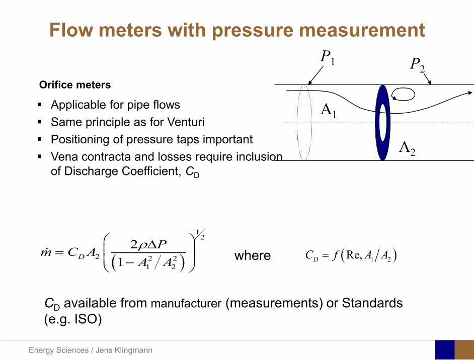
Energy Sciences Jens Klingmann
Flow meters with pressure measurement
Orifice meters
A1
A2
P1 P2
Applicable for pipe flows Same principle as for Venturi Positioning of pressure taps important Vena contracta and losses require inclusion
of Discharge Coefficient CD
( )
12
2 2 21 2
21D
Pm C AA Aρ ∆ =
minus where ( )1 2ReDC f A A=
CD available from manufacturer (measurements) or Standards (eg ISO)
Energy Sciences Jens Klingmann
Coriolis flow meter
An actuator (not shown) induces a vibration of the tubes
When there is mass flow Coriolis forces induce twisting of the tubes
degree of phase-shift is a measure for the amount of mass that is flowing through the tubes
Energy Sciences Jens Klingmann
Thermal flow meter Heat is added electrically to the flow Temperature is measured before and after heat addition
pP mC T∆=
Energy Sciences Jens Klingmann
Ultrasonic flow meters
Ultrasound is emitted to small particles in the flow (dust or other) Reflections of the sound is frequency shifted by the Doppler effect The frequency change is proportional to the particles velocity (volume flow
meter)
Energy Sciences Jens Klingmann
Inductive flow metersA magnetic flowmeter is based upon Faradays Law
The voltage induced across any conductor as it moves at right angles through a magnetic field is proportional to the velocity of that conductor
E is proportional to V x B x D where
E = The voltage generated in a conductorV = The velocity of the conductorB = The magnetic field strengthD = The length of the conductor
NB electric conductivity is required
Energy Sciences Jens Klingmann
Temperature measurements
Thermocouples
The basis established by Thomas Johann Seebeck in 1821
A conductor generates a voltage when subjected to a temperature gradient
To measure this voltage one must use a second conductor material which generates a different voltage under the same temperature gradient
Energy Sciences Jens Klingmann
Pressure sensing
1 2p pgt 2p p2 may be the atmosphere a static pressure tap or a known reference pressure
The strain of the diaphragm (or itrsquos deflection) may be measured by a number of electric methods
Diaphragm
Energy Sciences Jens Klingmann
Pressure sensingPiezoresistive Strain Gage
Uses the piezoresistive effect of bonded or formed strain gauges to detect strain due to applied pressure
Capacitive
Uses a diaghragm and pressure cavity to create a variable capacitor to detect strain due to applied pressure
Magnetic
Measures the displacement of a diaphragm by means of changes in inductance (reluctance) LVDT Hall Effect or by eddy current principal
Piezoelectric
Uses the piezoelectric effect in certain materials such as quartz to measure the strain upon the sensing mechanism due to pressure
Potentiometric
Uses the motion of a wiper along a resistive mechanism to detect the strain caused by applied pressure
Energy Sciences Jens Klingmann
3D highly instationary (periodic) flow Potentially very high velocities (Supersonic) Large temperature differences Low accessibility (difficult to probe between rotors) Low turbulence levels in most of the domain Very high turbulence in BL and wakes
Properties of measuring object
Point measurements
Energy Sciences Jens Klingmann
Conventional or non-opticalndash Static Pressure Measurementsndash Total Pressure Measurements
bull Multy hole probes
ndash Total Temperature ndash Hot Wire Anemometry (HWA)
Optical techniques for Velocity Measurementsndash Laser Two Focous (L2F)ndash Laser Doppler Anemometry (LDA)ndash Particle Image velocimetry (PIV)
Point Measurements
Energy Sciences Jens Klingmann
Static and total pressure
2 2 21 2 1
2 1 2 2 2C C CP P ρ ρ ρ
minus = minus =
2 0C =Stagnation point
C1Static pressure tap
Prandtl or Pitot tube
Apply the Bernoulli equation from free stream to stagnation point
21
2 12CP Pρ
= +or
We can also define a stagnation or total pressure
( )2
101 1 022
CP P Pρ= + =
Total pressure = Static pressure + dynamic pressure
or
Energy Sciences Jens Klingmann
Static pressure
Energy Sciences Jens Klingmann
Total Pressure and Temperature
Shrouded Probes
Shrouded Probe
Pitot or Prandtl tube
Sensitive to direction
Energy Sciences Jens Klingmann
Ludwig Prandtl 1875-1953
Ludwig Prandtl born at Freising Bavaria on February 4 1875 was a German Physicist famous for his work in aeronautics He qualified at Munchen in 1900 with a thesis on elastic stability and held the position of Professor of Applied Mechanics at Gottingen for forty-nine years (from 1904 until his death there on August 15 1953) In 1925 Prandtl became the Director of the Kaiser Wilhelm Institute for Fluid Mechanics His discovery in 1904 of the Boundary Layer which adjoins the surface of a body moving in a fluid led to an understanding of skin friction drag and of the way in which streamlining reduces the drag of airplane wings and other moving bodies His work on wing theory published in 1918 - 1919 followed that of FW Lanchester (1902-1907) but was carried out independently and elucidated the flow over airplane wings of finite span Prandtls work and decisive advances in boundary layer and wing theories became the basic material of aeronautics He also made important contributions to the theories of supersonic flow and of turbulence and contributed much to the development of wind tunnels and other aerodynamic equipment In addition he devised the soap-film analogy for the torsion of non-circular sections and wrote on the theory of plasticity and of meteorology
Energy Sciences Jens Klingmann
Total Pressure multy hole
Cobra Probe Yaw Probe
5 Hole Probe
Energy Sciences Jens Klingmann
5 Hole Probes Calibration
Energy Sciences Jens Klingmann
The inherent unsteadiness of the flow within turbomachines
Energy Sciences Jens Klingmann
Hot Wire Anemometry (HWA) The heat transfer from a thin (one micron)
electrically heated wire can be used to determine velocity
The resistance of the wire is temperature dependent Within a small temperature range it can be assumed linear R = R0+α R0(Tm-T0) where R0 is the resistance at a reference temperature T0 and Tm is the mean wire temperature
The thermal power induced in the wire is balanced by heat transfer to the surrounding fluid I2R=hπDL(Tm-T0) where h is the heat transfer coefficient and D and L the diameter and length of the wire respectively
E = I R
Energy Sciences Jens Klingmann
Constant Temperature Anemometry (CTA) The wire is often placed in a Whetstone bridge If the output from the
bridge is amplified and fed back to the bridge the resistance of the probe and thus the temperature will be held constant
This prevents the temperature of the wire to become excessive at low velocities
R1
R2 R3
Probe
Bridge Voltage
Energy Sciences Jens Klingmann
Constant Temperature Anemometry (CTA)
Energy Sciences Jens Klingmann
Characteristics of LDA (according to Dantec)
Invented by Yeh and Cummins in 1964 Velocity measurements in Fluid Dynamics (gas liquid) Up to 3 velocity components Non-intrusive measurements (optical technique) Absolute measurement technique (no calibration required) Very high accuracy Very high spatial resolution due to small measurement volume Tracer particles are required
Energy Sciences Jens Klingmann
LDA - Fringe Model
Focused Laser beams intersect and form the measurement volume Plane wave fronts beam waist in the plane of intersection Interference in the plane of intersection Pattern of bright and dark stripesplanes Fringes
Energy Sciences Jens Klingmann
LDA-measuring volume
d
x
x
y
y
z
z
e-2 CONTOUR
FRINGES
κ
κ
κ
κ
De-2
De-2
dml m
a
b
cx
b
z
ya
cd
d
=
=
=
J
J
J
J
JP
JP
JP
JD
JD
JD
+
+
+
a
b
c
d
κπλ
=minus sinD
f4l2e
m
κπλ
=minus cosD
f4D2e
m
Energy Sciences Jens Klingmann
Laser Two Focus
Energy Sciences Jens Klingmann
Laser Two Focus
Energy Sciences Jens Klingmann
PIV measurements
PIV is a fairly new technique capable of simultaneous velocity measurements at many points in a plane This gives information on large scale structures vorticity etc which is very difficult or impossible to obtain from one-point measuring techniques
PIV involves the illumination of a plane of the flow under investigation with a thin pulsed sheet of light The flow is seeded with particles
The light scattered from the particles and from successive pulses are being recorded either on film or a CCD array forming a multiple exposure of each particle image If the time between the pulses is known velocity can be determined as the ratio of the particle displacement and the elapsed time
t∆∆= xu
Energy Sciences Jens Klingmann
PIV
Energy Sciences Jens Klingmann
PIV measurements illumination
YA
G
YA
G
Two frequency doubled YAG Lasers aligned to one double pulsed laser sheet
Two or more separate light pulses can be obtained by chopping a continuous laser or from pulsed lasers
The limited pulse energies obtained from continuous lasers limits their applicability to low velocity flows or flows where large seeding particles can be used (ie liquid flows)
The low repetition rate of most pulsed lasers makes the use of two lasers advantageous
Energy Sciences Jens Klingmann
PIV measurements recording
High seeding density in laminar flame
Film or CCD-cameras Cross- or Auto-correlation
ndash ie both particle images on the same frame or on separate frames
CCD-camera requirementndash A many pixels as possiblendash 2k by 2k available 4k by 4k coming
Energy Sciences Jens Klingmann
PIV measurements analyses
Low seeding density (Number of seeding particles per unit volume)
Each particle image pair can be identified This is called particle tracking
High seeding density (PIV)
Small sub-regions of the image containing many particle image pairs are processed to obtain one velocity vector
Energy Sciences Jens Klingmann
PIV measurements analyses
Energy Sciences Jens Klingmann
PIV measurements analyses
( ) ( ) ( ) xsxxs dIIR 2A
1
I
+= int
Cross correlation between ( )x1I and ( )x2I
s is a two dimensional displacement vector
IA is the interrogation area
Cross correlation between
(
)
x
1
I
and
(
)
x
2
I
s is a two dimensional displacement vector
I
A
is the interrogation area
Energy Sciences Jens Klingmann
Energy Sciences Jens Klingmann
PIV from IOWA state university
Energy Sciences Jens Klingmann
PIV sample of evaluation
Energy Sciences Jens Klingmann
LDA PIV HWA Velocity range 01 mms ndash 300
ms 02 ndash 150 ms
Measuring Volume
D = 005 L = 05 mm
2 by 2 by 05 mm
L = 05 mm
Freq response O(10 000) Hz O(10) Hz O(100 000) Hz Calibration Yes No No Sensitivity to other than velocity
Low (ref Index) Low (ref Index) Large (temperature concentrationshellip)
Continuous Signal
Sometimes Seldom Always
Noise High High Low Turbulence intensity
No limitation Some limitation lt 20
Price O(1 000 000) SEK
O(1 000 000) SEK
O(50 000) SEK
Required Knowledge
High medium Low
Comparison of techniques
Energy Sciences Jens Klingmann
References experiments
R J Goldstein ldquoFluid Mechanics Measurementsrdquo Hemisphere Publishing 1983 A V Johansson amp P H Alfredsson ldquoExperimentella metoder inom
stroumlmningsmekanikenrdquo Inst Foumlr Mekanik KTH F Durst A Melling and J H Whitelaw ldquoPrincipals and Practice of Laser Doppler
Anemometryrdquo 1984 R J Adrian ldquoParticle-imaging techniques for experimental fluid mechnicsrdquo Ann Rev
Fluid Mech 1991
Energy Sciences Jens Klingmann
Sample of LDA-measurements
Rotor blade
Glas window
Emitted beams
Scattered Light
Adjustable mirror
Energy Sciences Jens Klingmann
Axial velocity sorted into 10 bins
0 1 2 3 4 5 6tangential coordinate (degrees)
-20
0
20
40
60
80
100
120
140
160Ax
ial v
eloc
ity a
nd s
tand
ard
devi
atio
n (m
s)
radial position 7 mm from inner window surfaceaxial position 23 mm behind rotor blades
Energy Sciences Jens Klingmann
Axial velocities in the radial-tangential plane
Energy Sciences Jens Klingmann
Airfoils NACA 4-digit
The NACA four-digit wing sections define the profile by
One digit describing maximum camber as percentage of the chord
One digit describing the distance of maximum camber from the airfoil leading edge in tens of percents of the chord
Two digits describing maximum thickness of the airfoil as percent of the chord
Example the NACA 2412 airfoil has a maximum camber of 2 located 40 (04 chords) from the leading edge with a maximum thickness of 12 of the chord
Four-digit series airfoils by default have maximum thickness at 30 of the chord (03 chords) from the leading edge
Energy Sciences Jens Klingmann
Airfoils NACA 4-digit
bull c is the chord lengthbull x is the position along
the chord from 0 to cbull y is the half thickness at
a given value of x (centerline to surface)
bull t is the maximum thickness as a fraction of the chord
Energy Sciences Jens Klingmann
Death by PowerPoint
| LDA | PIV | HWA | |||||
| Velocity range | 01 mms ndash 300 ms | 02 ndash 150 ms | |||||
| Measuring Volume | D = 005 L = 05 mm | 2 by 2 by 05 mm | L = 05 mm | ||||
| Freq response | O(10 000) Hz | O(10) Hz | O(100 000) Hz | ||||
| Calibration | Yes | No | No | ||||
| Sensitivity to other than velocity | Low (ref Index) | Low (ref Index) | Large (temperature concentrationshellip) | ||||
| Continuous Signal | Sometimes | Seldom | Always | ||||
| Noise | High | High | Low | ||||
| Turbulence intensity | No limitation | Some limitation | lt 20 | ||||
| Price | O(1 000 000) SEK | O(1 000 000) SEK | O(50 000) SEK | ||||
| Required Knowledge | High | medium | Low |
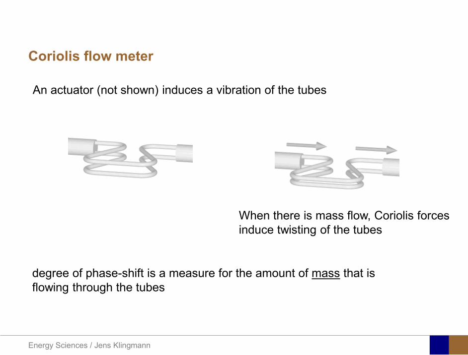
Energy Sciences Jens Klingmann
Coriolis flow meter
An actuator (not shown) induces a vibration of the tubes
When there is mass flow Coriolis forces induce twisting of the tubes
degree of phase-shift is a measure for the amount of mass that is flowing through the tubes
Energy Sciences Jens Klingmann
Thermal flow meter Heat is added electrically to the flow Temperature is measured before and after heat addition
pP mC T∆=
Energy Sciences Jens Klingmann
Ultrasonic flow meters
Ultrasound is emitted to small particles in the flow (dust or other) Reflections of the sound is frequency shifted by the Doppler effect The frequency change is proportional to the particles velocity (volume flow
meter)
Energy Sciences Jens Klingmann
Inductive flow metersA magnetic flowmeter is based upon Faradays Law
The voltage induced across any conductor as it moves at right angles through a magnetic field is proportional to the velocity of that conductor
E is proportional to V x B x D where
E = The voltage generated in a conductorV = The velocity of the conductorB = The magnetic field strengthD = The length of the conductor
NB electric conductivity is required
Energy Sciences Jens Klingmann
Temperature measurements
Thermocouples
The basis established by Thomas Johann Seebeck in 1821
A conductor generates a voltage when subjected to a temperature gradient
To measure this voltage one must use a second conductor material which generates a different voltage under the same temperature gradient
Energy Sciences Jens Klingmann
Pressure sensing
1 2p pgt 2p p2 may be the atmosphere a static pressure tap or a known reference pressure
The strain of the diaphragm (or itrsquos deflection) may be measured by a number of electric methods
Diaphragm
Energy Sciences Jens Klingmann
Pressure sensingPiezoresistive Strain Gage
Uses the piezoresistive effect of bonded or formed strain gauges to detect strain due to applied pressure
Capacitive
Uses a diaghragm and pressure cavity to create a variable capacitor to detect strain due to applied pressure
Magnetic
Measures the displacement of a diaphragm by means of changes in inductance (reluctance) LVDT Hall Effect or by eddy current principal
Piezoelectric
Uses the piezoelectric effect in certain materials such as quartz to measure the strain upon the sensing mechanism due to pressure
Potentiometric
Uses the motion of a wiper along a resistive mechanism to detect the strain caused by applied pressure
Energy Sciences Jens Klingmann
3D highly instationary (periodic) flow Potentially very high velocities (Supersonic) Large temperature differences Low accessibility (difficult to probe between rotors) Low turbulence levels in most of the domain Very high turbulence in BL and wakes
Properties of measuring object
Point measurements
Energy Sciences Jens Klingmann
Conventional or non-opticalndash Static Pressure Measurementsndash Total Pressure Measurements
bull Multy hole probes
ndash Total Temperature ndash Hot Wire Anemometry (HWA)
Optical techniques for Velocity Measurementsndash Laser Two Focous (L2F)ndash Laser Doppler Anemometry (LDA)ndash Particle Image velocimetry (PIV)
Point Measurements
Energy Sciences Jens Klingmann
Static and total pressure
2 2 21 2 1
2 1 2 2 2C C CP P ρ ρ ρ
minus = minus =
2 0C =Stagnation point
C1Static pressure tap
Prandtl or Pitot tube
Apply the Bernoulli equation from free stream to stagnation point
21
2 12CP Pρ
= +or
We can also define a stagnation or total pressure
( )2
101 1 022
CP P Pρ= + =
Total pressure = Static pressure + dynamic pressure
or
Energy Sciences Jens Klingmann
Static pressure
Energy Sciences Jens Klingmann
Total Pressure and Temperature
Shrouded Probes
Shrouded Probe
Pitot or Prandtl tube
Sensitive to direction
Energy Sciences Jens Klingmann
Ludwig Prandtl 1875-1953
Ludwig Prandtl born at Freising Bavaria on February 4 1875 was a German Physicist famous for his work in aeronautics He qualified at Munchen in 1900 with a thesis on elastic stability and held the position of Professor of Applied Mechanics at Gottingen for forty-nine years (from 1904 until his death there on August 15 1953) In 1925 Prandtl became the Director of the Kaiser Wilhelm Institute for Fluid Mechanics His discovery in 1904 of the Boundary Layer which adjoins the surface of a body moving in a fluid led to an understanding of skin friction drag and of the way in which streamlining reduces the drag of airplane wings and other moving bodies His work on wing theory published in 1918 - 1919 followed that of FW Lanchester (1902-1907) but was carried out independently and elucidated the flow over airplane wings of finite span Prandtls work and decisive advances in boundary layer and wing theories became the basic material of aeronautics He also made important contributions to the theories of supersonic flow and of turbulence and contributed much to the development of wind tunnels and other aerodynamic equipment In addition he devised the soap-film analogy for the torsion of non-circular sections and wrote on the theory of plasticity and of meteorology
Energy Sciences Jens Klingmann
Total Pressure multy hole
Cobra Probe Yaw Probe
5 Hole Probe
Energy Sciences Jens Klingmann
5 Hole Probes Calibration
Energy Sciences Jens Klingmann
The inherent unsteadiness of the flow within turbomachines
Energy Sciences Jens Klingmann
Hot Wire Anemometry (HWA) The heat transfer from a thin (one micron)
electrically heated wire can be used to determine velocity
The resistance of the wire is temperature dependent Within a small temperature range it can be assumed linear R = R0+α R0(Tm-T0) where R0 is the resistance at a reference temperature T0 and Tm is the mean wire temperature
The thermal power induced in the wire is balanced by heat transfer to the surrounding fluid I2R=hπDL(Tm-T0) where h is the heat transfer coefficient and D and L the diameter and length of the wire respectively
E = I R
Energy Sciences Jens Klingmann
Constant Temperature Anemometry (CTA) The wire is often placed in a Whetstone bridge If the output from the
bridge is amplified and fed back to the bridge the resistance of the probe and thus the temperature will be held constant
This prevents the temperature of the wire to become excessive at low velocities
R1
R2 R3
Probe
Bridge Voltage
Energy Sciences Jens Klingmann
Constant Temperature Anemometry (CTA)
Energy Sciences Jens Klingmann
Characteristics of LDA (according to Dantec)
Invented by Yeh and Cummins in 1964 Velocity measurements in Fluid Dynamics (gas liquid) Up to 3 velocity components Non-intrusive measurements (optical technique) Absolute measurement technique (no calibration required) Very high accuracy Very high spatial resolution due to small measurement volume Tracer particles are required
Energy Sciences Jens Klingmann
LDA - Fringe Model
Focused Laser beams intersect and form the measurement volume Plane wave fronts beam waist in the plane of intersection Interference in the plane of intersection Pattern of bright and dark stripesplanes Fringes
Energy Sciences Jens Klingmann
LDA-measuring volume
d
x
x
y
y
z
z
e-2 CONTOUR
FRINGES
κ
κ
κ
κ
De-2
De-2
dml m
a
b
cx
b
z
ya
cd
d
=
=
=
J
J
J
J
JP
JP
JP
JD
JD
JD
+
+
+
a
b
c
d
κπλ
=minus sinD
f4l2e
m
κπλ
=minus cosD
f4D2e
m
Energy Sciences Jens Klingmann
Laser Two Focus
Energy Sciences Jens Klingmann
Laser Two Focus
Energy Sciences Jens Klingmann
PIV measurements
PIV is a fairly new technique capable of simultaneous velocity measurements at many points in a plane This gives information on large scale structures vorticity etc which is very difficult or impossible to obtain from one-point measuring techniques
PIV involves the illumination of a plane of the flow under investigation with a thin pulsed sheet of light The flow is seeded with particles
The light scattered from the particles and from successive pulses are being recorded either on film or a CCD array forming a multiple exposure of each particle image If the time between the pulses is known velocity can be determined as the ratio of the particle displacement and the elapsed time
t∆∆= xu
Energy Sciences Jens Klingmann
PIV
Energy Sciences Jens Klingmann
PIV measurements illumination
YA
G
YA
G
Two frequency doubled YAG Lasers aligned to one double pulsed laser sheet
Two or more separate light pulses can be obtained by chopping a continuous laser or from pulsed lasers
The limited pulse energies obtained from continuous lasers limits their applicability to low velocity flows or flows where large seeding particles can be used (ie liquid flows)
The low repetition rate of most pulsed lasers makes the use of two lasers advantageous
Energy Sciences Jens Klingmann
PIV measurements recording
High seeding density in laminar flame
Film or CCD-cameras Cross- or Auto-correlation
ndash ie both particle images on the same frame or on separate frames
CCD-camera requirementndash A many pixels as possiblendash 2k by 2k available 4k by 4k coming
Energy Sciences Jens Klingmann
PIV measurements analyses
Low seeding density (Number of seeding particles per unit volume)
Each particle image pair can be identified This is called particle tracking
High seeding density (PIV)
Small sub-regions of the image containing many particle image pairs are processed to obtain one velocity vector
Energy Sciences Jens Klingmann
PIV measurements analyses
Energy Sciences Jens Klingmann
PIV measurements analyses
( ) ( ) ( ) xsxxs dIIR 2A
1
I
+= int
Cross correlation between ( )x1I and ( )x2I
s is a two dimensional displacement vector
IA is the interrogation area
Cross correlation between
(
)
x
1
I
and
(
)
x
2
I
s is a two dimensional displacement vector
I
A
is the interrogation area
Energy Sciences Jens Klingmann
Energy Sciences Jens Klingmann
PIV from IOWA state university
Energy Sciences Jens Klingmann
PIV sample of evaluation
Energy Sciences Jens Klingmann
LDA PIV HWA Velocity range 01 mms ndash 300
ms 02 ndash 150 ms
Measuring Volume
D = 005 L = 05 mm
2 by 2 by 05 mm
L = 05 mm
Freq response O(10 000) Hz O(10) Hz O(100 000) Hz Calibration Yes No No Sensitivity to other than velocity
Low (ref Index) Low (ref Index) Large (temperature concentrationshellip)
Continuous Signal
Sometimes Seldom Always
Noise High High Low Turbulence intensity
No limitation Some limitation lt 20
Price O(1 000 000) SEK
O(1 000 000) SEK
O(50 000) SEK
Required Knowledge
High medium Low
Comparison of techniques
Energy Sciences Jens Klingmann
References experiments
R J Goldstein ldquoFluid Mechanics Measurementsrdquo Hemisphere Publishing 1983 A V Johansson amp P H Alfredsson ldquoExperimentella metoder inom
stroumlmningsmekanikenrdquo Inst Foumlr Mekanik KTH F Durst A Melling and J H Whitelaw ldquoPrincipals and Practice of Laser Doppler
Anemometryrdquo 1984 R J Adrian ldquoParticle-imaging techniques for experimental fluid mechnicsrdquo Ann Rev
Fluid Mech 1991
Energy Sciences Jens Klingmann
Sample of LDA-measurements
Rotor blade
Glas window
Emitted beams
Scattered Light
Adjustable mirror
Energy Sciences Jens Klingmann
Axial velocity sorted into 10 bins
0 1 2 3 4 5 6tangential coordinate (degrees)
-20
0
20
40
60
80
100
120
140
160Ax
ial v
eloc
ity a
nd s
tand
ard
devi
atio
n (m
s)
radial position 7 mm from inner window surfaceaxial position 23 mm behind rotor blades
Energy Sciences Jens Klingmann
Axial velocities in the radial-tangential plane
Energy Sciences Jens Klingmann
Airfoils NACA 4-digit
The NACA four-digit wing sections define the profile by
One digit describing maximum camber as percentage of the chord
One digit describing the distance of maximum camber from the airfoil leading edge in tens of percents of the chord
Two digits describing maximum thickness of the airfoil as percent of the chord
Example the NACA 2412 airfoil has a maximum camber of 2 located 40 (04 chords) from the leading edge with a maximum thickness of 12 of the chord
Four-digit series airfoils by default have maximum thickness at 30 of the chord (03 chords) from the leading edge
Energy Sciences Jens Klingmann
Airfoils NACA 4-digit
bull c is the chord lengthbull x is the position along
the chord from 0 to cbull y is the half thickness at
a given value of x (centerline to surface)
bull t is the maximum thickness as a fraction of the chord
Energy Sciences Jens Klingmann
Death by PowerPoint
| LDA | PIV | HWA | |||||
| Velocity range | 01 mms ndash 300 ms | 02 ndash 150 ms | |||||
| Measuring Volume | D = 005 L = 05 mm | 2 by 2 by 05 mm | L = 05 mm | ||||
| Freq response | O(10 000) Hz | O(10) Hz | O(100 000) Hz | ||||
| Calibration | Yes | No | No | ||||
| Sensitivity to other than velocity | Low (ref Index) | Low (ref Index) | Large (temperature concentrationshellip) | ||||
| Continuous Signal | Sometimes | Seldom | Always | ||||
| Noise | High | High | Low | ||||
| Turbulence intensity | No limitation | Some limitation | lt 20 | ||||
| Price | O(1 000 000) SEK | O(1 000 000) SEK | O(50 000) SEK | ||||
| Required Knowledge | High | medium | Low |
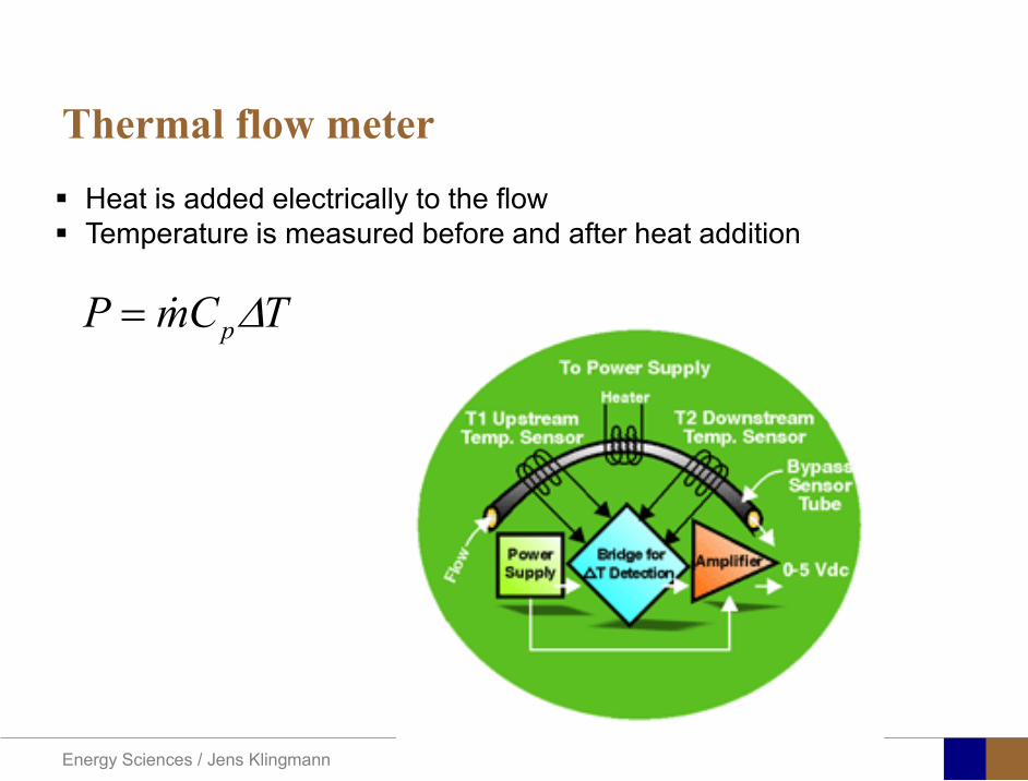
Energy Sciences Jens Klingmann
Thermal flow meter Heat is added electrically to the flow Temperature is measured before and after heat addition
pP mC T∆=
Energy Sciences Jens Klingmann
Ultrasonic flow meters
Ultrasound is emitted to small particles in the flow (dust or other) Reflections of the sound is frequency shifted by the Doppler effect The frequency change is proportional to the particles velocity (volume flow
meter)
Energy Sciences Jens Klingmann
Inductive flow metersA magnetic flowmeter is based upon Faradays Law
The voltage induced across any conductor as it moves at right angles through a magnetic field is proportional to the velocity of that conductor
E is proportional to V x B x D where
E = The voltage generated in a conductorV = The velocity of the conductorB = The magnetic field strengthD = The length of the conductor
NB electric conductivity is required
Energy Sciences Jens Klingmann
Temperature measurements
Thermocouples
The basis established by Thomas Johann Seebeck in 1821
A conductor generates a voltage when subjected to a temperature gradient
To measure this voltage one must use a second conductor material which generates a different voltage under the same temperature gradient
Energy Sciences Jens Klingmann
Pressure sensing
1 2p pgt 2p p2 may be the atmosphere a static pressure tap or a known reference pressure
The strain of the diaphragm (or itrsquos deflection) may be measured by a number of electric methods
Diaphragm
Energy Sciences Jens Klingmann
Pressure sensingPiezoresistive Strain Gage
Uses the piezoresistive effect of bonded or formed strain gauges to detect strain due to applied pressure
Capacitive
Uses a diaghragm and pressure cavity to create a variable capacitor to detect strain due to applied pressure
Magnetic
Measures the displacement of a diaphragm by means of changes in inductance (reluctance) LVDT Hall Effect or by eddy current principal
Piezoelectric
Uses the piezoelectric effect in certain materials such as quartz to measure the strain upon the sensing mechanism due to pressure
Potentiometric
Uses the motion of a wiper along a resistive mechanism to detect the strain caused by applied pressure
Energy Sciences Jens Klingmann
3D highly instationary (periodic) flow Potentially very high velocities (Supersonic) Large temperature differences Low accessibility (difficult to probe between rotors) Low turbulence levels in most of the domain Very high turbulence in BL and wakes
Properties of measuring object
Point measurements
Energy Sciences Jens Klingmann
Conventional or non-opticalndash Static Pressure Measurementsndash Total Pressure Measurements
bull Multy hole probes
ndash Total Temperature ndash Hot Wire Anemometry (HWA)
Optical techniques for Velocity Measurementsndash Laser Two Focous (L2F)ndash Laser Doppler Anemometry (LDA)ndash Particle Image velocimetry (PIV)
Point Measurements
Energy Sciences Jens Klingmann
Static and total pressure
2 2 21 2 1
2 1 2 2 2C C CP P ρ ρ ρ
minus = minus =
2 0C =Stagnation point
C1Static pressure tap
Prandtl or Pitot tube
Apply the Bernoulli equation from free stream to stagnation point
21
2 12CP Pρ
= +or
We can also define a stagnation or total pressure
( )2
101 1 022
CP P Pρ= + =
Total pressure = Static pressure + dynamic pressure
or
Energy Sciences Jens Klingmann
Static pressure
Energy Sciences Jens Klingmann
Total Pressure and Temperature
Shrouded Probes
Shrouded Probe
Pitot or Prandtl tube
Sensitive to direction
Energy Sciences Jens Klingmann
Ludwig Prandtl 1875-1953
Ludwig Prandtl born at Freising Bavaria on February 4 1875 was a German Physicist famous for his work in aeronautics He qualified at Munchen in 1900 with a thesis on elastic stability and held the position of Professor of Applied Mechanics at Gottingen for forty-nine years (from 1904 until his death there on August 15 1953) In 1925 Prandtl became the Director of the Kaiser Wilhelm Institute for Fluid Mechanics His discovery in 1904 of the Boundary Layer which adjoins the surface of a body moving in a fluid led to an understanding of skin friction drag and of the way in which streamlining reduces the drag of airplane wings and other moving bodies His work on wing theory published in 1918 - 1919 followed that of FW Lanchester (1902-1907) but was carried out independently and elucidated the flow over airplane wings of finite span Prandtls work and decisive advances in boundary layer and wing theories became the basic material of aeronautics He also made important contributions to the theories of supersonic flow and of turbulence and contributed much to the development of wind tunnels and other aerodynamic equipment In addition he devised the soap-film analogy for the torsion of non-circular sections and wrote on the theory of plasticity and of meteorology
Energy Sciences Jens Klingmann
Total Pressure multy hole
Cobra Probe Yaw Probe
5 Hole Probe
Energy Sciences Jens Klingmann
5 Hole Probes Calibration
Energy Sciences Jens Klingmann
The inherent unsteadiness of the flow within turbomachines
Energy Sciences Jens Klingmann
Hot Wire Anemometry (HWA) The heat transfer from a thin (one micron)
electrically heated wire can be used to determine velocity
The resistance of the wire is temperature dependent Within a small temperature range it can be assumed linear R = R0+α R0(Tm-T0) where R0 is the resistance at a reference temperature T0 and Tm is the mean wire temperature
The thermal power induced in the wire is balanced by heat transfer to the surrounding fluid I2R=hπDL(Tm-T0) where h is the heat transfer coefficient and D and L the diameter and length of the wire respectively
E = I R
Energy Sciences Jens Klingmann
Constant Temperature Anemometry (CTA) The wire is often placed in a Whetstone bridge If the output from the
bridge is amplified and fed back to the bridge the resistance of the probe and thus the temperature will be held constant
This prevents the temperature of the wire to become excessive at low velocities
R1
R2 R3
Probe
Bridge Voltage
Energy Sciences Jens Klingmann
Constant Temperature Anemometry (CTA)
Energy Sciences Jens Klingmann
Characteristics of LDA (according to Dantec)
Invented by Yeh and Cummins in 1964 Velocity measurements in Fluid Dynamics (gas liquid) Up to 3 velocity components Non-intrusive measurements (optical technique) Absolute measurement technique (no calibration required) Very high accuracy Very high spatial resolution due to small measurement volume Tracer particles are required
Energy Sciences Jens Klingmann
LDA - Fringe Model
Focused Laser beams intersect and form the measurement volume Plane wave fronts beam waist in the plane of intersection Interference in the plane of intersection Pattern of bright and dark stripesplanes Fringes
Energy Sciences Jens Klingmann
LDA-measuring volume
d
x
x
y
y
z
z
e-2 CONTOUR
FRINGES
κ
κ
κ
κ
De-2
De-2
dml m
a
b
cx
b
z
ya
cd
d
=
=
=
J
J
J
J
JP
JP
JP
JD
JD
JD
+
+
+
a
b
c
d
κπλ
=minus sinD
f4l2e
m
κπλ
=minus cosD
f4D2e
m
Energy Sciences Jens Klingmann
Laser Two Focus
Energy Sciences Jens Klingmann
Laser Two Focus
Energy Sciences Jens Klingmann
PIV measurements
PIV is a fairly new technique capable of simultaneous velocity measurements at many points in a plane This gives information on large scale structures vorticity etc which is very difficult or impossible to obtain from one-point measuring techniques
PIV involves the illumination of a plane of the flow under investigation with a thin pulsed sheet of light The flow is seeded with particles
The light scattered from the particles and from successive pulses are being recorded either on film or a CCD array forming a multiple exposure of each particle image If the time between the pulses is known velocity can be determined as the ratio of the particle displacement and the elapsed time
t∆∆= xu
Energy Sciences Jens Klingmann
PIV
Energy Sciences Jens Klingmann
PIV measurements illumination
YA
G
YA
G
Two frequency doubled YAG Lasers aligned to one double pulsed laser sheet
Two or more separate light pulses can be obtained by chopping a continuous laser or from pulsed lasers
The limited pulse energies obtained from continuous lasers limits their applicability to low velocity flows or flows where large seeding particles can be used (ie liquid flows)
The low repetition rate of most pulsed lasers makes the use of two lasers advantageous
Energy Sciences Jens Klingmann
PIV measurements recording
High seeding density in laminar flame
Film or CCD-cameras Cross- or Auto-correlation
ndash ie both particle images on the same frame or on separate frames
CCD-camera requirementndash A many pixels as possiblendash 2k by 2k available 4k by 4k coming
Energy Sciences Jens Klingmann
PIV measurements analyses
Low seeding density (Number of seeding particles per unit volume)
Each particle image pair can be identified This is called particle tracking
High seeding density (PIV)
Small sub-regions of the image containing many particle image pairs are processed to obtain one velocity vector
Energy Sciences Jens Klingmann
PIV measurements analyses
Energy Sciences Jens Klingmann
PIV measurements analyses
( ) ( ) ( ) xsxxs dIIR 2A
1
I
+= int
Cross correlation between ( )x1I and ( )x2I
s is a two dimensional displacement vector
IA is the interrogation area
Cross correlation between
(
)
x
1
I
and
(
)
x
2
I
s is a two dimensional displacement vector
I
A
is the interrogation area
Energy Sciences Jens Klingmann
Energy Sciences Jens Klingmann
PIV from IOWA state university
Energy Sciences Jens Klingmann
PIV sample of evaluation
Energy Sciences Jens Klingmann
LDA PIV HWA Velocity range 01 mms ndash 300
ms 02 ndash 150 ms
Measuring Volume
D = 005 L = 05 mm
2 by 2 by 05 mm
L = 05 mm
Freq response O(10 000) Hz O(10) Hz O(100 000) Hz Calibration Yes No No Sensitivity to other than velocity
Low (ref Index) Low (ref Index) Large (temperature concentrationshellip)
Continuous Signal
Sometimes Seldom Always
Noise High High Low Turbulence intensity
No limitation Some limitation lt 20
Price O(1 000 000) SEK
O(1 000 000) SEK
O(50 000) SEK
Required Knowledge
High medium Low
Comparison of techniques
Energy Sciences Jens Klingmann
References experiments
R J Goldstein ldquoFluid Mechanics Measurementsrdquo Hemisphere Publishing 1983 A V Johansson amp P H Alfredsson ldquoExperimentella metoder inom
stroumlmningsmekanikenrdquo Inst Foumlr Mekanik KTH F Durst A Melling and J H Whitelaw ldquoPrincipals and Practice of Laser Doppler
Anemometryrdquo 1984 R J Adrian ldquoParticle-imaging techniques for experimental fluid mechnicsrdquo Ann Rev
Fluid Mech 1991
Energy Sciences Jens Klingmann
Sample of LDA-measurements
Rotor blade
Glas window
Emitted beams
Scattered Light
Adjustable mirror
Energy Sciences Jens Klingmann
Axial velocity sorted into 10 bins
0 1 2 3 4 5 6tangential coordinate (degrees)
-20
0
20
40
60
80
100
120
140
160Ax
ial v
eloc
ity a
nd s
tand
ard
devi
atio
n (m
s)
radial position 7 mm from inner window surfaceaxial position 23 mm behind rotor blades
Energy Sciences Jens Klingmann
Axial velocities in the radial-tangential plane
Energy Sciences Jens Klingmann
Airfoils NACA 4-digit
The NACA four-digit wing sections define the profile by
One digit describing maximum camber as percentage of the chord
One digit describing the distance of maximum camber from the airfoil leading edge in tens of percents of the chord
Two digits describing maximum thickness of the airfoil as percent of the chord
Example the NACA 2412 airfoil has a maximum camber of 2 located 40 (04 chords) from the leading edge with a maximum thickness of 12 of the chord
Four-digit series airfoils by default have maximum thickness at 30 of the chord (03 chords) from the leading edge
Energy Sciences Jens Klingmann
Airfoils NACA 4-digit
bull c is the chord lengthbull x is the position along
the chord from 0 to cbull y is the half thickness at
a given value of x (centerline to surface)
bull t is the maximum thickness as a fraction of the chord
Energy Sciences Jens Klingmann
Death by PowerPoint
| LDA | PIV | HWA | |||||
| Velocity range | 01 mms ndash 300 ms | 02 ndash 150 ms | |||||
| Measuring Volume | D = 005 L = 05 mm | 2 by 2 by 05 mm | L = 05 mm | ||||
| Freq response | O(10 000) Hz | O(10) Hz | O(100 000) Hz | ||||
| Calibration | Yes | No | No | ||||
| Sensitivity to other than velocity | Low (ref Index) | Low (ref Index) | Large (temperature concentrationshellip) | ||||
| Continuous Signal | Sometimes | Seldom | Always | ||||
| Noise | High | High | Low | ||||
| Turbulence intensity | No limitation | Some limitation | lt 20 | ||||
| Price | O(1 000 000) SEK | O(1 000 000) SEK | O(50 000) SEK | ||||
| Required Knowledge | High | medium | Low |
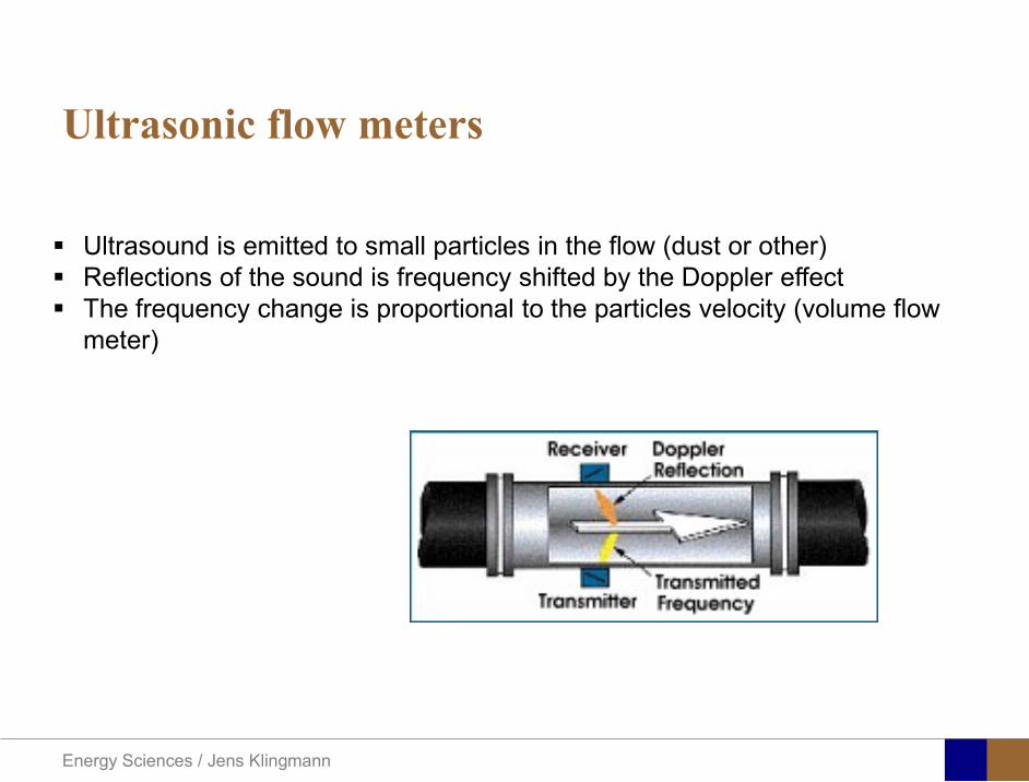
Energy Sciences Jens Klingmann
Ultrasonic flow meters
Ultrasound is emitted to small particles in the flow (dust or other) Reflections of the sound is frequency shifted by the Doppler effect The frequency change is proportional to the particles velocity (volume flow
meter)
Energy Sciences Jens Klingmann
Inductive flow metersA magnetic flowmeter is based upon Faradays Law
The voltage induced across any conductor as it moves at right angles through a magnetic field is proportional to the velocity of that conductor
E is proportional to V x B x D where
E = The voltage generated in a conductorV = The velocity of the conductorB = The magnetic field strengthD = The length of the conductor
NB electric conductivity is required
Energy Sciences Jens Klingmann
Temperature measurements
Thermocouples
The basis established by Thomas Johann Seebeck in 1821
A conductor generates a voltage when subjected to a temperature gradient
To measure this voltage one must use a second conductor material which generates a different voltage under the same temperature gradient
Energy Sciences Jens Klingmann
Pressure sensing
1 2p pgt 2p p2 may be the atmosphere a static pressure tap or a known reference pressure
The strain of the diaphragm (or itrsquos deflection) may be measured by a number of electric methods
Diaphragm
Energy Sciences Jens Klingmann
Pressure sensingPiezoresistive Strain Gage
Uses the piezoresistive effect of bonded or formed strain gauges to detect strain due to applied pressure
Capacitive
Uses a diaghragm and pressure cavity to create a variable capacitor to detect strain due to applied pressure
Magnetic
Measures the displacement of a diaphragm by means of changes in inductance (reluctance) LVDT Hall Effect or by eddy current principal
Piezoelectric
Uses the piezoelectric effect in certain materials such as quartz to measure the strain upon the sensing mechanism due to pressure
Potentiometric
Uses the motion of a wiper along a resistive mechanism to detect the strain caused by applied pressure
Energy Sciences Jens Klingmann
3D highly instationary (periodic) flow Potentially very high velocities (Supersonic) Large temperature differences Low accessibility (difficult to probe between rotors) Low turbulence levels in most of the domain Very high turbulence in BL and wakes
Properties of measuring object
Point measurements
Energy Sciences Jens Klingmann
Conventional or non-opticalndash Static Pressure Measurementsndash Total Pressure Measurements
bull Multy hole probes
ndash Total Temperature ndash Hot Wire Anemometry (HWA)
Optical techniques for Velocity Measurementsndash Laser Two Focous (L2F)ndash Laser Doppler Anemometry (LDA)ndash Particle Image velocimetry (PIV)
Point Measurements
Energy Sciences Jens Klingmann
Static and total pressure
2 2 21 2 1
2 1 2 2 2C C CP P ρ ρ ρ
minus = minus =
2 0C =Stagnation point
C1Static pressure tap
Prandtl or Pitot tube
Apply the Bernoulli equation from free stream to stagnation point
21
2 12CP Pρ
= +or
We can also define a stagnation or total pressure
( )2
101 1 022
CP P Pρ= + =
Total pressure = Static pressure + dynamic pressure
or
Energy Sciences Jens Klingmann
Static pressure
Energy Sciences Jens Klingmann
Total Pressure and Temperature
Shrouded Probes
Shrouded Probe
Pitot or Prandtl tube
Sensitive to direction
Energy Sciences Jens Klingmann
Ludwig Prandtl 1875-1953
Ludwig Prandtl born at Freising Bavaria on February 4 1875 was a German Physicist famous for his work in aeronautics He qualified at Munchen in 1900 with a thesis on elastic stability and held the position of Professor of Applied Mechanics at Gottingen for forty-nine years (from 1904 until his death there on August 15 1953) In 1925 Prandtl became the Director of the Kaiser Wilhelm Institute for Fluid Mechanics His discovery in 1904 of the Boundary Layer which adjoins the surface of a body moving in a fluid led to an understanding of skin friction drag and of the way in which streamlining reduces the drag of airplane wings and other moving bodies His work on wing theory published in 1918 - 1919 followed that of FW Lanchester (1902-1907) but was carried out independently and elucidated the flow over airplane wings of finite span Prandtls work and decisive advances in boundary layer and wing theories became the basic material of aeronautics He also made important contributions to the theories of supersonic flow and of turbulence and contributed much to the development of wind tunnels and other aerodynamic equipment In addition he devised the soap-film analogy for the torsion of non-circular sections and wrote on the theory of plasticity and of meteorology
Energy Sciences Jens Klingmann
Total Pressure multy hole
Cobra Probe Yaw Probe
5 Hole Probe
Energy Sciences Jens Klingmann
5 Hole Probes Calibration
Energy Sciences Jens Klingmann
The inherent unsteadiness of the flow within turbomachines
Energy Sciences Jens Klingmann
Hot Wire Anemometry (HWA) The heat transfer from a thin (one micron)
electrically heated wire can be used to determine velocity
The resistance of the wire is temperature dependent Within a small temperature range it can be assumed linear R = R0+α R0(Tm-T0) where R0 is the resistance at a reference temperature T0 and Tm is the mean wire temperature
The thermal power induced in the wire is balanced by heat transfer to the surrounding fluid I2R=hπDL(Tm-T0) where h is the heat transfer coefficient and D and L the diameter and length of the wire respectively
E = I R
Energy Sciences Jens Klingmann
Constant Temperature Anemometry (CTA) The wire is often placed in a Whetstone bridge If the output from the
bridge is amplified and fed back to the bridge the resistance of the probe and thus the temperature will be held constant
This prevents the temperature of the wire to become excessive at low velocities
R1
R2 R3
Probe
Bridge Voltage
Energy Sciences Jens Klingmann
Constant Temperature Anemometry (CTA)
Energy Sciences Jens Klingmann
Characteristics of LDA (according to Dantec)
Invented by Yeh and Cummins in 1964 Velocity measurements in Fluid Dynamics (gas liquid) Up to 3 velocity components Non-intrusive measurements (optical technique) Absolute measurement technique (no calibration required) Very high accuracy Very high spatial resolution due to small measurement volume Tracer particles are required
Energy Sciences Jens Klingmann
LDA - Fringe Model
Focused Laser beams intersect and form the measurement volume Plane wave fronts beam waist in the plane of intersection Interference in the plane of intersection Pattern of bright and dark stripesplanes Fringes
Energy Sciences Jens Klingmann
LDA-measuring volume
d
x
x
y
y
z
z
e-2 CONTOUR
FRINGES
κ
κ
κ
κ
De-2
De-2
dml m
a
b
cx
b
z
ya
cd
d
=
=
=
J
J
J
J
JP
JP
JP
JD
JD
JD
+
+
+
a
b
c
d
κπλ
=minus sinD
f4l2e
m
κπλ
=minus cosD
f4D2e
m
Energy Sciences Jens Klingmann
Laser Two Focus
Energy Sciences Jens Klingmann
Laser Two Focus
Energy Sciences Jens Klingmann
PIV measurements
PIV is a fairly new technique capable of simultaneous velocity measurements at many points in a plane This gives information on large scale structures vorticity etc which is very difficult or impossible to obtain from one-point measuring techniques
PIV involves the illumination of a plane of the flow under investigation with a thin pulsed sheet of light The flow is seeded with particles
The light scattered from the particles and from successive pulses are being recorded either on film or a CCD array forming a multiple exposure of each particle image If the time between the pulses is known velocity can be determined as the ratio of the particle displacement and the elapsed time
t∆∆= xu
Energy Sciences Jens Klingmann
PIV
Energy Sciences Jens Klingmann
PIV measurements illumination
YA
G
YA
G
Two frequency doubled YAG Lasers aligned to one double pulsed laser sheet
Two or more separate light pulses can be obtained by chopping a continuous laser or from pulsed lasers
The limited pulse energies obtained from continuous lasers limits their applicability to low velocity flows or flows where large seeding particles can be used (ie liquid flows)
The low repetition rate of most pulsed lasers makes the use of two lasers advantageous
Energy Sciences Jens Klingmann
PIV measurements recording
High seeding density in laminar flame
Film or CCD-cameras Cross- or Auto-correlation
ndash ie both particle images on the same frame or on separate frames
CCD-camera requirementndash A many pixels as possiblendash 2k by 2k available 4k by 4k coming
Energy Sciences Jens Klingmann
PIV measurements analyses
Low seeding density (Number of seeding particles per unit volume)
Each particle image pair can be identified This is called particle tracking
High seeding density (PIV)
Small sub-regions of the image containing many particle image pairs are processed to obtain one velocity vector
Energy Sciences Jens Klingmann
PIV measurements analyses
Energy Sciences Jens Klingmann
PIV measurements analyses
( ) ( ) ( ) xsxxs dIIR 2A
1
I
+= int
Cross correlation between ( )x1I and ( )x2I
s is a two dimensional displacement vector
IA is the interrogation area
Cross correlation between
(
)
x
1
I
and
(
)
x
2
I
s is a two dimensional displacement vector
I
A
is the interrogation area
Energy Sciences Jens Klingmann
Energy Sciences Jens Klingmann
PIV from IOWA state university
Energy Sciences Jens Klingmann
PIV sample of evaluation
Energy Sciences Jens Klingmann
LDA PIV HWA Velocity range 01 mms ndash 300
ms 02 ndash 150 ms
Measuring Volume
D = 005 L = 05 mm
2 by 2 by 05 mm
L = 05 mm
Freq response O(10 000) Hz O(10) Hz O(100 000) Hz Calibration Yes No No Sensitivity to other than velocity
Low (ref Index) Low (ref Index) Large (temperature concentrationshellip)
Continuous Signal
Sometimes Seldom Always
Noise High High Low Turbulence intensity
No limitation Some limitation lt 20
Price O(1 000 000) SEK
O(1 000 000) SEK
O(50 000) SEK
Required Knowledge
High medium Low
Comparison of techniques
Energy Sciences Jens Klingmann
References experiments
R J Goldstein ldquoFluid Mechanics Measurementsrdquo Hemisphere Publishing 1983 A V Johansson amp P H Alfredsson ldquoExperimentella metoder inom
stroumlmningsmekanikenrdquo Inst Foumlr Mekanik KTH F Durst A Melling and J H Whitelaw ldquoPrincipals and Practice of Laser Doppler
Anemometryrdquo 1984 R J Adrian ldquoParticle-imaging techniques for experimental fluid mechnicsrdquo Ann Rev
Fluid Mech 1991
Energy Sciences Jens Klingmann
Sample of LDA-measurements
Rotor blade
Glas window
Emitted beams
Scattered Light
Adjustable mirror
Energy Sciences Jens Klingmann
Axial velocity sorted into 10 bins
0 1 2 3 4 5 6tangential coordinate (degrees)
-20
0
20
40
60
80
100
120
140
160Ax
ial v
eloc
ity a
nd s
tand
ard
devi
atio
n (m
s)
radial position 7 mm from inner window surfaceaxial position 23 mm behind rotor blades
Energy Sciences Jens Klingmann
Axial velocities in the radial-tangential plane
Energy Sciences Jens Klingmann
Airfoils NACA 4-digit
The NACA four-digit wing sections define the profile by
One digit describing maximum camber as percentage of the chord
One digit describing the distance of maximum camber from the airfoil leading edge in tens of percents of the chord
Two digits describing maximum thickness of the airfoil as percent of the chord
Example the NACA 2412 airfoil has a maximum camber of 2 located 40 (04 chords) from the leading edge with a maximum thickness of 12 of the chord
Four-digit series airfoils by default have maximum thickness at 30 of the chord (03 chords) from the leading edge
Energy Sciences Jens Klingmann
Airfoils NACA 4-digit
bull c is the chord lengthbull x is the position along
the chord from 0 to cbull y is the half thickness at
a given value of x (centerline to surface)
bull t is the maximum thickness as a fraction of the chord
Energy Sciences Jens Klingmann
Death by PowerPoint
| LDA | PIV | HWA | |||||
| Velocity range | 01 mms ndash 300 ms | 02 ndash 150 ms | |||||
| Measuring Volume | D = 005 L = 05 mm | 2 by 2 by 05 mm | L = 05 mm | ||||
| Freq response | O(10 000) Hz | O(10) Hz | O(100 000) Hz | ||||
| Calibration | Yes | No | No | ||||
| Sensitivity to other than velocity | Low (ref Index) | Low (ref Index) | Large (temperature concentrationshellip) | ||||
| Continuous Signal | Sometimes | Seldom | Always | ||||
| Noise | High | High | Low | ||||
| Turbulence intensity | No limitation | Some limitation | lt 20 | ||||
| Price | O(1 000 000) SEK | O(1 000 000) SEK | O(50 000) SEK | ||||
| Required Knowledge | High | medium | Low |
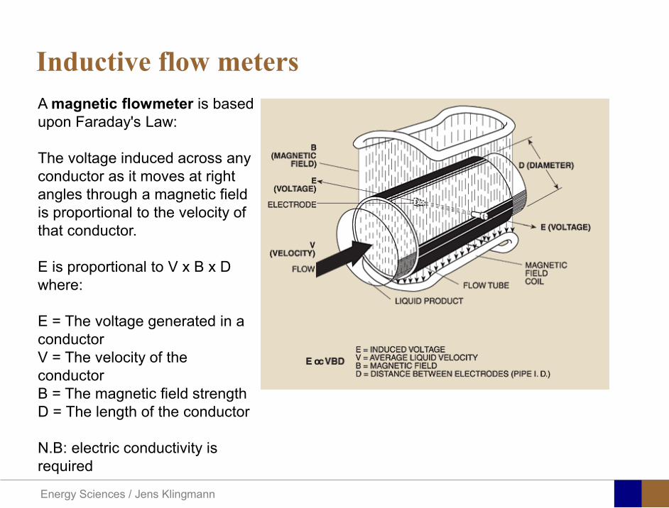
Energy Sciences Jens Klingmann
Inductive flow metersA magnetic flowmeter is based upon Faradays Law
The voltage induced across any conductor as it moves at right angles through a magnetic field is proportional to the velocity of that conductor
E is proportional to V x B x D where
E = The voltage generated in a conductorV = The velocity of the conductorB = The magnetic field strengthD = The length of the conductor
NB electric conductivity is required
Energy Sciences Jens Klingmann
Temperature measurements
Thermocouples
The basis established by Thomas Johann Seebeck in 1821
A conductor generates a voltage when subjected to a temperature gradient
To measure this voltage one must use a second conductor material which generates a different voltage under the same temperature gradient
Energy Sciences Jens Klingmann
Pressure sensing
1 2p pgt 2p p2 may be the atmosphere a static pressure tap or a known reference pressure
The strain of the diaphragm (or itrsquos deflection) may be measured by a number of electric methods
Diaphragm
Energy Sciences Jens Klingmann
Pressure sensingPiezoresistive Strain Gage
Uses the piezoresistive effect of bonded or formed strain gauges to detect strain due to applied pressure
Capacitive
Uses a diaghragm and pressure cavity to create a variable capacitor to detect strain due to applied pressure
Magnetic
Measures the displacement of a diaphragm by means of changes in inductance (reluctance) LVDT Hall Effect or by eddy current principal
Piezoelectric
Uses the piezoelectric effect in certain materials such as quartz to measure the strain upon the sensing mechanism due to pressure
Potentiometric
Uses the motion of a wiper along a resistive mechanism to detect the strain caused by applied pressure
Energy Sciences Jens Klingmann
3D highly instationary (periodic) flow Potentially very high velocities (Supersonic) Large temperature differences Low accessibility (difficult to probe between rotors) Low turbulence levels in most of the domain Very high turbulence in BL and wakes
Properties of measuring object
Point measurements
Energy Sciences Jens Klingmann
Conventional or non-opticalndash Static Pressure Measurementsndash Total Pressure Measurements
bull Multy hole probes
ndash Total Temperature ndash Hot Wire Anemometry (HWA)
Optical techniques for Velocity Measurementsndash Laser Two Focous (L2F)ndash Laser Doppler Anemometry (LDA)ndash Particle Image velocimetry (PIV)
Point Measurements
Energy Sciences Jens Klingmann
Static and total pressure
2 2 21 2 1
2 1 2 2 2C C CP P ρ ρ ρ
minus = minus =
2 0C =Stagnation point
C1Static pressure tap
Prandtl or Pitot tube
Apply the Bernoulli equation from free stream to stagnation point
21
2 12CP Pρ
= +or
We can also define a stagnation or total pressure
( )2
101 1 022
CP P Pρ= + =
Total pressure = Static pressure + dynamic pressure
or
Energy Sciences Jens Klingmann
Static pressure
Energy Sciences Jens Klingmann
Total Pressure and Temperature
Shrouded Probes
Shrouded Probe
Pitot or Prandtl tube
Sensitive to direction
Energy Sciences Jens Klingmann
Ludwig Prandtl 1875-1953
Ludwig Prandtl born at Freising Bavaria on February 4 1875 was a German Physicist famous for his work in aeronautics He qualified at Munchen in 1900 with a thesis on elastic stability and held the position of Professor of Applied Mechanics at Gottingen for forty-nine years (from 1904 until his death there on August 15 1953) In 1925 Prandtl became the Director of the Kaiser Wilhelm Institute for Fluid Mechanics His discovery in 1904 of the Boundary Layer which adjoins the surface of a body moving in a fluid led to an understanding of skin friction drag and of the way in which streamlining reduces the drag of airplane wings and other moving bodies His work on wing theory published in 1918 - 1919 followed that of FW Lanchester (1902-1907) but was carried out independently and elucidated the flow over airplane wings of finite span Prandtls work and decisive advances in boundary layer and wing theories became the basic material of aeronautics He also made important contributions to the theories of supersonic flow and of turbulence and contributed much to the development of wind tunnels and other aerodynamic equipment In addition he devised the soap-film analogy for the torsion of non-circular sections and wrote on the theory of plasticity and of meteorology
Energy Sciences Jens Klingmann
Total Pressure multy hole
Cobra Probe Yaw Probe
5 Hole Probe
Energy Sciences Jens Klingmann
5 Hole Probes Calibration
Energy Sciences Jens Klingmann
The inherent unsteadiness of the flow within turbomachines
Energy Sciences Jens Klingmann
Hot Wire Anemometry (HWA) The heat transfer from a thin (one micron)
electrically heated wire can be used to determine velocity
The resistance of the wire is temperature dependent Within a small temperature range it can be assumed linear R = R0+α R0(Tm-T0) where R0 is the resistance at a reference temperature T0 and Tm is the mean wire temperature
The thermal power induced in the wire is balanced by heat transfer to the surrounding fluid I2R=hπDL(Tm-T0) where h is the heat transfer coefficient and D and L the diameter and length of the wire respectively
E = I R
Energy Sciences Jens Klingmann
Constant Temperature Anemometry (CTA) The wire is often placed in a Whetstone bridge If the output from the
bridge is amplified and fed back to the bridge the resistance of the probe and thus the temperature will be held constant
This prevents the temperature of the wire to become excessive at low velocities
R1
R2 R3
Probe
Bridge Voltage
Energy Sciences Jens Klingmann
Constant Temperature Anemometry (CTA)
Energy Sciences Jens Klingmann
Characteristics of LDA (according to Dantec)
Invented by Yeh and Cummins in 1964 Velocity measurements in Fluid Dynamics (gas liquid) Up to 3 velocity components Non-intrusive measurements (optical technique) Absolute measurement technique (no calibration required) Very high accuracy Very high spatial resolution due to small measurement volume Tracer particles are required
Energy Sciences Jens Klingmann
LDA - Fringe Model
Focused Laser beams intersect and form the measurement volume Plane wave fronts beam waist in the plane of intersection Interference in the plane of intersection Pattern of bright and dark stripesplanes Fringes
Energy Sciences Jens Klingmann
LDA-measuring volume
d
x
x
y
y
z
z
e-2 CONTOUR
FRINGES
κ
κ
κ
κ
De-2
De-2
dml m
a
b
cx
b
z
ya
cd
d
=
=
=
J
J
J
J
JP
JP
JP
JD
JD
JD
+
+
+
a
b
c
d
κπλ
=minus sinD
f4l2e
m
κπλ
=minus cosD
f4D2e
m
Energy Sciences Jens Klingmann
Laser Two Focus
Energy Sciences Jens Klingmann
Laser Two Focus
Energy Sciences Jens Klingmann
PIV measurements
PIV is a fairly new technique capable of simultaneous velocity measurements at many points in a plane This gives information on large scale structures vorticity etc which is very difficult or impossible to obtain from one-point measuring techniques
PIV involves the illumination of a plane of the flow under investigation with a thin pulsed sheet of light The flow is seeded with particles
The light scattered from the particles and from successive pulses are being recorded either on film or a CCD array forming a multiple exposure of each particle image If the time between the pulses is known velocity can be determined as the ratio of the particle displacement and the elapsed time
t∆∆= xu
Energy Sciences Jens Klingmann
PIV
Energy Sciences Jens Klingmann
PIV measurements illumination
YA
G
YA
G
Two frequency doubled YAG Lasers aligned to one double pulsed laser sheet
Two or more separate light pulses can be obtained by chopping a continuous laser or from pulsed lasers
The limited pulse energies obtained from continuous lasers limits their applicability to low velocity flows or flows where large seeding particles can be used (ie liquid flows)
The low repetition rate of most pulsed lasers makes the use of two lasers advantageous
Energy Sciences Jens Klingmann
PIV measurements recording
High seeding density in laminar flame
Film or CCD-cameras Cross- or Auto-correlation
ndash ie both particle images on the same frame or on separate frames
CCD-camera requirementndash A many pixels as possiblendash 2k by 2k available 4k by 4k coming
Energy Sciences Jens Klingmann
PIV measurements analyses
Low seeding density (Number of seeding particles per unit volume)
Each particle image pair can be identified This is called particle tracking
High seeding density (PIV)
Small sub-regions of the image containing many particle image pairs are processed to obtain one velocity vector
Energy Sciences Jens Klingmann
PIV measurements analyses
Energy Sciences Jens Klingmann
PIV measurements analyses
( ) ( ) ( ) xsxxs dIIR 2A
1
I
+= int
Cross correlation between ( )x1I and ( )x2I
s is a two dimensional displacement vector
IA is the interrogation area
Cross correlation between
(
)
x
1
I
and
(
)
x
2
I
s is a two dimensional displacement vector
I
A
is the interrogation area
Energy Sciences Jens Klingmann
Energy Sciences Jens Klingmann
PIV from IOWA state university
Energy Sciences Jens Klingmann
PIV sample of evaluation
Energy Sciences Jens Klingmann
LDA PIV HWA Velocity range 01 mms ndash 300
ms 02 ndash 150 ms
Measuring Volume
D = 005 L = 05 mm
2 by 2 by 05 mm
L = 05 mm
Freq response O(10 000) Hz O(10) Hz O(100 000) Hz Calibration Yes No No Sensitivity to other than velocity
Low (ref Index) Low (ref Index) Large (temperature concentrationshellip)
Continuous Signal
Sometimes Seldom Always
Noise High High Low Turbulence intensity
No limitation Some limitation lt 20
Price O(1 000 000) SEK
O(1 000 000) SEK
O(50 000) SEK
Required Knowledge
High medium Low
Comparison of techniques
Energy Sciences Jens Klingmann
References experiments
R J Goldstein ldquoFluid Mechanics Measurementsrdquo Hemisphere Publishing 1983 A V Johansson amp P H Alfredsson ldquoExperimentella metoder inom
stroumlmningsmekanikenrdquo Inst Foumlr Mekanik KTH F Durst A Melling and J H Whitelaw ldquoPrincipals and Practice of Laser Doppler
Anemometryrdquo 1984 R J Adrian ldquoParticle-imaging techniques for experimental fluid mechnicsrdquo Ann Rev
Fluid Mech 1991
Energy Sciences Jens Klingmann
Sample of LDA-measurements
Rotor blade
Glas window
Emitted beams
Scattered Light
Adjustable mirror
Energy Sciences Jens Klingmann
Axial velocity sorted into 10 bins
0 1 2 3 4 5 6tangential coordinate (degrees)
-20
0
20
40
60
80
100
120
140
160Ax
ial v
eloc
ity a
nd s
tand
ard
devi
atio
n (m
s)
radial position 7 mm from inner window surfaceaxial position 23 mm behind rotor blades
Energy Sciences Jens Klingmann
Axial velocities in the radial-tangential plane
Energy Sciences Jens Klingmann
Airfoils NACA 4-digit
The NACA four-digit wing sections define the profile by
One digit describing maximum camber as percentage of the chord
One digit describing the distance of maximum camber from the airfoil leading edge in tens of percents of the chord
Two digits describing maximum thickness of the airfoil as percent of the chord
Example the NACA 2412 airfoil has a maximum camber of 2 located 40 (04 chords) from the leading edge with a maximum thickness of 12 of the chord
Four-digit series airfoils by default have maximum thickness at 30 of the chord (03 chords) from the leading edge
Energy Sciences Jens Klingmann
Airfoils NACA 4-digit
bull c is the chord lengthbull x is the position along
the chord from 0 to cbull y is the half thickness at
a given value of x (centerline to surface)
bull t is the maximum thickness as a fraction of the chord
Energy Sciences Jens Klingmann
Death by PowerPoint
| LDA | PIV | HWA | |||||
| Velocity range | 01 mms ndash 300 ms | 02 ndash 150 ms | |||||
| Measuring Volume | D = 005 L = 05 mm | 2 by 2 by 05 mm | L = 05 mm | ||||
| Freq response | O(10 000) Hz | O(10) Hz | O(100 000) Hz | ||||
| Calibration | Yes | No | No | ||||
| Sensitivity to other than velocity | Low (ref Index) | Low (ref Index) | Large (temperature concentrationshellip) | ||||
| Continuous Signal | Sometimes | Seldom | Always | ||||
| Noise | High | High | Low | ||||
| Turbulence intensity | No limitation | Some limitation | lt 20 | ||||
| Price | O(1 000 000) SEK | O(1 000 000) SEK | O(50 000) SEK | ||||
| Required Knowledge | High | medium | Low |
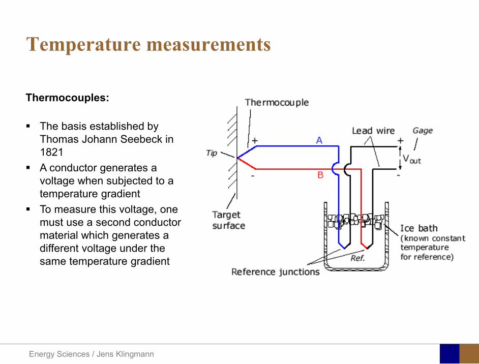
Energy Sciences Jens Klingmann
Temperature measurements
Thermocouples
The basis established by Thomas Johann Seebeck in 1821
A conductor generates a voltage when subjected to a temperature gradient
To measure this voltage one must use a second conductor material which generates a different voltage under the same temperature gradient
Energy Sciences Jens Klingmann
Pressure sensing
1 2p pgt 2p p2 may be the atmosphere a static pressure tap or a known reference pressure
The strain of the diaphragm (or itrsquos deflection) may be measured by a number of electric methods
Diaphragm
Energy Sciences Jens Klingmann
Pressure sensingPiezoresistive Strain Gage
Uses the piezoresistive effect of bonded or formed strain gauges to detect strain due to applied pressure
Capacitive
Uses a diaghragm and pressure cavity to create a variable capacitor to detect strain due to applied pressure
Magnetic
Measures the displacement of a diaphragm by means of changes in inductance (reluctance) LVDT Hall Effect or by eddy current principal
Piezoelectric
Uses the piezoelectric effect in certain materials such as quartz to measure the strain upon the sensing mechanism due to pressure
Potentiometric
Uses the motion of a wiper along a resistive mechanism to detect the strain caused by applied pressure
Energy Sciences Jens Klingmann
3D highly instationary (periodic) flow Potentially very high velocities (Supersonic) Large temperature differences Low accessibility (difficult to probe between rotors) Low turbulence levels in most of the domain Very high turbulence in BL and wakes
Properties of measuring object
Point measurements
Energy Sciences Jens Klingmann
Conventional or non-opticalndash Static Pressure Measurementsndash Total Pressure Measurements
bull Multy hole probes
ndash Total Temperature ndash Hot Wire Anemometry (HWA)
Optical techniques for Velocity Measurementsndash Laser Two Focous (L2F)ndash Laser Doppler Anemometry (LDA)ndash Particle Image velocimetry (PIV)
Point Measurements
Energy Sciences Jens Klingmann
Static and total pressure
2 2 21 2 1
2 1 2 2 2C C CP P ρ ρ ρ
minus = minus =
2 0C =Stagnation point
C1Static pressure tap
Prandtl or Pitot tube
Apply the Bernoulli equation from free stream to stagnation point
21
2 12CP Pρ
= +or
We can also define a stagnation or total pressure
( )2
101 1 022
CP P Pρ= + =
Total pressure = Static pressure + dynamic pressure
or
Energy Sciences Jens Klingmann
Static pressure
Energy Sciences Jens Klingmann
Total Pressure and Temperature
Shrouded Probes
Shrouded Probe
Pitot or Prandtl tube
Sensitive to direction
Energy Sciences Jens Klingmann
Ludwig Prandtl 1875-1953
Ludwig Prandtl born at Freising Bavaria on February 4 1875 was a German Physicist famous for his work in aeronautics He qualified at Munchen in 1900 with a thesis on elastic stability and held the position of Professor of Applied Mechanics at Gottingen for forty-nine years (from 1904 until his death there on August 15 1953) In 1925 Prandtl became the Director of the Kaiser Wilhelm Institute for Fluid Mechanics His discovery in 1904 of the Boundary Layer which adjoins the surface of a body moving in a fluid led to an understanding of skin friction drag and of the way in which streamlining reduces the drag of airplane wings and other moving bodies His work on wing theory published in 1918 - 1919 followed that of FW Lanchester (1902-1907) but was carried out independently and elucidated the flow over airplane wings of finite span Prandtls work and decisive advances in boundary layer and wing theories became the basic material of aeronautics He also made important contributions to the theories of supersonic flow and of turbulence and contributed much to the development of wind tunnels and other aerodynamic equipment In addition he devised the soap-film analogy for the torsion of non-circular sections and wrote on the theory of plasticity and of meteorology
Energy Sciences Jens Klingmann
Total Pressure multy hole
Cobra Probe Yaw Probe
5 Hole Probe
Energy Sciences Jens Klingmann
5 Hole Probes Calibration
Energy Sciences Jens Klingmann
The inherent unsteadiness of the flow within turbomachines
Energy Sciences Jens Klingmann
Hot Wire Anemometry (HWA) The heat transfer from a thin (one micron)
electrically heated wire can be used to determine velocity
The resistance of the wire is temperature dependent Within a small temperature range it can be assumed linear R = R0+α R0(Tm-T0) where R0 is the resistance at a reference temperature T0 and Tm is the mean wire temperature
The thermal power induced in the wire is balanced by heat transfer to the surrounding fluid I2R=hπDL(Tm-T0) where h is the heat transfer coefficient and D and L the diameter and length of the wire respectively
E = I R
Energy Sciences Jens Klingmann
Constant Temperature Anemometry (CTA) The wire is often placed in a Whetstone bridge If the output from the
bridge is amplified and fed back to the bridge the resistance of the probe and thus the temperature will be held constant
This prevents the temperature of the wire to become excessive at low velocities
R1
R2 R3
Probe
Bridge Voltage
Energy Sciences Jens Klingmann
Constant Temperature Anemometry (CTA)
Energy Sciences Jens Klingmann
Characteristics of LDA (according to Dantec)
Invented by Yeh and Cummins in 1964 Velocity measurements in Fluid Dynamics (gas liquid) Up to 3 velocity components Non-intrusive measurements (optical technique) Absolute measurement technique (no calibration required) Very high accuracy Very high spatial resolution due to small measurement volume Tracer particles are required
Energy Sciences Jens Klingmann
LDA - Fringe Model
Focused Laser beams intersect and form the measurement volume Plane wave fronts beam waist in the plane of intersection Interference in the plane of intersection Pattern of bright and dark stripesplanes Fringes
Energy Sciences Jens Klingmann
LDA-measuring volume
d
x
x
y
y
z
z
e-2 CONTOUR
FRINGES
κ
κ
κ
κ
De-2
De-2
dml m
a
b
cx
b
z
ya
cd
d
=
=
=
J
J
J
J
JP
JP
JP
JD
JD
JD
+
+
+
a
b
c
d
κπλ
=minus sinD
f4l2e
m
κπλ
=minus cosD
f4D2e
m
Energy Sciences Jens Klingmann
Laser Two Focus
Energy Sciences Jens Klingmann
Laser Two Focus
Energy Sciences Jens Klingmann
PIV measurements
PIV is a fairly new technique capable of simultaneous velocity measurements at many points in a plane This gives information on large scale structures vorticity etc which is very difficult or impossible to obtain from one-point measuring techniques
PIV involves the illumination of a plane of the flow under investigation with a thin pulsed sheet of light The flow is seeded with particles
The light scattered from the particles and from successive pulses are being recorded either on film or a CCD array forming a multiple exposure of each particle image If the time between the pulses is known velocity can be determined as the ratio of the particle displacement and the elapsed time
t∆∆= xu
Energy Sciences Jens Klingmann
PIV
Energy Sciences Jens Klingmann
PIV measurements illumination
YA
G
YA
G
Two frequency doubled YAG Lasers aligned to one double pulsed laser sheet
Two or more separate light pulses can be obtained by chopping a continuous laser or from pulsed lasers
The limited pulse energies obtained from continuous lasers limits their applicability to low velocity flows or flows where large seeding particles can be used (ie liquid flows)
The low repetition rate of most pulsed lasers makes the use of two lasers advantageous
Energy Sciences Jens Klingmann
PIV measurements recording
High seeding density in laminar flame
Film or CCD-cameras Cross- or Auto-correlation
ndash ie both particle images on the same frame or on separate frames
CCD-camera requirementndash A many pixels as possiblendash 2k by 2k available 4k by 4k coming
Energy Sciences Jens Klingmann
PIV measurements analyses
Low seeding density (Number of seeding particles per unit volume)
Each particle image pair can be identified This is called particle tracking
High seeding density (PIV)
Small sub-regions of the image containing many particle image pairs are processed to obtain one velocity vector
Energy Sciences Jens Klingmann
PIV measurements analyses
Energy Sciences Jens Klingmann
PIV measurements analyses
( ) ( ) ( ) xsxxs dIIR 2A
1
I
+= int
Cross correlation between ( )x1I and ( )x2I
s is a two dimensional displacement vector
IA is the interrogation area
Cross correlation between
(
)
x
1
I
and
(
)
x
2
I
s is a two dimensional displacement vector
I
A
is the interrogation area
Energy Sciences Jens Klingmann
Energy Sciences Jens Klingmann
PIV from IOWA state university
Energy Sciences Jens Klingmann
PIV sample of evaluation
Energy Sciences Jens Klingmann
LDA PIV HWA Velocity range 01 mms ndash 300
ms 02 ndash 150 ms
Measuring Volume
D = 005 L = 05 mm
2 by 2 by 05 mm
L = 05 mm
Freq response O(10 000) Hz O(10) Hz O(100 000) Hz Calibration Yes No No Sensitivity to other than velocity
Low (ref Index) Low (ref Index) Large (temperature concentrationshellip)
Continuous Signal
Sometimes Seldom Always
Noise High High Low Turbulence intensity
No limitation Some limitation lt 20
Price O(1 000 000) SEK
O(1 000 000) SEK
O(50 000) SEK
Required Knowledge
High medium Low
Comparison of techniques
Energy Sciences Jens Klingmann
References experiments
R J Goldstein ldquoFluid Mechanics Measurementsrdquo Hemisphere Publishing 1983 A V Johansson amp P H Alfredsson ldquoExperimentella metoder inom
stroumlmningsmekanikenrdquo Inst Foumlr Mekanik KTH F Durst A Melling and J H Whitelaw ldquoPrincipals and Practice of Laser Doppler
Anemometryrdquo 1984 R J Adrian ldquoParticle-imaging techniques for experimental fluid mechnicsrdquo Ann Rev
Fluid Mech 1991
Energy Sciences Jens Klingmann
Sample of LDA-measurements
Rotor blade
Glas window
Emitted beams
Scattered Light
Adjustable mirror
Energy Sciences Jens Klingmann
Axial velocity sorted into 10 bins
0 1 2 3 4 5 6tangential coordinate (degrees)
-20
0
20
40
60
80
100
120
140
160Ax
ial v
eloc
ity a
nd s
tand
ard
devi
atio
n (m
s)
radial position 7 mm from inner window surfaceaxial position 23 mm behind rotor blades
Energy Sciences Jens Klingmann
Axial velocities in the radial-tangential plane
Energy Sciences Jens Klingmann
Airfoils NACA 4-digit
The NACA four-digit wing sections define the profile by
One digit describing maximum camber as percentage of the chord
One digit describing the distance of maximum camber from the airfoil leading edge in tens of percents of the chord
Two digits describing maximum thickness of the airfoil as percent of the chord
Example the NACA 2412 airfoil has a maximum camber of 2 located 40 (04 chords) from the leading edge with a maximum thickness of 12 of the chord
Four-digit series airfoils by default have maximum thickness at 30 of the chord (03 chords) from the leading edge
Energy Sciences Jens Klingmann
Airfoils NACA 4-digit
bull c is the chord lengthbull x is the position along
the chord from 0 to cbull y is the half thickness at
a given value of x (centerline to surface)
bull t is the maximum thickness as a fraction of the chord
Energy Sciences Jens Klingmann
Death by PowerPoint
| LDA | PIV | HWA | |||||
| Velocity range | 01 mms ndash 300 ms | 02 ndash 150 ms | |||||
| Measuring Volume | D = 005 L = 05 mm | 2 by 2 by 05 mm | L = 05 mm | ||||
| Freq response | O(10 000) Hz | O(10) Hz | O(100 000) Hz | ||||
| Calibration | Yes | No | No | ||||
| Sensitivity to other than velocity | Low (ref Index) | Low (ref Index) | Large (temperature concentrationshellip) | ||||
| Continuous Signal | Sometimes | Seldom | Always | ||||
| Noise | High | High | Low | ||||
| Turbulence intensity | No limitation | Some limitation | lt 20 | ||||
| Price | O(1 000 000) SEK | O(1 000 000) SEK | O(50 000) SEK | ||||
| Required Knowledge | High | medium | Low |
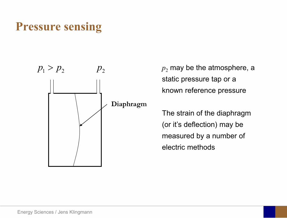
Energy Sciences Jens Klingmann
Pressure sensing
1 2p pgt 2p p2 may be the atmosphere a static pressure tap or a known reference pressure
The strain of the diaphragm (or itrsquos deflection) may be measured by a number of electric methods
Diaphragm
Energy Sciences Jens Klingmann
Pressure sensingPiezoresistive Strain Gage
Uses the piezoresistive effect of bonded or formed strain gauges to detect strain due to applied pressure
Capacitive
Uses a diaghragm and pressure cavity to create a variable capacitor to detect strain due to applied pressure
Magnetic
Measures the displacement of a diaphragm by means of changes in inductance (reluctance) LVDT Hall Effect or by eddy current principal
Piezoelectric
Uses the piezoelectric effect in certain materials such as quartz to measure the strain upon the sensing mechanism due to pressure
Potentiometric
Uses the motion of a wiper along a resistive mechanism to detect the strain caused by applied pressure
Energy Sciences Jens Klingmann
3D highly instationary (periodic) flow Potentially very high velocities (Supersonic) Large temperature differences Low accessibility (difficult to probe between rotors) Low turbulence levels in most of the domain Very high turbulence in BL and wakes
Properties of measuring object
Point measurements
Energy Sciences Jens Klingmann
Conventional or non-opticalndash Static Pressure Measurementsndash Total Pressure Measurements
bull Multy hole probes
ndash Total Temperature ndash Hot Wire Anemometry (HWA)
Optical techniques for Velocity Measurementsndash Laser Two Focous (L2F)ndash Laser Doppler Anemometry (LDA)ndash Particle Image velocimetry (PIV)
Point Measurements
Energy Sciences Jens Klingmann
Static and total pressure
2 2 21 2 1
2 1 2 2 2C C CP P ρ ρ ρ
minus = minus =
2 0C =Stagnation point
C1Static pressure tap
Prandtl or Pitot tube
Apply the Bernoulli equation from free stream to stagnation point
21
2 12CP Pρ
= +or
We can also define a stagnation or total pressure
( )2
101 1 022
CP P Pρ= + =
Total pressure = Static pressure + dynamic pressure
or
Energy Sciences Jens Klingmann
Static pressure
Energy Sciences Jens Klingmann
Total Pressure and Temperature
Shrouded Probes
Shrouded Probe
Pitot or Prandtl tube
Sensitive to direction
Energy Sciences Jens Klingmann
Ludwig Prandtl 1875-1953
Ludwig Prandtl born at Freising Bavaria on February 4 1875 was a German Physicist famous for his work in aeronautics He qualified at Munchen in 1900 with a thesis on elastic stability and held the position of Professor of Applied Mechanics at Gottingen for forty-nine years (from 1904 until his death there on August 15 1953) In 1925 Prandtl became the Director of the Kaiser Wilhelm Institute for Fluid Mechanics His discovery in 1904 of the Boundary Layer which adjoins the surface of a body moving in a fluid led to an understanding of skin friction drag and of the way in which streamlining reduces the drag of airplane wings and other moving bodies His work on wing theory published in 1918 - 1919 followed that of FW Lanchester (1902-1907) but was carried out independently and elucidated the flow over airplane wings of finite span Prandtls work and decisive advances in boundary layer and wing theories became the basic material of aeronautics He also made important contributions to the theories of supersonic flow and of turbulence and contributed much to the development of wind tunnels and other aerodynamic equipment In addition he devised the soap-film analogy for the torsion of non-circular sections and wrote on the theory of plasticity and of meteorology
Energy Sciences Jens Klingmann
Total Pressure multy hole
Cobra Probe Yaw Probe
5 Hole Probe
Energy Sciences Jens Klingmann
5 Hole Probes Calibration
Energy Sciences Jens Klingmann
The inherent unsteadiness of the flow within turbomachines
Energy Sciences Jens Klingmann
Hot Wire Anemometry (HWA) The heat transfer from a thin (one micron)
electrically heated wire can be used to determine velocity
The resistance of the wire is temperature dependent Within a small temperature range it can be assumed linear R = R0+α R0(Tm-T0) where R0 is the resistance at a reference temperature T0 and Tm is the mean wire temperature
The thermal power induced in the wire is balanced by heat transfer to the surrounding fluid I2R=hπDL(Tm-T0) where h is the heat transfer coefficient and D and L the diameter and length of the wire respectively
E = I R
Energy Sciences Jens Klingmann
Constant Temperature Anemometry (CTA) The wire is often placed in a Whetstone bridge If the output from the
bridge is amplified and fed back to the bridge the resistance of the probe and thus the temperature will be held constant
This prevents the temperature of the wire to become excessive at low velocities
R1
R2 R3
Probe
Bridge Voltage
Energy Sciences Jens Klingmann
Constant Temperature Anemometry (CTA)
Energy Sciences Jens Klingmann
Characteristics of LDA (according to Dantec)
Invented by Yeh and Cummins in 1964 Velocity measurements in Fluid Dynamics (gas liquid) Up to 3 velocity components Non-intrusive measurements (optical technique) Absolute measurement technique (no calibration required) Very high accuracy Very high spatial resolution due to small measurement volume Tracer particles are required
Energy Sciences Jens Klingmann
LDA - Fringe Model
Focused Laser beams intersect and form the measurement volume Plane wave fronts beam waist in the plane of intersection Interference in the plane of intersection Pattern of bright and dark stripesplanes Fringes
Energy Sciences Jens Klingmann
LDA-measuring volume
d
x
x
y
y
z
z
e-2 CONTOUR
FRINGES
κ
κ
κ
κ
De-2
De-2
dml m
a
b
cx
b
z
ya
cd
d
=
=
=
J
J
J
J
JP
JP
JP
JD
JD
JD
+
+
+
a
b
c
d
κπλ
=minus sinD
f4l2e
m
κπλ
=minus cosD
f4D2e
m
Energy Sciences Jens Klingmann
Laser Two Focus
Energy Sciences Jens Klingmann
Laser Two Focus
Energy Sciences Jens Klingmann
PIV measurements
PIV is a fairly new technique capable of simultaneous velocity measurements at many points in a plane This gives information on large scale structures vorticity etc which is very difficult or impossible to obtain from one-point measuring techniques
PIV involves the illumination of a plane of the flow under investigation with a thin pulsed sheet of light The flow is seeded with particles
The light scattered from the particles and from successive pulses are being recorded either on film or a CCD array forming a multiple exposure of each particle image If the time between the pulses is known velocity can be determined as the ratio of the particle displacement and the elapsed time
t∆∆= xu
Energy Sciences Jens Klingmann
PIV
Energy Sciences Jens Klingmann
PIV measurements illumination
YA
G
YA
G
Two frequency doubled YAG Lasers aligned to one double pulsed laser sheet
Two or more separate light pulses can be obtained by chopping a continuous laser or from pulsed lasers
The limited pulse energies obtained from continuous lasers limits their applicability to low velocity flows or flows where large seeding particles can be used (ie liquid flows)
The low repetition rate of most pulsed lasers makes the use of two lasers advantageous
Energy Sciences Jens Klingmann
PIV measurements recording
High seeding density in laminar flame
Film or CCD-cameras Cross- or Auto-correlation
ndash ie both particle images on the same frame or on separate frames
CCD-camera requirementndash A many pixels as possiblendash 2k by 2k available 4k by 4k coming
Energy Sciences Jens Klingmann
PIV measurements analyses
Low seeding density (Number of seeding particles per unit volume)
Each particle image pair can be identified This is called particle tracking
High seeding density (PIV)
Small sub-regions of the image containing many particle image pairs are processed to obtain one velocity vector
Energy Sciences Jens Klingmann
PIV measurements analyses
Energy Sciences Jens Klingmann
PIV measurements analyses
( ) ( ) ( ) xsxxs dIIR 2A
1
I
+= int
Cross correlation between ( )x1I and ( )x2I
s is a two dimensional displacement vector
IA is the interrogation area
Cross correlation between
(
)
x
1
I
and
(
)
x
2
I
s is a two dimensional displacement vector
I
A
is the interrogation area
Energy Sciences Jens Klingmann
Energy Sciences Jens Klingmann
PIV from IOWA state university
Energy Sciences Jens Klingmann
PIV sample of evaluation
Energy Sciences Jens Klingmann
LDA PIV HWA Velocity range 01 mms ndash 300
ms 02 ndash 150 ms
Measuring Volume
D = 005 L = 05 mm
2 by 2 by 05 mm
L = 05 mm
Freq response O(10 000) Hz O(10) Hz O(100 000) Hz Calibration Yes No No Sensitivity to other than velocity
Low (ref Index) Low (ref Index) Large (temperature concentrationshellip)
Continuous Signal
Sometimes Seldom Always
Noise High High Low Turbulence intensity
No limitation Some limitation lt 20
Price O(1 000 000) SEK
O(1 000 000) SEK
O(50 000) SEK
Required Knowledge
High medium Low
Comparison of techniques
Energy Sciences Jens Klingmann
References experiments
R J Goldstein ldquoFluid Mechanics Measurementsrdquo Hemisphere Publishing 1983 A V Johansson amp P H Alfredsson ldquoExperimentella metoder inom
stroumlmningsmekanikenrdquo Inst Foumlr Mekanik KTH F Durst A Melling and J H Whitelaw ldquoPrincipals and Practice of Laser Doppler
Anemometryrdquo 1984 R J Adrian ldquoParticle-imaging techniques for experimental fluid mechnicsrdquo Ann Rev
Fluid Mech 1991
Energy Sciences Jens Klingmann
Sample of LDA-measurements
Rotor blade
Glas window
Emitted beams
Scattered Light
Adjustable mirror
Energy Sciences Jens Klingmann
Axial velocity sorted into 10 bins
0 1 2 3 4 5 6tangential coordinate (degrees)
-20
0
20
40
60
80
100
120
140
160Ax
ial v
eloc
ity a
nd s
tand
ard
devi
atio
n (m
s)
radial position 7 mm from inner window surfaceaxial position 23 mm behind rotor blades
Energy Sciences Jens Klingmann
Axial velocities in the radial-tangential plane
Energy Sciences Jens Klingmann
Airfoils NACA 4-digit
The NACA four-digit wing sections define the profile by
One digit describing maximum camber as percentage of the chord
One digit describing the distance of maximum camber from the airfoil leading edge in tens of percents of the chord
Two digits describing maximum thickness of the airfoil as percent of the chord
Example the NACA 2412 airfoil has a maximum camber of 2 located 40 (04 chords) from the leading edge with a maximum thickness of 12 of the chord
Four-digit series airfoils by default have maximum thickness at 30 of the chord (03 chords) from the leading edge
Energy Sciences Jens Klingmann
Airfoils NACA 4-digit
bull c is the chord lengthbull x is the position along
the chord from 0 to cbull y is the half thickness at
a given value of x (centerline to surface)
bull t is the maximum thickness as a fraction of the chord
Energy Sciences Jens Klingmann
Death by PowerPoint
| LDA | PIV | HWA | |||||
| Velocity range | 01 mms ndash 300 ms | 02 ndash 150 ms | |||||
| Measuring Volume | D = 005 L = 05 mm | 2 by 2 by 05 mm | L = 05 mm | ||||
| Freq response | O(10 000) Hz | O(10) Hz | O(100 000) Hz | ||||
| Calibration | Yes | No | No | ||||
| Sensitivity to other than velocity | Low (ref Index) | Low (ref Index) | Large (temperature concentrationshellip) | ||||
| Continuous Signal | Sometimes | Seldom | Always | ||||
| Noise | High | High | Low | ||||
| Turbulence intensity | No limitation | Some limitation | lt 20 | ||||
| Price | O(1 000 000) SEK | O(1 000 000) SEK | O(50 000) SEK | ||||
| Required Knowledge | High | medium | Low |
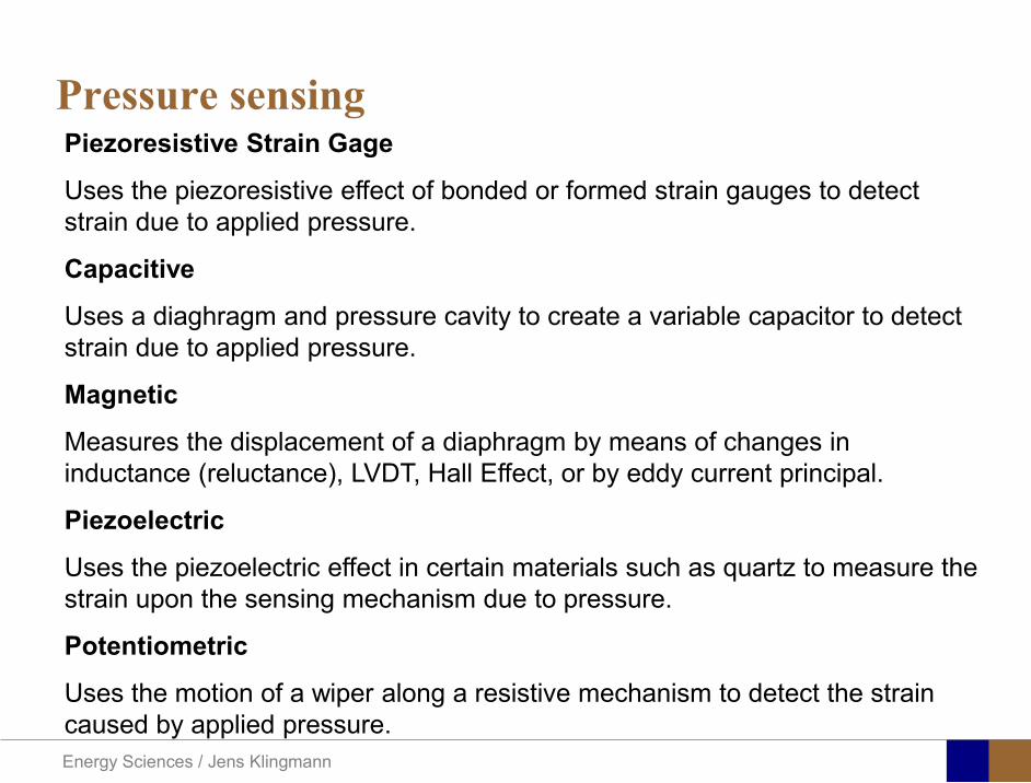
Energy Sciences Jens Klingmann
Pressure sensingPiezoresistive Strain Gage
Uses the piezoresistive effect of bonded or formed strain gauges to detect strain due to applied pressure
Capacitive
Uses a diaghragm and pressure cavity to create a variable capacitor to detect strain due to applied pressure
Magnetic
Measures the displacement of a diaphragm by means of changes in inductance (reluctance) LVDT Hall Effect or by eddy current principal
Piezoelectric
Uses the piezoelectric effect in certain materials such as quartz to measure the strain upon the sensing mechanism due to pressure
Potentiometric
Uses the motion of a wiper along a resistive mechanism to detect the strain caused by applied pressure
Energy Sciences Jens Klingmann
3D highly instationary (periodic) flow Potentially very high velocities (Supersonic) Large temperature differences Low accessibility (difficult to probe between rotors) Low turbulence levels in most of the domain Very high turbulence in BL and wakes
Properties of measuring object
Point measurements
Energy Sciences Jens Klingmann
Conventional or non-opticalndash Static Pressure Measurementsndash Total Pressure Measurements
bull Multy hole probes
ndash Total Temperature ndash Hot Wire Anemometry (HWA)
Optical techniques for Velocity Measurementsndash Laser Two Focous (L2F)ndash Laser Doppler Anemometry (LDA)ndash Particle Image velocimetry (PIV)
Point Measurements
Energy Sciences Jens Klingmann
Static and total pressure
2 2 21 2 1
2 1 2 2 2C C CP P ρ ρ ρ
minus = minus =
2 0C =Stagnation point
C1Static pressure tap
Prandtl or Pitot tube
Apply the Bernoulli equation from free stream to stagnation point
21
2 12CP Pρ
= +or
We can also define a stagnation or total pressure
( )2
101 1 022
CP P Pρ= + =
Total pressure = Static pressure + dynamic pressure
or
Energy Sciences Jens Klingmann
Static pressure
Energy Sciences Jens Klingmann
Total Pressure and Temperature
Shrouded Probes
Shrouded Probe
Pitot or Prandtl tube
Sensitive to direction
Energy Sciences Jens Klingmann
Ludwig Prandtl 1875-1953
Ludwig Prandtl born at Freising Bavaria on February 4 1875 was a German Physicist famous for his work in aeronautics He qualified at Munchen in 1900 with a thesis on elastic stability and held the position of Professor of Applied Mechanics at Gottingen for forty-nine years (from 1904 until his death there on August 15 1953) In 1925 Prandtl became the Director of the Kaiser Wilhelm Institute for Fluid Mechanics His discovery in 1904 of the Boundary Layer which adjoins the surface of a body moving in a fluid led to an understanding of skin friction drag and of the way in which streamlining reduces the drag of airplane wings and other moving bodies His work on wing theory published in 1918 - 1919 followed that of FW Lanchester (1902-1907) but was carried out independently and elucidated the flow over airplane wings of finite span Prandtls work and decisive advances in boundary layer and wing theories became the basic material of aeronautics He also made important contributions to the theories of supersonic flow and of turbulence and contributed much to the development of wind tunnels and other aerodynamic equipment In addition he devised the soap-film analogy for the torsion of non-circular sections and wrote on the theory of plasticity and of meteorology
Energy Sciences Jens Klingmann
Total Pressure multy hole
Cobra Probe Yaw Probe
5 Hole Probe
Energy Sciences Jens Klingmann
5 Hole Probes Calibration
Energy Sciences Jens Klingmann
The inherent unsteadiness of the flow within turbomachines
Energy Sciences Jens Klingmann
Hot Wire Anemometry (HWA) The heat transfer from a thin (one micron)
electrically heated wire can be used to determine velocity
The resistance of the wire is temperature dependent Within a small temperature range it can be assumed linear R = R0+α R0(Tm-T0) where R0 is the resistance at a reference temperature T0 and Tm is the mean wire temperature
The thermal power induced in the wire is balanced by heat transfer to the surrounding fluid I2R=hπDL(Tm-T0) where h is the heat transfer coefficient and D and L the diameter and length of the wire respectively
E = I R
Energy Sciences Jens Klingmann
Constant Temperature Anemometry (CTA) The wire is often placed in a Whetstone bridge If the output from the
bridge is amplified and fed back to the bridge the resistance of the probe and thus the temperature will be held constant
This prevents the temperature of the wire to become excessive at low velocities
R1
R2 R3
Probe
Bridge Voltage
Energy Sciences Jens Klingmann
Constant Temperature Anemometry (CTA)
Energy Sciences Jens Klingmann
Characteristics of LDA (according to Dantec)
Invented by Yeh and Cummins in 1964 Velocity measurements in Fluid Dynamics (gas liquid) Up to 3 velocity components Non-intrusive measurements (optical technique) Absolute measurement technique (no calibration required) Very high accuracy Very high spatial resolution due to small measurement volume Tracer particles are required
Energy Sciences Jens Klingmann
LDA - Fringe Model
Focused Laser beams intersect and form the measurement volume Plane wave fronts beam waist in the plane of intersection Interference in the plane of intersection Pattern of bright and dark stripesplanes Fringes
Energy Sciences Jens Klingmann
LDA-measuring volume
d
x
x
y
y
z
z
e-2 CONTOUR
FRINGES
κ
κ
κ
κ
De-2
De-2
dml m
a
b
cx
b
z
ya
cd
d
=
=
=
J
J
J
J
JP
JP
JP
JD
JD
JD
+
+
+
a
b
c
d
κπλ
=minus sinD
f4l2e
m
κπλ
=minus cosD
f4D2e
m
Energy Sciences Jens Klingmann
Laser Two Focus
Energy Sciences Jens Klingmann
Laser Two Focus
Energy Sciences Jens Klingmann
PIV measurements
PIV is a fairly new technique capable of simultaneous velocity measurements at many points in a plane This gives information on large scale structures vorticity etc which is very difficult or impossible to obtain from one-point measuring techniques
PIV involves the illumination of a plane of the flow under investigation with a thin pulsed sheet of light The flow is seeded with particles
The light scattered from the particles and from successive pulses are being recorded either on film or a CCD array forming a multiple exposure of each particle image If the time between the pulses is known velocity can be determined as the ratio of the particle displacement and the elapsed time
t∆∆= xu
Energy Sciences Jens Klingmann
PIV
Energy Sciences Jens Klingmann
PIV measurements illumination
YA
G
YA
G
Two frequency doubled YAG Lasers aligned to one double pulsed laser sheet
Two or more separate light pulses can be obtained by chopping a continuous laser or from pulsed lasers
The limited pulse energies obtained from continuous lasers limits their applicability to low velocity flows or flows where large seeding particles can be used (ie liquid flows)
The low repetition rate of most pulsed lasers makes the use of two lasers advantageous
Energy Sciences Jens Klingmann
PIV measurements recording
High seeding density in laminar flame
Film or CCD-cameras Cross- or Auto-correlation
ndash ie both particle images on the same frame or on separate frames
CCD-camera requirementndash A many pixels as possiblendash 2k by 2k available 4k by 4k coming
Energy Sciences Jens Klingmann
PIV measurements analyses
Low seeding density (Number of seeding particles per unit volume)
Each particle image pair can be identified This is called particle tracking
High seeding density (PIV)
Small sub-regions of the image containing many particle image pairs are processed to obtain one velocity vector
Energy Sciences Jens Klingmann
PIV measurements analyses
Energy Sciences Jens Klingmann
PIV measurements analyses
( ) ( ) ( ) xsxxs dIIR 2A
1
I
+= int
Cross correlation between ( )x1I and ( )x2I
s is a two dimensional displacement vector
IA is the interrogation area
Cross correlation between
(
)
x
1
I
and
(
)
x
2
I
s is a two dimensional displacement vector
I
A
is the interrogation area
Energy Sciences Jens Klingmann
Energy Sciences Jens Klingmann
PIV from IOWA state university
Energy Sciences Jens Klingmann
PIV sample of evaluation
Energy Sciences Jens Klingmann
LDA PIV HWA Velocity range 01 mms ndash 300
ms 02 ndash 150 ms
Measuring Volume
D = 005 L = 05 mm
2 by 2 by 05 mm
L = 05 mm
Freq response O(10 000) Hz O(10) Hz O(100 000) Hz Calibration Yes No No Sensitivity to other than velocity
Low (ref Index) Low (ref Index) Large (temperature concentrationshellip)
Continuous Signal
Sometimes Seldom Always
Noise High High Low Turbulence intensity
No limitation Some limitation lt 20
Price O(1 000 000) SEK
O(1 000 000) SEK
O(50 000) SEK
Required Knowledge
High medium Low
Comparison of techniques
Energy Sciences Jens Klingmann
References experiments
R J Goldstein ldquoFluid Mechanics Measurementsrdquo Hemisphere Publishing 1983 A V Johansson amp P H Alfredsson ldquoExperimentella metoder inom
stroumlmningsmekanikenrdquo Inst Foumlr Mekanik KTH F Durst A Melling and J H Whitelaw ldquoPrincipals and Practice of Laser Doppler
Anemometryrdquo 1984 R J Adrian ldquoParticle-imaging techniques for experimental fluid mechnicsrdquo Ann Rev
Fluid Mech 1991
Energy Sciences Jens Klingmann
Sample of LDA-measurements
Rotor blade
Glas window
Emitted beams
Scattered Light
Adjustable mirror
Energy Sciences Jens Klingmann
Axial velocity sorted into 10 bins
0 1 2 3 4 5 6tangential coordinate (degrees)
-20
0
20
40
60
80
100
120
140
160Ax
ial v
eloc
ity a
nd s
tand
ard
devi
atio
n (m
s)
radial position 7 mm from inner window surfaceaxial position 23 mm behind rotor blades
Energy Sciences Jens Klingmann
Axial velocities in the radial-tangential plane
Energy Sciences Jens Klingmann
Airfoils NACA 4-digit
The NACA four-digit wing sections define the profile by
One digit describing maximum camber as percentage of the chord
One digit describing the distance of maximum camber from the airfoil leading edge in tens of percents of the chord
Two digits describing maximum thickness of the airfoil as percent of the chord
Example the NACA 2412 airfoil has a maximum camber of 2 located 40 (04 chords) from the leading edge with a maximum thickness of 12 of the chord
Four-digit series airfoils by default have maximum thickness at 30 of the chord (03 chords) from the leading edge
Energy Sciences Jens Klingmann
Airfoils NACA 4-digit
bull c is the chord lengthbull x is the position along
the chord from 0 to cbull y is the half thickness at
a given value of x (centerline to surface)
bull t is the maximum thickness as a fraction of the chord
Energy Sciences Jens Klingmann
Death by PowerPoint
| LDA | PIV | HWA | |||||
| Velocity range | 01 mms ndash 300 ms | 02 ndash 150 ms | |||||
| Measuring Volume | D = 005 L = 05 mm | 2 by 2 by 05 mm | L = 05 mm | ||||
| Freq response | O(10 000) Hz | O(10) Hz | O(100 000) Hz | ||||
| Calibration | Yes | No | No | ||||
| Sensitivity to other than velocity | Low (ref Index) | Low (ref Index) | Large (temperature concentrationshellip) | ||||
| Continuous Signal | Sometimes | Seldom | Always | ||||
| Noise | High | High | Low | ||||
| Turbulence intensity | No limitation | Some limitation | lt 20 | ||||
| Price | O(1 000 000) SEK | O(1 000 000) SEK | O(50 000) SEK | ||||
| Required Knowledge | High | medium | Low |
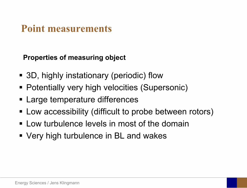
Energy Sciences Jens Klingmann
3D highly instationary (periodic) flow Potentially very high velocities (Supersonic) Large temperature differences Low accessibility (difficult to probe between rotors) Low turbulence levels in most of the domain Very high turbulence in BL and wakes
Properties of measuring object
Point measurements
Energy Sciences Jens Klingmann
Conventional or non-opticalndash Static Pressure Measurementsndash Total Pressure Measurements
bull Multy hole probes
ndash Total Temperature ndash Hot Wire Anemometry (HWA)
Optical techniques for Velocity Measurementsndash Laser Two Focous (L2F)ndash Laser Doppler Anemometry (LDA)ndash Particle Image velocimetry (PIV)
Point Measurements
Energy Sciences Jens Klingmann
Static and total pressure
2 2 21 2 1
2 1 2 2 2C C CP P ρ ρ ρ
minus = minus =
2 0C =Stagnation point
C1Static pressure tap
Prandtl or Pitot tube
Apply the Bernoulli equation from free stream to stagnation point
21
2 12CP Pρ
= +or
We can also define a stagnation or total pressure
( )2
101 1 022
CP P Pρ= + =
Total pressure = Static pressure + dynamic pressure
or
Energy Sciences Jens Klingmann
Static pressure
Energy Sciences Jens Klingmann
Total Pressure and Temperature
Shrouded Probes
Shrouded Probe
Pitot or Prandtl tube
Sensitive to direction
Energy Sciences Jens Klingmann
Ludwig Prandtl 1875-1953
Ludwig Prandtl born at Freising Bavaria on February 4 1875 was a German Physicist famous for his work in aeronautics He qualified at Munchen in 1900 with a thesis on elastic stability and held the position of Professor of Applied Mechanics at Gottingen for forty-nine years (from 1904 until his death there on August 15 1953) In 1925 Prandtl became the Director of the Kaiser Wilhelm Institute for Fluid Mechanics His discovery in 1904 of the Boundary Layer which adjoins the surface of a body moving in a fluid led to an understanding of skin friction drag and of the way in which streamlining reduces the drag of airplane wings and other moving bodies His work on wing theory published in 1918 - 1919 followed that of FW Lanchester (1902-1907) but was carried out independently and elucidated the flow over airplane wings of finite span Prandtls work and decisive advances in boundary layer and wing theories became the basic material of aeronautics He also made important contributions to the theories of supersonic flow and of turbulence and contributed much to the development of wind tunnels and other aerodynamic equipment In addition he devised the soap-film analogy for the torsion of non-circular sections and wrote on the theory of plasticity and of meteorology
Energy Sciences Jens Klingmann
Total Pressure multy hole
Cobra Probe Yaw Probe
5 Hole Probe
Energy Sciences Jens Klingmann
5 Hole Probes Calibration
Energy Sciences Jens Klingmann
The inherent unsteadiness of the flow within turbomachines
Energy Sciences Jens Klingmann
Hot Wire Anemometry (HWA) The heat transfer from a thin (one micron)
electrically heated wire can be used to determine velocity
The resistance of the wire is temperature dependent Within a small temperature range it can be assumed linear R = R0+α R0(Tm-T0) where R0 is the resistance at a reference temperature T0 and Tm is the mean wire temperature
The thermal power induced in the wire is balanced by heat transfer to the surrounding fluid I2R=hπDL(Tm-T0) where h is the heat transfer coefficient and D and L the diameter and length of the wire respectively
E = I R
Energy Sciences Jens Klingmann
Constant Temperature Anemometry (CTA) The wire is often placed in a Whetstone bridge If the output from the
bridge is amplified and fed back to the bridge the resistance of the probe and thus the temperature will be held constant
This prevents the temperature of the wire to become excessive at low velocities
R1
R2 R3
Probe
Bridge Voltage
Energy Sciences Jens Klingmann
Constant Temperature Anemometry (CTA)
Energy Sciences Jens Klingmann
Characteristics of LDA (according to Dantec)
Invented by Yeh and Cummins in 1964 Velocity measurements in Fluid Dynamics (gas liquid) Up to 3 velocity components Non-intrusive measurements (optical technique) Absolute measurement technique (no calibration required) Very high accuracy Very high spatial resolution due to small measurement volume Tracer particles are required
Energy Sciences Jens Klingmann
LDA - Fringe Model
Focused Laser beams intersect and form the measurement volume Plane wave fronts beam waist in the plane of intersection Interference in the plane of intersection Pattern of bright and dark stripesplanes Fringes
Energy Sciences Jens Klingmann
LDA-measuring volume
d
x
x
y
y
z
z
e-2 CONTOUR
FRINGES
κ
κ
κ
κ
De-2
De-2
dml m
a
b
cx
b
z
ya
cd
d
=
=
=
J
J
J
J
JP
JP
JP
JD
JD
JD
+
+
+
a
b
c
d
κπλ
=minus sinD
f4l2e
m
κπλ
=minus cosD
f4D2e
m
Energy Sciences Jens Klingmann
Laser Two Focus
Energy Sciences Jens Klingmann
Laser Two Focus
Energy Sciences Jens Klingmann
PIV measurements
PIV is a fairly new technique capable of simultaneous velocity measurements at many points in a plane This gives information on large scale structures vorticity etc which is very difficult or impossible to obtain from one-point measuring techniques
PIV involves the illumination of a plane of the flow under investigation with a thin pulsed sheet of light The flow is seeded with particles
The light scattered from the particles and from successive pulses are being recorded either on film or a CCD array forming a multiple exposure of each particle image If the time between the pulses is known velocity can be determined as the ratio of the particle displacement and the elapsed time
t∆∆= xu
Energy Sciences Jens Klingmann
PIV
Energy Sciences Jens Klingmann
PIV measurements illumination
YA
G
YA
G
Two frequency doubled YAG Lasers aligned to one double pulsed laser sheet
Two or more separate light pulses can be obtained by chopping a continuous laser or from pulsed lasers
The limited pulse energies obtained from continuous lasers limits their applicability to low velocity flows or flows where large seeding particles can be used (ie liquid flows)
The low repetition rate of most pulsed lasers makes the use of two lasers advantageous
Energy Sciences Jens Klingmann
PIV measurements recording
High seeding density in laminar flame
Film or CCD-cameras Cross- or Auto-correlation
ndash ie both particle images on the same frame or on separate frames
CCD-camera requirementndash A many pixels as possiblendash 2k by 2k available 4k by 4k coming
Energy Sciences Jens Klingmann
PIV measurements analyses
Low seeding density (Number of seeding particles per unit volume)
Each particle image pair can be identified This is called particle tracking
High seeding density (PIV)
Small sub-regions of the image containing many particle image pairs are processed to obtain one velocity vector
Energy Sciences Jens Klingmann
PIV measurements analyses
Energy Sciences Jens Klingmann
PIV measurements analyses
( ) ( ) ( ) xsxxs dIIR 2A
1
I
+= int
Cross correlation between ( )x1I and ( )x2I
s is a two dimensional displacement vector
IA is the interrogation area
Cross correlation between
(
)
x
1
I
and
(
)
x
2
I
s is a two dimensional displacement vector
I
A
is the interrogation area
Energy Sciences Jens Klingmann
Energy Sciences Jens Klingmann
PIV from IOWA state university
Energy Sciences Jens Klingmann
PIV sample of evaluation
Energy Sciences Jens Klingmann
LDA PIV HWA Velocity range 01 mms ndash 300
ms 02 ndash 150 ms
Measuring Volume
D = 005 L = 05 mm
2 by 2 by 05 mm
L = 05 mm
Freq response O(10 000) Hz O(10) Hz O(100 000) Hz Calibration Yes No No Sensitivity to other than velocity
Low (ref Index) Low (ref Index) Large (temperature concentrationshellip)
Continuous Signal
Sometimes Seldom Always
Noise High High Low Turbulence intensity
No limitation Some limitation lt 20
Price O(1 000 000) SEK
O(1 000 000) SEK
O(50 000) SEK
Required Knowledge
High medium Low
Comparison of techniques
Energy Sciences Jens Klingmann
References experiments
R J Goldstein ldquoFluid Mechanics Measurementsrdquo Hemisphere Publishing 1983 A V Johansson amp P H Alfredsson ldquoExperimentella metoder inom
stroumlmningsmekanikenrdquo Inst Foumlr Mekanik KTH F Durst A Melling and J H Whitelaw ldquoPrincipals and Practice of Laser Doppler
Anemometryrdquo 1984 R J Adrian ldquoParticle-imaging techniques for experimental fluid mechnicsrdquo Ann Rev
Fluid Mech 1991
Energy Sciences Jens Klingmann
Sample of LDA-measurements
Rotor blade
Glas window
Emitted beams
Scattered Light
Adjustable mirror
Energy Sciences Jens Klingmann
Axial velocity sorted into 10 bins
0 1 2 3 4 5 6tangential coordinate (degrees)
-20
0
20
40
60
80
100
120
140
160Ax
ial v
eloc
ity a
nd s
tand
ard
devi
atio
n (m
s)
radial position 7 mm from inner window surfaceaxial position 23 mm behind rotor blades
Energy Sciences Jens Klingmann
Axial velocities in the radial-tangential plane
Energy Sciences Jens Klingmann
Airfoils NACA 4-digit
The NACA four-digit wing sections define the profile by
One digit describing maximum camber as percentage of the chord
One digit describing the distance of maximum camber from the airfoil leading edge in tens of percents of the chord
Two digits describing maximum thickness of the airfoil as percent of the chord
Example the NACA 2412 airfoil has a maximum camber of 2 located 40 (04 chords) from the leading edge with a maximum thickness of 12 of the chord
Four-digit series airfoils by default have maximum thickness at 30 of the chord (03 chords) from the leading edge
Energy Sciences Jens Klingmann
Airfoils NACA 4-digit
bull c is the chord lengthbull x is the position along
the chord from 0 to cbull y is the half thickness at
a given value of x (centerline to surface)
bull t is the maximum thickness as a fraction of the chord
Energy Sciences Jens Klingmann
Death by PowerPoint
| LDA | PIV | HWA | |||||
| Velocity range | 01 mms ndash 300 ms | 02 ndash 150 ms | |||||
| Measuring Volume | D = 005 L = 05 mm | 2 by 2 by 05 mm | L = 05 mm | ||||
| Freq response | O(10 000) Hz | O(10) Hz | O(100 000) Hz | ||||
| Calibration | Yes | No | No | ||||
| Sensitivity to other than velocity | Low (ref Index) | Low (ref Index) | Large (temperature concentrationshellip) | ||||
| Continuous Signal | Sometimes | Seldom | Always | ||||
| Noise | High | High | Low | ||||
| Turbulence intensity | No limitation | Some limitation | lt 20 | ||||
| Price | O(1 000 000) SEK | O(1 000 000) SEK | O(50 000) SEK | ||||
| Required Knowledge | High | medium | Low |
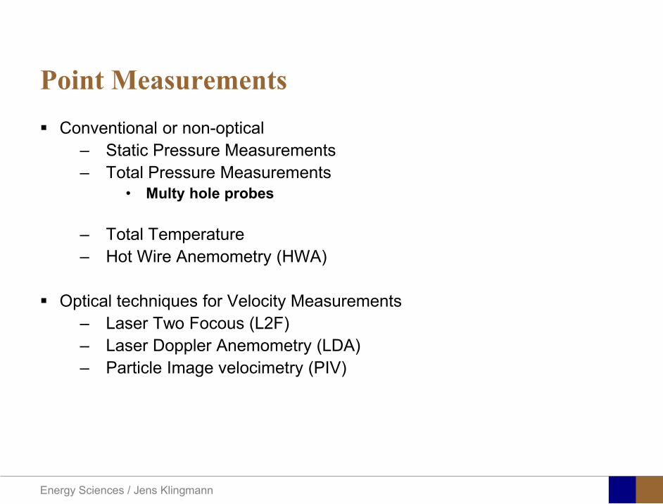
Energy Sciences Jens Klingmann
Conventional or non-opticalndash Static Pressure Measurementsndash Total Pressure Measurements
bull Multy hole probes
ndash Total Temperature ndash Hot Wire Anemometry (HWA)
Optical techniques for Velocity Measurementsndash Laser Two Focous (L2F)ndash Laser Doppler Anemometry (LDA)ndash Particle Image velocimetry (PIV)
Point Measurements
Energy Sciences Jens Klingmann
Static and total pressure
2 2 21 2 1
2 1 2 2 2C C CP P ρ ρ ρ
minus = minus =
2 0C =Stagnation point
C1Static pressure tap
Prandtl or Pitot tube
Apply the Bernoulli equation from free stream to stagnation point
21
2 12CP Pρ
= +or
We can also define a stagnation or total pressure
( )2
101 1 022
CP P Pρ= + =
Total pressure = Static pressure + dynamic pressure
or
Energy Sciences Jens Klingmann
Static pressure
Energy Sciences Jens Klingmann
Total Pressure and Temperature
Shrouded Probes
Shrouded Probe
Pitot or Prandtl tube
Sensitive to direction
Energy Sciences Jens Klingmann
Ludwig Prandtl 1875-1953
Ludwig Prandtl born at Freising Bavaria on February 4 1875 was a German Physicist famous for his work in aeronautics He qualified at Munchen in 1900 with a thesis on elastic stability and held the position of Professor of Applied Mechanics at Gottingen for forty-nine years (from 1904 until his death there on August 15 1953) In 1925 Prandtl became the Director of the Kaiser Wilhelm Institute for Fluid Mechanics His discovery in 1904 of the Boundary Layer which adjoins the surface of a body moving in a fluid led to an understanding of skin friction drag and of the way in which streamlining reduces the drag of airplane wings and other moving bodies His work on wing theory published in 1918 - 1919 followed that of FW Lanchester (1902-1907) but was carried out independently and elucidated the flow over airplane wings of finite span Prandtls work and decisive advances in boundary layer and wing theories became the basic material of aeronautics He also made important contributions to the theories of supersonic flow and of turbulence and contributed much to the development of wind tunnels and other aerodynamic equipment In addition he devised the soap-film analogy for the torsion of non-circular sections and wrote on the theory of plasticity and of meteorology
Energy Sciences Jens Klingmann
Total Pressure multy hole
Cobra Probe Yaw Probe
5 Hole Probe
Energy Sciences Jens Klingmann
5 Hole Probes Calibration
Energy Sciences Jens Klingmann
The inherent unsteadiness of the flow within turbomachines
Energy Sciences Jens Klingmann
Hot Wire Anemometry (HWA) The heat transfer from a thin (one micron)
electrically heated wire can be used to determine velocity
The resistance of the wire is temperature dependent Within a small temperature range it can be assumed linear R = R0+α R0(Tm-T0) where R0 is the resistance at a reference temperature T0 and Tm is the mean wire temperature
The thermal power induced in the wire is balanced by heat transfer to the surrounding fluid I2R=hπDL(Tm-T0) where h is the heat transfer coefficient and D and L the diameter and length of the wire respectively
E = I R
Energy Sciences Jens Klingmann
Constant Temperature Anemometry (CTA) The wire is often placed in a Whetstone bridge If the output from the
bridge is amplified and fed back to the bridge the resistance of the probe and thus the temperature will be held constant
This prevents the temperature of the wire to become excessive at low velocities
R1
R2 R3
Probe
Bridge Voltage
Energy Sciences Jens Klingmann
Constant Temperature Anemometry (CTA)
Energy Sciences Jens Klingmann
Characteristics of LDA (according to Dantec)
Invented by Yeh and Cummins in 1964 Velocity measurements in Fluid Dynamics (gas liquid) Up to 3 velocity components Non-intrusive measurements (optical technique) Absolute measurement technique (no calibration required) Very high accuracy Very high spatial resolution due to small measurement volume Tracer particles are required
Energy Sciences Jens Klingmann
LDA - Fringe Model
Focused Laser beams intersect and form the measurement volume Plane wave fronts beam waist in the plane of intersection Interference in the plane of intersection Pattern of bright and dark stripesplanes Fringes
Energy Sciences Jens Klingmann
LDA-measuring volume
d
x
x
y
y
z
z
e-2 CONTOUR
FRINGES
κ
κ
κ
κ
De-2
De-2
dml m
a
b
cx
b
z
ya
cd
d
=
=
=
J
J
J
J
JP
JP
JP
JD
JD
JD
+
+
+
a
b
c
d
κπλ
=minus sinD
f4l2e
m
κπλ
=minus cosD
f4D2e
m
Energy Sciences Jens Klingmann
Laser Two Focus
Energy Sciences Jens Klingmann
Laser Two Focus
Energy Sciences Jens Klingmann
PIV measurements
PIV is a fairly new technique capable of simultaneous velocity measurements at many points in a plane This gives information on large scale structures vorticity etc which is very difficult or impossible to obtain from one-point measuring techniques
PIV involves the illumination of a plane of the flow under investigation with a thin pulsed sheet of light The flow is seeded with particles
The light scattered from the particles and from successive pulses are being recorded either on film or a CCD array forming a multiple exposure of each particle image If the time between the pulses is known velocity can be determined as the ratio of the particle displacement and the elapsed time
t∆∆= xu
Energy Sciences Jens Klingmann
PIV
Energy Sciences Jens Klingmann
PIV measurements illumination
YA
G
YA
G
Two frequency doubled YAG Lasers aligned to one double pulsed laser sheet
Two or more separate light pulses can be obtained by chopping a continuous laser or from pulsed lasers
The limited pulse energies obtained from continuous lasers limits their applicability to low velocity flows or flows where large seeding particles can be used (ie liquid flows)
The low repetition rate of most pulsed lasers makes the use of two lasers advantageous
Energy Sciences Jens Klingmann
PIV measurements recording
High seeding density in laminar flame
Film or CCD-cameras Cross- or Auto-correlation
ndash ie both particle images on the same frame or on separate frames
CCD-camera requirementndash A many pixels as possiblendash 2k by 2k available 4k by 4k coming
Energy Sciences Jens Klingmann
PIV measurements analyses
Low seeding density (Number of seeding particles per unit volume)
Each particle image pair can be identified This is called particle tracking
High seeding density (PIV)
Small sub-regions of the image containing many particle image pairs are processed to obtain one velocity vector
Energy Sciences Jens Klingmann
PIV measurements analyses
Energy Sciences Jens Klingmann
PIV measurements analyses
( ) ( ) ( ) xsxxs dIIR 2A
1
I
+= int
Cross correlation between ( )x1I and ( )x2I
s is a two dimensional displacement vector
IA is the interrogation area
Cross correlation between
(
)
x
1
I
and
(
)
x
2
I
s is a two dimensional displacement vector
I
A
is the interrogation area
Energy Sciences Jens Klingmann
Energy Sciences Jens Klingmann
PIV from IOWA state university
Energy Sciences Jens Klingmann
PIV sample of evaluation
Energy Sciences Jens Klingmann
LDA PIV HWA Velocity range 01 mms ndash 300
ms 02 ndash 150 ms
Measuring Volume
D = 005 L = 05 mm
2 by 2 by 05 mm
L = 05 mm
Freq response O(10 000) Hz O(10) Hz O(100 000) Hz Calibration Yes No No Sensitivity to other than velocity
Low (ref Index) Low (ref Index) Large (temperature concentrationshellip)
Continuous Signal
Sometimes Seldom Always
Noise High High Low Turbulence intensity
No limitation Some limitation lt 20
Price O(1 000 000) SEK
O(1 000 000) SEK
O(50 000) SEK
Required Knowledge
High medium Low
Comparison of techniques
Energy Sciences Jens Klingmann
References experiments
R J Goldstein ldquoFluid Mechanics Measurementsrdquo Hemisphere Publishing 1983 A V Johansson amp P H Alfredsson ldquoExperimentella metoder inom
stroumlmningsmekanikenrdquo Inst Foumlr Mekanik KTH F Durst A Melling and J H Whitelaw ldquoPrincipals and Practice of Laser Doppler
Anemometryrdquo 1984 R J Adrian ldquoParticle-imaging techniques for experimental fluid mechnicsrdquo Ann Rev
Fluid Mech 1991
Energy Sciences Jens Klingmann
Sample of LDA-measurements
Rotor blade
Glas window
Emitted beams
Scattered Light
Adjustable mirror
Energy Sciences Jens Klingmann
Axial velocity sorted into 10 bins
0 1 2 3 4 5 6tangential coordinate (degrees)
-20
0
20
40
60
80
100
120
140
160Ax
ial v
eloc
ity a
nd s
tand
ard
devi
atio
n (m
s)
radial position 7 mm from inner window surfaceaxial position 23 mm behind rotor blades
Energy Sciences Jens Klingmann
Axial velocities in the radial-tangential plane
Energy Sciences Jens Klingmann
Airfoils NACA 4-digit
The NACA four-digit wing sections define the profile by
One digit describing maximum camber as percentage of the chord
One digit describing the distance of maximum camber from the airfoil leading edge in tens of percents of the chord
Two digits describing maximum thickness of the airfoil as percent of the chord
Example the NACA 2412 airfoil has a maximum camber of 2 located 40 (04 chords) from the leading edge with a maximum thickness of 12 of the chord
Four-digit series airfoils by default have maximum thickness at 30 of the chord (03 chords) from the leading edge
Energy Sciences Jens Klingmann
Airfoils NACA 4-digit
bull c is the chord lengthbull x is the position along
the chord from 0 to cbull y is the half thickness at
a given value of x (centerline to surface)
bull t is the maximum thickness as a fraction of the chord
Energy Sciences Jens Klingmann
Death by PowerPoint
| LDA | PIV | HWA | |||||
| Velocity range | 01 mms ndash 300 ms | 02 ndash 150 ms | |||||
| Measuring Volume | D = 005 L = 05 mm | 2 by 2 by 05 mm | L = 05 mm | ||||
| Freq response | O(10 000) Hz | O(10) Hz | O(100 000) Hz | ||||
| Calibration | Yes | No | No | ||||
| Sensitivity to other than velocity | Low (ref Index) | Low (ref Index) | Large (temperature concentrationshellip) | ||||
| Continuous Signal | Sometimes | Seldom | Always | ||||
| Noise | High | High | Low | ||||
| Turbulence intensity | No limitation | Some limitation | lt 20 | ||||
| Price | O(1 000 000) SEK | O(1 000 000) SEK | O(50 000) SEK | ||||
| Required Knowledge | High | medium | Low |
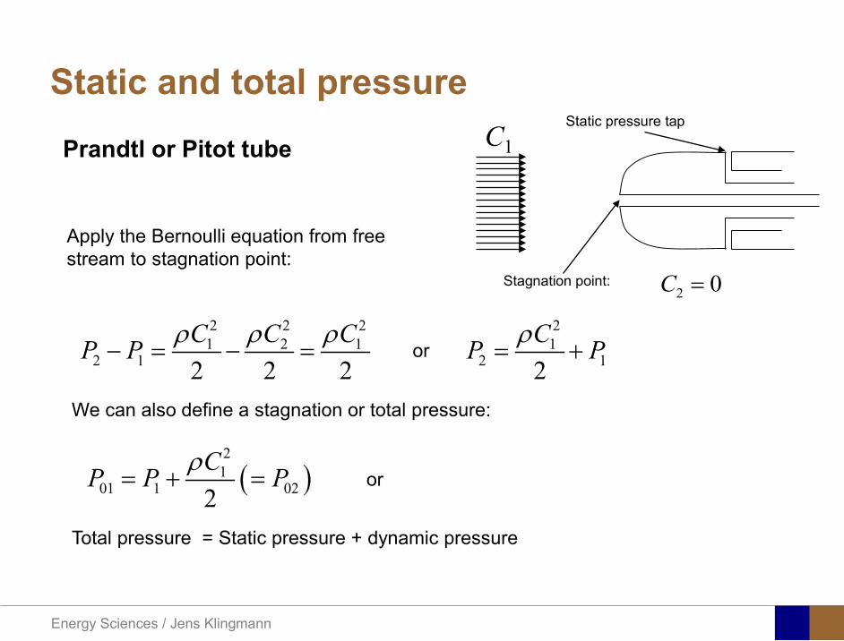
Energy Sciences Jens Klingmann
Static and total pressure
2 2 21 2 1
2 1 2 2 2C C CP P ρ ρ ρ
minus = minus =
2 0C =Stagnation point
C1Static pressure tap
Prandtl or Pitot tube
Apply the Bernoulli equation from free stream to stagnation point
21
2 12CP Pρ
= +or
We can also define a stagnation or total pressure
( )2
101 1 022
CP P Pρ= + =
Total pressure = Static pressure + dynamic pressure
or
Energy Sciences Jens Klingmann
Static pressure
Energy Sciences Jens Klingmann
Total Pressure and Temperature
Shrouded Probes
Shrouded Probe
Pitot or Prandtl tube
Sensitive to direction
Energy Sciences Jens Klingmann
Ludwig Prandtl 1875-1953
Ludwig Prandtl born at Freising Bavaria on February 4 1875 was a German Physicist famous for his work in aeronautics He qualified at Munchen in 1900 with a thesis on elastic stability and held the position of Professor of Applied Mechanics at Gottingen for forty-nine years (from 1904 until his death there on August 15 1953) In 1925 Prandtl became the Director of the Kaiser Wilhelm Institute for Fluid Mechanics His discovery in 1904 of the Boundary Layer which adjoins the surface of a body moving in a fluid led to an understanding of skin friction drag and of the way in which streamlining reduces the drag of airplane wings and other moving bodies His work on wing theory published in 1918 - 1919 followed that of FW Lanchester (1902-1907) but was carried out independently and elucidated the flow over airplane wings of finite span Prandtls work and decisive advances in boundary layer and wing theories became the basic material of aeronautics He also made important contributions to the theories of supersonic flow and of turbulence and contributed much to the development of wind tunnels and other aerodynamic equipment In addition he devised the soap-film analogy for the torsion of non-circular sections and wrote on the theory of plasticity and of meteorology
Energy Sciences Jens Klingmann
Total Pressure multy hole
Cobra Probe Yaw Probe
5 Hole Probe
Energy Sciences Jens Klingmann
5 Hole Probes Calibration
Energy Sciences Jens Klingmann
The inherent unsteadiness of the flow within turbomachines
Energy Sciences Jens Klingmann
Hot Wire Anemometry (HWA) The heat transfer from a thin (one micron)
electrically heated wire can be used to determine velocity
The resistance of the wire is temperature dependent Within a small temperature range it can be assumed linear R = R0+α R0(Tm-T0) where R0 is the resistance at a reference temperature T0 and Tm is the mean wire temperature
The thermal power induced in the wire is balanced by heat transfer to the surrounding fluid I2R=hπDL(Tm-T0) where h is the heat transfer coefficient and D and L the diameter and length of the wire respectively
E = I R
Energy Sciences Jens Klingmann
Constant Temperature Anemometry (CTA) The wire is often placed in a Whetstone bridge If the output from the
bridge is amplified and fed back to the bridge the resistance of the probe and thus the temperature will be held constant
This prevents the temperature of the wire to become excessive at low velocities
R1
R2 R3
Probe
Bridge Voltage
Energy Sciences Jens Klingmann
Constant Temperature Anemometry (CTA)
Energy Sciences Jens Klingmann
Characteristics of LDA (according to Dantec)
Invented by Yeh and Cummins in 1964 Velocity measurements in Fluid Dynamics (gas liquid) Up to 3 velocity components Non-intrusive measurements (optical technique) Absolute measurement technique (no calibration required) Very high accuracy Very high spatial resolution due to small measurement volume Tracer particles are required
Energy Sciences Jens Klingmann
LDA - Fringe Model
Focused Laser beams intersect and form the measurement volume Plane wave fronts beam waist in the plane of intersection Interference in the plane of intersection Pattern of bright and dark stripesplanes Fringes
Energy Sciences Jens Klingmann
LDA-measuring volume
d
x
x
y
y
z
z
e-2 CONTOUR
FRINGES
κ
κ
κ
κ
De-2
De-2
dml m
a
b
cx
b
z
ya
cd
d
=
=
=
J
J
J
J
JP
JP
JP
JD
JD
JD
+
+
+
a
b
c
d
κπλ
=minus sinD
f4l2e
m
κπλ
=minus cosD
f4D2e
m
Energy Sciences Jens Klingmann
Laser Two Focus
Energy Sciences Jens Klingmann
Laser Two Focus
Energy Sciences Jens Klingmann
PIV measurements
PIV is a fairly new technique capable of simultaneous velocity measurements at many points in a plane This gives information on large scale structures vorticity etc which is very difficult or impossible to obtain from one-point measuring techniques
PIV involves the illumination of a plane of the flow under investigation with a thin pulsed sheet of light The flow is seeded with particles
The light scattered from the particles and from successive pulses are being recorded either on film or a CCD array forming a multiple exposure of each particle image If the time between the pulses is known velocity can be determined as the ratio of the particle displacement and the elapsed time
t∆∆= xu
Energy Sciences Jens Klingmann
PIV
Energy Sciences Jens Klingmann
PIV measurements illumination
YA
G
YA
G
Two frequency doubled YAG Lasers aligned to one double pulsed laser sheet
Two or more separate light pulses can be obtained by chopping a continuous laser or from pulsed lasers
The limited pulse energies obtained from continuous lasers limits their applicability to low velocity flows or flows where large seeding particles can be used (ie liquid flows)
The low repetition rate of most pulsed lasers makes the use of two lasers advantageous
Energy Sciences Jens Klingmann
PIV measurements recording
High seeding density in laminar flame
Film or CCD-cameras Cross- or Auto-correlation
ndash ie both particle images on the same frame or on separate frames
CCD-camera requirementndash A many pixels as possiblendash 2k by 2k available 4k by 4k coming
Energy Sciences Jens Klingmann
PIV measurements analyses
Low seeding density (Number of seeding particles per unit volume)
Each particle image pair can be identified This is called particle tracking
High seeding density (PIV)
Small sub-regions of the image containing many particle image pairs are processed to obtain one velocity vector
Energy Sciences Jens Klingmann
PIV measurements analyses
Energy Sciences Jens Klingmann
PIV measurements analyses
( ) ( ) ( ) xsxxs dIIR 2A
1
I
+= int
Cross correlation between ( )x1I and ( )x2I
s is a two dimensional displacement vector
IA is the interrogation area
Cross correlation between
(
)
x
1
I
and
(
)
x
2
I
s is a two dimensional displacement vector
I
A
is the interrogation area
Energy Sciences Jens Klingmann
Energy Sciences Jens Klingmann
PIV from IOWA state university
Energy Sciences Jens Klingmann
PIV sample of evaluation
Energy Sciences Jens Klingmann
LDA PIV HWA Velocity range 01 mms ndash 300
ms 02 ndash 150 ms
Measuring Volume
D = 005 L = 05 mm
2 by 2 by 05 mm
L = 05 mm
Freq response O(10 000) Hz O(10) Hz O(100 000) Hz Calibration Yes No No Sensitivity to other than velocity
Low (ref Index) Low (ref Index) Large (temperature concentrationshellip)
Continuous Signal
Sometimes Seldom Always
Noise High High Low Turbulence intensity
No limitation Some limitation lt 20
Price O(1 000 000) SEK
O(1 000 000) SEK
O(50 000) SEK
Required Knowledge
High medium Low
Comparison of techniques
Energy Sciences Jens Klingmann
References experiments
R J Goldstein ldquoFluid Mechanics Measurementsrdquo Hemisphere Publishing 1983 A V Johansson amp P H Alfredsson ldquoExperimentella metoder inom
stroumlmningsmekanikenrdquo Inst Foumlr Mekanik KTH F Durst A Melling and J H Whitelaw ldquoPrincipals and Practice of Laser Doppler
Anemometryrdquo 1984 R J Adrian ldquoParticle-imaging techniques for experimental fluid mechnicsrdquo Ann Rev
Fluid Mech 1991
Energy Sciences Jens Klingmann
Sample of LDA-measurements
Rotor blade
Glas window
Emitted beams
Scattered Light
Adjustable mirror
Energy Sciences Jens Klingmann
Axial velocity sorted into 10 bins
0 1 2 3 4 5 6tangential coordinate (degrees)
-20
0
20
40
60
80
100
120
140
160Ax
ial v
eloc
ity a
nd s
tand
ard
devi
atio
n (m
s)
radial position 7 mm from inner window surfaceaxial position 23 mm behind rotor blades
Energy Sciences Jens Klingmann
Axial velocities in the radial-tangential plane
Energy Sciences Jens Klingmann
Airfoils NACA 4-digit
The NACA four-digit wing sections define the profile by
One digit describing maximum camber as percentage of the chord
One digit describing the distance of maximum camber from the airfoil leading edge in tens of percents of the chord
Two digits describing maximum thickness of the airfoil as percent of the chord
Example the NACA 2412 airfoil has a maximum camber of 2 located 40 (04 chords) from the leading edge with a maximum thickness of 12 of the chord
Four-digit series airfoils by default have maximum thickness at 30 of the chord (03 chords) from the leading edge
Energy Sciences Jens Klingmann
Airfoils NACA 4-digit
bull c is the chord lengthbull x is the position along
the chord from 0 to cbull y is the half thickness at
a given value of x (centerline to surface)
bull t is the maximum thickness as a fraction of the chord
Energy Sciences Jens Klingmann
Death by PowerPoint
| LDA | PIV | HWA | |||||
| Velocity range | 01 mms ndash 300 ms | 02 ndash 150 ms | |||||
| Measuring Volume | D = 005 L = 05 mm | 2 by 2 by 05 mm | L = 05 mm | ||||
| Freq response | O(10 000) Hz | O(10) Hz | O(100 000) Hz | ||||
| Calibration | Yes | No | No | ||||
| Sensitivity to other than velocity | Low (ref Index) | Low (ref Index) | Large (temperature concentrationshellip) | ||||
| Continuous Signal | Sometimes | Seldom | Always | ||||
| Noise | High | High | Low | ||||
| Turbulence intensity | No limitation | Some limitation | lt 20 | ||||
| Price | O(1 000 000) SEK | O(1 000 000) SEK | O(50 000) SEK | ||||
| Required Knowledge | High | medium | Low |
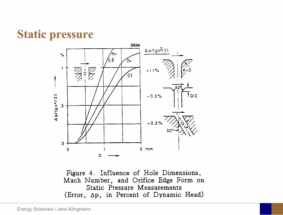
Energy Sciences Jens Klingmann
Static pressure
Energy Sciences Jens Klingmann
Total Pressure and Temperature
Shrouded Probes
Shrouded Probe
Pitot or Prandtl tube
Sensitive to direction
Energy Sciences Jens Klingmann
Ludwig Prandtl 1875-1953
Ludwig Prandtl born at Freising Bavaria on February 4 1875 was a German Physicist famous for his work in aeronautics He qualified at Munchen in 1900 with a thesis on elastic stability and held the position of Professor of Applied Mechanics at Gottingen for forty-nine years (from 1904 until his death there on August 15 1953) In 1925 Prandtl became the Director of the Kaiser Wilhelm Institute for Fluid Mechanics His discovery in 1904 of the Boundary Layer which adjoins the surface of a body moving in a fluid led to an understanding of skin friction drag and of the way in which streamlining reduces the drag of airplane wings and other moving bodies His work on wing theory published in 1918 - 1919 followed that of FW Lanchester (1902-1907) but was carried out independently and elucidated the flow over airplane wings of finite span Prandtls work and decisive advances in boundary layer and wing theories became the basic material of aeronautics He also made important contributions to the theories of supersonic flow and of turbulence and contributed much to the development of wind tunnels and other aerodynamic equipment In addition he devised the soap-film analogy for the torsion of non-circular sections and wrote on the theory of plasticity and of meteorology
Energy Sciences Jens Klingmann
Total Pressure multy hole
Cobra Probe Yaw Probe
5 Hole Probe
Energy Sciences Jens Klingmann
5 Hole Probes Calibration
Energy Sciences Jens Klingmann
The inherent unsteadiness of the flow within turbomachines
Energy Sciences Jens Klingmann
Hot Wire Anemometry (HWA) The heat transfer from a thin (one micron)
electrically heated wire can be used to determine velocity
The resistance of the wire is temperature dependent Within a small temperature range it can be assumed linear R = R0+α R0(Tm-T0) where R0 is the resistance at a reference temperature T0 and Tm is the mean wire temperature
The thermal power induced in the wire is balanced by heat transfer to the surrounding fluid I2R=hπDL(Tm-T0) where h is the heat transfer coefficient and D and L the diameter and length of the wire respectively
E = I R
Energy Sciences Jens Klingmann
Constant Temperature Anemometry (CTA) The wire is often placed in a Whetstone bridge If the output from the
bridge is amplified and fed back to the bridge the resistance of the probe and thus the temperature will be held constant
This prevents the temperature of the wire to become excessive at low velocities
R1
R2 R3
Probe
Bridge Voltage
Energy Sciences Jens Klingmann
Constant Temperature Anemometry (CTA)
Energy Sciences Jens Klingmann
Characteristics of LDA (according to Dantec)
Invented by Yeh and Cummins in 1964 Velocity measurements in Fluid Dynamics (gas liquid) Up to 3 velocity components Non-intrusive measurements (optical technique) Absolute measurement technique (no calibration required) Very high accuracy Very high spatial resolution due to small measurement volume Tracer particles are required
Energy Sciences Jens Klingmann
LDA - Fringe Model
Focused Laser beams intersect and form the measurement volume Plane wave fronts beam waist in the plane of intersection Interference in the plane of intersection Pattern of bright and dark stripesplanes Fringes
Energy Sciences Jens Klingmann
LDA-measuring volume
d
x
x
y
y
z
z
e-2 CONTOUR
FRINGES
κ
κ
κ
κ
De-2
De-2
dml m
a
b
cx
b
z
ya
cd
d
=
=
=
J
J
J
J
JP
JP
JP
JD
JD
JD
+
+
+
a
b
c
d
κπλ
=minus sinD
f4l2e
m
κπλ
=minus cosD
f4D2e
m
Energy Sciences Jens Klingmann
Laser Two Focus
Energy Sciences Jens Klingmann
Laser Two Focus
Energy Sciences Jens Klingmann
PIV measurements
PIV is a fairly new technique capable of simultaneous velocity measurements at many points in a plane This gives information on large scale structures vorticity etc which is very difficult or impossible to obtain from one-point measuring techniques
PIV involves the illumination of a plane of the flow under investigation with a thin pulsed sheet of light The flow is seeded with particles
The light scattered from the particles and from successive pulses are being recorded either on film or a CCD array forming a multiple exposure of each particle image If the time between the pulses is known velocity can be determined as the ratio of the particle displacement and the elapsed time
t∆∆= xu
Energy Sciences Jens Klingmann
PIV
Energy Sciences Jens Klingmann
PIV measurements illumination
YA
G
YA
G
Two frequency doubled YAG Lasers aligned to one double pulsed laser sheet
Two or more separate light pulses can be obtained by chopping a continuous laser or from pulsed lasers
The limited pulse energies obtained from continuous lasers limits their applicability to low velocity flows or flows where large seeding particles can be used (ie liquid flows)
The low repetition rate of most pulsed lasers makes the use of two lasers advantageous
Energy Sciences Jens Klingmann
PIV measurements recording
High seeding density in laminar flame
Film or CCD-cameras Cross- or Auto-correlation
ndash ie both particle images on the same frame or on separate frames
CCD-camera requirementndash A many pixels as possiblendash 2k by 2k available 4k by 4k coming
Energy Sciences Jens Klingmann
PIV measurements analyses
Low seeding density (Number of seeding particles per unit volume)
Each particle image pair can be identified This is called particle tracking
High seeding density (PIV)
Small sub-regions of the image containing many particle image pairs are processed to obtain one velocity vector
Energy Sciences Jens Klingmann
PIV measurements analyses
Energy Sciences Jens Klingmann
PIV measurements analyses
( ) ( ) ( ) xsxxs dIIR 2A
1
I
+= int
Cross correlation between ( )x1I and ( )x2I
s is a two dimensional displacement vector
IA is the interrogation area
Cross correlation between
(
)
x
1
I
and
(
)
x
2
I
s is a two dimensional displacement vector
I
A
is the interrogation area
Energy Sciences Jens Klingmann
Energy Sciences Jens Klingmann
PIV from IOWA state university
Energy Sciences Jens Klingmann
PIV sample of evaluation
Energy Sciences Jens Klingmann
LDA PIV HWA Velocity range 01 mms ndash 300
ms 02 ndash 150 ms
Measuring Volume
D = 005 L = 05 mm
2 by 2 by 05 mm
L = 05 mm
Freq response O(10 000) Hz O(10) Hz O(100 000) Hz Calibration Yes No No Sensitivity to other than velocity
Low (ref Index) Low (ref Index) Large (temperature concentrationshellip)
Continuous Signal
Sometimes Seldom Always
Noise High High Low Turbulence intensity
No limitation Some limitation lt 20
Price O(1 000 000) SEK
O(1 000 000) SEK
O(50 000) SEK
Required Knowledge
High medium Low
Comparison of techniques
Energy Sciences Jens Klingmann
References experiments
R J Goldstein ldquoFluid Mechanics Measurementsrdquo Hemisphere Publishing 1983 A V Johansson amp P H Alfredsson ldquoExperimentella metoder inom
stroumlmningsmekanikenrdquo Inst Foumlr Mekanik KTH F Durst A Melling and J H Whitelaw ldquoPrincipals and Practice of Laser Doppler
Anemometryrdquo 1984 R J Adrian ldquoParticle-imaging techniques for experimental fluid mechnicsrdquo Ann Rev
Fluid Mech 1991
Energy Sciences Jens Klingmann
Sample of LDA-measurements
Rotor blade
Glas window
Emitted beams
Scattered Light
Adjustable mirror
Energy Sciences Jens Klingmann
Axial velocity sorted into 10 bins
0 1 2 3 4 5 6tangential coordinate (degrees)
-20
0
20
40
60
80
100
120
140
160Ax
ial v
eloc
ity a
nd s
tand
ard
devi
atio
n (m
s)
radial position 7 mm from inner window surfaceaxial position 23 mm behind rotor blades
Energy Sciences Jens Klingmann
Axial velocities in the radial-tangential plane
Energy Sciences Jens Klingmann
Airfoils NACA 4-digit
The NACA four-digit wing sections define the profile by
One digit describing maximum camber as percentage of the chord
One digit describing the distance of maximum camber from the airfoil leading edge in tens of percents of the chord
Two digits describing maximum thickness of the airfoil as percent of the chord
Example the NACA 2412 airfoil has a maximum camber of 2 located 40 (04 chords) from the leading edge with a maximum thickness of 12 of the chord
Four-digit series airfoils by default have maximum thickness at 30 of the chord (03 chords) from the leading edge
Energy Sciences Jens Klingmann
Airfoils NACA 4-digit
bull c is the chord lengthbull x is the position along
the chord from 0 to cbull y is the half thickness at
a given value of x (centerline to surface)
bull t is the maximum thickness as a fraction of the chord
Energy Sciences Jens Klingmann
Death by PowerPoint
| LDA | PIV | HWA | |||||
| Velocity range | 01 mms ndash 300 ms | 02 ndash 150 ms | |||||
| Measuring Volume | D = 005 L = 05 mm | 2 by 2 by 05 mm | L = 05 mm | ||||
| Freq response | O(10 000) Hz | O(10) Hz | O(100 000) Hz | ||||
| Calibration | Yes | No | No | ||||
| Sensitivity to other than velocity | Low (ref Index) | Low (ref Index) | Large (temperature concentrationshellip) | ||||
| Continuous Signal | Sometimes | Seldom | Always | ||||
| Noise | High | High | Low | ||||
| Turbulence intensity | No limitation | Some limitation | lt 20 | ||||
| Price | O(1 000 000) SEK | O(1 000 000) SEK | O(50 000) SEK | ||||
| Required Knowledge | High | medium | Low |
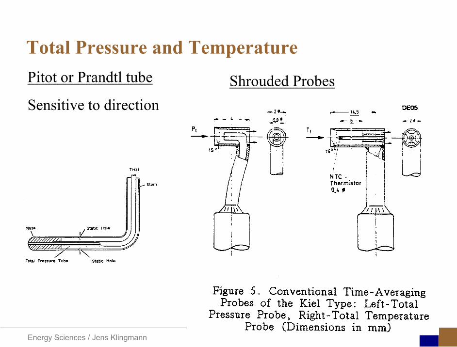
Energy Sciences Jens Klingmann
Ludwig Prandtl 1875-1953
Ludwig Prandtl born at Freising Bavaria on February 4 1875 was a German Physicist famous for his work in aeronautics He qualified at Munchen in 1900 with a thesis on elastic stability and held the position of Professor of Applied Mechanics at Gottingen for forty-nine years (from 1904 until his death there on August 15 1953) In 1925 Prandtl became the Director of the Kaiser Wilhelm Institute for Fluid Mechanics His discovery in 1904 of the Boundary Layer which adjoins the surface of a body moving in a fluid led to an understanding of skin friction drag and of the way in which streamlining reduces the drag of airplane wings and other moving bodies His work on wing theory published in 1918 - 1919 followed that of FW Lanchester (1902-1907) but was carried out independently and elucidated the flow over airplane wings of finite span Prandtls work and decisive advances in boundary layer and wing theories became the basic material of aeronautics He also made important contributions to the theories of supersonic flow and of turbulence and contributed much to the development of wind tunnels and other aerodynamic equipment In addition he devised the soap-film analogy for the torsion of non-circular sections and wrote on the theory of plasticity and of meteorology
Energy Sciences Jens Klingmann
Total Pressure multy hole
Cobra Probe Yaw Probe
5 Hole Probe
Energy Sciences Jens Klingmann
5 Hole Probes Calibration
Energy Sciences Jens Klingmann
The inherent unsteadiness of the flow within turbomachines
Energy Sciences Jens Klingmann
Hot Wire Anemometry (HWA) The heat transfer from a thin (one micron)
electrically heated wire can be used to determine velocity
The resistance of the wire is temperature dependent Within a small temperature range it can be assumed linear R = R0+α R0(Tm-T0) where R0 is the resistance at a reference temperature T0 and Tm is the mean wire temperature
The thermal power induced in the wire is balanced by heat transfer to the surrounding fluid I2R=hπDL(Tm-T0) where h is the heat transfer coefficient and D and L the diameter and length of the wire respectively
E = I R
Energy Sciences Jens Klingmann
Constant Temperature Anemometry (CTA) The wire is often placed in a Whetstone bridge If the output from the
bridge is amplified and fed back to the bridge the resistance of the probe and thus the temperature will be held constant
This prevents the temperature of the wire to become excessive at low velocities
R1
R2 R3
Probe
Bridge Voltage
Energy Sciences Jens Klingmann
Constant Temperature Anemometry (CTA)
Energy Sciences Jens Klingmann
Characteristics of LDA (according to Dantec)
Invented by Yeh and Cummins in 1964 Velocity measurements in Fluid Dynamics (gas liquid) Up to 3 velocity components Non-intrusive measurements (optical technique) Absolute measurement technique (no calibration required) Very high accuracy Very high spatial resolution due to small measurement volume Tracer particles are required
Energy Sciences Jens Klingmann
LDA - Fringe Model
Focused Laser beams intersect and form the measurement volume Plane wave fronts beam waist in the plane of intersection Interference in the plane of intersection Pattern of bright and dark stripesplanes Fringes
Energy Sciences Jens Klingmann
LDA-measuring volume
d
x
x
y
y
z
z
e-2 CONTOUR
FRINGES
κ
κ
κ
κ
De-2
De-2
dml m
a
b
cx
b
z
ya
cd
d
=
=
=
J
J
J
J
JP
JP
JP
JD
JD
JD
+
+
+
a
b
c
d
κπλ
=minus sinD
f4l2e
m
κπλ
=minus cosD
f4D2e
m
Energy Sciences Jens Klingmann
Laser Two Focus
Energy Sciences Jens Klingmann
Laser Two Focus
Energy Sciences Jens Klingmann
PIV measurements
PIV is a fairly new technique capable of simultaneous velocity measurements at many points in a plane This gives information on large scale structures vorticity etc which is very difficult or impossible to obtain from one-point measuring techniques
PIV involves the illumination of a plane of the flow under investigation with a thin pulsed sheet of light The flow is seeded with particles
The light scattered from the particles and from successive pulses are being recorded either on film or a CCD array forming a multiple exposure of each particle image If the time between the pulses is known velocity can be determined as the ratio of the particle displacement and the elapsed time
t∆∆= xu
Energy Sciences Jens Klingmann
PIV
Energy Sciences Jens Klingmann
PIV measurements illumination
YA
G
YA
G
Two frequency doubled YAG Lasers aligned to one double pulsed laser sheet
Two or more separate light pulses can be obtained by chopping a continuous laser or from pulsed lasers
The limited pulse energies obtained from continuous lasers limits their applicability to low velocity flows or flows where large seeding particles can be used (ie liquid flows)
The low repetition rate of most pulsed lasers makes the use of two lasers advantageous
Energy Sciences Jens Klingmann
PIV measurements recording
High seeding density in laminar flame
Film or CCD-cameras Cross- or Auto-correlation
ndash ie both particle images on the same frame or on separate frames
CCD-camera requirementndash A many pixels as possiblendash 2k by 2k available 4k by 4k coming
Energy Sciences Jens Klingmann
PIV measurements analyses
Low seeding density (Number of seeding particles per unit volume)
Each particle image pair can be identified This is called particle tracking
High seeding density (PIV)
Small sub-regions of the image containing many particle image pairs are processed to obtain one velocity vector
Energy Sciences Jens Klingmann
PIV measurements analyses
Energy Sciences Jens Klingmann
PIV measurements analyses
( ) ( ) ( ) xsxxs dIIR 2A
1
I
+= int
Cross correlation between ( )x1I and ( )x2I
s is a two dimensional displacement vector
IA is the interrogation area
Cross correlation between
(
)
x
1
I
and
(
)
x
2
I
s is a two dimensional displacement vector
I
A
is the interrogation area
Energy Sciences Jens Klingmann
Energy Sciences Jens Klingmann
PIV from IOWA state university
Energy Sciences Jens Klingmann
PIV sample of evaluation
Energy Sciences Jens Klingmann
LDA PIV HWA Velocity range 01 mms ndash 300
ms 02 ndash 150 ms
Measuring Volume
D = 005 L = 05 mm
2 by 2 by 05 mm
L = 05 mm
Freq response O(10 000) Hz O(10) Hz O(100 000) Hz Calibration Yes No No Sensitivity to other than velocity
Low (ref Index) Low (ref Index) Large (temperature concentrationshellip)
Continuous Signal
Sometimes Seldom Always
Noise High High Low Turbulence intensity
No limitation Some limitation lt 20
Price O(1 000 000) SEK
O(1 000 000) SEK
O(50 000) SEK
Required Knowledge
High medium Low
Comparison of techniques
Energy Sciences Jens Klingmann
References experiments
R J Goldstein ldquoFluid Mechanics Measurementsrdquo Hemisphere Publishing 1983 A V Johansson amp P H Alfredsson ldquoExperimentella metoder inom
stroumlmningsmekanikenrdquo Inst Foumlr Mekanik KTH F Durst A Melling and J H Whitelaw ldquoPrincipals and Practice of Laser Doppler
Anemometryrdquo 1984 R J Adrian ldquoParticle-imaging techniques for experimental fluid mechnicsrdquo Ann Rev
Fluid Mech 1991
Energy Sciences Jens Klingmann
Sample of LDA-measurements
Rotor blade
Glas window
Emitted beams
Scattered Light
Adjustable mirror
Energy Sciences Jens Klingmann
Axial velocity sorted into 10 bins
0 1 2 3 4 5 6tangential coordinate (degrees)
-20
0
20
40
60
80
100
120
140
160Ax
ial v
eloc
ity a
nd s
tand
ard
devi
atio
n (m
s)
radial position 7 mm from inner window surfaceaxial position 23 mm behind rotor blades
Energy Sciences Jens Klingmann
Axial velocities in the radial-tangential plane
Energy Sciences Jens Klingmann
Airfoils NACA 4-digit
The NACA four-digit wing sections define the profile by
One digit describing maximum camber as percentage of the chord
One digit describing the distance of maximum camber from the airfoil leading edge in tens of percents of the chord
Two digits describing maximum thickness of the airfoil as percent of the chord
Example the NACA 2412 airfoil has a maximum camber of 2 located 40 (04 chords) from the leading edge with a maximum thickness of 12 of the chord
Four-digit series airfoils by default have maximum thickness at 30 of the chord (03 chords) from the leading edge
Energy Sciences Jens Klingmann
Airfoils NACA 4-digit
bull c is the chord lengthbull x is the position along
the chord from 0 to cbull y is the half thickness at
a given value of x (centerline to surface)
bull t is the maximum thickness as a fraction of the chord
Energy Sciences Jens Klingmann
Death by PowerPoint
| LDA | PIV | HWA | |||||
| Velocity range | 01 mms ndash 300 ms | 02 ndash 150 ms | |||||
| Measuring Volume | D = 005 L = 05 mm | 2 by 2 by 05 mm | L = 05 mm | ||||
| Freq response | O(10 000) Hz | O(10) Hz | O(100 000) Hz | ||||
| Calibration | Yes | No | No | ||||
| Sensitivity to other than velocity | Low (ref Index) | Low (ref Index) | Large (temperature concentrationshellip) | ||||
| Continuous Signal | Sometimes | Seldom | Always | ||||
| Noise | High | High | Low | ||||
| Turbulence intensity | No limitation | Some limitation | lt 20 | ||||
| Price | O(1 000 000) SEK | O(1 000 000) SEK | O(50 000) SEK | ||||
| Required Knowledge | High | medium | Low |
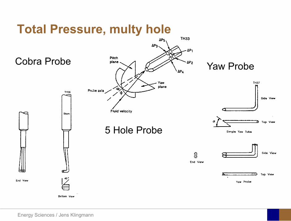
Energy Sciences Jens Klingmann
Total Pressure multy hole
Cobra Probe Yaw Probe
5 Hole Probe
Energy Sciences Jens Klingmann
5 Hole Probes Calibration
Energy Sciences Jens Klingmann
The inherent unsteadiness of the flow within turbomachines
Energy Sciences Jens Klingmann
Hot Wire Anemometry (HWA) The heat transfer from a thin (one micron)
electrically heated wire can be used to determine velocity
The resistance of the wire is temperature dependent Within a small temperature range it can be assumed linear R = R0+α R0(Tm-T0) where R0 is the resistance at a reference temperature T0 and Tm is the mean wire temperature
The thermal power induced in the wire is balanced by heat transfer to the surrounding fluid I2R=hπDL(Tm-T0) where h is the heat transfer coefficient and D and L the diameter and length of the wire respectively
E = I R
Energy Sciences Jens Klingmann
Constant Temperature Anemometry (CTA) The wire is often placed in a Whetstone bridge If the output from the
bridge is amplified and fed back to the bridge the resistance of the probe and thus the temperature will be held constant
This prevents the temperature of the wire to become excessive at low velocities
R1
R2 R3
Probe
Bridge Voltage
Energy Sciences Jens Klingmann
Constant Temperature Anemometry (CTA)
Energy Sciences Jens Klingmann
Characteristics of LDA (according to Dantec)
Invented by Yeh and Cummins in 1964 Velocity measurements in Fluid Dynamics (gas liquid) Up to 3 velocity components Non-intrusive measurements (optical technique) Absolute measurement technique (no calibration required) Very high accuracy Very high spatial resolution due to small measurement volume Tracer particles are required
Energy Sciences Jens Klingmann
LDA - Fringe Model
Focused Laser beams intersect and form the measurement volume Plane wave fronts beam waist in the plane of intersection Interference in the plane of intersection Pattern of bright and dark stripesplanes Fringes
Energy Sciences Jens Klingmann
LDA-measuring volume
d
x
x
y
y
z
z
e-2 CONTOUR
FRINGES
κ
κ
κ
κ
De-2
De-2
dml m
a
b
cx
b
z
ya
cd
d
=
=
=
J
J
J
J
JP
JP
JP
JD
JD
JD
+
+
+
a
b
c
d
κπλ
=minus sinD
f4l2e
m
κπλ
=minus cosD
f4D2e
m
Energy Sciences Jens Klingmann
Laser Two Focus
Energy Sciences Jens Klingmann
Laser Two Focus
Energy Sciences Jens Klingmann
PIV measurements
PIV is a fairly new technique capable of simultaneous velocity measurements at many points in a plane This gives information on large scale structures vorticity etc which is very difficult or impossible to obtain from one-point measuring techniques
PIV involves the illumination of a plane of the flow under investigation with a thin pulsed sheet of light The flow is seeded with particles
The light scattered from the particles and from successive pulses are being recorded either on film or a CCD array forming a multiple exposure of each particle image If the time between the pulses is known velocity can be determined as the ratio of the particle displacement and the elapsed time
t∆∆= xu
Energy Sciences Jens Klingmann
PIV
Energy Sciences Jens Klingmann
PIV measurements illumination
YA
G
YA
G
Two frequency doubled YAG Lasers aligned to one double pulsed laser sheet
Two or more separate light pulses can be obtained by chopping a continuous laser or from pulsed lasers
The limited pulse energies obtained from continuous lasers limits their applicability to low velocity flows or flows where large seeding particles can be used (ie liquid flows)
The low repetition rate of most pulsed lasers makes the use of two lasers advantageous
Energy Sciences Jens Klingmann
PIV measurements recording
High seeding density in laminar flame
Film or CCD-cameras Cross- or Auto-correlation
ndash ie both particle images on the same frame or on separate frames
CCD-camera requirementndash A many pixels as possiblendash 2k by 2k available 4k by 4k coming
Energy Sciences Jens Klingmann
PIV measurements analyses
Low seeding density (Number of seeding particles per unit volume)
Each particle image pair can be identified This is called particle tracking
High seeding density (PIV)
Small sub-regions of the image containing many particle image pairs are processed to obtain one velocity vector
Energy Sciences Jens Klingmann
PIV measurements analyses
Energy Sciences Jens Klingmann
PIV measurements analyses
( ) ( ) ( ) xsxxs dIIR 2A
1
I
+= int
Cross correlation between ( )x1I and ( )x2I
s is a two dimensional displacement vector
IA is the interrogation area
Cross correlation between
(
)
x
1
I
and
(
)
x
2
I
s is a two dimensional displacement vector
I
A
is the interrogation area
Energy Sciences Jens Klingmann
Energy Sciences Jens Klingmann
PIV from IOWA state university
Energy Sciences Jens Klingmann
PIV sample of evaluation
Energy Sciences Jens Klingmann
LDA PIV HWA Velocity range 01 mms ndash 300
ms 02 ndash 150 ms
Measuring Volume
D = 005 L = 05 mm
2 by 2 by 05 mm
L = 05 mm
Freq response O(10 000) Hz O(10) Hz O(100 000) Hz Calibration Yes No No Sensitivity to other than velocity
Low (ref Index) Low (ref Index) Large (temperature concentrationshellip)
Continuous Signal
Sometimes Seldom Always
Noise High High Low Turbulence intensity
No limitation Some limitation lt 20
Price O(1 000 000) SEK
O(1 000 000) SEK
O(50 000) SEK
Required Knowledge
High medium Low
Comparison of techniques
Energy Sciences Jens Klingmann
References experiments
R J Goldstein ldquoFluid Mechanics Measurementsrdquo Hemisphere Publishing 1983 A V Johansson amp P H Alfredsson ldquoExperimentella metoder inom
stroumlmningsmekanikenrdquo Inst Foumlr Mekanik KTH F Durst A Melling and J H Whitelaw ldquoPrincipals and Practice of Laser Doppler
Anemometryrdquo 1984 R J Adrian ldquoParticle-imaging techniques for experimental fluid mechnicsrdquo Ann Rev
Fluid Mech 1991
Energy Sciences Jens Klingmann
Sample of LDA-measurements
Rotor blade
Glas window
Emitted beams
Scattered Light
Adjustable mirror
Energy Sciences Jens Klingmann
Axial velocity sorted into 10 bins
0 1 2 3 4 5 6tangential coordinate (degrees)
-20
0
20
40
60
80
100
120
140
160Ax
ial v
eloc
ity a
nd s
tand
ard
devi
atio
n (m
s)
radial position 7 mm from inner window surfaceaxial position 23 mm behind rotor blades
Energy Sciences Jens Klingmann
Axial velocities in the radial-tangential plane
Energy Sciences Jens Klingmann
Airfoils NACA 4-digit
The NACA four-digit wing sections define the profile by
One digit describing maximum camber as percentage of the chord
One digit describing the distance of maximum camber from the airfoil leading edge in tens of percents of the chord
Two digits describing maximum thickness of the airfoil as percent of the chord
Example the NACA 2412 airfoil has a maximum camber of 2 located 40 (04 chords) from the leading edge with a maximum thickness of 12 of the chord
Four-digit series airfoils by default have maximum thickness at 30 of the chord (03 chords) from the leading edge
Energy Sciences Jens Klingmann
Airfoils NACA 4-digit
bull c is the chord lengthbull x is the position along
the chord from 0 to cbull y is the half thickness at
a given value of x (centerline to surface)
bull t is the maximum thickness as a fraction of the chord
Energy Sciences Jens Klingmann
Death by PowerPoint
| LDA | PIV | HWA | |||||
| Velocity range | 01 mms ndash 300 ms | 02 ndash 150 ms | |||||
| Measuring Volume | D = 005 L = 05 mm | 2 by 2 by 05 mm | L = 05 mm | ||||
| Freq response | O(10 000) Hz | O(10) Hz | O(100 000) Hz | ||||
| Calibration | Yes | No | No | ||||
| Sensitivity to other than velocity | Low (ref Index) | Low (ref Index) | Large (temperature concentrationshellip) | ||||
| Continuous Signal | Sometimes | Seldom | Always | ||||
| Noise | High | High | Low | ||||
| Turbulence intensity | No limitation | Some limitation | lt 20 | ||||
| Price | O(1 000 000) SEK | O(1 000 000) SEK | O(50 000) SEK | ||||
| Required Knowledge | High | medium | Low |
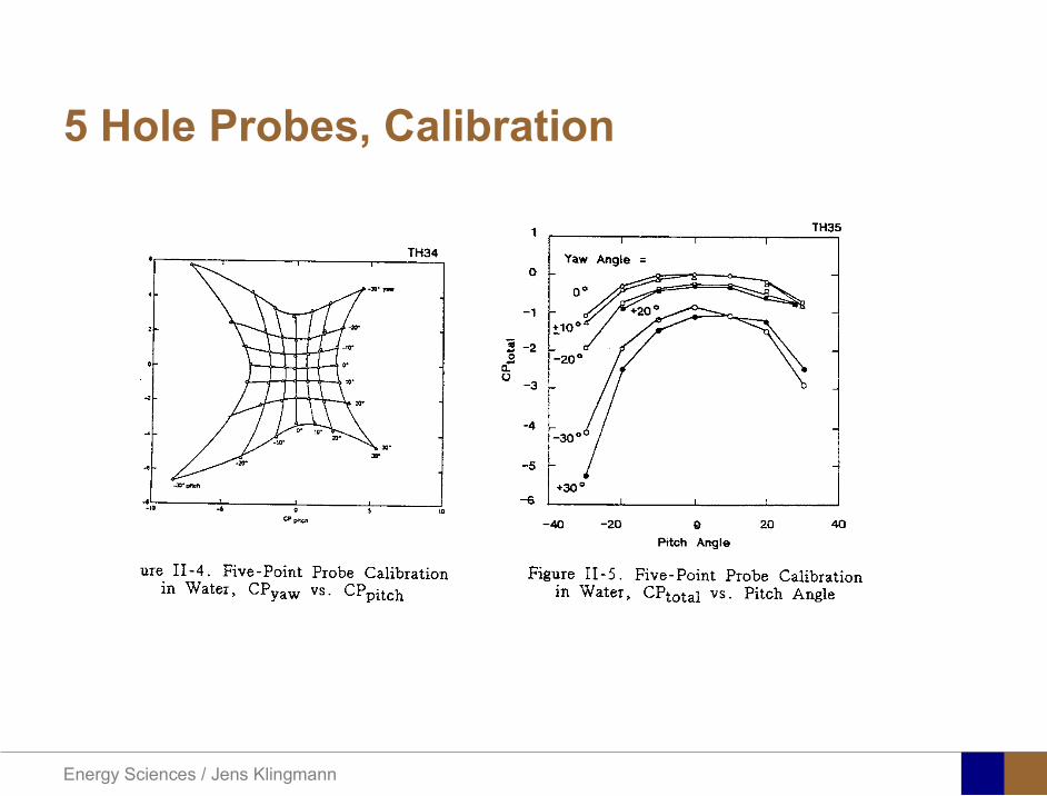
Energy Sciences Jens Klingmann
5 Hole Probes Calibration
Energy Sciences Jens Klingmann
The inherent unsteadiness of the flow within turbomachines
Energy Sciences Jens Klingmann
Hot Wire Anemometry (HWA) The heat transfer from a thin (one micron)
electrically heated wire can be used to determine velocity
The resistance of the wire is temperature dependent Within a small temperature range it can be assumed linear R = R0+α R0(Tm-T0) where R0 is the resistance at a reference temperature T0 and Tm is the mean wire temperature
The thermal power induced in the wire is balanced by heat transfer to the surrounding fluid I2R=hπDL(Tm-T0) where h is the heat transfer coefficient and D and L the diameter and length of the wire respectively
E = I R
Energy Sciences Jens Klingmann
Constant Temperature Anemometry (CTA) The wire is often placed in a Whetstone bridge If the output from the
bridge is amplified and fed back to the bridge the resistance of the probe and thus the temperature will be held constant
This prevents the temperature of the wire to become excessive at low velocities
R1
R2 R3
Probe
Bridge Voltage
Energy Sciences Jens Klingmann
Constant Temperature Anemometry (CTA)
Energy Sciences Jens Klingmann
Characteristics of LDA (according to Dantec)
Invented by Yeh and Cummins in 1964 Velocity measurements in Fluid Dynamics (gas liquid) Up to 3 velocity components Non-intrusive measurements (optical technique) Absolute measurement technique (no calibration required) Very high accuracy Very high spatial resolution due to small measurement volume Tracer particles are required
Energy Sciences Jens Klingmann
LDA - Fringe Model
Focused Laser beams intersect and form the measurement volume Plane wave fronts beam waist in the plane of intersection Interference in the plane of intersection Pattern of bright and dark stripesplanes Fringes
Energy Sciences Jens Klingmann
LDA-measuring volume
d
x
x
y
y
z
z
e-2 CONTOUR
FRINGES
κ
κ
κ
κ
De-2
De-2
dml m
a
b
cx
b
z
ya
cd
d
=
=
=
J
J
J
J
JP
JP
JP
JD
JD
JD
+
+
+
a
b
c
d
κπλ
=minus sinD
f4l2e
m
κπλ
=minus cosD
f4D2e
m
Energy Sciences Jens Klingmann
Laser Two Focus
Energy Sciences Jens Klingmann
Laser Two Focus
Energy Sciences Jens Klingmann
PIV measurements
PIV is a fairly new technique capable of simultaneous velocity measurements at many points in a plane This gives information on large scale structures vorticity etc which is very difficult or impossible to obtain from one-point measuring techniques
PIV involves the illumination of a plane of the flow under investigation with a thin pulsed sheet of light The flow is seeded with particles
The light scattered from the particles and from successive pulses are being recorded either on film or a CCD array forming a multiple exposure of each particle image If the time between the pulses is known velocity can be determined as the ratio of the particle displacement and the elapsed time
t∆∆= xu
Energy Sciences Jens Klingmann
PIV
Energy Sciences Jens Klingmann
PIV measurements illumination
YA
G
YA
G
Two frequency doubled YAG Lasers aligned to one double pulsed laser sheet
Two or more separate light pulses can be obtained by chopping a continuous laser or from pulsed lasers
The limited pulse energies obtained from continuous lasers limits their applicability to low velocity flows or flows where large seeding particles can be used (ie liquid flows)
The low repetition rate of most pulsed lasers makes the use of two lasers advantageous
Energy Sciences Jens Klingmann
PIV measurements recording
High seeding density in laminar flame
Film or CCD-cameras Cross- or Auto-correlation
ndash ie both particle images on the same frame or on separate frames
CCD-camera requirementndash A many pixels as possiblendash 2k by 2k available 4k by 4k coming
Energy Sciences Jens Klingmann
PIV measurements analyses
Low seeding density (Number of seeding particles per unit volume)
Each particle image pair can be identified This is called particle tracking
High seeding density (PIV)
Small sub-regions of the image containing many particle image pairs are processed to obtain one velocity vector
Energy Sciences Jens Klingmann
PIV measurements analyses
Energy Sciences Jens Klingmann
PIV measurements analyses
( ) ( ) ( ) xsxxs dIIR 2A
1
I
+= int
Cross correlation between ( )x1I and ( )x2I
s is a two dimensional displacement vector
IA is the interrogation area
Cross correlation between
(
)
x
1
I
and
(
)
x
2
I
s is a two dimensional displacement vector
I
A
is the interrogation area
Energy Sciences Jens Klingmann
Energy Sciences Jens Klingmann
PIV from IOWA state university
Energy Sciences Jens Klingmann
PIV sample of evaluation
Energy Sciences Jens Klingmann
LDA PIV HWA Velocity range 01 mms ndash 300
ms 02 ndash 150 ms
Measuring Volume
D = 005 L = 05 mm
2 by 2 by 05 mm
L = 05 mm
Freq response O(10 000) Hz O(10) Hz O(100 000) Hz Calibration Yes No No Sensitivity to other than velocity
Low (ref Index) Low (ref Index) Large (temperature concentrationshellip)
Continuous Signal
Sometimes Seldom Always
Noise High High Low Turbulence intensity
No limitation Some limitation lt 20
Price O(1 000 000) SEK
O(1 000 000) SEK
O(50 000) SEK
Required Knowledge
High medium Low
Comparison of techniques
Energy Sciences Jens Klingmann
References experiments
R J Goldstein ldquoFluid Mechanics Measurementsrdquo Hemisphere Publishing 1983 A V Johansson amp P H Alfredsson ldquoExperimentella metoder inom
stroumlmningsmekanikenrdquo Inst Foumlr Mekanik KTH F Durst A Melling and J H Whitelaw ldquoPrincipals and Practice of Laser Doppler
Anemometryrdquo 1984 R J Adrian ldquoParticle-imaging techniques for experimental fluid mechnicsrdquo Ann Rev
Fluid Mech 1991
Energy Sciences Jens Klingmann
Sample of LDA-measurements
Rotor blade
Glas window
Emitted beams
Scattered Light
Adjustable mirror
Energy Sciences Jens Klingmann
Axial velocity sorted into 10 bins
0 1 2 3 4 5 6tangential coordinate (degrees)
-20
0
20
40
60
80
100
120
140
160Ax
ial v
eloc
ity a
nd s
tand
ard
devi
atio
n (m
s)
radial position 7 mm from inner window surfaceaxial position 23 mm behind rotor blades
Energy Sciences Jens Klingmann
Axial velocities in the radial-tangential plane
Energy Sciences Jens Klingmann
Airfoils NACA 4-digit
The NACA four-digit wing sections define the profile by
One digit describing maximum camber as percentage of the chord
One digit describing the distance of maximum camber from the airfoil leading edge in tens of percents of the chord
Two digits describing maximum thickness of the airfoil as percent of the chord
Example the NACA 2412 airfoil has a maximum camber of 2 located 40 (04 chords) from the leading edge with a maximum thickness of 12 of the chord
Four-digit series airfoils by default have maximum thickness at 30 of the chord (03 chords) from the leading edge
Energy Sciences Jens Klingmann
Airfoils NACA 4-digit
bull c is the chord lengthbull x is the position along
the chord from 0 to cbull y is the half thickness at
a given value of x (centerline to surface)
bull t is the maximum thickness as a fraction of the chord
Energy Sciences Jens Klingmann
Death by PowerPoint
| LDA | PIV | HWA | |||||
| Velocity range | 01 mms ndash 300 ms | 02 ndash 150 ms | |||||
| Measuring Volume | D = 005 L = 05 mm | 2 by 2 by 05 mm | L = 05 mm | ||||
| Freq response | O(10 000) Hz | O(10) Hz | O(100 000) Hz | ||||
| Calibration | Yes | No | No | ||||
| Sensitivity to other than velocity | Low (ref Index) | Low (ref Index) | Large (temperature concentrationshellip) | ||||
| Continuous Signal | Sometimes | Seldom | Always | ||||
| Noise | High | High | Low | ||||
| Turbulence intensity | No limitation | Some limitation | lt 20 | ||||
| Price | O(1 000 000) SEK | O(1 000 000) SEK | O(50 000) SEK | ||||
| Required Knowledge | High | medium | Low |
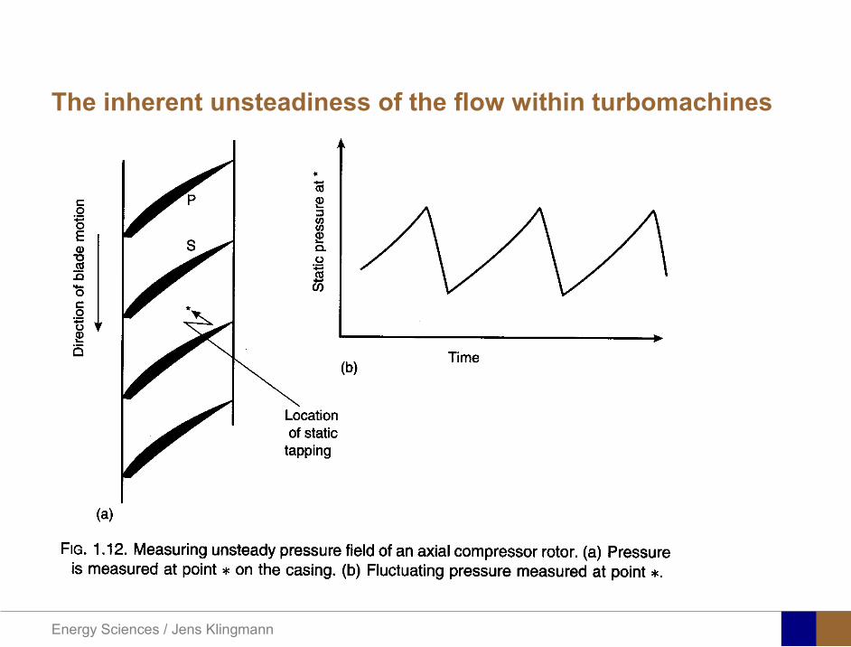
Energy Sciences Jens Klingmann
The inherent unsteadiness of the flow within turbomachines
Energy Sciences Jens Klingmann
Hot Wire Anemometry (HWA) The heat transfer from a thin (one micron)
electrically heated wire can be used to determine velocity
The resistance of the wire is temperature dependent Within a small temperature range it can be assumed linear R = R0+α R0(Tm-T0) where R0 is the resistance at a reference temperature T0 and Tm is the mean wire temperature
The thermal power induced in the wire is balanced by heat transfer to the surrounding fluid I2R=hπDL(Tm-T0) where h is the heat transfer coefficient and D and L the diameter and length of the wire respectively
E = I R
Energy Sciences Jens Klingmann
Constant Temperature Anemometry (CTA) The wire is often placed in a Whetstone bridge If the output from the
bridge is amplified and fed back to the bridge the resistance of the probe and thus the temperature will be held constant
This prevents the temperature of the wire to become excessive at low velocities
R1
R2 R3
Probe
Bridge Voltage
Energy Sciences Jens Klingmann
Constant Temperature Anemometry (CTA)
Energy Sciences Jens Klingmann
Characteristics of LDA (according to Dantec)
Invented by Yeh and Cummins in 1964 Velocity measurements in Fluid Dynamics (gas liquid) Up to 3 velocity components Non-intrusive measurements (optical technique) Absolute measurement technique (no calibration required) Very high accuracy Very high spatial resolution due to small measurement volume Tracer particles are required
Energy Sciences Jens Klingmann
LDA - Fringe Model
Focused Laser beams intersect and form the measurement volume Plane wave fronts beam waist in the plane of intersection Interference in the plane of intersection Pattern of bright and dark stripesplanes Fringes
Energy Sciences Jens Klingmann
LDA-measuring volume
d
x
x
y
y
z
z
e-2 CONTOUR
FRINGES
κ
κ
κ
κ
De-2
De-2
dml m
a
b
cx
b
z
ya
cd
d
=
=
=
J
J
J
J
JP
JP
JP
JD
JD
JD
+
+
+
a
b
c
d
κπλ
=minus sinD
f4l2e
m
κπλ
=minus cosD
f4D2e
m
Energy Sciences Jens Klingmann
Laser Two Focus
Energy Sciences Jens Klingmann
Laser Two Focus
Energy Sciences Jens Klingmann
PIV measurements
PIV is a fairly new technique capable of simultaneous velocity measurements at many points in a plane This gives information on large scale structures vorticity etc which is very difficult or impossible to obtain from one-point measuring techniques
PIV involves the illumination of a plane of the flow under investigation with a thin pulsed sheet of light The flow is seeded with particles
The light scattered from the particles and from successive pulses are being recorded either on film or a CCD array forming a multiple exposure of each particle image If the time between the pulses is known velocity can be determined as the ratio of the particle displacement and the elapsed time
t∆∆= xu
Energy Sciences Jens Klingmann
PIV
Energy Sciences Jens Klingmann
PIV measurements illumination
YA
G
YA
G
Two frequency doubled YAG Lasers aligned to one double pulsed laser sheet
Two or more separate light pulses can be obtained by chopping a continuous laser or from pulsed lasers
The limited pulse energies obtained from continuous lasers limits their applicability to low velocity flows or flows where large seeding particles can be used (ie liquid flows)
The low repetition rate of most pulsed lasers makes the use of two lasers advantageous
Energy Sciences Jens Klingmann
PIV measurements recording
High seeding density in laminar flame
Film or CCD-cameras Cross- or Auto-correlation
ndash ie both particle images on the same frame or on separate frames
CCD-camera requirementndash A many pixels as possiblendash 2k by 2k available 4k by 4k coming
Energy Sciences Jens Klingmann
PIV measurements analyses
Low seeding density (Number of seeding particles per unit volume)
Each particle image pair can be identified This is called particle tracking
High seeding density (PIV)
Small sub-regions of the image containing many particle image pairs are processed to obtain one velocity vector
Energy Sciences Jens Klingmann
PIV measurements analyses
Energy Sciences Jens Klingmann
PIV measurements analyses
( ) ( ) ( ) xsxxs dIIR 2A
1
I
+= int
Cross correlation between ( )x1I and ( )x2I
s is a two dimensional displacement vector
IA is the interrogation area
Cross correlation between
(
)
x
1
I
and
(
)
x
2
I
s is a two dimensional displacement vector
I
A
is the interrogation area
Energy Sciences Jens Klingmann
Energy Sciences Jens Klingmann
PIV from IOWA state university
Energy Sciences Jens Klingmann
PIV sample of evaluation
Energy Sciences Jens Klingmann
LDA PIV HWA Velocity range 01 mms ndash 300
ms 02 ndash 150 ms
Measuring Volume
D = 005 L = 05 mm
2 by 2 by 05 mm
L = 05 mm
Freq response O(10 000) Hz O(10) Hz O(100 000) Hz Calibration Yes No No Sensitivity to other than velocity
Low (ref Index) Low (ref Index) Large (temperature concentrationshellip)
Continuous Signal
Sometimes Seldom Always
Noise High High Low Turbulence intensity
No limitation Some limitation lt 20
Price O(1 000 000) SEK
O(1 000 000) SEK
O(50 000) SEK
Required Knowledge
High medium Low
Comparison of techniques
Energy Sciences Jens Klingmann
References experiments
R J Goldstein ldquoFluid Mechanics Measurementsrdquo Hemisphere Publishing 1983 A V Johansson amp P H Alfredsson ldquoExperimentella metoder inom
stroumlmningsmekanikenrdquo Inst Foumlr Mekanik KTH F Durst A Melling and J H Whitelaw ldquoPrincipals and Practice of Laser Doppler
Anemometryrdquo 1984 R J Adrian ldquoParticle-imaging techniques for experimental fluid mechnicsrdquo Ann Rev
Fluid Mech 1991
Energy Sciences Jens Klingmann
Sample of LDA-measurements
Rotor blade
Glas window
Emitted beams
Scattered Light
Adjustable mirror
Energy Sciences Jens Klingmann
Axial velocity sorted into 10 bins
0 1 2 3 4 5 6tangential coordinate (degrees)
-20
0
20
40
60
80
100
120
140
160Ax
ial v
eloc
ity a
nd s
tand
ard
devi
atio
n (m
s)
radial position 7 mm from inner window surfaceaxial position 23 mm behind rotor blades
Energy Sciences Jens Klingmann
Axial velocities in the radial-tangential plane
Energy Sciences Jens Klingmann
Airfoils NACA 4-digit
The NACA four-digit wing sections define the profile by
One digit describing maximum camber as percentage of the chord
One digit describing the distance of maximum camber from the airfoil leading edge in tens of percents of the chord
Two digits describing maximum thickness of the airfoil as percent of the chord
Example the NACA 2412 airfoil has a maximum camber of 2 located 40 (04 chords) from the leading edge with a maximum thickness of 12 of the chord
Four-digit series airfoils by default have maximum thickness at 30 of the chord (03 chords) from the leading edge
Energy Sciences Jens Klingmann
Airfoils NACA 4-digit
bull c is the chord lengthbull x is the position along
the chord from 0 to cbull y is the half thickness at
a given value of x (centerline to surface)
bull t is the maximum thickness as a fraction of the chord
Energy Sciences Jens Klingmann
Death by PowerPoint
| LDA | PIV | HWA | |||||
| Velocity range | 01 mms ndash 300 ms | 02 ndash 150 ms | |||||
| Measuring Volume | D = 005 L = 05 mm | 2 by 2 by 05 mm | L = 05 mm | ||||
| Freq response | O(10 000) Hz | O(10) Hz | O(100 000) Hz | ||||
| Calibration | Yes | No | No | ||||
| Sensitivity to other than velocity | Low (ref Index) | Low (ref Index) | Large (temperature concentrationshellip) | ||||
| Continuous Signal | Sometimes | Seldom | Always | ||||
| Noise | High | High | Low | ||||
| Turbulence intensity | No limitation | Some limitation | lt 20 | ||||
| Price | O(1 000 000) SEK | O(1 000 000) SEK | O(50 000) SEK | ||||
| Required Knowledge | High | medium | Low |
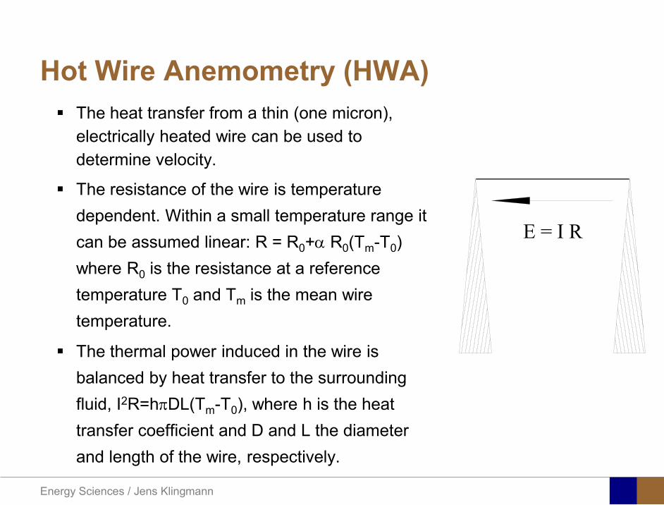
Energy Sciences Jens Klingmann
Hot Wire Anemometry (HWA) The heat transfer from a thin (one micron)
electrically heated wire can be used to determine velocity
The resistance of the wire is temperature dependent Within a small temperature range it can be assumed linear R = R0+α R0(Tm-T0) where R0 is the resistance at a reference temperature T0 and Tm is the mean wire temperature
The thermal power induced in the wire is balanced by heat transfer to the surrounding fluid I2R=hπDL(Tm-T0) where h is the heat transfer coefficient and D and L the diameter and length of the wire respectively
E = I R
Energy Sciences Jens Klingmann
Constant Temperature Anemometry (CTA) The wire is often placed in a Whetstone bridge If the output from the
bridge is amplified and fed back to the bridge the resistance of the probe and thus the temperature will be held constant
This prevents the temperature of the wire to become excessive at low velocities
R1
R2 R3
Probe
Bridge Voltage
Energy Sciences Jens Klingmann
Constant Temperature Anemometry (CTA)
Energy Sciences Jens Klingmann
Characteristics of LDA (according to Dantec)
Invented by Yeh and Cummins in 1964 Velocity measurements in Fluid Dynamics (gas liquid) Up to 3 velocity components Non-intrusive measurements (optical technique) Absolute measurement technique (no calibration required) Very high accuracy Very high spatial resolution due to small measurement volume Tracer particles are required
Energy Sciences Jens Klingmann
LDA - Fringe Model
Focused Laser beams intersect and form the measurement volume Plane wave fronts beam waist in the plane of intersection Interference in the plane of intersection Pattern of bright and dark stripesplanes Fringes
Energy Sciences Jens Klingmann
LDA-measuring volume
d
x
x
y
y
z
z
e-2 CONTOUR
FRINGES
κ
κ
κ
κ
De-2
De-2
dml m
a
b
cx
b
z
ya
cd
d
=
=
=
J
J
J
J
JP
JP
JP
JD
JD
JD
+
+
+
a
b
c
d
κπλ
=minus sinD
f4l2e
m
κπλ
=minus cosD
f4D2e
m
Energy Sciences Jens Klingmann
Laser Two Focus
Energy Sciences Jens Klingmann
Laser Two Focus
Energy Sciences Jens Klingmann
PIV measurements
PIV is a fairly new technique capable of simultaneous velocity measurements at many points in a plane This gives information on large scale structures vorticity etc which is very difficult or impossible to obtain from one-point measuring techniques
PIV involves the illumination of a plane of the flow under investigation with a thin pulsed sheet of light The flow is seeded with particles
The light scattered from the particles and from successive pulses are being recorded either on film or a CCD array forming a multiple exposure of each particle image If the time between the pulses is known velocity can be determined as the ratio of the particle displacement and the elapsed time
t∆∆= xu
Energy Sciences Jens Klingmann
PIV
Energy Sciences Jens Klingmann
PIV measurements illumination
YA
G
YA
G
Two frequency doubled YAG Lasers aligned to one double pulsed laser sheet
Two or more separate light pulses can be obtained by chopping a continuous laser or from pulsed lasers
The limited pulse energies obtained from continuous lasers limits their applicability to low velocity flows or flows where large seeding particles can be used (ie liquid flows)
The low repetition rate of most pulsed lasers makes the use of two lasers advantageous
Energy Sciences Jens Klingmann
PIV measurements recording
High seeding density in laminar flame
Film or CCD-cameras Cross- or Auto-correlation
ndash ie both particle images on the same frame or on separate frames
CCD-camera requirementndash A many pixels as possiblendash 2k by 2k available 4k by 4k coming
Energy Sciences Jens Klingmann
PIV measurements analyses
Low seeding density (Number of seeding particles per unit volume)
Each particle image pair can be identified This is called particle tracking
High seeding density (PIV)
Small sub-regions of the image containing many particle image pairs are processed to obtain one velocity vector
Energy Sciences Jens Klingmann
PIV measurements analyses
Energy Sciences Jens Klingmann
PIV measurements analyses
( ) ( ) ( ) xsxxs dIIR 2A
1
I
+= int
Cross correlation between ( )x1I and ( )x2I
s is a two dimensional displacement vector
IA is the interrogation area
Cross correlation between
(
)
x
1
I
and
(
)
x
2
I
s is a two dimensional displacement vector
I
A
is the interrogation area
Energy Sciences Jens Klingmann
Energy Sciences Jens Klingmann
PIV from IOWA state university
Energy Sciences Jens Klingmann
PIV sample of evaluation
Energy Sciences Jens Klingmann
LDA PIV HWA Velocity range 01 mms ndash 300
ms 02 ndash 150 ms
Measuring Volume
D = 005 L = 05 mm
2 by 2 by 05 mm
L = 05 mm
Freq response O(10 000) Hz O(10) Hz O(100 000) Hz Calibration Yes No No Sensitivity to other than velocity
Low (ref Index) Low (ref Index) Large (temperature concentrationshellip)
Continuous Signal
Sometimes Seldom Always
Noise High High Low Turbulence intensity
No limitation Some limitation lt 20
Price O(1 000 000) SEK
O(1 000 000) SEK
O(50 000) SEK
Required Knowledge
High medium Low
Comparison of techniques
Energy Sciences Jens Klingmann
References experiments
R J Goldstein ldquoFluid Mechanics Measurementsrdquo Hemisphere Publishing 1983 A V Johansson amp P H Alfredsson ldquoExperimentella metoder inom
stroumlmningsmekanikenrdquo Inst Foumlr Mekanik KTH F Durst A Melling and J H Whitelaw ldquoPrincipals and Practice of Laser Doppler
Anemometryrdquo 1984 R J Adrian ldquoParticle-imaging techniques for experimental fluid mechnicsrdquo Ann Rev
Fluid Mech 1991
Energy Sciences Jens Klingmann
Sample of LDA-measurements
Rotor blade
Glas window
Emitted beams
Scattered Light
Adjustable mirror
Energy Sciences Jens Klingmann
Axial velocity sorted into 10 bins
0 1 2 3 4 5 6tangential coordinate (degrees)
-20
0
20
40
60
80
100
120
140
160Ax
ial v
eloc
ity a
nd s
tand
ard
devi
atio
n (m
s)
radial position 7 mm from inner window surfaceaxial position 23 mm behind rotor blades
Energy Sciences Jens Klingmann
Axial velocities in the radial-tangential plane
Energy Sciences Jens Klingmann
Airfoils NACA 4-digit
The NACA four-digit wing sections define the profile by
One digit describing maximum camber as percentage of the chord
One digit describing the distance of maximum camber from the airfoil leading edge in tens of percents of the chord
Two digits describing maximum thickness of the airfoil as percent of the chord
Example the NACA 2412 airfoil has a maximum camber of 2 located 40 (04 chords) from the leading edge with a maximum thickness of 12 of the chord
Four-digit series airfoils by default have maximum thickness at 30 of the chord (03 chords) from the leading edge
Energy Sciences Jens Klingmann
Airfoils NACA 4-digit
bull c is the chord lengthbull x is the position along
the chord from 0 to cbull y is the half thickness at
a given value of x (centerline to surface)
bull t is the maximum thickness as a fraction of the chord
Energy Sciences Jens Klingmann
Death by PowerPoint
| LDA | PIV | HWA | |||||
| Velocity range | 01 mms ndash 300 ms | 02 ndash 150 ms | |||||
| Measuring Volume | D = 005 L = 05 mm | 2 by 2 by 05 mm | L = 05 mm | ||||
| Freq response | O(10 000) Hz | O(10) Hz | O(100 000) Hz | ||||
| Calibration | Yes | No | No | ||||
| Sensitivity to other than velocity | Low (ref Index) | Low (ref Index) | Large (temperature concentrationshellip) | ||||
| Continuous Signal | Sometimes | Seldom | Always | ||||
| Noise | High | High | Low | ||||
| Turbulence intensity | No limitation | Some limitation | lt 20 | ||||
| Price | O(1 000 000) SEK | O(1 000 000) SEK | O(50 000) SEK | ||||
| Required Knowledge | High | medium | Low |
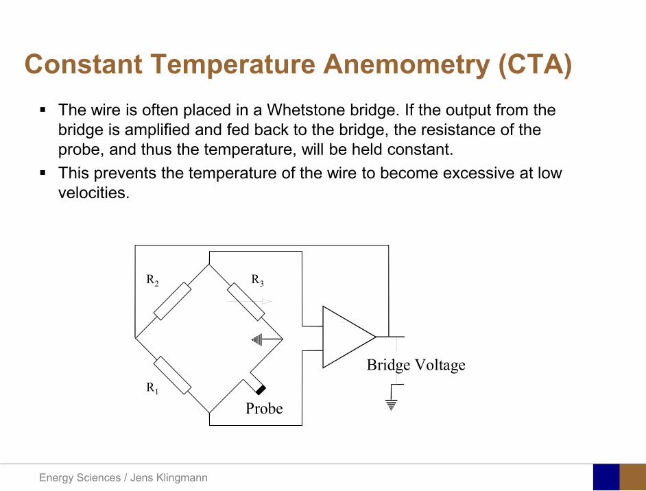
Energy Sciences Jens Klingmann
Constant Temperature Anemometry (CTA) The wire is often placed in a Whetstone bridge If the output from the
bridge is amplified and fed back to the bridge the resistance of the probe and thus the temperature will be held constant
This prevents the temperature of the wire to become excessive at low velocities
R1
R2 R3
Probe
Bridge Voltage
Energy Sciences Jens Klingmann
Constant Temperature Anemometry (CTA)
Energy Sciences Jens Klingmann
Characteristics of LDA (according to Dantec)
Invented by Yeh and Cummins in 1964 Velocity measurements in Fluid Dynamics (gas liquid) Up to 3 velocity components Non-intrusive measurements (optical technique) Absolute measurement technique (no calibration required) Very high accuracy Very high spatial resolution due to small measurement volume Tracer particles are required
Energy Sciences Jens Klingmann
LDA - Fringe Model
Focused Laser beams intersect and form the measurement volume Plane wave fronts beam waist in the plane of intersection Interference in the plane of intersection Pattern of bright and dark stripesplanes Fringes
Energy Sciences Jens Klingmann
LDA-measuring volume
d
x
x
y
y
z
z
e-2 CONTOUR
FRINGES
κ
κ
κ
κ
De-2
De-2
dml m
a
b
cx
b
z
ya
cd
d
=
=
=
J
J
J
J
JP
JP
JP
JD
JD
JD
+
+
+
a
b
c
d
κπλ
=minus sinD
f4l2e
m
κπλ
=minus cosD
f4D2e
m
Energy Sciences Jens Klingmann
Laser Two Focus
Energy Sciences Jens Klingmann
Laser Two Focus
Energy Sciences Jens Klingmann
PIV measurements
PIV is a fairly new technique capable of simultaneous velocity measurements at many points in a plane This gives information on large scale structures vorticity etc which is very difficult or impossible to obtain from one-point measuring techniques
PIV involves the illumination of a plane of the flow under investigation with a thin pulsed sheet of light The flow is seeded with particles
The light scattered from the particles and from successive pulses are being recorded either on film or a CCD array forming a multiple exposure of each particle image If the time between the pulses is known velocity can be determined as the ratio of the particle displacement and the elapsed time
t∆∆= xu
Energy Sciences Jens Klingmann
PIV
Energy Sciences Jens Klingmann
PIV measurements illumination
YA
G
YA
G
Two frequency doubled YAG Lasers aligned to one double pulsed laser sheet
Two or more separate light pulses can be obtained by chopping a continuous laser or from pulsed lasers
The limited pulse energies obtained from continuous lasers limits their applicability to low velocity flows or flows where large seeding particles can be used (ie liquid flows)
The low repetition rate of most pulsed lasers makes the use of two lasers advantageous
Energy Sciences Jens Klingmann
PIV measurements recording
High seeding density in laminar flame
Film or CCD-cameras Cross- or Auto-correlation
ndash ie both particle images on the same frame or on separate frames
CCD-camera requirementndash A many pixels as possiblendash 2k by 2k available 4k by 4k coming
Energy Sciences Jens Klingmann
PIV measurements analyses
Low seeding density (Number of seeding particles per unit volume)
Each particle image pair can be identified This is called particle tracking
High seeding density (PIV)
Small sub-regions of the image containing many particle image pairs are processed to obtain one velocity vector
Energy Sciences Jens Klingmann
PIV measurements analyses
Energy Sciences Jens Klingmann
PIV measurements analyses
( ) ( ) ( ) xsxxs dIIR 2A
1
I
+= int
Cross correlation between ( )x1I and ( )x2I
s is a two dimensional displacement vector
IA is the interrogation area
Cross correlation between
(
)
x
1
I
and
(
)
x
2
I
s is a two dimensional displacement vector
I
A
is the interrogation area
Energy Sciences Jens Klingmann
Energy Sciences Jens Klingmann
PIV from IOWA state university
Energy Sciences Jens Klingmann
PIV sample of evaluation
Energy Sciences Jens Klingmann
LDA PIV HWA Velocity range 01 mms ndash 300
ms 02 ndash 150 ms
Measuring Volume
D = 005 L = 05 mm
2 by 2 by 05 mm
L = 05 mm
Freq response O(10 000) Hz O(10) Hz O(100 000) Hz Calibration Yes No No Sensitivity to other than velocity
Low (ref Index) Low (ref Index) Large (temperature concentrationshellip)
Continuous Signal
Sometimes Seldom Always
Noise High High Low Turbulence intensity
No limitation Some limitation lt 20
Price O(1 000 000) SEK
O(1 000 000) SEK
O(50 000) SEK
Required Knowledge
High medium Low
Comparison of techniques
Energy Sciences Jens Klingmann
References experiments
R J Goldstein ldquoFluid Mechanics Measurementsrdquo Hemisphere Publishing 1983 A V Johansson amp P H Alfredsson ldquoExperimentella metoder inom
stroumlmningsmekanikenrdquo Inst Foumlr Mekanik KTH F Durst A Melling and J H Whitelaw ldquoPrincipals and Practice of Laser Doppler
Anemometryrdquo 1984 R J Adrian ldquoParticle-imaging techniques for experimental fluid mechnicsrdquo Ann Rev
Fluid Mech 1991
Energy Sciences Jens Klingmann
Sample of LDA-measurements
Rotor blade
Glas window
Emitted beams
Scattered Light
Adjustable mirror
Energy Sciences Jens Klingmann
Axial velocity sorted into 10 bins
0 1 2 3 4 5 6tangential coordinate (degrees)
-20
0
20
40
60
80
100
120
140
160Ax
ial v
eloc
ity a
nd s
tand
ard
devi
atio
n (m
s)
radial position 7 mm from inner window surfaceaxial position 23 mm behind rotor blades
Energy Sciences Jens Klingmann
Axial velocities in the radial-tangential plane
Energy Sciences Jens Klingmann
Airfoils NACA 4-digit
The NACA four-digit wing sections define the profile by
One digit describing maximum camber as percentage of the chord
One digit describing the distance of maximum camber from the airfoil leading edge in tens of percents of the chord
Two digits describing maximum thickness of the airfoil as percent of the chord
Example the NACA 2412 airfoil has a maximum camber of 2 located 40 (04 chords) from the leading edge with a maximum thickness of 12 of the chord
Four-digit series airfoils by default have maximum thickness at 30 of the chord (03 chords) from the leading edge
Energy Sciences Jens Klingmann
Airfoils NACA 4-digit
bull c is the chord lengthbull x is the position along
the chord from 0 to cbull y is the half thickness at
a given value of x (centerline to surface)
bull t is the maximum thickness as a fraction of the chord
Energy Sciences Jens Klingmann
Death by PowerPoint
| LDA | PIV | HWA | |||||
| Velocity range | 01 mms ndash 300 ms | 02 ndash 150 ms | |||||
| Measuring Volume | D = 005 L = 05 mm | 2 by 2 by 05 mm | L = 05 mm | ||||
| Freq response | O(10 000) Hz | O(10) Hz | O(100 000) Hz | ||||
| Calibration | Yes | No | No | ||||
| Sensitivity to other than velocity | Low (ref Index) | Low (ref Index) | Large (temperature concentrationshellip) | ||||
| Continuous Signal | Sometimes | Seldom | Always | ||||
| Noise | High | High | Low | ||||
| Turbulence intensity | No limitation | Some limitation | lt 20 | ||||
| Price | O(1 000 000) SEK | O(1 000 000) SEK | O(50 000) SEK | ||||
| Required Knowledge | High | medium | Low |
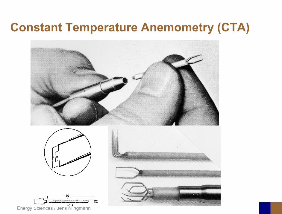
Energy Sciences Jens Klingmann
Constant Temperature Anemometry (CTA)
Energy Sciences Jens Klingmann
Characteristics of LDA (according to Dantec)
Invented by Yeh and Cummins in 1964 Velocity measurements in Fluid Dynamics (gas liquid) Up to 3 velocity components Non-intrusive measurements (optical technique) Absolute measurement technique (no calibration required) Very high accuracy Very high spatial resolution due to small measurement volume Tracer particles are required
Energy Sciences Jens Klingmann
LDA - Fringe Model
Focused Laser beams intersect and form the measurement volume Plane wave fronts beam waist in the plane of intersection Interference in the plane of intersection Pattern of bright and dark stripesplanes Fringes
Energy Sciences Jens Klingmann
LDA-measuring volume
d
x
x
y
y
z
z
e-2 CONTOUR
FRINGES
κ
κ
κ
κ
De-2
De-2
dml m
a
b
cx
b
z
ya
cd
d
=
=
=
J
J
J
J
JP
JP
JP
JD
JD
JD
+
+
+
a
b
c
d
κπλ
=minus sinD
f4l2e
m
κπλ
=minus cosD
f4D2e
m
Energy Sciences Jens Klingmann
Laser Two Focus
Energy Sciences Jens Klingmann
Laser Two Focus
Energy Sciences Jens Klingmann
PIV measurements
PIV is a fairly new technique capable of simultaneous velocity measurements at many points in a plane This gives information on large scale structures vorticity etc which is very difficult or impossible to obtain from one-point measuring techniques
PIV involves the illumination of a plane of the flow under investigation with a thin pulsed sheet of light The flow is seeded with particles
The light scattered from the particles and from successive pulses are being recorded either on film or a CCD array forming a multiple exposure of each particle image If the time between the pulses is known velocity can be determined as the ratio of the particle displacement and the elapsed time
t∆∆= xu
Energy Sciences Jens Klingmann
PIV
Energy Sciences Jens Klingmann
PIV measurements illumination
YA
G
YA
G
Two frequency doubled YAG Lasers aligned to one double pulsed laser sheet
Two or more separate light pulses can be obtained by chopping a continuous laser or from pulsed lasers
The limited pulse energies obtained from continuous lasers limits their applicability to low velocity flows or flows where large seeding particles can be used (ie liquid flows)
The low repetition rate of most pulsed lasers makes the use of two lasers advantageous
Energy Sciences Jens Klingmann
PIV measurements recording
High seeding density in laminar flame
Film or CCD-cameras Cross- or Auto-correlation
ndash ie both particle images on the same frame or on separate frames
CCD-camera requirementndash A many pixels as possiblendash 2k by 2k available 4k by 4k coming
Energy Sciences Jens Klingmann
PIV measurements analyses
Low seeding density (Number of seeding particles per unit volume)
Each particle image pair can be identified This is called particle tracking
High seeding density (PIV)
Small sub-regions of the image containing many particle image pairs are processed to obtain one velocity vector
Energy Sciences Jens Klingmann
PIV measurements analyses
Energy Sciences Jens Klingmann
PIV measurements analyses
( ) ( ) ( ) xsxxs dIIR 2A
1
I
+= int
Cross correlation between ( )x1I and ( )x2I
s is a two dimensional displacement vector
IA is the interrogation area
Cross correlation between
(
)
x
1
I
and
(
)
x
2
I
s is a two dimensional displacement vector
I
A
is the interrogation area
Energy Sciences Jens Klingmann
Energy Sciences Jens Klingmann
PIV from IOWA state university
Energy Sciences Jens Klingmann
PIV sample of evaluation
Energy Sciences Jens Klingmann
LDA PIV HWA Velocity range 01 mms ndash 300
ms 02 ndash 150 ms
Measuring Volume
D = 005 L = 05 mm
2 by 2 by 05 mm
L = 05 mm
Freq response O(10 000) Hz O(10) Hz O(100 000) Hz Calibration Yes No No Sensitivity to other than velocity
Low (ref Index) Low (ref Index) Large (temperature concentrationshellip)
Continuous Signal
Sometimes Seldom Always
Noise High High Low Turbulence intensity
No limitation Some limitation lt 20
Price O(1 000 000) SEK
O(1 000 000) SEK
O(50 000) SEK
Required Knowledge
High medium Low
Comparison of techniques
Energy Sciences Jens Klingmann
References experiments
R J Goldstein ldquoFluid Mechanics Measurementsrdquo Hemisphere Publishing 1983 A V Johansson amp P H Alfredsson ldquoExperimentella metoder inom
stroumlmningsmekanikenrdquo Inst Foumlr Mekanik KTH F Durst A Melling and J H Whitelaw ldquoPrincipals and Practice of Laser Doppler
Anemometryrdquo 1984 R J Adrian ldquoParticle-imaging techniques for experimental fluid mechnicsrdquo Ann Rev
Fluid Mech 1991
Energy Sciences Jens Klingmann
Sample of LDA-measurements
Rotor blade
Glas window
Emitted beams
Scattered Light
Adjustable mirror
Energy Sciences Jens Klingmann
Axial velocity sorted into 10 bins
0 1 2 3 4 5 6tangential coordinate (degrees)
-20
0
20
40
60
80
100
120
140
160Ax
ial v
eloc
ity a
nd s
tand
ard
devi
atio
n (m
s)
radial position 7 mm from inner window surfaceaxial position 23 mm behind rotor blades
Energy Sciences Jens Klingmann
Axial velocities in the radial-tangential plane
Energy Sciences Jens Klingmann
Airfoils NACA 4-digit
The NACA four-digit wing sections define the profile by
One digit describing maximum camber as percentage of the chord
One digit describing the distance of maximum camber from the airfoil leading edge in tens of percents of the chord
Two digits describing maximum thickness of the airfoil as percent of the chord
Example the NACA 2412 airfoil has a maximum camber of 2 located 40 (04 chords) from the leading edge with a maximum thickness of 12 of the chord
Four-digit series airfoils by default have maximum thickness at 30 of the chord (03 chords) from the leading edge
Energy Sciences Jens Klingmann
Airfoils NACA 4-digit
bull c is the chord lengthbull x is the position along
the chord from 0 to cbull y is the half thickness at
a given value of x (centerline to surface)
bull t is the maximum thickness as a fraction of the chord
Energy Sciences Jens Klingmann
Death by PowerPoint
| LDA | PIV | HWA | |||||
| Velocity range | 01 mms ndash 300 ms | 02 ndash 150 ms | |||||
| Measuring Volume | D = 005 L = 05 mm | 2 by 2 by 05 mm | L = 05 mm | ||||
| Freq response | O(10 000) Hz | O(10) Hz | O(100 000) Hz | ||||
| Calibration | Yes | No | No | ||||
| Sensitivity to other than velocity | Low (ref Index) | Low (ref Index) | Large (temperature concentrationshellip) | ||||
| Continuous Signal | Sometimes | Seldom | Always | ||||
| Noise | High | High | Low | ||||
| Turbulence intensity | No limitation | Some limitation | lt 20 | ||||
| Price | O(1 000 000) SEK | O(1 000 000) SEK | O(50 000) SEK | ||||
| Required Knowledge | High | medium | Low |
Energy Sciences Jens Klingmann
Characteristics of LDA (according to Dantec)
Invented by Yeh and Cummins in 1964 Velocity measurements in Fluid Dynamics (gas liquid) Up to 3 velocity components Non-intrusive measurements (optical technique) Absolute measurement technique (no calibration required) Very high accuracy Very high spatial resolution due to small measurement volume Tracer particles are required
Energy Sciences Jens Klingmann
LDA - Fringe Model
Focused Laser beams intersect and form the measurement volume Plane wave fronts beam waist in the plane of intersection Interference in the plane of intersection Pattern of bright and dark stripesplanes Fringes
Energy Sciences Jens Klingmann
LDA-measuring volume
d
x
x
y
y
z
z
e-2 CONTOUR
FRINGES
κ
κ
κ
κ
De-2
De-2
dml m
a
b
cx
b
z
ya
cd
d
=
=
=
J
J
J
J
JP
JP
JP
JD
JD
JD
+
+
+
a
b
c
d
κπλ
=minus sinD
f4l2e
m
κπλ
=minus cosD
f4D2e
m
Energy Sciences Jens Klingmann
Laser Two Focus
Energy Sciences Jens Klingmann
Laser Two Focus
Energy Sciences Jens Klingmann
PIV measurements
PIV is a fairly new technique capable of simultaneous velocity measurements at many points in a plane This gives information on large scale structures vorticity etc which is very difficult or impossible to obtain from one-point measuring techniques
PIV involves the illumination of a plane of the flow under investigation with a thin pulsed sheet of light The flow is seeded with particles
The light scattered from the particles and from successive pulses are being recorded either on film or a CCD array forming a multiple exposure of each particle image If the time between the pulses is known velocity can be determined as the ratio of the particle displacement and the elapsed time
t∆∆= xu
Energy Sciences Jens Klingmann
PIV
Energy Sciences Jens Klingmann
PIV measurements illumination
YA
G
YA
G
Two frequency doubled YAG Lasers aligned to one double pulsed laser sheet
Two or more separate light pulses can be obtained by chopping a continuous laser or from pulsed lasers
The limited pulse energies obtained from continuous lasers limits their applicability to low velocity flows or flows where large seeding particles can be used (ie liquid flows)
The low repetition rate of most pulsed lasers makes the use of two lasers advantageous
Energy Sciences Jens Klingmann
PIV measurements recording
High seeding density in laminar flame
Film or CCD-cameras Cross- or Auto-correlation
ndash ie both particle images on the same frame or on separate frames
CCD-camera requirementndash A many pixels as possiblendash 2k by 2k available 4k by 4k coming
Energy Sciences Jens Klingmann
PIV measurements analyses
Low seeding density (Number of seeding particles per unit volume)
Each particle image pair can be identified This is called particle tracking
High seeding density (PIV)
Small sub-regions of the image containing many particle image pairs are processed to obtain one velocity vector
Energy Sciences Jens Klingmann
PIV measurements analyses
Energy Sciences Jens Klingmann
PIV measurements analyses
( ) ( ) ( ) xsxxs dIIR 2A
1
I
+= int
Cross correlation between ( )x1I and ( )x2I
s is a two dimensional displacement vector
IA is the interrogation area
Cross correlation between
(
)
x
1
I
and
(
)
x
2
I
s is a two dimensional displacement vector
I
A
is the interrogation area
Energy Sciences Jens Klingmann
Energy Sciences Jens Klingmann
PIV from IOWA state university
Energy Sciences Jens Klingmann
PIV sample of evaluation
Energy Sciences Jens Klingmann
LDA PIV HWA Velocity range 01 mms ndash 300
ms 02 ndash 150 ms
Measuring Volume
D = 005 L = 05 mm
2 by 2 by 05 mm
L = 05 mm
Freq response O(10 000) Hz O(10) Hz O(100 000) Hz Calibration Yes No No Sensitivity to other than velocity
Low (ref Index) Low (ref Index) Large (temperature concentrationshellip)
Continuous Signal
Sometimes Seldom Always
Noise High High Low Turbulence intensity
No limitation Some limitation lt 20
Price O(1 000 000) SEK
O(1 000 000) SEK
O(50 000) SEK
Required Knowledge
High medium Low
Comparison of techniques
Energy Sciences Jens Klingmann
References experiments
R J Goldstein ldquoFluid Mechanics Measurementsrdquo Hemisphere Publishing 1983 A V Johansson amp P H Alfredsson ldquoExperimentella metoder inom
stroumlmningsmekanikenrdquo Inst Foumlr Mekanik KTH F Durst A Melling and J H Whitelaw ldquoPrincipals and Practice of Laser Doppler
Anemometryrdquo 1984 R J Adrian ldquoParticle-imaging techniques for experimental fluid mechnicsrdquo Ann Rev
Fluid Mech 1991
Energy Sciences Jens Klingmann
Sample of LDA-measurements
Rotor blade
Glas window
Emitted beams
Scattered Light
Adjustable mirror
Energy Sciences Jens Klingmann
Axial velocity sorted into 10 bins
0 1 2 3 4 5 6tangential coordinate (degrees)
-20
0
20
40
60
80
100
120
140
160Ax
ial v
eloc
ity a
nd s
tand
ard
devi
atio
n (m
s)
radial position 7 mm from inner window surfaceaxial position 23 mm behind rotor blades
Energy Sciences Jens Klingmann
Axial velocities in the radial-tangential plane
Energy Sciences Jens Klingmann
Airfoils NACA 4-digit
The NACA four-digit wing sections define the profile by
One digit describing maximum camber as percentage of the chord
One digit describing the distance of maximum camber from the airfoil leading edge in tens of percents of the chord
Two digits describing maximum thickness of the airfoil as percent of the chord
Example the NACA 2412 airfoil has a maximum camber of 2 located 40 (04 chords) from the leading edge with a maximum thickness of 12 of the chord
Four-digit series airfoils by default have maximum thickness at 30 of the chord (03 chords) from the leading edge
Energy Sciences Jens Klingmann
Airfoils NACA 4-digit
bull c is the chord lengthbull x is the position along
the chord from 0 to cbull y is the half thickness at
a given value of x (centerline to surface)
bull t is the maximum thickness as a fraction of the chord
Energy Sciences Jens Klingmann
Death by PowerPoint
| LDA | PIV | HWA | |||||
| Velocity range | 01 mms ndash 300 ms | 02 ndash 150 ms | |||||
| Measuring Volume | D = 005 L = 05 mm | 2 by 2 by 05 mm | L = 05 mm | ||||
| Freq response | O(10 000) Hz | O(10) Hz | O(100 000) Hz | ||||
| Calibration | Yes | No | No | ||||
| Sensitivity to other than velocity | Low (ref Index) | Low (ref Index) | Large (temperature concentrationshellip) | ||||
| Continuous Signal | Sometimes | Seldom | Always | ||||
| Noise | High | High | Low | ||||
| Turbulence intensity | No limitation | Some limitation | lt 20 | ||||
| Price | O(1 000 000) SEK | O(1 000 000) SEK | O(50 000) SEK | ||||
| Required Knowledge | High | medium | Low |
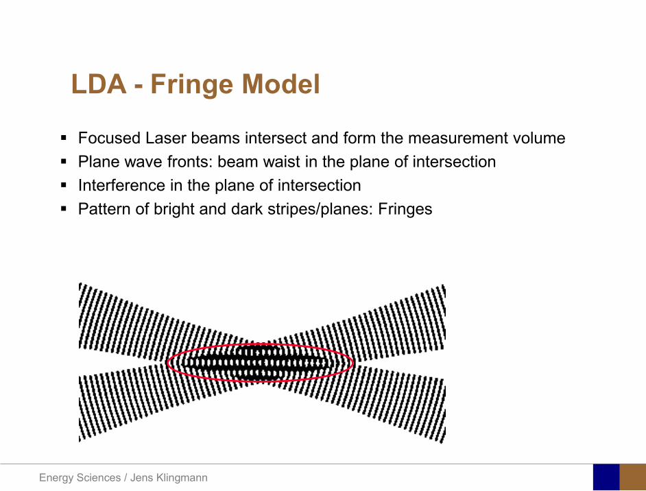
Energy Sciences Jens Klingmann
LDA - Fringe Model
Focused Laser beams intersect and form the measurement volume Plane wave fronts beam waist in the plane of intersection Interference in the plane of intersection Pattern of bright and dark stripesplanes Fringes
Energy Sciences Jens Klingmann
LDA-measuring volume
d
x
x
y
y
z
z
e-2 CONTOUR
FRINGES
κ
κ
κ
κ
De-2
De-2
dml m
a
b
cx
b
z
ya
cd
d
=
=
=
J
J
J
J
JP
JP
JP
JD
JD
JD
+
+
+
a
b
c
d
κπλ
=minus sinD
f4l2e
m
κπλ
=minus cosD
f4D2e
m
Energy Sciences Jens Klingmann
Laser Two Focus
Energy Sciences Jens Klingmann
Laser Two Focus
Energy Sciences Jens Klingmann
PIV measurements
PIV is a fairly new technique capable of simultaneous velocity measurements at many points in a plane This gives information on large scale structures vorticity etc which is very difficult or impossible to obtain from one-point measuring techniques
PIV involves the illumination of a plane of the flow under investigation with a thin pulsed sheet of light The flow is seeded with particles
The light scattered from the particles and from successive pulses are being recorded either on film or a CCD array forming a multiple exposure of each particle image If the time between the pulses is known velocity can be determined as the ratio of the particle displacement and the elapsed time
t∆∆= xu
Energy Sciences Jens Klingmann
PIV
Energy Sciences Jens Klingmann
PIV measurements illumination
YA
G
YA
G
Two frequency doubled YAG Lasers aligned to one double pulsed laser sheet
Two or more separate light pulses can be obtained by chopping a continuous laser or from pulsed lasers
The limited pulse energies obtained from continuous lasers limits their applicability to low velocity flows or flows where large seeding particles can be used (ie liquid flows)
The low repetition rate of most pulsed lasers makes the use of two lasers advantageous
Energy Sciences Jens Klingmann
PIV measurements recording
High seeding density in laminar flame
Film or CCD-cameras Cross- or Auto-correlation
ndash ie both particle images on the same frame or on separate frames
CCD-camera requirementndash A many pixels as possiblendash 2k by 2k available 4k by 4k coming
Energy Sciences Jens Klingmann
PIV measurements analyses
Low seeding density (Number of seeding particles per unit volume)
Each particle image pair can be identified This is called particle tracking
High seeding density (PIV)
Small sub-regions of the image containing many particle image pairs are processed to obtain one velocity vector
Energy Sciences Jens Klingmann
PIV measurements analyses
Energy Sciences Jens Klingmann
PIV measurements analyses
( ) ( ) ( ) xsxxs dIIR 2A
1
I
+= int
Cross correlation between ( )x1I and ( )x2I
s is a two dimensional displacement vector
IA is the interrogation area
Cross correlation between
(
)
x
1
I
and
(
)
x
2
I
s is a two dimensional displacement vector
I
A
is the interrogation area
Energy Sciences Jens Klingmann
Energy Sciences Jens Klingmann
PIV from IOWA state university
Energy Sciences Jens Klingmann
PIV sample of evaluation
Energy Sciences Jens Klingmann
LDA PIV HWA Velocity range 01 mms ndash 300
ms 02 ndash 150 ms
Measuring Volume
D = 005 L = 05 mm
2 by 2 by 05 mm
L = 05 mm
Freq response O(10 000) Hz O(10) Hz O(100 000) Hz Calibration Yes No No Sensitivity to other than velocity
Low (ref Index) Low (ref Index) Large (temperature concentrationshellip)
Continuous Signal
Sometimes Seldom Always
Noise High High Low Turbulence intensity
No limitation Some limitation lt 20
Price O(1 000 000) SEK
O(1 000 000) SEK
O(50 000) SEK
Required Knowledge
High medium Low
Comparison of techniques
Energy Sciences Jens Klingmann
References experiments
R J Goldstein ldquoFluid Mechanics Measurementsrdquo Hemisphere Publishing 1983 A V Johansson amp P H Alfredsson ldquoExperimentella metoder inom
stroumlmningsmekanikenrdquo Inst Foumlr Mekanik KTH F Durst A Melling and J H Whitelaw ldquoPrincipals and Practice of Laser Doppler
Anemometryrdquo 1984 R J Adrian ldquoParticle-imaging techniques for experimental fluid mechnicsrdquo Ann Rev
Fluid Mech 1991
Energy Sciences Jens Klingmann
Sample of LDA-measurements
Rotor blade
Glas window
Emitted beams
Scattered Light
Adjustable mirror
Energy Sciences Jens Klingmann
Axial velocity sorted into 10 bins
0 1 2 3 4 5 6tangential coordinate (degrees)
-20
0
20
40
60
80
100
120
140
160Ax
ial v
eloc
ity a
nd s
tand
ard
devi
atio
n (m
s)
radial position 7 mm from inner window surfaceaxial position 23 mm behind rotor blades
Energy Sciences Jens Klingmann
Axial velocities in the radial-tangential plane
Energy Sciences Jens Klingmann
Airfoils NACA 4-digit
The NACA four-digit wing sections define the profile by
One digit describing maximum camber as percentage of the chord
One digit describing the distance of maximum camber from the airfoil leading edge in tens of percents of the chord
Two digits describing maximum thickness of the airfoil as percent of the chord
Example the NACA 2412 airfoil has a maximum camber of 2 located 40 (04 chords) from the leading edge with a maximum thickness of 12 of the chord
Four-digit series airfoils by default have maximum thickness at 30 of the chord (03 chords) from the leading edge
Energy Sciences Jens Klingmann
Airfoils NACA 4-digit
bull c is the chord lengthbull x is the position along
the chord from 0 to cbull y is the half thickness at
a given value of x (centerline to surface)
bull t is the maximum thickness as a fraction of the chord
Energy Sciences Jens Klingmann
Death by PowerPoint
| LDA | PIV | HWA | |||||
| Velocity range | 01 mms ndash 300 ms | 02 ndash 150 ms | |||||
| Measuring Volume | D = 005 L = 05 mm | 2 by 2 by 05 mm | L = 05 mm | ||||
| Freq response | O(10 000) Hz | O(10) Hz | O(100 000) Hz | ||||
| Calibration | Yes | No | No | ||||
| Sensitivity to other than velocity | Low (ref Index) | Low (ref Index) | Large (temperature concentrationshellip) | ||||
| Continuous Signal | Sometimes | Seldom | Always | ||||
| Noise | High | High | Low | ||||
| Turbulence intensity | No limitation | Some limitation | lt 20 | ||||
| Price | O(1 000 000) SEK | O(1 000 000) SEK | O(50 000) SEK | ||||
| Required Knowledge | High | medium | Low |
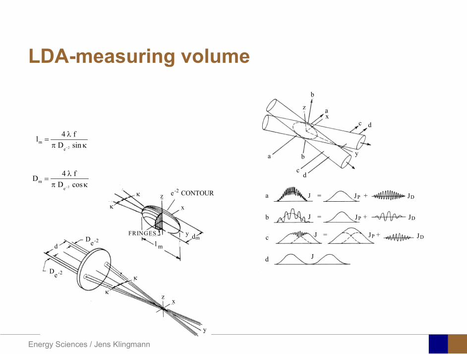
Energy Sciences Jens Klingmann
LDA-measuring volume
d
x
x
y
y
z
z
e-2 CONTOUR
FRINGES
κ
κ
κ
κ
De-2
De-2
dml m
a
b
cx
b
z
ya
cd
d
=
=
=
J
J
J
J
JP
JP
JP
JD
JD
JD
+
+
+
a
b
c
d
κπλ
=minus sinD
f4l2e
m
κπλ
=minus cosD
f4D2e
m
Energy Sciences Jens Klingmann
Laser Two Focus
Energy Sciences Jens Klingmann
Laser Two Focus
Energy Sciences Jens Klingmann
PIV measurements
PIV is a fairly new technique capable of simultaneous velocity measurements at many points in a plane This gives information on large scale structures vorticity etc which is very difficult or impossible to obtain from one-point measuring techniques
PIV involves the illumination of a plane of the flow under investigation with a thin pulsed sheet of light The flow is seeded with particles
The light scattered from the particles and from successive pulses are being recorded either on film or a CCD array forming a multiple exposure of each particle image If the time between the pulses is known velocity can be determined as the ratio of the particle displacement and the elapsed time
t∆∆= xu
Energy Sciences Jens Klingmann
PIV
Energy Sciences Jens Klingmann
PIV measurements illumination
YA
G
YA
G
Two frequency doubled YAG Lasers aligned to one double pulsed laser sheet
Two or more separate light pulses can be obtained by chopping a continuous laser or from pulsed lasers
The limited pulse energies obtained from continuous lasers limits their applicability to low velocity flows or flows where large seeding particles can be used (ie liquid flows)
The low repetition rate of most pulsed lasers makes the use of two lasers advantageous
Energy Sciences Jens Klingmann
PIV measurements recording
High seeding density in laminar flame
Film or CCD-cameras Cross- or Auto-correlation
ndash ie both particle images on the same frame or on separate frames
CCD-camera requirementndash A many pixels as possiblendash 2k by 2k available 4k by 4k coming
Energy Sciences Jens Klingmann
PIV measurements analyses
Low seeding density (Number of seeding particles per unit volume)
Each particle image pair can be identified This is called particle tracking
High seeding density (PIV)
Small sub-regions of the image containing many particle image pairs are processed to obtain one velocity vector
Energy Sciences Jens Klingmann
PIV measurements analyses
Energy Sciences Jens Klingmann
PIV measurements analyses
( ) ( ) ( ) xsxxs dIIR 2A
1
I
+= int
Cross correlation between ( )x1I and ( )x2I
s is a two dimensional displacement vector
IA is the interrogation area
Cross correlation between
(
)
x
1
I
and
(
)
x
2
I
s is a two dimensional displacement vector
I
A
is the interrogation area
Energy Sciences Jens Klingmann
Energy Sciences Jens Klingmann
PIV from IOWA state university
Energy Sciences Jens Klingmann
PIV sample of evaluation
Energy Sciences Jens Klingmann
LDA PIV HWA Velocity range 01 mms ndash 300
ms 02 ndash 150 ms
Measuring Volume
D = 005 L = 05 mm
2 by 2 by 05 mm
L = 05 mm
Freq response O(10 000) Hz O(10) Hz O(100 000) Hz Calibration Yes No No Sensitivity to other than velocity
Low (ref Index) Low (ref Index) Large (temperature concentrationshellip)
Continuous Signal
Sometimes Seldom Always
Noise High High Low Turbulence intensity
No limitation Some limitation lt 20
Price O(1 000 000) SEK
O(1 000 000) SEK
O(50 000) SEK
Required Knowledge
High medium Low
Comparison of techniques
Energy Sciences Jens Klingmann
References experiments
R J Goldstein ldquoFluid Mechanics Measurementsrdquo Hemisphere Publishing 1983 A V Johansson amp P H Alfredsson ldquoExperimentella metoder inom
stroumlmningsmekanikenrdquo Inst Foumlr Mekanik KTH F Durst A Melling and J H Whitelaw ldquoPrincipals and Practice of Laser Doppler
Anemometryrdquo 1984 R J Adrian ldquoParticle-imaging techniques for experimental fluid mechnicsrdquo Ann Rev
Fluid Mech 1991
Energy Sciences Jens Klingmann
Sample of LDA-measurements
Rotor blade
Glas window
Emitted beams
Scattered Light
Adjustable mirror
Energy Sciences Jens Klingmann
Axial velocity sorted into 10 bins
0 1 2 3 4 5 6tangential coordinate (degrees)
-20
0
20
40
60
80
100
120
140
160Ax
ial v
eloc
ity a
nd s
tand
ard
devi
atio
n (m
s)
radial position 7 mm from inner window surfaceaxial position 23 mm behind rotor blades
Energy Sciences Jens Klingmann
Axial velocities in the radial-tangential plane
Energy Sciences Jens Klingmann
Airfoils NACA 4-digit
The NACA four-digit wing sections define the profile by
One digit describing maximum camber as percentage of the chord
One digit describing the distance of maximum camber from the airfoil leading edge in tens of percents of the chord
Two digits describing maximum thickness of the airfoil as percent of the chord
Example the NACA 2412 airfoil has a maximum camber of 2 located 40 (04 chords) from the leading edge with a maximum thickness of 12 of the chord
Four-digit series airfoils by default have maximum thickness at 30 of the chord (03 chords) from the leading edge
Energy Sciences Jens Klingmann
Airfoils NACA 4-digit
bull c is the chord lengthbull x is the position along
the chord from 0 to cbull y is the half thickness at
a given value of x (centerline to surface)
bull t is the maximum thickness as a fraction of the chord
Energy Sciences Jens Klingmann
Death by PowerPoint
| LDA | PIV | HWA | |||||
| Velocity range | 01 mms ndash 300 ms | 02 ndash 150 ms | |||||
| Measuring Volume | D = 005 L = 05 mm | 2 by 2 by 05 mm | L = 05 mm | ||||
| Freq response | O(10 000) Hz | O(10) Hz | O(100 000) Hz | ||||
| Calibration | Yes | No | No | ||||
| Sensitivity to other than velocity | Low (ref Index) | Low (ref Index) | Large (temperature concentrationshellip) | ||||
| Continuous Signal | Sometimes | Seldom | Always | ||||
| Noise | High | High | Low | ||||
| Turbulence intensity | No limitation | Some limitation | lt 20 | ||||
| Price | O(1 000 000) SEK | O(1 000 000) SEK | O(50 000) SEK | ||||
| Required Knowledge | High | medium | Low |
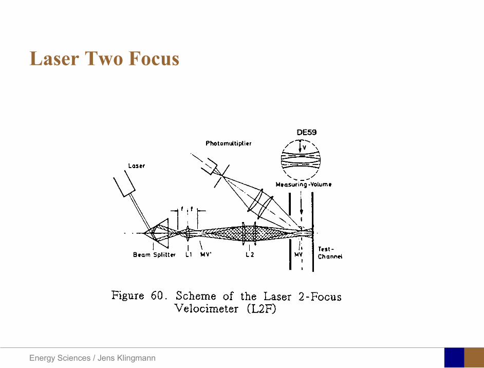
Energy Sciences Jens Klingmann
Laser Two Focus
Energy Sciences Jens Klingmann
Laser Two Focus
Energy Sciences Jens Klingmann
PIV measurements
PIV is a fairly new technique capable of simultaneous velocity measurements at many points in a plane This gives information on large scale structures vorticity etc which is very difficult or impossible to obtain from one-point measuring techniques
PIV involves the illumination of a plane of the flow under investigation with a thin pulsed sheet of light The flow is seeded with particles
The light scattered from the particles and from successive pulses are being recorded either on film or a CCD array forming a multiple exposure of each particle image If the time between the pulses is known velocity can be determined as the ratio of the particle displacement and the elapsed time
t∆∆= xu
Energy Sciences Jens Klingmann
PIV
Energy Sciences Jens Klingmann
PIV measurements illumination
YA
G
YA
G
Two frequency doubled YAG Lasers aligned to one double pulsed laser sheet
Two or more separate light pulses can be obtained by chopping a continuous laser or from pulsed lasers
The limited pulse energies obtained from continuous lasers limits their applicability to low velocity flows or flows where large seeding particles can be used (ie liquid flows)
The low repetition rate of most pulsed lasers makes the use of two lasers advantageous
Energy Sciences Jens Klingmann
PIV measurements recording
High seeding density in laminar flame
Film or CCD-cameras Cross- or Auto-correlation
ndash ie both particle images on the same frame or on separate frames
CCD-camera requirementndash A many pixels as possiblendash 2k by 2k available 4k by 4k coming
Energy Sciences Jens Klingmann
PIV measurements analyses
Low seeding density (Number of seeding particles per unit volume)
Each particle image pair can be identified This is called particle tracking
High seeding density (PIV)
Small sub-regions of the image containing many particle image pairs are processed to obtain one velocity vector
Energy Sciences Jens Klingmann
PIV measurements analyses
Energy Sciences Jens Klingmann
PIV measurements analyses
( ) ( ) ( ) xsxxs dIIR 2A
1
I
+= int
Cross correlation between ( )x1I and ( )x2I
s is a two dimensional displacement vector
IA is the interrogation area
Cross correlation between
(
)
x
1
I
and
(
)
x
2
I
s is a two dimensional displacement vector
I
A
is the interrogation area
Energy Sciences Jens Klingmann
Energy Sciences Jens Klingmann
PIV from IOWA state university
Energy Sciences Jens Klingmann
PIV sample of evaluation
Energy Sciences Jens Klingmann
LDA PIV HWA Velocity range 01 mms ndash 300
ms 02 ndash 150 ms
Measuring Volume
D = 005 L = 05 mm
2 by 2 by 05 mm
L = 05 mm
Freq response O(10 000) Hz O(10) Hz O(100 000) Hz Calibration Yes No No Sensitivity to other than velocity
Low (ref Index) Low (ref Index) Large (temperature concentrationshellip)
Continuous Signal
Sometimes Seldom Always
Noise High High Low Turbulence intensity
No limitation Some limitation lt 20
Price O(1 000 000) SEK
O(1 000 000) SEK
O(50 000) SEK
Required Knowledge
High medium Low
Comparison of techniques
Energy Sciences Jens Klingmann
References experiments
R J Goldstein ldquoFluid Mechanics Measurementsrdquo Hemisphere Publishing 1983 A V Johansson amp P H Alfredsson ldquoExperimentella metoder inom
stroumlmningsmekanikenrdquo Inst Foumlr Mekanik KTH F Durst A Melling and J H Whitelaw ldquoPrincipals and Practice of Laser Doppler
Anemometryrdquo 1984 R J Adrian ldquoParticle-imaging techniques for experimental fluid mechnicsrdquo Ann Rev
Fluid Mech 1991
Energy Sciences Jens Klingmann
Sample of LDA-measurements
Rotor blade
Glas window
Emitted beams
Scattered Light
Adjustable mirror
Energy Sciences Jens Klingmann
Axial velocity sorted into 10 bins
0 1 2 3 4 5 6tangential coordinate (degrees)
-20
0
20
40
60
80
100
120
140
160Ax
ial v
eloc
ity a
nd s
tand
ard
devi
atio
n (m
s)
radial position 7 mm from inner window surfaceaxial position 23 mm behind rotor blades
Energy Sciences Jens Klingmann
Axial velocities in the radial-tangential plane
Energy Sciences Jens Klingmann
Airfoils NACA 4-digit
The NACA four-digit wing sections define the profile by
One digit describing maximum camber as percentage of the chord
One digit describing the distance of maximum camber from the airfoil leading edge in tens of percents of the chord
Two digits describing maximum thickness of the airfoil as percent of the chord
Example the NACA 2412 airfoil has a maximum camber of 2 located 40 (04 chords) from the leading edge with a maximum thickness of 12 of the chord
Four-digit series airfoils by default have maximum thickness at 30 of the chord (03 chords) from the leading edge
Energy Sciences Jens Klingmann
Airfoils NACA 4-digit
bull c is the chord lengthbull x is the position along
the chord from 0 to cbull y is the half thickness at
a given value of x (centerline to surface)
bull t is the maximum thickness as a fraction of the chord
Energy Sciences Jens Klingmann
Death by PowerPoint
| LDA | PIV | HWA | |||||
| Velocity range | 01 mms ndash 300 ms | 02 ndash 150 ms | |||||
| Measuring Volume | D = 005 L = 05 mm | 2 by 2 by 05 mm | L = 05 mm | ||||
| Freq response | O(10 000) Hz | O(10) Hz | O(100 000) Hz | ||||
| Calibration | Yes | No | No | ||||
| Sensitivity to other than velocity | Low (ref Index) | Low (ref Index) | Large (temperature concentrationshellip) | ||||
| Continuous Signal | Sometimes | Seldom | Always | ||||
| Noise | High | High | Low | ||||
| Turbulence intensity | No limitation | Some limitation | lt 20 | ||||
| Price | O(1 000 000) SEK | O(1 000 000) SEK | O(50 000) SEK | ||||
| Required Knowledge | High | medium | Low |
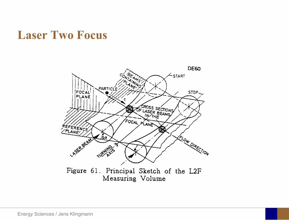
Energy Sciences Jens Klingmann
Laser Two Focus
Energy Sciences Jens Klingmann
PIV measurements
PIV is a fairly new technique capable of simultaneous velocity measurements at many points in a plane This gives information on large scale structures vorticity etc which is very difficult or impossible to obtain from one-point measuring techniques
PIV involves the illumination of a plane of the flow under investigation with a thin pulsed sheet of light The flow is seeded with particles
The light scattered from the particles and from successive pulses are being recorded either on film or a CCD array forming a multiple exposure of each particle image If the time between the pulses is known velocity can be determined as the ratio of the particle displacement and the elapsed time
t∆∆= xu
Energy Sciences Jens Klingmann
PIV
Energy Sciences Jens Klingmann
PIV measurements illumination
YA
G
YA
G
Two frequency doubled YAG Lasers aligned to one double pulsed laser sheet
Two or more separate light pulses can be obtained by chopping a continuous laser or from pulsed lasers
The limited pulse energies obtained from continuous lasers limits their applicability to low velocity flows or flows where large seeding particles can be used (ie liquid flows)
The low repetition rate of most pulsed lasers makes the use of two lasers advantageous
Energy Sciences Jens Klingmann
PIV measurements recording
High seeding density in laminar flame
Film or CCD-cameras Cross- or Auto-correlation
ndash ie both particle images on the same frame or on separate frames
CCD-camera requirementndash A many pixels as possiblendash 2k by 2k available 4k by 4k coming
Energy Sciences Jens Klingmann
PIV measurements analyses
Low seeding density (Number of seeding particles per unit volume)
Each particle image pair can be identified This is called particle tracking
High seeding density (PIV)
Small sub-regions of the image containing many particle image pairs are processed to obtain one velocity vector
Energy Sciences Jens Klingmann
PIV measurements analyses
Energy Sciences Jens Klingmann
PIV measurements analyses
( ) ( ) ( ) xsxxs dIIR 2A
1
I
+= int
Cross correlation between ( )x1I and ( )x2I
s is a two dimensional displacement vector
IA is the interrogation area
Cross correlation between
(
)
x
1
I
and
(
)
x
2
I
s is a two dimensional displacement vector
I
A
is the interrogation area
Energy Sciences Jens Klingmann
Energy Sciences Jens Klingmann
PIV from IOWA state university
Energy Sciences Jens Klingmann
PIV sample of evaluation
Energy Sciences Jens Klingmann
LDA PIV HWA Velocity range 01 mms ndash 300
ms 02 ndash 150 ms
Measuring Volume
D = 005 L = 05 mm
2 by 2 by 05 mm
L = 05 mm
Freq response O(10 000) Hz O(10) Hz O(100 000) Hz Calibration Yes No No Sensitivity to other than velocity
Low (ref Index) Low (ref Index) Large (temperature concentrationshellip)
Continuous Signal
Sometimes Seldom Always
Noise High High Low Turbulence intensity
No limitation Some limitation lt 20
Price O(1 000 000) SEK
O(1 000 000) SEK
O(50 000) SEK
Required Knowledge
High medium Low
Comparison of techniques
Energy Sciences Jens Klingmann
References experiments
R J Goldstein ldquoFluid Mechanics Measurementsrdquo Hemisphere Publishing 1983 A V Johansson amp P H Alfredsson ldquoExperimentella metoder inom
stroumlmningsmekanikenrdquo Inst Foumlr Mekanik KTH F Durst A Melling and J H Whitelaw ldquoPrincipals and Practice of Laser Doppler
Anemometryrdquo 1984 R J Adrian ldquoParticle-imaging techniques for experimental fluid mechnicsrdquo Ann Rev
Fluid Mech 1991
Energy Sciences Jens Klingmann
Sample of LDA-measurements
Rotor blade
Glas window
Emitted beams
Scattered Light
Adjustable mirror
Energy Sciences Jens Klingmann
Axial velocity sorted into 10 bins
0 1 2 3 4 5 6tangential coordinate (degrees)
-20
0
20
40
60
80
100
120
140
160Ax
ial v
eloc
ity a
nd s
tand
ard
devi
atio
n (m
s)
radial position 7 mm from inner window surfaceaxial position 23 mm behind rotor blades
Energy Sciences Jens Klingmann
Axial velocities in the radial-tangential plane
Energy Sciences Jens Klingmann
Airfoils NACA 4-digit
The NACA four-digit wing sections define the profile by
One digit describing maximum camber as percentage of the chord
One digit describing the distance of maximum camber from the airfoil leading edge in tens of percents of the chord
Two digits describing maximum thickness of the airfoil as percent of the chord
Example the NACA 2412 airfoil has a maximum camber of 2 located 40 (04 chords) from the leading edge with a maximum thickness of 12 of the chord
Four-digit series airfoils by default have maximum thickness at 30 of the chord (03 chords) from the leading edge
Energy Sciences Jens Klingmann
Airfoils NACA 4-digit
bull c is the chord lengthbull x is the position along
the chord from 0 to cbull y is the half thickness at
a given value of x (centerline to surface)
bull t is the maximum thickness as a fraction of the chord
Energy Sciences Jens Klingmann
Death by PowerPoint
| LDA | PIV | HWA | |||||
| Velocity range | 01 mms ndash 300 ms | 02 ndash 150 ms | |||||
| Measuring Volume | D = 005 L = 05 mm | 2 by 2 by 05 mm | L = 05 mm | ||||
| Freq response | O(10 000) Hz | O(10) Hz | O(100 000) Hz | ||||
| Calibration | Yes | No | No | ||||
| Sensitivity to other than velocity | Low (ref Index) | Low (ref Index) | Large (temperature concentrationshellip) | ||||
| Continuous Signal | Sometimes | Seldom | Always | ||||
| Noise | High | High | Low | ||||
| Turbulence intensity | No limitation | Some limitation | lt 20 | ||||
| Price | O(1 000 000) SEK | O(1 000 000) SEK | O(50 000) SEK | ||||
| Required Knowledge | High | medium | Low |
Energy Sciences Jens Klingmann
PIV measurements
PIV is a fairly new technique capable of simultaneous velocity measurements at many points in a plane This gives information on large scale structures vorticity etc which is very difficult or impossible to obtain from one-point measuring techniques
PIV involves the illumination of a plane of the flow under investigation with a thin pulsed sheet of light The flow is seeded with particles
The light scattered from the particles and from successive pulses are being recorded either on film or a CCD array forming a multiple exposure of each particle image If the time between the pulses is known velocity can be determined as the ratio of the particle displacement and the elapsed time
t∆∆= xu
Energy Sciences Jens Klingmann
PIV
Energy Sciences Jens Klingmann
PIV measurements illumination
YA
G
YA
G
Two frequency doubled YAG Lasers aligned to one double pulsed laser sheet
Two or more separate light pulses can be obtained by chopping a continuous laser or from pulsed lasers
The limited pulse energies obtained from continuous lasers limits their applicability to low velocity flows or flows where large seeding particles can be used (ie liquid flows)
The low repetition rate of most pulsed lasers makes the use of two lasers advantageous
Energy Sciences Jens Klingmann
PIV measurements recording
High seeding density in laminar flame
Film or CCD-cameras Cross- or Auto-correlation
ndash ie both particle images on the same frame or on separate frames
CCD-camera requirementndash A many pixels as possiblendash 2k by 2k available 4k by 4k coming
Energy Sciences Jens Klingmann
PIV measurements analyses
Low seeding density (Number of seeding particles per unit volume)
Each particle image pair can be identified This is called particle tracking
High seeding density (PIV)
Small sub-regions of the image containing many particle image pairs are processed to obtain one velocity vector
Energy Sciences Jens Klingmann
PIV measurements analyses
Energy Sciences Jens Klingmann
PIV measurements analyses
( ) ( ) ( ) xsxxs dIIR 2A
1
I
+= int
Cross correlation between ( )x1I and ( )x2I
s is a two dimensional displacement vector
IA is the interrogation area
Cross correlation between
(
)
x
1
I
and
(
)
x
2
I
s is a two dimensional displacement vector
I
A
is the interrogation area
Energy Sciences Jens Klingmann
Energy Sciences Jens Klingmann
PIV from IOWA state university
Energy Sciences Jens Klingmann
PIV sample of evaluation
Energy Sciences Jens Klingmann
LDA PIV HWA Velocity range 01 mms ndash 300
ms 02 ndash 150 ms
Measuring Volume
D = 005 L = 05 mm
2 by 2 by 05 mm
L = 05 mm
Freq response O(10 000) Hz O(10) Hz O(100 000) Hz Calibration Yes No No Sensitivity to other than velocity
Low (ref Index) Low (ref Index) Large (temperature concentrationshellip)
Continuous Signal
Sometimes Seldom Always
Noise High High Low Turbulence intensity
No limitation Some limitation lt 20
Price O(1 000 000) SEK
O(1 000 000) SEK
O(50 000) SEK
Required Knowledge
High medium Low
Comparison of techniques
Energy Sciences Jens Klingmann
References experiments
R J Goldstein ldquoFluid Mechanics Measurementsrdquo Hemisphere Publishing 1983 A V Johansson amp P H Alfredsson ldquoExperimentella metoder inom
stroumlmningsmekanikenrdquo Inst Foumlr Mekanik KTH F Durst A Melling and J H Whitelaw ldquoPrincipals and Practice of Laser Doppler
Anemometryrdquo 1984 R J Adrian ldquoParticle-imaging techniques for experimental fluid mechnicsrdquo Ann Rev
Fluid Mech 1991
Energy Sciences Jens Klingmann
Sample of LDA-measurements
Rotor blade
Glas window
Emitted beams
Scattered Light
Adjustable mirror
Energy Sciences Jens Klingmann
Axial velocity sorted into 10 bins
0 1 2 3 4 5 6tangential coordinate (degrees)
-20
0
20
40
60
80
100
120
140
160Ax
ial v
eloc
ity a
nd s
tand
ard
devi
atio
n (m
s)
radial position 7 mm from inner window surfaceaxial position 23 mm behind rotor blades
Energy Sciences Jens Klingmann
Axial velocities in the radial-tangential plane
Energy Sciences Jens Klingmann
Airfoils NACA 4-digit
The NACA four-digit wing sections define the profile by
One digit describing maximum camber as percentage of the chord
One digit describing the distance of maximum camber from the airfoil leading edge in tens of percents of the chord
Two digits describing maximum thickness of the airfoil as percent of the chord
Example the NACA 2412 airfoil has a maximum camber of 2 located 40 (04 chords) from the leading edge with a maximum thickness of 12 of the chord
Four-digit series airfoils by default have maximum thickness at 30 of the chord (03 chords) from the leading edge
Energy Sciences Jens Klingmann
Airfoils NACA 4-digit
bull c is the chord lengthbull x is the position along
the chord from 0 to cbull y is the half thickness at
a given value of x (centerline to surface)
bull t is the maximum thickness as a fraction of the chord
Energy Sciences Jens Klingmann
Death by PowerPoint
| LDA | PIV | HWA | |||||
| Velocity range | 01 mms ndash 300 ms | 02 ndash 150 ms | |||||
| Measuring Volume | D = 005 L = 05 mm | 2 by 2 by 05 mm | L = 05 mm | ||||
| Freq response | O(10 000) Hz | O(10) Hz | O(100 000) Hz | ||||
| Calibration | Yes | No | No | ||||
| Sensitivity to other than velocity | Low (ref Index) | Low (ref Index) | Large (temperature concentrationshellip) | ||||
| Continuous Signal | Sometimes | Seldom | Always | ||||
| Noise | High | High | Low | ||||
| Turbulence intensity | No limitation | Some limitation | lt 20 | ||||
| Price | O(1 000 000) SEK | O(1 000 000) SEK | O(50 000) SEK | ||||
| Required Knowledge | High | medium | Low |
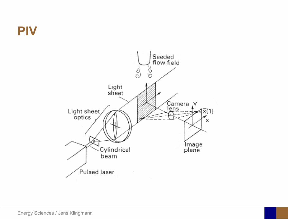
Energy Sciences Jens Klingmann
PIV
Energy Sciences Jens Klingmann
PIV measurements illumination
YA
G
YA
G
Two frequency doubled YAG Lasers aligned to one double pulsed laser sheet
Two or more separate light pulses can be obtained by chopping a continuous laser or from pulsed lasers
The limited pulse energies obtained from continuous lasers limits their applicability to low velocity flows or flows where large seeding particles can be used (ie liquid flows)
The low repetition rate of most pulsed lasers makes the use of two lasers advantageous
Energy Sciences Jens Klingmann
PIV measurements recording
High seeding density in laminar flame
Film or CCD-cameras Cross- or Auto-correlation
ndash ie both particle images on the same frame or on separate frames
CCD-camera requirementndash A many pixels as possiblendash 2k by 2k available 4k by 4k coming
Energy Sciences Jens Klingmann
PIV measurements analyses
Low seeding density (Number of seeding particles per unit volume)
Each particle image pair can be identified This is called particle tracking
High seeding density (PIV)
Small sub-regions of the image containing many particle image pairs are processed to obtain one velocity vector
Energy Sciences Jens Klingmann
PIV measurements analyses
Energy Sciences Jens Klingmann
PIV measurements analyses
( ) ( ) ( ) xsxxs dIIR 2A
1
I
+= int
Cross correlation between ( )x1I and ( )x2I
s is a two dimensional displacement vector
IA is the interrogation area
Cross correlation between
(
)
x
1
I
and
(
)
x
2
I
s is a two dimensional displacement vector
I
A
is the interrogation area
Energy Sciences Jens Klingmann
Energy Sciences Jens Klingmann
PIV from IOWA state university
Energy Sciences Jens Klingmann
PIV sample of evaluation
Energy Sciences Jens Klingmann
LDA PIV HWA Velocity range 01 mms ndash 300
ms 02 ndash 150 ms
Measuring Volume
D = 005 L = 05 mm
2 by 2 by 05 mm
L = 05 mm
Freq response O(10 000) Hz O(10) Hz O(100 000) Hz Calibration Yes No No Sensitivity to other than velocity
Low (ref Index) Low (ref Index) Large (temperature concentrationshellip)
Continuous Signal
Sometimes Seldom Always
Noise High High Low Turbulence intensity
No limitation Some limitation lt 20
Price O(1 000 000) SEK
O(1 000 000) SEK
O(50 000) SEK
Required Knowledge
High medium Low
Comparison of techniques
Energy Sciences Jens Klingmann
References experiments
R J Goldstein ldquoFluid Mechanics Measurementsrdquo Hemisphere Publishing 1983 A V Johansson amp P H Alfredsson ldquoExperimentella metoder inom
stroumlmningsmekanikenrdquo Inst Foumlr Mekanik KTH F Durst A Melling and J H Whitelaw ldquoPrincipals and Practice of Laser Doppler
Anemometryrdquo 1984 R J Adrian ldquoParticle-imaging techniques for experimental fluid mechnicsrdquo Ann Rev
Fluid Mech 1991
Energy Sciences Jens Klingmann
Sample of LDA-measurements
Rotor blade
Glas window
Emitted beams
Scattered Light
Adjustable mirror
Energy Sciences Jens Klingmann
Axial velocity sorted into 10 bins
0 1 2 3 4 5 6tangential coordinate (degrees)
-20
0
20
40
60
80
100
120
140
160Ax
ial v
eloc
ity a
nd s
tand
ard
devi
atio
n (m
s)
radial position 7 mm from inner window surfaceaxial position 23 mm behind rotor blades
Energy Sciences Jens Klingmann
Axial velocities in the radial-tangential plane
Energy Sciences Jens Klingmann
Airfoils NACA 4-digit
The NACA four-digit wing sections define the profile by
One digit describing maximum camber as percentage of the chord
One digit describing the distance of maximum camber from the airfoil leading edge in tens of percents of the chord
Two digits describing maximum thickness of the airfoil as percent of the chord
Example the NACA 2412 airfoil has a maximum camber of 2 located 40 (04 chords) from the leading edge with a maximum thickness of 12 of the chord
Four-digit series airfoils by default have maximum thickness at 30 of the chord (03 chords) from the leading edge
Energy Sciences Jens Klingmann
Airfoils NACA 4-digit
bull c is the chord lengthbull x is the position along
the chord from 0 to cbull y is the half thickness at
a given value of x (centerline to surface)
bull t is the maximum thickness as a fraction of the chord
Energy Sciences Jens Klingmann
Death by PowerPoint
| LDA | PIV | HWA | |||||
| Velocity range | 01 mms ndash 300 ms | 02 ndash 150 ms | |||||
| Measuring Volume | D = 005 L = 05 mm | 2 by 2 by 05 mm | L = 05 mm | ||||
| Freq response | O(10 000) Hz | O(10) Hz | O(100 000) Hz | ||||
| Calibration | Yes | No | No | ||||
| Sensitivity to other than velocity | Low (ref Index) | Low (ref Index) | Large (temperature concentrationshellip) | ||||
| Continuous Signal | Sometimes | Seldom | Always | ||||
| Noise | High | High | Low | ||||
| Turbulence intensity | No limitation | Some limitation | lt 20 | ||||
| Price | O(1 000 000) SEK | O(1 000 000) SEK | O(50 000) SEK | ||||
| Required Knowledge | High | medium | Low |
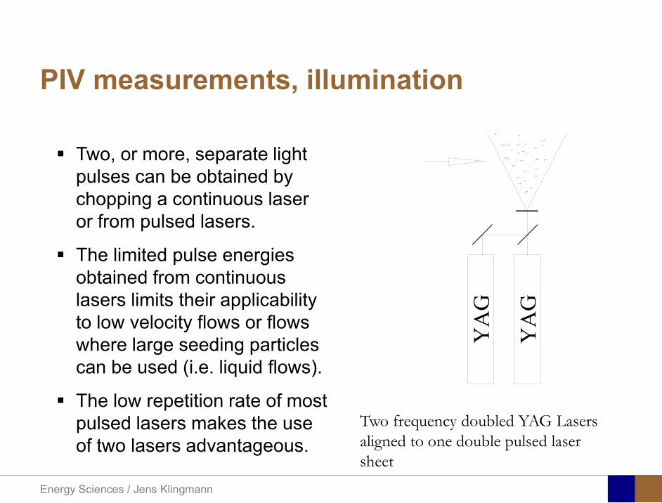
Energy Sciences Jens Klingmann
PIV measurements illumination
YA
G
YA
G
Two frequency doubled YAG Lasers aligned to one double pulsed laser sheet
Two or more separate light pulses can be obtained by chopping a continuous laser or from pulsed lasers
The limited pulse energies obtained from continuous lasers limits their applicability to low velocity flows or flows where large seeding particles can be used (ie liquid flows)
The low repetition rate of most pulsed lasers makes the use of two lasers advantageous
Energy Sciences Jens Klingmann
PIV measurements recording
High seeding density in laminar flame
Film or CCD-cameras Cross- or Auto-correlation
ndash ie both particle images on the same frame or on separate frames
CCD-camera requirementndash A many pixels as possiblendash 2k by 2k available 4k by 4k coming
Energy Sciences Jens Klingmann
PIV measurements analyses
Low seeding density (Number of seeding particles per unit volume)
Each particle image pair can be identified This is called particle tracking
High seeding density (PIV)
Small sub-regions of the image containing many particle image pairs are processed to obtain one velocity vector
Energy Sciences Jens Klingmann
PIV measurements analyses
Energy Sciences Jens Klingmann
PIV measurements analyses
( ) ( ) ( ) xsxxs dIIR 2A
1
I
+= int
Cross correlation between ( )x1I and ( )x2I
s is a two dimensional displacement vector
IA is the interrogation area
Cross correlation between
(
)
x
1
I
and
(
)
x
2
I
s is a two dimensional displacement vector
I
A
is the interrogation area
Energy Sciences Jens Klingmann
Energy Sciences Jens Klingmann
PIV from IOWA state university
Energy Sciences Jens Klingmann
PIV sample of evaluation
Energy Sciences Jens Klingmann
LDA PIV HWA Velocity range 01 mms ndash 300
ms 02 ndash 150 ms
Measuring Volume
D = 005 L = 05 mm
2 by 2 by 05 mm
L = 05 mm
Freq response O(10 000) Hz O(10) Hz O(100 000) Hz Calibration Yes No No Sensitivity to other than velocity
Low (ref Index) Low (ref Index) Large (temperature concentrationshellip)
Continuous Signal
Sometimes Seldom Always
Noise High High Low Turbulence intensity
No limitation Some limitation lt 20
Price O(1 000 000) SEK
O(1 000 000) SEK
O(50 000) SEK
Required Knowledge
High medium Low
Comparison of techniques
Energy Sciences Jens Klingmann
References experiments
R J Goldstein ldquoFluid Mechanics Measurementsrdquo Hemisphere Publishing 1983 A V Johansson amp P H Alfredsson ldquoExperimentella metoder inom
stroumlmningsmekanikenrdquo Inst Foumlr Mekanik KTH F Durst A Melling and J H Whitelaw ldquoPrincipals and Practice of Laser Doppler
Anemometryrdquo 1984 R J Adrian ldquoParticle-imaging techniques for experimental fluid mechnicsrdquo Ann Rev
Fluid Mech 1991
Energy Sciences Jens Klingmann
Sample of LDA-measurements
Rotor blade
Glas window
Emitted beams
Scattered Light
Adjustable mirror
Energy Sciences Jens Klingmann
Axial velocity sorted into 10 bins
0 1 2 3 4 5 6tangential coordinate (degrees)
-20
0
20
40
60
80
100
120
140
160Ax
ial v
eloc
ity a
nd s
tand
ard
devi
atio
n (m
s)
radial position 7 mm from inner window surfaceaxial position 23 mm behind rotor blades
Energy Sciences Jens Klingmann
Axial velocities in the radial-tangential plane
Energy Sciences Jens Klingmann
Airfoils NACA 4-digit
The NACA four-digit wing sections define the profile by
One digit describing maximum camber as percentage of the chord
One digit describing the distance of maximum camber from the airfoil leading edge in tens of percents of the chord
Two digits describing maximum thickness of the airfoil as percent of the chord
Example the NACA 2412 airfoil has a maximum camber of 2 located 40 (04 chords) from the leading edge with a maximum thickness of 12 of the chord
Four-digit series airfoils by default have maximum thickness at 30 of the chord (03 chords) from the leading edge
Energy Sciences Jens Klingmann
Airfoils NACA 4-digit
bull c is the chord lengthbull x is the position along
the chord from 0 to cbull y is the half thickness at
a given value of x (centerline to surface)
bull t is the maximum thickness as a fraction of the chord
Energy Sciences Jens Klingmann
Death by PowerPoint
| LDA | PIV | HWA | |||||
| Velocity range | 01 mms ndash 300 ms | 02 ndash 150 ms | |||||
| Measuring Volume | D = 005 L = 05 mm | 2 by 2 by 05 mm | L = 05 mm | ||||
| Freq response | O(10 000) Hz | O(10) Hz | O(100 000) Hz | ||||
| Calibration | Yes | No | No | ||||
| Sensitivity to other than velocity | Low (ref Index) | Low (ref Index) | Large (temperature concentrationshellip) | ||||
| Continuous Signal | Sometimes | Seldom | Always | ||||
| Noise | High | High | Low | ||||
| Turbulence intensity | No limitation | Some limitation | lt 20 | ||||
| Price | O(1 000 000) SEK | O(1 000 000) SEK | O(50 000) SEK | ||||
| Required Knowledge | High | medium | Low |
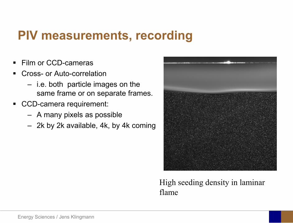
Energy Sciences Jens Klingmann
PIV measurements recording
High seeding density in laminar flame
Film or CCD-cameras Cross- or Auto-correlation
ndash ie both particle images on the same frame or on separate frames
CCD-camera requirementndash A many pixels as possiblendash 2k by 2k available 4k by 4k coming
Energy Sciences Jens Klingmann
PIV measurements analyses
Low seeding density (Number of seeding particles per unit volume)
Each particle image pair can be identified This is called particle tracking
High seeding density (PIV)
Small sub-regions of the image containing many particle image pairs are processed to obtain one velocity vector
Energy Sciences Jens Klingmann
PIV measurements analyses
Energy Sciences Jens Klingmann
PIV measurements analyses
( ) ( ) ( ) xsxxs dIIR 2A
1
I
+= int
Cross correlation between ( )x1I and ( )x2I
s is a two dimensional displacement vector
IA is the interrogation area
Cross correlation between
(
)
x
1
I
and
(
)
x
2
I
s is a two dimensional displacement vector
I
A
is the interrogation area
Energy Sciences Jens Klingmann
Energy Sciences Jens Klingmann
PIV from IOWA state university
Energy Sciences Jens Klingmann
PIV sample of evaluation
Energy Sciences Jens Klingmann
LDA PIV HWA Velocity range 01 mms ndash 300
ms 02 ndash 150 ms
Measuring Volume
D = 005 L = 05 mm
2 by 2 by 05 mm
L = 05 mm
Freq response O(10 000) Hz O(10) Hz O(100 000) Hz Calibration Yes No No Sensitivity to other than velocity
Low (ref Index) Low (ref Index) Large (temperature concentrationshellip)
Continuous Signal
Sometimes Seldom Always
Noise High High Low Turbulence intensity
No limitation Some limitation lt 20
Price O(1 000 000) SEK
O(1 000 000) SEK
O(50 000) SEK
Required Knowledge
High medium Low
Comparison of techniques
Energy Sciences Jens Klingmann
References experiments
R J Goldstein ldquoFluid Mechanics Measurementsrdquo Hemisphere Publishing 1983 A V Johansson amp P H Alfredsson ldquoExperimentella metoder inom
stroumlmningsmekanikenrdquo Inst Foumlr Mekanik KTH F Durst A Melling and J H Whitelaw ldquoPrincipals and Practice of Laser Doppler
Anemometryrdquo 1984 R J Adrian ldquoParticle-imaging techniques for experimental fluid mechnicsrdquo Ann Rev
Fluid Mech 1991
Energy Sciences Jens Klingmann
Sample of LDA-measurements
Rotor blade
Glas window
Emitted beams
Scattered Light
Adjustable mirror
Energy Sciences Jens Klingmann
Axial velocity sorted into 10 bins
0 1 2 3 4 5 6tangential coordinate (degrees)
-20
0
20
40
60
80
100
120
140
160Ax
ial v
eloc
ity a
nd s
tand
ard
devi
atio
n (m
s)
radial position 7 mm from inner window surfaceaxial position 23 mm behind rotor blades
Energy Sciences Jens Klingmann
Axial velocities in the radial-tangential plane
Energy Sciences Jens Klingmann
Airfoils NACA 4-digit
The NACA four-digit wing sections define the profile by
One digit describing maximum camber as percentage of the chord
One digit describing the distance of maximum camber from the airfoil leading edge in tens of percents of the chord
Two digits describing maximum thickness of the airfoil as percent of the chord
Example the NACA 2412 airfoil has a maximum camber of 2 located 40 (04 chords) from the leading edge with a maximum thickness of 12 of the chord
Four-digit series airfoils by default have maximum thickness at 30 of the chord (03 chords) from the leading edge
Energy Sciences Jens Klingmann
Airfoils NACA 4-digit
bull c is the chord lengthbull x is the position along
the chord from 0 to cbull y is the half thickness at
a given value of x (centerline to surface)
bull t is the maximum thickness as a fraction of the chord
Energy Sciences Jens Klingmann
Death by PowerPoint
| LDA | PIV | HWA | |||||
| Velocity range | 01 mms ndash 300 ms | 02 ndash 150 ms | |||||
| Measuring Volume | D = 005 L = 05 mm | 2 by 2 by 05 mm | L = 05 mm | ||||
| Freq response | O(10 000) Hz | O(10) Hz | O(100 000) Hz | ||||
| Calibration | Yes | No | No | ||||
| Sensitivity to other than velocity | Low (ref Index) | Low (ref Index) | Large (temperature concentrationshellip) | ||||
| Continuous Signal | Sometimes | Seldom | Always | ||||
| Noise | High | High | Low | ||||
| Turbulence intensity | No limitation | Some limitation | lt 20 | ||||
| Price | O(1 000 000) SEK | O(1 000 000) SEK | O(50 000) SEK | ||||
| Required Knowledge | High | medium | Low |
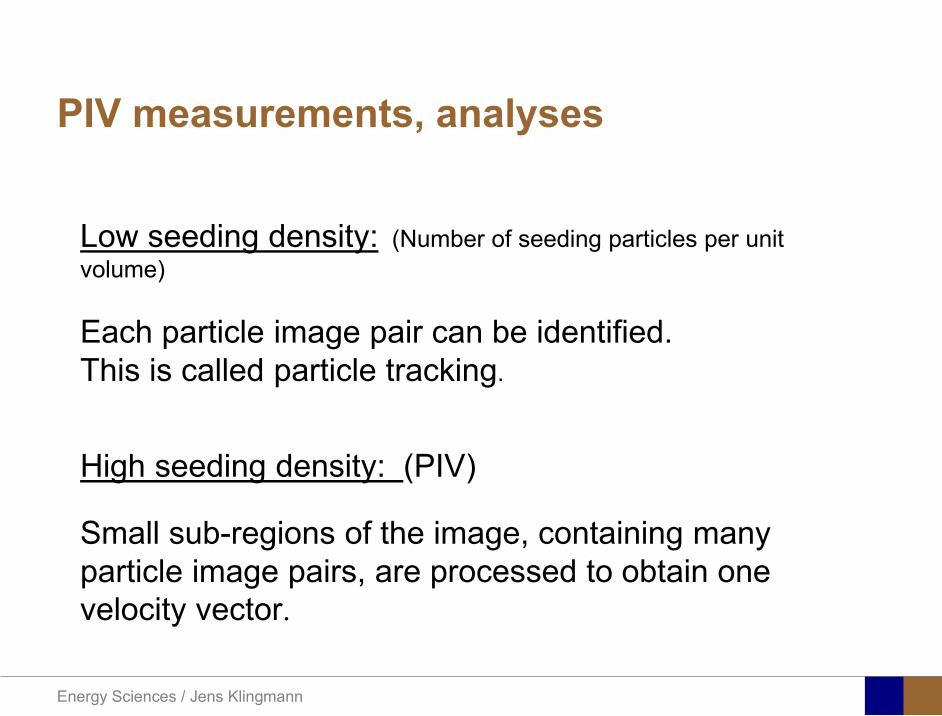
Energy Sciences Jens Klingmann
PIV measurements analyses
Low seeding density (Number of seeding particles per unit volume)
Each particle image pair can be identified This is called particle tracking
High seeding density (PIV)
Small sub-regions of the image containing many particle image pairs are processed to obtain one velocity vector
Energy Sciences Jens Klingmann
PIV measurements analyses
Energy Sciences Jens Klingmann
PIV measurements analyses
( ) ( ) ( ) xsxxs dIIR 2A
1
I
+= int
Cross correlation between ( )x1I and ( )x2I
s is a two dimensional displacement vector
IA is the interrogation area
Cross correlation between
(
)
x
1
I
and
(
)
x
2
I
s is a two dimensional displacement vector
I
A
is the interrogation area
Energy Sciences Jens Klingmann
Energy Sciences Jens Klingmann
PIV from IOWA state university
Energy Sciences Jens Klingmann
PIV sample of evaluation
Energy Sciences Jens Klingmann
LDA PIV HWA Velocity range 01 mms ndash 300
ms 02 ndash 150 ms
Measuring Volume
D = 005 L = 05 mm
2 by 2 by 05 mm
L = 05 mm
Freq response O(10 000) Hz O(10) Hz O(100 000) Hz Calibration Yes No No Sensitivity to other than velocity
Low (ref Index) Low (ref Index) Large (temperature concentrationshellip)
Continuous Signal
Sometimes Seldom Always
Noise High High Low Turbulence intensity
No limitation Some limitation lt 20
Price O(1 000 000) SEK
O(1 000 000) SEK
O(50 000) SEK
Required Knowledge
High medium Low
Comparison of techniques
Energy Sciences Jens Klingmann
References experiments
R J Goldstein ldquoFluid Mechanics Measurementsrdquo Hemisphere Publishing 1983 A V Johansson amp P H Alfredsson ldquoExperimentella metoder inom
stroumlmningsmekanikenrdquo Inst Foumlr Mekanik KTH F Durst A Melling and J H Whitelaw ldquoPrincipals and Practice of Laser Doppler
Anemometryrdquo 1984 R J Adrian ldquoParticle-imaging techniques for experimental fluid mechnicsrdquo Ann Rev
Fluid Mech 1991
Energy Sciences Jens Klingmann
Sample of LDA-measurements
Rotor blade
Glas window
Emitted beams
Scattered Light
Adjustable mirror
Energy Sciences Jens Klingmann
Axial velocity sorted into 10 bins
0 1 2 3 4 5 6tangential coordinate (degrees)
-20
0
20
40
60
80
100
120
140
160Ax
ial v
eloc
ity a
nd s
tand
ard
devi
atio
n (m
s)
radial position 7 mm from inner window surfaceaxial position 23 mm behind rotor blades
Energy Sciences Jens Klingmann
Axial velocities in the radial-tangential plane
Energy Sciences Jens Klingmann
Airfoils NACA 4-digit
The NACA four-digit wing sections define the profile by
One digit describing maximum camber as percentage of the chord
One digit describing the distance of maximum camber from the airfoil leading edge in tens of percents of the chord
Two digits describing maximum thickness of the airfoil as percent of the chord
Example the NACA 2412 airfoil has a maximum camber of 2 located 40 (04 chords) from the leading edge with a maximum thickness of 12 of the chord
Four-digit series airfoils by default have maximum thickness at 30 of the chord (03 chords) from the leading edge
Energy Sciences Jens Klingmann
Airfoils NACA 4-digit
bull c is the chord lengthbull x is the position along
the chord from 0 to cbull y is the half thickness at
a given value of x (centerline to surface)
bull t is the maximum thickness as a fraction of the chord
Energy Sciences Jens Klingmann
Death by PowerPoint
| LDA | PIV | HWA | |||||
| Velocity range | 01 mms ndash 300 ms | 02 ndash 150 ms | |||||
| Measuring Volume | D = 005 L = 05 mm | 2 by 2 by 05 mm | L = 05 mm | ||||
| Freq response | O(10 000) Hz | O(10) Hz | O(100 000) Hz | ||||
| Calibration | Yes | No | No | ||||
| Sensitivity to other than velocity | Low (ref Index) | Low (ref Index) | Large (temperature concentrationshellip) | ||||
| Continuous Signal | Sometimes | Seldom | Always | ||||
| Noise | High | High | Low | ||||
| Turbulence intensity | No limitation | Some limitation | lt 20 | ||||
| Price | O(1 000 000) SEK | O(1 000 000) SEK | O(50 000) SEK | ||||
| Required Knowledge | High | medium | Low |
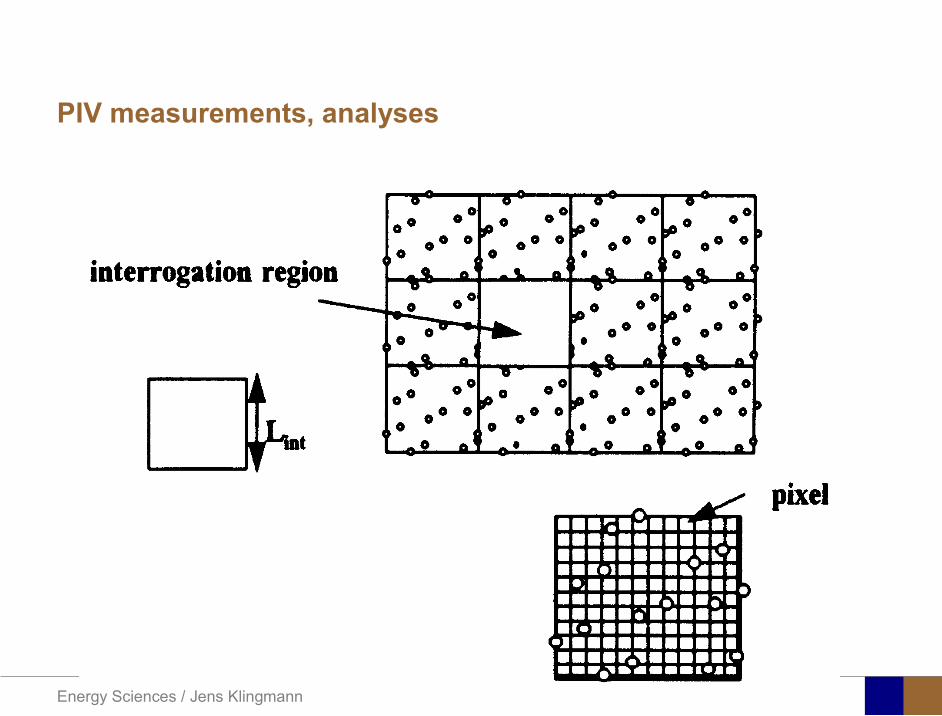
Energy Sciences Jens Klingmann
PIV measurements analyses
Energy Sciences Jens Klingmann
PIV measurements analyses
( ) ( ) ( ) xsxxs dIIR 2A
1
I
+= int
Cross correlation between ( )x1I and ( )x2I
s is a two dimensional displacement vector
IA is the interrogation area
Cross correlation between
(
)
x
1
I
and
(
)
x
2
I
s is a two dimensional displacement vector
I
A
is the interrogation area
Energy Sciences Jens Klingmann
Energy Sciences Jens Klingmann
PIV from IOWA state university
Energy Sciences Jens Klingmann
PIV sample of evaluation
Energy Sciences Jens Klingmann
LDA PIV HWA Velocity range 01 mms ndash 300
ms 02 ndash 150 ms
Measuring Volume
D = 005 L = 05 mm
2 by 2 by 05 mm
L = 05 mm
Freq response O(10 000) Hz O(10) Hz O(100 000) Hz Calibration Yes No No Sensitivity to other than velocity
Low (ref Index) Low (ref Index) Large (temperature concentrationshellip)
Continuous Signal
Sometimes Seldom Always
Noise High High Low Turbulence intensity
No limitation Some limitation lt 20
Price O(1 000 000) SEK
O(1 000 000) SEK
O(50 000) SEK
Required Knowledge
High medium Low
Comparison of techniques
Energy Sciences Jens Klingmann
References experiments
R J Goldstein ldquoFluid Mechanics Measurementsrdquo Hemisphere Publishing 1983 A V Johansson amp P H Alfredsson ldquoExperimentella metoder inom
stroumlmningsmekanikenrdquo Inst Foumlr Mekanik KTH F Durst A Melling and J H Whitelaw ldquoPrincipals and Practice of Laser Doppler
Anemometryrdquo 1984 R J Adrian ldquoParticle-imaging techniques for experimental fluid mechnicsrdquo Ann Rev
Fluid Mech 1991
Energy Sciences Jens Klingmann
Sample of LDA-measurements
Rotor blade
Glas window
Emitted beams
Scattered Light
Adjustable mirror
Energy Sciences Jens Klingmann
Axial velocity sorted into 10 bins
0 1 2 3 4 5 6tangential coordinate (degrees)
-20
0
20
40
60
80
100
120
140
160Ax
ial v
eloc
ity a
nd s
tand
ard
devi
atio
n (m
s)
radial position 7 mm from inner window surfaceaxial position 23 mm behind rotor blades
Energy Sciences Jens Klingmann
Axial velocities in the radial-tangential plane
Energy Sciences Jens Klingmann
Airfoils NACA 4-digit
The NACA four-digit wing sections define the profile by
One digit describing maximum camber as percentage of the chord
One digit describing the distance of maximum camber from the airfoil leading edge in tens of percents of the chord
Two digits describing maximum thickness of the airfoil as percent of the chord
Example the NACA 2412 airfoil has a maximum camber of 2 located 40 (04 chords) from the leading edge with a maximum thickness of 12 of the chord
Four-digit series airfoils by default have maximum thickness at 30 of the chord (03 chords) from the leading edge
Energy Sciences Jens Klingmann
Airfoils NACA 4-digit
bull c is the chord lengthbull x is the position along
the chord from 0 to cbull y is the half thickness at
a given value of x (centerline to surface)
bull t is the maximum thickness as a fraction of the chord
Energy Sciences Jens Klingmann
Death by PowerPoint
| LDA | PIV | HWA | |||||
| Velocity range | 01 mms ndash 300 ms | 02 ndash 150 ms | |||||
| Measuring Volume | D = 005 L = 05 mm | 2 by 2 by 05 mm | L = 05 mm | ||||
| Freq response | O(10 000) Hz | O(10) Hz | O(100 000) Hz | ||||
| Calibration | Yes | No | No | ||||
| Sensitivity to other than velocity | Low (ref Index) | Low (ref Index) | Large (temperature concentrationshellip) | ||||
| Continuous Signal | Sometimes | Seldom | Always | ||||
| Noise | High | High | Low | ||||
| Turbulence intensity | No limitation | Some limitation | lt 20 | ||||
| Price | O(1 000 000) SEK | O(1 000 000) SEK | O(50 000) SEK | ||||
| Required Knowledge | High | medium | Low |
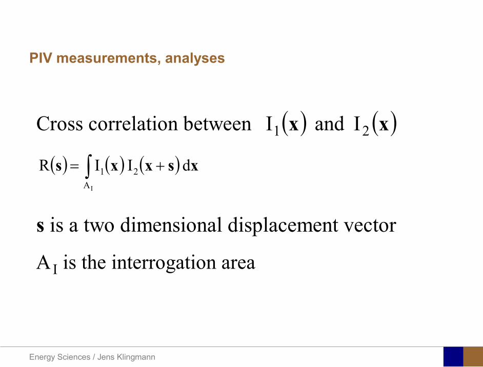
Energy Sciences Jens Klingmann
PIV measurements analyses
( ) ( ) ( ) xsxxs dIIR 2A
1
I
+= int
Cross correlation between ( )x1I and ( )x2I
s is a two dimensional displacement vector
IA is the interrogation area
Cross correlation between
(
)
x
1
I
and
(
)
x
2
I
s is a two dimensional displacement vector
I
A
is the interrogation area
Energy Sciences Jens Klingmann
Energy Sciences Jens Klingmann
PIV from IOWA state university
Energy Sciences Jens Klingmann
PIV sample of evaluation
Energy Sciences Jens Klingmann
LDA PIV HWA Velocity range 01 mms ndash 300
ms 02 ndash 150 ms
Measuring Volume
D = 005 L = 05 mm
2 by 2 by 05 mm
L = 05 mm
Freq response O(10 000) Hz O(10) Hz O(100 000) Hz Calibration Yes No No Sensitivity to other than velocity
Low (ref Index) Low (ref Index) Large (temperature concentrationshellip)
Continuous Signal
Sometimes Seldom Always
Noise High High Low Turbulence intensity
No limitation Some limitation lt 20
Price O(1 000 000) SEK
O(1 000 000) SEK
O(50 000) SEK
Required Knowledge
High medium Low
Comparison of techniques
Energy Sciences Jens Klingmann
References experiments
R J Goldstein ldquoFluid Mechanics Measurementsrdquo Hemisphere Publishing 1983 A V Johansson amp P H Alfredsson ldquoExperimentella metoder inom
stroumlmningsmekanikenrdquo Inst Foumlr Mekanik KTH F Durst A Melling and J H Whitelaw ldquoPrincipals and Practice of Laser Doppler
Anemometryrdquo 1984 R J Adrian ldquoParticle-imaging techniques for experimental fluid mechnicsrdquo Ann Rev
Fluid Mech 1991
Energy Sciences Jens Klingmann
Sample of LDA-measurements
Rotor blade
Glas window
Emitted beams
Scattered Light
Adjustable mirror
Energy Sciences Jens Klingmann
Axial velocity sorted into 10 bins
0 1 2 3 4 5 6tangential coordinate (degrees)
-20
0
20
40
60
80
100
120
140
160Ax
ial v
eloc
ity a
nd s
tand
ard
devi
atio
n (m
s)
radial position 7 mm from inner window surfaceaxial position 23 mm behind rotor blades
Energy Sciences Jens Klingmann
Axial velocities in the radial-tangential plane
Energy Sciences Jens Klingmann
Airfoils NACA 4-digit
The NACA four-digit wing sections define the profile by
One digit describing maximum camber as percentage of the chord
One digit describing the distance of maximum camber from the airfoil leading edge in tens of percents of the chord
Two digits describing maximum thickness of the airfoil as percent of the chord
Example the NACA 2412 airfoil has a maximum camber of 2 located 40 (04 chords) from the leading edge with a maximum thickness of 12 of the chord
Four-digit series airfoils by default have maximum thickness at 30 of the chord (03 chords) from the leading edge
Energy Sciences Jens Klingmann
Airfoils NACA 4-digit
bull c is the chord lengthbull x is the position along
the chord from 0 to cbull y is the half thickness at
a given value of x (centerline to surface)
bull t is the maximum thickness as a fraction of the chord
Energy Sciences Jens Klingmann
Death by PowerPoint
| LDA | PIV | HWA | |||||
| Velocity range | 01 mms ndash 300 ms | 02 ndash 150 ms | |||||
| Measuring Volume | D = 005 L = 05 mm | 2 by 2 by 05 mm | L = 05 mm | ||||
| Freq response | O(10 000) Hz | O(10) Hz | O(100 000) Hz | ||||
| Calibration | Yes | No | No | ||||
| Sensitivity to other than velocity | Low (ref Index) | Low (ref Index) | Large (temperature concentrationshellip) | ||||
| Continuous Signal | Sometimes | Seldom | Always | ||||
| Noise | High | High | Low | ||||
| Turbulence intensity | No limitation | Some limitation | lt 20 | ||||
| Price | O(1 000 000) SEK | O(1 000 000) SEK | O(50 000) SEK | ||||
| Required Knowledge | High | medium | Low |
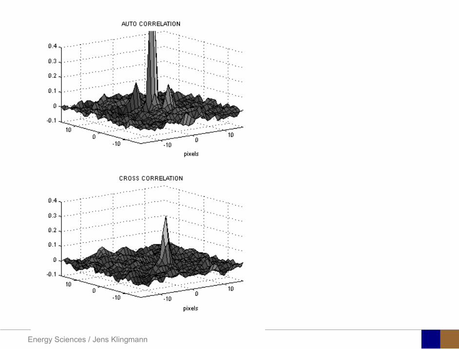
Energy Sciences Jens Klingmann
Energy Sciences Jens Klingmann
PIV from IOWA state university
Energy Sciences Jens Klingmann
PIV sample of evaluation
Energy Sciences Jens Klingmann
LDA PIV HWA Velocity range 01 mms ndash 300
ms 02 ndash 150 ms
Measuring Volume
D = 005 L = 05 mm
2 by 2 by 05 mm
L = 05 mm
Freq response O(10 000) Hz O(10) Hz O(100 000) Hz Calibration Yes No No Sensitivity to other than velocity
Low (ref Index) Low (ref Index) Large (temperature concentrationshellip)
Continuous Signal
Sometimes Seldom Always
Noise High High Low Turbulence intensity
No limitation Some limitation lt 20
Price O(1 000 000) SEK
O(1 000 000) SEK
O(50 000) SEK
Required Knowledge
High medium Low
Comparison of techniques
Energy Sciences Jens Klingmann
References experiments
R J Goldstein ldquoFluid Mechanics Measurementsrdquo Hemisphere Publishing 1983 A V Johansson amp P H Alfredsson ldquoExperimentella metoder inom
stroumlmningsmekanikenrdquo Inst Foumlr Mekanik KTH F Durst A Melling and J H Whitelaw ldquoPrincipals and Practice of Laser Doppler
Anemometryrdquo 1984 R J Adrian ldquoParticle-imaging techniques for experimental fluid mechnicsrdquo Ann Rev
Fluid Mech 1991
Energy Sciences Jens Klingmann
Sample of LDA-measurements
Rotor blade
Glas window
Emitted beams
Scattered Light
Adjustable mirror
Energy Sciences Jens Klingmann
Axial velocity sorted into 10 bins
0 1 2 3 4 5 6tangential coordinate (degrees)
-20
0
20
40
60
80
100
120
140
160Ax
ial v
eloc
ity a
nd s
tand
ard
devi
atio
n (m
s)
radial position 7 mm from inner window surfaceaxial position 23 mm behind rotor blades
Energy Sciences Jens Klingmann
Axial velocities in the radial-tangential plane
Energy Sciences Jens Klingmann
Airfoils NACA 4-digit
The NACA four-digit wing sections define the profile by
One digit describing maximum camber as percentage of the chord
One digit describing the distance of maximum camber from the airfoil leading edge in tens of percents of the chord
Two digits describing maximum thickness of the airfoil as percent of the chord
Example the NACA 2412 airfoil has a maximum camber of 2 located 40 (04 chords) from the leading edge with a maximum thickness of 12 of the chord
Four-digit series airfoils by default have maximum thickness at 30 of the chord (03 chords) from the leading edge
Energy Sciences Jens Klingmann
Airfoils NACA 4-digit
bull c is the chord lengthbull x is the position along
the chord from 0 to cbull y is the half thickness at
a given value of x (centerline to surface)
bull t is the maximum thickness as a fraction of the chord
Energy Sciences Jens Klingmann
Death by PowerPoint
| LDA | PIV | HWA | |||||
| Velocity range | 01 mms ndash 300 ms | 02 ndash 150 ms | |||||
| Measuring Volume | D = 005 L = 05 mm | 2 by 2 by 05 mm | L = 05 mm | ||||
| Freq response | O(10 000) Hz | O(10) Hz | O(100 000) Hz | ||||
| Calibration | Yes | No | No | ||||
| Sensitivity to other than velocity | Low (ref Index) | Low (ref Index) | Large (temperature concentrationshellip) | ||||
| Continuous Signal | Sometimes | Seldom | Always | ||||
| Noise | High | High | Low | ||||
| Turbulence intensity | No limitation | Some limitation | lt 20 | ||||
| Price | O(1 000 000) SEK | O(1 000 000) SEK | O(50 000) SEK | ||||
| Required Knowledge | High | medium | Low |
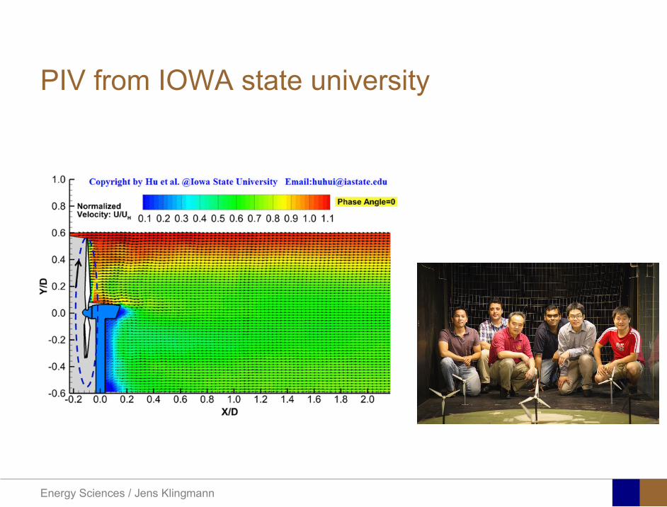
Energy Sciences Jens Klingmann
PIV from IOWA state university
Energy Sciences Jens Klingmann
PIV sample of evaluation
Energy Sciences Jens Klingmann
LDA PIV HWA Velocity range 01 mms ndash 300
ms 02 ndash 150 ms
Measuring Volume
D = 005 L = 05 mm
2 by 2 by 05 mm
L = 05 mm
Freq response O(10 000) Hz O(10) Hz O(100 000) Hz Calibration Yes No No Sensitivity to other than velocity
Low (ref Index) Low (ref Index) Large (temperature concentrationshellip)
Continuous Signal
Sometimes Seldom Always
Noise High High Low Turbulence intensity
No limitation Some limitation lt 20
Price O(1 000 000) SEK
O(1 000 000) SEK
O(50 000) SEK
Required Knowledge
High medium Low
Comparison of techniques
Energy Sciences Jens Klingmann
References experiments
R J Goldstein ldquoFluid Mechanics Measurementsrdquo Hemisphere Publishing 1983 A V Johansson amp P H Alfredsson ldquoExperimentella metoder inom
stroumlmningsmekanikenrdquo Inst Foumlr Mekanik KTH F Durst A Melling and J H Whitelaw ldquoPrincipals and Practice of Laser Doppler
Anemometryrdquo 1984 R J Adrian ldquoParticle-imaging techniques for experimental fluid mechnicsrdquo Ann Rev
Fluid Mech 1991
Energy Sciences Jens Klingmann
Sample of LDA-measurements
Rotor blade
Glas window
Emitted beams
Scattered Light
Adjustable mirror
Energy Sciences Jens Klingmann
Axial velocity sorted into 10 bins
0 1 2 3 4 5 6tangential coordinate (degrees)
-20
0
20
40
60
80
100
120
140
160Ax
ial v
eloc
ity a
nd s
tand
ard
devi
atio
n (m
s)
radial position 7 mm from inner window surfaceaxial position 23 mm behind rotor blades
Energy Sciences Jens Klingmann
Axial velocities in the radial-tangential plane
Energy Sciences Jens Klingmann
Airfoils NACA 4-digit
The NACA four-digit wing sections define the profile by
One digit describing maximum camber as percentage of the chord
One digit describing the distance of maximum camber from the airfoil leading edge in tens of percents of the chord
Two digits describing maximum thickness of the airfoil as percent of the chord
Example the NACA 2412 airfoil has a maximum camber of 2 located 40 (04 chords) from the leading edge with a maximum thickness of 12 of the chord
Four-digit series airfoils by default have maximum thickness at 30 of the chord (03 chords) from the leading edge
Energy Sciences Jens Klingmann
Airfoils NACA 4-digit
bull c is the chord lengthbull x is the position along
the chord from 0 to cbull y is the half thickness at
a given value of x (centerline to surface)
bull t is the maximum thickness as a fraction of the chord
Energy Sciences Jens Klingmann
Death by PowerPoint
| LDA | PIV | HWA | |||||
| Velocity range | 01 mms ndash 300 ms | 02 ndash 150 ms | |||||
| Measuring Volume | D = 005 L = 05 mm | 2 by 2 by 05 mm | L = 05 mm | ||||
| Freq response | O(10 000) Hz | O(10) Hz | O(100 000) Hz | ||||
| Calibration | Yes | No | No | ||||
| Sensitivity to other than velocity | Low (ref Index) | Low (ref Index) | Large (temperature concentrationshellip) | ||||
| Continuous Signal | Sometimes | Seldom | Always | ||||
| Noise | High | High | Low | ||||
| Turbulence intensity | No limitation | Some limitation | lt 20 | ||||
| Price | O(1 000 000) SEK | O(1 000 000) SEK | O(50 000) SEK | ||||
| Required Knowledge | High | medium | Low |
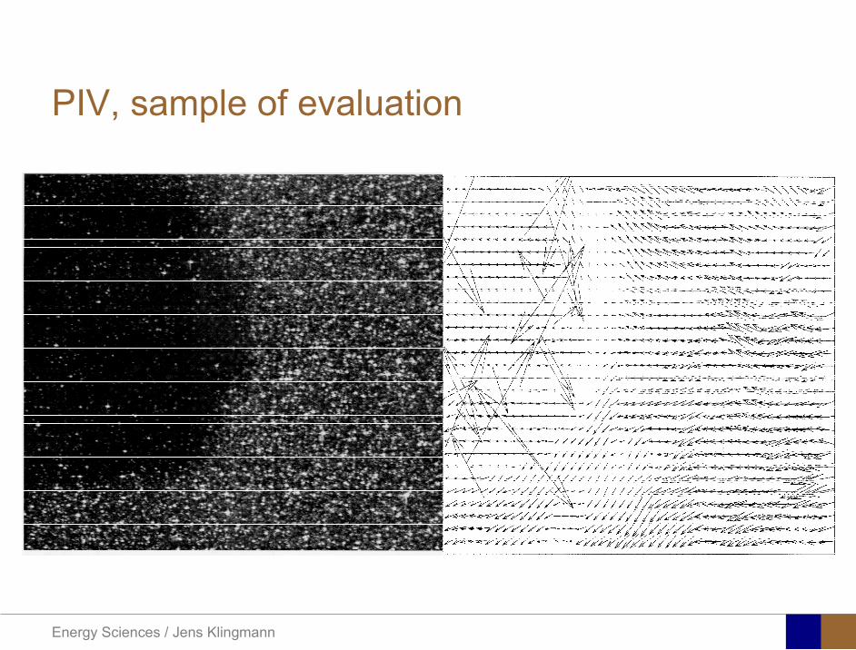
Energy Sciences Jens Klingmann
PIV sample of evaluation
Energy Sciences Jens Klingmann
LDA PIV HWA Velocity range 01 mms ndash 300
ms 02 ndash 150 ms
Measuring Volume
D = 005 L = 05 mm
2 by 2 by 05 mm
L = 05 mm
Freq response O(10 000) Hz O(10) Hz O(100 000) Hz Calibration Yes No No Sensitivity to other than velocity
Low (ref Index) Low (ref Index) Large (temperature concentrationshellip)
Continuous Signal
Sometimes Seldom Always
Noise High High Low Turbulence intensity
No limitation Some limitation lt 20
Price O(1 000 000) SEK
O(1 000 000) SEK
O(50 000) SEK
Required Knowledge
High medium Low
Comparison of techniques
Energy Sciences Jens Klingmann
References experiments
R J Goldstein ldquoFluid Mechanics Measurementsrdquo Hemisphere Publishing 1983 A V Johansson amp P H Alfredsson ldquoExperimentella metoder inom
stroumlmningsmekanikenrdquo Inst Foumlr Mekanik KTH F Durst A Melling and J H Whitelaw ldquoPrincipals and Practice of Laser Doppler
Anemometryrdquo 1984 R J Adrian ldquoParticle-imaging techniques for experimental fluid mechnicsrdquo Ann Rev
Fluid Mech 1991
Energy Sciences Jens Klingmann
Sample of LDA-measurements
Rotor blade
Glas window
Emitted beams
Scattered Light
Adjustable mirror
Energy Sciences Jens Klingmann
Axial velocity sorted into 10 bins
0 1 2 3 4 5 6tangential coordinate (degrees)
-20
0
20
40
60
80
100
120
140
160Ax
ial v
eloc
ity a
nd s
tand
ard
devi
atio
n (m
s)
radial position 7 mm from inner window surfaceaxial position 23 mm behind rotor blades
Energy Sciences Jens Klingmann
Axial velocities in the radial-tangential plane
Energy Sciences Jens Klingmann
Airfoils NACA 4-digit
The NACA four-digit wing sections define the profile by
One digit describing maximum camber as percentage of the chord
One digit describing the distance of maximum camber from the airfoil leading edge in tens of percents of the chord
Two digits describing maximum thickness of the airfoil as percent of the chord
Example the NACA 2412 airfoil has a maximum camber of 2 located 40 (04 chords) from the leading edge with a maximum thickness of 12 of the chord
Four-digit series airfoils by default have maximum thickness at 30 of the chord (03 chords) from the leading edge
Energy Sciences Jens Klingmann
Airfoils NACA 4-digit
bull c is the chord lengthbull x is the position along
the chord from 0 to cbull y is the half thickness at
a given value of x (centerline to surface)
bull t is the maximum thickness as a fraction of the chord
Energy Sciences Jens Klingmann
Death by PowerPoint
| LDA | PIV | HWA | |||||
| Velocity range | 01 mms ndash 300 ms | 02 ndash 150 ms | |||||
| Measuring Volume | D = 005 L = 05 mm | 2 by 2 by 05 mm | L = 05 mm | ||||
| Freq response | O(10 000) Hz | O(10) Hz | O(100 000) Hz | ||||
| Calibration | Yes | No | No | ||||
| Sensitivity to other than velocity | Low (ref Index) | Low (ref Index) | Large (temperature concentrationshellip) | ||||
| Continuous Signal | Sometimes | Seldom | Always | ||||
| Noise | High | High | Low | ||||
| Turbulence intensity | No limitation | Some limitation | lt 20 | ||||
| Price | O(1 000 000) SEK | O(1 000 000) SEK | O(50 000) SEK | ||||
| Required Knowledge | High | medium | Low |
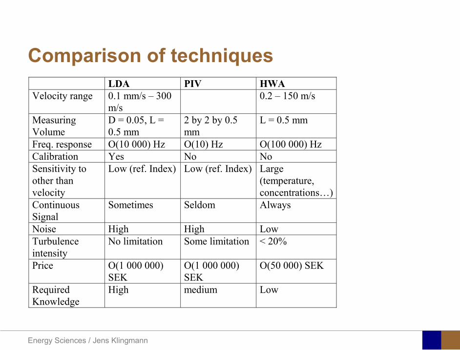
Energy Sciences Jens Klingmann
LDA PIV HWA Velocity range 01 mms ndash 300
ms 02 ndash 150 ms
Measuring Volume
D = 005 L = 05 mm
2 by 2 by 05 mm
L = 05 mm
Freq response O(10 000) Hz O(10) Hz O(100 000) Hz Calibration Yes No No Sensitivity to other than velocity
Low (ref Index) Low (ref Index) Large (temperature concentrationshellip)
Continuous Signal
Sometimes Seldom Always
Noise High High Low Turbulence intensity
No limitation Some limitation lt 20
Price O(1 000 000) SEK
O(1 000 000) SEK
O(50 000) SEK
Required Knowledge
High medium Low
Comparison of techniques
Energy Sciences Jens Klingmann
References experiments
R J Goldstein ldquoFluid Mechanics Measurementsrdquo Hemisphere Publishing 1983 A V Johansson amp P H Alfredsson ldquoExperimentella metoder inom
stroumlmningsmekanikenrdquo Inst Foumlr Mekanik KTH F Durst A Melling and J H Whitelaw ldquoPrincipals and Practice of Laser Doppler
Anemometryrdquo 1984 R J Adrian ldquoParticle-imaging techniques for experimental fluid mechnicsrdquo Ann Rev
Fluid Mech 1991
Energy Sciences Jens Klingmann
Sample of LDA-measurements
Rotor blade
Glas window
Emitted beams
Scattered Light
Adjustable mirror
Energy Sciences Jens Klingmann
Axial velocity sorted into 10 bins
0 1 2 3 4 5 6tangential coordinate (degrees)
-20
0
20
40
60
80
100
120
140
160Ax
ial v
eloc
ity a
nd s
tand
ard
devi
atio
n (m
s)
radial position 7 mm from inner window surfaceaxial position 23 mm behind rotor blades
Energy Sciences Jens Klingmann
Axial velocities in the radial-tangential plane
Energy Sciences Jens Klingmann
Airfoils NACA 4-digit
The NACA four-digit wing sections define the profile by
One digit describing maximum camber as percentage of the chord
One digit describing the distance of maximum camber from the airfoil leading edge in tens of percents of the chord
Two digits describing maximum thickness of the airfoil as percent of the chord
Example the NACA 2412 airfoil has a maximum camber of 2 located 40 (04 chords) from the leading edge with a maximum thickness of 12 of the chord
Four-digit series airfoils by default have maximum thickness at 30 of the chord (03 chords) from the leading edge
Energy Sciences Jens Klingmann
Airfoils NACA 4-digit
bull c is the chord lengthbull x is the position along
the chord from 0 to cbull y is the half thickness at
a given value of x (centerline to surface)
bull t is the maximum thickness as a fraction of the chord
Energy Sciences Jens Klingmann
Death by PowerPoint
| LDA | PIV | HWA | |||||
| Velocity range | 01 mms ndash 300 ms | 02 ndash 150 ms | |||||
| Measuring Volume | D = 005 L = 05 mm | 2 by 2 by 05 mm | L = 05 mm | ||||
| Freq response | O(10 000) Hz | O(10) Hz | O(100 000) Hz | ||||
| Calibration | Yes | No | No | ||||
| Sensitivity to other than velocity | Low (ref Index) | Low (ref Index) | Large (temperature concentrationshellip) | ||||
| Continuous Signal | Sometimes | Seldom | Always | ||||
| Noise | High | High | Low | ||||
| Turbulence intensity | No limitation | Some limitation | lt 20 | ||||
| Price | O(1 000 000) SEK | O(1 000 000) SEK | O(50 000) SEK | ||||
| Required Knowledge | High | medium | Low |
Energy Sciences Jens Klingmann
References experiments
R J Goldstein ldquoFluid Mechanics Measurementsrdquo Hemisphere Publishing 1983 A V Johansson amp P H Alfredsson ldquoExperimentella metoder inom
stroumlmningsmekanikenrdquo Inst Foumlr Mekanik KTH F Durst A Melling and J H Whitelaw ldquoPrincipals and Practice of Laser Doppler
Anemometryrdquo 1984 R J Adrian ldquoParticle-imaging techniques for experimental fluid mechnicsrdquo Ann Rev
Fluid Mech 1991
Energy Sciences Jens Klingmann
Sample of LDA-measurements
Rotor blade
Glas window
Emitted beams
Scattered Light
Adjustable mirror
Energy Sciences Jens Klingmann
Axial velocity sorted into 10 bins
0 1 2 3 4 5 6tangential coordinate (degrees)
-20
0
20
40
60
80
100
120
140
160Ax
ial v
eloc
ity a
nd s
tand
ard
devi
atio
n (m
s)
radial position 7 mm from inner window surfaceaxial position 23 mm behind rotor blades
Energy Sciences Jens Klingmann
Axial velocities in the radial-tangential plane
Energy Sciences Jens Klingmann
Airfoils NACA 4-digit
The NACA four-digit wing sections define the profile by
One digit describing maximum camber as percentage of the chord
One digit describing the distance of maximum camber from the airfoil leading edge in tens of percents of the chord
Two digits describing maximum thickness of the airfoil as percent of the chord
Example the NACA 2412 airfoil has a maximum camber of 2 located 40 (04 chords) from the leading edge with a maximum thickness of 12 of the chord
Four-digit series airfoils by default have maximum thickness at 30 of the chord (03 chords) from the leading edge
Energy Sciences Jens Klingmann
Airfoils NACA 4-digit
bull c is the chord lengthbull x is the position along
the chord from 0 to cbull y is the half thickness at
a given value of x (centerline to surface)
bull t is the maximum thickness as a fraction of the chord
Energy Sciences Jens Klingmann
Death by PowerPoint
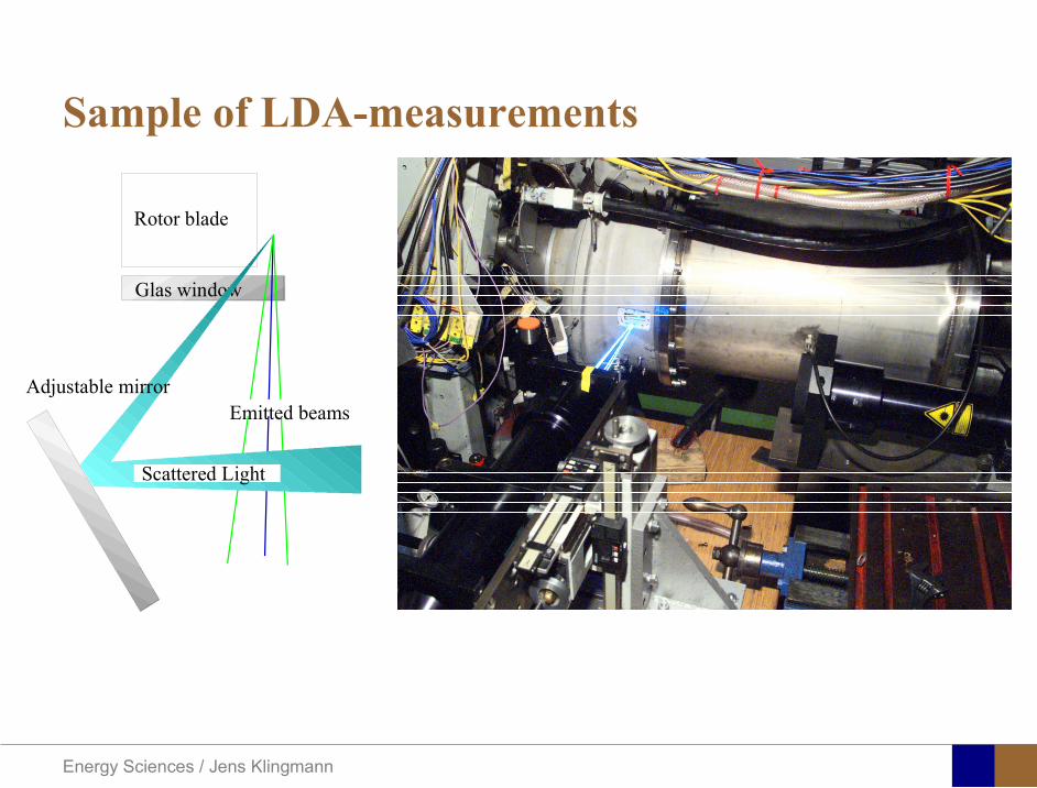
Energy Sciences Jens Klingmann
Sample of LDA-measurements
Rotor blade
Glas window
Emitted beams
Scattered Light
Adjustable mirror
Energy Sciences Jens Klingmann
Axial velocity sorted into 10 bins
0 1 2 3 4 5 6tangential coordinate (degrees)
-20
0
20
40
60
80
100
120
140
160Ax
ial v
eloc
ity a
nd s
tand
ard
devi
atio
n (m
s)
radial position 7 mm from inner window surfaceaxial position 23 mm behind rotor blades
Energy Sciences Jens Klingmann
Axial velocities in the radial-tangential plane
Energy Sciences Jens Klingmann
Airfoils NACA 4-digit
The NACA four-digit wing sections define the profile by
One digit describing maximum camber as percentage of the chord
One digit describing the distance of maximum camber from the airfoil leading edge in tens of percents of the chord
Two digits describing maximum thickness of the airfoil as percent of the chord
Example the NACA 2412 airfoil has a maximum camber of 2 located 40 (04 chords) from the leading edge with a maximum thickness of 12 of the chord
Four-digit series airfoils by default have maximum thickness at 30 of the chord (03 chords) from the leading edge
Energy Sciences Jens Klingmann
Airfoils NACA 4-digit
bull c is the chord lengthbull x is the position along
the chord from 0 to cbull y is the half thickness at
a given value of x (centerline to surface)
bull t is the maximum thickness as a fraction of the chord
Energy Sciences Jens Klingmann
Death by PowerPoint
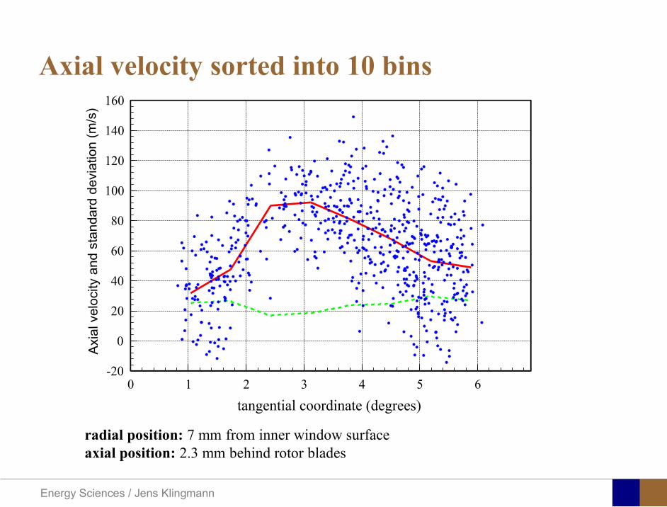
Energy Sciences Jens Klingmann
Axial velocity sorted into 10 bins
0 1 2 3 4 5 6tangential coordinate (degrees)
-20
0
20
40
60
80
100
120
140
160Ax
ial v
eloc
ity a
nd s
tand
ard
devi
atio
n (m
s)
radial position 7 mm from inner window surfaceaxial position 23 mm behind rotor blades
Energy Sciences Jens Klingmann
Axial velocities in the radial-tangential plane
Energy Sciences Jens Klingmann
Airfoils NACA 4-digit
The NACA four-digit wing sections define the profile by
One digit describing maximum camber as percentage of the chord
One digit describing the distance of maximum camber from the airfoil leading edge in tens of percents of the chord
Two digits describing maximum thickness of the airfoil as percent of the chord
Example the NACA 2412 airfoil has a maximum camber of 2 located 40 (04 chords) from the leading edge with a maximum thickness of 12 of the chord
Four-digit series airfoils by default have maximum thickness at 30 of the chord (03 chords) from the leading edge
Energy Sciences Jens Klingmann
Airfoils NACA 4-digit
bull c is the chord lengthbull x is the position along
the chord from 0 to cbull y is the half thickness at
a given value of x (centerline to surface)
bull t is the maximum thickness as a fraction of the chord
Energy Sciences Jens Klingmann
Death by PowerPoint
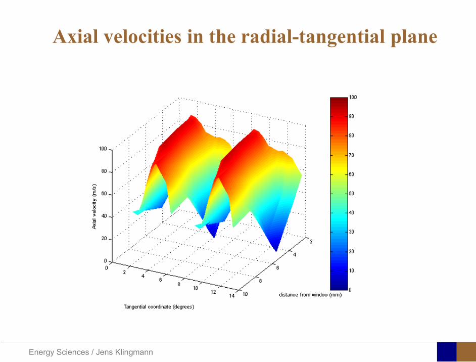
Energy Sciences Jens Klingmann
Axial velocities in the radial-tangential plane
Energy Sciences Jens Klingmann
Airfoils NACA 4-digit
The NACA four-digit wing sections define the profile by
One digit describing maximum camber as percentage of the chord
One digit describing the distance of maximum camber from the airfoil leading edge in tens of percents of the chord
Two digits describing maximum thickness of the airfoil as percent of the chord
Example the NACA 2412 airfoil has a maximum camber of 2 located 40 (04 chords) from the leading edge with a maximum thickness of 12 of the chord
Four-digit series airfoils by default have maximum thickness at 30 of the chord (03 chords) from the leading edge
Energy Sciences Jens Klingmann
Airfoils NACA 4-digit
bull c is the chord lengthbull x is the position along
the chord from 0 to cbull y is the half thickness at
a given value of x (centerline to surface)
bull t is the maximum thickness as a fraction of the chord
Energy Sciences Jens Klingmann
Death by PowerPoint
Energy Sciences Jens Klingmann
Airfoils NACA 4-digit
The NACA four-digit wing sections define the profile by
One digit describing maximum camber as percentage of the chord
One digit describing the distance of maximum camber from the airfoil leading edge in tens of percents of the chord
Two digits describing maximum thickness of the airfoil as percent of the chord
Example the NACA 2412 airfoil has a maximum camber of 2 located 40 (04 chords) from the leading edge with a maximum thickness of 12 of the chord
Four-digit series airfoils by default have maximum thickness at 30 of the chord (03 chords) from the leading edge
Energy Sciences Jens Klingmann
Airfoils NACA 4-digit
bull c is the chord lengthbull x is the position along
the chord from 0 to cbull y is the half thickness at
a given value of x (centerline to surface)
bull t is the maximum thickness as a fraction of the chord
Energy Sciences Jens Klingmann
Death by PowerPoint
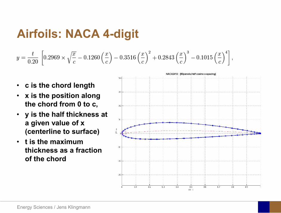
Energy Sciences Jens Klingmann
Airfoils NACA 4-digit
bull c is the chord lengthbull x is the position along
the chord from 0 to cbull y is the half thickness at
a given value of x (centerline to surface)
bull t is the maximum thickness as a fraction of the chord
Energy Sciences Jens Klingmann
Death by PowerPoint
Energy Sciences Jens Klingmann
Death by PowerPoint


![Teori-Teori Hak Asasi Manusia · Teori-Teori Hak Asasi Manusia [ Human Rights Theories ] Herlambang Perdana Wiratraman Faculty of Law, Universitas Airlangga 5 September 2017](https://img.pdfslide.us/doc/110x75/5c8769a909d3f2c77a8bb0f5/teori-teori-hak-asasi-manusia-teori-teori-hak-asasi-manusia-human-rights-theories.jpg)