THEORY OFMEASURE AND INTEGRATION

0 Introduction

Probability theory looks back to a history of almost 300 years. Indeed, J.Bernoulli’s law of large numbers, which was published post mortem in 1713can be considered the mother of all probabilistic theorems. In those days, andeven almost 200 years later, mathematicians had a fairly heuristic idea aboutprobability. So the probability of an event usually was understood as thelimit of the relative frequencies of a series of independent trials “under usualcircumstances”. This apparently coincides with both, the naive intuition ofwhat probability is, as well as with the prediction of the law of large numbers.On the other hand, it is not at all easy to work with such a definition ofprobability, nor is it simple to make it mathematically rigorous.In 1900 the German mathematician D. Hilbert was invited to give a plenarylecture on the World Congress Of Mathematics, that was being held in Paris.There he introduced his famous 23 problems in mathematics. Those problemstriggered the development of the mathematics in the next 50 years. Eventoday some of those questions are still wide open. His sixth question was:

“Give an axiomatic approach to probability theory and physics”.

Of course the axiomatization of physics is tremendously difficult and stillunsolved. The question of giving an axiomatic foundation of probabilitytheory was approached in the 1930’s by the Russian mathematician A.N.Kolmogorov. He linked probability to the then relatively new theory of mea-sures by defining a probability to be a measure with mass 1 on the set ofoutcomes of a random experiment.This theory of measure and integration on the other hand had started todevelop in the middle of the 19th century. Until then the only integrablefunctions that were known were the continuous mappings from R to R. It wasnot until B. Riemann’s Habilitation-Thesis in 1854 that the correspondingdefinition of an integral (which went back to A. Cauchy ) was extended to

1

certain non-continuous functions. Yet the Riemann integral has two decisivedrawbacks :

1. Certain non - continuous functions, which we would like to equip withan integral, are not Riemann-integrable. One of the most famous ex-amples was given by P. G. L. Dirichlet:

δQ(x) =

{1 if x ∈ Q

0 otherwise

Considering δQ as a function from [0, 1] to [0, 1] , its integral would givethe ”size” of Q in [0, 1] , and therefore is interesting.

2. The rules for interchanging limits of sequences of functions with theintegral are rather strict. Recall that if fn, f : R → R are Riemann -integrable functions and

fn(x) → f(x) as n →∞for all x, we know that∫

fn(x)dx→∫

f(x)dx

only ifsupx∈R

|fn(x)− f(x)| → 0.

This obstacle was overcome by E. Borel and H. Lebesgue at the begin-ning of the 20th century. They found a system of subsets of R (the so-called Borel σ−algebra) which they could assign a ”measure” to, thatagrees on intervals with their length. The corresponding integral in-tegrates more functions than the Riemann-integral and is more liberalconcerning interchanging limits of functions with integral-signs.

In the following 30 years the concepts of σ-algebra, measure, and integralwere generalized to arbitrary sets. Thus A. N. Kolmogorov could rely onsolid foundations, when he linked probability theory to measure theory inthe early 1930’s.

In this course we will give the basic concepts of measure theory. We will showhow to extend a measure from some system of subsets of a given set to a much

2

larger family of subsets. The idea here is that for a small system of sets, suchas the intervals in R, we have an intuitive idea what their measure is supposedto be (namely their length in the example). But if we know the measure ofsuch sets, we also know it for disjoint unions, complements, intersections,etc. This will lead to a whole class of measurable sets. After that we willconstruct an integral that is based on this new concept of measure.In the case that the underlying set is R the new integral (which is then alsocalled the Lebesgue - integral) will be seen to be ”more powerful” than theRiemann - integral. The new measures and integrals on arbitrary sets giveto new concepts for the convergence of a sequence of functions to a limit.These concepts will be discussed and compared to each other.

Already in a first course in probability one learns that measure ν on R areparticularly nice, if there is a function

h : R → R+{0}

such that

ν(A) =

∫A

h(x)dx, A ⊆ R.

h then is called a density. We will see in a more general context, when suchdensities exist.

Also in probability one learns that the most relevant case is not the caseof just one experiment but that of a sequence of experiments that do notinfluence each other and have the same probability mechanism.

This gives rise to several questions:

• How do we extend a measure ν on a set S to a measure ν⊗n on Sn?

• How can we integrate with respect to such a measure? (Intuitivelywe would like to first integrate the first variable, then the second etc.Fubini’s theorem say that this is the right tactics).

• Are there infinite sequences of independent trials of a random experi-ment? Can we play ”heads and tails” infinitely often, i.e. can we givea meaning to ν⊗∞?

3

These questions will be answered in the last section. As can be seen theinterest in measure theory can be driven by different forces. First of all thetheory of measure and integration is an important step in the developmentof modern analysis. Concepts as Lebesgue - measure or Lebesgue - integralbelong to the tool box of every modern mathematician. Moreover measuretheory is intrinsically linked to probability theory. This in turn is the root ofmany other areas, such as statistical mechanism, statistics, or mathematicalfinance.

1 σ-Algebras and their Generators, Systems

of Sets

In this section we are going to discuss the form of the systems of subsets ofa given set Ω on which we want to define a measure. Since we would likethis system of sets as large as possible (we want to measure as many sets aspossible) the most natural choice would be the power set P (Ω). We will latersee that this choice is not always possible. Hence we ask for the minimumrequirements a system of sets A ⊂ P(Ω) is supposed to fulfill:Of course, we want to measure the whole set Ω. Moreover, if we can measureA ⊂ Ω, we also want to measure its complement Ac. Finally, if we candetermine the size of a sequence of sets (An)n∈N, An ⊂ Ω, we also want toknow the size of

⋃n∈N An.

This leads to

Definition 1.1 A system A ⊂ P(Ω) is called a σ - algebra over Ω, if

Ω ∈ A (1.1)

A ∈ A =⇒ Ac ∈ A (1.2)

If An ∈ Afor n = 1, 2, . . . then also⋃n∈N

An ∈ A. (1.3)

Example 1.2 1. P (Ω) is a σ-algebra.

4

2. Let A be σ-algebra over Ω and Ω′ ⊆ Ω, then

A′ := {Ω′ ∩A : A ∈ A}

is a σ - algebra over Ω′.

3. Let Ω, Ω′ be sets and A a σ-algebra over Ω. Let

T : Ω → Ω′

be a mapping. Then

A′ :={A′ ⊂ Ω′ : T−1[A′] ∈ A}

is a σ-algebra over Ω′.

Exercise 1.3 Prove Example 1.2.3.

Exercise 1.4 In the situation of Example 1.2.3. consider the system

T [A] := {T (A) : A ∈ A} .

Is this also a σ - algebra over Ω′?

Exercise 1.5 Let I be an index set and Ai, i ∈ I be σ - algebras over thesame set Ω. Show that ⋂

i∈I

Ai

is also a σ-algebra.

Exercise 1.6 Show that in general the union of two σ-algebras over the sameset Ω, i.e.

A1 ∪ A2 := {A ∈ A1 or A ∈ A2}is not a σ-algebra.

Corollary 1.7 Let E ⊂ P (Ω) be a set system. Then there exists a smallestσ-algebra σ (E), that contains E .

5

Proof. ConsiderS := {A is a σ-algebra, E ⊂ A}

Thenσ (E) =

⋂A∈S

A

is a σ - algebra. Obviously E ⊂ σ (E) and σ (E) is smallest possible.

If A is a σ - algebra and A = σ (E) for some E ⊂ P (Ω), E is called agenerator of A. Often we will consider situations where E already possessessome of the structure of a σ - algebra. We will give those separate names:

Definition 1.8 A system of sets R ⊂ P (Ω) is called a ring, if it satisfies

∅ ∈ R (1.4)

A, B ∈ R =⇒ A\B ∈ R (1.5)

A, B ∈ R =⇒ A ∪B ∈ R (1.6)

If additionallyΩ ∈ R (1.7)

then R is called an algebra.

Note that for every R that is a ring and A, B ∈ R

A ∩ B = A\ (A\B) ∈ R

Theorem 1.9 R ⊂ P (Ω) is an algebra, if and only if (1.1),(1.2) and (1.6)are fulfilled.

Proof. By definition an algebra has properties (1.1) and (1.6). (1.2) followsfrom (1.5).The converse follows from

A\B = A ∩ Bc = (Ac ∪B)c ,

and ∅ = Ωc.

6

Exercise 1.10 Consider for a set ΩA = {A ⊂ Ω, A is finite or Acis finite}.Show that A is an algebra, but not a σ-algebra for infinite Ω.

Sometimes it is difficult to determine whether a given system of sets is aσ- algebra or not. The following notion goes back to Dynkin and helps toresolve these problems.

Definition 1.11 A system D ⊂ P (Ω) is called a Dynkin - system, if itsatisfies

Ω ∈ D (1.8)

D ∈ D =⇒ Dc ∈ D (1.9)

For every sequence (Dn)n∈N of pairwise disjoint sets in (1.10)

D, their union⋃n∈N

Dnis also in D.

Example 1.12 1. Every σ - algebra is a Dynkin - system.

2. Let |Ω| be finite and |Ω| = 2n, n ∈ N.

ThenD = {D ⊂ Ω, |D| is even}

is a Dynkin - system. If n> 1, D is not an algebra, hence also not a σ- algebra.

We will now try to work out the connection between Dynkin - system and σ- algebras.

Lemma 1.13 If D is a Dynkin-system then

D, E ∈ D, D ⊂ E =⇒ E \D ∈ D (1.11)

Proof. Note that D ∩ Ec = ∅. Thus (D ∪Ec)c = E ∩Dc = E\D ∈ D.We are now ready to prove

7

Theorem 1.14 A Dynkin - system D is a σ - algebra if and only if for anytwo A, B ∈ D we have

A ∩B ∈ D (1.12)

Proof. First note that if D is a σ-algebra and A, B ∈ D, then

A ∩ B = (Ac ∪ Bc)c ∈ D.

On the other hand any Dynkin-system satisfies (1.1), and (1.2). Supposethat it moreover satisfies (1.12), and that D1, D2, D3, . . . ∈ D. Write

D′n :=

n⋃i=1

Di.

The sequence (D′n)n is increasing. According to (1.11) the sets D′

n \D′n−1 =

D′n \ (D′

n ∩D′n−1) belong to D. But setting D′

0 = ∅ we obtain

∞⋃n=1

Dn =

∞⋃n=1

(D′

n\D′n−1

) ∈ Dthe latter because the sets

(D′

n\D′n−1

)are pairwise disjoint.

Similar to the case of σ-algebras for every system of sets E ⊂ P (Ω) thereis a smallest Dynkin-system D (E) generated by (and containing) E . Theimportance of Dynkin system mainly is due to the following

Theorem 1.15 For every E , with

A, B ∈ E =⇒ A ∩B ∈ Ewe have

D (E) = σ (E) .

Proof. Since every σ-algebra is a Dynkin-system and σ (E) contains E , wesee that

D (E) ⊆ σ (E) .

On the other hand, if we knew that D (E) was a σ-algebra, we would havethat also

σ (E) ⊆ D (E) .

8

Following Theorem 1.14 we only need to prove thatD (E) is ∩-stable, i.e. thatwith any two sets it contains its intersection. To show this for D ∈ D (E)put

DD = {Q ∈ P(Ω) : Q ∩D ∈ D(E)} (1.13)

One easily verifies that DD is a Dynkin - system (see the exercise below).For each E ∈ E we know from the conditions on E that E ⊂ DE and henceD (E) ⊆ DE . But this shows that for each D ∈ D (E) and each E ∈ E we havethat E∩D ∈ D (E). This means that E ⊆ DD and therefore also D (E) ⊆ DD

for all D ∈ DD. Translating this back this means that

E ∩D ∈ D (E) for all E,D ∈ D (E)

which is exactly what is required in Theorem 1.14

Exercise 1.16 Show that DD as defined in (1.13) is a Dynkin-system.

Exercise 1.17 Let Ω be a set and A, B ⊆ Ω. Determine D ({A, B}). Showthat

σ ({A, B}) = D ({A, B})if and only if one of the sets A ∩B, Ac ∩ B, A ∩ Bc, Ac ∩ Bc is empty.

2 Volume, Pre-measure, measure

In this section we will meet again the ideas that were already sketched in theintroduction: Often, when we want to construct the measure of certain sets,we already have an idea how it should act on certain elementary sets. Forexample, in Rd, we have the intuitive (and correct) feeling that a measurethat assigns to a rectangle [a, b[= [a1, b1[× . . . [ad, bd[ its geometric volume,i.e.

∏di=1 (bi − ai) may be interesting to study. The question, whether we

can also measure sets other than rectangles, then arises naturally. Can wee.g. measure the size of a circle? Already since Archimedes we know thatone possibility is to approximate the circle by a sequence of (smaller andsmaller) rectangles. Of course, this heavily relies on the fact that the classof rectangles is rich enough. In principle, there is nothing special about thecase Ω = Rd and the volume being defined on the rectangles, even though wewill treat this case in some detail in the following section. In this section we

9

will develop the concepts of volume, measure and pre-measure and discussits properties. Then we will see that a volume may be extended (basicallyby applying the idea of tighter and tighter coverings) to a σ-algebra of sets.

Definition 2.1 Let R be a ring. A set function

μ : R → [0,∞] (2.1)

is called a volume, if it satisfies

μ (∅) = 0 (2.2)

and

μ

(n⋃

i=1

Ai

)=

n∑i=1

μ (Ai) (2.3)

for all pairwise disjoint sets A1, . . . , An ∈ R and all n ∈ N. A volume iscalled a pre - measure if

μ

(∞⋃i=1

Ai

)=

∞∑i=1

μ (Ai) (2.4)

for all pairwise disjoint sequence (Ai)i∈N ∈ R.We will call (2.3) finite additivity and (2.4) σ-additivity.

Example 2.2 Let R be a ring over the set Ω and for ω ∈ Ω define

δω (A) =

{1 ω ∈ A0 otherwise

for A ∈ R. Then δω (·) is a pre-measure.

Exercise 2.3 Let Ω be a countably infinite set and A be the algebra

A := {A ⊆ Ω : A finite or Ac finite} .

Define

μ (A) =

{0 if A is finite1 if Ac is finite

for A∈ A. Show that μ is a volume, but not a pre - measure.

10

We will now discuss further properties of a volume function.

Lemma 2.4 R be a ring and A, B, A1, A2, . . . ∈ R. Let μ be a volume onR. Then:

μ (A ∪ B) + μ (A ∩ B) = μ (A) + μ (B) (2.5)

A ⊆ B =⇒ μ (A) ≤ μ (B) (2.6)

A ⊆ B, μ (A) < ∞ =⇒ μ (B\A) = μ (B)− μ (A) (2.7)

μ(

n⋃i=1

Ai) ≤n∑

i=1

μ (Ai) (2.8)

and if the (Ai)i∈N are pairwise disjoint and⋃∞

n=1 Ai ∈ R∞∑

n=1

μ (An) ≤ μ

(∞⋃i=1

An

). (2.9)

Proof. : Note thatA ∪ B = A ∪ (B\A)

andB = (A ∩ B) ∪ (B\A)

and that these unions are disjoint implying that

μ (A ∪B) = μ (A) + μ (B\A) (2.10)

andμ (B) = μ (A ∩ B) + μ (B\A) . (2.11)

By adding the right hand side of (2.10) and the left hand side of (2.11) thisyields

μ (A ∪B) + μ (A ∩ B) + μ (B\A) = μ (A) + μ (B) + μ (B\A) .

If μ (B\A) <∞ this is equivalent with (2.5). Otherwise μ (A ∪ B) = μ (B) =∞ and (2.5) is obvious.For A ⊆ B equation (2.11) becomes

μ (B) = μ (A) + μ (B\A)

11

which readily implies (2.6) and (2.7). Defining now B1 := A1, Bk :=

Ak\(⋃k−1

i=1 Ai

), we see that the B1, . . . , Bn are pairwise disjoint and Bk ⊆ Ak.

Thus

μ

(n⋃

i=1

Ai

)= μ

(n⋃

i=1

Bi

)=

n∑i=1

μ (Bi) ≤n∑

i=1

μ (Ai) .

Eventually for (2.9) remark that for A =⋃∞

i=1 Ai we have that

μ

(n⋃

i=1

Ai

)=

n∑i=1

μ (Ai) ≤ μ (A)

and (2.9) follows by taking the limit n →∞.Note that, if μ is a pre-measure one obtains for A1, A2, .. ∈ R with

⋃∞i=1 Ai ∈

R by setting

B1 := A1 . . . Bk := Ak\(

k−1⋃i=1

Ai

), . . .

that

μ

( ∞⋃n=1

An

)= μ

( ∞⋃n=1

Bn

)=

∞∑n=1

μ (Bn) ≤∞∑

n=1

μ (Ak) . (2.12)

The following theorem relates σ - additivity to certain continuity propertiesof pre - measures. To facilitate notation write En ↑ E if E1 ⊂ E2 ⊂ . . .andE =

⋃∞n=1 En and write En ↓ E if E1 ⊃ E2 ⊃ . . . and E =

⋂∞n=1 En.

Theorem 2.5 Let R be a ring and μ be a volume on R. Consider

(a) μ is a pre - measure.

(b) For (An)n , An ∈ R, An ↑ A ∈ R it holds

limn→∞

μ (An) = μ(A)

(c) For (An)n , An ∈ R, An ↓ A ∈ R and μ (An) < ∞ it holds

limn→∞

μn (An) = μ (A)

12

(d) For all (An)n , An ∈ R with μ (An) < ∞ and An ↓ ∅ it holds

limn→∞

μ (An) = 0.

Then

(a) ⇔ (b) ⇒ (c) ⇔ (d)

If μ is finite (a)− (d) are even equivalent.

Proof. a =⇒ b : Define A0 := ∅ and Bn := An\An−1. Then the Bn arepairwise disjoint and

⋃∞n=1 Bn = A. Thus

μ (A) =

∞∑n=1

μ (Bn) = limn→∞

n∑i=1

μ (Bi) = limn→∞

μ (An) .

b =⇒ a : Let (An) be pairwise disjoint in R with⋃∞

n=1 An ∈ R. By puttingBn =

⋃ni=1 Ai, we obtain Bn ↑ A and thus

μ(A) = limn→∞

μ(Bn) = limn→∞

μ

(n⋃

i=1

Ai

)= lim

n→∞

n∑i=1

μ (Ai) .

Thus μ is σ - additive.

b =⇒ c : Consider Bn := A1\An. Then An ↓ A implies Bn ↑ B := A1\A.Thus from (b) we get

μ (B) = μ (A1\A) = limn→∞

μ (A1\An) = μ (A1)− limn→∞

μ (An)

If μ (An) < ∞ we know that also μ (A) < ∞ (since An ⊇ A) and therefore

μ (A1\A) = μ (A1)− μ (A) and

μ (A1\An) = μ (A1)− μ (An) for all n ∈ N.

This implies c.

c =⇒ d : is obvious.

d =⇒ c : If An ↓ A, then An\A ↓ ∅. Since μ (A) ≤ μ (An) <∞ we obtain

μ (An)− μ (A) = μ (An\A) → 0

13

which implies (c).

Eventually, if μ,∞ on R, also

c =⇒ b : If An ↑ A, then A\An ↓ ∅. This together with the finiteness of μimplies

0 = limn→∞

μ (A\An) = limn→∞

[μ (A)− μ (An)],

which in turn implies (b).Now we are ready to define the central object of this course:

Definition 2.6 A pre-measure μ on a σ-algebra A is called a measure. Ifμ(Ω) < ∞ the measure μ is called finite; if there is a sequence of Ωn ∈ A,Ωn ↑ Ω,μ (Ωn) < ∞, μ is called σ-finite.

Example 2.7 1. If R in Example 2.2 is a σ-algebra the δω defined thereis a measure. δω is called the Dirac measure concentrated in ω.

2. Let Ω be an arbitrary set and A be a σ - algebra on Ω. Then

μ (A) =

{ |A| if |A| is finite∞ otherwise

for A ∈ R defines a measure on R. μ is called the counting measure.

Exercise 2.8 Let μ be a volume over a ring R. Show that for A1, . . . , An ∈R

μ

(n⋃

i=1

Ai

)=

n∑k=1

∑1≤i1<...<ik≤n

(−1)k+1μ (Ain ∩ .. ∩ Aik) . (2.13)

We will now discuss the key problem in this section: Under which conditioncan a volume μ on a ring R be extended to a larger σ-algebra, i.e. underwhich condition does there exist a σ-algebra A ⊇ R and a measure μ on A,such that μ | R = μ. Apparently we already have met a necessary condition: μ needs to be a pre-measure (because a measure has the corresponding σ-additivity property). We will now see that condition is also sufficient (whichjustifies the name pre-measure).

Theorem 2.9 (Caratheodory) For every pre-measure μ on a ring R over Ωthere is at least one way to extend μ to a measure on σ (R).

14

Proof. The proof in the first step follows the geometric idea of covering agiven set as neatly as possible. So for Q ⊆ Ω denote by C (Q) the set of allsequences (An)n; An ∈ R with Q ⊆ ⋃∞

n=1 An. Define μ on P (Ω) by

μ∗ (Q) :=

{inf {∑∞

n=1 μ (An) , (An)n ∈ C (Q)} ,if C (Q) �= ∅∞ otherwise

(2.14)

This function has the following properties

μ∗ (∅) = 0 (2.15)

μ∗ (Q1) ≤ μ∗ (Q2) if Q1 ⊆ Q2 (2.16)

μ∗( ∞⋃

n=1

Qn

)≤

∞∑n=1

μ∗ (Qn) (2.17)

for all sequence (Qn)n,Qn ∈ P (Ω). This has to be shown in Exercise 2.10below. Now note that moreover for all A ∈ R and Q ∈ P (Ω).

μ∗ (Q) ≥ μ∗ (Q ∩ A) + μ∗ (Q ∩Ac) (2.18)

andμ∗ (A) = μ (A) (2.19)

For the proof of (2.18) it may, of course, be assumed μ∗ (Q) < ∞, thusC (Q) �= ∅. Hence by finite additivity

∞∑n=1

μ (An) =∞∑

n=1

μ (An ∩ A) +∞∑

n=1

μ (An ∩Ac)

for all (An)n ∈ C (Q). Moreover (An ∩A)n ∈ C (Q ∩A) and (An\A)n ∈C (Q\A). Thus

∑∞n=1 μ (An) ≥ μ∗ (Q ∩ A) + μ∗ (Q\A). This implies (2.18).

(2.19) follows since (A, ∅, ∅, . . .) ∈ C (A), because μ (A) ≤ μ∗ (A).The impor-tance of the observations discussed above lies in the fact that we will showthe system A∗ of all sets fulfilling (2.18) is a σ-algebra and that μ∗ | A∗ isa measure. (2.18) shows that R ⊂ A∗, thus σ (R) ⊆ A∗. (2.19) eventuallyshows that μ∗ | R = μ, hence μ∗ is a continuation of μ, which is what wehave been looking for. The proof will thus be concluded by Definition 2.11and Theorem 2.12 below.

15

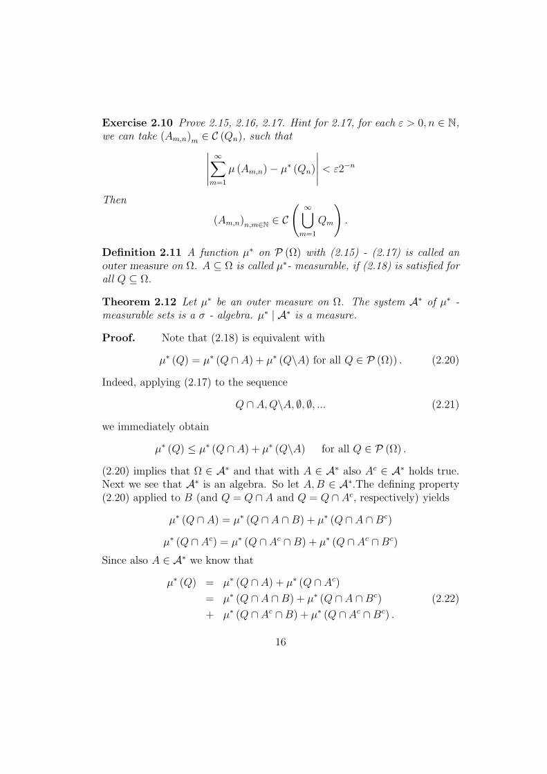
Exercise 2.10 Prove 2.15, 2.16, 2.17. Hint for 2.17, for each ε > 0, n ∈ N,we can take (Am,n)m ∈ C (Qn), such that∣∣∣∣∣

∞∑m=1

μ (Am,n)− μ∗ (Qn)

∣∣∣∣∣ < ε2−n

Then

(Am,n)n,m∈N∈ C

( ∞⋃m=1

Qm

).

Definition 2.11 A function μ∗ on P (Ω) with (2.15) - (2.17) is called anouter measure on Ω. A ⊆ Ω is called μ∗- measurable, if (2.18) is satisfied forall Q ⊆ Ω.

Theorem 2.12 Let μ∗ be an outer measure on Ω. The system A∗ of μ∗ -measurable sets is a σ - algebra. μ∗ | A∗ is a measure.

Proof. Note that (2.18) is equivalent with

μ∗ (Q) = μ∗ (Q ∩ A) + μ∗ (Q\A) for all Q ∈ P (Ω)) . (2.20)

Indeed, applying (2.17) to the sequence

Q ∩A, Q\A, ∅, ∅, ... (2.21)

we immediately obtain

μ∗ (Q) ≤ μ∗ (Q ∩A) + μ∗ (Q\A) for all Q ∈ P (Ω) .

(2.20) implies that Ω ∈ A∗ and that with A ∈ A∗ also Ac ∈ A∗ holds true.Next we see that A∗ is an algebra. So let A, B ∈ A∗.The defining property(2.20) applied to B (and Q = Q ∩ A and Q = Q ∩ Ac, respectively) yields

μ∗ (Q ∩ A) = μ∗ (Q ∩ A ∩ B) + μ∗ (Q ∩ A ∩Bc)

μ∗ (Q ∩ Ac) = μ∗ (Q ∩Ac ∩ B) + μ∗ (Q ∩ Ac ∩Bc)

Since also A ∈ A∗ we know that

μ∗ (Q) = μ∗ (Q ∩ A) + μ∗ (Q ∩ Ac)

= μ∗ (Q ∩ A ∩ B) + μ∗ (Q ∩A ∩Bc) (2.22)

+ μ∗ (Q ∩ Ac ∩B) + μ∗ (Q ∩Ac ∩ Bc) .

16

Since this is true for all Q ∈ P (Ω) we may also replace Q by Q∩ (A ∪ B) toobtain

μ∗ (Q ∩ (A ∪ B)) = μ∗ (Q ∩ A ∩B) + μ∗ (Q ∩A ∩ Bc) + μ∗ (Q ∩ Ac ∩B)(2.23)

for all Q ∈ P (Ω). (2.22) together with (2.23) gives

μ∗ (Q) = μ∗ (Q ∩ (A ∪B)) + μ∗ (Q\ (A ∪ B))

for all Q ∈ P (Ω). This shows that A∪B ∈ A∗. In the next two steps we willsee that the algebra A∗ is a ∩ - stable Dynkin - system, thus a σ - algebra.So let (An)n be a sequence of pairwise disjoint sets in A∗ and set A :=⋃∞

n=1 An. (2.23) yields by induction:

μ∗(

Q ∩n⋃

i=1

Ai

)=

n∑i=1

μ∗ (Q ∩ Ai)

for all n ∈ N, Q ∈ P (Ω).Taking into account that from the above we knowthat Bn :=

⋃ni=1 Ai ∈ A∗ and that Q\Bn ⊇ Q\A and therefore

μ∗ (Q\Bn) ≥ μ∗ (Q\A)

we obtain

μ∗ (Q) = μ∗ (Q ∩ Bn) + μ∗ (Q\Bn) ≥n∑

i=1

μ∗ (Q ∩ Ai) + μ∗ (Q\A) .

Using (2.17) this gives

μ∗ (Q) ≥∞∑i=1

μ∗ (Q ∩ Ai) + μ∗ (Q\A) ≥ μ∗ (Q ∩ A) + μ∗ (Q\A) .

This, according to what we said at the beginning of this proof, even yields:

μ∗ (Q) = μ∗ (Q ∩ A) + μ∗ (Q\A) =

∞∑i=1

μ∗ (Q ∩Ai) + μ∗ (Q\A) . (2.24)

This means that A ∈ A∗. Therefore we have shown that A∗is a Dynkin- system. Moreover A∗ is an algebra. But a Dynkin - system, that is an

17

algebra , is ∩ - stable (because A∩B = (Ac ∪Bc)c. Thus we see that A∗ isa ∩ - stable Dynkin - system, hence a σ - algebra.Choosing A = Q in (2.24) gives

μ∗ (A) =

∞∑i=1

μ∗ (Ai)

which means that μ∗ restricted to A∗ is a measure.

Of course, it would be nice to know, that μ continued to A∗ not only exists,but also is unique. This in many important cases indeed is true. We bring afrequently applied technique using Dynkin-system into action.

Theorem 2.13 Let E be a ∩ - stable generator of a σ - algebra A over Ω.Assume there is a sequence (En)n , En ∈ E with

⋃∞i=1 Ei = Ω. Assume that

μ1, μ2 are two measure on A with

μ1 (E) = μ2 (E) for all E ∈ E (2.25)

andμ1 (En) <∞ for all n ∈ N. (2.26)

Then μ1 = μ2.

Proof. Let EE be the system of all E ∈ E with μ1 (E) = μ2 (E) < ∞. Foran arbitrary E ∈ EE consider

DE := {D ∈ A : μ1 (E ∩D) = μ2 (E ∩D)} .

In Exercise 2.14 below it has to be show that DE is a Dynkin - system.Since E is ∩ - stable we have E ⊂ DE , because of (2.25) and the definitionof DE . Thus D (E) ⊆ DE . On the other hand the ∩ - stability of E yieldsA = D (E) = σ (E) and hence (since DE ⊂ A), that DE = A. Thus

μ1 (E ∩ A) = μ2 (E ∩ A) (2.27)

for all E ∈ EE and A ∈ A. Because of (2.26) this in particular means that

μ1 (En ∩ A) = μ2 (En ∩ A)

18

for all A ∈ A, n ∈ N. The rest of the proof consists of slicing A into pieces.Put

F1 := E1 and Fn := En\(

n−1⋃i=1

Ei

)n ∈ N.

Then the (Fn) are pairwise disjoint with Fn ⊂ En and⋃∞n=1 Fn =

⋃∞n=1 En = Ω. Since Fn ∩A ∈ A we obtain from(2.27):

μ1 (Fn ∩ A) = μ1 (En ∩ Fn ∩A) = μ2 (En ∩ Fn ∩ A) = μ2 (Fn ∩ A) .

for all A ∈ A and n ∈ N. Since

A =

∞⋃n=1

(Fn ∩ A)

the σ -additivity of μ1and μ2 gives

μ1 (A) =∞∑

n=1

μ1 (Fn ∩ A) =∞∑

n=1

μ2 (Fn ∩A) = μ2 (A) for all A ∈ A

which is μ1 = μ2.

Exercise 2.14 Show that DE as defined in the proof of Theorem 2.13 is aDynkin - system.

Theorem 2.9, 2.12, and 2.13 can be summarized in the following

Theorem 2.15 Every σ-finite pre-measure on a ring R over a set Ω can beuniquely extended to a measure μ on σ (R).

Proof. Only uniqueness still needs to be proven. But this is immediate fromTheorem 2.13: Since μ is σ-finite, the ring R possesses all properties of thegenerator in Theorem 2.13.Already the construction given in the proof of Theorem 2.9 suggests that forA ∈ A∗ its measure μ (A) can be approximated by measures on the ring.This is formalized in

Theorem 2.16 Let μ be a finite measure on a σ - algebra A over Ω, whichis generated by an algebra A0 over Ω. Then for A ∈ A there exists a sequence(Cn)n∈N , Cn ∈ A0 with

μ (AΔCn) → 0 (2.28)

as n →∞. Here for any two sets A, B ⊆ Ω

AΔB := A\B ∪ B\A.

19

Proof. Let ε > 0, A ∈ A. According to (2.14) there is a sequence (An)n∈N

in A0 with⋃∞

n=1 An ⊇ A and

0 ≤∞∑

n=1

μ (An)− μ (A) <ε

2(2.29)

Set Cn :=⋃n

i=1 Ai and A′ :=⋃∞

n=1 An. Then Cn ↑ A′ and A′\Cn ↓ ∅. μ isfinite and thus ∅ - continuous, therefore

μ (A′\Cn0) <ε

2

for some n0. Now

A� Cn0 = (A\Cn0) ∪ (Cn0\A) ⊂ (A′\Cn0) ∪ (A′\A)

and hence

μ (A� Cn0) ≤ μ (A′\Cn0) + μ (A′\A)

≤ μ (A′\Cn0) +

∞∑n=1

μ (An)− μ (A) < ε

because of (2.29) and (2). This proves the theorem.

Exercise 2.17 Let μ = δω be the Dirac - measure on a ring R over Ω.Assume {ω} =

⋂∞n=1 An and Ω =

⋃∞n=1 Bn, for two sequences (An)n , (Bn)n

in R. Prove that:

a) The outer measure μ∗ generated by μ assigns 1 or 0 to A ∈ P (Ω),depending on whether ω ∈ A or not.

b) A∗ = P (Ω).

c) μ∗ = δω on P (Ω).

Exercise 2.18 A measure μ over a σ - algebra A is called complete, if N ∈A, μ (N) = 0, N ′ ⊂ N implies N ′ ∈ A. Show that:

a) μ∗|A∗ as defined in Theorem 2.12 is complete.

b) Let A be a σ - algebra over Ω and {ω} ∈ A.

δω (the Dirac measure) is complete, if and only if A = P (Ω).

20

3 Lebesgue-measure

From a technical point of view this section starts by applying the conceptsdeveloped in Section 2 to a particular, yet important case, the case of Rd. Asalready mentioned here we have an intuitive idea what the measure for fairlyeasy geometric objects, say e.g. rectangles should be. We want to extendthis measure to more subtle sets.

Definition 3.1 Let a, b ∈ Rd.By the rectangle [a, b[ we mean the set

[a, b[:={x ∈ Rd : ai ≤ xi < bi, i = 1...d

}Similarly, we define ]a, b[, ]a, b], and [a, b]Let moreover

J d :={[a, b[: a, b ∈ Rd

}and

Fd :=

{n⋃

i=1

Ji, n ∈ N,Ji ∈ J d

}.

Exercise 3.2 For I, J ∈ J d it holds I ∩ J ∈ J d and I\J ∈ Fd

Exercise 3.3 Let F ∈ Fd. Then there exists I1, ..., In ∈ J d, Ii ∩ Ij = ∅ fori �= j, such that

F =n⋃

i=1

Ii.

Exercise 3.4 Fd is a ring over Rd.

These preparations, of course, were necessary to apply the techniques ob-tained in Section 2. Now we will turn to discussing the corresponding volumeon Fd, which will turn out to be the geometric volume.

Definition 3.5 Let I ∈ J d, I = [a, b[. We define

λ (I) =

{ ∏di=1 (bi − ai) if I �= ∅

0 otherwise

Theorem 3.6 There exists a unique volume λ on Fd such that λ extends λon J d. λ is a pre-measure.

21

Proof. Following Exercise 3.2 the set F ∈ Fd may be written as F =⋃n

i=1 Ii

with pairwise disjoint Ii ∈ Fd. Since a volume has to be additive, there isonly one way to define λ (F ), namely

λ (F ) =

n∑i=1

λ (Ii) .

Of course, we need to check that this construction is well defined. To thisend we write

F =

n⋃i=1

Ii =

m⋃j=1

Jj

where the Ii, Jj ∈ J d and the (Ii) are pairwise disjoint as well as the (Jj).Wethen need to see that

n∑i=1

λ (Ii) =m∑

j=1

λ (Ji) .

First note, if [a, b[∈ J d, a1 is such that

a1 < a1 < b1 and ai = ai for i ≥ 2, then

[a, b[= [a, a[ ∪ [a, b[,

as well as

λ ([a, b[) =

d∏i=1

(bi − ai)

= [(b1 − a1) + (a1 − a1)]d∏

i=2

(bi − ai)

=d∏

i=1

(b1 − a1) +d∏

i=1

(a1 − a1)

= λ ([a, b[) + λ ([a, a[) .

Induction over: gives that for ai ≤ ci ≤ bi

λ ([a, b[) = λ ([a, b[) + λ ([c, b[) .

22

Another induction gives that, if J d � I =⋃n

i=1 Ii with Ii ∈ J d, that

λ (I) =n∑

i=1

λ (I) .

So λ defined above is well defined on J d. Eventually let F ∈ Fd be of theform

F =

n⋃i=1

Ii =

m⋃j=1

Jm

with Ii, Jj ∈ J d and (Ii) pairwise disjoint as well as the (Jj). Then (Ii ∩ Jj) i≤nj≤m

is a common refinement of both the (Ii)i and the (Jj) and, of course the setsIi ∩ Jj are pairwise disjoint. Then applying the above

n∑i=1

λ (Ii) =n∑

i=1

m∑j=1

λ (Ii ∩ Jj)

=

m∑j=1

n∑i=1

λ (Ii ∩ Jj) =

m∑j=1

λ (Jj) .

Hence defining

λ (F ) :=

n∑i=1

λ (Ii)

we obtain a well defined and finite volume on Fd. To see that λ indeedalso is a pre - measure, we only need to check that λ is ∅ - finite (this is anapplication of Theorem 2.5, since λ is finite on each [a, b[, if a �= −∞, b �= ∞).So let (Fn)n∈N be a decreasing sequence in Fd. We will show that

δ := limn→∞

λ (Fn) = infn→∞

λ (Fn) > 0

implies that⋂∞

n=1 Fn �= ∅. We will use a definition of compactness that statesthat an intersection of a sequence of decreasing closed sets is empty if andonly if one of the sets is empty. To be more precise:Since each Fn is a finite union of disjoint elements in J d we may find Gn ∈ Fd

withGn ⊂ Gn ⊂ Fn and

|λ (Gn)− λ (Fn)| ≤ 2−nδ.

23

Put Hn :=⋂n

i=1 Gi, then Hn ∈ Fd and Hn ⊇ Hn+1 as well as Hn ⊆ Gn ⊆ Fn.Fn is bounded. Thus

(Hn

)n

is a sequence of bounded and hence compact

subsets of Rd with Fn ⊇ Hn+1. Thus⋂∞

n=0 Hn �= ∅ (and therefore also⋂∞n=1 Fn �= ∅), if only Hn �= ∅ for each n. To this end we show

λ (Hn) ≥ λ (Fn)− δ(1− 2−n

) ≥ δ2−n (3.1)

where only the first inequality has to be proven. This will be done by induc-tion over n. For n = 1 (3.1) is true since H1 = G1 and λ (F1) − λ (G1) ≤ δ

2.

Assuming that the hypothesis is true for n we know that

λ (Hn) ≥ λ (Fn)− δ(1− 2−n

)as well as

λ (Gn+1) ≥ λ (Fn+1)− δ2−(n+1)

and Gn+1 ∪Hn ⊆ Fn+1 ∪ Fn = Fn. Putting this together yields:

λ (Hn+1) ≥ λ (Fn+1)− δ2−(n+1) − δ(1− 2−n

)≥ λ (Fn+1)− δ

(1− 2−(n+1)

).

This proves Hn �= ∅ for all n and thus the theorem.Thus we know that λ is a σ -finite pre - measure on the ring Fd. ApplyingTheorem 2.15 we immediately obtain

Corollary 3.7 The pre - measure λ on Fd can be uniquely extended to ameasure λ on σ

(Fd).

Definition 3.8 The measure λ in Corollary 3.7 is called the Lebesgue - mea-sure. σ

(Fd)

is called the Borel σ - algebra and abbreviated by Bd. Sometimeswe will also write λd instead of λ to emphasize its dimension dependence.

Note that, of course, also λd is σ - finite. We will now first discuss the formof the σ - algebra Bd a bit more in detail. From a topological point of viewthe following result is very satisfactory:

Theorem 3.9 Denote by Od, Cd, and Kd the systems of all open, closed, andcompact subsets of Rd, respectively. Then

Bd = σ(Od

)= σ

(Cd)

= σ(Kd

)(3.2)

24

Proof. Note that Kd ⊆ Cd and therefore σ(Kd

) ⊆ σ(Cd). On the other

hand every set C ∈ Cd is the countable union of a sequence of sets Cn ∈ Kd.Indeed, if

Kn :={x ∈ Rd : ||x|| ≤ n

}then C =

⋃∞n=1 (C ∩Kn). But then Cd ⊆ σ

(Kd)

which together with theabove shows that σ

(Cd)

= σ(Kd

). On the other hand the complement of a

closed set is an open set and thus

σ(Od

)= σ

(Kd)

= σ(Cd).

Eventually we show that σ(Od

)= Bd. To this end first note that [a, b[∈ J d

may be written as a countable intersection of ]a(n), b[, where

a(n) =

(a1 − 1

n, .., ad − 1

n

).

Thus Bd = σ(J d

) ⊆ σ(Od

). On the other hand ]a, b[∈ Od is the union of

]a(n), b[∈ J d, where

a(n) =

(a1 +

1

n, .., ad +

1

n

).

On the other hand every open set G ∈ Od can be written as a countableunion of ]a, b[∈ Od (e.g. those with rational coordinates). This shows thatσ(Od

) ⊆ Bd, thus σ(Od

)= Bd and hence proves the theorem.

In some exercises we will now discuss the Lebesgue measure of some fairlysimple subsets of Rd.

Exercise 3.10 Let H be a hypersurface in Rd, that is perpendicular to oneof the coordinate extras. Prove that λd (H) = 0.

Exercise 3.11 Prove that every countable subset of Rd has Lebesgue measurezero.

The Lebesgue measure introduced above is the prototype of a Borel measure,i. e. of a measure on

(Rd,Bd

). A closer look to its construction reveals that

in dimension one of the starting point is the attach the measure b− a to aninterval [a, b[. This is geometrically reasonable, but in general (in particular,if we think of probability measures) not necessary. One might in generalattach a measure F (b) − F (a) to [a, b[. For that F has to be increasing(otherwise some intervals have negative measure) and left - continuous, sincexn ↑ x implies [y, xn[↑ [y, x[ and thus μ ([y, xn[)→ μ ([y, x[) for every measureμ.

25

Definition 3.12 A function F is called measure generating, if F is increas-ing and left continuous.

The following theorem will not be proven in this course. Its proof is to alarge extend similar to the construction of Lebesgue measure.

Theorem 3.13 Let F be measure generating. Then there exists a uniquemeasure μF on B1with

μF ([a, b[) = F (b)− F (a) .

Moreover, if G is another measure generating function on R with μF = μG,the F = G + c for some constant c.

In a subsequent course in probability theory a special role will be playedby probability measure, i. e. measures which have total mass one. Ofcourse, they can be obtained from the finite measures by normalization.Concentrating on (R, B1) again, we see that μF is a probability measure on(R, B1), if and only if limx→∞ F (x) − limy→−∞ F (y) = 1.Usually one takeslimx→∞ F (x) = 1.In order to continue the discussion of Lebesgue - measure, we need to inter-lude on the connection of measures and mappings. This is done in the nextsection.

Exercise 3.14 (a bit of typology (!!) which we needed in this section): Let Kbe compact. Let(An)n be a sequence of closed subsets of K with

⋂ni=1 Ai �= ∅

for all n.Then also∞⋂i=1

Ai �= ∅.

4 Measurable mappings and image measures

Assume that we have a set Ω an σ - algebra A on Ω ( we will call (Ω,A) ameasurable space). Moreover assume μ is a measure on A. In this sectionwe will discuss how to ”teleport” μ to another measurable space (Ω′, A′) bya mapping.

Definition 4.1 Let (Ω,A) , (Ω′,A′) be measurable spaces. A mapping T :Ω → Ω′ is called A− A′ - measurable, if

T−1 (A′) ∈ A for all A′ ∈ A.′ (4.1)

26

Example 4.2 Every constant mapping is measurable, since

T−1 (A′) ∈ {∅, Ω) for all A′ ∈ A′.

Exercise 4.3 Let (Ω,A) , (Ω′,A′) be two measurable spaces. Let E ′ be agenerator of A′. Show that T : Ω → Ω is A−A′ - measurable if and only if

T−1 (E ′) ∈ A for all E ′ ∈ E ′. (4.2)

Apply this to show that every continuous function T : Rd → Rd′ is Bd − Bd′

- measurable.

Exercise 4.4 Let T1 : (Ω1,A1) → (Ω2,A2) and T2 : (Ω2,A2) → (Ω3,A3) bemeasurable mappings. Then T2 ◦ T1 is A1 −A3 - measurable.

One could in principles discuss more properties of measurable functions alongthe lines of set theoretic topology. We will rather refrain from that and nowdiscuss how measures are ”teleported”.

Theorem 4.5 Let T : (Ω,A) → (Ω′,A′) be measurable. Then for everymeasure μ on (Ω,A)

T (μ) (A′) := μ(T−1 (A′)

), A′ ∈ A′

defines a measure on (Ω′,A′).

Proof. The only thing that needs to be understood is that, if (A′n)n∈N is

pairwise disjoint in A′ then (T−1 (A′n))n∈N is pairwise disjoint in A,and that

T−1

( ∞⋃n=1

A′n

)=

∞⋃n=1

T−1 (A′n) .

The rest follows easily.

Definition 4.6 The measure T (μ) in the situation of Theorem 4.5 is calledthe image measure of μ under the mapping T .

A very important example, namely that of(Rd,Bd

)and the mappings T

being translations will be discusses in Section 5 below.

27

5 Further properties of Lebesgue measure

In this section we will study some further properties of Lebesgue measure.A special focus will be on its behavior under certain linear mappings. Letus start with one of the easiest cases, that of a translation: A translation bya ∈ Rd is a mapping Ta : Rd → Rd with Ta (x) = a + x for all x ∈ Rd.

Proposition 5.1 Lebesgue measure is translation - invariant, i.e. Ta

(λd)

=λd for all a ∈ Rd.

Proof. This follows immediately since for each I ∈ J d we have by definition

λd (I) = Ta

(λd)(I) .

As it next turns out this property is characteristic of Lebesgue measure. LetW := [0, 1[ be the unit cube in Rd (0 and 1 are d - vectors). Then:

Theorem 5.2 Let μ be a measure on(Rd,Bd

)with Ta (μ) = μ for all a ∈ Rd

andα := μ(W ) < ∞. (5.1)

Thenμ = α λd. (5.2)

i.e. Lebesgue measure is the unique translation - invariant measure up toscaling.

Proof. The trick is that μ (W ) also determines μ (Wn) for small cubes ofside length 1

nand that every I ∈ J d may be arbitrary well approximated by

Wn′s. More precisely let

Wn = [0,1

n[∈ J d

Thenμ (Wn) =

α

nd. (5.3)

Indeed W is the disjoint union of nd copies of Wn, which by translationinvariance all have the same μ - measure. This gives (5.3).Moreover, for [a, b[∈ J d with a = (a1, ..., ad) , b = (b1, ..., bd) , ai, bi ∈ Q for alli = 1...d, we see in the same way

μ ([a, b[) = αλd ([a, b[) . (5.4)

28

Indeed, for n large enough, we may partition [a, b[ into little cubes of sidelength 1

n. For each of these cubes the relation holds, thus also for their finite

union. Eventually

J drat :=

{[a, b[∈ J d : a, b have rational coordinates

}(5.5)

is a ∩ - stable generator of Bd. Hence, if μ and αλd agree on J drat they agree

on Bd, which was our claim.

Exercise 5.3 Show that J drat as defined in (??) is a ∩ - stable generator of

Bd.

We will now see that for Lebesgue measure to exist, finite dimensionality isessential: ”Lebesgue measure in R∞ does not exist”.

Theorem 5.4 In (R∞,B∞) there is no translation invariant measure λ, thatassigns mass a positive, finite to any bounded set W , i.e. with

0 < λ (W ) <∞.

Proof. Assume such a λ exists. Take a closed Ball of radius 0 < ε <√

22

.Denote by

Bε (y) := {x ∈ R∞ : ‖x− y‖ < ε} .

Bε (0) has positive measure because it contains a small cube (e.g. of sidelength ε

4). On the other hand the (Bε (ei))

∞i=1 are all disjoint (here ei denotes

the i’th unit vector) and ( ∞⋃i=1

Bε (ei)

)⊆ B3(0). (5.6)

(5.7) implies that λ (⋃∞

i=1 Bε (ei)) is finite. On the other by translation in-variance all Bε (ei) have the same measure. But since all Bε (ei) are disjoint⋃∞

i=1 Bε (ei) then has infinite measure. This is a contradiction.The translation invariance of Lebesgue measure also the main obstacle thatprevents all subsets of Rd from being measurable:

Theorem 5.5 Bd �= P (Rd), i.e. there is a non - measurable subset of Rd.

29

Proof. Introduce the equivalence relation ∼ on R (we will just treat thecase d = 1, which is sufficient), via

x ∼ y :⇐⇒ x− y ∈ Q (5.7)

We consider the equivalence classes with respect to ∼. Since for any x ∈ R,there is n ∈ Q with n ≤ x < n + 1, we may choose a representative for eachof the equivalence classes in [0, 1[. That means that there is a set K ⊂ [0, 1[which contains exactly one element of each equivalence class. (Note that herethe axiom of choice plays an important role).The set K satisfies⋃

y∈Q

(y + k) = R (5.8)

andy1 �= y2 ⇒ (y1 + K) ∩ (y2 + K) = ∅. (5.9)

But this leads to a contradiction as follows. Assume K was measurable.Then

λ

(⋃y∈Q

(y + k)

)= λ (R) =∞

Due to translation invariance of λ:

λ (y + K) = λ (K) for all y ∈ Q

Since Q is countable λ (K) thus cannot be zero. On the other hand⋃y∈Q∩[0,1]

(y + K) ⊆ [0, 2[.

Thus λ (K) cannot be non - zero, either Q ∩ [0, 1] is infinite). This is acontradiction. Hence K is not measurable.At the end of this section we will discuss the relation of Lebesgue measurewith more general mappings. To this end introduce the space

W (Rd)

:={T : Rd → Rd : d (T (x) , T (y)) = d (x, y) for all x, y ∈ R

}Recall that W (

Rd)

contains exactly those mappings that can be written asa orthogonal, linear mapping plus a shift. Under T ∈ W (

Rd)

a geometricfigure will be moved to a congruent figure. We will now see that the Lebesguemeasure is invariant under T ∈ W (

Rd).

30

Theorem 5.6 For each T ∈ W it holds T (λd) = λd.

Proof. Since T ∈ W can be written as

T (x) = T0(x) + a, , x ∈ R

where a ∈ Rd and T0 is orthogonal and we already know that Lebesguemeasure is translation invariant, it suffices to consider the case that T usorthogonal, in particular T (0) = 0. For such a T , a ∈ Rd, and b = T−1(a) itholds

Ta ◦ T = T ◦ Tb (5.10)

where Tc(x) = x + c (Exercise 5.7 below). Using that λd is translationinvariant we thus obtain

Ta(T (λd)) = T (Tb(λd)) = T (λd)

for all a ∈ Rd. But this means that μ := T (λd) is translation invariant.Hence T (λd) = αλd, with α = μ(W ), and W = [0, 1[. Consider

B1(0) := {x ∈ Rd : ||x|| ≤ 1}.With T also T−1 is orthogonal and hence T−1[B1(0)] := B1(0). ThereforeT (λd) = αλd gives

λd(B1(0)) = λd(T−1[B1(0)]) = T (λd)(B1(0)) = αλd(B1(0)).

Since λd(B1(0)) /∈ {0,∞} this implies α = 1.

Exercise 5.7 Show formula (5.10) above.

Exercise 5.8 Show that any hypersurface H ⊂ Rd has Lebesgue measure λd

zero.

Eventually we will turn to general linear mappings T with det T = 0 (thereason for this restriction will become clear in (5.11) below.

Theorem 5.9 For every T ∈ GL(d, Rd) we have

T (λd) =1

|detT |λd. (5.11)

31

Proof. Let T ∈ GL(d, Rd) be an invertible, linear mapping. The samecomputation as in the proof of Theorem 5.7 shows that T (λd) is translationinvariant. Since

Φ(T ) := T (λd)(W ) < ∞ (W := [0, 1[)

we obtainT (λd) = Φ(T )(λd). (5.12)

To determine Φ(T ) we note that for S ∈ GL(d, Rd)

Φ(S · T ) = Φ(S)Φ(T ) (5.13)

(see Exercise 5.10 below). This means Φ is a homorphism from GL(d, R)into the multiplicative group R \ {0}. Hence we know from linear algebrathat there is an homomorphism

φ : R \ {0} → R \ {0}such that

Φ(T ) = φ(det T ).

Thus if det T = 1 we know Φ(T ) = 1. For arbitrary T put γ := det T �= 0.For α �= 0 let

Dα : (x1, . . . , xd) �→ (x1, . . . xd−1, αxd).

Obviously det Dα = α. Putting S := T ◦ D1/γ we see that det S = 1 withT = S ◦Dγ. Since Dγ is translation- invariant in the first d− 1 coordinatesand the d’th coordinate is stretched by a factor γ we see that

Dγ(λd) =

1

|γ|λd.

This is immediately checked for intervals and goes through for arbitrary setsby the standard arguments. Since Φ is a homorphism with Φ(S) = 1 weobtain

Φ(T ) = Φ(S ◦Dγ) = Φ(S)Φ(Dγ) = Φ(Dγ) =1

|γ| =1

| detT | .

Exercise 5.10 Check that Φ defined in (5.12) fulfills (5.13).

Exercise 5.11 Let T : Rd → Rd be a linear mapping with det T = 0. Showthat for all A ∈ Bd there is a measurable set N ⊂ Rd with λd(N) = 0 andT (A) ⊆ N . Hence (5.11) holds true in a certain sense.

32

6 First steps towards integration

In this section we will start to construct an integral from a given measure.But why would we do so? Let us consider

Example 6.1 An option is the right to buy an option at a certain time T0

and for a certain price P0. We buy this option a time 0 for price p. At thispoint of time the price of the stock is known to be K0. After that it developsrandomly such that at time T0 its price can be described by a probabilitymeasure μ on R+. How much can we expect to gain from the option webought? Obviously, if the price of the stock at time T0, which we denote byKT0 is less than P0 we do not execute our option because we can get the stockat a lower price on the the stock market. Otherwise we gain KT0−P0. Takinginto account that we paid p for the option our total win or loss is thus givenby

f(KT0) = (KT0 − P0)+ − p

where (x)+ := max(x, 0). Since KT0 is random our average win will be givenby “summing f with weights μ(·)”. Now R is uncountable so we would ratherwant to compute ∫

f(KT0)dμ(KT0),

if we just knew what this was. An integration theory will thus also be a firststep into the theory of option pricing, which we will treat in much greaterdetail, when we also know, how to describe the measure μ appearing in thisexample.

For good reasons (e.e. since the supremum of a series of R-valued functionsmake also take the value infinity) we aim at integrating functions with valuesin R := R ∪ {±∞}. The Borel σ-algebra there is defined as

B1:= {B, B ∪ {∞}, B ∪ {−∞}, B ∪ {∞} ∪ {−∞}|B ∈ B1}.

Is is obvious that B1is a σ-algebra with

R ∩ B1:= B1.

A function f : Ω → R will then be called a numeric function if it is A−B1-

measurable.

33

Example 6.2 The most relevant class of numeric functions for the followingis the class of indicators

1A(ω) :=

{1 ω ∈ A0 ω /∈ A

for A ∈ A.

Exercise 6.3 Check that the following rules for computations with indicatorshold true

• A ⊆ B ⇒ 1A ≤ 1B A, B ∈ A.

• 1⋃∞i=1 Ai

= supi 1AiAi ∈ A.

• 1⋂∞i=1 Ai

=∏∞

i=1 1AiAi ∈ A.

Let us first establish a criterion for numeric functions.

Proposition 6.4 Let (Ω,A) be a measurable space. Then f : Ω → R is

A− B1-measurable, if and only if

{f ≥ α} ∈ A for all α ∈ R (6.1)

Proof. We only need to show that J := {[α,∞], α ∈ R} generates B1. First

note that [a, b[= [a,∞] \ [b,∞]. This implies σ(J ) = B1 ⊆ J . MoreoverJ contains the points {∞} :=

⋂∞n=1[n,∞] and {−∞} := R \⋃∞

n=1[−n,∞].This does the job.

Exercise 6.5 Show that the following are equivalent

1. f is A−B1-measurable.

2. {f ≥ α} ∈ A for all α ∈ R.

3. {f > α} ∈ A for all α ∈ R.

4. {f < α} ∈ A for all α ∈ R.

5. {f ≤ α} ∈ A for all α ∈ R.

Proposition 6.6 Let f, g be numeric functions. Then {f ≤ g}, {f < g},{f = g}, and {f �= g} are measurable.

34

Proof. Since Q is countable the assertion follows from

{f < g} =⋂q∈Q

{f < q} ∩ {q < g}

and

{f ≤ g} = {g < f}c, {f = g} = {g ≤ f} ∩ {f ≤ g}, {f �= g} = {f = g}c.

Proposition 6.7 Let f, g be numeric functions. Then also f ± g and f · g– if well defined – are measurable.

Proof. First note that with g also −g is measurable, since {−g ≤ α} ={g ≥ −α}. Thus with f + g also f − g will be measurable. Moreover with galso g + t, t ∈ R is measurable, since {g + t ≤ a} = {g ≤ α − t}. Now forreal functions f, g

{f + g ≤ α} = {f ≤ −g + α}which according to the above and Proposition 6.6 proves measurability off ± g. Moreover

f · g =1

4

[(f + g)2 − (f − g)2

].

Now with f also f 2 is measurable, since

{f 2 ≤ α} = {f ≤ √α} ∩ {f ≥ −√α}.This shows the assertion for real functions. The extension to numeric func-tions is immediate, since, if well defined, the sets {f ± g = ±∞} and{f · g = ±∞} are measurable.

Theorem 6.8 Let (fn)n∈N be a sequence of numeric functions on a measur-able set (Ω,A). Then the following functions are measurable with respect toA:

supn

fn, infn

fn, lim sup fn, lim infn

fn

Proof. sup fn is measurable, because

{supn

fn ≤ α} =∞⋂

n=1

{fn ≤ α}.

Moreover infn fn = − supn−fn, lim sup fn = infn supm≥n fm, and lim infn fn =− lim sup−fn. Thus all the functions are measurable.

35

Corollary 6.9 Let f, (fn)n∈N be measurable functions on a measurable set(Ω,A). Then for all n

infm=1...n

fm and supm=1...n

fm (6.2)

and (if existent)lim

nfn (6.3)

and |f | are measurable.

Proof. (6.2) follows by setting fk = fn for all k ≥ n in the above theorem.For (6.3) recall that, if lim fn exists, then lim fn = lim sup fn. Eventually

|f | = f+ − f−

where f+ = max(f, 0) and f− = (−f)+ are measurable.

Exercise 6.10 Show that the measurability of |f | in general does not implythe measurability of f .

7 The construction of the integral

We will start to construct the integral inspired by the idea which also tothe Riemann integral: If (Ω,A) is a measurable space with measure μ, andA ∈ A, then the indicator function 1A geometrically describes a ”rectangle”in Ω× R with sidelengths μ(A) and 1. Hence∫

1Adμ

should be μ(A). Yet we will see that therer is an importante differencebetween the integral we are going to cunstruct and the Riemann integral.This basically can be described by the fact that the above idea also works,if A is just measurable but not an interval as in the case of the Riemannintegral. Let us start with the defintion of the first functions we want tointegrate:

36

Definition 7.1 Let (Ω,A) be a measurable space. A step function is a func-tion of the form

f(ω) =n∑

i=1

αi1Ai(ω).

Here Ai ∈ A, i = 1, . . . , n are pairwise disjoint with⋃

Ai = Ω and αi ≥ 0.The set of step functions on (Ω,A) will be abbreviated by

E := E(Ω,A). (7.1)

Definition 7.1 and the considerations of Section 6 imply

Lemma 7.2 Let u, v ∈ E, α ∈ R+, then αu, u+v, max{u, v}, min{u, v} ∈ E.

Proof. Obvious from Section 6.We will now prepare the integration of step functions

Lemma 7.3 Let u ∈ E:

u =

m∑i=1

αi1Ai=

n∑i=1

βi1Bi.

Thenm∑

i=1

αiμ(Ai) =n∑

i=1

βiμ(Bi).

Proof. Note that ⋃Bi =

⋃Ai = Ω

and the (Ai) (and the (Bi) respectively) are pairwise disjoint. Then Ai =⋃nj=1(Ai ∩Bj) as well as Bj =

⋃mi=1(Ai ∩ Bj). Additivity of μ yields

μ(Ai) =n∑

j=1

μ(Ai ∩Bj) and μ(Bj) =m∑

i=1

μ(Ai ∩ Bj).

Taking on consideration that on (Ai ∩ Bj) we have that αi = βj we obtain

m∑i=1

αiμ(Ai) =∑i,j

αiμ(Ai ∩Bj) =∑i,j

βiμ(Ai ∩Bj)

=

n∑i=1

βiμ(Bi)

37

Definition 7.4 Let u ∈ E with representation

u =n∑

i=1

αi1Ai. (7.2)

Then ∫udμ :=

n∑i=1

αiμ(Ai)

is called the (μ)-integral of u. Here μ is a measure on (Ω,A).∫

udμ isindependent of the special representation chosen in (7.2).

Proposition 7.5 Let u, v ∈ E, α ∈ R+, and A ∈ A. Then∫1Adμ = μ(A), (7.3)

∫αudμ = α

∫udμ, (7.4)∫

u + vdμ =

∫udμ +

∫vdμ, (7.5)

u ≤ v ⇒∫

udμ ≤∫

vdμ (7.6)

Proof. (7.3) and (7.4) are obvious.For (7.5) consider two representations

u =m∑

i=1

αi1Aiv =

n∑j=1

βj1Bj. (7.7)

Then u + v is a step function again with

u + v =∑i,j

(αi + βj)1Ai∩Bj.

38

Since Ai =⋃n

j=1(Ai ∩Bj) as well as Bj =⋃m

i=1(Ai ∩Bj) and (Ai)i and (Bj)j

form a partition we obtain∫u + vdμ =

∑i,j

αi + βjμ(Ai ∩Bj)

=∑i,j

αiμ(Ai ∩Bj) +∑i,j

βjμ(Ai ∩ Bj)

=∑

i

αiμ(Ai) +∑

j

βjμ(AiBj)

=

∫udμ +

∫vdμ.

For (7.6) we start again with the decomposition (7.7) and write

u =∑i,j

αi1Ai∩Bjand v =

∑i,j

βj1Ai∩Bj.

Then u ≤ v implies that αi ≤ βj on Ai ∩Bj �= ∅. Thus∫udμ =

∑i,j

αiμ(Ai ∩ Bj) ≤∑i,j

βjμ(Ai ∩ Bj) =

∫vdμ.

Eventually we see that if u ∈ E and Ai ∈ A, αi ∈ R+ are such that

u =

n∑i=1

αi1Ai

(note that we do not require the (Ai)i to be a partition anymore, then (7.3)- (7.5) imply that still

∫udμ =

∑ni=1 αiμ(Ai).

Exercise 7.6 Is Dirichlet’s function defined by

1Q(x) =

{1 x ∈ Q

0 otherwise

a step function. If so what is its integral?

39

We will now turn to defining the integral of a numeric function. This willfirst be done for positive functions, since afterwards we will decompose anarbitrary function into positive and negative part. The key idea will be toapproximate a given function by step functions. Of course, we also need tocheck afterwards that also the corresponding integrals of the step functionsconverge to a limit. In this case we can define the integral of the givenfunction as the limit of the integrals of the approximating step functions.The major difference between this construction, which is due to Lebesgueand the Riemann integral is that we start with a measure on A. Hence wedo not need indicators on nice sets, such as intervals to approximate a givenfunction.The following lemma plays a key role for our further steps

Lemma 7.7 Let u, (un)n ∈ E and let (un) be increasing. Then

u ≤ supn

un ⇒∫

udμ ≤ supn

∫undμ.

Proof. Let u be given by

u =

m∑i=1

αi1Ai

with Ai ∈ A and αi ∈ R+. Let α ∈ (0, 1). As un is measurable

Bn := {un ≥ αu} ∈ A.

By definition of Bn: un ≥ αu1Bn, hence∫undμ ≥ α

∫u1Bndμ.

Now (un) in increasing and u ≤ supn un. Thus Bn ↑ Ω and also Ai ∩Bn ↑ Ai

for all i. Hence continuity from below of μ gives

∫udμ =

m∑i=1

αiμ(Ai) = limn→∞

m∑i=1

αiμ(Ai ∩ Bn)

= limn→∞

∫u1Bndμ.

40

This yields

supn

∫undμ ≥ α

∫u1Bndμ = α lim

n→∞

∫u1Bndμ

= α

∫udμ.

Since α ∈ (0, 1) was arbitrary this proves the lemma.

Corollary 7.8 For two increasing sequences (un) and (vn) in E it holds that

sup un = sup vn ⇒ supn

∫undμ = sup

n

∫vndμ (7.8)

Proof. We have that un ≤ sup vm and vm ≤ sup un for all n, m. Thus theresult is implied by the previous lemma.

Definition 7.9 Let E∗(Ω,A) = E∗ denote the set of all numeric functions,such that there is an increasing sequence (un) in E such that

f = sup un.

The point is that Corollary 7.8 tells us that supn

∫undμ is independent of

the particular choice of the sequence (un) by which we approximate f . Wemay thus define

Definition 7.10 Let f ∈ E∗. We define the integral of f with respect to μby ∫

fdμ = supn

∫undμ

where (un) is an increasing sequence in E such that

f = sup un.

Remark that E ⊆ E∗.

Exercise 7.11 Check that the following holds for f, g ∈ E∗, α ∈ R+.

αf, f + g, f · g, min f, g, max f, g ∈ E∗

∫αfdμ = α

∫fdμ,

41

∫f + gdμ =

∫fdμ +

∫gdμ,

f ≤ g ⇒∫

fdμ ≤∫

gdμ

Exercise 7.11 tell that the integral is a positive,increasing linear form on thespace of integrable functions. An approach due to Daniell starts with suchforms and interprets them as integrals We cannot follow this track here.It might not be too surprising that Lemma 7.7 is inherited by functionsf ∈ E∗. However the following that goes Back to B. Levi is an essentialimprovement over theorems that try to combine limits of functions withRiemann integration.

Theorem 7.12 (monotone convergence):Let (fn)n be an increasing sequence in E∗. Then sup fn ∈ E∗ and∫

sup fndμ = sup

∫fndμ. (7.9)

Proof. Put f := sup fn. For fn ∈ E∗ there is a sequence (um,n)m in E thatincreases with limit fn. Lemma 7.2 shows that

vm := max (um,1, ...um,m) ∈ E.

Since the (um,n) are increasing, so is (vm)m. Apparently vm ≤ fm, thus vm ≤.On the other hand for m ≤ n we have um,n ≤ vm and hence

supm∈N

umn = fn ≤ supm∈N

vm.

Therefore sup vm = f , which means that f ∈ E∗. But then∫

fdμ =sup

∫vndμ by definition. Now vn ≤ fn implies

∫vndμ ≤ ∫

fndμ. Thisshows that ∫

fdμ ≤∫

fndμ.

But the converse inequality∫

fdμ ≥ ∫ fndμ is obvious from fn ≤ f for alln ∈ N.

42

Corollary 7.13 Let (fn)n be a sequence in E∗, then

∞∑n=1

fn ∈ E∗

and ∫ ∞∑n=1

fndμ =

∞∑n=1

∫fndμ.

Proof. Apply Theorem 7.12 to (f1 + ... + fn)n.

Exercise 7.14 Show that for the Dirac-measure δω it holds∫fdδω = f (ω)

for all f ∈ E∗.

Example 7.15 Let Ω = N and A = P (Ω). Because of σ- additivity ameasure μ on (N, P (N)) is uniquely determined by αn := μ ({n}). In this casef ∈ E∗, whenever it is a positive numeric function. Indeed put fn = f · 1{n};then fn ∈ E∗ and f =

∑∞n=1 fn. So Corollary 7.13 shows that f ∈ E∗ and∫

fdμ =

∞∑n=1

f (n)αn.

The above example raises the question how large a subset of the numericfunctions the set E∗ is. The answer is somewhat surprising, though easy toverify.

Theorem 7.16 f ∈ E∗ if and only if f is a positive, numeric function.

Proof. One direction is obvious. For the other let

Ain =

{ {f ≥ i

2n

} ∩ {f < i+12n

}i = 0, ..., n2n − 1

{f ≥ n} i = n2n

and

un =n2n∑i=0

i

2n1Ain

.

Obviously un ∈ E and (un)n is increasing. Eventually sup un = f , since eitherf (u) = ∞,then un (ω) = n for all n, or |un (ω)− f (ω)| < 1

2n , otherwise, forn large enough.

43

Exercise 7.17 Prove that every bounded numeric function on (Ω,A) is theuniform limit of an increasing sequence of stepfunctions.

In a final step we can now define what we mean with the integral of anarbitrary numeric function. Recall that for a numeric function f we mayintroduce

f+ := max (f, 0) and f− := max (−f, 0) .

Then f = f+ − f−. The additivity requirement for integrals immediatelyleads to the following

Definition 7.18 A numeric function is called integrable, if∫f+dμ and

∫f−dμ.are

real numbers. Then ∫fdμ :=

∫f+dμ−

∫f−dμ. (7.10)

Remark 7.19 1. (7.10) also makes sense, if one of∫f+dμ and

∫f−dμ

are infinite (but not both). In this case one talks about quasi - integra-bility.

2. If Ω = Rd,A = Bd, and μ = λd one also talks about the Lebesgue -integral.

We conclude this section by discussing integrability properties of functions:

Theorem 7.20 The following are equivalent for a numeric function f .

1. f is integrable

2. There are integrable functions u ≥ 0 and v ≥ 0, such that f = u− v.

3. There is a integrable function g, such that |f | ≤ g

4. |f | is integrable.

Proof. : ”1 =⇒ 2”: If f is integrable, so are f+ and f−, hence u = f+

and v = f− does the job.”2 =⇒ 3”: Note that f = u− v ≤ u + v and −f = v− u ≤ u + v. Thus

|f | ≤ g := u + v and g is integrable.”3 =⇒ 4”: This follows, since the integral is an increasing function:∫ |f | dμ ≤ ∫ gdμ < ∞.”4 =⇒ 1”: Since f+ ≤ |f | and f− ≤ |f |, the integrability of f+and f−

follows again from monotonicity.

44

Exercise 7.21 Let f ,g be integrable, α ∈ R. Show that αf ,f +g, max (f, g),min (f, g) are integrable and that∫

αfdμ = α

∫fdμ and

∫f + gdμ =

∫fdμ +

∫gdμ.

Proposition 7.22 Let f, g be integrable. Then

f ≤ g =⇒∫

fdμ ≤∫

gdμ (7.11)

∣∣∣∣∫

fdμ

∣∣∣∣ ≤∫|f | dμ (7.12)

(7.12) is called the triangle - inequality.

Proof. f ≤ g implies that f+ ≤ g+ and f− ≥ g−. Hence (7.11) follows fromthe monotonicity of the integral on E∗.(7.12) is a special case of (7.11), since f ≤ |f | as well as −f ≤ |f |.Definition 7.23 Let (Ω,A) be a measurable space and μ a measure on it.Then

L1 (μ) := {f : Ω → R, f is integrable}is defined to be the space of all integrable functions.

Exercise 7.24 Prove that L1 (μ) together with (pointwise) addition and mul-tiplication with real numbers is a real vector space.

Example 7.25 1. Consider the situation of Example 7.15. From whatwas shown there it evident that

L1 (μ) :=

{f : N → R :

∞∑n=1

|f (n)|αn < ∞}

.

2. Let (Ω,A, μ) be such that μ is finite, i. e. μ (Ω) < ∞. Then

{f : f ≡ const} ⊆ L1/μ.

Hence due to Theorem 7.20 also

{f : Ω → R, f is bounded } ⊆ L1 (μ) .

45

3. Let μ, ν be measure on (Ω,A). f : Ω → R (a numeric function) is(μ + ν) - integrable, if and only if it’s μ - integrable and ν - integrable.Then ∫

fd (μ + ν) =

∫fdμ +

∫fdν. (7.13)

Indeed, if f is a step function, this is obvious. If f ∈ E∗ the usualapproximation step yields (7.13). Eventually, if f is arbitrary we de-compose f = f+ − f− as usual. In particular

L (μ + ν) = L (μ) ∩ L (ν) .

So far we have just considered integration over the whole space Ω. Integralsover measurable sets A ⊆ Ω are indeed easy to define:

Definition 7.26 Let f ∈ E∗∪L1 (μ). Then for A ∈ A we define the integralover A as ∫

A

fdμ :=

∫f1Adμ.

In particular∫

fdμ =∫

Ωfdμ.

Exercise 7.27 Check the following:∫A∪B

fdμ =

∫A

fdμ +

∫B

fdμ−∫

A∩B

fdμ (7.14)

and

f |A ≤ g|A =⇒∫

A

fdμ ≤∫

A

gdμ. (7.15)

It can be shown and is intuitively clear that∫

Afdμ can also be defined by

restricting (Ω,A, μ) to A, i.e. by considering A furnished with the σ - algebraA ∩ A := {B ∩ A : B ∈ A} and the measure μ | A(B) := μ (B ∩ A) , B ∈A ∩ A. We will refrain from giving a proof for this obvious fact here.

Exercise 7.28 Let (Ω,A) be a measurable space and μ a finite measure on(Ω,A). Show that if f is the uniform limit of a sequence (fn)n∈N in L1 (μ),then f ∈ L1 (μ). Why is finiteness of μ necessary?[Hint: Construct gn ∈L1 (μ) with 0 ≤ gn ≤ 1 and

∫gndμ ≥ n2 and consider fn :=

∑ni=1 i−2gi].

46

8 Almost - everywhere existing properties

A closer look at the last section reveals that nothing really changes, if wemodify e.g. a given function on a set of measure 0. This will be formalizedand discussed in the present section.

Definition 8.1 We will say that a property is true μ - almost everywhere ona measurable space (Ω,A) with measure μ, if there is a set N with μ (N) = 0,such that the property holds true on Ω\N .

Example 8.2 The Dirichlet function 1Q is zero λ1 - almost everywhere, wealso write

1Q = 0 λ1 − a.e.

(this is true since λ1 [Q] = 0).

The following theorem in a modified form is well known for Riemann inte-gration

Theorem 8.3 Let f ∈ E∗ (Ω,A). Then∫fdμ = 0⇔ f = 0 μ− a.e.

Proof. Since f is measurable

N := {f �= 0} = {f > 0} ∈ A.

We show ∫fdμ = 0 ⇔ μ (N) = 0.

First let∫

fdμ = 0. Now An :={f ≥ 1

n

} ∈ A for all n ∈ N. FurthermoreAn ↑ N . Obviously f ≥ 1

n1An and thus

0 =

∫fdμ ≥

∫1

n1Andμ =

1

nμ (An) .

Therefore μ (An) = 0 for all n which shows that μ (N) = 0.On the other hand, if μ (N) = 0 then un := n1N ∈ E for all n ∈ N and∫undμ = 0. Put g := sup un, then (by definition) g ∈ E∗, un ↑ g and∫gdμ = sup

∫undμ = 0. But f ≤ g which shows that

∫fdμ = 0.

47

Exercise 8.4 Let f be A-measurable and N ∈ A be such that μ(N) = 0.Show that ∫

N

fdμ = 0.

Theorem 8.5 Let f, g be measurable numeric function such that f = g μ−a.eon Ω. Thena) If f ≥ 0 and g ≥ 0 then

∫fdμ =

∫gdμ

b) If f is integrable, then so is g and∫

fdμ =∫

gdμ.

Proof. a) f = g μ − a.e. implies that f − g = 0 μ − a.e.. Hence fromTheorem 8.3 we obtain∫

(f − g) dμ = 0 =⇒∫

fdμ =

∫gdμ.

b) It follows from f = g μ − a.e. hence from a) we get∫

f+dμ =∫g+dμ and

∫f−dμ =

∫g−dμ. This proves the result.

Corollary 8.6 Let f, g be measurable, numeric functions with |f | ≤ g μ−a.e. Then with g also f is μ - integrable.

Proof. Consider g′ = max (g, |f |). Then g = g′ μ− a.e. Thus also g′ is μ -integrable. But |f | ≤ g′ everywhere. This proves the result.It seems evident that an integrable function cannot become too large (sinceotherwise the integral becomes infinite). This is formalized by

Theorem 8.7 Let f be μ - integrable. Then |f | <∞ μ− a.e. and {f �= 0}has σ - finite measure.

Proof. Denote by N := {|f | = ∞} ∈ A. Then for all α ∈ R we haveα1N ≤ |f | and hence αμ (N) ≤ ∫ |f | dμ < ∞. This gives μ (N) = 0. Forpart two we may assume that f ≥ 0 (since |f | and f have the same zeros).Then

{f �= 0} = {f > 0} =

∞⋃n=1

{f ≥ 1

n

}=:

∞⋃n=1

An.

But 1An ≤ nf and hence. Hence

μ (An) ≤∫

fdμ <∞.

48

This proves the theorem, since⋃∞

n=1 An = {f �= 0}.Theorem 8.7 has the following consequence: Assume that f : Ω′ → R is ameasurable function on Ω′ ⊆ Ω, such that Ω\Ω′ ⊆ N with μ (N) = 0. If wethen consider an extension f of f to all of Ω then either any extension is μ -integrable, or none of them is. This justifies:

Definition 8.8 Let f be a μ - almost everywhere defined, measurable, nu-meric function. We will call f μ - integrable, if there is an extension f :Ω → R of f that is μ - integrable. We define∫

fdμ :=

∫fdμ.

Exercise 8.9 For two functions f, g defined on (Ω,A, μ) assume that f = gμ− a.e.. Show that generally measurability of f does not imply that also g ismeasurable.

9 The spaces Lp (μ)

In Section 7 we already met the space of all integrable functions L1 (μ). Wesaw that it is a vectorspace. To make it also a field L1 (μ) needed also to beclosed under products, i.e. with f, g ∈ L1 (μ), we would also need to havef · g ∈ L1 (μ). This is not completely impossible, since we already saw, thatthe product of two measurable functions is measurable again. The followingexample show that this is not inherited by integrable functions.

Example 9.1 Let (Ω,A) = (N,P (N)) and μ ({u}) = αn = n−p−1. Definef (n) = n.For 1 < p < ∞, f (n) is integrable but f p (n) is not, e.g. for p = 2, f 2 is notintegrable.

We will now start to investigate, when |f |p is integrable. In the sequel p ≥ 1.Note that for any measurable, numeric function f : Ω → R, also |f |p is

measurable, since {|f |p ≥ α} is either Ω or equal to{|f | ≥ α

1p

}. Thus for

every such f the quantity

Np (f) :=

(∫|f |p dμ

) 1p

(9.1)

49

is defined with 0 ≤ Np (f) ≤ +∞. Evidently,

Np (αf) = |α|Np (f) .

Two inequalities are central for Np (·).

Theorem 9.2 Let p > 1 and q be defined by

1

p+

1

q= 1 (9.2)

Then for any two measurable, numeric functions f, g on Ω it holds

N1 (fg) ≤ Np (f)Nq (g) (9.3)

This is called the Holder inequality.

Proof. Without loss of generality f ≥ 0 and g ≥ 0. Put σ := Np (f) andτ := Nq(g). We may further assume that σ > 0 and τ > 0. (If, namely σ = 0or τ = 0 then f = 0 or g = 0 μ - almost - surely and thus and thus alsof · g = 0 μ − a.s. and hence N1(fg) = 0.) On the other hand, we may alsoassume σ < +∞ and τ < +∞.In Exercise 9.3 we will see that Bernoulli’s inequality

(1 + η)1p ≤ η

p+ 1 for all η ∈ R+ (9.4)

holds true. Putting ξ := 1 + η this yields

ξ1p ≤ ξ

p+

1

qfor all ξ ≥ 1. (9.5)

For any two numbers x, y ∈ R+ either x ≤ y or y > x, thus either xy−1 ≥ 1 orx−1y ≥ 1. Hence, if we put ξ := max {xy−1, x−1y}, we know ξ ≥ 1. Insertingthis into (9.5) yields

x1p y

1q ≤ 1

px +

1

qy for all x, y ∈ R+. (9.6)

Choose x := (f (ω) /σ)p and y := (g (ω) /τ)q for ω ∈ Ω with f (ω) < ∞ andg (ω) <∞, then

1

στfg ≤ 1

σppf p +

1

τ qqgq. (9.7)

50

(9.7) is obvious on {f = +∞} ∪ {g = +∞}. Integrating (9.7) yields∫fgdμ ≤ στ

which is (9.3).

Exercise 9.3 Show that the Bernoulli inequality (9.4) holds true.

Theorem 9.4 Let f, g be measurable, numeric functions such that f + g isdefined on the entire set Ω. Then for 1 ≤ p <∞:

Np (f + g) ≤ Np (f) + Np (g) . (9.8)

Proof. Since |f + g| ≤ Np |f |+ |g| we have

Np (f + g) ≤ Np (|f |+ |g|)in thus is suffices to consider f ≥ 0 and g ≥ 0. First note that for p = 1(9.8) holds true with equality. So we may assume that 1 < p < +∞. Againwe choose q such that 1

p+ 1

q= 1. Eventually we may assume that Np(f) and

Np(g) are finite. But then

(f + g)p ≤ (2 max (f, g))p = 2p max (f p, gp) ≤ 2p (f p + gp) ,

which implies that (f + g)p is integrable and therefore Np (f + g) < ∞. Butnow: ∫

(f + g)p dμ =

∫f (f + g)p−1 dμ +

∫(f + g)p−1 gdμ. (9.9)

Applying Holder’s inequality to both summands on the right hand side of(9.9) yields ∫

(f + g)p dμ ≤ Np (f)Nq((f + g)p−1)

Np (g)Nq((f + g)p−1)

= (Np (f) + Np (g)) Nq((f + g)p−1)

Since q (p− 1) = p this gives

(Np (f + g))p ≤ [Np(f) + Np(g)] (Np(f + g))p−1

As Np(f + g) < ∞ this gives (9.8).What we have proven so far are results about p - times integrable functions.They will now be given a name:

51

Definition 9.5 A function f : Ω → R is called p - times integrable, if it ismeasurable and |f |p is integrable. The space of all p - times integrable func-tions is called Lp (μ). In case p = 2 we also speak about square - integrability.

Exercise 9.6 Let f, g be p - times integrable. Then so is αf for α ∈ R

and f + g, as well as max (f, g) and min (f, g). Eventually f is p - timesintegrable if and only if f+ and f− are p - times - integrable.

Holder’s inequality immediately yields

Theorem 9.7 The product of a p - times integrable function and a q - timesintegrable function is integrable if 1

p+ 1

q= 1.

Corollary 9.8 Let μ (Ω) < ∞. Then every p - times integrable function is1 - times integrable, 1 < p < ∞.

Proof. Since μ (Ω) < ∞ the constant function, 1 is q - times integrable.Hence f = f · 1 is integrable as a consequence of Theorem 9.7.

Exercise 9.9 Show that the finiteness assumption on μ in Corrollary 9.8 isessential.

As a consequence of Theorem 9.7 we also show:

Theorem 9.10 Let f : Ω → R p - times integrable (1 ≤ p <∞) and g :Ω → R be bounded by some α ∈ R+. Then f · g is p -times integrable.

Proof. : We know |g| ≤ α. But then |gf | ≤ α |f |, and α |f | is p - timesintegrable. This shows the assertion.As a last step we turn to the case p = 1. Define

L∞ (μ) := {f : Ω → R, f is measure and μ− a.e. bounded}

Trivially L∞ (μ) is a vector space over R.

52

10 Convergence Theorems

Here we will discuss the spaces Lp (μ) introduced in the last section. Thecentral observation here is that Np(f) defines a semi - norm on Lp (μ) isdefined by the properties:

Np : Lp (μ)→ R+

Np(αf) = |α|Np(f) (10.1)

Np(f + g) = Np(f) + Np(g) (10.2)

(10.2) implies the triangle inequality for

dp (f, g) := Np(f − g) f, g ∈ Lp (μ) .

The reason for that Np(·) is only a semi-norm and dp(·, ·) is only a pseudo-metrics is that Np(f) = 0 does not imply f ≡ 0, but only f = 0 μ − a.e.(correspondingly dp(f, g) = 0 only implies f = g μ− a.e.). We can considerconvergence with respect to this semi - norm by saying that fn converges tof in Lp (in symbols fn →Lp

f), if dp (fn, f) → 0. Indeed, there is a slightdifficulty with this definition, since the limit is not unique - as mentionedabove. This is, of course, a nuissance for any sort of convergence. So for-mally we will work on the quotient space Lp(μ)

μwhere f �μ g :⇐⇒ f = g

μ − a.e. Here the limit with respect to dp (fn, f) is unique, since Np(·)is a

norm on Lp(μ) μ

.

As a first step we establish a lemma that is central for all of integrationtheory and probability theory.

Lemma 10.1 (Fatou) Let (Ω,A) be a measurable space with measure μ.Then for all sequences (fn)n of measurable, positive (fn ≥ 0) functions itholds: ∫

lim inf fndμ ≤ lim inf

∫fndμ. (10.3)

Proof. As was shown previously f := lim infn→∞ fn and gn := infm≥n fn arein E∗. By definition of the lim inf gn ↑ f and therefore∫

fdμ = supn∈N

∫gndμ = lim

n→∞

∫gndμ. (10.4)

53

Eventually, fm ≥ gn for all m ≥ n and hence∫gndμ ≤ inf

m≥n

∫fmdμ (10.5)

(10.5) together with (10.4) gives (10.3).Choosing as fn = 1An, An ∈ A, lim infn→∞ 1An is given by

lim infn→∞

An :=

∞⋃n=1

∞⋂m=n

Am. (10.6)

Hence lim inf An is the set of all ω ∈ Ω that are in all but a finite number ofAm’s. Similarly one defines

lim sup An :=

∞⋂n=1

∞⋃m=n

Am, (10.7)

the set of all ω ∈ Ω that are contained in infinitely many of the An’s. Easycalculation shows that

(lim sup An)c = lim inf (Acn) .

Exercise 10.2 Derive the following from Fatou’s lemma:a) μ (lim infn→∞ An) ≤ lim infn→∞ μ (An)b) If μ is finite, then

μ

(lim sup

n→∞An

)≥ lim sup

n→∞μ (An) .

It is surprisingly easy to derive from Fabou’s lemma our first convergenceresult, that relates almost sure convergence to convergence in Lp (μ).

Theorem 10.3 (Riesz) Let (fn)n be a sequence in Lp(μ) with fn → f ∈Lp(μ) μ− a.e. Then fn converges in Lp(μ) to f , if and only if

limn→∞

∫|fn|p dμ =

∫|f |p dμ (10.8)

54

Proof. Note that

Np(f) = Np(f − g + g) ≤ Np(f − g) + Np(g)

andNp(−g) = Np(g)

imply| Np(f)−Np(g) |≤ Np(f ± g). (10.9)

Hence, if fn →Lp(μ) f then Np(fn− f) → 0 and so (10.8) follows from (10.9).For the converse note that for α, β ∈ R+ one has |α− β|p ≤ (α + β)p ≤2p(αp + βp). Hence

gn := 2p(|fn|p + |f |p)− |fn − f |p , n ∈ N

defines a sequence of non - negative functions in L1(μ). Since fn → f μ−a.e.we know gn → 2p+1 |f |p μ − a.e.. This is also the lim inf of the gn’s. Thus(10.8) together with Fatou’s lemma yields∫

2p+1 |f |p dμ =

∫lim infn→∞

gndμ ≤ lim infn→∞

∫gndμ

=(10.8) 2p+1

∫|f |p − lim sup

∫|fn − f |p dμ.

Therefore

lim supn→∞

∫|fn − f |p dμ ≤ 0.

Our next major goal is to prove a second criterion for when the convergenceof fn to f implies the Lp - convergence of fn to f : This will reveal thatthe Lebesgue - integral is a major improvement over the Riemann - integral.In a preparatory step we generalize the Minkowski - inequality to series offunctions.

Lemma 10.4 Let (fn)n be a sequence in E∗(Ω,A). Then

Np(∞∑i=1

fn) ≤∞∑

n=1

Np (fn) (1 ≤ p < ∞) . (10.10)

55

Proof. Put sn := f1 + .. + fn. Then by Minkowski’s inequality:

Np(sn) ≤n∑

i=n

Np(fi) ≤∞∑i=1

Np(fi).

sn is increasing and converges to∑∞

n=1 fn and so the p’th powers. By mono-tone convergence:

Np(

∞∑n=1

fn) = supn

Np(sn)

and by what we have seen before thus

Np(

∞∑n=1

fn) ≤∞∑

n=1

Np(fn).

The following theorem goes back to H. Lebesgue and often is called Lebesgue’sconvergence theorem or the dominated convergence Theorem.

Theorem 10.5 Let (fn) be a sequence in Lp(μ), 1 ≤ p < +∞, that convergesμ− a.e. on Ω. Let g : Ω → R+ be in Lp(μ) with

|fn| ≤ g, n ∈ N. (10.11)

Then there is f : Ω → R with fn → f μ. − a.e. Every such f is in Lp(μ)and fn →Lp

f .

Proof. First we kick out those sets which just spoil our calculations: thereare nullsets M1, M2 such that lim fn ∈ R exists on M c

1 and such that g < ∞on M c

2 (for that note that gp is integrable). Define

f(ω) =

{limn→∞ fn(ω) ω ∈ (M1 ∪M2)

c

0 ω ∈M1 ∪M2

Then f : Ω → R and f is A - measurable. fn → f μ − a.e. Since |f | ≤ gμ− a.e. |f |p ∈ L1(μ). We define

gn := |fn − f |p

and aim to show∫

gndμ = 0. By definition

0 ≤ gn ≤ (|fn|+ |f |)p ≤ (|f |+ g)p .

56

Thus with h := (|fn|+ g)p also gn is integrable. Applying Fatou’s lemma to(h− gn)n yields.∫

lim inf (h− gn) dμ ≤ lim inf

∫(h− gn) dμ

=

∫hdμ− lim sup

∫gndμ. (10.12)

Now fn → f μ.− a.e. and therefore gn → 0μ− a.e. and thus∫lim inf (h− gn) dμ→

∫hdμ.

Hence (10.12) gives lim sup∫

gndμ ≤ 0. This proves the theorem.

Theorem 7.12 and Theorem 10.5 are a major improvement over the case ofthe Riemann integral. There the only case where one might conclude fromfn → f that also

∫fndx→ ∫

fdx is, if fn converges to f uniformly. Here theconditions are essentially relaxed. The way we achieved this improvementwas to take a partitioning of Ω (which in the case of Lebesgue integrationis R) that is more adapted to the given function f than the partitioning byintervals in the Riemann case.The last theorem told us, that, if fn converges pointwise to a limit f andf is bounded by a p-integrable function (and fn, f are p - integrable), thenthe convergence is in Lp. A natural question to ask is, when there is such alimit f , or, in other words, when does a Cauchy sequence in Lp(μ) converge?The answer is given by the following theorem, that for p = 2 goes back to F.Riesz and E. Fischer:

Theorem 10.6 Every Cauchy sequence (fn)n in Lp(μ) converges in Lp tosome limit f ∈ Lp. A subsequence of (fn)n converges to fμ− a.e.

Proof. Since (fn) is a Cauchy sequence, we can find a subsequence (fnk)k

such thatNp(fnk+1

− fnk) ≤ 2−k.

Putgk := fnk+1

− fnk

and

g :=∞∑

n=1

|gk|

57

Then Lemma 10.4 implies

Np(g) ≤∞∑

n=1

Np(gk) ≤∞∑

n=1

2−k = 1.

Thus the A - measurable function g is p - integrable and thus μ− a.e. finite,i.e.

∑gn converges μ − a.e. absolutely. But

∑mk=1 gk = fnm+1 − fn1. Thus

(fnk)k converges μ− a.e. on Ω. Moreover∣∣fnk+1

∣∣ = |g1 + ... + gn + fn1| ≤ g + |fn1 | .g + |fn1| is p - times integrable. Therefore (fnk)k

satisfies the conditions ofthe dominated convergence theorem. Thus there exists f ∈ Lp(μ) such thatfnk

→Lpf . But now (fn)n is a Cauchy - sequence. Hence, if the subsequence

(fnk)k converges in Lp to f , so does (fn)n. Indeed given ε > 0 , there is N0,

such thatNp(fn − fm) ≤ ε for all n, m ≥ N0.

On the other hand since fnk→Lp

f there is N1 such that

Np(fnk− f) ≤ ε for all nk ≥ N1

Now for N = max(N0, N1) we obtain if n, nk ≥ N that

Np(fn − f) ≤ Np(fn − fnk) + Np(fnk

− f) ≤ 2ε

Let us now illustrate that in general a sequence that converges in Lp doesnot need to converge μ− a.e.

Example 10.7 Let Ω = [0, 1[ and μ := λ1 on A := B1 ∩ Ω. For n ∈ N

choose k, h ∈ N such that n = 2h + k < 2h+1. This choice is unique. Put

An : [k2−h, (k + 1)2−h[ and fn := 1An.

Then ∫f p

ndμ =

∫fndμ = μ(An) = 2−h

Since h →∞ as n →∞ the sequence fn converges to zero in Lp (λ1) for allp. On the other hand: for no ω ∈ Ω is (fn) convergent. Indeed, for ω ∈ Ωand h = 0, 1, 2, ... there is a unique k with ω ∈ A2h+k. If k < 2h − 1 we haveω /∈ A2h+k+1, if h = 2h − 1 and h ≥ 1 we have ω /∈ A2h+1

58

On the other hand almost everywhere convergence does not imply Lp - con-vergence either:

Example 10.8 Let Ω = [0, 1[,A = B1 ∩ Ω and μ = λ1 | Ω. Choose An =[0, 1

n[ and fn = n21[0, 1

n[ = n21An. Then fn → 0 λ1 − a.e., but for every

1 ≤ p < ∞. ∫|fn|p dμ = np →n→∞ ∞.

Thus Np(fn) does not converge to zero.

The following exercise follows from Theorem 10.6:

Exercise 10.9 Let (fn) be a Cauchy sequence in Lp(μ) that converges μ−a.e.to a real, A - measurable function f : Ω → R. Then f ∈ Lp(μ) and fn → fin Lp(μ).

We already learned that the spaces Lp are not closed under products. Butif f, g are in some Lp and Lq then one might well say something about f · g.This is also true for convergence results:

Theorem 10.10 Let (fn)n be a sequence in Lp(μ) converging in Lp(μ) tosome f ∈ Lp(μ), and let (gn)n be a sequence in Lq(μ) converging in Lq(μ) tosome g ∈ Lq(μ). Here 1

p+ 1

q= 1 then (fngn)n converges to f · g in L1(μ).

Proof. From the triangle inequality one gets:

|fngn − fg| ≤ |fn − f | |gn|+ |f | |gn − g|Applying Holder’s inequality yields:

N1(fngn − fg) ≤ Np(fn − f)Nq(gn) + Np(f)Nq(gn − g).

This gives the assertion of the theorem.The following is of particular importance in probability theory.

Exercise 10.11 Let μ be finite. Show that for 1 ≤ p′ ≤ p < ∞ and ameasurable, numeric function

Np′(f) ≤ Np(f)μ1p′ − 1

p (Ω)

andLp(μ) ⊆ Lp′(μ).

Moreover show that convergence in Lp(μ) implies convergence in Lp′(μ).

59

Exercise 10.12 Show that Theorem 10.10 also holds true for p = 1 andq = ∞.

A last remark concerning the spaces Lp(μ). Consider

Lp(μ) =Lp(μ)

� μ

where � μ is the equivalence modulo μ− a.e. equality, i.e. f �μ g :⇔ f = gμ− a.e. Then it is seen that Lp(μ) is a vector space with norm∥∥∥f∥∥∥

p=

∫|f |pdμ

where f ∈ Lp(μ). L2(μ) even is a Hilbert space with inner product

< f, g >:=

∫f gdμ.

This goes beyond the scope of this course. As a consequence of the above wewill now discuss the realtion between Riemann - and Lebesgue - integrationin greater details. We will first treat the case of integrals in compact intervals[a, b].

Theorem 10.13 Let f : [a, b] → R be a Borel - measurable function. Iff is Riemann - integrable, then it is also Lebesgue - integrable and the twointegrals coincide.

Proof. Let τ : a = α0 ≤ α1 ≤ α2 ≤ .. ≤ αn = b be a partition of [a, b].Riemann - integration theory requires to consider

Lτ :=

n∑i=1

φi(αi − αi−1) and Uτ :=

n∑i=1

Φi(αi − αi−1)

whereφi = inf{f(x), x ∈ [αi−1, αi]} and

Φi := sup{f(x), x ∈ [αi−1, αi]}.Now note that for μ = λ1 the functions

lτ :=

n∑i=1

li1Aiand uτ =

n∑i=1

Φi1Ai

60

where Ai = [αi−1, αi]) are μ - integrable with

Lτ =

∫lτdμ and Uτ =

∫uτdμ.

Since f is Rieman integrable, there is a sequence of nested partitions of[a, b], such that (Lτn)n and (Uτn)n have the same limit in R. By definitionthe corresponding sequences (Uτn) and (lτn) are decreasing and increasing,respectively and the function

q := limn→∞

(uτn − lτn)

exists. Noting that uτn ≥ lτn we may apply Fatou’s lemma to obtain

0 ≤∫

qdμ ≤ limn→∞

(Uτn − Lτn) = 0

This shows that q = 0 λ−a.e. and since moreover lτn ≤ f ≤ nτn this showsthat limn→∞ lτn = f λ1 − a.e.Now Riemann - integrability of f implies that f is bounded and henceLebesgue - integrable, since λ ([a, b]) is finite. Thus (|�τn |) may be domi-nated by a λ - integrable function. Thus by dominated convergence∫

fdλ =

∫lim �τndλ = lim

∫lτndλ = lim

n→∞Lτn =

∫fdx.

Remark 10.14 Recall that e.g. Dirichlet’s function 1Q (x) is not Riemann- integrable, but, as was shown in the exercises, well Lebesgue - integrablewith integral zero. So the Lebesgue - integral on [a, b] is indeed an extensionof the Riemann - integration. The case of unbounded intervals is a quickconsequence:

Corollary 10.15 Let f ≥ 0, f : R → R be B1 - measurable. Let f be Rie-mann - integrable on each interval [a, b], a < b ∈ R. f is Lebesgue - integrable,if and only if the limiting Riemann - integrals

ρ := limn→∞

∫ n

−n

f(x)dx

exists. In this case ρ equals the Lebesgue - integral.

61

Proof. Let ρn be the Riemann - integral of f over An = [−n, n]. Theorem10.13 tells us that

ρn =

∫An

fdλ1 =

∫R

1Anfdλ1.

Moreover f1An ↑ f and hence

sup ρn =

∫fdλ.

f is Riemann integrable if and only if sup ρn < ∞ and then ρ = sup ρn. Thisproves the assertion.

Applying Corollary 10.15 to f+ and f− (defined in the usual sense) shows thatRiemann - integral and Lebesgue - integral of arbitrary Borel - measurablefunctions agree if |f | is Riemann - integrable on R. Of course this is alsotrue, if I ⊆ R is an arbitrary interval. On the other hand the existence of theRiemann integral on R does not imply Lebesgue - integrability in general,this is shown in the following extended exercise:

Exercise 10.16 Consider the function f : R+ → R given by f(x) := 1x

sin(x).a) Show that f can be extended to a continuous function in 0.b) Show that f is Riemann - integrable on R+

{0}, i.e. shows that

lima→∞

∫ a

0

sin x

xdx exists.

c) Show that f is not Lebesgue - integrable. Hint:

|sin x|x

≥ 1

(k + 1)π|sin x| .

11 Stochastic Convergence

In the previous section we already studied two different convergence criteria:μ− a.e. convergence and convergence in Lp(μ). In this section we introducea third concept, called stochastic convergence. Stochastic convergence ispartially motivated by the Weak Law of Large Numbers, hence by probabilitytheory, but also is interesting in it’s own rights. As usual we consider ameasure space (Ω,A, μ)

62

Definition 11.1 A sequence (fn)n of measurable, real functions is calledstochastically convergent (or convergent in measure) to a measurable functionf : Ω → R, if for each ε > 0 and every A ∈ A with μ(A) <∞ it holds

limn→∞

μ({|fn − f | ≥ εright} ∩A) = 0. (11.1)

In particular, if μ is finite (11.1) is equivalent with

limn→∞

μ ({|fn − f | ≥ ε}) = 0 (11.2)

for all ε > 0.

For non - finite (e.g. σ - finite) measures (11.1) and (11.2) are in general notequivalent. This is illustrated by

Example 11.2 Let Ω = N and A = P (N). μ is uniquely defined by μ ({n}) =1n. Obviously μ is σ -finite. Consider An = {n, n + 1, ...} and fn = 1An. fn

converges stochastically to zero, since for all 0 < ε < 1 the set {fn ≥ ε}equals An. But An ↓ ∅, which implies μ (An ∩ A) = 0 for all A ∈ P (N)of finite measure. On the other hand μ(An) = ∞ for all n ∈ N since theharmonic series diverges.

Now we will ask ourselves the question whether stochastic limits are uniquelydefined.

Theorem 11.3 a) Let (fn)n be stochastically convergent to f and f ∗ = fμ− a.e. Then (fn)n also converges stochastically to f ∗.b) Any two limits of a stochastically convergent sequence are μ − a.e. equal,if μ is σ - finite.

Proof. a) Is obvious since {fn − f}∩A and {fn − f ∗} ∩A only differ by ann-independent nulset.b) Let f and f ∗ be stochastic limits of a sequence (fn), then the triangleinequality yields for ε > 0:

{|f − f ∗| ≥ ε} ≤{|fn − f | ≥ ε

2

}∪{|fn − f ∗| ≥ ε

2

}.

Thus

μ ({|f − f ∗| ≥ ε} ∩ A) ≤ μ({|fn − f | ≥ ε

2

}∩A

)+μ({|fn − f ∗| ≥ ε

2

}∩A

)

63

Since the two summands on the right hand side tend to zero as n →∞, weobtain

μ ({|f − f ∗| ≥ ε} ∩A) = 0

for all ε > 0 and A ∈ A with μ(A) < ∞. But then f = f ∗ μ− a.e. on A,since

{f = f ∗} ∩A =

∞⋃k=1

{|f − f ∗| ≥ 1

k

}∩ A

has μ - measure zero. Choosing a sequence An ∈ A with An ↑ Ω andμ(An) < ∞ gives the desired result.

Let us see that σ - finiteness in Theorem 11.4 b) is indeed necessary:

Example 11.4 Let (Ω,P (Ω) , μ), where Ω = {w0, w1} and μ ({w0}) = 0and μ ({w1}) = +∞. Then the constant sequence fn = 0 for all n convergesto any arbitrary function f : Ω → R stochastically.

The following inequality is a key tool in probability theory and establishesthe link between stochastic convergence and convergence in Lp.

Lemma 11.5 Let f : Ω → R be measurable. Moreover let g : R → R+ bestrictly increasing. Then for all ε > 0 the following inequality (Chebyskev -Markov inequality) holds:

μ (f ≥ ε) ≤ 1

g(ε)

∫g(f)dμ. (11.3)

Here we assume that∫

g(f)dμ exists.

Proof. Define Aε := {f ≥ ε} ∈ A. Then∫g(f)dμ ≥

∫Aε

g(f)dμ ≥∫

Aε

g(ε) = g(ε)μ (Aε) .

An immediate consequence is

Theorem 11.6 Let (fn)n be a sequence in Lp(μ). If (fn) converges to f ∈Lp(μ) in Lp then it also converges μ - stochastically.

64

Proof. Applying the Chebyshev - Markov inequality to |fn − f | and withg(x) = xp (which is increasing and positive on R+) we get

μ ({|fn − f | ≥ ε} ∩ A) ≤ μ ({|fn − f | ≥ ε}) ≤ ε−p

∫|fn − f |p dμ

The last expression converges to zero by the Lp (μ) - convergence of fn to f .

Theorem 11.6 shows that stochastic convergence is weaker than Lp - con-vergence. The next theorem reveals that it also is weaker than almost -everywhere convergence.

Theorem 11.7 Let (fn) be a sequence of functions on Ω, that are measurableand converge μ− a.e. to a measurable, real function f on Ω. Then (fn) alsoconverges μ - stochastically to f .

Proof. Since

{|fn − f | ≥ ε} ⊆{

supm≥n

|fm − f | ≥ ε

}

and therefore

μ ({|fn − f | ≥ ε} ∩ A) ≤ μ

({supm≥n

|fm − f | ≥ ε

}∩A

)

for all ε > 0 and A ∈ A. The assertion therefore is a consequence of thefollowing lemma, since for A with μ (A) <∞, μ |A⊂Ahas finite mass.

Lemma 11.8 Let μ be finite. The (fn)n (a sequence of measurable, realfunctions on Ω) converges μ−a.e. to zero, if one of the following (equivalent)conditions is satisfied:

limn→∞

μ({supm≥n

|fm| ≥ ε}) = 0 for all ε > 0 (11.4)

limn→∞

μ({supm≥n

|fm| > ε}) = 0 for all ε > 0 (11.5)

μ({lim supn→∞

{|fn| > ε}) = 0 for all ε > 0. (11.6)

65

Proof. Let us first see that (11.4) is equivalent with the μ−a.e. convergence.For ε > 0 and n ∈ N put

Aεn :=

{supm≥n

|fm| ≥ ε

}.

Obviously n �→ Aεn and ε �→ Aε

n are decreasing. Thus k �→ A1kn is increasing.

If we define eventually

A := {ω : limn→∞

fn(ω) = 0} = {ω : limn→∞

sup fn(ω) = 0

then since lim sup fn is measurable A ∈ A. Obviously

A =

∞⋂k=1

∞⋃n=1

(A

1kn

)c

=⋂α>0

∞⋃n=1

(Aαn)c

and thus

Ac =∞⋃

k=1

∞⋂n=1

A1kn =

⋃α>0

∞⋂n=1

Aαn.

Therefore ∞⋂n=1

A1kn → Ac and A

1kn ↓

∞⋂m=1

A1km.

Consequently

μ (Ac) = supk

μ

( ∞⋂n=1

A1kn

)= sup

kinf μ(A

1kn ) (11.7)

since μ as a finite measure is continuous from above and below. Thus fn

converges to zero μ − a.e. if and only if the number in (11.7) is zero. Butthis is the case, if and only if

infn

μ(A

1kn

)= lim

n→∞μ(A

1kn

)= 0 for all k ∈ N.

This shows the equivalence of (11.4) with μ− a.e. convergence.

(11.4) and (11.5) are obviously equivalent. The equivalence of (11.5) with(11.6) follows from

limn→∞

μ

({supm≥n

|fm| > ε

})= μ (lim sup{|fn| > ε) for all ε > 0. (11.8)

66

To see (11.8) put

Bn :=∞⋃

m=n

{|fm| > ε} and B := {lim supn→∞

{|fn| > ε.

Then on the one hand Bn ↓ B and thus lim μ (Bn) = μ (B), on the otherhand

Bn =

∞⋃m=n

{|fm| > ε} = {supm≥n

|fm| > ε.

This implies (11.8) and therefore shows the lemma.The following two examples show that there are indeed situations, where (fn)converges stochastically but not almost everywhere or in Lp.

Example 11.9 Consider the situation of Example 10.7. There we con-structed an example where (fn) converges to 0 in Lp, for all 1 ≤ p < ∞but not μ − α.e. As a consequence of Theorem 11.7 then(fn) also convergesalso μ -stochastically but still not μ− a.e.

Example 11.10 Consider the situation of Example 10.8. There we con-structed a situation, where (fn) converges to 0 μ−a.e. and hence μ - stochas-tically (as a consequence of Theorem 11.8) but not in Lp (μ), 1 ≤ p < ∞.

To motivate the following theorem one should have a closer look at Example10.10. There we have the situation of intervals of width 2−hn,hn →∞, wan-dering around in the unit interval [0, 1]. Since there width 2−hn convergesto zero, the sequence of indicators on these intervals goes λ1- stochasticallyto zero. On the other hand, because of the intervals wandering around, theconvergence is not λ1 − a.e. But, of course, if we concentrate on the sub-sequence of indicators on intervals containing zero, this subsequence doesconverge λ1 − a.e. The following theorem states that there is a general prin-ciple behind this observation:

Theorem 11.11 For any sequence (fn) of measurable real functions thatconverges μ - stochastically to a measurable, real limit f and any A ∈ A withμ (A) < ∞ there is a subsequence of (fn) that converges μ− a.e. on A.

Proof. Without loss of generality μ (Ω) < ∞ and A = Ω. By the triangleinequality

{|fm − fn| ≥ ε} ≤{|fn − f | ≥ ε

2

}+{|fm − f | ≥ ε

2

}

67

and since the right hand side goes to zero the left hand side can be madearbitrary small, e.g. smaller than ε. Thus, if (ηk) is a sequence of positivenumbers with ∞∑

n=1

ηk < +∞

then for each k ∈ N there is nk with

μ ({|fm − fnk| ≥ ηk}) ≤ ηk

for all m ≥ nk and all k ∈ N. Putting

Ak :={∣∣fnk+1

− fnk

∣∣ ≥ ηk

}we arrive at ∞∑

k=1

μ (Ak) ≤∞∑

k=1

ηk <∞

which implies

limn→∞

∞∑k=n

μ (Ak) = 0.

For A := lim sup An this means μ (A) = 0, since A ⊂ ⋃∞k=n Ak and there-

fore μ (A) ≤ ∑∞k=n μ (Ak). But on Ω \ A (which is a set of full measure)∣∣fnk+1

− fnk

∣∣ ≥ ηk can only happen finitely often. Now, since∑

ηk < ∞, theseries ∞∑

k=1

∣∣fnk+1(ω)− fnk

(ω)∣∣

converges absolutely, but this means that (fnk) converges to a measurable

function f ∗ : Ω → R. This converge is on ΩA

hence μ − a.e. But then (fnk)

also converges stochastically to f ∗. Hence f ∗ = f .The following exercise shows that stochastic convergence may even be char-acterized by a subsequence principle:

Exercise 11.12 Let (fn) be a sequence of measurable real functions. Showthat (fn) converges to a measurable, real limit f stochastically, if for all A ∈A with μ (A) < ∞ and all subsequences (fnk

) of (fn) there is a subsubsequence(fnk

) that converges μ− a.e. on A to f .

68

Exercise 11.13 Let (fn) and (gn) be stochastically convergent to f and g,respectively. Show that for α, β ∈ R the sequence αfn+βgn converges stochas-tically to αf + βg. What about max (fn, gn) and min (fn, gn)?

Exercise 11.14 Is the following relaxation of Exercise 11.12 also true: (fn)converges μ-stochastically to a limit f , if it contains a μ−a.e.to f convergentsubsequence?

The following is a very useful consequence of Exercise 11.12:

Exercise 11.15 Let (fn)n be a sequence of real, measurable functions thatconverges stochastically to a real, measurable limit f . Let ϕ : R → R becontinuous. Then (ϕ ◦ fn)n converges stochastically to ϕ ◦ f .

12 The Radon-Nikodym Theorem

Already in a first course in probability one encounters measures of a veryspecial form, absolutely continuous probability distributions. For such aprobability μ it holds that there is a function h : R → R+ (the density) thatis λ1 - integrable (and such that

∫R

h(x)dλ(x) = 1) such that for each A ∈ B1

μ(A) =

∫A

h(x)dx.

The advantage of studying such measures is directly visible: they are compa-rable with Lebesgue - measure. In particular they are continuous (thereforetheir name) with respect to Lebesgue measure, i.e. for ε > 0 there existsδ > 0, such that if

λ(A) ≤ δ then μ(A) ≤ ε. (12.1)

The most prominent example of an absolutely continuous measure is thenormal distribution in one dimension with density

h(x) =1√2π

e−x2

2 .

In this section we will ask ourselves the question, when for two measuresμ and ν (on the same measurable space (Ω,A)) there is a A-measurablefunction h, such that for all A ∈ A

μ(A) =

∫A

h(x)dν(x). (12.2)

69

It turns out that the answer to this question is intrinsically related to acontinuity property as in (12.1).

Definition 12.1 Let h ≥ 0 be a measurable function h : (Ω,A) → R+. The

measure μ defined by (12.2) is called the measure with density h with respectto ν and is also abbreviated by

μ = hν. (12.3)

Exercise 12.2 Show that μ = hν in the situation of Definition 12.1 indeeddefines a measure.

Before discussing Definition 12.1 we will also baptist property (12.1).

Definition 12.3 A measure μ on A is called continuous with respect to ameasure ν on A if every N ∈ A with ν(N) = 0 also has μ - measure zero:μ (N) = 0.

Let us now study consequences of these two definitions.

Theorem 12.4 Let ν = fμ with f ∈ E∗. Then for all ϕ ∈ E∗ it holds∫ϕdν =

∫ϕfdμ (12.4)

Moreover a function ϕ : Ω → R is ν - integrable if and only if ϕ · f · is μ -integrable and in this case (12.4) holds as well.

Proof. We first check the assertion for step functions

ϕ =n∑

i=1

αi1Ai, Ai ∈ A.

Then ∫ϕdν =

n∑i=1

αiν(Ai) =

n∑i=1

αi

∫1Ai

fdμ =

∫ϕdμ. (12.5)

An arbitrary φ ∈ E∗ is approximated by a sequence (un) in E with un ↑ ϕ.Then also unf ↑ ϕf which together with (12.5) implies (12.4) by monotoneconvergence. For an arbitrary integrable ϕ (12.4) follows by decomposing ϕinto ϕ+ and ϕ− and applying additivity of the integral.

70

Exercise 12.5 Show that, if ν = fμ and ϕ = gν with f, g ∈ E∗, thenϕ = (gf)μ = g(fμ).

Next we discuss the question whether densities are unique:

Theorem 12.6 For f, g ∈ E∗ it holds:

f = g μ− a.e. =⇒ fμ = gμ (12.6)

If f or g are μ - integrable the converse of (12.6) also holds true.

Proof. f = g μ− a.e. implies f1A = g1Aμ− a.e. for all A ∈ A. Thus∫A

fdμ =

∫A

gdμ for all A ∈ A

i.e. fμ = gμ. Now assume that f is μ - integrable and fμ = gμ. Then alsog is μ - integrable. Consider N := {f > g} ∈ A, and

h := 1Nf − 1Ng.

Since 1Nf ≤ f, 1Ng ≤ g, the functions 1Nf and 1Ng are μ - integrable andbecause of fμ = gμ they have the same μ integral. Thus∫

hdμ =

∫N

fdμ−∫

N

gdμ = 0

This shows μ(N) = 0. Interchanging f and g gives μ (f �= g) = 0.Let us now study the second property. Continuity of two measure

Theorem 12.7 Let μ, ν be two measures on (Ω,A), and assume that ν isfinite. ν is μ - continuous if and only if for each ε > 0 there is a δ > 0 suchthat

μ (A) ≤ δ =⇒ ν (A) ≤ ε for all A ∈ A. (12.7)

Proof. One direction is easy: If (12.7) holds, ν (A) ≤ ε for all A withμ(A) = 0 and all ε > 0. Thus ν (A) = 0 for all A with μ (A) = 0, i.e. ν is μ- continuous.

On the other hand assume (12.7) was wrong. Hence there is ε > 0 and asequence (An)n in A with

μ (An) ≤ 2−n and ν (An) > ε, n ∈ N.

71

Define

A := lim supn→∞

An =∞⋂

n=1

∞⋃m=n

Am ∈ A,

then on the one hand

μ (A) ≤ μ

( ∞⋃m=n

Am

)≤

∞∑m=n

μ (Am) = 2−n+1, n ∈ N

hence μ (A) = 0, and on the other hand

ν (A) ≥ lim sup ν (An) ≥ ε > 0.

Here for the first inequality we used that ν is finite. Thus ν is not μ -continuous.

We now turn to the central question of this section: What is the relation ofDefinition 12.1 and Definition 12.3? To prepare for the answer of this questionwe first prove an important theorem from Hilbert space theory (Recall thata Hilbert space is a normed, complete, linear space with a norm coming froman inner product. The prototype of a Hilbert space, is the space L2 (μ) withinner product < f, g >=

∫fgdμ.).

Theorem 12.8 (Riesz representation theorem): Let λ : H → R be a linear,continuous functional on a Hilbert space H. Then there exists a λ ∈ H withλ (x) =< x, λ > for all x ∈ H.

Proof. Let Hλ := {x ∈ H : λ(x) = 0} (if λ �≡ 0, in which case the assertionis trivial). Hλ is closed, since λ is continuous. Let a ∈ H\H1 and a0 ∈ Hλ

be its orthogonal projection onto Hλ. Obviously 0 �= a − a0 ∈ H+λ (the

orthogonal complement of Hλ). Put a1 := a−ao

‖a−a0‖ ∈ H 1λ. Then

λ(a1) =1

‖a− a0‖λ (a) �= 0

and thus x− λ(x)λ(a1)

a1 ∈ Hλ is well - defined and

< x− λ (x)

λ (a1)a1, a1 >= 0.

72

Solving this for λ (x) gives

λ (x1) = λ (a1) < x, a1 > .

Defining aλ := λ (a1) a1 yields λ (x) =< x, aλ >.The following theorem is absolutely central in the entire field of measuretheory and probability theory. It has also coined the name Radon - Nihodymdensity for the density of a μ - continuous measure ν. One also writes ν � μ,if ν is μ - continuous and dν

dμfor the density of ν with respect to μ.

Theorem 12.9 (Radon - Nikodym): Let μ, ν be measures on (Ω,A). If μis σ - finite, the following are equivalent:(i) ν has a density with respect to μ(ii) ν � μ.

Proof. : (i) =⇒ (ii) has already been proven.(ii) =⇒ (i) : We start with the case that μ, ν are finite. Put λ := μ + ν.Since λ is finite L2(λ) ⊆ L2(ν) ⊆ L1 (ν). For f ∈ L2 (λ) put

Λ (f) :=

∫fdν

Then

|Λ(f)| ≤ ν (Ω)12

(∫ ∣∣f 2∣∣ dν

) 12

≤ ν (Ω)12

(∫ ∣∣f 2∣∣ dλ

)12

= ν (Ω)12 ||f ||2.

Therefore Λ : L2(λ) → R is a linear, bounded and hence continuous function.Following Theorem 12.8 we see that there is a f0 ∈ L2 (λ) with

Λ(f) =

∫fdν =

∫f · f0dλ =< f, f0 > (12.8)

for all f ∈ L2(λ). In particular, for f = 1E, E ∈ A :

ν (E) =

∫E

f0dλ ≥ 0.

Thus f0 ≥ 0, ν − a.e. On the other hand:∫E

(1− f0)dλ = λ(E)− ν(E) = μ(E) ≥ 0,

73

for all E ∈ A, hence f0 ≤ 1. We choose such a 0 ≤ f0 ≤ 1 with (12.8).Define Ω1 = {f0 = 1},Ω2 := {0 < f0 < 1}, and Ω3 := {f0 = 0}. Then for allE ∈ A∫

E

(1− f0) dν = ν (E)−∫

E

f0dν =

∫E

f0dλ−∫

E

f0dν =

∫E

f0dμ.

For E = Ω1 this implies μ(Ω1) = 0 and hence (since ν � μ) that ν(Ω1) = 0.Using the usual approximation techniques we obtain for all f : Ω2 → R+

∫Ω2

f (1− f0) dν =

∫Ω2

ff0dμ.

Applying this to f = 1E

(1−f0), E ⊆ Ω2, E ∈ A we get

ν(E) =

∫E

f0

1− f0dμ.

Taking into account that ν (Ω3) = 0 we obtain

ν (E) = ν (E ∩ Ω2) =

∫E∩Ω2

f0

1− f0dμ.

This shows that by defining

dν

dμ(ω) := f(ν) :=

{ f0

1−f0ω ∈ Ω2

0 otherwise

}

f is a density for ν with respect to μ.

In a second step we assume that μ(Ω) < ν(Ω) = ∞. We will present apartition of Ω into pairwise disjoint sets Ω0, Ω1, ... ∈ A,with Ω =

⋃∞i=0 Ωi and

a) For A ∈ Ω0 ∩ A either μ (A) = ν (A) = 0 or μ (A) > 0 and ν (A) = +∞holdsb) ν (Ωn) < +∞ ,for all n ∈ N To see this let

Q : = {Q ∈ A : ν(Q) < +∞} and

α : = supQ∈Q

μ (Q) .

By definition there is a sequence (Qm) in Q with α = lim μ(Qm). Thissequence may be chosen to be increasing. Then Q0 =

⋃∞n=1 Qn ∈ A has μ -

74

measure μ (Q0) = α. Our candidate for Ω0 is Qc0. Indeed, take A ∈ Qc

0 ∩ Awith ν (A) < +∞. Then Qm ∪ A ∈ Q for all m, hence μ (Qm ∪A) ≤ α forall and thus

μ (Q0 ∪A) = lim μ(Qm ∪ A) ≤ α.

Now A ∩Q0 = ∅ and therefore μ (Q0 ∪ A) = μ(Q0) + μ(A) = α + μ(A) ≤ α.This implies μ(A) = 0. Since eventually ν � μ we also have ν (A) = 0. Thisshow that a) is fulfilled for Ω0 = Qc

0. b) is satisfied for Ωm := Qm\Qm−1 and

Ω1 = Q1.

Defining μn := μ | Ωn ∩ A and νn | Ωn ∩ A we know νn � μn, for n =0, 1, 2.... For n ≥ 1 the measure νn and μn are finite. By the previousconsiderations we know that there is a measurable function fn ≥ 0 on Ωn

with νn = fnμn. On Ωo we may put f0 ≡ +∞ to obtain ν0 = f0μo (due toproberty). Concetenating the fi’s to

f(ω) = fi(ω)1Ωi(�)

we see that ν = fμ.

In the final last step we also assume that μ is σ - finite. Then there exits aμ - integrable function h on Ω with 0 < h (ω) < +∞ for all ω ∈ Ω. Indeed,there is a sequence (An)n in A with An ↑ Ω and μ (An) < +∞. Then we canfind 0 < ηn ≤ 2−n with ηnμ(An) ≤ 2−n.Therefore

h =∞∑

n=1

ηn1An

does the job.But the measure hμ is finite and has the same nulsets as μ.Hence ν � hμ. By what we have seen above there is a function f ≥ 0 suchthat ν = f(hμ) = (fh)μ. Hence (fh) is a density for ν with respect to μ.This proves the theorem.

Exercise 12.10 Show that the Dirac measure δx on B1(δx(a) = 1 if x ∈ Aand 0 otherwise) does not have a density with respect to λ1.

13 Uniform integrability

A very useful application of stochastic convergence is an extension of thedominated convergence theorem:

75

Theorem 10.5 states that, if fn converges μ − a.e. to a limit f and this isbounded by a p - integrable function then the convergence is also in Lp.Examples 10.8 and 11.10 show that this condition is sufficient but not at allnecessary: There do exist examples of sequences that converge in Lp, butnot almost everywhere. The following definition helps to turn Theorem 10.5into an equivalence statement.

Definition 13.1 A family (fi)i∈I of measurable numeric function is calleduniformly integrable, if for each ε > 0 there is an integrable g : Ω → R+ with∫

{|fi|≥g}|fi| dμ ≤ ε (13.1)

for all fi.

Example 13.2 Every finite set {f1, ..., fn} of μ - integrable functions is uni-formly integrable. For g we may take 2 max {|f1| , ..., |fn|}.Example 13.3 Let Ω = N,A = P (N) and μ be defined by μ ({n}) = 2−n.Then μ is finite. hence all constants are integrable. Define fn = 1{n}2nn−1.Then (fn) are uniformly integrable. Indeed for the constant, integrable func-tion g ≡ α it holds ∫

{fn≥α}fndμ ≤ 1

n.

This shows uniform integrability since for ε > 0 we may choose g ≡ α := 21ε .

Note, however that the smallest function g majorizing all the fn is g (n) = 2n

n,

which is not integrable.

The following characterization of uniform integrability turns out to very use-ful:

Theorem 13.4 A family of functions (fi)i∈I is uniformly μ - integrable, ifand only if it satisfies the following two conditions:

supi

∫|fi| dμ < ∞ (13.2)

For every ε > 0, there is a μ - integrable h ≥ 0 and a δ > 0 such that for allA ∈ A ∫

A

hdμ ≤ δ ⇒∫

A

|fi| dμ ≤ ε, i ∈ I (13.3)

76

Proof. For all A ∈ A, f : Ω → R measurable and g : Ω → R+ integrable itholds∫

A

|f | dμ =

∫A∩{|f |≥g}

|f | dμ +

∫A∩{|f |<g}

|f | dμ ≤∫{|f |≥g}

|f | dμ +

∫A

gdμ.

For A = Ω we obtain:∫|f | dμ ≤

∫{|f |≥g}

|f | dμ +

∫gdμ.

Now assume (fi)i∈I is uniformly integrable and choose g as a ε2

- bound in(13.1). Choosing h := g and δ := ε

2we obtain (13.2) and (13.3). If, on the

other hand, (13.2) and (13.3) are satisfied then choose h and δ ≥ 0 as in(11.11). Observe that ∫

|fi| dμ ≥∫{|f |≥αh}

αhdμ

which gives ∫{|f |≥αh}

hdμ ≤ 1

α

∫|fi| dμ.

Since this is true for all i ∈ I and supi

∫ |fi| dμ < ∞ we may choose α solarge that ∫

{|fi|≥αh}hdμ ≤ δ =⇒

∫{|fi|≥αh}

|fi| dμ ≤ ε:

This shows that αh is an ε - bound in (13.1).We are now ready to prove a first generalization of Theorem 10.5:

Theorem 13.5 Let (fn)n be a sequence in Lp (μ). Then the following areequivalent:(i) (fn) converges in Lp (μ)ii) (fn) converges stochastically and (|fn|p) are uniformly μ - integrable.

Proof. (i) =⇒ (ii). Since converge in Lp (μ) implies stochastic convergence,we just need to show the uniform integrability part. Since

∫ |fn|p dμ→∫ |f |p dμ condition (13.2) is satisfied. Now for all A ∈ A(∫A

|fn|p dμ

)1

p≤

(∫A

|fn − f |p dμ

)1

p+

(∫A

|f |p dμ

)

≤ Np (fn − f) +

(∫A

|f |p dμ

) 1p

77

For ε > 0 there is n0, such that for all n ≥ n0

Np(fn − f) <1

2ε1

p

(since fn → f in Lp). Thus choosing δ := 2−pε and h = max(|f1|p , ..., |fno |p , |f |pwe obtain also (13.3). Hence Theorem 13.4 proves uniform integrability.(ii) =⇒ (i) : This is a bit more involved. Since we already know that Lp iscomplete we just need to show that (fn)n is a Lp - Cauchy - sequence, i.e.that for fmn := fm − fn

limm,n→∞

∫|fmn| pdμ = 0.

Exercise 11.22 below shows that (|fmn|p) is uniformly integrable. Choosinggo as an ε - bound for this sequence in (13.1), we see that g : g ◦ 1

pis p -

times integrable and that∫{|fmn|≥g}

|fmn|p dμ ≤ ε m, n ∈ N. (13.4)

Splitting the integral∫|fmn|p dμ =

∫{|fmn|≥g}

|fmn|p dμ +

∫{|fmn|<g}

|fmn|p dμ

we see that we only need to make the second summand small. Now gpμ is afinite measure on A and hence continuous from above. As⋂

n>0

{g < η} = {g = 0}

we can therefore find η > 0 such that∫{g<η}

gpdμ ≤ ε.

But then also ∫{|fmn|<g}∩{g<η}

|fmn|p dμ ≤∫{g<η}

gdμ ≤ ε. (13.5)

78

Applying the Chebyshev-Markov inequality with x �→ xp, we see that

μ ({g ≥ η}) ≤∫

gpdμ

ηp<∞.

Now (fm) is a stochastic Cauchy sequence, so

limm,n→∞

μ ({|fm − fn| ≥} ∩A) = 0

for all A ∈ A with μ (A) < ∞ and all α > 0. Combining this with the lastobservation we obtain for

Amn := {|fmn| ≥ α} ∩ {g ≥ η}that

limm,n→∞

(Amn) = 0.

Now we choose α > 0 so small that(α

η

)p ∫gpdμ ≤ ε

gpμ is obviously μ - continuous. By Theorem 12.7 we can then find no suchthat ∫

Amn

gpdμ ≤ ε

for all m, n ≥ n0. But then also∫{|fmn|<g}∩Amn

|fmn|p dμ ≤∫

Amn

gpdμ ≤ ε. (13.6)

Eventually another application of the Chebysher - Markov - inequality givesfor

Amn := {|fmn| < α} ∩ {g ≥ η} ,

that∫{|fmn|<g}∩A′

mn

|fmn|p dμ ≤ αpμ ({g ≥ η}) ≤(

α

η

)∫gpdμ ≤ ε. (13.7)

Combining (13.4)-(13.7) we see that∫|fmn|p dμ ≤ 4?ε.

79

As ε > 0 was arbitrary, this proves the theorem.To conclude this section with one more equivalence relation between Lp -convergence and other conditions we need to prove one more lemma:

Lemma 13.6 Let (fn) , fn ≥ 0 be sequence in L1 (μ). Assume fn convergesμ - stochastically to f ≥ 0, f ∈ L1(μ). If moreover

limn→∞

∫fndμ =

∫fdμ

then fn converges to f in L1 (μ).

Proof. : Consider the sequence (f ∧ fn)n (where f1g = min(f, g)). Since0 ≤ f ∧ fn ≤ f the sequence (f1fn) is uniformly integrable (it suffies to findan ε - bound in (13.1) for f). On the other hand

0 ≤ f − (f ∧ fn) ≤ |fn − f |which implies that (f ∧ fn) → f . According to Theorem 13.5 (f ∧ fn) thenconverges to f in L1 (μ), i.e.

limn→∞

∫f ∧ fndμ =

∫fdμ. (13.8)

Note that f + fn = f ∨ fn + f ∧ fn (where f ∨ g = max(f, g)). Thus (13.8)implies

limn→∞

∫f ∨ fndμ =

∫fdμ. (13.9)

(13.8) and (13.9) together imply the assertion since

|fn − f | = f ∨ fn − f ∧ fn

Now we can present a final improvement of Theorem 10.5 and theorem 13.5:

Theorem 13.7 For each sequence (fn) in Lp(μ) that converges μ - stochas-tically to a function f ∈ Lp(μ) the following are equivalent:(i) (fn) converges to f in Lp(μ)(ii) (|fn|p) is uniformly integrable.(iii) We have

limn→∞

∫|fn|p dμ =

∫|f |p dμ.

80

Proof. Theorem 13.5 tells that (i) and (ii) are equivalent.(i) ⇒ (iii): As we already saw in Section 10:

|Np(fn)−Np(f)| ≤ Np(fn − f)→n→∞ 0.

(iii) ⇒ (ii): Since (fn) converges to f μ - stochastically Exercise 11.16implies that also (|fn|p) converges stochastically to |f |p. Then lemma 13.6shows that (|fn|p) converges to |f |p in L1. Then following Theorem 13.5 -with p = 1 - this implies uniform integrability.

Exercise 13.8 Show that a family (fi, i ∈ I) of measurable, numeric func-tions is uniformly integrable, if for all ε > 0 there is an integrable h ≥ 0 suchthat ∫

(|fi| − h)+ dμ ≤ ε

for all i ∈ I.

Exercise 13.9 A sequence (fn) in Lp(μ) converges to fμ − a.e. Show thatf ∈ Lp(μ) and the convergence is in Lp(μ), if and only if (|fn|p) is uniformlyintegrable.

14 Product measures and Fubini’s theorem

So far we have considered the case of n single measurable space (Ω,A) withmeasure μ on it. We will learn in a probability theory class that, if μ (Ω) = 1,this can describe the outcome of a random experiment. But actually inprobability theory one is interested in the situation where such a randomexperiment is performed a large number of trials independently. How canthis be modelled? Already in a first introductory course in probability onelearns, that the independence assumption corresponds with multiplying theprobabilities. As measures such probabilities are product measures where, ifrestricted to one of the components of the underlying product space, theremeasures ought to be the same (since we perform one and the same exper-iment a large number of times). But how does one define such measureproperly, how does one integrate with respect to them? These questions aretackled in this section. The generic example is d -dimensional Lebesgue mea-sure λd. As a matter of fact, the generating sets for λd are the d -dimensional

81

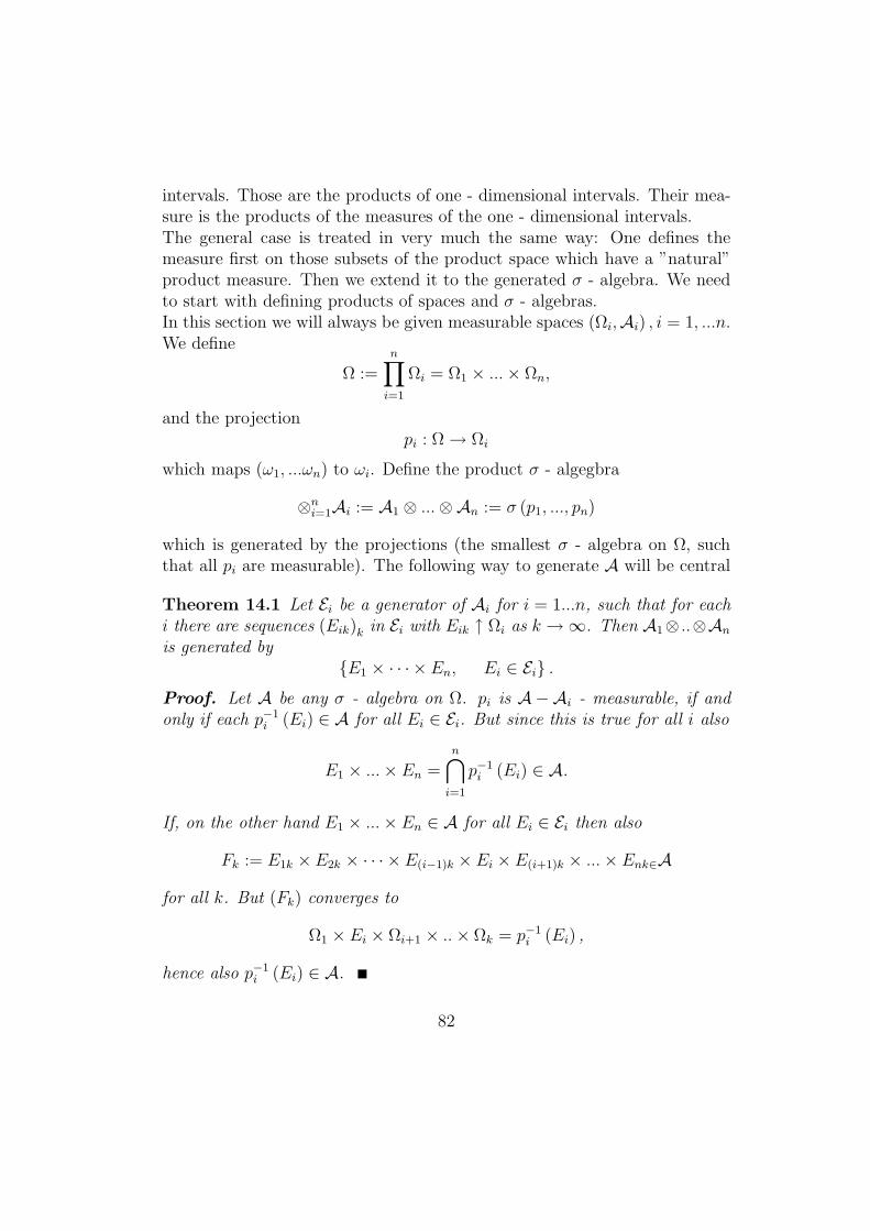
intervals. Those are the products of one - dimensional intervals. Their mea-sure is the products of the measures of the one - dimensional intervals.The general case is treated in very much the same way: One defines themeasure first on those subsets of the product space which have a ”natural”product measure. Then we extend it to the generated σ - algebra. We needto start with defining products of spaces and σ - algebras.In this section we will always be given measurable spaces (Ωi,Ai) , i = 1, ...n.We define

Ω :=

n∏i=1

Ωi = Ω1 × ...× Ωn,

and the projectionpi : Ω → Ωi

which maps (ω1, ...ωn) to ωi. Define the product σ - algegbra

⊗ni=1Ai := A1 ⊗ ...⊗An := σ (p1, ..., pn)

which is generated by the projections (the smallest σ - algebra on Ω, suchthat all pi are measurable). The following way to generate A will be central

Theorem 14.1 Let Ei be a generator of Ai for i = 1...n, such that for eachi there are sequences (Eik)k in Ei with Eik ↑ Ωi as k →∞. Then A1⊗ ..⊗An

is generated by{E1 × · · · × En, Ei ∈ Ei} .

Proof. Let A be any σ - algebra on Ω. pi is A−Ai - measurable, if andonly if each p−1

i (Ei) ∈ A for all Ei ∈ Ei. But since this is true for all i also

E1 × ...× En =n⋂

i=1

p−1i (Ei) ∈ A.

If, on the other hand E1 × ...× En ∈ A for all Ei ∈ Ei then also

Fk := E1k ×E2k × · · · ×E(i−1)k × Ei × E(i+1)k × ...× Enk∈Afor all k. But (Fk) converges to

Ω1 × Ei × Ωi+1 × ..× Ωk = p−1i (Ei) ,

hence also p−1i (Ei) ∈ A.

82

Exercise 14.2 Prove that the condition of Eik ↑ Ωi is actually needed in theprevious theorem.

Example 14.3 Choosing Ωi = R for all i, Ai = B1 for all i and Ei = J 1,then obviously

{E1 × ..× En, Ei ∈ Ei} = J d.

With Theorem 14.1 this gives Bd = B1 × ..× Bk. As we saw in Section 5 λn

is the unique measure on Bn with

λn(I1 × ..× In) = λ1(I1)....λ1(In)

for all Ii ∈ J 1.

The above example immediately raises the following question: Given measureμi on (Ωi,Ai). Under which conditions is there a measure π on (Ω,A) suchthat

π (E1 × ..× En) = μ(E1)...μ (En) (14.1)

for all Ei ∈ Ei (and the Ei generators of Ai)? When is such a π unique?The second question can be answered at once:

Theorem 14.4 If each generator Ei of Ai is⋂

- stable and contains a se-quence (Eik) with Eik ↑ Ωi and μ (Eik), there is at most one π as given in(14.1)

Proof. DefineE := {E1..× En, Ei ∈ Ei} .

Theorem 14.1 shows that E generators A1 ⊗ ..⊗An. Since(n∏

i=1

Ei

)∩(

n∏i=1

Fi

)=

n∏i=1

(Ei ∩ Fi)

with Ei also E is ∩ - stable. Moreover

Ek := E1k × ..× Enk ↑ Ω.

The assertion follows thus from Theorem 2.13, since

π (Ek) = μ1 (E1k) ....μn (Enk) <∞.

83

We will now turn to answering the first question as well, i. e. we will con-struct the product of two measure spaces (Ω1,A1, μ1) and (Ω2,A2, μ2). Thegeneralization to arbitrary n is then a fairly standard induction argument.For Q ⊆ Ω1 × Ω2 and ωi ∈ Ωi, i = 1, 2, we will first define

Qω1 := {ω2 ∈ Ω2 : (ω1, ω2) ∈ Q}and

Qω2 := {ω1 ∈ Ω1 : (ω1, ω2) ∈ Q}Then we obtain

Lemma 14.5 14.5: Let Q ∈ A1 ⊗ A2. Then for arbitrary ω1 ∈ Ω, andω2 ∈ Ω2, Qω1∈A2 and Qω1 ∈ A1.

Proof. For Q, Q1, Q2, ... ≤ Ω1 × Ω2 and arbitrary ω1 ∈ Ω, it holds

(Ω\Q)ω1= Ω2\Qω1

as well as (∞⋃i=1

Qi

)ω1

=

∞⋃i=1

(Qi)ω1.

Moreover Ωω1 = Ω2 and more generally

(A1 × A2)ω1= 1ω1(A1) · A2

(Ai ⊂ Ωi). Thus for all ω1 ∈ Ω,

A′:= {Q ⊂ Ω : Qω1 ∈ A2}

is a σ - algebra over the set Ω. A′contains all A1 × A2, Ai ∈ Ai. But from

Theorem 14.1 we have that A1 ⊗ A2 is the smallest such σ - algebra. Thisproves the lemma for Qω1 . The proof for Qw2 is analogous.

According to the previous lemma we may measure Qω1 with μ2 and Qω2 withμ1. Moreover we can show

Lemma 14.6 Assume that μ1, μ2 are σ - finite. Then for all Q ∈ A1 ⊗A2

the functionsω1 �−→ μ2(Qω1) and ω2 �−→ μ2(Qω2)

(defined on Ω1 and Ω2 respectively) are A1 - measurable and A2 - measurable,respectively.

84

Proof. Define ςQ(ω1) = μ2(Qω1). First assume μ2(Ω2) < ∞. Define

D := {D ∈ A1 ⊗A2, ςD is A1 - measurable} . (14.2)

Then D is a Dynkin - system that contains all sets of the form A1×A2, Ai ∈Aωi = 1, 2 (Exercise 14.7). The system E of all sets A1×A2, Ai ∈ Ai, i = 1, 2is ∩ - stable and generates A1 ⊗A2. Thus D (E) = A1 ⊗A2 and because ofE ⊆ D ⊆ A1 ⊗A2 we obtain D = A1 ⊗A2.

If μ2 is only σ - finite, there is a sequence (Bn) in A2 with Bn ↑ Ω2 andμ2 (Bn) < ∞. For all n the measure μ2,n(A2) := μ2(A2 ∩ Bn) is finite. Thusω1 �−→ μ2,n (Qω1) is measurable with respect to A1 for Q ∈ A1 ⊗A2. But

supn

μ2,n(Qω1) = μ2(Qω1),

since μ2 as a measure is continuous from below. As the supremum of mea-surable functions is measurable this shows the assertion for ω1 �→ μ2(ωω1).The other assertion is proved analogously.

Exercise 14.7 Show that D as defined in (14.2) is a Dynkin - system thatcontains E (as in Lemma 14.6).

Now the existence of a product measure follows easily.

Theorem 14.8 Let (Ωi,Ai, μi), i = 1, 2 be σ - finite measure spaces. Thenthere is a unique measure π on A1 ⊗A2 with

π (A1 ×A2) = μ1(A1) · μ2(A2) (14.3)

for all Ai ∈ Ai, i = 1, 2. For each Q ∈ A1 ⊗A2 it holds

π (Q) =

∫μ2(Qω1)μ1(dω1) =

∫μ1 (Qω2) μ2(dω1). (14.4)

Obviously, if μ1, μ2 are σ - finite, so is π.

Proof. Again let ςQ(ω1) = μ2(Qω1). Define π (Q) :=∫

ςQdμ1. For eachsequence (Qn) of pairwise disjoint sets in A1⊗A2 it holds ς∪Qn =

∑ςQn and

thus by monotone convergence

π

( ∞⋃n=1

Qn

)=

∞∑n=1

π (Qn) .

85

Because of ς∅ = 0 also π (∅) = 0 and thus π is a measure on A1 ⊗A2. π hasproperty (14.3) since

ςA1×A2 = μ2(A2)1Ai

and thereforeπ(A1 ×A2) = μ1(A1) · μ2(A2).

In the same way we can define a measure on A1 ⊗A2 by

π′(Q) =

∫μ1(Qω2)μ2(dω2)

Applying Theorem 14.4 to E1 = A1 and E2 = A2 gives that there is at mostone such measure, hence π

′= π and the second equality in (14.4) follows.

Definition 14.9 In the situation of Theorem 14.8 the unique measure π withproperty (14.3) is called the product measure of μ1 and μ2 and demoted byμ1 ⊗ μ2.

The most prominent example of a product measure is, of course, Lebesguemeasure, where we have

λ2 = λ1 ⊗ λ1 or, more generally, λm+n = λm ⊗ λn.

We will now turn to integration with respect to product measures. To sim-plify notation let us write

ω2 �−→ fω1(ω2) := f (ω1, ω2)

andω1 �−→ fω2(ω1) := f (ω1, ω2)

for a function f : Ω1 × Ω2 → Ω′

(for a set Ω′) and ω1 ∈ Ω1, ω2 ∈ Ω2. For

Q ∈ A1 ⊗A2 we obviously have

(1Q)ω1= 1Qω1

and (1Q)ω2 = 1Qω1. (14.5)

The following is immediate from Lemma 14.5

Exercise 14.10 For each(Ω

′,A′)

and each measurable mapping

f : Ω1 × Ω2 → Ω′

the mappings fω1 and fω2, respectively, are A2 - A′- measurable and A1 -

A′- measurable, respectively. Prove this.

86

Already formula (14.4) gives an idea of how integration with respect to μ1⊗μ2

should look like. The following two theorems, that are due to Tonelli andFubini, respectively generalize (14.4) to μ1 ⊗ μ2 - integrable functions.

Theorem 14.11 (Tonelli) Let (Ωi,Ai, μi) , i = 1, 2 two σ - finite measur-able spaces and

f : Ω1 ⊗ Ω2 → R+

be A1 ⊗A2 - measurable. Then

ω2 �−→∫

fω2dμ1 and ω1 �−→∫

fω2dμ2

are A1 - measurable and A2 - measurable, respectively. Eventually:∫fd (μ1 ⊗ μ2) =

∫ (∫fω2dμ1

)μ2(dω2) (14.6)

=

∫ (∫fω1dμ2

)μ1 (dω1) .

Proof. : Put Ω := Ω1 × Ω2,A := A1 ⊗A2, and π := μ1 ⊗ μ2. Startingwith step functions

f =n∑

i=1

αi1Qi , αi ≥ 0, Qi ∈ A,

then fω2 =∑

αi1Qi

ω2and due to (14.5)

∫fω2dμ1 =

n∑i=1

αiμ1(Qiω2

).

Hence ω2 �−→∫

fω2dμ is A2 - measurable. Using (14.4) we get

∫ (∫fω2dμ1

)μ2(dω2) =

n∑i=1

αiπ(Qi) =

∫fdπ

hence the first equality in 814.6).arbitrary A - measurable f ≥ 0 let (un) be a sequence of step - functionswith un ↑ f . Then (using the first part of this proof)

(un

ω2

)is a sequence of

87

step - functions (with respect to A2) with unω2↑ fω2 . From what we have

already proved we obtain that

ω2 �→ ϕn (ω2) :=

∫un

ω2dμ1

is increasing with supremum

(14.7) ω2 �−→∫

fω2dμ1.

Hence also the function defined in (14.7) is measurable and hence by mono-tone convergence∫ (∫

fω2dμ2

)μ2(dω2) = sup

n

∫ϕndμ2

= supn

∫undπ,

where for the second equality we used the first step of this proof. By thechoice of (un) we thus have ∫

ϕndμ2 ↑∫

fdπ

which gives ∫(

∫fω2dμ1)μ2(dω2) =

∫fdn.

Analogous considerations conclude the proof of the theorem.

Theorem 14.12 (Fubini) Let (Ωi,Ai, μi) , i = 1, 2 be two σ - finite mea-sure spaces and

f : Ω1 × Ω2 → R

be a measurable, integrable (with respect to μ1 ⊗ μ2) function. Then fω1 isμ2 - integrable μ1 − a.e. in ω1 and fω2 is μ1 - integrable μ2 − a.e. Hence thefollowing function are defined a.e.:

ω1 �→∫

fω1dμ2 and ω2 �→∫

fω2dμ1.

Both these functions are integrable (with respect to μ1 and μ2, respectively)and (14.6) holds.

88

Proof. : Obviously

|fωi| = |f |ωi

,(f+

ωi

)=(f+)

ωi,(f−

ωi

)=(f−)

ωi.

Applying (14.6) to |f | and μ1 ⊗ μ2 we obtain∫ (∫|fω1 | dμ2

)dμ1 =

∫ (∫|fω2 | dμ1

)dμ2

=

∫|f | dμ1 ⊗ μ2 < ∞.

Thus ω1 �→∫ |fω1 | dμ2 is finite μ1 − a.e., thus μ1 − a.e. also μ2 - integrable.

Therefore

ω1 �→∫

fω1dμ2 =

∫f+

ω1dμ2 −

∫f−

ωidμ2

is μ1−a.e. defined and A1 - measurable. Applying Theorem 14.11 to f+ andf− we arrive at:∫ (∫

fω1dμ2

)dμ1 =

∫ (∫f+

ω1dμ2

)dμ1 −

∫ (∫f−

ω1dμ2

)dμ1

=

∫f+dπ −

∫f−dπ =

∫fdπ.

Interchanging the roles of ω1 and ω2 concludes the proof.

The generalizations to an arbitrary (but finite) number of factors will nowbe left to the reader. The proofs work by induction.

Exercise 14.13 Let μ1, ..., μn be σ - finite measures on (Ω1,A1) , ..., (Ωn,An).Then there is a unique measure π on A1 ⊗ ...⊗An with

π(A1 × ..× An) = μ1(A1)...μ (An)

for all Ai ∈ Ai. Prove this.

Definition 14.14 The measure π in Exercise 14.13 is called the productmeasure of μ1, ..., μn and denoted by

⊗ni=1μi = μ,⊗...⊗ μn.

In very much the same way one extends Fubini’s theorem to the case ofseveral factors.

89

Exercise 14.15 In the situation of Exercise 14.13 let f : Ω,×..Ωn → R be a⊗n

i=1μi - integrable function. Then for any permutation i1, ..., in of the indices1, ...n: ∫

fd (μ1 ⊗ ..⊗ μn) =

∫(.. (f (ω1..., ωn) μi1dωi

) μindωi

Prove this.

Exercise 14.16 Let Br(x0) be the closed ball of radius r centered in x0 inRd. Put

αd := λd(k, (0)).

90