Embed Size (px)
Citation preview
Lecture Notes in PhysicsEditorial Board
R. Beig, Wien, AustriaW. Beiglböck, Heidelberg, GermanyW. Domcke, Garching, GermanyB.-G. Englert, SingaporeU. Frisch, Nice, FranceP. Hänggi, Augsburg, GermanyG. Hasinger, Garching, GermanyK. Hepp, Zürich, SwitzerlandW. Hillebrandt, Garching, GermanyD. Imboden, Zürich, SwitzerlandR. L. Jaffe, Cambridge, MA, USAR. Lipowsky, Potsdam, GermanyH. v. Löhneysen, Karlsruhe, GermanyI. Ojima, Kyoto, JapanD. Sornette, Nice, France, and Zürich, SwitzerlandS. Theisen, Potsdam, GermanyW. Weise, Garching, GermanyJ. Wess, München, GermanyJ. Zittartz, Köln, Germany
The Lecture Notes in PhysicsThe series Lecture Notes in Physics (LNP), founded in 1969, reports new developmentsin physics research and teaching – quickly and informally, but with a high quality andthe explicit aim to summarize and communicate current knowledge in an accessible way.Books published in this series are conceived as bridging material between advanced grad-uate textbooks and the forefront of research and to serve three purposes:
• to be a compact and modern up-to-date source of reference on a well-defined topic
• to serve as an accessible introduction to the field to postgraduate students andnonspecialist researchers from related areas
• to be a source of advanced teaching material for specialized seminars, courses andschools
Both monographs and multi-author volumes will be considered for publication. Editedvolumes should, however, consist of a very limited number of contributions only. Pro-ceedings will not be considered for LNP.
Volumes published in LNP are disseminated both in print and in electronic formats, theelectronic archive being available at springerlink.com. The series content is indexed, ab-stracted and referenced by many abstracting and information services, bibliographic net-works, subscription agencies, library networks, and consortia.
Proposals should be sent to a member of the Editorial Board, or directly to the managingeditor at Springer:
Christian CaronSpringer HeidelbergPhysics Editorial Department ITiergartenstrasse 1769121 Heidelberg / [email protected]
D. HusemöllerM. JoachimB. JurcoM. Schottenloher
Basic Bundle Theoryand K-CohomologyInvariantsWith contributions by Siegfried Echterhoff, StefanFredenhagen and Bernhard Krötz
Authors
D. Husemöller B. JurcoMPI für Mathematik MPI für MathematikVivatsgasse 7 Vivatsgasse 753111 Bonn, Germany 53111 Bonn, [email protected] [email protected]
M. Joachim M. SchottenloherUniversität Münster Universität MünchenMathematisches Institut Mathematisches InstitutEinsteinstr. 62 Theresienstr. 3948149 Münster, Germany 80333 München, [email protected] Martin.Schottenloher@Mathematik.
Uni-Muenchen.deContributors
Siegfried Echterhoff (Chap. 17, Appendix) Bernhard Krötz (Chap. 16, Appendix)Mathematisches Institut MPI für Mathematik, Bonn, GermanyWestfälische Wilhelms-UniversitätMünster, Germany
Stefan Fredenhagen (Physical Background to the K-Theory Classificationof D-Branes), MPI für Gravitationsphysik, Potsdam, Germany
D. Husemöller et al., Basic Bundle Theory and K-Cohomology Invariants, Lect. NotesPhys. 726 (Springer, Berlin Heidelberg 2008), DOI 10.1007/ 978-3-540-74956-1
Library of Congress Control Number: 2007936164
ISSN 0075-8450ISBN 978-3-540-74955-4 Springer Berlin Heidelberg New York
This work is subject to copyright. All rights are reserved, whether the whole or part of the material isconcerned, specifically the rights of translation, reprinting, reuse of illustrations, recitation, broadcasting,reproduction on microfilm or in any other way, and storage in data banks. Duplication of this publicationor parts thereof is permitted only under the provisions of the German Copyright Law of September 9,1965, in its current version, and permission for use must always be obtained from Springer. Violationsare liable for prosecution under the German Copyright Law.
Springer is a part of Springer Science+Business Mediaspringer.comc© Springer-Verlag Berlin Heidelberg 2008
The use of general descriptive names, registered names, trademarks, etc. in this publication does not imply,even in the absence of a specific statement, that such names are exempt from the relevant protective lawsand regulations and therefore free for general use.
Typesetting: by the authors and Integra using a Springer LATEX macro packageCover design: eStudio Calamar S.L., F. Steinen-Broo, Pau/Girona, Spain
Printed on acid-free paper SPIN: 12043415 5 4 3 2 1 0
Dedicated to the memory of Julius Wess
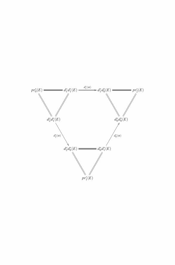
pr∗0(E) d∗1d∗
1(E) d∗1d∗
0(E) pr∗2(E)
d∗2d∗
1(E) d∗0d∗
0(E)
d∗2d∗
0(E) d∗0d∗
1(E)
pr∗1(E)
d∗1(α)��
��������������
��������������
��������������
��������������
��������������
��������������
��������������
��������������
d∗2(α)
����������������
d∗0(α)
����������������
��������������
��������������
��������������
��������������
Preface
This lecture notes volume has its origins in a course by Husemoller on fibre bundlesand twisted K-theory organized by Brano Jurco for physics students at the LMU inMunchen, summer term 2003. The fact that K-theory invariants, and in particulartwisted K-theory invariants, were being used in the geometric aspects of mathemat-ical physics created the need for an accessible treatment of the subject. The coursesurveyed the book Fibre Bundles, 3rd. Ed. 1994, Springer-Verlag by Husemoller,and covered topics used in mathematical physics related to K-theory invariants. Thisbook is referred to just by its title throughout the text.
The idea of lecture notes came up by J. Wess in 2003 in order to serve severalpurposes. Firstly, they were to be a supplement to the book Fibre Bundles providingcompanion reading and alternative approaches to certain topics; secondly, they wereto survey some of the basic results of background to K-theory, for example operatoralgebra K-theory, not covered in the Fibre Bundles; and finally the notes wouldcontain information on the relation to physics. This we have done in the surveyfollowing this introduction “Physical background to the K-theory classification ofD-branes: Introduction and references” tracing the papers how and where K-theoryinvariants started to play a role in string theory. The basic references to physics aregiven at the end of this survey, while the mathematics references are at the end ofthe volume.
Other lectures of Husemoller had contributed to the text of the notes. During2001/2002 in Munster resp. during Summer 2002 in Munchen, Husemoller gaveGraduate College courses on the topics in the notes, organized by Joachim Cuntzresp. Martin Schottenloher, and in the Summer 2001, he had a regular course onC*-algebras and K-theory in Munchen. The general question of algebra bundleswas studied with the support of Professor Cuntz in Munster during short periodsfrom 2003 to 2005. Finally, Husemoller lectured on these topics during a workshopat IPM, Tehran, Iran, September 2005. It is with a great feeling of gratitude thatthese lecture opportunities are remembered here.
The notes are organized into five parts. The first part on basic bundle theoryemphasizes the concept of bundle as one treats the concepts of set, space, homotopy,group, or ring in basic mathematics. A bundle is just a map called the projectionfrom the total space to its base space. As with commutative groups, topological
vii
viii Preface
groups, transformation groups, and Lie groups, the concept of bundle is enhancedor enriched with additional axioms and structures leading to etale bundles, principalbundles, fibre bundles, vector bundles, and algebra bundles. A topic discussed inthe first part, which is not taken up in the Fibre Bundles, is the Serre–Swan theoremwhich relates vector bundles on a compact space X with finitely generated projectivemodules over the ring C(X) of continuous complex valued functions on the space X .This is one of the points where topological, algebraic, and operator K-theory cometogether.
The second part of the notes takes up the homotopy classification of principalbundles and fibre bundles. Applications to the case of vector bundles are consideredand the role of homotopy theory in K-theory is developed. This is related to the factthat K-theory is a representable functor on the homotopy category. The theory ofcharacteristic classes in describing orientation and spin structures on vector bundlesis carried out in detail, also leading to the notion of a string structure on a bundleand on a manifold.
There are various versions of topological K-theory, and their relation to Bott peri-odicity is considered in the third part of the notes. An advanced version of operatorK-theory, called KK-theory which integrates K-cohomology and K-homology, isintroduced, and various features are sketched.
The fourth part of the notes begins with algebra bundles with fibres that are eithermatrix algebras or algebras of bounded operators on a separable Hilbert space. Theinfinite dimensional algebra bundles are classified by only one characteristic classin the integral third cohomology group of the base space along the lines of theclassification of complex line bundles with its first Chern class in the integral secondcohomology group of the base space. The twisting of twisted K-theory is given byan infinite dimensional algebra bundle, and the twisted K-theory is defined in termsof cross sections of Fredholm bundles related to the algebra bundle describing thetwist under consideration.
A fundamental theme in bundle theory centers around the gluing of local bundledata related to bundles into a global object. In the fifth part we return to this themeand study gluing on open sets in a topological space of not just simple bundle databut also data in a more general category where the gluing data may satisfy transitiv-ity conditions only up to an isomorphism. The resulting objects are gerbes or stacks.
August 2007 Dale Husemoller
Contents
Physical Background to the K-Theory Classification of D-Branes:Introduction and References . . . . . . . . . . . . . . . . . . . . . . . . . . . . . . . . . . . . . . . . . 1
Part I Bundles over a Space and Modules over an Algebra
1 Generalities on Bundles and Categories . . . . . . . . . . . . . . . . . . . . . . . . . . . 91 Bundles Over a Space . . . . . . . . . . . . . . . . . . . . . . . . . . . . . . . . . . . . . . . 92 Examples of Bundles . . . . . . . . . . . . . . . . . . . . . . . . . . . . . . . . . . . . . . . 113 Two Operations on Bundles . . . . . . . . . . . . . . . . . . . . . . . . . . . . . . . . . . 134 Category Constructions Related to Bundles . . . . . . . . . . . . . . . . . . . . . 145 Functors Between Categories . . . . . . . . . . . . . . . . . . . . . . . . . . . . . . . . . 166 Morphisms of Functors or Natural Transformations . . . . . . . . . . . . . . 187 Etale Maps and Coverings . . . . . . . . . . . . . . . . . . . . . . . . . . . . . . . . . . . 20References . . . . . . . . . . . . . . . . . . . . . . . . . . . . . . . . . . . . . . . . . . . . . . . . . . . . . 22
2 Vector Bundles . . . . . . . . . . . . . . . . . . . . . . . . . . . . . . . . . . . . . . . . . . . . . . . . . 231 Bundles of Vector Spaces and Vector Bundles . . . . . . . . . . . . . . . . . . . 232 Isomorphisms of Vector Bundles and Induced Vector Bundles . . . . . 253 Image and Kernel of Vector Bundle Morphisms . . . . . . . . . . . . . . . . . 264 The Canonical Bundle Over the Grassmannian Varieties . . . . . . . . . . 285 Finitely Generated Vector Bundles . . . . . . . . . . . . . . . . . . . . . . . . . . . . 296 Vector Bundles on a Compact Space . . . . . . . . . . . . . . . . . . . . . . . . . . . 317 Collapsing and Clutching Vector Bundles on Subspaces . . . . . . . . . . 318 Metrics on Vector Bundles . . . . . . . . . . . . . . . . . . . . . . . . . . . . . . . . . . . 33Reference . . . . . . . . . . . . . . . . . . . . . . . . . . . . . . . . . . . . . . . . . . . . . . . . . . . . . . 34
3 Relation Between Vector Bundles, Projective Modules, andIdempotents . . . . . . . . . . . . . . . . . . . . . . . . . . . . . . . . . . . . . . . . . . . . . . . . . . . 351 Local Coordinates of a Vector Bundle Given by Global Functions
over a Normal Space . . . . . . . . . . . . . . . . . . . . . . . . . . . . . . . . . . . . . . . . 362 The Full Embedding Property of the Cross Section Functor . . . . . . . 373 Finitely Generated Projective Modules . . . . . . . . . . . . . . . . . . . . . . . . . 384 The Serre–Swan Theorem . . . . . . . . . . . . . . . . . . . . . . . . . . . . . . . . . . . 40
ix
x Contents
5 Idempotent Classes Associated to Finitely Generated ProjectiveModules . . . . . . . . . . . . . . . . . . . . . . . . . . . . . . . . . . . . . . . . . . . . . . . . . . 42
4 K-Theory of Vector Bundles, of Modules, and of Idempotents . . . . . . . 451 Generalities on Adding Negatives . . . . . . . . . . . . . . . . . . . . . . . . . . . . . 452 K-Groups of Vector Bundles . . . . . . . . . . . . . . . . . . . . . . . . . . . . . . . . . 473 K-Groups of Finitely Generated Projective Modules . . . . . . . . . . . . . . 484 K-Groups of Idempotents . . . . . . . . . . . . . . . . . . . . . . . . . . . . . . . . . . . . 505 K-Theory of Topological Algebras . . . . . . . . . . . . . . . . . . . . . . . . . . . . 51References . . . . . . . . . . . . . . . . . . . . . . . . . . . . . . . . . . . . . . . . . . . . . . . . . . . . . 54
5 Principal Bundles and Sections of Fibre Bundles: Reduction of theStructure and the Gauge Group I . . . . . . . . . . . . . . . . . . . . . . . . . . . . . . . . 551 Bundles Defined by Transformation Groups . . . . . . . . . . . . . . . . . . . . 552 Definition and Examples of Principal Bundles . . . . . . . . . . . . . . . . . . . 573 Fibre Bundles . . . . . . . . . . . . . . . . . . . . . . . . . . . . . . . . . . . . . . . . . . . . . . 584 Local Coordinates for Fibre Bundles . . . . . . . . . . . . . . . . . . . . . . . . . . 585 Extension and Restriction of Structure Group . . . . . . . . . . . . . . . . . . . 606 Automorphisms of Principal Bundles and Gauge Groups . . . . . . . . . . 62Reference . . . . . . . . . . . . . . . . . . . . . . . . . . . . . . . . . . . . . . . . . . . . . . . . . . . . . . 62
Part II Homotopy Classification of Bundles and Cohomology: ClassifyingSpaces
6 Homotopy Classes of Maps and the Homotopy Groups . . . . . . . . . . . . . 651 The Space Map(X ,Y) . . . . . . . . . . . . . . . . . . . . . . . . . . . . . . . . . . . . . . . 652 Continuity of Substitution and Map(X×T,Y ) . . . . . . . . . . . . . . . . . . . 663 Free and Based Homotopy Classes of Maps . . . . . . . . . . . . . . . . . . . . 674 Homotopy Categories . . . . . . . . . . . . . . . . . . . . . . . . . . . . . . . . . . . . . . . 685 Homotopy Groups of a Pointed Space . . . . . . . . . . . . . . . . . . . . . . . . . 696 Bundles on a Cylinder B×[0,1] . . . . . . . . . . . . . . . . . . . . . . . . . . . . . . . 72
7 The Milnor Construction: Homotopy Classification of PrincipalBundles . . . . . . . . . . . . . . . . . . . . . . . . . . . . . . . . . . . . . . . . . . . . . . . . . . . . . . . 751 Basic Data from a Numerable Principal Bundle . . . . . . . . . . . . . . . . . 752 Total Space of the Milnor Construction . . . . . . . . . . . . . . . . . . . . . . . . 763 Uniqueness up to Homotopy of the Classifying Map . . . . . . . . . . . . . 784 The Infinite Sphere as the Total Space of the Milnor Construction . . 80References . . . . . . . . . . . . . . . . . . . . . . . . . . . . . . . . . . . . . . . . . . . . . . . . . . . . . 81
8 Fibrations and Bundles: Gauge Group II . . . . . . . . . . . . . . . . . . . . . . . . . 831 Factorization, Lifting, and Extension in Square Diagrams . . . . . . . . . 842 Fibrations and Cofibrations . . . . . . . . . . . . . . . . . . . . . . . . . . . . . . . . . . 853 Fibres and Cofibres: Loop Space and Suspension . . . . . . . . . . . . . . . . 884 Relation Between Loop Space and Suspension Group Structures
on Homotopy Classes of Maps [X,Y]∗∗∗ . . . . . . . . . . . . . . . . . . . . . . . . . 90
Contents xi
5 Outline of the Fibre Mapping Sequence and Cofibre MappingSequence . . . . . . . . . . . . . . . . . . . . . . . . . . . . . . . . . . . . . . . . . . . . . . . . . 91
6 From Base to Fibre and From Fibre to Base . . . . . . . . . . . . . . . . . . . . . 937 Homotopy Characterization of the Universal Bundle . . . . . . . . . . . . . 958 Application to the Classifying Space of the Gauge Group . . . . . . . . . 959 The Infinite Sphere as the Total Space of a Universal Bundle . . . . . . 96Reference . . . . . . . . . . . . . . . . . . . . . . . . . . . . . . . . . . . . . . . . . . . . . . . . . . . . . . 96
9 Cohomology Classes as Homotopy Classes: CW-Complexes . . . . . . . . . 971 Filtered Spaces and Cell Complexes . . . . . . . . . . . . . . . . . . . . . . . . . . . 982 Whitehead’s Characterization of Homotopy Equivalences . . . . . . . . . 993 Axiomatic Properties of Cohomology and Homology . . . . . . . . . . . . 1004 Construction and Calculation of Homology
and Cohomology . . . . . . . . . . . . . . . . . . . . . . . . . . . . . . . . . . . . . . . . . . . 1035 Hurewicz Theorem . . . . . . . . . . . . . . . . . . . . . . . . . . . . . . . . . . . . . . . . . 1056 Representability of Cohomology by Homotopy Classes . . . . . . . . . . . 1057 Products of Cohomology and Homology . . . . . . . . . . . . . . . . . . . . . . . 1068 Introduction to Morse Theory . . . . . . . . . . . . . . . . . . . . . . . . . . . . . . . . 107References . . . . . . . . . . . . . . . . . . . . . . . . . . . . . . . . . . . . . . . . . . . . . . . . . . . . . 109
10 Basic Characteristic Classes . . . . . . . . . . . . . . . . . . . . . . . . . . . . . . . . . . . . . 1111 Characteristic Classes of Line Bundles . . . . . . . . . . . . . . . . . . . . . . . . . 1112 Projective Bundle Theorem and Splitting Principle . . . . . . . . . . . . . . . 1133 Chern Classes and Stiefel–Whitney Classes of Vector Bundles . . . . . 1144 Elementary Properties of Characteristic Classes . . . . . . . . . . . . . . . . . 1175 Chern Character and Related Multiplicative Characteristic Classes . 1186 Euler Class . . . . . . . . . . . . . . . . . . . . . . . . . . . . . . . . . . . . . . . . . . . . . . . . 1217 Thom Space, Thom Class, and Thom Isomorphism . . . . . . . . . . . . . . 1228 Stiefel–Whitney Classes in Terms of Steenrod Operations . . . . . . . . . 1229 Pontrjagin classes . . . . . . . . . . . . . . . . . . . . . . . . . . . . . . . . . . . . . . . . . . 125References . . . . . . . . . . . . . . . . . . . . . . . . . . . . . . . . . . . . . . . . . . . . . . . . . . . . . 125
11 Characteristic Classes of Manifolds . . . . . . . . . . . . . . . . . . . . . . . . . . . . . . 1271 Orientation in Euclidean Space and on Manifolds . . . . . . . . . . . . . . . . 1272 Poincare Duality on Manifolds . . . . . . . . . . . . . . . . . . . . . . . . . . . . . . . 1293 Thom Class of the Tangent Bundle and Duality . . . . . . . . . . . . . . . . . 1304 Euler Class and Euler Characteristic of a Manifold . . . . . . . . . . . . . . . 1315 Wu’s Formula for the Stiefel–Whitney Classes of a Manifold . . . . . . 1326 Cobordism and Stiefel–Whitney Numbers . . . . . . . . . . . . . . . . . . . . . . 1337 Introduction to Characteristic Classes and Riemann–Roch . . . . . . . . 134Reference . . . . . . . . . . . . . . . . . . . . . . . . . . . . . . . . . . . . . . . . . . . . . . . . . . . . . . 135
xii Contents
12 Spin Structures . . . . . . . . . . . . . . . . . . . . . . . . . . . . . . . . . . . . . . . . . . . . . . . . 1371 The Groups Spin(n) and Spinc(n) . . . . . . . . . . . . . . . . . . . . . . . . . . . . . . 1372 Orientation and the First Stiefel–Whitney Class . . . . . . . . . . . . . . . . . 1393 Spin Structures and the Second Stiefel–Whitney Class . . . . . . . . . . . . 1404 Spinc Structures and the Third Integral Stiefel–Whitney Class . . . . . 1415 Relation Between Characteristic Classes of Real
and Complex Vector Bundles . . . . . . . . . . . . . . . . . . . . . . . . . . . . . . . . . 1426 Killing Homotopy Groups in a Fibration . . . . . . . . . . . . . . . . . . . . . . . 142
Part III Versions of K-Theory and Bott Periodicity
13 G-Spaces, G-Bundles, and G-Vector Bundles . . . . . . . . . . . . . . . . . . . . . . 1491 Relations Between Spaces and G-Spaces: G-Homotopy . . . . . . . . . . . 1492 Generalities on G-Bundles . . . . . . . . . . . . . . . . . . . . . . . . . . . . . . . . . . . 1523 Generalities on G-Vector Bundles . . . . . . . . . . . . . . . . . . . . . . . . . . . . . 1534 Special Examples of G-Vector Bundles . . . . . . . . . . . . . . . . . . . . . . . . 1555 Extension and Homotopy Problems for G-Vector Bundles
for G a Compact Group . . . . . . . . . . . . . . . . . . . . . . . . . . . . . . . . . . . . . 1576 Relations Between Complex and Real G-Vector Bundles . . . . . . . . . . 1587 KRG-Theory . . . . . . . . . . . . . . . . . . . . . . . . . . . . . . . . . . . . . . . . . . . . . . . 159References . . . . . . . . . . . . . . . . . . . . . . . . . . . . . . . . . . . . . . . . . . . . . . . . . . . . . 161
14 Equivariant K-Theory Functor KG : Periodicity, ThomIsomorphism, Localization, and Completion . . . . . . . . . . . . . . . . . . . . . . 1631 Associated Projective Space Bundle to a G-Equivariant Bundle . . . . 1632 Assertion of the Periodicity Theorem for a Line Bundle . . . . . . . . . . 1643 Thom Isomorphism . . . . . . . . . . . . . . . . . . . . . . . . . . . . . . . . . . . . . . . . . 1674 Localization Theorem of Atiyah and Segal . . . . . . . . . . . . . . . . . . . . . 1705 Equivariant K-Theory Completion Theorem of Atiyah and Segal . . . 172References . . . . . . . . . . . . . . . . . . . . . . . . . . . . . . . . . . . . . . . . . . . . . . . . . . . . . 173
15 Bott Periodicity Maps and Clifford Algebras . . . . . . . . . . . . . . . . . . . . . . 1751 Vector Bundles and Their Principal Bundles and Metrics . . . . . . . . . . 1752 Homotopy Representation of K-Theory . . . . . . . . . . . . . . . . . . . . . . . . 1763 The Bott Maps in the Periodicity Series . . . . . . . . . . . . . . . . . . . . . . . . 1794 KR∗
G(X) and the Representation Ring RR(G) . . . . . . . . . . . . . . . . . . . . 1805 Generalities on Clifford Algebras and Their Modules . . . . . . . . . . . . . 1816 KR−q
G (*) and Modules Over Clifford Algebras . . . . . . . . . . . . . . . . . . 1847 Bott Periodicity and Morse Theory . . . . . . . . . . . . . . . . . . . . . . . . . . . . 1858 The Graded Rings KU∗(∗) and KO∗(∗) . . . . . . . . . . . . . . . . . . . . . . . . 187References . . . . . . . . . . . . . . . . . . . . . . . . . . . . . . . . . . . . . . . . . . . . . . . . . . . . . 188
Contents xiii
16 Gram–Schmidt Process, Iwasawa Decomposition, and Reduction ofStructure . . . . . . . . . . . . . . . . . . . . . . . . . . . . . . . . . . . . . . . . . . . . . . . . . . . . . . 1891 Classical Gram–Schmidt Process . . . . . . . . . . . . . . . . . . . . . . . . . . . . . 1892 Definition of Basic Linear Groups . . . . . . . . . . . . . . . . . . . . . . . . . . . . . 1903 Iwasawa Decomposition for GL and SL . . . . . . . . . . . . . . . . . . . . . . . . 1914 Applications to Structure Group Reduction for Principal Bundles
Related to Vector Bundles . . . . . . . . . . . . . . . . . . . . . . . . . . . . . . . . . . . 1925 The Special Case of SL222(R) and the Upper Half Plane . . . . . . . . . . . 1936 Relation Between SL222(R) and SL222(C) with the Lorentz Groups . . . 194A Appendix: A Novel Characterization of the Iwasawa
Decomposition of a Simple Lie Group (by B. Krotz) . . . . . . . . . . . . . 195References . . . . . . . . . . . . . . . . . . . . . . . . . . . . . . . . . . . . . . . . . . . . . . . . . . . . . 201
17 Topological Algebras: G-Equivariance and KK-Theory . . . . . . . . . . . . . 2031 The Module of Cross Sections for a G-Equivariant Vector Bundle . . 2042 G-Equivariant K-Theory and the K-Theory of Cross Products . . . . . . 2053 Generalities on Topological Algebras: Stabilization . . . . . . . . . . . . . . 2074 Ell(X) and Ext(X) Pairing with K-Theory to Z . . . . . . . . . . . . . . . . . . . 2095 Extensions: Universal Examples . . . . . . . . . . . . . . . . . . . . . . . . . . . . . . 2126 Basic Examples of Extensions for K-Theory . . . . . . . . . . . . . . . . . . . . 2157 Homotopy Invariant, Half Exact, and Stable Functors . . . . . . . . . . . . 2198 The Bivariant Functor kk∗(A, B) . . . . . . . . . . . . . . . . . . . . . . . . . . . . . . 2209 Bott Map and Bott Periodicity . . . . . . . . . . . . . . . . . . . . . . . . . . . . . . . . 221A Appendix: The Green–Julg Theorem (by S. Echterhoff ) . . . . . . . . . . . 223References . . . . . . . . . . . . . . . . . . . . . . . . . . . . . . . . . . . . . . . . . . . . . . . . . . . . . 226
Part IV Algebra Bundles: Twisted K-Theory
18 Isomorphism Classification of Operator Algebra Bundles . . . . . . . . . . . 2291 Vector Bundles and Algebra Bundles . . . . . . . . . . . . . . . . . . . . . . . . . . 2302 Principal Bundle Description and Classifying Spaces . . . . . . . . . . . . . 2313 Homotopy Classification of Principal Bundles . . . . . . . . . . . . . . . . . . 2334 Classification of Operator Algebra Bundles . . . . . . . . . . . . . . . . . . . . . 235References . . . . . . . . . . . . . . . . . . . . . . . . . . . . . . . . . . . . . . . . . . . . . . . . . . . . . 239
19 Brauer Group of Matrix Algebra Bundles and K-Groups . . . . . . . . . . . 2411 Properties of the Morphism αn . . . . . . . . . . . . . . . . . . . . . . . . . . . . . . . 2412 From Brauer Groups to Grothendieck Groups . . . . . . . . . . . . . . . . . . . 2433 Stability I: Vector Bundles . . . . . . . . . . . . . . . . . . . . . . . . . . . . . . . . . . . 2444 Stability II: Characteristic Classes of Algebra Bundles
and Projective K-Group . . . . . . . . . . . . . . . . . . . . . . . . . . . . . . . . . . . . . 2455 Rational Class Groups . . . . . . . . . . . . . . . . . . . . . . . . . . . . . . . . . . . . . . 2466 Sheaf Theory Interpretation . . . . . . . . . . . . . . . . . . . . . . . . . . . . . . . . . . 247Reference . . . . . . . . . . . . . . . . . . . . . . . . . . . . . . . . . . . . . . . . . . . . . . . . . . . . . . 249
xiv Contents
20 Analytic Definition of Twisted K-Theory . . . . . . . . . . . . . . . . . . . . . . . . . . 2511 Cross Sections and Fibre Homotopy Classes of Cross Sections . . . . . 2512 Two Basic Analytic Results in Bundle Theory and K-Theory . . . . . . 2523 Twisted K-Theory in Terms of Fredholm Operators . . . . . . . . . . . . . . 253
21 The Atiyah–Hirzebruch Spectral Sequence in K-Theory . . . . . . . . . . . . 2551 Exact Couples: Their Derivation and Spectral Sequences . . . . . . . . . 2552 Homological Spectral Sequence for a Filtered Object . . . . . . . . . . . . . 2563 K-Theory Exact Couples for a Filtered Space . . . . . . . . . . . . . . . . . . . 2584 Atiyah–Hirzebruch Spectral Sequence for K-Theory . . . . . . . . . . . . . 2605 Formulas for Differentials . . . . . . . . . . . . . . . . . . . . . . . . . . . . . . . . . . . 2626 Calculations for Products of Real Projective Spaces . . . . . . . . . . . . . . 2637 Twisted K-Theory Spectral Sequence . . . . . . . . . . . . . . . . . . . . . . . . . . 264Reference . . . . . . . . . . . . . . . . . . . . . . . . . . . . . . . . . . . . . . . . . . . . . . . . . . . . . . 264
22 Twisted Equivariant K-Theory and the Verlinde Algebra . . . . . . . . . . . 2651 The Verlinde Algebra as the Quotient of the Representation Ring . . . 2662 The Verlinde Algebra for SU(2) and sl(2) . . . . . . . . . . . . . . . . . . . . . . 2683 The G-Bundles on G with the Adjoint G–Action . . . . . . . . . . . . . . . . . 2714 A Version of the Freed–Hopkins–Teleman Theorem . . . . . . . . . . . . . 273References . . . . . . . . . . . . . . . . . . . . . . . . . . . . . . . . . . . . . . . . . . . . . . . . . . . . . 274
Part V Gerbes and the Three Dimensional Integral Cohomology Classes
23 Bundle Gerbes . . . . . . . . . . . . . . . . . . . . . . . . . . . . . . . . . . . . . . . . . . . . . . . . . 2771 Notation for Gluing of Bundles . . . . . . . . . . . . . . . . . . . . . . . . . . . . . . . 2772 Definition of Bundle Gerbes . . . . . . . . . . . . . . . . . . . . . . . . . . . . . . . . . 2803 The Gerbe Characteristic Class . . . . . . . . . . . . . . . . . . . . . . . . . . . . . . . 2814 Stability Properties of Bundle Gerbes . . . . . . . . . . . . . . . . . . . . . . . . . . 2835 Extensions of Principal Bundles Over a Central Extension . . . . . . . . 2846 Modules Over Bundle Gerbes and Twisted K-Theory . . . . . . . . . . . . . 284Reference . . . . . . . . . . . . . . . . . . . . . . . . . . . . . . . . . . . . . . . . . . . . . . . . . . . . . . 286
24 Category Objects and Groupoid Gerbes . . . . . . . . . . . . . . . . . . . . . . . . . . 2871 Simplicial Objects in a Category . . . . . . . . . . . . . . . . . . . . . . . . . . . . . . 2872 Categories in a Category . . . . . . . . . . . . . . . . . . . . . . . . . . . . . . . . . . . . . 2903 The Nerve of the Classifying Space Functor and Definition
of Algebraic K-Theory . . . . . . . . . . . . . . . . . . . . . . . . . . . . . . . . . . . . . . 2934 Groupoids in a Category . . . . . . . . . . . . . . . . . . . . . . . . . . . . . . . . . . . . . 2955 The Groupoid Associated to a Covering . . . . . . . . . . . . . . . . . . . . . . . . 2976 Gerbes on Groupoids . . . . . . . . . . . . . . . . . . . . . . . . . . . . . . . . . . . . . . . 2987 The Groupoid Gerbe Characteristic Class . . . . . . . . . . . . . . . . . . . . . . 300
Contents xv
25 Stacks and Gerbes . . . . . . . . . . . . . . . . . . . . . . . . . . . . . . . . . . . . . . . . . . . . . 3031 Presheaves and Sheaves with Values in Category . . . . . . . . . . . . . . . . 3042 Generalities on Adjoint Functors . . . . . . . . . . . . . . . . . . . . . . . . . . . . . . 3063 Categories Over Spaces (Fibred Categories) . . . . . . . . . . . . . . . . . . . . 3094 Prestacks Over a Space . . . . . . . . . . . . . . . . . . . . . . . . . . . . . . . . . . . . . . 3115 Descent Data . . . . . . . . . . . . . . . . . . . . . . . . . . . . . . . . . . . . . . . . . . . . . . 3156 The Stack Associated to a Prestack . . . . . . . . . . . . . . . . . . . . . . . . . . . . 3167 Gerbes as Stacks of Groupoids . . . . . . . . . . . . . . . . . . . . . . . . . . . . . . . 3188 Cohomological Classification of Principal G-Sheaves . . . . . . . . . . . . 3189 Cohomological Classification of Bands Associated with a Gerbe . . . 320
Bibliography . . . . . . . . . . . . . . . . . . . . . . . . . . . . . . . . . . . . . . . . . . . . . . . . . . . . . . . 323
Index of Notations . . . . . . . . . . . . . . . . . . . . . . . . . . . . . . . . . . . . . . . . . . . . . . . . . . 327
Notation for Examples of Categories . . . . . . . . . . . . . . . . . . . . . . . . . . . . . . . . . . 333
Index . . . . . . . . . . . . . . . . . . . . . . . . . . . . . . . . . . . . . . . . . . . . . . . . . . . . . . . . . . . . . 335

Physical Background to the K-TheoryClassification of D-Branes: Introductionand References
by S. Fredenhagen
Topological D-Brane Charges
In quantum field theories, we are often confronted with the situation that there areextended field configurations that are topologically different, for example, instan-tons and monopoles. They can carry charges that are topological invariants and soare conserved under small fluctuations. Similarly in string theory, D-branes carrytopological charges. In the semiclassical geometric description, these charges canbe understood as sources of Ramond–Ramond (RR) fields, higher form fields thatcouple electrically and magnetically to the D-branes. These charges have to be quan-tized, similar to the Dirac quantization of electric and magnetic charges in electro-dynamics.
The classification of D-branes and their charges was a topic of great importancesince their discovery. Minasian and Moore (1997) suggested that D-brane chargesare classified by K-theory and not just by homology as was proposed first. See Chap.4 and 9 for K-theory and cohomology as well as their connection in Part 3.
Drawbacks of the Homological Classification
To discuss the homological classification and its drawbacks, we consider D-branesin type II string theory on a spacetime with the topology R×M. Here, R representsthe time direction and M is a compact 9-manifold. Dp-branes are extended alongthe time direction and also wrapped around a p-dimensional submanifold of M.
The strategy to study D-brane charges is always the same, firstly, identify theset of all possible, static D-branes, and then quotient this set out by all dynamicaltransformations between different D-brane configurations. Viewing the D-brane asan object with tension, a static D-brane cannot have a boundary, and the wrappedp-dimensional submanifold is a p-cycle (of minimal volume). Smooth deformations
D. Husemoller et al.: Physical Background to the K-Theory Classification of D-Branes, Lect. Notes Phys. 726, 1–6(2008)DOI 10.1007/978-3-540-74956-1 1 © Springer-Verlag Berlin Heidelberg 2008
2 Physical Background to the K-Theory Classification of D-Branes
of the submanifold should not change the charge, so one could think that thesubmanifolds wrapped by D-branes are classified by homotopy classes of p-cyclesin M. This is not completely true, because there is one more dynamical input, namelybranes that are boundaries of (p + 1)-dimensional submanifolds are unstable, andthey can be removed (not smoothly, but with splitting and joining) from M alongthe (p + 1)-dimensional submanifold. So we conclude that D-brane charges areclassified by the homology group Hp(M,Z) (see Chap. 9; if M is noncompact, thecompactly supported homology has to be used, see Chap. 11). This has an interest-ing consequence as the group Hp(M,Z) can contain torsion elements, so it opensthe possibility of a process in which a stack of n coincident Dp-branes are annihi-lated. Such configurations can never preserve any supersymmetry. A superpositionof supersymmetric D-branes that satisfy a Bogomolnyi–Prasad–Sommerfield (BPS)bound can never decay. The homological classification thus captures stable D-branesthat are missed by supersymmetry-based classifications.
The homological classification—despite its successes—is not the correct one. Itcontains charges that are not conserved, and it contains charges that even cannot berealized by any physical brane. An example of the latter point is the Freed–Wittenanomaly (Freed and Witten) (1999) that forbids branes to wrap some nontrivialhomology cycles. To obtain the group of conserved charges, one has to subtractthe unphysical ones and quotient out the unstable ones—this leads naturally to theK-theory classification of D-brane charges (see Sect. 5 in (Diaconescu et al. 2003)).In the case of a non-trivial H-field, it leads to twisted K-theory, where the three-formfield H defines a class [H] in H3(M,Z) (see Chap. 20).
K-Theory Invariants (Minasian and Moore)
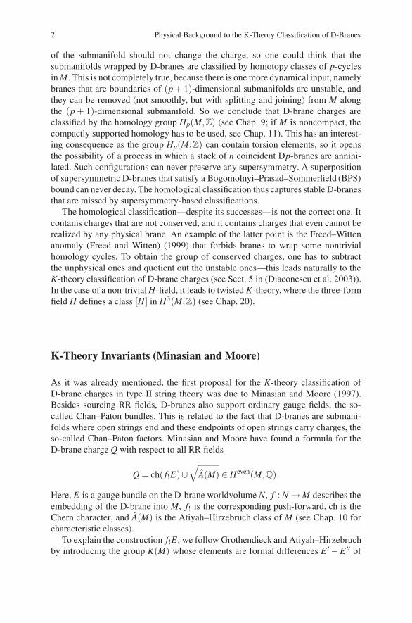
As it was already mentioned, the first proposal for the K-theory classification ofD-brane charges in type II string theory was due to Minasian and Moore (1997).Besides sourcing RR fields, D-branes also support ordinary gauge fields, the so-called Chan–Paton bundles. This is related to the fact that D-branes are submani-folds where open strings end and these endpoints of open strings carry charges, theso-called Chan–Paton factors. Minasian and Moore have found a formula for theD-brane charge Q with respect to all RR fields
Q = ch( f!E)∪√
A(M) ∈ Heven(M,Q).
Here, E is a gauge bundle on the D-brane worldvolume N, f : N → M describes theembedding of the D-brane into M, f! is the corresponding push-forward, ch is theChern character, and A(M) is the Atiyah–Hirzebruch class of M (see Chap. 10 forcharacteristic classes).
To explain the construction f!E , we follow Grothendieck and Atiyah–Hirzebruchby introducing the group K(M) whose elements are formal differences E ′ −E ′′ of
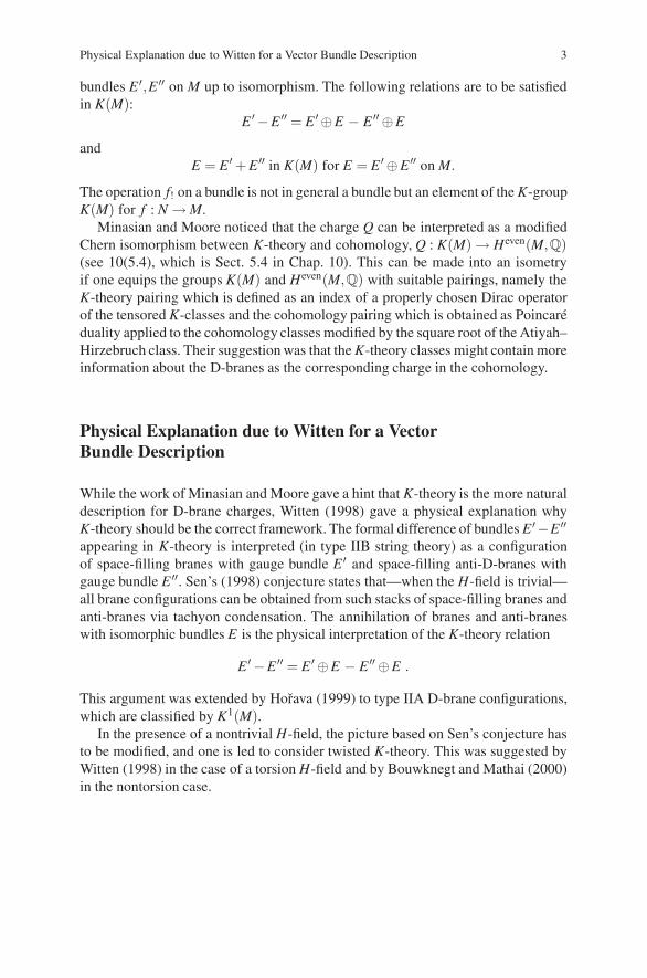
Physical Explanation due to Witten for a Vector Bundle Description 3
bundles E ′,E ′′ on M up to isomorphism. The following relations are to be satisfiedin K(M):
E ′ −E ′′ = E ′ ⊕E − E ′′ ⊕E
andE = E ′ + E ′′ in K(M) for E = E ′ ⊕E ′′ on M.
The operation f! on a bundle is not in general a bundle but an element of the K-groupK(M) for f : N → M.
Minasian and Moore noticed that the charge Q can be interpreted as a modifiedChern isomorphism between K-theory and cohomology, Q : K(M) → Heven(M,Q)(see 10(5.4), which is Sect. 5.4 in Chap. 10). This can be made into an isometryif one equips the groups K(M) and Heven(M,Q) with suitable pairings, namely theK-theory pairing which is defined as an index of a properly chosen Dirac operatorof the tensored K-classes and the cohomology pairing which is obtained as Poincareduality applied to the cohomology classes modified by the square root of the Atiyah–Hirzebruch class. Their suggestion was that the K-theory classes might contain moreinformation about the D-branes as the corresponding charge in the cohomology.
Physical Explanation due to Witten for a VectorBundle Description
While the work of Minasian and Moore gave a hint that K-theory is the more naturaldescription for D-brane charges, Witten (1998) gave a physical explanation whyK-theory should be the correct framework. The formal difference of bundles E ′−E ′′appearing in K-theory is interpreted (in type IIB string theory) as a configurationof space-filling branes with gauge bundle E ′ and space-filling anti-D-branes withgauge bundle E ′′. Sen’s (1998) conjecture states that—when the H-field is trivial—all brane configurations can be obtained from such stacks of space-filling branes andanti-branes via tachyon condensation. The annihilation of branes and anti-braneswith isomorphic bundles E is the physical interpretation of the K-theory relation
E ′ −E ′′ = E ′ ⊕E − E ′′ ⊕E .
This argument was extended by Horava (1999) to type IIA D-brane configurations,which are classified by K1(M).
In the presence of a nontrivial H-field, the picture based on Sen’s conjecture hasto be modified, and one is led to consider twisted K-theory. This was suggested byWitten (1998) in the case of a torsion H-field and by Bouwknegt and Mathai (2000)in the nontorsion case.
4 Physical Background to the K-Theory Classification of D-Branes
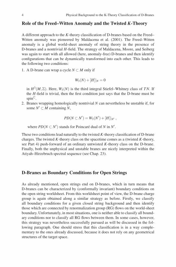
Role of the Freed–Witten Anomaly and the Twisted K-Theory
A different approach to the K-theory classification of D-branes based on the Freed–Witten anomaly was pioneered by Maldacena et al. (2001). The Freed–Wittenanomaly is a global world-sheet anomaly of string theory in the presence ofD-branes and a nontrivial H-field. The strategy of Maldacena, Moore, and Seibergwas again to start with all allowed (here, anomaly-free) D-branes and then identifyconfigurations that can be dynamically transformed into each other. This leads tothe following two conditions:
1. A D-brane can wrap a cycle N ⊂ M only if
W3(N)+ [H]|N = 0
in H3(M,Z). Here, W3(N) is the third integral Stiefel–Whitney class of T N. Ifthe H-field is trivial, then the first condition just says that the D-brane must bespinC.
2. Branes wrapping homologically nontrivial N can nevertheless be unstable if, forsome N′ ⊂ M containing N,
PD(N ⊂ N′) = W3(N′)+ [H]|N′ ,
where PD(N ⊂ N′) stands for Poincare dual of N in N′.
These two conditions lead naturally to the twisted K-theory classification of D-branecharges. The twisted K-theory class on the spacetime comes as a (twisted K-theory,see Part 4) push-forward of an ordinary untwisted K-theory class on the D-brane.Finally, both the unphysical and unstable branes are nicely interpreted within theAtiyah–Hirzebruch spectral sequence (see Chap. 23).
D-Branes as Boundary Conditions for Open Strings
As already mentioned, open strings end on D-branes, which in turn means thatD-branes can be characterized by (conformally invariant) boundary conditions onthe open string worldsheet. From this worldsheet point of view, the D-brane chargegroup is again obtained along a similar strategy as before. Firstly, we classifyall boundary conditions for a given closed string background and then identifythose which are connected by renormalization group (RG) flows on the world-sheetboundary. Unfortunately, in most situations, one is neither able to classify all bound-ary conditions nor to classify all RG flows between them. In some cases, however,this strategy was nevertheless successfully pursued as will be discussed in the fol-lowing paragraph. One should stress that this classification is in a way comple-mentary to the ones already discussed, because it does not rely on any geometricalstructures of the target space.
Suggested Reading 5
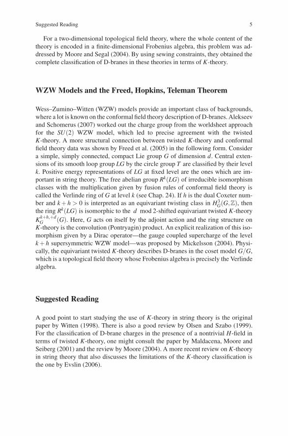
For a two-dimensional topological field theory, where the whole content of thetheory is encoded in a finite-dimensional Frobenius algebra, this problem was ad-dressed by Moore and Segal (2004). By using sewing constraints, they obtained thecomplete classification of D-branes in these theories in terms of K-theory.
WZW Models and the Freed, Hopkins, Teleman Theorem
Wess–Zumino–Witten (WZW) models provide an important class of backgrounds,where a lot is known on the conformal field theory description of D-branes. Alekseevand Schomerus (2007) worked out the charge group from the worldsheet approachfor the SU(2) WZW model, which led to precise agreement with the twistedK-theory. A more structural connection between twisted K-theory and conformalfield theory data was shown by Freed et al. (2005) in the following form. Considera simple, simply connected, compact Lie group G of dimension d. Central exten-sions of its smooth loop group LG by the circle group T are classified by their levelk. Positive energy representations of LG at fixed level are the ones which are im-portant in string theory. The free abelian group Rk(LG) of irreducible isomorphismclasses with the multiplication given by fusion rules of conformal field theory iscalled the Verlinde ring of G at level k (see Chap. 24). If h is the dual Coxeter num-ber and k + h > 0 is interpreted as an equivariant twisting class in H3
G(G,Z), thenthe ring Rk(LG) is isomorphic to the d mod 2-shifted equivariant twisted K-theoryKk+h,+d
G (G). Here, G acts on itself by the adjoint action and the ring structure onK-theory is the convolution (Pontryagin) product. An explicit realization of this iso-morphism given by a Dirac operator—the gauge coupled supercharge of the levelk + h supersymmetric WZW model—was proposed by Mickelsson (2004). Physi-cally, the equivariant twisted K-theory describes D-branes in the coset model G/G,which is a topological field theory whose Frobenius algebra is precisely the Verlindealgebra.
Suggested Reading
A good point to start studying the use of K-theory in string theory is the originalpaper by Witten (1998). There is also a good review by Olsen and Szabo (1999).For the classification of D-brane charges in the presence of a nontrivial H-field interms of twisted K-theory, one might consult the paper by Maldacena, Moore andSeiberg (2001) and the review by Moore (2004). A more recent review on K-theoryin string theory that also discusses the limitations of the K-theory classification isthe one by Evslin (2006).
6 Physical Background to the K-Theory Classification of D-Branes
References
Alekseev, A., Schomerus, V.: RR charges of D2-branes in the WZW model (arXiv:hep-th/0007096)Bouwknegt, P., Mathai, V.: D-branes, B-fields and twisted K-theory. JHEP 0003:007 (2000)
(arXiv:hep-th/0002023)Diaconescu, D.E., Moore, G.W., Witten, E.: E(8) gauge theory, and a derivation of K-theory from
M-theory. Adv. Theor. Math. Phys. 6:1031 (2003) (arXiv:hep-th/0005090)Evslin, J.: What does(n’t) K-theory classify? (arXiv:hep-th/0610328)Freed, D.S., Witten, E.: Anomalies in string theory with D-branes, Asian J. Math., Vol. 3, 4:819–
851 (1999) (arXiv:hep-th/9907189)Freed, D.S., Hopkins, M.J., Teleman, C.: Twisted K-theory and Loop Group Representations
(arXiv:math/0312155)Freed, D.S., Hopkins, M.J., Teleman, C.: Loop Groups and Twisted K-Theory II
(arXiv:math/0511232)Horava, P.: Type IIA D-branes, K-theory, and matrix theory. Adv. Theor. Math. Phys. 2:1373 (1999)
(arXiv:hep-th/9812135)Maldacena, J.M., Moore, G.W., Seiberg, N.: D-brane instantons and K-theory charges. JHEP
0111:062 (2001) (arXiv:hep-th/0108100)Mickelsson, J.: Gerbes, (twisted) K-theory, and the supersymmetric WZW model, Infinite dimen-
sional groups and manifolds, IRMA Lect. Math. Theor. Phys. Vol. 5, 93–107; de Gruyter; Berlin(2004) (arXiv:hep-th/0206139)
Minasian, R. and Moore, G.W.: K-theory and Ramond-Ramond charge. JHEP 9711:002 (1997)(arXiv:hep-th/9710230)
Moore, G.W., Segal, G.: D-branes and K-theory in 2D topological field theory (arXiv:hep-th/0609042)
Moore, G.W.: K-theory from a physical perspective; Topology, geometry and quantum field theory,London Math. Soc. Lecture Note Ser., Vol. 308, 194–234, Cambridge Univ. Press, Cambridge,(2004) (arXiv:hep-th/0304018)
Olsen, K., Szabo, R.J.: Constructing D-branes from K-theory. Adv. Theor. Math. Phys. 3:889(1999) (arXiv:hep-th/9907140)
Sen, A.: Tachyon condensation on the brane antibrane system. JHEP 9808:012 (1998) (arXiv:hep-th/9805170)
Witten, E.: D-branes and K-theory. JHEP 9812:019 (1998) (arXiv:hep-th/9810188)
Part IBundles over a Space and Modules
over an Algebra
In his notes, “A General Theory of Fibre Spaces with Structure Sheaf” publishedby Kansas University (1955 resp. 1958), Grothendieck found it useful for generalquestions to think of a map p : E → B as an object which he called a fibre space.The fibres Eb = p−1(b) are parametrized by elements b ∈ B and assembled in theset E =
⋃b∈B Eb in terms of the topology of E .
Since fibre space had already a precise meaning in the thesis of Serre, we fol-lowed the Grothendieck idea but changed the terminology to bundle as in FibreBundles. The term bundle fits with the idea that a bundle with additional structurewould be compatible with the usual terminology for such notions as vector bundle,principal bundle, and fibre bundle as explained in Chaps. 2 and 5.
Later Grothendieck extended the idea of associating to a category C , the categoryof morphisms or bundles p : E → B. The idea of the category of morphisms is foundin many contexts in mathematics. For example, a variety or scheme p : X → S over ascheme S is considered as a family of varieties or schemes Xs = p−1(s) parametrizedby s ∈ S.
In another direction, we can associate to a space X the C∗-algebra C(X) of allbounded continuous functions f : X →C with the uniform norm || f ||= supx∈X | f (x)|.In the case of a compact X , we can recover X from the algebra C(X) as the spaceof maximal ideals. This is the Gelfand–Naimark theorem. For compact B, we candescribe vector bundles over B as finitely generated projective modules over C(B).This is the Serre–Swan theorem which is proved in Chap. 3. In this same chapter, wego further and show how finitely generated projective modules M over a ring R andidempotents e = e2 in the matrix algebras Mn(R) are related. Isomorphism classesof projective modules correspond to algebraic equivalence classes of idempotents inall the possible matrix algebras.
In Chap. 4, we relate stable classes of vector bundles over X to stable classes offinitely generated projective C(X)-modules. Then, we relate stable classes of finitelygenerated projective R-modules to stable classes of idempotents e ∈ Mn(R) for alln. These are the three versions of K-theory discussed in the first part.
As preparation for the homotopy version of K-theory considered in Part II, weintroduce the basic properties of principal fibre bundles in Chap. 5. Every vectorbundle is the fibre bundle of a principal GL(n)-bundle, and frequently, the specialextra features of a vector bundle can be described in terms of the related principalbundle. Local triviality is considered, and the related notion of descent which playsa basic role in algebraic geometry is introduced for principal bundles. The principalbundle is also the natural domain for the study of the gauge group of a bundle.
Grothendieck, A.: A General Theory of Fibre Spaces with Structure Sheaf, University of Kansas,Lawrence (1955)
Grothendieck, A.: Le groupe de Brauer. Part I. Seminaire Bourbaki, Vol. 9, Exp. 290: 199–219University of Kansas, Lawrence, 1955
Chapter 1Generalities on Bundles and Categories
This is a preliminary chapter introducing much of the general terminology in thetopology of bundles with the general language of category theory. We use the termbundle in the most general context, and then in the next chapters, we define the mainconcepts of our study, that is, vector bundles, principal bundles, and fibre bundles,as bundles with additional structure.
In Grothendieck’s notes “A General Theory of Fibre Spaces with StructureSheaf,” University of Kansas, Lawrence, 1955 (resp. 1958) he mentions that “thefunctor aspect of the notions dealt with has been stressed through, and as it nowappears should have been stressed even more.”
Hopefully, we are carrying this out to the appropriate extent in this approach tobundles mixed with a general introduction to category theory where examples aredrawn from the theory of bundles. The reader with a background in category theoryand topology will see only a slightly different approach from the usual one.
We will introduce several notations used through the book, for example, (set),(top), (gr), and (k) denote, respectively, the categories of sets, spaces, groups, andk-modules for a commutative ring k. These are explained in the context of the defini-tion of a category in Sect. 4 and in the notations for categories at the end of the book.
Chap. 2 of Fibre Bundles (Husemoller 1994) is a reference for this chapter.
1 Bundles Over a Space
The following section, as mentioned in the introduction, is motivated byGrothendieck’s Kansas notes where we use the term “bundle” instead of “fibrespace.” A space is a topological space, and a map or mapping is a continuousfunction.
1.1. Definition Let B be a space. A bundle E over B is a map p : E → B. The spaceE is called the total space of the bundle, the space B is called the base space of thebundle, the map p is called the projection of the bundle, and for each b ∈ B, thesubspace p−1(b), denoted often by Eb, is called the fibre of the bundle over b ∈ B.
D. Husemoller et al.: Generalities on Bundles and Categories, Lect. Notes Phys. 726, 9–22 (2008)DOI 10.1007/978-3-540-74956-1 2 © Springer-Verlag Berlin Heidelberg 2008
10 1 Generalities on Bundles and Categories
1.2. Example The product bundle B×Y over B with fibre Y is the product spacewith the projection prB = p : B×Y → B. Observe that the fibre (B×Y )b = {b}×Ywhich is isomorphic to Y for all b∈B. Another general example comes by restrictinga bundle p : E →B to subspaces p|E ′ : E ′ →B′, where E ′ is a subspace of E and B′ isa subspace of B with the property that p(E ′)⊂ B′. Many bundles arise as restrictionsof a product bundle.
1.3. Definition A morphism from the bundle p : E → B to the bundle p′ : E ′ → Bover B is a map u : E → E ′ such that p′u = p.
This condition p′u = p is equivalent to the condition u(Eb) ⊂ E ′b for all b ∈ B,
that is, a morphism u is a map which is fibre preserving. The identity E → E isa morphism, and if u′ : E ′ → E ′′ is a second morphism of bundles over B, thenu′u : E → E ′′ is a morphism of bundles.
In Sect. 4, we give the formal definition of a category, but for now, we can speakof this data of bundles and morphisms of bundles with composition as a category. Itis the category (bun/B) of bundles over B.
In fact, we can relate bundles over distinct base spaces with morphisms general-izing (1.3).
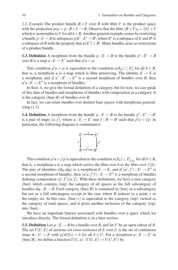
1.4. Definition A morphism from the bundle p : E → B to the bundle p′ : E ′ → B′is a pair of maps (u, f ), where u : E → E ′ and f : B → B′ such that p′u = f p. Inparticular, the following diagram is commutative
Eu ��
p
��
E ′
p′��
Bf �� B′ .
This condition p′u = f p is equivalent to the condition u(Eb)⊂E ′f (b) for all b∈B,
that is, a morphism u is a map which carries the fibre over b to the fibre over f (b).The pair of identities (idE ,idB) is a morphism E → E , and if (u′, f ′) : E ′ → E ′′ isa second morphism of bundles, then (u′u, f ′ f ) : E → E ′′ is a morphism of bundlesdefining composition (u′, f ′)(u, f ). With these definitions, we have a new category(bun) which contains (top) the category of all spaces as the full subcategory ofbundles idB : B → B. Each category (bun/B) is contained in (bun) as a subcategorybut not as a full subcategory except in the case where B reduces to a point ∗ orthe empty set. In this case, (bun/∗) is equivalent to the category (top) viewed asthe category of total spaces, and it gives another inclusion of the category (top)into (bun).
We have an important functor associated with bundles over a space which weintroduce directly. The formal definition is in a later section.
1.5. Definition Let p : E → B be a bundle over B, and let U be an open subset of B.The set Γ(U,E) of sections (or cross sections) of E over U is the set of continuousmaps σ : U → E with p(σ(b)) = b for all b ∈ U . For a morphism u : E → E ′ in(bun/B), we define a function Γ(U,u) : Γ(U,E) → Γ(U,E ′) by
1.2 Examples of Bundles 11
Γ(U,u)(σ) = uσ ∈ Γ(U,E ′)
for σ ∈ Γ(U,E).
The formal algebraic properties of the set of cross sections are explained in tworemarks (5.5) and (5.6).
1.6. Example Let p : E = B×Y → B be the product bundle with p(b,y) = b as in(1.2). A cross section σ over an open subset U ⊂ X is a map σ : U → E = B×Y ofthe form
σ(b) = (b, fσ (b))
for b ∈U. This means that Γ(U,E) is just equivalent to the set of maps fσ : U → Yto the fibre Y .
Now, we consider the special case of an induced bundle where the general con-cept is considered in Sect. 3.
1.7. Definition Let A be a subspace of a space B and let p : E → B be in (bun/B).Then, the restriction E|A is the restriction q = p|p−1(A) : p−1(A) → A in (bun/A)so that as a space E|A = p−1(A). For a morphism u : E → E ′, the morphism u|A :E|A → E ′|A is the subspace restriction.
For a pair of subspaces C ⊂ A ⊂ B, we have E|C = (E|A)|C, and the restrictionis a functor (bun/B) → (bun/A) as will be further discussed in Sect. 5. With therestriction, we can introduce an important concept.
1.8. Definition A bundle p : E → B is locally trivial with fibre Y provided eachb ∈ B has an open neighborhood U with E|U isomorphic to the product bundlepr1 : U ×Y →U . A bundle p : E → B is trivial with fibre Y provided it is isomorphicto the product bundle pr1 : B×Y → B.
2 Examples of Bundles
Many examples come under the following construction which consists of an arbi-trary base space and finite dimensional vector spaces in the fibre. In general, thedefinitions and examples extend to the case of an infinite dimensional vector spacewith a given topology as a fibre, for example, an infinite dimensional Hilbert space.See Chaps. 20–22.
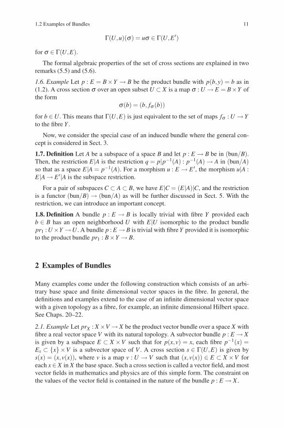
2.1. Example Let prX : X ×V → X be the product vector bundle over a space X withfibre a real vector space V with its natural topology. A subvector bundle p : E → Xis given by a subspace E ⊂ X ×V such that for p(x,v) = x, each fibre p−1(x) =Ex ⊂ {x}×V is a subvector space of V . A cross section s ∈ Γ(U,E) is given bys(x) = (x,v(x)), where v is a map v : U → V such that (x,v(x)) ∈ E ⊂ X ×V foreach x∈ X in X the base space. Such a cross section is called a vector field, and mostvector fields in mathematics and physics are of this simple form. The constraint onthe values of the vector field is contained in the nature of the bundle p : E → X .
12 1 Generalities on Bundles and Categories
For the next example, we use the inner product
(x|y) = x0y0 + . . .+ xnyn
for x,y ∈ Rn+1 in Euclidean space.
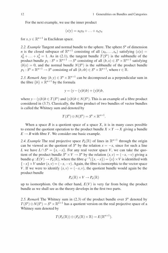
2.2. Example Tangent and normal bundle to the sphere. The sphere Sn of dimensionn is the closed subspace of R
n+1 consisting of all (x0, . . . ,xn) satisfying (x|x) =x2
0 + . . . + x2n = 1. As in (2.1), the tangent bundle T (Sn) is the subbundle of the
product bundle p1 : Sn ×Rn+1 → Sn consisting of all (b,x) ∈ Sn ×R
n+1 satisfying(b|x) = 0, and the normal bundle N(Sn) is the subbundle of the product bundlep1 : Sn ×R
n+1 → Sn consisting of all (b,tb) ∈ Sn ×Rn+1, where t ∈ R.
2.3. Remark Any (b,y) ∈ Sn ×Rn+1 can be decomposed as a perpendicular sum in
the fibre {b}×Rn+1 by the formula
y = (y− (y|b)b)+ (y|b)b,
where y− (y|b)b ∈ T (Sn) and (y|b)b ∈ N(Sn). This is an example of a fibre productconsidered in (3.7). Classically, the fibre product of two bundles of vector bundlesis called the Whitney sum and denoted by
T (Sn)⊕N(Sn) = Sn ×Rn+1.
When a space B is a quotient space of a space X , it is in many cases possibleto extend the quotient operation to the product bundle X ×Y → X giving a bundleE → B with fibre Y . We consider one basic example.
2.4. Example The real projective space Pn(R) of lines in Rn+1 through the origin
can be viewed as the quotient of Sn by the relation x = −x, since for such a lineL we have L ∩ Sn = {x,−x}. For any real vector space V , we can take the quo-tient of the product bundle Sn ×V → Sn by the relation (x,v) = (−x,−v) giving abundle q : E(V ) → Pn(R), where the fibre q−1({x,−x}) = {x}×V is identified with{−x}×V under (x,v) = (−x,−v). Again, the fibre is isomorphic to the vector spaceV . If we were to identify (x,v) = (−x,v), the quotient bundle would again be theproduct bundle
Pn(R)×V → Pn(R)
up to isomorphism. On the other hand, E(V ) is very far from being the productbundle as we shall see as the theory develops in the first two parts.
2.5. Remark The Whitney sum in (2.3) of the product bundle over Sn denoted byT (Sn)⊕N(Sn) = Sn ×R
n+1 has a quotient version on the real projective space of aWhitney sum denoted by
T (Pn(R))⊕ (Pn(R)×R) = E(Rn+1).
1.3 Two Operations on Bundles 13
Here, T (Pn(R)) is the tangent bundle to the real projective space Pn(R), and therelation (b,y) = (−b,−y) becomes under the sum
y = (y− (y|b)b)+ (y|b)b
the relation
(b,y− (y|b)b)⊕ (b,(y|b)b)= (−b,−(y− (y|−b)(−b))⊕ (−b,(y|b)(−b))
The second term is a product since (b|y) = (−b|− y) is independent of the repre-sentative of {b,−b}.
2.6. Remark We have a natural double winding giving P1(R) = S1, the circle. Thespace S1 ×R is a band, and E(R) over S1 or the real projective line P1(R) is theMobius band.
3 Two Operations on Bundles
The first operation on bundles transfers a bundle from one space to another undera continuous map, but before doing the general case, let us introduce the followingdefinition.
3.1. Definition Let f : B′ →B be a continuous map, and let p : E →B be in (bun/B).Then the induced bundle f−1(E) is the subspace f−1(E) ⊂ B′ ×E consisting ofall (b′,x) ∈ B′ ×E such that f (b′) = p(x) together with the restriction of the firstprojection q : B′ ×E → B′ to the subspace f−1(E). For a morphism u : E → E ′ overB, the morphism f−1(u) : f−1(E) → f−1(E ′) is the map defined by f−1(u)(b′,x) =(b′,u(x)) for (b′,x) ∈ f−1(E).
We also use the notation f ∗(E) → B′ for the induced bundle f−1(E) → B′.
3.2. Remark The bundles f−1(E) → B and the bundle morphisms f−1(u) define afunctor from the category (bun/B) to the category (bun/B′) in the sense that for theidentity idE , the induced map f−1(idE) is the identity on f−1(E) and for a compositeof two bundle morphisms u : E → E ′ and u′ : E ′ → E ′′, we have a composition oftwo bundle morphisms f−1(u′u) = f−1(u′) f−1(u).
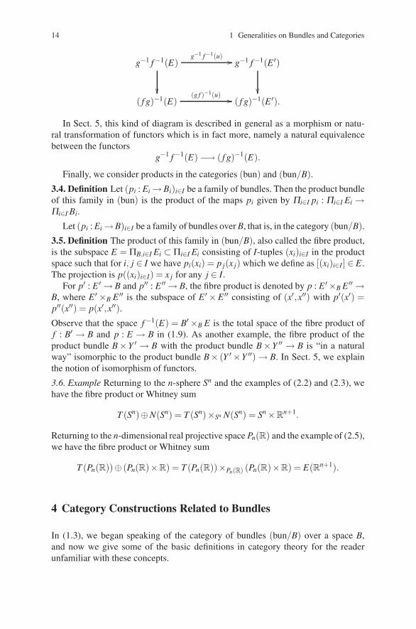
3.3. Remark For two continuous maps g : B′′ → B′ and f : B′ → B and for a bun-dle p : E → B in (bun/B), we have a natural isomorphism given by a projectiong−1 f−1(E) → ( f g)−1(E) which carries (b′′,(b′,x)) to (b′′,x). Since b′ = g(b′′) isdetermined by b′′, this projection is an isomorphism under which for a morphismu : E → E ′ we have a commutative diagram as in (1.7)
14 1 Generalities on Bundles and Categories
g−1 f−1(E)
��
g−1 f−1(u) �� g−1 f−1(E ′)
��( f g)−1(E)
(g f )−1(u) �� ( f g)−1(E ′).
In Sect. 5, this kind of diagram is described in general as a morphism or natu-ral transformation of functors which is in fact more, namely a natural equivalencebetween the functors
g−1 f−1(E) −→ ( f g)−1(E).
Finally, we consider products in the categories (bun) and (bun/B).
3.4. Definition Let (pi : Ei → Bi)i∈I be a family of bundles. Then the product bundleof this family in (bun) is the product of the maps pi given by Πi∈I pi : Πi∈I Ei →Πi∈I Bi.
Let (pi : Ei →B)i∈I be a family of bundles over B, that is, in the category (bun/B).
3.5. Definition The product of this family in (bun/B), also called the fibre product,is the subspace E = ΠB,i∈I Ei ⊂ Πi∈I Ei consisting of I-tuples (xi)i∈I in the productspace such that for i, j ∈ I we have pi(xi) = p j(x j) which we define as [(xi)i∈I ] ∈ E .The projection is p((xi)i∈I) = x j for any j ∈ I.
For p′ : E ′ → B and p′′ : E ′′ → B, the fibre product is denoted by p : E ′ ×B E ′′ →B, where E ′ ×B E ′′ is the subspace of E ′ ×E ′′ consisting of (x′,x′′) with p′(x′) =p′′(x′′) = p(x′,x′′).Observe that the space f−1(E) = B′ ×B E is the total space of the fibre product off : B′ → B and p : E → B in (1.9). As another example, the fibre product of theproduct bundle B×Y ′ → B with the product bundle B×Y ′′ → B is “in a naturalway” isomorphic to the product bundle B× (Y ′ ×Y ′′) → B. In Sect. 5, we explainthe notion of isomorphism of functors.
3.6. Example Returning to the n-sphere Sn and the examples of (2.2) and (2.3), wehave the fibre product or Whitney sum
T (Sn)⊕N(Sn) = T (Sn)×Sn N(Sn) = Sn ×Rn+1.
Returning to the n-dimensional real projective space Pn(R) and the example of (2.5),we have the fibre product or Whitney sum
T (Pn(R))⊕ (Pn(R)×R) = T (Pn(R))×Pn(R) (Pn(R)×R) = E(Rn+1).
4 Category Constructions Related to Bundles
In (1.3), we began speaking of the category of bundles (bun/B) over a space B,and now we give some of the basic definitions in category theory for the readerunfamiliar with these concepts.
1.4 Category Constructions Related to Bundles 15
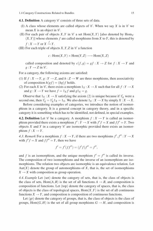
4.1. Definition A category C consists of three sets of data.
(I) A class whose elements are called objects of C . When we say X is in C wemean X is an object in C .
(II) For each pair of objects X ,Y in C a set Hom(X ,Y ) [also denoted by HomC
(X ,Y )] whose elements f are called morphisms from X to Y , this is denoted by
f : X → Y or Xf→ Y .
(III) For each triple of objects X ,Y,Z in C a function
c : Hom(X ,Y )×Hom(Y,Z) −→ Hom(X ,Z)
called composition and denoted by c( f ,g) = g f : X → Z for f : X → Y andg : Y → Z in C .
For a category, the following axioms are satisfied:
(1) If f : X → Y, g : Y → Z, and h : Z →W are three morphisms, then associativityof composition h(g f ) = (hg) f holds.
(2) For each X in C , there exists a morphism 1X : X → X such that for all f : Y → Xand g : X → Y we have f = 1X f and g1X = g.
Observe that 1X : X → X satisfying the axiom (2) is unique because if 1′X were asecond one, then 1′X = 1′X 1X = 1X . We also denote 1X : X → X by simply X : X → X .
Before considering examples of categories, we introduce the notion of isomor-phism in a category. It is a general concept in category theory, and in a specificcategory it is something which has to be identified, not defined, in special examples.
4.2. Definition Let C be a category. A morphism f : X → Y is called an isomor-phism provided there exists a morphism f ′ : Y → X with f ′ f = X and f f ′ = Y . Twoobjects X and Y in a category C are isomorphic provided there exists an isomor-phism f : X → Y .
4.3. Remark For a morphism f : X → Y , if there are two morphisms f ′, f ′′ : Y → Xwith f ′ f = X and f f ′′ = Y , then we have
f ′ = f ′( f f ′′) = ( f ′ f ) f ′′ = f ′′,
and f is an isomorphism, and the unique morphism f ′ = f ′′ is called its inverse.The composition of two isomorphisms and the inverse of an isomorphism are iso-morphisms. The relation two objects are isomorphic is an equivalence relation. LetAut(X) denote the group of automorphisms of X , that is, the set of isomorphismsX → X with composition as group operation.
4.4. Example Let (set) denote the category of sets, that is, the class of objects isthe class of sets, Hom(A,B) is the set of all functions A → B, and composition iscomposition of functions. Let (top) denote the category of spaces, that is, the classof objects is the class of topological spaces, Hom(X ,Y ) is the set of all continuousfunctions X → Y , and composition is composition of continuous functions.
Let (gr) denote the category of groups, that is, the class of objects is the class ofgroups, Hom(G,H) is the set of all group morphisms G → H, and composition is
16 1 Generalities on Bundles and Categories
composition of group morphisms. For a commutative ring k with unit, we denote by(k) the category of k-modules, that is, the class of objects is the class of (unitary)k-modules, Hom(M,N) is the set of all k-linear functions M → N, and compositionis composition of k-linear functions.
4.5. Remark The isomorphisms in (set) are the bijective functions, the isomor-phisms in (top) are the bijective continuous maps whose inverse function iscontinuous, the isomorphisms in (gr) are the bijective group morphisms, and theisomorphisms in (k) for a commutative ring k are the bijective k-linear maps.
4.6. Definition A subcategory C ′ of a category C is a category where the objects ofC ′ form a subclass of the objects in C and whose morphism set HomC ′(X ′,Y ′) is asubset of HomC (X ′,Y ′) such that the composition function for C ′ is the restrictionof the composition function for C . A subcategory C ′ of a category C is called fullprovided HomC ′(X ′,Y ′) = HomC (X ′,Y ′) for X ′,Y ′ in C ′.
Observe that a full subcategory C ′ of a category C is determined by its subclassof objects. For the ring of integers Z, a Z-module is just an abelian group, and hencethe category of abelian groups (ab) = (Z) is a full subcategory of (gr) determinedby the groups satisfying the commutative law.
Using the previous section as a model, we are able to define bundles in any cate-gory C .
The category (bun) becomes the category Mor(C ) of morphisms in C , and thecategory (bun/B) becomes the category C /B of objects E over B, that is, morphismsp : E → B.
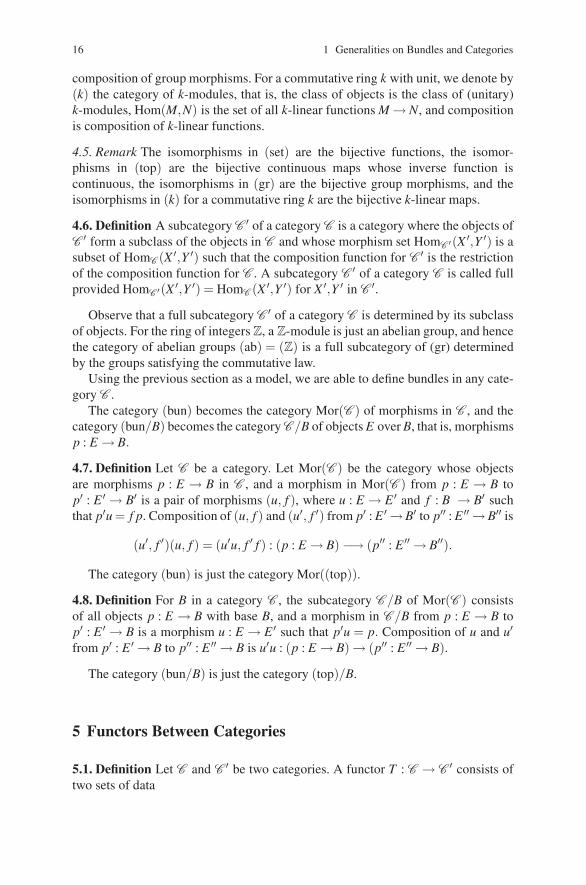
4.7. Definition Let C be a category. Let Mor(C ) be the category whose objectsare morphisms p : E → B in C , and a morphism in Mor(C ) from p : E → B top′ : E ′ → B′ is a pair of morphisms (u, f ), where u : E → E ′ and f : B → B′ suchthat p′u = f p. Composition of (u, f ) and (u′, f ′) from p′ : E ′ →B′ to p′′ : E ′′ →B′′ is
(u′, f ′)(u, f ) = (u′u, f ′ f ) : (p : E → B) −→ (p′′ : E ′′ → B′′).
The category (bun) is just the category Mor((top)).
4.8. Definition For B in a category C , the subcategory C /B of Mor(C ) consistsof all objects p : E → B with base B, and a morphism in C /B from p : E → B top′ : E ′ → B is a morphism u : E → E ′ such that p′u = p. Composition of u and u′from p′ : E ′ → B to p′′ : E ′′ → B is u′u : (p : E → B) → (p′′ : E ′′ → B).
The category (bun/B) is just the category (top)/B.
5 Functors Between Categories
5.1. Definition Let C and C ′ be two categories. A functor T : C → C ′ consists oftwo sets of data
1.5 Functors Between Categories 17
(I) A function T from the objects in C to the objects in C ′, hence the function typeof notation for a functor.
(II) For each pair of objects X ,Y in C we have a function T : HomC (X ,Y ) →HomC ′(T (X),T (Y )), that is, if u : X → Y is a morphism in C , then T (u) :T (X) → T (Y ) is a morphism in C ′.
For a functor, the following axioms are satisfied.
(1) If u : X → Y and v : Y → Z are two morphisms in C , then for the compositesT (vu) = T (v)T (u) : T (X) → T (Z) in C ′.
(2) For an object X in C , we have T (idX ) = idT (X) in C ′. In particular the notationX : X → X under T becomes T (X) : T (X) → T (X).
5.2. Proposition If F : C →C ′ is a functor and if u : X →Y is an isomorphism in Cwith inverse u−1 : Y → X, then T (u) : T (X) → T (Y ) is an isomorphism in C ′ withinverse
T (u)−1 = T (u−1) : T (Y ) −→ T (X).
Proof. This follows directly from the axioms for a functor.
5.3. Elementary Operations If F : C → C ′ and F ′ : C ′ → C ′′ are two functors,then the composite on objects and morphisms F ′F : C → C ′′ is a functor, for it isimmediate to check axioms (1) and (2). The identity functor idC : C → C is theidentity on objects and morphisms of C . If we think of categories as objects andfunctors as morphisms between categories, then we have the first idea about thecategory of categories. Unfortunately, the concept has to be modified, and this wedo in later chapters.
5.4. Examples The functor F : (top) → (set) which deletes the system of open setsof a space X leaving the underlying set is an elementary example. The functorsassigning to a bundle p : E → B the total space T (p : E → B) = E or the base spaceB(p : E → B) = B are defined as functors T : (bun/B)→ (top) or B : (bun)→ (top).
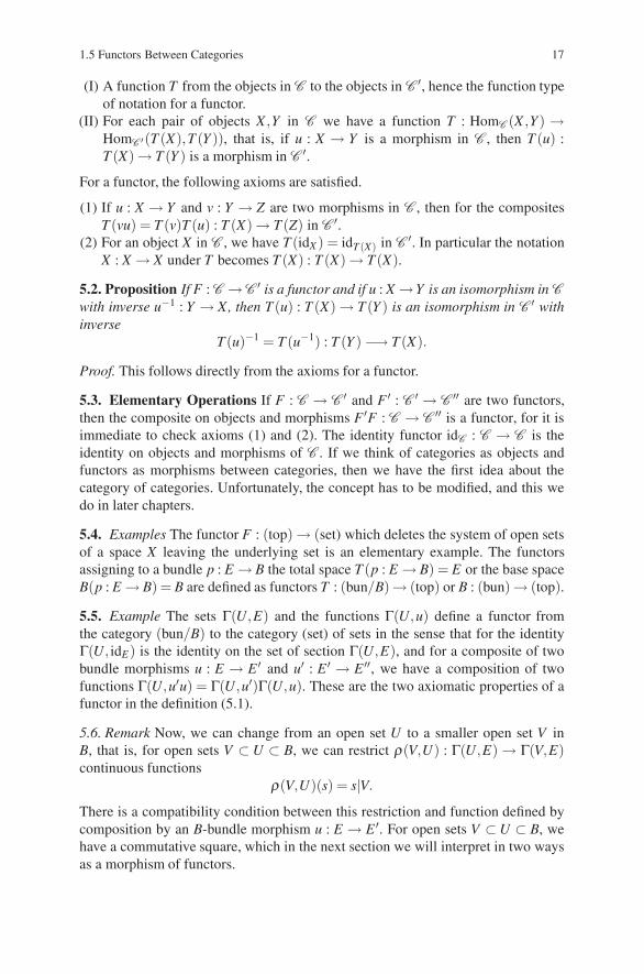
5.5. Example The sets Γ(U,E) and the functions Γ(U,u) define a functor fromthe category (bun/B) to the category (set) of sets in the sense that for the identityΓ(U, idE) is the identity on the set of section Γ(U,E), and for a composite of twobundle morphisms u : E → E ′ and u′ : E ′ → E ′′, we have a composition of twofunctions Γ(U,u′u) = Γ(U,u′)Γ(U,u). These are the two axiomatic properties of afunctor in the definition (5.1).
5.6. Remark Now, we can change from an open set U to a smaller open set V inB, that is, for open sets V ⊂ U ⊂ B, we can restrict ρ(V,U) : Γ(U,E) → Γ(V,E)continuous functions
ρ(V,U)(s) = s|V.
There is a compatibility condition between this restriction and function defined bycomposition by an B-bundle morphism u : E → E ′. For open sets V ⊂ U ⊂ B, wehave a commutative square, which in the next section we will interpret in two waysas a morphism of functors.
18 1 Generalities on Bundles and Categories
Γ(U,E)
ρ(V,U)��
Γ(U,u) �� Γ(U,E ′)
ρ(V,U)��
Γ(V,E)Γ(V,u) �� Γ(V,E ′)
Now, we formulate a definition where this kind of diagram is described in generalas a morphism or natural transformation of functors in the next section.
6 Morphisms of Functors or Natural Transformations
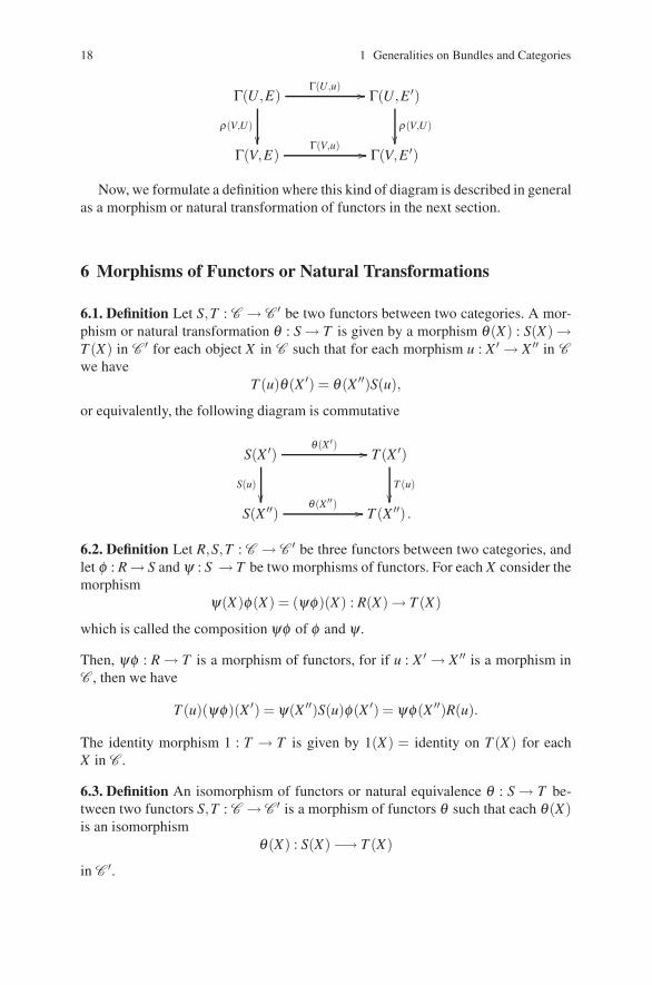
6.1. Definition Let S,T : C → C ′ be two functors between two categories. A mor-phism or natural transformation θ : S → T is given by a morphism θ (X) : S(X) →T (X) in C ′ for each object X in C such that for each morphism u : X ′ → X ′′ in Cwe have
T (u)θ (X ′) = θ (X ′′)S(u),
or equivalently, the following diagram is commutative
S(X ′)
S(u)��
θ(X ′) �� T (X ′)
T (u)��
S(X ′′)θ(X ′′) �� T (X ′′) .
6.2. Definition Let R,S,T : C → C ′ be three functors between two categories, andlet φ : R → S and ψ : S → T be two morphisms of functors. For each X consider themorphism
ψ(X)φ(X) = (ψφ)(X) : R(X) → T (X)
which is called the composition ψφ of φ and ψ .
Then, ψφ : R → T is a morphism of functors, for if u : X ′ → X ′′ is a morphism inC , then we have
T (u)(ψφ)(X ′) = ψ(X ′′)S(u)φ(X ′) = ψφ(X ′′)R(u).
The identity morphism 1 : T → T is given by 1(X) = identity on T (X) for eachX in C .
6.3. Definition An isomorphism of functors or natural equivalence θ : S → T be-tween two functors S,T : C → C ′ is a morphism of functors θ such that each θ (X)is an isomorphism
θ (X) : S(X) −→ T (X)
in C ′.
1.6 Morphisms of Functors 19
If θ (X)−1 is inverse of each θ (X), then the family of
θ (X)−1 : T (X) −→ S(X)
defines a morphism θ−1 : T → S of functors which is inverse to θ : S → T in thesense of the composition defined in (6.2).
6.4. Definition A functor T : C ′ → C ′′ is an equivalence of categories providedthere exists a functor S : C ′′ → C ′ such that the composite ST is isomorphic to idC ′ ,the identity functor on C ′, and T S is isomorphic to idC ′′ the identity functor on C ′′.
The composition of two equivalences of categories is again an equivalence ofcategories.
6.5. Definition Two categories C ′ and C ′′ are equivalent provided there exists anequivalence of categories C ′ → C ′′.
Observe that equivalence of categories is a weaker relation than isomorphism ofcategories. It almost never happens that two categories are isomorphic, but equiva-lent categories will have a bijection between isomorphism classes and related mor-phism sets. In fact, this is the way of recognizing that a functor is an equivalence bystarting with its mapping properties on the morphism sets.
6.6. Definition A functor T : X → Y is faithful (resp. fully faithful, full) pro-vided for every pair of objects X ,X ′ in X the function T : HomX (X ,X ′) →HomY (T (X),T (X ′)) is injective (resp. bijective, surjective).
The functors F : (top)→ (set) and F : (gr)→ (set) which assign to a topologicalspace or a group its underlying set are faithful functors. In the next proposition,we have a useful criterion for a functor to be an equivalence from one categoryto another. In Chap. 3, we apply this criterion to show that the category of vectorbundles on X is equivalent to the category of finitely generated projective C(X)-modules.
6.7. Proposition A functor T : X → Y is an equivalence of categories if and onlyif T is fully faithful and for each object Y in Y , there exists an object X in X withT (X) isomorphic to Y in Y .
Proof. If S : Y →X is an inverse up to isomorphisms with the identity functor, thenT : HomX (X ,X ′)→ HomY (T (X),T (X ′)) is a bijection with inverse constructed bycomposing
S : HomY (T (X),T (X ′)) → HomX (ST (X),ST (X ′))
with the isomorphism HomX (ST (X),ST (X ′)) → HomX (X ,X ′). Hence, T is fullyfaithful. Since for each Y in Y , the object Y in Y is isomorphic to T S(Y ), the secondcondition is satisfied for an equivalence of categories.
20 1 Generalities on Bundles and Categories
Conversely, we wish to construct S : Y → X by defining S on objects. For eachY , we choose an object S(Y ) = X in X together with an isomorphism θ (Y ) : Y →T (X) = T S(Y ). This is possible by the hypothesis, and we proceed to define
S : HomY (Y,Y ′) −→ HomX (S(Y ),S(Y ′))
as the composite of θ (Y ′,Y ) : HomY (Y,Y ′) → HomY (T S(Y ),T S(Y ′)) given byθ (Y ′,Y ) f = θ (Y ′) fθ (Y )−1 and the inverse of the bijection T defined as T−1 :HomY (T S(Y ),T S(Y ′))→HomX (S(Y ),S(Y ′)). The two properties of a functor fol-low for S from the observation that T is a functor and the following relations holdθ (Y ′′,Y )( f ′ f ) = θ (Y ′′,Y ′)( f ′)θ (Y ′,Y )( f ) and θ (Y,Y )(idY ) = idT S(Y ).
Finally, the morphisms θ (Y ) define an isomorphism θ : Y → TS(Y ) from theidentity on the category Y to T S, and ST was defined so that it is the identity onX . This proves the proposition.
7 Etale Maps and Coverings
7.1. Definition A map f : Y →X is open (resp. closed) provided for each open (resp.closed) subset V ⊂ Y , the direct image f (V ) is open (resp. closed) in X .
7.2. Example An inclusion map j : Y →X of a subspace Y ⊂ X is open (resp. closed)if and only if Y is an open (resp. closed) subspace of X . Any projection p j :Πi∈IXi →Xj from a product to a factor space is open. A projection pY : X ×Y → Y is closedfor all Y if and only if X is a quasicompact space.
7.3. Remark A space Y is separated (or Hausdorff) provided the following equiva-lent conditions are satisfied.
(1) For y,y′ ∈ Y with y = y′, there exists open neighborhoods V of y and V ′ of y′ inY with V ∩V ′ empty.
(2) The intersection of all closed neighborhoods V of any y ∈ Y is just {y}.(3) The diagonal map ΔY : Y → Y ×Y is a closed map.
This is a basic definition and assertion in general topology. Observe that condi-tion (3) can be formulated in terms of the diagonal subset Δ ⊂ Y ×Y being a closedsubset.
7.4. Remark Let f ,g : X → Y be two maps into a separated space. The set of allx ∈ X , where f (x) = g(x) is the closed subset ( f ,g)−1(Δ(Y )), where ( f ,g)(x) =( f (x),g(x)) defines the continuous map ( f ,g) : X → Y ×Y .
7.5. Definition A map f : Y → X is etale provided either of the following equivalentconditions are satisfied.
(1) For each y ∈ Y , there exists open neighborhoods V of y in Y and U of f (y) inX such that f (V ) = U and f |V : V →U is a homeomorphism. This condition isoften referred to as the map f is a local homeomorphism which is another termfor an etale map.
(2) The map f is open and the diagonal map ΔYY : Y → Y ×X Y is an open map.
1.7 Etale Maps and Coverings 21
A bundle p : E → X in (bun/X) is an etale (resp. open) bundle provided the map pis an etale (resp. open) map.
For the proof of the equivalence of (1) and (2), we assume firstly (1). Tosee that f is open, we consider an open subset W of Y and y ∈ W . There ex-ists open neighborhoods V of y in W and U of f (y) in X such that f (V ) = Uand f |V : V → U is a homeomorphism. Thus U , is an open neighborhood off (y) ∈ f (W ) contained in f (W ), and f is an open map. To see that the diagonalset Δ(Y ) is open in Y ×X Y , we consider (y,y) ∈ Δ(Y ). From the local homeomor-phism condition (1), there exists open neighborhoods V of y in Y and U of f (y)in X such that f (V ) = U and f |V : V → U is a homeomorphism. Then we haveV ×U V ⊂ Δ(Y ).
Conversely, we assume (2). Since Δ(Y ) is open in Y ×X Y , there exists an open setV ⊂ Y with (V ×V)∩ (Y ×Y ) ⊂ Y ×X Y . Then f (V ) = U is an open neighborhoodof f (y) in X and the open map f restricts to an open map f |V : V → U which is abijection since (V ×V)∩ (Y ×Y ) ⊂ Y×X Y. This establishes the equivalence of (1)and (2).
7.6. Notation The full subcategory of (bun/X) determined by the etale bundles overX is denoted by (et/X).
7.7. Proposition Let p : E → X be an etale (resp. open) bundle. For each mapf : Y → X, the induced bundle q : f−1(E) → Y is an etale (resp. open) bun-dle.
Proof. To show that q is open, we consider an open set W in f−1(E) and (y,x) ∈W ⊂ f−1(E). Then, there exists open sets V in Y and U in E such that (y,x) ∈(V ×U)∩ f−1(E) ⊂W. Then we have
y ∈ q((V ×U)∩ f−1(E)) ⊂V ∩ f−1(p(U)) ⊂ q(W ),
and this shows that q(W ) and hence also q is open.To show that q is a local homeomorphism if p is, we consider (y,x) ∈ f−1(E)
and an open neighborhood V of x ∈ E such that p|V : V → p(V ) is a homeomor-phism. Then we form the open set W = ( f−1(p(V ))×V)∩ f−1(E) in f−1(E) with(y,x) ∈ W . Observe that q|W : W → q(W ) is a homeomorphism. This proves theproposition.
7.8. Corollary If p : E → X is an etale (resp. open) bundle and if Y ⊂ X isa subspace of X, then p|p−1(Y ) : E|Y = p−1(Y ) → Y is an etale (resp. open)bundle.
7.9. Example Let D be a discrete space. Then the product bundle p = pX : X ×D →X is an etale bundle. This is called the product bundle with discrete fibre. In fact,for each z ∈ D, the restriction p|X ×{z} : X ×{z}→ X is a homeomorphism whenrestricted to the open set X ×{z} ⊂ X ×D.
Now, we are in position to define coverings in the mature context and describethe category of coverings as a full subcategory of the category of bundles.
22 1 Generalities on Bundles and Categories
7.10. Definition A covering p : E → X is an etale bundle which is locally isomor-phic to a product bundle with discrete fibre. A trivial covering p : E → X is a bundleisomorphic to a product bundle with discrete fibre D. We denote by (cov/X) the fullsubcategory of (et/X) and hence of (bun/X) determined by the coverings over X .
References
Grothendieck, A.: A General Theory of Fibre Spaces with Structure Sheaf. University of Kansas,Lawrence (1955) (2nd edition 1958)
Husemoller, D.: Fibre Bundles, 3rd ed. Springer-Verlag, New York (1994)
Chapter 2Vector Bundles
The notion of vector bundle is a basic extension to the geometric domain of thefundamental idea of a vector space. Given a space X , we take a real or complexfinite dimensional vector space V and make V the fibre of a bundle over X , whereeach fibre is isomorphic to this vector space. The simplest way to do this is to formthe product X ×V and the projection prX : X ×V → X onto the first factor. This isthe product vector bundle with base X and fibre V .
On first sight, the product bundle appears to have no special features, but it con-tains other vector bundles which often reflect the topology of X in a strong way. Thishappens, for example, for the tangent bundle and the normal bundle to the sphereswhich are discussed in 1(2.2) and 1(2.3). All bundles of vector spaces that we willconsider will have the local triviality property, namely, they are locally isomorphicto a product bundle. The product bundle is also basic because most of the vectorbundles we will be considering will be subvector bundles of a product vector bundleof higher dimension. In some cases, they will be so twisted that they can only livein an infinite dimensional product vector bundle.
We will begin by formulating the concept of bundles of vector spaces over X .These will not be necessarily locally trivial, but they form a well-defined conceptand category. Then, a vector bundle is a locally trivial bundle of vector spaces. Thepoint of this distinction is that being a vector bundle is a bundle of vector spaceswith an additional axiom and not an additional structure. The local charts whichresult are not new elements of structure but only a property, but to state the property,we need the notion of bundle of vector spaces. After this is done, we will be dealingwith just vector bundles.
Chapter 3 of Fibre Bundles (Husemoller 1994) is a reference for this chapter.
1 Bundles of Vector Spaces and Vector Bundles
All the vector spaces under consideration are defined either over the real numbersR or the complex numbers C. We need to use the scalars explicitly, and if eithernumber system applies, we will use the symbol F to denote either the field of realor the field of complex numbers.
D. Husemoller et al.: Vector Bundles, Lect. Notes Phys. 726, 23–34 (2008)DOI 10.1007/978-3-540-74956-1 3 © Springer-Verlag Berlin Heidelberg 2008
24 2 Vector Bundles
1.1. Definition A bundle of vector spaces over B is a bundle p : E → B with twoadditional structures
E ×B E −→ E and F ×E −→ E
defined over B called addition and scalar multiplication, respectively. As maps overB, they restrict to each fibre
Eb ×Eb = (E ×B E)b −→ Eb and F ×Eb = (F ×E)b −→ Eb,
and the basic axiom is that they define a vector space structure over F on each fibre.We require further that the function which assigns to each b ∈ B the unique zero0b ∈ Eb is a continuous section.
Although it is not so necessary, we will usually require that the fibres are finitedimensional, hence the subspace topology on the fibres will be the usual vectorspace topology. In the infinite dimensional case, the main difference is that one hasto preassign a topology on the vector space compatible with addition and scalarmultiplication. Bundles of infinite dimensional vector spaces are treated in moredetail in Chap. 20.
1.2. Example Let V be a finite dimensional F-vector space with the usual topology,and let p : B×V → B be the product bundle. Then, the usual vector space structureon V defines a bundle of vector space structure on the product bundle by
(b,v′)+ (b,v′′) = (b,v′ + v′′) and k(b,v) = (b,kv), for k ∈ F.
If p : E → B is a bundle of vector spaces and if A ⊂ B is a subspace, then therestriction q : E|A→A is a bundle of vector spaces with the restriction of the globallydefined addition and scalar multiplication. Now, this can be generalized as in 1(2.1)to subbundles of vector spaces.
1.3. Definition Let p : E ′ → B and p : E ′′ → B be two bundles of vector spaces overB. A morphism u : E ′ → E ′′ of bundles of vector spaces over B is a morphism ofbundles such that the restriction to each fibre u|E ′
b : E ′b → E ′′
b is a linear map.
1.4. Remark The composition of morphisms of bundles of vector spaces over Bis again a morphism of bundles of vector spaces over B. Hence, it defines acategory.
1.5. Example Let p : E → B be a bundle of vector spaces, and let A be a subspaceof B. Then, the restriction to a subspace p|(E|A) : E|A → A is a bundle of vectorspaces.
Now, we are in a position to make the main definition of this chapter.
1.6. Definition A vector bundle p : E → B is a bundle of vector spaces such thatevery point b∈ B has an open neighborhoodU with the restriction p|(E|U) : E|U →U isomorphic to the product bundle of vectors spaces pr1 : U ×V →U .
2.2 Isomorphisms of Vector Bundles and Induced Vector Bundles 25
Now, we will always be working with vector bundles and observe that the conceptof bundle of vector spaces was only introduced as a means of defining the localtriviality property of vector bundles. Of course, this could have been done moredirectly, but in this way, we try to illustrate the difference between structure andaxiom.
1.7. Definition A morphism u : E ′ → E ′′ of vector bundles over B is a morphism ofthe bundles of vector spaces from E ′ to E ′′.
1.8. Remark The composition of morphisms of vector bundles over B is again amorphism of vector bundles over B. Hence, it defines a category of vector bundlesover B. A trivial vector bundle is one which is isomorphic to a product vector bundle.
1.9. Example Let E ′ → B and E ′′ → B be two bundles of vector spaces over B. Thefibre product E ′ ×B E ′′, also denoted by E ′ ⊕E ′′, is a bundle of vector spaces. IfE ′ and E ′′ are vector bundles, then E ′ ⊕E ′′ is also a vector bundle. For the productbundles B×V ′ and B×V ′′, the fibre product or Whitney sum is given by (B×V ′)⊕(B×V ′′) = B× (V ′ ⊕V ′′). The terminology of Whitney sum comes from the directsum and the notation E ′ ⊕E ′′ from the direct sum of vector spaces.
1.10. Definition Let E ′,E ′′ and E be three vector bundles over X . A vector bundlemorphism β : E ′ ⊕E ′′ = E ′ ×X E ′′ → E is bilinear provided β |(E ′ ⊕E ′′)x : (E ′ ⊕E ′′)x → Ex is a bilinear map of vector spaces. The tensor product E ′ ⊗E ′′ of E ′ andE ′′ is a specific choice of a vector bundle with a bilinear morphism θ : E ′ ⊕E ′′ →E ′⊗E ′′ which has the universal property that every bilinear morphism β : E ′⊕E ′′ →E factors uniquely as uθ , where u : E ′ ⊗E ′′ → E is a morphism of vector bundles.Note that this is the usual definition of the tensor product for X a point.
2 Isomorphisms of Vector Bundles and Induced Vector Bundles
In the next result, we use the vector bundle local triviality axiom.
2.1. Proposition Let u : E ′ → E ′′ be a morphism of vector bundles over a space Bsuch that ub : E ′
b →E ′′b is an isomorphism for each b∈B. Then, u is an isomorphism.
Proof. The inverse v : E ′′ → E ′ of u exists fibrewise as a function. The only questionis its continuity, and this we check on an open covering of the form u : E ′|U →E ′′|U ,where E ′ and E ′′ are each trivial bundles. In this case, the restriction of u withinverse v has the form u : U × Fn → U × Fn with formula u(b,y) = (b,T (b)y),where T : U → GLn(F) is a continuous map. Then, v(b,z) = (b,T (b)−1(z)) is alsocontinuous. This proves the proposition.
2.2. Proposition Let p : E → B be a bundle of vector spaces over B, and let f : B′ →B be a continuous map. Then, the induced bundle f−1E → B′ has the structure of abundle of vector spaces such that the natural f -morphism w : f−1E → E over eachb′ ∈ B′ on the fibre
26 2 Vector Bundles
wb′ : ( f−1E)b′ −→ E f (b′)
is a vector space isomorphism. If E is a vector bundle, then f−1E is a vector bundle.
Proof. Recall that the induced bundle f−1E is a subspace of B′ ×E consisting of all(b′,x) with f (b′) = p(x). Then, we use f−1(E ×B E) = f−1(E)×B′ f−1(E), and thesum function on the bundle of vector spaces must be of the form (b′,x)+ (b′,y) =(b′,x+y). Then, scalar multiplication must be of the form a(b′,y) = (b′,ay). In bothcases, these functions are continuous, and moreover, on the fibre wb′ : ( f−1E)b′ →E f (b′) is a vector space isomorphism.
Finally, if E is a product bundle, then f−1E is a product bundle, and if E is locallytrivial, then f−1E is locally trivial, for it is trivial over open sets f−1(W ), where Eis trivial over W . This proves the proposition.
2.3. Proposition Let (u, f ) : (p′ : E ′ →B′)→ (p : E →B) be a morphism of bundles,where p′ and p are vector bundles such that over each b′ ∈ B′ on the fibre ub′ : E ′
b′ →E f (b′) is a morphism of vector spaces. Then, u factors by a morphism v : E ′ →f−1E of vector bundles over B′ followed by the natural f -morphism w : f−1E → E.Moreover, if over each b′ ∈ B′ on the fibre ub′ : E ′
b′ → E f (b′) is a isomorphism ofvector spaces, then v : E ′ → f−1E is an isomorphism of vector bundles over B′.
Proof. The factorization of u is given by v(x′) = (p′(x′),u(x′)), and it is a vectorbundle morphism since u is linear on each fibre. Moreover, wv(x′) = u(x′) showsthat it is a factorization. If ub′ is an isomorphism on the fibre of E ′ at b′, then
vb′(x′) = (b′,ub′(x′))
is an isomorphism E f (b′) → f−1(E)b′ = {b′}×E f (b′). Thus, we can apply (2.1) toobtain the last statement. This proves the proposition.
3 Image and Kernel of Vector Bundle Morphisms
3.1. Remark The vector bundle morphism w : [0,1]×F → [0,1]×F defined by theformula w(t,z) = (t,tz) has a fibrewise kernel and a fibrewise image, but neither isa vector subbundle because the local triviality condition is not satisfied at 0 ∈ [0,1],where the kernel jumps from zero and the image reduces to zero.
In order to study this phenomenon, we recall some elementary conditions on rankof matrices.
3.2. Notation Let Mq,n(F) denote the F-vector space of q×n matrices over F , thatis, q rows and n columns of scalars from F . For q = n, we abbreviate the notationMn,n(F)= Mn(F) and denote by GLn(F) the group of invertible n×n matrices undermatrix multiplication. We give these spaces as usual the natural Euclidean topology.We have Mq,n(C) = Mq,n(R) + Mq,n(R)i, and using blocks of matrices, we have
2.3 Image and Kernel of Vector Bundle Morphisms 27
the natural inclusion Mq,n(R)+ Mq,n(R)i ⊂ M2q,2n(R), where A + Bi is mapped to(A 00 B
)∈ M2q,2n(R).
3.3. Definition The rank filtration RkMq,n(F) on Mq,n(F) is the increasing filtrationof all A ∈ Mq,n(F) with rank (A) ≤ k. We denote by R=kMq,n(F) = RkMq,n(F)−Rk−1Mq,n(F).
Clearly, we have for the rank filtration
{0} = R0Mq,n(F) ⊂ . . . ⊂ RkMq,n(F) ⊂ . . . ⊂ Rmin{q,n}Mq,n(F) = Mq,n(F).
For square matrices, we have R=nMn(F) = GLn(F), the group of invertible n by nmatrices with coefficients in F .
3.4. Remark The sets RkMq,n(F) in the rank filtration are closed sets which for F =R or C can be described as consisting of all matrices A for which all (k+1)×(k+1)subdeterminants are zero. The group GLn(F) is the group of all square matrices Awith det(A) = 0. Since the determinant is a polynomial function, these subsets arealgebraic varieties. In particular, the terms of the filtration RkMq,n(F) are closedsubsets of Mq,n(F), and GLn(F) is an open subset of Mn(F). The same is true forF = H, and we will see that it depends on only knowing that GLn(H) is an opensubset of Mn(H) by the subdeterminant characterization of rank.
3.5. Proposition Let u : E ′ → E ′′ be a morphism of vector bundles over a space B.If rank (ub) is locally constant, then the bundles of vector spaces ker(u) and im(u)are vector bundles.
Proof. We form the subspace⋃
b∈B ker(ub) = ker(u) ⊂ E ′ and the subspace⋃
b∈Bim(ub) = im(u) ⊂ E ′′. With the restriction of the projections E ′ → B and E ′′ → B,the subbundles ker(u) and im(u) are bundles of vector spaces. In order to showthat they are vector bundles under the rank hypothesis, we can restrict to an openneighborhood U of any point of B, where both E ′ and E ′′ are trivial and ub hasconstant rank q.
Choose an isomorphism to the product bundle, and then u can be representedby a vector bundle morphism w : U ×Fn → U ×Fm which has the form w(b,y) =(b,T (b)y). As a continuous function T : U → Mm,n , the matrix T (b) has rank qover U . For each x ∈ U , we can choose a change of coordinates so that T (b) =(
A(b) B(b)C(b) D(b)
)such that
A(x) ∈ GLq(F), B(x) = 0, C(x) = 0, D(x) = 0,
and choosing a subopen neighborhood of x in U , called again U , we can assumethat A(b) is invertible for all b ∈U . Here, we use that GLq(F)⊂ Mq(F) is open. Letπ : U ×Fn →U ×Fn−q denote the projection on the second factor, and note that forx ∈ U , it is the projection onto the ker(T (x)). Since T (b) has constant rank q and
28 2 Vector Bundles
A(b) is invertible, the restriction π |ker(w) = π |U × ker(T (b)) is an isomorphismU ×ker(T (b)) → U ×Fn−q. Hence, we see that ker(w) is locally trivial and thus avector bundle.
If wt : U ×Fm → U ×Fn is the morphism given by the transpose matrix T (b)t
and the formula wt(b,y) = (b,T (b)t y), then im(w) = ker(wt ) is also a vector bundle.This proves the proposition.
A very useful case where we know the rank is locally constant and used in thenext chapter is in the following proposition.
3.6. Proposition Let e = e2 : E → E be an idempotent endomorphism of a vectorbundle p : E → B over B. Then, the set of b ∈ B with rank(eb) = q is open andclosed in B. Hence, ker(e) and im(e) are vector bundles, and E = ker(e)×B im(e) =ker(e)⊕ im(e).
Proof. Since on each fibre the identity 1 = eb +(1− eb) is the sum of two comple-mentary projections, we have rank (eb)+rank(1− eb) = n. The set of all b ∈ B withrank(eb) = q is at the same time the set of all b ∈ B with rank (eb) ≤ q and rank(1− eb) ≤ n− q, which is a closed set, and the set of all b ∈ B with rank(eb) ≥ qand rank(1− eb) ≥ n− q, which is an open set. Now apply (3.5). This proves theproposition.
4 The Canonical Bundle Over the Grassmannian Varieties
4.1. Definition Let X be a union of an increasing family of subspaces
X0 ⊂ . . . ⊂ XN ⊂ XN+1 ⊂ . . . ⊂ lim−→N XN = X
with the weak topology, that is a subset M ⊂ X is closed if and only if Xm ∩M isclosed in Xm for all m ≥ 0.
Another name for the weak topology is the inductive limit topology.
The following inductive limits have the weak topology which start with the inclu-sions
FN ⊂ FN+1 ⊂ . . . ⊂ lim−→N FN = F∞.
4.2. Definition Let Pn(FN) denote the subspace of (FN)n consisting of linearly inde-pendent n-tuples of vectors in FN . Let Grn(FN) denote the quotient space of Pn(FN)which assigns to a linearly independent n-tuple the subspace FN of dimension n ofwhich the n-tuple is basis. The space Grn(FN) is called the Grassmann variety ofn-dimensional subspaces of FN , and Pn(FN) is called the Stiefel variety of linearlyindependent frames in N-dimensional space.
4.3. Remark The quotient morphism q : Pn(FN) → Grn(FN) has the structure of aprincipal GLn(F) bundle with right action Pn(FN)×GLn(F) → Pn(FN) given byright multiplication of an n-tuple of vectors and by n×n matrix of scalars
2.5 Finitely Generated Vector Bundles 29
(x1, . . . .,xn).(ai, j) = (y1, . . . ,yn),
where ∑ni=1xiai, j = y j for i, j = 1, . . . ,n. The subject of principal bundles is taken up
in Chap. 5 and we will return to this example.
There are natural inclusions
Pn(FN) ⊂ Pn(FN+1) and Grn(FN) ⊂ Grn(FN+1)
induced by the inclusion of FN ⊂ FN+1 = FN ⊕F as zero in the last coordinate.
4.4. Definition The product bundle Grn(FN) × FN has two subvector bundles:En(N) consisting of all (W,v) ∈ Grn(FN)×FN with v ∈W and ⊥EN−n(N) consist-ing of all (W,v) ∈ Grn(FN)×FN with v ⊥W , that is, v is orthogonal to all vectorsin W . The vector bundle En(N) is called the universal vector bundle over Grn(FN).
4.5. Remark If pW denotes the orthogonal projection of FN onto W , then wehave an isomorphism θ : Grn(FN)×FN → En(N)⊕ ⊥EN−n(N) onto the Whitneysum, where θ (W,v) = (W, pW (v)) ⊕ (W,v − pW (v)). Over the natural inclusionGrn(FN) ⊂ Grn(FN+1), there is the natural inclusion of product vector bundlesGrn(FN)×FN ⊂ Grn(FN+1)×FN+1 which under θ induces natural inclusions ofthe Whitney sum factors En(N) ⊂ En(N + 1) and ⊥EN−n(N) ⊂ ⊥EN+1−n(N + 1).
Now, we consider the inductive limit spaces and vector bundles as N goes toinfinity.
4.6. Remark The inductive limit construction of (4.1) yields the n-dimensional vec-tor bundle
En = lim−→ N≥nEn(N) −→ lim−→N≥n Grn(FN) = Grn(F∞).
This vector bundle has the universal property saying that every reasonable vectorbundle is induced from it and under certain circumstances, from the subbundles onthe finite Grassmann varieties as we see in the next section.
5 Finitely Generated Vector Bundles
5.1. Theorem The following six properties of a vector bundle E over X of dimensionn and given N ≥ n are equivalent:
(1) There is a continuous w : E → FN with w|Ex : Ex → FN a linear monomorphismfor each x ∈ X.
(2) There is a vector bundle morphism (u, f ) : E → En(N) which is an isomorphismon each fibre of E.
(3) There is an isomorphism E → f ∗(En(N)) over X for some continuous map f :X → Grn(FN).
30 2 Vector Bundles
(4) There is a vector bundle E ′ over X and an isomorphism φ : E⊕E ′ → X ×FN tothe trivial N-dimensional bundle over X.
(5) There exists a surjective vector bundle morphism ψ : X × FN → E which issurjective on each fibre.
(6) There exist continuous sections s1, . . . ,sN ∈ Γ(X ,E) such that the vectors s1(x),. . . ,sN(x) generate the vector space Ex for each x ∈ X.
Proof. We begin with a circle of implications.
(1) implies (2): Given w : E → FNas in (1), we define the morphism of vector bun-dles (u, f ) : E → En(N) by f (x) = w(Ex) and u(v) = (Eπ(v),w(v)) ∈ En(N) forv ∈ E and π : E → X the projection.
(2) implies (3): Given (u, f ) as in (2), we factor u by the induced bundle Eu′→
f ∗(En(N)) u′′→ En(N), where u′ : E → f ∗(En(N)) is a fibrewise isomorphism,hence the desired isomorphism in (3).
(3) implies (4): Given the isomorphism E → f ∗(En(N)) as in (3), we defineE ′ = f ∗(⊥EN−n(N)) and take the Whitney sum leading to an isomorphism E ⊕E ′ → f ∗(En(N))⊕ f ∗(⊥EN−n(N)) = f ∗(En(N)⊕⊥ EN−n(N)). Since En(N)⊕⊥EN−n(N) = Grn(FN)×FN , the product bundle, and a map induces the productbundle to a trivial bundle, we have an isomorphism E ⊕E ′ → X ×FNas in (4).
(4) implies (1): Given an isomorphism v : E ⊕ E ′ → X × FN over X . Using theinjection j : E → E ⊕E ′ and the projection pr2 : X ×FN → FN , we form thecomposite w = (pr2)v j : E → FN , and this is the desired map in (1), where therestriction w|Ex : Ex → FN is a linear monomorphism for each x ∈ X .
(4) implies (5): We use the inverse X × FN → E ⊕ E ′ to the isomorphism in (4)composed with the projection E ⊕E ′ → E to obtain a vector bundle morphismv : X ×FN → E which is surjective on each fibre.Conversely, (5) implies (4) by considering the kernel E ′ = ker(ψ) of ψ which isa subvector bundle of rank N−n and its orthogonal complement E ′′ which is thesubvector bundle of all (x,v) with v ⊥ ker(ψ)x. The restriction ψ |E ′′ : E ′′ → Eis a fibrewise isomorphism and hence an isomorphism of vector bundles. Thedesired morphism is the sum of φ = (ψ |E ′′)−1 ⊕ j : E ⊕ ker(ψ) = E ⊕E ′ →X ×FN in (4).
(5) and (6) are equivalent. For the natural basic sections σi(x) = (x,ei) of the trivialbundle X ×FN have images si = ψσi given by ψ with (5) for each i = 1, . . . ,Nand conversely ψ is defined by a set of N sections si in (6) by the conditionψ(x,a1, . . . ,aN) = a1s1(x)+ · · ·+ aNsN(x). Finally, the equivalence of (5) and(6) follows by observing that ψ(x, ) is surjective over x ∈ X if and only ifs1(x), . . . ,sN(x) generates Ex. This proves the theorem.
5.2. Definition A vector bundle satisfying any of the equivalent conditions of (5.1)is called finitely generated.
For N = n, we have the following corollary.
5.3. Corollary The following six properties of a vector bundle E over X of dimen-sion n are equivalent:
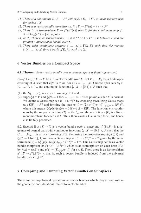
2.7 Collapsing and Clutching Vector Bundles 31
(1) There is a continuous w : E → Fn with w|Ex : Ex → Fn, a linear isomorphismfor each x ∈ X.
(2) There is a vector bundle morphism (u, f ) : E → En(n) = {∗}×Fn.(3) There is an isomorphism E → f ∗(En(n)) over X for the continuous map f :
X → Grn(Fn) = {∗}, a point.(4) or (5) There is an isomorphism E → X ×Fn or X ×Fn → E between E and the
product n-dimensional bundle over X.(6) There exist continuous sections s1, . . . ,sn ∈ Γ(X ,E) such that the vectors
s1(x), . . . ,sn(x) form a basis of Ex for each x ∈ X.
6 Vector Bundles on a Compact Space
6.1. Theorem Every vector bundle over a compact space is finitely generated.
Proof. Let p : E → X be a F-vector bundle over X . Let V1, . . . ,Vm be a finite opencovering of X such that E|Vi is trivial for all i = 1, . . . ,m. Choose open sets U1 ⊂V1, . . . ,Um ⊂Vm and continuous functions ξi : X → [0,1] ⊂ F such that
(1) the U1, . . . ,Um is an open covering of X and(2) supp(ξi) ⊂Vi and ξi|Ui = 1 for i = 1, . . . ,m. This is possible since X is normal.
We define a Gauss map w : E → (Fn)m by choosing trivializing Gauss mapswi : E|Vi → Fn and forming the map w(v) = (ξi(p(v))wi(v))1≤i≤m ∈ (Fn)m,where this means ξi(p(v))wi(v) = 0 if v ∈ E −E|Vi. The function w is contin-uous by the support condition (2) on the ξi, and the restriction w|Ex is a linearmonomorphism for each x ∈X . Thus, there exists a Gauss map for E , and henceE is finitely generated.
6.2. Remark If p : E → X is a vector bundle over a space and if (Ui,Vi) is a se-quence of normal pairs with continuous functions ξi : X → [0,1] ⊂ F such that theU1, . . . ,Um, . . . is an open covering of X , then using the properties supp(ξi)⊂Vi andξi|Ui = 1 for i ≥ 1, we have a Gauss map w : E → (Fn)∞ = F∞ given by the sameformula w(v) = (ξi(p(v))wi(v))1≤i ∈ (Fn)∞ = F∞. This Gauss map defines a vectorbundle morphism (u, f ) : E → En(∞) which is an isomorphism on each fibre of Eby f (x) = w(Ex) and u(v) = (Ep(v),w(v)) for v ∈ E . Then, there is an isomorphismu′ : E → f ∗(En(∞)), that is, such a vector bundle is induced from the universalbundle over Grn(F∞).
7 Collapsing and Clutching Vector Bundles on Subspaces
There are two topological operations on vector bundles which play a basic role inthe geometric considerations related to vector bundles.
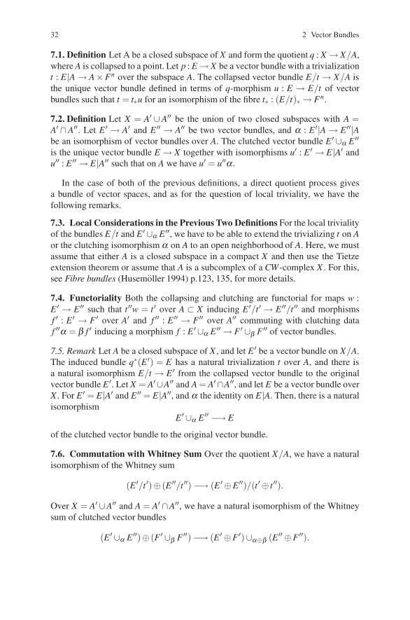
32 2 Vector Bundles
7.1. Definition Let A be a closed subspace of X and form the quotient q : X → X/A,where A is collapsed to a point. Let p : E →X be a vector bundle with a trivializationt : E|A → A×Fn over the subspace A. The collapsed vector bundle E/t → X/A isthe unique vector bundle defined in terms of q-morphism u : E → E/t of vectorbundles such that t = t∗u for an isomorphism of the fibre t∗ : (E/t)∗ → Fn.
7.2. Definition Let X = A′ ∪ A′′ be the union of two closed subspaces with A =A′ ∩A′′. Let E ′ → A′ and E ′′ → A′′ be two vector bundles, and α : E ′|A → E ′′|Abe an isomorphism of vector bundles over A. The clutched vector bundle E ′ ∪α E ′′is the unique vector bundle E → X together with isomorphisms u′ : E ′ → E|A′ andu′′ : E ′′ → E|A′′ such that on A we have u′ = u′′α .
In the case of both of the previous definitions, a direct quotient process givesa bundle of vector spaces, and as for the question of local triviality, we have thefollowing remarks.
7.3. Local Considerations in the Previous Two Definitions For the local trivialityof the bundles E/t and E ′ ∪α E ′′, we have to be able to extend the trivializing t on Aor the clutching isomorphism α on A to an open neighborhood of A. Here, we mustassume that either A is a closed subspace in a compact X and then use the Tietzeextension theorem or assume that A is a subcomplex of a CW -complex X . For this,see Fibre bundles (Husemoller 1994) p.123, 135, for more details.
7.4. Functoriality Both the collapsing and clutching are functorial for maps w :E ′ → E ′′ such that t ′′w = t ′ over A ⊂ X inducing E ′/t ′ → E ′′/t ′′ and morphismsf ′ : E ′ → F ′ over A′ and f ′′ : E ′′ → F ′′ over A′′ commuting with clutching dataf ′′α = β f ′ inducing a morphism f : E ′ ∪α E ′′ → F ′ ∪β F ′′ of vector bundles.
7.5. Remark Let A be a closed subspace of X , and let E ′ be a vector bundle on X/A.The induced bundle q∗(E ′) = E has a natural trivialization t over A, and there isa natural isomorphism E/t → E ′ from the collapsed vector bundle to the originalvector bundle E ′. Let X = A′ ∪A′′ and A = A′ ∩A′′, and let E be a vector bundle overX . For E ′ = E|A′ and E ′′ = E|A′′, and α the identity on E|A. Then, there is a naturalisomorphism
E ′ ∪α E ′′ −→ E
of the clutched vector bundle to the original vector bundle.
7.6. Commutation with Whitney Sum Over the quotient X/A, we have a naturalisomorphism of the Whitney sum
(E ′/t ′)⊕ (E ′′/t ′′) −→ (E ′ ⊕E ′′)/(t ′ ⊕ t ′′).
Over X = A′ ∪A′′ and A = A′ ∩A′′, we have a natural isomorphism of the Whitneysum of clutched vector bundles
(E ′ ∪α E ′′)⊕ (F ′ ∪β F ′′) −→ (E ′ ⊕F ′)∪α⊕β (E ′′ ⊕F ′′).
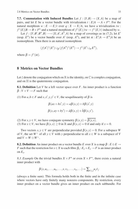
2.8 Metrics on Vector Bundles 33
7.7. Commutation with Induced Bundles Let f : (Y,B) → (X ,A) be a map ofpairs, and let E be a vector bundle with trivialization t : E|A → A× Fn. For thenatural morphism w : E → E/t over q : X → X/A, we have a trivialization tw :f ∗(E)|B → B×Fn and a natural morphism of f ∗(E)/tw → f ∗(E/t) induced by w.
Let f : (Y ;B′,B′′,B) −→ (X ;A′,A′′,A) be a map of coverings as in (7.2), let E ′(resp. E ′′) be a vector bundle over A′ (resp. A′′), and let α : E ′|A → E ′′|A be anisomorphism. Then there is an natural isomorphism
( f |A′)∗(E ′)∪β ( f |A′′)∗(E ′′) → f ∗(E ′ ∪α E ′′),
where β = f ∗(α).
8 Metrics on Vector Bundles
Let z denote the conjugation which on R is the identity, on C is complex conjugation,and on H is the quaternionic conjugation.
8.1. Definition Let V be a left vector space over F . An inner product is a functionβ : V ×V → F such that
(1) For a,b ∈ F and x,x′,y,y′ ∈V , the sesquilinearity of β is
β (ax + bx′,y) = aβ (x,y)+ bβ (x′,y)
β (x,ay + by′) = aβ (x,y)+ bβ (x,y′).
(2) For x,y ∈V , we have conjugate symmetry β (x,y) = β (y,x).(3) For x ∈V , we have β (x,x) ≥ 0 in R and β (x,x) = 0 if and only if x = 0.
Two vectors x,y ∈ V are perpendicular provided β (x,y) = 0. For a subspace Wof V , the set W⊥ of all y ∈ V with y perpendicular to all x ∈ W is a subspace of Vand V = W ⊕W⊥.
8.2. Definition An inner product on a vector bundle E over X is a map β : E ⊕E →F such that the restriction for x∈ X to each fibre βx : Ex×Ex →F is an inner producton Ex.
8.3. Example On the trivial bundles X ×Fn or even X ×F∞, there exists a naturalinner product with
β (x,u1, . . . ,un, . . . ,x,v1, . . . ,vn, . . .) =∑1≤ ju jv j
(always a finite sum). This formula holds both in the finite and in the infinite casewhere vectors have only finitely many nonzero components. By restriction, everyinner product on a vector bundle gives an inner product on each subbundle. For
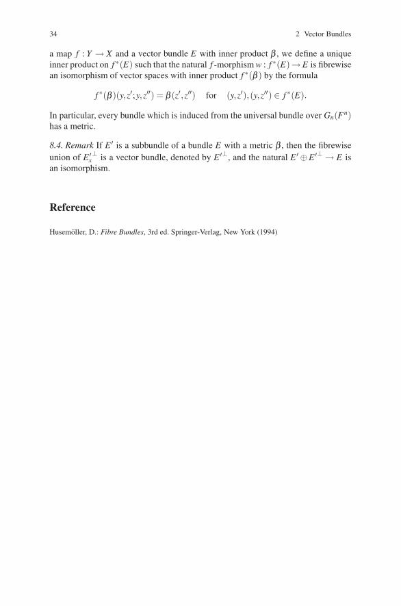
34 2 Vector Bundles
a map f : Y → X and a vector bundle E with inner product β , we define a uniqueinner product on f ∗(E) such that the natural f -morphism w : f ∗(E)→ E is fibrewisean isomorphism of vector spaces with inner product f ∗(β ) by the formula
f ∗(β )(y,z′;y,z′′) = β (z′,z′′) for (y,z′),(y,z′′) ∈ f ∗(E).
In particular, every bundle which is induced from the universal bundle over Gn(Fn)has a metric.
8.4. Remark If E ′ is a subbundle of a bundle E with a metric β , then the fibrewiseunion of E ′
x⊥ is a vector bundle, denoted by E ′⊥, and the natural E ′ ⊕E ′⊥ → E is
an isomorphism.
Reference
Husemoller, D.: Fibre Bundles, 3rd ed. Springer-Verlag, New York (1994)
Chapter 3Relation Between Vector Bundles, ProjectiveModules, and Idempotents
The main theorem is that there is an equivalence of the category of complex vec-tor bundles on a space X with the category of finitely generated projective C(X)-modules, where C(X) is the C-algebra of continuous complex valued functions onX . For this, we need a suitable hypothesis on X . The module associated to a vec-tor bundle E is the C(X)-module of cross sections Γ(X ,E), and the cross sectionfunctor Γ : (vect/X) → (C(X)) is the functor which sets up the equivalence of cate-gories between the category of (complex) vector bundles (vect/X) on X and the fullsubcategory of finitely generated projective modules in the category (C(X)) of allC(X)-modules.
The first assertion in this direction is the full embedding property of the crosssection functor
Γ : HomX(E ′,E ′′) −→ HomC(X)(Γ(X ,E ′),Γ(X ,E ′′)),
that is, Γ is a bijection. This is proved in Sect. 2 after some local to global pre-liminaries in Sect. 1 which are typical of normal spaces. Then, the remainder ofthe argument in Sect. 3 revolves around seeing that under additional hypotheses,Γ(X ,E) is indeed a finitely generated projective, and every finitely generated pro-jective module over C(X) is isomorphic to some Γ(X ,E). This is the case for acompact space X , and for a locally compact space, we can modify the assertion interms of vanishing and triviality at infinity.
The main result in this chapter is due independently to Jean-Pierre Serre andRichard Swan. It is often referred to as the Serre–Swan correspondence betweenvector bundles over a space X and finitely generated projective modules over thealgebra C(X).
In the process of showing that every projective module comes from a vectorbundle, we start with relations between idempotent elements in matrix algebras.The algebraic relation leads to another description of vector bundles and projectivemodules as classes of idempotents.
D. Husemoller et al.: Relation Between Vector Bundles, Projective Modules, and Idempotents, Lect. Notes Phys. 726,35–44 (2008)DOI 10.1007/978-3-540-74956-1 4 © Springer-Verlag Berlin Heidelberg 2008
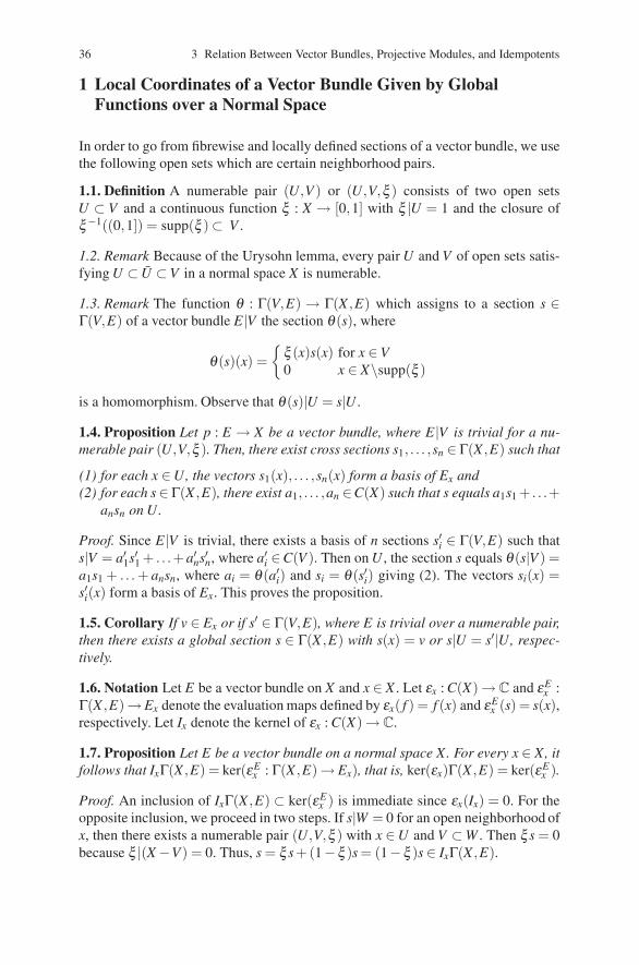
36 3 Relation Between Vector Bundles, Projective Modules, and Idempotents
1 Local Coordinates of a Vector Bundle Given by GlobalFunctions over a Normal Space
In order to go from fibrewise and locally defined sections of a vector bundle, we usethe following open sets which are certain neighborhood pairs.
1.1. Definition A numerable pair (U,V ) or (U,V,ξ ) consists of two open setsU ⊂ V and a continuous function ξ : X → [0,1] with ξ |U = 1 and the closure ofξ−1((0,1]) = supp(ξ )⊂ V .
1.2. Remark Because of the Urysohn lemma, every pair U and V of open sets satis-fying U ⊂ U ⊂V in a normal space X is numerable.
1.3. Remark The function θ : Γ(V,E) → Γ(X ,E) which assigns to a section s ∈Γ(V,E) of a vector bundle E|V the section θ (s), where
θ (s)(x) ={ξ (x)s(x) for x ∈V0 x ∈ X\supp(ξ )
is a homomorphism. Observe that θ (s)|U = s|U .
1.4. Proposition Let p : E → X be a vector bundle, where E|V is trivial for a nu-merable pair (U,V,ξ ). Then, there exist cross sections s1, . . . ,sn ∈ Γ(X ,E) such that
(1) for each x ∈U, the vectors s1(x), . . . ,sn(x) form a basis of Ex and(2) for each s ∈ Γ(X ,E), there exist a1, . . . ,an ∈C(X) such that s equals a1s1 + . . .+
ansn on U.
Proof. Since E|V is trivial, there exists a basis of n sections s′i ∈ Γ(V,E) such thats|V = a′1s′1 + . . .+a′ns′n, where a′i ∈C(V ). Then on U , the section s equals θ (s|V ) =a1s1 + . . . + ansn, where ai = θ (a′i) and si = θ (s′i) giving (2). The vectors si(x) =s′i(x) form a basis of Ex. This proves the proposition.
1.5. Corollary If v ∈ Ex or if s′ ∈ Γ(V,E), where E is trivial over a numerable pair,then there exists a global section s ∈ Γ(X ,E) with s(x) = v or s|U = s′|U, respec-tively.
1.6. Notation Let E be a vector bundle on X and x ∈ X . Let εx : C(X) → C and εEx :
Γ(X ,E)→Ex denote the evaluation maps defined by εx( f ) = f (x) and εEx (s) = s(x),
respectively. Let Ix denote the kernel of εx : C(X) → C.
1.7. Proposition Let E be a vector bundle on a normal space X. For every x ∈ X, itfollows that IxΓ(X ,E) = ker(εE
x : Γ(X ,E)→ Ex), that is, ker(εx)Γ(X ,E) = ker(εEx ).
Proof. An inclusion of IxΓ(X ,E) ⊂ ker(εEx ) is immediate since εx(Ix) = 0. For the
opposite inclusion, we proceed in two steps. If s|W = 0 for an open neighborhood ofx, then there exists a numerable pair (U,V,ξ ) with x ∈ U and V ⊂W . Then ξ s = 0because ξ |(X −V) = 0. Thus, s = ξ s+(1− ξ )s = (1− ξ )s ∈ IxΓ(X ,E).
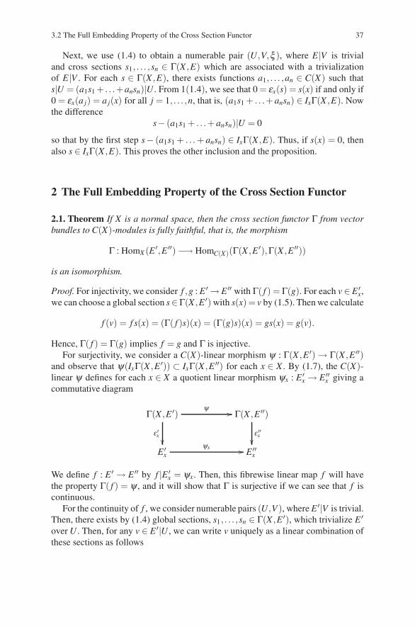
3.2 The Full Embedding Property of the Cross Section Functor 37
Next, we use (1.4) to obtain a numerable pair (U,V,ξ ), where E|V is trivialand cross sections s1, . . . ,sn ∈ Γ(X ,E) which are associated with a trivializationof E|V . For each s ∈ Γ(X ,E), there exists functions a1, . . . ,an ∈ C(X) such thats|U = (a1s1 + . . .+ansn)|U . From 1(1.4), we see that 0 = εx(s) = s(x) if and only if0 = εx(a j) = a j(x) for all j = 1, . . . ,n, that is, (a1s1 + . . .+ ansn) ∈ IxΓ(X ,E). Nowthe difference
s− (a1s1 + . . .+ ansn)|U = 0
so that by the first step s− (a1s1 + . . . + ansn) ∈ IxΓ(X ,E). Thus, if s(x) = 0, thenalso s ∈ IxΓ(X ,E). This proves the other inclusion and the proposition.
2 The Full Embedding Property of the Cross Section Functor
2.1. Theorem If X is a normal space, then the cross section functor Γ from vectorbundles to C(X)-modules is fully faithful, that is, the morphism
Γ : HomX (E ′,E ′′) −→ HomC(X)(Γ(X ,E ′),Γ(X ,E ′′))
is an isomorphism.
Proof. For injectivity, we consider f ,g : E ′ → E ′′ with Γ( f ) = Γ(g). For each v ∈ E ′x,
we can choose a global section s∈Γ(X ,E ′) with s(x) = v by (1.5). Then we calculate
f (v) = f s(x) = (Γ( f )s)(x) = (Γ(g)s)(x) = gs(x) = g(v).
Hence, Γ( f ) = Γ(g) implies f = g and Γ is injective.For surjectivity, we consider a C(X)-linear morphism ψ : Γ(X ,E ′) → Γ(X ,E ′′)
and observe that ψ(IxΓ(X ,E ′)) ⊂ IxΓ(X ,E ′′) for each x ∈ X . By (1.7), the C(X)-linear ψ defines for each x ∈ X a quotient linear morphism ψx : E ′
x → E ′′x giving a
commutative diagram
Γ(X ,E ′)
ε ′x��
ψ �� Γ(X ,E ′′)
ε ′′x��
E ′x
ψx �� E ′′x
We define f : E ′ → E ′′ by f |E ′x = ψx. Then, this fibrewise linear map f will have
the property Γ( f ) = ψ , and it will show that Γ is surjective if we can see that f iscontinuous.
For the continuity of f , we consider numerable pairs (U,V ), where E ′|V is trivial.Then, there exists by (1.4) global sections, s1, . . . ,sn ∈ Γ(X ,E ′), which trivialize E ′over U . Then, for any v ∈ E ′|U , we can write v uniquely as a linear combination ofthese sections as follows
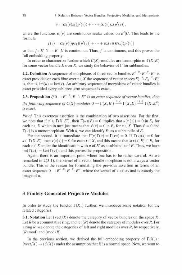
38 3 Relation Between Vector Bundles, Projective Modules, and Idempotents
v = α1(v)s1(p′(v))+ · · ·+αn(v)sn(p′(v)),
where the functions αi(v) are continuous scalar valued on E ′|U . This leads to theformula
f (v) = α1(v)(ψs1)(p′(v))+ · · ·+αn(v)(ψsn)(p′(v))
so that f : E ′|U → E ′′|U is continuous. Thus, f is continuous, and this proves thefull embedding property.
In order to characterize further which C(X)-modules are isomorphic to Γ(X ,E)for some vector bundle E over X , we study the behavior of Γ for subbundles.
2.2. Definition A sequence of morphisms of three vector bundles E ′ u→ Ev→ E ′′ is
exact provided on each fibre over x∈X the sequence of vector spaces E ′x
u→Exv→E ′′
xis, that is, im(u) = ker(v). An arbitrary sequence of morphisms of vector bundles isexact provided every subthree term sequence is exact.
2.3. Proposition If 0 → E ′ u→ Ev→ E ′′ is an exact sequence of vector bundles, then
the following sequence of C(X)-modules 0 → Γ(X ,E ′)Γ(u)−→ Γ(X ,E)
Γ(v)−→ Γ(X ,E ′′)is exact.
Proof. This exactness assertion is the combination of two assertions. For the first,we note that if s′ ∈ Γ(X ,E ′), then Γ(u)(s′) = 0 implies that u(s′(x)) = 0 in Ex foreach x ∈ X which in turn just means that s′(x) = 0 in Ex for x ∈ X . Thus s′ = 0 andΓ(u) is a monomorphism. With u, we can identify E ′ as a subbundle of E .
For the second, it is immediate that Γ(v)Γ(u) = Γ(vu) = 0. If Γ(v)(s) = 0 fors ∈ Γ(X ,E), then v(s(x)) = 0 for each x ∈ X , and this means that s(x) ∈ E ′
x ⊂ Ex foreach x ∈ X under the identification with u of E ′ as a subbundle of E . Thus, we haveim(Γ(u)) = ker(Γ(v)), and this proves the proposition.
Again, there is an important point where one has to be rather careful. As weremarked in 2(3.1), the kernel of a vector bundle morphism is not always a vectorbundle. This is the reason for formulating the previous assertion in terms of anexact sequence 0 → E ′ u→ E
v→ E ′′, where the kernel of v exists and is exactly theimage of u.
3 Finitely Generated Projective Modules
In order to study the functor Γ(X ,) further, we introduce some notation for therelated categories.
3.1. Notation Let (vect/X) denote the category of vector bundles on the space X .Let R be a commutative ring, and let (R) denote the category of modules over R. Fora ring R, we denote the categories of left and right modules over R, by respectively,(R\mod) and (mod/R).
In the previous section, we derived the full embedding property of Γ(X ,) :(vect/X)→ (C(X)) under the assumption that X is a normal space. Now, we want to
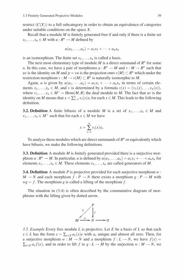
3.3 Finitely Generated Projective Modules 39
restrict (C(X)) to a full subcategory in order to obtain an equivalence of categoriesunder suitable conditions on the space X .
Recall that a module M is finitely generated free if and only if there is a finite setx1, . . . ,xn ∈ M with u : Rn → M defined by
u(a1, . . . ,an) = a1x1 + · · ·+ anxn
is an isomorphism. The finite set x1, . . . ,xn is called a basis.The next most elementary type of module M is a direct summand of Rn for some
n. In this case, we have a pair of morphisms u : Rn → M and v : M → Rn such thatuv is the identity on M and p = vu is the projection onto v(M) ⊂ Rn which under therestriction morphism v : M → v(M) ⊂ Rn is naturally isomorphic to M.
Again, u is given by u(a1, · · · ,an) = a1x1 + · · ·+ anxn in terms of certain ele-ments x1, . . . ,xn ∈ M, and v is determined by a formula v(x) = (v1(x), . . . ,vn(x)),where v1, . . . ,vn ∈ M∨ = Hom(M,R) the dual module to M. The fact that uv is theidentity on M means that x =∑n
i=1 vi(x)xi for each x ∈ M. This leads to the followingdefinition.
3.2. Definition A finite bibasis of a module M is a set of x1, . . . ,xn ∈ M andv1, . . . ,vn ∈ M∨ such that for each x ∈ M we have
x =n
∑i=1
vi(x)xi.
To analyze these modules which are direct summands of Rn or equivalently whichhave bibasis, we make the following definitions.
3.3. Definition A module M is finitely generated provided there is a surjective mor-phism u : Rn → M. In particular, u is defined by u(a1, . . . ,an) = a1x1 + · · ·+anxn forelements x1, . . . ,xn ∈ M. These elements x1, . . . ,xn are called generators of M.
3.4. Definition A module P is projective provided for each surjective morphism w :M → N and each morphism f : P → N there exists a morphism g : P → M withwg = f . The morphism g is called a lifting of the morphism f .
The situation in (3.4) is often described by the commutative diagram of mor-phisms with the lifting given by dotted arrow.
Pg
��f
��M
w �� N �� 0
3.5. Example Every free module L is projective. Let E be a basis of L so that eachx ∈ L has the form x = ∑e∈E ae(x)e with ae unique and almost all zero. Then, fora surjective morphism w : M → N and a morphism f : L → N, we have f (x) =∑e∈E ae f (e), and in order to lift f to g : L → M by the surjection w : M → N, we
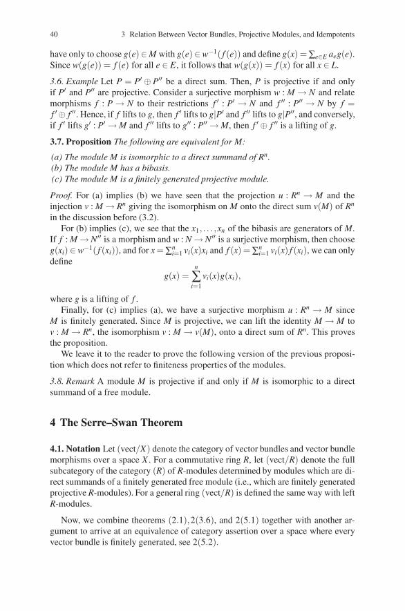
40 3 Relation Between Vector Bundles, Projective Modules, and Idempotents
have only to choose g(e)∈ M with g(e)∈ w−1( f (e)) and define g(x) =∑e∈E aeg(e).Since w(g(e)) = f (e) for all e ∈ E , it follows that w(g(x)) = f (x) for all x ∈ L.
3.6. Example Let P = P′ ⊕ P′′ be a direct sum. Then, P is projective if and onlyif P′ and P′′ are projective. Consider a surjective morphism w : M → N and relatemorphisms f : P → N to their restrictions f ′ : P′ → N and f ′′ : P′′ → N by f =f ′ ⊕ f ′′. Hence, if f lifts to g, then f ′ lifts to g|P′ and f ′′ lifts to g|P′′, and conversely,if f ′ lifts g′ : P′ → M and f ′′ lifts to g′′ : P′′ → M, then f ′ ⊕ f ′′ is a lifting of g.
3.7. Proposition The following are equivalent for M:
(a) The module M is isomorphic to a direct summand of Rn.(b) The module M has a bibasis.(c) The module M is a finitely generated projective module.
Proof. For (a) implies (b) we have seen that the projection u : Rn → M and theinjection v : M → Rn giving the isomorphism on M onto the direct sum v(M) of Rn
in the discussion before (3.2).For (b) implies (c), we see that the x1, . . . ,xn of the bibasis are generators of M.
If f : M → N′′ is a morphism and w : N → N′′ is a surjective morphism, then chooseg(xi)∈ w−1( f (xi)), and for x =∑n
i=1 vi(x)xi and f (x) =∑ni=1 vi(x) f (xi), we can only
define
g(x) =n
∑i=1
vi(x)g(xi),
where g is a lifting of f .Finally, for (c) implies (a), we have a surjective morphism u : Rn → M since
M is finitely generated. Since M is projective, we can lift the identity M → M tov : M → Rn, the isomorphism v : M → v(M), onto a direct sum of Rn. This provesthe proposition.
We leave it to the reader to prove the following version of the previous proposi-tion which does not refer to finiteness properties of the modules.
3.8. Remark A module M is projective if and only if M is isomorphic to a directsummand of a free module.
4 The Serre–Swan Theorem
4.1. Notation Let (vect/X) denote the category of vector bundles and vector bundlemorphisms over a space X . For a commutative ring R, let (vect/R) denote the fullsubcategory of the category (R) of R-modules determined by modules which are di-rect summands of a finitely generated free module (i.e., which are finitely generatedprojective R-modules). For a general ring (vect/R) is defined the same way with leftR-modules.
Now, we combine theorems (2.1),2(3.6), and 2(5.1) together with another ar-gument to arrive at an equivalence of category assertion over a space where everyvector bundle is finitely generated, see 2(5.2).
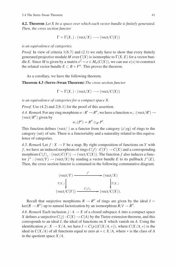
3.4 The Serre–Swan Theorem 41
4.2. Theorem Let X be a space over which each vector bundle is finitely generated.Then, the cross section functor
Γ= Γ(X ,) : (vect/X) −→ (vect/C(X))
is an equivalence of categories.
Proof. In view of criteria 1(6.7) and (2.1) we only have to show that every finitelygenerated projective module M over C(X) is isomorphic to Γ(X ,E) for a vector bun-dle E . Since M is given by a matrix e2 = e ∈ Mn(C(X)), we can use e(x) to constructthe related vector bundle E ⊂ B×Fn. This proves the theorem.
As a corollary, we have the following theorem.
Theorem 4.3 (Serre–Swan Theorem) The cross section functor
Γ= Γ(X ,) : (vect/X) −→ (vect/C(X))
is an equivalence of categories for a compact space X.
Proof. Use (4.2) and 2(6.1) for the proof of this assertion.
4.4. Remark For any ring morphism w : R′ →R′′, we have a function w∗ :(vect/R′)→(vect/R′′) given by
w∗(P′) = R′′ ⊗R′ P′.
This function defines (vect/ ) as a functor from the category (c\rg) of rings to thecategory (set) of sets. There is a functoriality and a naturality related to this equiva-lence of categories.
4.5. Remark Let f : X → Y be a map. By right composition of functions on Y withf , we have an induced morphism of rings C( f ) : C(Y ) →C(X) and a correspondingmorphism C( f )∗ : (vect/C(Y ))→ (vect/C(X)). The function f also induces a func-tor f ∗ : (vect/Y ) → (vect/X) by sending a vector bundle E to its pullback f ∗(E).Then, the cross section functor is contained in the following commutative diagram.
(vect/Y )
Γ(Y,)��
f ∗ �� (vect/X)
Γ(X ,)��
(vect/C(Y ))C( f )∗ �� (vect/C(X)).
Recall that surjective morphisms R → R′′ of rings are given by the ideal I =ker(R → R′′) up to natural factorization by an isomorphism R/I → R′′.4.6. Remark Each inclusion j : A → X of a closed subspace A into a compact spaceX defines a surjective C( j) : C(X)→C(A) by the Tietze extension theorem, and thiscorresponds to an ideal I, the ideal of functions on X which vanish on A. Using theidentification p : X → X/A, we have I = C(p)(C(X/A,∗)), where C(X/A,∗) is theideal in C(X/A) of all functions equal to zero at ∗ ∈ X/A, where ∗ is the class of Ain the quotient space X/A.
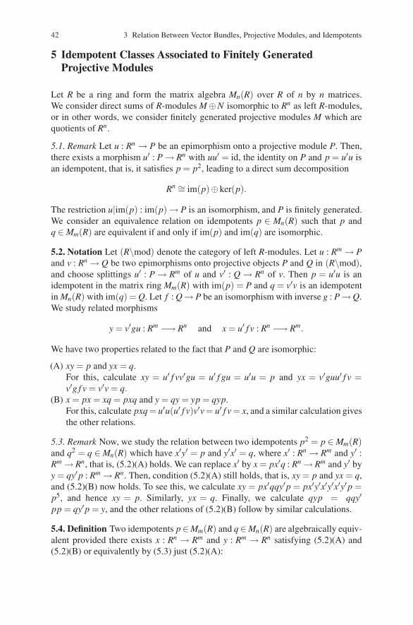
42 3 Relation Between Vector Bundles, Projective Modules, and Idempotents
5 Idempotent Classes Associated to Finitely GeneratedProjective Modules
Let R be a ring and form the matrix algebra Mn(R) over R of n by n matrices.We consider direct sums of R-modules M ⊕N isomorphic to Rn as left R-modules,or in other words, we consider finitely generated projective modules M which arequotients of Rn.
5.1. Remark Let u : Rn → P be an epimorphism onto a projective module P. Then,there exists a morphism u′ : P → Rn with uu′ = id, the identity on P and p = u′u isan idempotent, that is, it satisfies p = p2, leading to a direct sum decomposition
Rn ∼= im(p)⊕ker(p).
The restriction u|im(p) : im(p) → P is an isomorphism, and P is finitely generated.We consider an equivalence relation on idempotents p ∈ Mn(R) such that p andq ∈ Mm(R) are equivalent if and only if im(p) and im(q) are isomorphic.
5.2. Notation Let (R\mod) denote the category of left R-modules. Let u : Rm → Pand v : Rn → Q be two epimorphisms onto projective objects P and Q in (R\mod),and choose splittings u′ : P → Rm of u and v′ : Q → Rn of v. Then p = u′u is anidempotent in the matrix ring Mm(R) with im(p) = P and q = v′v is an idempotentin Mn(R) with im(q) = Q. Let f : Q → P be an isomorphism with inverse g : P → Q.We study related morphisms
y = v′gu : Rm −→ Rn and x = u′ f v : Rn −→ Rm.
We have two properties related to the fact that P and Q are isomorphic:
(A) xy = p and yx = q.For this, calculate xy = u′ f vv′gu = u′ f gu = u′u = p and yx = v′guu′ f v =v′g f v = v′v = q.
(B) x = px = xq = pxq and y = qy = yp = qyp.For this, calculate pxq = u′u(u′ f v)v′v = u′ f v = x, and a similar calculation givesthe other relations.
5.3. Remark Now, we study the relation between two idempotents p2 = p ∈ Mm(R)and q2 = q ∈ Mn(R) which have x′y′ = p and y′x′ = q, where x′ : Rn → Rm and y′ :Rm → Rn, that is, (5.2)(A) holds. We can replace x′ by x = px′q : Rn → Rm and y′ byy = qy′p : Rm → Rn. Then, condition (5.2)(A) still holds, that is, xy = p and yx = q,and (5.2)(B) now holds. To see this, we calculate xy = px′qqy′p = px′y′x′y′x′y′p =p5, and hence xy = p. Similarly, yx = q. Finally, we calculate qyp = qqy′pp = qy′p = y, and the other relations of (5.2)(B) follow by similar calculations.
5.4. Definition Two idempotents p∈Mm(R) and q∈ Mn(R) are algebraically equiv-alent provided there exists x : Rn → Rm and y : Rm → Rn satisfying (5.2)(A) and(5.2)(B) or equivalently by (5.3) just (5.2)(A):
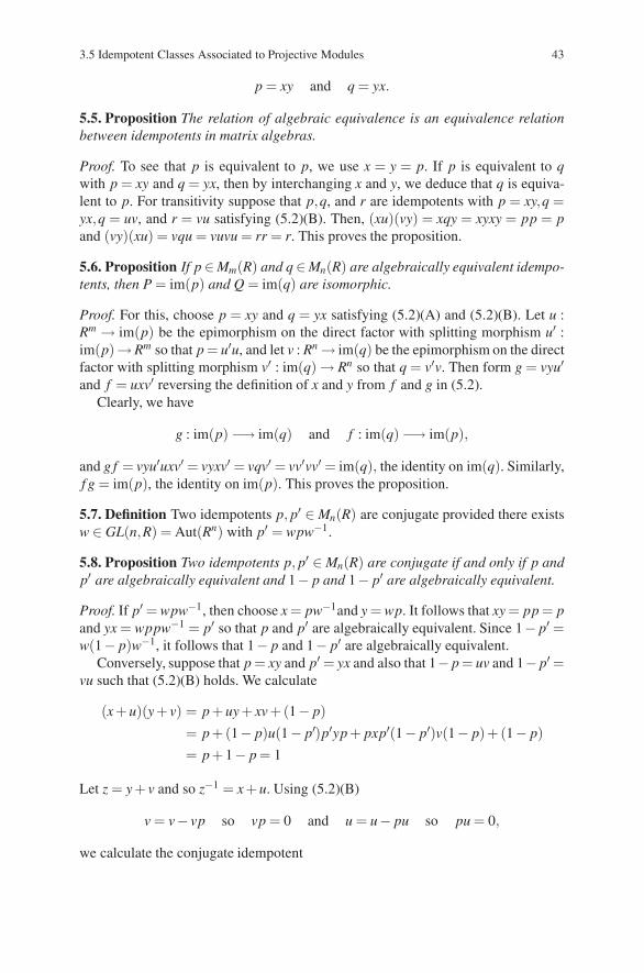
3.5 Idempotent Classes Associated to Projective Modules 43
p = xy and q = yx.
5.5. Proposition The relation of algebraic equivalence is an equivalence relationbetween idempotents in matrix algebras.
Proof. To see that p is equivalent to p, we use x = y = p. If p is equivalent to qwith p = xy and q = yx, then by interchanging x and y, we deduce that q is equiva-lent to p. For transitivity suppose that p,q, and r are idempotents with p = xy,q =yx,q = uv, and r = vu satisfying (5.2)(B). Then, (xu)(vy) = xqy = xyxy = pp = pand (vy)(xu) = vqu = vuvu = rr = r. This proves the proposition.
5.6. Proposition If p ∈ Mm(R) and q ∈ Mn(R) are algebraically equivalent idempo-tents, then P = im(p) and Q = im(q) are isomorphic.
Proof. For this, choose p = xy and q = yx satisfying (5.2)(A) and (5.2)(B). Let u :Rm → im(p) be the epimorphism on the direct factor with splitting morphism u′ :im(p)→Rm so that p = u′u, and let v : Rn → im(q) be the epimorphism on the directfactor with splitting morphism v′ : im(q) → Rn so that q = v′v. Then form g = vyu′and f = uxv′ reversing the definition of x and y from f and g in (5.2).
Clearly, we have
g : im(p) −→ im(q) and f : im(q) −→ im(p),
and g f = vyu′uxv′ = vyxv′ = vqv′ = vv′vv′ = im(q), the identity on im(q). Similarly,f g = im(p), the identity on im(p). This proves the proposition.
5.7. Definition Two idempotents p, p′ ∈ Mn(R) are conjugate provided there existsw ∈ GL(n,R) = Aut(Rn) with p′ = wpw−1.
5.8. Proposition Two idempotents p, p′ ∈ Mn(R) are conjugate if and only if p andp′ are algebraically equivalent and 1− p and 1− p′ are algebraically equivalent.
Proof. If p′ = wpw−1, then choose x = pw−1and y = wp. It follows that xy = pp = pand yx = wppw−1 = p′ so that p and p′ are algebraically equivalent. Since 1− p′ =w(1− p)w−1, it follows that 1− p and 1− p′ are algebraically equivalent.
Conversely, suppose that p = xy and p′ = yx and also that 1− p = uv and 1− p′ =vu such that (5.2)(B) holds. We calculate
(x + u)(y + v) = p + uy + xv +(1− p)= p +(1− p)u(1− p′)p′yp + pxp′(1− p′)v(1− p)+ (1− p)= p + 1− p = 1
Let z = y + v and so z−1 = x + u. Using (5.2)(B)
v = v− vp so vp = 0 and u = u− pu so pu = 0,
we calculate the conjugate idempotent
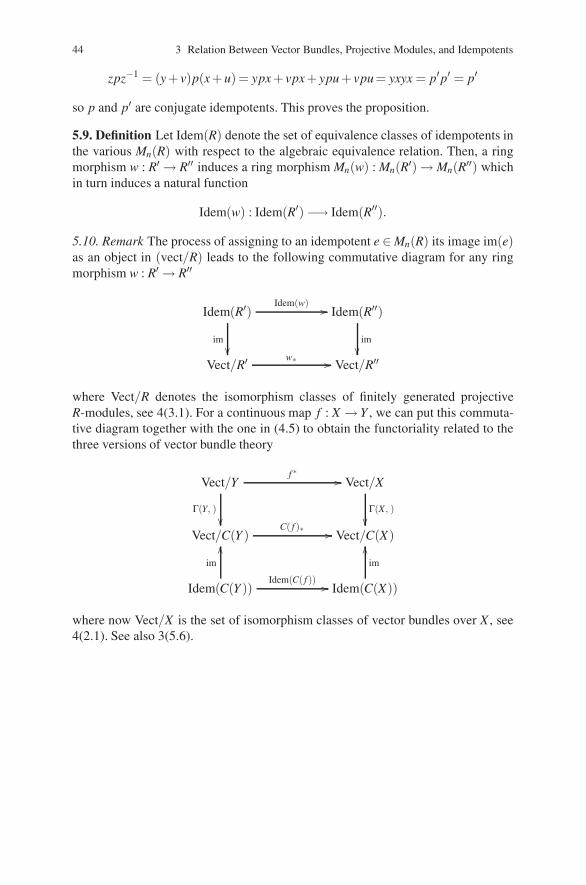
44 3 Relation Between Vector Bundles, Projective Modules, and Idempotents
zpz−1 = (y + v)p(x + u) = ypx + vpx + ypu + vpu = yxyx = p′p′ = p′
so p and p′ are conjugate idempotents. This proves the proposition.
5.9. Definition Let Idem(R) denote the set of equivalence classes of idempotents inthe various Mn(R) with respect to the algebraic equivalence relation. Then, a ringmorphism w : R′ → R′′ induces a ring morphism Mn(w) : Mn(R′) → Mn(R′′) whichin turn induces a natural function
Idem(w) : Idem(R′) −→ Idem(R′′).
5.10. Remark The process of assigning to an idempotent e ∈ Mn(R) its image im(e)as an object in (vect/R) leads to the following commutative diagram for any ringmorphism w : R′ → R′′
Idem(R′)
im��
Idem(w) �� Idem(R′′)
im��
Vect/R′ w∗ �� Vect/R′′
where Vect/R denotes the isomorphism classes of finitely generated projectiveR-modules, see 4(3.1). For a continuous map f : X → Y , we can put this commuta-tive diagram together with the one in (4.5) to obtain the functoriality related to thethree versions of vector bundle theory
Vect/Y
Γ(Y, )��
f ∗ �� Vect/X
Γ(X , )��
Vect/C(Y )C( f )∗ �� Vect/C(X)
Idem(C(Y ))
im
��
Idem(C( f )) �� Idem(C(X))
im
��
where now Vect/X is the set of isomorphism classes of vector bundles over X , see4(2.1). See also 3(5.6).
Chapter 4K-Theory of Vector Bundles, of Modules,and of Idempotents
We wish to consider the isomorphism classes of vector bundles over a space Xor in view of the correspondences in the previous chapter, either the isomorphismclasses of finitely generated modules over C(X) or algebraic equivalence classes ofidempotents in the matrix algebras Mn(C(X)) for all n. In each of the three cases,the direct sum leads to a natural addition on this sets of classes, and with the tensorproduct, there is a second algebraic operation of product. Unfortunately, these setsof isomorphism classes are not a ring under these operations, but only a semiring.The unfulfilled ring axiom is that each element must have a negative.
In the first section, we see how these semirings map universally into rings in thesame way as the natural numbers map into the integers N → Z, and the resultingclass groups or rings are called the K-groups of vector bundles, K-groups of finitelygenerated projective modules, or the K-groups of matrix ring idempotents. Usingthe results of the previous chapter, we can show that these semirings and the corre-sponding K-rings are all isomorphic. Finally, we consider some special features oftopological algebras, especially C∗-algebras.
1 Generalities on Adding Negatives
There is a universal mapping of a commutative monoid (or semigroup) into a com-mutative group and a universal mapping of a commutative semiring in a ring. Thisis an elementary exercise in the study of functors with universal properties, and itis the basic construction needed to go from isomorphism classes to stable classes ofvector bundles, projective modules, and idempotents.
1.1. Notation Let (s\ab) denote the category of abelian semigroups with com-position written additively and morphisms f : A′ → A′′ satisfying f (0) = 0 andf (x + y) = f (x)+ f (y) for x,y ∈ A′. Let (ab) denote the full subcategory of (s\ab)determined by the abelian groups.
D. Husemoller et al.: K-Theory of Vector Bundles, of Modules, and of Idempotents, Lect. Notes Phys. 726, 45–54(2008)DOI 10.1007/978-3-540-74956-1 5 © Springer-Verlag Berlin Heidelberg 2008
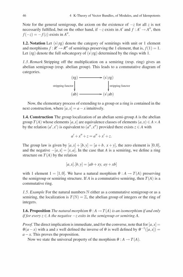
46 4 K-Theory of Vector Bundles, of Modules, and of Idempotents
Note for the general semigroup, the axiom on the existence of −z for all z is notnecessarily fulfilled, but on the other hand, if −z exists in A′ and f : A′ → A′′, thenf (−z) = − f (z) exists in A′′.
1.2. Notation Let (s\rg) denote the category of semirings with unit or 1 elementand morphisms f : R′ → R′′ of semirings preserving the 1 element, that is, f (1) = 1.Let (rg) denote the full subcategory of (s\rg) determined by the rings with 1.
1.3. Remark Stripping off the multiplication on a semiring (resp. ring) gives anabelian semigroup (resp. abelian group). This leads to a commutative diagram ofcategories.
(rg)
stripping functor��
�� (s\rg)
stripping functor��
(ab) �� (s\ab)
Now, the elementary process of extending to a group or a ring is contained in thenext construction, where [a,x] = a− x intuitively.
1.4. Construction The group localization of an abelian semi-group A is the abeliangroup T (A) whose elements [a,x] are equivalence classes of elements (a,x) ∈ A×Aby the relation (a′,x′) is equivalent to (a′′,x′′) provided there exists z ∈ A with
a′ + x′′+ z = a′′ + x′ + z.
The group law is given by [a,x]+ [b,y] = [a + b, x + y], the zero element is [0,0],and the negative −[a,x] = [x,a]. In the case that A is a semiring, we define a ringstructure on T (A) by the relation
[a,x].[b,y] = [ab + xy, ay + xb]
with 1 element 1 = [1,0]. We have a natural morphism θ : A → T (A) preservingthe semigroup or semiring structure. If A is a commutative semiring, then T (A) is acommutative ring.
1.5. Example For the natural numbers N either as a commutative semigroup or as asemiring, the localization is T (N) = Z, the abelian group of integers or the ring ofintegers.
1.6. Proposition The natural morphism θ : A→ T (A) is an isomorphism if and onlyif for every z ∈ A the negative −z exits in the semigroup or semiring A.
Proof. The direct implication is immediate, and for the converse, note that for [a,x]=θ (a− x) with a and x well defined the inverse of θ is well defined by θ−1([a,x]) =a− x. This proves the proposition.
Now we state the universal property of the morphism θ : A → T (A).
4.2 K-Groups of Vector Bundles 47
1.7. Proposition Let f : A → G be a morphism of commutative semigroups, whereG is a group. Then, there exists a unique morphism of groups h : T (A) → G withhθ = f . Let f : A → R be a morphism of semirings, where R is a ring. Then, thereexists a unique morphism of rings h : T (A) → R with hθ = f .
Proof. In both cases h([a,x]) = f (a)− f (x), and it must satisfy this formula showingthe uniqueness.
2 K-Groups of Vector Bundles
2.1. Definition Let Vect/X denote the isomorphism classes [E] of vector bundles Eover X with the semiring structure
[E ′]+ [E ′′] = [E ′ ⊕E ′′] and [E ′].[E ′′] = [E ′ ⊗E ′′].
The zero vector bundle is the zero class, and the trivial line bundle is the unit in thecommutative semiring.
2.2. Remark Let f : X → Y be a map between spaces. The inverse image of vectorbundles defines a semiring morphism
Vect/ f : Vect/Y −→ Vect/X
given by the formula Vect/ f ([E]) = [ f ∗(E)]. For a second map g : Y → Z, we havethe contravariant functor property
Vect/g f = Vect/ f ◦Vect/g : Vect/Z −→ Vect/X .
2.3. Definition The Grothendieck K-functor on the category (top) of spaces andmaps is defined by ring localization
K(X) = T (Vect/X).
2.4. Remark The universal property makes K into a functor K : (top) → (c\rg)op
into the opposite category of the category of commutative rings. The functorial-ity of K follows from the functoriality of Vect/ and the induced morphisms on theK-rings is defined by applying (1.7) to the following commutative diagram for amap f : X → Y relating a semiring and its continuation as a ring.
Vect/Y
�
f ∗ �� Vect/X
�
K(Y )K( f ) �� K(X).
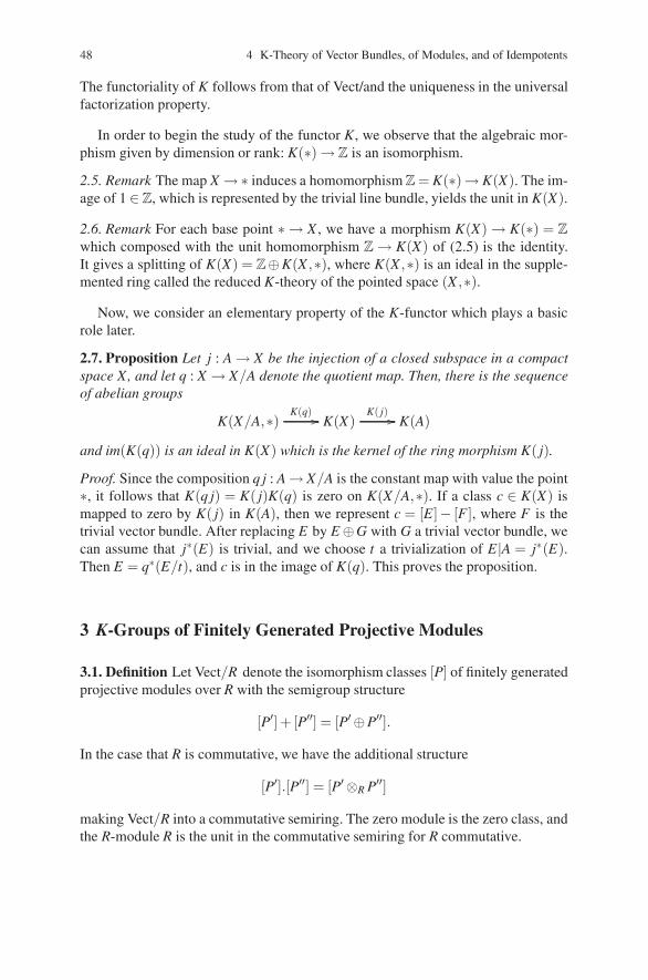
48 4 K-Theory of Vector Bundles, of Modules, and of Idempotents
The functoriality of K follows from that of Vect/and the uniqueness in the universalfactorization property.
In order to begin the study of the functor K, we observe that the algebraic mor-phism given by dimension or rank: K(∗) → Z is an isomorphism.
2.5. Remark The map X →∗ induces a homomorphism Z = K(∗)→ K(X). The im-age of 1 ∈ Z, which is represented by the trivial line bundle, yields the unit in K(X).
2.6. Remark For each base point ∗ → X , we have a morphism K(X) → K(∗) = Z
which composed with the unit homomorphism Z → K(X) of (2.5) is the identity.It gives a splitting of K(X) = Z⊕K(X ,∗), where K(X ,∗) is an ideal in the supple-mented ring called the reduced K-theory of the pointed space (X ,∗).
Now, we consider an elementary property of the K-functor which plays a basicrole later.
2.7. Proposition Let j : A → X be the injection of a closed subspace in a compactspace X, and let q : X → X/A denote the quotient map. Then, there is the sequenceof abelian groups
K(X/A,∗) K(q) �� K(X)K( j) �� K(A)
and im(K(q)) is an ideal in K(X) which is the kernel of the ring morphism K( j).
Proof. Since the composition q j : A → X/A is the constant map with value the point∗, it follows that K(q j) = K( j)K(q) is zero on K(X/A,∗). If a class c ∈ K(X) ismapped to zero by K( j) in K(A), then we represent c = [E]− [F ], where F is thetrivial vector bundle. After replacing E by E ⊕G with G a trivial vector bundle, wecan assume that j∗(E) is trivial, and we choose t a trivialization of E|A = j∗(E).Then E = q∗(E/t), and c is in the image of K(q). This proves the proposition.
3 K-Groups of Finitely Generated Projective Modules
3.1. Definition Let Vect/R denote the isomorphism classes [P] of finitely generatedprojective modules over R with the semigroup structure
[P′]+ [P′′] = [P′ ⊕P′′].
In the case that R is commutative, we have the additional structure
[P′].[P′′] = [P′ ⊗R P′′]
making Vect/R into a commutative semiring. The zero module is the zero class, andthe R-module R is the unit in the commutative semiring for R commutative.
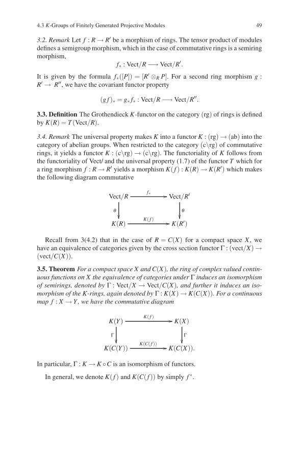
4.3 K-Groups of Finitely Generated Projective Modules 49
3.2. Remark Let f : R → R′ be a morphism of rings. The tensor product of modulesdefines a semigroup morphism, which in the case of commutative rings is a semiringmorphism,
f∗ : Vect/R −→ Vect/R′.
It is given by the formula f∗([P]) = [R′ ⊗R P]. For a second ring morphism g :R′ → R′′, we have the covariant functor property
(g f )∗ = g∗ f∗ : Vect/R −→ Vect/R′′.
3.3. Definition The Grothendieck K-functor on the category (rg) of rings is definedby K(R) = T (Vect/R).
3.4. Remark The universal property makes K into a functor K : (rg)→ (ab) into thecategory of abelian groups. When restricted to the category (c\rg) of commutativerings, it yields a functor K : (c\rg) → (c\rg). The functoriality of K follows fromthe functoriality of Vect/ and the universal property (1.7) of the functor T which fora ring morphism f : R → R′ yields a morphism K( f ) : K(R) → K(R′) which makesthe following diagram commutative
Vect/R
�
f∗ �� Vect/R′
�
K(R)K( f ) �� K(R′)
Recall from 3(4.2) that in the case of R = C(X) for a compact space X , wehave an equivalence of categories given by the cross section functor Γ : (vect/X)→(vect/C(X)).
3.5. Theorem For a compact space X and C(X), the ring of complex valued contin-uous functions on X the equivalence of categories under Γ induces an isomorphismof semirings, denoted by Γ : Vect/X → Vect/C(X), and further it induces an iso-morphism of the K-rings, again denoted by Γ : K(X) → K(C(X)). For a continuousmap f : X → Y, we have the commutative diagram
K(Y )
��
K( f ) �� K(X)
��
K(C(Y ))K(C( f )) �� K(C(X)).
In particular, Γ : K → K ◦C is an isomorphism of functors.
In general, we denote K( f ) and K(C( f )) by simply f ∗.
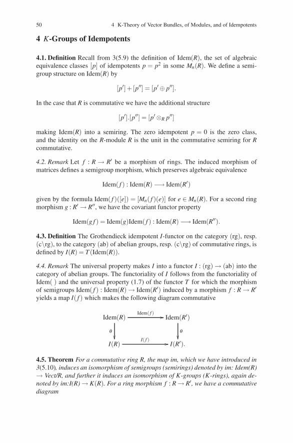
50 4 K-Theory of Vector Bundles, of Modules, and of Idempotents
4 K-Groups of Idempotents
4.1. Definition Recall from 3(5.9) the definition of Idem(R), the set of algebraicequivalence classes [p] of idempotents p = p2 in some Mn(R). We define a semi-group structure on Idem(R) by
[p′]+ [p′′] = [p′ ⊕ p′′].
In the case that R is commutative we have the additional structure
[p′].[p′′] = [p′ ⊗R p′′]
making Idem(R) into a semiring. The zero idempotent p = 0 is the zero class,and the identity on the R-module R is the unit in the commutative semiring for Rcommutative.
4.2. Remark Let f : R → R′ be a morphism of rings. The induced morphism ofmatrices defines a semigroup morphism, which preserves algebraic equivalence
Idem( f ) : Idem(R) −→ Idem(R′)
given by the formula Idem( f )([e]) = [Mn( f )(e)] for e ∈ Mn(R). For a second ringmorphism g : R′ → R′′, we have the covariant functor property
Idem(g f ) = Idem(g)Idem( f ) : Idem(R) −→ Idem(R′′).
4.3. Definition The Grothendieck idempotent I-functor on the category (rg), resp.(c\rg), to the category (ab) of abelian groups, resp. (c\rg) of commutative rings, isdefined by I(R) = T (Idem(R)).
4.4. Remark The universal property makes I into a functor I : (rg) → (ab) into thecategory of abelian groups. The functoriality of I follows from the functoriality ofIdem( ) and the universal property (1.7) of the functor T for which the morphismof semigroups Idem( f ) : Idem(R) → Idem(R′) induced by a morphism f : R → R′yields a map I( f ) which makes the following diagram commutative
Idem(R)
�
Idem( f ) �� Idem(R′)
�
I(R)I( f ) �� I(R′).
4.5. Theorem For a commutative ring R, the map im, which we have introduced in3(5.10), induces an isomorphism of semigroups (semirings) denoted by im: Idem(R)→ Vect/R, and further it induces an isomorphism of K-groups (K-rings), again de-noted by im:I(R) → K(R). For a ring morphism f : R → R′, we have a commutativediagram
4.5 K-Theory of Topological Algebras 51
I(R)
im��
I( f ) �� I(R′)
im��
K(R)K( f ) �� K(R′).
In particular, im : I → K is an isomorphism of functors.
Proof. We have only to check the multiplicative property of the morphism im in caseR is commutative. For this, we consider p ∈ Mm(R) with p2 = p and q∈ Mn(R) withq2 = q and form P = p(Rm) and Q = q(Rn). The tensor product of the two directsum decompositions Rm = P⊕P′ and Rn = Q⊕Q′ has the form
Rmn = (P⊗Q)⊕ [(P⊗Q′)⊕ (P′ ⊗Q)⊕ (Q⊗Q′)]= im(p⊗q)⊕ [(P⊗Q′)⊕ (P′ ⊗Q)⊕ (Q⊗Q′)].
This proves the theorem.
5 K-Theory of Topological Algebras
In Chap. 3, Sect. 4, we related vector bundles over X to finitely generated projectivemodules over A = C(X), the algebra of continuous complex valued functions onX . We get the same results for the algebra of bounded continuous functions whichwe also denote by C(X). In the algebraic setting, these modules were related toidempotents in matrix algebras over the matrix algebras Mn(A) for a general algebrain Sect. 5 of Chap. 3. In the first four sections of this chapter, the class group orK-groups of vector bundles, finitely generated projective modules, and idempotentswere introduced.
5.1. Remark For the study of class groups, we see that there is a large interface be-tween the topology of bundles and the algebra of certain modules. There is anotherimportant connection namely with the area of functional analysis, and it starts in thefollowing two elementary ways:
(1) The algebra C(X) has a natural ∗-algebra structure. This leads to the possibilityof using only projections, that is, just selfadjoint idempotents. The ∗-structureis given by defining f ∗ of an element f by f ∗(x) = f (x) for x ∈ X .
(2) The algebra C(X) of bounded continuous functions has a norm ‖ f‖ = supx∈X| f (x)| making C(X) into a special topological algebra, namely a Banach alge-bra, that is, a complete normed algebra. At a very early stage in the developmentof topological K-theory, Banach algebras played an important role giving alter-native proofs of Bott periodicity, which is a fundamental subject considered inChap. 15.
5.2. Remark At the center of this interface between K-theory coming from topologyand the use of analysis in K-theory is the Atiyah–Singer index theorem. Indices like
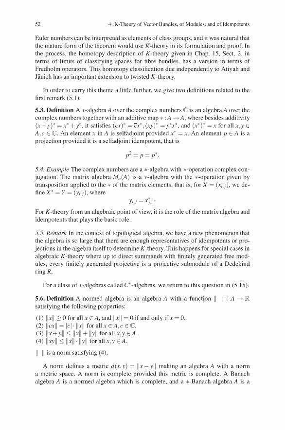
52 4 K-Theory of Vector Bundles, of Modules, and of Idempotents
Euler numbers can be interpreted as elements of class groups, and it was natural thatthe mature form of the theorem would use K-theory in its formulation and proof. Inthe process, the homotopy description of K-theory given in Chap. 15, Sect. 2, interms of limits of classifying spaces for fibre bundles, has a version in terms ofFredholm operators. This homotopy classification due independently to Atiyah andJanich has an important extension to twisted K-theory.
In order to carry this theme a little further, we give two definitions related to thefirst remark (5.1).
5.3. Definition A ∗-algebra A over the complex numbers C is an algebra A over thecomplex numbers together with an additive map ∗ : A → A, where besides additivity(x + y)∗ = x∗ + y∗, it satisfies (cx)∗ = cx∗,(xy)∗ = y∗x∗, and (x∗)∗ = x for all x,y ∈A,c ∈ C. An element x in A is selfadjoint provided x∗ = x. An element p ∈ A is aprojection provided it is a selfadjoint idempotent, that is
p2 = p = p∗.
5.4. Example The complex numbers are a ∗-algebra with ∗-operation complex con-jugation. The matrix algebra Mn(A) is a ∗-algebra with the ∗-operation given bytransposition applied to the ∗ of the matrix elements, that is, for X = (xi, j), we de-fine X∗ = Y = (yi, j), where
yi, j = x∗j,i .
For K-theory from an algebraic point of view, it is the role of the matrix algebra andidempotents that plays the basic role.
5.5. Remark In the context of topological algebra, we have a new phenomenon thatthe algebra is so large that there are enough representatives of idempotents or pro-jections in the algebra itself to determine K-theory. This happens for special cases inalgebraic K-theory where up to direct summands with finitely generated free mod-ules, every finitely generated projective is a projective submodule of a Dedekindring R.
For a class of ∗-algebras called C∗-algebras, we return to this question in (5.15).
5.6. Definition A normed algebra is an algebra A with a function ‖ ‖ : A → R
satisfying the following properties:
(1) ‖x‖ ≥ 0 for all x ∈ A, and ‖x‖ = 0 if and only if x = 0.(2) ‖cx‖ = |c| · ‖x‖ for all x ∈ A,c ∈ C.(3) ‖x + y‖ ≤ ‖x‖+‖y‖ for all x,y ∈ A.(4) ‖xy‖ ≤ ‖x‖ · ‖y‖ for all x,y ∈ A.
‖ ‖ is a norm satisfying (4).
A norm defines a metric d(x,y) = ‖x − y‖ making an algebra A with a norma metric space. A norm is complete provided this metric is complete. A Banachalgebra A is a normed algebra which is complete, and a ∗-Banach algebra A is a
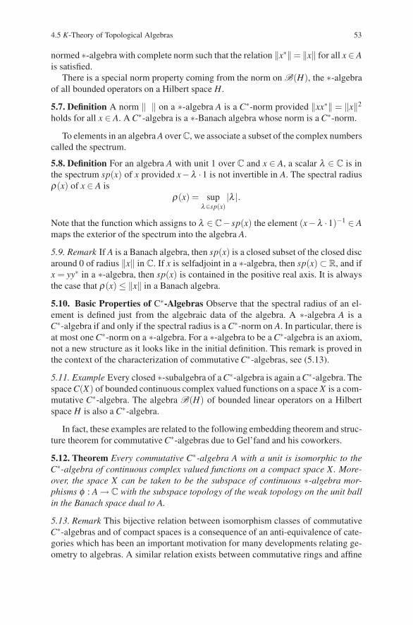
4.5 K-Theory of Topological Algebras 53
normed ∗-algebra with complete norm such that the relation ‖x∗‖= ‖x‖ for all x ∈ Ais satisfied.
There is a special norm property coming from the norm on B(H), the ∗-algebraof all bounded operators on a Hilbert space H.
5.7. Definition A norm ‖ ‖ on a ∗-algebra A is a C∗-norm provided ‖xx∗‖ = ‖x‖2
holds for all x ∈ A. A C∗-algebra is a ∗-Banach algebra whose norm is a C∗-norm.
To elements in an algebra A over C, we associate a subset of the complex numberscalled the spectrum.
5.8. Definition For an algebra A with unit 1 over C and x ∈ A, a scalar λ ∈ C is inthe spectrum sp(x) of x provided x−λ ·1 is not invertible in A. The spectral radiusρ(x) of x ∈ A is
ρ(x) = supλ∈sp(x)
|λ |.
Note that the function which assigns to λ ∈ C− sp(x) the element (x−λ ·1)−1 ∈ Amaps the exterior of the spectrum into the algebra A.
5.9. Remark If A is a Banach algebra, then sp(x) is a closed subset of the closed discaround 0 of radius ‖x‖ in C. If x is selfadjoint in a ∗-algebra, then sp(x) ⊂ R, and ifx = yy∗ in a ∗-algebra, then sp(x) is contained in the positive real axis. It is alwaysthe case that ρ(x) ≤ ‖x‖ in a Banach algebra.
5.10. Basic Properties of C∗-Algebras Observe that the spectral radius of an el-ement is defined just from the algebraic data of the algebra. A ∗-algebra A is aC∗-algebra if and only if the spectral radius is a C∗-norm on A. In particular, there isat most one C∗-norm on a ∗-algebra. For a ∗-algebra to be a C∗-algebra is an axiom,not a new structure as it looks like in the initial definition. This remark is proved inthe context of the characterization of commutative C∗-algebras, see (5.13).
5.11. Example Every closed ∗-subalgebra of a C∗-algebra is again a C∗-algebra. Thespace C(X) of bounded continuous complex valued functions on a space X is a com-mutative C∗-algebra. The algebra B(H) of bounded linear operators on a Hilbertspace H is also a C∗-algebra.
In fact, these examples are related to the following embedding theorem and struc-ture theorem for commutative C∗-algebras due to Gel’fand and his coworkers.
5.12. Theorem Every commutative C∗-algebra A with a unit is isomorphic to theC∗-algebra of continuous complex valued functions on a compact space X. More-over, the space X can be taken to be the subspace of continuous ∗-algebra mor-phisms φ : A → C with the subspace topology of the weak topology on the unit ballin the Banach space dual to A.
5.13. Remark This bijective relation between isomorphism classes of commutativeC∗-algebras and of compact spaces is a consequence of an anti-equivalence of cate-gories which has been an important motivation for many developments relating ge-ometry to algebras. A similar relation exists between commutative rings and affine
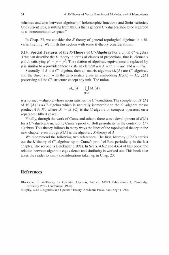
54 4 K-Theory of Vector Bundles, of Modules, and of Idempotents
schemes and also between algebras of holomorphic functions and Stein varieties.One current idea, resulting from this, is that a general C∗-algebra should be regardedas a “noncommutative space.”
In Chap. 23, we consider the K-theory of general topological algebras in a bi-variant setting. We finish this section with some K-theory considerations.
5.14. Special Features of the K-Theory of C∗-Algebras For a unital C∗-algebraA we can describe the K-theory in terms of classes of projections, that is, elementsp ∈ A satisfying p∗ = p = p2. The relation of algebraic equivalence is replaced byp is similar to q provided there exists an element u ∈ A with p = uu∗ and q = u∗u.
Secondly, if A is a C∗-algebra, then all matrix algebras Mn(A) are C∗-algebras,and the direct sum with the zero matrix gives an embedding Mn(A) → Mn+q(A)preserving all the C∗-structure except any unit. The union
M∞(A) =⋃0≤n
Mn(A)
is a normed ∗-algebra whose norm satisfies the C∗-condition. The completion K (A)of M∞(A) is a C∗-algebra which is naturally isomorphic to the C∗-algebra tensorproduct A⊗K , where K = K (C) is the C-algebra of compact operators on aseparable Hilbert space.
Finally, through the work of Cuntz and others, there was a development of K(A)for a C∗-algebra A including Cuntz’s proof of Bott periodicity in the context of C∗-algebras. This theory follows in many ways the lines of the topological theory in thenext chapter even though K(A) is the algebraic K-theory of A.
We recommend the following two references. The first, Murphy (1990) carriesout the K-theory of C∗-algebras up to Cuntz’s proof of Bott periodicity in the lastchapter. The second is Blackadar (1998). In Sects. 4.6.2 and 4.6.4 of this book, therelation between algebraic equivalence and similarity is worked out. This book alsotakes the reader to many considerations taken up in Chap. 23.
References
Blackadar, B.: K-Theory for Operator Algebras, 2nd ed, MSRI Publications 5, CambridgeUniversity Press, Cambridge (1998)
Murphy, G.J.: C-algebras and Operator Theory. Academic Press, San Diego (1990)
Chapter 5Principal Bundles and Sections of FibreBundles: Reduction of the Structureand the Gauge Group I
In this chapter, we consider bundles p : E → B where a topological group G actson the fibres through an action of G on the total space E . This is just an actionE ×G → E of G on E such that p(xs) = p(x) for all x ∈ E and s ∈ G. In par-ticular, there is a restriction Eb ×G → Eb of the globally defined action to eachfibre Eb, b ∈ B, of the bundle. A principal G-bundle is a bundle p : P → B withan additional algebraic and continuity action property implying, for example, thatall fibres are isomorphic to G by any map G → Pb of the form s �→ us for anyu ∈ Pb and all s ∈ G. For a principal G-bundle p : P → B and a left G-space Y ,we have the fibre bundle construction q : P[Y ] = P×G Y → B. Vector bundles areexamples of fibre bundles where G = GL(n), the general linear group, and Y isan n-dimensional vector space. The characterization of sections in Γ(B,P[Y ]) bycertain maps P → Y plays a fundamental role in applications of principal bundletheory. We outline two important aspects within principal bundle theory in thischapter. At first, the reduction of the structure group G of a principal bundle P.The second aspect is the study of AutG(P), the automorphism group of the principalG-bundle P.
Chapter 4 of Fibre Bundles (Husemoller 1994) is a reference for this chapter.
1 Bundles Defined by Transformation Groups
1.1. Definition A topological group G is a set G together with a group structure andtopology on G such that the function (s, t) �→ st−1 is a continuous map G×G → G.A morphism f : G′ → G′′ of topological groups is a function which is both a groupmorphism and a continuous map.
This continuity condition on (s, t) �→ st−1 is equivalent to G×G → G, (s, t) �→ s tand G → G, s �→ s−1 being continuous maps.
D. Husemoller et al.: Principal Bundles and Sections of Fibre Bundles: Reduction of the Structure and the GaugeGroup I, Lect. Notes Phys. 726, 55–62 (2008)DOI 10.1007/978-3-540-74956-1 6 © Springer-Verlag Berlin Heidelberg 2008
56 5 Principal Bundles and Sections of Fibre Bundles
1.2. Example The vector spaces Rn and C
n with the addition of vectors as well asthe matrix groups GL(n,R) and GL(n,C) with the usual composition are topologicalgroups. A subgroup H of a topological group G with the subspace topology is againa topological group. The determinant det : GL(n) → GL(1) is an example of a mor-phism of topological groups, and its kernel SL(n) with the subspace topology is aclosed subgroup.
1.3. Definition Let G be a topological group. A right G-space X is a space X to-gether with a map X ×G → X denoted by (x,s) �→ xs satisfying the algebraic ax-ioms:
(1) x(st) = (xs)t for x ∈ X and s,t ∈ G.(2) x1 = x for x ∈ X and 1 the identity of the group.
A morphism f : X → Y of right G-spaces is a map f : X → Y of spaces satisfyingf (xs) = f (x)s for x ∈ X and s ∈ G. Such morphisms are also called G-equivariantmaps or G-maps. The category of right G-spaces we denote (G\top).
A left G-space X is one with a map G×X → X having the algebraic properties(st)x = s(tx) as in (1) and 1x = x. A left G-space has a natural right G-space structuregiven by xs = s−1x, and a right G-space has a natural left G-space structure givenby sx = xs−1. Of course, these two concepts are equivalent under this involutionarycorrespondence G → G, s �→ s−1.
1.4. Example The group GL(n,F) acts on the vectors Fn by matrix multiplicationleaving 0 fixed, and hence, it also acts on Fn −{0}. We will return to other actionslater. The two-element group {±1} acts on each sphere Sn, and the circle T = {eiθ}acts on all odd dimensional spheres S2n−1 ⊂ C
n via complex multiplication.
1.5. Definition Let X be a right (left) G-space. A point x ∈ X is called a fixed pointif xs = x (or sx = x resp.) for all s ∈ G. We denote the subspace of fixed points byeither XG or Fix(X)
For example, Fix(Fn) = {0} is an example for the matrix groups GL(n,F) actionon Fn.
1.6. Definition For a G-space, the orbit of x ∈ X , denoted by xG, is equal to theset of all xs for a right action and Gx equal the set of all sx for a left action. LetX/G denote the set of orbits for a right action with projection q : X → X/G givenby q(x) = xG, and let G\X denote the set of orbits for a left action with projectionq : X → G\X . The orbit space has the quotient topology under the projections.
1.7. Remark For a G-space X , the map x �→ xs is an isomorphism, with inverse x �→x(s−1). Also the projection π : X →X/G is an open map since π(W ) is open in X/Gfor each open set W of X from the formula π−1π(W) =
⋃s∈G Ws.
1.8. Definition A G-bundle p : E → B is a bundle with a right G-space structureE ×G → E on E such that p(xs) = p(x) for all x ∈ E and s ∈ G. A morphism(u, f ) : E ′ → E ′′ of G-bundles p′ : E ′ → B′ and p′′ : E ′′ → B′′ is a morphism of

5.2 Definition and Examples of Principal Bundles 57
bundles, so p′′u = f p′, and u is a G-map, so u(xs) = u(x)s for all s ∈ G and x ∈ E ′.The category of G-bundles is denoted by (G−bun). Note that in later chapters weconsider more general bundles and call them still G-bundles. These are bundleswhere G acts on the base B as well and p is equivariant, see 13(2.1).
1.9. Remark There is the functor (G\top) → (G−bun) which assigns to a right G-space X the G-bundle q : X →X/G = B. Most G-bundles that we will consider comeby this functor from G-spaces.
2 Definition and Examples of Principal Bundles
2.1. Definition A free G-space X is a right G-space X such that the subspace X∗ ofX ×X consisting of all (x,xs) ∈ X ×X has a unique continuous function τ : X∗ → Gwith the property that x′τ(x′,x′′) = x′′.
If x′s = x′′, then τ(x′,x′′) = s, and in particular xs′ = xs′′ implies that s′ = s′′ in G.
2.2. Definition A principal bundle is a G-bundle p : P →B in the sense of (1.8) suchthat P is a free G-space and the natural morphism P/G → B is an isomorphism. Aprincipal bundle morphism (u, f ) : P′ → P′′ is a morphism of G-bundles which areprincipal bundles p′ : P′ → B′ and p′′ : P′′ → B′′.
2.3. Example A basic example comes from a closed subgroup G ⊂ H and p : H →H/G the quotient map is an example of a principal G-bundle. If p′ : P′ → B′ is aprincipal G′-bundle and if p′′ : P′′ → B′′ is a principal G′′-bundle, then the prod-uct bundle p′ × p′′ : P′ ×P′′ → B′ ×B′′ is a principal G′ ×G′′-bundle. In the casewhere B = B′ = B′′, the fibre product q : P′ ×B P′′ → B is a principal G′ ×G′′-bundle.
2.4. Theorem Every morphism of principal bundles over B is an isomorphism.
2.5. Remark It is easy to see that a morphism u : P′ → P′′ is a bijection on each fibre,and hence, it has an inverse function. In Fibre Bundles (Husemoller 1994), 4(3.2)on p. 43, it is proved to be continuous using the translation maps τ of P′ and P′′(Husemoller 1994, p. 43).
2.6. Example Let p : P → B be a principal G-bundle, and let f : B′ → B be acontinuous map. The induced bundle f−1P → B′ has a G-bundle structure with(b′,x)s = (b′,xs), and it is a principal bundle with τ((b′,x1),(b′,x2)) = τ(x1,x2)for P. The morphism (w, f ) : f−1P → P is a morphism of principal bundles.
2.7. Proposition If p : P → B is a principal G-bundle and if f : B′ → B is a con-tinuous map, then f−1P → B′ is a principal bundle. If (u, f ) : P′ → P is a mor-phism of principal G-bundles, then u factors as a principal G-bundle isomorphismv : P′ → f−1P and the canonical f -morphism w : f−1P → P.
Again, observe that v(x′) = (p′(x′),u(x′)) is a formula for the desired factoriza-tion as in the case of vector bundles.
58 5 Principal Bundles and Sections of Fibre Bundles
3 Fibre Bundles
3.1. Definition Let P be a principal G-bundle P over B and let Y be a left G-space Y . Form the quotient P×Y → P[Y ] = P×G Y , where the right action of Gon P ×Y is given by (x,y)s = (xs,s−1y). The associated fibre bundle to P withfibre Y is the space P[Y ] together with the projection pY : P[Y ] → B given bypY ((x,y)G) = p(x).
In the literature, the notation P×G Y is also used to denote P[Y ], but this no-tation conflicts with the usual notation of fibre product, so that we will not useit here.
3.2. Remark There is a map Y → p−1Y (b) for each choice of x with p(x) = b given
by y �→ (x,y)G. Since τ is continuous, it follows that this map is an isomorphism.
3.3. Example Each n-dimensional vector bundle E over B is isomorphic to a fibrebundle Vn(E)[Fn] for the group GL(n,F). The principal GL(n,F)-bundle Vn(E) is
called the frame bundle associated with E , and it is the subbundle of E×B(n). . . ×BE
whose fibre over a point b consists of n-tuples of vectors (v1, . . . ,vn) in Eb which arelinearly independent.
3.4. Example Each n by n matrix algebra bundle A over B is isomorphic to a fibrebundle Wn(A)[Mn(F)] for the group PGL(n,F) = GL(n,F)/GL(1,F). The principalPGL(n,F)-bundle Wn(A)[Mn(F)] is called the matrix frame bundle associated withA, and it is the subbundle of Homalg(Mn(F),A) of algebra morphisms Mn(K) into
the fibres of A and is a subspace of n2 fibre product of A with itself over B.The description of cross sections of a fibre bundle is very basic because the result
is in terms of equivariant maps from the principal bundle space to the fibre of thefibre bundle.
3.5. Theorem Let p : P → B be a principal G-bundle, and let Y be a left G-space.The set of cross sections Γ(B,P[Y ]) of the fibre bundle P[Y ] → B are in bijectivecorrespondence with maps φ : P → Y satisfying φ(xs) = s−1φ(x).
3.6. Remark Let φ : P → Y be a map satisfying φ(xs) = s−1φ(x), and form the mapσφ (xG) = (x,φ(x))G which is a well-defined continuous section.
If σ is a section of P[Y ], then it has the form σ(xG) = (x,φσ (x))G = (xs,s−1φσ(x))G which implies that φσ satisfies the relation φσ (xs) = s−1φσ (x). To deduce thecontinuity of φσ from the continuity of σ , we use the continuity of the translationfunction, see Fibre Bundles (Husemoller 1994), 4(8.1) on page 48, or leave it as anexercise for the reader.
4 Local Coordinates for Fibre Bundles
4.1. Trivial Bundles For the product G-principal bundle B×G and for any productfibre bundle B×Y over B, the automorphisms are each given by maps g : B → G
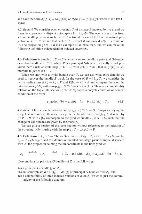
5.4 Local Coordinates for Fibre Bundles 59
and have the form αg(b,s) = (b,g(b)s) or αg(b,y) = (b,g(b)y), where Y is a left G-space.
4.2. Remark We consider open coverings Ui of a space B indexed by i ∈ I, and weform the coproduct or disjoint union space U = �i∈IUi. The open cover arises froma fibre bundle p : E → B such that E|Ui is trivial for each i ∈ I. For the natural pro-jection q : U → B, we see that each E|Ui is trivial if and only if q∗(E) is trivial onU . The projection q : U → B is an example of an etale map, and we can make thefollowing definition independent of indexed coverings.
4.3. Definition A bundle p : E → B whether a vector bundle, a principal G-bundle,or a fibre bundle E = P[Y ], where P is a principal G-bundle, is locally trivial pro-vided there exists an etale map q : U → B with q∗(E) trivial, that is, q∗(E) is iso-morphic to pr : U ×Y →U .
When we start with a trivial bundle over U , we can ask what extra data do weneed to recover the bundle E on B. In the case of B =
⋃i∈I Ui, we consider the
two trivializations E|Ui → Ui × F and E|Uj → Uj ×F and compare them on theintersection Ui∩Uj with a map gi, j : Ui∩Uj →G as in (4.1). There is a compatibilityrelation on the triple intersection Ui ∩Uj ∩Uk called a cocycle condition or descentcondition of the form
gi,k(b)gk, j(b) = gi, j(b) for b ∈Ui ∩Uj ∩Uk. (4.1)
4.4. Remark For a double indexed family gi, j : Ui ∩Uj → G of maps satisfying thecocycle condition (∗), there exists a principal bundle over B =
⋃i∈I Ui, denoted by
p : P → B, with P|Ui isomorphic to the product bundle Ui ×G → Ui such that thechange of coordinates are given by the maps gi, j.
We can give a version of this construction without reference to the indexing ofthe covering, only starting with the map q : U = �i∈IUi → B.
4.5. Definition Let q : U → B be an etale map. Let Z0 = U , let Z1 = U ×B U , and letZ2 = U ×B U ×B U , and this defines our related two-stage pseudosimplicial space Zwith di, the projection deleting the ith coordinate in the fibre product
Z2d0,d1,d2 �� Z1
d0,d1 �� Z0 and with did j = d j−1di for i < j.
Descent data for principal G-bundles of Z is the following:
(a) a principal G-bundle Q on Z0,(b) an isomorphism α : d∗
1(Q) → d∗0(Q) of principal G-bundles over Z1, and
(c) a compatibility of three induced versions of α on Z2 which is just the commu-tativity of the following diagram,
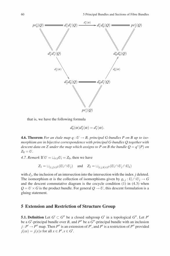
60 5 Principal Bundles and Sections of Fibre Bundles
pr∗0(Q) d∗1d∗
1(Q) d∗1d∗
0(Q) pr∗2(Q)
d∗2d∗
1(Q) d∗0d∗
0(Q)
d∗2d∗
0(Q) d∗0d∗
1(Q)
pr∗1(Q)
d∗1(α)��
��������������
��������������
��������������
��������������
��������������
��������������
��������������
��������������
d∗2(α)
����������������
d∗0(α)
����������������
��������������
��������������
��������������
��������������
that is, we have the following formula
d∗0(α)d∗
2(α) = d∗1(α).
4.6. Theorem For an etale map q : U → B, principal G-bundles P on B up to iso-morphism are in bijective correspondence with principal G-bundles Q together withdescent data on Z under the map which assigns to P on B the bundle Q = q∗(P) onZ0 = U.
4.7. Remark If U = �i∈IUi = Z0, then we have
Z1 = �(i, j)∈I2(Ui ∩Uj) and Z2 = �(i, j,k)∈I3(Ui ∩Uj ∩Uk)
with d j, the inclusion of an intersection into the intersection with the index j deleted.The isomorphism α is the collection of isomorphisms given by gi, j : Ui ∩Uj → Gand the descent commutative diagram is the cocycle condition (1) in (4.3) whenQ = U ×G is the product bundle. For general Q →U , this descent formulation is agluing statement.
5 Extension and Restriction of Structure Group
5.1. Definition Let G′ ⊂ G′′ be a closed subgroup G′ in a topological G′′. Let P′be a G′-principal bundle over B, and P′′ be a G′′-principal bundle with an inclusionj : P′ → P′′ map. Then P′′ is an extension of P′, and P′ is a restriction of P′′ providedj(xs) = j(x)s for all x ∈ P′,s ∈ G′.
5.5 Extension and Restriction of Structure Group 61
It is always possible to extend the structure group.
5.2. Proposition Let P′ be a G′-principal bundle, where G′ is a closed subgroupof G′′. Then, the fibre bundle P′[G′′] has a principal G′′-bundle structure, and thenatural morphism given by P′ = P′[G′] → P′[G′′] = P′′ is an extension of P′.
The restriction of the structure group is not always possible, and it depends onthe existence of a cross section for a related fibre bundle.
5.3. Proposition Let P′′ be a G′′-principal bundle, where G′ is a closed subgroupof G′′. Then, there exists a restriction of P′′ to a G′-principal bundle P′ ⊂ P′′ if andonly if P′′[G′′/G′] has a cross section.
Proof . If P′ → P′′ exists, then P′[G′/G′] = B → P′′[G′′/G′] is the desired sec-tion, and if σ : B → P′′[G′′/G′] is a cross section, then it corresponds to a mapφ : P′′ →G′′/G′ with φ(xs) = s−1φ(x). The subbundle P′ has total space φ−1(eG′)⊂P′′.
5.4. Remark Using the notation of (5.1), we consider local coordinates gi, j : Ui ∩Uj → G′ of P′, and these can be taken to be the local coordinates with values inG′′ ⊃ G′. Starting with local coordinates gi, j : Ui ∩Uj → G′′ of P′′, we can restrictthe bundle to G′ if and only if there exists hi : Ui → G′′ with higi, jh
−1j : Ui ∩Uj →
G′ ⊂ G′′.
These concepts extend from a general inclusion G′ ⊂ G′′ to the case of a generalcontinuous homomorphism w : G′ → G′′.
5.5. Definition Let w : G′ → G′′ be a morphism of topological groups, and let B bea base space.
(a) The extension of a principal G′-bundle P′ over B is P′′ = P′[G′′] = P′ ×G′G′′
with the G′′-principal bundle structure given by
[x′,s′′]t ′′ = [x′,s′′t ′′],
where [x′t ′,s′′] = [x′,w(t ′)s′′] for x′ ∈ P′, t ′ ∈ G′, and s′′, t ′′ ∈ G′′.(b) A restriction of a principal G′′-bundle P′′ over B is a principal G′-bundle P′ over
B such that the extension of P′ to a principal G′′-bundle P′[G′′] is isomorphic toP′′ as a principal G′′-bundle.
(c) A G′-structure on a principal G′′-bundle P′′ over B is an equivalence class ofpairs (P′,v), where P′ is a G′-principal bundle restriction of P′′, and v : P′[G′′]→P′′ is an isomorphism of principal G′′-bundles. Two pairs (P′
1,v1) and (P′2,v2)
defining a G′-structure on P′′ are equivalent provided there exists an isomor-phism u : P′
1 → P′2 of principal G′-bundles with v2 ◦ u[G′′] = v1.
5.6. Terminology When G′ = SO(n) in (5.5), a G′-structure is called an orientation,and when G′ = Spin(n) (cf. 12 (1.5) and 12 (3)), it is called a spin structure.
62 5 Principal Bundles and Sections of Fibre Bundles
6 Automorphisms of Principal Bundles and Gauge Groups
6.1. Definition Let p : P → B be a principal G-bundle. The gauge group AutB(P) ofP is the space of all gauge transformations of P, that is, all maps u ∈ Map(P,P) with
pu = p and u(xs) = u(x)s for all s ∈ G, x ∈ P.
In particular, we see that a gauge transformation is just an automorphism of theprincipal bundle since u−1 : P → P is defined and continuous. There are two otherways of looking at gauge transformations.
6.2. Proposition For a principal bundle P, there is a bijective correspondence be-tween the following three sets:
(1) gauge transformations u : P → P,(2) continuous maps φ : P → G with φ(xs) = s−1φ(x)s for x ∈ P,s ∈ G, and(3) cross sections of the fibre bundle P[Ad(G)].
Proof . The bijection between the sets defined by the condition (2) and condition(3) is just the description of the set of cross sections of a fibre bundle (5.1). If φ isgiven by (2), then we define uφ (x) = xφ(x), and we calculate uφ (xs) = xss−1φ(x)s =uφ (x)s. Conversely, if u : P → P is a gauge transformation, then u(x) = xφu(x), andthe automorphism property u(xs) = u(x)s implies that u(xs) = xsφu(xs) = xφu(x)s,and hence it follows that φu satisfies φu(xs) = s−1φu(x)s. This sets up the correspon-dence and proves the proposition.
6.3. Summary Relations In (a) we summarize the bijection between (1) and (2),and in (b) we summarize the bijection between (2) and (3):
(a) From φ : P→G we form uφ (x) = xφ(x), and from u : P→ P we form φu : P→Gby u(x) = xφu(x).
(b) From φ : P → G we form σφ (xG) = (x,φ(x)) mod G, and from σ : B →P[Ad(G)] we have σ(xG) = (x,φσ (x)) mod G.
Reference
Husemoller, D.: Fibre Bundles, 3rd ed. Springer-Verlag, New York (1994)
Part IIHomotopy Classification of Bundles
and Cohomology: Classifying Spaces
In the first part, Chaps. 1–5, principal bundles, fibre bundles, and vector bundles overa space were introduced and studied. Of special importance was the fact that a vectorbundle is a particular example of a fibre bundle which comes with a principal bundlein the background. In this part, Chaps. 6–12, the homotopy theory and classificationof bundles is considered. For this, we begin with the basic definition of homotopybetween two maps f ′, f ′′ : X → Y in terms of a map h : X × [0,1]→ Y .
If p : E → B is a bundle over B, then the product with the unit interval p× [0,1] :E × [0,1] → B× [0,1] is a bundle over B× [0,1] with the same fibres in the sensethat (E × [0,1])(b,t) = Eb. The vector bundles, principal bundles, and fibre bundleshave a converse property, that is, under suitable local triviality in these three cases abundle q : E ′ → B× [0,1] is isomorphic to
p× [0,1] : E × [0,1]−→ B× [0,1],
where E = E ′|(B×{0}). This is the homotopy invariance of bundles.Two maps f ′, f ′′ : X →Y are homotopic provided there is a map h : X× [0,1]→Y ,
called a homotopy from f ′ to f ′′, and if q : E →Y is a type of bundle with homotopyinvariance property, then f ′−1(E) and f ′′−1(E) are isomorphic over X
There is a converse for this theorem for the Milnor construction contained inChap. 7, that is, if two bundles are isomorphic, then the maps are homotopic. Thesehomotopy questions lead to fibre space questions. In Chaps. 9–12, the cohomologyproperties of bundles are considered, especially the theory of characteristic classes.
Chapter 6Homotopy Classes of Mapsand the Homotopy Groups
In this chapter, we prepare the basic definitions on the homotopy relation betweenmaps. These ideas apply everywhere in geometry, and it is usually the case thatinvariants of maps which are interesting are those which are the same for two ho-motopic maps.
A homotopy from X to Y is a map h : X × [0,1]→Y , and in terms of the variablesx ∈ X and t ∈ [0,1], it can be written either as h(x,t), as h(x)(t), or as ht(x). Thisgives three interpretations of homotopy which are discussed in the first sections.For example, ht(x) suggests a deformation from h0 : X → Y to h1 : X → Y which isanother name for a homotopy from h0 to h1. The form h(x)(t) suggests that for eachx ∈ X the function t �→ h(x)(t) is a path in the space Y and a homotopy from thisperspective is just a map from X to the space of paths on Y . The homotopy groupsπn(X ,x0) of a space X with base point x0 are defined either as certain (equivalenceclasses of) maps of the n-sphere Sn or of the n-cube In into the space X . We show thatthey are in general commutative groups except for the fundamental group π1(X).
The cylinder space X × [0,1] over X plays clearly a basic role in the study ofhomotopy properties. For bundles, we will consider those classes of vector bun-dles, principal bundles, and fibre bundles which have the property that a bundlep : E → B × [0,1] is isomorphic to (E|(B ×{0}))× [0,1]. This is the homotopyinvariance property of bundles. This implies that two homotopic maps induce iso-morphic bundles.
1 The Space Map(X,,,Y)
As a set, Map(X ,Y ) is the set of all continuous functions f : X → Y . For L ⊂ X andM ⊂ Y , we use the notation 〈L,M〉 for the subset of all f ∈ Map(X ,Y ) such thatf (L) ⊂ M. A space or set is compact provided it satisfies the Heine–Borel coveringproperty and the Hausdorff separation condition.
D. Husemoller et al.: Homotopy Classes of Maps and the Homotopy Groups, Lect. Notes Phys. 726, 65–74 (2008)DOI 10.1007/978-3-540-74956-1 7 © Springer-Verlag Berlin Heidelberg 2008
66 6 Homotopy Classes of Maps and the Homotopy Groups
1.1. Definition The compact open topology on Map(X ,Y ) is the topology generatedby all sets 〈K,V 〉, where K is a compact subset of X and V is an open subset of Y .
Recall this means that T ⊂ Map(X ,Y ) is open in the compact open topologyif and only if for all f ∈ T there exists compact subsets Ki ⊂ X and open subsetsVi ⊂Y for i = 1, . . . ,m such that f ∈ 〈K1,V1〉∩ . . .∩〈Km,Vm〉 ⊂ T . The compact opentopology works best for separated (Hausdorff) spaces, and we will assume that ourspaces are separated. It is needed in the following remark.
1.2. Remark If Φ is a family of open sets generating the topology of Y , then theset of all 〈K,W 〉, where K is compact in X and W ∈ Φ generates the topology ofMap(X ,Y ).
1.3. Functoriality Let u : X ′ →X and v :Y →Y ′ be two continuous maps. Then, u∗ :Map(X ,Y )→ Map(X ′,Y ) defined by u∗( f ) = f u and v∗ : Map(X ,Y )→ Map(X ,Y ′)defined by v∗( f ) = v f are continuous. In addition, let u′ : X ′′ → X ′ and v′ : Y → Y ′′be two continuous maps. Then, we have the following relations for f ∈ Map(X ,Y ): u∗(v∗( f )) = v f u = v∗(u∗( f )),(uu′)∗ = (u′)∗u∗, and (v′v)∗ = v′∗v∗.
2 Continuity of Substitution and Map(X×××T,Y)
2.1. Definition For three spaces X ,T , and Y we define a map
c : Map(X ×T,Y) −→ Map(X ,Map(T,Y ))
by the requirement that c( f )(x)(t) = f (x,t) for f ∈ Map(X ×T,Y ). This is a well-defined continuous map by (1.2), and it is also clearly injective. Moreover, it restrictsto a topological isomorphism c : Map(X ×T,Y) → im(c) ⊂ Map(X ,Map(T,Y )),where the image of c, denoted by im(c), has the subspace topology.
2.2. Definition For two spaces T and Y , the evaluation function
e : Map(T,Y )×T → Y
is given by the formula e( f ,t) = f (t).
2.3. Proposition Let T be an arbitrary space. The evaluation function e : Map(T,Y )× T → Y is continuous for every Y if and only if the map c : Map(X ×T,Y) →Map(X ,Map(T,Y )) is surjective for all spaces X.
Proof. If e for T is continuous, then for g ∈ Map(X ,Map(T,Y )) we have g = c( f ),where f (x, t) = e(g(x),t). Conversely if c is surjective, then e = c−1(idMap(T,Y )) iscontinuous for the case X = Map(T,Y ). This proves the proposition.
2.4. Example If T is a locally compact space, then the evaluation function e :Map(T,Y )× T → Y is continuous for all spaces Y , and hence by (2.3), the mapc : Map(X ×T,Y ) → Map(X ,Map(T,Y )) is an isomorphism of spaces (also calleda homeomorphism).
6.3 Free and Based Homotopy Classes of Maps 67
3 Free and Based Homotopy Classes of Maps
For many considerations, especially those related to algebraic structures, it is im-portant to consider spaces X together with a given point in X .
3.1. Definition A pointed space X is a pair consisting of a space X together with apoint x0 ∈ X , called the base point. Let X and Y be two pointed spaces. A pointedmap f : X → Y is a map f of the underlying spaces such that f (x0) = y0.
Another name for a pointed map is a base-point-preserving map. In many caseswe use the symbol ∗ for the base point, and then base-point-preserving is the relationf (∗) = ∗. Clearly, the composition of two pointed maps is again a pointed map.
3.2. Definition As before, (top) denotes the category of spaces and continuous func-tions. The category of pointed spaces and pointed maps is denoted by (top)∗. Thenatural stripping (or forgetful) functor (top)∗ → (top) assigns to a pointed space itsunderlying space and to a pointed map the same map.
There are two notions of homotopy corresponding to the two categories: (top),where (free) homotopies are defined, and (top)∗, where pointed homotopies or base-point-preserving homotopies are defined.
3.3. Definition Two maps f ′, f ′′ : X → Y in (top) are homotopic provided there ex-ists a map h : X × [0,1] → Y with h(x,0) = f ′(x) and h(x,1) = f ′′(x). Two mapsf ′, f ′′ : X →Y in (top)∗ are homotopic provided there exists a map h : X × [0,1]→Ywith h(∗,t) = ∗, h(x,0) = f ′(x) and h(x,1) = f ′′(x).
3.4. Example If f ′, f ′′ : X → Rm are two maps, then
ht(x) = (1− t) f ′(x)+ t f ′′(x)
is a homotopy between f ′ and f ′′. If f ′ and f ′′ preserve a base point, then ht(∗) = ∗.
If in the previous definition we denote h(x,t) by ft(x), then ft(x) is either a one-parameter family of maps ft : X → Y which preserve base point in the case (top)∗or it is map
X −→ Map([0,1],Y )
equal to f ′ at t = 0 and f ′′ at t = 1. In other words, f0 = f ′ and f1 = f ′′.
3.5. Remark The homotopy relation is an equivalence relation, that is,
(1) it is reflexive meaning that f : X → Y is homotopic to itself by the homotopyh(x,t) = f (x) for all x ∈ X ,t ∈ [0,1],
(2) it is symmetric meaning that if f is homotopic to f ′ say with a homotopy h(x, t),then f ′ is homotopic to f with, for example, h′(x, t) = h(x,1− t), and
(3) it is transitive meaning that if f is homotopic to f ′ and f ′ is homotopic to f ′′,then f is homotopic to f ′′. If h(x,t) is a homotopy from f to f ′ and if h′(x, t) isa homotopy from f ′ to f ′′, then we define a homotopy h′′(x,t) by the relation
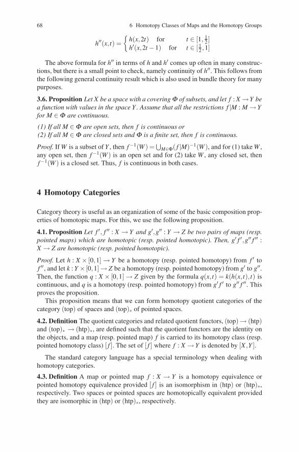
68 6 Homotopy Classes of Maps and the Homotopy Groups
h′′(x,t) ={
h(x,2t) for t ∈ [1, 12 ]
h′(x,2t −1) for t ∈ [ 12 ,1]
The above formula for h′′ in terms of h and h′ comes up often in many construc-tions, but there is a small point to check, namely continuity of h′′. This follows fromthe following general continuity result which is also used in bundle theory for manypurposes.
3.6. Proposition Let X be a space with a coveringΦ of subsets, and let f : X →Y bea function with values in the space Y . Assume that all the restrictions f |M : M → Yfor M ∈Φ are continuous.
(1) If all M ∈Φ are open sets, then f is continuous or(2) If all M ∈Φ are closed sets and Φ is a finite set, then f is continuous.
Proof. If W is a subset of Y , then f−1(W ) =⋃
M∈Φ( f |M)−1(W ), and for (1) take W ,any open set, then f−1(W ) is an open set and for (2) take W , any closed set, thenf−1(W ) is a closed set. Thus, f is continuous in both cases.
4 Homotopy Categories
Category theory is useful as an organization of some of the basic composition prop-erties of homotopic maps. For this, we use the following proposition.
4.1. Proposition Let f ′, f ′′ : X → Y and g′,g′′ : Y → Z be two pairs of maps (resp.pointed maps) which are homotopic (resp. pointed homotopic). Then, g′ f ′,g′′ f ′′ :X → Z are homotopic (resp. pointed homotopic).
Proof. Let h : X × [0,1] → Y be a homotopy (resp. pointed homotopy) from f ′ tof ′′, and let k : Y × [0,1]→ Z be a homotopy (resp. pointed homotopy) from g′ to g′′.Then, the function q : X × [0,1] → Z given by the formula q(x,t) = k(h(x, t), t) iscontinuous, and q is a homotopy (resp. pointed homotopy) from g′ f ′ to g′′ f ′′. Thisproves the proposition.
This proposition means that we can form homotopy quotient categories of thecategory (top) of spaces and (top)∗ of pointed spaces.
4.2. Definition The quotient categories and related quotient functors, (top)→ (htp)and (top)∗ → (htp)∗, are defined such that the quotient functors are the identity onthe objects, and a map (resp. pointed map) f is carried to its homotopy class (resp.pointed homotopy class) [ f ]. The set of [ f ] where f : X → Y is denoted by [X ,Y ].
The standard category language has a special terminology when dealing withhomotopy categories.
4.3. Definition A map or pointed map f : X → Y is a homotopy equivalence orpointed homotopy equivalence provided [ f ] is an isomorphism in (htp) or (htp)∗,respectively. Two spaces or pointed spaces are homotopically equivalent providedthey are isomorphic in (htp) or (htp)∗, respectively.
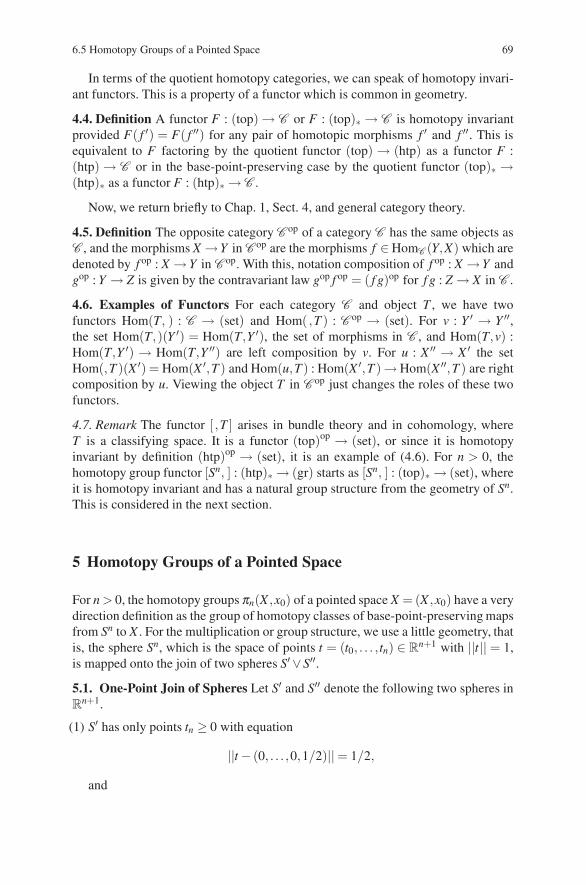
6.5 Homotopy Groups of a Pointed Space 69
In terms of the quotient homotopy categories, we can speak of homotopy invari-ant functors. This is a property of a functor which is common in geometry.
4.4. Definition A functor F : (top) → C or F : (top)∗ → C is homotopy invariantprovided F( f ′) = F( f ′′) for any pair of homotopic morphisms f ′ and f ′′. This isequivalent to F factoring by the quotient functor (top) → (htp) as a functor F :(htp) → C or in the base-point-preserving case by the quotient functor (top)∗ →(htp)∗ as a functor F : (htp)∗ → C .
Now, we return briefly to Chap. 1, Sect. 4, and general category theory.
4.5. Definition The opposite category C op of a category C has the same objects asC , and the morphisms X →Y in C op are the morphisms f ∈ HomC (Y,X) which aredenoted by f op : X → Y in C op. With this, notation composition of f op : X →Y andgop : Y → Z is given by the contravariant law gop f op = ( f g)op for f g : Z → X in C .
4.6. Examples of Functors For each category C and object T , we have twofunctors Hom(T, ) : C → (set) and Hom( ,T ) : C op → (set). For v : Y ′ → Y ′′,the set Hom(T,)(Y ′) = Hom(T,Y ′), the set of morphisms in C , and Hom(T,v) :Hom(T,Y ′) → Hom(T,Y ′′) are left composition by v. For u : X ′′ → X ′ the setHom(,T )(X ′) = Hom(X ′,T ) and Hom(u,T ) : Hom(X ′,T )→ Hom(X ′′,T ) are rightcomposition by u. Viewing the object T in C op just changes the roles of these twofunctors.
4.7. Remark The functor [ ,T ] arises in bundle theory and in cohomology, whereT is a classifying space. It is a functor (top)op → (set), or since it is homotopyinvariant by definition (htp)op → (set), it is an example of (4.6). For n > 0, thehomotopy group functor [Sn, ] : (htp)∗ → (gr) starts as [Sn, ] : (top)∗ → (set), whereit is homotopy invariant and has a natural group structure from the geometry of Sn.This is considered in the next section.
5 Homotopy Groups of a Pointed Space
For n > 0, the homotopy groups πn(X ,x0) of a pointed space X = (X ,x0) have a verydirection definition as the group of homotopy classes of base-point-preserving mapsfrom Sn to X . For the multiplication or group structure, we use a little geometry, thatis, the sphere Sn, which is the space of points t = (t0, . . . ,tn) ∈ R
n+1 with ||t|| = 1,is mapped onto the join of two spheres S′ ∨S′′.
5.1. One-Point Join of Spheres Let S′ and S′′ denote the following two spheres inR
n+1.
(1) S′ has only points tn ≥ 0 with equation
||t − (0, . . . ,0,1/2)||= 1/2,
and
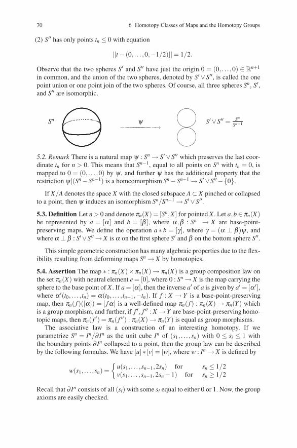
70 6 Homotopy Classes of Maps and the Homotopy Groups
(2) S′′ has only points tn ≤ 0 with equation
||t − (0, . . . ,0,−1/2)||= 1/2.
Observe that the two spheres S′ and S′′ have just the origin 0 = (0, . . . ,0) ∈ Rn+1
in common, and the union of the two spheres, denoted by S′ ∨S′′, is called the onepoint union or one point join of the two spheres. Of course, all three spheres Sn, S′,and S′′ are isomorphic.
��
��
��
��Sn S′ ∨S′′ = Sn
Sn−1ψ−−−−−−−−−−−−−−−→
5.2. Remark There is a natural map ψ : Sn → S′ ∨S′′ which preserves the last coor-dinate tn for n > 0. This means that Sn−1, equal to all points on Sn with tn = 0, ismapped to 0 = (0, . . . ,0) by ψ , and further ψ has the additional property that therestriction ψ |(Sn −Sn−1) is a homeomorphism Sn −Sn−1 → S′ ∨S′′ − {0}.
If X/A denotes the space X with the closed subspace A ⊂ X pinched or collapsedto a point, then ψ induces an isomorphism Sn/Sn−1 → S′ ∨S′′.
5.3. Definition Let n > 0 and denote πn(X) = [Sn,X ] for pointed X . Let a,b∈ πn(X)be represented by a = [α] and b = [β ], where α,β : Sn → X are base-point-preserving maps. We define the operation a ∗ b = [γ], where γ = (α ⊥ β )ψ , andwhere α ⊥ β : S′ ∨S′′ → X is α on the first sphere S′ and β on the bottom sphere S′′.
This simple geometric construction has many algebraic properties due to the flex-ibility resulting from deforming maps Sn → X by homotopies.
5.4. Assertion The map ∗ : πn(X)×πn(X) → πn(X) is a group composition law onthe set πn(X) with neutral element e = [0], where 0 : Sn → X is the map carrying thesphere to the base point of X . If a = [α], then the inverse a′ of a is given by a′ = [α ′],where α ′(t0, . . . ,tn) = α(t0, . . . ,tn−1,−tn). If f : X → Y is a base-point-preservingmap, then πn( f )([α]) = [ fα] is a well-defined map πn( f ) : πn(X) → πn(Y ) whichis a group morphism, and further, if f ′, f ′′ : X →Y are base-point-preserving homo-topic maps, then πn( f ′) = πn( f ′′) : πn(X) → πn(Y ) is equal as group morphisms.
The associative law is a construction of an interesting homotopy. If weparametrize Sn = In/∂ In as the unit cube In of (s1, . . . ,sn) with 0 ≤ si ≤ 1 withthe boundary points ∂ In collapsed to a point, then the group law can be describedby the following formulas. We have [u]∗ [v] = [w], where w : In → X is defined by
w(s1, . . . ,sn) ={
u(s1, . . . ,sn−1,2sn) for sn ≤ 1/2v(s1, . . . ,sn−1,2sn −1) for sn ≥ 1/2
Recall that ∂ In consists of all (si) with some si equal to either 0 or 1. Now, the groupaxioms are easily checked.
6.5 Homotopy Groups of a Pointed Space 71
5.5. Remark We can summarize the properties of πn for n > 0 as follows, namelythat πn : (htp)∗ → (gr) is a functor with values in the category of groups (gr). Inthe special case n = 0, we have π0 : (htp)∗ → (set)∗ as just a functor with values inthe category of pointed sets. The group π1(X) is also called the fundamental groupor Poincare group while in general πn(X) is called the nth homotopy group of thepointed space X .
5.6. Example The group πn(Sn) = Z, where the isomorphism is given by the degreeof the map deg : πn(Sn) → Z. For n = 1 and S1 ⊂ C, the unit circle in the complexplane
deg[α] =1
2π i
∫
α
dzz
is the winding number. For the wedge of two circles, the group π1(S1 ∨S1) = Z∗Z,the free group on two generators.
This brings up the question of commutativity of the homotopy groups, and forthis we go back to the second definition of the homotopy groups introduced in thecontext of the associative law.
5.7. Second definition of πππn(X) In (5.4), we parametrized the n-sphere Sn as In/∂ In
as the unit cube In of (s1, . . . ,sn) with 0 ≤ si ≤ 1 with the boundary points ∂ In
collapsed to a point. For the ith variable, we have a group law ∗(i) described by thefollowing formulas. We have [u] ∗(i) [v] = [wi], where wi : In → X is given by theformulas
u ∗(i) v(s1, . . . ,sn) = wi(s1, . . . ,sn) ={
u(s1, . . . ,2si, . . . ,sn) if sn ≤ 1/2v(s1, . . . ,2si −1, . . . ,sn) if sn ≥ 1/2
Recall that ∂ In consists of all (si) with some s j equal to either 0 or 1. Observethat for i < j, we have the following distributive formula (u ∗(i) v) ∗( j) (u′ ∗(i) v′) =(u ∗( j) u′)∗(i) (v∗( j) v′) and for the related homotopy classes
([u]∗(i) [v])∗( j) ([u′]∗(i) [v
′]) = ([u]∗( j) [u′])∗(i) ([v]∗( j) [v
′]).
This leads to the following algebraic lemma which applies to only homotopy classes,and it is not true on the level of functions since there is no unit property.
5.8. Lemma Let (E,e) be a pointed set with two laws of composition
∗′ : E ×E → E and ∗ ′′ : E ×E → E
with e as unit and satisfying the following distributive law
(a ∗′ b)∗ ′′ (a′ ∗′ b′) = (a ∗ ′′a′)∗′ (b ∗ ′′b′) for all a, b, a′, b′ ∈ E.
Then a∗′ b = a∗ ′′b, and the law of composition is commutative, that is, a∗b = b∗afor all a,b ∈ E.
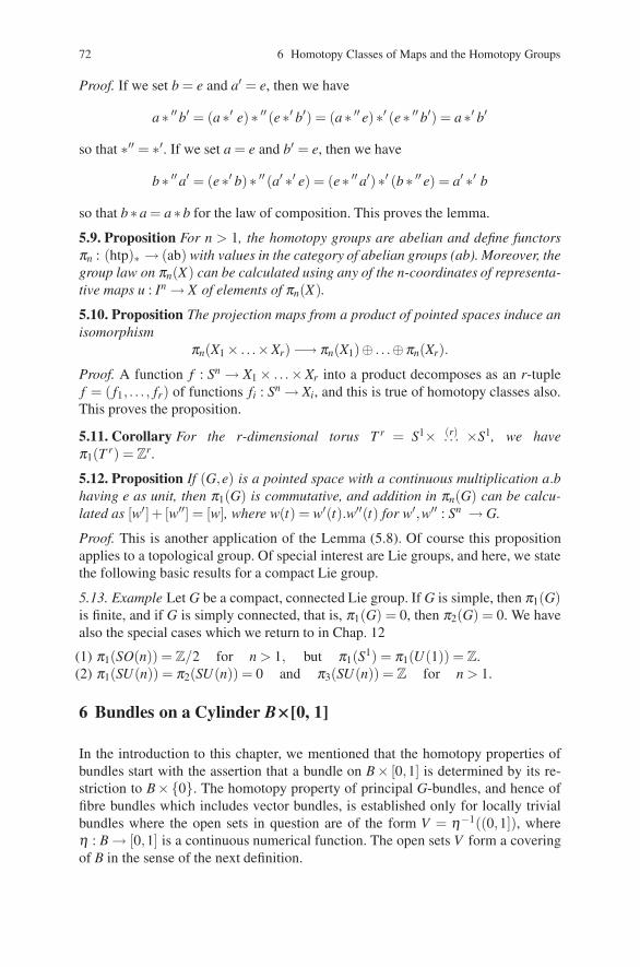
72 6 Homotopy Classes of Maps and the Homotopy Groups
Proof. If we set b = e and a′ = e, then we have
a ∗ ′′b′ = (a ∗′ e)∗ ′′ (e∗′ b′) = (a ∗ ′′ e)∗′ (e∗ ′′b′) = a ∗′ b′
so that ∗′′ = ∗′. If we set a = e and b′ = e, then we have
b ∗ ′′a′ = (e∗′ b)∗ ′′ (a′ ∗′ e) = (e∗ ′′a′)∗′ (b ∗ ′′ e) = a′ ∗′ b
so that b ∗ a = a ∗ b for the law of composition. This proves the lemma.
5.9. Proposition For n > 1, the homotopy groups are abelian and define functorsπn : (htp)∗ → (ab) with values in the category of abelian groups (ab). Moreover, thegroup law on πn(X) can be calculated using any of the n-coordinates of representa-tive maps u : In → X of elements of πn(X).
5.10. Proposition The projection maps from a product of pointed spaces induce anisomorphism
πn(X1 × . . .×Xr) −→ πn(X1)⊕ . . .⊕πn(Xr).
Proof. A function f : Sn → X1 × . . .×Xr into a product decomposes as an r-tuplef = ( f1, . . . , fr) of functions fi : Sn → Xi, and this is true of homotopy classes also.This proves the proposition.
5.11. Corollary For the r-dimensional torus T r = S1× (r). . . ×S1, we haveπ1(T r) = Z
r.
5.12. Proposition If (G,e) is a pointed space with a continuous multiplication a.bhaving e as unit, then π1(G) is commutative, and addition in πn(G) can be calcu-lated as [w′]+ [w′′] = [w], where w(t) = w′(t).w′′(t) for w′,w′′ : Sn → G.
Proof. This is another application of the Lemma (5.8). Of course this propositionapplies to a topological group. Of special interest are Lie groups, and here, we statethe following basic results for a compact Lie group.
5.13. Example Let G be a compact, connected Lie group. If G is simple, then π1(G)is finite, and if G is simply connected, that is, π1(G) = 0, then π2(G) = 0. We havealso the special cases which we return to in Chap. 12
(1) π1(SO(n)) = Z/2 for n > 1, but π1(S1) = π1(U(1)) = Z.(2) π1(SU(n)) = π2(SU(n)) = 0 and π3(SU(n)) = Z for n > 1.
6 Bundles on a Cylinder B×××[0, 1]
In the introduction to this chapter, we mentioned that the homotopy properties ofbundles start with the assertion that a bundle on B× [0,1] is determined by its re-striction to B×{0}. The homotopy property of principal G-bundles, and hence offibre bundles which includes vector bundles, is established only for locally trivialbundles where the open sets in question are of the form V = η−1((0,1]), whereη : B → [0,1] is a continuous numerical function. The open sets V form a coveringof B in the sense of the next definition.
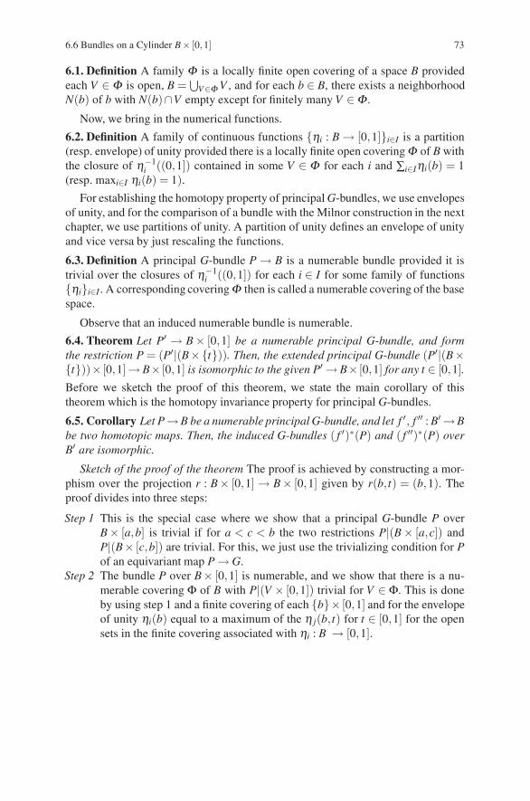
6.6 Bundles on a Cylinder B× [0,1] 73
6.1. Definition A family Φ is a locally finite open covering of a space B providedeach V ∈ Φ is open, B =
⋃V∈ΦV , and for each b ∈ B, there exists a neighborhood
N(b) of b with N(b)∩V empty except for finitely many V ∈Φ .
Now, we bring in the numerical functions.
6.2. Definition A family of continuous functions {ηi : B → [0,1]}i∈I is a partition(resp. envelope) of unity provided there is a locally finite open coveringΦ of B withthe closure of η−1
i ((0,1]) contained in some V ∈ Φ for each i and ∑i∈Iηi(b) = 1(resp. maxi∈I ηi(b) = 1).
For establishing the homotopy property of principal G-bundles, we use envelopesof unity, and for the comparison of a bundle with the Milnor construction in the nextchapter, we use partitions of unity. A partition of unity defines an envelope of unityand vice versa by just rescaling the functions.
6.3. Definition A principal G-bundle P → B is a numerable bundle provided it istrivial over the closures of η−1
i ((0,1]) for each i ∈ I for some family of functions{ηi}i∈I . A corresponding coveringΦ then is called a numerable covering of the basespace.
Observe that an induced numerable bundle is numerable.
6.4. Theorem Let P′ → B × [0,1] be a numerable principal G-bundle, and formthe restriction P = (P′|(B×{t})). Then, the extended principal G-bundle (P′|(B×{t}))× [0,1]→ B× [0,1] is isomorphic to the given P′ → B× [0,1] for any t ∈ [0,1].Before we sketch the proof of this theorem, we state the main corollary of thistheorem which is the homotopy invariance property for principal G-bundles.
6.5. Corollary Let P→B be a numerable principal G-bundle, and let f ′, f ′′ : B′ →Bbe two homotopic maps. Then, the induced G-bundles ( f ′)∗(P) and ( f ′′)∗(P) overB′ are isomorphic.
Sketch of the proof of the theorem The proof is achieved by constructing a mor-phism over the projection r : B× [0,1] → B× [0,1] given by r(b, t) = (b,1). Theproof divides into three steps:
Step 1 This is the special case where we show that a principal G-bundle P overB× [a,b] is trivial if for a < c < b the two restrictions P|(B × [a,c]) andP|(B× [c,b]) are trivial. For this, we just use the trivializing condition for Pof an equivariant map P → G.
Step 2 The bundle P over B× [0,1] is numerable, and we show that there is a nu-merable covering Φ of B with P|(V × [0,1]) trivial for V ∈ Φ. This is doneby using step 1 and a finite covering of each {b}× [0,1] and for the envelopeof unity ηi(b) equal to a maximum of the η j(b, t) for t ∈ [0,1] for the opensets in the finite covering associated with ηi : B → [0,1].
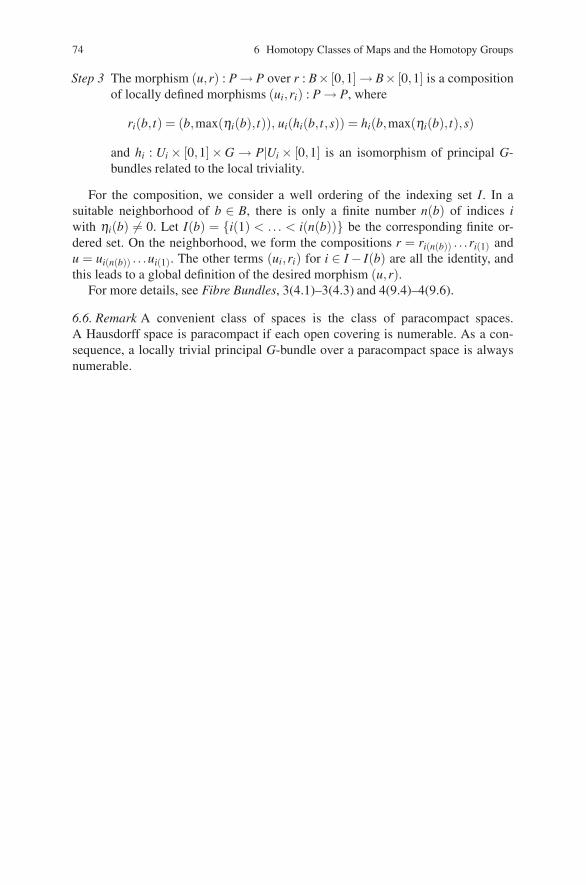
74 6 Homotopy Classes of Maps and the Homotopy Groups
Step 3 The morphism (u,r) : P → P over r : B× [0,1] → B× [0,1] is a compositionof locally defined morphisms (ui,ri) : P → P, where
ri(b, t) = (b,max(ηi(b),t)), ui(hi(b,t,s)) = hi(b,max(ηi(b), t),s)
and hi : Ui × [0,1]×G → P|Ui × [0,1] is an isomorphism of principal G-bundles related to the local triviality.
For the composition, we consider a well ordering of the indexing set I. In asuitable neighborhood of b ∈ B, there is only a finite number n(b) of indices iwith ηi(b) = 0. Let I(b) = {i(1) < .. . < i(n(b))} be the corresponding finite or-dered set. On the neighborhood, we form the compositions r = ri(n(b)) . . .ri(1) andu = ui(n(b)) . . .ui(1). The other terms (ui,ri) for i ∈ I − I(b) are all the identity, andthis leads to a global definition of the desired morphism (u,r).
For more details, see Fibre Bundles, 3(4.1)–3(4.3) and 4(9.4)–4(9.6).
6.6. Remark A convenient class of spaces is the class of paracompact spaces.A Hausdorff space is paracompact if each open covering is numerable. As a con-sequence, a locally trivial principal G-bundle over a paracompact space is alwaysnumerable.
Chapter 7The Milnor Construction: HomotopyClassification of Principal Bundles
For a given topological group G, we consider all the principal bundles. At first, itlooks like finding all principal G-bundles over a space might be a great task, butthere is a special construction of a principal G-bundle due to Milnor. It has theproperty that all other numerable principal G-bundles over all possible spaces areinduced from this particular bundle. Thus, it is called the universal principal G-bundle, and its base space is called the classifying space B(G) = BG = BG of thegroup G.
Not only do we prove that all principal G-bundles P over a space are inducedfrom the Milnor universal bundle G-bundle E(G) → B(G) over B(G), see (2.9), butthere is a homotopy uniqueness theorem which says that if two maps induce iso-morphic bundles, then the maps are homotopic to each other. This should be putside by side with the result of the previous chapter which says that homotopic mapsinduce isomorphic principal bundles. This follows from the analysis of bundles overa space of the form B× [0,1].
Main assertion The function which assigns to a homotopy class [ f ] in [B,B(G)] theisomorphism class of the principal bundle f−1(E(G)) over B is a bijection of theset [B,B(G)] onto the set of isomorphism classes of numerable principal G-bundlesover B, see (3.3).
We conclude the chapter with some specific examples of the Milnor constructionwhere the involved spaces En(G) and E(G) (to be defined in Sect. 2) are just spheres.
Chapter 4, Sect. 11–13 of Fibre Bundles (Husemoller 1994) is a reference forthis chapter.
1 Basic Data from a Numerable Principal Bundle
1.1. Remark If a principal G-bundle P → B is trivial over an open set of the formη−1((0,1]) ⊂ B, where η : B → [0,1] is a map, then we have an isomorphism ofbundles over η−1((0,1]) of the form
D. Husemoller et al.: The Milnor Construction: Homotopy Classification of Principal Bundles, Lect. Notes Phys. 726,75–81 (2008)DOI 10.1007/978-3-540-74956-1 8 © Springer-Verlag Berlin Heidelberg 2008
76 7 The Milnor Construction: Homotopy Classification of Principal Bundles
P|η−1((0,1]) −→ η−1((0,1])×G,
which we can compose with η−1((0,1])×G → (0,1]×G defined simply by (b,s)which is mapped to (η(b),s).
One way to think about the Milnor total space construction is that we wish topiece together these image spaces consisting of elements (t,s) with t > 0 and s ∈ Ginto a global object. The first step is to see how to extend (0,1]×G at t = 0 to(0,1]×G ⊂ [0,1]×G/({0}×G) by adding one point.
Now, the functions η will come from a partition of unity which is indexed by anarbitrary set. It would be useful to have control over this arbitrary set, and with thenext proposition, it is possible to always use a countable set.
1.2. Proposition Let P be a numerable principal G-bundle over a space B. Then,there exists a countable partition of unity {ηn} with P|η−1
n ((0,1]), a trivialG-bundle.
Proof. We start with a partition of unity ξi indexed by i ∈ I, I is an arbitrary set. Foreach b ∈ B, we have the finite set I(b) of i ∈ I with ξi(b) > 0, and for each finitesubset J ⊂ I, we have the open subset V (J) ⊂ B of b ∈ B with ξ j(b) > ξi(b) forall j ∈ J and i ∈ I − J. Let ξJ(b) = max{0,min j∈J,i∈I−J(ξ j(b)− ξi(b))}, and thenobserve that V (J) = ξ−1
J ((0,1]).Now, if the number of elements #
J′ = #J′′ for two distinct finite sets J′,J′′ ⊂ I, then the intersection V (J′)∩V (J′′) isempty since ξ j′(b) > ξ j′′(b) and ξ j′′(b) > ξ j′(b) cannot hold simultaneously.
Let Vm =⋃
#J=m V (J) and let ξm = ∑#J=m ξJ . Again, we have ξ−1m ((0,1]) = Vm,
and P|Vm is trivial because it is trivial over each open set V (J) in the disjoint uniongiving Vm. Finally, the desired partition of unity is
ηm(b) =ξm(b)
∑n≥0 ξn(b)
with η−1m ((0,1]) = Vm.
2 Total Space of the Milnor Construction
In order to see the natural character of the Milnor construction, we return to the localcharts of a principal bundle coming from a countable open covering as in (1.2).
2.1. Remark Let π : P → B be a principal G-bundle trivial over the open sets of acovering of the form η−1
n ((0,1]) together with isomorphisms
wn : P|η−1n ((0,1]) −→ η−1
n ((0,1])×G,
which we can compose with η−1n ((0,1])×G → (0,1]×G. The projection onto the
second factor gives maps
7.2 Total Space of the Milnor Construction 77
un : P|η−1n ((0,1]) −→ G
with un(xs) = un(x)s for x ∈ P, s ∈ G. Then, we have the relation wn(x) = (π(x),un
(x)). It is now this data (ηn,un) which we wish to assemble into the Milnor con-struction and a G-equivariant map.
Partitions of unity map the space into simplexes.
2.2. Definition The affine n-simplex An is the compact subset of Rn+1 consisting of
all t = (ti) ∈ Rn+1 satisfying t0 + . . .+ tn = 1 and ti ≥ 0.
For example, A0 is a point, A1 is a closed segment, A2 is a triangle, and A3 is atetrahedron. Singular homology is constructed by mappings of affine simplexes intoa space, while a map η : B → An corresponds to a partition of unity on B of n + 1open subsets.
2.3. Definition (Finite Case) We start with the data (ηi,ui) and over the open setWn = η−1
0 ((0,1])∪ . . .∪ η−1n ((0,1]). We form the product An ×Gn+1 and take a
quotient En(G) where elements are written as double n+1 tuples (t0 : s0, . . . ,tn : sn)with t ∈ An and each si ∈ G. The equivalence relation is the following as an equalityin En(G), where
(t ′0 : s′0, . . . ,t′n : s′n) = (t ′′0 : s′′0 , . . . ,t
′′n : s′′n)
if and only if t ′i = t ′′i , and when t ′i = t ′′i > 0, we require s′i = s′′i .In particular, when t ′i = t ′′i = 0, there is no relation between s′i and s′′i reducing to
a single point.
2.4. Principal Action We have an action En(G)×G → En(G) given by the for-mula (t0 : s0, . . . ,tn : sn)s = (t0 : s0s, . . . ,tn : sns), and this action is principal withcontinuous
τi((t ′0 : s′0, . . . ,t′n : s′n),(t
′′0 : s′′0 , . . . ,t
′′n : s′′n)) = (s′i)
−1s′′i
on the open subset where t ′i = t ′′i > 0.
2.5. Basic Assertion The data (ηi,ui), where i ≤ n, is equivalent to a mapv : P|Wn → En(G) satisfying v(xs) = v(x)s. The relation comes by looking at thecoordinates of which gives a formula for v(x), that is,
v(x) = (η0(π(x)) : u0(x), . . . ,ηn(π(x)) : un(x)).
Now, we extend the basic assertion for a finite part of the local trivializing datato the case of a countable family.
2.6. Definition (Countable Case) We start with the data (ηi,ui) and the opencovering {η−1
i ((0,1])} of B. We see that the natural inclusion of the productsAn ×Gn+1 ⊂ An+1 ×Gn+2 passes to the quotient En(G) ⊂ En+1(G) as an injection.The elements written as double n+1 tuples (t0 : s0, . . . ,tn : sn) are carried to the dou-ble n + 2 tuples (t0 : s0, . . . ,tn : sn,0 : 1) for 1 ∈ G, the identity, si ∈ G, and t ∈ An.The equivalence relation in En+1(G) induces the equivalence relation in En(G), andthe inclusion is G-equivariant.
78 7 The Milnor Construction: Homotopy Classification of Principal Bundles
2.7. Definition (Milnor Construction) The total space of the Milnor universal prin-cipal G-bundle is E(G) =
⋃0≤n En(G) with the weak topology, that is, a subset
M ⊂ E(G) is closed if and only if M ∩En(G) is closed in En(G) for each n. TheMilnor classifying space is the quotient E(G)/G = B(G).
2.8. Basic Assertion The data (ηi,ui) is equivalent to a map v : P→E(G) satisfyingv(xs) = v(x)s. The relation comes as in the finite case by looking at the coordinatesof which gives a formula for v(x), that is,
v(x) = (η0(π(x)) : u0(x), . . . ,ηn(π(x)) : un(x), . . .).
2.9. Basic Universal Property of the Milnor Construction The Milnor principalG-bundle is π : E(G) → E(G)/G. The bundle is numerable with partition of unitygiven by
ωi(t0 : s0, . . . ,tn : sn, . . .) = ti
and a principal action with translation functions
τi((t ′0 : s′0, . . . ,t′n : s′n, . . .),(t
′′0 : s′′0 , . . . ,t ′′n : s′′n , . . .)) = (s′i)
−1s′′i .
For each numerable principal G-bundle π : P → B with localizing data, (ηi,ui)gives arise to a G-equivariant map v : P → E(G) with formula v(x) = (η0(π(x)) :u0(x), . . . ,ηn(π(x)) : un(x), . . .). The map v : P → E(G) defines a quotient map f :B → B(G), and the pair (v, f ) : P → E(G) is a morphism of principalG-bundles.
Finally, we have an isomorphism P → f−1(E(G)) over B induced by v using thegeneral result 5(2.4). In particular, every numerable principal G-bundle P over B isof the form f−1(E(G)) for some map f : B → B(G). From 6(6.5), two homotopicmaps f : B → B(G) give isomorphic-induced bundles. This property holds for B(G)replaced by any space B′. In the case of maps B → B(G) the converse holds, thatis, if two maps f ′, f ′′ : B → B(G) have the property that the two induced bundlesf ′−1(E(G)) and f ′′−1(E(G)) are isomorphic, then f ′ and f ′′ are homotopic. Wesketch this in the next section.
3 Uniqueness up to Homotopy of the Classifying Map
We consider various maps B(G) → B(G) induced by G-equivalent maps E(G) →E(G).
3.1. Notation Let E(G,ev) (resp. E(G,odd)) be the subspace of E(G) consisting of(t0 : s0, . . . ,tn : sn, . . .) with t2i = 0 (resp. t2i+1 = 0). Let B(G,ev) = E(G,ev)/G ⊂B(G) and B(G,odd) = E(G,odd)/G ⊂ B(G). Now, we define hev
s : E(G) → E(G)with image E(G,ev) for s = 0 and hodd
s : E(G) → E(G) with image E(G,odd) fors = 0 such that these in turn induce the homotopies
gevs : B(G) −→ B(G) and godd
s : B(G) −→ B(G)
7.3 Uniqueness up to Homotopy of the Classifying Map 79
which for s = 0 have disjoint images, namely B(G,ev) and B(G,odd), and whichfor s = 1 are both the identity.
The details we leave to the reader who can find them in the paragraph just before4(12.3) of Fibre Bundles. These deformations are used in the following theoremwhich completes the last step in the homotopy classification theorem announced inthe introduction.
3.2. Theorem Let f ′, f ′′ : B → B(G) be maps such that the induced bundles( f ′)−1(E(G)) and ( f ′′)−1(E(G)) are isomorphic. Then, the maps f ′ and f ′′ arehomotopic.
Proof. The first step is to use the homotopies described in (3.1) to modify f ′ andf ′′ so that f ′(B) ⊂ B(G,odd) and f ′′(B) ⊂ B(G,ev). Assuming that f ′ and f ′′ havethis property, we have a principal bundle P over B and principal bundle morphisms(u′, f ′) : P → E(G,odd) ⊂ E(G) and (u′′, f ′′) : P → E(G,ev) ⊂ E(G).
Now, we define a principal G-bundle morphism (u, f ) : P× I →E(G) with f |X ×{0} = f ′ and f |X × {1} = f ′′ in order to prove the theorem. This is done by aformula for u starting with desired properties for t = 0 and t = 1 where for x ∈ P,we have from u′ and u′′ the values
u(x,0) = (t0(x) : s0(x),0,t2(x) : s2(x),0, . . .)
andu(x,1) = (0,t1(x) : s1(x),0,t3(x) : s3(x),0, . . .).
Now, prolong to u(x,t) by the formula
u(x,t) = ((1− t)t0(x) : s0(x),tt1(x) : s1,(1− t)t2(x) : s2(x), tt3(x) : s3(x), . . .).
Clearly, we have u(xs,t) = u(x,t)s for (x,t) ∈ P × [0,1] and s ∈G. Hence, theG-equivariant map u : P× [0,1]→ E(G) defines the homotopy f : B× [0,1]→B(G)with f (b,0) = f ′(b) and f (b,1) = f ′′(b). This proves the theorem.
Now, we return to the introduction of this chapter.
3.3. Main Assertion The function which assigns to a homotopy class[ f ]∈ [B,B(G)]the isomorphism class of the principal bundle f−1(E(G)) over B is a bijection of theset [B,B(G)] onto the set of isomorphism classes of numerable principal G-bundlesover B.
Proof. It is a well-defined function by 6(6.5). It is injective by (3.2), and it is sur-jective by (2.9). This proves the homotopy classification of numerable principalG-bundles in terms of the Milnor construction.
3.4. Remark Let w : G′ → G′′ be a morphism of topological groups inducing a mapBw : BG′ → BG′′ on the classifying spaces, and let B be a base space.
(a) Let P′ be the principal G′-bundle ( f ′)∗(EG′) for a map f ′ : B → BG′ into theclassifying space. The extension of P′ to the principal G′′-bundle is given by( f ′′)∗(EG′′), where f ′′ = (Bw)◦ f ′.
80 7 The Milnor Construction: Homotopy Classification of Principal Bundles
(b) A restriction of a principal G′′-bundle P′′ = ( f ′′)∗(EG′′) for f ′′ : B→ BG′′ is anyP′ = ( f ′)∗(EG′′), where (Bw)◦ f ′ and f ′′ are homotopic. In particular, extensionand restriction of structure groups of principal bundles on B is determined bythe function
[B,Bw] : [B,BG′] → [B,BG′′]
on homotopy classes of maps into classifying spaces.(c) Let w : G′ → G′′ be a morphism of topological groups inducing a map Bw :
BG′ → BG′′ on the classifying spaces. Let P′′ = ( f ′′)∗(EG′) be a principal G′′-bundle on B, where f ′′ : B → BG′′. A G′-structure on P′′ is an equivalence classof maps f ′ : B → BG′ such that (Bw) ◦ f ′ and f ′′ are homotopic. Two mapsf ′0, f ′1 : B → BG′ are equivalent provided there is a homotopy ht : B → BG′ withh0 = f ′0, h1 = f ′1, and (Bw)◦ ht = (Bw)◦ f ′0 for all t ∈ [0,1].
4 The Infinite Sphere as the Total Space of the MilnorConstruction
4.1. Unit Sphere in the Real Numbers The zero dimensional sphere S0 is thespace of t ∈ R = R
1 with |t | = 1, that is, S0 = {+1,−1}, and under multiplicationof these two real numbers, it is the group of two elements. Every x ∈ R is of theform x = r(±1) for some r ≥ 0, and for x = 0, the strictly positive r is unique and isthe absolute value |x | = r.
4.2. Unit Sphere in the Complex Numbers The one-dimensional sphere S1 is thespace of z ∈ C = R
2 with |z | = 1, that is, S1 = {e2π it : t ∈ [0,1]} the circle of anglest. Under multiplication of complex numbers, it is a group called the circle group.
There is one more sphere which is the topological group of numbers in a numbersystem, and this is S3, the group of unit quaternions.
4.3. Quaternions The skew field H of quaternions is given by H = R1⊕Ri ⊕R j ⊕Rk, where the basis elements i, j,k of the quaternions satisfy the relationsi2 = j2 = k2 = −1 and
i j = k = − ji, jk = i = −k j, and ki = j = −ik.
We can write H = C⊕C j with k = i j and multiplication given by z j = jz for z ∈ C
and z = x− iy the complex conjugate of z = x + iy. For a quaternion q = a + bi +c j + d j, the quaternion conjugate is given by q = a−bi− c j−dk. It has propertiessimilar to the complex conjugate, namely qq = a2 +b2 +c2 +d2 is the norm squared|q |2 = qq and q = q. Moreover, quaternionic conjugation is antimultiplicative, thatis, one has q′q′′ = q′′ q′.
4.4. Unit Sphere in the Quaternions The three-dimensional sphere can be para-metrized by the unit quaternions q ∈ H so with |q | = 1. Moreover, under
References 81
quaternionic multiplication, it is a topological group isomorphic to SU(2). Everyq ∈ H is of the form q = |q |u, where u ∈ S3 is a unit quaternion.
Now, we show how to view certain spheres as the total space in the Milnor con-struction in a very concrete way.
4.5. Spheres as En(G) and Infinite Spheres as E(G)
(a) (Real case) For a point (x0, . . . ,xm−1) ∈ Sm−1, we introduce ti = x2i and si = +1
if xi ≥ 0 and si = −1 if xi < 0. Then, the map from (x0, . . . ,xm−1) ∈ Sm−1 to (t0 :s0, . . . ,tm−1 : sm−1) ∈ Em−1({±1}) is a topological isomorphism, and with thesame formulas, we have a topological isomorphism S∞ → E({±1}), where S∞
is the increasing union⋃
n Sn with the inductive limit topology. These mappingsare S0 or {±1}-equivariant.
(b) (Complex case) For a point (z0, . . . ,zm−1) ∈ S2m−1, we introduce ti = |zi |2 andsi = zi/|zi |. Then, the map from (z0, . . . ,zm−1) ∈ S2m−1 to (t0 : s0, . . . ,tm−1 :sm−1) ∈ Em−1(S1) is a topological isomorphism, and with the same formu-las, we have a topological isomorphism S∞ → E(S1). These mappings areS1-equivariant.
(c) (Quaternionic case) For a point (q0, . . . ,qm−1) ∈ S4m−1, we introduce ti = |qi |2and si = qi/|qi |. Then, the map from (q0, . . . ,qm−1)∈ S4m−1 to (t0 : s0, . . . ,tm−1 :sm−1) ∈ Em−1(S3) is a topological isomorphism, and with the same formu-las, we have a topological isomorphism S∞ → E(S3). These mappings are S3-equivariant.
4.6. Other Constructions of B(G) There are other constructions of a numerableprincipal G-bundle E(G) → B(G) with the key property that E(G) is contractible,and hence, by a theorem of Steenrod (1951, Sect. 19), it can be used to induceand classify up to isomorphism numerable principal G-bundles. In particular, therealso is the construction of a classifying space BG which is functorial for groupmorphisms G′ → G′′ in all cases and which in contrast to the Milnor constructionhas the property that the projections G′ ×G′′ → G′ and G′ ×G′′ → G′′ induce ahomeomorphism B(G′ ×G′′) = B(G′)×B(G′′). If G is an abelian group, then thegroup law G×G→G is a morphism of groups and induces a map B(G×G) = B(G)which when composed with the inverse of the product isomorphism gives an abeliangroup structure B(G)×B(G) = B(G), and then the classifying space constructioncan be iterated to obtain Bn(G) = B(Bn−1) inductively.
References
Husemoller, D.: Fibre Bundles, 3rd ed. Springer-Verlag, New York (1994)Steenrod, N.E.: Topology of Fibre Bundles. Princeton University Press, Princeton, NJ (1951)

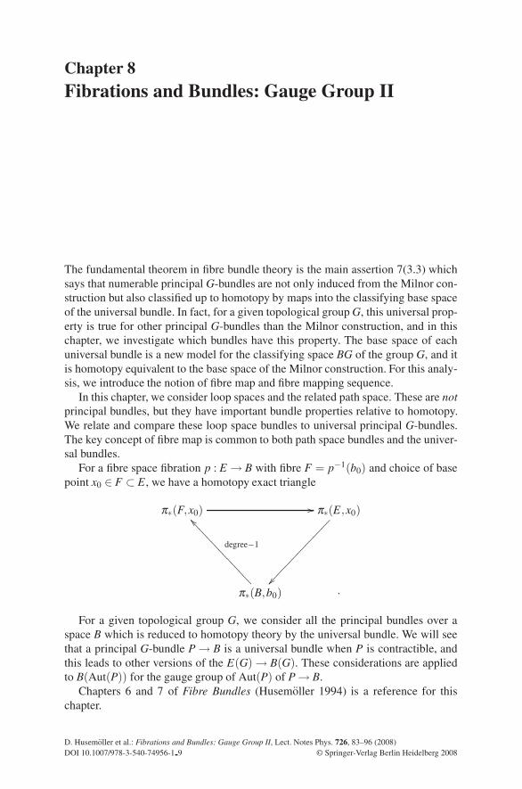
Chapter 8Fibrations and Bundles: Gauge Group II
The fundamental theorem in fibre bundle theory is the main assertion 7(3.3) whichsays that numerable principal G-bundles are not only induced from the Milnor con-struction but also classified up to homotopy by maps into the classifying base spaceof the universal bundle. In fact, for a given topological group G, this universal prop-erty is true for other principal G-bundles than the Milnor construction, and in thischapter, we investigate which bundles have this property. The base space of eachuniversal bundle is a new model for the classifying space BG of the group G, and itis homotopy equivalent to the base space of the Milnor construction. For this analy-sis, we introduce the notion of fibre map and fibre mapping sequence.
In this chapter, we consider loop spaces and the related path space. These are notprincipal bundles, but they have important bundle properties relative to homotopy.We relate and compare these loop space bundles to universal principal G-bundles.The key concept of fibre map is common to both path space bundles and the univer-sal bundles.
For a fibre space fibration p : E → B with fibre F = p−1(b0) and choice of basepoint x0 ∈ F ⊂ E , we have a homotopy exact triangle
π∗(F,x0) �� π∗(E,x0)
�����������������
π∗(B,b0)
degree−1
���������������.
For a given topological group G, we consider all the principal bundles over aspace B which is reduced to homotopy theory by the universal bundle. We will seethat a principal G-bundle P → B is a universal bundle when P is contractible, andthis leads to other versions of the E(G) → B(G). These considerations are appliedto B(Aut(P)) for the gauge group of Aut(P) of P → B.
Chapters 6 and 7 of Fibre Bundles (Husemoller 1994) is a reference for thischapter.
D. Husemoller et al.: Fibrations and Bundles: Gauge Group II, Lect. Notes Phys. 726, 83–96 (2008)DOI 10.1007/978-3-540-74956-1 9 © Springer-Verlag Berlin Heidelberg 2008
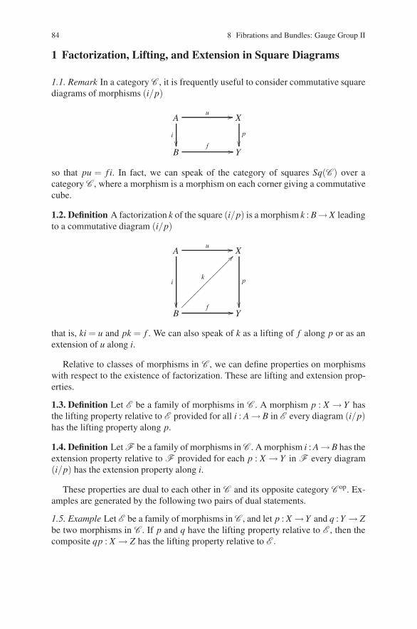
84 8 Fibrations and Bundles: Gauge Group II
1 Factorization, Lifting, and Extension in Square Diagrams
1.1. Remark In a category C , it is frequently useful to consider commutative squarediagrams of morphisms (i/p)
A
i��
u �� X
p
��B
f �� Y
so that pu = f i. In fact, we can speak of the category of squares Sq(C ) over acategory C , where a morphism is a morphism on each corner giving a commutativecube.
1.2. Definition A factorization k of the square (i/p) is a morphism k : B→X leadingto a commutative diagram (i/p)
A
i
��
u �� X
p
��B
k
���������������� f �� Y
that is, ki = u and pk = f . We can also speak of k as a lifting of f along p or as anextension of u along i.
Relative to classes of morphisms in C , we can define properties on morphismswith respect to the existence of factorization. These are lifting and extension prop-erties.
1.3. Definition Let E be a family of morphisms in C . A morphism p : X → Y hasthe lifting property relative to E provided for all i : A → B in E every diagram (i/p)has the lifting property along p.
1.4. Definition Let F be a family of morphisms in C . A morphism i : A→B has theextension property relative to F provided for each p : X → Y in F every diagram(i/p) has the extension property along i.
These properties are dual to each other in C and its opposite category C op. Ex-amples are generated by the following two pairs of dual statements.
1.5. Example Let E be a family of morphisms in C , and let p : X →Y and q : Y → Zbe two morphisms in C . If p and q have the lifting property relative to E , then thecomposite qp : X → Z has the lifting property relative to E .
8.2 Fibrations and Cofibrations 85
1.6. Example Let F be a family of morphisms in C , and let i : A → B and j : B →Cbe two morphisms in C . If i and j have the extension property relative to F , thenthe composite ji : A →C has the extension property relative to F .
1.7. Example Let E be a family of morphisms in C , and let p : X →Y be a morphismwith the lifting property relative to E . If Y ′ → Y is any morphism in C , then theinduced morphism
p′ : X ′ = Y ′ ×Y X −→ Y ′
has the lifting property relative to E . Recall that the induced morphism is the pro-jection from the fibre product to the first factor.
1.8. Example Let F be a family of morphisms in C , and let i : A→B be a morphismwith the extension property relative to F . If A → A′ is any morphism in C , then thecoinduced morphism
i′ : A′ −→ B′ = A′�AB
has the extension property relative to F . Recall that the coinduced morphism is theinjection into the cofibre coproduct of the first factor.
1.9. Remark We will apply these general lifting properties to homotopy theory.This was first done by Quillen in LN 43 where he presented an axiomatic ver-sion of homotopy theory which seems to be the most promising approach to anaxiomatic version of homotopy theory. This has become especially clear in recentyears.
2 Fibrations and Cofibrations
Now, we use the elementary factorization formalism of the previous section to de-scribe fibrations, also called fibre maps, and cofibrations, also called cofibre maps.For this, we need the classes E of elementary cofibrations and F of elementaryfibrations.
2.1. Definition The elementary fibration associated with any space Y is the mapε : Map([0,1],Y )→Y given by evaluation ε(γ) = γ(0) for a path γ ∈ Map([0,1],Y ).The elementary cofibration associated with any space A is the map β : A→ A× [0,1]given by inclusion β (a) = (a,0) on the bottom of the cylinder over A.
2.2. Definition A map p : X → Y is a fibration provided any square (β/p) with anyelementary cofibration β : A → A× [0,1] has the lifting property along p. A mapi : A → B is a cofibration provided any square (i/ε) with any elementary fibrationε : Map([0,1],Y ) → Y has the extension property along i.
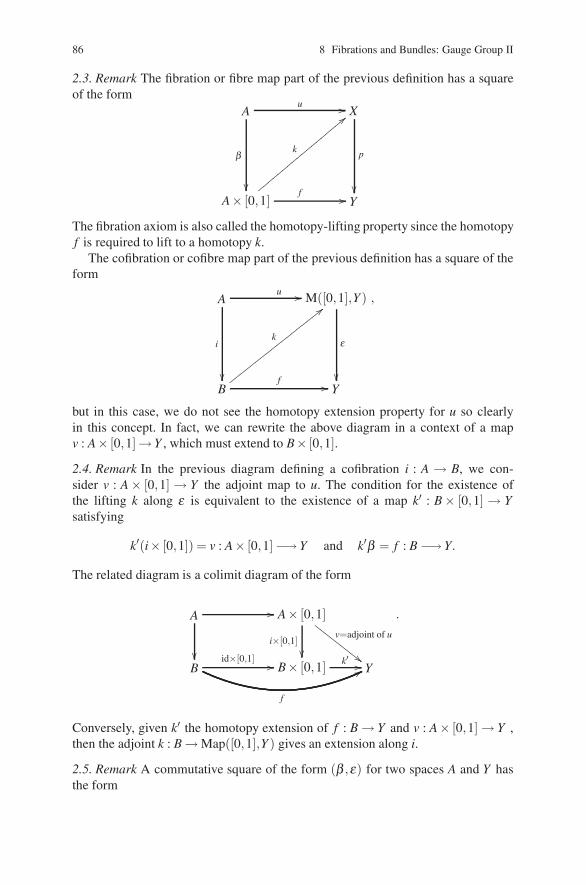
86 8 Fibrations and Bundles: Gauge Group II
2.3. Remark The fibration or fibre map part of the previous definition has a squareof the form
A
β
��
u �� X
p
��A× [0,1]
k
�������������������� f �� Y
The fibration axiom is also called the homotopy-lifting property since the homotopyf is required to lift to a homotopy k.
The cofibration or cofibre map part of the previous definition has a square of theform
A
i
��
u �� M([0,1],Y )
ε
��B
k
�������������������� f �� Y
,
but in this case, we do not see the homotopy extension property for u so clearlyin this concept. In fact, we can rewrite the above diagram in a context of a mapv : A× [0,1]→ Y , which must extend to B× [0,1].
2.4. Remark In the previous diagram defining a cofibration i : A → B, we con-sider v : A × [0,1] → Y the adjoint map to u. The condition for the existence ofthe lifting k along ε is equivalent to the existence of a map k′ : B × [0,1] → Ysatisfying
k′(i× [0,1]) = v : A× [0,1]−→ Y and k′β = f : B −→ Y.
The related diagram is a colimit diagram of the form
A
��
�� A× [0,1]
i×[0,1]��
v=adjoint of u
��
B
f
id×[0,1] �� B× [0,1] k′ �� Y
.
Conversely, given k′ the homotopy extension of f : B → Y and v : A× [0,1] → Y ,then the adjoint k : B → Map([0,1],Y ) gives an extension along i.
2.5. Remark A commutative square of the form (β ,ε) for two spaces A and Y hasthe form
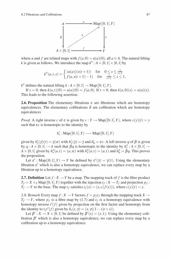
8.2 Fibrations and Cofibrations 87
A
β
��
u �� Map([0,1],Y )
ε
��A× [0,1]
k
�� f �� Y
where u and f are related maps with f (a,0) = u(a)(0), all a ∈ A. The natural liftingk is given as follows. We introduce the map k′′ : A× [0,1]× [0,1] by
k′′(a,t,s) ={
(u(a))(s(t + 1)) for 0 ≤ s ≤ 1t+1
f (a,s(t + 1)−1) for 1t+1 ≤ s ≤ 1,
k′′ defines the natural lifting k : A× [0,1]→ Map([0,1],Y ).If s = 0, then k(a,t)(0) = u(a)(0) = f (a,0). If t = 0, then k(a,0)(s) = u(a)(s).
This leads to the following assertion.
2.6. Proposition The elementary fibrations ε are fibrations which are homotopyequivalences. The elementary cofibrations δ are cofibration which are homotopyequivalences
Proof. A right inverse c of ε is given by c : Y → Map([0,1],Y ), where c(y)(t) = ysuch that εc is homotopic to the identity by
h′s : Map([0,1],Y ) −→ Map([0,1],Y )
given by h′s(γ)(t) = γ(st) with h′1(γ) = γ and h′0 = εc. A left inverse q of β is givenby q : A× [0,1] → A such that βq is homotopic to the identity by h′′s : A× [0,1] →A× [0,1] given by h′′s (a,t) = (a,st) with h′′1(a,t) = (a, t) and h′′0 = βq. This provesthe proposition.
Let ε ′ : Map([0,1],Y ) → Y be defined by ε ′(γ) = γ(1). Using the elementaryfibration ε ′ which is also a homotopy equivalence, we can replace every map by afibration up to a homotopy equivalence.
2.7. Definition Let f : X → Y be a map. The mapping track of f is the fibre productTf = X ×Y Map([0,1],Y ) together with the injection t f : X → Tf and projection p f :Tf → Y to the base. The map t f satisfies t f (x) = (x,c( f (x))), where c(y)(t) = y.
2.8. Remark Every map f : X →Y factors f = p f t f through the mapping track X →Tf → Y , where p f is a fibre map by (1.7) and t f is a homotopy equivalence withhomotopy inverse t ′( f ) given by projection on the first factor and homotopy fromthe identity to t f t ′( f ) given by hs(x,γ) = (x,γ((1− s)t + s)).
Let β ′ : X → X × [0,1] be defined by β ′(x) = (x,1). Using the elementary cofi-bration β ′ which is also a homotopy equivalence, we can replace every map by acofibration up to a homotopy equivalence.
88 8 Fibrations and Bundles: Gauge Group II
2.9. Definition Let f : X →Y be a map. The mapping cylinder of f is the cofibre co-product Mf =Y �X X × [0,1] together with the injection q f : X → Mf and projectionm f : Mf → Y to the factor Y . The map q f (x) = f (x) = (x,1) in Mf .
2.10. Remark Every map f : X →Y factors f = m f q f through the mapping cylinderX → Tf → Y , where q f is a cofibre map by (1.8) and m f is a homotopy equivalencewith homotopy inverse m′( f )(y) = y in the first summand of the cofibre coproductand homotopy defined by
hs(y) = y and hs(x,t) = (x,(1− s)t + s).
At s = 0, it is the identity and h1 = m′( f )m f .
2.11. Remark There are essentially two versions of the definition of fibre maps orfibration. The first is due to Hurewicz, where the lifting property is required for allelementary β : A → A× [0,1]. The second is due to Serre, where the lifting propertyis required only for all finite complexes A or equivalently all n-cubes A = [0,1]n.
3 Fibres and Cofibres: Loop Space and Suspension
The definition of fibration and cofibration do not refer to base points, and the same istrue of the replacement of f : X →Y by a fibre map p f : Tf →Y or by a cofibre mapq f : X → Mf . Now base points arise naturally when we consider fibres and cofibresof a map.
3.1. Definition Let f : X → Y be a map. For each y ∈Y , the fibre of f over y ∈ Y isthe subspace Xy = f−1(y) → X with inclusion in X . The cofibre of f is the quotientspace Y/ f (X), where the image f (X) in Y is reduced to a point. When f : X → Y isbase point preserving, the fibre F of f is defined to be the fibre over the base pointof Y with base point from X . When f is base point preserving, the base point of thecofibre C = Y/ f (X) is the class of f (X) in the cofibre C. There are two three termsequences which we wish to study
F → Xf−→ Y and X
f−→ Y →C.
Fibres are related to fibrations and cofibres to cofibrations by the following exact-ness properties.
3.2. Theorem Let F → X be the fibre of a pointed fibre map f : X → Y . For eachpointed space T , we have an exact sequence of pointed sets
[T,F]∗ −→ [T,X ]∗ −→ [T,Y ]∗.
When the space T is a finite complex like a sphere, then the assertion holds alsofor a Serre fibration.
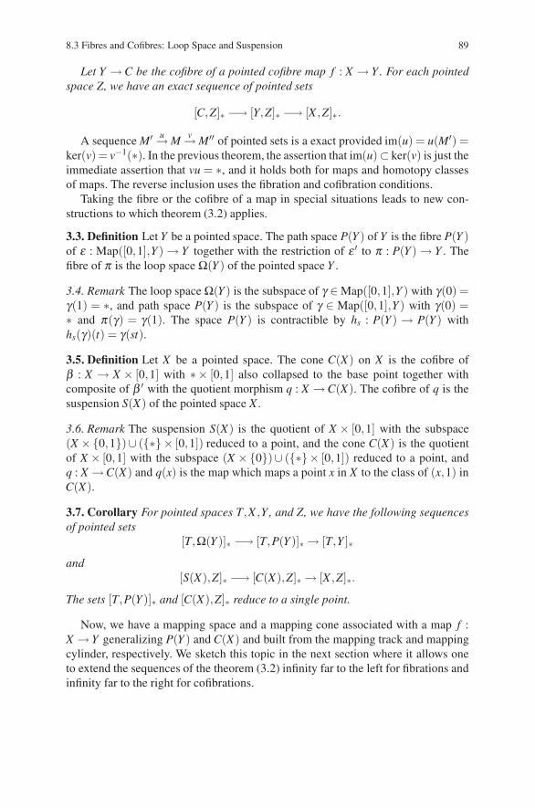
8.3 Fibres and Cofibres: Loop Space and Suspension 89
Let Y → C be the cofibre of a pointed cofibre map f : X → Y. For each pointedspace Z, we have an exact sequence of pointed sets
[C,Z]∗ −→ [Y,Z]∗ −→ [X ,Z]∗.
A sequence M′ u→ Mv→ M′′ of pointed sets is a exact provided im(u) = u(M′) =
ker(v) = v−1(∗). In the previous theorem, the assertion that im(u)⊂ ker(v) is just theimmediate assertion that vu = ∗, and it holds both for maps and homotopy classesof maps. The reverse inclusion uses the fibration and cofibration conditions.
Taking the fibre or the cofibre of a map in special situations leads to new con-structions to which theorem (3.2) applies.
3.3. Definition Let Y be a pointed space. The path space P(Y ) of Y is the fibre P(Y )of ε : Map([0,1],Y ) → Y together with the restriction of ε ′ to π : P(Y ) → Y . Thefibre of π is the loop space Ω(Y ) of the pointed space Y .
3.4. Remark The loop space Ω(Y ) is the subspace of γ ∈ Map([0,1],Y ) with γ(0) =γ(1) = ∗, and path space P(Y ) is the subspace of γ ∈ Map([0,1],Y ) with γ(0) =∗ and π(γ) = γ(1). The space P(Y ) is contractible by hs : P(Y ) → P(Y ) withhs(γ)(t) = γ(st).
3.5. Definition Let X be a pointed space. The cone C(X) on X is the cofibre ofβ : X → X × [0,1] with ∗× [0,1] also collapsed to the base point together withcomposite of β ′ with the quotient morphism q : X → C(X). The cofibre of q is thesuspension S(X) of the pointed space X .
3.6. Remark The suspension S(X) is the quotient of X × [0,1] with the subspace(X ×{0,1})∪ ({∗}× [0,1]) reduced to a point, and the cone C(X) is the quotientof X × [0,1] with the subspace (X ×{0})∪ ({∗}× [0,1]) reduced to a point, andq : X →C(X) and q(x) is the map which maps a point x in X to the class of (x,1) inC(X).
3.7. Corollary For pointed spaces T,X ,Y, and Z, we have the following sequencesof pointed sets
[T,Ω(Y )]∗ −→ [T,P(Y )]∗ → [T,Y ]∗
and[S(X),Z]∗ −→ [C(X),Z]∗ → [X ,Z]∗.
The sets [T,P(Y )]∗ and [C(X),Z]∗ reduce to a single point.
Now, we have a mapping space and a mapping cone associated with a map f :X → Y generalizing P(Y ) and C(X) and built from the mapping track and mappingcylinder, respectively. We sketch this topic in the next section where it allows oneto extend the sequences of the theorem (3.2) infinity far to the left for fibrations andinfinity far to the right for cofibrations.
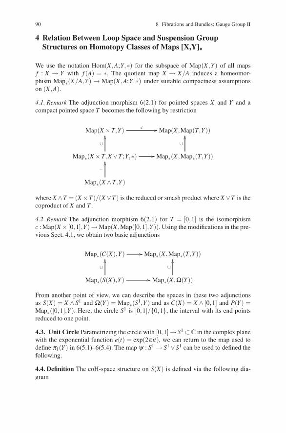
90 8 Fibrations and Bundles: Gauge Group II
4 Relation Between Loop Space and Suspension GroupStructures on Homotopy Classes of Maps [X,Y]∗∗∗
We use the notation Hom(X ,A;Y,∗) for the subspace of Map(X ,Y ) of all mapsf : X → Y with f (A) = ∗. The quotient map X → X/A induces a homeomor-phism Map∗(X/A,Y ) → Map(X ,A;Y,∗) under suitable compactness assumptionson (X ,A).
4.1. Remark The adjunction morphism 6(2.1) for pointed spaces X and Y and acompact pointed space T becomes the following by restriction
Map(X ×T,Y ) c �� Map(X ,Map(T,Y ))
Map∗(X ×T,X ∨T ;Y,∗) ��
∪��
Map∗(X ,Map∗(T,Y ))
∪��
Map∗(X ∧T,Y )
=
��
where X ∧T = (X ×T )/(X ∨T ) is the reduced or smash product where X ∨T is thecoproduct of X and T .
4.2. Remark The adjunction morphism 6(2.1) for T = [0,1] is the isomorphismc : Map(X × [0,1],Y)→ Map(X ,Map([0,1],Y )). Using the modifications in the pre-vious Sect. 4.1, we obtain two basic adjunctions
Map∗(C(X),Y ) �� Map∗(X ,Map∗(T,Y ))
Map∗(S(X),Y )
∪��
�� Map∗(X ,Ω(Y ))
∪��
From another point of view, we can describe the spaces in these two adjunctionsas S(X) = X ∧ S1 and Ω(Y ) = Map∗(S1,Y ) and as C(X) = X ∧ [0,1] and P(Y ) =Map∗([0,1],Y ). Here, the circle S1 is [0,1]/{0,1}, the interval with its end pointsreduced to one point.
4.3. Unit Circle Parametrizing the circle with [0,1]→ S1 ⊂C in the complex planewith the exponential function e(t) = exp(2π it), we can return to the map used todefine π1(Y ) in 6(5.1)–6(5.4). The map ψ : S1 → S1 ∨S1 can be used to defined thefollowing.
4.4. Definition The coH-space structure on S(X) is defined via the following dia-gram
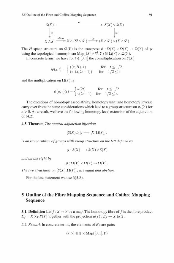
8.5 Outline of the Fibre and Cofibre Mapping Sequence 91
S(X)ψ ��
∼=��
S(X)∨S(X)
∼=��
X ∧S1id∧ψ �� X ∧ (S1 ∨S1)
∼= �� (X ∧S1)∨ (X ∧S1)
The H-space structure on Ω(Y ) is the transpose φ : Ω(Y )×Ω(Y ) → Ω(Y ) of ψusing the topological isomorphism Map∗(S1 ∨S1,Y ) ∼=Ω(Y )×Ω(Y ).
In concrete terms, we have for t ∈ [0,1] the comultiplication on S(X)
ψ(x,t) ={
((x,2t),∗) for t ≤ 1/2(∗,(x,2t −1)) for 1/2 ≤ t
and the multiplication on Ω(Y ) is
φ(u,v)(t) ={
u(2t) for t ≤ 1/2v(2t −1) for 1/2 ≤ t.
The questions of homotopy associativity, homotopy unit, and homotopy inversecarry over from the same considerations which lead to a group structure on πn(Y ) forn > 0. As a result, we have the following homotopy level extension of the adjunctionof (4.2).
4.5. Theorem The natural adjunction bijection
[S(X),Y ]∗ −→ [X ,Ω(Y )]∗
is an isomorphism of groups with group structure on the left defined by
ψ : S(X)−→ S(X)∨S(X)
and on the right byφ :Ω(Y )×Ω(Y) →Ω(Y ) .
The two structures on [S(X),Ω(Y)]∗ are equal and abelian.
For the last statement we use 6(5.8).
5 Outline of the Fibre Mapping Sequence and Cofibre MappingSequence
5.1. Definition Let f : X →Y be a map. The homotopy fibre of f is the fibre productE f = X ×Y P(Y ) together with the projection a( f ) : E f → X to X .
5.2. Remark In concrete terms, the elements of E f are pairs
(x,γ) ∈ X ×Map([0,1],Y )
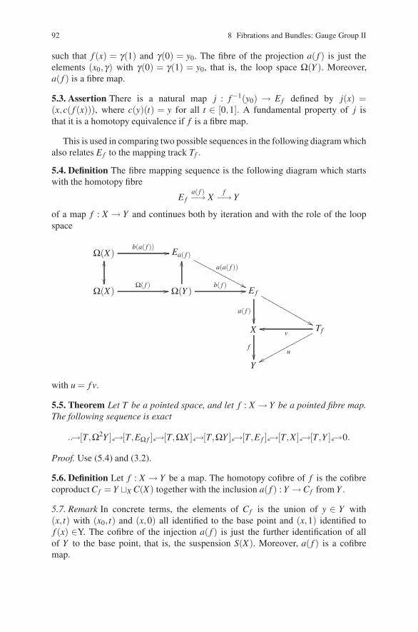
92 8 Fibrations and Bundles: Gauge Group II
such that f (x) = γ(1) and γ(0) = y0. The fibre of the projection a( f ) is just theelements (x0,γ) with γ(0) = γ(1) = y0, that is, the loop space Ω(Y ). Moreover,a( f ) is a fibre map.
5.3. Assertion There is a natural map j : f−1(y0) → E f defined by j(x) =(x,c( f (x))), where c(y)(t) = y for all t ∈ [0,1]. A fundamental property of j isthat it is a homotopy equivalence if f is a fibre map.
This is used in comparing two possible sequences in the following diagram whichalso relates E f to the mapping track Tf .
5.4. Definition The fibre mapping sequence is the following diagram which startswith the homotopy fibre
E fa( f )−→ X
f−→ Y
of a map f : X → Y and continues both by iteration and with the role of the loopspace
Ω(X)��
��
b(a( f )) �� Ea( f )
a(a( f ))
�������
������
��
Ω(X)Ω( f ) �� Ω(Y )
��
b( f ) �� E f
�������
������
��
a( f )��
X
f
��
Tfv��
u��
Y
with u = f v.
5.5. Theorem Let T be a pointed space, and let f : X → Y be a pointed fibre map.The following sequence is exact
..→[T,Ω2Y ]∗→[T,EΩ f ]∗→[T,ΩX ]∗→[T,ΩY ]∗→[T,E f ]∗→[T,X ]∗→[T,Y ]∗→0.
Proof. Use (5.4) and (3.2).
5.6. Definition Let f : X → Y be a map. The homotopy cofibre of f is the cofibrecoproduct Cf = Y �X C(X) together with the inclusion a( f ) : Y →Cf from Y .
5.7. Remark In concrete terms, the elements of Cf is the union of y ∈ Y with(x,t) with (x0,t) and (x,0) all identified to the base point and (x,1) identified tof (x) ∈Y. The cofibre of the injection a( f ) is just the further identification of allof Y to the base point, that is, the suspension S(X). Moreover, a( f ) is a cofibremap.
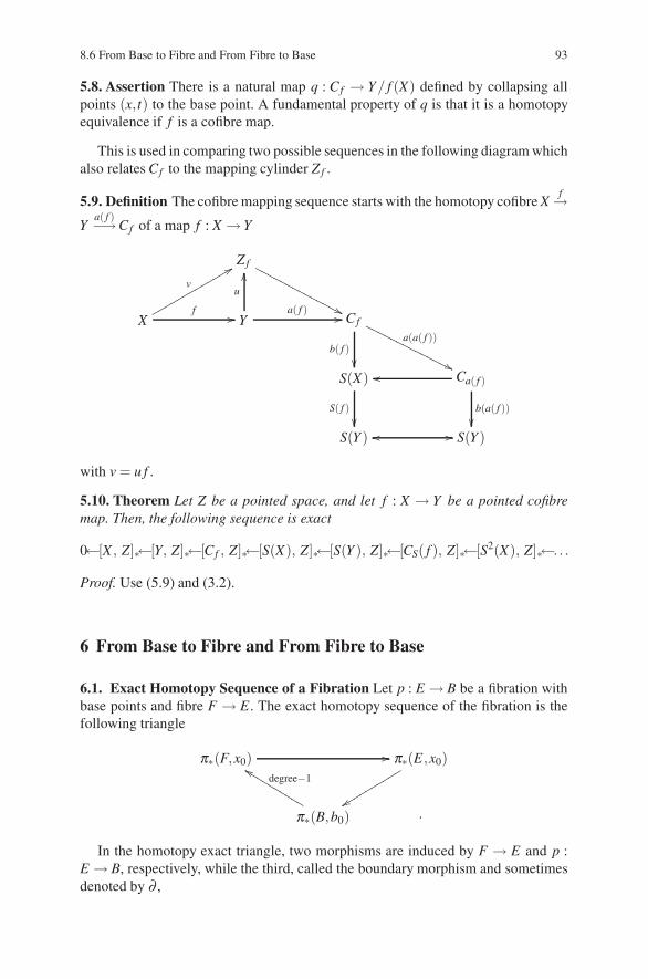
8.6 From Base to Fibre and From Fibre to Base 93
5.8. Assertion There is a natural map q : Cf → Y/ f (X) defined by collapsing allpoints (x, t) to the base point. A fundamental property of q is that it is a homotopyequivalence if f is a cofibre map.
This is used in comparing two possible sequences in the following diagram whichalso relates Cf to the mapping cylinder Zf .
5.9. Definition The cofibre mapping sequence starts with the homotopy cofibre Xf→
Ya( f )−→Cf of a map f : X → Y
Zf
�������
������
���
X
v
��������������� f �� Y
u
��
a( f ) �� Cf
b( f )��
a(a( f ))
�������
������
���
S(X)
S( f )��
Ca( f )��
b(a( f ))��
S(Y ) �� �� S(Y )
with v = u f .
5.10. Theorem Let Z be a pointed space, and let f : X → Y be a pointed cofibremap. Then, the following sequence is exact
0←[X , Z]∗←[Y, Z]∗←[Cf , Z]∗←[S(X), Z]∗←[S(Y ), Z]∗←[CS( f ), Z]∗←[S2(X), Z]∗←. . .
Proof. Use (5.9) and (3.2).
6 From Base to Fibre and From Fibre to Base
6.1. Exact Homotopy Sequence of a Fibration Let p : E → B be a fibration withbase points and fibre F → E . The exact homotopy sequence of the fibration is thefollowing triangle
π∗(F,x0) �� π∗(E,x0)
��������
����
π∗(B,b0)
degree−1������������
.
In the homotopy exact triangle, two morphisms are induced by F → E and p :E → B, respectively, while the third, called the boundary morphism and sometimesdenoted by ∂ ,
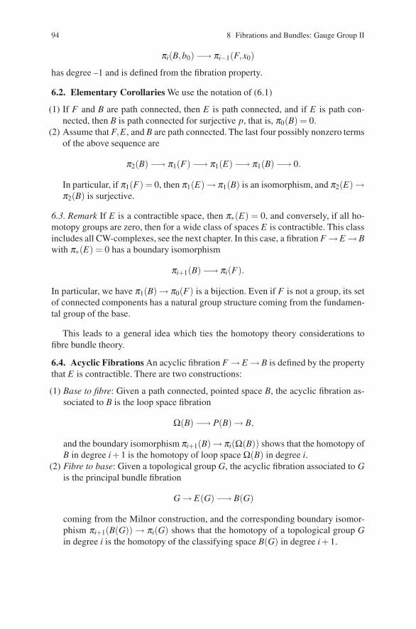
94 8 Fibrations and Bundles: Gauge Group II
πi(B,b0) −→ πi−1(F,x0)
has degree –1 and is defined from the fibration property.
6.2. Elementary Corollaries We use the notation of (6.1)
(1) If F and B are path connected, then E is path connected, and if E is path con-nected, then B is path connected for surjective p, that is, π0(B) = 0.
(2) Assume that F,E , and B are path connected. The last four possibly nonzero termsof the above sequence are
π2(B) −→ π1(F) −→ π1(E) −→ π1(B) −→ 0.
In particular, if π1(F) = 0, then π1(E)→ π1(B) is an isomorphism, and π2(E)→π2(B) is surjective.
6.3. Remark If E is a contractible space, then π∗(E) = 0, and conversely, if all ho-motopy groups are zero, then for a wide class of spaces E is contractible. This classincludes all CW-complexes, see the next chapter. In this case, a fibration F →E →Bwith π∗(E) = 0 has a boundary isomorphism
πi+1(B) −→ πi(F).
In particular, we have π1(B) → π0(F) is a bijection. Even if F is not a group, its setof connected components has a natural group structure coming from the fundamen-tal group of the base.
This leads to a general idea which ties the homotopy theory considerations tofibre bundle theory.
6.4. Acyclic Fibrations An acyclic fibration F → E → B is defined by the propertythat E is contractible. There are two constructions:
(1) Base to fibre: Given a path connected, pointed space B, the acyclic fibration as-sociated to B is the loop space fibration
Ω(B) −→ P(B) → B,
and the boundary isomorphism πi+1(B)→ πi(Ω(B)) shows that the homotopy ofB in degree i+ 1 is the homotopy of loop space Ω(B) in degree i.
(2) Fibre to base: Given a topological group G, the acyclic fibration associated to Gis the principal bundle fibration
G → E(G) −→ B(G)
coming from the Milnor construction, and the corresponding boundary isomor-phism πi+1(B(G)) → πi(G) shows that the homotopy of a topological group Gin degree i is the homotopy of the classifying space B(G) in degree i+ 1.
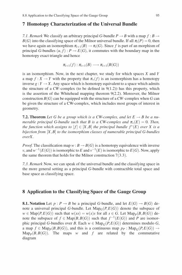
8.8 Application to the Classifying Space of the Gauge Group 95
7 Homotopy Characterization of the Universal Bundle
7.1. Remark We classify an arbitrary principal G-bundle P → B with a map f : B →B(G) into the classifying space of the Milnor universal bundle. If all πi(P) = 0, thenwe have again an isomorphism πi+1(B) → πi(G). Since f is part of an morphism ofprincipal G-bundles (u, f ) : P → E(G), it commutes with the boundary map in thehomotopy exact triangle and hence
πi+1( f ) : πi+1(B) −→ πi+1(B(G))
is an isomorphism. Now, in the next chapter, we study for which spaces X and Ya map f : X → Y with the property that π∗( f ) is an isomorphism has a homotopyinverse g : Y → X . Any space which is homotopy equivalent to a space which admitsthe structure of a CW -complex (to be defined in 9(1.2)) has this property, whichis the assertion of the Whitehead mapping theorem 9(2.2). Moreover, the Milnorconstruction B(G) can be equipped with the structure of a CW -complex when G canbe given the structure of a CW-complex, which includes most groups of interest ingeometry.
7.2. Theorem Let G be a group which is a CW-complex, and let E → B be a nu-merable principal G-bundle such that B is a CW-complex and π∗(E) = 0. Then,the function which assigns to [ f ] ∈ [X ,B] the principal bundle f ∗(E) over X is abijection from [X ,B] to the isomorphism classes of numerable principal G-bundlesoverX.
Proof. The classification map w : B → B(G) is a homotopy equivalence with inversev, and w−1(E(G)) is isomorphic to E and v−1(E) is isomorphic to E(G). Now, applythe same theorem that holds for the Milnor construction 7(3.3).
7.3. Remark Now, we can speak of the universal bundle and the classifying space inthe more general setting as a principal G-bundle with contractible total space andbase space as classifying space.
8 Application to the Classifying Space of the Gauge Group
8.1. Notation Let p : P → B be a principal G-bundle, and let E(G) → B(G) de-note a universal principal G-bundle. Let MapG(P,E(G)) denote the subspace ofw ∈ Map(P,E(G)) such that w(xs) = w(x)s for all s ∈ G. Let MapP(B,B(G)) de-note the subspace of f ∈ Map(B,B(G)) such that f−1(E(G)) and P are isomor-phic principal G-bundles over B. Each w ∈ MapG(P,E(G)) determines modulo G,a map f ∈ MapP(B,B(G)), and this is a continuous map pP : MapG(P,E(G)) →MapP(B,B(G)). The maps w and f are related by the commutativediagram
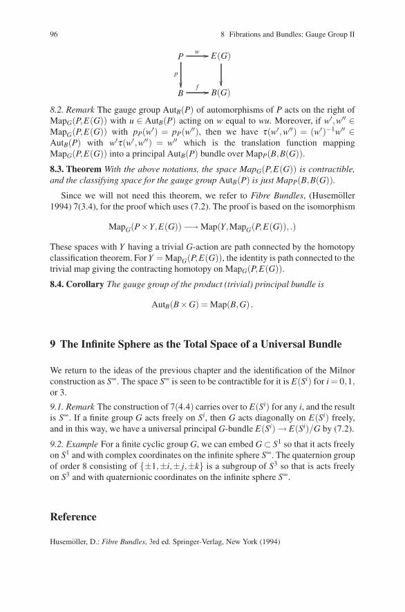
96 8 Fibrations and Bundles: Gauge Group II
P
p
��
w �� E(G)
��B
f �� B(G)
8.2. Remark The gauge group AutB(P) of automorphisms of P acts on the right ofMapG(P,E(G)) with u ∈ AutB(P) acting on w equal to wu. Moreover, if w′,w′′ ∈MapG(P,E(G)) with pP(w′) = pP(w′′), then we have τ(w′,w′′) = (w′)−1w′′ ∈AutB(P) with w′τ(w′,w′′) = w′′ which is the translation function mappingMapG(P,E(G)) into a principal AutB(P) bundle over MapP(B,B(G)).
8.3. Theorem With the above notations, the space MapG(P,E(G)) is contractible,and the classifying space for the gauge group AutB(P) is just MapP(B,B(G)).
Since we will not need this theorem, we refer to Fibre Bundles, (Husemoller1994) 7(3.4), for the proof which uses (7.2). The proof is based on the isomorphism
MapG(P×Y,E(G)) −→ Map(Y,MapG(P,E(G)), .)
These spaces with Y having a trivial G-action are path connected by the homotopyclassification theorem. For Y = MapG(P,E(G)), the identity is path connected to thetrivial map giving the contracting homotopy on MapG(P,E(G)).
8.4. Corollary The gauge group of the product (trivial) principal bundle is
AutB(B×G) = Map(B,G) .
9 The Infinite Sphere as the Total Space of a Universal Bundle
We return to the ideas of the previous chapter and the identification of the Milnorconstruction as S∞. The space S∞ is seen to be contractible for it is E(Si) for i = 0,1,or 3.
9.1. Remark The construction of 7(4.4) carries over to E(Si) for any i, and the resultis S∞. If a finite group G acts freely on Si, then G acts diagonally on E(Si) freely,and in this way, we have a universal principal G-bundle E(Si) → E(Si)/G by (7.2).
9.2. Example For a finite cyclic group G, we can embed G ⊂ S1 so that it acts freelyon S1 and with complex coordinates on the infinite sphere S∞. The quaternion groupof order 8 consisting of {±1,±i,± j,±k} is a subgroup of S3 so that is acts freelyon S3 and with quaternionic coordinates on the infinite sphere S∞.
Reference
Husemoller, D.: Fibre Bundles, 3rd ed. Springer-Verlag, New York (1994)
Chapter 9Cohomology Classes as Homotopy Classes:CW-Complexes
We consider filtered spaces and especially CW-complexes. Using the cofibre con-structions, we discuss the Whitehead mapping theorem. This characterization ofhomotopy equivalence was already used in the study of the uniqueness properties ofclassifying spaces. This completes a question left open in the previous chapter.
The usual definition of cohomology arises in terms of the dual of homology ei-ther directly for coefficients in a field or in terms of chains and cochains as linearforms on chain groups. These chains can arise very geometrically as cell chainsor more generally as simplicial chains. The cochains can be algebraic linear func-tionals or as in the case of manifolds they can be differential forms which becomelinear functionals on chains of simplexes upon integration over the simplexes andsumming over the chain.
There is another perspective on the cohomology of X discovered by Eilenbergand MacLane in terms of homotopy classes of maps of X into an Eilenberg–MacLane space K(G,n). This is a topological space which has the homotopy typeof a CW-complex and is characterized by its homotopy groups
πi(K(G),n)) ={
G if n = i0 if n = i
There is a canonical cohomology class ιn ∈ Hn(K(G,n),G) corresponding to theidentity morphism in Hom(G,G), where
Hom(G,G) = Hom(Hn(G,n),G) = Hn(K(G,n),G)
is part of the universal coefficient theorem.In this chapter, we use the notion of cofibre maps and the cofibre sequence for a
map. This is needed to establish cohomology properties of the K-theory functor andin the discussion of the above result that cohomology is defined also by maps into aclassifying space which in this case it is a K(π ,n).
Spanier (1963) is a reference for this chapter.
D. Husemoller et al.: Cohomology Classes as Homotopy Classes: CW-Complexes, Lect. Notes Phys. 726, 97–109(2008)DOI 10.1007/978-3-540-74956-1 10 © Springer-Verlag Berlin Heidelberg 2008
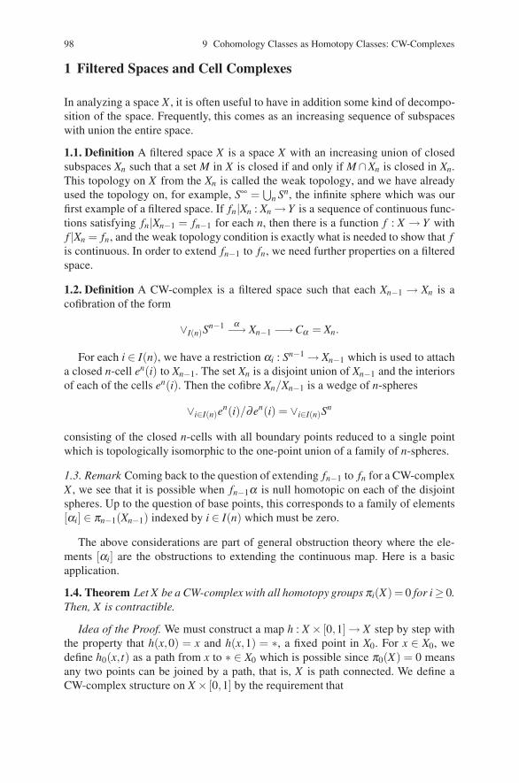
98 9 Cohomology Classes as Homotopy Classes: CW-Complexes
1 Filtered Spaces and Cell Complexes
In analyzing a space X , it is often useful to have in addition some kind of decompo-sition of the space. Frequently, this comes as an increasing sequence of subspaceswith union the entire space.
1.1. Definition A filtered space X is a space X with an increasing union of closedsubspaces Xn such that a set M in X is closed if and only if M ∩Xn is closed in Xn.This topology on X from the Xn is called the weak topology, and we have alreadyused the topology on, for example, S∞ =
⋃n Sn, the infinite sphere which was our
first example of a filtered space. If fn|Xn : Xn → Y is a sequence of continuous func-tions satisfying fn|Xn−1 = fn−1 for each n, then there is a function f : X → Y withf |Xn = fn, and the weak topology condition is exactly what is needed to show that fis continuous. In order to extend fn−1 to fn, we need further properties on a filteredspace.
1.2. Definition A CW-complex is a filtered space such that each Xn−1 → Xn is acofibration of the form
∨I(n)Sn−1 α−→ Xn−1 −→Cα = Xn.
For each i ∈ I(n), we have a restriction αi : Sn−1 → Xn−1 which is used to attacha closed n-cell en(i) to Xn−1. The set Xn is a disjoint union of Xn−1 and the interiorsof each of the cells en(i). Then the cofibre Xn/Xn−1 is a wedge of n-spheres
∨i∈I(n)en(i)/∂en(i) = ∨i∈I(n)S
n
consisting of the closed n-cells with all boundary points reduced to a single pointwhich is topologically isomorphic to the one-point union of a family of n-spheres.
1.3. Remark Coming back to the question of extending fn−1 to fn for a CW-complexX , we see that it is possible when fn−1α is null homotopic on each of the disjointspheres. Up to the question of base points, this corresponds to a family of elements[αi] ∈ πn−1(Xn−1) indexed by i ∈ I(n) which must be zero.
The above considerations are part of general obstruction theory where the ele-ments [αi] are the obstructions to extending the continuous map. Here is a basicapplication.
1.4. Theorem Let X be a CW-complex with all homotopy groups πi(X) = 0 for i≥ 0.Then, X is contractible.
Idea of the Proof. We must construct a map h : X × [0,1] → X step by step withthe property that h(x,0) = x and h(x,1) = ∗, a fixed point in X0. For x ∈ X0, wedefine h0(x,t) as a path from x to ∗ ∈ X0 which is possible since π0(X) = 0 meansany two points can be joined by a path, that is, X is path connected. We define aCW-complex structure on X × [0,1] by the requirement that
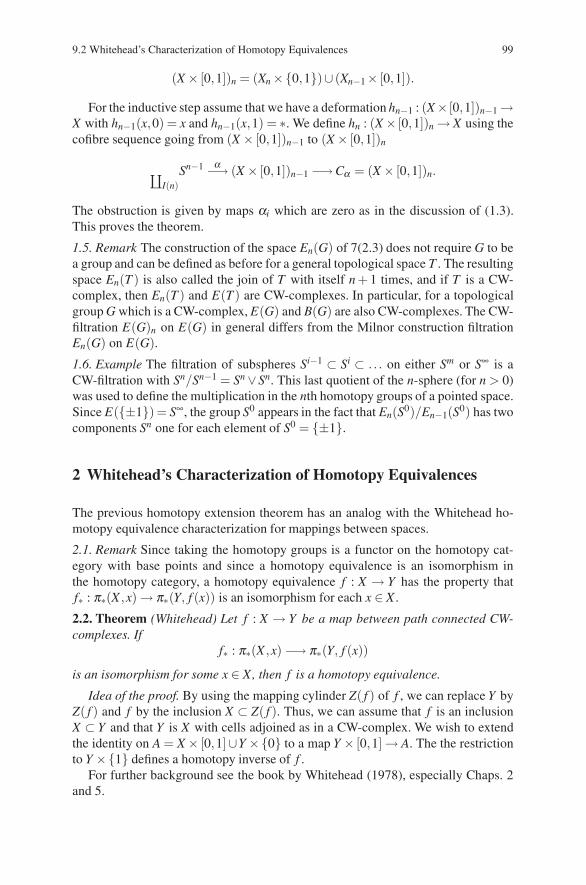
9.2 Whitehead’s Characterization of Homotopy Equivalences 99
(X × [0,1])n = (Xn ×{0,1})∪ (Xn−1× [0,1]).
For the inductive step assume that we have a deformation hn−1 : (X× [0,1])n−1 →X with hn−1(x,0) = x and hn−1(x,1) = ∗. We define hn : (X × [0,1])n → X using thecofibre sequence going from (X × [0,1])n−1 to (X × [0,1])n
∐I(n)
Sn−1 α−→ (X × [0,1])n−1 −→Cα = (X × [0,1])n.
The obstruction is given by maps αi which are zero as in the discussion of (1.3).This proves the theorem.
1.5. Remark The construction of the space En(G) of 7(2.3) does not require G to bea group and can be defined as before for a general topological space T . The resultingspace En(T ) is also called the join of T with itself n + 1 times, and if T is a CW-complex, then En(T ) and E(T ) are CW-complexes. In particular, for a topologicalgroup G which is a CW-complex, E(G) and B(G) are also CW-complexes. The CW-filtration E(G)n on E(G) in general differs from the Milnor construction filtrationEn(G) on E(G).
1.6. Example The filtration of subspheres Si−1 ⊂ Si ⊂ . . . on either Sm or S∞ is aCW-filtration with Sn/Sn−1 = Sn ∨Sn. This last quotient of the n-sphere (for n > 0)was used to define the multiplication in the nth homotopy groups of a pointed space.Since E({±1})= S∞, the group S0 appears in the fact that En(S0)/En−1(S0) has twocomponents Sn one for each element of S0 = {±1}.
2 Whitehead’s Characterization of Homotopy Equivalences
The previous homotopy extension theorem has an analog with the Whitehead ho-motopy equivalence characterization for mappings between spaces.
2.1. Remark Since taking the homotopy groups is a functor on the homotopy cat-egory with base points and since a homotopy equivalence is an isomorphism inthe homotopy category, a homotopy equivalence f : X → Y has the property thatf∗ : π∗(X ,x) → π∗(Y, f (x)) is an isomorphism for each x ∈ X .
2.2. Theorem (Whitehead) Let f : X → Y be a map between path connected CW-complexes. If
f∗ : π∗(X ,x) −→ π∗(Y, f (x))
is an isomorphism for some x ∈ X, then f is a homotopy equivalence.
Idea of the proof. By using the mapping cylinder Z( f ) of f , we can replace Y byZ( f ) and f by the inclusion X ⊂ Z( f ). Thus, we can assume that f is an inclusionX ⊂ Y and that Y is X with cells adjoined as in a CW-complex. We wish to extendthe identity on A = X × [0,1]∪Y ×{0} to a map Y × [0,1] → A. The the restrictionto Y ×{1} defines a homotopy inverse of f .
For further background see the book by Whitehead (1978), especially Chaps. 2and 5.
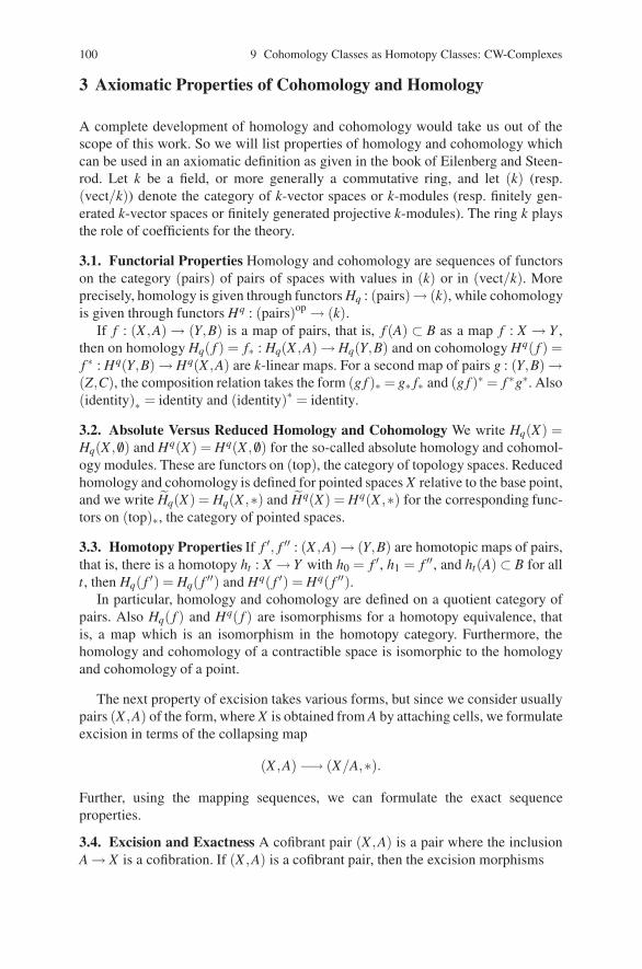
100 9 Cohomology Classes as Homotopy Classes: CW-Complexes
3 Axiomatic Properties of Cohomology and Homology
A complete development of homology and cohomology would take us out of thescope of this work. So we will list properties of homology and cohomology whichcan be used in an axiomatic definition as given in the book of Eilenberg and Steen-rod. Let k be a field, or more generally a commutative ring, and let (k) (resp.(vect/k)) denote the category of k-vector spaces or k-modules (resp. finitely gen-erated k-vector spaces or finitely generated projective k-modules). The ring k playsthe role of coefficients for the theory.
3.1. Functorial Properties Homology and cohomology are sequences of functorson the category (pairs) of pairs of spaces with values in (k) or in (vect/k). Moreprecisely, homology is given through functors Hq : (pairs)→ (k), while cohomologyis given through functors Hq : (pairs)op → (k).
If f : (X ,A) → (Y,B) is a map of pairs, that is, f (A) ⊂ B as a map f : X → Y ,then on homology Hq( f ) = f∗ : Hq(X ,A) → Hq(Y,B) and on cohomology Hq( f ) =f ∗ : Hq(Y,B) → Hq(X ,A) are k-linear maps. For a second map of pairs g : (Y,B) →(Z,C), the composition relation takes the form (g f )∗ = g∗ f∗ and (g f )∗ = f ∗g∗. Also(identity)∗ = identity and (identity)∗ = identity.
3.2. Absolute Versus Reduced Homology and Cohomology We write Hq(X) =Hq(X , /0) and Hq(X) = Hq(X , /0) for the so-called absolute homology and cohomol-ogy modules. These are functors on (top), the category of topology spaces. Reducedhomology and cohomology is defined for pointed spaces X relative to the base point,and we write Hq(X) = Hq(X ,∗) and Hq(X) = Hq(X ,∗) for the corresponding func-tors on (top)∗, the category of pointed spaces.
3.3. Homotopy Properties If f ′, f ′′ : (X ,A) → (Y,B) are homotopic maps of pairs,that is, there is a homotopy ht : X → Y with h0 = f ′, h1 = f ′′, and ht(A) ⊂ B for allt, then Hq( f ′) = Hq( f ′′) and Hq( f ′) = Hq( f ′′).
In particular, homology and cohomology are defined on a quotient category ofpairs. Also Hq( f ) and Hq( f ) are isomorphisms for a homotopy equivalence, thatis, a map which is an isomorphism in the homotopy category. Furthermore, thehomology and cohomology of a contractible space is isomorphic to the homologyand cohomology of a point.
The next property of excision takes various forms, but since we consider usuallypairs (X ,A) of the form, where X is obtained from A by attaching cells, we formulateexcision in terms of the collapsing map
(X ,A) −→ (X/A,∗).
Further, using the mapping sequences, we can formulate the exact sequenceproperties.
3.4. Excision and Exactness A cofibrant pair (X ,A) is a pair where the inclusionA → X is a cofibration. If (X ,A) is a cofibrant pair, then the excision morphisms
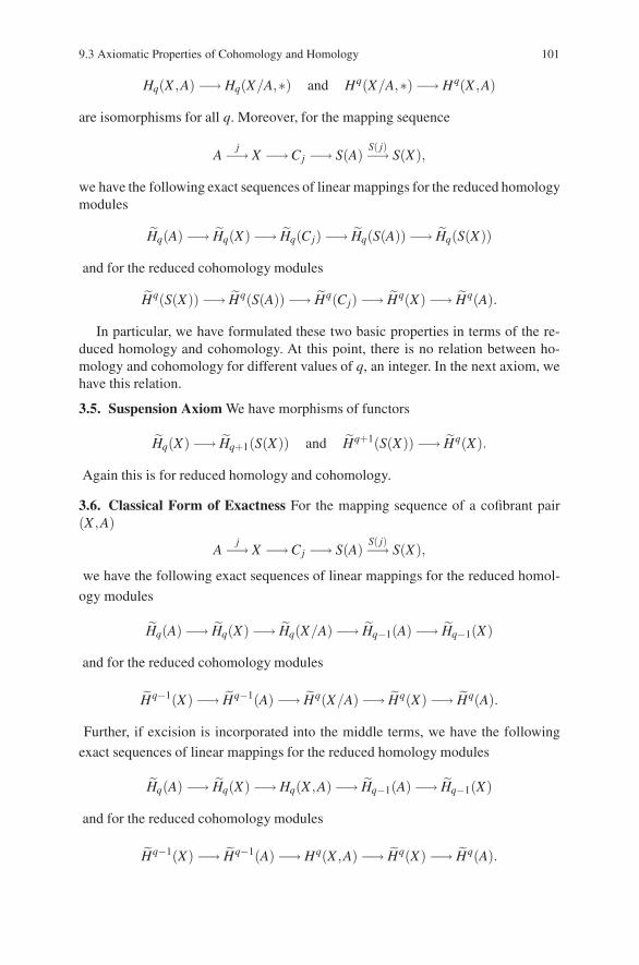
9.3 Axiomatic Properties of Cohomology and Homology 101
Hq(X ,A) −→ Hq(X/A,∗) and Hq(X/A,∗)−→ Hq(X ,A)
are isomorphisms for all q. Moreover, for the mapping sequence
Aj−→ X −→Cj −→ S(A)
S( j)−→ S(X),
we have the following exact sequences of linear mappings for the reduced homologymodules
Hq(A) −→ Hq(X) −→ Hq(Cj) −→ Hq(S(A)) −→ Hq(S(X))
and for the reduced cohomology modules
Hq(S(X)) −→ Hq(S(A)) −→ Hq(Cj) −→ Hq(X) −→ Hq(A).
In particular, we have formulated these two basic properties in terms of the re-duced homology and cohomology. At this point, there is no relation between ho-mology and cohomology for different values of q, an integer. In the next axiom, wehave this relation.
3.5. Suspension Axiom We have morphisms of functors
Hq(X) −→ Hq+1(S(X)) and Hq+1(S(X)) −→ Hq(X).
Again this is for reduced homology and cohomology.
3.6. Classical Form of Exactness For the mapping sequence of a cofibrant pair(X ,A)
Aj−→ X −→Cj −→ S(A)
S( j)−→ S(X),
we have the following exact sequences of linear mappings for the reduced homol-
ogy modules
Hq(A) −→ Hq(X) −→ Hq(X/A) −→ Hq−1(A) −→ Hq−1(X)
and for the reduced cohomology modules
Hq−1(X) −→ Hq−1(A) −→ Hq(X/A)−→ Hq(X) −→ Hq(A).
Further, if excision is incorporated into the middle terms, we have the following
exact sequences of linear mappings for the reduced homology modules
Hq(A) −→ Hq(X) −→ Hq(X ,A) −→ Hq−1(A) −→ Hq−1(X)
and for the reduced cohomology modules
Hq−1(X) −→ Hq−1(A) −→ Hq(X ,A) −→ Hq(X) −→ Hq(A).
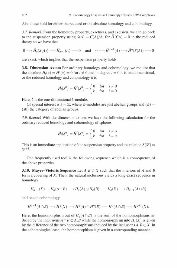
102 9 Cohomology Classes as Homotopy Classes: CW-Complexes
Also these hold for either the reduced or the absolute homology and cohomology.
3.7. Remark From the homotopy property, exactness, and excision, we can go backto the suspension property using S(A) = C(A)/A, for H(CA) = 0 in the reducedtheory so we have that
0 −→ Hq(S(A)) −→ Hq−1(A) −→ 0 and 0 −→ Hq−1(A) −→ Hq(S(A)) −→ 0
are exact, which implies that the suspension property holds.
3.8. Dimension Axiom For ordinary homology and cohomology, we require thatthe absolute Hi(∗) = Hi(∗) = 0 for i = 0 and in degree i = 0 it is one dimensional,or the reduced homology and cohomology it is
Hi(S0) = Hi(S0) ={
0 for i = 0k for i = 0.
Here, k is the one-dimensional k-module.Of special interest is k = Z, where Z-modules are just abelian groups and (Z) =
(ab) the category of abelian groups.
3.9. Remark With the dimension axiom, we have the following calculation for theordinary reduced homology and cohomology of spheres
Hi(Sq) = Hi(Sq) ={
0 for i = qk for i = q.
This is an immediate application of the suspension property and the relation S(Sq) =Sq+1.
One frequently used tool is the following sequence which is a consequence ofthe above properties.
3.10. Mayer–Vietoris Sequence Let A,B ⊂ X such that the interiors of A and Bform a covering of X . Then, the natural inclusions yields a long exact sequence inhomology
Hq+1(X) → Hq(A∩B) −→ Hq(A)⊕Hq(B) −→ Hq(X) −→ Hq−1(A∩B)
and one in cohomology
Hq−1(A∩B) −→ Hq(X) −→ Hq(A)⊕Hq(B) −→ Hq(A∩B) −→ Hq+1(X).
Here, the homomorphism out of Hq(A∩B) is the sum of the homomorphisms in-duced by the inclusions A∩B ⊂ A,B while the homomorphism into Hq(X) is givenby the difference of the two homomorphisms induced by the inclusions A,B ⊂ X . Inthe cohomological case, the homomorphism is given in a corresponding manner.
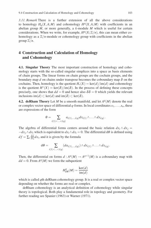
9.4 Construction and Calculation of Homology and Cohomology 103
3.11. Remark There is a further extension of all the above considerationsto homology Hq(X ,A;M) and cohomology Hq(X ,A;M) with coefficients in anabelian group M, or more generally, a k-module M which is useful for certainconsiderations. When we write, for example, Hq(X ;Z/n), this can mean either co-homology as a Z/n-module or cohomology group with coefficients in the abeliangroup Z/n.
4 Construction and Calculation of Homologyand Cohomology
4.1. Singular Theory The most important construction of homology and coho-mology starts with the so-called singular simplices into a space as basis elementsof chain groups. The linear forms on chain groups are the cochain groups, and theboundary map d on chains under transpose becomes the coboundary map δ on thecochains. Then, homology is the quotient H∗(X) = ker(d)/im(d) and cohomologyis the quotient H∗(X) = ker(δ )/im(δ ). In the process of defining these conceptsprecisely, one shows that dd = 0 and hence also δδ = 0 which yields the relevantinclusions im(d) ⊂ ker(d) and im(δ ) ⊂ ker(δ ).
4.2. deRham Theory Let M be a smooth manifold, and let Aq(M) denote the realor complex vector space of differential q-forms. In local coordinates x1, . . . ,xn, theseare expressions of the form
θ = ∑i(1)<...<i(q)
ai(1),...,i(q)dxi(1)∧ . . .∧dxi(q) .
The algebra of differential forms centers around the basic relation dxi ∧ dx j =−dx j ∧dxi which is equivalent to dxi∧dxi = 0. The differential dθ is defined using
d f = ∑i∂ f∂xi
dxi, and it is given by the formula
dθ = ∑i(1)<...<i(q)
(dai(1),...,i(q))∧dxi(1)∧ . . .∧dxi(q).
Then, the differential on forms d : Aq(M) → Aq+1(M) is a coboundary map withdd = 0. From Aq(M) we form the subquotient
HqDR(M) =
ker(d)im(d)
which is called qth deRham cohomology group. It is a real or complex vector spacedepending on whether the forms are real or complex.
deRham cohomology is an analytical definition of cohomology while singulartheory is topological. Both play a fundamental role in topology and geometry. Forfurther reading see Spanier (1963) or Warner (1971).
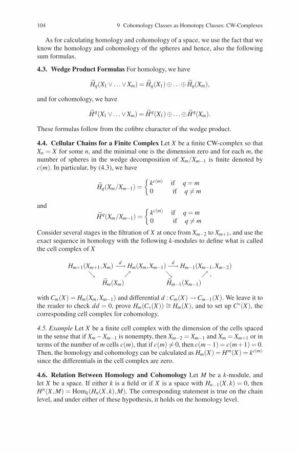
104 9 Cohomology Classes as Homotopy Classes: CW-Complexes
As for calculating homology and cohomology of a space, we use the fact that weknow the homology and cohomology of the spheres and hence, also the followingsum formulas.
4.3. Wedge Product Formulas For homology, we have
Hq(X1 ∨ . . .∨Xm) = Hq(X1)⊕ . . .⊕ Hq(Xm),
and for cohomology, we have
Hq(X1 ∨ . . .∨Xm) = Hq(X1)⊕ . . .⊕ Hq(Xm).
These formulas follow from the cofibre character of the wedge product.
4.4. Cellular Chains for a Finite Complex Let X be a finite CW-complex so thatXn = X for some n, and the minimal one is the dimension zero and for each m, thenumber of spheres in the wedge decomposition of Xm/Xm−1 is finite denoted byc(m). In particular, by (4.3), we have
Hq(Xm/Xm−1) ={
kc(m) if q = m0 if q = m
and
Hq(Xm/Xm−1) ={
kc(m) if q = m0 if q = m
Consider several stages in the filtration of X at once from Xm−2 to Xm+1, and use theexact sequence in homology with the following k-modules to define what is calledthe cell complex of X
Hm+1(Xm+1,Xm) d−→ Hm(Xm,Xm−1)d−→ Hm−1(Xm−1,Xm−2)
↘ ↗ ↘ ↗ ,
Hm(Xm) Hm−1(Xm−1)
with Cm(X) = Hm(Xm,Xm−1) and differential d : Cm(X) →Cm−1(X). We leave it tothe reader to check dd = 0, prove Hm(C∗(X)) ∼= Hm(X), and to set up C∗(X), thecorresponding cell complex for cohomology.
4.5. Example Let X be a finite cell complex with the dimension of the cells spacedin the sense that if Xm −Xm−1 is nonempty, then Xm−2 = Xm−1 and Xm = Xm+1 or interms of the number of m cells c(m), that if c(m) = 0, then c(m−1) = c(m+1) = 0.Then, the homology and cohomology can be calculated as Hm(X) = Hm(X) = kc(m)
since the differentials in the cell complex are zero.
4.6. Relation Between Homology and Cohomology Let M be a k-module, andlet X be a space. If either k is a field or if X is a space with Hn−1(X ,k) = 0, thenHn(X ,M) = Homk(Hn(X ,k),M). The corresponding statement is true on the chainlevel, and under either of these hypothesis, it holds on the homology level.
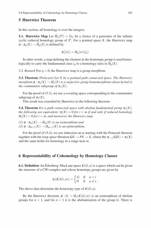
9.6 Representability of Cohomology by Homotopy Classes 105
5 Hurewicz Theorem
In this section, all homology is over the integers.
5.1. Hurewicz Map Let Hn(Sn) = Zin be a choice of a generator of the infinitecyclic reduced homology group of Sn. For a pointed space X , the Hurewicz mapφ : πq(X) → Hq(X) is defined by
φ([w]) = Hq(w)(iq).
In other words, a map defining the element in the homotopy group is used homo-logically to carry the fundamental class iq to a homology class in Hq(X).
5.2. Remark For q > 0, the Hurewicz map is a group morphism.
5.3. Theorem (Poincare) Let X be a pointed path connected space. The Hurewiczmorphism φ : π1(X) → H1(X) is a surjective group homomorphism whose kernel isthe commutator subgroup of π1(X).
For the proof of (5.3), we use a covering space corresponding to the commutatorsubgroup of π1(X).
This result was extended by Hurewicz to the following theorem.
5.4. Theorem For a path connected space with abelian fundamental group π1(X),the following are equivalent: πi(X) = 0 for i < m if and only if reduced homologyHi(X) = 0 for i < m, and moreover, the Hurewicz map
(1) φ : πm(X) → Hm(X) is an isomorphism and(2) φ : πm+1(X) → Hm+1(X) is an epimorphism.
For the proof of (5.4), we use induction on m starting with the Poincare theoremtogether with the loop space fibrationΩX → PX → X , where the πi−1(ΩX) = πi(X)and the same holds for homology in a range near m.
6 Representability of Cohomology by Homotopy Classes
6.1. Definition An Eilenberg–MacLane space K(G,n) is a space which can be giventhe structure of a CW-complex and whose homotopy groups are given by
πi(K(G),n)) ={
G if n = i0 if n = i ,
The above data determine the homotopy type of K(G,n).
By the Hurewicz theorem, φ : G → Hn(K(G,n)) is an isomorphism of abeliangroups for n > 1, and for n = 1 it is the abelianization of the group G. There is
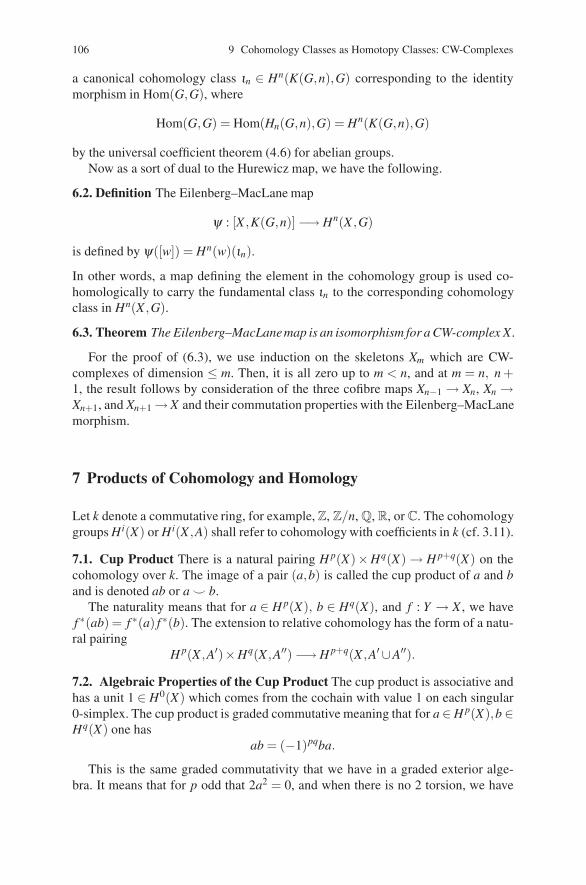
106 9 Cohomology Classes as Homotopy Classes: CW-Complexes
a canonical cohomology class ιn ∈ Hn(K(G,n),G) corresponding to the identitymorphism in Hom(G,G), where
Hom(G,G) = Hom(Hn(G,n),G) = Hn(K(G,n),G)
by the universal coefficient theorem (4.6) for abelian groups.Now as a sort of dual to the Hurewicz map, we have the following.
6.2. Definition The Eilenberg–MacLane map
ψ : [X ,K(G,n)] −→ Hn(X ,G)
is defined by ψ([w]) = Hn(w)(ιn).
In other words, a map defining the element in the cohomology group is used co-homologically to carry the fundamental class ιn to the corresponding cohomologyclass in Hn(X ,G).
6.3. Theorem The Eilenberg–MacLanemap is an isomorphism for a CW-complex X.
For the proof of (6.3), we use induction on the skeletons Xm which are CW-complexes of dimension ≤ m. Then, it is all zero up to m < n, and at m = n, n +1, the result follows by consideration of the three cofibre maps Xn−1 → Xn, Xn →Xn+1, and Xn+1 →X and their commutation properties with the Eilenberg–MacLanemorphism.
7 Products of Cohomology and Homology
Let k denote a commutative ring, for example, Z, Z/n, Q, R, or C. The cohomologygroups Hi(X) or Hi(X ,A) shall refer to cohomology with coefficients in k (cf. 3.11).
7.1. Cup Product There is a natural pairing H p(X)×Hq(X) → H p+q(X) on thecohomology over k. The image of a pair (a,b) is called the cup product of a and band is denoted ab or a � b.
The naturality means that for a ∈ H p(X), b ∈ Hq(X), and f : Y → X , we havef ∗(ab) = f ∗(a) f ∗(b). The extension to relative cohomology has the form of a natu-ral pairing
H p(X ,A′)×Hq(X ,A′′) −→ H p+q(X ,A′ ∪A′′).
7.2. Algebraic Properties of the Cup Product The cup product is associative andhas a unit 1 ∈ H0(X) which comes from the cochain with value 1 on each singular0-simplex. The cup product is graded commutative meaning that for a ∈ H p(X),b ∈Hq(X) one has
ab = (−1)pqba.
This is the same graded commutativity that we have in a graded exterior alge-bra. It means that for p odd that 2a2 = 0, and when there is no 2 torsion, we have
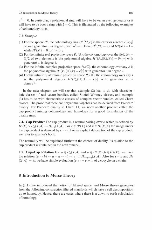
9.8 Introduction to Morse Theory 107
a2 = 0. In particular, a polynomial ring will have to be on an even generator or itwill have to be over a ring with 2 = 0. This is illustrated by the following examplesof cohomology rings.
7.3. Example
(1) For the sphere Sq, the cohomology ring H∗(Sq,k) is the exterior algebra E[a;q]on one generator a in degree q with a2 = 0. Here, H0(Sq) = k and Hq(Sq) = k.awhile Hi(Sq) = 0 for i = 0,q.
(2) For the infinite real projective space P∞(R), the cohomology over the field F2 =Z/2 of two elements is the polynomial algebra H∗(P∞(R),F2) = F2[w] withgenerator w in degree 1.
(3) For the infinite complex projective space P∞(C), the cohomology over any k isthe polynomial algebra H∗(P∞(R),k) = k[c] with generator c in degree 2.
(4) For the infinite quaternionic projective space P∞(H), the cohomology over any kis the polynomial algebra H∗(P∞(H),k) = k[v] with generator v indegree 4.
In the next chapter, we will see that example (2) has to do with character-istic classes of real vector bundles, called Stiefel–Whitney classes, and example(3) has to do with characteristic classes of complex vector bundles, called Chernclasses. The proof that these are polynomial algebras can be derived from Poincareduality. For Poincare duality in Chap. 11, we need another product called thecap product mixing cohomology and homology for a good formulation of theduality map.
7.4. Cap Product The cap product is a natural pairing over k which is defined byHi(X)×Hn(X ,A) → Hn−i(X ,A). For c ∈ Hi(X) and u ∈ Hn(X ,A) the image underthe cap product is denoted by c � u. For an explicit description of the cap product,we refer to Spanier’s book.
The naturality will be explained further in the context of duality. Its relation to thecup product is contained in the next remark.
7.5. Cup–Cap Relation For u ∈ Hn(X ,A) and a ∈ H p(X),b ∈ Hq(X), we havethe relation (a � b) � u = a � (b � u) in Hn−p−q(X ,A). Also for i = n and H0
(X ,A) = k, we have simple evaluation 〈c,u〉 = c � u of a cocycle on a chain.
8 Introduction to Morse Theory
In (1.1), we introduced the notion of filtered space, and Morse theory generatesfrom the following construction filtered manifolds which have a cell decompositionup to homotopy. Hence, there are cases where there is a down to earth calculationof homology.
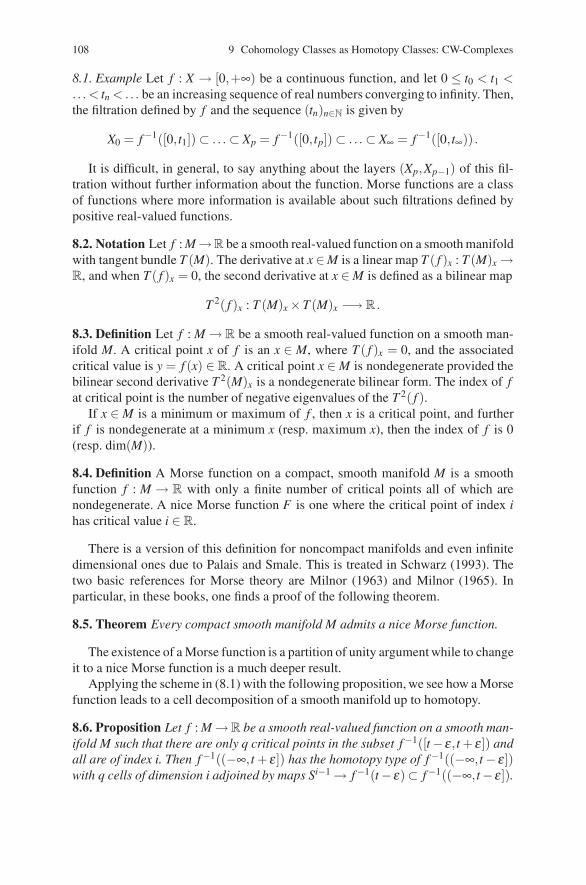
108 9 Cohomology Classes as Homotopy Classes: CW-Complexes
8.1. Example Let f : X → [0,+∞) be a continuous function, and let 0 ≤ t0 < t1 <.. . < tn < .. . be an increasing sequence of real numbers converging to infinity. Then,the filtration defined by f and the sequence (tn)n∈N is given by
X0 = f−1([0,t1]) ⊂ . . . ⊂ Xp = f−1([0,tp]) ⊂ . . . ⊂ X∞ = f−1([0, t∞)) .
It is difficult, in general, to say anything about the layers (Xp,Xp−1) of this fil-tration without further information about the function. Morse functions are a classof functions where more information is available about such filtrations defined bypositive real-valued functions.
8.2. Notation Let f : M →R be a smooth real-valued function on a smooth manifoldwith tangent bundle T (M). The derivative at x ∈ M is a linear map T ( f )x : T (M)x →R, and when T ( f )x = 0, the second derivative at x ∈ M is defined as a bilinear map
T 2( f )x : T (M)x ×T (M)x −→ R .
8.3. Definition Let f : M → R be a smooth real-valued function on a smooth man-ifold M. A critical point x of f is an x ∈ M, where T ( f )x = 0, and the associatedcritical value is y = f (x) ∈ R. A critical point x ∈ M is nondegenerate provided thebilinear second derivative T 2(M)x is a nondegenerate bilinear form. The index of fat critical point is the number of negative eigenvalues of the T 2( f ).
If x ∈ M is a minimum or maximum of f , then x is a critical point, and furtherif f is nondegenerate at a minimum x (resp. maximum x), then the index of f is 0(resp. dim(M)).
8.4. Definition A Morse function on a compact, smooth manifold M is a smoothfunction f : M → R with only a finite number of critical points all of which arenondegenerate. A nice Morse function F is one where the critical point of index ihas critical value i ∈ R.
There is a version of this definition for noncompact manifolds and even infinitedimensional ones due to Palais and Smale. This is treated in Schwarz (1993). Thetwo basic references for Morse theory are Milnor (1963) and Milnor (1965). Inparticular, in these books, one finds a proof of the following theorem.
8.5. Theorem Every compact smooth manifold M admits a nice Morse function.
The existence of a Morse function is a partition of unity argument while to changeit to a nice Morse function is a much deeper result.
Applying the scheme in (8.1) with the following proposition, we see how a Morsefunction leads to a cell decomposition of a smooth manifold up to homotopy.
8.6. Proposition Let f : M →R be a smooth real-valued function on a smooth man-ifold M such that there are only q critical points in the subset f−1([t −ε, t +ε]) andall are of index i. Then f−1((−∞,t + ε]) has the homotopy type of f−1((−∞,t − ε])with q cells of dimension i adjoined by maps Si−1 → f−1(t −ε)⊂ f−1((−∞,t−ε]).
References 109
8.7. Remark In fact, a Morse function not only can be used to control the homotopytype of M but also its diffeomorphism type. The attachment of the sphere in theprevious proposition can be done up to diffeomorphism by thickening Si−1 ⊂ Si−1×Dn−i and attaching Di ×Dn−i, called a handle. This is also explained very well inthe books of Milnor cited above.
References
Milnor, J.: Morse theory. Ann. of Math. Stud. 51 (1963)Milnor, J.: Lectures on the h-Cobordism Theorem. Princeton University Press, Princeton, NJ
(1965)Schwarz, M.: Morse Homology. Birkhauser, Basel (1993)Spanier, E.: Algebraic Topology. McGraw-Hill, New York (1963)Warner, F.: Foundations of Differential Manifolds and Lie Groups. Springer-Verlag, New York
(1984) (reprint of the1971 edition.)Whitehead, G.: Elements of homotopy theory. Springer Graduate Texts, Vol. 61. Springer Verlag,
New York (1978)

Chapter 10Basic Characteristic Classes
The theory of characteristic cohomology classes of bundles especially vector bun-dles grew up in several contexts like the notion of cohomology of a space. It wasnatural to try and make calculations with bundles in terms of cohomology for tworeasons. With homology and cohomology, there were combinatorial tools for com-putation. Then, cohomology and bundles each had contravariant properties undercontinuous mappings. The first definitions of characteristic classes were given byobstructions to existence to cross sections of a bundle or related fibre bundle. Ex-amples of this can be found in the book by Steenrod (1951).
With the understanding of the cohomology of fibre spaces including the Lerayspectral sequence, the theory of characteristic classes was developed along moreintrinsic lines. It was clear that the separate theories of Chern classes for complexvector bundles and of Stiefel–Whitney classes of real vector bundles had a parallelstructure. This became completely clear with Hirzebruch’s axiomatization of theChern classes which carries over immediately to Stiefel–Whitney classes. In the firstsections, we carry this out using an approach of Grothendieck which also works inthe context of algebraic geometry.
Then, we have the Euler class and Pontrjagin classes which are introduced alsoby elementary fibre space methods. Pontrjagin classes can be related nicely to Chernclasses. Then, it becomes clear that with splitting principles for vector bundles intoline bundles that families of characteristic classes can be introduced from powerseries by their properties on line bundles. From this, we generate important classesin the theory of manifolds, that is, the Todd class, the L-class, and the A-class, andthese classes evaluated on the fundamental homology class of a manifold lead tospecific characteristic numbers. This is considered in the next chapter.
Chapter 17 of Fibre Bundles (Husemoller 1994) is a reference for this chapter.The topic is also treated in Milnor and Stasheff (1974).
1 Characteristic Classes of Line Bundles
The theory of characteristic classes starts with the observation that the same spacecan be the classifying space for bundles, so of the form B(G), and for cohomology
D. Husemoller et al.: Basic Characteristic Classes, Lect. Notes Phys. 726, 111–125 (2008)DOI 10.1007/978-3-540-74956-1 11 © Springer-Verlag Berlin Heidelberg 2008
112 10 Basic Characteristic Classes
classes, so of the form K(Π ,n). There are two cases of this coincidence. The firstis related with real vector bundles while the second is related to complex vectorbundles.
1.1. The Real Infinite-Dimensional Projective Space P∞∞∞(R) It classifies threetypes of objects:
(1) real line bundles over a space X , for P∞(R) has a universal real line bundle,(2) double coverings of a space X , so P∞(R) = B({±1}), and(3) one-dimensional cohomology classes on X with values in the group Z/2Z or
{±1} of two elements, so P∞(R) = K(Z/2Z,1).
A real line bundle L on a space X is classified by a homotopy class of mapsu : X → P∞(R) = K(Z/2Z,1). The related cohomology class in H1(X ,Z/2Z) =[X ,K(Z/2Z,1)], denoted by w1(L), is called the first Stiefel–Whitney class of L.
1.2. The Complex Infinite-Dimensional Projective Space P∞∞∞(C) It classifiesthree types of objects:
(1) complex line bundles over a space X , for P∞(C) has a universal complex linebundle,
(2) principal circle bundles over a space X , so that P∞(C) = B(S1), and(3) two-dimensional cohomology classes on X with values in the group Z of inte-
gers, so P∞(C) = K(Z,2).
A complex line bundle L on a space X is classified by a homotopy class of mapsu : X → P∞(C) = K(Z,2). The related cohomology class in H2(X ,Z) = [X ,K(Z,2)],denoted by c1(L), is called the first Chern class of L.
1.3. Notation Let PicC(X) (resp. PicR(X)) denote the group of isomorphism classesof complex (resp. real) line bundles on X with group operation induced by the tensorproduct. The trivial line bundle is the unit, and the dual is the negative.
1.4. Remark Then with the induced line bundle, we define two functors into abeliangroups
PicC, PicR : (top)op −→ (ab).
The characteristic classes w1 and c1 define isomorphisms of functors
w1 : PicR() −→ H1( ,Z/2Z) and c1 : PicC() −→ H2( ,Z)
defined on the opposite category of topological spaces to the category of abeliangroups. This is the essentially unique situation where the characteristic class com-pletely determines the bundle.
In higher dimensions, there are more characteristic classes of a vector bundle, butthey are usually not enough characteristic classes to classify the isomorphism classof the vector bundles. In the next section, we introduce the fibre space results whichare used to define general characteristic classes in terms of the characteristic classof line bundles.
10.2 Projective Bundle Theorem and Splitting Principle 113
2 Projective Bundle Theorem and Splitting Principle
2.1. Definition Let E be a vector bundle over X . Let q : P(E)→ X be the associatedbundle of projective spaces, where the fibre q−1(x) = P(E)x is the projective spaceof linear forms on the fibre Ex.
Observe that if E|U is trivial, then q : P(E|U)→U is trivial, and if E = f−1(E ′) isan induced bundle, then q : P(E) → X is the induced associated bundle f−1(P(E ′))of projective spaces.
2.2. Remark On the associated bundle of projective spaces q : P(E) → X , there is aline bundle LE → P(E) with the property that LE |P(E)x is the canonical line bundleon the projective space P(E)x for each x ∈ X .
The next two theorems, the first for complex vector bundles and the second forreal vector bundles, are easy consequences of the cohomology spectral sequence fora fibre map q, but they can also be proved for bundles of finite type with an inductiveMayer–Vietoris argument (i.e., by iteratively using (3.10)).
2.3. Theorem The associated bundle of projective spaces q : P(E) → X for ann-dimensional complex vector bundle p : E → X has an injective integral cohomol-ogy morphism q∗ : H∗(X)→H∗(P(E)) making H∗(P(E)) into a free H∗(X)-modulewith basis
1,c1(LE), . . . ,c1(LE)n−1.
2.4. Theorem The associated bundle of projective spaces q : P(E) → X for an n-dimensional real vector bundle p : E → X has an injective mod 2 cohomology mor-phism q∗ : H∗(X ,F2) → H∗(P(E),F2) making H∗(P(E),F2) into a free H∗(X ,F2)-module with basis
1,w1(LE), . . . ,w1(LE)n−1.
The following two theorems are useful for uniqueness results and for doing cer-tain calculations.
2.5. Theorem For an arbitrary complex vector bundle E over a space B, we have amap f : B′ → B with two properties:
(1) f ∗ : H∗(B,Z) → H∗(B′,Z) is injective and(2) f ∗(E) = ⊕iLi, where the Li are line bundles over B′ .
2.6. Theorem For an arbitrary real vector bundle E over a space B we have a mapf : B′ → B with two properties:
(1) f ∗ : H∗(B,F2) → H∗(B′,F2) is injective and(2) f ∗(E) = ⊕iLi, where the Li are line bundles.
For the proofs of theorems (2.5) and (2.6), we use induction on the dimension of thevector bundle E . For line bundles, there is nothing to prove. Using the associatedbundle of projective spaces q : P(E) → B for the n-dimensional vector bundle p :E → B, we have q−1(E) = LE ⊕QE , where LE is the canonical line bundle on P(E)
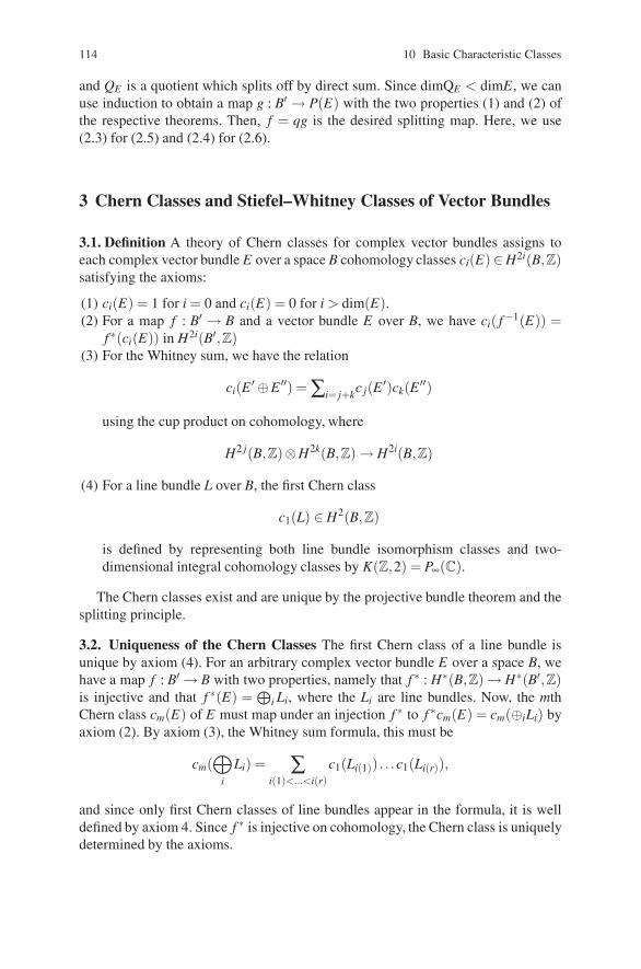
114 10 Basic Characteristic Classes
and QE is a quotient which splits off by direct sum. Since dimQE < dimE , we canuse induction to obtain a map g : B′ → P(E) with the two properties (1) and (2) ofthe respective theorems. Then, f = qg is the desired splitting map. Here, we use(2.3) for (2.5) and (2.4) for (2.6).
3 Chern Classes and Stiefel–Whitney Classes of Vector Bundles
3.1. Definition A theory of Chern classes for complex vector bundles assigns toeach complex vector bundle E over a space B cohomology classes ci(E)∈H2i(B,Z)satisfying the axioms:
(1) ci(E) = 1 for i = 0 and ci(E) = 0 for i > dim(E).(2) For a map f : B′ → B and a vector bundle E over B, we have ci( f−1(E)) =
f ∗(ci(E)) in H2i(B′,Z)(3) For the Whitney sum, we have the relation
ci(E ′ ⊕E ′′) =∑i= j+kc j(E ′)ck(E ′′)
using the cup product on cohomology, where
H2 j(B,Z)⊗H2k(B,Z) → H2i(B,Z)
(4) For a line bundle L over B, the first Chern class
c1(L) ∈ H2(B,Z)
is defined by representing both line bundle isomorphism classes and two-dimensional integral cohomology classes by K(Z,2) = P∞(C).
The Chern classes exist and are unique by the projective bundle theorem and thesplitting principle.
3.2. Uniqueness of the Chern Classes The first Chern class of a line bundle isunique by axiom (4). For an arbitrary complex vector bundle E over a space B, wehave a map f : B′ → B with two properties, namely that f ∗ : H∗(B,Z) → H∗(B′,Z)is injective and that f ∗(E) =
⊕i Li, where the Li are line bundles. Now, the mth
Chern class cm(E) of E must map under an injection f ∗ to f ∗cm(E) = cm(⊕iLi) byaxiom (2). By axiom (3), the Whitney sum formula, this must be
cm(⊕
i
Li) = ∑i(1)<...<i(r)
c1(Li(1)) . . .c1(Li(r)),
and since only first Chern classes of line bundles appear in the formula, it is welldefined by axiom 4. Since f ∗ is injective on cohomology, the Chern class is uniquelydetermined by the axioms.
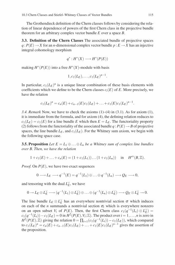
10.3 Chern Classes and Stiefel–Whitney Classes of Vector Bundles 115
The Grothendieck definition of the Chern classes follows by considering the rela-tion of linear dependence of powers of the first Chern class in the projective bundletheorem for an arbitrary complex vector bundle E over a space B.
3.3. Definition of the Chern Classes The associated bundle of projective spacesq : P(E)→X for an n-dimensional complex vector bundle p : E →X has an injectiveintegral cohomology morphism
q∗ : H∗(X) −→ H∗(P(E))
making H∗(P(E)) into a free H∗(X)-module with basis
1,c1(LE), . . . ,c1(LE)n−1.
In particular, c1(LE)n is a unique linear combination of these basis elements withcoefficients which we define to be the Chern classes ci(E) of E . More precisely, wehave the relation
c1(LE)n = cn(E)+ cn−1(E)c1(LE)+ . . .+ c1(E)c1(LE)n−1.
3.4. Remark Now, we have to check the axioms (1)–(4) in (3.1). As for axiom (1),it is immediate from the formula, and for axiom (4), the defining relation reduces toc1(LE) = c1(E) for a line bundle E which then E = LE . The functoriality property(2) follows from the functoriality of the associated bundle q : P(E)→B of projectivespaces, the line bundle LE , and c1(LE). For the Whitney sum axiom, we begin withthe following space case.
3.5. Proposition Let E = L1 ⊕ . . .⊕ Ln be a Whitney sum of complex line bundlesover B. Then, we have the relation
1 + c1(E)+ . . .+ cn(E) = (1 + c1(L1)) . . . (1 + c1(Ln)) in Hev(B,Z).
Proof. On P(E), we have two exact sequences
0 −→ LE −→ q−1(E) = q−1(L1)⊕ . . .⊕q−1(Ln) −→ QE −→ 0,
and tensoring with the dual L∨E , we have
0 → LE ⊗L∨E −→ (q−1(L1)⊗L∨
E)⊕ . . .⊕ (q−1(Ln)⊗L∨E) −→ QE ⊗L∨
E → 0.
The line bundle LE ⊗ L∨E has an everywhere nontrivial section σ which induces
on each of the n summands a nontrivial section σi which is everywhere nonzeroon an open subset Vi of P(E). Then, the first Chern class c1(q−1(Li) ⊗ L∨
E) =c1(q−1(Li))−c1(LE) = 0 in H2(P(E),Vi;Z). The product over i = 1, . . . ,n is zero inH2(P(E),Z) giving the relation 0 =∏i=1(c1(q−1(Li))− c1(LE)), which comparedto c1(LE)n = cn(E)+ cn−1(E)c1(LE)+ . . .+ c1(E)c1(LE)n−1 gives the assertion ofthe proposition.
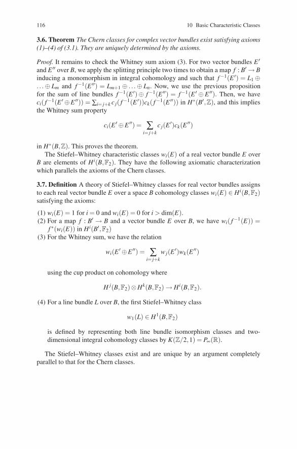
116 10 Basic Characteristic Classes
3.6. Theorem The Chern classes for complex vector bundles exist satisfying axioms(1)–(4) of (3.1). They are uniquely determined by the axioms.
Proof. It remains to check the Whitney sum axiom (3). For two vector bundles E ′and E ′′ over B, we apply the splitting principle two times to obtain a map f : B′ → Binducing a monomorphism in integral cohomology and such that f−1(E ′) = L1 ⊕. . .⊕ Lm and f−1(E ′′) = Lm+1 ⊕ . . .⊕ Ln. Now, we use the previous propositionfor the sum of line bundles f−1(E ′)⊕ f−1(E ′′) = f−1(E ′ ⊕ E ′′). Then, we haveci( f−1(E ′ ⊕E ′′)) = ∑i= j+k c j( f−1(E ′))ck( f−1(E ′′)) in H∗(B′,Z), and this impliesthe Whitney sum property
ci(E ′ ⊕E ′′) = ∑i= j+k
c j(E ′)ck(E ′′)
in H∗(B,Z). This proves the theorem.The Stiefel–Whitney characteristic classes wi(E) of a real vector bundle E over
B are elements of Hi(B,F2). They have the following axiomatic characterizationwhich parallels the axioms of the Chern classes.
3.7. Definition A theory of Stiefel–Whitney classes for real vector bundles assignsto each real vector bundle E over a space B cohomology classes wi(E) ∈ Hi(B,F2)satisfying the axioms:
(1) wi(E) = 1 for i = 0 and wi(E) = 0 for i > dim(E).(2) For a map f : B′ → B and a vector bundle E over B, we have wi( f−1(E)) =
f ∗(wi(E)) in Hi(B′,F2)(3) For the Whitney sum, we have the relation
wi(E ′ ⊕E ′′) = ∑i= j+k
wj(E ′)wk(E ′′)
using the cup product on cohomology where
H j(B,F2)⊗Hk(B,F2) → Hi(B,F2).
(4) For a line bundle L over B, the first Stiefel–Whitney class
w1(L) ∈ H1(B,F2)
is defined by representing both line bundle isomorphism classes and two-dimensional integral cohomology classes by K(Z/2,1) = P∞(R).
The Stiefel–Whitney classes exist and are unique by an argument completelyparallel to that for the Chern classes.
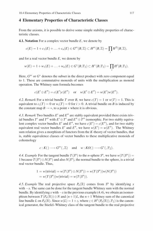
10.4 Elementary Properties of Characteristic Classes 117
4 Elementary Properties of Characteristic Classes
From the axioms, it is possible to derive some simple stability properties of charac-teristic classes.
4.1. Notation For a complex vector bundle E , we denote by
c(E) = 1 + c1(E)+ . . .+ cn(E) ∈ Gev(B,Z) ⊂ Hev(B,Z) =∏i
H2i(B,Z),
and for a real vector bundle E , we denote by
w(E) = 1 + w1(E)+ . . .+ wn(E) ∈ G∗(B,F2) ⊂ H∗(B,F2) =∏i
Hi(B,F2).
Here, Gev or G∗ denotes the subset in the direct product with zero component equalto 1. These are commutative monoids of units with the multiplication as monoidoperation. The Whitney sum formula becomes
c(E ′ ⊕E ′′) = c(E ′)c(E ′′) or w(E ′ ⊕E ′′) = w(E ′)w(E ′′).
4.2. Remark For a trivial bundle T over B, we have c(T ) = 1 or w(T ) = 1. This isequivalent to ci(T ) = 0 or wi(T ) = 0 for i > 0. A trivial bundle on B is induced bythe constant map B →∗, to a point ∗ where it is obvious.
4.3. Remark Two bundles E ′ and E ′′ are stably equivalent provided there exists triv-ial bundles T ′ and T ′′ with E ′ ⊕T ′ and E ′′ ⊕T ′′ isomorphic. For two stably equiva-lent complex vector bundles E ′ and E ′′, we have c(E ′) = c(E ′′), and for two stablyequivalent real vector bundles E ′ and E ′′, we have w(E ′) = w(E ′′). The Whitneysum relation gives a morphism of functors from the K-theory of vector bundles, thatis, stable equivalence classes of vector bundles to these multiplicative monoids ofcohomology
c : K() −→ Gev( ,Z) and w : KO() −→ G∗( ,F2).
4.4. Example For the tangent bundle T (Sn) to the n-sphere Sn, we have w(T (Sn)) =1 because T (Sn)⊕N(Sn) and also N(Sn), the normal bundle to the sphere, is a trivialreal vector bundle. Thus,
1 = w(trivial) = w(T (Sn)⊕N(Sn)) = w(T (Sn))w(N(Sn))= w(T (Sn))w(trivial) = w(T (Sn)).
4.5. Example The real projective space Pn(R) comes from Sn by identifying xwith −x. The same can be done for the tangent bundle Whitney sum with the normalbundle. By identifying x with−x in the previous example (4.4), we obtain an isomor-phism between T (Pn(R))⊕N and (n+1)L, the n+1 Whitney sum of the canonicalline bundle L on Pn(R). Since w(L) = 1+ z, where z ∈ H1(Pn(R)),F2) is the canon-ical generator, the Stiefel–Whitney class of the tangent bundle to the real projective
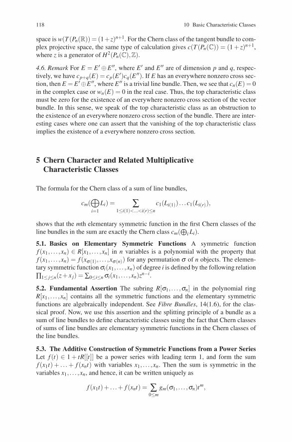
118 10 Basic Characteristic Classes
space is w(T (Pn(R)) = (1+z)n+1. For the Chern class of the tangent bundle to com-plex projective space, the same type of calculation gives c(T (Pn(C)) = (1 + z)n+1,where z is a generator of H2(Pn(C),Z).
4.6. Remark For E = E ′ ⊕E ′′, where E ′ and E ′′ are of dimension p and q, respec-tively, we have cp+q(E) = cp(E ′)cq(E ′′). If E has an everywhere nonzero cross sec-tion, then E = E ′⊕E ′′, where E ′′ is a trivial line bundle. Then, we see that cn(E) = 0in the complex case or wn(E) = 0 in the real case. Thus, the top characteristic classmust be zero for the existence of an everywhere nonzero cross section of the vectorbundle. In this sense, we speak of the top characteristic class as an obstruction tothe existence of an everywhere nonzero cross section of the bundle. There are inter-esting cases where one can assert that the vanishing of the top characteristic classimplies the existence of a everywhere nonzero cross section.
5 Chern Character and Related MultiplicativeCharacteristic Classes
The formula for the Chern class of a sum of line bundles,
cm(⊕i=1
Li) = ∑1≤i(1)<...<i(r)≤n
c1(Li(1)) . . .c1(Li(r)),
shows that the mth elementary symmetric function in the first Chern classes of theline bundles in the sum are exactly the Chern class cm(
⊕i Li).
5.1. Basics on Elementary Symmetric Functions A symmetric functionf (x1, . . . ,xn) ∈ R[x1, . . . ,xn] in n variables is a polynomial with the property thatf (x1, . . . ,xn) = f (xσ(1), . . . ,xσ(n)) for any permutation σ of n objects. The elemen-tary symmetric functionσi(x1, . . . ,xn) of degree i is defined by the following relation∏1≤ j≤n(z+ x j) = ∑0≤i≤nσi(x1, . . . ,xn)zn−i.
5.2. Fundamental Assertion The subring R[σ1, . . . ,σn] in the polynomial ringR[x1, . . . ,xn] contains all the symmetric functions and the elementary symmetricfunctions are algebraically independent. See Fibre Bundles, 14(1.6), for the clas-sical proof. Now, we use this assertion and the splitting principle of a bundle as asum of line bundles to define characteristic classes using the fact that Chern classesof sums of line bundles are elementary symmetric functions in the Chern classes ofthe line bundles.
5.3. The Additive Construction of Symmetric Functions from a Power SeriesLet f (t) ∈ 1 + tR[[t]] be a power series with leading term 1, and form the sumf (x1t) + . . . + f (xnt) with variables x1, . . . ,xn. Then the sum is symmetric in thevariables x1, . . . ,xn, and hence, it can be written uniquely as
f (x1t)+ . . .+ f (xnt) = ∑0≤m
gm(σ1, . . . ,σn)tm,
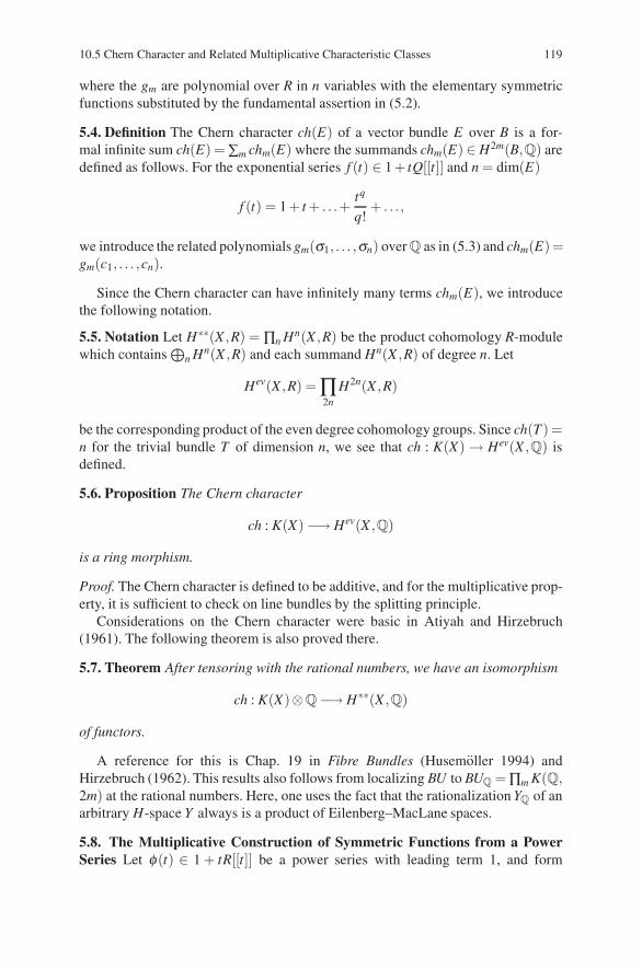
10.5 Chern Character and Related Multiplicative Characteristic Classes 119
where the gm are polynomial over R in n variables with the elementary symmetricfunctions substituted by the fundamental assertion in (5.2).
5.4. Definition The Chern character ch(E) of a vector bundle E over B is a for-mal infinite sum ch(E) =∑m chm(E) where the summands chm(E) ∈ H2m(B,Q) aredefined as follows. For the exponential series f (t) ∈ 1 + tQ[[t]] and n = dim(E)
f (t) = 1 + t + . . .+tq
q!+ . . . ,
we introduce the related polynomials gm(σ1, . . . ,σn) over Q as in (5.3) and chm(E)=gm(c1, . . . ,cn).
Since the Chern character can have infinitely many terms chm(E), we introducethe following notation.
5.5. Notation Let H∗∗(X ,R) =∏n Hn(X ,R) be the product cohomology R-modulewhich contains
⊕n Hn(X ,R) and each summand Hn(X ,R) of degree n. Let
Hev(X ,R) =∏2n
H2n(X ,R)
be the corresponding product of the even degree cohomology groups. Since ch(T ) =n for the trivial bundle T of dimension n, we see that ch : K(X) → Hev(X ,Q) isdefined.
5.6. Proposition The Chern character
ch : K(X) −→ Hev(X ,Q)
is a ring morphism.
Proof. The Chern character is defined to be additive, and for the multiplicative prop-erty, it is sufficient to check on line bundles by the splitting principle.
Considerations on the Chern character were basic in Atiyah and Hirzebruch(1961). The following theorem is also proved there.
5.7. Theorem After tensoring with the rational numbers, we have an isomorphism
ch : K(X)⊗Q −→ H∗∗(X ,Q)
of functors.
A reference for this is Chap. 19 in Fibre Bundles (Husemoller 1994) andHirzebruch (1962). This results also follows from localizing BU to BUQ =∏m K(Q,2m) at the rational numbers. Here, one uses the fact that the rationalization YQ of anarbitrary H-space Y always is a product of Eilenberg–MacLane spaces.
5.8. The Multiplicative Construction of Symmetric Functions from a PowerSeries Let φ(t) ∈ 1 + tR[[t]] be a power series with leading term 1, and form
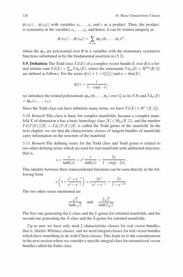
120 10 Basic Characteristic Classes
φ(x1t) . . .φ(xnt) with variables x1, . . . ,xn and t as a product. Then, the productis symmetric in the variables x1, . . . ,xn, and hence, it can be written uniquely as
φ(x1t) . . .φ(xnt) = ∑0≤m
ψm(σ1, . . . ,σn)tn,
where the ψm are polynomial over R in n variables with the elementary symmetricfunctions substituted in by the fundamental assertion in (5.2).
5.9. Definition The Todd class T d(E) of a complex vector bundle E over B is a for-mal infinite sum Td(E) = ∑m T dm(E), where the summands T dm(E) ∈ H2m(B,Q)are defined as follows. For the series φ(t) ∈ 1 + tQ[[t]] and n = dim(E)
φ(t) =t
1− exp(−t),
we introduce the related polynomialsψm(σ1, . . . ,σn) over Q as in (5.8) and T dm(E)= ψm(c1, . . . ,cn).
Since the Todd class can have infinitely many terms, we have T d(E) ∈ H∗∗(X ,Q).
5.10. Remark This class is basic for complex manifolds, because a complex mani-fold X of dimension n has a basic homology class [X ] ∈ H2n(X ,Z), and the numberT d(T (X)))[X ] = T dn(T (X))[X ] is called the Todd genus of the manifold. In thenext chapter, we see that the characteristic classes of tangent bundles of manifoldscarry information on the structure of the manifold.
5.11. Remark The defining series for the Todd class and Todd genus is related totwo other defining series which are used for real manifolds with additional structure,that is,
x +x
tanh(x)= ex x
sinh(x)=
2x1− exp(−2x)
.
This identity between three transcendental functions can be seen directly in the fol-lowing form
x
(1 +
ex + e−x
ex − e−x
)= x
2ex
ex − e−x =2x
1− e−2x .
The two other series mentioned are√
ztanh
√z
and2√
zsinh2
√z.
The first one generating the L-class and the L-genus for oriented manifolds, and thesecond one generating the A-class and the A-genus for oriented manifolds.
Up to now we have only mod 2 characteristic classes for real vector bundles,that is, Stiefel–Whitney classes, and we need integral classes for real vector bundleswhich have something to do with Chern classes. This leads us to the considerationsin the next section where we consider a specific integral class for oriented real vectorbundles called the Euler class.
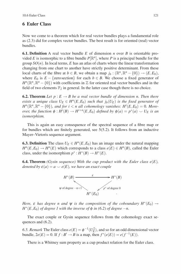
10.6 Euler Class 121
6 Euler Class
Now we come to a theorem which for real vector bundles plays a fundamental roleas (2.3) did for complex vector bundles. The best result is for oriented (real) vectorbundles.
6.1. Definition A real vector bundle E of dimension n over B is orientable pro-vided E is isomorphic to a fibre bundle P[Rn], where P is a principal bundle for thegroup SO(n). In local terms, E has an atlas of charts where the linear transformationchanging from one chart to another have strictly positive determinant. From theselocal charts of the fibre at b ∈ B, we obtain a map jb : (Rn,Rn −{0}) → (E,E0),where E0 is E − {zerosection} for each b ∈ B. We choose a fixed generator ofHn(Rn,Rn −{0}) with coefficients in Z for oriented real vector bundles and in thefield of two elements F2 in general. In the latter case though there is no choice.
6.2. Theorem Let p : E → B be a real vector bundle of dimension n. Then thereexists a unique class UE ∈ Hn(E,E0) such that jb(UE) is the fixed generator ofHn(Rn,Rn −{0}), and for i < n all cohomology vanishes: Hi(E,E0) = 0. More-over, the function φ : Hi(B) → Hi+n(E,E0) defined by φ(a) = p∗(a) � UE is anisomorphism.
This is again an easy consequence of the spectral sequence of a fibre map orfor bundles which are finitely generated, see 5(5.2). It follows from an inductiveMayer–Vietoris sequence argument.
6.3. Definition The class UE ∈ Hn(E,E0) has an image under the natural mappingHn(E,E0) → Hn(E) which corresponds to a class e(E) ∈ Hn(B), called the Eulerclass, under the isomorphism p∗ : H∗(B) → H∗(E).
6.4. Theorem (Gysin sequence) With the cup product with the Euler class e(E),denoted by ε(a) = a � e(E), we have an exact couple
H∗(B) ε �� H∗(B)
p∗ of degree 0�����������
H∗(E0)ψ of degree −n+1
�����������.
Here, ε has degree n and ψ is the composition of the coboundary H∗(E0) →H∗(E,E0) of degree 1 with the inverse of φ in (6.2) of degree −n.
The exact couple or Gysin sequence follows from the cohomology exact se-quences and (6.2).
6.5. Remark The Euler class e(E) = φ−1(U2E), and so for an odd dimensional vector
bundle, 2e(E) = 0. If f : B′ → B is a map, then f ∗(e(E)) = e( f−1(E)).
There is a Whitney sum property as a cup product relation for the Euler class.
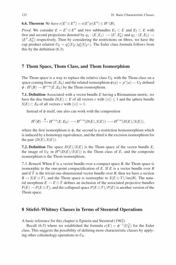
122 10 Basic Characteristic Classes
6.6. Theorem We have e(E ′ ⊕E ′′) = e(E ′)e(E ′′) ∈ H∗(B).
Proof. We consider E = E ′ ⊕ E ′′ and two subbundles E1 ⊂ E and E2 ⊂ E withfirst and second projections denoted by q1 : (E,E1) → (E ′,E ′
0) and q2 : (E,E2) →(E ′′,E ′′
0 ) respectively. Then by considering the restrictions on fibres, we have thecup product relation UE = q∗1(UE ′)q∗2(UE ′′). The Euler class formula follows fromthis by the definition (6.3).
7 Thom Space, Thom Class, and Thom Isomorphism
The Thom space is a way to replace the relative class UE with the Thom class on aspace coming from (E,E0) and the related isomorphism φ(a) = p∗(a) �UE definedφ : Hi(B) → Hi+n(E,E0) by the Thom isomorphism.
7.1. Definition Associated with a vector bundle E having a Riemannian metric, wehave the disc bundle D(E) ⊂ E of all vectors v with ||v|| ≤ 1 and the sphere bundleS(E) ⊂ E0 of all vectors v with ||v|| = 1.
Instead of φ itself, one also can work with the composition
Hi(B)φ−→ Hi+n(E,E0) −→ Hi+n(D(E),S(E)) −→ Hi+n(D(E)/S(E)),
where the first isomorphism is φ , the second is a restriction homomorphism whichis induced by a homotopy equivalence, and the third is the excision isomorphism forthe pair (D(E),S(E)).
7.2. Definition The space D(E)/S(E) is the Thom space of the vector bundle E ,the image of UE in Hn(D(E)/S(E)) is the Thom class of E , and the compositeisomorphism is the Thom isomorphism.
7.3. Remark When E is a vector bundle over a compact space B, the Thom space isisomorphic to the one-point compactification of E . If E is a vector bundle over Band if T is the trivial one-dimensional vector bundle over B, then we have a sectionB → S(E ⊕T ), and the Thom space is isomorphic to S(E ⊕ T )/im(B). The natu-ral morphism E → E ⊕T defines an inclusion of the associated projective bundlesP(E)→ P(E⊕T ), and the collapsed space P(E⊕T )/P(E) is another version of theThom space.
8 Stiefel–Whitney Classes in Terms of Steenrod Operations
A basic reference for this chapter is Epstein and Steenrod (1962).Recall (6.5) where we established the formula e(E) = φ−1(U2
E) for the Eulerclass. This suggests the possibility of defining more characteristic classes by apply-ing other cohomology operations to UE .
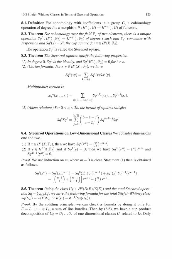
10.8 Stiefel–Whitney Classes in Terms of Steenrod Operations 123
8.1. Definition For cohomology with coefficients in a group G, a cohomologyoperation of degree i is a morphism θ : H∗( ,G) → H∗+i( ,G) of functors.
8.2. Theorem For cohomology over the field F2 of two elements, there is a uniqueoperation Sqi : H∗( ,F2) → H∗+i( ,F2) of degree i such that Sqi commutes withsuspension and Sqi(x) = x2, the cup square, for x ∈ Hi(X ,F2).
The operation Sqi is called the Steenrod square.
8.3. Theorem The Steenrod squares satisfy the following properties.
(1) In degree 0, Sq0 is the identity, and Sqi|Hn( ,F2) = 0 for i > n.(2) (Cartan formula) For x,y ∈ H∗(X ,F2), we have
Sqk(xy) = ∑k=i+ j
Sqi(x)Sq j(y).
Multiproduct version is
Sqq(x1 . . .xr) = ∑i(1)+...+i(r)=q
Sqi(1)(x1) . . .Sqi(r)(xr).
(3) (Adem relations) For 0 < a < 2b, the iterate of squares satisfies
SqaSqb =[a/2]
∑j=0
(b−1− j
a−2 j
)Sqa+b− jSq j.
8.4. Steenrod Operations on Low-Dimensional Classes We consider dimensionsone and two.
(1) If x ∈ H1(X ,F2), then we have Sqi(xm) =(m
i
)xm+i.
(2) If y ∈ H2(X ,F2) and if Sq1(y) = 0, then we have Sq2i(ym) = (mi )ym+i and
Sq2i+1(ym) = 0.
Proof. We use induction on m, where m = 0 is clear. Statement (1) then is obtainedas follows.
Sqi(xm) = Sqi(x.xm−1) = Sq0(x).Sqi(xm−1)+ Sq1(x).Sqi−1(xm−1)=[(
m−1i
)+(
m−1i−1
)]xm+i =
(mi
)xm+i.
8.5. Theorem Using the class UE ∈ Hn(D(E)/S(E)) and the total Steenrod opera-tion Sq =∑0≤i Sqi, we have the following formula for the total Stiefel–Whitney classSq(UE) = w(E)UE or w(E) = φ−1(Sq(UE)).
Proof. By the splitting principle, we can check a formula by doing it only forE = L1 ⊕ . . .⊕ Ln, a sum of line bundles. Then by (6.6), we have a cup productdecomposition of UE = U1 . . .Un of one-dimensional classes Ui related to Li. Only
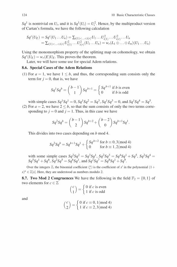
124 10 Basic Characteristic Classes
Sq1 is nontrivial on Ui, and it is Sq1(Ui) = U2i . Hence, by the multiproduct version
of Cartan’s formula, we have the following calculation
Sqr(UE) = Sqr(U1 . . .Un) = ∑i(1)<...<i(r)U1 . . .U2i(1) . . .U
2i(r) . . .Un
= ∑i(1)<...<i(r)U2i(1) . . .U
2i(r)(U1 . . .Un) = wr(L1 ⊕ . . .⊕Ln)(U1 . . .Un)
Using the monomorphism property of the splitting map on cohomology, we obtainSqr(UE) = wr(E)UE . This proves the theorem.
Later, we will have some use for special Adem relations.
8.6. Special Cases of the Adem Relations
(1) For a = 1, we have 1 ≤ b, and thus, the corresponding sum consists only theterm for j = 0, that is, we have
Sq1Sqb =(
b−11
)Sqb+1 =
{Sqb+1 if b is even0 if b is odd
with simple cases Sq1Sq1 = 0, Sq1Sq2 = Sq3, Sq1Sq3 = 0, and Sq1Sq4 = Sq5.(2) For a = 2, we have 2 ≤ b, so that the sum consists of only the two terms corre-
sponding to j = 0 and j = 1. Thus, in this case we have
Sq2Sqb =(
b−12
)Sqb+2 +
(b−2
0
)Sqb+1Sq1.
This divides into two cases depending on b mod 4.
Sq2Sqb = Sqb+1Sq1 +{
Sqb+2 for b ≡ 0,3(mod 4)0 for b ≡ 1,2(mod 4)
with some simple cases Sq2Sq2 = Sq3Sq1, Sq2Sq3 = Sq4Sq1 + Sq5, Sq2Sq4 =Sq5Sq1 + Sq6, Sq2Sq5 = Sq6Sq1, and Sq2Sq7 = Sq8Sq1 + Sq9.
Over the integers Z, the binomial coefficient (ni ) is the coefficient of xi in the polynomial (1+
x)n ∈ Z[x]. Here, they are understood as numbers modulo 2.
8.7. Two Mod 2 Congruences We have the following in the field F2 = {0,1} oftwo elements for c ∈ Z ( c
1
)={
0 if c is even1 if c is odd
and ( c2
)={
0 if c ≡ 0,1(mod 4)1 if c ≡ 2,3(mod 4)
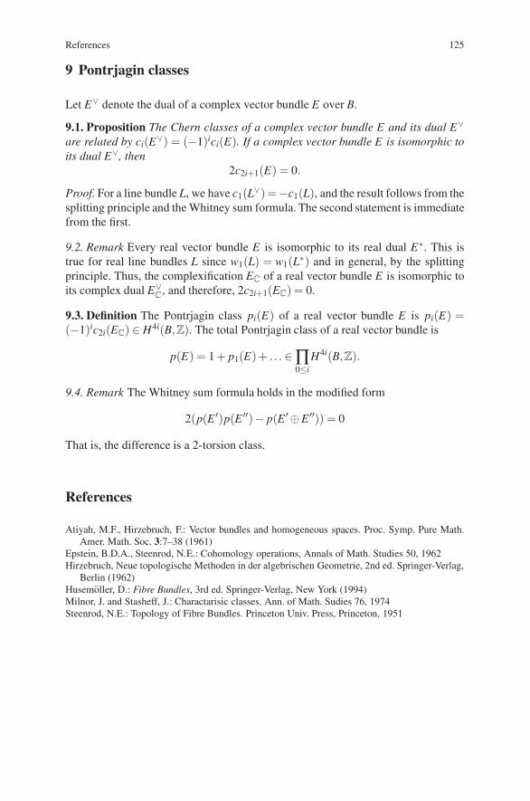
References 125
9 Pontrjagin classes
Let E∨ denote the dual of a complex vector bundle E over B.
9.1. Proposition The Chern classes of a complex vector bundle E and its dual E∨are related by ci(E∨) = (−1)ici(E). If a complex vector bundle E is isomorphic toits dual E∨, then
2c2i+1(E) = 0.
Proof. For a line bundle L, we have c1(L∨) =−c1(L), and the result follows from thesplitting principle and the Whitney sum formula. The second statement is immediatefrom the first.
9.2. Remark Every real vector bundle E is isomorphic to its real dual E∗. This istrue for real line bundles L since w1(L) = w1(L∗) and in general, by the splittingprinciple. Thus, the complexification EC of a real vector bundle E is isomorphic toits complex dual E∨
C, and therefore, 2c2i+1(EC) = 0.
9.3. Definition The Pontrjagin class pi(E) of a real vector bundle E is pi(E) =(−1)ic2i(EC) ∈ H4i(B,Z). The total Pontrjagin class of a real vector bundle is
p(E) = 1 + p1(E)+ . . . ∈∏0≤i
H4i(B,Z).
9.4. Remark The Whitney sum formula holds in the modified form
2(p(E ′)p(E ′′)− p(E ′ ⊕E ′′)) = 0
That is, the difference is a 2-torsion class.
References
Atiyah, M.F., Hirzebruch, F.: Vector bundles and homogeneous spaces. Proc. Symp. Pure Math.Amer. Math. Soc. 3:7–38 (1961)
Epstein, B.D.A., Steenrod, N.E.: Cohomology operations, Annals of Math. Studies 50, 1962Hirzebruch, Neue topologische Methoden in der algebrischen Geometrie, 2nd ed. Springer-Verlag,
Berlin (1962)Husemoller, D.: Fibre Bundles, 3rd ed. Springer-Verlag, New York (1994)Milnor, J. and Stasheff, J.: Charactarisic classes. Ann. of Math. Sudies 76, 1974Steenrod, N.E.: Topology of Fibre Bundles. Princeton Univ. Press, Princeton, 1951

Chapter 11Characteristic Classes of Manifolds
A topological manifold M of dimension n has a fundamental class denoted byωM or[M]∈Hn(M,Z/2Z), and when it has an orientation, this class is defined in Hn(M,Z)with the same notation. In each case, the cap product
() � [M] : Hi(M) → Hn−i(M)
for a closed manifold M is an isomorphism called Poincare duality. This internalsymmetry between homology and cohomology is a fundamental property of man-ifolds. When the manifold has a boundary ∂M or when it is not compact, thenPoincare duality must be modified, but it is always given by cap product with thefundamental class in Hn(Mn,Z) for the oriented case and in Hn(Mn,Z/2) for thegeneral case.
A smooth manifold M of dimension n has two complementary real vector bun-dles: the tangent bundle T (M) of dimension n and the normal bundle ν(M) to someembedding of M into Euclidean space. The Whitney sum T (M)⊕ν(M) is a trivialbundle on M which is the restriction to M of the trivial tangent bundle on Euclideanspace. For the characteristic classes with the Whitney sum property, it is essentiallyequivalent to work either the characteristic classes of the tangent bundle or the nor-mal bundle.
Polynomial combinations of characteristic classes of the tangent bundle can beevaluated on the fundamental class [M], and the result is characteristic numberswhich can be related to other invariants of the manifold. These numbers are relatedto homological invariants of the manifold and in many cases to other geometric in-variants of the manifold and bundles on the manifold. In the last section, we illustratethis with an explication of the Riemann-Roch-Hirzebruch theorem.
Chapter 18 of Fibre Bundles (Husemoller 1994) is a reference for this chapter.
1 Orientation in Euclidean Space and on Manifolds
1.1. Linear Orientation A nonsingular linear map A : Rn → R
n preserves orien-tation provided det(A) > 0. The subgroup of GL(n,R) of orientation-preserving
D. Husemoller et al.: Characteristic Classes of Manifolds, Lect. Notes Phys. 726, 127–135 (2008)DOI 10.1007/978-3-540-74956-1 12 © Springer-Verlag Berlin Heidelberg 2008
128 11 Characteristic Classes of Manifolds
maps is denoted by GL+(n,R), and its compact form is the rotation group SO(n) =O(n)∩GL+(n,R). Here, what is critical for linear orientation is a basis of the vectorspace R
n. To extend the concept of orientation to nonlinear maps, we use homology.
1.2. Topological Orientation To define orientation, we must choose generatorsαn−1 ∈ Hn−1(Sn−1) = Z, which for any open set U in R
n and x ∈ U ⊂ Rn corre-
sponds by exactness and excision to a generator αx ∈ Hn(U,U − x) = Z. A homeo-morphism f : (U,U − x) → (V,V − f (x)) preserves (resp. reverses) orientation at xprovided f∗(αx) = +α f (x) (resp. −α f (x)).
There are corresponding elements βn−1 ∈ Hn−1(Sn−1) = Z and βx ∈ Hn(U,U −x) = Z, and orientation preserving and reversing is the same in cohomology. In thecase of a linear f , the determinant definition and the homological definition give thesame result. Again by excision Hn(Mn,Mn − x) = Z, and there are two generatorsfor any manifold Mn of dimension n.
1.3. Orientation for Manifolds An orientation of an n-dimensional manifold Mis a system of generators ωx ∈ Hn(M,M − x) indexed by x ∈ M such that for anyopen ball B ⊂ M and x,y ∈ B, the classes ωx and ωy correspond under the followinginclusion-induced isomorphisms
Hn(M,M − x) ←− Hn(M,M −B)−→ Hn(M,M − y).
1.4. Remark When a manifold M has an orientation, we use integral homology, butwithout an orientation, we implicitly use homology over Z/2Z, where there is onenonzero element ωx in the relevant homology group ωx ∈ Hn(M,M − x,Z/2Z).
For a given orientation ωx ∈ Hn(M,M − x), we define classes ωK ∈ Hn(M,M −K) using the induced morphisms r : H∗(M,M −L) → H∗(M,M −K) for compactsubsets K ⊂ L in M.
1.5. Proposition Let M be an n-dimensional topological manifold. For each com-pact subset K of M, we have Hi(M,M − K) = 0 for i > n, and a class a ∈Hn(M,M − K) is zero if and only if for all x ∈ K we have rx(a) = 0, whererx : Hn(M,M −K)→ Hn(M,M − x) is induced by inclusion.
1.6. Proposition Let (ωx)x∈M be an orientation of a topological manifold M of di-mension n. For each compact subset K ⊂M, there exists a class ωK ∈Hn(M,M−K)such that rx(ωK) =ωx for all x∈K, where again rx : Hn(M,M−K)→Hn(M,M−x)is induced by inclusion.
These two results on orientation in a manifold are proved by using the Mayer–Vietoris sequence for K′ ∪K′′ = K and K′ ∩K′′ starting with closed balls B wherethe classes ωB are immediately defined. Then, we use finite coverings of compactsets by small balls.
We thus have an orientation class ωM for oriented compact manifolds M. Thereare appropriate definitions for the general case, which we shall not describe here.
11.2 Poincare Duality on Manifolds 129
2 Poincare Duality on Manifolds
Using the orientation classes ωK constructed in (1.6) for an n-dimensional manifoldM, we now consider certain cap products related to pairs (K,V ), where K ⊂ V iscompact and V ⊂ M is open in M.
2.1. Remark The inclusion j : (V,V −K) −→ (M,M −K) induces isomorphisms inhomology and in cohomology by excision
j∗ :H∗(V,V −K) → H∗(M,M −K) and j∗ :H∗(M,M −K) → H∗(V,V −K).
With these notations, we obtain a diagram using the cap product mixing coho-mology and homology with values in homology.
2.2. Cap Product Diagram With the above notation, we have the following com-mutative diagram with the right vertical arrow an isomorphism
Hi(M)⊗Hn(M,M −K)cap ��
j∗⊗( j∗)−1
��
Hn−i(M,M −K)
Hi(V )⊗Hn(V,V −K)cap �� Hn−i(V,V −K)
j∗
��
Now, we fix one of the variables in the cap product to be an orientation classωK ∈ Hn(M,M −K).
2.3. Definition The dualizing morphism relative to a pair K ⊂ V ⊂ M as above isDK,V : Hi(V ) → Hn−i(M,M −K) given by DK,V (a) = j∗(a � j−1∗ (ωK)). Then, wetake the limit of V ⊃V ′ ⊃ K giving a second dualizing morphism DK defined on thedirect limit
Hi(K) = lim−→K⊂V Hi(V )
asDK : Hi(K) −→ Hn−i(M,M −K)
using the cap product diagram.
It is this second dualizing morphism DK which leads to Poincare duality.
2.4. Theorem Let M be a manifold with orientation. Then, the dualizing morphism
DK : Hi(K) −→ Hn−i(M,M −K)
is an isomorphism for all compact subsets K of M.
Proof. This is proved by using Mayer–Vietoris for K′ ∪K′′ = K and K′ ∩K′′ startingwith closed balls B, where the classes ωB are immediately defined. Then, we usefinite coverings of compact sets by small balls.
The first corollary is the classical Poincare duality theorem where Hi(K) =Hi(M).
130 11 Characteristic Classes of Manifolds
2.5. Theorem Let M be a compact n-dimensional manifold with orientation ωM.Then, DM : Hi(M) → Hn−i(M) is an isomorphism i = 0, . . . ,n.
The second corollary is the classical Alexander duality theorem.
2.6. Theorem Let K be a compact subset of Rn. Then, the morphism Hi(K) →
Hn−i−1(Rn −K,∗) which is the composition of
DK : Hi(K) → Hn−i(Rn,Rn −K)
and the boundary morphism
Hn−i(Rn,Rn −K) → Hn−i−1(Rn −K,∗)
is an isomorphism.
2.7. Remark If K has a neighborhood base of open sets each of which has K asa deformation retract, then the limit cohomology Hi(K) is isomorphic to singularhomology Hi(K).
3 Thom Class of the Tangent Bundle and Duality
3.1. Remark Let T (M) be the tangent bundle of a smooth manifold M. Then, Mhas an orientation ωx ∈ Hn(M,M − x) if and only if T (M) has a class UT (M) ∈Hn(T (M),T (M)0), where T (M)0 = T (M)−{zero section}. In general the classesare Z/2 classes, but M has an orientation (as an integral class) if and only if T (M)has the structure of an SO(n) fibre bundle.
Associated with the orientation of M, we have the dualizing morphism DK :Hi(K)→Hn−i(M,M−K) which we wish to characterize in terms of the class UT(M)transfer to a class UM on M×M by using the exponential morphism expx : T (M)x →M for a Riemannian metric on M, where expx(v) is the value at t = 1 of the uniquegeodesic through x with tangent vector v for t = 0.
3.2. Notation We use ht(x,v) = (expx(−tv),expx(v)) to define a diffeomorphismht : (D(T (M)),D0(T (M))) → (Nt(Δ ,M ×M),Nt (Δ ,M ×M)−Δ) for all t ∈ [0,1],where Nt(Δ ,M × M) is a closed manifold neighborhood of Δ in M × M. Withthis ht , we define a homotopy of diffeomorphisms onto closed submanifolds kt :(D(T (M)),D0(T (M)),M) → (M ×M,M ×M −Δ ,Δ) by kt(x,v) = (ht(x,v),(x)),where x is the projection of v from the tangent bundle T (M) to M.
3.3. Remark Using excision, we have an isomorphism
(ht)∗ : H∗(M×M,M×M−Δ) −→ H∗(D(T (M)),D0(T (M))).
Now, we bring in the basic cohomology class UT (M) in 10(6.2) for the tangentbundle T (M). Again, it is a Z/2-class in the general case and an integral class whenT (M), or equivalently M, has an orientation.
11.4 Euler Class and Euler Characteristic of a Manifold 131
3.4. Definition The relative product class U ′M of M is defined by the relation
(ht)∗(U ′M) = UT (M) and the fundamental product class UM = j∗(U ′
M)∈ Hn(M×M),where j : M×M → (M×M,M×M−Δ) is the inclusion.
3.5. Remark By evaluating cocycles on cycles, we obtain a pairing 〈 , 〉 : Hi(X ,R)×Hi(X ,R) → R. We apply this to X = M and X = M×M and to R = Z and Z/2.
In terms of the fundamental product class, we have three pairing formulas whichare proved in the Fibre bundles, 18(6.3), 18(6.4), and 18(6.5) (Husemoller 1994).
3.6. Proposition Let M be a closed, connected manifold with orientation class [M]and fundamental product class UM.
(1) For a ∈ H p(M) and b ∈ Hq(M), we have UM(a×b) = (−1)pqUM(b×a).(2) We have the pairing 〈UM,1× [M]〉= 1.(3) For any class U ∈ Hn(M ×M) with (1) and (2) as for UM and a ∈ H p(M),c ∈
Hp(M) we have the pairing
〈a,c〉 = (−1)n+p〈U,c× (a � [M])〉,
where D(a) = a � [M] defined as D : H p(M) → Hn−p(M) is the dualizing mor-phism.
3.7. Application to Poincare Duality Over a Field Let F be a field which is F2 =Z/2, the field of two elements for a general closed manifold M. Let D(a) = a � [M]defined by D : H p(M,F) → Hn−p(M,F) be the Poincare duality isomorphism. Thefact that D is an isomorphism can be seen from the pairing for a ∈ H p(M), c ∈Hp(M)
〈a,c〉 = (−1)n+p〈U,c× (a � [M])〉for two reasons: Firstly, 〈a,c〉 = 0 for all c ∈ Hp(M) if and only if a = 0, andhence, D is a monomorphism. Secondly, cohomology over a field H p(M,F) =Hom(Hp(M),F) = Hp(M,F)∨ is just the dual of homology so that homology andcohomology in degree p have the same dimension. This combined with the twomonomorphisms
D : H p(M,F) −→ Hn−p(M,F) and D : Hn−p(M,F) −→ Hp(M,F)
shows that D is an isomorphism.
4 Euler Class and Euler Characteristic of a Manifold
4.1. Definition Let X be a space with finite total dimensional homology. The Eulercharacteristic χ(X) of X is given by χ(X) = ∑i(−1)i dimQ(Hi(X ,Q)).
The reader with a background with the universal coefficient theorem can showthat for any field F , we can calculate
132 11 Characteristic Classes of Manifolds
χ(X) =∑i(−1)i dimF(Hi(X ,F)) or χ(X) =∑
i(−1)i dimF(Hi(X ,F)).
The Euler characteristic of M are calculated in terms of the Euler class of thetangent bundle in the next theorem which is proved in 18(7.2) of Fibre Bundles(Husemoller 1994).
4.2. Theorem Let Mn be a closed, connected, oriented manifold with [M]′ ∈Hn(M,Z) a generator with 〈[M]′, [M]〉 = 1. Then the Euler class e(T (M)) of thetangent bundle is given by
e(T (M)) = χ(M)[M]′.
4.3. Corollary Let Mn be a closed, connected, orientable manifold with an every-where nonzero vector field. Then, χ(M) = 0.
It is a theorem of H. Hopf that the converse is also true. The result is illustratedby χ(S2n) = 2 and χ(S2n+1) = 0, where odd-dimensional spheres have such an ev-erywhere nonzero vector field and even spheres do not.
5 Wu’s Formula for the Stiefel–Whitney Classes of a Manifold
The Steenrod squares Sq = ∑i Sqi and the Stiefel–Whitney class w(E) of a bundleare related by the form w(E) = φ−1(Sq(UE)), see 10(8.5). Using Poincare dualityand its relation to UM , we have the Wu class and its relation to the Stiefel–Whitneyclasses of the tangent bundle.
5.1. Notation Let Sqtr : H∗(X)→ H∗(X) denote the transpose of the (total) Steenrodsquare Sq : H∗(X) → H∗(X). In particular, we have 〈Sq(a),b〉 = 〈a,Sqtr(b)〉 fora ∈ H∗(X), b ∈ H∗(X).
5.2. Definition Let M be closed manifold with Poincare duality isomorphism D :Hi(M) → Hn−i(M) and fundamental class [M]. The Wu class of M is v =D−1(Sqtr([M])).
The Wu class has the property that
〈a,D(v)〉 = 〈a,Sqtr([M])〉 = 〈Sq(a), [M]〉 = 〈a,v � [M]〉 = 〈av, [M]〉.
5.3. Theorem Let M be a closed smooth manifold. Then, the Stiefel-Whitney classw(M) = w(T (M)) of the tangent bundle is given as the Steenrod square of the Wuclass w(M) = Sq(v).
For the proof using (3.6), see 18(8.2) of Fibre Bundles (Husemoller 1994).
5.4. Corollary The Stiefel–Whitney classes of closed manifolds are homotopy in-variants of the manifold.
5.5. Corollary If v =∑i vi, where vi ∈ Hi(M), then we have vi = 0 for 2i > dim(M).
11.6 Cobordism and Stiefel–Whitney Numbers 133
6 Cobordism and Stiefel–Whitney Numbers
6.1. Notation Let M′ and M′′ be two n-dimensional manifolds with M = M′ �M′′,the disjoint union. Then, the fundamental class of M′ �M′′ is [M′ �M′′] = [M′] +[M′′] with suitable injections for Hn(M′ �M′′) = Hn(M′)⊕Hn(M′′). In particular,when M′ and M′′ are oriented, then M′ and M′′ have the sum orientation. In gen-eral, we have the Z/2-orientation class. There is one special case where M′ orM′′ is empty, and then M′ = M′ � /0. Also −M′ is M′ with the orientation class−[M′] = [−M′].
6.2. Definition Two manifolds M′ and M′′ are cobordant provided there exists amanifold W n+1 with boundary such that the boundary ∂W = M′ �M′′. Two orientedmanifolds M′ and M′′ are oriented cobordant provided there exists a manifold Wwith an orientation [W ]∈Hn+1(W,∂W ) with ∂W = M′−M′′ so that the homologicalboundary ∂ [W ] = [M′]− [M′′]. A manifold M is a boundary-provided M, and theempty manifold are cobounding, that is, there exists W with ∂W = M.
6.3. Example For any manifold M, we can form W = M × [−1,1], and we see that∂W = M �M in the unoriented sense. For any manifold M with a fixed point-freeinvolution, T : M → M, that is, T 2 = identity and T (x) = x for all x ∈ M, we canidentify (x, t) with (T (x),−t) in the product M × [−1,1] and obtain a smooth quo-tient manifold W with ∂W = M. Then, relation ∂W = M is an oriented cobordismwhen M is oriented and T is orientation preserving.
Two spaces with involutions are Sn and the odd-dimensional projective spacesP2n+1(R). The odd-dimensional projective space has a fixed point-free involutioncoming from the quotient of multiplication by i on the odd-dimensional sphere S2n+1
as a subspace of Cn+1.
Now, we can consider combinations of characteristic classes which are evaluatedon the fundamental class [M] of a manifold M to give the so-called characteristicnumbers of the manifold M.
6.4. Definition The Stiefel–Whitney number of a manifold M corresponding to
the monomial w = wr(1)1 . . .wr(n)
n is 〈w, [M]〉 ∈ Z/2. The Pontrjagin number of anoriented manifold M with orientation class [M] corresponding to the monomial
p = pr(1)1 . . . pr(n)
n is 〈p, [M]〉 ∈ Z. In both cases, the characteristic classes are thecharacteristic classes of the tangent bundle.
For n = dim(M), there is one Stiefel–Whitney number for each sequencer(1), . . . ,r(n) with n = 1.r(1)+ 2.r(2)+ . . . + n.r(n), and for oriented M, there isone Pontrjagin number for each sequence r(1), . . . ,r(n) with n = 4.r(1)+ 8.r(2)+. . . + 4n.r(n). Now, these numbers are related to the concept of cobordism by thefollowing theorem of Pontrjagin.
6.5. Theorem Let Mn be a closed manifold which is the boundary Mn = ∂W n+1 ofa manifold with boundary. Then, all Stiefel–Whitney numbers of M are zero. If M′and M′′ are cobordant manifolds, then the corresponding Stiefel–Whitney numbersof M′ and M′′ are equal.
134 11 Characteristic Classes of Manifolds
Proof. The key remark for the proof is that T (W )|M = T (M)⊕L, where L is thetrivial line bundle. Hence, the top combinations of characteristic classes are zero onthis restriction. Now use that [W ] ∈ Hn+1(W,M) maps to [M] ∈ Hn(M) under theboundary operator.
For further details, see 18(9.2) of Fibre Bundles (Husemoller 1994).
6.6. Remark The corresponding theorem holds for Pontrjagin numbers and orientedcobordism.
6.7. Remark There are also stunning converses to Pontrjagin’s result. Thom showedin the 1950s that two closed manifolds are cobordant if their Stiefel–Whitneynumbers agree. Little later, Wall proved a corresponding result for oriented cobor-dism. Two oriented closed manifolds are oriented cobordant if their Stiefel–Whitneynumbers and their Pontrjagin numbers agree.
7 Introduction to Characteristic Classes and Riemann–Roch
We have seen that characteristic classes evaluated on the orientation class havea geometric significance for cobordism, but when this topological significancewas being worked out by Thom, Hirzebruch was applying characteristic classesto the Riemann–Roch problem. This was explained later in two ways: Firstly,Grothendieck extended the work of Hirzebruch to the algebraic domain formulat-ing and proving a Riemann–Roch theorem for an algebraic morphism. Secondly,Atiyah–Singer extended the Hirzebruch Riemann–Roch theorem to an index theo-rem for elliptic operators. In fact, the first proof of the index theorem was using thecobordism methods of Hirzebruch. In the last 50 years, there has been an explosionin mathematics around these ideas with many far reaching applications. We will justtouch on a modest amount of the first ideas of Hirzebruch.
7.1. Topological Notation Consider a compact complex manifold X of complexdimension n. Then, X is a real compact, oriented manifold of real-dimensional 2nwith an orientation class [X ] ∈ H2n(X ,Z) coming from the complex structure sinceU(n) ⊂ SO(2n). The complex tangent bundle of complex dimension n has Chernclasses c1, . . . ,cn, where ci = ci(T (X)) which contains topological information andinformation about the complex geometry.
7.2. Geometric Notation Consider a complex analytic vector bundle E on X ofdimension r. Then, the C-vector space Γ(X ,E) of complex analytic sections of Ehas the basic property that it is finitely generated (since X is assumed to be compact),which makes the question of a formula for its dimension an interesting problem. Thecomplex vector bundle E also has Chern classes c1(E), . . . ,cr(E).
7.3. Remark If we consider an exact sequence of complex analytic vector bundles0 → E ′ → E → E ′′ → 0, then we have only a left exact sequence for the sections
Reference 135
0 −→ Γ(X ,E ′) −→ Γ(X ,E) −→ Γ(X ,E ′′).
This leads to a sheaf cohomology theory Hi(X ,E), where Γ(X ,E) = H0(X ,E).Again, we have finite dimensionality of these cohomology vector spaces and avanishing above 2dim(E). Instead of considering one dimension, we group allthe dimensions into a Euler characteristic χ(E) = ∑0≤i(−1)i dimC Hi(X ,E) whichwill have an additive property relative to short exact sequences of analytic vec-tor bundles, that is, χ(E) = χ(E ′) + χ(E ′′), in the case of the exact sequence0 → E ′ → E → E ′′ → 0.
It is this Euler characteristic which is used to extend the classical Riemann–Rochfor a curve and a complex line bundle to a general smooth projective algebraic vari-ety X . With the above notations, we have the Riemann–Roch–Hirzebruch formula.
7.4. Theorem For the Todd class T d(X) of T (X) and the Chern character ch(E),we have
χ(E) = (ch(E)Td(X))[M]
Recall from 10(5.5) that the Chern character and from 10(5.8) that the Toddclass of a vector bundle is defined in terms of Chern classes.
In dimension 1, where X is a closed Riemann surface or the complex points ona smooth algebraic complete algebraic curve, we recover the usual Riemann–Rochtheorem.
Corollary 7.5 (Riemann–Roch Theorem) For a line bundle L on a closed Riemannsurface X, we have
dimC H0(X ,L)−dimC H1(X ,L) = deg(L)+ 1−g,
where g is the genus of X.
The term deg(L) comes from ch(L) and 1−g from T d(X) in the right-hand sideof (7.4). The vector space H1(X ,L) is isomorphic to H0(X ,K ⊗ L(−1)⊗) by Serreduality.
Reference
Husemoller, D.: Fibre Bundles, 3rd ed. Springer-Verlag, New York (1994)

Chapter 12Spin Structures
Orientation of a real vector bundle E can be described in terms of the O(n)-associated principal bundle. Namely, orientability is equivalent to the property thatthe structure group of the bundle can be reduced to SO(n) ⊂ O(n).
The group Spin(n) is a double cover of the rotation group SO(n). A spin struc-ture on an oriented vector bundle is a lifting of the SO(n)-structure group of thebundle to the Spin(n)-structure group. This all takes place with the associated prin-cipal bundles, and it is one place where the vector bundle’s associated principalbundle plays an essential role. The group Spinc(n) = (Spin(n)× S1)/Γ combinesreal oriented bundle data by the projection Spinc(n) → Spin(n)/Γ′ = SO(n) forΓ′ = {1,e}, e2 = 1 ∈ Spin(n), and complex line bundle data by the other projec-tion Spinc(n) → S1/Γ′′ for Γ′′ = {1,−1} ⊂ S1. A Spinc(n) structure on an orientedvector bundle is a lifting of the SO(n)-structure group of the bundle to the groupSpinc(n).
1 The Groups Spin(n) and Spinc(n)
1.1. Orthogonal and Rotation Groups In the discussion of vector bundles, wehave used orthogonal group principal bundles. On the orthogonal group in n-dimensions O(n), we have the determinant surjection with kernel SO(n), the rotationgroup as kernel in the following kernel exact sequence
1 −→ SO(n) = ker(det) −→ O(n) det−→ O(1) = {±1}.
Note that SO(1) = 1, SO(2) = S1, and SO(3) ∼= P3(R), the three-dimensional pro-jective space where elements in the three-dimensional rotation group are given byan axis of rotation and an angle ≤ π . So the rotation is an element of the ball B(0,π)of radius π in R
3 but with x and −x identified for ||x|| = || − x|| = π . This is theprojective space in three dimensions.
D. Husemoller et al.: Spin Structures, Lect. Notes Phys. 726, 137–145 (2008)DOI 10.1007/978-3-540-74956-1 13 © Springer-Verlag Berlin Heidelberg 2008
138 12 Spin Structures
1.2. Remark The first homotopy groups of SO(n) are given by the following:
π0(SO(n)) = 0, π1(SO(n)) ={
Z for n = 2Z/2Z for n > 2
π2(SO(n)) = 0, π3(SO(n)) ={
0 for n = 2Z for n > 2
.
1.3. Spin Group The Spin(n) group is the universal covering group of SO(n) forn > 2. For n = 2, we require Spin(2) = S1.
Since π1(SO(n)) = Z/2Z for n > 2, the universal covering group
{1,ε} −→ Spin(n)−→ SO(n)
is a twofold covering so that the kernel is {1,ε} with ε2 = 1. For n = 2, we considerformally the twofold covering
Spin(2) = S1 −→ SO(2) = S1
with kernel = {±1}.1.4. Example The group Spin(3) is isomorphic to S3, the topological group of unitquaternions q = q0 + q1i+ q2 j + q3k ∈ H so that ||q|| = 1, where ||q||2 = q2
0 + q21 +
q22 + q2
3. The quaternion conjugation is defined by the formula q = q0 −q1i−q2 j−q3k for q = q0 + q1i + q2 j + q3k. A quaternion u is a unit quaternion if and onlyif u−1 = u. The rotation of an element u ∈ S3 on the purely imaginary quaternionsIm(H) = Ri + R j + Rk, which is given by the formula r(u)(q) = uqu−1, defines atwofold cover
r : Spin(3) = S3 −→ SO(Im(H)) = SO(3).
There is a parallel discussion of the double cover
r : Spin(n)−→ SO(n)
using Clifford algebras instead of the quaternions.
1.5. Clifford Algebra The Clifford algebra Cl(n) is the unital algebra over the realnumbers generated by n elements e1, . . . ,en satisfying relations
eie j + e jei = −2δi, j 1 ≤ i, j ≤ n.
In particular, we have the anticommutativity eie j =−e jei for i = j and the e2i =−1.
A basis of the algebra consists of monomials ei(1) . . .ei(r), where 1 ≤ i(1) < .. . <i(r) ≤ n. In particular, there are exactly 2n monomials. Observe that
(a1e1 + . . .+ anen)(b1e1 + . . .+ bnen) =−2(a1b1 + . . .+ anbn)+ (a1b2 −a2b1)e1e2 + . . .+(an−1bn −anbn−1)en−1en.
In particular, every nonzero u = a1e1 + . . . + anen with ||a|| = 1 is a unit in thealgebra, and the conjugation by u on the space Re1 + . . .+Ren carries this space into
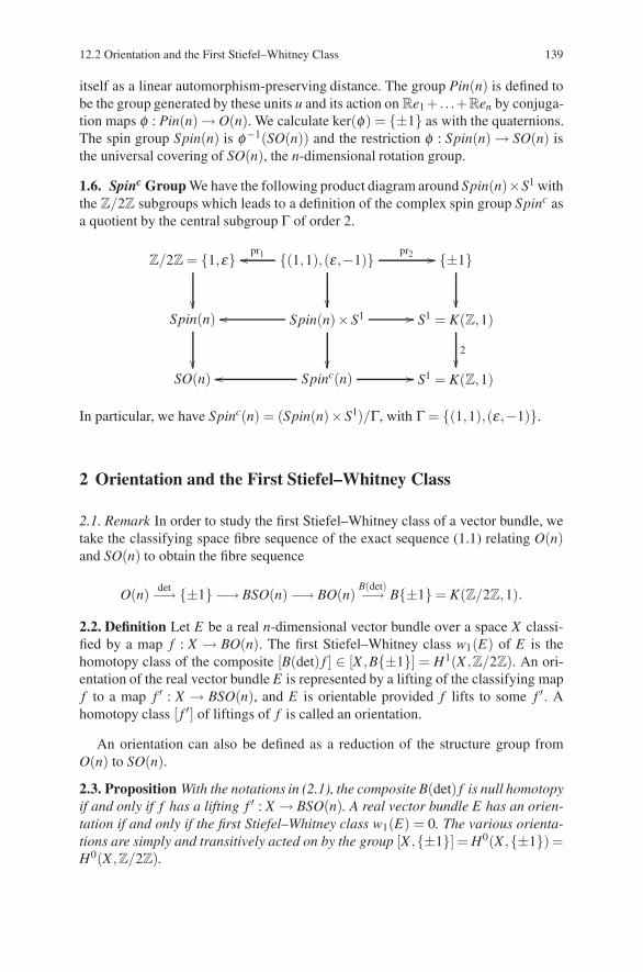
12.2 Orientation and the First Stiefel–Whitney Class 139
itself as a linear automorphism-preserving distance. The group Pin(n) is defined tobe the group generated by these units u and its action on Re1 + . . .+Ren by conjuga-tion maps φ : Pin(n)→ O(n). We calculate ker(φ) = {±1} as with the quaternions.The spin group Spin(n) is φ−1(SO(n)) and the restriction φ : Spin(n) → SO(n) isthe universal covering of SO(n), the n-dimensional rotation group.
1.6. Spinc Group We have the following product diagram around Spin(n)×S1 withthe Z/2Z subgroups which leads to a definition of the complex spin group Spinc asa quotient by the central subgroup Γ of order 2.
Z/2Z = {1,ε}
��
{(1,1),(ε,−1)}pr1�� pr2 ��
��
{±1}
��Spin(n)
��
Spin(n)×S1��
��
�� S1 = K(Z,1)
2��
SO(n) Spinc(n)�� �� S1 = K(Z,1)
In particular, we have Spinc(n) = (Spin(n)×S1)/Γ, with Γ= {(1,1),(ε,−1)}.
2 Orientation and the First Stiefel–Whitney Class
2.1. Remark In order to study the first Stiefel–Whitney class of a vector bundle, wetake the classifying space fibre sequence of the exact sequence (1.1) relating O(n)and SO(n) to obtain the fibre sequence
O(n) det−→ {±1} −→ BSO(n) −→ BO(n)B(det)−→ B{±1}= K(Z/2Z,1).
2.2. Definition Let E be a real n-dimensional vector bundle over a space X classi-fied by a map f : X → BO(n). The first Stiefel–Whitney class w1(E) of E is thehomotopy class of the composite [B(det) f ] ∈ [X ,B{±1}] = H1(X ,Z/2Z). An ori-entation of the real vector bundle E is represented by a lifting of the classifying mapf to a map f ′ : X → BSO(n), and E is orientable provided f lifts to some f ′. Ahomotopy class [ f ′] of liftings of f is called an orientation.
An orientation can also be defined as a reduction of the structure group fromO(n) to SO(n).
2.3. Proposition With the notations in (2.1), the composite B(det) f is null homotopyif and only if f has a lifting f ′ : X → BSO(n). A real vector bundle E has an orien-tation if and only if the first Stiefel–Whitney class w1(E) = 0. The various orienta-tions are simply and transitively acted on by the group [X ,{±1}] = H0(X ,{±1}) =H0(X ,Z/2Z).
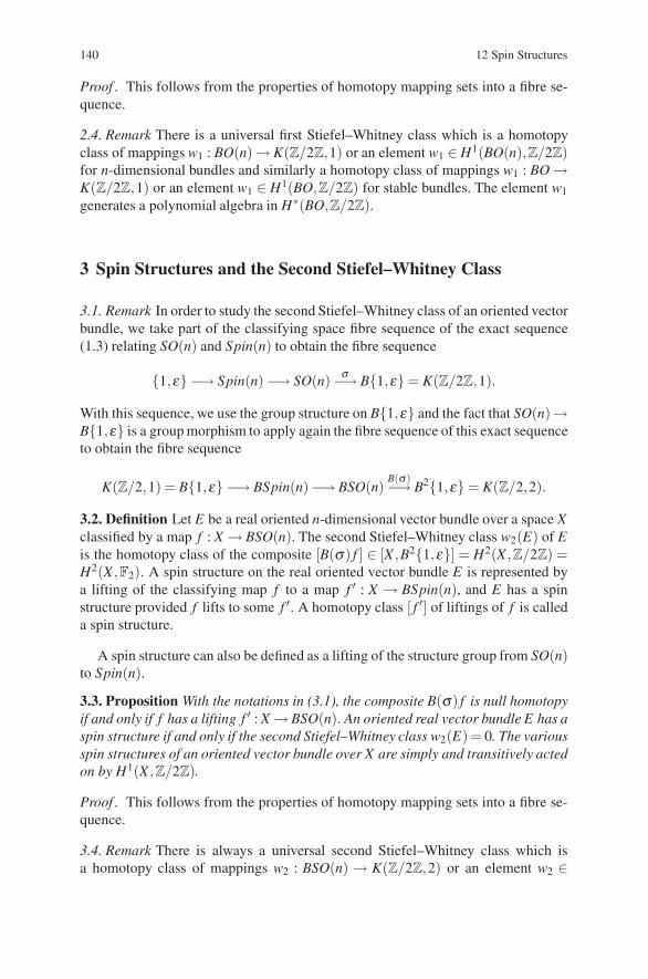
140 12 Spin Structures
Proof . This follows from the properties of homotopy mapping sets into a fibre se-quence.
2.4. Remark There is a universal first Stiefel–Whitney class which is a homotopyclass of mappings w1 : BO(n)→ K(Z/2Z,1) or an element w1 ∈ H1(BO(n),Z/2Z)for n-dimensional bundles and similarly a homotopy class of mappings w1 : BO →K(Z/2Z,1) or an element w1 ∈ H1(BO,Z/2Z) for stable bundles. The element w1
generates a polynomial algebra in H∗(BO,Z/2Z).
3 Spin Structures and the Second Stiefel–Whitney Class
3.1. Remark In order to study the second Stiefel–Whitney class of an oriented vectorbundle, we take part of the classifying space fibre sequence of the exact sequence(1.3) relating SO(n) and Spin(n) to obtain the fibre sequence
{1,ε} −→ Spin(n)−→ SO(n) σ−→ B{1,ε} = K(Z/2Z,1).
With this sequence, we use the group structure on B{1,ε} and the fact that SO(n)→B{1,ε} is a group morphism to apply again the fibre sequence of this exact sequenceto obtain the fibre sequence
K(Z/2,1) = B{1,ε} −→ BSpin(n)−→ BSO(n)B(σ)−→ B2{1,ε} = K(Z/2,2).
3.2. Definition Let E be a real oriented n-dimensional vector bundle over a space Xclassified by a map f : X → BSO(n). The second Stiefel–Whitney class w2(E) of Eis the homotopy class of the composite [B(σ) f ] ∈ [X ,B2{1,ε}] = H2(X ,Z/2Z) =H2(X ,F2). A spin structure on the real oriented vector bundle E is represented bya lifting of the classifying map f to a map f ′ : X → BSpin(n), and E has a spinstructure provided f lifts to some f ′. A homotopy class [ f ′] of liftings of f is calleda spin structure.
A spin structure can also be defined as a lifting of the structure group from SO(n)to Spin(n).
3.3. Proposition With the notations in (3.1), the composite B(σ) f is null homotopyif and only if f has a lifting f ′ : X →BSO(n). An oriented real vector bundle E has aspin structure if and only if the second Stiefel–Whitney class w2(E) = 0. The variousspin structures of an oriented vector bundle over X are simply and transitively actedon by H1(X ,Z/2Z).
Proof . This follows from the properties of homotopy mapping sets into a fibre se-quence.
3.4. Remark There is always a universal second Stiefel–Whitney class which isa homotopy class of mappings w2 : BSO(n) → K(Z/2Z,2) or an element w2 ∈
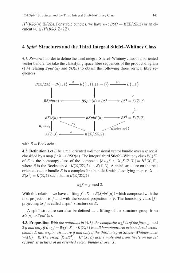
12.4 Spinc Structures and the Third Integral Stiefel–Whitney Class 141
H2(BSO(n),Z/2Z). For stable bundles, we have w2 : BSO → K(Z/2Z,2) or an el-ement w2 ∈ H2(BSO,Z/2Z).
4 Spinc Structures and the Third Integral Stiefel–Whitney Class
4.1. Remark In order to define the third integral Stiefel–Whitney class of an orientedvector bundle, we take the classifying space fibre sequences of the product diagram(1.4) relating Spinc(n) and SO(n) to obtain the following three vertical fibre se-quences
B(Z/2Z) = B{1,ε}
��
B{(1,1),(ε,−1)}pr1��
��
pr2 �� B{±1}
��BSpin(n)
��
BSpin(n)×BS1
��
�� �� BS1 = K(Z,2)
2��
BSO(n)w2
���������
��������
W3=δw2
��
BSpinc(n)
��
�� �� BS1 = K(Z,2)
reduction mod 2��������
������
�
K(Z,3) K(Z/2Z,2)�
with δ = Bockstein.
4.2. Definition Let E be a real oriented n-dimensional vector bundle over a space Xclassified by a map f : X → BSO(n). The integral third Stiefel–Whitney class W3(E)of E is the homotopy class of the composite [δw2 f ] ∈ [X ,K(Z,3)] = H3(X ,Z),where δ is the Bockstein δ : K(Z/2Z,2) → K(Z,3). A spinc structure on the realoriented vector bundle E is a complex line bundle L with classifying map g : X →B(S1) = K(Z,2) such that in K(Z/2Z,2)
w2 f = g mod 2.
With this relation, we have a lifting f ′ : X → B(Spinc(n)) which composed with thefirst projection is f and with the second projection is g. The homotopy class [ f ′]projecting to f is called a spinc structure on E .
A spinc structure can also be defined as a lifting of the structure group fromSO(n) to Spinc(n).
4.3. Proposition With the notations in (4.1), the composite w2 f is of the form g mod2 if and only if δw2 f =W3 f : X →K(Z,3) is null homotopic. An oriented real vectorbundle E has a spinc structure if and only if the third integral Stiefel–Whitney classW3(E) = 0. The group [X ,BS1] = H2(X ,Z) acts simply and transitively on the setof spinc structures of an oriented vector bundle E over X.
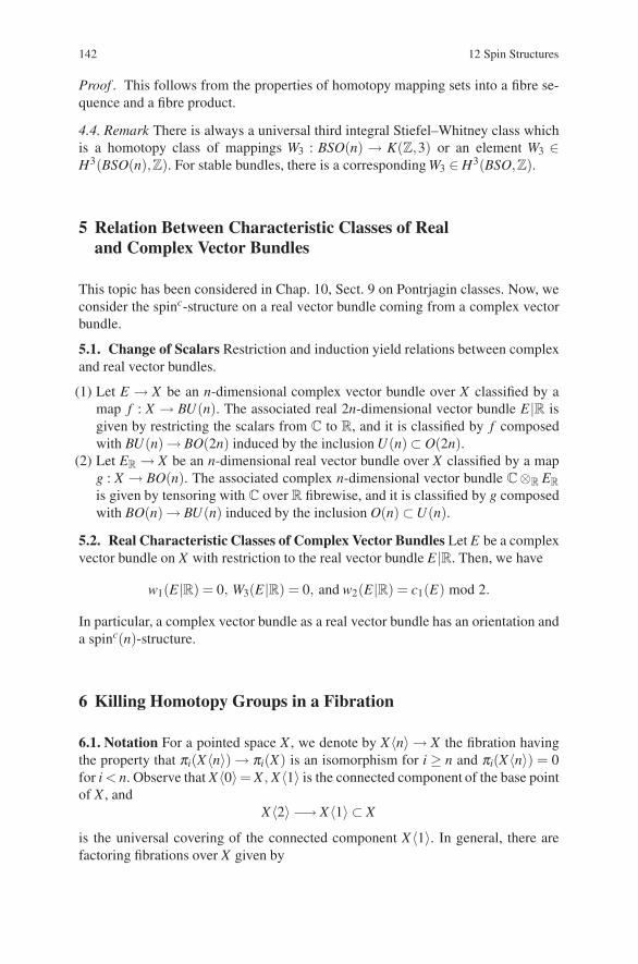
142 12 Spin Structures
Proof . This follows from the properties of homotopy mapping sets into a fibre se-quence and a fibre product.
4.4. Remark There is always a universal third integral Stiefel–Whitney class whichis a homotopy class of mappings W3 : BSO(n) → K(Z,3) or an element W3 ∈H3(BSO(n),Z). For stable bundles, there is a corresponding W3 ∈ H3(BSO,Z).
5 Relation Between Characteristic Classes of Realand Complex Vector Bundles
This topic has been considered in Chap. 10, Sect. 9 on Pontrjagin classes. Now, weconsider the spinc-structure on a real vector bundle coming from a complex vectorbundle.
5.1. Change of Scalars Restriction and induction yield relations between complexand real vector bundles.
(1) Let E → X be an n-dimensional complex vector bundle over X classified by amap f : X → BU(n). The associated real 2n-dimensional vector bundle E|R isgiven by restricting the scalars from C to R, and it is classified by f composedwith BU(n) → BO(2n) induced by the inclusion U(n) ⊂ O(2n).
(2) Let ER → X be an n-dimensional real vector bundle over X classified by a mapg : X → BO(n). The associated complex n-dimensional vector bundle C⊗R ER
is given by tensoring with C over R fibrewise, and it is classified by g composedwith BO(n) → BU(n) induced by the inclusion O(n) ⊂U(n).
5.2. Real Characteristic Classes of Complex Vector Bundles Let E be a complexvector bundle on X with restriction to the real vector bundle E|R. Then, we have
w1(E|R) = 0, W3(E|R) = 0, and w2(E|R) = c1(E) mod 2.
In particular, a complex vector bundle as a real vector bundle has an orientation anda spinc(n)-structure.
6 Killing Homotopy Groups in a Fibration
6.1. Notation For a pointed space X , we denote by X〈n〉 → X the fibration havingthe property that πi(X〈n〉) → πi(X) is an isomorphism for i ≥ n and πi(X〈n〉) = 0for i < n. Observe that X〈0〉= X , X〈1〉 is the connected component of the base pointof X , and
X〈2〉 −→ X〈1〉 ⊂ X
is the universal covering of the connected component X〈1〉. In general, there arefactoring fibrations over X given by
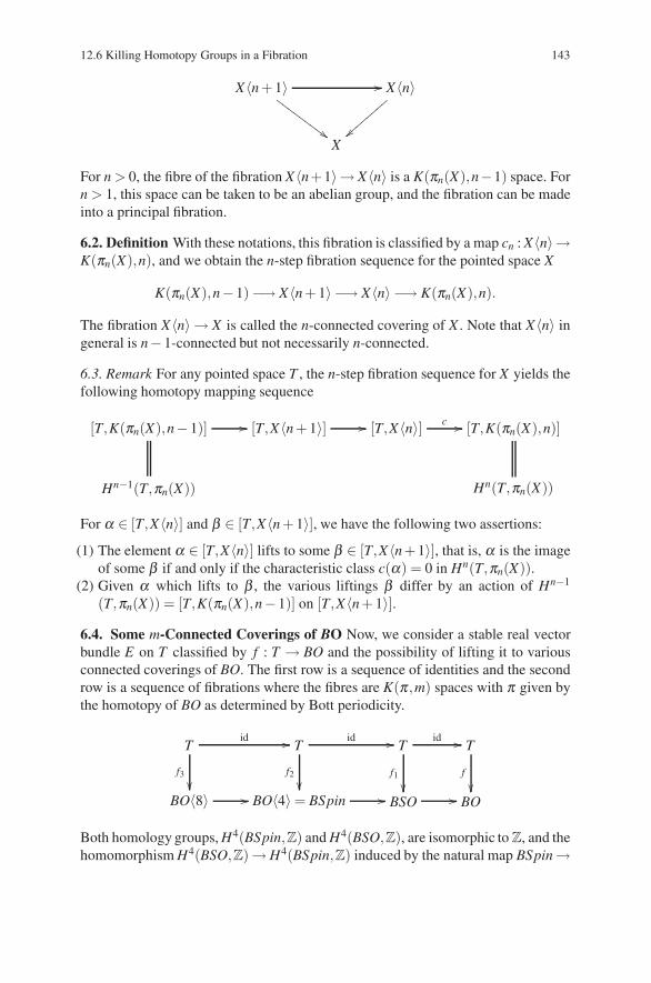
12.6 Killing Homotopy Groups in a Fibration 143
X〈n + 1〉
�����
����
���� X〈n〉
����������
X
For n > 0, the fibre of the fibration X〈n+1〉→ X〈n〉 is a K(πn(X),n−1) space. Forn > 1, this space can be taken to be an abelian group, and the fibration can be madeinto a principal fibration.
6.2. Definition With these notations, this fibration is classified by a map cn : X〈n〉→K(πn(X),n), and we obtain the n-step fibration sequence for the pointed space X
K(πn(X),n−1)−→ X〈n + 1〉 −→ X〈n〉 −→ K(πn(X),n).
The fibration X〈n〉 → X is called the n-connected covering of X . Note that X〈n〉 ingeneral is n−1-connected but not necessarily n-connected.
6.3. Remark For any pointed space T , the n-step fibration sequence for X yields thefollowing homotopy mapping sequence
[T,K(πn(X),n−1)] �� [T,X〈n + 1〉] �� [T,X〈n〉] c �� [T,K(πn(X),n)]
Hn−1(T,πn(X)) Hn(T,πn(X))
For α ∈ [T,X〈n〉] and β ∈ [T,X〈n + 1〉], we have the following two assertions:
(1) The element α ∈ [T,X〈n〉] lifts to some β ∈ [T,X〈n+1〉], that is, α is the imageof some β if and only if the characteristic class c(α) = 0 in Hn(T,πn(X)).
(2) Given α which lifts to β , the various liftings β differ by an action of Hn−1
(T,πn(X)) = [T,K(πn(X),n−1)] on [T,X〈n + 1〉].6.4. Some m-Connected Coverings of BO Now, we consider a stable real vectorbundle E on T classified by f : T → BO and the possibility of lifting it to variousconnected coverings of BO. The first row is a sequence of identities and the secondrow is a sequence of fibrations where the fibres are K(π ,m) spaces with π given bythe homotopy of BO as determined by Bott periodicity.
Tid ��
f3��
T
f2��
id �� T
f1��
id �� T
f
��BO〈8〉 �� BO〈4〉 = BSpin �� BSO �� BO
Both homology groups, H4(BSpin,Z) and H4(BSO,Z), are isomorphic to Z, and thehomomorphism H4(BSO,Z)→ H4(BSpin,Z) induced by the natural map BSpin→
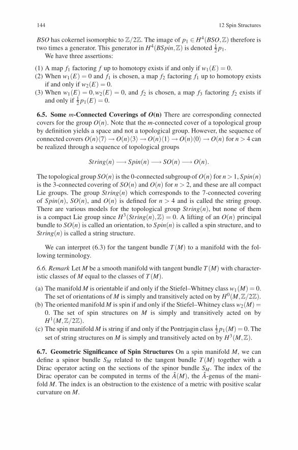
144 12 Spin Structures
BSO has cokernel isomorphic to Z/2Z. The image of p1 ∈ H4(BSO,Z) therefore istwo times a generator. This generator in H4(BSpin,Z) is denoted 1
2 p1.We have three assertions:
(1) A map f1 factoring f up to homotopy exists if and only if w1(E) = 0.(2) When w1(E) = 0 and f1 is chosen, a map f2 factoring f1 up to homotopy exists
if and only if w2(E) = 0.(3) When w1(E) = 0,w2(E) = 0, and f2 is chosen, a map f3 factoring f2 exists if
and only if 12 p1(E) = 0.
6.5. Some m-Connected Coverings of O(n) There are corresponding connectedcovers for the group O(n). Note that the m-connected cover of a topological groupby definition yields a space and not a topological group. However, the sequence ofconnected covers O(n)〈7〉→ O(n)〈3〉→ O(n)〈1〉→ O(n)〈0〉→ O(n) for n > 4 canbe realized through a sequence of topological groups
String(n)−→ Spin(n)−→ SO(n)−→ O(n).
The topological group SO(n) is the 0-connected subgroup of O(n) for n > 1, Spin(n)is the 3-connected covering of SO(n) and O(n) for n > 2, and these are all compactLie groups. The group String(n) which corresponds to the 7-connected coveringof Spin(n), SO(n), and O(n) is defined for n > 4 and is called the string group.There are various models for the topological group String(n), but none of themis a compact Lie group since H3(String(n),Z) = 0. A lifting of an O(n) principalbundle to SO(n) is called an orientation, to Spin(n) is called a spin structure, and toString(n) is called a string structure.
We can interpret (6.3) for the tangent bundle T (M) to a manifold with the fol-lowing terminology.
6.6. Remark Let M be a smooth manifold with tangent bundle T (M) with character-istic classes of M equal to the classes of T (M).
(a) The manifold M is orientable if and only if the Stiefel–Whitney class w1(M) = 0.The set of orientations of M is simply and transitively acted on by H0(M,Z/2Z).
(b) The oriented manifold M is spin if and only if the Stiefel–Whitney class w2(M) =0. The set of spin structures on M is simply and transitively acted on byH1(M,Z/2Z).
(c) The spin manifold M is string if and only if the Pontrjagin class 12 p1(M) = 0. The
set of string structures on M is simply and transitively acted on by H3(M,Z).
6.7. Geometric Significance of Spin Structures On a spin manifold M, we candefine a spinor bundle SM related to the tangent bundle T (M) together with aDirac operator acting on the sections of the spinor bundle SM . The index of theDirac operator can be computed in terms of the A(M), the A-genus of the mani-fold M. The index is an obstruction to the existence of a metric with positive scalarcurvature on M.
12.6 Killing Homotopy Groups in a Fibration 145
6.8. Remark Conjecturally, there is a similar interpretation of the existence of stringstructures on M in terms of spinors and Dirac operators on the free loop spaceΛ(M)of M. The index of the Dirac operator would be the Witten index, and it is con-jecturally an obstruction to the existence of a metric with positive Ricci curvatureon M.

Part IIIVersions of K-Theory and Bott Periodicity
We consider complex and real K-theory from the point of view of the theory ofvector bundles on compact spaces, from the point of view of operator algebra, andfrom the homotopy point of view using classifying spaces. The G-equivariant K-theory is introduced in the context of the Grothendieck construction together withthe Atiyah real theory relating complex, self-conjugate, and real versions in termsof one equivariant construction. Bott periodicity and the Thom isomorphism have arather direct meaning in this context as developed by Atiyah. This is carried out inChap. 13 and 14. This is the version which is easily adopted to the questions aroundthe index theorem.
In Chap. 15, the homotopy version of K-theory of a space X with K(X) identifiedwith [X ,Z×BU ] is considered. This is the classification space approach which arisesout of the classifying space approach to fibre bundles. In fact, BU is an increasinginductive limit or colimit lim−→nBU(n), and the real K-theory KO(X) is isomorphic
to [X ,Z×BO]. In this context, Bott periodicity is a series of maps into loop spaceswhich have certain relation to Clifford algebras. These maps are homotopy equiva-lences, and their relation to Clifford algebras is pointed out.
In Chap. 16, we prove some of the homotopy properties of general linear groupsby elementary considerations.
In Chap. 18, the operator formulation of equivariant K-theory is carried out. For acompact space X , we form the C∗-algebra C(X) of continuous C-valued functions,and the C∗-algebra K-theory K0(C(X)) is isomorphic to K0(X), the K-theory ofvector bundles. For a compact group G acting on a compact space X we form thecross product C∗-algebra G �C(X), and the C∗-algebra K-theory K0(G �C(X)) isnaturally isomorphic to K0
G(X), the K-theory of G-equivariant vector bundles onX considered by Atiyah and Segal. In this context, Bott periodicity comes fromanalysis of Toplitz operators.
Chapter 13G-Spaces, G-Bundles, and G-Vector Bundles
In this chapter, we introduce the basic notions related to objects being acted on bya group G. Since the objects like spaces and bundles have topologies, we will as-sume that the group is a topological group. Let G be a topological group which iseventually a compact Lie group. We consider G-spaces X and G-vector bundles witha base G-space. The aim is to develop the theory in a parallel fashion to ordinarybundle theory taking into account the G-action on both the base space and the totalspace together with actions between fibres. There are some generalities which ap-ply to bundles in general including principal bundles which we outline in the firstsections. A G-vector bundle over a point is just a representation of G on a vectorspace. In particular, we analyze part of the properties of G-vector bundles in termsof representation theory of G. Since the representation theory of compact groups iswell understood, we will restrict ourselves to this case for the more precise theory,but compact groups will play a role for topological reasons too. For example, weshow that G-homotopic maps always induce isomorphic G-vector bundles when Gis compact.
Of special interest is the group G of two elements. The symbol (τ) is a symbol forthe group on two elements with generator τ which is always an involution under anyaction. The first example is that of complex conjugation τ(a + ib) = a− ib, whereτ : C→C. We incorporate the concept real structures in K-theory using (τ)-bundlesand mix this with the G-equivariant theory, for it plays a basic role in the relationbetween complex and real structures on vector bundles.
1 Relations Between Spaces and G-Spaces: G-Homotopy
In Chap. 5, Sect. 1, we introduced the basic notions of G-spaces and the G-equivariant maps between G-spaces as background for principal bundles where Gacted on total space-preserving fibres. We extend these concepts so that G can actalso on the base space. This consists of making certain functors more explicit.
D. Husemoller et al.: G-Spaces, G-Bundles, and G-Vector Bundles, Lect. Notes Phys. 726, 149–161 (2008)DOI 10.1007/978-3-540-74956-1 14 © Springer-Verlag Berlin Heidelberg 2008
150 13 G-Spaces, G-Bundles, and G-Vector Bundles
1.1. Notation for the Basic Categories and Functors Let (top) be the categoryof spaces and maps, and let (G\top) be the category of G-spaces and G-equivariantmaps. If G is the trivial group, (G\top) can be identified with (top). For two G-spaces, X and Y , one obtains the space Map(X ,Y ) of all continuous maps from Xto Y . It carries a natural G-action which is motivated and specified in remark 1.5 anddefinition 1.6 below.
For a homomorphism ρ : H → G of topological groups, the restriction functorRes : (G\top) → (H\top) assigns to a G-space X the H-space X with the actionθ : G×X → X given by the composition
θ (ρ× id) : H ×X → G×X → X .
The trivial G-space functor Tr : (top) → (G\top) assigns to a space W the G-spaceTr(W ) = W as a space with trivial G-action. The stripping (or forgetful) functorStr : (G\top) → (top) assigns to a G-space X the space Str(X) = X viewed as aspace without G-action. The functor Tr can be identified with the restriction functorinduced by the homomorphism which maps G to the trivial group while the strippingfunctor Str can be identified with the restriction functor induced by the inclusion ofthe trivial group into G.
The functor Res has both a left and a right adjoint.
1.2. Biadjunctions of Res The induction functor Ind : (H\top) → (G\top) as-signs to an H-space X the quotient G ×HX which is obtained by identifying(gρ(h−1),x)) = (g,hx) for all g ∈ G,h ∈ H, and x ∈ X . The quotient is regardedas a G-space via the action induced by left multiplication on the first factor. Thefunctor is a left adjoint to the functor Res, that is, for every G-space W , one has
MapG(G×HX ,W ) = MapH(X ,Res(W ))
The coinduction functor Coind : (G\top) → (H\top) assigns to an H-space Ythe H-space MapH(G,Y ), where G is regarded as the H-space where an elementh ∈ H acts on G by left multiplication with ρ(h)−1. That is, the space MapH(G,Y )consists of all maps φ : G → Y satisfying where an element h ∈ H acts on G byleft multiplication via ρ . More specifically, MapH(G,Y ) consists of all maps φ :G → Y satisfying tφ(s) = φ(ρ(t)s) for all s ∈ G and t ∈ H. The space MapH(G,Y )is regarded as a G-space with the action of an element s ∈ G on a function φ ∈MapH(G,Y ) is given by (s.φ)(s′) = φ(s′s). The functor Coind is right adjoint toRes, that is, in terms of morphism sets, we have
MapH(Res(X),Y ) = MapG(X ,Coind(Y ))
From the above, we obtain biadjunctions to the functors Tr and Str.
1.3. Biadjunctions of Tr Let X be a G-space. We have two spaces Quot(X) =G\X and Fix(X) = MapG(∗,X) ⊂ X with, respectively, the quotient and subspacetopologies from X . They correspond to the induction and the coinduction functor
13.1 Relations Between Spaces and G-Spaces: G-Homotopy 151
for the homomorphism which maps G to the trivial group. We therefore have thefollowing adjunction relations
Quot � Tr and Tr � Fix : (G\top)−→ (top).
In terms of morphism sets we have, for G-spaces W , the natural isomorphisms
Map(G\X ,W ) = MapG(X ,Tr(W ))
andMapG(Tr(W ),Y ) = Map(W,Fix(Y )) .
1.4. Biadjunctions of Str Let W be a space. For the inclusion of the trivial groupinto G, the adjunctions of (1.2) specialize to the adjunction relation
G× ( .) � Str and Str � Map(G, .) : (top) −→ (G\top).
In terms of morphism sets, we have the natural isomorphisms
MapG(G×W,Y) = Map(W,Str(Y ))
andMapG(X ,Map(G,W )) = Map(Str(X),W ).
This adjunction relation depends on the adjunction
Map(X ×T,Y) = Map(X ,Map(T,Y )) ,
which we discussed in Sect. 1 and 2 of Chap. 6.The adjunction for spaces
c : Map(X ×T,Y ) → Map(X ,Map(T,Y ))
where c( f )(x)(t) = f (x,t) plays a basic role for the concept of homotopy of maps.We extend adjunction to G-spaces in order to consider G-homotopy.
1.5. Remark Let X , T , and Y be G-spaces. The G-structure on X ×T is given by therelation s(x,t) = (sx,st), and a G-map f : X ×T →Y satisfies the relation s f (x, t) =f (sx,st). In order that f (x)(t) : X → Map(T,Y ) be a G-morphism, we must havef (sx)(t) = [s. f (x)](t), or in other terms, we require that
f (sx,t) = f (sx,ss−1t) = s f (x,s−1t) = [s. f (x)](t),
and this leads to the action G×Map(T,Y ) → Map(T,Y ), where
(s.u)(t) = su(s−1t) for s ∈ G, t ∈ T.
1.6. Definition The action G × Map(T,Y ) → Map(T,Y ) given by the formulas.u(t) = (s.u)(t) = su(s−1t) for s ∈ G, t ∈ T makes Map(T,Y ) into a G-space. Now,we can use 6(2.4) in the G-equivariant setting.
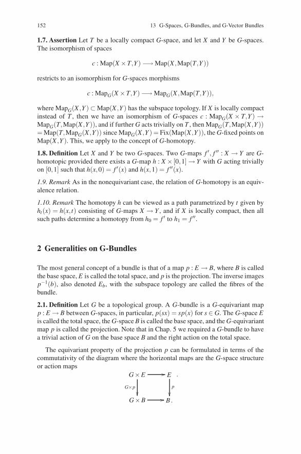
152 13 G-Spaces, G-Bundles, and G-Vector Bundles
1.7. Assertion Let T be a locally compact G-space, and let X and Y be G-spaces.The isomorphism of spaces
c : Map(X ×T,Y) −→ Map(X ,Map(T,Y ))
restricts to an isomorphism for G-spaces morphisms
c : MapG(X ×T,Y ) −→ MapG(X ,Map(T,Y )),
where MapG(X ,Y )⊂ Map(X ,Y ) has the subspace topology. If X is locally compactinstead of T , then we have an isomorphism of G-spaces c : MapG(X × T,Y ) →MapG(T,Map(X ,Y )), and if further G acts trivially on T , then MapG(T,Map(X ,Y ))= Map(T,MapG(X ,Y )) since MapG(X ,Y ) = Fix(Map(X ,Y )), the G-fixed points onMap(X ,Y ). This, we apply to the concept of G-homotopy.
1.8. Definition Let X and Y be two G-spaces. Two G-maps f ′, f ′′ : X → Y are G-homotopic provided there exists a G-map h : X × [0,1] → Y with G acting triviallyon [0,1] such that h(x,0) = f ′(x) and h(x,1) = f ′′(x).
1.9. Remark As in the nonequivariant case, the relation of G-homotopy is an equiv-alence relation.
1.10. Remark The homotopy h can be viewed as a path parametrized by t given byht(x) = h(x, t) consisting of G-maps X → Y , and if X is locally compact, then allsuch paths determine a homotopy from h0 = f ′ to h1 = f ′′.
2 Generalities on G-Bundles
The most general concept of a bundle is that of a map p : E → B, where B is calledthe base space, E is called the total space, and p is the projection. The inverse imagesp−1(b), also denoted Eb, with the subspace topology are called the fibres of thebundle.
2.1. Definition Let G be a topological group. A G-bundle is a G-equivariant mapp : E → B between G-spaces, in particular, p(sx) = sp(x) for s ∈ G. The G-space Eis called the total space, the G-space B is called the base space, and the G-equivariantmap p is called the projection. Note that in Chap. 5 we required a G-bundle to havea trivial action of G on the base space B and the right action on the total space.
The equivariant property of the projection p can be formulated in terms of thecommutativity of the diagram where the horizontal maps are the G-space structureor action maps
G×E
G×p
��
�� E
p
��G×B �� B .
.
13.3 Generalities on G-Vector Bundles 153
2.2. Definition Let p′ : E ′ → B′ and p′′ : E ′′ → B′′ be two G-bundles. A morphismis a pair of G-equivariant maps u : E ′ → E ′′ and f : B′ → B′′ defined, respectively,on the total spaces and base spaces such that p′′u = f p′. The composition of G-bundle morphisms is defined by composing the maps on the total and base spaces.In the case that B′ = B′′ = B and f is the identity on B, the morphism u : E ′ → E ′′ iscalled a B-morphism of G-bundles. The composition of two B-morphisms is againa B-morphism of G-bundles.
2.3. Remark Let p : E → B be a G-bundle, and let b ∈ B and s ∈ G with sb ∈ B.The action of s on E restricts to fibres Eb → Esb as an isomorphism with inverse theaction of s−1 on the fibres.
2.4. Notation Let p : E → B be a G-bundle, and let Γ(B,E) denote the set of allsections of p : E → B, that is, all maps σ : B → E with p(σ(b)) = b for all b∈ B. Wegive Γ(B,E) the subspace topology from the compact open topology on Map (B,E).It is a G-space with action (sσ)(b) = s(σ(s−1b)) for b ∈ B, s ∈ G, and σ ∈ Γ(B,E).A G-equivariant section σ ∈ Γ(B,E) is one with sσ = σ for all s ∈ G, and the subsetof G-equivariant sections is denoted by ΓG(B,E).
2.5. Definition Let p′ : E ′ → B′ and p′′ : E ′′ → B′′ be two G-bundles. The productG-bundle is p′ × p′′ : E ′ × E ′ → B′ × B′′. In the case that B′ = B′′ = B, the fibreproduct G-bundle is q : E ′ ×B E ′′ → B, the fibre product of bundles with G-actions(x′,x′′) = (sx′,sx′′), where the condition p′(x′) = p′′(x′′) implies p′(sx′) = p′′(sx′′).
2.6. Definition Let p : E → B be a G-bundle, and let f : B′ → B be a G-map. Then,the induced bundle f−1(E) with total space f−1(E) ⊂ B′ ×E defined by the con-dition (b′,x) ∈ f−1(E) if and only if f (b′) = p(x), and projection q : f−1(E) → B′given by q(b′,x) = b′ has a G-bundle structure, where s(b′,x) = (sb′,sx).
2.7. Remark Let p′ : E ′ → B′ and p′′ : E ′′ → B′′ be two G-bundles with a morphismconsisting of a pair of G-equivariant maps u : E ′ → E ′′ and f : B′ → B′′ defined,respectively, on the total spaces and base spaces such that p′′u = f p′. Then, thereis a factorization u = u′′u′ of u as a G-bundle morphism u′ : E ′ → f−1(E ′′) over B′and u′′ : f−1(E ′′) → E ′′ as a G-bundle morphism over f . The formulas are u′(x′) =(p′(x′),u(x′)) and u′′(b′,x′′) = x′′.
3 Generalities on G-Vector Bundles
The primary interest in this chapter is in (finite dimensional) complex vector bun-dles, and in the course of our discussion, real and quaternionic vector bundles willarise within the equivariant structure. As usual, G denotes a topological group.
3.1. Definition Let X be a G-space. A G-vector bundle over X is a G-map p : E → Xwhich is a G-bundle and a vector bundle such that for all s∈ G, the action of s : Eb →Esb is a vector space isomorphism.
154 13 G-Spaces, G-Bundles, and G-Vector Bundles
Observe that if sb = b, then s acts as a linear automorphism of the vector spacefibre Eb.
3.2. Definition Let p′ : E ′ → X ′ and p′′ : E ′′ → X ′′ be two G-vector bundles, andlet f : X ′ → X ′′ be a G-map. An f -morphism u : E ′ → E ′′ of G-vector bundlesis a morphism of G-bundles which also is a morphism of vector bundles. WhenX ′ = X ′′ = X and f is the identity on X , then u is called an X-morphism of G-vectorbundles.
3.3. Categories of G-Vector Bundles Let X be a G-space. The categories of realand complex G-vector bundles over X are denoted by VectR(X ,G) and VectC(X ,G).Tensoring with C (over R) gives a functor VectR(X ,G) → VectC(X ,G), and reduc-ing the scalar multiplication from the complex numbers C to the real numbers R
gives a functor VectC(X ,G) → VectR(X ,G). The composition of the first functorfollowed by the second is a functor VectR(X ,G) → VectR(X ,G) which carries areal G-bundle V to V ⊕V over (X ,G). The composition of the second functor fol-lowed by the first is a functor VectC(X ,G) → VectC(X ,G) which carries a complexG-bundle E to E ⊕E∗ over (X ,G).
3.4. Remark In (2.4), the G-action on the set of sections Γ(X ,E) was introduced fora G-vector bundle. The space Γ(X ,E) of sections is, first of all, a vector space withthe usual addition and scalar multiplication given by the formula
(a′σ ′ + a′′σ ′′)(b) = a′σ ′(b)+ a′′σ ′′(b)
for σ ′,σ ′′ ∈ Γ(X ,E) and scalars a′ and a′′. Moreover, by (1.4), the action of s ∈ Ginduces the identities
(s(a′σ ′ + a′′σ ′′))(b) = s((a′σ ′ + a′′σ ′′)(s−1b)) =a′s(σ ′(s−1b)+ a′′s(σ ′′)(s−1b) = a′(sσ ′)(b)+ a′′(sσ ′′)(b)
for b ∈ X ,s ∈ G, and σ ∈ Γ(X ,E) showing that Γ(X ,E) is a G-vector space. If u :E ′ →E ′′ is an X-morphism of G-vector bundles, then Γ(u)(σ)(b) = u(σ(b)) definesa morphism Γ(u) : Γ(X ,E ′)→ Γ(X ,E ′′) of G-vector spaces, because sΓ(u)(σ)(b) =su(σ(b)) = su(σ(s−1b)) = u(s(σ(s−1b))) = Γ(u)(sσ)(b).
Finally, the cross section vector space is a functor from the categories of complexand real G-vector bundles
Γ(X ,) : VectC(X ,G) −→ RepC(G) and Γ(X ,) : VectR(X ,G) −→ RepR(G)
to the categories RepC(G) and RepR(G) of, respectively, complex and real (notnecessarily finite dimensional) representations of G. The question of continuity ofsuch representations will not be discussed here.
3.5. Definition Let p′ : E ′ → X ′ and p′′ : E ′′ → X ′′ be two G-vector bundles. Theproduct p′ × p′′ : E ′ ×E ′′ → X ′ ×X ′′ is a G-vector bundle. In the case that X ′ =X ′′ = X , the fibre product q : E ′ ×X E ′′ → X is a G-vector bundle.
13.4 Special Examples of G-Vector Bundles 155
3.6. Definition Let p : E → X be a G-vector bundle, and let f : X ′ → X be a G-map.Then, the induced bundle f−1(E) is a G-vector bundle as can be checked immedi-ately from the total space f−1(E)⊂ X ′×E defined by the condition (b′,x)∈ f−1(E)if and only if f (b′) = p(x) and projection q : f−1(E) → X ′ given by q(b′,x) = b′has a G-bundle structure, where s(b′,x) = (sb′,sx) and vector bundle structurea′(b′,x1)+ a′′(b′,x2) = (b,a′x1 + a′′x2).
As with (2.7), we have the following remark.
3.7. Remark Let p′ : E ′ → X ′ and p′′ : E ′′ → X ′′ be two G-vector bundles with amorphism consisting of a pair of maps u : E ′ → E ′′ and f : X ′ → X ′′ defined, re-spectively, on the total spaces and base spaces such that p′′u = f p′. Then, there isa factorization u = u′′u′ of u as a G-vector bundle morphism u′ : E ′ → f−1(E ′′)over X ′ and u′′ : f−1(E ′′) → E ′′, a G-vector bundle morphism over f . This followsimmediately from the formulas u′(x′) = (p′(x′),u(x′)) and u′′(b′,x′′) = x′′.
3.8. Definition Analogously, as in Chap. 4, Sect. 2, one defines the G-equivariantK-theory ring KG(X) of a G-space X as the Grothendieck construction applied tothe semiring of isomorphism classes of G-vector bundles on X .
4 Special Examples of G-Vector Bundles
We consider three special cases of G-vector bundles.
4.1. Example Let E be a G-vector bundle over a space B which is trivial as a vectorbundle. This means that p : E → B is isomorphic to prB : B×V → B, where V is acomplex vector space. For this product G-bundle, we have an action G×B → B andthe product B×V with V has a G-action G×B×V → B×V of the form
s(b,v) = (sb,J(s,b)v),
where J : G×B → End(V ) is a continuous function. For the unit of the action, wemust have J(1,b) = idV for all b ∈ B, and for the associativity of the action, we musthave
(stb,J(st,b)v) = st(b,v) = s(tb,J(t,b)v) = (stb,J(s,tb)J(t,b)v),
or for all b ∈ B and s,t ∈ G, the cocycle relation (or chain rule)
J(st,b) = J(s,tb)J(t,b).
When s = t = 1, we have J(1,b) = J(1,b)J(1,b) so that if J(1,b) is invertible, thenwe have automatically J(1,b) = 1. Otherwise, it is only an idempotent.
Conversely, for a continuous function J : G×B → End(V ) satisfying J(1,b) = 1and J(st,b) = J(s,tb)J(t,b), the product bundle has a G-bundle structure given bys(b,v) = (b,J(b,s)v). If we change the trivialization by a function C : B → GL(V ),
156 13 G-Spaces, G-Bundles, and G-Vector Bundles
then we have a new G-bundle structure where J′(b,s) = C(sb)J(b,s)C(b)−1, for ifψ(b,v) = (b,C(b)v), then the action
(sb,J′(b,s)v) = ψsψ−1(b,v) = ψs(b,C(b)−1v) =ψ(sb,J(b,s)C(b)−1v) = (sb,C(sb)J(b,s)C(b)−1v).
This gives what is called the cobounding relation between J and J′, that is, J′(b,s) =C(sb)J(b,s)C(b)−1.
4.2. Homogeneous Space Let X be a G-space with a transitive G-action, andchoose a point x ∈ X with stabilizer subgroup Gx. Then, there is a natural con-tinuous bijection f : G/Gx → X of G-spaces, where f (tGx) = tx. We assume that fis a topological isomorphism and hence, G-space isomorphism. This is the case forG compact and X separated.
4.3. Example Let p : E → G/H be a G-vector bundle over the homogeneous spaceG/H. As we have seen in (3.1), the stabilizer subgroup Gx = H of 1.H = x actson the fibre Ex of E over x as a group representation. We can form the quotientG×H Ex of the product G×Ex which projects to G×H x = G/H as a vector bundleq : G×H Ex → G/H. This is the fibre bundle construction, and we denote this fibrebundle also by q : G[Ex]→ G/H. Next, there is a natural morphismα : G×H Ex →Eof vector bundles over G/H given by α(s,v) = sv ∈ E . Since α(sh−1,hv) = α(s,v),the formula defines a morphism of vector bundles which is an isomorphism on eachfibre. Hence, it is an isomorphism.
Conversely, to each representation V of H, we can associate a natural G-vectorbundle G[V ] = G×H V → G×H ∗ = G/H over G/H.
4.4. Example Let B be a G-space with trivial G action, that is, sb = b for all s ∈G,b ∈ B. Then, a G-vector bundle structure on a vector bundle p : E → B is just agroup morphism
G −→ Aut(E/B).
To go further, we assume that G be a compact group. Then, we can analyze thestructure of E in terms of a choice of representatives Vi of the various isomorphismsclasses of irreducible representations of G. Let I denote the set of these isomorphismclasses. Since G is compact, these representatives Vi are finite dimensional. If V isa finite dimensional representation of G, then the natural map
⊕i∈I HomG(Vi,V )⊗
Vi → V is an isomorphism where we use the relation HomG(Vi,Vj) = Cδi, j. LetEi denote the product vector bundle B×Vi over B. Then HomG(Ei,E j) = C(B)δi, j,where C(B) is the C-algebra of continuous complex valued functions on B. Thus, theisomorphism for representations extends to the following isomorphism for vectorbundles ⊕
i∈I
HomG(Ei,E)⊗Ei −→ E.
Recall that End(Vi) ∼= Vi ⊗V ∗i and that the completion of
⊕i∈I End(Vi) are isomor-
phic to L2(G), the space of L2-functions on G with respect to Haar measure. This isthe content of the Peter–Weyl theorem.
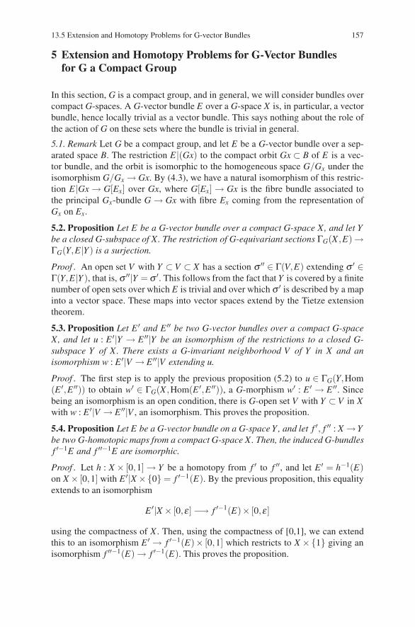
13.5 Extension and Homotopy Problems for G-vector Bundles 157
5 Extension and Homotopy Problems for G-Vector Bundlesfor G a Compact Group
In this section, G is a compact group, and in general, we will consider bundles overcompact G-spaces. A G-vector bundle E over a G-space X is, in particular, a vectorbundle, hence locally trivial as a vector bundle. This says nothing about the role ofthe action of G on these sets where the bundle is trivial in general.
5.1. Remark Let G be a compact group, and let E be a G-vector bundle over a sep-arated space B. The restriction E|(Gx) to the compact orbit Gx ⊂ B of E is a vec-tor bundle, and the orbit is isomorphic to the homogeneous space G/Gx under theisomorphism G/Gx → Gx. By (4.3), we have a natural isomorphism of this restric-tion E|Gx → G[Ex] over Gx, where G[Ex] → Gx is the fibre bundle associated tothe principal Gx-bundle G → Gx with fibre Ex coming from the representation ofGx on Ex.
5.2. Proposition Let E be a G-vector bundle over a compact G-space X, and let Ybe a closed G-subspace of X. The restriction of G-equivariant sections ΓG(X ,E)→ΓG(Y,E|Y ) is a surjection.
Proof . An open set V with Y ⊂ V ⊂ X has a section σ ′′ ∈ Γ(V,E) extending σ ′ ∈Γ(Y,E|Y ), that is, σ ′′|Y = σ ′. This follows from the fact that Y is covered by a finitenumber of open sets over which E is trivial and over which σ ′ is described by a mapinto a vector space. These maps into vector spaces extend by the Tietze extensiontheorem.
5.3. Proposition Let E ′ and E ′′ be two G-vector bundles over a compact G-spaceX, and let u : E ′|Y → E ′′|Y be an isomorphism of the restrictions to a closed G-subspace Y of X. There exists a G-invariant neighborhood V of Y in X and anisomorphism w : E ′|V → E ′′|V extending u.
Proof . The first step is to apply the previous proposition (5.2) to u ∈ ΓG(Y,Hom(E ′,E ′′)) to obtain w′ ∈ ΓG(X ,Hom(E ′,E ′′)), a G-morphism w′ : E ′ → E ′′. Sincebeing an isomorphism is an open condition, there is G-open set V with Y ⊂ V in Xwith w : E ′|V → E ′′|V , an isomorphism. This proves the proposition.
5.4. Proposition Let E be a G-vector bundle on a G-space Y , and let f ′, f ′′ : X →Ybe two G-homotopic maps from a compact G-space X. Then, the induced G-bundlesf ′−1E and f ′′−1E are isomorphic.
Proof . Let h : X × [0,1] → Y be a homotopy from f ′ to f ′′, and let E ′ = h−1(E)on X × [0,1] with E ′|X ×{0} = f ′−1(E). By the previous proposition, this equalityextends to an isomorphism
E ′|X × [0,ε] −→ f ′−1(E)× [0,ε]
using the compactness of X . Then, using the compactness of [0,1], we can extendthis to an isomorphism E ′ → f ′−1(E)× [0,1] which restricts to X ×{1} giving anisomorphism f ′′−1(E) → f ′−1(E). This proves the proposition.
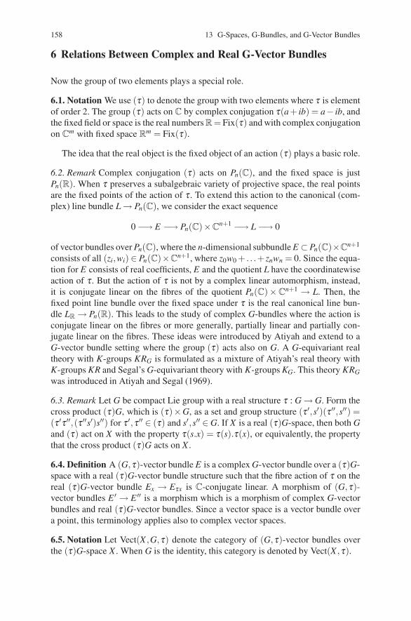
158 13 G-Spaces, G-Bundles, and G-Vector Bundles
6 Relations Between Complex and Real G-Vector Bundles
Now the group of two elements plays a special role.
6.1. Notation We use (τ) to denote the group with two elements where τ is elementof order 2. The group (τ) acts on C by complex conjugation τ(a+ ib) = a− ib, andthe fixed field or space is the real numbers R = Fix(τ) and with complex conjugationon C
m with fixed space Rm = Fix(τ).
The idea that the real object is the fixed object of an action (τ) plays a basic role.
6.2. Remark Complex conjugation (τ) acts on Pn(C), and the fixed space is justPn(R). When τ preserves a subalgebraic variety of projective space, the real pointsare the fixed points of the action of τ . To extend this action to the canonical (com-plex) line bundle L → Pn(C), we consider the exact sequence
0 −→ E −→ Pn(C)×Cn+1 −→ L −→ 0
of vector bundles over Pn(C), where the n-dimensional subbundle E ⊂Pn(C)×Cn+1
consists of all (zi,wi) ∈ Pn(C)×Cn+1, where z0w0 + . . .+ znwn = 0. Since the equa-
tion for E consists of real coefficients, E and the quotient L have the coordinatewiseaction of τ . But the action of τ is not by a complex linear automorphism, instead,it is conjugate linear on the fibres of the quotient Pn(C)×C
n+1 → L. Then, thefixed point line bundle over the fixed space under τ is the real canonical line bun-dle LR → Pn(R). This leads to the study of complex G-bundles where the action isconjugate linear on the fibres or more generally, partially linear and partially con-jugate linear on the fibres. These ideas were introduced by Atiyah and extend to aG-vector bundle setting where the group (τ) acts also on G. A G-equivariant realtheory with K-groups KRG is formulated as a mixture of Atiyah’s real theory withK-groups KR and Segal’s G-equivariant theory with K-groups KG. This theory KRG
was introduced in Atiyah and Segal (1969).
6.3. Remark Let G be compact Lie group with a real structure τ : G → G. Form thecross product (τ)G, which is (τ)×G, as a set and group structure (τ ′,s′)(τ ′′,s′′) =(τ ′τ ′′,(τ ′′s′)s′′) for τ ′,τ ′′ ∈ (τ) and s′,s′′ ∈ G. If X is a real (τ)G-space, then both Gand (τ) act on X with the property τ(s.x) = τ(s).τ(x), or equivalently, the propertythat the cross product (τ)G acts on X .
6.4. Definition A (G,τ)-vector bundle E is a complex G-vector bundle over a (τ)G-space with a real (τ)G-vector bundle structure such that the fibre action of τ on thereal (τ)G-vector bundle Ex → Eτx is C-conjugate linear. A morphism of (G,τ)-vector bundles E ′ → E ′′ is a morphism which is a morphism of complex G-vectorbundles and real (τ)G-vector bundles. Since a vector space is a vector bundle overa point, this terminology applies also to complex vector spaces.
6.5. Notation Let Vect(X ,G,τ) denote the category of (G,τ)-vector bundles overthe (τ)G-space X . When G is the identity, this category is denoted by Vect(X ,τ).
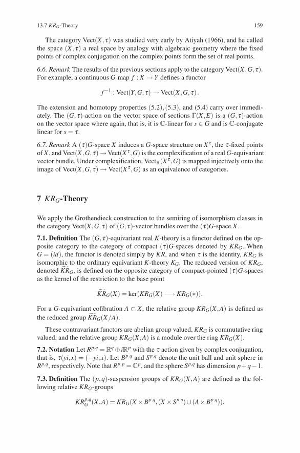
13.7 KRG-Theory 159
The category Vect(X ,τ) was studied very early by Atiyah (1966), and he calledthe space (X ,τ) a real space by analogy with algebraic geometry where the fixedpoints of complex conjugation on the complex points form the set of real points.
6.6. Remark The results of the previous sections apply to the category Vect(X ,G,τ).For example, a continuous G-map f : X → Y defines a functor
f−1 : Vect(Y,G,τ) → Vect(X ,G,τ) .
The extension and homotopy properties (5.2),(5.3), and (5.4) carry over immedi-ately. The (G,τ)-action on the vector space of sections Γ(X ,E) is a (G,τ)-actionon the vector space where again, that is, it is C-linear for s ∈ G and is C-conjugatelinear for s = τ .
6.7. Remark A (τ)G-space X induces a G-space structure on X τ , the τ-fixed pointsof X , and Vect(X ,G,τ)→Vect(X τ ,G) is the complexification of a real G-equivariantvector bundle. Under complexification, VectR(X τ ,G) is mapped injectively onto theimage of Vect(X ,G,τ) → Vect(X τ ,G) as an equivalence of categories.
7 KRG-Theory
We apply the Grothendieck construction to the semiring of isomorphism classes inthe category Vect(X ,G,τ) of (G,τ)-vector bundles over the (τ)G-space X .
7.1. Definition The (G,τ)-equivariant real K-theory is a functor defined on the op-posite category to the category of compact (τ)G-spaces denoted by KRG. WhenG = (id), the functor is denoted simply by KR, and when τ is the identity, KRG isisomorphic to the ordinary equivariant K-theory KG. The reduced version of KRG,denoted KRG, is defined on the opposite category of compact-pointed (τ)G-spacesas the kernel of the restriction to the base point
KRG(X) = ker(KRG(X) −→ KRG(∗)).
For a G-equivariant cofibration A ⊂ X , the relative group KRG(X ,A) is defined asthe reduced group KRG(X/A).
These contravariant functors are abelian group valued, KRG is commutative ringvalued, and the relative group KRG(X ,A) is a module over the ring KRG(X).
7.2. Notation Let Rp,q = Rq ⊕ iRp with the τ action given by complex conjugation,
that is, τ(yi,x) = (−yi,x). Let Bp,q and Sp,q denote the unit ball and unit sphere inRp,q, respectively. Note that Rp,p = C
p, and the sphere Sp,q has dimension p+q−1.
7.3. Definition The (p,q)-suspension groups of KRG(X ,A) are defined as the fol-lowing relative KRG-groups
KRp,qG (X ,A) = KRG(X ×Bp,q,(X ×Sp,q)∪ (A×Bp,q)).
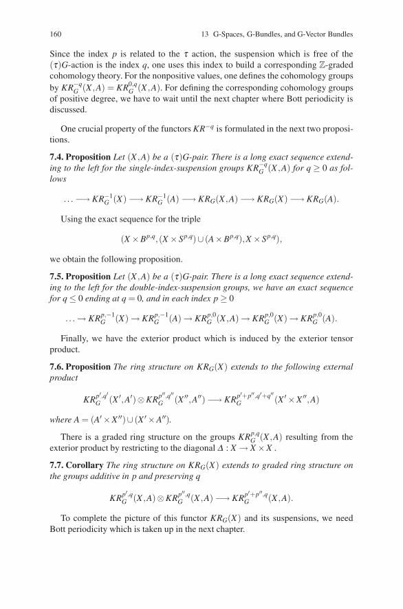
160 13 G-Spaces, G-Bundles, and G-Vector Bundles
Since the index p is related to the τ action, the suspension which is free of the(τ)G-action is the index q, one uses this index to build a corresponding Z-gradedcohomology theory. For the nonpositive values, one defines the cohomology groupsby KR−q
G (X ,A) = KR0,qG (X ,A). For defining the corresponding cohomology groups
of positive degree, we have to wait until the next chapter where Bott periodicity isdiscussed.
One crucial property of the functors KR−q is formulated in the next two proposi-tions.
7.4. Proposition Let (X ,A) be a (τ)G-pair. There is a long exact sequence extend-ing to the left for the single-index-suspension groups KR−q
G (X ,A) for q ≥ 0 as fol-lows
. . . −→ KR−1G (X) −→ KR−1
G (A) −→ KRG(X ,A) −→ KRG(X) −→ KRG(A).
Using the exact sequence for the triple
(X ×Bp,q,(X ×Sp,q)∪ (A×Bp,q),X ×Sp,q),
we obtain the following proposition.
7.5. Proposition Let (X ,A) be a (τ)G-pair. There is a long exact sequence extend-ing to the left for the double-index-suspension groups, we have an exact sequencefor q ≤ 0 ending at q = 0, and in each index p ≥ 0
. . . → KRp,−1G (X) → KRp,−1
G (A) → KRp,0G (X ,A) → KRp,0
G (X) → KRp,0G (A).
Finally, we have the exterior product which is induced by the exterior tensorproduct.
7.6. Proposition The ring structure on KRG(X) extends to the following externalproduct
KRp′,q′G (X ′,A′)⊗KRp′′,q′′
G (X ′′,A′′) −→ KRp′+p′′,q′+q′′G (X ′ ×X ′′,A)
where A = (A′ ×X ′′)∪ (X ′ ×A′′).
There is a graded ring structure on the groups KRp,qG (X ,A) resulting from the
exterior product by restricting to the diagonal Δ : X → X ×X .
7.7. Corollary The ring structure on KRG(X) extends to graded ring structure onthe groups additive in p and preserving q
KRp′,qG (X ,A)⊗KRp′′,q
G (X ,A) −→ KRp′+p′′,qG (X ,A).
To complete the picture of this functor KRG(X) and its suspensions, we needBott periodicity which is taken up in the next chapter.
References 161
References
Atiyah, M.F.: Power Operations in K-theory. Quarterly J. Math. Oxford 17(2): 165–193 (1966)Atiyah, M.F., Segal, G.G.: Equivariant K-theory and completion. J. Differential Geom. 3:
1–18 (1969)

Chapter 14Equivariant K-Theory Functor KG : Periodicity,Thom Isomorphism, Localization,and Completion
Using the Grothendieck construction in the preceding chapter, we defined the func-tors KG for real and complex G-bundles and the Atiyah real KRG by mapping thesemiring of G-vector bundles into its ring envelope. We saw that the basic proper-ties of the equivariant versions of vector bundle theory have close parallels with theusual vector bundle theory, and the same is true for the related relative K-theories.This we carry further in this chapter for the version of topological K-theory that hasclose relations to index theory.
The simple form of Bott periodicity for complex K-theory is the isomorphismK(X)⊗K(S2) → K(X × S2). The 2-sphere S2 which also can be identified as theone-dimensional complex projective space P1(C) plays a basic role. We can say thatthis is the periodicity theorem for a trivial line bundle X ×C → X over X . For thecase of KRG periodicity and Thom isomorphism, it is convenient to have a versionof the Bott isomorphism for any line bundle L → X over a space X or space X withinvolution τ .
We survey two basic results of Atiyah and Segal: the localization theory and thecompletion theorem for the calculation of K-theory of classifying spaces.
1 Associated Projective Space Bundle to a G-Equivariant Bundle
As usual for a vector space V , the associated projective space P(V ) is the spaceof one-dimensional linear subspaces W ⊂ V . In algebraic geometry, it is usuallydefined as the space of one-dimensional quotients V →U . The canonical line bundleL → P(V ) is the subbundle L ⊂ P(V )×V of the product of (W,x) with x ∈W or thequotient construction of P(V ), the canonical line bundle L → P(V ) is the quotientline bundle P(V )×V → L of {U}×U for V → U in P(V ). If G acts on V , then Gacts on P(V ) in both cases, and when V is a (G,τ)-vector space, then (τ)G also actson P(V ) in both cases. This all carries over to vector bundles.
1.1. Definition Let E → X be a (G,τ)-vector bundle over X with G-actionG× E → E . The associated projective bundle is p : P(E) → X , where the fibre
D. Husemoller et al.: Equivariant K-Theory Functor KG : Periodicity, Thom Isomorphism, Localization, andCompletion, Lect. Notes Phys. 726, 163–173 (2008)DOI 10.1007/978-3-540-74956-1 15 © Springer-Verlag Berlin Heidelberg 2008
164 14 Equivariant K-Theory Functor KG
P(E)x = P(Ex) is the associated projective space of the vector space fibre Ex. The(G,τ)-bundle structure on p : P(E)→ X comes from the (G,τ)-vector bundle struc-ture on the vector bundle E over X . The canonical line bundle LE on P(E) is also a(G,τ)-equivariant bundle which is the canonical line bundle on each fibre. We usethe quotient version, and this means that the following diagram with LE and its dualL∨
E as (G,τ)-line bundles over P(E) with (τ)G actions.
(τ)G×L∨E
��
�� (τ)G× p−1(E)
��
�� (τ)G×LE
��L∨
E�� p−1(E) �� LE
1.2. Remark For a one-dimensional vector space U and nonzero u ∈ U we havefor any finite-dimensional vector space V , an isomorphism of vector spaces V →U ⊗V,v �→ u⊗ v. It induces an isomorphism P(V ) → P(U ⊗V) which is indepen-dent of u. Hence, for each line bundle L and vector bundle E over X , we have awell-defined isomorphism of projective space bundles P(E) → P(L⊗ E).
2 Assertion of the Periodicity Theorem for a Line Bundle
The following theorem was introduced for a finite group G by Atiyah and proved fora compact group by Segal. It is based on a careful analysis of the clutching functionsfor a bundle over X ×S2 in terms of a Fourier series. We here give a treatment withinthe real setting.
2.1. Theorem Let L be a (G,τ)-equivariant line bundle over a (τ)G-space X withcorresponding class a = [L] ∈ KRG(X). The ring morphism
θ : KRG(X)[t]/(t −1)(ta−1)−→ KRG(P(L⊕C))
defined by θ (t) = [LL⊕C] is a well-defined isomorphism.
If we apply the theorem to trivial one-dimensional bundles, we obtain the follow-ing corollary. Therefore, note that as (τ)G-spaces, we have S1,1 ∼= P(C2).
2.2. Corollary For a (τ)G-space X, the ring morphism
θ : KRG(X)[t]/(t −1)2 −→ KRG(X ×S1,1)
defined by θ (t) = [LC⊕C] is a well-defined isomorphism.
2.3. Preliminaries to a Sketch of the Proof of (2.1) Choose a metric on L invariantunder the involution τ or in general (G,τ)-structure. The unit circle bundle S is then
14.2 Periodicity Theorem for a Line Bundle 165
a real space. The section z of π∗(L) defined by the inclusion S → L is a real sectiontogether with all its powers zk. The function z is the clutching function for (1,L).To see that (1,z,L) is the bundle H∨ defined as the subbundle of π∗(L⊕1), we notethat for each y ∈ P(L⊕1)x, the fibre H∨
y is a subspace of (L⊕1)x with H∨∞ = Lx ⊕0
and H∨0 = 0⊕1x. In particular, the composition
H∨ −→ π∗(L⊕1) −→ π∗(1)
induced by the projection L⊕1 → 1 defines an isomorphism
f0 : H∨|P0 −→ π∗0 (1),
and similarly, the composition H∨ → π∗(L⊕1) → π∗(L) induced by the projectionL⊕1 → L defines an isomorphism
f∞ : H∨|P∞ −→ π∗0 (L).
Hence, f = f0 f−1∞ : π∗(1)→ π∗(L) is a clutching function for H∨. For y∈ Sx , f (y) is
the isomorphism whose graph is H∨y . Since H∨
y is the subspace of Lx⊕1x generatedby y⊕1, where y ∈ Sx ⊂ Lx, 1 ∈ C, we see that f is our section z. Thus, we have anisomorphism of real bundles Hk⊗ → (1,z−k,L(−k)⊗).
Now, for any clutching function f ∈ ΓHom(π∗(E0),π∗(E∞)) which is a real sec-tion, there is a Fourier series with coefficients real sections ak of Hom(Lk⊗⊗E0,E∞)given by τ(x) = x
ak(x) = ak(x) = − 12π i
∫
Sx
fx(zx)−k−1dzx =1
2π i
∫
Sx
fx(zx)−k−1dz = ak(x),
where τ reverses the orientation of Sx and f and z are real. At a real point x ∈ X , thecondition that fx is real becomes fx(e−iθ ) = fx(eiθ ), which implies that the Fouriercoefficients are real.
The Fourier series is approximated with a finite Laurent series, and this in turnis linearized by adding dimensions so that only a function in x added to a functionin x times z remains. This is the linear case, and the real structure goes through theanalysis.
It remains to analyze the linear case. In this case, we split the linear clutchingfunction p for two vector bundles E0 and E∞ into two parts p = p+ ⊕ p− withhomotopies p(t) = p+(t)⊕ p−(t), where
p+(t) = a+z+ tb+ and p−(t) = ta−z+ b− for t ∈ [0,1]
leading to an isomorphism between (E0, p,E∞) and the direct sum
(E0+,z,L⊗E0
+)⊕ (E0−,1,E0
−) .
For this, we use the fact that for a linear operator T : V → V on a finite-dimensional space, the complex integral
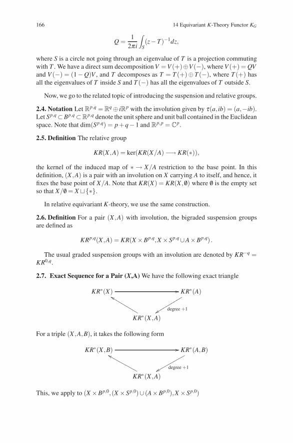
166 14 Equivariant K-Theory Functor KG
Q =1
2π i
∫
S(z−T)−1dz,
where S is a circle not going through an eigenvalue of T is a projection commutingwith T . We have a direct sum decomposition V = V (+)⊕V(−), where V (+) = QVand V (−) = (1−Q)V , and T decomposes as T = T (+)⊕T (−), where T (+) hasall the eigenvalues of T inside S and T (−) has all the eigenvalues of T outside S.
Now, we go to the related topic of introducing the suspension and relative groups.
2.4. Notation Let Rp,q = R
q ⊕ iRp with the involution given by τ(a, ib) = (a,−ib).Let Sp,q ⊂Bp,q ⊂R
p,q denote the unit sphere and unit ball contained in the Euclideanspace. Note that dim(Sp,q) = p + q−1 and R
p,p = Cp.
2.5. Definition The relative group
KR(X ,A) = ker(KR(X/A) −→ KR(∗)),
the kernel of the induced map of ∗ → X/A restriction to the base point. In thisdefinition, (X ,A) is a pair with an involution on X carrying A to itself, and hence, itfixes the base point of X/A. Note that KR(X) = KR(X , /0) where /0 is the empty setso that X/ /0 = X �{∗}.
In relative equivariant K-theory, we use the same construction.
2.6. Definition For a pair (X ,A) with involution, the bigraded suspension groupsare defined as
KRp,q(X ,A) = KR(X ×Bp,q,X ×Sp,q∪A×Bp,q) .
The usual graded suspension groups with an involution are denoted by KR−q =KR0,q.
2.7. Exact Sequence for a Pair (X,A) We have the following exact triangle
KR∗(X) �� KR∗(A)
degree +1��������
����
KR∗(X ,A)
������������
For a triple (X ,A,B), it takes the following form
KR∗(X ,B) �� KR∗(A,B)
degree +1��������
����
KR∗(X ,A)
������������
This, we apply to (X ×Bp,0,(X ×Sp,0)∪ (A×Bp,0),X ×Sp,0)
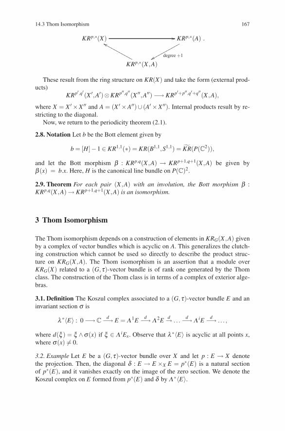
14.3 Thom Isomorphism 167
KRp,∗(X) �� KRp,∗(A)
degree +1��������
�����
KRp,∗(X ,A)
�������������
.
These result from the ring structure on KR(X) and take the form (external prod-ucts)
KRp′,q′(X ′,A′)⊗KRp′′,q′′(X ′′,A′′) −→ KRp′+p′′,q′+q′′(X ,A),
where X = X ′ ×X ′′ and A = (X ′ ×A′′)∪ (A′ ×X ′′). Internal products result by re-stricting to the diagonal.
Now, we return to the periodicity theorem (2.1).
2.8. Notation Let b be the Bott element given by
b = [H]−1 ∈ KR1,1(∗) = KR(B1,1,S1,1) = KR(P(C2)),
and let the Bott morphism β : KRp,q(X ,A) → KRp+1,q+1(X ,A) be given byβ (x) = b.x. Here, H is the canonical line bundle on P(C)2.
2.9. Theorem For each pair (X ,A) with an involution, the Bott morphism β :KRp,q(X ,A) → KRp+1,q+1(X ,A) is an isomorphism.
3 Thom Isomorphism
The Thom isomorphism depends on a construction of elements in KRG(X ,A) givenby a complex of vector bundles which is acyclic on A. This generalizes the clutch-ing construction which cannot be used so directly to describe the product struc-ture on KRG(X ,A). The Thom isomorphism is an assertion that a module overKRG(X) related to a (G,τ)-vector bundle is of rank one generated by the Thomclass. The construction of the Thom class is in terms of a complex of exterior alge-bras.
3.1. Definition The Koszul complex associated to a (G,τ)-vector bundle E and aninvariant section σ is
λ ∗〈E〉 : 0 −→ Cd−→ E =Λ1E
d−→Λ2Ed→ . . .
d−→Λ iEd−→ . . . ,
where d(ξ ) = ξ ∧σ(x) if ξ ∈ Λ iEx. Observe that λ ∗〈E〉 is acyclic at all points x,where σ(x) = 0.
3.2. Example Let E be a (G,τ)-vector bundle over X and let p : E → X denotethe projection. Then, the diagonal δ : E → E ×X E = p∗(E) is a natural sectionof p∗(E), and it vanishes exactly on the image of the zero section. We denote theKoszul complex on E formed from p∗(E) and δ by Λ∗〈E〉.
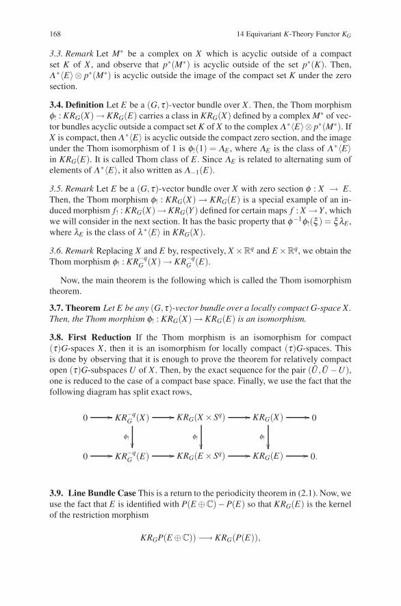
168 14 Equivariant K-Theory Functor KG
3.3. Remark Let M∗ be a complex on X which is acyclic outside of a compactset K of X , and observe that p∗(M∗) is acyclic outside of the set p∗(K). Then,Λ∗〈E〉⊗ p∗(M∗) is acyclic outside the image of the compact set K under the zerosection.
3.4. Definition Let E be a (G,τ)-vector bundle over X . Then, the Thom morphismφ! : KRG(X)→ KRG(E) carries a class in KRG(X) defined by a complex M∗ of vec-tor bundles acyclic outside a compact set K of X to the complexΛ∗〈E〉⊗ p∗(M∗). IfX is compact, thenΛ∗〈E〉 is acyclic outside the compact zero section, and the imageunder the Thom isomorphism of 1 is φ!(1) = ΛE , where ΛE is the class of Λ∗〈E〉in KRG(E). It is called Thom class of E . Since ΛE is related to alternating sum ofelements of Λ∗〈E〉, it also written as Λ−1(E).
3.5. Remark Let E be a (G,τ)-vector bundle over X with zero section φ : X → E .Then, the Thom morphism φ! : KRG(X) → KRG(E) is a special example of an in-duced morphism f! : KRG(X)→ KRG(Y ) defined for certain maps f : X →Y , whichwe will consider in the next section. It has the basic property that φ−1φ!(ξ ) = ξλE ,where λE is the class of λ ∗〈E〉 in KRG(X).
3.6. Remark Replacing X and E by, respectively, X ×Rq and E ×R
q, we obtain theThom morphism φ! : KR−q
G (X) → KR−qG (E).
Now, the main theorem is the following which is called the Thom isomorphismtheorem.
3.7. Theorem Let E be any (G,τ)-vector bundle over a locally compact G-space X.Then, the Thom morphism φ! : KRG(X) → KRG(E) is an isomorphism.
3.8. First Reduction If the Thom morphism is an isomorphism for compact(τ)G-spaces X , then it is an isomorphism for locally compact (τ)G-spaces. Thisis done by observing that it is enough to prove the theorem for relatively compactopen (τ)G-subspaces U of X . Then, by the exact sequence for the pair (U ,U −U),one is reduced to the case of a compact base space. Finally, we use the fact that thefollowing diagram has split exact rows,
0 �� KR−qG (X) ��
φ!
��
KRG(X ×Sq) ��
φ!
��
KRG(X) ��
φ!
��
0
0 �� KR−qG (E) �� KRG(E ×Sq) �� KRG(E) �� 0.
3.9. Line Bundle Case This is a return to the periodicity theorem in (2.1). Now, weuse the fact that E is identified with P(E ⊕C)−P(E) so that KRG(E) is the kernelof the restriction morphism
KRGP(E ⊕C)) −→ KRG(P(E)),
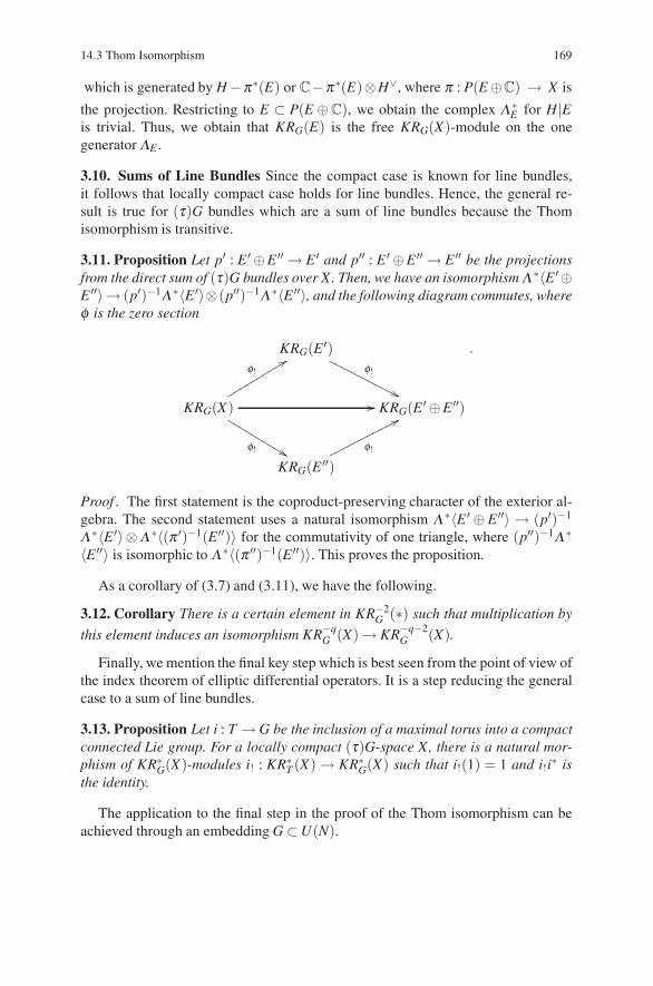
14.3 Thom Isomorphism 169
which is generated by H −π∗(E) or C−π∗(E)⊗H∨, where π : P(E ⊕C) → X is
the projection. Restricting to E ⊂ P(E ⊕C), we obtain the complex Λ∗E for H|E
is trivial. Thus, we obtain that KRG(E) is the free KRG(X)-module on the onegeneratorΛE .
3.10. Sums of Line Bundles Since the compact case is known for line bundles,it follows that locally compact case holds for line bundles. Hence, the general re-sult is true for (τ)G bundles which are a sum of line bundles because the Thomisomorphism is transitive.
3.11. Proposition Let p′ : E ′ ⊕E ′′ → E ′ and p′′ : E ′ ⊕E ′′ → E ′′ be the projectionsfrom the direct sum of (τ)G bundles over X. Then, we have an isomorphismΛ∗〈E ′⊕E ′′〉→ (p′)−1Λ∗〈E ′〉⊗(p′′)−1Λ∗〈E ′′〉, and the following diagram commutes, whereφ is the zero section
KRG(E ′)φ!
�������
������
KRG(X) ��
φ! �������
�����
φ!
������������KRG(E ′ ⊕E ′′)
KRG(E ′′)φ!
�����������
.
Proof . The first statement is the coproduct-preserving character of the exterior al-gebra. The second statement uses a natural isomorphism Λ∗〈E ′ ⊕ E ′′〉 → (p′)−1
Λ∗〈E ′〉 ⊗Λ∗〈(π ′)−1(E ′′)〉 for the commutativity of one triangle, where (p′′)−1Λ∗〈E ′′〉 is isomorphic to Λ∗〈(π ′′)−1(E ′′)〉. This proves the proposition.
As a corollary of (3.7) and (3.11), we have the following.
3.12. Corollary There is a certain element in KR−2G (∗) such that multiplication by
this element induces an isomorphism KR−qG (X) → KR−q−2
G (X).
Finally, we mention the final key step which is best seen from the point of view ofthe index theorem of elliptic differential operators. It is a step reducing the generalcase to a sum of line bundles.
3.13. Proposition Let i : T → G be the inclusion of a maximal torus into a compactconnected Lie group. For a locally compact (τ)G-space X, there is a natural mor-phism of KR∗
G(X)-modules i! : KR∗T (X) → KR∗
G(X) such that i!(1) = 1 and i!i∗ isthe identity.
The application to the final step in the proof of the Thom isomorphism can beachieved through an embedding G ⊂U(N).
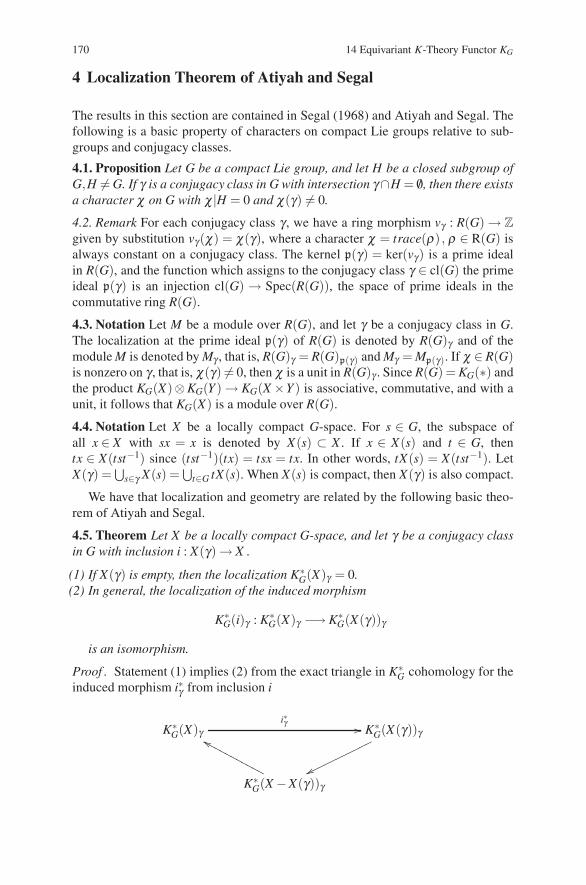
170 14 Equivariant K-Theory Functor KG
4 Localization Theorem of Atiyah and Segal
The results in this section are contained in Segal (1968) and Atiyah and Segal. Thefollowing is a basic property of characters on compact Lie groups relative to sub-groups and conjugacy classes.
4.1. Proposition Let G be a compact Lie group, and let H be a closed subgroup ofG,H = G. If γ is a conjugacy class in G with intersection γ∩H = /0, then there existsa character χ on G with χ |H = 0 and χ(γ) = 0.
4.2. Remark For each conjugacy class γ , we have a ring morphism vγ : R(G) → Z
given by substitution vγ(χ) = χ(γ), where a character χ = trace(ρ) , ρ ∈ R(G) isalways constant on a conjugacy class. The kernel p(γ) = ker(vγ) is a prime idealin R(G), and the function which assigns to the conjugacy class γ ∈ cl(G) the primeideal p(γ) is an injection cl(G) → Spec(R(G)), the space of prime ideals in thecommutative ring R(G).
4.3. Notation Let M be a module over R(G), and let γ be a conjugacy class in G.The localization at the prime ideal p(γ) of R(G) is denoted by R(G)γ and of themodule M is denoted by Mγ , that is, R(G)γ = R(G)p(γ) and Mγ = Mp(γ). If χ ∈ R(G)is nonzero on γ , that is, χ(γ) = 0, then χ is a unit in R(G)γ . Since R(G) = KG(∗) andthe product KG(X)⊗KG(Y ) → KG(X ×Y ) is associative, commutative, and with aunit, it follows that KG(X) is a module over R(G).
4.4. Notation Let X be a locally compact G-space. For s ∈ G, the subspace ofall x ∈ X with sx = x is denoted by X(s) ⊂ X . If x ∈ X(s) and t ∈ G, thentx ∈ X(tst−1) since (tst−1)(tx) = tsx = tx. In other words, tX(s) = X(tst−1). LetX(γ) =
⋃s∈γ X(s) =
⋃t∈G tX(s). When X(s) is compact, then X(γ) is also compact.
We have that localization and geometry are related by the following basic theo-rem of Atiyah and Segal.
4.5. Theorem Let X be a locally compact G-space, and let γ be a conjugacy classin G with inclusion i : X(γ) → X .
(1) If X(γ) is empty, then the localization K∗G(X)γ = 0.
(2) In general, the localization of the induced morphism
K∗G(i)γ : K∗
G(X)γ −→ K∗G(X(γ))γ
is an isomorphism.
Proof . Statement (1) implies (2) from the exact triangle in K∗G cohomology for the
induced morphism i∗γ from inclusion i
K∗G(X)γ
i∗γ �� K∗G(X(γ))γ
��������
�����
K∗G(X −X(γ))γ
�������������
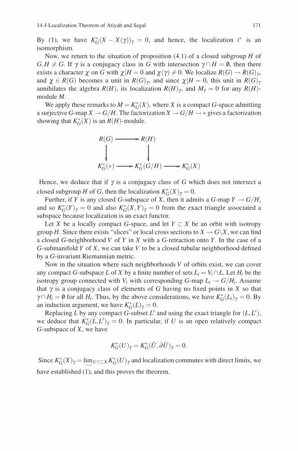
14.4 Localization Theorem of Atiyah and Segal 171
By (1), we have K∗G(X − X(γ))γ = 0, and hence, the localization i∗ is an
isomorphism.Now, we return to the situation of proposition (4.1) of a closed subgroup H of
G,H = G. If γ is a conjugacy class in G with intersection γ ∩H = /0, then thereexists a character χ on G with χ |H = 0 and χ(γ) = 0. We localize R(G) → R(G)γ ,and χ ∈ R(G) becomes a unit in R(G)γ , and since χ |H = 0, this unit in R(G)γannihilates the algebra R(H), its localization R(H)γ , and Mγ = 0 for any R(H)-module M.
We apply these remarks to M = K∗G(X), where X is a compact G-space admitting
a surjective G-map X →G/H. The factorization X →G/H →∗ gives a factorizationshowing that K∗
G(X) is an R(H)-module.
R(G)
��
�� R(H)
��K∗
G(∗) �� K∗G(G/H) �� K∗
G(X)
Hence, we deduce that if γ is a conjugacy class of G which does not intersect a
closed subgroup H of G, then the localization K∗G(X)γ = 0.
Further, if Y is any closed G-subspace of X , then it admits a G-map Y → G/H,and so K∗
G(Y )γ = 0 and also K∗G(X ,Y )γ = 0 from the exact triangle associated a
subspace because localization is an exact functor.Let X be a locally compact G-space, and let Y ⊂ X be an orbit with isotropy
group H. Since there exists “slices” or local cross sections to X → G\X , we can finda closed G-neighborhood V of Y in X with a G-retraction onto Y . In the case of aG-submanifold Y of X , we can take V to be a closed tubular neighborhood definedby a G-invariant Riemannian metric.
Now in the situation where such neighborhoods V of orbits exist, we can coverany compact G-subspace L of X by a finite number of sets Li = Vi∩L. Let Hi be theisotropy group connected with Vi with corresponding G-map Li → G/Hi. Assumethat γ is a conjugacy class of elements of G having no fixed points in X so thatγ ∩Hi = /0 for all Hi. Thus, by the above considerations, we have K∗
G(Li)γ = 0. Byan induction argument, we have K∗
G(L)γ = 0.Replacing L by any compact G-subset L′ and using the exact triangle for (L,L′),
we deduce that K∗G(L,L′)γ = 0. In particular, if U is an open relatively compact
G-subspace of X , we have
K∗G(U)γ = K∗
G(U ,∂U)γ = 0.
Since K∗G(X)γ = lim−→U⊂⊂X K∗
G(U)γ and localization commutes with direct limits, we
have established (1), and this proves the theorem.
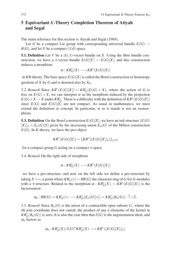
172 14 Equivariant K-Theory Functor KG
5 Equivariant K-Theory Completion Theorem of Atiyahand Segal
The main reference for this section is Atiyah and Segal (1969).Let G be a compact Lie group with corresponding universal bundle E(G) →
B(G), and let X be a compact (τ)G-space.
5.1. Definition Let V be a (G,τ)-vector bundle on X . Using the fibre bundle con-struction, we have a τ-vector bundle E(G)[V ] → E(G)[X ], and this constructioninduces a morphism
α : KR∗G(X) −→ KR∗(E(G)[X ])
in KR-theory. The base space E(G)[X ] is called the Borel construction or homotopy
quotient of X by G and is denoted also by XG.
5.2. Remark Since KR∗(E(G)[X ]) = KR∗G(E(G) × X), where the action of G is
free on E(G)×X , we can interpret α as the morphism induced by the projectionE(G)×X →X under KR∗
G. There is a difficulty with the definition of KR∗(E(G)[X ])since E(G) and E(G)[X ] are not compact. As usual in mathematics, we mustextend the definition or concept. In particular, α as it stands is not an isomor-phism.
5.3. Definition On the Borel construction E(G)[X ], we have an ind-structure (E(G)[X ])n = En(G)[X ] given by the increasing union En(G) of the Milnor constructionE(G). In K-theory, we have the pro-object
KR∗(E(G)[X ]) = {KR∗((E(G)[X ])n)}n∈N
for a compact group G acting on a compact τ-space.
5.4. Remark On the right side of morphism
α : KR∗G(X) −→ KR∗(E(G)[X ])
we have a pro-structure, and now on the left side we define a pro-structure by
taking X = ∗, a point where KRG(∗) = RR(G) the character ring of G for G-moduleswith a τ-structure. Related to the morphism α : KR∗
G(X) → KR∗(E(G)[X ]) is thefactorization
αn : RR(G) = KR∗G(∗) −→ KR∗
G(En(G)[∗]) = KR∗G(Bn(G)) ε−→ Z.
5.5. Remark Since Bn(G) is the union of n contractible open subsets Ui, where theith join coordinate does not vanish, the product of any n elements of the kernel inKR∗
G(Bn(G)) is zero. It is also the case then that I(G) is the augmentation ideal, andαn factors as
αn : KR∗G(X)/I(G)nKR∗
G(X) −→ KR∗((E(G)[X ])n).
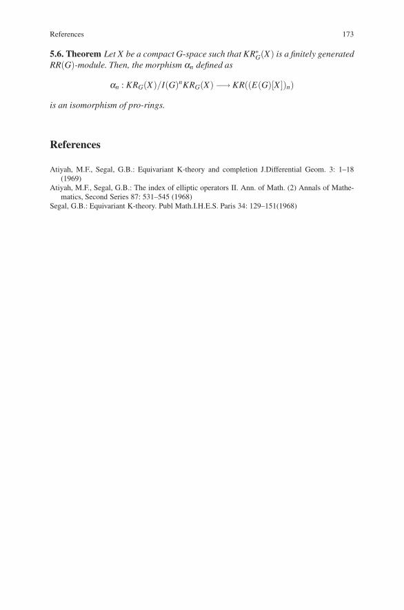
References 173
5.6. Theorem Let X be a compact G-space such that KR∗G(X) is a finitely generated
RR(G)-module. Then, the morphism αn defined as
αn : KRG(X)/I(G)nKRG(X) −→ KR((E(G)[X ])n)
is an isomorphism of pro-rings.
References
Atiyah, M.F., Segal, G.B.: Equivariant K-theory and completion J.Differential Geom. 3: 1–18(1969)
Atiyah, M.F., Segal, G.B.: The index of elliptic operators II. Ann. of Math. (2) Annals of Mathe-matics, Second Series 87: 531–545 (1968)
Segal, G.B.: Equivariant K-theory. Publ Math.I.H.E.S. Paris 34: 129–151(1968)

Chapter 15Bott Periodicity Maps and Clifford Algebras
Before there was K-theory, there was Bott periodicity. It was a result of the analysisof homogeneous spaces, their loop spaces, and classifying spaces of limits of Liegroups. In a parallel study of Clifford algebras, we see a periodicity which has muchto do with Bott periodicity. This is pointed out in this chapter.
When topological K-theory was introduced by analogy with Grothendieck’s co-herence sheaf K-theory, Bott periodicity was there and made possible an entire co-homology theory. Immediately, the vector bundle class approach to K-theory wascoupled with the homotopy theory as in the discussion of the universal bundles andclassifying spaces. The universal bundles of a group became the classifying spaceof K-theory by a simple limiting process. These limit spaces is the domain of thefirst forms of K-theory.
For complex vector bundles, the group GL(n,C) and its compact subgroup U(n)both play a role. The fact that the use of principal bundles over U(n) or overGL(n,C) follows from the existence of a Hermitian metric on vector bundles. Thereis another approach which we take up in the next chapter by the classical Gram–Schmidt process. We use the compact forms, that is, U(n), for the homotopy classi-fication of K-theory.
After the homotopy analysis of Bott periodicity, we consider the Clifford algebradescription. This we do in the context of KR-theory as in the previous chapter.
1 Vector Bundles and Their Principal Bundles and Metrics
In 2(8.2), we introduced the notion of a metric on a vector bundle, and in 2(8.3)using the metric on the universal bundle, we saw that every vector bundle has ametric.
1.1. Remark When we associate the principal bundle to a complex vector bundle,we can either use changes of coordinates in GL(n,C) preserving only the linearstructure or changes of coordinates in U(n) preserving the linear and metric struc-tures. An n-dimensional C-vector bundle E over X is of the form P[Cn], where P is
D. Husemoller et al.: Bott Periodicity Maps and Clifford Algebras, Lect. Notes Phys. 726, 175–188 (2008)DOI 10.1007/978-3-540-74956-1 16 © Springer-Verlag Berlin Heidelberg 2008
176 15 Bott Periodicity Maps and Clifford Algebras
a GL(n,C)-principal bundle or of the form P′[Cn], where P′ is a U(n)-principal bun-dle associated to P by reduction of the structure group from GL(n,C) to the groupU(n) of unitary n by n matrices.
1.2. Remark In terms of the classifying spaces, the set of isomorphism classesVectn(B) of n-dimensional complex vector bundles over B can be identified witheither [B,BGL(n,C)] or [B,BU(n)]. The process of assigning to an n-dimensionalC-vector bundle E the Whitney sum with the trivial bundle E ⊕C
q (or E ×Cq) cor-
responds to the inclusions GL(n,C) → GL(n + q,C) and U(n) → U(n + q) whichinduce in terms of either homotopy description the functions corresponding to sta-bilization of vector bundles
[B,BGL(C,n)] −→ [B,BGL(C,n + q)] and [B,BU(n)]−→ [B,BU(n + q)].
1.3. Remark Similar assertions hold for real and quaternion vector bundles wherestabilization takes, respectively, the form
[B,BGL(R,n)] −→ [B,BGL(R,n + q)] and [B,BO(n)] −→ [B,BO(n + q)].
[B,BGL(H,n)] −→ [B,BGL(H,n + q)] and [B,BSp(n)]→ [B,BSp(n + q)].
Here, H is the quaternions and Sp(n) is the symplectic subgroup of quaternioniclinear maps preserving the H-metric. In the case of U(n) and O(n), we have thesubgroups of determinant 1 matrices.
2 Homotopy Representation of K-Theory
K-theory is the result of stabilization using the inclusions of the formU(n)→ U(n+q). Hence, we introduce the following limit groups.
2.1. Definition For each of the five sorts of groups in (1.2) and (1.3), we have thefollowing five direct limit groups
O =⋃n≥0
O(n), SO =⋃n≥0
SO(n) ,
U =⋃n≥0
U(n), SU =⋃n≥0
SU(n), and Sp =⋃n≥0
Sp(n).
We give them the usual direct limit topology, and they are topological groups withrespect to this topology.
2.2. Remark The classifying spaces of these groups can be described as limit spaces
BO =⋃n≥0
BO(n), BSO =⋃n≥0
BSO(n), BU =⋃n≥0
BU(n),
15.2 Homotopy Representation of K-Theory 177
BSU =⋃n≥0
BSU(n), and BSp =⋃n≥0
BSp(n).
In the case of a compact space, X we have the following relations
[X ,BO] = lim−→ n≥0 [X ,BO(n)], [X ,BSO] = lim−→ n≥0 [X ,BSO(n)],
[X ,BU ] = lim−→ n≥0 [X ,BU(n)], [X ,BSU ] = lim−→ n≥0 [X ,BSU(n)],
and [X ,BSp] = lim−→ n≥0 [X ,BSp(n)] .
Hence, the stabilized bundle theory, that is, K-theory, has a homotopy interpreta-tion as homotopy classes of maps on a compact space due to the interchanging ofincreasing unions inside [X , ] with inductive limits outside of the sets of homotopyclasses of maps. Explicitly, f : X → BU(n) and f ′ : X → BU(n + q) represent thesame points in lim−→n≥0[X ,BU(n)] if and only if [ f ′] = [ j f ] for the natural inclusion
j : BU(n)→ BU(n + q).
2.3. Remark In each of the five sequences of groups, denoted by G(n) → G(n + q),we have a natural inclusion
G(m)×G(n)−→ G(m+ n)
inducing on the classifying spaces a map BG(m)×BG(n)→ BG(m+n). After suit-able choices all of which lead to homotopic equivalent maps, we have a map on thelimit group G×G → G. This observation can be applied to the following cases.
On the limit-classifying spaces, we have multiplications
BO×BO −→ BO, BSO×BSO−→ BSO,
BU ×BU −→ BU, BSU ×BSU −→ BSU, and BSp×BSp→ BSp.
These are called the H-space structures on the five limit-classifying spaces.As with loop spaces, these are not strictly associative maps, but they are
homotopy-associative maps. They induce maps
[X ,BG]∗ × [X ,BG]∗ = [X ,BG×BG]∗ −→ [X ,BG]∗
and
[X ,Z×BG]∗× [X ,Z×BG]∗ = [X ,Z×BG×Z×BG]∗ −→ [X ,Z×BG]∗
making [X ,BG]∗ and [X ,Z×BG]∗ into groups for each of the five cases G = O, SO,U,SU , or Sp.
2.4. Remark We have the following formulas for real and complex K-theory of aspace where the isomorphisms are given by inducing the universal bundle on someBU(n) ⊂ BU or BO(n) ⊂ BO.
178 15 Bott Periodicity Maps and Clifford Algebras
[X ,Z×BU ]∗ −→ K(X) and [X ,Z×BO]∗ −→ KO(X).
These isomorphisms should be thought of as the analogue of the Eilenberg-MacLaneisomorphism 9(6.2) for K-theory.
Here the base point plays a role in that [ , ]∗ refers to base-point-preserving mapsand homotopies, and the extra factor of Z takes care of the possibly nonconnected X .Now we return to the suspension extension of the previous chapter, 14(2.6), wherewe handle the situation more directly without a relative theory.
2.5. Definition We define negative K-groups by
K−q(X) = [Sq ∧X ,BU ]∗ and KO−q(X) = [Sq ∧X ,BO]∗.
These are functors on the category of pointed spaces and pointed homotopyclasses of maps. They have all of the properties of classical cohomology theorycontained in Chap. 9, Sect. 3, for example, the suspension property K−q+1(S(X))→K−q(X) is an isomorphism. At this point, the K-groups are defined only for negativeindices, but using the following adjunction relation, we see the relevance of know-ing the loop spaces Ωp(Y ) = Map∗(Sp,Y ) of the infinite classical groups and theirclassifying spaces.
2.6. Assertion The isomorphisms of spaces
Map(X ×Sp,Y ) → Map(X ,Map(Sp,Y ))
andMap(X ×Sp,Y ) → Map(Sp,Map(X ,Y ))
of 6(2.1) restrict on the right and pass to a quotient on the left to give isomorphismsof pointed spaces
Map∗(X ∧Sp,Y ) −→ Map∗(Sp,Map∗(X ,Y ))
orMap∗(S
p(X),Y ) −→Ωp(Map∗(X ,Y ))
andMap∗(X ∧Sp,Y ) −→ Map∗(X ,Map∗(S
p,Y ))
orMap∗(S
p(X),Y ) −→ Map∗(X ,Ωp(Y )) .
For homotopy classes, the last isomorphism takes the form
[Sp(X),Y ]∗ −→ [X ,Ωp(Y )]∗.
2.7. Remark The last result implies that the suspensions for K-theory have anotherform using loop spaces of BU or BO, that is, we have
K−q(X) = [Sq ∧X ,BU ]∗ = [X ,Ωq(BU)]∗
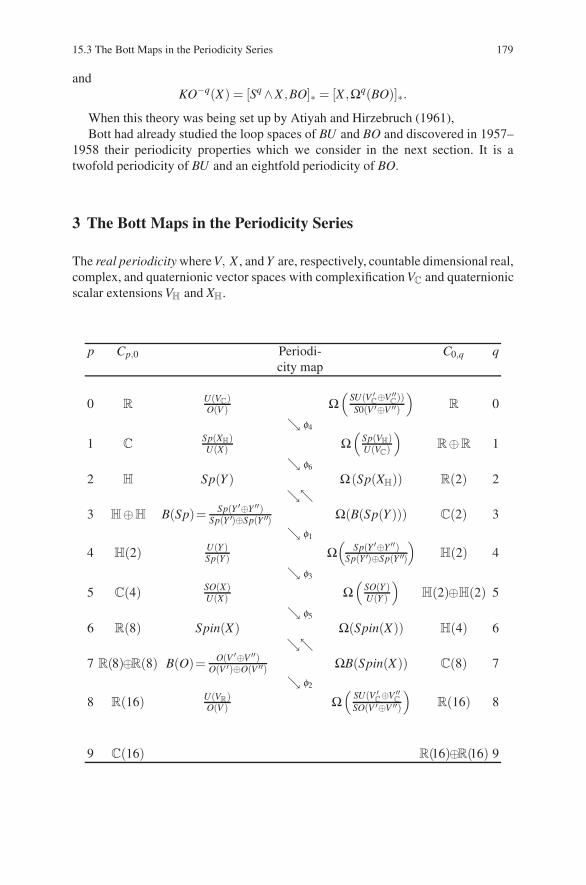
15.3 The Bott Maps in the Periodicity Series 179
andKO−q(X) = [Sq ∧X ,BO]∗ = [X ,Ωq(BO)]∗.
When this theory was being set up by Atiyah and Hirzebruch (1961),Bott had already studied the loop spaces of BU and BO and discovered in 1957–
1958 their periodicity properties which we consider in the next section. It is atwofold periodicity of BU and an eightfold periodicity of BO.
3 The Bott Maps in the Periodicity Series
The real periodicity where V, X , and Y are, respectively, countable dimensional real,complex, and quaternionic vector spaces with complexification VC and quaternionicscalar extensions VH and XH.
p Cp,0 Periodi- C0,q qcity map
0 RU(VC)O(V ) Ω
(SU(V ′
C⊕V ′′
C))
S0(V ′⊕V ′′)
)R 0
↘ φ4
1 CSp(XH)U(X) Ω
(Sp(VH)U(VC)
)R⊕R 1
↘ φ6
2 H Sp(Y ) Ω(Sp(XH)) R(2) 2↘↖
3 H⊕H B(Sp)= Sp(Y ′⊕Y ′′)Sp(Y ′)⊕Sp(Y ′′) Ω(B(Sp(Y ))) C(2) 3
↘ φ1
4 H(2) U(Y )Sp(Y) Ω
(Sp(Y ′⊕Y ′′)
Sp(Y ′)⊕Sp(Y ′′)
)H(2) 4
↘ φ3
5 C(4) SO(X)U(X) Ω
(SO(Y )U(Y )
)H(2)⊕H(2) 5
↘ φ5
6 R(8) Spin(X) Ω(Spin(X)) H(4) 6↘↖
7 R(8)⊕R(8) B(O)= O(V ′⊕V ′′)O(V ′)⊕O(V ′′) ΩB(Spin(X)) C(8) 7
↘ φ2
8 R(16) U(VR)O(V ) Ω
(SU(V ′
C⊕V ′′
C
SO(V ′⊕V ′′)
)R(16) 8
9 C(16) R(16)⊕R(16) 9
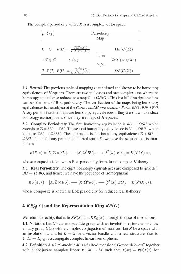
180 15 Bott Periodicity Maps and Clifford Algebras
The complex periodicity where X is a complex vector space.
p C(p) PeriodicityMap
0 C B(U) = U(X ′⊕X ′′)U(X ′)⊕U(X ′′) ΩB(U(X))
↘ φO
1 C⊕C U(X) ΩSU(X ′ ⊕X ′′)↘↖
2 C(2) B(U) = U(X ′⊕X ′′)U(X ′)⊕U(X ′′) ΩB(U(X))
3.1. Remark The previous table of mappings are defined and shown to be homotopyequivalences of H-spaces. There are two real cases and one complex case where thehomotopy equivalence reduces to a map G→ΩB(G). This is a full description of thevarious elements of Bott periodicity. The verification of the maps being homotopyequivalences is the subject of the Cartan and Moore seminar, Paris, ENS 1959-1960.A key point is that the maps are homotopy equivalences if they are shown to inducehomology isomorphisms since they are maps of H-spaces.
3.2. Complex Periodicity The first homotopy equivalence is BU → ΩSU whichextends to Z×BU →ΩU . The second homotopy equivalence is U →ΩBU , whichloops to ΩU → Ω2BU . The composite is the homotopy equivalence Z × BU →Ω2BU . Thus, for any pointed connected space X , we have the sequence of isomor-phisms
K(X ,∗) = [X ,Z×BU ]∗ −→ [X ,Ω2BU ]∗ −→ [S2(X),BU ]∗ = K(S2(X),∗),
whose composite is known as Bott periodicity for reduced complex K-theory.
3.3. Real Periodicity The eight homotopy equivalences are composed to give Z×BO →Ω8BO, and hence, we have the sequence of isomorphisms
KO(X ,∗) = [X ,Z×BO]∗ −→ [X ,Ω8BO]∗ −→ [S8(X),BO]∗ = K(S8(X),∗),
whose composite is known as Bott periodicity for reduced real K-theory.
4 KR∗G(X) and the Representation Ring RR(G)
We return to reality, that is to KR(X) and KRG(X), through the use of involutions.
4.1. Notation Let G be a compact Lie group with an involution τ , for example, theunitary group U(n) with τ complex conjugation of matrices. Let X be a space withan involution τ , and let E → X be a vector bundle with a real structure, that is,τ : Ex → Eτ(x) is a conjugate complex linear isomorphism.
4.2. Definition A (G,τ)-module M is a finite-dimensional G-module over C togetherwith a conjugate complex linear τ : M → M such that τ(sx) = τ(s)τ(x) for
15.5 Generalities on Clifford Algebras and Their Modules 181
s ∈ G,x ∈M. Let RR(G) denote the representation ring of (G,τ)-modules. We havetwo maps relating it with the complex representation, or character, ring R(G) of G,namely σ : RR(G)→ R(G) and ρ : R(G)→ RR(G), where σ(M) is M without τ andρ(N) = N ⊕ N with τ(x′,x′′) = (x′′,x′), the flip between two factors.
4.3. Remark The simple (G,τ)-modules S divide into three classes depending onEnd(G,τ)(S) which is either R,C, or H.
(1) End(G,τ)(S) = R : σ(E) is as simple as a G-module over C,(2) End(G,τ)(S) = C : S = ρ(N), where N and N are nonisomorphic, and(3) End(G,τ)(S) = H : S = ρ(N), where N and N are isomorphic.
These three types of simple (G,τ)-modules S decompose the simple modules intothe disjoint union of three sets which are the basis elements of the three subgroupsRR(G), RC(G), and RH(G) giving a direct sum decomposition
RR(G) = RR(G)⊕RC(G)⊕RH(G).
In Fibre Bundles, 14(11), we have a characterization of real, complex, and quater-nionic representations, see theorem 14(11.4) and the three corollaries which follow(Husemoller 1994).
4.4. Remark If G acts trivially on X , then there is a natural isomorphism KG(X) →R(G)⊗K(X) where a vector bundle E is carried to ⊕SS⊗HomG(S,E). This iso-morphism carries over to spaces X with involution τ with the same correspondence
KRG(X) −→ RR(G)⊗KR(X).
Finally, putting together this decomposition with the three fold decomposition ofthe previous remark, we have for trivial G-spaces with τ-structure a decomposition
KRG(X) −→ [RR(G)⊗KR(X)]⊕ [RC(G)⊗KC(X)]⊕ [RH(G)⊗KH(X)],
where KR(X),KC(X), and KH(X), respectively, are the Grothendieck group of real,complex, and quaternionic vector bundles, respectively, on X .
Note that KC(X) is just K(X), and it is independent of the involution for a com-plex vector bundle E decomposes as E0 ⊕ τ∗(E0), where E0 is the subvector bundleof E where the two complex structures coincide.
5 Generalities on Clifford Algebras and Their Modules
The following is a summary of some of the results in Fibre Bundles, chap. 12 onClifford algebras (Husemoller 1994). We will be primarily interested in the subjectover the real and complex numbers. We use the symbol F for such a field.
5.1. Definition A quadratic form (V, f ) over F is an F-vector space V of finite di-mension together with a function f : V ×V → F satisfying
(1) f (a′x′ + a′′x′′,y) = a′ f (x′,y)+ a′′ f (x′′,y) for all a′,a′′ ∈ F and x′,x′′,y ∈V and(2) f (x,y) = f (y,x) for all x,y ∈V.
182 15 Bott Periodicity Maps and Clifford Algebras
The first axiom says that f (x,y) is a linear form in x for fixed y ∈ V , and thesecond axiom says that also f (x,y) is a linear form in Y for fixed x ∈V. We also usethe terminology of symmetric bilinear form for quadratic form. It is the same over afield with 2 = 0 in F so that we can divide by it.
5.2. Definition The direct sum or Witt sum of two quadratic forms is given by(V ′, f ′)⊕ (V ′′, f ′′) = (V ′ ⊕V ′′, f ′ ⊕ f ′′), where
( f ′ ⊕ f ′′)((x′,x′′),(y′,y′′)) = f ′(x′,y′)+ f ′′(x′′,y′′).
In particular for v′ ∈V ′ and v′′ ∈V ′′, we have ( f ′ ⊕ f ′′)(v′,v′′) = 0, that is, these twovectors are perpendicular in the direct sum.
5.3. Definition Let (V, f ) be a quadratic form over F. The Clifford algebra of(V, f ) is a pair (C( f ),θ ) consisting of an algebra C( f ) over F and a linear mapθ : V →C( f ), where θ (x)2 = f (x,x).1 in the algebra C( f ) with the following uni-versal property: For any other F-linear map α : V → A into an algebra over F withthe property that α(x)2 = f (x,x).1, there exists a morphism u : C( f )→A of algebraswith α = uθ . Moreover, u is unique with respect to the property that α = uθ .
5.4. Remark The Clifford algebra of (V, f ) exists and is unique up to isomorphism.The universal property gives uniqueness. As for existence, we can start with thetensor algebra T (V ) =
⊕n V⊗n on V and divide by the ideal generated by all x⊗x−
f (x,x).1 for x ∈V. Then θ : V →C( f ) is the quotient of V → T (V ).The universal property of the Clifford algebra follows from that of T (V ) and the
generators of the ideal in T (V ) divided out to construct C( f ).
5.5. Involution and Even/Odd Grading of the Clifford Algebra There is an invo-lution β of C( f ) by applying the universal property of (C( f ),θ ) to −θ . This yieldsa splitting C( f ) = C( f )0 ⊕C( f )1, where C( f )i is the subspace of x ∈ C( f ) withβ (x) = (−1)ix.
The example of the Clifford algebra brings us to the study of Z/2-graded orparity-graded objects. For two elements x,y ∈ V viewed as elements in C( f )1, wehave the commutativity relation in C( f )0 ⊂C( f )
xy + yx = 2 f (x,y).1 .
For these parity-graded objects, either modules or algebras always coming in twoparts indexed 0 and 1 or equally well by even and odd we organize the tensor productinto a graded object.
5.6. Graded Tensor Product Let L = L0 ⊕ L1 and M = M0 ⊕M1 be two gradedmodules. The graded tensor product L ⊗M = (L ⊗M)0 ⊕ (L ⊗M)1, where (L ⊗M)0 = (L0 ⊗M0)⊕ (L1 ⊗M1) and (L ⊗M)1 = (L0 ⊗M1)⊕ (L1 ⊗M0). The newingredient is that the involution τ : L⊗M → M ⊗L depends on the grading with asign τ(x⊗ y) = (−1)i jy⊗ x, where x ∈ Li and y ∈ Mj.
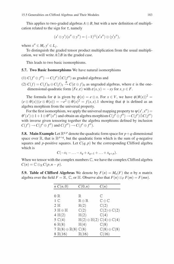
15.5 Generalities on Clifford Algebras and Their Modules 183
This applies to two-graded algebras A⊗B, but with a new definition of multipli-cation related to the sign for τ , namely
(x′ ⊗ y′)(x′′ ⊗ y′′) = (−1)i j(x′x′′)⊗ (y′y′′),
where x′′ ∈ Mi,y′ ∈ Lj.To distinguish the graded tensor product multiplication from the usual multipli-
cation, we will write A⊗B in the graded case.
This leads to two basic isomorphisms.
5.7. Two Basic Isomorphisms We have natural isomorphisms
(1) C( f ′ ⊕ f ′′) →C( f ′)⊗C( f ′′) as graded algebras and
(2) C( f ) = C( f )0 ⊕C( f )1φ→ C(ε ⊕ f )0 as ungraded algebras, where ε is the one-
dimensional quadratic form (Fe,ε) with ε(x,y) = −xy for x,y ∈ F .
The formula for φ is given by φ(x) = e⊗ x. For x ∈ V , we have φ(θ (x))2 =(e ⊗ θ (x))(e ⊗ θ (x)) = −e2 ⊗ θ (x)2 = f (x,x).1 showing that φ is defined as analgebra morphism from the universal property.
For the first isomorphism, we apply the universal mapping property toψ(x′,x′′)=θ ′(x′)⊗1+1⊗θ ′′(x′′) and obtain an algebra morphism C( f ′ ⊕ f ′′)→C( f ′)⊗C( f ′′)with inverse given tensoring together the algebra morphisms defined by inclusionC( f ′) →C( f ′ ⊕ f ′′) and C( f ′′) →C( f ′ ⊕ f ′′).
5.8. Main Example Let Rq,p denote the quadratic form space for p+q-dimensional
space over R, that is Rp+q, but the quadratic form which is the sum of q-negative
squares and p-positive squares. Let C(q, p) be the corresponding Clifford algebrawhich is
C(−x1 − . . .− xq + xq+1 + . . .+ xq+p).
When we tensor with the complex numbers C, we have the complex Clifford algebraC(n) = C⊗R C(p,n− p).
5.9. Table of Clifford Algebras We denote by F(n) = Mn(F) the n by n matrixalgebra over the field F = R, C, or H. Observe also that F(n)⊗F F(m) = F(mn).
n C(n,0) C(0,n) C(n)
0 R R C
1 C R⊕R C⊕C
2 H R(2) C(2)3 H⊕H C(2) C(2)⊕C(2)4 H(2) H(2) C(4)5 C(4) H(2)⊕H(2) C(4)⊕C(4)6 R(8) H(4) C(8)7 R(8)⊕R(8) C(8) C(8)⊕C(8)8 R(16) R(16) C(16)
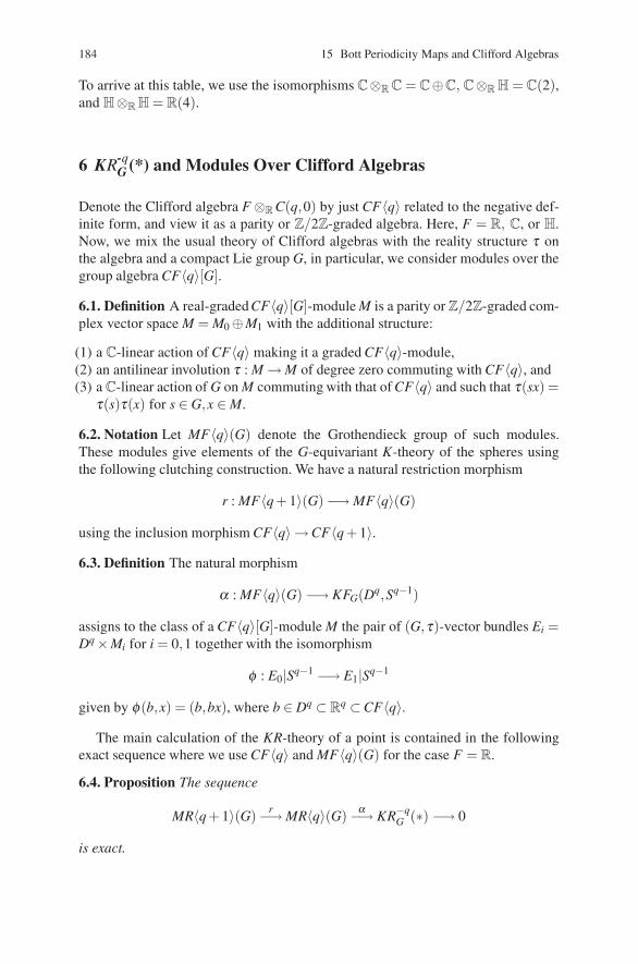
184 15 Bott Periodicity Maps and Clifford Algebras
To arrive at this table, we use the isomorphisms C⊗R C = C⊕C, C⊗R H = C(2),and H⊗R H = R(4).
6 KR-qG (*) and Modules Over Clifford Algebras
Denote the Clifford algebra F ⊗R C(q,0) by just CF〈q〉 related to the negative def-inite form, and view it as a parity or Z/2Z-graded algebra. Here, F = R, C, or H.Now, we mix the usual theory of Clifford algebras with the reality structure τ onthe algebra and a compact Lie group G, in particular, we consider modules over thegroup algebra CF〈q〉[G].
6.1. Definition A real-graded CF〈q〉[G]-module M is a parity or Z/2Z-graded com-plex vector space M = M0 ⊕M1 with the additional structure:
(1) a C-linear action of CF〈q〉 making it a graded CF〈q〉-module,(2) an antilinear involution τ : M → M of degree zero commuting with CF〈q〉, and(3) a C-linear action of G on M commuting with that of CF〈q〉 and such that τ(sx) =
τ(s)τ(x) for s ∈ G,x ∈ M.
6.2. Notation Let MF〈q〉(G) denote the Grothendieck group of such modules.These modules give elements of the G-equivariant K-theory of the spheres usingthe following clutching construction. We have a natural restriction morphism
r : MF〈q + 1〉(G)−→ MF〈q〉(G)
using the inclusion morphism CF〈q〉 →CF〈q + 1〉.6.3. Definition The natural morphism
α : MF〈q〉(G) −→ KFG(Dq,Sq−1)
assigns to the class of a CF〈q〉[G]-module M the pair of (G,τ)-vector bundles Ei =Dq ×Mi for i = 0,1 together with the isomorphism
φ : E0|Sq−1 −→ E1|Sq−1
given by φ(b,x) = (b,bx), where b ∈ Dq ⊂ Rq ⊂CF〈q〉.
The main calculation of the KR-theory of a point is contained in the followingexact sequence where we use CF〈q〉 and MF〈q〉(G) for the case F = R.
6.4. Proposition The sequence
MR〈q + 1〉(G) r−→ MR〈q〉(G) α−→ KR−qG (∗) −→ 0
is exact.
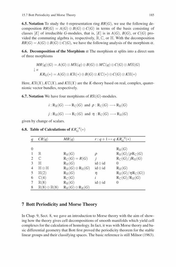
15.7 Bott Periodicity and Morse Theory 185
6.5. Notation To study the τ-representation ring RR(G), we use the following de-composition RR(G) = A(G)⊕ B(G)⊕C(G) in terms of the basis consisting ofclasses [E] of irreducible G-modules, that is, [E] is in A(G), B(G), or C(G) pro-vided the commuting algebra is, respectively, R,C, or H. With the decompositionRR(G) = A(G)⊕B(G)⊕C(G), we have the following analysis of the morphism α .
6.6. Decomposition of the Morphism α The morphism α splits into a direct sumof three morphisms
MR〈q〉(G) = A(G)⊗MR(q)⊕B(G)⊗MC(q)⊕C(G)⊗MH(G)↓ α
KRG(∗) = A(G)⊗KR(∗)⊕B(G)⊗KC(∗)⊕C(G)⊗KH(∗)
Here, KR(X),KC(X),and KH(X) are the K-theory based on real, complex, quater-nionic vector bundles, respectively.
6.7. Notation We have four morphisms of RR(G)-modules.
i : RR(G) −→ RC(G) and ρ : RC(G) −→ RR(G)
j : RH(G) −→ RC(G) and η : RC(G) −→ RH(G)
given by change of scalars.
6.8. Table of Calculations of KR−qG (∗)
q CR〈q〉 MR〈q〉 r : q + 1 �→ q KR−qG (∗)
0 RR(G)1 R RR(G) ρ RR(G)/ρRC(G)2 C RC(G) = R(G) j RC(G)/ jRH(G)3 H RH(G) id⊕ id 04 H⊕H RH(G)⊕RH(G) id⊕ id RH(G)5 H(2) RH(G) η RH(G)/ηRC(G))6 C(4) RC(G) i RC(G)/RH(G)7 R(8) RR(G) id⊕ id 08 R(8)⊕R(8) RR(G)⊕RR(G)
7 Bott Periodicity and Morse Theory
In Chap. 9, Sect. 8, we gave an introduction to Morse theory with the aim of show-ing how the theory gives cell decompositions of smooth manifolds which yield cellcomplexes for the calculation of homology. In fact, it was with Morse theory and ba-sic differential geometry that Bott first proved the periodicity theorem for the stablelinear groups and their classifying spaces. The basic reference is still Milnor (1963).
186 15 Bott Periodicity Maps and Clifford Algebras
The book has four parts, and for the purposes of Chap. 9 in this lecture notes, partI of Milnors book would be sufficient, but for the periodicity theorem, the entirebook is needed. In Part II, there is a very readable introduction to some Riemanniangeometry, and in Part III, it is applied to the variation of geodesics. This variationaltheory centers on the index theory of critical points for the energy functional, andthe indices are related to a cell decomposition of loop space where the geodesics arenow critical points. In the first section of the part IV, there is a general discussionconcerning the space of geodesics on homogeneous spaces as a subspace of loopspace. For this, we use the space
Ω(SU(2m) : I,−I)
of paths from the identity matrix I to the negative −I of the identity matrix, butΩ(SU(2m) : I,−I) is homotopically equivalent to theΩ(SU(2m) : I), loop space onSU(2m), by the map which multiplies each element ofΩ(SU(2m) : I,−I) by a fixedpath from −I to I.
7.1. Assertion The space of minimal geodesics from I to −I in SU(2m) is homeo-morphic to the complex Grassmann manifold Gm(C2m). Every minimal geodesicsfrom I to −I has index ≥ 2m+ 2.
Here, the space of minimal geodesics from I to −I in SU(2m) is considered as asubspace of Ω(SU(2m) : I,−I), and hence, there is an inclusion map
Gm(C2m) −→Ω(SU(2m) : I,−I),
whose connectivity can be measured. This is done by viewing Ω(SU(2m) : I,−I)as built from Grassmann manifold with cells of high dimension determined by theindex of other geodesics.
This assertion is the statement of the two Lemmas 23.1 and 23.2 of Milnor’sbook (1965, p.128). Its proof is based on calculus of variations application of Morsetheory which is explained in Part III and the first part of Part IV of the book. It is amodern account of Marston Morse’s theory of calculus of variations in large. Thisgives the periodicity theorem in the following unstable form.
7.2. Unstable Periodicity Theorem The inclusion map
Gm(C2m) −→Ω(SU(2m) : I,−I)
induces an isomorphism of homotopy groups in dimensions i ≤ 2m
πi(Gm(C2m) −→ πi(Ω(SU(2m) : I,−I)) −→ πi+1(SU(2m)) .
To obtain the homotopy periodicity of the unitary groups, we use the four fibra-tions and related isomorphisms of homotopy groups coming from the exact homo-topy sequence
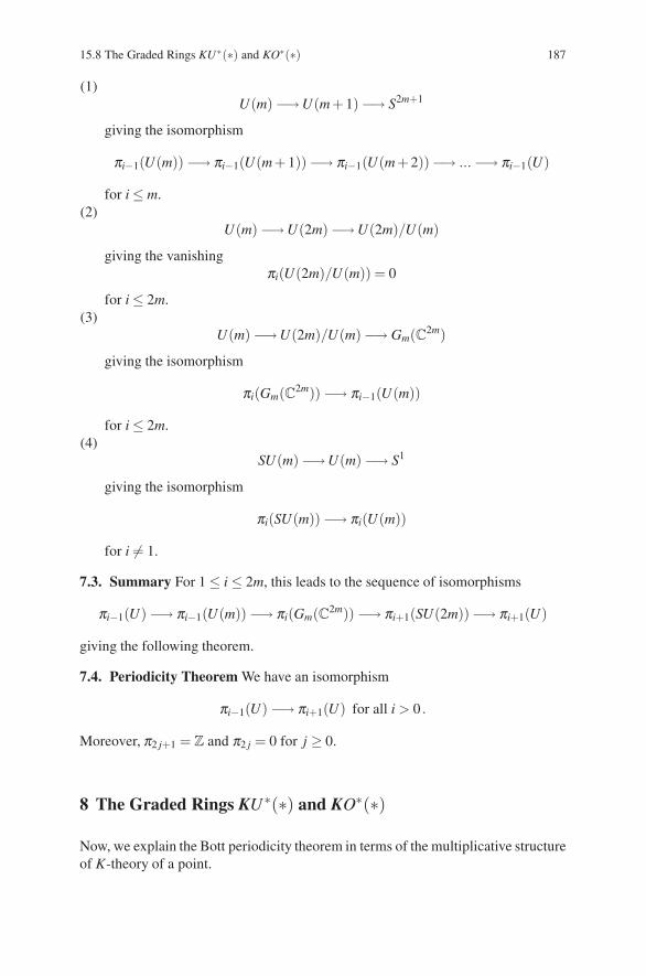
15.8 The Graded Rings KU∗(∗) and KO∗(∗) 187
(1)U(m) −→U(m+ 1)−→ S2m+1
giving the isomorphism
πi−1(U(m)) −→ πi−1(U(m+ 1))−→ πi−1(U(m+ 2))−→ ... −→ πi−1(U)
for i ≤ m.(2)
U(m) −→U(2m)−→U(2m)/U(m)
giving the vanishingπi(U(2m)/U(m)) = 0
for i ≤ 2m.(3)
U(m) −→U(2m)/U(m)−→ Gm(C2m)
giving the isomorphism
πi(Gm(C2m)) −→ πi−1(U(m))
for i ≤ 2m.(4)
SU(m)−→U(m) −→ S1
giving the isomorphism
πi(SU(m)) −→ πi(U(m))
for i = 1.
7.3. Summary For 1 ≤ i ≤ 2m, this leads to the sequence of isomorphisms
πi−1(U) −→ πi−1(U(m)) −→ πi(Gm(C2m)) −→ πi+1(SU(2m))−→ πi+1(U)
giving the following theorem.
7.4. Periodicity Theorem We have an isomorphism
πi−1(U) −→ πi+1(U) for all i > 0 .
Moreover, π2 j+1 = Z and π2 j = 0 for j ≥ 0.
8 The Graded Rings KU∗(∗) and KO∗(∗)
Now, we explain the Bott periodicity theorem in terms of the multiplicative structureof K-theory of a point.
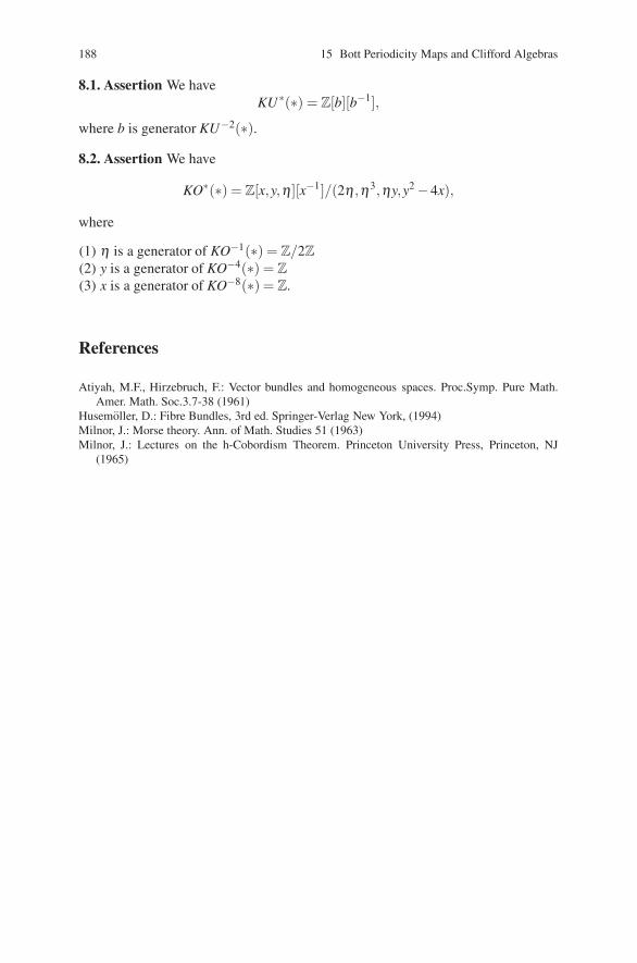
188 15 Bott Periodicity Maps and Clifford Algebras
8.1. Assertion We haveKU∗(∗) = Z[b][b−1],
where b is generator KU−2(∗).8.2. Assertion We have
KO∗(∗) = Z[x,y,η ][x−1]/(2η ,η3,ηy,y2 −4x),
where
(1) η is a generator of KO−1(∗) = Z/2Z
(2) y is a generator of KO−4(∗) = Z
(3) x is a generator of KO−8(∗) = Z.
References
Atiyah, M.F., Hirzebruch, F.: Vector bundles and homogeneous spaces. Proc.Symp. Pure Math.Amer. Math. Soc.3.7-38 (1961)
Husemoller, D.: Fibre Bundles, 3rd ed. Springer-Verlag New York, (1994)Milnor, J.: Morse theory. Ann. of Math. Studies 51 (1963)Milnor, J.: Lectures on the h-Cobordism Theorem. Princeton University Press, Princeton, NJ
(1965)
Chapter 16Gram–Schmidt Process, IwasawaDecomposition, and Reduction of Structurein Principal Bundles
Using the classical Gram–Schmidt process from the beginning linear algebra, weare able to derive group theory results about the linear groups and reduction ofstructure group results for vector bundles. By starting with these very elementaryconsiderations, we see that there are applications to both group representation theoryas well as to the topology of groups, their classifying spaces, and principal bundles.
This theory also has applications to modular forms which play an important rolein systems with an SL(2,Z)-symmetry. One example is the Verlinde algebra whicharises later in a twisted K-theory calculation.
1 Classical Gram–Schmidt Process
1.1. Notation Let again F denote one of the following three topological fields ofscalars: the real numbers R, the complex numbers C, or the quaternions H. An F-Hilbert space H is a vector space H over F with an inner product ( | ) : H ×H → Fwhich is linear in the first variable, conjugate linear in the second variable, hermitiansymmetric, that is, (y|x) = (x|y) for all x,y∈ H, and nondegenerate, that is, (x|x) > 0for all x = 0 in H.
1.2. Definition For a positive integer n and an F-Hilbert space H, the space Ln(H)is the open subspace of Hn consisting of linearly independent n-tuples of vectors,the space On(H) is the closed subspace of Hn consisting of n-tuples y1, . . . ,yn whichare orthogonal, that is, (yi|y j) = 0 for i = j, and the space ONn(H) is the closedsubspace of n-tuples z1, . . . ,zn which are orthonormal, that is, (zi | z j) = δi, j.
There is a simple pair of operations for the sequence of spaces ONn(H) ⊂On(H) ⊂ Ln(H) which is retracting to a subspace. These two retractions are calledthe Gram–Schmidt process.
1.3. Gram–Schmidt Process for On(H)⊂⊂⊂Ln(H) To x1, . . . ,xn in Ln(H), we as-sociate y1, . . . ,yn in On(H) such that the subspace generated by y1, . . . ,yi is equal to
D. Husemoller et al.: Gram–Schmidt Process, Iwasawa Decomposition, and Reduction of Structure in PrincipalBundles, Lect. Notes Phys. 726, 189–201 (2008)DOI 10.1007/978-3-540-74956-1 17 © Springer-Verlag Berlin Heidelberg 2008
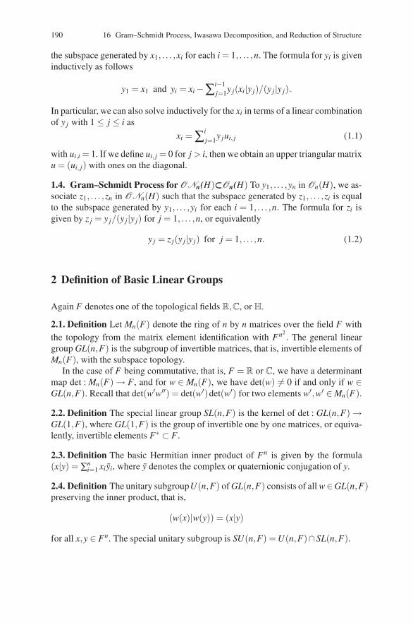
190 16 Gram–Schmidt Process, Iwasawa Decomposition, and Reduction of Structure
the subspace generated by x1, . . . ,xi for each i = 1, . . . ,n. The formula for yi is giveninductively as follows
y1 = x1 and yi = xi −∑i−1j=1y j(xi|y j)/(y j|y j).
In particular, we can also solve inductively for the xi in terms of a linear combinationof y j with 1 ≤ j ≤ i as
xi =∑ij=1y jui, j (1.1)
with ui,i = 1. If we define ui, j = 0 for j > i, then we obtain an upper triangular matrixu = (ui, j) with ones on the diagonal.
1.4. Gram–Schmidt Process for ONn(H)⊂⊂⊂On(H) To y1, . . . ,yn in On(H), we as-sociate z1, . . . ,zn in ONn(H) such that the subspace generated by z1, . . . ,zi is equalto the subspace generated by y1, . . . ,yi for each i = 1, . . . ,n. The formula for zi isgiven by z j = y j/(y j|y j) for j = 1, . . . ,n, or equivalently
y j = z j(y j|y j) for j = 1, . . . ,n. (1.2)
2 Definition of Basic Linear Groups
Again F denotes one of the topological fields R,C, or H.
2.1. Definition Let Mn(F) denote the ring of n by n matrices over the field F withthe topology from the matrix element identification with Fn2
. The general lineargroup GL(n,F) is the subgroup of invertible matrices, that is, invertible elements ofMn(F), with the subspace topology.
In the case of F being commutative, that is, F = R or C, we have a determinantmap det : Mn(F) → F , and for w ∈ Mn(F), we have det(w) = 0 if and only if w ∈GL(n,F). Recall that det(w′w′′) = det(w′)det(w′) for two elements w′,w′ ∈ Mn(F).
2.2. Definition The special linear group SL(n,F) is the kernel of det : GL(n,F) →GL(1,F), where GL(1,F) is the group of invertible one by one matrices, or equiva-lently, invertible elements F∗ ⊂ F .
2.3. Definition The basic Hermitian inner product of Fn is given by the formula(x|y) = ∑n
i=1 xiyi, where y denotes the complex or quaternionic conjugation of y.
2.4. Definition The unitary subgroupU(n,F) of GL(n,F) consists of all w∈GL(n,F)preserving the inner product, that is,
(w(x)|w(y)) = (x|y)
for all x,y ∈ Fn. The special unitary subgroup is SU(n,F) = U(n,F)∩SL(n,F).
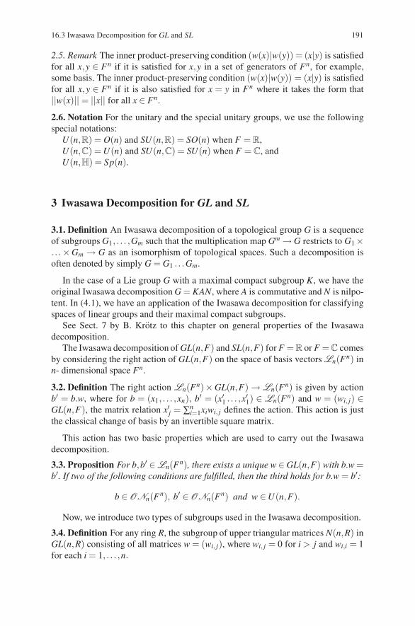
16.3 Iwasawa Decomposition for GL and SL 191
2.5. Remark The inner product-preserving condition (w(x)|w(y)) = (x|y) is satisfiedfor all x,y ∈ Fn if it is satisfied for x,y in a set of generators of Fn, for example,some basis. The inner product-preserving condition (w(x)|w(y)) = (x|y) is satisfiedfor all x,y ∈ Fn if it is also satisfied for x = y in Fn where it takes the form that||w(x)|| = ||x|| for all x ∈ Fn.
2.6. Notation For the unitary and the special unitary groups, we use the followingspecial notations:
U(n,R) = O(n) and SU(n,R) = SO(n) when F = R,U(n,C) = U(n) and SU(n,C) = SU(n) when F = C, andU(n,H) = Sp(n).
3 Iwasawa Decomposition for GL and SL
3.1. Definition An Iwasawa decomposition of a topological group G is a sequenceof subgroups G1, . . . ,Gm such that the multiplication map Gm → G restricts to G1 ×. . .×Gm → G as an isomorphism of topological spaces. Such a decomposition isoften denoted by simply G = G1 . . .Gm.
In the case of a Lie group G with a maximal compact subgroup K, we have theoriginal Iwasawa decomposition G = KAN, where A is commutative and N is nilpo-tent. In (4.1), we have an application of the Iwasawa decomposition for classifyingspaces of linear groups and their maximal compact subgroups.
See Sect. 7 by B. Krotz to this chapter on general properties of the Iwasawadecomposition.
The Iwasawa decomposition of GL(n,F) and SL(n,F) for F = R or F = C comesby considering the right action of GL(n,F) on the space of basis vectors Ln(Fn) inn- dimensional space Fn.
3.2. Definition The right action Ln(Fn)×GL(n,F) → Ln(Fn) is given by actionb′ = b.w, where for b = (x1, . . . ,xn), b′ = (x′1 . . . ,x′1) ∈ Ln(Fn) and w = (wi, j) ∈GL(n,F), the matrix relation x′j = ∑n
i=1xiwi, j defines the action. This action is justthe classical change of basis by an invertible square matrix.
This action has two basic properties which are used to carry out the Iwasawadecomposition.
3.3. Proposition For b,b′ ∈ Ln(Fn), there exists a unique w ∈ GL(n,F) with b.w =b′. If two of the following conditions are fulfilled, then the third holds for b.w = b′:
b ∈ ONn(Fn), b′ ∈ ONn(Fn) and w ∈U(n,F).
Now, we introduce two types of subgroups used in the Iwasawa decomposition.
3.4. Definition For any ring R, the subgroup of upper triangular matrices N(n,R) inGL(n,R) consisting of all matrices w = (wi, j), where wi, j = 0 for i > j and wi,i = 1for each i = 1, . . . ,n.
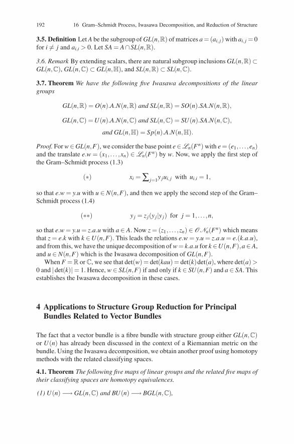
192 16 Gram–Schmidt Process, Iwasawa Decomposition, and Reduction of Structure
3.5. Definition Let A be the subgroup of GL(n,R) of matrices a =(ai, j) with ai, j = 0for i = j and ai,i > 0. Let SA = A∩SL(n,R).
3.6. Remark By extending scalars, there are natural subgroup inclusions GL(n,R)⊂GL(n,C), GL(n,C) ⊂ GL(n,H), and SL(n,R) ⊂ SL(n,C).
3.7. Theorem We have the following five Iwasawa decompositions of the lineargroups
GL(n,R) = O(n).A.N(n,R) and SL(n,R) = SO(n).SA.N(n,R),
GL(n,C) = U(n).A.N(n,C) and SL(n,C) = SU(n).SA.N(n,C),
and GL(n,H) = Sp(n).A.N(n,H).
Proof. For w∈GL(n,F), we consider the base point e∈Ln(Fn) with e = (e1, . . . ,en)and the translate e.w = (x1, . . . ,xn) ∈ Ln(Fn) by w. Now, we apply the first step ofthe Gram–Schmidt process (1.3)
(∗) xi =∑ j=1y jui, j with ui,i = 1,
so that e.w = y.u with u ∈ N(n,F), and then we apply the second step of the Gram–Schmidt process (1.4)
(∗∗) y j = z j(y j|y j) for j = 1, . . . ,n,
so that e.w = y.u = z.a.u with a ∈ A. Now z = (z1, . . . ,zn) ∈ ONn(Fn) which meansthat z = e.k with k ∈U(n,F). This leads the relations e.w = y.u = z.a.u = e.(k.a.u),and from this, we have the unique decomposition of w = k.a.u for k ∈U(n,F),a∈A,and u ∈ N(n,F) which is the Iwasawa decomposition of GL(n,F).
When F = R or C, we see that det(w) = det(kau)= det(k)det(a), where det(a)>0 and |det(k)|= 1. Hence, w ∈ SL(n,F) if and only if k ∈ SU(n,F) and a ∈ SA. Thisestablishes the Iwasawa decomposition in these cases.
4 Applications to Structure Group Reduction for PrincipalBundles Related to Vector Bundles
The fact that a vector bundle is a fibre bundle with structure group either GL(n,C)or U(n) has already been discussed in the context of a Riemannian metric on thebundle. Using the Iwasawa decomposition, we obtain another proof using homotopymethods with the related classifying spaces.
4.1. Theorem The following five maps of linear groups and the related five maps oftheir classifying spaces are homotopy equivalences.
(1) U(n) −→ GL(n,C) and BU(n) −→ BGL(n,C),
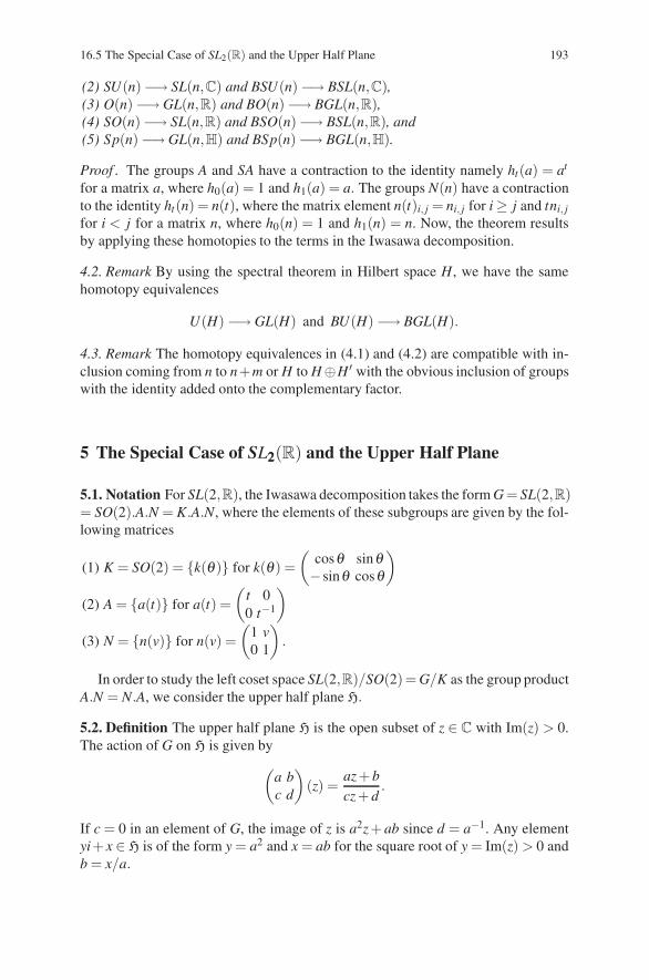
16.5 The Special Case of SL2(R) and the Upper Half Plane 193
(2) SU(n)−→ SL(n,C) and BSU(n)−→ BSL(n,C),(3) O(n) −→ GL(n,R) and BO(n) −→ BGL(n,R),(4) SO(n)−→ SL(n,R) and BSO(n)−→ BSL(n,R), and(5) Sp(n)−→ GL(n,H) and BSp(n)−→ BGL(n,H).
Proof . The groups A and SA have a contraction to the identity namely ht(a) = at
for a matrix a, where h0(a) = 1 and h1(a) = a. The groups N(n) have a contractionto the identity ht(n) = n(t), where the matrix element n(t)i, j = ni, j for i ≥ j and tni, j
for i < j for a matrix n, where h0(n) = 1 and h1(n) = n. Now, the theorem resultsby applying these homotopies to the terms in the Iwasawa decomposition.
4.2. Remark By using the spectral theorem in Hilbert space H, we have the samehomotopy equivalences
U(H) −→ GL(H) and BU(H) −→ BGL(H).
4.3. Remark The homotopy equivalences in (4.1) and (4.2) are compatible with in-clusion coming from n to n+m or H to H⊕H ′ with the obvious inclusion of groupswith the identity added onto the complementary factor.
5 The Special Case of SL222(R) and the Upper Half Plane
5.1. Notation For SL(2,R), the Iwasawa decomposition takes the form G = SL(2,R)= SO(2).A.N = K.A.N, where the elements of these subgroups are given by the fol-lowing matrices
(1) K = SO(2) = {k(θ )} for k(θ ) =(
cosθ sinθ−sinθ cosθ
)
(2) A = {a(t)} for a(t) =(
t 00 t−1
)
(3) N = {n(v)} for n(v) =(
1 v0 1
).
In order to study the left coset space SL(2,R)/SO(2)= G/K as the group productA.N = N.A, we consider the upper half plane H.
5.2. Definition The upper half plane H is the open subset of z ∈ C with Im(z) > 0.The action of G on H is given by
(a bc d
)(z) =
az+ bcz+ d
.
If c = 0 in an element of G, the image of z is a2z+ ab since d = a−1. Any elementyi+ x ∈ H is of the form y = a2 and x = ab for the square root of y = Im(z) > 0 andb = x/a.
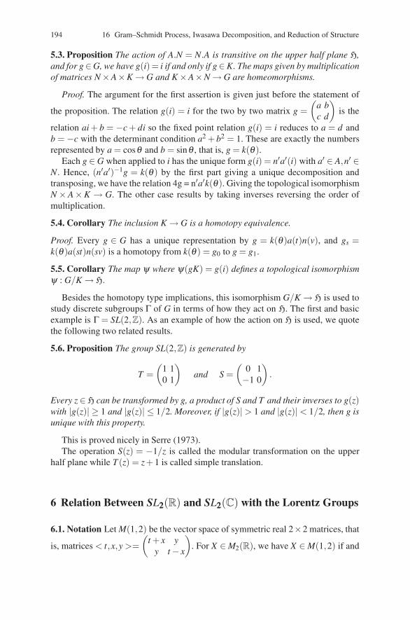
194 16 Gram–Schmidt Process, Iwasawa Decomposition, and Reduction of Structure
5.3. Proposition The action of A.N = N.A is transitive on the upper half plane H,and for g∈G, we have g(i)= i if and only if g∈K. The maps given by multiplicationof matrices N ×A×K → G and K ×A×N → G are homeomorphisms.
Proof. The argument for the first assertion is given just before the statement of
the proposition. The relation g(i) = i for the two by two matrix g =(
a bc d
)is the
relation ai + b = −c + di so the fixed point relation g(i) = i reduces to a = d andb = −c with the determinant condition a2 + b2 = 1. These are exactly the numbersrepresented by a = cosθ and b = sinθ , that is, g = k(θ ).
Each g ∈ G when applied to i has the unique form g(i) = n′a′(i) with a′ ∈ A,n′ ∈N. Hence, (n′a′)−1g = k(θ ) by the first part giving a unique decomposition andtransposing, we have the relation 4g = n′a′k(θ ). Giving the topological isomorphismN × A×K → G. The other case results by taking inverses reversing the order ofmultiplication.
5.4. Corollary The inclusion K → G is a homotopy equivalence.
Proof. Every g ∈ G has a unique representation by g = k(θ )a(t)n(v), and gs =k(θ )a(st)n(sv) is a homotopy from k(θ ) = g0 to g = g1.
5.5. Corollary The map ψ where ψ(gK) = g(i) defines a topological isomorphismψ : G/K → H.
Besides the homotopy type implications, this isomorphism G/K → H is used tostudy discrete subgroups Γ of G in terms of how they act on H. The first and basicexample is Γ = SL(2,Z). As an example of how the action on H is used, we quotethe following two related results.
5.6. Proposition The group SL(2,Z) is generated by
T =(
1 10 1
)and S =
(0 1−1 0
).
Every z ∈H can be transformed by g, a product of S and T and their inverses to g(z)with |g(z)| ≥ 1 and |g(z)| ≤ 1/2. Moreover, if |g(z)| > 1 and |g(z)| < 1/2, then g isunique with this property.
This is proved nicely in Serre (1973).The operation S(z) = −1/z is called the modular transformation on the upper
half plane while T (z) = z+ 1 is called simple translation.
6 Relation Between SL222(R) and SL222(C) with the Lorentz Groups
6.1. Notation Let M(1,2) be the vector space of symmetric real 2×2 matrices, that
is, matrices < t,x,y >=(
t + x yy t − x
). For X ∈ M2(R), we have X ∈ M(1,2) if and
16.A Appendix 195
only if Xt = X . The space M(1,2) is a vector space over R of dimension 3, and thedeterminant
det < t,x,y >= t2 − x2 − y2
is the Lorentz metric for one-time coordinate and two-space coordinates.Let M(1,3) be the vector space of Hermitian complex 2× 2 matrices, that is,
matrices < t,x,y,z >=(
t + x y + izy− iz t − x
). For Z ∈ M2(C), we have Z ∈ M(1,3) if and
only if Z∗ = Z. The space M(1,3) is a vector space over R of dimension 4 and thedeterminant
det < t,x,y,z >= t2 − x2 − y2 − z2
is the Lorentz metric for one-time coordinate and three-space coordinates. Note thatM(1,2) ⊂ M(1,3) is the subspace where z = 0.
6.2. The Morphism θθθ ::: SSSLLL222(R)→→→ OOO(((111,,,222))) For A ∈ SL2(R), we define θ (A)(X) =AXA−1 and we see that θ (A)(X) ∈ M(1,2) for X ∈ M(1,2). Moreover,det(θ (A)(X)) = det(X) for X ∈ M(1,2) showing that θ (A) ∈ O(1,2), the Lorentzgroup of type (1,2).
6.3. The Morphism θθθ ::: SSSLLL222(C)→→→ OOO(((111,,,333))) For A ∈ SL2(C), we define θ (A)(Z) =AZA−1 and we see that θ (A)(Z) ∈ M(1,3) for Z ∈ M(1,3). Moreover,det(θ (A)(Z)) = det(Z) for Z ∈ M(1,3) showing that θ (A) ∈ O(1,3), the Lorentzgroup of type (1,3).
6.4. Remark We see that θ (A′A′′) = θ (A′)θ (A′′) in both cases, and the two defi-nitions of θ are compatible under restriction to SL2(R) ⊂ SL2(C) and M(1,2) ⊂M(1,3). The kernel ker(θ ) of θ , that is the matrices A of SL2(C) with θ (A) = iden-tity, consists of the two elements ±I, where I is the identity matrix.
6.5. Remark Using θ , the Iwasawa decompositions SL2(R) = SO(2).A.N andSL2(C) = SU(2).A′.N′ give Iwasawa decompositions of O(1,2) and O(1,3), respec-tively. Observe that the image of θ is of finite index in the Lorentz groups O(1,2)and O(1,3). This allows us to study the Lorentz groups using SL2(R) and SL2(C).
A Appendix: A Novel Characterization of the IwasawaDecomposition of a Simple Lie Group (by B. Krotz)
This appendix is about (essential) uniqueness of the Iwasawa (or horospherical)decomposition G = KAN of a semisimple Lie group G. This means:
A.1. Theorem Assume that G is a connected Lie group with simple Lie algebra g.Assume that G = KL for some closed subgroups K,L < G with K ∩L discrete. Thenup to order, the Lie algebra k of K is maximally compact, and the Lie algebra l of Lis isomorphic to a+n, the Lie algebra of AN.
A.2. General Facts on Decompositions of Lie Groups. For a group G, a subgroupH < G, and an element g ∈ G, we define Hg = gHg−1.
196 16 Gram–Schmidt Process, Iwasawa Decomposition, and Reduction of Structure
A.3. Lemma Let G be a group and H,L < G subgroups. Then, the following state-ments are equivalent:
(i) G = HL and H ∩L = {1}.(ii) G = HLg and H ∩Lg = {1} for all g ∈ G.
Proof. Clearly, we only have to show that (ii) ⇒ (i). Suppose that G = HL withH ∩L = {1}. Then, we can write g ∈ G as g = hl for some h ∈ H and l ∈ L. Observethat Lg = Lh and so
H ∩Lg = H ∩Lh = Hh ∩Lh = (H ∩L)h = {1} .
Moreover, we record
HLg = HLh = HLh = Gh = G .
In the sequel, capital Latin letters will denote real Lie groups and the correspond-ing lower case fractur letters will denote the associated Lie algebra, that is, G is aLie group with Lie algebra g.
A.4. Lemma Let G be a Lie group and H,L < G closed subgroups. Then, the fol-lowing statements are equivalent:
(i) G = HL with H ∩L = {1}.(ii) The multiplication map
H ×L → G, (h, l) �→ hl
is an analytic diffeomorphism.
Proof. Standard structure theory.If G is a Lie group with closed subgroups H,L < G such that G = HL with
H ∩L = {1}, then we refer to (G,H,L) as a decomposition triple.
A.5. Lemma Let (G,H,L) be a decomposition triple. Then:
(∀g ∈ G) g = h+ Ad(g)l and h∩Ad(g)l = {0} . (A.1)
Proof. In view of Lemma A.4, the map H×L →G, (h, l) �→ hl is a diffeomorphism.In particular, the differential at (1,1) is a diffeomorphism which means that g =h+ l, h∩ l = {0}. As we may replace L by Lg, for example Lemma A.3, the assertionfollows.Question 1 Assume that G is connected. Is it then true that (G,H,L) is a decompo-sition triple if and only if the algebraic condition (A.1) is satisfied.
A.6. Remark If the Lie algebra g splits into a direct sum of subalgebra g = h+ l, thenwe cannot conclude in general that G = HL holds. For example, let h = m+a+n bea minimal parabolic subalgebra and l = n be the opposite of n. Then, HL = MANNis the open Bruhat cell in G. A similar example is when g = sl(n,R) with h the
16.A Appendix 197
upper triangular matrices and l = so(p,n− p) for 0 < p < n. In this case, HL ⊂ Gis a proper open subset. Notice that in both examples, condition (A.1) is violated ash∩Ad(g)l = {0} for appropriate g ∈ G.
A.7. The Case of One Factor Being Maximal Compact. Throughout this section,G denotes a semisimple-connected Lie group with associated Cartan decompositiong = k + p. Set K = expk and note that Ad(K) is maximal compact subgroup inAd(G).
For what follows we have to recall some results of Mostow on maximal solvablesubalgebras in g. Let c ⊂ g be a Cartan subalgebra. Replacing c by an appropriateAd(G)-conjugate, we may assume that c = t0 + a0 with t0 ⊂ k and a0 ⊂ p. WriteΣ = Σ(a,g) ⊂ a∗\{0} for the nonzero ada0-spectrum on g. For α ∈ Σ , write gα forthe associated eigenspcae. Call X ∈ a0 regular if α(X) = 0 for all α ∈ Σ . Associatedto a regular element X ∈ a, we associate a nilpotent subalgebra
nX =⊕α∈Σα(X)>0
gα .
If a ⊂ p happens to be maximal abelian, then we will write n instead of nX .With this notation we have the following
A.8. Theorem Let g be a semisimple Lie algebra. Then, the following assertionshold:
(i) Every maximal solvable subalgebra r of g contains a Cartan subalgebra c of g.(ii) Up to conjugation with an element of Ad(G), every maximal solvable subalge-
bra of g is of the formr = c+nX
for some regular element X ∈ a0.
Proof. Lemma A.14 and Mostow (1961).We choose a maximal abelian subspace a⊂ p and write Σ = Σ(g,a) for the asso-
ciated root system. For a choice of positive roots, we obtain a unipotent subalgebran. Write m = zk(a) and fix a Cartan subalgebra t ⊂ m. Write A,N,T for the analyticsubgroups of G corresponding to a, n, t. Notice that t+a+n is a maximal solvablesubalgebra by Theorem A.8.
A.9. Lemma Let L < G be a closed subgroup such that G = KL with K ∩L = {1}.Then, there is an Iwasawa decomposition G = NAK such that
N ⊂ L ⊂ TAN and L # LT/T # AN . (A.2)
Conversely, if L is a closed subgroup of G satisfying (A.2), then G = KL withK ∩L = {1}.
198 16 Gram–Schmidt Process, Iwasawa Decomposition, and Reduction of Structure
Proof. Our first claim is that L contains no nontrivial compact subgroups. In fact,let LK ⊂ L be a compact subgroup. As all maximal compact subgroups of G areconjugate, we find a g ∈ G such that Lg
K ⊂ K. But LgK ∩K ⊂ Lg ∩K = {1} by Lemma
A.3. This establishes our claim.Next, we show that L is solvable. For that, let L = SL ×RL be a Levi decompo-
sition, where S is semisimple and R is reductive. If S = 1, then there is a nontrivialmaximal compact subgroup SK ⊂ S. Hence, S = 1 by our previous claim and L = RL
is solvable.Next, we turn to the specific structure of l, the Lie algebra of l. Let r = c+nX be a
maximal solvable subalgebra of g which contains l. As before, we write c = t0 +a0
for the Cartan subalgebra of r. We claim that a0 = a is maximal abelian in p. In fact,notice that l∩ t0 = {0} and so l ↪→ r/t0 # a0 +nX injects as vector spaces. Hence,
dim l = dima+ dimn ≤ dima0 + dimnX .
But, dima0 ≤ dima and dimnX ≤ dimn and therefore a = a0. Hence, r = t+a+n.As l# r/t as vector spaces, we thus get hat L# LT/T #R/T #AN as homogeneousspaces. We now show that N ⊂ L which will follow from n ⊂ [l, l]. For that, choosea regular element X ∈ a. By what we know already, we then find an element Y ∈ tsuch that X +Y ∈ l. Notice that ad(X +Y ) is invertible on n and hence n⊂ [X +Y,n].Finally, observe that
[X +Y,n] = [X +Y,r] = [X +Y, l+ t] = [X +Y, l]
which concludes the proof of the first assertion of the lemma.Finally, the second assertion of the lemma is immediate from the Iwasawa de-
composition of G.
A.10. Manifold Decompositions for Decomposition Triples. Throughout thissection, G denotes a connected Lie group.
Let (G,H,L) be a decomposition triple and let us fix maximal compact subgroupsKH and KL of H and L, respectively. We choose a maximal compact subgroup K ofG such that KH ⊂ K. As we are free to replace L by any conjugate Lg, we mayassume in addition that KL ⊂ K.
We then have the following fact, see also Lemma A.4 and Oniscik (1969).
A.11. Lemma Let (G,H,L) be a decomposition triple. Then, (K,KH ,KL) is a de-composition triple, that is, the map
KH ×KL → K, (h, l) �→ hl
is a diffeomorphism.
Before we prove the lemma, we recall a fundamental result of Mostow concern-ing the topology of a connected Lie group G, cf. Mostow (1952). If K < G is a
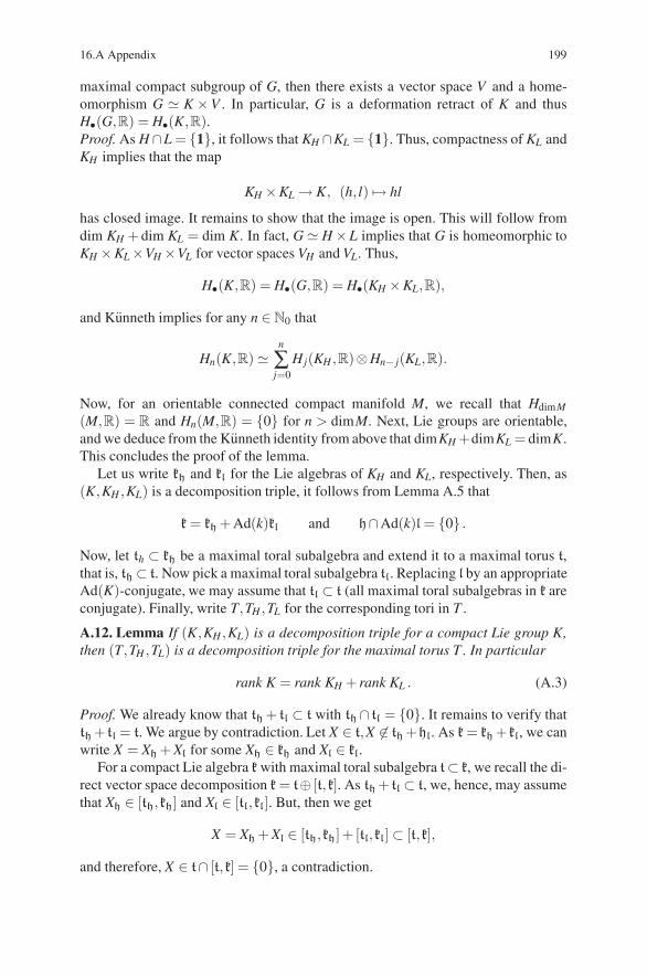
16.A Appendix 199
maximal compact subgroup of G, then there exists a vector space V and a home-omorphism G # K ×V . In particular, G is a deformation retract of K and thusH•(G,R) = H•(K,R).Proof. As H ∩L = {1}, it follows that KH ∩KL = {1}. Thus, compactness of KL andKH implies that the map
KH ×KL → K, (h, l) �→ hl
has closed image. It remains to show that the image is open. This will follow fromdim KH + dim KL = dim K. In fact, G # H ×L implies that G is homeomorphic toKH ×KL ×VH ×VL for vector spaces VH and VL. Thus,
H•(K,R) = H•(G,R) = H•(KH ×KL,R),
and Kunneth implies for any n ∈ N0 that
Hn(K,R) #n
∑j=0
Hj(KH ,R)⊗Hn− j(KL,R).
Now, for an orientable connected compact manifold M, we recall that HdimM
(M,R) = R and Hn(M,R) = {0} for n > dimM. Next, Lie groups are orientable,and we deduce from the Kunneth identity from above that dimKH +dimKL = dimK.This concludes the proof of the lemma.
Let us write kh and kl for the Lie algebras of KH and KL, respectively. Then, as(K,KH ,KL) is a decomposition triple, it follows from Lemma A.5 that
k = kh + Ad(k)kl and h∩Ad(k)l = {0} .
Now, let th ⊂ kh be a maximal toral subalgebra and extend it to a maximal torus t,that is, th ⊂ t. Now pick a maximal toral subalgebra tl. Replacing l by an appropriateAd(K)-conjugate, we may assume that tl ⊂ t (all maximal toral subalgebras in k areconjugate). Finally, write T,TH ,TL for the corresponding tori in T .
A.12. Lemma If (K,KH ,KL) is a decomposition triple for a compact Lie group K,then (T,TH ,TL) is a decomposition triple for the maximal torus T . In particular
rank K = rank KH + rank KL . (A.3)
Proof. We already know that th + tl ⊂ t with th ∩ tl = {0}. It remains to verify thatth + tl = t. We argue by contradiction. Let X ∈ t,X ∈ th +hl. As k = kh + kl, we canwrite X = Xh + Xl for some Xh ∈ kh and Xl ∈ kl.
For a compact Lie algebra k with maximal toral subalgebra t⊂ k, we recall the di-rect vector space decomposition k = t⊕ [t,k]. As th + tl ⊂ t, we, hence, may assumethat Xh ∈ [th,kh] and Xl ∈ [tl,kl]. But, then we get
X = Xh + Xl ∈ [th,kh]+ [tl,kl] ⊂ [t,k],
and therefore, X ∈ t∩ [t,k] = {0}, a contradiction.
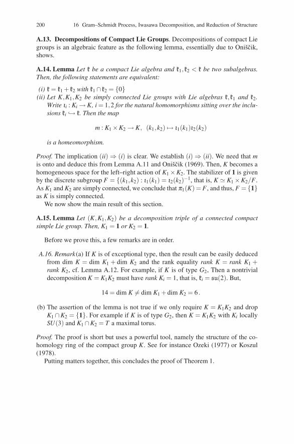
200 16 Gram–Schmidt Process, Iwasawa Decomposition, and Reduction of Structure
A.13. Decompositions of Compact Lie Groups. Decompositions of compact Liegroups is an algebraic feature as the following lemma, essentially due to Oniscik,shows.
A.14. Lemma Let k be a compact Lie algebra and k1,k2 < k be two subalgebras.Then, the following statements are equivalent:
(i) k = k1 + k2 with k1 ∩ k2 = {0}(ii) Let K,K1,K2 be simply connected Lie groups with Lie algebras k,k1 and k2.
Write ιi : Ki → K, i = 1,2 for the natural homomorphisms sitting over the inclu-sions ki ↪→ k. Then the map
m : K1 ×K2 → K, (k1,k2) �→ ι1(k1)ι2(k2)
is a homeomorphism.
Proof. The implication (ii) ⇒ (i) is clear. We establish (i) ⇒ (ii). We need that mis onto and deduce this from Lemma A.11 and Oniscik (1969). Then, K becomes ahomogeneous space for the left–right action of K1 ×K2. The stabilizer of 1 is givenby the discrete subgroup F = {(k1,k2) : ι1(k1) = ι2(k2)−1, that is, K # K1 ×K2/F .As K1 and K2 are simply connected, we conclude that π1(K) = F , and thus, F = {1}as K is simply connected.
We now show the main result of this section.
A.15. Lemma Let (K,K1,K2) be a decomposition triple of a connected compactsimple Lie group. Then, K1 = 1 or K2 = 1.
Before we prove this, a few remarks are in order.
A.16. Remark(a) If K is of exceptional type, then the result can be easily deducedfrom dim K = dim K1 + dim K2 and the rank equality rank K = rank K1 +rank K2, cf. Lemma A.12. For example, if K is of type G2, Then a nontrivialdecomposition K = K1K2 must have rank Ki = 1, that is, ki = su(2). But,
14 = dim K = dim K1 + dim K2 = 6 .
(b) The assertion of the lemma is not true if we only require K = K1K2 and dropK1 ∩K2 = {1}. For example if K is of type G2, then K = K1K2 with Ki locallySU(3) and K1 ∩K2 = T a maximal torus.
Proof. The proof is short but uses a powerful tool, namely the structure of the co-homology ring of the compact group K. See for instance Ozeki (1977) or Koszul(1978).
Putting matters together, this concludes the proof of Theorem 1.
References 201
References
Koszul, J.L.: Variante d’un theoreme de H. Ozeki: Osaka J. Math. 15: 547–551 (1978)Mostow, G.D.: On the L2-space of a Lie group. Amer. J. Math. 74: 920–928 (1952)Mostow, G.D.: On maximal subgroups of real Lie groups. Ann. Math. 74(3): 503–517 (1961)Oniscik, A.L.: Decompositions of reductive Lie groups. Mat. Sb. (N.S.) bf 80(122): 553–599
(1969)Ozeki, H.: On a transitive transformation group of a compact group manifold. Osaka J. Math, 14:
519–531 (1977)

Chapter 17Topological Algebras: G-Equivarianceand KK-Theory
In three previous Chaps. 13–15, we have developed the theory of G-equivariant vec-tor bundles over a compact space X for a compact group G. In Chap. 3, vector bun-dles over a compact space X were related to finitely generated projective modulesover the algebra C(X). The K-theory of X was described in terms of projections inthe C∗-algebra C(X) tensored with the compact operators in 4(5.14), that is, K0(X)is naturally isomorphic to C∗-algebra K-theory K(C(X)).
In fact, the K-theory K(A) is defined for all C∗-algebras A, and this introduces thepossibility of a geometric interpretation of the K-theory for more general classes oftopological algebras. The beginnings of this point of view arises when we consideran algebra related to a compact group G acting on a compact space X . This is anoncommutative algebra, called the cross product algebra G � A, where A = C(X),whose K-theory turns out to be the G-equivariant K-theory KG(X). This theory isoutlined in Sects. 1 and 2.
This step leads to a broad extension of the theory involving other topologicalalgebras, called m-algebras and locally convex algebras. The K-theory of these al-gebras, which includes C∗-algebras, has many formal properties of the K-theory ofspaces. We outline aspects of the theory in this chapter in Sects. 3–10.
The index theory of elliptic operators leads to K-theory invariants and suggesteda version of K-homology theory with geometric and analytical data evolving “K-cycles.” These cycles were first introduced by Atiyah and were related to extensiongroups Ext(B,A) by Brown–Douglas–Fillmore. Kasparov has developed a bivarianttheory KK(A,B) for C∗-algebras with a G-equivariant version KKG(A,B). Cuntzhas extended the theory to locally convex algebras and a related bivariant theoryk(A,B).
We give a short descriptive introduction to these constructions including thesmooth case which arises with smooth manifolds naturally, because smooth func-tion spaces are usually only locally convex. Since in one chapter it is only possibleto give a sketch of the theory, we will make frequent references to the books denotedby 〈B〉 or 〈CMR〉, that is, respectively, Blackadar (1998) and Cuntz et al. (2007).
D. Husemoller et al.: Topological Algebras: G-Equivariance and KK-Theory, Lect. Notes Phys. 726, 203–226 (2008)DOI 10.1007/978-3-540-74956-1 18 © Springer-Verlag Berlin Heidelberg 2008
204 17 Topological Algebras: G-Equivariance and KK-Theory
1 The Module of Cross Sections for a G-EquivariantVector Bundle
In 3(2.1), we have studied the cross section functor for vector bundles
Γ : HomX (E ′,E ′′) −→ HomC(X)(Γ(X ,E ′),Γ(X ,E ′′))
with full embedding and equivalence properties under suitable conditions into thecategory of finitely generated projective modules over the algebra C(X). We wishto extend this picture to modules and spaces with G-action. We need the followingconventions and definitions.
Convention 1.1 As in Chap. 3 and 13, X is a compact space and G is a compactgroup. The C∗-topology on C(X) is also the compact open topology. For a vectorbundle E over X, we give Γ(X ,E), the compact open topology and all automorphismgroups occurring get the compact open topology too.
1.2. Definition For a G-space X , we define a multiplicative map α : G→Aut(C(X))by the formula α(s)( f )(x) = f (s−1x). A topological algebra A with continuousgroup homomorphism α : G → Aut(A) is called a G-algebra.
We extend this definition to cross sections of any vector G-vector bundle E overa G-space X using the notation s# : Es−1x → Ex which is by definition of a G-vectorbundle a C-linear isomorphism between fibres of E .
1.3. Definition Let E be a G-equivariant vector bundle over a space X . The leftG-action on Γ(X ,E) is the continuous group homomorphismα : G→Aut(Γ(X ,E)),where α(s)(σ)(x) = s#σ(s−1x).
1.4. Remark The map α is C(X)-linear on the vector space Γ(X ,E) in the sense itsatisfies the equivariance formula
α(s)( fσ) = α(s)( f )α(s)α(σ)
for the action of f ∈ C(X) = Γ(X ,X ×C) on σ ∈ Γ(X ,E). For this, we use thecalculation
α(st)(σ)(x) = (st)#σ((st)−1x) = s#t#σ(t−1s−1x)
= s#α(t)(σ)(s−1x) = α(s)α(t)(σ)(x).
1.5. Definition Let A be a topological algebra with G-action. A (G,A)-module M isa left A-module together with a linear continuous G-action on M such that s(ax) =s(a)s(x), where s∈ G, a∈ A, and x∈ M. Let (G,A)Mod denote the category of (G,A)-modules and morphisms consisting of A-linear G-equivariant maps.
1.6. Example The cross section module Γ(X ,E) of a G-vector bundle E is a (G,C(X))-module. The cross section module is a functor
Γ : VectG(X) →(G,C(X)) Mod.
17.2 G-Equivariant K-Theory and the K-Theory of Cross Products 205
In order to relate two G-equivariant K-groups for A = C(X), we have the follow-ing version of the Serre–Swan theorem using the full subcategory Vect(G,C(X)) ofobjects in (G,C(X))Mod which are finitely generated projective C(X)-modules.
1.7. Theorem Let G be a compact group acting on a compact space X. The crosssection functor Γ : VectG(X) → Vect(G,C(X)) is an equivalence of categories.
Proof . This theorem is proved by averaging over the compact group the equiv-alence of categories Γ(X , ) : (vect/X) → (vect/C(X)), see 3(4.3). The functorΓ : VectG(X) → Vect(G,C(X)) is faithful as a restriction of a faithful functor, and
Γ : HomG(E ′,E ′′) −→ Hom(G,C(X))(Γ(X ,E ′),Γ(X ,E ′′))
is a bijection for f ∈ Hom(G,C(X))(Γ(X ,E ′),Γ(X ,E ′′), there is v : E ′ → E ′′ a mor-phism of vector bundles with Γ(v) = f . The average u of v will be G-equivariant andsatisfies Γ(u) = f , giving a full embedding. To show the restriction of Γ in the as-sertion is an equivalence, we note the key step is to take an object M in (G,C(X))Modand choose a surjective (G,A)-morphism w : An → M together with an A-linearv : M → An which is a section of w. We average v to u and wv = M to wu = M. Inthis way, we construct enough G-equivariant vector bundles on X in order that Γis an equivalence of categories.
1.8. Definition Using the category VectG(X) of G-equivariant vector bundles overX , we can form the Grothendieck group KG(X) to obtain G-equivariant K-theoryK0
G(X).
1.9. Definition Using the category Vect(G,A) of finitely generated projective (G,A)-modules, we can form the Grothendieck group KG(A) to obtain G-equivariantK-theory of a G-algebra A.
As before, the K-theory of a space can be calculated in terms of the K-theory ofalgebras, but now in the equivariant setting.
1.10. Corollary Let G be a compact group acting on a compact space X. The crosssection functor Γ induces an isomorphism of the K-groups
KG(X)∼=−→ KG(C(X)).
See 〈B〉, 11.4, for more details.
2 G-Equivariant K-Theory and the K-Theory of Cross Products
In Chap. 4, Sect. 5, we saw that a C∗ property on an algebra could lead to additionalproperties of the K-theory. In this section, we outline how for a compact group G theG-equivariant K-theory for a C∗-algebra A can be described using the usual K-theoryof the related crossed product C∗-algebra G � A, where G is a compact group.
206 17 Topological Algebras: G-Equivariance and KK-Theory
2.1. Cross Products of Groups For a topological group G acting on another topo-logical group H by α : G → Aut(H), there is a cross product group G � H and arelated topological group extension
Hi−→ G � H
π−→ G,
where as a space G � H is the product space H ×G, with π(a,u) = u and i(a) =(a,1). The multiplication on G � H is given by the formula
(a′,u′) · (a′′,u′′) = (a′α(u′)(a′′),u′u′′) for (a′,u′),(a′′,u′′) ∈ G � H.
It is easy to check that (1,1) is the unit, and for the relation
(a,u)−1 = (α(u−1)a−1,u−1),
we calculate
(a,u) · (α(u−1)a−1,u−1) = (aα(u)α(u−1)a−1,uu−1) = (1,1).
2.2. Example For a field F , its affine group Aff(F) is
F+ −→ Aff(F) = F∗� F+ −→ F∗,
where Aff(F) is a subgroup of the permutation group of F consisting of substitutionsa + ux and group law
(a′ + u′x) · (a′′ + u′′x) = a′ + u′(a′′ + u′′x)+ b′ = (a′ + u′(a′′))+ (u′u′′)x.
The group Aff(F) is called the affine group of the line.There is a matrix realization of Aff(F) with group law given by
(u′ 0a′ 1
)(u′′ 0a′′ 1
)=(
u′u′′ 0a′ + u′a′′ 1
).
Now, we give the mapping spaces C(G,A) and L1(G,A) the structure of aG-algebra.
2.3. Definition Let G be a locally compact group, let A be a Banach ∗-algebra, andlet α : G → Aut(A) be an action of G on A. Let Cc(G,A) be the ∗-algebra of com-pactly supported continuous functions G → A. The ∗-algebra structure is defined bythe convolution multiplication
(a ∗ b)(s) =∫
a(t)αt(b)(t−1s)dt for s,t ∈ G,a,b ∈Cc(G,α,A)
and the ∗-operation
(a∗)(s) = δ (s)−1αs(a)(s−1)∗ for s ∈ G,a ∈Cc(G,A).
17.3 Generalities on Topological Algebras: Stabilization 207
For the locally compact group G, the modular function is δ : G → R∗+ defined by
the formula d(s−1) = δ (s)−1ds. We use the fact that it is morphism of topologicalgroups.
2.4. Definition The cross product G � A is the enveloping C∗-algebra of Cc(G,A).
2.5. Remark The question of whether there are units or approximate units is thefirst issue. In fact, we can choose a sequence of elements in C(G) which give anapproximate identity in C(G,A) or L1(G,A).
To assign to a G-equivariant module over A a cross algebra, we follow thisprocedure.
2.6. Definition Let E be a G-equivariant A-module. Then, E is considered as a rightL1(G,A)-module by the following formula
x∫
a(g)Egdg =∫αg−1(xa(g))dg
for x ∈ E , a ∈ L1(G,A).
2.7. Proposition Let E be a G-equivariant A-module which is of the form eMm(A),where e is a projection. The E considered as a right L1(G,A)-module is of the formpMn(L1(G,A)), where p is a projection.
For a sketch of a proof, we make the following remarks. We can find a G-equivariant A-module E ′ such that E ⊕E ′ is isomorphic A⊗W , where W is finitedimensional with the action of g ∈ G on a⊗w ∈ A⊗W given by αg(a)⊗ gW (w),where gW is a representation of G on the finite-dimensional W . We use the fact thatthe G-representation W is of the form e′L1(G) and put together e and e′ to obtain p.
2.8. Theorem Let G be a compact group acting on a compact space X with crossproduct algebra G �C(X). Then, there is an isomorphism between
KG(C(X)) and K(G �C(X)) .
See 〈B〉, 11.7.1, and the appendix (Sect. 10) by S. Echterhoff to this chapter.The importance of this section is that for a compact G, we do not need a sepa-
rate G-equivariant theory for operator algebra K-theory as in the case of compactG-spaces.
3 Generalities on Topological Algebras: Stabilization
3.1. Definition Let V be a complex vector space. A seminorm p on V is a functionp : V → R such that
208 17 Topological Algebras: G-Equivariance and KK-Theory
(a) p(x) ≥ 0 for all x ∈V ,(b) p(cx) = |c|p(x) for all x ∈V , c ∈ C, and(c) p(x + y) ≤ p(x)+ p(y) for all x,y ∈V .
If V is an algebra, then p is submultiplicative provided it satisfies also(d) p(xy) ≤ p(x)p(y) for all x,y ∈V .
A seminorm is a norm provided p(x) = 0 implies x = 0
3.2. Definition A locally convex vector space V is a topological vector space wherethe topology is defined by the open balls given by a family of seminorms. A locallyconvex topological algebra A is a topological algebra whose underlying vector spaceis locally convex. An m-algebra A is a locally convex topological algebra with thetopology given by submultiplicative seminorms.
The continuity of the multiplication A×A→ A in the definition of locally convextopological algebras can be formulated in terms of seminorms to the effect that forevery seminorm p on A, there exists a seminorm q on A such that p(xy) ≤ q(x)q(y)for all x,y ∈ A.
Let (C∗\alg),(m\alg),and (lc\alg) denote the categories of C∗-algebras, m-algebras, and locally convex algebras, respectively.
3.3. Definition Let A be a locally convex algebra. For each locally compact spaceX , we denote by C(X ,A) the algebra of all continuous functions f : X → A whichvanishes at ∞, that is, for each neighborhood U of the origin in A, there exists acompact subset K ⊂ X with f (X −K) ⊂U .
For a smooth manifold X ⊂Rn, we denote by C∞(X ,A) the algebra of all smooth
functions f : X → A which vanishes at ∞ along with all derivatives.The reader should be aware that the notations C(X),C(X ,A) as well as C∞(X),
C∞(X ,A) are used for different spaces in different contexts.Each seminorm p on A gives rise to a seminorm p( f ) on C(X ,A) denoted by p( f )
or pX( f ) = maxx∈X p( f (x)). In the case where X ⊂ Rm is a smooth submanifold,
each seminorm p on A gives rise to an infinite family of seminorms pn( f ) definedby
pn( f ) = maxx∈X ,|J|≤n|∂ J f (x)|,where as usual ∂ J is an iterated derivative of f given by J = { j(1), . . . , j(m)} and
∂ J = ∂ j(1)1 . . .∂ j(m)
m . Of course we can extend these definitions to manifolds X whichare not necessarily embedded into R
n.
The following construction is used for describing homotopy and extensions usedin K-theory.
3.4. Definition Let I be a finite interval, and let A be a locally convex algebra. LetA(I) or AI denote the subalgebra of continuous functions f ∈ C(I,A), satisfyingf (t) = 0 for an open end point t of I otherwise no condition. Let A∞(I) or A∞Idenote the subalgebra of smooth functions f ∈ C∞(I,A) satisfying f (i)(t) = 0 forany end point of t ∈ I, where i > 0 and f (t) = 0 for an open end point t of I.
17.4 Ell(X) and Ext(X) Pairing with K-Theory to Z 209
For t ∈ I, we have a substitution morphism εt : AI → A and εt : A∞I → A, whereεt( f ) = f (t) ∈ A. This leads to the concept of homotopy and of diffeotopy, that is,smooth homotopy.
3.5. Definition Two morphisms f ′, f ′′ : A → B of locally convex algebras are homo-topic (resp. smoothly homotopic) provided there exists a morphism h : A → B[0,1](resp. h : A → B∞[0,1]) with ε0h = f ′ and ε1h = f ′′.
If there exists a homotopy with end points not necessarily zero, then there exists ahomotopy with zero end points, see 〈CMR〉, 6.1. Now, it follows that the homotopyand smooth homotopy are equivalence relations.
Stabilizations involve making algebras larger by embedding into matrix algebrasand their related completions.
3.6. Remark For an arbitrary algebra, we have embeddings
A −→ M2(A) −→ . . . −→ Mn(A) −→ . . . −→ M∞(A) =⋃0<n
Mn(A).
These embeddings result from putting zero in the bottom and the right entriesMn(A) → Mn+q(A). Note the unit is not preserved. A ∗-structure extends to thematrices by using also the transpose of the matrix, and any seminorm extends byusing the operator seminorm for matrices relative to each seminorm on A.
3.7. Definition Let K denote the C∗-algebra completion of M∞(C), and for a C∗algebra A, let K (A) denote the C∗ completion of M∞(A).
3.8. Remark The algebra K can be identified with the closed subalgebra of compactoperators in B(H), the algebra of bounded operators on an infinite dimensionalseparable Hilbert space H. We use also the notation K (H) for K in this case.
3.9. Definition Let K ∞ denote the m-algebra of all N×N matrices (ai, j) for whichthe following seminorms
pn((ai, j)) =∑i, j|1 + i|n|1 + j|n|ai, j|
are finite. Such matrices are called rapidly decreasing, and the algebra K ∞ is calledthe algebra of all smooth compact operators. The algebra also can be regarded as analgebra of operators acting on an infinite-dimensional separable Hilbert space.
4 Ell(X) and Ext(X) Pairing with K-Theory to Z
We consider two functors Ell(X) and Ext(X) which lead to KK-theory throughtheir pairing with K-theory to Z. This pairing suggests that they are related with
210 17 Topological Algebras: G-Equivariance and KK-Theory
K-homology. The first Ell(X) was introduced by Atiyah in the context of elliptic op-erators on a compact manifold X , and the second Ext(X) was introduced by Brown,Douglas, and Fillmore as a step toward an extension theory for C∗-algebras.
Ell(X) is the set of index data on a manifold X which maps onto the K-homologyK0(X) of the space X . It was introduced by Atiyah and is related to the Fredholmdata associated with an elliptic pseudodifferential operator between two vector bun-dles on a manifold X . It is a natural extension of the work on the Atiyah–Singerindex theorem. At this point, we leave the main theme of these notes and only pro-vide a sketch of the ideas.
4.1. Remark Let D : Γ∞(M,E ′) → Γ∞(M,E ′′) be a pseudodifferential operator ofdegree zero between two smooth complex vector bundles on a smooth manifold. IfD is elliptic, then D extends to a Fredholm operator
F ′ : H ′ = L2(M,E ′) → H ′′ = L2(M,E ′′).
The index of F ′ is called the analytic index of D, denoted by inda(D). If φ ′ and φ ′′are the action of smooth functions f ∈ C∞(M) on H ′ and H ′′, respectively, whereφ ′ : C∞(M) →B(H ′) and φ ′′ : C∞(M) →B(H ′′) are ∗-algebra morphisms, then thedifference
φ ′′( f )F ′ −F ′φ ′( f ) ∈ K (H ′,H ′′)
the vector space of compact operators H ′ → H ′′. There is also a Fredholm operatorF ′′ : H ′′ → H ′ with F ′F ′′ − 1 ∈ K (H ′′), F ′′F ′ − 1 ∈ K (H ′), and F ′′ − (F ′)∗ ∈K (H ′,H ′′).
4.2. Remark We can form the nth direct sum of this situation with the notationH ′〈n〉 = (H ′)n⊕, H ′′〈n〉 = (H ′′)n⊕, and with actions φ ′〈n〉, φ ′′〈n〉, and with a Fred-holm operator
F ′〈n〉 = (F ′)n⊕ : H ′〈n〉 −→ H ′′〈n〉satisfying the compact operator commutator property
φ ′′〈n〉( f )F ′〈n〉−F ′〈n〉φ ′〈n〉( f ) ∈ K (H ′〈n〉,H ′′〈n〉).
4.3. Definition Let Ell(X) be the set of triples (H,φ ,F), where H is the gradedHilbert space H0 = H ′ and H1 = H ′′, φ = (φ ′,φ ′′) : C(X)→ End(H)0 is a ∗-algebramorphism into the graded bounded operators of even degree, and
F =(
0 F ′F ′′ 0
): H → H
is operator of odd degree such that this data satisfies the following conditions:
(1) [φ( f ),F ] = φ( f )F −Fφ( f ) ∈ K (H),(2) FF∗ −1 ∈ K (H), and(3) F −F∗ ∈ K (H).
17.4 Ell(X) and Ext(X) Pairing with K-Theory to Z 211
Conditions (2) and (3) are the Fredholm conditions. With this grading concept,we put the two Hilbert spaces into one graded Hilbert space and the other data comesin this graded setting.
4.4. Pairing with K000(X) = K000(((CCC(((XXX)))))) K000(X) = K000(((CCC(((XXX)))))) For the index theorem,the pairing
Ell(X)×K0(C(X)) −→ Z
assigns to a triple (H,φ ,F) and a projection class [p] ∈ K0(C(X)), where p2 = p =p∗ ∈ Mn(C(X)), the index of F ′〈n〉|ker(pφ〈n〉), where pφ〈n〉 ∈ C(X)n which actson H ′〈n〉 as in (4.2) and ker(φ〈n〉(p)) ⊂ H ′〈n〉.
This pairing is part of the Kasparov product when Ell(X) and K0(X) are inter-preted in terms of KK-theory. The next pairing comes from the extension theorydeveloped by Brown, Douglas, and Fillmore.
4.5. Definition The group Ext(X) is the set of isomorphism classes of extensions ofC(X) by K = K (H) on a separable H. Such an extension is a type of short exactsequence
0 −→ K −→ Eπ−→C(X) −→ 0,
where π is a surjective C∗-algebra morphism with kernel isomorphic to K .In general, we can replace C(X) by any C∗ algebra B, and with the usual notation
for extensions, we have Ext(X) = Ext(C(X),K )
4.6. Remark There is a basic extension with kernel K = K (H) namely as an idealin B(H), the C∗-algebra K (H) is an extension over the quotient algebra A (H) =B(H)/K (H) called the Calkin algebra. The elements in Ext(X) can be shown tobe in bijective correspondence with ∗-morphisms τ : C(X) → A (H) = A up tounitary equivalence in A under certain circumstances.
4.7. Remark In terms of this classification we can explain the abelian semigroup onExt by forming for τ ′ : C(X) → A (H ′) and τ ′′ : C(X) → A (H ′′) the sum τ ′ ⊕ τ ′′ :C(X) → A (H ′ ⊕H ′′). In fact, this semigroup Ext(X) usually is a group.
4.8. Example For X ⊂C, the elements of Ext(X) are given by normal elements of Awith spectrum X . Another formulation of this is to take T ∈ B(H) with [T,T ∗] =T T ∗ − T ∗T in K (H) such that the essential spectrum of T is X . This element istrivial in Ext(X) if and only if T = N + K for some normal N ∈ B(H) and K ∈K (H).
4.9. Functorial Properties A continuous f : X → Y induces a ∗-homomorphismC( f ) : C(Y ) →C(X), and this in turn induces by a fibre product construction
f∗(0 → K → E ′ →C(X) → 0) = (0 → K → E ′′ →C(Y ) → 0),
where E ′′ = E ′ ×C(X) C(Y ), and hence, we have f∗ : Ext(X) → Ext(Y ) the inducedmorphism. If g : Y → Z is a second map, then (g f )∗ = g∗ f∗.
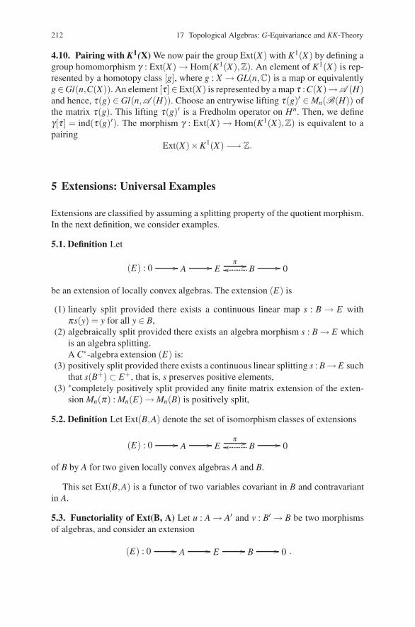
212 17 Topological Algebras: G-Equivariance and KK-Theory
4.10. Pairing with K111(X) We now pair the group Ext(X) with K1(X) by defining agroup homomorphism γ : Ext(X) → Hom(K1(X),Z). An element of K1(X) is rep-resented by a homotopy class [g], where g : X → GL(n,C) is a map or equivalentlyg∈Gl(n,C(X)). An element [τ]∈Ext(X) is represented by a map τ :C(X)→A (H)and hence, τ(g) ∈ Gl(n,A (H)). Choose an entrywise lifting τ(g)′ ∈ Mn(B(H)) ofthe matrix τ(g). This lifting τ(g)′ is a Fredholm operator on Hn. Then, we defineγ[τ] = ind(τ(g)′). The morphism γ : Ext(X) → Hom(K1(X),Z) is equivalent to apairing
Ext(X)×K1(X) −→ Z.
5 Extensions: Universal Examples
Extensions are classified by assuming a splitting property of the quotient morphism.In the next definition, we consider examples.
5.1. Definition Let
(E) : 0 �� A �� Eπ �� B�� �� 0
be an extension of locally convex algebras. The extension (E) is
(1) linearly split provided there exists a continuous linear map s : B → E withπs(y) = y for all y ∈ B,
(2) algebraically split provided there exists an algebra morphism s : B → E whichis an algebra splitting.A C∗-algebra extension (E) is:
(3) positively split provided there exists a continuous linear splitting s : B →E suchthat s(B+) ⊂ E+, that is, s preserves positive elements,
(3) ∗completely positively split provided any finite matrix extension of the exten-sion Mn(π) : Mn(E) → Mn(B) is positively split,
5.2. Definition Let Ext(B,A) denote the set of isomorphism classes of extensions
(E) : 0 �� A �� Eπ �� B�� �� 0
of B by A for two given locally convex algebras A and B.
This set Ext(B,A) is a functor of two variables covariant in B and contravariantin A.
5.3. Functoriality of Ext(B, A) Let u : A → A′ and v : B′ → B be two morphismsof algebras, and consider an extension
(E) : 0 �� A �� E �� B �� 0 .
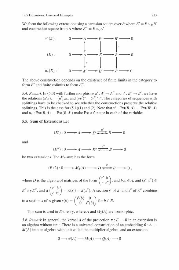
17.5 Extensions: Universal Examples 213
We form the following extension using a cartesian square over B where E ′ = E×B B′and cocartesian square from A where E ′′ = E ∗A A′
v∗(E) : 0 �� A ����
��
E ′ ��
��
B′ ��
v
��
0
(E) : 0 �� A
u
��
�� E ��
��
B ����
��
0
u∗(E) : 0 �� A′ �� E ′ �� B �� 0 .
The above construction depends on the existence of finite limits in the category toform E ′ and finite colimits to form E ′′.
5.4. Remark In (5.3) with further morphisms u′ : A′ → A′′ and v′ : B′′ → B′, we havethe relations (u′u)∗ = (u′)∗u∗ and (vv′)∗ = (v′)∗v∗. The categories of sequences withsplittings have to be checked to see whether the constructions preserve the relativesplittings. This is the case for (5.1)(1) and (2). Note that v∗ : Ext(B,A) → Ext(B′,A)and u∗ : Ext(B,A) → Ext(B,A′) make Ext a functor in each of the variables.
5.5. Sum of Extensions Let
(E ′) : 0 �� A �� E ′ π ′ �� B�� �� 0
and
(E ′′) : 0 �� A �� E ′′ π ′′ �� B�� �� 0
be two extensions. The M2-sum has the form
(E/2) : 0 �� M2(A) �� Dπ �� B�� �� 0 ,
where D is the algebra of matrices of the form
(x′ bc x′′
), and b,c ∈ A, and (x′,x′′) ∈
E ′ ×B E ′′, and π(
x′ bc x′′
)= π(x′) = π(x′′). A section s′ of π ′ and s′′ of π ′′ combine
to a section s of π given s(b) =(
s′(b) 00 s′′(b)
)for b ∈ B.
This sum is used in E-theory, where A and M2(A) are isomorphic.
5.6. Remark In general, the kernel A of the projection π : E → B in an extension isan algebra without unit. There is a universal construction of an embedding θ : A →M(A) into an algebra with unit called the multiplier algebra, and an extension
0 −→ θ (A) −→ M(A) −→ Q(A) −→ 0
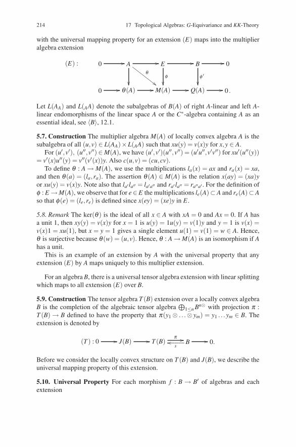
214 17 Topological Algebras: G-Equivariance and KK-Theory
with the universal mapping property for an extension (E) maps into the multiplieralgebra extension
(E) : 0 �� A ��
��
θ
��
E ��
φ��
B ��
φ ′
��
0
0 �� θ (A) �� M(A) �� Q(A) �� 0 .
Let L(AA) and L(AA) denote the subalgebras of B(A) of right A-linear and left A-linear endomorphisms of the linear space A or the C∗-algebra containing A as anessential ideal, see 〈B〉, 12.1.
5.7. Construction The multiplier algebra M(A) of locally convex algebra A is thesubalgebra of all (u,v) ∈ L(AA)×L(AA) such that xu(y) = v(x)y for x,y ∈ A.
For (u′,v′), (u′′,v′′)∈ M(A), we have (u′,v′)(u′′,v′′) = (u′u′′,v′v′′) for xu′(u′′(y))= v′(x)u′′(y) = v′′(v′(x))y. Also c(u,v) = (cu,cv).
To define θ : A → M(A), we use the multiplications la(x) = ax and ra(x) = xa,and then θ (a) = (la,ra). The assertion θ (A) ∈ M(A) is the relation x(ay) = (xa)yor xu(y) = v(x)y. Note also that la′ la′′ = la′a′′ and ra′ la′′ = ra′′a′ . For the definition ofφ : E →M(A), we observe that for e∈E the multiplications le(A)⊂ A and re(A)⊂Aso that φ(e) = (le,re) is defined since x(ey) = (xe)y in E .
5.8. Remark The ker(θ ) is the ideal of all x ∈ A with xA = 0 and Ax = 0. If A hasa unit 1, then xy(y) = v(x)y for x = 1 is u(y) = 1u(y) = v(1)y and y = 1 is v(x) =v(x)1 = xu(1), but x = y = 1 gives a single element u(1) = v(1) = w ∈ A. Hence,θ is surjective because θ (w) = (u,v). Hence, θ : A → M(A) is an isomorphism if Ahas a unit.
This is an example of an extension by A with the universal property that anyextension (E) by A maps uniquely to this multiplier extension.
For an algebra B, there is a universal tensor algebra extension with linear splittingwhich maps to all extension (E) over B.
5.9. Construction The tensor algebra T (B) extension over a locally convex algebraB is the completion of the algebraic tensor algebra
⊕1≤n Bn⊗ with projection π :
T (B) → B defined to have the property that π(y1 ⊗ . . .⊗ ym) = y1 . . .ym ∈ B. Theextension is denoted by
(T ) : 0 �� J(B) �� T (B)π �� Bs
�� �� 0.
Before we consider the locally convex structure on T (B) and J(B), we describe theuniversal mapping property of this extension.
5.10. Universal Property For each morphism f : B → B′ of algebras and eachextension
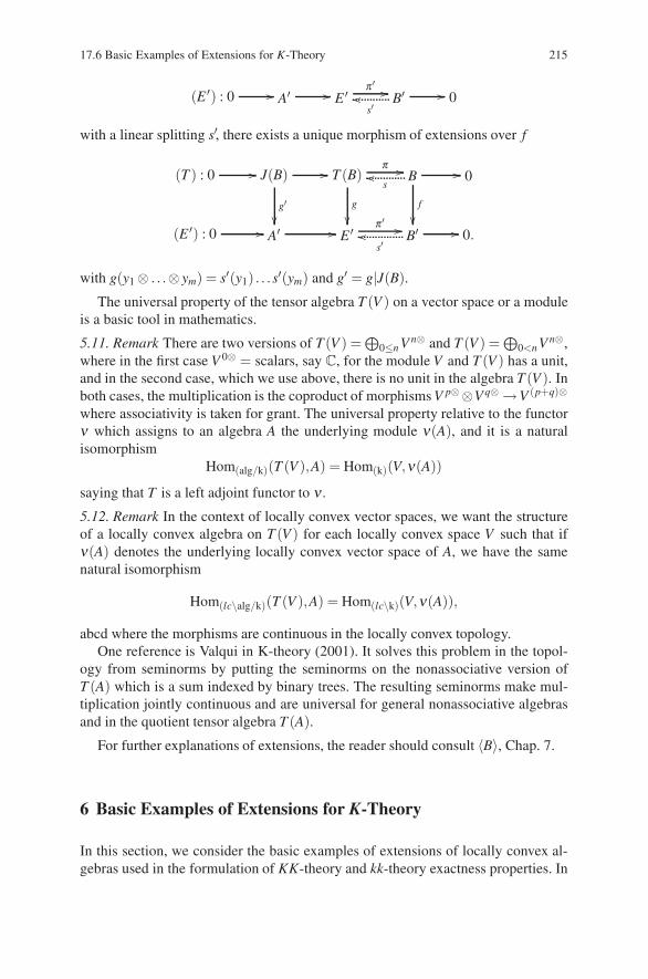
17.6 Basic Examples of Extensions for K-Theory 215
(E ′) : 0 �� A′ �� E ′ π ′ ��B′
s′�� �� 0
with a linear splitting s′, there exists a unique morphism of extensions over f
(T ) : 0 �� J(B) ��
g′
��
T (B)
g
��
π �� B
f
��
s�� �� 0
(E ′) : 0 �� A′ �� E ′ π ′ ��B′
s′�� �� 0.
with g(y1 ⊗ . . .⊗ ym) = s′(y1) . . . s′(ym) and g′ = g|J(B).
The universal property of the tensor algebra T (V ) on a vector space or a moduleis a basic tool in mathematics.
5.11. Remark There are two versions of T (V ) =⊕
0≤n V n⊗ and T (V ) =⊕
0<nV n⊗,where in the first case V 0⊗ = scalars, say C, for the module V and T (V ) has a unit,and in the second case, which we use above, there is no unit in the algebra T (V ). Inboth cases, the multiplication is the coproduct of morphisms V p⊗⊗V q⊗ →V (p+q)⊗where associativity is taken for grant. The universal property relative to the functorν which assigns to an algebra A the underlying module ν(A), and it is a naturalisomorphism
Hom(alg/k)(T (V ),A) = Hom(k)(V,ν(A))
saying that T is a left adjoint functor to ν .
5.12. Remark In the context of locally convex vector spaces, we want the structureof a locally convex algebra on T (V ) for each locally convex space V such that ifν(A) denotes the underlying locally convex vector space of A, we have the samenatural isomorphism
Hom(lc\alg/k)(T (V ),A) = Hom(lc\k)(V,ν(A)),
abcd where the morphisms are continuous in the locally convex topology.One reference is Valqui in K-theory (2001). It solves this problem in the topol-
ogy from seminorms by putting the seminorms on the nonassociative version ofT (A) which is a sum indexed by binary trees. The resulting seminorms make mul-tiplication jointly continuous and are universal for general nonassociative algebrasand in the quotient tensor algebra T (A).
For further explanations of extensions, the reader should consult 〈B〉, Chap. 7.
6 Basic Examples of Extensions for K-Theory
In this section, we consider the basic examples of extensions of locally convex al-gebras used in the formulation of KK-theory and kk-theory exactness properties. In
216 17 Topological Algebras: G-Equivariance and KK-Theory
many cases, there is a continuous and smooth version of the extension. See 〈B〉, 8.2,for these definitions in the case of C∗-algebras.
6.1. Definition Let B be a locally convex algebra. The continuous cone C(B) andsuspension S(B) extension is
0 −→ S(B) = B(0,1) −→C(B) = B(0,1]q−→ B −→ 0,
where the projection q( f ) = f (1). The smooth cone C∞(B) and smooth suspensionS∞(B) extension is
0 −→ S∞(B) = B∞(0,1) −→C∞(B) = B∞(0,1]q−→ B −→ 0.
6.2. Remark There is a continuous homotopy ht : C(B) → C(B) and a smooth ho-motopy ht : C∞(B) → C∞(B) both given by the formula ht( f )(s) = f (ts) form thebase point to the identity h1( f ) = f , or in other words, the cones are contractible inthe continuous and smooth senses.
6.3. Definition Let u : A → B be a morphism of algebras. The mapping cylinder ofu is the fibre product Z(u) = A×B B[0,1], and the mapping cone of u is the fibreproduct C(u) = A×B B(0,1], where q : B[0,1]→ B and q : B(0,1] → B are given byq( f ) = f (1). We have the smooth versions the mapping cylinder and mapping coneZ∞(u) = A×B B∞[0,1] and C∞(u) = A×B B∞(0,1] also.
6.4. Homotopy Properties of the Mapping Cylinder We have two morphisms oflocally convex algebras ξ = ξ (u) : A → Z(u) given by ξ (x) = x, f (a)(1) and η =η(u) : Z(u) → A given by η(x, f ) = x. The composite ηξ = idA and the compositeξη(x, f ) = x is homotopic to idZ(u) with ks(x, f )(t) = (x, f ((1−s)t +s), where k0 =idZ(u) and k1 = ξη . The smooth version of the relation between A and Z∞(u) holdsby analogy where the homotopy ks is a smooth homotopy.
6.5. Extensions Defined by the Mapping Cylinder and Cone The projection p :Z(u) → B given by p(x, f ) = f (0) defines a natural extension
0 −→C(u) −→ Z(u)p−→ B −→ 0.
Furthermore, if u has a linear section σ : B → A of u, then p has a linear sectionσ ′(y) = (σ(y),y(t) = y) for all t. Combining (6.4) and (6.5), we have an extensionup to homotopy of special importance
[u] : C(u)a(u)−→ A
u−→ B.
The kernel of the surjective algebra morphism a(u) : C(u) → A is just C(u)/A =S(B), and we have the following basic mapping cone extension for u : A → B.
0 −→ S(B)b(u)−→C(u)
a(u)−→ A −→ 0.
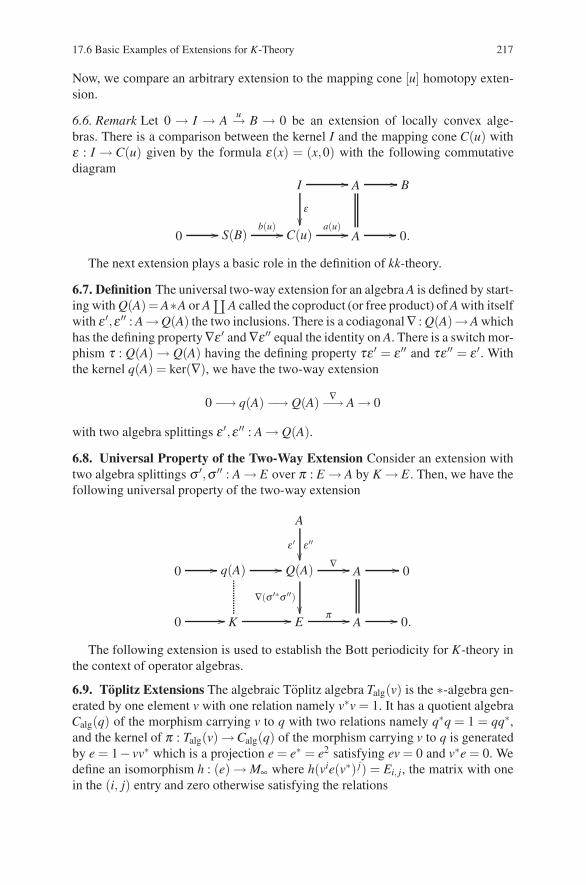
17.6 Basic Examples of Extensions for K-Theory 217
Now, we compare an arbitrary extension to the mapping cone [u] homotopy exten-sion.
6.6. Remark Let 0 → I → Au→ B → 0 be an extension of locally convex alge-
bras. There is a comparison between the kernel I and the mapping cone C(u) withε : I → C(u) given by the formula ε(x) = (x,0) with the following commutativediagram
I ��
�
A �� B
0 �� S(B)b(u) �� C(u)
a(u) �� A �� 0.
The next extension plays a basic role in the definition of kk-theory.
6.7. Definition The universal two-way extension for an algebra A is defined by start-ing with Q(A)= A∗A or A
∐A called the coproduct (or free product) of A with itself
with ε ′,ε ′′ : A→Q(A) the two inclusions. There is a codiagonal∇ : Q(A)→A whichhas the defining property∇ε ′ and∇ε ′′ equal the identity on A. There is a switch mor-phism τ : Q(A) → Q(A) having the defining property τε ′ = ε ′′ and τε ′′ = ε ′. Withthe kernel q(A) = ker(∇), we have the two-way extension
0 −→ q(A) −→ Q(A) ∇−→ A → 0
with two algebra splittings ε ′,ε ′′ : A → Q(A).
6.8. Universal Property of the Two-Way Extension Consider an extension withtwo algebra splittings σ ′,σ ′′ : A → E over π : E → A by K → E . Then, we have thefollowing universal property of the two-way extension
A
ε ′ ε ′′��
0 �� q(A) �� Q(A)
∇(σ ′∗σ ′′)��
∇ �� A �� 0
0 �� K �� Eπ �� A �� 0.
The following extension is used to establish the Bott periodicity for K-theory inthe context of operator algebras.
6.9. Toplitz Extensions The algebraic Toplitz algebra Talg(v) is the ∗-algebra gen-erated by one element v with one relation namely v∗v = 1. It has a quotient algebraCalg(q) of the morphism carrying v to q with two relations namely q∗q = 1 = qq∗,and the kernel of π : Talg(v) →Calg(q) of the morphism carrying v to q is generatedby e = 1− vv∗ which is a projection e = e∗ = e2 satisfying ev = 0 and v∗e = 0. Wedefine an isomorphism h : (e) → M∞ where h(vie(v∗) j) = Ei, j, the matrix with onein the (i, j) entry and zero otherwise satisfying the relations
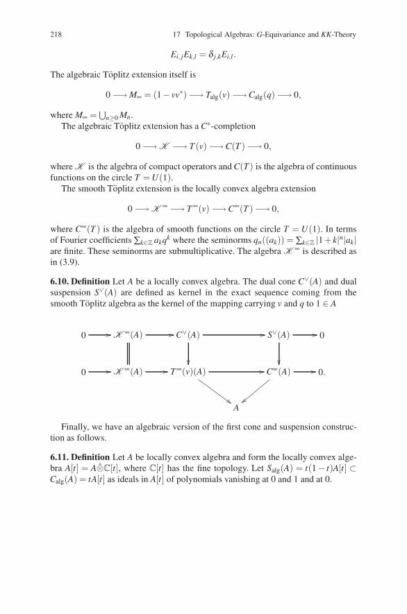
218 17 Topological Algebras: G-Equivariance and KK-Theory
Ei, jEk,l = δ j,kEi,l .
The algebraic Toplitz extension itself is
0 −→ M∞ = (1− vv∗) −→ Talg(v) −→Calg(q) −→ 0,
where M∞ =⋃
n≥0 Mn.The algebraic Toplitz extension has a C∗-completion
0 −→ K −→ T (v) −→C(T ) −→ 0,
where K is the algebra of compact operators and C(T ) is the algebra of continuousfunctions on the circle T = U(1).
The smooth Toplitz extension is the locally convex algebra extension
0 −→ K ∞ −→ T∞(v) −→C∞(T ) −→ 0,
where C∞(T ) is the algebra of smooth functions on the circle T = U(1). In termsof Fourier coefficients ∑k∈Z akqk where the seminorms qn((ak)) = ∑k∈Z |1+ k|n|ak|are finite. These seminorms are submultiplicative. The algebra K ∞ is described asin (3.9).
6.10. Definition Let A be a locally convex algebra. The dual cone C∨(A) and dualsuspension S∨(A) are defined as kernel in the exact sequence coming from thesmooth Toplitz algebra as the kernel of the mapping carrying v and q to 1 ∈ A
0 �� K ∞(A) �� C∨(A)
��
�� S∨(A)
��
�� 0
0 �� K ∞(A) �� T∞(v)(A)
�����
����
���� C∞(A)
����������
�� 0.
A
Finally, we have an algebraic version of the first cone and suspension construc-tion as follows.
6.11. Definition Let A be locally convex algebra and form the locally convex alge-bra A[t] = A⊗C[t], where C[t] has the fine topology. Let Salg(A) = t(1− t)A[t] ⊂Calg(A) = tA[t] as ideals in A[t] of polynomials vanishing at 0 and 1 and at 0.
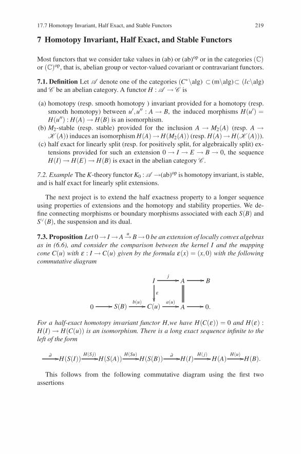
17.7 Homotopy Invariant, Half Exact, and Stable Functors 219
7 Homotopy Invariant, Half Exact, and Stable Functors
Most functors that we consider take values in (ab) or (ab)op or in the categories (C)or (C)op, that is, abelian group or vector-valued covariant or contravariant functors.
7.1. Definition Let A denote one of the categories (C∗\alg) ⊂ (m\alg)⊂ (lc\alg)and C be an abelian category. A functor H : A → C is
(a) homotopy (resp. smooth homotopy ) invariant provided for a homotopy (resp.smooth homotopy) between u′,u′′ : A → B, the induced morphisms H(u′) =H(u′′) : H(A) → H(B) is an isomorphism.
(b) M2-stable (resp. stable) provided for the inclusion A → M2(A) (resp. A →K (A)) induces an isomorphism H(A)→H(M2(A)) (resp. H(A)→H(K (A))).
(c) half exact for linearly split (resp. for positively split, for algebraically split) ex-tensions provided for such an extension 0 → I → E → B → 0, the sequenceH(I) → H(E) → H(B) is exact in the abelian category C .
7.2. Example The K-theory functor K0 : A →(ab)op is homotopy invariant, is stable,and is half exact for linearly split extensions.
The next project is to extend the half exactness property to a longer sequenceusing properties of extensions and the homotopy and stability properties. We de-fine connecting morphisms or boundary morphisms associated with each S(B) andS∨(B), the suspension and its dual.
7.3. Proposition Let 0→ I →Au→B→ 0 be an extension of locally convex algebras
as in (6.6), and consider the comparison between the kernel I and the mappingcone C(u) with ε : I → C(u) given by the formula ε(x) = (x,0) with the followingcommutative diagram
Ij ��
�
A �� B
0 �� S(B)b(u) �� C(u)
a(u) �� A �� 0.
For a half-exact homotopy invariant functor H,we have H(C(ε)) = 0 and H(ε) :H(I) → H(C(u)) is an isomorphism. There is a long exact sequence infinite to theleft of the form
∂ ��H(S(I))H(S j) ��H(S(A))
H(Su) ��H(S(B)) ∂ ��H(I)H( j) �� H(A)
H(u) ��H(B).
This follows from the following commutative diagram using the first twoassertions
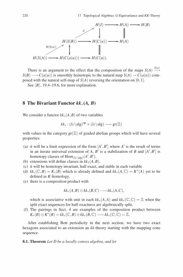
220 17 Topological Algebras: G-Equivariance and KK-Theory
H(I)
��
�� H(A) �� H(B)
H(S(B))��
��
��
∂�������������
H(C(u)) �� H(A)
H(S(A)) ��
H(S(u))������������
H(C(a(u))) �� H(C(u)).
There is an argument to the effect that the composition of the maps S(A)S(u)−→
S(B) −→C(a(u)) is smoothly homotopic to the natural map S(A) →C(a(u)) com-posed with the natural self-map of S(A) reversing the orientation on [0,1].
See 〈B〉, 19.4–19.6, for more explanation.
8 The Bivariant Functor kk∗(A, B)
We consider a functor kk∗(A,B) of two variables
kk∗ : (lc\alg)op × (lc\alg) −→ gr(Z)
with values in the category gr(Z) of graded abelian groups which will have severalproperties:
(a) it will be a limit expression of the form [A′,B′] where A′ is the result of termsin an iterate universal extension of A, B′ is a stabilization of B and [A′,B′] ishomotopy classes of Hom(lc\alg)(A′,B′),
(b) extensions will define classes in kk1(A,B),(c) it will be homotopy invariant, half exact, and stable in each variable(d) kk∗(C,B) = K∗(B) which is already defined and kk∗(A,C) = K∗(A) yet to be
defined as K-homology,(e) there is a composition product with
kk∗(A,B)⊗ kk∗(B,C) −→ kk∗(A,C),
which is associative with unit in each kk∗(A,A) and kk∗(C,C) = Z when thesplit exact sequences for half-exactness are algebraically split,
(f) The pairings in Sect. 4 are examples of the composition product betweenK∗(B)⊗K∗(B) = kk∗(C,B)⊗ kk∗(B,C) −→ kk∗(C,C) = Z.
After establishing Bott periodicity in the next section, we have two exacthexagons associated to an extension an kk-theory starting with the mapping conesequence.
8.1. Theorem Let D be a locally convex algebra, and let
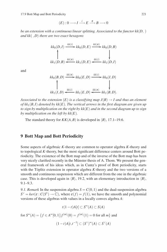
17.9 Bott Map and Bott Periodicity 221
(E) : 0 −→ Ii−→ E
π−→ B −→ 0
be an extension with a continuous linear splitting. Associated to the functor kk(D, )and kk( ,D) there are two exact hexagons
kk0(D, I)kk(i) �� kk0(D,E)
kk(π) �� kk0(D,B)
��kk1(D,B)
��
kk1(D,E)kk(π)�� kk1(D, I)
kk(i)��
and
kk0(B,D)kk(π) �� kk0(E,D)
kk(i) �� kk0(I,D)
��kk1(I,D)
��
kk1(E,D)kk(i)�� kk1(B,D).
kk(π)��
Associated to the extension (E) is a classifying map J(B) → I and thus an elementof kk1(B, I) denoted by kk(E). The vertical arrows in the first diagram are given upto sign by multiplication on the right by kk(E) and in the second diagram up to signby multiplication on the left by kk(E).
The standard theory for KK(A,B) is developed in 〈B〉, 17.1–19.6.
9 Bott Map and Bott Periodicity
Some aspects of algebraic K-theory are common to operator algebra K-theory andto topological K-theory, but the most significant difference centers around Bott pe-riodicity. The existence of the Bott map and of the inverse of the Bott map has beenvery nicely clarified recently in the Munster thesis of A. Thom. We present the gen-eral framework of his ideas which, as in Cuntz’s proof of Bott periodicity, startswith the Toplitz extension in operator algebra K-theory and the two versions of asmooth and continuous suspension which are different from the one in the algebraiccase. This is developed again in 〈B〉, 19.2, with an elementary introduction in 〈B〉,9.1–9.3.
9.1. Remark In the suspension algebra S = C(0,1) and the dual-suspension algebraS∨ = ker(ε : C(S1) → C), where ε( f ) = f (1), we have the smooth and polynomialversions of these algebras with values in a locally convex algebra A:
t(1− t)A[t]⊂ S∞(A) ⊂ S(A)
for S∞(A) = { f ∈ A∞[0,1]| f (m)(0) = f (m)(1) = 0 for all m} and
(1− t)A[t,t−1] ⊂ (S∨)∞(A) ⊂ S∨(A)
222 17 Topological Algebras: G-Equivariance and KK-Theory
for (S∨)∞(A) = { f ∈ A∞(S1)| f (m)(1) = 0 for all m}. The two continuous and thetwo smooth versions are isomorphic by change of variable g ∈ S∨(A) is mappedto f (t) = g(e2π it), f ∈ S(A). On the other hand, the algebraic subalgebras do notcorrespond at all since there is no algebraic exponential map.
9.2. Definition Let kk∗ be a kk-theory for which the dual mapping cone is zero.Then, there is an excision for the reduced Toplitz extension
K (A) −→C∨(A) −→ S∨(A)
The unstable inverse Bott morphism ψ : SS∨(A) → K (A) is the image of theidentity idS∨(A) under the composition of the boundary and the inverse boundarymorphisms
kki(S∨(A),S∨(A)) −→ kki−1(S∨(A),K (A)) −→ kki(S(S∨(A)),K (A)).
Again K (A) is the compact operator stabilization of A.
9.3. Definition An inverse Bott morphism φ : S(S∨(A)) → A is a morphism whichcomposed with the natural stabilization A → K (A) gives the unstable inverse Bottmorphism.
9.4. Proposition Let kk∗ be a K -stable theory with extension for the Toplitz ex-tension. Then, there exists a unique inverse Bott morphism which is the image ofthe unstable inverse Bott morphism ψ : S(S∨(A)) → K (A) under the inverse of thenatural stabilization isomorphism
kki(S∨(S(A)),K (A)) → kki(S∨(S(A)),A).
For the Bott morphism itself, we have similar considerations with the followingalgebra morphism induced by an inclusion
j : S3 = S(H) →U(2) ⊂ M2(C),
where j(w) is the left multiplication of w on the quaternions H and hence on C2 as
a unitary matrix. We can view j as an element in M2(C0(S3)).
9.5. Definition The Bott algebra morphism C0(S1) → M2(C0(S3)) is the uniquemorphism of C∗-algebras which carries q = e2π iθ to the map j ∈ M2(C0(S3)) and bytaking the tensor product with a locally convex algebra the corresponding morphism
θ : S∨(A) → M2((S∨)3(A))
In the C∗-algebra case, the functors S and S∨ are identified.
9.6. Definition A Bott morphism S∨(A) → (S∨)3(A) is any morphism whose com-position with the stabilization morphism
(S∨)3(A) → M2((S∨)3(A))
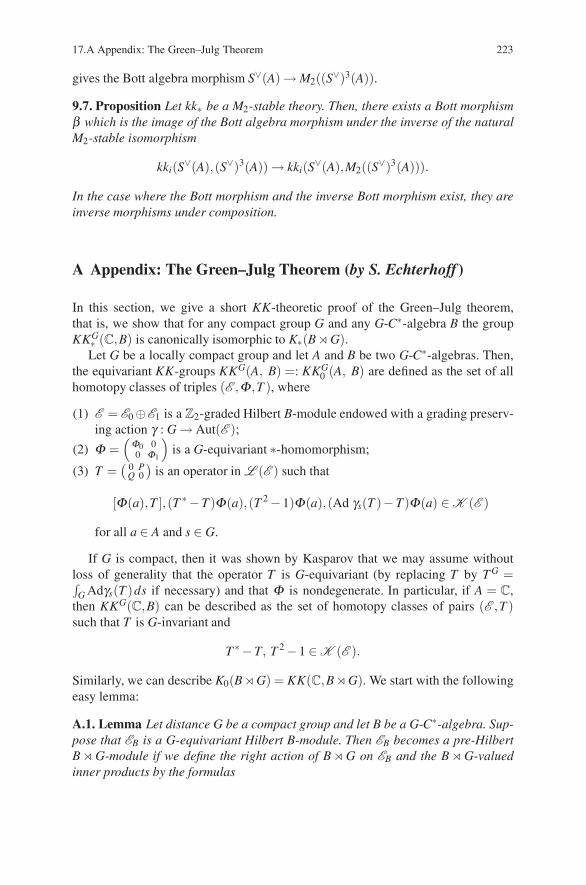
17.A Appendix: The Green–Julg Theorem 223
gives the Bott algebra morphism S∨(A) → M2((S∨)3(A)).
9.7. Proposition Let kk∗ be a M2-stable theory. Then, there exists a Bott morphismβ which is the image of the Bott algebra morphism under the inverse of the naturalM2-stable isomorphism
kki(S∨(A),(S∨)3(A)) → kki(S∨(A),M2((S∨)3(A))).
In the case where the Bott morphism and the inverse Bott morphism exist, they areinverse morphisms under composition.
A Appendix: The Green–Julg Theorem (by S. Echterhoff )
In this section, we give a short KK-theoretic proof of the Green–Julg theorem,that is, we show that for any compact group G and any G-C∗-algebra B the groupKKG∗ (C,B) is canonically isomorphic to K∗(B � G).
Let G be a locally compact group and let A and B be two G-C∗-algebras. Then,the equivariant KK-groups KKG(A, B) =: KKG
0 (A, B) are defined as the set of allhomotopy classes of triples (E ,Φ,T ), where
(1) E = E0 ⊕E1 is a Z2-graded Hilbert B-module endowed with a grading preserv-ing action γ : G → Aut(E );
(2) Φ =(Φ0 00 Φ1
)is a G-equivariant ∗-homomorphism;
(3) T =( 0 P
Q 0
)is an operator in L (E ) such that
[Φ(a),T ],(T ∗ −T )Φ(a),(T 2 −1)Φ(a),(Ad γs(T )−T)Φ(a) ∈ K (E )
for all a ∈ A and s ∈ G.
If G is compact, then it was shown by Kasparov that we may assume withoutloss of generality that the operator T is G-equivariant (by replacing T by T G =∫
G Adγs(T )ds if necessary) and that Φ is nondegenerate. In particular, if A = C,then KKG(C,B) can be described as the set of homotopy classes of pairs (E ,T )such that T is G-invariant and
T ∗ −T, T 2 −1 ∈ K (E ).
Similarly, we can describe K0(B� G) = KK(C,B� G). We start with the followingeasy lemma:
A.1. Lemma Let distance G be a compact group and let B be a G-C∗-algebra. Sup-pose that EB is a G-equivariant Hilbert B-module. Then EB becomes a pre-HilbertB � G-module if we define the right action of B � G on EB and the B � G-valuedinner products by the formulas
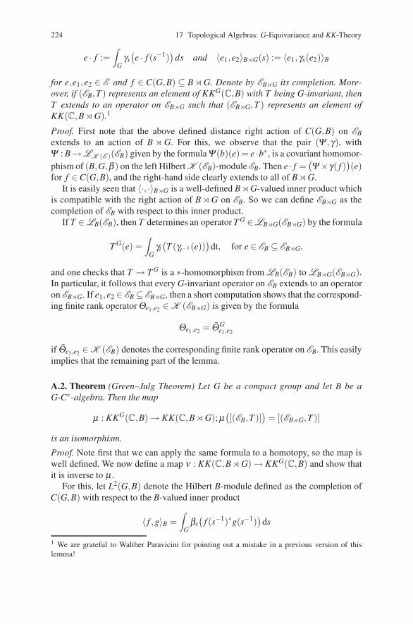
224 17 Topological Algebras: G-Equivariance and KK-Theory
e · f :=∫
Gγs(e · f (s−1)
)ds and 〈e1,e2〉B�G(s) := 〈e1,γs(e2)〉B
for e,e1,e2 ∈ E and f ∈ C(G,B) ⊆ B � G. Denote by EB�G its completion. More-over, if (EB,T ) represents an element of KKG(C,B) with T being G-invariant, thenT extends to an operator on EB�G such that (EB�G,T ) represents an element ofKK(C,B � G).1
Proof. First note that the above defined distance right action of C(G,B) on EB
extends to an action of B � G. For this, we observe that the pair (Ψ ,γ), withΨ : B→LK (E )(EB) given by the formulaΨ(b)(e) = e ·b∗, is a covariant homomor-phism of (B,G,β ) on the left Hilbert K (EB)-module EB. Then e · f =
(Ψ×γ( f )
)(e)
for f ∈C(G,B), and the right-hand side clearly extends to all of B � G.It is easily seen that 〈·, ·〉B�G is a well-defined B� G-valued inner product which
is compatible with the right action of B � G on EB. So we can define EB�G as thecompletion of EB with respect to this inner product.
If T ∈LB(EB), then T determines an operator T G ∈LB�G(EB�G) by the formula
T G(e) =∫
Gγt(T (γt−1(e))
)dt, for e ∈ EB ⊆ EB�G,
and one checks that T → T G is a ∗-homomorphism from LB(EB) to LB�G(EB�G).In particular, it follows that every G-invariant operator on EB extends to an operatoron EB�G. If e1,e2 ∈ EB ⊆ EB�G, then a short computation shows that the correspond-ing finite rank operatorΘe1,e2 ∈ K (EB�G) is given by the formula
Θe1,e2 = ΘGe1,e2
if Θe1,e2 ∈ K (EB) denotes the corresponding finite rank operator on EB. This easilyimplies that the remaining part of the lemma.
A.2. Theorem (Green–Julg Theorem) Let G be a compact group and let B be aG-C∗-algebra. Then the map
μ : KKG(C,B) → KK(C,B � G);μ([(EB,T )]
)= [(EB�G,T )]
is an isomorphism.
Proof. Note first that we can apply the same formula to a homotopy, so the map iswell defined. We now define a map ν : KK(C,B � G) → KKG(C,B) and show thatit is inverse to μ .
For this, let L2(G,B) denote the Hilbert B-module defined as the completion ofC(G,B) with respect to the B-valued inner product
〈 f ,g〉B =∫
Gβs(
f (s−1)∗g(s−1))
ds
1 We are grateful to Walther Paravicini for pointing out a mistake in a previous version of thislemma!
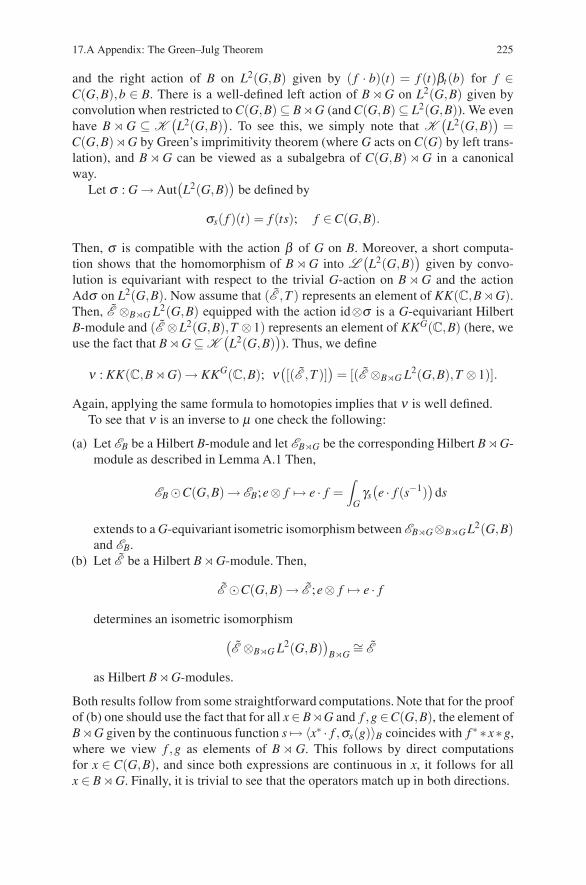
17.A Appendix: The Green–Julg Theorem 225
and the right action of B on L2(G,B) given by ( f · b)(t) = f (t)βt(b) for f ∈C(G,B),b ∈ B. There is a well-defined left action of B � G on L2(G,B) given byconvolution when restricted to C(G,B) ⊆ B�G (and C(G,B) ⊆ L2(G,B)). We evenhave B � G ⊆ K
(L2(G,B)
). To see this, we simply note that K
(L2(G,B)
)=
C(G,B)� G by Green’s imprimitivity theorem (where G acts on C(G) by left trans-lation), and B � G can be viewed as a subalgebra of C(G,B) � G in a canonicalway.
Let σ : G → Aut(L2(G,B)
)be defined by
σs( f )(t) = f (ts); f ∈C(G,B).
Then, σ is compatible with the action β of G on B. Moreover, a short computa-tion shows that the homomorphism of B � G into L
(L2(G,B)
)given by convo-
lution is equivariant with respect to the trivial G-action on B � G and the actionAdσ on L2(G,B). Now assume that (E ,T ) represents an element of KK(C,B� G).Then, E ⊗B�G L2(G,B) equipped with the action id⊗σ is a G-equivariant HilbertB-module and (E ⊗L2(G,B),T ⊗1) represents an element of KKG(C,B) (here, weuse the fact that B � G ⊆ K
(L2(G,B)
)). Thus, we define
ν : KK(C,B � G)→ KKG(C,B); ν([(E ,T )]
)= [(E ⊗B�G L2(G,B),T ⊗1)].
Again, applying the same formula to homotopies implies that ν is well defined.To see that ν is an inverse to μ one check the following:
(a) Let EB be a Hilbert B-module and let EB�G be the corresponding Hilbert B� G-module as described in Lemma A.1 Then,
EB %C(G,B) → EB;e⊗ f �→ e · f =∫
Gγs(e · f (s−1)
)ds
extends to a G-equivariant isometric isomorphism between EB�G⊗B�G L2(G,B)and EB.
(b) Let E be a Hilbert B � G-module. Then,
E %C(G,B) → E ;e⊗ f �→ e · f
determines an isometric isomorphism(E ⊗B�G L2(G,B)
)B�G
∼= E
as Hilbert B � G-modules.
Both results follow from some straightforward computations. Note that for the proofof (b) one should use the fact that for all x∈ B�G and f ,g ∈C(G,B), the element ofB�G given by the continuous function s �→ 〈x∗ · f ,σs(g)〉B coincides with f ∗ ∗x∗g,where we view f ,g as elements of B � G. This follows by direct computationsfor x ∈ C(G,B), and since both expressions are continuous in x, it follows for allx ∈ B � G. Finally, it is trivial to see that the operators match up in both directions.
226 17 Topological Algebras: G-Equivariance and KK-Theory
A.3. Remark We should remark, that the above Theorem A.2 is a special case ofa more general result for crossed products by proper actions due to Kasparovand Skandalis (Theorem 5.4). There also exist important generalizations to propergroupoids by Tu (2005) (Proposition 6.25) and Paravicini (2007), where the latterprovides a version within Lafforgue’s Banach KK-theory. For the original proof ofthe Green–Julg theorem for compact groups we refer to Julg (1981).
References
Blackadar, B.: K-Theory for Operator Algebras, 2nd ed. Cambridge University Press, Cambridge(1998)
Cuntz, J., Meyer, R., Rosenberg, J.: Topological and Bivariant K-Theory. Birkhauser, Basel (2007)Valqui, C.: Universal extension and excision for topological algebras. K-Theory 22: 145–160
(2001)Julg, P.: K-thorie equivariante et produits croises. C. R. Acad. Sci. Paris Ser. I Math. 292(13):
629–632 (1981)Kasparov, G., Skandalis, G.: Groups acting properly on “bolic” spaces and the Novikov conjecture.
Annals of Math. 158: 165–206 (2003)Tu, J.-L.: La conjecture de Novikov pour les fouilletages hyperboliques. K-Theory 16(2) 129–184
(1999)Paravicini, W.: Ph.D. Dissertation. Munster, “KK-Theory for Banach Algebras and Proper
Groupoids” (2006)
Part IVAlgebra Bundles: Twisted K-Theory
In Part I, we introduced the generalities on bundles over a space. In Chaps. 1,2, and5, we described them as a family of spaces fibred over a base space. In Chap. 3, wesaw that bundles could be described by other data using modules over a functionalgebra, and then in Chap. 4, the stability phenomenon of K-theory was introduced.In Part II, topological twisting coming in principal bundles and vector bundles isstudied from the point of view of homotopy theory and of cohomology where clas-sifying spaces and characteristic classes play a role, respectively.
In Part IV, we consider higher order twisting on vector bundles in terms of al-gebra bundles. The first such example is matrix algebra bundles clearly related tovector bundles and also operator algebra bundles with fibre B(H), the bounded op-erators on separable Hilbert space H. Matrix algebra is just the case when H is finitedimension and so B(H) = Mn(C).
Associated to an operator bundle A over a space X is a characteristic classα(A) ∈ H3(X ,Z) introduced by Dixmier and Douady which completely classifiesthe algebra bundle in the same way that the first Chern class c1(L) completely clas-sifies line bundles up to all isomorphisms.
The next step is to consider the Fredholm elements in operator algebra bundleswhen the algebra bundle is trivial, this leads to ordinary K-theory, and in general,this is our first approach to twisted K-theory. Ordinary K-theory can be defined ashomotopy classes of maps into Fredholm operators, and twisted K-theory can bedefined as homotopy classes of cross sections of fibre bundles associated to a givenalgebra bundle with fibre, the Fredholm operators. In particular, the twisted K-theorygroups over X depend on an extra object, an operator (algebra) bundle A and its extraparameter the characteristic class α = α(A) ∈ H3(X ,Z). The realization as twistedK-theory and the term itself is due to Rosenberg (1989).
Chapter 18Isomorphism Classification of OperatorAlgebra Bundles
We consider algebra bundles where the fibre is an algebra of bounded operators ina separable Hilbert space H over the complex numbers. If the Hilbert space H isinfinite dimensional, the algebra is either B the algebra of all bounded operators onH or K the algebra of compact operators in B, and we refer to these bundles asoperator algebra bundles. If the Hilbert space H is finite dimensional, the algebrais just the n2-dimensional matrix algebra Mn(C), and we refer to these bundles asmatrix algebra bundles.
As with vector bundles, these bundles have a fibre bundle interpretation so thatthe structure is governed by a related principal bundle over the automorphism groupof the algebra. The classification of these algebra bundles is just a homotopy analysisof this automorphism group of the algebra.
For an algebra bundle A over X , we associate a characteristic classα(A) ∈ H3(X ,Z) using the homotopy classification of principal bundles. With thischaracteristic class, we have an isomorphism classification of infinite dimensionaloperator algebra bundles over X which is contained in the next two statements:
(1) Two operator algebra bundles A′ and A′′ over X are isomorphic if and only ifα(A′) = α(A′′) ∈ H3(X ,Z).
(2) Every element of H3(X ,Z) is of the form α(A) for some operator algebra bun-dle over X .
There are two corresponding statements for the first Chern class c1(L) of complexline bundles over X .
The three-dimensionalcharacteristic class was discovered as a Cech cohomologyclass by Grothendieck in the finite-dimensional case and by Dixmier and Douadyin the general case. The homotopy version was pointed out by Rosenberg. Operatoralgebra bundles were treated by Fell (1959) and by Dixmier and Douady (1963),where the Cech H3 classification is given.
The classification of operator algebra bundles is very simple for the same rea-son that the only infinite-dimensional Hilbert bundles are the trivial ones. This isthe Kuiper theorem, see 22(2.1), which says that the automorphism group of an
D. Husemoller et al.: Isomorphism Classification of Operator Algebra Bundles, Lect. Notes Phys. 726, 229–239 (2008)DOI 10.1007/978-3-540-74956-1 19 © Springer-Verlag Berlin Heidelberg 2008
230 18 Isomorphism Classification of Operator Algebra Bundles
infinite-dimensional separable Hilbert space is contractible, and in particular, thenits classifying space is contractible also.
Matrix algebra bundles were considered by Serre and Grothendieck, and the sub-ject was treated as an introduction to Grothendieck’s three Seminar Bourbaki ex-poses which appeared also in the collection Dix Exposes. The same homotopy anal-ysis used for operator algebra bundles applies to Mn-matrix algebra bundles A overX . The result is a characteristic class αn(A)∈ nH3(X ,Z) with values in the subgroupof a ∈ H3(X ,Z) with n ·a = 0, that is, n-torsion elements. Grothendieck gave a de-scription of this class using sheaf theory. In the finite-dimensional case, we do notobtain an isomorphism classification theory as with operator algebras, for all matrixalgebra bundles of the form End(E) where E is a vector bundle have the propertythat αn(End(E)) = 0. To each matrix bundle A′, there is an operator algebra bundleA with α(A) = α(A′), and A is unique up to isomorphism. This bundle A associatedto A′ can be constructed by tensoring the trivial operator bundle A with A′.
This leads to the following refinement of the classification theorem
(3) An operator algebra bundle A is of the form of a Mn-matrix algebra bundletensor with the trivial operator algebra bundle if and only if α(A) is an n-torsionelement in H3(X ,Z).
Returning to line bundles, we recall the related result which says that a line bun-dle L over X is flat if and only if c1(L) is a torsion element in H2(X ,Z).
For the convenience of the reader, certain features of vector bundle theory whichare treated in Chaps. 2, 5 and 7 are repeated in a parallel manner to algebra bundletheory.
1 Vector Bundles and Algebra Bundles
1.1. Definition A vector bundle E over a space X is a bundle p : E → X togetherwith bundle morphisms E ×X E → E and C×E → E over X such that these opera-tions make each fibre into a vector space over C. Moreover, each point has an openneighborhood U such that E|U is isomorphic to the product vector bundle U ×C
n.If all the fibres of E are n-dimensional, then E is called an n-dimensional, vectorbundle.
1.2. Notation Let Vectn(X) denote the isomorphism classes of n-dimensional vec-tor bundles over X . For a map f : X → Y and a vector bundle E over Y , the inducedbundle f ∗(E) has a natural vector bundle structure with morphism f ∗(E) → E overf such that on the fibres it restricts to an isomorphism of vector spaces. Hence,Vectn : (top)op → (set) is a functor from the opposite category of spaces (top) to thecategory of sets (set).
1.3. Definition A matrix algebra bundle A over a space X is a bundle p : A → X to-gether with bundle morphisms A×X A→A and C×A→A such that these operations
18.2 Principal Bundle Description and Classifying Spaces 231
make each fibre into a matrix algebra over C. Moreover, each point has an openneighborhood U such that A|U is isomorphic to the product matrix algebra bundleU ×Mn(C). If all the fibres of A are n by n matrix algebras, then A is called an n byn matrix algebra bundle.
1.4. Notation Let Algn(X) denote the isomorphism classes of n by n matrix alge-bra bundles over X . For a map f : X → Y and a matrix algebra bundle A over Y ,the induced bundle f ∗(A) has a natural matrix algebra bundle structure with mor-phism f ∗(A) → A over f such that the restrictions to the fibres are isomorphisms ofalgebras. Hence, Algn : (top)op → (set) is a functor.
1.5. Definition There is a natural morphism of functors
End : Vectn −→ Algn
which assigns to each vector bundle E the endomorphism matrix algebra bundleEnd(E) = E ⊗E∨ as a vector bundle with multiplication given by using the evalua-tion morphism E∨ ⊗E → X ×C.
This operation commutes with the induced bundle construction so that it definesa morphism of functors. These End(E) are examples of finite-dimensional algebrabundles reflecting the vector bundle structure of E .
1.6. Remark Let H be a separable infinite-dimensional Hilbert space, and let B =B(H) be the algebra of bounded operators on H with the ideal K = K (H) ofcompact operators. As in definition (1.1), we can define Hilbert space vector bun-dles which are locally of the form U ×H, and as in definition (1.3), we can de-fine operator algebra bundles in two ways which are locally of the form U ×B orU ×K .
1.7. Remark In fact, all infinite-dimensional Hilbert space bundles are trivial, andthe reason stems, as we have mentioned before, from the contractibility of the auto-morphism group of the Hilbert space H which is used to glue locally trivial bundlestogether into a global bundle. This follows clearly from the fibre bundle structure ofall the bundles under consideration.
We leave the description of the categories of algebra bundles to the reader.
2 Principal Bundle Description and Classifying Spaces
2.1. Notation For a topological group G and a space X , we denote the set of iso-morphism classes of locally trivial principal G-bundles by PrinG(X). Further, if Yis a left G-space and P is a principal G-bundle, then the associated fibre bundleP[Y ] = P×G Y = P×Y/G, the quotient of P×Y by the relation (x,y), is equivalentto (xs,s−1y) for all s ∈ G.
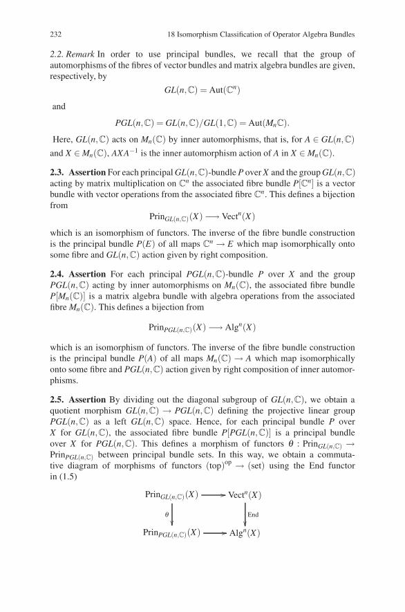
232 18 Isomorphism Classification of Operator Algebra Bundles
2.2. Remark In order to use principal bundles, we recall that the group ofautomorphisms of the fibres of vector bundles and matrix algebra bundles are given,respectively, by
GL(n,C) = Aut(Cn)
and
PGL(n,C) = GL(n,C)/GL(1,C) = Aut(MnC).
Here, GL(n,C) acts on Mn(C) by inner automorphisms, that is, for A ∈ GL(n,C)and X ∈ Mn(C), AXA−1 is the inner automorphism action of A in X ∈ Mn(C).
2.3. Assertion For each principal GL(n,C)-bundle P over X and the group GL(n,C)acting by matrix multiplication on C
n the associated fibre bundle P[Cn] is a vectorbundle with vector operations from the associated fibre C
n. This defines a bijectionfrom
PrinGL(n,C)(X) −→ Vectn(X)
which is an isomorphism of functors. The inverse of the fibre bundle constructionis the principal bundle P(E) of all maps C
n → E which map isomorphically ontosome fibre and GL(n,C) action given by right composition.
2.4. Assertion For each principal PGL(n,C)-bundle P over X and the groupPGL(n,C) acting by inner automorphisms on Mn(C), the associated fibre bundleP[Mn(C)] is a matrix algebra bundle with algebra operations from the associatedfibre Mn(C). This defines a bijection from
PrinPGL(n,C)(X) −→ Algn(X)
which is an isomorphism of functors. The inverse of the fibre bundle constructionis the principal bundle P(A) of all maps Mn(C) → A which map isomorphicallyonto some fibre and PGL(n,C) action given by right composition of inner automor-phisms.
2.5. Assertion By dividing out the diagonal subgroup of GL(n,C), we obtain aquotient morphism GL(n,C) → PGL(n,C) defining the projective linear groupPGL(n,C) as a left GL(n,C) space. Hence, for each principal bundle P overX for GL(n,C), the associated fibre bundle P[PGL(n,C)] is a principal bundleover X for PGL(n,C). This defines a morphism of functors θ : PrinGL(n,C) →PrinPGL(n,C) between principal bundle sets. In this way, we obtain a commuta-tive diagram of morphisms of functors (top)op → (set) using the End functorin (1.5)
PrinGL(n,C)(X) ��
�
Vectn(X)
End��
PrinPGL(n,C)(X) �� Algn(X)
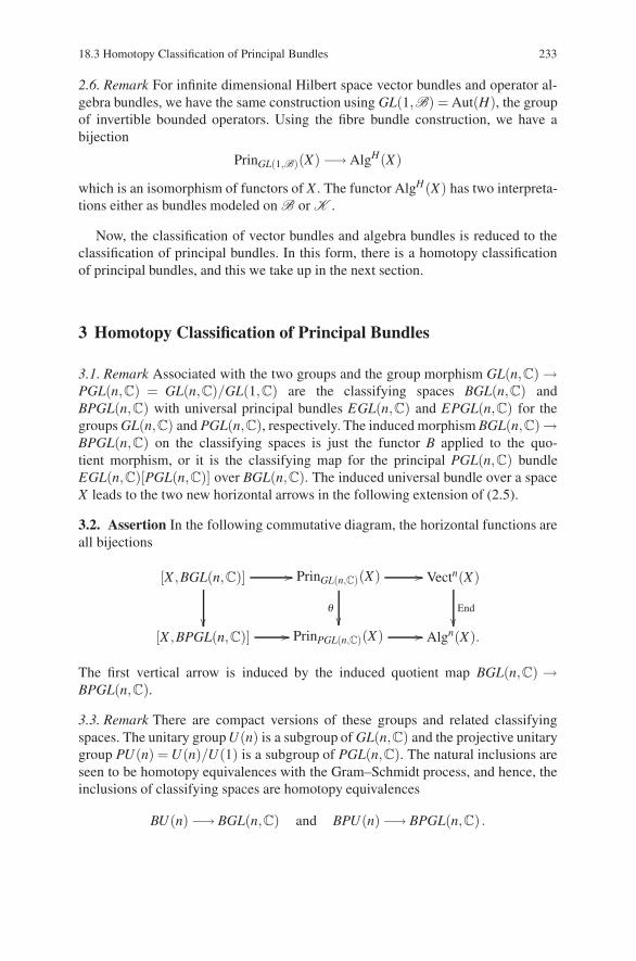
18.3 Homotopy Classification of Principal Bundles 233
2.6. Remark For infinite dimensional Hilbert space vector bundles and operator al-gebra bundles, we have the same construction using GL(1,B) = Aut(H), the groupof invertible bounded operators. Using the fibre bundle construction, we have abijection
PrinGL(1,B)(X) −→ AlgH(X)
which is an isomorphism of functors of X . The functor AlgH(X) has two interpreta-tions either as bundles modeled on B or K .
Now, the classification of vector bundles and algebra bundles is reduced to theclassification of principal bundles. In this form, there is a homotopy classificationof principal bundles, and this we take up in the next section.
3 Homotopy Classification of Principal Bundles
3.1. Remark Associated with the two groups and the group morphism GL(n,C) →PGL(n,C) = GL(n,C)/GL(1,C) are the classifying spaces BGL(n,C) andBPGL(n,C) with universal principal bundles EGL(n,C) and EPGL(n,C) for thegroups GL(n,C) and PGL(n,C), respectively. The induced morphism BGL(n,C)→BPGL(n,C) on the classifying spaces is just the functor B applied to the quo-tient morphism, or it is the classifying map for the principal PGL(n,C) bundleEGL(n,C)[PGL(n,C)] over BGL(n,C). The induced universal bundle over a spaceX leads to the two new horizontal arrows in the following extension of (2.5).
3.2. Assertion In the following commutative diagram, the horizontal functions areall bijections
[X ,BGL(n,C)] ��
��
PrinGL(n,C)(X)
�
�� Vectn(X)
End
��[X ,BPGL(n,C)] �� PrinPGL(n,C)(X) �� Algn(X).
The first vertical arrow is induced by the induced quotient map BGL(n,C) →BPGL(n,C).
3.3. Remark There are compact versions of these groups and related classifyingspaces. The unitary group U(n) is a subgroup of GL(n,C) and the projective unitarygroup PU(n) = U(n)/U(1) is a subgroup of PGL(n,C). The natural inclusions areseen to be homotopy equivalences with the Gram–Schmidt process, and hence, theinclusions of classifying spaces are homotopy equivalences
BU(n) −→ BGL(n,C) and BPU(n)−→ BPGL(n,C) .
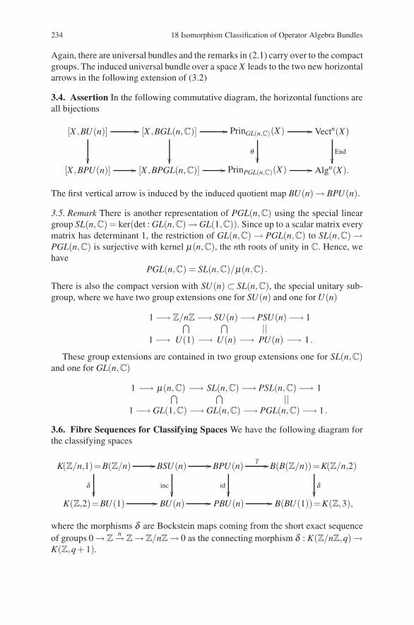
234 18 Isomorphism Classification of Operator Algebra Bundles
Again, there are universal bundles and the remarks in (2.1) carry over to the compactgroups. The induced universal bundle over a space X leads to the two new horizontalarrows in the following extension of (3.2)
3.4. Assertion In the following commutative diagram, the horizontal functions areall bijections
[X ,BU(n)] ��
��
[X ,BGL(n,C)] ��
��
PrinGL(n,C)(X) ��
�
Vectn(X)
End��
[X ,BPU(n)] �� [X ,BPGL(n,C)] �� PrinPGL(n,C)(X) �� Algn(X).
The first vertical arrow is induced by the induced quotient map BU(n)→ BPU(n).
3.5. Remark There is another representation of PGL(n,C) using the special lineargroup SL(n,C) = ker(det : GL(n,C)→ GL(1,C)). Since up to a scalar matrix everymatrix has determinant 1, the restriction of GL(n,C) → PGL(n,C) to SL(n,C) →PGL(n,C) is surjective with kernel μ(n,C), the nth roots of unity in C. Hence, wehave
PGL(n,C) = SL(n,C)/μ(n,C) .
There is also the compact version with SU(n) ⊂ SL(n,C), the special unitary sub-group, where we have two group extensions one for SU(n) and one for U(n)
1 −→ Z/nZ −→ SU(n)−→ PSU(n)−→ 1⋂ ⋂ ||1 −→ U(1) −→ U(n) −→ PU(n) −→ 1 .
These group extensions are contained in two group extensions one for SL(n,C)and one for GL(n,C)
1 −→ μ(n,C) −→ SL(n,C) −→ PSL(n,C)−→ 1⋂ ⋂ ||1 −→ GL(1,C) −→ GL(n,C) −→ PGL(n,C) −→ 1 .
3.6. Fibre Sequences for Classifying Spaces We have the following diagram forthe classifying spaces
K(Z/n,1)=B(Z/n)
�
��BSU(n)
inc��
��BPU(n)
id��
γ �� B(B(Z/n))=K(Z/n,2)
�
K(Z,2)=BU(1) �� BU(n) �� PBU(n) �� B(BU(1))=K(Z,3),
where the morphisms δ are Bockstein maps coming from the short exact sequenceof groups 0 → Z
n→ Z → Z/nZ → 0 as the connecting morphism δ : K(Z/nZ,q)→K(Z,q + 1).
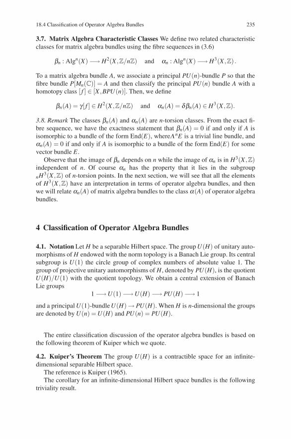
18.4 Classification of Operator Algebra Bundles 235
3.7. Matrix Algebra Characteristic Classes We define two related characteristicclasses for matrix algebra bundles using the fibre sequences in (3.6)
βn : Algn(X) −→ H2(X ,Z/nZ) and αn : Algn(X) −→ H3(X ,Z) .
To a matrix algebra bundle A, we associate a principal PU(n)-bundle P so that thefibre bundle P[Mn(C)] = A and then classify the principal PU(n) bundle A with ahomotopy class [ f ] ∈ [X ,BPU(n)]. Then, we define
βn(A) = γ[ f ] ∈ H2(X ,Z/nZ) and αn(A) = δβn(A) ∈ H3(X ,Z).
3.8. Remark The classes βn(A) and αn(A) are n-torsion classes. From the exact fi-bre sequence, we have the exactness statement that βn(A) = 0 if and only if A isisomorphic to a bundle of the form End(E), whereΛnE is a trivial line bundle, andαn(A) = 0 if and only if A is isomorphic to a bundle of the form End(E) for somevector bundle E .
Observe that the image of βn depends on n while the image of αn is in H3(X ,Z)independent of n. Of course αn has the property that it lies in the subgroupnH3(X ,Z) of n-torsion points. In the next section, we will see that all the elementsof H3(X ,Z) have an interpretation in terms of operator algebra bundles, and thenwe will relate αn(A) of matrix algebra bundles to the class α(A) of operator algebrabundles.
4 Classification of Operator Algebra Bundles
4.1. Notation Let H be a separable Hilbert space. The group U(H) of unitary auto-morphisms of H endowed with the norm topology is a Banach Lie group. Its centralsubgroup is U(1) the circle group of complex numbers of absolute value 1. Thegroup of projective unitary automorphisms of H, denoted by PU(H), is the quotientU(H)/U(1) with the quotient topology. We obtain a central extension of BanachLie groups
1 −→U(1)−→U(H) −→ PU(H) −→ 1
and a principal U(1)-bundle U(H)→ PU(H). When H is n-dimensional the groupsare denoted by U(n) = U(H) and PU(n) = PU(H).
The entire classification discussion of the operator algebra bundles is based onthe following theorem of Kuiper which we quote.
4.2. Kuiper’s Theorem The group U(H) is a contractible space for an infinite-dimensional separable Hilbert space.
The reference is Kuiper (1965).The corollary for an infinite-dimensional Hilbert space bundles is the following
triviality result.
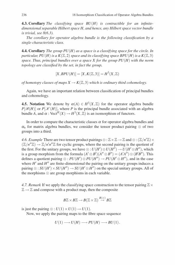
236 18 Isomorphism Classification of Operator Algebra Bundles
4.3. Corollary The classifying space BU(H) is contractible for an infinite-dimensional separable Hilbert space H, and hence, any Hilbert space vector bundleis trivial, see 8(6.3).
The corollary for operator algebra bundle is the following classification by asingle-characteristic class.
4.4. Corollary The group PU(H) as a space is a classifying space for the circle. Inparticular, PU(H) is a K(Z,2) space and its classifying space BPU(H) is a K(Z,3)space. Thus, principal bundles over a space X for the group PU(H) with the normtopology are classified by the set, in fact the group,
[X ,BPU(H)] = [X ,K(Z,3)] = H3(X ,Z)
of homotopy classes of maps X → K(Z,3) which is ordinary third cohomology.
Again, we have an important relation between classification of principal bundlesand cohomology.
4.5. Notation We denote by α(A) ∈ H3(X ,Z) for the operator algebra bundleP[B(H)] or P[K (H)], where P is the principal bundle associated with an algebrabundle A, and α : VectH(X) → H3(X ,Z) is an isomorphism of functors.
In order to compare the characteristic classes α for operator algebra bundles andαn for matrix algebra bundles, we consider the tensor product pairing ⊗ of twogroups into a third.
4.6. Example There are two tensor product pairings⊗ : Z×Z→Z and⊗ : (Z/n′Z)×(Z/n′′Z) → Z/n′n′′Z for cyclic groups, where the second pairing is the quotient ofthe first. For the unitary groups, we have ⊗ : U(H ′)⊗U(H ′′)→U(H ′ ⊗H ′′), whichis a group morphism from the formula (A′ ⊗B′)(A′′ ⊗B′′) = (A′A′′)⊗ (B′B′′). Thisdefines a quotient pairing ⊗ : PU(H ′)⊗PU(H ′′) → PU(H ′ ⊗H ′′), and in the casewhere H ′ and H ′′ are finite-dimensional the pairing on the unitary groups induces apairing ⊗ : SU(H ′)×SU(H ′′) → SU(H ′ ⊗H ′′) on the special unitary groups. All ofthe morphisms ⊗ are group morphisms in each variable.
4.7. Remark If we apply the classifying space construction to the tensor pairing Z×Z → Z and compose with a product map, then the composite
BZ×BZ → B(Z×Z)B(⊗)→ BZ
is just the pairing ⊗ : U(1)×U(1)→U(1).Now, we apply the pairing maps to the fibre space sequence
U(1)−→U(H) −→ PU(H) −→ BU(1) .
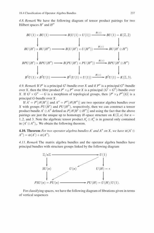
18.4 Classification of Operator Algebra Bundles 237
4.8. Remark We have the following diagram of tensor product pairings for twoHilbert spaces H ′ and H ′′
BU(1)×BU(1)
��
�� B(U(1)×U(1))
��
B(⊗) �� BU(1) = K(Z,2)
��BU(H ′)×BU(H ′′)
��
�� B(U(H ′)×U(H ′′))
��
B(⊗) �� BU(H ′ ⊗H ′′)
��BPU(H ′)×BPU(H ′′)
��
�� B(PU(H ′)×PU(H ′′))
��
B(⊗) �� BPU(H ′ ⊗H ′′)
��B2U(1)×B2U(1) �� B2(U(1)×U(1))
B(⊗) �� B2U(1) = K(Z,3).
4.9. Remark If P′ is a principal G′-bundle over X and if P′′ is a principal G′′-bundleover X , then the fibre product P′ ×X P′′ over X is a principal (G′ ×G′′)-bundle overX . If G′ ×G′′ → G is a morphism of topological groups, then (P′ ×X P′′)[G] is aprincipal G-bundle over X .
If A′ = P′[B(H ′)] and A′′ = P′′[B(H ′′)] are two operator algebra bundles overX with groups PU(H ′) and PU(H ′′), respectively, then we can construct a tensorproduct bundle A′ ⊗A′′ defined as P[B(H ′ ⊗H ′′)] and using the fact that the abovepairings are just the unique up to homotopy H-space structure on K(Z,n) for n =1,2, and 3. Note the algebraic tensor product A′
x ⊗A′′x is in general only contained
in (A′ ⊗A′′)x. We obtain the following theorem.
4.10. Theorem For two operator algebra bundles A′ and A′′ on X, we have α(A′ ⊗A′′) = α(A′)+α(A′′).
4.11. Remark The matrix algebra bundles and the operator algebra bundles haveprincipal bundles with structure groups linked by the following diagram
Z/nZ ��
��
U(1)
��������
������
��
��SU(n)
��
U(n)
��
U(H) = ∗
��PSU(n) = PU(n) �� PU(H) = U(H)/U(1).
For classifying spaces, we have the following diagram of fibrations given in termsof vertical sequences
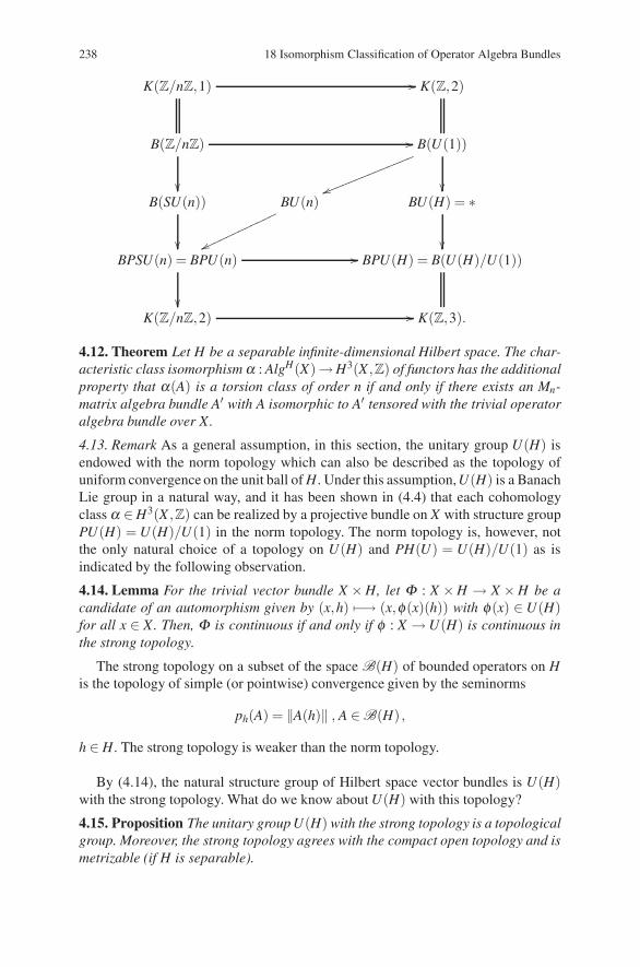
238 18 Isomorphism Classification of Operator Algebra Bundles
K(Z/nZ,1) �� K(Z,2)
B(Z/nZ) ��
��
B(U(1))
��������
������
��
��B(SU(n))
��
BU(n)
��������
������
BU(H) = ∗
��BPSU(n) = BPU(n)
��
�� BPU(H) = B(U(H)/U(1))
K(Z/nZ,2) �� K(Z,3).
4.12. Theorem Let H be a separable infinite-dimensional Hilbert space. The char-acteristic class isomorphism α : AlgH(X)→H3(X ,Z) of functors has the additionalproperty that α(A) is a torsion class of order n if and only if there exists an Mn-matrix algebra bundle A′ with A isomorphic to A′ tensored with the trivial operatoralgebra bundle over X.
4.13. Remark As a general assumption, in this section, the unitary group U(H) isendowed with the norm topology which can also be described as the topology ofuniform convergence on the unit ball of H. Under this assumption,U(H) is a BanachLie group in a natural way, and it has been shown in (4.4) that each cohomologyclass α ∈ H3(X ,Z) can be realized by a projective bundle on X with structure groupPU(H) = U(H)/U(1) in the norm topology. The norm topology is, however, notthe only natural choice of a topology on U(H) and PH(U) = U(H)/U(1) as isindicated by the following observation.
4.14. Lemma For the trivial vector bundle X ×H, let Φ : X ×H → X ×H be acandidate of an automorphism given by (x,h) �−→ (x,φ(x)(h)) with φ(x) ∈ U(H)for all x ∈ X. Then, Φ is continuous if and only if φ : X → U(H) is continuous inthe strong topology.
The strong topology on a subset of the space B(H) of bounded operators on His the topology of simple (or pointwise) convergence given by the seminorms
ph(A) = ‖A(h)‖ , A ∈ B(H) ,
h ∈ H. The strong topology is weaker than the norm topology.
By (4.14), the natural structure group of Hilbert space vector bundles is U(H)with the strong topology. What do we know about U(H) with this topology?
4.15. Proposition The unitary group U(H) with the strong topology is a topologicalgroup. Moreover, the strong topology agrees with the compact open topology and ismetrizable (if H is separable).
References 239
The first statement is in sharp contrast to several claims in the correspondingliterature on quantization of symmetries and in other publications. Even in recentpublications as, for example, in the article Twisted K-theory of Atiyah and Segal(2005), it is stated that U(H) is not a topological group with respect to the strongtopology. But the proof is very simple. For example, U �→ U−1 is continuous inU0 ∈ U (H), since for h ∈ H and ε > 0 one defines g = U−1
0 (h) and obtains for allU ∈U(H):
∥∥U−10 (h)−U−1(h)
∥∥=∥∥g−U−1U0(g)
∥∥= ‖U(g)−U0(g)‖ .
Hence,∥∥U−1
0 (h)−U−1(h)∥∥ < ε for all U ∈ U(H) with ‖U0(g)−V(g)‖ < ε . That
U(H) is a topological group in the strong topology in contrast to GL(H) can beattributed to the fact that U(H) is equicontinuous. The equicontinuity of U(H) asa set of operators also accounts for the coincidence of the strong and the compactopen topology and the metrizability.
A much deeper result is the contractibility of U(H) in the strong topology whichis shown in the above mentioned article. As a consequence much of classification re-sults are parallel to the norm topology case, in particular the results in (4.3) and (4.4).
4.16. Corollary Let U(H) be the topological group with the strong topology and letPU(H) = U(H)/U(1) with the quotient topology. Then, any Hilbert space vectorbundle over X with structure group U(H) is trivial. And the principal bundles overX for the group PU(H) are classified by H3(X ,Z).
References
Atiyah, M.F., Segal, G.B.: Twisted K-Theory and cohomology (2005) (arXiv:math.KT/0510674)Dixmier, J. Douady, A.: Champs continus d’espaces Hilbertiens et de C*-algebres. Bull. Soc. Math.
France 91: 2227–284 (1963)Kuiper, N.H.: The homotopy type of the unitary group of Hilbert space. Topology 3:19–30 (1965)

Chapter 19Brauer Group of Matrix Algebra Bundlesand K-Groups
Before using the characteristic class isomorphism
α : AlgH(X) −→ H3(X ,Z)
to study its role in extending vector bundle K-theory, we analyze further the ma-trix bundle theory using the restriction αn : Algn(X) →n H3(X ,Z) of α to Algn(X)which is a group morphism in the corollary (1.4). In the context of sheaf theory, wehave already derived a multiplicative property of the morphisms αn and βn. Now,we carry this out in the context of classifying space theory.
This leads naturally into the question of the Brauer group of all matrix algebrabundles with the relation A′ and A′′ are Brauer equivalent provided that A′ ⊗ End(E ′)and A′′ ⊗ End(E ′′) are isomorphic over X for two vector bundles E ′ and E ′′. Theresult is the Brauer group B(X) of a space X which is a form of K-group or Klas-sengruppe in the sense of Grothendieck. We study the stability properties of thisgroup.
The reader with a special interest in twisted K-theory can go directly to the nextchapter. The last section discusses a sheaf theory approach to matrix algebra bundlesfor completeness of the discussion. It is not used in the later chapters.
1 Properties of the Morphism αααn
The group morphism property of αn follows the line of argument as we establishedthe same property of α in 20(4.8) using 20(4.9) to obtain 20(4.10).
1.1. Remark Now, we apply the pairing maps of 20(4.6) to the fibre space sequenceassociated with matrix algebra bundles
Z/mZ −→ SU(H) −→ PU(H) −→ B(Z/mZ),
dimH = m in the case of ⊗ : (Z/n′Z)× (Z/n′′Z) → (Z/n′n′′Z).
D. Husemoller et al.: Brauer Group of Matrix Algebra Bundles and K-Groups, Lect. Notes Phys. 726, 241–249 (2008)DOI 10.1007/978-3-540-74956-1 20 © Springer-Verlag Berlin Heidelberg 2008
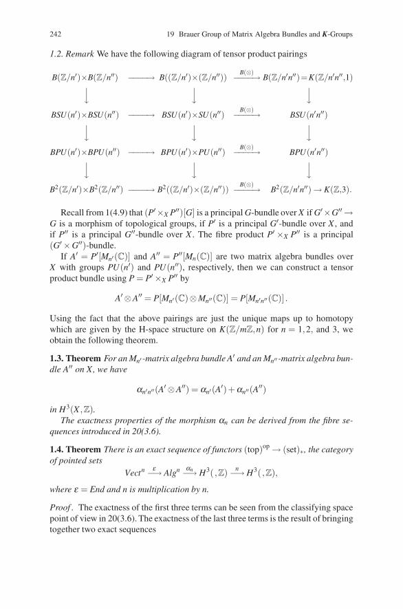
242 19 Brauer Group of Matrix Algebra Bundles and K-Groups
1.2. Remark We have the following diagram of tensor product pairings
B(Z/n′)×B(Z/n′′) −−−−→ B((Z/n′)×(Z/n′′))B(⊗)−−−−→ B(Z/n′n′′)=K(Z/n′n′′,1)
⏐⏐�⏐⏐�
⏐⏐�BSU(n′)×BSU(n′′) −−−−→ BSU(n′)×SU(n′′)
B(⊗)−−−−→ BSU(n′n′′)⏐⏐�⏐⏐�
⏐⏐�BPU(n′)×BPU(n′′) −−−−→ BPU(n′)×PU(n′′)
B(⊗)−−−−→ BPU(n′n′′)⏐⏐�⏐⏐�
⏐⏐�B2(Z/n′)×B2(Z/n′′) −−−−→ B2((Z/n′)×(Z/n′′))
B(⊗)−−−−→ B2(Z/n′n′′) → K(Z,3).
Recall from 1(4.9) that (P′×X P′′)[G] is a principal G-bundle over X if G′×G′′ →G is a morphism of topological groups, if P′ is a principal G′-bundle over X , andif P′′ is a principal G′′-bundle over X . The fibre product P′ ×X P′′ is a principal(G′ ×G′′)-bundle.
If A′ = P′[Mn′(C)] and A′′ = P′′[Mn(C)] are two matrix algebra bundles overX with groups PU(n′) and PU(n′′), respectively, then we can construct a tensorproduct bundle using P = P′ ×X P′′ by
A′ ⊗A′′ = P[Mn′(C)⊗Mn′′(C)] = P[Mn′n′′(C)] .
Using the fact that the above pairings are just the unique maps up to homotopywhich are given by the H-space structure on K(Z/mZ,n) for n = 1,2, and 3, weobtain the following theorem.
1.3. Theorem For an Mn′ -matrix algebra bundle A′ and an Mn′′ -matrix algebra bun-dle A′′ on X, we have
αn′n′′(A′ ⊗A′′) = αn′(A′)+αn′′(A′′)
in H3(X ,Z).The exactness properties of the morphism αn can be derived from the fibre se-
quences introduced in 20(3.6).
1.4. Theorem There is an exact sequence of functors (top)op → (set)∗, the categoryof pointed sets
Vectn ε−→ Algn αn−→ H3( ,Z) n−→ H3( ,Z),
where ε = End and n is multiplication by n.
Proof . The exactness of the first three terms can be seen from the classifying spacepoint of view in 20(3.6). The exactness of the last three terms is the result of bringingtogether two exact sequences
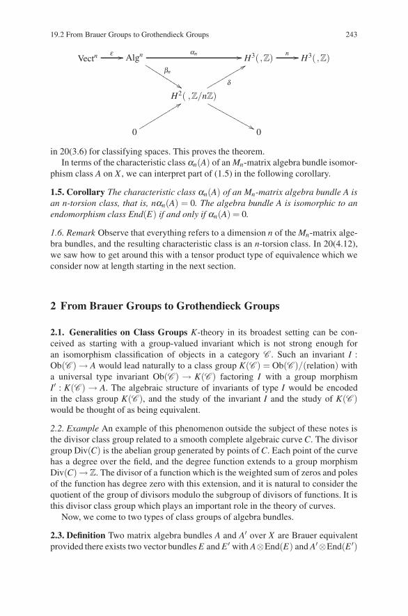
19.2 From Brauer Groups to Grothendieck Groups 243
Vectnε �� Algn αn ��
βn
�������
�����
H3( ,Z)n �� H3( ,Z)
H2( ,Z/nZ)δ
������������
�������
������
�
0
�������������0
in 20(3.6) for classifying spaces. This proves the theorem.In terms of the characteristic class αn(A) of an Mn-matrix algebra bundle isomor-
phism class A on X , we can interpret part of (1.5) in the following corollary.
1.5. Corollary The characteristic class αn(A) of an Mn-matrix algebra bundle A isan n-torsion class, that is, nαn(A) = 0. The algebra bundle A is isomorphic to anendomorphism class End(E) if and only if αn(A) = 0.
1.6. Remark Observe that everything refers to a dimension n of the Mn-matrix alge-bra bundles, and the resulting characteristic class is an n-torsion class. In 20(4.12),we saw how to get around this with a tensor product type of equivalence which weconsider now at length starting in the next section.
2 From Brauer Groups to Grothendieck Groups
2.1. Generalities on Class Groups K-theory in its broadest setting can be con-ceived as starting with a group-valued invariant which is not strong enough foran isomorphism classification of objects in a category C . Such an invariant I :Ob(C ) → A would lead naturally to a class group K(C ) = Ob(C )/(relation) witha universal type invariant Ob(C ) → K(C ) factoring I with a group morphismI′ : K(C ) → A. The algebraic structure of invariants of type I would be encodedin the class group K(C ), and the study of the invariant I and the study of K(C )would be thought of as being equivalent.
2.2. Example An example of this phenomenon outside the subject of these notes isthe divisor class group related to a smooth complete algebraic curve C. The divisorgroup Div(C) is the abelian group generated by points of C. Each point of the curvehas a degree over the field, and the degree function extends to a group morphismDiv(C)→Z. The divisor of a function which is the weighted sum of zeros and polesof the function has degree zero with this extension, and it is natural to consider thequotient of the group of divisors modulo the subgroup of divisors of functions. It isthis divisor class group which plays an important role in the theory of curves.
Now, we come to two types of class groups of algebra bundles.
2.3. Definition Two matrix algebra bundles A and A′ over X are Brauer equivalentprovided there exists two vector bundles E and E ′ with A⊗End(E) and A′⊗End(E ′)
244 19 Brauer Group of Matrix Algebra Bundles and K-Groups
isomorphic. The set Br(A) of Brauer equivalence class cl(A) of matrix algebra bun-dles together with the group structure given by cl(A) · cl(A′) = cl(A⊗A′) is calledthe Brauer group.
From the isomorphism Aop⊗A→End(Vect(A)), where Vect(A) is the underlyingvector bundle of the algebra, we see that cl(Aop) = cl(A)−1 which gives the inverse.
2.4. Remark In line with the generalization of (2.1), we can define the characteris-tic class α : Br(A) → Tors(H3(X ,Z)) on the Brauer classes by α(cl(A)) = αn(A),where A is an Mn-matrix algebra representative of the class cl(A) ∈ Br(A).
We have the following theorem of Serre which we just quote now.
2.5. Theorem If X is a finite complex, then the characteristic class α : Br(A) →Tors(H3(X ,Z)) is an isomorphism.
Recall that reindexing of MnMq gives Mn(Mq(C)) = Mnq(C).
2.6. Definition Two matrix algebras A and A′ over X are stably equivalent providedthere exists n and n′ with Mn(A) and Mn′(A′) isomorphic. The set KP(X) of stableequivalence classes {A} of matrix algebra bundles A together with the semigroupstructure given by {A′} · {A′′} = {A′ ⊗A′′} is called the projective K-group.
There is a natural morphism KP(X) → Br(X), where {A} �→ cl(A). We considerKP(X) and Br(X) as K-groups in the sense of Grothendieck further in the next threesections.
3 Stability I: Vector Bundles
Now, we return to Grothendieck who pointed out the importance of the class theoryfor coherent sheaves and vector bundles.
3.1. Definition Two vector bundles E and E ′ over X are K-equivalent provided thatthere exists a trivial bundle T with E ⊕T and E ′ ⊕T isomorphic. Let [E] denote theK-equivalence class of E on X .
If [E] is a K-equivalence class on Y and if f : X → Y is a continuous function,then f ∗[E] = [ f ∗E] is well-defined K-equivalence class on X which defines a functor[ ] on (top)op with values in the category of semirings.
3.2. Notation Let [X ] denote the set of K-equivalence classes [E] of bundles on Xwith the semiring structure
[E ′]+ [E ′′] = [E ′ ⊕E ′′] and [E ′] · [E ′′] = [E ′ ⊗E ′′] .
Let K(X) denote the universal abelian group. Then, K(X) is also the universal com-mutative ring on the semigroup [X ]. Further, the universal constructions lead to afunctor K : (top)op → (c\rg) with values in the category of commutative rings.
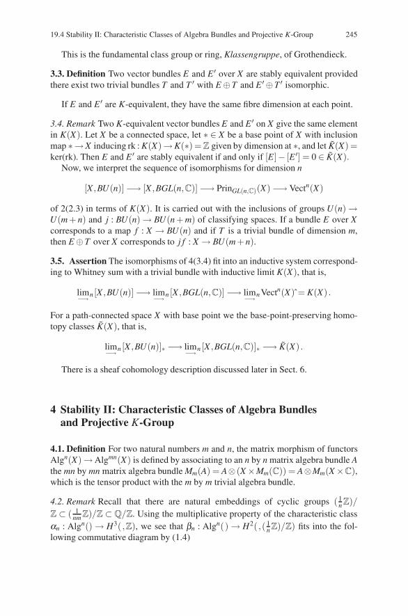
19.4 Stability II: Characteristic Classes of Algebra Bundles and Projective K-Group 245
This is the fundamental class group or ring, Klassengruppe, of Grothendieck.
3.3. Definition Two vector bundles E and E ′ over X are stably equivalent providedthere exist two trivial bundles T and T ′ with E ⊕T and E ′ ⊕T ′ isomorphic.
If E and E ′ are K-equivalent, they have the same fibre dimension at each point.
3.4. Remark Two K-equivalent vector bundles E and E ′ on X give the same elementin K(X). Let X be a connected space, let ∗ ∈ X be a base point of X with inclusionmap ∗→X inducing rk : K(X)→K(∗) = Z given by dimension at ∗, and let K(X) =ker(rk). Then E and E ′ are stably equivalent if and only if [E]− [E ′] = 0 ∈ K(X).
Now, we interpret the sequence of isomorphisms for dimension n
[X ,BU(n)] −→ [X ,BGL(n,C)] −→ PrinGL(n,C)(X) −→ Vectn(X)
of 2(2.3) in terms of K(X). It is carried out with the inclusions of groups U(n) →U(m + n) and j : BU(n) → BU(n + m) of classifying spaces. If a bundle E over Xcorresponds to a map f : X → BU(n) and if T is a trivial bundle of dimension m,then E ⊕T over X corresponds to j f : X → BU(m+ n).
3.5. Assertion The isomorphisms of 4(3.4) fit into an inductive system correspond-ing to Whitney sum with a trivial bundle with inductive limit K(X), that is,
lim−→ n [X ,BU(n)] −→ lim−→ n [X ,BGL(n,C)] −→ lim−→ n Vectn(X ) = K(X) .
For a path-connected space X with base point we the base-point-preserving homo-topy classes K(X), that is,
lim−→ n [X ,BU(n)]∗ −→ lim−→ n [X ,BGL(n,C)]∗ −→ K(X) .
There is a sheaf cohomology description discussed later in Sect. 6.
4 Stability II: Characteristic Classes of Algebra Bundlesand Projective K-Group
4.1. Definition For two natural numbers m and n, the matrix morphism of functorsAlgn(X)→ Algmn(X) is defined by associating to an n by n matrix algebra bundle Athe mn by mn matrix algebra bundle Mm(A) = A⊗ (X ×Mm(C)) = A⊗Mm(X ×C),which is the tensor product with the m by m trivial algebra bundle.
4.2. Remark Recall that there are natural embeddings of cyclic groups ( 1n Z)/
Z ⊂ ( 1nm Z)/Z ⊂ Q/Z. Using the multiplicative property of the characteristic class
αn : Algn() → H3( ,Z), we see that βn : Algn() → H2( ,( 1n Z)/Z) fits into the fol-
lowing commutative diagram by (1.4)
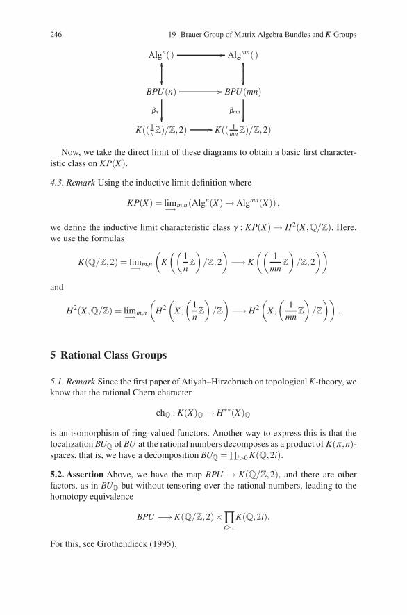
246 19 Brauer Group of Matrix Algebra Bundles and K-Groups
Algn() ����
��
Algmn()��
��BPU(n) ��
βn
��
BPU(mn)
βmn
��K(( 1
n Z)/Z,2) �� K(( 1mn Z)/Z,2)
Now, we take the direct limit of these diagrams to obtain a basic first character-istic class on KP(X).
4.3. Remark Using the inductive limit definition where
KP(X) = lim−→m,n(Algn(X) → Algmn(X)) ,
we define the inductive limit characteristic class γ : KP(X) → H2(X ,Q/Z). Here,we use the formulas
K(Q/Z,2) = lim−→m,n
(K
((1n
Z
)/Z,2
)−→ K
((1
mnZ
)/Z,2
))
and
H2(X ,Q/Z) = lim−→m,n
(H2(
X ,
(1n
Z
)/Z
)−→ H2
(X ,
(1
mnZ
)/Z
)).
5 Rational Class Groups
5.1. Remark Since the first paper of Atiyah–Hirzebruch on topological K-theory, weknow that the rational Chern character
chQ : K(X)Q → H∗∗(X)Q
is an isomorphism of ring-valued functors. Another way to express this is that thelocalization BUQ of BU at the rational numbers decomposes as a product of K(π ,n)-spaces, that is, we have a decomposition BUQ =∏i>0 K(Q,2i).
5.2. Assertion Above, we have the map BPU → K(Q/Z,2), and there are otherfactors, as in BUQ but without tensoring over the rational numbers, leading to thehomotopy equivalence
BPU −→ K(Q/Z,2)×∏i>1
K(Q,2i).
For this, see Grothendieck (1995).
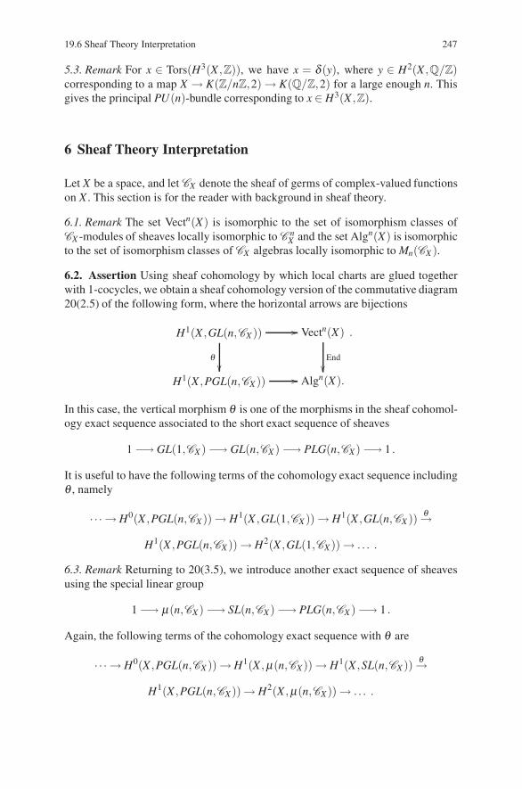
19.6 Sheaf Theory Interpretation 247
5.3. Remark For x ∈ Tors(H3(X ,Z)), we have x = δ (y), where y ∈ H2(X ,Q/Z)corresponding to a map X → K(Z/nZ,2) → K(Q/Z,2) for a large enough n. Thisgives the principal PU(n)-bundle corresponding to x ∈ H3(X ,Z).
6 Sheaf Theory Interpretation
Let X be a space, and let CX denote the sheaf of germs of complex-valued functionson X . This section is for the reader with background in sheaf theory.
6.1. Remark The set Vectn(X) is isomorphic to the set of isomorphism classes ofCX -modules of sheaves locally isomorphic to C n
X and the set Algn(X) is isomorphicto the set of isomorphism classes of CX algebras locally isomorphic to Mn(CX ).
6.2. Assertion Using sheaf cohomology by which local charts are glued togetherwith 1-cocycles, we obtain a sheaf cohomology version of the commutative diagram20(2.5) of the following form, where the horizontal arrows are bijections
H1(X ,GL(n,CX )) ��
�
Vectn(X)
End��
H1(X ,PGL(n,CX )) �� Algn(X).
.
In this case, the vertical morphism θ is one of the morphisms in the sheaf cohomol-ogy exact sequence associated to the short exact sequence of sheaves
1 −→ GL(1,CX ) −→ GL(n,CX ) −→ PLG(n,CX) −→ 1 .
It is useful to have the following terms of the cohomology exact sequence includingθ , namely
· · · → H0(X ,PGL(n,CX)) → H1(X ,GL(1,CX )) → H1(X ,GL(n,CX )) θ→
H1(X ,PGL(n,CX )) → H2(X ,GL(1,CX )) → . . . .
6.3. Remark Returning to 20(3.5), we introduce another exact sequence of sheavesusing the special linear group
1 −→ μ(n,CX) −→ SL(n,CX) −→ PLG(n,CX ) −→ 1 .
Again, the following terms of the cohomology exact sequence with θ are
· · · → H0(X ,PGL(n,CX )) → H1(X ,μ(n,CX)) → H1(X ,SL(n,CX )) θ→
H1(X ,PGL(n,CX )) → H2(X ,μ(n,CX)) → . . . .
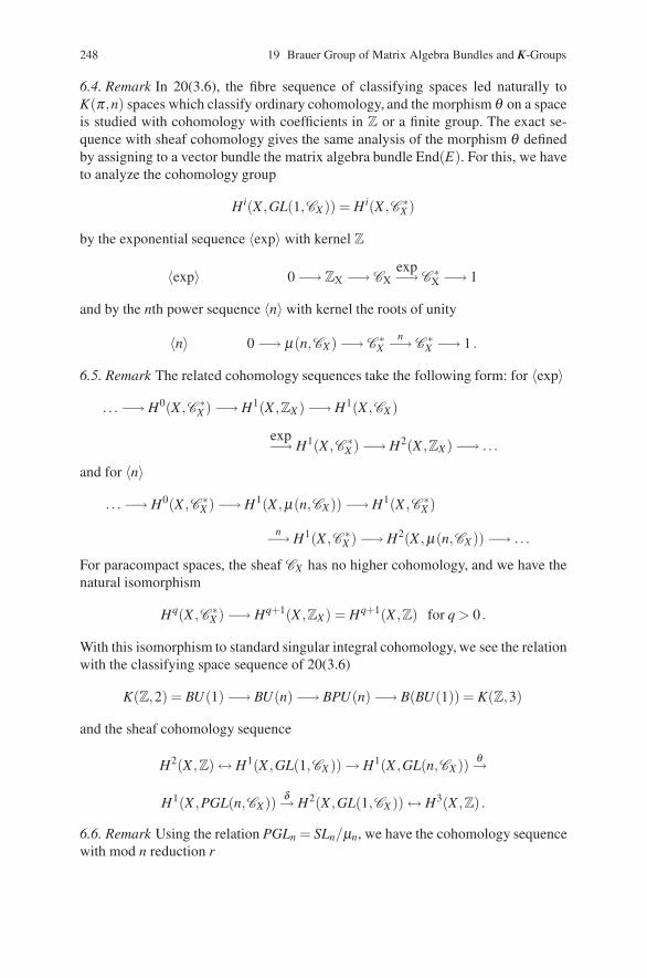
248 19 Brauer Group of Matrix Algebra Bundles and K-Groups
6.4. Remark In 20(3.6), the fibre sequence of classifying spaces led naturally toK(π ,n) spaces which classify ordinary cohomology, and the morphism θ on a spaceis studied with cohomology with coefficients in Z or a finite group. The exact se-quence with sheaf cohomology gives the same analysis of the morphism θ definedby assigning to a vector bundle the matrix algebra bundle End(E). For this, we haveto analyze the cohomology group
Hi(X ,GL(1,CX )) = Hi(X ,C ∗X )
by the exponential sequence 〈exp〉 with kernel Z
〈exp〉 0 −→ ZX −→ CXexp−→ C ∗
X −→ 1
and by the nth power sequence 〈n〉 with kernel the roots of unity
〈n〉 0 −→ μ(n,CX ) −→ C ∗X
n−→ C ∗X −→ 1 .
6.5. Remark The related cohomology sequences take the following form: for 〈exp〉
. . . −→ H0(X ,C ∗X ) −→ H1(X ,ZX ) −→ H1(X ,CX )
exp−→ H1(X ,C ∗X ) −→ H2(X ,ZX ) −→ . . .
and for 〈n〉
. . . −→ H0(X ,C ∗X ) −→ H1(X ,μ(n,CX)) −→ H1(X ,C ∗
X )
n−→ H1(X ,C ∗X ) −→ H2(X ,μ(n,CX )) −→ . . .
For paracompact spaces, the sheaf CX has no higher cohomology, and we have thenatural isomorphism
Hq(X ,C ∗X ) −→ Hq+1(X ,ZX) = Hq+1(X ,Z) for q > 0 .
With this isomorphism to standard singular integral cohomology, we see the relationwith the classifying space sequence of 20(3.6)
K(Z,2) = BU(1) −→ BU(n) −→ BPU(n) −→ B(BU(1)) = K(Z,3)
and the sheaf cohomology sequence
H2(X ,Z) ↔ H1(X ,GL(1,CX )) → H1(X ,GL(n,CX )) θ→
H1(X ,PGL(n,CX)) δ→ H2(X ,GL(1,CX )) ↔ H3(X ,Z) .
6.6. Remark Using the relation PGLn = SLn/μn, we have the cohomology sequencewith mod n reduction r
Reference 249
H1(X ,μ(n,CX))→H1(X ,SL(n,CX)) θ→H1(X ,PGL(n,CX)) δ ′→H2(X ,μ(n,CX)),
together with the maps
H1(X ,μ(n,CX )) rδ−→ H2(X ,Z/nZ) and H2(X ,μ(n,CX )) → H3(X ,Z).
Reference
Grothendieck, A.: Le groupe de Brauer. Part I. Seminaire Bourbaki, Vol. 9, Exp. 290: 199–219(1995)

Chapter 20Analytic Definition of Twisted K-Theory
As pointed out in the previous chapter, there are several approaches to ordinarycomplex K-theory. Each of these approaches leads to a version of twisted K-theory.The basic data for twisted K-theory is an operator algebra bundle A over X . Thetwisted K-group is denoted by Kα (X), where the characteristic class α of A is partof the data α(A) = α ∈ H3(X ,Z).
First, we consider twisted K-theory in terms of the Fredholm subbundle Fred(A)⊂A over X . We relate mappings from X into the Fredholm operators Fred(H) andcross sections of the Fredholm subbundle over X . The twisted K-group of X rela-tive to the algebra bundle A is given by fibre homotopy classes of cross sections ofFred(A).
Ordinary K-theory is also described by mappings into a space Fred(H). Map-pings into Fred(H) can be thought as cross sections of the trivial bundle with fibreFred(H). By replacing the trivial bundle with fibre Fred(H) with a nontrivial bundlewith fibre Fred(H), we obtain a twisted K-theory from classes of cross sections ofthis nontrivial bundle.
Secondly, we introduce the C∗-algebra of sections Γ(X ,K (A)) of the algebrabundle. The K-theory of a C∗-algebra is the twisted K-group relative to the algebrabundle A over X .
Operator bundles with fibre B = B(H) or with fibre K = K (H) are equivalentsince they both have an automorphism group PU(H) up to homotopy. The bundleswith fibre B are more useful for a Fredholm operator approach to twisted K-theorywhile the bundles with a fibre K appear more naturally in the operator K-theoryapproach to twisted K-theory.
1 Cross Sections and Fibre Homotopy Classes of Cross Sections
1.1. Definition A cross section s of a bundle p : E → B is map s : B → E withps = idB. Let Γ(B,E) denote the set of all cross sections of E over B.
The condition ps = idB is equivalent to s(b) ∈ Eb for all b ∈ B.
D. Husemoller et al.: Analytic Definition of Twisted K-Theory, Lect. Notes Phys. 726, 251–253 (2008)DOI 10.1007/978-3-540-74956-1 21 © Springer-Verlag Berlin Heidelberg 2008
252 20 Analytic Definition of Twisted K-Theory
1.2. Example For the product bundle p : B×Y →B, the set of cross sectionsΓ(B,B×X) can be identified with the set Map(B,Y ) of mappings form B to Y . A cross sectionof the product bundle has the form s(b) = (b, f (b)), where f : B→Y is a continuousfunction, and conversely, f determines s f uniquely by the formula s f (b) = (b, f (b)).
For many invariants of continuous functions f : X → Y between two spaces Xand Y , the function itself is less important than the deformation class or homotopyclass of the mapping. This leads to the following two basic definitions.
1.3. Definition A homotopy between two maps f ′, f ′′ : X → Y is a map h : X ×[0,1] → Y such that f ′(x) = h(x,0) and f ′′(x) = h(x,1). Two maps f ′, f ′′ : X → Yare homotopic provided there exists a homotopy from f ′ to f ′′.
Homotopy of maps is an equivalence relation on the set Map(X ,Y ). We denotethe set of homotopy classes [ f ] : X → Y by [X ,Y ]. The set [X ,Y ] is a quotient ofMap(X ,Y ).
1.4. Definition Let s′ s′′ : B → E be two cross sections of p : E → B. A fibre ho-motopy between s′ and s′′ is a homotopy h such that ph(b,t) = b for all b ∈ B andt ∈ [0,1]. Two cross sections s′ s′′ : B → E are fibre homotopic (or fibre homotopi-cally equivalent) provided there exists a fibre homotopy map from s′ to s′′.
Fibre homotopy of sections is an equivalence relation on the set Γ(B,E) of crosssections of p : E → B. Let [Γ](B,E) denote the set of fibre homotopy classes of crosssections of p : E → B. Then [Γ](B,E) is a quotient set of Γ(B,E).
1.5. Remark For the trivial bundle p : B×Y → B, the function which assigns to amap f : B→Y in Map(B,Y ) the cross section s f (b)= (b, f (b)) in Γ(B,B×Y ) carrieshomotopy equivalent f to fibre homotopy equivalent cross sections. This defines anatural bijection [B,Y ] → [Γ](B,B×Y) of the bijection Map(B,Y ) → Γ(B,B×Y).
2 Two Basic Analytic Results in Bundle Theory and K-Theory
2.1. Theorem (Kuiper) Let H be a separable infinite-dimensional Hilbert space.The unitary group U(H) with the norm topology is a contractible group.
2.2. Theorem (Atiyah–Janich). Let H be a separable infinite-dimensional Hilbertspace. There is a natural morphism of functors on compact spaces [X ,Fred(H)] →K(X) with the following property: If f : X → Fred(H) is a map with ker( f (x)) andcoker( f (x)) locally of constant dimension, then the image of [ f ] is E ′ −E ′′, whereE ′ and E ′′ are the subbundles of the trivial X ×H → X with fibres
E ′x = x×ker(f(x)) and E′
x = x×ker(f(x)∗) .
This map [X ,Fred(H)] → K(X) is an isomorphism of functors on the opposite cate-gory of compact spaces and continuous map.
Recall that bundles of C∗-algebras with fibres isomorphic to B(H) up toisomorphism are classified by elements in [X ,B(PU(H))]. Moreover, for a sepa-rable infinite-dimensional H, the space BPU(H) is a K(Z,3).
20.3 Twisted K-Theory in Terms of Fredholm Operators 253
2.3. Corollary For a separable infinite-dimensional H, the bundles of C∗-algebraswith fibres isomorphic to B(H) are classified by an element t ∈ H3(X ,Z).
3 Twisted K-Theory in Terms of Fredholm Operators
For each t ∈ H3(X ,Z), we define Kt(X) the twisted K-theory over X using Fredholmoperators in the related B(H)-bundle A(t) or related principal PU(H) bundle P(t),where P(t)[B(H)] and A(t) are isomorphic as B(H) bundles. We use the followingremark in order to bring in Fredholm operators.
3.1. Remark The automorphisms in PU(H) or more broadly PGL(H) preserve theopen subspace Fred ⊂ B(H). Hence, we have a subbundle P(t)[Fred] or Fred(A(t))where the fibre Fred(A(t))x = Fred(A(t)x) which is isomorphic to Fred(H).
Thus, the Fredholm elements in the fibre of a bundle of B(H) algebras have ameaning independent of the local chart of the bundle. Now building on the Atiyah–Janich theorem, we can extend the notion of K-theory to a twisted version usingB(H) algebras.
3.2. Definition For t ∈ H3(X ,Z), the twisted K-group Kt(X) of X relative to thetwisting t is [Γ](X ,Fred(A(t)).
In the previous definition of the group Kt (X), there is a choice made for thealgebra bundle A(t) which is unique up to isomorphism. In fact, we could define thetwisted K-theory relative to operator algebra bundles A by KA(X) = [Γ](X ,Fred(A)),and with this form of the definition, we have the following functoriality.
3.3. Functoriality For untwisted K-theory, any map f : X →Y induces f ∗ : K(Y ) =[Y,BU ] → [X ,BU ] = K(X) by composition from the right. For cross sections f ∗ =Γ( f ) : Γ(Y,E) → Γ(X , f ∗(E)) or fibre homotopy classes of cross sections[Γ]( f ) : [Γ](Y,E) → [Γ] (X , f ∗(E)) are defined. This means that functoriality is formaps or homotopy classes of maps where the twisting by the bundles are related byinverse images under mappings in the category with twistings.

Chapter 21The Atiyah–Hirzebruch Spectral Sequencein K-Theory
Now that we have K-theory and its generalization, we discuss the Atiyah–Hirzebruchspectral sequence relating the ordinary cohomology to K-theory. Since cohomologyis known for many spaces, with this spectral sequence, it is possible in some case tocalculate the K-theory or more generally the twisted K-theory of the space by thisspectral sequence.
The spectral sequence is a tool introduced into algebraic topology at the end of1940 originating with the ideas of Jean Leray. He was studying the effect of mappingon homology in order to extend the existing fixed point theorems used in the theoryof nonlinear partial differential equations. A spectral sequence is a family of chaincomplexes linked together via their homology, and we introduce the concept via theexact couple originating with William Massey.
Any filtered space X with filtration X0 ⊂ X1 ⊂ . . . ⊂ Xn ⊂ . . . ⊂ X =⋃
n Xn hasa spectral sequence for any type of K-theory or cohomology theory E∗(X) whichanalyzes the group E∗ in terms of the value on the relative layers E∗(Xn,Xn−1) fromthe filtration X . We begin by explaining what is an exact couple and its derivedcouple and then consider the related spectral sequence. Then this is applied to theK-theory of a filtered space. With a spectral sequence, it is usually the E2 term whichlends itself to calculation. This is the case with the K-theory spectral sequence wherethe E2 term is calculated in terms of ordinary cohomology, and the spectral sequenceitself “converges” to the K-theory.
Finally, we illustrate how the spectral sequence leads to interesting special cal-culations in K-theory and string theory. The twisted K-theory spectral sequence wasfirst studied in Rosenberg (1989).
1 Exact Couples: Their Derivation and Spectral Sequences
1.1. Definition An exact couple (A,E,α,β ,γ) is a pair of objects A and E withmorphisms giving a diagram
D. Husemoller et al.: The Atiyah–Hirzebruch Spectral Sequence in K-Theory, Lect. Notes Phys. 726, 255–264 (2008)DOI 10.1007/978-3-540-74956-1 22 © Springer-Verlag Berlin Heidelberg 2008
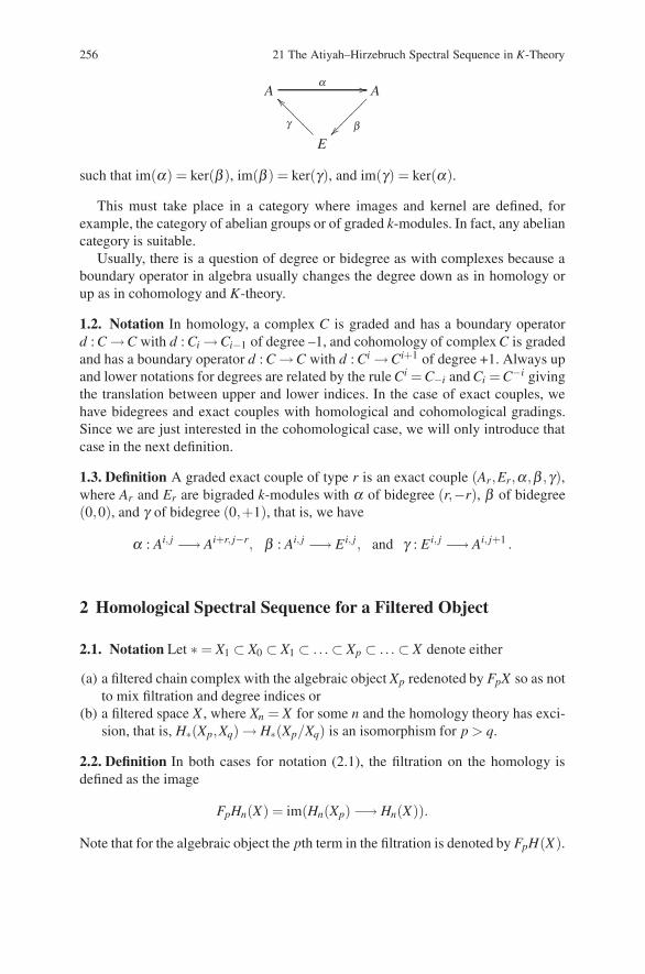
256 21 The Atiyah–Hirzebruch Spectral Sequence in K-Theory
Aα �� A
β �������
E
γ
!!�������
such that im(α) = ker(β ), im(β ) = ker(γ), and im(γ) = ker(α).
This must take place in a category where images and kernel are defined, forexample, the category of abelian groups or of graded k-modules. In fact, any abeliancategory is suitable.
Usually, there is a question of degree or bidegree as with complexes because aboundary operator in algebra usually changes the degree down as in homology orup as in cohomology and K-theory.
1.2. Notation In homology, a complex C is graded and has a boundary operatord : C →C with d : Ci →Ci−1 of degree –1, and cohomology of complex C is gradedand has a boundary operator d : C →C with d : Ci →Ci+1 of degree +1. Always upand lower notations for degrees are related by the rule Ci = C−i and Ci = C−i givingthe translation between upper and lower indices. In the case of exact couples, wehave bidegrees and exact couples with homological and cohomological gradings.Since we are just interested in the cohomological case, we will only introduce thatcase in the next definition.
1.3. Definition A graded exact couple of type r is an exact couple (Ar,Er,α,β ,γ),where Ar and Er are bigraded k-modules with α of bidegree (r,−r), β of bidegree(0,0), and γ of bidegree (0,+1), that is, we have
α : Ai, j −→ Ai+r, j−r, β : Ai, j −→ Ei, j, and γ : Ei, j −→ Ai, j+1 .
2 Homological Spectral Sequence for a Filtered Object
2.1. Notation Let ∗ = X1 ⊂ X0 ⊂ X1 ⊂ . . . ⊂ Xp ⊂ . . . ⊂ X denote either
(a) a filtered chain complex with the algebraic object Xp redenoted by FpX so as notto mix filtration and degree indices or
(b) a filtered space X , where Xn = X for some n and the homology theory has exci-sion, that is, H∗(Xp,Xq) → H∗(Xp/Xq) is an isomorphism for p > q.
2.2. Definition In both cases for notation (2.1), the filtration on the homology isdefined as the image
FpHn(X) = im(Hn(Xp) −→ Hn(X)).
Note that for the algebraic object the pth term in the filtration is denoted by FpH(X).
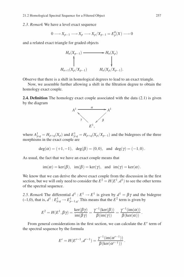
21.2 Homological Spectral Sequence for a Filtered Object 257
2.3. Remark We have a level exact sequence
0 −→ Xp−1 −→ Xp −→ Xp/Xp−1 = E0p(X) −→ 0
and a related exact triangle for graded objects
Hn(Xp−1) �� Hn(Xp)
��Hn+1(Xp/Xp−1)
��
Hn(Xp/Xp−1).
Observe that there is a shift in homological degrees to lead to an exact triangle.Now, we assemble further allowing a shift in the filtration degree to obtain the
homology exact couple.
2.4. Definition The homology exact couple associated with the data (2.1) is givenby the diagram
A1 α �� A1
��������
E1,
γ
""��������
where A1p,q = Hp+q(Xp) and E1
p,q = Hp+q(Xp/Xp−1) and the bidegrees of the threemorphisms in the exact couple are
deg(α) = (+1,−1), deg(β ) = (0,0), and deg(γ) = (−1,0) .
As usual, the fact that we have an exact couple means that
im(α) = ker(β ), im(β ) = ker(γ), and im(γ) = ker(α) .
We know that we can derive the above exact couple from the discussion in the firstsection, but we will only need to consider the E2 = H(E1,d1) to see the other termsof the spectral sequence.
2.5. Remark The differential d1 : E1 → E1 is given by d1 = βγ and the bidegree(–1,0), that is, d1 : E1
p,q → E1p−1,q. This means that the E2 term is given by
E2 = H(E1,βγ) =ker(βγ)im(βγ)
=γ−1(ker(β ))β (im(γ))
=γ−1(im(α))β (ker(α))
.
From general considerations in the first section, we can calculate the Er term ofthe spectral sequence by the formula
Er = H(Er−1,dr−1) =γ−1(im(αr−1))β (ker(αr−1))
.
258 21 The Atiyah–Hirzebruch Spectral Sequence in K-Theory
Now, we are interested in what might be called the elementary convergenceproperties of the above spectral sequence arising in homology. This means thatEr
p,q = Er+1p,q = Er+2
p,q = . . . for some r.
2.6. Finiteness Assumption Returning to the notation of (2.1), we assume that for(a) FpHn(X) = Xn for p > n or (b) Xm = X for some m which is interpreted as adimension. There we have Er
p,q = Er+1p,q = Er+2
p,q = . . . = E∞p,q by definition.The final step in this discussion is to calculate this limit or stable E∞ in terms of
FpH(X) of (2.2).
2.7. Theorem Let X be a filtered object satisfying the finiteness assumption of (2.6).Then
E∞p,q =FpHp+q(X)
Fp−1Hp+q(X)= E0
p,q(H(X)) .
Proof . We calculate for large r
E∞p,q = Erp,q =
γ−1(im(αr−1))β (ker(αr−1))
=im(β )
β (ker(Hp+q(Xp) → Hp+q(X)))
β ′−→ Hp+q(Xp)(ker(Hp+q(Xp) → Hp+q(X))+ (im(Hp+q(Xp−1) → Hp+q(Xp))
,
where β ′ is induced by β and is an isomorphism. This quotient is mapped isomor-phically by the induced map H(Xp) → H(X) giving
E∞p,q =im(Hp+q(Xp) → Hp+q(X))
im(Hp+q(Xp−1) → Hp+q(X))=
FpHp+q(X)Fp−1Hp+q(X)
= E0p,q(H(X)) .
3 K-Theory Exact Couples for a Filtered Space
Continuing with the notation (2.1)(b) for a filtered space, we apply the K-theoryfunctor to the triple of spaces Xp−1 ⊂Xp ⊂X and related reduced spaces Xp/Xp−1 →X/Xp−1 → X/Xp. What we define for the K functor K∗ can be carried out for anycohomology theory E∗.
3.1. Definition The filtration F pK∗(X) on the K-theory of X is defined by either theimage or kernel
F p(KmX) = im(Km(X/Xp−1) → Km(X)) = ker(Km(X) → Km(Xp−1)) .
3.2. Remark Observe that the factorization
X −→ X/Xp−1 −→ X/Xp
shows that F pKm(X) ⊃ F p+1Km(X) so that the filtration is decreasing.
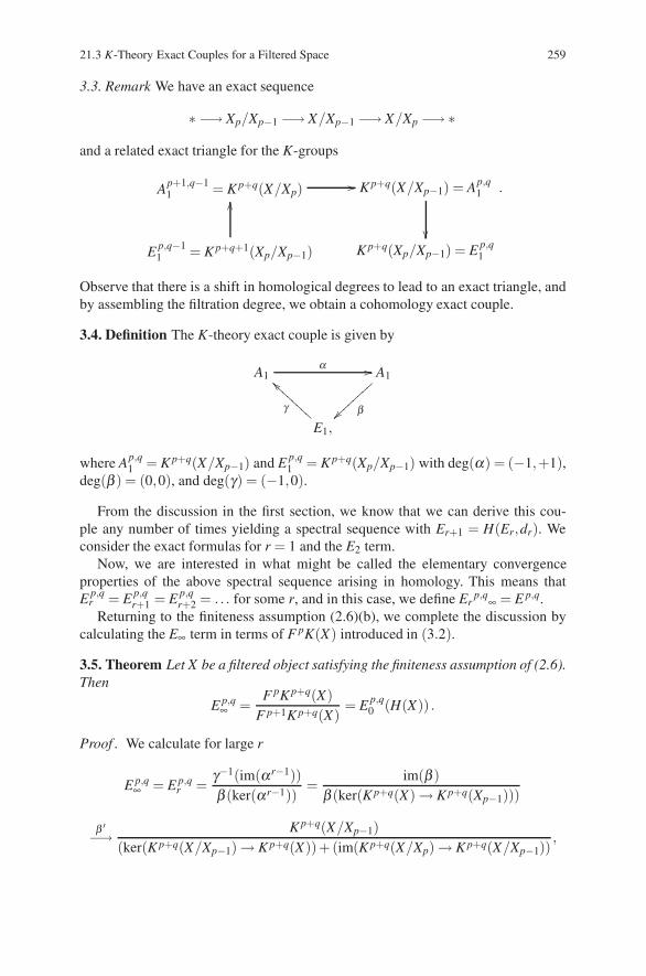
21.3 K-Theory Exact Couples for a Filtered Space 259
3.3. Remark We have an exact sequence
∗ −→ Xp/Xp−1 −→ X/Xp−1 −→ X/Xp −→ ∗
and a related exact triangle for the K-groups
Ap+1,q−11 = K p+q(X/Xp) �� K p+q(X/Xp−1) = Ap,q
1
��E p,q−1
1 = K p+q+1(Xp/Xp−1)
��
K p+q(Xp/Xp−1) = E p,q1
.
Observe that there is a shift in homological degrees to lead to an exact triangle, andby assembling the filtration degree, we obtain a cohomology exact couple.
3.4. Definition The K-theory exact couple is given by
A1α �� A1
�
E1,
γ
""!!!!!!!!
where Ap,q1 = K p+q(X/Xp−1) and E p,q
1 = K p+q(Xp/Xp−1) with deg(α) = (−1,+1),deg(β ) = (0,0), and deg(γ) = (−1,0).
From the discussion in the first section, we know that we can derive this cou-ple any number of times yielding a spectral sequence with Er+1 = H(Er,dr). Weconsider the exact formulas for r = 1 and the E2 term.
Now, we are interested in what might be called the elementary convergenceproperties of the above spectral sequence arising in homology. This means thatE p,q
r = E p,qr+1 = E p,q
r+2 = . . . for some r, and in this case, we define Erp,q∞ = E p,q.
Returning to the finiteness assumption (2.6)(b), we complete the discussion bycalculating the E∞ term in terms of F pK(X) introduced in (3.2).
3.5. Theorem Let X be a filtered object satisfying the finiteness assumption of (2.6).Then
E p,q∞ =
F pK p+q(X)F p+1K p+q(X)
= E p,q0 (H(X)) .
Proof . We calculate for large r
E p,q∞ = E p,q
r =γ−1(im(αr−1))β (ker(αr−1))
=im(β )
β (ker(K p+q(X) → K p+q(Xp−1)))
β ′−→ K p+q(X/Xp−1)(ker(K p+q(X/Xp−1) → K p+q(X))+ (im(K p+q(X/Xp) → K p+q(X/Xp−1))
,
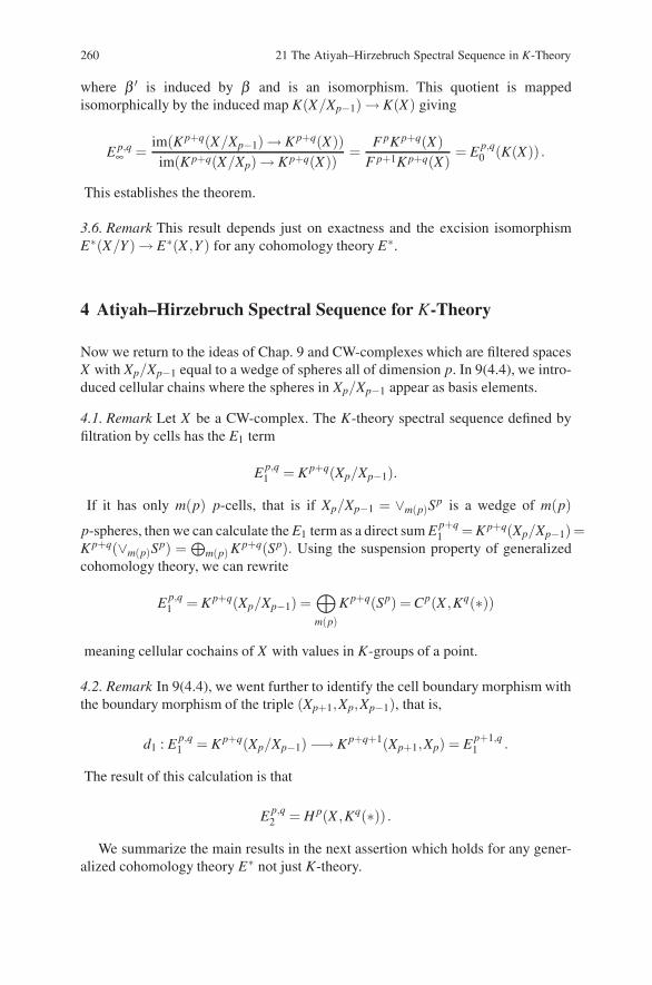
260 21 The Atiyah–Hirzebruch Spectral Sequence in K-Theory
where β ′ is induced by β and is an isomorphism. This quotient is mappedisomorphically by the induced map K(X/Xp−1) → K(X) giving
E p,q∞ =
im(K p+q(X/Xp−1) → K p+q(X))im(K p+q(X/Xp) → K p+q(X))
=F pK p+q(X)
F p+1K p+q(X)= E p,q
0 (K(X)) .
This establishes the theorem.
3.6. Remark This result depends just on exactness and the excision isomorphismE∗(X/Y ) → E∗(X ,Y ) for any cohomology theory E∗.
4 Atiyah–Hirzebruch Spectral Sequence for K-Theory
Now we return to the ideas of Chap. 9 and CW-complexes which are filtered spacesX with Xp/Xp−1 equal to a wedge of spheres all of dimension p. In 9(4.4), we intro-duced cellular chains where the spheres in Xp/Xp−1 appear as basis elements.
4.1. Remark Let X be a CW-complex. The K-theory spectral sequence defined byfiltration by cells has the E1 term
E p,q1 = K p+q(Xp/Xp−1).
If it has only m(p) p-cells, that is if Xp/Xp−1 = ∨m(p)Sp is a wedge of m(p)
p-spheres, then we can calculate the E1 term as a direct sum E p+q1 = K p+q(Xp/Xp−1)=
K p+q(∨m(p)Sp) =
⊕m(p) K p+q(Sp). Using the suspension property of generalized
cohomology theory, we can rewrite
E p,q1 = K p+q(Xp/Xp−1) =
⊕
m(p)
K p+q(Sp) = Cp(X ,Kq(∗))
meaning cellular cochains of X with values in K-groups of a point.
4.2. Remark In 9(4.4), we went further to identify the cell boundary morphism withthe boundary morphism of the triple (Xp+1,Xp,Xp−1), that is,
d1 : E p,q1 = K p+q(Xp/Xp−1) −→ K p+q+1(Xp+1,Xp) = E p+1,q
1 .
The result of this calculation is that
E p,q2 = H p(X ,Kq(∗)) .
We summarize the main results in the next assertion which holds for any gener-alized cohomology theory E∗ not just K-theory.
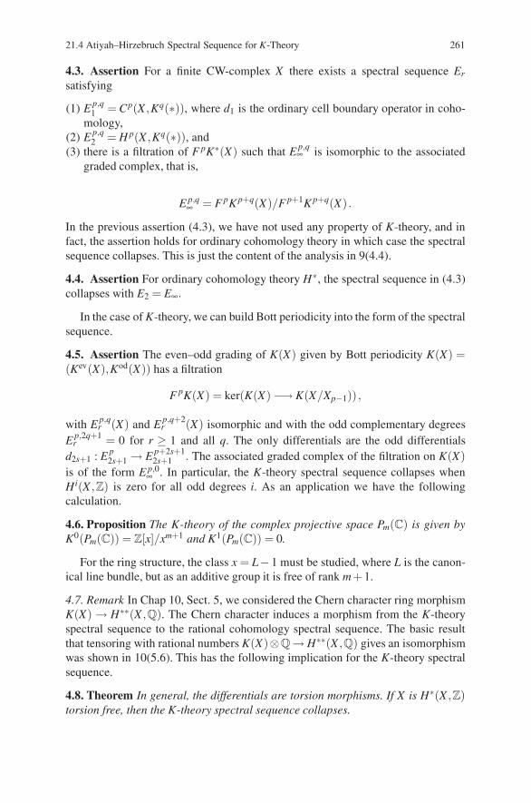
21.4 Atiyah–Hirzebruch Spectral Sequence for K-Theory 261
4.3. Assertion For a finite CW-complex X there exists a spectral sequence Er
satisfying
(1) E p,q1 = Cp(X ,Kq(∗)), where d1 is the ordinary cell boundary operator in coho-
mology,(2) E p,q
2 = H p(X ,Kq(∗)), and(3) there is a filtration of F pK∗(X) such that E p,q
∞ is isomorphic to the associatedgraded complex, that is,
E p,q∞ = F pK p+q(X)/F p+1K p+q(X) .
In the previous assertion (4.3), we have not used any property of K-theory, and infact, the assertion holds for ordinary cohomology theory in which case the spectralsequence collapses. This is just the content of the analysis in 9(4.4).
4.4. Assertion For ordinary cohomology theory H∗, the spectral sequence in (4.3)collapses with E2 = E∞.
In the case of K-theory, we can build Bott periodicity into the form of the spectralsequence.
4.5. Assertion The even–odd grading of K(X) given by Bott periodicity K(X) =(Kev(X),Kod(X)) has a filtration
F pK(X) = ker(K(X) −→ K(X/Xp−1)) ,
with E p,qr (X) and E p,q+2
r (X) isomorphic and with the odd complementary degreesE p,2q+1
r = 0 for r ≥ 1 and all q. The only differentials are the odd differentialsd2s+1 : E p
2s+1 → E p+2s+12s+1 . The associated graded complex of the filtration on K(X)
is of the form E p,0∞ . In particular, the K-theory spectral sequence collapses when
Hi(X ,Z) is zero for all odd degrees i. As an application we have the followingcalculation.
4.6. Proposition The K-theory of the complex projective space Pm(C) is given byK0(Pm(C)) = Z[x]/xm+1 and K1(Pm(C)) = 0.
For the ring structure, the class x = L−1 must be studied, where L is the canon-ical line bundle, but as an additive group it is free of rank m+ 1.
4.7. Remark In Chap 10, Sect. 5, we considered the Chern character ring morphismK(X) → H∗∗(X ,Q). The Chern character induces a morphism from the K-theoryspectral sequence to the rational cohomology spectral sequence. The basic resultthat tensoring with rational numbers K(X)⊗Q→ H∗∗(X ,Q) gives an isomorphismwas shown in 10(5.6). This has the following implication for the K-theory spectralsequence.
4.8. Theorem In general, the differentials are torsion morphisms. If X is H∗(X ,Z)torsion free, then the K-theory spectral sequence collapses.

262 21 The Atiyah–Hirzebruch Spectral Sequence in K-Theory
5 Formulas for Differentials
In (4.8), we saw that all differentials in the K-theory spectral sequence are torsionoperations, it is natural to look for formulas for the differentials which involve coho-mology operations with finite field coefficients. Besides the Bockstein operations,we expect the Steenrod operations. For p = 2, we used the Steenrod squaring opera-tions in 10(8.2) and 10(8.3) to give another formula for the Stiefel–Whitney classesin 10(8.5).
5.1. Remark In 10(8.6)(1) we had the formula
Sq2a+1 = Sq1Sq2a : Hi(X ,F2) −→ Hi+2a+1(X ,F2),
where Sq1 : Hi+2a(X ,F2) → Hi+2a+1(X ,F2) is the Bockstein morphism associatedwith the exact sequence of groups
0 −→ Z/2Z −→ Z/4Z −→ Z/2Z −→ 0 .
In turn, this exact sequence of groups is a quotient of the multiplication by two
exact sequence of groups 0 → Z2→ Z → Z/2Z = F2 → 0 so there is a factorization
of Sq1 = rδ , where
(1) δ : H j(X ,F2) → H j+1(X ,Z) is the Bockstein associated with multiplication bytwo exact sequence and
(2) r : Hq(X ,Z) → Hq(X ,F2) is the reduction mod 2-induced morphism in coho-mology. For an odd degree, we can define an integral-valued Steenrod square
Sq2a+1 = δSq2a : Hi(X ,F2) −→ Hi+2a+1(X ,Z) .
Finally, with the reduction mod 2 morphism, we have an integral operationSq2a+1 = δSq2ar : Hi(X ,Z) → Hi+2a+1(X ,Z) .
5.2. Remark The first two odd degree cases in the previous discussion are Sq1
and Sq3. The integral version of Sq1 is factorized by Hi(X ,Z) r→ Hi(X ,F2)δ→
Hi+1(X ,Z), where r is the reduction mod 2 and δ is the Bockstein. The integralversion of Sq3 is defined by Sq3 : Hi(X ,Z) → Hi+3(X ,Z) as in (5.1)(2). It was re-alized by Atiyah and Hirzebruch that this is the first nontrivial differential in thecomplex K-theory spectral sequence. This is always a torsion operation which iskilled by 2, and the differentials are torsion morphisms.
5.3. Proposition In the complex K-theory spectral sequence, the first terms are
E p,q3 = E p,q
2 ={
H p(X ,Z) for q even0 for q odd ,
and the first possibly nontrivial differential is
d3 = Sq3 : Hi(X ,Z) = E p,q3 −→ E p+3,q−2
3 = H p+3(X ,Z) .
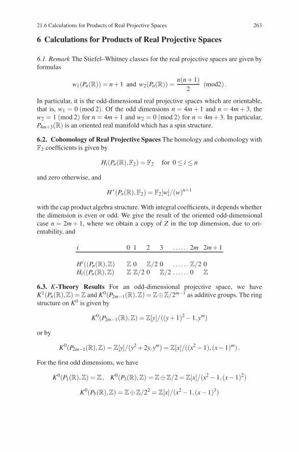
21.6 Calculations for Products of Real Projective Spaces 263
6 Calculations for Products of Real Projective Spaces
6.1. Remark The Stiefel–Whitney classes for the real projective spaces are given byformulas
w1(Pn(R)) = n + 1 and w2(Pn(R)) =n(n + 1)
2(mod2) .
In particular, it is the odd-dimensional real projective spaces which are orientable,that is, w1 = 0 (mod 2). Of the odd dimensions n = 4m + 1 and n = 4m + 3, thew2 = 1 (mod 2) for n = 4m + 1 and w2 = 0 (mod 2) for n = 4m + 3. In particular,P4m+3(R) is an oriented real manifold which has a spin structure.
6.2. Cohomology of Real Projective Spaces The homology and cohomology withF2 coefficients is given by
Hi(Pn(R),F2) = F2 for 0 ≤ i ≤ n
and zero otherwise, and
H∗(Pn(R),F2) = F2[w]/(w)n+1
with the cap product algebra structure. With integral coefficients, it depends whetherthe dimension is even or odd. We give the result of the oriented odd-dimensionalcase n = 2m + 1, where we obtain a copy of Z in the top dimension, due to ori-entability, and
i 0 1 2 3 . . . . . . 2m 2m+ 1
Hi((Pn(R),Z) Z 0 Z/2 0 . . . . . . Z/2 0Hi((Pn(R),Z) Z Z/2 0 Z/2 . . . . . . 0 Z
6.3. K-Theory Results For an odd-dimensional projective space, we haveK1(Pn(R),Z) = Z and K0(P2m−1(R),Z) = Z⊕Z/2m−1 as additive groups. The ringstructure on K0 is given by
K0(P2m−1(R),Z) = Z[y]/((y + 1)2 −1,ym)
or by
K0(P2m−1(R),Z) = Z[y]/(y2 + 2y,ym) = Z[x]/((x2 −1),(x−1)m) .
For the first odd dimensions, we have
K0(P1(R),Z) = Z , K0(P3(R),Z) = Z⊕Z/2 = Z[x]/(x2 −1,(x−1)2)
K0(P5(R),Z) = Z⊕Z/22 = Z[x]/(x2 −1,(x−1)3)
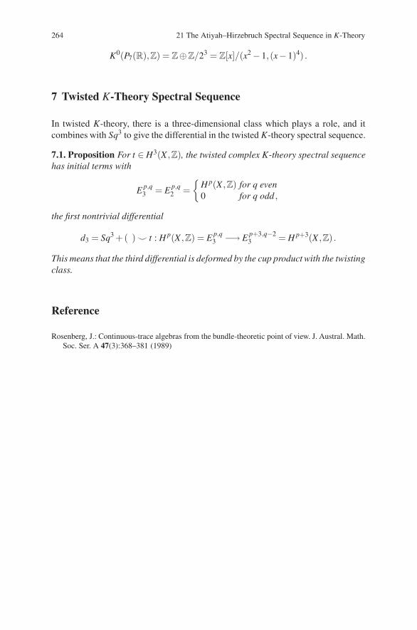
264 21 The Atiyah–Hirzebruch Spectral Sequence in K-Theory
K0(P7(R),Z) = Z⊕Z/23 = Z[x]/(x2 −1,(x−1)4) .
7 Twisted K-Theory Spectral Sequence
In twisted K-theory, there is a three-dimensional class which plays a role, and itcombines with Sq3 to give the differential in the twisted K-theory spectral sequence.
7.1. Proposition For t ∈ H3(X ,Z), the twisted complex K-theory spectral sequencehas initial terms with
E p,q3 = E p,q
2 ={
H p(X ,Z) for q even0 for q odd ,
the first nontrivial differential
d3 = Sq3 +( ) � t : H p(X ,Z) = E p,q3 −→ E p+3,q−2
3 = H p+3(X ,Z) .
This means that the third differential is deformed by the cup product with the twistingclass.
Reference
Rosenberg, J.: Continuous-trace algebras from the bundle-theoretic point of view. J. Austral. Math.Soc. Ser. A 47(3):368–381 (1989)
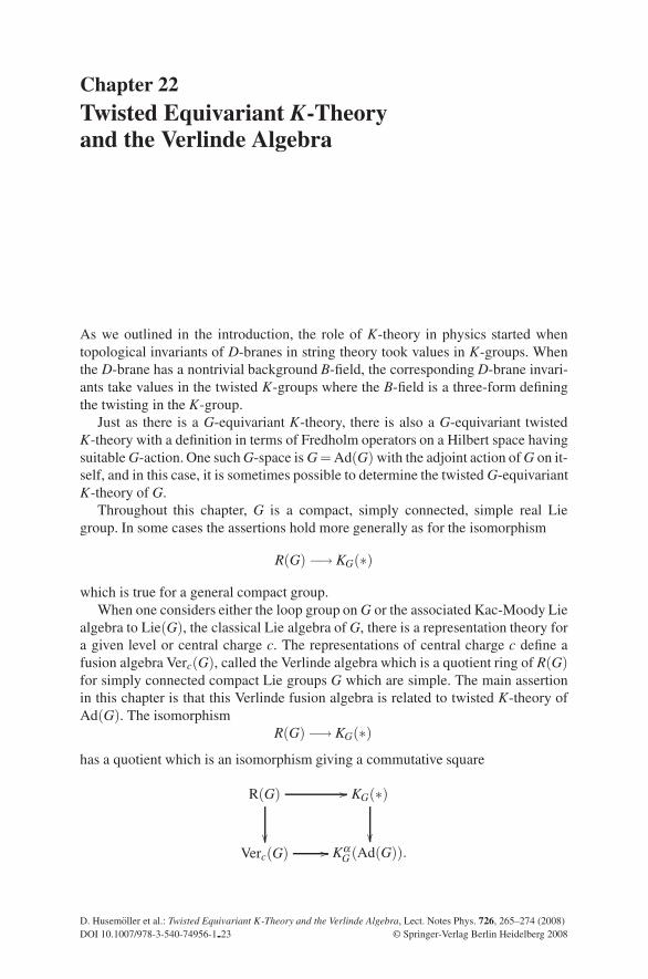
Chapter 22Twisted Equivariant K-Theoryand the Verlinde Algebra
As we outlined in the introduction, the role of K-theory in physics started whentopological invariants of D-branes in string theory took values in K-groups. Whenthe D-brane has a nontrivial background B-field, the corresponding D-brane invari-ants take values in the twisted K-groups where the B-field is a three-form definingthe twisting in the K-group.
Just as there is a G-equivariant K-theory, there is also a G-equivariant twistedK-theory with a definition in terms of Fredholm operators on a Hilbert space havingsuitable G-action. One such G-space is G = Ad(G) with the adjoint action of G on it-self, and in this case, it is sometimes possible to determine the twisted G-equivariantK-theory of G.
Throughout this chapter, G is a compact, simply connected, simple real Liegroup. In some cases the assertions hold more generally as for the isomorphism
R(G) −→ KG(∗)
which is true for a general compact group.When one considers either the loop group on G or the associated Kac-Moody Lie
algebra to Lie(G), the classical Lie algebra of G, there is a representation theory fora given level or central charge c. The representations of central charge c define afusion algebra Verc(G), called the Verlinde algebra which is a quotient ring of R(G)for simply connected compact Lie groups G which are simple. The main assertionin this chapter is that this Verlinde fusion algebra is related to twisted K-theory ofAd(G). The isomorphism
R(G) −→ KG(∗)has a quotient which is an isomorphism giving a commutative square
R(G) ��
��
KG(∗)
��Verc(G) �� Kα
G (Ad(G)).
D. Husemoller et al.: Twisted Equivariant K-Theory and the Verlinde Algebra, Lect. Notes Phys. 726, 265–274 (2008)DOI 10.1007/978-3-540-74956-1 23 © Springer-Verlag Berlin Heidelberg 2008
266 22 Twisted Equivariant K-Theory and the Verlinde Algebra
Some of the background material for this chapter is taken from lectures in Bonnof Gerd Faltings. Some of the calculations are taken from Gregory Moore whereone finds a physical explanation of the role of the third differential in the Atiyah–Hirzebruch spectral sequence for twisted K-theory which was discussed in the lastsection of the previous Chap. 23.
1 The Verlinde Algebra as the Quotientof the Representation Ring
There is a Verlinde algebra associated with a finite-dimensional simple complex Liealgebra and a level c. Recall that to a simple and simply connected compact realLie group G, we can form the complex Lie algebra g = Lie(G)⊗R C . This sets upa bijection between isomorphism classes of simple, simply connected compact realLie groups and the isomorphism classes of finite-dimensional simple complex Liealgebras. The representation rings are also isomorphic under this correspondence.The Verlinde algebra Verc(g) of representations of the loop algebra L(g) of level orcentral charge c with fusion product corresponds to the algebra of positive energyrepresentations of level c ≥ 0 of the loop Lie group L(G) with the fusion product(Witten (1993)).
1.1. Notation Let g be a Lie algebra over the complex numbers, and let A be anassociative algebra. The Lie algebra structure on g⊗A is given by the formula
[u⊗a,v⊗b] = [u,v]⊗ab or [au,bv] = ab [u,v]
for u,v ∈ g , a,b ∈ A . Two special cases are
g[t] = g⊗C C[t] and g[t,t−1] = g⊗C C[t,t−1],
where the second case g[t,t−1] is called the Lie algebra of algebraic loops withvalues in g.
The affine Kac–Moody algebra g corresponding to a given Lie algebra g refersto a basic extension of the Lie algebra g[t,t−1] of loops with values in g, see (1.4).We consider the construction in the following case.
1.2. Simple Lie Algebra Let g be a finite-dimensional simple Lie algebra over C.Choose a Cartan subalgebra h⊂ g whose action on g gives the root system. Choicesof positive root systems correspond to decompositions
g = h⊕n+⊕n−,
where n+ and n− are the nilpotent subalgebras of g with a basis of the positive andnegative roots, respectively. Let P be the weight lattice relative to h ⊂ g, and let P+
denote the positive weights relative to the Borel subalgebra b = h⊕n+ ⊂ g.On the simple Lie algebra g, we have an invariant bilinear form
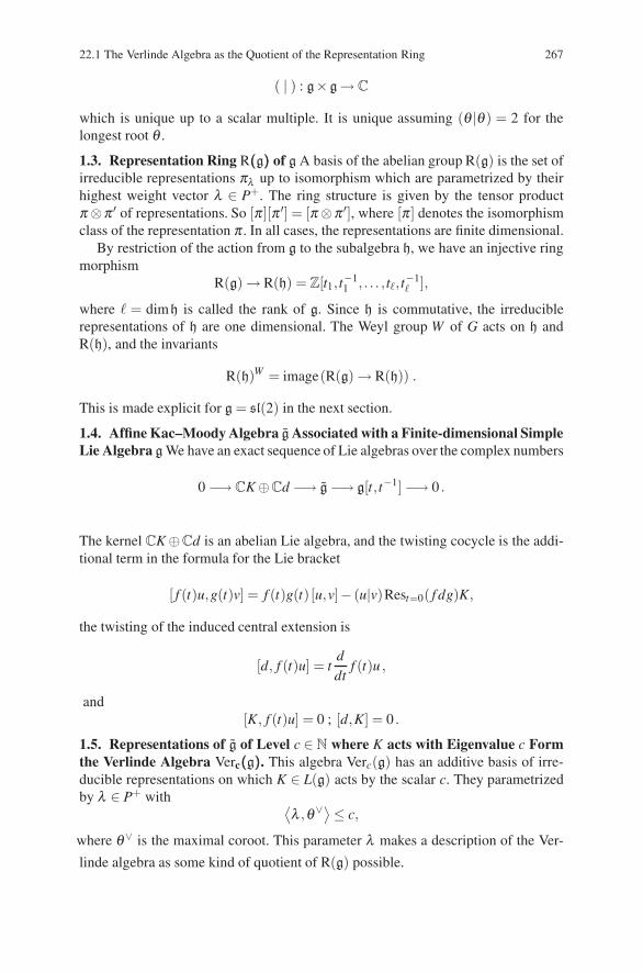
22.1 The Verlinde Algebra as the Quotient of the Representation Ring 267
( | ) : g×g→ C
which is unique up to a scalar multiple. It is unique assuming (θ |θ ) = 2 for thelongest root θ .
1.3. Representation Ring R(((g))) of g A basis of the abelian group R(g) is the set ofirreducible representations πλ up to isomorphism which are parametrized by theirhighest weight vector λ ∈ P+. The ring structure is given by the tensor productπ⊗π ′ of representations. So [π ][π ′] = [π⊗π ′], where [π ] denotes the isomorphismclass of the representation π . In all cases, the representations are finite dimensional.
By restriction of the action from g to the subalgebra h, we have an injective ringmorphism
R(g) → R(h) = Z[t1,t−11 , . . . ,t�, t
−1� ],
where � = dimh is called the rank of g. Since h is commutative, the irreduciblerepresentations of h are one dimensional. The Weyl group W of G acts on h andR(h), and the invariants
R(h)W = image(R(g) → R(h)) .
This is made explicit for g = sl(2) in the next section.
1.4. Affine Kac–Moody Algebra g Associated with a Finite-dimensional SimpleLie Algebra g We have an exact sequence of Lie algebras over the complex numbers
0 −→ CK ⊕Cd −→ g −→ g[t, t−1] −→ 0 .
The kernel CK ⊕Cd is an abelian Lie algebra, and the twisting cocycle is the addi-tional term in the formula for the Lie bracket
[ f (t)u,g(t)v] = f (t)g(t) [u,v]− (u|v)Rest=0( f dg)K,
the twisting of the induced central extension is
[d, f (t)u] = tddt
f (t)u ,
and[K, f (t)u] = 0 ; [d,K] = 0 .
1.5. Representations of g of Level c ∈ N where K acts with Eigenvalue c Formthe Verlinde Algebra Verc(((g))). This algebra Verc(g) has an additive basis of irre-ducible representations on which K ∈ L(g) acts by the scalar c. They parametrizedby λ ∈ P+ with ⟨
λ ,θ∨⟩≤ c,
where θ∨ is the maximal coroot. This parameter λ makes a description of the Ver-
linde algebra as some kind of quotient of R(g) possible.
268 22 Twisted Equivariant K-Theory and the Verlinde Algebra
1.6. Assertion The Verlinde algebra Verc(g) is the quotient ring of R(g) by anideal Ic. Additively, Verc(g) is a finitely generated free abelian group which is aGrothendieck group of central charge c representations of L(g).
The product on Verc(g) has an independent definition called the fusion product.In the quotient process, it comes from the tensor product of representations.
1.7. Generators of the Ideal Ic in R(g) To describe the generators of the ideal Ic,we denote the fundamental weights by Λi, where 0 ≤ i ≤ � = dimh. For an affineweight of level c,
Λ = λ + cΛ0 + ad
with λ ∈ P+ , a ∈ C, the action of an element w ∈ Waff in the affine Weyl group isgiven by the formula
w ·Λ = w · (λ + cΛ0 + ad) = w(λ ,c)+ cΛ0 +(a−dw(λ ,c))d,
where w(λ ,c) ∈ P+ and dw(λ ,c) ∈ Z. For a weight λ , the action takes the form
w ·λ = w · (λ +ρ)−ρ called shift action, where ρ = ∑�i=0Λi.
1.8. Basic Assertion The ideal Ic = ker(R(g) → Verc(g)) is generated by the ele-ments of the form
[λ ]− (−1)�(w)[w(λ ,c)] , λ ∈ P+ ,
where �(w) = length of w ∈ Waff . The basic reference is Sect. 2.2 in Feigin et al.(2002).
2 The Verlinde Algebra for SU(2) and sl(2)
As an example, we work out the Verlinde algebra Verc(SU(2)) = Verc(sl(2)) for thecompact group SU(2) and the corresponding Lie algebra Lie(SU(2))∼= sl(2) of twoby two complex matrices of trace zero. This algebra which we denote in this sectionby Verc is a quotient of the ring of characters R(SU(2)) of the group SU(2) or alsoof the Grothendieck ring R(sl(2)) of representations of the Lie algebra sl(2). Thestructure is very explicit since the rings R(SU(2)) ∼= R(sl(2)) are both isomorphicto the polynomial ring in one variable over Z, and the Verlinde algebra is a quotientalgebra which is of finite rank over Z.
2.1. Remark As a ring of characters, R(SU(2)) is determined by the monomorphismR(SU(2)) → R(U(1)) where the circle group T = U(1) is the maximal torus. Wehave R(U(1)) = Z[t,t−1] where t = e2π iθ , and hence, it is the ring of finite Fourierseries. The image of the monomorphism R(SU(2))→ R(U(1)) is the subring of thefinite Fourier series f (t) with the property that f (t) = f ( 1
t ).
2.2. Lemma A finite Fourier series f (t) satisfies f (t) = f ( 1t ) if and only if f (t) =
g(t + 1t ), where g(x) ∈ Z[x] is a polynomial.
22.2 The Verlinde Algebra for SU(2) and sl(2) 269
The proof results from the relation
tn+1 + t−n−1 = (t + t−1)(tn + t−n)− (tn−1 + t−n+1) ,
which generates the inductive procedure.
2.3. Proposition As a subring of R(U(1)) = Z[t,t−1], the ring R(SU(2)) is the poly-nomial ring Z[x], where x = t + t−1.
2.4. Remark The irreducible representations of the Lie group SU(2) or of the Lie al-gebra sl(2) are parametrized by natural numbers and are denoted by V (n) , n ∈ N ,where dimCV (n) = n + 1 . Under the natural injective ring homomorphismR(sl(2)) → R(h) = Z[t,t−1], the class of V (n) becomes the polynomial
[n](t) = tn + tn−2 + . . .+ t−n+2 + t−n .
In R(sl(2)), we denote the element representing the irreducible V (n) also by [n].For example, the first V (0) is the trivial one-dimensional representation, V (1) is
the standard two-dimensional matrix representation, and V (2) is thethree-dimensional adjoint representation of sl(2) on itself. We denote that V (n) = 0for n < 0.
2.5. Proposition For the multiplicative structure on the irreducible representations,we can calculate with the Clebsch–Gordan inductive rule
V (n)⊗V(m) = V (m+ n)⊕V(n−1)⊗V(m−1)
the formula
V (n)⊗V(m) = V (m+ n)⊕ . . .⊕V(n−m) for n ≥ m .
For the proof, we consider again the embedding if R(sl(2)) as a subring of R(h) =Z[t, t−1]. The image of the class of V (n) is given by tn + tn−2 + . . .+ t−n+2 + t−n .Now,
(tn + tn−2 + . . .+ t−n+2 + t−n)(tm + tm−2 + . . .+ t−m+2 + t−m) =tn+m + tn+m−2 + . . .+ t−n+m+2 + t−n+m
tn+m−2 + tn+m−4 . . .+ t−n+m + t−n+m−2
tn+m−4 . . .+ t−n+m + t−n+m−2 + t−n+m−4
. . . . . . . . .t−n+m + t−n+m−2 + . . .+ t−n−m+2 + t−n−m
which after reordering and summing the terms gives
(tn+m + tn+m−2 + . . .+ t−n−m+2 + t−n−m)+(tn−1 + . . .+ t−n+1)(tm−1 + . . .+ t−m+1)
which is the desired formula.
2.6. Example The first special cases are V (n)⊗V (0) = V (n) and V (n)⊗V (1) =V (n + 1)⊕V(n−1) which are formally the same as the character formula
270 22 Twisted Equivariant K-Theory and the Verlinde Algebra
(t + t−1)(tn + tn−2 + . . .+ t−n)=(tn+1 + tn−1 + · · ·+ t−n−1)+(tn−1 + tn−3 + · · ·+ t−n+1)
used in describing R(SU(2)). In particular, V (2)⊗V(1) =V (3)⊕V(1) is the adjointaction on the two by two matrices.
2.7. Proposition The Grothendieck ring R(sl(2)) of finite-dimensional represen-tations is the polynomial ring Z[x], where x is the class of the standard two-dimensional representation V (1) of sl(2). It is the polynomial ring in one variable xover the integers. As an abelian group, R(sl(2)) is of countable rank having a basisgiven by the isomorphism classes [V (n)] of irreducible representations.
To describe the Verlinde algebra as a quotient ring
Z[t,t−1] ⊃ R(sl(2)) −→ Verc(sl(2))
of the representation ring R(sl(2)), we use the following prescription.Associated with each c ∈ N, we have the reflection σc of the integers Z given by
σc(n) = 2c− n around c and fixing c. The conditions of (1.8) for the generators ofthe ideal Ic in the case of Verc(sl(2)) take the form
[c + 1]∈ Ic and [n]+ [2c + 2−n]∈ Ic for 0 < n < c + 1 .
The quotient π : R(sl(2)) → Verc(sl(2)), which depends on the central charge c,is defined by the two conditions:
(1) π(V (c + 1)) = 0 and(2) π(V (n)+V(2c + 2−n)) = 0 for 0 < n < c + 1.
2.8. Proposition The ideal Ic in R(sl(2)) is a principal ideal generated by [c + 1]the class of the irreducible representation of dimension c + 2.
To see that one relation is sufficient, we have as given [c+1]∈ Ic and the relation
V (m)⊗V(1) = V (m+ 1)⊕V(m−1)
for all m ∈ N shows that for m = c+1 that we have [n]+ [σc(n)] ∈ Ic for n = c, andby an elementary descending induction also for 0 < n < c + 1. Hence, the kernel isa principal ideal generated by [c + 1].
The following theorem can be worked out from the above description, see thearticle of Faltings (1995), on the Verlinde formula.
2.9. Theorem The algebra Verc(sl(2)) is isomorphic to Z[x]/( fc(x)), where
fc(x) = ∏ζ 2c+2=1,ζ =±1/inverse
(x− (ζ +
1ζ
))
.
22.3 The G-Bundles on G with the Adjoint G–Action 271
In this formula, ζ and 1ζ are grouped together in one term giving a total of c factors.
In particular, the algebra has degree c and tensored with Q is a product of totallyreal fields and CM fields. Another form of fc is
fc(x) =c
∏m=1
(x−(
exp
(m
2c + 22π i
)+ exp
(− m
2c + 22π i
)))
=c
∏m=1
(x−2cos
(m
2c + 22π))
.
To determine the multiplicative structure of the Verlinde algebrasVerc(sl(2)) = Verc(SU(2)), we recall the character of the irreducible representa-tion V (n) on R(U(1)).
2.10. Remark For g ∈ R[t, t−1
], where R is a commutative ring, we have used the
fact that g(t) = g( 1t ) if and only if there exists f (x) ∈ R [x] with
g(t) = f (t +1t) .
Also g(t) = tm + . . . + t−m if and only if f is monic, f (x) = xm+ lower terms. Ifu ∈ R∗, then
g(u) = 0 if and only if f
(u +
1u
)= 0 .
Applying this to tc + tc−2 + . . .+ t−c which appears in the factorization
tc+1 − tc−1 = (t − t−1)(tc + tc−2 + . . .+ t−c) ,
we see for ζ 2c+2 = 1, ζ 2 = 1, that
0 = g(ζ ), where g(t) = tc + tc−2 + . . .+ t−c .
Each ζ + 1ζ is one of the c different roots of the monic polynomial fc(x), hence the
above formula for fc(x).
3 The G-Bundles on G with the Adjoint G–Action
To see that G×G modulo G with the diagonal action is a G-space isomorphic to Gwith the adjoint action, we make the following remarks.
3.1. Definition The left-diagonal action of G on G×G is given by
G× (G×G)→ G×G is s(x,y) = (sx,sy)
and the right-diagonal action of G on G×G is given by
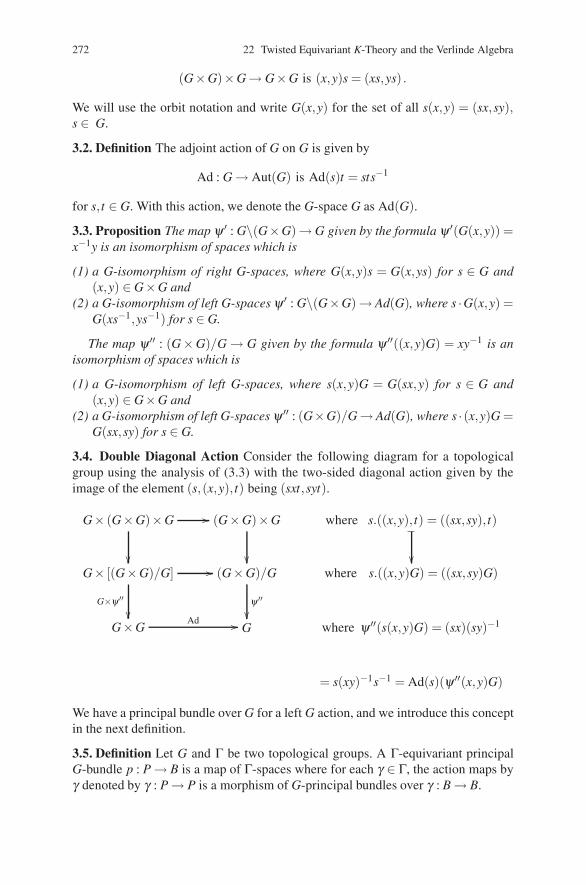
272 22 Twisted Equivariant K-Theory and the Verlinde Algebra
(G×G)×G → G×G is (x,y)s = (xs,ys) .
We will use the orbit notation and write G(x,y) for the set of all s(x,y) = (sx,sy),s ∈ G.
3.2. Definition The adjoint action of G on G is given by
Ad : G → Aut(G) is Ad(s)t = sts−1
for s,t ∈ G. With this action, we denote the G-space G as Ad(G).
3.3. Proposition The map ψ ′ : G\(G×G)→ G given by the formula ψ ′(G(x,y)) =x−1y is an isomorphism of spaces which is
(1) a G-isomorphism of right G-spaces, where G(x,y)s = G(x,ys) for s ∈ G and(x,y) ∈ G×G and
(2) a G-isomorphism of left G-spaces ψ ′ : G\(G×G)→ Ad(G), where s ·G(x,y) =G(xs−1,ys−1) for s ∈ G.
The map ψ ′′ : (G×G)/G → G given by the formula ψ ′′((x,y)G) = xy−1 is anisomorphism of spaces which is
(1) a G-isomorphism of left G-spaces, where s(x,y)G = G(sx,y) for s ∈ G and(x,y) ∈ G×G and
(2) a G-isomorphism of left G-spaces ψ ′′ : (G×G)/G → Ad(G), where s · (x,y)G =G(sx,sy) for s ∈ G.
3.4. Double Diagonal Action Consider the following diagram for a topologicalgroup using the analysis of (3.3) with the two-sided diagonal action given by theimage of the element (s,(x,y),t) being (sxt,syt).
G× (G×G)×G ��
��
(G×G)×G
��
where s.((x,y),t) = ((sx,sy), t)"
��G× [(G×G)/G] ��
G×ψ ′′
��
(G×G)/G
ψ ′′
��
where s.((x,y)G) = ((sx,sy)G)
G×GAd �� G where ψ ′′(s(x,y)G) = (sx)(sy)−1
= s(xy)−1s−1 = Ad(s)(ψ ′′(x,y)G)
We have a principal bundle over G for a left G action, and we introduce this conceptin the next definition.
3.5. Definition Let G and Γ be two topological groups. A Γ-equivariant principalG-bundle p : P → B is a map of Γ-spaces where for each γ ∈ Γ, the action maps byγ denoted by γ : P → P is a morphism of G-principal bundles over γ : B → B.
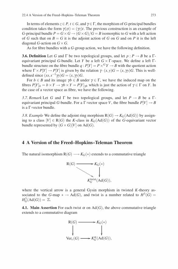
22.4 A Version of the Freed–Hopkins–Teleman Theorem 273
In terms of elements z∈P, t ∈G, and γ ∈Γ, the morphism of G-principal bundlescondition takes the form γ(zt) = (γz)t. The previous construction is an example ofG-principal bundle P = G×G → (G×G)/G = B isomorphic to G with a left actionof G such that on B = G it is the adjoint action of G on G and on P it is the leftdiagonal G-action on G×G.
As for fibre bundles with a G-group action, we have the following definition.
3.6. Definition Let G and Γ be two topological groups, and let p : P → B be a Γ-equivariant principal G-bundle. Let Y be a left G× Γ-space. We define a left Γ-bundle structure on the fibre bundle q : P[Y ] = P×G Y → B with the quotient actionwhere Γ×P[Y ] → P[Y ] is given by the relation γ · (x,y)G = (x,γy)G. This is well-defined since (xs,s−1γy)G = (x,γy)G.
For b ∈ B and its image γb ∈ B under γ ∈ Γ, we have the induced map on thefibres P[Y ]b = b×Y → γb×Y = P[Y ]γb which is just the action of γ ∈ Γ on Y . Inthe case of a vector space as fibre, we have the following.
3.7. Remark Let G and Γ be two topological groups, and let P → B be a Γ-equivariant principal G-bundle. For a Γ-vector space V , the fibre bundle P[V ] → Bis a Γ-vector bundle.
3.8. Example We define the adjoint ring morphism R(G) → KG(Ad(G)) by assign-ing to a class [V ] ∈ R(G) the K-class in KG(Ad(G)) of the G-equivariant vectorbundle represented by (G×G)[V ] on Ad(G).
4 A Version of the Freed–Hopkins–Teleman Theorem
The natural isomorphism R(G) −→ KG(∗) extends to a commutative triangle
R(G) ��
�������
�����
KG(∗)
��Ktwist
G (Ad(G)),
where the vertical arrow is a general Gysin morphism in twisted K-theory as-sociated to the G-map ∗ → Ad(G), and twist is a number related to H3(G) =H3
G(Ad(G)) = Z.
4.1. Main Assertion For each twist α on Ad(G), the above commutative triangleextends to a commutative diagram
R(G) ��
��
KG(∗)
��Verc(G) �� Kα
G (Ad(G)),
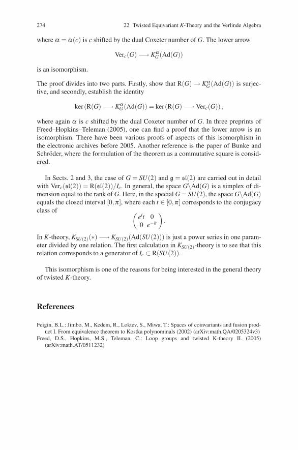
274 22 Twisted Equivariant K-Theory and the Verlinde Algebra
where α = α(c) is c shifted by the dual Coxeter number of G. The lower arrow
Verc(G) −→ KαG (Ad(G))
is an isomorphism.
The proof divides into two parts. Firstly, show that R(G) → KαG (Ad(G)) is surjec-
tive, and secondly, establish the identity
ker(R(G) −→ KαG (Ad(G)) = ker(R(G) −→ Verc(G)) ,
where again α is c shifted by the dual Coxeter number of G. In three preprints ofFreed–Hopkins–Teleman (2005), one can find a proof that the lower arrow is anisomorphism. There have been various proofs of aspects of this isomorphism inthe electronic archives before 2005. Another reference is the paper of Bunke andSchroder, where the formulation of the theorem as a commutative square is consid-ered.
In Sects. 2 and 3, the case of G = SU(2) and g = sl(2) are carried out in detailwith Verc(sl(2)) = R(sl(2))/Ic. In general, the space G\Ad(G) is a simplex of di-mension equal to the rank of G. Here, in the special G = SU(2), the space G\Ad(G)equals the closed interval [0,π ], where each t ∈ [0,π ] corresponds to the conjugacyclass of (
eit 00 e−it
).
In K-theory, KSU(2)(∗) −→ KSU(2)(Ad(SU(2))) is just a power series in one param-eter divided by one relation. The first calculation in KSU(2)-theory is to see that thisrelation corresponds to a generator of Ic ⊂ R(SU(2)).
This isomorphism is one of the reasons for being interested in the general theoryof twisted K-theory.
References
Feigin, B.L.: Jimbo, M., Kedem, R., Loktev, S., Miwa, T.: Spaces of coinvariants and fusion prod-uct I. From equivalence theorem to Kostka polynominals (2002) (arXiv:math.QA/0205324v3)
Freed, D.S., Hopkins, M.S., Teleman, C.: Loop groups and twisted K-theory II. (2005)(arXiv:math.AT/0511232)
Part VGerbes and the Three Dimensional
Integral Cohomology Classes
In Part IV, we considered algebra bundle over a space B which has a characteristicclass in H3(B,Z). In this part, we introduce other geometric objects giving rise to athree-dimensional integral characteristic cohomology class. For some background,we return to the local coordinate condition (1) in 5(4.3), giving a 1-cocycle,
gi, j(b)g j,k(b)gk,i(b) = 1 for b ∈Ui ∩Uj ∩Uk , (4.1)
and extend it to a condition of the form
gi, j(b)g j,k(b)gk,i(b) = λi, j,k(b) for b ∈Ui ∩Uj ∩Uk (4.2)
where λi, j,k(b) for b ∈ Ui ∩Uj ∩Uk is a higher level of twisting in terms of theextra data of the 2-cocycle λi, j,k(b) for b ∈Ui ∩Uj ∩Uk. When this is formulated inmore intrinsic terms, it comes under the name of “gerbe,” which is an object gluedtogether with by condition (2). If the condition (2) can be reduced to that of (1),then we have again a bundle.
The reason that algebra bundles lead to twisting conditions on change of coor-dinates in vector bundles is that the functions gi, j(b) relating two trivial algebrabundles over Ui ∩Uj have values in PGL, while for vector bundles, the change ofcoordinates has values in GL. When the local change of coordinate functions gi, j(b)in PGL satisfying (1) above are lifted to αi, j(b) ∈ GL, the condition (1) takes thetwisted form
αi, j(b)α j,k(b)αk,i(b) = λi, j,k(b) for b ∈Ui ∩Uj ∩Uk, (4.3)
where λi, j,k(b) for b ∈Ui ∩Uj ∩Uk has its values in GL(1) = ker(GL → PGL). Thisis an example of the higher level twisting in terms of the extra data of the GL(1) val-ued 2-cocycle λi, j,k(b) for b∈Ui∩Uj∩Uk. The characteristic class α(A)∈H3(X ,Z)is the image under the connecting morphism of the class [λi, j,k] ∈ H2(X ,GL(1))coming from the long exact sequence associated to the exponential exact sequencee(t) = exp(2π it)
0 −→ Z −→ C −→ C∗ −→ 1 .
With gerbes, we have other examples of this lifting to a twisted class as in thecondition (3).
In the three chapters of this part, we illustrate this process from (1) to (3) withincreasing generality. Finally, arriving at Grothendieck’s approach in Chap. 27 withan introduction to stacks and gerbes.
All the topics in this Part V would merit a more extensive development, but wehave included this sketch as an introduction.
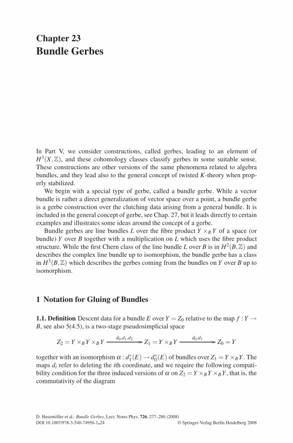
Chapter 23Bundle Gerbes
In Part V, we consider constructions, called gerbes, leading to an element ofH3(X ,Z), and these cohomology classes classify gerbes in some suitable sense.These constructions are other versions of the same phenomena related to algebrabundles, and they lead also to the general concept of twisted K-theory when prop-erly stabilized.
We begin with a special type of gerbe, called a bundle gerbe. While a vectorbundle is rather a direct generalization of vector space over a point, a bundle gerbeis a gerbe construction over the clutching data arising from a general bundle. It isincluded in the general concept of gerbe, see Chap. 27, but it leads directly to certainexamples and illustrates some ideas around the concept of a gerbe.
Bundle gerbes are line bundles L over the fibre product Y ×B Y of a space (orbundle) Y over B together with a multiplication on L which uses the fibre productstructure. While the first Chern class of the line bundle L over B is in H2(B,Z) anddescribes the complex line bundle up to isomorphism, the bundle gerbe has a classin H3(B,Z) which describes the gerbes coming from the bundles on Y over B up toisomorphism.
1 Notation for Gluing of Bundles
1.1. Definition Descent data for a bundle E over Y = Z0 relative to the map f : Y →B, see also 5(4.5), is a two-stage pseudosimplicial space
Z2 = Y ×B Y ×B Yd0,d1,d2 �� Z1 = Y ×B Y
d0,d1 �� Z0 = Y
together with an isomorphism α : d∗1(E)→ d∗
0(E) of bundles over Z1 = Y ×B Y . Themaps di refer to deleting the ith coordinate, and we require the following compati-bility condition for the three induced versions of α on Z2 = Y ×B Y ×B Y , that is, thecommutativity of the diagram
D. Husemoller et al.: Bundle Gerbes, Lect. Notes Phys. 726, 277–286 (2008)DOI 10.1007/978-3-540-74956-1 24 © Springer-Verlag Berlin Heidelberg 2008
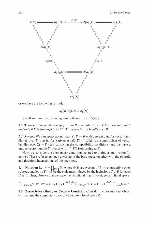
278 23 Bundle Gerbes
pr∗0(E) d∗1d∗
1(E) d∗1d∗
0(E) pr∗2(E)
d∗2d∗
1(E) d∗0d∗
0(E)
d∗2d∗
0(E) d∗0d∗
1(E)
pr∗1(E)
d∗1(α)��
��������������
��������������
��������������
��������������
��������������
��������������
��������������
��������������
d∗2(α)
����������������
d∗0(α)
����������������
��������������
��������������
��������������
��������������
or we have the following formula
d∗0(α)d∗
2(α) = d∗1(α).
Recall we have the following gluing theorem as in 5(4.6).
1.2. Theorem For an etale map f : Y → B, a bundle E over Y has descent data ifand only if E is isomorphic to f−1(V ), where V is a bundle over B.
1.3. Remark We can speak about maps f : Y → B with descent data for vector bun-dles E over B, that is, for a given α : d∗
1(E) → d∗0(E) an isomorphism of vector
bundles over Z1 = Y ×B Y satisfying the compatibility conditions, and we have aunique vector bundle E ′ over B with f ∗(E ′) isomorphic to E .
Now, we consider the elementary conditions related to gluing as motivation forgerbes. These refer to an open covering of the base space together with the twofoldand threefold intersections of the open sets.
1.4. Notation Let Y =∐
U∈ΦU , where Φ is a covering of B by contractible opensubsets, and let π : Y → B be the etale map induced by the inclusions U ⊂ B for eachU ∈Φ. Then, observe that we have the simplicial maps two-stage simplicial space
∐U,V,W∈ΦU ∩V ∩W = Y ×B Y ×B Y
d0 ,d1 ,d2−→ ∐U,V∈ΦU ∩V = Y ×B Y
d0,d1−→∐U∈ΦU =Y .
1.5. Zero-Order Gluing or Cocycle Condition Consider the cosimplicial objectby mapping the simplicial space of (1.4) into a fixed space Z
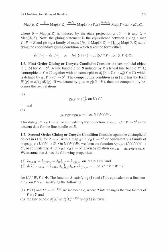
23.1 Notation for Gluing of Bundles 279
Map(B,Z) δ �� Map(Y,Z)δ0,δ1 �� Map(Y×BY,Z)
δ0,δ1,δ2�� Map(Y×BY ×BY,Z),
where δ = Map(π ,Z) is induced by the etale projection π : Y → B and δi =Map(di,Z). Now, the gluing statement is the equivalence between giving a mapf : B → Z and giving a family of maps ( fU ) ∈ Map(Y,Z) =∏U∈ΦMap(U,Z) satis-fying the coboundary gluing condition which takes the form either
δ0( fU ) = δ1( fU ) or fU |(U ∩V ) = fV |(U ∩V) for U,V ∈Φ .
1.6. First-Order Gluing or Cocycle Condition Consider the cosimplicial objectin (1.5) for Z = S1. A line bundle L on B induces by π a trivial line bundle π∗(L)isomorphic to Y ×C together with an isomorphism d∗
1(Y ×C) → d∗0(Y ×C) which
is defined by g : Y ×B Y → S1. The compatibility condition as in (1.1) has the formδ ∗1 (g) = δ ∗0 (g)δ ∗2 (g). If we denote by gU,V = g|(U ∩V ), then the compatibility be-comes the two relations
(a)gU,V = g−1
V,U on U ∩V
and(b)
gU,V gV,W gW,U = 1 on U ∩V ∩W .
This data g : Y ×X Y → S1 or equivalently the collection of gU,V : U ∩V → S1 is thedescent data for the line bundle on B.
1.7. Second-Order Gluing or Cocycle Condition Consider again the cosimplicialobject in (1.5) for Z = S1 with a map g : Y ×B Y → S1 or equivalently a family ofmaps gU,V : U ∩V → S1. On U ∩V ∩W , we form the function λU,V,W : U ∩V ∩W →S1, or equivalently, λ : Y ×B Y ×B Y → S1 given by relation λU,V,W = gU,V gV,W gW,U .We assume that λ has the following properties:
(1) λU,V,W = λ−1U,W,V = λ−1
W,V,U = λ−1V,U,W on U ∩V ∩W and
(2) δ (λ )U,V,W,T = λV,W,Tλ−1U,W,TλU,V,Tλ−1
U,V,W = 1 on U ∩V ∩W ∩T
for U,V,W,T ∈Φ. The function λ satisfying (1) and (2) is equivalent to a line bun-dle L on Y ×B Y satisfying the following:
(a) τ∗(L) and L∨ = L(−1)⊗ are isomorphic, where τ interchanges the two factors ofY ×B Y and
(b) the line bundle d∗0(L)⊗d∗
1(L)(−1)⊗⊗d∗2(L) is trivial.
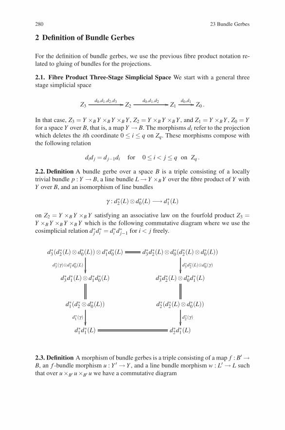
280 23 Bundle Gerbes
2 Definition of Bundle Gerbes
For the definition of bundle gerbes, we use the previous fibre product notation re-lated to gluing of bundles for the projections.
2.1. Fibre Product Three-Stage Simplicial Space We start with a general threestage simplicial space
Z3d0,d1,d2,d3 �� Z2
d0,d1,d2 �� Z1d0,d1 �� Z0 .
In that case, Z3 = Y ×B Y ×B Y ×B Y , Z2 = Y ×B Y ×B Y , and Z1 = Y ×B Y , Z0 = Yfor a space Y over B, that is, a map Y → B. The morphisms di refer to the projectionwhich deletes the ith coordinate 0 ≤ i ≤ q on Zq. These morphisms compose withthe following relation
did j = d j−1di for 0 ≤ i < j ≤ q on Zq .
2.2. Definition A bundle gerbe over a space B is a triple consisting of a locallytrivial bundle p : Y → B, a line bundle L → Y ×B Y over the fibre product of Y withY over B, and an isomorphism of line bundles
γ : d∗2(L)⊗d∗
0(L) −→ d∗1(L)
on Z2 = Y ×B Y ×B Y satisfying an associative law on the fourfold product Z3 =Y ×B Y ×B Y ×B Y which is the following commutative diagram where we use thecosimplicial relation d∗
j d∗i = d∗
i d∗j−1 for i < j freely.
d∗3(d∗
2(L)⊗d∗0(L))⊗d∗
1d∗0(L)
d∗3(γ)⊗d∗1 d∗0(L)��
d∗3d∗
2(L)⊗d∗0(d
∗2(L)⊗d∗
0(L))
d∗3 d∗2(L)⊗d∗0(γ)��
d∗3d∗
1(L)⊗d∗1d∗
0(L) d∗3d∗
2(L)⊗d∗0d∗
1(L)
d∗1(d
∗2 ⊗d∗
0(L))
d∗1(γ)��
d∗2(d∗
2(L)⊗d∗0(L))
d∗2(γ)��
d∗1d∗
1(L) d∗2d∗
1(L)
2.3. Definition A morphism of bundle gerbes is a triple consisting of a map f : B′ →B, an f -bundle morphism u : Y ′ → Y , and a line bundle morphism w : L′ → L suchthat over u×B′ u×B′ u we have a commutative diagram
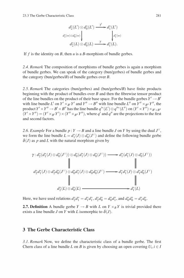
23.3 The Gerbe Characteristic Class 281
d∗2(L′)⊗d∗
0(L′)
γ ′ ��
d∗2(w)⊗d∗0(w)��
d∗1(L
′)
d∗1(w)��
d∗2(L)⊗d∗
0(L)γ �� d∗
1(L).
If f is the identity on B, then u is a B-morphism of bundle gerbes.
2.4. Remark The composition of morphisms of bundle gerbes is again a morphismof bundle gerbes. We can speak of the category (bun/gerbes) of bundle gerbes andthe category (bun/gerbes/B) of bundle gerbes over B.
2.5. Remark The categories (bun/gerbes) and (bun/gerbes/B) have finite productsbeginning with the product of bundles over B and then the fibrewise tensor productof the line bundles on the product of their base space. For the bundle gerbes Y ′ → B′with line bundle L′ on Y ′ ×B′ Y ′ and Y ′′ → B′′ with line bundle L′′ on Y ′′ ×B′′ Y ′′, theproduct Y ′×Y ′′ → B′×B′′ has the line bundle q′∗(L′)⊗q′′∗(L′′) on (Y ′ ×Y ′′)×B′×B′′(Y ′×Y ′′) = (Y ′×B′Y ′)×(Y ′′×B′′ Y ′′), where q′ and q′′ are the projections to the firstand second factors.
2.6. Example For a bundle p : Y → B and a line bundle J on Y by using the dual J∨,we form the line bundle L = d∗
1(J)⊗d∗0(J
∨) and define the following bundle gerbeδ (J) as p and L with the natural morphism given by
γ : d∗2(d
∗1(J)⊗d∗
0(J∨))⊗d∗
0(d∗1(J)⊗d∗
0(J∨)) �� d∗
1(d∗1(J)⊗d∗
0(J∨))
d∗2d∗
1(J)⊗d∗2d∗
0(J∨)⊗d∗
0d∗1(J)⊗d∗
0d∗0(J∨) �� d∗
1d∗1(J)⊗d∗
1d∗0(J∨)
d∗2(L)⊗d∗
0(L) �� d∗1(L)
Here, we have used relations d∗2d∗
1 = d∗1d∗
1 , d∗2d∗
0 = d∗0d∗
1 , and d∗0d∗
0 = d∗1d∗
0 .
2.7. Definition A bundle gerbe Y → B with L on Y ×B Y is trivial provided thereexists a line bundle J on Y with L isomorphic to δ (J).
3 The Gerbe Characteristic Class
3.1. Remark Now, we define the characteristic class of a bundle gerbe. The firstChern class of a line bundle L on B is given by choosing an open covering Ui, i ∈ I
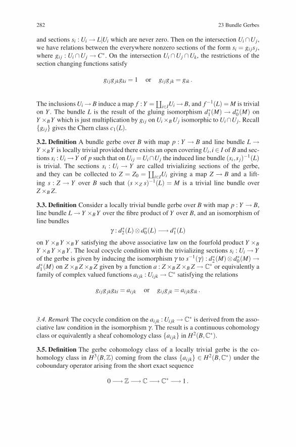
282 23 Bundle Gerbes
and sections si : Ui → L|Ui which are never zero. Then on the intersection Ui ∩Uj,we have relations between the everywhere nonzero sections of the form si = gi js j,where gi j : Ui ∩Uj → C∗. On the intersection Ui ∩Uj ∩Uk, the restrictions of thesection changing functions satisfy
gi jg jkgki = 1 or gi jg jk = gik .
The inclusions Ui → B induce a map f : Y =∐
i∈IUi → B, and f−1(L) = M is trivialon Y . The bundle L is the result of the gluing isomorphism d∗
1(M) → d∗0(M) on
Y ×B Y which is just multiplication by gi j on Ui×B Uj isomorphic to Ui∩Uj. Recall{gi j} gives the Chern class c1(L).
3.2. Definition A bundle gerbe over B with map p : Y → B and line bundle L →Y ×BY is locally trivial provided there exists an open covering Ui, i ∈ I of B and sec-tions si : Ui →Y of p such that on Ui j =Ui∩Uj the induced line bundle (si,s j)−1(L)is trivial. The sections si : Ui → Y are called trivializing sections of the gerbe,and they can be collected to Z = Z0 =
∐i∈IUi giving a map Z → B and a lift-
ing s : Z → Y over B such that (s ×Z s)−1(L) = M is a trivial line bundle overZ ×B Z.
3.3. Definition Consider a locally trivial bundle gerbe over B with map p : Y → B,line bundle L → Y ×B Y over the fibre product of Y over B, and an isomorphism ofline bundles
γ : d∗2(L)⊗d∗
0(L) −→ d∗1(L)
on Y ×B Y ×B Y satisfying the above associative law on the fourfold product Y ×B
Y ×B Y ×B Y . The local cocycle condition with the trivializing sections si : Ui → Yof the gerbe is given by inducing the isomorphism γ to s−1(γ) : d∗
2(M)⊗d∗0(M) →
d∗1(M) on Z ×B Z ×B Z given by a function a : Z ×B Z ×B Z → C
∗ or equivalently afamily of complex valued functions ai jk : Ui jk → C
∗ satisfying the relations
gi jg jkgki = ai jk or gi jg jk = ai jkgik .
3.4. Remark The cocycle condition on the ai jk : Ui jk → C∗ is derived from the asso-
ciative law condition in the isomorphism γ . The result is a continuous cohomologyclass or equivalently a sheaf cohomology class {ai jk} in H2(B,C∗).
3.5. Definition The gerbe cohomology class of a locally trivial gerbe is the co-homology class in H3(B,Z) coming from the class {ai jk} ∈ H2(B,C∗) under thecoboundary operator arising from the short exact sequence
0 −→ Z −→ C −→ C∗ −→ 1 .
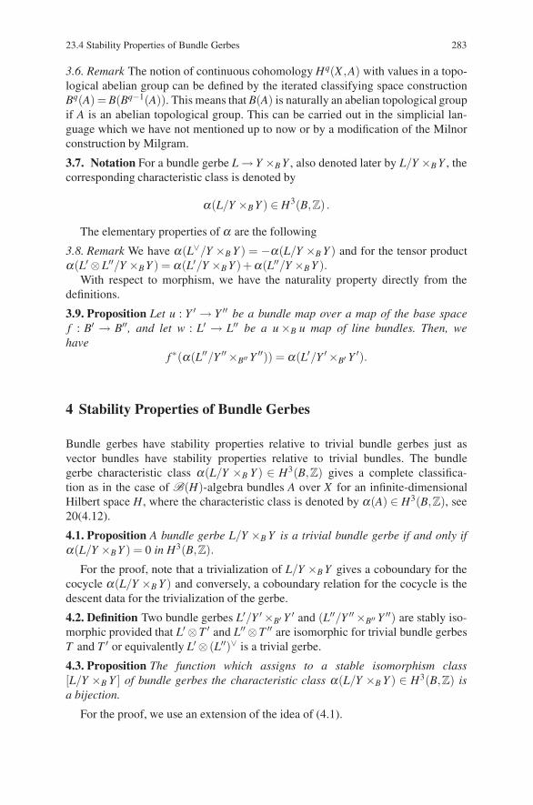
23.4 Stability Properties of Bundle Gerbes 283
3.6. Remark The notion of continuous cohomology Hq(X ,A) with values in a topo-logical abelian group can be defined by the iterated classifying space constructionBq(A) = B(Bq−1(A)). This means that B(A) is naturally an abelian topological groupif A is an abelian topological group. This can be carried out in the simplicial lan-guage which we have not mentioned up to now or by a modification of the Milnorconstruction by Milgram.
3.7. Notation For a bundle gerbe L → Y ×B Y , also denoted later by L/Y ×B Y , thecorresponding characteristic class is denoted by
α(L/Y ×B Y ) ∈ H3(B,Z) .
The elementary properties of α are the following
3.8. Remark We have α(L∨/Y ×B Y ) = −α(L/Y ×B Y ) and for the tensor productα(L′ ⊗L′′/Y ×B Y ) = α(L′/Y ×B Y )+α(L′′/Y ×B Y ).
With respect to morphism, we have the naturality property directly from thedefinitions.
3.9. Proposition Let u : Y ′ → Y ′′ be a bundle map over a map of the base spacef : B′ → B′′, and let w : L′ → L′′ be a u ×B u map of line bundles. Then, wehave
f ∗(α(L′′/Y ′′ ×B′′ Y ′′)) = α(L′/Y ′ ×B′ Y ′).
4 Stability Properties of Bundle Gerbes
Bundle gerbes have stability properties relative to trivial bundle gerbes just asvector bundles have stability properties relative to trivial bundles. The bundlegerbe characteristic class α(L/Y ×B Y ) ∈ H3(B,Z) gives a complete classifica-tion as in the case of B(H)-algebra bundles A over X for an infinite-dimensionalHilbert space H, where the characteristic class is denoted by α(A) ∈ H3(B,Z), see20(4.12).
4.1. Proposition A bundle gerbe L/Y ×B Y is a trivial bundle gerbe if and only ifα(L/Y ×B Y ) = 0 in H3(B,Z).
For the proof, note that a trivialization of L/Y ×B Y gives a coboundary for thecocycle α(L/Y ×B Y ) and conversely, a coboundary relation for the cocycle is thedescent data for the trivialization of the gerbe.
4.2. Definition Two bundle gerbes L′/Y ′ ×B′ Y ′ and (L′′/Y ′′ ×B′′ Y ′′) are stably iso-morphic provided that L′ ⊗T ′ and L′′ ⊗T ′′ are isomorphic for trivial bundle gerbesT and T ′ or equivalently L′ ⊗ (L′′)∨ is a trivial gerbe.
4.3. Proposition The function which assigns to a stable isomorphism class[L/Y ×B Y ] of bundle gerbes the characteristic class α(L/Y ×B Y ) ∈ H3(B,Z) isa bijection.
For the proof, we use an extension of the idea of (4.1).
284 23 Bundle Gerbes
5 Extensions of Principal Bundles Over a Central Extension
In geometry, structure groups of bundles usually are reduced by putting additionalstructure on the basic geometric construction. This is the case with vector bundleswhere by introducing a metric the structure groups are reduced from GL(n,C) tothe compact U(n). The fact that it is always possible to reduce the structure groupfrom the general linear group to the unitary group is related to the fact that all vectorbundles can be endowed with a metric.
In physics, structure groups of bundles are changed by going from thesymmetries of a classical system which are representations to the symmetries ofthe related quantized system which are projective representations. This change instructure group is measured by a characteristic class.
5.1. Notation Let1 −→ C
∗ −→ G′ −→ G −→ 1
be a central extension with classifying space sequence
. . . −→ G −→ B(C∗) −→ B(G′) γ−→ B(G)β−→ B(B(C∗)) = K(Z,3) .
As mentioned in (3.6), the double classifying space B(B(C∗)) can be defined, andthe map β and the map G → B(C∗) come from a similar construction.
5.2. Extension of Structure Group Class Let P be a principal G-bundle over Bwith a classifying map fP : B → B(G). We look for a G′ principal bundle whichfactors P′ → P → B, where the first map is G′ → G equivariant. In particular, thequotient map P′/C
∗ → P is defined and G-equivariant. This principal G′-bundle isclassified by a map fP′ : B→ BG′ where γ fP′ = fP up to homotopy, see 7(3.3). Sincewe have a fibre sequence, we have the following assertion:
5.3. Proposition The principal G-bundle P has a lifting to P′ if and only if the three-dimensional cohomology class defines β fP as 0 in H3(B,Z).
We denote the obstruction to lifting by α(P) = β fP in H3(B,Z).These considerations resemble the role of w1 for an orientation of a vector bun-
dle, see 12(2.3).
6 Modules Over Bundle Gerbes and Twisted K-Theory
Starting with a B(H) algebra bundle, we introduce the related twisted K-theory byusing the action of a bundle gerbe on gerbe modules. The stability theory of gerbemodules gives another formulation of twisted K-theory, see 22(3.2).
Recall that a bundle gerbe L →Y ×BY or just L/Y ×BY has a structure morphismγ : d∗
2(L)⊗d∗0(L)→ d∗
1(L) on Y ×BY ×B Y satisfying an associative law on the four-fold product Y ×B Y ×B Y ×B Y .
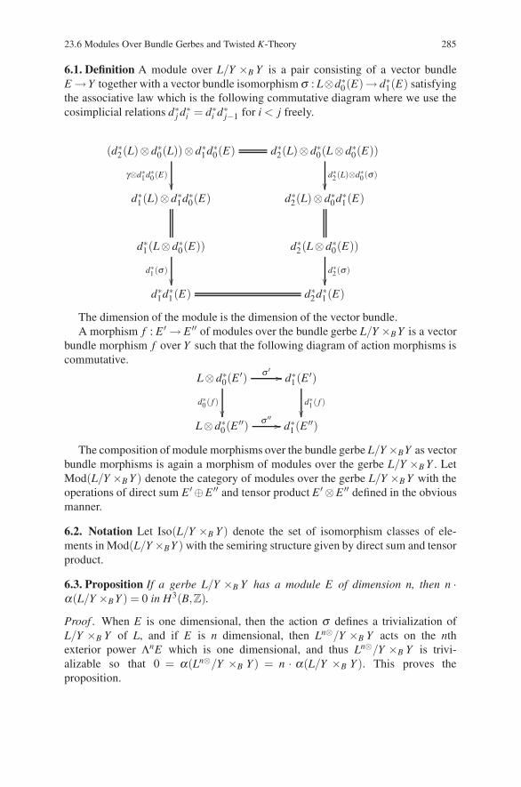
23.6 Modules Over Bundle Gerbes and Twisted K-Theory 285
6.1. Definition A module over L/Y ×B Y is a pair consisting of a vector bundleE →Y together with a vector bundle isomorphism σ : L⊗d∗
0(E)→ d∗1(E) satisfying
the associative law which is the following commutative diagram where we use thecosimplicial relations d∗
j d∗i = d∗
i d∗j−1 for i < j freely.
(d∗2(L)⊗d∗
0(L))⊗d∗1d∗
0(E)
γ⊗d∗1 d∗0(E)��
d∗2(L)⊗d∗
0(L⊗d∗0(E))
d∗2(L)⊗d∗0(σ)��
d∗1(L)⊗d∗
1d∗0(E) d∗
2(L)⊗d∗0d∗
1(E)
d∗1(L⊗d∗
0(E))
d∗1(σ)��
d∗2(L⊗d∗
0(E))
d∗2(σ)��
d∗1d∗
1(E) d∗2d∗
1(E)
The dimension of the module is the dimension of the vector bundle.A morphism f : E ′ → E ′′ of modules over the bundle gerbe L/Y ×B Y is a vector
bundle morphism f over Y such that the following diagram of action morphisms iscommutative.
L⊗d∗0(E
′) σ ′��
d∗0( f )��
d∗1(E ′)
d∗1( f )��
L⊗d∗0(E
′′) σ ′′�� d∗
1(E ′′)
The composition of module morphisms over the bundle gerbe L/Y ×BY as vectorbundle morphisms is again a morphism of modules over the gerbe L/Y ×B Y . LetMod(L/Y ×B Y ) denote the category of modules over the gerbe L/Y ×B Y with theoperations of direct sum E ′ ⊕E ′′ and tensor product E ′ ⊗E ′′ defined in the obviousmanner.
6.2. Notation Let Iso(L/Y ×B Y ) denote the set of isomorphism classes of ele-ments in Mod(L/Y ×BY ) with the semiring structure given by direct sum and tensorproduct.
6.3. Proposition If a gerbe L/Y ×B Y has a module E of dimension n, then n ·α(L/Y ×B Y ) = 0 in H3(B,Z).
Proof . When E is one dimensional, then the action σ defines a trivialization ofL/Y ×B Y of L, and if E is n dimensional, then Ln⊗/Y ×B Y acts on the nthexterior power ΛnE which is one dimensional, and thus Ln⊗/Y ×B Y is trivi-alizable so that 0 = α(Ln⊗/Y ×B Y ) = n · α(L/Y ×B Y ). This proves theproposition.
286 23 Bundle Gerbes
6.4. Proposition A trivialization of L/Y ×B Y defines a semiring morphism Mod(L/Y ×B Y ) → Vect(B). Further, two stably equivalent gerbes (L′/Y ′ ×B Y ′) and(L′′/Y ′′ ×B Y ′′) have isomorphic semiring Mod(L′/Y ′ ×B Y ′) andMod(L′′/Y ′′ ×B Y ′′).
Observe that the action of a trivialized gerbe is just descent data for a bundle, andstabilizing relations gives also descent data for comparing the module categories.
6.5. Definition Let B be a compact space. For a given torsion element α ∈ H3(B,Z)the twisted K-theory constructed by bundle gerbes is the Grothendieck group Kα (B)of the semigroup Iso(L/Y ×B Y ) where α = α(L/Y ×B Y ).
For the comparison of this definition of twisted K-theory with 22(3.2), we usethe class defined for the extension in (5.1)
1 −→ C∗ −→ G′ −→ G −→ 1,
where G′ = GL(H) and G = PGL(H). An algebra bundle has the form P[B(H)],where P is a principal U(H)-bundle or B(H)-bundle. This has a clear relationto the gerbe, and the sections of the Fredholm subbundle is related to gerbemodules.
We will not go into this further here, but the interested reader can find the detailsand also the discussion of the nontorsion case in the reference: Bouwknegt et al.(2002). In the references of this paper, one will find articles developing the theoryof bundle gerbes including the first paper of Murray.
Reference
Bouwknegt, P., Carey, A.L., Mathai, V., Murray, M.K., Stevenson, D.: Twisted K-theory andK-theory of bundle gerbes. Comm. Math. Phys. 228: 17–45 (2002)
Chapter 24Category Objects and Groupoid Gerbes
We introduce the notions of category objects and groupoid objects in a category Cwith finite fibre products. A groupoid object is a category object with an inversionstructure morphism which sometimes is unique. In this case, a groupoid is a categoryobject with an axiom, otherwise it is a category with additional structure. For this,we begin with n-level pseudosimplicial objects in a category in order to formulatethe notion of a category object. These have been used already for a description oflocal triviality of bundles and the construction of bundles from local data or fromdescent data. Then, we go further with simplicial objects, geometric realization, thenerve of a category, and the final step in the detour away from gerbes to the definitionof algebraic K-theory. All this illustrates the vast influence of these general conceptsin mathematics for which there are more and more applications to physics.
Groupoid gerbes are line bundles over the morphism space G(1) in a groupoidG(∗), which in case G = G(1) is a group, correspond to central extensions. In thecase of bundle gerbes, these groupoid gerbes are line bundles L over the fibre productY ×B Y of a space Y over B together with a multiplication which uses the fibre prod-uct structure. Moreover, for bundle gerbes, there is a line bundle isomorphism onY ×B Y ×B Y with an associativity condition on Y ×B Y ×B Y ×B Y , and for groupoidgerbes, there is a line bundle isomorphism on G(1)×G(0) G(1) with an associativitycondition on
G(1)×G(0) G(1)×G(0) G(1) .
The line bundle on G(1) usually is taken to be symmetric with respect to the inversemapping of the groupoid.
1 Simplicial Objects in a Category
In several places, we have already used the formalism of part of a simplicial object toorganize data and axioms especially for the local description of bundles, see 5(4.5)and 25(1.1), for the basic ingredients of a bundle gerbe 25(2.2). We will use theseconcepts to describe the category objects and groupoid objects in a category C .
D. Husemoller et al.: Category Objects and Groupoid Gerbes, Lect. Notes Phys. 726, 287–301 (2008)DOI 10.1007/978-3-540-74956-1 25 © Springer-Verlag Berlin Heidelberg 2008
288 24 Category Objects and Groupoid Gerbes
1.1. Definition An n-level pseudosimplicial object in a category C is a sequence ofobjects Zq for 0 ≤ q ≤ n in C together with morphisms di : Zq → Zq−1 for 0 ≤ i ≤ qin C such that
did j = d j−1di : Zq −→ Zq−2
for 0 ≤ i < j ≤ q. A morphism of n-level pseudosimplicial objects is a sequence ofmorphisms fq : Z′
q → Z′′q for 0 ≤ q ≤ n such that
di fn = fn−1di for 1 ≤ i ≤ n .
The reason for the term pseudosimplicial instead of simplicial is that a simpli-cial object Z.will also have morphisms s j : Zq → Zq+1 for 0 ≤ j ≤ q with suitablerelations.
We can display every morphism and object easily up to three levels
Z3d0,d1,d2,d3 �� Z2
d0,d1,d2 �� Z1d0,d1 �� Z0.
and for descent questions for a bundle E over Y = Z0, the terms arise as fibre prod-ucts relative to a map f : Y → B
Z2 = Y ×B Y ×B Yd0,d1,d2 �� Z1 = Y ×B Y
d0,d1 �� Z0 = Y .
This extends further with Z3 = Y ×B Y ×B Y ×B Y , Z2 = Y ×B Y ×B Y , Z1 = Y ×B Y ,and Z0 =Y , the morphisms di refer to the projection which deletes the ith coordinate0 ≤ i ≤ q on Zq.
1.2. Definition Associated to a first level or first stage pseudosimplicial object
Z1 = Z(1)d0,d1−→ Z(0) = Z0 in a category, we have an object, namely the fibre product
denoted by Z(1)∗Z0 Z(1) = Z(1)d0(×Z(0))d1Z(1) which has a first and second pro-jection denoted by pr1 = d2 : Z(1)∗Z0 Z(1) → Z(1) and pr2 = d0 : Z(1)∗Z0 Z(1) →Z(1), respectively. Note that d2 is the last factor deleted and d0 is the first factordeleted in the case Z(1) = Z(0)×B Z(0) for f : Z(0) → B.
We have used pseudosimplicial objects of order n to organize gluing data, andnow we consider the complete concept of a simplicial object, and in the case ofsimplicial set, we define a filtered space called the geometric realization.
1.3. Definition A simplicial object X. in a category C is a sequence of objects Xn
for n ≥ 0 in C together with morphisms in C defined by
di(X) = di : Xn −→ Xn−1 and s j(X) = s j : Xn −→ Xn+1
for 0 ≤ i, j ≤ n such that the following relations hold
(1) did j = d j−1di (i < j)(2) sis j = s jsi−1 (i > j)
24.1 Simplicial Objects in a Category 289
and
(3) dis j =
⎧⎨⎩
s j−1di (i < j)1 (i = j, j + 1)s jdi−1 (i > j + 1) .
1.4. Definition A morphism f. : X.→ Y. of simplicial objects in a category is asequence of morphisms fn : Xn → Yn satisfying the relations
di(Y ) fn = fn−1di(X) and si(Y ) fn = fn+1si(X)
with 0 ≤ i, j ≤ n.
1.5. Remark The composition of two morphisms f. : X.→Y.and g.: Y.→ Z.definedby the relation (g f )n = gn fn is a morphism X.→ Z. of simplicial objects in thecategory C . With these definitions, we have the category Δ(C ) of simplicial objectsin C .
We introduce a topological space associated to a simplicial set, or in other words,we define a functor R : Δ(set) → (top) from the category of simplicial sets to thecategory of topological spaces, called geometric realization using affine simplexes.
1.6. Definition The affine simplex A(n) is the closed subset of the compact cube[0,1]n+1 ⊂R
n+1 consisting of all points (t0, . . . ,tn)∈ [0,1]n+1 ⊂Rn+1 with t0 + . . .+
tn = 1. The coordinates ti of these points in A(n) are called barycentric coordinates.
1.7. Remark The boundary ∂A(n) of A(n) is related to the cosimplicial operationsδi : A(n−1)→ A(n) defined for 0 ≤ i ≤ n in barycentric coordinates by
δi(t0, . . . ,tn−1) = (t0, . . . ,ti−1,0, ti, . . . ,tn−1) .
The boundary ∂A(n) =⋃
i∈[n] im(δi) is a union of the images of the face morphismsδi for i ∈ [n] = {0,1, . . . ,n} .
1.8. Remark The iterates of the cosimplicial operations satisfy δ jδi = δiδ j−1 :A(n−2)→ A(n) for 0 ≤ i < j ≤ n, where both compositions will take (t0, . . . ,tn−2)to (t0, . . . ,ti−1,0, ti, . . . t j−1,0,t j, . . . ,tn−2). The other cosimplicial operations σi :A(n + 1)→ A(n) for 0 ≤ j ≤ n are defined by the formulas
σ j(t0, . . . ,tn+1) = (t0, . . . ,t j−1,t j + t j+1, t j+2, . . . ,tn+1) .
1.9. Definition The geometric realization R(X.) of a simplicial set X. is the quotientof the disjoint union
∐0≤nXn ×A(n) by the simplicial relations which are generated
by(di(x),t) ∼ (x,δi(t)) and (s j(x′), t ′) ∼ (x′,σ j(t ′))
for x ∈ Xn, t ∈ A(n−1), x′ ∈ Xn−1, t ′ ∈ A(n + 1) for 0 ≤ i, j ≤ n.
1.10. Remark The homology and cohomology of the space R(X.) can be calcu-lated in terms of the simplicial set X.. The geometric realization R(X.) is a fil-tered space with R(X.)k being the image of
∐0≤n≤kXn ×A(n) in R(X.), and level
290 24 Category Objects and Groupoid Gerbes
R(X.)k/R(X.)k−1 is a wedge of k-spheres each one for each element of Xk −∐0≤ j≤ks j(Xk−1), the set of nondegenerate k-simplexes in X..Thus, a simplicial set generates a filtered space whose homology is controlled by
the combinatorial topology of the simplicial set.
2 Categories in a Category
This is a short introduction to the concept of category in a form leading to the defi-nition of category objects in a category X .
2.1. Small Categories as Pairs of Sets Let C be a small category which meansthat the class of objects C(0) is a set. Form the set C(1) equal to the disjoint unionof all Hom(X ,Y ) for X ,Y ∈ C(0). These two sets are connected by several func-tions. Firstly, we have the domain (left) and ring (right) functions l,r : C(1)→C(0)defined by the requirement that
l(Hom(X ,Y )) = {X} and r(Hom(X ,Y )) = {Y}
on the disjoint union. For C(1), we have f : l( f ) → r( f ) is a notation for the mor-phism f in C.
Secondly, we have an identity morphism for each object of C which is a functione : C(0) →C(1) having the property that le and re are the identities on C(0). Here,e(X) = idX : X → X for e ∈ Hom(X ,X).
Thirdly, we have composition g f of two morphisms f and g but only in casewhere r( f ) = l(g). Hence, composition is not defined in general on the entireproduct C(1) ×C(1), but it is defined on all subsets of the form Hom(X ,Y )×Hom(Y,Z) ∈C(1)×C(1). This subset is called the fibre product of r : C(1)→C(0)and l : C(1)→C(0) consisting of pairs ( f ,g) ∈C(1)×C(1) where r( f ) = l(g). Thefibre product is denoted by C(1)r×
C(0)lC(1) with two projections r, l : C(1)r×
C(0)lC(1)→
C(0) defined by
l( f ,g) = l( f ) and r( f ,g) = r(g).
Then, composition is defined by m : C(1)r×C(0)l
C(1) → C(1), where m( f ,g) = g f
satisfying lm( f ,g) = l( f ,g) = l( f ) and rm( f ,g) = r( f ,g) = r(g) . Now, the readercan supply the unit and associativity axioms.
Fourthly, the notion of opposite category C op where f : X → Y in C be-comes f op : Y → X in C op, and (g f )op = f opgop can be described as C op =(C(0),C(1),e, lop = r,rop = l,mop = mτ), where τ is the flip in the fibre productτ : C (1)r×
C(0)lC(1) →C(1)r×
C(0)lC(1).
2.2. Remark We rewrite the previous setup where left l is replaced by d1 delet-ing the first factor and right r is replaced by d0 deleting the 0-factor in a pairusing the second-level pseudosimplicial notation of the previous section l = d1,
24.2 Categories in a Category 291
r = d0 : C(1)→C(0). Furthermore, we have the fibre product mixing d0 and d1
giving C(1) ∗C(0) C(1) = C(1)r×C(0)l
C(1) with the projection on the second and first
factors d0,d2 : C(1) ∗C(0) C(1) → C(1), respectively. A category object structurefills in this picture with a morphism d1 : C(1) ∗C(0) C(1) → C(1) extending thestructure to a second-level pseudosimplicial object where C(2) = C(1) ∗C(0) C(1)giving d0,d1,d2 : C(2) → C(1). In addition, we have a base or identity morphisme : C(0) →C(1).
2.3. Definition Let C be a category with finite fibre products. A category objectC(∗) in C is a sextuple (C(0),C(1), l,r,e,m) consisting of two objects, C(0) andC(1), and four morphisms
(1) l,r : C(1) →C(0) called domain (left) and range (right)(2) e : C(0) →C(1) a unit morphism, and(3) m : C(1)r×
C(0)lC(1) → C(1) called multiplication or composition satisfying the
following axioms:
(Cat1) The compositions le and re are the identities in C(0).(Cat2) Domain and range are compatible with multiplication
C(1)r×C(0)l
C(1) m ��
pr1/pr2
��
C(1)
l/r
��(C(1))
l/r �� C(0)
(Cat3) (associativity) The following diagram is commutative
C(1)r×C(0)l
C(1)r×C(0)l
C(1) m×C(1) ��
C(1)×m��
C(1)r×C(0)l
C(1)
m
��C(1)r×
C(0)lC(1) m �� C(1)
(Cat4) (unit property of e) m(C(1),er) and m(le,C(1)) are each identities on C(1).
2.4. Definition A morphism u(∗) : C′(∗)→C′′(∗) from the category object C′(∗) inC to the category object C′′(∗) in C is a pair of morphisms u(0) : C′(0) → C′′(0)and u(1) : C′(1) → C′′(1) commuting with the four structure morphisms of C′(∗)and C′′(∗). The following diagrams have to be commutative
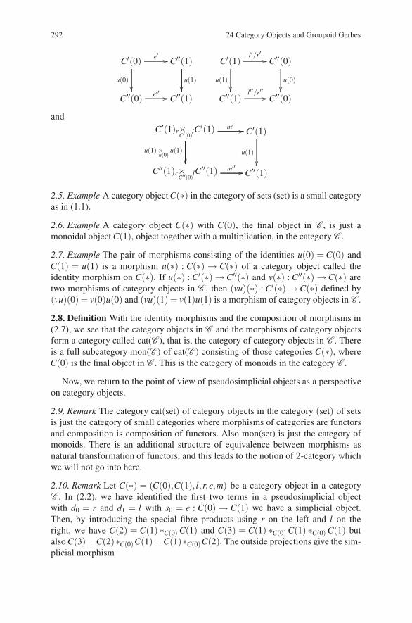
292 24 Category Objects and Groupoid Gerbes
C′(0)
u(0)��
e′ �� C′′(1)
u(1)��
C′′(0) e′′ �� C′′(1)
C′(1)l′/r′ ��
u(1)��
C′′(0)
u(0)��
C′′(1)l′′/r′′ �� C′′(0)
andC′(1)r×
C′(0)lC′(1) m′
��
u(1)×u(0)
u(1)
��
C′(1)
u(1)
��C′′(1)r×
C′′(0)lC′′(1) m′′
�� C′′(1)
2.5. Example A category object C(∗) in the category of sets (set) is a small categoryas in (1.1).
2.6. Example A category object C(∗) with C(0), the final object in C , is just amonoidal object C(1), object together with a multiplication, in the category C .
2.7. Example The pair of morphisms consisting of the identities u(0) = C(0) andC(1) = u(1) is a morphism u(∗) : C(∗) → C(∗) of a category object called theidentity morphism on C(∗). If u(∗) : C′(∗) → C′′(∗) and v(∗) : C′′(∗) → C(∗) aretwo morphisms of category objects in C , then (vu)(∗) : C′(∗) → C(∗) defined by(vu)(0) = v(0)u(0) and (vu)(1) = v(1)u(1) is a morphism of category objects in C .
2.8. Definition With the identity morphisms and the composition of morphisms in(2.7), we see that the category objects in C and the morphisms of category objectsform a category called cat(C ), that is, the category of category objects in C . Thereis a full subcategory mon(C ) of cat(C ) consisting of those categories C(∗), whereC(0) is the final object in C . This is the category of monoids in the category C .
Now, we return to the point of view of pseudosimplicial objects as a perspectiveon category objects.
2.9. Remark The category cat(set) of category objects in the category (set) of setsis just the category of small categories where morphisms of categories are functorsand composition is composition of functors. Also mon(set) is just the category ofmonoids. There is an additional structure of equivalence between morphisms asnatural transformation of functors, and this leads to the notion of 2-category whichwe will not go into here.
2.10. Remark Let C(∗) = (C(0),C(1), l,r,e,m) be a category object in a categoryC . In (2.2), we have identified the first two terms in a pseudosimplicial objectwith d0 = r and d1 = l with s0 = e : C(0) → C(1) we have a simplicial object.Then, by introducing the special fibre products using r on the left and l on theright, we have C(2) = C(1) ∗C(0) C(1) and C(3) = C(1) ∗C(0) C(1) ∗C(0) C(1) butalso C(3) =C(2)∗C(0)C(1) = C(1)∗C(0)C(2). The outside projections give the sim-plicial morphism
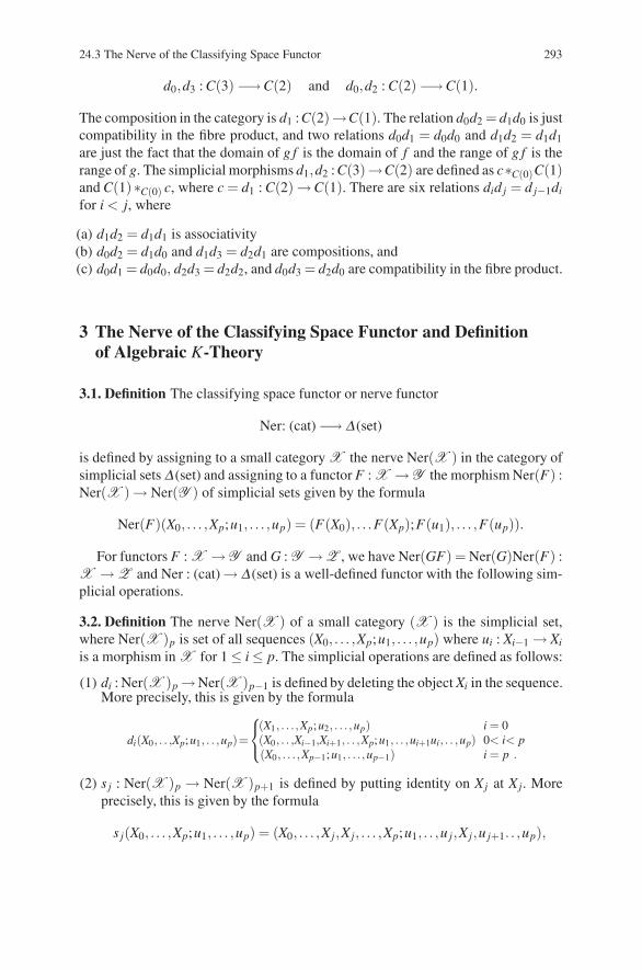
24.3 The Nerve of the Classifying Space Functor 293
d0,d3 : C(3) −→C(2) and d0,d2 : C(2) −→C(1).
The composition in the category is d1 :C(2)→C(1). The relation d0d2 = d1d0 is justcompatibility in the fibre product, and two relations d0d1 = d0d0 and d1d2 = d1d1
are just the fact that the domain of g f is the domain of f and the range of g f is therange of g. The simplicial morphisms d1,d2 : C(3)→C(2) are defined as c∗C(0)C(1)and C(1)∗C(0) c, where c = d1 : C(2) →C(1). There are six relations did j = d j−1di
for i < j, where
(a) d1d2 = d1d1 is associativity(b) d0d2 = d1d0 and d1d3 = d2d1 are compositions, and(c) d0d1 = d0d0, d2d3 = d2d2, and d0d3 = d2d0 are compatibility in the fibre product.
3 The Nerve of the Classifying Space Functor and Definitionof Algebraic K-Theory
3.1. Definition The classifying space functor or nerve functor
Ner: (cat) −→ Δ (set)
is defined by assigning to a small category X the nerve Ner(X ) in the category ofsimplicial sets Δ (set) and assigning to a functor F : X →Y the morphism Ner(F) :Ner(X ) → Ner(Y ) of simplicial sets given by the formula
Ner(F)(X0, . . . ,Xp;u1, . . . ,up) = (F(X0), . . .F(Xp);F(u1), . . . ,F(up)).
For functors F : X →Y and G : Y →Z , we have Ner(GF) = Ner(G)Ner(F) :X → Z and Ner : (cat) → Δ (set) is a well-defined functor with the following sim-plicial operations.
3.2. Definition The nerve Ner(X ) of a small category (X ) is the simplicial set,where Ner(X )p is set of all sequences (X0, . . . ,Xp;u1, . . . ,up) where ui : Xi−1 → Xi
is a morphism in X for 1 ≤ i ≤ p. The simplicial operations are defined as follows:
(1) di : Ner(X )p →Ner(X )p−1 is defined by deleting the object Xi in the sequence.More precisely, this is given by the formula
di(X0, . . ,Xp;u1, . . ,up)=
⎧⎨⎩
(X1, . . .,Xp;u2, . . . ,up) i = 0(X0, . . ,Xi−1,Xi+1, . . ,Xp;u1, . . ,ui+1ui, . . ,up) 0< i< p(X0, . . .,Xp−1;u1, . . .,up−1) i = p .
(2) s j : Ner(X )p → Ner(X )p+1 is defined by putting identity on Xj at Xj. Moreprecisely, this is given by the formula
s j(X0, . . . ,Xp;u1, . . . ,up) = (X0, . . . ,Xj,Xj, . . . ,Xp;u1, . . ,u j,Xj,u j+1. . ,up),
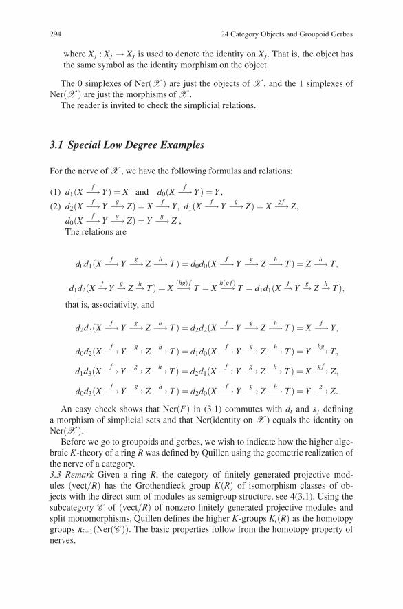
294 24 Category Objects and Groupoid Gerbes
where Xj : Xj → Xj is used to denote the identity on Xj. That is, the object hasthe same symbol as the identity morphism on the object.
The 0 simplexes of Ner(X ) are just the objects of X , and the 1 simplexes ofNer(X ) are just the morphisms of X .
The reader is invited to check the simplicial relations.
3.1 Special Low Degree Examples
For the nerve of X , we have the following formulas and relations:
(1) d1(Xf−→ Y ) = X and d0(X
f−→ Y ) = Y ,
(2) d2(Xf−→ Y
g−→ Z) = Xf−→ Y, d1(X
f−→ Yg−→ Z) = X
g f−→ Z,
d0(Xf−→ Y
g−→ Z) = Yg−→ Z ,
The relations are
d0d1(Xf−→ Y
g−→ Zh−→ T ) = d0d0(X
f−→ Yg−→ Z
h−→ T ) = Zh−→ T,
d1d2(Xf→ Y
g→ Zh→ T ) = X
(hg) f−→ T = Xh(g f )−→ T = d1d1(X
f→ Yg→ Z
h→ T ),
that is, associativity, and
d2d3(Xf−→ Y
g−→ Zh−→ T ) = d2d2(X
f−→ Yg−→ Z
h−→ T ) = Xf−→ Y,
d0d2(Xf−→ Y
g−→ Zh−→ T ) = d1d0(X
f−→ Yg−→ Z
h−→ T ) = Yhg−→ T,
d1d3(Xf−→ Y
g−→ Zh−→ T ) = d2d1(X
f−→ Yg−→ Z
h−→ T ) = Xg f−→ Z,
d0d3(Xf−→ Y
g−→ Zh−→ T ) = d2d0(X
f−→ Yg−→ Z
h−→ T ) = Yg−→ Z.
An easy check shows that Ner(F) in (3.1) commutes with di and s j defininga morphism of simplicial sets and that Ner(identity on X ) equals the identity onNer(X ).
Before we go to groupoids and gerbes, we wish to indicate how the higher alge-braic K-theory of a ring R was defined by Quillen using the geometric realization ofthe nerve of a category.3.3 Remark Given a ring R, the category of finitely generated projective mod-ules (vect/R) has the Grothendieck group K(R) of isomorphism classes of ob-jects with the direct sum of modules as semigroup structure, see 4(3.1). Using thesubcategory C of (vect/R) of nonzero finitely generated projective modules andsplit monomorphisms, Quillen defines the higher K-groups Ki(R) as the homotopygroups πi−1(Ner(C )). The basic properties follow from the homotopy property ofnerves.
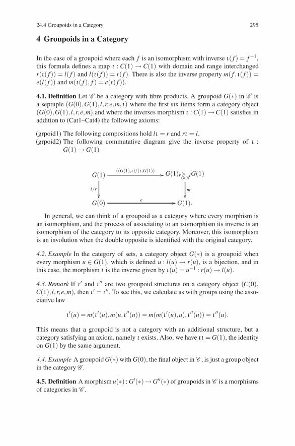
24.4 Groupoids in a Category 295
4 Groupoids in a Category
In the case of a groupoid where each f is an isomorphism with inverse ι( f ) = f−1,this formula defines a map ι : C(1) → C(1) with domain and range interchangedr(ι( f )) = l( f ) and l(ι( f )) = r( f ). There is also the inverse property m( f , ι( f )) =e(l( f )) and m(ι( f ), f ) = e(r( f )).
4.1. Definition Let C be a category with fibre products. A groupoid G(∗) in C isa septuple (G(0),G(1), l,r,e,m, ι) where the first six items form a category object(G(0),G(1), l,r,e,m) and where the inverses morphism ι : C(1) →C(1) satisfies inaddition to (Cat1–Cat4) the following axioms:
(grpoid1) The following compositions hold lι = r and rι = l.(grpoid2) The following commutative diagram give the inverse property of ι :
G(1) → G(1)
G(1)((G(1),ι)/(ι,G(1)) ��
l/r
��
G(1)r×G(0)l
G(1)
m
��G(0) e �� G(1).
In general, we can think of a groupoid as a category where every morphism isan isomorphism, and the process of associating to an isomorphism its inverse is anisomorphism of the category to its opposite category. Moreover, this isomorphismis an involution when the double opposite is identified with the original category.
4.2. Example In the category of sets, a category object G(∗) is a groupoid whenevery morphism u ∈ G(1), which is defined u : l(u) → r(u), is a bijection, and inthis case, the morphism ι is the inverse given by ι(u) = u−1 : r(u) → l(u).
4.3. Remark If ι ′ and ι ′′ are two groupoid structures on a category object (C(0),C(1), l,r,e,m), then ι ′ = ι ′′. To see this, we calculate as with groups using the asso-ciative law
ι ′(u) = m(ι ′(u),m(u, ι ′′(u)) = m(m(ι ′(u),u), ι ′′(u)) = ι ′′(u).
This means that a groupoid is not a category with an additional structure, but acategory satisfying an axiom, namely ι exists. Also, we have ιι = G(1), the identityon G(1) by the same argument.
4.4. Example A groupoid G(∗) with G(0), the final object in C , is just a group objectin the category G .
4.5. Definition A morphism u(∗) : G′(∗)→G′′(∗) of groupoids in C is a morphismsof categories in C .
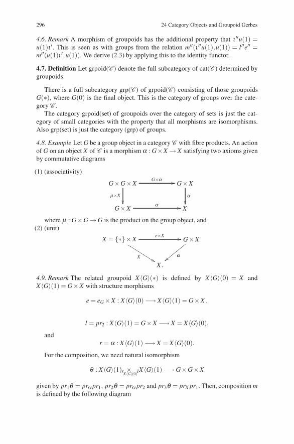
296 24 Category Objects and Groupoid Gerbes
4.6. Remark A morphism of groupoids has the additional property that ι ′′u(1) =u(1)ι ′. This is seen as with groups from the relation m′′(ι ′′u(1),u(1)) = l′′e′′ =m′′(u(1)ι ′,u(1)). We derive (2.3) by applying this to the identity functor.
4.7. Definition Let grpoid(C ) denote the full subcategory of cat(C ) determined bygroupoids.
There is a full subcategory grp(C ) of grpoid(C ) consisting of those groupoidsG(∗), where G(0) is the final object. This is the category of groups over the cate-gory C .
The category grpoid(set) of groupoids over the category of sets is just the cat-egory of small categories with the property that all morphisms are isomorphisms.Also grp(set) is just the category (grp) of groups.
4.8. Example Let G be a group object in a category C with fibre products. An actionof G on an object X of C is a morphism α : G×X → X satisfying two axioms givenby commutative diagrams
(1) (associativity)
G×G×X
μ×X
��
G×α �� G×X
�
G×Xα �� X
where μ : G×G → G is the product on the group object, and(2) (unit)
X = {∗}×Xe×X ��
X �������
�����
G×X
�#########
X .
4.9. Remark The related groupoid X〈G〉(∗) is defined by X〈G〉(0) = X andX〈G〉(1) = G×X with structure morphisms
e = eG ×X : X〈G〉(0) −→ X〈G〉(1) = G×X ,
l = pr2 : X〈G〉(1) = G×X −→ X = X〈G〉(0),
andr = α : X〈G〉(1) −→ X = X〈G〉(0).
For the composition, we need natural isomorphism
θ : X〈G〉(1)r ×X〈G〉(0)l
X〈G〉(1) −→ G×G×X
given by pr1θ = prG pr1, pr2θ = prG pr2 and pr3θ = prX pr1. Then, composition mis defined by the following diagram
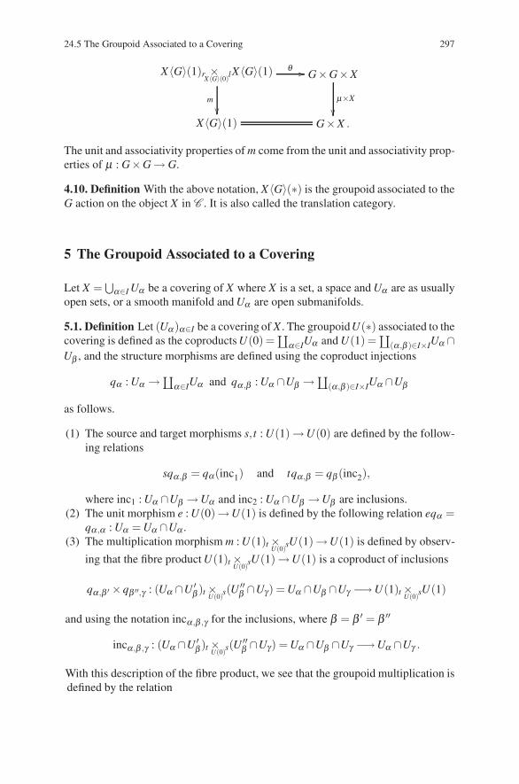
24.5 The Groupoid Associated to a Covering 297
X〈G〉(1)r ×X〈G〉(0)l
X〈G〉(1) θ ��
m
��
G×G×X
μ×X
��X〈G〉(1) G×X .
The unit and associativity properties of m come from the unit and associativity prop-erties of μ : G×G → G.
4.10. Definition With the above notation, X〈G〉(∗) is the groupoid associated to theG action on the object X in C . It is also called the translation category.
5 The Groupoid Associated to a Covering
Let X =⋃α∈I Uα be a covering of X where X is a set, a space and Uα are as usually
open sets, or a smooth manifold and Uα are open submanifolds.
5.1. Definition Let (Uα)α∈I be a covering of X . The groupoidU(∗) associated to thecovering is defined as the coproducts U(0) =
∐α∈IUα and U(1) =
∐(α ,β )∈I×IUα ∩
Uβ , and the structure morphisms are defined using the coproduct injections
qα : Uα →∐α∈IUα and qα ,β : Uα ∩Uβ →∐(α ,β )∈I×IUα ∩Uβ
as follows.
(1) The source and target morphisms s,t : U(1) →U(0) are defined by the follow-ing relations
sqα ,β = qα(inc1) and tqα ,β = qβ (inc2),
where inc1 : Uα ∩Uβ →Uα and inc2 : Uα ∩Uβ →Uβ are inclusions.(2) The unit morphism e : U(0)→U(1) is defined by the following relation eqα =
qα ,α : Uα = Uα ∩Uα .(3) The multiplication morphism m : U(1)t ×
U(0)sU(1)→U(1) is defined by observ-
ing that the fibre product U(1)t ×U(0)s
U(1) →U(1) is a coproduct of inclusions
qα ,β ′ ×qβ ′′,γ : (Uα ∩U ′β )t ×
U(0)s(U ′′β ∩Uγ) = Uα ∩Uβ ∩Uγ −→U(1)t ×
U(0)sU(1)
and using the notation incα ,β ,γ for the inclusions, where β = β ′ = β ′′
incα ,β ,γ : (Uα ∩U ′β )t ×
U(0)s(U ′′β ∩Uγ) = Uα ∩Uβ ∩Uγ −→Uα ∩Uγ .
With this description of the fibre product, we see that the groupoid multiplication isdefined by the relation
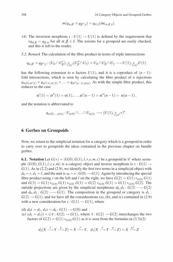
298 24 Category Objects and Groupoid Gerbes
m(qα ,β ′ ×qβ ′′,γ ) = qα ,γ(incα ,β ,γ).
(4) The inversion morphism ι : U(1) → U(1) is defined by the requirement thatιqα ,β = qβ ,α for all α,β ∈ I. The axioms for a groupoid are easily checked,and this is left to the reader.
5.2. Remark The calculation of the fibre product in terms of triple intersections
qα ,β ′ ×qβ ′′,γ : (Uα ∩U ′β )t ×
U(0)s(U ′′β ∩Uγ) = Uα ∩Uβ ∩Uγ −→U(1)t ×
U(0)sU(1)
has the following extension to n factors U(1), and it is a coproduct of (n − 1)-fold intersections, which is seen by calculating the fibre product of n injectionsqα(0),α ′(1) × qα ′′(1),α ′(2) × . . .× qα ′′(n−1),α(n). As with the simple fibre product, thisreduces to the case
α ′(1) = α ′′(1) = α(1), . . . ,α ′(n−1) = α ′′(n−1) = α(n−1) ,
and the notation is abbreviated to
qα(0),...,α(n) : Uα(0)∩ . . .∩Uα(n) −→ (U(1)t ×U(0)s
∗)n .
6 Gerbes on Groupoids
Now, we return to the simplicial notation for a category which is a groupoid in orderto carry over to groupoids the ideas contained in the previous chapter on bundlegerbes.
6.1. Notation Let G(∗) = (G(0),G(1), l,r,e,m, ι) be a groupoid in C where sextu-ple (G(0),G(1), l,r,e,m) is a category object and inverse morphism is ι : G(1) →G(1). As in (2.2) and (2.9), we identify the first two terms in a simplicial object withd0 = r, d1 = l, and the unit is s0 = e : G(0)→ G(1). Again by introducing the specialfibre product using r on the left and l on the right, we have G(2) = G(1)∗G(0) G(1)and G(3) = G(1) ∗G(0) G(1) ∗G(0) G(1) = G(2) ∗G(0) G(1) = G(1) ∗G(0) G(2). Theoutside projections are given by the simplicial morphisms d0,d3 : G(3) −→ G(2)and d0,d2 : G(2) −→ G(1) . The composition in the groupoid or category is d1 :G(2) → G(1), and we have all the considerations (a), (b), and (c) contained in (2.9)with a new consideration for ι : G(1) → G(1), where
(d) d0ι = d1, d1ι = d0 : G(1) → G(0) and(e) ιd1 = d1(ι × ι)τ : G(2) → G(1), where τ : G(2) → G(2) interchanges the two
factors of G(2) = G(1)∗G(0) G(1) as it is seen from the formulas in (3.3)(2)
d2(Xf−→ Y
g−→ Z) = Xf−→ Y, d1(X
f−→ Yg−→ Z) = X
g f−→ Z
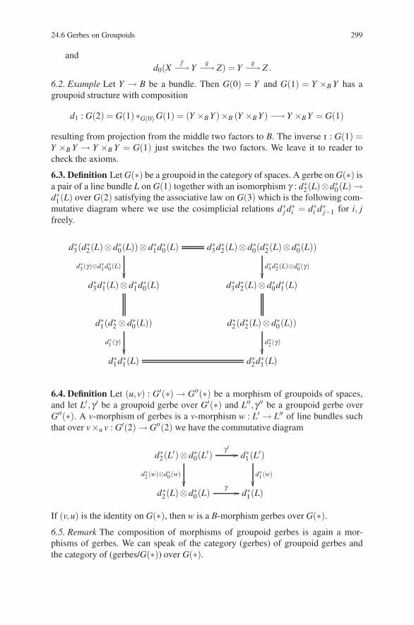
24.6 Gerbes on Groupoids 299
andd0(X
f−→ Yg−→ Z) = Y
g−→ Z .
6.2. Example Let Y → B be a bundle. Then G(0) = Y and G(1) = Y ×B Y has agroupoid structure with composition
d1 : G(2) = G(1)∗G(0) G(1) = (Y ×B Y )×B (Y ×B Y ) −→ Y ×B Y = G(1)
resulting from projection from the middle two factors to B. The inverse ι : G(1) =Y ×B Y → Y ×B Y = G(1) just switches the two factors. We leave it to reader tocheck the axioms.
6.3. Definition Let G(∗) be a groupoid in the category of spaces. A gerbe on G(∗) isa pair of a line bundle L on G(1) together with an isomorphism γ : d∗
2(L)⊗d∗0(L) →
d∗1(L) over G(2) satisfying the associative law on G(3) which is the following com-
mutative diagram where we use the cosimplicial relations d∗j d∗
i = d∗i d∗
j−1 for i, jfreely.
d∗3(d∗
2(L)⊗d∗0(L))⊗d∗
1d∗0(L)
d∗3(γ)⊗d∗1 d∗0(L)��
d∗3d∗
2(L)⊗d∗0(d
∗2(L)⊗d∗
0(L))
d∗3 d∗2(L)⊗d∗0(γ)��
d∗3d∗
1(L)⊗d∗1d∗
0(L) d∗3d∗
2(L)⊗d∗0d∗
1(L)
d∗1(d
∗2 ⊗d∗
0(L))
d∗1(γ)��
d∗2(d∗
2(L)⊗d∗0(L))
d∗2(γ)��
d∗1d∗
1(L) d∗2d∗
1(L)
6.4. Definition Let (u,v) : G′(∗) → G′′(∗) be a morphism of groupoids of spaces,and let L′,γ ′ be a groupoid gerbe over G′(∗) and L′′,γ ′′ be a groupoid gerbe overG′′(∗). A v-morphism of gerbes is a v-morphism w : L′ → L′′ of line bundles suchthat over v×u v : G′(2) → G′′(2) we have the commutative diagram
d∗2(L′)⊗d∗
0(L′)
γ ′ ��
d∗2(w)⊗d∗0(w)��
d∗1(L′)
d∗1(w)��
d∗2(L)⊗d∗
0(L)γ �� d∗
1(L)
If (v,u) is the identity on G(∗), then w is a B-morphism gerbes over G(∗).6.5. Remark The composition of morphisms of groupoid gerbes is again a mor-phisms of gerbes. We can speak of the category (gerbes) of groupoid gerbes andthe category of (gerbes/G(∗)) over G(∗).
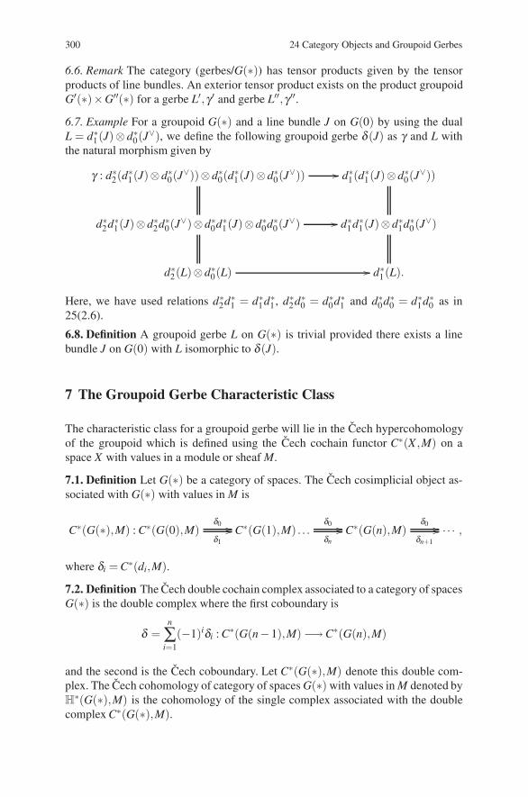
300 24 Category Objects and Groupoid Gerbes
6.6. Remark The category (gerbes/G(∗)) has tensor products given by the tensorproducts of line bundles. An exterior tensor product exists on the product groupoidG′(∗)×G′′(∗) for a gerbe L′,γ ′ and gerbe L′′,γ ′′.
6.7. Example For a groupoid G(∗) and a line bundle J on G(0) by using the dualL = d∗
1(J)⊗ d∗0(J
∨), we define the following groupoid gerbe δ (J) as γ and L withthe natural morphism given by
γ : d∗2(d
∗1(J)⊗d∗
0(J∨))⊗d∗
0(d∗1(J)⊗d∗
0(J∨)) �� d∗
1(d∗1(J)⊗d∗
0(J∨))
d∗2d∗
1(J)⊗d∗2d∗
0(J∨)⊗d∗
0d∗1(J)⊗d∗
0d∗0(J∨) �� d∗
1d∗1(J)⊗d∗
1d∗0(J∨)
d∗2(L)⊗d∗
0(L) �� d∗1(L).
Here, we have used relations d∗2d∗
1 = d∗1d∗
1, d∗2d∗
0 = d∗0d∗
1 and d∗0d∗
0 = d∗1d∗
0 as in25(2.6).
6.8. Definition A groupoid gerbe L on G(∗) is trivial provided there exists a linebundle J on G(0) with L isomorphic to δ (J).
7 The Groupoid Gerbe Characteristic Class
The characteristic class for a groupoid gerbe will lie in the Cech hypercohomologyof the groupoid which is defined using the Cech cochain functor C∗(X ,M) on aspace X with values in a module or sheaf M.
7.1. Definition Let G(∗) be a category of spaces. The Cech cosimplicial object as-sociated with G(∗) with values in M is
C∗(G(∗),M) : C∗(G(0),M)δ0 ��δ1
�� C∗(G(1),M) . . .δ0 ��δn
�� C∗(G(n),M)δ0 ��δn+1
�� . . . ,
where δi = C∗(di,M).
7.2. Definition The Cech double cochain complex associated to a category of spacesG(∗) is the double complex where the first coboundary is
δ =n
∑i=1
(−1)iδi : C∗(G(n−1),M) −→C∗(G(n),M)
and the second is the Cech coboundary. Let C∗(G(∗),M) denote this double com-plex. The Cech cohomology of category of spaces G(∗) with values in M denoted byH
∗(G(∗),M) is the cohomology of the single complex associated with the doublecomplex C∗(G(∗),M).
24.7 The Groupoid Gerbe Characteristic Class 301
7.3. Remark Let G(∗) be a groupoid gerbe with line bundle L on G(1) together withan isomorphism γ : d∗
2(L)⊗d∗0(L) → d∗
1(L) over G(2) satisfying the associative lawon G(3). The Cech cocycle representing the first Chern class c(1)(L) of L is a cocyclein C2(G(1),Z) of the associated single complex of the double complex C∗(G(∗),Z).
7.4. Definition With previous notation in (7.3), the characteristic class of gerbe(G(∗),L) denoted by α(G(∗),L) is the cohomology class in H
∗(G(∗)),Z) repre-sented by c(1)(L).
7.5. Remark If the groupoid gerbe (G(∗),L) is trivial, then c(1)(L) is trivial in thefirst direction, and the characteristic class α(G(∗),L) = 0.

Chapter 25Stacks and Gerbes
A basic structure in mathematics for the study of a space X is to give to each open setan object A(U) in a category C together with restriction morphisms rV,U : A(U) →A(V ) for V ⊂U satisfying rU,U is the identity and the composition property
rW,U = rW,V rV,U for W ⊂V ⊂U .
Such a structure is called a presheaf with values in C .Again, there is a gluing condition which is realized by a universal construction.
To formulate this, we use adjoint functors which are introduced in Sect. 2. An ex-ample of such a functor is the sheaf associated to a presheaf.
In this chapter, we consider another approach to gerbes by the more generalconcept of stack. A stack over a space X is a configuration of categories over Xassociated to open sets of X with various gluing properties. Instead of gluing triv-ial bundles to obtain a general bundle, we consider categories FU indexed by theopen subsets of a space X together with restriction functors rV,U : FU → FV forV ⊂U . Normally, we expect to have the composition property rW,U = rW,V rV,U forW ⊂ V ⊂ U of a presheaf, but now we can only assume that a third element ofstructure is given, namely an isomorphism between the functors rW,U and rW,V rV,U .When these data satisfy a suitable coherence relation, this triple of data is called acategory over X . This concept was introduced by Grothendieck with the term fibredcategory over X . It is a generalization of the presheaf of categories where the keyfeature is that transitivity of restriction is just defined up to isomorphism.
Although the entire collection of categories, denoted by F (U) or FU , over opensets do not form a presheaf, but only a presheaf up to an isomorphism in the transi-tivity relation, it is possible to extract from the category over X various presheaveson X . The condition that these presheaves are sheaves of sets is the first step informulating the definition of a stack. We have seen that descent conditions play abasic role in many parts of bundle theory, and we formulate descent data conceptsin a category over a space. The condition that a category over a space be a stack isformulated in terms of descent data in a category being realized as objects in thecategory.
D. Husemoller et al.: Stacks and Gerbes, Lect. Notes Phys. 726, 303–322 (2008)DOI 10.1007/978-3-540-74956-1 26 © Springer-Verlag Berlin Heidelberg 2008
304 25 Stacks and Gerbes
1 Presheaves and Sheaves with Values in Category
In Chap. 5, principal bundles are introduced without reference to local charts, butin 5(4.5), we describe what form a local description would take using an etale mapq : U → B, where U is related to an open covering of B. Then in terms of thisdescription with the concept of descent data, we are able to reverse the process andgo from descent data back to a principal bundle. Now, we return to these conceptswhich are also basic in sheaf theory with a brief introduction to sheaf theory as apreliminary to the discussion of stacks and their related gerbes.
1.1. Definition Let X be a topological space, and let C be a category. A presheaf Pon X with values in C assigns to each open set U of X an object P(U) in C and toeach inclusion V ⊂U of open sets in X a morphism rV,U : P(U) → P(V ) in C suchthat the following two axioms hold:
(a) rU,U = identity on P(U) and(b) rW,U = rW,V rV,U : P(U) → P(W ) for open sets W ⊂V ⊂U .
1.2. Remark For a topological space X , we have the category Op(X) coming fromthe ordered set of open subsets of X . There is at most one morphism V →U , and themorphism set HomOp(X)(V,U) is the inclusion V ⊂U otherwise is empty. With thiscategory, we see that the presheaf P with values in the category C is just a functorP : Op(X)op → C on the opposite category, that is, a contravariant functor.
A sheaf is defined as a presheaf where gluing is always possible, or in otherwords, descent data is always realized. For the definition we use products in thecategory.
1.3. Definition A presheaf F on X with values in category C is a sheaf providedthat for all open coverings U the following sequence is exact
F(U) �� ∏U ′∈U F(U ′) ���� ∏(U ′ ,U ′′)∈U 2 F(U ′ ∩U ′′) .
Here, the first morphism in C is defined from the restriction F(U) → F(U ′), andthe second pair of morphisms is defined from two restrictions
F(U ′) → F(U ′ ∩U ′′) and F(U ′′) → F(U ′ ∩U ′′)
in all cases commuting with the projections from the product.We remark that the exactness says that the object F(U) is completely determined
from its restrictions to all objects F(U ′) in the open covering U =∐
U ′∈U U ′ and ifthe family of objects F(U ′) in C have the property that their restrictions to overlap-ping open sets in F(U ′ ∩U ′′) are the same, then we can glue the objects together toan object in F(U) over the open set U covered by the U ′ ∈ U .
1.4. Remark But this is not exactly the gluing that takes place for bundles where weuse an isomorphism between the two restrictions of a′ ∈ F(U ′) → F(U ′ ∩U ′′) andof a′′ ∈ F(U ′′) → F(U ′ ∩U ′′) in F(U ′ ∩U ′′) over the overlapping set U ′ ∩U ′′. The
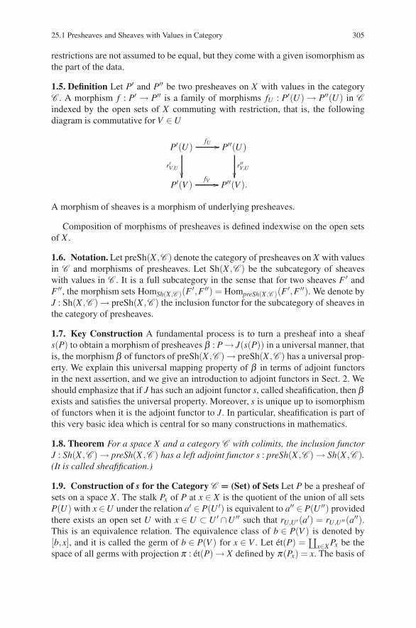
25.1 Presheaves and Sheaves with Values in Category 305
restrictions are not assumed to be equal, but they come with a given isomorphism asthe part of the data.
1.5. Definition Let P′ and P′′ be two presheaves on X with values in the categoryC . A morphism f : P′ → P′′ is a family of morphisms fU : P′(U) → P′′(U) in Cindexed by the open sets of X commuting with restriction, that is, the followingdiagram is commutative for V ∈U
P′(U)fU ��
r′V,U
��
P′′(U)
r′′V,U
��P′(V )
fV �� P′′(V ).
A morphism of sheaves is a morphism of underlying presheaves.
Composition of morphisms of presheaves is defined indexwise on the open setsof X .
1.6. Notation. Let preSh(X ,C ) denote the category of presheaves on X with valuesin C and morphisms of presheaves. Let Sh(X ,C ) be the subcategory of sheaveswith values in C . It is a full subcategory in the sense that for two sheaves F ′ andF ′′, the morphism sets HomSh(X ,C )(F ′,F ′′) = HompreSh(X ,C )(F ′,F ′′). We denote byJ : Sh(X ,C ) → preSh(X ,C ) the inclusion functor for the subcategory of sheaves inthe category of presheaves.
1.7. Key Construction A fundamental process is to turn a presheaf into a sheafs(P) to obtain a morphism of presheaves β : P → J(s(P)) in a universal manner, thatis, the morphism β of functors of preSh(X ,C )→ preSh(X ,C ) has a universal prop-erty. We explain this universal mapping property of β in terms of adjoint functorsin the next assertion, and we give an introduction to adjoint functors in Sect. 2. Weshould emphasize that if J has such an adjoint functor s, called sheafification, then βexists and satisfies the universal property. Moreover, s is unique up to isomorphismof functors when it is the adjoint functor to J. In particular, sheafification is part ofthis very basic idea which is central for so many constructions in mathematics.
1.8. Theorem For a space X and a category C with colimits, the inclusion functorJ : Sh(X ,C ) → preSh(X ,C ) has a left adjoint functor s : preSh(X ,C ) → Sh(X ,C ).(It is called sheafification.)
1.9. Construction of s for the Category C === (Set) of Sets Let P be a presheaf ofsets on a space X . The stalk Px of P at x ∈ X is the quotient of the union of all setsP(U) with x ∈U under the relation a′ ∈ P(U ′) is equivalent to a′′ ∈ P(U ′′) providedthere exists an open set U with x ∈ U ⊂ U ′ ∩U ′′ such that rU,U ′ (a′) = rU,U ′′(a′′).This is an equivalence relation. The equivalence class of b ∈ P(V ) is denoted by[b,x], and it is called the germ of b ∈ P(V ) for x ∈ V . Let et(P) =
∐x∈X Px be the
space of all germs with projection π : et(P) → X defined by π(Px) = x. The basis of
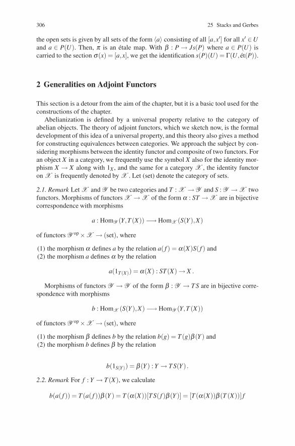
306 25 Stacks and Gerbes
the open sets is given by all sets of the form 〈a〉 consisting of all [a,x′] for all x′ ∈Uand a ∈ P(U). Then, π is an etale map. With β : P → Js(P) where a ∈ P(U) iscarried to the section σ(x) = [a,x], we get the identification s(P)(U) = Γ(U, et(P)).
2 Generalities on Adjoint Functors
This section is a detour from the aim of the chapter, but it is a basic tool used for theconstructions of the chapter.
Abelianization is defined by a universal property relative to the category ofabelian objects. The theory of adjoint functors, which we sketch now, is the formaldevelopment of this idea of a universal property, and this theory also gives a methodfor constructing equivalences between categories. We approach the subject by con-sidering morphisms between the identity functor and composite of two functors. Foran object X in a category, we frequently use the symbol X also for the identity mor-phism X → X along with 1X , and the same for a category X , the identity functoron X is frequently denoted by X . Let (set) denote the category of sets.
2.1. Remark Let X and Y be two categories and T : X →Y and S : Y →X twofunctors. Morphisms of functors X → X of the form α : ST → X are in bijectivecorrespondence with morphisms
a : HomY (Y,T (X)) −→ HomX (S(Y ),X)
of functors Y op ×X → (set), where
(1) the morphism α defines a by the relation a( f ) = α(X)S( f ) and(2) the morphism a defines α by the relation
a(1T (X)) = α(X) : ST(X) → X .
Morphisms of functors Y → Y of the form β : Y → T S are in bijective corre-spondence with morphisms
b : HomX (S(Y ),X) −→ HomY (Y,T (X))
of functors Y op ×X → (set), where
(1) the morphism β defines b by the relation b(g) = T (g)β (Y ) and(2) the morphism b defines β by the relation
b(1S(Y)) = β (Y ) : Y → T S(Y ) .
2.2. Remark For f : Y → T (X), we calculate
b(a( f )) = T (a( f ))β (Y ) = T (α(X))[T S( f )β (Y )] = [T (α(X))β (T (X))] f
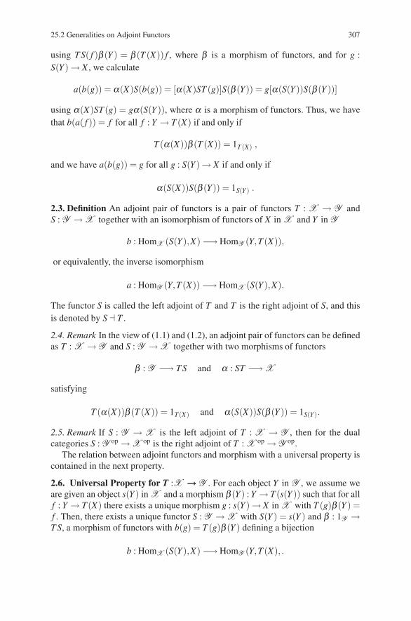
25.2 Generalities on Adjoint Functors 307
using TS( f )β (Y ) = β (T (X)) f , where β is a morphism of functors, and for g :S(Y ) → X , we calculate
a(b(g)) = α(X)S(b(g)) = [α(X)ST (g)]S(β (Y)) = g[α(S(Y ))S(β (Y ))]
using α(X)ST (g) = gα(S(Y )), where α is a morphism of functors. Thus, we havethat b(a( f )) = f for all f : Y → T (X) if and only if
T (α(X))β (T (X)) = 1T (X) ,
and we have a(b(g)) = g for all g : S(Y ) → X if and only if
α(S(X))S(β (Y)) = 1S(Y ) .
2.3. Definition An adjoint pair of functors is a pair of functors T : X → Y andS : Y → X together with an isomorphism of functors of X in X and Y in Y
b : HomX (S(Y ),X) −→ HomY (Y,T (X)),
or equivalently, the inverse isomorphism
a : HomY (Y,T (X)) −→ HomX (S(Y ),X).
The functor S is called the left adjoint of T and T is the right adjoint of S, and thisis denoted by S � T .
2.4. Remark In the view of (1.1) and (1.2), an adjoint pair of functors can be definedas T : X → Y and S : Y → X together with two morphisms of functors
β : Y −→ TS and α : ST −→ X
satisfying
T (α(X))β (T (X)) = 1T(X) and α(S(X))S(β (Y )) = 1S(Y).
2.5. Remark If S : Y → X is the left adjoint of T : X → Y , then for the dualcategories S : Y op → X op is the right adjoint of T : X op → Y op.
The relation between adjoint functors and morphism with a universal property iscontained in the next property.
2.6. Universal Property for T :X →→→ Y . For each object Y in Y , we assume weare given an object s(Y ) in X and a morphism β (Y ) : Y → T (s(Y )) such that for allf : Y → T (X) there exists a unique morphism g : s(Y ) → X in X with T (g)β (Y ) =f . Then, there exists a unique functor S : Y → X with S(Y ) = s(Y ) and β : 1Y →T S, a morphism of functors with b(g) = T (g)β (Y ) defining a bijection
b : HomX (S(Y ),X) −→ HomY (Y,T (X), .
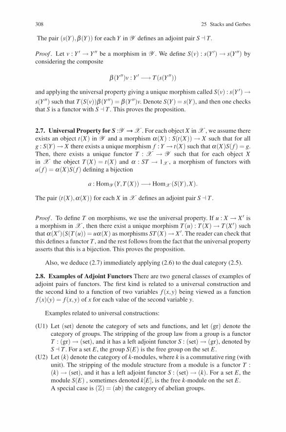
308 25 Stacks and Gerbes
The pair (s(Y ),β (Y )) for each Y in Y defines an adjoint pair S � T.
Proof . Let v : Y ′ → Y ′′ be a morphism in Y . We define S(v) : s(Y ′) → s(Y ′′) byconsidering the composite
β (Y ′′)v : Y ′ −→ T (s(Y ′′))
and applying the universal property giving a unique morphism called S(v) : s(Y ′)→s(Y ′′) such that T (S(v))β (Y ′′) = β (Y ′′)v. Denote S(Y ) = s(Y ), and then one checksthat S is a functor with S � T . This proves the proposition.
2.7. Universal Property for S :Y →→→X . For each object X in X , we assume thereexists an object t(X) in Y and a morphism α(X) : S(t(X)) → X such that for allg : S(Y ) → X there exists a unique morphism f : Y → t(X) such that α(X)S( f ) = g.Then, there exists a unique functor T : X → Y such that for each object Xin X the object T (X) = t(X) and α : ST → 1X , a morphism of functors witha( f ) = α(X)S( f ) defining a bijection
a : HomY (Y,T (X)) −→ HomX (S(Y ),X).
The pair (t(X),α(X)) for each X in X defines an adjoint pair S � T .
Proof . To define T on morphisms, we use the universal property. If u : X → X ′ isa morphism in X , then there exist a unique morphism T (u) : T (X) → T (X ′) suchthat α(X ′)(S(T (u)) = uα(X) as morphisms ST (X)→ X ′. The reader can check thatthis defines a functor T , and the rest follows from the fact that the universal propertyasserts that this is a bijection. This proves the proposition.
Also, we deduce (2.7) immediately applying (2.6) to the dual category (2.5).
2.8. Examples of Adjoint Functors There are two general classes of examples ofadjoint pairs of functors. The first kind is related to a universal construction andthe second kind to a function of two variables f (x,y) being viewed as a functionf (x)(y) = f (x,y) of x for each value of the second variable y.
Examples related to universal constructions:
(U1) Let (set) denote the category of sets and functions, and let (gr) denote thecategory of groups. The stripping of the group law from a group is a functorT : (gr) → (set), and it has a left adjoint functor S : (set) → (gr), denoted byS � T . For a set E , the group S(E) is the free group on the set E .
(U2) Let (k) denote the category of k-modules, where k is a commutative ring (withunit). The stripping of the module structure from a module is a functor T :(k) → (set), and it has a left adjoint functor S : (set) → (k). For a set E , themodule S(E) , sometimes denoted k[E], is the free k-module on the set E .A special case is (Z) = (ab) the category of abelian groups.
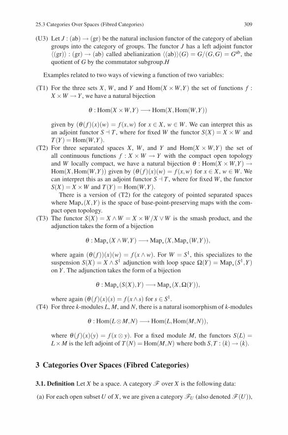
25.3 Categories Over Spaces (Fibred Categories) 309
(U3) Let J : (ab) → (gr) be the natural inclusion functor of the category of abeliangroups into the category of groups. The functor J has a left adjoint functor〈(gr)〉 : (gr) → (ab) called abelianization 〈(ab)〉(G) = G/(G,G) = Gab, thequotient of G by the commutator subgroup.H
Examples related to two ways of viewing a function of two variables:
(T1) For the three sets X , W , and Y and Hom(X ×W,Y ) the set of functions f :X ×W → Y , we have a natural bijection
θ : Hom(X ×W,Y) −→ Hom(X ,Hom(W,Y ))
given by (θ ( f )(x)(w) = f (x,w) for x ∈ X , w ∈ W . We can interpret this asan adjoint functor S � T , where for fixed W the functor S(X) = X ×W andT (Y ) = Hom(W,Y ).
(T2) For three separated spaces X , W , and Y and Hom(X ×W,Y ) the set ofall continuous functions f : X ×W → Y with the compact open topologyand W locally compact, we have a natural bijection θ : Hom(X ×W,Y ) →Hom(X ,Hom(W,Y )) given by (θ ( f )(x)(w) = f (x,w) for x ∈ X , w ∈ W . Wecan interpret this as an adjoint functor S � T , where for fixed W , the functorS(X) = X ×W and T (Y ) = Hom(W,Y ).
There is a version of (T2) for the category of pointed separated spaceswhere Map∗(X ,Y ) is the space of base-point-preserving maps with the com-pact open topology.
(T3) The functor S(X) = X ∧W = X ×W/X ∨W is the smash product, and theadjunction takes the form of a bijection
θ : Map∗(X ∧W,Y ) −→ Map∗(X ,Map∗(W,Y )),
where again (θ ( f ))(x)(w) = f (x ∧ w). For W = S1, this specializes to thesuspension S(X) = X ∧ S1 adjunction with loop space Ω(Y ) = Map∗(S1,Y )on Y . The adjunction takes the form of a bijection
θ : Map∗(S(X),Y ) −→ Map∗(X ,Ω(Y )),
where again (θ ( f )(x)(s) = f (x∧ s) for s ∈ S1.(T4) For three k-modules L, M, and N, there is a natural isomorphism of k-modules
θ : Hom(L⊗M,N) −→ Hom(L,Hom(M,N)),
where θ ( f )(x)(y) = f (x ⊗ y). For a fixed module M, the functors S(L) =L×M is the left adjoint of T (N) = Hom(M,N) where both S,T : (k) → (k).
3 Categories Over Spaces (Fibred Categories)
3.1. Definition Let X be a space. A category F over X is the following data:
(a) For each open subset U of X , we are given a category FU (also denoted F (U)),
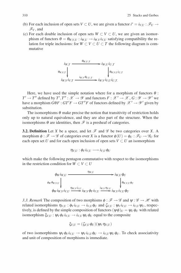
310 25 Stacks and Gerbes
(b) For each inclusion of open sets V ⊂U , we are given a functor i∗ = iV,U : FU →FV , and
(c) For each double inclusion of open sets W ⊂ V ⊂ U , we are given an isomor-phism of functors θ = θW,V,U : iW,U → iW,V iV,U satisfying compatibility the re-lation for triple inclusions: for W ⊂ V ⊂U ⊂ T the following diagram is com-mutative
iW,T
θW,V,T
��
θW,U,T �� iW,U iU,T
θW,V,U iU,T
��iW,V iV,T
iW,VθV,U,T �� iW,V iV,U iU,T.
Here, we have used the simple notation where for a morphism of functors θ :T ′ → T ′′ defined by T ′,T ′′ : X → Y and functors F : X ′ → X , G : Y → Y ′ wehave a morphism GθF : GT ′F → GT ′′F of functors defined by X ′ → Y ′ given bysubstitution.
The isomorphisms θ make precise the notion that transitivity of restriction holdsonly up to natural equivalence, and they are also part of the structure. When theisomorphisms θ are identities, then F is a presheaf of categories.
3.2. Definition Let X be a space, and let F and G be two categories over X . Amorphism φ : F → G of categories over X is a functor φ(U) = φU : FU → GU foreach open set U and for each open inclusion of open sets V ⊂U an isomorphism
ηV,U : φV iV,U −→ iV,UφU
which make the following pentagon commutative with respect to the isomorphismsin the restriction condition for W ⊂V ⊂U
φW iW,U
φWθW,V,U
��
ηW,U �� iW,UφU
θW,V,UφU
��φW iW,V iV,U
ηW,V iV,U�� iW,VφV iV,UiW,VηV,U�� iW,V iV,UφU
3.3. Remark The composition of two morphisms φ : F → G and ψ : G → H withrelated isomorphisms ηV,U : φV iV,U → iV,UφU and ζV,U : ψV iV,U → iV,UψU , respec-tively, is defined by the simple composition of functors (ψφ)U =ψUφU with relatedisomorphism ξV,U : ψVφV iV,U → iV,UψUφU equal to the composite
ξV,U = (ζV,UφU)(ψVηV,U)
of two isomorphisms ψVφV iV,U → ψV iV,UφU → iV,UψUφU . To check associativityand unit of composition of morphisms is immediate.
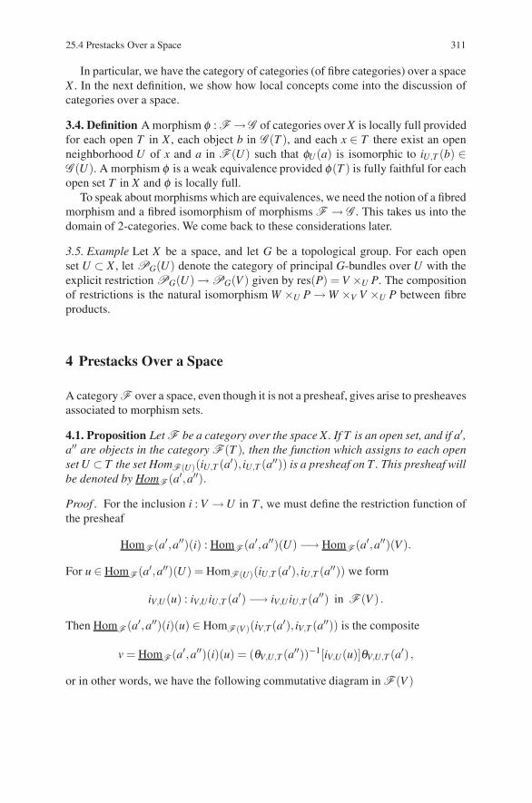
25.4 Prestacks Over a Space 311
In particular, we have the category of categories (of fibre categories) over a spaceX . In the next definition, we show how local concepts come into the discussion ofcategories over a space.
3.4. Definition A morphism φ : F →G of categories over X is locally full providedfor each open T in X , each object b in G (T ), and each x ∈ T there exist an openneighborhood U of x and a in F (U) such that φU(a) is isomorphic to iU,T (b) ∈G (U). A morphism φ is a weak equivalence provided φ(T ) is fully faithful for eachopen set T in X and φ is locally full.
To speak about morphisms which are equivalences, we need the notion of a fibredmorphism and a fibred isomorphism of morphisms F → G . This takes us into thedomain of 2-categories. We come back to these considerations later.
3.5. Example Let X be a space, and let G be a topological group. For each openset U ⊂ X , let PG(U) denote the category of principal G-bundles over U with theexplicit restriction PG(U) → PG(V ) given by res(P) = V ×U P. The compositionof restrictions is the natural isomorphism W ×U P → W ×V V ×U P between fibreproducts.
4 Prestacks Over a Space
A category F over a space, even though it is not a presheaf, gives arise to presheavesassociated to morphism sets.
4.1. Proposition Let F be a category over the space X. If T is an open set, and if a′,a′′ are objects in the category F (T ), then the function which assigns to each openset U ⊂ T the set HomF (U)(iU,T (a′), iU,T (a′′)) is a presheaf on T . This presheaf willbe denoted by HomF (a′,a′′).
Proof . For the inclusion i : V →U in T , we must define the restriction function ofthe presheaf
HomF (a′,a′′)(i) : HomF (a′,a′′)(U) −→ HomF (a′,a′′)(V ).
For u ∈ HomF (a′,a′′)(U) = HomF (U)(iU,T (a′), iU,T (a′′)) we form
iV,U(u) : iV,UiU,T (a′) −→ iV,UiU,T (a′′) in F (V ) .
Then HomF (a′,a′′)(i)(u) ∈ HomF (V )(iV,T (a′), iV,T (a′′)) is the composite
v = HomF (a′,a′′)(i)(u) = (θV,U,T (a′′))−1[iV,U(u)]θV,U,T (a′) ,
or in other words, we have the following commutative diagram in F (V )
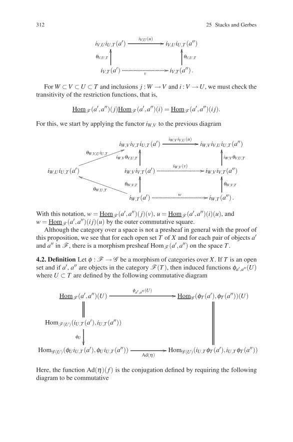
312 25 Stacks and Gerbes
iV,U iU,T (a′)iV,U (u)
�� iV,UiU,T (a′′)
iV,T (a′)
θV,U,T
��
v�� iV,T (a′′) .
θV,U,T
��
For W ⊂V ⊂U ⊂ T and inclusions j : W →V and i : V →U , we must check thetransitivity of the restriction functions, that is,
HomF (a′,a′′)( j)HomF (a′,a′′)(i) = HomF (a′,a′′)(i j).
For this, we start by applying the functor iW,V to the previous diagram
iW,V iV,T iU,T (a′)iW,V iV,U (u)
�� iW,V iV,U iU,T (a′′)
iW,U iU,T (a′)
θW,V,U iU,T##$$$$$$$$$$$$$$$iW,V iV,T (a′)
iW,VθV,U,T
��
iW,V (v)�� iW,V iV,T (a′′)
iW,VθV,U,T
��
iW,T (a′)θW,U,T
$$%%%%%%%%%%%%%%%%θW,V,T
��
w �� iW,T (a′′) .
θW,V,T
��
With this notation, w = HomF (a′,a′′)( j)(v), u = HomF (a′,a′′)(i)(u), andw = HomF (a′,a′′)(i j)(u) by the outer commutative square.
Although the category over a space is not a presheaf in general with the proof ofthis proposition, we see that for each open set T of X and for each pair of objects a′and a′′ in F , there is a morphism presheaf HomF (a′,a′′) on the space T .
4.2. Definition Let φ : F → G be a morphism of categories over X . If T is an openset and if a′, a′′ are objects in the category F (T ), then induced functions φa′,a′′(U)where U ⊂ T are defined by the following commutative diagram
HomF (a′,a′′)(U)φa′ ,a′′ (U)
�� HomG (φT (a′),φT (a′′))(U)
HomF (U)(iU,T (a′), iU,T (a′′))
φU
��HomG (U)(φU iU,T (a′),φU iU,T (a′′))
Ad(η)�� HomG (U)(iU,TφT (a′), iU,TφT (a′′))
Here, the function Ad(η)( f ) is the conjugation defined by requiring the followingdiagram to be commutative
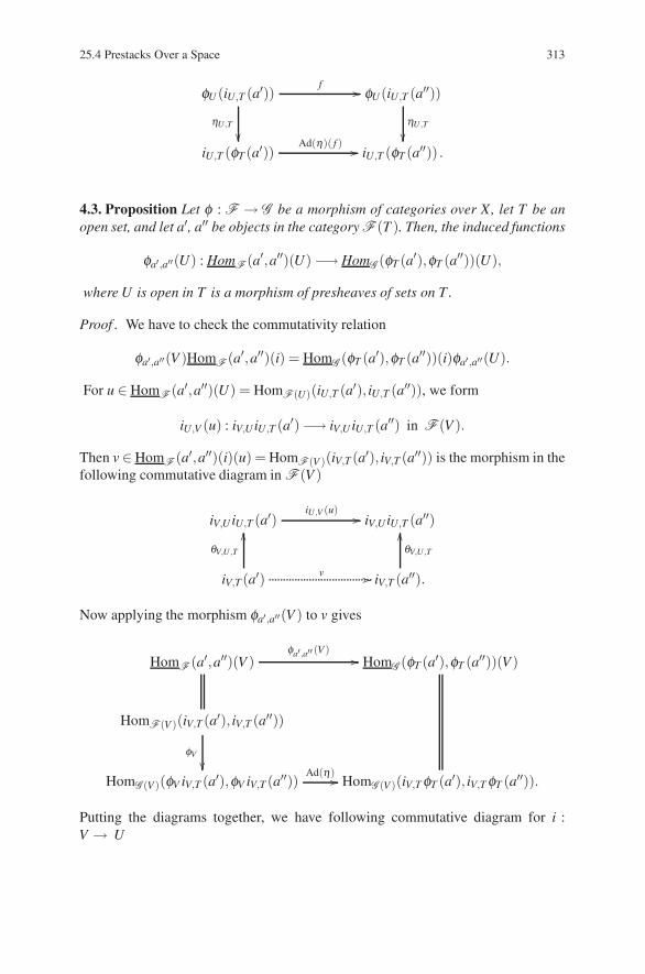
25.4 Prestacks Over a Space 313
φU (iU,T (a′))
ηU,T
��
f �� φU(iU,T (a′′))
ηU,T
��iU,T (φT (a′))
Ad(η)( f ) �� iU,T (φT (a′′)) .
4.3. Proposition Let φ : F → G be a morphism of categories over X, let T be anopen set, and let a′, a′′ be objects in the category F (T ). Then, the induced functions
φa′,a′′(U) : HomF (a′,a′′)(U) −→ HomG (φT (a′),φT (a′′))(U),
where U is open in T is a morphism of presheaves of sets on T .
Proof . We have to check the commutativity relation
φa′,a′′(V )HomF (a′,a′′)(i) = HomG (φT (a′),φT (a′′))(i)φa′ ,a′′(U).
For u ∈ HomF (a′,a′′)(U) = HomF (U)(iU,T (a′), iU,T (a′′)), we form
iU,V (u) : iV,UiU,T (a′) −→ iV,U iU,T (a′′) in F (V ).
Then v ∈ HomF (a′,a′′)(i)(u) = HomF (V )(iV,T (a′), iV,T (a′′)) is the morphism in thefollowing commutative diagram in F (V )
iV,U iU,T (a′)iU,V (u)
�� iV,UiU,T (a′′)
iV,T (a′)
θV,U,T
��
v �� iV,T (a′′).
θV,U,T
��
Now applying the morphism φa′,a′′(V ) to v gives
HomF (a′,a′′)(V )φa′,a′′ (V )
�� HomG (φT (a′),φT (a′′))(V )
HomF (V )(iV,T (a′), iV,T (a′′))
φV
��HomG (V )(φV iV,T (a′),φV iV,T (a′′))
Ad(η) �� HomG (V )(iV,TφT (a′), iV,TφT (a′′)).
Putting the diagrams together, we have following commutative diagram for i :V → U
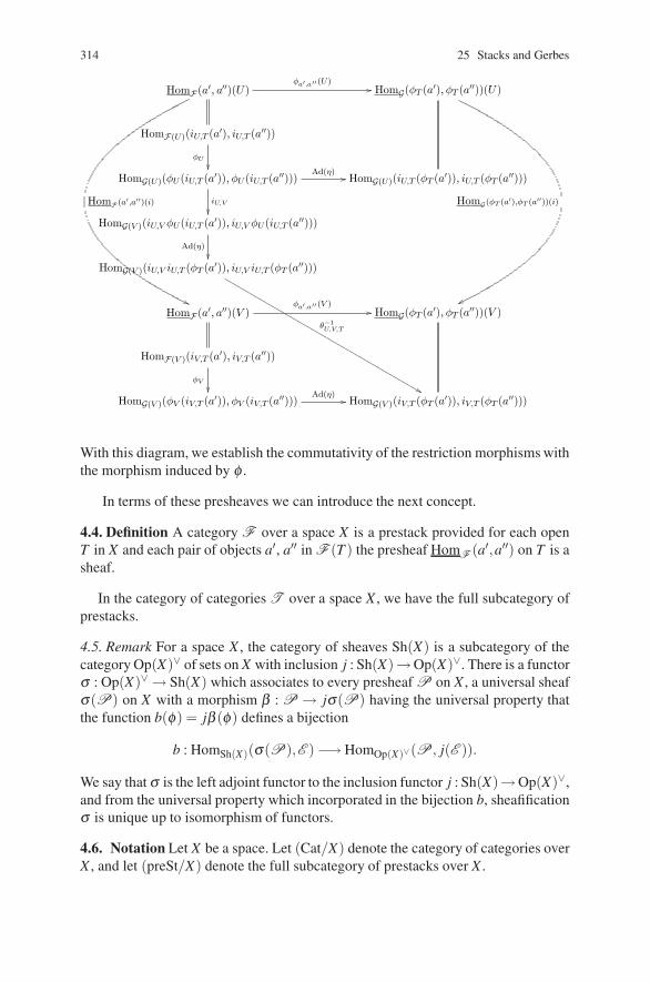
314 25 Stacks and Gerbes
HomF (a , a )(U)
HomF (a ,a )(i)
φa ,a (U)HomG(φT (a ),φT (a ))(U)
HomG(φT (a ),φT (a ))(i)
HomF(U)(iU,T (a ), iU,T (a ))
φU
HomG(U)(φU (iU,T (a )),φU (iU,T (a )))Ad(η)
iU,V
HomG(U)(iU,T (φT (a )), iU,T (φT (a )))
HomG(V )(iU,V φU (iU,T (a )), iU,V φU (iU,T (a )))
Ad(η)
HomG(V )(iU,V iU,T (φT (a )), iU,V iU,T (φT (a )))
θ−1U,V,T
HomF (a , a )(V )φa ,a (V )
HomG(φT (a ),φT (a ))(V )
HomF(V )(iV,T (a ), iV,T (a ))
φV
HomG(V )(φV (iV,T (a )),φV (iV,T (a )))Ad(η)
HomG(V )(iV,T (φT (a )), iV,T (φT (a )))
With this diagram, we establish the commutativity of the restriction morphisms withthe morphism induced by φ .
In terms of these presheaves we can introduce the next concept.
4.4. Definition A category F over a space X is a prestack provided for each openT in X and each pair of objects a′, a′′ in F (T ) the presheaf HomF (a′,a′′) on T is asheaf.
In the category of categories T over a space X , we have the full subcategory ofprestacks.
4.5. Remark For a space X , the category of sheaves Sh(X) is a subcategory of thecategory Op(X)∨ of sets on X with inclusion j : Sh(X)→Op(X)∨. There is a functorσ : Op(X)∨ → Sh(X) which associates to every presheaf P on X , a universal sheafσ(P) on X with a morphism β : P → jσ(P) having the universal property thatthe function b(φ) = jβ (φ) defines a bijection
b : HomSh(X)(σ(P),E ) −→ HomOp(X)∨(P, j(E )).
We say that σ is the left adjoint functor to the inclusion functor j : Sh(X)→Op(X)∨,and from the universal property which incorporated in the bijection b, sheafificationσ is unique up to isomorphism of functors.
4.6. Notation Let X be a space. Let (Cat/X) denote the category of categories overX , and let (preSt/X) denote the full subcategory of prestacks over X .
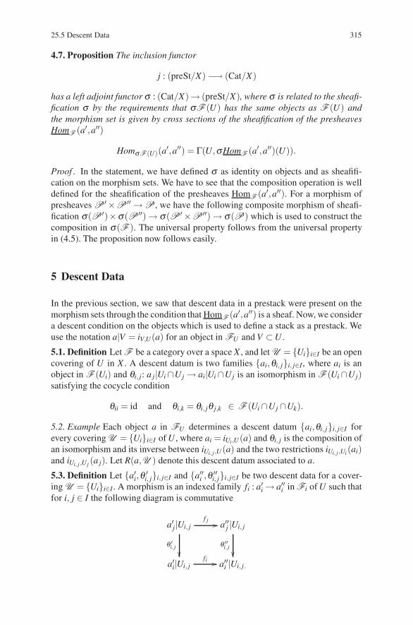
25.5 Descent Data 315
4.7. Proposition The inclusion functor
j : (preSt/X) −→ (Cat/X)
has a left adjoint functor σ : (Cat/X)→ (preSt/X), where σ is related to the sheafi-fication σ by the requirements that σF (U) has the same objects as F (U) andthe morphism set is given by cross sections of the sheafification of the presheavesHomF (a′,a′′)
HomσF (U)(a′,a′′) = Γ(U,σHomF (a′,a′′)(U)).
Proof . In the statement, we have defined σ as identity on objects and as sheafifi-cation on the morphism sets. We have to see that the composition operation is welldefined for the sheafification of the presheaves HomF (a′,a′′). For a morphism ofpresheaves P ′ ×P ′′ → P , we have the following composite morphism of sheafi-fication σ(P ′)×σ(P ′′) → σ(P ′ ×P ′′) → σ(P) which is used to construct thecomposition in σ(F ). The universal property follows from the universal propertyin (4.5). The proposition now follows easily.
5 Descent Data
In the previous section, we saw that descent data in a prestack were present on themorphism sets through the condition that HomF (a′,a′′) is a sheaf. Now, we considera descent condition on the objects which is used to define a stack as a prestack. Weuse the notation a|V = iV,U(a) for an object in FU and V ⊂U .
5.1. Definition Let F be a category over a space X , and let U = {Ui}i∈I be an opencovering of U in X . A descent datum is two families {ai,θi, j}i, j∈I , where ai is anobject in F (Ui) and θi, j: a j|Ui ∩Uj → ai|Ui ∩Uj is an isomorphism in F (Ui ∩Uj)satisfying the cocycle condition
θii = id and θi,k = θi, jθ j,k ∈ F (Ui ∩Uj ∩Uk).
5.2. Example Each object a in FU determines a descent datum {ai,θi, j}i, j∈I forevery covering U = {Ui}i∈I of U , where ai = iUi ,U(a) and θi, j is the composition ofan isomorphism and its inverse between iUi, j ,U(a) and the two restrictions iUi, j ,Ui(ai)and iUi, j ,Uj (a j). Let R(a,U ) denote this descent datum associated to a.
5.3. Definition Let {a′i,θ ′i, j}i, j∈I and {a′′i ,θ ′′i, j}i, j∈I be two descent data for a cover-ing U = {Ui}i∈I . A morphism is an indexed family fi : a′i → a′′i in Fi of U such thatfor i, j ∈ I the following diagram is commutative
a′j|Ui, j
θ ′i, j
��
f j �� a′′j |Ui, j
θ ′′i, j
��a′i|Ui, j
fi �� a′′i |Ui, j.
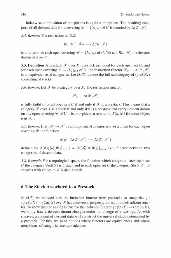
316 25 Stacks and Gerbes
Indexwise composition of morphisms is again a morphism. The resulting cate-gory of all descent data for a covering U = {Ui}i∈I of U is denoted by Δ(U ,F ).
5.4. Remark The restriction in (5.2)
R( ,U ) : FU −→ Δ(U ,F )
is a functor for each open covering U = {Ui}i∈I of U . We call R(a,U ) the descentdatum of a on U .
5.5. Definition A prestack F over X is a stack provided for each open set U , andfor each open covering U = {Ui}i∈I of U , the restriction functor FU → Δ(U ,F )is an equivalence of categories. Let (St/X) denote the full subcategory of (preSt/X)consisting of stacks.
5.6. Remark Let F be a category over X . The restriction functor
FU → Δ(U ,F )
is fully faithful for all open sets U if and only if F is a prestack. This means that acategory F over X is a stack if and only if it is a prestack and every descent datumon any open covering U of U is isomorphic to a restriction R(a,U ) for some objecta in FU .
5.7. Remark If φ : F ′ →F ′′ is a morphism of categories over X , then for each opencovering U the function
Δ(φ) : Δ(U ,F ′) −→ Δ(U ,F ′′)
defined by Δ(φ)({a′i,θ ′i, j}i, j∈I) = {φ(a′i),φ(θ ′i, j)}i, j∈I is a functor between twocategories of descent data.
5.8. Example For a topological space, the function which assigns to each open setU the category Vect(U) is a stack and to each open set U the category Sh(U,C ) ofsheaves with values in C is also a stack.
6 The Stack Associated to a Prestack
In (4.7), we showed how the inclusion functor from prestacks to categories j :(preSt/X)→ (Cat/X) over X has a universal property, that is, it is a left adjoint func-tor. To show that the analog is true for the inclusion functor j : (St/X)→ (preSt/X),we study how a descent datum changes under the change of coverings. As withsheaves, a colimit of descent data will construct the universal stack determined bya prestack. For this, we need notions where functors are equivalences and wheremorphisms of categories are equivalences.
25.6 The Stack Associated to a Prestack 317
6.1. Definition A functor F : C ′ → C ′′ is faithful (resp. full, fully faithful) providedF : HomC ′(X ,Y )→ HomC ′′(F(X),F(Y )) is injective (resp. surjective, bijective) forall objects X in C and all objects Y in C ′.
Faithful, full, and fully faithful are properties preserved by composition offunctors.
6.2. Definition A functor F : C ′ →C ′′ is an equivalence provided F is fully faithfuland surjective up to isomorphism, that is, for each object Z in C ′′, there exists anobject X in C ′ with F(X) and Z isomorphic.
6.3. Remark A functor F : C ′ → C ′′ is an equivalence if and only if there existsa functor G : C ′′ → C ′ such that GF is isomorphic to identity on C ′ and FG isisomorphic to the identity on C ′′. It is the case that G is both right and left adjointof F , and for this reason, the first step in studying whether or not a functor F is anequivalence is to look for a left or right adjoint functor of F .
In (3.4), we introduced the notion of locally full morphisms of categories over X .Now, we consider equivalences of categories over a space.
6.4. Definition A morphism φ : F → G of categories over X is an equivalence pro-vided φ(U) : FU → GU is an equivalence of categories for each open set U in X . Amorphism φ : F → G of categories over X is a weak equivalence provided φ(U) isfully faithful for each open set U in X and φ is locally full.
6.5. Remark Let φ : F → G be an equivalence of categories over X . Then, F is aprestack (resp. stack) over X if and only if G is a prestack (resp. stack).
6.6. Remark If φ : F → G is a weak equivalence of prestacks over X and if F is astack, then φ is an equivalence. In other words, the local surjectivity gives arise tosurjectivity map up to isomorphism by descent construction.
Similarly, we have the factorization property.
6.7. Remark Let φ : F ′ → F ′′ is a weak equivalence of prestacks over X andψ ′ : F ′ → G be a morphism of prestacks over X . If G is a stack, then there existsa morphism ψ ′′ : F ′′ → G of prestacks over X such that ψ ′′φ and ψ ′ are naturallyequivalent morphisms.
With sheaves, the inclusion J : Sh(X ,C ) → preSh(X ,C ) has a left adjoint, butwith the inclusion Stack(X)→ preSt(X), we must use the following definition whichis based on the assertion (6.7).
6.8. Definition For a prestack F over X , the associated stack is a pair consisting ofa stack s(F ) together with a weak equivalence φ : F → s(F ).
6.9. Theorem For a prestack F over X, the associated stack exists and is uniqueup to a strong equivalence.
The uniqueness is contained in (6.7), and the existence is a colimit constructionas with the associated sheaf to a presheaf. The limit is over all coverings related tothe descent data where for a sheaf of sets the related colimit is given by forming thestacks of the presheaf.
318 25 Stacks and Gerbes
7 Gerbes as Stacks of Groupoids
We have considered gerbes as bundle gerbes and groupoid gerbes. Now, we returnto the concept of a gerbe in terms of groupoids over a space X .
7.1. Definition A gerbe G on X is a stack over X such that each G (U) is a groupoidand the union of all open sets U such that G (U) is nonempty is X . It satisfies thefollowing local connectivity or transitivity condition: For two objects a′, a′′ in anyG (U) and x in U , there exists an open set V with x ∈ V ⊂ U and a morphism u :iV,U(a′) → iV,U(a′′).
The basic example extends the idea of principal bundle. Instead of a group westart with a sheaf G of groups over X .
7.2. Definition A principal G-sheaf P over X is a sheaf of sets with an action P×G → P over X of sheaves such that X is the union of all U with P(U) = Γ(U,P)nonempty and G(U) is free and transitive on P(U) for each open subset U of X .A morphism P′ → P′′ of principal G-sheaves is a morphism of sheaves commutingwith the action G.
Another word for principal G-sheaf is torsor (it is a rather silly word).
7.3. Remark In terms of the etale spaces over X , the action is defined by s(P)×s(G) → s(P) over X , where s(P) → X is surjective and projection and action s(P)×s(G) → s(P) is a homeomorphism.
7.4. Remark The trivial principal G-sheaf is G itself, and a principal G-sheaf P isisomorphic to G if and only if P(X) = Γ(X ,P) is nonempty. Then, any elementdefines an isomorphism G → P by the action on the cross section of P over X .
7.5. Example Let G be a sheaf over X . Let (BunG(U)) denote the category ofprincipal G(U) sheaves over U . Then, (BunG(U)) is a gerbe over X .
There are two cohomological classifications by H1(X ,G) for isomorphism classesof principal G-sheaves for a sheaf of groups and by H2(X ,L) for gerbes G over Xwith given band L, see Sect. 9.
8 Cohomological Classification of Principal G-Sheaves
The cohomological classification of sheaves, bundles, and gerbes depends on theautomorphisms of trivial bundles.
8.1. Remark The automorphism group of the trivial principal G-bundle G is just thegroup of cross sections Γ(X ,G) where to a cross section σ we associate the auto-morphism uσ : G → G given by uσ (U) : G(U) → G(U) given by uσ (τ) = τ(σ |U).
8.2. Principal G-Sheaves Trivial Over an Open Covering Let G be a group sheafover the space X , and let U = {Ui}i∈I be an open covering of X . For a principal
25.8 Cohomological Classification of Principal G-Sheaves 319
G-sheaf P where P|Ui is trivial, we choose a section σi ∈ Γ(Ui,P) defining the triv-ialization. By (8.1) over Ui, j = Ui ∩Uj, we have a section gi, j ∈ Γ(Ui, j,G) such thaton Ui, j, we have (σi|Ui, j)gi, j = (σ j|Ui, j).
(1) Cocycle Condition: Over the triple intersection Ui, j,k = Ui ∩Uj ∩Uk, we havethe cocycle relation
gi, jg j,k = gi,k.
(2) Change of Section Leads to a Coboundary Relation: For a second set of sectionsσ ′
i we have new g′i, j such that on Ui, j, we have (σ ′i |Ui, j)g′i, j = (σ ′
j|Ui, j). The twosets of sections are related again by elements bi ∈ Γ(Ui,G), where σ ′
i = σibi.Hence, we have the cobounding relation
big′i, j = gi, jb j or g′i, j = b−1
i gi, jb j on Ui, j
which follows from the following substitutions
σigi, jb j = σ jb j = σ ′j = σ ′
i g′i, j = σibig′i, j.
8.3. Definition Let G be a sheaf of groups on a space X , and let U = (Ui)i∈I be anopen covering of X . The first cohomology set H1(U ,G) of the covering U of Xwith values in the sheaf G is the set of cocycles (gi, j)i, j∈I with values in G wheregi, j ∈Γ(Ui, j,G) modulo the cobounding equivalence g′i, j = b−1
i gi, jb j, where sectionsbi ∈ Γ(Ui,G) for i ∈ I.
8.4. Remark Let (gi, j)i, j∈I be a cocycle with values in G relative to a covering U ={Ui}i∈I . Then, there is a principal G-sheaf P, where P|Ui is trivial for each i ∈ I andthe trivializations are related by the isomorphism defined by gi, j on Ui, j. Moreover,two cocycles (gi, j)i, j∈I and (g′i, j)i, j∈I define isomorphic principal G-sheaves if andonly if they are cobounding. This gives the following proposition.
8.5. Proposition The cohomology set H1(U ,G) classifies principal G-sheaveswhich are trivial on all Ui ∈ U up to isomorphism.
To remove the dependence on the covering U in (8.5), we introduce a certaincolimit.
8.6. Definition Let G be a sheaf of groups on a space X . The first Cech cohomologyset H1(X ,G) is the colimit of all H1(U ,G) over the open coverings U of X . Amorphism between coverings U = {Ui}i∈I → B = {Vi}i∈I is defined by a functionθ : J → I, where Uθ( j) ⊃Vj for all j ∈ J in order to define the colimit.
In terms of the first Cech cohomology set, we have the classification of all princi-pal G-sheaves because each principal G-sheaf is trivial for some open covering of X .
8.7. Proposition The cohomology set H1(X ,G) classifies principal G-sheaves up toisomorphisms.
320 25 Stacks and Gerbes
9 Cohomological Classification of Bands Associated with a Gerbe
The cohomological classification of bands in a gerbe depends on various sheavesassociated to the gerbe.
9.1. Sheaves on Open Sets in a Covering Let G be a gerbe over X . Then, for eachobject in G(T ) over an open T ⊂ X , the automorphisms
AutG(a,a) = HomG(a,a)
is a sheaf on T . Let X =⋃
i∈I Ui be an open covering of X , and let ai be an object inG(Ui). Then, AutG(ai,ai)is a sheaf of groups on Ui.
9.2. Relating Automorphism Sheaves on Over Lapping Ui∩∩∩Uj open Sets Withthe notations of (9.1) and for an open covering
Ui, j = Ui ∩Uj =⋃
k∈I(i, j)
Ui, j(k),
we have an isomorphism
wi, j(k) : res(ai) −→ res(a j)
in G(Ui, j(k)).
9.3. Band Datum for G and the Coverings Ui∩∩∩Uj =⋃⋃⋃
k∈∈∈I(i,j)Ui,j(k) With previous
isomorphismwi, j(k) : res(ai) −→ res(a j)
in G(Ui, j(k)) we can conjugate to obtain a morphism
λi, j(k) = Ad(wi, j(k)) : Aut(ai)|Ui, j(k) −→ Aut(a j)|Ui, j(k)
which is an isomorphism of sheaves of groups.
9.4. Equivalence Class of Covering Band Datum for a Gerbe G Two choices in(9.3) of
wi, j(k) : res(ai) −→ res(a j)
give morphismsλi, j(k) = Ad(wi, j(k))
differing by inner automorphisms. Hence, the band data is
{Aut(ai), λi, j(k) ∈ Out(ai,a j)}
which describes the gerbe.
9.5. Outer Automorphism Sheaves For a group sheaf G over X , we have Aut(G),the automorphism sheaf and the exact sequence of sheaves
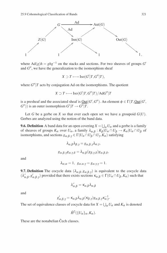
25.9 Cohomological Classification of Bands 321
GAd ��
Ad
%%&&&
&&&&
&&Aut(G)
&&''''
''''
'
Z(G)
'' Inn(G)
�����������
&&'''
''''
'''
Out(G)
%%
1
'' 1
��#########1 1 ,
where Ad(g)h = ghg−1 on the stacks and sections. For two sheaves of groups G′and G′′, we have the generalization to the isomorphism sheaf
X ⊃ T �−→ Iso(G′|T,G′′|T ),
where G′′|T acts by conjugation Ad on the isomorphisms. The quotient
X ⊃ T �−→ Iso(G′|T,G′′|T )/AdG′′|T
is a presheaf and the associated sheaf is Out(G′,G′′). An element φ ∈ Γ(T,Out(G′,G′′)) is an outer isomorphism G′|T → G′′|T .
Let G be a gerbe on X so that over each open set we have a groupoid G(U).Gerbes are analyzed using the notion of the band data.
9.6. Definition A band data for an open covering X =⋃αUα and a gerbe is a family
of sheaves of groups Kα over Uα , a family λα ,β : Kβ |Uα ∩Uβ → Kα |Uα ∩Uβ ofisomorphisms, and sections gα ,β ,γ ∈ Γ(Uα ∩Uβ ∩Uγ ,Kα) satisfying
λα ,βλβ ,γ = gα ,β ,γλα ,γ ,
gα ,β ,γgα ,γ,δ = λα ,β (gβ ,γ,δ )gα ,β ,δ ,
andλα ,α = 1, gα ,α ,γ = gα ,γ,γ = 1.
9.7. Definition The cocycle data (λα ,β ,gα ,β ,γ) is equivalent to the cocycle data(λ ′α ,β ,g
′α ,β ,γ) provided that there exists sections κα ,β ∈ Γ(Uα ∩Uβ ,Kα) such that
λ ′α ,β = κα ,βλα ,β
andg′α ,β ,γ = κα ,βλα ,β (κβ ,γ)gα ,β ,γκ−1
α ,γ .
The set of equivalence classes of cocycle data for X =⋃αUα and Kα is denoted
H2({Uα}α ,Kα ).
These are the nonabelian Cech classes.
322 25 Stacks and Gerbes
9.8. Remark If Kαs are sheaves of abelian groups, we can speak of a gerbe withan abelian band. If, moreover, sheaves Kα over the opens Uα are isomorphic torestrictions Kα ∼ K|Uα for each α ∈ I of the constant sheaf K = S1 and λα ,β = 1for all Uα ,β , we get bundle gerbes in the sense of Chap. 25.
Bibliography
Adams, J.F., Stable homotopy and generalised homology. Chicago Lectures in Math, University ofChicago (1974)
Atiyah, M.F., On the K-theory of compact Lie groups. Topology 4: 95–99 (1965)Atiyah, M.F., K-theory and reality. Quart. J. Math. Oxford Ser. 17(2): 367–386 (1966)Atiyah, M.F., Topological quantum field theory. Publ. Math. Inst. Hautes Etudes Sci. 68: 175–186
(1989)Atiyah, M.F., K-theory past and present. Sitzungsberichte der Berliner Mathematischen Gesell-
schaft. 411–417 (arXiv:math.KT/001221) (2001)Atiyah, M.F., Bott, R., Shapiro, A.: Clifford modules. Topology 3(1): 3–38 (1964)Atiyah M.F., Segal, G.B.: Twisted K-theory. Ukrainian Math. Bull. 1 (arXiv:math.KT/0407054)
(2004)Atiyah M.F., Singer, I.M.: Index theory for skew-adjoint Fredholm operators. Publ. Inst. Hautes
Etudes Sci. 37: 5–26 (1969)Beilinson, A., Drinfeld, V.: Chiral Algebras. American Mathematical Society Colloquium Publi-
cations, Vol. 51, Providence, RI (2004)Blackadar, B.: K-Theory for Operator Algebras. Mathematical Sciences Research Institute Publi-
cations, 5th ed. Springer Verlag, New York (1986)Borel, A., Serre, J.-P.: Le theoreme de Riemann-Roch (d’apres Grothendieck). Bull. Soc. Math.
France, 86: 97–136 (1958)Borel, A.: Seminar on transformation groups. Ann. of Math. Stud. 46 (1960)Borel, A.: Sous-Groupes commutatifs et torsion des groupes de Lie compacts connexes. Tohoku
Math. J. 13: 216–240 (1961)Bott, R.: Homogeneous vector bundles. Ann. Math. 66: 203–248 (1957)Bott, R.: The space of loops on a Lie group. Mich. Math. J. 5: 35–61 (1958)Bott, R.: Some remarks on the periodicity theorems. Colloque de Topologie, Lille (1959)Brown, L.G., Douglas, R.G., Fillmore, P.A.: Extensions of C∗-algebras and K-homology. Ann. of
Math. 105: 265–324 (1977)Brylinski, J.-L.: Loop Spaces, Characteristic Classes and Geometric Quantization. Birkhauser,
Boston (1993)Carey, A.L., Wang, B.L.: Thom isomorphism and push-forward map in twisted K-theory (2005)
(arXiv:math.KT/0507414)Connes, A.: Noncommutative Geometry. Academic Press (1994)Dixmier, J.: C*-algebras. North-Holland, Amsterdam and New York (1977)Dold, A.: Partitions of unity in the theory of fibrations. Ann. of Math. 78: 223–255 (1963)Donovan, P., Karoubi, M.: Graded Brauer groups and K-theory with local coefficients. Publ. Math.
I.H.E.S. 38: 5–25 (1970)Duistermaat, J.J., Kolk, J.A.C.: Lie Groups. Springer Verlag, Berlin (2000)Eilenberg, S., Steenrod, N.E.: Foundations of Algebraic Topology. Princeton University Press
Princeton, NJ (1952)
323
324 Bibliography
Feigin, B.L., Frenkel, E.V.: Affine Kac-Moody algebras and semi-infinite flag manifolds. Comm.Math. Phys. 128: 161–189 (1990)
Freed, D.S.: The Verlinde algebra is twisted equivariant K-theory. Turkish. J. Math. 25: 159–167(2001) (arXiv:math.RT/0101038)
Freed, D.S.: Twisted K-theory and loop groups. Proc. Int. Congress of Mathematicians. 3: 419–430(2002)
Freed, D.S., Hopkins, M.S., Teleman, C.: Loop groups and twisted K-theory III. (2003a) (arXiv:math.AT/0312155)
Freed, D.S., Hopkins, M.S., Teleman, C.: Twisted K-theory and loop group representations I.(2003) (arXiv:math.AT/0312155)
Frenkel, I.B., Garland, H., Zuckerman, G.J.: Semi-infinite cohomology and string theory. Proc.Nat. Acad. Sci. U.S.A. 83: 8442–8446 (1986)
Garland, H., Lepowsky, J.: Lie algebra homology and the Macdonald-Kac formulas. Invent. Math.34: 37–76 (1976)
Hirzebruch, F.: Some problems on differentiable and complex manifolds. Ann. of Math. 60:213–236 (1954)
James, I.M., Segal, G.B.: On equivariant homotopy type. Topology 17: 267–272 (1987)Kac, V.G.: Infinite Dimensional Lie Algebras 3rd ed. Cambridge University Press, Cambridge
(1990)Kirillov, A.A.: Lectures on the orbit method. Graduate Studies in Mathematics, Vol. 64 American
Mathematical Society, (2004)Kostant, B.: Lie algebra cohomology and the generalized Borel-Weil theorem. Ann. of Math. 74:
329–387 (1961)Kostant, B.: A cubic Dirac operator and the emergence of Euler number mulitplets of representa-
tions for equal rank subgroups. Duke Math. J. 100: 447–501 (1999)Kostant, B.: A generalization of the Bott-Borel-Weil theorem and Euler number multiplets of rep-
resentations. Lett. Math. Phys. 52(1): 61–78 (2000)Kostant, B., Sternberg, S.: Symplectic reduction, BRS cohomology, and infinite-dimensional Clif-
ford algebras. Ann. Phys. 176: 49–113 (1987)Kumar, S.: Demazure character formula in arbitrary Kac-Moody setting. Invent. Math. 89: 395–423
(1987)Landweber, G.D.: Multiplets of representations and Kostant’s Dirac operator for equal rank loop
groups. Duke Math. J. 110: 121–160 (2001)Laredo, J.V.: Positive energy representations of the loop groups of non-simply connected Lie
groups. Comm. Math. Phys. 207: 307–339 (1999)Lawson, H.B., Michelsson, M.L.: Spin geometry. Princeton Mathematical Series, Vol. 38. Prince-
ton University Press, Princeton, NJ (1989)Madsen, I., Rosenberg, J.: The universal coefficient theorem for equivariant K-theory of real and
complex C*-algebras. In: Kaminker J., Millet K., Schochet C (eds.) Index Theory of EllipticOperators, Foliations, and Operator Algebras, [Contemp. Math. 70 Amer. Math. Soc., Provi-dence, RI, 145–173] (1998)
Mickelsson, J.: Twisted K-theory invariants. Lett. in Math. Phys. 71: 109–121 (2005) (arXiv:math.AT/0401130)
Mickelsson, J.: Gerbes, (twisted) K-theory, and the super-symmetric WZW model. Lect. Math.Theor. Phys. 5: 93–107 (2004)
Moore, G., Segal, G.: D-branes and K-theory in topological field theory (2006) (arXiv:hep-th/0609042)
Murphy, G.J.: C∗-algebras and operator theory. Academic Press (1990)Pressley, A., Segal, G.: Loop Groups. Oxford University Press, New York (1986)Quillen, D.G.: Homotopical Algebra. Springer Lecture Notes, Vol. 43 (1967)Quillen, D.G.: Rational homotopy theory, Ann. Math. 90: 205–295 (1969)Quillen, D.G.: Superconnections and the Chern character. Topology. 24: 89–95 (1985)
Bibliography 325
Rosenberg, J.: Homological invariants of extensions of C*-algebras. In: Kadison R.V.(ed.) Op-erator Algebras and Applications [Proc. Sympos. Pure Math. 38, Part 1. Amer. Math. Soc.,Providence, RI, 35–75] (1982)
Schottenloher, M.: A mathematical introduction to conformal field theory. Lect. Notes Phys. m43.Springer-Verlag, Heidelberg (1997) (2nd edition to appear)
Segal, G.B.: Classifying spaces and spectral sequences. Publ. Math. I.H.E.S. Paris, 34:105–112 (1968)
Segal, G.B.: Fredholm complexes. Quart. J. Math. 21: 385–402 (1970)Segal, G.B.: Topological structures in string theory. Phil. Trans. R. Soc. Ser. A. 359: 1389–1398
(2001)Sorger, C.: La formule de Verlinde. Seminaire Bourbaki, 1994/95. Asterisque 237: 87–114 (1996)Steenrod, N.E.: A convenient category of topological spaces. Michigan Math. J. 14: 133–152
(1967)Sullivan, D.: Infinitesimal computations in topology. Inst. Hautes Etudes Sci. Publ. Math. 47:
269–331 (1977)Taubes, C.H.: Notes on the Dirac operator on loop space. Unpublished manuscript (1989)Teleman, C.: Borel-Weil-Bott theory on the moduli stack of G-bundles over a curve. Invent. Math.
134: 1–57 (1998)Teleman, C.: K-theory of the moduli of principal bundles on a surface and deformations of the
Verlinde algebra. Topology, Geometry and Quantum Field Theory: Proceedings of the 2002Oxford Symposium in Honour of the 60th Birthday of Graeme Segal. CUP (2004)
Thom, R.: Espaces fibres en spheres et carres de Steenrod. Ann. Sci. Ecole. Norm. Sup. 69 (1952),109–182
Tu, J.-L. and Xu, P.: Chern character for twisted K-theory of orbifolds. (2005) (arXiv: math.KT/0505267)
Wendt, R.: A character formula for certain representations of loop groups based on non-simplyconnected Lie groups. Math. Z. 247: 549–580 (2004)
Witten, E.: The Verlinde Algebra and the Cohomology of the Grassmannian. Gemoetry, topology,& physics conf. Proc. Lecture Notes Gerom. Topology, IV, 357–422 Int. Press, Cambridge, MA(1995) (arXiv: hep-th/9312104)
Wood, R.: Banach algebras and Bott periodicity. Topology 4(6): 371–389 (1965)

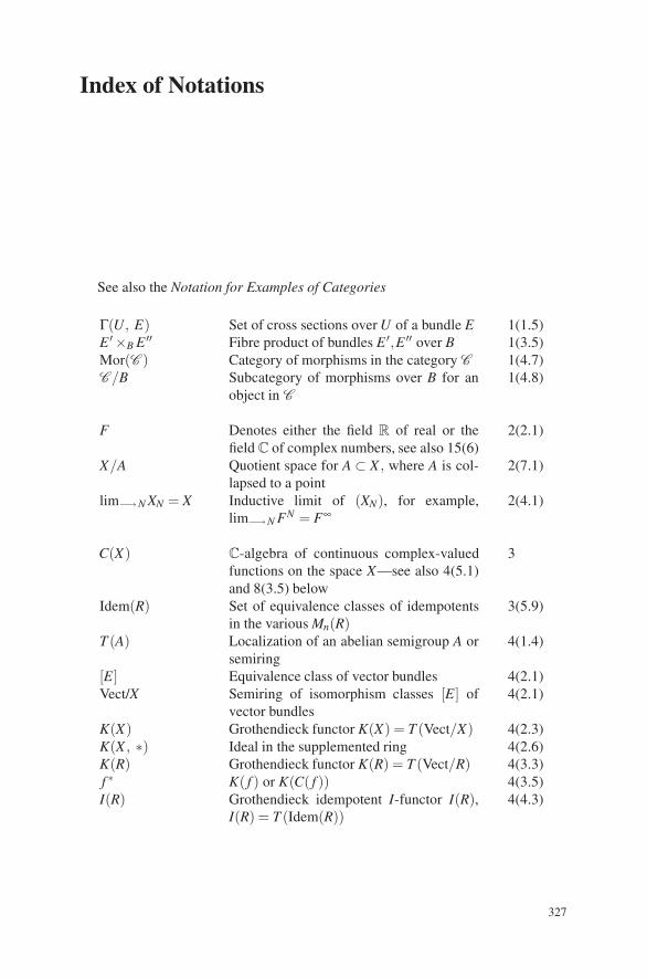
Index of Notations
See also the Notation for Examples of Categories
Γ(U, E) Set of cross sections over U of a bundle E 1(1.5)E ′ ×B E ′′ Fibre product of bundles E ′,E ′′ over B 1(3.5)Mor(C ) Category of morphisms in the category C 1(4.7)C /B Subcategory of morphisms over B for an
object in C1(4.8)
F Denotes either the field R of real or thefield C of complex numbers, see also 15(6)
2(2.1)
X/A Quotient space for A ⊂ X , where A is col-lapsed to a point
2(7.1)
lim−→N XN = X Inductive limit of (XN), for example,lim−→N FN = F∞
2(4.1)
C(X) C-algebra of continuous complex-valuedfunctions on the space X—see also 4(5.1)and 8(3.5) below
3
Idem(R) Set of equivalence classes of idempotentsin the various Mn(R)
3(5.9)
T (A) Localization of an abelian semigroup A orsemiring
4(1.4)
[E] Equivalence class of vector bundles 4(2.1)Vect/X Semiring of isomorphism classes [E] of
vector bundles4(2.1)
K(X) Grothendieck functor K(X) = T (Vect/X) 4(2.3)K(X , ∗) Ideal in the supplemented ring 4(2.6)K(R) Grothendieck functor K(R) = T (Vect/R) 4(3.3)f ∗ K( f ) or K(C( f )) 4(3.5)I(R) Grothendieck idempotent I-functor I(R),
I(R) = T (Idem(R))4(4.3)
327
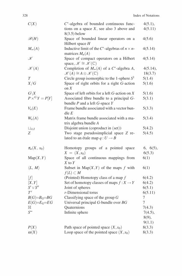
328 Index of Notations
C(X) C∗-algebra of bounded continuous func-tions on a space X , see also 3 above and8(3.5) below
4(5.1),4(5.11)
B(H) Space of bounded linear operators on aHilbert space H
4(5.6)
M∞(A) Inductive limit of the C∗-algebras of n×n-matrices Mn(A)
4(5.14)
K Space of compact operators on a Hilbertspace, K ∼= K (C)
4(5.14)
K (A) Completion of M∞(A) of a C∗-algebra A,K (A) ∼= A⊗K (C)
4(5.14),18(3.7)
T Circle group isomorphic to the 1-sphere S1 5(1.4)X/G Space of right orbits for a right G-action
on X5(1.6)
G\X Space of left orbits for a left G-action on X 5(1.6)P×G Y = P[Y ] Associated fibre bundle to a principal G-
bundle P and a left G-space Y5(3.1)
Vn(E) Frame bundle associated with a vector bun-dle E
5(3.3)
Wn(A) Matrix frame bundle associated with a ma-trix algebra bundle A
5(3.4)
�i∈I Disjoint union (coproduct in (set)) 5(4.2)Z Two stage pseudosimplicial space Z re-
lated to an etale map q : U → B5(4.5)
πn(X , x0) Homotopy groups of a pointed spaceX = (X ,x0)
6, 6(5),6(5.3)
Map(X ,Y ) Space of all continuous mappings fromX to Y
6(1)
〈L, M〉 Subset in Map(X ,Y ) of the maps f withf (L) ⊂ M
6(1)
[ f ] (Pointed) Homotopy class of a map f 6(4.2)[X ,Y ] Set of homotopy classes of maps f : X →Y 6(4.2)S′ ∨S′′ Joint of spheres 6(5.1)T r r-Dimensional torus 6(5.11)B(G)=BG=BG Classifying space of the group G 7E(G)=EG=EG Universal principal G-bundle over BG 7H Quaternions 7(4.3)S∞ Infinite sphere 7(4.5),
8(9),9(1.1)
P(X) Path space of pointed space (X ,x0) 8(3.3)ω(X) Loop space of the pointed space (X ,x0) 8(3.3)
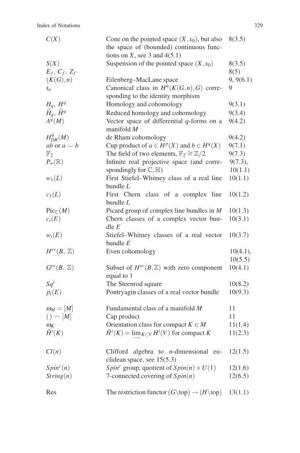
Index of Notations 329
C(X) Cone on the pointed space (X ,x0), but alsothe space of (bounded) continuous func-tions on X , see 3 and 4(5.1)
8(3.5)
S(X) Suspension of the pointed space (X ,x0) 8(3.5)E f , Cf , Zf 8(5)(K(G),n) Eilenberg–MacLane space 9, 9(6.1)ιn Canonical class in Hn(K(G,n),G) corre-
sponding to the identity morphism9
Hq, Hq Homology and cohomology 9(3.1)Hq, Hq Reduced homology and cohomology 9(3.4)Aq(M) Vector space of differential q-forms on a
manifold M9(4.2)
HqDR(M) de Rham cohomology 9(4.2)
ab or a � b Cup product of a ∈ H p(X) and b ∈ Hq(X) 9(7.1)F2 The field of two elements, F2
∼= Z/2 9(7.3)P∞(R) Infinite real projective space (and corre-
spondingly for C,H)9(7.3),10(1.1)
w1(L) First Stiefel–Whitney class of a real linebundle L
10(1.1)
c1(L) First Chern class of a complex linebundle L
10(1.2)
PicC(M) Picard group of complex line bundles in M 10(1.3)ci(E) Chern classes of a complex vector bun-
dle E10(3.1)
wi(E) Stiefel–Whitney classes of a real vectorbundle E
10(3.7)
Hev(B, Z) Even cohomology 10(4.1),10(5.5)
Gev(B, Z) Subset of Hev(B,Z) with zero componentequal to 1
10(4.1)
Sqi The Steenrod square 10(8.2)pi(E) Pontryagin classes of a real vector bundle 10(9.3)
ωM = [M] Fundamental class of a manifold M 11() � [M] Cap product 11ωK Orientation class for compact K ∈ M 11(1.4)Hi(K) Hi(K) = lim−→ K⊂V Hi(V ) for compact K 11(2.3)
Cl(n) Clifford algebra to n-dimensional eu-clidean space, see 15(5.3)
12(1.5)
Spinc(n) Spinc group, quotient of Spin(n)×U(1) 12(1.6)String(n) 7-connected covering of Spin(n) 12(6.5)
Res The restriction functor (G\top)→ (H\top) 13(1.1)
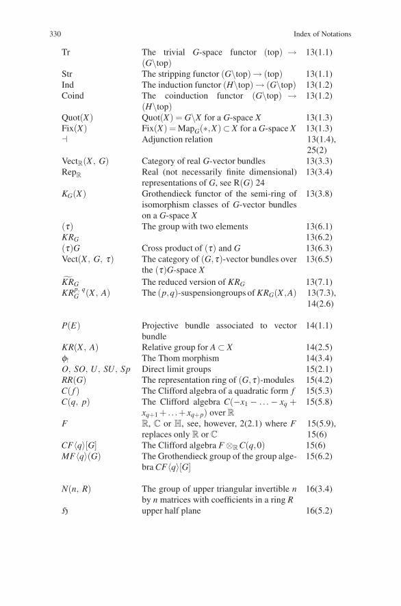
330 Index of Notations
Tr The trivial G-space functor (top) →(G\top)
13(1.1)
Str The stripping functor (G\top)→ (top) 13(1.1)Ind The induction functor (H\top) → (G\top) 13(1.2)Coind The coinduction functor (G\top) →
(H\top)13(1.2)
Quot(X) Quot(X) = G\X for a G-space X 13(1.3)Fix(X) Fix(X) = MapG(∗,X)⊂ X for a G-space X 13(1.3)� Adjunction relation 13(1.4),
25(2)VectR(X , G) Category of real G-vector bundles 13(3.3)RepR Real (not necessarily finite dimensional)
representations of G, see R(G) 2413(3.4)
KG(X) Grothendieck functor of the semi-ring ofisomorphism classes of G-vector bundleson a G-space X
13(3.8)
(τ) The group with two elements 13(6.1)KRG 13(6.2)(τ)G Cross product of (τ) and G 13(6.3)Vect(X , G, τ) The category of (G,τ)-vector bundles over
the (τ)G-space X13(6.5)
KRG The reduced version of KRG 13(7.1)KRp, q
G (X , A) The (p,q)-suspensiongroups of KRG(X ,A) 13(7.3),14(2.6)
P(E) Projective bundle associated to vectorbundle
14(1.1)
KR(X , A) Relative group for A ⊂ X 14(2.5)φ! The Thom morphism 14(3.4)O, SO, U, SU, Sp Direct limit groups 15(2.1)RR(G) The representation ring of (G,τ)-modules 15(4.2)C( f ) The Clifford algebra of a quadratic form f 15(5.3)C(q, p) The Clifford algebra C(−x1 − . . . − xq +
xq+1 + . . .+ xq+p) over R
15(5.8)
F R, C or H, see, however, 2(2.1) where Freplaces only R or C
15(5.9),15(6)
CF〈q〉[G] The Clifford algebra F ⊗R C(q,0) 15(6)MF〈q〉(G) The Grothendieck group of the group alge-
bra CF〈q〉[G]15(6.2)
N(n, R) The group of upper triangular invertible nby n matrices with coefficients in a ring R
16(3.4)
H upper half plane 16(5.2)
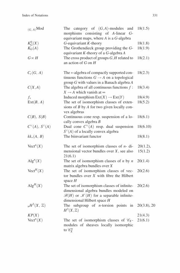
Index of Notations 331
(G, A)Mod The category of (G,A)-modules andmorphisms consisting of A-linear G-equivariant maps, where A is a G-algebra
18(1.5)
K0G(X) G-equivariant K-theory 18(1.8)
KG(A) The Grothendieck group providing the G-equivariant K-theory of a G-algebra A
18(1.9)
G � H The cross product of groups G,H related toan action of G on H
18(2.1)
Cc(G, A) The ∗-algebra of compactly supported con-tinuous functions G → A on a topologicalgroup G with values in a Banach algebra A
18(2.3)
C(X ,A) The algebra of all continuous functions f :X → A which vanish at ∞
18(3.4)
f∗ Induced morphism Ext(X) → Ext(Y ) 18(4.9)Ext(B, A) The set of isomorphism classes of exten-
sions of B by A for two given locally con-vex algebras
18(5.2)
C(B), S(B) Continuous cone resp. suspension of a lo-cally convex algebra B
18(6.1)
C∨(A), S∨(A) Dual cone C∨(A) resp. dual suspensionS∨(A) of a locally convex algebra
18(6.10)
kk∗(A, B) The biinvariant functor 18(8.1)
Vectn(X) The set of isomorphism classes of n- di-mensional vector bundles over X , see also21(6.1)
20(1.2),15(1.2)
Algn(X) The set of isomorphism classes of n by nmatrix algebra bundles over X
20(1.4)
VectH(X) The set of isomorphism classes of vec-tor bundles over X with fibre the Hilbertspace H
20(2.6)
AlgH(X) The set of isomorphism classes of infinite-dimensional algebra bundles modeled onB(H) or K (H) for a separable infinite-dimensional Hilbert space H
20(2.6)
nH3(X , Z) The subgroup of n-torsion points inH3(X ,Z)
20(3.8), 20
KP(X) 21(4.3)Vectn(X) The set of isomorphism classes of CX -
modules of sheaves locally isomorphicto C n
X
21(6.1)
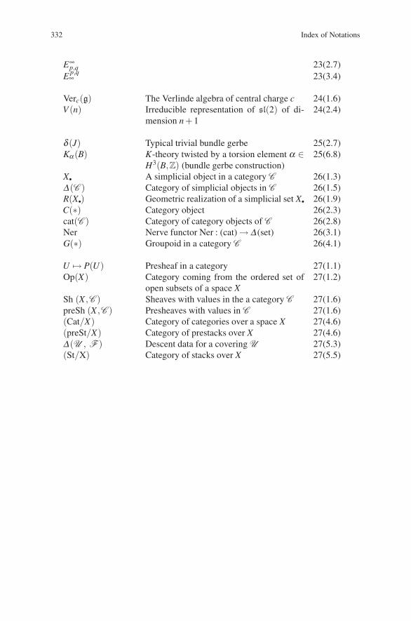
332 Index of Notations
E∞p,q 23(2.7)E p,q∞ 23(3.4)
Verc(g) The Verlinde algebra of central charge c 24(1.6)V (n) Irreducible representation of sl(2) of di-
mension n + 124(2.4)
δ (J) Typical trivial bundle gerbe 25(2.7)Kα(B) K-theory twisted by a torsion element α ∈
H3(B,Z) (bundle gerbe construction)25(6.8)
X. A simplicial object in a category C 26(1.3)Δ(C ) Category of simplicial objects in C 26(1.5)R(X.) Geometric realization of a simplicial set X. 26(1.9)C(∗) Category object 26(2.3)cat(C ) Category of category objects of C 26(2.8)Ner Nerve functor Ner : (cat) → Δ (set) 26(3.1)G(∗) Groupoid in a category C 26(4.1)
U �→ P(U) Presheaf in a category 27(1.1)Op(X) Category coming from the ordered set of
open subsets of a space X27(1.2)
Sh (X ,C ) Sheaves with values in the a category C 27(1.6)preSh (X ,C ) Presheaves with values in C 27(1.6)(Cat/X) Category of categories over a space X 27(4.6)(preSt/X) Category of prestacks over X 27(4.6)Δ(U , F ) Descent data for a covering U 27(5.3)(St/X) Category of stacks over X 27(5.5)
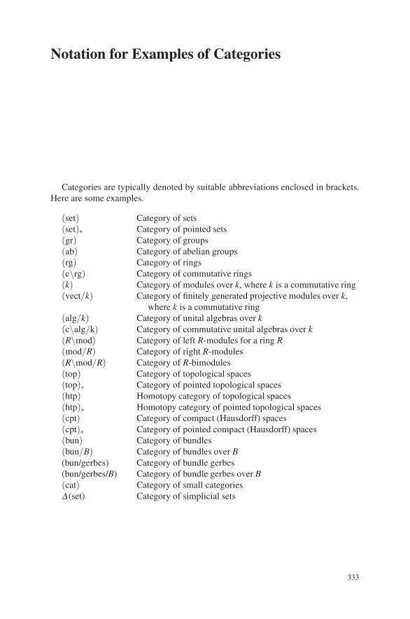
Notation for Examples of Categories
Categories are typically denoted by suitable abbreviations enclosed in brackets.Here are some examples.
(set) Category of sets(set)∗ Category of pointed sets(gr) Category of groups(ab) Category of abelian groups(rg) Category of rings(c\rg) Category of commutative rings(k) Category of modules over k, where k is a commutative ring(vect/k) Category of finitely generated projective modules over k,
where k is a commutative ring(alg/k) Category of unital algebras over k(c\alg/k) Category of commutative unital algebras over k(R\mod) Category of left R-modules for a ring R(mod/R) Category of right R-modules(R\mod/R) Category of R-bimodules(top) Category of topological spaces(top)∗ Category of pointed topological spaces(htp) Homotopy category of topological spaces(htp)∗ Homotopy category of pointed topological spaces(cpt) Category of compact (Hausdorff) spaces(cpt)∗ Category of pointed compact (Hausdorff) spaces(bun) Category of bundles(bun/B) Category of bundles over B(bun/gerbes) Category of bundle gerbes(bun/gerbes/B) Category of bundle gerbes over B(cat) Category of small categoriesΔ (set) Category of simplicial sets
333

Index
(G,A)-module M, 204(G,τ)-equivariant real K-theory, 159(p,q)-suspension groups, 159∗-Banach algebra, 53∗-algebra, 52E-theory, 213F-Hilbert space, 189G-action on Γ(X,E), 204G-algebra, 204G-bundle, 56G-equivariant K-theory, 265G-equivariant K-theory K0
G(X), 205G-equivariant K-theory of a G-algebra A, 205G-equivariant section, 153G-space, 56H-space, 91H-space structures, 177K-cycles, 203K-equivalent, 244K-groups, 51K-theory exact couple, 259K-theory functor, 219L-class, 111, 120L-genus for oriented manifolds, 120M′ u→ M
v→ M′′ , 89M2-stable (resp. stable), 219M2-sum of extensions, 213Spin(3), 138Spin(n) group, 138Spin(n)-structure, 137Spinc(n) structure, 137A-class, 111, 120A-genus for oriented manifolds, 120τ-vector bundle, 172Γ-equivariant principal G-bundle p : P → B,
272m-algebra, 208
n-connected covering of X , 143n-level pseudosimplicial object, 288nth power sequence 〈n〉, 248nth homotopy group, 71etale, 20, 21, 318Cech cosimplicial object associated with, 300
a groupoid, 299abelian category, 256abelianization, 306absolute homology and cohomology modules,
100action of G on an object X , 296acyclic fibration, 94Adem relations, 123adjoint action, 265, 272adjoint pair of functors, 307adjoint ring morphism, 273affine n-simplex, 77affine Kac–Moody algebra, 266affine simplex, 289Alexander duality theorem, 130algebra B(H) of bounded linear operators on
a Hilbert space H, 53algebraic Toplitz algebra, 217algebraic Toplitz extension, 218algebraically equivalent, 42associated bundle of projective spaces, 113associated fibre bundle, 58associated Kac-Moody Lie algebra, 265associated projective bundle, 163associated stack, 317Atiyah–Hirzebruch class, 2Atiyah–Hirzebruch spectral sequence, 4automorphisms of the fibres, 232axiomatic characterization, 116axiomatic version of homotopy theory, 85
335
336 Index
Banach Lie group, 235band, 13band data, 321base space, 9bijective functions, 16Borel construction, 172Borel subalgebra, 266Bott algebra morphism, 222Bott element, 167Bott morphism, 167, 222Bott periodicity, 163Bott periodicity for reduced complex K-theory,
180Bott periodicity for reduced real K-theory, 180boundary isomorphism, 94boundary morphism, 93Brauer equivalent, 241, 243Brauer group, 241bundle, 9bundle E over B, 9bundle gerbe, 277, 282, 284, 285bundle gerbe has a class, 277bundle of vector spaces, 24
cap product, 107, 127Cartan formula, 123Cartan subalgebra, 266categories over spaces, 309category, 15, 16category object, 287category object structure, 291category of categories, 17category of k-modules, 16category of groups, 15category of sets, 15category of spaces, 15category of squares, 84cellular chains, 104central charge c, 265, 266central extension, 284change of section, 319change the trivialization, 155characteristic class isomorphism, 238characteristic class of gerbe, 301characteristic classes for matrix algebra
bundles, 235characteristic numbers, 127Chern character, 2, 135Chern character ring morphism, 261Chern class of a sum of line bundles, 118Chern class of the tangent bundle, 118Chern classes, 107, 111circle, 90class group, 51
classifying space, 81, 83classifying space construction, 81classifying space functor or nerve functor, 293classifying spaces, 176Clebsch–Gordan inductive rule, 269Clifford algebra, 138, 182closed, 20clutched vector bundle, 32clutching function, 165cobordant, 133cocycle condition, 59, 319cocycle data, 321cocycle relation, 155cofibrant pair, 100cofibration, 85cofibre, 89cofibre mapping sequence, 93coH-space, 90cohomology, 100cohomology operation, 123collapsed vector bundle, 32commutation with induced bundles, 33compact group, 156compact Lie group, 200compact open topology, 66, 239complex infinite-dimensional projective space,
112complex vector bundle, 142composite, 17composite of two bundle morphisms, 13composition, 15, 18, 310composition of G-bundle morphisms, 153comultiplication on S(X), 91cone, 89conjugacy class, 170conjugate, 43continuous cone, 216contractibility, 239cosimplicial operations, 289critical point, 108cross product G � A, 207cross section, 11, 251cross section functor Γ, 37cross section of the product bundle, 252cross section vector space is a functor, 154cross sections, 10crossed products, 226cup product, 106cup–cap relation, 107CW-complex, 98
D-brane, 1, 3decomposition, 195decomposition triple, 196
Index 337
deRham Theory, 103descent condition, 59, 303Descent data, 277descent data, 315descent data for principal G-bundles, 59descent data for vector bundles, 278diffeomorphism type, 109diffeotopy, 209differential q-forms, 103dimension axiom, 102Dirac operator, 5double diagonal action, 272dual of a complex vector bundle E, 125dualizing morphism, 129
Eilenberg–MacLane isomorphism, 178Eilenberg–MacLane map, 106Eilenberg–MacLane space, 105Eilenberg–MacLane space K(G,n), 97elementary cofibration, 85elementary fibration, 85elementary symmetric function, 118Ell(X), 210endomorphism matrix algebra bundle, 231equivalence, 317equivalence classes of idempotents in, 44equivalence of categories, 19equivalent categories, 19equivariant KK-groups, 223Euler characteristic, 131Euler class, 111, 121, 132evaluation function, 66even/odd grading, 182exact couple, 255exact sequences, 101exact triangle for KR∗(X), 166excision morphisms, 100exponential sequence 〈exp〉, 248extension of a principal G′-bundle P′, 61extension of structure group class, 284extension property, 84extension theory, 211
factorization, 84faithful functor, 19, 317fibration, 85fibre, 9, 89fibre bundle E = P[Y ], 59fibre homotopic, 252fibre homotopically equivalent, 252fibre homotopy, 252fibre homotopy classes, 252fibre mapping sequence, 92fibre product, 12, 14
fibre product of bundles with G-action, 153fibre space fibration, 83fibred category, 303filtered space, 98finite bibasis, 39finitely generated, 30finitely generated projective module, 40first Cech cohomology, 319first Chern class of the line bundle, 277first Chern class of L, 112first cohomology set, 319first nontrivial differential, 264first Stiefel–Whitney class, 139first Stiefel–Whitney class of L, 112first-order gluing, 279fixed point, 56formula for the total Stiefel–Whitney class,
123Fredholm conditions, 211free G-space, 57Frobenius algebra, 5full embedding property of the cross section
functor, 35full subcategory, 16fully faithful functor, 19, 37, 317functor, 16, 17functor faithful, 317functoriality, 253fundamental group, 71fusion product, 266
gauge group AutB(P), 96gauge group AutB(P) of P, 62gauge transformation, 62Gauss map, 31geometric realization, 289gerbe, 277, 299, 318graded exact couple of type r, 256graded ring structure, 160graded tensor product, 182Gram–Schmidt process, 189Grassmann variety, 28Green’s imprimitivity theorem, 225Green–Julg Theorem, 224Grothendieck K-functor, 47Grothendieck idempotent I-functor, 50Grothendieck ring, 268group SL(2,Z), 194group localization, 46group of automorphisms, 15groupoid, 226, 295groupoid U(∗) associated to the covering, 297groupoid associated to the G action on the
object X , 297
338 Index
groupoid gerbe, 300groupoid object, 287Gysin sequence, 121
half exact, 219handle, 109Hausdorff space, 20higher algebraic K-theory of a ring R, 294Hilbert B-module, 223Hilbert space vector bundles, 231homology, 100homology exact couple, 257homotopic, 67homotopy, 65, 219homotopy equivalence, 68homotopy invariant, 69homotopy (resp. smooth homotopy) invariant,
219homotopy cofibre of f , 92homotopy equivalence, 99homotopy fibre, 91homotopy invariance of bundles, 64homotopy quotient categories, 68homotopy relation, 67Hurewicz fibration, 88Hurewicz map, 105Hurewicz theorem, 105
idempotents, 42, 43inclusion, 129index, 108index theorem for elliptic operators, 134induced bundle, 13, 25, 153inductive limit topology, 28inner product, 33inner product on a vector bundle, 33integral third Stiefel–Whitney class, 141inverse, 15irreducible representations, 156, 267isomorphism, 15isomorphism of functors, 18Iwasawa, 195Iwasawa decomposition of a topological group,
191
k∗, 220K-Theory of C∗-Algebras, 54Kasparov product, 211Koszul complex, 167Kuiper’s theorem, 235
left G-space, 56Lie algebra of algebraic loops, 266lifting property, 84
limit topology, 176linearly independent n-tuples, 189localization at the prime ideal, 170locally convex vector space, 208locally convex topological algebra, 208locally full, 81, 311locally trivial, 11, 59, 282long exact sequence, 160loop space, 89Lorentz metric, 195
Mobius band, 13map, 20mapping cone, 89, 216mapping cone of u, 216mapping cylinder, 88, 99, 216mapping cylinder of u, 216mapping space, 89mapping track, 87matrix algebra bundle, 230Mayer–Vietoris sequence, 102, 121metric with positive scalar curvature, 144Milnor principal G-bundle, 78Milnor total space construction, 76Milnor universal principal G-bundle, 78module over, 285morphism, 24, 25, 289, 295, 305, 310morphism of n-level pseudosimplicial, 288morphism of bundle gerbes, 280morphism of functors, 18morphism of two G-bundles, 153Morse theory, 107, 185multiplication on Ω(Y ), 91multiplier algebra, 214
natural equivalence, 18natural transformation, 18nice Morse function, 108nondegenerate, 108norm topology, 235, 236, 238normal bundle ν(M), 127normed algebra, 52numerable bundle, 73numerable covering of the base space, 73numerable pair, 36
objects, 15one point union, 70open, 20open bundle, 21operator algebra bundles, 231opposite category, 69or one point join, 70orientable, 121, 144
Index 339
orientation, 61, 128, 137, 139, 144orientation classes ωK , 129orientation of an n-dimensional manifold M,
128original Iwasawa decomposition G = KAN,
191orthogonal, 189orthonormal, 189outer automorphism sheaves, 320
pairing with, 211pairing with K111(X), 212paracompact space, 74parity-graded objects, 182partition (resp. envelope of unity, 73path space, 89periodicity theorem, 168, 187Peter–Weyl theorem, 156Poincare duality, 107, 127Poincare duality isomorphism, 132Poincare duality theorem, 129Poincare group, 71pointed homotopy equivalence, 68pointed map, 67pointed space, 67Pontrjagin class, 111, 125Pontrjagin numbers, 134presheaf, 303, 304prestack, 314principal G-bundle, 59principal G-sheaf, 318, 319principal bundle, 57principal bundle morphism, 57product G-principal bundle, 58product bundle, 10, 14, 23projection, 9projective, 39projective bundle theorem, 115
quadratic form, 181quantum field theories, 1quasicompact space, 20Quillen, 85
rank filtration, 27real (τ)G-vector bundle, 158real infinite-dimensional projective space, 112real periodicity, 179real projective space, 12real vector bundle, 121reduced homology and cohomology, 100related groupoid, 296relation, 114relative group, 166
representations, 268restriction, 11restriction of a principal G′′-bundle P′′, 61Riemann surface, 135Riemann–Roch theorem, 135Riemann-Roch-Hirzebruch theorem, 127right G-space, 56ring structure, 160
second dualizing morphism, 129second Stiefel–Whitney class, 140second-level pseudosimplicial
object, 291second-order gluing, 279section, 10seminorm, 207separated space, 20Serre fibration, 88Serre–Swan Theorem, 41set of index data, 210sheaf, 304sheaf of groups, 319sheafification, 305simple, 238simple Lie group, 195simplicial object, 288singular simplices, 103smooth, 216smooth cone, 216smooth suspension, 216smooth Toplitz extension, 218space, 74special linear group, 190spectral radius, 53spectrum, 53spin, 144spin structure, 61, 140, 144spinc structure, 141splitting principle, 114, 119, 125stability properties of characteristic classes,
117stabilized bundle theory, 177stable equivalence classes, 244stably equivalent, 117, 244, 245stably isomorphic, 283stack, 303Steenrod square, 123Stiefel variety, 28Stiefel–Whitney class, 4, 107, 111, 132Stiefel–Whitney class for the real projective
space, 263Stiefel–Whitney class of the tangent bundle,
117Stiefel–Whitney numbers, 133
340 Index
string, 144string structure, 144string theory, 4strong topology, 238subcategory, 16substitution morphism, 209supersymmetry, 2suspension, 89, 178, 216suspension axiom, 101symmetric function, 118
tangent and normal bundle, 12tangent bundle T (M), 127tensor algebra T (B), 214theory of adjoint functors, 306third integral Stiefel–Whitney
class, 141Thom class of E, 168Thom isomorphism, 168Thom morphism, 168Tietze extension theorem, 157Todd class, 111, 120, 135Todd genus of the manifold, 120topological group, 55topology, 238total space, 9trivial, 300trivial vector bundle, 25trivializing sections of the gerbe, 282
twisted K-theory, 3, 4
unitary group, 238universal coefficient theorem, 106, 131universal first Stiefel–Whitney class, 140universal principal G-bundle, 95universal property, 29, 306universal two-way extension, 217universal vector bundle over Grn(FN), 29unstable periodicity theorem, 186upper half plane, 193
vector, 25vector bundle, 23, 24, 30, 230, 244, 245vector field, 11Verlinde algebra, 265, 266
weak topology, 28, 78, 98Wedge Product, 104Whitehead mapping theorem 9(2.2), 95Whitney sum, 12, 114Whitney sum formula, 125Whitney sum property, 121winding number, 71Witten index, 145Wu class, 132
zero-order gluing, 278