The Wage Effects of Job Polarization:Evidence from the Allocation of Talents

Michael J. Boehm ∗

April 2014

Abstract This article studies the wage effects of job polarization on 27 year old maleworkers from the cohorts of the National Longitudinal Survey of Youth. Guided by aRoy model of occupational choice I compare workers who have characteristics that putthem into high-, middle-, and low-skill occupations over the two cohorts. Results indicatethat the relative wages of middle-skill occupation workers have dropped. The effect ofjob polarization on the overall wage distribution that is implied by the model explainsthe increase at the top of the actual distribution but it has difficulty matching the increaseat the bottom.

Keywords: Job Polarization; Wage Inequality; Talent Allocation; Roy ModelJEL Classification Numbers: J23, J24, J31

∗ University of Bonn and Centre for Economic Performance (LSE), mboehm1@uni-bonn.de. This is a funda-mental revision of my job market paper entitled “Has Job Polarization Squeezed the Middle Class? Evidencefrom the Allocation of Talents”. I am extremely grateful to my supervisor Steve Pischke. I very much thankYona Rubinstein, Alan Manning, Luis Garicano, David Autor, David Dorn, Pedro Carneiro, John Van Reenen,Guy Michaels, Esteban Aucejo, Barbara Petrongolo, Claudia Steinwender, Johannes Boehm, Georg Graetz,Martin Watzinger, and Pinar Hosafci as well as participants at various seminars and conferences for theircomments. I also thank Joseph Altonji, Prashant Bharadwaj, and Fabian Lange for sharing their data andcode, and Steve McClaskie for support with the NLSY data.

1 Introduction

Over the last two decades, the labor market in the United States has experienced a pro-

found polarization of employment. In particular, the aggregate share of jobs in middle-

skill production and clerical occupations has declined by almost seven percentage points

since the end of the 1980s while the share of jobs in high-skill professional and manage-

rial occupations as well as low-skill services occupations has surged. This has coincided

with a polarization of wages, whereby earnings in the middle of the wage distribution

have stagnated or even fallen while earnings at the top and at the bottom have increased

substantially (compare Acemoglu and Autor 2011 and see figures 1 and 2 for the data

used in this paper).

Pioneering research by Autor, Levy, and Murnane (2003) and others1 has shown that

the main driver of job polarization was a rapid improvement of computer technology

which could replace the routine work that is intensively carried out in middle-skill occu-

pations (“routine-biased technological change”). It thus seems natural to hypothesize that

the polarization of wages was shaped by the same demand-side forces (e.g. Autor, Katz,

and Kearney, 2006; Acemoglu and Autor, 2011; Autor and Dorn, 2013). Indeed, recent

empirical studies have examined several aspects of the relationship between job polariza-

tion and workers’ wages (Autor and Dorn, 2013; Cortes, 2014; Dustmann, Ludsteck, and

Schönberg, 2009; Mishel, Shierholz, and Schmitt, 2013).

The purpose of this paper is to build on the existing work and to employ a unified

economic framework in order to estimate the wage effect of job polarization on specific

groups of workers as well as its effect on the overall wage distribution.2 In particular, I

use the theory and empirics of the Roy (1951) model to address the following questions:

first, have the relative wages of workers in the middle-skill occupations declined as the

demand-side explanation for job polarization predicts? Second, how have the wage rates

paid for a constant unit of effective labor in the high-, middle-, and low-skill occupations

changed with polarization? Third, what was the effect of job polarization on the overall

wage distribution and, in particular, could it have generated the polarization of wages

that we observe in the data?

In order to answer these questions, I construct two representative cross-sections of

27 years old male workers at the end of the 1980s and at the end of the 2000s from the

two cohorts of the National Longitudinal Survey of Youth (NLSY79 and NLSY97). The

1Goos and Manning (2007), Autor, Katz, and Kearney (2006), Michaels, Natraj, and Van Reenen (2013),Acemoglu and Autor (2011), Autor and Dorn (2013).

2Note that throughout the paper I write “the wage effect of job polarization” as a shorthand for “theeffect on wages of the declining relative demand for middle-skill occupations that leads to job polarization”.

1

workers in the sample are born in 1957–1964 and 1980–1982 and they are 27 years old in

1984–1992 and 2007–2009, respectively. Although this is arguably a specific labor market

group during a particular time period, the NLSY has substantial advantages over more

commonly used data sets: it provides consistent, early-determined, and multidimensional

measures of worker talents—such as mathematical, verbal, and mechanical test scores

and risky behaviors—which predict occupational choices and wages.3 This allows me to

study the wages of the kind of individuals who are more and less likely to work in the

middle-skill compared to the high- and the low-skill occupations over these two decades

of rapid job polarization.4

The paper’s empirical strategy comparing the same kind of workers across two points

in time is informed by the Roy model of occupational choice, which calls for such an

approach. In the Roy model, workers have different skills in the high-, middle-, and low-

skill occupations that are a function of underlying talents. Once technological change

or international trade decrease the demand for labor in the middle-skill occupations,

wage rates fall and workers move out of there. Hence we observe job polarization. The

Roy model further says that to estimate the wage effects of job polarization one should

not compare changes in wages across occupations—because the selection of skills in

occupations changes together with the wage rates—but the (kind of) workers who started

out across different occupations.5

I start by analyzing the sorting of workers into occupations in the end of the 1980s

using multinomial choice regressions in the NLSY79. I find that, conditional on the other

talents, workers with high math talent are likely to choose the high-skill occupation,

workers with high mechanical talent are likely to choose the middle-skill occupation,

and workers with high verbal talent are likely to choose the high- or the low-skill occu-

pation but not the middle. This indicates a systematic sorting of workers into occupations

according to their relative talent endowments and it enables me to construct predicted

probabilities for every worker in both datasets to enter the high-, middle-, and low-skill

occupation in the end of the 1980s.6

3In fact the timing in my dataset is comparable to the 1988–2008 period considered separately in Ace-moglu and Autor (2011). For example, refer to their figures 9 and 10.

4While some recent papers argue that job polarization has been going on for much longer than the lastcouple of decades (Bárány and Siegel, 2013; Mishel, Shierholz, and Schmitt, 2013), most studies find it wasstrongest during the 1990s.

5Using a model that is related to the Roy framework, Acemoglu and Autor (2011) have similar concernsabout a simple comparison of wages across tasks: “[...] because the allocation of workers to tasks is endoge-nous, the wages paid to a set of workers previously performing a given task can fall even as the wages paidto the workers now performing that task rise [...]”.

6In a recent paper, Speer (2014) conducts a related analysis of worker sorting into jobs. His results onthe sorting of math, verbal, and mechanical talents into occupational tasks are similar to the ones describedhere.

2

I use these predicted probabilities to study how the wages of workers who were

likely to choose to work in the three occupations in the end of the 1980s have changed

over time. Effectively, this amounts to a wage regression on the occupational propensities

interacted with a dummy for the period at the end of the 2000s. Under the assumption

that the distribution of fundamental worker skills conditional on the detailed talents

has been constant between the NLSY79 and the NLSY97, these regressions identify the

changing returns over time to working in the high- and low-skill occupation versus the

middle-skill occupation in the end of the 1980s.7

The results from the regressions on occupational propensities indicate that the wages

of middle-skill occupation workers declined substantially over the polarization period. I

find that the positive wage effect associated with a one percentage point higher propen-

sity to work in the high- compared to the middle-skill occupation almost doubled from

.31 to .60 percent. The negative wage effect associated with a one percentage point higher

propensity to work in the low-skill occupation attenuated from −1.65 to −.95 percent.

Moreover, workers with a high propensity to enter the middle-skill occupations in the

1980s suffered even an absolute decline in their expected real wages. These findings are

robust to controlling for absolute skill measures, such as educational attainment, which

supports the idea that it is relative occupational skills rather than absolute skills whose

returns have changed over time.

The above results answer the first question of the paper about how middle-skill work-

ers have fared in terms of relative wages over time. In fact, so far no formal setup of the

Roy framework was needed for the analysis. However, applying the Roy model becomes

essential in order to answer the second question about the change in the equilibrium

wage rates across occupations. This is because wages rates are not directly observed in

the data and thus need to be inferred from within the model. To identify the wage rates

empirically, I assume that log wages are additively separable into wage rates and skills

and that the production function of talents into skills is fixed over time.

Under these assumptions, one can quite straightforwardly estimate the relative change

in wage rates across occupations in the Roy model. My estimates indicate that the rel-

ative wage rate in the high- compared to the middle-skill occupation increased by 25

percent since the end of the 1980s and the relative wage rate in the low-skill occupation

increased by 33 percent. The former rate is estimated relatively precisely while the latter

is imprecise and not statistically significant. Nonetheless, overall the results suggest sub-

stantially declining relative wage rates for a constant quality of work in the middle-skill

7The fact that the level and cross-correlation of talents have not changed between the NLSY79 and theNLSY97 supports the identification assumption.

3

occupations over time.

The wage rate estimates also help approaching the third question of the paper about

the effect of job polarization on the overall wage distribution. I assign each worker in the

NLSY79 the estimated change in wage rates according to his occupation. The resulting

counterfactual distribution qualitatively matches the increase in wages at the top of the

actual distribution compared to the middle. However, it does not reproduce much of the

surge of wages in the bottom of the actual distribution.

Where does the asymmetry of rising wages rates for the high- and the low-skill occu-

pations and a rise in the top of the counterfactual wage distribution but not in the bottom

stem from? The reason is that low-skill occupation workers now move up in the wage

distribution, which lifts not only the (low) quantiles where they started out but also the

(middle) quantiles where they end up. The inverse happens for workers in middle-skill

occupations but with the same effect on the wage distribution so that it becomes flat-

ter in the lower half. However, the opposite happens at the top of the wage distribution:

high-skill occupation workers, who are predominantly in the upper parts of the wage dis-

tribution now get another boost to their wages. This not only lifts their original quantiles

but also the even higher quantiles that they end up in.8 These mechanical movements

within the wage distribution may be part of the reason why in some countries and time

periods we observe rapid job polarization but no “wage polarization”, that is no increase

in relative wages at the bottom of the wage distribution.9

This paper is related to recent studies that examine the relationship between job po-

larization and wages. First, Acemoglu and Autor (2011), Mishel, Shierholz, and Schmitt

(2013), and Dustmann, Ludsteck, and Schönberg (2009) examine the common occurrence

of job polarization and wage polarization across time periods and locations. They do

not find that job polarization is generally accompanied by substantial wage polarization.

Second, Autor and Dorn (2013) examine the employment and wage trends of local labor

markets and find that local labor markets that were initially more specialized in routine

tasks experienced a stronger polarization of occupational wages. Third, using longitu-

dinal data, Cortes (2014) compares the wage profiles of workers who move out of the

middle-skill occupations into the high- and low-skill occupations to those workers who

remain behind. He finds that the movers experience stronger wage growth over the long

8Another effect on the wage distribution within the Roy model that is omitted here is the wage effect ofindividuals leaving the middle-skill occupation. In section 7 I examine this effect and find that it needs to berelatively extreme to generate the necessary surge in wages at the bottom of the wage distribution.

9Note that wage polarization in this study refers to the polarization of the individual wage distributionwhile in some other studies it refers to the polarization of the occupational wage distribution.

4

run.10

The current paper builds on these existing studies by estimating the wage effect of

job polarization on the groups of workers who start out in the high-, middle-, and low-

skill occupations as well as the effect on the overall wage distribution within a unified

economic framework. Moreover, it provides one explanation for why we may observe

rapid job polarization that does have an effect on workers’ wages but not a lot of wage

polarization in some countries and time periods.

In addition the Roy model employed in this paper is closely related to other theoreti-

cal frameworks used in the literature on job polarization. For example, the survey article

by Acemoglu and Autor (2011) provides a Ricardian assignment model of skills to tasks

where polarization amounts to the substitution of machines for certain tasks previously

performed by labor. The model predicts that those workers who have a comparative

advantage in tasks for which the relative market price decreases will be displaced and

find their relative wages decline. Moreover, the replacement of tasks in the middle of

the skill distribution at the same time generates job- as well as wage polarization within

their framework. Other models that generate similar predictions include Autor, Levy, and

Murnane (2003), Autor, Katz, and Kearney (2006), Jung and Mercenier (2014), and Autor

and Dorn (2013).11

An aspect in which the Roy model is more general than the above frameworks is that

it features an unrestricted distribution of skill.12 This is empirically relevant as it allows

for an overlap in wage distributions across occupations which is a salient feature of the

data. It also allows for workers moving up and down in the wage distribution as a result

of changes in wage rates across occupations. In a model where skills’ rankings are fixed

in terms of the wages that they generate, one cannot have this phenomenon that leads to

the flattening of the lower half of the wage distribution under job polarization.13

The paper continues as follows. Section 2 constructs a sample of workers in the NLSY

10In addition, Firpo, Fortin, and Lemieux (2011) use a decomposition method to assess the contribution ofdifferent factors to the change in the wage distribution over the last three decades. Their results indicate animportant role for technology and de-unionization in the 1980s and the 1990s, and for offshoring from the1990s onward.

11Feng and Graetz (2013) generate job and wage polarization in a model where firms’ automation choicesare endogenous. They argue that these predictions result from automation in general and are thus not aunique consequence of the information and communication technology revolution.

12The exceptions are Autor, Levy, and Murnane (2003) and Firpo, Fortin, and Lemieux (2011) who use theRoy model as well.

13Finally, some papers have proposed additional drivers of job polarization over “routine-biased techno-logical change”. For example, Acemoglu and Autor (2011) and Goos, Manning, and Salomons (2014) haveexamined the role of offshoring and international trade. Mazzolari and Ragusa (2013) and Bárány and Siegel(2013), among others, proposed the demand for consumption of low-skill occupation output coupled withgeneral technological change. Since the Roy model is a partial equilibrium model of the supply side of thelabor market, I do not need to take a stand about what are the exact drivers of job polarization in this study.

5

that has outcomes similar to a comparable sample in the commonly used Current Popu-

lation Survey (CPS) and which features the qualitatively same job polarization and wage

polarization we observe in the U.S. for that time period. Section 3 studies the worker

sorting into occupations according to the talent measures available in the NLSY. Section

4 estimates the changes in relative wages for workers who sort themselves into the dif-

ferent occupations according to their talents. These results are interpreted within the Roy

model in section 5, while section 6 uses the model to estimate the change in occupation-

specific wage rates. With the help of these wage rates, section 7 assesses the impact of job

polarization on the overall wage distribution. The last section concludes.

2 Data and Empirical Facts

I use data from the National Longitudinal Survey of Youth (NLSY) cohorts of 1979 and

1997, which contain detailed information on individuals’ fundamental talents that is

not available in other datasets. The dataset is constructed such that its distribution of

wages and occupations are comparable to the more standard Current Population Survey

Merged Outgoing Rotation Groups (CPS) over the same period.

The individuals in my sample are 27 years old in 1984–1992 and 2007–2009, respec-

tively.14 This timing is similar to the 1988–2008 period considered separately in figures 9

and 10 in Acemoglu and Autor (2011). In fact, the years 2008–09 are a crisis period in the

U.S. labor market and a recent paper by Jaimovich and Siu (2014) argues that recessions

are closely linked to surges of job polarization. When I split my NLSY and CPS data

into 2007 and 2008–09 no systematically different wage- or job polarization facts appear

between the two periods. I therefore continue with the pooled data.

The sample selection and attrition weighting for the NLSY sample is done closely in

line with a recent paper by Altonji, Bharadwaj, and Lange (2012). Since attrition in the

NLSY97 is higher than in the NLSY79, Altonji, Bharadwaj, and Lange (2012) examine

it in detail. They conclude that after appropriate weighting any potential biases are not

forbidding. I also construct labor supply by hours worked and real hourly wages as in

Lemieux (2006). The details of the sample construction can be found in section A of the

appendix. Table 1 accounts for how I end up with a sample of 3,054 and 1,207 individuals

in the NLSY79 and the NLSY97, respectively.

14I do not use the 2010 and 2011 samples of the NLSY97 because wages are substantially lower andoccupations are worse compared to the CPS and I could not find out what is the reason for this. Also,the AFQT scores of those members of the 1983–84 birth cohorts who work as 27 year olds in 2010–11 aresubstantially lower than the AFQT scores of the working 1980–82 cohorts.

6

The overall (male) labor force experienced substantial wage polarization from the end

of the 1980s to the end of the 2000s. That is, wages increased substantially at the top of the

distribution and somewhat less in the bottom but hardly at all in the middle. Moreover,

there was job polarization in the sense that employment in the middle-skill occupations

decreased and employment in the high-skill and low-skill occupations increased. For the

details of these facts, see the survey paper by Acemoglu and Autor (2011).

I start with the wage distribution in my sample. Figure 1 graphs the change in log real

wages by distribution quantile in the NLSY79 and the NLSY97 and for the same years

and age group in the CPS. We see that the changes in the NLSY and the CPS align well

for both cohorts. Hence there is wage polarization in the NLSY which is similar to what

can be found in the CPS.

The second important fact is job polarization. I follow recent studies in the literature

which delineate occupation groups along the lines of their routine and non-routine task

content (e.g. Acemoglu and Autor, 2011; Cortes, 2014; Jaimovich and Siu, 2014). Specif-

ically, managerial, professional, and technical occupations are grouped as high-skill (or

non-routine cognitive); sales, office and administrative, production, and operator and la-

borer occupations as middle-skill (or routine); and protective, food, cleaning and personal

service occupations as low-skill (or non-routine manual).

Figure 2 graphs the percentage point change of employment in the high-, middle-,

and low-skill occupations for the NLSY79 and NLSY97 and compared to the CPS. We

can see that the employment share of middle-skill occupations is declining substantially

while the employment share of the high- and the low-skill occupations is rising. Hence

there is job polarization in the NLSY sample and it is close to what can be found for 27

year olds in the CPS.

Before moving on, figure 3 plots the change in average real wages in the high-,

middle-, and low-skill occupations in the NLSY and, for comparison again, the CPS.

While wages in high-skill occupations have increased robustly in levels and compared

to the other two occupations, wages in low-skill occupations have lost somewhat further

ground against wages in middle-skill occupations in the NLSY and also slightly in the

CPS.15 One might find this surprising under the demand side explanation for job polar-

ization, which should decrease employment and wages in the middle at the same time.

Yet, just as the size of occupations, the composition of skills in occupations does not stay

15Note that the small differences between wages, occupational employment, and occupational wages inthe NLSY and the CPS sample are unlikely to stem from systematic attrition or non-test-taking in the NLSY.This is because sample attrition or non-test-taking are much lower in the NLSY79 than the NLSY97, whilethe differences between CPS and NLSY are equally large for the two cohorts.

7

constant when relative demands change.16 If we want to get at the wage effects of job po-

larization we need to properly account for such changes in skill selection. In order to do

this, I study which kind of workers sort into the high-, middle-, and low-skill occupations

in the next section.

3 Talent Sorting into Occupations

3.1 Measures of Talent

The NLSY data provide a long array of characteristics of its respondents. Out of these,

I focus on variables that are early determined, that are relevant for occupational choices

and wages, that should approximate different dimensions of skill, and that can be com-

pared over the two cohorts.17

Table 2 reports labor force averages of NLSY variables that fulfill the four criteria

(“early skill determinants”) and some demographic variables and contemporary skill

determinants that are available in more standard datasets. In terms of the early skill

determinants, I construct composite measures of mathematical, verbal, and mechanical

talent by combining test scores on mathematics knowledge, paragraph comprehension

and word knowledge, and mechanical comprehension and auto- and shop information,

respectively. In addition, I report the AFQT score, which is sometimes taken as a measure

of general intelligence.18

There are a couple of advantages of using the early skill determinants—and in par-

ticular the composite measures of mathematical, verbal, and mechanical talent—for the

purpose of this study: First, the (joint) distribution of test scores is quite stable over the

two cohorts while educational attainment increased. In addition, education measures

have a lot of bunching at points like high school graduate (12 years of education) or

college graduate (16 years of education). Therefore, the test scores should enable me to

better capture similar individuals across the two cohorts. Second, early skill determinants

should be relatively exogenous to the change in an individual’s occupational choice due

16Also other studies find a further decrease in low-skill compared to middle-skill occupation wages (Goosand Manning, 2007). Autor and Dorn (2013) find that relative wages in clerical occupations rise while quan-tities fall.

17The popular non-cognitive skill measures of locus of control and self-esteem have to be left out of theanalysis because they are not available in the NLSY97.

18All these measures are taken from the Armed Services Vocational Aptitude Battery of tests (ASVAB)which consists of ten components: arithmetic reasoning, word knowledge, paragraph comprehension, math-ematics knowledge, general science, numerical operations, coding speed, auto and shop information, me-chanical comprehension, and electronics information. The breakup into mathematical, verbal, and mechan-ical talent is similar to what a factor analysis of test scores suggests. AFQT is essentially the average ofarithmetic reasoning, word knowledge, paragraph comprehension, and mathematics knowledge.

8

to job polarization. This is because test scores are not very malleable, they are measured

before entry into the labor market in the NLSY97, and before job polarization was widely

known.19 Finally, the test scores provide proxies for multiple dimensions of individuals’

skills. Thus, they can be used to determine comparative advantage in different occupa-

tions.

Before moving on, we see from table 2 that the level of AFQT, which is a measure

of IQ, does not change in the male labor force over the two cohorts. In addition, table

3 reports that the cross-correlation of the composite test scores and AFQT remained

virtually the same. This supports my identification assumption in the following that the

tests measure similar dimensions of talent over the two cohorts and that “within test

score groups” individuals can be considered on average the same across cohorts.20

3.2 Sorting into Occupations

Figure 4 depicts average mathematical, verbal, and mechanical talent in the three occu-

pation groups in both cohorts. We see that the levels of the three talents are substantially

higher in the high-skill occupation than in the middle-skill occupation which, in turn, is

higher than the low-skill occupation. Thus, there is a clear ordering of absolute advantage

in occupations independent of the talent considered. This underlines the appropriates of

terming them high-, middle-, and low-skill.

However, in the absence of restrictions to enter occupations, workers’ choice should

not be governed by their absolute but by their comparative advantage and thus depend

on their relative skills (for example, compare Sattinger, 1993). We see in figure 4 that aver-

age mathematical talent in the high-skill occupation is higher than average verbal or me-

chanical talent, while average mechanical talent is considerably higher in the middle-skill

occupation than mathematical or verbal talent. Verbal talent is higher than mathematical

and mechanical talent in the low-skill occupation.

This suggests sorting according to comparative advantage and multidimensional skills

as in the well-known Roy (1951) model—with workers who have high math talent choos-

ing the high-skill occupation, workers who have relatively high mechanical talent choos-

ing the middle-skill occupation, and workers who have relatively high verbal talent

choosing the low-skill occupation. It is also intuitive, since high analytical skills are re-

quired to pursue a career in managerial, professional, or technical jobs while individuals

19For example, the first academic papers about polarization by Autor, Levy, and Murnane and Goos andManning were published in 2003 and 2007, respectively.

20One early determined characteristic that is not constant is race. In particular, the share of Hispanics roseby 8 percentage points. I try to deal with this by controlling for race in all analyses.

9

who have relatively strong mechanical skills or a practical inclination may prefer to work

in production or clerical jobs. Verbal skills may be relatively helpful to communicate in

personal and protective service occupations. In this case, the uniform absolute ranking

of occupations in the three talents should stem from the high cross-correlations between

them as seen in table 3.

To test the idea of sorting according to comparative advantage I run multinomial

choice regressions. Let {Kit} be a set of indicator variables that take the value of 1 when

individual i works in occupation Kε{L, M, H} and zero otherwise. The timing is such that

t = 0 when the members of the NLSY79 are 27 years old and t = 1 when the members of

the NLSY97 are 27 years old. I model the conditional choice probabilities as multinomial

logit (MNL):

pK(xit, t) =exp(bK0t + bK1tx1it + ... + bKJtxJit)

∑G=H,M,L exp(bG0t + bG1tx1it + ... + bGJtxJit), (1)

where pK(xit, t) denotes the probability in point in time t to enter occupation K for an

individual of talent vector xit, and xjit represents an element of that talent vector.

Maximum likelihood estimation of equation (1) yields the coefficients of this model

and it provides conditional probabilities (“propensities”) to enter each occupation based

on the observable talents. As is shown in section 5, these propensities can be interpreted

as individuals’ predicted relative skills in an occupation as opposed to the other two

occupations.

Table 5 reports the results from the multinomial choice regressions. These extract

the marginal effect of an additional unit of each talent on occupational choice when

the respective other talents are held constant. For ease of discussion, focus on the first

column which gives the sorting into high- and low-skill occupations relative to the omit-

ted middle-skill occupation in the NLSY79. Conditional on the other talents, a one unit

higher math score is associated with an about 4.7 percent higher probability to enter the

high-skill versus the middle- or the low-skill occupation. A one unit higher mechanical

score is associated with a 1.4 and 2.3 percent lower probability to enter the high- and the

low-skill occupation as opposed to the middle-skill occupation, respectively. In contrast,

a one unit higher verbal score decreases the probability to enter the middle- as opposed

to the high- or the low-skill occupation by about two percent. Thus, the idea of sorting

according to comparative advantage is strongly supported by these regressions and they

are the same when looking at the NLSY97.21

21Speer (2014) finds similar results about the sorting of math, verbal, and mechanical talents into occupa-tional tasks.

10

Finally, the regressions in columns two and four of table 5 are run for creating the

propensities to enter occupations based on observables that are used in the following.

The test scores are split into terciles in order to also allow for polarization in the demand

for skill levels as suggested by one-dimensional skill models. Moreover, normalized mea-

sures of illicit activities and engagement in precocious sex are added.

Table 4 reports the predicted values from the NLSY79 sorting regression in column

two of table 5 in both the NLSY79 and the NLSY97. We see that the distribution of “1980s

occupational propensities” is remarkably stable over the two cohorts. Hence, the joint

distribution of observable talents which are relevant for occupational choice is virtually

unchanged. This is in line with the constant correlations across test scores in table 3 and

it supports the identification assumption in the next section.

4 Polarization’s Relative Wage Effect

The prevalent view is that job polarization is a demand-side phenomenon. Thus, the

wages of middle-skill workers should fall over time compared to the wages of high-

and low-skill workers. I exploit the sorting results of the last section to study the wages

of workers who have different probabilities to enter the high-, middle-, and low-skill

occupations.

In order to do this I estimate ordinary least squares (OLS) regressions for pooled data

of the form

wit = α0 + α1 pH(xit, 0) + α2 pL(xit, 0) + α3 × NLSY97+ (2)

+ α4 pH(xit, 0)× NLSY97 + α5 pL(xit, 0)×NLSY97 + ε it,

where NLSY97 is a dummy for whether a particular observation is from the NLSY97

(in fact that t = 1), and pH(xit, 0) and pL(xit, 0) are the probabilities to choose the high-

and the low-skill occupation in the NLSY79. Hence, the approach is to study the change

in average wages for types of workers that have different propensities to work in high-,

middle-, and low-skill occupations and it is similar to what Acemoglu and Autor (2011)

recommend in their paper.22 The parameters of interest in regression (2) are the changing

relative returns to a higher probability in the NLSY79 of working in the high- and the

low-skill occupation compared to the middle-skill occupation α4 and α5.

22In Acemoglu and Autor (2011)’s words “[...] the approach here exploits the fact that task specializationin the cross section is informative about the comparative advantage of various skill groups, and it marriesthis source of information to a well-specified hypothesis about how the wages of skill groups that differ intheir comparative advantage should respond [...]”.

11

Of course, the occupational choice probabilities are not directly available in the data

and they have to be estimated in a preceding step in the NLSY79 along the lines of

the previous section. The parameter estimates are then used to predict pH(xit, 0) and

pL(xit, 0) for each individual in the NLSY79 and the NLSY97. This makes the estimation

of (2) a two-step procedure. In fact, two-step estimation procedures are used throughout

this paper since the empirical strategy exploits measuring relative skills in occupations

with respect to observable talents and then relates these relative skills to changes in the

returns to talents.

In terms of the two-step procedure used here, two clarifications are in order. First, I

use the multinomial logit model from the last section to specify pK(xit, 0). Alternatively, a

multinomial probit or a linear probability model give similar results. Second, I bootstrap

the standard errors in the second stage regression (2) to reflect the fact that pH(xit, 0) and

pL(xit, 0) are estimates and thus possess sampling variation.

Table 6 reports the results from wage regression (2). Unsurprisingly, in column one we

see that a higher propensity to enter the high-skill occupation compared to the omitted

middle-skill occupation is associated with a significantly higher wage. The reverse is true

for the propensity to enter the low-skill occupation.

Job polarization should however change the returns to propensities over time, which

are indicated in the table by “x NLSY97”. We see that the coefficients change strongly

and significantly in the expected direction. For the propensity to enter the high-skill oc-

cupation, the coefficient almost doubles (from .31 to .60) while the coefficient for entering

the low-skill occupation rises by almost a third (from −1.65 to −.95).23

For illustration of the effect of different propensities to enter the three occupations,

figure 5 plots the predictions from linear wage regressions on each propensity at a time

together with their probability densities. In the upper two sub-figures we see that the

positive wage effect of a higher propensity to enter the high-skill occupation increases

further while the negative wage effect of the propensity to enter the low-skill occupa-

tion attenuates. In contrast, for the propensity to enter the middle-skill occupation the

already slightly negative wage effect deteriorates substantially. For individuals with a

very high propensity to enter the middle, which is quite frequent in the data, expected

real wages even decline during the two decades between the NLSY79 and the NLSY97.

23The level of the change in the low-skill coefficient is twice that of the high-skill coefficient, which maycome as a surprise. However, note that it is also much less precisely estimated. Moreover, when scaling thesize of the estimates by the respective standard deviations of the propensities reported in table 4, the changein the effect of the propensity to enter the high-skill occupation is larger: a one standard deviation increasein the high- and low-skill propensities, respectively, is associated with a 11.3 percent higher and 5.2 percentlower wage in the NLSY97 compared to a 5.9 percent higher and 8.4 percent lower wage in the NLSY79.

12

This is indicated by the crossing of the two lines.

Column two of table 6 adds to the first stage occupational choice regression a dummy

for whether the individual completed a four year college or more. We can see that, on top

of the talents, this contemporary skill determinant does not alter the conclusions about

the changing returns to occupational propensities between the two NLSYs. The results

are similar if we add more detailed education dummies in the first stage.

The identification of changes in returns to propensities in regression (2) is based on

the assumption that for a given vector of observed talents xit workers are in expectation

the same in terms of their unobserved occupational productivities over the two cohorts.

Tables 2 and 3 provided support for this assumption as they showed that the level and

cross-correlation of observable early skill determinants is similar in the NLSY79 and

NLSY97. In addition, table 4 showed that the distribution of predicted propensities is

similar in the NLSY79 and NLSY97. Given this identification assumption, the changes of

the propensity coefficients provide the increase in average wages that is associated with

relative advantage in the high- or the low-skill occupation compared to the middle.

So far, the result in column one and two of table 6 do not exclude the possible influ-

ence of other factors than job polarization on wages of workers with relative advantage

in the high- or the low-skill occupations. In particular, skill-biased technological change

(SBTC) that is independent of occupational demand constitutes an alternative hypothesis

to polarization and may thus have an important effect on talent returns. According to

this view, relative advantage in high-, middle-, and low-skill occupations is not impor-

tant because returns to skills rise across the board. If we allowed for SBTC in regression

(2) with all the talents included on top of polarization in the second stage, the identifi-

cation would have to rely on the functional form of pH(xit, 0) and pL(xit, 0), because the

same variables that are used for estimating the propensities are directly entered into the

wage regression. This would lead to near multicollinearity of the explanatory variables in

the regression and to imprecise estimates. In additional regressions, I thus use education

indicators as absolute skill measures in the second-stage wage regression.

The remaining two columns of table 6 assess the potential importance of the SBTC

hypothesis versus polarization. Column three adds to the wage regression a dummy for

whether the individual completed a four-year college or more. On the one hand, we see

that the level of the coefficient on the propensity to enter the high-skill occupation drops

all the way to zero but that the changes in both coefficients are remarkably stable. On

the other hand, the level of return to college is large and highly significant while its

change does not significantly increase once I control for the propensities. The result is

13

similar if I control for four different degree dummies (high school dropout and graduate,

some college, and at least four year college) in column four. This suggests that Mincerian

returns to education are important to explain wages in the cross-section, but that they

seem to have less power than relative skills in occupations to explain the change in wages

that took place over the twenty years from the NLSY79 to the NLSY97.

5 Theoretical Framework

This section develops a Roy (1951) model of occupational choice in order to interpret the

empirical results so far within a more explicit theoretical framework. Moreover, I will

estimate key parameters of this framework—the occupation specific wage rates—in the

next section.

5.1 General Setup

Let each worker i choose the occupation that offers him the highest wage:24

Wit = max{WHit, WMit, WLit}, (3)

where {H, M, L} again index the high-, middle-, and low-skill occupation, respectively.

These wages are composed of the product of i’s skill to carry out work in occupation

Kε{H, M, L} (SKit) and the equilibrium market price (or wage rate) that prevails for that

work in point in time t (ΠKt).

As we have seen in section 3, workers choose systematically different occupations

according to their talents. This suggests that the SKits depend on workers’ talents in dif-

ferent ways. Thus, the same mixture of talents yields different levels of skill in different

occupations. In addition, two workers who have the same level of skill in one occupa-

tion will not generally have the same level of skill in the other two occupations. This is

different from a one-dimensional model of skill.

An illustrative way to formalize these ideas is Heckman and Sedlacek (1985)’s linear

24The model can be set up more generally with a decision rule according to utilities instead of wages.Moreover, a richer model could also feature dynamic occupational choice according to (expected) life-timeutility, (occupation-specific) skill acquisition through experience, and costs of occupational mobility. Thepredictions about job polarization’s effect on occupational choices and wages of this richer setup would bequalitatively the same as in the static and purely pecuniary model, while the estimation in my data wouldonly be possible under restrictive assumptions that make it no more realistic than the static and pecuniarymodel.

14

factor formulation of log wages:

wKit = πKt + sKit = πKt + βK0 + βK1x1it + ... + βKJ xJit + uKit, (4)

where the small sKit and πKt denote the log of occupation K specific skill and price,

xit = [x1it, ..., xjit, ..., xJit]′ are the observed talents, the βKjs are the corresponding linear

projection coefficients, and uKit is an orthogonal regression error which represents the

unobserved component of skill in occupation K. Note that this specification for sKit is

just an intuitive example and that all the results in the following hold for a general

dependency of occupation-specific skills on talents.

One can now interpret the sorting results of section 3 within this framework. For

the sake of brevity, I only give a crude intuition: Suppose that the productivity of the

math talent in the high-skill occupation is high in relative and in absolute terms (i.e. the

βHj corresponding to math is a large number), the productivity of mechanical (verbal)

talent is relatively high (low) in the middle-skill occupation, and that the talents are not

particularly productive in the low-skill occupation. Moreover, suppose that the intercept

βK0 in the low-skill occupation is high while it is lower in the middle-skill occupation and

lowest in the high-skill occupation. Thus, many workers can do the low-skill occupation

decently, while a subset of individuals with relatively high mechanical talent can do the

middle-skill occupation well, and only few individuals with high relative and absolute

math talent can do the high-skill job well.

Suppose, in addition, that the talents are substantially positively correlated in the pop-

ulation as shown in table 3. Then, we will find the evidence about talent sorting reported

in figure 4 and table 5: workers in the high-, middle-, and the low-skill occupations have

relatively high math, mechanical, and verbal talents, respectively. In addition, average

talents and wages are highest in the high-skill occupation and they are lowest in the

low-skill occupation but still there exists substantial dispersion of skills within occupa-

tions such that middle-skill (low-skill) occupation workers obtaining higher wages than

high-skill (and middle-skill) occupation workers are not uncommon. The latter empirical

fact cannot be generated in a one-dimensional skill setup or in a setup with homogenous

skills in the low-skill occupation while it is easily explained in the Roy model. Moreover,

the Roy model allows for workers moving up or down in the wage distribution if the

relative compensation in their occupation increases or decreases, respectively. This turns

out to be an important factor in the discussion about the change in the overall wage

distribution in section 7.

But how should one think about job polarization within the model? The previous liter-

15

ature as well as the above empirical findings indicate that job polarization is a demand-

side phenomenon. The natural way to model a demand shift for work in occupations,

given a more or less constant supply, is that it changes the relative market equilibrium

prices for occupation-specific skills:25

4(πH − πM) > 0 and 4(πL − πM) > 0. (5)

If (the relative) πMt falls, the wage that every worker could earn in the middle-skill

occupation wMit will fall. Hence, some of the individuals who previously preferred work-

ing in the middle-skill occupation will now switch to either the high- or the low-skill

occupation. This immediately generates job polarization as seen in figure 2.

The above are economically intuitive interpretations of the facts about workers’ oc-

cupational choices within and across NLSY cohorts. However, the focus of this paper is

on the wage effects of polarization about which the Roy model can provide additional

empirical predictions. Since the argument in the following is rather involved and the

three-occupation case requires complex notation, I use a simplified version of the model

with two occupations from now on. The results can be extended to the three-occupation

case for the empirical analysis as shown in appendix B.

5.2 A Simplified Model to Study the Wage Effects of Polarization

Assume there are only two occupations, middle M and nonmiddle N, with 4(πN −πM) > 0 under polarization. Moreover, for simplicity and without loss of generality

assume βK0 = 0. I indicate the difference between N and M occupation variables by a

tilde, i.e. πt ≡ πNt − πMt, β ≡ βN − βM, and ui ≡ uNi − uMi. I suppress the index t for

the J vector of talents xi and for uKi because the only variables that change in the model

are the prices πNt and πMt and their functions. Wages in occupations Kε{N, M} become:

wKit = πKt + sKi = πKt + βKxi + uKi. (6)

How do the wages of workers who have a comparative advantage in the middle

occupation change over time? Since we do not observe the same individual workers in

both points in time (the counter-factual), the prediction from the Roy model will have

to be in terms of conditional moments with respect to observable talents. Let Kit be an

25This assumption (or result) is similar to many other models on job polarization (e.g. Autor, Levy, andMurnane, 2003; Autor, Katz, and Kearney, 2006; Cortes, 2014; Acemoglu and Autor, 2011; Autor and Dorn,2013).

16

indicator variable that takes the value of 1 when individual i works in occupation K and

zero otherwise and consider his expected wage conditional on his observables xi:

E(wit|xi) = E(wMit|xi, Nit = 1) + pN(xi, πt) [E(wNit|xi, Nit = 1)− E(wMit|xi, Nit = 0)] ,

where the notation

pN(xi, πt) = Pr(ui > −(πt + βxi))

now emphasizes the fact that the probability to enter occupation N is a function of the

differences in price per unit of skill between the two occupations. All of the economics of

the Roy model can be found in this equation because the probability pN(xi, πt) and the

conditional wages E(wKit|xi, Kit) are determined by the worker’s optimal choice given

his skills and the prices that he faces. Note that βxi is the expected relative skill given

xi and, for a fixed πt, pN(xi, πt) is a monotone function of it. The propensity to enter

occupation N for worker i estimated from the data can thus be interpreted as a predictor

of his relative skill in occupation N.

Analogous to equation (5), job polarization implies 4(πN − πM) > 0. I start by con-

sidering the change in worker i’s wages for a marginal shift in prices:

dwit =

dπN if Nit = 1

dπM if Nit = 0,

where d denotes a marginal change. Thus, due to the optimality of workers’ occupational

choice and the envelope theorem,26 the effect on wages of a marginal change in πKts is

only the direct price effect

dE(wit|xi) = dπM + pN(xi, πt)d(πN − πM). (7)

According to prediction (7), under the polarization hypothesis, workers who are ceteris

paribus more likely to enter the nonmiddle occupation are expected to see their relative

wages increase.

This qualitative prediction holds beyond the margin as well. That is, the expected

overall wage gain from polarization rises with the initial probability to work in the non-

middle occupation. Note that the change in worker i’s expected wage is the sum over his

marginal expected wage changes along the adjustment path from π0 to π1. Hence, we

26A version of the envelope theorem also holds for optimization problems where agents’ choices arediscreet (e.g. see Milgrom and Segal, 2002).

17

can integrate prediction (7) from t = 0 to t = 1 to obtain:

E(wi1|xi)− E(wi0|xi) = 4πM +∫ π1

π0

pN(xi, πt)dπt, (8)

where the structure of pN(xi, πt) = Pr(ui > −(πt + βxi)) illustrates that on the adjust-

ment path of prices, the ranking of pN(xi, πt) with respect to xi remains unchanged.27

Appendix B shows that the result (8) carries over to the three occupation case an-

alyzed in the empirics. This is the same result as in Acemoglu and Autor (2011) and

other papers about the wages of workers who have a comparative advantage in tasks

for which the relative market price decreases—obtained from a general model of labor

supply with multidimensional skills. Hence, the empirical findings of section 4 on the

changing returns to working in the high-, middle-, and low-skill occupations are in line

with the predictions of the Roy model: the model predicts that individuals who have a

higher propensity to work in the nonmiddle occupations experience a higher increase

in average wages over time. Moreover, it illustrates that the changing returns to occu-

pational propensities include the direct price effect as well as the reallocation effect of

workers moving into the nonmiddle occupations.

Before moving on, it seems appropriate to discuss in more detail the assumption

that polarization amounts to changes in occupation-specific wage rates πKt in equation

(5). This assumption has two components. First, the conditional distribution of talents

does not change over the two cohorts. In the Heckman and Sedlacek (1985) example of

equation (4) it means that the distribution of uKit conditional on the vector xit does not

depend on t. This was assumed from the outset of the paper and supporting evidence

was reported.

27Another way of deriving equation (8) is illustrative: Concentrate on a specific worker i first and noteagain that πt ≡ πNt − πMt, 4πt > 0, and Nit is an indicator for working in occupation N such that wit =wMit + Nit(wNit −wMit). Defining the relative price that makes i indifferent as πi

t ≡ −si = −(sNi − sMi), weget:

wi1 − wi0 = 4πM + Ni1(wNi1 − wMi1)− Ni0(wNi0 − wMi0)

= 4πM +

4πN −4πM = π1 − π0 if Ni0 = 1, Ni1 = 1π1 + si = π1 − πi

t if Ni0 = 0, Ni1 = 10 if Ni0 = 0, Ni1 = 0

= 4πM +∫ π1

π0

Nitdπt.

Taking expectations w.r.t. ui conditional on xi on the top left and bottom of this equation gives result (8).Hence, since within occupations the wage gain is constant, the overall gain for a specific worker dependssolely on the “distance” of the adjustment that the worker is still in the middle (πi

N − πN0) and already inthe nonmiddle (πN1 − πi

N) occupation. This principle is the same for expected wages and probabilities ofbeing in the nonmiddle occupation.

18

Second, only the demand levels—and thus market prices—for occupation-specific

work but not the production of work are changing. In terms of the Heckman and Sedlacek

(1985) example, the πKts are affected by polarization but the βKjs are not. This may not

entirely be true, since Autor, Levy, and Murnane (2003) and Spitz-Oener (2006) have

shown that the task content of occupations has been changing over time. Still, for the

purpose of interpreting the reduced-form estimates so far it was largely innocuous. It

may also not be too problematic for the estimation in the next section if the production

function (or task content) of all occupations is changing in the same direction (i.e. the

βKJs changing in the same direction for all K).28

6 Estimating the Change in Occupational Wage Rates

This section estimates the change in the relative wage rates that are paid across occu-

pations between the NLSY79 and the NLSY97. The wage rates are not only of interest

in their own right but they are also crucial to assess the effect of job polarization on

the overall wage distribution. To see this consider figure 6. It depicts the counterfactual

change in the overall wage distribution when I assign workers in the NLSY79 the chang-

ing returns to their observable characteristics that were estimated in section 4. We can

see that neither the occupational propensities nor a specification that adds the returns to

college can generate much of the change in the actual wage distribution.

Why is this the case? The reason is that observable characteristics in fact cannot ex-

plain a large part of the variation in wages or sorting within a given period.29 Hence,

they are also unlikely to capture a large part of the changes in wages across periods.

Therefore, we need to get hold of the changing returns to unobservable characteristics as

well as observables. Estimating the wage rates in the Roy model provides a way to do

this because the wage rates apply to both observable and unobservable characteristics in

equation (4).

6.1 Estimation Approach

I explain the method with the help of my two-occupation setup. Appendix C shows how

this can be extended to the three-occupation model for the actual estimation.

According to result (8), the overall change in worker i’s expected relative wage is the

28Cortes (2014) makes the same restriction in his estimation and he argues in a similar vein.29With or without education dummies on top of talents, observables can only explain 10-15 percent of the

variation in wages for 27 year old males. They also explain 11-13 percent of the variation in sorting in table4.

19

integral over his marginal expected wage changes along the adjustment path from π0 to

π1:

E(wi1|xi)− E(wi0|xi) = 4πM +∫ π1

π0

pN(xi, πt)dπt. (8)

In this equation, I want to estimate the distance between π1 and π0 (i.e.4π) and possibly

4πM. I know E(wit|xi) and pN(xi, πt) in points in time t = 0 and t = 1 in the sense that I

can consistently estimate them from my primary data. However, I do not know pN(xi, πt)

within the interval tε(0, 1) and I will need to make an assumption on it.

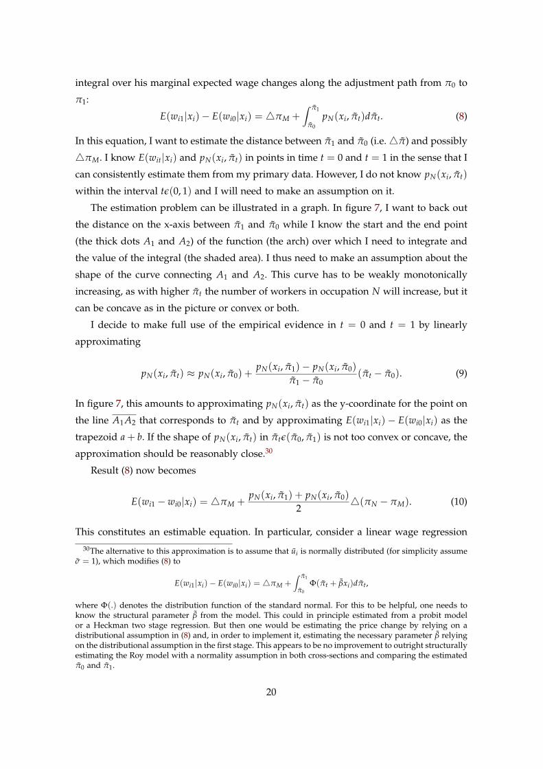
The estimation problem can be illustrated in a graph. In figure 7, I want to back out

the distance on the x-axis between π1 and π0 while I know the start and the end point

(the thick dots A1 and A2) of the function (the arch) over which I need to integrate and

the value of the integral (the shaded area). I thus need to make an assumption about the

shape of the curve connecting A1 and A2. This curve has to be weakly monotonically

increasing, as with higher πt the number of workers in occupation N will increase, but it

can be concave as in the picture or convex or both.

I decide to make full use of the empirical evidence in t = 0 and t = 1 by linearly

approximating

pN(xi, πt) ≈ pN(xi, π0) +pN(xi, π1)− pN(xi, π0)

π1 − π0(πt − π0). (9)

In figure 7, this amounts to approximating pN(xi, πt) as the y-coordinate for the point on

the line A1A2 that corresponds to πt and by approximating E(wi1|xi)− E(wi0|xi) as the

trapezoid a + b. If the shape of pN(xi, πt) in πtε(π0, π1) is not too convex or concave, the

approximation should be reasonably close.30

Result (8) now becomes

E(wi1 − wi0|xi) = 4πM +pN(xi, π1) + pN(xi, π0)

24(πN − πM). (10)

This constitutes an estimable equation. In particular, consider a linear wage regression

30The alternative to this approximation is to assume that ui is normally distributed (for simplicity assumeσ = 1), which modifies (8) to

E(wi1|xi)− E(wi0|xi) = 4πM +∫ π1

π0

Φ(πt + βxi)dπt,

where Φ(.) denotes the distribution function of the standard normal. For this to be helpful, one needs toknow the structural parameter β from the model. This could in principle estimated from a probit modelor a Heckman two stage regression. But then one would be estimating the price change by relying on adistributional assumption in (8) and, in order to implement it, estimating the necessary parameter β relyingon the distributional assumption in the first stage. This appears to be no improvement to outright structurallyestimating the Roy model with a normality assumption in both cross-sections and comparing the estimatedπ0 and π1.

20

along the lines of the “reduced-form” estimation (2):

wit = α0 + α1 pN(xi) + α3 × NLSY97 + α4 pN(xi)× NLSY97 + ε it, (11)

with pN(xi) ≡ pN(xi ,π1)+pN(xi ,π0)2 . By property of OLS α3 + α4 pN(xi) provides the best

linear predictor of E(wi1 − wi0|pN(xi)). But according to result (10), this is the same as

E(wi1 − wi0|xi). Therefore α4 identifies 4(πN − πM) and α3 identifies 4πM.

6.2 Empirical Results

Appendix C shows how the estimation approach can be extended to three occupations

for the empirical analysis. Equation (12) reports the results from this procedure:

wit = 183.05(3.64)

+ .25(.07)

pH(xit)− 1.48(.18)

pL(xit)− 4.24(7.70)

× NLSY97+

+ 0.25(0.12)

pH(xit)× NLSY97 + 0.33(0.38)

pL(xit)×NLSY97 + ε it, (12)

where pK(xit) =pK(xi ,π1)+pK(xi ,π0)

2 for Kε{H, L} and the standard errors are bootstrapped

again to account for the fact that the pK(xit)s are estimates themselves.

Equation (12) indicates that the relative equilibrium log wage rates that are paid for

a constant unit of skill across occupations have changed substantially between the two

NLSYs. First, the relative wage rate in the high-skill occupation increased by 25 percent

compared to the middle-skill occupation. At a standard error of .12 this difference is also

statistically significant at the five percent level. Further, the relative wage rate in the low-

skill occupation also rose by about 33 percent. However, due to the high standard error

this difference is not statistically significant. Finally, the absolute wage rate that is offered

in the middle-skill occupation decreased slightly by about 4 percent. Again this is not

statistically significant.

Table 7 reports that the results in equation (12) are quite robust across estimation

methods and specifications. Estimating (12) including a college dummy analogous to

column two of table 6 yields a relative wage rate increase in the high- and the low-

skill occupation of 23 and 41 percent, respectively. Using a minimum distance estimation

technique applied in earlier versions of this paper gives an optimal minimum distance

estimate of 20 and 31 percent, respectively (for details refer to Boehm, 2013).31 This pro-

31The minimum distance estimator was on the moment conditions for talent returns implied by equation(10). This was somewhat technical and replaced by the more straightforward linear regression estimator inorder to improve the readability of the paper. Using different weighting matrices than the asymptoticallyoptimal one, however, led to the estimate for the change in the relative low-skill occupation wage rate to be

21

cedure also provided a test of the restrictions implied by the model which is reported in

table 7. We can see that the model is narrowly not rejected at the 10 percent level. Finally,

in a recent study Cortes (2014) estimates occupation-specific wage rates using panel data

from the Panel Study of Income Dynamics. His results indicate that the relative wage rate

for high- and low-skill occupations rose by around 40 and 25 percent from the mid-1980s

to 2007, respectively.32

Overall, therefore, the results reported in this section paint a picture of falling demand

for work in the middle-skill occupations which manifests itself in substantially declining

relative wage rates that are offered there. The next section will use these relative wage

rate changes in order to assess the effect that the demand shifts may have had on the

overall wage distribution.

7 Polarization’s Effect on the Wage Distribution

This last section assesses the effect that job polarization may have had on the change in

overall wage inequality. I start by generating a counterfactual wage distribution that is

due to the changes in occupation-specific wage rates estimated in the last section. Then I

check whether the remaining difference with the actual distribution may in principle be

explained by the wage effects of workers reallocating out of the middle-skill occupations.

I conduct these exercises in the NLSY and in the CPS data from section 2. To use

the CPS is now possible again because assigning the estimated skill prices only requires

knowledge of workers’ occupations and not their talents anymore. Thus note that, condi-

tional on having obtained the “correct” price estimates from the NLSY, the idiosyncracies

of either dataset should not drive my conclusions in this section.

I use the price estimates from regression (12) and assign them to every worker in the

initial cohort according to his occupation. In figure 8 we can see that in both datasets the

increase of wages at the top of the distribution is reproduced quite well by the estimated

price changes alone. However, despite a slight increase at the bottom, the lower half

of the counterfactual wage distribution is relatively flat. Thus, the counterfactual wage

distribution does not match the surge in the actual distribution in the NLSY or CPS.

This seems surprising given the substantial relative wage rate increase in the low-skill

occupation of 33 percent.

Figures 9 and 10 reveal why the high relative wage rate change and the resulting

relative wage increase for low-skill occupation workers do not achieve much in terms of

around zero.32These wage rate estimates are read off figure 5 in Cortes’ paper.

22

lifting the bottom of the counterfactual wage distribution. First, in figure 9 I plot the share

of low-, middle-, and high-skill workers into the actual initial wage distribution. We see

that in both the NLSY and the CPS the share of low-skill occupation workers declines

monotonically with the quantiles of the wage distribution while the share of high-skill

occupation workers increases. The share of middle-skill occupation workers features a

hump shape—rising up to around the 30th percentile and then slowly declining.

Therefore, a drop in the wage rate for middle-skill occupations will strongest hit

workers who already started out in the lower third of the wage distribution. Moreover,

all three curves are relatively flat, which indicates that the dispersion of wages within

the three occupation groups is large and that they are overlapping substantially. Hence, a

decline in the wage rate for middle-skill occupations will drag down the wages of many

low earners at the same time as many middle-earners. This smoothes the impact of the

price changes in the lower half of the wage distribution.

Second, 10 depicts a smoothed version of the counterfactual from figure 8 and an

alternative counterfactual where workers’ quantiles in the original distribution of the

NLSY79 are kept constant.33 This alternative counterfactual is related to plots presented

in other studies of wage changes in occupations against their initial ranking in the 1980s

(e.g. Acemoglu and Autor, 2011; Autor and Dorn, 2013).

In the figure we see that if we force all of the workers’ wage change impacts on their

original quantile, and thus shut down that they move up or down the wage distribution

depending on their occupations, the rise in the lower half of the counterfactual is stronger

while it is weaker in the upper half. Overtaking therefore flattens the wage distribution

at the bottom and steepens it at the top. Due to this we do not observe much wage polar-

ization in the data despite the existence of job polarization and an associated substantial

decline in middle-skill occupation wage rates.

Overtaking is a potential explanation as to why in some countries and time periods

there is rapid job polarization but not a lot of wage polarization. In fact, the overtaking

effect can only exist in models like the Roy model which feature a multidimensional

distribution of skill. Such models also allow for overlapping wage distributions across

occupations as we have seen in figure 9.

Finally, is there a way within the Roy model that job polarization could have gener-

ated the wage polarization that we observe in the actual data? So far, the analysis ignored

33The lines are smoothed because for the counterfactual under fixed quantiles the individuals who corre-spond to these quantiles exclusively determine their change. This makes the non-smoothed counterfactualdistribution very spiky.

23

the wage effect on workers who reallocate out of the middle-skill occupations.34 The rea-

son is that without additional assumptions about the distribution of workers’ skills, the

model and empirical results of the previous sections are silent about this effect. There-

fore, the analysis in the following should be considered a calibration exercise that assesses

whether one can in principle match the remaining differences between the actual and the

counterfactual wage distribution with the reallocation effect.

In the data, there is a net outflow from the middle- to the low-skill and to the high-

skill occupation of three and 3.5 percent of the overall workforce, respectively. Therefore, I

assume that the lowest earners in the middle who make up three percent of the workforce

switch into the low-skill occupation and assign them a fifteen percent wage increase,

that is, about half of the maximum wage increase that they could possibly obtain from

switching (33%− 4%).35

Figure 11 plots the resulting counterfactual wage distribution. This fits the actual

quite well, especially in the CPS.36 Moreover, the reallocation effect that underlies it

seems qualitatively plausible. The low-earners in the middle-skill occupations may re-

ally have a strong incentive to switch jobs once the relative demand shock hits and it

is also conceivable that they could do so gainfully. For example, given probably not too

different skill requirements, someone who would have been a low-earning worker in a

factory in the 1980s may instead relatively easily become a janitor today.

While qualitatively plausible, the assumptions that are made in order to match the

wage distribution in figure 11 are strong. First, the concentrated switching of low-earners

from the middle-skill occupation requires that the population distribution of potential

wages in the low-skill occupation be condensed, so that the low-earners are the first to

find it profitable to “switch down”. This is hard to reconcile with the fact that the empir-

ical wage distributions of the low- and the middle-skill occupation overlap substantially

in both cross-sections. Second, the gains from switching that I need to assume are quite

large.

34Workers who optimally choose to leave their initial occupations have wage increases compared to stay-ing. This is even true when they “switch down” into low-skill occupations.

35An additional one percent of low earners is assumed to move to the high-skill occupation with the samewage gain.

36Previous versions of the paper in addition reported actual and counterfactual changes in average wagesacross occupations (e.g. see Boehm, 2013). The calibrated reallocation effect also helped to bring those actualand counterfactual closer together.

24

8 Conclusion

This article has studied the wage effects of job polarization on 27 year old male workers

across the two cohorts of the National Longitudinal Survey of Youth. In order to account

for endogenous selection of skill out of the middle-skill occupations, I have examined

the wages of groups of workers who are differentially likely to work in high-, middle-,

and low-skill occupations in the NLSY79 according to their talents. I have then used the

Roy (1951) model of occupational choice in order to estimate the changes in occupation-

specific wage rates and to assess the effect that job polarization may have had on the

overall wage distribution.

My findings indicate that workers who have talents that would have made them likely

to work in middle-skill occupations in the 1980s have experienced a substantial decline

in their relative wages and possibly even a decline in their absolute wages. Further, the

workers in the NLSY97 are young enough such that they are unlikely to have had ac-

quired much occupational experience when rapid job polarization occurred during the

1990s. Since occupation- or task-specific experience makes it more costly to change oc-

cupations in response to job polarization (Gathmann and Schönberg, 2010), the relative

wage effects on the workers in my dataset might in fact be a lower bound of what hap-

pened to the more experienced overall workforce.

My findings further indicate that the equilibrium wage rates that are paid for a con-

stant unit of skill across occupations have shifted in favor of the high- and of the low-skill

occupations. Job polarization can explain the rise of inequality in the upper half of the

actual wage distribution but it has a hard time explaining the increase of wages at the

bottom of the actual wage distribution. Whether this last result is due to the data and

assumptions used in this paper or whether job polarization does not by itself generate

substantial wage polarization seems to be an important question for further research.

References

Acemoglu, D., and D. Autor (2011): “Chapter 12 - Skills, Tasks and Technologies: Impli-

cations for Employment and Earnings,” vol. 4, Part B of Handbook of Labor Economics,

pp. 1043 – 1171. Elsevier.

Altonji, J. G., P. Bharadwaj, and F. Lange (2012): “Changes in the Characteristics of

American Youth: Implications for Adult Outcomes,” Journal of Labor Economics, 30(4),

pp. 783–828.

25

Aughinbaugh, A., and R. M. Gardecki (2007): “Attrition in the National Longitudinal

Survey of Youth 1997,” Mimeo.

Autor, D. H., and D. Dorn (2013): “The Growth of Low-Skill Service Jobs and the Po-

larization of the US Labor Market,” American Economic Review, 103(5), 1553–97.

Autor, D. H., L. F. Katz, and M. S. Kearney (2006): “The Polarization of the U.S. Labor

Market,” American Economic Review, 96(2), 189–194.

Autor, D. H., F. Levy, and R. J. Murnane (2003): “The Skill Content of Recent Techno-

logical Change: An Empirical Exploration,” The Quarterly Journal of Economics, 118(4),

1279–1333.

Bárány, Z., and C. Siegel (2013): “Job polarization and structural change,” Working Paper.

Boehm, M. J. (2013): “Has Job Polarization Squeezed the Middle Class? Evidence from

the Allocation of Talents,” Centre for Economic Performance Discussion Paper, 1215.

Cortes, G. M. (2014): “Where Have the Middle-Wage Workers Gone? A Study of Polar-

ization Using Panel Data,” Working Paper.

Dustmann, C., J. Ludsteck, and U. Schönberg (2009): “Revisiting the German wage

structure,” The Quarterly Journal of Economics, 124(2), 843–881.

Feng, A., and G. Graetz (2013): “Rise of the Machines: The Effects of Labor-Saving

Innovations on Jobs and Wages,” LSE Mimeo.

Firpo, S., N. M. Fortin, and T. Lemieux (2011): “Occupational Tasks and Changes in the

Wage Structure,” IZA Discussion Paper, 5542.

Gathmann, C., and U. Schönberg (2010): “How General Is Human Capital? A Task-

Based Approach,” Journal of Labor Economics, 28(1), 1–49.

Goos, M., and A. Manning (2007): “Lousy and Lovely Jobs: The Rising Polarization of

Work in Britain,” The Review of Economics and Statistics, 89(1), 118–133.

Goos, M., A. Manning, and A. Salomons (2014): “Explaining Job Polarization: Routine-

Biased Technological Change and Offshoring,” Forthcoming American Economic Review,

pp. 1–35.

Heckman, J. J., and G. Sedlacek (1985): “Heterogeneity, Aggregation, and Market Wage

Functions: An Empirical Model of Self-Selection in the Labor Market,” Journal of Polit-

ical Economy, 93(6), pp. 1077–1125.

26

Jaimovich, N., and H. E. Siu (2014): “The Trend is the Cycle: Job Polarization and Jobless

Recoveries,” Working Paper.

Jung, J., and J. Mercenier (2014): “Routinization-Biased Technical Change and Global-

ization: Understanding Labor Market Polarization,” Working Paper.

Lemieux, T. (2006): “Increasing Residual Wage Inequality: Composition Effects, Noisy

Data, or Rising Demand for Skill?,” American Economic Review, 96(3), 461–498.

Mazzolari, F., and G. Ragusa (2013): “Spillovers from high-skill consumption to low-

skill labor markets,” Review of Economics and Statistics, 95(1), 74–86.

Michaels, G., A. Natraj, and J. Van Reenen (2013): “Has ICT Polarized Skill Demand?

Evidence from Eleven Countries over 25 years,” Review of Economics and Statistics, 96(1),

60–77.

Milgrom, P., and I. Segal (2002): “Envelope Theorems for Arbitrary Choice Sets,” Econo-

metrica, 70(2), 583–601.

Mishel, L., H. Shierholz, and J. Schmitt (2013): “Don’t Blame the Robots: Assessing

the Job Polarization Explanation of Growing Wage Inequality,” EPI Working Paper.

Mulligan, C. B., and Y. Rubinstein (2008): “Selection, Investment, and Women’s Rela-

tive Wages Over Time,” The Quarterly Journal of Economics, 123(3), 1061–1110.

Roy, A. D. (1951): “Some Thoughts on the Distribution of Earnings,” Oxford Economic

Papers, 3(2), 135–146.

Sattinger, M. (1993): “Assignment Models of the Distribution of Earnings,” Journal of

Economic Literature, 31(2), pp. 831–880.

Speer, J. D. (2014): “Pre-Market Skills, Occupational Choice, and Career Progression,”

Working Paper.

Spitz-Oener, A. (2006): “Technical Change, Job Tasks, and Rising Educational Demands:

Looking outside the Wage Structure,” Journal of Labor Economics, 24(2), 235–270.

27

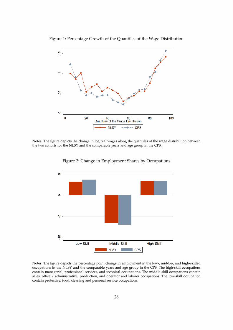
Figure 1: Percentage Growth of the Quantiles of the Wage Distribution

Notes: The figure depicts the change in log real wages along the quantiles of the wage distribution betweenthe two cohorts for the NLSY and the comparable years and age group in the CPS.

Figure 2: Change in Employment Shares by Occupations

Notes: The figure depicts the percentage point change in employment in the low-, middle-, and high-skilledoccupations in the NLSY and the comparable years and age group in the CPS. The high-skill occupationscontain managerial, professional services, and technical occupations. The middle-skill occupations containsales, office / administrative, production, and operator and laborer occupations. The low-skill occupationcontain protective, food, cleaning and personal service occupations.

28

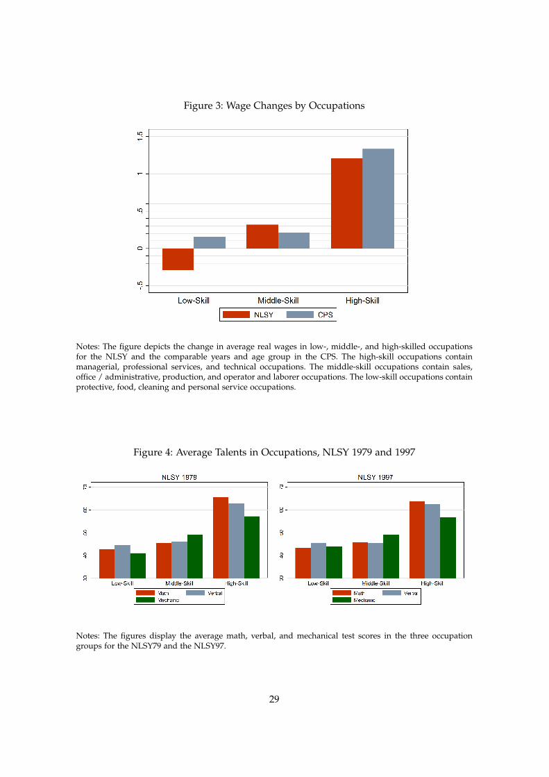
Figure 3: Wage Changes by Occupations

Notes: The figure depicts the change in average real wages in low-, middle-, and high-skilled occupationsfor the NLSY and the comparable years and age group in the CPS. The high-skill occupations containmanagerial, professional services, and technical occupations. The middle-skill occupations contain sales,office / administrative, production, and operator and laborer occupations. The low-skill occupations containprotective, food, cleaning and personal service occupations.

Figure 4: Average Talents in Occupations, NLSY 1979 and 1997

Notes: The figures display the average math, verbal, and mechanical test scores in the three occupationgroups for the NLSY79 and the NLSY97.

29

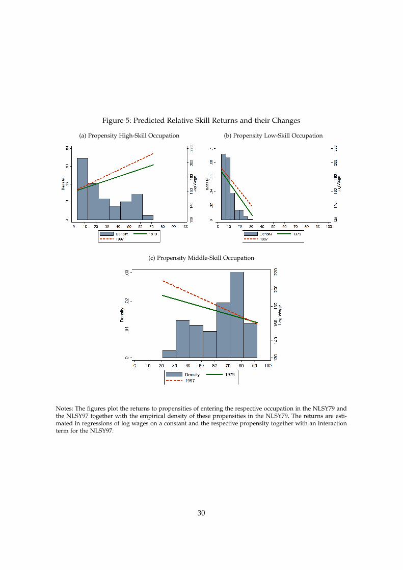
Figure 5: Predicted Relative Skill Returns and their Changes

(a) Propensity High-Skill Occupation (b) Propensity Low-Skill Occupation

(c) Propensity Middle-Skill Occupation

Notes: The figures plot the returns to propensities of entering the respective occupation in the NLSY79 andthe NLSY97 together with the empirical density of these propensities in the NLSY79. The returns are esti-mated in regressions of log wages on a constant and the respective propensity together with an interactionterm for the NLSY97.

30

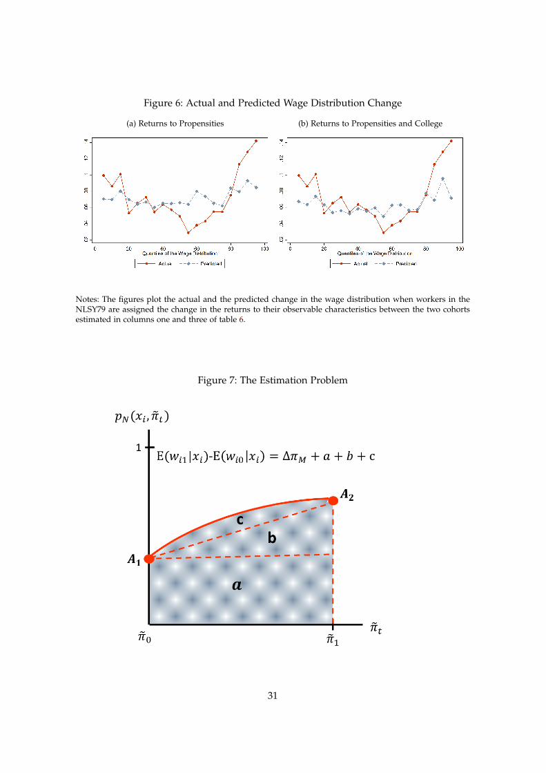
Figure 6: Actual and Predicted Wage Distribution Change

(a) Returns to Propensities (b) Returns to Propensities and College

Notes: The figures plot the actual and the predicted change in the wage distribution when workers in theNLSY79 are assigned the change in the returns to their observable characteristics between the two cohortsestimated in columns one and three of table 6.

Figure 7: The Estimation Problem

31

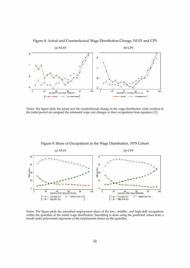
Figure 8: Actual and Counterfactual Wage Distribution Change, NLSY and CPS

(a) NLSY (b) CPS

Notes: The figure plots the actual and the counterfactual change in the wage distribution when workers inthe initial period are assigned the estimated wage rate changes in their occupations from equation (12).

Figure 9: Share of Occupations in the Wage Distribution, 1979 Cohort

(a) NLSY (b) CPS

Notes: The figure plots the smoothed employment share of the low-, middle-, and high-skill occupationswithin the quantiles of the initial wage distribution. Smoothing is done using the predicted values from afourth order polynomial regression of the employment shares on the quantiles.

32

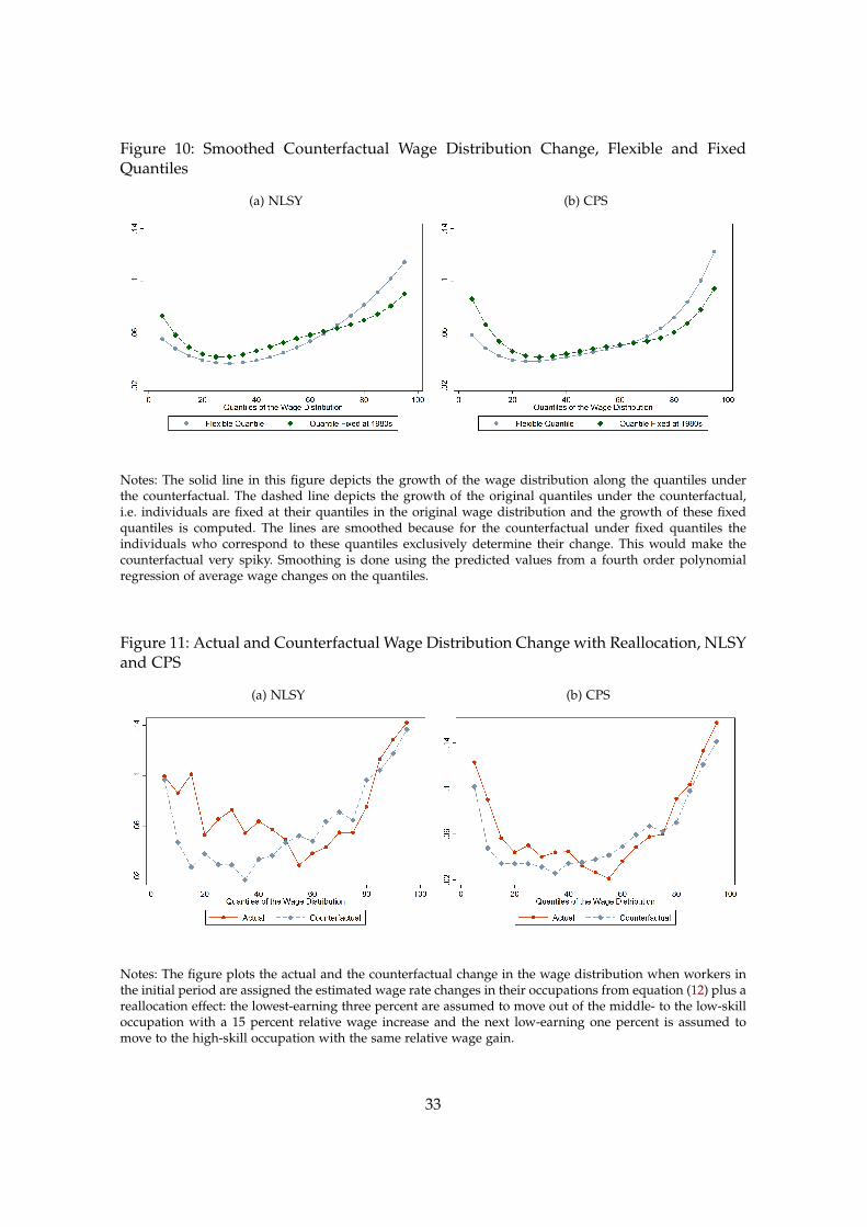
Figure 10: Smoothed Counterfactual Wage Distribution Change, Flexible and FixedQuantiles

(a) NLSY (b) CPS

Notes: The solid line in this figure depicts the growth of the wage distribution along the quantiles underthe counterfactual. The dashed line depicts the growth of the original quantiles under the counterfactual,i.e. individuals are fixed at their quantiles in the original wage distribution and the growth of these fixedquantiles is computed. The lines are smoothed because for the counterfactual under fixed quantiles theindividuals who correspond to these quantiles exclusively determine their change. This would make thecounterfactual very spiky. Smoothing is done using the predicted values from a fourth order polynomialregression of average wage changes on the quantiles.

Figure 11: Actual and Counterfactual Wage Distribution Change with Reallocation, NLSYand CPS

(a) NLSY (b) CPS

Notes: The figure plots the actual and the counterfactual change in the wage distribution when workers inthe initial period are assigned the estimated wage rate changes in their occupations from equation (12) plus areallocation effect: the lowest-earning three percent are assumed to move out of the middle- to the low-skilloccupation with a 15 percent relative wage increase and the next low-earning one percent is assumed tomove to the high-skill occupation with the same relative wage gain.

33

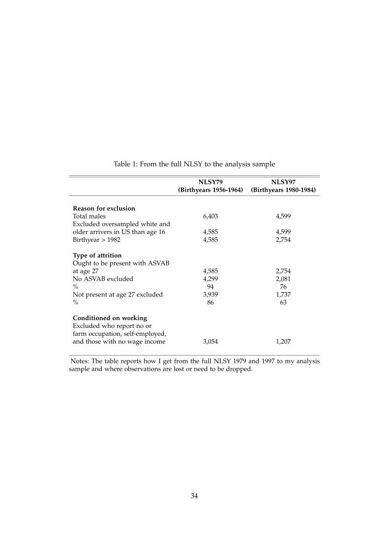
Table 1: From the full NLSY to the analysis sample

NLSY79 NLSY97(Birthyears 1956-1964) (Birthyears 1980-1984)

Reason for exclusionTotal males 6,403 4,599Excluded oversampled white andolder arrivers in US than age 16 4,585 4,599Birthyear > 1982 4,585 2,754

Type of attritionOught to be present with ASVABat age 27 4,585 2,754No ASVAB excluded 4,299 2,081% 94 76Not present at age 27 excluded 3,939 1,737% 86 63

Conditioned on workingExcluded who report no orfarm occupation, self-employed,and those with no wage income 3,054 1,207

Notes: The table reports how I get from the full NLSY 1979 and 1997 to my analysissample and where observations are lost or need to be dropped.

34

Table 2: Labor Supply with Respect to Average Demographics, Early, and ContemporarySkill Determinants

NLSY79 NLSY97

Nbr of observations 3051 1210Percentage of observations 71.60 28.40

DemographicsAge 27.00 27.00White 0.80 0.72Black 0.13 0.14Hispanic 0.06 0.14

Early skill determinantsAFQT 167.31 167.65Low AFQT Tercile 0.34 0.33Middle AFQT Tercile 0.33 0.34High AFQT Tercile 0.33 0.32

Math Score (NCE) 50.45 50.73Verbal Score (NCE) 50.26 50.49Mechanical Score (NCE) 50.41 50.69

Illicit Activities (NCE, Measured 1980) 49.98 50.01Precocious Sex (NCE, Measured 1983) 49.91 50.24

Mother’s Education (Years) 11.86 13.11Father’s Education (Years) 10.83 13.09

Contemporary skill determinantsHigh School Dropout (HSD) 0.12 0.07High School Graduate (HSG) 0.43 0.58Some College (SC) 0.20 0.06College Graduate (CG) 0.19 0.24Advanced Degree (AD) 0.06 0.04

North East 0.22 0.17North Central 0.29 0.25South 0.32 0.35West 0.17 0.21

Notes: The table shows average demographics and skillproxies in the NLSY79 and NLSY97 for all individualsweighted by hours worked. NCE indicates variables inthe population (including non-workers) are standardizedto “normal curve equivalents” with mean 50 and standarddeviation 21.06. This is done when absolute values of thesevariables cannot be compared over the two cohorts.

35

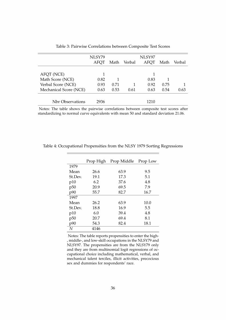
Table 3: Pairwise Correlations between Composite Test Scores

NLSY79 NLSY97AFQT Math Verbal AFQT Math Verbal

AFQT (NCE) 1 1Math Score (NCE) 0.82 1 0.83 1Verbal Score (NCE) 0.93 0.71 1 0.92 0.75 1Mechanical Score (NCE) 0.63 0.53 0.61 0.63 0.54 0.63

Nbr Observations 2936 1210

Notes: The table shows the pairwise correlations between composite test scores afterstandardizing to normal curve equivalents with mean 50 and standard deviation 21.06.

Table 4: Occupational Propensities from the NLSY 1979 Sorting Regressions

Prop High Prop Middle Prop Low1979Mean 26.6 63.9 9.5St.Dev. 19.1 17.3 5.1p10 6.2 37.6 4.8p50 20.9 69.5 7.9p90 55.7 82.7 16.71997Mean 26.2 63.9 10.0St.Dev. 18.8 16.9 5.5p10 6.0 39.4 4.8p50 20.7 69.4 8.1p90 54.3 82.4 18.1N 4146

Notes: The table reports propensities to enter the high-, middle-, and low-skill occupations in the NLSY79 andNLSY97. The propensities are from the NLSY79 onlyand they are from multinomial logit regressions of oc-cupational choice including mathematical, verbal, andmechanical talent terciles, illicit activities, precocioussex and dummies for respondents’ race.

36

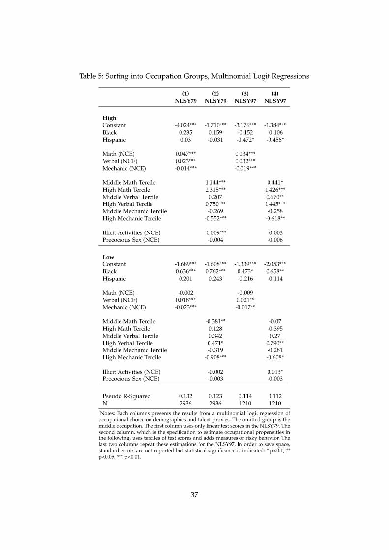
Table 5: Sorting into Occupation Groups, Multinomial Logit Regressions

(1) (2) (3) (4)NLSY79 NLSY79 NLSY97 NLSY97

HighConstant -4.024*** -1.710*** -3.176*** -1.384***Black 0.235 0.159 -0.152 -0.106Hispanic 0.03 -0.031 -0.472* -0.456*

Math (NCE) 0.047*** 0.034***Verbal (NCE) 0.023*** 0.032***Mechanic (NCE) -0.014*** -0.019***

Middle Math Tercile 1.144*** 0.441*High Math Tercile 2.315*** 1.426***Middle Verbal Tercile 0.207 0.670**High Verbal Tercile 0.750*** 1.445***Middle Mechanic Tercile -0.269 -0.258High Mechanic Tercile -0.552*** -0.618**

Illicit Activities (NCE) -0.009*** -0.003Precocious Sex (NCE) -0.004 -0.006

LowConstant -1.689*** -1.608*** -1.339*** -2.053***Black 0.636*** 0.762*** 0.473* 0.658**Hispanic 0.201 0.243 -0.216 -0.114

Math (NCE) -0.002 -0.009Verbal (NCE) 0.018*** 0.021**Mechanic (NCE) -0.023*** -0.017**

Middle Math Tercile -0.381** -0.07High Math Tercile 0.128 -0.395Middle Verbal Tercile 0.342 0.27High Verbal Tercile 0.471* 0.790**Middle Mechanic Tercile -0.319 -0.281High Mechanic Tercile -0.908*** -0.608*

Illicit Activities (NCE) -0.002 0.013*Precocious Sex (NCE) -0.003 -0.003

Pseudo R-Squared 0.132 0.123 0.114 0.112N 2936 2936 1210 1210

Notes: Each columns presents the results from a multinomial logit regression ofoccupational choice on demographics and talent proxies. The omitted group is themiddle occupation. The first column uses only linear test scores in the NLSY79. Thesecond column, which is the specification to estimate occupational propensities inthe following, uses terciles of test scores and adds measures of risky behavior. Thelast two columns repeat these estimations for the NLSY97. In order to save space,standard errors are not reported but statistical significance is indicated: * p<0.1, **p<0.05, *** p<0.01.

37

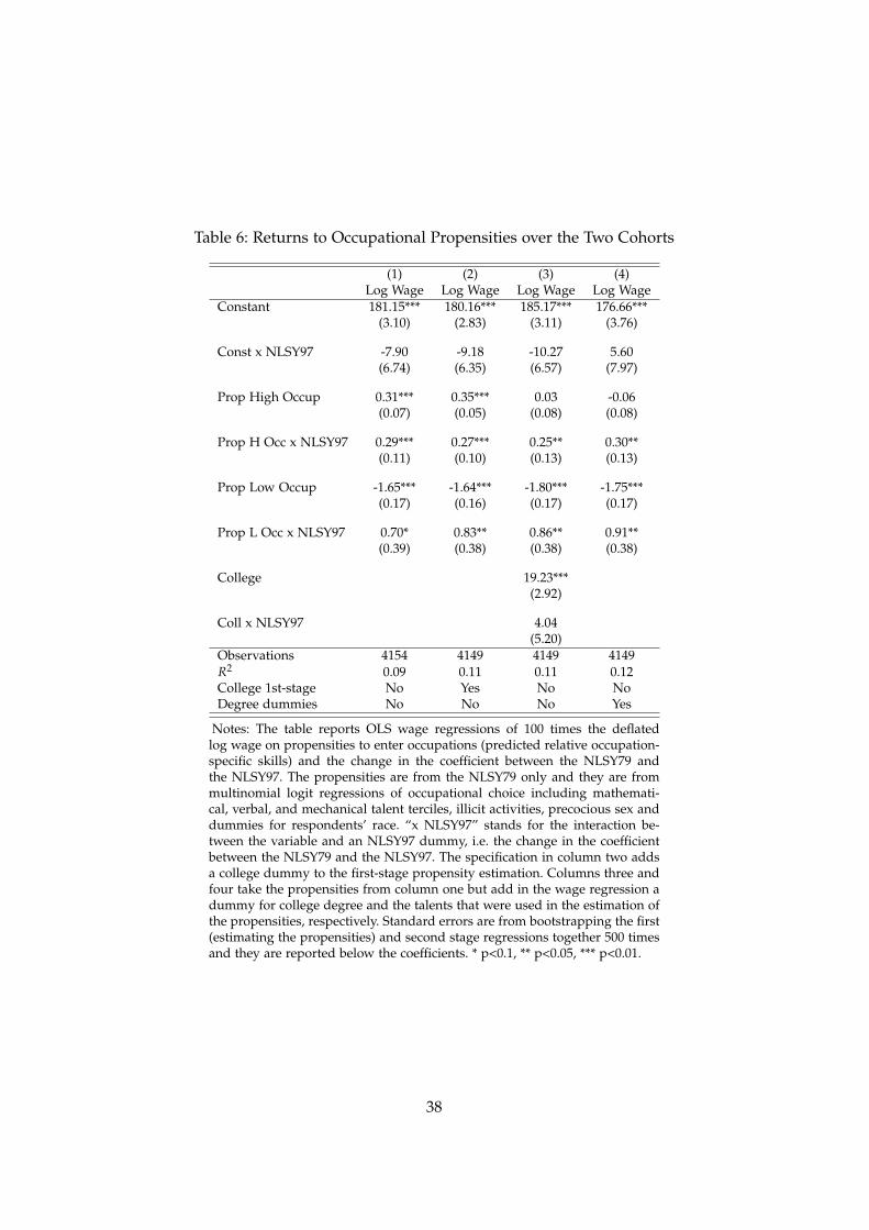
Table 6: Returns to Occupational Propensities over the Two Cohorts

(1) (2) (3) (4)Log Wage Log Wage Log Wage Log Wage

Constant 181.15*** 180.16*** 185.17*** 176.66***(3.10) (2.83) (3.11) (3.76)

Const x NLSY97 -7.90 -9.18 -10.27 5.60(6.74) (6.35) (6.57) (7.97)

Prop High Occup 0.31*** 0.35*** 0.03 -0.06(0.07) (0.05) (0.08) (0.08)

Prop H Occ x NLSY97 0.29*** 0.27*** 0.25** 0.30**(0.11) (0.10) (0.13) (0.13)

Prop Low Occup -1.65*** -1.64*** -1.80*** -1.75***(0.17) (0.16) (0.17) (0.17)

Prop L Occ x NLSY97 0.70* 0.83** 0.86** 0.91**(0.39) (0.38) (0.38) (0.38)

College 19.23***(2.92)

Coll x NLSY97 4.04(5.20)

Observations 4154 4149 4149 4149R2 0.09 0.11 0.11 0.12College 1st-stage No Yes No NoDegree dummies No No No Yes

Notes: The table reports OLS wage regressions of 100 times the deflatedlog wage on propensities to enter occupations (predicted relative occupation-specific skills) and the change in the coefficient between the NLSY79 andthe NLSY97. The propensities are from the NLSY79 only and they are frommultinomial logit regressions of occupational choice including mathemati-cal, verbal, and mechanical talent terciles, illicit activities, precocious sex anddummies for respondents’ race. “x NLSY97” stands for the interaction be-tween the variable and an NLSY97 dummy, i.e. the change in the coefficientbetween the NLSY79 and the NLSY97. The specification in column two addsa college dummy to the first-stage propensity estimation. Columns three andfour take the propensities from column one but add in the wage regression adummy for college degree and the talents that were used in the estimation ofthe propensities, respectively. Standard errors are from bootstrapping the first(estimating the propensities) and second stage regressions together 500 timesand they are reported below the coefficients. * p<0.1, ** p<0.05, *** p<0.01.

38

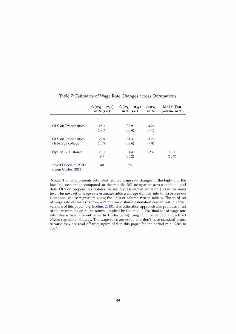
Table 7: Estimates of Wage Rate Changes across Occupations

4(πH −πM) 4(πL−πM) 4πM Model Testin % (s.e.) in % (s.e.) in % (p-value in %)

OLS on Propensities 25.1 32.9 -4.24(12.3) (38.4) (7.7)

OLS on Propensities 22.9 41.3 -5.26(1st-stage college) (10.9) (38.6) (7.8)

Opt. Min. Distance 20.1 31.4 -2.4 13.1(9.7) (35.2) (10.7)

Fixed Effects in PSID 40 25(from Cortes, 2014)

Notes: The table presents estimated relative wage rate changes in the high- and thelow-skill occupation compared to the middle-skill occupation across methods anddata. OLS on propensities restates the result presented in equation (12) in the maintext. The next set of wage rate estimates adds a college dummy into to first-stage oc-cupational choice regression along the lines of column two in table 6. The third setof wage rate estimates is from a minimum distance estimation carried out in earlierversions of this paper (e.g. Boehm, 2013). This estimation approach also provides a testof the restrictions on talent returns implied by the model. The final set of wage rateestimates is from a recent paper by Cortes (2014) using PSID panel data and a fixedeffects regression strategy. The wage rates are crude and don’t have standard errorsbecause they are read off from figure of 5 in this paper for the period mid-1980s to2007.

39

Appendix

A Detailed Sample Construction

I use data from the National Longitudinal Survey of Youth (NLSY) cohort of 1979 and

1997. As is necessary for this paper, the NLSY studies provide detailed information about

individuals’ background, education, and labor market outcomes.

I restrict my attention to males for several reasons.37 Firstly, polarization seems to have

had the most dire effect on males (Acemoglu and Autor, 2011). Secondly, female hours

worked and thus the type of selection of females into the labor market (see Mulligan

and Rubinstein, 2008) changed substantially over the two NLSYs. In addition, females

made strides in educational attainment, their wages rose across the whole distribution,

and attitudes towards them and discrimination against them in the labor market seem

to have changed drastically. Thus, there are diverse changes in (the structure of) female

labor supply and demand that are likely to work aside from the forces of polarization.

Restricting the analysis to males provides a cleaner comparison of workers across the

two decades between the NLSY79 and the NLSY97.

I evaluate individuals’ labor market outcomes at age 27 with the NLSY79 birth cohorts

of 1957–64 reaching that age in 1984–92 and the NLSY97 birth cohorts of 1980–82 reaching

it in 2007–09. Table 1 summarizes how the sample restrictions, attrition, and labor market

participation for males reduce my sample size from 6,403 to 3,054 and from 4,599 to 1,207

males in the NLSY79 and the NLSY97, respectively. I restrict the sample to individuals

who participated in the Armed Services Vocational Aptitude Battery of tests (ASVAB) in

the first survey year. This restriction is necessary because the ASVAB provides measures

of different dimensions of talent for each individual that are comparable over the two

cohorts.

The participation in ASVAB is substantially lower in the NLSY97 than the NLSY79

where almost everyone participated. Moreover, sample attrition at age 27 is higher in

the NLSY97 than the NLSY79 and overall only 63 percent of the NLSY79 participated

in ASVAB and are also present at age 27. This problem is known (e.g. Altonji, Bharad-

waj, and Lange, 2012; Aughinbaugh and Gardecki, 2007) and the attrition and non-test-

participation rates in my data closely line up with those reported in the study by Altonji,

Bharadwaj, and Lange (2012, henceforth ABL). The only difference is that ABL consider

outcomes at the younger age of 22 and thus have slightly lower attrition rates.

37Other papers in the literature that do this include Firpo, Fortin, and Lemieux (2011) and Cortes (2014).

40

In their paper, ABL note that the higher attrition rate in the NLSY97 may be partly

due to NLSY97 respondents being first interviewed at ages 12–16 versus ages 14–21 for

the NLSY79 and thus had more time to attrit. ABL further extensively examine the po-

tential non-randomness of attrition and non-test-participation and its likely impact in

biasing important labor market outcomes. Aughinbaugh and Gardecki (2007) do a simi-

lar exercise but focus on social and educational outcomes. Both studies find evidence that

attrition is not random with respect to youths’ outcomes and their backgrounds. How-

ever, Aughinbaugh and Gardecki (2007) conclude that attrition from the NLSY97 does

not appear to affect inference when estimating the three outcomes at age 20 that they

are considering and ABL decide that the differences between non-attriters and the whole

sample are not forbidding.

Moreover, ABL carefully select the samples of NLSY79 and NLSY97 to make them

comparable to one another and compute weights that adjust for attrition and non-test-

participation on observable characteristics. I closely follow their procedures for construct-

ing my own sample.38 First, I follow ABL in excluding from the NLSY79 immigrants who

arrived in the United States after age 16. This is done because the scope of the NLSY97

(age 12–16) also doesn’t include older than age 16 arrivals. Second, I exclude the eco-

nomically disadvantaged whites and military supplemental samples from the NLSY79

because they were discontinued early on in the survey and thus don’t provide labor mar-

ket outcomes at age 27 (or for ABL’s purposes). Table 1 reports that 1,818 observations

are dropped by making these restrictions to the sample. For each individual I retain the

observation that is closest to 27 years and 6 months of age and then measure labor market

and final educational outcomes from this observation.

ABL use a probit model to adjust the NLSY79 and NLSY97 base year sample weights

to account for attrition and non-test-participation according to several observable charac-

teristics, such as parental education, parental presence at age 14, indicators by birth-year,

urban and SMSA residence status, indicator variables for race and gender, and an inter-

viewer coded variable describing the attitude of the respondent during the interview. I

also employ a probit model to adjust weights for attrition and non-test-participation and

use the same specification and variables as ABL apart from leaving out parental presence

at age 14. Alternatively, a fully stratified set of indicators for birthyear, year, sex, and

race, as employed by the Bureau of Labor Statistics for weighting, yields very similar

38Thus, for more information on the sample construction and for statistics on the effects of attrition,please refer to ABL in addition to the description provided here. I would like to thank Prashant Bharadwajfor providing me with their data and do-files.

41

results.39 As ABL do in their paper, I proceed from this point with the assumption that,

after attrition weighting, my two NLSY samples are representative of the population of

young Americans that they are supposed to cover. These samples have the size of 3,939

and 1,737 individuals in the NLSY79 and the NLSY97, respectively.

I follow Lemieux (2006), who uses CPS May Outgoing Rotation Group data, in how

I compute wages and in defining the sample of working individuals (henceforth labor

supply). I use hourly wages reported for the current main job instead and normalize

them to 1979 real values by adjusting with the PCE deflator provided by the St.Louis

Federal Reserve Bank.40 While Lemieux (2006) removes outliers with 1979 real hourly

wages below $1 and above $100, I remove the high wages from $40 onward because my

NLSY wage data is very inaccurate for values above this threshold.

Finally, in order to condition on the sample of working individuals, I keep all in-

dividuals who report not to be self-employed, and who are employed in a non-farm,

non-fishing and non-forestry occupation according to the Census 1990 three-digit occu-

pation classification. This leaves me with an analysis sample of 3,054 and 1,207 males in

the NLSY79 and NLSY97, respectively (compare table 1 again). As in Lemieux (2006) I

weight all of those individuals by the number of hours that they work per week on top

of the sample weights that are adjusted for test-participation and attrition.

B Generalization of the Theory to Three Occupations

In the following I derive predictions (7) and (8) for the three-occupation case. For ease of

exposition, wages in occupations (4) are reproduced here:

wKit = πKt + sKit.

Note that sKit can be a general function of observable talents xit and unobservables. From

equation (3) and the wages in occupations we have:

wit =

wHit = πHt + sHit if Hit = 1

wMit = πMt + sMit if Mit = 1

wLit = πLt + sLit if Lit = 1

39I thank Steve McClaskie and Jay Zagorsky for providing me with the official attrition-adjusted sampleweighting program for the NLSY.

40Source: “Personal Consumption Expenditures: Chain-type Price Index (PCECTPI)”, accessed 2012-8-14,http://research.stlouisfed.org/fred2/series/PCECTPI

42

When occupational wage rates change, by the envelope theorem, the marginal change in

worker i’s wage becomes

dwit =

dπH if Hit = 1

dπM if Mit = 1

dπL if Lit = 1.

Thanks to its linearity, the expected change in wage given talents xit and initial prices

πt can be written as

E(dwit|xit, πt) = pH(xit, πt)dπH + pM(xit, πt)dπM + pL(xit, πt)dπL,

where pK(xit, πt) is the probability for an individual of talent vector xit to enter occu-

pation K under prices πt. Exploiting that the three probabilities sum to one gives the

three-occupation analogue to equation (7):

dE(wit|xit, πt) = dπMt + pH(xit, πHMt, πLMt)dπHMt + pL(xit, πHMt, πLMt)dπLMt, (13)

where πKMt ≡ πKt − πMt for Kε{H, L},

pH(xit, πHMt, πLMt) = Pr[sHit − sMit > −(πHt − πMt),

sHit − sLit > −(πHt − πLt)],

and similarly for pL(xit, πHMt, πLMt). According to prediction (13), workers who are ce-

teris paribus more likely to enter the high- or the low-skill occupation are expected to

experience higher increases in wages.

Holding constant πHMt and πLMt at t = 0 and integrating equation (13) with respect

to πMt we get

E(wit|xit, πM1, πHM0, πLM0)− E(wit|xit, πM0, πHM0, πLM0) = 4πM.

Similarly,

E(wit|xit, πM1, πHM1, πLM0)− E(wit|xit, πM1, πHM0, πLM0) =∫ πHM1

πHM0

pH(xit, πHMt, πLM0)dπHMt

E(wit|xit, πM1, πHM1, πLM1)− E(wit|xit, πM1, πHM1, πLM0) =∫ πLM1

πLM0

pL(xit, πHM1, πLMt)dπLMt.

43

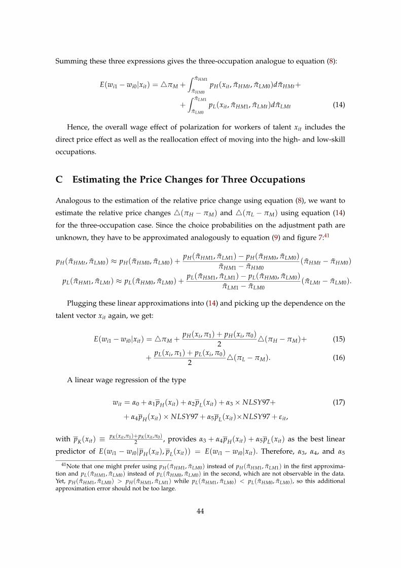
Summing these three expressions gives the three-occupation analogue to equation (8):

E(wi1 − wi0|xit) = 4πM +∫ πHM1

πHM0

pH(xit, πHMt, πLM0)dπHMt+

+∫ πLM1

πLM0

pL(xit, πHM1, πLMt)dπLMt (14)

Hence, the overall wage effect of polarization for workers of talent xit includes the

direct price effect as well as the reallocation effect of moving into the high- and low-skill

occupations.

C Estimating the Price Changes for Three Occupations

Analogous to the estimation of the relative price change using equation (8), we want to

estimate the relative price changes 4(πH − πM) and 4(πL − πM) using equation (14)

for the three-occupation case. Since the choice probabilities on the adjustment path are

unknown, they have to be approximated analogously to equation (9) and figure 7:41

pH(πHMt, πLM0) ≈ pH(πHM0, πLM0) +pH(πHM1, πLM1)− pH(πHM0, πLM0)

πHM1 − πHM0(πHMt − πHM0)

pL(πHM1, πLMt) ≈ pL(πHM0, πLM0) +pL(πHM1, πLM1)− pL(πHM0, πLM0)

πLM1 − πLM0(πLMt − πLM0).

Plugging these linear approximations into (14) and picking up the dependence on the

talent vector xit again, we get:

E(wi1 − wi0|xit) = 4πM +pH(xi, π1) + pH(xi, π0)

24(πH − πM)+ (15)

+pL(xi, π1) + pL(xi, π0)

24(πL − πM). (16)

A linear wage regression of the type

wit = α0 + α1 pH(xit) + α2 pL(xit) + α3 × NLSY97+ (17)

+ α4 pH(xit)× NLSY97 + α5 pL(xit)×NLSY97 + ε it,

with pK(xit) ≡ pK(xit,π1)+pK(xit,π0)2 , provides α3 + α4 pH(xit) + α5 pL(xit) as the best linear

predictor of E(wi1 − wi0|pH(xit), pL(xit)) = E(wi1 − wi0|xit). Therefore, α3, α4, and α5

41Note that one might prefer using pH(πHM1, πLM0) instead of pH(πHM1, πLM1) in the first approxima-tion and pL(πHM1, πLM0) instead of pL(πHM0, πLM0) in the second, which are not observable in the data.Yet, pH(πHM1, πLM0) > pH(πHM1, πLM1) while pL(πHM1, πLM0) < pL(πHM0, πLM0), so this additionalapproximation error should not be too large.

44

identify the wage rate changes 4πM, 4(πH − πM), and 4(πL − πM), respectively.

45